Computational Intelligence: Computational Intelligence: Methods and ApplicationsMethods and Applications

Lecture 19 Pruning of decision trees

Source: Włodzisław Duch; Dept. of Informatics, UMK; Google: W Duch

PruningPruningHow to avoid overfitting and deal with the noise in data?

1. Stop splitting the nodes if the number of samples is too small to make reliable decisions.

2. Stop if the proportion of samples from a single class (node purity) is larger than a given threshold - forward pruning.

3. Create a tree that fits all data and then simplify it - backward pruning.

• Prune to improve the results on a validation set or on a crossvalidation test partition, not on the training set!

• Use the MDL (Minimum Description Length) principle:Minimize Size(Tree) + Size(Tree(Errors))

• Evaluate splits looking not at the effects on the next level but a few levels deeper, using beam-search instead of best-first search; for small trees exhaustive search is possible.

DT DT for breast cancerfor breast cancerDT DT for breast cancerfor breast cancer

Leave only the most important nodes, even if they are not pure, prune the rest.

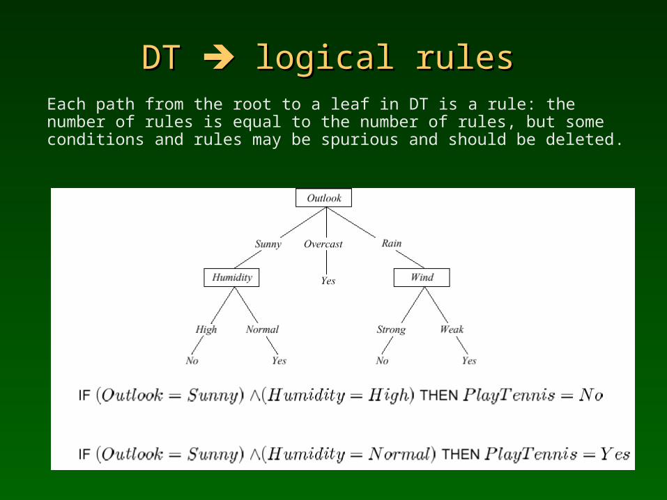
DT DT logical ruleslogical rulesEach path from the root to a leaf in DT is a rule: the number of rules is equal to the number of rules, but some conditions and rules may be spurious and should be deleted.

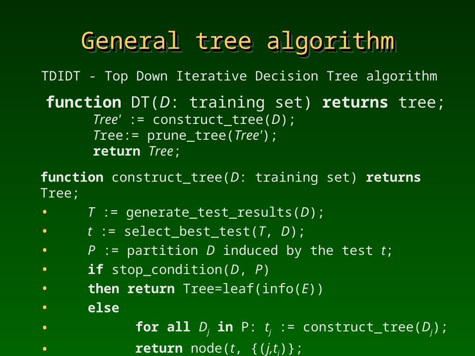
General tree algorithmGeneral tree algorithmGeneral tree algorithmGeneral tree algorithmTDIDT - Top Down Iterative Decision Tree algorithm

function DT(D: training set) returns tree;Tree' := construct_tree(D);Tree:= prune_tree(Tree');return Tree;

function construct_tree(D: training set) returns Tree;• T := generate_test_results(D);• t := select_best_test(T, D);• P := partition D induced by the test t;• if stop_condition(D, P)• then return Tree=leaf(info(E))• else

• for all Dj in P: tj := construct_tree(Dj);

• return node(t, {(j,tj)};

ID 3 ID 3 ID3: Interactive Dichotomizer, version 3, initially called CLS (Concept Learning System), R. Quinlan (1986)

Works only with nominal attributes.For numerical attributes separate discretization step is needed.

Splits selected using the information gain criterion Gain(D,X).

The node is divided into as many branches, as the number of unique values in attribute X.

ID3 creates trees with high information gain near the root, leading to locally optimal trees that are globally sub-optimal.

No pruning has been used.

ID3 algorithm evolved into a very popular C4.5 tree (and C5, commercial version).

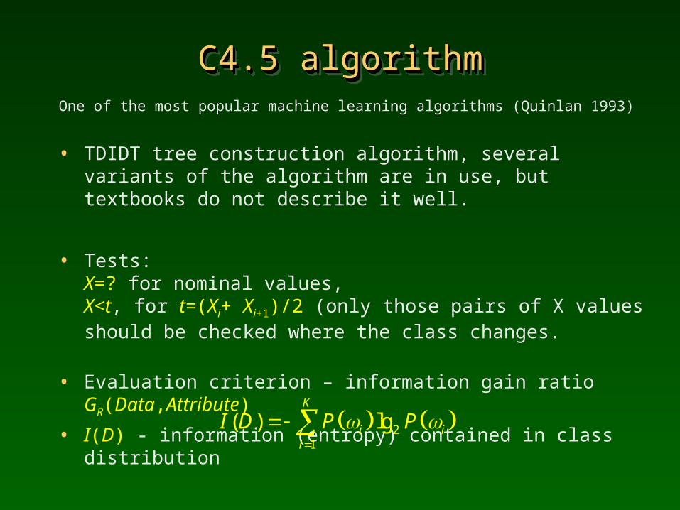
C4.5 algorithmC4.5 algorithmC4.5 algorithmC4.5 algorithmOne of the most popular machine learning algorithms (Quinlan 1993)

• TDIDT tree construction algorithm, several variants of the algorithm are in use, but textbooks do not describe it well.

• Tests: X=? for nominal values, X<t, for t=(Xi+ Xi+1)/2 (only those pairs of X values should be checked where the class changes.

• Evaluation criterion – information gain ratio GR(Data,Attribute)

• I(D) - information (entropy) contained in class distribution 21

( ) lgK

i ii

I D P P

C4.5 criterionC4.5 criterionC4.5 criterionC4.5 criterionInformation gain: calculate information in the parent node and in the children nodes created by the split, subtract this information weighting it by the percentage of data that falls into k children’s nodes:

• Information gain ratio GR(D,X) is equal to the information gain divided by the amount of information in the split-generated data distribution:

1

( , ) ( )k

ii

i

DG D X I D I D

D

21

( , ) lgk

i iS

i

D DI D X

D D

( , ) ( , ) / ( , )R SG D X G D X I D X

Why ratio? To avoid preferences of attributes with many values.

IS decreases the information gain for nodes that have many children.

CHAID CHAID CHi-squared Automatic Interaction Detection, in SPSS (but not in WEKA), one of the most popular trees in data mining packages.

Split criterion for the attribute X is based on 2 test that measures correlations between two distributions.

For a test, for example selecting a threshold X<X0 (or X=X0) for each attribute, a distribution of classes N(c|Test=True) is obtained; it forms a contingency table: class vs. tests.

If there is no correlation with the class distribution then

P(c|Test=True)=P(c)P(Test=True)

N(c|Test=True)=N(c)N(Test=True)

Compare the actual results nij obtained for each test with

these expectation eij; if they match well then the test is not worth much.

2 test measures the probability that they match by chance: select tests with the largest 2 value for (nijeij )2

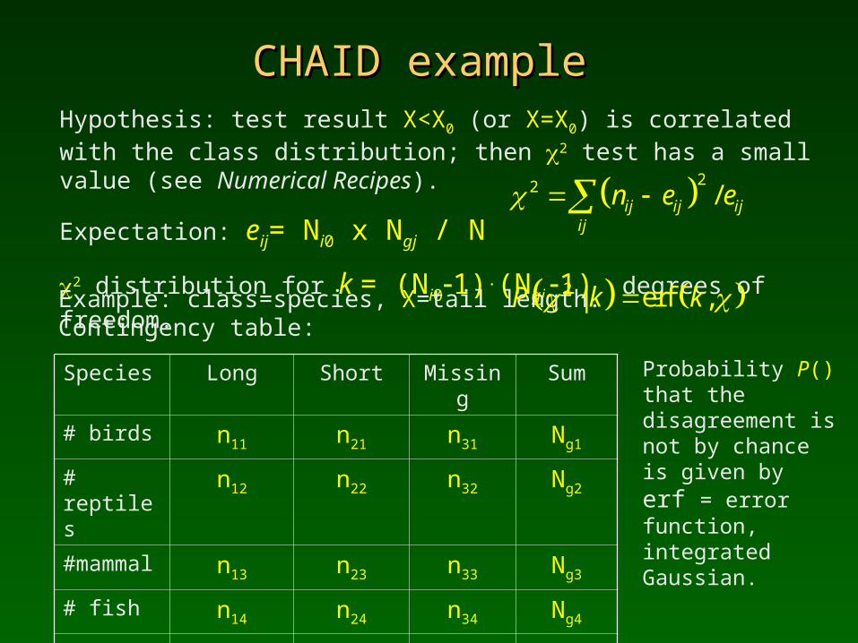
CHAID CHAID exampleexampleHypothesis: test result X<X0 (or X=X0) is correlated with the class distribution; then 2 test has a small value (see Numerical Recipes).

Expectation: eij= Ni0 x Ngj / N

2 distribution for k = (Ni01).(Ngj 1) degrees of freedom.

Species Long Short Missing Sum

# birds n11 n21 n31 Ng1

# reptiles

n12 n22 n32 Ng2

#mammal

n13 n23 n33 Ng3

# fish n14 n24 n34 Ng4

Sum N10 N20 N30 N

Example: class=species, X=tail length. Contingency table:

22 /ij ij ijij

n e e

2 | erf ,P k k

Probability P() that the disagreement is not by chance is given by erf = error function, integrated Gaussian.

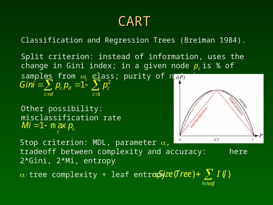
CARTCARTClassification and Regression Trees (Breiman 1984).

Split criterion: instead of information, uses the change in Gini index; in a given node pc is % of samples from c class; purity of node is:

Stop criterion: MDL, parameter , tradeoff between complexity and accuracy: here 2*Gini, 2*Mi, entropy

tree complexity + leaf entropy

2

1

1C C

c d cc d c

Gini p p p

1 max cc

Mi p

( ) ( )l leaf

Size Tree I l

Other possibility: misclassification rate

Other treesOther trees

See the entry in WIKIpedia on decision trees.

Several interesting trees for classification and regression are at the page of Wei-Yin Loh.

YaDT: Yet another Decision Tree builder.

RuleQuest has See 5, a new version of C4.5 with some comparisons. Only a demo version is available. Look also at their Magnum Opus software to discover interesting patters – association rules, and k-optimal rule discovery.

Occam Tree from Visionary Tools.

Computational Intelligence: Computational Intelligence: Methods and ApplicationsMethods and Applications

Lecture 20 SSV & other trees

Source: Włodzisław Duch; Dept. of Informatics, UMK; Google: W Duch

GhostMiner PhilosophyGhostMiner PhilosophyGhostMiner PhilosophyGhostMiner Philosophy

• There is no free lunch – provide different type of tools for knowledge discovery. Decision tree, neural, neurofuzzy, similarity-based, committees.

• Provide tools for visualization of data.• Support the process of knowledge discovery/model

building and evaluating, organizing it into projects.

GhostMiner, data mining tools from our lab.

http://www.fqspl.com.pl/ghostminer/

or write “Ghostminer” in Google.

• Separate the process of model building and knowledge discovery from model use =>

GhostMiner Developer & GhostMiner Analyzer.

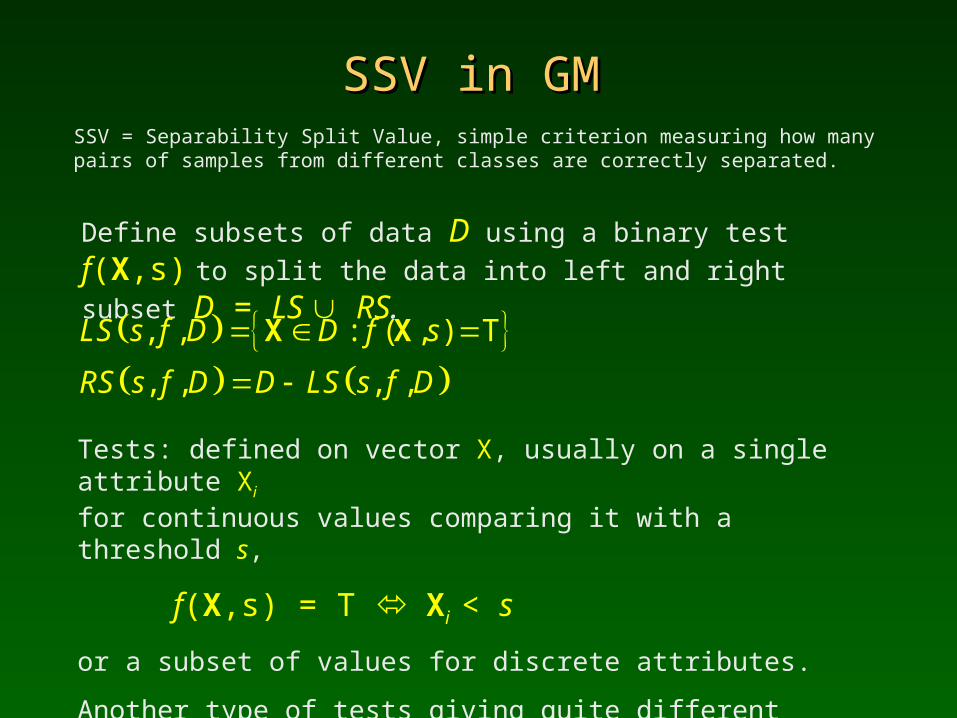
SSVSSV in GM in GMSSV = Separability Split Value, simple criterion measuring how many pairs of samples from different classes are correctly separated.

Tests: defined on vector X, usually on a single attribute Xi for continuous values comparing it with a threshold s,

f(X,s) = T Xi < s

or a subset of values for discrete attributes.

Another type of tests giving quite different shapes of decision borders is based on distances from prototypes.

Define subsets of data D using a binary test f(X,s) to split the data into left and right subset D = LS RS.

, , : ( , ) T

, , , ,

LS s f D D f s

RS s f D D LS s f D

X X

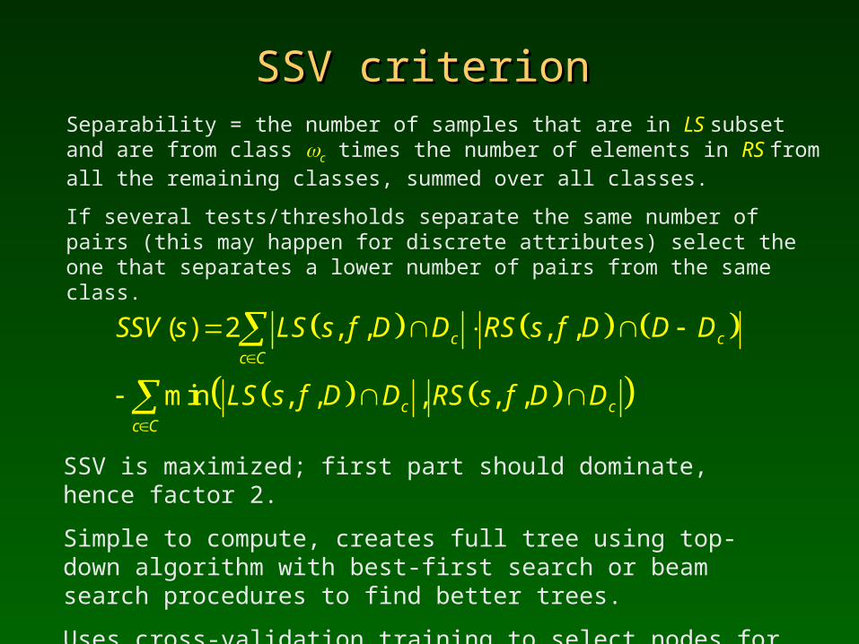
SSVSSV criterion criterionSeparability = the number of samples that are in LS subset and are from class c times the number of elements in RS from all the remaining classes, summed over all classes.

If several tests/thresholds separate the same number of pairs (this may happen for discrete attributes) select the one that separates a lower number of pairs from the same class.

SSV is maximized; first part should dominate, hence factor 2.

Simple to compute, creates full tree using top-down algorithm with best-first search or beam search procedures to find better trees.

Uses cross-validation training to select nodes for backward pruning.

( ) 2 , , , ,

min , , , , ,

c cc C

c cc C

SSV s LS s f D D RS s f D D D

LS s f D D RS s f D D

SSVSSV parameters parametersGeneralization strategy: defines how the pruning is done.

First, try to find optimal parameters for pruning: final number of leaf nodes, or pruning degree k = remove all nodes that increased accuracy by k samples only.

Given pruning degree or given nodes count define these parameters by hand.

“Optimal” uses cross-validation training to determine these parameters: the number of CV folds and their type has to be selected.

Optimal numbers: minimize sum of errors in the test parts of CV training.

Search strategy: use the nodes of tree created so far and:

use the best-first search, i.e. select the next node for splitting; use beam search: keep ~10 best trees, expand them; avoids local maxima of the SSV criterion function but rarely gives better results.

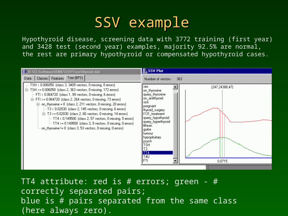
SSV SSV exampleexampleHypothyroid disease, screening data with 3772 training (first year) and 3428 test (second year) examples, majority 92.5% are normal, the rest are primary hypothyroid or compensated hypothyroid cases.

TT4 attribute: red is # errors; green - # correctly separated pairs; blue is # pairs separated from the same class (here always zero).

Wine data exampleWine data exampleWine data exampleWine data example

• alcohol content • ash content • magnesium content • flavanoids content • proanthocyanins phenols

content • OD280/D315 of diluted wines

Wine robot

• malic acid content • alkalinity of ash • total phenols content • nonanthocyanins phenols

content • color intensity • hue• proline.

Chemical analysis of wine from grapes grown in the same region in Italy, but derived from three different cultivars.Task: recognize the source of wine sample.13 quantities measured, continuous features:

C4.5 tree for WineC4.5 tree for WineC4.5 tree for WineC4.5 tree for WineJ48 pruned tree: using reduced error (3x crossvalidation) pruning: ------------------OD280/D315 <= 2.15| alkalinity <= 18.1: 2 (5.0/1.0)| alkalinity > 18.1: 3 (31.0/1.0)OD280/D315 > 2.15| proline <= 750: 2 (43.0/2.0)| proline > 750: 1 (40.0/2.0)

Number of Leaves : 4Size of the tree : 7Correctly Classified Instances 161 90.44 %Incorrectly Classified Instances 17 9.55 %Total Number of Instances 178

WEKA/RM outputWEKA/RM outputWEKA/RM outputWEKA/RM outputWEKA output contains confusion matrix, RM has transposed matrix

a b c <= classified as 56 3 0 | a = 1 (class number)

4 65 2 | b = 2 P(true|predicted) 3 1 44 | c = 3

2x2 matrix: TP FN P+

FP TN P

P+(M) P(M) 1

WEKA: TP Rate FP Rate Precision Recall F-Measure Class 0.949 0.059 0.889 0.949 0.918 1 0.915 0.037 0.942 0.915 0.929 2 0.917 0.015 0.957 0.917 0.936 3

Pr=Precision=TP/(TP+FP)

R =Recall = TP/(TP+FN)

F-Measure = 2Pr*R/(P+R)

WEKA/RM output infoWEKA/RM output infoWEKA/RM output infoWEKA/RM output infoOther output information:

Kappa statistic 0.8891(corrects for chance agreement)

Mean absolute error 0.0628

Root mean squared error 0.2206

Root relative squared error 47.0883%Relative absolute error 14.2992%

1 1

2

1

1

2

1

1

1

| ;

| ;

| ;

K K

ii i ii i

K

i ii

n

k

n

k

n

kn

k

N N M N N M

N N N M

P M YMAE

n

P M YRMS

n

P M YRAE

Y Y

X X

X X

X X

X

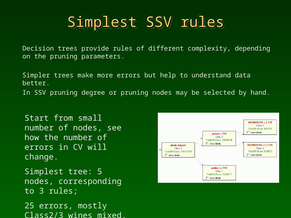
Simplest SSV rulesSimplest SSV rulesSimplest SSV rulesSimplest SSV rules

Decision trees provide rules of different complexity, depending on the pruning parameters.

Simpler trees make more errors but help to understand data better.

In SSV pruning degree or pruning nodes may be selected by hand.

Start from small number of nodes, see how the number of errors in CV will change.

Simplest tree: 5 nodes, corresponding to 3 rules;

25 errors, mostly Class2/3 wines mixed.

Wine – SSV 5 rulesWine – SSV 5 rulesWine – SSV 5 rulesWine – SSV 5 rulesLower pruning leads to more complex but more accurate tree.

7 nodes, corresponding to 5 rules;

10 errors, mostly Class2/3 wines mixed.

Try to lower the pruning degree or increase the node number and observe the influence on the error.

av. 3 nodes train 10x: 87,0±2,1% test 80,6±5,4±2,1%

av. 7 nodes train 10x: 98,1±1,0% test 92,1±4,9±2,0%

av.13 nodes train 10x: 99,7±0,4% test 90,6±5,1±1,6%

Wine – SSV optimal rulesWine – SSV optimal rulesWine – SSV optimal rulesWine – SSV optimal rules

Various solutions may be found, depending on the search parameters: 5 rules with 12 premises, making 6 errors, 6 rules with 16 premises and 3 errors, 8 rules, 25 premises, and 1 error.

if OD280/D315 > 2.505 proline > 726.5 color > 3.435 then class 1

if OD280/D315 > 2.505 proline > 726.5 color < 3.435 then class 2

if OD280/D315 < 2.505 hue > 0.875 malic-acid < 2.82 then class 2

if OD280/D315 > 2.505 proline < 726.5 then class 2

if OD280/D315 < 2.505 hue < 0.875 then class 3

if OD280/D315 < 2.505 hue > 0.875 malic-acid > 2.82 then class 3

What is the optimal complexity of rules? Use crossvalidation to estimate optimal pruning for best generalization.

DT summaryDT summaryDT: fast and easy, recursive partitioning.

Advantages:

easy to use, very few parameters to set, no data preprocessing;

frequently give very good results, easy to interpret, and convert to logical rules, work with nominal and numerical data.

Applications: classification and regression.

Almost all Data Mining software packages have decision trees.

Some problems with DT:

few data, large number of continuous attributes, unstable; lower parts of trees are less reliable, splits on small subsets of data;DT knowledge expressive abilities are rather limited, for example it is hard to create a concept: “majority are for it”, easy for M-of-N rules.

Computational Intelligence: Computational Intelligence: Methods and ApplicationsMethods and Applications

Lecture 21 Linear discrimination, linear machines

Source: Włodzisław Duch; Dept. of Informatics, UMK; Google: W Duch

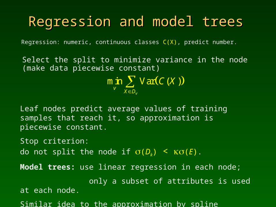
Regression and model treesRegression and model treesRegression: numeric, continuous classes C(X), predict number.

Leaf nodes predict average values of training samples that reach it, so approximation is piecewise constant.

Stop criterion:

do not split the node if (Dk) < (E).

Model trees: use linear regression in each node;

only a subset of attributes is used at each node.

Similar idea to the approximation by spline functions.

min Var ( )v

vX D

C X

Select the split to minimize variance in the node (make data piecewise constant)

Some DT ideasSome DT ideasMany improvements have been proposed.General idea: divide and conquer.

Multi-variate trees: provide more complex decision borders; trees using Fisher or Linear Discrimination Analysis;perceptron trees, neural trees.

Split criteria:

information gain near the root, accuracy near leaves;pruning based on logical rules, works also near the

root;

Committees of trees:

learning many trees on randomized data (boosting) or CV,

learning with different pruning parameters.

Fuzzy trees, probability evaluating trees, forests of trees ...

http://www.stat.wisc.edu/~loh/ Quest, Cruise, Guide, Lotus trees

DT tests and expressive powerDT tests and expressive powerDT: fast and easy, recursive partitioning of data – powerful idea.

Typical DT with tests on values of single attribute has rather limited knowledge expression abilities.

For example, if N=10 people vote Yes/No, and the decision is taken when the number of Yes votes > the number of No votes (a concept: “majority are for it”), the data looks as follows:

1 0 0 0 1 1 1 0 1 0 No

1 1 0 0 1 1 1 0 1 0 Yes

0 1 0 0 1 1 1 0 1 0 No

Univariate DT will not learn from such data, unless a new test is introduced: ||X-W||>5, or WX>5, with W=[1 1 1 1 1 1 1 1 1 1]

Another way to express it is by the M-of-N rule:

IF at least 5-of-10 (Vi=1) Then Yes.

Linear discriminationLinear discriminationLinear combination WX > , with fixed W, defines a half-space.

WX = 0 defines a hyperplane orthogonal to W, passing through 0

WX > 0 is the half-space in the direction of W vector

WX > is the half-space, shifted by in the direction of W vector.

Linear discrimination: separate different classes of data using hyperplanes, learn the best W parameters from data.

( )T ( ) 10 for

0 otherwise.

ii

XW X

Special case of Bayesian approach (identical covariance matrices);special test for decision trees.Frequently a single hyperplane is sufficient to separate data, especially in high-dimensional spaces!

Linear discriminant functionsLinear discriminant functionsLinear discriminant function gW(X) = WTX + W0

Terminology: W is the weight vector, W0 is the bias term (why?).

IF gW(X)>0 Then Class 1, otherwise Class 2

W = [W0, W1 ... Wd] usually includes W0, and X=[1,X1, .. Xd]

Discrimination function for classification may include in addition a step function (WTX) = ±1.

Graphical representation of the discriminant function gW(X)=(WTX)

One LD function may separate pairs of classes; for more classes or if strongly non-linear decision borders are needed many LD functions may be used. If smooth sigmoidal output is used LD is called a “perceptron”.

Distance from the planeDistance from the planegW(X) = 0 for two vectors on the d-D decision hyperplane means:

WTX(1) = W0=WTX(2), or WT(X(1)X(2))=0, so WT is (normal to) the plane. How far is arbitrary X from the decision hyperplane?

X= Xp+ DW(X) V; but WTXpW0,

therefore WTX = W0+ DW(X) ||W||

Hence the signed distance: X

Xp

WDW

XW

Distance = scaled value of discriminant function, measures the

confidence in classification; smaller ||W|| => greater confidence.

TT0

0

gWD V

W

W

XW XX V X

W W

Let V =W/||W|| be the unit vector normal to the plane and V0=W0/||W||

K-class problemsK-class problemsFor K classes: separate each class from the rest using K hyperplanes – but then ...

Perhaps separate each pair of classes using K(K-1)/2 planes?

Fig. 5.3,

Duda, Hart, Stork

Still ambiguous

region persist.

Linear machineLinear machineDefine K discriminant functions:

gi(X)=W(i)TX+W0i , i =1 .. K

IF gi(X) > gj(X), for all j≠i, Then select i

Linear machine creates K convex decision regions Ri, largest gi(X)

Hij hyperplane is defined by:

gi(X) = gj(X) => (W(i)W(j))TX + (W0iW0j) = 0

W = (W(i)W(j)) is orthogonal to Hij plane; distance to this plane is

DW(X)=(gi(X)gj(X))/||W||

Linear machines for 3 and 5 classes, same as one prototype + distance.Fig. 5.4, Duda, Hart, Stork

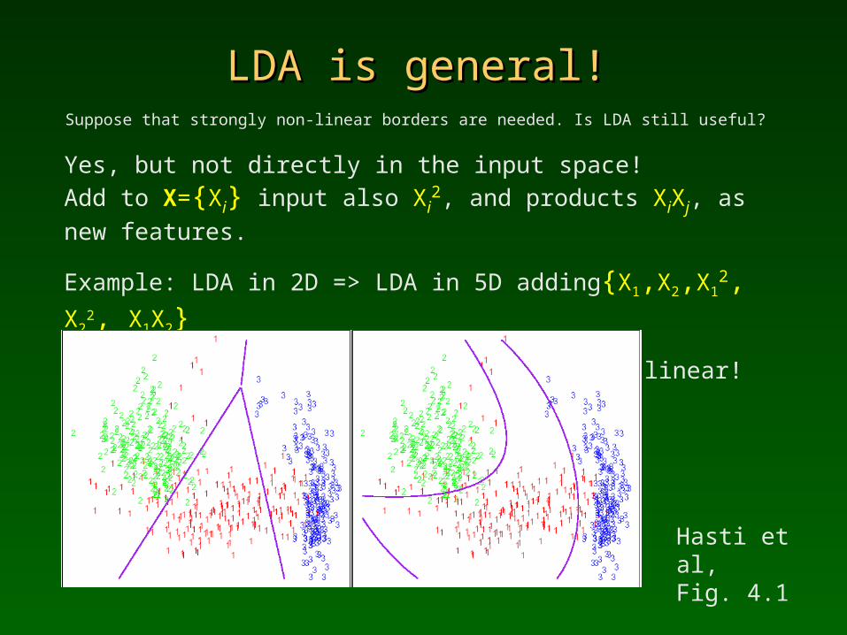
LDA is general!LDA is general!Suppose that strongly non-linear borders are needed. Is LDA still useful?

Yes, but not directly in the input space!

Add to X={Xi} input also Xi2, and products XiXj, as new features.

Example: LDA in 2D => LDA in 5D adding{X1,X2,X12, X2

2, X1X2}

g(X1,X2)=W1X1+...+W5X1X2+W0 is now non-linear!

Hasti et al, Fig. 4.1

LDA – how?LDA – how?How to find W?There are many methods, the whole Chapter 5 in Duda, Hart & Stork is devoted to the linear discrimination methods.

LDA methods differ by:

formulation of criteria defining W;

on-line versions for incoming data, off-line for fixed data;

the use of numerical methods: least-mean square, relaxation, pseudoinverse, iterative corrections, Ho-Kashyap algorithms, stochastic approximations, linear programming algorithms ...

“Far more papers have been written about linear discriminants than the subject deserves” (Duda, Hart, Stork 2000).

Interesting papers on this subject are still being written ...

LDA – regression approachLDA – regression approachLinear regression model (implemented in WEKA)

Y=gW(X)=WTX+W0

Fit the data to the known (X,Y) values, even if Y=1.

Common statistical approach:

use LMS (Least Mean Square) method, minimize the Residual Sum of Squares (RSS).

2( ) ( )

1

2

( ) ( )0

1 1

RSSn

i i

i

n di i

j ji i

Y g

Y W W X

WW X

LDA – regression formulationLDA – regression formulationIn matrix form with X0=1, and W0

If X was square and non-singular than W = (XT)-1Y but nd+1

( )T ( ) ( ) ( ) (1) ( )0 1

2 TT T T

, ,..., ; = ,... ; 1 x

RSS

i i i i ndX X X d n

X X X X

W Y X W Y X W Y X W

(1) (1) (1)1 00 1

(2) (2) (2)2 1T 0 1

( ) ( ) ( )0 1

d

d

n n nn dd

Y WX X X

Y WX X X

Y WX X X

Y X W

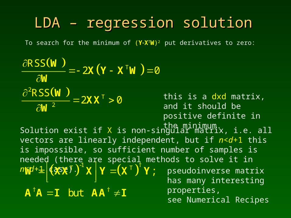
LDA – regression solutionLDA – regression solutionTo search for the minimum of (YXTW)2 put derivatives to zero:

Solution exist if X is non-singular matrix, i.e. all vectors are linearly independent, but if n<d+1 this is impossible, so sufficient number of samples is needed (there are special methods to solve it in n<d+1 case).

T

2T

2

RSS2 0

RSS2 0

WX Y X W

W

WXX

Wthis is a dxd matrix, and it should be positive definite in the minimum.

-1 †T T

† †

;

but

W XX X Y X Y

A A I AA I

pseudoinverse matrix has many interesting properties, see Numerical Recipes http://www.nr.com

LSM evaluationLSM evaluation

The solution using the pseudoinverse matrix is one of many possible approach to LDA (for 10 other see for ex. Duda and Hart).Is it the best result? Not always.

For singular X due to the linearly dependent features, the method is corrected by removing redundant features.

Good news: Least Mean Square estimates have the lowest variance among all linear estimates.

Bad news: hyperplanes found in this way may not separate even the linearly separable data!

Why? LMS minimizes squares of distances,not the classification margin.

Wait for SVMs to do that ...