The Pennsylvania State University

The Graduate School

Department of Aerospace Engineering

COMPUTATIONAL INVESTIGATION OF A BOUNDARY-LAYER INGESTION

PROPULSION SYSTEM FOR THE COMMON RESEARCH MODEL

A Thesis in

Aerospace Engineering

by

© 2016 Brennan Blumenthal

Submitted in Partial Fulfillment of the Requirements

for the Degree of Master of Science

May 2016

https://ntrs.nasa.gov/search.jsp?R=20160005086 2018-07-16T10:25:33+00:00Z

ii

The thesis of Brennan Blumenthal was reviewed and approved* by the following: Mark D. Maughmer Professor of Aerospace Engineering Thesis Co-Adviser Sven Schmitz Assistant Professor of Aerospace Engineering Thesis Co-Adviser George A. Lesieutre Professor of Aerospace Engineering Head of Department of Aerospace Engineering *Signatures are on file in the Graduate School

iii

ABSTRACT

This thesis will examine potential propulsive and aerodynamic benefits of integrating a

boundary-layer ingestion (BLI) propulsion system with a typical commercial aircraft using the

Common Research Model geometry and the NASA Tetrahedral Unstructured Software System

(TetrUSS). The Numerical Propulsion System Simulation (NPSS) environment will be used to

generate engine conditions for CFD analysis. Improvements to the BLI geometry will be made

using the Constrained Direct Iterative Surface Curvature (CDISC) design method. Previous

studies have shown reductions of up to 25% in terms of propulsive power required for cruise for

other axisymmetric geometries using the BLI concept.

An analysis of engine power requirements, drag, and lift coefficients using the baseline

and BLI geometries coupled with the NPSS model are shown. Potential benefits of the BLI

system relating to cruise propulsive power are quantified using a power balance method and a

comparison to the baseline case is made. Iterations of the BLI geometric design are shown and

any improvements between subsequent BLI designs presented. Simulations are conducted for a

cruise flight condition of Mach 0.85 at an altitude of 38,500 feet and an angle of attack of 2° for

all geometries. A comparison between available wind tunnel data, previous computational results,

and the original CRM model is presented for model verification purposes along with full results

for BLI power savings.

Results indicate a 14.3% reduction in engine power requirements at cruise for the BLI

configuration over the baseline geometry. Minor shaping of the aft portion of the fuselage using

CDISC has been shown to increase the benefit from boundary-layer ingestion further, resulting in

a 15.6% reduction in power requirements for cruise as well as a drag reduction of eighteen counts

over the baseline geometry.

iv

TABLE OF CONTENTS

LIST OF FIGURES ................................................................................................................. vi  

LIST OF TABLES ................................................................................................................... ix

NOMENCLATURE USED ..................................................................................................... x

ABBREVIATIONS USED ...................................................................................................... xiii

ACKNOWLEDGEMENTS ..................................................................................................... xiv  

Chapter 1 Introduction ............................................................................................................ 1  

Section 1.1 - Boundary-layer Ingestion Theory (Quasi One-Dimensional) .................... 1   Section 1.2 - Boundary-layer Ingestion Theory (Two-Dimensional) .............................. 7  

Section 1.3 - Boundary-layer Ingestion Theory (Free-Stream/BLI Propulsor) ............... 11 Section 1.4 - Podded Engine vs. Embedded Engine ........................................................ 15 Section 1.5 - Objectives and Thesis Scope ...................................................................... 17

Chapter 2 Research Focus ....................................................................................................... 18  

Section 2.1 - Previous Studies .......................................................................................... 18 Section 2.2 - The Common Research Model ................................................................... 19 Section 2.3 - Assessing the BLI Benefit .......................................................................... 21 Section 2.4 - Methodology Overview .............................................................................. 23 Section 2.5 - Methodology for Comparison of Non-BLI and BLI Geometries ............... 24

Chapter 3 Software Packages .................................................................................................. 26

Section 3.1 - Grid Generation - GridTool and VGrid ...................................................... 26   Section 3.2 - Flow Solver - USM3D ................................................................................ 29  

Section 3.3 - Numerical Propulsion System Simulation (NPSS) ..................................... 29 Section 3.4 - Constrained Direct Iterative Surface Curvature (CDISC) .......................... 30

Chapter 4 USM3D Code Validation and Engine Model Generation ...................................... 32

Section 4.1 - Wind-Tunnel Testing .................................................................................. 33   Section 4.2 - USM3D Code Validation - Computational Methods ................................. 35  

Section 4.3 - USM3D Code Validation - Results and Discussion ................................... 37 Section 4.4 - Engine Model Generation - Underwing ...................................................... 40 Section 4.5 - Engine Model Generation - Actuator Disc ................................................. 43

Chapter 5 Baseline Results and BLI Implementation ............................................................. 45

Section 5.1 - Baseline Geometry - Engine Model ............................................................ 45   Section 5.2 - Baseline Geometry - Power, Drag, and Thrust ........................................... 46  

Section 5.3 - Baseline Geometry - Boundary-Layer & Actuator Disc Implementation .. 49

v

Chapter 6 BLI Results ............................................................................................................. 55

Section 6.1 - BLI - First Iteration ..................................................................................... 55  Section 6.2 - BLI - Second Iteration ................................................................................ 63 Section 6.3 - CDISC Geometry Without BLI .................................................................. 73

Chapter 7 Conclusions and Future Work ................................................................................ 76 Appendix A CRM NTF Wind-Tunnel Data ............................................................................ 79

Appendix B CRM Drag Prediction Workshop Computational Results (Original Geometry) .. 82

Appendix C NPSS PAX300 Engine Model Raw Data ............................................................ 83

References ............................................................................................................................... 84

vi

LIST OF FIGURES

Figure 1-1: Conceptual benefit of BLI – podded geometry versus idealized BLI geometry ... 2  

Figure 1-2: 2D Airframe with control volume. ........................................................................ 7  

Figure 1-3: Control Volume for 2D BLI propulsor with mid-plane ........................................ 9

Figure 1-4: Control volume for free-stream propulsor ............................................................ 11  

Figure 1-5: Ideal BLI propulsor control volume. ..................................................................... 13

Figure 1-6: Comparison of podded and embedded engine. ..................................................... 16

Figure 2-1: Full Common Research Model geometry ............................................................. 20  

Figure 2-2: Baseline Common Research Model with internal engine geometry ..................... 21

Figure 3-1: GridTool surface definition of baseline Common Research Model geometry. .... 27  

Figure 3-2: VGrid surface mesh of baseline Common Research Model geometry ................. 27

Figure 3-3: VGrid grid growth of baseline Common Research Model geometry ................... 28

Figure 3-4: CDISC system flow chart ..................................................................................... 31

Figure 4-1: Aerial view of the National Transonic Facility ..................................................... 32  

Figure 4-2: Sketch of National Transonic Facility tunnel circuit ............................................ 33

Figure 4-3: Photo of the Common Research Model in the National Transonic Facility ......... 34

Figure 4-4: L2-norm solution convergence for CRM computational model ........................... 36  

Figure 4-5: Comparison of USM3D computational results and NTF data for CD ................... 38

Figure 4-6: Comparison of USM3D computational results and NTF data for CL ................... 38  

Figure 4-7: Comparison of USM3D computational results and NTF data for Cm ................... 39

Figure 4-8: Internal view of underwing nacelle geometry and boundary conditions .............. 40

Figure 4-9: NPSS PAX300 engine cycle model block diagram .............................................. 41  

Figure 4-10: Schematic of NPSS model geometry .................................................................. 42

vii

Figure 5-1: Underwing engine, Cp contour plot ....................................................................... 45

Figure 5-2: Underwing engine, Mach number contour plot .................................................... 45

Figure 5-3: Underwing engine, Mach number contour plot - inlet face .................................. 46

Figure 5-4: Plot of engine power coefficient, Cpk – baseline geometry ................................... 47

Figure 5-5: Plot of drag coefficient, CD – baseline geometry .................................................. 48

Figure 5-6: Plot of thrust (lbf) – baseline geometry ................................................................ 48

Figure 5-7: Velocity contour plot, expansion zone .................................................................. 49

Figure 5-8: Velocity contour plot, approximate BL and disc location, x-z view .................... 50

Figure 5-9: Velocity contour plot, approximate BL and disc location, x-y view .................... 51

Figure 5-10: Velocity contour plot, actuator disc constraint, x-z view .................................... 52

Figure 5-11: Velocity contour plot, iso-slice at actuator disc location .................................... 53

Figure 6-1: Viscous grid generation, actuator disc .................................................................. 55

Figure 6-2: L2-norm solution convergence for BLI model ..................................................... 56

Figure 6-3: Cp contour plot - aft fuselage, baseline geometry, z-x plane ................................ 57

Figure 6-4: Cp contour plot - aft fuselage, BLI geometry, z-x plane ....................................... 57

Figure 6-5: Cp contour plot, actuator disc ‘in’ face .................................................................. 58

Figure 6-6: Cp contour plot, actuator disc ‘out’ face ................................................................ 58

Figure 6-7: Velocity contour plot, BLI geometry actuator disc ‘in’ face ................................ 59

Figure 6-8: Velocity contour plot of wake, baseline geometry ................................................ 60

Figure 6-9: Velocity contour plot of wake, BLI geometry ...................................................... 60

Figure 6-10: Velocity contour plot, iso-slice at actuator disc location, BLI geometry ............ 61

Figure 6-11: Plot of engine power coefficient, Cpk – baseline and BLI geometry ................... 62

Figure 6-12: Plot of drag coefficient, CD – baseline and BLI geometry .................................. 63

Figure 6-13: CDISC design stations ........................................................................................ 64

Figure 6-14: CDISC Cp design constraint, station one ............................................................ 65

viii

Figure 6-15: CDISC Cp design constraint – station three ........................................................ 66

Figure 6-16: Original and CDISC (actual) Cp – station one .................................................... 66

Figure 6-17: Original and CDISC (actual) Cp – station three .................................................. 67

Figure 6-18: Original and CDISC (actual) Cp – stations two and four ................................... 67

Figure 6-19: Original and CDISC (actual) vertical height – station one ................................. 68

Figure 6-20: Original and CDISC (actual) vertical height – station three ............................... 68

Figure 6-21: Original and CDISC (actual) thickness – stations two and four ......................... 69

Figure 6-22: Original (blue) and updated mesh (red), side view ............................................. 69

Figure 6-23: Original (blue) and updated mesh (red), top view .............................................. 70

Figure 6-24: Velocity contour plot, close up – original BLI geometry ................................... 71

Figure 6-25: Velocity contour plot, close up – CDISC redesigned BLI geometry .................. 71

Figure 6-26: Plot of engine power coefficient, Cpk – baseline, and BLI geometries. .............. 72

Figure 6-27: Plot of drag coefficient, CD – baseline and BLI geometries. .............................. 73

Figure 6-28: Plot of engine power coefficient, Cpk – all geometries ........................................ 74

Figure 6-29: Plot of drag coefficient, CD – all geometries ....................................................... 75

ix

LIST OF TABLES

Table 2-1: Reference quantities for Common Research Model geometry ............................... 20

Table 4-1: Summary of USM3D computational results – verification study .......................... 37

Table 5-1: Axial force, drag and engine power coefficients for baseline geometry ................ 47

Table 7-1: Summary of data .................................................................................................... 76

x

NOMENCLATURE USED

AR – Aspect ratio

Aj – Jet exit area

CD – Drag coefficient

CL – Lift coefficient

Cm – Pitching moment coefficient

CT – Thrust coefficient (USM3D actuator disc parameter)

Cp – Pressure coefficient

CPk – Net propulsor power coefficient

Cref – Mean aerodynamic chord, inch

Cx – Stream-wise force coefficient

D – Drag force, lbf

DA – Drag due to airframe, lbf

F – Force, lbf

Fx – Net stream-wise axial force, lbf

J – Advance ratio (USM3D actuator disc parameter)

K – Kinetic energy, ft-lbf

L – Lift force, lbf

M – Mach number

ṁ - Mass flow, slug/s

𝑛 – Normal unit vector

P – Fan power, lbf/s

Padded – Power added to flow, lbf/s

pjet - Static nozzle pressure (USM3D engine parameter)

xi

Pk - Mechanical power across the propulsor inflow and outflow faces, lbf/s

Prequired – Power required for cruise, lbf/s

Ps - Shaft power from moving surfaces, lbf/s

Pv - Volumetric power within a flow field, lbf/s

p0 – Stagnation pressure at engine exit face, lb/in2

p∞ – Free-stream pressure, lb/in2

p0∞ - Free-stream stagnation pressure, lb/in2

p0jet - Stagnation pressure of the jet (USM3D engine parameter) T – Thrust, lbf T∞ – Free-stream temperature, °F T0jet - Stagnation temperature of the jet (USM3D engine parameter)

q – Dynamic pressure, lb/in2

Re – Reynolds number

Sref – Surface reference area, inch2

U – Potential energy, ft-lbf

u – Flow velocity, ft/s

uj – Velocity above free-stream, ft/s

uj' – Velocity above free-stream, BLI propulsor ft/s

urotor tip – Rotor tip speed, ft/s

uw – Velocity relative to ingested wake, ft/s

u1 – Velocity relative to inlet, ft/s

u2 – Velocity relative to exhaust, ft/s

u∞ - Free-stream velocity, ft/s

V – Velocity magnitude

Xref – Moment reference center, X coordinate, inch

xii

Yref – Moment reference center, Y coordinate, inch

y+ - Dimensionless wall distance

Zref – Moment reference center, Z coordinate, inch

α – Angle of attack, °

δ – Boundary-layer thickness, inch

γ – Ratio of specific heat

Λ – Taper ratio

η - Efficiency

ρ – Density, lb/ft3

ϕ – Dissipation, ft-lbf

Ω – Angular velocity, °/s

xiii

ABBREVIATIONS USED

BL – Boundary-layer

BLI – Boundary-layer Ingestion

BWB – Blended Wing Body

CAD – Computer Aided Design

CDISC – Constrained Direct Iterative Surface Curvature

CFD – Computational Fluid Dynamics

CRM – Common Research Model

DLR – German Aerospace Center

DPW – Drag Prediction Workshop

JAXA – Japan Aerospace Exploration Agency

MP – Mid-plane

NAS – NASA Advanced Supercomputing Division

NASA – National Aeronautics and Space Administration

NPSS – Numerical Propulsion System Simulation

NTF – National Transonic Facility

SST – Sheer Stress Transport

TetrUSS – Tetrahedral Unstructured Software System

FDS - Roe’s Flux-Difference Splitting

USM3D – Euler and Navier-Stokes flow solver, part of TetrUSS package

VGrid – Unstructured grid generator, part of TetrUSS package

xiv

ACKNOWLEDGEMENTS

I would like to thank my advisors Dr. Mark Maughmer and Dr. Sven Schmitz for

their support. Additionally, I would like to thank NASA Langley Research Center for providing

this opportunity. I also want to thank Alaa Elmiligui, Karl Geiselhart and Dick Campbell for all

their help and guidance along the way. A special thanks to Michael Wiese and Norma Farr from

NASA Geometry Laboratory for all their help with the CRM model.

This thesis is dedicated to my mom, Mary Ann Cullen, my dad, Andrew Blumenthal, and

all of my friends, without whom none of this would be possible. Illegitimi non carborundum

1

Chapter 1 – Introduction

1.1 – Boundary-layer Ingestion Theory (Quasi One-Dimensional)

Current civil aircraft configurations, as well as some military aircraft, make use of a

propulsion system where the engines are mounted to the airframe via pylons in order to avoid

unwanted aerodynamic interactions between the engine intake and interference generated by the

airframe. While these configurations have been very successful, a growing interest in the

aerospace community to increase aircraft performance by reducing drag and overall fuel

consumption has led to interest in the application of boundary-layer ingestion (BLI) technologies.

The main principle of this BLI concept for the purposes of this study is to reduce the

overall propulsive power required by the aircraft by integrating an additional propulsor in the aft

section of the fuselage, where the lower velocity boundary-layer can be ingested by the engine

intake.

The BLI concept is derived from the more general concept of wake ingestion, which has

been in use in marine propulsion for a number of years.1 By re-energizing the wake generated by

the airframe through the use of boundary-layer ingestion, overall energy waste can be decreased,

thus allowing the aircraft to move through the air with less propulsive power than would be

required with current podded nacelle configurations. The potential benefit of BLI can be

understood by looking at two idealized situations as shown below in Figure 1-1: a typical podded

nacelle geometry with no boundary-layer ingestion, and the same geometry with 100% of the

wake ingested by the engine (an ideal situation).

2

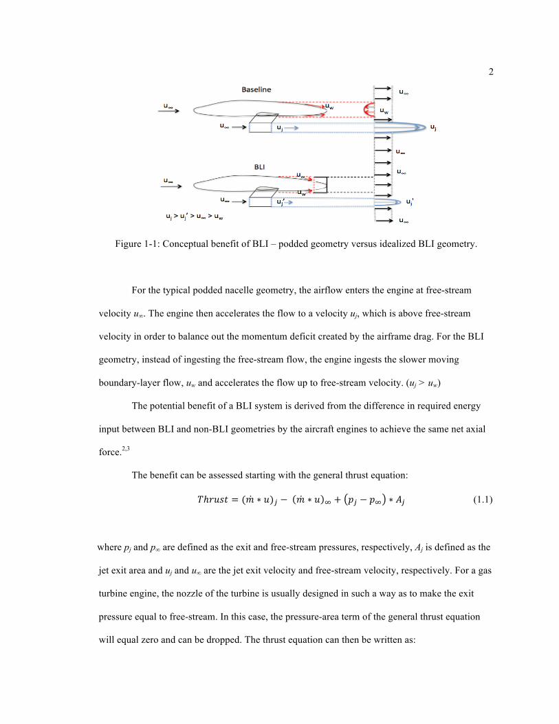
Figure 1-1: Conceptual benefit of BLI – podded geometry versus idealized BLI geometry.

For the typical podded nacelle geometry, the airflow enters the engine at free-stream

velocity u∞. The engine then accelerates the flow to a velocity uj, which is above free-stream

velocity in order to balance out the momentum deficit created by the airframe drag. For the BLI

geometry, instead of ingesting the free-stream flow, the engine ingests the slower moving

boundary-layer flow, uw and accelerates the flow up to free-stream velocity. (uj > uw)

The potential benefit of a BLI system is derived from the difference in required energy

input between BLI and non-BLI geometries by the aircraft engines to achieve the same net axial

force.2,3

The benefit can be assessed starting with the general thrust equation:

𝑇ℎ𝑟𝑢𝑠𝑡 = (𝑚 ∗ 𝑢)! −   𝑚 ∗ 𝑢 ! + 𝑝! − 𝑝! ∗ 𝐴! (1.1)

where pj and p∞ are defined as the exit and free-stream pressures, respectively, Aj is defined as the

jet exit area and uj and u∞ are the jet exit velocity and free-stream velocity, respectively. For a gas

turbine engine, the nozzle of the turbine is usually designed in such a way as to make the exit

pressure equal to free-stream. In this case, the pressure-area term of the general thrust equation

will equal zero and can be dropped. The thrust equation can then be written as:

3

𝑇ℎ𝑟𝑢𝑠𝑡 = 𝑇 = (𝑚 ∗ 𝑢)! −   𝑚 ∗ 𝑢 ! (1.2)

It can also be assumed that the exit mass flow rate is nearly equal to the free-stream mass flow

rate, although this assumption may not be perfectly accurate as fuel is added to the flow for

combustion, and bleed air is taken from the engines for use in other aircraft systems. From this,

Eq. 1.2 can be rewritten as follows:

𝑇 =  𝑚 ∗ 𝑢!   − 𝑢!   (1.3)

For cruise conditions, this total net axial force (thrust) is equal to the overall drag force of

the aircraft, DA. In addition, uw is defined as the flow velocity relative to the ingested wake.

𝑇 = 𝑚 ∗ 𝑢!   − 𝑢! =  𝑚 ∗ 𝑢! − 𝑢! =  𝐷! (1.4)

Next, the total energy added to the system, Emechanical is defined as the sum of potential

energy, U and kinetic energy, K.

𝐸!"#!!"#$!% = 𝑈 + 𝐾 (1.5)

Since there is no change in potential energy of the system, the total mechanical energy

added to the system is equal to the kinetic energy, K, added to the system by the engine, which

can then be written as:

𝐸!"#!!"#$!% = 𝐾 = !!∗𝑚 ∗ 𝑢! (1.6)

The total change in kinetic energy for the non-BLI case can then be written as the

difference between the free-stream velocity u∞, and the jet engine exit velocity, uj.

 𝐸!"#!!"#$!%,!""#" =  !!∗𝑚 ∗ 𝑢!! −  

!!∗𝑚 ∗ 𝑢!! =   !

!∗𝑚 ∗ 𝑢!! −  𝑢!! (1.7)

4

The rate at which this mechanical energy is added to the flow, P, can then be obtained by

substituting in mass flow rate, 𝑚.

𝑃!""#",!"!!!"# =  !!∗𝑚 ∗ 𝑢!! − 𝑢!! (1.8)

Equation 1.8 can be rewritten as:

𝑃!""#",!"!!!"# =!!∗𝑚 ∗ 𝑢! − 𝑢! ∗ 𝑢! + 𝑢! (1.9)

Substituting Eq. 1.3 in above, the rate at which mechanical energy is added to the non-BLI

system can be written as:

𝑃!""#",!"!!!"# =!!∗ (𝑢! + 𝑢!) (1.10)

The (useful) power required for flight is defined as:

𝑃!"#$%!"& = 𝐷! ∗ 𝑢! (1.11)

Substituting Eq. 1.4 for DA,

𝑃!"#$%!"& = 𝑚 ∗ 𝑢! − 𝑢! ∗ 𝑢! (1.12)

Now, for the BLI concept, the assumption that 100% of the boundary-layer is ingested by

the engine and accelerated back up to free-stream velocity is made. In addition, an assumption

that the non-BLI and BLI cases will have equivalent mass flow rates is made. This assumption

will be discussed in further detail in subsequent sections. The thrust provided by the BLI engine

can be written as:

𝑇ℎ𝑟𝑢𝑠𝑡 = 𝑚 ∗ 𝑢!   − 𝑢! =  𝑚 ∗ 𝑢! − 𝑢! =  𝐷! (1.13)

The rate of energy added to the flow by the BLI engine is:

5

               𝑃!""#",      !"# =  !!∗ 𝑢!! − 𝑢!! = !

!∗ 𝑢!! − 𝑢!! = !

!∗ (𝑢! + 𝑢!) (1.14)

The required power for flight for the BLI geometry is the same as for the podded nacelle:

𝑃!"#$%!"& = 𝐷! ∗ 𝑢! = 𝑚 ∗ 𝑢! − 𝑢! ∗ 𝑢! (1.15)

A comparison of Eq. (1.14) and (1.10) shows that:

!!∗ (𝑢! + 𝑢!)  <  

!!∗ (𝑢! + 𝑢!)       (1.16)

From this, it is evident that less propulsive power is required by the boundary-layer

ingestion geometry than the conventional geometry to maintain the same axial force and

assuming the same mass flow rate.

The difference in energy input between the BLI and non-BLI scenario arises due to the

fact that for a specific required force, less power needs to be added to a flow that enters the

engine at a lower velocity.

The assumption of equal mass flow rates for the BLI and non-BLI cases will not hold

when trying to directly compare a BLI propulsor to a propulsor in free-stream. The boundary-

layer flow will have a lower mass flow rate by virtue of its velocity being lower than that of the

free-stream flow. The assumption of equal mass flow rates is instead based on the notion that the

BLI propulsor will only be able to ingest a certain percentage of mass flow that the free-stream

propulsor can. This percentage of the free-stream mass flow rate is assumed to be the point of

comparison for the equal mass flow rate assumption in the equations above. For example, assume

that a free-stream propulsor has a mass flow rate of 20 kg/s but a BLI propulsor can ingest only 5

kg/s. The 5 kg/s is assumed to be the point of comparison for equal mass flow rates, ṁ, in the

equations above. This means that although the BLI propulsor can ingest only a portion of the

6

mass flow that the free-stream propulsor can, this smaller portion is used more efficiently in the

BLI case compared to the non-BLI case and results in a lower energy input for the BLI system to

produce the same amount of thrust as the non-BLI system. This will be discussed in further detail

in subsequent chapters.

Consider an engine where the flow enters at a velocity u1 and exits at a velocity u2. As

shown in Eq. 1.3, the thrust created by the engine is:

𝑇 = 𝑚Δ𝑢 =  𝑚 ∗ (𝑢! − 𝑢!) (1.17)

as in Eq. 1.8, the power added to the flow by the engine is:

𝑃!""#" =!!𝑢!! − 𝑢!! (1.18)

Substituting Eq. 1.17 in above yields:

𝑃!""#" = 𝑇 ∗ !!!!!!

= 𝑇 ∗ (𝑢! +!!!) (1.19)

From Eqs. 1.16 and 1.19, it can be seen that for a constant mass flow rate and desired propulsive

force, Δ𝑢 is constant. A decrease in the intake velocity, u1, which would be achieved by ingesting

the boundary-layer flow that is moving slower than the free-stream flow that an underwing engine

would see, results in a decrease in the amount of power that needs to be added to the flow by the

propulsion system in order to achieve that same desired propulsive force. It is important to note

however, that this analysis does not take into account various losses that would be expected due

to the non-uniform velocity distribution of the boundary-layer, various engine efficiencies (fan,

compressors, etc.) and increases in wetted area due to implementation of a BLI system.4

7

1.2 – Boundary-layer Ingestion Theory (Two-Dimensional)

Although the above assessment is quasi one-dimensional, it is possible to perform a more

rigorous analysis of BLI using a two-dimensional case.5, 6 First, a 2D body along with a control

volume is introduced with inlet and outlet planes perpendicular to the flow. The control volume is

assumed such that the static pressure of the boundary is equal to the ambient static pressure.

Figure 1-2: 2D Airframe with control volume.

A power balance method will be used for analysis. In this method, wake energy is

conserved and consists of two parts – the energy dissipated in the wake region and the kinetic

energy left in the exit plane shown as the dashed line behind the 2D body in Figure 1-2 above.

The momentum equation states that the defect calculated at the exit plane is equal to the

body profile drag of the 2D airframe.

𝐷 =   𝜌𝑢(𝑉!!!"#$ − 𝑢)𝑑𝑦 (1.20)

Within the control volume, this drag force should be balanced by a propulsive force. This

propulsive force is considered to be doing all of the work on the fluid inside the assumed control

volume and is the only energy input to the system. This input energy can be expressed as the

profile drag multiplied by the free-stream velocity.

𝐸!"#$% = 𝐷 ∗  𝑉! =  𝑉! 𝜌𝑢(𝑉!!!" − 𝑢)𝑑𝑦 (1.21)

8

The dissipation due to the boundary-layer can be expressed as the difference between the

free-stream kinetic energy at the inlet plane and the boundary-layer kinetic energy measured at

the exit plane.

𝜙!" =  !!∗ 𝜌𝑢 𝑉!! − 𝑢! 𝑑𝑦

!!"#$ (1.22)

In this system, the exit plane can be considered the end of the boundary-layer and the

beginning of the wake. The energy of this wake will be equal to the kinetic energy deposited in

the exit plane. Once past the exit plane, the wake velocity will eventually be increased until it

matches free-stream velocity due to the viscous force of the body wake. The kinetic energy,

which flows out of the control volume, will eventually dissipate in the far field. For the 2D case,

only the axial component of the wake and kinetic energy are involved.

𝐸!"#$,!"#$ = 𝐸!"#$,!"#$%"& =!!∗ 𝜌𝑢 𝑉! − 𝑢 !𝑑𝑦!

!"#$ (1.23)

where (V∞ - u) is the wake flow perturbation velocity. For the fluid inside the control volume, the

energy flux out is the wake kinetic energy.

The kinetic energy of the fluid inside the control volume can be expressed as the sum of

the boundary-layer dissipation, 𝜙!", and the energy flux out, 𝐸!"#$,!"#$:

𝐸!"#$%&'! =12∗ 𝜌𝑢 𝑉!! − 𝑢! +   𝑉! − 𝑢 !

!

!"#$𝑑𝑦

𝐸!"#$%&'( =   𝜌𝑢 𝑉!! − 𝑉! ∗ 𝑢 𝑑𝑦!!"#$ (1.24)

A comparison between the input energy, Einput, (Eq. 1.21) and the energy consumption, Econsumed,

(Eq. 1.24) shows that they are equivalent.

9

𝐸!"#$% = 𝑉! 𝜌𝑢(𝑉!!!"#$ − 𝑢)𝑑𝑦 =  𝐸!"#$%&'( =   𝜌𝑢 𝑉!! − 𝑉! ∗ 𝑢 𝑑𝑦!

!"#$ (1.25)

From this, it is evident that the boundary-layer dissipation and wake energy balance out the power

required to overcome the drag.6

𝐷 ∗ 𝑉! =  𝜙!" +  𝐸!"#$,!"#$ (1.26)

For the 2D BLI case, an ideal propulsor that is capable of perfectly filling in the wake

generated is introduced behind the airframe. The pressure field generated by this ‘ideal propulsor’

is assumed to be small enough so as not to interfere with the profile of the incoming boundary-

layer, although this assumption would not necessarily hold true for a real world application.

For analysis, a control volume is assumed to enclose the body of the aircraft as well as

the propulsor. Inside the control volume, an additional, mid-plane is generated and is chosen to be

between the airframe and propulsor in such a way that the trailing edge of the airframe or the

propulsor does not affect the local pressure distribution along this plane.

Figure 1-3: Control Volume for 2D BLI propulsor with mid-plane (Dashed line).

The only energy consumption inside this assumed control volume would be the dissipation inside

the boundary-layer, which is the kinetic energy loss between the free-stream flow at the inlet

plane and the loss from the boundary-layer flow at the mid-plane defined previously in Eq. 1.24

𝐸!"#$%&'( =  𝜙!" = 𝜌𝑢 𝑉!! − 𝑉! ∗ 𝑢 𝑑𝑦!!" (1.27)

10

The only kinetic energy input into this system will be from the propulsor, which ingests the BL

flow and accelerates it to free-stream velocity. This can be expressed as the difference between

the kinetic energy at the mid-plane and the measured kinetic energy of the boundary-layer flow.

𝐸!"#$% =  𝐸!"#!$%&#",!"# = 𝜌𝑢 𝑉!! − 𝑉! ∗ 𝑢 𝑑𝑦!!" (1.28)

Following the principle of conservation of energy for a finite control volume, the energy input by

the propulsor will balance out the dissipation of the boundary-layer.

𝐸!"#!$%&#",!"# =  𝜙!" (1.29)

Since this is an idealized case, it is assumed that the BLI propulsor is capable of perfect wake

filling, which means that the momentum of the control volume has a net zero balance.

The body drag of the 2D case can be defined as the momentum loss from the inlet plane

to the mid-plane, as described in Eq 1.20 previously.

𝐷 =   𝜌𝑢(𝑉!!!" − 𝑢)𝑑𝑦 (1.30)

This body drag is balanced by the propulsor thrust, which can be defined as the momentum

increase from the mid-plane to the outlet plane of the control volume.

𝑇 =   𝜌𝑢(𝑉!!!" − 𝑢)𝑑𝑦 (1.31)

The propulsive efficiency is defined as the thrust power (equal to drag power) divided by

the kinetic energy input into the system from the propulsor. From this definition, it is possible to

achieve a propulsive efficiency greater than 100%.

𝜂!"#$%&'#",!"# =!∗!!

!!"#$%&'#",!"#= !∗!!

!!"#$%&'#",!"#=  !!"!!!"#$,!"#$  

!!" (1.32)

11

1.3 – Boundary-layer Ingestion-Theory (Free-Stream/BLI Propulsor)

In addition to the quasi one-dimensional and two-dimensional assessments, a comparison

between a free-stream propulsor and an ideal BLI propulsor can be made. For the free-stream

propulsor, a 2D actuator disc is used as the propulsor. This disc is enclosed in a control volume

comprised of a streamtube, as well as inlet and outflow planes, as shown below:

Figure 1-4: Control volume for free-stream propulsor.

The only increase in kinetic energy in the control volume from the inlet to the outlet plane arises

from the work done by the actuator disc:

𝐸!"#$% = 𝐸!"#!$%&#" =!!∗ 𝜌𝑢 𝑢! − 𝑉!! 𝑑𝑦

!!"#$ (1.33)

The disc generates momentum excess (thrust) by accelerating the free-stream fluid in the control

volume. The thrust generated can be expressed as:

𝑇 =   𝜌𝑢(𝑉!!!"#$ − 𝑢)𝑑𝑦 (1.34)

The momentum excess generated is balanced by the energy output, thrust power.

𝑇 ∗ 𝑉! =  𝑉! 𝜌𝑢(𝑉!!!"#$ − 𝑢)𝑑𝑦 (1.35)

The kinetic energy of the propulsor is the same as described in Eq. 1.22. Since the viscous

dissipation is always positive and should bring the wake velocity to match the free-stream

12

velocity, it does not matter if the wake velocity is higher or lower than free-stream velocity. In

addition, the propulsor wake kinetic energy is the total flux out of the control volume.

𝐸!"#$,!"#!$%&#" = 𝐸!"#$,!"#$%"& =!!∗ 𝜌𝑢 𝑢 − 𝑉! !𝑑𝑦!

!"#$ (1.36)

Hence, the total energy out of the control volume will be the thrust power (Eq. 1.35) and the wake

kinetic energy (Eq. 1.36).

𝐸!"#,!"!#$   = 𝑇 ∗ 𝑉! + 𝐸!"#$,!"#!$%&#"

= 𝜌𝑢[𝑉! 𝑢 − 𝑉! + !!∗ 𝑢 − 𝑉! !]𝑑𝑦!

!"#$

= !!𝜌𝑢 𝑢! − 𝑉!! 𝑑𝑦

!!"#$ (1.37)

Comparing the energy input to the system from Eq. 1.33 to the total energy out of the control

volume, Eq. 1.37 it can be seen that the total amount of energy for the system is conserved.

In addition, the kinetic energy input to the system by the free-stream propulsor will be equal to

the thrust power and wake kinetic energy of the propulsor

𝐸!"#!$%&#",!"##$%"#&' = 𝑇 ∗ 𝑉! + 𝐸!"#$,!"#!$%&#" (1.38)

The propulsive efficiency of the free-stream propulsor can then be expressed as the thrust

power divided by the total energy input:

𝜂!"#!$%&#",!"##$%"#&' = !∗!!!!"#$%&'#",!"##$%"&#'

= !∗!!!∗!!!!!"#$,!"#!$%&#"

(1.39)

which shows that the propulsive efficiency of a free-stream propulsor is always less than one.

For the ideal BLI propulsor, a similar control volume as in the free-stream propulsor is

established. However, instead of free-stream fluid as the input to the case of the control volume, a

13

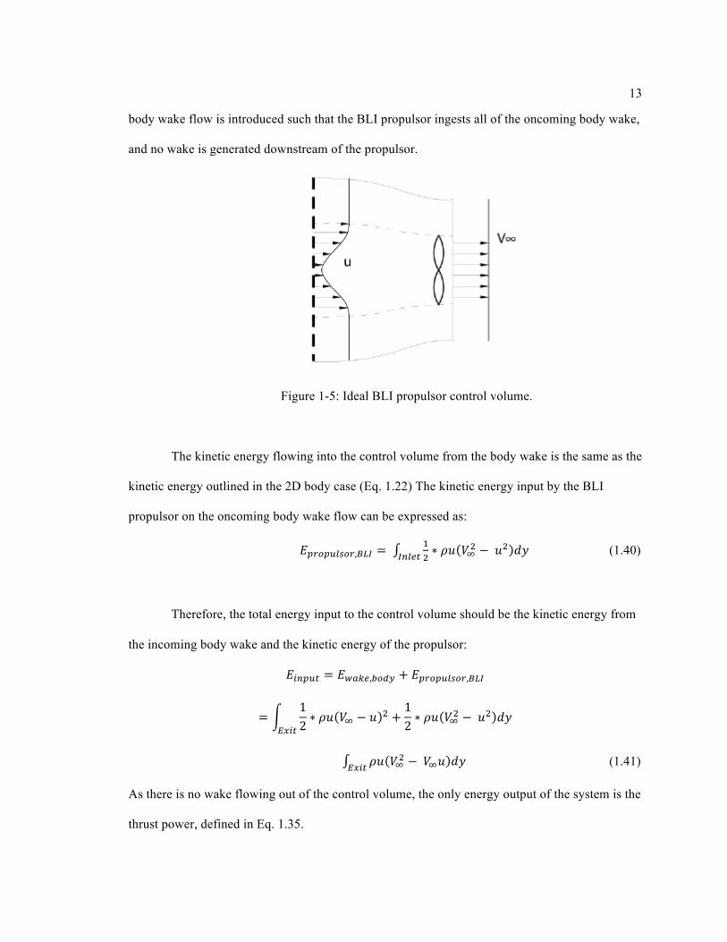
body wake flow is introduced such that the BLI propulsor ingests all of the oncoming body wake,

and no wake is generated downstream of the propulsor.

Figure 1-5: Ideal BLI propulsor control volume.

The kinetic energy flowing into the control volume from the body wake is the same as the

kinetic energy outlined in the 2D body case (Eq. 1.22) The kinetic energy input by the BLI

propulsor on the oncoming body wake flow can be expressed as:

𝐸!"#!$%&#",!"# =  !!∗ 𝜌𝑢 𝑉!! −  𝑢! 𝑑𝑦

!!"#$% (1.40)

Therefore, the total energy input to the control volume should be the kinetic energy from

the incoming body wake and the kinetic energy of the propulsor:

𝐸!"#$% = 𝐸!"#$,!"#$ + 𝐸!"#!$%&#",!"#

=12∗ 𝜌𝑢 𝑉! − 𝑢 ! +

12∗ 𝜌𝑢 𝑉!! −  𝑢! 𝑑𝑦

!

!"#$

𝜌𝑢 𝑉!! −  𝑉!𝑢 𝑑𝑦!!"#$ (1.41)

As there is no wake flowing out of the control volume, the only energy output of the system is the

thrust power, defined in Eq. 1.35.

14

Comparing the energy input into the system in Eq. 1.33 and the energy output in Eq.

1.35, it is evident that conservation of energy is satisfied, and the energy for a BLI propulsor can

be summed as follows:

𝐸!"#$,!"#$ + 𝐸!"#!$%&#",!"# = 𝐸!"#$"# = 𝑇 ∗ 𝑉! (1.42)

The efficiency of the BLI propulsor can be written as the ratio of output energy to input energy.

𝜂!"#!$%&#",!"# =!∗!!

!!"#$%&'#",!"#= !!"#$,!"#$!!!"#!$%&#",!!"

!!"#$%&'#",!"# (1.43)

From Eq. 1.43 it is evident that the BLI propulsor has a higher efficiency than that of a

free-stream propulsor (Eq. 1.39).

There are several key differences between the free-stream propulsor case and the BLI

propulsor. The BLI propulsor generates thrust through momentum deficit cancellation from the

incoming boundary-layer or wake. The free-stream propulsor, on the other hand, generates

momentum excess by accelerating the free-stream fluid. If the BLI propulsor were not present,

the momentum deficit that arises from the body wake would be reduced by the viscous

dissipation by the ambient pressure. However, the BLI propulsor is able to recover the generated

momentum deficit immediately by pressure work. In essence, for the free-stream propulsor, only

the energy input by the propulsor contributes to overall thrust, while for a BLI propulsor, both the

body wake that is generated before the propulsor as well as the energy input to the flow by the

propulsor contribute to overall thrust and therefore an overall higher propulsive efficiency.

15

1.4 - Podded Engine vs. Embedded Engine

In order to ingest the developing boundary-layer, it is necessary to embed the engines

within the actual airframe. While this configuration is necessary to study and potentially

implement the boundary-layer ingestion concept, several design considerations need to be taken

into account when comparing the embedded engine to podded nacelle design.

One of the most obvious advantages to embedding the engines is the reduction of the

overall size of the underwing engine and nacelle. By reducing the wetted area of the underwing

nacelle and engine, it is possible to achieve a reduction in drag and therefore a reduction in power

required for the aircraft. However, it is important to note that it may be necessary to increase the

size of the fuselage to house the engine – this potential increase in fuselage size could offset or

even outweigh any reduction in wetted area achieved through sizing down the underwing nacelle.

Sizing down the external nacelle and engine could allow for a reduced overall aircraft weight as

well. However, again this benefit could potentially be negated by additional structures needed to

support the embedded engine. Another possible advantage of the embedded engine design is that

reducing the size and weight of the hanging podded engines while simultaneously adding an

engine in the tail section of the fuselage can help to minimize the downward pitching moment

associated with having the engines forward of the center of gravity. Finally, embedded engines

offer the ability to reduce the overall noise of the aircraft.7

It is important to keep in mind the disadvantages associated with embedding the engine

within the airframe as well. The first drawback is that while there is ongoing research in the area,

boundary-layer ingestion is still an unproven technology. The second disadvantage relates

primarily to the efficiency of the boundary-layer ingestion system – the potential for non-uniform

flow at the inlet and fan face. The non-uniform flow could impact overall engine efficiency and

lead to a decrease in performance, which may outweigh the potential benefits of the BLI system.

16

Depending on the geometry of the inlet duct, boundary-layer separation and secondary flows are

also distinct possibilities. In addition, fan face distortion may lead to a degradation of engine

performance, vibration, and structural issues.8, 9 Another disadvantage of the embedded engine

design is that the airframe and engine designs become much more integrated and more

complicated as changing one significantly would affect the other. The embedded design also

could mean increased difficulty in maintaining and servicing the engine as compared to a podded

counterpart. Table 2-1 shows a summary of the advantages and disadvantages associated with

each engine design type.

Figure 1-6: Comparison of podded and embedded engines.

17

1.5 – Objectives and Thesis Scope

The main objective of this thesis is to computationally verify if there is any benefit in

terms of reduced propulsive power requirements and drag reduction to be gained from

implementing BLI on a conventional commercial aircraft geometry, as well as to quantify and

make a 1st round attempt to improve on any such benefit. The principle success criteria for this

work will be to determine whether such a system might yield a net aerodynamic or propulsive

benefit and whether this topic warrants additional study.

The next chapter will discuss previous work and published literature in the area of

boundary-layer ingestion as it applies to aircraft, along with potential issues. The Common

Research Model (CRM) geometry will be introduced and methodology used to determine

potential BLI benefit will be examined. Chapter 3 will highlight the software packages used in

this study. Chapter 4 will present a code validation and discuss engine model generation. Chapter

5 will present baseline results and BLI implementation. Chapter 6 will present results for the BLI

geometries. Chapter 7 will present conclusions and recommendations for potential future work.

18

Chapter 2 – Research Focus

2.1 – Previous Studies

The concept of boundary-layer ingestion has been around for several decades, with the

first works published in the mid 1940s. In one of these early studies, Smith and Roberts10

examined an aircraft that used suction slots located along the wing and fuselage to ingest the

boundary-layer in order to prevent or delay turbulent transition. In his study, Smith compared

three engine configurations for the aircraft: a turbojet engine with boundary-layer suction, a

turbojet, and a turboprop engine. Smith and Robert’s tests showed that the engine, which included

boundary-layer ingestion had a reduced fuel consumption of almost 33 percent as well as

increased CL and L/D compared to the turbojet without boundary-layer ingestion for the same

aircraft.

In the 1980s, Goldschmied11 designed a small integrated, self-propelled wind-tunnel

model using a concept referred to as the Goldschmied propulsor. This propulsor included a slot

around the aft portion of the geometry to allow for boundary-layer ingestion. Wind-tunnel testing

was conducted with this model, both in an unpowered and boundary-layer ingesting

configuration. Using the data collected from the wind tunnel, Goldschmied was able to show that

ingesting the boundary-layer allowed for a propulsion power reduction of 50 percent over the

unpowered configuration. However, recently an attempt to recreate these wind tunnel test results

for propulsion power reduction at the California Polytechnic State University wind-tunnel using a

Goldschmied propulsor proved unsuccessful.12

In the 1970s, Douglas13 conducted a study of aircraft with and without boundary-layer

ingestion. Although Douglas made some assumptions about the compressibility of the flow, inlet

losses and the conditions at which it entered the engine, he was able to show that the boundary-

19

layer ingestion resulted in a reduction of the kinetic energy of the wake and the jet, resulting in a

propulsive efficiency improvement of 16 percent over the non-ingesting aircraft.

More recent studies have combined boundary-layer ingestion technology with blended

wing body (BWB) geometry configurations in order to reduce specific fuel consumption for the

aircraft.14,15,16 These studies all show a reduction in the mechanical power required by the

propulsor as compared to a typical podded nacelle configuration.

A recent experimental investigation conducted by Drela into the merits of boundary-layer

ingestion using an electric ducted fan propulsor mounted behind an NACA 0040 body of

revolution showed a power savings benefit of 25 percent over the baseline, non boundary-layer

ingesting case.17

There have also been several studies focused on assessing and reducing flow distortions

at the fan inlet face, which could effect engine efficiency and therefore overall performance of a

boundary-layer ingesting system.15, 18, 19 However, this study will focus on quantifying the

aerodynamic benefit of BLI for the CRM geometry rather than BLI effects on engine

performance.

2.2 – The Common Research Model

The baseline geometry used for the purposes of this study will be the Common Research

Model (CRM). The Common Research Model was developed by a consortium of both public and

private sector groups including, but not limited to, Boeing, Cessna, JAXA (Japan Aerospace

Exploration Agency) and DLR (German Aerospace Center), in conjunction with NASA in order

to help develop computational fluid dynamic (CFD) applications and validate their results.

The Common Research Model geometry itself is representative of a typical transonic

transportation aircraft designed to fly at a cruise Mach number of M=0.85 with a nominal lift

20

coefficient of CL=0.50, a Reynolds number of Re=40 million per reference chord, and an aspect-

ratio of AR=9.0. The geometry and data, including all wind-tunnel tests and CFD results

associated with the Common Research Model, are all open-source and available to the public.20

Table 2-1: Reference quantities for CRM geometry

Sref 594,720.0 in2 Trap-Wing Area 576,000.0 in2

Cref 275.80 in Span 2313.50 in Xref 1325.90 in Yref 468.75 in Zref 177.95 in Λ 0.275

AR 9

The most recent baseline CRM geometry consists of a tube-like body, wing, nacelle,

pylon, and horizontal tail. However, there are various configurations of the CRM geometry

available, which do not include some of these features.21

Figure 2-1: Full Common Research Model geometry.

For the purposes of this study, a semi-span geometry consisting of the aircraft fuselage,

wing, underwing nacelle, and horizontal tail will be used. A semi-span model will be used in

21

order to save computational resources. The boundary-layer ingesting system will be placed aft of

the horizontal tail. At this time, the underwing nacelle on the CRM is flow through only and does

not have any internal engine geometry. It is possible to use a simple inflow and outflow plane to

model the underwing engine, however, a more robust internal engine geometry will be added in

order to allow for a more accurate and realistic representation of engine power requirements and

assessment of BLI. These changes will be discussed in detail in the following chapters.

Figure 2-2: Baseline Common Research Model with internal engine geometry.

2.3 – Assessing the BLI Benefit

To assess the potential benefit of BLI, the baseline geometry with only underwing

engines will be compared to the integrated BLI geometry. Computations will be performed for

both the baseline and BLI geometries and compared to determine potential BLI benefit. This

potential benefit will be assessed via a power balance method outlined by Drela.22

For this method, the benefit of BLI will be derived from reducing the power dissipation

in the overall flow field by reducing stream-wise velocities and wasted kinetic energy left by the

aircraft. This is accomplished by filling in the wake generated by the airframe with the BLI

propulsor, as shown in Figure 1-1. This power balance method allows for the unification of

22

boundary-layer losses and propulsor losses of the aircraft rather than attempting to tediously

separate out the thrust and drag forces on the aircraft. The potential benefit of a BLI system is

likely to be affected by the fan performance of the engine due to distorted flow at the inlet of the

propulsor. Drela’s power balance method allows for the separation of the fan efficiency from the

propulsive efficiency of the aircraft, allowing for an easier assessment of potential benefit.

There are three sources of mechanical power within a flow field as outlined by Drela: Pk,

which is the net mechanical power across the propulsor inflow and outflow faces, Ps, which is

shaft power from moving surfaces, and Pv, which is the power due to volumetric work within a

flow field. For a control volume encompassing the propulsor and in the low-speed case, the only

flow field power source left is Pk, which can be defined as the volume flux of total pressure

across the inflow and outflow faces of the engine

𝑃! = 𝑝!! − 𝑝!  𝑉   ∙ 𝑛  𝑑𝑆 (2.1)

where p0 is the stagnation pressure at the engine face, p0∞ is the free-stream stagnation pressure, V

is the inlet velocity at the propulsor face, and 𝑛 is the vector normal to the fan face. The area

integral is taken over both inflow and outflow propulsor planes, so Pk is a measure of net engine

flow power while internal propulsor losses are irrelevant, allowing the engine fan efficiency to be

separated from the aerodynamics of the BLI geometry.15

Since thrust and drag forces are difficult to separate out for a BLI system, the net stream-

wise force, Fx, will be used to aid in the analysis. A non-dimensional net stream-wise force

coefficient, Cx, will also be defined as follows.

𝐶! =!!

!!!!"# (2.2)

where q∞ is the free-stream dynamic pressure and Sref is the reference area of the geometry.

𝐶!! =!!

!!!!!!"# (2.3)

23

As Sref may change between geometry iterations, a dimensionless net propulsor power coefficient,

Cpk, is defined to allow for effective comparison between non-BLI and BLI geometries using the

net mechanical power, Pk defined previously in Eq. 2.1.

The aerodynamic benefit of the BLI system can be expressed as follows:

𝐵𝐿𝐼  𝑏𝑒𝑛𝑒𝑓𝑖𝑡 =(!!!)  !"!!!"#!  (!!!)  !"#

(!!!)  !"!!!"# (2.4)

2.4 – Methodology Overview

In order to determine the aerodynamic effects and potential benefits of a boundary-layer

ingestion system on the Common Research Model (CRM), several different iterations of the

CRM geometry were used. The baseline geometry consists of an unaltered semi-span CRM

geometry incorporating an underwing nacelle with added internal engine geometry, as shown in

Figure 2-2. Unstructured viscous grids were generated using NASA Langley’s GridTool and

VGrid grid generation packages. The Numerical Propulsion System Simulation (NPSS) software

was used to simulate an engine cycle similar to that of the GE90-115B gas turbine engine at

cruise conditions using publicly available data. This engine simulation was used to determine the

engine inlet and exit boundary conditions for the underwing nacelle. USM3D was used as the

flow solver. Each geometry was run for a total of 25,000 iterations on the NASA Pleiades

supercomputer in order to ensure solution convergence. The model was run at cruise conditions

of Mach 0.85 and an altitude of 38500 feet with 2° angle of attack and no sideslip. As outlined

previously, net propulsor power and net horizontal force coefficients were calculated.

After the baseline run and calculations were completed, the CRM geometry was altered

to incorporate the BLI system. For this, an actuator disc was placed at the approximate fan

location on the empennage of the fuselage to represent the BLI system. The rest of the geometry,

24

including underwing nacelle remained unchanged. The same cruise conditions outlined above

were used and once again the net propulsor power, net horizontal force, and drag coefficients

were calculated.

Once the first BLI run was completed, the BLI integrated geometry was modified slightly

in an attempt to eliminate unwanted flow conditions and to optimize potential benefits of the

system. The exact changes to the geometry are discussed in detail in later sections. These changes

to the BLI geometric design were made using the Constrained Direct Iterative Surface Curvature

(CDISC) design method, which will also be discussed in subsequent sections.

Once all of the simulations were completed, any aerodynamic or propulsive power

savings benefit from the BLI system as compared to the non-BLI configuration was determined.

An assessment of the boundary-layer ingestion concept for this application was made and future

work recommended.

2.5 – Methodology for Comparison of Non-BLI and BLI Geometries

For an equivalent mass flow rate, it has been shown in Section 1-1, that a BLI system

requires less propulsive power than a conventional non-BLI system to achieve the same desired

axial force. However, since the BLI system by definition ingests the slower moving boundary-

layer air, it is difficult and impractical to actually design the BLI system in such a way as to have

the same mass flow rate as that of an underwing engine. Instead, the BLI system will be

constrained so as to ingest only the mass flow present in the developing boundary-layer and

accelerate it up to free-stream velocity as a way to supplement thrust generated by the underwing

engines instead of attempting to replace them. This has several implications: 1) A portion of the

overall required thrust for cruise will now be produced more efficiently by the BLI system

compared to the underwing engine. 2) The underwing engine now needs to produce less thrust

25

overall since the BLI system is contributing a portion of the total thrust required, which should

reduce the amount of propulsive power required by the underwing engine. 3) Since the BLI

system is accelerating and ingesting the boundary-layer, there should be some benefit in terms of

reduced drag on the fuselage that would not be present in a conventional propulsive system,

although this will likely be dependent on the actual geometry alterations made to incorporate the

BLI system.

In order to fairly compare the required propulsive power for the BLI and non-BLI

systems at cruise, the net axial force coefficient, CX, will be constrained to be zero for all

configurations. CX is computed by summing the axial component of the integrated pressure and

viscous forces on all airframe surfaces. The BLI engine will be modeled to ingest the developing

boundary-layer and accelerate it up to free-stream velocity, while the underwing engine will be

modeled using the parameters derived from the NPSS model and adjusted accordingly in order to

achieve a zero net axial force for the aircraft.

26

Chapter 3 – Software Packages

3.1 – Grid Generation: GridTool and VGrid

The surface triangulations along with the field tetrahedral volume grids were generated

using the GridTool and VGrid software developed at NASA Langley Research Center.23 VGrid is

a fully functional, user oriented unstructured grid generator created by NASA Langley Research

Center in conjunction with the private company, ViGYAN, in order to make grid generation

around complex geometries easier and less time consuming.

In order to use VGrid and create the grid required for flow analysis, it is first necessary to

provide VGrid with a complete and accurate surface geometry definition. This is done through

the use of GridTool. GridTool serves as a connection between Computer Aided Design (CAD)

software, such as Solidworks or CATIA, and grid generation software such as VGrid.24

Once a CAD geometry has been created, it is uploaded to GridTool in the form of an

IGES file where the user specifies curves along the geometry. These curves are connected and

turned into surface patches that define the solid boundary of the geometry. Source terms are

added as well in order to provide VGrid with starting information for grid generation. These

source terms can be placed anywhere, allowing the user to focus grid growth in specific areas of

interest.25

27

Figure 3-1: GridTool surface definition of baseline Common Research Model.

Once the geometry has been defined and sources have been placed in GridTool, VGrid

takes the completed file package and uses it as a basis for the unstructured advancing front grid

generation. First, VGrid creates a surface mesh based on the surface patches and sources that the

user defined previously.

Figure 3-2: VGrid surface mesh of original Common Research Model geometry.

Once the surface mesh has been generated, VGrid begins the advancing front grid

generation at the sources defined previously. These sources can be considered simple heat

28

sources. VGrid solves the heat equation using a Gauss-Seidel method to iteratively determine grid

growth and spatial variation of the cells.26 As soon as one layer is complete, the next layer is

calculated, and this process continues until the entire domain is complete. VGrid also easily

allows users to specify whether the generated grid will include viscous layers or be completely

inviscid. For viscous grid generation - as was used in this study, VGrid uniformly covers the

geometry with an automatically calculated amount of viscous cell layers based on geometry

complexity.

Figure 3-3: VGrid grid growth of original Common Research Model.

After grid generation is complete, the file packages are saved and can be uploaded to the

desired flow solver. For this work, a rectangular box that encompasses the vehicle was used to

define the computational far-field domain boundaries. Each face of this rectangular box is located

several body lengths away from the configuration in the upstream, radial, and downstream

directions. As a general practice, each final converged solution is analyzed to ensure that the

viscous sub-layer has been grid resolved and that average y+, the non-dimensional wall distance is

less than 1. Each grid for the study consists of approximately 49.8 million cells.

29

3.2 – Flow solver - USM3D

There are a wide variety of flow solvers available, commercially and non-commercially,

each with varying features, advantages, and drawbacks depending on desired application. For the

purposes of this study, USM3D will be used. USM3D is the flow solver portion of the TetrUSS

(Tetrahedral Unstructured Software System) package that also includes GridTool and VGrid,

which have been discussed previously.

USM3D is a tetrahedral cell-centered, finite volume Euler and Navier-Stokes flow solver

capable of both viscous and inviscid calculations.27 USM3D uses Roe’s flux-difference splitting

to compute inviscid flux quantities across the faces of the tetrahedral cells generated in VGrid.28

The flow solver features a number of turbulence models including Spalart-Allmaras, k-epsilon,

and sheer stress transport (SST), and can be used with static and dynamic structured,

unstructured, and chimera grids. Time integration follows the implicit point Gauss-Seidel

algorithm, explicit Runge-Kutta approach and local time stepping for convergence acceleration.29

For the purposes of this study, Roe’s flux-difference splitting (FDS) method along with the

Spalart-Allmaras turbulence model with no flux limiter were used.

3.3 – Numerical Propulsion System Simulation - NPSS

The Numerical Propulsion System Simulation (NPSS) was developed at NASA Glenn

Research Center in conjunction with other federal agencies and private industry partners with the

goal of increasing confidence in propulsion system design through the use of advanced, validated

computational models of fluid mechanics, combustion, structural mechanics, controls, materials,

and manufacturing processes.

30

NPSS is a component-based, object-oriented, engine cycle simulator capable of

simulating the aerothermodynamic cycle for gas turbines and other complex systems. The system

uses a linked building block approach to define system configurations, which allow for single and

multi-point design as well as steady-state and transient analysis. NPSS focuses on the integration

of aerodynamics, structures, and heat transfer along with the concept of numerical zooming

between zero-dimensional, one, two and three-dimensional engine codes.30, 31, 32 An engine model

similar to the GE90-115B, the PAX30033, 34, 35 is used to generate the engine conditions for use in

CFD analyses.

3.4 – Constrained Direct Iterative Surface Curvature (CDISC)

The Constrained Direct Iterative Surface Curvature (CDISC) software package is a

knowledge-based inverse design approach. Geometry and flow information from a preliminary

analysis is passed from the flow solver to the CDISC module. Surface coordinates and pressure

coefficients are extracted from the initial analysis. Specific design areas (e.g., a portion of the

wing, an area of the fuselage) as well as target pressures, flow, and geometry constraints for these

areas are designated by the user. CDISC iteratively alters the surface geometry in an attempt to

match the surface pressures in the design areas to the target pressures prescribed by the user.

Once the surface geometry is altered, the volume grid is then modified based on the surface

geometry changes and input back into the flow solver for further analysis. This iterative process

repeats until the extracted surface pressures match input target pressures.36

31

Figure 3-4: CDISC system flow chart.

32

Chapter 4 – USM3D Code Validation

4.1 – Wind-Tunnel Testing

In order to determine the validity of the computational results pertaining to potential

benefits of BLI using the CRM with added internal engine geometry obtained for this study, it is

first necessary to compare computational results for the CRM unaltered geometry to previous

computational results and available wind-tunnel test data. Previous experimental investigations

using a variant of the CRM geometry with no underwing nacelle have been completed at the

NASA Langley National Transonic Facility (NTF) as part of the Drag Prediction Workshop

(DPW) series.37 The data obtained through these experimental investigations are available online

as part of the Common Research Model project38 and will be used for CFD verification.

Figure 4-1: Aerial View of the National Transonic Facility.

33

The National Transonic Facility, shown in Fig. 4-1 is the world’s largest pressurized

cryogenic wind tunnel and provides the highest transonic Reynolds number testing capability in

the world. Fig. 4-2 shows a schematic of the NTF tunnel circuit. The NTF is a closed circuit, fan-

driven, continuous flow wind tunnel, which allows for testing of aircraft geometries at conditions

ranging from subsonic through supersonic speeds, using either air at ambient conditions or

gaseous nitrogen at temperatures as low as -260°F. The test section is 8.2 ft by 8.2 ft by 25 ft with

a slotted ceiling and floor. The facility can operate at pressures ranging from 15 to 125 psia and a

Mach number of 0.2 to 1.2. The tunnel has a maximum Reynolds number of 146 x 106 at Mach

1.39, 40, 41

Figure 4-2: Sketch of NTF Tunnel Circuit (Dimensions in Feet).

Several different configurations of the CRM model were tested in the NTF tunnel. For

the purposes of this verification, the CRM wing/body/tail geometry was used. As stated earlier,

34

the CRM is designed for a cruise Mach number of 0.85 with a CL of 0.5. The wind tunnel model

has an aspect ratio of 9.0, a leading edge sweep of 35 degrees, a wing reference area of 3.01 ft2

and wing span of 62.47 in2 with a mean aerodynamic chord of 7.45 inches. The model was

mounted in the tunnel using a blade sting arrangement as shown in Figure 4-3.37

Figure 4-3: Photo of the Common Research Model in the National Transonic Facility.

Testing was conducted at Reynolds numbers of 5, 19.8 and 30 million based on mean

aerodynamic chord. Temperatures ranged from -250°F to 120°F with free-stream Mach numbers

ranging from 0.7 to 0.87. Data was collected over an angle-of-attack range of -3° to 12° for

Reynolds number of 5 million and -3° to 6° for Reynolds numbers of 19.8 and 30 million. The

reduced angle-of-attack range for the higher Reynolds number tests were to ensure model and

balance stresses would not exceed prescribed safety values. In addition, flow angularity

measurements were made and upflow corrections ranging from 0.092° to 0.173° were applied to

the final data along with corrections for wall interference, tunnel buoyancy, lift interference, and

model blockage. Lastly, a video model deformation measurement technique previously employed

at the NTF42 was used to determine wing twist and deflection due to aerodynamic loading.

35

4.2 – USM3D Code Validation – Computational Methods

The GridTool and VGRID software packages43 were used to generate an unstructured

tetrahedral grid for the wing/body/tail CRM geometry. VGrid uses an advancing-front method for

generating Euler tetrahedral grids and an advancing layer method for thin-layer viscous grid

generation for Navier-Stokes analysis. Geometry boundaries for the model are defined as a

combination of an IGES file model geometry and bi-linear surface patches, which are user-

specified in GridTool. Specific grid variables such as grid spacing, cell stretching, and minimum

angle are also defined by the user in GridTool via placement of a combination of volume, nodal,

and linear sources.

The surface mesh generated in VGRID is created through the triangulation of the user-

defined surface patches with a two-dimensional version of the advancing front method. This

surface mesh is then used as the initial front for the tetrahedral volume grid generation.

The surface mesh for the baseline geometry consisted of a total of 65 surface patches

with a volume grid size of approximately 26.2 million unstructured tetrahedral cells with a y+

value < 1. The computational domain extended roughly 10 body lengths from the airframe in all

directions.

USM3D was used for computational analysis. Roe’s flux-difference splitting44 was used

to compute the inviscid flux quantities across each cell face. The one-equation Spalart-Altmaras

model45 was used for turbulence modeling. Steady-state solutions were achieved using an implicit

backward-Euler time-stepping scheme.46 A total of twenty-five thousand iterations were run. The

computational model used first-order spatial accuracy for the first five thousand iterations in

order to overcome any initial transients in the model and second-order accuracy for the final

twenty thousand iterations. Simulations were run over a range of angles of attack from 0° to 5° at

a Reynolds number of 5 million based on mean aerodynamic chord (7.45 inches). A symmetry

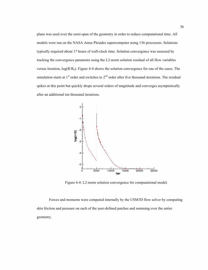
36

plane was used over the semi-span of the geometry in order to reduce computational time. All

models were run on the NASA Ames Pleiades supercomputer using 136 processors. Solutions

typically required about 17 hours of wall-clock time. Solution convergence was assessed by

tracking the convergence parameter using the L2-norm solution residual of all flow variables

versus iteration, log(R/R0). Figure 4-4 shows the solution convergence for one of the cases. The

simulation starts at 1st order and switches to 2nd order after five thousand iterations. The residual

spikes at this point but quickly drops several orders of magnitude and converges asymptotically

after an additional ten thousand iterations.

Figure 4-4: L2-norm solution convergence for computational model.

Forces and moments were computed internally by the USM3D flow solver by computing

skin friction and pressure on each of the user-defined patches and summing over the entire

geometry.

37

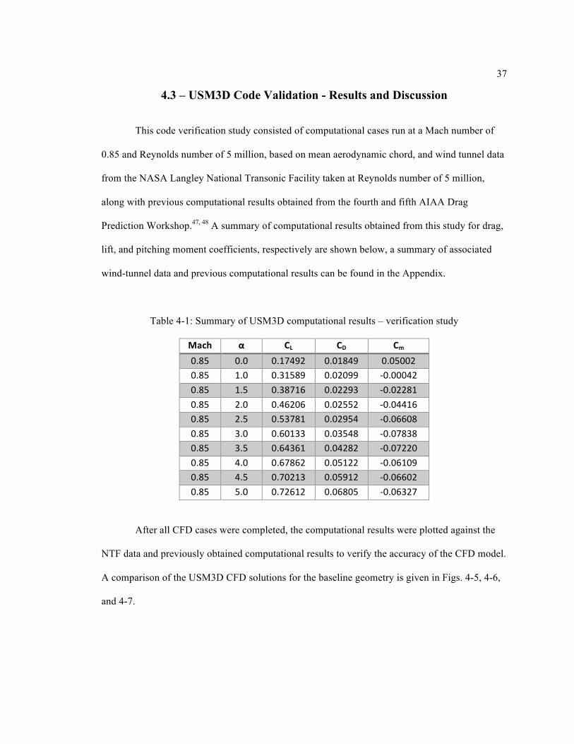
4.3 – USM3D Code Validation - Results and Discussion

This code verification study consisted of computational cases run at a Mach number of

0.85 and Reynolds number of 5 million, based on mean aerodynamic chord, and wind tunnel data

from the NASA Langley National Transonic Facility taken at Reynolds number of 5 million,

along with previous computational results obtained from the fourth and fifth AIAA Drag

Prediction Workshop.47, 48 A summary of computational results obtained from this study for drag,

lift, and pitching moment coefficients, respectively are shown below, a summary of associated

wind-tunnel data and previous computational results can be found in the Appendix.

Table 4-1: Summary of USM3D computational results – verification study

Mach   α   CL   CD   Cm  0.85   0.0   0.17492   0.01849   0.05002  0.85   1.0   0.31589   0.02099   -­‐0.00042  0.85   1.5   0.38716   0.02293   -­‐0.02281  0.85   2.0   0.46206   0.02552   -­‐0.04416  0.85   2.5   0.53781   0.02954   -­‐0.06608  0.85   3.0   0.60133   0.03548   -­‐0.07838  0.85   3.5   0.64361   0.04282   -­‐0.07220  0.85   4.0   0.67862   0.05122   -­‐0.06109  0.85   4.5   0.70213   0.05912   -­‐0.06602  0.85   5.0   0.72612   0.06805   -­‐0.06327  

After all CFD cases were completed, the computational results were plotted against the

NTF data and previously obtained computational results to verify the accuracy of the CFD model.

A comparison of the USM3D CFD solutions for the baseline geometry is given in Figs. 4-5, 4-6,

and 4-7.

38

Figure 4-5: Comparison of USM3D results and NTF data for CD, at Re=5 million, M=0.85.

Figure 4-6: Comparison of USM3D results and NTF data for CL, at Re=5 million, M=0.85.

−2 −1 0 1 2 3 4 5 60.01

0.02

0.03

0.04

0.05

0.06

0.07CD vs Alpha − Current and Previous USM3D Results & NTF Wind Tunnel Data Comparison

Alpha, degrees

CD −

Dra

g co

effic

ient

Current USM3DPrevious USM3D − OriginalT197R223T197R212T197R106

−2 −1 0 1 2 3 4 5 6−0.2

−0.1

0

0.1

0.2

0.3

0.4

0.5

0.6

0.7

0.8CL vs Alpha − Current and Previous USM3D Results & NTF Wind Tunnel Data Comparison

Alpha, degrees

CL −

Lift

coef

ficie

nt

Current USM3DPrevious USM3D − OriginalT197R223T197R212T197R106

39

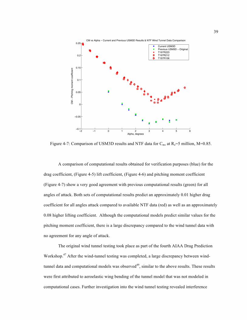
Figure 4-7: Comparison of USM3D results and NTF data for Cm, at Re=5 million, M=0.85.

A comparison of computational results obtained for verification purposes (blue) for the

drag coefficient, (Figure 4-5) lift coefficient, (Figure 4-6) and pitching moment coefficient

(Figure 4-7) show a very good agreement with previous computational results (green) for all

angles of attack. Both sets of computational results predict an approximately 0.01 higher drag

coefficient for all angles attack compared to available NTF data (red) as well as an approximately

0.08 higher lifting coefficient. Although the computational models predict similar values for the

pitching moment coefficient, there is a large discrepancy compared to the wind tunnel data with

no agreement for any angle of attack.

The original wind tunnel testing took place as part of the fourth AIAA Drag Prediction

Workshop.47 After the wind-tunnel testing was completed, a large discrepancy between wind-

tunnel data and computational models was observed49, similar to the above results. These results

were first attributed to aeroelastic wing bending of the tunnel model that was not modeled in

computational cases. Further investigation into the wind tunnel testing revealed interference

−2 −1 0 1 2 3 4 5 6−0.1

−0.05

0

0.05

0.1

0.15

0.2

0.25CM vs Alpha − Current and Previous USM3D Results & NTF Wind Tunnel Data Comparison

Alpha, degrees

CM

− P

itchi

ng m

omen

t coe

ffici

ent

Current USM3DPrevious USM3D − OriginalT197R223T197R212T197R106

40

effects from the wind tunnel support system as at least part of the reason for the discrepancy,

especially in the pitching moment coefficient.47, 48, 49

Overall, apart from the pitching moment coefficient results, there is a decent agreement

between the computational results and available wind tunnel data. As such, the computational

results obtained in this study are considered to be validated against CFD results obtained during

the Drag Prediction Workshop.

4.4 – Engine Model Generation - Underwing

In order to determine the existence of, and quantify any potential benefit that might arise

through the use of BLI, it is necessary to develop a working engine model for the underwing

engine. USM3D allows for the modeling of jet engines through the use of inflow, core outflow,

and fan bypass outflow boundary conditions defined on the solid model geometry before grid

generation. As the CRM model currently uses flow through nacelles and does not have any

engine geometry, a model based on publically available engine geometry for the GE90-115B, the

PAX300 will be added to the CRM underwing nacelle. 32

The internal engine geometry will consist of an inlet hub, inflow plane (green), core exit

(red), bypass fan exit (yellow) and plug sections as shown in Figure 4-8 below.

Figure 4-8: Internal view of underwing nacelle geometry and boundary conditions.

41

It is not necessary or practical to model the various compressors, ducts, and other

components of the engine in USM3D, as this is done in NPSS. Engine conditions are specified by

the user and applied to the core exit and bypass fan exit faces of the engine.29

The inflow engine parameters are determined automatically within USM3D through a

mass-flux balance method, with the fan and jet flows determined by adjusting the average back

pressure across the inlet face. Using an averaged back pressure, the mass flux is balanced and

distortion on the plane is maintained. The outflow conditions for the engine are determined

through non-dimensional user-prescribed inputs for static nozzle pressure, pjet, stagnation pressure

of the jet, p0jet, and stagnation temperature of the jet, T0jet, for both the core and bypass fan

flows.29 These six variables – three for each exit section, are calculated using the NPSS model

and input into USM3D.

The PAX300 NPSS engine model, developed at NASA Glenn and used previously to

model a GE90-115B similar engine35 is used to generate the above USM3D inputs. The amount

of thrust that the engine model produces will be throttled in order to attain cruise conditions and

provide a point of comparison between the BLI and non-BLI systems. Figure 4-9 shows the

NPSS block schematic for the engine model, while Figure 4-10 shows a schematic of the engine

geometry.

Figure 4-9: NPSS PAX300 engine cycle model.

42

Figure 4-10: Geometry of NPSS model (inches).

From the NPSS output for the fan bypass and core flows shown in Appendix C, the

USM3D inputs for the core and bypass flows are calculated as follows:

𝑝!"# = 𝑝! (4.1)

𝑝!!"# = 𝑝!"!#$,!"#/𝑝! (4.2)

𝑇!!"# = 𝑇!"!#$,!"#/𝑇! (4.3)

These parameters will be used to model the underwing engine conditions for all geometry

iterations as well as determine the relationship between the axial force coefficient, CX, and engine

power coefficient, Cpk. An actuator disc, which will be discussed further in the following section

will be used to model the BLI system.

43

4.5 – Engine Model Generation – Actuator Disc

An actuator disc representing an electric fan or similar propulsion system will be used to

model the BLI propulsor. The use of an electric fan instead of a full turbofan engine will help to

reduce any weight penalty or adverse pitching moment that might be incurred from adding the

BLI system to the fuselage. Several previous studies involving BLI have made use of an

embedded engine design featuring an S-duct and inlet.4, 10, 13-19 The use of an open actuator disc

for the BLI system eliminates losses and complicated design problems that would typically be

encountered in the duct and inlet of such a system, allowing for a larger net benefit to be seen

from the BLI system. In addition, since the boundary-layer flow will likely be turbulent and

heavily distorted, the use of an actuator disc model will allow for the modeling of stagnation

pressure losses and should give a more accurate representation of the exit flow of the BLI

propulsion system compared to simple inflow and outflow planes. While it is possible to

implement a half actuator disc for the semi-span geometry, it is much easier in terms of grid

generation to mirror the semi-span geometry into a full configuration and implement a full

actuator disc. As the engine power, drag, and lift coefficients are all dimensionless, comparison

between the semi-span and full-span models should not present an issue. The actuator disc will be

placed at the approximate fan location near the aft portion of the fuselage where it can be fully

immersed in the developing boundary-layer and wake of the aircraft, and a uniform pressure rise

will be imposed across it. This actuator disc will be used to ingest only the slower moving

boundary-layer and accelerate the flow to match free-stream velocity, filling in the wake and thus

generating a portion of the thrust required for cruise. Since the disc will only be accelerating the

boundary-layer flow to match free-stream velocity, the amount of thrust it can produce will be

largely dependent on the mass flow rate of the boundary-layer. Based on the results from the

44

baseline configuration, the radius of the half-disc as well as advance ratio, J, and thrust

coefficient of the actuator disc, CT, required as input for USM3D will be calculated as29

𝐽 = !!"#"!  !"#!!

    (4.4)

𝐶! =!(!!!!!)

!!"#$∗!!(!!"#$∗!)! (4.5)

where ρ∞ is the free-stream density, uw is the velocity of the flow in the boundary-layer, and Ω is

the angular velocity of the actuator disc.

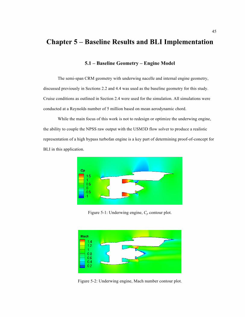
45

Chapter 5 – Baseline Results and BLI Implementation

5.1 – Baseline Geometry – Engine Model

The semi-span CRM geometry with underwing nacelle and internal engine geometry,

discussed previously in Sections 2.2 and 4.4 was used as the baseline geometry for this study.

Cruise conditions as outlined in Section 2.4 were used for the simulation. All simulations were

conducted at a Reynolds number of 5 million based on mean aerodynamic chord.

While the main focus of this work is not to redesign or optimize the underwing engine,

the ability to couple the NPSS raw output with the USM3D flow solver to produce a realistic

representation of a high bypass turbofan engine is a key part of determining proof-of-concept for

BLI in this application.

Figure 5-1: Underwing engine, Cp contour plot.

Figure 5-2: Underwing engine, Mach number contour plot.

46

Figure 5-3: Underwing engine, Mach number contour plot – inlet face.

Figures 5-1 and 5-2 show a two-dimensional cut through the underwing engine. From

this, it can be seen that the flow through the engine inlet is subsonic with no shocks apparent.

Figure 5-3 shows a Mach contour at the engine inlet face with a maximum Mach number of less

than 0.6, indicating a good inlet design. The exit flow is close to Mach 1, which is desirable for

high bypass turbofan engines. In addition, there does appear to be a small low-speed zone near

the engine plug, which could be reduced by making the plug larger. However, as this zone is

relatively small and the intent is to investigate BLI and not optimize the underwing engine, the

plug dimensions will remain unchanged. Overall, the NPSS model yielded good results and

should allow for a reasonable assessment of BLI in this application.

5.2 – Baseline Geometry – Power, Drag, and Thrust

As defined in Section 2.3, axial force, drag, and net propulsor power coefficients were

calculated for the baseline geometry and are presented below. The axial force coefficient, Cx, was

computed over all surfaces. The drag coefficient, CD, was computed over only the solid surfaces,

and the engine power coefficient, Cpk, was computed over the engine inlet, bypass exit, and core

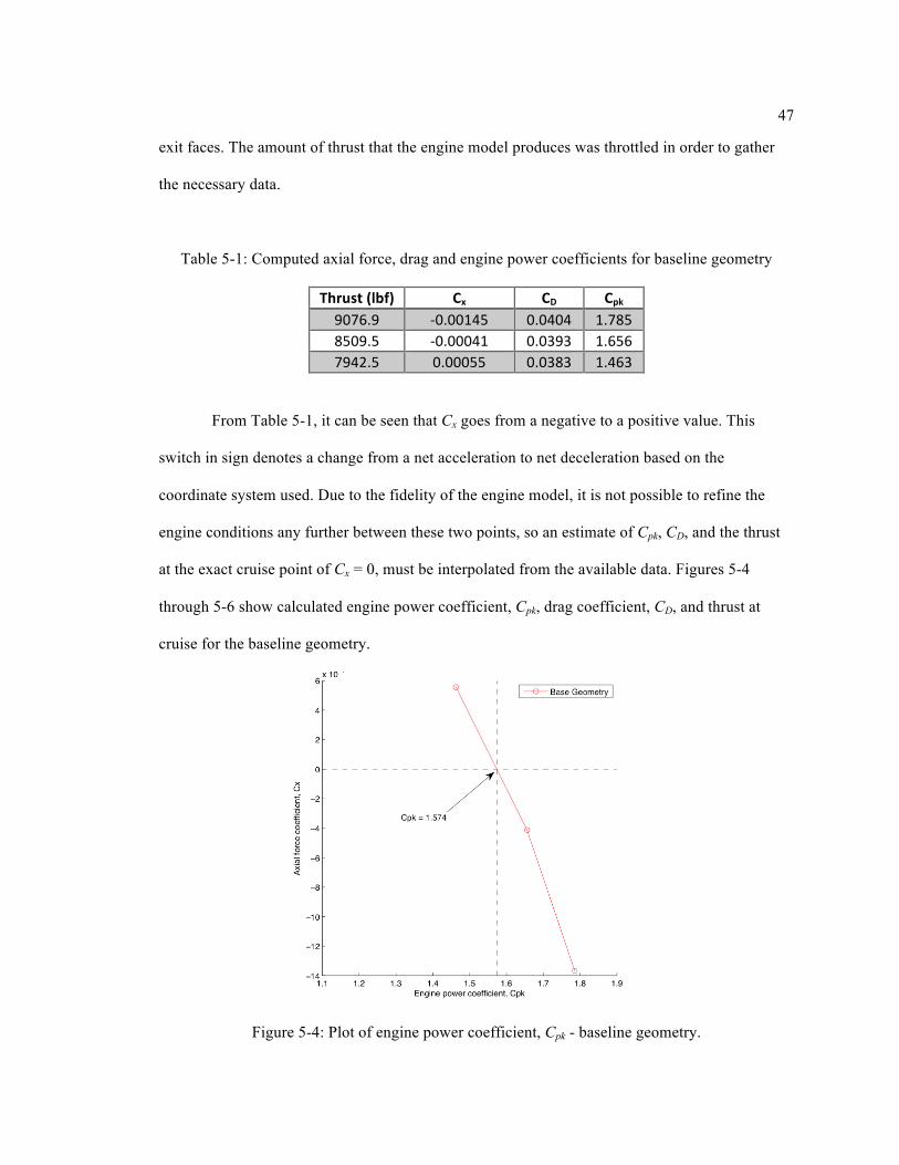
47

exit faces. The amount of thrust that the engine model produces was throttled in order to gather

the necessary data.

Table 5-1: Computed axial force, drag and engine power coefficients for baseline geometry

Thrust  (lbf)   Cx   CD   Cpk  9076.9   -­‐0.00145   0.0404   1.785  8509.5   -­‐0.00041   0.0393   1.656  7942.5   0.00055   0.0383   1.463  

From Table 5-1, it can be seen that Cx goes from a negative to a positive value. This

switch in sign denotes a change from a net acceleration to net deceleration based on the

coordinate system used. Due to the fidelity of the engine model, it is not possible to refine the

engine conditions any further between these two points, so an estimate of Cpk, CD, and the thrust

at the exact cruise point of Cx = 0, must be interpolated from the available data. Figures 5-4

through 5-6 show calculated engine power coefficient, Cpk, drag coefficient, CD, and thrust at

cruise for the baseline geometry.

Figure 5-4: Plot of engine power coefficient, Cpk - baseline geometry.

48

Figure 5-5: Plot of drag coefficient, Cd - baseline geometry.

Figure 5-6: Plot of thrust (lbf) – baseline geometry.

49

From the data, an engine power coefficient of Cpk = 1.574, drag coefficient of CD =

0.03894, and total thrust of 8268.17 lbf for the semi-span baseline geometry at cruise conditions

are computed. In addition, a nominal value of CL = 0.378 was calculated across all engine

conditions.

5.3 – Baseline Geometry – Boundary-Layer & Actuator Disc Implementation

In addition to the various coefficients computed above, it is also necessary to look at the

developing boundary-layer and wake produced by the aircraft in order to implement a BLI

system. The boundary-layer thickness, δ, is defined as the normal distance from the geometry to a

point where the flow velocity is that of the free-stream:

𝑢 𝑦 =  0.99𝑢! (5.1)

At the defined cruise condition, the free-stream velocity is 822.8 ft/s. Therefore, from

Eq. 5.1, the boundary-layer occurs at a point normal to the geometry where u < 814.6 ft/s.

Figure 5-7: Velocity contour plot, boundary-layer.

50

Figure 5-7 presents a contour plot of the empennage of the fuselage with u < 814.6 ft/s in blue.

From this, it can be seen that the boundary-layer developing along the length of the fuselage

along with the wake behind the aircraft. Unfortunately, there is an expansion area located at the

aft end of the fuselage where the actuator disc for the BLI system is to be placed. This expansion

area makes it difficult to pick out the exact location of the BL, so an approximation for the BL

thickness must be used. The BL/wake thickness was approximated by following the contour of

the developing boundary-layer along the fuselage and extending this contour out into the wake

region as shown by the black lines in Fig. 5-8.

Figure 5-8: Velocity contour plot, approximate BL and disc location, x-z view.

The actuator disc will be placed at the center of the flat portion of the empennage as

shown in Figure 5-8. At this location the boundary-layer/wake is approximately 195 inches thick

in the z direction.

51

Figure 5-9: Velocity contour plot, approximate BL and disc location, x-y view.

Figure 5-9 shows a top-down view of the developing boundary-layer and wake. There is

some interference from the tail; however, the boundary-layer thickness at the actuator disc

location can again be approximated by following the contour of the BL further up the fuselage. At

the actuator disc location, the boundary-layer/wake is approximately 91 inches thick in the y

direction.

As stated previously, for the purposes of this work, the slower moving boundary-layer

flow will be ingested and accelerated to match stream velocity. Since the exit velocity of the disc

is designed to be free-stream velocity, there is no point to ingesting free-stream air in this

application. The radius of the disc can therefore be constrained so that it is not ingesting free-

stream air, as areas of the disc in the free-stream would generate thrust by accelerating the flow to

above free-stream velocity. As shown in Figures 5-8 and 5-9, the boundary-layer and wake are

not uniform in radius at the actuator disc location. Therefore, the radius of the disc will be further

confined to be the smallest distance from the center of the disc to the edge of the approximate

boundary-layer edge location in any direction.

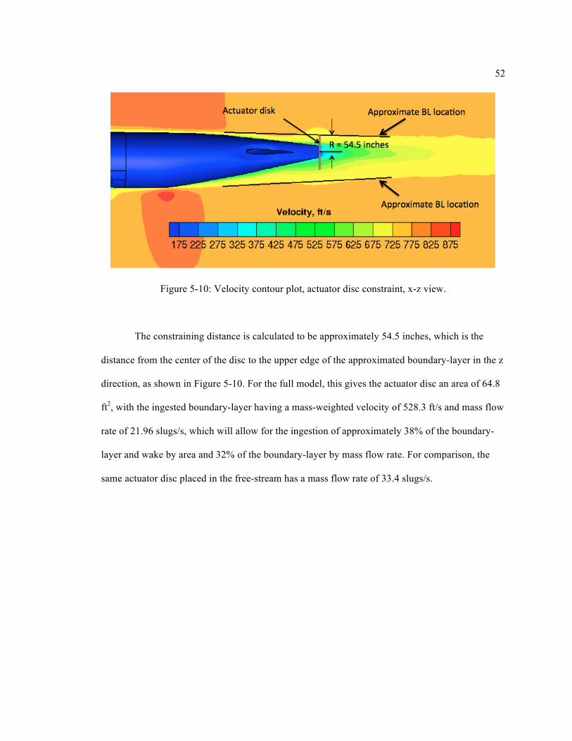
52

Figure 5-10: Velocity contour plot, actuator disc constraint, x-z view.

The constraining distance is calculated to be approximately 54.5 inches, which is the

distance from the center of the disc to the upper edge of the approximated boundary-layer in the z

direction, as shown in Figure 5-10. For the full model, this gives the actuator disc an area of 64.8

ft2, with the ingested boundary-layer having a mass-weighted velocity of 528.3 ft/s and mass flow

rate of 21.96 slugs/s, which will allow for the ingestion of approximately 38% of the boundary-

layer and wake by area and 32% of the boundary-layer by mass flow rate. For comparison, the

same actuator disc placed in the free-stream has a mass flow rate of 33.4 slugs/s.

53

Figure 5-11: Velocity contour plot, iso-slice at actuator disc location.

Although in an ideal situation 100% of the boundary-layer would be ingested, since the

maximum exit velocity of the BLI system is constrained to be equal to free-stream velocity, there

is a diminishing return on how large the system is versus how much benefit can be derived from

it. Using the definition of a boundary-layer given in Eq. 5.1 and the general thrust equation from

Eq. 1.2, it is certainly possible to take flow at 99% u∞, and generate thrust by imparting a slight

acceleration. However, far more thrust and therefore net benefit can be generated by taking the

slower moving flow found deeper in the boundary-layer and accelerating that to match u∞, since

this would create a larger Δu. The ‘sweet spot’ for how much of the boundary-layer to ingest will

be largely dependent on the type of propulsion system, how efficient the system is, and what

velocity constraints, if any, are placed on the exit flow, however, that is not the focus of this

54

study. In addition, the larger the BLI system is, the larger the potential weight and drag penalties

of implementing the system will be.

As can be seen in Figure 5-11 above, the actuator disc in this case is not ingesting the full

boundary-layer, shown in yellow, as the location and size of the actuator disc is constrained by

the approximated boundary-layer edge. However, the disc is ingesting a large portion of the

slowest boundary-layer flow, shown in green and blue. This should allow for a good

approximation of the net benefit of BLI and reduction in power savings without being too

idealistic as to be unreasonable in the real world.

Using Eq. 1.2, the ingested boundary-layer mass weighted velocity of 528.3 ft/s as the

inlet velocity, the mass flow rate of 21.96 slugs/s and constraining the exit velocity to match free-

stream, or 822.8 ft/s, the actuator disc should produce 1,454 lbf of thrust, approximately 8.8% of

the total thrust required for cruise.

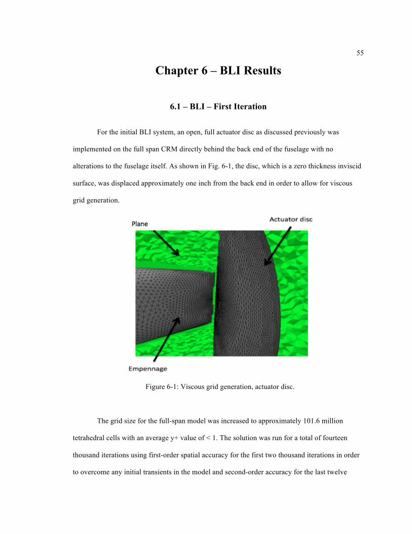
55

Chapter 6 – BLI Results

6.1 – BLI – First Iteration

For the initial BLI system, an open, full actuator disc as discussed previously was

implemented on the full span CRM directly behind the back end of the fuselage with no

alterations to the fuselage itself. As shown in Fig. 6-1, the disc, which is a zero thickness inviscid

surface, was displaced approximately one inch from the back end in order to allow for viscous

grid generation.

Figure 6-1: Viscous grid generation, actuator disc.

The grid size for the full-span model was increased to approximately 101.6 million

tetrahedral cells with an average y+ value of < 1. The solution was run for a total of fourteen

thousand iterations using first-order spatial accuracy for the first two thousand iterations in order

to overcome any initial transients in the model and second-order accuracy for the last twelve

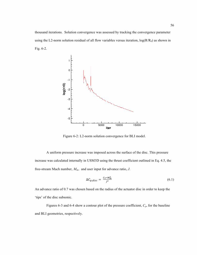
56

thousand iterations. Solution convergence was assessed by tracking the convergence parameter

using the L2-norm solution residual of all flow variables versus iteration, log(R/R0) as shown in

Fig. 6-2.

Figure 6-2: L2-norm solution convergence for BLI model.

A uniform pressure increase was imposed across the surface of the disc. This pressure

increase was calculated internally in USM3D using the thrust coefficient outlined in Eq. 4.5, the

free-stream Mach number, M∞, and user input for advance ratio, J.

∆𝐶!,!"#$ =  !!∗!!!

!! (6.1)

An advance ratio of 0.7 was chosen based on the radius of the actuator disc in order to keep the

‘tips’ of the disc subsonic.

Figures 6-3 and 6-4 show a contour plot of the pressure coefficient, Cp, for the baseline

and BLI geometries, respectively.

57

Figure 6-3: Cp contour plot, baseline geometry, z-x plane.

Figure 6-4: Cp contour plot, BLI geometry, z-x plane.

Figure 6-4 shows the actuator disc is imparting a slight pressure jump to the incoming flow with

the highest Cp occurring on the empennage where the geometry terminates abruptly. As can be

seen in Figures 5-8 and 5-10, this abrupt end to the geometry causes a low velocity zone and large

58

wake to develop behind the aircraft, contributing to an increase in drag and engine power

requirements. Figures 6-5 and 6-6 show Cp contour plots of the ‘in’ and ‘out’ faces of the actuator

disc, respectively. Again, the disc is shown to be imposing a pressure jump on the incoming flow,

with the highest Cp occurring at the center of the disc where the geometry terminates.

Figure 6-5: Cp contour plot, actuator disc ‘in’ face.

Figure 6-6: Cp contour plot, actuator disc ‘out’ face.

Figure 6-7 shows a velocity contour plot of the flow coming into the actuator disc.

From Equation 5.1, any flow where u < 814.6 ft/s is by definition, boundary-layer flow. From the

contour plot, it is evident that the actuator disc is entirely immersed in the boundary-layer/wake

of the aircraft, however the velocity profile is not uniform. The top portion of the disc has the

59

fastest moving flow, with a maximum velocity of 775.8 ft/s. Relative to the top portion of the

disc, the sides and bottom have slower moving flow due to interference from the horizontal tail

wake and the taper from the bottom of the fuselage. The center of the disc where the fuselage

comes to an end has a minimum velocity of 159.8 ft/s, approximately 19.4% that of free-stream.

The mass weighted velocity at the disc exit is 630.9 ft/s, an increase of 102.5 ft/s over the

baseline geometry.

Figure 6-7: Velocity contour plot, BLI geometry actuator disc ‘in’ face.

Figures 6-8 and 6-9 show velocity contour plots of the wake for the baseline and BLI

geometries.

60

Figure 6-8: Velocity contour plot of wake, baseline geometry.

Figure 6-9: Velocity contour plot of wake, BLI geometry.

From these, it is evident that implementing the actuator disc does have a moderate effect on the

aircraft wake, although it is not completely eliminated as intended. Figure 6-10 shows an

isometric view of the wake and actuator disc.

61

Figure 6-10: Velocity contour plot, iso-slice at actuator disc location, BLI geometry.

The actuator disc looks to be fully immersed in the wake/boundary-layer although there is a large

portion of the wake/boundary-layer flow that is not ingested by the disc. Compared to the

baseline geometry, shown in Fig. 5-11, the lower velocity regions, particularly the green and blue,

which represent the lowest velocity areas, are all reduced in size and length. In addition, the

overall length of the wake is reduced.

The engine power coefficient, Cpk, and axial force coefficient, Cx, were calculated for the

BLI geometry and plotted against previous results for the baseline geometry. Since it was not

possible to refine the engine model any further between the data points, Cpk at the exact cruise

point of Cx = 0 was interpolated from the available data.

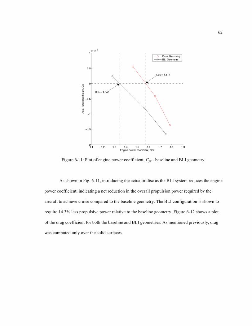
62

Figure 6-11: Plot of engine power coefficient, Cpk - baseline and BLI geometry.

As shown in Fig. 6-11, introducing the actuator disc as the BLI system reduces the engine

power coefficient, indicating a net reduction in the overall propulsion power required by the

aircraft to achieve cruise compared to the baseline geometry. The BLI configuration is shown to

require 14.3% less propulsive power relative to the baseline geometry. Figure 6-12 shows a plot

of the drag coefficient for both the baseline and BLI geometries. As mentioned previously, drag

was computed only over the solid surfaces.

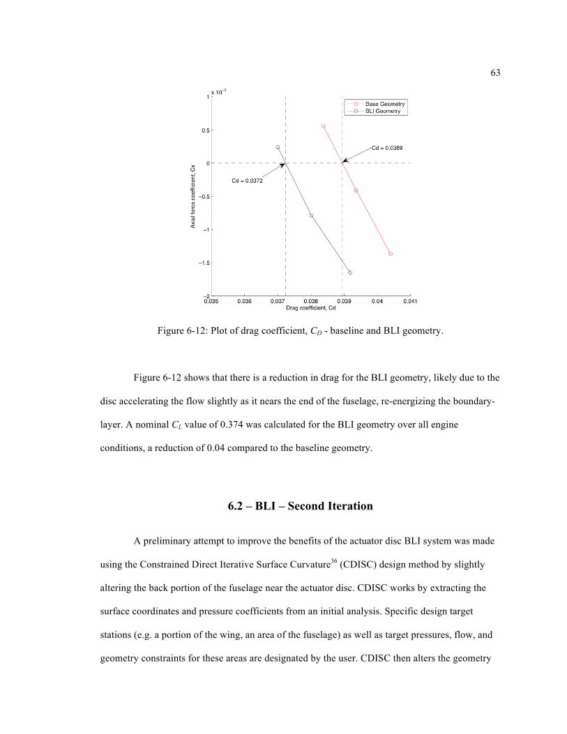
63

Figure 6-12: Plot of drag coefficient, CD - baseline and BLI geometry.

Figure 6-12 shows that there is a reduction in drag for the BLI geometry, likely due to the

disc accelerating the flow slightly as it nears the end of the fuselage, re-energizing the boundary-

layer. A nominal CL value of 0.374 was calculated for the BLI geometry over all engine

conditions, a reduction of 0.04 compared to the baseline geometry.

6.2 – BLI – Second Iteration

A preliminary attempt to improve the benefits of the actuator disc BLI system was made

using the Constrained Direct Iterative Surface Curvature36 (CDISC) design method by slightly

altering the back portion of the fuselage near the actuator disc. CDISC works by extracting the

surface coordinates and pressure coefficients from an initial analysis. Specific design target

stations (e.g. a portion of the wing, an area of the fuselage) as well as target pressures, flow, and

geometry constraints for these areas are designated by the user. CDISC then alters the geometry

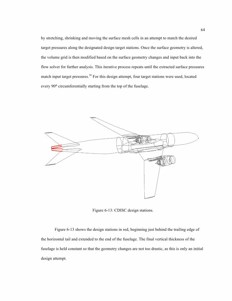
64

by stretching, shrinking and moving the surface mesh cells in an attempt to match the desired

target pressures along the designated design target stations. Once the surface geometry is altered,

the volume grid is then modified based on the surface geometry changes and input back into the

flow solver for further analysis. This iterative process repeats until the extracted surface pressures

match input target pressures.36 For this design attempt, four target stations were used, located

every 90° circumferentially starting from the top of the fuselage.

Figure 6-13: CDISC design stations.

Figure 6-13 shows the design stations in red, beginning just behind the trailing edge of

the horizontal tail and extended to the end of the fuselage. The final vertical thickness of the

fuselage is held constant so that the geometry changes are not too drastic, as this is only an initial

design attempt.

65

The surface pressures for the original BLI geometry were extracted, and a design

constraint was imposed on Cp over the top and bottom of the fuselage to increase the average

surface pressure of the design area. By increasing Cp in this area, the idea is that the flow will

‘squeeze’ the fuselage, causing a net forward force, similar to pinching an ice cube and having it

shoot forward. Normally, this geometry change would be expected to decelerate the flow,

increasing the boundary-layer and wake. However, as the BLI system is located close by, any

decrease in velocity should actually be beneficial to the BLI system and contribute to the overall

power reduction. Figures 6-14 and 6-15 show the imposed design constraints for stations one and

three plotted against location along the target stations. Design station one is the top of the

fuselage and design station three is the bottom. No design constraints were imposed on stations

two and four, located on the sides of the fuselage. However, as CDISC blends the geometry

changes between the stations the surface mesh was altered slightly at these locations.

Figure 6-14: CDISC Cp design constraint, station one.

66

Figure 6-15: CDISC Cp design constraint – station three.

Figures 6-16 through 6-18 show the actual change in Cp across all stations. Figures 6-19

and 6-20 show the changes in geometry in terms of vertical height for stations one and three,

while Figure 6-21 shows changes in geometry in terms of thickness for stations two and four.

Figure 6-16: Original and CDISC (actual) Cp - station one.

67

Figure 6-17: Original and CDISC (actual) Cp - station three.

Figure 6-18: Original and CDISC (actual) Cp - stations two and four.

68

Figure 6-19: Original and CDISC (actual) vertical height - station one.

Figure 6-20: Original and CDISC (actual) vertical height - station three.

69

Figure 6-21: Original and CDISC (actual) thickness - stations two and four.

Figure 6-22 below shows the side view of the original surface mesh (blue) and redesigned

CDISC mesh (red) with Figure 6-23 showing a top view.

Figure 6-22: Original (blue) and updated mesh (red), side view.

70

Figure 6-23: Original (blue) and updated mesh (red), top view.

Figures 6-24 and 6-25 show close-up velocity contour plot nears the redesigned areas in

both the original and updated BLI geometries.

71

Figure 6-24: Velocity contour plot, close up - original BLI geometry.

Figure 6-25: Velocity contour plot, close up – CDISC redesigned BLI geometry.

For the CDISC redesigned BLI geometry, there is a small increase in the area of the low

velocity zone, shown in green, both on the upper and lower portions of the empennage, although

since the upper area went through a more drastic change (relatively), the change is more

72

noticeable compared to the lower surface. There was no noticeable change in the wake flow for

the redesigned geometry.

Again, the engine power coefficient, Cpk, and axial force coefficient, Cx, were calculated

for the redesigned BLI geometry and plotted against previous results for both the baseline and

original BLI geometries.

Figure 6-26: Plot of engine power coefficient, Cpk – baseline, and BLI geometries.

As Figure 6-26 shows, the geometry modifications introduced by CDISC led to a slight

decrease in the engine power coefficient at cruise. The redesigned BLI configuration is shown to

require 15.6% less propulsive power relative to the baseline geometry, a 1.3% improvement over

the original BLI geometry.

73

Figure 6-27: Plot of drag coefficient, CD - baseline and BLI geometries.

Figure 6-27 is a plot of the drag coefficient for all geometries at this point. There is a

reduction in drag of approximately eighteen counts for the redesigned BLI geometry compared to

the original BLI geometry. A nominal CL value of 0.373 was calculated for the CDISC BLI

geometry over all engine conditions, a reduction of 0.05 compared to the baseline geometry.

6.3 – CDISC Geometry Without BLI

As it is unclear at this point whether the additional reduction in engine power

requirements at cruise for the CDISC BLI geometry compared to the first iteration BLI

configuration arises out of improved performance of the fuselage itself, an increased benefit

derived from the BLI system, or else a combination of both, an additional study was done to

determine where this benefit comes from. To this end, the actuator disc representing the BLI

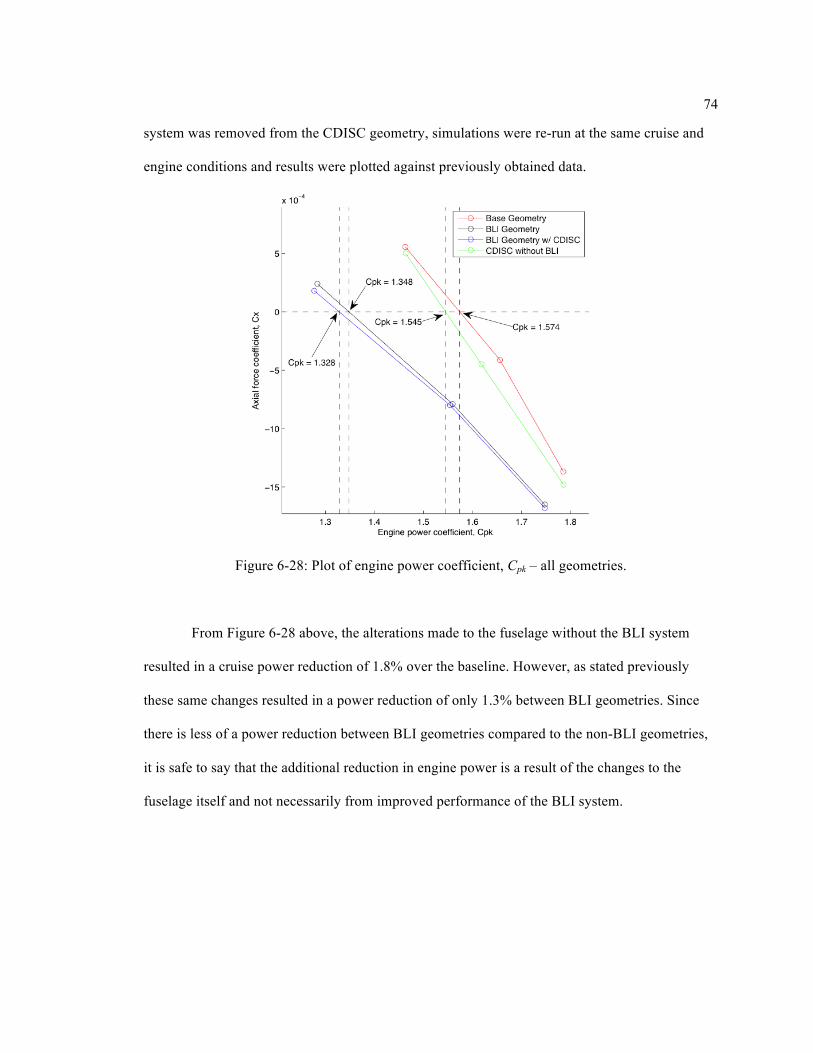
74

system was removed from the CDISC geometry, simulations were re-run at the same cruise and

engine conditions and results were plotted against previously obtained data.

Figure 6-28: Plot of engine power coefficient, Cpk – all geometries.

From Figure 6-28 above, the alterations made to the fuselage without the BLI system

resulted in a cruise power reduction of 1.8% over the baseline. However, as stated previously

these same changes resulted in a power reduction of only 1.3% between BLI geometries. Since

there is less of a power reduction between BLI geometries compared to the non-BLI geometries,

it is safe to say that the additional reduction in engine power is a result of the changes to the

fuselage itself and not necessarily from improved performance of the BLI system.

75

Figure 6-29: Plot of drag coefficient, CD – all geometries.

Figure 6-29 is a plot of the drag coefficient for all geometries. There is a small reduction

in drag of approximately 3 counts between the non-BLI geometries. A nominal CL of 0.377 was

calculated as well over all engine conditions, a reduction of 0.01 compared to the baseline.

76

Chapter 7 – Conclusions and Future Work

An unstructured grid-based computational solution encompassing multiple geometries

and several different computational tools has been demonstrated, along with a methodology for

evaluating the benefit of boundary-layer ingestion for conventional aircraft. The GridTool/VGrid

advancing front grid generation software has proven itself to be a quick and easy way to generate

unstructured tetrahedral grids for analysis.

The USM3D flow solver has been verified against both previous computational results,

and data gathered during earlier experiments using the Common Research Model geometry. The

NPSS software has been shown to provide useful inputs for CFD analysis, allowing for the

realistic modeling of turbojet engines in this application. In addition, CDISC has been shown to

be a useful tool for geometry modification and design.

From the analysis above, it is evident that the combination of BLI both with and without

fuselage shaping provides a significant reduction in terms of propulsive power required for cruise.

This benefit has been shown to be the result of a combination of wake filling and using the slower

moving boundary-layer flow for propulsion instead of free-stream air, as outlined in Section 1.1.

It is important to note that as the wake was only moderately reduced by the introduction of the

BLI system, the majority of the benefit of BLI, in terms of cruise propulsive power reduction,

seems to stem from the reduction in velocity of the incoming flow into the propulsor.

Table 7-1: Summary of data Geometry   Cpk   Power  Reduction   CD   CL  

Baseline   1.574   -­‐   0.0389   0.378  

BLI   1.348   14.30%   0.0372   0.374  BLI  w/  CDISC   1.328   15.60%   0.0371   0.373  CDISC  w/o  BLI   1.545   1.80%   0.0386   0.377  

77

The current BLI propulsor model imparts a uniform pressure jump across the actuator

disc, which may not be entirely accurate when the fan encounters an inlet distortion. An actual

fan would impart a smaller pressure rise to the portion of the flow with higher stagnation pressure

and larger pressure rise to the portion of the fluid with lower stagnation pressure. These

differences in pressure rise across the fluid could affect flow behavior upstream of the actuator

disc as well as the exhaust flow. The implementation of a more advanced actuator disc boundary

condition with a radially varying pressure distribution is recommended to improve accuracy of

results for BLI implementation.

As this study used a non-descript, open actuator disc propulsion system to model the BLI

system, the implementation of a more real-world propulsion system would improve the

trustworthiness of calculated potential benefits as well as allow for evaluation of system-

dependent losses. A trade study to determine a list of viable candidates (e.g., open propeller,

ducted electric fan, small turbofan engine) using current technology, or the development of a

specifically designed propulsion system and implementation of said system, would yield more

accurate results on the exact amount of power savings from the use of BLI as it is implemented

here. The use of a full propulsion system model over the representative actuator disc would also

allow for assessments of any weight penalties or reduction in benefits from flow distortion

through the inlet, fan face and/or nacelle depending on the chosen system as these are not

modeled in this study.

In order to better understand the prospective power savings and how a BLI system might

affect other subsystems and flight variables, additional computations should be conducted at

alternate operating conditions and flight regimes.

Overall, airframe propulsion integration and the implementation of a BLI system present

a complex and challenging design optimization problem. Aircraft engines are sized for take off,

with the operating cruise point being a percentage of full throttle. By introducing BLI, it may be

78

possible to scale down the size of the engines, thus reducing wetted area and overall drag, which

would increase the benefit of BLI at a system level even further. However, the addition of a BLI

system will likely add weight to the aircraft, which will then require more overall thrust at take

off. If the BLI system does not produce at least that much additional thrust, the size of the wing

mounted engines as well as the wing area would need to be increased, further increasing weight

and cost. Also, keeping the engine sized the same for take off but throttling down to a lower

operating cruise point may cause the propulsive efficiency to decrease and specific fuel

consumption to increase, however the total mission fuel would likely decrease. In addition, at a

lower operating cruise point, harmful environmental emissions should go down due to lower

combustor temperature and overall pressure ratio of the engine.

The purpose of this work is not to declare whether or not BLI should be implemented in

the real world, but instead serve as a starting point for designing and evaluating the potential

benefit of a BLI system in this application. This analysis shows that implementing an ideal BLI

system in the above fashion can provide a significant benefit in terms of propulsive power

reduction, and therefore warrants further, more detailed study. However, this analysis does not

take into account systemic losses that would be dependent on actual engine design and

implementation. In addition, this work does not look into the structural effects that implementing

a BLI system might have. Ideally, the entire system, including required thrust, wing area, aircraft

weight, and engine design variables would be ‘clean sheet’ designed to meet the desired design

goals.

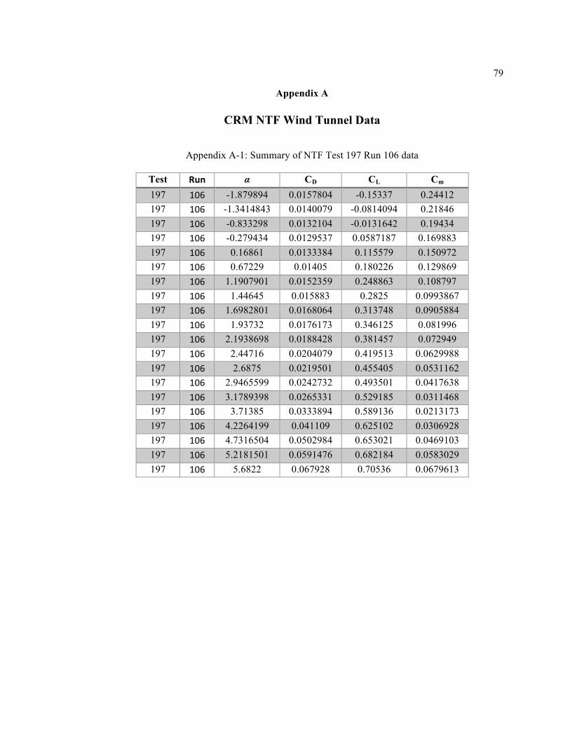
79

Appendix A

CRM NTF Wind Tunnel Data

Appendix A-1: Summary of NTF Test 197 Run 106 data

Test Run   α CD CL Cm 197 106   -1.879894 0.0157804 -0.15337 0.24412 197 106   -1.3414843 0.0140079 -0.0814094 0.21846 197 106   -0.833298 0.0132104 -0.0131642 0.19434 197 106   -0.279434 0.0129537 0.0587187 0.169883 197 106   0.16861 0.0133384 0.115579 0.150972 197 106   0.67229 0.01405 0.180226 0.129869 197 106   1.1907901 0.0152359 0.248863 0.108797 197 106   1.44645 0.015883 0.2825 0.0993867 197 106   1.6982801 0.0168064 0.313748 0.0905884 197 106   1.93732 0.0176173 0.346125 0.081996 197 106   2.1938698 0.0188428 0.381457 0.072949 197 106   2.44716 0.0204079 0.419513 0.0629988 197 106   2.6875 0.0219501 0.455405 0.0531162 197 106   2.9465599 0.0242732 0.493501 0.0417638 197 106   3.1789398 0.0265331 0.529185 0.0311468 197 106   3.71385 0.0333894 0.589136 0.0213173 197 106   4.2264199 0.041109 0.625102 0.0306928 197 106   4.7316504 0.0502984 0.653021 0.0469103 197 106   5.2181501 0.0591476 0.682184 0.0583029 197 106   5.6822 0.067928 0.70536 0.0679613

80

Appendix A-2: Summary of NTF Test 197 Run 212 data

Test Run α CD CL Cm 197 212 -1.894889 0.0158155 -0.156053 0.247697 197 212 -1.3711417 0.0139335 -0.0843766 0.221229 197 212 -0.852494 0.0130211 -0.012736 0.195088 197 212 -0.340141 0.0128991 0.0552993 0.170471 197 212 0.18526 0.0132408 0.124915 0.146103 197 212 0.6332 0.0138949 0.185137 0.12562 197 212 1.14826 0.0150403 0.253606 0.103328 197 212 1.65223 0.0166269 0.321664 0.083173 197 212 2.1674099 0.018868 0.394969 0.0628901 197 212 2.6693501 0.0221117 0.469879 0.0411987 197 212 3.1863902 0.0274211 0.548422 0.0154148 197 212 3.42717 0.0303659 0.579569 0.0077223 197 212 3.6796 0.0340755 0.604435 0.0076886 197 212 3.9324999 0.0382287 0.6207 0.0141976 197 212 4.1713099 0.0423526 0.633198 0.0234076 197 212 4.44066 0.0462981 0.651115 0.028958 197 212 4.6926999 0.0513781 0.663898 0.0393433 197 212 4.9317999 0.0568659 0.672498 0.0485809 197 212 5.17417 0.0615611 0.688738 0.0543055

81

Appendix A-3: Summary of NTF Test 197 Run 223 data

Test Run α CD CL Cm 197 223 -1.869527 0.015171 -0.150633 0.244115 197 223 -1.3657908 0.0133506 -0.0810448 0.219056 197 223 -0.856144 0.0125017 -0.0126557 0.194982 197 223 -0.266849 0.0124258 0.0643977 0.168564 197 223 0.15118 0.0126944 0.117232 0.150746 197 223 0.65416 0.0133921 0.182451 0.129616 197 223 1.17843 0.0145631 0.24955 0.10902 197 223 1.6840899 0.0161834 0.316505 0.0896705 197 223 2.19101 0.018312 0.385785 0.0716468 197 223 2.7014499 0.0215968 0.461266 0.0511705 197 223 3.1919298 0.0260419 0.532785 0.0296709 197 223 3.4520502 0.0292578 0.568413 0.0200747 197 223 3.6886899 0.0323765 0.594448 0.0166259 197 223 3.96029 0.0362509 0.618774 0.0181338 197 223 4.2396798 0.0411017 0.634602 0.0260361 197 223 4.4393797 0.0446382 0.647316 0.0323528 197 223 4.7344003 0.0502719 0.662502 0.0420438 197 223 4.9451799 0.0537701 0.675932 0.0473132 197 223 5.2196603 0.0592415 0.690287 0.0549618

82

Appendix B

CRM Drag Prediction Workshop Computational Results (original geometry)

Appendix B-1: Summary of fourth AIAA DPW CRM computational data

Mach   Re,  million   α   CD   CL   Cm  0.85   5   0   0.01874   0.17783   0.05477  0.85   5   1   0.02127   0.31918   0.00446  0.85   5   1.5   0.02323   0.39074   -­‐0.01814  0.85   5   2   0.02585   0.46611   -­‐0.03992  0.85   5   2.5   0.02995   0.54239   -­‐0.06249  0.85   5   3   0.03601   0.60689   -­‐0.0756  0.85   5   3.5   0.04348   0.65109   -­‐0.07092  0.85   5   4   0.05195   0.68657   -­‐0.05971  0.85   5   4.5   0.05926   0.70655   -­‐0.07213  0.85   5   5   0.06842   0.73105   -­‐0.06316  

83

Appendix C

NPSS PAX300 engine model raw data

84

References

1. Smith, L. H., “Wake Ingestion Propulsion Benefit,” Journal of Propulsion and Power, vol. 9, 1993, pp. 74–82.

2. Arntz, A., Atinault, O., Destarac, D., and Merlen, A., “Exergy-based Aircraft Aeropropulsive Performance Assessment: CFD Application to Boundary-layer Ingestion,” 32nd AIAA Applied Aerodynamics Conference, 2014.

3. Plas, A., Crichton, D., Sargeant, M., Hynes, T., Greitzer, E., Hall, C., and Madani, V., “Performance of a Boundary-layer Ingesting (BLI) Propulsion System,” 45th AIAA Aerospace Sciences Meeting and Exhibit, Aug. 2007.

4. Küchemann, D., and Johanna W., Aerodynamics of propulsion. Vol. 2. McGraw-Hill, 1953, pp. 205-209.

5. Anderson, John David, Fundamentals of Aerodynamics, 3rd ed. Boston: McGraw-Hill, 2001.

6. Lv, Peijan., Rao, Arvind G. “Conceptual Analysis of Boundary-layer Ingestion Towards Aircraft Propulsion Integration.” ISBAE Paper No. 2013-1436 Proceedings of the International Society of Air Breathing Engines, At Busan, South Korea, 2013.

7. Manneville, A., Pilczer, D., and Spakovszky, Z., “Noise Reduction Assessments and Preliminary Design Implications for a Functionally-Silent Aircraft,” 10th AIAA/CEAS Aeroacoustics Conference, Oct. 2004.

8. Owens, L., Allan, B., and Gorton, S., “Boundary-Layer-Ingesting Inlet Flow Control,” 44th AIAA Aerospace Sciences Meeting and Exhibit, Sep. 2006.

9. Kawai, Ronald T., Douglas M. Friedman, and Leonel Serrano. “Blended Wing Body (BWB) Boundary-layer Ingestion (BLI) Inlet Configuration and System Studies.” NASA CR-214534, 2006.

10. Smith, A. M. O. and Roberts, H., “The Jet Airplane Utilizing Boundary-layer Air for Propulsion,” Journal of the Aeronautical Sciences (Institute of the Aeronautical Sciences), vol. 14, 1947, pp. 97–109.

11. F. R. Goldschmied, “On the Aerodynamic Optimization of Mini-RPV and Small GA Aircraft,” 2nd Applied Aerodynamics Conference, 1984.

12. Roepke, Joshua. "An Experimental Investigation of a Goldschmied Propulsor." MSc Thesis, California Polytechnic State University, 2012.

13. Douglas, W., “Propulsive Efficiency with Boundary-layer Ingestion,” McDonnell Douglas Report MDC J0860, 1970.

14. Daggett, David L., Ron Kawai, and Doug Friedman. "Blended Wing Body Systems Studies: Boundary-layer Ingestion Inlets with Active Flow Control." NASA CR-212670, 2003.

85

15. Uranga, A., Drela, M., Greitzer, E., Titchener, N., Lieu, M., Siu, N., Huang, A., Gatlin, G. M., and Hannon, J., “Preliminary Experimental Assessment of the Boundary-layer Ingestion Benefit for the D8 Aircraft,” 52nd Aerospace Sciences Meeting, Oct. 2014.

16. Pandya, S. A., Uranga, A., Espitia, A., and Huang, A., “Computational Assessment of the Boundary-layer Ingesting Nacelle Design of the D8 Aircraft,” 52nd Aerospace Sciences Meeting, Oct. 2014.

17. Sabo, K. M., and Drela, M., “Benefits of Boundary-layer Ingestion Propulsion,”53rd AIAA Aerospace Sciences Meeting, Mar. 2015.

18. Berrier, B., and Allan, B., “Experimental and Computational Evaluation of Flush-Mounted, S-Duct Inlets,” 42nd AIAA Aerospace Sciences Meeting and Exhibit, May 2004.

19. Rodriguez, D., “A Multidisciplinary Optimization Method for Designing Boundary-layer Ingesting Inlets,” 9th AIAA/ISSMO Symposium on Multidisciplinary Analysis and Optimization, Apr. 2002

20. Vassberg, J., Dehaan, M., Rivers, M., and Wahls, R., “Development of a Common Research Model for Applied CFD Validation Studies,” 26th AIAA Applied Aerodynamics Conference, 2008.

21. Yamamoto, K., Tanaka, K., and Murayama, M., “Comparison Study of Drag Prediction for the 4th CFD Drag Prediction Workshop using Structured and Unstructured Mesh Methods,” 28th AIAA Applied Aerodynamics Conference, 2010.

22. Drela, M., “Power Balance in Aerodynamic Flows,” 27th AIAA Applied Aerodynamics Conference, 2009.

23. Pirzadeh, S., “Progress Toward a User-Oriented Unstructured Viscous Grid Generator,” 34th Aerospace Sciences Meeting and Exhibit, 1996.

24. Geolab NASA Langley, GridTool Training Manual. NASA Langley, VA, 1998.

25. Garriz, Javier A., VGrid 3.2 Reference Documents. ViGYAN Inc., 1998.

26. Pirzadeh, S., “Viscous Unstructured Three-Dimensional Grids by the Advancing-Layers Method,” 32nd Aerospace Sciences Meeting and Exhibit, Oct. 1994.

27. Frink, N. T., “Upwind Scheme for Solving the Euler Equations on Unstructured Tetrahedral Meshes,” AIAA Journal, vol. 30, 1992, pp. 70–77.

28. Roe, P., “Characteristic-Based Schemes for the Euler Equations,” Annual Review of Fluid Mechanics, vol. 18, Jan. 1986, pp. 337–365.

29. "TetrUSS: USM3D Overview." TetrUSS: USM3Dns Online Manual. NASA Langley Research Center, 8 Aug. 2003. Web. 1 Feb. 2015. <http://tetruss.larc.nasa.gov/usm3d/overview.html>.

30. Lytle, John K. "The Numerical Propulsion System Simulation: An Overview." NASA CR-209915, 2000.

86

31. "Basic NPSS Gas Turbine Engine Modeling." Wolverine Ventures, 10 June 2010. Web. 13 Jan. 2015. <http://www.wolverine-ventures.com/images/pdf/basic_npss.pdf>.

32. Turner, M. G., Reed, J. A., Ryder, R., and Veres, J. P., “Multi-Fidelity Simulation of a Turbofan Engine With Results Zoomed Into Mini-Maps for a Zero-D Cycle Simulation,” Volume 2: Turbo Expo 2004, 2004.

33. Hartwich, P., and Frink, N., “Estimation of Propulsion-Induced Effects on Transonic Flows over a Hypersonic Configuration,” 30th Aerospace Sciences Meeting and Exhibit, Jun. 1992.

34. Kirby, M., Barros, P., and Mavris, D., “Enhancing the Environmental Policy Making Process with the FAA's EDS Analysis Tool,” 47th AIAA Aerospace Sciences Meeting including The New Horizons Forum and Aerospace Exposition, May 2009.

35. Jones, S., NASA GRC Reference model for 90000 lb thrust class direct-drive turbofan, 2011.

36. Campbell, R., “Efficient Viscous Design of Realistic Aircraft Configurations,” 29th AIAA, Fluid Dynamics Conference, 1998.

37. Rivers, M., and Dittberner, A., “Experimental Investigations of the NASA Common Research Model (Invited),” 28th AIAA Applied Aerodynamics Conference, 2010.

38. Rivers, Melissa. "NASA Common Research Model - Experimental Data." NASA Common Research Model - Experimental Data. 1 Mar. 2014. Web. 5 Feb. 2015. <http://commonresearchmodel.larc.nasa.gov/experimental-data/>.

39. Gloss, B. B., “Current Status and Some Future Test Directions for the US National Transonic Facility. Wind Tunnels and Wind Tunnel Test Techniques,” Royal Aeronautical Society, 1992.

40. "National Transonic Facility (NTF)." National Transonic Facility (NTF). NASA Langley, 1 Sept. 2013. Web. 5 Jan. 2015. http://gftd.larc.nasa.gov/facilities/ntf.html>.

41. Fuller, Dennis E., B. B. Gloss, and D. Nystrom. "Guide for Users of the National Transonic Facility." NASA CR-110242, 1981.

42. Burner, A. W., and Liu, T., “Videogrammetric Model Deformation Measurement Technique,” Journal of Aircraft, vol. 38, 2001, pp. 745–754.

43. Pirzadeh, S., “Advanced Unstructured Grid Generation for Complex Aerodynamics Applications,” 26th AIAA Applied Aerodynamics Conference, 2008.

44. Frink, N. T., “Upwind Scheme for Solving the Euler Equations on Unstructured Tetrahedral Meshes,” AIAA Journal, vol. 30, 1992, pp. 70–77.

45. Abdol-Hamid, K., Frink, N., Deere, K., and Pandya, M., “Propulsion Simulations Using Advanced Turbulence Models with the Unstructured-Grid CFD Tool, TetrUSS,” 42nd AIAA Aerospace Sciences Meeting and Exhibit, May 2004.

87

46. Anderson, W., and Bonhaus, D. L., “An Implicit Upwind Algorithm for Computing Turbulent Flows on Unstructured Grids,” Computers & Fluids, vol. 23, 1994, pp. 1–21.

47. Morrison, J., “Statistical Analysis of CFD Solutions from the Fourth AIAA Drag Prediction Workshop,” 28th AIAA Applied Aerodynamics Conference, 2010.

48. Levy, D., Laflin, K., Vassberg, J., Tinoco, E., Mani, M., Rider, B., Brodersen, O., Crippa, S., Rumsey, C., Wahls, R., Morrison, J., Mavriplis, D., and Murayama, M., “Summary of Data from the Fifth AIAA CFD Drag Prediction Workshop,” 51st AIAA Aerospace Sciences Meeting including the New Horizons Forum and Aerospace Exposition, May 2013.

49. Rivers, M., and Hunter, C., “Support System Effects on the NASA Common Research Model,” 50th AIAA Aerospace Sciences Meeting including the New Horizons Forum and Aerospace Exposition, Sep. 2012.