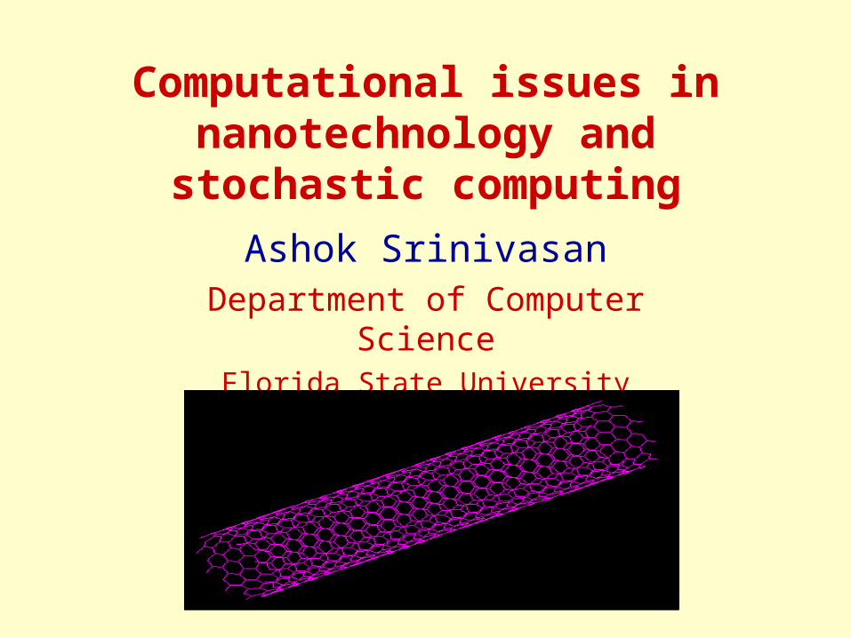
Computational issues in nanotechnology and stochastic computing

Ashok SrinivasanDepartment of Computer Science

Florida State University

Motivation

• Research areas– Parallel algorithms– Scientific computing– Discrete algorithms– Applications

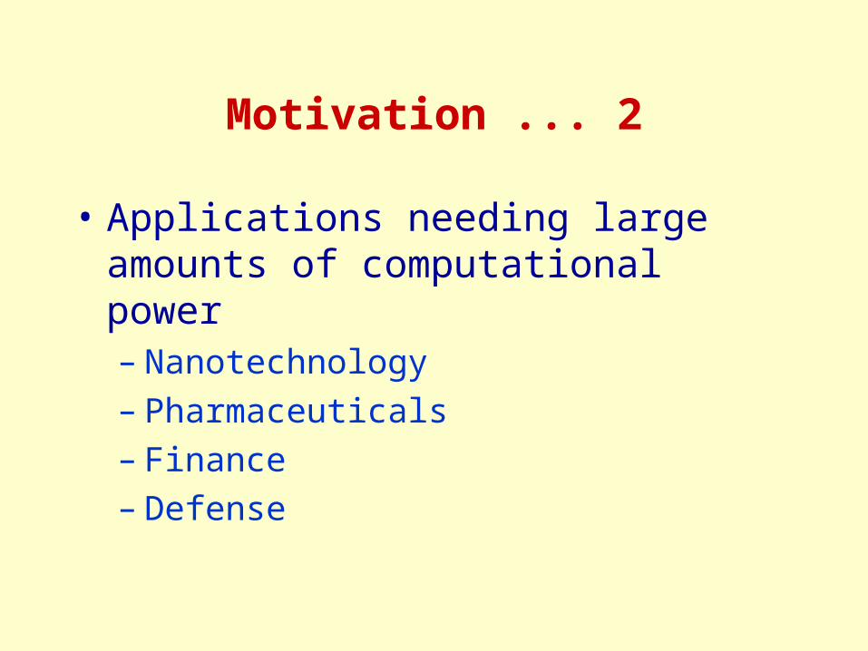
Motivation ... 2

• Applications needing large amounts of computational power– Nanotechnology– Pharmaceuticals– Finance– Defense

Motivation ... 3

• New computational paradigms– Grid computing– Massive parallelism

• Need new algorithmic paradigms– Develop algorithms and software tools for

the computational environment 5 to 10 years from now

Motivation ... 4

• Algorithms– Scalable– Latency tolerant

• Enabling technologies– Fault tolerant– Usable software tools

Outline

• Applications– Nanotechnology

• Background• Sequential computation• Parallelization• Research issues

• Algorithms– Stochastic techniques

• Scalable parallelization• Linear algebra• Applications

Applications

• Nanotechnology– Background– Sequential computation– Parallelization– Research issues

Background

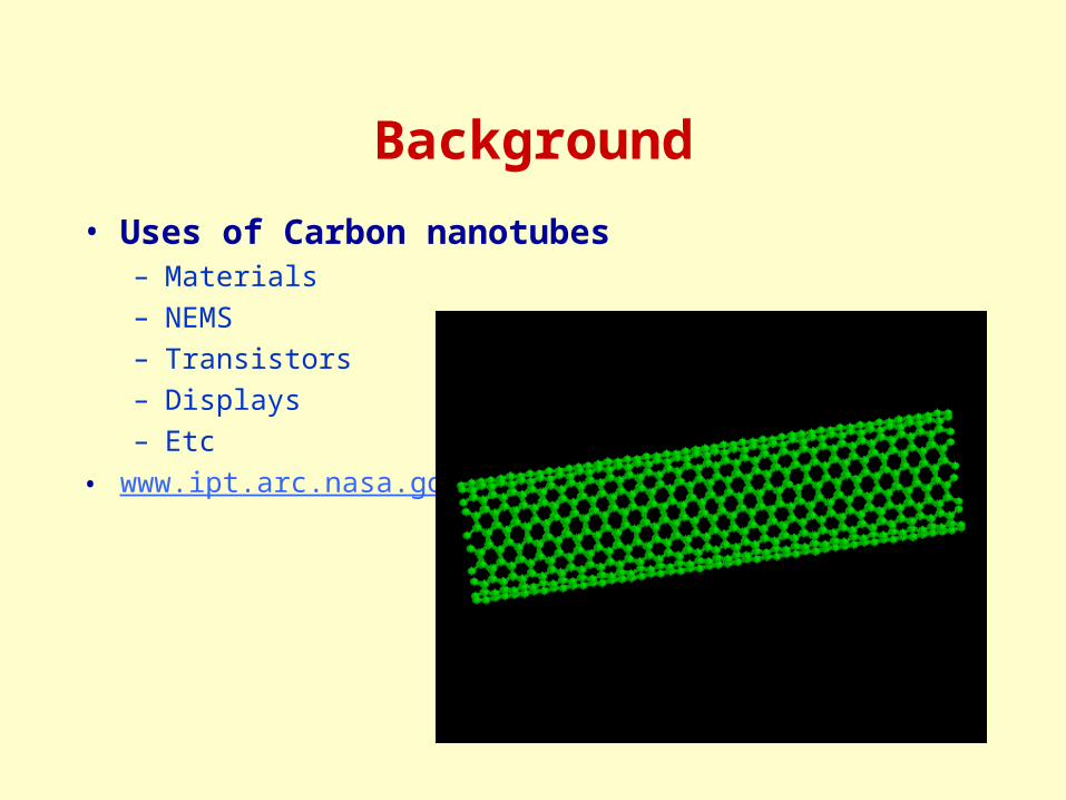
• Uses of Carbon nanotubes– Materials– NEMS– Transistors– Displays– Etc

• www.ipt.arc.nasa.gov

Sequential computation

• Molecular dynamics, using Brenner’s potential– Short-range interactions– Neighbors can change

dynamically during the course of the simulation

– Computational scheme• Find force on each particle due to

interactions with “close” neighbors• Update position and velocity of

each atom

Conventional particle methods, with pair-wise interactions

Force computations

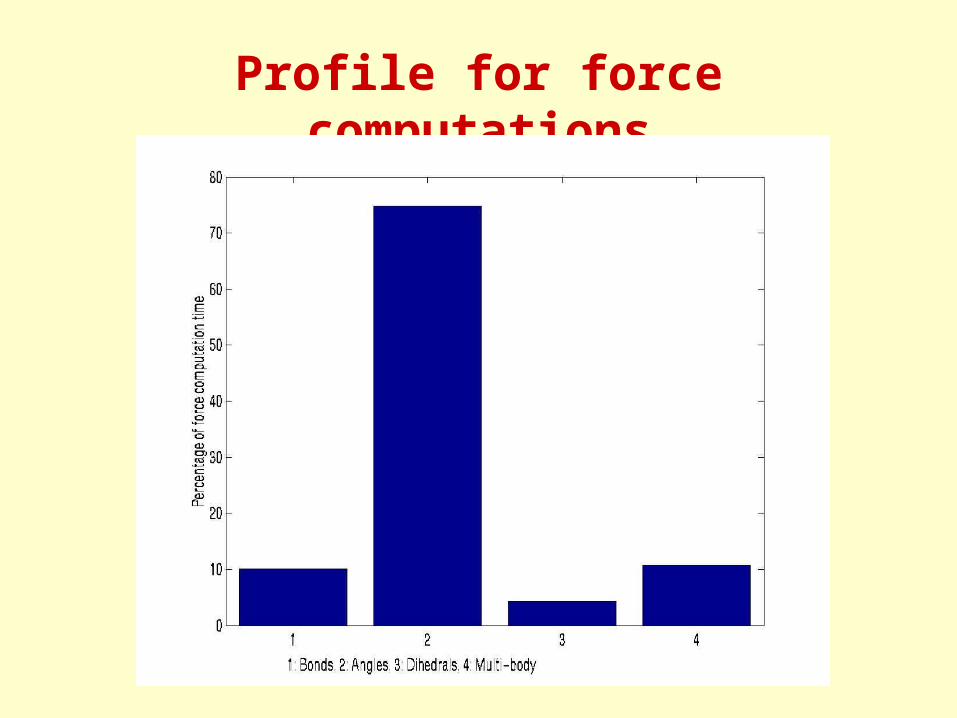
• Bond angles

• Pair interactions

• Dihedral

• Multibody

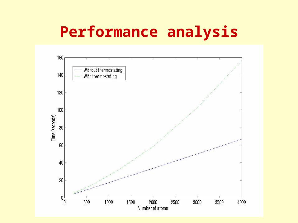
Performance analysis

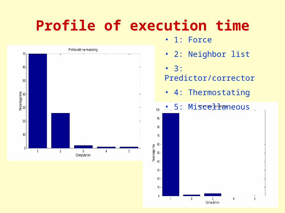
Profile of execution time• 1: Force

• 2: Neighbor list

• 3: Predictor/corrector

• 4: Thermostating

• 5: Miscellaneous

Profile for force computations

Neighbor search

• Neighbor lists– Crude algorithm

• Compare each pair, and determine if they are close enough

• O(N2) for N atoms

– Cell based algorithm• Divide space into cells• Place atoms in their respective cells• Compare atoms only in neighboring cells• Problem

– Many empty cells– Inefficient use of memory

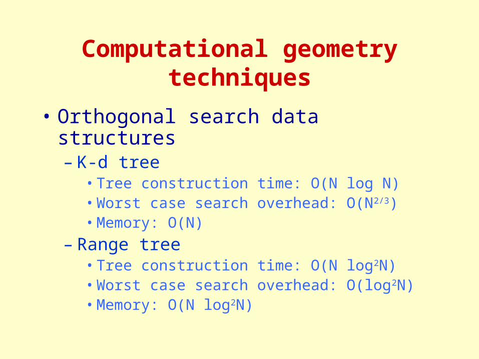
Computational geometry techniques

• Orthogonal search data structures– K-d tree

• Tree construction time: O(N log N)• Worst case search overhead: O(N2/3)• Memory: O(N)

– Range tree• Tree construction time: O(N log2N)• Worst case search overhead: O(log2N)• Memory: O(N log2N)

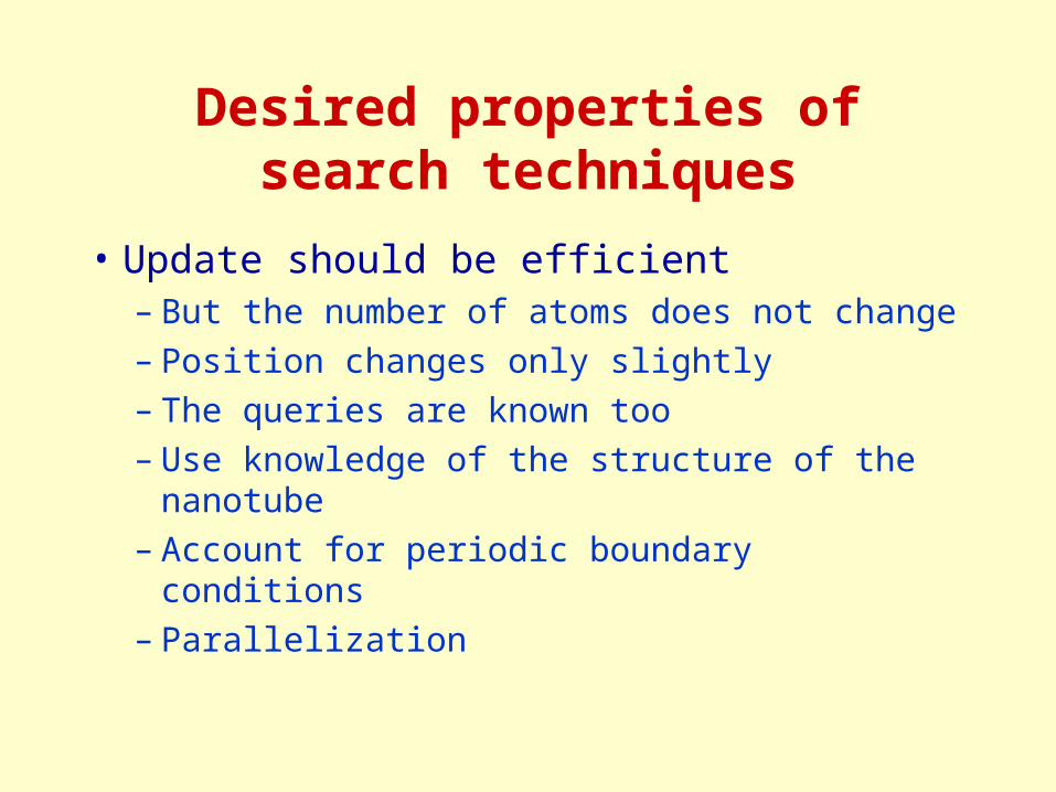
Desired properties of search techniques

• Update should be efficient– But the number of atoms does not change– Position changes only slightly– The queries are known too– Use knowledge of the structure of the

nanotube– Account for periodic boundary conditions– Parallelization

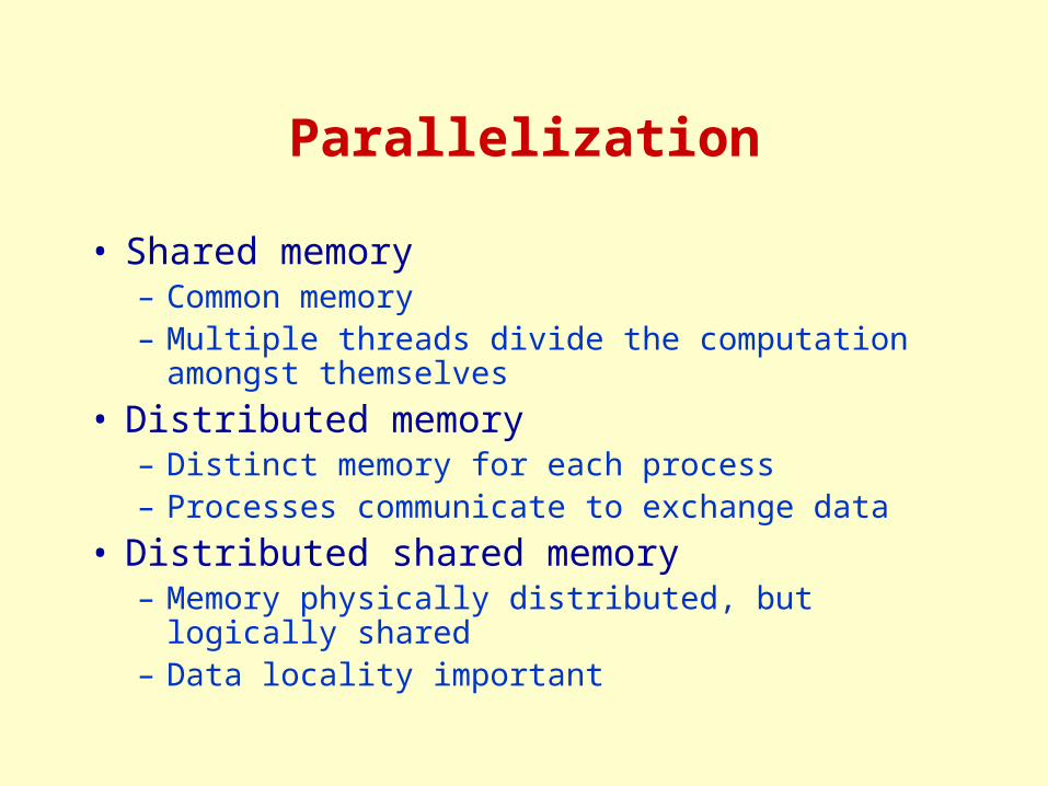
Parallelization

• Shared memory– Common memory– Multiple threads divide the computation amongst

themselves

• Distributed memory– Distinct memory for each process– Processes communicate to exchange data

• Distributed shared memory– Memory physically distributed, but logically shared– Data locality important

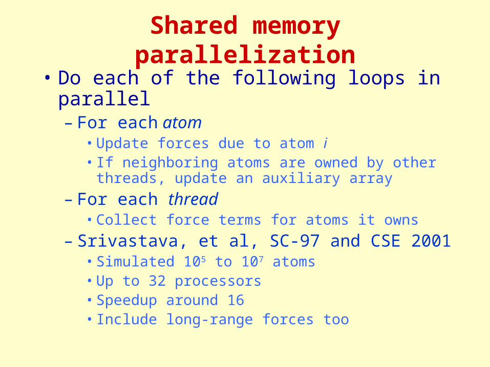
Shared memory parallelization

• Do each of the following loops in parallel– For each atom

• Update forces due to atom i• If neighboring atoms are owned by other

threads, update an auxiliary array

– For each thread• Collect force terms for atoms it owns

– Srivastava, et al, SC-97 and CSE 2001• Simulated 105 to 107 atoms• Up to 32 processors• Speedup around 16• Include long-range forces too

Message passing parallelization

• Decompose domain into cells– Each cell contains its atoms

• Assign a set of adjacent cells to each processor

• Each processor computes values for its cells– Communicates with neighbors when their data is

needed

• Caglar and Griebel, World scientific, 1999– Simulated 108 atoms on up to 512 processors– Linear speedup for 160,000 atoms on 64

processors

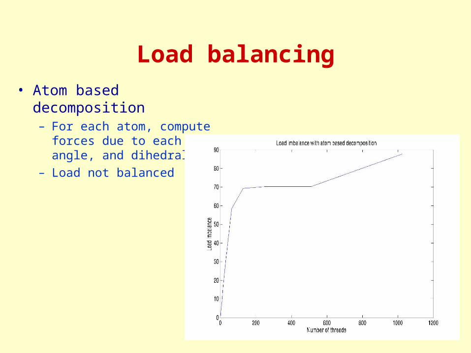
Load balancing• Atom based decomposition

– For each atom, compute forces due to each bond, angle, and dihedral

– Load not balanced

Load balancing ... 2• Bond based decomposition

– For each bond, compute forces due to that bond, angles, and dihedrals

– Finer grained– Load still not

balanced!

Load balancing ... 3

• Load imbalance was not caused by granularity– Symmetry is used to reduce calculations through

– If i > j, don’t compute for bond (i,j)

• So threads get unequal load

– Change condition to• If i+j is even, don’t compute bond (i,j) if i > j• If i+j is odd, don’t compute bond (i,j) if i < j• Does not work, due to regular structure of nanotube

– Use a different condition to balance load

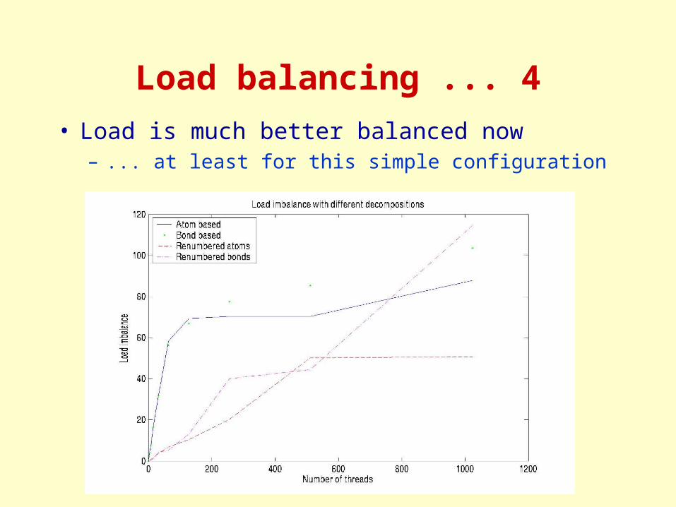
Load balancing ... 4

• Load is much better balanced now– ... at least for this simple configuration

Locality• Locality important to reduce cache misses

• Current scheme based on lexical ordering

• Alternate: Decompose based on a breadth first search traversal of the atom-interaction graph

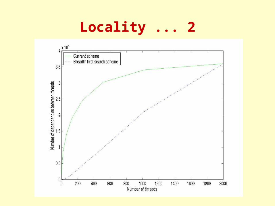
Locality ... 2

Research issues

• Neighbor search– More efficient data structures– Update should be efficient

• But the number of atoms does not change• Position changes only slightly

– The queries are known too– May be able to use knowledge of the structure of

the nanotube– Account for periodic boundary conditions– Parallelization

Research issues ... 2

• Load balancing and locality– Better graph based techniques– Geometric partitioning– Dynamic schemes– Use structure of the tube

• Spectral partitioning

• Multi-scale– Space– Time

Algorithms

• Stochastic techniques– Scalable parallelization– Linear algebra– Applications

Scalable parallelization• Conventional Monte Carlo parallelization

– Perform identical computations on each processor, but with a different random number sequence

– Finally, combine the results– Latency tolerant and fault tolerant

Linear algebra

• Linear solvers

• Matrix-vector multiplication

• Smallest eigenvalue and eigenvector

• Largest eigenvalue and eigenvector

Monte Carlo power method• Obtain the eigenvector for the largest eigenvalue as

– Amh, as m approaches infinity for some h

– Use a random walk of length m to estimate Amh

• Initial probabilities given by P = |h|/|h|

• Transition probability from state to state by p = |a|/|a|

• Define random variables Wi as W0 = hk0/Pk0, Wi =

Wi-1 akiki-1 / pkiki-1, where ki = i th state of random walk

• Then E(Wiki) = (Aih), where is the Kronecker delta function (ij = 1 if i = j, and 0 otherwise).

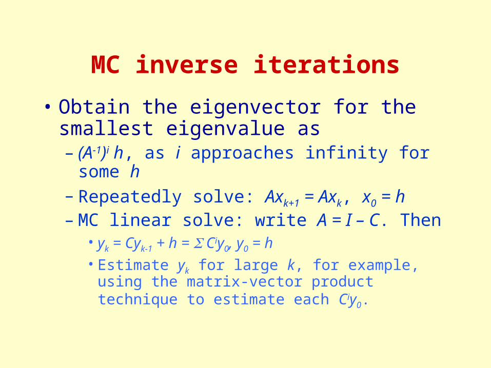
MC inverse iterations

• Obtain the eigenvector for the smallest eigenvalue as– (A-1)i h, as i approaches infinity for some h– Repeatedly solve: Axk+1 = Axk, x0 = h– MC linear solve: write A = I – C. Then

• yk = Cyk-1 + h = Ciy0, y0 = h• Estimate yk for large k, for example, using the

matrix-vector product technique to estimate each Ciy0.

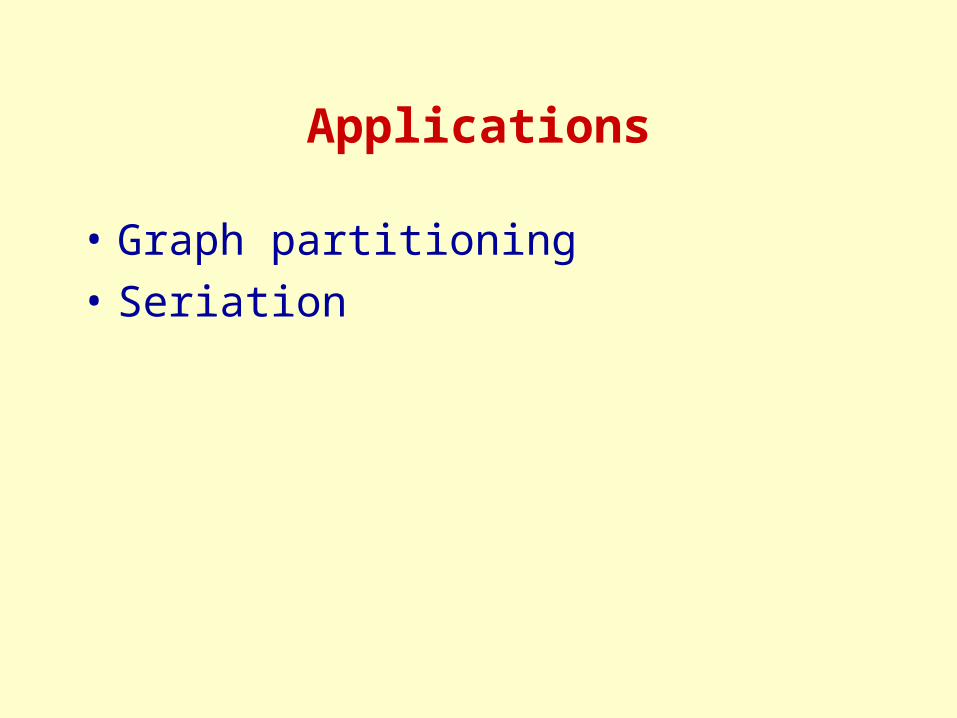
Applications

• Graph partitioning

• Seriation

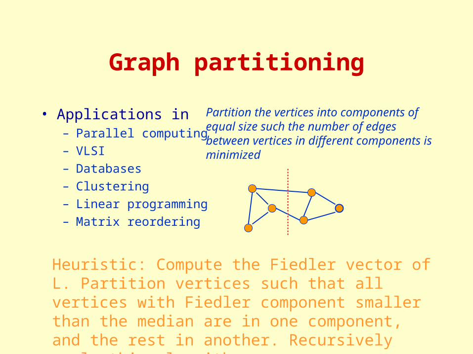
Graph partitioning

• Applications in– Parallel computing– VLSI– Databases– Clustering– Linear programming– Matrix reordering

Partition the vertices into components of equal size such the number of edges between vertices in different components is minimized

Heuristic: Compute the Fiedler vector of L. Partition vertices such that all vertices with Fiedler component smaller than the median are in one component, and the rest in another. Recursively apply this algorithm.

Seriation

• Applications in– DNA sequencing– Matrix envelope

reduction– Archaeological dating

Given a similarity function f, find a permutation such that (i) < (j) < (k) implies f(i,j) > f(i,k)

Heuristic: Compute the Fiedler vector of L. Order vertices by the values of the corresponding components of the Fiedler vector.

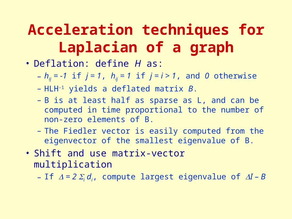
Acceleration techniques for Laplacian of a graph

• Deflation: define H as: – hij = -1 if j = 1, hij = 1 if j = i > 1, and 0 otherwise

– HLH-1 yields a deflated matrix B.– B is at least half as sparse as L, and can be

computed in time proportional to the number of non-zero elements of B.

– The Fiedler vector is easily computed from the eigenvector of the smallest eigenvalue of B.

• Shift and use matrix-vector multiplication– If = 2 i di, compute largest eigenvalue of I – B

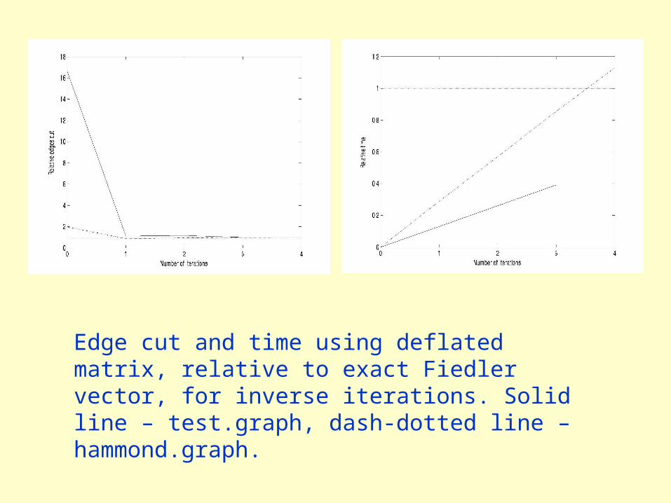
Edge cut and time using deflated matrix, relative to exact Fiedler vector, for inverse iterations. Solid line – test.graph, dash-dotted line – hammond.graph.

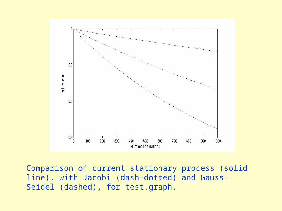
Comparison of current stationary process (solid line), with Jacobi (dash-dotted) and Gauss-Seidel (dashed), for test.graph.

Research issues

• We have developed non-Jacobi based techniques, with theoretically better properties

• Other stationary and non-stationary methods

• Use the structure of the application, for example the nanotube, to accelerate convergence