Embed Size (px)
Citation preview
14
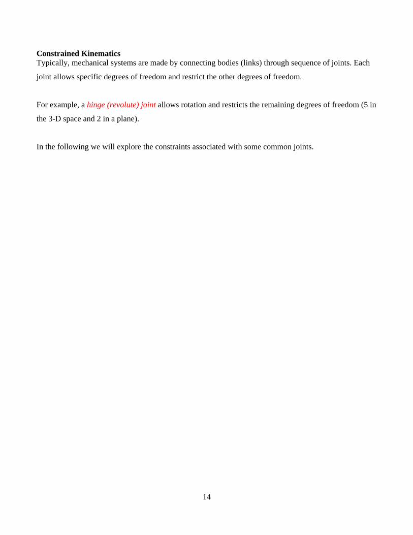
Constrained Kinematics Typically, mechanical systems are made by connecting bodies (links) through sequence of joints. Each
joint allows specific degrees of freedom and restrict the other degrees of freedom.
For example, a hinge (revolute) joint allows rotation and restricts the remaining degrees of freedom (5 in
the 3-D space and 2 in a plane).
In the following we will explore the constraints associated with some common joints.
15
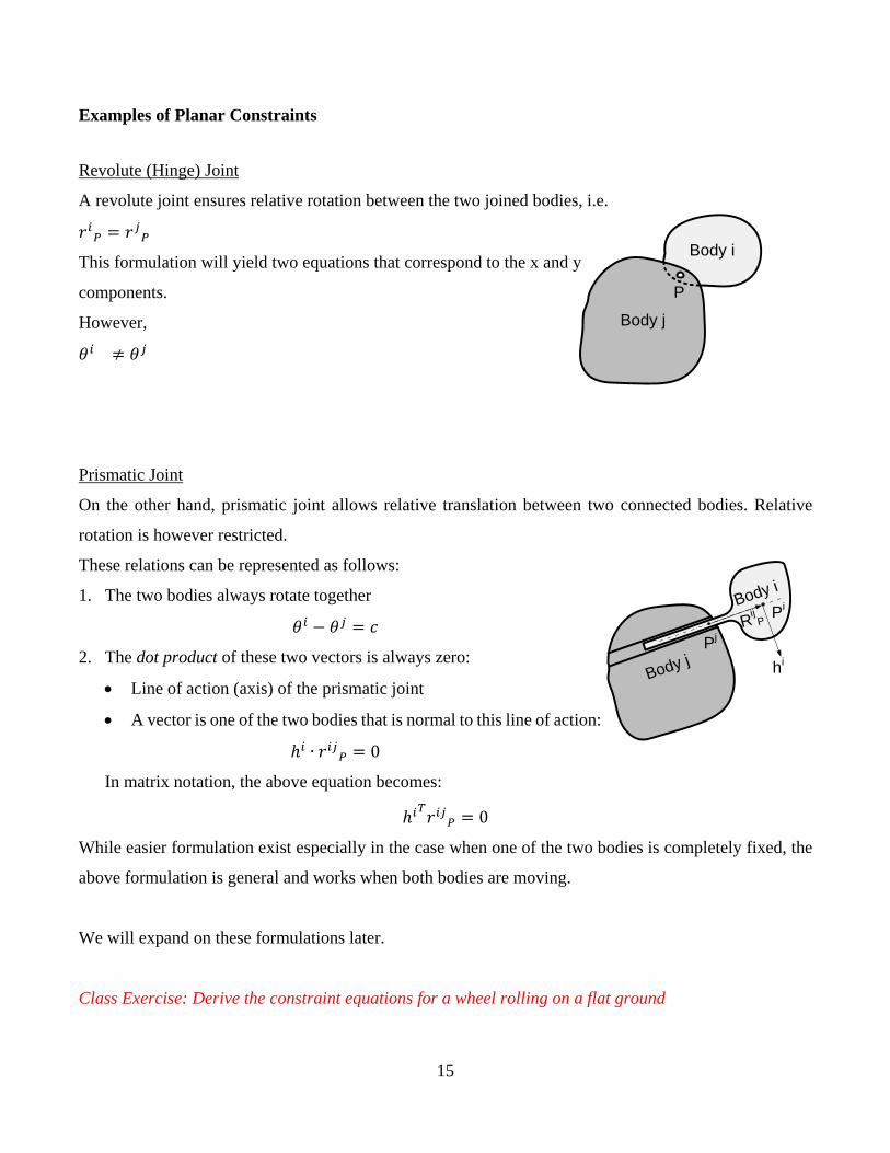
Examples of Planar Constraints
Revolute (Hinge) Joint
A revolute joint ensures relative rotation between the two joined bodies, i.e.
𝑟𝑟𝑖𝑖𝑃𝑃 = 𝑟𝑟𝑗𝑗𝑃𝑃
This formulation will yield two equations that correspond to the x and y
components.
However,
𝜃𝜃𝑖𝑖 ≠ 𝜃𝜃𝑗𝑗
Prismatic Joint
On the other hand, prismatic joint allows relative translation between two connected bodies. Relative
rotation is however restricted.
These relations can be represented as follows:
1. The two bodies always rotate together
𝜃𝜃𝑖𝑖 − 𝜃𝜃𝑗𝑗 = 𝑐𝑐
2. The dot product of these two vectors is always zero:
• Line of action (axis) of the prismatic joint
• A vector is one of the two bodies that is normal to this line of action:
ℎ𝑖𝑖 ∙ 𝑟𝑟𝑖𝑖𝑗𝑗𝑃𝑃 = 0
In matrix notation, the above equation becomes:
ℎ𝑖𝑖𝑇𝑇𝑟𝑟𝑖𝑖𝑗𝑗𝑃𝑃 = 0 While easier formulation exist especially in the case when one of the two bodies is completely fixed, the
above formulation is general and works when both bodies are moving.
We will expand on these formulations later.
Class Exercise: Derive the constraint equations for a wheel rolling on a flat ground
θi
Body i
Body j
P
θi
Body j
Body i
Pj
Pi
hi
RijP
16
Computational Kinematic Approach
• Classical kinematics can be used to accurately formulate equations describing the kinematics of
variables of a machine in terms of its input motion.
• Formulating these equations required a prior knowledge of the geometry and sequence of joints
within the machine.
• However, in any computer-aided software, the user creates a machine on the spot. In this case,
classical approach cannot be used. Instead, a computational approach can be general enough to solve
the kinematics of any machine.
• Kinematic analysis can be viewed as solving a set of algebraic equations that describes the joint
connectivity of a certain machine.
• Another approach is to combine the equations and solve them.
• The resulting system of the coupled equations can be solved using numerical techniques.
• This is the technique used by most computer simulation software packages.
17
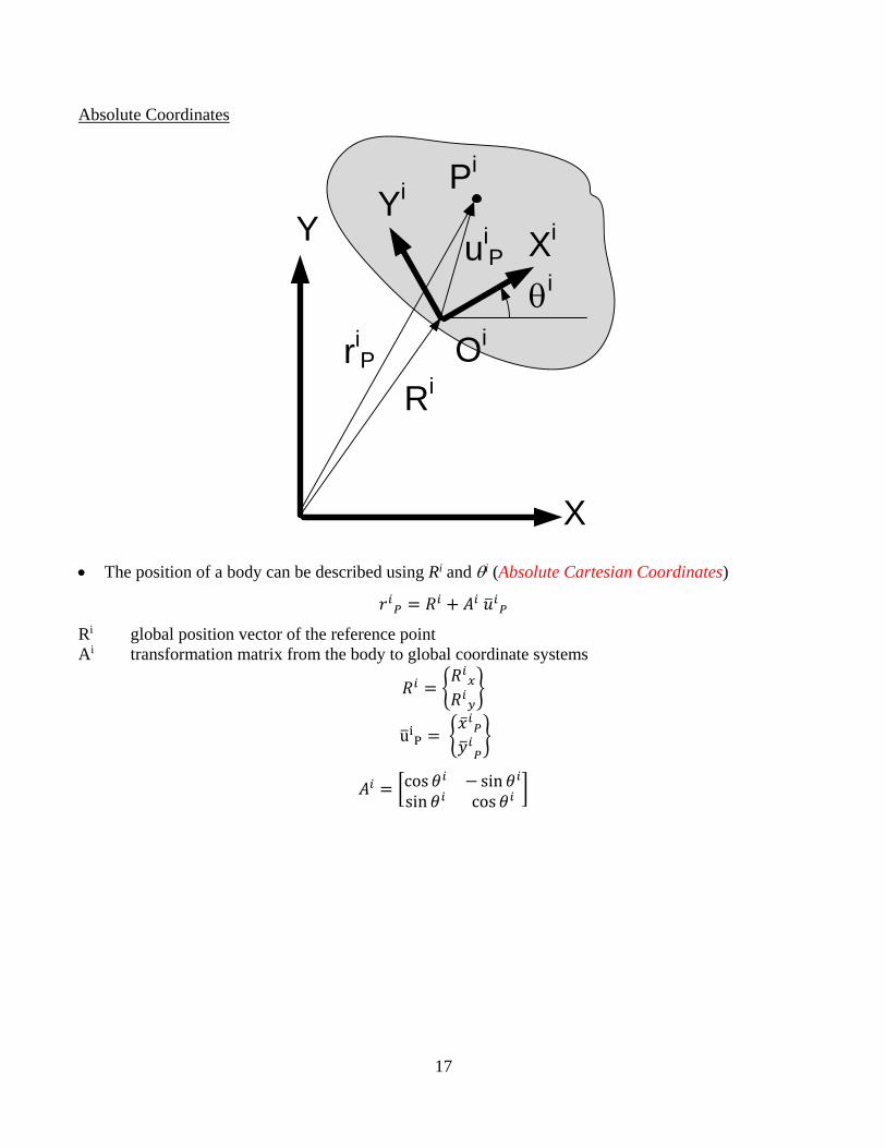
Absolute Coordinates
X
Y XiYi
θi
Pi
Ri
uiP
riP Oi
• The position of a body can be described using Ri and θi (Absolute Cartesian Coordinates)
𝑟𝑟𝑖𝑖𝑃𝑃 = 𝑅𝑅𝑖𝑖 + 𝐴𝐴𝑖𝑖 𝑢𝑢�𝑖𝑖𝑃𝑃
Ri global position vector of the reference point Ai transformation matrix from the body to global coordinate systems
𝑅𝑅𝑖𝑖 = �𝑅𝑅𝑖𝑖𝑥𝑥𝑅𝑅𝑖𝑖𝑦𝑦
�
u�iP = ��̅�𝑥𝑖𝑖𝑃𝑃𝑦𝑦�𝑖𝑖𝑃𝑃
�
𝐴𝐴𝑖𝑖 = �cos𝜃𝜃𝑖𝑖 − sin𝜃𝜃𝑖𝑖sin𝜃𝜃𝑖𝑖 cos 𝜃𝜃𝑖𝑖
�
18
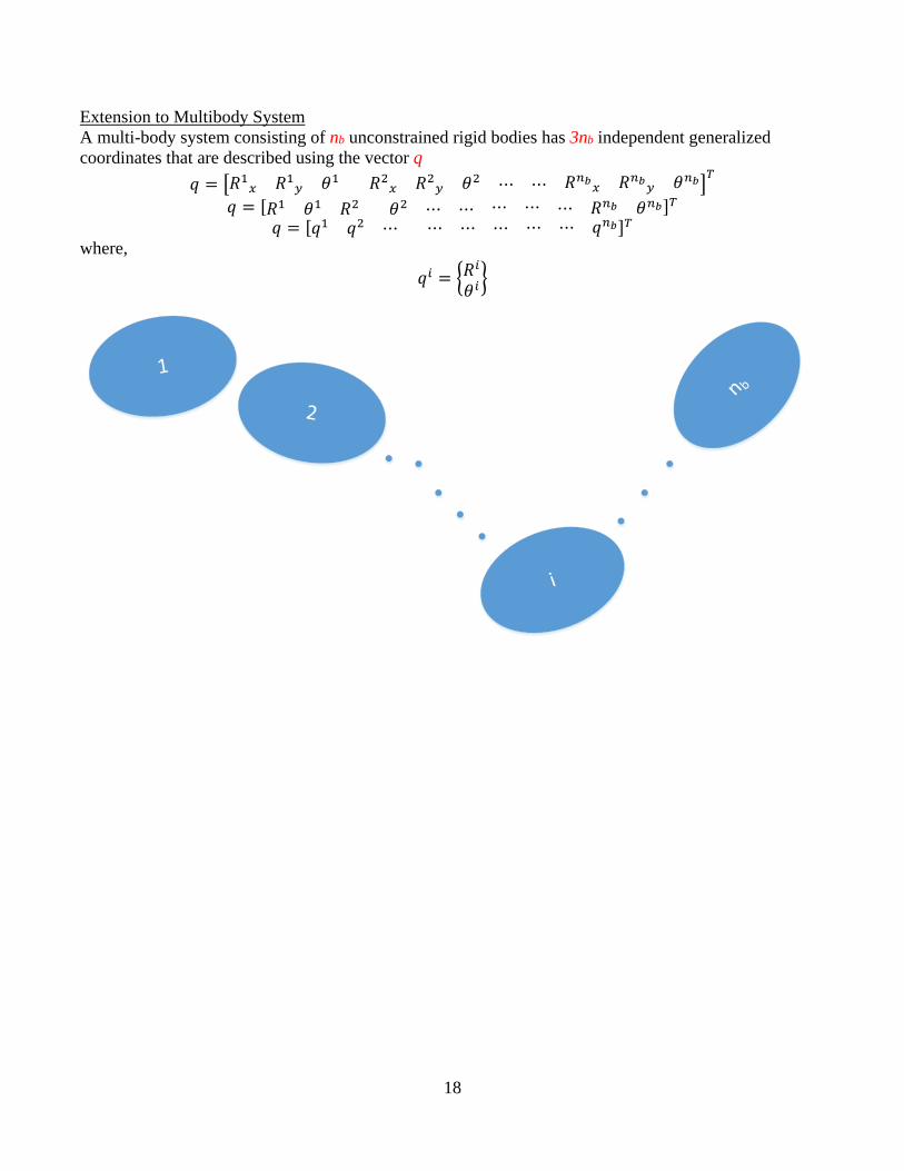
Extension to Multibody System A multi-body system consisting of nb unconstrained rigid bodies has 3nb independent generalized coordinates that are described using the vector q
𝑞𝑞 = �𝑅𝑅1𝑥𝑥 𝑅𝑅1𝑦𝑦 𝜃𝜃1 𝑅𝑅2𝑥𝑥 𝑅𝑅2𝑦𝑦 𝜃𝜃2 ⋯ ⋯ 𝑅𝑅𝑛𝑛𝑏𝑏𝑥𝑥 𝑅𝑅𝑛𝑛𝑏𝑏𝑦𝑦 𝜃𝜃𝑛𝑛𝑏𝑏�𝑇𝑇 𝑞𝑞 = [𝑅𝑅1 𝜃𝜃1 𝑅𝑅2 𝜃𝜃2 ⋯ ⋯ ⋯ ⋯ ⋯ 𝑅𝑅𝑛𝑛𝑏𝑏 𝜃𝜃𝑛𝑛𝑏𝑏]𝑇𝑇
𝑞𝑞 = [𝑞𝑞1 𝑞𝑞2 ⋯ ⋯ ⋯ ⋯ ⋯ ⋯ 𝑞𝑞𝑛𝑛𝑏𝑏]𝑇𝑇 where,
𝑞𝑞𝑖𝑖 = �𝑅𝑅𝑖𝑖
𝜃𝜃𝑖𝑖�

19
Kinematic Constraints The relation between two bodies i and j can be related by the following equation
𝑟𝑟𝑖𝑖𝑃𝑃 − 𝑟𝑟𝑗𝑗𝑃𝑃 = 𝑓𝑓(𝑡𝑡)
Or,
�𝑅𝑅𝑖𝑖 + 𝐴𝐴𝑖𝑖 𝑢𝑢�𝑖𝑖𝑃𝑃� − �𝑅𝑅𝑗𝑗 + 𝐴𝐴𝑖𝑖 𝑢𝑢�𝑗𝑗𝑃𝑃� = 𝑓𝑓(𝑡𝑡)
f(t) is a known function of time
20
Ground Constraints
A body that has zero degrees of freedom (ground or fixed link)
𝑞𝑞𝑖𝑖 = 𝑐𝑐
It is convenient to have the coordinates of frame i matching those of the global frame or,
�𝑅𝑅𝑖𝑖𝑥𝑥𝑅𝑅𝑖𝑖𝑥𝑥𝜃𝜃𝑖𝑖� = 0
21
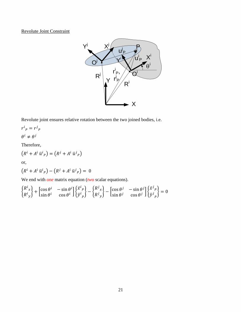
Revolute Joint Constraint
X
Y
Xi
θi
Ri
uiP
Oi
P
Yi
XjYj
Rj
Oj
ujP
riP,
rjP
Revolute joint ensures relative rotation between the two joined bodies, i.e.
𝑟𝑟𝑖𝑖𝑃𝑃 = 𝑟𝑟𝑗𝑗𝑃𝑃
𝜃𝜃𝑖𝑖 ≠ 𝜃𝜃𝑗𝑗
Therefore,
�𝑅𝑅𝑖𝑖 + 𝐴𝐴𝑖𝑖 𝑢𝑢�𝑖𝑖𝑃𝑃� = �𝑅𝑅𝑗𝑗 + 𝐴𝐴𝑖𝑖 𝑢𝑢�𝑗𝑗𝑃𝑃�
or,
�𝑅𝑅𝑖𝑖 + 𝐴𝐴𝑖𝑖 𝑢𝑢�𝑖𝑖𝑃𝑃� − �𝑅𝑅𝑗𝑗 + 𝐴𝐴𝑖𝑖 𝑢𝑢�𝑗𝑗𝑃𝑃� = 0
We end with one matrix equation (two scalar equations).
�𝑅𝑅𝑖𝑖𝑥𝑥𝑅𝑅𝑖𝑖𝑦𝑦
� + �cos𝜃𝜃𝑖𝑖 − sin𝜃𝜃𝑖𝑖sin𝜃𝜃𝑖𝑖 cos 𝜃𝜃𝑖𝑖
� ��̅�𝑥𝑖𝑖𝑃𝑃𝑦𝑦�𝑖𝑖𝑃𝑃
� − �𝑅𝑅𝑗𝑗𝑥𝑥𝑅𝑅𝑗𝑗𝑦𝑦
� − �cos 𝜃𝜃𝑗𝑗 − sin𝜃𝜃𝑗𝑗sin𝜃𝜃𝑗𝑗 cos 𝜃𝜃𝑗𝑗
� ��̅�𝑥𝑗𝑗𝑃𝑃𝑦𝑦�𝑗𝑗𝑃𝑃
� = 0

22
Prismatic Joint
θi
Body j
Body i
Pj
Pi
hi Qirij P
Prismatic joint allows relative translation between the connected bodies. Relative rotation is however
restricted as two bodies have to rotate together, which means,
𝜃𝜃𝑖𝑖 − 𝜃𝜃𝑗𝑗 = 𝑐𝑐
On the other hand, one of the two bodies is free to slide in and out of the other one along a specified line
of action. Geometrically, this can be represented using two vectors:
• The line of action connecting two points on j and i respectively as in the figure above and
• A vector in Body i that is normal to this line of action
Regardless of the orientations of these two bodies, these two vectors will always remain normal to each
other. This relation can be represented using dot product of these two vectors:
ℎ𝑖𝑖𝑇𝑇𝑟𝑟𝑖𝑖𝑗𝑗𝑃𝑃 = 0
where,
ℎ𝑖𝑖 = 𝐴𝐴𝑖𝑖� 𝑢𝑢�𝑖𝑖𝑃𝑃 − 𝑢𝑢�𝑖𝑖𝑄𝑄�
𝑟𝑟𝑖𝑖𝑗𝑗𝑃𝑃 = 𝑟𝑟𝑖𝑖𝑃𝑃 − 𝑟𝑟𝑗𝑗𝑃𝑃 = �𝑅𝑅𝑖𝑖 + 𝐴𝐴𝑖𝑖 𝑢𝑢�𝑖𝑖𝑃𝑃� − �𝑅𝑅𝑗𝑗 + 𝐴𝐴𝑖𝑖 𝑢𝑢�𝑗𝑗𝑃𝑃�
These equations can be combined as,
�𝜃𝜃𝑖𝑖 − 𝜃𝜃𝑗𝑗 − 𝑐𝑐ℎ𝑖𝑖𝑇𝑇𝑟𝑟𝑖𝑖𝑗𝑗𝑃𝑃
� = �00�
23
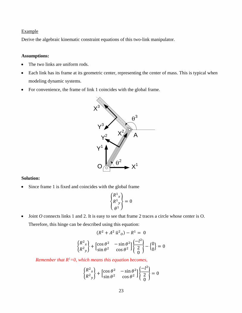
Example
Derive the algebraic kinematic constraint equations of this two-link manipulator.
Assumptions:
• The two links are uniform rods.
• Each link has its frame at its geometric center, representing the center of mass. This is typical when
modeling dynamic systems.
• For convenience, the frame of link 1 coincides with the global frame.
X1
Y1
X3
θ2O
Y3
X2
Y2
θ3
A
Solution:
• Since frame 1 is fixed and coincides with the global frame
�𝑅𝑅1𝑥𝑥𝑅𝑅1𝑦𝑦𝜃𝜃1
� = 0
• Joint O connects links 1 and 2. It is easy to see that frame 2 traces a circle whose center is O.
Therefore, this hinge can be described using this equation:
(𝑅𝑅2 + 𝐴𝐴2 𝑢𝑢�2𝑂𝑂) − 𝑅𝑅1 = 0
�𝑅𝑅2𝑥𝑥𝑅𝑅2𝑦𝑦
� + �cos𝜃𝜃2 − sin𝜃𝜃2sin𝜃𝜃2 cos𝜃𝜃2
� �−𝑙𝑙2
20� − �00� = 0
Remember that R1=0, which means this equation becomes,
�𝑅𝑅2𝑥𝑥𝑅𝑅2𝑦𝑦
� + �cos 𝜃𝜃2 − sin𝜃𝜃2sin𝜃𝜃2 cos 𝜃𝜃2
� �−𝑙𝑙2
20� = 0
24
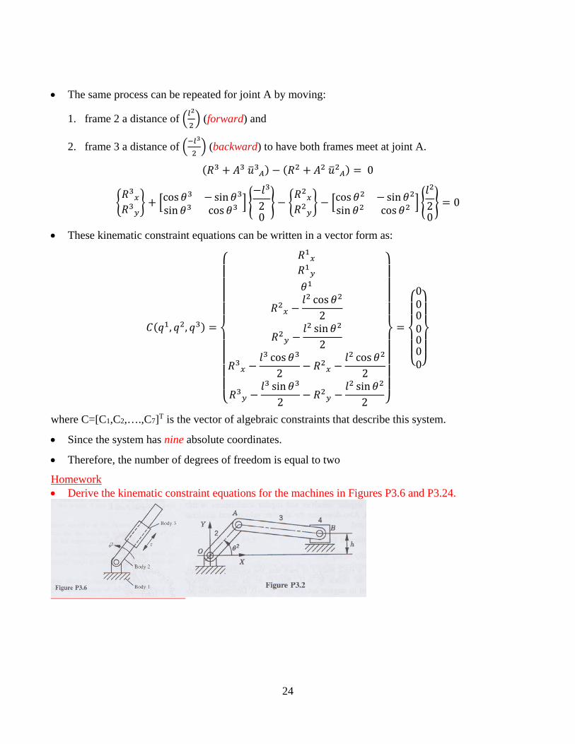
• The same process can be repeated for joint A by moving:
1. frame 2 a distance of �𝑙𝑙2
2� (forward) and
2. frame 3 a distance of �−𝑙𝑙3
2� (backward) to have both frames meet at joint A.
(𝑅𝑅3 + 𝐴𝐴3 𝑢𝑢�3𝐴𝐴) − (𝑅𝑅2 + 𝐴𝐴2 𝑢𝑢�2𝐴𝐴) = 0
�𝑅𝑅3𝑥𝑥𝑅𝑅3𝑦𝑦
� + �cos𝜃𝜃3 − sin𝜃𝜃3sin𝜃𝜃3 cos𝜃𝜃3
� �−𝑙𝑙3
20� − �
𝑅𝑅2𝑥𝑥𝑅𝑅2𝑦𝑦
� − �cos𝜃𝜃2 − sin𝜃𝜃2sin𝜃𝜃2 cos𝜃𝜃2
� �𝑙𝑙2
20� = 0
• These kinematic constraint equations can be written in a vector form as:
𝐶𝐶(𝑞𝑞1, 𝑞𝑞2, 𝑞𝑞3) =
⎩⎪⎪⎪⎪⎨
⎪⎪⎪⎪⎧ 𝑅𝑅1𝑥𝑥
𝑅𝑅1𝑦𝑦𝜃𝜃1
𝑅𝑅2𝑥𝑥 −𝑙𝑙2 cos 𝜃𝜃2
2
𝑅𝑅2𝑦𝑦 −𝑙𝑙2 sin𝜃𝜃2
2
𝑅𝑅3𝑥𝑥 −𝑙𝑙3 cos𝜃𝜃3
2− 𝑅𝑅2𝑥𝑥 −
𝑙𝑙2 cos 𝜃𝜃2
2
𝑅𝑅3𝑦𝑦 −𝑙𝑙3 sin𝜃𝜃3
2− 𝑅𝑅2𝑦𝑦 −
𝑙𝑙2 sin𝜃𝜃2
2 ⎭⎪⎪⎪⎪⎬
⎪⎪⎪⎪⎫
=
⎩⎪⎨
⎪⎧
0000000⎭⎪⎬
⎪⎫
where C=[C1,C2,….,C7]T is the vector of algebraic constraints that describe this system.
• Since the system has nine absolute coordinates.
• Therefore, the number of degrees of freedom is equal to two
Homework • Derive the kinematic constraint equations for the machines in Figures P3.6 and P3.24.
25
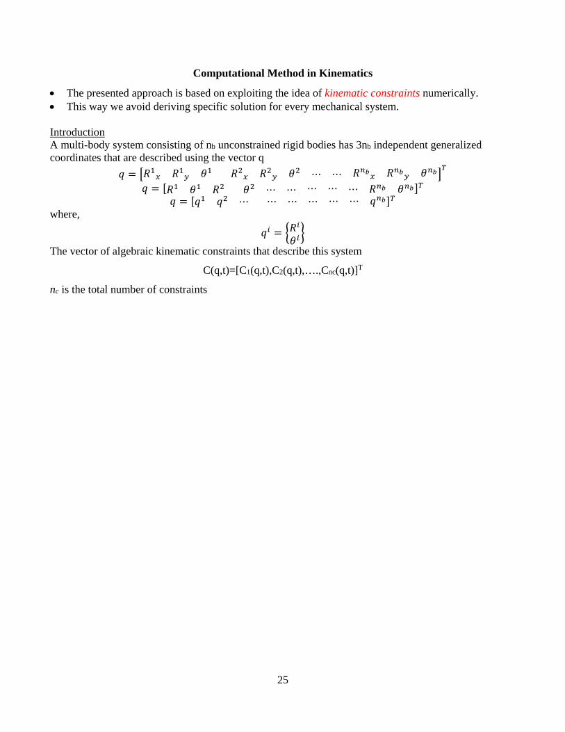
Computational Method in Kinematics
• The presented approach is based on exploiting the idea of kinematic constraints numerically. • This way we avoid deriving specific solution for every mechanical system. Introduction A multi-body system consisting of nb unconstrained rigid bodies has 3nb independent generalized coordinates that are described using the vector q
𝑞𝑞 = �𝑅𝑅1𝑥𝑥 𝑅𝑅1𝑦𝑦 𝜃𝜃1 𝑅𝑅2𝑥𝑥 𝑅𝑅2𝑦𝑦 𝜃𝜃2 ⋯ ⋯ 𝑅𝑅𝑛𝑛𝑏𝑏𝑥𝑥 𝑅𝑅𝑛𝑛𝑏𝑏𝑦𝑦 𝜃𝜃𝑛𝑛𝑏𝑏�𝑇𝑇 𝑞𝑞 = [𝑅𝑅1 𝜃𝜃1 𝑅𝑅2 𝜃𝜃2 ⋯ ⋯ ⋯ ⋯ ⋯ 𝑅𝑅𝑛𝑛𝑏𝑏 𝜃𝜃𝑛𝑛𝑏𝑏]𝑇𝑇
𝑞𝑞 = [𝑞𝑞1 𝑞𝑞2 ⋯ ⋯ ⋯ ⋯ ⋯ ⋯ 𝑞𝑞𝑛𝑛𝑏𝑏]𝑇𝑇 where,
𝑞𝑞𝑖𝑖 = �𝑅𝑅𝑖𝑖
𝜃𝜃𝑖𝑖�
The vector of algebraic kinematic constraints that describe this system
C(q,t)=[C1(q,t),C2(q,t),….,Cnc(q,t)]T
nc is the total number of constraints
26
Categories of Mechanical Systems
Mechanical systems can be divided into:
1. Dynamically-Driven: The number of the constraint equations is less than the number of the system
coordinates (nc < n).
Dynamics forces are needed to perform the analysis.
Example: A ball falling toward ground.
• No driving input
• No kinematic constraint
• The result is 0 equations that are less than the number of degrees of freedom of the system (3))
2. Kinematically-Driven: The number of the linearly independent constraint equations is equal to the
number of the system coordinates (nc = n).
Example: The two-link manipulator
• Adding the number of driving inputs to the constraints equations (2 inputs to 7 constraints).
• The result is 9 equations that are equal the number of degrees of freedom of the system (3x3))
This chapter focuses on the Kinematically-Driven systems only.
Dynamically-Driven system will be analyzed later.
27
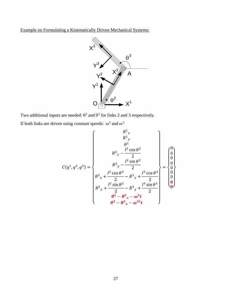
Example on Formulating a Kinematically Driven Mechanical Systems:
X1
Y1
X3
θ2O
Y3
X2
Y2
θ3
A
Two additional inputs are needed: θ2 and θ3 for links 2 and 3 respectively.
If both links are driven using constant speeds: ω2 and ω3,
𝐶𝐶(𝑞𝑞1, 𝑞𝑞2, 𝑞𝑞3) =
⎩⎪⎪⎪⎪⎪⎪⎨
⎪⎪⎪⎪⎪⎪⎧ 𝑅𝑅1𝑥𝑥
𝑅𝑅1𝑦𝑦𝜃𝜃1
𝑅𝑅2𝑥𝑥 −𝑙𝑙2 cos 𝜃𝜃2
2
𝑅𝑅2𝑦𝑦 −𝑙𝑙2 sin𝜃𝜃2
2
𝑅𝑅2𝑥𝑥 +𝑙𝑙2 cos 𝜃𝜃2
2− 𝑅𝑅3𝑥𝑥 +
𝑙𝑙3 cos𝜃𝜃3
2
𝑅𝑅2𝑦𝑦 +𝑙𝑙2 sin𝜃𝜃2
2− 𝑅𝑅3𝑦𝑦 +
𝑙𝑙3 sin𝜃𝜃3
2𝜽𝜽𝟐𝟐 − 𝜽𝜽𝟐𝟐𝒐𝒐 − 𝝎𝝎𝟐𝟐𝒕𝒕𝜽𝜽𝟑𝟑 − 𝜽𝜽𝟑𝟑𝒐𝒐 − 𝝎𝝎𝟑𝟑𝟐𝟐𝒕𝒕 ⎭
⎪⎪⎪⎪⎪⎪⎬
⎪⎪⎪⎪⎪⎪⎫
=
⎩⎪⎪⎨
⎪⎪⎧
0000000𝟎𝟎𝟎𝟎⎭⎪⎪⎬
⎪⎪⎫
28
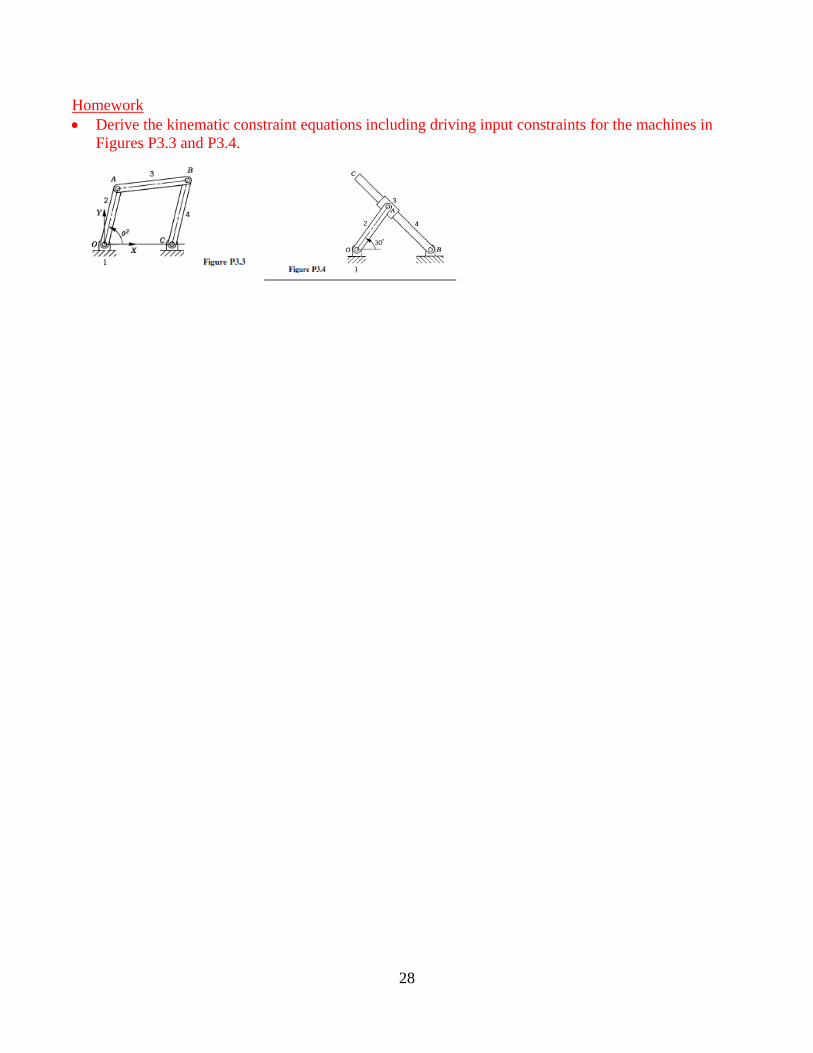
Homework • Derive the kinematic constraint equations including driving input constraints for the machines in
Figures P3.3 and P3.4.
29
Position Analysis
• The kinematic constraints equations are of trigonometric natures and are generally nonlinear.
• While a closed form solution can be obtained in many cases, it has to be performed at each case
separately.
• A computer-driven (computational) approach requires solving these equations using a numerical
method.
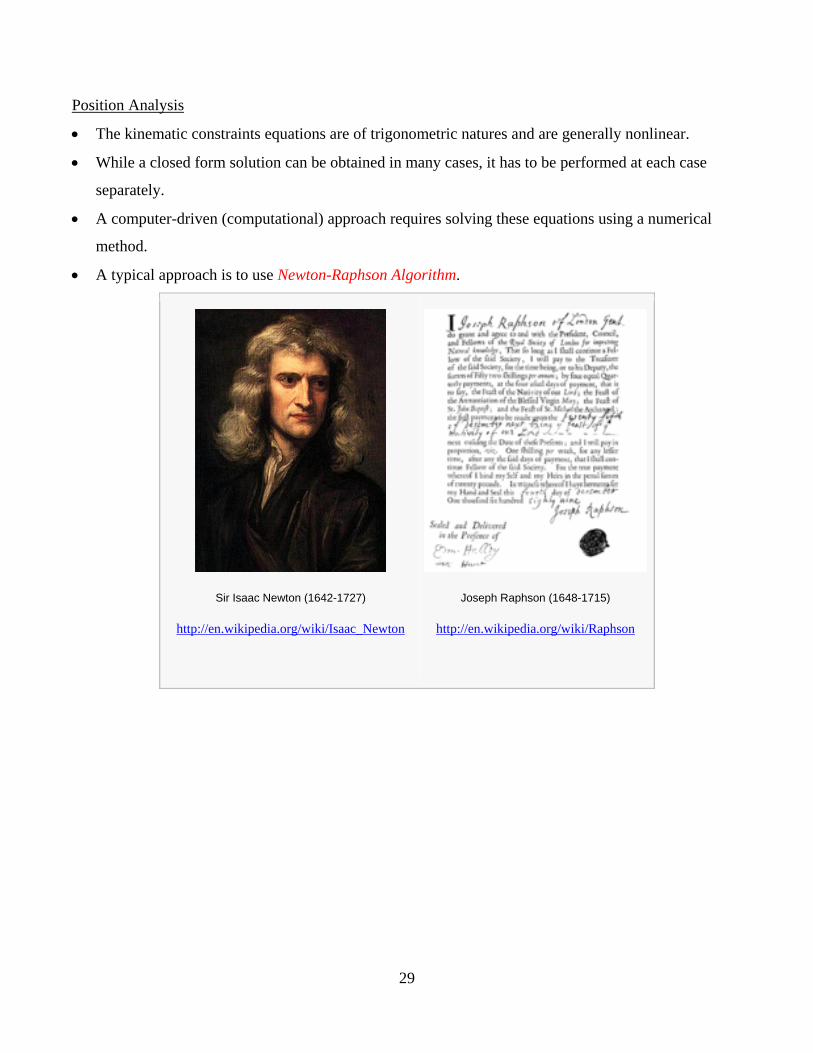
• A typical approach is to use Newton-Raphson Algorithm.
Sir Isaac Newton (1642-1727)
http://en.wikipedia.org/wiki/Isaac_Newton
Joseph Raphson (1648-1715)
http://en.wikipedia.org/wiki/Raphson
30
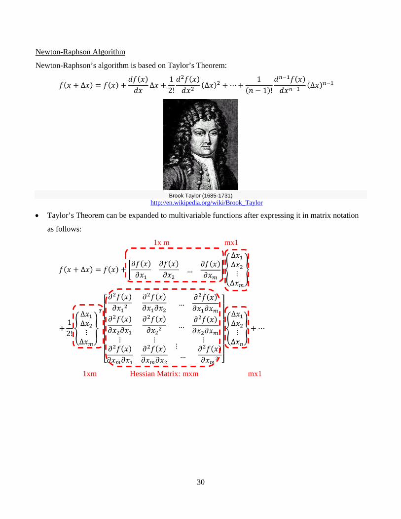
Newton-Raphson Algorithm
Newton-Raphson’s algorithm is based on Taylor’s Theorem:
𝑓𝑓(𝑥𝑥 + ∆𝑥𝑥) = 𝑓𝑓(𝑥𝑥) +𝑑𝑑𝑓𝑓(𝑥𝑥)𝑑𝑑𝑥𝑥
∆𝑥𝑥 +12!𝑑𝑑2𝑓𝑓(𝑥𝑥)𝑑𝑑𝑥𝑥2
(∆𝑥𝑥)2 + ⋯+1
(𝑛𝑛 − 1)!𝑑𝑑𝑛𝑛−1𝑓𝑓(𝑥𝑥)𝑑𝑑𝑥𝑥𝑛𝑛−1
(∆𝑥𝑥)𝑛𝑛−1
Brook Taylor (1685-1731)
http://en.wikipedia.org/wiki/Brook_Taylor
• Taylor’s Theorem can be expanded to multivariable functions after expressing it in matrix notation
as follows:
1x m mx1
𝑓𝑓(𝑥𝑥 + ∆𝑥𝑥) = 𝑓𝑓(𝑥𝑥) + �𝜕𝜕𝑓𝑓(𝑥𝑥)𝜕𝜕𝑥𝑥1
𝜕𝜕𝑓𝑓(𝑥𝑥)𝜕𝜕𝑥𝑥2
…𝜕𝜕𝑓𝑓(𝑥𝑥)𝜕𝜕𝑥𝑥𝑚𝑚
��
∆𝑥𝑥1∆𝑥𝑥2⋮
∆𝑥𝑥𝑚𝑚
�
+12!�
∆𝑥𝑥1∆𝑥𝑥2⋮
∆𝑥𝑥𝑚𝑚
�
𝑇𝑇
⎣⎢⎢⎢⎢⎢⎢⎡ 𝜕𝜕
2𝑓𝑓(𝑥𝑥)𝜕𝜕𝑥𝑥12
𝜕𝜕2𝑓𝑓(𝑥𝑥)𝜕𝜕𝑥𝑥1𝜕𝜕𝑥𝑥2
…𝜕𝜕2𝑓𝑓(𝑥𝑥)𝜕𝜕𝑥𝑥1𝜕𝜕𝑥𝑥𝑚𝑚
𝜕𝜕2𝑓𝑓(𝑥𝑥)𝜕𝜕𝑥𝑥2𝜕𝜕𝑥𝑥1
𝜕𝜕2𝑓𝑓(𝑥𝑥)𝜕𝜕𝑥𝑥22
…𝜕𝜕2𝑓𝑓(𝑥𝑥)𝜕𝜕𝑥𝑥2𝜕𝜕𝑥𝑥𝑚𝑚
⋮𝜕𝜕2𝑓𝑓(𝑥𝑥)𝜕𝜕𝑥𝑥𝑚𝑚𝜕𝜕𝑥𝑥1
⋮𝜕𝜕2𝑓𝑓(𝑥𝑥)𝜕𝜕𝑥𝑥𝑚𝑚𝜕𝜕𝑥𝑥2
⋮ …
⋮ 𝜕𝜕2𝑓𝑓(𝑥𝑥)𝜕𝜕𝑥𝑥𝑚𝑚2 ⎦
⎥⎥⎥⎥⎥⎥⎤
�
∆𝑥𝑥1∆𝑥𝑥2⋮
∆𝑥𝑥𝑛𝑛
� + ⋯
1xm Hessian Matrix: mxm mx1
31
• If we have a set of functions, we can apply Taylor’s Theorem to them by expanding the above
equation,
𝐶𝐶(𝑞𝑞𝑖𝑖 + ∆𝑞𝑞𝑖𝑖 , 𝑡𝑡) = 𝐶𝐶(𝑞𝑞𝑖𝑖 , 𝑡𝑡) + 𝐶𝐶𝑞𝑞𝑖𝑖∆𝑞𝑞𝑖𝑖 + ⋯ (ℎ𝑖𝑖𝑖𝑖ℎ𝑒𝑒𝑟𝑟 𝑜𝑜𝑟𝑟𝑑𝑑𝑒𝑒𝑟𝑟 𝑡𝑡𝑒𝑒𝑟𝑟𝑡𝑡𝑡𝑡) ∆𝑞𝑞 = [∆𝑞𝑞1 ∆𝑞𝑞2 ⋯ ⋯ ⋯ ⋯ ⋯ ⋯ ∆𝑞𝑞𝑛𝑛]𝑇𝑇
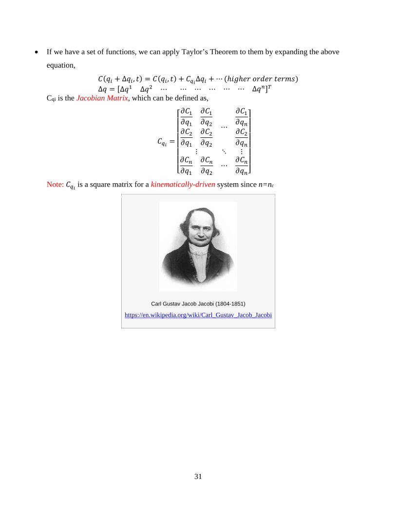
Cqi is the Jacobian Matrix, which can be defined as,
𝐶𝐶𝑞𝑞𝑖𝑖 =
⎣⎢⎢⎢⎢⎢⎢⎡𝜕𝜕𝐶𝐶1𝜕𝜕𝑞𝑞1
𝜕𝜕𝐶𝐶1𝜕𝜕𝑞𝑞2
𝜕𝜕𝐶𝐶2𝜕𝜕𝑞𝑞1
𝜕𝜕𝐶𝐶2𝜕𝜕𝑞𝑞2
⋯
𝜕𝜕𝐶𝐶1𝜕𝜕𝑞𝑞𝑛𝑛𝜕𝜕𝐶𝐶2𝜕𝜕𝑞𝑞𝑛𝑛
⋮ ⋱ ⋮𝜕𝜕𝐶𝐶𝑛𝑛𝜕𝜕𝑞𝑞1
𝜕𝜕𝐶𝐶𝑛𝑛𝜕𝜕𝑞𝑞2
⋯𝜕𝜕𝐶𝐶𝑛𝑛𝜕𝜕𝑞𝑞𝑛𝑛⎦
⎥⎥⎥⎥⎥⎥⎤
Note: 𝐶𝐶𝑞𝑞𝑖𝑖 is a square matrix for a kinematically-driven system since n=nc
Carl Gustav Jacob Jacobi (1804-1851)
https://en.wikipedia.org/wiki/Carl_Gustav_Jacob_Jacobi
32
If the constraint equations are linearly independent1, C is a nonsingular matrix.
Assuming 𝑞𝑞𝑖𝑖 + ∆𝑞𝑞𝑖𝑖 to be the exact solution, then
𝐶𝐶(𝑞𝑞𝑖𝑖 + ∆𝑞𝑞𝑖𝑖 , 𝑡𝑡) = 0
Therefore,
𝐶𝐶(𝑞𝑞𝑖𝑖 , 𝑡𝑡) + 𝐶𝐶𝑞𝑞𝑖𝑖∆𝑞𝑞𝑖𝑖 + ⋯ = 0
If the assumed solution is close enough to the correct solution, the second order and higher terms can
be neglected, which means:
𝐶𝐶(𝑞𝑞𝑖𝑖 , 𝑡𝑡) + 𝐶𝐶𝑞𝑞𝑖𝑖∆𝑞𝑞𝑖𝑖 ≈ 0
𝐶𝐶𝑞𝑞𝑖𝑖∆𝑞𝑞𝑖𝑖 = −𝐶𝐶(𝑞𝑞𝑖𝑖 , 𝑡𝑡)
∆𝑞𝑞𝑖𝑖 = −𝐶𝐶𝑞𝑞𝑖𝑖−1𝐶𝐶(𝑞𝑞𝑖𝑖 , 𝑡𝑡)
Remember that the constraint Jacobian matrix 𝐶𝐶𝑞𝑞𝑖𝑖 is assumed to be nonsingular, i.e., an inverse of
𝐶𝐶𝑞𝑞𝑖𝑖 exists.
The equation can be then solved for the vector of the Newton Differences, ∆𝑞𝑞𝑖𝑖
The vector is updated as,
𝑞𝑞𝑖𝑖+1 = 𝑞𝑞𝑖𝑖 + ∆𝑞𝑞𝑖𝑖
where, i is the iteration number. The updated vector can be used to reconstruct the equation above.
The process continues until:
|∆𝑞𝑞𝑖𝑖| < 𝜖𝜖1 or,
|𝐶𝐶(𝑞𝑞𝑖𝑖 , 𝑡𝑡)| < 𝜖𝜖2
The above termination criteria means that search stops because either: 1. The changes of the vector have become extremely small or, 2. The Kinematic Constraints matrix approaches zero Note: ε1 is a vector while ε2 is a one value.
1 Linearly independent constraints is a set of unique constraints where no constraint can be expressed in terms of the other ones.
33
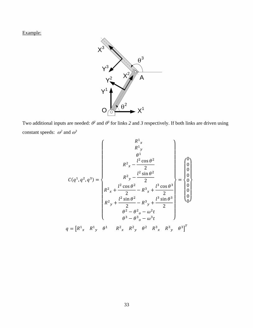
Example:
X1
Y1
X3
θ2O
Y3
X2
Y2
θ3
A
Two additional inputs are needed: θ2 and θ3 for links 2 and 3 respectively. If both links are driven using
constant speeds: ω2 and ω3
𝐶𝐶(𝑞𝑞1, 𝑞𝑞2, 𝑞𝑞3) =
⎩⎪⎪⎪⎪⎪⎪⎨
⎪⎪⎪⎪⎪⎪⎧ 𝑅𝑅1𝑥𝑥
𝑅𝑅1𝑦𝑦𝜃𝜃1
𝑅𝑅2𝑥𝑥 −𝑙𝑙2 cos 𝜃𝜃2
2
𝑅𝑅2𝑦𝑦 −𝑙𝑙2 sin𝜃𝜃2
2
𝑅𝑅2𝑥𝑥 +𝑙𝑙2 cos𝜃𝜃2
2− 𝑅𝑅3𝑥𝑥 +
𝑙𝑙3 cos 𝜃𝜃3
2
𝑅𝑅2𝑦𝑦 +𝑙𝑙2 sin𝜃𝜃2
2− 𝑅𝑅3𝑦𝑦 +
𝑙𝑙3 sin𝜃𝜃3
2𝜃𝜃2 − 𝜃𝜃2𝑜𝑜 − 𝜔𝜔2𝑡𝑡𝜃𝜃3 − 𝜃𝜃3𝑜𝑜 − 𝜔𝜔3𝑡𝑡 ⎭
⎪⎪⎪⎪⎪⎪⎬
⎪⎪⎪⎪⎪⎪⎫
=
⎩⎪⎪⎨
⎪⎪⎧
000000000⎭⎪⎪⎬
⎪⎪⎫
𝑞𝑞 = �𝑅𝑅1𝑥𝑥 𝑅𝑅1𝑦𝑦 𝜃𝜃1 𝑅𝑅2𝑥𝑥 𝑅𝑅2𝑦𝑦 𝜃𝜃2 𝑅𝑅3𝑥𝑥 𝑅𝑅3𝑦𝑦 𝜃𝜃3�𝑇𝑇
34
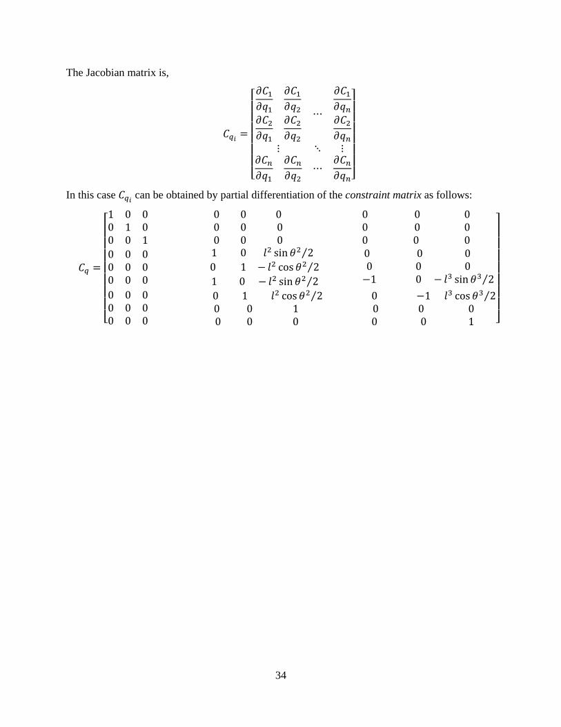
The Jacobian matrix is,
𝐶𝐶𝑞𝑞𝑖𝑖 =
⎣⎢⎢⎢⎢⎢⎢⎡𝜕𝜕𝐶𝐶1𝜕𝜕𝑞𝑞1
𝜕𝜕𝐶𝐶1𝜕𝜕𝑞𝑞2
𝜕𝜕𝐶𝐶2𝜕𝜕𝑞𝑞1
𝜕𝜕𝐶𝐶2𝜕𝜕𝑞𝑞2
⋯
𝜕𝜕𝐶𝐶1𝜕𝜕𝑞𝑞𝑛𝑛𝜕𝜕𝐶𝐶2𝜕𝜕𝑞𝑞𝑛𝑛
⋮ ⋱ ⋮𝜕𝜕𝐶𝐶𝑛𝑛𝜕𝜕𝑞𝑞1
𝜕𝜕𝐶𝐶𝑛𝑛𝜕𝜕𝑞𝑞2
⋯𝜕𝜕𝐶𝐶𝑛𝑛𝜕𝜕𝑞𝑞𝑛𝑛⎦
⎥⎥⎥⎥⎥⎥⎤
In this case 𝐶𝐶𝑞𝑞𝑖𝑖 can be obtained by partial differentiation of the constraint matrix as follows:
𝐶𝐶𝑞𝑞 =
⎣⎢⎢⎢⎢⎢⎢⎢⎡1 0 00 1 00 0 1
0 0 0 0 0 0 0 0 0
0 0 00 0 0
0 0 00 0 00 0 00 0 0
1 0 𝑙𝑙2 sin𝜃𝜃2 2⁄ 0 1 − 𝑙𝑙2 cos𝜃𝜃2 2⁄ 1 0 − 𝑙𝑙2 sin𝜃𝜃2 2⁄
0 0 0 0 0 0
−1 0 − 𝑙𝑙3 sin𝜃𝜃3 2⁄0 0 00 0 00 0 0
0 1 𝑙𝑙2 cos𝜃𝜃2 2⁄ 0 0 1 0 0 0
0 −1 𝑙𝑙3 cos 𝜃𝜃3 2⁄ 0 0 0 0 0 1 ⎦
⎥⎥⎥⎥⎥⎥⎥⎤
35
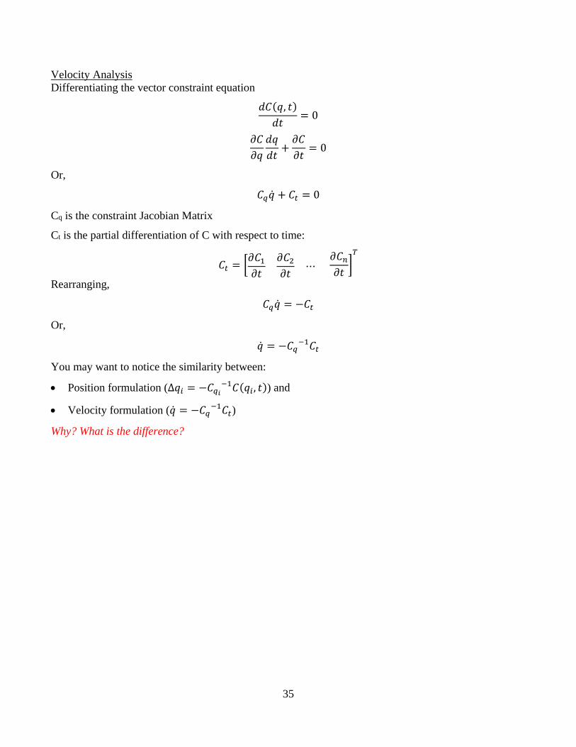
Velocity Analysis Differentiating the vector constraint equation
𝑑𝑑𝐶𝐶(𝑞𝑞, 𝑡𝑡)𝑑𝑑𝑡𝑡
= 0
𝜕𝜕𝐶𝐶𝜕𝜕𝑞𝑞
𝑑𝑑𝑞𝑞𝑑𝑑𝑡𝑡
+𝜕𝜕𝐶𝐶𝜕𝜕𝑡𝑡
= 0
Or,
𝐶𝐶𝑞𝑞�̇�𝑞 + 𝐶𝐶𝑡𝑡 = 0
Cq is the constraint Jacobian Matrix
Ct is the partial differentiation of C with respect to time:
𝐶𝐶𝑡𝑡 = �𝜕𝜕𝐶𝐶1𝜕𝜕𝑡𝑡
𝜕𝜕𝐶𝐶2𝜕𝜕𝑡𝑡
⋯ 𝜕𝜕𝐶𝐶𝑛𝑛𝜕𝜕𝑡𝑡
�𝑇𝑇
Rearranging,
𝐶𝐶𝑞𝑞�̇�𝑞 = −𝐶𝐶𝑡𝑡
Or,
�̇�𝑞 = −𝐶𝐶𝑞𝑞−1𝐶𝐶𝑡𝑡
You may want to notice the similarity between:
• Position formulation (∆𝑞𝑞𝑖𝑖 = −𝐶𝐶𝑞𝑞𝑖𝑖−1𝐶𝐶(𝑞𝑞𝑖𝑖 , 𝑡𝑡)) and
• Velocity formulation (�̇�𝑞 = −𝐶𝐶𝑞𝑞−1𝐶𝐶𝑡𝑡)
Why? What is the difference?
36
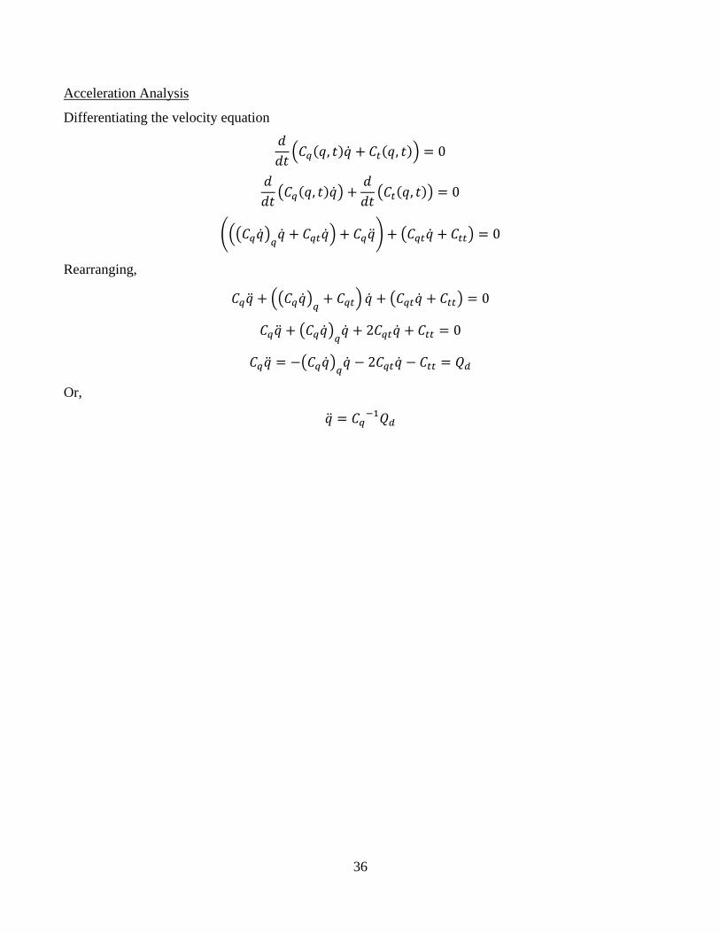
Acceleration Analysis
Differentiating the velocity equation 𝑑𝑑𝑑𝑑𝑡𝑡�𝐶𝐶𝑞𝑞(𝑞𝑞, 𝑡𝑡)�̇�𝑞 + 𝐶𝐶𝑡𝑡(𝑞𝑞, 𝑡𝑡)� = 0
𝑑𝑑𝑑𝑑𝑡𝑡�𝐶𝐶𝑞𝑞(𝑞𝑞, 𝑡𝑡)�̇�𝑞� +
𝑑𝑑𝑑𝑑𝑡𝑡�𝐶𝐶𝑡𝑡(𝑞𝑞, 𝑡𝑡)� = 0
���𝐶𝐶𝑞𝑞�̇�𝑞�𝑞𝑞�̇�𝑞 + 𝐶𝐶𝑞𝑞𝑡𝑡�̇�𝑞� + 𝐶𝐶𝑞𝑞�̈�𝑞� + �𝐶𝐶𝑞𝑞𝑡𝑡�̇�𝑞 + 𝐶𝐶𝑡𝑡𝑡𝑡� = 0
Rearranging,
𝐶𝐶𝑞𝑞�̈�𝑞 + ��𝐶𝐶𝑞𝑞�̇�𝑞�𝑞𝑞 + 𝐶𝐶𝑞𝑞𝑡𝑡� �̇�𝑞 + �𝐶𝐶𝑞𝑞𝑡𝑡�̇�𝑞 + 𝐶𝐶𝑡𝑡𝑡𝑡� = 0
𝐶𝐶𝑞𝑞�̈�𝑞 + �𝐶𝐶𝑞𝑞�̇�𝑞�𝑞𝑞�̇�𝑞 + 2𝐶𝐶𝑞𝑞𝑡𝑡�̇�𝑞 + 𝐶𝐶𝑡𝑡𝑡𝑡 = 0
𝐶𝐶𝑞𝑞�̈�𝑞 = −�𝐶𝐶𝑞𝑞�̇�𝑞�𝑞𝑞�̇�𝑞 − 2𝐶𝐶𝑞𝑞𝑡𝑡�̇�𝑞 − 𝐶𝐶𝑡𝑡𝑡𝑡 = 𝑄𝑄𝑑𝑑
Or,
�̈�𝑞 = 𝐶𝐶𝑞𝑞−1𝑄𝑄𝑑𝑑
37
Homework
• Solve Problem 3.19
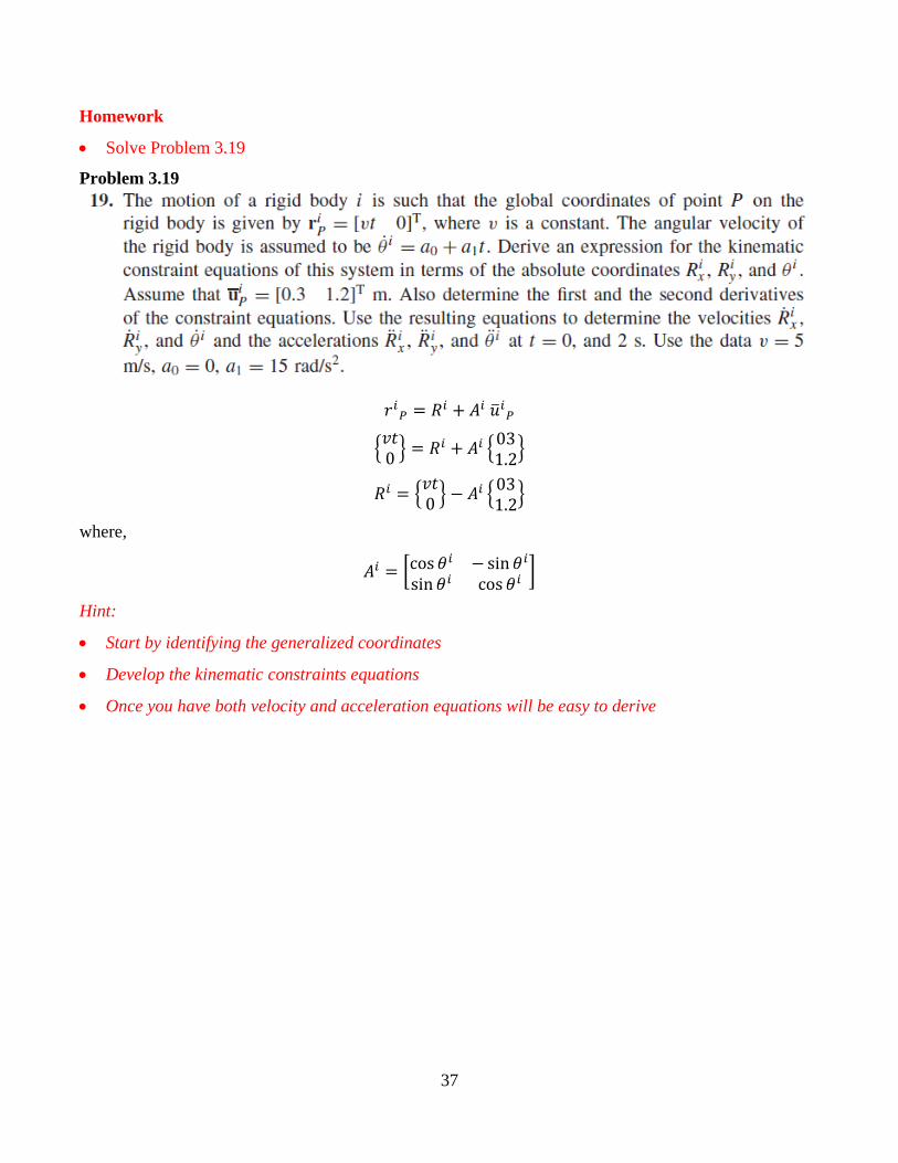
Problem 3.19
𝑟𝑟𝑖𝑖𝑃𝑃 = 𝑅𝑅𝑖𝑖 + 𝐴𝐴𝑖𝑖 𝑢𝑢�𝑖𝑖𝑃𝑃
�𝑣𝑣𝑡𝑡0 � = 𝑅𝑅𝑖𝑖 + 𝐴𝐴𝑖𝑖 �031.2�
𝑅𝑅𝑖𝑖 = �𝑣𝑣𝑡𝑡0 � − 𝐴𝐴𝑖𝑖 �031.2�
where,
𝐴𝐴𝑖𝑖 = �cos𝜃𝜃𝑖𝑖 − sin𝜃𝜃𝑖𝑖sin𝜃𝜃𝑖𝑖 cos 𝜃𝜃𝑖𝑖
�
Hint:
• Start by identifying the generalized coordinates
• Develop the kinematic constraints equations
• Once you have both velocity and acceleration equations will be easy to derive
38
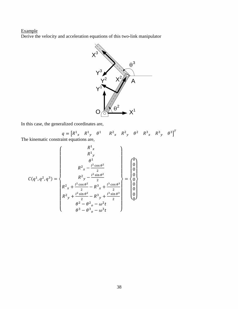
Example Derive the velocity and acceleration equations of this two-link manipulator
X1
Y1
X3
θ2O
Y3
X2Y2
θ3
A
In this case, the generalized coordinates are,
𝑞𝑞 = �𝑅𝑅1𝑥𝑥 𝑅𝑅1𝑦𝑦 𝜃𝜃1 𝑅𝑅2𝑥𝑥 𝑅𝑅2𝑦𝑦 𝜃𝜃2 𝑅𝑅3𝑥𝑥 𝑅𝑅3𝑦𝑦 𝜃𝜃3�𝑇𝑇 The kinematic constraint equations are,
𝐶𝐶(𝑞𝑞1, 𝑞𝑞2, 𝑞𝑞3) =
⎩⎪⎪⎪⎪⎪⎨
⎪⎪⎪⎪⎪⎧ 𝑅𝑅1𝑥𝑥
𝑅𝑅1𝑦𝑦𝜃𝜃1
𝑅𝑅2𝑥𝑥 −𝑙𝑙2 cos𝜃𝜃2
2
𝑅𝑅2𝑦𝑦 −𝑙𝑙2 sin𝜃𝜃2
2
𝑅𝑅2𝑥𝑥 + 𝑙𝑙2 cos𝜃𝜃2
2− 𝑅𝑅3𝑥𝑥 + 𝑙𝑙3 cos𝜃𝜃3
2
𝑅𝑅2𝑦𝑦 + 𝑙𝑙2 sin𝜃𝜃2
2− 𝑅𝑅3𝑦𝑦 + 𝑙𝑙3 sin𝜃𝜃3
2𝜃𝜃2 − 𝜃𝜃2𝑜𝑜 − 𝜔𝜔2𝑡𝑡𝜃𝜃3 − 𝜃𝜃3𝑜𝑜 − 𝜔𝜔3𝑡𝑡 ⎭
⎪⎪⎪⎪⎪⎬
⎪⎪⎪⎪⎪⎫
=
⎩⎪⎪⎨
⎪⎪⎧
000000000⎭⎪⎪⎬
⎪⎪⎫
39
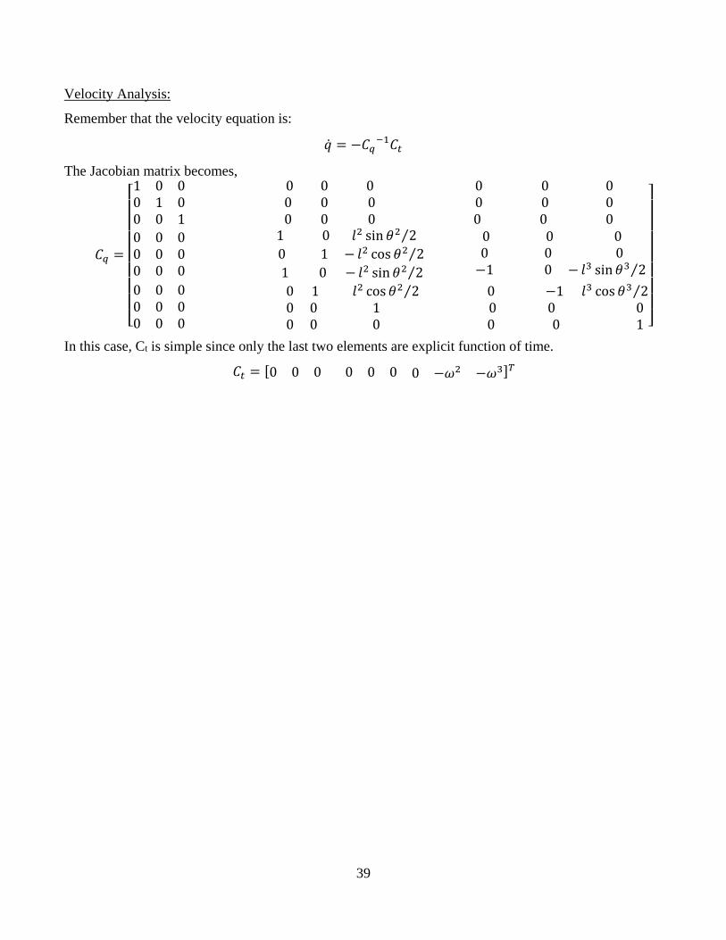
Velocity Analysis:
Remember that the velocity equation is:
�̇�𝑞 = −𝐶𝐶𝑞𝑞−1𝐶𝐶𝑡𝑡
The Jacobian matrix becomes,
𝐶𝐶𝑞𝑞 =
⎣⎢⎢⎢⎢⎢⎢⎢⎡1 0 00 1 00 0 1
0 0 0 0 0 0 0 0 0
0 0 00 0 00 0 0
0 0 00 0 00 0 0
1 0 𝑙𝑙2 sin𝜃𝜃2 2⁄ 0 1 − 𝑙𝑙2 cos 𝜃𝜃2 2⁄ 1 0 − 𝑙𝑙2 sin𝜃𝜃2 2⁄
0 0 0 0 0 0
−1 0 − 𝑙𝑙3 sin𝜃𝜃3 2⁄0 0 00 0 00 0 0
0 1 𝑙𝑙2 cos𝜃𝜃2 2⁄ 0 0 1 0 0 0
0 −1 𝑙𝑙3 cos𝜃𝜃3 2⁄ 0 0 0 0 0 1 ⎦
⎥⎥⎥⎥⎥⎥⎥⎤
In this case, Ct is simple since only the last two elements are explicit function of time.
𝐶𝐶𝑡𝑡 = [0 0 0 0 0 0 0 −𝜔𝜔2 −𝜔𝜔3]𝑇𝑇
40
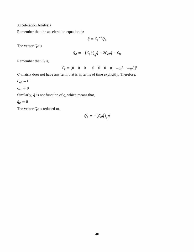
Acceleration Analysis
Remember that the acceleration equation is:
�̈�𝑞 = 𝐶𝐶𝑞𝑞−1𝑄𝑄𝑑𝑑
The vector Qd is
𝑄𝑄𝑑𝑑 = −�𝐶𝐶𝑞𝑞�̇�𝑞�𝑞𝑞�̇�𝑞 − 2𝐶𝐶𝑞𝑞𝑡𝑡�̇�𝑞 − 𝐶𝐶𝑡𝑡𝑡𝑡
Remember that Ct is,
𝐶𝐶𝑡𝑡 = [0 0 0 0 0 0 0 −𝜔𝜔2 −𝜔𝜔3]𝑇𝑇
Ct matrix does not have any term that is in terms of time explicitly. Therefore,
𝐶𝐶𝑞𝑞𝑡𝑡 = 0
𝐶𝐶𝑡𝑡𝑡𝑡 = 0
Similarly, �̇�𝑞 is not function of q, which means that,
�̇�𝑞𝑞𝑞 = 0
The vector Qd is reduced to,
𝑄𝑄𝑑𝑑 = −�𝐶𝐶𝑞𝑞�̇�𝑞�𝑞𝑞�̇�𝑞

41
Since,
𝐶𝐶𝑞𝑞�̇�𝑞 =
⎣⎢⎢⎢⎢⎢⎢⎢⎡1 0 00 1 00 0 1
0 0 0 0 0 0 0 0 0
0 0 00 0 00 0 0
0 0 00 0 00 0 0
1 0 𝑙𝑙2 sin𝜃𝜃2 2⁄ 0 1 − 𝑙𝑙2 cos𝜃𝜃2 2⁄ 1 0 − 𝑙𝑙2 sin𝜃𝜃2 2⁄
0 0 0 0 0 0
−1 0 − 𝑙𝑙3 sin𝜃𝜃3 2⁄0 0 00 0 00 0 0
0 1 𝑙𝑙2 cos 𝜃𝜃2 2⁄ 0 0 1 0 0 0
0 −1 𝑙𝑙3 cos𝜃𝜃3 2⁄ 0 0 0 0 0 1 ⎦
⎥⎥⎥⎥⎥⎥⎥⎤
⎩⎪⎪⎪⎪⎨
⎪⎪⎪⎪⎧�̇�𝑅
1𝑥𝑥
�̇�𝑅1𝑦𝑦𝜃𝜃1̇�̇�𝑅2𝑥𝑥�̇�𝑅2𝑦𝑦𝜃𝜃2̇�̇�𝑅3𝑥𝑥�̇�𝑅3𝑦𝑦𝜃𝜃3̇ ⎭
⎪⎪⎪⎪⎬
⎪⎪⎪⎪⎫
𝐶𝐶𝑞𝑞�̇�𝑞 =
⎩⎪⎪⎪⎪⎨
⎪⎪⎪⎪⎧ �̇�𝑅1
𝑥𝑥
�̇�𝑅1𝑦𝑦
𝜃𝜃1̇
�̇�𝑅2𝑥𝑥 + 𝜃𝜃2̇ 𝑙𝑙2 sin𝜃𝜃2 2⁄
�̇�𝑅2𝑦𝑦 − 𝜃𝜃2̇ 𝑙𝑙2 cos𝜃𝜃2 2⁄
�̇�𝑅2𝑥𝑥 − 𝜃𝜃2̇ 𝑙𝑙2 sin𝜃𝜃2 2 − �̇�𝑅3
𝑥𝑥⁄ − 𝜃𝜃3̇𝑙𝑙3 sin𝜃𝜃3 2⁄�̇�𝑅2
𝑦𝑦 + 𝜃𝜃2̇ 𝑙𝑙2 cos𝜃𝜃2 2 − �̇�𝑅3𝑦𝑦� + 𝜃𝜃3̇𝑙𝑙3 cos𝜃𝜃3 2⁄
𝜃𝜃2̇
𝜃𝜃3̇ ⎭⎪⎪⎪⎪⎬
⎪⎪⎪⎪⎫
�𝐶𝐶𝑞𝑞�̇�𝑞�𝑞𝑞�̇�𝑞
=
⎣⎢⎢⎢⎢⎢⎢⎢⎢⎡0 0 00 0 00 0 0
0 0 00 0 00 0 0
0 0 00 0 00 0 0
0 0 00 0 00 0 0
0 0 𝜃𝜃2̇ 𝑙𝑙2 cos 𝜃𝜃2 2⁄ 0 0 𝜃𝜃2̇ 𝑙𝑙2 sin𝜃𝜃2 2⁄ 0 0 −𝜃𝜃2̇ 𝑙𝑙2 cos 𝜃𝜃2 2⁄
0 0 0 0 0 0 0 0 −𝜃𝜃3̇ 𝑙𝑙3 cos𝜃𝜃3 2⁄
0 0 00 0 00 0 0
0 0 −𝜃𝜃2̇ 𝑙𝑙2 sin𝜃𝜃2 2⁄0 0 00 0 0
0 0 −𝜃𝜃3̇ 𝑙𝑙3 sin𝜃𝜃3 2⁄ 0 0 0 0 0 0 ⎦
⎥⎥⎥⎥⎥⎥⎥⎥⎤
⎩⎪⎪⎪⎪⎨
⎪⎪⎪⎪⎧�̇�𝑅
1𝑥𝑥
�̇�𝑅1𝑦𝑦
𝜃𝜃1̇
�̇�𝑅2𝑥𝑥
�̇�𝑅2𝑦𝑦
𝜃𝜃2̇
�̇�𝑅3𝑥𝑥
�̇�𝑅3𝑦𝑦
𝜃𝜃3̇ ⎭⎪⎪⎪⎪⎬
⎪⎪⎪⎪⎫
Therefore,
42
�𝐶𝐶𝑞𝑞�̇�𝑞�𝑞𝑞�̇�𝑞 =
⎩⎪⎪⎪⎪⎪⎪⎨
⎪⎪⎪⎪⎪⎪⎧
000
𝜃𝜃2̇2𝑙𝑙2 cos 𝜃𝜃2
2
𝜃𝜃2̇2𝑙𝑙2 sin 𝜃𝜃2
2
−𝜃𝜃2̇2
𝑙𝑙2 cos 𝜃𝜃2
2−𝜃𝜃3̇2
𝑙𝑙3 cos 𝜃𝜃3
2
−𝜃𝜃2̇2
𝑙𝑙2 sin 𝜃𝜃2
2−𝜃𝜃3̇2
𝑙𝑙3 sin 𝜃𝜃3
200 ⎭
⎪⎪⎪⎪⎪⎪⎬
⎪⎪⎪⎪⎪⎪⎫
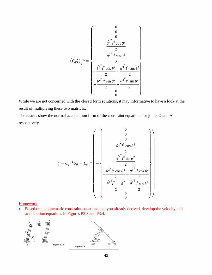
While we are not concerned with the closed form solutions, it may informative to have a look at the
result of multiplying these two matrices.
The results show the normal acceleration form of the constraint equations for joints O and A
respectively.
�̈�𝑞 = 𝐶𝐶𝑞𝑞−1𝑄𝑄𝑑𝑑 = 𝐶𝐶𝑞𝑞−1
⎝
⎜⎜⎜⎜⎜⎜⎜⎜⎜⎜⎜⎛
−
⎩⎪⎪⎪⎪⎪⎪⎨
⎪⎪⎪⎪⎪⎪⎧
000
𝜃𝜃2̇2𝑙𝑙2 cos 𝜃𝜃2
2
𝜃𝜃2̇2𝑙𝑙2 sin 𝜃𝜃2
2
−𝜃𝜃2̇2
𝑙𝑙2 cos 𝜃𝜃2
2−𝜃𝜃3̇2
𝑙𝑙3 cos 𝜃𝜃3
2
−𝜃𝜃2̇2
𝑙𝑙2 sin 𝜃𝜃2
2−𝜃𝜃3̇2
𝑙𝑙3 sin 𝜃𝜃3
200 ⎭
⎪⎪⎪⎪⎪⎪⎬
⎪⎪⎪⎪⎪⎪⎫
⎠
⎟⎟⎟⎟⎟⎟⎟⎟⎟⎟⎟⎞
Homework • Based on the kinematic constraint equations that you already derived, develop the velocity and
acceleration equations in Figures P3.3 and P3.4.

43
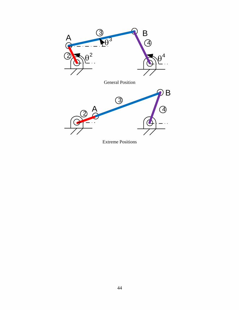
Special Cases in Kinematic Analysis
Degenerate (Extreme) Configurations
• Let’s start by discussing degenerate configurations, which are the ones when a mechanical system
loses on or more degrees of freedom.
• Extreme position is associated with a reduction in the order of the geometry of the machines or
degeneracy (e.g., triangular to straight line or quadrilateral to triangular)
• Extreme positions are associated with the loss of (zero) velocity. This should make sense as the
machine is changing direction
• Here are some examples:
23 4
θ2 θ3
A
Bx4B
General Position
23
4
A BO
2 34
A BO
Extreme Positions
44
2
34
θ2
θ3A B
θ4
General Position
2
34A
B
Extreme Positions
45
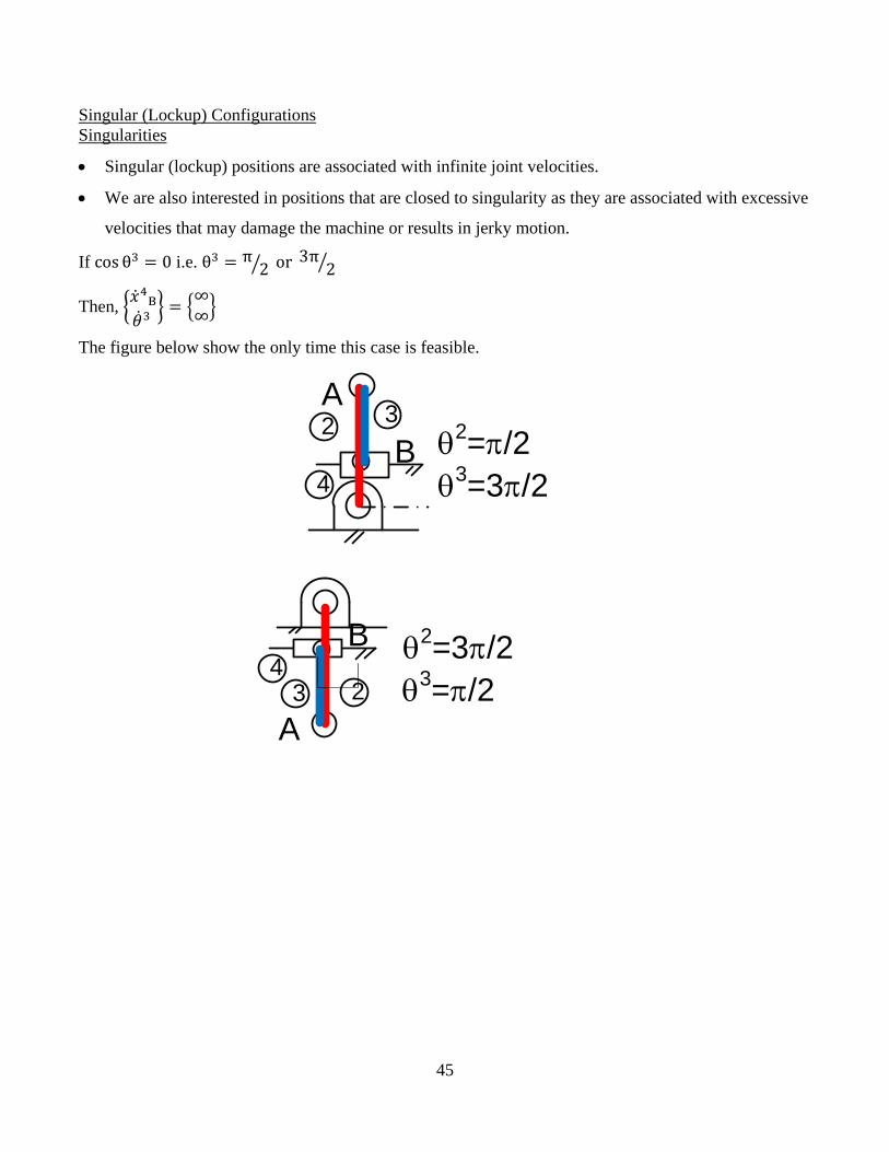
Singular (Lockup) Configurations Singularities
• Singular (lockup) positions are associated with infinite joint velocities.
• We are also interested in positions that are closed to singularity as they are associated with excessive
velocities that may damage the machine or results in jerky motion.
If cos θ3 = 0 i.e. θ3 = π2� or 3π 2�
Then, ��̇�𝑥4B
�̇�𝜃3 � = �∞∞�
The figure below show the only time this case is feasible.
2 3
4θ2=π/2
A
Bθ3=3π/2
234
θ2=3π/2
A
Bθ3=π/2