Computational methods for microbial cell factory engineering … · Computational methods for microbial cell factory engineering aided by evolution PhD Thesis by Kristian Jensen December

General rights Copyright and moral rights for the publications made accessible in the public portal are retained by the authors and/or other copyright owners and it is a condition of accessing publications that users recognise and abide by the legal requirements associated with these rights.

Users may download and print one copy of any publication from the public portal for the purpose of private study or research.

You may not further distribute the material or use it for any profit-making activity or commercial gain

You may freely distribute the URL identifying the publication in the public portal If you believe that this document breaches copyright please contact us providing details, and we will remove access to the work immediately and investigate your claim.

Downloaded from orbit.dtu.dk on: May 24, 2020

Computational methods for microbial cell factory engineering aided by evolution

Jensen, Kristian

Publication date:2019

Document VersionPublisher's PDF, also known as Version of record

Link back to DTU Orbit

Citation (APA):Jensen, K. (2019). Computational methods for microbial cell factory engineering aided by evolution.

https://orbit.dtu.dk/en/publications/d967529c-d4c9-4976-ae33-0bc111de8676

Growthcondition

Evolvedcondition

0.0 0.2 0.4 0.6 0.8 1.0 /h

Cit rulline

Ornithine

Sperm idine

1,5-diam inopentane

1,3-diam inopropane

Ethylenediam ine

HMDA

HMDA st rains

0.0 0.2 0.4 0.6 0.8 /h

Ethanolam ine

1,2-pentanediol

1,5-pentanediol

1,4-butanediol

1,3-propanediol

2,3-butanediol

2,3-butanediol st rains

0.0 0.2 0.4 0.6 /h

Malate

Itaconate

Fumarate

Sebacate

Pimelate

Succinate

Adipate

Adipate st rains

0.0 0.2 0.4 0.6 0.8 /h

2-methy lhexanoate

4-methy lvalerate

Isovalerate

2-methy lbutyrate

Valerate

Butyrate

Isobutyrate

Isobutyrate st rains

HMDA

PUTR

12PD

23BD

GLU

T

ADIP

HEX

A

OCTA

IBUA

COUM

BUT

NaC

l

M9

BUT

COUM

IBUA

OCTA

HEXA

ADIP

GLUT

23BD

12PD

PUTR

HMDA

HMDA PUTR 12PD 23BD GLUT ADIP HEXA OCTA COUM IBUA BUT

0.3

0.2

0.1

0.0

0.1

0.2

Relativeglob

altoleranc

e

0.2 0.1 0.0 0.1 0.2 0.3

Relat ive M9 growth rate

0.3

0.2

0.1

0.0

0.1

0.2

Relativeglob

altoleranc

e

0.1 0.0 0.1 0.2 0.3

Relat ive NaCl tolerance

0.3

0.2

0.1

0.0

0.1

0.2

Relativeglob

altoleranc

e

Computational methods formicrobial cell factory engineeringaided by evolution

DTU BiosustainThe Novo Nordisk Foundation Center for Biosustainability

Kristian JensenPhD ThesisDecember 2018

Computationalmethodsformicrobialcellfactoryengineeringaidedbyevolution

PhD Thesis by Kristian Jensen

December 2018

The Novo Nordisk Foundation Center for Biosustainability

Technical University of Denmark

II

Computational methods for microbial cell factory engineering aided by evolution

PhD thesis by Kristian Jensen

Principal supervisor: Markus Herrgård

Co-supervisor: Nikolaus Sonnenschein

III

IV

Preface

This thesis is written as partial fulfillment of the requirements for obtaining a PhD degree at the

Technical University of Denmark. The work included in the thesis has been carried out at the Novo

Nordisk Foundation Center for Biosustainability in the period from January 2016 to December 2018.

Part of the work was done in Uwe Sauer’s lab at the Eidgenössiche Technische Hochschule Zürich in

Switzerland in the fall of 2017. The work has been supervised by Professor Markus Herrgård and

Senior Researcher Nikolaus Sonnenschein and was funded by the Technical University of Denmark

and the Novo Nordisk Foundation.

Kristian Jensen

Kgs. Lyngby, December 2018

V

Abstract

Increasing global temperatures and limited fossil resources make it increasingly urgent to find

alternative ways of producing fuels and chemicals. Metabolic engineering offers a promising

solution to this problem by using microbes as cell factories for manufacturing a diverse set of

products from renewable resources. However, cell factory development requires extensive

knowledge of microbial biology as well as expensive and time-consuming strain engineering. Non-

rational methods allow the strain development process to be accelerated by taking advantage of

evolutionary processes.

This thesis addresses the integration of adaptive laboratory evolution into cell factory development

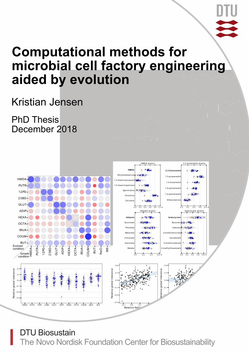
workflows through computational methods. By studying a large set of Escherichia coli strains

evolved to tolerate 11 different chemicals of industrial relevance, it was shown that there is

significant cross-tolerance between compounds of the same chemical class, and that pre-evolving

strains to tolerate a product can improve production rates when the evolved strain is engineered

with a production pathway. Metabolic profiling of the evolved strains using direct-injection mass

spectrometry showed that strains evolved in the same conditions had converged to similar

metabolic phenotypes, suggesting that metabolism is involved in chemical tolerance. It was shown

that the effects of individual mutations could be predicted, both by directly comparing the

metabolic profiles of evolved strains to previously measured metabolic profiles of knockout strains,

as well as using deep neural networks to predict metabolite level changes directly from genetic

perturbations.

Adaptive laboratory evolution can be used to optimize growth rates under various growth

conditions, but through clever strain engineering it is possible to couple production to growth,

thereby allowing optimization of production rate. This thesis also presents an algorithm based on

genome-scale metabolic modelling that can predict genetic modifications that enable growth-

coupling in combination with addition of specific supplements to the growth medium. The algorithm

could predict known growth-coupled strain designs that are shown to work in vivo as well as novel

promising strain designs, for production of itaconic acid, propionic acid and for product methylation.

VI

Resumé

På grund af stigende globale temperaturer og begrænsede fossile ressourcer er det kritisk at finde

alternative måder at producere kemikalier og brændstoffer. Dette problem kan løses ved at

konstruere mikrobielle cellefabrikker der kan producere en bred vifte af produkter fra vedvarende

ressourcer. Anvendelse af cellefabrikker kræver dog en vidtrækkende viden om mikrobiel biologi

såvel som dyr og tidskrævende udvikling af mikrobielle stammer. Gennem brug af non-rationelle

metoder kan stammeudviklingsprocessen accelereres ved at udnytte evolutionære processer.

Denne afhandling omhandler integrering af adaptiv laboratorieevolution i udvikling af cellefabrikker

gennem beregningsmetoder. Ved at studere et stort antal Escherichia coli stammer der er

evolutionært udviklet til at tolerere 11 forskellige industrielt relevante kemikalier, blev det vist at

der er betydelig kryds-tolerans mellem stoffer der har kemiske ligheder. Derudover blev det vist at

brugen af laboratorieevolution til at forbedre en stammes produkttolerans også kan øge stammens

evne til at producere stoffet, når der er blevet indsat en produktionspathway. Metabolisk profilering

af de evolutionært udviklede stammer ved hjælp af direct-injection massespektrometri viste at

stammer udviklet under de samme betingelser havde konvergeret til lignende metaboliske profiler,

hvilket tyder på at metabolisme er involveret i kemisk tolerans. Det blev yderligere vist at

individuelle mutationers effekter kunne forudsiges både ved at sammenligne de målte metaboliske

profiler med tidligere målte metaboliske profiler for knockout-stammer, samt ved at anvende dybe

neurale netværk til at forudsige ændringer i metabolitniveauer direkte fra genetiske ændringer.

Adaptiv laboratorieevolution kan bruges til at optimere vækstrate under forskellige betingelser,

men gennem snedige stammedesigns er det muligt at koble produktion til vækst, hvorved

produktionsraten kan optimeres. Denne afhandling præsenterer også en algoritme baseret på

metaboliske modeller i genoskala, som kan forudsige genetiske ændringer der kan forårsage

vækstkobling i kombination med at specifikke supplementer tilføjes til vækstmediet. Algoritmen

kunne forudsige kendte vækstkoblede stammedesigns som tidligere er valideret in vivo, og kunne

også forudsige nye lovende designs til produktion at itakonsyre, propionsyre samt til produkt-

methylering.

VII

Acknowledgements

Even though the last three year have been hard, they have also been extremely rewarding. There

are a number of people without whom I could not have completed this thesis, and who have made

the process more enjoyable. I owe those people a lot of gratitude.

First, I would like to thank Markus Herrgård for giving me the opportunity to do a PhD at the Center

for Biosustainability, and who has helped me with lots of guidance, advice and feedback along the

way. I would also like to thank Nikolaus Sonnenschein who has co-supervised my work and helped

with good ideas and critical questions. Furthermore, I would like to thank Joaõ Cardoso, who as my

master thesis supervisor introduced me to the world of metabolic modelling and computational

strain design. I also want to thank Anne Sofie Lærke Hansen for directing my attention towards the

Center for Biosustainability in the first place, and for many fun and inspiring conversations ever

since.

During my PhD I have been lucky to supervise several talented master students: I am grateful to

Anders Ellegaard, Christina Bligaard Pedersen and Valentijn Broeken for their excellent work and for

many interesting discussions along the way.

Several of the projects described in this thesis have been done in collaboration with other

researchers whom I thank for their respective contributions. During my stay at ETH Zürich I received

lots of valuable help and support from Mattia Zampieri, for which I am also very grateful.

Additionally, I am thankful to a large group of people who have made the past three years a lot more

fun: Kristian for the many evenings we spent on crazy engineering projects; Christian, Christian,

Niko, Christoffer and Carsten for all the fun hours playing music in the bunker; Phillpp and Karin for

being great office mates at ETHZ; Biotek-10 for making every Wednesday something to look forward

to; a long list of colleagues including (in no particular order) Ida, Ruben, Kira, Pasquale, Svetlana,

Alexandra, Maja, Alicia and Michael for lots of fun at various parties, balls, and bar crawls; and all

past and present members of the SIMS group for the fantastic work environment.

Finally, I want to thank my parents and Mikkel, Sif and Agnes for many enjoyable times during

holidays and weekends, as well as Eya for your company and all your support, which means the

world to me.

VIII

List of publications

Publications included in this thesis

Lennen, R., Jensen, K., Mohammed, E., Malla, S., Börner, R., Özdemir, E., Bonde, I., Koza, A.,

Pedersen, L., Schöning, L., Sonnenschein, N., Palsson, B., Sommer, M., Feist, A., Nielsen, A.,

Herrgård, M. (in preparation). Parallel laboratory evolutions reveal general chemical tolerance

mechanisms and enhance chemical production. (Chapter 1)

Jensen, K., Gudmundsson, S., & Herrgård, M. (2018). Enhancing Metabolic Models with Genome-

Scale Experimental Data. Systems Biology, 337–350. (Chapter 4)

Jensen, K., Broeken, V.F., Hansen, A.S.L., Sonnenschein, N., Herrgård, M. (submitted). OptCouple:

Joint simulation of gene knockouts, insertions and medium modifications for prediction of

growth-coupled strain designs. (Chapter 5)

Contributions to the following publications were made during the work of this thesis, but are not

included in the thesis

Jensen, K., Cardoso, J., & Sonnenschein, N. (2016). Optlang: An algebraic modeling language for

mathematical optimization. Journal of Open Source Software.

Cardoso, J.G.R., Jensen, K., Lieven, C., Hansen, A.S.L., Galkina, S., Beber, M., Özdemir, E., Herrgård,

M.J., Redestig, H., Sonnenschein, N. (2018). Cameo: A Python Library for Computer Aided

Metabolic Engineering and Optimization of Cell Factories. ACS Synthetic Biology, 7(4), 1163-

1166.

Cardoso, J. G. R., Zeidan, A. A., Jensen, K., Sonnenschein, N., Neves, A. R., & Herrgård, M. J. (2018).

MARSI: metabolite analogues for rational strain improvement. Bioinformatics, 34(13), 2319-

2321.

Rugbjerg, P., Genee, H. J., Jensen, K., Sarup-Lytzen, K., & Sommer, M. O. A. (2016). Molecular Buffers

Permit Sensitivity Tuning and Inversion of Riboswitch Signals. A C S Synthetic Biology, 5(7),

632-638.

IX

List of abbreviations

12PD: 1,2-propanediol

23BD: 2,3-butanediol

ADIP: Adipate

AKG: Alpha-ketoglutarate

ALE: Adaptive laboratory evolution

BUT: Butanol

COUM: p-Coumarate

FC: Fold-change

FBA: Flux balance analysis

GIMME: Gene Inactivity Moderated by Metabolism and Expression

GLUT: Glutarate

HEXA: Hexanoate

HPLC: High-performance liquid chromatography

HMDA: Hexamethylenediamine

IBUA: Isobutyrate

MCMC: Markov-chain monte carlo

MCS: Minimal cut sets

MFA: Metabolic flux analysis

MILP: Mixed integer linear programming

MLP: Multilayer perceptron

OCTA: Octanoate

PEP: Phosphoenolpyruvate

X

PUTR: Putrescine

RBA: Resource balance analysis

RI: Refractive index

SAH: S-adenosylhomocysteine

SAM: S-adenosylmethionine

t-SNE: t-distributed Stochastic Neighbour Embedding

XI

Table of contents

PREFACE .................................................................................................................................................................. IV

ABSTRACT ................................................................................................................................................................. V

RESUMÉ ................................................................................................................................................................... VI

ACKNOWLEDGEMENTS ........................................................................................................................................... VII

LIST OF PUBLICATIONS ........................................................................................................................................... VIII

LIST OF ABBREVIATIONS .......................................................................................................................................... IX

TABLE OF CONTENTS ............................................................................................................................................... XI

THESIS OUTLINE ..................................................................................................................................................... XIII

PART I: METABOLIC ENGINEERING AND EVOLUTIONARY METHODS ......................................................................... 1

CHAPTER 1: PARALLEL LABORATORY EVOLUTIONS REVEAL GENERAL CHEMICAL TOLERANCE MECHANISMS AND

ENHANCE CHEMICAL PRODUCTION ......................................................................................................................... 10

1.1 INTRODUCTION ........................................................................................................................................................... 11 1.2 MATERIALS AND METHODS ........................................................................................................................................... 12 1.3 RESULTS .................................................................................................................................................................... 18 1.4 DISCUSSION ............................................................................................................................................................... 27 1.5 CONCLUSION .............................................................................................................................................................. 31 1.6 REFERENCES ............................................................................................................................................................... 31 1.7 SUPPLEMENTARY MATERIALS ........................................................................................................................................ 35

CHAPTER 2: THE METABOLISM OF EVOLVED TOLERANCE ......................................................................................... 44

2.1 INTRODUCTION ........................................................................................................................................................... 44 2.2 METHODS ................................................................................................................................................................. 45 2.3 RESULTS AND DISCUSSION ............................................................................................................................................. 49 2.4 CONCLUSIONS ............................................................................................................................................................ 64 2.5 REFERENCES ............................................................................................................................................................... 65 2.6 SUPPLEMENTARY MATERIALS ........................................................................................................................................ 68

CHAPTER 3: A DEEP NEURAL NETWORK FOR PROPAGATION OF SIGNALS THROUGH A METABOLIC NETWORK ........ 69

3.1 INTRODUCTION ........................................................................................................................................................... 69 3.2 METHODS ................................................................................................................................................................. 71 3.3 RESULTS AND DISCUSSION ............................................................................................................................................. 74 3.4 CONCLUSION .............................................................................................................................................................. 79

XII

3.5 REFERENCES ............................................................................................................................................................... 79 3.6 SUPPLEMENTARY MATERIALS ........................................................................................................................................ 82

PART II: MODEL-BASED STRAIN DESIGN ................................................................................................................... 84

CHAPTER 4: ENHANCING METABOLIC MODELS WITH GENOME-SCALE EXPERIMENTAL DATA .................................. 86

4.1 RECONSTRUCTION AND ANALYSIS OF METABOLIC NETWORKS ............................................................................................... 87 4.2 CONSTRAINING METABOLIC MODELS WITH TRANSCRIPTOMICS AND PROTEOMICS DATA ............................................................. 89 4.3 MODELS OF METABOLISM AND MACROMOLECULAR EXPRESSION ........................................................................................... 92 4.4 AUGMENTING MODELS WITH METABOLOMICS DATA ........................................................................................................... 94 4.5 COMBINING METABOLIC MODELS AND MACHINE LEARNING METHODS ................................................................................... 97 4.6 CONCLUSIONS ............................................................................................................................................................ 99 4.7 REFERENCES ............................................................................................................................................................... 99

CHAPTER 5: OPTCOUPLE: JOINT SIMULATION OF GENE KNOCKOUTS, INSERTIONS AND MEDIUM MODIFICATIONS

FOR PREDICTION OF GROWTH-COUPLED STRAIN DESIGNS .................................................................................... 106

5.1 INTRODUCTION ......................................................................................................................................................... 107 5.2 MATERIALS AND METHODS ......................................................................................................................................... 109 5.3 CALCULATION ........................................................................................................................................................... 113 5.4 RESULTS AND DISCUSSION ........................................................................................................................................... 115 5.5 CONCLUSION ............................................................................................................................................................ 123 5.6 ACKNOWLEDGEMENTS ............................................................................................................................................... 123 5.7 REFERENCES ............................................................................................................................................................. 123 5.8 SUPPLEMENTARY MATERIALS ...................................................................................................................................... 127

CONCLUDING REMARKS ........................................................................................................................................ 130

XIII

Thesis outline

A major challenge of modern society is the need to find sustainable methods for upholding our

current way of living. This necessitates the development of renewable alternatives to oil-derived

fuels and chemicals. Using microbial cell factories to produce useful and valuable chemicals from

sustainable resources is a promising solution to this problem. However, developing successful cell

factories by employing metabolic engineering is a slow and difficult process that is impeded by our

limited understanding of microbial metabolism.

This thesis addresses the use of so-called non-rational engineering – specifically adaptive laboratory

evolution (ALE) – which leverages evolutionary processes to quickly optimize cell factories without

requiring comprehensive knowledge about the functioning of the cell. The thesis, which will focus

on computational methods that can be used in combination with ALE, is divided into two parts: Part

I (Chapters 1-3) focuses on methods that can help understand the evolved strains resulting from

ALE, while Part II (Chapters 4-5) focuses on the use of mathematical models to design selection

conditions that can be used to optimize production characteristics.

Chapter 1 contains a manuscript for a research article describing study where Escherichia coli was

evolved to tolerate high concentrations of various potential products. Through genome sequencing

and growth characterization we found that overall chemical tolerance obtained in the different

evolution conditions varied widely, and that only very few mutations were universally observed

across strains from a given condition. Furthermore, we found that evolving strains to tolerate a

compound can also have beneficial effects on the strains’ ability to produce the compound. This

work was done in collaboration with other researchers at the Center for Biosustainability, and

mainly the data analysis parts, i.e. analysis of genome sequences and growth profiles, were done as

part of this thesis.

Chapter 2 describes a follow-up study to Chapter 1, where all the evolved tolerant strains were

subjected to metabolomics analysis in order to study how the evolution of tolerance affects

metabolism. It was found that strains evolved under the same condition tend to be very similar

metabolically, such that all the tested conditions had a specific characteristic metabolic phenotype.

This suggests that strains evolved on the same condition reach the same phenotype despite

XIV

considerable differences in genotype. Furthermore, the metabolic profiles of the evolved strains

were combined with previously published metabolomics data and used to predict how each

observed mutation impacts the function of the gene(s) it affects. Finally, a time-series perturbation

analysis was used to investigate how different toxic environments affect metabolism.

Chapter 3 describes a machine learning method for predicting how genetic perturbations affect

metabolite levels. The method is based on a deep neural network and the main novelty is using

biological networks through which signals in the input data are propagated. The motivation for

developing such a method was to take advantage of prior knowledge encoded in networks for

various prediction tasks using graph-structured input and output data. While the obtained

predictive performance limits the practical use of the method, it represents a proof-of-concept of

the technical feasibility of propagating input signals through a graph in a way that is inferred from

the data.

Chapter 4 contains a published book chapter about metabolic modeling and methods for integration

of genome-scale experimental data. The chapter is a review of existing literature and serves as an

introduction to the field of metabolic modeling.

Chapter 5 contains a manuscript for a research article presenting OptCouple, a new modeling

algorithm for identifying strain designs where production is coupled to growth, such that ALE can

be used to optimize production. The main novelty of the algorithm is the possibility of

simultaneously finding knockouts, gene insertions and additions to the growth medium, which in

combination cause production to be growth-coupled. The algorithm is validated by showing that it

can predict existing growth-coupled strain designs, that are shown to work in vivo, as well as new

strain designs that are predicted to be growth-coupled in silico.

Both Part I and Part II begin with a short overview that introduces key concepts and frames the

chapters in a larger context. While Chapters 2 and 3 are not manuscripts in preparation, they are

both structured as research articles and will be adapted and submitted for publication in scientific

journals in the future.

1

Part I: Metabolic engineering and evolutionary methods

The use of microbes in the production of various commodities is an old practice that has been

around for many centuries across most known cultures. The two major examples of this – bread and

beverages – are both based on the growth of yeast in a sugary substrate taking advantage of

microbe’s natural production of carbon dioxide and ethanol. In more recent times the use of

microorganisms to produce chemicals has become increasingly deliberate and directed. Early

examples of microbial chemical production include using filamentous fungi to produce organic

acids, e.g. citric acid (Max et al., 2010), and using the bacterium Clostridium acetobutylicum to

produce acetone and butanol (Weizmann and Rosenfeld, 1937). Culturing microbes solely for the

purpose of production, in contrast to as part of food production, allows employing various process

optimizations to maximize production outcomes specifically. Through such process optimization

techniques, the efficiency of industrial applications of microbial production has steadily increased.

While manufacturers up until the late 20th century have had to rely on optimizations regarding the

physicochemical parameters of the processes, the possibility of modifying the production strain

allowed further improvements to be made. This was first done through a process of random

mutagenesis and subsequent screening (Rowlands, 1984), while the later availability of genetic

engineering techniques opened new venues to the targeted creation of mutant strains with

modified characteristics, including production capabilities (Nielsen, 2001). An example of targeted

engineering of a production strain is the insertion of genes from other organisms, introducing a new

metabolic pathway in the production strain. This can be beneficial as many natural producers of a

target compound may be hard to culture in a production process. Transferring the pathway to

another organism can thus improve production. An example of this was the production of

cephalosporin antibiotics, which are naturally produced by fungal Acremonium species, in the

common laboratory organism Penicillium chrysogenum (Cantwell et al., 1992). Another type of

modifications frequently made during strain engineering is the deletion of native genes to improve

production, e.g. by reducing formation of byproducts. An example of this was a reduction in oxalic

acid formation during expression of heterologous proteins in the fungus Aspergillus niger, by

deleting a gene encoding an oxaloacetate hydrolase (Pedersen et al., 2000).

2

The practice of genetically modifying microbial organisms to obtain good production strains is

known as metabolic engineering and has become increasingly widespread since the 1990’s (Bailey,

1991; Nielsen, 2017). Even though examples of successful metabolic engineering abound, it is by no

means an easy process, owing to the overwhelming complexity of microbial biology. Most efforts to

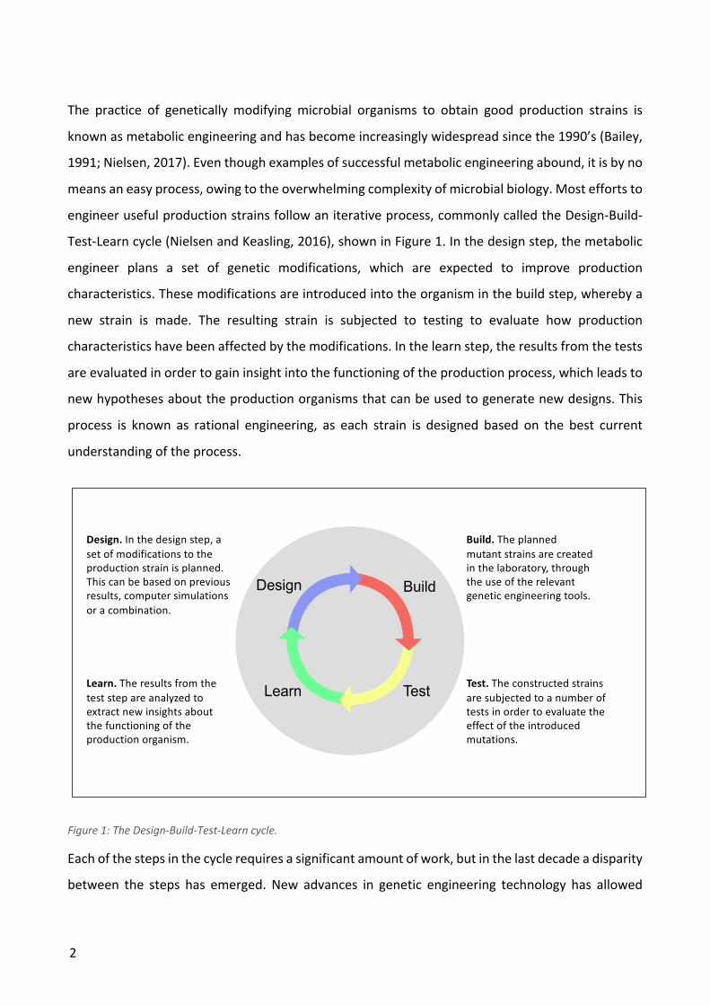
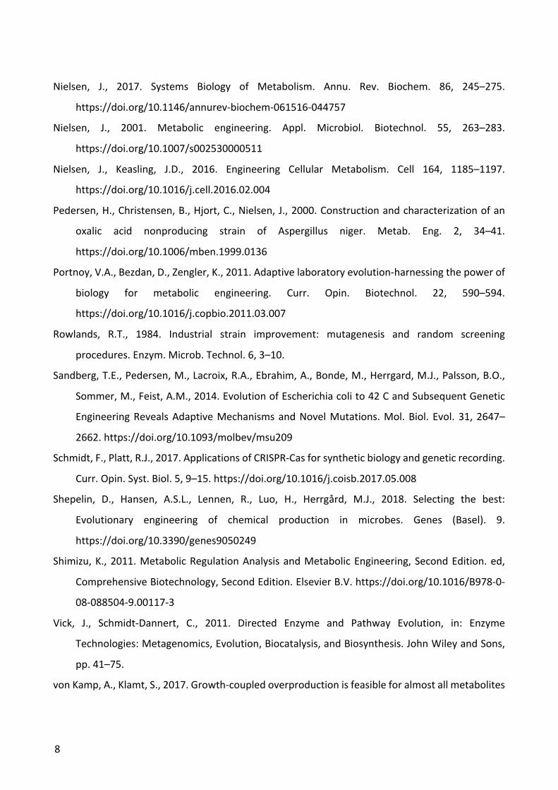
engineer useful production strains follow an iterative process, commonly called the Design-Build-

Test-Learn cycle (Nielsen and Keasling, 2016), shown in Figure 1. In the design step, the metabolic

engineer plans a set of genetic modifications, which are expected to improve production

characteristics. These modifications are introduced into the organism in the build step, whereby a

new strain is made. The resulting strain is subjected to testing to evaluate how production

characteristics have been affected by the modifications. In the learn step, the results from the tests

are evaluated in order to gain insight into the functioning of the production process, which leads to

new hypotheses about the production organisms that can be used to generate new designs. This

process is known as rational engineering, as each strain is designed based on the best current

understanding of the process.

Figure 1: The Design-Build-Test-Learn cycle.

Each of the steps in the cycle requires a significant amount of work, but in the last decade a disparity

between the steps has emerged. New advances in genetic engineering technology has allowed

Learn Test

BuildDesign

Design. In the design step, a set of modifications to the production strain is planned. This can be based on previousresults, computer simulations or a combination.

Build. The plannedmutant strains are createdin the laboratory, throughthe use of the relevant genetic engineering tools.

Test. The constructed strainsare subjected to a number of tests in order to evaluate the effect of the introducedmutations.

Learn. The results from the test step are analyzed to extract new insights aboutthe functioning of the production organism.

3

genetic modifications to be performed faster than ever (Schmidt and Platt, 2017), and even the

synthesis of completely novel DNA sequences can now be done routinely (Chao et al., 2015).

Additionally, many assays in the testing step can be done with a very high throughput, due to the

increasing availability of laboratory automation systems (Nielsen and Keasling, 2016). This leaves a

significant bottleneck in the design and learn steps. In other words, the main challenges in metabolic

engineering are currently more concerned with deciding what do to than with actually doing it.

Several approaches to evening out this disparity have been developed. One approach is to simply

take advantage of the increased testing throughput to collect more extensive systems data on the

production strains. This allows more comprehensive characterization of the developed strains, such

that subsequent strain design can focus on addressing the specific problems that are identified (Lee

and Kim, 2015). An example is to use transcriptomics analyses to identify problematic regulatory

effects of overproducing the target compound, e.g. causing inhibition in the production pathway or

precursor supply (Shimizu, 2011). Overproducing a target compound can also lead to broad

physiological problems in the cell such as cofactor imbalances or energy deficits, which can also be

identified through detailed strain analysis and subsequently addressed by targeted modifications

(Liu et al., 2018).

Another approach for overcoming the bottleneck in the learn and design steps is to also take

advantage of the high throughput in the build step, to create and screen a large number of strains

thereby increasing the chance that one of them has improved production properties. The

effectiveness of this depends on the throughput of the screening assay being used. This approach

represents a deviation from the Design-Build-Test-Learn cycle towards what could be called non-

rational engineering, where decisions are not made based on a theoretical understanding, but on

the achieved screening results alone (Shepelin et al., 2018). Non-rational engineering is an

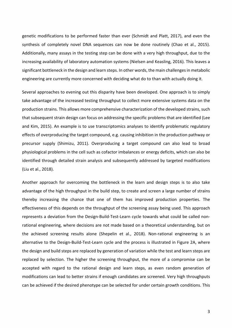
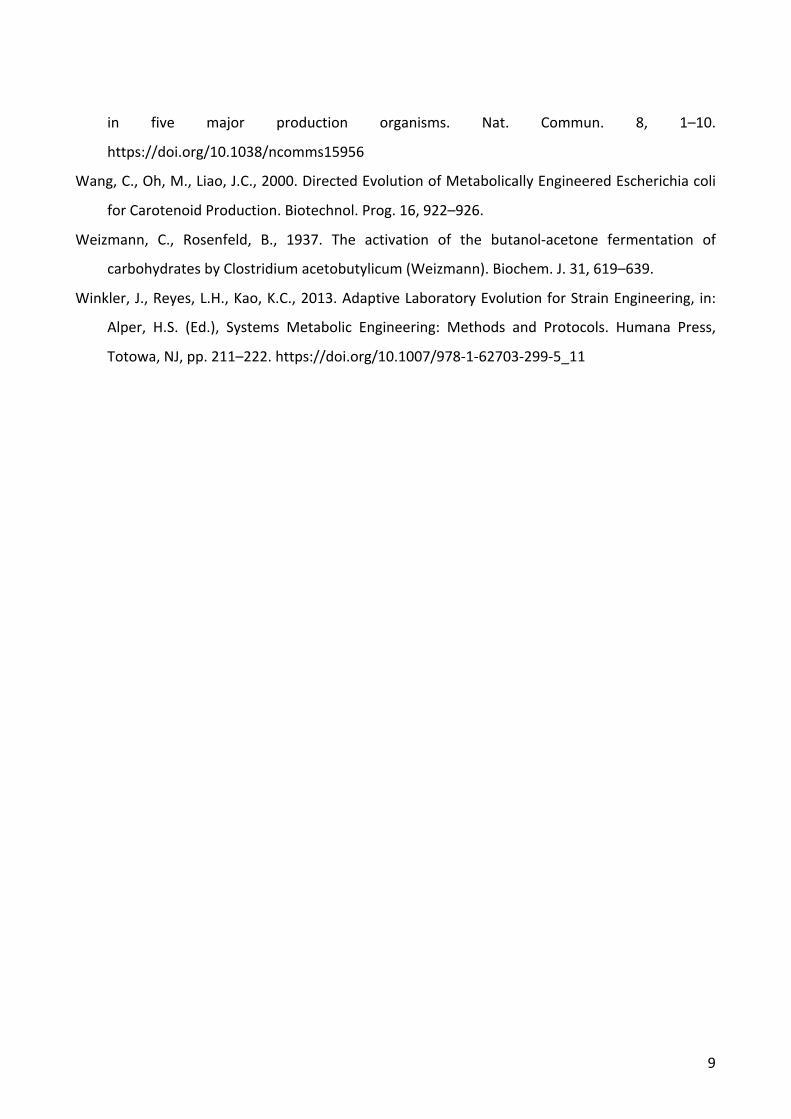
alternative to the Design-Build-Test-Learn cycle and the process is illustrated in Figure 2A, where

the design and build steps are replaced by generation of variation while the test and learn steps are

replaced by selection. The higher the screening throughput, the more of a compromise can be

accepted with regard to the rational design and learn steps, as even random generation of

modifications can lead to better strains if enough candidates are screened. Very high throughputs

can be achieved if the desired phenotype can be selected for under certain growth conditions. This

4

allows rapid identification of the best performing mutants among millions of variants. The non-

rational engineering process can either utilize artificially created genetic variation in specific regions,

e.g. through error-prone PCR, resulting in a method known as directed evolution (Vick and Schmidt-

Dannert, 2011), or, if the desired phenotype can be selected for, it can rely on the naturally occurring

mutations in a continuously grown culture, giving rise to an iterative selection process known as

adaptive laboratory evolution (ALE) (Portnoy et al., 2011). Directed evolution is useful if the

metabolic engineer has a good idea of which genes or DNA regions should be mutated to improve

the desired strain characteristic, as a large and diverse library of variants can be generated quickly.

It has for example been used to modify heterologous pathway enzymes taken from thermophilic

organisms to function better in Escherichia coli (Atsumi and Liao, 2008; Wang et al., 2000). ALE takes

advantage of natural selection by continuously passaging a culture to fresh media, whereby mutants

with increased growth rates will outcompete the other cells and become enriched in the culture

(Winkler et al., 2013). The ALE process can be used to optimize microbial strains on a systems level,

without any prior hypotheses about which genes should be targeted to increase growth and is very

similar to natural evolution. After application of ALE, the final culture, or isolates from it, is subjected

to sequencing to learn which mutations have arisen and might be responsible for the improved

growth rate (Figure 2B).

Figure 2: A) Illustration of how ALE can replace manual iterations through the Design-Build-Test-Learn cycle. B) The process of ALE through serial passaging of cultures. After a desired increase in fitness has been observed, isolates from the ALE experiment may be sequenced to investigate which mutations are responsible for the improvements.

A B

5

Some traits of production strain performance are inherently related to growth and can thus be easily

optimized with ALE. An example of this is substrate utilization. Growing cells on a sub-optimal

substrate allows them to gradually adapt to the new condition, as there is a constant selection

pressure for the cells that grow fastest on the new substrate (Apel et al., 2016). Evolution for

substrate utilization can be a very useful part of strain engineering, as economic considerations can

constrain the use of usual laboratory substrates in the production process (Hansen et al., 2017).

Another growth-related trait that is easy to evolve is tolerance to toxic environments (Mohamed et

al., 2017). This can also be easily achieved by growing cells in the toxic environment, whereby the

most tolerant mutant strains will continuously be selected. In strain engineering this can be useful

for overcoming product toxicity, which is the phenomenon where the production strain is inhibited

by the compound it is producing. Product toxicity limits the attainable titers in the production

process and thus the economic feasibility (Hansen et al., 2017). Additionally, during production

processes the production strains are often grown under stressful conditions, e.g. due to suboptimal

aeration and mixing and the use of complex feedstocks that may contain inhibitors or toxic residue

from pretreatment. Chapter 1 describes these issues in more detail as well as an application of ALE

to study the evolution of tolerance and the effect this has on the production characteristics of the

strains.

Arguably the most important characteristic of a production strain, at least for high-value products,

is the production rate of the compound of interest. The production rate is not inherently related to

growth, rather there is in general a tradeoff between biomass production and product formation.

This tradeoff is a consequence of mass balance as both are sinks for limited cellular resources, the

most important of which being carbon. Some compounds, however, are obligate by-products of

growth, which means that the cell cannot grow without producing them. Such compounds are said

to be growth-coupled and include for example ethanol and lactate under anaerobic growth of

Saccharomyces cerevisiae and E. coli respectively (Clark, 1989; Deken, 1966). In addition to

compounds that are naturally growth-coupled it is possible, through clever strain engineering, to

construct mutant strains where the compound of interest is coupled to growth (von Kamp and

Klamt, 2017). If a compound is growth-coupled it is possible to use ALE to indirectly optimize the

production rate through selection of faster growing strains. Making production of a target

compound growth-coupled often requires introduction of genetic modifications that are not

6

intuitively obvious. It can therefore be beneficial to use model-based computational methods in the

strain design process in order to engineer specific desired phenotypes, such as growth-coupling

(Feist et al., 2010). Computational strain design and methods for constructing growth-coupled

strains will be addressed in Part II of this thesis.

After performing ALE and obtaining one or more mutant strains with improved characteristics, it is

most often of interest to sequence the genome of the strains. The mutants might have accumulated

random mutations that can have a detrimental effect on overall strain performance and must be

reverted before the strain is used for production. Alternatively, a core set of mutations responsible

for improved growth, can be identified and reintroduced into the background strain (Shepelin et al.,

2018). Additionally, sequencing the mutants can allow investigation of the mechanisms through

which growth was improved (Sandberg et al., 2014). This can be useful for gaining an understanding

of the strain’s characteristics and might allow for more direct rational strain engineering in the

future. Unfortunately, it is rarely obvious why the mutations that arise in the evolved strains confer

improvements in the phenotype. This challenge raises the need for a variety of experimental and

computational methods for interpreting the sequencing results of strains evolved using ALE

(Shepelin et al., 2018). Furthermore, the evolved strains can be probed in other ways to explore

how their physiology has been altered through the ALE process. This can include growth

characterization in various conditions or systems analyses such as transcriptomics or metabolomics.

In combination with the genomic information gained from sequencing this can give a deeper

understanding of the process through which the evolved strain improved. An example of how

metabolomics can be used to elucidate details about evolved strains and the evolution process is

described in Chapter 2, using the strains constructed in the study described in Chapter 1. Chapter 3

describes a novel machine learning method for relating genetic mutations to changes in metabolism

in a systematic way. Such a method can potentially help understand the effects of mutations

observed in ALE experiments, as well as integrate other systems-level data obtained from evolved

strains.

References

Apel, A.R., Ouellet, M., Szmidt-middleton, H., Keasling, J.D., 2016. Evolved hexose transporter

enhances xylose uptake and glucose / xylose co-utilization in Saccharomyces cerevisiae. Nat.

7

Publ. Gr. 1–10. https://doi.org/10.1038/srep19512

Atsumi, S., Liao, J.C., 2008. Directed evolution of Methanococcus jannaschii citramalate synthase

for biosynthesis of 1-propanol and 1-butanol by Escherichia coli. Appl. Environ. Microbiol. 74,

7802–7808. https://doi.org/10.1128/AEM.02046-08

Bailey, J.E., 1991. Toward a science of metabolic engineering. Science (80-. ). 252, 1668–1675.

Cantwell, C., Beckmann, R., Whiteman, P., Queener, S.W., Abraham, E.P., 1992. Isolation of

deacetoxycephalosporin C from fermentation broths of Penicillium chrysogenum

transformants: Construction of a new fungal biosynthetic pathway. Proc. R. Soc. B Biol. Sci. 248,

283–289. https://doi.org/10.1098/rspb.1992.0073

Chao, R., Yuan, Y., Zhao, H., 2015. Building biological foundries for next-generation synthetic

biology. Sci. China Life Sci. 58, 658–665. https://doi.org/10.1007/s11427-015-4866-8

Clark, D.P., 1989. The fermentation pathways of Escherichia coli. FEMS Microbiol. Rev. 63, 223–234.

Deken, R.H., 1966. The Crabtree Effect: A Regulatory System in Yeast. J. Gen. Microbiol. 149–156.

Feist, A.M., Zielinski, D.C., Orth, J.D., Schellenberger, J., Herrgard, M.J., Palsson, B.O., 2010. Model-

driven evaluation of the production potential for growth-coupled products of Escherichia coli.

Metab. Eng. 12, 173–186. https://doi.org/10.1016/j.ymben.2009.10.003

Hansen, A.S.L., Lennen, R.M., Sonnenschein, N., Herrgård, M.J., 2017. Systems biology solutions for

biochemical production challenges. Curr. Opin. Biotechnol. 45, 85–91.

https://doi.org/10.1016/j.copbio.2016.11.018

Lee, S.Y., Kim, H.U., 2015. Systems strategies for developing industrial microbial strains. Nat.

Biotechnol. 33, 1061–1072. https://doi.org/10.1038/nbt.3365

Liu, J., Li, H., Zhao, G., Caiyin, Q., Qiao, J., 2018. Redox cofactor engineering in industrial

microorganisms: strategies, recent applications and future directions. J. Ind. Microbiol.

Biotechnol. 45, 313–327. https://doi.org/10.1007/s10295-018-2031-7

Max, B., Salgado, J.M., Rodríguez, N., Cortés, S., Converti, A., Domínguez, J.M., 2010.

Biotechnological production of citric acid. Brazilian J. Microbiol. 41, 862–875.

https://doi.org/10.1590/S1517-83822010000400005

Mohamed, E.T., Wang, S., Lennen, R.M., Herrgård, M.J., Simmons, B.A., Singer, S.W., Feist, A.M.,

2017. Generation of a platform strain for ionic liquid tolerance using adaptive laboratory

evolution. Microb. Cell Fact. 16, 1–15. https://doi.org/10.1186/s12934-017-0819-1

8

Nielsen, J., 2017. Systems Biology of Metabolism. Annu. Rev. Biochem. 86, 245–275.

https://doi.org/10.1146/annurev-biochem-061516-044757

Nielsen, J., 2001. Metabolic engineering. Appl. Microbiol. Biotechnol. 55, 263–283.

https://doi.org/10.1007/s002530000511

Nielsen, J., Keasling, J.D., 2016. Engineering Cellular Metabolism. Cell 164, 1185–1197.

https://doi.org/10.1016/j.cell.2016.02.004

Pedersen, H., Christensen, B., Hjort, C., Nielsen, J., 2000. Construction and characterization of an

oxalic acid nonproducing strain of Aspergillus niger. Metab. Eng. 2, 34–41.

https://doi.org/10.1006/mben.1999.0136

Portnoy, V.A., Bezdan, D., Zengler, K., 2011. Adaptive laboratory evolution-harnessing the power of

biology for metabolic engineering. Curr. Opin. Biotechnol. 22, 590–594.


Rowlands, R.T., 1984. Industrial strain improvement: mutagenesis and random screening

procedures. Enzym. Microb. Technol. 6, 3–10.

Sandberg, T.E., Pedersen, M., Lacroix, R.A., Ebrahim, A., Bonde, M., Herrgard, M.J., Palsson, B.O.,

Sommer, M., Feist, A.M., 2014. Evolution of Escherichia coli to 42 C and Subsequent Genetic

Engineering Reveals Adaptive Mechanisms and Novel Mutations. Mol. Biol. Evol. 31, 2647–

2662. https://doi.org/10.1093/molbev/msu209

Schmidt, F., Platt, R.J., 2017. Applications of CRISPR-Cas for synthetic biology and genetic recording.

Curr. Opin. Syst. Biol. 5, 9–15. https://doi.org/10.1016/j.coisb.2017.05.008

Shepelin, D., Hansen, A.S.L., Lennen, R., Luo, H., Herrgård, M.J., 2018. Selecting the best:

Evolutionary engineering of chemical production in microbes. Genes (Basel). 9.

https://doi.org/10.3390/genes9050249

Shimizu, K., 2011. Metabolic Regulation Analysis and Metabolic Engineering, Second Edition. ed,

Comprehensive Biotechnology, Second Edition. Elsevier B.V. https://doi.org/10.1016/B978-0-

08-088504-9.00117-3

Vick, J., Schmidt-Dannert, C., 2011. Directed Enzyme and Pathway Evolution, in: Enzyme

Technologies: Metagenomics, Evolution, Biocatalysis, and Biosynthesis. John Wiley and Sons,

pp. 41–75.

von Kamp, A., Klamt, S., 2017. Growth-coupled overproduction is feasible for almost all metabolites

9

in five major production organisms. Nat. Commun. 8, 1–10.

https://doi.org/10.1038/ncomms15956

Wang, C., Oh, M., Liao, J.C., 2000. Directed Evolution of Metabolically Engineered Escherichia coli

for Carotenoid Production. Biotechnol. Prog. 16, 922–926.

Weizmann, C., Rosenfeld, B., 1937. The activation of the butanol-acetone fermentation of

carbohydrates by Clostridium acetobutylicum (Weizmann). Biochem. J. 31, 619–639.

Winkler, J., Reyes, L.H., Kao, K.C., 2013. Adaptive Laboratory Evolution for Strain Engineering, in:

Alper, H.S. (Ed.), Systems Metabolic Engineering: Methods and Protocols. Humana Press,

Totowa, NJ, pp. 211–222. https://doi.org/10.1007/978-1-62703-299-5_11

10

Chapter 1: Parallel laboratory evolutions reveal general

chemical tolerance mechanisms and enhance chemical

production

Rebecca Lennen1*, Kristian Jensen1*, Elsayed T. Mohammed1, Sailesh Malla1, Rosa A. Börner1, Emre

Özdemir1, Ida Bonde1, Anna Koza1, Lasse E. Pedersen1, Lars Y. Schöning1, Nikolaus Sonnenschein1,

Bernhard Ø. Palsson1,2, Morten A. Sommer1, Adam Feist1,2, Alex T. Nielsen1**, Markus J. Herrgård1**

* These authors contributed equally to the work

** Co-corresponding authors

1) The Novo Nordisk Foundation Center for Biosustainability, Technical University of Denmark,

Building 220, Kemitorvet, 2800 Kgs. Lyngby, Denmark

2) Department of Bioengineering, University of California, San Diego

Abstract

Tolerance toward high concentrations of product is a major barrier to achieving economically viable

processes for biobased chemical production. Product tolerance cannot currently be rationally

engineered due to lack of knowledge of the cellular mechanisms of chemical toxicity and tolerance.

We used an automated platform to evolve parallel populations of Escherichia coli to tolerate

previously toxic concentrations of 11 chemicals that have applications as polymer precursors,

chemical intermediates, or biofuels. Re-sequencing of isolates from 88 independently evolved

populations, reconstruction of mutations, transcriptomic and proteomic analyses, and cross-

compound tolerance profiling was employed to uncover general and specific tolerance mechanisms.

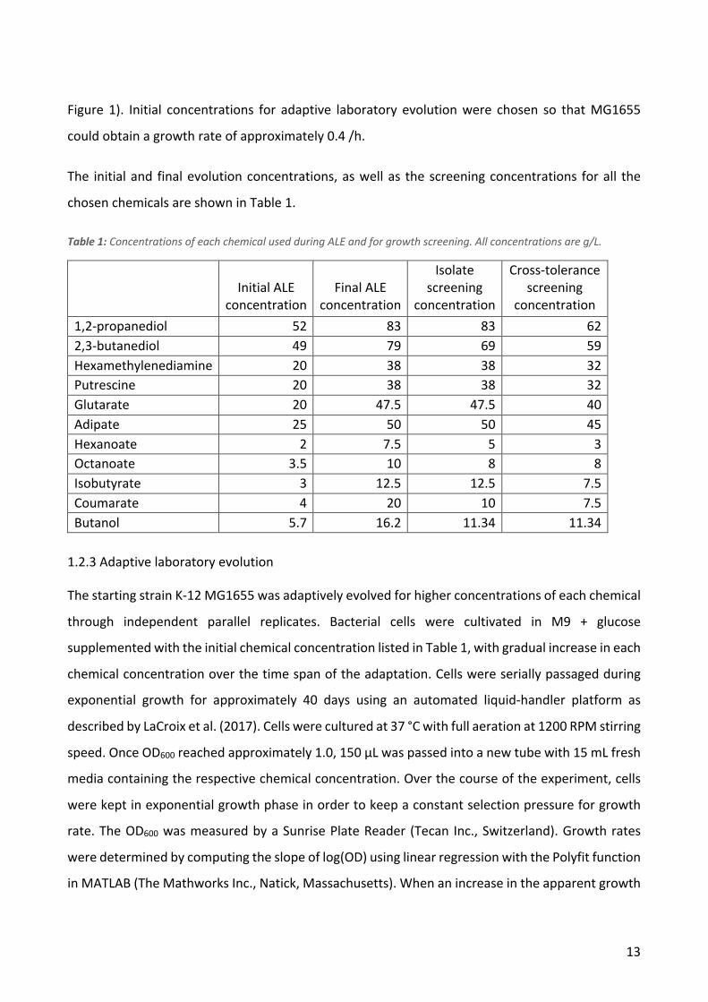
We found that the broad tolerance of strains to chemicals varied significantly depending on the

condition under which the strain was evolved in and that strains that acquired high levels of

osmotolerance were also tolerant to most chemicals. Specific genetic tolerance mechanisms

included alterations in regulatory, cell wall, and broad transcriptional and translational functions, as

well as more chemical-specific mechanisms related to transport and metabolism. Finally, we show

that pre-tolerizing the host strain can significantly enhance endogenous production of chemicals

and is especially valuable when a large number of independently evolved isolates are screened.

11

1.1 Introduction

Despite significant advances in synthetic and systems biology tools to engineer and study

metabolism, developing microbial strains for commercial-level production of chemicals still remains

a challenge (Van Dien, 2013). One of the major problems relates to the stressful conditions that

production strains encounter in large-scale industrial production processes where numerous

stresses that are not encountered in laboratory conditions are present (Deparis et al., 2017). Some

of these stresses relate to the presence of high concentrations of a carbon source or toxic

compounds related to feedstock processing such as ionic liquids (Mohamed et al., 2017).

Irrespective of the production system or substrate, cells will encounter high intracellular and

extracellular levels of the primary product that they have been engineered to produce. Frequently,

high levels of such products can have inhibitory effects on the host organism, which effectively limits

the titers that can be achieved and thereby the economic feasibility of the process. This issue can

be overcome by engineering a production strain that is tolerant to higher titers of the product,

however rational engineering of tolerance to either native or non-native chemical products is rarely

possible due to a lack of knowledge about the molecular mechanisms of tolerance. This often

necessitates choosing an otherwise difficult to engineer production host that already has desirable

tolerance characteristics. Alternatively, one can use non-rational approaches to obtain strains with

high chemical tolerance by mutagenesis, screening of transporter and other libraries, or adaptive

laboratory evolution (ALE) (Hansen et al., 2017). ALE in particular has been successfully used to

obtain strains that tolerate product chemicals (Winkler and Kao, 2014). In some cases the

mechanisms of chemical tolerance have been at least partially deciphered through resequencing

and other omics approaches applied to evolved strains (Haft et al., 2014; Kildegaard et al., 2014;

Reyes et al., 2013), but in most cases the full toxicity and tolerance mechanisms remain to be

determined. While ALE applied to product tolerance has resulted in strains that increase actual

production of the target chemical (Mundhada et al., 2017), in many cases these strains have not

shown improved production (Atsumi et al., 2010; Kildegaard et al., 2014).

Here we take a broad approach to elucidating mechanisms of chemical tolerance across a wide

spectrum of chemicals enabled by automated ALE as well as systematic genomic and phenotypic

analyses of the resulting large collection of evolved strains. This approach allows us to determine

12

general features of chemical tolerance and build a large dataset as a reference for future tolerance

studies. For two products we also investigate whether pre-evolving for tolerance can significantly

improve production. A similar approach has been previously take to study adaptation to diverse

stresses including some non-native chemical stresses in E. coli (Horinouchi et al., 2017), but in the

present study we use significantly higher concentrations of chemicals to mimic industrially relevant

conditions and evolve and characterize a significantly larger number of strains per condition.

1.2 Materials and Methods

1.2.1 Strains and media

E. coli K-12 MG1655 (ATCC 47076) strain was used as a starting point strain for the adaptive

laboratory evolution experiments and as reference strain for all subsequent characterization.

Chemicals were purchased from either Sigma-Aldrich (Merck KGaA, Darmstadt, Germany) or Fisher

Scientific (Part of Thermo-Fisher Scientific). Plasmids for isobutyric acid and 2,3-butanediol

production were obtained from the authors (Xu et al., 2014; Zhang et al., 2011).

M9 glucose medium supplemented with 10 g/L glucose was formulated with 1x M9 salts, 2 mM

MgSO4, 100 µM CaCl2 and 1x trace elements. A stock solution of 10x M9 salts consisted of 68 g/L

Na2HPO4 anhydrous, 30 g/L KH2PO4, 5 g/L NaCl, and 10 g/L NH4Cl dissolved in Milli-Q filtered water

and autoclaved. M9 trace elements stock concentration was a 2000x solution containing of 3.0 g/L

FeSO4·7H2O, 4.5 g/L ZnSO4·7H2O, 0.3 g/L CoCl2·6H2O, 0.4 g/L Na2MoO4·2H2O, 4.5 g/L CaCl2·H2O, 0.2

g/L CuSO4·2H2O, 1.0 g/L H3BO3, 15 g/L disodium ethylene-diamine-tetra-acetate, 0.1 g/L KI, 0.7 g/L

MnCl2·4H2O in Milli-Q filtered water and sterile filtered.

1.2.2 Selection of initial chemical concentrations

The toxicity of each of the chemicals was tested by screening growth of MG1655 in different

concentrations. Biological triplicates of E. coli MG1655 were cultivated at 37 °C with 300 RPM

shaking. After 14 to 18 h, the cultures were inoculated into M9 + 0.2 % glucose and one of the

chosen chemicals at different concentrations. The cultures were then incubated in a BioLector

microbioreactor system (m2p-labs GmbH, Baesweiler, Germany) at 37 °C with 1,000-rpm shaking.

The growth rates at different concentrations were calculated for each chemical (Supplementary

13

Figure 1). Initial concentrations for adaptive laboratory evolution were chosen so that MG1655

could obtain a growth rate of approximately 0.4 /h.

The initial and final evolution concentrations, as well as the screening concentrations for all the

chosen chemicals are shown in Table 1.

Table 1: Concentrations of each chemical used during ALE and for growth screening. All concentrations are g/L.

Initial ALE

concentration

Final ALE

concentration

Isolate screening

concentration

Cross-tolerance screening

concentration 1,2-propanediol 52 83 83 62 2,3-butanediol 49 79 69 59 Hexamethylenediamine 20 38 38 32 Putrescine 20 38 38 32 Glutarate 20 47.5 47.5 40 Adipate 25 50 50 45 Hexanoate 2 7.5 5 3 Octanoate 3.5 10 8 8 Isobutyrate 3 12.5 12.5 7.5 Coumarate 4 20 10 7.5 Butanol 5.7 16.2 11.34 11.34

1.2.3 Adaptive laboratory evolution

The starting strain K-12 MG1655 was adaptively evolved for higher concentrations of each chemical

through independent parallel replicates. Bacterial cells were cultivated in M9 + glucose

supplemented with the initial chemical concentration listed in Table 1, with gradual increase in each

chemical concentration over the time span of the adaptation. Cells were serially passaged during

exponential growth for approximately 40 days using an automated liquid-handler platform as

described by LaCroix et al. (2017). Cells were cultured at 37 °C with full aeration at 1200 RPM stirring

speed. Once OD600 reached approximately 1.0, 150 µL was passed into a new tube with 15 mL fresh

media containing the respective chemical concentration. Over the course of the experiment, cells

were kept in exponential growth phase in order to keep a constant selection pressure for growth

rate. The OD600 was measured by a Sunrise Plate Reader (Tecan Inc., Switzerland). Growth rates

were determined by computing the slope of log(OD) using linear regression with the Polyfit function

in MATLAB (The Mathworks Inc., Natick, Massachusetts). When an increase in the apparent growth

14

rate was achieved (average growth rate for all of the parallel replicates) at a particular

concentration, the chemical concentration was increased by 10-15%. This process was repeated in

cycles until a significant increase in tolerated concentration was achieved. In incidents where the

increase in the chemical concentration caused cells to crash, i.e. cell death, chemical concentration

was reduced to a level that allowed cell growth. Periodically, samples were frozen in 25% v/v

glycerol and stored at -80 °C for further use.

1.2.4 Growth screening of ALE isolates

1.2.4.1 Primary tolerance screening

Populations from evolution endpoints were plated on LB agar plates and 10 individual colonies from

each population were screen for growth at the maximum concentration for which robust growth

rates were achieved during the evolution. Cultures of wild-type strain, E. coli K-12 MG1655, were

used as controls. The isolates were inoculated in 500 µL M9 + glucose in deep-well plates and

incubated in plate shaker at 37 °C and 300 RPM. The next day, cells were diluted 10X in M9 + glucose

and 30 µL was transferred to clear-bottom 96 half-deep plates containing M9 + glucose

supplemented with the corresponding toxic chemical at concentrations as in Table 1 (isolate

screening concentration). The plates were incubated at 37 °C with 225 RPM shaking in a Growth

Profiler screening platform (EnzyScreen BV, Heemstede, Netherlands). The resulting growth curves

for all isolates were inspected qualitatively for isolates exhibiting robust growth as assessed by lag

time, final OD and growth rate. Each of the 10 isolates from the primary screening was grouped

according to close similarities based on the above criteria. For each population, isolates

representative of each group were picked (2-3 isolates per population).

1.2.4.1 Cross-tolerance screening

The E. coli strains were inoculated into 300 µl of M9 + glucose medium in 96 deep well plates (in

biological triplicates) and the cultures were incubated at 37°C and 300 RPM for overnight. Next day,

30 µl of a 10-fold was added to 270 µl of M9 + glucose supplemented with chemicals in 96 well plate

and the plates incubated in growth profiler (EnzyScreen BV, Heemstede, The Netherlands) at 37 °C

and 225 RPM. The chemical concentrations are shown in Table 1 (Cross-tolerance screening

concentration).

15

1.2.5 Genome editing of E.coli

Strains containing the relevant single gene deletions were obtained from the Keio Collection and

were transduced into the MG1655 background strain using the protocol described in (Lennen et al.,

2011). Multiple gene deletions were constructed using the protocol described in (Lennen et al.,

2011). Site directed changes in the E. coli genome of evolved strains were done using the protocol

described in (Lennen et al., 2015).

1.2.6 Quantification of 2,3-butanediol production

The hsdR gene was deleted from each of the strains evolved on 2,3-butanediol. The strains were

then transformed with pET-RABC plasmid (Xu et al., 2014) and precultured in 300 µl of M9 + glucose

supplemented with 5 g/L yeast extract and kanamycin (50 µg/mL) in 96 deep well plate and

incubated at 37 °C with 300 RPM overnight (incubated for 20 h) in quadruplicates. E. coli MG1655

ΔhsdR/pET-RABC was used as a control. The following day, 20 µL of pre-inoculum was transferred

into 2 mL of ALE-M9-YE-Km media in 24 deep well plates and incubated at 30 °C and 300 RPM. At

24 h and 48 h, optical densities of the culture broths were determined at 600 nm (OD600nm). Then,

400 µL of the cultures were harvested, centrifuged at 4000 RPM for 10 min and 30 µL of the collected

supernatants were injected into high performance liquid chromatography (HPLC). Subsequently, the

samples were subjected to electrospray ionization mass analysis.

The amounts of 2,3-butanediol in the supernatants were quantified by HPLC (Ultimate 3000,

Thermo Scientific, USA) equipped with an organic acid analysis column, Aminex® HPX-87H ion

exclusion column (300 mm x 7.8 mm, Bio-Rad Laboratories, Denmark) connected to a refractive

Index (RI) detector and a UV detector (205 nm, 210 nm, 254 nm and 280 nm). An isocratic elution

with flow rate of 0.5 mL/min of 5 mM sulphuric acid was used for 30 min. Under these conditions,

stereoisomers of 2,3-butanediol were detected under the RI detector channel at the retention times

of 17.4 min and 18.3 min. Using the peak areas of the stereoisomers, total amount of 2,3-butanediol

was calculated. For absolute quantification a calibration curve was drawn using 1, 5, 10, 12.5, 15

and 25 g/L concentrations (y = 6.5119x + 0.5464, R² = 0.9999).

The exact mass of the compounds was analyzed by using Oribtrap Fusion (Thermo Scientific, USA)

with a Dionex 3000 RX HPLC system (Thermo Scientific, USA) in the positive and negative ion mode.

16

1.2.7 Quantification of isobutyrate production

The yqhD gene was deleted from each of the strains evolved on isobutyrate. The strains were then

transformed with pIBA1 and pIBA7 plasmids (Zhang et al., 2011) and precultured into 300 µl of LB

media supplemented with kanamycin (50 µg/mL) and ampicillin (100 µg/mL) in 96 deep well plate

and incubated at 37 ºC with 300 RPM overnight (incubated for 18 h) (in quadruplicates). E. coli

MG1655 ΔyqhD/pIBA1/pIBA7 was used as a control. The following day, 24 µL of pre-inoculum was

transferred into 2.4 mL of half-FIT media (1:1 FIT media: MOPS of 200 mM) media supplemented

with antibiotics. Then the culture plates were incubated at 30 °C and 300 RPM. After 6 hours of

incubation, OD600 was measured and the cultures were induced with 100 µM of IPTG and continued

the incubation at 30 °C and 300 RPM. At 24 h, 48 and 72 h, OD600 was measured again. Then, 300

µl of the cultures were harvested, centrifuged at 4000 RPM for 10 min and 30 µL of the collected

supernatants were injected into HPLC. Subsequently, the samples were subjected to electrospray

ionization mass analysis.

The amounts of isobutyrate in the supernatants were quantified by HPLC (Ultimate 3000, Thermo

Scientific, USA) equipped with an organic acid analysis column, Aminex® HPX-87H ion exclusion

column (300 mm x 7.8 mm, Bio-Rad Laboratories, Denmark) connected to a refractive Index (RI)

detector and a UV detector (205 nm, 210 nm, 254 nm and 280 nm). An isocratic elution with flow

rate of 0.5 mL min-1 of 5 mM sulphuric acid was used for 30 min. Under these conditions, isobutyrate

was detected under the 210 nm UV channel at a retention time of 20.3 min. Using the peak area,

total amount of isobutyrate was calculated. For absolute quantification a calibration curve was

drawn using 0.5, 1, 2.5, 4, 5, 7.5 10, and 12.5 g/L concentrations (y = 35.487x - 2.3142, R² = 0.9993).

1.2.8 Resequencing

Genomic libraries were generated using the TruSeq® Nano DNA LT Library Prep Kit (Illumina Inc.,

San Diego CA). Briefly, 100 ng of genomic DNA diluted in 52.5 µL TE buffer was fragmented in Covaris

Crimp Cap microtubes on a Covaris E220 ultrasonicator (Woburn, MA) with 5% duty factor, 175 W

peak incident power, 200 cycles/burst, and 50-s duration under frequency sweeping mode at 5.5 to

6°C (Illumina recommendations for a 350-bp average fragment size). The ends of fragmented DNA

were repaired by T4 DNA polymerase, Klenow DNA polymerase, and T4 polynucleotide kinase. The

Klenow exo minus enzyme was then used to add an 'A' base to the 3' end of the DNA fragments.

17

The adapters were ligated to the ends of the DNA fragments, and the DNA fragments ranging from

300 - 400 bp were recovered by beads purification. Finally, the adapter-modified DNA fragments

were enriched by 3 cycle PCR. Final concentration of each library was measured by Qubit® 2.0

Fluorimeter and Qubit DNA Broad range assay (Life Technologies). Average dsDNA library size was

determined using the Agilent DNA 7500 kit on an Agilent 2100 Bioanalyzer. Libraries were

normalized and pooled in 10 mM Tris-Cl, pH 8.0, plus 0.05% Tween 20 to the final concentration of

10 nM. Denaturated in 0.2N NaOH, 10 pm pool of 20 libraries in 600 µL ice-cold HT1 buffer was

loaded onto the flow cell provided in the MiSeq Reagent kit v2 (300 cycles) (Illumina Inc., San Diego

CA) 300 cycles and sequenced on a MiSeq (Illumina Inc., San Diego CA) platform with a paired-end

protocol and read lengths of 151 nt.

1.2.9 Resequencing data analysis

The Illumina sequencing reads were analyzed with the Breseq pipeline (Deatherage and Barrick,

2014) through the ALEdb platform (Phaneuf et al., 2018) to generate lists of mutations for each

evolved strain. The reference strain for this analysis was E. coli K-12 MG1655 with the Genbank

accession number NC_000913.3.

1.2.9.1 Mapping mutations to genes

Each mutation was mapped to one or more genes. Intragenic mutations were mapped to any

gene(s) whose coding sequence overlapped with the mutation. Intergenic mutations were mapped

to the closest gene downstream from the mutation.

1.2.10 Growth data analysis

The growth curves generated by the instruments were processed using the croissance python

package (http://github.com/biosustain/croissance), which performs automated growth phase

identification and growth parameter fitting. Biomass concentration was quantified by OD600 values.

For each extracted growth rate, a normalized growth rate was calculated by subtracting the mean

growth rate of the wild-type strain, MG1655, on the same plate and in the same medium. This was

done to remove the effects of any between-plate and between-experiment growth variations.

The croissance algorithm consists of two separate steps:

18

Step 1: The growth curve is smoothed and analyzed to find regions of exponential growth. This is

done by identifying time intervals where the first- and second-order time derivatives of the

smoothed biomass function are strictly positive.

Step 2: Each growth phase identified in step 1 is fitted with an exponential function of the form

!(#) = & ∙ ()∙* + , (1)

where μ (growth rate) is of particular interest in this study. The offset parameter b is included to

enable analysis of growth curves that are not background-subtracted.

Post-processing was done to filter the returned growth rates. This served both to exclude growth

rates from growth phases that were not thought to be real, and to select between several growth

phases in the same growth curve. Growth rates higher than 1.5 h-1 were excluded, as were growth

phases where the absolute value of the fitted offset parameter b was larger than a certain threshold,

c (0.5 for growth profiler curves, 4 for Biolector curves). Growth phases where the initial biomass

concentration deviated more than c from the fitted offset b were also excluded, as these were likely

to be secondary growth phases. Furthermore, growth curves starting after a certain time point were

also excluded. This was done to prevent growth from contaminations from being used. The chosen

time cutoff was dependent on the growth conditions (30-40 hours). Very short growth phases were

also excluded as they were most likely artifacts. For standard M9 glucose cultures growth phases

shorter than 2 hours were excluded, while the cutoff was 5 hours for cultures in the stress

conditions.

1.3 Results

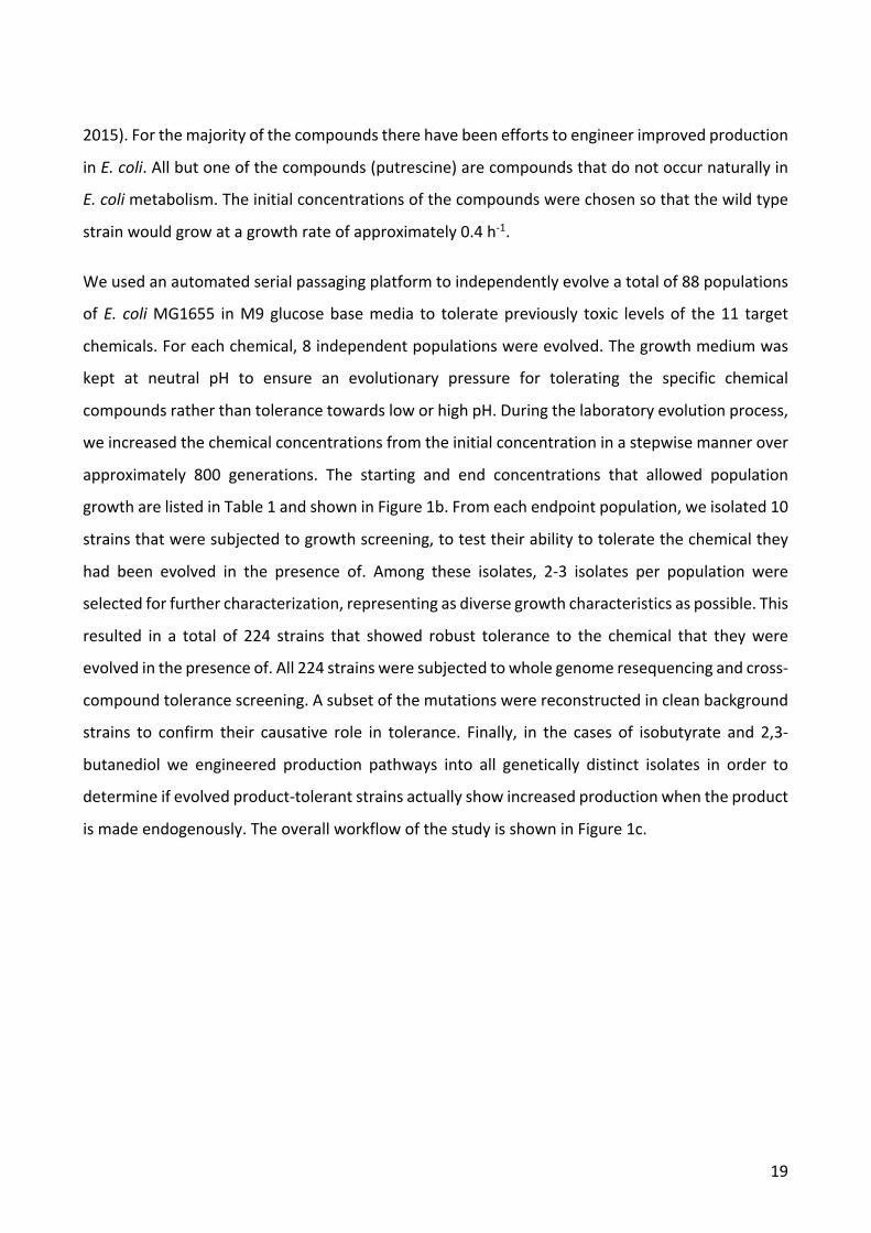
We selected 11 chemical compounds representing a diversity of chemical categories with variable

initial levels of toxicity to E. coli (Figure 1a). We chose the chemicals to 1) include compounds that

have potential as a bio-based product, 2) have examples of multiple chemical compound classes

(diols, diamines, diacids, fatty acids, aromatic compounds), 3) include in four cases two examples of

the same compound class, and 4) to have compounds that had the right solubility and volatility

profile to allow ALE and downstream characterization. We included two compounds (octanoate and

n-butanol) that have previously been used in ALE studies in E. coli (Reyes et al., 2013; Royce et al.,

19

2015). For the majority of the compounds there have been efforts to engineer improved production

in E. coli. All but one of the compounds (putrescine) are compounds that do not occur naturally in

E. coli metabolism. The initial concentrations of the compounds were chosen so that the wild type

strain would grow at a growth rate of approximately 0.4 h-1.

We used an automated serial passaging platform to independently evolve a total of 88 populations

of E. coli MG1655 in M9 glucose base media to tolerate previously toxic levels of the 11 target

chemicals. For each chemical, 8 independent populations were evolved. The growth medium was

kept at neutral pH to ensure an evolutionary pressure for tolerating the specific chemical

compounds rather than tolerance towards low or high pH. During the laboratory evolution process,

we increased the chemical concentrations from the initial concentration in a stepwise manner over

approximately 800 generations. The starting and end concentrations that allowed population

growth are listed in Table 1 and shown in Figure 1b. From each endpoint population, we isolated 10

strains that were subjected to growth screening, to test their ability to tolerate the chemical they

had been evolved in the presence of. Among these isolates, 2-3 isolates per population were

selected for further characterization, representing as diverse growth characteristics as possible. This

resulted in a total of 224 strains that showed robust tolerance to the chemical that they were

evolved in the presence of. All 224 strains were subjected to whole genome resequencing and cross-

compound tolerance screening. A subset of the mutations were reconstructed in clean background

strains to confirm their causative role in tolerance. Finally, in the cases of isobutyrate and 2,3-

butanediol we engineered production pathways into all genetically distinct isolates in order to

determine if evolved product-tolerant strains actually show increased production when the product

is made endogenously. The overall workflow of the study is shown in Figure 1c.

20

Figure 1: a) Chemicals selected for the study grouped by chemical category. b) Initial and final concentrations of the chemicals used during ALE. c) Overall workflow of the study.

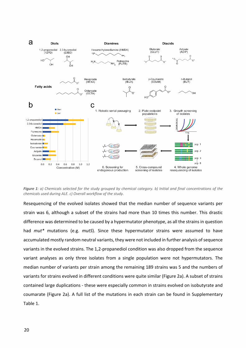
Resequencing of the evolved isolates showed that the median number of sequence variants per

strain was 6, although a subset of the strains had more than 10 times this number. This drastic

difference was determined to be caused by a hypermutator phenotype, as all the strains in question

had mut* mutations (e.g. mutS). Since these hypermutator strains were assumed to have

accumulated mostly random neutral variants, they were not included in further analysis of sequence

variants in the evolved strains. The 1,2-propanediol condition was also dropped from the sequence

variant analyses as only three isolates from a single population were not hypermutators. The

median number of variants per strain among the remaining 189 strains was 5 and the numbers of

variants for strains evolved in different conditions were quite similar (Figure 2a). A subset of strains

contained large duplications - these were especially common in strains evolved on isobutyrate and

coumarate (Figure 2a). A full list of the mutations in each strain can be found in Supplementary

Table 1.

21

To investigate which cellular functions were affected by the mutations, the functional domains of

all the mutated genes were analyzed (Figure 2b). More than half of the variants affect genes with

regulatory or transport functions, indicating that these gene classes play a significant role in the

evolution of tolerance.

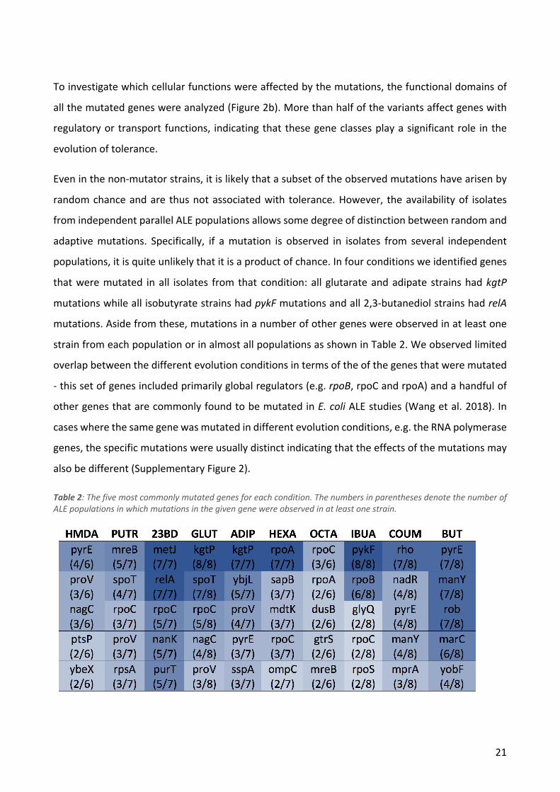
Even in the non-mutator strains, it is likely that a subset of the observed mutations have arisen by

random chance and are thus not associated with tolerance. However, the availability of isolates

from independent parallel ALE populations allows some degree of distinction between random and

adaptive mutations. Specifically, if a mutation is observed in isolates from several independent

populations, it is quite unlikely that it is a product of chance. In four conditions we identified genes

that were mutated in all isolates from that condition: all glutarate and adipate strains had kgtP

mutations while all isobutyrate strains had pykF mutations and all 2,3-butanediol strains had relA

mutations. Aside from these, mutations in a number of other genes were observed in at least one

strain from each population or in almost all populations as shown in Table 2. We observed limited

overlap between the different evolution conditions in terms of the of the genes that were mutated

- this set of genes included primarily global regulators (e.g. rpoB, rpoC and rpoA) and a handful of

other genes that are commonly found to be mutated in E. coli ALE studies (Wang et al. 2018). In

cases where the same gene was mutated in different evolution conditions, e.g. the RNA polymerase

genes, the specific mutations were usually distinct indicating that the effects of the mutations may

also be different (Supplementary Figure 2).

Table 2: The five most commonly mutated genes for each condition. The numbers in parentheses denote the number of ALE populations in which mutations in the given gene were observed in at least one strain.

22

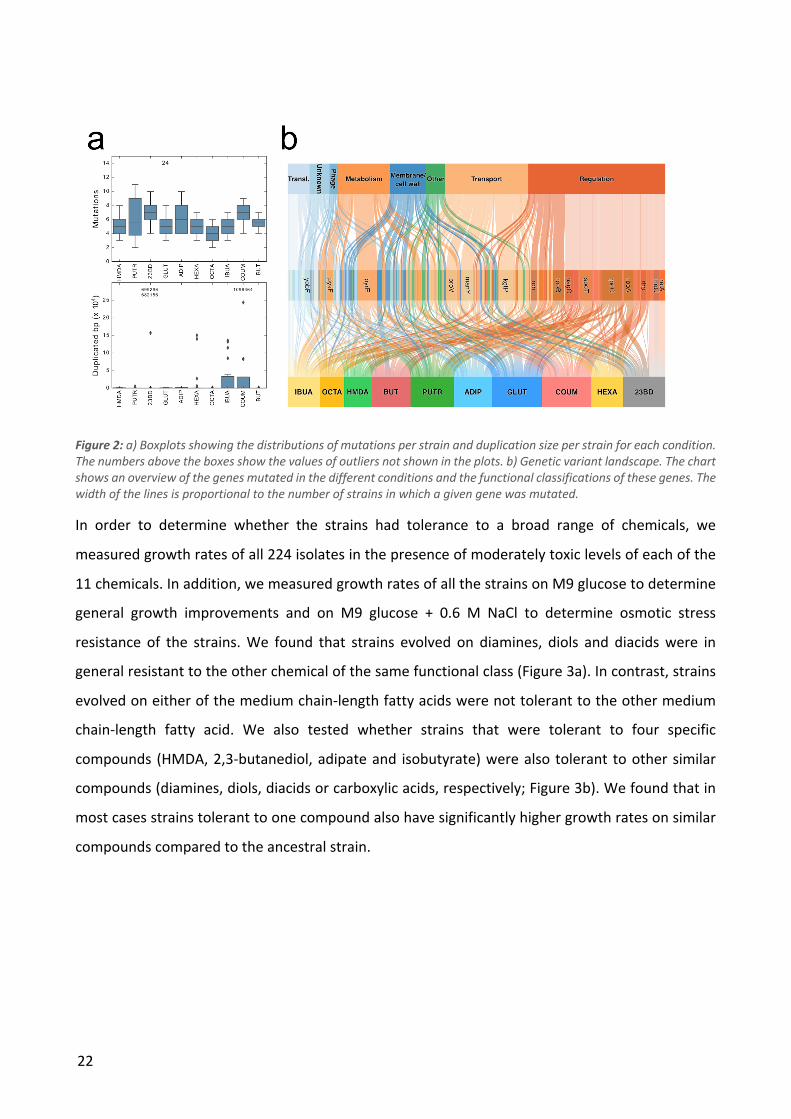
Figure 2: a) Boxplots showing the distributions of mutations per strain and duplication size per strain for each condition. The numbers above the boxes show the values of outliers not shown in the plots. b) Genetic variant landscape. The chart shows an overview of the genes mutated in the different conditions and the functional classifications of these genes. The width of the lines is proportional to the number of strains in which a given gene was mutated.

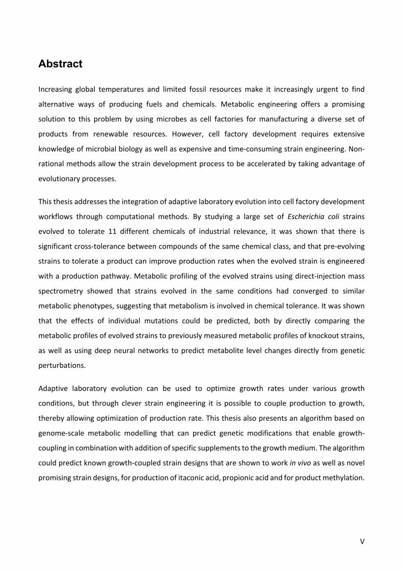
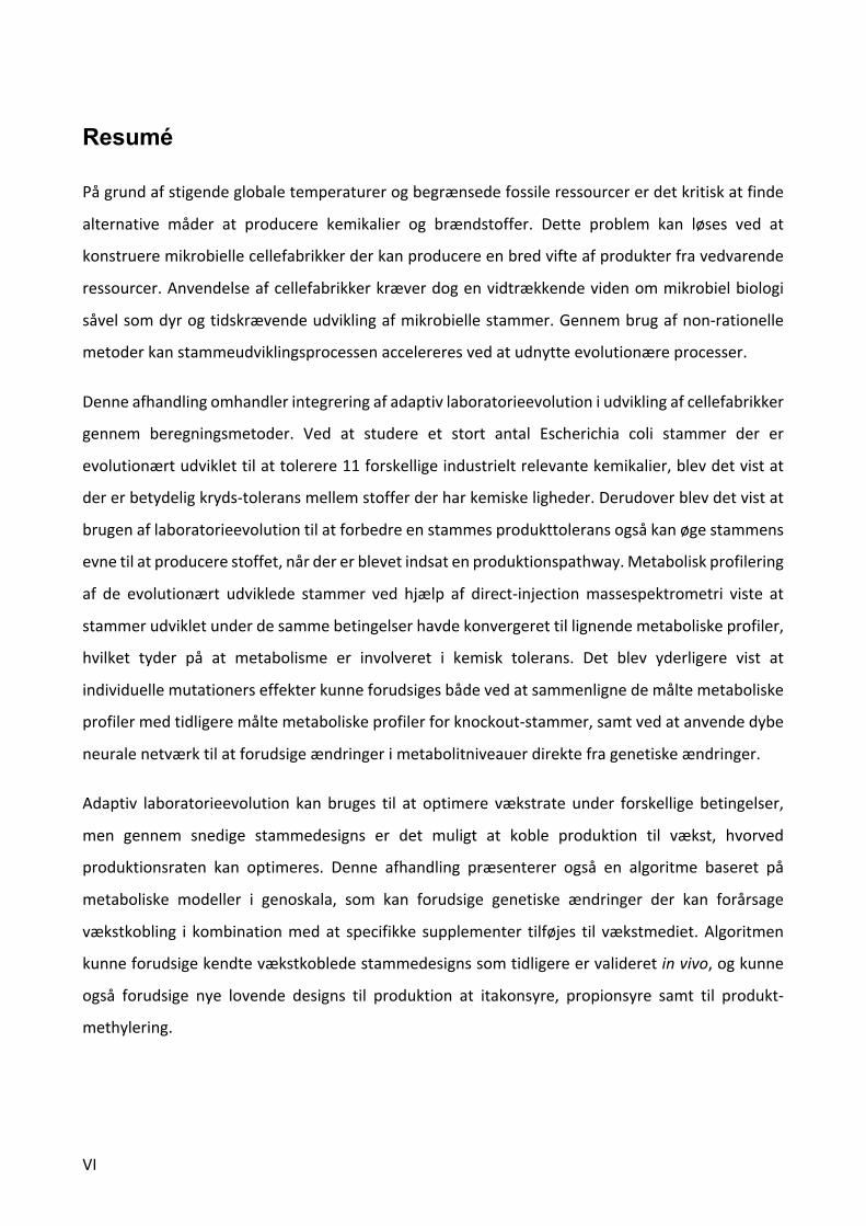
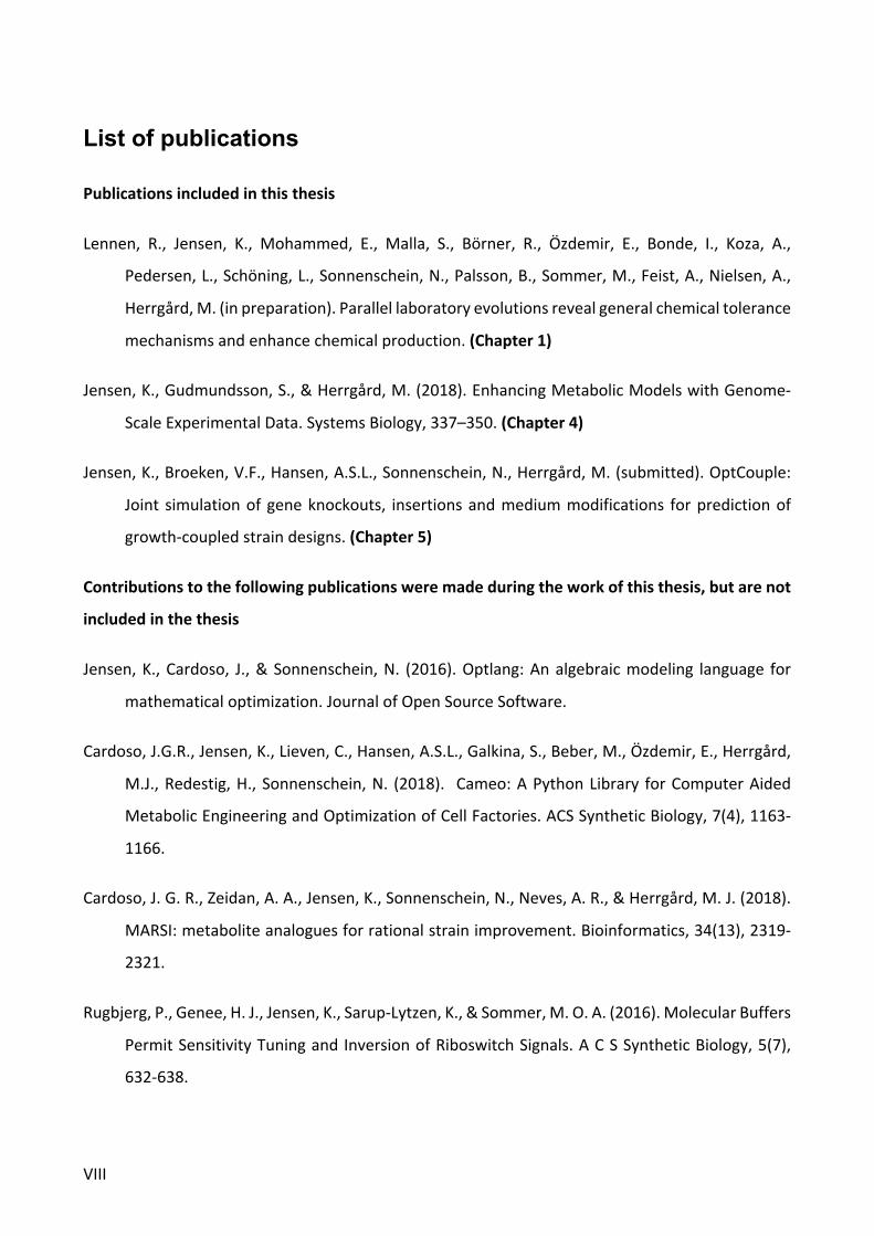
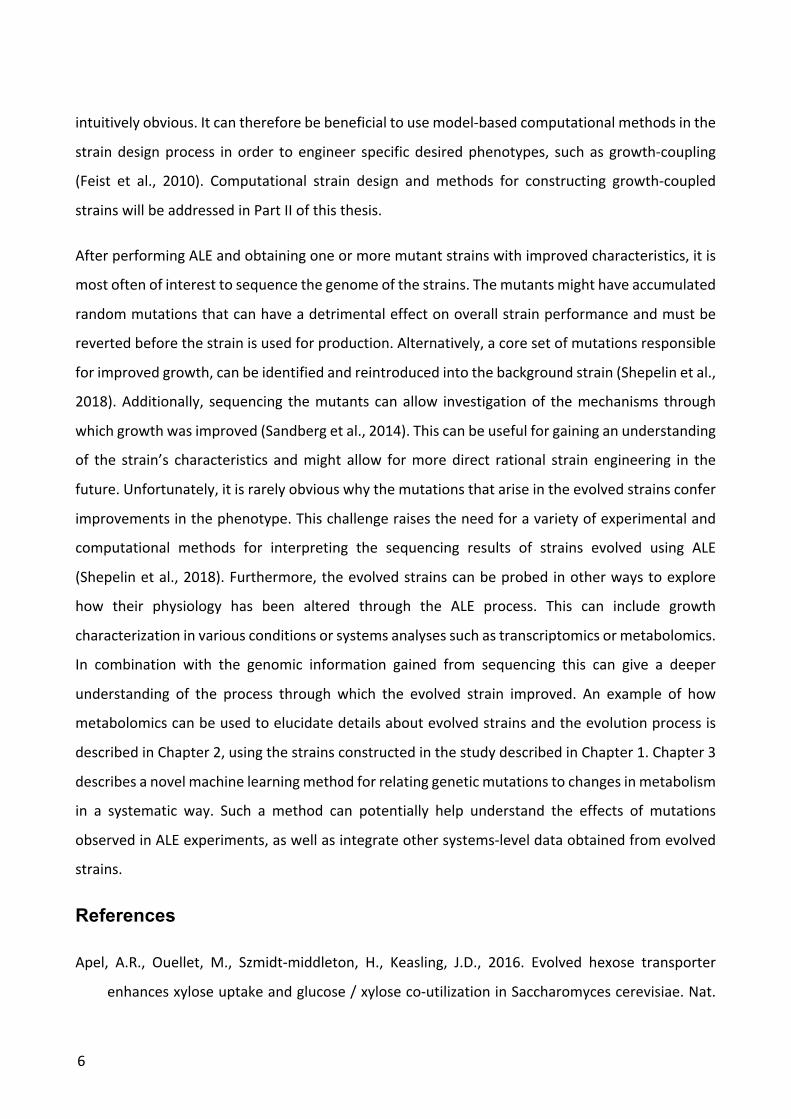
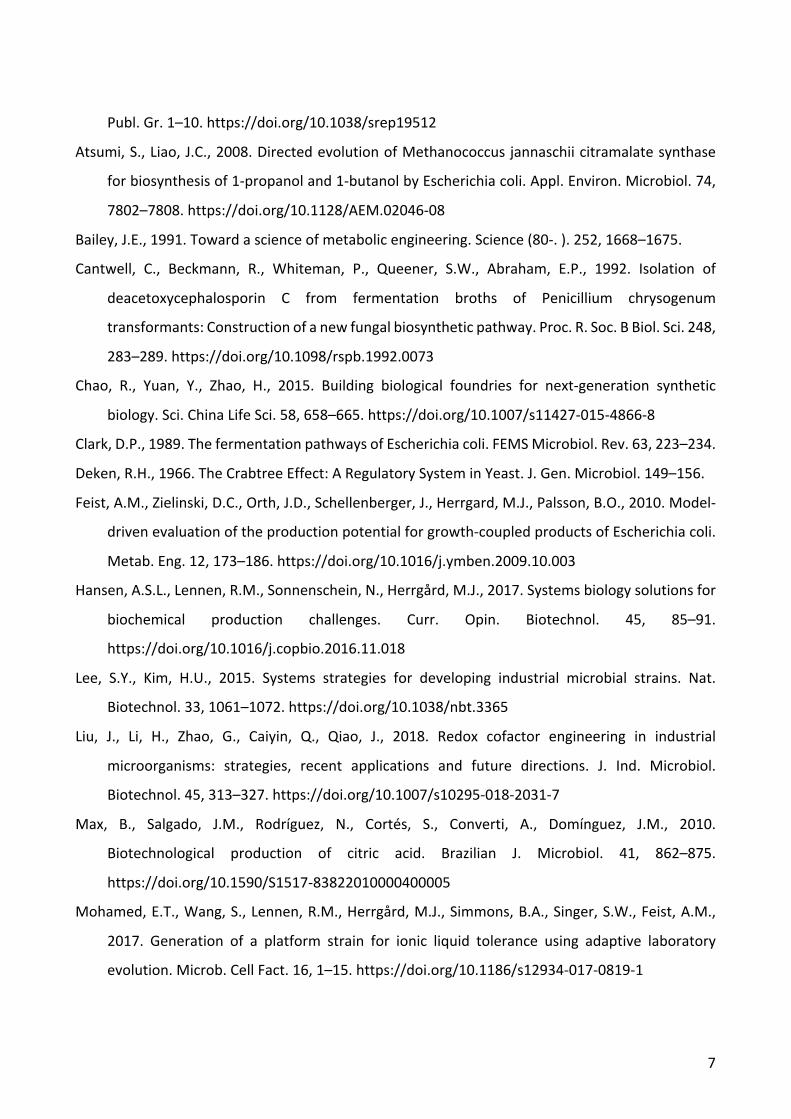
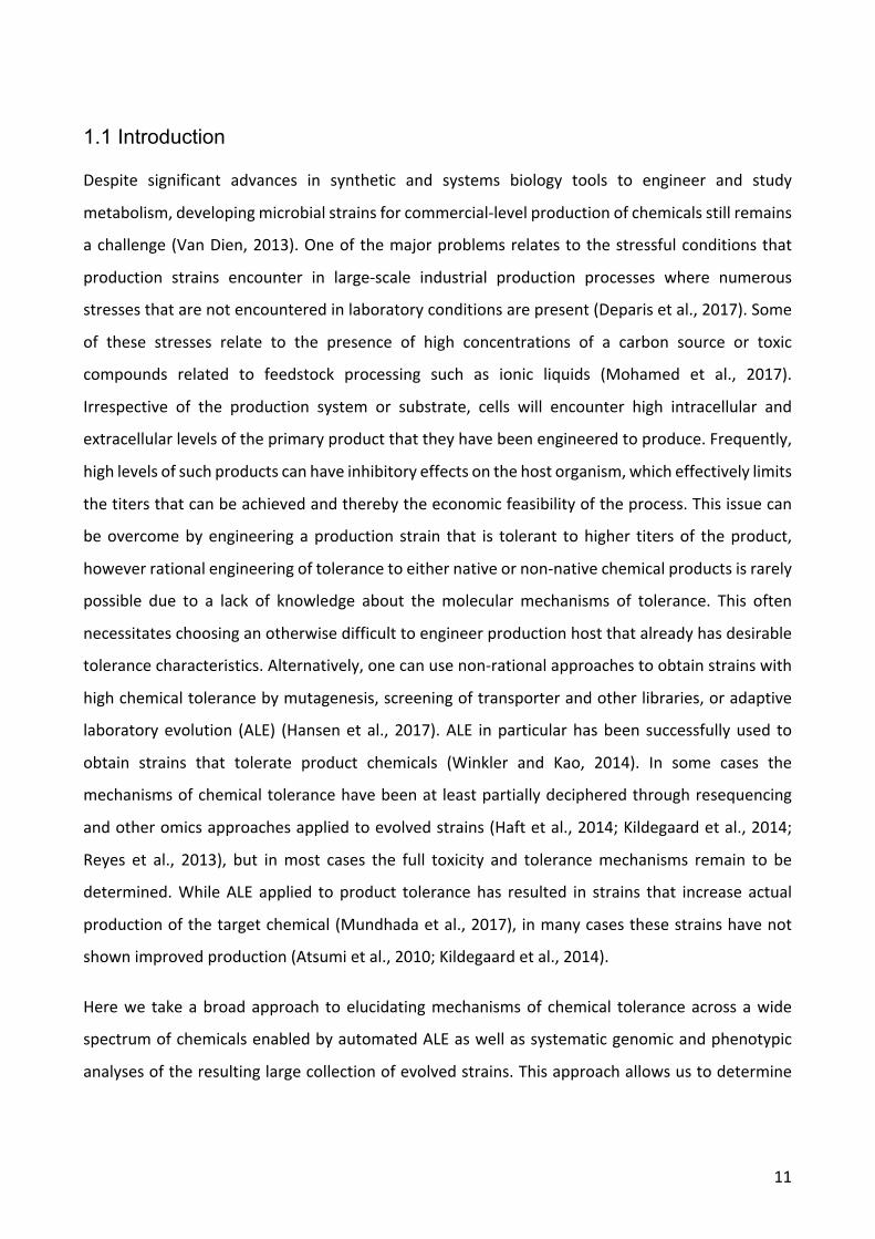
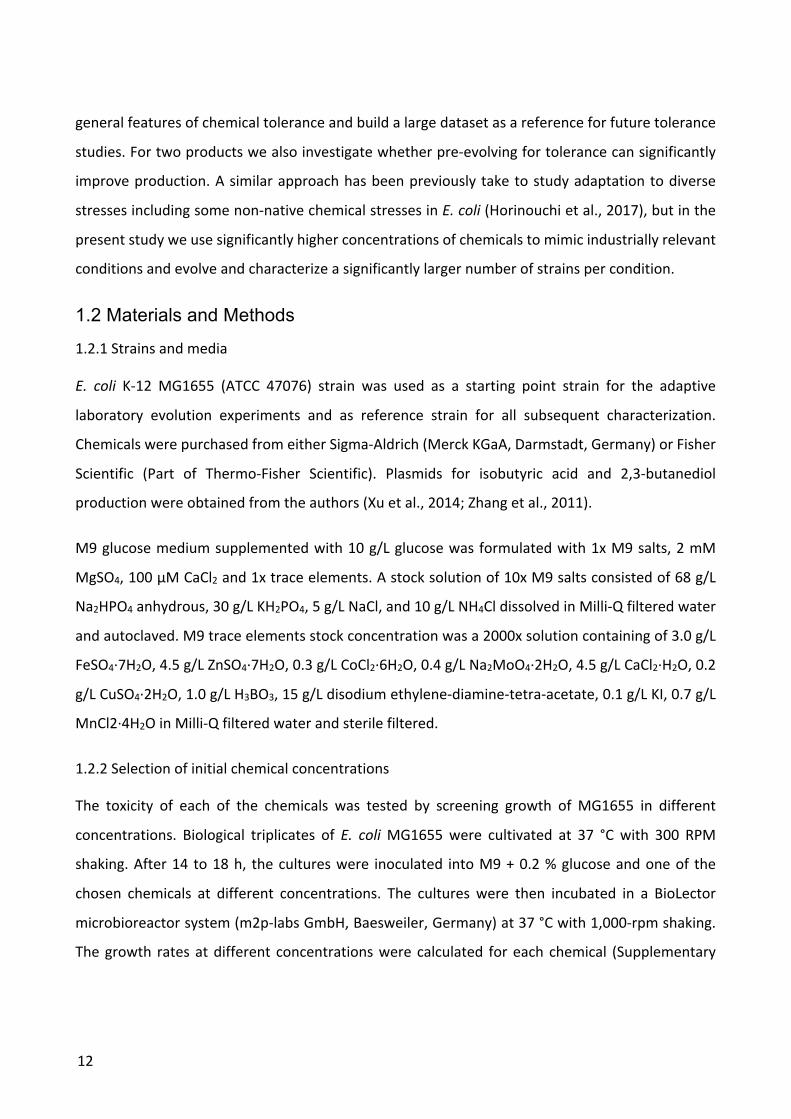
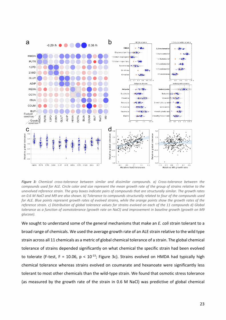
In order to determine whether the strains had tolerance to a broad range of chemicals, we

measured growth rates of all 224 isolates in the presence of moderately toxic levels of each of the

11 chemicals. In addition, we measured growth rates of all the strains on M9 glucose to determine

general growth improvements and on M9 glucose + 0.6 M NaCl to determine osmotic stress

resistance of the strains. We found that strains evolved on diamines, diols and diacids were in

general resistant to the other chemical of the same functional class (Figure 3a). In contrast, strains

evolved on either of the medium chain-length fatty acids were not tolerant to the other medium

chain-length fatty acid. We also tested whether strains that were tolerant to four specific

compounds (HMDA, 2,3-butanediol, adipate and isobutyrate) were also tolerant to other similar

compounds (diamines, diols, diacids or carboxylic acids, respectively; Figure 3b). We found that in

most cases strains tolerant to one compound also have significantly higher growth rates on similar

compounds compared to the ancestral strain.

23

Figure 3: Chemical cross-tolerance between similar and dissimilar compounds. a) Cross-tolerance between the compounds used for ALE. Circle color and size represent the mean growth rate of the group of strains relative to the unevolved reference strain. The grey boxes indicate pairs of compounds that are structurally similar. The growth rates on 0.6 M NaCl and M9 are also shown. b) Tolerance to compounds structurally related to four of the compounds used for ALE. Blue points represent growth rates of evolved strains, while the orange points show the growth rates of the reference strain. c) Distribution of global tolerance values for strains evolved on each of the 11 compounds d) Global tolerance as a function of osmotolerance (growth rate on NaCl) and improvement in baseline growth (growth on M9 glucose).

We sought to understand some of the general mechanisms that make an E. coli strain tolerant to a

broad range of chemicals. We used the average growth rate of an ALE strain relative to the wild type

strain across all 11 chemicals as a metric of global chemical tolerance of a strain. The global chemical

tolerance of strains depended significantly on what chemical the specific strain had been evolved

to tolerate (F-test, F = 10.06, p < 10-13; Figure 3c). Strains evolved on HMDA had typically high

chemical tolerance whereas strains evolved on coumarate and hexanoate were significantly less

tolerant to most other chemicals than the wild-type strain. We found that osmotic stress tolerance

(as measured by the growth rate of the strain in 0.6 M NaCl) was predictive of global chemical

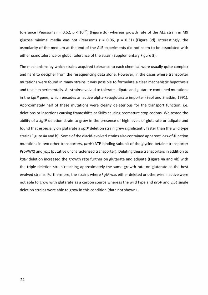
24

tolerance (Pearson’s r = 0.52, p < 10-20) (Figure 3d) whereas growth rate of the ALE strain in M9

glucose minimal media was not (Pearson’s r = 0.06, p = 0.31) (Figure 3d). Interestingly, the

osmolarity of the medium at the end of the ALE experiments did not seem to be associated with

either osmotolerance or global tolerance of the strain (Supplementary Figure 3).

The mechanisms by which strains acquired tolerance to each chemical were usually quite complex

and hard to decipher from the resequencing data alone. However, in the cases where transporter

mutations were found in many strains it was possible to formulate a clear mechanistic hypothesis

and test it experimentally. All strains evolved to tolerate adipate and glutarate contained mutations

in the kgtP gene, which encodes an active alpha-ketoglutarate importer (Seol and Shatkin, 1991).

Approximately half of these mutations were clearly deleterious for the transport function, i.e.

deletions or insertions causing frameshifts or SNPs causing premature stop codons. We tested the

ability of a kgtP deletion strain to grow in the presence of high levels of glutarate or adipate and

found that especially on glutarate a kgtP deletion strain grew significantly faster than the wild type

strain (Figure 4a and b). Some of the diacid-evolved strains also contained apparent loss-of-function

mutations in two other transporters, proV (ATP-binding subunit of the glycine-betaine transporter

ProVWX) and ybjL (putative uncharacterized transporter). Deleting these transporters in addition to

kgtP deletion increased the growth rate further on glutarate and adipate (Figure 4a and 4b) with

the triple deletion strain reaching approximately the same growth rate on glutarate as the best

evolved strains. Furthermore, the strains where kgtP was either deleted or otherwise inactive were

not able to grow with glutarate as a carbon source whereas the wild type and proV and yjbL single

deletion strains were able to grow in this condition (data not shown).

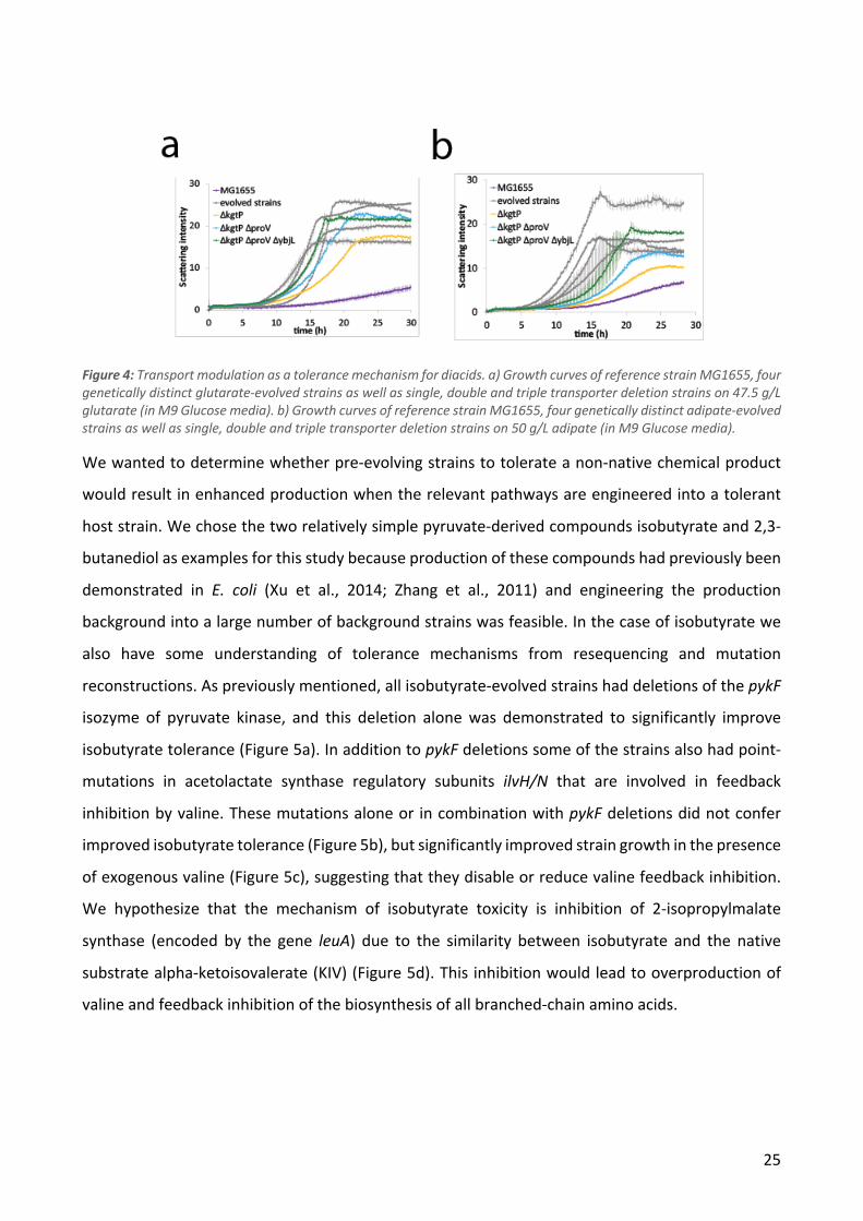
25

Figure 4: Transport modulation as a tolerance mechanism for diacids. a) Growth curves of reference strain MG1655, four genetically distinct glutarate-evolved strains as well as single, double and triple transporter deletion strains on 47.5 g/L glutarate (in M9 Glucose media). b) Growth curves of reference strain MG1655, four genetically distinct adipate-evolved strains as well as single, double and triple transporter deletion strains on 50 g/L adipate (in M9 Glucose media).

We wanted to determine whether pre-evolving strains to tolerate a non-native chemical product

would result in enhanced production when the relevant pathways are engineered into a tolerant

host strain. We chose the two relatively simple pyruvate-derived compounds isobutyrate and 2,3-

butanediol as examples for this study because production of these compounds had previously been

demonstrated in E. coli (Xu et al., 2014; Zhang et al., 2011) and engineering the production

background into a large number of background strains was feasible. In the case of isobutyrate we

also have some understanding of tolerance mechanisms from resequencing and mutation

reconstructions. As previously mentioned, all isobutyrate-evolved strains had deletions of the pykF

isozyme of pyruvate kinase, and this deletion alone was demonstrated to significantly improve

isobutyrate tolerance (Figure 5a). In addition to pykF deletions some of the strains also had point-

mutations in acetolactate synthase regulatory subunits ilvH/N that are involved in feedback

inhibition by valine. These mutations alone or in combination with pykF deletions did not confer

improved isobutyrate tolerance (Figure 5b), but significantly improved strain growth in the presence

of exogenous valine (Figure 5c), suggesting that they disable or reduce valine feedback inhibition.

We hypothesize that the mechanism of isobutyrate toxicity is inhibition of 2-isopropylmalate

synthase (encoded by the gene leuA) due to the similarity between isobutyrate and the native

substrate alpha-ketoisovalerate (KIV) (Figure 5d). This inhibition would lead to overproduction of

valine and feedback inhibition of the biosynthesis of all branched-chain amino acids.

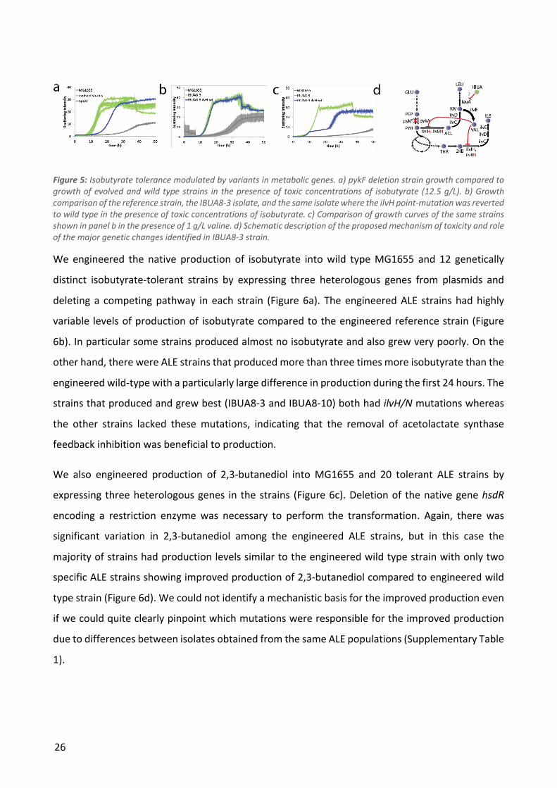
26

Figure 5: Isobutyrate tolerance modulated by variants in metabolic genes. a) pykF deletion strain growth compared to growth of evolved and wild type strains in the presence of toxic concentrations of isobutyrate (12.5 g/L). b) Growth comparison of the reference strain, the IBUA8-3 isolate, and the same isolate where the ilvH point-mutation was reverted to wild type in the presence of toxic concentrations of isobutyrate. c) Comparison of growth curves of the same strains shown in panel b in the presence of 1 g/L valine. d) Schematic description of the proposed mechanism of toxicity and role of the major genetic changes identified in IBUA8-3 strain.

We engineered the native production of isobutyrate into wild type MG1655 and 12 genetically

distinct isobutyrate-tolerant strains by expressing three heterologous genes from plasmids and

deleting a competing pathway in each strain (Figure 6a). The engineered ALE strains had highly

variable levels of production of isobutyrate compared to the engineered reference strain (Figure

6b). In particular some strains produced almost no isobutyrate and also grew very poorly. On the

other hand, there were ALE strains that produced more than three times more isobutyrate than the

engineered wild-type with a particularly large difference in production during the first 24 hours. The

strains that produced and grew best (IBUA8-3 and IBUA8-10) both had ilvH/N mutations whereas

the other strains lacked these mutations, indicating that the removal of acetolactate synthase

feedback inhibition was beneficial to production.

We also engineered production of 2,3-butanediol into MG1655 and 20 tolerant ALE strains by

expressing three heterologous genes in the strains (Figure 6c). Deletion of the native gene hsdR

encoding a restriction enzyme was necessary to perform the transformation. Again, there was

significant variation in 2,3-butanediol among the engineered ALE strains, but in this case the

majority of strains had production levels similar to the engineered wild type strain with only two

specific ALE strains showing improved production of 2,3-butanediol compared to engineered wild

type strain (Figure 6d). We could not identify a mechanistic basis for the improved production even

if we could quite clearly pinpoint which mutations were responsible for the improved production

due to differences between isolates obtained from the same ALE populations (Supplementary Table

1).

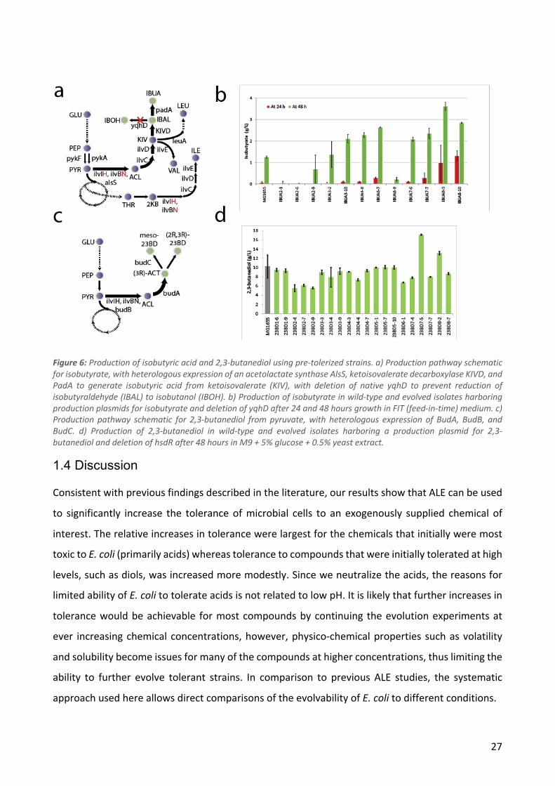
27

Figure 6: Production of isobutyric acid and 2,3-butanediol using pre-tolerized strains. a) Production pathway schematic for isobutyrate, with heterologous expression of an acetolactate synthase AlsS, ketoisovalerate decarboxylase KIVD, and PadA to generate isobutyric acid from ketoisovalerate (KIV), with deletion of native yqhD to prevent reduction of isobutyraldehyde (IBAL) to isobutanol (IBOH). b) Production of isobutyrate in wild-type and evolved isolates harboring production plasmids for isobutyrate and deletion of yqhD after 24 and 48 hours growth in FIT (feed-in-time) medium. c) Production pathway schematic for 2,3-butanediol from pyruvate, with heterologous expression of BudA, BudB, and BudC. d) Production of 2,3-butanediol in wild-type and evolved isolates harboring a production plasmid for 2,3-butanediol and deletion of hsdR after 48 hours in M9 + 5% glucose + 0.5% yeast extract.

1.4 Discussion

Consistent with previous findings described in the literature, our results show that ALE can be used

to significantly increase the tolerance of microbial cells to an exogenously supplied chemical of

interest. The relative increases in tolerance were largest for the chemicals that initially were most

toxic to E. coli (primarily acids) whereas tolerance to compounds that were initially tolerated at high

levels, such as diols, was increased more modestly. Since we neutralize the acids, the reasons for

limited ability of E. coli to tolerate acids is not related to low pH. It is likely that further increases in

tolerance would be achievable for most compounds by continuing the evolution experiments at

ever increasing chemical concentrations, however, physico-chemical properties such as volatility

and solubility become issues for many of the compounds at higher concentrations, thus limiting the

ability to further evolve tolerant strains. In comparison to previous ALE studies, the systematic

approach used here allows direct comparisons of the evolvability of E. coli to different conditions.

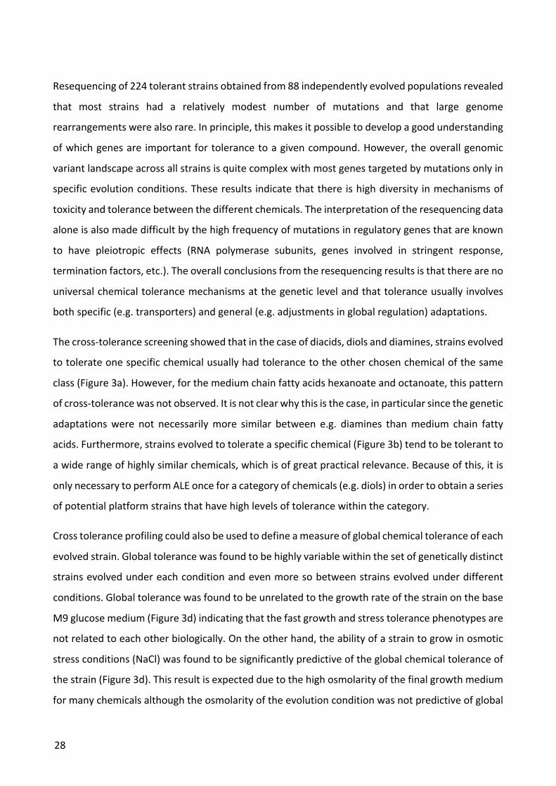
28

Resequencing of 224 tolerant strains obtained from 88 independently evolved populations revealed

that most strains had a relatively modest number of mutations and that large genome

rearrangements were also rare. In principle, this makes it possible to develop a good understanding

of which genes are important for tolerance to a given compound. However, the overall genomic

variant landscape across all strains is quite complex with most genes targeted by mutations only in

specific evolution conditions. These results indicate that there is high diversity in mechanisms of

toxicity and tolerance between the different chemicals. The interpretation of the resequencing data

alone is also made difficult by the high frequency of mutations in regulatory genes that are known

to have pleiotropic effects (RNA polymerase subunits, genes involved in stringent response,

termination factors, etc.). The overall conclusions from the resequencing results is that there are no

universal chemical tolerance mechanisms at the genetic level and that tolerance usually involves

both specific (e.g. transporters) and general (e.g. adjustments in global regulation) adaptations.

The cross-tolerance screening showed that in the case of diacids, diols and diamines, strains evolved

to tolerate one specific chemical usually had tolerance to the other chosen chemical of the same

class (Figure 3a). However, for the medium chain fatty acids hexanoate and octanoate, this pattern

of cross-tolerance was not observed. It is not clear why this is the case, in particular since the genetic

adaptations were not necessarily more similar between e.g. diamines than medium chain fatty

acids. Furthermore, strains evolved to tolerate a specific chemical (Figure 3b) tend to be tolerant to

a wide range of highly similar chemicals, which is of great practical relevance. Because of this, it is

only necessary to perform ALE once for a category of chemicals (e.g. diols) in order to obtain a series

of potential platform strains that have high levels of tolerance within the category.

Cross tolerance profiling could also be used to define a measure of global chemical tolerance of each

evolved strain. Global tolerance was found to be highly variable within the set of genetically distinct

strains evolved under each condition and even more so between strains evolved under different

conditions. Global tolerance was found to be unrelated to the growth rate of the strain on the base

M9 glucose medium (Figure 3d) indicating that the fast growth and stress tolerance phenotypes are

not related to each other biologically. On the other hand, the ability of a strain to grow in osmotic

stress conditions (NaCl) was found to be significantly predictive of the global chemical tolerance of

the strain (Figure 3d). This result is expected due to the high osmolarity of the final growth medium

for many chemicals although the osmolarity of the evolution condition was not predictive of global

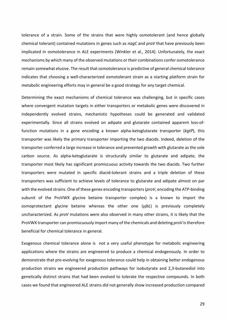
29

tolerance of a strain. Some of the strains that were highly osmotolerant (and hence globally

chemical tolerant) contained mutations in genes such as nagC and proV that have previously been

implicated in osmotolerance in ALE experiments (Winkler et al., 2014). Unfortunately, the exact

mechanisms by which many of the observed mutations or their combinations confer osmotolerance

remain somewhat elusive. The result that osmotolerance is predictive of general chemical tolerance

indicates that choosing a well-characterized osmotolerant strain as a starting platform strain for

metabolic engineering efforts may in general be a good strategy for any target chemical.

Determining the exact mechanisms of chemical tolerance was challenging, but in specific cases

where convergent mutation targets in either transporters or metabolic genes were discovered in

independently evolved strains, mechanistic hypotheses could be generated and validated

experimentally. Since all strains evolved on adipate and glutarate contained apparent loss-of-

function mutations in a gene encoding a known alpha-ketoglutarate transporter (kgtP), this

transporter was likely the primary transporter importing the two diacids. Indeed, deletion of the

transporter conferred a large increase in tolerance and prevented growth with glutarate as the sole

carbon source. As alpha-ketoglutarate is structurally similar to glutarate and adipate, the

transporter most likely has significant promiscuous activity towards the two diacids. Two further

transporters were mutated in specific diacid-tolerant strains and a triple deletion of these

transporters was sufficient to achieve levels of tolerance to glutarate and adipate almost on par

with the evolved strains. One of these genes encoding transporters (proV, encoding the ATP-binding

subunit of the ProVWX glycine betaine transporter complex) is a known to import the

osmoprotectant glycine betaine whereas the other one (yjbL) is previously completely

uncharacterized. As proV mutations were also observed in many other strains, it is likely that the

ProVWX transporter can promiscuously import many of the chemicals and deleting proV is therefore

beneficial for chemical tolerance in general.

Exogenous chemical tolerance alone is not a very useful phenotype for metabolic engineering

applications where the strains are engineered to produce a chemical endogenously. In order to

demonstrate that pre-evolving for exogenous tolerance could help in obtaining better endogenous

production strains we engineered production pathways for isobutyrate and 2,3-butanediol into

genetically distinct strains that had been evolved to tolerate the respective compounds. In both

cases we found that engineered ALE strains did not generally show increased production compared

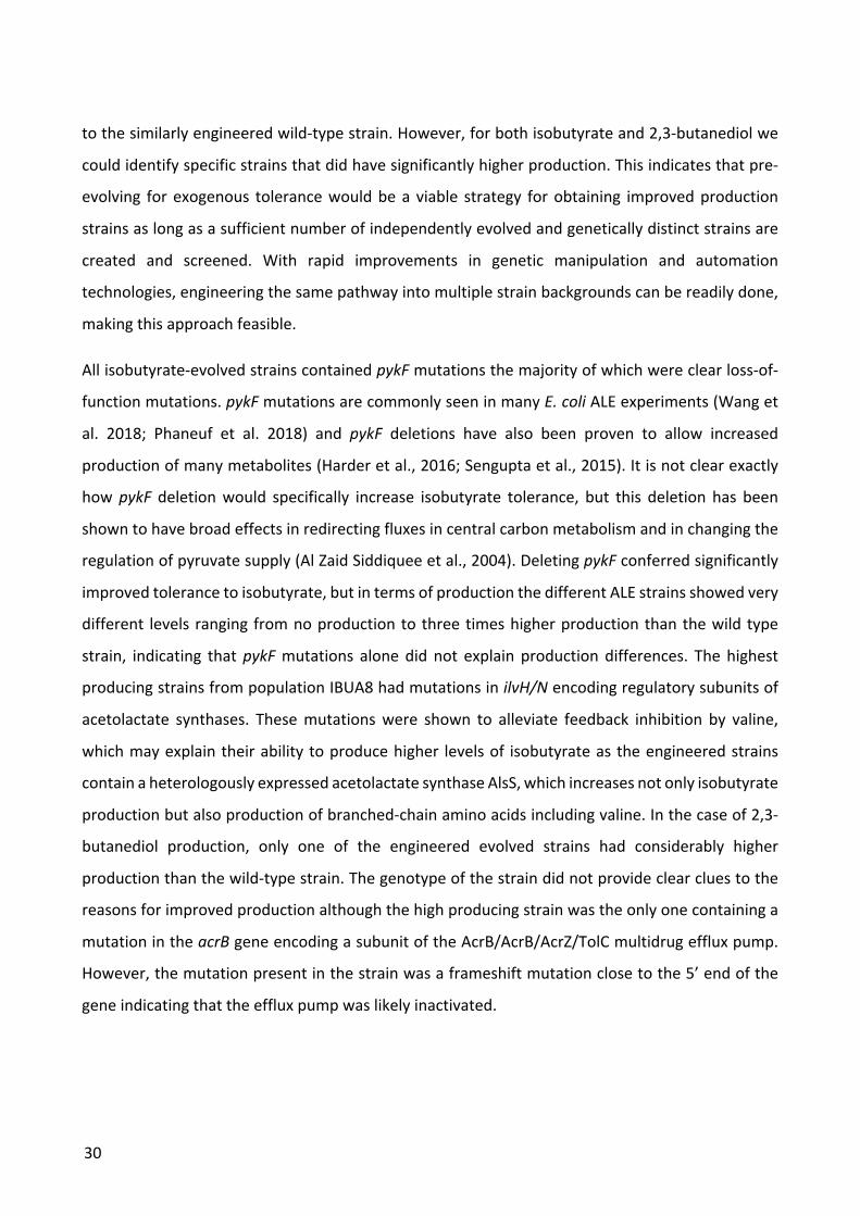
30

to the similarly engineered wild-type strain. However, for both isobutyrate and 2,3-butanediol we

could identify specific strains that did have significantly higher production. This indicates that pre-

evolving for exogenous tolerance would be a viable strategy for obtaining improved production

strains as long as a sufficient number of independently evolved and genetically distinct strains are

created and screened. With rapid improvements in genetic manipulation and automation

technologies, engineering the same pathway into multiple strain backgrounds can be readily done,

making this approach feasible.

All isobutyrate-evolved strains contained pykF mutations the majority of which were clear loss-of-

function mutations. pykF mutations are commonly seen in many E. coli ALE experiments (Wang et

al. 2018; Phaneuf et al. 2018) and pykF deletions have also been proven to allow increased

production of many metabolites (Harder et al., 2016; Sengupta et al., 2015). It is not clear exactly

how pykF deletion would specifically increase isobutyrate tolerance, but this deletion has been

shown to have broad effects in redirecting fluxes in central carbon metabolism and in changing the

regulation of pyruvate supply (Al Zaid Siddiquee et al., 2004). Deleting pykF conferred significantly

improved tolerance to isobutyrate, but in terms of production the different ALE strains showed very

different levels ranging from no production to three times higher production than the wild type

strain, indicating that pykF mutations alone did not explain production differences. The highest

producing strains from population IBUA8 had mutations in ilvH/N encoding regulatory subunits of

acetolactate synthases. These mutations were shown to alleviate feedback inhibition by valine,

which may explain their ability to produce higher levels of isobutyrate as the engineered strains

contain a heterologously expressed acetolactate synthase AlsS, which increases not only isobutyrate

production but also production of branched-chain amino acids including valine. In the case of 2,3-

butanediol production, only one of the engineered evolved strains had considerably higher

production than the wild-type strain. The genotype of the strain did not provide clear clues to the

reasons for improved production although the high producing strain was the only one containing a

mutation in the acrB gene encoding a subunit of the AcrB/AcrB/AcrZ/TolC multidrug efflux pump.

However, the mutation present in the strain was a frameshift mutation close to the 5’ end of the

gene indicating that the efflux pump was likely inactivated.

31

1.5 Conclusion

In this study we used ALE to evolve strains of E. coli to tolerate high concentrations of 11 different

industrially relevant chemicals. The tolerated concentrations increased by factors of 60 % to 400 %.

Genome sequencing of the evolved strains showed that the median number of mutations per strain

was 6, and that only a small degree of mutation overlap was seen between conditions and even

between independently evolved strains in the same condition. This made it difficult to infer

mechanisms of tolerance in all but a couple of cases. Cross-compound tolerance screening revealed

a general trend of cross-tolerance between compounds of the same class. This suggests that a single

broadly tolerant platform strain could be used for production of several compounds of the same

class. Furthermore, we observed that tolerance to high osmolarity was predictive of the overall

tolerance to all 11 compounds, suggesting that high osmolarity is a significant factor of toxicity at

the utilized concentrations. For two compounds, the evolved strains were transformed with

plasmids carrying production pathways and screened for improved production compared to the

wild-type. In both cases we could identify strains that produced considerably better than the wild-

type, although the majority of evolved strains had similar or reduced production compared to the

wild-type. This suggests that pre-evolving a strain to tolerate the target compound before

engineering production can be a viable strategy as long as a large number of independently evolved

strains can be isolated and screened.

1.6 References

Al Zaid Siddiquee, K., Arauzo-Bravo, M.J., Shimizu, K., 2004. Metabolic flux analysis of pykF gene

knockout Escherichia coli based on 13C-labeling experiments together with measurements of

enzyme activities and intracellular metabolite concentrations. Appl. Microbiol. Biotechnol.

63, 407–417. https://doi.org/10.1007/s00253-003-1357-9

Atsumi, S., Wu, T.Y., Machado, I.M.P., Huang, W.C., Chen, P.Y., Pellegrini, M., Liao, J.C., 2010.

Evolution, genomic analysis, and reconstruction of isobutanol tolerance in Escherichia coli.

Mol. Syst. Biol. 6, 1–11. https://doi.org/10.1038/msb.2010.98

Deatherage, D.E., Barrick, J.E., 2014. Identification of mutations in laboratory evolved microbes

from next-generation sequencing data using breseq. Methods Mol. Biol. 1151, 165–188.

32

https://doi.org/10.1007/978-1-4939-0554-6

Deparis, Q., Claes, A., Foulquié-Moreno, M.R., Thevelein, J.M., 2017. Engineering tolerance to

industrially relevant stress factors in yeast cell factories. FEMS Yeast Res. 17, 1–17.

https://doi.org/10.1093/femsyr/fox036

Haft, R.J.F., Keating, D.H., Schwaegler, T., Schwalbach, M.S., Vinokur, J., Tremaine, M., Peters, J.M.,

Kotlajich, M. V., Pohlmann, E.L., Ong, I.M., Grass, J.A., Kiley, P.J., Landick, R., 2014. Correcting

direct effects of ethanol on translation and transcription machinery confers ethanol tolerance

in bacteria. Proc. Natl. Acad. Sci. 111, E2576–E2585.

https://doi.org/10.1073/pnas.1401853111

Hansen, A.S.L., Lennen, R.M., Sonnenschein, N., Herrgård, M.J., 2017. Systems biology solutions

for biochemical production challenges. Curr. Opin. Biotechnol. 45, 85–91.


Harder, B.J., Bettenbrock, K., Klamt, S., 2016. Model-based metabolic engineering enables high

yield itaconic acid production by Escherichia coli. Metab. Eng. 38, 29–37.

https://doi.org/10.1016/j.ymben.2016.05.008

Horinouchi, T., Suzuki, S., Kotani, H., Tanabe, K., Sakata, N., Shimizu, H., Furusawa, C., 2017.

Prediction of Cross-resistance and Collateral Sensitivity by Gene Expression profiles and

Genomic Mutations. Sci. Rep. 7, 1–11. https://doi.org/10.1038/s41598-017-14335-7

Kildegaard, K.R., Hallström, B.M., Blicher, T.H., Sonnenschein, N., Jensen, N.B., Sherstyk, S.,

Harrison, S.J., Maury, J., Herrgård, M.J., Juncker, A.S., Forster, J., Nielsen, J., Borodina, I.,

2014. Evolution reveals a glutathione-dependent mechanism of 3-hydroxypropionic acid

tolerance. Metab. Eng. 26, 57–66. https://doi.org/10.1016/j.ymben.2014.09.004

LaCroix, R.A., Palsson, B.O., Feist, A.M., 2017. A model for designing adaptive laboratory evolution

experiments. Appl. Environ. Microbiol. 83. https://doi.org/10.1128/AEM.03115-16

Lennen, R.M., Kruziki, M.A., Kumar, K., Zinkel, R.A., Burnum, K.E., Lipton, M.S., Hoover, S.W.,

Ranatunga, D.R., Wittkopp, T.M., Marner, W.D., Pfleger, B.F., 2011. Membrane stresses

33

induced by overproduction of free fatty acids in Escherichia coli. Appl. Environ. Microbiol. 77,

8114–8128. https://doi.org/10.1128/AEM.05421-11

Lennen, R.M., Nilsson Wallin, A.I., Pedersen, M., Bonde, M., Luo, H., Herrgård, M.J., Sommer,

M.O.A., 2015. Transient overexpression of DNA adenine methylase enables efficient and

mobile genome engineering with reduced off-target effects. Nucleic Acids Res. 44, 1–14.

https://doi.org/10.1093/nar/gkv1090

Mohamed, E.T., Wang, S., Lennen, R.M., Herrgård, M.J., Simmons, B.A., Singer, S.W., Feist, A.M.,

2017. Generation of a platform strain for ionic liquid tolerance using adaptive laboratory

evolution. Microb. Cell Fact. 16, 1–15. https://doi.org/10.1186/s12934-017-0819-1

Mundhada, H., Seoane, J.M., Schneider, K., Koza, A., Christensen, H.B., Klein, T., Phaneuf, P. V.,

Herrgard, M., Feist, A.M., Nielsen, A.T., 2017. Increased production of L-serine in Escherichia

coli through Adaptive Laboratory Evolution. Metab. Eng. 39, 141–150.


Phaneuf, P. V, Gos, D., Palsson, B.O., Feist, A.M., 2018. ALEdb 1.0: A Database of Mutations from

Adaptive Laboratory Evolution Experimentation.

Reyes, L.H., Abdelaal, A.S., Kao, K.C., 2013. Genetic determinants for n-butanol tolerance in

evolved escherichia coli mutants: Cross adaptation and antagonistic pleiotropy between n-

butanol and other stressors. Appl. Environ. Microbiol. 79, 5313–5320.

https://doi.org/10.1128/AEM.01703-13

Royce, L.A., Yoon, J.M., Chen, Y., Rickenbach, E., Shanks, J. V., Jarboe, L.R., 2015. Evolution for

exogenous octanoic acid tolerance improves carboxylic acid production and membrane

integrity. Metab. Eng. 29, 180–188. https://doi.org/10.1016/j.ymben.2015.03.014

Sengupta, S., Jonnalagadda, S., Goonewardena, L., Juturu, V., 2015. Metabolic engineering of a

novel muconic acid biosynthesis pathway via 4-hydroxybenzoic acid in Escherichia coli. Appl.

Environ. Microbiol. 81, 8037–8043. https://doi.org/10.1128/AEM.01386-15

Seol, W., Shatkin, A.J., 1991. Escherichia coli kgtP encodes an alpha-ketoglutarate transporter.

34

Proc. Natl. Acad. Sci. 88, 3802–3806.

Van Dien, S., 2013. From the first drop to the first truckload: Commercialization of microbial

processes for renewable chemicals. Curr. Opin. Biotechnol. 24, 1061–1068.


Winkler, J.D., Garcia, C., Olson, M., Callaway, E., Kao, K.C., 2014. Evolved osmotolerant escherichia

coli mutants frequently exhibit defective N-acetylglucosamine catabolism and point

mutations in cell shape-regulating protein MreB. Appl. Environ. Microbiol. 80, 3729–3740.

https://doi.org/10.1128/AEM.00499-14

Winkler, J.D., Kao, K.C., 2014. Recent advances in the evolutionary engineering of industrial

biocatalysts. Genomics 104, 406–411. https://doi.org/10.1016/j.ygeno.2014.09.006

Xu, Y., Chu, H., Gao, C., Tao, F., Zhou, Z., Li, K., Li, L., Ma, C., Xu, P., 2014. Systematic metabolic

engineering of Escherichia coli for high-yield production of fuel bio-chemical 2,3-butanediol.


Zhang, K., Woodruff, A.P., Xiong, M., Zhou, J., Dhande, Y.K., 2011. A synthetic metabolic pathway

for production of the platform chemical isobutyric acid. ChemSusChem 4, 1068–1070.

https://doi.org/10.1002/cssc.201100045

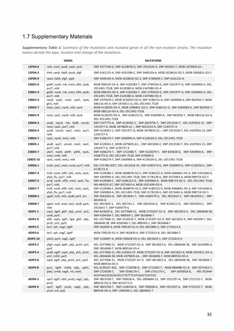
35

1.7 Supplementary Materials

Supplementary Table 1: Summary of the mutations and mutated genes in all the non-mutator strains. The mutation names denote the type, location and change of the mutations.

GENES MUTATIONS

12PD4-6 relA, metJ, yeaR, sspA, rpsA SNP-3377240-G, SNP-4128078-G, SNP-2912634-G, SNP-962923-T, MOB-1879829-Δ1-:

12PD6-3 lrhA, rpoA, fabR, dusA, yfgF SNP-4161155-A, SNP-4261586-C, SNP-3440194-A, MOB-2628616-IS2-5, MOB-2406831-IS2-5

12PD6-9 rpoA, fabR, yfgF, ypjA SNP-3440194-A, MOB-2628616-IS2-5, SNP-2780609-C, SNP-4161155-A

23BD1-6 gabP, nanK, rnb, metJ, elfA, rpoB, purT, relA

MOB-998193-IS5-4, SNP-4182583-T, SNP-2794550-G, SNP-1931977-G, SNP-3369969-A, DEL-2911491-7528, SNP-4128380-A, MOB-1347480-IS5-4

23BD1-9 gabP, nanK, rnb, metJ, elfA, rpoB, purT, relA

MOB-998193-IS5-4, SNP-4182583-T, SNP-2794550-G, SNP-1931977-G, SNP-3369969-A, DEL-2911491-7528, SNP-4128380-A, MOB-1347480-IS5-4

23BD2-4 nanK, uspC, metJ, rpoC, rpsA, gtrS, relA

SNP-1979639-C, MOB-4128293-IS5-4, SNP-4186152-G, SNP-3369969-A, SNP-962056-T, MOB-580116-IS5-4, SNP-2470411-G, DEL-2911491-7528

23BD2-7 metJ, rpoC, nanK, relA, rpsA MOB-4128293-IS5-4, MOB-1096841-IS2-5, SNP-4186152-G, SNP-3369969-A, SNP-962056-T, MOB-580116-IS5-4, DEL-2911491-7528

23BD2-9 metJ, rpoC, nanK, relA, rpsA MOB-4128293-IS5-4, SNP-4186152-G, SNP-3369969-A, SNP-962056-T, MOB-580116-IS5-4, DEL-2911491-7528

23BD4-3 yeaR, mprA, rnb, fadB, umuD, metJ, rpoC, purT, relA

SNP-1347775-A, SNP-4128361-C, SNP-2810756-T, SNP-2913536-T, DEL-4187816-15, SNP-1931977-G, MOB-1879829-Δ1-:, SNP-4031019-A, SNP-1230727-A

23BD4-4 yeaR, umuD, rpoC, metJ, purT, relA

SNP-4128361-C, SNP-1931977-G, MOB-1879829-Δ1-:, SNP-2913536-T, DEL-4187816-15, SNP-1230727-A

23BD4-7 rpoC, nanK, metJ, relA SNP-4186274-T, SNP-3369969-A, SNP-4128169-G, DEL-2911491-7528

23BD5-1 yeaR, spoT, umuD, metJ, rpoC, purT, relA

SNP-4128361-C, MOB-1879829-Δ1-:, SNP-3823036-C, SNP-2913536-T, DEL-4187816-15, SNP-1931977-G, SNP-1230727-A

23BD5-7 ybeT, nanK, ybhP, ydhK, rpoC, metJ, zntR, relA

SNP-4186274-T, SNP-1722386-T, SNP-4128379-T, SNP-824028-G, SNP-3369969-A, SNP-3438773-G, DEL-2911491-7528, SNP-679090-G

23BD5-10 rpoC, nanK, metJ, relA SNP-4186274-T, SNP-3369969-A, SNP-4128169-G, DEL-2911491-7528

23BD6-1 essD, rpoC, metJ, nusG, purT, relA DEL-575786-3027, DEL-2912618-10, SNP-4185573-G, SNP-1930993-G, SNP-4128250-C, SNP-4178172-G

23BD7-4 treR, nanK, elfD, tolC, metJ, rpoC, yhjA, flu, purT, relA

SNP-4128386-C, MOB-3668878-IS2-5, SNP-4186152-G, MOB-4466841-IS5-4, SNP-1931668-G, SNP-3369969-A, DEL-2911491-7528, SNP-3178128-G, SNP-2073463-A, MOB-998719-IS2-5

23BD7-5 acrB, nanK, elfD, metJ, rpoC, flu, purT, relA

SNP-4128386-C, SNP-4186152-G, SNP-3369969-A, MOB-998719-IS2-5, DEL-2911491-7528, INS-484102-AT, SNP-2073463-A, MOB-1931499-IS5-4

23BD7-7 treR, nanK, elfD, tolC, metJ, rpoC, yhjA, flu, purT, relA

SNP-4128386-C, MOB-3668878-IS2-5, SNP-4186152-G, MOB-4466841-IS5-4, SNP-1931668-G, SNP-3369969-A, DEL-2911491-7528, SNP-3178128-G, SNP-2073463-A, MOB-998719-IS2-5

23BD8-2 ygaH, iscR, relA, rpoB, pyrE, lon SNP-2661816-G, SNP-2913641-T, SNP-4184579-G, DEL-3815810-1, SNP-2810459-C, SNP-461034-G

23BD8-7 ygaH, iscR, metJ, lacZ, rpoB, pyrE, relA

DEL-3815810-1, DEL-365742-1, SNP-2661816-G, SNP-4128212-G, SNP-2810459-C, SNP-2913641-T, SNP-4184579-G

ADIP1-1 sspA, kgtP, gltP, ybjL, proV, yicC, uvrB, pyrE

SNP-814029-G, DEL-3377068-21, MOB-2725207-IS1-9, SNP-3815823-A, DEL-2804648-38, SNP-4294366-T, DEL-889569-1, SNP-3816848-T

ADIP1-9 allD, sspA, kgtP, ligA, gltP, ybjL, proV, yicC, pyrE

DEL-3377068-21, SNP-2530235-T, MOB-2725207-IS1-9, SNP-3815823-A, SNP-546309-T, DEL-2804648-38, SNP-4294366-T, DEL-889569-1, SNP-3816848-T

ADIP2-5 lacY, rph, nagC, kgtP SNP-362830-A, MOB-700529-IS1-9, DEL-3815884-2, SNP-2725613-A

ADIP2-6 lacY, rph, nagC, kgtP MOB-700529-IS1-9, SNP-362830-A, SNP-2725613-A, DEL-3815884-2

ADIP2-10 ydcD, pyrE, nagC, kgtP SNP-1530007-A, MOB-700628-IS5-4, DEL-3815810-1, SNP-2725613-A

ADIP3-2 yfgO, sspA, kgtP, ybjL, proV, yicC, pyrE

DEL-3377068-21, MOB-2725207-IS1-9, SNP-3815823-A, DEL-2804648-38, SNP-2614996-G, SNP-3816848-T, MOB-889534-IS5-4

ADIP3-4 yeaR, kgtP, sspA, ybjL, yhiL, proV, yicC, mltD, pyrE

DEL-3377068-21, INS-233963-GT, MOB-2725207-IS1-9, SNP-3815823-A, MOB-3633911-IS5-4, DEL-2804648-38, MOB-1879829-Δ1-:, SNP-3816848-T, MOB-889534-IS5-4

ADIP3-8 sspA, kgtP, ybjL, proV, yicC, pyrE DEL-3377068-21, MOB-2725207-IS1-9, SNP-3815823-A, DEL-2804648-38, SNP-3816848-T, MOB-889534-IS5-4

ADIP4-8 purL, kgtP, malQ, ybjL, yphC, pdxJ, srmB, nagA, rnt, metL

DEL-4130167-462, SNP-1728708-G, SNP-2713302-T, MOB-889488-IS1-9, SNP-2675452-C, SNP-2724590-T, SNP-3548179-T, SNP-2701175-C, SNP-2693818-G, INS-702444-GCATAACGCGCACGCCCTGTTTCATCAGCTCATCGC

ADIP6-3 spoT, kgtP, ubiE, proQ, nagC, ybjL, proV

SNP-3823700-T, SNP-700928-A, DEL-2804864-13, SNP-1915297-A, SNP-2725155-T, MOB-889534-IS5-4, SNP-4019173-G

ADIP6-9 spoT, kgtP, proQ, nagC, ybjL, proV, icd, ycjG

SNP-3823700-T, SNP-1196319-A, SNP-700928-A, SNP-1915297-A, SNP-2725155-T, MOB-889534-IS5-4, SNP-1389396-C, DEL-2804835-7

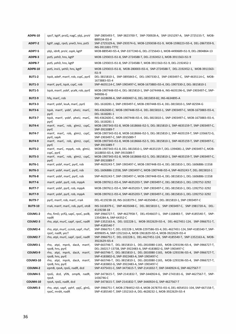
36

ADIP6-10 spoT, kgtP, proQ, nagC, ybjL, proV SNP-2805493-T, SNP-3823700-T, SNP-700928-A, SNP-1915297-A, SNP-2725155-T, MOB-889534-IS5-4

ADIP7-2 kgtP, yagL, rpoS, yneO, hns, pstS SNP-2725329-A, SNP-293574-G, MOB-1293038-IS1-9, MOB-1598223-IS5-4, DEL-2867359-9, INS-3911001-TTTC

ADIP7-5 ybjL, idnR, proV, sspA, kgtP MOB-889540-IS5-4, SNP-3377240-G, DEL-2725643-1, MOB-4490689-IS1-9, DEL-2804864-13

ADIP8-3 pstS, yehD, hns, kgtP MOB-1293015-IS1-8, SNP-2724588-T, DEL-2192452-1, MOB-3911563-IS1-9

ADIP8-7 pstS, yehD, hns, kgtP MOB-1293015-IS1-8, SNP-2724588-T, MOB-3911563-IS1-9, DEL-2192452-1

ADIP8-10 pstS, insI1, yehD, hns, kgtP MOB-1293015-IS1-8, MOB-280003-IS5-4, SNP-2724588-T, DEL-2192452-1, MOB-3911563-IS1-9

BUT1-2 tqsA, adeP, manY, rob, cspC, pyrE DEL-3815810-1, SNP-3895843-C, DEL-1907330-2, SNP-1903497-C, SNP-4635114-C, MOB-1673883-IS5-4

BUT1-3 manY, pyrE, tqsA, cspC, rob SNP-4635114-C, SNP-1903497-C, MOB-1673883-IS5-4, DEL-1907330-2, DEL-3815810-1

BUT1-5 tqsA, manY, yobF, ycaN, rob, pyrE MOB-1907448-IS5-4, DEL-3815810-1, SNP-1674448-A, INS-4635196-G, SNP-1903497-C, SNP-949006-G

BUT2-9 hfq, marC, rob SNP-1618698-A, SNP-4400407-G, DEL-3815859-82, INS-4634895-A

BUT3-3 manY, yobF, leuA, marC, pyrE DEL-1618281-1, SNP-1903497-C, MOB-1907448-IS5-4, DEL-3815810-1, SNP-82594-G

BUT3-6 tqsA, manY, yobF, pheU, marC, pyrE

INS-4362600-C, MOB-1907448-IS5-4, DEL-3815810-1, SNP-1903497-C, MOB-1673883-IS5-4, DEL-1618281-1

BUT3-7 tqsA, manY, yobF, pheU, marC, pyrE

INS-4362600-C, MOB-1907448-IS5-4, DEL-3815810-1, SNP-1903497-C, MOB-1673883-IS5-4, DEL-1618281-1

BUT4-4 manY, marC, rob, glmU, cspC, pyrE

MOB-1907343-IS1-8, MOB-1618666-IS2-5, DEL-3815810-1, SNP-4635159-T, SNP-1903497-C, SNP-3915089-T

BUT4-7 manY, marC, rob, glmU, cspC, pyrE, sapA

MOB-1907343-IS1-8, MOB-1618666-IS2-5, DEL-3815810-1, SNP-4635159-T, SNP-1356672-G, SNP-1903497-C, SNP-3915089-T



BUT5-2 manY, marC, mppA, rob, glmU, cspC, pyrE

MOB-1907343-IS1-8, DEL-3815810-1, SNP-4635159-T, DEL-1394081-2, SNP-1903497-C, MOB-1618850-IS5-4, SNP-3915089-T



BUT6-1 manY, yobF, marC, pyrE, rob SNP-4635243-T, SNP-1903497-C, MOB-1907448-IS5-4, DEL-3815810-1, DEL-1606886-11558

BUT6-3 manY, yobF, marC, pyrE, rob DEL-1606886-11558, SNP-1903497-C, MOB-1907448-IS5-4, SNP-4635243-T, DEL-3815810-1

BUT6-8 manY, yobF, marC, pyrE, rob SNP-4635243-T, SNP-1903497-C, MOB-1907448-IS5-4, DEL-3815810-1, DEL-1606886-11558

BUT7-6 manY, yobF, pyrE, rob, mppA MOB-1907611-IS5-4, SNP-4635203-T, SNP-1903497-C, DEL-3815810-1, DEL-1392752-3292



BUT9-7 pyrE, manY, rob, marC, rraA DEL-4119238-18, INS-1618379-C, SNP-4635048-C, DEL-3815810-1, SNP-1903497-C

BUT9-10 rraA, manY, marC, rob, pyrE, otsB INS-1618379-C, SNP-4635048-C, DEL-3815810-1, SNP-1903497-C, SNP-1981720-A, DEL-4119238-18

COUM1-2 rho, fimD, ycfQ, sapC, rpoC, polB, nadR

SNP-3966727-T, SNP-4627958-T, DEL-4546637-1, SNP-1168483-T, SNP-4185540-T, SNP-1354284-A, SNP-64352-C

COUM2-3 rho, atpI, murC, sapF, rpoC, nadR SNP-1352163-A, DEL-102228-1, MOB-3922629-IS5-4, DEL-4627451-124, SNP-3966751-T, SNP-4185540-T

COUM2-4 rho, atpI, murC, ccmA, sapF, rhaT, rpoC, nadR, yecT

SNP-3966751-T, DEL-102228-1, MOB-2297586-IS5-4, DEL-4627451-124, SNP-4185540-T, SNP-4099695-A, SNP-1352163-A, MOB-1961829-IS5-4, MOB-3922629-IS5-4

COUM2-7 rho, atpI, murC, sapF, rpoC, nadR SNP-3966751-T, DEL-102228-1, DEL-4627451-124, SNP-4185540-T, SNP-1352163-A, MOB-3922629-IS5-4

COUM3-1 rho, atpI, mprA, dacA, manY, rpoB, hns, pyrE

SNP-663746-T, DEL-3815810-1, DEL-2810080-1165, MOB-1293196-IS5-4, SNP-3966727-T, DEL-260217-13738, SNP-3922483-A, SNP-4183802-G, SNP-1903497-C


SNP-663746-T, DEL-3815810-1, DEL-2810080-1165, MOB-1293196-IS5-4, SNP-3966727-T, SNP-4183802-G, SNP-3922483-A, SNP-1903497-C


SNP-663746-T, DEL-3815810-1, DEL-2810080-1165, MOB-1293196-IS5-4, SNP-3966727-T, SNP-4183802-G, SNP-3922483-A, SNP-1903497-C

COUM4-2 epmB, rpoA, rpsG, nadR, dcd SNP-4375431-C, SNP-3473615-T, SNP-2141832-T, SNP-3440924-G, SNP-4627567-T

COUM4-5 rpsG, dcd, yfiN, ompN, nadR, rpoA

SNP-3473615-T, SNP-2141832-T, SNP-3440924-G, SNP-2743181-G, SNP-4627567-T, SNP-1436746-C

COUM4-10 rpoA, rpsG, nadR, dcd SNP-3473615-T, SNP-2141832-T, SNP-3440924-G, SNP-4627567-T

COUM5-3 rho, atpI, sapF, yphF, ypjC, glnG, rpoC, mrdA, nadR

SNP-3966751-T, MOB-2784452-IS5-4, MOB-2678755-IS5-4, DEL-4054531-104, SNP-667158-T, SNP-4185540-T, SNP-1352163-A, DEL-4628232-1, MOB-3922629-IS5-4

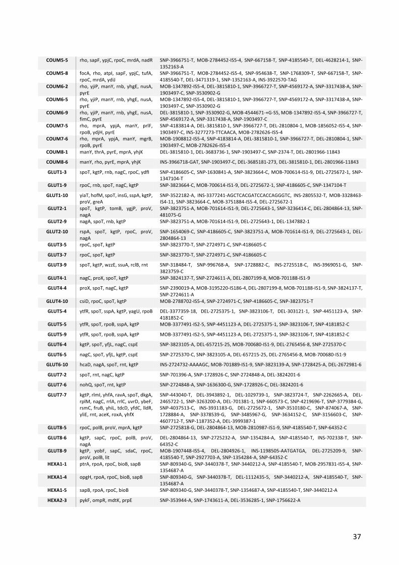
37

COUM5-5 rho, sapF, ypjC, rpoC, mrdA, nadR SNP-3966751-T, MOB-2784452-IS5-4, SNP-667158-T, SNP-4185540-T, DEL-4628214-1, SNP-1352163-A

COUM5-8 focA, rho, atpI, sapF, ypjC, tufA, rpoC, mrdA, ydiJ

SNP-3966751-T, MOB-2784452-IS5-4, SNP-954638-T, SNP-1768309-T, SNP-667158-T, SNP-4185540-T, DEL-3471319-1, SNP-1352163-A, INS-3922570-TAG

COUM6-2 rho, yjiP, manY, rnb, yhgE, nusA, pyrE

MOB-1347892-IS5-4, DEL-3815810-1, SNP-3966727-T, SNP-4569172-A, SNP-3317438-A, SNP-1903497-C, SNP-3530902-G

COUM6-5 rho, yjiP, manY, rnb, yhgE, nusA, pyrE

MOB-1347892-IS5-4, DEL-3815810-1, SNP-3966727-T, SNP-4569172-A, SNP-3317438-A, SNP-1903497-C, SNP-3530902-G

COUM6-9 rho, yjiP, manY, rnb, yhgE, nusA, fimC, pyrE

DEL-3815810-1, SNP-3530902-G, MOB-4544671-+G-S5, MOB-1347892-IS5-4, SNP-3966727-T, SNP-4569172-A, SNP-3317438-A, SNP-1903497-C

COUM7-5 rho, mprA, ypjA, manY, prlF, rpoB, ydjH, pyrE

SNP-4183814-A, DEL-3815810-1, SNP-3966727-T, DEL-2810804-1, MOB-1856052-IS5-4, SNP-1903497-C, INS-3277273-TTCAACA, MOB-2782626-IS5-4

COUM7-6 rho, mprA, ypjA, manY, mgrB, rpoB, pyrE

MOB-1908812-IS5-4, SNP-4183814-A, DEL-3815810-1, SNP-3966727-T, DEL-2810804-1, SNP-1903497-C, MOB-2782626-IS5-4

COUM8-1 manY, thrA, pyrE, mprA, yhjK DEL-3815810-1, DEL-3683736-1, SNP-1903497-C, SNP-2374-T, DEL-2801966-11843

COUM8-6 manY, rho, pyrE, mprA, yhjK INS-3966718-GAT, SNP-1903497-C, DEL-3685181-273, DEL-3815810-1, DEL-2801966-11843

GLUT1-3 spoT, kgtP, rnb, nagC, rpoC, ydfI SNP-4186605-C, SNP-1630841-A, SNP-3823664-C, MOB-700614-IS1-9, DEL-2725672-1, SNP-1347104-T

GLUT1-9 rpoC, rnb, spoT, nagC, kgtP SNP-3823664-C, MOB-700614-IS1-9, DEL-2725672-1, SNP-4186605-C, SNP-1347104-T

GLUT1-10 yiaT, hofM, spoT, insG, sspA, kgtP, proV, greA

SNP-3522182-A, INS-3377241-AGCTCACGATCCACCAGGGTC, INS-2805532-T, MOB-3328463-IS4-11, SNP-3823664-C, MOB-3751884-IS5-4, DEL-2725672-1

GLUT2-1 spoT, kgtP, tomB, ygjP, proV, nagA

SNP-3823751-A, MOB-701614-IS1-9, DEL-2725643-1, SNP-3236414-C, DEL-2804864-13, SNP-481075-G

GLUT2-9 nagA, spoT, rnb, kgtP SNP-3823751-A, MOB-701614-IS1-9, DEL-2725643-1, DEL-1347882-1

GLUT2-10 rspA, spoT, kgtP, rpoC, proV, nagA

SNP-1654069-C, SNP-4186605-C, SNP-3823751-A, MOB-701614-IS1-9, DEL-2725643-1, DEL-2804864-13

GLUT3-5 rpoC, spoT, kgtP SNP-3823770-T, SNP-2724971-C, SNP-4186605-C

GLUT3-7 rpoC, spoT, kgtP SNP-3823770-T, SNP-2724971-C, SNP-4186605-C

GLUT3-9 spoT, kgtP, wzzE, ssuA, rclB, rnt SNP-318484-T, SNP-996768-A, SNP-1728882-C, INS-2725518-C, INS-3969051-G, SNP-3823759-C

GLUT4-1 nagC, proX, spoT, kgtP SNP-3824137-T, SNP-2724611-A, DEL-2807199-8, MOB-701188-IS1-9

GLUT4-4 proX, spoT, nagC, kgtP SNP-2390019-A, MOB-3195220-IS186-4, DEL-2807199-8, MOB-701188-IS1-9, SNP-3824137-T, SNP-2724611-A

GLUT4-10 csiD, rpoC, spoT, kgtP MOB-2788702-IS5-4, SNP-2724971-C, SNP-4186605-C, SNP-3823751-T

GLUT5-4 ytfR, spoT, sspA, kgtP, yagU, rpoB DEL-3377359-18, DEL-2725375-1, SNP-3823106-T, DEL-303121-1, SNP-4451123-A, SNP-4181852-C

GLUT5-5 ytfR, spoT, rpoB, sspA, kgtP MOB-3377491-IS2-5, SNP-4451123-A, DEL-2725375-1, SNP-3823106-T, SNP-4181852-C

GLUT5-9 ytfR, spoT, rpoB, sspA, kgtP MOB-3377491-IS2-5, SNP-4451123-A, DEL-2725375-1, SNP-3823106-T, SNP-4181852-C

GLUT6-4 kgtP, spoT, yfjL, nagC, cspE SNP-3823105-A, DEL-657215-25, MOB-700680-IS1-9, DEL-2765456-8, SNP-2725370-C

GLUT6-5 nagC, spoT, yfjL, kgtP, cspE SNP-2725370-C, SNP-3823105-A, DEL-657215-25, DEL-2765456-8, MOB-700680-IS1-9

GLUT6-10 hcaD, nagA, spoT, rnt, kgtP INS-2724732-AAAAGC, MOB-701889-IS1-9, SNP-3823139-A, SNP-1728425-A, DEL-2672981-6

GLUT7-2 spoT, rnt, nagC, kgtP SNP-701396-A, SNP-1728926-C, SNP-2724848-A, DEL-3824201-6

GLUT7-6 nohQ, spoT, rnt, kgtP SNP-2724848-A, SNP-1636300-G, SNP-1728926-C, DEL-3824201-6

GLUT7-7 kgtP, rlmI, yhfA, ravA, spoT, dkgA, rplM, nagC, rrlA, rrlC, uvrD, ybeF, rsmC, fruB, yhiL, tdcD, yfdC, lldR, yliE, rnt, aceK, roxA, yhfX

SNP-443040-T, DEL-3943892-1, DEL-1029739-1, SNP-3823724-T, SNP-2262665-A, DEL-2465722-1, SNP-3263200-A, DEL-701381-1, SNP-660573-C, SNP-4219696-T, SNP-3779384-G, SNP-4037513-C, INS-3931183-G, DEL-2725672-1, SNP-3510180-C, SNP-874067-A, SNP-1728884-A, SNP-3378539-G, SNP-3485967-G, SNP-3634152-C, SNP-3156603-C, SNP-4607712-T, SNP-1187352-A, DEL-3999387-1

GLUT8-5 rpoC, polB, proV, mprA, kgtP SNP-2725818-G, DEL-2804864-13, MOB-2810987-IS1-9, SNP-4185540-T, SNP-64352-C

GLUT8-6 kgtP, sapC, rpoC, polB, proV, nagA

DEL-2804864-13, SNP-2725232-A, SNP-1354284-A, SNP-4185540-T, INS-702338-T, SNP-64352-C

GLUT8-9 kgtP, yobF, sapC, sdaC, rpoC, proV, polB, lit

MOB-1907448-IS5-4, DEL-2804926-1, INS-1198505-AATGATGA, DEL-2725209-9, SNP-4185540-T, SNP-2927703-A, SNP-1354284-A, SNP-64352-C

HEXA1-1 ptrA, rpoA, rpoC, bioB, sapB SNP-809340-G, SNP-3440378-T, SNP-3440212-A, SNP-4185540-T, MOB-2957831-IS5-4, SNP-1354687-A

HEXA1-4 opgH, rpoA, rpoC, bioB, sapB SNP-809340-G, SNP-3440378-T, DEL-1112435-5, SNP-3440212-A, SNP-4185540-T, SNP-1354687-A

HEXA1-5 sapB, rpoA, rpoC, bioB SNP-809340-G, SNP-3440378-T, SNP-1354687-A, SNP-4185540-T, SNP-3440212-A

HEXA2-3 pykF, ompR, mdtK, prpE SNP-353944-A, SNP-1743611-A, DEL-3536285-1, SNP-1756622-A

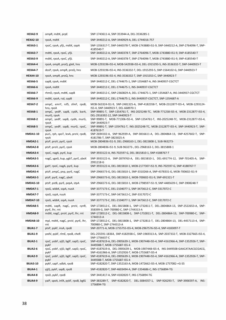
38

HEXA2-9 ompR, mdtK, prpE SNP-1743611-A, SNP-353944-A, DEL-3536285-1

HEXA2-10 rpoA, mdtK SNP-3440212-A, SNP-3440929-A, DEL-1744016-757

HEXA3-1 rpoC, rpoA, yfjL, mdtK, sapA SNP-1356317-T, SNP-3440378-T, MOB-1743880-IS1-9, SNP-3440212-A, SNP-2764096-T, SNP-4185540-T

HEXA3-7 mdtK, rpoA, rpoC, yfjL SNP-3440212-A, SNP-3440378-T, SNP-2764096-T, MOB-1743880-IS1-9, SNP-4185540-T

HEXA3-9 mdtK, rpoA, rpoC, yfjL SNP-3440212-A, SNP-3440378-T, SNP-2764096-T, MOB-1743880-IS1-9, SNP-4185540-T

HEXA4-4 rpoA, ompR, proQ, glxK, hns MOB-1293196-IS5-4, MOB-542938-IS5-4, DEL-1915293-5, INS-3536332-T, SNP-3440923-T

HEXA4-7 dosP, rpoA, ompR, proQ, hns MOB-1293196-IS5-4, INS-3536332-T, DEL-1915293-5, SNP-1564102-G, SNP-3440923-T

HEXA4-10 rpoA, ompR, proQ, hns MOB-1293196-IS5-4, INS-3536332-T, SNP-1915353-C, SNP-3440923-T

HEXA6-5 sapB, rpoA, mdtK SNP-3440212-C, DEL-1744675-1, SNP-1354687-A, INS-3440937-CGCTCT

HEXA6-6 rpoA, mdtK SNP-3440212-C, DEL-1744675-1, INS-3440937-CGCTCT

HEXA6-7 rhmD, rpoA, mdtK, sapB SNP-3440212-C, SNP-2360829-A, DEL-1744675-1, SNP-1354687-A, INS-3440937-CGCTCT

HEXA6-9 mdtK, rpoA, rsd, sapB SNP-3440212-C, DEL-1744675-1, INS-3440937-CGCTCT, SNP-1354687-A

HEXA7-2 ompC, emrY, rsfS, sfmF, rpoB, hns, rpoA

MOB-563324-IS1-9, SNP-2481325-A, SNP-4182358-T, MOB-2312877-IS5-4, MOB-1293124-IS5-4, SNP-3440923-T, DEL-668970-1

HEXA8-1 ompC, yedP, sapB, cydA, barA, murG, rpoA

SNP-99891-T, SNP-1354761-T, INS-2025248-TC, MOB-771258-IS5-4, MOB-2312877-IS5-4, DEL-2916392-12, SNP-3440923-T

HEXA8-2 ompC, yedP, sapB, cydA, murG, rpoA

SNP-99891-T, MOB-771306-IS5-4, SNP-1354761-T, INS-2025248-TC, MOB-2312877-IS5-4, SNP-3440923-T

HEXA8-5 ompC, yedP, sapB, murG, rpoC, rpoA

SNP-99891-T, SNP-1354761-T, INS-2025248-TC, MOB-2312877-IS5-4, SNP-3440923-T, SNP-4187619-T

HMDA1-10 purL, rph, spoT, lexA, proV, rpoB, rpsA

SNP-2694102-A, SNP-962939-A, SNP-3816611-A, DEL-2804864-13, SNP-4257602-T, SNP-4181786-T, SNP-3823025-A

HMDA2-1 ptsP, proV, pyrE, rpsA MOB-2804836-IS1-9, DEL-2968163-1, DEL-3815808-1, SUB-963273-

HMDA2-8 ptsP, proV, pyrE, rpsA MOB-2804836-IS1-9, SUB-963273-, DEL-2968163-1, DEL-3815808-1

HMDA3-4 rpoC, nagA, pyrE, kup SNP-3933122-A, INS-702597-G, DEL-3815810-1, SNP-4188767-T

HMDA3-5 nagC, ygeG, kup, ygbT, pyrE, ybeX SNP-3933122-A, SNP-2879763-A, DEL-3815810-1, DEL-691774-12, SNP-701405-A, SNP-2991218-G

HMDA3-6 gatY, rpoC, nagA, pyrE, kup SNP-3933122-A, DEL-3815810-1, MOB-2177307-IS1-9, INS-702597-G, SNP-4188767-T

HMDA5-4 ptsP, ampC, pnp, pyrE, nagC SNP-2966573-G, DEL-3815810-1, SNP-3310266-A, SNP-4378331-G, MOB-700602-IS1-9

HMDA5-5 ptsP, pyrE, nagC, ybeX SNP-2966573-G, DEL-3815810-1, MOB-700602-IS1-9, SNP-691321-T

HMDA5-10 ptsP, pstB, pyrE, pepA, stpA SNP-2966573-G, DEL-3815810-1, MOB-2798597-IS1-9, SNP-4485639-C, SNP-3908248-T

HMDA7-1 rpsG, wbbK, sspA, nusA SNP-3377173-C, DEL-2104077-1, SNP-3473612-C, SNP-3317072-C

HMDA7-7 rpsG, sspA, nusA SNP-3377173-C, SNP-3473612-C, SNP-3317072-C

HMDA7-10 rpsG, wbbK, sspA, nusA SNP-3377173-C, DEL-2104077-1, SNP-3473612-C, SNP-3317072-C

HMDA8-5 mdtK, xapR, nagC, proV, cynR, pyrE, lhr, rnt

SNP-1728512-C, DEL-3815808-1, SNP-1732811-T, DEL-2804864-13, SNP-2522653-A, SNP-358399-G, SNP-700980-C, SNP-1744313-A

HMDA8-9 mdtK, nagC, proV, pyrE, lhr, rnt SNP-1728512-C, DEL-3815808-1, SNP-1732811-T, DEL-2804864-13, SNP-700980-C, SNP-1744313-A

HMDA8-10 mpl, mdtK, nagC, proV, pyrE, lhr, rnt

SNP-1728512-C, DEL-3815808-1, SNP-1732811-T, DEL-2804864-13, DEL-4457113-4, SNP-700980-C, SNP-1744313-A

IBUA1-7 ptsP, pykF, insA, rpoB SNP-20771-A, MOB-1755755-IS5-4, MOB-2967576-IS5-4, SNP-4183097-T

IBUA1-9 yedV, pykF, rlmE, rpoB, cheR DEL-255591-18364, SNP-4182938-C, SNP-1969313-A, SNP-2037332-T, MOB-3327665-IS5-4, SNP-1756637-C

IBUA2-1 rpsC, yobF, yijD, bglF, sapD, rpoC, pykF

SNP-4187619-A, DEL-3905639-1, MOB-1907448-IS5-4, SNP-4161966-A, SNP-1352926-T, SNP-3449388-T, MOB-1755687-IS5-4


SNP-4187619-A, DEL-3905639-1, MOB-1907448-IS5-4, INS-3449508-GAACATAACGCGACG, SNP-4161966-A, SNP-1352926-T, MOB-1755687-IS5-4


SNP-4187619-A, DEL-3905639-1, MOB-1907448-IS5-4, SNP-4161966-A, SNP-1352926-T, SNP-3449388-T, MOB-1755687-IS5-4

IBUA3-10 pykF, sapF, ydbA, rpoB SNP-4182820-T, SNP-1352163-A, MOB-1472662-IS5-4, MOB-1757082-+G-S5

IBUA4-1 yjjQ, pykF, sapB, rpoB SNP-4182820-T, SNP-4603494-A, SNP-1354686-C, INS-1756894-TG

IBUA4-8 rpsD, pykF, rpoB SNP-3441417-A, SNP-4182820-T, INS-1756894-TG

IBUA4-9 yaiP, speA, infA, pykF, rpoB, bglG SNP-383289-T, SNP-4182820-T, DEL-3084357-1, SNP-926293-T, SNP-3906597-A, INS-1756894-TG

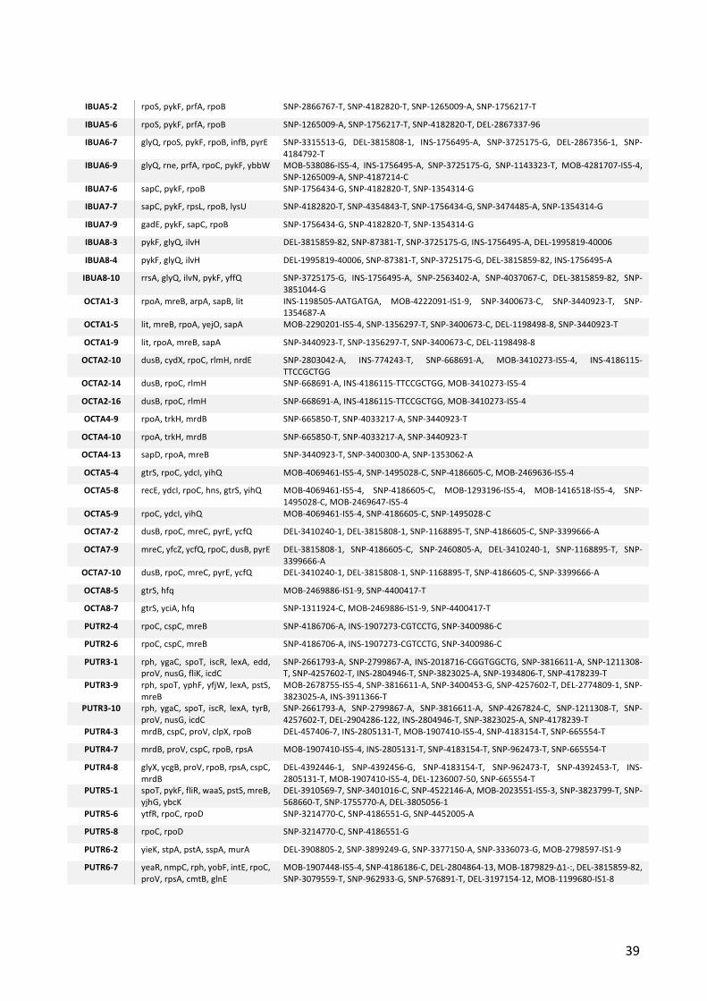
39

IBUA5-2 rpoS, pykF, prfA, rpoB SNP-2866767-T, SNP-4182820-T, SNP-1265009-A, SNP-1756217-T

IBUA5-6 rpoS, pykF, prfA, rpoB SNP-1265009-A, SNP-1756217-T, SNP-4182820-T, DEL-2867337-96

IBUA6-7 glyQ, rpoS, pykF, rpoB, infB, pyrE SNP-3315513-G, DEL-3815808-1, INS-1756495-A, SNP-3725175-G, DEL-2867356-1, SNP-4184792-T

IBUA6-9 glyQ, rne, prfA, rpoC, pykF, ybbW MOB-538086-IS5-4, INS-1756495-A, SNP-3725175-G, SNP-1143323-T, MOB-4281707-IS5-4, SNP-1265009-A, SNP-4187214-C

IBUA7-6 sapC, pykF, rpoB SNP-1756434-G, SNP-4182820-T, SNP-1354314-G

IBUA7-7 sapC, pykF, rpsL, rpoB, lysU SNP-4182820-T, SNP-4354843-T, SNP-1756434-G, SNP-3474485-A, SNP-1354314-G

IBUA7-9 gadE, pykF, sapC, rpoB SNP-1756434-G, SNP-4182820-T, SNP-1354314-G

IBUA8-3 pykF, glyQ, ilvH DEL-3815859-82, SNP-87381-T, SNP-3725175-G, INS-1756495-A, DEL-1995819-40006

IBUA8-4 pykF, glyQ, ilvH DEL-1995819-40006, SNP-87381-T, SNP-3725175-G, DEL-3815859-82, INS-1756495-A

IBUA8-10 rrsA, glyQ, ilvN, pykF, yffQ SNP-3725175-G, INS-1756495-A, SNP-2563402-A, SNP-4037067-C, DEL-3815859-82, SNP-3851044-G

OCTA1-3 rpoA, mreB, arpA, sapB, lit INS-1198505-AATGATGA, MOB-4222091-IS1-9, SNP-3400673-C, SNP-3440923-T, SNP-1354687-A

OCTA1-5 lit, mreB, rpoA, yejO, sapA MOB-2290201-IS5-4, SNP-1356297-T, SNP-3400673-C, DEL-1198498-8, SNP-3440923-T

OCTA1-9 lit, rpoA, mreB, sapA SNP-3440923-T, SNP-1356297-T, SNP-3400673-C, DEL-1198498-8

OCTA2-10 dusB, cydX, rpoC, rlmH, nrdE SNP-2803042-A, INS-774243-T, SNP-668691-A, MOB-3410273-IS5-4, INS-4186115-TTCCGCTGG

OCTA2-14 dusB, rpoC, rlmH SNP-668691-A, INS-4186115-TTCCGCTGG, MOB-3410273-IS5-4

OCTA2-16 dusB, rpoC, rlmH SNP-668691-A, INS-4186115-TTCCGCTGG, MOB-3410273-IS5-4

OCTA4-9 rpoA, trkH, mrdB SNP-665850-T, SNP-4033217-A, SNP-3440923-T

OCTA4-10 rpoA, trkH, mrdB SNP-665850-T, SNP-4033217-A, SNP-3440923-T

OCTA4-13 sapD, rpoA, mreB SNP-3440923-T, SNP-3400300-A, SNP-1353062-A

OCTA5-4 gtrS, rpoC, ydcI, yihQ MOB-4069461-IS5-4, SNP-1495028-C, SNP-4186605-C, MOB-2469636-IS5-4

OCTA5-8 recE, ydcI, rpoC, hns, gtrS, yihQ MOB-4069461-IS5-4, SNP-4186605-C, MOB-1293196-IS5-4, MOB-1416518-IS5-4, SNP-1495028-C, MOB-2469647-IS5-4

OCTA5-9 rpoC, ydcI, yihQ MOB-4069461-IS5-4, SNP-4186605-C, SNP-1495028-C

OCTA7-2 dusB, rpoC, mreC, pyrE, ycfQ DEL-3410240-1, DEL-3815808-1, SNP-1168895-T, SNP-4186605-C, SNP-3399666-A

OCTA7-9 mreC, yfcZ, ycfQ, rpoC, dusB, pyrE DEL-3815808-1, SNP-4186605-C, SNP-2460805-A, DEL-3410240-1, SNP-1168895-T, SNP-3399666-A

OCTA7-10 dusB, rpoC, mreC, pyrE, ycfQ DEL-3410240-1, DEL-3815808-1, SNP-1168895-T, SNP-4186605-C, SNP-3399666-A

OCTA8-5 gtrS, hfq MOB-2469886-IS1-9, SNP-4400417-T

OCTA8-7 gtrS, yciA, hfq SNP-1311924-C, MOB-2469886-IS1-9, SNP-4400417-T

PUTR2-4 rpoC, cspC, mreB SNP-4186706-A, INS-1907273-CGTCCTG, SNP-3400986-C

PUTR2-6 rpoC, cspC, mreB SNP-4186706-A, INS-1907273-CGTCCTG, SNP-3400986-C

PUTR3-1 rph, ygaC, spoT, iscR, lexA, edd, proV, nusG, fliK, icdC

SNP-2661793-A, SNP-2799867-A, INS-2018716-CGGTGGCTG, SNP-3816611-A, SNP-1211308-T, SNP-4257602-T, INS-2804946-T, SNP-3823025-A, SNP-1934806-T, SNP-4178239-T

PUTR3-9 rph, spoT, yphF, yfjW, lexA, pstS, mreB

MOB-2678755-IS5-4, SNP-3816611-A, SNP-3400453-G, SNP-4257602-T, DEL-2774809-1, SNP-3823025-A, INS-3911366-T

PUTR3-10 rph, ygaC, spoT, iscR, lexA, tyrB, proV, nusG, icdC

SNP-2661793-A, SNP-2799867-A, SNP-3816611-A, SNP-4267824-C, SNP-1211308-T, SNP-4257602-T, DEL-2904286-122, INS-2804946-T, SNP-3823025-A, SNP-4178239-T

PUTR4-3 mrdB, cspC, proV, clpX, rpoB DEL-457406-7, INS-2805131-T, MOB-1907410-IS5-4, SNP-4183154-T, SNP-665554-T

PUTR4-7 mrdB, proV, cspC, rpoB, rpsA MOB-1907410-IS5-4, INS-2805131-T, SNP-4183154-T, SNP-962473-T, SNP-665554-T

PUTR4-8 glyX, ycgB, proV, rpoB, rpsA, cspC, mrdB

DEL-4392446-1, SNP-4392456-G, SNP-4183154-T, SNP-962473-T, SNP-4392453-T, INS-2805131-T, MOB-1907410-IS5-4, DEL-1236007-50, SNP-665554-T

PUTR5-1 spoT, pykF, fliR, waaS, pstS, mreB, yjhG, ybcK

DEL-3910569-7, SNP-3401016-C, SNP-4522146-A, MOB-2023551-IS5-3, SNP-3823799-T, SNP-568660-T, SNP-1755770-A, DEL-3805056-1

PUTR5-6 ytfR, rpoC, rpoD SNP-3214770-C, SNP-4186551-G, SNP-4452005-A

PUTR5-8 rpoC, rpoD SNP-3214770-C, SNP-4186551-G

PUTR6-2 yieK, stpA, pstA, sspA, murA DEL-3908805-2, SNP-3899249-G, SNP-3377150-A, SNP-3336073-G, MOB-2798597-IS1-9

PUTR6-7 yeaR, nmpC, rph, yobF, intE, rpoC, proV, rpsA, cmtB, glnE

MOB-1907448-IS5-4, SNP-4186186-C, DEL-2804864-13, MOB-1879829-Δ1-:, DEL-3815859-82, SNP-3079559-T, SNP-962933-G, SNP-576891-T, DEL-3197154-12, MOB-1199680-IS1-8

40

PUTR6-10 yeaR, nmpC, rph, tdcR, yobF, tolA, yjcF, proV, rpsA, cmtB, intE

MOB-1907448-IS5-4, SNP-3267294-T, DEL-777151-48, SNP-4282760-C, DEL-2804864-13, MOB-1879829-Δ1-:, DEL-3815859-82, SNP-3079559-T, SNP-962933-G, SNP-576891-T, MOB-1199680-IS1-8

PUTR7-1 rpsA, spoT, mreB, nusA SNP-3823799-A, SNP-3316916-C, SNP-962922-T, SNP-3400811-T

PUTR7-7 rpoD, rpoB, murA SNP-3214770-C, SNP-3335317-G, SNP-4183154-T

PUTR7-9 rpoD, mdtJ, rpoB, murA SNP-4183154-T, SNP-3335317-G, DEL-1673532-181, SNP-3214770-C

PUTR8-3 spoT, rpsG, proX, mreB, pyrE, argG

SNP-3400195-A, SNP-3318960-A, DEL-3815808-1, INS-2807248-T, SNP-3473612-C, SNP-3823811-A

PUTR8-6 yedP, spoT, rpsG, nagC, proX, mreB, leuL, pyrE, argG

SNP-2025435-A, SNP-3400195-A, SNP-3318960-A, DEL-3815808-1, INS-2807248-T, DEL-83679-3, DEL-701233-1, SNP-3473612-C, SNP-3823811-A

PUTR8-10 spoT, rpsG, nagC, proX, mreB, sfmH, pyrE, argG

SNP-3400195-A, SNP-3318960-A, DEL-3815808-1, INS-2807248-T, DEL-700785-47, SNP-3473612-C, SNP-562667-C, SNP-3823811-A

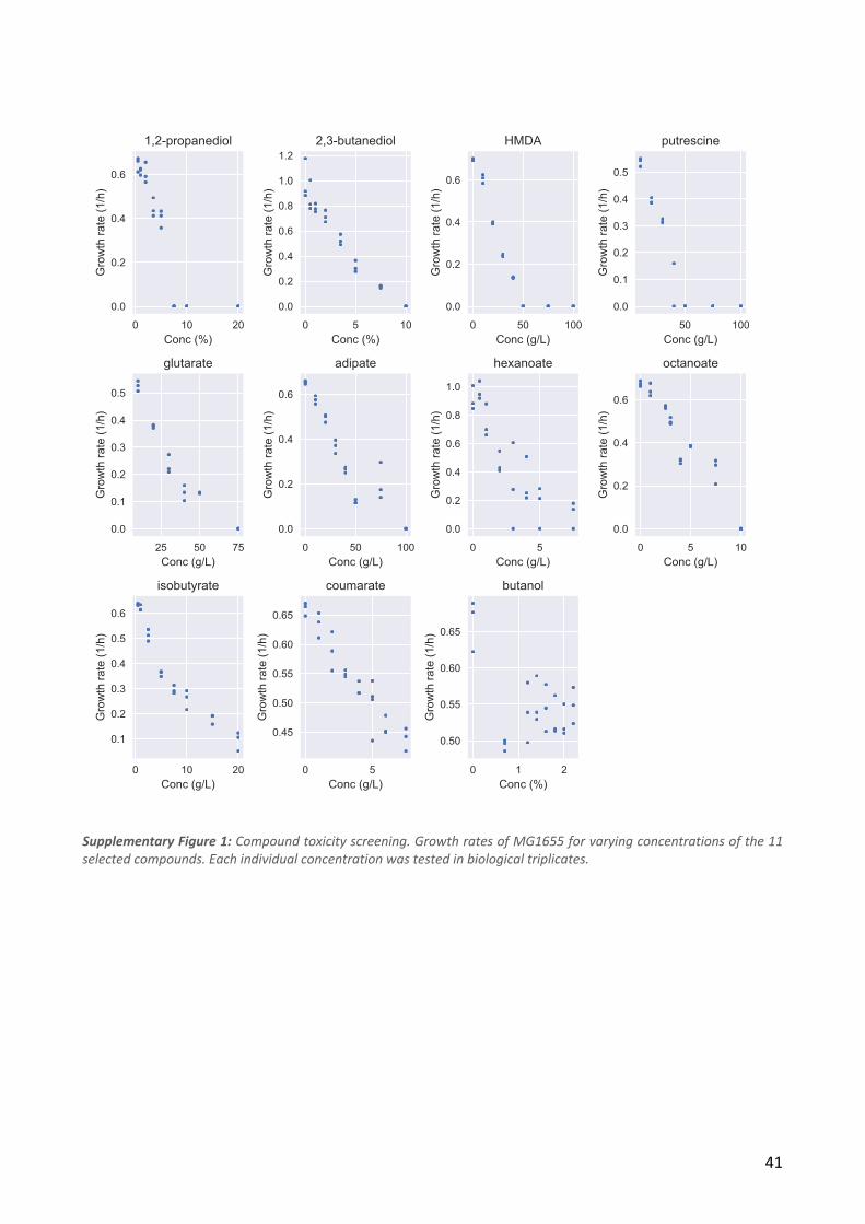
41

Supplementary Figure 1: Compound toxicity screening. Growth rates of MG1655 for varying concentrations of the 11 selected compounds. Each individual concentration was tested in biological triplicates.

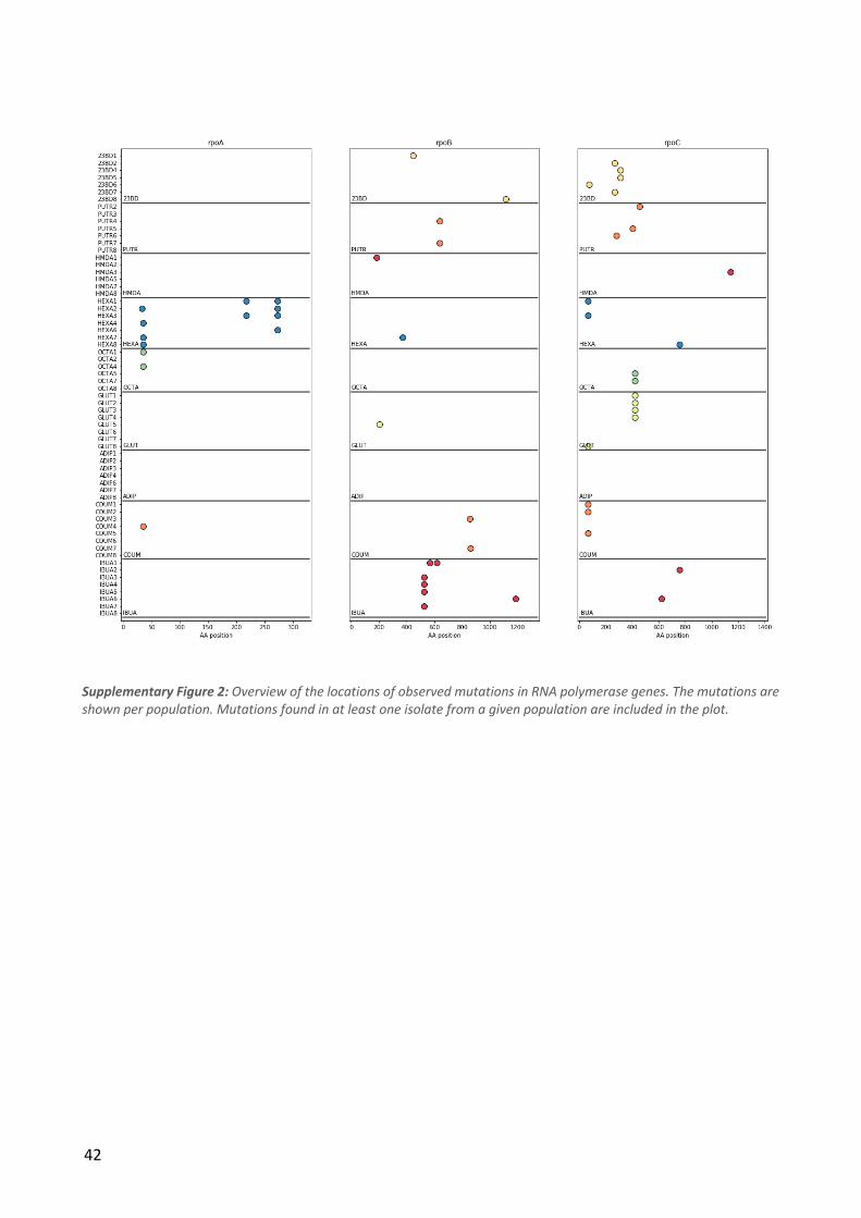
42

Supplementary Figure 2: Overview of the locations of observed mutations in RNA polymerase genes. The mutations are shown per population. Mutations found in at least one isolate from a given population are included in the plot.

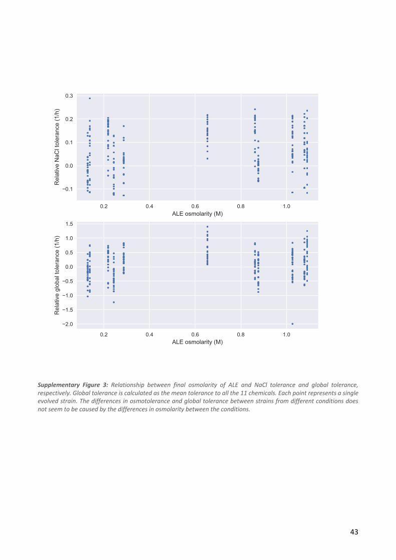
43

Supplementary Figure 3: Relationship between final osmolarity of ALE and NaCl tolerance and global tolerance, respectively. Global tolerance is calculated as the mean tolerance to all the 11 chemicals. Each point represents a single evolved strain. The differences in osmotolerance and global tolerance between strains from different conditions does not seem to be caused by the differences in osmolarity between the conditions.

44

Chapter 2: The metabolism of evolved tolerance

2.1 Introduction

As seen in the previous chapter, ALE can be used to quickly produce strains with improved

characteristics for a target phenotype. Specifically, it was demonstrated that strain tolerance to

several industrially relevant products could be improved significantly through ALE. Sequencing the

evolved strains allows identification of the exact genetic changes that give rise to the improved

phenotypes. Although such improvements can be very valuable in a strain engineering process, it is

often desirable to also obtain a deeper understanding of the evolved strains and the observed

mutations, i.e. what impact a mutation has on the cell, and why the presence of the mutation

confers a growth advantage in the evolution condition. Elucidating such mechanisms of adaptation

requires further characterization of the evolved strains in order to investigate how each strain

differs from the unevolved parent strain. For instance, changes in regulation or metabolism can give

indications of key cellular mechanisms that mediate the adaptive improvement of a desirable

phenotype such as tolerance.

In metabolic engineering, where the ultimate objective is to reroute metabolic flux to production

pathways, adaptive changes in metabolism are especially interesting. A key question to ask after

successful strain optimization with ALE is thus whether the mutations have caused metabolic

perturbations, and whether these perturbations are related to the observed growth adaptations.

Metabolic changes are amenable to study using metabolomics methods, or other methods that

derive from metabolomics such as fluxomics. While fluxomics would be the most informative way

to examine metabolic flux rerouting, this approach primarily gives information on central carbon

metabolism and is also challenging to apply to large numbers of strains due to the experimental

and computational efforts required (Niedenführ et al., 2015). Metabolomics on the other hand can

be performed relatively quickly and cheaply and also provides insight into the functioning of the

strain’s metabolism. Data obtained with different metabolomics methods differ with regard to both

quality, e.g. the precision of the measurements and whether the data is absolute or relative; and

quantity, e.g. how many metabolites are covered and how quickly a sample can be run (Griffiths and

Wang, 2010). Since there is usually a trade-off between quality and quantity, the choice of method

depends on the requirements for the specific use case.

45

In this chapter a metabolomic characterisation of the ALE strains obtained from the study in Chapter

1 will be described. For this analysis a high-throughput, high-coverage untargeted metabolomics

method (Fuhrer et al., 2011) was chosen, sacrificing some data quality in exchange for the ability to

characterize a larger number of strains. The chosen method is a direct-injection mass-spectrometry

method, meaning that the samples are injected into a mass spectrometer without any prior

chromatography. Whereas more traditional chromatography-coupled mass-spectrometry methods

provide a list of ions annotated with mass-charge ratio and column retention time, a direct-injection

method only provides mass-to-charge ratio (Fuhrer and Zamboni, 2015). This makes the subsequent

metabolite annotation less accurate and prevents discrimination of isomers but increases

throughput dramatically. The method does not use any standards, which limits measurements to

relative ion intensities but allows a high coverage of known metabolites to be obtained. Objectives

of the metabolomic characterization of the tolerant ALE strains were to:

1. Determine the metabolic similarity between strains evolved to tolerate the same or different

chemicals

2. Investigate to which extent metabolism is involved in the evolution of chemical tolerance

3. Use the metabolomics information to elucidate in more detail the effect of each mutation

observed in the evolved trains.

In addition to the metabolomic characterization of the ALE strains, metabolomics was also used to

try to characterize the toxic effects of each chemical to a wild type strain from a metabolic

perspective.

2.2 Methods

2.2.1 Strains

The strains used in this study were isolates from a series of evolution experiments designed to

evolve chemical tolerance to industrially relevant compounds (See Chapter 1). All these strains were

derived from E. coli K12 MG1655, which was also used as the reference strain for all analyses. As

almost all strains evolved on 1,2-propanediol were hypermutators, no strains from this condition

were included in this study. Due to problems with evaporation during the butanol evolutions, the

evolved strains did not have significant increases butanol tolerance and were also not included in

46

this study. The strains that were used were evolved on 2,3-butanediol (23BD), hexamethylene-

diamine (HMDA), putrescine (PUTR), glutarate (GLUT), adipate (ADIP), hexanoate (HEXA), octanoate

(OCTA), isobutyrate (IBUA) and coumarate (COUM).

2.2.2 Mass spectrometry

All metabolomics data was obtained from an Agilent qTOF 6550 instrument, using a direct injection

method with no prior chromatography step (Fuhrer et al., 2011).

2.2.3 Cultivations

All cultures were grown in triplicates in 96-deep well plates with sandwich cover lids at 37 deg.C

with shaking at 300 rpm. The growth medium was M9 (6.8 g/L Na2HPO, 3 g/L KH2PO4, 1 g/L NH4Cl,

0.5 g/L NaCl, 1 mM MgSO4, 0.1 mM CaCl2) with 1% glucose. Additionally, the medium contained the

following trace elements: 22.17 µM ethylenediaminetetraacetate, 7.82 µM ZnSO, 1.77 µM MnCl2,

0.63 µM CoCl2, 0.51 µM CuSO4, 0.83 µM Na2MoO4, 5.40 µM FeSO4, 8.09 µM H3BO3, 0.30 µM KI.

2.2.4 Metabolic profile characterization

2.2.4.1 Sampling

The strains were cultivated overnight and reinoculated in fresh medium. In each cultivation plate

the MG1655 reference strain was inoculated to 12 different starting densities over a 15-fold range

in order to obtain a large number of reference metabolite measurements at different densities.

When the cultures were at densities between OD600 of 0.5 and 1.5 they were sampled at three to

four timepoints with approximately 1-hour intervals. The samples (30 µL of each culture) were

immediately quenched in 120 µL cold extraction solution (50% methanol, 50% acetonitrile). The

densities of the cultures were measured on a Tecan Sunrise plate reader at each sampling.

The quenched samples were incubated at -18 deg.C for 2 hours and centrifuged at 3000x g for 10

minutes. The supernatants were transferred to clean plates, which were sealed and kept at -80

deg.C until the time of mass spectrometry measurements.

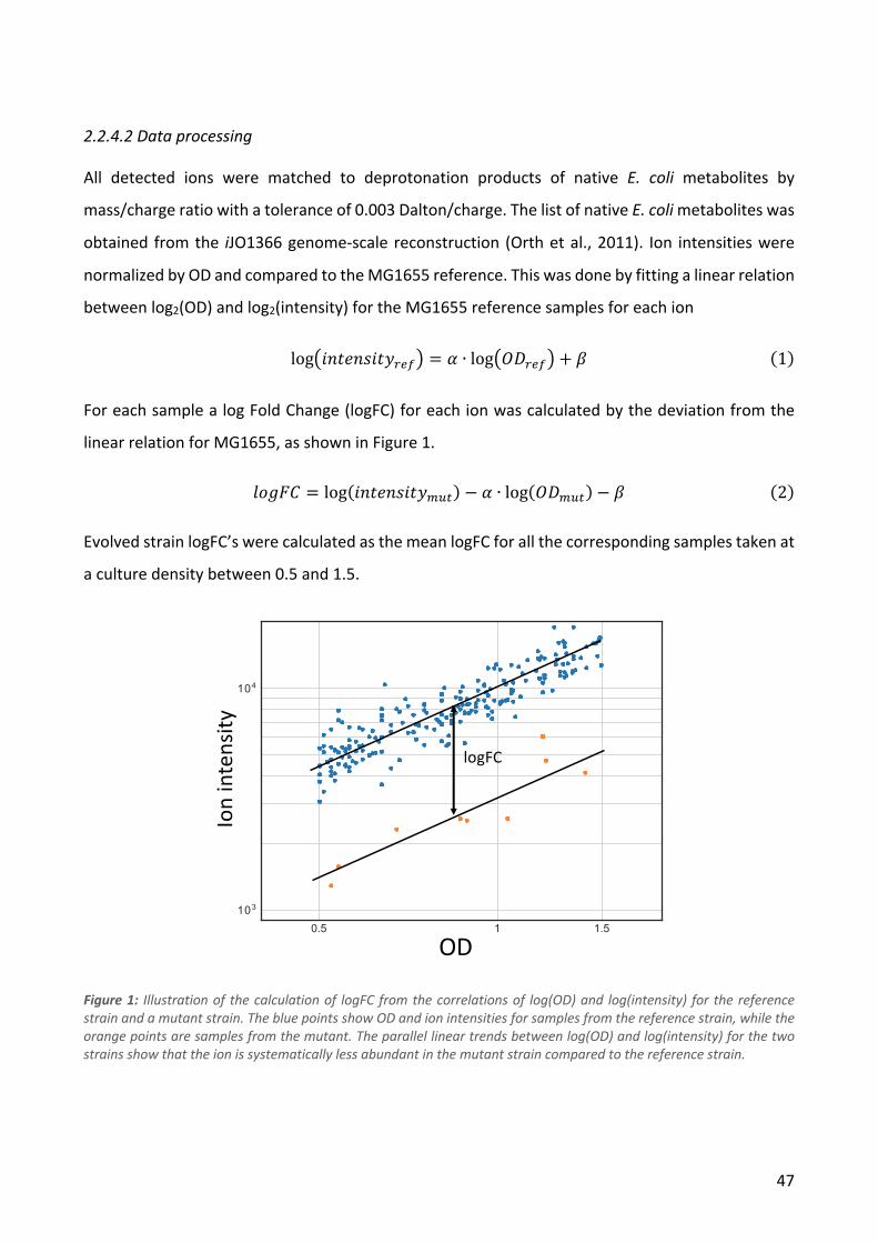
47

2.2.4.2 Data processing

All detected ions were matched to deprotonation products of native E. coli metabolites by

mass/charge ratio with a tolerance of 0.003 Dalton/charge. The list of native E. coli metabolites was

obtained from the iJO1366 genome-scale reconstruction (Orth et al., 2011). Ion intensities were

normalized by OD and compared to the MG1655 reference. This was done by fitting a linear relation

between log2(OD) and log2(intensity) for the MG1655 reference samples for each ion

log123#(342#56789 = : ∙ log1;<6789 + = (1)

For each sample a log Fold Change (logFC) for each ion was calculated by the deviation from the

linear relation for MG1655, as shown in Figure 1.

>?@AB = log(23#(342#5CD*) − : ∙ log(;<CD*) − = (2)

Evolved strain logFC’s were calculated as the mean logFC for all the corresponding samples taken at

a culture density between 0.5 and 1.5.

Figure 1: Illustration of the calculation of logFC from the correlations of log(OD) and log(intensity) for the reference strain and a mutant strain. The blue points show OD and ion intensities for samples from the reference strain, while the orange points are samples from the mutant. The parallel linear trends between log(OD) and log(intensity) for the two strains show that the ion is systematically less abundant in the mutant strain compared to the reference strain.

0.5 1 1.5103

104

OD

Ion

inte

nsity

logFC

48

2.2.5 Chemical perturbation

2.2.5.1 Sampling

Cultures of MG1655 were grown in M9 medium with 1% glucose overnight and reinoculated in fresh

medium inside a 37 deg.C climate chamber where all the chemical perturbation experiments were

carried out using temperature-equilibrated equipment and materials. When the cultures reached

OD 1, a sample of 20 µL was transferred to 80 µL cold extraction mix, as a baseline measurement.

390 µL of culture was then transferred to a well containing 10 µL of a solution of the given chemical

and quickly mixed by pipetting. Immediately after, 200 µL of the perturbed culture was aspirated in

an electronic pipette. At each sampling time 20 µL was dispensed into 80 µL of cold extraction mix.

Sampling times were 10, 20, 30, 45, 60, 80, 100, 120, 180 and 300 seconds after perturbation. This

was replicated for three separate cultures per perturbation chemical, and nine cultures for

perturbation with water. The used perturbation concentrations are shown in Table 1.

2.2.5.2 Data processing

All detected ions were matched to deprotonation products of native E. coli metabolites by

mass/charge ratio with a tolerance of 0.003 Dalton/charge. The list of native E. coli metabolites was

obtained from the iJO1366 genome-scale reconstruction (Orth et al., 2011). For each annotated ion,

the response to each chemical perturbation was compared to the response to the water

perturbation. A linear model was used to identify significant interactions between metabolites and

chemical perturbations, i.e. metabolites that responded differently to perturbation with the

chemical compared to water. The linear model was given as:

log(5G) = : + =HIJKG*GIJL + =*GC7G + =HIJKG*GIJL:*GC7L + NG (3)

The left-hand term is the logarithm of the intensity of the ion in question for a sample 2, while the

right-hand side contains the intercept and the parameters associated with the condition and time

point of sample 2, as well as the residual, NG. The significance of the interaction term was tested

using analysis of variance. For each condition the interaction p-values for each ion were corrected

for multiple comparisons using the Benjamini-Hochberg False Discovery Rate (Benjamini and

Hochberg, 1995). A corrected p-value less than 0.05 was considered evidence that the time-

dependent response of the ion was different between the perturbation condition and the water

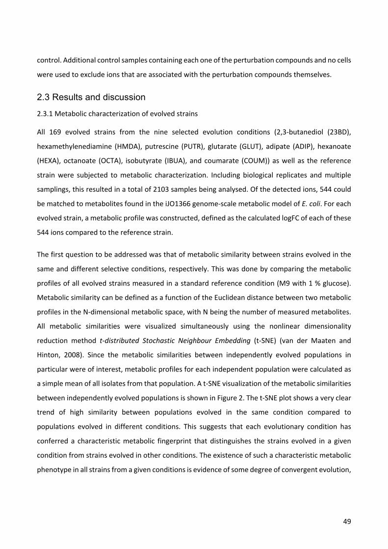
49

control. Additional control samples containing each one of the perturbation compounds and no cells

were used to exclude ions that are associated with the perturbation compounds themselves.

2.3 Results and discussion

2.3.1 Metabolic characterization of evolved strains

All 169 evolved strains from the nine selected evolution conditions (2,3-butanediol (23BD),

hexamethylenediamine (HMDA), putrescine (PUTR), glutarate (GLUT), adipate (ADIP), hexanoate

(HEXA), octanoate (OCTA), isobutyrate (IBUA), and coumarate (COUM)) as well as the reference

strain were subjected to metabolic characterization. Including biological replicates and multiple

samplings, this resulted in a total of 2103 samples being analysed. Of the detected ions, 544 could

be matched to metabolites found in the iJO1366 genome-scale metabolic model of E. coli. For each

evolved strain, a metabolic profile was constructed, defined as the calculated logFC of each of these

544 ions compared to the reference strain.

The first question to be addressed was that of metabolic similarity between strains evolved in the

same and different selective conditions, respectively. This was done by comparing the metabolic

profiles of all evolved strains measured in a standard reference condition (M9 with 1 % glucose).

Metabolic similarity can be defined as a function of the Euclidean distance between two metabolic

profiles in the N-dimensional metabolic space, with N being the number of measured metabolites.

All metabolic similarities were visualized simultaneously using the nonlinear dimensionality

reduction method t-distributed Stochastic Neighbour Embedding (t-SNE) (van der Maaten and

Hinton, 2008). Since the metabolic similarities between independently evolved populations in

particular were of interest, metabolic profiles for each independent population were calculated as

a simple mean of all isolates from that population. A t-SNE visualization of the metabolic similarities

between independently evolved populations is shown in Figure 2. The t-SNE plot shows a very clear

trend of high similarity between populations evolved in the same condition compared to

populations evolved in different conditions. This suggests that each evolutionary condition has

conferred a characteristic metabolic fingerprint that distinguishes the strains evolved in a given

condition from strains evolved in other conditions. The existence of such a characteristic metabolic

phenotype in all strains from a given conditions is evidence of some degree of convergent evolution,

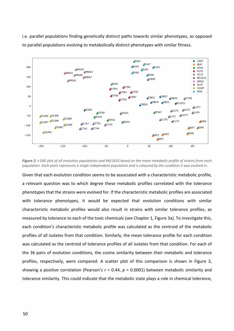
50

i.e. parallel populations finding genetically distinct paths towards similar phenotypes, as opposed

to parallel populations evolving to metabolically distinct phenotypes with similar fitness.

Figure 2: t-SNE plot of all evolution populations and MG1655 based on the mean metabolic profile of strains from each population. Each point represents a single independent population and is coloured by the condition it was evolved in.

Given that each evolution condition seems to be associated with a characteristic metabolic profile,

a relevant question was to which degree these metabolic profiles correlated with the tolerance

phenotypes that the strains were evolved for. If the characteristic metabolic profiles are associated

with tolerance phenotypes, it would be expected that evolution conditions with similar

characteristic metabolic profiles would also result in strains with similar tolerance profiles, as

measured by tolerance to each of the toxic chemicals (see Chapter 1, Figure 3a). To investigate this,

each condition’s characteristic metabolic profile was calculated as the centroid of the metabolic

profiles of all isolates from that condition. Similarly, the mean tolerance profile for each condition

was calculated as the centroid of tolerance profiles of all isolates from that condition. For each of

the 36 pairs of evolution conditions, the cosine similarity between their metabolic and tolerance

profiles, respectively, were compared. A scatter plot of this comparison is shown in Figure 3,

showing a positive correlation (Pearson’s r = 0.44, p = 0.0001) between metabolic similarity and

tolerance similarity. This could indicate that the metabolic state plays a role in chemical tolerance,

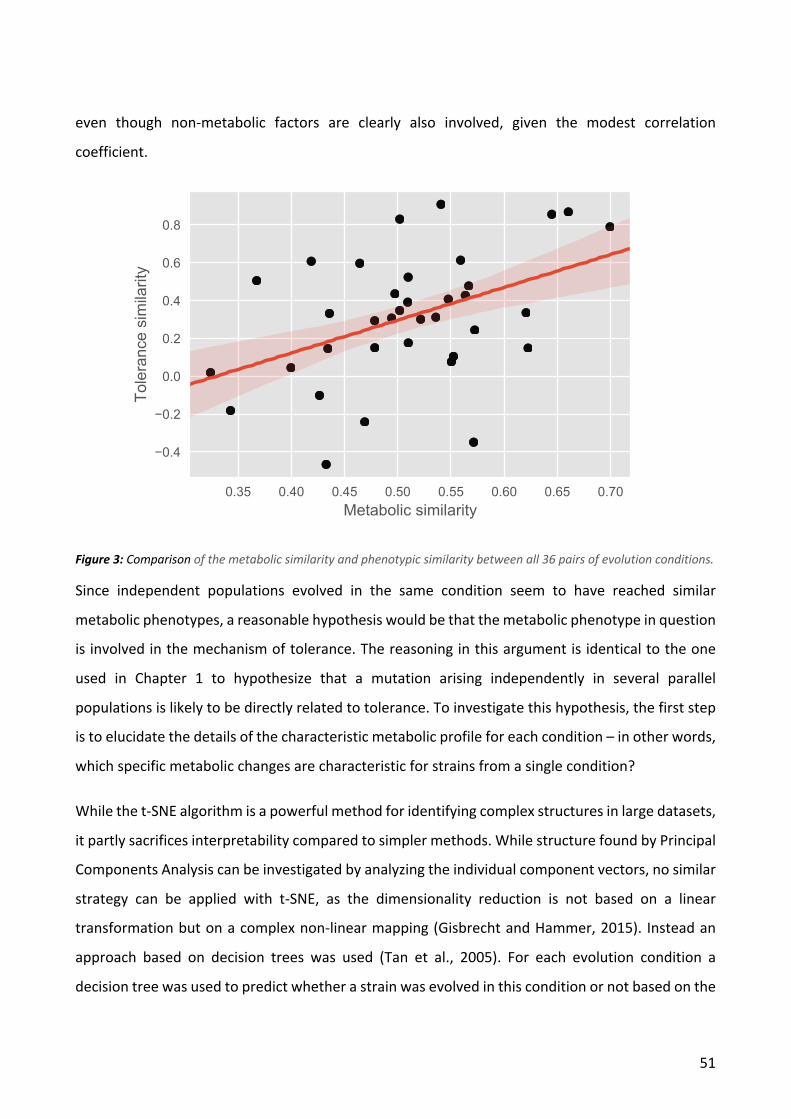
51

even though non-metabolic factors are clearly also involved, given the modest correlation

coefficient.

Figure 3: Comparison of the metabolic similarity and phenotypic similarity between all 36 pairs of evolution conditions.

Since independent populations evolved in the same condition seem to have reached similar

metabolic phenotypes, a reasonable hypothesis would be that the metabolic phenotype in question

is involved in the mechanism of tolerance. The reasoning in this argument is identical to the one

used in Chapter 1 to hypothesize that a mutation arising independently in several parallel

populations is likely to be directly related to tolerance. To investigate this hypothesis, the first step

is to elucidate the details of the characteristic metabolic profile for each condition – in other words,

which specific metabolic changes are characteristic for strains from a single condition?

While the t-SNE algorithm is a powerful method for identifying complex structures in large datasets,

it partly sacrifices interpretability compared to simpler methods. While structure found by Principal

Components Analysis can be investigated by analyzing the individual component vectors, no similar

strategy can be applied with t-SNE, as the dimensionality reduction is not based on a linear

transformation but on a complex non-linear mapping (Gisbrecht and Hammer, 2015). Instead an

approach based on decision trees was used (Tan et al., 2005). For each evolution condition a

decision tree was used to predict whether a strain was evolved in this condition or not based on the

52

measured metabolites. Because the rules of a fitted decision tree can be easily inspected, this

allowed identification of metabolites that are important for distinguishing strains from a given

condition from the remaining strains. Important metabolites were found by inspecting the nodes

near the root of the tree. The usefulness of each single metabolite for distinguishing strains could

then be visualized by showing the distribution of relative concentrations of this metabolite within

each group of strains (Figure 4). Each panel of Figure 4 displays the logFC values for a metabolite

that was found to be important for distinguishing strains from at least one of the evolution

conditions. The points represent strains, separated by the conditions they were evolved in. This

analysis shows that there are indeed metabolites in all conditions, that have consistently either

increased or decreased concentrations in most strains. This confirms the pattern seen from Figure

2 of strains from the same condition being metabolically similar.

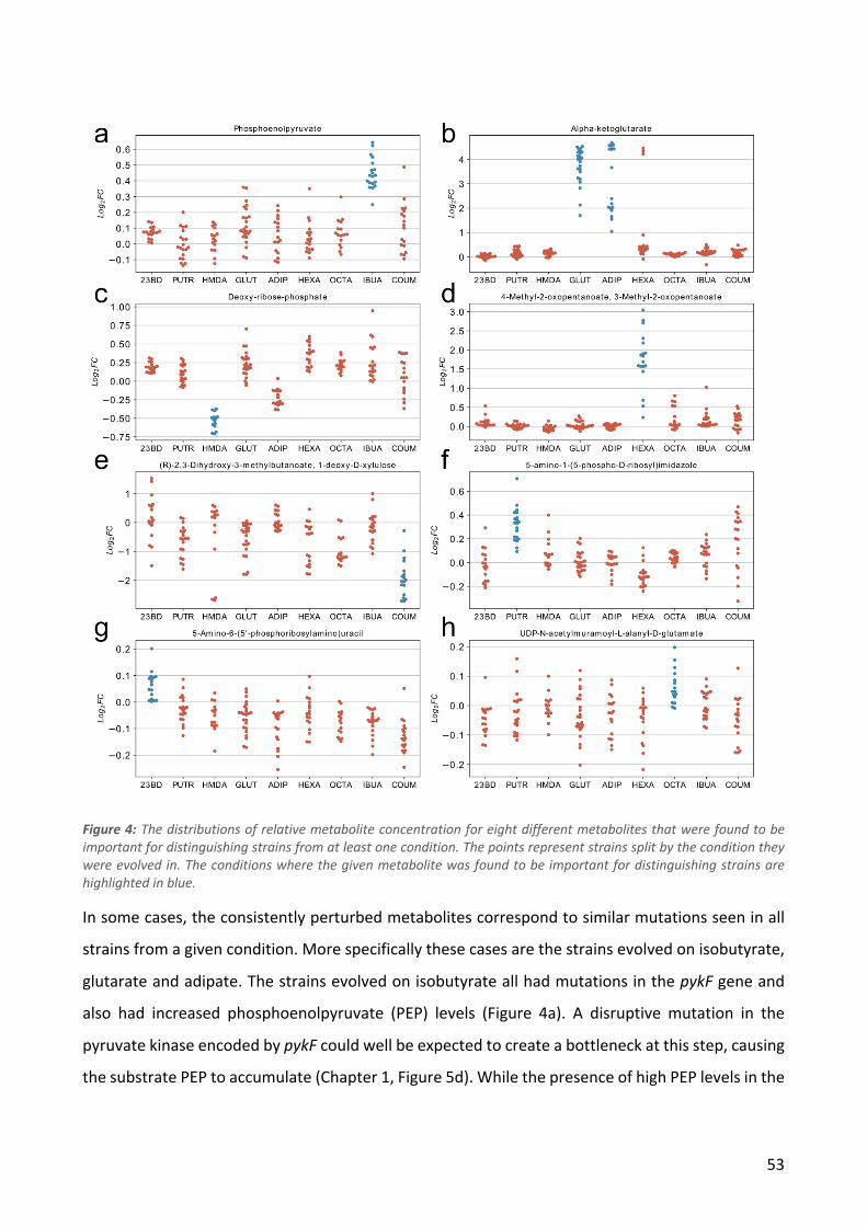
53

Figure 4: The distributions of relative metabolite concentration for eight different metabolites that were found to be important for distinguishing strains from at least one condition. The points represent strains split by the condition they were evolved in. The conditions where the given metabolite was found to be important for distinguishing strains are highlighted in blue.

In some cases, the consistently perturbed metabolites correspond to similar mutations seen in all

strains from a given condition. More specifically these cases are the strains evolved on isobutyrate,

glutarate and adipate. The strains evolved on isobutyrate all had mutations in the pykF gene and

also had increased phosphoenolpyruvate (PEP) levels (Figure 4a). A disruptive mutation in the

pyruvate kinase encoded by pykF could well be expected to create a bottleneck at this step, causing

the substrate PEP to accumulate (Chapter 1, Figure 5d). While the presence of high PEP levels in the

54

isobutyrate strains is not surprising, it can help understand the effect of pykF mutations in these

strains. PEP is a known regulator of upper glycolysis, specifically by inhibiting phosphofructokinase

activity (Uyeda, 2006), and thus the isobutyrate strains presumably have decreased flux through the

Embden-Meyerhof-Parnas pathway and increased flux through the Entner-Doudoroff or pentose

phosphate pathways instead. The strains evolved on glutarate and adipate all had mutations in the

kgtP gene, and also had very high levels of alpha-ketoglutarate (AKG) (Figure 4b). Since kgtP encodes

an active AKG importer (Seol and Shatkin, 1991) this might seem unintuitive. This result can however

be explained by AKG leaking out through the cell membrane, which has previously been

documented (Yan et al., 2011). In the absence of a transporter to bring AKG back in, it will

accumulate extracellularly resulting in high concentrations in the whole-culture sample being

injected into the mass spectrometer.

The above cases are examples of convergent evolution on the genetic level, as all the independent

populations have mutations in the same gene, which can explain the corresponding metabolic

feature (high PEP or AKG levels respectively). In other conditions there is evidence of convergent

evolution on the metabolic level, as all isolated strains share certain metabolic characteristics

despite not having specific mutations in common. Examples of such conditions are HMDA and

hexanoate. All the strains evolved on HMDA had decreased levels of deoxy-ribose-phosphate

(Figure 4c). This cannot be explained by a common genetic change, as no single gene was mutated

in all these strains. Indeed, one population did not have any mutational overlap with any one of the

remaining populations. Likewise, all strains evolved on hexanoate had increased levels of methyl-2-

oxopentanoate (Figure 4d) even if these strains do not share any universal mutations. The presence

of characteristic phenotypic (e.g. metabolic) commonalities between strains with little or no genetic

overlap might provide insight into the mechanisms with which individual genes contribute to

tolerance. If gene A is mutated in some strains while gene B is mutated in other strains, it is likely

that tolerance arises mechanistically from an effect that genes A and B have in common. In trivial

cases genes A and B might simply be analogous, e.g. subunits of the same complex or different steps

in a linear pathway, whereas if A and B have diverse sets of effects, such as transcriptional

regulators, overlaying the two sets of effects with each other might indicate which effects are

important for tolerance. While this method can be used for many different types of phenotypic

55

effects, the effects of each mutation must generally first be characterized, and thus, depending on

the effect phenotype in question, a significant amount of work is required.

Further analyses were performed to elucidate the relationship between mutations and metabolic

profiles in the evolved strains. A simple statistical model with a specific metabolite as dependent

variable and mutations as independent variables could be used, but due to the very high degree of

collinearity between the mutations (because of common ancestry as well as shared evolution

conditions), fitting such a model was not considered feasible. Instead, previously published data on

the relationship between genes and metabolites was used, in the form of metabolomics data for all

single-gene knockout E. coli strains in the Keio collection (Fuhrer et al., 2017). This data provides

information on the associations between genes and metabolites and can help estimate the impact

on gene function of the individual mutations observed in the evolved strains, which is generally not

known. A statistical model was used having the full metabolite profile as dependent variable and

the impact of each mutation on the affected gene(s) as independent variable, given the gene

knockout metabolite data from Fuhrer et al. (2017). To keep the model complexity reasonable some

simplifying assumptions were made. First, the impact of a mutation on the function of a gene was

quantified as a continuous univariate variable ranging from loss-of-function through neutral to gain-

of-function. Second, the combined effect of several mutations on the metabolic profile was

assumed to simply be the sum of each individual mutation effects on the metabolic profile. The

resulting model is a multivariate linear model given by

P = Q ∙ R ∙ S ∙ T + N (4)

Y is the matrix of relative metabolite concentrations in the evolved strains and has shape Nstrains x

Nmetabolites. X is a binary design matrix encoding the mutations found in each strain and has shape

Nstrains x Nmutations, where Nmutations is the number of unique mutations identified in the evolved

strains. W is the parameter to be fitted and is a diagonal Nmutations x Nmutations matrix, where the

diagonal contains the estimated impact score of each mutation (loss-of-function, neutral or gain-of-

function). M is a second binary design matrix encoding which genes each mutation affects, and has

shape Nmutations x Ngenes, where Ngenes is the number of unique mutated genes in the evolved strains.

Finally, K is a Ngenes x Nmetabolites matrix containing the relative metabolite concentrations in each

single-gene knockout strain. The parameter matrix W was fitted through gradient descent by

56

minimizing the sum of squares of the error term, N. The fitted model can be used to get estimated

impact scores, predicting whether each mutation has a loss-of-function or gain-of-function effect.

A positive estimated impact score was interpreted as loss-of-function, while a negative estimated

impact score was interpreted as gain-of-function.

Validating the estimated mutation impacts is difficult since, as mentioned earlier, it is not known

what the real impacts of most mutations are. However, a rough classification into expected

deleterious and non-deleterious mutations can be made based on their type and location in the

genome alone. For deletions, insertions and mobile element insertions, a mutation was expected to

be deleterious if it was within the coding sequence of a gene, while the majority of mutations

located outside of coding sequences were not expected to be deleterious. For SNP’s only nonsense

(stop codon inducing) polymorphisms would be expected to be highly deleterious. Comparing the

impacts estimated from mutation location to the impacts estimated by the model using

metabolomics data showed that mutations expected to be deleterious were significantly more often

estimated to have loss-of-function impacts (83 out of 156) compared to mutations not expected to

be deleterious based on location (111 out of 305) (Fisher’s exact test, p < 0.001). This pattern of

association between impact estimated from mutation location and impact estimated from

metabolomics data is apparent in all four types of mutations, as seen from Figure 5, which shows

the fraction of mutations of different types being estimated to have loss-of-function impacts. This

supports the validity of interpreting the impact scores estimated with the model using

metabolomics data as an indicator of whether the mutation has a gain-of-function or loss-of-

function effect. It is worth noting however, that the location-estimated impact of a mutation cannot

be regarded as a classification of the true impact, and thus the predictive performance of the model-

estimates cannot be accurately assessed. Particularly the assumption that all missense SNP’s are

non-deleterious is dubious, given the knowledge that many proteins are indeed sensitive to amino-

acid substitutions in active sites.

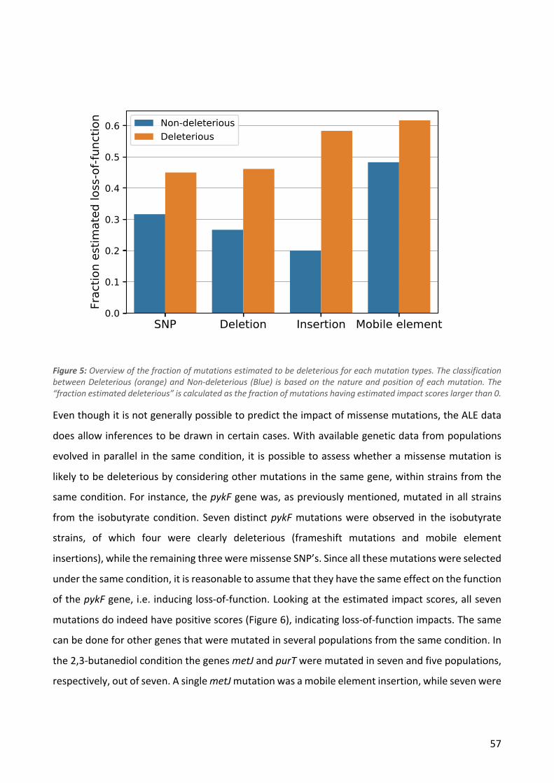
57

Figure 5: Overview of the fraction of mutations estimated to be deleterious for each mutation types. The classification between Deleterious (orange) and Non-deleterious (Blue) is based on the nature and position of each mutation. The “fraction estimated deleterious” is calculated as the fraction of mutations having estimated impact scores larger than 0.

Even though it is not generally possible to predict the impact of missense mutations, the ALE data

does allow inferences to be drawn in certain cases. With available genetic data from populations

evolved in parallel in the same condition, it is possible to assess whether a missense mutation is

likely to be deleterious by considering other mutations in the same gene, within strains from the

same condition. For instance, the pykF gene was, as previously mentioned, mutated in all strains

from the isobutyrate condition. Seven distinct pykF mutations were observed in the isobutyrate

strains, of which four were clearly deleterious (frameshift mutations and mobile element

insertions), while the remaining three were missense SNP’s. Since all these mutations were selected

under the same condition, it is reasonable to assume that they have the same effect on the function

of the pykF gene, i.e. inducing loss-of-function. Looking at the estimated impact scores, all seven

mutations do indeed have positive scores (Figure 6), indicating loss-of-function impacts. The same

can be done for other genes that were mutated in several populations from the same condition. In

the 2,3-butanediol condition the genes metJ and purT were mutated in seven and five populations,

respectively, out of seven. A single metJ mutation was a mobile element insertion, while seven were

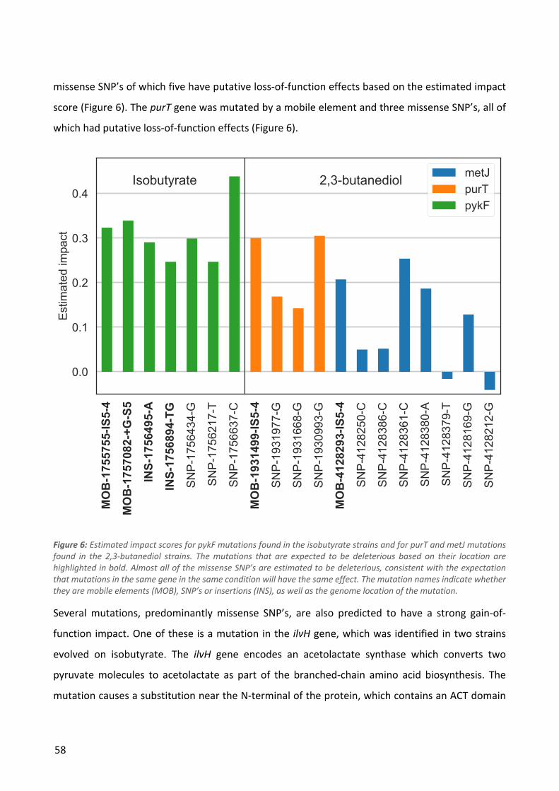
58

missense SNP’s of which five have putative loss-of-function effects based on the estimated impact

score (Figure 6). The purT gene was mutated by a mobile element and three missense SNP’s, all of

which had putative loss-of-function effects (Figure 6).

Figure 6: Estimated impact scores for pykF mutations found in the isobutyrate strains and for purT and metJ mutations found in the 2,3-butanediol strains. The mutations that are expected to be deleterious based on their location are highlighted in bold. Almost all of the missense SNP’s are estimated to be deleterious, consistent with the expectation that mutations in the same gene in the same condition will have the same effect. The mutation names indicate whether they are mobile elements (MOB), SNP’s or insertions (INS), as well as the genome location of the mutation.

Several mutations, predominantly missense SNP’s, are also predicted to have a strong gain-of-

function impact. One of these is a mutation in the ilvH gene, which was identified in two strains

evolved on isobutyrate. The ilvH gene encodes an acetolactate synthase which converts two

pyruvate molecules to acetolactate as part of the branched-chain amino acid biosynthesis. The

mutation causes a substitution near the N-terminal of the protein, which contains an ACT domain

MOB-1755755-IS

5-4

MOB-1757082-+G-S5

INS-1756495-A

INS-1756894-TG

SNP-1756434-G

SNP-1756217-T

SNP-1756637-C

MOB-1931499-IS

5-4

SNP-1931977-G

SNP-1931668-G

SNP-1930993-G

MOB-4128293-IS

5-4

SNP-4128250-C

SNP-4128386-C

SNP-4128361-C

SNP-4128380-A

SNP-4128379-T

SNP-4128169-G

SNP-4128212-G

0.0

0.1

0.2

0.3

0.4

Estimated

impact

Isobutyrate 2,3-butanediol metJpurTpykF

59

responsible for feedback inhibition by valine. The strains harboring the mutation had increased

levels of valine (see Supplementary Figure 1), consistent with a disruption of feedback regulation of

valine biosynthesis. Such a deregulation of an enzyme would indeed be an example of a gain-of-

function mutation, as the catalytic activity would be expected to increase. The enzymatic conversion

of pyruvate into acetolactate is also the first step of the isobutyrate biosynthesis pathway that was

inserted into the evolved strains (Zhang et al., 2011). Interestingly, the strains with the mutation in

ilvH or an equivalent mutation in the ACT domain mutation of the isozyme ilvN seemed to be able

to produce isobutyrate significantly better than the other evolved strains (Chapter 1, Figure 6b

(IBUA8-3 and IBUA8-10)). This could indicate that conversion of pyruvate into acetolactate is a

limiting step in the production pathway due to allosteric inhibition by valine. Since valine and

isobutyrate are chemically similar, it is also possible that the acetolactate synthase is inhibited by

isobutyrate, resulting in deficient production of branched-chain amino acids.

Another example of a mutation predicted to have a gain-of-function effect is a nonsense mutation

in the rpoS gene, found in the isobutyrate strains, which encodes the stress-associated sigma factor,

VW. Although the induced stop codon truncates the protein by 54 amino acids, removing the sigma

factor’s domain 4 in its entirety, the estimated impact score of the mutation suggests that it confers

a gain-of-function. In vitro experiments have shown that the deletion of domain 4, does not abolish

the activity of VW (Gowrishankar et al., 2003). If deletion of domain 4 affects the regulation of VW it

is possible that this will have a positive effect on VW activity.

Overall, the linear model based on metabolic profiles of the evolved strains and knockout strains

shows predictive value in estimating the impact a given mutation has on the gene(s) it affects,

although the accuracy is hard to assess due to the true impact of most of the observed mutations

being unknown. Since the data for the knockout strains need only be collected once for a given

organism, metabolic profiling of evolved strains can be an easy way to gain some insight into the

nature of the observed mutations. A drawback of the method is that the metabolic effects of

knockouts can only be measured for non-essential genes. Thus, the method is unable to provide

information on mutations that affect essential genes. A potential solution to this challenge would

be to use a library of over- or underexpression strains as references either for all genes or just for

the essential genes.

60

2.3.2 Perturbation time-course metabolomics

The results presented above allow some insight to be gained into how the evolved strains have

achieved tolerance, but in order to completely describe this process, the mechanisms of toxicity for

the ALE conditions must be known. The nature of the toxic effects of the ALE compounds were

investigated by perturbing wild-type MG1655 with each of nine chemicals and measuring the short-

term metabolic responses. This approach allows detection of direct interactions between

metabolism and the perturbing chemical, and thus quantification of the degree to which the toxic

effects are related to metabolism. To avoid major problems with ion suppression in the mass

spectrometry measurements, perturbation concentrations in the 160-180 µM range were used.

Even though this was significantly below the concentrations used in the ALE experiments as well as

the minimal inhibitory concentrations (Chapter 1, Supplementary Figure 1), it was hypothesized that

direct metabolic effects, e.g. from allosteric inhibition might still be observed. In addition to the nine

ALE chemicals, a range of control perturbations were also carried out. The control compounds

included antibiotics, amino acids, a synthetic uncoupler of the proton gradient and an oxidative

stressor (Table 1). The purpose of the control compounds was to validate that the experimental

method can be used to detect known metabolic responses. Furthermore, in case such responses

could be detected, it might be possible to compare the response to a chemical with unknown

mechanism of toxicity to the responses to the control compounds, for which the effects are largely

known.

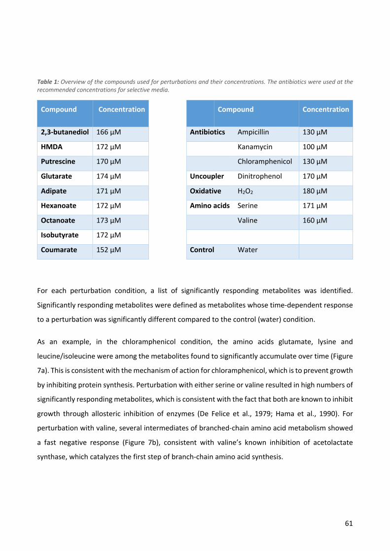
61

Table 1: Overview of the compounds used for perturbations and their concentrations. The antibiotics were used at the recommended concentrations for selective media.

Compound Concentration Compound Concentration

2,3-butanediol 166 µM Antibiotics Ampicillin 130 µM

HMDA 172 µM Kanamycin 100 µM

Putrescine 170 µM Chloramphenicol 130 µM

Glutarate 174 µM Uncoupler Dinitrophenol 170 µM

Adipate 171 µM Oxidative H2O2 180 µM

Hexanoate 172 µM Amino acids Serine 171 µM

Octanoate 173 µM Valine 160 µM

Isobutyrate 172 µM

Coumarate 152 µM Control Water

For each perturbation condition, a list of significantly responding metabolites was identified.

Significantly responding metabolites were defined as metabolites whose time-dependent response

to a perturbation was significantly different compared to the control (water) condition.

As an example, in the chloramphenicol condition, the amino acids glutamate, lysine and

leucine/isoleucine were among the metabolites found to significantly accumulate over time (Figure

7a). This is consistent with the mechanism of action for chloramphenicol, which is to prevent growth

by inhibiting protein synthesis. Perturbation with either serine or valine resulted in high numbers of

significantly responding metabolites, which is consistent with the fact that both are known to inhibit

growth through allosteric inhibition of enzymes (De Felice et al., 1979; Hama et al., 1990). For

perturbation with valine, several intermediates of branched-chain amino acid metabolism showed

a fast negative response (Figure 7b), consistent with valine’s known inhibition of acetolactate

synthase, which catalyzes the first step of branch-chain amino acid synthesis.

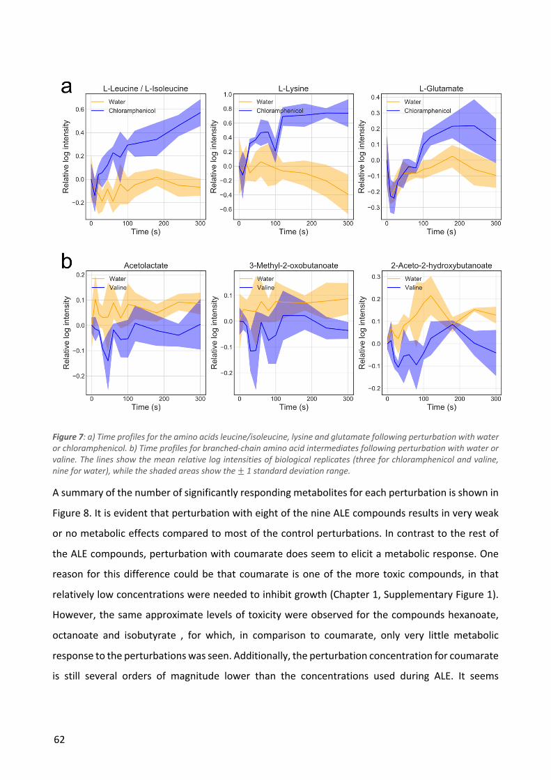
62

Figure 7: a) Time profiles for the amino acids leucine/isoleucine, lysine and glutamate following perturbation with water or chloramphenicol. b) Time profiles for branched-chain amino acid intermediates following perturbation with water or valine. The lines show the mean relative log intensities of biological replicates (three for chloramphenicol and valine, nine for water), while the shaded areas show the ± 1 standard deviation range.

A summary of the number of significantly responding metabolites for each perturbation is shown in

Figure 8. It is evident that perturbation with eight of the nine ALE compounds results in very weak

or no metabolic effects compared to most of the control perturbations. In contrast to the rest of

the ALE compounds, perturbation with coumarate does seem to elicit a metabolic response. One

reason for this difference could be that coumarate is one of the more toxic compounds, in that

relatively low concentrations were needed to inhibit growth (Chapter 1, Supplementary Figure 1).

However, the same approximate levels of toxicity were observed for the compounds hexanoate,

octanoate and isobutyrate , for which, in comparison to coumarate, only very little metabolic

response to the perturbations was seen. Additionally, the perturbation concentration for coumarate

is still several orders of magnitude lower than the concentrations used during ALE. It seems

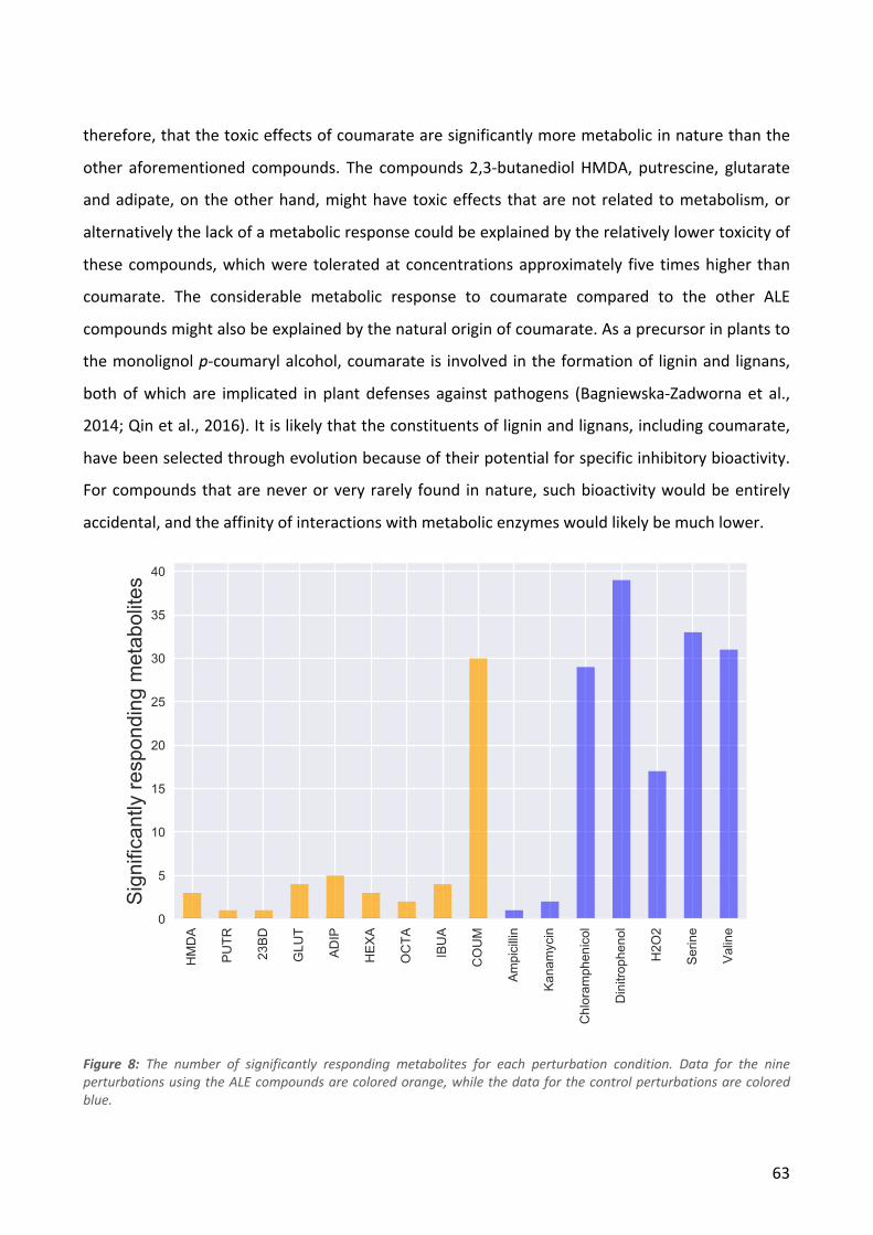
63

therefore, that the toxic effects of coumarate are significantly more metabolic in nature than the

other aforementioned compounds. The compounds 2,3-butanediol HMDA, putrescine, glutarate

and adipate, on the other hand, might have toxic effects that are not related to metabolism, or

alternatively the lack of a metabolic response could be explained by the relatively lower toxicity of

these compounds, which were tolerated at concentrations approximately five times higher than

coumarate. The considerable metabolic response to coumarate compared to the other ALE

compounds might also be explained by the natural origin of coumarate. As a precursor in plants to

the monolignol p-coumaryl alcohol, coumarate is involved in the formation of lignin and lignans,

both of which are implicated in plant defenses against pathogens (Bagniewska-Zadworna et al.,

2014; Qin et al., 2016). It is likely that the constituents of lignin and lignans, including coumarate,

have been selected through evolution because of their potential for specific inhibitory bioactivity.

For compounds that are never or very rarely found in nature, such bioactivity would be entirely

accidental, and the affinity of interactions with metabolic enzymes would likely be much lower.

Figure 8: The number of significantly responding metabolites for each perturbation condition. Data for the nine perturbations using the ALE compounds are colored orange, while the data for the control perturbations are colored blue.

64

While the results from the control perturbations show that metabolic responses to a chemical

perturbation can be detected using time-course metabolomics, only little information could be

gained on the ALE compounds. Since a likely reason for the limited metabolic response to eight out

of nine ALE compounds is that the perturbation concentrations were too low, the method might be

better suited for investigating chemicals that are toxic at such low concentrations. On the contrary,

the results for ampicillin and kanamycin, which were used at concentrations at which growth is

inhibited, show that a metabolic response will not necessarily be seen just because the compound

is toxic at the perturbation concentration. The lack of metabolic responses for these two antibiotics

can be explained by their mechanisms of action: Ampicillin inhibits the synthesis of cell wall (Tomasz,

1979), while kanamycin causes mistranslation (Davies and Wright, 1971), both of which will likely

only have a modest effect on cell metabolism within the time-frame of the experiment.

In cases where a metabolic response is detected, it would in principle be possible to use the

responses of each metabolite to identify the specific mechanism of toxicity of a given chemical, e.g.

targets for allosteric inhibition. As this would allow rapid identification of chemical-metabolism

interactions, future work focusing on this aspect would be of value.

2.4 Conclusions

In this study high-throughput metabolomics was used to metabolically characterize a group of

strains evolved to tolerate nine different chemicals, and to investigate the mechanisms of action for

these chemicals. The metabolic profile characterizations of the evolved tolerant strains showed a

strong association between metabolic profile and the condition each strain was evolved under.

Additionally, a characteristic metabolic phenotype for a given evolution condition was often

observed across strains with very little or no genetic commonality. This indicates that the metabolic

phenotype is representative of the phenotypic changes that lead to improved tolerance, and that

tolerance against a given chemical is achieved through very similar phenotypic mechanisms even

though different strains have found different mutational paths to this phenotype. Taking advantage

of previously published data on the metabolic effects of single-gene knockouts in E. coli, it was

possible to use the metabolic profiles of the evolved strains to infer the impact of individual

mutations on the functionality of the affected gene. Although the method showed promising

65

potential for differentiating between deleterious and non-deleterious mutations, additional

validation is needed on mutations with known effects.

Using time-course metabolomics in perturbation experiments to elucidate details of chemical

toxicity proved to be difficult due to technical limitations on perturbation concentrations in

combination with the relatively low toxicity of some chemicals. However, results for a set of control

perturbations suggested that the metabolomics approach can be used to quantify the degree of

metabolic response to a chemical perturbation. Specific metabolite responses consistent with the

known effects of two different control perturbations could be identified, demonstrating that the

method might be used to infer mechanisms of action from the observed responses.

2.5 References

Bagniewska-Zadworna, A., Barakat, A., Łakomy, P., Smoliński, D.J., Zadworny, M., 2014. Lignin and

lignans in plant defence: Insight from expression profiling of cinnamyl alcohol dehydrogenase

genes during development and following fungal infection in Populus. Plant Sci. 229, 111–121.

https://doi.org/10.1016/j.plantsci.2014.08.015

Benjamini, Y., Hochberg, Y., 1995. Controlling the False Discovery Rate: a Practical and Powerful

Approach to Multiple Testing. J. R. Stat. Soc. Ser. B 57, 289–300.

Davies, J., Wright, G.D., 1971. Bacterial resistance to aminoglycoside antibiotics. J. Infect. Dis. 124,

S7–S10. https://doi.org/10.1093/infdis/124.Supplement_1.S7

De Felice, M., Levinthal, M., Iaccarino, M., Guardiola, J., 1979. Growth inhibition as a consequence

of antagonism between related amino acids: Effect of valine in Escherichia coli K-12.

Microbiol. Rev. 43, 42–58.

Fuhrer, T., Heer, D., Begemann, B., Zamboni, N., 2011. High-throughput, accurate mass

metabolome profiling of cellular extracts by flow injection-time-of-flight mass spectrometry.

Anal. Chem. 83, 7074–7080. https://doi.org/10.1021/ac201267k

Fuhrer, T., Zamboni, N., 2015. High-throughput discovery metabolomics. Curr. Opin. Biotechnol.

66

31, 73–78. https://doi.org/10.1016/j.copbio.2014.08.006

Fuhrer, T., Zampieri, M., Sévin, D.C., Sauer, U., Zamboni, N., 2017. Genomewide landscape of

gene–metabolome associations in Escherichia coli. Mol. Syst. Biol. 13, 907.

https://doi.org/10.15252/msb.20167150

Gisbrecht, A., Hammer, B., 2015. Data visualization by nonlinear dimensionality reduction. Wiley

Interdiscip. Rev. Data Min. Knowl. Discov. 5, 51–73. https://doi.org/10.1002/widm.1147

Gowrishankar, J., Yamamoto, K., Subbarayan, P.R., Ishimana, A., 2003. In Vitro Properties of RpoS

Mutants of Escherichia coli with Postulated N-Terminal Subregion 1.1 or C-Terminal Region 4

Deleted. J. Bacteriol. 185, 2673–2679. https://doi.org/10.1128/JB.185.8.2673

Griffiths, W.J., Wang, Y., 2010. Mass Spectrometry in Metabolomics, in: Molecular Analysis and

Genome Discovery: Second Edition. John Wiley and Sons, pp. 271–298.

Hama, H., Sumita, Y., Kakutani, Y., Tsuda, M., Tsuchiya, T., 1990. Target of serine inhibition in

Escherichia coli. Biochem. Biophys. Res. Commun. 168, 1–6.

Niedenführ, S., Wiechert, W., Nöh, K., 2015. How to measure metabolic fluxes: A taxonomic guide

for 13C fluxomics. Curr. Opin. Biotechnol. 34, 82–90.


Orth, J.D., Conrad, T.M., Na, J., Lerman, J. a, Nam, H., Feist, A.M., Palsson, B.Ø., 2011. A

comprehensive genome-scale reconstruction of Escherichia coli metabolism. Mol. Syst. Biol.

7, 1–9. https://doi.org/10.1038/msb.2011.65

Qin, L., Li, W.C., Liu, L., Zhu, J.Q., Li, X., Li, B.Z., Yuan, Y.J., 2016. Inhibition of lignin-derived phenolic

compounds to cellulase. Biotechnol. Biofuels 9, 1–10. https://doi.org/10.1186/s13068-016-

0485-2

Seol, W., Shatkin, A.J., 1991. Escherichia coli kgtP encodes an alpha-ketoglutarate transporter.

Proc. Natl. Acad. Sci. 88, 3802–3806.

Tan, P.-N., Steinbach, M., Kumar, V., 2005. Introduction to data mining, 1st ed. Pearson Addison

67

Wesley, Boston.

Tomasz, A., 1979. The Mechanism of the Irreversible Antimicrobial Effects of Penicillins: How the

Beta-Lactam Antibiotics Kill and Lyse Bacteria. Annu. Rev. Microbiol. 33, 113–137.

https://doi.org/10.1146/annurev.mi.33.100179.000553

Uyeda, K., 2006. Phosphofructokinase, in: Advances in Enzymology and Related Areas of Molecular

Biology. John Wiley & Sons, Ltd, pp. 193–244. https://doi.org/10.1002/9780470122938.ch4

van der Maaten, L., Hinton, G., 2008. Visualizing Data using t-SNE. J. Mach. Learn. Res. 9, 2579–

2605.

Yan, D., Lenz, P., Hwa, T., 2011. Overcoming fluctuation and leakage problems in the quantification

of intracellular 2-oxoglutarate levels in Escherichia coli. Appl. Environ. Microbiol. 77, 6763–

6771. https://doi.org/10.1128/AEM.05257-11

Zhang, K., Woodruff, A.P., Xiong, M., Zhou, J., Dhande, Y.K., 2011. A synthetic metabolic pathway

for production of the platform chemical isobutyric acid. ChemSusChem 4, 1068–1070.

https://doi.org/10.1002/cssc.201100045

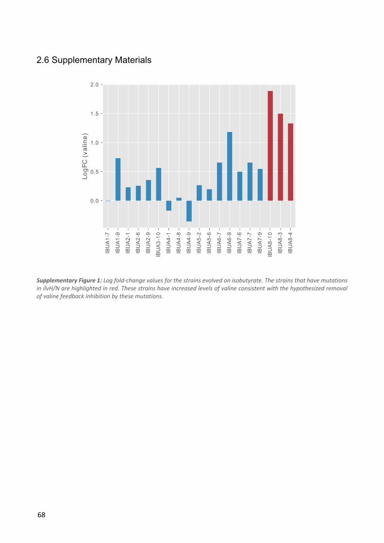
68


Supplementary Figure 1: Log fold-change values for the strains evolved on isobutyrate. The strains that have mutations in ilvH/N are highlighted in red. These strains have increased levels of valine consistent with the hypothesized removal of valine feedback inhibition by these mutations.

69

Chapter 3: A deep neural network for propagation of signals

through a metabolic network

3.1 Introduction

In recent years there has been a rapid increase in the performance of machine learning algorithms

on a variety of problems. The main factor in this trend has been the advent of deep neural networks

(LeCun, Bengio, & Hinton, 2015). Traditional neural networks, also known as multilayer perceptrons

(MLP), have been in use since the 1980’s (Hopfield, 1988), but had started to lose popularity in the

2000’s in favor of other algorithms such as support vector machines and other kernel-based

methods (Hofmann, Schölkopf, & Smola, 2008).

One of the features that has allowed modern deep neural networks to outperform most other

machine learning algorithms is the introduction of specialized layer architectures in addition to the

fully connected hidden layers found in MLP’s (LeCun et al., 2015). The most widespread specialized

architectures are convolutional layers, which have successfully been used to process image,

tomogram, and video data (Bernal et al., 2018; Karpathy et al., 2014; Krizhevsky, Sutskever, &

Hinton, 2012), and recurrent layers which have allowed advances in analysis of sequence data,

particularly in natural language processing (Bahdanau, Cho, & Bengio, 2015; Lipton, Berkowitz, &

Elkan, 2015). Whereas traditional MLP’s and other machine learning algorithms usually require that

each data point is described by a vector of features, a large advantage of convolutional layers and

recurrent layers is that they can take input without or with only minimal processing, e.g. raw pixel

or text data. They can thus function as trainable feature extractors, that can learn to derive

characteristics from the data with predictive value for the given problem.

Various problems within biology have benefited from the use of convolutional as well as recurrent

neural networks. Convolutional networks have for example been used to identifying binding motifs

for DNA- and RNA-binding proteins using a convolutional layer as trainable position weight matrices

(Alipanahi, Delong, Weirauch, & Frey, 2015) and automated detection of subcellular protein

localization in yeast from microscopy images (Pärnamaa & Parts, 2017). Recurrent neural networks

in turn have been used among other things to predict protein secondary structure from amino acid

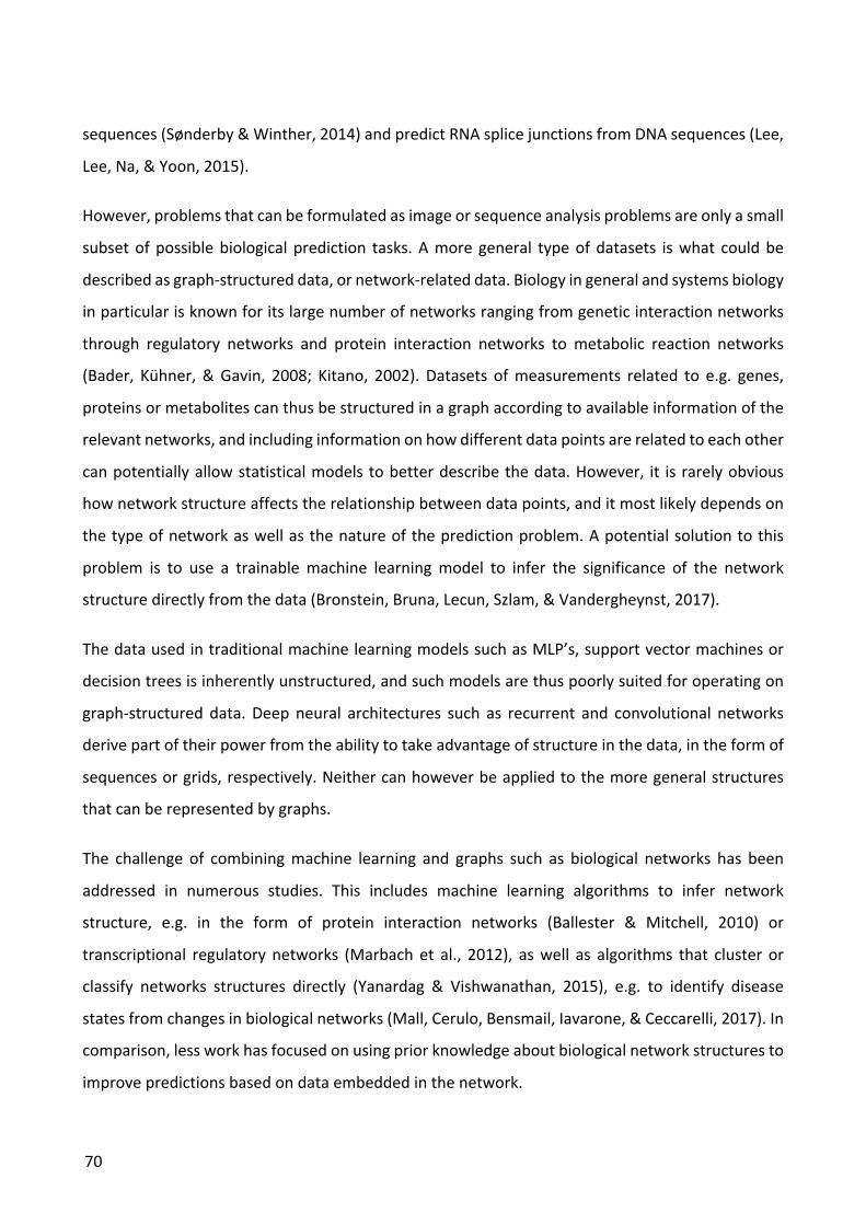
70

sequences (Sønderby & Winther, 2014) and predict RNA splice junctions from DNA sequences (Lee,

Lee, Na, & Yoon, 2015).

However, problems that can be formulated as image or sequence analysis problems are only a small

subset of possible biological prediction tasks. A more general type of datasets is what could be

described as graph-structured data, or network-related data. Biology in general and systems biology

in particular is known for its large number of networks ranging from genetic interaction networks

through regulatory networks and protein interaction networks to metabolic reaction networks

(Bader, Kühner, & Gavin, 2008; Kitano, 2002). Datasets of measurements related to e.g. genes,

proteins or metabolites can thus be structured in a graph according to available information of the

relevant networks, and including information on how different data points are related to each other

can potentially allow statistical models to better describe the data. However, it is rarely obvious

how network structure affects the relationship between data points, and it most likely depends on

the type of network as well as the nature of the prediction problem. A potential solution to this

problem is to use a trainable machine learning model to infer the significance of the network

structure directly from the data (Bronstein, Bruna, Lecun, Szlam, & Vandergheynst, 2017).

The data used in traditional machine learning models such as MLP’s, support vector machines or

decision trees is inherently unstructured, and such models are thus poorly suited for operating on

graph-structured data. Deep neural architectures such as recurrent and convolutional networks

derive part of their power from the ability to take advantage of structure in the data, in the form of

sequences or grids, respectively. Neither can however be applied to the more general structures

that can be represented by graphs.

The challenge of combining machine learning and graphs such as biological networks has been

addressed in numerous studies. This includes machine learning algorithms to infer network

structure, e.g. in the form of protein interaction networks (Ballester & Mitchell, 2010) or

transcriptional regulatory networks (Marbach et al., 2012), as well as algorithms that cluster or

classify networks structures directly (Yanardag & Vishwanathan, 2015), e.g. to identify disease

states from changes in biological networks (Mall, Cerulo, Bensmail, Iavarone, & Ceccarelli, 2017). In

comparison, less work has focused on using prior knowledge about biological network structures to

improve predictions based on data embedded in the network.

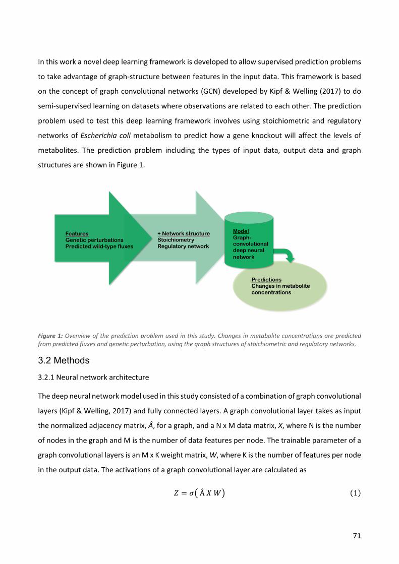
71

In this work a novel deep learning framework is developed to allow supervised prediction problems

to take advantage of graph-structure between features in the input data. This framework is based

on the concept of graph convolutional networks (GCN) developed by Kipf & Welling (2017) to do

semi-supervised learning on datasets where observations are related to each other. The prediction

problem used to test this deep learning framework involves using stoichiometric and regulatory

networks of Escherichia coli metabolism to predict how a gene knockout will affect the levels of

metabolites. The prediction problem including the types of input data, output data and graph

structures are shown in Figure 1.

Figure 1: Overview of the prediction problem used in this study. Changes in metabolite concentrations are predicted from predicted fluxes and genetic perturbation, using the graph structures of stoichiometric and regulatory networks.

3.2 Methods

3.2.1 Neural network architecture

The deep neural network model used in this study consisted of a combination of graph convolutional

layers (Kipf & Welling, 2017) and fully connected layers. A graph convolutional layer takes as input

the normalized adjacency matrix, Â, for a graph, and a N x M data matrix, X, where N is the number

of nodes in the graph and M is the number of data features per node. The trainable parameter of a

graph convolutional layers is an M x K weight matrix, W, where K is the number of features per node

in the output data. The activations of a graph convolutional layer are calculated as

Y = V1ÂQR9 (1)

+ Network structureStoichiometryRegulatory network

ModelGraph-convolutional deep neuralnetwork

PredictionsChanges in metaboliteconcentrations

FeaturesGenetic perturbationsPredicted wild-type fluxes

72

where V is the chosen non-linearity function (Kipf & Welling, 2017). The adjacency matrix is

normalized using its degree matrix, D

Â = <\]^_<\

]^ (2)

which preserves symmetry in the adjacency matrix and ensures that all rows sum to one (Kipf &

Welling, 2017).

The graph convolutional layers used here were extended to allow the simultaneous use of several

graph structures of a given set of nodes. The activations were instead calculated as

Y = V(`ÂGQRG

a

Gb]

) (3)

with i denoting the index of each graph structure and the corresponding weight matrix. During

training this was implemented by letting Â be an L x N x N tensor and W be an L x M x K tensor and

summing over the dimension corresponding to L.

Four consecutive graph convolutional layers were used with the output of one feeding into the next.

The activations from each of the four graph convolutional layers were concatenated into a single

layer, yielding an N X TcDC matrix, with TcDC being the sum of K in each respective layer. This

corresponds to an individual feature vector of length TcDC for each node in the graph. Finally, these

feature vectors were fed into an MLP with a single hidden layer ending with a softmax output layer.

The weights of this MLP were shared between all graph nodes.

All layers except the output layer used the leaky rectified nonlinearity (Maas, Hannun, & Ng, 2013):

d(!) = e!2d! > 00.01 ∙ !2d! ≤ 0 (4)

3.2.2 Training data

The dataset used for training was obtained from the online supplementary material of Fuhrer,

Zampieri, Sévin, Sauer, & Zamboni (2017).

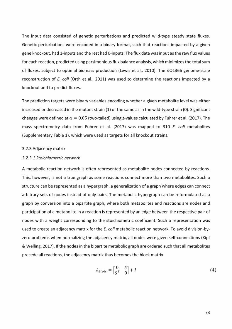
73

The input data consisted of genetic perturbations and predicted wild-type steady state fluxes.

Genetic perturbations were encoded in a binary format, such that reactions impacted by a given

gene knockout, had 1-inputs and the rest had 0-inputs. The flux data was input as the raw flux values

for each reaction, predicted using parsimonious flux balance analysis, which minimizes the total sum

of fluxes, subject to optimal biomass production (Lewis et al., 2010). The iJO1366 genome-scale

reconstruction of E. coli (Orth et al., 2011) was used to determine the reactions impacted by a

knockout and to predict fluxes.

The prediction targets were binary variables encoding whether a given metabolite level was either

increased or decreased in the mutant strain (1) or the same as in the wild-type strain (0). Significant

changes were defined at : = 0.05 (two-tailed) using z-values calculated by Fuhrer et al. (2017). The

mass spectrometry data from Fuhrer et al. (2017) was mapped to 310 E. coli metabolites

(Supplementary Table 1), which were used as targets for all knockout strains.

3.2.3 Adjacency matrix

3.2.3.1 Stoichiometric network

A metabolic reaction network is often represented as metabolite nodes connected by reactions.

This, however, is not a true graph as some reactions connect more than two metabolites. Such a

structure can be represented as a hypergraph, a generalization of a graph where edges can connect

arbitrary sets of nodes instead of only pairs. The metabolic hypergraph can be reformulated as a

graph by conversion into a bipartite graph, where both metabolites and reactions are nodes and

participation of a metabolite in a reaction is represented by an edge between the respective pair of

nodes with a weight corresponding to the stoichiometric coefficient. Such a representation was

used to create an adjacency matrix for the E. coli metabolic reaction network. To avoid division-by-

zero problems when normalizing the adjacency matrix, all nodes were given self-connections (Kipf

& Welling, 2017). If the nodes in the bipartite metabolic graph are ordered such that all metabolites

precede all reactions, the adjacency matrix thus becomes the block matrix

_W*IGH = k 0 llm 0

n + o (4)

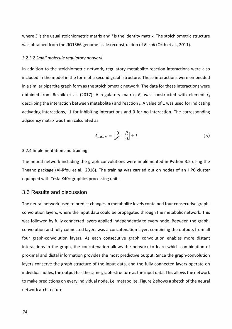
74

where S is the usual stoichiometric matrix and I is the identity matrix. The stoichiometric structure

was obtained from the iJO1366 genome-scale reconstruction of E. coli (Orth et al., 2011).

3.2.3.2 Small molecule regulatory network

In addition to the stoichiometric network, regulatory metabolite-reaction interactions were also

included in the model in the form of a second graph structure. These interactions were embedded

in a similar bipartite graph form as the stoichiometric network. The data for these interactions were

obtained from Reznik et al. (2017). A regulatory matrix, R, was constructed with element rij

describing the interaction between metabolite i and reaction j. A value of 1 was used for indicating

activating interactions, -1 for inhibiting interactions and 0 for no interaction. The corresponding

adjacency matrix was then calculated as

_Wpqr = k 0 ssm 0

n + o (5)

3.2.4 Implementation and training

The neural network including the graph convolutions were implemented in Python 3.5 using the

Theano package (Al-Rfou et al., 2016). The training was carried out on nodes of an HPC cluster

equipped with Tesla K40c graphics processing units.


The neural network used to predict changes in metabolite levels contained four consecutive graph-

convolution layers, where the input data could be propagated through the metabolic network. This

was followed by fully connected layers applied independently to every node. Between the graph-

convolution and fully connected layers was a concatenation layer, combining the outputs from all

four graph-convolution layers. As each consecutive graph convolution enables more distant

interactions in the graph, the concatenation allows the network to learn which combination of

proximal and distal information provides the most predictive output. Since the graph-convolution

layers conserve the graph structure of the input data, and the fully connected layers operate on

individual nodes, the output has the same graph-structure as the input data. This allows the network

to make predictions on every individual node, i.e. metabolite. Figure 2 shows a sketch of the neural

network architecture.

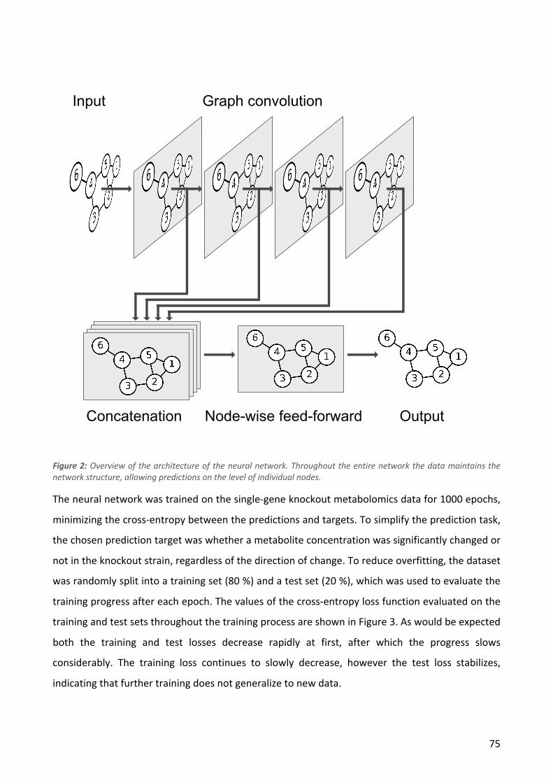
75

Figure 2: Overview of the architecture of the neural network. Throughout the entire network the data maintains the network structure, allowing predictions on the level of individual nodes.

The neural network was trained on the single-gene knockout metabolomics data for 1000 epochs,

minimizing the cross-entropy between the predictions and targets. To simplify the prediction task,

the chosen prediction target was whether a metabolite concentration was significantly changed or

not in the knockout strain, regardless of the direction of change. To reduce overfitting, the dataset

was randomly split into a training set (80 %) and a test set (20 %), which was used to evaluate the

training progress after each epoch. The values of the cross-entropy loss function evaluated on the

training and test sets throughout the training process are shown in Figure 3. As would be expected

both the training and test losses decrease rapidly at first, after which the progress slows

considerably. The training loss continues to slowly decrease, however the test loss stabilizes,

indicating that further training does not generalize to new data.

Input Graph convolution

Concatenation Node-wise feed-forward Output

76

Figure 3: The values of the cross-entropy loss function evaluated on the training and test sets, respectively, following each training epoch.

The network weights from the epoch with the best test performance were chosen for further

evaluation. The overall balanced accuracy of the predictions on the test set was 0.58. Figure 4 shows

summary plots of the prediction results. Figure 4a shows the positive prediction rates for the actual

negatives (no change) and actual positives (change) respectively, while Figure 4b shows the

distributions of output scores and Figure 4c shows the receiver operating characteristic. These

results suggest that the neural network has derived some predictive value from the input data and

the graph structure, although the predictive performance is only slightly better than random

guessing. The plots in Figure 4 also indicate that the predictions show a clear bias towards positive

predictions, despite the dataset containing only around 5 % positive examples.

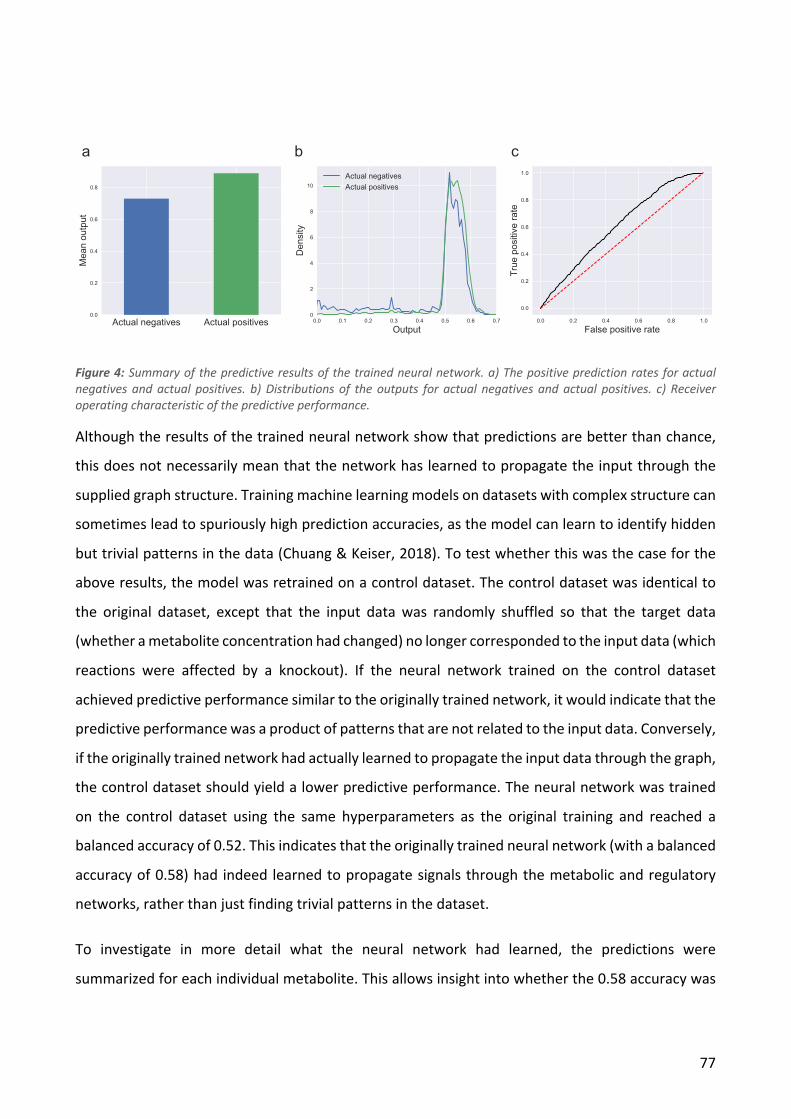
77

Figure 4: Summary of the predictive results of the trained neural network. a) The positive prediction rates for actual negatives and actual positives. b) Distributions of the outputs for actual negatives and actual positives. c) Receiver operating characteristic of the predictive performance.

Although the results of the trained neural network show that predictions are better than chance,

this does not necessarily mean that the network has learned to propagate the input through the

supplied graph structure. Training machine learning models on datasets with complex structure can

sometimes lead to spuriously high prediction accuracies, as the model can learn to identify hidden

but trivial patterns in the data (Chuang & Keiser, 2018). To test whether this was the case for the

above results, the model was retrained on a control dataset. The control dataset was identical to

the original dataset, except that the input data was randomly shuffled so that the target data

(whether a metabolite concentration had changed) no longer corresponded to the input data (which

reactions were affected by a knockout). If the neural network trained on the control dataset

achieved predictive performance similar to the originally trained network, it would indicate that the

predictive performance was a product of patterns that are not related to the input data. Conversely,

if the originally trained network had actually learned to propagate the input data through the graph,

the control dataset should yield a lower predictive performance. The neural network was trained

on the control dataset using the same hyperparameters as the original training and reached a

balanced accuracy of 0.52. This indicates that the originally trained neural network (with a balanced

accuracy of 0.58) had indeed learned to propagate signals through the metabolic and regulatory

networks, rather than just finding trivial patterns in the dataset.

To investigate in more detail what the neural network had learned, the predictions were

summarized for each individual metabolite. This allows insight into whether the 0.58 accuracy was

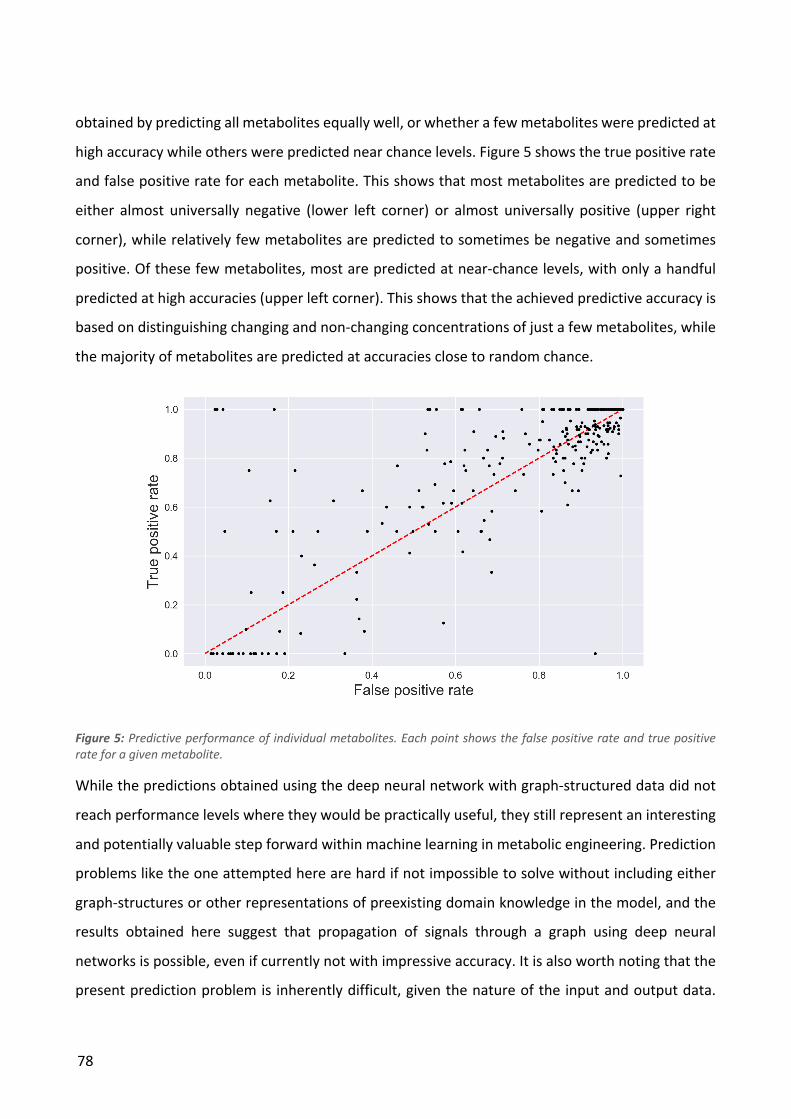
78

obtained by predicting all metabolites equally well, or whether a few metabolites were predicted at

high accuracy while others were predicted near chance levels. Figure 5 shows the true positive rate

and false positive rate for each metabolite. This shows that most metabolites are predicted to be

either almost universally negative (lower left corner) or almost universally positive (upper right

corner), while relatively few metabolites are predicted to sometimes be negative and sometimes

positive. Of these few metabolites, most are predicted at near-chance levels, with only a handful

predicted at high accuracies (upper left corner). This shows that the achieved predictive accuracy is

based on distinguishing changing and non-changing concentrations of just a few metabolites, while

the majority of metabolites are predicted at accuracies close to random chance.

Figure 5: Predictive performance of individual metabolites. Each point shows the false positive rate and true positive rate for a given metabolite.

While the predictions obtained using the deep neural network with graph-structured data did not

reach performance levels where they would be practically useful, they still represent an interesting

and potentially valuable step forward within machine learning in metabolic engineering. Prediction

problems like the one attempted here are hard if not impossible to solve without including either

graph-structures or other representations of preexisting domain knowledge in the model, and the

results obtained here suggest that propagation of signals through a graph using deep neural

networks is possible, even if currently not with impressive accuracy. It is also worth noting that the

present prediction problem is inherently difficult, given the nature of the input and output data.

79

Most machine learning problems use a rich set of input features to predict one or a few outputs,

while the prediction of metabolic changes from genetic perturbations uses a sparse input vector to

predict a rich set of output features. Future work on graph-structured deep learning might focus on

amending the input data with further informative features and experimenting with additional graph

relationships between the nodes.

3.4 Conclusion

In this study a novel deep neural network was presented for propagating input signals through

graph-structured stoichiometric and regulatory networks of metabolites and reactions. The network

was tested by using genetic knockouts to predict changes in metabolite levels throughout the

metabolic network. The obtained balanced accuracy of 0.58 showed that the network could learn

some rules for relating genetic perturbations to metabolite levels, but further investigation showed

that the performance was driven by good predictions on a few metabolites and near-chance

predictions on most metabolites. Training the network on a control dataset showed that the

predictive performance can indeed largely be ascribed to propagation of the input signals through

the supplied graph-structures.

3.5 References Al-Rfou, R., Alain, G., Almahairi, A., Angermueller, C., Bahdanau, D., Ballas, N., … Zhang, Y. (2016).

Theano: A Python framework for fast computation of mathematical expressions. ArXiv,

abs/1605.0. Retrieved from http://arxiv.org/abs/1605.02688

Alipanahi, B., Delong, A., Weirauch, M. T., & Frey, B. J. (2015). Predicting the sequence specificities

of DnA- and RnA-binding proteins by deep learning. Nature Biotechnology, 33(8), 831–838.

https://doi.org/10.1038/nbt.3300

Bader, S., Kühner, S., & Gavin, A. (2008). Interaction networks for systems biology. FEBS Letters, 582,

1220–1224. https://doi.org/10.1016/j.febslet.2008.02.015

Bahdanau, D., Cho, K., & Bengio, Y. (2015). Neural Machine Translation by Jointly Learning to Align

and Translate. ArXiv.

Ballester, P. J., & Mitchell, J. B. O. (2010). A machine learning approach to predicting protein-ligand

binding affinity with applications to molecular docking. Bioinformatics, 26(9), 1169–1175.

https://doi.org/10.1093/bioinformatics/btq112

80

Bernal, J., Kushibar, K., Asfaw, D. S., Valverde, S., Oliver, A., Martí, R., & Lladó, X. (2018). Deep

convolutional neural networks for brain image analysis on magnetic resonance imaging: a

review. Artificial Intelligence In Medicine, 1–18. https://doi.org/10.1016/j.artmed.2018.08.008

Bronstein, M. M., Bruna, J., Lecun, Y., Szlam, A., & Vandergheynst, P. (2017). Geometric Deep

Learning: Going beyond Euclidean data. IEEE Signal Processing Magazine, 34(4), 18–42.

https://doi.org/10.1109/MSP.2017.2693418

Chuang, K. V, & Keiser, M. J. (2018). Comment on “Predicting reaction performance in C – N cross-

coupling using machine learning.” Science, 8603, 1–3.

Fuhrer, T., Zampieri, M., Sévin, D. C., Sauer, U., & Zamboni, N. (2017). Genomewide landscape of

gene–metabolome associations in Escherichia coli. Molecular Systems Biology, 13(1), 907.

https://doi.org/10.15252/msb.20167150

Hofmann, T., Schölkopf, B., & Smola, A. J. (2008). Kernel Methods in Machine Learning. The Annals

of Statistics, 36(3), 1171–1220. https://doi.org/10.1214/009053607000000677

Hopfield, J. J. (1988). Artificial Neural Networks. IEEE Circuits and Devices Magazine, 4(5), 3–10.

Karpathy, A., Toderici, G., Shetty, S., Leung, T., Sukthankar, R., & Fei-Fei, L. (2014). Large-scale Video

Classification with Convolutional Neural Networks. IEEE Conference on Computer Vision and

Pattern Recognition, 1725–1732. https://doi.org/10.1109/CVPR.2014.223

Kipf, T. N., & Welling, M. (2017). Semi-Supervised Classification with Graph Convolutional Networks.

In ICLR 2017 (pp. 1–14). https://doi.org/10.1051/0004-6361/201527329

Kitano, H. (2002). Systems Biology: A Brief Overview. Science, 295, 1662–1665.

Krizhevsky, A., Sutskever, I., & Hinton, G. E. (2012). ImageNet Classification with Deep Convolutional

Neural Networks. Proceedings of Advances in Neural Information Processing Systems, 25,

1090–10.

LeCun, Y., Bengio, Y., & Hinton, G. (2015). Deep learning. Nature, 521, 436–444.

https://doi.org/10.1038/nature14539

Lee, B., Lee, T., Na, B., & Yoon, S. (2015). DNA-Level Splice Junction Prediction using Deep Recurrent

Neural Networks. ArXiv.

Lewis, N. E., Hixson, K. K., Conrad, T. M., Lerman, J. A., Charusanti, P., Polpitiya, A. D., … Palsson, B.

(2010). Omic data from evolved E. coli are consistent with computed optimal growth from

genome-scale models. Molecular Systems Biology, 6(390).

81

https://doi.org/10.1038/msb.2010.47

Lipton, Z. C., Berkowitz, J., & Elkan, C. (2015). A Critical Review of Recurrent Neural Networks for

Sequence Learning. ArXiv.

Maas, A. L., Hannun, A. Y., & Ng, A. Y. (2013). Rectifier Nonlinearities Improve Neural Network

Acoustic Models. ArXiv. https://doi.org/10.1016/0010-0277(84)90022-2

Mall, R., Cerulo, L., Bensmail, H., Iavarone, A., & Ceccarelli, M. (2017). Detection of statistically

significant network changes in complex biological networks. BMC Systems Biology, 11(1), 1–17.

https://doi.org/10.1186/s12918-017-0412-6

Marbach, D., Costello, J. C., Küffner, R., Vega, N. M., Prill, R. J., Camacho, D. M., … Zimmer, R. (2012).

Wisdom of crowds for robust gene network inference. Nature Methods, 9(8), 796–804.

https://doi.org/10.1038/nmeth.2016

Orth, J. D., Conrad, T. M., Na, J., Lerman, J. a, Nam, H., Feist, A. M., & Palsson, B. Ø. (2011). A

comprehensive genome-scale reconstruction of Escherichia coli metabolism. Molecular

Systems Biology, 7(535), 1–9. https://doi.org/10.1038/msb.2011.65

Pärnamaa, T., & Parts, L. (2017). Accurate Classification of Protein Subcellular Localization from

High-Throughput Microscopy Images Using Deep Learning. Genes, Genomes, Genetics, 7,

1385–1392. https://doi.org/10.1534/g3.116.033654/-/DC1

Reznik, E., Christodoulou, D., Goldford, J. E., Briars, E., Sauer, U., Segrè, D., & Noor, E. (2017).

Genome-Scale Architecture of Small Molecule Regulatory Networks and the Fundamental

Trade-Off between Regulation and Enzymatic Activity. Cell Reports, 20(11), 2666–2677.

https://doi.org/10.1016/j.celrep.2017.08.066

Sønderby, S. K., & Winther, O. (2014). Protein Secondary Structure Prediction with Long Short Term

Memory Networks. ArXiv.

Yanardag, P., & Vishwanathan, S. V. N. (2015). Deep Graph Kernels. Proceedings of the 21th ACM

SIGKDD International Conference on Knowledge Discovery and Data Mining - KDD ’15, 1365–

1374. https://doi.org/10.1145/2783258.2783417

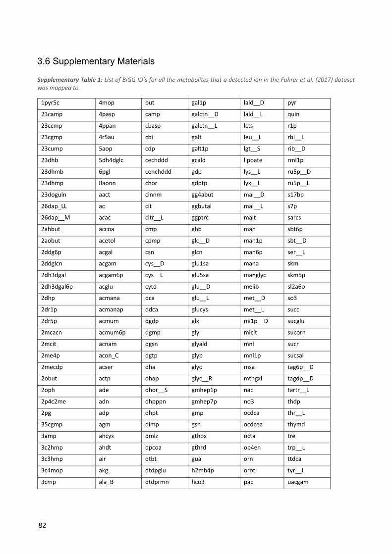
82


Supplementary Table 1: List of BiGG ID’s for all the metabolites that a detected ion in the Fuhrer et al. (2017) dataset was mapped to.

1pyr5c 4mop but gal1p lald__D pyr

23camp 4pasp camp galctn__D lald__L quin

23ccmp 4ppan cbasp galctn__L lcts r1p

23cgmp 4r5au cbi galt leu__L rbl__L

23cump 5aop cdp galt1p lgt__S rib__D

23dhb 5dh4dglc cechddd gcald lipoate rml1p

23dhmb 6pgl cenchddd gdp lys__L ru5p__D

23dhmp 8aonn chor gdptp lyx__L ru5p__L

23doguln aact cinnm gg4abut mal__D s17bp

26dap_LL ac cit ggbutal mal__L s7p

26dap__M acac citr__L ggptrc malt sarcs

2ahbut accoa cmp ghb man sbt6p

2aobut acetol cpmp glc__D man1p sbt__D

2ddg6p acgal csn glcn man6p ser__L

2ddglcn acgam cys__D glu1sa mana skm

2dh3dgal acgam6p cys__L glu5sa manglyc skm5p

2dh3dgal6p acglu cytd glu__D melib sl2a6o

2dhp acmana dca glu__L met__D so3

2dr1p acmanap ddca glucys met__L succ

2dr5p acmum dgdp glx mi1p__D sucglu

2mcacn acmum6p dgmp gly micit sucorn

2mcit acnam dgsn glyald mnl sucr

2me4p acon_C dgtp glyb mnl1p sucsal

2mecdp acser dha glyc msa tag6p__D

2obut actp dhap glyc__R mthgxl tagdp__D

2oph ade dhor__S gmhep1p nac tartr__L

2p4c2me adn dhpppn gmhep7p no3 thdp

2pg adp dhpt gmp ocdca thr__L

35cgmp agm dimp gsn ocdcea thymd

3amp ahcys dmlz gthox octa tre

3c2hmp ahdt dpcoa gthrd op4en trp__L

3c3hmp air dtbt gua orn ttdca

3c4mop akg dtdpglu h2mb4p orot tyr__L

3cmp ala_B dtdprmn hco3 pac uacgam

83

3dhq ala__D dtmp hdca pant__R uacmam

3dhsk ala__L dxyl5p hdcea pap udp

3gmp alaala e4p his__L paps udpacgal

3hcinnm all__D enter histd phe__L udpg

3hpp altrn f1p hom__L phpyr udpgal

3hpppn ametam f6p hqn pi ump

3mob amp fc1p hxan pnto__R ura

3mop ara5p fdp ichor ppal uri

3pg arbt fgam icit ppbng val__L

3ump arbt6p fpram ile__L ppgpp xan

4abut arg__L fprica indole pphn xmp

4ahmmp argsuc fru inost ppi xu5p__D

4ampm asn__L g1p ins pro__L xu5p__L

4c2me asp__L g3p itp pser__L xyl__D

4crsol aspsa g3pc kdo ptrc xylu__D

4hbz athr__L g3pe kdo8p pyam5p xylu__L

4hoxpacd atp g6p lac__D pydam

4hthr btal gal lac__L pydx5p

84

Part II: Model-based strain design

As previously mentioned, designing microbial strains for chemical production processes is a difficult

and time-consuming task. The first part of this thesis explored how non-rational methods,

particularly adaptive laboratory evolution (ALE), can be used to improve certain characteristics of

production strains. Some traits, such as tolerance as shown in Chapter 1, can be easily improved in

ALE experiments, but many production-related traits such as product yields or production rates that

cannot be trivially selected for, are harder to optimize with evolutionary processes. For this reason,

development of good production strains almost always also requires utilization of rational

engineering methods. Because of the complexity of microbial metabolism, and physiology in

general, genetically modifying a strain can sometimes have unintuitive effects on the functioning of

the cell, which makes rational design difficult. To aid in the understanding of how genetic

modifications impact cellular processes, mathematical models of the cell can therefore be a valuable

tool, with mathematical models of metabolism being of particular relevance for metabolic

engineering. Metabolic models can enable system-wide analysis of the cell and e.g. help predict

genes that should be overexpressed in order to produce a target compound (Choi, Lee, Kim, & Woo,

2010) or construct novel pathways for synthesizing a product of interest (Pharkya, Burgard, &

Maranas, 2004). Some models only require knowledge of the organism’s metabolic capabilities,

much of which can be inferred from the annotated genome (Faria, Rocha, Rocha, & Henry, 2018),

while other models can integrate experimental data such as transcriptomics or proteomics in order

to improve the predictive accuracy. Chapter 4 will provide an introduction to genome-scale models

of metabolism and review different methods for integrating large-scale data into the models.

While genome-scale metabolic models can be utilized in rational computational strain design, they

can also be used in combination with non-rational methods, e.g. ALE. It is possible to engineer

microbial strains that must produce a given metabolite in order to grow, i.e. where production is

growth-coupled (Feist et al., 2010). Since ALE is based on continuous selection of fast-growing

mutant strains, in cases where production is growth-coupled, ALE will thus indirectly select mutants

that have an increased production rate for the growth-coupled chemical. Growth-coupled strains

can in principle be constructed without the use of computational tools, but due to the complex

structure of metabolism, algorithms based on genome-scale metabolic models allow identification

85

of non-obvious growth-coupled designs (Klamt & Mahadevan, 2015). In Chapter 5 a novel algorithm

for predicting growth-coupled designs is presented and validated by its ability to identify known

experimentally validated growth-coupled designs as well as unknown designs that are growth-

coupled in silico.

References

Choi, H. S., Lee, S. Y., Kim, T. Y., & Woo, H. M. (2010). In silico identification of gene amplification

targets for improvement of lycopene production. Applied and Environmental Microbiology,

76(10), 3097–3105. https://doi.org/10.1128/AEM.00115-10

Faria, J. P., Rocha, M., Rocha, I., & Henry, C. S. (2018). Methods for automated genome-scale

metabolic model reconstruction. Biochemical Society Transactions, 46, 931–936.

Feist, A. M., Zielinski, D. C., Orth, J. D., Schellenberger, J., Herrgard, M. J., & Palsson, B. O. (2010).

Model-driven evaluation of the production potential for growth-coupled products of

Escherichia coli. Metabolic Engineering, 12(3), 173–186.


Klamt, S., & Mahadevan, R. (2015). On the feasibility of growth-coupled product synthesis in

microbial strains. Metabolic Engineering, 30, 166–178.


Pharkya, P., Burgard, A. P., & Maranas, C. D. (2004). OptStrain : A computational framework for

redesign of microbial production systems OptStrain : A computational framework for

redesign of microbial production systems. Genome Research, (814), 2367–2376.

https://doi.org/10.1101/gr.2872004

86

Chapter 4: Enhancing metabolic models with genome-scale

experimental data

Kristian Jensen*, Steinn Gudmundsson** & Markus J. Herrgård*

© Springer Nature. Printed with permission (license number 4483540249077)

*The Novo Nordisk Foundation Center for Biosustainability, Technical University of Denmark,


**Center for Systems Biology, University of Iceland, Sturlugata 8, IS 101 Reykjavik, Iceland

Abstract

Genome-scale metabolic reconstructions have found widespread use in scientific research as

structured representations of knowledge about an organism’s metabolism and as starting points for

metabolic simulations. With few simplifying assumptions, genome-scale models of metabolism can

be used to estimate intra-cellular reaction rates in any organism for which a well-curated metabolic

reconstruction is available. However, with the rapid increase in the availability of genome-scale

data, there is ample opportunity to refine the predictions made by metabolic models by integrating

experimental data. In this chapter, we review different methods for combining genome-scale

metabolic models with genome-scale experimental data, such as transcriptomics, proteomics and

metabolomics. Integrating experimental data into the models generally results in more precise and

accurate simulations of cellular metabolism.

87

4.1 Reconstruction and analysis of metabolic networks

It is essential to study metabolism in order to describe and understand the functioning of living cells.

The chemical conversion of nutrients into energy, biomass and secondary products is one of the

main components of the cellular phenotype, and a defining characteristic of life. Since the metabolic

capabilities of an organism are ultimately determined by its genotype, advances in genome

sequencing technologies during the last two decades have had a substantial impact on our

knowledge about metabolism. With a fully annotated whole genome sequence of an organism, it is

feasible to compile a database of all the biochemical reactions that can be catalyzed inside the cell.

Besides a list of reactions and their stoichiometries, such a database, called a genome-scale

metabolic reconstruction, often includes information that links each reaction to the genes encoding

the enzymes that catalyze it (Price et al. 2004). The earliest published genome-scale reconstructions

were for organisms with small genomes such as Haemophilus influenzae (Schilling and Palsson 2000)

and Escherichia coli (Edwards and Palsson 2000), but reconstructions for more complex organisms

including Saccharomyces cerevisiae (Förster et al. 2003), Arabidopsis thaliana (de Oliveira Dal’Molin

et al. 2010) and Homo sapiens (Duarte et al. 2007) have followed since. Revised versions of genome-

scale metabolic reconstructions are often published when new genes are discovered or annotated

functions of known genes are updated.

A genome-scale metabolic reconstruction allows systematic analysis of the metabolic network of an

organism, and can even form a starting point for whole-cell simulations (Orth et al. 2010; Karr et al.

2012). In order to perform such analyses, the genome-scale reconstruction must be formulated as

a mathematical model, e.g. in the form of a system of differential equations,

tut#

= v ∙ w(u, y) (1)

Here S denotes the stoichiometric matrix, derived from the genome-scale reconstruction with

element sij denoting the stoichiometric coefficient of metabolite i in reaction j, and x is a vector of

concentrations of all metabolites in the cell. Reaction rates, v, are a function of current metabolite

concentrations and kinetic parameters, k. Given initial metabolite concentrations, the system of

differential equations is readily solved numerically. While the formulation is conceptually simple, its

88

use on the genome-scale is impeded by limited knowledge of the many kinetic parameters

(McCloskey et al. 2013).

To avoid the issue of unknown kinetic parameters, constraint-based metabolic modeling methods

are often used instead. Constraint-based modeling imposes constraints on the system and finds

metabolic reaction rates that are consistent with these constraints. The most central constraint is

the assumption of steady-state, where the concentrations of internal metabolites are assumed to

be constant. This corresponds to setting the left-hand side of Equation 1 to zero and results in a

system of linear equations,

v ∙ w = z (2)

that can be solved for the reaction rates or metabolic fluxes, v (Orth et al. 2010). The kinetic

parameters are not accounted for explicitly in constraint-based models, which only require the

stoichiometric matrix to be known. For most genome-scale reconstructions, the system of equations

is underdetermined, meaning that an infinite number of flux solutions exist. One way to address

this issue is to identify a solution that optimizes a specific objective. This is based on an assumption

that the cell has evolved to maximize some biological objective, e.g. production of ATP or production

of biomass. Production of biomass is modeled through a bulk-reaction that consumes biomass

constituents such as nucleotides and amino acids in empirically determined ratios (Orth et al. 2010).

This method is known as flux balance analysis (FBA) and has become the foundation of most work

in constraint-based metabolic modeling. Performing flux balance analysis requires the solution of a

linear optimization problem. The result is a set of reaction rates that satisfy the constraints of the

system and is consistent with the defined biological objective.

Despite the simple formulation and strong assumptions, FBA has proven useful in a number of

metabolic modeling applications, to predict the rates of metabolic reactions, typically called the flux

distribution (McCloskey et al. 2013). It can been used for instance to predict essential metabolic

genes, i.e. genes that are required for the synthesis of one or more biomass constituents. This is

done by simply removing corresponding reactions from the model and performing FBA. If the

maximal biomass flux is zero in the knockout model, the gene is expected to be essential.

Comparisons with experimental data from single-knockout studies have shown good

89

correspondence with the results of FBA-based essentiality predictions in E. coli and other bacteria

such as Pseudomonas aeruginosa (Edwards and Palsson 2000; Oberhardt et al. 2008). In other

organisms, e.g. S. cerevisiae, predictions of essentiality are less accurate, and for multiple knockouts

in particular there is only a very low correlation between experimental data and FBA predictions

(Heavner and Price 2015).

The assumption of maximization of biomass production as a metabolic objective is often reasonable

for microorganisms during exponential growth, but it will clearly not hold for most mammalian cells

or other multicellular organisms whose evolutionary pressure has selected for far more complex

traits than simply growth at the cellular level. As replacement for FBA, Markov chain Monte Carlo

(MCMC) methods can be used to uniformly sample the feasible steady-state flux space described by

Equation 2. MCMC methods provide an estimate of the joint probability distribution of fluxes and

do not depend on a pre-specified biological objective. The applications of random sampling methods

include the analysis of red blood cells under storage conditions (Bordbar et al. 2016), aspirin

resistance in platelets (Thomas et al. 2015), transcriptional regulation in human adipocytes

(Mardinoglu et al. 2014) and in bacterial communities in the human gut (Shoaie et al. 2013), as well

as the metabolic re-wiring that takes place in epithelial to mesenchymal transition during the

development of breast cancer (Halldorsson et al. 2017).

4.2 Constraining metabolic models with transcriptomics and proteomics data

Although mass balance is an essential principle, metabolism is constrained by other factors and

physical principles as well. FBA assumes that the cell can use all metabolic reactions at a given time

in the combination that gives the highest biomass production. However, this is contradicted by the

fact that only a proportion of an organism’s genes will be transcriptionally active at the same time.

Thus further constraints can be imposed on the model by leveraging information about the

transcriptional state of the cell. This can be used to create context-specific models from generic

models, such as the generic human reconstruction Recon1 (Duarte et al. 2007), as well as to improve

the accuracy of flux predictions. The simplest realization of this idea utilizes the fact that an enzyme

cannot catalyze any reaction flux if its encoding gene is not expressed. Reactions catalyzed by genes

with transcript levels below a defined threshold can thus be forced to be inactive by removing them

from the model. Flux distributions obtained with such a constrained model were found to be more

90

strongly correlated to experimentally measured fluxes in S. cerevisiae compared to an

unconstrained model (Åkesson et al. 2004). More sophisticated algorithms minimize the difference

between the predicted flux distribution and the gene expression data. The Gene Inactivity

Moderated by Metabolism and Expression (GIMME) algorithm (Becker and Palsson 2008) finds flux

values which minimize the utilization of reactions with low expression levels, in order to meet pre-

specified metabolic requirements such as growth. The iMAT method developed by Shlomi and

coworkers (Shlomi et al. 2008) alleviates the need for a pre-specified cellular objective and is

therefore suitable for analyzing mammalian cells and tissues. The method partitions gene

expression values into three groups, corresponding to high, moderate and low expression and then

maximizes the number of reactions with flux levels in agreement with the expression states. This

enabled identification of tissue-specific metabolic activities in different human tissues, and the

construction of tissue-specific models of human metabolism. An extension of iMAT was used to

construct a model of cancer metabolism from Recon1 and expression data from cancer cell lines in

the NCI-60 collection. The cancer model was then used to identify several cytostatic drug targets,

and generate a list of potential selective anti-cancer treatments (Folger et al. 2011).

Since Åkesson and coworkers first used gene-expression data to constrain metabolic models, a large

number of methods that integrate expression data and flux predictions have been published. An

evaluation of many of these methods, by their ability to predict flux distributions in E. coli and S.

cerevisiae, showed that none of them performed significantly better than parsimonious FBA, an

extension of FBA that finds the flux distribution with the smallest sum of fluxes that can support the

optimal objective value (Machado and Herrgård 2014). This suggests that gene transcription levels

do not correlate strongly with reaction fluxes, at least in microbial cells, which is not surprising

considering that translational efficiency, post-translational modifications and allosteric regulation

all have an effect on fluxes as well.

A step closer to the actual reactions than mRNA abundance is protein concentration. A certain

correlation between mRNA and protein concentration is to be expected (Gry et al. 2009), and

several methods for integrating gene expression data into metabolic models can indeed use protein

abundance data with the same algorithms, simply by replacing gene expression thresholds with

protein abundance thresholds (Becker and Palsson 2008; Machado and Herrgård 2014). However,

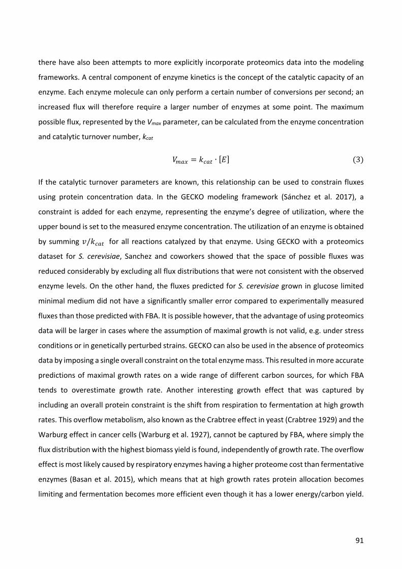
91

there have also been attempts to more explicitly incorporate proteomics data into the modeling

frameworks. A central component of enzyme kinetics is the concept of the catalytic capacity of an

enzyme. Each enzyme molecule can only perform a certain number of conversions per second; an

increased flux will therefore require a larger number of enzymes at some point. The maximum

possible flux, represented by the Vmax parameter, can be calculated from the enzyme concentration

and catalytic turnover number, kcat

{C|} = ~H|* ∙ [Ä] (3)

If the catalytic turnover parameters are known, this relationship can be used to constrain fluxes

using protein concentration data. In the GECKO modeling framework (Sánchez et al. 2017), a

constraint is added for each enzyme, representing the enzyme’s degree of utilization, where the

upper bound is set to the measured enzyme concentration. The utilization of an enzyme is obtained

by summing Ç/~H|* for all reactions catalyzed by that enzyme. Using GECKO with a proteomics

dataset for S. cerevisiae, Sanchez and coworkers showed that the space of possible fluxes was

reduced considerably by excluding all flux distributions that were not consistent with the observed

enzyme levels. On the other hand, the fluxes predicted for S. cerevisiae grown in glucose limited

minimal medium did not have a significantly smaller error compared to experimentally measured

fluxes than those predicted with FBA. It is possible however, that the advantage of using proteomics

data will be larger in cases where the assumption of maximal growth is not valid, e.g. under stress

conditions or in genetically perturbed strains. GECKO can also be used in the absence of proteomics

data by imposing a single overall constraint on the total enzyme mass. This resulted in more accurate

predictions of maximal growth rates on a wide range of different carbon sources, for which FBA

tends to overestimate growth rate. Another interesting growth effect that was captured by

including an overall protein constraint is the shift from respiration to fermentation at high growth

rates. This overflow metabolism, also known as the Crabtree effect in yeast (Crabtree 1929) and the

Warburg effect in cancer cells (Warburg et al. 1927), cannot be captured by FBA, where simply the

flux distribution with the highest biomass yield is found, independently of growth rate. The overflow

effect is most likely caused by respiratory enzymes having a higher proteome cost than fermentative

enzymes (Basan et al. 2015), which means that at high growth rates protein allocation becomes

limiting and fermentation becomes more efficient even though it has a lower energy/carbon yield.

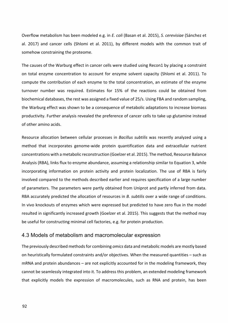
92

Overflow metabolism has been modeled e.g. in E. coli (Basan et al. 2015), S. cerevisiae (Sánchez et

al. 2017) and cancer cells (Shlomi et al. 2011), by different models with the common trait of

somehow constraining the proteome.

The causes of the Warburg effect in cancer cells were studied using Recon1 by placing a constraint

on total enzyme concentration to account for enzyme solvent capacity (Shlomi et al. 2011). To

compute the contribution of each enzyme to the total concentration, an estimate of the enzyme

turnover number was required. Estimates for 15% of the reactions could be obtained from

biochemical databases, the rest was assigned a fixed value of 25/s. Using FBA and random sampling,

the Warburg effect was shown to be a consequence of metabolic adaptations to increase biomass

productivity. Further analysis revealed the preference of cancer cells to take up glutamine instead

of other amino acids.

Resource allocation between cellular processes in Bacillus subtilis was recently analyzed using a

method that incorporates genome-wide protein quantification data and extracellular nutrient

concentrations with a metabolic reconstruction (Goelzer et al. 2015). The method, Resource Balance

Analysis (RBA), links flux to enzyme abundance, assuming a relationship similar to Equation 3, while

incorporating information on protein activity and protein localization. The use of RBA is fairly

involved compared to the methods described earlier and requires specification of a large number

of parameters. The parameters were partly obtained from Uniprot and partly inferred from data.

RBA accurately predicted the allocation of resources in B. subtilis over a wide range of conditions.

In vivo knockouts of enzymes which were expressed but predicted to have zero flux in the model

resulted in significantly increased growth (Goelzer et al. 2015). This suggests that the method may

be useful for constructing minimal cell factories, e.g. for protein production.

4.3 Models of metabolism and macromolecular expression

The previously described methods for combining omics data and metabolic models are mostly based

on heuristically formulated constraints and/or objectives. When the measured quantities – such as

mRNA and protein abundances – are not explicitly accounted for in the modeling framework, they

cannot be seamlessly integrated into it. To address this problem, an extended modeling framework

that explicitly models the expression of macromolecules, such as RNA and protein, has been

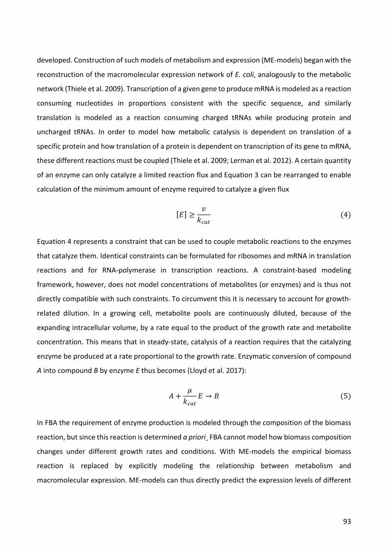
93

developed. Construction of such models of metabolism and expression (ME-models) began with the

reconstruction of the macromolecular expression network of E. coli, analogously to the metabolic

network (Thiele et al. 2009). Transcription of a given gene to produce mRNA is modeled as a reaction

consuming nucleotides in proportions consistent with the specific sequence, and similarly

translation is modeled as a reaction consuming charged tRNAs while producing protein and

uncharged tRNAs. In order to model how metabolic catalysis is dependent on translation of a

specific protein and how translation of a protein is dependent on transcription of its gene to mRNA,

these different reactions must be coupled (Thiele et al. 2009; Lerman et al. 2012). A certain quantity

of an enzyme can only catalyze a limited reaction flux and Equation 3 can be rearranged to enable

calculation of the minimum amount of enzyme required to catalyze a given flux

[Ä] ≥Ç~H|*

(4)

Equation 4 represents a constraint that can be used to couple metabolic reactions to the enzymes

that catalyze them. Identical constraints can be formulated for ribosomes and mRNA in translation

reactions and for RNA-polymerase in transcription reactions. A constraint-based modeling

framework, however, does not model concentrations of metabolites (or enzymes) and is thus not

directly compatible with such constraints. To circumvent this it is necessary to account for growth-

related dilution. In a growing cell, metabolite pools are continuously diluted, because of the

expanding intracellular volume, by a rate equal to the product of the growth rate and metabolite

concentration. This means that in steady-state, catalysis of a reaction requires that the catalyzing

enzyme be produced at a rate proportional to the growth rate. Enzymatic conversion of compound

A into compound B by enzyme E thus becomes (Lloyd et al. 2017):

_ +Ö~H|*

Ä → á (5)

In FBA the requirement of enzyme production is modeled through the composition of the biomass

reaction, but since this reaction is determined a priori¸ FBA cannot model how biomass composition

changes under different growth rates and conditions. With ME-models the empirical biomass

reaction is replaced by explicitly modeling the relationship between metabolism and

macromolecular expression. ME-models can thus directly predict the expression levels of different

94

proteins, which can be compared with omics datasets. A ME-model of the thermophilic bacterium

Thermotoga maritima (Lerman et al. 2012), found moderate correlations between predicted and

experimentally measured mRNA profiles (r= 0.54), protein expression profiles (r = 0.57), as well as

proteome amino acid composition (r = 0.79). A ME-model of E. coli showed improved prediction of

growth rates in different nutrient conditions compared to FBA (Thiele et al. 2012), and could

accurately predict several internal fluxes (O’Brien et al. 2013). Additionally, since ME-models

explicitly include the cost of producing the enzymes required for various pathways, they implicitly

limit the total proteome size and thus also capture metabolic overflow effects, such as the acetate

overflow metabolism in E. coli (O’Brien et al. 2013).

Whereas traditional constraint-based metabolic models include, and can thus directly predict,

growth rate, uptake and secretion rates and internal fluxes, ME-models can additionally predict

expression profiles and proteome composition, and thus they can also be directly constrained by

expression and proteomics data. Because of this, ME-models represent an intuitive and theoretically

justified method of integrating transcriptomics and proteomics data into metabolic models. They

have not yet found broad usage in the metabolic modeling community, presumably because of the

time it takes to run simulations (several orders of magnitude higher than with FBA), and the lack of

related model and software infrastructure, but these issues are continuously being addressed (Yang

et al. 2016; Lloyd et al. 2017).

4.4 Augmenting models with metabolomics data

In a discussion of data integration in metabolic models, it is impossible not to mention

metabolomics. Different analytical methods, e.g. enzymatic assays, chromatography and mass

spectrometry, can be used to take snapshots of the cellular metabolism with varying resolution,

coverage, precision and throughput. However, they all provide useful information about the

concentrations of metabolite pools in the cell. One of the earliest uses of metabolomics data to

improve metabolic modeling was metabolic flux analysis (MFA), which utilizes time-course

metabolite concentration data from cultures fed with isotopically labeled substrates to infer flux

values in the metabolic network (Stephanopoulos 1999; Sauer 2006). This is done by monitoring

how the isotopes, e.g. 13C or 15N, spread to downstream metabolite pools over time. The advantage

of this method is that the resulting fluxes can be used directly to constrain metabolic models or to

95

compare the validity of different simulation methods. However, MFA is labor- and cost intensive

and works best on a smaller subset of the entire metabolic network, typically just the central carbon

metabolism (Antoniewicz 2015; Gopalakrishnan and Maranas 2015).

Changes in extracellular metabolite concentrations over time can be used to estimate uptake and

secretion rates and constrain the flux space. However, since constraint-based modeling frameworks

model fluxes under an assumption of steady-state, internal metabolite concentration data at a

single time point without isotopic labeling cannot be directly utilized. Despite this, metabolomics

data can still be used to either constrain the models or to provide new insights in combination with

the simulation results. In order to model cells that are not in steady-state, such as human blood cells

undergoing physiological changes during storage, Bordbar and coworkers devised a method called

unsteady-state FBA (Bordbar et al. 2017). Using time-course metabolomics they determined the

rate of accumulation or depletion for internal metabolites, which was then modeled by adding

source and sink reactions to the metabolic model. These reactions were then constrained to have

fluxes corresponding to the experimentally determined rates of concentration changes. Subsequent

MFA revealed that the fluxes predicted with this method were more accurate than those obtained

by regular FBA.

Aside from enforcing steady state, a commonly used constraint in constraint-based models is to

force certain fluxes to only go in one direction. This is straightforward for some reactions whose

thermodynamics make it practically irreversible under biological conditions. Other reactions are

closer to equilibrium and can go in both directions depending on specific conditions. The

spontaneous direction of a reaction can be calculated by the formula

Δâä = Δâä° + så>?@(ç) (6)

If the left-hand side (the reaction Gibbs free energy) is negative, the reaction will proceed

spontaneously in the forward direction, while it will proceed spontaneously in the reverse direction

if the reaction Gibbs free energy is positive. Δâä° is the reaction Gibbs free energy under standard

conditions, RT is the gas constant times the absolute temperature and Q is the reaction quotient,

containing the concentrations of the reaction products and substrates. The standard Gibbs free

energy must in principle be determined experimentally, but in most cases it can be calculated from

96

the structure of the participating metabolites and already known reaction Gibbs free energies for

other reactions (Noor et al. 2013). This means that a dataset of metabolite concentrations can be

used to constrain reactions to a specific direction depending on the specific metabolic conditions,

reducing the space of feasible fluxes significantly (Soh and Hatzimanikatis 2014). In many simulated

growth conditions, it can be sufficient simply to constrain reaction directionalities according to the

most common mode of operation without regard to actual metabolite concentrations. Some

reactions however, occur in the unconventional direction under extreme conditions, such as very

high CO2 concentrations. In such cases using thermodynamics and metabolite data to inform

reaction directionalities will be particularly beneficial and can lead to more accurate simulations

(Soh et al. 2012).

Constraint-based simulations can also be combined with metabolomics data in another way. In

addition to calculating a flux distribution, simulating a constraint-based model also provides so-

called shadow prices. Each shadow price is linked to a metabolite and reflects how much the

objective function, e.g. growth, could be improved if the model were allowed to get some of that

metabolite “for free”. In other words a shadow price is a measure of how limiting a given

metabolite’s mass balance is for the objective function. Depending on the algorithm used to solve

the FBA problem, shadow prices are either a byproduct of the solution process or can be obtained

with modest computational effort.

Zampieri and coworkers investigated the evolution of antibiotic resistance in E. coli using adaptive

laboratory evolution (Zampieri et al. 2017). By maximizing and minimizing flux through each

reaction in the model and calculating the shadow prices, the authors could identify reactions, which,

when maximized or minimized, resulted in shadow prices that were consistent with the observed

patterns of metabolite concentration changes. Those reactions were hypothesized as being targets

of evolution, whose flux should be increased in order to increase antibiotic resistance.

Besides constraint-based modeling, the most common way to simulate cellular metabolism is with

kinetic models. This involves the solution of the system of differential equations shown in Eq. 1 from

given initial metabolite concentrations. As previously described, one of the challenges with this

approach is the requirement of knowing the values of all the kinetic parameters of the system. For

small biochemical systems, the kinetic parameters can sometimes be determined individually

97

through in vitro experiments, but for genome-scale models this is not feasible. Additionally there is

no guarantee that the in vitro kinetic parameters are representative of how an enzyme functions in

vivo (Teusink et al. 2000). Instead of the bottom-up approach of experimentally determining each

parameter, a top-down approach may be used, where the model parameters might initially be

estimated from prior information, such as in vitro data, but are predominantly selected by fitting

simulation results to genome-scale experimental data. This has long been done for small-scale

networks, using metabolomics and MFA data (Jamshidi and Palsson 2008; Srinivasan et al. 2015),

however with continual increases in dataset sizes and computing power, it has also become feasible

to do this for genome-scale networks. Recently a genome-scale kinetic model of E. coli was

published along with estimated values for all kinetic parameters (Khodayari and Maranas 2016). The

model parameters were fitted using experimental flux data and model predictions were validated

against metabolomics data. In addition the model could quantitatively predict product yields of 24

different compound in 320 mutant strains, which was considerably better than the constraint-based

simulation methods it was tested against. In another study kinetic models of human red blood cells

were used to investigate individual variations in susceptibility to side effects of the hepatitis B drug

Ribavirin (Bordbar et al. 2015). By measuring intracellular metabolite levels in red blood cells of 24

patients, they could determine individual kinetic parameter values for each of the patients, and

show that those parameters were predictive of whether the patient was sensitive to side effects.

Furthermore, the identified relationships between kinetic parameters and sensitivity to drug side-

effect were consistent with known mechanisms of Ribavirin side effects. These results show that

kinetic modeling frameworks have the potential to significantly outperform constraint-based

simulations, and that with modern omics technologies and computer power, it is feasible to

parametrize them sufficiently to predict metabolic behavior (Saa and Nielsen 2017).

4.5 Combining metabolic models and machine learning methods

The term machine learning covers a broad range of methods where large datasets are used to infer

relationships between variables or to predict various outcomes from given input data. Often this is

done without much consideration of specific mechanisms of the studied phenomena. Such data-

driven methods can of course be applied to metabolic data, but with limited connection to biological

mechanisms, the results are often difficult to interpret. Instead, machine learning methods can be

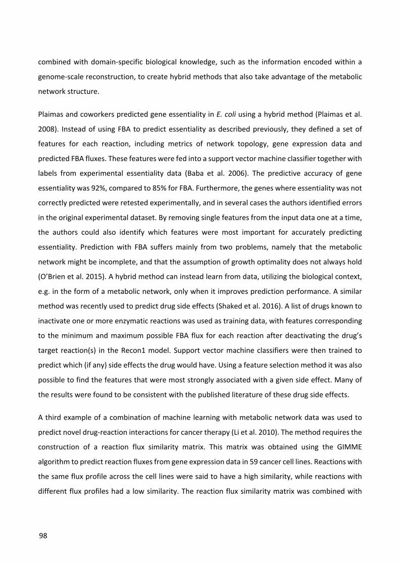
98

combined with domain-specific biological knowledge, such as the information encoded within a

genome-scale reconstruction, to create hybrid methods that also take advantage of the metabolic

network structure.

Plaimas and coworkers predicted gene essentiality in E. coli using a hybrid method (Plaimas et al.

2008). Instead of using FBA to predict essentiality as described previously, they defined a set of

features for each reaction, including metrics of network topology, gene expression data and

predicted FBA fluxes. These features were fed into a support vector machine classifier together with

labels from experimental essentiality data (Baba et al. 2006). The predictive accuracy of gene

essentiality was 92%, compared to 85% for FBA. Furthermore, the genes where essentiality was not

correctly predicted were retested experimentally, and in several cases the authors identified errors

in the original experimental dataset. By removing single features from the input data one at a time,

the authors could also identify which features were most important for accurately predicting

essentiality. Prediction with FBA suffers mainly from two problems, namely that the metabolic

network might be incomplete, and that the assumption of growth optimality does not always hold

(O’Brien et al. 2015). A hybrid method can instead learn from data, utilizing the biological context,

e.g. in the form of a metabolic network, only when it improves prediction performance. A similar

method was recently used to predict drug side effects (Shaked et al. 2016). A list of drugs known to

inactivate one or more enzymatic reactions was used as training data, with features corresponding

to the minimum and maximum possible FBA flux for each reaction after deactivating the drug’s

target reaction(s) in the Recon1 model. Support vector machine classifiers were then trained to

predict which (if any) side effects the drug would have. Using a feature selection method it was also

possible to find the features that were most strongly associated with a given side effect. Many of

the results were found to be consistent with the published literature of these drug side effects.

A third example of a combination of machine learning with metabolic network data was used to

predict novel drug-reaction interactions for cancer therapy (Li et al. 2010). The method requires the

construction of a reaction flux similarity matrix. This matrix was obtained using the GIMME

algorithm to predict reaction fluxes from gene expression data in 59 cancer cell lines. Reactions with

the same flux profile across the cell lines were said to have a high similarity, while reactions with

different flux profiles had a low similarity. The reaction flux similarity matrix was combined with

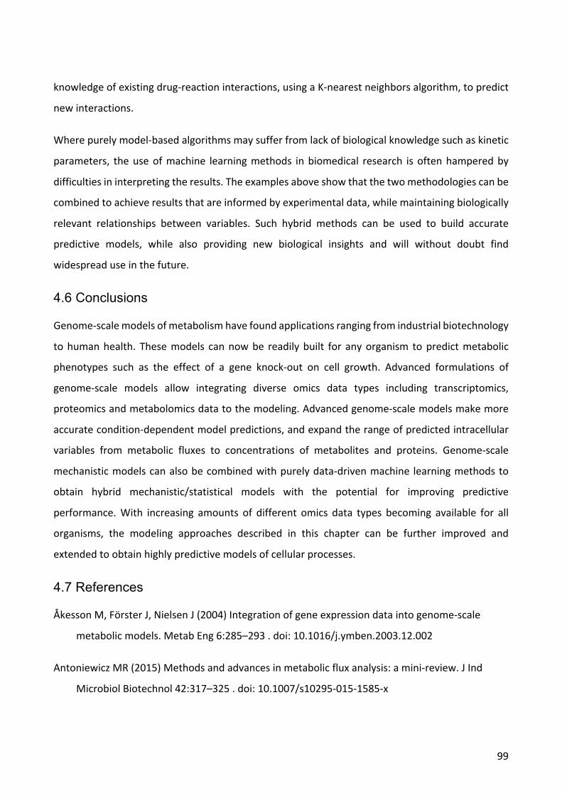
99

knowledge of existing drug-reaction interactions, using a K-nearest neighbors algorithm, to predict

new interactions.

Where purely model-based algorithms may suffer from lack of biological knowledge such as kinetic

parameters, the use of machine learning methods in biomedical research is often hampered by

difficulties in interpreting the results. The examples above show that the two methodologies can be

combined to achieve results that are informed by experimental data, while maintaining biologically

relevant relationships between variables. Such hybrid methods can be used to build accurate

predictive models, while also providing new biological insights and will without doubt find

widespread use in the future.

4.6 Conclusions

Genome-scale models of metabolism have found applications ranging from industrial biotechnology

to human health. These models can now be readily built for any organism to predict metabolic

phenotypes such as the effect of a gene knock-out on cell growth. Advanced formulations of

genome-scale models allow integrating diverse omics data types including transcriptomics,

proteomics and metabolomics data to the modeling. Advanced genome-scale models make more

accurate condition-dependent model predictions, and expand the range of predicted intracellular

variables from metabolic fluxes to concentrations of metabolites and proteins. Genome-scale

mechanistic models can also be combined with purely data-driven machine learning methods to

obtain hybrid mechanistic/statistical models with the potential for improving predictive

performance. With increasing amounts of different omics data types becoming available for all

organisms, the modeling approaches described in this chapter can be further improved and

extended to obtain highly predictive models of cellular processes.

4.7 References

Åkesson M, Förster J, Nielsen J (2004) Integration of gene expression data into genome-scale

metabolic models. Metab Eng 6:285–293 . doi: 10.1016/j.ymben.2003.12.002

Antoniewicz MR (2015) Methods and advances in metabolic flux analysis: a mini-review. J Ind

Microbiol Biotechnol 42:317–325 . doi: 10.1007/s10295-015-1585-x

100

Baba T, Ara T, Hasegawa M, Takai Y, Okumura Y, Baba M, Datsenko KA, Tomita M, Wanner BL,

Mori H (2006) Construction of Escherichia coli K-12 in-frame, single-gene knockout mutants:

the Keio collection. Mol Syst Biol 2: . doi: 10.1038/msb4100050

Basan M, Hui S, Okano H, Zhang Z, Shen Y, Williamson JR, Hwa T (2015) Overflow metabolism in

Escherichia coli results from efficient proteome allocation. Nature 528:99–104 . doi:

10.1038/nature15765

Becker SA, Palsson BO (2008) Context-specific metabolic networks are consistent with

experiments. PLoS Comput Biol 4: . doi: 10.1371/journal.pcbi.1000082

Bordbar A, Johansson PI, Paglia G, Harrison SJ, Wichuk K, Magnusdottir M, Valgeirsdottir S, Gybel-

Brask M, Ostrowski SR, Palsson S, Rolfsson O, Sigurjónsson OE, Hansen MB, Gudmundsson S,

Palsson BO (2016) Identified metabolic signature for assessing red blood cell unit quality is

associated with endothelial damage markers and clinical outcomes. Transfusion 56:852–862 .

doi: 10.1111/trf.13460

Bordbar A, McCloskey D, Zielinski DC, Sonnenschein N, Jamshidi N, Palsson BO (2015) Personalized

Whole-Cell Kinetic Models of Metabolism for Discovery in Genomics and Pharmacodynamics.

Cell Syst 1:283–292 . doi: 10.1016/j.cels.2015.10.003

Bordbar A, Yurkovich JT, Paglia G, Rolfsson O, Sigurjónsson ÓE, Palsson BO (2017) Elucidating

dynamic metabolic physiology through network integration of quantitative time-course

metabolomics. Sci Rep 7: . doi: 10.1038/srep46249

Crabtree HG (1929) Observations on the carbohydrate metabolism of tumours. Biochem J 23:536–

45 . doi: 10.1042/bj0230536

de Oliveira Dal’Molin CG, Quek L-E, Palfreyman RW, Brumbley SM, Nielsen LK (2010) AraGEM, a

Genome-Scale Reconstruction of the Primary Metabolic Network in Arabidopsis. Plant Physiol

152:579–589 . doi: 10.1104/pp.109.148817

Duarte NC, Becker SA, Jamshidi N, Thiele I, Mo ML, Vo TD, Srivas R, Palsson BO (2007) Global

reconstruction of the human metabolic network based on genomic and bibliomic data. Proc

101

Natl Acad Sci 104:1777–1782 . doi: 10.1073/pnas.0610772104

Edwards JS, Palsson BO (2000) The Escherichia coli MG1655 in silico metabolic genotype: Its

definition, characteristics, and capabilities. Proc Natl Acad Sci 97:5528–5533 . doi:

10.1073/pnas.97.10.5528

Folger O, Jerby L, Frezza C, Gottlieb E, Ruppin E, Shlomi T (2011) Predicting selective drug targets

in cancer through metabolic networks. Mol Syst Biol 7:527–527 . doi: 10.1038/msb.2011.63

Förster J, Famili I, Palsson BO, Nielsen J (2003) Large-scale evaluation of in silico gene deletions in

Saccharomyces cerevisiae. Omi A J Integr Biol 7:193–202 . doi:

10.1089/153623103322246584

Goelzer A, Muntel J, Chubukov V, Jules M, Prestel E, Nölker R, Mariadassou M, Aymerich S, Hecker

M, Noirot P, Becher D, Fromion V (2015) Quantitative prediction of genome-wide resource

allocation in bacteria. Metab Eng 32:232–243 . doi: 10.1016/j.ymben.2015.10.003

Gopalakrishnan S, Maranas CD (2015) 13C metabolic flux analysis at a genome-scale. Metab Eng

32:12–22 . doi: 10.1016/j.ymben.2015.08.006

Gry M, Rimini R, Strömberg S, Asplund A, Pontén F, Uhlén M, Nilsson P (2009) Correlations

between RNA and protein expression profiles in 23 human cell lines. BMC Genomics 10:365 .

doi: 10.1186/1471-2164-10-365

Halldorsson S, Rohatgi N, Magnusdottir M, Choudhary KS, Gudjonsson T, Knutsen E, Barkovskaya

A, Hilmarsdottir B, Perander M, Mælandsmo GM, Gudmundsson S, Rolfsson Ó (2017)

Metabolic re-wiring of isogenic breast epithelial cell lines following epithelial to mesenchymal

transition. Cancer Lett 396:117–129 . doi: 10.1016/j.canlet.2017.03.019

Heavner BD, Price ND (2015) Comparative Analysis of Yeast Metabolic Network Models Highlights

Progress, Opportunities for Metabolic Reconstruction. PLoS Comput Biol 11:1–26 . doi:

10.1371/journal.pcbi.1004530

Jamshidi N, Palsson BØ (2008) Formulating genome-scale kinetic models in the post-genome era.

102

Mol Syst Biol 4:171 . doi: 10.1038/msb.2008.8

Karr JR, Sanghvi JC, MacKlin DN, Gutschow M, Jacobs JM, Bolival B, Assad-Garcia N, Glass JI, Covert

MW (2012) A whole-cell computational model predicts phenotype from genotype. Cell

150:389–401 . doi: 10.1016/j.cell.2012.05.044

Khodayari A, Maranas CD (2016) A genome-scale Escherichia coli kinetic metabolic model k-

ecoli457 satisfying flux data for multiple mutant strains. Nat. Commun. 7:13806

Lerman JA, Hyduke DR, Latif H, Portnoy VA, Lewis NE, Orth JD, Schrimpe-Rutledge AC, Smith RD,

Adkins JN, Zengler K, Palsson BO (2012) In silico method for modelling metabolism and gene

product expression at genome scale. Nat Commun 3:929 . doi: 10.1038/ncomms1928

Li L, Zhou X, Ching W-K, Wang P (2010) Predicting enzyme targets for cancer drugs by profiling

human metabolic reactions in NCI-60 cell lines. BMC Bioinformatics 11:501 . doi:

10.1186/1471-2105-11-501

Lloyd CJ, Ebrahim A, Yang L, King ZA, Catoiu E, O’Brien EJ, Liu JK, Palsson BO (2017) COBRAme: A

Computational Framework for Building and Manipulating Models of Metabolism and Gene

Expression. bioRxiv 106559 . doi: http://dx.doi.org/10.1101/106559

Machado D, Herrgård M (2014) Systematic Evaluation of Methods for Integration of

Transcriptomic Data into Constraint-Based Models of Metabolism. PLoS Comput Biol 10: . doi:

10.1371/journal.pcbi.1003580

Mardinoglu A, Agren R, Kampf C, Asplund A, Nookaew I, Jacobson P, Walley AJ, Froguel P, Carlsson

LM, Uhlen M, Nielsen J (2014) Integration of clinical data with a genome-scale metabolic

model of the human adipocyte. Mol Syst Biol 9:649–649 . doi: 10.1038/msb.2013.5

McCloskey D, Palsson BØ, Feist AM (2013) Basic and applied uses of genome-scale metabolic

network reconstructions of Escherichia coli. Mol Syst Biol 9:661 . doi: 10.1038/msb.2013.18

Noor E, Haraldsdóttir HS, Milo R, Fleming RMT (2013) Consistent Estimation of Gibbs Energy Using

Component Contributions. PLoS Comput Biol 9: . doi: 10.1371/journal.pcbi.1003098

103

O’Brien EJ, Lerman JA, Chang RL, Hyduke DR, Palsson BO (2013) Genome-scale models of

metabolism and gene expression extend and refine growth phenotype prediction. Mol Syst

Biol 9:693–693 . doi: 10.1038/msb.2013.52

O’Brien EJ, Monk JM, Palsson BO (2015) Using genome-scale models to predict biological

capabilities. Cell 161:971–987 . doi: 10.1016/j.cell.2015.05.019

Oberhardt MA, Puchałka J, Fryer KE, Martins Dos Santos VAP, Papin JA (2008) Genome-scale

metabolic network analysis of the opportunistic pathogen Pseudomonas aeruginosa PAO1. J

Bacteriol 190:2790–2803 . doi: 10.1128/JB.01583-07

Orth JD, Thiele I, Palsson BØ (2010) What is flux balance analysis? Nat Biotechnol 28:245–248 . doi:

10.1038/nbt.1614

Plaimas K, Mallm J-P, Oswald M, Svara F, Sourjik V, Eils R, Konig R (2008) Machine learning based

analyses on metabolic networks supports high-throughput knockout screens. BMC Syst Biol

2:67 . doi: 10.1186/1752-0509-2-67

Price ND, Reed JL, Palsson BØ (2004) Genome-scale models of microbial cells: evaluating the

consequences of constraints. Nat Rev Microbiol 2:886–897 . doi: 10.1038/nrmicro1023

Saa PA, Nielsen LK (2017) Formulation, construction and analysis of kinetic models of metabolism:

A review of modelling frameworks. Biotechnol Adv 0–1 . doi:

10.1016/j.biotechadv.2017.09.005

Sánchez BJ, Zhang C, Nilsson A, Lahtvee P, Kerkhoven EJ, Nielsen J (2017) Improving the phenotype

predictions of a yeast genome-scale metabolic model by incorporating enzymatic constraints.

Mol Syst Biol 13:935 . doi: 10.15252/msb.20167411

Sauer U (2006) Metabolic networks in motion: 13C-based flux analysis. Mol Syst Biol 2:1–10 . doi:

10.1038/msb4100109

Schilling CH, Palsson BØ (2000) Assessment of the Metabolic Capabilities of Haemophilus

influenzae Rd through a Genome-scale Pathway Analysis. J Theor Biol 203:249–283 . doi:

104

10.1006/jtbi.2000.1088

Shaked I, Oberhardt MA, Atias N, Sharan R, Ruppin E (2016) Metabolic Network Prediction of Drug

Side Effects. Cell Syst 2:209–213 . doi: 10.1016/j.cels.2016.03.001

Shlomi T, Benyamini T, Gottlieb E, Sharan R, Ruppin E (2011) Genome-scale metabolic modeling

elucidates the role of proliferative adaptation in causing the warburg effect. PLoS Comput

Biol 7:1–8 . doi: 10.1371/journal.pcbi.1002018

Shlomi T, Cabili MN, Herrgård MJ, Palsson BØ, Ruppin E (2008) Network-based prediction of

human tissue-specific metabolism. Nat Biotechnol 26:1003–1010 . doi: 10.1038/nbt.1487

Shoaie S, Karlsson F, Mardinoglu A, Nookaew I, Bordel S, Nielsen J (2013) Understanding the

interactions between bacteria in the human gut through metabolic modeling. Sci Rep 3:2532 .

doi: 10.1038/srep02532

Soh KC, Hatzimanikatis V (2014) Constraining the Flux Space Using Thermodynamics and

Integration of Metabolomics Data. In: Krömer JO, Nielsen LK, Blank LM (eds) Metabolic Flux

Analysis: Methods and Protocols. Springer New York, New York, NY, pp 49–63

Soh KC, Miskovic L, Hatzimanikatis V (2012) From network models to network responses:

Integration of thermodynamic and kinetic properties of yeast genome-scale metabolic

networks. FEMS Yeast Res 12:129–143 . doi: 10.1111/j.1567-1364.2011.00771.x

Srinivasan S, Cluett WR, Mahadevan R (2015) Constructing kinetic models of metabolism at

genome-scales: A review. Biotechnol J 10:1345–1359 . doi: 10.1002/biot.201400522

Stephanopoulos G (1999) Metabolic Fluxes and Metabolic Engineering. Metab Eng 1:1–11 . doi:

10.1006/mben.1998.0101

Teusink B, Passarge J, Reijenga CA, Esgalhado E, Van Der Weijden CC, Schepper M, Walsh MC,

Bakker BM, Van Dam K, Westerhoff H V., Snoep JL (2000) Can yeast glycolysis be understood

terms of vitro kinetics of the constituent enzymes? Testing biochemistry. Eur J Biochem

267:5313–5329 . doi: 10.1046/j.1432-1327.2000.01527.x

105

Thiele I, Fleming RMT, Que R, Bordbar A, Diep D, Palsson BO (2012) Multiscale Modeling of

Metabolism and Macromolecular Synthesis in E. coli and Its Application to the Evolution of

Codon Usage. PLoS One 7: . doi: 10.1371/journal.pone.0045635

Thiele I, Jamshidi N, Fleming RMT, Palsson BO (2009) Genome-scale reconstruction of escherichia

coli’s transcriptional and translational machinery: A knowledge base, its mathematical

formulation, and its functional characterization. PLoS Comput Biol 5: . doi:

10.1371/journal.pcbi.1000312

Thomas A, Rahmanian S, Bordbar A, Palsson BØ, Jamshidi N (2015) Network reconstruction of

platelet metabolism identifies metabolic signature for aspirin resistance. Sci Rep 4:3925 . doi:

10.1038/srep03925

Warburg O, Wind F, Negelein E (1927) The metabolism of tumors in the body. J Gen Physiol 8:519–

530 . doi: 10.1085/jgp.8.6.519

Yang L, Ma D, Ebrahim A, Lloyd CJ, Saunders MA, Palsson BO (2016) solveME: fast and reliable

solution of nonlinear ME models. BMC Bioinformatics 17:391 . doi: 10.1186/s12859-016-

1240-1

Zampieri M, Enke T, Chubukov V, Ricci V, Piddock L, Sauer U (2017) Metabolic constraints on the

evolution of antibiotic resistance. Mol Syst Biol 13:917 . doi: 10.15252/msb.20167028

106

Chapter 5: OptCouple: joint simulation of gene knockouts,

insertions and medium modifications for prediction of growth-

coupled strain designs

Kristian Jensen1, Valentijn Broeken1, Anne Sofie Lærke Hansen1, Nikolaus Sonnenschein1, Markus J.

Herrgård1*

1 The Novo Nordisk Foundation Center for Biosustainability, Technical University of Denmark,


* Correspondence: [email protected]

Abstract

Biological production of chemicals is an attractive alternative to petrochemical-based production,

due to advantages in environmental impact and the spectrum of feasible targets. However,

engineering microbial strains to overproduce a compound of interest can be a long, costly and

painstaking process. If production can be coupled to cell growth it is possible to use adaptive

laboratory evolution to increase the production rate. Strategies for coupling production to growth,

however, are often not trivial to find. Here we present OptCouple, a constraint-based modeling

algorithm to simultaneously identify combinations of gene knockouts, insertions and medium

supplements that lead to growth-coupled production of a target compound. We validated the

algorithm by showing that it can find novel strategies that are growth-coupled in silico for a

compound that has not been coupled to growth previously, as well as reproduce known growth-

coupled strain designs for two different target compounds. Furthermore, we used OptCouple to

construct an alternative design with potential for higher production. We provide an efficient and

easy-to-use implementation of the OptCouple algorithm in the cameo Python package for

computational strain design.

107

5.1 Introduction

The use of microorganisms as cell factories offers the possibility of producing a wide range of

chemicals from renewable sources, as well as manufacturing natural compounds too complicated

for chemical synthesis in large amounts (Becker and Wittmann, 2015). However, successfully

engineering microorganisms to produce a target compound most often requires trial-and-error

experimentation with different possible pathways, and even when production is achieved, many

iterations of subsequent optimization are usually necessary to increase production rate and yield to

satisfy industrial needs (Lee and Kim, 2015).

One strategy for optimizing chemical production in microbial strains is to utilize the power of natural

selection in adaptive laboratory evolution (ALE) experiments (Portnoy et al., 2011; Shepelin et al.,

2018). This allows the identification of mutant strains with enhanced viability under the evolution

conditions. The inherent selection for cells that are able to grow faster than the rest of the

population makes it easy to optimize for characteristics such as product tolerance or substrate

utilization, while directly improving production characteristics such as production rate, titer and

yield is more difficult (Hansen et al., 2017; Shepelin et al., 2018). Indeed, with the advent of more

and more methods, models, and databases for automated running and analysis of ALE experiments,

such as eVOLVER (Wong et al., 2018), ALEsim (LaCroix et al., 2017), and ALEdb (Phaneuf et al., 2018),

the need for new selective pressures by clever strain and experimental design becomes the primary

challenge for evolutionary strain engineering.

Using evolution to improve biochemical production rates can be achieved by coupling production

to growth, i.e. ensuring that production is a necessary by-product of cell growth, such that

adaptations that increase the growth rate of the cells will also increase production. For a review of

examples of successful growth-coupling for biochemical production, see e.g. Shepelin et al. (2018).

A recent successful example is the growth-coupling of itaconic acid production in Escherichia coli by

four gene deletions, a downregulation, and glutamate supplementation that ensure formation of

itaconic acid to prevent accumulation of PEP inside the cell (Harder et al., 2016). The design was

aided by the computation of minimal cut sets (MCS), which are sets of gene knockouts that will

prevent all undesirable flux distributions while maintaining the ability to produce the target

compound (Klamt and Gilles, 2004; von Kamp and Klamt, 2014).

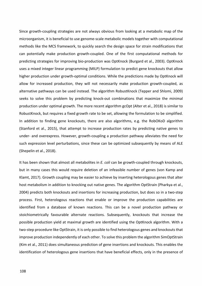
108

Since growth-coupling strategies are not always obvious from looking at a metabolic map of the

microorganism, it is beneficial to use genome-scale metabolic models together with computational

methods like the MCS framework, to quickly search the design space for strain modifications that

can potentially make production growth-coupled. One of the first computational methods for

predicting strategies for improving bio-production was OptKnock (Burgard et al., 2003). OptKnock

uses a mixed integer linear programming (MILP) formulation to predict gene knockouts that allow

higher production under growth-optimal conditions. While the predictions made by OptKnock will

allow for increased production, they will not necessarily make production growth-coupled, as

alternative pathways can be used instead. The algorithm RobustKnock (Tepper and Shlomi, 2009)

seeks to solve this problem by predicting knock-out combinations that maximize the minimal

production under optimal growth. The more recent algorithm gcOpt (Alter et al., 2018) is similar to

RobustKnock, but requires a fixed growth rate to be set, allowing the formulation to be simplified.

In addition to finding gene knockouts, there are also algorithms, e.g. the RobOKoD algorithm

(Stanford et al., 2015), that attempt to increase production rates by predicting native genes to

under- and overexpress. However, growth-coupling a production pathway alleviates the need for

such expression level perturbations, since these can be optimized subsequently by means of ALE

(Shepelin et al., 2018).

It has been shown that almost all metabolites in E. coli can be growth-coupled through knockouts,

but in many cases this would require deletion of an infeasible number of genes (von Kamp and

Klamt, 2017). Growth coupling may be easier to achieve by inserting heterologous genes that alter

host metabolism in addition to knocking out native genes. The algorithm OptStrain (Pharkya et al.,

2004) predicts both knockouts and insertions for increasing production, but does so in a two-step

process. First, heterologous reactions that enable or improve the production capabilities are

identified from a database of known reactions. This can be a novel production pathway or

stoichiometrically favourable alternate reactions. Subsequently, knockouts that increase the

possible production yield at maximal growth are identified using the OptKnock algorithm. With a

two-step procedure like OptStrain, it is only possible to find heterologous genes and knockouts that

improve production independently of each other. To solve this problem the algorithm SimOptStrain

(Kim et al., 2011) does simultaneous prediction of gene insertions and knockouts. This enables the

identification of heterologous gene insertions that have beneficial effects, only in the presence of

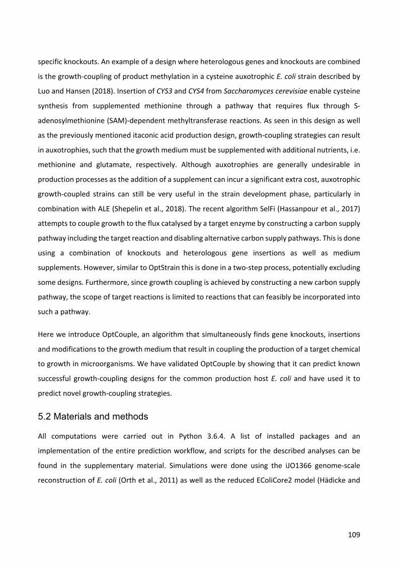
109

specific knockouts. An example of a design where heterologous genes and knockouts are combined

is the growth-coupling of product methylation in a cysteine auxotrophic E. coli strain described by

Luo and Hansen (2018). Insertion of CYS3 and CYS4 from Saccharomyces cerevisiae enable cysteine

synthesis from supplemented methionine through a pathway that requires flux through S-

adenosylmethionine (SAM)-dependent methyltransferase reactions. As seen in this design as well

as the previously mentioned itaconic acid production design, growth-coupling strategies can result

in auxotrophies, such that the growth medium must be supplemented with additional nutrients, i.e.

methionine and glutamate, respectively. Although auxotrophies are generally undesirable in

production processes as the addition of a supplement can incur a significant extra cost, auxotrophic

growth-coupled strains can still be very useful in the strain development phase, particularly in

combination with ALE (Shepelin et al., 2018). The recent algorithm SelFi (Hassanpour et al., 2017)

attempts to couple growth to the flux catalysed by a target enzyme by constructing a carbon supply

pathway including the target reaction and disabling alternative carbon supply pathways. This is done

using a combination of knockouts and heterologous gene insertions as well as medium

supplements. However, similar to OptStrain this is done in a two-step process, potentially excluding

some designs. Furthermore, since growth coupling is achieved by constructing a new carbon supply

pathway, the scope of target reactions is limited to reactions that can feasibly be incorporated into

such a pathway.

Here we introduce OptCouple, an algorithm that simultaneously finds gene knockouts, insertions

and modifications to the growth medium that result in coupling the production of a target chemical

to growth in microorganisms. We have validated OptCouple by showing that it can predict known

successful growth-coupling designs for the common production host E. coli and have used it to

predict novel growth-coupling strategies.

5.2 Materials and methods

All computations were carried out in Python 3.6.4. A list of installed packages and an

implementation of the entire prediction workflow, and scripts for the described analyses can be

found in the supplementary material. Simulations were done using the iJO1366 genome-scale

reconstruction of E. coli (Orth et al., 2011) as well as the reduced EColiCore2 model (Hädicke and

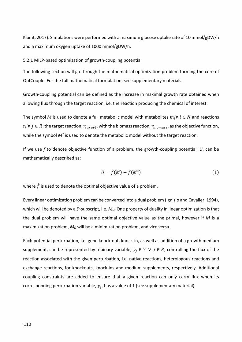
110

Klamt, 2017). Simulations were performed with a maximum glucose uptake rate of 10 mmol/gDW/h

and a maximum oxygen uptake of 1000 mmol/gDW/h.

5.2.1 MILP-based optimization of growth-coupling potential

The following section will go through the mathematical optimization problem forming the core of

OptCouple. For the full mathematical formulation, see supplementary materials.

Growth-coupling potential can be defined as the increase in maximal growth rate obtained when

allowing flux through the target reaction, i.e. the reaction producing the chemical of interest.

The symbol M is used to denote a full metabolic model with metabolites èG∀2 ∈ í and reactions

ìî∀ï ∈ s, the target reaction, ì*|6ñ7*, with the biomass reaction, ìóGIC|cc, as the objective function,

while the symbol M* is used to denote the metabolic model without the target reaction.

If we use f to denote objective function of a problem, the growth-coupling potential, U, can be

mathematically described as:

ò = dô(S) − dô(S∗) (1)

where dô is used to denote the optimal objective value of a problem.

Every linear optimization problem can be converted into a dual problem (Ignizio and Cavalier, 1994),

which will be denoted by a D-subscript, i.e. MD. One property of duality in linear optimization is that

the dual problem will have the same optimal objective value as the primal, however if M is a

maximization problem, MD will be a minimization problem, and vice versa.

Each potential perturbation, i.e. gene knock-out, knock-in, as well as addition of a growth medium

supplement, can be represented by a binary variable, 5î ∈ P∀ï ∈ s, controlling the flux of the

reaction associated with the given perturbation, i.e. native reactions, heterologous reactions and

exchange reactions, for knockouts, knock-ins and medium supplements, respectively. Additional

coupling constraints are added to ensure that a given reaction can only carry flux when its

corresponding perturbation variable, 5î, has a value of 1 (see supplementary material).

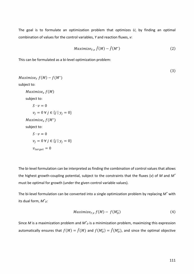
111

The goal is to formulate an optimization problem that optimizes U, by finding an optimal

combination of values for the control variables, Y and reaction fluxes, v:

S&!2è2õ(ú,ùdô(S) − dô(S∗) (2)

This can be formulated as a bi-level optimization problem:

(3)

S&!2è24(úd(S) − d(S∗)

subject to:

S&!2è24(ùd(S)

subject to:

l ∙ Ç = 0

Çî = 0∀ï ∈ {ï|5î = 0}

S&!2è24(ùd(S∗)

subject to:

l ∙ Ç = 0

Çî = 0∀ï ∈ {ï|5î = 0}

Ç*|6ñ7* = 0

The bi-level formulation can be interpreted as finding the combination of control values that allows

the highest growth-coupling potential, subject to the constraints that the fluxes (v) of M and M*

must be optimal for growth (under the given control variable values).

The bi-level formulation can be converted into a single optimization problem by replacing M* with

its dual form, M*D:

S&!2è2õ(ú,ùd(S) − d(S°∗ ) (4)

Since M is a maximization problem and M*D is a minimization problem, maximizing this expression

automatically ensures that d(S) = dô(S) and d(S°∗ ) = dô(S°

∗ ), and since the optimal objective

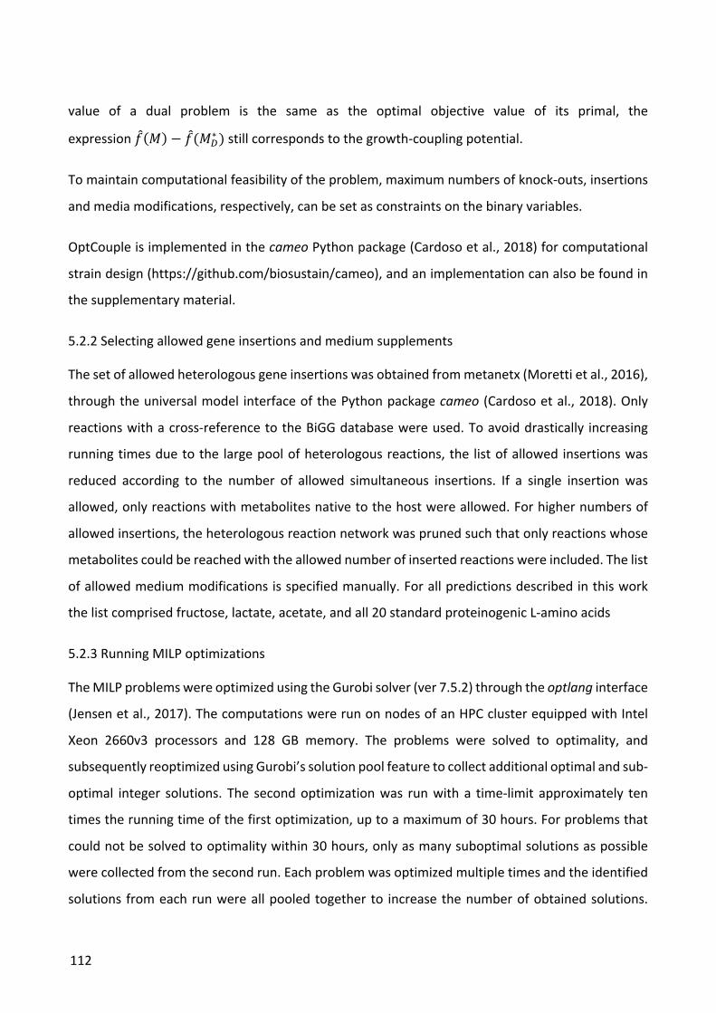
112

value of a dual problem is the same as the optimal objective value of its primal, the

expression dô(S) − dô(S°∗ ) still corresponds to the growth-coupling potential.

To maintain computational feasibility of the problem, maximum numbers of knock-outs, insertions

and media modifications, respectively, can be set as constraints on the binary variables.

OptCouple is implemented in the cameo Python package (Cardoso et al., 2018) for computational

strain design (https://github.com/biosustain/cameo), and an implementation can also be found in

the supplementary material.

5.2.2 Selecting allowed gene insertions and medium supplements

The set of allowed heterologous gene insertions was obtained from metanetx (Moretti et al., 2016),

through the universal model interface of the Python package cameo (Cardoso et al., 2018). Only

reactions with a cross-reference to the BiGG database were used. To avoid drastically increasing

running times due to the large pool of heterologous reactions, the list of allowed insertions was

reduced according to the number of allowed simultaneous insertions. If a single insertion was

allowed, only reactions with metabolites native to the host were allowed. For higher numbers of

allowed insertions, the heterologous reaction network was pruned such that only reactions whose

metabolites could be reached with the allowed number of inserted reactions were included. The list

of allowed medium modifications is specified manually. For all predictions described in this work

the list comprised fructose, lactate, acetate, and all 20 standard proteinogenic L-amino acids

5.2.3 Running MILP optimizations

The MILP problems were optimized using the Gurobi solver (ver 7.5.2) through the optlang interface

(Jensen et al., 2017). The computations were run on nodes of an HPC cluster equipped with Intel

Xeon 2660v3 processors and 128 GB memory. The problems were solved to optimality, and

subsequently reoptimized using Gurobi’s solution pool feature to collect additional optimal and sub-

optimal integer solutions. The second optimization was run with a time-limit approximately ten

times the running time of the first optimization, up to a maximum of 30 hours. For problems that

could not be solved to optimality within 30 hours, only as many suboptimal solutions as possible

were collected from the second run. Each problem was optimized multiple times and the identified

solutions from each run were all pooled together to increase the number of obtained solutions.

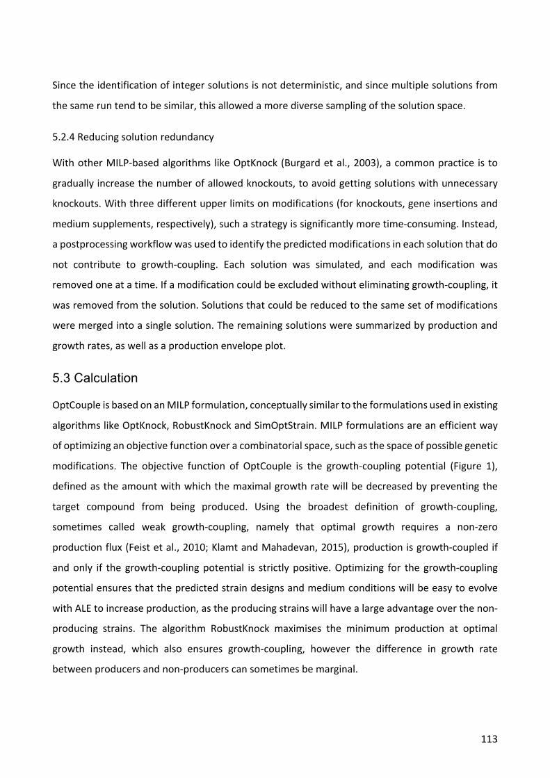
113

Since the identification of integer solutions is not deterministic, and since multiple solutions from

the same run tend to be similar, this allowed a more diverse sampling of the solution space.

5.2.4 Reducing solution redundancy

With other MILP-based algorithms like OptKnock (Burgard et al., 2003), a common practice is to

gradually increase the number of allowed knockouts, to avoid getting solutions with unnecessary

knockouts. With three different upper limits on modifications (for knockouts, gene insertions and

medium supplements, respectively), such a strategy is significantly more time-consuming. Instead,

a postprocessing workflow was used to identify the predicted modifications in each solution that do

not contribute to growth-coupling. Each solution was simulated, and each modification was

removed one at a time. If a modification could be excluded without eliminating growth-coupling, it

was removed from the solution. Solutions that could be reduced to the same set of modifications

were merged into a single solution. The remaining solutions were summarized by production and

growth rates, as well as a production envelope plot.

5.3 Calculation

OptCouple is based on an MILP formulation, conceptually similar to the formulations used in existing

algorithms like OptKnock, RobustKnock and SimOptStrain. MILP formulations are an efficient way

of optimizing an objective function over a combinatorial space, such as the space of possible genetic

modifications. The objective function of OptCouple is the growth-coupling potential (Figure 1),

defined as the amount with which the maximal growth rate will be decreased by preventing the

target compound from being produced. Using the broadest definition of growth-coupling,

sometimes called weak growth-coupling, namely that optimal growth requires a non-zero

production flux (Feist et al., 2010; Klamt and Mahadevan, 2015), production is growth-coupled if

and only if the growth-coupling potential is strictly positive. Optimizing for the growth-coupling

potential ensures that the predicted strain designs and medium conditions will be easy to evolve

with ALE to increase production, as the producing strains will have a large advantage over the non-

producing strains. The algorithm RobustKnock maximises the minimum production at optimal

growth instead, which also ensures growth-coupling, however the difference in growth rate

between producers and non-producers can sometimes be marginal.

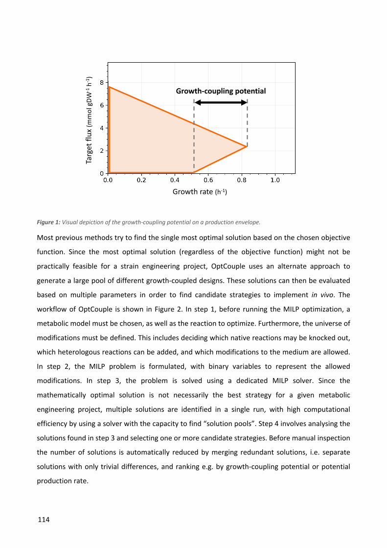
114

Figure 1: Visual depiction of the growth-coupling potential on a production envelope.

Most previous methods try to find the single most optimal solution based on the chosen objective

function. Since the most optimal solution (regardless of the objective function) might not be

practically feasible for a strain engineering project, OptCouple uses an alternate approach to

generate a large pool of different growth-coupled designs. These solutions can then be evaluated

based on multiple parameters in order to find candidate strategies to implement in vivo. The

workflow of OptCouple is shown in Figure 2. In step 1, before running the MILP optimization, a

metabolic model must be chosen, as well as the reaction to optimize. Furthermore, the universe of

modifications must be defined. This includes deciding which native reactions may be knocked out,

which heterologous reactions can be added, and which modifications to the medium are allowed.

In step 2, the MILP problem is formulated, with binary variables to represent the allowed

modifications. In step 3, the problem is solved using a dedicated MILP solver. Since the

mathematically optimal solution is not necessarily the best strategy for a given metabolic

engineering project, multiple solutions are identified in a single run, with high computational

efficiency by using a solver with the capacity to find “solution pools”. Step 4 involves analysing the

solutions found in step 3 and selecting one or more candidate strategies. Before manual inspection

the number of solutions is automatically reduced by merging redundant solutions, i.e. separate

solutions with only trivial differences, and ranking e.g. by growth-coupling potential or potential

production rate.

Growth rate (h-1)

Targ

et fl

ux (m

mol

gDW

-1h-1

)Growth-coupling potential

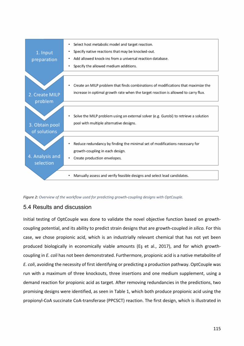
115

Figure 2: Overview of the workflow used for predicting growth-coupling designs with OptCouple.


Initial testing of OptCouple was done to validate the novel objective function based on growth-

coupling potential, and its ability to predict strain designs that are growth-coupled in silico. For this

case, we chose propionic acid, which is an industrially relevant chemical that has not yet been

produced biologically in economically viable amounts (Eş et al., 2017), and for which growth-

coupling in E. coli has not been demonstrated. Furthermore, propionic acid is a native metabolite of

E. coli, avoiding the necessity of first identifying or predicting a production pathway. OptCouple was

run with a maximum of three knockouts, three insertions and one medium supplement, using a

demand reaction for propionic acid as target. After removing redundancies in the predictions, two

promising designs were identified, as seen in Table 1, which both produce propionic acid using the

propionyl-CoA succinate CoA-transferase (PPCSCT) reaction. The first design, which is illustrated in

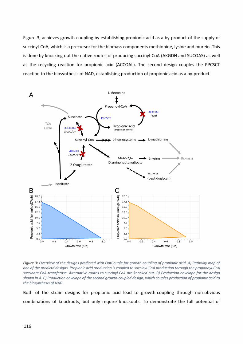
116

Figure 3, achieves growth-coupling by establishing propionic acid as a by-product of the supply of

succinyl-CoA, which is a precursor for the biomass components methionine, lysine and murein. This

is done by knocking out the native routes of producing succinyl-CoA (AKGDH and SUCOAS) as well

as the recycling reaction for propionic acid (ACCOAL). The second design couples the PPCSCT

reaction to the biosynthesis of NAD, establishing production of propionic acid as a by-product.

Figure 3: Overview of the designs predicted with OptCouple for growth-coupling of propionic acid. A) Pathway map of one of the predictd designs. Propionic acid production is coupled to succinyl-CoA production through the propanoyl-CoA succinate CoA-transferase. Alternative routes to succinyl-CoA are knocked out. B) Production envelope for the design shown in A. C) Production envelope of the second growth-coupled design, which couples production of propionic acid to the biosynthesis of NAD.

Both of the strain designs for propionic acid lead to growth-coupling through non-obvious

combinations of knockouts, but only require knockouts. To demonstrate the full potential of

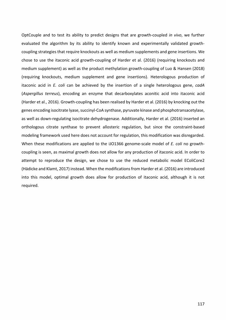
117

OptCouple and to test its ability to predict designs that are growth-coupled in vivo, we further

evaluated the algorithm by its ability to identify known and experimentally validated growth-

coupling strategies that require knockouts as well as medium supplements and gene insertions. We

chose to use the itaconic acid growth-coupling of Harder et al. (2016) (requiring knockouts and

medium supplement) as well as the product methylation growth-coupling of Luo & Hansen (2018)

(requiring knockouts, medium supplement and gene insertions). Heterologous production of

itaconic acid in E. coli can be achieved by the insertion of a single heterologous gene, cadA

(Aspergillus terreus), encoding an enzyme that decarboxylates aconitic acid into itaconic acid

(Harder et al., 2016). Growth-coupling has been realised by Harder et al. (2016) by knocking out the

genes encoding isocitrate lyase, succinyl-CoA synthase, pyruvate kinase and phosphotransacetylase,

as well as down-regulating isocitrate dehydrogenase. Additionally, Harder et al. (2016) inserted an

orthologous citrate synthase to prevent allosteric regulation, but since the constraint-based

modeling framework used here does not account for regulation, this modification was disregarded.

When these modifications are applied to the iJO1366 genome-scale model of E. coli no growth-

coupling is seen, as maximal growth does not allow for any production of itaconic acid. In order to

attempt to reproduce the design, we chose to use the reduced metabolic model EColiCore2

(Hädicke and Klamt, 2017) instead. When the modifications from Harder et al. (2016) are introduced

into this model, optimal growth does allow for production of itaconic acid, although it is not

required.

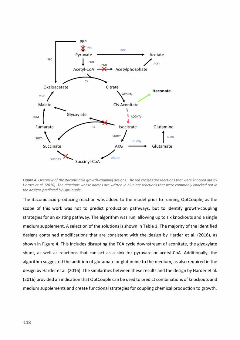
118

Figure 4: Overview of the itaconic acid growth-coupling designs. The red crosses are reactions that were knocked out by Harder et al. (2016). The reactions whose names are written in blue are reactions that were commonly knocked out in the designs predicted by OptCouple.

The itaconic acid-producing reaction was added to the model prior to running OptCouple, as the

scope of this work was not to predict production pathways, but to identify growth-coupling

strategies for an existing pathway. The algorithm was run, allowing up to six knockouts and a single

medium supplement. A selection of the solutions is shown in Table 1. The majority of the identified

designs contained modifications that are consistent with the design by Harder et al. (2016), as

shown in Figure 4. This includes disrupting the TCA cycle downstream of aconitate, the glyoxylate

shunt, as well as reactions that can act as a sink for pyruvate or acetyl-CoA. Additionally, the

algorithm suggested the addition of glutamate or glutamine to the medium, as also required in the

design by Harder et al. (2016). The similarities between these results and the design by Harder et al.

(2016) provided an indication that OptCouple can be used to predict combinations of knockouts and

medium supplements and create functional strategies for coupling chemical production to growth.

119

While the results obtained for growth-coupling of itaconic acid demonstrated the utility of the

algorithm for predicting knockouts and medium modifications, they did not require prediction of

gene insertions. To test the ability of OptCouple to predict such modifications, the product

methylation growth-coupling design of Luo & Hansen (2018) was used. This time the iJO1366

genome-scale model was chosen, as the modifications suggested by Luo & Hansen (2018) do confer

growth-coupling in this context. To predict designs for product methylation, a dummy reaction

converting SAM into S-adenosylhomocysteine (SAH) and an exportable methyl group metabolite

was created and used as target reaction. The algorithm was run with a single knockout, two

insertions and one medium supplement allowed. Among the predicted strategies we found a design

that consisted of the exact same combination of modifications as suggested by Luo & Hansen (2018),

while designs with several minor variations were also predicted. These variations consisted of

different knockouts or insertions but resulted in the same general mechanism of growth-coupling,

by requiring product methylation to convert SAM into SAH as part of the conversion of

supplemented methionine into cysteine required for biomass production. The ability to predict the

exact design of the validated methylation growth-coupling, as well as alternative seemingly

equivalent designs, indicates that OptCouple can reliably be used to predict new feasible growth-

coupling strategies, requiring a combination of gene knockouts, insertions and medium

supplements.

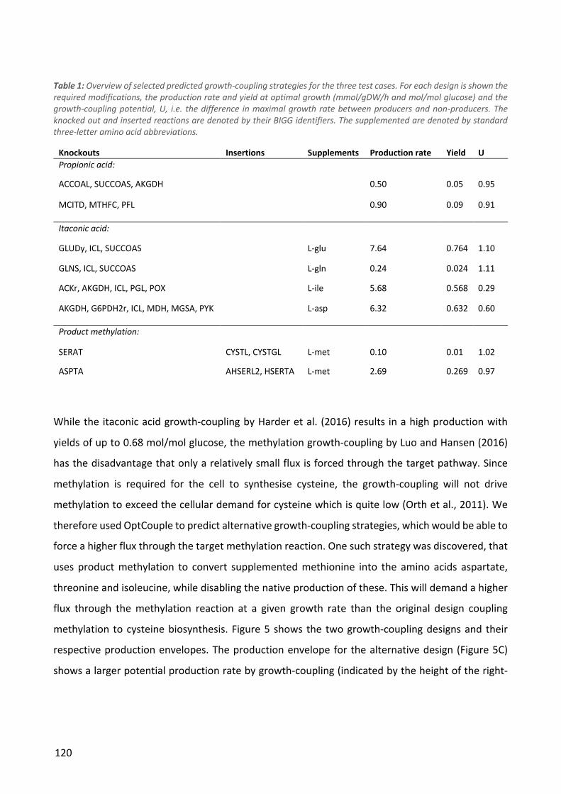
120

Table 1: Overview of selected predicted growth-coupling strategies for the three test cases. For each design is shown the required modifications, the production rate and yield at optimal growth (mmol/gDW/h and mol/mol glucose) and the growth-coupling potential, U, i.e. the difference in maximal growth rate between producers and non-producers. The knocked out and inserted reactions are denoted by their BIGG identifiers. The supplemented are denoted by standard three-letter amino acid abbreviations.

Knockouts Insertions Supplements Production rate Yield U Propionic acid:

ACCOAL, SUCCOAS, AKGDH 0.50 0.05 0.95

MCITD, MTHFC, PFL 0.90 0.09 0.91 Itaconic acid:

GLUDy, ICL, SUCCOAS L-glu 7.64 0.764 1.10

GLNS, ICL, SUCCOAS L-gln 0.24 0.024 1.11

ACKr, AKGDH, ICL, PGL, POX L-ile 5.68 0.568 0.29

AKGDH, G6PDH2r, ICL, MDH, MGSA, PYK L-asp 6.32 0.632 0.60 Product methylation:

SERAT CYSTL, CYSTGL L-met 0.10 0.01 1.02

ASPTA AHSERL2, HSERTA L-met 2.69 0.269 0.97

While the itaconic acid growth-coupling by Harder et al. (2016) results in a high production with

yields of up to 0.68 mol/mol glucose, the methylation growth-coupling by Luo and Hansen (2016)

has the disadvantage that only a relatively small flux is forced through the target pathway. Since

methylation is required for the cell to synthesise cysteine, the growth-coupling will not drive

methylation to exceed the cellular demand for cysteine which is quite low (Orth et al., 2011). We

therefore used OptCouple to predict alternative growth-coupling strategies, which would be able to

force a higher flux through the target methylation reaction. One such strategy was discovered, that

uses product methylation to convert supplemented methionine into the amino acids aspartate,

threonine and isoleucine, while disabling the native production of these. This will demand a higher

flux through the methylation reaction at a given growth rate than the original design coupling

methylation to cysteine biosynthesis. Figure 5 shows the two growth-coupling designs and their

respective production envelopes. The production envelope for the alternative design (Figure 5C)

shows a larger potential production rate by growth-coupling (indicated by the height of the right-

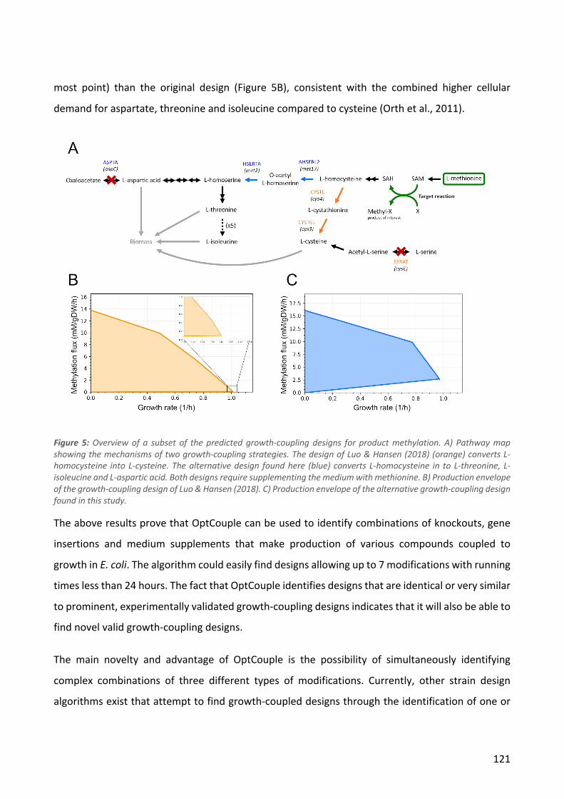
121

most point) than the original design (Figure 5B), consistent with the combined higher cellular

demand for aspartate, threonine and isoleucine compared to cysteine (Orth et al., 2011).

Figure 5: Overview of a subset of the predicted growth-coupling designs for product methylation. A) Pathway map showing the mechanisms of two growth-coupling strategies. The design of Luo & Hansen (2018) (orange) converts L-homocysteine into L-cysteine. The alternative design found here (blue) converts L-homocysteine in to L-threonine, L-isoleucine and L-aspartic acid. Both designs require supplementing the medium with methionine. B) Production envelope of the growth-coupling design of Luo & Hansen (2018). C) Production envelope of the alternative growth-coupling design found in this study.

The above results prove that OptCouple can be used to identify combinations of knockouts, gene

insertions and medium supplements that make production of various compounds coupled to

growth in E. coli. The algorithm could easily find designs allowing up to 7 modifications with running

times less than 24 hours. The fact that OptCouple identifies designs that are identical or very similar

to prominent, experimentally validated growth-coupling designs indicates that it will also be able to

find novel valid growth-coupling designs.

The main novelty and advantage of OptCouple is the possibility of simultaneously identifying

complex combinations of three different types of modifications. Currently, other strain design

algorithms exist that attempt to find growth-coupled designs through the identification of one or

122

two types of modifications simultaneously. Recent examples are SimOptStrain (Kim et al., 2011) that

simultaneously identifies gene knockouts and insertions, whereas SelFi (Hassanpour et al., 2017)

can suggest all three types of modifications, but only medium supplements and gene knockouts are

identified simultaneously. Several successful designs, however, such as the product methylation

growth-coupling (Luo and Hansen, 2018), show that considering all three types of modifications at

once can enable the identification of new growth-coupling strategies.

OptCouple guarantees that the resulting designs are truly growth-coupled. This is in contrast to e.g.

SimOptStrain, which uses the same objective function as OptKnock, and thus does not specifically

predict growth-coupling, as competing pathways are still allowed. A potential drawback of using the

growth-coupling potential as objective function in OptCouple is that there is no explicit optimization

of the target flux that can be achieved by growth-coupling. An example of this issue is seen in the

identified growth-coupling strategies for propionic acid. The design identified by OptCouple ensures

the production of propionic acid to supply the cell with either NAD or methionine, lysine and murein,

all of which are only needed in relatively small amounts. The consequence is that the growth-

coupled production rate of propionic acid will not be sufficient for a commercially viable process,

given the modest market price of propionic acid (Rodriguez et al., 2014). Even though this limits the

practical utility of some growth-coupling strategies identified by OptCouple, it does not significantly

reduce the utility of the algorithm itself. Computationally predicted strain designs should always be

assessed manually before being implemented in the laboratory, as their feasibility can also be

affected by a range of factors not considered in the models, e.g. thermodynamics, regulation,

toxicity, etc. Through the use of suboptimal solution pools, OptCouple can quickly identify many

design alternatives, which means that many candidate designs are obtained, increasing the

likelihood that at least one will be deemed feasible and have a high growth-coupled production rate.

As with all model-based predictions, the quality of the results strongly depends on the quality of the

model that was used. As one of the most commonly used organisms for metabolic modeling, the E.

coli genome-scale model is relatively comprehensive. While nothing prevents OptCouple from being

used in other organisms, the predicted designs should be curated even more thoroughly if a less

complete metabolic model is used. The in vivo presence of enzymes that are not accounted for in

the model can effectively abolish the growth-coupling of a predicted design, as they can allow the

123

cell to circumvent the growth-coupling mechanism. Conversely, if a model contains reactions that

are not active in vivo, e.g. due to transcriptional repression, some growth-coupling strategies will

require more modifications in silico than they would in practice. This is seen in the experimentally

validated itaconic acid growth-coupling design (Harder et al., 2016), which does not show growth-

coupling when simulated with iJO1366, whereas the reduced model EColiCore2 did allow

production at optimal growth. However, during optimization with ALE, repressed reactions could

become active allowing the cell to circumvent growth-coupling mechanisms predicted with reduced

models. Therefore, it would most likely be preferable to use the most complete model available for

the chosen organism.

5.5 Conclusion

OptCouple is an MILP-based optimization algorithm that can find combinations of gene knockouts,

heterologous gene insertions, and additions to the growth medium, that allow the stoichiometric

coupling of a product of interest to growth. In our validation tests OptCouple was able to reproduce

successful growth-coupling designs from the published literature and find alternative designs that

allow for a higher production flux. Furthermore, we showed that OptCouple can be used to predict

novel candidate growth-coupling designs for target compounds where no growth-coupling has

previously been demonstrated.

5.6 Acknowledgements

This project has received funding from the European Union’s Horizon 2020 research and innovation

programme under grant agreement No 686070. Furthermore, we acknowledge financial support

from the Novo Nordisk Foundation. The funding agencies were not involved in planning or carrying

out the study. ASLH declares financial interest as co-inventor of patent WO2018037098.

5.7 References

Alter, T.B., Blank, L.M., Ebert, B.E., 2018. Determination of growth-coupling strategies and their

underlying principles. bioRxiv. https://doi.org/https://doi.org/10.1101/258996

Becker, J., Wittmann, C., 2015. Advanced biotechnology: Metabolically engineered cells for the bio-

based production of chemicals and fuels, materials, and health-care products. Angew. Chemie

124

- Int. Ed. 54, 3328–3350. https://doi.org/10.1002/anie.201409033

Burgard, A.P., Pharkya, P., Maranas, C.D., 2003. OptKnock: A Bilevel Programming Framework for

Identifying Gene Knockout Strategies for Microbial Strain Optimization. Biotechnol. Bioeng. 84,

647–657. https://doi.org/10.1002/bit.10803

Cardoso, J.G.R., Jensen, K., Lieven, C., Hansen, A.S.L., Galkina, S., Beber, M., Özdemir, E., Herrgård,

M.J., Redestig, H., Sonnenschein, N., 2018. Cameo: A Python Library for Computer Aided

Metabolic Engineering and Optimization of Cell Factories. ACS Synth. Biol. 7, 1163–1166.

https://doi.org/10.1021/acssynbio.7b00423

Eş, I., Khaneghah, A.M., Hashemi, S.M.B., Koubaa, M., 2017. Current advances in biological

production of propionic acid. Biotechnol. Lett. 39, 635–645. https://doi.org/10.1007/s10529-

017-2293-6

Feist, A.M., Zielinski, D.C., Orth, J.D., Schellenberger, J., Herrgard, M.J., Palsson, B.O., 2010. Model-

driven evaluation of the production potential for growth-coupled products of Escherichia coli.


Hädicke, O., Klamt, S., 2017. EColiCore2: A reference network model of the central metabolism of

Escherichia coli and relationships to its genome-scale parent model. Sci. Rep. 7, 1–15.

https://doi.org/10.1038/srep39647

Hansen, A.S.L., Lennen, R.M., Sonnenschein, N., Herrgård, M.J., 2017. Systems biology solutions for

biochemical production challenges. Curr. Opin. Biotechnol. 45, 85–91.


Harder, B.J., Bettenbrock, K., Klamt, S., 2016. Model-based metabolic engineering enables high yield

itaconic acid production by Escherichia coli. Metab. Eng. 38, 29–37.


Hassanpour, N., Ullah, E., Yousofshahi, M., Nair, N.U., Hassoun, S., 2017. Selection Finder (SelFi): A

computational metabolic engineering tool to enable directed evolution of enzymes. Metab.

Eng. Commun. 4, 37–47. https://doi.org/10.1016/j.meteno.2017.02.003

Ignizio, J.P., Cavalier, T.M., 1994. Duality and Sensitivity Analysis, in: Ignizio, J.P., Cavalier, T.M. (Eds.),

125

Linear Programming. Prentice Hall, Englewood Cliffs, NJ.

Jensen, K., G.R. Cardoso, J., Sonnenschein, N., 2017. Optlang: An algebraic modeling language for

mathematical optimization. J. Open Source Softw. 2, 139. https://doi.org/10.21105/joss.00139

Kim, J., Reed, J.L., Maravelias, C.T., 2011. Large-Scale Bi-Level strain design approaches and Mixed-

Integer programming solution techniques. PLoS One 6.

https://doi.org/10.1371/journal.pone.0024162

Klamt, S., Gilles, E.D., 2004. Minimal cut sets in biochemical reaction networks. Bioinformatics 20,

226–234. https://doi.org/10.1093/bioinformatics/btg395

Klamt, S., Mahadevan, R., 2015. On the feasibility of growth-coupled product synthesis in microbial

strains. Metab. Eng. 30, 166–178. https://doi.org/10.1016/j.ymben.2015.05.006

LaCroix, R.A., Palsson, B.O., Feist, A.M., 2017. A model for designing adaptive laboratory evolution

experiments. Appl. Environ. Microbiol. 83. https://doi.org/10.1128/AEM.03115-16

Lee, S.Y., Kim, H.U., 2015. Systems strategies for developing industrial microbial strains. Nat.

Biotechnol. 33, 1061–1072. https://doi.org/10.1038/nbt.3365

Luo, H., Hansen, A.S.L., 2018. Method of improving methyltransferase activity. WO2018037098.

Moretti, S., Martin, O., Van Du Tran, T., Bridge, A., Morgat, A., Pagni, M., 2016. MetaNetX/MNXref

- Reconciliation of metabolites and biochemical reactions to bring together genome-scale

metabolic networks. Nucleic Acids Res. 44, D523–D526. https://doi.org/10.1093/nar/gkv1117

Orth, J.D., Conrad, T.M., Na, J., Lerman, J. a, Nam, H., Feist, A.M., Palsson, B.Ø., 2011. A

comprehensive genome-scale reconstruction of Escherichia coli metabolism. Mol. Syst. Biol. 7,

1–9. https://doi.org/10.1038/msb.2011.65

Phaneuf, P. V, Gos, D., Palsson, B.O., Feist, A.M., 2018. ALEdb 1.0: A Database of Mutations from

Adaptive Laboratory Evolution Experimentation.

Pharkya, P., Burgard, A.P., Maranas, C.D., 2004. OptStrain: A computational framework for redesign

of microbial production systems. Genome Res. 2367–2376.

https://doi.org/10.1101/gr.2872004

126

Portnoy, V.A., Bezdan, D., Zengler, K., 2011. Adaptive laboratory evolution-harnessing the power of

biology for metabolic engineering. Curr. Opin. Biotechnol. 22, 590–594.


Rodriguez, B.A., Stowers, C.C., Pham, V., Cox, B.M., 2014. The production of propionic acid, propanol

and propylene via sugar fermentation: An industrial perspective on the progress, technical

challenges and future outlook. Green Chem. 16, 1066–1076.

https://doi.org/10.1039/c3gc42000k

Shepelin, D., Hansen, A.S.L., Lennen, R., Luo, H., Herrgård, M.J., 2018. Selecting the best:

Evolutionary engineering of chemical production in microbes. Genes (Basel). 9.

https://doi.org/10.3390/genes9050249

Stanford, N.J., Millard, P., Swainston, N., 2015. RobOKoD: microbial strain design for

(over)production of target compounds. Front. Cell Dev. Biol. 3, 1–12.

https://doi.org/10.3389/fcell.2015.00017

Tepper, N., Shlomi, T., 2009. Predicting metabolic engineering knockout strategies for chemical

production: Accounting for competing pathways. Bioinformatics 26, 536–543.

https://doi.org/10.1093/bioinformatics/btp704

von Kamp, A., Klamt, S., 2017. Growth-coupled overproduction is feasible for almost all metabolites

in five major production organisms. Nat. Commun. 8, 1–10.

https://doi.org/10.1038/ncomms15956

von Kamp, A., Klamt, S., 2014. Enumeration of Smallest Intervention Strategies in Genome-Scale

Metabolic Networks. PLoS Comput. Biol. 10. https://doi.org/10.1371/journal.pcbi.1003378

Wong, B.G., Mancuso, C.P., Kiriakov, S., Bashor, C.J., Khalil, A.S., 2018. Precise, automated control

of conditions for high-throughput growth of yeast and bacteria with eVOLVER. Nat. Biotechnol.

36, 614–623. https://doi.org/10.1038/nbt.4151

127


Mathematical formulation of OptCouple

The metabolic model used in OptCouple is given by a set of metabolites èG∀2 ∈ í, and a set of

metabolic reactions ìî∀ï ∈ s. A stoichiometric matrix S encodes which metabolites participate in

each reaction (Orth et al., 2010). R is partitioned by the three subsets, sJ|*Gù7, s¢7*76I£IñIDc and

s|KKG*GIJc, representing native reactions, heterologous reactions and boundary reactions for

potential medium additions, respectively. Furthermore, some reactions ìî∀ï ∈ sG667ù76cGó£7 can

only proceed in the forward direction, while the remaining reactions can proceed in both directions.

Each reaction is associated with a binary control variable, 5î ∈ P∀ï ∈ s.

The primal problem (M) optimizes biomass production subject to stoichiometric constraints, limited

glucose uptake and genetic modifications, Y:

S&!2è24(wÇóGIC|cc

subject to:

∑ 4Gî ∙ Çîî∈q = 0∀2 ∈ í

ÇîCGJ ∙ 5î ≤ Çî ≤ Çî

C|} ∙ 5î∀ï ∈ s

Çñ£H_D¶*|ß7 ≤ 10

Çî ≥ 0∀ï ∈ sG667ù76cGó£7

5î ∈ {0, 1}, ∀ï ∈ s

∑ (1 − 5î)î∈q®©™L´¨ ≤ TJ|*Gù7

∑ 5îî∈q≠¨™¨ÆØ∞Ø±Ø≤≥ ≤ T¢7*76I£IñIDc

∑ 5îî∈q©¥¥L™LØ®≥ ≤ T|KKG*GIJc

128

The problem can be modified to not allow flux in the target reaction ì*|6ñ7*, resulting in M*:

S&!2è24(wÇóGIC|cc

subject to:

∑ 4Gî ∙ Çî = 0,|q|îb] ∀2 ∈ í


C|} ∙ 5î,∀ï ∈ s

Ç*|6ñ7* = 0

Çñ£H_D¶*|ß7 ≤ 10

Çî ≥ 0,∀ï ∈ sG667ù76cGó£7

5î ∈ {0, 1}, ∀ï ∈ s

∑ (1 − 5î)î∈q®©™L´¨ ≤ TJ|*Gù7



M* can then be converted to its dual form, S°∗ (as described by Burgard et al. (2003)):

S232è24(µ,∂10 ∙ Öñ£DHIc7_D¶*|ß7

subject to:

∑ ∑Gc*IGH¢ ∙ 4Gî + Öî = 0,∀ï ∈ s,ï ≠ ,2?è&44|r|

Gb]

∑ ∑Gc*IGH¢ ∙ 4G,óGIC|cc + ÖóGIC|cc = 1|r|

Gb]

ÖîCGJ ∙ 11 − 5î9 ≤ Öî ≤ Öî

C|} ∙ (1 − 5G),∀ï ∈ s, ï ≠ #&ì@(#

5î ∈ {0, 1}, ∀ï ∈ s

∑ (1 − 5î)î∈q®©™L´¨ ≤ TJ|*Gù7



Here ∑Gc*IGH¢ represent dual variables of the stoichiometric constraints in the primal, while ÖG

represent other flux bounds. The minimum and maximum values, ÖîCGJ and Öî

C|} as well as

129

ÇîCGJand Çî

C|}can be found by sequentially minimizing and maximizing the variables or by using a

sufficiently large constant (the big-M method).

The two problems S and SK∗ are combined and optimized simultaneously, together with the binary

variables Y:

S&!2è24(w,∂,µ,πÇóGIC|cc − 10 ∙ Öñ£DHIc7_D¶*|ß7 OptCouple

subject to:

∑ 4Gî ∙ Çî = 0|q|îb] ∀2 ∈ í


C|} ∙ 5î∀ï ∈ s

Çñ£H_D¶*|ß7 ≤ 10

Çî ≥ 0∀ï ∈ sG667ù76cGó£7

∑ ∑Gc*IGH¢ ∙ 4Gî + Öî = 0,∀ï ∈ s,ï ≠ ,2?è&44|r|

Gb]

∑ ∑Gc*IGH¢ ∙ 4G,óGIC|cc + ÖóGIC|cc = 1|r|

Gb]

ÖîCGJ ∙ 11 − 5î9 ≤ Öî ≤ Öî

C|} ∙ (1 − 5G),∀ï ∈ s, ï ≠ #&ì@(#

5î ∈ {0, 1}, ∀ï ∈ s

∑ (1 − 5î)î∈q®©™L´¨ ≤ TJ|*Gù7



References

Burgard, A.P., Pharkya, P., Maranas, C.D., 2003. OptKnock: A Bilevel Programming Framework for

Identifying Gene Knockout Strategies for Microbial Strain Optimization. Biotechnol. Bioeng. 84,

647–657. https://doi.org/10.1002/bit.10803

Orth, J.D., Thiele, I., Palsson, B.Ø., 2010. What is flux balance analysis? Nat. Biotechnol. 28, 245–

248. https://doi.org/10.1038/nbt.1614

130

Concluding remarks

Adaptive laboratory evolution (ALE) can be a valuable addition to rational engineering during

development of microbial cell factories. Sequencing of evolved isolates can reveal new engineering

targets for the evolved phenotype that could not have been predicted from preexisting knowledge.

Additionally, studying the evolved strains can yield insight into the mechanisms with which the

targeted phenotype improved.

In this thesis, it was shown that ALE could be used to improve chemical tolerance of Escherichia coli

– a phenotype that is difficult to engineer rationally due to a lack of knowledge about toxicity

mechanisms. The concentrations of chemicals that the evolved strains could tolerate were high

enough to be relevant in the context of bioproduction. Although only little information could be

gained about the mechanisms of tolerance, cross-compound screenings revealed that tolerance to

one compound tends to be generalizable to a wide range of chemically similar compounds. This

demonstrates that it is possible to use broadly tolerant platform strains for production of several

products, without having to evolve tolerance to each individual product. For two compounds it was

also shown that some evolved tolerant strains were able to produce the respective compounds at

higher rates than the background strain, further demonstrating the utility of ALE in cell factory

development.

Metabolomic characterization of the evolved strains showed a high degree of convergent evolution

on the metabolic level despite only limited convergence on the genetic level. This suggests that

metabolism plays a significant role in tolerance against the tested chemicals. The metabolic profiles

of the evolved strains were also used to develop a method for predicting the impact of a mutation

on the gene that it affects. This method can be beneficial in interpreting the mutations that are

observed after an ALE experiment and is not limited to strains evolved for tolerance. Another

method for interpreting mutations observed in ALE was presented, which was based on deep neural

networks. While artificial intelligence and machine learning have the potential to revolutionize the

field of metabolic engineering like it has other fields, it is still limited by the comparatively small

datasets available in biology.

131

The greatest challenge of using ALE in cell factory engineering is finding ways to select for the

phenotype that is to be improved. In particular it is desirable to be able to select for mutants that

produce a target compound at high rates. This is possible by making production coupled to growth

such that the target compound becomes a necessary by-product. Although growth-coupling

production usually requires complicated rewiring of metabolism, it can be done through the use of

mathematical models of metabolism. This thesis presented a new model-based algorithm for

identifying genetic modifications that cause growth-coupling in combination with one or more

supplements to the growth medium. The algorithm allowed prediction of promising design

strategies for growth-coupling, however these strategies need to be validated in vivo and are not

guaranteed to work. Future work might focus on directly integrating experimental data into

algorithms for predicting growth-coupling in order to improve predictions and make the predicted

designs more likely to function in vivo, which would further increase the effectiveness of ALE for cell

factory development.

Documents

Computational methods for microbial cell factory engineering … · Computational methods for microbial cell factory engineering aided by evolution PhD Thesis by Kristian Jensen December