Embed Size (px)
Citation preview
Acta mater. 49 (2001) 3899–3918www.elsevier.com/locate/actamat
COMPUTATIONAL MODELING OF THE FORWARD ANDREVERSE PROBLEMS IN INSTRUMENTED SHARP
INDENTATION
M. DAO, N. CHOLLACOOP, K. J. VAN VLIET, T. A. VENKATESH and S. SURESH†Department of Materials Science and Engineering, Massachusetts Institute of Technology, Cambridge,
MA 02139, USA
( Received 23 April 2001; received in revised form 6 August 2001; accepted 7 August 2001 )
Abstract—A comprehensive computational study was undertaken to identify the extent to which elasto-plastic properties of ductile materials could be determined from instrumented sharp indentation and to quantifythe sensitivity of such extracted properties to variations in the measured indentation data. Large deformationfinite element computations were carried out for 76 different combinations of elasto-plastic properties thatencompass the wide range of parameters commonly found in pure and alloyed engineering metals: Young’smodulus,E, was varied from 10 to 210 GPa, yield strength,sy, from 30 to 3000 MPa, and strain hardeningexponent,n, from 0 to 0.5, and the Poisson’s ratio,n, was fixed at 0.3. Using dimensional analysis, a newset of dimensionless functions were constructed to characterize instrumented sharp indentation. From thesefunctions and elasto-plastic finite element computations, analytical expressions were derived to relate inden-tation data to elasto-plastic properties. Forward and reverse analysis algorithms were thus established; theforward algorithms allow for the calculation of a unique indentation response for a given set of elasto-plasticproperties, whereas the reverse algorithms enable the extraction of elasto-plastic properties from a given setof indentation data. A representative plastic strainer was identified as a strain level which allows for theconstruction of a dimensionless description of indentation loading response, independent of strain hardeningexponentn. The proposed reverse analysis provides a unique solution of the reduced Young’s modulusE*,a representative stresssr, and the hardnesspave. These values are somewhat sensitive to the experimentalscatter and/or error commonly seen in instrumented indentation. With this information, values ofsy and ncan be determined for the majority of cases considered here, provided that the assumption of power lawhardening adequately represents the full uniaxial stress–strain response. These plastic properties, however, arevery strongly influenced by even small variations in the parameters extracted from instrumented indentationexperiments. Comprehensive sensitivity analyses were carried out for both forward and reverse algorithms,and the computational results were compared with experimental data for two materials. 2001 ActaMaterialia Inc. Published by Elsevier Science Ltd. All rights reserved.
Keywords: Indentation; Mechanical properties; Finite element simulation; Large deformation; Representa-tive strain
1. INTRODUCTION
The mechanical characterization of materials has longbeen represented by their hardness values [1, 2].Recent technological advances have led to the generalavailability of depth-sensing instrumented micro- andnanoindentation experiments (e.g. [1–14]). Nanoind-enters provide accurate measurements of the continu-ous variation of indentation loadP down to µN, asa function of the indentation depthh down to nm.Experimental investigations of indentation have beenconducted on many material systems to extract hard-
† To whom all correspondence should be addressed. Tel.:+1-617-253-3320; Fax:+1-617-253-0868.
E-mail address: [email protected] (S. Suresh)
1359-6454/01/$20.00 2001 Acta Materialia Inc. Published by Elsevier Science Ltd. All rights reserved.PII: S1359-6454 (01)00295-6
ness and other mechanical properties and/or residualstresses (e.g., [3–5, 9, 13–17], among many others).
Concurrently, comprehensive theoretical and com-putational studies have emerged to elucidate the con-tact mechanics and deformation mechanisms in orderto systematically extract material properties fromPversush curves obtained from instrumented inden-tation (e.g., [3, 5, 11, 12, 16–21]). For example, thehardness and Young’s modulus can be obtained fromthe maximum load and the initial unloading slopeusing the methods suggested by Oliver and Pharr [5]or Doerner and Nix [3]. The elastic and plasticproperties may be computed through a procedure pro-posed by Giannakopoulos and Suresh [20], and theresidual stresses may be extracted by the method ofSuresh and Giannakopoulos [22]. Thin film systemshave also been studied using finite element compu-tations [23–25].

3900 DAO et al.: INSTRUMENTED SHARP INDENTATION
Using the concept of self-similarity, simple butgeneral results of elasto-plastic indentation responsehave been obtained. To this end, Hill et al. [26]developed a self-similar solution for the plastic inden-tation of a power law plastic material under sphericalindentation, where Meyer’s law† was given a rigor-ous theoretical basis. Later, for an elasto-plasticmaterial, self-similar approximations of sharp (i.e.,Berkovich and Vickers) indentation were compu-tationally obtained by Giannakopoulos et al. [18] andLarsson et al. [27]. More recently, scaling functionswere applied to study bulk [11, 12, 19] and coatedmaterial systems [25]. Kick’s Law (i.e., P = Ch2 dur-ing loading, where loading curvature C is a materialconstant) was found to be a natural outcome of thedimensional analysis of sharp indentation (e.g., [11]).
Despite these advances, several fundamental issuesremain that require further examination:
1. A set of analytical functions, which takes intoaccount the pile-up/sink-in effects and the largedeformation characteristics of the indentation,needs to be established in order to avoid detailedFEM computations after each indentation test.These functions can be used to accurately predictthe indentation response from a given set of elasto-plastic properties (forward algorithms), and toextract the elasto-plastic properties from a givenset of indentation data (reverse algorithms). Gian-nakopoulos, Larsson and Vestergaard [18] andlater Giannakopoulos and Suresh [20] proposed acomprehensive analytical framework to extractelasto-plastic properties from a single set of P�h data. Their results, as will be shown later in thisstudy, were formulated using mainly small defor-mation FEM results (although they performed anumber of large deformation computations).Cheng and Cheng [11, 12, 19], using an includedapex angle of the indenter of 68°, proposed a set ofuniversal dimensionless functions based on largedeformation FEM computations, but did not estab-lish a full set of closed-form analytical functions.
2. Under what conditions and/or assumptions can weextract a single set of elasto-plastic properties froma single P�h curve with reasonable accuracy?Cheng and Cheng [19] and Venkatesh et al. [21]discussed this issue. However, without an accurateanalytical framework based on large deformationtheory, this issue cannot be addressed.
3. What are the similarities and differences betweenthe large and small deformation-based analyticalformulations? Chaudhri [28] estimated that equiv-alent strains of 25–36% were present in the
† Meyer’s law for spherical indentation states that
P =Kam
Dm�2, where m is a hardening factor, D is the indenter’s
diameter, a is the contact radius of the indenter, and K is amaterial constant.
indented specimen near the tip of the Vickersindenter. These experimentally observed largestrains justify the need for large deformation basedtheories in modeling instrumented sharp inden-tation tests.
In this paper, these issues will be addressed withinthe context of sharp indentation and continuum analy-sis.
2. THEORETICAL AND COMPUTATIONALCONSIDERATIONS
2.1. Problem formulation and associated nomencla-ture
Figure 1 shows the typical P�h response of an ela-sto-plastic material to sharp indentation. During load-ing, the response generally follows the relationdescribed by Kick’s Law,
P � Ch2 (1)
where C is the loading curvature. The average contact
pressure, pave =Pm
Am
(Am is the true projected contact
area measured at the maximum load Pm), can beidentified with the hardness of the indented material.The maximum indentation depth hm occurs at Pm, and
the initial unloading slope is defined asdPu
dh |hm
, where
Pu is the unloading force. The Wt term is the totalwork done by load P during loading, We is thereleased (elastic) work during unloading, and thestored (plastic) work Wp = Wt�We. The residualindentation depth after complete unloading is hr.
As discussed by Giannakopoulos and Suresh [20],
C,dPu
dh |hm
andhr
hm
are three independent quantities that
can be directly obtained from a single P�h curve.
Fig. 1. Schematic illustration of a typical P�h response of anelasto-plastic material to instrumented sharp indentation.

3901DAO et al.: INSTRUMENTED SHARP INDENTATION
The question remains whether these parameters aresufficient to uniquely determine the indentedmaterial’s elasto-plastic properties.
Plastic behavior of many pure and alloyed engin-eering metals can be closely approximated by a powerlaw description, as shown schematically in Fig. 2. Asimple elasto-plastic, true stress–true strain behavioris assumed to be
s � �Ee, for s�sy
Ren, for s�sy
(2)
where E is the Young’s modulus, R a strength coef-ficient, n the strain hardening exponent, sy the initialyield stress and ey the corresponding yield strain,such that
sy � Eey � Reny (3)
Here the yield stress sy is defined at zero offset strain.The total effective strain, e, consists of two parts, eyand ep:
e � ey � ep (4)
where ep is the nonlinear part of the total effectivestrain accumulated beyond ey. With equations (3) and(4), when s�sy, equation (2) becomes
s � sy�1 �Esy
ep�n
(5)
To complete the material constitutive description,
Fig. 2. The power law elasto-plastic stress–strain behavior usedin the current study.
Poisson’s ratio is designated as n, and the incrementaltheory of plasticity with von Mises effective stress (J2
flow theory) is assumed.With the above assumptions and definitions, a
material’s elasto-plastic behavior is fully determinedby the parameters E, n, sy and n. Alternatively, withthe constitutive law defined in equation (2), the powerlaw strain hardening assumption reduces the math-ematical description of plastic properties to two inde-pendent parameters. This pair could be described asa representative stress sr (defined at ep = er, where eris a representative strain) and the strain-hardeningexponent n, or as sy and sr.
2.2. Dimensional analysis and universal functions
Cheng and Cheng [11, 12] and Tunvisut et al. [25]have used dimensional analysis to propose a numberof dimensionless universal functions, with the aid ofcomputational data points calculated via the FiniteElement Method (FEM). Here, a number of newdimensionless functions are described in the follow-ing paragraphs.
As discussed in Section 2.1, one can use a materialparameter set (E, n, sy and n), (E, n, sr and n) or (E,n, sy and sr) to describe the constitutive behavior.Therefore, the specific functional forms of the univer-sal dimensionless functions are not unique (but differ-ent definitions are interdependent if power law strainhardening is assumed). For instrumented sharp inden-tation, a particular material constitutive description(e.g., power-law strain hardening) yields its own dis-tinct set of dimensionless functions. One may chooseto use any plastic strain to be the representative strainer, where the corresponding sr is used to describe thedimensionless functions. However, the representativestrain which best normalizes a particular dimen-sionless function with respect to strain hardening willbe a distinct value.
Here, we present a set of universal dimensionlessfunctions and their closed-form relationship betweenindentation data and elasto-plastic properties (withinthe context of the present computational results). Thisset of functions leads to new algorithms for accuratelypredicting the P�h response from known elasto-plas-tic properties (forward algorithms) and new algor-ithms for systematically extracting the indentedmaterial’s elasto-plastic properties from a single setof P�h data (reverse algorithms).
For a sharp indenter (conical, Berkovich or Vick-ers, with fixed indenter shape and tip angle) indentingnormally into a power law elasto-plastic solid, theload P can be written as
P � P(h,E,v,Ei,vi,sy,n), (6)
where Ei is Young’s modulus of the indenter, and ni
is its Poisson’s ratio. This functionality is often sim-plified (e.g., [29]) by combining elasticity effects ofan elastic indenter and an elasto-plastic solid as

3902 DAO et al.: INSTRUMENTED SHARP INDENTATION
P � P(h,E∗,sy,n), (7)
where
E∗ � �1�v2
E�
1�v2i
Ei��1
(8)
Alternatively, equation (7) can be written as
P � P(h,E∗,sr,n) (9)
or
P � P(h,E∗,sy,sr) (10)
Applying the � theorem in dimensional analysis, equ-ation (9) becomes
P � srh2�1�E∗
sr
,n�, (11a)
and thus
C �Ph2 � sr�1�E∗
sr
,n�. (11b)
where �1 is a dimensionless function. Similarly,applying the � theorem to equation (10), loading cur-vature C may alternatively be expressed as
C �Ph2 � sy�
A1�E∗
sy
,sr
sy� (12a)
or
C �Ph2 � sr�
B1�E∗
sr
,sy
sr� (12b)
where �A1 and �B
1 are dimensionless functions. Thedimensionless functions given in equations (11) and(12) are different from those proposed in [11, 12],where the normalization was taken with respect to E*instead of sr or sy.
During nanoindentation experiments, especiallywhen the indentation depth is about 100–1000 nm,size-scale-dependent indentation effects have beenpostulated (e.g., [8, 30, 31]). These possible size-scale-dependent effects on hardness have been mod-eled using higher order theories (e.g., [30, 31]). If theindentation is sufficiently deep (typically deeper than
1 µm), then the scale dependent effects become smalland may be ignored. In the current study, any scaledependent effects are assumed to be insignificant. Itis clear from equations (11) and (12) that, for an iso-tropic and homogeneous material, P = Ch2 is thenatural outcome of the dimensional analysis for asharp indenter; loading curvature C is a material con-stant which is independent of indentation depth. It isalso noted that, depending on the choices of (er, sr),there are an infinite number of ways to define thedimensionless function �1. However, with theassumption of power-law strain hardening, it can beshown that one definition of �1 is easily convertedto another definition.
If the unloading force is represented as Pu, theunloading slope is given by
dPu
dh�
dPu
dh(h,hm,E,v,Ei,vi,sr,n) (13a)
or, assuming that elasticity effects are characterizedby E*, the unloading slope is given by
dPu
dh�
dPu
dh(h,hm,E∗,sr,n) (13b)
Dimensional analysis yields
dPu
dh� E∗h�0
2�hm
h,sr
E∗,n� (14)
Evaluating equation (14) at h = hm gives
dPu
dh |h � hm
� E∗hm�02�1,sr
E∗,n� (15)
� E∗hm�2�E∗
sr,n�
Similarly, Pu itself can be expressed as
Pu � Pu(h,hm,E∗,sr,n) � E∗h2�u�hm
h,sr
E∗,n�(16)
When Pu = 0, the specimen is fully unloaded and,thus, h = hr. Therefore, upon complete unloading,
0 � �u�hm
hr
,sr
E∗,n� (17)
Rearranging equation (17),

3903DAO et al.: INSTRUMENTED SHARP INDENTATION
hr
hm
� �3�sr
E∗,n� (18)
Thus, the three universal dimensionless functions, �1,�2 and �3, can be used to relate the indentationresponse to mechanical properties.
2.3. Computational model
Axisymmetric two-dimensional and full three-dimensional finite element models were constructedto simulate the indentation response of elasto-plasticsolids. Figure 3(a) schematically shows the conicalindenter, where q is the included half angle of theindenter, hm is the maximum indentation depth, andam is the contact radius measured at hm. The true pro-jected contact area Am, with pile-up or sink-in effectstaken into account, for a conical indenter is thus
Am � pa2m (19)
Figure 3(b) shows the mesh design for axisymmetriccalculations. The semi-infinite substrate of theindented solid was modeled using 8100 four-noded,bilinear axisymmetric quadrilateral elements, where afine mesh near the contact region and a graduallycoarser mesh further from the contact region weredesigned to ensure numerical accuracy. At themaximum load, the minimum number of contact
Fig. 3. Computational modeling of instrumented sharp indentation. (a) Schematic drawing of the conicalindenter, (b) mesh design for axisymmetric finite element calculations, (c) overall mesh design for the Berkovichindentation calculations, and (d) detailed illustration of the area that directly contacts the indenter tip in (c).
elements in the contact zone was no less than 16 ineach FEM computation. The mesh was well-tested forconvergence and was determined to be insensitive tofar-field boundary conditions.
Three-dimensional finite element models incorpor-ating the inherent six-fold or eight-fold symmetry ofa Berkovich or a Vickers indenter, respectively, werealso constructed. A total of 11,150 and 10,401 eight-noded, isoparametric elements was used for Berkov-ich and Vickers indentation, respectively. Figure 3(c)shows the overall mesh design for the Berkovichindentation, while Fig. 3(d) details the area thatdirectly contacts the indenter tip. Computations wereperformed using the general purpose finite elementpackage ABAQUS [32]. The three-dimensional meshdesign was verified against the three-dimensionalresults obtained from the mesh used previously byLarsson et al. [27]. Unless specified otherwise, largedeformation theory was assumed throughout theanalysis.
For a conical indenter, the projected contact areais A = ph2tan2q; for a Berkovich indenter,A = 24.56h2; for a Vickers indenter, A = 24.50h2. Inthis study, the three-dimensional indentation inducedvia Berkovich or Vickers geometries was approxi-mated with axisymmetric two-dimensional models bychoosing the apex angle q such that the projectedarea/depth of the two-dimensional cone was the sameas that for the Berkovich or Vickers indenter. Forboth Berkovich and Vickers indenters, the corre-
3904 DAO et al.: INSTRUMENTED SHARP INDENTATION
sponding apex angle q of the equivalent cone waschosen as 70.3°. Axisymmetric two-dimensionalcomputational results will be referenced in theremainder of the paper unless otherwise specified. Inall finite element computations, the indenter wasmodeled as a rigid body, and the contact was modeledas frictionless. Detailed pile-up and sink-in effectswere more accurately accounted for by the largedeformation FEM computations, as compared tosmall deformation computations.
2.4. Comparison of experimental and computationalresults
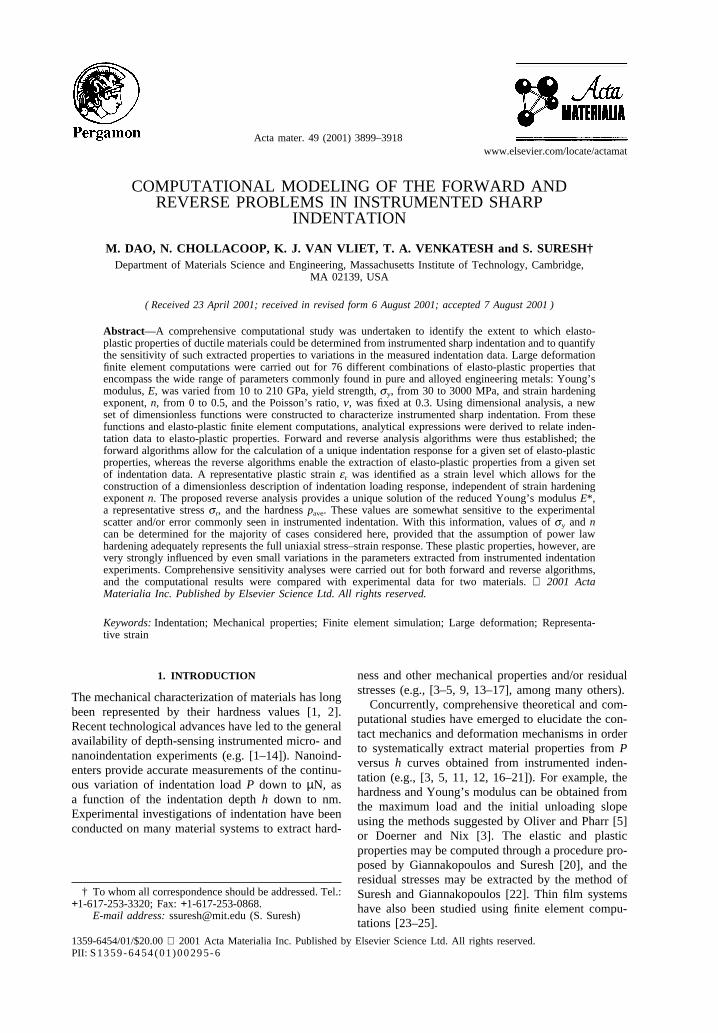
Two aluminum alloys were obtained for experi-mental investigation: 6061-T6511 and 7075-T651aluminum, both in the form of 2.54 cm diameter,extruded round bar stock. Two compression speci-mens (0.5 cm diameter, 0.75 cm height) weremachined from each bar such that the compressionaxis was parallel to the extrusion direction. Simpleuniaxial compression tests were conducted on aservo-hydraulic universal testing machine at a cross-head speed of 0.2 mm/min. Crosshead displacementwas obtained from a calibrated LVDT (linear voltage-displacement transducer). As each specimen wascompressed to 45% engineering strain, the specimenends were lubricated with Teflon lubricant to pre-vent barreling. Intermittent unloading was conductedto allow for repeated measurement of Young’s modu-lus and relubrication of the specimen ends. Recordedload–displacement data were converted to true stress–true strain data. Although the true stress–true strainresponses were well approximated by power law fits,these experimental stress–strain data were used asdirect input for FEM simulations, rather than themathematical approximations (see Fig. 4). For 7075-T651 aluminum, the measured Young’s modulus wasE = 70.1 GPa; and for 6061-T6511 aluminum,E = 66.8 GPa.
Indentation specimens were machined from thesame round bar stock as discs of the bar diameter (3mm thickness). Each specimen was polished to 0.06µm surface finish with colloidal silica. These speci-
Fig. 4. Experimental uniaxial compression stress–strain curvesof both 6061-T6511 aluminum and 7075-T651 aluminum
specimens, respectively.
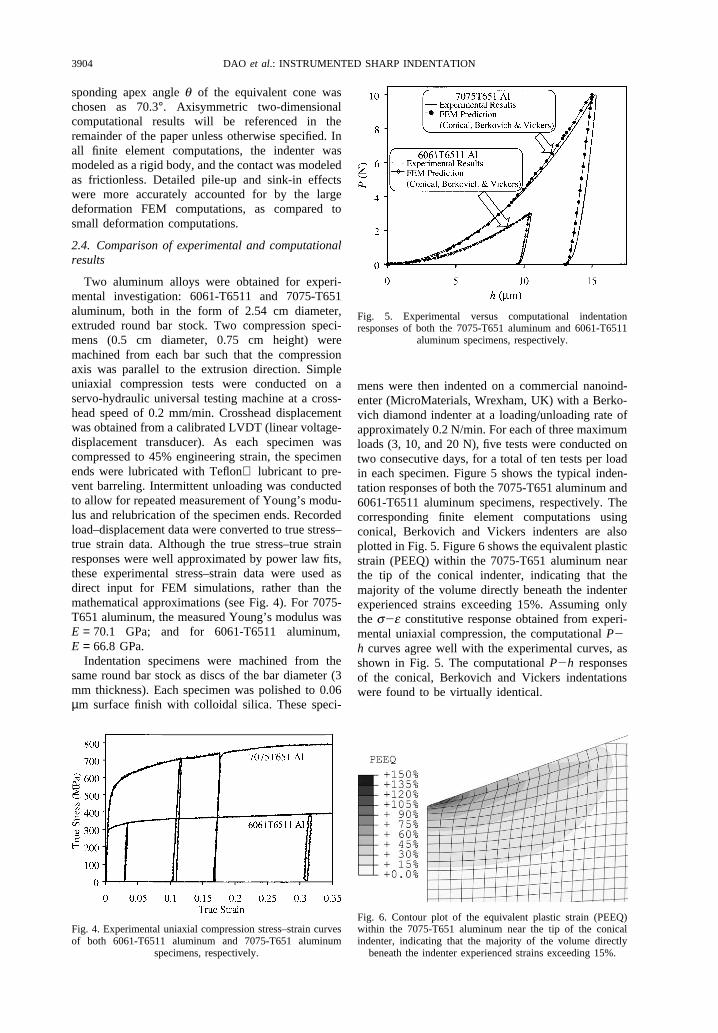
Fig. 5. Experimental versus computational indentationresponses of both the 7075-T651 aluminum and 6061-T6511
aluminum specimens, respectively.
mens were then indented on a commercial nanoind-enter (MicroMaterials, Wrexham, UK) with a Berko-vich diamond indenter at a loading/unloading rate ofapproximately 0.2 N/min. For each of three maximumloads (3, 10, and 20 N), five tests were conducted ontwo consecutive days, for a total of ten tests per loadin each specimen. Figure 5 shows the typical inden-tation responses of both the 7075-T651 aluminum and6061-T6511 aluminum specimens, respectively. Thecorresponding finite element computations usingconical, Berkovich and Vickers indenters are alsoplotted in Fig. 5. Figure 6 shows the equivalent plasticstrain (PEEQ) within the 7075-T651 aluminum nearthe tip of the conical indenter, indicating that themajority of the volume directly beneath the indenterexperienced strains exceeding 15%. Assuming onlythe s�e constitutive response obtained from experi-mental uniaxial compression, the computational P�h curves agree well with the experimental curves, asshown in Fig. 5. The computational P�h responsesof the conical, Berkovich and Vickers indentationswere found to be virtually identical.
Fig. 6. Contour plot of the equivalent plastic strain (PEEQ)within the 7075-T651 aluminum near the tip of the conicalindenter, indicating that the majority of the volume directly
beneath the indenter experienced strains exceeding 15%.

3905DAO et al.: INSTRUMENTED SHARP INDENTATION
Table 1. Four cases studied to compare large vs small deformation theory
Case System E (GPa) Yield strength (MPa) n n
A Zinc alloy 9 300 0.05 0.3B Refractory alloy 80 1500 0.05 0.3C Aluminum alloy 70 300 0.05 0.28D Steel 210 500 0.1 0.27
2.5. Large deformation vs small deformation
Giannakopoulos et al. [18], Larsson et al. [27],Giannakopoulos and Suresh [20], and Venkatesh etal. [21] have proposed a systematic methodology toextract elasto-plastic properties from a single P�hcurve. The loading curvature C was given as
C � M1s0.29�1 �sy
s0.29��M2 � ln�E∗
sy�� (20)
where M1 and M2 are computationally derived con-stants which depend on indenter geometry. It is inter-esting to note that, after rewriting s0.29(1 + sy/s0.29)as sy(1 + s0.29/sy), equation (20) is consistent withequation (12a).
Figure 7 shows the comparison between the largedeformation solution, small deformation solution andthe predictions from equation (20), using the fourmodel materials listed in Venkatesh et al. [21] (seeTable 1). From Fig. 7, it is evident that equation (20)agrees well with the small deformation results andthat, for all four cases studied, large deformationtheory always predicts a stiffer loading response.
In addition, 76 different cases covering materialparameters of most engineering metals were studiedcomputationally. Detailed examination showed thatlarge deformation solutions are not readily describedby equation (20), but rather are better approximatedwithin ±10% (for the conical indenter withq = 70.3°) by a new universal function given by
Fig. 7. Comparison between the large deformation solution,small deformation solution and the previous formulation [equ-ation (20)] using four model materials. For all four cases stud-ied, large deformation theory always predicts a stiffer loading
response.
C � N1s0.29�1 �sy
s0.29��N2 � ln� E∗
s0.29�� (21)
where N1 = 9.4509 and N2 = �1.2433 are compu-tationally derived constants specific to the indentergeometry. This expression is consistent with thedimensionless function shown in equation (12b).
3. COMPUTATIONAL RESULTS
A comprehensive parametric study of 76 additionalcases was conducted (see Appendix A for a completelist of parameters). These cases represented the rangeof parameters of mechanical behavior found in com-mon engineering metals: that is, Young’s modulus Eranged from 10 to 210 GPa, yield strength sy from30 to 3000 MPa, strain hardening exponent n from 0to 0.5, and Poisson’s ratio n was fixed at 0.3. Theaxisymmetric finite element model was used to obtaincomputational results unless otherwise specified.
3.1. Representative strain and universal dimen-sionless functions
The first dimensionless function of interest is �1
in equation (11). From equation (11),
�1�E∗
sr
,n� �Csr
(22)
The specific functional form of �1 depends on thechoice of er and sr. Figure 8 shows the compu-tationally obtained results using three different valuesof er (i.e., ep = 0.01, 0.033 and 0.29) and the corre-sponding sr. The results in Fig. 8 indicate that forer�0.033, �1 increased with increasing n; for er�0.033, �1 decreased with increasing n. Minimizingthe relative errors using a least squares algorithm, itis confirmed that when er = 0.033, a polynomial func-
tion �1� E∗
s0.033� =
Cs0.033
†fits all 76 data points within
a ±2.85% error [see Fig. 8(b)]. A representative strainof er = 0.033 was thus identified. The correspondingdimensionless function �1 normalized with respect tos0.033 was found to be independent of the strain hard-ening exponent n. This result indicates that, for agiven value of E*, all power law plastic, true stress–true strain responses that exhibit the same true stress
† See Appendix B for a complete listing of the function.

3906 DAO et al.: INSTRUMENTED SHARP INDENTATION
Fig. 8. Dimensionless function �1 constructed using three different values of er(i.e.,ep = 0.01, 0.033 and 0.29)and the corresponding sr, respectively. For er�0.033, �1 increased with increasing n; for er�0.033, �1
decreased with increasing n. A representative plastic strain er = 0.033 can be identified as a strain level whichallows for the construction of �1 to be independent of strain hardening exponent n.
Fig. 9. For a given value of E*, all power law plastic, truestress–true strain responses that exhibit the same true stress at3.3% true plastic strain give the same indentation loading cur-vature C. A collection of such plastic stress–strain curves are
schematically illustrated in the figure.
at 3.3% true plastic strain give the same indentationloading curvature C (see Fig. 9). It is noted that thisresult was obtained within the specified range ofmaterial parameters using the material constitutivebehavior defined by equation (2).
Figure 10 show the dimensionless functions �2 and�3. Within a ±2.5% and a ±0.77% error,
�2�E∗
sr
,n� =1
E∗hm
dPu
dh |hm
†and �3�sr
E∗,n� =hr
hm
†fit all
76 sets of computed data shown in Fig. 10(a) and(b), respectively.
Several other (approximate) dimensionless func-tions were also computationally derived. Figure 11(a)
shows the dimensionless function �4� hr
hm� =
pave
E∗
†
within ±13.85% of the computationally obtainedvalues for the 76 cases studied. It is noted that the
verified range for �4 is 0.5�hr
hm
�0.98. Figure 11(b)
shows dimensionless function �5�hr
hm� =
Wp
Wt
†within
±2.38% of the numerically computed values for the76 cases. The verified range for function �5 is the
same as that for �4, i.e. 0.5�hr
hm
�0.98. From Fig.
11(b), it is obvious thatWp
Wt
=hr
hm
is not a good
approximation except whenhr
hm
approaches unity.
According to King [33],
† See Appendix B for a complete listing of the function.

3907DAO et al.: INSTRUMENTED SHARP INDENTATION
Fig. 10. Dimensionless functions (a) �2�E∗
sr,n� and (b)
�3�sr
E∗,n�.
E∗ �1
c∗√Am
dPu
dh |hm
(23)
where linear elastic analysis gives c∗ = 1.167 for theBerkovich indenter, 1.142 for the Vickers indenterand 1.128 for the conical indenter. Large deformationelasto-plastic analysis of the 76 cases showed thatc∗�1.1957 (within ±0.9% error) for the conicalindenter with q = 70.3°. This value of c*, which takesinto account the elasto-plastic finite deformation priorto the unloading, is about 6% higher than the small-deformation, linear-elastic solution. It is noted thatthe initial unloading response is expected to beentirely elastic, and the linear elastic solution is quiteaccurate compared to the large deformation solution.Assuming the same relative influence of the largedeformation elasto-plastic solution on the elastic sol-ution for the Berkovich and Vickers geometries, theadjusted values of c* were proposed to be 1.2370 and1.2105, respectively. This completes anotherimportant dimensionless function �6,
�6 �1
E∗√Am
dPu
dh |hm
� c∗ (24)
Fig. 11. Dimensionless functions (a) �4�hr
hm� and (b) �5�hr
hm�.
For a conical indenter with q = 70.3°, noting thatAm = pa2
m, equation (24) can be rewritten as
�6C �1
E∗am
dPu
dh |hm
� c∗√p�2.12 (25)
Note that equation (25) is simply a revision of equ-ation (23) in light of the computationally derivedvalues of c*. In Oliver and Pharr [5], c∗√p = 2 (i.e.,c∗ = 1.128, the linear elastic solution) was used.Table 2 tabulates the values of c* used in the currentstudy and in the literature.
Table 2. The values of c* used in the current study
c* Small deformation Large deformationlinear elastic elasto-plasticsolutiona solutionb
Conical 1.128 1.1957Berkovich 1.167 1.2370Vickers 1.142 1.2105
a King [33]b Proposed in the current study

3908 DAO et al.: INSTRUMENTED SHARP INDENTATION
It is noted that �3 and �4 are interdependent, i.e.,function �4 together with dimensionless functions�1, �2 and �6, can be used to solve for �3. Function
�5 relatesWp
Wt
tohr
hm
. Alternative and/or more concise
universal dimensionless functions (i.e., �1 to �5),which fit the same set of data taken from the 76 casesexamined in the present study, may also be explored.
3.2. Forward analysis algorithms
The forward analysis leads to prediction of theP�h response from known elasto-plastic properties.With the available dimensionless functions �1, �2,�3, �4, �5 and �6, the forward analysis algorithm isreadily constructed. One such set of algorithms is
shown in Flow Chart 1. Alternatively,hr
hm
can also be
obtained using function �3 instead of �4. As dis-cussed earlier, �3 and �4 are interdependent func-tions.
To verify the accuracy of the proposed algorithms,
Flow Chart 1: Forward Analysis Algorithms
uniaxial compression and indentation experimentswere conducted in two materials: 7075-T651 alumi-num and 6061-T6511 aluminum. Values for E and sy
were obtained from the resulting experimental truestress–true total strain data. The value for s0.033 wasthen determined from the true stress–true plasticstrain data. Finally, a power law equation was fit tothe true stress–true plastic strain data (see Fig. 4) toestimate a value for n (see Table 3). The Poisson’sratio n was not experimentally determined, and wasassigned a typical value of 0.33 for aluminum alloys.The parameters Ei and ni were assigned values of1100 GPa and 0.07, respectively; these are typicalvalues for diamond taken from the literature [34].Microhardness specimens were prepared identicallyto the microindentation specimens, and were indentedon a commercial microhardness tester to a maximumload of 0.1 kgf over a total test time of 20 s. Vickershardness was calculated as HV = 1.8544P/D2, whereP is load (in kgf) and D is the average length of theindentation diagonals (in mm) as observed under an

3909DAO et al.: INSTRUMENTED SHARP INDENTATION
Table 3. Mechanical property values used in the forward analysis
n from power VickersMaterial E (GPa) n E* (GPa) sy (MPa) s0.033 (MPa) pave (MPa)
law fit hardness
Al 6061-T6511 66.8 0.33 70.2a 284b 338 0.08 104.7c 1108d
Al 7075-T651 70.1 0.33 73.4a 500b 617.5 0.122 174.1c 1842d
a Calculated from equation (8) using Ei = 1100 GPa and ni = 0.07 for the diamond indenterb Estimated at 0% offset strainc Averaged from 10 and 5 hardness tests (P = 0.1 kgf) for Al 6061-T6511 and Al 7075-T651 specimens, respectivelyd Estimated from the hardness number assuming that changes in impression size during unloading can be ignored
optical microscope with a 40× objective lens. Thealgorithm shown in Flow Chart 1 was applied to solve
for C,hr
hm
, Am, pave anddPu
dh |hm
. Table 3 lists the mech-
anical property values used in the forward analysis.Table 4(a) and (b) list the predictions from the for-ward analysis, along with the values extracted fromthe experimental indentation data for 7075-T651aluminum and 6061-T6511 aluminum specimens,respectively. As proposed in [5], the experimental
values ofdPu
dh |hm
listed in Table 4 were obtained by
first fitting a power law function Pu = A(h�hr)m to67% of the unloading data and then evaluating thederivative at h = hm. From Table 4, it is evident that
Table 4. Forward analysis results on Al 6061-T6511 and Al 7075-T651 (max. load =3 N)
C (GPa) %err Ca Wp/Wt %err Wp/WtdPu
dh |hm
(kN/m) %errdPu
dh |hm
(a) Al 6061-T6511Test 1 27.4 �1.6% 4768 1.6% 0.902 0.8%Test 2 28.2 1.2% 4800 2.3% 0.905 1.2%Test 3 27.2 �2.4% 4794 2.2% 0.904 1.1%Test 4 27.3 �2.2% 4671 �0.4% 0.889 �0.6%Test 5 27.0 �3.2% 4762 1.5% 0.889 �0.6%Test 6 27.6 �0.9% 4491 �4.2% 0.891 �0.4%Ave 27.4 4715 0.896STDEVb 0.6 110.9 0.007STDEV/Xprediction 2.1% 2.4% 0.8%Forward prediction 27.9 4691 0.894(assume n = 0.33and Berkovich c*)
(b) Al 7075-T651Test 1 42.0 �4.2% 3665 2.2% 0.833 1.0%Test 2 40.9 �6.9% 3658 2.1% 0.838 1.7%Test 3 42.3 �3.7% 3654 1.9% 0.832 1.0%Test 4 43.1 �1.7% 3744 4.5% 0.836 1.5%Test 5 43.5 �0.7% 3789 5.7% 0.839 1.8%Test 6 44.6 1.6% 3706 3.4% 0.831 0.9%Ave 42.7 3703 0.835STDEVb 1.6 128.1 0.011STDEV/Xprediction 3.7% 3.6% 1.3%Forward prediction 43.9 3585 0.824(assume n = 0.33and Berkovich c*)
a All errors were computed asXtest�Xprediction
Xprediction
, where X represents a variable
b STDEV = �1N�
N
i = 1
(Xtest�Xprediction)2, where X represents a variable
the present forward analysis results are in good agree-ment with the experimental P�h curves.
3.3. Reverse analysis algorithms
The reverse analysis implies estimation of the ela-sto-plastic properties from one complete (i.e., loadingand full unloading) P�h curve. In a similar manner,the dimensionless functions �1, �2, �3, �4, �5 and�6 allow us to construct the reverse algorithms. A setof the reverse analysis algorithms is shown in FlowChart 2. Alternatively, due to the interdependencebetween �3 and �4, the dimensionless function �3
can be used instead of �4 to solve the reverse prob-lem, although this alternative set of algorithmsinvolving �3 is not as straightforward as that pro-posed in Flow Chart 2. For those experiments for
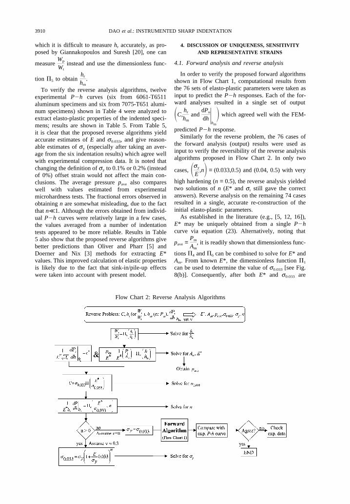
3910 DAO et al.: INSTRUMENTED SHARP INDENTATION
which it is difficult to measure hr accurately, as pro-posed by Giannakopoulos and Suresh [20], one can
measureWp
Wt
instead and use the dimensionless func-
tion �5 to obtainhr
hm
.
To verify the reverse analysis algorithms, twelveexperimental P�h curves (six from 6061-T6511aluminum specimens and six from 7075-T651 alumi-num specimens) shown in Table 4 were analyzed toextract elasto-plastic properties of the indented speci-mens; results are shown in Table 5. From Table 5,it is clear that the proposed reverse algorithms yieldaccurate estimates of E and s0.033, and give reason-able estimates of sy (especially after taking an aver-age from the six indentation results) which agree wellwith experimental compression data. It is noted thatchanging the definition of sy to 0.1% or 0.2% (insteadof 0%) offset strain would not affect the main con-clusions. The average pressure pave also compareswell with values estimated from experimentalmicrohardness tests. The fractional errors observed inobtaining n are somewhat misleading, due to the factthat n�1. Although the errors obtained from individ-ual P�h curves were relatively large in a few cases,the values averaged from a number of indentationtests appeared to be more reliable. Results in Table5 also show that the proposed reverse algorithms givebetter predictions than Oliver and Pharr [5] andDoerner and Nix [3] methods for extracting E*values. This improved calculation of elastic propertiesis likely due to the fact that sink-in/pile-up effectswere taken into account with present model.
Flow Chart 2: Reverse Analysis Algorithms
4. DISCUSSION OF UNIQUENESS, SENSITIVITYAND REPRESENTATIVE STRAINS
4.1. Forward analysis and reverse analysis
In order to verify the proposed forward algorithmsshown in Flow Chart 1, computational results fromthe 76 sets of elasto-plastic parameters were taken asinput to predict the P�h responses. Each of the for-ward analyses resulted in a single set of output
�C,hr
hm
anddPu
dh |hm
� which agreed well with the FEM-
predicted P�h response.Similarly for the reverse problem, the 76 cases of
the forward analysis (output) results were used asinput to verify the reversibility of the reverse analysisalgorithms proposed in Flow Chart 2. In only two
cases, �sy
E,n� = (0.033,0.5) and (0.04, 0.5) with very
high hardening (n = 0.5), the reverse analysis yieldedtwo solutions of n (E* and sr still gave the correctanswers). Reverse analysis on the remaining 74 casesresulted in a single, accurate re-construction of theinitial elasto-plastic parameters.
As established in the literature (e.g., [5, 12, 16]),E* may be uniquely obtained from a single P�hcurve via equation (23). Alternatively, noting that
pave =Pm
Am
, it is readily shown that dimensionless func-
tions �4 and �6 can be combined to solve for E* andAm. From known E*, the dimensionless function �1
can be used to determine the value of s0.033 [see Fig.8(b)]. Consequently, after both E* and s0.033 are

3911DAO et al.: INSTRUMENTED SHARP INDENTATION
Tab
le5.
Rev
erse
anal
ysis
onA
l60
61-T
6511
and
Al
7075
-T65
1(m
ax.
load
=3N
;as
sum
en
=0.
3)
Oliv
eran
dPh
arr
[5]
Doe
rner
and
Nix
[3]
Cur
rent
met
hod
usin
gB
erko
vich
c*E
*(G
Pa)
%er
rE
*E
*(G
Pa)
%er
rE
*E
*(G
Pa)
%er
rE
*s
0.0
33
(MPa
)%
errs
0.0
33
ns
y(M
Pa)
%er
rs
yp a
ve
(MPa
)%
err
p ave
(a)
Al
6061
-T65
11T
est
185
.822
.2%
a85
.321
.5%
67.6
�3.
7%33
4.5
�1.
0%0.
002
333.
117
.3%
904
�18
.4%
Tes
t2
87.7
25.0
%87
.324
.4%
66.1
�5.
8%34
9.4
3.4%
034
9.4
23.0
%84
9�
23.4
%T
est
386
.022
.5%
85.6
22.0
%66
.5�
5.3%
332.
8�
1.5%
033
2.8
17.2
%86
0�
22.4
%T
est
484
.119
.7%
83.9
19.5
%75
.06.
8%32
2.9
�4.
5%0.
234
171.
0�
39.8
%11
503.
8%T
est
585
.021
.1%
85.0
21.0
%77
.810
.8%
315.
9�
6.5%
0.29
812
8.0
�54
.9%
1198
8.1%
Tes
t6
81.4
16.0
%80
.915
.3%
67.9
�3.
4%33
7.4
�0.
2%0.
088
278.
5�
1.9%
1025
�7.
5%A
ve85
.084
.770
.133
2.1
0.10
426
5.5
998
STD
EV
b14
.914
.64.
512
.287
.717
6.5
21.3
%20
.8%
6.5%
3.6%
30.9
%15
.9%
STE
DV
Xex
p
(b)
Al
7075
-T65
1T
est
184
.314
.8%
a83
.313
.5%
73.7
0.5%
579.
3�
6.2%
0.13
045
7.1
�8.
6%17
99�
2.3%
Tes
t2
83.4
13.6
%82
.812
.8%
71.5
�2.
6%56
4.2
�8.
6%0.
085
486.
2�
2.8%
1656
�10
.1%
Tes
t3
84.5
15.2
%84
.014
.5%
74.0
0.8%
583.
2�
5.6%
0.13
245
8.2
�8.
4%18
07�
1.9%
Tes
t4
87.5
19.2
%87
.218
.8%
75.4
2.8%
595.
6�
3.6%
0.09
850
0.7
0.1%
1780
�3.
4%T
est
589
.421
.9%
88.4
20.4
%76
.64.
4%59
9.6
�2.
9%0.
088
513.
42.
7%17
56�
4.7%
Tes
t6
88.2
20.2
%87
.419
.0%
76.5
4.2%
620.
40.
5%0.
108
513.
42.
7%18
701.
5%A
ve86
.285
.574
.659
0.4
0.10
748
8.2
1778
STD
EV
b13
.012
.32.
232
.426
.291
17.7
%16
.8%
3.0%
5.2%
5.3%
4.9%
STE
DV
Xex
p
aA
ller
rors
wer
eco
mpu
ted
asX
rev.a
nal
ysi
s�X̄
exp
X̄ex
p
,w
here
Xre
pres
ents
ava
riab
le
bST
DE
V=�1 N
�N
i=
1
(Xre
v.a
nal
ysi
s�X̄
exp)2
,w
here
Xre
pres
ents
ava
riab
le

3912 DAO et al.: INSTRUMENTED SHARP INDENTATION
determined, strain hardening exponent n can bedetermined by dimensionless function �2 or �3 [seeFig. 10(a) and (b)]. It was found in the current studythat, when the assumptions of the model are valid, asingle value for E* and s0.033 can be determined for
all cases. Furthermore, except for cases wheresy
E�
0.033 and n�0.3, one single value of n can bedetermined as well (although both sy and n are highlysensitive to even small variations in P�h response).
Examining Fig. 10(a) in detail, whensy
E�
0.033�sy
E∗�0.03� and n�0.3, the n = 0.5 curve
crossed the other three curves, which indicates thesolution of n may not be unique using dimensionlessfunction �2 in that region; a single solution of n maybe obtained using dimensionless function �3 instead.The above arguments regarding uniqueness can onlybe valid when the P�h responses can be measuredaccurately and precisely. Therefore, with accurateP�h curves, the uniqueness of the reverse problemcan be ensured for low hardening materials (i.e.,n�0.3); the uniqueness can also be preserved ifsy
E∗�0.03 for higher hardening materials (i.e., 0.3�
n�0.5). Considering the fact that each of the dimen-sionless functions �1, �2, …, and �6 carries a smallamount of uncertainty, definitive conclusions can notbe drawn as yet regarding the uniqueness of the
reverse analysis whensy
E∗�0.03 and 0.3�n�0.5.
Table 6 summarizes the above-mentioned results.Cheng and Cheng [19] examined whether uniaxial
stress–strain relationships of materials can beuniquely determined by matching the loading andunloading P�h curves, calculated using their FEManalysis and scaling relationships, with those meas-ured experimentally. By showing that there could bemultiple stress–strain curves for a given set of loadingand unloading curves, they concluded that thematerial stress–strain behavior may not be uniquelydetermined from the loading and unloading P�hresponse alone. We examined all seven casespresented in [19]. For the four cases presented in Fig.
Table 6. Uniqueness of reverse analysis
Mechanical property Solution unique?
E* YesHardness (pave) Yessr Yessy when n�0.3 Yes
when 0.3�n�0.5Yes
andsy
E∗�0.03
when 0.3�n�0.5?
andsy
E∗�0.03
3(a) of [19], the values ofsy
E∗ are beyond the range
of the current study. That is, the ratio ofsy
E∗given by
these four cases (�10�1) may not accurately describeany metallic engineering alloys (see, e.g., [35]), butmay describe certain ceramics or engineering poly-mers which are not well-described by power law plas-ticity. Therefore, the non-uniqueness of these cases isphysically irrelevant to the scope of our analysis. Incontrast, the cases reported in Fig. 3(b) of [19] are
within our range of parameters (sy
E∗�10�2 to 10�3).
The current forward analysis predicts three P�hresponses which are statistically unique in terms of
the calculated curve parameters such as C,hr
hm
and
dPu
dh |hm
. This statistical uniqueness does not directly
contradict Cheng and Cheng’s assertion of non-uniqueness, as they used a different apex angle intheir FEM simulations, and as the P�h curves appearvisually similar. The maximum variation in curveparameters calculated by our forward analysis of
these three cases was an 8% change indPu
dh |hm
. The
present reverse analysis provides a unique solution inthat, even if the calculated loading curvatures (C)were mathematically identical for two separate P�h
responses, small variations in terms ofdPu
dh |hm
orhr
hm
are sufficient to calculate a unique value of n and,consequently, a unique value of sy for each case.However, these small variations in curve parametersmay not be visually apparent when plotting theseP�h responses simultaneously. In fact, as experi-mental scatter may cause such variation in P�h curveparameters, the issue of sensitivity in these analysesis an important consideration.
4.2. Sensitivity to forward analysis, reverse analysisand apex angle
For forward analysis, the sensitivity of the pre-dicted P�h response parameters to variations in theinput mechanical properties of the indented materialwas investigated for the 76 cases examined in thisstudy. The results showed that a ±5% change in anyone input parameter (i.e., E*, sy or n), would lead tovariations of less than ±6% in the predicted results
�C,hr
hm
anddPu
dh |hm
�.
As discussed in Venkatesh et al. [21], the accuracywith which the mechanical properties of the indentedmaterial can be estimated through reverse analysiscould depend strongly on the accuracy with whichthe P�h responses are measured. The sensitivity of

3913DAO et al.: INSTRUMENTED SHARP INDENTATION
the estimated mechanical properties to variations inthe input parameters obtained from the P�h curveswas investigated for the 76 cases examined in thisstudy as well. For each of these cases, the sensitivityof the estimated elasto-plastic properties to variations
in the three P�h curve parameters—C,dPu
dh |hm
, and
Wp
Wt—about their respective reference values (as esti-
mated from the forward analysis) was examined. Theresults are summarized in Table 7. In general, sensi-tivity to reverse analysis is different for each individ-ual case, thus the maximum variations listed in Table7 are conservative estimates.
It is evident that E* displayed weak sensitivity with
respect to C anddPu
dh |hm
, and moderate sensitivity to
Wp
Wt
; sr displayed weak sensitivity with respect to
Wp
Wt
, and moderate sensitivity to both C anddPu
dh |hm
; for
low hardening materials (n�0.1), sy displayed mod-
erate sensitivity to C anddPu
dh |hm
, and strong sensitivity
toWp
Wt
; for higher hardening materials (n�0.1), sy dis-
played strong sensitivity to all three parameters; pave
displayed weak sensitivity to C anddPu
dh |hm
, and mod-
erate sensitivity toWp
Wt
. The results of the reverse sen-
sitivity analysis shown in Table 7 are consistent withthe reverse analyses of experimental P�h curveslisted in Table 5. The greater scatter in computed sy
values in Table 5 reflects the stronger sensitivity withrespect to sy. If data scatter is random in nature, it isexpected that taking the averaged value from a num-ber of indentation tests may significantly reduce theerror, as clearly demonstrated in Table 5.
In addition, the sensitivity of the P�h response ascomputed from FEM calculations to variations in theapex angle q of the indenter was investigated for thefour cases A, B, C and D listed in Table 1. The resultsare summarized in Table 8 and Fig. 12, where therespective reference values (as calculated from theFEM computed P�h curves) were taken atq = 70.3°. From Fig. 12 and Table 8, the dependence
of C,dPu
dh |hm
andWp
Wt
to variations in the apex angle
appears to be quite significant and approximately lin-ear. Taking q = 68° as used in [11, 12, 19] as anexample, deviation from the reference apex angle by2.3° results in maximum variations of �20%,
�11.7% and +5.7% in terms of C,dPu
dh |hm
andWp
Wt
respectively (see Table 8). As evident in Table 7,variations of this magnitude are beyond the error tol-erance limit of reverse analysis. The universal func-tions based on a 68° apex angle may significantly dif-fer from those obtained using a 70.3° apex angle,although certain trends with respect to various para-meters may be similar. Commercially available dia-mond indenters are normally within ±0.5° of thespecified apex angle. The resulting maximum vari-ations in P�h curve parameters as estimated fromFEM computations are around ±3%, ±3%, and ±1%
in terms of C,dPu
dh |hm
andWp
Wt
respectively, which are
within the error tolerance limit of the reverse analysis.
4.3. Representative strains
The concept of representative strain was first intro-duced by Tabor [1] to relate its corresponding rep-resentative stress to the hardness value. Tabor [1] sug-gested a representative plastic strain of 8–10% basedon experimental observations. This original definitiondoes not represent any apparent physical transition inmechanical response. Giannakopoulos et al. [18] andGiannakopoulos and Suresh [20] used a “character-istic strain” of 29–30% within the context of equation(20). Giannakopoulos and Suresh [20] suggested thatthe region of material experiencing strains beyond29% under the indenter exhibits plastic “cutting”characteristics and may be modeled using slip linetheory. In the current study, a representative plasticstrain er = 0.033 was identified as a strain level whichallows for the construction of a dimensionlessdescription of the indentation loading response [i.e.,equation (11b)], independent of strain hardeningexponent n. Here, the underlying connectionsbetween these three different definitions and the cor-responding representative strain levels are discussed.
To understand these different representative strainvalues, it is important to note that the dimensionlessfunction �1 in Fig. 8(b), used to identify er = 0.033has a different functional form than that used by theearlier researchers, e.g., equation (20). Therefore, itis possible for these different definitions to result indifferent solutions. Equation (21) is a modification ofequation (20) and, as mentioned in Section 2.5, canfit all 76 cases studied reasonably well. For low strainhardening materials, s0.29�sr(�sy), and thus equ-ation (21) can be rewritten as
C�N1s0.29�1 �sy
s0.29��N2 � ln�E∗
sr��
� �sy � s0.29
2 �2N1�N2 � ln�E∗
sr�� (26)
� �sy � s0.29
2 ��1N�E∗
sr�
within a ±5.5% error of equation (21) for all the 76cases computed in the current study; �1N is a dimen-

3914 DAO et al.: INSTRUMENTED SHARP INDENTATION
Tab
le7.
Sens
itivi
tyto
reve
rse
anal
ysis
Cha
nges
inin
put
para
met
ers
2%
inC
±4%
inC
±2%
indP
u
dh| h
m
±2%
inW
p
Wt
±4%
indP
u
dh| h
m
±4%
inW
p
Wt
Max
imum
vari
atio
nsin
E*
2%
±4%
9.
5%
4%±8
%
19%
estim
ated
prop
ertie
sa
s0.0
33
+12%
/�10
%�
8%/+
11%
0.9%
+29%
/�19
%�
15%
/+25
%±1
.7%
sy
b(n
�0.
1)+1
8%/�
24%
�22
%/+
16%
+31%
/�45
%+2
8%/�
43%
�39
%/+
24%
+39%
/�96
%s
yb
(n�
0.1)
+85%
/�29
%�
27%
/+81
%+7
0%/�
33%
+103
%/�
53%
�50
%/+
96%
+71%
/�57
%p a
ve
2%
±4%
�18
%/+
20%
4%
±8%
�34
%/+
42%
aA
ller
rors
wer
eco
mpu
ted
asX
var
ied�
Xre
fere
nce
Xre
fere
nce
,w
here
Xre
pres
ents
ava
riab
le
bE
stim
ated
byse
tting
n=
0w
hen
ther
ear
em
ultip
leso
lutio
nsor
noso
lutio
nfo
rn,
orse
tting
n=
0.5
whe
nth
eso
lutio
nfo
rn
isgr
eate
rth
an0.
5(w
hich
isou
tsid
eth
esc
ope
ofou
rpa
ram
eter
stud
y)

3915DAO et al.: INSTRUMENTED SHARP INDENTATION
Table 8. Apex angle sensitivity of A, B, C, and D four cases
68° 69° 70.3° (reference) 72°Maximumvariations�Apex
angle
�C/Cref �20.4% �12.1% 0% +19.3%
�11.7% �7.7% 0% +9.0%��dP
dh�/�dPdh�ref
+5.7% +3.0% 0% �4.8%��Wp
Wt�/�Wp
Wt�
ref
Fig. 12. Sensitivity of (a) loading curvature C and (b) plastic work ratioWp
Wtto variations in apex angle for
four model materials. A two-degree variation in apex angle resulted in 15–20% variations in loading curvature
C and up to 6% variations in plastic work ratioWp
Wt
.
sionless function. One can solve for er that gives sr
as an arithmetic average between sy and s0.29:
sr �sy � s0.29
2(27)
If it is assumed that sy�s|e = 0.002, then equation(27) becomes
Renr �R·0.002n � R·0.29n
2(28)
and thus
er��0.002n � 0.29n
2 �1n
(29)
For low hardening materials with 0�n�0.15, equ-ation (29) gives 0.024�er�0.038, which is fairlyclose to 0.033. This exercise indicates that: (1)er = 0.033 obtained in the current study is fundamen-tally linked to the “characteristic strain” of 0.29 givenin the literature, and the differences in the magnitude
of the strain come from their different functionaldefinitions; (2) s0.033 taken at the 0.033 representativestrain is a “weighted average” of the stresses over therange between ey and ep = 0.29. Additional compu-tations confirmed that stress–strain behavior beyondep = 0.29 has little effect on a material’s P�hresponse.
Earlier studies by Tabor [1] and Johnson [15] gavea representative strain at about er = 0.08. This esti-mation relied on experimental data which indicatedthat
Hsr
�pave
sr
�3.0 (30)
where H is the hardness expressed in units of press-ure. Again, it is noted that the functional form definedby equation (30) is different from those used to definerepresentative strains of 3.3% or 29%, and it is naturalthat different functions may lead to different results.To better understand this problem, a new dimen-sionless function can be defined
pave
sr
� �7�sr
E∗,n� (31)
3916 DAO et al.: INSTRUMENTED SHARP INDENTATION
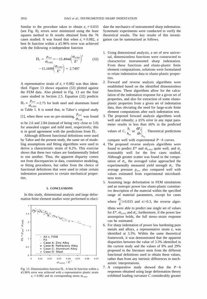
Similar to the procedure taken to obtain er = 0.033(see Fig. 8), errors were minimized using the leastsquares method to fit results obtained from the 76cases studied. It was found that when er = 0.082, abest fit function within a ±5.96% error was achievedwith the following n-independent function
�7 �pave
s0.082
��15.4944�s0.082
E∗ �2
(32)
�15.1699�s0.082
E∗ � � 2.7497
A representative strain of er = 0.082 was thus ident-ified. Figure 13 shows equation (32) plotted againstthe FEM data. Also plotted in Fig. 13 are the fourcases studied in Section 2.5. Equation (32) predicts
�7 =pave
s0.082
�2.75 for both steel and aluminum listed
in Table 1. It is noted that, in Tabor’s original study
[1], when there was no pre-straining,pave
s0.08
was found
to be 2.6 and 2.84 (instead of being very close to 3.0)for annealed copper and mild steel, respectively; thisis in good agreement with the predictions from �7.
Although different functional definitions were usedby Tabor and the present study, the same set of mode-ling assumptions and fitting algorithms were used toderive a characteristic strain of 8.2%. This exerciseshows that these two values are fundamentally linkedto one another. Thus, the apparent disparity comesnot from discrepancies in data, constitutive modeling,or fitting procedures, but rather from the choice offunctional definitions that were used to relate certainindentation parameters to certain mechanical proper-ties.
5. CONCLUSIONS
In this study, dimensional analysis and large defor-mation finite element studies were performed to eluci-
Fig. 13. Dimensionless function �7. A best fit function within a±5.96% error was achieved with a representative plastic strain
er = 0.082 and its corresponding stress s0.082.
date the mechanics of instrumented sharp indentation.Systematic experiments were conducted to verify thetheoretical results. The key results of this investi-gation can be summarized as follows.
1. Using dimensional analysis, a set of new univer-sal, dimensionless functions were constructed tocharacterize instrumented sharp indentation.From these functions and elasto-plastic finiteelement computations, solutions were formulatedto relate indentation data to elasto-plastic proper-ties.
2. Forward and reverse analysis algorithms wereestablished based on the identified dimensionlessfunctions. These algorithms allow for the calcu-lation of the indentation response for a given set ofproperties, and also for extraction of some elasto-plastic properties from a given set of indentationdata, thus obviating the need for large-scale finiteelement computations after each indentation test.
3. The proposed forward analysis algorithms workwell and robustly; a ±5% error in any input para-meter results in less than ±6% in the predicted
values of C,hr
hm
ordPu
dh |hm
. Theoretical predictions
compare well with experimental P�h curves.4. The proposed reverse analysis algorithms were
found to predict E* and s0.033 quite well, and sy
reasonably well for the few cases studied.Although greater scatter was found in the compu-tation of sy, the averaged value approached theexperimentally measured yield strength sy. Theaverage pressure pave also compared well withvalues estimated from experimental microhard-ness tests.
5. Assuming large deformation in FEM simulationsand an isotropic power law elasto-plastic constitut-ive description of the material within the specifiedrange of material parameters, except for cases
wheresy
E�0.033 and n�0.3, the reverse algor-
ithms were able to predict one single set of valuesfor E*, s0.033 and sy; furthermore, if the power lawassumption holds, the full stress–strain responsecan be estimated.
6. For sharp indentation of power law hardening puremetals and alloys, a representative strain er wasidentified at 3.3%. Within the same theoreticalframework, it was demonstrated that the apparentdisparities between the value of 3.3% identified inthe current study and the values of 8% and 29%proposed in the literature stem from the differentfunctional definitions used to obtain these values,rather than from any intrinsic differences in mech-anistic interpretations.
7. A comparative study showed that the P�hresponses obtained using large deformation theoryexhibited loading curvature C considerably greater

3917DAO et al.: INSTRUMENTED SHARP INDENTATION
than those obtained using small deformationtheory.
8. Comprehensive sensitivity analyses were carriedout for both forward and reverse algorithms. For-ward analysis algorithms were found to be accur-ate and robust. For the sensitivity to reverse analy-sis, E*, s0.033 and pave displayed weak or moderate
sensitivity to variations in C,dPu
dh |hm
, andWp
Wt
; for
low hardening materials (n�0.1), sy displayed
moderate sensitivity to C anddPu
dh |hm
, and strong
sensitivity toWp
Wt
; for higher hardening materials
(n�0.1), sy displayed strong sensitivity to all threeparameters. Sensitivity of the P�h responses toapex angle deviations were found to be significantwith even a 1–2° deviation; nevertheless, the P�h response variations with respect to apex angledeviations less than ±0.5° were within the toler-ance limit of the reverse analysis.
9. We note that plastic properties of materialsextracted from instrumented indentation are verysensitive to even small variations in the P�hresponses. Nevertheless, the present compu-tational study provides a mean to determine theseplastic properties, which may not be easilyobtainable by other means in small volume struc-tures, and further provides an indication of thelevel of the sensitivity to experimental inden-tation data.
Acknowledgements—This research was supported by a subcon-tract to MIT through the Center for Thermal Spray Researchat Stony Brook, under the National Science Foundation GrantDMR-0080021, and by the Defense University ResearchInitiative on Nano-Technology (DURINT) on “Damage andFailure Resistant Nanostructured Materials and InterfacialCoatings” which is funded at MIT by the Office of NavalResearch, Grant No. N00014-01-1-0808. KJVV is funded bythe National Defense Science and Engineering Graduate Fel-lowship. The authors gratefully acknowledge helpful and sti-mulating discussions with Dr A.E. Giannakopoulos and Mr Y.J.Choi during the course of this study.
REFERENCES
1. Tabor, D., Hardness of Metals. Clarendon Press, Oxford,1951.
2. Tabor, D., Rev. Phys. Technol., 1970, 1, 145.3. Doener, M. F. and Nix, W. D., J. Mater. Res., 1986, 1, 601.4. Pharr, G. M. and Cook, R. F., J. Mater. Res., 1990, 5, 847.5. Oliver, W. C. and Pharr, G. M., J. Mater. Res., 1992, 7,
1564.6. Field, J. S. and Swain, M. V., J. Mater. Res., 1993, 8, 297.7. Field, J. S. and Swain, M. V., J. Mater. Res., 1995, 10, 101.8. Gerberich, W. W., Nelson, J. C., Lilleodden, E. T., Ander-
son, P. and Wyrobek, J. T., Acta mater., 1996, 44, 3585.9. Bolshakov, A., Oliver, W. C. and Pharr, G. M., J. Mater.
Res., 1997, 11, 760.10. Alcala, J., Giannakopoulos, A. E. and Suresh, S., J. Mater.
Res., 1998, 13, 1390.
11. Cheng, Y. T. and Cheng, C. M., J. Appl. Phys., 1998,84, 1284.
12. Cheng, Y. T. and Cheng, C. M., Appl. Phys. Lett., 1998,73, 614.
13. Suresh, S., Nieh, T. -G. and Choi, B. W., Scripta mater.,1999, 41, 951.
14. Gouldstone, A., Koh, H. -J., Zeng, K. -Y., Giannako-poulos, A. E. and Suresh, S., Acta mater., 2000, 48, 2277.
15. Johnson, K. L., J. Mech. Phys. Solids, 1970, 18, 115.16. Suresh, S., Alcala, J. and Giannakopoulos, A. E., US Pat-
ent No. 6,134,954, October 24, 2000.17. Dao, M., Chollacoop, N., Van Vliet, K. J., Venkatesh, T.
A. and Suresh S., US Provisional Patent, filed with the USPatent Office on March 7, 2001.
18. Giannakopoulos, A. E., Larsson, P. -L. and Vestergaard,R., Int. J. Solids Struct., 1994, 31, 2679.
19. Cheng, Y. T. and Cheng, C. M., J. Mater. Res., 1999,14, 3493.
20. Giannakopoulos, A. E. and Suresh, S., Scripta mater.,1999, 40, 1191.
21. Venkatesh, T. A., Van Vliet, K. J., Giannakopoulos, A. E.and Suresh, S., Scripta mater., 2000, 42, 833.
22. Suresh, S. and Giannakopoulos, A. E., Acta mater., 1998,46, 5755.
23. Bhattacharya, A. K. and Nix, W. D., Int. J. Solids Struct.,1988, 24, 881.
24. Laursen, T. A. and Simo, J. C., J. Mater. Res., 1992, 7,618.
25. Tunvisut, K., O’Dowd, N. P. and Busso, E. P., Int. J. SolidsStruct., 2001, 38, 335.
26. Hill, R., Storakers, B. and Zdunek, A. B., Proc. Roy. Soc.Lond. A, 1989, 423, 301.
27. Larsson, P. -L., Giannakopoulos, A. E., Soderlund, E.,Rowcliffe, D. J. and Vestergaard, R., Int. J. Solids Struct.,1996, 33, 221.
28. Chaudhri, M. M., Acta mater., 1998, 46, 3047.29. Johnson, K. L., Contact Mechanics. Cambridge University
Press, London, 1985.30. Fleck, N. A. and Hutchinson, J. W., J. Mech. Phys. Solids,
1993, 41, 1825.31. Gao, H., Huang, Y., Nix, W. D. and Hutchinson, J. W., J.
Mech. Phys. Solids, 1999, 47, 1239.32. ABAQUS Theory Manual Version 6.1. Hibbitt, Karlsson
and Sorensen Inc, Pawtucket, 2000.33. King, R. B., Int. J. Solids Struct., 1987, 23, 1657.34. MatWeb: http://www.matweb.com, 2001, by Automation
Creations, Inc.35. Ashby, M. F., Materials Selection in Mechanical Design.
Butterworth Heinemann, Boston, 1999.
APPENDIX A
In this study, large deformation finite element com-putational simulations of depth-sensing indentationwere carried out for 76 different combinations of ela-sto-plastic properties that encompass the wide rangeof parameters commonly found in pure and alloyedengineering metals; Young’s modulus, E, was variedfrom 10 to 210 GPa, yield strength, sy, from 30 to3000 MPa, and strain hardening exponent, n, from 0to 0.5, and the Poisson’s ratio, n, was fixed at 0.3.Table A1 tabulates the elasto-plastic parameters usedin these 76 cases.
APPENDIX B
In this appendix, six of the dimensionless functionsidentified in Section 3.1, i.e. �1, �2, �3, �4, �5 and�6, are listed explicitly.

3918 DAO et al.: INSTRUMENTED SHARP INDENTATION
Table A1. Elasto-plastic parameters used in the present study
E (GPa) sy (MPa) sy/E
19 combinations of10 30 0.003
E and sya
10 100 0.0110 300 0.0350 200 0.00450 600 0.01250 1000 0.0250 2000 0.0490 500 0.00555690 1500 0.01666790 3000 0.033333130 1000 0.007692130 2000 0.015385130 3000 0.023077170 300 0.001765170 1500 0.008824170 3000 0.017647210 300 0.001429210 1800 0.008571210 3000 0.014286
a For each one of the 19 cases listed above, strain-hardening exponentn is varied from 0, 0.1, 0.3 to 0.5, resulting a total of 76 different cases
�1 �Cs0.033
� �1.131�ln� E∗
s0.033��3
� 13.635�ln� E∗
s0.033��2
(B1)
�30.594�ln� E∗
s0.033�� � 29.267
�2�E∗
sr
,n� �1
E∗hm
dPu
dh |hm
� (�1.40557n3
� 0.77526n2 � 0.15830n
�0.06831)�ln� E∗
s0.033��3
� (17.93006n3
�9.22091n2�2.37733n (B2)
� 0.86295)�ln� E∗
s0.033��2
� (
�79.99715n3 � 40.55620n2 � 9.00157n
�2.54543)�ln� E∗
s0.033�� � (122.65069n3
�63.88418n2�9.58936n � 6.20045)
�3�sr
E∗,n� �hr
hm
� (0.010100n2
� 0.0017639n
�0.0040837)�ln�s0.033
E∗ ��3
� (0.14386n2
� 0.018153n�0.088198)�ln�s0.033
E∗ ��2
(B3)
� (0.59505n2 � 0.034074n
�0.65417)�ln�s0.033
E∗ �� � (0.58180n2
�0.088460n�0.67290)
�4 �pave
E∗ �0.268536�0.9952495 (B4)
�hr
hm�1.1142735
�5 �Wp
Wt
� 1.612171.13111
�1.74756��1.49291�hr
hm�2.535334
� (B5)
�0.075187� hr
hm�1.135826
�6 �1
E∗√Am
dPu
dh |hm
� c∗ (B6)
where values of c* are tabulated in Table 2.