Embed Size (px)
Citation preview

Computational Prediction of ThermodynamicProperties of Organic Molecules in Aqueous
Solutions
Dissertation
zur Erlangung des akademischen Grades eines
Doktors der Naturwissenschaften– Dr. rer. nat. –
vorgelegt von
Ekaterina L. Ratkova
geboren in Zhdanov, USSR
Fakultät für Chemie
derUniversität Duisburg-Essen
2011

Die vorliegende Arbeit wurde im Zeitraum von Januar 2009 bis Mai 2011 im Arbeitskreis
von PhD, DSc, Priv.-Doz. Maxim V. Fedorov am Max-Planck-Institut für Mathematik in den
Naturwissenschaften, Leipzig, durchgeführt.
Tag der Disputation: 21.07.2011
Gutachter: PhD, DSc, Priv.-Doz. Maxim V. Fedorov
Prof. Dr. Eckhard Spohr
Prof. Dr. Philippe A. Bopp
Vorsitzender: Prof. Dr. Eckart Hasselbrink

CONTENTS 2
Contents
1 Introduction 7
2 Theoretical Background 16
2.1 Molecular Ornstein-Zernike integral equation . . . . . . . . . . . . . . . . . . 16
2.2 3D Reference Interaction Site Model (3D RISM) . . . . . . . . . . . . . . . . 17
2.3 1D Reference Interaction Site Model (1D RISM) . . . . . . . . . . . . . . . . 19
2.4 Hydration Free Energy Expressions within the 1D RISM approach . . . . . . . 22
2.5 Thermodynamic parameters within the 3D RISM approach . . . . . . . . . . . 25
2.6 Partial molar volume expressions in RISM approaches . . . . . . . . . . . . . 25
3 Computational Details 26
3.1 1D RISM calculations . . . . . . . . . . . . . . . . . . . . . . . . . . . . . . . 26
3.2 3D RISM calculations . . . . . . . . . . . . . . . . . . . . . . . . . . . . . . . 28
3.3 Multigrid technique . . . . . . . . . . . . . . . . . . . . . . . . . . . . . . . . 29
3.3.1 One-level Picard iterations . . . . . . . . . . . . . . . . . . . . . . . . 31
3.3.2 Two-grid iteration . . . . . . . . . . . . . . . . . . . . . . . . . . . . 32
3.3.3 Multi-grid iterations . . . . . . . . . . . . . . . . . . . . . . . . . . . 33
4 Structural Descriptors Correction (SDC) model 35
4.1 The QSPR basis of the model . . . . . . . . . . . . . . . . . . . . . . . . . . . 35
4.2 Multi-parameter linear regression . . . . . . . . . . . . . . . . . . . . . . . . . 39
4.3 Training and test sets . . . . . . . . . . . . . . . . . . . . . . . . . . . . . . . 40
4.4 Choice of descriptors . . . . . . . . . . . . . . . . . . . . . . . . . . . . . . . 41
4.4.1 n−Alkanes. . . . . . . . . . . . . . . . . . . . . . . . . . . . . . . . . 41
4.4.2 Nonlinear alkanes. . . . . . . . . . . . . . . . . . . . . . . . . . . . . 41
4.4.3 Other compounds. . . . . . . . . . . . . . . . . . . . . . . . . . . . . 44
4.5 Optimal set of corrections . . . . . . . . . . . . . . . . . . . . . . . . . . . . . 47
5 Results and Discussion 48
5.1 PMV estimations with 1D and 3D RISM approaches . . . . . . . . . . . . . . 48
5.2 1D RISM-SDC model with OPLS partial charges . . . . . . . . . . . . . . . . 52
5.2.1 Calibration of the model . . . . . . . . . . . . . . . . . . . . . . . . . 52
5.2.2 The model predictive ability . . . . . . . . . . . . . . . . . . . . . . . 55
5.2.3 Comparison with other HFE expressions . . . . . . . . . . . . . . . . 59

CONTENTS 3
5.3 1D RISM-SDC model with QM-derived partial charges . . . . . . . . . . . . . 65
5.3.1 Performance of the model . . . . . . . . . . . . . . . . . . . . . . . . 65
5.3.2 The model predictive ability for pollutants . . . . . . . . . . . . . . . . 72
5.4 3D RISM-SDC model . . . . . . . . . . . . . . . . . . . . . . . . . . . . . . . 81
5.4.1 Comparison of uncorrected data . . . . . . . . . . . . . . . . . . . . . 81
5.4.2 Correction for the cavity formation (3D RISM-UC model) . . . . . . . 82
5.4.3 Corrections for the functional groups . . . . . . . . . . . . . . . . . . 86
5.4.4 The 3D RISM-SDC model predictive ability . . . . . . . . . . . . . . 87
5.5 Comparison of the RISM-SDC model with the cheminformatics approach . . . 92
6 Summary 94
7 Literature 99
8 Appendix 1 119
9 Appendix 2 150
9.1 List of Abbreviations . . . . . . . . . . . . . . . . . . . . . . . . . . . . . . . 150
9.2 Short summary . . . . . . . . . . . . . . . . . . . . . . . . . . . . . . . . . . 153
9.3 List of Publications . . . . . . . . . . . . . . . . . . . . . . . . . . . . . . . . 154
9.4 Curriculum Vitae (CV) . . . . . . . . . . . . . . . . . . . . . . . . . . . . . . 159
9.5 Erkärung . . . . . . . . . . . . . . . . . . . . . . . . . . . . . . . . . . . . . 162
9.6 Acknowledgements . . . . . . . . . . . . . . . . . . . . . . . . . . . . . . . . 163

LIST OF FIGURES 4
List of Figures
1 Thermodynamic cycle of a dissolution process. . . . . . . . . . . . . . . . . . 8
2 Hydration free energy in environmental chemistry . . . . . . . . . . . . . . . . 9
3 Estimations of experimental expenses . . . . . . . . . . . . . . . . . . . . . . 12
4 Classification of computational methods . . . . . . . . . . . . . . . . . . . . . 13
5 Correlation functions in the 3D and 1D RISM approaches . . . . . . . . . . . . 18
6 Scheme of HFE calculations within the RISM approach . . . . . . . . . . . . . 21
7 Parameters of RISM calculations . . . . . . . . . . . . . . . . . . . . . . . . . 26
8 3D RISM. Benchmark for the buffer distance . . . . . . . . . . . . . . . . . . 30
9 3D RISM. Benchmark for the spacing . . . . . . . . . . . . . . . . . . . . . . 30
10 Quantitative Structure – Property Relationship approach . . . . . . . . . . . . 36
11 Schematic representation of molecule in the SDC model . . . . . . . . . . . . 38
12 Errors connected with non-polar interactions . . . . . . . . . . . . . . . . . . . 43
13 Errors connected with specific interactions . . . . . . . . . . . . . . . . . . . . 44
14 Set of structural descriptors . . . . . . . . . . . . . . . . . . . . . . . . . . . . 46
15 Contributions of the PMV . . . . . . . . . . . . . . . . . . . . . . . . . . . . 48
16 Comparison of the calculated PMVs and experimental data . . . . . . . . . . . 51
17 Examples of SDC model’s contributions . . . . . . . . . . . . . . . . . . . . . 53
18 HFEs calculated by the 1D RISM-SDC(OPLSq) model for the training set . . . 54
19 Partial charges for heavy atoms of benzene, phenol, and benzyl alcohol . . . . . 56
20 HFEs predicted by the 1D RISM-SDC(OPLSq) model for the test set . . . . . . 58
21 Comparison of different HFE expressions . . . . . . . . . . . . . . . . . . . . 59
22 HFEs calculated by the 1D RISM-SDC(GF) model . . . . . . . . . . . . . . . 63
23 HFEs obtained with the HNC closure . . . . . . . . . . . . . . . . . . . . . . 64
24 Representation of errors for phenol fragment . . . . . . . . . . . . . . . . . . . 67
25 1D RISM-SDC model with different charges . . . . . . . . . . . . . . . . . . . 68
26 Errors of the model with different partial charges . . . . . . . . . . . . . . . . 68
27 The model predictive ability for polychlorinated benzenes . . . . . . . . . . . . 74
28 Apparatus for the Henry’s law constants determination . . . . . . . . . . . . . 75
29 Experimental data for PCB congeners . . . . . . . . . . . . . . . . . . . . . . 78
30 HFEs of PCBs obtained with different implicit solvation models . . . . . . . . 79
31 Uncorrected HFEs calculated within 1D and 3D RISM approaches . . . . . . . 81
32 Correlation between the DPMV and the HFE error for the 3D RISM . . . . . . 82

LIST OF FIGURES 5
33 The correlation for druglike molecules . . . . . . . . . . . . . . . . . . . . . . 83
34 Errors of HFEs calculated by the cavity corrected HFE expressions . . . . . . . 86
35 Performance of the 3D RISM-SDC model for training set. . . . . . . . . . . . 88
36 3D RISM-SDC model predictive ability . . . . . . . . . . . . . . . . . . . . . 89
37 Errors corresponded to specific interactions. RISM-SDC(KH) models . . . . . 90
38 HFEs calculated by the RISM-SDC(KH) models for training set . . . . . . . . 91
39 Comparison of the RISM-SDC models with the cheminformatics approach . . . 93

LIST OF TABLES 6
List of Tables
1 Correlation coefficients for different sets of descriptors . . . . . . . . . . . . . 47
2 Experimental values of PMV . . . . . . . . . . . . . . . . . . . . . . . . . . . 49
3 Parameters of the 1D RISM-SDC(PW) model . . . . . . . . . . . . . . . . . . 52
4 Statistical profile of the 1D RISM-SDC(OPLSq) model . . . . . . . . . . . . . 57
5 Parameters of the 1D RISM-SDC(GF) model . . . . . . . . . . . . . . . . . . 60
6 Parameters of the 1D RISM-SDC(OPLSq) model with the HNC closure . . . . 62
7 Parameters of 1D RISM calculations . . . . . . . . . . . . . . . . . . . . . . . 62
8 Parameters of the 1D RISM-SDC(QMq) model . . . . . . . . . . . . . . . . . 66
9 Comparison of partial charges for 2-methylpropane . . . . . . . . . . . . . . . 69
10 OPLS and CHELPG partial charges for toluene . . . . . . . . . . . . . . . . . 70
11 Comparison of partial charges for heterocyclic solutes . . . . . . . . . . . . . . 71
12 1D RISM-SDC(QMq) model parameters for pollutants . . . . . . . . . . . . . 73
13 Efficiency of different implicit models for PCBs . . . . . . . . . . . . . . . . . 76
14 Experimental and calculated HFEs for polychlorinated benzenes . . . . . . . . 80
15 3D RISM-UC. Experimental and calculated HFEs for druglike molecules . . . 84
16 Coefficients of the cavity corrected HFE expression . . . . . . . . . . . . . . . 85
17 Parameters of 3D RISM-SDC models for specific interactions . . . . . . . . . 87
18 3D RISM-SDC model with KH HFE expression . . . . . . . . . . . . . . . . . 92
19 Comparison of the 1D RISM-SDC model the cheminformatics approach . . . . 94
20 Composition of the training set and test set for the 1D RISM-SDC model . . . 119
21 Data obtained by the 1D and 3D RISM-SDC model for the training set . . . . . 131

1 INTRODUCTION 7
1 Introduction
Water is the most widespread and important media in the world. Almost all global environmen-
tal processes deal with water. Indeed, oceans cover about 71 % of the Earth globe surface, water
accumulates in the sky forming clouds, and it accesses all lands on the Earth via precipitations.
Moreover, all biochemical processes take place in aqueous media: protein-ligand binding, par-
ticles transport in the blood stream, synthesis of biopolymers, etc. In chemical industry water
remains one of the most widely used solvents [1].
The hydration free energy (HFE) is one of the key parameters characterizing the aqueous
solution of a solute. First, HFE shows the strength of solute-water interactions which is impor-
tant for such processes as biopolymer stabilization in aqueous solutions (proteins, DNA, etc.)
[2, 3, 4, 5, 6]. Second, HFE is crucial for the complex formation and binding processes taking
place in aqueous media. It determines the free energy loss in the process of partial dehydration
of interacting molecules which inevitably occurs during direct contact formation in solution
(e.g., ligand binding to a protein) [7, 8, 9]. Third, HFE of a compound determines partition of
the compound between gaseous and aqueous phases, and, thus, is significant for modeling of
molecules’ pathways in the environment (see the paragraph HFE in environmental chemistry)
[10, 11].
HFE equals the change of the Gibbs free energy that accompanies the transfer of solute
from gaseous phase to aqueous solution [12]. We note, that the amount of the transferred solute
molecules should be consistent with HFE units (e.g. HFE expressed in the terms of kcal/mol
corresponds to the transfer of 1 mole of the solutes molecules).
HFE also can be defined from the thermodynamic cycle: crystal – gaseous phase – solution
(Fig. 1). In this case, HFE can be derived in terms of two other thermodynamic properties:
sublimation free energy and solution free energy. Sublimation free energy (ΔGsub) equals to
the change of the Gibbs free energy that accompanies the transfer of the solute from crystal to
gaseous phase, while solution free energy (ΔGsoln) equals to the change of the Gibbs free energy
that accompanies the transfer of the solute from crystal to diluted aqueous solution (Fig. 1).
ΔGhyd = ΔGsoln − ΔGsub (1)
Another important physical/chemical property that characterizes a solute molecule behavior
in a solution is the partial molar volume (PMV). It is a thermodynamic quantity which indi-
cates how volume of a solution varies with addition of component i to the system at constant
temperature and pressure:

1 INTRODUCTION 8
Figure 1: Thermodynamic cycle of a dissolution process. The solution free energy (ΔGsoln) of a
compound can be represented a s a sum of the hydration free energy (ΔGhyd) and the sublimation
free energy (ΔGsub).
V =(∂V∂ni
)T,P,n j�i
(2)
One should note that the PMV contains not only information about the immersed solute
geometry but also the important data about the solute-solvent interactions.
HFE in environmental chemistry. HFE determines the partition of solute molecules be-
tween gaseous and aqueous phases which is required for modeling of the air-water exchange
in the environmental chemistry [10, 11, 13, 14, 15]. Nowadays, one of the most important
environmental and ecological problems is understanding and clarifying the global fate of per-
sistent organic pollutants (POPs) which are characterized by: (i) long-term persistence, (ii)
long-range atmospheric transport and deposition, (iii) bioaccumulation, (iv) adverse effects on
biota [16, 17, 11, 18]. For a long time, in many countries, POPs (such as polychlorobiphenyls,
hexachlorobenzene, etc.) were used in agriculture as pesticides, fungicides, and agents control-
ling arthropods [16]. Although POPs have been banned from further use and production [19],
their persistence in biological compartments (e.g., soil, water, plants, and sediment) means that
they still pose a significant environmental hazard. The semivolatile nature of POPs allows them
to evaporate from the soil and water into the atmosphere, where they can exist both in gaseous
and particle-absorbed forms (these can be atmospheric aerosol particles, e.g., cloud droplets,
as well as dust particles). Both forms allow long-range transport and deposition of POPs [11].

1 INTRODUCTION 9
Figure 2: Hydration free energy(ΔGhyd
)is an important thermodynamic parameter to describe
main processes of a molecule distribution between atmosphere and water (see Eq. 3, Eq. 5)
Several dominant mechanisms that determine the distribution of POPs between atmosphere and
water are shown in Fig. 2.
There are several physical/chemical properties of POPs that determine their global fate: va-
por pressure, aqueous solubility, partition coefficients between different media, and half-lives in
air, solid, and water. These parameters are intensively used in mathematical models describing
the global fate and long-range transport of POPs [20, 21, 22, 23, 14]. One of the most important
parameters in these models is the flux across surfaces, which characterizes the exchange of the
compound between compartments [15, 11]. As an example, the flux of molecules i between
two compartments 1 and 2 can be modeled by:
F1→2 = K1/2(i)(C1(i) −
C2(i)Pi,eq
), (3)
where F1→2 is the flux (g ·m−2 · s−1) from compartment 1 to compartment 2; K1/2(i) is the kinetic
parameter represented by the mass transfer coefficient on the molecules i (m · s−1); C1(i) and
C2(i) are molecular concentrations of the molecules i in the compartments 1 and 2, respectively
(g · m−3); Pi,eq is the equilibrium partition coefficient of the molecules i between the two com-
partments.
Thus, accurate data for the partition coefficients are of a high importance for modeling POPs
exchange between compartments. In the case of the air-water flux, the widely used partition co-
efficient is the Henry’s law constant (KH) which shows the distribution of a compound between

1 INTRODUCTION 10
gaseous phase and aqueous phase [24]:
KH =[i]aq
[i]g(4)
where [i]aq and [i]g are equilibrium molecular concentrations of the molecules i in aqueous and
gaseous phases, respectively.
We note that the KH is closely related with the HFE as:
ΔGhyd = −RT ln (KH) , (5)
where ΔGhyd is the hydration free energy, KH is the Henry’s law constant, R is the ideal gas
constant, and T is the temperature.
HFE in biochemistry. Many physical/chemical properties of bioactive molecules are defined
by their solvation, which can be estimated from their HFEs. For example, HFEs have been
used in the calculation of acid-base dissociation constants (pKa, pKb) (Eq. 6) [25], aqueous
solubilities (Eq. 7) [26, 27], octanol-water partition coefficients (Eq. 8) [28, 29, 30], and
protein-ligand binding affinities (Eq. 9) [31].
ΔG(aq)reaction = ΔG(g)reaction + ΔGhyd(A
−) + ΔGhyd(H+) − ΔGhyd(HA),
= ln(10)RT pKa,(6)
Here ΔG(aq)reaction and ΔG(g)reaction are free energies of the reaction (dissociation of the acid HA) in
aqueous solution and gaseous phase, accordingly, ΔGhyd(A−), ΔGhyd(H+), and ΔGhyd(HA) are
hydration free energies of acidic anion A−, proton H+, and protonated acid HA, accordingly,
pKa is the acid dissociation constant, R is the ideal gas constant, T is the temperature.
ΔGsub + ΔGhyd = −RT ln(Vm · S aq
), (7)
Here ΔGsub is the sublimation free energy, ΔGhyd is the hydration free energy, Vm is the molar
volume of the solute, and S aq is the aqueous solubility.
− ln(10)RT log Poct/wat = ΔGsolv(oct) − ΔGhyd, (8)
Here log Poct/wat is the logarithm of partition coefficient of the solute between water and octanol,
ΔGsolv(oct) is the solvation free energy in octanol.
ΔG(aq)reaction = ΔG(g)reaction + ΔGhyd(PL) −
(ΔGhyd(P) + ΔGhyd(L)
),
= −RT lnKcomp,(9)

1 INTRODUCTION 11
Here ΔGhyd(PL), ΔGhyd(P), and ΔGhyd(L) are hydration free energies of the protein-ligand com-
plex, the free protein, and the free ligand, accordingly, Kcomp is the complex formation constant.
As these physical/chemical properties are used in predicting the pharmacokinetics behavior
of novel pharmaceutical molecules (e.g., oral digestion, membrane penetration, and absorption
in different tissues [27, 29, 32]) accurate and fast methods for determination of HFEs would
have wide-spread benefits.
Experimental methods for HFE determination. Despite the great importance of HFEs,
there are not many reliable experimental data sources available to the scientific community
[33, 34, 35]. One reason for this observation is that it is difficult to measure HFE directly. Usu-
ally, to obtain HFEs for a compound one performs several measurements of solubility and vapor
pressure at different temperatures [12, 30, 36, 37, 38, 39] (Fig. 3). These experiments are often
complicated by the fact that many interesting compounds have low chemical stabilities and/or
low solubilities [40, 41]. In total, it may take up to one month to obtain the HFE for one solute,
which is too slow for applications to practical problems in the natural sciences (Figure 3).
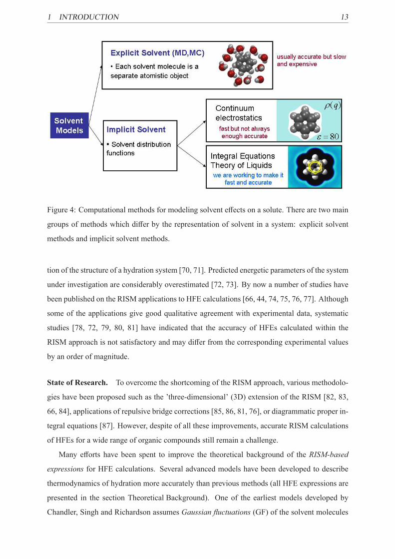
Computational methods for HFE predictions. Computations offer an alternative way to
obtain HFEs. At the present time, there is a lot of work being done in this direction [42, 43, 44,
45, 46, 47, 48, 49, 50, 51, 52, 53]. There are two main groups of methods which differ by the
representation of solvent in a system (Fig. 4). The first group of methods (molecular dynamics
and Monte Carlo methods) treats solvent explicitly via taking into account detailed structure of
the solvent molecules. Due to that they provide the most accurate HFE predictions but require
sufficient computational resources [45, 54, 42, 43, 55, 26, 56, 57, 47, 58, 59].
In turn, the second group of methods - implicit solvent methods, contains more rough
approximations of the solvent structure in the system which allow one to obtain thermody-
namic parameters of solvation without large computational expenses but with less accuracy
[60, 44, 61]. Nowadays, the most challenging task is to develop an HFE prediction by the
implicit solvent models with the accuracy comparable to those for explicit models.
The most widely used approximation for implicit models treats solvent as a continuum me-
dia which is characterized by the dielectric constant (continuum methods) [60, 44, 61]. The
approximation fails to reproduce specific interactions such as hydrogen bonds. Nevertheless,
such simplification of the system allows accurate HFE predictions for neutral monofunctional
solutes but leads to sufficient errors of HFE for polyfunctional compounds [62]. Range of sol-
vation continuum models (SMx) which reduce the errors with a number of empirical corrections

1 INTRODUCTION 12
Figure 3: It is difficult to measure HFE directly. Usually, to obtain HFEs for a compound one
performs several measurements of solubility and vapor pressure at different temperatures. The
figure shows estimations of the number of experimental points and the time of measurements
to obtain HFE value for one compound [12, 30, 36, 37, 38, 39] (ΔGsoln is the solution free
energy, Vm is molar volume, S aq is aqueous solubility, ΔGTsub is the sublimation free energy at
temperature T , P and P0 are the vapor pressure of the compound and the atmospheric pressure,
accordingly, R is the ideal gas constant)
allows one to improve results for HFE predictions [63, 33]. In addition, the continuum models
can be combined with quantum mechanical description of solutes in a straightforward manner
that allows one to model the solvent effects on the electronic structure of the solute [60, 44, 61].
Another approximation is one of the most promising for describing hydration processes
because it has an intermediate position between the fully atomistic representation of the sol-
vent structure (MD, MC) and the continuum models. Within the approximation the solvent
molecules are treated as a set of sites (atoms) interacted via potentials. The solvent density
distribution around a solute molecule is described with a set of correlation functions that are
connected via set of integral equations – the Reference Interaction Sites Model (RISM) of
the integral equation theory (IET) of molecular liquids [64, 65, 66, 67, 68, 69]. The original
RISM method pioneered by Chandler and Andersen [64] requires a solution of the site-site
Ornstein-Zernike (SSOZ) integral equations combined with a local algebraic relation, so-called
hypernetted chain (HNC) closure (see the section Theoretical Background).
However, it was shown that the RISM approach allows only the qualitative correct descrip-
1 INTRODUCTION 13
Figure 4: Computational methods for modeling solvent effects on a solute. There are two main
groups of methods which differ by the representation of solvent in a system: explicit solvent
methods and implicit solvent methods.
tion of the structure of a hydration system [70, 71]. Predicted energetic parameters of the system
under investigation are considerably overestimated [72, 73]. By now a number of studies have
been published on the RISM applications to HFE calculations [66, 44, 74, 75, 76, 77]. Although
some of the applications give good qualitative agreement with experimental data, systematic
studies [78, 72, 79, 80, 81] have indicated that the accuracy of HFEs calculated within the
RISM approach is not satisfactory and may differ from the corresponding experimental values
by an order of magnitude.
State of Research. To overcome the shortcoming of the RISM approach, various methodolo-
gies have been proposed such as the ’three-dimensional’ (3D) extension of the RISM [82, 83,
66, 84], applications of repulsive bridge corrections [85, 86, 81, 76], or diagrammatic proper in-
tegral equations [87]. However, despite of all these improvements, accurate RISM calculations
of HFEs for a wide range of organic compounds still remain a challenge.
Many efforts have been spent to improve the theoretical background of the RISM-based
expressions for HFE calculations. Several advanced models have been developed to describe
thermodynamics of hydration more accurately than previous methods (all HFE expressions are
presented in the section Theoretical Background). One of the earliest models developed by
Chandler, Singh and Richardson assumes Gaussian fluctuations (GF) of the solvent molecules

1 INTRODUCTION 14
[88]. Although GF free energy expression provides better agreement with experimental data
for some solutes [78], it is not widely used due to the improper account of molecular effects
for polar solutes [79]. Later, yet another approach referred as the partial wave (PW) model
has been proposed by Ten-no and Iwata [89]. This approach is based on the distributed partial
wave expansion of solvent molecules around the solute [89]. The recent analysis [80] has
indicated that the PW model sufficiently overestimates HFE for non-polar solutes. However,
the analysis [80] showed also significant correlations between the error of HFEs calculated with
PW method and solutes’ partial molar volume (PMV). The corresponding correction on PMV
was implemented in the Partial Wave Correction (PWC) model [80]. For 19 organic solutes
the PWC model provided better agreement with experimental data than the original PW model.
However, due to the inherent limitations of the PWC model (poor parameterization and small
number of corrections), it cannot be applied ’as is’ for a wide range of organic solutes [80].
Parameterization of a property with a set of corrections is a common practice these days
known as a quantitative structure - activity/property relationships (QSAR/QSPR) within chem-
informatics [90, 26, 91, 92, 93, 94, 95, 27, 29]. With respect to HFE calculations, such
parametrization has been used for implicit models to improve the accuracy of calculations
within the framework of continuum electrostatics [63, 33, 96, 97, 27, 53]. The choice of
mathematical model for the parametrization is rather wide: statistical analysis [98], physical
assumptions (e.g. the linear response theory [99, 100]), etc. The number of required descriptors
for empirical corrections may vary from just a few of them (e.g., descriptors based on physi-
cal/chemical properties of solutes [97]) to up to a 102−103 descriptors (e.g., descriptors derived
from the group/atom contribution approach [101]). Application of the atomic or group structural
descriptors becomes complicated for polyfunctional compounds due to the enormous number
of the descriptors (each combination of functional groups requires its own descriptor) [101, 53].
In turn, more general physical/chemical descriptors can be successfully applied only for some
particular classes of solutes, but it is difficult to transfer the descriptors from one chemical class
of solutes to another.
Aims of the study. Aims of this thesis are (i) to develop a hybrid model based on the combi-
nation of HFEs obtained by RISM with a small set of structural corrections to improve the poor
accuracy of thermodynamics calculations with RISM approaches; (ii) to analyze the perfor-
mance of the model with different input parameters and to find their optimal combination; (iii)
to analyze the model predictive ability on a wide range of compounds from different chemical
classes; (iv) to compare the accuracy of thermodynamic parameters obtained by the model with

1 INTRODUCTION 15
that for standard methods (e.g., continuum solvation models) and the corresponding cheminfor-
matics approach with the same set of descriptors.

2 THEORETICAL BACKGROUND 16
2 Theoretical Background
2.1 Molecular Ornstein-Zernike integral equation
The integral equation theory (IET) of molecular liquids is a statistical mechanics approach to
describe thermodynamic properties of molecular liquids. This theory is based on the method of
distribution ρ(n)(r1, ..., rn,Θ1, ...,Θn) and correlation functions g(n)(r1, ..., rn,Θ1, ...,Θn) in clas-
sical statistical mechanics [102, 103, 104] (symbol (n) – represents the n-particle distribu-
tion/correlation function, ri and Θi are spatial and orientation coordinates of the i-th molecule).
Within the framework of IET, the fundamental six-dimensional molecular Ornstein-Zernike
(MOZ) integral equation can be written, which operates with pair correlation functions
g(2)mk(r1, r2,Θ1,Θ2) of different components of the liquid (indexesm, k denote the component type
in liquid) [104, 102]. For homogeneous liquids, the correlation functions depend only on the rel-
ative position and orientation of molecules with respect to one another, thus the pair correlation
function can be written as g(2)mk(r1 − r2,Θ1 −Θ2). The MOZ equations can be more conveniently
written via the total correlation functions, hmk(r1 − r2,Θ1 − Θ2) = gmk(r1 − r2,Θ1 − Θ2) − 1.
The MOZ equations relate the total correlation functions with the so-called direct correlation
functions cmk(r1 − r2,Θ1 − Θ2) [104, 66] (the meaning of the direct correlation function is not
straightforward but can be understood via the density functional theory of molecular liquids
[104, 105, 103]):
hmk(r1 − r2,Θ1 − Θ2) = cmk(r1 − r2,Θ1 − Θ2)+Ncomponent∑t=1
ρt
8π2
∫R3
∫Ω
cmt(r1 − r3,Θ1 − Θ3)hmt(r2 − r3,Θ2 − Θ3)dr3dΘ3,
m = 1...Ncomponent, k = 1...Ncomponent
(10)
where ρt is the bulk density of the t-th component of the system, Ncomponent is the number of
components,Θ = {ψ, θ, ϕ} is the set of Euler angles: ψ ∈ [0, 2π], θ ∈ [0, π], ϕ ∈ [0, 2π]; Ω
contains all possible orientations of a molecule, and 8π2 is the "phase volume" of Ω [104].
To calculate the HFE, we consider a system containing only two components: a solute in a
pure water. In the case of an infinitely dilute solution (when the density of solute component
tends to zero), the MOZ equations can be split into three independent equations, operating with
solvent - solvent, solute - solvent and solute - solute correlation functions, respectively, which
can be solved separately [66].
The MOZ equations are difficult to solve because of the high dimensionality of the problem.
There are several methods originating from the work of Chandler et al. [64], generally named
2 THEORETICAL BACKGROUND 17
Reference Interaction Site Models (RISM), which can reduce the dimensionality of original
MOZ equations, and are used nowadays for a wide range of applications in chemical sciences
[106, 107, 80, 108, 84, 5, 109, 110].
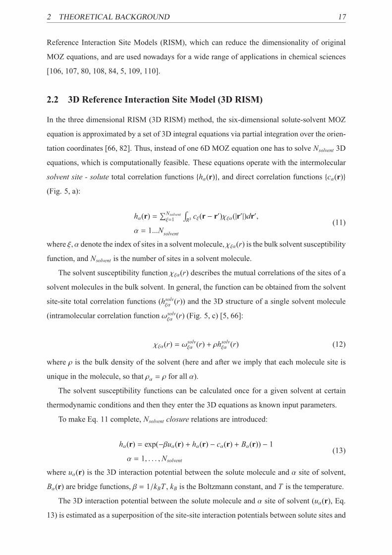
2.2 3D Reference Interaction Site Model (3D RISM)
In the three dimensional RISM (3D RISM) method, the six-dimensional solute-solvent MOZ
equation is approximated by a set of 3D integral equations via partial integration over the orien-
tation coordinates [66, 82]. Thus, instead of one 6D MOZ equation one has to solve Nsolvent 3D
equations, which is computationally feasible. These equations operate with the intermolecular
solvent site - solute total correlation functions {hα(r)}, and direct correlation functions {cα(r)}
(Fig. 5, a):
hα(r) =∑Nsolventξ=1
∫R3 cξ(r − r
′)χξα(|r′|)dr′,
α = 1...Nsolvent(11)
where ξ, α denote the index of sites in a solvent molecule, χξα(r) is the bulk solvent susceptibility
function, and Nsolvent is the number of sites in a solvent molecule.
The solvent susceptibility function χξα(r) describes the mutual correlations of the sites of a
solvent molecules in the bulk solvent. In general, the function can be obtained from the solvent
site-site total correlation functions (hsolvξα(r)) and the 3D structure of a single solvent molecule
(intramolecular correlation function ωsolvξα(r) (Fig. 5, c) [5, 66]:
χξα(r) = ωsolvξα (r) + ρhsolvξα (r) (12)
where ρ is the bulk density of the solvent (here and after we imply that each molecule site is
unique in the molecule, so that ρα = ρ for all α).
The solvent susceptibility functions can be calculated once for a given solvent at certain
thermodynamic conditions and then they enter the 3D equations as known input parameters.
To make Eq. 11 complete, Nsolvent closure relations are introduced:
hα(r) = exp(−βuα(r) + hα(r) − cα(r) + Bα(r)) − 1
α = 1, . . . ,Nsolvent(13)
where uα(r) is the 3D interaction potential between the solute molecule and α site of solvent,
Bα(r) are bridge functions, β = 1/kBT , kB is the Boltzmann constant, and T is the temperature.
The 3D interaction potential between the solute molecule and α site of solvent (uα(r), Eq.
13) is estimated as a superposition of the site-site interaction potentials between solute sites and

2 THEORETICAL BACKGROUND 18
Figure 5: Correlation functions in the 3D and 1D RISM approaches. (a) 3D intermolecular
solute-solvent correlation function hα(r) around a model solute; (b) 1D spherically-symmetric
correlations: site-site intramolecular (ωss′(r)) between the site of solute molecule and inter-
molecular (hsα(r)) correlation functions between sites of solute and solvent molecules. The
inset plot shows the radial projections of solute site-oxygen water density correlation functions.
(c) Solvent-solvent correlations in both 1D and 3D RISM methods: site-site intramolecular cor-
relation functions (ωsolvγξ(r)) and intermolecular correlation functions (hsolv
αξ(r)) between sites of
solvent molecules. The inset shows the radial projections of water solvent site-site density cor-
relation functions: oxygen-oxygen (OO, blue dashed), oxygen-hydrogen (OH, green solid) and
hydrogen-hydrogen (HH, red dash-dotted).

2 THEORETICAL BACKGROUND 19
the particular solvent site (usα(r), where index s denotes the site in a solute molecule and index
α is the site in a solvent molecule), which depend only on the absolute distance between the two
sites:
uα(r) =Nsolute∑s=1
usα(|rs − r|) (14)
where rs is the radius-vector of solute site (atom).
We used the common form of the site-site interaction potential represented by the long-range
electrostatic term uelsα(r) and short-range Lennard-Jones (LJ) term uLJsα (r) as:
usα(r) = uelsα(r) + uLJsα (r),
uelsα(r) =qsqαr ; uLJsα (r) = 4εLJsα
[(σLJsαr
)12−
(σLJsαr
)6],
(15)
where r = |rs − r|, {qs, qα} are the partial electrostatic charges of the corresponding solute and
solvent sites, and {εLJsα , σLJsα } are the LJ solute-solvent interaction parameters.
In general, the bridge functions Bα(r) in Eq. 13 can be written as an infinite series of
integrals over high order correlation functions and are therefore practically incomputable. Thus,
some approximations are introduced [65, 111, 66]. The most straightforward and widely used
model is the HNC closure, which sets Bα(r) to zero [112]. However, due to the uncontrolled
growth of the argument of the exponent the use of the HNC closure can lead to divergence of the
numerical solution of the RISM equations. One way to overcome this problem is to linearize
the exponential function for arguments larger than a certain constant C:
hα(r) =
⎧⎪⎪⎪⎨⎪⎪⎪⎩ exp(Ξα(r)) − 1 when Ξα(r) < C
Ξα(r) + exp(C) −C − 1 when Ξα(r) > C(16)
where Ξα(r) = −βuα(r) + hα(r) − cα(r). The partially linearized HNC (PLHNC) closure for the
case C = 0 was proposed by Hirata and Kovalenko in [113]. We note that in the literature the
combination of the PLHNC closure relations (Eq. 16) and the 3D RISM equations (Eq. 11) are
usually referred to as 3D RISM-KH theory [5, 108], but for succinctness we will use 3D RISM
instead.
2.3 1D Reference Interaction Site Model (1D RISM)
In the one dimensional RISM (1D RISM) approach, the 3D RISM equations are further approx-
imated by a set of one-dimensional integral equations, operating with the intermolecular solvent

2 THEORETICAL BACKGROUND 20
site - solute site total correlation functions {hsα(r)}, and direct correlation functions {csα(r)} (s, α
denote the index of sites in solute and solvent molecules respectively) [66, 64] (see Fig. 5, b):
hsα(r) =Nsolute∑s′=1
Nsolvent∑ξ=1
∫R3
∫R3ωss′(|r1 − r′|)cs′ξ(|r′ − r′′|)χξα(|r′′ − r2|)dr′dr′′ (17)
where r = |r1 − r2| and χξα(r) are the bulk solvent susceptibility functions, Nsolute and Nsolvent are
the number of sites in the solute molecule and the solvent molecule, ωss′(r) = δ(r − rss′)/(4πr2ss′)
are intramolecular correlation functions describing the 3D structure of the solute molecule (rss′
is the distance between the sites s and s′ of the solute molecule, δ is the Dirac delta function).
To make the 1D RISM equations complete, Nsolute × Nsolvent site-site closure relations are
introduced:hsα(r) = exp(−βusα(r) + hsα(r) − csα(r) + Bsα(r)) − 1
s = 1, . . . ,Nsolute; α = 1, . . . ,Nsolvent(18)
where usα(r) is a pair interaction potential between the sites s and α, Bsα(r) are site-site bridge
functions, β = 1/kBT , kB is the Boltzmann constant, T is the temperature.
The PLHNC closure in the case of 1D RISM reads as:
hsα(r) =
⎧⎪⎪⎪⎨⎪⎪⎪⎩ exp(Ξsα(r)) − 1 when Ξsα(r) < C
Ξsα(r) + exp(C) −C − 1 when Ξsα(r) > C(19)
where Ξsα(r) = −βusα(r) + hsα(r) − csα(r) and C is set to zero.
In the case of the 1D RISM method, instead of Nsolvent 3D RISM equations one has to solve
Nsolute × Nsolvent 1D equations, which requires much less computation.
The calculation scheme for the both 3D RISM and 1D RISM is shown in Fig. 6

2THEORETIC
ALBACKGROUND
21
Figure 6: Scheme of HFE calculations in the RISM approach. Upper rectangles show the input data for the solute and solvent molecules. Here {xi, yi, zi}
are the spatial coordinates of the site i, {σi, εi} are the LJ parameters of the site i, {qi} is the partial charge on the site i. The RISM solver contains
the corresponding closure and RISM equations and is shown as a grey rectangle. We note that the solute site-site intramolecular correlation functions,
{ωss′(r)}, are used only in the 1D RISM approach (that is why it has a dashed arrow).

2 THEORETICAL BACKGROUND 22
2.4 Hydration Free Energy Expressions within the 1D RISM approach
Chemical potential (μ) of a thermodynamic system is the amount by which the energy of the
system would change if an additional particle was introduced, with the entropy and volume
held fixed. Let us consider a thermodynamic system containing n constituent species. Its total
internal energy U is postulated to be a function of the entropy S , the volume V , and the number
of particles of each species N1, ...,Nn: U = f (S ,V,N1, ...,Nn). By referring to U as the internal
energy, it is emphasized that the energy contributions resulting from the interactions between
the system and external objects are excluded. The chemical potential of the i-th species, μi is
defined as the partial derivative:
μi =
(∂U∂Ni
)S ,V,Nj�i
, (20)
where the subscripts emphasize that the entropy, volume, and the other particle numbers are to
be kept constant.
Laboratory experiments are often performed under conditions of constant temperature T and
pressure P. Under these conditions, the chemical potential corresponds to the partial derivative
of the Gibbs energy with respect to number of particles:
μi =
(∂G∂Ni
)T,P,Nj�i
. (21)
In the case of the infinitely diluted solution the change in chemical potential in the process of
hydration, Δμhyd, corresponds to the HFE. Within the RISM approach for HFE calculations one
has to determine the relationship between the change of chemical potential (Δμhyd) and pair
correlation functions (g(2)(r1, r2,Θ1,Θ2)).
Generally, the thermodynamic integration can be used for this purpose [77, 114]. The main
idea behind the method is the following. To compute the free energy of a system, one should
find the reversible pathway in the coordinates pressure-temperature (in the case of the Gibbs
free energy) that links the system under investigation and the reference system for which the
value of free energy is known.
Let us consider the system containing N particles with the potential energy function U. We
assume that U depends linearly on a coupling parameter λ such that, for λ = 0, U corresponds
to the potential energy of the reference system I, while for λ = 1 we will obtain the potential
energy of the system under investigation II [114].
The partition function for a system with a potential energy function that corresponds to a
value of λ between 0 and 1 is:

2 THEORETICAL BACKGROUND 23
Q(N, P,T, λ) =1
Λ3NN!
∫drN exp
[−βU(λ)
], (22)
where Λ =√2πh2mkT is the thermal de Broglie wavelength, h is Planck’s constant, m is the mass of
the particle, k is Boltzmann’s constant, T is the temperature, β = 1/kBT .
The derivative of the Gibbs free energy with respect to λ can be written as an ensemble
average [114]:
(∂G(λ)∂λ
)N,P,T
= − 1β∂∂λlnQ(N, P,T, λ) = − 1
βQ(N,P,T,λ)∂Q(N,P,T,λ)
∂λ
=
∫drN (∂U(λ)/∂λ) exp−βU(λ)∫
drN exp−βU(λ)
=⟨∂U(λ)∂λ
⟩λ,
(23)
where G is the Gibbs free energy, Q is the partition function (Eq. 22), λ is the coupling param-
eter, < ... >λ denotes an ensemble average.
The free energy difference between systems I and II can be obtained by the Kirkwood’s
integral equation [115]:
G(λ = 1) −G(λ = 0) =∫ 1
0dλ
⟨∂U(λ)∂λ
⟩λ
. (24)
Within the 1D RISM approach in the case infinitely diluted solution Eq. 24 can be written
as following:
βΔμhyd = 4πρ∑sα
∫ 1
0dλ
∫ ∞
0(1 + hsα(r, λ))
∂Usα∂λ
r2dr, (25)
where Δμhyd is the change of the chemical potential in the process of hydration, β = 1/kBT , ρ is
the density of solvent, Usα(r, λ) is the interaction potential.
Equation 25 requires calculations of the total correlation function hsα(r, λ) at various λ.
In average, to determine the HFE for one compound one should to perform about 10 – 100
computer simulations, which in the case of complex organic molecules requires an enormous
computer resources.
Chandler [88], Singer [112], and Ten-no [72] showed that at some approximations Eq. 25
can be replaced by simpler models which allow one obtaining the value of Δμhyd from the total
hsα(r) and direct csα(r) correlation functions on the base of single-point computer simulation. In
this thesis we discussed the accuracy of the most popular HFE expressions, namely HNC (Eq.
26) [112, 66], GF (Eq. 27) [88], KH (Eq. 28) [116], PW (Eq. 29) [72], HNCB expression (Eq.
30) [85], and PWC (Eq. 32) [80], which are given by the equations below.
ΔμHNChyd = 2πρkBTNsolute∑s=1
Nsolvent∑α=1
∞∫0
[−2csα(r) − hsα(r) (csα(r) − hsα(r))] r2dr (26)

2 THEORETICAL BACKGROUND 24
ΔμGFhyd = 2πρkBTNsolute∑s=1
Nsolvent∑α=1
∞∫0
[−2csα(r) − csα(r)hsα(r)] r2dr (27)
ΔμKHhyd = ΔμGFhyd + 2πρkBT
Nsolute∑s=1
Nsolvent∑α=1
∞∫0
h2sα(r)Θ(−hsα(r))r2dr (28)
ΔμPWhyd = ΔμGFhyd + 2πρkBT
Nsolute∑s=1
Nsolvent∑α=1
∞∫0
hsα(r)hsα(r)r2dr (29)
where r = |r1 − r2| and
hsα(|r2 − r1|) =Nsolute∑s′=1
Nsolvent∑ξ=1
∫R3
∫R3
ωss′(|r1 − r′|)hs′ξ(|r′ − r′′|)ωsolvαξ (|r′′ − r2|)dr′dr′′,
ωss′(r) and ωsolvαξ (r) are the elements of matricesW−1,W−1
solv which are inverses to the matrices
W = [ωss′(r)]Nsolute×Nsolute and Wsolv =[ωsolvαξ(r)
]Nsolvent×Nsolvent
built from the solute and solvent
intramolecular correlation functions ωss′(r) and ωsolvαξ (r) respectively.
The HFE expression for the HNCB model is [85]:
ΔμHNCBhyd = ΔμHNChyd +
2πρkBT∑sα
∞∫0
(hsα(r) + 1)(e−BRsα(r) − 1)r2dr.
(30)
Here {BRsα(r)} are repulsive bridge correction functions, defined for each pair of solute s and
solvent α atoms by the expression:
exp(−BRsα(r)) =∏ξ�α
⟨ωαξ ∗ exp
(−βεsξ
(σsξr
)12)⟩(31)
where ωαξ(r) are the solvent intramolecular correlation functions, and σsξ and εsξ are the site-
site parameters of the pair-wise LJ potential.
The PWC HFE expression is given by:
ΔμPWChyd = ΔμPWhyd + aρβ
−1V + bδOH, (32)
where ΔμPWhyd is HFE obtained by the PW HFE expression (Eq. 29), ρ is the number density of
solvent (water), V is the partial molar volume of the solute (see Eq. 35), and deltaOH is the delta-
function which equals 1 if OH-group presents in the solute molecule, otherwise it equals zero,
a and b are the correction coefficients which are determined by the corresponding regression
against the experimental values of the HFEs for a training set [80].

2 THEORETICAL BACKGROUND 25
2.5 Thermodynamic parameters within the 3D RISM approach
Within the framework of the 3D RISM theory there are few approximate expressions that allow
one to calculate HFEs analytically from the total and direct correlation functions. In this thesis,
we discussed the accuracy of the GF HFE expression adopted by Kovalenko and Hirata for the
3D RISM case [108] (Eq. 33), and the KH free energy expression proposed by Kovalenko and
Hirata for the PLHNC closure [113] (Eq. 34) [116].
Δμ3DRIS M−GFhyd = ρkBTNsolvent∑α=1
∫R3
[−cα(r) −
12cα(r)hα(r)
]dr; (33)
Δμ3DRIS M−KHhyd = ρkBTNsolvent∑α=1
∫R3
[12h2α(r)Θ(−hα(r)) − cα(r) −
12cα(r)hα(r)
]dr, (34)
where ρ is the number density of a solute sites α, Θ(x) is the Heaviside step function:
Θ(x) =
⎧⎪⎪⎪⎨⎪⎪⎪⎩ 1 f or x > 0,
0 f or x < 0
2.6 Partial molar volume expressions in RISM approaches
The dimensionless PMV (DPMV) calculations within the framework of the 1D RISM approach
for the case of infinitely diluted solution can be obtained using the following expression [80]:
ρV = 1 +4πρNsolute
∑s
∞∫0
(hsolvoo (r) − hso(r)
)r2dr, (35)
where hsolvoo (r) is the total oxygen-to-oxygen correlation function of bulk water, hso(r) is the total
correlation function between the solute site s and the water oxygen.
Within the 3D RISM approach we estimate the solute DPMV via solute-solvent site corre-
lation functions using the following expression [117, 118, 3]:
ρV = ρkBTη⎛⎜⎜⎜⎜⎜⎝1 − ρ Nsolvent∑
α=1
∫R3cα(r)dr
⎞⎟⎟⎟⎟⎟⎠ (36)
where η is the pure solvent isothermal compressibility.

3 COMPUTATIONAL DETAILS 26
3 Computational Details
3.1 1D RISM calculations
The HFEs were calculated with the 1D RISM method using the home-made collection of nu-
merical routines developed by our group [77, 119, 120]. Calculations were performed for the
case of infinitely diluted aqueous solutions at T=300K. We used the Lue and Blankschtein ver-
sion of the modified SPC/E model of water (MSPC/E) [121], proposed earlier by Pettitt and
Rossky [122]. It differs from the original SPC/E water model [123] by the addition of LJ po-
tential parameters for the water hydrogen (σLJHw = 0.8Å and εLJHw = 0.046 kcal/mol), which were
altered to prevent possible divergence of the algorithm [124, 78, 85, 80]. We took the MSPC/E
bulk solvent correlation functions from the work [125] where they were calculated by RISM
equations for solvent-solvent correlations [66] using wavelet-based algorithms [126, 127].
Figure 7: (a) Representation of the 3D-grid box in calculations of total correlation function
(hα(r), where α is the solvent site) within the 3D RISM. Grid points are shown only at the edges
of the 3D-box. Benchmarking of the input parameters (spacing and buffer) is discussed in the
section Benchmarks of the 3D RISM calculations. (b) Representation of a grid in calculations
of total site-site correlation function (hsα(r), where s and α are solute and solvent sites, accord-
ingly) within the 1D RISM. Number of grid points and values of grid step and cutoff distance
are specified in the text.

3 COMPUTATIONAL DETAILS 27
The set of the 1D RISM equations was solved by the standard numerical iterative scheme
using the Bessel-Fourier transforms for the calculation of the convolution integrals [65, 119]. To
speeding-up the iterations the multigrid technique was used (see the sectionMultigrid technique).
Six levels of numerical grids were employed for the calculations. The coarsest grid, where the
most of the iterations were done, had 128 grid points and grid-step of 0.4 Bohr (0.212 Å) (see
Figure 7, b). The solution was obtained on the finest grid, which had 4096 grid points, grid step
was 0.05 Bohr (0.0265 Å) and cutoff distance was 204.8 Bohr (108.4 Å). The accuracy of the
iterations was controlled by the norm of difference between the solutions on the sequential iter-
ations (Eq. 37). Iteration process was stopped when the accuracy of n-th iteration had reached
the threshold εthres: Δn < εthres.
Δn =1
NsoluteNsolvent
Nsolute∑s=1
Nsolvent∑α=1
⎡⎢⎢⎢⎢⎢⎢⎢⎢⎣∞∫0
[(h(n+1)sα (r) − h(n)sα (r)
)−
(c(n+1)sα (r) − c(n)sα (r)
)]2dr
⎤⎥⎥⎥⎥⎥⎥⎥⎥⎦12
(37)
where h(n)sα (r), c(n)sα (r), h(n+1)sα (r), c(n+1)sα (r) are the total and direct correlation functions approxima-
tions on the n-th and (n + 1)-th iteration steps respectively.
In the current work, the RISM equations were solved up to the accuracy εthres = 10−4. To
check, whether this accuracy is sufficient for the accurate HFE calculations additional numerical
experiments were performed. It was shown, that for 10 randomly chosen non-polar compounds
the numerical error of the 1D RISMHFE calculations with PWmethod is about 0.008 kcal/mol.
For polar compounds the numerical error is approximately 0.024 kcal/mol. These errors are
essentially lower than a typical error of experimental HFE measurements (∼ 0.24 kcal/mol)
[36]. Therefore, we assume that the numerical accuracy εthres = 10−4 is sufficient.
To perform the calculations one needs three sets of input data: 1) solute atomic coordinates,
2) partial charges on the atoms, and 3) the atoms’ LJ potential parameters (see Fig. 6). Coor-
dinates for linear alkanes, several alkylbenzenes and phenols were taken from the Cambridge
Structural Database [128]. Due to the fact that hydrogen positions determined by standard
X-ray methods differ systematically from those determined by neutron methods [129], we op-
timized the length of the carbon-hydrogen bonds (C-H) using the QM (quantum mechanical)
energy minimization at the MP2/6-311G** level of theory with constrained bonds between
heavy atoms (e.g. C-C). The geometrical parameters of all other solutes (not presented in the
Cambridge Structural Database) were found by the structural optimization at the same level of
theory but without geometrical constrains for the bond lengths between heavy atoms. For all
QM calculations we used Gaussian 03 quantum chemistry software [130]. We modeled all com-
pounds with OPLS-AA (Optimized Potential for Liquid Simulations - All Atom) LJ potential

3 COMPUTATIONAL DETAILS 28
parameters [131, 132, 133]. These parameters were assigned to each atom automatically by the
Maestro software (the Schroedinger Inc.).
We consider two types of partial charges. First one is the OPLS-AA partial charges (for the
sake of brevity, in the rest of the paper we will use for them the shorter abbreviation OPLS). The
second set of partial charges was obtained with the CHELPG procedure [134] at MP2/6-311G**
and B3LYP/6-31G** levels of theory using the Gaussian 03 quantum chemistry software [130].
Comparison of the partial charges for several aliphatic and aromatic compounds is presented in
the section 1D RISM-SDC model with QM-derived partial charges.
We note, that the convergence of the RISM calculations with the original geometric mixing
rules (Eq. 38) is very poor (see Table 7).
⎧⎪⎪⎪⎪⎪⎨⎪⎪⎪⎪⎪⎩σsα =
√σs · σα
εsα =√εs · εα
(38)
To avoid this problem with convergence we performed calculations with the Lorentz-Berthelot
mixing rule for the solute-water LJ potential parameters [135]:⎧⎪⎪⎪⎪⎪⎨⎪⎪⎪⎪⎪⎩σsα =
σs+σα2
εsα =√εs · εα
(39)
The set of structural descriptors was assigned to each molecules automatically using the
computer program "checkmol" [136] and Python scripts.
3.2 3D RISM calculations
The 3D RISM calculations were performed using the NAB simulation package [137] in the
AmberTools 1.4 set of routines [138]. The 3D-grid around a solute was generated such that the
minimal distance between any solute atom and the edge of solvent box (buffer in NAB notation)
was equal to 30 Å, whereas the linear grid spacing in each of the three directions was 0.3 Å (see
the paragraph Benchmarks of the 3D RISM calculations). We employed the MDIIS iterative
scheme [139], where we used 5 MDIIS vectors, MDIIS step size - 0.7, and residual tolerance is
10−10. The PLHNC closure was used for solution of the 3D RISM equations.
The solvent susceptibility functions for 3D RISM calculations were obtained by the 1D
RISM method present in the AmberTools 1.4. The dielectrically consistent 1D RISM (DRISM)
was employed [140] with the PLHNC closure [113]. The grid size for 1D-functions was 0.025
Å, which gave a total of 16384 grid points. We employed the MDIIS iterative scheme [139],

3 COMPUTATIONAL DETAILS 29
where we used 20 MDIIS vectors, MDIIS step size - 0.3, and residual tolerance - 10−12. The
solvent was considered to be pure water with the number density 0.0333 Å−3, a dielectric con-
stant of 78.497, at a temperature of 300K. The final susceptibility solvent site-site functions
were stored and then used as input for the 3D RISM calculations.
Within the 3D RISM approach we perform HFE calculations with the following solutes pa-
rameters:
(1) Coordinates of each molecule were optimized using the AM1 Hamiltonian [141] via the an-
techamber [142] suite, which uses the sqm [138] program for semiempirical QM calculations.
The initial configurations for these QM geometry optimizations were taken from the previous
1D RISM calculations (see the section above).
(2) Atomic partial charges were calculated using the AM1-BCC method [143, 144, 142] imple-
mented in the antechamber from the AmberTools 1.4 package [138].
(3) The LJ parameters from the General Amber Force Field (GAFF) [142] were assigned to
solute atoms with the antechamber and he tleap programs [142]. In the case of 1D RISM cal-
culations, for all atoms with zero GAFF LJ potential parameters the following parameters were
used σLJ =0.4 Å and εLJ =0.1185 kcal/mol to prevent divergence of the algorithm.
In this thesis, we compare the accuracy of the 1D RISM and the 3D RISM for HFE calcula-
tions. To make the comparison consistent, we performed additional 1D RISM HFE calculations
with the same solutes parameters.
Benchmarks of the 3D RISM calculations. Two input parameters in the 3D RISM were
investigated in [145]. Buffer, the smallest distance between solute atoms and a 3D box side and
spacing, the distance between grid points in 3D-grid (Figure 7). The tolerance (the L2 norm of
the difference between two subsequent solutions of 3D RISM iterations) was set to 10−10 and
the number of vectors used by MDIIS solver was 5 following the works of the developers of the
3D RISM in the AmberTools [137, 138]. The benchmarks were performed on a paracetamol
molecule as a solute. It was found that accurate HFE calculations within the 3D RISM approach
(error in a range of 0.02 kcal/mol) can be achieved with the following parameters: buffer = 30
Å, spacing = 0.3 Å.
3.3 Multigrid technique
Even for the simplest case of an isotropic liquid the IET of molecular liquids requires a non-
trivial numerical solution of a system of integral equations of the Ornstein-Zernike (OZ) type

3 COMPUTATIONAL DETAILS 30
Figure 8: Numeric errors of the HFE of paracetamol calculated by the KH free energy expres-
sion as a function of the buffer distance. The value calculated with buffer = 50◦A is chosen to
be a reference. The spacing and tolerance were set to be 0.5◦A and 10−10, respectively.
Figure 9: Numeric errors of the HFE of paracetamol calculated by the KH free energy expres-
sion as a function of spacing. The value calculated with spacing = 0.25◦A is chosen to be a
reference. The buffer and tolerance were set to be 30◦A and 10−10, respectively.

3 COMPUTATIONAL DETAILS 31
[105]. The complexity of solution dramatically increases with the increasing number of different
interacting sites of the system [146, 66, 137]. The most simple and straightforward algorithm to
solve the OZ-type equations is the Picard algorithm (see the section One-level Picard iterations)
which is based on a successive substitution scheme (this method is sometimes called “direct it-
eration method”). This technique is easy to implement but it suffers from poor convergence
[147, 66, 77]. These days multigrid numerical methods [148, 149, 150, 151, 152] become
very popular in different areas of science and engineering. The multigrid approach to com-
plex computational problems is actively used in computational chemistry to accelerate quantum
chemistry calculations [153, 154, 155, 156] as well as for the treatment of electrostatic interac-
tions in classical molecular dynamics simulations [157, 158]. A universal multigrid technique
for the numerical solution of the OZ type integral equations was implemented in the home-
made collection of numerical routines developed by our group [77, 119, 120]. This approach
is based on ideas coming from the multigrid methods for numerical solutions of integral equa-
tions [148, 149]. Instead of the nested iteration method used in [147] the coarse-grid correction
method was used. It had been shown to provide better convergence than the nested iteration
method [148].
3.3.1 One-level Picard iterations
There are only a few special cases where Eqs. (17) and (18) can be solved analytically and,
therefore, numerical solutions are necessary. For numerical calculations, the Fourier represen-
tation of the OZ equation, is usually applied:
h(k) − c(k) =ρc2(k)1 − ρc(k)
, (40)
where the hat means the Fourier transform (FT).
For numerical treatment of the OZ equation it is common to introduce a new function γ(r) =
h(r) − c(r) and rewrite Eqs. (18) and (40) in the following way:
c(r) = exp[−βU(r) + γ(r) + B(r)] − 1 − γ(r), (41)
and
γ(k) =ρc2(k)1 − ρc(k)
. (42)
One can reformulate the problem of finding a numerical solution of the system (41) –(42)
with functions γ(r) and c(r) represented on a grid ΩL as the solution of a nonlinear equation:
γ(r) = F(γ(r)), (43)

3 COMPUTATIONAL DETAILS 32
where F(γ(r)) is given by
F(γ(r)) = T−1 ∗ρ(T ∗ c(r))2
1 − ρ(T ∗ c(r)), (44)
and c(r) is given by Eq. (41). Here T and T−1 are Fourier transformation (FT) and inverse
Fourier transformation (IFT), accordingly.
The simplest way of finding the numerical solution of (Eq. 43) is the Picard scheme of
successive iterations [159, 160] where an i-iteration is given by:
γi(r) := F(γi−1(r)). (45)
To facilitate the convergence the damped Picard method [160] is often used where the i-th
iteration is given as
γi(r) := εF(γi−1(r)) + (1 − ε)γi−1(r), 0 < ε ≤ 1; (46)
where ε is a damping parameter. In the following we will refer on the damped Picard method
applied to the problem (Eq. 41) as Picard method and denote an n-steps Picard iteration for (Eq.
41) as
γ(r) := Υn(γ(r), ε). (47)
We note that the convergence of the method is not guaranteed and normally it is quite slow.
Nevertheless, the method is still commonly used in the theory of liquids (often in combination
with other methods) [66, 77] because it is very easy to implement.
3.3.2 Two-grid iteration
In this subsection we will briefly describe the two-grid iteration method (TGM) which is the
base for the construction of multi-grid iterations [148, 149]. The proposed approach mimics the
idea of the TGM method for linear problems with coarse-grid correction [148, 149].
Let us firstly introduce two inter-grid conversion operators: a restriction or fine-to-coarse
operator R which maps the function f from the fine grid ΩL to the coarse grid ΩL−1 :
fL−1 = R ∗ fL, (48)
and a reciprocal operator to restriction - prolongation or coarse-to-fine operator P which inter-
polates the function f given on the coarse grid ΩL−1 to the fine grid ΩL:
fL = P ∗ fL−1. (49)
3 COMPUTATIONAL DETAILS 33
There are many possible choices of these operators and advantages and disadvantages of some
of them are well described in [148]. In our work we use the trivial injection [148, 149] for the
restriction operator I and the cubic spline interpolation [160] for the prolongation operator P.
Let us now consider the problem of finding a numerical solution of Eq. (43) on the fine grid
ΩL starting from an initial guess initialL .
Let us assume that there is an iterative process Φ0 (e.g. Eq. (47) with a reasonably large
n) which gives an accurate numerical solution of the problem on the coarse grid ΩL−1 starting
from γinitialL−1 = R ∗ γinitialL
γacc.L−1 = Φ0(γinitialL−1 ). (50)
Therefore, the correction or defect of the solution on the level L − 1 is given by
dL−1 = γacc.L−1 − γinitialL−1 . (51)
The main idea of the TGM iterations is to interpolate this correction to the fine level L using
the prolongation operator P and improve the solution on this level as:
γL = γinitialL + P ∗ dL−1. (52)
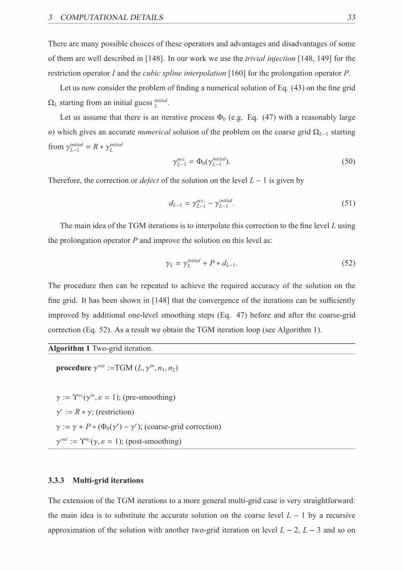
The procedure then can be repeated to achieve the required accuracy of the solution on the
fine grid. It has been shown in [148] that the convergence of the iterations can be sufficiently
improved by additional one-level smoothing steps (Eq. 47) before and after the coarse-grid
correction (Eq. 52). As a result we obtain the TGM iteration loop (see Algorithm 1).
Algorithm 1 Two-grid iteration.
procedure γout :=TGM (L, γin, n1, n2)
γ := Υn1(γin, ε = 1); (pre-smoothing)
γr := R ∗ γ; (restriction)
γ := γ + P ∗ (Φ0(γr) − γr); (coarse-grid correction)
γout := Υn2(γ, ε = 1); (post-smoothing)
3.3.3 Multi-grid iterations
The extension of the TGM iterations to a more general multi-grid case is very straightforward:
the main idea is to substitute the accurate solution on the coarse level L − 1 by a recursive
approximation of the solution with another two-grid iteration on level L − 2, L − 3 and so on

3 COMPUTATIONAL DETAILS 34
until the coarsest level L0 where the coarsest solution is found as γacc.0 = Φ0(γinitial0 ). As the
general principles of the multi-grid iterations construction are well explained in [148] we will
only briefly describe our algorithm below:
Algorithm 2Multi-grid iteration.
procedure γout :=MGM (L, γin, n1, n2, μ)
if L = 0 then γout := Φ0(γin) else
γ := Υn1(γin, ε = 1); (pre-smoothing)
γr := R ∗ γ; (restriction)
for j := 1 step 1 until μ do γout :=MGM(L − 1, γr, n1, n2), μ)
γ := γ + P ∗ (γout − γr), (coarse-grid correction)
γout := Υn2(γ, ε = 1); (post-smoothing)
The parameter μ is rarely chosen bigger than 2 when the iteration is usually called W-
iteration. If μ is equal to 1 it is common to call such iteration as V-iteration. In all our calcula-
tions we used n1 = n2 = 1 steps for pre- and post-smoothing.
As there is no way to find an exact solution of the problem the choice ofΦ0 is quite ambigu-
ous. It could be, e.g., the Picard process (Eq. 47) with a sufficiently large number of iterations
as well as the more efficient but more computationally expensive Newton-Raphson iterations
algorithm [160, 77] or any other numerical procedure which can provide a coarse-grid solution
with a reasonable accuracy (see [159, 147, 120]).

4 STRUCTURAL DESCRIPTORS CORRECTION (SDC) MODEL 35
4 Structural Descriptors Correction (SDC) model
4.1 The QSPR basis of the model
Quantitative Structure - Property Relationship (QSPR) models are based on the idea that a
physical/chemical property can be related to a set of molecular descriptors of the compound
[161, 91]. The main assumption behind the QSPR approach is that similar molecules have
similar properties. Thus, one can predict a property of a target compound using its structural in-
formation and the mathematical relationship, obtained previously on a separate set of molecules
(training set). We note that the predictive ability of the QSPR approach strongly depends on
the choice of molecules for the training set and quality of experimental data for the selected
molecules.
The mathematical relationship obtained in a QSPR model may be linear (single- or multi-
parameter linear regression) or non-linear (neural networks, random forests, etc.). In this thesis
we consider only linear regression models. In the case that the property of interest Y is related to
one molecular descriptor D, the corresponding one-parameter linear regression can be written
as
Y = a0 + aD, (53)
where Y and D are vectors of the property values and the molecular descriptor values for a
training set of molecules, accordingly. Alternatively, the property Y may depend linearly on
several molecular descriptors. It this case, the corresponding multi-parameter regression can be
found as (see the section Multi-parameter linear regression for details):
Y = a0 + a1D1 + a2D2 + a3D3 + · · · + anDn= a0 +
∑ni=1 aiDi.
(54)
The basic stages in developing a QSPR model are the following (see Fig. 10):
1. Preparation of input parameters: Select a set of molecules on which the QSPR model
will be obtained and store a set of 1D (or 2D) structural information of the selected
molecules as well as their experimental values of the property of interest in a computer-
acceptable format. The majority of molecular descriptors (generated in the next step) re-
quire the 3D structure of the molecules as an initial parameter [162] which can be either
extracted from experimental data (e.g. X-ray structures from the Cambridge Structural
Database [128]) or determined with a computational software (e.g., with Gaussian 03
chemical software [130] which combines a molecular editor (for 2D structure generation)
with a geometry optimization routine).
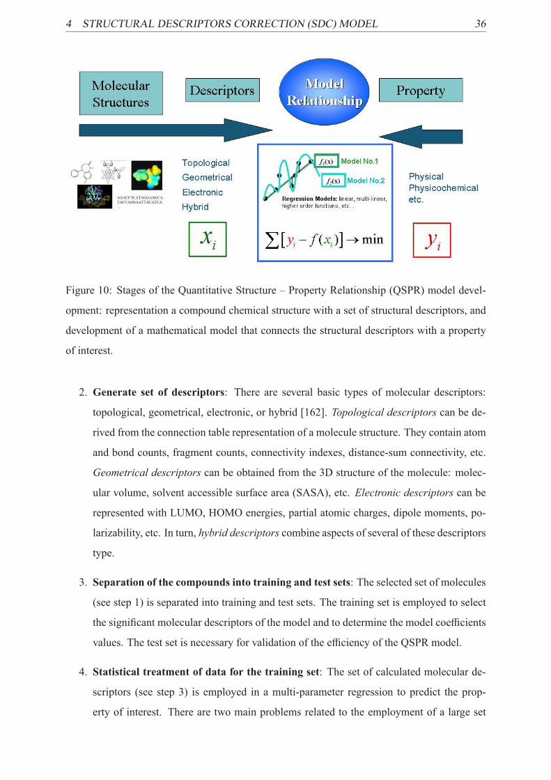
4 STRUCTURAL DESCRIPTORS CORRECTION (SDC) MODEL 36
Figure 10: Stages of the Quantitative Structure – Property Relationship (QSPR) model devel-
opment: representation a compound chemical structure with a set of structural descriptors, and
development of a mathematical model that connects the structural descriptors with a property
of interest.
2. Generate set of descriptors: There are several basic types of molecular descriptors:
topological, geometrical, electronic, or hybrid [162]. Topological descriptors can be de-
rived from the connection table representation of a molecule structure. They contain atom
and bond counts, fragment counts, connectivity indexes, distance-sum connectivity, etc.
Geometrical descriptors can be obtained from the 3D structure of the molecule: molec-
ular volume, solvent accessible surface area (SASA), etc. Electronic descriptors can be
represented with LUMO, HOMO energies, partial atomic charges, dipole moments, po-
larizability, etc. In turn, hybrid descriptors combine aspects of several of these descriptors
type.
3. Separation of the compounds into training and test sets: The selected set of molecules
(see step 1) is separated into training and test sets. The training set is employed to select
the significant molecular descriptors of the model and to determine the model coefficients
values. The test set is necessary for validation of the efficiency of the QSPR model.
4. Statistical treatment of data for the training set: The set of calculated molecular de-
scriptors (see step 3) is employed in a multi-parameter regression to predict the prop-
erty of interest. There are two main problems related to the employment of a large set

4 STRUCTURAL DESCRIPTORS CORRECTION (SDC) MODEL 37
of descriptors: (i) number of regression equations can be estimated as 2n − 1, where n
is the number of descriptors [163], which in the case of 102 descriptors is enormous,
(ii) calculated molecular descriptors are, usually, non-orthogonal (i.e., the corresponding
correlation coefficients deviate significantly from zero). Employment of non-orthogonal
descriptors leads to several QSPR equations which provide similar predictive accuracies.
Identification of relevant descriptors can be performed with, for example, the step-wise
strategy proposed by Katritzky [161] which involves extraction of the most relevant de-
scriptors with the Fisher criterion.
5. Prediction: Application of the obtained QSPR model to the test set of compounds; anal-
ysis of the accuracy of the obtained results using statistical measures such as the mean of
the error (Eq. 55), the standard deviation of the error (Eq. 56), and the root mean square
of the error (Eq. 57).
mean(ε) ≡ ε =1N
N∑i=1
εi (55)
std(ε) ≡ σ(ε) =
√√1N
N∑i=1
(εi − ε)2 (56)
rms(ε) =
√√1N
N∑i=1
ε2i =√σ(ε)2 + ε2 (57)
The semi-empirical model proposed in this thesis differs from standard QSPR models:
• Firstly, as a property of interest we chose not the physical/chemical parameter (hydra-
tion free energy) but the difference between its experimental and RISM-calculated values
(modeling error):
ε = Δμexphyd − Δμ
modelhyd , (58)
where Δμexphyd is the experimental value of HFE, Δμmodelhyd is the HFE calculated by the RISM
approach (superscribe model denotes the RISM-based HFE expression, e.g. PW, GF,
etc.).
• Secondly, we assume that the modeling error can be parameterized with a small set of
structural corrections associated with the main structural features of solutes: partial molar
volume, aromatic rings, electron-donating/withdrawing substituents, etc.
Employment of these descriptors should simplify the procedure of the multi-parameter
equation development because almost all these descriptors are independent and the to-
tal number of these primary fragments is small (see the section Choice of descriptors).
4 STRUCTURAL DESCRIPTORS CORRECTION (SDC) MODEL 38
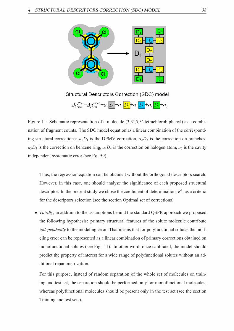
Figure 11: Schematic representation of a molecule (3,3’,5,5’-tetrachlorobiphenyl) as a combi-
nation of fragment counts. The SDC model equation as a linear combination of the correspond-
ing structural corrections: a1D1 is the DPMV correction, a2D2 is the correction on branches,
a3D3 is the correction on benzene ring, a4D4 is the correction on halogen atom, a0 is the cavity
independent systematic error (see Eq. 59).
Thus, the regression equation can be obtained without the orthogonal descriptors search.
However, in this case, one should analyze the significance of each proposed structural
descriptor. In the present study we chose the coefficient of determination, R2, as a criteria
for the descriptors selection (see the section Optimal set of corrections).
• Thirdly, in addition to the assumptions behind the standard QSPR approach we proposed
the following hypothesis: primary structural features of the solute molecule contribute
independently to the modeling error. That means that for polyfunctional solutes the mod-
eling error can be represented as a linear combination of primary corrections obtained on
monofunctional solutes (see Fig. 11). In other word, once calibrated, the model should
predict the property of interest for a wide range of polyfunctional solutes without an ad-
ditional reparametrization.
For this purpose, instead of random separation of the whole set of molecules on train-
ing and test set, the separation should be performed only for monofunctional molecules,
whereas polyfunctional molecules should be present only in the test set (see the section
Training and test sets).
4 STRUCTURAL DESCRIPTORS CORRECTION (SDC) MODEL 39
The methods described above resulted in a semi-empirical functional, first proposed in this
thesis, which combines the HFE calculated by RISM with a set of structural corrections to
remove its error - the Structural Descriptors Correction (SDC) model:
ΔμSDChyd = Δμmodelhyd +
∑i
amodeli Di + amodel0 (59)
where Δμmodelhyd is the HFE calculated with a model HFE expression within the RISM approach,
the second term is the set of structural corrections, amodel0 is a constant (the meaning of this term
will be explained below).
4.2 Multi-parameter linear regression
Let us consider a training set containing N molecules. Let Δμexp(1) , . . . ,Δμexp(N) be the experimen-
tally measured HFEs of the molecules 1, . . . ,N respectively. Let Δμm(1), . . . ,Δμm(N) be the HFEs of
molecules 1, . . . ,N, calculated via the RISM approach using the HFE expression m (m = PW,
GF, etc.). We define the vector Y of the differences between the experimental and calculated
HFE values:
Y = (y1, . . . , yN)T , where yi = Δμexp(i) − Δμm(i), i = 1, . . . ,N (60)
Let D(i)1 , . . . ,D(i)n be the values of descriptors of the i-th molecule, where i = 1, . . . ,N. We define
the matrix of descriptor values:
D =
⎛⎜⎜⎜⎜⎜⎜⎜⎜⎜⎜⎜⎜⎜⎜⎜⎜⎜⎜⎜⎜⎜⎜⎜⎝
D(1)1 . . . D(1)n 1
D(2)1 . . . D(2)n 1... · · · ...
...
D(N)1 . . . D(N)n 1
⎞⎟⎟⎟⎟⎟⎟⎟⎟⎟⎟⎟⎟⎟⎟⎟⎟⎟⎟⎟⎟⎟⎟⎟⎠(61)
We vary the free coefficients to obtain the best agreement between the SDC model and the
experimental measurements. For this purpose, we apply the standard least squares technique
[98]. Let a be the vector of the free coefficients:
a = (a1, . . . , an,C)T (62)
We can find the vector δ of the errors of the model:
δ = Y − Da (63)
Our goal is to minimize the squared error Δ:
Δ =
N∑i=1
δ2i → min (64)

4 STRUCTURAL DESCRIPTORS CORRECTION (SDC) MODEL 40
To find a minimum we calculate the partial derivatives of the squared error Δ with respect
to the free coefficients and set them to be zero:⎧⎪⎪⎪⎪⎪⎪⎪⎪⎪⎨⎪⎪⎪⎪⎪⎪⎪⎪⎪⎩
∂Δ
∂ak=
∑Ni=1 δiD
(i)k = 0
k = 1, . . . , n∂Δ
∂C=
∑Ni=1 δi = 0
(65)
The Eqs. (65) can be written in a matrix form:
DTδ = DT (Y − Da) = 0 (66)
From the Eq. (66) one may find the free coefficients a:
a =(DTD
)−1DTY (67)
4.3 Training and test sets
Development of the SDC model requires two sets of molecules, training and test. The training
set is necessary for the model calibration. Particularly, the training set of compounds is used
to select significant molecular descriptors and to derive the SDC model coefficients values. In
turn, the test set of compounds is utilized for analysis of the accuracy of predicted results and
estimation of the SDC model predictive ability.
In this thesis, we used the internal set of 185 experimental HFEs for neutral organic small
solutes which was compiled from different literature sources [101, 164, 33, 34, 165, 45, 35].
The chosen solutes can be represented as a combination of several moieties: alkyl, alkenyl,
phenyl, hydroxyl, halo, aldehyde, carbonyl, ether, etc. In the present work we specified also
phenol fragment as a separate moiety. We name solutes consisting of either only alkyl moiety
or its combination with only one other moiety as "simple" solutes. In turn, we name solutes
consisting of combination of alkyl moiety with several others (of the same or different types)
as polyfragment. One of the basic ideas of the SDC model is to calibrate it on the training set
of "simple" organic molecules which can have only one functional group (substituent) apart
from an alkyl chain. Following this idea, we used a training set of 65 "simple" solutes for
the SDC model calibration. Another 120 solutes formed the internal test set, which contained
60 "simple" solutes from the same chemical classes as used in the training set as well as 60
polyfragment solutes. Detailed information about the training and test sets is presented in the
Appendix 1 together with the corresponding experimental HFEs.

4 STRUCTURAL DESCRIPTORS CORRECTION (SDC) MODEL 41
As an external test setwe used the set of 220 experimental HFEs for persistent organic pollu-
tants: 11 polychlorinated benzenes (see Table 14) and 209 polychlorobiphenyls (see Appendix
1), and the set of 21 druglike molecules (see Table 15).
4.4 Choice of descriptors
4.4.1 n−Alkanes.
First we considered the training set of n−alkanes that have no specific interactions with water
molecules, and, therefore, the excluded volume effect makes a significant contribution to their
hydration [166, 34, 45]. Several descriptors have been proposed which take into account the ex-
cluded volume effect: the solvent accessible surface area (SASA) [166, 167, 168], partial molar
volume (PMV) [80], their combination [169], number of carbon atoms [170], etc. In the present
work we used the dimensionless PMV (DPMV) descriptor obtained within the corresponding
RISM approach, ρV (where V is the solute partial molar volume and ρ is the number den-
sity of the solvent). The DPMV calculations within the framework of the 1D RISM approach
for the case of infinitely diluted solution are straightforward (Eq. 35) [80]. It is known that
n−alkanes have a linear relationship between their experimental HFEs and excluded volume
[166, 167, 168, 170]. For the given training set of n−alkanes we plotted both Δμexphyd and ΔμPWhyd
versus DPMV calculated by 1D RISM (Fig. 12, a). The 1D RISM-PW method gives qual-
itatively correct results (a linear dependence between ΔμPWhyd and DPMV), but the dependence
for the calculated data is considerably shifted with respect to the corresponding experimental
data, and these dependencies have different slopes. The major shift of the calculated data can
be corrected with the aPW0 free coefficient (-3.58 kcal/mol) of the SDC model (Eq. 59, the last
term). This correction eliminates a general systematic error of the 1D RISM which does not
depend on the solute PMV. For the sake of brevity, in the rest of the thesis we will mainly talk
only about contributions of the solute structure descriptors, although all calculations were done
including the aPW0 correction as well. We correct the slope of the HFEs calculated with the PW
method by the DPMV correction (aPW1 D1, where D1 =DPMV and aPW1 is the slope for the linear
dependence between ε (see Eq. 58) and DPMV for n−alkanes). We note, that this correction
was first proposed in [80].
4.4.2 Nonlinear alkanes.
On Fig. 12 (b) we plotted the difference between HFEs calculated with the aPW1 D1 correction
and corresponding values of Δμexphyd versus the DPMV for the whole training set of alkanes to

4 STRUCTURAL DESCRIPTORS CORRECTION (SDC) MODEL 42
check whether this correction is sufficient to provide a reasonable accuracy of HFE calculations
for branched alkanes. As one can see (Fig. 12, b), for n−alkanes the difference is close to zero.
The differences for the branched alkanes are shifted up with respect to those for n−alkanes.
We assumed that the values of the shifts are approximately constant for the alkanes with the
same number of branches and do not depend on DPMV. Analysis of the Fig. 12 (b) shows
that the shifts are proportional to the number of branches (Nbr). Thus, an introduction of one
branch into the carbon skeleton of a solute has a constant effect on the error of calculated
HFEs. This effect can be considered by another systematic error of the 1D RISM approach
which overestimates the influence of branches on the HFE. Therefore, we introduce another
correction for the number of branches in the carbon skeleton (aPW2 D2, where D2 = Nbr). Finally,
we found that for alkanes it is sufficient to use the combination of aPW1 D1 correction with the
aPW2 D2 correction to significantly decrease the error of calculated HFEs.

4STRU
CTURALDESC
RIPTO
RSCORRECTIO
N(SD
C)MODEL
43
Figure 12: a) HFEs calculated by the 1D RISM with the PW free energy expression ΔμPWhyd and experimental values Δμexphyd versus DPMV (ρV) for the
training set of n−alkanes. b) Difference between calculated Δμ(1)hyd and experimental Δμexphyd data (where Δμ
(1)hyd = Δμ
PWhyd + a
PW1 D1 + a
PW0 ) versus DPMV for
linear and branched alkanes (the training set).

4 STRUCTURAL DESCRIPTORS CORRECTION (SDC) MODEL 44
Figure 13: The difference between calculated Δμ(2)hyd and experimental Δμexphyd HFEs (where
Δμ(2)hyd = Δμ
PWhyd +a
PW1 D1+a
PW2 D2+a
PW0 ) versus Δμ
exphyd for the training set of solutes. Dashed lines
indicate mean values of the difference inside of chemical classes. Arrows indicate the biases of
mean values of corresponding molecular set with respect to zero.
4.4.3 Other compounds.
Next, we analyzed whether the described above empirical corrections (aPW1 D1 and aPW2 D2) are
sufficient to provide an accurate estimation of HFEs for all other chemical classes from the
training set. Figure 13 shows the differences between values of HFEs calculated with these
corrections and the corresponding experimental data against Δμexphyd for the whole training set of
solutes. The differences for all classes of solutes (except alkanes) are biased with respect to zero.
Each class of solutes has its own bias, but the standard deviation inside of the most of the classes
is small (Fig. 13). Thus, we supposed that the bias for each chemical class can be removed by
the use of the appropriate fragment correction. From this observation we may conclude that
introducing one of the functional groups for each class of solutes introduces a constant error in
the HFE calculated with 1D RISM approach. This result reveals the hidden systematic errors
in the 1D RISM method due to which the values of HFE are over- or underestimated for solutes
with different functional groups.
Previously it was found that the 1D RISM method considerably overestimates the specific

4 STRUCTURAL DESCRIPTORS CORRECTION (SDC) MODEL 45
interactions of solutes with water (e.g. H-bonds formation) that results in too low values of
corresponding HFEs [80, 171, 172]. For alcohols this drawback of the 1D RISM is illustrated
by Fig. 13 (green triangles). However, the phenol fragment effect on the HFE is not so clear.
From the Figure 13 (red diamonds) it is obvious that the phenol fragment contribution can not
be treated as a sum of OH-group and benzene ring contributions. Thus, we had to introduce a
descriptor for the number of phenol fragments (Nph). The detailed analysis of the correction for
the phenol fragment is shown in the section Results and Discussion.
Therefore, to obtain a high accuracy predictions for HFE calculations for a given set of so-
lutes we introduced a number of fragment descriptors associated with specific solute structures:
number of branches in a carbon skeleton (Nbr), number of double bonds (Ndb), number of ben-
zene rings (Nbz), number of hydroxyl groups (NOH), number of phenol fragments (Nph), number
of halogen atoms (Nhal), number of ether groups (Neth), number of aldehyde groups (Nald), and
number of ketone groups (Nket). Thus, for the given set of solutes (see Training and test sets)
the second term of the SDC model (Eq. 59) consists of 10 structural descriptors: 1 hybrid-type
descriptor, DPMV (it contains the information about both non-polar and specific solute-solvent
interactions) and 9 topological (fragment-based) descriptors. Representatives for each of given
class of solutes and their structural features requiring corrections are presented on Fig. 14. As
the 1D RISM approach takes into account the molecular details of the solvent structure, one can
see that each of specified structural features changes the solvent distribution around the solute
(Fig. 14).

4STRU
CTURALDESC
RIPTO
RSCORRECTIO
N(SD
C)MODEL
46
Figure 14: Structural descriptors illustrated on the representatives of chemical classes used in this thesis: a) alkene; b) alkane; c) haloalkane; d) alcohol;
e) benzene; f) ether; g) aldehyde; h) phenol; i) ketone. Gray balls are carbons, white balls are hydrogens, red balls are oxygens, and the green ball is
chlorine atom. The colormaps illustrate approximate water density distribution around the molecules, reconstructed from the 1D site-site g(r) (we denote
the positions of water molecules as the positions of water oxygens).

4 STRUCTURAL DESCRIPTORS CORRECTION (SDC) MODEL 47
4.5 Optimal set of corrections
To obtain an optimal combination of corrections we analyzed the influence of each term of
Eq. (59) on the coefficient of determination R2 (Eq. 68). We chose the following criteria for
the selection of corrections. If the difference between the coefficient of determination for the
SDC model with the total set of corrections and a reduced set (without one correction) is less
than 0.005, then the correction may be excluded. As one can see (Table 1), differences for all
considered sets of corrections are bigger that this criteria. Thus, the final equation of the 1D
RISM-SDC model contains all corrections, proposed in the previous section.
R2 = 1 −∑ni=1(yi − fi)2∑i(yni=1 − y)2
, (68)
where n is the number of observations, yi are the observed values, fi are the modeled (predicted)
values, y is the mean of the observed data.
Table 1: Correlation coefficients of multi-parameter linear regressions for the SDC model with
different sets of corrections. The analysis was made for HFEs obtained by the 1D RISM with
the PW method and the PLHNC closure. The total set of corrections is shown in Table 3. Each
correction is significant.Set of corrections R2 R2total − R
2current
Total 0.947 0.000
without aPW0 0.852 0.096
without aPW1 D1 0.466 0.481
without aPW2 D2 0.795 0.153
without aPW3 D3 0.935 0.012
without aPW4 D4 0.904 0.043
without aPW5 D5 0.938 0.010
without aPW6 D6 0.933 0.014
without aPW7 D7 0.866 0.081
without aPW8 D8 0.901 0.047
without aPW9 D9 0.937 0.010
without aPW10 D10 0.861 0.087

5 RESULTS AND DISCUSSION 48
5 Results and Discussion
5.1 PMV estimations with 1D and 3D RISM approaches
The partial molar volume (PMV) is a useful quantity that shows not only information about the
immersed solute structure but also the important data about the solute-solvent interactions. One
should note that the PMV is a thermodynamic quantity and it cannot be presented as only a
geometric volume (van der Waals volume, molecular volume, etc.) of the solute [3, 173]. The
common way of the PMV analysis is its representation as a sum of contributions. According to
works [174, 3, 118] the PMV of solute at infinite dilution can be decomposed into the following
terms:
V = VW + VT︸����︷︷����︸VC
+VI + kBTχT , (69)
where VC ("cavity" volume) is the volume of the cavity created in the solvent large enough to
accommodate the solute molecule; it contains two contributions: (i) the solute "intrinsic" vol-
ume (for low molecular weight solutes it can be approximated by the van der Waals volume VW)
and (ii) the "thermal" ("empty", "void" [3, 173]) volume VT associated with thermally induced
molecular vibrations of both the solute and solvent molecules which lead to creation of empty
space around the solute molecule [174, 118] (see Fig. 15); VI ("interaction" volume) corre-
sponds to the decreasing of the system volume because of specific interactions between water
Figure 15: The solute’s cavity volume as a combination of two contributions: (i) the solute
"intrinsic" volume (for low molecular weight solutes it can be approximated by the van der
Waals volume, VW), (ii) the "thermal" volume VT .

5 RESULTS AND DISCUSSION 49
molecules and the solute molecule; kBTχT is the ideal term that describes the volume effect
related to the kinetic contribution to the pressure of a solute molecule due to translation degrees
of freedom, where χT is the isothermal compressibility of pure solvent, kB is the Boltzmann
constant, T is the temperature. It was found that the value of the ideal term is only about 1
cm3 · mol−1 [174], and therefore usually can be ignored.
In the current work we use the PMV obtained by the 1D and 3D RISM approaches as a
hybrid descriptor of the RISM-SDC model (see the section Choice of descriptors). However,
before employing the descriptor, we estimated the accuracy of calculated PMVs. For this pur-
pose, we collected experimental values of PMV from available literature sources [101, 175, 176,
177, 178] and revealed a lack of data for small organic molecules (in particular, for non-polar
solutes) (see Table 2). Comparison of averaged experimental PMVs with the corresponding
PMV values obtained by the 1D and 3D RISM is shown on Figure 16 (a). We obtained strong
linear correlations between experimental and calculated PMV values for both the 1D RISM
(r = 0.984) and the 3D RISM (r = 0.988). We note that the corrections were shown previously
for 20 amino acids in [179].
Table 2: Experimental values of partial molar volume from
available literature sources (cm3 ·mol−1). Values obtained by
different authors are in good agreement with each other. As
one can see, there is a lack of experimental data for non-polar
solutes.
Name [101] [175] [176] [177] [178] mean value
ethane 51.20 52.00 51.60
methane 37.30 37.30 37.30
propane 67.00 69.00 68.00
buta-1,3-diene 68.30 68.30
ethylbenzene 114.50 114.80 114.65
n-propylbenzene 130.80 130.80
toluene 97.71 97.50 98.40 97.87
2-methylbutan-2-ol 102.50 101.30 101.9
2-methylpropan-1-ol 86.75 86.50 86.70 86.65
butan-1-ol 86.48 86.60 86.60 86.60 86.57
Continued on next page

5 RESULTS AND DISCUSSION 50
Table 2 – continued from previous page
Name [101] [175] [176] [177] [178] mean value
butan-2-ol 86.65 86.60 86.60 86.62
ethanol 55.12 55.10 55.10 55.10 55.11
heptan-1-ol 133.43 133.00 133.22
hexan-1-ol 117.56 118.70 118.50 118.25
hexan-3-ol 117.14 117.14 117.14
methanol 38.25 38.15 38.20 38.20
pentan-1-ol 102.88 102.40 102.40 102.56
pentan-2-ol 102.55 102.55
pentan-3-ol 101.28 101.20 101.20 101.23
propan-1-ol 70.63 70.70 70.60 70.64
propan-2-ol 71.93 71.80 71.95 71.89
3-methylbutan-2-one 95.00 95.00
4-methylpentan-2-one 95.00 95.00
butanone 82.90 82.50 82.90 82.77
pentan-2-one 98.00 98.00 98.00 98.00
pentan-3-one 98.08 98.08
propanone 66.80 66.80
di-n-propyl ether 115.00 115.00
diethyl ether 90.40 90.40 90.40 90.40
diisopropyl ether 115.00 115.00
1,2-dimethoxyethane 95.88 95.70 95.79
2-butoxyethanol 122.91 122.91
2-ethoxyethanol 90.97 90.97
2-propoxyethanol 107.10 107.10
3-hydroxybenzaldehyde 97.90 97.90
4-hydroxybenzaldehyde 96.90 96.90
dimethoxymethane 80.50 80.50
As one can see (Figure 16, b), the PMVs obtained by the 3D RISM are slightly deviate from
the experimental data with a bias linearly related with the size of solutes. In turn, the PMVs
obtained by the 1D RISM approach significantly deviate from the experimental ones. However,

5 RESULTS AND DISCUSSION 51
Figure 16: (a) Comparison of PMVs calculated by the 1D RISM (Eq. 35) and 3D RISM (Eq. 36)
and averaged experimental values for alkanes, diene, alkylbenzenes, alcohols, ketones, ethers,
and several polyfragment solutes (see Table 2). Dashed line illustrates the ideal correlation,
while solid lines show the line-of-best-fit. (b) Difference between calculated and experimental
PMVs versus experimental data. As one can see, PMVs obtained by the 3D RISM are slightly
deviate from the experimental data with a bias linearly related with the size of solutes. In
turn, the PMVs obtained by the 1D RISM approach significantly deviate from the experimental
values with a bias rapidly increased with the increase of the solute size.
the bias also linearly depends from the size of a solute (rapidly increases with the increase of
the solute size). The linear behavior of errors in both the 1D and 3D RISM approaches allows
one to eliminate the errors with the following equation:
V = bRIS M1 · VRIS M + bRIS M0 , (70)
where VRIS M is the PMV obtained by RISM approach, bRIS M1 is a scaling coefficient (b1DRIS M1 =
1.60 and b3DRIS M1 = 1.04), bRIS M0 is an intercept (b1DRIS M0 = −16.35 cm3 · mol−1 and b3DRIS M0 =
−2.64 cm3 · mol−1). In the rest of the work we used PMV in Å3.
In this thesis for the RISM-SDC model we used uncorrected PMV values obtained within
the same RISM approach. In this case, the coefficients bRIS M0 and bRIS M1 contribute to values of
the corresponding a0 and a1 coefficients of the RISM-SDC model (see Eq. 59).

5 RESULTS AND DISCUSSION 52
5.2 1D RISM-SDC model with OPLS partial charges
5.2.1 Calibration of the model
Values of coefficients {aPWi } of the 1D RISM-SDC model with OPLS solute’s partial charges
– the 1D RISM-SDC(OPLSq) model, (Eq. 59) with the considered set of descriptors (see the
section Choice of descriptors) were obtained by the multi-parameter linear regression analysis
(see the section Multi-parameter linear regression) with the training set of solutes (see the sec-
tion Training and test sets). Regression analysis was performed with the function regress from
Matlab Statistics Toolbox (MATLAB version 7.8.0.347(R2009a), the MathWorks Inc., 2009).
Results are shown in Table 3. All determined coefficients have the same order of magnitude
showing that each descriptor from the considered set is significant.
Table 3: Descriptors and the corresponding multi-parameter linear regression coefficients of the
1D RISM-SDC model with the PW free energy expression (see Eq. 59).
Descriptor Coefficient (kcal/mol)
Dimensionless partial molar volume (D1 = ρV) aPW1 = -1.51
Number of branches (D2 = Nbr) aPW2 = 1.07
Number of double bonds (D3 = Ndb) aPW3 = -0.92
Number of benzene rings (D4 = Nbz) aPW4 = -1.70
Number of OH-groups (D5 = NOH) aPW5 = 0.73
Number of phenol fragments (D6 = Nph) aPW6 = -1.52
Number of halogen atoms (D7 = NHal) aPW7 = -2.10
Number of ether groups (D8 = Neth) aPW8 = -1.69
Number of aldehyde groups (D9 = Nald) aPW9 = -0.91
Number of ketone groups (D10 = Nket) aPW10 = -2.44
In Fig. 17 the 1D RISM-SDC(OPLSq) model’s corrections together with experimental and
calculated HFEs are shown for two solutes: non-polar alkane (2,3-dimethylpentane) and polar
alcohol (2-methylpentan-3-ol). For the simplicity of comparison these two solutes were chosen
in such a way that they have almost the same structure but different side groups at the third
carbon atom. As one can see, the HFEs calculated with the uncorrected PW method (Fig. 17,
upper grey bars) are overestimated for both solutes: alkane with positive Δμexphyd and alcohol with
negative Δμexphyd (Fig. 17, red bars). As it was shown above, the major part of the difference
between ΔμPWhyd and Δμexphyd can be eliminated with the a
PW0 and DPMV (aPW1 D1) corrections.
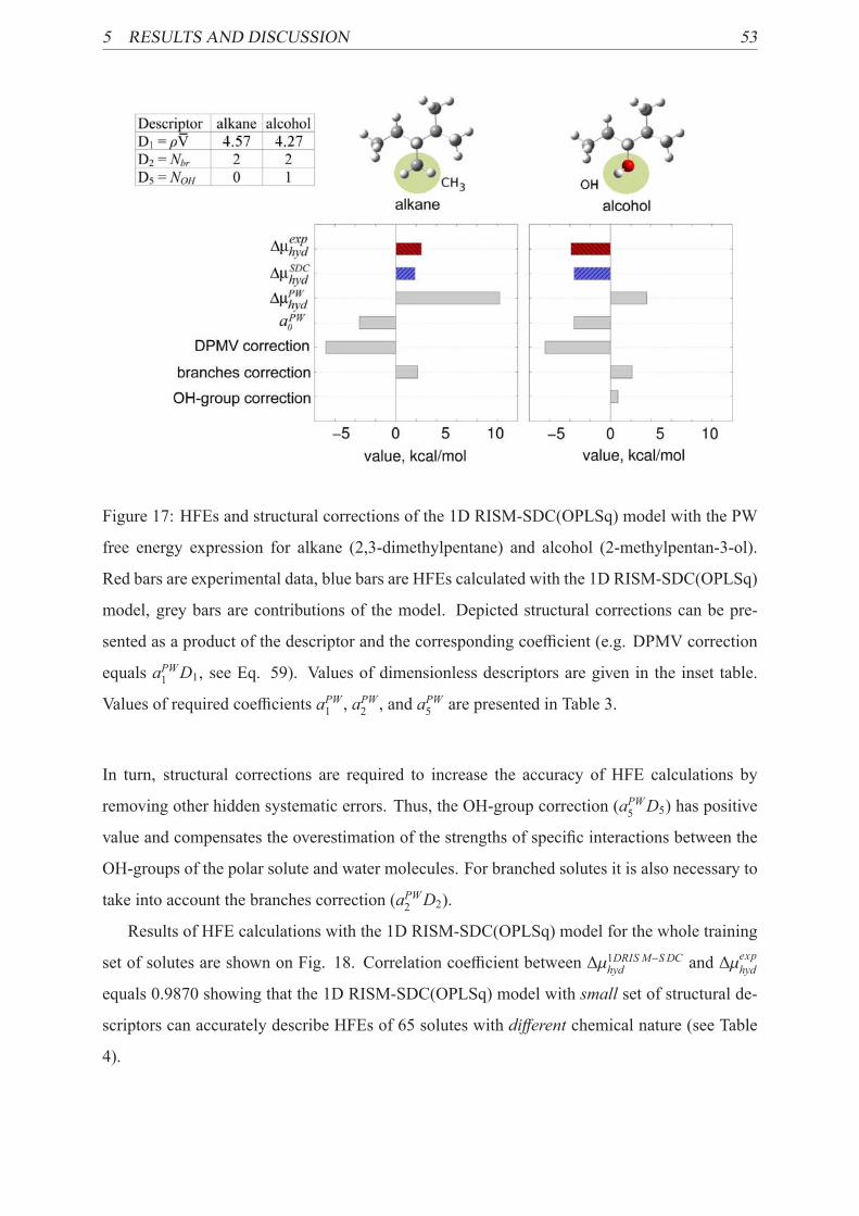
5 RESULTS AND DISCUSSION 53
Figure 17: HFEs and structural corrections of the 1D RISM-SDC(OPLSq) model with the PW
free energy expression for alkane (2,3-dimethylpentane) and alcohol (2-methylpentan-3-ol).
Red bars are experimental data, blue bars are HFEs calculated with the 1D RISM-SDC(OPLSq)
model, grey bars are contributions of the model. Depicted structural corrections can be pre-
sented as a product of the descriptor and the corresponding coefficient (e.g. DPMV correction
equals aPW1 D1, see Eq. 59). Values of dimensionless descriptors are given in the inset table.
Values of required coefficients aPW1 , aPW2 , and a
PW5 are presented in Table 3.
In turn, structural corrections are required to increase the accuracy of HFE calculations by
removing other hidden systematic errors. Thus, the OH-group correction (aPW5 D5) has positive
value and compensates the overestimation of the strengths of specific interactions between the
OH-groups of the polar solute and water molecules. For branched solutes it is also necessary to
take into account the branches correction (aPW2 D2).
Results of HFE calculations with the 1D RISM-SDC(OPLSq) model for the whole training
set of solutes are shown on Fig. 18. Correlation coefficient between Δμ1DRIS M−SDChyd and Δμexphydequals 0.9870 showing that the 1D RISM-SDC(OPLSq) model with small set of structural de-
scriptors can accurately describe HFEs of 65 solutes with different chemical nature (see Table
4).

5RESU
LTSANDDISC
USSIO
N54
Figure 18: (a) Correlation between HFEs calculated by the 1D RISM-SDC(OPLSq) model with the PLHNC closure and the PW free energy expression
(ΔμSDChyd ) and experimental values (Δμexphyd) for the training set of solutes. Solid line shows the ideal correlation, while dashed lines illustrate the std of
the error. (b) Difference between ΔμSDChyd and Δμexphyd versus experimental HFEs for the training set. Dashed lines indicate the corresponding std of the
difference (see Table 4).
5 RESULTS AND DISCUSSION 55
5.2.2 The model predictive ability
The predictive ability of the 1D RISM-SDC(OPLSq) model was analyzed using the internal
test set of 120 solutes and the same set of coefficients from Table 3 as for the training set.
Comparison of the predicted and experimental HFEs is shown on Fig. 20. As we previously
noted, the test set contains 60 polyfragment solutes. Among them there are dienes, dihydric al-
cohols, unsaturated aliphatic alcohols, styrenes, phenyl alcohols, di- and polychloroalkanes,
chlorobenzenes, chlorophenols, hydroxybenzaldehydes, alkenals, alkoxyphenones, oxyalco-
hols, phenylethers, and alkoxyphenols. As one can see (Fig. 20), the proposed 1D RISM-
SDC(OPLSq) model allows to predict HFEs of "simple" solutes with high accuracy. Details of
the model statistical profile are presented in Table 4.
In the case of polyfragment solutes, predictability of the 1D RISM-SDC(OPLSq) model is
sensitive to the chemical nature of solutes. One can see on Fig. 20, several polyfragment solutes
for which the difference Δμ1DRIS M−SDChyd − Δμexphyd exceeds the std of the error. Some of them are
small chloroalkanes (Nhal equals 2-5). Others are chlorobenzenes with 3 or 4 chlorine atoms.
We suppose that the main reason of this deviation is the fact that OPLS partial charges do not
take into account redistribution of electron density around electronegative groups.
We analyzed the ability to describe properties of polyfragment solutes with OPLS charges
on phenols as an example. For this purpose we made the comparison of three solutes, benzene,
phenol, and phenyl alcohol (Fig 19). In the case of benzene each type of atoms has its own
OPLS partial charge. QM-derived partial charges differ for symmetric atoms in the third digit
after point. As it was shown above (see the section Choice of descriptors) the phenol fragment
contribution can not be treated as a plain sum of the OH-group and benzene ring contributions.
Results of the regression analysis confirm that even taking into account all required corrections
(DPMV, branches, benzene ring, and OH-group corrections) the difference Δμcalchyd − Δμexphyd for
phenols is sufficiently biased with respect to zero (it is about 2 kcal/mol). We attribute this
effect to the oversimplified character of OPLS partial charges for phenol. It is well known that
substitution of a benzene hydrogen to an OH-group (electron-donating substituent) influences
the electron density distribution and, correspondingly, the partial charges on carbon atoms in
phenols [180]. The OPLS partial charges take into account only the change of the partial charge
on the carbon atom closest to OH-group (it has q =0.150 instead of q = -0.115 for benzene’s
carbons) [131]. All other atoms in benzene ring have the same parameters as for the "neat"
benzene (see Fig. 19). However, partial charges on other carbon atoms also change because
of the electron density redistribution, and, as a result, meta−, orto−, and para−positions in the

5 RESULTS AND DISCUSSION 56
Figure 19: Partial charges for heavy atoms of benzene, phenol, and benzyl alcohol. For simplic-
ity the hydrogen atoms are not shown. There are the two numbers next to each symmetry-unique
atom in the solute. The first number (in blue) is OPLS partial charge and the second number (in
magenta) is the QM-derived partial charge obtained with CHELPG procedure [134] at MP2/6-
311G** level of theory using the Gaussian 03 software [130]. Blue and magenta circles near
the numbers show the approximate ratio of the corresponding partial charges.
phenol ring become distinguishable (the mesomeric effect [180]). OPLS partial charges do not
reflect these details. Thus, phenols properties are not described in a proper way. Consequently,
we included the subset of phenols into the training set and introduced additional correction for
the number of phenol fragments (aPW6 D6, where D6 is the total number of phenol fragments).
However, the OPLS partial charges perform satisfactory for phenyl alcohols containing a carbon
spacer between the benzene ring and the OH-group which neglects the influence of oxygen on
the aromatic system (see Fig. 19). In this case the HFE correction can be approximated as a
sum of the benzene ring and the OH-group contributions with the additional DPMV correction
for the spacer.
For the rest of polyfragment solutes the deviation of predicted HFEs is comparable for
those of "simple" from the test set. That means that coefficients of the model determined with
the training set of "simple" solutes are transferable to polyfragment solutes. This indicates a
great potential of the 1D RISM-SDC(OPLSq) model for HFE predictions of various organic
molecules.
To analyze the accuracy of the data obtained with the 1D RISM-SDC(OPLSq) model we
calculated the mean values and standard deviation (std) of the difference Δμ1DRIS M−SDChyd − Δμexphyd

5 RESULTS AND DISCUSSION 57
Table 4: Composition of the training and test sets by chemical classes. Statistical profile of
the 1D RISM-SDC(OPLSq) model with the PW free energy expression: mean value and the
standard deviation (std) of the difference Δμ1DRIS M−SDChyd − Δμexphyd for the training and test sets of
solutes (kcal/mol).
Chemical class Fragmenta Training Set Test Set
N mean std N mean std
alkanes R-R(Rn) 11 0.00 0.36 11 -0.10 0.38
alkenes R=R 6 0.00 0.36 5 0.39 0.56
alkylbenzenes Ph(Rm) 6 0.00 0.32 11 0.27 0.67
monohydric alcohols R(OH) 8 0.00 0.38 14 0.18 0.35
phenols Ph(Rl)(OH) 5 0.00 0.31 8 0.19 0.46
chloroalkanes R-Hal 10 0.00 0.48 0 − −
aldehydes R-CHO 6 0.00 0.81 4 -0.20 0.25
ketones (R2)C=O 6 0.00 0.15 7 -0.53 0.33
ethers R-O-R 7 0.00 0.45 0 − −
Polyfragment Solutesb c 0 − − 60 -1.15 1.44
TOTAL: 65 0.00 0.45 120 -0.55 1.24
a [R= alkyl; n = 2, 3; m = 1 . . . 6; l = 1 . . . 5];b dienes, dihydric alcohols, unsaturated aliphatic alcohols, styrenes, phenyl alcohols, di-
and polychloroalkanes, chlorobenzenes, chlorophenols, hydroxybenzaldehydes, alkenals,
alkoxyphenones, oxyalcohols, phenylethers, alkoxyphenols;c combinations of the previous fragments
for both training and test sets (Table 4). As one can see, even with polychloroalkanes and
chlorobenzenes the std does not exceed 1.24 kcal/mol for the test set of solutes. We analyzed
whether this difference is biased with respect to zero. For this purpose we calculated mean
value of the difference Δμ1DRIS M−SDChyd − Δμexphyd . For the test set of solutes it equals -0.55 ± 0.11
kcal/mol (in this case and in the rest of the thesis the error of mean is the std divided by the
square root of number of solutes). As one can see, the difference between experimental and
predicted data is slightly biased, and the accuracy of the predicted HFEs depends mostly on the
deviation of calculated data.

5RESU
LTSANDDISC
USSIO
N58
Figure 20: (a) Correlation between HFEs calculated by the 1D RISM-SDC(OPLSq) model with the PLHNC closure and the PW free energy expression
(ΔμSDChyd ) and experimental values (Δμexphyd) for the internal test set of solutes. Solid line illustrates the ideal correlation, whereas dashed lines show the
std of error. (b) Difference between ΔμSDChyd and Δμexphyd versus experimental HFEs for the test set. Dashed lines indicate the corresponding the std of the
difference.

5 RESULTS AND DISCUSSION 59
5.2.3 Comparison with other hydration free energy expressions
We compared the accuracy of HFEs calculated with different 1D RISM HFE expressions (see
the section Hydration Free Energy Expressions within the 1D RISM approach) for the test set
of 120 solutes. The mean values and std of the difference Δμmethodhyd − Δμexphyd for each of the
methods are presented in Fig. 21. As one can see, HNC and KH HFE expressions (Eqs. 26,
Figure 21: Normal distribution functions of the difference Δμmethodhyd − Δμexphyd . Accuracy of HFEs
calculations with different RISM HFE expressions is given in the table on the right: mean value
and standard deviation (std) of the difference for the test set of 120 solutes (kcal/mol). Data for
HNC and HNCB methods were calculated with HNC closure, data for all other methods were
obtained with PLHNC closure. The inset figure shows the same data for a smaller scale of HFE
coordinate.
28) give significantly overestimated values of HFE. The bias of the difference Δμmodelhyd − Δμexphydwith respect to zero is the major contribution to the error (mean value of the difference is 38.8
kcal/mol). However, the bias removing is not sufficient to get a reasonable accuracy of HFE
calculations with the HNC and KH free energy expressions because the std of the error is con-
siderable (∼ 0.13 kcal/mol). HFEs calculated with the PW free energy expression (Eq. 29) are
also biased with respect to experimental data (mean value of the difference ΔμPWhyd − Δμexphyd is
10.91 ± 0.20 kcal/mol) but they are characterized with the noticeably less standard deviation.

5 RESULTS AND DISCUSSION 60
Thus, removing the bias of the error provides an ability to predict HFEs with high accuracy. Ap-
plication of the PWCmodel for the correction of PW data leads to the decrease of the difference
between experimental and calculated values (mean value of the difference ΔμPWChyd −Δμexphyd is 0.63
± 0.18 kcal/mol) but it only weakly affects the std of the error. In turn, the PW data corrected
with the 1D RISM-SDC(OPLSq) model are less biased with respect to experimental values
(see above), with the std of the error is 1.5 times less than that for the PW method. Thus, the
1D RISM-SDC(OPLSq) model improves the quality of the initial PW model and considerably
reduces the error of HFE calculation.
Figure 21 shows that the HFEs calculated with the GF HFE expression (Eq. 27) are less
biased with respect to the experimental values than the PW-calculated HFEs but have the std
of error is about 1.5 times higher as that for the PW data. Nevertheless, we applied the 1D
RISM-SDC(OPLSq) model for the GF data as well (see the results below).
1D RISM-SDC(OPLSq) model with GF free energy expression. In parallel with the PW
data correction by the 1D RISM-SDC(OPLSq) model we perform the correction of the HFEs
calculated with the GF HFE expression. Correlation coefficients were also obtained via the
multi-parameter regression analysis. One can find the corresponding regression parameters in
Table 5.
Table 5: Descriptors and the corresponding multi-parameter linear regression coefficients of the
1D RISM-SDC model with the GF free energy expression (see Eq. 59).Descriptor Coefficient (kcal/mol)
Dimensionless partial molar volume (D1 = ρV) aGF1 = 0.64
Number of branches (D2 = Nbr) aGF2 = 1.39
Number of double bonds (D3 = Ndb) aGF3 = −1.23
Number of benzene rings (D4 = Nbz) aGF4 = −2.04
Number of OH-groups (D5 = NOH) aGF5 = 3.33
Number of phenol fragments (D6 = Nph) aGF6 = −2.35
Number of halogen atoms (D7 = NHal) aGF7 = −2.39
Number of ether groups (D8 = Neth) aGF8 = −1.38
Number of aldehyde groups (D9 = Nald) aGF9 = −0.07
Number of ketone groups (D10 = Nket) aGF10 = −2.02
It is known that the GF method overestimates the specific interactions [78, 79]. Indeed, the
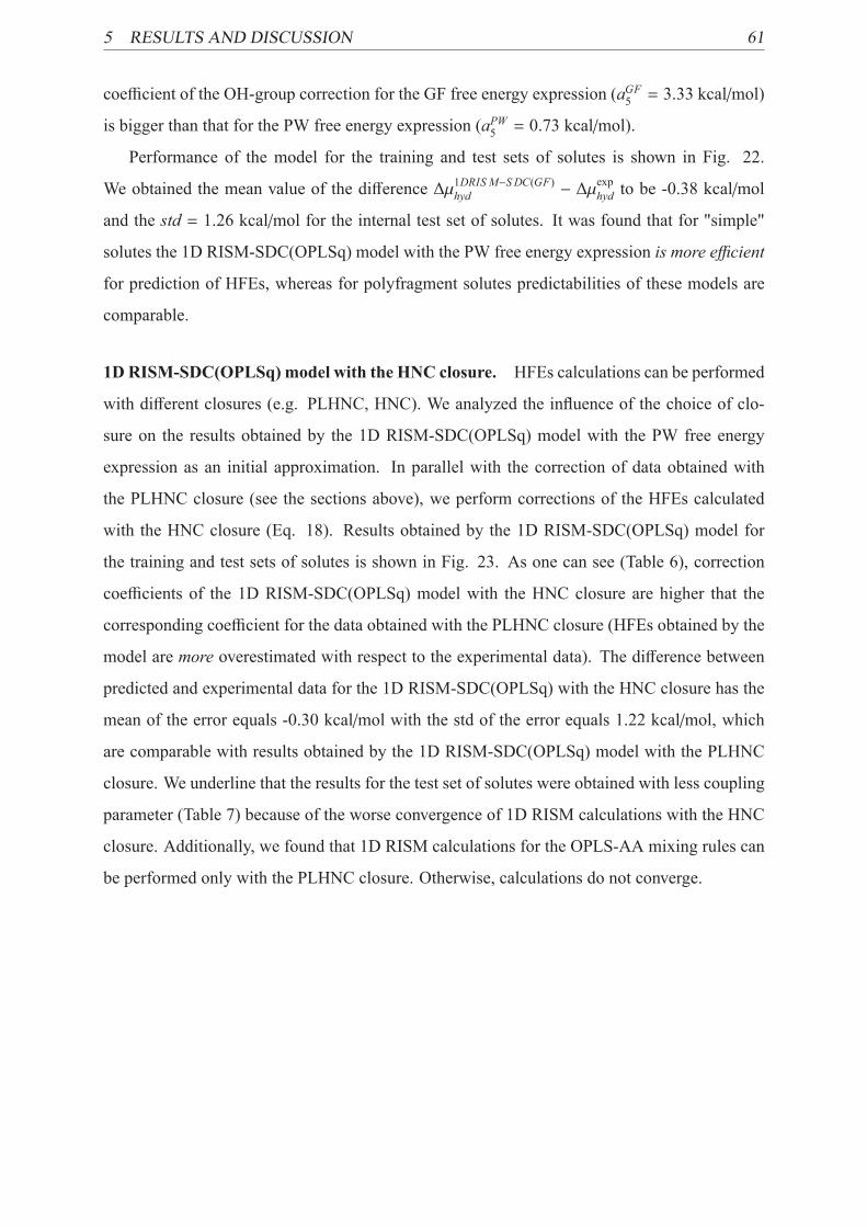
5 RESULTS AND DISCUSSION 61
coefficient of the OH-group correction for the GF free energy expression (aGF5 = 3.33 kcal/mol)
is bigger than that for the PW free energy expression (aPW5 = 0.73 kcal/mol).
Performance of the model for the training and test sets of solutes is shown in Fig. 22.
We obtained the mean value of the difference Δμ1DRIS M−SDC(GF)hyd − Δμexphyd to be -0.38 kcal/mol
and the std = 1.26 kcal/mol for the internal test set of solutes. It was found that for "simple"
solutes the 1D RISM-SDC(OPLSq) model with the PW free energy expression is more efficient
for prediction of HFEs, whereas for polyfragment solutes predictabilities of these models are
comparable.
1D RISM-SDC(OPLSq) model with the HNC closure. HFEs calculations can be performed
with different closures (e.g. PLHNC, HNC). We analyzed the influence of the choice of clo-
sure on the results obtained by the 1D RISM-SDC(OPLSq) model with the PW free energy
expression as an initial approximation. In parallel with the correction of data obtained with
the PLHNC closure (see the sections above), we perform corrections of the HFEs calculated
with the HNC closure (Eq. 18). Results obtained by the 1D RISM-SDC(OPLSq) model for
the training and test sets of solutes is shown in Fig. 23. As one can see (Table 6), correction
coefficients of the 1D RISM-SDC(OPLSq) model with the HNC closure are higher that the
corresponding coefficient for the data obtained with the PLHNC closure (HFEs obtained by the
model are more overestimated with respect to the experimental data). The difference between
predicted and experimental data for the 1D RISM-SDC(OPLSq) with the HNC closure has the
mean of the error equals -0.30 kcal/mol with the std of the error equals 1.22 kcal/mol, which
are comparable with results obtained by the 1D RISM-SDC(OPLSq) model with the PLHNC
closure. We underline that the results for the test set of solutes were obtained with less coupling
parameter (Table 7) because of the worse convergence of 1D RISM calculations with the HNC
closure. Additionally, we found that 1D RISM calculations for the OPLS-AA mixing rules can
be performed only with the PLHNC closure. Otherwise, calculations do not converge.
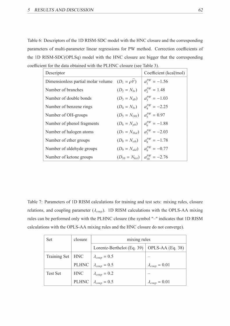
5 RESULTS AND DISCUSSION 62
Table 6: Descriptors of the 1D RISM-SDC model with the HNC closure and the corresponding
parameters of multi-parameter linear regressions for PW method. Correction coefficients of
the 1D RISM-SDC(OPLSq) model with the HNC closure are bigger that the corresponding
coefficient for the data obtained with the PLHNC closure (see Table 3).Descriptor Coefficient (kcal/mol)
Dimensionless partial molar volume (D1 = ρV) aPW1 = −1.56
Number of branches (D2 = Nbr) aPW2 = 1.48
Number of double bonds (D3 = Ndb) aPW3 = −1.03
Number of benzene rings (D4 = Nbz) aPW4 = −2.25
Number of OH-groups (D5 = NOH) aPW5 = 0.97
Number of phenol fragments (D6 = Nph) aPW6 = −1.88
Number of halogen atoms (D7 = NHal) aPW7 = −2.03
Number of ether groups (D8 = Neth) aPW8 = −1.78
Number of aldehyde groups (D9 = Nald) aPW9 = −0.77
Number of ketone groups (D10 = Nket) aPW10 = −2.76
Table 7: Parameters of 1D RISM calculations for training and test sets: mixing rules, closure
relations, and coupling parameter (λcoup). 1D RISM calculations with the OPLS-AA mixing
rules can be performed only with the PLHNC closure (the symbol "–" indicates that 1D RISM
calculations with the OPLS-AA mixing rules and the HNC closure do not converge).
Set closure mixing rules
Lorentz-Berthelot (Eq. 39) OPLS-AA (Eq. 38)
Training Set HNC λcoup = 0.5 –
PLHNC λcoup = 0.5 λcoup = 0.01
Test Set HNC λcoup = 0.2 –
PLHNC λcoup = 0.5 λcoup = 0.01

5RESU
LTSANDDISC
USSIO
N63
Figure 22: HFEs obtained by the 1D RISM-SDC(OPLSq) model with the PLHNC closure and the GF free energy expression (ΔμSDC+GFhyd ) versus the
experimental values for training and internal test sets of solutes. Solid lines show the ideal correlation, while dashed lines indicate the std of the error.

5RESU
LTSANDDISC
USSIO
N64
Figure 23: HFEs calculated by the 1D RISM-SDC(OPLSq) model with the PW free energy expression and the HNC closure (ΔμSDChyd ) versus the experi-
mental values for training and internal test sets of solutes. Solid lines show the ideal correlation, while dashed lines indicate the std of the error.
5 RESULTS AND DISCUSSION 65
5.3 1D RISM-SDC model with QM-derived partial charges
We have shown that the 1D RISM-SDC(OPLSq) model allows one to obtain HFEs for "sim-
ple" solutes with high accuracy (see the section The model predictive ability). In the case of
polyfragment solutes, the 1D RISM-SDC(OPLSq) model is more sensitive to the chemical na-
ture of solutes. Thus, the model allows one to predict HFEs with an accuracy of about 1 kcal/mol
for chlorinated benzenes with fewer than three chlorine atoms but it provides worse results for
chlorinated benzenes with larger number of chlorine atoms. The main reason of this deviation
is the fact that OPLS partial charges are not sensitive to the mesomeric effect in polyfragment
solutes (Fig. 19).
We found that the quality of the 1D RISM-SDC model can be significantly improved by
the model reparametrization using QM-derived partial charges instead of the originally used
OPLS partial charges – the 1D RISM-SDC(QMq) model. The further developed the 1D RISM-
SDC(QMq) model was applied for HFE predictions of persistent organic pollutants (see the
section The model predictive ability for pollutants). In this thesis we tested the partial charges
obtained by the CHELPG procedure [134] with the Gaussian 03 software [130] at MP2/6-
311G** and B3LYP/6-31G** levels of theory. The MP2/6-311G** method was used for the 1D
RISM-SDC(QMq) model calibration and testing (see the section Performance of the model). In
the case of pollutants, employment of this level of theory is quite expensive. Due to this fact,
HFE calculations for pollutants were performed with the partial charges obtained at B3LYP/6-
31G** level of theory.
5.3.1 Performance of the model
Values of coefficients {aPWi } of the 1D RISM-SDC(QMq) model with the same set of descriptors
were obtained by the multi-parameter linear regression analysis on the same training set of
solutes. Results are shown in Table 8.
As we showed above (Fig. 19), QM-derived partial charges are sensitive to the nature of
substituents in aromatic systems. Particularly, they are able to reproduce the mesomeric effect
in the phenol. Thus, error of HFE for phenols can be represented as a sum of contributions from
benzene ring and OH-group (Fig. 24, b). Due to that, the 1D RISM-SDC(QMq) model does
not contain the correction on phenol fragment (Table 8).
Predictive ability of the model with both OPLS and QM-derived partial charges for the in-
ternal test set of 120 solutes is shown in Figures 25 and 26. As it was discussed in the section
The model predictive ability, for "simple" solutes one should use the 1D RISM-SDC model

5 RESULTS AND DISCUSSION 66
with OPLS partial charges. Such combination allows one to obtain HFEs with small bias with
respect to experimental data and the standard deviation is about 0.5 kcal/mol (see Table 4, "sim-
ple" solutes). The main reason of the high performance of the 1D RISM-SDC(OPLSq) model
is the fact that the OPLS force field parameters were derived on the set of "simple" compounds
[131, 132, 133]. Analysis of the OPLS and QM-derived partial charges for 2-methylpropane
(see Table 9) showed that on one hydrogen (H6) the partial charges obtained by the CHELPG
procedure at different levels of theory have negative values. The same results (negative charges
on hydrogens) were obtained for linear alkanes, alkenes, and alcohols. Due to this drawback of
the analyzed QM-derived partial charges the corresponding 1D RISM-SDC(QMq) model per-
forms worse for "simple" and non-aromatic polyfragment solutes (Figures 25, 26). However,
in the case of aromatic solutes the QM-derived partial charges are sensitive to the electron-
donating/withdrawing nature of substituents, whereas the OPLS partial charges do not reflect
these details (see the partial charges of toluene in Table 10 and data for phenol in Fig. 19).
In this case, results obtained with the QM-derived charges are more reliable. Thus, for further
Table 8: Descriptors and the corresponding multiple regression coefficients of the 1D RISM-
SDC(QMq) model. The QM-derived partial charges are sensitive to the nature of substituents
in aromatic systems and are able to reproduce the mesomeric effect. Thus, error of HFE for
phenols can be represented as a sum of contributions from benzene ring and OH-group, and the
corresponding correction a6D6 can be removed (value of the corresponding coefficient aPW6 was
set to zero).
Descriptor Coefficient (kcal/mol)
Dimensionless partial molar volume (D1 = ρV) aPW1 = -1.60
Number of branches (D2 = Nbr) aPW2 = 1.03
Number of double bonds (D3 = Ndb) aPW3 = -0.37
Number of benzene rings (D4 = Nbz) aPW4 = -2.69
Number of OH-groups (D5 = NOH) aPW5 = -0.73
Number of phenol fragments (D6 = Nph) aPW6 = 0.00
Number of halogen atoms (D7 = NHal) aPW7 = -1.30
Number of ether groups (D8 = Neth) aPW8 = -1.06
Number of aldehyde groups (D9 = Nald) aPW9 = 0.68
Number of ketone groups (D10 = Nket) aPW10 = -0.60

5 RESULTS AND DISCUSSION 67
Figure 24: The difference between calculated (Δμ(2)hyd) and experimental (Δμexphyd) HFEs (where
Δμ(2)hyd = Δμ
PWhyd + a
PW1 D1 + a
PW2 D2 + a
PW0 ) versus experimental data for the training set of solutes.
Dashed lines indicate the mean of errors for chemical classes. Arrows indicate biases of the
mean values of corresponding molecular set with respect to zero. (a) Results for the 1D RISM-
SDC(OPLSq) model (equivalent to the Fig. 13); (b) Results for the 1D RISM-SDC(QMq)
model. As one can see, QM-derived partial charges are sensitive to the nature of substituents
in aromatic systems (they are able to reproduce the mesomeric effect). Thus, error of HFE for
phenols can be represented as a sum of contributions from benzene ring and OH-group.
HFE calculations we used the 1D RISM-SDC model with the QM-derived partial charges.
We note that for heterocyclic solutes the OPLS parameters were derived by the CHELPG
procedure at RHF/6-31G* level of theory using the Gaussian 94 software [131, 132, 133]. Com-
parison of the OPLS partial charges for pyridine, furan, and quinoline with the corresponding
partial charges obtained with the CHELPG procedure using Gaussian 03 software [130] at dif-
ferent levels of theory is shown in Table 11.

5 RESULTS AND DISCUSSION 68
Figure 25: Performance of the 1D RISM-SDC model with different sets of partial charges for
the internal test set of compounds. Solid lines correspond to the ideal correlation, while dashed
lines depict the std of the error. Solid circles indicate polyfragment aromatic solutes. Dashed
circles illustrate polyfragment non-aromatic solutes.
Figure 26: The mean and the std of errors of HFEs calculated by the 1D RISM-SDC model
with different sets of solutes’ partial charges. The errors are shown for two groups of solutes
from the test set: "simple" solutes and polyfragment compounds. In the case of polyfragment
solutes there are two bars for each parameter: transparent for all polyfragment solutes and solid
for aromatic polyfragment solutes only.

5 RESULTS AND DISCUSSION 69
Table 9: OPLS and CHELPG partial charges for 2-methylpropane (see the chemical structure
on the right). For the hydrogen atom 6H the partial charges obtained by the CHELPG procedure
at different levels of theory have negative values (see the bold text).
Atom OPLS CHELPG
RHF MP2 B3LYP MP2
6-31G* 6-311G**
1C -0.180 -0.400 -0.337 -0.297 -0.342
2H 0.060 0.086 0.062 0.053 0.062
3H 0.060 0.092 0.067 0.054 0.067
4H 0.060 0.086 0.062 0.053 0.062
5C -0.060 0.471 0.534 0.501 0.553
6H 0.060 -0.063 -0.097 -0.099 -0.103
7C -0.180 -0.407 -0.345 -0.285 -0.349
8H 0.060 0.093 0.069 0.051 0.069
9H 0.060 0.088 0.064 0.050 0.064
10H 0.060 0.088 0.064 0.050 0.064
11C -0.180 -0.391 -0.329 -0.276 -0.331
12H 0.060 0.083 0.060 0.047 0.059
13H 0.060 0.083 0.060 0.048 0.059
14H 0.060 0.090 0.065 0.050 0.064

5 RESULTS AND DISCUSSION 70
Table 10: Comparison of partial charges for toluene. Due to the electron-donating nature of the
CH3-group, toluene has a redistribution of the electron density in the phenyl ring (mesomeric ef-
fect). The CHELPG partial charges are sensitive to this effect. The partial charge on the carbon
atom 2C has a positive value (see the italic text). Carbon atoms at orto− and para−positions
(3C, 5C, 7C) have more negative partial charges. The OPLS partial charges do not reflect these
details.
Atom OPLS CHELPG
RHF MP2 B3LYP B3LYP MP2
6-31G* 6-311G**
1C -0.065 -0.226 -0.242 -0.240 -0.222 -0.236
2C -0.115 0.229 0.214 0.203 0.193 0.215
3C -0.115 -0.254 -0.235 -0.203 -0.200 -0.239
4C -0.115 -0.058 -0.059 -0.059 -0.047 -0.055
5C -0.115 -0.149 -0.155 -0.117 -0.140 -0.158
6C -0.115 -0.062 -0.059 -0.061 -0.045 -0.055
7C -0.115 -0.247 -0.235 -0.200 -0.199 -0.239
8H 0.060 0.065 0.068 0.067 0.064 0.067
9H 0.060 0.062 0.068 0.066 0.062 0.067
10H 0.060 0.065 0.070 0.070 0.065 0.069
11H 0.115 0.133 0.128 0.108 0.106 0.130
12H 0.115 0.101 0.099 0.085 0.081 0.097
13H 0.115 0.108 0.110 0.089 0.096 0.109
14H 0.115 0.101 0.099 0.085 0.079 0.097
15H 0.115 0.133 0.128 0.108 0.108 0.130

5 RESULTS AND DISCUSSION 71
Table 11: OPLS and CHELPG partial charges for hete-
rocyclic solutes. Data for symmetric atoms are skipped.
The atom numeration was taken from OPLS-AA force field
[131].
Atom OPLS CHELPG
RHF B3LYP MP2 MP2
6-31G* 6-311G**
pyridine
N -0.678 -0.687 -0.598 -0.673 -0.402
C1 0.473 0.487 0.416 0.466 0.139
C2 -0.447 -0.466 -0.380 -0.462 -0.233
C3 0.227 0.245 0.194 0.242 0.023
H1 0.012 0.010 0.004 0.019 0.117
H2 0.155 0.158 0.136 0.159 0.108
H3 0.065 0.063 0.054 0.066 0.115
furan
O -0.190 -0.185 -0.151 -0.195 -0.169
C1 -0.019 -0.019 -0.018 -0.025 -0.038
C2 -0.154 -0.160 -0.145 -0.155 -0.140
H1 0.142 0.141 0.122 0.147 0.144
H2 0.126 0.131 0.117 0.131 0.128
Continued on next page

5 RESULTS AND DISCUSSION 72
Table 11 – continued from previous page
quinoline
N1 -0.694 -0.701 -0.618 -0.683 -0.681
C2 0.425 0.440 0.367 0.408 0.410
C3 -0.359 -0.366 -0.298 -0.359 -0.357
C4 -0.008 -0.027 -0.012 -0.022 -0.030
C5 -0.197 -0.209 -0.162 -0.211 -0.222
C6 -0.112 -0.133 -0.112 -0.125 -0.121
C7 -0.070 -0.025 -0.028 -0.041 -0.037
C8 -0.307 -0.349 -0.288 -0.329 -0.333
C9 0.563 0.575 0.504 0.554 0.555
C10 -0.051 -0.026 -0.034 -0.023 -0.012
H2 0.028 0.024 0.017 0.036 0.035
H3 0.146 0.147 0.123 0.146 0.143
H4 0.119 0.125 0.096 0.124 0.127
H5 0.133 0.136 0.110 0.138 0.141
H6 0.113 0.117 0.100 0.115 0.112
H7 0.114 0.101 0.090 0.107 0.105
H8 0.157 0.168 0.138 0.165 0.165
5.3.2 The model predictive ability for persistent organic pollutants
The predictive ability of the 1D RISM-SDC(QMq) model for HFE calculations was analyzed
on the external test set of 220 persistent organic pollutants: 11 polychlorinated benzenes (from
chlorobenzene to hexachlorobenzene, Table 14) and 209 polychlorobiphenyls, PCBs (see Ap-
pendix 1). As it was mentioned above, for the set of pollutants the partial charges were obtained
with the CHELPG procedure at B3LYP/6-31G** level of theory because of its low level of
computational expenses. Parameters of the 1D RISM-SDC(QMq) model were obtained by fit-
ting against a training set of "simple" solutes containing 22 alkanes, 17 alkylbenzenes, and 7

5 RESULTS AND DISCUSSION 73
monochlorobenzenes. List of employed descriptors and values of the model coefficients are
shown in Table 12.
Table 12: Descriptors and the corresponding multi-regression coefficients of the 1D RISM-
SDC(QMq) model for the training set of solutes (see description of the set in the text).
Descriptor Coefficient (kcal/mol)
aPW0 = -4.19
Dimensionless partial molar volume (D1 = ρV) aPW1 = -1.48
Number of branches (D2 = Nbr) aPW2 = 0.98
Number of benzene rings (D3 = Nbenz) aPW3 = -3.11
Number of halogen atoms (D4 = Nhal) aPW4 = -1.30
We note that the reliable experimental data are very important for estimations of the accu-
racy of predicted results. Due to that, before the analysis of calculated data we performed an
estimation of reliability of experimentally obtained HFE values for each class of compounds
from each class of compound from the external test set.
Polychlorinated benzenes (PCBzs). The set of experimental HFEs for PCBzs was compiled
from different literature sources: (i) HFEs were taken from [107]; (ii) logP(water/gas) values
were collected from [34] and recalculated to HFEs with Eq. 71; (iii) KH constants were taken
from [181, 182, 183, 184] and recalculated to HFEs with Eq. 5.
Δμhyd = − ln(10)RT log P(water/gas), (71)
where Δμhyd is the hydration free energy, log P(water/gas) is the logarithm of the partition
coefficient between gaseous phase and water, R is the ideal gas constant, T is the temperature.
First of all, we analyzed the difference between the experimental HFEs for PCBzs ob-
tained by different sources (see Table 14). Despite the fact that for several solutes (1,2,3-
trichlorobenzene, 1,3,5-trichlorobenzene, and hexachlorobenzene) the HFE values that were
recalculated from log P(water/gas) and KH differ by 0.5–0.6 kcal/mol (see Table 14), on av-
erage, HFE values obtained with different techniques deviate from the mean value by 0.2–0.3
kcal/mol. Thus, we concluded that experimental data for polychlorinated benzenes are suffi-
ciently accurate and can be used for the estimation of the accuracy of the predicted data.
The comparison of the predicted and experimental HFE values is shown in Fig. 27. To
quantify the accuracy, we calculated statistical parameters of the error ε = Δμcalchyd −Δμexphyd for the

5 RESULTS AND DISCUSSION 74
Figure 27: Correlation between the experimental HFE and values predicted by the 1D RISM-
SDC(QMq) model for the test set of polychlorinated benzenes. The insert data show the statis-
tical profile of the error ε = Δμcalchyd − Δμexphyd . Solid line illustrates the ideal correlation. Dashed
lines indicate the std(ε).
test set of polychlorinated benzenes (Fig. 27, insert data). As one can see, results obtained with
the 1D RISM-SDC(QMq) model are nonbiased (mean of the error equals 0.02 ± 0.11 kcal/mol)
and the standard deviation of the error is in the range of the deviation between different sources
of correspondent experimental data (∼ 0.4 kcal/mol).
Polychlorobiphenyls (PCBs). For PCBs, experimental values of neither HFE nor log P(water/gas)
are available in the literature. However, since 1980s, there have been several experimental in-
vestigations of KH of PCBs reported, where the experiments were carried out with two dynamic
techniques: (i) the gas stripping method (GSM) [185, 186, 187, 188] and (ii) the "wetted-wall
column" (WWC) or the concurrent flow technique [189, 190, 191]. All values are presented in
Fig. 29a; corresponding HFEs recalculated with Eq. 5 are presented in Fig. 29b. One can see
that the experimental KH values are presented mainly by two sets of data obtained by the GSM
(Bamford (2000) [186]) and the WWC technique (Brunner (1990) [190]). Other sets of KH
values are not very large and contain about 20-30 values from 209 possible. Figure 29 shows
that, for the same solutes, experimental KH values from the GSM and WWC sets can differ

5 RESULTS AND DISCUSSION 75
Figure 28: Schematic representation of apparatus for measurements of Henry’s law constants
(adapted from [192]): (a) Apparatus for the gas stripping method; (b) Apparatus for the wetted-
wall column technique. In the case of the gas stripping method, a compound is stripped from the
aqueous phase into a gaseous phase using a bubble column apparatus. The sorption of the solute
molecules to the surface of gas bubbles leads to higher compound’s concentration in gaseous
phase which, in turn, leads to overestimated KH value. With the wetted-wall column technique
one can avoid this drawback. In this case, the compound is equilibrated between thin layer of
water and concurrent flow of gas within the contact region, and sorption of the solute molecules
does not happened.
considerably. The difference increases with the increase in the number of chlorine atoms in a
solute. In terms of HFE, the difference varies from 1 kcal/mol for lighter PCB congeners (PCB
with 4 − 5 chlorine atoms) to up to 3 kcal/mol for heavier congeners (higher chlorinated PCBs)
(Fig. 29b).
Recently it was found that the GSM overestimate KH values for highly chlorinated biphenyls
[193, 194]. The problem is hidden in the technical implementation of the GSM. Within the
method, the KH of a compound is determined as a ration of equilibrium concentration of the
compound in aqueous solution and vapor, accordingly. The compound is stripped from the
aqueous phase into a gaseous phase using a bubble column apparatus (see Fig. 28, a). It was
found that the sorption of the solute molecules to the surface of gas bubbles leads to higher
compound concentration in the gaseous phase, which, in turn, results in the overestimated KH
value. With the WWC technique, one can avoid this drawback. The technical implementation

5 RESULTS AND DISCUSSION 76
of the method consists of the equilibration of a compound between a thin layer of water and a
concurrent flow of gas within the contact region (see Fig. 28, b). Due to that, we accepted the
experimental data obtained by the WWC method [190] as the most reliable set. Unfortunately,
the total number of experimental values published in [190] is only 57 from 209 possible.
Table 13: Statistical profiles of errors for results obtained by the implicit solvent models for the
test set of polychlorobiphenyls (N = 57): mean value, standard deviation (std), and root mean
square (rms) of the error ε = Δμcalchyd − Δμexphyd (kcal/mol); r is the correlation coefficient. Results
obtained by the SM6 and COSMO-SAC methods were collected form [195].
Model: 1D RISM-PW 1D RISM-SDC SM6 [195] COSMO-SAC [195]
mean(ε) 20.35 -0.72 1.28 1.15
std(ε) 1.62 0.55 0.78 0.94
rms(ε) 20.42 0.91 1.50 1.49
r -0.80 0.65 -0.35 -0.70
A comparison of HFEs, predicted by the 1D RISM-SDC(QMq) model, with the experimen-
tal data (Table 13) shows that the calculated values are biased with respect to experimental ones,
mean(ε) =-0.72 ± 0.07 kcal/mol, but have a small standard deviation of error. Figure 30 shows
that the error remains the same for the whole set of PCBs and does not increase for the heavier
PCB congeners.
Also, we performed a comparison of our results with HFEs obtained by other implicit mod-
els, SM6 and COSMO-SAC (the data were taken from [195]). Both of them treat the solvent
as a homogeneous medium characterized by its dielectric constant (continuum solvent meth-
ods). Statistical analysis of the literature results is shown in Table 13. As one can see (Fig.
30), HFEs obtained by these models are in a good agreement with each other. However, the
models allow predictions of HFE with high accuracy only for light congeners, whereas for the
heavier PCBs, the error of HFE increases with the increase in the number of chlorine atoms.
In the case of the highly chlorinated biphenyls (NCl = 8 − 9), the error is ∼ 3 kcal/mol. We
explain these results as follows. In the case of lighter PCB congeners, the chlorine atoms are
well-separated from each other. Thus, the total effect of chlorine atoms interactions with the
solvent molecules can be presented as a sum of single chlorine atoms’ contributions. Increasing
the number of chlorine atoms in biphenyl leads to the interference of the chlorine atoms’ inter-
actions with the solvent molecules and, as a result, to a nonlinearity of the solvent response in

5 RESULTS AND DISCUSSION 77
the process of hydration. We underline that the 1D RISM approach considers these effects in a
proper way, even in the case of higher chlorinated compounds. In turn, the continuum solvent
models (S M6 and COSMO-SAC) are not sensitive to the nonlinear solvent response. These re-
sults of this work show the potential of the 1D RISM-SDC(QMq) approach for the description
of hydration/solvation process for a wide range of chemical solutes.
The reported bias of the error of HFE obtained within the 1D RISM approach can be related
to the error of the biphenyl ring representation (∼ 0.3 kcal/mol). One way to overcome this
drawback is to introduce an additional correction for the biphenyl fragment. However, we
assume that the employment of more advanced 3D RISM will be the more efficient solution of
this problem.

5 RESULTS AND DISCUSSION 78
Figure 29: Experimental data for polychlorobiphenyls (PCBs): (a) Henry’s law constants, KH,
obtained with the wetted-wall column technique (WWC) [190, 191], the gas stripping method
(GSM) [185, 186, 187], or the modified GSM (MGSM) [188]; (b) HFEs recalculated from KH.
Dashed lines show the separation of the whole set of PCBs with respect to number of chlorine
atoms (shown on the top). Black arrows show deviation of experimental data.

5RESU
LTSANDDISC
USSIO
N79
Figure 30: Errors for HFEs predicted by the 1D RISM-SDC(QMq) model with the PLHNC closure and PW free energy expression and literature data
taken from [195] for the test set of polychlorobiphenyls (PCBs). Dashed lines show the separation of the whole set of PCBs with respect to number of
chlorine atoms (shown on the top). One can see that the error of solvation continuum models (SM6 and COSMO-SAC) increases with the increase of the
number of chlorine atoms in biphenyl, whereas error of data predicted with 1D RISM-SDC(QMq) model is constant for all PCBs.

5RESU
LTSANDDISC
USSIO
N80
Table 14: Descriptors of the 1D RISM-SDC model (Eq.
59) for polychlorinated benzenes. Hydration free energies
(ΔGhyd) predicted by the uncorrected PW free energy ex-
pression and the 1D RISM-SDC(QMq) model. Experimen-
tal values were averaged over different sources(expaverage
);
exp|max|−|min| shows the difference between the maximum and
minimum values from different literature sources.
Name D1 D2 D3 D4 ΔGhyd, kcal mol−1
ρV branch benzene hal 1D RISM-PW 1D RISM-SDC expaverage exp|max|−|min|
1,2,3,4-tetrachlorobenzene 5.24 4 1 4 14.75 -1.83 -1.32 [34, 181, 184] 0.07
1,2,3-trichlorobenzene 4.85 3 1 3 13.77 -1.79 -1.49 [34, 184] 0.50
1,2,4,5-tetrachlorobenzene 5.30 4 1 4 15.40 -1.27 -1.34 [34, 184] 0.00
1,2,4-trichlorobenzene 4.89 3 1 3 14.23 -1.40 -1.22 [34, 181, 184] 0.29
1,2-dichlorobenzene 4.45 2 1 2 12.85 -1.69 -1.47 [107, 34, 181, 182, 184] 0.27
1,3,5-trichlorobenzene 4.93 3 1 3 14.71 -1.97 -1.09 [34, 184] 0.63
1,3-dichlorobenzene 4.48 2 1 2 13.24 -1.34 -1.13 [34, 182, 184] 0.29
1,4-dichlorobenzene 4.49 2 1 2 13.15 -1.44 -1.15 [34, 182, 184] 0.21
2-chlorotoluene 4.52 2 1 1 12.76 -0.55 -1.14 [34] −
chlorobenzene 4.04 1 1 1 11.98 -1.51 -1.07 [107, 34, 181, 182, 184] 0.22
hexachlorobenzene 5.95 6 1 6 16.33 -2.17 -2.26 [184, 183] 0.50

5 RESULTS AND DISCUSSION 81
5.4 3D RISM-SDC model
In the Introduction it was underlined that to overcome the drawbacks of the 1D RISM approach
its three-dimensional extension (3D RISM) was proposed [82, 83, 66, 84]. In the 3D RISM
method, the six-dimensional solute-solvent MOZ equation is approximated by a set of 3D inte-
gral equations via partial integration over the orientation coordinates (see the section
Theoretical Background).
In this section we compare the accuracy of the 1D RISM and the 3D RISM for HFE cal-
culations. To make the comparison consistent we performed additional 1D RISM calculations
with the same set of parameters as for the 3D RISM (see the section Computational Details).
For the rest of the thesis we use only one type on solutes partial charges (QM-derived). That is
why, the corresponding charge notation for the SDC model will be skipped.
5.4.1 Comparison of uncorrected data
Figure 31: HFEs obtained by the 1D and 3D RISM with the PLHNC closure using the GF free
energy expressions ( ΔμGFhyd) versus experimental values for the training set of solutes. Solid lines
show the ideal correlation. The 3D RISM approach performs much worse than 1D RISM. We
suppose that within the 1D RISM approach there is an effective cancellation of errors, which
does not happened in the 3D RISM.
HFEs were calculated for the training set of compounds using 1D and 3D RISM approaches
with the corresponding GF free energy expressions (Eqs. 33, 27). For both RISM approaches
the calculated values are considerably overestimated (Fig. 31). Unexpectedly, the 3D RISM
approach performs much worse than 1D RISM (the mean absolute error is 2.4 kcal/mol for

5 RESULTS AND DISCUSSION 82
1D RISM approach instead of 17.6 kcal/mol for 3D RISM). We suppose that within the 1D
RISM approach there is an effective cancellation of errors caused by the involved approxima-
tions, while 3D RISM contains less approximations and this cancellation does not happen. The
enormous errors between RISM-calculated and experimental HFE show that the uncorrected
RISM approaches are not able to provide quantitative description of hydration for wide range
of solutes.
5.4.2 Correction for the cavity formation (3D RISM-UC model)
In the section Choice of descriptors it has been shown that the errors of th HFEs calculated
by 1D RISM approach strongly depend on the PMV of the solute in water. This suggests
that the 1D RISM theory overestimates the energy required to create a cavity for a solute in
solution. This observation allows us to assume that the DPMV can be used with a proper
scaling coefficient for the correction of the 3D RISM-data as well. Indeed, we observed the
high correlation between the difference Δμ3DRIS M−GFhyd − Δμexphyd and the DPMV (Fig. 32). The
correlation coefficients are r = 0.99 and r = 0.97 for the training and test sets, respectively.
The results suggest that the calculated DPMV can be used as a Universal Correction (UC) to
Figure 32: Correlation between the dimensionless partial molar volume (ρV) and the difference
between the 3D RISM calculated and experimental HFEs. The solid line indicates the line-of-
best-fit. The strong linear correlation was obtained for all organic solutes from the training and
test sets.

5 RESULTS AND DISCUSSION 83
Figure 33: Correlation between the error in the HFEs calculated by the 3D RISM with the
PLHNC closure using the GF free energy expression: ΔμGFhyd − Δμexphyd , and the dimensionless
partial molar volume, ρV . Red crosses are small organic molecules; black dots are druglike
solutes. The pharmaceutical molecules lie on the line-of-best-fit calculated for simple organic
molecules (the solid red line).
improve the accuracy of HFEs calculated by the 3D RISM and the GF free energy expression:
Δμ3DRIS M−UChyd = Δμ3DRIS M−GFhyd + aGF1 (ρV) + aGF0 , (72)
where Δμ3DRIS M−GFhyd is the HFE obtained by the 3D RISM-GF method, ρV is the dimension-
less partial molar volume (DPMV), aGF1 (-3.31 kcal/mol) is the scaling coefficient, aGF0 (1.15
kcal/mol) is the intercept. Values of the scaling coefficient the intercept are obtained by linear
regression against the training data.
The 3D RISM-UC model gives very good predictions of HFEs for the test set of 185 organic
compounds from different chemical classes with the mean of the error equals 0.11 kcal/mol,
the std of the error equals 0.99 kcal/mol, and correlation coefficient between predicted and
experimental data equals 0.94. To demonstrate the transferability of the 3D RISM-UC model’s
coefficients we have used it to calculate HFEs for the external test set of 21 neutral druglike
molecules. We found that uncorrected HFEs for druglike compounds obtained by the 3D RISM-
GF method also have a strong linear correlation with the DPMV (r = 0.99). Moreover, the
pharmaceutical molecules lie on the line-of-best-fit calculated for the simple organic molecules
(Figure 33). Results obtained by the 3D RISM-UC model are shown in Table 15. As one can

5 RESULTS AND DISCUSSION 84
Table 15: Experimental and calculated parameters for the external test set of 21 druglike
molecule; Δμexphyd is the experimental HFE. Δμ3DRIS M−GFhyd is the (uncorrected) HFE calculated
by the 3D RISM using the GF HFE expression (kcal/mol;. ρV is the dimensionless partial mo-
lar volume, where ρ is the number density of the solution; Δμ3DRIS M−UChyd is the HFE calculated
using the 3D RISM-UC model (kcal/mol).
Molecule Δμexphyd Ref. Δμ3DRIS M−GFhyd ρV Δμ3DRIS M−UChyd
Paracetamol -14.83 [36] 5.25 6.18 -14.07
N-(3-hydroxyphenyl)acetamide -13.93 [38] 5.48 6.17 -13.81
Fenbufen -12.75 [196] 19.10 10.50 -14.15
N-(2-hydroxyphenyl)acetamide -11.61 [38] 7.27 6.18 -12.07
Phenacetin -10.91 [36] 13.08 7.94 -11.91
Ketoprofen -10.83 [197] 20.86 10.62 -12.77
2-methoxybenzoic acid -10.32 [39] 7.95 6.02 -10.85
Naproxen -10.35 [197] 18.68 9.51 -11.39
Acetanilide -9.72 [36] 8.41 6.04 -10.46
Methylparaben -9.52 [197] 8.76 6.07 -10.20
Propylparaben -9.35 [197] 15.17 7.80 -9.38
Diflunisal -7.63 [197] 19.70 8.76 -7.93
Ethylparaben -9.20 [197] 11.98 6.97 -9.89
4-methoxybenzoic acid -9.15 [39] 9.20 6.02 -9.63
3-methoxybenzoic acid -8.93 [39] 9.36 6.01 -9.43
Butylparaben -8.74 [197] 18.08 8.63 -9.13
Flurbiprofen -8.68 [197] 22.40 10.01 -9.26
Ibuprofen -7.01 [197] 24.70 9.98 -6.87
Tolfenamic acid -6.71 [198] 24.44 10.01 -7.22
Diclofenac -6.30 [199] 25.73 10.80 -8.49
Flufenamic -5.68 [200] 23.21 9.97 -8.34
see, for the set of 21 pharmaceutical molecules, the HFEs calculated by the 3D RISM-UCmodel
with the same set of coefficients are in good agreement with the corresponding experimental
data (mean of error is -0.72 kcal/mol, std of error is 0.78 kcal/mol, and rms of error is 1.06
kcal/mol).
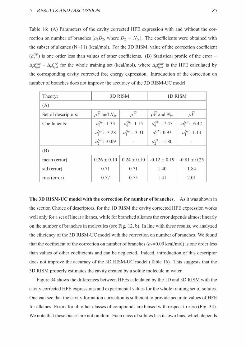
5 RESULTS AND DISCUSSION 85
Table 16: (A) Parameters of the cavity corrected HFE expression with and without the cor-
rection on number of branches (a2D2, where D2 = Nbr). The coefficients were obtained with
the subset of alkanes (N=11) (kcal/mol). For the 3D RISM, value of the correction coefficient
(aGF2 ) is one order less than values of other coefficients. (B) Statistical profile of the error =
Δμcalchyd − Δμexphyd for the whole training set (kcal/mol), where Δμ
calchyd is the HFE calculated by
the corresponding cavity corrected free energy expression. Introduction of the correction on
number of branches does not improve the accuracy of the 3D RISM-UC model.
Theory: 3D RISM 1D RISM
(A)
Set of descriptors: ρV and Nbr ρV ρV and Nbr ρV
Coefficients: aGF0 : 1.33 aGF0 : 1.15 aGF0 : -7.47 aGF0 : -6.42
aGF1 : -3.28 aGF1 : -3.31 aGF1 : 0.93 aGF1 : 1.13
aGF2 : -0.09 - aGF2 : -1.80 -
(B)
mean (error) 0.26 ± 0.10 0.24 ± 0.10 -0.12 ± 0.19 -0.81 ± 0.25
std (error) 0.71 0.71 1.40 1.84
rms (error) 0.77 0.75 1.41 2.01
The 3D RISM-UC model with the correction for number of branches. As it was shown in
the section Choice of descriptors, for the 1D RISM the cavity corrected HFE expression works
well only for a set of linear alkanes, while for branched alkanes the error depends almost linearly
on the number of branches in molecules (see Fig. 12, b). In line with these results, we analyzed
the efficiency of the 3D RISM-UC model with the correction on number of branches. We found
that the coefficient of the correction on number of branches (a2=0.09 kcal/mol) is one order less
than values of other coefficients and can be neglected. Indeed, introduction of this descriptor
does not improve the accuracy of the 3D RISM-UC model (Table 16). This suggests that the
3D RISM properly estimates the cavity created by a solute molecule in water.
Figure 34 shows the differences between HFEs calculated by the 1D and 3D RISM with the
cavity corrected HFE expressions and experimental values for the whole training set of solutes.
One can see that the cavity formation correction is sufficient to provide accurate values of HFE
for alkanes. Errors for all other classes of compounds are biased with respect to zero (Fig. 34).
We note that these biases are not random. Each class of solutes has its own bias, which depends

5 RESULTS AND DISCUSSION 86
Figure 34: Errors of HFEs calculated by the cavity corrected HFE expressions plotted against
the corresponding experimental HFEs. Dashed lines indicate the standard deviation of the error.
(a) Results for the 1D RISM approach (here Δμ(2)hyd = ΔμGFhyd+a
GF1 D1+a
GF2 D2+a
GF0 ; see Table 16).
The subfigure is analogous to Figure 13. (b) Results for the 3D RISM-UC model (Eq. 72). The
predicted HFEs for molecules from different chemical classes are biased from the corresponding
experimental values by almost constant values with small deviations inside groups.
on the structural features of molecules. Moreover, there is a small std of error inside each
class of the compounds. In the case of 3D RISM, the std is considerably less then that of data
calculated by the 1D RISM. Thus, HFE predictions by the 3D RISM approach can be improved
more efficiently by introducing of empirical corrections for different functional groups.
5.4.3 Corrections for the functional groups
The remaining discrepancy of the difference between calculated and experimental HFEs can
be attributed to systematic errors in the RISM free energy calculations associated with cer-
tain functional groups. The values of the corresponding coefficients in the RISM-SDC ap-
proaches indicate the magnitude of the systematic errors. As one can see (Table 17), the 3D
RISM-SDC approach underestimates considerably the impact of hydrogen bond formation be-
tween hydroxyl group and water molecules on the HFE (corresponding coefficient a5 equals
-1.53 kcal/mol). Moreover, significant errors are associated with the halogen atoms, aldehyde
and benzene ring groups (the corresponding correction coefficients are -0.76, 0.79, and 0.56
kcal/mol, respectively), while the errors for the other groups are relatively small. In the case of
the 1D RISM-SDC approach, the absolute value for the majority of the coefficients is more then
1 kcal/mol, which indicates that there are considerable systematic errors in the 1D RISM pre-
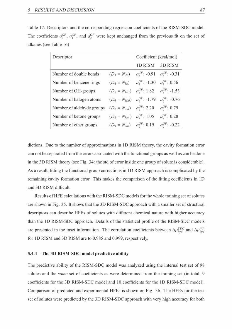
5 RESULTS AND DISCUSSION 87
Table 17: Descriptors and the corresponding regression coefficients of the RISM-SDC model.
The coefficients aGF0 , aGF1 , and a
GF2 were kept unchanged from the previous fit on the set of
alkanes (see Table 16)
Descriptor Coefficient (kcal/mol)
1D RISM 3D RISM
Number of double bonds (D3 = Ndb) aGF3 : -0.91 aGF3 : -0.31
Number of benzene rings (D4 = Nbz) aGF4 : -1.30 aGF4 : 0.56
Number of OH-groups (D5 = NOH) aGF5 : 1.82 aGF5 : -1.53
Number of halogen atoms (D6 = NHal) aGF6 : -1.79 aGF6 : -0.76
Number of aldehyde groups (D7 = Nald) aGF7 : 2.20 aGF7 : 0.79
Number of ketone groups (D8 = Nket ) aGF8 : 1.05 aGF8 : 0.28
Number of ether groups (D9 = Neth) aGF9 : 0.19 aGF9 : -0.22
dictions. Due to the number of approximations in 1D RISM theory, the cavity formation error
can not be separated from the errors associated with the functional groups as well as can be done
in the 3D RISM theory (see Fig. 34: the std of error inside one group of solute is considerable).
As a result, fitting the functional group corrections in 1D RISM approach is complicated by the
remaining cavity formation error. This makes the comparison of the fitting coefficients in 1D
and 3D RISM difficult.
Results of HFE calculations with the RISM-SDCmodels for the whole training set of solutes
are shown in Fig. 35. It shows that the 3D RISM-SDC approach with a smaller set of structural
descriptors can describe HFEs of solutes with different chemical nature with higher accuracy
than the 1D RISM-SDC approach. Details of the statistical profile of the RISM-SDC models
are presented in the inset information. The correlation coefficients between ΔμSDChyd and Δμexphydfor 1D RISM and 3D RISM are to 0.985 and 0.999, respectively.
5.4.4 The 3D RISM-SDC model predictive ability
The predictive ability of the RISM-SDC model was analyzed using the internal test set of 98
solutes and the same set of coefficients as were determined from the training set (in total, 9
coefficients for the 3D RISM-SDC model and 10 coefficients for the 1D RISM-SDC model).
Comparison of predicted and experimental HFEs is shown on Fig. 36. The HFEs for the test
set of solutes were predicted by the 3D RISM-SDC approach with very high accuracy for both

5 RESULTS AND DISCUSSION 88
Figure 35: (a, b) HFEs corrected with the 1D and 3D RISM-SDC models (ΔμSDChyd ) versus
experimental values for the training set of solutes. Solid lines show the ideal correlation. Dashed
lines indicate the corresponding std of error (see the inset data, values are in kcal/mol). (c,
d) Difference between the SDC-corrected and experimental HFEs versus experimental values
for 1D RISM and 3D RISM, respectively. Dashed lines indicate the corresponding std of the
difference.
simple and polyfragment molecules. The rms of the error is 0.47 kcal/mol which is of the same
order of magnitude as the experimental accuracy (0.2-0.5 kcal/mol [30, 36, 38, 197, 49]).
The HFEs predicted by the 1D RISM-SDC approach are considerably biased with respect
to corresponding experimental values. We note that the bias is present only for compounds con-
taining a benzene ring (e.g. alkylbenzenes, chlorobenzenes, and chlorophenols). We attribute
this to the fact that the corrections for the number of branches were obtained from the training set
of alkanes only. Indeed, for the 1D RISM-SDCmodel in the section The model predictive ability
we showed that, having obtained these corrections on the whole training set of compounds via
multi-parameter linear regression, the 1D RISM-SDC approach performs well for both aliphatic
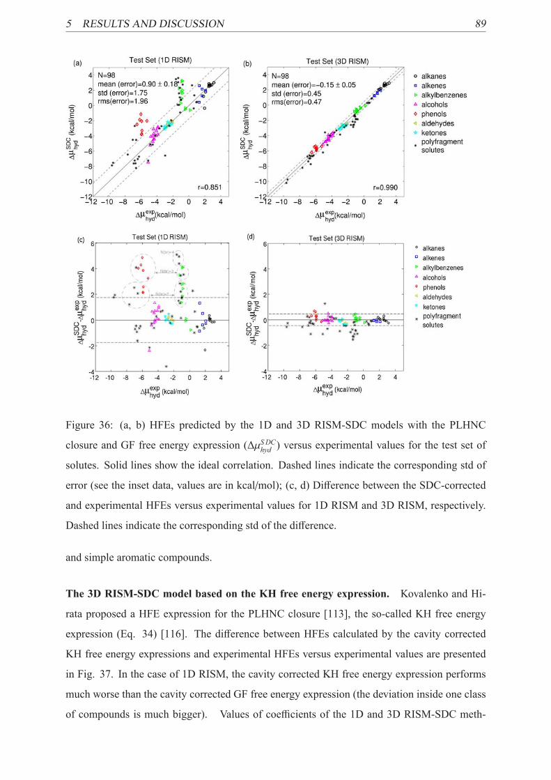
5 RESULTS AND DISCUSSION 89
Figure 36: (a, b) HFEs predicted by the 1D and 3D RISM-SDC models with the PLHNC
closure and GF free energy expression (ΔμSDChyd ) versus experimental values for the test set of
solutes. Solid lines show the ideal correlation. Dashed lines indicate the corresponding std of
error (see the inset data, values are in kcal/mol); (c, d) Difference between the SDC-corrected
and experimental HFEs versus experimental values for 1D RISM and 3D RISM, respectively.
Dashed lines indicate the corresponding std of the difference.
and simple aromatic compounds.
The 3D RISM-SDC model based on the KH free energy expression. Kovalenko and Hi-
rata proposed a HFE expression for the PLHNC closure [113], the so-called KH free energy
expression (Eq. 34) [116]. The difference between HFEs calculated by the cavity corrected
KH free energy expressions and experimental HFEs versus experimental values are presented
in Fig. 37. In the case of 1D RISM, the cavity corrected KH free energy expression performs
much worse than the cavity corrected GF free energy expression (the deviation inside one class
of compounds is much bigger). Values of coefficients of the 1D and 3D RISM-SDC meth-

5 RESULTS AND DISCUSSION 90
Figure 37: The difference between HFEs calculated with the cavity correction based on the
KH free energy expression and experimental HFEs (Δμcalchyd −ΔμSDChyd ) versus experimental values
(where Δμ(2)hyd = ΔμKHhyd + a
KH1 D1 + a
KH2 D2 + a
KH0 ). The subfigure is analogous to Figure 13.
Dashed lines indicate the corresponding std of the difference (see Table 18). In the case of the
1D RISM, the cavity corrected HFE expression performs much worse than that for 3D RISM
approach (the deviation inside one class of compounds is much bigger).
ods based on the KH free energy expression (Eqs. 28 and 34) were obtained with the training
set of the compounds following the methodology described above. Results are presented in
Table 18. Predictive ability of the 1D and 3D RISM-SDC models with KH HFE expression
for both training and test sets is shown in Fig. 38. Statistical data of these models are shown
in the inset information. Analysis of the models efficiency allows us to conclude that the 1D
RISM-SDC model with the KH free energy expression performs worse than that with GF free
energy expression. In turn, the 3D RISM-SDC model is almost not sensitive to the initial HFE
approximation.
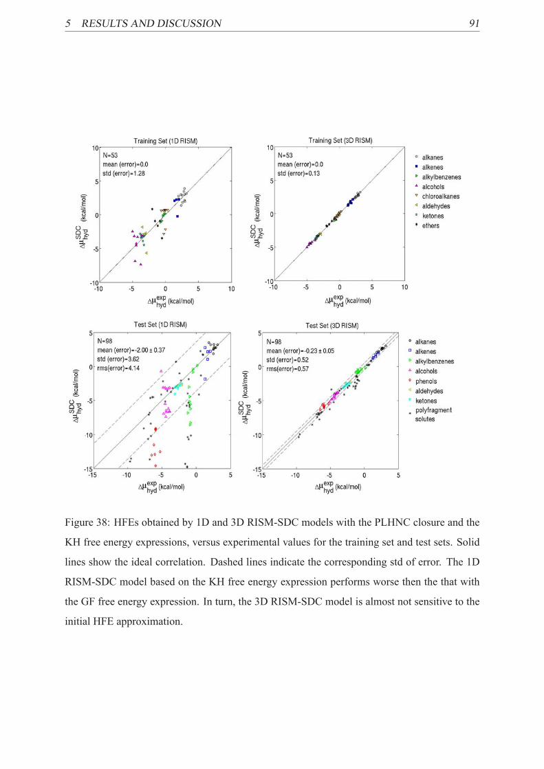
5 RESULTS AND DISCUSSION 91
Figure 38: HFEs obtained by 1D and 3D RISM-SDC models with the PLHNC closure and the
KH free energy expressions, versus experimental values for the training set and test sets. Solid
lines show the ideal correlation. Dashed lines indicate the corresponding std of error. The 1D
RISM-SDC model based on the KH free energy expression performs worse then the that with
the GF free energy expression. In turn, the 3D RISM-SDC model is almost not sensitive to the
initial HFE approximation.
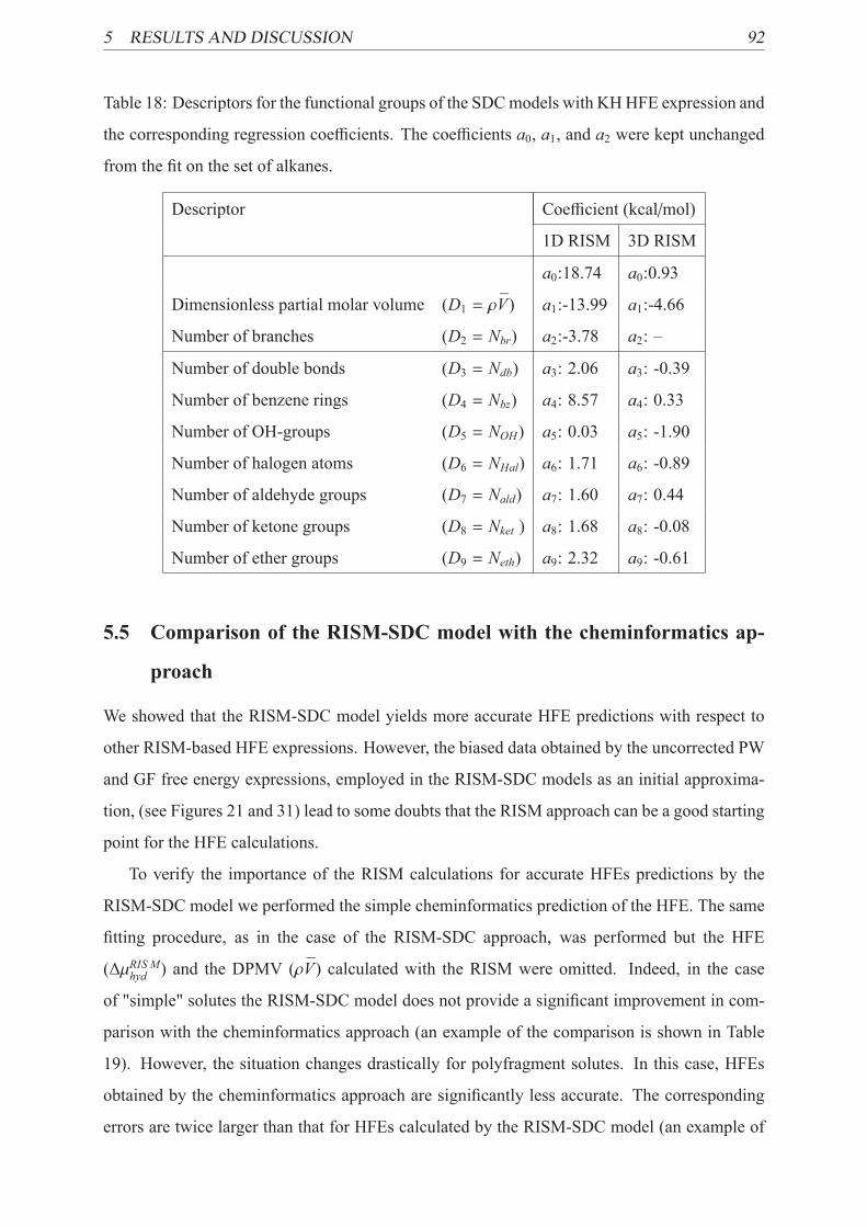
5 RESULTS AND DISCUSSION 92
Table 18: Descriptors for the functional groups of the SDCmodels with KHHFE expression and
the corresponding regression coefficients. The coefficients a0, a1, and a2 were kept unchanged
from the fit on the set of alkanes.
Descriptor Coefficient (kcal/mol)
1D RISM 3D RISM
a0:18.74 a0:0.93
Dimensionless partial molar volume (D1 = ρV) a1:-13.99 a1:-4.66
Number of branches (D2 = Nbr) a2:-3.78 a2: –
Number of double bonds (D3 = Ndb) a3: 2.06 a3: -0.39
Number of benzene rings (D4 = Nbz) a4: 8.57 a4: 0.33
Number of OH-groups (D5 = NOH) a5: 0.03 a5: -1.90
Number of halogen atoms (D6 = NHal) a6: 1.71 a6: -0.89
Number of aldehyde groups (D7 = Nald) a7: 1.60 a7: 0.44
Number of ketone groups (D8 = Nket ) a8: 1.68 a8: -0.08
Number of ether groups (D9 = Neth) a9: 2.32 a9: -0.61
5.5 Comparison of the RISM-SDC model with the cheminformatics ap-
proach
We showed that the RISM-SDC model yields more accurate HFE predictions with respect to
other RISM-based HFE expressions. However, the biased data obtained by the uncorrected PW
and GF free energy expressions, employed in the RISM-SDC models as an initial approxima-
tion, (see Figures 21 and 31) lead to some doubts that the RISM approach can be a good starting
point for the HFE calculations.
To verify the importance of the RISM calculations for accurate HFEs predictions by the
RISM-SDC model we performed the simple cheminformatics prediction of the HFE. The same
fitting procedure, as in the case of the RISM-SDC approach, was performed but the HFE
(ΔμRIS Mhyd ) and the DPMV (ρV) calculated with the RISM were omitted. Indeed, in the case
of "simple" solutes the RISM-SDC model does not provide a significant improvement in com-
parison with the cheminformatics approach (an example of the comparison is shown in Table
19). However, the situation changes drastically for polyfragment solutes. In this case, HFEs
obtained by the cheminformatics approach are significantly less accurate. The corresponding
errors are twice larger than that for HFEs calculated by the RISM-SDC model (an example of

5 RESULTS AND DISCUSSION 93
Figure 39: There is a doubt that the RISM approach (the corresponding expression is denoted by
the green circle) can be a good starting point for accurate HFE calculations. To clarify this ques-
tion, we compare the data obtained by the 1D RISM-SDC(OPLSq) model with those derived
from the cheminformatics calculations based on the same set of descriptors (the corresponding
expression is denoted by the claret red rectangle).
On plots: Difference between HFEs obtained by the 1D RISM-SDC(OPLSq) model (left plot)
and the cheminformatics approach (right plot) for the polyfragment solutes from the test set.
Solid lines correspond to the mean of the difference between calculated and experimental data.
Dashed lines indicate the corresponding std of the difference. As one can see, the cheminfor-
matics approach calculations are significantly less accurate.
the comparison is shown in Figure 39).
This comparison indicates that the RISM approach represents the main important features
of the hydration phenomena which are not accessible in the cheminformatics approach.

6 SUMMARY 94
Table 19: Statistical profile of the 1D RISM-SDC(OPLSq) model (Eq. 59) and the chemin-
formatics approach (the SDC model without HFE and DPMV calculated by the RISM) for
"simple" and polyfragment solutes from the test set. In the case of polyfragment solutes, the
cheminformatics approach is significantly less efficient. The errors of HFEs obtained within the
cheminformatics framework are twice larger than that calculated with the use of the 1D RISM-
SDC (OPLSq) model. Values of the mean of error, the standard deviation (std) of the error, and
maximal deviation (|max|) of the error are in kcal/mol.
1D RISM-SDC(OPLSq) model Cheminformatics
“simple“ solutes (N = 60)
mean 0.06 -0.03
std 0.53 0.54
|max| 1.35 1.37
polyfragment solutes (N = 60)
mean -1.15 -3.10
std 1.44 2.70
|max| 5.83 9.05
TOTAL test set (N = 120)
mean -0.55 -1.57
std 1.24 2.48
|max| 5.83 9.05
6 Summary
1. We showed that the poor accuracy of hydration thermodynamics calculations with a
molecular integral equation theory, Reference Interaction Site Model (RISM), can be con-
siderably improved with a set of corrections associated with details of molecular structure.
In this thesis we developed a novel hybrid RISM-based method for calculation of hydra-
tion thermodynamics, the Structural Descriptors Correction (SDC)model (RISM-SDC).
The method uses a thermodynamic quantity obtained by RISM as an initial approximation
and a set of corrections to decrease the error of the calculated parameter. Each correc-
tion in the RISM-SDC model can be represented as a structural descriptor (Di) multiplied
by the corresponding correction coefficient (ai). One important descriptor (D1) is the di-
mensionless partial molar volume calculated by RISM. The rest of the structural descrip-
6 SUMMARY 95
tors correspond to the number of specific molecular fragments (double bonds, aromatic
rings, electron-donating/withdrawing substituents, etc.). The correction coefficients ai are
found by training the model on a set of monofunctional compounds. For the first time,
we showed that the RISM-SDC model allows to achieve the chemical accuracy of sol-
vation thermodynamics predictions within the RISM approach, that has been a challenge
for over 40 years [64, 112, 88, 116, 89, 85, 80]. In this thesis we demonstrated the high
efficiency of the proposed approach for predicting important hydration thermodynamic
quantities, hydration free energy (HFE) and partial molar volume (PMV).
2. We collected experimental values of PMV from available literature sources and analyzed
their quality. We revealed a lack of experimental data for small organic molecules (es-
pecially for non-polar compounds). In this thesis we showed strong linear correlations
between the experimental PMVs and corresponding values calculated by the 1D RISM
and 3D RISM on solutes from different chemical classes. We demonstrated small errors
of PMV obtained by the 3D RISM and significant errors of the corresponding values ob-
tained by the 1D RISM. However, we found that in both cases the errors can be corrected
with two empirical parameters.
3. To evaluate the general accuracy of HFEs obtained by RISM approach we collected
a large database (∼ 450 compounds) of corresponding experimental values from avail-
able literature sources. We performed a detailed analysis of the data errors and possible
sources of them.
For the first time, for the 1D RISM approach we performed a consistent comparison of
efficiency of existing HFE expressions (HNC, KH, HNCB, PW, GF, PWC) on a large
set of 120 compounds from different chemical classes. The comparison showed that
all analyzed HFE expressions give considerably overestimated HFEs for both non-polar
and polar solutes. The worst results were obtained by the HNC and KH free energy
expressions. In turn, the PW and GF free energy expressions were found to be the most
promising for the further development, since there is a potential opportunity to improve
HFEs obtained by these expressions with structural corrections.
4. In this thesis, for the first time, we performed a detailed analysis of errors of HFEs cal-
culated by the 1D RISM approach with the PW free energy expression. We found that
the major part of errors can be eliminated with the correction on partial molar volume
and free coefficient aPW0 which removes a general systematic error of the 1D RISM. To

6 SUMMARY 96
increase the accuracy of HFE calculations we developed a small set of corrections asso-
ciated with main structural features of chemical solutes (double bonds, aromatic rings,
electron-donating/withdrawing substituents, etc.). That resulted in the 1D RISM-SDC
model to estimate HFEs of organic molecules.
5. We found that efficiency of the 1D RISM-SDC model depends on the choice of RISM pa-
rameters and the methods used to describe solute molecules (e.g. atomic partial charges).
The optimal set of initial parameters was investigated to get the best performance of the
model.
(a) 1D RISM parameters (closure relation and HFE expression).
It was found out that the model predictive ability is almost not sensitive to the choice
of closure relation (HNC, PLHNC). However, the 1D RISM-SDC model with the
PLHNC closure is more efficient, since in many cases 1D RISM calculations with the
HNC closure do not converge. We showed that for "simple" solutes the 1D RISM-
SDC model with the PW free energy expression performs better than that with the
GF free energy expression. However, the accuracies of the model predictions for
polyfragment solutes are comparable for both free energy expressions.
(b) Solutes parameters.
For all molecules in the study we use estimations of the 3D structure obtained fromX-
ray data [128] and/or the structural optimization at MP2/6-311G** (B3LYP/6-31G**
for pollutants) level of theory [130]. In this thesis, we tested two sets of solutes’
partial charges: (i) OPLS (ii) QM-derived using the optimized structures. It was
shown that the model with OPLS partial charges gives reasonably accurate HFEs
only for "simple" organic molecules, whereas the model with the QM-derived partial
charges tested here allows HFE to be calculated accurately for polyfragment aromatic
solutes.
6. The results of the thesis show that for a fixed set of input parameters the RISM-SDC
model coefficients, {ai}, can be transferred to molecules of different chemical classes.
The 1D RISM-SDC model with QM-derived partial charges was tested on such polyfrag-
ment solutes as polychlorinated aromatic pollutants. We demonstrated that different struc-
tural features of a solute molecule contribute independently to the HFE error. Thus, for
polyfragment solutes HFE errors can be represented as a linear combination of structural
corrections calibrated on a set of "simple" solutes. This indicates a great potential of the

6 SUMMARY 97
RISM-SDC model to be used for HFE predictions of a wide range of organic solutes.
We compared HFEs predicted by the 1D RISM-SDC model with available experimen-
tal data, results of other standard methods such as continuum solvation models [195],
and data obtained by the cheminformatics approach (the SDC model without the RISM
calculated HFEs). We found that the 1D RISM-SDC model predicts reasonably well
the HFEs for both "simple" and polyfragment organic molecules (rms of error is ∼ 1.0
kcal/mol). This suggests that, despite of the number of approximations, the 1D RISM
approach is able to reproduce the non-linear solvent response around polyfunctional so-
lutes. However, neither the continuum solvent models nor the proposed cheminformatics
approach take into account this effect. These results allowed us to conclude that 1D
RISM-calculated HFEs are the essential part of the SDC model.
7. We showed the SDC model can be further improved by its combination with the 3D
RISM approach, which allowed to predict HFEs for small organic compounds with the
experimental accuracy (rms of error is ∼ 0.5 kcal/mol). We demonstrate that the 3D
RISM-SDC model requires less number of structural corrections compared to the 1D
RISM-SDC model. Particularly, the 3D RISM does not require the correction on num-
ber of branches because it properly estimates the cavity created by a solute molecule in
water. We found that the 3D RISM-SDC model is almost not sensitive to the initial HFE
expression and can be efficiently used with both GF and KH free energy expressions.
In this thesis, for the first time, we revealed that HFEs obtained by the 3D RISM can
be efficiently scaled with only one correction based on the PMV of solute. We showed
that the correction is universal for multiple different classes of organic molecules, from
"simple" organic compounds to druglike molecules (rms of error of predicted HFEs for
both cases is ∼ 1.0 kcal/mol).
Outlook.
The RISM-SDC model, proposed in this thesis, is a promising theoretical approach to pre-
dict thermodynamics of solvation. The RISM-SDC methodology can be easily applied to at
least two fields of computational chemistry: (1) high-throughput calculations of HFEs for large
databases of compounds (e.g. in pharmaceutical drug discovery or in assessing the environ-
mental fate of pollutant molecules, where the time required for each calculation is important
as well as the accuracy); (2) hybrid MC/RISM calculations where MC technique is applied for
sampling the conformations changes of a solute molecule in solution treated with the RISM

6 SUMMARY 98
approach [66]. 1 Both applications require many RISM calculations of HFEs (for many com-
pounds in the first case, and for many different MC-steps in the second case).
The results of this thesis show that for both "simple" and polyfragment solutes the 3D RISM-
SDC model predicts HFEs with a high accuracy (rms of error is ∼ 0.5 kcal/mol), whereas
the 1D RISM-SDC model with the same parameters provides moderate accuracy with the rms
of error is ∼ 1.0 kcal/mol. However a single 1D RISM-SDC calculation takes only a few
seconds on a PC, whereas a single 3D RISM-SDC HFE calculation is approximately 100 times
more computationally expensive. Therefore we suggest that one should use the 1D RISM-SDC
model for large scale high throughput screening of molecule hydration properties, while further
refinement of these properties for selected compounds should be carried out with the more
computationally expensive, but more accurate, 3D RISM-SDC model.
The fact that it is possible to improve the accuracy of RISM-based HFE predictions with the
SDC model opens up many new questions to theoreticians working in the field of the IET of
Molecular Liquids. There is no straightforward method to identify which approximation used
in the RISM theories (e.g. neglecting the bridge functional, reducing the order of 6D Ornstein-
Zernike equation, etc.) makes the most significant contribution to the error in calculated HFE.
We believe that more theoretical works in IET will bring more understanding of approximations
behind the RISM approach and provoke development of new methods of HFE calculation which
will allow more accurate predictions at lower computational cost.
The current limiting factor in further SDC model development is a lack of experimental
thermodynamic data for polyfragment organic molecules (e.g. pollutants, druglike molecules,
etc.). Computational and theoretical scientists can do very little to improve the situation in this
respect, but we hope that our results and analysis of available experimental data will provoke
experimentalists to revisit the question and, hopefully, to make additional independent measure-
ments of HFE. Such new experimental data would be very valuable in creating and testing new
models.
1In the MC/RISM approach the energy function in the Boltzmann factor is taken as a sum of the conformational
energy of a molecule and the HFE; the SDC model can be used in the MC/RISM approach to improve the accuracy
of HFEs of a molecule in a fixed conformation calculated on each MC-step.
99
7 Literature
[1] G. Wypych. Handbook of solvents. Toronto-New York, 2001.
[2] M. Kinoshita, Y. Okamoto, and F. Hirata. Solvent effects on conformational stability
of peptides: RISM analyses. Journal of Molecular Liquids, 90(1-3):195–204, February
2001.
[3] T. Imai, Y. Harano, M. Kinoshita, A. Kovalenko, and F. Hirata. Theoretical analysis on
changes in thermodynamic quantities upon protein folding: Essential role of hydration.
Journal of Chemical Physics, 126(22):225102, June 2007.
[4] M. Kinoshita, Y. Okamoto, and F. Hirata. Analysis on conformational stability of C-
peptide of ribonuclease a in water using the reference interaction site model theory and
Monte Carlo simulated annealing. Journal of Chemical Physics, 110(8):4090–4100,
February 1999.
[5] D. Casanova, S. Gusarov, A. Kovalenko, and T. Ziegler. Evaluation of the SCF com-
bination of KS-DFT and 3D-RISM-KH; Solvation effect on conformational equilibria,
tautomerization energies, and activation barriers. Journal of Chemical Theory and Com-
putation, 3(2):458–476, March 2007.
[6] G. N. Chuev and M. V. Fedorov. Reference interaction site model study of self-
aggregating cyanine dyes. J. Chem. Phys., 131(7):1323–1329, 2009.
[7] Y. Levy and J. N. Onuchic. Water and proteins: A love-hate relationship. Proceedings of
the National Academy of Sciences of the United States of America, 101(10):3325–3326,
March 2004.
[8] G. Hummer. Molecular Binding Under water’s influence. Nature Chemistry, 2(11):906–
907, November 2010.
[9] Riccardo Baron, Piotr Setny, and J. Andrew McCammon. Water in Cavity – Ligand
Recognition. Journal of the American Chemical Society, 132(34):12091–12097, 2010.
[10] D. Mackay, W. Y. Shiu, and K. C. Ma. Illustrated Handbook of Physical-Chemical Prop-
erties and Environmental Fate for Organic Chemicals, Volume 2, Polynuclear Aromatic
Hydrocarbons, Polychlorinated Dioxins, and Dibenzofurans. Lewis Publishers, 1992.

100
[11] K. T. Valsaraj and L. J. Thibodeaux. On the Physicochemical Aspects of the Global
Fate and Long-range atmospheric Transport of Persistent Organic Pollutants. Journal of
Physical Chemistry Letters, 1(11):1694–1700, June 2010.
[12] G. A. Krestov, N. P. Novosyolov, I. S. Perelygin, A. M. Kolker, L. P. Safonova, V. D.
Ovchinnikova, and V. N. Trostin, editors. Ionic solvation. Ellis Horwood Series in
Inorganic Chemistry. Horwood, New York, 1994.
[13] S. L. Gong, P. Huang, T. L. Zhao, L. Sahsuvar, L. A. Barrie, J. W. Kaminski, Y. F. Li,
and T. Niu. Gem/POPs: a global 3-D dynamic model for semi-volatile persistent organic
pollutants - Part 1: Model description and evaluations of air concentrations. Atmospheric
Chemistry and Physics, 7(15):4001–4013, 2007.
[14] A. Strand and O. Hov. A model strategy for the simulation of chlorinated hydrocarbon
distributions in the global environment. Water Air and Soil Pollution, 86(1-4):283–316,
January 1996.
[15] P. S. Liss and P. G. Slater. Flux of Gases across the Air-sea Interface. Nature,
247(5438):181–184, 1974.
[16] H. W. Vallack, D. J. Bakker, I. Brandt, E. Brostrom Lunden, A. Brouwer, K. R. Bull, C.
Gough, R. Guardans, I. Holoubek, B. Jansson, R. Koch, J. Kuylenstierna, A. Lecloux,
D. Mackay, P. McCutcheon, P. Mocarelli, and R. D. F. Taalman. Controlling persistent
organic pollutants - what next? Environmental Toxicology and Pharmacology, 6(3):143–
175, November 1998.
[17] K. C. Jones and P. de Voogt. Persistent organic pollutants (POPs): state of the science.
Environmental Pollution, 100(1-3):209–221, 1999.
[18] P. H. Wine. Atmospheric and Environmental Physical Chemistry: Pollutants without
borders. Journal of Physical Chemistry Letters, 1(11):1749–1751, June 2010.
[19] Aarhus Protocol on Persistent Organic Pollutants (POPs). WWW page, 1998.
[20] D. Mackay. Multimedia Environmental Models: The Fugacity Approach. CRC Press, 2
edition, February 2001.
[21] A. Beyer and M. Biziuk. Environmental Fate and Global Distribution of Polychlori-
nated Biphenyls. Reviews of Environmental Contamination and Toxicology, 201:137–
158, 2009.

101
[22] M. Scheringer, F. Wegmann, K. Fenner, and K. Hungerbuhler. Investigation of the cold
condensation of persistent organic pollutants with a global multimedia fate model. Envi-
ronmental Science and Technology, 34(9):1842–1850, May 2000.
[23] F. Wania and D. Mackay. The Global Distribution Model. A Non-steady State Multicom-
partment mass Balance Model of the Fate of Persistent Organic Pollutants in the Global
Environment. Technical report, University of Toronto at Scarborough; Trent University,
2000.
[24] Converting Henry’s Law Constants. (accessed November 25, 2010).
[25] J. H. Jensen, H. Li, A. D. Robertson, and P. A. Molina. Prediction and rationalization of
protein pk(a) values using QM and QM/MMmethods. Journal of Physical Chemistry A,
109(30):6634–6643, August 2005.
[26] W. L. Jorgensen and E. M. Duffy. Prediction of drug solubility from structure. Adv. Drug
Delivery Rev., 54(3):355–366, March 2002.
[27] D. S. Palmer, A. Llinas, I. Morao, G. M. Day, J. M. Goodman, R. C. Glen, and J. B. O.
Mitchell. Predicting intrinsic aqueous solubility by a thermodynamic cycle. Mol. Phar-
maceutics, 5(2):266–279, March 2008.
[28] N. M. Garrido, A. J. Queimada, M. Jorge, E. A. Macedo, and I. G. Economou. 1-
octanol/water Partition Coefficients of n-alkanes fromMolecular simulations of Absolute
Solvation Free Energies. Journal of Chemical Theory and Computation, 5(9):2436–2446,
September 2009.
[29] L. D. Hughes, D. S. Palmer, F. Nigsch, and J. B. O. Mitchell. Why are some properties
more difficult to predict than others? A study of QSPR models of solubility, melting
point, and Log P. J. Chem. Inf. Model., 48(1):220–232, January 2008.
[30] G. L. Perlovich and A. Bauer Brandl. Solvation of Drugs as a Key for Understanding Par-
titioning and Passive transport Exemplified by Nsaids. Curr. Drug Delivery, 1(3):213–
226, July 2004.
[31] J. M. J. Swanson, R. H. Henchman, and J. A. McCammon. Revisiting free energy calcu-
lations: A theoretical connection to MM/PBSA and direct calculation of the association
free energy. Biophysical Journal, 86(1):67–74, 2004.

102
[32] E. H. Kerns and L. Di. Drug-like properties: concepts, structure design and methods:
from ADME to toxicity optimization. Academic Press, 2008.
[33] C. J. Cramer and D. G. Truhlar. Am1-sm2 And Pm3-sm3 Parameterized Scf Solvation
Models For Free-energies in Aqueous-solution. J. Comput.-Aided Mol. Des., 6(6):629–
666, December 1992.
[34] M. H. Abraham, J. Andonianhaftvan, G. S. Whiting, A. Leo, and R. S. Taft. Hydrogen-
bonding .34. The Factors That Influence The Solubility Of gases And Vapors In Water
At 298-k, And A New Method For Its Determination. J. Chem. Soc. Perkin Trans. 2,
(8):1777–1791, August 1994.
[35] W. L. Jorgensen, J. P. Ulmschneider, and J. Tirado Rives. Free energies of hydration from
a generalized Born model and an All-atom force field. J. Phys. Chem. B, 108(41):16264–
16270, October 2004.
[36] G. L. Perlovich, T. V. Volkova, and A. Bauer Brandl. Towards an understanding of
the molecular mechanism of solvation of drug molecules: A thermodynamic approach
by crystal lattice energy, sublimation, and solubility exemplified by paracetamol, ac-
etanilide, and phenacetin. J. Pharm. Sci., 95(10):2158–2169, October 2006.
[37] G. L. Perlovich, T. V. Volkova, and A. Bauer Brandl. Towards an understanding of the
molecular mechanism of solvation of drug molecules: A thermodynamic approach by
crystal lattice energy, sublimation, and solubility exemplified by hydroxybenzoic acids.
J. Pharm. Sci., 95(7):1448–1458, July 2006.
[38] G. L. Perlovich, T. V. Volkova, A. N. Manin, and A. Bauer Brandl. Influence of position
and size of substituents on the mechanism of partitioning: A thermodynamic study on ac-
etaminophens, hydroxybenzoic acids, and parabens. AAPS Pharm. Sci. Tech., 9(1):205–
216, March 2008.
[39] G. L. Perlovich, T. V. Volkova, A. N. Manin, and A. Bauer Brandl. Extent and mecha-
nism of solvation and partitioning of isomers of substituted benzoic acids: A thermody-
namic study in the solid state and in solution. J. Pharm. Sci., 97(9):3883–3896, Septem-
ber 2008.
[40] X. Zielenkiewicz, G. L. Perlovich, and M. Wszelaka Rylik. The vapour pressure and
the enthalpy of sublimation. Determination by inert gas flow method. J. Therm. Anal.
Calorim., 57(1):225–234, 1999.
103
[41] F. L. Mota, A. R. Carneiro, A. J. Queimada, S. P. Pinho, and E. A. Macedo. Temperature
and solvent effects in the solubility of some pharmaceutical compounds: Measurements
and modeling. Eur. J. Pharm. Sci., 37(3-4):499–507, June 2009.
[42] P. Kollman. Free-energy Calculations - Applications To Chemical And Biochemical
phenomena. Chem. Rev., 93(7):2395–2417, November 1993.
[43] W. L. Jorgensen and J. TiradoRives. Free energies of hydration for organic molecules
from Monte Carlo simulations. Perspectives Drug Discovery Des., 3:123–138, 1995.
[44] B. Roux and T. Simonson. Implicit solvent models. Biophys. Chem., 78(1-2):1–20, April
1999.
[45] E. M. Duffy and W. L. Jorgensen. Prediction of properties from simulations: Free ener-
gies of solvation in hexadecane, octanol, and water. J. Am. Chem. Soc., 122(12):2878–
2888, March 2000.
[46] M. Orozco and F. J. Luque. Theoretical methods for the description of the solvent effect
in biomolecular systems. Chem. Rev., 100(11):4187–4225, November 2000.
[47] J. Westergren, L. Lindfors, T. Hoglund, K. Luder, S. Nordholm, and R. Kjellander.
In silico prediction of drug solubility: 1. Free energy of hydration. J. Phys. Chem. B,
111(7):1872–1882, February 2007.
[48] A. Nicholls, D. L. Mobley, J. P. Guthrie, J. D. Chodera, C. I. Bayly, M. D. Cooper, and
V. S. Pande. Predicting small-molecule solvation free energies: An informal blind test
for computational chemistry. J. Med. Chem., 51(4):769–779, February 2008.
[49] J. P. Guthrie. A Blind Challenge for Computational Solvation Free Energies: Introduc-
tion and Overview. J. Phys. Chem. B, 113(14):4501–4707, April 2009.
[50] A. Klamt, F. Eckert, and M. Diedenhofen. Prediction of the Free Energy of Hydration of
a Challenging Set of pesticide-like Compounds. J. Phys. Chem. B, 113(14):4508–4510,
M 2009.
[51] A. V. Marenich, C. J. Cramer, and D. G. Truhlar. Performance of Sm6, Sm8, and Smd
on the Sampl1 Test Set for the Prediction of Small-molecule Solvation Free Energies. J.
Phys. Chem. B, 113(14):4538–4543, March 2009.

104
[52] D. L. Mobley, C. I. Bayly, M. D. Cooper, and K. A. Dill. Predictions of Hydra-
tion Free Energies from All-atom Molecular Dynamics simulations. J. Phys. Chem. B,
113(14):4533–4537, March 2009.
[53] T. Sulea, D. Wanapun, S. Dennis, and E. O. Purisima. Prediction of Sampl-1 Hydration
Free Energies Using a Continuum Electrostatics-dispersion model. J. Phys. Chem. B,
113(14):4511–4520, March 2009.
[54] C. A. Reynolds, P. M. King, and W. G. Richards. Free-energy Calculations In Molecular
Biophysics. Mol. Phys., 76(2):251–275, June 1992.
[55] N. Matubayasi and M. Nakahara. Theory of solutions in the energetic representation. I.
Formulation. J. Chem. Phys., 113(15):6070–6081, October 2000.
[56] N. Matubayasi and M. Nakahara. An approach to the solvation free energy in terms of
the distribution functions of the solute-solvent interaction energy. J. Mol. Liq., 119(1-
3):23–29, May 2005.
[57] M. R. Shirts and V. S. Pande. Solvation free energies of amino acid side chain analogs
for common molecular mechanics water models. J. Chem. Phys., 122(13):134508, April
2005.
[58] N. Matubayasi. Free-energy Analysis of Solvation with the Method of Energy Represen-
tation. Frontiers Biosci., 14:3536–3549, January 2009.
[59] J. L. Knight and C. L. Brooks. lambda-dynamics Free Energy Simulation Methods. J.
Comput. Chem., 30(11):1692–1700, August 2009.
[60] J. Tomasi and M. Persico. Molecular-interactions In Solution - An Overview Of Meth-
ods Based on Continuous Distributions Of The Solvent. Chem. Rev., 94(7):2027–2094,
November 1994.
[61] J. Tomasi, B. Mennucci, and R. Cammi. Quantum mechanical continuum solvation mod-
els. Chem. Rev., 105(8):2999–3094, August 2005.
[62] J. Kongsted, P. Soderhjelm, and U. Ryde. How accurate are continuum solvation models
for drug-like molecules? Journal of Computer-aided Molecular Design, 23(7):395–409,
July 2009.

105
[63] C. J. Cramer and D. G. Truhlar. General Parameterized Scf Model For Free-energies Of
Solvation In aqueous-solution. J. Am. Chem. Soc., 113(22):8305–8311, October 1991.
[64] D. Chandler and H. C. Andersen. Optimized cluster expansions for classical fluids. 2.
Theory of molecular liquids. J. Chem. Phys., 57(5):1930–1937, 1972.
[65] P. A. Monson and G. P. Morriss. Recent Progress in the Statistical-mechanics of Inter-
action Site fluids. Adv. Chem. Phys., 77:451–550, 1990.
[66] F. Hirata, editor.Molecular theory of solvation. Kluwer Academic Publishers, Dordrecht,
Netherlands, 2003.
[67] M. Kinoshita. Structure of aqueous electrolyte solutions near a hydrophobic surface.
Condens. Matter Phys., 10(3):387–396, 2007.
[68] M. Kinoshita. Molecular origin of the hydrophobic effect: Analysis using the angle-
dependent integral equation theory. J. Chem. Phys., 128(2):024507, January 2008.
[69] M. Kinoshita and M. Suzuki. A statistical-mechanical analysis on the hypermobile water
around a large solute with high surface charge density. J. Chem. Phys., 130(1):014707,
January 2009.
[70] N. Yoshida, S. Phongphanphanee, Y. Maruyama, T. Imai, and F. Hirata. Selective ion-
binding by protein probed with the 3D-RISM theory. Journal of the American Chemical
Society, 128(37):12042–12043, September 2006.
[71] J. S. Perkyns, G. C. Lynch, J. J. Howard, and B. M. Pettitt. Protein solvation from theory
and simulation: Exact treatment of coulomb interactions in three-dimensional theories.
Journal of Chemical Physics, 132(6):064106, February 2010.
[72] S. Ten-no. Free energy of solvation for the reference interaction site model: Critical
comparison of expressions. J. Chem. Phys., 115(8):3724–3731, August 2001.
[73] S. Ten-no, J. Jung, H. Chuman, and Y. Kawashima. Assessment of free energy expres-
sions in RISM integral equation theory: theoretical prediction of partition coefficients
revisited. Molecular Physics, 108(3-4):327–332, 2010.
[74] F. Hirata. Chemical processes in solution studied by an integral equation theory of molec-
ular liquids. Bull. Chem. Soc. Jpn., 71(7):1483–1499, 1998.

106
[75] G. N. Chuev, S. Chiodo, S. E. Erofeeva, M. V. Fedorov, N. Russo, and E. Sicilia. A
quasilinear RISM approach for the computation of solvation free energy of ionic species.
Chem. Phys. Lett., 418(4-6):485–489, February 2006.
[76] S. Chiodo, G. N. Chuev, S. E. Erofeeva, M. V. Fedorov, N. Russo, and E. Sicilia. Com-
parative Study of Electrostatic Solvent Response by RISM and PCM methods. Int. J.
Quantum Chem., 107:265–274, 2006.
[77] M. V. Fedorov and A. A. Kornyshev. Unravelling the solvent response to neutral and
charged solutes. Mol. Phys., 105(1):1–16, January 2007.
[78] P. H. Lee and G. M. Maggiora. Solvation Thermodynamics Of Polar-molecules In
Aqueous-solution By the XRISM Method. J. Phys. Chem., 97(39):10175–10185,
September 1993.
[79] K. Sato, H. Chuman, and S. Ten no. Comparative study on solvation free energy ex-
pressions in reference interaction site model integral equation theory. J. Phys. Chem. B,
109(36):17290–17295, September 2005.
[80] G. N. Chuev, M. V. Fedorov, and J. Crain. Improved estimates for hydration free energy
obtained by the reference interaction site model. Chem. Phys. Lett., 448(4-6):198–202,
2007.
[81] G. N. Chuev, M. V. Fedorov, S. Chiodo, N. Russo, and E. Sicilia. Hydration of ionic
species studied by the reference interaction site model with a repulsive bridge correction.
J. Comput. Chem., 29(14):2406–2415, 2008.
[82] D. Beglov and B. Roux. An integral equation to describe the solvation of polar molecules
in liquid water. J. Phys. Chem., 101:7821–7826, 1997.
[83] Q. H. Du, D. Beglov, and B. Roux. Solvation free energy of polar and nonpolar molecules
in water: An extended interaction site integral equation theory in three dimensions. J.
Phys. Chem. B, 104(4):796–805, February 2000.
[84] T. Imai, K. Oda, A. Kovalenko, F. Hirata, and A. Kidera. Ligand Mapping on Protein
Surfaces by the 3D-RISM Theory: Toward computational Fragment-based Drug Design.
J. Am. Chem. Soc., 131(34):12430–12440, September 2009.

107
[85] A. Kovalenko and F. Hirata. Hydration free energy of hydrophobic solutes studied by a
reference interaction site model with a repulsive bridge correction and a thermodynamic
perturbation method. J. Chem. Phys., 113:2793–2805, 2000.
[86] A. Kovalenko, F. Hirata, and M. Kinoshita. Hydration structure and stability of Met-
enkephalin studied by a three-dimensional reference interaction site model with a re-
pulsive bridge correction and a thermodynamic perturbation method. J. Chem. Phys.,
113(21):9830–9836, December 2000.
[87] M. Marucho, C. T. Kelley, and B. M. Pettitt. Solutions of the optimized closure integral
equation theory: Heteronuclear polyatomic fluids. J. Chem. Theory Comput., 4(3):385–
396, March 2008.
[88] D. Chandler, Y. Singh, and D.M. Richardson. Excess Electrons In Simple Fluids .1. Gen-
eral Equilibrium-theory for Classical Hard-sphere Solvents. J. Chem. Phys., 81(4):1975–
1982, 1984.
[89] S. Ten-no and S. Iwata. On the connection between the reference interaction site model
integral equation theory and the partial wave expansion of the molecular Ornstein-
Zernike equation. J. Chem. Phys., 111(11):4865–4868, 1999.
[90] N. Jain and S. H. Yalkowsky. Estimation of the aqueous solubility I: Application to
organic nonelectrolytes. J. Pharm. Sci., 90(2):234–252, February 2001.
[91] J. Gasteiger, editor. Handbook of Chemoinformatics. 4 Bde. From Data to Knowledge.
Wiley-VCH, 1 edition, 2003.
[92] K. F. McClure, Y. A. Abramov, E. R. Laird, J. T. Barberia, W. L. Cai, T. J. Carty, S. R.
Cortina, D. E. Danley, A. J. Dipesa, K. M. Donahue, M. A. Dombroski, N. C. Elliott,
C. A. Gabel, S. G. Han, T. R. Hynes, P. K. LeMotte, M. N. Mansour, E. S. Marr, M. A.
Letavic, J. Pandit, D. B. Ripin, F. J. Sweeney, D. Tan, and Y. Tao. Theoretical and
experimental design of atypical kinase inhibitors: Application to p38 Map kinase. J.
Med. Chem., 48(18):5728–5737, September 2005.
[93] K. F. McClure, M. A. Letavic, A. S. Kalgutkar, C. A. Gabel, L. Audoly, J. T. Barberia,
J. F. Braganza, D. Carter, T. J. Carty, S. R. Cortina, M. A. Dombroski, K. M. Donahue,
N. C. Elliott, C. P. Gibbons, C. K. Jordan, A. V. Kuperman, J. M. Labasi, R. E. LaLiberte,
J. M. McCoy, B. M. Naiman, K. L. Nelson, H. T. Nguyen, K. M. Peese, F. J. Sweeney,

108
T. J. Taylor, C. E. Trebino, Y. A. Abramov, E. R. Laird, W. A. Volberg, J. Zhou, J.
Bach, and F. Lombardo. Structure-activity relationships of triazolopyridine oxazole p38
inhibitors: Identification of candidates for clinical development. Bioorg. Med. Chem.
Lett., 16(16):4339–4344, August 2006.
[94] A. Varnek and A. Tropsha, editors. Chemoinformatics: Approaches to Virtual Screening.
RSC Publishing, Cambridge, England, 1 edition, 2008.
[95] L. A. Reiter, C. S. Jones, W. H. Brissette, S. P. McCurdy, Y. A. Abramov, J. Bordner,
F. M. DiCapua, M. J. Munchhof, D. M. Rescek, I. J. Samardjiev, and J. M. Withka.
Molecular features crucial to the activity of pyrimidine benzamide-based thrombopoietin
receptor agonists. Bioorg. Med. Chem. Lett., 18(9):3000–3006, May 2008.
[96] K. T. No, S. G. Kim, K. H. Cho, and H. A. Scheraga. Description of hydration free
energy density as a function of molecular physical properties. Biophys. Chem., 78(1-
2):127–145, April 1999.
[97] Y. Y. In, H. H. Chai, and K. T. No. A partition coefficient calculation method with the
Sfed model. J. Chem. Inf. Model., 45(2):254–263, March 2005.
[98] R. J. Barlow. Statistics: A Guide to the Use of Statistical Methods in the Physical Sci-
ences. Wiley, reprint edition, July 1989.
[99] J. Aqvist, C. Medina, and J. E. Samuelsson. A New Method For Predicting Binding-
affinity In Computer-aided Drug design. Protein Eng., 7(3):385–391, March 1994.
[100] H. A. Carlson and W. L. Jorgensen. An Extended Linear-response Method For Deter-
mining Free-energies of Hydration. J. Phys. Chem., 99(26):10667–10673, June 1995.
[101] S. Cabani, P. Gianni, Mollica V., and L. Lepori. Group Contributions to the Thermody-
namic Properties of Non-ionic organic Solutes in Dilute Aqueous-solution. J. Solution
Chem., 10(8):563–595, 1981.
[102] Terrell L. Hill. Statistical Mechanics: Principles and Selected Applications. Dover
Publications, July 1987.
[103] V.I. Kalikmanov. Statistical physics of fluids: basic concepts and applications. Berlin;
New York: Springer, 2001.
[104] A. Ben-Naim. Molecular Theory of Solutions. Oxford University Press, USA, 2006.

109
[105] J.-P. Hansen and I. R. McDonald. Theory of Simple Liquids, 4th ed. Elsevier Academic
Press, Amsterdam, The Netherlands, 2000.
[106] D. S. Palmer, V. P. Sergiievskyi, F. Jensen, and M. V. Fedorov. Accurate calculations
of the hydration free energies of druglike molecules using the reference interaction site
model. Journal of Chemical Physics, 133(4):044104, July 2010.
[107] E. L. Ratkova, G. N. Chuev, V. P. Sergiievskyi, and M. V. Fedorov. An Accurate Predic-
tion of Hydration Free Energies by Combination of Molecular Integral Equations Theory
with Structural Descriptors. Journal of Physical Chemistry B, 114(37):12068–12079,
2010.
[108] S. Genheden, T. Luchko, S. Gusarov, A. Kovalenko, and U. Ryde. AnMm/3D-RISMAp-
proach for Ligand Binding Affinities. Journal of Physical Chemistry B, 114(25):8505–
8516, July 2010.
[109] S. Phongphanphanee, N. Yoshida, and F. Hirata. On the proton exclusion of aquaporins:
A statistical mechanics study. Journal of the American Chemical Society, 130(5):1540–
1541, February 2008.
[110] S. M. Kast, J. Heil, S. Gussregen, and K. F. Schmidt. Prediction of tautomer ratios
by embedded-cluster integral equation theory. Journal of Computer-aided Molecular
Design, 24(4):343–353, April 2010.
[111] D. M. Duh and A. D. J. Haymet. Integral-equation Theory For Uncharged Liquids:
The Lennard-jones fluid And The Bridge Function. J. Chem. Phys., 103(7):2625–2633,
August 1995.
[112] S. J. Singer and D. Chandler. Free-energy Functions in the Extended RISM Approxima-
tion. Mol. Phys., 55(3):621–625, 1985.
[113] A. Kovalenko and F. Hirata. Potential of mean force between two molecular ions in
a polar molecular solvent: A study by the three-dimensional reference interaction site
model. J. Phys. Chem. B, 103:7942–7957, 1999.
[114] Daan Frenkel and Berend Smit. Understanding molecular simulation. Academic Press,
2002.
[115] J. G. Kirkwood. Statistical Mechanics of Fluid Mixtures. Journal of Chemical Physics,
3:300–313, 1935.

110
[116] A. Kovalenko and F. Hirata. Potentials of mean force of simple ions in ambient aque-
ous solution. II. Solvation structure from the three-dimensional reference interaction
site model approach, and comparison with simulations. Journal of Chemical Physics,
112(23):10403–10417, June 2000.
[117] T. Imai, M. Kinoshita, and F. Hirata. Theoretical study for partial molar volume of amino
acids in aqueous solution: Implication of ideal fluctuation volume. Journal of Chemical
Physics, 112(21):9469–9478, June 2000.
[118] T. Imai, Y. Harano, A. Kovalenko, and F. Hirata. Theoretical study for volume changes
associated with the helix-coil transition of peptides. Biopolymers, 59(7):512–519, De-
cember 2001.
[119] M. V. Fedorov, H. J. Flad, G. N. Chuev, L. Grasedyck, and B. N. Khoromskij. A struc-
tured low-rank wavelet solver for the Ornstein-Zernike integral equation. Computing,
80(1):47–73, May 2007.
[120] V. P. Sergiievskyi, W. Hackbusch, and M. V. Fedorov. Multi-grid Solver for the Ref-
erence Interaction Site Model of Molecular liquids Theory. Journal of Computational
Chemistry, 2011.
[121] L. Lue and D. Blankschtein. Liquid-state theory of hydrocarbon water-
systemsapplication to methane, ethane, and propane. J. Phys. Chem., 96(21):8582–8594,
October 1992.
[122] B. M. Pettitt and P. J. Rossky. Integral-equation predictions of liquid-state structure
for waterlike intermolecular potentials. Journal of Chemical Physics, 77(3):1451–1457,
1982.
[123] H. J. C. Berendsen, J. R. Grigera, and T. P. Straatsma. The missing term in effective pair
potentials. J. Phys. Chem., 91(24):6269–6271, November 1987.
[124] F. Hirata and P. J. Rossky. An Extended RISM Equation For Molecular Polar Fluids.
Chem. Phys. Lett., 83(2):329–334, 1981.
[125] G. N. Chuev and M. V. Fedorov. Wavelet algorithm for solving integral equations of
molecular liquids. a test for the reference interaction site model. J. Comput. Chem.,
25(11):1369–1377, August 2004.

111
[126] G. N. Chuev and M. V. Fedorov. Wavelet treatment of radial distribution functions of
solutes. Phys. Rev. E, 68(2):027702, AUG 2003.
[127] G. N. Chuev and M. V. Fedorov. Wavelet treatment of structure and thermodynamics of
simple liquids. J. Chem. Phys., 120(3):1191–1196, January 2004.
[128] D. A. Fletcher, R. F. McMeeking, and D. Parkin. The United Kingdom Chemical
Database Service. J. Chem. Inf. Comp. Sci., 36(4):746–749, July 1996.
[129] H. Hope and T. Ottersen. Accurate Determination Of Hydrogen Positions From X-ray
Data .1. Structure Of S-diformohydrazide At 85 K. Acta Crystallogr., Sect. B: Struct.
Sci., 34:3623–3626, 1978.
[130] M. J. Frisch, G. W. Trucks, H. B. Schlegel, G. E. Scuseria, M. A. Robb, J. R. Cheese-
man, J. A. Montgomery, Jr. T. Vreven, K. N. Kudin, J. C. Burant, J. M. Millam, S. S.
Iyengar, J. Tomasi, V. Barone, B. Mennucci, M. Cossi, G. Scalmani, N. Rega, G. A.
Petersson, H. Nakatsuji, M. Hada, M. Ehara, K. Toyota, R. Fukuda, J. Hasegawa, M.
Ishida, T. Nakajima, Y. Honda, O. Kitao, H. Nakai, M. Klene, X. Li, J. E. Knox, H. P.
Hratchian, J. B. Cross, V. Bakken, C. Adamo, J. Jaramillo, R. Gomperts, R. E. Strat-
mann, O. Yazyev, A. J. Austin, R. Cammi, C. Pomelli, J. W. Ochterski, P. Y. Ayala, K.
Morokuma, G. A. Voth, P. Salvador, J. J. Dannenberg, V. G. Zakrzewski, S. Dapprich,
A. D. Daniels, M. C. Strain, O. Farkas, D. K. Malick, A. D.nd Rabuck, K. Raghavachari,
J. B. Foresman, J. V. Ortiz, Q. Cui, A. G. Baboul, S. Clifford, J. Cioslowski, B. B. Ste-
fanov, G. Liu, A. Liashenko, P. Piskorz, I. Komaromi, R. L. Martin, D. J. Fox, T. Keith,
M. A. Al Laham, C. Y. Peng, A. Nanayakkara, M. Challacombe, P. M. W. Gill, B. John-
son, W. Chen, M. W. Wong, C. Gonzalez, and J. A. Pople. Gaussian 03. Gaussian, Inc.,
Wallingford, CT, 2004.
[131] W. L. Jorgensen, D. S. Maxwell, and J. TiradoRives. Development and testing of the
OPLS all-atom force field on conformational energetics and properties of organic liquids.
J. Am. Chem. Soc., 118(45):11225–11236, November 1996.
[132] G. A. Kaminski, R. A. Friesner, J. Tirado Rives, and W. L. Jorgensen. Evaluation and
reparametrization of the OPLS-AA force field for proteins via comparison with accurate
quantum chemical calculations on peptides. J. Phys. Chem. B, 105(28):6474–6487, July
2001.

112
[133] M. P. Jacobson, G. A. Kaminski, R. A. Friesner, and C. S. Rapp. Force field validation
using protein side chain prediction. J. Phys. Chem. B, 106(44):11673–11680, November
2002.
[134] C. M. Breneman and K. B. Wiberg. Determining Atom-centered Monopoles From
Molecular Electrostatic potentials. The Need For High Sampling Density In Formamide
Conformational-analysis. Journal of Computational Chemistry, 11(3):361–373, April
1990.
[135] M. P. Allen and D. J. Tildesley, editors. Computer Simulation of Liquids. Clarendon
Press, Oxford, 1987.
[136] H.J. Feldman, M. Dumontier, S. Ling, N. Haider, and C.W.V. Hogue. A chemical ontol-
ogy for identification of functional groups and semantic comparison of small molecules.
FEBS Lett., 579(21):4685–4691, June 2005.
[137] T. Luchko, S. Gusarov, D. R. Roe, C. Simmerling, D. A. Case, J. Tuszynski, and A.
Kovalenko. Three-dimensional Molecular Theory of Solvation Coupled with Molecu-
lar dynamics in Amber. Journal of Chemical Theory and Computation, 6(3):607–624,
March 2010.
[138] D. A. Case, T. E. Cheatham, T. Darden, H. Gohlke, R. Luo, K. M. Merz, A. Onufriev, C.
Simmerling, B. Wang, and R. J. Woods. The Amber biomolecular simulation programs.
Journal of Computational Chemistry, 26(16):1668–1688, December 2005.
[139] A. Kovalenko, S. Ten No, and F. Hirata. Solution of three-dimensional reference in-
teraction site model and hypernetted chain equations for simple point charge water by
modified method of direct inversion in iterative subspace. Journal of Computational
Chemistry, 20(9):928–936, July 1999.
[140] J. S. Perkyns and B. M. Pettitt. A Dielectrically Consistent Interaction Site Theory For
Solvent Electrolyte mixtures. Chemical Physics Letters, 190(6):626–630, March 1992.
[141] M. J. S. Dewar, E. G. Zoebisch, E. F. Healy, and J. J. P. Stewart. The Development
And Use Of Quantum-mechanical Molecular-models .76. am1 - A New General-purpose
Quantum-mechanical Molecular-model. Journal of the American Chemical Society,
107(13):3902–3909, 1985.

113
[142] J. M. Wang, W. Wang, P. A. Kollman, and D. A. Case. Automatic atom type and bond
type perception in molecular mechanical calculations. Journal of Molecular Graphics
and Modelling, 25(2):247–260, October 2006.
[143] A. Jakalian, B. L. Bush, D. B. Jack, and C. I. Bayly. Fast, efficient generation of high-
quality atomic Charges. AM1-BCC model: I. Method. Journal of Computational Chem-
istry, 21(2):132–146, January 2000.
[144] A. Jakalian, D. B. Jack, and C. I. Bayly. Fast, efficient generation of high-quality atomic
charges. AM1-BCC model: Ii. Parameterization and validation. Journal of Computa-
tional Chemistry, 23(16):1623–1641, December 2002.
[145] A. I. Frolov, E. L. Ratkova, D. S. Palmer, and M. V. Fedorov. Supporting Information
to the article "Hydration Thermodynamics using the Reference Interaction Site Model:
Speed or Accuracy?". The Journal of Physical Chemistry B, 2011.
[146] M. Kinoshita, Y. Okamoto, and F. Hirata. Calculation of hydration free energy for a
solute with many atomic sites using the RISM theory: A robust and efficient algorithm.
Journal of Computational Chemistry, 18(10):1320–1326, July 1997.
[147] C. T. Kelley and B. M. Pettitt. A fast solver for the Ornstein-Zernike equations. Journal
of Computational Physics, 197(2):491–501, JUL 2004.
[148] W. Hackbusch. Multi-grid methods and Applications. Springer-Verlag, Berlin, 1985.
[149] W. L. Briggs. A Multigrid Tutorial. SIAM, Philadelphia, 1987.
[150] R.E. Bank, T.F. Dupont, and H. Yserentant. The hierarchical basis multigrid methods.
Numerische Mathematik, 52(4):427–458, 1988.
[151] J.C. Xu. Iterative methods by space decomposition and subspace correction. SIAM
Review, 34(4):581–613, 1992.
[152] P. Vanek, J. Mandel, and M. Brezina. Algebraic multigrid by smoothed aggregation for
second and fourth order elliptic problems. Computing, 56(3):179–196, 1996. Interna-
tional GAMM-Workshop on Multi-Level Methods, Meisdorf Harz, Germany Sep. 26-28,
1994.
[153] M. Heiskanen, T. Torsti, M.J. Puska, and R.M. Nieminen. Multigrid method for elec-
tronic structure calculations. Physical Review B, 63(24):245106, JUN 15 2001.

114
[154] W. Janke and T. Sauer. Multicanonical multigrid Monte-Carlo method. Physical Review
E, 49(4, Part B):3475–3479, APR 1994.
[155] J.R. Chelikowsky, L. Kronik, and I. Vasiliev. Time-dependent density-functional cal-
culations for the optical spectra of molecules, clusters, and nanocrystals. Journal of
Physics-Condensed Matter, 15(35):R1517–R1547, 2003.
[156] F. Gygi and G. Galli. Real-space adaptive-coordinate electronic-structure calculations.
Physical Review B, 52(4):R2229–R2232, 1995.
[157] C. Sagui and T. Darden. Multigrid methods for classical molecular dynamics simulations
of biomolecules. Journal of Chemical Physics, 114(15):6578–6591, 2001.
[158] B. Honig and A. Nicholls. Classical Electrostatics in Biology and Chemistry. Science,
268(5214):1144–1149, May 1995.
[159] C. T. Kelley. Iterative methods for linear and nonlinear equations, volume 16 of Fron-
tiers in Applied Mathematics. SIAM, Philadelphia, 1995.
[160] W. H. Press, S. A. Teukolsky, W. T. Vetterling, and B. P. Flannery. Numerical Recipes
in C. The Art of Scientific Computing. Cambridge University Press: New York, 1996.
[161] Alan R. Katritzky, Victor S. Lobanov, and Mati Karelson. QSPR: the correlation and
quantitative prediction of chemical and physical properties from structure. Chem. Soc.
Rev., 24:279–287, 1995.
[162] R. Todeschini and Consonni V. Molecular Descriptors for Chemoinformatics. WILEY-
VCH, Weinheim, 2009.
[163] N.M. O’Boyle, D.S. Palmer, F. Nigsch, and J.B.O. Mitchell. Simultaneous feature se-
lection and parameter optimisation using an artificial ant colony: case study of melting
point prediction. Chemistry Central Journal, 2, 2008.
[164] A. Ben-Naim and Y. Marcus. Solvation thermodynamics of nonionic solutes. J. Chem.
Phys., 81(4):2016–2027, 1984.
[165] N. A. McDonald, H. A. Carlson, and W. L. Jorgensen. Free energies of solvation in
chloroform and water from a linear response approach. J. Phys. Org. Chem., 10(7):563–
576, July 1997.

115
[166] H. S. Ashbaugh, E. W. Kaler, and M. E. Paulaitis. Hydration and conformational equilib-
ria of simple hydrophobic and amphiphilic solutes. Biophys. J., 75(2):755–768, August
1998.
[167] H. S. Ashbaugh, E. W. Kaler, and M. E. Paulaitis. A universal surface area correlation
for molecular hydrophobic phenomena. J. Am. Chem. Soc., 121(39):9243–9244, October
1999.
[168] E. Gallicchio, M. M. Kubo, and R. M. Levy. Enthalpy-entropy and cavity decomposition
of alkane hydration free energies: Numerical results and implications for theories of
hydrophobic solvation. J. Phys. Chem. B, 104(26):6271–6285, July 2000.
[169] G. N. Chuev and V. F. Sokolov. Hydration of hydrophobic solutes treated by the funda-
mental measure approach. J. Phys. Chem. B, 110(37):18496–18503, September 2006.
[170] J. Z. Wu and J. M. Prausnitz. Pairwise-additive hydrophobic effect for alkanes in water.
Proc. Natl. Acad. Sci. U. S. A., 105(28):9512–9515, July 2008.
[171] T. Ichiye and D. Chandler. Hypernetted Chain Closure Reference Interaction SiteMethod
Theory of Structure And Thermodynamics For Alkanes In Water. J. Phys. Chem.,
92(18):5257–5261, September 1988.
[172] J. Perkyns and B.M. Pettitt. Dependence of hydration free energy on solute size. J. Phys.
Chem., 100(4):1323–1329, 1996.
[173] L Lepori and P Gianni. Partial molar volumes of ionic and nonionic organic solutes in
water: A simple additivity scheme based on the intrinsic volume approach. J. Solution
Chem., 29(5):405–447, May 2000.
[174] T V Chalikian and K J Bresiauer. On volume changes accompanying conformational
transitions of biopolymers. Biopolymers, 39(5):619–626, November 1996. PMID:
8875817.
[175] H Durchschlag and P Zipper. Calculation of the partial volume of organic compounds
and polymers. Ultracentrifugation, 94:20–39, 1994.
[176] Andrey V. Plyasunov and Everett L. Shock. Thermodynamic functions of hydration of
hydrocarbons at 298.15 K and 0.1 MPa. Geochimica et Cosmochimica Acta, 64(3):439–
468, February 2000.

116
[177] JT Edward, PG Farrell, and F Shahidi. Partial molar volumes of organic-compounds in
water .1. ethers, ketones, esters and alcohols. J. Chem. Soc. -Faraday Trans. I, 73:705–
714, 1977.
[178] Seiji Sawamura, Ken’ichi Nagaoka, and Tohru Machikawa. Effects of Pressure and
Temperature on the Solubility of Alkylbenzenes in Water: Volumetric Property of Hy-
drophobic Hydration. The Journal of Physical Chemistry B, 105(12):2429–2436, March
2001.
[179] T. Imai. Molecular theory of partial molar volume and its applications to biomolecular
systems. Condens. Matter Phys., 10(3):343–361, 2007.
[180] M. Hornby and J. Peach, editors. Foundations of organic chemistry. Oxford University
Press, Oxford ; New York, 1993.
[181] S. A. Ryu and S. J. Park. A rapid determination method of the air/water partition coeffi-
cient and its application. Fluid Phase Equilibria, 161(2):295–304, July 1999.
[182] R. A. Ashworth, G. B. Howe, M. E. Mullins, and T. N. Rogers. Air Water Partitioning
Coefficients of Organics In Dilute Aqueous-solutions. Journal of Hazardous Materials,
18(1):25–36, April 1988.
[183] L. M. Jantunen and T. F. Bidleman. Henry’s law constants for hexachlorobenzene, p,p’-
DDE and components of technical chlordane and estimates of gas exchange for Lake
Ontario. Chemosphere, 62(10):1689–1696, March 2006.
[184] S. A. Rounds and J. F. Pankow. Determination of Selected Chlorinated Benzenes In
Water By Purging directly To A Capillary Column With Whole Column Cryotrapping
and electron-capture Detection. Journal of Chromatography, 629(2):321–327, January
1993.
[185] FrankM. Dunnivant, John T. Coates, and AlanW. Elzerman. Experimentally determined
Henry’s law constants for 17 polychlorobiphenyl congeners. Environmental Science and
Technology, 22(4):448–453, 1988.
[186] H. A. Bamford, D. L. Poster, and J. E. Baker. Henry’s law constants of polychlorinated
biphenyl congeners and their variation with temperature. Journal of Chemical and Engi-
neering Data, 45(6):1069–1074, November 2000.

117
[187] H. A. Bamford, D. L. Poster, R. E. Huie, and J. E. Baker. Using extrathermodynamic
relationships to model the temperature dependence of Henry’s law constants of 209 PCB
congeners. Environmental Science and Technology, 36(20):4395–4402, October 2002.
[188] F. K. Lau, M. J. Charles, and T. M. Cahill. Evaluation of gas-stripping methods for the
determination of Henry’s law constants for polybrominated diphenyl ethers and poly-
chlorinated biphenyls. Journal of Chemical and Engineering Data, 51(3):871–878, May
2006.
[189] N.J. Fendinger and D.E. Glotgelty. Henry law constants for selected pesticides, Pahs and
PCBs. Environ. Toxicol. Chem., 9(6):731–735, 1990.
[190] Siegfried Brunner, Eduard Hornung, Helmut Santl, Egmont Wolff, Otto G. Piringer,
Joachim Altschuh, and Rainer Brueggemann. Henry’s law constants for polychlorinated
biphenyls: experimental determination and structure-property relationships. Environ-
mental Science and Technology, 24(11):1751–1754, 1990.
[191] F. Fang, S. G. Chu, and C. S. Hong. Air-water Henry’s law constants for PCB congeners:
Experimental determination and modeling of structure-property relationship. Analytical
Chemistry, 78(15):5412–5418, August 2006.
[192] H. A. Bamford, J. E. Baker, and D. L. Poster. Review of methods and measurements
of selected hydrophobic organic contaminant aqueous solubilities, vapor pressures, and
air-water partition coefficients. NIST special publication 928. U. S. Government Printing
Office Washington, 1998.
[193] Kai-Uwe Goss, Frank Wania, Michael S. McLachlan, Donald Mackay, and Rene P.
Schwarzenbach. Comment on Reevaluation of Air-water Exchange Fluxes of PCBs in
Green Bay and Southern Lake Michigan. Environ.Sci.Technol., 38(5):1626–1628, 2004.
PMID: 15046371.
[194] Chubashini Shunthirasingham, Ying Duan Lei, and Frank Wania. Evidence of Bias in
Air-water Henry’s Law Constants for Semivolatile Organic Compounds Measured by
Inert Gas Stripping. Environ. Sci. Technol., 41(11):3807–3814, 2007. PMID: 17612153.
[195] Kathy L. Phillips, Stanley I. Sandler, Richard W. Greene, and Dominic M. Di Toro.
Quantum Mechanical Predictions of the Henry’s Law Constants and Their Temperature
Dependence for the 209 Polychlorinated Biphenyl Congeners. Environmental Science
and Technology, 42(22):8412–8418, 2008.

118
[196] S. V. Kurkov and G. L. Perlovich. Thermodynamic studies of Fenbufen, Diflunisal, and
Flurbiprofen: Sublimation, solution and solvation of biphenyl substituted drugs. Inter-
national Journal of Pharmaceutics, 357(1-2):100–107, June 2008.
[197] M. T. Geballe, A. G. Skillman, A. Nicholls, J. P. Guthrie, and P. J. Taylor. The
Sampl2 blind prediction challenge: introduction and overview. Journal of Computer-
aided Molecular Design, 24(4):259–279, April 2010.
[198] A. O. Surov, P. Szterner, W. Zielenkiewicz, and G. L. Perlovich. Thermodynamic and
structural study of tolfenamic acid polymorphs. Journal of Pharmaceutical and Biomed-
ical Analysis, 50(5):831–840, December 2009.
[199] G. L. Perlovich, A. O. Surov, L. K. Hansen, and A. Bauer Brandl. Energetic aspects
of diclofenac acid in crystal modifications and in solutions - Mechanism of solvation,
partitioning and distribution. Journal of Pharmaceutical Sciences, 96(5):1031–1042,
May 2007.
[200] G. L. Perlovich, A. O. Surov, and A. Bauer Brandl. Thermodynamic properties of flufe-
namic and niflumic acids - Specific and non-specific interactions in solution and in crystal
lattices, mechanism of solvation, partitioning and distribution. Journal of Pharmaceuti-
cal and Biomedical Analysis, 45(4):679–687, November 2007.
[201] K Ballschmiter and M Zell. Analysis of polychlorinated biphenyls (PCB) by glass-
capillary gas-chromatigraphy - composition of technical aroclor-PCB and clophen-PCB
mixtures. Fresenius Zeitschrift fur Analytische Chemie, 302:20–31, 1980.

8APPEN
DIX1
119
8 Appendix 1
Table 20: Composition of the training set (a) and test set
(b). The SDC model descriptors for molecules. Experimen-
tal HFEs [34, 101, 164, 35, 33, 45, 165] and corresponding
values calculated by 1D RISM with the PLHNC closure and
PW, GF free energy expressions as well as the 1D RISM-
SDC(OPLSq) model based on these expressions (kcal/mol).
Solutes parameters (partial charges and LJ parameters) were
taken from the OPLS-AA force fields [131, 132, 133].
Name ρV br db benz OH ph hal eth ald ket ΔμPWhyd ΔμGFhyd ΔμSDC+PWhyd ΔμSDC+GFhyd Δμ
exphyd Set
2,2,4-trimethylpentane 4.86 3 0 0 0 0 0 0 0 0 9.79 -0.65 2.07 1.52 2.87 a
2,2,5-trimethylhexane 5.39 3 0 0 0 0 0 0 0 0 10.67 -0.94 2.14 1.58 2.79 a
2,2-dimethylbutane 4.14 2 0 0 0 0 0 0 0 0 10.22 2.20 2.52 2.53 2.57 a
2,4-dimethylpentane 4.65 2 0 0 0 0 0 0 0 0 11.15 1.98 2.69 2.63 2.87 a
2-methylbutane 3.86 1 0 0 0 0 0 0 0 0 11.25 4.34 2.90 3.10 2.38 a
2-methylhexane 4.88 1 0 0 0 0 0 0 0 0 12.83 3.65 2.94 3.06 2.93 a
n-decane 6.57 0 0 0 0 0 0 0 0 0 16.33 3.87 2.83 2.97 3.16 a
n-hexane 4.54 0 0 0 0 0 0 0 0 0 13.33 5.23 2.89 3.03 2.50 a
Continued on next page

8APPEN
DIX1
120
Table 20 – continued from previous page
Name ρV br db benz OH ph hal eth ald ket ΔμPWhyd ΔμGFhyd ΔμSDC+PWhyd ΔμSDC+GFhyd Δμ
exphyd Set
n-octane 5.57 0 0 0 0 0 0 0 0 0 14.96 4.67 2.96 3.13 2.89 a
n-pentane 4.04 0 0 0 0 0 0 0 0 0 12.47 5.47 2.79 2.96 2.36 a
propane 3.00 0 0 0 0 0 0 0 0 0 10.70 5.96 2.57 2.79 1.97 a
2,2-dimethylpentane 4.63 2 0 0 0 0 0 0 0 0 11.07 1.73 2.63 2.38 2.88 b
2,3,4-trimethylpentane 4.82 3 0 0 0 0 0 0 0 0 9.56 -0.45 1.90 1.70 2.56 b
2,3-dimethylpentane 4.57 2 0 0 0 0 0 0 0 0 10.59 1.64 2.24 2.24 2.52 b
2-methylpentane 4.36 1 0 0 0 0 0 0 0 0 11.95 3.93 2.84 3.01 2.52 b
3-methylhexane 4.81 1 0 0 0 0 0 0 0 0 12.26 3.20 2.48 2.56 2.71 b
3-methylpentane 4.29 1 0 0 0 0 0 0 0 0 11.37 3.47 2.36 2.51 2.51 b
ethane 2.45 0 0 0 0 0 0 0 0 0 9.56 5.94 2.27 2.42 1.84 b
methane 1.79 0 0 0 0 0 0 0 0 0 7.66 5.11 1.37 1.17 1.98 b
n-butane 3.47 0 0 0 0 0 0 0 0 0 11.35 5.52 2.53 2.64 2.09 b
n-heptane 5.04 0 0 0 0 0 0 0 0 0 14.08 4.91 2.88 3.04 2.63 b
n-nonane 6.05 0 0 0 0 0 0 0 0 0 15.56 4.19 2.84 2.95 3.14 b
3-methylbut-1-ene 3.81 1 1 0 0 0 0 0 0 0 11.39 4.87 2.19 2.37 1.82 a
but-1-ene 3.38 0 1 0 0 0 0 0 0 0 11.17 5.78 1.55 1.63 1.37 a
ethene 2.22 0 1 0 0 0 0 0 0 0 8.41 5.21 0.55 0.31 1.28 a
Continued on next page

8APPEN
DIX1
121
Table 20 – continued from previous page
Name ρV br db benz OH ph hal eth ald ket ΔμPWhyd ΔμGFhyd ΔμSDC+PWhyd ΔμSDC+GFhyd Δμ
exphyd Set
hept-1-ene 4.93 0 1 0 0 0 0 0 0 0 13.81 5.04 1.86 1.86 1.66 a
hex-1-ene 4.41 0 1 0 0 0 0 0 0 0 12.94 5.27 1.77 1.77 1.64 a
non-1-ene 5.95 0 1 0 0 0 0 0 0 0 15.43 4.44 1.93 1.91 2.06 a
2-methylbut-2-ene 3.84 1 1 0 0 0 0 0 0 0 11.90 5.69 2.66 3.21 1.31 b
oct-1-ene 5.45 0 1 0 0 0 0 0 0 0 14.68 4.79 1.94 1.94 2.08 b
pent-1-ene 3.90 0 1 0 0 0 0 0 0 0 12.11 5.58 1.71 1.74 1.66 b
propene 2.84 0 1 0 0 0 0 0 0 0 10.06 5.81 1.27 1.30 1.29 b
trans-hept-2-ene 4.98 0 1 0 0 0 0 0 0 0 14.42 5.66 2.39 2.52 1.67 b
ethylbenzene 4.59 1 0 1 0 0 0 0 0 0 10.59 2.35 -0.57 -0.45 -0.73 a
n-butylbenzene 5.59 1 0 1 0 0 0 0 0 0 12.19 1.58 -0.47 -0.60 -0.40 a
n-hexylbenzene 6.60 1 0 1 0 0 0 0 0 0 13.67 0.87 -0.51 -0.67 -0.04 a
n-pentylbenzene 6.09 1 0 1 0 0 0 0 0 0 12.87 1.21 -0.54 -0.65 -0.23 a
n-propylbenzene 5.11 1 0 1 0 0 0 0 0 0 11.66 2.23 -0.28 -0.25 -0.53 a
toluene 4.14 1 0 1 0 0 0 0 0 0 10.06 2.94 -0.40 -0.16 -0.84 a
1,2,3-trimethylbenzene 4.93 3 0 1 0 0 0 0 0 0 8.49 -0.71 -1.04 -0.52 -1.21 b
1,2,4-trimethylbenzene 5.06 3 0 1 0 0 0 0 0 0 9.52 0.23 -0.21 0.50 -0.83 b
1,3,5-trimethylbenzene 5.1 3 0 1 0 0 0 0 0 0 9.77 0.33 -0.01 0.62 -0.90 b
Continued on next page

8APPEN
DIX1
122
Table 20 – continued from previous page
Name ρV br db benz OH ph hal eth ald ket ΔμPWhyd ΔμGFhyd ΔμSDC+PWhyd ΔμSDC+GFhyd Δμ
exphyd Set
2-ethyltoluene 4.92 2 0 1 0 0 0 0 0 0 9.44 0.30 -1.14 -0.91 -1.04 b
4-ethyltoluene 5.14 2 0 1 0 0 0 0 0 0 11.01 1.62 0.10 0.55 -0.95 b
isobutylbenzene 5.34 2 0 1 0 0 0 0 0 0 10.21 -0.21 -1.00 -1.16 0.16 b
m-xylene 4.64 2 0 1 0 0 0 0 0 0 10.13 1.85 -0.02 0.47 -0.82 b
o-xylene 4.53 2 0 1 0 0 0 0 0 0 9.31 1.17 -0.69 -0.29 -0.90 b
p-xylene 4.69 2 0 1 0 0 0 0 0 0 10.55 2.27 0.32 0.91 -0.80 b
sec-butylbenzene 5.35 2 0 1 0 0 0 0 0 0 10.46 0.02 -0.76 -0.92 -0.45 b
tert-butylbenzene 5.15 3 0 1 0 0 0 0 0 0 9.13 -1.38 -0.73 -1.06 -0.44 b
2-methylbutan-1-ol 3.85 1 0 0 1 0 0 0 0 0 2.84 -6.87 -4.75 -4.79 -4.42 a
3-methylbutan-1-ol 3.88 1 0 0 1 0 0 0 0 0 3.74 -6.03 -3.90 -3.94 -4.42 a
4-methylpentan-2-ol 4.29 2 0 0 1 0 0 0 0 0 2.86 -7.92 -4.33 -4.17 -3.74 a
butan-1-ol 3.54 0 0 0 1 0 0 0 0 0 3.86 -4.88 -4.33 -4.38 -4.72 a
butan-2-ol 3.46 1 0 0 1 0 0 0 0 0 2.62 -6.06 -4.39 -4.23 -4.60 a
decan-1-ol 6.60 0 0 0 1 0 0 0 0 0 8.76 -6.62 -4.07 -4.17 -3.64 a
ethanol 2.47 0 0 0 1 0 0 0 0 0 1.63 -4.82 -4.95 -5.00 -5.00 a
heptan-1-ol 5.09 0 0 0 1 0 0 0 0 0 6.50 -5.56 -4.04 -4.08 -4.23 a
2-methylbutan-2-ol 3.78 2 0 0 1 0 0 0 0 0 2.52 -7.15 -3.91 -3.73 -4.43 b
Continued on next page

8APPEN
DIX1
123
Table 20 – continued from previous page
Name ρV br db benz OH ph hal eth ald ket ΔμPWhyd ΔμGFhyd ΔμSDC+PWhyd ΔμSDC+GFhyd Δμ
exphyd Set
2-methylpentan-2-ol 4.28 2 0 0 1 0 0 0 0 0 3.31 -7.50 -3.87 -3.76 -3.93 b
2-methylpentan-3-ol 4.26 2 0 0 1 0 0 0 0 0 3.57 -7.13 -3.59 -3.40 -3.89 b
2-methylpropan-1-ol 3.43 1 0 0 1 0 0 0 0 0 2.88 -5.72 -4.08 -3.91 -4.51 b
hexan-1-ol 4.57 0 0 0 1 0 0 0 0 0 5.69 -5.27 -4.07 -4.12 -4.39 b
hexan-3-ol 4.48 1 0 0 1 0 0 0 0 0 4.64 -6.33 -3.91 -3.85 -4.07 b
methanol 1.88 0 0 0 1 0 0 0 0 0 -0.07 -5.46 -5.76 -6.02 -5.11 b
nonan-1-ol 6.10 0 0 0 1 0 0 0 0 0 8.02 -6.24 -4.05 -4.12 -3.89 b
octan-1-ol 5.60 0 0 0 1 0 0 0 0 0 7.26 -5.88 -4.05 -4.08 -4.09 b
pentan-1-ol 4.05 0 0 0 1 0 0 0 0 0 4.71 -5.09 -4.25 -4.28 -4.52 b
pentan-2-ol 3.97 1 0 0 1 0 0 0 0 0 3.51 -6.29 -4.26 -4.13 -4.39 b
pentan-3-ol 3.93 1 0 0 1 0 0 0 0 0 3.23 -6.65 -4.49 -4.52 -4.35 b
propan-1-ol 3.02 0 0 0 1 0 0 0 0 0 3.10 -4.45 -4.32 -4.28 -4.83 b
propan-2-ol 2.97 1 0 0 1 0 0 0 0 0 2.29 -5.25 -3.97 -3.73 -4.76 b
3,5-dimethylphenol 4.63 3 0 1 1 1 0 0 0 0 4.16 -6.42 -5.70 -5.45 -6.27 a
3-ethylphenol 4.59 2 0 1 1 1 0 0 0 0 4.45 -6.05 -6.42 -6.49 -6.26 a
4-ethylphenol 4.61 2 0 1 1 1 0 0 0 0 4.59 -5.91 -6.30 -6.34 -6.14 a
p-cresol 4.15 2 0 1 1 1 0 0 0 0 4.12 -5.29 -6.09 -6.01 -6.14 a
Continued on next page

8APPEN
DIX1
124
Table 20 – continued from previous page
Name ρV br db benz OH ph hal eth ald ket ΔμPWhyd ΔμGFhyd ΔμSDC+PWhyd ΔμSDC+GFhyd Δμ
exphyd Set
phenol 3.61 1 0 1 1 1 0 0 0 0 3.53 -4.68 -6.92 -7.13 -6.61 a
2,3-dimethylphenol 4.51 3 0 1 1 1 0 0 0 0 4.15 -6.24 -5.54 -5.34 -6.16 b
2,4-dimethylphenol 4.64 3 0 1 1 1 0 0 0 0 4.88 -5.62 -4.99 -4.64 -6.01 b
2,5-dimethylphenol 4.65 3 0 1 1 1 0 0 0 0 4.06 -6.35 -5.82 -5.37 -5.92 b
2,6-dimethylphenol 4.55 3 0 1 1 1 0 0 0 0 4.08 -6.24 -5.66 -5.32 -5.27 b
3,4-dimethylphenol 4.55 3 0 1 1 1 0 0 0 0 3.47 -6.99 -6.27 -6.07 -6.51 b
4-n-propylphenol 5.12 2 0 1 1 1 0 0 0 0 5.68 -6.04 -5.99 -6.14 -5.91 b
4-tert-butylphenol 5.15 4 0 1 1 1 0 0 0 0 3.25 -9.57 -6.33 -6.88 -5.95 b
o-cresol 4.12 2 0 1 1 1 0 0 0 0 4.63 -4.71 -5.53 -5.45 -5.88 b
1-chlorobutane 3.93 0 0 0 0 0 1 0 0 0 11.32 4.52 -0.31 -0.45 -0.16 a
1-chloroheptane 5.48 0 0 0 0 0 1 0 0 0 13.92 3.80 -0.05 -0.19 0.29 a
1-chlorohexane 4.97 0 0 0 0 0 1 0 0 0 13.14 4.13 -0.06 -0.18 0.00 a
1-chloropentane 4.45 0 0 0 0 0 1 0 0 0 12.20 4.32 -0.21 -0.32 -0.07 a
1-chloropropane 3.42 0 0 0 0 0 1 0 0 0 10.48 4.88 -0.37 -0.42 -0.30 a
2-chloro-2-methylpropane 3.78 2 0 0 0 0 1 0 0 0 10.83 4.31 1.57 2.02 1.09 a
2-chlorobutane 3.85 1 0 0 0 0 1 0 0 0 10.98 4.38 0.54 0.74 0.00 a
2-chloropropane 3.37 1 0 0 0 0 1 0 0 0 10.28 4.80 0.58 0.86 -0.25 a
Continued on next page

8APPEN
DIX1
125
Table 20 – continued from previous page
Name ρV br db benz OH ph hal eth ald ket ΔμPWhyd ΔμGFhyd ΔμSDC+PWhyd ΔμSDC+GFhyd Δμ
exphyd Set
chloroethane 2.9 0 0 0 0 0 1 0 0 0 9.29 4.77 -0.78 -0.86 -0.63 a
chloromethane 2.35 0 0 0 0 0 1 0 0 0 7.74 4.20 -1.49 -1.78 -0.54 a
acetaldehyde 2.37 0 0 0 0 0 0 0 1 0 4.65 0.15 -3.42 -3.50 -3.51 a
butyraldehyde 3.45 0 0 0 0 0 0 0 1 0 6.81 0.12 -2.90 -2.83 -3.18 a
formaldehyde 1.81 0 0 0 0 0 0 0 1 0 2.75 -0.88 -4.48 -4.88 -2.76 a
isobutyraldehyde 3.40 1 0 0 0 0 0 0 1 0 6.60 -0.02 -1.95 -1.62 -2.86 a
pentanal 3.97 0 0 0 0 0 0 0 1 0 7.68 -0.17 -2.81 -2.79 -3.03 a
propionaldehyde 2.93 0 0 0 0 0 0 0 1 0 5.71 0.14 -3.21 -3.15 -3.44 a
heptanal 5.00 0 0 0 0 0 0 0 1 0 9.42 -0.62 -2.64 -2.59 -2.67 b
hexanal 4.49 0 0 0 0 0 0 0 1 0 8.51 -0.41 -2.76 -2.71 -2.81 b
nonanal 6.02 0 0 0 0 0 0 0 1 0 10.96 -1.30 -2.62 -2.62 -2.07 b
octanal 5.52 0 0 0 0 0 0 0 1 0 10.22 -0.95 -2.61 -2.59 -2.29 b
3-methylbutan-2-one’ 3.79 2 0 0 0 0 0 0 0 1 6.54 -1.04 -3.07 -2.9549 -3.25 a
butanone 3.41 1 0 0 0 0 0 0 0 1 6.39 -0.22 -3.72 -2.95 -3.71 a
hexan-2-one 4.46 1 0 0 0 0 0 0 0 1 8.43 -0.43 -3.26 -3.76 -3.29 a
pentan-2-one 3.93 1 0 0 0 0 0 0 0 1 7.43 -0.26 -3.46 -3.31 -3.52 a
pentan-3-one 3.96 1 0 0 0 0 0 0 0 1 7.23 -0.44 -3.71 -3.48 -3.41 a
Continued on next page

8APPEN
DIX1
126
Table 20 – continued from previous page
Name ρV br db benz OH ph hal eth ald ket ΔμPWhyd ΔμGFhyd ΔμSDC+PWhyd ΔμSDC+GFhyd Δμ
exphyd Set
propanone 2.87 1 0 0 0 0 0 0 0 1 5.55 0.06 -3.74 -3.63 -3.81 a
4-methylpentan-2-one 4.28 2 0 0 0 0 0 0 0 1 7.16 -1.64 -3.19 -3.24 -3.05 b
decan-2-one 6.48 1 0 0 0 0 0 0 0 1 11.55 -1.75 -3.20 -3.34 -2.34 b
heptan-2-one 4.96 1 0 0 0 0 0 0 0 1 9.16 -0.77 -3.29 -3.34 -3.04 b
nonan-2-one 5.98 1 0 0 0 0 0 0 0 1 10.83 -1.36 -3.16 -3.27 -2.50 b
nonan-5-one 6.02 1 0 0 0 0 0 0 0 1 11.09 -1.13 -2.96 -3.02 -2.65 b
octan-2-one 5.48 1 0 0 0 0 0 0 0 1 9.98 -1.06 -3.24 -3.30 -2.88 b
undecan-2-one 6.99 1 0 0 0 0 0 0 0 1 12.26 -2.12 -3.25 -3.40 -2.16 b
di-n-butyl ether 5.91 0 0 0 0 0 0 1 0 0 13.43 1.86 -0.78 -0.84 -0.83 a
di-n-propyl ether 4.93 0 0 0 0 0 0 1 0 0 12.26 3.06 -0.47 -0.26 -1.16 a
diethyl ether 3.85 0 0 0 0 0 0 1 0 0 9.38 2.36 -1.72 -1.65 -1.60 a
diisopropyl ether 4.56 2 0 0 0 0 0 1 0 0 9.04 -0.11 -1.00 -0.89 -0.53 a
dimethyl ether 2.69 0 0 0 0 0 0 1 0 0 6.79 1.98 -2.55 -2.76 -1.90 a
methyl tert-butylether 3.97 2 0 0 0 0 0 1 0 0 7.61 -0.37 -1.54 -1.52 -2.21 a
methylethyl ether 3.26 0 0 0 0 0 0 1 0 0 8.03 2.08 -2.18 -2.30 -2.01 a
1,1,1,2-tetrachloroethane 4.29 2 0 0 0 0 4 0 0 0 12.92 6.27 -3.42 -2.86 -1.28 b
1,1,1-trichloroethane 3.86 2 0 0 0 0 3 0 0 0 11.71 5.53 -1.89 -1.49 -0.19 b
Continued on next page

8APPEN
DIX1
127
Table 20 – continued from previous page
Name ρV br db benz OH ph hal eth ald ket ΔμPWhyd ΔμGFhyd ΔμSDC+PWhyd ΔμSDC+GFhyd Δμ
exphyd Set
1,1,2,2-tetrachloroethane 4.19 2 0 0 0 0 4 0 0 0 12.11 5.46 -4.07 -3.74 -2.47 b
1,1,2-trichloroethane 3.77 1 0 0 0 0 3 0 0 0 8.99 2.90 -5.52 -5.57 -1.99 b
1,1-dichloroethane 3.35 1 0 0 0 0 2 0 0 0 10.15 4.93 -1.64 -1.41 -0.85 b
1,1-dichloroethene 3.20 1 1 0 0 0 2 0 0 0 11.44 6.92 -1.03 -0.75 0.25 b
1,2,3,4-tetrachlorobenzene 5.13 4 0 1 0 0 4 0 0 0 11.88 3.66 -5.29 -4.19 -1.34 b
1,2,3,5-tetrachlorobenzene 5.14 4 0 1 0 0 4 0 0 0 12.37 4.07 -4.81 -3.78 -1.62 b
1,2,3-trichlorobenzene 4.75 3 0 1 0 0 3 0 0 0 12.09 4.60 -3.48 -2.50 -1.24 b
1,2,4,5-tetrachlorobenzene 5.17 4 0 1 0 0 4 0 0 0 12.59 4.26 -4.64 -3.57 -1.34 b
1,2,4-trichlorobenzene 4.83 3 0 1 0 0 3 0 0 0 12.90 5.31 -2.78 -1.74 -1.12 b
1,2-dichlorobenzene 4.34 2 0 1 0 0 2 0 0 0 11.77 4.95 -2.14 -1.41 -1.41 b
1,2-dichloroethane 3.34 0 0 0 0 0 2 0 0 0 10.03 4.66 -2.81 -3.07 -1.77 b
1,2-dichloropropane 3.78 1 0 0 0 0 2 0 0 0 9.67 3.25 -2.76 -2.82 -1.27 b
1,2-dimethoxyethane 4.01 0 0 0 0 0 0 2 0 0 8.10 0.09 -4.94 -5.19 -4.84 b
1,2-ethanediol 2.53 0 0 0 2 0 0 0 0 0 -2.83 -11.81 -8.77 -8.64 -7.75 b
1,3,5-trichlorobenzene 4.84 3 0 1 0 0 3 0 0 0 13.37 5.73 -2.33 -1.32 -0.78 b
1,3-dichlorobenzene 4.39 2 0 1 0 0 2 0 0 0 12.46 5.58 -1.51 -0.75 -0.98 b
1,3-dichloropropane 3.83 0 0 0 0 0 2 0 0 0 9.47 2.83 -4.11 -4.59 -1.90 b
Continued on next page

8APPEN
DIX1
128
Table 20 – continued from previous page
Name ρV br db benz OH ph hal eth ald ket ΔμPWhyd ΔμGFhyd ΔμSDC+PWhyd ΔμSDC+GFhyd Δμ
exphyd Set
1,4-dichlorobenzene 4.40 2 0 1 0 0 2 0 0 0 12.52 5.62 -1.49 -0.70 -1.01 b
1,4-dichloropentane 4.76 1 0 0 0 0 2 0 0 0 11.24 2.60 -2.67 -2.84 -2.32 b
2,3-dimethylbuta-1,3-diene 4.04 2 2 0 0 0 0 0 0 0 11.35 4.72 1.95 2.52 0.40 b
2-butoxyethanol 4.85 0 0 0 1 0 0 1 0 0 5.23 -6.73 -6.64 -6.78 -6.26 b
2-chlorophenol 3.95 2 0 1 1 1 1 0 0 0 3.35 -5.35 -8.66 -8.59 -2.82 b
2-chlorotoluene 4.51 2 0 1 0 0 1 0 0 0 11.94 4.54 -0.12 0.68 -1.14 b
2-ethoxyethanol 3.82 0 0 0 1 0 0 1 0 0 3.22 -6.47 -7.09 -7.17 -6.70 b
2-methoxyphenol 4.29 2 0 1 1 1 0 1 0 0 2.25 -7.71 -9.85 -9.72 -5.58 b
2-methylbuta-1,3-diene 3.65 1 2 0 0 0 0 0 0 0 11.01 5.25 1.13 1.42 0.68 b
2-methylstyrene 4.87 2 1 1 0 0 0 0 0 0 10.66 2.06 -0.77 -0.42 -1.24 b
2-phenylethanol 4.61 1 0 1 1 0 0 0 0 0 3.81 -7.25 -6.63 -6.72 -6.80 b
2-propoxyethanol 4.33 0 0 0 1 0 0 1 0 0 4.40 -6.37 -6.70 -6.75 -6.41 b
3-chlorophenol 4.00 2 0 1 1 1 1 0 0 0 4.95 -3.75 -7.13 -6.95 -6.61 b
3-hydroxybenzaldehyde 4.08 2 0 1 1 1 0 0 1 0 1.38 -8.71 -9.62 -9.55 -9.51 b
3-methoxyphenol 4.32 2 0 1 1 1 0 1 0 0 3.93 -6.01 -8.22 -7.99 -7.66 b
3-phenylpropanol 5.12 1 0 1 1 0 0 0 0 0 2.96 -9.42 -8.25 -8.57 -6.93 b
4-chloro-3-methylphenol 4.48 3 0 1 1 1 1 0 0 0 5.42 -4.38 -6.31 -5.89 -6.79 b
Continued on next page
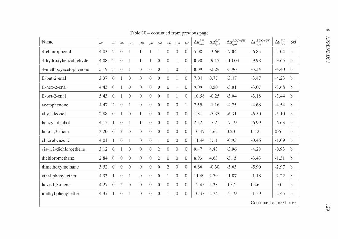
8APPEN
DIX1
129
Table 20 – continued from previous page
Name ρV br db benz OH ph hal eth ald ket ΔμPWhyd ΔμGFhyd ΔμSDC+PWhyd ΔμSDC+GFhyd Δμ
exphyd Set
4-chlorophenol 4.03 2 0 1 1 1 1 0 0 0 5.08 -3.66 -7.04 -6.85 -7.04 b
4-hydroxybenzaldehyde 4.08 2 0 1 1 1 0 0 1 0 0.98 -9.15 -10.03 -9.98 -9.65 b
4-methoxyacetophenone 5.19 3 0 1 0 0 0 1 0 1 8.09 -2.29 -5.96 -5.34 -4.40 b
E-but-2-enal 3.37 0 1 0 0 0 0 0 1 0 7.04 0.77 -3.47 -3.47 -4.23 b
E-hex-2-enal 4.43 0 1 0 0 0 0 0 1 0 9.09 0.50 -3.01 -3.07 -3.68 b
E-oct-2-enal 5.43 0 1 0 0 0 0 0 1 0 10.58 -0.25 -3.04 -3.18 -3.44 b
acetophenone 4.47 2 0 1 0 0 0 0 0 1 7.59 -1.16 -4.75 -4.68 -4.54 b
allyl alcohol 2.88 0 1 0 1 0 0 0 0 0 1.81 -5.35 -6.31 -6.50 -5.10 b
benzyl alcohol 4.12 1 0 1 1 0 0 0 0 0 2.52 -7.21 -7.19 -6.99 -6.63 b
buta-1,3-diene 3.20 0 2 0 0 0 0 0 0 0 10.47 5.62 0.20 0.12 0.61 b
chlorobenzene 4.01 1 0 1 0 0 1 0 0 0 11.44 5.11 -0.93 -0.46 -1.09 b
cis-1,2-dichloroethene 3.12 0 1 0 0 0 2 0 0 0 9.47 4.83 -3.96 -4.28 -0.93 b
dichloromethane 2.84 0 0 0 0 0 2 0 0 0 8.93 4.63 -3.15 -3.43 -1.31 b
dimethoxymethane 3.52 0 0 0 0 0 0 2 0 0 6.66 -0.30 -5.63 -5.90 -2.97 b
ethyl phenyl ether 4.93 1 0 1 0 0 0 1 0 0 11.49 2.79 -1.87 -1.18 -2.22 b
hexa-1,5-diene 4.27 0 2 0 0 0 0 0 0 0 12.45 5.28 0.57 0.46 1.01 b
methyl phenyl ether 4.37 1 0 1 0 0 0 1 0 0 10.33 2.74 -2.19 -1.59 -2.45 b
Continued on next page
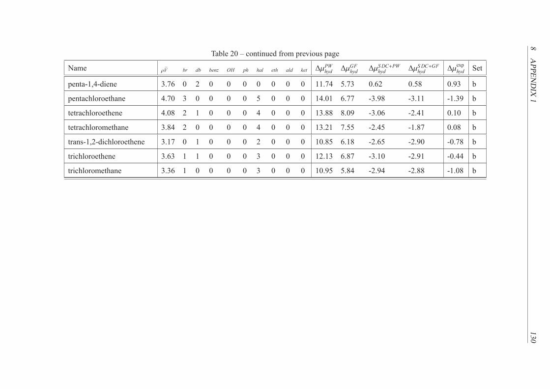
8APPEN
DIX1
130
Table 20 – continued from previous page
Name ρV br db benz OH ph hal eth ald ket ΔμPWhyd ΔμGFhyd ΔμSDC+PWhyd ΔμSDC+GFhyd Δμ
exphyd Set
penta-1,4-diene 3.76 0 2 0 0 0 0 0 0 0 11.74 5.73 0.62 0.58 0.93 b
pentachloroethane 4.70 3 0 0 0 0 5 0 0 0 14.01 6.77 -3.98 -3.11 -1.39 b
tetrachloroethene 4.08 2 1 0 0 0 4 0 0 0 13.88 8.09 -3.06 -2.41 0.10 b
tetrachloromethane 3.84 2 0 0 0 0 4 0 0 0 13.21 7.55 -2.45 -1.87 0.08 b
trans-1,2-dichloroethene 3.17 0 1 0 0 0 2 0 0 0 10.85 6.18 -2.65 -2.90 -0.78 b
trichloroethene 3.63 1 1 0 0 0 3 0 0 0 12.13 6.87 -3.10 -2.91 -0.44 b
trichloromethane 3.36 1 0 0 0 0 3 0 0 0 10.95 5.84 -2.94 -2.88 -1.08 b

8APPEN
DIX1
131
Table 21: Composition of the training and test sets. The
SDC model descriptors for molecules. Experimental HFEs
(Δμexp) [34, 101, 164, 35, 33, 45, 165] and corresponding
values calculated by 1D and 3D RISM with the PLHNC clo-
sure using the GF free energy expression as well as corre-
sponding 1D and 3D RISM-SDC models based on this ex-
pression (kcal/mol). Solutes parameters are: AM1-BCC par-
tial charges and GAFF LJ parameters
Name D1 D2 D3 D4 D5 D6 D7 D8 D9 ΔμRIS M−GF ΔμRIS M−SDC Δμexp
ρV br db benz OH hal ald ket eth 1D 3D 1D 3D
Training Set
2,2,4-trimethylpentane 4.87 3 0 0 0 0 0 0 0 5.09 15.28 2.47 2.83 2.87
2,2,5-trimethylhexane 5.40 3 0 0 0 0 0 0 0 4.45 23.90 2.70 3.07 2.79
2,2-dimethylbutane 4.16 2 0 0 0 0 0 0 0 4.74 21.04 2.85 2.50 2.57
2,4-dimethylpentane 4.66 2 0 0 0 0 0 0 0 4.90 18.19 3.04 2.70 2.87
2-methylbutane 3.88 1 0 0 0 0 0 0 0 5.30 12.43 2.79 2.34 2.38
2-methylhexane 4.89 1 0 0 0 0 0 0 0 0.00 25.89 3.09 2.70 2.93
n-decane 6.57 0 0 0 0 0 0 0 0 -0.27 28.97 3.20 3.21 3.16
Continued on next page

8APPEN
DIX1
132
Table 21 – continued from previous page
Name D1 D2 D3 D4 D5 D6 D7 D8 D9 ΔμRIS M−GF ΔμRIS M−SDC Δμexp
ρV br db benz OH hal ald ket eth 1D 3D 1D 3D
n-hexane 4.55 0 0 0 0 0 0 0 0 2.85 20.41 2.49 2.55 2.50
n-octane 5.55 0 0 0 0 0 0 0 0 2.57 23.39 2.84 2.86 2.89
n-pentane 4.01 0 0 0 0 0 0 0 0 4.58 15.24 2.07 2.39 2.36
propane 3.02 0 0 0 0 0 0 0 0 4.91 12.36 1.76 2.14 1.97
3-methylbut-1-ene 3.84 1 1 0 0 0 0 0 0 -4.25 12.88 2.28 1.53 1.82
but-1-ene 3.42 0 1 0 0 0 0 0 0 4.84 17.77 0.96 1.37 1.37
hept-1-ene 4.95 0 1 0 0 0 0 0 0 4.20 23.56 1.74 1.84 1.66
hex-1-ene 4.43 0 1 0 0 0 0 0 0 5.28 16.49 1.45 1.67 1.64
non-1-ene 5.97 0 1 0 0 0 0 0 0 -3.72 12.84 2.14 2.15 2.06
ethylbenzene 4.60 1 0 1 0 0 0 0 0 -1.61 11.79 -0.62 -0.77 -0.73
n-butylbenzene 5.59 1 0 1 0 0 0 0 0 -5.13 16.21 -0.43 -0.35 -0.40
n-hexylbenzene 6.59 1 0 1 0 0 0 0 0 -1.50 2.81 -0.16 -0.03 -0.04
n-pentylbenzene 6.08 1 0 1 0 0 0 0 0 6.16 13.55 -0.37 -0.20 -0.23
n-propylbenzene 5.11 1 0 1 0 0 0 0 0 -2.63 10.05 -0.35 -0.58 -0.53
2-methylbutan-1-ol 3.81 1 0 0 1 0 0 0 0 -3.45 10.42 -4.55 -4.39 -4.42
3-methylbutan-1-ol 3.83 1 0 0 1 0 0 0 0 -0.80 8.82 -4.00 -4.49 -4.42
Continued on next page

8APPEN
DIX1
133
Table 21 – continued from previous page
Name D1 D2 D3 D4 D5 D6 D7 D8 D9 ΔμRIS M−GF ΔμRIS M−SDC Δμexp
ρV br db benz OH hal ald ket eth 1D 3D 1D 3D
4-methylpentan-2-ol 4.27 2 0 0 1 0 0 0 0 -1.19 8.71 -3.20 -3.93 -3.74
butan-1-ol 3.48 0 0 0 1 0 0 0 0 5.18 9.46 -5.04 -4.67 -4.72
butan-2-ol 3.43 1 0 0 1 0 0 0 0 -4.14 27.33 -4.10 -4.39 -4.60
decan-1-ol 6.54 0 0 0 1 0 0 0 0 1.73 23.95 -3.69 -3.72 -3.64
ethanol 2.41 0 0 0 1 0 0 0 0 2.58 18.20 -6.03 -4.99 -5.00
heptan-1-ol 5.03 0 0 0 1 0 0 0 0 2.10 12.28 -4.17 -4.19 -4.23
1-chlorobutane 3.93 0 0 0 0 1 0 0 0 -0.16 18.58 -0.50 -0.14 -0.16
1-chloroheptane 5.47 0 0 0 0 1 0 0 0 -2.62 4.31 0.29 0.33 0.29
1-chlorohexane 4.96 0 0 0 0 1 0 0 0 2.06 16.71 0.11 0.19 0.00
1-chloropentane 4.44 0 0 0 0 1 0 0 0 5.51 22.17 -0.21 0.04 -0.07
1-chloropropane 3.42 0 0 0 0 1 0 0 0 -3.21 18.68 -0.77 -0.29 -0.30
2-chlorobutane 3.87 1 0 0 0 1 0 0 0 5.70 19.27 0.73 -0.24 0.00
2-chloropropane 3.39 1 0 0 0 1 0 0 0 -1.05 14.66 0.61 -0.47 -0.25
chloroethane 2.89 0 0 0 0 1 0 0 0 -1.40 8.77 -1.38 -0.55 -0.63
acetaldehyde 2.39 0 0 0 0 0 1 0 0 1.67 9.29 -4.54 -3.61 -3.51
butyraldehyde 3.47 0 0 0 0 0 1 0 0 1.33 22.56 -3.24 -3.10 -3.18
Continued on next page

8APPEN
DIX1
134
Table 21 – continued from previous page
Name D1 D2 D3 D4 D5 D6 D7 D8 D9 ΔμRIS M−GF ΔμRIS M−SDC Δμexp
ρV br db benz OH hal ald ket eth 1D 3D 1D 3D
isobutyraldehyde 3.42 1 0 0 0 0 1 0 0 4.55 32.31 -1.69 -3.10 -2.86
pentanal 3.97 0 0 0 0 0 1 0 0 5.72 20.77 -2.96 -2.92 -3.03
propionaldehyde 2.95 0 0 0 0 0 1 0 0 0.66 28.32 -3.59 -3.28 -3.44
3-methylbutan-2-one 3.89 1 0 0 0 0 0 1 0 5.14 26.45 -2.60 -3.35 -3.25
butanone 3.53 0 0 0 0 0 0 1 0 5.79 17.87 -3.93 -3.67 -3.71
hexan-2-one 4.55 0 0 0 0 0 0 1 0 0.93 25.44 -3.22 -3.26 -3.29
pentan-2-one 4.04 0 0 0 0 0 0 1 0 1.85 19.62 -3.59 -3.45 -3.52
pentan-3-one 4.06 0 0 0 0 0 0 1 0 4.96 27.92 -3.11 -3.26 -3.41
propanone 2.99 0 0 0 0 0 0 1 0 -0.93 11.76 -4.52 -3.98 -3.80
di-n-butyl ether 5.84 0 0 0 0 0 0 0 1 -0.49 11.91 -0.49 -0.81 -0.83
di-n-propyl ether 4.86 0 0 0 0 0 0 0 1 -1.39 11.62 -0.55 -1.13 -1.16
diethyl ether 3.78 0 0 0 0 0 0 0 1 6.41 12.30 -2.04 -1.59 -1.60
diisopropyl ether 4.54 2 0 0 0 0 0 0 1 -0.89 5.81 0.01 -0.87 -0.53
methylethyl ether 3.15 0 0 0 0 0 0 0 1 -1.06 5.83 -3.06 -1.73 -2.01
Test Set
2,2-dimethylpentane 4.64 2 0 0 0 0 0 0 0 6.82 20 2.72 2.70 2.88
Continued on next page

8APPEN
DIX1
135
Table 21 – continued from previous page
Name D1 D2 D3 D4 D5 D6 D7 D8 D9 ΔμRIS M−GF ΔμRIS M−SDC Δμexp
ρV br db benz OH hal ald ket eth 1D 3D 1D 3D
2,3,4-trimethylpentane 4.83 3 0 0 0 0 0 0 0 7.22 20.20 2.66 2.70 2.56
2,3-dimethylpentane 4.58 2 0 0 0 0 0 0 0 5.78 17.48 2.66 2.57 2.52
2-methylpentane 4.37 1 0 0 0 0 0 0 0 1.04 18.93 2.86 2.52 2.52
3-methylhexane 4.82 1 0 0 0 0 0 0 0 7.34 20.25 2.64 2.67 2.71
3-methylpentane 4.31 1 0 0 0 0 0 0 0 6.43 18.01 2.50 2.52 2.51
ethane 2.48 0 0 0 0 0 0 0 0 1.89 19.34 1.20 2.06 1.84
methane 1.83 0 0 0 0 0 0 0 0 4.71 14.95 -0.35 2.08 1.97
n-butane 3.49 0 0 0 0 0 0 0 0 -0.99 10.72 1.80 2.22 2.09
n-heptane 5.06 0 0 0 0 0 0 0 0 6.85 18.36 2.72 2.71 2.63
n-nonane 6.05 0 0 0 0 0 0 0 0 1.77 19.50 3.00 3.02 3.14
2-methylbut-2-ene 3.90 1 1 0 0 0 0 0 0 5.30 15.40 2.61 1.18 1.31
oct-1-ene 5.46 0 1 0 0 0 0 0 0 5.34 15.40 2.00 1.98 2.08
pent-1-ene 3.93 0 1 0 0 0 0 0 0 2.26 23.32 1.28 1.52 1.66
propene 2.87 0 1 0 0 0 0 0 0 0.23 25.58 0.42 1.19 1.29
trans-hept-2-ene 5.01 0 1 0 0 0 0 0 0 4.53 16.63 2.16 1.68 1.67
1,2,3-trimethylbenzene 4.94 3 0 1 0 0 0 0 0 2.26 23.03 2.28 -1.02 -1.21
Continued on next page

8APPEN
DIX1
136
Table 21 – continued from previous page
Name D1 D2 D3 D4 D5 D6 D7 D8 D9 ΔμRIS M−GF ΔμRIS M−SDC Δμexp
ρV br db benz OH hal ald ket eth 1D 3D 1D 3D
1,2,4-trimethylbenzene 5.08 3 0 1 0 0 0 0 0 -4.54 13.78 3.26 -0.89 -0.83
1,3,5-trimethylbenzene 5.11 3 0 1 0 0 0 0 0 -3.92 14.07 3.17 -0.93 -0.90
2-ethyltoluene 4.93 2 0 1 0 0 0 0 0 -4.84 13.46 0.31 -1.03 -1.04
4-ethyltoluene 5.15 2 0 1 0 0 0 0 0 -4.71 13.74 1.80 -0.62 -0.95
isobutylbenzene 5.34 2 0 1 0 0 0 0 0 -5.29 14.59 -0.61 -0.15 0.16
m-xylene 4.65 2 0 1 0 0 0 0 0 3.79 16.06 1.62 -1 -0.82
o-xylene 4.55 2 0 1 0 0 0 0 0 -5.21 8.74 0.93 -1.08 -0.90
p-xylene 4.69 2 0 1 0 0 0 0 0 0.88 18.83 2.02 -1.01 -0.80
sec-butylbenzene 5.35 2 0 1 0 0 0 0 0 5.56 16.06 -0.51 -0.38 -0.45
tert-butylbenzene 5.15 3 0 1 0 0 0 0 0 5.38 14.19 -0.33 -0.61 -0.44
2-methylbutan-2-ol 3.79 2 0 0 1 0 0 0 0 -4.58 13.44 -3.10 -4.05 -4.43
2-methylpentan-2-ol 4.28 2 0 0 1 0 0 0 0 -4.92 16.41 -2.98 -3.81 -3.93
2-methylpentan-3-ol 4.25 2 0 0 1 0 0 0 0 -4.74 16.26 -2.82 -3.81 -3.89
2-methylpropan-1-ol 3.39 1 0 0 1 0 0 0 0 4.45 20.67 -3.98 -4.54 -4.51
hexan-1-ol 4.52 0 0 0 1 0 0 0 0 -3.28 10.14 -4.40 -4.35 -4.39
hexan-3-ol 4.46 1 0 0 1 0 0 0 0 1.60 17.69 -3.36 -3.88 -4.07
Continued on next page

8APPEN
DIX1
137
Table 21 – continued from previous page
Name D1 D2 D3 D4 D5 D6 D7 D8 D9 ΔμRIS M−GF ΔμRIS M−SDC Δμexp
ρV br db benz OH hal ald ket eth 1D 3D 1D 3D
methanol 1.78 0 0 0 1 0 0 0 0 -6.34 12.24 -7.49 -5.16 -5.11
nonan-1-ol 6.04 0 0 0 1 0 0 0 0 -5.12 11.74 -3.82 -3.88 -3.89
octan-1-ol 5.54 0 0 0 1 0 0 0 0 -5.18 13.04 -3.99 -4.04 -4.09
pentan-1-ol 3.99 0 0 0 1 0 0 0 0 -3.15 9.87 -4.76 -4.52 -4.52
pentan-2-ol 3.94 1 0 0 1 0 0 0 0 -10.14 5.78 -3.69 -4.17 -4.39
pentan-3-ol 3.91 1 0 0 1 0 0 0 0 -6.86 9.31 -4.45 -4.64 -4.35
propan-1-ol 2.97 0 0 0 1 0 0 0 0 3.82 23.40 -5.23 -4.80 -4.83
propan-2-ol 2.94 1 0 0 1 0 0 0 0 4.16 20.54 -4.10 -4.88 -4.76
2,3-dimethylphenol 4.52 3 0 1 1 0 0 0 0 -7.19 14.62 -1.87 -5.70 -6.16
2,4-dimethylphenol 4.64 3 0 1 1 0 0 0 0 -3.56 12.64 -1.14 -5.63 -6.01
2,5-dimethylphenol 4.64 3 0 1 1 0 0 0 0 -3.16 9.91 -2.06 -6.16 -5.92
2,6-dimethylphenol 4.55 3 0 1 1 0 0 0 0 2.17 19.73 -2.03 -5.64 -5.27
3,4-dimethylphenol 4.56 3 0 1 1 0 0 0 0 -10.48 5.32 -2.49 -6.42 -6.51
4-n-propylphenol 5.11 2 0 1 1 0 0 0 0 -2.27 14.71 -3.76 -5.91 -5.91
4-tert-butylphenol 5.15 4 0 1 1 0 0 0 0 -5.17 16.39 -3.80 -5.95 -5.95
o-cresol 4.12 2 0 1 1 0 0 0 0 -8.84 18.62 -3.31 -5.74 -5.88
Continued on next page

8APPEN
DIX1
138
Table 21 – continued from previous page
Name D1 D2 D3 D4 D5 D6 D7 D8 D9 ΔμRIS M−GF ΔμRIS M−SDC Δμexp
ρV br db benz OH hal ald ket eth 1D 3D 1D 3D
heptanal 5 0 0 0 0 0 1 0 0 -0.90 7.12 -2.45 -2.62 -2.67
hexanal 4.49 0 0 0 0 0 1 0 0 -0.95 13.02 -2.74 -2.79 -2.81
nonanal 6.01 0 0 0 0 0 1 0 0 -1.57 18.75 -2.13 -2.31 -2.07
octanal 5.51 0 0 0 0 0 1 0 0 -3.45 11.54 -2.25 -2.45 -2.29
4-methylpentan-2-one 4.38 1 0 0 0 0 0 1 0 -3.32 5.01 -2.80 -3.13 -3.05
decan-2-one 6.56 0 0 0 0 0 0 1 0 -6.86 8.63 -2.61 -2.62 -2.34
heptan-2-one 5.05 0 0 0 0 0 0 1 0 5.89 11.64 -3.08 -3.08 -3.04
nonan-2-one 6.07 0 0 0 0 0 0 1 0 4.06 13.10 -2.64 -2.77 -2.50
nonan-5-one 6.08 0 0 0 0 0 0 1 0 -2.31 26.18 -2.19 -2.50 -2.65
octan-2-one 5.56 0 0 0 0 0 0 1 0 -1.78 8.07 -2.81 -2.94 -2.88
undecan-2-one 7.06 0 0 0 0 0 0 1 0 6.36 9.52 -2.44 -2.44 -2.16
1,2,3,4-tetrachloro-benzene 5.32 4 0 1 0 4 0 0 0 0.67 16.01 3.07 -3.33 -1.34
1,2,3,5-tetrachloro-benzene 5.33 4 0 1 0 4 0 0 0 -1.38 17.56 3.47 -3.06 -1.62
1,2,3-trichlorobenzene 4.88 3 0 1 0 3 0 0 0 -1.84 17.36 1.60 -2.89 -1.24
1,2,4,5-tetrachloro-benzene 5.36 4 0 1 0 4 0 0 0 5.75 17.76 3.62 -3.09 -1.34
1,2,4-trichlorobenzene 4.96 3 0 1 0 3 0 0 0 -2.97 15.82 2.33 -2.56 -1.12
Continued on next page

8APPEN
DIX1
139
Table 21 – continued from previous page
Name D1 D2 D3 D4 D5 D6 D7 D8 D9 ΔμRIS M−GF ΔμRIS M−SDC Δμexp
ρV br db benz OH hal ald ket eth 1D 3D 1D 3D
1,2-dichlorobenzene 4.42 2 0 1 0 2 0 0 0 -3.67 16.36 0.09 -2.38 -1.41
1,2-dimethoxyethane 3.79 0 0 0 0 0 0 0 1 -1.65 14.47 -5.11 -3.57 -4.84
1,3,5-trichlorobenzene 4.97 3 0 1 0 3 0 0 0 -0.43 22.72 2.76 -2.20 -0.78
1,3-dichlorobenzene 4.46 2 0 1 0 2 0 0 0 2.45 16.58 0.72 -2.03 -0.98
1,4-dichlorobenzene 4.48 2 0 1 0 2 0 0 0 5.41 6.79 0.77 -2.07 -1.01
2,3-dimethylbuta-1,3-diene 4.10 2 2 0 0 0 0 0 0 -3.50 1.28 2.65 0.04 0.40
2-butoxyethanol 4.72 0 0 0 1 0 0 0 1 0.48 12.89 -6.74 -6.56 -6.26
2-chlorotoluene 4.54 2 0 1 0 1 0 0 0 6.01 14.94 1.07 -1.45 -1.14
2-ethoxyethanol 3.68 0 0 0 1 0 0 0 1 5.48 23.64 -7.62 -6.96 -6.70
2-methylbuta-1,3-diene 3.70 1 2 0 0 0 0 0 0 4.83 29.35 1.34 0.14 0.68
2-methylstyrene 4.89 2 1 1 0 0 0 0 0 -3.80 24.44 0.08 -1.61 -1.24
2-phenylethanol 4.55 1 0 1 1 0 0 0 0 -1.88 23.32 -7.25 -7.06 -6.80
2-propoxyethanol 4.20 0 0 0 1 0 0 0 1 -1.44 23.55 -7.05 -6.69 -6.41
3-chlorophenol 4.02 2 0 1 1 1 0 0 0 -2.46 23.11 -4.54 -6.89 -6.61
3-hydroxybenzaldehyde 4.01 2 0 1 1 0 1 0 0 -3.80 11.09 -7.55 -9.94 -9.51
3-methoxyphenol 4.22 2 0 1 1 0 0 0 1 1.87 16.27 -6.46 -8.41 -7.66
Continued on next page

8APPEN
DIX1
140
Table 21 – continued from previous page
Name D1 D2 D3 D4 D5 D6 D7 D8 D9 ΔμRIS M−GF ΔμRIS M−SDC Δμexp
ρV br db benz OH hal ald ket eth 1D 3D 1D 3D
3-phenylpropanol 5.05 1 0 1 1 0 0 0 0 5.28 25.04 -7.63 -7.42 -6.93
4-chloro-3-methyl- phenol 4.50 3 0 1 1 1 0 0 0 -3.50 21.56 -2.70 -6.87 -6.79
4-chlorophenol 4.05 2 0 1 1 1 0 0 0 -1.58 20.42 -4.52 -6.97 -7.04
4-hydroxybenzaldehyde 4.01 2 0 1 1 0 1 0 0 -2.11 20.25 -7.89 -10.39 -9.65
E-but-2-enal 3.37 0 1 0 0 0 1 0 0 2.81 16.58 -3.95 -4.04 -4.23
E-hex-2-enal 4.41 0 1 0 0 0 1 0 0 6.00 16.41 -3.02 -3.59 -3.68
E-oct-2-enal 5.40 0 1 0 0 0 1 0 0 6.17 14.99 -2.73 -3.30 -3.44
acetophenone 4.52 1 0 1 0 0 0 1 0 -2.83 12.91 -5.15 -5.32 -4.54
allyl alcohol 2.83 0 1 0 1 0 0 0 0 -3.51 13.36 -7.25 -6.26 -5.10
benzyl alcohol 4.05 1 0 1 1 0 0 0 0 -4.25 12.87 -8.24 -7.81 -6.63
buta-1,3-diene 3.25 0 2 0 0 0 0 0 0 -2.35 7.21 -0.38 0.23 0.61
chlorobenzenes 4.04 1 0 1 0 1 0 0 0 -2.99 7.27 -0.92 -1.59 -1.09
dimethoxymethane 3.26 0 0 0 0 0 0 0 2 6.13 10.62 -6.60 -3.91 -2.97
ethyl phenyl ether 4.88 1 0 1 0 0 0 0 1 -0.33 22.32 -1.94 -2.76 -2.22
hexa-1,5-diene 4.31 0 2 0 0 0 0 0 0 -1.77 21.83 0.47 0.85 1.01
methyl phenyl ether 4.29 1 0 1 0 0 0 0 1 5.87 22.05 -2.68 -2.99 -2.45
Continued on next page
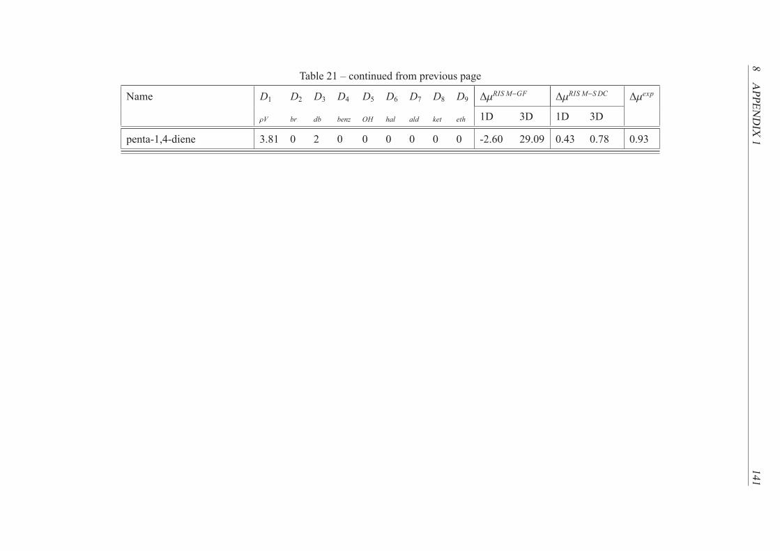
8APPEN
DIX1
141
Table 21 – continued from previous page
Name D1 D2 D3 D4 D5 D6 D7 D8 D9 ΔμRIS M−GF ΔμRIS M−SDC Δμexp
ρV br db benz OH hal ald ket eth 1D 3D 1D 3D
penta-1,4-diene 3.81 0 2 0 0 0 0 0 0 -2.60 29.09 0.43 0.78 0.93
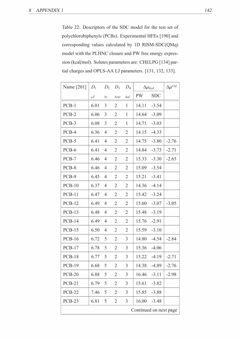
8 APPENDIX 1 142
Table 22: Descriptors of the SDC model for the test set of
polychlorobiphenyls (PCBs). Experimental HFEs [190] and
corresponding values calculated by 1D RISM-SDC(QMq)
model with the PLHNC closure and PW free energy expres-
sion (kcal/mol). Solutes parameters are: CHELPG [134] par-
tial charges and OPLS-AA LJ parameters. [131, 132, 133].
Name [201] D1 D2 D3 D4 Δμhyd Δμexp
ρV br benz hal PW SDC
PCB-1 6.01 3 2 1 14.11 -3.54
PCB-2 6.06 3 2 1 14.64 -3.09
PCB-3 6.08 3 2 1 14.71 -3.03
PCB-4 6.36 4 2 2 14.15 -4.33
PCB-5 6.41 4 2 2 14.75 -3.80 -2.76
PCB-6 6.41 4 2 2 14.84 -3.73 -2.71
PCB-7 6.46 4 2 2 15.33 -3.30 -2.65
PCB-8 6.46 4 2 2 15.09 -3.54
PCB-9 6.45 4 2 2 15.21 -3.41
PCB-10 6.37 4 2 2 14.36 -4.14
PCB-11 6.47 4 2 2 15.42 -3.24
PCB-12 6.49 4 2 2 15.60 -3.07 -3.05
PCB-13 6.48 4 2 2 15.48 -3.19
PCB-14 6.49 4 2 2 15.76 -2.91
PCB-15 6.50 4 2 2 15.59 -3.10
PCB-16 6.72 5 2 3 14.80 -4.54 -2.84
PCB-17 6.78 5 2 3 15.36 -4.06
PCB-18 6.77 5 2 3 15.22 -4.19 -2.71
PCB-19 6.68 5 2 3 14.38 -4.89 -2.76
PCB-20 6.88 5 2 3 16.46 -3.11 -2.98
PCB-21 6.79 5 2 3 15.61 -3.82
PCB-22 7.46 5 2 3 15.85 -3.88
PCB-23 6.81 5 2 3 16.00 -3.48
Continued on next page

8 APPENDIX 1 143
Table 22 – continued from previous page
Name [201] D1 D2 D3 D4 Δμhyd Δμexp
ρV br benz hal PW SDC
PCB-24 6.75 5 2 3 15.17 -4.21 -2.79
PCB-25 6.84 5 2 3 16.02 -3.49
PCB-26 6.83 5 2 3 15.93 -3.57 -2.84
PCB-27 6.77 5 2 3 15.15 -4.25
PCB-28 6.88 5 2 3 16.27 -3.30 -2.84
PCB-29 6.82 5 2 3 16.14 -3.34
PCB-30 6.79 5 2 3 15.79 -3.65
PCB-31 6.87 5 2 3 16.05 -3.50 -3.26
PCB-32 6.78 5 2 3 15.18 -4.23
PCB-33 6.82 5 2 3 15.72 -3.77
PCB-34 6.83 5 2 3 15.92 -3.57
PCB-35 6.86 5 2 3 16.23 -3.32
PCB-36 6.87 5 2 3 16.48 -3.07 -2.94
PCB-37 6.88 5 2 3 16.30 -3.27 -3.26
PCB-38 6.84 5 2 3 16.27 -3.24
PCB-39 6.88 5 2 3 16.47 -3.10
PCB-40 7.09 6 2 4 15.38 -4.82 -3.26
PCB-41 7.10 6 2 4 15.63 -4.58 -3.05
PCB-42 7.14 6 2 4 15.96 -4.32 -3.05
PCB-43 7.13 6 2 4 15.98 -4.27
PCB-44 7.13 6 2 4 15.77 -4.49
PCB-45 7.05 6 2 4 15.22 -4.92
PCB-46 7.04 6 2 4 14.99 -5.13
PCB-47 7.20 6 2 4 16.53 -3.83 -2.88
PCB-48 7.16 6 2 4 16.25 -4.05
PCB-49 7.82 6 2 4 16.15 -4.03
PCB-50 7.09 6 2 4 15.85 -4.35
PCB-51 7.09 6 2 4 15.56 -4.63
Continued on next page

8 APPENDIX 1 144
Table 22 – continued from previous page
Name [201] D1 D2 D3 D4 Δμhyd Δμexp
ρV br benz hal PW SDC
PCB-52 7.17 6 2 4 16.18 -4.14 -2.84
PCB-53 7.08 6 2 4 15.43 -4.76
PCB-54 6.98 6 2 4 14.68 -5.35
PCB-55 7.17 6 2 4 16.28 -4.03
PCB-56 7.17 6 2 4 16.21 -4.11
PCB-57 7.21 6 2 4 16.67 -3.71 -3.15
PCB-58 7.20 6 2 4 16.47 -3.89
PCB-59 7.14 6 2 4 15.94 -4.33
PCB-60 7.21 6 2 4 16.57 -3.80
PCB-61 7.15 6 2 4 16.37 -3.91
PCB-62 7.13 6 2 4 16.18 -4.08 -2.82
PCB-63 7.23 6 2 4 16.80 -3.60
PCB-64 7.16 6 2 4 16.04 -4.25
PCB-65 7.12 6 2 4 16.08 -4.16
PCB-66 7.23 6 2 4 16.81 -3.59
PCB-67 7.22 6 2 4 16.90 -3.49 -3.26
PCB-68 7.25 6 2 4 17.03 -3.40
PCB-69 7.19 6 2 4 16.52 -3.82
PCB-70 7.21 6 2 4 16.65 -3.73 -3.26
PCB-71 7.14 6 2 4 15.90 -4.37
PCB-72 7.24 6 2 4 16.85 -3.57
PCB-73 7.15 6 2 4 16.16 -4.14
PCB-74 7.26 6 2 4 17.06 -3.38 -3.26
PCB-75 7.20 6 2 4 16.62 -3.74
PCB-76 7.17 6 2 4 16.32 -3.99
PCB-77 7.25 6 2 4 17.02 -3.41
PCB-78 7.22 6 2 4 16.92 -3.48
PCB-79 7.26 6 2 4 17.21 -3.24
Continued on next page

8 APPENDIX 1 145
Table 22 – continued from previous page
Name [201] D1 D2 D3 D4 Δμhyd Δμexp
ρV br benz hal PW SDC
PCB-80 7.27 6 2 4 17.44 -3.02
PCB-81 7.24 6 2 4 17.04 -3.38
PCB-82 7.46 7 2 5 16.23 -4.84
PCB-83 7.49 7 2 5 16.59 -4.52
PCB-84 7.41 7 2 5 15.82 -5.16
PCB-85 7.52 7 2 5 16.80 -4.35 -3.50
PCB-86 7.46 7 2 5 16.41 -4.65
PCB-87 7.51 7 2 5 16.62 -4.51 -3.43
PCB-88 7.42 7 2 5 16.24 -4.77
PCB-89 7.40 7 2 5 15.80 -5.18
PCB-90 7.54 7 2 5 17.12 -4.07
PCB-91 7.46 7 2 5 16.40 -4.66
PCB-92 7.53 7 2 5 16.98 -4.19
PCB-93 7.42 7 2 5 16.23 -4.77
PCB-94 7.44 7 2 5 16.26 -4.77
PCB-95 7.46 7 2 5 16.29 -4.77
PCB-96 7.35 7 2 5 15.46 -5.43
PCB-97 7.52 7 2 5 16.75 -4.40 -3.43
PCB-98 7.45 7 2 5 16.41 -4.64
PCB-99 7.57 7 2 5 17.29 -3.93
PCB-100 7.51 7 2 5 16.97 -4.16 -3.40
PCB-101 8.23 7 2 5 16.77 -4.11
PCB-102 7.46 7 2 5 16.45 -4.62 -3.32
PCB-103 7.50 7 2 5 16.87 -4.25
PCB-104 7.40 7 2 5 16.10 -4.88
PCB-105 7.55 7 2 5 17.10 -4.10
PCB-106 7.53 7 2 5 17.11 -4.06
PCB-107 7.58 7 2 5 17.37 -3.87
Continued on next page

8 APPENDIX 1 146
Table 22 – continued from previous page
Name [201] D1 D2 D3 D4 Δμhyd Δμexp
ρV br benz hal PW SDC
PCB-108 7.58 7 2 5 17.31 -3.92
PCB-109 7.52 7 2 5 16.94 -4.21
PCB-110 7.52 7 2 5 16.66 -4.49
PCB-111 7.60 7 2 5 17.58 -3.68
PCB-112 7.52 7 2 5 16.83 -4.31
PCB-113 7.53 7 2 5 16.93 -4.24
PCB-114 7.57 7 2 5 17.30 -3.92
PCB-115 7.54 7 2 5 17.08 -4.10
PCB-116 7.44 7 2 5 16.59 -4.44
PCB-117 7.53 7 2 5 17.01 -4.15
PCB-118 7.61 7 2 5 17.65 -3.63
PCB-119 7.57 7 2 5 17.28 -3.94
PCB-120 7.61 7 2 5 17.82 -3.46 -3.60
PCB-121 7.58 7 2 5 17.57 -3.67
PCB-122 7.54 7 2 5 16.86 -4.32
PCB-123 7.59 7 2 5 17.46 -3.79
PCB-124 7.56 7 2 5 17.30 -3.92
PCB-125 7.48 7 2 5 16.47 -4.63
PCB-126 7.62 7 2 5 17.74 -3.55
PCB-127 7.63 7 2 5 17.94 -3.36
PCB-128 7.81 8 2 6 18.03 -3.86
PCB-129 7.82 8 2 6 17.00 -4.92 -3.99
PCB-130 7.87 8 2 6 17.39 -4.59 -3.84
PCB-131 7.82 8 2 6 17.23 -4.69
PCB-132 7.88 8 2 6 17.78 -4.22 -3.74
PCB-133 7.54 8 2 6 17.13 -4.06
PCB-134 7.78 8 2 6 16.76 -5.09 -3.68
PCB-135 8.28 8 2 6 18.43 -4.48 -3.60
Continued on next page

8 APPENDIX 1 147
Table 22 – continued from previous page
Name [201] D1 D2 D3 D4 Δμhyd Δμexp
ρV br benz hal PW SDC
PCB-136 7.71 8 2 6 16.24 -5.52
PCB-137 7.87 8 2 6 17.52 -4.46
PCB-138 7.89 8 2 6 17.57 -4.45 -4.18
PCB-139 7.86 8 2 6 17.26 -4.71
PCB-140 7.82 8 2 6 17.21 -4.70
PCB-141 7.86 8 2 6 17.35 -4.63 -4.13
PCB-142 8.39 8 2 6 17.56 -5.83
PCB-143 7.76 8 2 6 16.60 -5.22
PCB-144 7.83 8 2 6 17.29 -4.63
PCB-145 7.72 8 2 6 16.47 -5.29
PCB-146 7.92 8 2 6 17.88 -4.18 -4.08
PCB-147 7.83 8 2 6 17.36 -4.57 -3.65
PCB-148 7.86 8 2 6 17.61 -4.35
PCB-149 7.84 8 2 6 17.22 -4.71
PCB-150 7.07 8 2 6 13.99 -6.81
PCB-151 7.82 8 2 6 17.23 -4.69 -3.57
PCB-152 7.72 8 2 6 16.46 -5.29
PCB-153 7.83 8 2 6 17.22 -4.70
PCB-154 7.88 8 2 6 17.78 -4.22
PCB-155 7.66 8 2 6 16.43 -5.25
PCB-156 7.92 8 2 6 17.83 -4.22
PCB-157 7.92 8 2 6 17.70 -4.36
PCB-158 7.90 8 2 6 17.70 -4.33
PCB-159 7.93 8 2 6 18.02 -4.06 -4.21
PCB-160 7.84 8 2 6 17.35 -4.58 -4.21
PCB-161 7.91 8 2 6 17.93 -4.11
PCB-162 7.35 8 2 6 15.46 -5.44
PCB-163 7.89 8 2 6 17.59 -4.43 -4.38
Continued on next page

8 APPENDIX 1 148
Table 22 – continued from previous page
Name [201] D1 D2 D3 D4 Δμhyd Δμexp
ρV br benz hal PW SDC
PCB-164 7.86 8 2 6 17.26 -4.71
PCB-165 7.91 8 2 6 17.90 -4.15 -3.99
PCB-166 7.85 8 2 6 17.47 -4.49
PCB-167 7.96 8 2 6 18.29 -3.82
PCB-168 7.91 8 2 6 17.86 -4.18
PCB-169 7.98 8 2 6 18.41 -3.74
PCB-170 8.19 9 2 7 17.78 -5.00 -4.68
PCB-171 8.15 9 2 7 17.62 -5.10
PCB-172 8.22 9 2 7 18.14 -4.69 -4.46
PCB-173 8.09 9 2 7 17.15 -5.48 -4.42
PCB-174 8.13 9 2 7 17.40 -5.29 -4.42
PCB-175 8.19 9 2 7 18.05 -4.71
PCB-176 8.08 9 2 7 17.24 -5.38
PCB-177 8.14 9 2 7 17.54 -5.17
PCB-178 8.18 9 2 7 17.95 -4.81 -4.13
PCB-179 8.08 9 2 7 17.23 -5.39 -4.10
PCB-180 8.25 9 2 7 18.36 -4.50 -4.62
PCB-181 8.15 9 2 7 17.75 -4.96
PCB-182 8.17 9 2 7 17.94 -4.80
PCB-183 8.21 9 2 7 18.22 -4.59
PCB-184 8.13 9 2 7 17.86 -4.83
PCB-185 8.14 9 2 7 17.60 -5.09 -4.34
PCB-186 7.04 9 2 7 13.46 -7.61
PCB-187 7.04 9 2 7 13.47 -7.60
PCB-188 8.13 9 2 7 17.84 -4.84
PCB-189 8.28 9 2 7 18.43 -4.47
PCB-190 8.21 9 2 7 18.02 -4.79
PCB-191 8.24 9 2 7 18.28 -4.57
Continued on next page

8 APPENDIX 1 149
Table 22 – continued from previous page
Name [201] D1 D2 D3 D4 Δμhyd Δμexp
ρV br benz hal PW SDC
PCB-192 8.23 9 2 7 18.27 -4.56
PCB-193 8.23 9 2 7 18.10 -4.74
PCB-194 8.55 10 2 8 18.51 -5.11
PCB-195 8.24 10 2 8 17.54 -5.63 -4.56
PCB-196 8.50 10 2 8 18.37 -5.18 -4.62
PCB-197 8.45 10 2 8 18.21 -5.27
PCB-198 8.49 10 2 8 18.32 -5.21 -4.42
PCB-199 8.50 10 2 8 18.30 -5.25 -4.62
PCB-200 8.39 10 2 8 17.56 -5.83
PCB-201 8.45 10 2 8 18.21 -5.27
PCB-202 8.45 10 2 8 18.17 -5.31 -4.27
PCB-203 8.52 10 2 8 18.54 -5.04
PCB-204 8.43 10 2 8 18.18 -5.27
PCB-205 8.56 10 2 8 18.59 -5.04
PCB-206 8.81 11 2 9 18.65 -5.67
PCB-207 8.75 11 2 9 18.52 -5.72
PCB-208 8.75 11 2 9 18.47 -5.77
PCB-209 8.88 12 2 10 17.70 -7.05

9 APPENDIX 2 150
9 Appendix 2
9.1 List of Abbreviations
1D one dimensional
3D three dimensional
6D six dimensional
AM1 Austin model 1
AM1-BCC Austin model 1 with bond charge correction
B3LYP Becke, three-parameter, Lee-Yang-Parr exchange-correlation functional
CHELPG charges from electrostatic potential using a grid method
COSMO-SAC conductor-like screening model – segment activity coefficient
DPMV dimensionless partial molar volume
DRISM dielectrically consistent reference interaction sites model
FT Fourier transformation
GAFF General Amber force field
GF Gaussian fluctuations
GSM gas stripping method
HFE hydration free energy
HNC hypernetted chain
HNCB hypernetted chain closure with repulsive bridge correction functions
HOMO highest occupied molecular orbital
IET integral equation theory
IFT inverse Fourier transformation
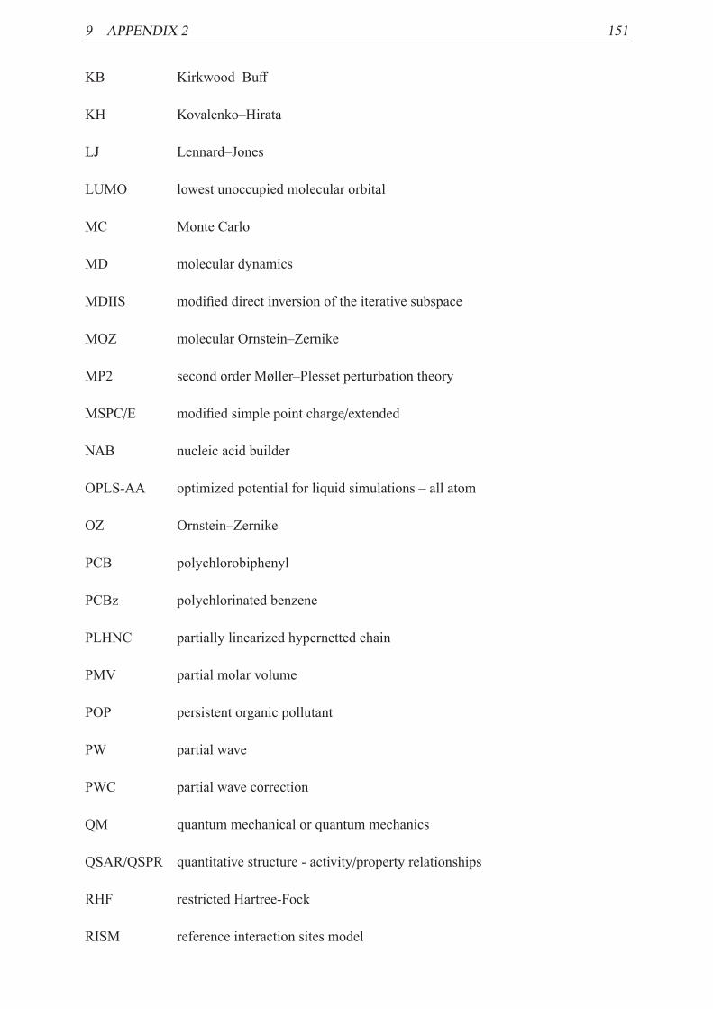
9 APPENDIX 2 151
KB Kirkwood–Buff
KH Kovalenko–Hirata
LJ Lennard–Jones
LUMO lowest unoccupied molecular orbital
MC Monte Carlo
MD molecular dynamics
MDIIS modified direct inversion of the iterative subspace
MOZ molecular Ornstein–Zernike
MP2 second order Møller–Plesset perturbation theory
MSPC/E modified simple point charge/extended
NAB nucleic acid builder
OPLS-AA optimized potential for liquid simulations – all atom
OZ Ornstein–Zernike
PCB polychlorobiphenyl
PCBz polychlorinated benzene
PLHNC partially linearized hypernetted chain
PMV partial molar volume
POP persistent organic pollutant
PW partial wave
PWC partial wave correction
QM quantum mechanical or quantum mechanics
QSAR/QSPR quantitative structure - activity/property relationships
RHF restricted Hartree-Fock
RISM reference interaction sites model

9 APPENDIX 2 152
rms root mean square
SASA solvent accessible surface area
SDC structural descriptors correction
SMx solvation model No. x
SMILES simplified molecular input line entry specification
SPC/E simple point charge/extended
SSOZ site-site Ornstein–Zernike
std standard deviation
TGM two-grid iteration method
UC universal correction
WWC wetted-wall column

9 APPENDIX 2 153
9.2 Short summary
We showed that the poor accuracy of hydration thermodynamics calculations with a molecular
integral equation theory, Reference Interaction Site Model (RISM), can be considerably im-
proved with a set of corrections associated with details of molecular structure. In this thesis we
developed a novel hybrid RISM-based method for calculation of hydration thermodynamics,
the Structural Descriptors Correction (SDC) model (RISM-SDC). The method uses a ther-
modynamic quantity obtained by RISM as an initial approximation and a set of corrections to
decrease the error of the calculated parameter. Each correction in the RISM-SDC model can
be represented as a structural descriptor (Di) multiplied by the corresponding correction coeffi-
cient (ai). One important descriptor (D1) is the dimensionless partial molar volume calculated
by RISM. The rest of the structural descriptors correspond to the number of specific molecu-
lar fragments (double bonds, aromatic rings, electron-donating/withdrawing substituents, etc.).
The correction coefficients ai are found by training the model on a set of monofunctional com-
pounds. For the first time, we showed that the RISM-SDCmodel allows to achieve the chemical
accuracy of solvation thermodynamics predictions within the RISM approach, that has been a
challenge for over 40 years [64, 112, 88, 116, 89, 85, 80]. In this thesis we demonstrated the
high efficiency of the proposed approach for predicting important hydration thermodynamic
quantities, hydration free energy (HFE) and partial molar volume (PMV).

9 APPENDIX 2 154
9.3 List of Publications
Reviewed Articles.
a) In press:
1. Palmer D. S., Chuev G. N., Ratkova E. L., Fedorov M. V. "In silico screening of bioactive
and biomimetic solutes by Integral Equation Theory", Curr. Pharm. Des. (accepted).
2. Palmer D. S., Frolov A. I., Ratkova E. L., Fedorov M. V. "Towards a Universal Model
to Calculate the Solvation Thermodynamics of Druglike Molecules: The Importance of
New Experimental Databases", Mol. Pharmaceutics (in press).
b) Published:
1. Ratkova E. L., Fedorov M. V. "Combination of RISM and Cheminformatics for Efficient
Predictions of Hydration Free Energy of Polyfragment Molecules: Application to a Set
of Organic Pollutants", J. Chem. Theory Comput. 2011, DOI: 10.1021/ct100654h.
2. Frolov A. I., Ratkova E. L. Palmer, D. S., Fedorov, M. V. "Hydration Thermodynamics
using the Reference Interaction Site Model: Speed or Accuracy?", J. Phys. Chem. B
2011, DOI: 10.1021/jp111271c.
3. Ratkova E. L., Chuev G. N., Sergiievskyi V. P., Fedorov M. V. "An Accurate Prediction
of Hydration Free Energies by Combination of Molecular Integral Equations Theory with
Structural Descriptors", J. Phys. Chem. B 2010, 114, 12068–12079.
4. Palmer D. S., Frolov A. I., Ratkova E. L., Fedorov M. V. "Towards a universal method to
calculate hydration free energies: a 3D reference interaction site model with partial molar
volume correction", J. Phys.: Condens. Matter 2010, 22, 492101.
5. Sheinin V. B., Semeikin A. S., Ratkova E. L., Lubimova T. V. "Synthesis and Investigation
of Basicity of Diporphyrin with Polyethylenoxide Spacer", Macroheterocycle, 2009, 2,
168–171.
6. Kochergina L. A., Ratkova E. L. "Thermodynamics of complex formation of cobalt(II)
ions with D,L-threonine in aqueous solutions", Russ. J. Coord. Chem., 2009, 1, 43–50.
7. Sheinin V. B., Ratkova E. L., Mamardashvili N. Zh. "pH-depending porphyrin based
receptor for bromide-ions selective binding", J. Porphyrins Phthalocyanines, 2008, 12,
1211–1219.

9 APPENDIX 2 155
8. Sheinin V. B., Simonova O. R., Ratkova E. L. "Effect of pH on Formation of Metallopor-
phyrins",Macroheterocycle, 2008, 1, 72.
9. Kochergina L. A., Ratkova E. L., Emeljanov A. V. "Standard enthalpies of formation of
the phenylalanine isomers and the products of their dissociation in aqueous solutions", J.
Therm. Anal. Cal., 2008, 91, 775–778.
10. Kochergina L. A., Ratkova E. L. "Thermochemical investigation of equilibriums in sys-
tem copper(II) ion - D,L-threonine in aqueous solution", Russ. J. Coord. Chem., 2008,
34, 407-412.
11. Kochergina L. A., Ratkova E. L. "The thermodynamic characteristics of complex forma-
tion in the copper(II) ion - L-phenylalanine system in aqueous solution", Russ. J. Coord.
Chem., 2008, 34, 612–618.
12. Kochergina L. A., Ratkova E. L., Gorboletova G. G. "The thermodynamic characteristics
of complex formation in the zinc(II) ion - threonine system in aqueous solution", Russ. J.
Phys. Chem. A, 2007, 81, 643–650.
13. Kochergina L. A., Ratkova E. L. "Key values of thermochemistry of D,L-threonine and L-
proline in aqueous solutions", News of institutes of higher education. Series of Chemistry
and Chemical technology, 2007, 50, 34-36 (in Russian)
Abstracts
a) for oral presentations :
1. Ratkova E. L. "Solvation of Bioactive Compounds: Bridging Length Scales by Theory
and Experiment", Seminar, Institute of Theoretical Physics, Free University of Berlin,
Germany, 2011.
2. Ratkova E. L. "Combination of RISM and cheminformatics approaches for hydration free
energy prediction: Different levels of accuracy", "DUE-L" workshop, Sundern/Hagen,
Germany, 2010.
3. Ratkova E. L. , Sergiievskyi V. P., Fedorov M. V. "Hybrid method for accurate and fast
prediction of hydration free energy of small organic solutes", Trilateral Seminar (Russia

9 APPENDIX 2 156
- Germany - France) "Solvation in Complex Liquids: Bridging Length Scales by The-
ory and Experiment", Max Planck Institute for Mathematics in the Sciences, Leipzig,
Germany, 2010, p. 24.
4. Ratkova E. L., Sheinin V. B. "Theoretical investigation of pH-controlled sensors based
on porphyrins", 10th International Conference "Physical and Coordination Chemistry of
porphyrins and their analogs" (ICPC-10), Ivanovo, Russia, 2009, p. 156.
5. Ratkova E. L. "Investigation of pH-controlled porphyrinium receptors for halogen an-
ions", Students scientific-research conference "Scientific Days-2009", Ivanovo State Uni-
versity of Chemistry and Technology, Ivanovo, Russia, 2009, p. 136.
6. Ratkova E. L., Sheinin V. B. "New type of pH dependent anion receptors on the base of
porphyrins", VII Regional Students scientific conference with international participation
"Fundamental sciences for the specialist of the new century". ISUCT, Ivanovo, Russia,
2008, p.53
b) for posters:
1. Ratkova E. L., Sergiievskyi V. P., Chuev G. N., Fedorov M. V. "Reference Interaction
Site Model with Structural Descriptors Correction as an Efficient Tool for Hydration Free
Energy Predictions", 241st ACS National Meeting and Exposition, Anaheim, California,
USA, 2011, COMP division, poster No. 180.
2. Ratkova E. L. , Sergiievskyi V. P., Fedorov M. V. "Accurate Hydration Thermodynamics
Prediction for Organic Molecules by the 1D RISM-SDC Approach ", European Winter
School on Physical Organic Chemistry (E-WiSPOC), Bressanone (Brixen), Italy, 2011,
p. 613.
3. Ratkova E. L., Sergiievskyi V. P., Chuev G. N., Fedorov M. V. "Accurate prediction of hy-
dration free energy of organic molecules with Reference Interaction Site Model & Struc-
tural Corrections (SC/RISM)", Workshop "Solvation of bioactive compounds: bridging
theory, computation and experiment", Max Planck Institute for Mathematics in the Sci-
ences, Leipzig, Germany, 2010, p. 63.
4. Ratkova E. L., Sergiievskyi V. P., Chuev G. N., Fedorov M. V. "Chemical potential cal-
culations with improved RISM method. The balance between computational cost and

9 APPENDIX 2 157
accuracy", 5th Flash Conference of ERA-Chemistry "Big Task of Water. Building and
Destroying Molecules in Water", Abtei Frauenwötth/Chiemsee, Germany, 2009, p. P19
5. Ratkova E. L., Sheinin V. B., "Thermodynamics if anion binding by pH-controlled por-
phyrinium receptor in acetonitrile", Kazan, Russia, 2009, p. 210.
6. Ratkova E. L., Sheinin V. B., Mamardashvili N. Zh. "Controlled anionic receptor based
on the 3,7,13,17-tetramethyl-2,8,12,18-tetrabutyl-5-[3-(4-pyridylpenta-ethylenoxide)-
oxiphenyl]porphyn", International Summer School "Supramolecular Systems in Chem-
istry and Biology", Tuapse, Russia, 2008, p. 98.
7. Ratkova E. L., Sheinin V. B., Mamardashvili N. Zh. "pH-controlled porphyrinium recep-
tor on bromide-ions", II International Forum "Analytics and Analysts", Voronezh, Russia,
2008, p. 154.
8. Ratkova E. L., Sheinin V. B., Mamardashvili N. Zh. "pH-Dependent Porphyrin "Ladder"
Aggregation in Acetonitrile", 5th International Conference on Porphyrins and Phthalocya-
nines (ICPP-5), Moscow, Russia, 2008, p.464
9. Ratkova E. L., Sheinin V. B., Mamardashvili N. Zh. "Appearance of nano-size effects in
system H2P(ms − 3 − CH3OPh) − HClO4 −CH3CN", II Regional conference for young
scientists "Theoretical and experimental chemistry of liquid-phase systems". Ivanovo,
Russia, 2007, p. 115
10. Ratkova E. L., Kochergina L. A. "Thermochemical investigation of equilibriums of com-
plex formation copper(II) ions with phenylalanine in aqueous solutions", XXIII Interna-
tional Chugaev conference of coordination chemistry. Odessa, 2007, ÑA.598
11. Ratkova E. L., Kochergina L. A. "Particularities of thermodynamic investigation of reac-
tion of complex formation of D,L-threonine with transition metal ions", ÐeVIII Mendeleev
congress of general and practical chemistry. Moscow, Russia, 2007, V.4, p.572
12. Ratkova E. L., Kochergina L. A. "Standard enthalpies of formation of aliphatic amino
acids and the products of their dissociation in aqueous solutions", XVI International Con-
ference on Chemical Thermodynamics in Russia (RCCT 2007) and X International Con-
ference on The Problems of Solvation and Complex Formation in Solutions. Suzdal,
2007, p. 1/S-83

9 APPENDIX 2 158
13. Ratkova E. L., Kochergina L. A. "Thermodynamic parameters of complex formation of
D,L-threonine in aqueous solutions", XVI International Conference on Chemical Ther-
modynamics in Russia (RCCT 2007) and X International Conference on The Problems
of Solvation and Complex Formation in Solutions. Suzdal, 2007, p. 2/S-191.
14. Ratkova E. L., Kochergina L. A., Emeljanov A. V. "Standard enthalpies of formation of
the phenylalanine isomers and the products of their dissociation in aqueous solutions",
XVI International Conference on Chemical Thermodynamics in Russia (RCCT 2007)
and X International Conference on The Problems of Solvation and Complex Formation
in Solutions. Suzdal, 2007, p. 5/S-568.
15. Ratkova E. L., Kochergina L. A. "Thermochemical investigation of equilibriums in sys-
tem cobalt(II) ions - D,L-threonine in aqueous solutions", Students scientific conference
"Scientific Days-2007. Fundamental sciences for the specialist of the new century".
Ivanovo, Russia, 2007, p.365.
16. Ratkova E. L., Kochergina L. A. "Thermodynamics of complex formation of copper(II)
ions with D,L-threonine in aqueous solutions", Students scientific conference "Scientific
Days-2007. Fundamental sciences for the specialist of the new century". Ivanovo, Russia,
2007, p.193.
17. Ratkova E. L., Kochergina L. A. "Thermodynamic parameters of complex formation of
copper(II) ions with D,L-threonine in aqueous solutions", VI Regional Students scientific
conference with international participation "Fundamental sciences for the specialist of the
new century". ISUCT, Ivanovo, Russia, 2006, p.59.
18. Ratkova E. L., Kochergina L. A., Sviridova I. A. "Thermodynamic parameters of complex
formation of transition metals ions with phenylalanine in aqueous solutions", Students
scientific conference with international participation "Scientific Days" (in the structure of
regional festival "New science for Ivanovo region development"). Ivanovo, Russia, 2005,
p.47.
19. Ratkova E. L., Kochergina L. A. "Thermodynamics of acid-basic interactions in D,L-
threonine solution", V Regional Students scientific conference with international partic-
ipation "Fundamental sciences for the specialist of the new century". Ivanovo, Russia,
2004, p.23.


9 APPENDIX 2 162
9.5 Erkärung
Hiermit versichere ich, dass ich die vorliegende Arbeit mit dem Titel
"Computational Prediction of Thermodynamic Properties of Organic Molecules in Aqueous
Solutions"
selbst verfasst und keine auβer den angegebenen Hilfsmitteln und Quellen benutzt habe, und
dass die Arbeit in dieser oder ähnlicher Form noch bei keiner anderen Universität eingereicht
wurde.
Leipzig, im Mai 2011
9 APPENDIX 2 163
9.6 Acknowledgements
It is a pleasure to thank the many people who made this thesis possible.
First and foremost I offer my deep and sincere gratitude to my supervisor, Dr. Maxim V. Fe-
dorov, PhD, DSc, Priv.-Doz., Leader of the Computational Physical Chemistry and Biophysics
Group, Max Planck Institute for Mathematics in the Sciences. His wide knowledge, logical
way of thinking, and patience have been of great value for me. His detailed and constructive
comments have been an important support throughout this thesis.
I would like to express my deepest appreciation to Prof. Dr. Eckhard Spohr and Prof. Dr.
Dr. h.c. Wolfgang Hackbusch for their invaluable assistance encouragement and helpful guid-
ance through this thesis. I would like to show my gratitude to Prof. Gennady N. Chuev who
introduced me to the field of statistical mechanics and Prof. Philippe A. Bopp for his guidance
in molecular dynamics. I would like to thank many teachers from the Ivanovo State University
of Chemistry and Technology and the Institute of Solution Chemistry of the Russian Academy
of Science Prof. Dr. Yuriy V. Chistyakov, Prof. Dr. Olga V. Lefedova, Prof. Dr. Michael
G. Kiselev, Dr. Alexander V. Burov, Prof. Dr. Georgiy V. Girichev, Prof. Dr. Alexander I.
Maksimov, Prof. Dr. Michael V. Ulitin, Prof. Dr. Elena V. Antina, Dr. Elena L. Gavrilova, and
Dr. Vladimir B. Sheinin for their deeply interesting lectures in fields of general chemistry, com-
putational chemistry, mathematics, physics, physical chemistry, biochemistry, supramolecular
chemistry, etc.
I owe my deepest gratitude to my co-workers Volodymyr Sergiievskyi for the 1D RISM
computer program ("RISM-MOL") enhanced by the multigrid technique, Andrey Frolov for
benchmarks of the 3D RISM calculations and "raw" 3D RISM-data, and Dr. David S. Palmer
for help in the analysis of experimental data for druglike compounds. Their extensive discus-
sions around my work have been very helpful for this study. I am indebted to my colleagues
Kathleen and TomKirchner, Dr. Nicolaj Georgi, Anastasia Romanova, and Roman Saburdjajew
to support me.
I am very grateful to the Guest support service of Max Planck Institute for providing me with
an environment where I can do my research without spending much time on practical everyday
matters associated with my living in Leipzig (accommodation, visas, etc). Honestly speaking,
I have not heard of any better support service for scientists anywhere else. I am particularly
thankful to our Guest Program Manager, Ms. Heike Rackwitz, who made my movement to
the Institute to be very easy and well organized. At the beginning of my stay in Leipzig I
lived in the comfortable guest house with all necessary facilities (kitchen, furniture, laundry,

9 APPENDIX 2 164
etc.). In addition, Ms. Rackwitz very quickly resolved all visa-related issues for me and my
parents who visited me. Really, I had many issues related with the everyday life in Germany
(doctors, residence permits, etc) and all the time our administrators helped me to solve them
in a very efficient way. I am very grateful to all our secretaries and members of our Library
Group (led by Mr. Ingo Brüggemann) and Computer Group (led by Mr. Rainer Kleinrensing)
for their daily work to organize our living and working in the Institute: Ms. Heike Rackwitz,
Ms. Valeria Hünniger, Ms. Theresa Petsch, Ms. Elke Herrmann, Ms. Katrin Scholz, Ms.
Saskia Gutzschebauch, Ms. Gertraude Torkler, Ms. Jana Gregor, Ms. Antje Vandenberg, Ms.
Johanna Göpfert, and Ms. Katarzyna Baier. I really appreciate this support as it allows me to
fully concentrate on my scientific problems without spending much time on the organization of
everyday life. I think what a great administrative support of our researchers at the Institute is
the key to effective scientific work.
I am very grateful to secretaries and members of International Office of the University of
Duisburg-Essen Ms. Gudrin Ciolek, Ms. Olga Zaglov, and Ms. Elke Kalle. Their advertence,
invaluable assistance, and consultations have been an important support throughout this thesis.
I acknowledge the supercomputing support from the John von Neumann-Institut für Com-
puting (NIC), Juelich Supercomputing Centre (JSC), Forschungszentrum Juelich GmbH, Ger-
many. Project ID: HLZ18. This work was partially supported by Deutsche Forschungsgemein-
schaft (DFG) - German Research Foundation, Research Grant FE 1156/2-1 and REA - Research
Executive Agency, Grant No. 247500 "BioSol", Programme: FP7-PEOPLE-2009-IRSES. I
would like to acknowledge the use of the Chemical Database Service at Daresbury.
My special gratitude is due to my mother, Nina P. Ratkova, and my father, Leonid D. Ratkov,
for their loving support.