�

Computational Problem: Keplerian Orbits

April 10, 2006

1 Part 1

1.1 Problem

For the case of an infinite central mass and an orbiting test mass, integrate a circular orbit and an eccentric orbit. Carry out the integration for several orbits, in both the circular and eccentric orbit cases, to verify that the orbits close. Check that energy and angular momentum are conserved around the orbit.

1.2 Solution

For this part of the problem, we arbitrarily set µ = GM = 1026 – of the order of the sun­earth system – in order to have an increased physical intuition for the problem. We will begin orbital calculations at apsis, meaning that V R = 0 and that the orbital velocity is at a minimum. From physical · intuition, we can imagine that 25000 steps of length 100000 seconds will be sufficient to determine several orbits, and we find this to be confirmed computationally.

1.2.1 Circular Orbit

µIn order to have a circular orbit, V = R . At this velocity, the gravitational µacceleration

R2 is precisely opposite to the (fictitious) centrifugal force V 2 .R

The following figure shows the circular orbit created by the parameters x0 = 1014 cm, y0 = 0 cm, vx0 = 0, and vy0 = 106 cm/s.

1

Several completions of the orbit are shown on the figure, the non­obviousness of which confirms the orbits’ closure. (Multiple orbits will clearly be shown in the following figures.) We now want to show that angular momentum and energy are conserved. We note L ∝ R × V and E ∝ V 2, and then graph L and E normalized against their maxima.

2

�

Indeed, we see that both angular momentum and energy are conserved, as was expected.

1.2.2 Elliptical Orbit

For this part of the problem, we maintain the parameters designated for the circular orbit, save for the initial velocity. We begin at apsis with an orbital velocity < µ

R , in following case chosen to be 5.0 × 105 cm/s.

Again, several completions of the orbit are shown on the figure, the non­obviousness of which confirms the orbits’ closure. We now want to show that angular momentum is conserved. We note L ∝ R × V and again graph L normalized against its maximum.

3

We see that angular momentum and total energy are conserved. But unlike in the case of a circular orbit, the velocity and orbital distance vary, so the kinetic and potential energy varies as well. Energy per unit mass

E 1V 2(of the orbiting body) is thus given by In order to seeµ= −this variation, the kinetic and potential energies, normalized against their

.2 Rm

maxima, are graphed below.

These graphs give visual confirmation, that when scaled appropriately, the sum of kinetic and potential energy is indeed the constant function graphed above. These graphs also provide visual confirmation that multiple orbits (approximately 9) were plotted.

4

2 Part 2

2.1 Problem

Compute the orbits of two objects of comparable (but unequal) mass orbiting their common center of mass. Carry out the calculations for both circular and eccentric orbits.

2.2 Solution

In this section, we again choose arbitrary values which give our system some physical significance. We take M1 and M2 to be objects of around 3 and 1 solar masses respectively. More explicitly, we take µ1 = GM1 = 3 × 1026

and µ2 = GM2 = 1026 . We will always locate the center of mass of system at the origin of our graphs.

2.2.1 Circular Orbit

We arbitrarily choose an orbital separation of 4 × 1014 cm. From that as­sumption, the masses, Newton’s Third Law, and a knowledge of uniform circular motion, we can determine the initial conditions which will yield a system in a circular orbit. We omit the calculations for brevity, conclud­ing that the intital conditions x1 = −1014 cm, y1 = 0 cm, vx1 = 0, and vy1 = −2.5 × 105 cm/s. x2 = 3 × 1014 cm, y2 = 0 cm, vx2 = 0, and vy2 = 7.5 × 105 cm/s. From these initial conditions, the equations of motion were integrated over 30000 steps, each having a length of 100000 seconds.

2.2.2 Elliptical Orbit

We continue to use the same intial separation and masses. By changing the velocities in a manner which ensures that the total system momentum is 0, one can create elliptical orbits in which the center of mass remains fixed. Again, omitting the calculations, we use the initial conditions x1 = −1014

cm, y1 = 0 cm, vx1 = 0, vy1 = −1.5 × 105 cm/s, x2 = 3 × 1014 cm, y2 = 0 cm, vx2 = 0, and vy2 = 4.5 × 105 cm/s. Again, from these initial conditions, the equations of motion were integrated over 30000 steps, each having a length of 100000 seconds.

5

6

3 Part 3

3.1 Problem

Compute the precessing orbit of the mass in Part 1, if the potential is of the form

φ = −GM

(1)R − Rg

where Rg = 2GM/c2 is the Schwarzschild radius associated with mass M. Consider cases where a/Rg = 5, 10, and 50. Make the orbit eccentric enough to be able to discern the precession, but avoid periastron distances near 3Rg . Expand the potential (or the force) in a series involving terms in Rg ; retain only the first post­Newtonian term. Use this form of the potential to find an analytic expression for the angular precession per orbit. Compare the analytic and numerical results. Finally, for fun, try to produce a circular orbit with r ≤ 3Rg , and with r ≥ 3Rg , and contrast the results.

3.2 Solution

We proceed much in the same manner as in Part 1, arbitrarily setting µ = GM = 9 × 1026, essentially giving us a non­rotating, 6.75 solar mass black hole. Given this µ, we find that the Schwarzschild radius, Rg , is 2 × 106 cm.

3.2.1 Force from Potential

In what follows, it will be useful to have an expression for the force. We know

F = −�φ (2)

Thus,

F = −µ

(R − Rg )2 (3)

3.2.2 Circular Orbits with this Pseudo­GR Potential

In order to choose initial parameters for our elliptical orbits, it will be in­structive to examine the velocities of circular orbits at the apsis distance. (We continue to use Newtonian mechanics, excepting the potential.) For a circular orbit, we know that the gravitation force will be balanced by the (fictitious) cetrifugal force. We write

2

(R − µ

Rg )2 = v

R (4)

7

� µR

v =(R − Rg )2 (5)

For circular orbits at 5Rg , 10Rg , and 50Rg , we then can calculate that � v(5Rg ) = 5/32c ≈ 1.186 × 1010cm/s (6)

v(10Rg ) = √

5/9c ≈ 7.454 × 109cm/s (7)

v(50Rg ) = 5/49c ≈ 3.061 × 109cm/s (8)

3.2.3 Precessing Orbits

For the sake of simplicity, we will choose orbits in which Rapsis = 5Rg , 10Rg , and 50Rg . (rapsis as opposed to a) From our knowledge of circular orbits, we can choose initial velocities which will create orbits which have sufficient precession, but without passing inside 3Rg . Graphically, we will examine these orbits over a few periods to see the amount of precession and over a large number of periods to see the full effect.

3.2.4 Precessing Orbit at ≈ 5Rg

A precessing orbit with Rapsis = 5Rg and Rperiapsis ≈ 4Rg can be created with the initial parameters x0 = 107 cm, y0 = 0 cm, vx0 = 0, and vy0 = 1.15×1010 cm/s. In both cases, the orbit is integrated over 30000 time steps, but to display many periods, the time step is lengthened from 6 × 10−7 s to 1 × 10−5 s.

8

3.2.5 Precessing Orbit at ≈ 10Rg

A precessing orbit with Rapsis = 10Rg and Rperiapsis ≈ 7.5Rg can be created with the initial parameters x0 = 2 × 107 cm, y0 = 0 cm, vx0 = 0, and vy0 = 7 × 109 cm/s. In both cases, the orbit is integrated over 30000 time steps, but to display many periods, the time step is lengthened from 2×10−6

s to 5 × 10−5 s.

3.2.6 Precessing Orbit at ≈ 50Rg

A precessing orbit with Rapsis = 50Rg and Rperiapsis ≈ 25Rg can be created with the initial parameters x0 = 108 cm, y0 = 0 cm, vx0 = 0, and vy0 = 2.5 × 109 cm/s. In both cases, the orbit is integrated over 30000 time steps, but to display many periods, the time step is lengthened from 2 × 10−5 s to 1.5 × 10−4 s.

9

� �

� �

3.2.7 Parameters of Precessing Orbits

Apsis 5Rg 10Rg 50Rg

Periapsis 3.85Rg 7.35Rg 24.2Rg

a 4.43Rg 8.70Rg 37.1Rg

e 0.13 0.15 0.35 Precession 0.59 0.16 0.03

The first four parameters were directly determined from the data. The precession given as δ such that (1 + δ) × 2π gives the number of radians between successive periapses.

3.2.8 Series Expansion of Potential

We can write the potential in the form

µ 1 φ = −

r 1 − Rr g

(9)

This can be expanded in series, when r > Rg to

φ = −µ r

�

1 + Rg

r + �

Rg

r

�2

+ · · · �

≈ −µ r −

µRg

r2 (10)

Then, we can write the force as

F = µ r2 +

2µRg

r3 (11)

3.2.9 Determination of Precession Rate

To estimate the precession rate from the expanded potential, we will approx­imately solve the two body problem using the expanded force and Newtonian assumptions. By using the conservation of angular momentum, the following is easily obtained.

d2r µ 2µRg L2

(12)= + dt2 r2 r3 −

r3

Applying conservation of angular momentum again, we can obtain the ex­pression

d 1 dr µ 2µRg 1 (13)+ +

dθ r2 dθ L2 rL2 − r

Substituting, u = 1/r we can write

d2u µ 2µRg u + u = + (14)

dθ2 L2 L2

10

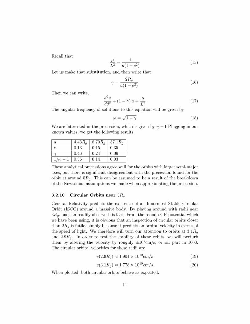
Recall that µ

=1

L2 a(1 − e2) (15)

Let us make that substitution, and then write that

2Rgγ =

a(1 − e2) (16)

Then we can write, d2u dθ2 + (1 − γ) u =

µ L2 (17)

The angular frequency of solutions to this equation will be given by � ω = 1 − γ (18)

1We are interested in the precession, which is given by ω − 1 Plugging in our known values, we get the following results.

a 4.43Rg 8.70Rg 37.1Rg

e 0.13 0.15 0.35 γ 0.46 0.24 0.06 1/ω − 1 0.36 0.14 0.03

These analytical precessions agree well for the orbits with larger semi­major axes, but there is significant disagreement with the precession found for the orbit at around 5Rg . This can be assumed to be a result of the breakdown of the Newtonian assumptions we made when approximating the precession.

3.2.10 Circular Orbits near 3Rg

General Relativity predicts the existence of an Innermost Stable Circular Orbit (ISCO) around a massive body. By playing around with radii near 3Rg , one can readily observe this fact. From the pseudo­GR potential which we have been using, it is obvious that an inspection of circular orbits closer than 2Rg is futile, simply because it predicts an orbital velocity in excess of the speed of light. We therefore will turn our attention to orbits at 3.1Rg

and 2.9Rg . In order to test the stability of these orbits, we will perturb them by altering the velocity by roughly ±107cm/s, or ±1 part in 1000. The circular orbital velocities for these radii are

v(2.9Rg ) ≈ 1.901 × 1010cm/s (19)

v(3.1Rg ) ≈ 1.778 × 1010cm/s (20)

When plotted, both circular orbits behave as expected.

11

When one perturbs the orbits outward, the orbit at 3.1Rg appears stable. Looking at the orbit at 2.9Rg , there is an obvious difference in behavior, but it is not obvious whether the orbit is stable.

When one perturbs the orbit inward, the orbit at 3.1Rg continues to appear stable, but it is quite obvious that the orbit at 2.9Rg is not.

12