Computational Proof as Experiment:Probabilistic Algorithms from aThermodynamic Perspective?,??

Krishna V. Palem

Center for Research on Embedded Systems and Technology,Georgia Institute of Technology, Atlanta GA 30332, USA.

palem@ece.gatech.edu(http://www.crest.gatech.edu)

Abstract. A novel framework for the design and analysis ofenergy-awarealgo-rithms is presented, centered around a deterministicBit-level (Boltzmann) Ran-dom Access Machineor BRAM model of computing, as well its probabilistic coun-terpart, theRABRAM. Using this framework, it is shown for the first time thatprobabilistic algorithms can yield asymptotic savings in the energy consumed,over their deterministic counterparts. Concretely, we show that theexpected en-ergy savingsderived from a probabilisticRABRAM algorithm for solving thedis-tinct vector problem(or DVP for short ) introduced here, overanydeterministic

BRAM algorithm grows asΩ(

nlog(

nn−ε log(n)

)), even though the correspond-

ing deterministic and probabilistic algorithms have the same (asymptotic) time-complexity ofΘ(n). Also, our probabilistic algorithm is guaranteed to be correctwith a probabilityp≥ (1− 1

nc ) (for a constantc chosen as a design parameter). Asusualn denotes the length of the input instance of theDVP measured in the num-ber of bits. These results are derived in the context of a technology-independentcomplexity measure for energy consumption introduced here, referred to aslog-ical work. In keeping with the theme of the symposium, the introduction to thiswork is presented in the context of “computational proof” (algorithm) and the“work done” to achieve it (its energy complexity characterized as logical work).

1 Introduction

The word “fact” conjures up images of a sense of definitiveness in that there is a beliefin its absolutetruth. This notion is the very essence of modern mathematical theories,with their foundational framework based on (formal) languages such as thepredicatecalculus. Thus, following Whitehead and Russell’s seminal formalization of mathemat-ical reasoning embodied in their Principia [32], the very notion of the consistency of anaxiomatic theory disallows even a hint of a doubt about a fact, often referred to as athe-orem(or its subsidiarylemma) in modern as well as ancient mathematical thought. The

? This work is supported in part by DARPA under seedling contract #F30602-02-2-0124.?? A version of this work appeared in The Proceedings ofThe International Symposium on Veri-

fication (Theory and Practice),Taormina, Italy, Jun 29–Jul 4, 2003.

2

modern foundations of verification as proof, with emphasis on its automatic or mecha-nized form, applied to problems motivated in large part from within the disciplines ofcomputer science and electrical engineering (see Manna for example [13, 14]) are alsobound in essential ways to this notion of an absolute ordeterministictruth.

A concomitant to this absolute notion of truth, and a significant contribution of themathematical theory of computing (referred to in popular terms as theoretical computerscience) is the notion of thecomplexityor equivalently, the “degree of difficulty” ofsuch a proof. Thus, starting with Rabin’s [23] work as a harbinger with further con-tributions by Blum [1], the notion of a machine independent measure ofcomplexityled to the widely used formulations of Hartmanis and Stearns [7]—essentially withinthe context of a deterministic mechanistic approach to proof. Here, a deterministicalgorithm—equivalently, any execution of a Turing machine’s program [29]—uponhalting, is viewed as proving a theorem or fact, stated as a decision problem. For ex-ample, determining the outcome of the celebratedhalting problem [14, 29] would con-stitute proving such a theorem in the context of a given instance, where an answer ofa yeswould imply that the Turing machine program given as the input would halt withcertainty.

Both this notion of absolute truth as well as the deterministic (Turing machinebased) approach to arriving at it mechanically are subject to philosophically signifi-cant revision if one considers alternate approaches that arenot deterministic. A criticalfirst step involves non-deterministic approaches with the foundations laid by Rabin andScott [25]. Based on these foundations, Cook’s [4] (and Levin’s [12]) characterizationsof NP as a resource bounded class of proofs, whose remarkable richness was demon-strated by Karp [9], elevated NP to a complexity class of great importance, and theaccompanying P=?NP question to its exalted status. Here, while the approach to prov-ing is not based on the traditional deterministic transition of a Turing machine, themeaning of truth one associates with the final outcome—acceptor reject—continues tobe definite or deterministic.

Moving beyond nondeterminism, the early use of statistical methods with empha-sis on probability can be found in Karp’s [10] introduction ofaverage case analysis.Compelled by the need to better understand the gap between the empirical behaviorand the results of pessimal (mathematical) analysis of algorithms (or a determination oflengths of proofs in our sense), in Karp’s approach, the input is associated with a prob-ability distribution. Thus, while the proof itself is deterministic, its difficulty, length, ormore precisely itsexpected time complexityis determined by averaging over all possibleinputs.

A striking shift in the notion of proof as well as the truth associated with it em-anated from the innovation ofprobabilistic methods and algorithms. In this context,both the method or “primitive” proof-step (of the underlying program) as well as the cer-tainty associated with the proof undergo profound revision. Schwartz [26] anticipatedthe eventual impact of the role of probability in the context of these influential devel-opments best: “The startling success of the Rabin-Strassen-Solovay (see Rabin [24])algorithm, together with the intriguing foundational possibility that axioms of random-ness may constitute a useful fundamental source of mathematical truth independent of,but supplementary to, the standard axiomatic structure of mathematics (see Chaitin and

3

Schwartz [3]), suggests that probabilistic algorithms ought to be sought vigorously.”Thus, in this probabilistic context, both the deduction step as well as the meaning oftruth are both associated with probabilities as opposed to certainties. For convenience,let us refer to these as probabilistic proofs (or algorithms when convenient).

With this as background, we now consider the long and fruitful relationship be-tween the notions of proof in the domain of mathematics and its remarkable use in thephysical sciences over the past several centuries. Historically, mathematical theorieshave served remarkably well in characterizing and deducing truths about the universein a variety of domains, with notable successes in mechanics (classical and quantum),relativity and cosmology, and physical chemistry to name a few areas—see von Neu-mann’s [31] development of quantum mechanics as a notable example. In this role,knowledge about the physical world is derived from mathematical frameworks, meth-ods, and proofs, which could include the above mentioned algorithmic form of proof aswell. Thus, in all of the above endeavors, thedirection for deriving knowledge, is from(applying) mathematicsto (creating knowledge about) physical reality. By contrast, inthis work, we are concerned with the opposite direction—fromusing computational de-vices rooted in the reality of the physical universe such as transistors,to establishing(computationally derived) mathematical facts or theories. Let us, for convenience (andwithout a careful and scholarly study of the possible use of this concept by philosophersearlier on), refer to this opposing perspective as areversal of ontological direction,wherein the physical universe and its empirical laws form the basis for all deductionof mathematical facts through computational proof. To clarify, the reversal in “onto-logical direction” which this work (and earlier publications of this author on which itis based [18, 19]) explores, refers to the fact that the physical universe and its laws asembodied in computing devices form the basis for (algorithmically) generating math-ematical knowledge, by contrast with the traditional andoppositedirection whereinmathematical methods produce knowledge about the physical world.

To reiterate, in all of our work, the meaning we associate with proof will be thatassociated with the execution of a Turing machine program, and we will be interested inthe “complexity” of realizing such a (mechanized proof) in the physical universe. Thus,to reiterate, we will consider a concrete and physically realizable form of a proof—such as that generated by a theorem-prover executing on a conventional microprocessor,or perhaps its Archimedian predecessor—as a physical counterpart of Putnam’s [22]“verificationist” approach by contrast with (as observed by him [22]) the “Platonic”approach with “evidence that the mind has mysterious faculties of grasping concepts”(or “perceiving mathematical objects...”).

Continuing, a first and important observation about the universe of physical objectssuch as modern microprocessors is that their inherent behavior is best described statis-tically. Thus, all notions ofdeterminismare “approximations”in that they are only truewith sufficiently high probability. (See Meindl [15] and Stein [27] for a deterministicinterpretation of the values 0 and 1 within the context of switching based computingthrough electrical devices, to better understand this point.) Specifically, the approxima-tions to determinism are derived by investing (sufficiently) large amount of energy tomake the probability of error small [15]. Building on this observation, the work de-scribed in this paper characterizes the (somewhat oversimplified in this introduction)

4

fact that the process of computational proof entails physical “work”,which in turn con-sumes energydescribed in its most elegant form through statistical thermodynamics.The crux of our thesis is that since nature at its very heart, or our perception of it aswe understand it today is statistical at a (sufficiently) small, albeit classical scale—side-stepping the debate whether “God does or does not play dice” (attributed to Ein-stein to whom a statistical foundation for physical reality was a source of considerableconcern)—the most natural physical models for algorithmic proof or verification us-ing fine-grained physical devices such as increasingly small transistors, are essentiallyprobabilistic, and their energy consumption is a crucial figure of merit!For complete-ness, we reiterate here that following the principle of reversal of ontological direction,we are only concerned with the discovery of mathematical knowledge via computa-tional proofs realized through the dynamics of a physical computing device, such as therepeated switching of semiconductor devices in a microprocessor.

Now, considering the specific technical contributions of this work, in order to de-scribe and analyze these physically realized proofs or algorithms, we introduce (Sec-tion 2) a simpleenergy-awaremodel for computing: theBit-level (Boltzmann) Ran-dom Access Machineor BRAM , as well as its probabilistic variant, theRABRAM (inSection 2.4). Specifically, each primitive step or transition of these models involves achange of state—realized in a canonical way through a transition function associatedwith a finite state control as in Turing machines [29]—that mirrors a corresponding andexplicit change in some physically realizable device. One variant of such a realization isthrough the notion of aswitching step[15, 19] whereas an earlier more abstract variationis through the notion of anemulation[18] of the transition in the physical universe.

Any computational proof (or equivalently algorithm) described in such a model hasan associated technology-independentenergy complexity, introduced aslogical workinSection 3 for the deterministic as well as the probabilistic cases. Historically, the inter-est and subsequently the success of probabilistic algorithms within the context of algo-rithm design, was to derive (asymptotically) faster algorithms. Assuming that all stepstake (about) the same amount of energy, traditional analysis based on time-complexitywill trivially imply that a probabilistic algorithm might consume less energy, becauseit computes and solves problems faster—shorter running time implies lesser switchingenergy. In contrast to these obvious advantages, we show in Section 4 that the energy ad-vantages offered by probabilistic algorithms can be more subtle and varied. Concretely,we prove that for thedistinct vector problemor DVP with an input ofn bits, a proba-bilistic algorithm and its deterministic counterpart take the same number of (time) stepsasymptotically, whereas the probabilistic approach yieldsenergy savingsthat grow asn→ ∞.

Briefly, solving theDVP involves computationally (in theBRAM or RABRAM model)proving that a givenn− tuple defined on the set of symbols0,1 has the symbol 1in all of its n positions; the answer to this decision question (or theorem) isYES ifindeed all positions of the inputn− tuple have the symbol 1 and the answer isNO

otherwise. In this paper, we are interested in the followingdensevariant of theDVP :the inputn− tuple either has no 0 symbol in it, or if it does have a 0 symbol, it haslog(n) such symbols. For this (dense) version of theDVP problem, which for conve-nience will be referred to as theDVP problem in the sequel (defined in Section 4.1),

5

we prove that a novelprobabilistic value amplificationalgorithm, proves the (algorith-mic) theorem, or resolves the associated decision question with an error probabilitybound above by1

nc (for a constantc chosen as a design parameter) using anexpected

(2n+ logk(n))κT ln(

2[1− ε logn

n

])Joules, where 0< ε < 1 andk > 2 are constants.

The algorithm and its associated analysis are outlined in Section 4. In an earlier publica-tion, this author proved [18] that any deterministicBRAM algorithm for solving theDVP

consumes at least(2n− log(n)+1)κT ln2 Joules; this is a lower bound1. By combiningthese two facts, we show that through the use of the probabilistic algorithm introduced

here, the expected savings in energy measured in Joules grows asΩ(

nlog(

nn−ε log(n)

)),

for a constant 0< ε < 1, and for ann bit input to theDVP. Thus both the energy savingsas well as the error probability are respectively monotone increasing and decreasingfunctions ofn. To the best of our knowledge, this result is the first of its kind that estab-lishes an asymptotic improvement in the energy consumed.

These models and analysis methodology build on the following results (from [17,19]) that bridge computational complexity and statistical thermodynamics for the firsttime: a single deterministic computation step, which corresponds to a switching step,consumes at leastκT ln(2) Joules, and this is a lower bound. Furthermore, using proba-bilistic computational steps (or switching), the energy consumed by each step is boundabove byκT ln(2p) Joules, where p≥ 1

2 is the probability that the transition is cor-rect; (1− p) is the per-step error probability.Also, κ is the well-known Boltzmann’sconstant,T is the temperature of the thermodynamic system, and ln is the natural log-arithm. In all of this work, the physical models are based on the statistical and henceprobabilistic generalizations of switches formulated originally by Szilard [11] withinthe context of clarifying the celebrated Maxwell’s demon paradox [11, 30]. A detailedcomparison and bibliography of relevant work from the related field referred to as theThermodynamics of Computing can be found in [19]. Additionally, Feynman [5] pro-vides a simple and lucid introduction to the interplay between thermodynamically basedphysical models of computing, mathematical models, and abstractions such as Turingmachines.

2 The Bit-level (Boltzmann) Random Access Machine -BRAM

In this section, we will introduce our machine model for computing, exclusively oper-ating in thelogical domain. However, to reiterate, a fundamental theorem of this workis that each of itsstate transitions—explained below—can be associated with definiteamounts of energy expenditure. Furthermore, this energy consumption can also be pre-cisely related to the inherent amount of energy needed to compute, using this model.Significantly, aBRAM model will allow us to abstract away all aspects of the underly-ing physics and characterize energy purely in the world in which models of computa-tion such as Turing machines are realized. We anticipate this as being helpful from the

1 While the analysis is based on the technology-independent notion of logical work, we presentthe corresponding energy consumption results implied by idealized physical devices switchingat thermal equilibrium, referred to as a quasistatic process in classical thermodynamics [28].

6

perspective of algorithm analysis and design—an exercise which, in aBRAM, can bedecoupled from the specificities of physical implementations.

The BRAM however does provide a bridge to the physical world through the en-ergy costs associated with the transitions of itsfinite state control(defined below). Thisbridge to the world of implementation and energy allows us to define the novel complex-ity measure oflogical work as detailed in Section 3, which characterizes the “energycomplexity” of the algorithm being designed.

2.1 Informal Introduction to a BRAM

Informally, a BRAM (a bit-level random access machine2) has aprogramwith a finitenumber ofstates. The transition from a current state to the next involves evaluating theassociatedtransition functionleading to the “reading” of one or more bits of an inputfrom a specific memory location, transitioning to a new state and writing a new bit valuein a designated memory location. The number of bits read is dependent of the size ofthealphabet, to be defined below. Every execution starts in a uniqueSTART state, andhalts upon reaching a uniqueSTOPstate.

To extend such models to account for the energy consumed, we define aBRAM

(somewhat) formally. For a computer scientist, defining aBRAM based on well-understoodelements of a random access machine (orRAM) is elementary; however, we define ithere for completeness. The textbook by Papadimitriou [21] provides a rigorous andcomplete introduction to models such as Turing machines and random access machinesincluding definitions of conventional measures of complexity for representing time andspace. This book also provides a comprehensive introduction to the numerous well-understood interrelationships between classes of (time and space) complexity, and canserve as an excellent guide to the topic of defining models of computation in classicalcontexts, not concerned with energy.

2.2 Defining aBRAM

A BRAM consists of several components, which will be introduced in the rest of thissection.

The BRAM Program Following convention, theprogramP is represented as a five-tuplePC,Σ,R,δ,Q. Note that conventionally, variants of the program are referred toas thefinite state control.

The Set of States- PC is the set of states. Each statepci ∈ PC has designated loca-tions inmemory, defined below, that serve respectively as its input and output. Withoutloss of generality, let the states be labeled 1,2,3, . . . , |PC|. The setQ consists of threespecial states,START , STOPandUNDEFINED-STATE not inPC.

The Alphabet of theBRAM - Σ is a finite alphabet, and without loss of generality,we will use the set1,2, . . . |Σ|, which includes the empty symbolφ to denote this

2 Given aBRAM ’s eventual connection with energy and its statistical interpretation, one can alsointerpret the acronym to mean a Boltzmann random access machine.

7

alphabet. From the standpoint of algorithm design, in most cases, it suffices to workwith an alphabet drawn from the setΣ = 0,1, which is the case throughout this paperwhenever aBRAM (or a RABRAM ) is used to analyze an algorithm. However, we notein passing that the size of the alphabet|Σ| has important consequences to the preciseenergy behavior of the associated state transitions3. Therefore, the contexts wherein themore restricted alphabet is used need to be distinguished from those contexts in whichthe more general alphabet of size|Σ|> 2 is used.

The Address Registers of the States in PC- These registers are places where theinput and output addresses of a state are stored. In conventional computer science andengineering parlance, aBRAM uses a form of accessing memory that is referred toas indirect addressing. We shall return to a discussion of the role of these registersin Section 2.3. Theaddress registers, represented by the setR is partitioned into twoclassesRin and Rout; these are both sets (of registers) where each registerρin

j ∈ Rin

(ρoutj ∈Rout) is a (potentially unbounded) linearly ordered set of elements referred to as

cells< sj,1,sj,2, . . . ,sj,k > (< t j,1, t j,2, . . . , t j,k >). Each of the cellssl (tl ) is associatedwith a value from the set0,1,φ. We note that even though the overall alphabet may beof size|Σ|> 2, each cell in the registers either stores a single bit, or is empty. Further-more, if the value associated with such an element isφ (empty or not defined) for somevalue ofk′ ≤ k, then the value associated with allsj,k′′ (t j,k′′ ) is φ for all k′ ≤ k′′ ≤ k;thus, in the general case, the values stored in any of the address registers are a contin-uous “run” of values from the set0,1 followed by a run, possibly of length zero, ofthe symbolφ.

We associate the pairρinj ∈ Rin andρout

j ∈ Rout uniquely with the statepcj . For agiven state, intuitively, these pair of registers yield the addresses from where the inputσ is to be read, and to where the outputσ′ (if any) is to be “written” respectively.It is important to note that these addresses can in fact be the registers themselves. Thepotentially unbounded lengths of the registers denote the fact that the range of addressesbeing accessed (corresponding to the length of a Turing machine’s tape for example)could be unbounded4.

The Transition Function- We are now ready to define the transition functionδ,which will play a central role in characterizing the energy behavior of computations. Inits most general form, a transition function is based on an alphabet of size|Σ| ≥ 2.

Syntactically,δ : (PC∪START )×Σ→ (PC∪Q−START )×Σ is the transitionfunction. Wheneverδ(pci ,σ ∈ Σ) = (pcj ,σ′ ∈ Σ), we say thatδ transitions frompci tothenext-state pcj with σ as input andσ′ as the output.

Some useful remarks about the transition function follow. First, we note that thestateUNDEFINED-STATE is in the range ofδ. Given a statepci , let νi denote the numberof symbols fromΣ for which δ transitions into a state inPC∪ STOP, as opposedinto theUNDEFINED-STATE . For the remaining(|Σ| − νi) symbols,δ transitions intoUNDEFINED-STATE . (This is one way of defining transitions of varying “arity”νi as-sociated with statepci , thus allowing states with varying number of successors withan alphabet of fixed size). In this setting, it is trivial to verify that given an alphabet

3 For convenience, to avoid the use ofde function,|Σ| is assumed to be a power of 2 throughout.4 In any terminating computation, there will be a limit on this bound, typically specified as a

function of the length of the input [21].

8

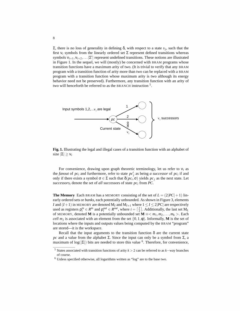
Σ, there is no loss of generality in definingδ, with respect to a statesj , such that thefirst νi symbols from the linearly ordered setΣ represent defined transitions whereassymbolsνi+1,νi+2, . . . |Σ′| represent undefined transitions. These notions are illustratedin Figure 1. In the sequel, we will (mostly) be concerned withBRAM programs whosetransition functions have a maximum arity of two. (It is trivial to verify that anyBRAM

program with a transition function of arity more than two can be replaced with aBRAM

program with a transition function whose maximum arity is two although its energybehavior need not be preserved). Furthermore, any transition function with an arity oftwo will henceforth be referred to as theBRANCH instruction5.

pc νi successors

Input symbols 1,2,…νi are legal

Current state

1

2

νi

Fig. 1. Illustrating the legal and illegal cases of a transition function with an alphabet ofsize|Σ| ≥ νi

For convenience, drawing upon graph theoretic terminology, let us refer toνi asthe fanoutof pci and furthermore, refer to statepc′j as beinga successorof pci if andonly if there exists a symbolσ ∈ Σ such thatδ(pci ,σ) yields pcj as the next state. Letsuccessorsi denote the set ofall successors of statepci from PC.

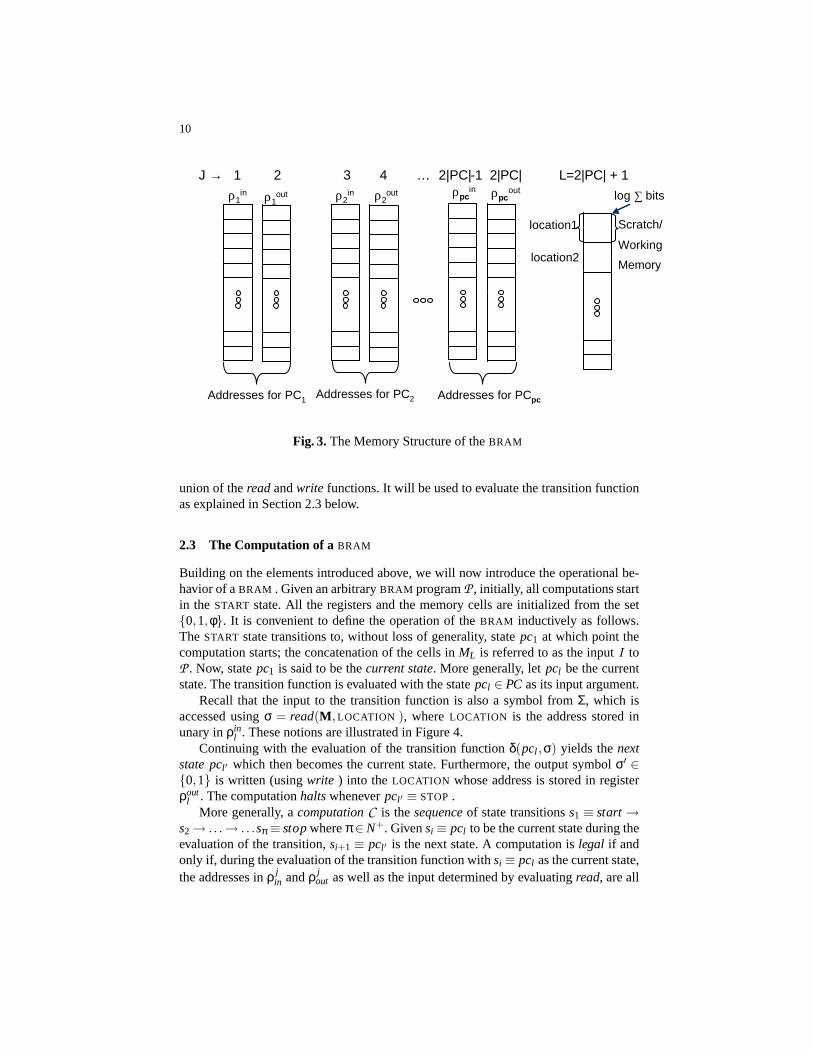
The Memory EachBRAM has aMEMORY consisting of the set ofL = (2|PC|+1) lin-early ordered sets orbanks, each potentially unbounded. As shown in Figure 3, elementsI and(I +1) in MEMORY are denoted MI and MI+1 where 1≤ I ≤ 2|PC| are respectivelyused as registersρin

i ∈ Rin andρouti ∈ Rout, wherei = d I

2e. Additionally, the last set MLof MEMORY, denotedM is a potentially unbounded setM ≡< m1,m2, . . . ,mk >. Eachcell mj is associated with an element from the set0,1,φ. Informally, M is the set oflocations where the inputs and outputs values being computed by theBRAM “program”are stored—it is the workspace.

Recall that the input arguments to the transition functionδ are the current statepc and a value from the alphabetΣ. Since the input can only be a symbol fromΣ, amaximum of log(|Σ|) bits are needed to store this value6. Therefore, for convenience,

5 States associated with transition functions of arityk > 2 can be referred to ask−way branchesof course.

6 Unless specified otherwise, all logarithms written as “log” are to the base two.

9

pc

Successors of PC

Input

Current state

pc‘2

Alphabet ∑ = 1,2,3,4 U φ

pc'33

pc'44

pc'22

pc'11

Transition toInputpc'1

pc‘3

pc‘4

1

2

3

4

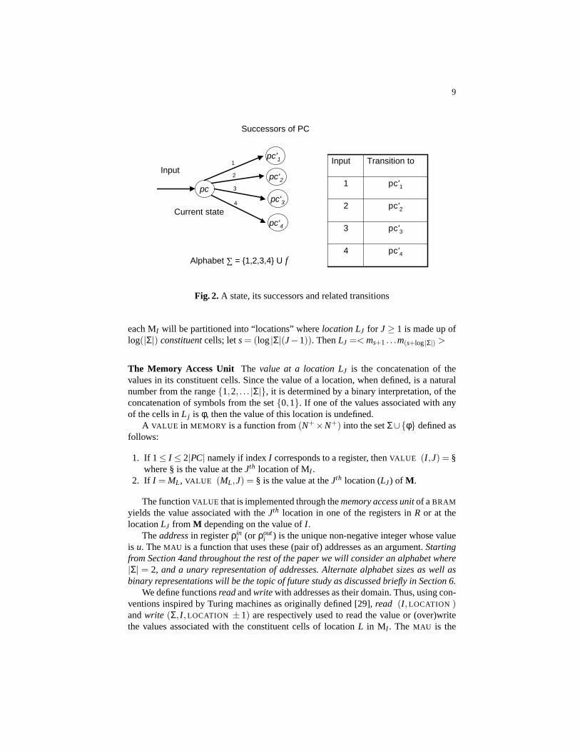
Fig. 2.A state, its successors and related transitions

each MI will be partitioned into “locations” wherelocation LJ for J ≥ 1 is made up oflog(|Σ|) constituentcells; lets= (log|Σ|(J−1)). ThenLJ =< ms+1 . . .m(s+log|Σ|) >

The Memory Access Unit The value at a location LJ is the concatenation of thevalues in its constituent cells. Since the value of a location, when defined, is a naturalnumber from the range1,2, . . . |Σ|, it is determined by a binary interpretation, of theconcatenation of symbols from the set0,1. If one of the values associated with anyof the cells inL j is φ, then the value of this location is undefined.

A VALUE in MEMORY is a function from(N+×N+) into the setΣ∪φ defined asfollows:

1. If 1≤ I ≤ 2|PC| namely if indexI corresponds to a register, thenVALUE (I ,J) = §where § is the value at theJth location of MI .

2. If I = ML, VALUE (ML,J) = § is the value at theJth location (LJ) of M .

The functionVALUE that is implemented through thememory access unitof aBRAM

yields the value associated with theJth location in one of the registers inR or at thelocationLJ from M depending on the value ofI .

Theaddressin registerρini (or ρout

i ) is the unique non-negative integer whose valueis u. TheMAU is a function that uses these (pair of) addresses as an argument.Startingfrom Section 4and throughout the rest of the paper we will consider an alphabet where|Σ| = 2, and a unary representation of addresses. Alternate alphabet sizes as well asbinary representations will be the topic of future study as discussed briefly in Section 6.

We define functionsreadandwrite with addresses as their domain. Thus, using con-ventions inspired by Turing machines as originally defined [29],read (I , LOCATION )andwrite (Σ, I , LOCATION ±1) are respectively used to read the value or (over)writethe values associated with the constituent cells of locationL in MI . The MAU is the

10

ρ1in ρ1

out ρ2in ρ2

out ρpcin ρpc

out

Addresses for PC1 Addresses for PC2 Addresses for PCpc

location1

location2

Scratch/

Working

Memory

log ∑ bits

J → 1 2 3 4 … 2|PC|-1 2|PC| L=2|PC| + 1

Fig. 3.The Memory Structure of theBRAM

union of thereadandwrite functions. It will be used to evaluate the transition functionas explained in Section 2.3 below.

2.3 The Computation of aBRAM

Building on the elements introduced above, we will now introduce the operational be-havior of aBRAM . Given an arbitraryBRAM programP , initially, all computations startin the START state. All the registers and the memory cells are initialized from the set0,1,φ. It is convenient to define the operation of theBRAM inductively as follows.The START state transitions to, without loss of generality, statepc1 at which point thecomputation starts; the concatenation of the cells inML is referred to as the inputI toP . Now, statepc1 is said to be thecurrent state. More generally, letpcl be the currentstate. The transition function is evaluated with the statepcl ∈ PC as its input argument.

Recall that the input to the transition function is also a symbol fromΣ, which isaccessed usingσ = read(M , LOCATION ), whereLOCATION is the address stored inunary inρin

l . These notions are illustrated in Figure 4.Continuing with the evaluation of the transition functionδ(pcl ,σ) yields thenext

state pcl ′ which then becomes the current state. Furthermore, the output symbolσ′ ∈0,1 is written (usingwrite ) into theLOCATION whose address is stored in registerρout

l . The computationhaltswheneverpcl ′ ≡ STOP.More generally, acomputationC is thesequenceof state transitionss1 ≡ start→

s2 → . . .→ . . .sπ ≡ stopwhereπ∈N+. Givensi ≡ pcl to be the current state during theevaluation of the transition,si+1 ≡ pcl ′ is the next state. A computation islegal if andonly if, during the evaluation of the transition function withsi ≡ pcl as the current state,the addresses inρ j

in andρ jout as well as the input determined by evaluatingread, are all

11

pcl

Input σ

δ(pcl , σ)

Next state pcl' Output value σ ’

WRITE σ’OUTPUT VALUE

CURRENT STATE = pcl'NEXT STATE?READ

Evaluate

Location

from ρlin

Location

from ρlout

Fig. 4. Illustrating the Evaluation of the Transition Function

defined. The computation isillegal otherwise. In the sequel, we will be concerned withlegal computations only and will, for convenience, refer to them simply as computa-tions.

Fact 1.All computations of aBRAM programP with inputI are the identical. Formally,given any two computationsCq = s1 ≡ START→ s2 → . . . → . . .sπ ≡ STOPandCr =s1 ≡ START→ s2 → . . .→ . . . sπ ≡ STOPgenerated by programP with inputsI andI ,sj = sj wheneverI ≡ I .

2.4 The RandomizedBRAM or RABRAM

A RABRAM is identical to aBRAM in all aspects except that the transition from thecurrent state to the next state occurs probabilistically. There are alternate forms ofdefining the particular approach through which this probabilistic transition is intro-duced into the formulation of aRABRAM. In our approach, the transition functionδ(a BRANCH ) from Section 2.2 is extended to a transition functionδr . Let P be theopen interval(1

2,1). Now,δr :((PC∪START )×Σ)→ ((PC∪Q−START )×Σ×P)is the probabilistic transition function. ConsideringΣ ≡ 0,1, let pcj and pck be thepossible successors ofpci , where j = k is allowed. For1

2 ≤ pi ∈ P ≤ 1, wheneverδr(pci ,σ = 0) = (pcj ,σ′ ∈ Σ, pi ∈P), δ transitions frompci into thenext-state pcj withσ = 0 as input, and withσ′ as output, with probabilitypi , and to statepck with σ′ as out-put with probability(1− pi). Note thatσ′ is the symbol fromΣ that is output wheneverδr yields a transition from statepci to next-statepck. The transition function withσ = 1can be defined accordingly. Let us refer to this branch instruction as a probabilisticBRANCH with probability parameterpi .

12

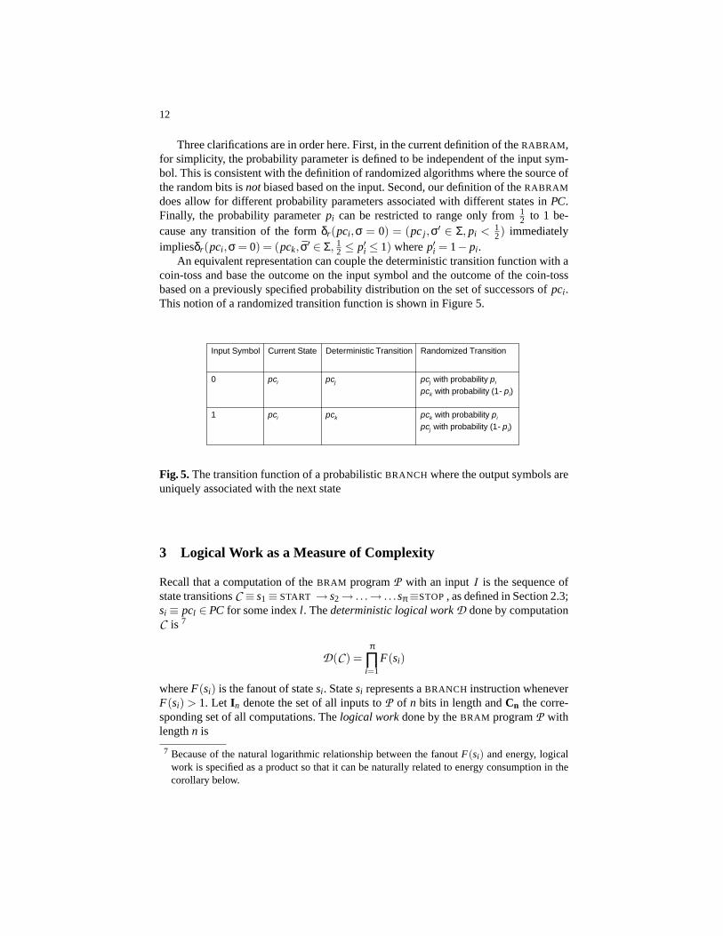
Three clarifications are in order here. First, in the current definition of theRABRAM,for simplicity, the probability parameter is defined to be independent of the input sym-bol. This is consistent with the definition of randomized algorithms where the source ofthe random bits isnotbiased based on the input. Second, our definition of theRABRAM

does allow for different probability parameters associated with different states inPC.Finally, the probability parameterpi can be restricted to range only from12 to 1 be-cause any transition of the formδr(pci ,σ = 0) = (pcj ,σ′ ∈ Σ, pi < 1

2) immediatelyimpliesδr(pci ,σ = 0) = (pck, σ′ ∈ Σ, 1

2 ≤ p′i ≤ 1) wherep′i = 1− pi .An equivalent representation can couple the deterministic transition function with a

coin-toss and base the outcome on the input symbol and the outcome of the coin-tossbased on a previously specified probability distribution on the set of successors ofpci .This notion of a randomized transition function is shown in Figure 5.

pci

pci

Current State

pck with probability pi

pcj with probability (1- pi)pck1

pcj with probability pi

pck with probability (1- pi)pcj0

Randomized TransitionDeterministic TransitionInput Symbol

Fig. 5.The transition function of a probabilisticBRANCH where the output symbols areuniquely associated with the next state

3 Logical Work as a Measure of Complexity

Recall that a computation of theBRAM programP with an inputI is the sequence ofstate transitionsC ≡ s1≡ START → s2→ . . .→ . . .sπ ≡STOP, as defined in Section 2.3;si ≡ pcl ∈ PC for some indexl . Thedeterministic logical workD done by computationC is 7

D(C ) =π

∏i=1

F(si)

whereF(si) is the fanout of statesi . Statesi represents aBRANCH instruction wheneverF(si) > 1. Let In denote the set of all inputs toP of n bits in length andCn the corre-sponding set of all computations. Thelogical workdone by theBRAM programP withlengthn is

7 Because of the natural logarithmic relationship between the fanoutF(si) and energy, logicalwork is specified as a product so that it can be naturally related to energy consumption in thecorollary below.

13

L(P ,n)≡ MAX∀C∈Cn(D(C ))

In earlier work [17, 19], this author established the following theorem in the contextof an idealized physical device at thermal equilibrium everywhere.

Theorem 1. The energy consumed in evaluating the transition function in the contexta state pci of anyBRAM programP is at leastκT ln(F(si)) Joules.

It follows that

Corollary 1. For a deterministicBRAM computation, the energy consumed by a pro-gramP with inputs of length n is no less thanκT ln(L(P ,n)) Joules.

Proof. Immediate from Theorem 1, the fact that energy is additive and the identity

ln

(π

∏i=1

F(si)

)=

π

∑i=1

ln(F(si))

Also, we recall (from [17, 19]) that

Theorem 2. The energy consumed in evaluating the transition function in the contexta state pci of anyRABRAM programPR can be as low asκT ln(F(si)p) Joules, wherep is the probability parameter8.

We note that in the context of computations realized through aRABRAM each statetransition is probabilistic. Therefore, Fact 1 does not apply and different computationsare possible with the same input. Thus, given a fixed inputI there exits afamily ofcomputationsCI where each computationC ∈ CI has a probabilityqc of occurrence.In this case, the notion of logical work has to be modified where theMAX function isapplied over theexpectedlength of the probabilistic computations fromCI . We definethe expected logical workfor an inputI to be the weighted sum (by the probabilitiesqc) of the fan-outs of the computations corresponding toI .

R (CI ,I ) = ∑∀C∈CI

qc2D(C )

Theprobabilistic logical workof a RABRAM programPR is defined to be

LR (PR ,n) = MAX∀CI∈CR (CI )

whereC is the set of all trajectory families associated withI ∈ I .

Let Cmax denote the family of computations definingLR (PR ,n) corresponding toan inputImax

8 Here the expression “as low as” is meant to imply an upper bound in an idealized system atthermal equilibrium everywhere, which can be realized by a quasistatic process. For exam-ple, these estimates can be potentially improved using “information theoretic compression”following Zurek [33].

14

Corollary 2. For a RABRAM programPR , the expected energy consumed with inputImax can be as low as

κT ∑∀C∈Cmax

qc2 ln(D(C ))

In the general case, thelogical workof an algorithmL might consist of determin-istic as well as probabilistic logical work components. As usual, given the nature ofasymptotic analysis and in this hybrid case, it will be sufficient only to consider thedominant term.

4 Design and Analysis of Algorithms in theBRAM and theRABRAM

In this Section, we will demonstrate the use of the models described in the previoussections, in the context of analyzing energy savings using probabilistic algorithms. Ourproblem of choice will be thedistinct vector problemor DVP for short, introduced inSection 4.1. In Section 4.2, we will outline a probabilistic algorithm for solving thisproblem, whose energy consumed is provably better thanany deterministic algorithmfor solving theDVP in the BRAM model. To establish this result, we have to provea lower bound on the deterministic logical work needed to solve this problem usingany (deterministic)BRAM algorithm (claimed in Section 5 and proved in this author’searlier work [18]). While the central ideas and some of the details are presented inthe sequel, complete proofs and other implementation specifics that are easy to verify,will be included in a full-version of the paper. Thus, this paper should be viewed as anextended abstract. For notational succinctness, we will use the symbolsi, j,k, l ,m andn in a new context throughout the rest of this paper, where this reuse will not cause anyambiguity.

4.1 The Distinct Vector ProblemDVP

Informally, theDVP is defined to be the problem of determining whether a givenn− tu-ple, defined on the set of symbols0,1, is distinct from ann− tuple which has thesymbol 1 in all of its positions. Formally,

Input: avector T≡< t1, t2, . . . , tn > whereT ∈ 0,1n such that

1. ti = 1 in all n positions or,2. ti = 0 for logn values ofi where 1≤ i ≤ n.

Additionally, a string of symbols with value 1, and lengthCOUNT is given where thelength is a design parameter which will determine the probability of correctness. In ourcaseCOUNT= clogn for an appropriately chosen constantc. Also the valuen is spec-ified as acounter.

Question: Is ti = 1 for all values ofi in unary, referred to asLENGTH, 1≤ i ≤ n ?

15

Let T denote the set of all possible inputs to theDVP. A RABRAM programPRsolves theDVP with probability p provided, given an input as defined above, it haltswith a symbol 1 denoting an answer of “yes” to the above question, in a designatedoutputcell in memory wheneverti = 1 for all values ofi 1≤ i ≤ n in T, and with thesymbol 0 otherwise, denoting the answer “no” with probability no less thanp. For con-venience, we will refer to the value in the celloutputto be theoutput bit.

4.2 A Probabilistic Algorithm PROBDVP

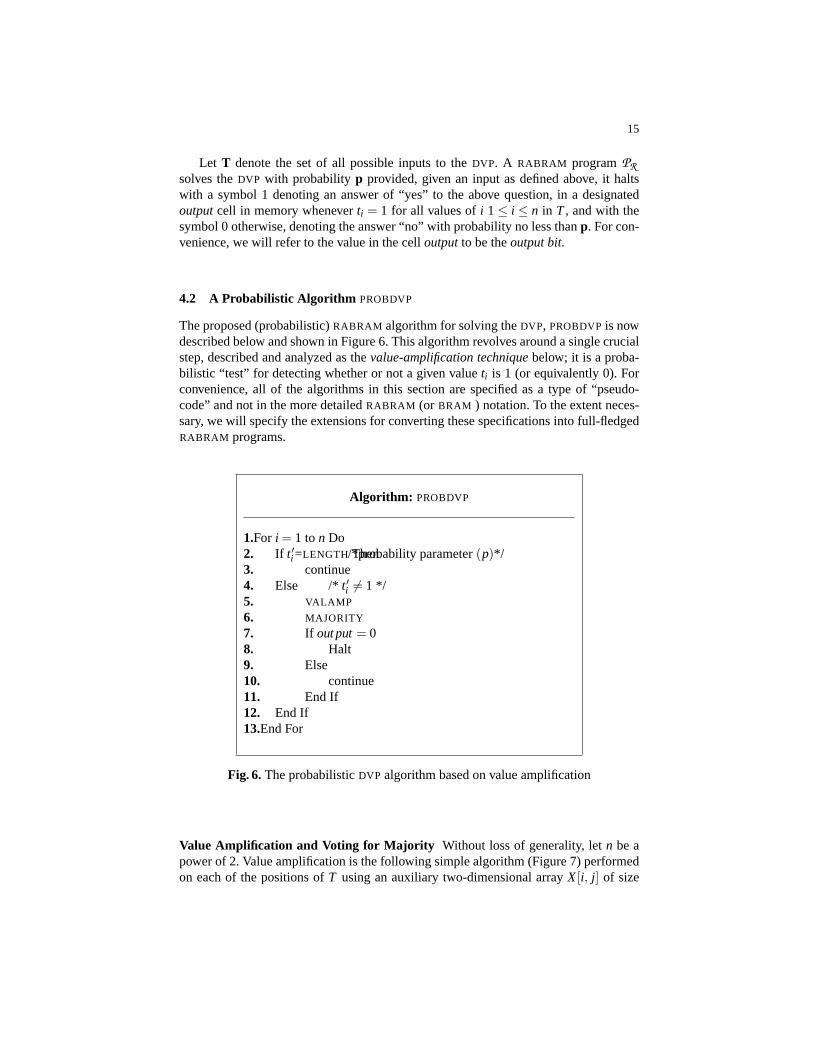
The proposed (probabilistic)RABRAM algorithm for solving theDVP, PROBDVPis nowdescribed below and shown in Figure 6. This algorithm revolves around a single crucialstep, described and analyzed as thevalue-amplification techniquebelow; it is a proba-bilistic “test” for detecting whether or not a given valueti is 1 (or equivalently 0). Forconvenience, all of the algorithms in this section are specified as a type of “pseudo-code” and not in the more detailedRABRAM (or BRAM ) notation. To the extent neces-sary, we will specify the extensions for converting these specifications into full-fledgedRABRAM programs.

Algorithm: PROBDVP

1.For i = 1 ton Do2. If t ′i =LENGTH Then/*probability parameter(p)*/3. continue4. Else /* t ′i 6= 1 */5. VALAMP

6. MAJORITY

7. If out put= 08. Halt9. Else10. continue11. End If12. End If13.End For

Fig. 6.The probabilisticDVP algorithm based on value amplification

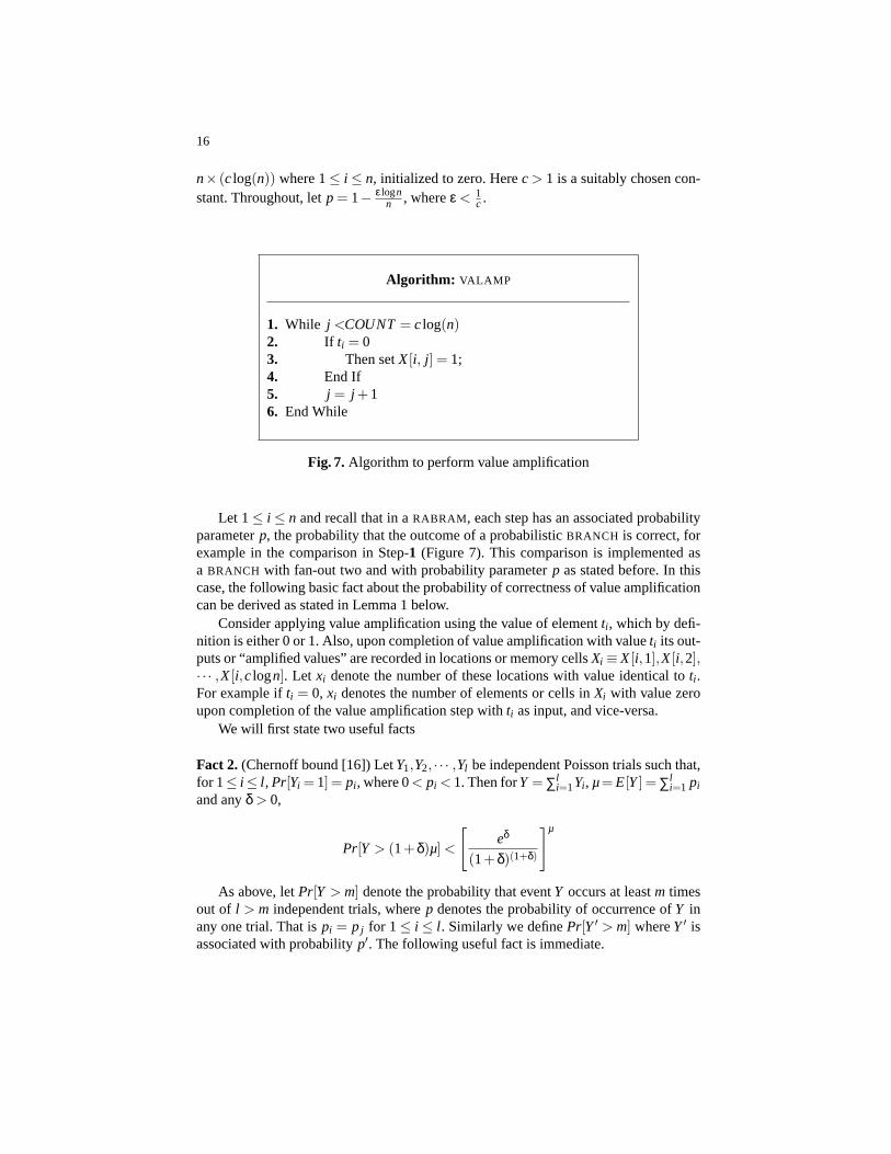
Value Amplification and Voting for Majority Without loss of generality, letn be apower of 2. Value amplification is the following simple algorithm (Figure 7) performedon each of the positions ofT using an auxiliary two-dimensional arrayX[i, j] of size

16

n× (clog(n)) where 1≤ i ≤ n, initialized to zero. Herec > 1 is a suitably chosen con-stant. Throughout, letp = 1− ε logn

n , whereε < 1c .

Algorithm: VALAMP

1. While j <COUNT= clog(n)2. If ti = 03. Then setX[i, j] = 1;4. End If5. j = j +16. End While

Fig. 7.Algorithm to perform value amplification

Let 1≤ i ≤ n and recall that in aRABRAM, each step has an associated probabilityparameterp, the probability that the outcome of a probabilisticBRANCH is correct, forexample in the comparison in Step-1 (Figure 7). This comparison is implemented asa BRANCH with fan-out two and with probability parameterp as stated before. In thiscase, the following basic fact about the probability of correctness of value amplificationcan be derived as stated in Lemma 1 below.

Consider applying value amplification using the value of elementti , which by defi-nition is either 0 or 1. Also, upon completion of value amplification with valueti its out-puts or “amplified values” are recorded in locations or memory cellsXi ≡X[i,1],X[i,2],· · · ,X[i,clogn]. Let xi denote the number of these locations with value identical toti .For example ifti = 0, xi denotes the number of elements or cells inXi with value zeroupon completion of the value amplification step withti as input, and vice-versa.

We will first state two useful facts

Fact 2.(Chernoff bound [16]) LetY1,Y2, · · · ,Yl be independent Poisson trials such that,for 1≤ i ≤ l , Pr[Yi = 1] = pi , where 0< pi < 1. Then forY = ∑l

i=1Yi , µ= E[Y] = ∑li=1 pi

and anyδ > 0,

Pr[Y > (1+δ)µ] <

[eδ

(1+δ)(1+δ)

]µ

As above, letPr[Y > m] denote the probability that eventY occurs at leastm timesout of l > m independent trials, wherep denotes the probability of occurrence ofY inany one trial. That ispi = p j for 1≤ i ≤ l . Similarly we definePr[Y′ > m] whereY′ isassociated with probabilityp′. The following useful fact is immediate.

17

Fact 3.Pr[Y > m] > Pr[Y′ > m] wheneverp > p′ for all l > 0 9

Using these facts, we can now prove

Lemma 1. In any single invocation of algorithmVALAMP with input value ti the (error)probability that the number of elements xi is less thanc

2 logn,

Pr[xi <c2

logn]≤ 1nc

for all n ≥ 2 and constantsc andε that are design parameters.

Proof. Suppose ˆp, the probability of a per-step error during value amplification bep= 1− 1

c′ for c′ > 1 a constant. Also, letyi = (clogn−xi), wherexi denotes the numberof elements or cells inXi with values identical toti . The expected values ofyi is denotedby µ= c

c′ logn.

Now,

Pr[yi >c2

logn] = Pr[yi > (1+δ)cc′

logn] (1)

for (1+δ) =c′

2for constantc′.

From Fact 2

Pr[yi > (1+δ) logn] ≤

ec′2 −1(

c′2

)( c′2

)

cc′ logn

(2)

≤ 1nc (3)

for any constant ˆc > 1, with an appropriate choice ofc andc′.The error probability(1−p) = ε logn

n < 1c′ for n = 2 andε < 2

c′ . Thereforeε lognn <

(1−p) for anyn> 2 since logn is a decreasing function inn∈N+. From this and Fact 3,the bound in inequality (2) above serves as an overestimate to the error probability.

Intuitively, the basic idea behind value amplification is that whenever the value at apositionti is probabilistically tested and found it be 0, its value is “suspect”. In this case,algorithmVALAMP performs repeated independent tests on the same bit, and sets theoutputbased on the majority of the tests. The result of an individual test will henceforthbe referred to as avote. Thedemocratic-votingalgorithm entitledMAJORITY (Figure 8)accomplishes the goal of counting the total number of votes and setting theoutputbitappropriately, based on a simple majority.

9 With my student Lakshmi N. Chakrapani, a new proof for the above relation has been devel-oped, which does not use the conventional combinatorial technique.

18

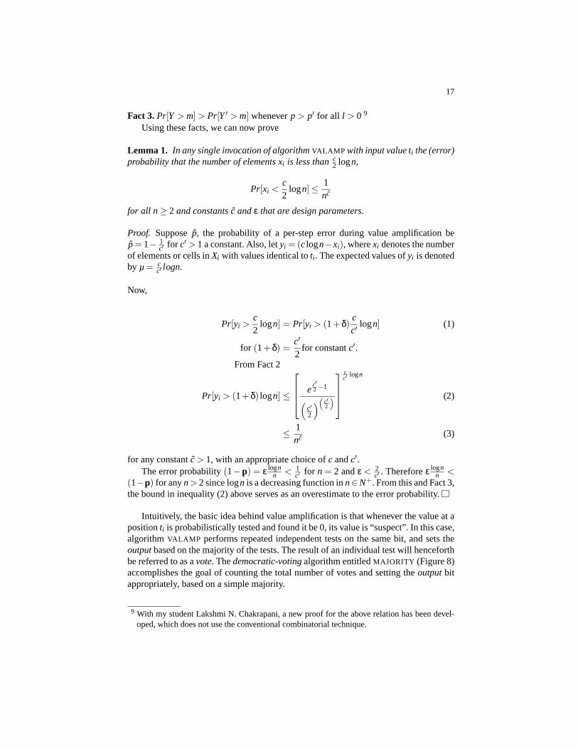
Algorithm: MAJORITY

1. If the number of entries with the symbol 1in X[i, j]: 1≤ j ≤ clog(n) is greater thanc2 log(n)2. Then setoutputto 0 and terminate.3. Else4. setoutputto 1 and terminate.5. End If

Fig. 8.Algorithm to count majority vote

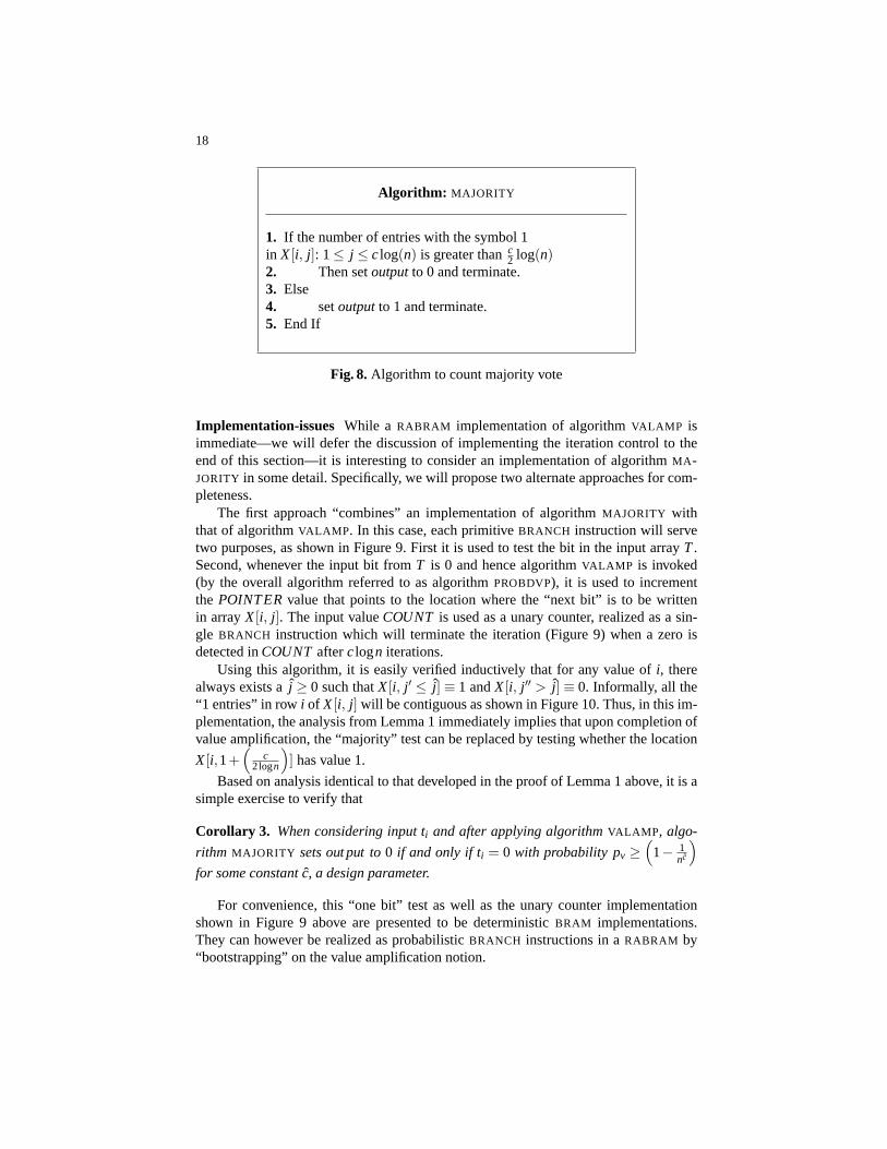
Implementation-issues While a RABRAM implementation of algorithmVALAMP isimmediate—we will defer the discussion of implementing the iteration control to theend of this section—it is interesting to consider an implementation of algorithmMA -JORITY in some detail. Specifically, we will propose two alternate approaches for com-pleteness.

The first approach “combines” an implementation of algorithmMAJORITY withthat of algorithmVALAMP . In this case, each primitiveBRANCH instruction will servetwo purposes, as shown in Figure 9. First it is used to test the bit in the input arrayT.Second, whenever the input bit fromT is 0 and hence algorithmVALAMP is invoked(by the overall algorithm referred to as algorithmPROBDVP), it is used to incrementthe POINTERvalue that points to the location where the “next bit” is to be writtenin arrayX[i, j]. The input valueCOUNT is used as a unary counter, realized as a sin-gle BRANCH instruction which will terminate the iteration (Figure 9) when a zero isdetected inCOUNT afterclogn iterations.

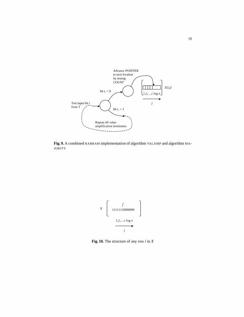
Using this algorithm, it is easily verified inductively that for any value ofi, therealways exists aj ≥ 0 such thatX[i, j ′ ≤ j]≡ 1 andX[i, j ′′ > j]≡ 0. Informally, all the“1 entries” in rowi of X[i, j] will be contiguous as shown in Figure 10. Thus, in this im-plementation, the analysis from Lemma 1 immediately implies that upon completion ofvalue amplification, the “majority” test can be replaced by testing whether the location

X[i,1+(

c2logn

)] has value 1.

Based on analysis identical to that developed in the proof of Lemma 1 above, it is asimple exercise to verify that

Corollary 3. When considering input ti and after applying algorithmVALAMP , algo-

rithm MAJORITY sets out put to0 if and only if ti = 0 with probability pv ≥(

1− 1nc

)for some constantc, a design parameter.

For convenience, this “one bit” test as well as the unary counter implementationshown in Figure 9 above are presented to be deterministicBRAM implementations.They can however be realized as probabilisticBRANCH instructions in aRABRAM by“bootstrapping” on the value amplification notion.

19

Test input bit i from T

bit ti = 0

bit ti = 1

Advance POINTERto next location by testing COUNT

1,2,….c log n

X[i,j]

j

Repeat till value amplification terminates

Fig. 9.A combinedRABRAM implementation of algorithmVALAMP and algorithmMA -JORITY

11111110000000

1,2,….c log n

j

jX

Fig. 10.The structure of any rowi in X

20

The second approach to realizing algorithmsVALAMP and MAJORITY is to con-sider separate implementations. Again, considering algorithmMAJORITY, we note thata straightforward approach to determining the majority will involve a tree-structuredcomputation withclogn leaves, where the output of the root is a value of 1 if and onlyif the number of entries in rowi of arrayX designatedXi is greater thanc2 logn. Each“node” of the tree represents some constant number, sayr, of tests, such that a value of1 is recorded iff both of its children are associated with a value of 1. The value ofr ischosen so that with(1− p) = ε logn

n , we have an overall error probability bounded aboveby 1

nc as in Corollary 3.

5 Analysis of Algorithm PROBDVP

The input lengthn is specified as a vector in unary ofn bits. The end of this counteris detected10 by the transition from a bit with value 1 to one with value 0. Consider-ing Algorithm PROBDVPfrom Section 4.2 above, we note that the counter that controlsthe iteration over the input vector can also be implemented through a single branch foreach position till the “end-of-array” symbol is detected in the input vectorT to deter-mine termination of the entire algorithm. To reiterate, for convenience, we assume thatthe branch instruction associated with this test is deterministic. Thus in its final imple-mentation algorithmPROBDVP is a “hybrid” algorithm with both probabilistic and de-terministic steps. Thus its complexity characterized in Theorem 3 has deterministic andprobabilistic logical work components. We again note that the probabilistic techniquesoutlined earlier can in fact be used to replace this deterministic test by a probabilistictest leading to a “non-hybrid” fully probabilistic implementation. For completeness werecall that each test in the “for” loop specified as Step-2 in algorithmPROBDVP (Fig-ure 6) is implemented using a probabilistic branch, with an associated error probabilityof p = ε log(n)

n .With this as background, letα andβ denote the number of times that that the branch

used to realize Step-2 is executed incorrectly—α denotes the number of times that anevent of typeA, wherein the input vector has a value 0 and the branch determined it tobe erroneously 1 occurs, whereasβ denotes the number of times that an event of typeBwherein an input value of 1 is erroneously determined to be 0. Similarly,λ denotes thenumber of times this step is executed correctly, and the corresponding event is said tobe of typeΛ. Λ0 denotes an event of typeΛ with an input symbol of 0, withΛ1 definedsimilarly.

Using the Chernoff bound (from Fact 2) once again, and using analysis similar tothat that used in the proof of Lemma 1, we can show that

Lemma 2. The probability thatα or β is greater than rlogn where r≤ 12, is bound

above by1nc , for suitably chosen constantsc and c.

10 In the probabilistic case, the end of array symbol can be represented as a strong of logn bitswith value 0 followed by a corresponding string of logn bits with value 1; in the deterministiccase, a single bit with value 1 will suffice.

21

The Expected Logical Work Done by Algorithm PROBDVP Using the above devel-opment as background, we are now ready to analyze the expected logical workLRdone by algorithmPROBDVP.

Fact 4.The value amplification in Step-5 of Algorithm PROBDVP is invoked iff eventsof typeB or Λ0 occur in Step-2.

From the above fact, we have

Theorem 3. The expected logical workLR (PROBDVP,n) = 2n+logk n for some positiveconstant k> 2 andL(PROBDVP,n) = 2n.

Proof. The logical work during each invocation of value amplification is triviallyclogn,for some constantc. Furthermore, the number of such invocations due to events of typeΛ0 is bound above by logn from the definition of the input to theDVP. From Lemma 2,the probability that the number of invocations of value amplification caused by eventsof typeB will exceedr logn is no more than1

nc . This in turn implies an expected logical

work of r log2n from events of typeB. Also the number of steps (BRANCH ) and hencelogical work that can be caused by events of typeΛ1 as well as typeA is cumulativelybound above byn. By noting that a unary implementation of a counter in Step-1 of thealgorithm using deterministic tests can be realized usingn+ 1 branches, we have thetheorem.

Expected Energy Savings Using AlgorithmPROBDVP In earlier work [18], we haveshown that theL(P ,n) of any deterministicBRAM algorithmP for solving theDVP

problem is bound below by 2n− logn+ 1. From this lower bound, from Theorem 3,and from Corollaries 1 and 2, we can claim that

Theorem 4. The expected savings in energy in Joules using AlgorithmPROBDVPover

any deterministic algorithm for solving theDVP grows asΩ(

nlog(

nn−ε logn

))Joules,

for constant0 < ε < 1, and is therefore monotone increasing in n.

5.1 Probability of Error of Algorithm PROBDVP

We note that errors can occur either due to events of typeA or of typeB. Based on theprobabilities these types of events, we have:

Theorem 5. The probability that AlgorithmPROBDVP will terminate correctly is atleastp = (1− 1

nc ) for c a constant and a design parameter.

Proof. We note that an incorrect termination occurs if and only if the input vector hadthe value 1 in all of its positions and upon termination, the value ofoutputwas 0 (eventsof typeB), which we will refer to asCase-1, and vice-versa, (events of typeA) whichwe will refer to asCase-2.

Case-1:From algorithmPROBDVP, let us consider events of typeB. From Lemma 1and Corollary 3, the probability of any one of these events settingout put= 0, ≤ 1

nc .

22

Since there are a total ofn positions and hence a maximum ofn such events, the ex-pected number of such events isε logn. The probability that any one of theseε lognsetsout put= 0 after value amplification is trivially bound above by1

nc−1 and therefore

we are done withc = c−1. (We note that performingclogl n trials, for a constantl ,in the algorithmvalampinstead of theclogn used in this paper, simplifies the calcula-tion of this bound, but does not affect the asymptotics of the energy complexity of thealgorithmPROBDVP. Further, using the bound onβ from Lemma 2 will yield a betterestimate ofc.)

Case-2:In this case there exists ati = 0. Then by the definition of theDVP, thereexist logn positions such thatt j = 0 at every one of these positions; letξ0 denote theset of all such indicesj. Considering events of typeA, we note from Lemma 2 that the

probability thatα < logn is bound below by(

1− 1nc

). Therefore, there exists one index

j ′ ∈ ξ0 such that upon execution of Step-2 of algorithmPROBDVPwith t j ′ as input, theresulting event is not of typeA with probabilityp′ ≥ 1− 1

nc . Therefore witht j ′ as input,Step-5 and Step-6 of algorithmPROBDVPwould have been executed with probabilityp′ and from Lemma 1.

6 Remarks and Conclusions

With the ever increasing emphasis on the energy consumed by computers and the needto minimize it, our goal here is to develop a framework and a supporting complexity(theory) that is technology independent, intending to parallel classical computationalcomplexity theory developed in the context of running-time and space (see Papadim-itriou [21] for details concerning the classical theory of computational complexity). Thework presented here is one approach towards accomplishing this goal wherein energyis the figure of merit—as opposed to traditional time or space. In this context, the mea-sure of complexity introduced here and referred to as logical work serves to provide anabstract, albeit representative measure of the energy consumed. Thus, while analyzingan algorithm as demonstrated in the context of theDVP for example, the logical workcan be the figure of merit that one seeks to improve, which is then easily “translated” todeduce energy gains, as demonstrated in Section 4.

The particular formulation presented here affords a clear separation of concernsbetween the energy behavior of an algorithm across the logical and physical levels, byintroducing an “abstract” estimate of energy-consuming behavior through logical work,which is independent of particular physical implementations. Subsequently, we providespecific translations from the domain of logical work, through idealized physical modelsof computing as summarized in Section 3, into the domain of energy.

Thus, using this framework, the specificphysicaldevices that implement the com-puting elements can be changed, without perturbing the algorithm framework affectingthe design and analysis where the latter constitute thelogical components of our frame-work. Furthermore, our particular choice of an idealized physical device abstracts awaydependencies on specific technologies, but nevertheless exposes the logical componentsof the framework to the inherent limits to energy consumed—specifically the idealized

23

physical devices used here are based on statistical thermodynamics building on the his-toric work of Maxwell [30], Boltzmann [2], and Gibbs [6], rather than being based ina specific physical domain such as transistors of a particular feature size for example.Furthermore, these idealized devices consume energy as they compute and once energyis consumed, the complexity measure of logical workirreversiblycharges for this ex-penditure; this is in contrast with thereversiblestyle of computing (see Feynman [5]for a survey) which allows energy consumed to be recovered allowing, in theory, com-putations to be realized with zero energy consumption.

From a utilitarian perspective of course, any framework such as that introduced inthis paper is “only as useful as the results that it can help achieve.” In this context, thecentral thesis established in this paper that is used to validate the value of this frameworkis: probabilistic techniques and algorithms—or, as referred to in the introduction andin keeping with the theme of this symposium, “probabilistic proofs”—yield expectedenergy savings, when compared to their deterministic counterparts.

Several directions of inquiry suggest themselves, given that the energy behaviorof algorithms in general and probabilistic algorithms in particular remains a largely un-chartered domain. While deferring the cataloging of such “open questions”—computationson finite-fields suggest themselves immediately as candidates for study—including thoseaimed at developing an energy-based complexity theory to a future publication, we willbriefly comment on some of the more immediate questions here.

An obvious first step is to consider other interesting as well as more meaningfulcandidate problems for demonstrating possible energy savings achieved through proba-bilistic algorithms or proofs. In this regard, results similar to those presented for theDVP

in Section 4 have been derived by this author forstring matching. The classical prob-abilistic algorithm for solving this problem based onfingerprintingis due to Karp andRabin [8]. Commenting on the specifics briefly, our energy savings are derived by ex-tending the notion of value amplification (from Section 4.2) rather than through the useof the Karp-Rabin fingerprints. It will be of interest to analyze fingerprinting from anenergy perspective using the framework provided by theBRAM and theRABRAM mod-els, and to systematically compare the power and scope of this technique with that ofvalue amplification. Specifically, the error probability of value amplification is higherthan the error probability achieved through fingerprinting. The first interesting ques-tion is to determine whether value amplification can yield the same error probabilityas fingerprinting does. Assuming that the probabilities of error are different, it will beinteresting to determine whether energy can be used to separate the complexity of fin-gerprinting from value amplification, even though both of then would yield algorithmsthat run inO(n).

All of the results presented in this paper were using unary representations of num-bers, as opposed to the more natural binary representation. This choice was deliberatein that in a model such as aBRAM , the particular choice of representation has an impacton the asymptotic energy behavior, and our interest in this (first) work is to understandthe energy behavior at the most elementary level possible. A basic question to considerin this regard is that of implementing a binarycounterand its accompanying arithmetic,and comparing it to the unary design used to implement iteration in realizing AlgorithmPROBDVPfor example.

24

A direction of inquiry that is only hinted at here but not elaborated upon, is the im-plication of this work to novel physical computing devices that are probabilistic. As theanalysis in Section 4 demonstrated, such implicit randomization in the (abstract) devicecan lead to energy improvements, even asymptotically. To reiterate, these improvementsare not due to faster running times that probabilistic algorithms might yield, but followfrom the following fundamental reason: using the idealized physical devices (from [17,19]) referred to above, a physical interpretation of randomization allows computationto be realized with higher thermodynamic-entropy (or Boltzmann-entropy) which is aphysical quantity, thus yielding energy savings. Pursuing realizations of such devicesand validating them in the context of implementing probabilistic algorithms promisesto be a particularly interesting direction for inquiry, which is being collaboratively pur-sued [20]. Intuitively, a physical interpretation of probabilistic computing can be viewedas “merely” riding the wave of naturally occurring thermodynamic phenomena, whichare best characterized statistically.

Acknowledgments

This work is supported in part by DARPA under seedling contract #F30602-02-2-0124

References

1. M. Blum. A machine-independent theory of the complexity of recursive functions.Journalof the ACM, 14(2):322–326, 1967.

2. L. Boltzmann. Further studies on the equilibrium distribution of heat energy among gasmolecules.Viennese Reports, Oct. 1872.

3. G. J. Chaitin and J. T. Schwartz. A note on monte carlo primality tests and algorithmicinformation theory.Communications on Pure and Applied Mathematics, 31:521–527, 1978.

4. S. A. Cook. The complexity of theorem proving procedures.The Third Annual ACM Sym-posium on the Theory of Computing, pages 151–158, 1971.

5. R. Feynman.Feynman Lectures on Computation. Addison-Wesley Publishing Company,1996.

6. J. W. Gibbs. On the equilibrium of heterogeneous substances.Transactions of the Connecti-cut Academy, 2:108–248, 1876.

7. J. Hartmanis and R. E. Stearns. On the computational complexity of algorithms.Transactionsof the American Mathematical Society, 117, 1965.

8. R. Karp and M. Rabin. Efficient randomized pattern matching algorithms.IBM Journal ofResearch and Development, 31(2):249–260, 1987.

9. R. M. Karp.Reducibility among combinatorial problems. Plenum Press New York, 1972.10. R. M. Karp. Probabilistic analysis of partitioning algorithms for the traveling-salesman prob-

lem in the plane.Mathematics of Operations Research,(USA), 2(3):209–224, Aug. 1977.11. H. Leff and A. F. Rex.Maxwell’s demon: Entropy, information, computing.Princeton Uni-

versity Press, Princeton, N. J., 1990.12. L. A. Levin. Universal sorting problems.Problems of Information Transmission, 9:265–266,

1973.13. Z. Manna. Properties of programs and the first-order predicate calculus.Journal of the ACM,

16(2):244–255, 1969.14. Z. Manna.Mathematical theory of computation. McGraw-Hill, 1974.

25

15. J. D. Meindl. Low power microelectronics: Retrospect and prospect.Proceedings of IEEE,pages 619–635, Apr. 1995.

16. R. Motwani and P. Raghavan.Randomized Algorithms. Cambridge University Press, 1995.17. K. V. Palem. Thermodynamics of randomized computing: A discipline for energy aware

algorithm design and analysis. Technical Report GIT-CC-02-56, Georgia Institute of Tech-nology, Nov. 2002.

18. K. V. Palem. Energy aware computation: From algorithms and thermodynamics to ran-domized (semiconductor) devices. Technical Report GIT-CC-03-10, Georgia Institute ofTechnology, Feb. 2003.

19. K. V. Palem. Energy aware computing through randomized switching. Technical ReportGIT-CC-03-16, Georgia Institute of Technology, May 2003.

20. K. V. Palem, S. Cheemalavagu, and P. Korkmaz. The physical representation of probabilisticbits (pbits) and the energy consumption of randomized switching.CREST Technical report,June 2003.

21. C. Papadimitriou.Computational Complexity. Addison-Wesley Publishing Company, 1994.22. H. Putnam. Models and reality.Journal of Symbolic Logic, XLV:464–482, 1980.23. M. O. Rabin. Degree of difficulty of computing a function and a partial ordering of recursive

sets. Technical Report 2, Hebrew University, Israel, 1960.24. M. O. Rabin. Probabilistic algorithm for testing primality.Journal of Number Theory,

12:128–138, 1980.25. M. O. Rabin and D. S. Scott. Finite automata and their decision problems.IBM Journal of

Research and Development, 3(2):115–125, 1959.26. J. T. Schwartz. Fast probabilistic algorithms for verification of polynomial identities.Journal

of the ACM, 27:701–717, 1980.27. K.-U. Stein. Noise-induced error rate as limiting factor for energy per operation in digital

ics. IEEE Journal of Solid-State Circuits, SC-31(5), 1977.28. R. C. Tolman.The Principles of Statistical Mechanics. Dover, 1980.29. A. Turing. On computable numbers, with an application to the entscheidungsproblem. In

Proceedings of the London Mathematics Society, number 42 in 2, 1936.30. H. von Baeyer.Maxwell’s Demon: Why warmth disperses and time passes. Random House,

1998.31. von Neumann J.Mathematical foundations of quantum mechanics. Princeton University

Press, Princeton, N. J., 1955.32. A. Whitehead and B. Russell.Principia Mathematica. Cambridge University Press, 1913.33. W. H. Zurek. Algorithmic randomness and physical entropy.Physical Review A, 40(8):4731–

4751, 1989.