Computational SeismologyLecture 3: Finite-difference Method

February 24, 2021

University of Toronto

TABLE OF CONTENTS

1. History of FD

2. Finite-difference approximation to derivatives

3. FD for 1D Acoustic wave equation

4. FD for 2D Acoustic wave equation

5. Elastic wave propagation in 2D

6. FD for 3D wave propagation

7. Miscellaneous Subjects related to FD

1

History of FD

Finite-difference method

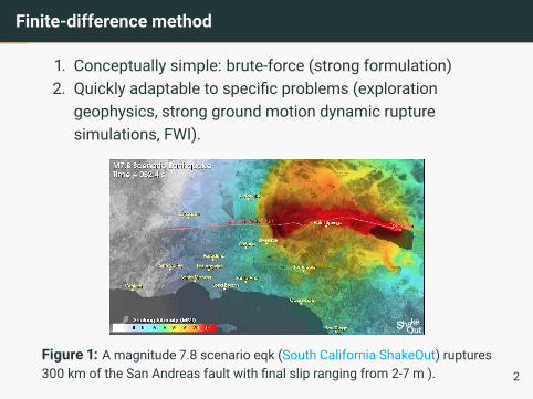
1. Conceptually simple: brute-force (strong formulation)2. Quickly adaptable to specific problems (exploration

geophysics, strong ground motion dynamic rupturesimulations, FWI).

Figure 1: A magnitude 7.8 scenario eqk (South California ShakeOut) ruptures300 km of the San Andreas fault with final slip ranging from 2-7 m ). 2

History of Finite-difference - 1

• First applications of FD: layered medium in cylindricalcoordinates (Alterman and Karal 1968); simulate Lovewaves (snapshots) by Boore (1970)

• Acoustic equations (Alford et al 1974), elastic equations(Kelly et al 1976)

• Staggered-grid formulation: introduced to solve ruturepropagation problem (Madariaga 1976, Virieux andMadariaga, 1982), elastic SH/P-SV waves (Virieux, 1984,1986)

• Parallel computing allowed for 3D applications: Frankeland Vidale (1992), Graves (1993), Olsen and Archuleta(1996), and Pitarka and Irikura (1996)

• Other rheology: viscoelastic (Day and Minster, 1984,Emmerich and Korn, 1987, Robertsson et al., 1994) andanisotropic (Igel et al., 1995)

3

History of Finite-difference - 2

• Spherical coordinates for global waves: first with theaxisymmetric approximation (Igel and Weber, 1995, Igeland Weber, 1996, Chaljub and Tarantola, 1997), 3Dspherical sections (Igel et al., 2002).

• Frictional boundary condition for dyanmic rupture analysis(Olsen et al., 1997); Failed node based on thresholdcriterion (Nielsen and Tarantola 1992)

• Free-surface boundary with strong topography:volcanology (Ohminato and Chouet, 1997), viscoelastic(Robertsson and Holliger, 1997), modified operators orhybrid schemes (Moczo et al., 2014); stronglyheterogeneous media (Moczo et al. 2002)

• FWI: in 2D Crase et al. (1990), and in 3D (Chen et al., 2007).FD is the prevailing method for forward solver for FWI inexploration seismology (Virieux and Operto, 2009).

4

Finite-difference approximation toderivatives

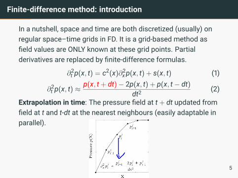
Finite-difference method: introduction

In a nutshell, space and time are both discretized (usually) onregular space–time grids in FD. It is a grid-based method asfield values are ONLY known at these grid points. Partialderivatives are replaced by finite-difference formulas.

∂2t p(x, t) = c2(x)∂2

xp(x, t) + s(x, t) (1)

∂2t p(x, t) ≈ p(x, t + dt)− 2p(x, t) + p(x, t− dt)

dt2(2)

Extrapolation in time: The pressure field at t + dt updated fromfield at t and t-dt at the nearest neighbours (easily adaptable inparallel).

5

Finite Differencing formulas

Forward differencing

df+

dx≈ f(x + dx)− f(x)

dx(3)

Centered differencing

dfc

dx≈ f(x + dx)− f(x− dx)

2dx(4)

Backward differencing

df−

dx≈ f(x)− f(x− dx)

dx(5)

How accurate are these differencing formulas?

6

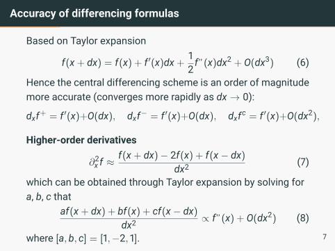
Accuracy of differencing formulas

Based on Taylor expansion

f(x + dx) = f(x) + f ′(x)dx +12f”(x)dx2 + O(dx3) (6)

Hence the central differencing scheme is an order of magnitudemore accurate (converges more rapidly as dx→ 0):

dxf+ = f ′(x)+O(dx), dxf− = f ′(x)+O(dx), dxfc = f ′(x)+O(dx2),

Higher-order derivatives

∂2x f ≈

f(x + dx)− 2f(x) + f(x− dx)

dx2(7)

which can be obtained through Taylor expansion by solving fora, b, c that

af(x + dx) + bf(x) + cf(x− dx)

dx2∝ f”(x) + O(dx2) (8)

where [a, b, c] = [1,−2, 1]. 7

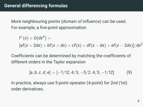
General differencing formulas

More neighbouring points (domain of influence) can be used.For example, a five-point approximation

f”(x) + O(dx4) =

[af(x + 2dx) + bf(x + dx) + cf(x) + df(x− dx) + ef(x− 2dx)]/dx2

Coefficients can be determined by matching the coefficients ofdifferent orders in the Taylor expansion

[a, b, c, d, e] = [−1/12,4/3,−5/2,4/3,−1/12] (9)

In practice, always use 5-point operator (4-point) for 2nd (1st)order derivatives.

8

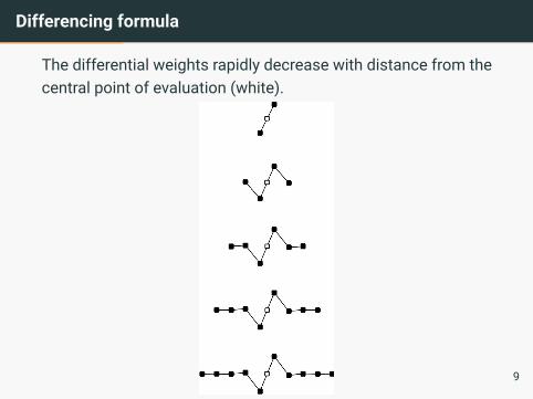
Differencing formula

The differential weights rapidly decrease with distance from thecentral point of evaluation (white).

9

FD for 1D Acoustic wave equation

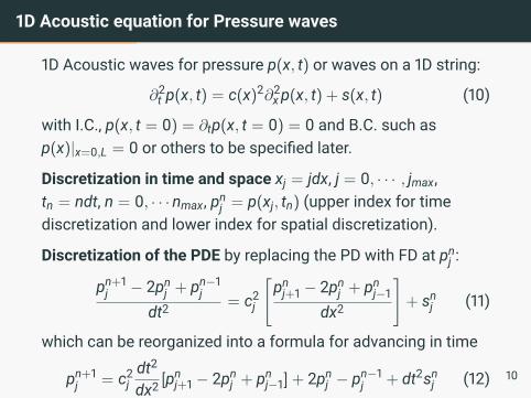
1D Acoustic equation for Pressure waves

1D Acoustic waves for pressure p(x, t) or waves on a 1D string:

∂2t p(x, t) = c(x)2∂2

xp(x, t) + s(x, t) (10)

with I.C., p(x, t = 0) = ∂tp(x, t = 0) = 0 and B.C. such asp(x)|x=0,L = 0 or others to be specified later.

Discretization in time and space xj = jdx, j = 0, · · · , jmax,tn = ndt, n = 0, · · · nmax, pn

j = p(xj, tn) (upper index for timediscretization and lower index for spatial discretization).

Discretization of the PDE by replacing the PD with FD at pnj :

pn+1j − 2pn

j + pn−1j

dt2= c2j

[pnj+1 − 2pn

j + pnj−1

dx2

]+ snj (11)

which can be reorganized into a formula for advancing in time

pn+1j = c2j

dt2

dx2[pn

j+1 − 2pnj + pn

j−1] + 2pnj − pn−1

j + dt2snj (12) 10

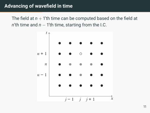
Advancing of wavefield in time

The field at n + 1’th time can be computed based on the field atn’th time and n− 1’th time, starting from the I.C.

11

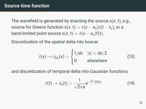
Source time function

The wavefield is generated by enacting the source s(x, t), e.g.,source for Greens function s(x, t) = δ(x− xs)δ(t− ts), or aband-limited point source s(x, t) = δ(x− xs)f(t).

Discretization of the spatial delta into boxcar

δ(x)→ δbc(x) =

1/dx |x| < dx/2

0 elsewhere(13)

and discretization of temporal delta into Gaussian functions

δ(t)→ δa(t) =1√2πa

e−t2/(2a) (14)

12

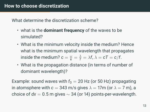
How to choose discretization

What determine the discretization scheme?

• what is the dominant frequency of the waves to besimulated?

• What is the minimum velocity inside the medium? Hencewhat is the minimum spatial wavelength that propagatesinside the medium? c = ω

k = λT = λf , λ = cT = c/f.

• What is the propagation distance (in terms of number ofdominant wavelength)?

Example: sound waves with f0 = 20 Hz (or 50 Hz) propagatingin atomsphere with c = 343 m/s gives λ = 17m (or λ = 7 m), achoice of dx = 0.5 m gives ∼ 34 (or 14) points-per-wavelength.

13

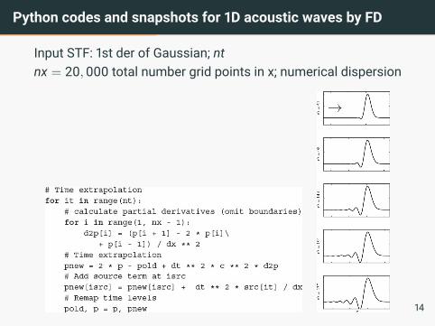
Python codes and snapshots for 1D acoustic waves by FD

Input STF: 1st der of Gaussian; ntnx = 20,000 total number grid points in x; numerical dispersion

14

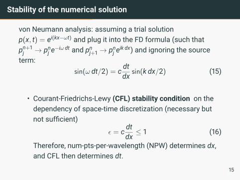
Stability of the numerical solution

von Neumann analysis: assuming a trial solutionp(x, t) = ei(kx−ωt) and plug it into the FD formula (such thatpn+1j → pn

j e−iω dt and pn

j+1 → pnj e

ik dx) and ignoring the sourceterm:

sin(ω dt/2) = cdtdx

sin(k dx/2) (15)

• Courant-Friedrichs-Lewy (CFL) stability condition on thedependency of space-time discretization (necessary butnot sufficient)

ε = cdtdx≤ 1 (16)

Therefore, num-pts-per-wavelength (NPW) determines dx,and CFL then determines dt.

15

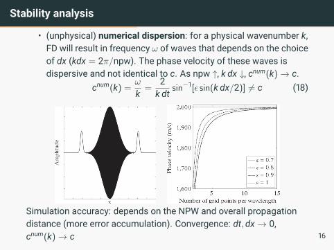
Stability analysissin(ω dt/2) = ε sin(k dx/2) (17)

• (unphysical) numerical dispersion: for a physical wavenumber k,FD will result in frequency ω of waves that depends on the choiceof dx (kdx = 2π/npw). The phase velocity of these waves isdispersive and not identical to c. As npw ↑, k dx ↓, cnum(k)→ c.

cnum(k) =ω

k=

2k dt

sin−1[ε sin(k dx/2)] 6= c (18)

Simulation accuracy: depends on the NPW and overall propagationdistance (more error accumulation). Convergence: dt, dx→ 0,cnum(k)→ c 16

FD for 2D Acoustic wave equation

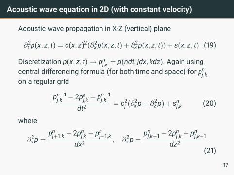
Acoustic wave equation in 2D (with constant velocity)

Acoustic wave propagation in X-Z (vertical) plane

∂2t p(x, z, t) = c(x, z)2(∂2

xp(x, z, t) + ∂2xp(x, z, t)) + s(x, z, t) (19)

Discretization p(x, z, t)→ pnj,k = p(ndt, jdx, kdz). Again using

central differencing formula (for both time and space) for pnj,k

on a regular grid

pn+1j,k − 2pn

j,k + pn−1j,k

dt2= c2j (∂2

xp + ∂2zp) + snj,k (20)

where

∂2xp =

pnj+1,k − 2pn

j,k + pnj−1,k

dx2, ∂2

zp =pnj,k+1 − 2pn

j,k + pnj,k−1

dz2(21)

17

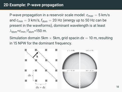
2D Example: P-wave propagation

P-wave propagation in a reservoir scale model: cmax = 5 km/sand cmin = 3 km/s, fdom = 20 Hz (energy up to 50 Hz can bepresent in the waveforms), dominant wavelength is at leastλdom=cmin/fdom=150 m.

Simulation domain 5km × 5km, grid spacin dx = 10 m, resultingin 15 NPW for the dominant frequency.

18

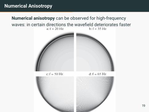
Numerical Anisotropy

Numerical anisotropy can be observed for high-frequencywaves: in certain directions the wavefield deteriorates faster

19

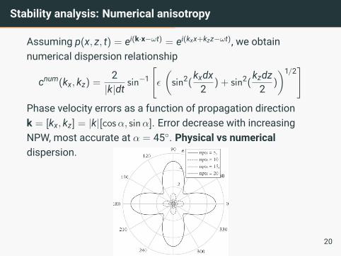
Stability analysis: Numerical anisotropy

Assuming p(x, z, t) = ei(k·x−ωt) = ei(kxx+kzz−ωt), we obtainnumerical dispersion relationship

cnum(kx, kz) =2|k|dt

sin−1

[ε

(sin2(

kxdx2

) + sin2(kzdz2

)

)1/2]

Phase velocity errors as a function of propagation directionk = [kx, kz] = |k|[cosα, sinα]. Error decrease with increasingNPW, most accurate at α = 45◦. Physical vs numericaldispersion.

20

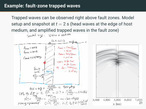
Example: fault-zone trapped waves

Trapped waves can be observed right above fault zones. Modelsetup and snapshot at t = 2 s (head waves at the edge of hostmedium, and amplified trapped waves in the fault zone)

21

1D elastic wave equations

Constitutive relationship in 1D for uy(x, t)

σij = λεkkδij + 2µεij (22)

becomesσxy = σyx = 2µεxy = µ∂xuy (23)

For simplicity, just use u(x, t) to represent uy(x, t), and the 1Delastic wave equation becomes

ρ∂2t u = ∂x(µ∂xu) + f (24)

and under discretization uji = u(idx, jdt),

ρiuj+1i − 2uj

i + uj−1i

dt2=µi+1u

ji+2 − µi+1u

ji − µi−1u

ji + µi−1u

ji−2

4 dx2+ f ji

Note u values on i± 1 are not used due to the asymmetry incentral difference formula for 1st order derivatives. Thisinefficiency can be improved by velocity-stress formulation. 22

Velocity–stress formulation

Goal: as error ∼ O(dx2), reducing dx by half, will give 1/4 of theerror. Rewrite the wave equation into a coupled first-order PDEsystem for (v, σ)

ρ∂tv = ∂xσ + f (25)

∂tσ = µ∂xv (26)

and still discretize on the regular grid in time and space:centered at (vji, σ

ji+1/2 by staggered-grid for

vj+1/2i = v(i dx, (j + 1/2) dt), and σj

i+1/2 = σ((i + 1/2) dx, j dt).

vj+1/2i − vj−1/2

idt

=σji+1/2 − σ

ji−1/2

ρidx+

f jiρi

(27)

σj+1i+1/2 − σ

ji+1/2

dt= µi+1/2

vj+1/2i+1 − vj+1/2

idx

(28)23

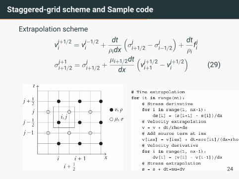
Staggered-grid scheme and Sample code

Extrapolation scheme

vj+1/2i = vj−1/2

i +dtρidx

(σji+1/2 − σ

ji−1/2

)+

dtρi

f ji

σj+1i+1/2 = σ

ji+1/2 +

µi+1/2dtdx

(vj+1/2i+1 − vj+1/2

i

)(29)

24

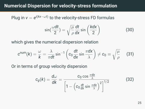
Numerical Dispersion for velocity-stress formulation

Plug in v = ei(kx−ωt) to the velocity-stress FD formulas

sin(ωdt2

) =

õ

ρ

dtdx

sin

(kdx2

)(30)

which gives the numerical dispersion relation

cnum(k) =ω

k=

λ

πdtsin−1

(c0

dtdx

sinπdxλ

)6= c0 ≡

õ

ρ(31)

Or in terms of group velocity dispersion

cg(k) =dωdk

=c0 cos πdxλ[

1−(c0 dt

dx sin πdxλ

)2]1/2 (32)

25

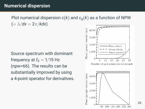
Numerical dispersion

Plot numerical dispersion c(k) and cg(k) as a function of NPW(= λ/dx = 2π/kdx)

Source spectrum with dominantfrequency at f0 = 1/15 Hz(npw=66). The results can besubstantially improved by usinga 4-point operator for derivatives.

26

Elastic wave propagation in 2D

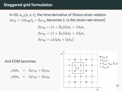
Staggered grid formulation

In 2D, vx,z(x, z; t), the time-derivative of Stress-strain relation∂tσij = λ∂tεkkδij + 2µεij, becomes (ε is the strain-rate tensor)

∂tσxx = (λ+ 2µ)∂xvx + λ∂zvz∂tσzz = (λ+ 2µ)∂zvz + λ∂xvx∂tσxz = µ(∂xvz + ∂zvx)

And EOM becomes

ρ∂tvx = ∂xσxx + ∂zσxz

ρ∂tvz = ∂zσxz + ∂zσzz

27

Boundary Condition

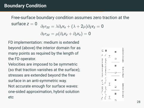
Free-surface boundary condition assumes zero traction at thesurface z = 0

∂tσzz = λ∂xvx + (λ+ 2µ)∂zvz = 0

∂tσzz = µ(∂xvz + ∂zvx) = 0

FD implementation: medium is extendedbeyond (above) the interior domain for asmany points as required by the length ofthe FD operator.Velocities are imposed to be symmetric(so that traction vanishes at the surface);stresses are extended beyond the freesurface in an anti-symmetric way.Not accurate enough for surface waves:one-sided approximation, hybrid solutionetc

28

FD for 3D wave propagation

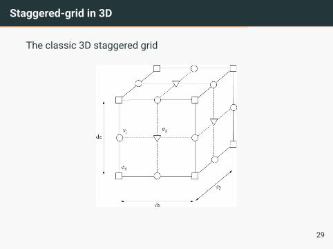
Staggered-grid in 3D

The classic 3D staggered grid

29

Miscellaneous Subjects related to FD

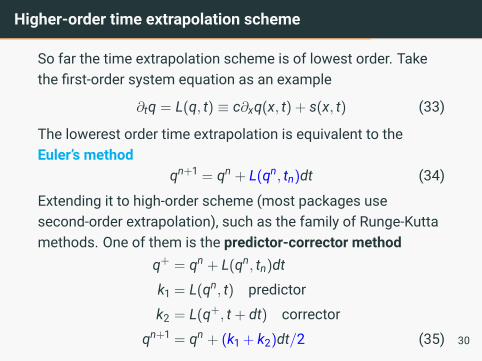
Higher-order time extrapolation scheme

So far the time extrapolation scheme is of lowest order. Takethe first-order system equation as an example

∂tq = L(q, t) ≡ c∂xq(x, t) + s(x, t) (33)

The lowerest order time extrapolation is equivalent to theEuler’s method

qn+1 = qn + L(qn, tn)dt (34)

Extending it to high-order scheme (most packages usesecond-order extrapolation), such as the family of Runge-Kuttamethods. One of them is the predictor-corrector method

q+ = qn + L(qn, tn)dt

k1 = L(qn, t) predictor

k2 = L(q+, t + dt) corrector

qn+1 = qn + (k1 + k2)dt/2 (35) 30

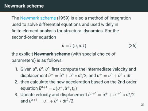
Newmark scheme

The Newmark scheme (1959) is also a method of integrationused to solve differential equations and used widely infinite-element analysis for structural dynamics. For thesecond-order equation

u = L(u, u, t) (36)

the explicit Newmark scheme (with special choice ofparameters) is as follows:

1. Given un, un, un, first compute the intermediate velocity anddisplacement u+ = un + un ∗ dt/2, and u+ = un + un ∗ dt

2. then calculate the new acceleration based on the 2nd-orderequation un+1 = L(u+, u+, tn)

3. Update velocity and displacement un+1 = u+ + un+1 ∗ dt/2and un+1 = u+ + un ∗ dt2/2

31

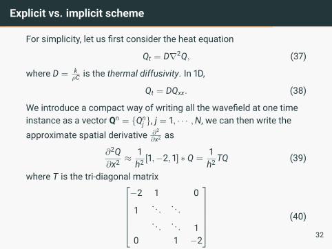
Explicit vs. implicit scheme

For simplicity, let us first consider the heat equation

Qt = D∇2Q, (37)

where D = kρC is the thermal diffusivity. In 1D,

Qt = DQxx. (38)

We introduce a compact way of writing all the wavefield at one timeinstance as a vector Qn = {Qn

j }, j = 1, · · · ,N, we can then write theapproximate spatial derivative ∂2

∂x2 as

∂2Q∂x2

≈ 1h2 [1,−2, 1] ∗ Q =

1h2TQ (39)

where T is the tri-diagonal matrix−2 1 0

1. . . . . .. . . . . . 1

0 1 −2

(40)

32

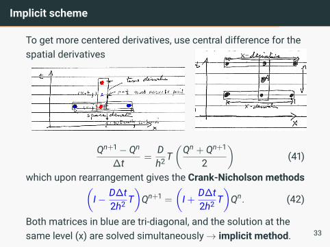
Implicit scheme

To get more centered derivatives, use central difference for thespatial derivatives

Qn+1 − Qn

∆t=

Dh2T

(Qn + Qn+1

2

)(41)

which upon rearrangement gives the Crank-Nicholson methods(I− D∆t

2h2 T)Qn+1 =

(I +

D∆t2h2 T

)Qn. (42)

Both matrices in blue are tri-diagonal, and the solution at thesame level (x) are solved simultaneously→ implicit method. 33

Cauchy-Kowaleski procedure

Ignoring the source term, the derivatives of q also satisfies theequation

∂j+1t q(x, t) = c∂x[∂ j

tq(x, t)] (43)

The time derivative of q(x, t) of any order can be replaced by thespatial derivative recursively. It has been used to Arbitraryhigh-orDER (ADER) schemes for the finite-volume anddiscontinuous Galerkin methods (e.g. Titarev and Toro 2002;Dumbser and Munz, 2005a)

34

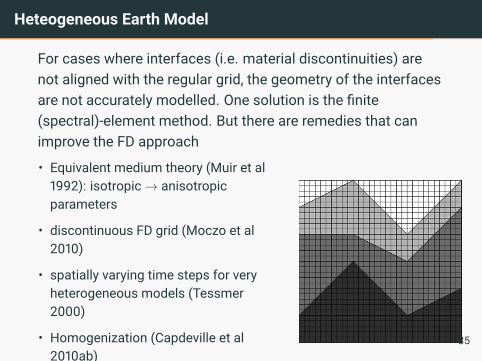
Heteogeneous Earth Model

For cases where interfaces (i.e. material discontinuities) arenot aligned with the regular grid, the geometry of the interfacesare not accurately modelled. One solution is the finite(spectral)-element method. But there are remedies that canimprove the FD approach

• Equivalent medium theory (Muir et al1992): isotropic→ anisotropicparameters

• discontinuous FD grid (Moczo et al2010)

• spatially varying time steps for veryheterogeneous models (Tessmer2000)

• Homogenization (Capdeville et al2010ab)

35

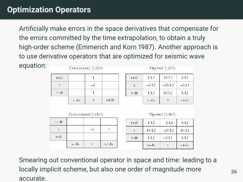
Optimization Operators

Artificially make errors in the space derivatives that compensate forthe errors committed by the time extrapolation, to obtain a trulyhigh-order scheme (Emmerich and Korn 1987). Another approach isto use derivative operators that are optimized for seismic waveequation:

Smearing out conventional operator in space and time: leading to alocally implicit scheme, but also one order of magnitude moreaccurate.

36

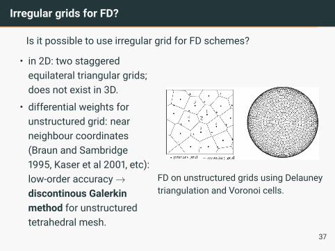
Irregular grids for FD?

Is it possible to use irregular grid for FD schemes?

• in 2D: two staggeredequilateral triangular grids;does not exist in 3D.

• differential weights forunstructured grid: nearneighbour coordinates(Braun and Sambridge1995, Kaser et al 2001, etc):low-order accuracy→discontinous Galerkinmethod for unstructuredtetrahedral mesh.

FD on unstructured grids using Delauneytriangulation and Voronoi cells.

37

Other coordinate systems

For the acoustic wave equation, assuming spherical coordinatesystem (r, θ, φ), and a model c(r, θ) and source s(r, θ) invariantin φ (i.e., zonal model or axisymmetric)

p = c2[1r2∂r(r2∂rp) +

1r2 sin θ

∂θ(sin θ∂θp)

]+ s (44)

which is much more complicated than the cartesian case.

• Singularity at θ = 0 (the pole)

• Regular discretization on r and theta leads to grid spacingdecrease with depth, while given the velocity in the mantle,we want grid spacing to increase with depth→ gridrefinement towards the surface, smaller time steps

38

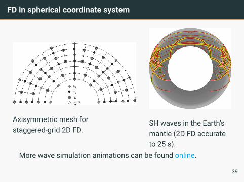
FD in spherical coordinate system

Axisymmetric mesh forstaggered-grid 2D FD.

SH waves in the Earth’smantle (2D FD accurateto 25 s).

More wave simulation animations can be found online.

39