Bill KaliesFlorida Atlantic University

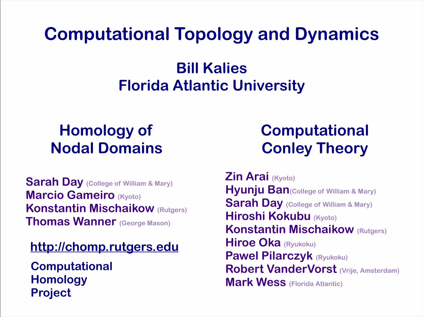
Computational Topology and Dynamics

Sarah Day (College of William & Mary)

Marcio Gameiro (Kyoto)

Konstantin Mischaikow (Rutgers)

Thomas Wanner (George Mason)

Homology of Nodal Domains

Computational Conley Theory

Zin Arai (Kyoto)

Hyunju Ban(College of William & Mary)

Sarah Day (College of William & Mary)

Hiroshi Kokubu (Kyoto)

Konstantin Mischaikow (Rutgers)

Hiroe Oka (Ryukoku)

Pawel Pilarczyk (Ryukoku)

Robert VanderVorst (Vrije, Amsterdam)

Mark Wess (Florida Atlantic)

http://chomp.rutgers.edu

ComputationalHomologyProject

Bill KaliesFlorida Atlantic University

Verified Homology of Nodal Domains

Sarah Day (College of William & Mary)

Marcio Gameiro (Kyoto)

Konstantin Mischaikow (Rutgers)

Thomas Wanner (George Mason)

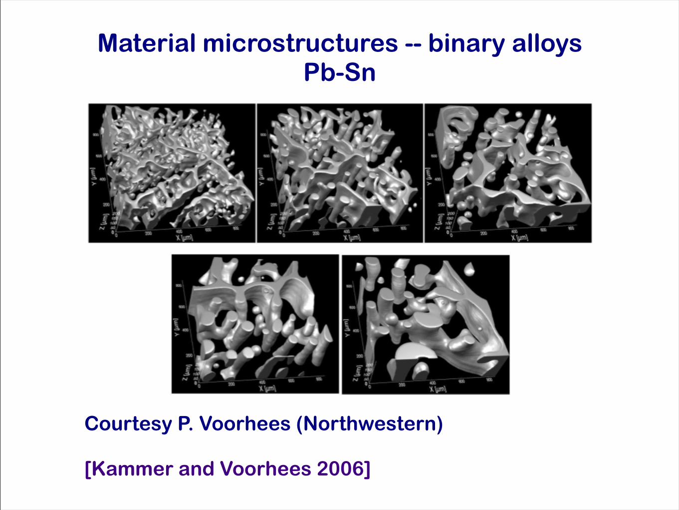
Material microstructures -- binary alloysPb-Sn

Courtesy P. Voorhees (Northwestern)

[Kammer and Voorhees 2006]

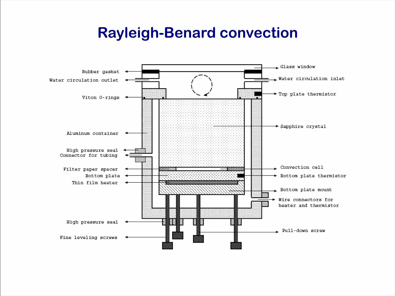
Rayleigh-Benard convection

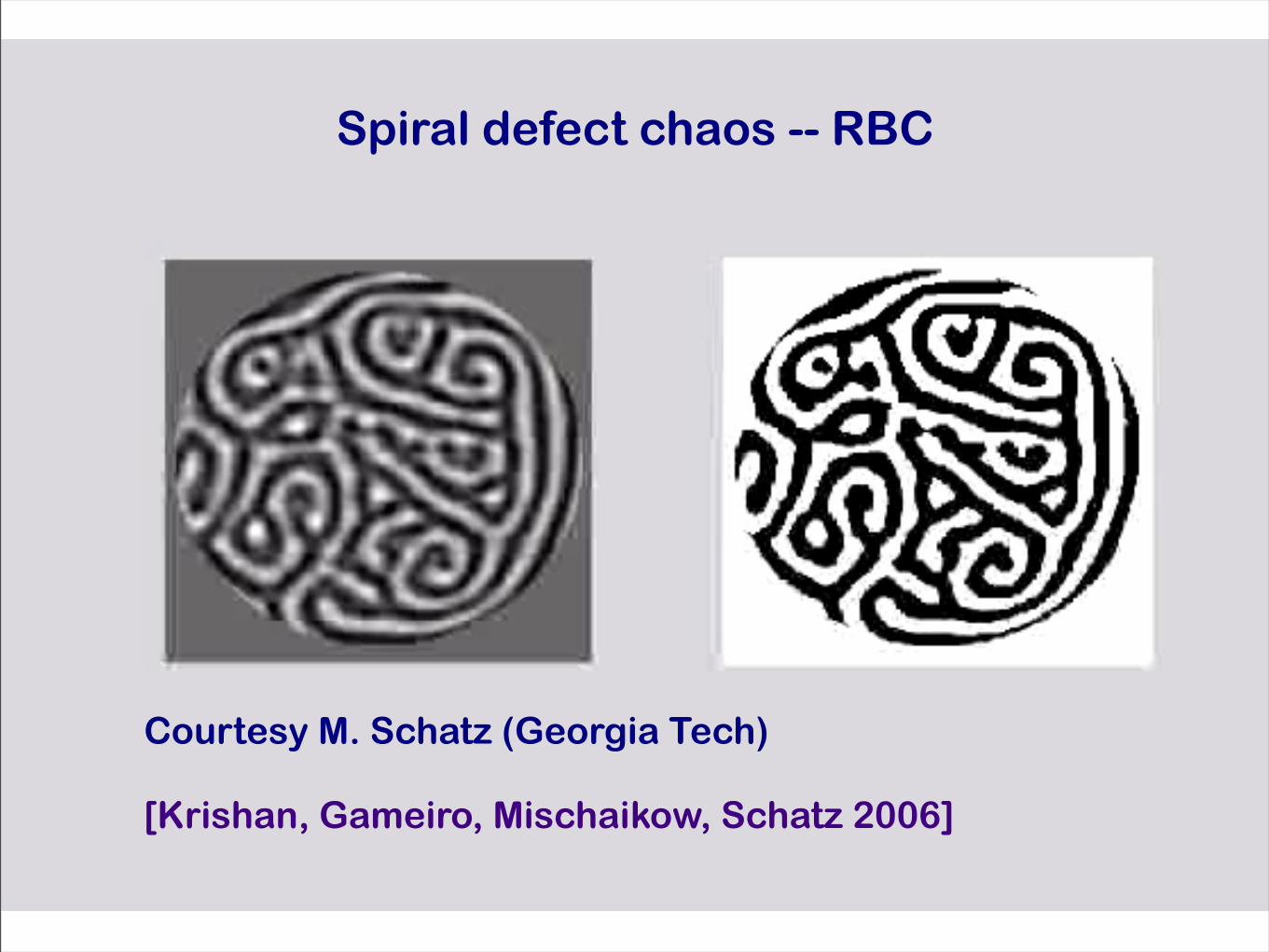
Spiral defect chaos -- RBC

Courtesy M. Schatz (Georgia Tech)

[Krishan, Gameiro, Mischaikow, Schatz 2006]

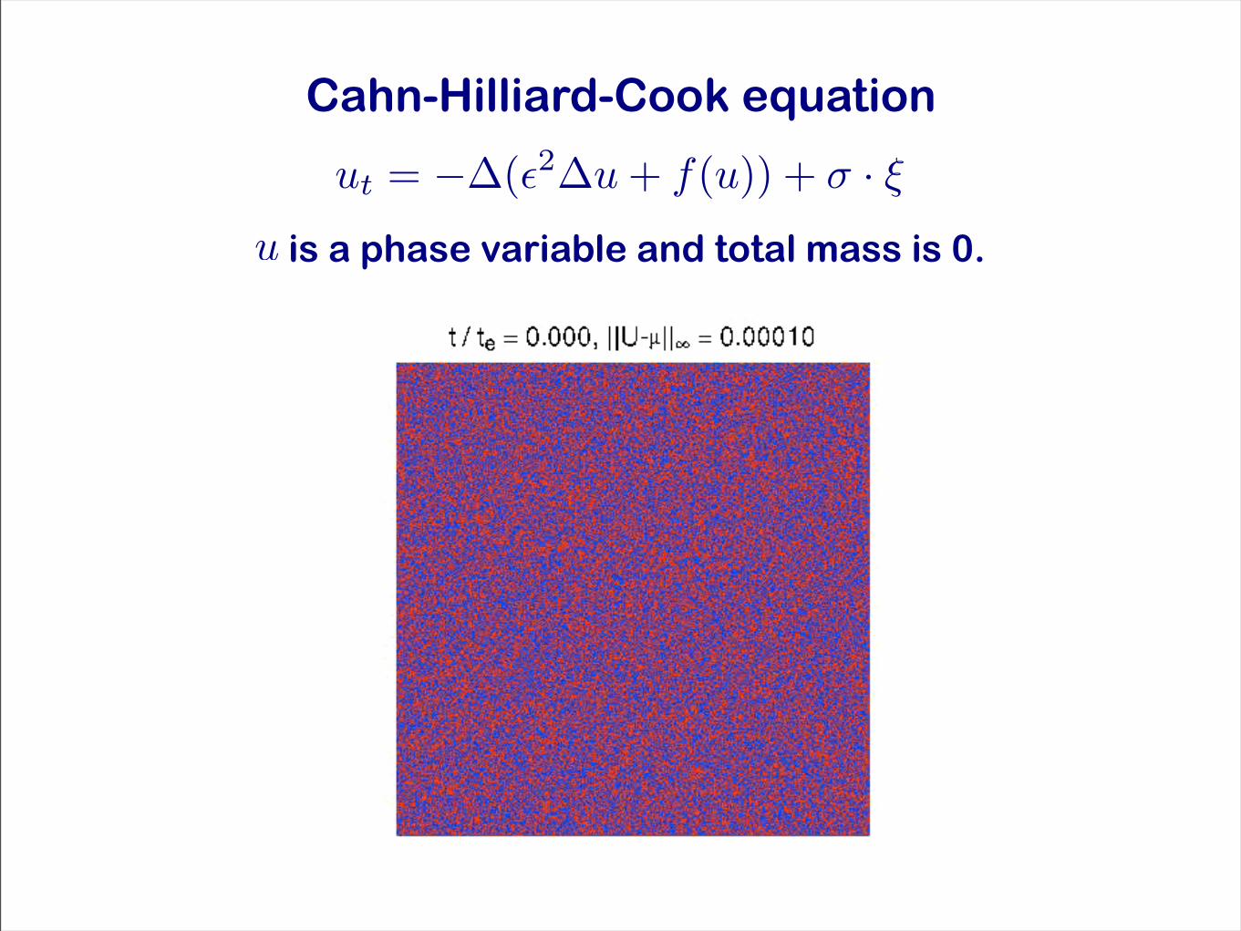
is a phase variable and total mass is 0.

Cahn-Hilliard-Cook equation

ut = !!(!2!u + f(u)) + " · #

u

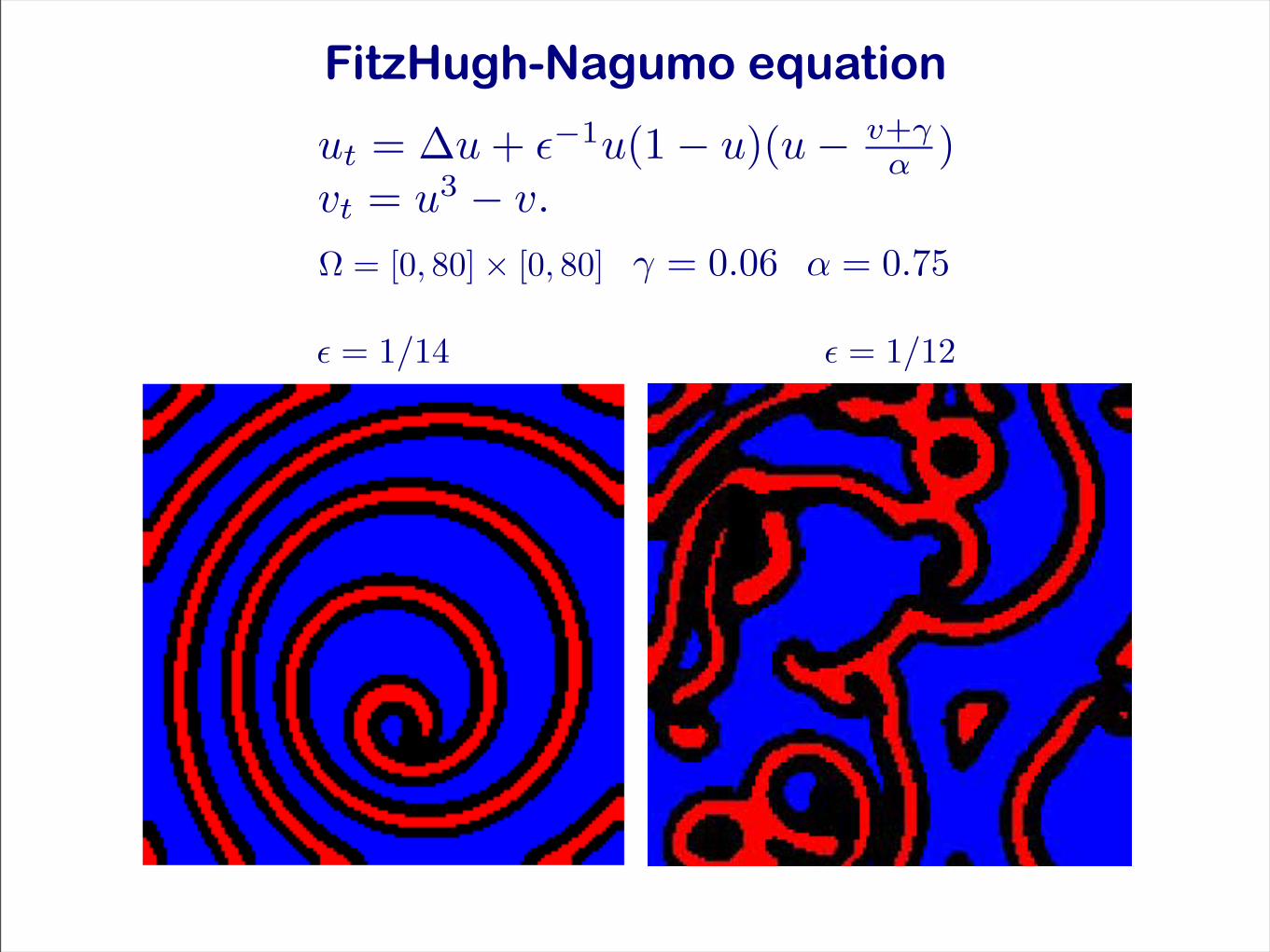
FitzHugh-Nagumo equation

ut = !u + !!1u(1! u)(u! v+!" )

vt = u3 ! v.

! = [0, 80]! [0, 80] ! = 0.75! = 0.06

! = 1/14 ! = 1/12

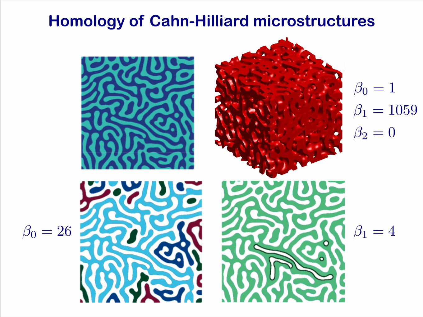
Homology of Cahn-Hilliard microstructures

!0 = 1!1 = 1059!2 = 0

!1 = 4!0 = 26

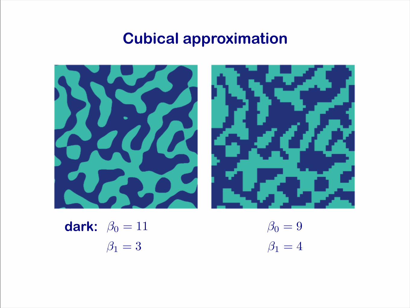
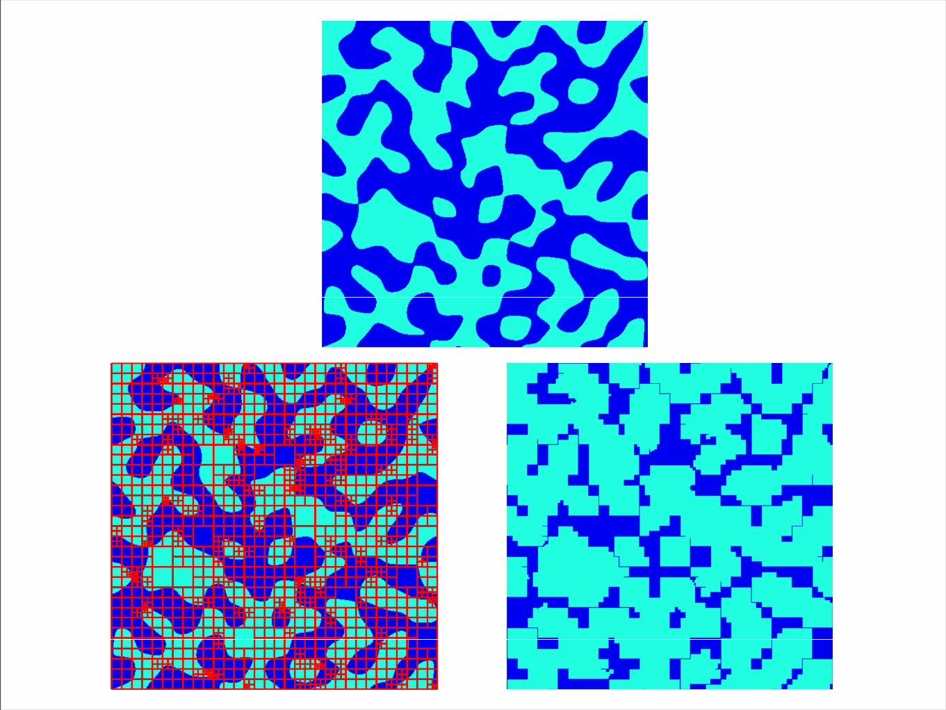
Cubical approximation

!0 = 11 !0 = 9

!1 = 3 !1 = 4dark:

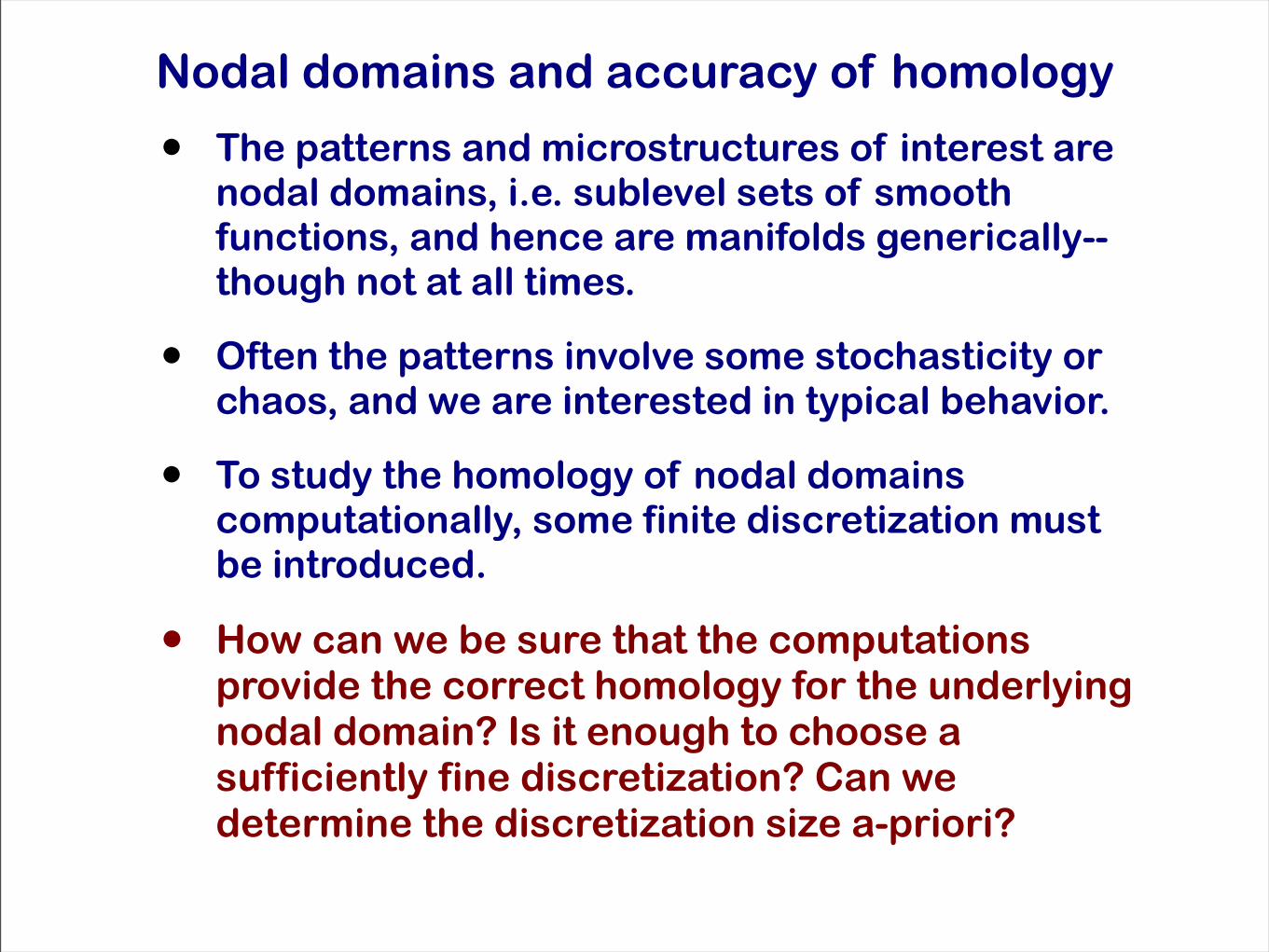
Nodal domains and accuracy of homology

• The patterns and microstructures of interest are nodal domains, i.e. sublevel sets of smooth functions, and hence are manifolds generically-- though not at all times.

• Often the patterns involve some stochasticity or chaos, and we are interested in typical behavior.

• To study the homology of nodal domains computationally, some finite discretization must be introduced.

• How can we be sure that the computations provide the correct homology for the underlying nodal domain? Is it enough to choose a sufficiently fine discretization? Can we determine the discretization size a-priori?

Time series of Betti numbers

In all three settings:

(1) Cahn-Hilliard simulations of material microstructures,

(2) spatial-temporal chaos in FitzHugh-Nagumo, (3) experimental spiral defect chaos

we find information from a direct topological study of the patterns that can be difficult to obtain or not noticed otherwise.

The main idea is to study the Betti numbers as a time series of data by thresholding the data on a finite grid to extract a cubical approximation to the pattern. Note that rectangular grids arise naturally in images and numerical solutions to PDE’s.

What is the goal?

CHC is one of several phenomenological models -- would like a quantitative measurement to make comparisons with experiments and between models.

SDC in RBC is easier to study experimentally than numerically, but then your data is a movie of a pattern of some observable, not values for fluid velocity. How do we quantitatively compare different experiments?

Spatial-temporal chaos is difficult to define and quantify precisely. The dynamics can be high-dimensional.

Computing Betti numbers is a huge reduction in information, is there any info left?

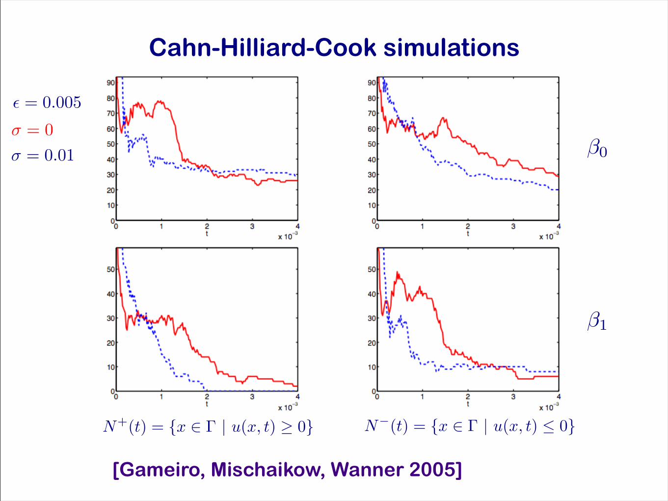
Cahn-Hilliard-Cook simulations

[Gameiro, Mischaikow, Wanner 2005]

!0

!1

! = 0.005

! = 0.01! = 0

N!(t) = {x ! ! | u(x, t) " 0}N+(t) = {x ! ! | u(x, t) " 0}

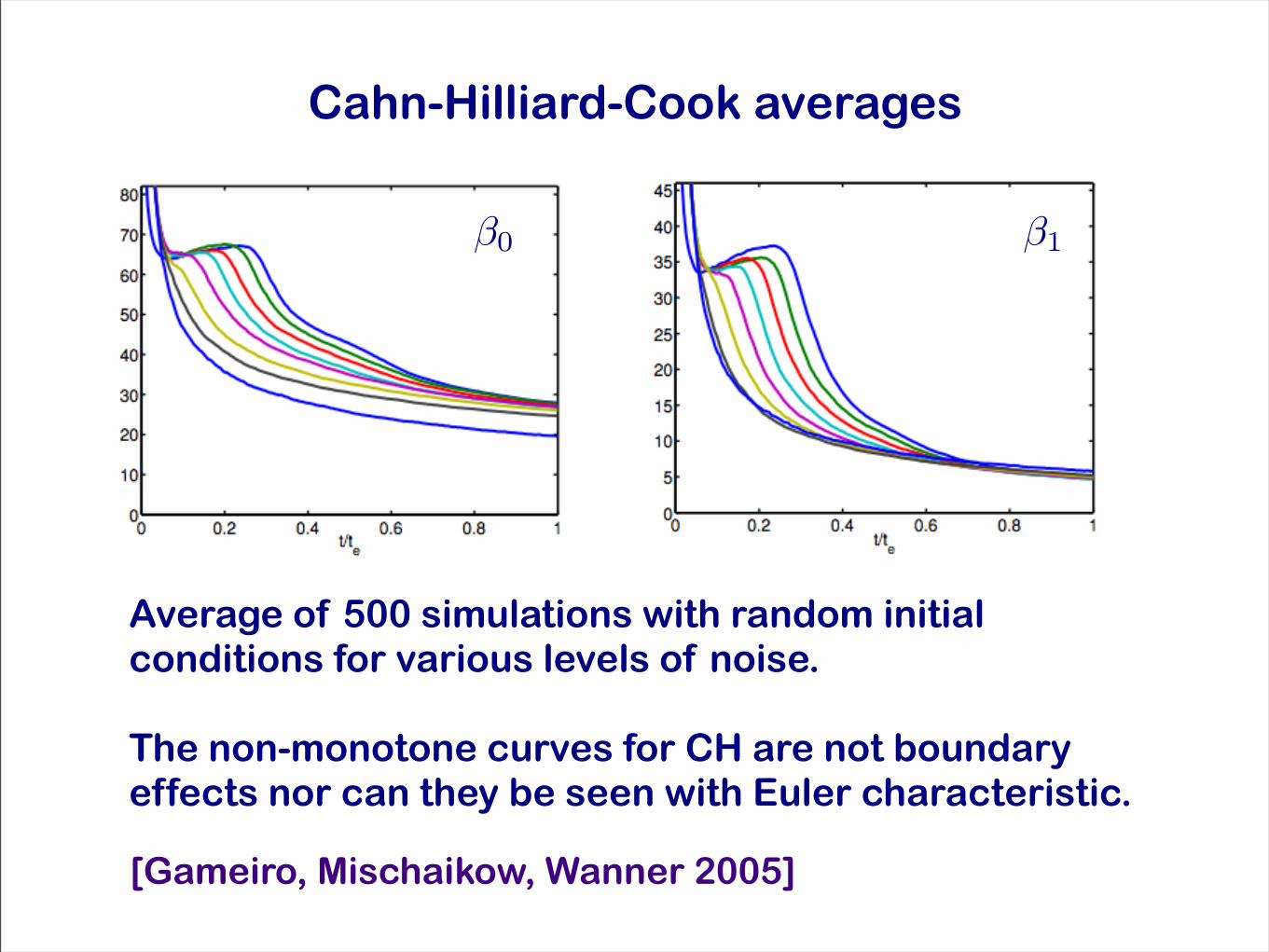
Cahn-Hilliard-Cook averages

!1!0

Average of 500 simulations with random initial conditions for various levels of noise.

The non-monotone curves for CH are not boundary effects nor can they be seen with Euler characteristic.

[Gameiro, Mischaikow, Wanner 2005]

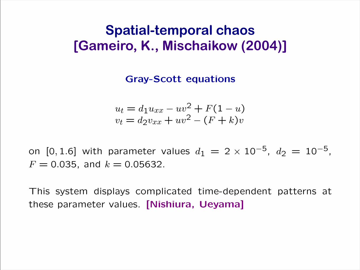
Gray-Scott equations

ut = d1uxx ! uv2 + F (1! u)vt = d2vxx + uv2 ! (F + k)v

on [0,1.6] with parameter values d1 = 2 " 10!5, d2 = 10!5,F = 0.035, and k = 0.05632.

This system displays complicated time-dependent patterns atthese parameter values. [Nishiura, Ueyama]

5

Spatial-temporal chaos [Gameiro, K., Mischaikow (2004)]

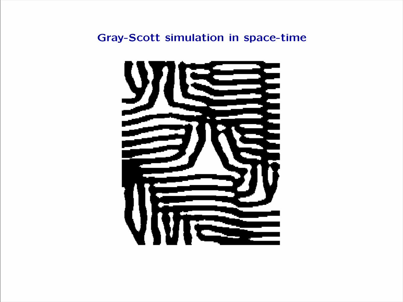
Gray-Scott simulation in space-time

6

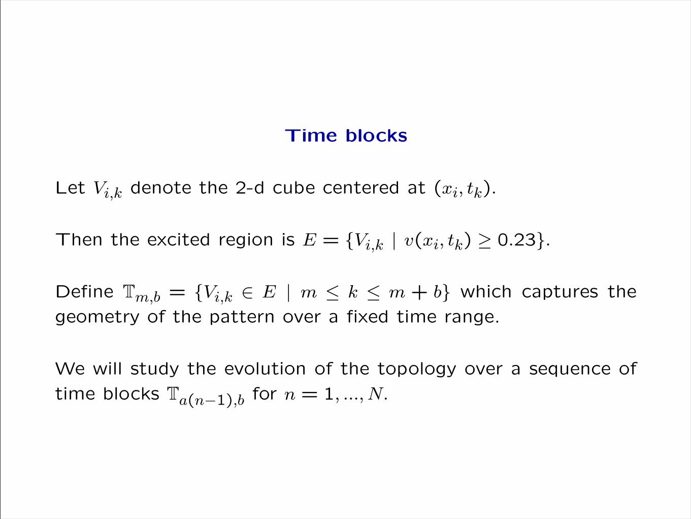
Time blocks

Let Vi,k denote the 2-d cube centered at (xi, tk).

Then the excited region is E = {Vi,k | v(xi, tk) ! 0.23}.

Define Tm,b = {Vi,k " E | m # k # m + b} which captures thegeometry of the pattern over a fixed time range.

We will study the evolution of the topology over a sequence oftime blocks Ta(n$1),b for n = 1, ..., N.

8

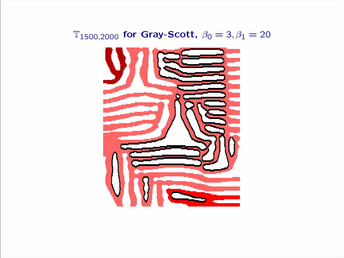
T1500,2000 for Gray-Scott, !0 = 3, !1 = 20

9

Betti numbers

To every topological space X, one can assign a sequence ofhomology groups Hi(X, Z).

In this setting of full cubical complexes, Hi(Ta(n!1),b, Z) " Z!i.

The integers !i # 0 are the Betti numbers of the time block.

We then generate a time series from each Betti number !i(n).

For d-dimensional complexes, !i = 0 for all i # d.

http://www.math.gatech.edu/$chomp [K., Pilarczyk]

10

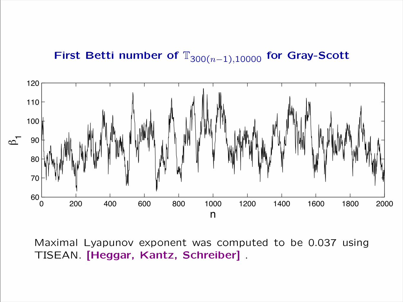
First Betti number of T300(n!1),10000 for Gray-Scott

0 200 400 600 800 1000 1200 1400 1600 1800 200060

70

80

90

100

110

120

n

!1

Maximal Lyapunov exponent was computed to be 0.037 usingTISEAN. [Heggar, Kantz, Schreiber] .

11

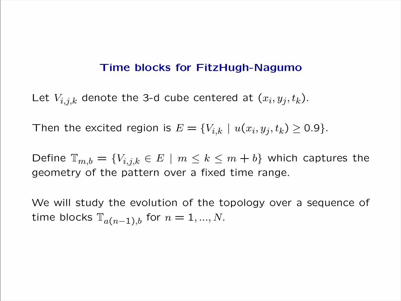
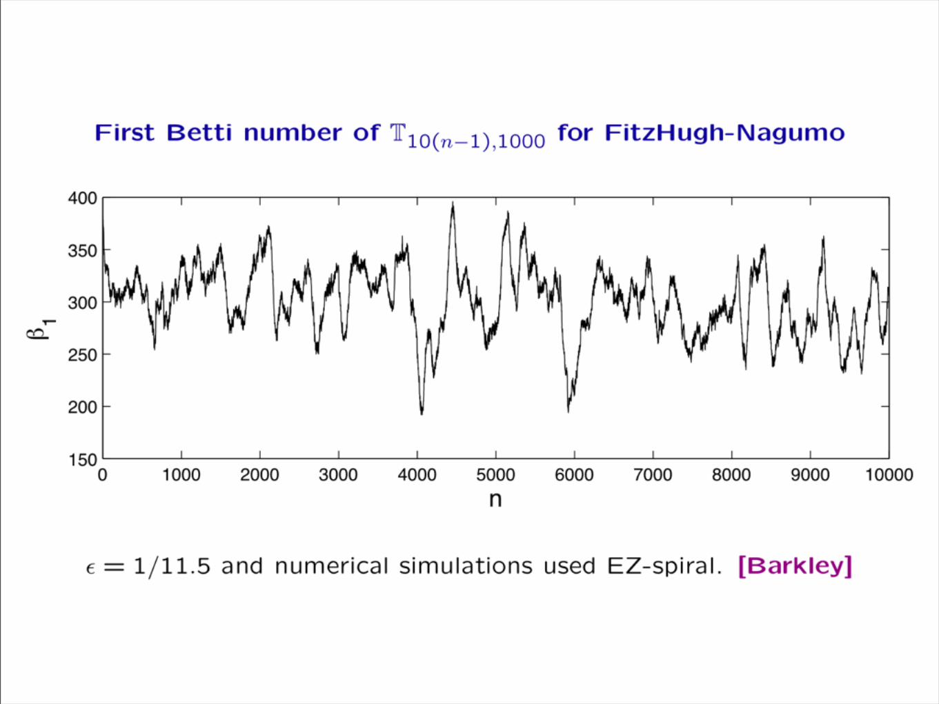
Time blocks for FitzHugh-Nagumo

Let Vi,j,k denote the 3-d cube centered at (xi, yj, tk).

Then the excited region is E = {Vi,k | u(xi, yj, tk) ! 0.9}.

Define Tm,b = {Vi,j,k " E | m # k # m + b} which captures thegeometry of the pattern over a fixed time range.

We will study the evolution of the topology over a sequence oftime blocks Ta(n$1),b for n = 1, ..., N.

12

FitzHugh-Nagumo equation

ut = !u + !!1u(1! u)(u! v+!" )

vt = u3 ! v.

! = [0, 80]! [0, 80] ! = 0.75! = 0.06

! = 1/14 ! = 1/12

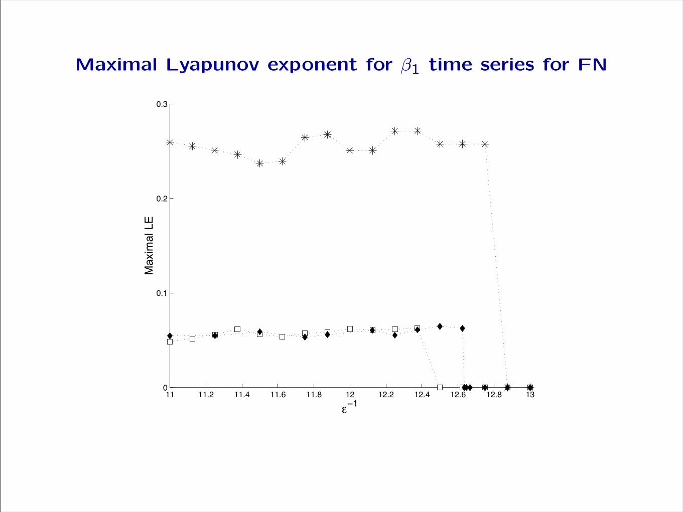
Maximal Lyapunov exponent for !1 time series for FN

!! !!"# !!"$ !!"% !!"& !# !#"# !#"$ !#"% !#"& !'(

("!

("#

("'

!!!

)*+,-*./01

15

Observations

The Lyapunov exponent is constant so not a good measurement to do parameter estimation.

The Lyapunov exponent for the Betti number time series drops to 0 before the time series of values at a fixed point in the domain.

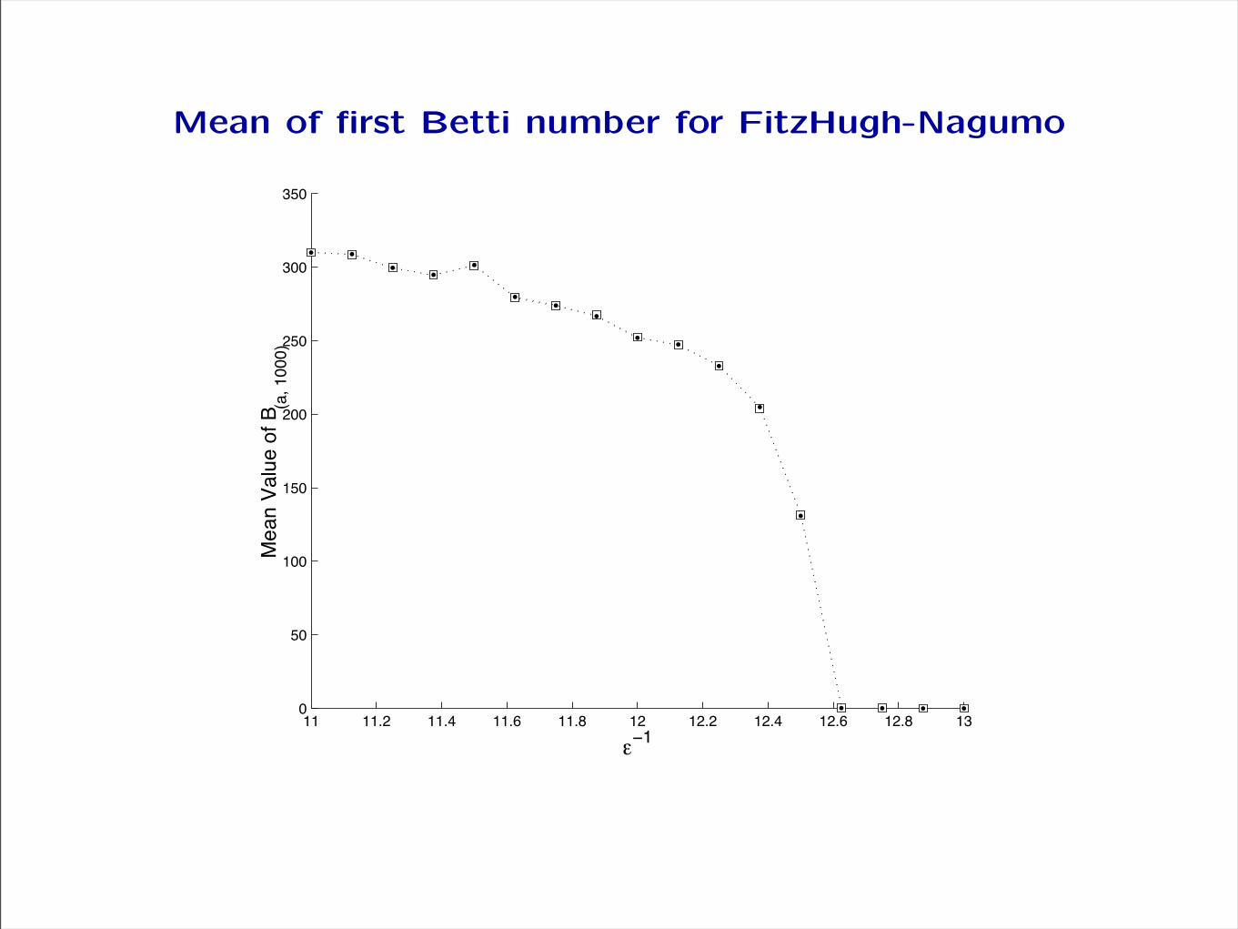
Mean of first Betti number for FitzHugh-Nagumo

!! !!"# !!"$ !!"% !!"& !# !#"# !#"$ !#"% !#"& !'(

)(

!((

!)(

#((

#)(

'((

')(

!!!

*+,-./,01+.23.45,6.!(((7

17

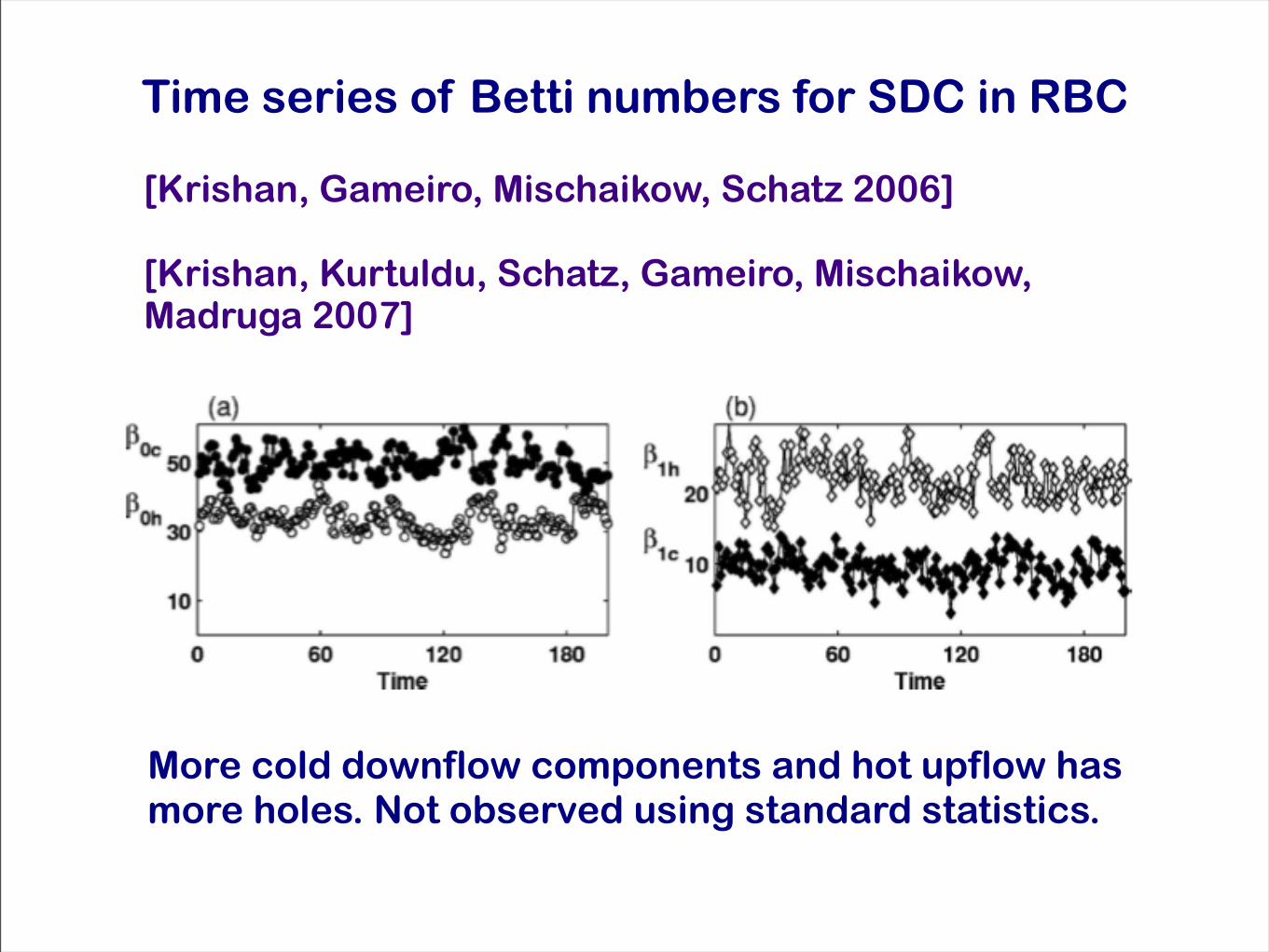
Time series of Betti numbers for SDC in RBC

[Krishan, Gameiro, Mischaikow, Schatz 2006]

[Krishan, Kurtuldu, Schatz, Gameiro, Mischaikow, Madruga 2007]

More cold downflow components and hot upflow has more holes. Not observed using standard statistics.

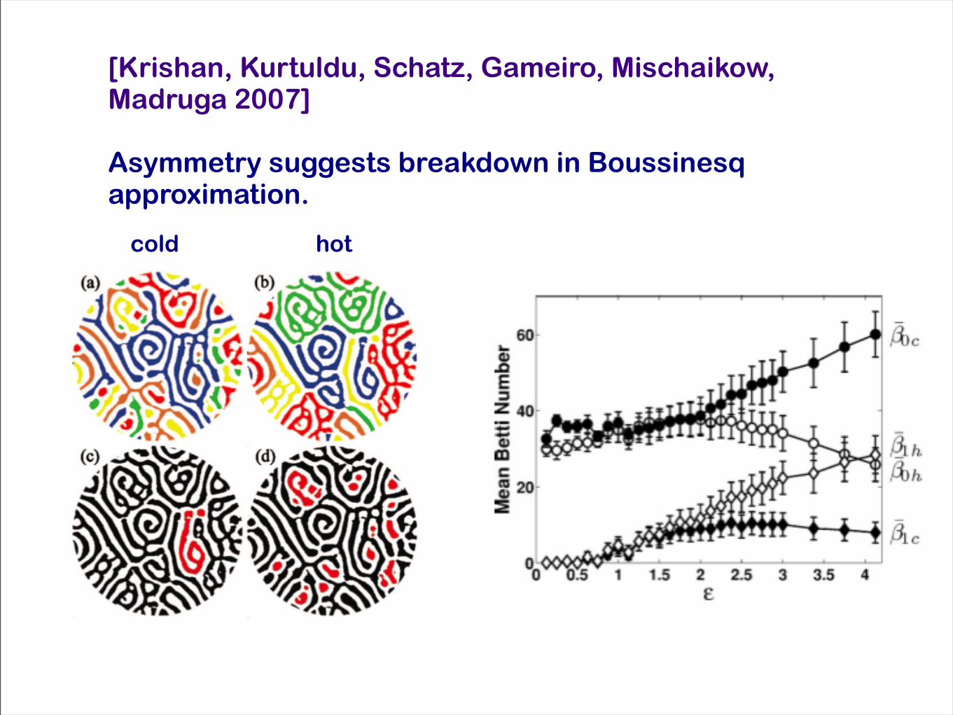
[Krishan, Kurtuldu, Schatz, Gameiro, Mischaikow, Madruga 2007]

Asymmetry suggests breakdown in Boussinesq approximation.

cold hot

Cubical approximation

!0 = 11 !0 = 9

!1 = 3 !1 = 4dark:

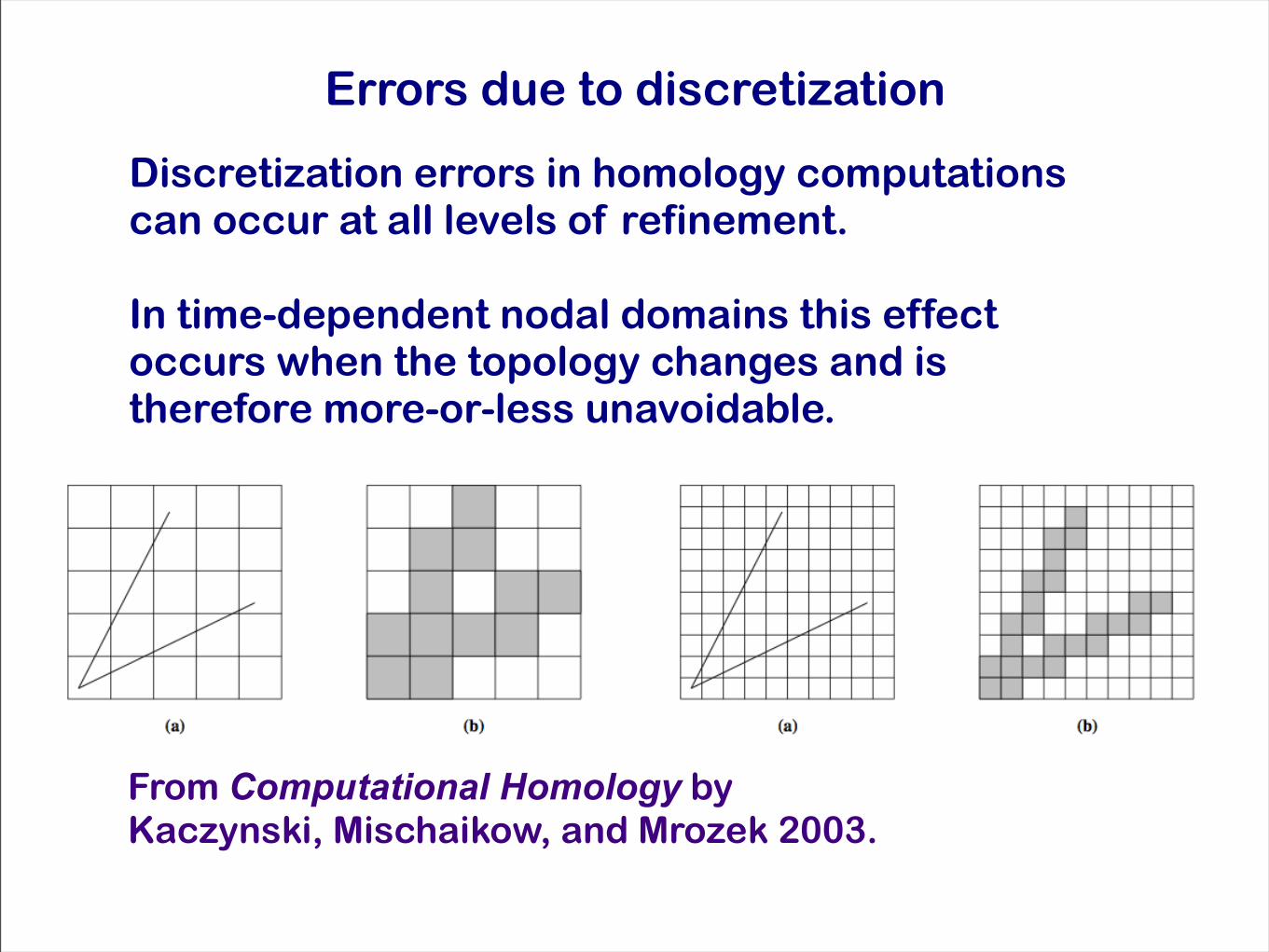
Errors due to discretization

Discretization errors in homology computations can occur at all levels of refinement.

In time-dependent nodal domains this effect occurs when the topology changes and is therefore more-or-less unavoidable.

From Computational Homology byKaczynski, Mischaikow, and Mrozek 2003.

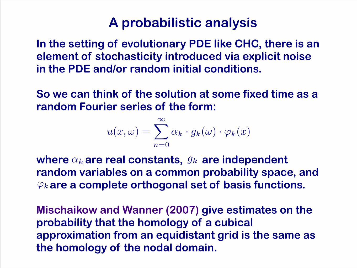
A probabilistic analysis

In the setting of evolutionary PDE like CHC, there is an element of stochasticity introduced via explicit noise in the PDE and/or random initial conditions.

So we can think of the solution at some fixed time as a random Fourier series of the form:

u(x, !) =!!

n=0

"k · gk(!) · #k(x)

where are real constants, are independent random variables on a common probability space, and are a complete orthogonal set of basis functions.

Mischaikow and Wanner (2007) give estimates on the probability that the homology of a cubical approximation from an equidistant grid is the same as the homology of the nodal domain.

!k gk

!k

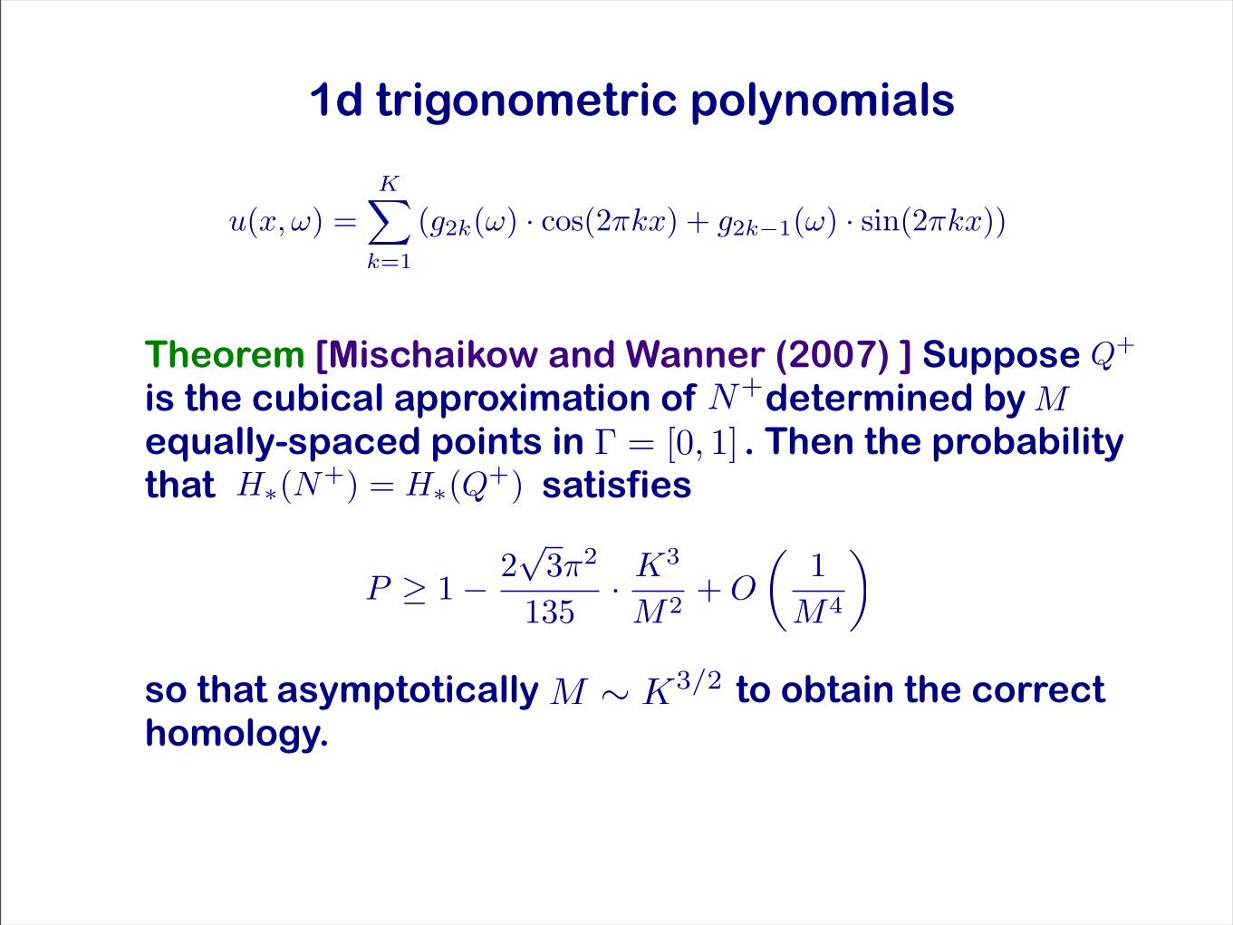
1d trigonometric polynomials

Theorem [Mischaikow and Wanner (2007) ] Suppose is the cubical approximation of determined by equally-spaced points in . Then the probability that satisfies

so that asymptotically to obtain the correct homology.

Q+

N+

u(x, !) =K!

k=1

(g2k(!) · cos(2"kx) + g2k!1(!) · sin(2"kx))

M! = [0, 1]

H!(N+) = H!(Q+)

P ! 1" 2#

3!2

135· K3

M2+ O

!1

M4

"

M ! K3/2

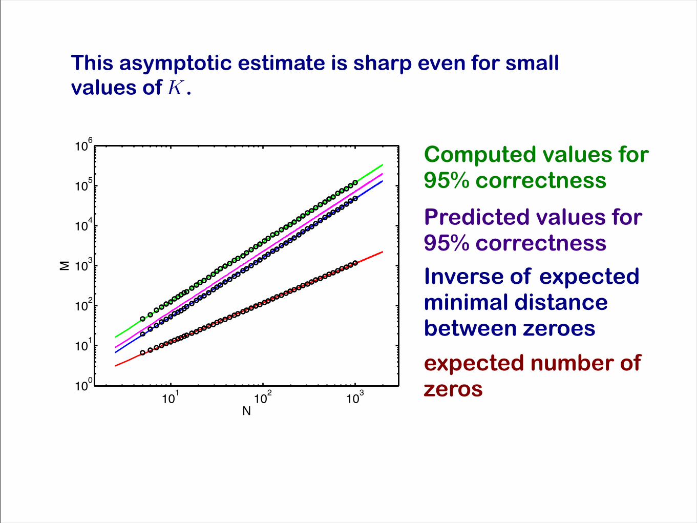
This asymptotic estimate is sharp even for small values of .

101

102

103

100

101

102

103

104

105

106

N

M

Predicted values for 95% correctness

Computed values for 95% correctness

Inverse of expected minimal distance between zeroes

expected number of zeros

K

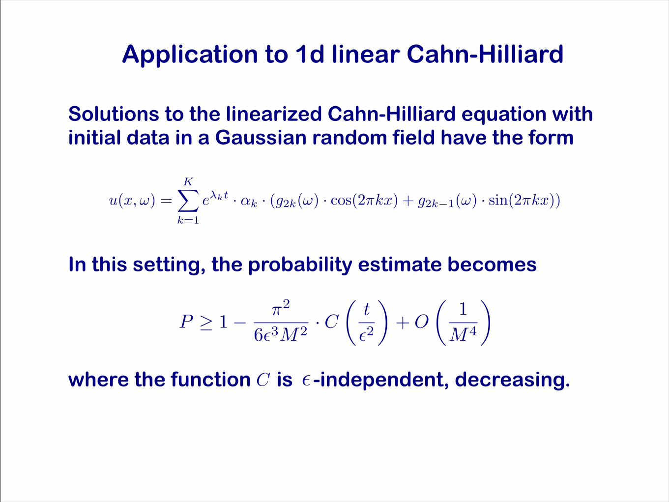
Application to 1d linear Cahn-Hilliard

Solutions to the linearized Cahn-Hilliard equation with initial data in a Gaussian random field have the form

u(x, !) =K!

k=1

e!kt · "k · (g2k(!) · cos(2#kx) + g2k!1(!) · sin(2#kx))

In this setting, the probability estimate becomes

P ! 1" !2

6"3M2· C

!t

"2

"+ O

!1

M4

"

where the function is -independent, decreasing.C !

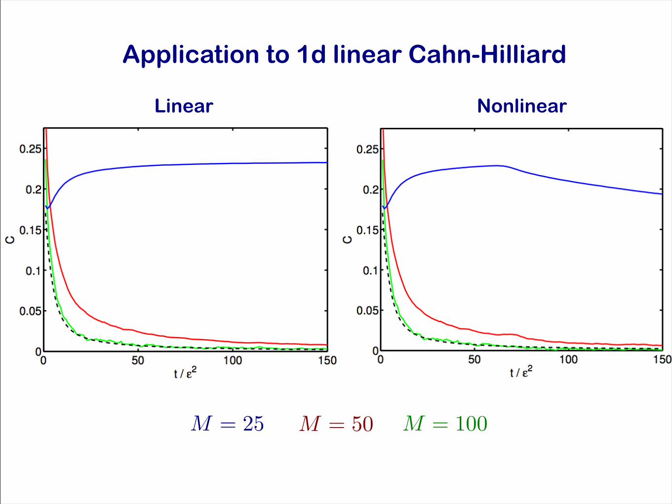
Application to 1d linear Cahn-Hilliard

Linear Nonlinear

M = 25 M = 50 M = 100

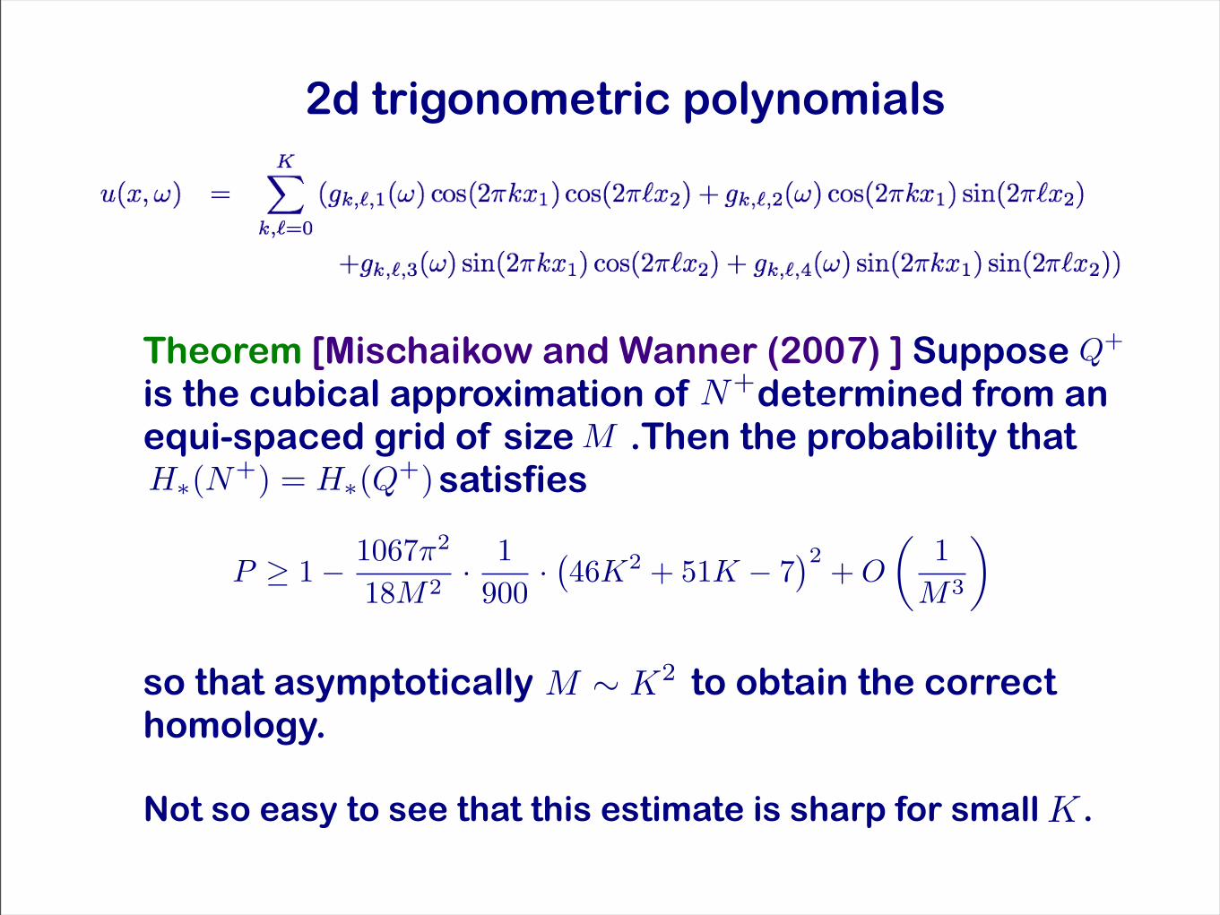
2d trigonometric polynomials

Theorem [Mischaikow and Wanner (2007) ] Suppose is the cubical approximation of determined from an equi-spaced grid of size .Then the probability that satisfies

Q+

N+

MH!(N+) = H!(Q+)

P ! 1" 1067!2

18M2· 1900

·!46K2 + 51K " 7

"2 + O

#1

M3

$

so that asymptotically to obtain the correct homology.

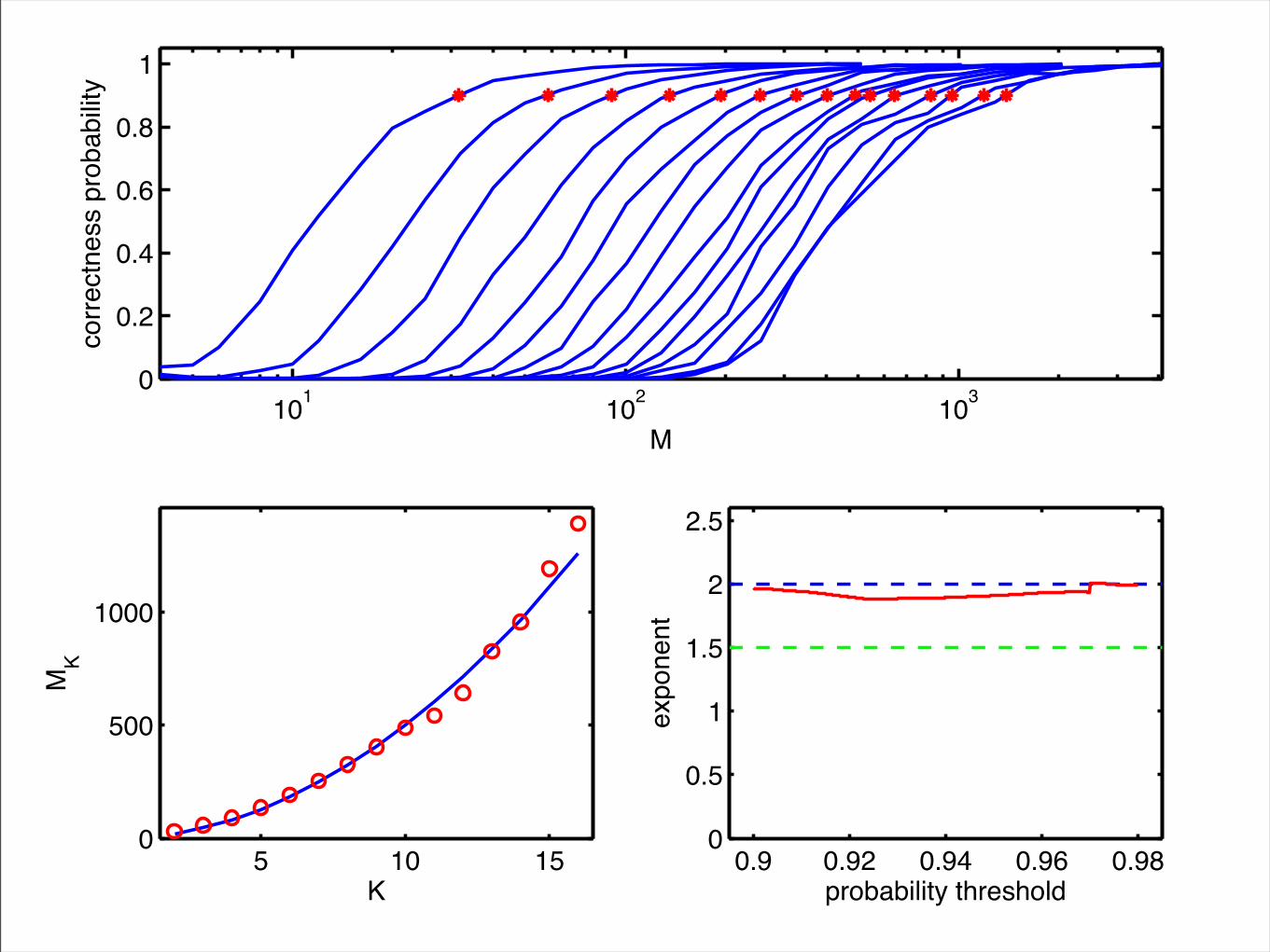
Not so easy to see that this estimate is sharp for small .

M ! K2

K

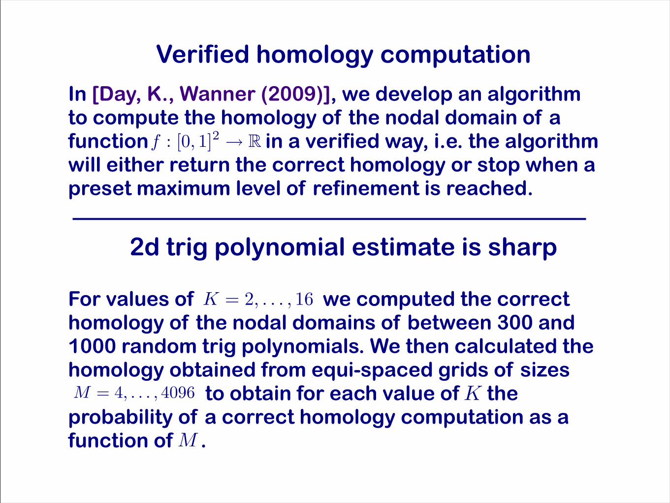
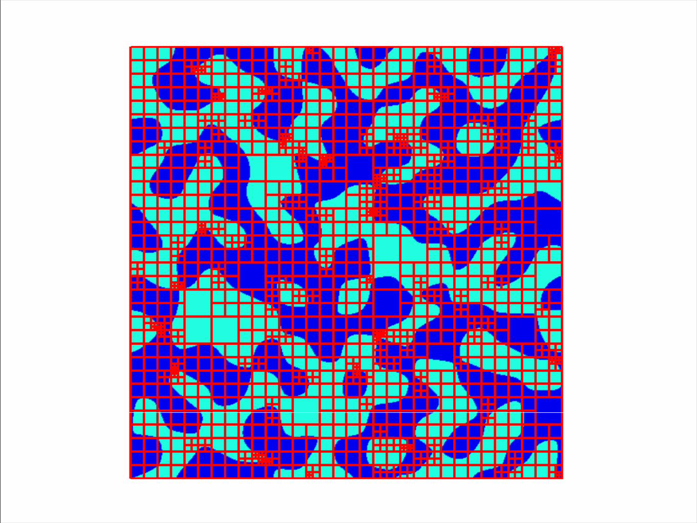
Verified homology computation

In [Day, K., Wanner (2009)], we develop an algorithm to compute the homology of the nodal domain of a function in a verified way, i.e. the algorithm will either return the correct homology or stop when a preset maximum level of refinement is reached.

f : [0, 1]2 ! R

2d trig polynomial estimate is sharp

For values of we computed the correct homology of the nodal domains of between 300 and 1000 random trig polynomials. We then calculated the homology obtained from equi-spaced grids of sizes to obtain for each value of the probability of a correct homology computation as afunction of .

K = 2, . . . , 16

M = 4, . . . , 4096 K

M

101

102

103

0

0.2

0.4

0.6

0.8

1

M

corr

ectn

ess p

robabili

ty

5 10 150

500

1000

K

MK

0.9 0.92 0.94 0.96 0.980

0.5

1

1.5

2

2.5

probability threshold

exponent

0 0.2 0.4 0.6 0.8 10

0.1

0.2

0.3

0.4

0.5

0.6

0.7

t / te

failu

re p

rob

ab

ility

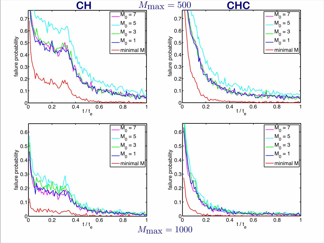
M0 = 7

M0 = 5

M0 = 3

M0 = 1

minimal M

0 0.2 0.4 0.6 0.8 10

0.1

0.2

0.3

0.4

0.5

0.6

t / te

failu

re p

rob

ab

ility

M0 = 7

M0 = 5

M0 = 3

M0 = 1

minimal M

0 0.2 0.4 0.6 0.8 10

0.1

0.2

0.3

0.4

0.5

0.6

t / te

failu

re p

robabili

ty

M0 = 7

M0 = 5

M0 = 3

M0 = 1

minimal M

0 0.2 0.4 0.6 0.8 10

0.1

0.2

0.3

0.4

0.5

0.6

0.7

t / te

failu

re p

rob

ab

ility

M0 = 7

M0 = 5

M0 = 3

M0 = 1

minimal M

Mmax = 500

Mmax = 1000

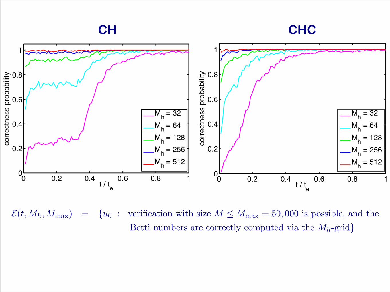
CH CHC

0 0.2 0.4 0.6 0.8 10

0.2

0.4

0.6

0.8

1

t / te

corr

ectn

ess p

robabili

ty

Mh = 32

Mh = 64

Mh = 128

Mh = 256

Mh = 512

E(t, Mh, Mmax) = {u0 : verification with size M !Mmax = 50, 000 is possible, and theBetti numbers are correctly computed via the Mh-grid}

CH CHC

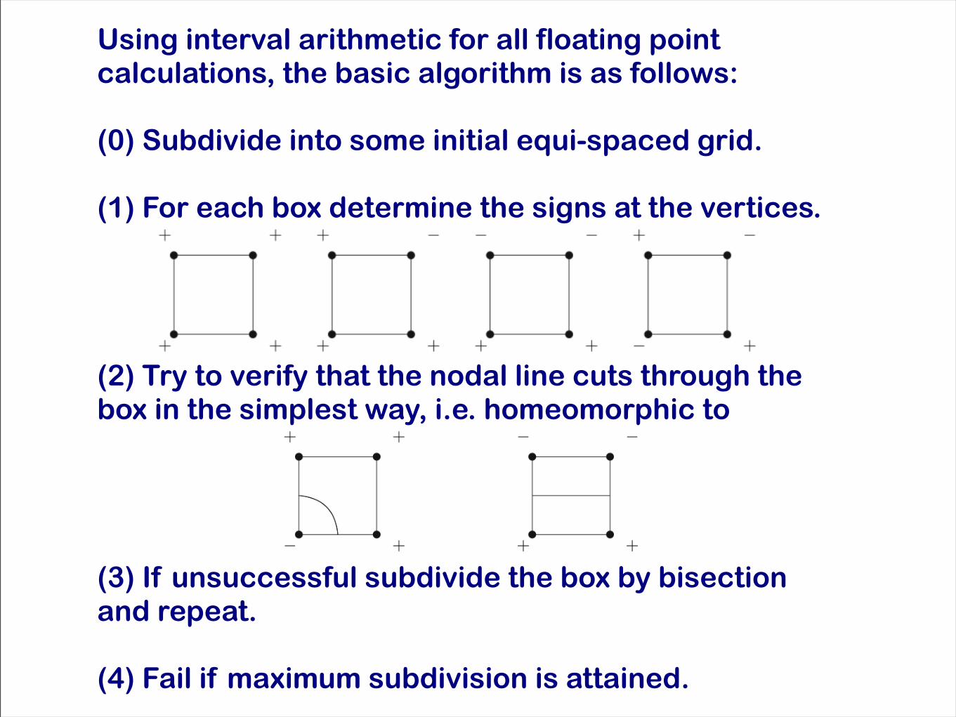
Using interval arithmetic for all floating point calculations, the basic algorithm is as follows:

(0) Subdivide into some initial equi-spaced grid.

(1) For each box determine the signs at the vertices.

(2) Try to verify that the nodal line cuts through the box in the simplest way, i.e. homeomorphic to

(3) If unsuccessful subdivide the box by bisectionand repeat.

(4) Fail if maximum subdivision is attained.

Conclusions

Computing a time series of Betti numbers directly from patterned images from experiment or simulationcan give new insight into dynamics of systems with complicated spatial and temporal dynamics.

One can estimate how fine a cubical approximation is needed to compute homology of nodal domains with a specified confidence depending on computable properties of the function.

It is often possible to correctly compute the homology of a nodal domain with verified numerical techniques.

Thank You!

Sarah Day (College of William & Mary)

Marcio Gameiro (Kyoto)

Konstantin Mischaikow (Rutgers)

Thomas Wanner (George Mason)

Supported by the National Science Foundation and the Department of Energy.

http://chomp.rutgers.edu