Embed Size (px)
Citation preview

Computations and structures in sl(n)-link homology.
Daniel Krasner
Advisor: Mikhail Khovanov
Submitted in partial fulfillment of the
Requirements for the degree
of Doctor of Philosophy
in the Graduate School of Arts and Sciences
COLUMBIA UNIVERSITY
2009

c©2009
Daniel Krasner
All Rights Reserved

Abstract
Computations and structures in sl(n)-link homology.
Daniel Krasner
The thesis studies sl(n) and HOMFLY-PT link homology. We begin by constructing a
version of sln)-link homology, which assigns the U(n)-equivariant cohomology of CPn−1 to
the unknot. This theory specializes to the Khovanonv-Rozansky sl(n)-homology and we are
motivated by the “universal” rank two Frobenius extension studied by M. Khovanov in (20)
for sl(2)-homology. This framework allows one to work with graded, rather than filtered,
objects and should prove useful in investigating structural properties of the sl(n)-homology
theories.
We proceed by using the diagrammatic calculus for Soergel bimodules, developed by B.
Elias and M. Khovanov in (1), to prove that Rouquier complexes, and ultimately HOMFLY-
PT link homology, is functorial. Upon doing so we are able to explicitly write the chain
map generators of the movie moves and compute over the integers. This is joint work with
B. Elias.
In suite, we take the above diagrammatic calculus and construct and integral version of
HOMFLY-PT link homology, which we also extend to an integral version of sl(n)-homology
with the aid Rasmussen’s specral sequences between the two (33). We reprove invariance
under the Reidemeister moves in this context and highlight the computational power of the
calculus at hand.
The last part of the thesis concerns an example. We show that for a particular class
of tangles the sl(n)-link homology is entirely “local,” i.e. has no “thick” edges, and its
homology depends only on the underlying Frobenius structure of the algebra assigned to
the unknot.

Contents
1 Introduction 1
2 Equivariant sl(n)-link homology 7
2.1 Introduction . . . . . . . . . . . . . . . . . . . . . . . . . . . . . . . . . . . . 7
2.2 Matrix Factorizations . . . . . . . . . . . . . . . . . . . . . . . . . . . . . . 14
2.3 Tangles and complexes . . . . . . . . . . . . . . . . . . . . . . . . . . . . . . 32
2.4 Invariance under the Reidemeister moves . . . . . . . . . . . . . . . . . . . 33
2.5 Remarks . . . . . . . . . . . . . . . . . . . . . . . . . . . . . . . . . . . . . . 39
3 Functoriality of Rouquier complexes 41
3.1 Soergel bimodules in representation theory and link homology . . . . . . . . 41
3.2 Constructions . . . . . . . . . . . . . . . . . . . . . . . . . . . . . . . . . . . 45
3.2.1 The Hecke Algebra . . . . . . . . . . . . . . . . . . . . . . . . . . . . 45
3.2.2 The Soergel Categorification . . . . . . . . . . . . . . . . . . . . . . 46
3.2.3 Soergel Diagrammatics . . . . . . . . . . . . . . . . . . . . . . . . . . 47
3.2.4 Braids and Movies . . . . . . . . . . . . . . . . . . . . . . . . . . . . 55
3.2.5 Rouquier Complexes . . . . . . . . . . . . . . . . . . . . . . . . . . . 59
3.2.6 Conventions . . . . . . . . . . . . . . . . . . . . . . . . . . . . . . . . 60
3.3 Definition of the Functor . . . . . . . . . . . . . . . . . . . . . . . . . . . . . 62
3.4 Checking the Movie Moves . . . . . . . . . . . . . . . . . . . . . . . . . . . 69
3.4.1 Simplifications . . . . . . . . . . . . . . . . . . . . . . . . . . . . . . 69
3.4.2 Movie Moves . . . . . . . . . . . . . . . . . . . . . . . . . . . . . . . 72
3.5 Additional Comments . . . . . . . . . . . . . . . . . . . . . . . . . . . . . . 86
i

3.5.1 The Benefits of Brute Force . . . . . . . . . . . . . . . . . . . . . . . 86
3.5.2 Working over Z . . . . . . . . . . . . . . . . . . . . . . . . . . . . . . 89
4 Intergral HOMFLY-PT and sl(n)-link homology 91
4.1 Background for diagrammatics of Soergel bimodules and Rouquier Complexes 91
4.2 The toolkit . . . . . . . . . . . . . . . . . . . . . . . . . . . . . . . . . . . . 92
4.2.1 Matrix factorizations . . . . . . . . . . . . . . . . . . . . . . . . . . . 93
4.2.2 Diagrammatics of Soergel bimodules . . . . . . . . . . . . . . . . . . 94
4.2.3 Hochschild (co)homology . . . . . . . . . . . . . . . . . . . . . . . . 95
4.3 The integral HOMFLY-PT complex . . . . . . . . . . . . . . . . . . . . . . 97
4.3.1 The matrix factorization construction . . . . . . . . . . . . . . . . . 97
4.3.2 The Soergel bimodule construction . . . . . . . . . . . . . . . . . . . 101
4.3.2.1 Diagrammatic Rouquier complexes . . . . . . . . . . . . . . 104
4.4 Checking the Reidemeister moves . . . . . . . . . . . . . . . . . . . . . . . . 105
4.4.1 Reidemeister I . . . . . . . . . . . . . . . . . . . . . . . . . . . . . . 106
4.4.2 Reidemeister II . . . . . . . . . . . . . . . . . . . . . . . . . . . . . . 108
4.4.3 Reidemeister III . . . . . . . . . . . . . . . . . . . . . . . . . . . . . 109
4.4.4 Observations . . . . . . . . . . . . . . . . . . . . . . . . . . . . . . . 112
4.5 Rasmussen’s spectral sequence and integral sl(n)-link homology . . . . . . . 113
5 A particular example in sl(n)-link homology 118
5.1 Introduction . . . . . . . . . . . . . . . . . . . . . . . . . . . . . . . . . . . . 118
5.2 A Review of Khovanov-Rozansky Homology . . . . . . . . . . . . . . . . . . 119
5.3 The Basic Calculation . . . . . . . . . . . . . . . . . . . . . . . . . . . . . . 125
5.4 Basic Tensor Product Calculation . . . . . . . . . . . . . . . . . . . . . . . . 131
5.5 The General Case . . . . . . . . . . . . . . . . . . . . . . . . . . . . . . . . . 136
5.6 Remarks . . . . . . . . . . . . . . . . . . . . . . . . . . . . . . . . . . . . . . 139
Bibliography 139
ii

List of Figures
1.1 Our main tangle and its reduced complex . . . . . . . . . . . . . . . . . . . 6
2.1 MOY graph skein relation [i] :=qi − q−i
q − q−1. . . . . . . . . . . . . . . . . . . . 11
2.2 Skein formula for Pn(L) . . . . . . . . . . . . . . . . . . . . . . . . . . . . . 11
2.3 Maps between resolutions . . . . . . . . . . . . . . . . . . . . . . . . . . . . 12
2.4 A planar graph . . . . . . . . . . . . . . . . . . . . . . . . . . . . . . . . . . 23
2.5 “Closing off” an arc . . . . . . . . . . . . . . . . . . . . . . . . . . . . . . . 24
2.6 Maps χ0 and χ1 . . . . . . . . . . . . . . . . . . . . . . . . . . . . . . . . . 25
2.7 Direct Sum Decomposition 0 . . . . . . . . . . . . . . . . . . . . . . . . . . 27
2.8 Direct Sum Decomposition I . . . . . . . . . . . . . . . . . . . . . . . . . . . 27
2.9 The map α . . . . . . . . . . . . . . . . . . . . . . . . . . . . . . . . . . . . 28
2.10 The map β . . . . . . . . . . . . . . . . . . . . . . . . . . . . . . . . . . . . 28
2.11 Direct Sum Decomposition II . . . . . . . . . . . . . . . . . . . . . . . . . . 29
2.12 Direct Sum Decomposition III . . . . . . . . . . . . . . . . . . . . . . . . . . 30
2.13 The map α . . . . . . . . . . . . . . . . . . . . . . . . . . . . . . . . . . . . 30
2.14 The map β . . . . . . . . . . . . . . . . . . . . . . . . . . . . . . . . . . . . 30
2.15 The factorizations in Direct Sum Decomposition IV . . . . . . . . . . . . . 31
2.16 Complexes associated to pos/neg crossings; the numbers below the diagrams
are cohomological degrees. . . . . . . . . . . . . . . . . . . . . . . . . . . . . 32
2.17 Diagram of a tangle . . . . . . . . . . . . . . . . . . . . . . . . . . . . . . . 33
2.18 Reidemeister I . . . . . . . . . . . . . . . . . . . . . . . . . . . . . . . . . . 34
iii

2.19 Reidemeister 1 complex . . . . . . . . . . . . . . . . . . . . . . . . . . . . . 34
2.20 Reidemeister 2a . . . . . . . . . . . . . . . . . . . . . . . . . . . . . . . . . . 35
2.21 Reidemeister 2a complex . . . . . . . . . . . . . . . . . . . . . . . . . . . . . 36
2.22 . . . . . . . . . . . . . . . . . . . . . . . . . . . . . . . . . . . . . . . . . . . 37
2.23 Reidemeister 3 complex . . . . . . . . . . . . . . . . . . . . . . . . . . . . . 38
2.24 Reidemeister 3 complex reduced . . . . . . . . . . . . . . . . . . . . . . . . 39
3.1 Braid movie moves 1− 8 . . . . . . . . . . . . . . . . . . . . . . . . . . . . . 57
3.2 Braid movie moves 9− 14 . . . . . . . . . . . . . . . . . . . . . . . . . . . . 58
3.3 Rouquier complex for right and left crossings . . . . . . . . . . . . . . . . . 59
3.4 Birth and Death of a crossing generators . . . . . . . . . . . . . . . . . . . . 62
3.5 Reidemeister 2 type movie move generators . . . . . . . . . . . . . . . . . . 63
3.6 Slide generators . . . . . . . . . . . . . . . . . . . . . . . . . . . . . . . . . . 64
3.7 Reidemeister 3 type movie move generators . . . . . . . . . . . . . . . . . . 66
3.8 Reidemeister 3 type movie move generators . . . . . . . . . . . . . . . . . . 67
3.9 Movie Move 1 associated to slide generator 1 . . . . . . . . . . . . . . . . . 73
3.10 Movie Move 1 associated to slide generator 3 . . . . . . . . . . . . . . . . . 74
3.11 Movie Move 2 . . . . . . . . . . . . . . . . . . . . . . . . . . . . . . . . . . . 74
3.12 Movie Move 3 . . . . . . . . . . . . . . . . . . . . . . . . . . . . . . . . . . . 75
3.13 Movie Move 4 . . . . . . . . . . . . . . . . . . . . . . . . . . . . . . . . . . . 75
3.14 Movie Move 5 . . . . . . . . . . . . . . . . . . . . . . . . . . . . . . . . . . . 76
3.15 Movie Move 6 . . . . . . . . . . . . . . . . . . . . . . . . . . . . . . . . . . . 76
3.16 Movie Move 7 . . . . . . . . . . . . . . . . . . . . . . . . . . . . . . . . . . . 77
3.17 Homotopy for Movie Move 7 . . . . . . . . . . . . . . . . . . . . . . . . . . . 78
3.18 Movie Move 8 . . . . . . . . . . . . . . . . . . . . . . . . . . . . . . . . . . . 80
3.19 Movie Move 9 . . . . . . . . . . . . . . . . . . . . . . . . . . . . . . . . . . . 81
3.20 Movie Move 11 . . . . . . . . . . . . . . . . . . . . . . . . . . . . . . . . . . 82
3.21 Movie Move 12 . . . . . . . . . . . . . . . . . . . . . . . . . . . . . . . . . . 83
3.22 Movie Move 13 . . . . . . . . . . . . . . . . . . . . . . . . . . . . . . . . . . 84
iv

3.23 Movie Move 14 . . . . . . . . . . . . . . . . . . . . . . . . . . . . . . . . . . 85
4.1 Crossings and resolutions . . . . . . . . . . . . . . . . . . . . . . . . . . . . 92
4.2 . . . . . . . . . . . . . . . . . . . . . . . . . . . . . . . . . . . . . . . . . . . 98
4.3 . . . . . . . . . . . . . . . . . . . . . . . . . . . . . . . . . . . . . . . . . . . 102
4.4 Diagrammatic Rouquier complex for right and left crossings . . . . . . . . . 105
4.5 The Reidemeister moves . . . . . . . . . . . . . . . . . . . . . . . . . . . . . 107
4.6 Reidemeister IIa complex with decomposition 4.3 . . . . . . . . . . . . . . . 108
4.7 Reidemeister IIa complex, removing one of the acyclic subcomplexes . . . . 109
4.8 Reidemeister IIa complex, removing a second acyclic subcomplex . . . . . . 109
4.9 Reidemeister III complex with decompositions 4.3 and 4.4 . . . . . . . . . . 110
4.10 Reidemeister III complex, with an acyclic subcomplex marked for removal . 110
4.11 Reidemeister III complex, with another acyclic subcomplex marked for removal111
4.12 Reidemeister III complex - the end result, after removal of all acyclic sub-
complexes . . . . . . . . . . . . . . . . . . . . . . . . . . . . . . . . . . . . . 112
5.1 Our main tangle and its reduced complex . . . . . . . . . . . . . . . . . . . 118
5.2 Maps χ0 and χ1 . . . . . . . . . . . . . . . . . . . . . . . . . . . . . . . . . 120
5.3 The map α in Direct Sum Decomposition I . . . . . . . . . . . . . . . . . . 123
5.4 The map β in Direct Sum Decomposition I . . . . . . . . . . . . . . . . . . 123
5.5 The map β in Direct Sum Decomposition II . . . . . . . . . . . . . . . . . . 124
5.6 Complexes associated to pos/neg crossings; the numbers below the diagrams
are cohomological degrees. . . . . . . . . . . . . . . . . . . . . . . . . . . . . 124
5.7 The tangle T and its complex . . . . . . . . . . . . . . . . . . . . . . . . . . 125
5.8 First part of the complex for T with decompositions . . . . . . . . . . . . . 126
5.9 The second part of the complex for T with decompositions . . . . . . . . . . 127
5.10 The reduced complex for tangle T . . . . . . . . . . . . . . . . . . . . . . . 130
5.11 Complex for the tensor product . . . . . . . . . . . . . . . . . . . . . . . . . 131
5.12 Calculating degree 0 to 1 . . . . . . . . . . . . . . . . . . . . . . . . . . . . 132
v

5.13 Degree 0 to 1 . . . . . . . . . . . . . . . . . . . . . . . . . . . . . . . . . . . 133
5.14 Calculating degree 1 to 2 . . . . . . . . . . . . . . . . . . . . . . . . . . . . 133
5.15 Calculating degree 1 to 2 . . . . . . . . . . . . . . . . . . . . . . . . . . . . 134
5.16 Calculating degree 2 and 3 . . . . . . . . . . . . . . . . . . . . . . . . . . . . 135
5.17 The tensor complex . . . . . . . . . . . . . . . . . . . . . . . . . . . . . . . 135
5.18 Tensoring the complex with another copy of the basic tangle T . . . . . . . 136
5.19 Decomposing the entries of the general tensor product . . . . . . . . . . . . 137
5.20 The complex of the k-fold tensor product . . . . . . . . . . . . . . . . . . . 138
5.21 The complex of the k-fold tensor product . . . . . . . . . . . . . . . . . . . 138
vi

Acknowledgments
The lightning speed at which my graduate studies at Columbia have passed is just one
indication at how genuinely good these years have been - there are many people directly re-
sponsible for making this experience so, from both the mathematical and non-mathematical
perspective.
Foremost comes my advisor Mikhail Khovanov, whose insights into mathematics, pa-
tience, and support on all fronts have been more than I could have hoped for. I thank him
for showing me what “structure” in mathematics means, and how beautiful this can be,
while at the same time always looking out for my best interests. I thank Peter Ozsvath
for his wonderful first-year algebraic topology class, which solidified my interest in topology
more than any other, keeping his door always open for questions and making my transition
into the “real” world much smoother than it could have been. For the many discussions at
Columbia, which have been so important to me, I would like to thank John Baldwin, Ben
Elias, Allison Gilmore, Eli Grigsby, Aaron Lauda, and Thomas Peters and for discussions
elsewhere Marco Mackaay, Jacob Rasmussen, Nicolai Reshetikhin, Lev Rozansky, Alexan-
der Shumakovitch, Pedro Vaz and Liam Watson - it is in these moments of conversation
that mathematics is most alive to me. In addition I thank Terrance Cope and Mary Young
for all of what they do at Columbia for us, whether we know it or not.
Then there are my parents... them I have to thank for essentially everything - if I were
to pick one block off this inexhaustible list, perhaps I would choose their openness, ability
to cope with any of my decisions and reservation in judgement. My sister I thank for being
able to deal with her older brother, and always somehow keeping faith regardless of the
immediate. My grandparents I thank for showing me the wide spectrum of outlook on
accomplishment. Thanks to Busia for showing me the pinnacle of nonchalance and laziness.
Matt DeLand I thank for making sure we were always “on our way” which, by the way, we
always were. And the final words I leave for my Bellas, who is the most wonderful person
I have ever met and who is no less than the world to me - her I thank for being there and
more.

To my parents,
To my sister,
And to my Bellas.
viii

Chapter 1 1
Chapter 1
Introduction
In the decade following the discovery of the Jones polynomial by V. Jones (14) in 1983 a
slew of new invariants in low dimensional topology came to light. Included in this extensive
list is a large family, known as “quantum link invariants,” which arises from quantum
groups and their representations. In brief, given a tangle T and an appropriate collection
of representations V1, . . . , Vk of a quantum group G, one constructs an element F (T ) of
the endomorphism ring of V1 ⊗ · · · ⊗ Vk, which is an invariant of T . “Closing off” the
tangle corresponds to taking trace of this operator F (T ), this trace being a polynomial in
R[q, q−1] with R generally a field or a commutative ring. The subject of quantum invariants
has not only played a pivotal role relating various branches of mathematics and physics
such as representation theory, operator algebras, low dimensional topology, and statistical
mechanics, but has evolved to be extremely interesting and powerful in its own right.
In (17) M. Khovanov constructed a link homology theory with Euler characteristic the
Jones, or sl(2), polynomial. From this work a completely novel viewpoint arose with regards
to quantum invariants - the viewpoint of categorification. Roughly speaking, categorification
refers to lifting a given mathematical structure to that of a higher order. For example: a
natural number can be regarded as the dimension of a vector space or the Euler characteristic
of a (co)-homology theory, a polynomial with integral coefficients as the quantum dimension
of a vector space or the Euler characteristic of a bi-graded homology theory, a group as

CHAPTER 1. INTRODUCTION 2
the Grothendieck group of some category, a group action as the consequence of functorial
actions on some category, etc. One approach to constructing Khovanov homology begins
with Kauffman’s solid-state model for the Jones polynomial. This is gotten by resolving each
crossing of a link diagram in either the oriented or un-oriented resolution and assigning to
each the polynomial (q+q−1)n where n is the number of circles resulting in a given resolution;
a weighted alternating sum, with weights corresponding to that of each resolution, is taken
and after some shifts one arrives at the Jones polynomial. The homology theory takes
this alternating sum and lifts it to a complex of tensor products of Frobenius algebras,
each of quantum dimension q + q−1, with appropriate shifts in the quantum grading; the
differential maps arise from the underlying Frobenius algebra structure, anti-commute, and
are grading preserving, so that the bi-graded Euler characteristic of the homology theory is
the same as that of the complex, i.e. the Jones polynomial. (We will discuss this and other
related constructions in great detail in the next chapter.) This categorification of the Jones
polynomial was a seminal moment in providing a completely new approach to quantum
invariants, has paved the way for a number of other categorification constructions, and
has proven to be powerful as well as deeply connected to other branches of mathematics.
One example of the breadth of Khovanov homology was seen when, using subsequent work
of E. S. Lee (25) on variants of the theory, J. Rasmussen found a purely combinatorial
proof of the Milnor conjecture for the slice genus of torus knots (34) (previously proved by
P. Kronheimer and T. Mrowka using gauge theory); moreover, applications to transverse
links and tight contact structures have also been discovered (32), (3); and perhaps what
is most surprising is the existence of a spectral sequence connecting Khovanov homology
and Heegaard Floer homology (31). Many papers have been written on or relating to this
subject and millions of examples have been calculated, but it is clear that more discoveries
are to come.
In the last few years categorification and, in particular, that of topological invariants
has flourished into a subject of its own right. This has been a study finding connections and
ramifications over a vast spectrum of mathematics, including areas such as low-dimensional
topology, representation theory, algebraic geometry, as well as others. Following the origi-
nal work of M. Khovanov on the categorification of the Jones polynomial in, came a slew

CHAPTER 1. INTRODUCTION 3
of link homology theories lifting other quantum invariants. With a construction that uti-
lized a tool previously developed in an algebra-geometric context - matrix factorizations
- M. Khovanov and L. Rozansky produced the sl(n) and HOMFLY-PT link homology
theories. Albeit computationally intensive, it was clear from the onset that thick interlac-
ing structure was hidden within. The most insightful and influential work in uncovering
these inner-connections was that of J. Rasmussen in (33), where he constructed a spectral
sequence from the HOMFLY-PT to the sl(n)-link homology. This was a major step in de-
constructing the pallet of how these theories come together, yet many structural questions
remained and still remain unanswered, waiting for a new approach. Close to the time of
the original work, M. Khovanov produced an equivalent categorification of the HOMFLY-
PT polynomial in (21), but this time using Hochschild homology of Soergel bimodules and
Rouquier complexes of (36). The latter proved to be more computation-friendly and was
used by B. Webster to calculate many examples in (43). However, at the present moment
the Khovanov and Khovanov-Rozansky approach is by far not the only one; these theories
and their generalizations to other representations and Lie algebras have come about via
Category O, derived categories of coherent sheaves, perverse sheaves on Grassmanians and
Springer fibers, as well as other geometric constructions (see for example (8), (9), (41),
(42)).
In the meantime of all this development, a new flavor of categorification came into light.
With the work of A. Lauda and M. Khovanov on the categorification of quantum groups
in (26), a diagrammatic calculus originating in the study of 2-categories arrived into the
foreground. This graphical approach proved quite fruitful and was soon used by B. Elias
and M. Khovanov in (1) to rewrite the work of Soergel , and en suite by B. Elias and
the author to repackage Rouquier’s complexes and to prove that they are functorial over
braid-cobordisms (2) (not just projectively functorial as was known before). An immediate
advantage to this construction was the inherent ease of calculation, at least comparative
ease, and the fact that it worked equally well over the integers as well as over fields.
The thesis is divided into four sections, each centered around a particular result and
conjectural motivation. Since most of these require different techniques and at times a
rather unique approach, we present the required background information separately for

CHAPTER 1. INTRODUCTION 4
each section, skipping only those details which have already been presented.
We begin with the construction of an “equivariant” version of sl(n)-link homology, which
was motivated by the study of the following conjecture.
Conjecture 1.1. Consider the deformation of sl(n)-homology that assigns
Hn,f(x)(unknot) = Q[α1, . . . , αk][x]/(f(x)) where f(x) = (x− α1)r1 . . . (x− αk)rk .
Then
Hn,f(x)(L) ∼=⊕
φ:c(L)→αi
k⊗i=1
Hki(Li)
where the sum is taken over colorings φ of the components of L by the roots αj and Li is
the sublink corresponding to components colored by αi, with Hki(Li) its sl(ki)-link homology.
The conjecture arose from the work of E. S. Lee (25) on sl(2)-link homology and later was
supported by M. Mackaay and P. Vaz (29) where they consider the corresponding scenario
for sl(3)-homology. Such a decomposition theorem would be interesting in its own right,
but would also tell a lot about of what to expect from sl(n)-homology as a link invariant.
The “equivariant” version allows us to consider this deformation in the context of graded
rather than filtered objects and is a direct generalization of Khovanov’s work on Frobenius
extension and link homology (20). The main result is the following:
Theorem 1.2. For every n ∈ N there exists a bigraded homology theory that is an invariant
of links, such that
Hn(unknot) = Q[a0, . . . , an−2][x]/(xn + an−2xn−2 + · · ·+ a1x+ a0),
where setting ai = 0 for 0 ≤ i ≤ n − 2 in the chain complex gives the Khovanov-Rozansky
invariant, i.e. a bigraded homology theory of links with Euler characteristic the quantum
sln-polynomial Pn(L).
The following chapter is a work joint with B. Elias; as mentioned above, this follows
from his and M. Khovanov’s diagrammatic calculus for Soergel bimodules. We extend this
graphical approach to Rouquier complexes and show the following:

CHAPTER 1. INTRODUCTION 5
Theorem 1.3. There is a functor F from the category of combinatorial braid cobordisms
to the category of complexes of Soergel bimodules up to homotopy, lifting Rouquier’s con-
struction (i.e. such that F sends crossings to Rouquier complexes).
This functoriality remains true even over Z and, in addition, we are able to exhibit all
movie move generators explicitly and calculate the movies with relative ease.
In the next chapter we extend the above results to produce an integral version of
HOMFLY-PT homology and utilizing Rasmussen’s spectral sequence from HOMFLY-PT
to sl(n)-link homology construct an integral version of the latter. (Previous integral con-
structions existed only for the sl(2) and sl(3) variants.) Once again, the graphical calculus
plays an invaluable role in the ease of calculations. We prove the following:
Theorem 1.4. Given a link L ⊂ S3, the groups H(L) and H(L) are invariants of L and
when tensored with Q are isomorphic to the unreduced and reduced versions, respectively,
of the Khovanov-Rozansky HOMFLY-PT link homology. Moreover, these integral homol-
ogy theories give rise to functors from the category of braid cobordisms to the category of
complexes of graded R-bimodules.
Theorem 1.5. Given a link L, there exists a spectral sequence En where the E1 page is
isomorphic to the integral HOMFLY-PT link homology of L, En is an invariant of L for
all n, and E∞ categorifies the quantum sl(n)-link polynomial PL(qn, q).
The last chapter takes a step back to the original Khovanov-Rozansky construction and
focuses on a particular class of tangles where the homology is of a rather unique flavor.
Using ideas from (4) we show that for this class of tangles, and hence for knots and links
composed of these, the Khovanov-Rozansky complex reduces to one that is quite simple, or
one without any “thick” edges. In particular we will consider the tangle in figure 1.1 and
show that its associated complex is homotopic to the one below, with some grading shifts
and basic maps which we leave out for now. All of the necessary details will be provided
within the chapter.
The inherent interest in this particular class of tangles, or what is implied by the above
result, comes from the fact that the complexes for the knots and links constructed from
them and their mirrors are entirely “local,” i.e. to calculate the homology we only need to

CHAPTER 1. INTRODUCTION 6
Figure 1.1: Our main tangle and its reduced complex
exploit the Frobenius structure of the underlying algebra assigned to the unknot. Hence,
here the calculations and complexity is similar to that of sl(2)-homology. We will also
discuss a general algorithm, basically the one described in (4), to compute these homology
groups in a more time-efficient manner. The chapter will end with a comparison our results
with similar computations in the version of sl(3)-homology found in (18), which we refer to
as the “foam” version (foams are certain types of cobordisms described in the sl(3) paper),
and give an explicit isomorphism between the two versions.

Chapter 2 7
Chapter 2
Equivariant sl(n)-link homology
2.1 Introduction
In (17), M. Khovanov introduced a bigraded homology theory of links, with Euler char-
acterstic the Jones polynomial, now widely known as “Khovanov homology.” In short, the
construction begins with the Kauffman solid-state model for the Jones polynomial and as-
sociates to it a complex where the ‘states’ are replaced by tensor powers of a certain Frobe-
nius algebra. In the most common variant, the Frobenius algebra in question is Z[x]/(x2),
a graded algebra with deg(1) = 1 and deg(x) = −1, i.e. of quantum dimension q−1 + q,
this being the value of the unreduced Jones polynomial of the unknot. This algebra defines
a 2-dimensional TQFT which provides the maps for the complex. (A 2-dimensional TQFT
is a tensor functor from oriented (1 + 1)-cobordisms to R-modules, with R a commutative
ring, that assigns R to the empty 1-manifold, a ring A to the circle, where A is also a
commutative ring with a map ι : R −→ A that is an inclusion, A ⊗R A to the disjoint
union of two circles, etc.) In (19) M. Khovanov extended this to an invariant of tangles
by associating to a tangle a complex of bimodules and showing that that the isomorphism
class of this complex is an invariant in the homotopy category. The operation of “closing
off” the tangles gave complexes isomorphic to the orginal construction for links.
Variants of this homology theory quickly followed. In (25), E.S. Lee deformed the algebra
above to Z[x]/(x2−1) introducing a different invariant, and constructed a spectral sequence
with E2 term Khovanov homology and E∞ term the ‘deformed’ version. Even though this
CHAPTER 2. EQUIVARIANT SL(N)-LINK HOMOLOGY 8
homology theory was no longer bigraded and was essentially trivial, it allowed Lee to prove
structural properties of Khovanov homology for alternating links. J. Rasmussen used Lee’s
construction to establish results about the slice genus of a knot, and give a purely combina-
torial proof of the Milnor conjecture (34). In (4), D. Bar-Natan introduced a series of such
invariants repackaging the original construction in, what he called, the “world of topological
pictures.” It became quickly obvious that these theories were not only powerful invariants,
but also interesting objects of study in their own right. M. Khovanov unified the above
constructions in (20), by studying how rank two Frobenius extensions of commutative rings
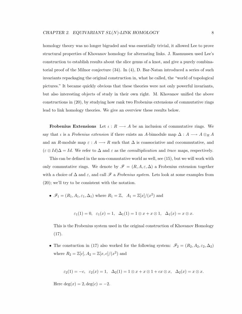
lead to link homology theories. We give an overview these results below.
Frobenius Extensions Let ι : R −→ A be an inclusion of commutative rings. We
say that ι is a Frobenius extension if there exists an A-bimodule map ∆ : A −→ A ⊗R A
and an R-module map ε : A −→ R such that ∆ is coassociative and cocommutative, and
(ε⊗ Id)∆ = Id. We refer to ∆ and ε as the comultiplication and trace maps, respectively.
This can be defined in the non-commutative world as well, see (15), but we will work with
only commutative rings. We denote by F = (R,A, ε,∆) a Frobenius extension together
with a choice of ∆ and ε, and call F a Frobenius system. Lets look at some examples from
(20); we’ll try to be consistent with the notation.
• F1 = (R1, A1, ε1,∆1) where R1 = Z, A1 = Z[x]/(x2) and
ε1(1) = 0, ε1(x) = 1, ∆1(1) = 1⊗ x+ x⊗ 1, ∆1(x) = x⊗ x.
This is the Frobenius system used in the original construction of Khovanov Homology
(17).
• The constuction in (17) also worked for the following system: F2 = (R2, A2, ε2,∆2)
where R2 = Z[c], A2 = Z[x, c]/(x2) and
ε2(1) = −c, ε2(x) = 1, ∆2(1) = 1⊗ x+ x⊗ 1 + cx⊗ x, ∆2(x) = x⊗ x.
Here deg(x) = 2, deg(c) = −2.

CHAPTER 2. EQUIVARIANT SL(N)-LINK HOMOLOGY 9
• F3 = (R3, A3, ε3,∆3) where R3 = Z[t], A3 = Z[x], ι : t 7−→ x2 and
ε3(1) = 0, ε3(x) = 1, ∆3(1) = 1⊗ x+ x⊗ 1, ∆3(x) = x⊗ x+ t1⊗ 1.
Here deg(x) = 2,deg(t) = 4 and the invariant becomes a complex of graded, free
Z[t]-modules (up to homotopy). This was Bar-Natan’s modification found in (4),
with t a formal variable equal to 1/8’th of his invariant of a closed genus 3 surface.
The framework of the Frobenius system F3 gives a nice interpretation of Rasmussen’s
results, allowing us to work with graded rather than filtered complexes, see (20) for a
more in-depth discussion.
• F5 = (R5, A5, ε5,∆5) where R5 = Z[h, t], A5 = Z[h, t][x]/(x2 − hx− t) and
ε5(1) = 0, ε5(x) = 1, ∆5(1) = 1⊗ x+ x⊗ 1− h1⊗ 1, ∆5(x) = x⊗ x+ t1⊗ 1.
Here deg(h) = 2,deg(t) = 4.
Proposition 2.1. (M.Khovanov (20)) Any rank two Frobenius system is obtained
from F5 by a composition of base change and twist.
[Given an invertible element y ∈ A we can “twist” ε and ∆, defining a new comultipli-
cation and counit by ε′(x) = ε(yx), ∆′(x) = ∆(y−1x) and, hence, arriving at a new
Frobenius system. For example: F1 and F2 differ by twisting with y = 1 + cx ∈ A2.]
We can say F5 is “universal” in the sense of the proposition, and this sytem will be
of central interest to us being the model case for the construction we embark on. For
example, by sending h −→ 0 in F5 we arrive at the system F3. Note, if we change to
a field of characteristic other than 2, h can be removed by sending x −→ x − h
2and
by modifying t = −h2
4.
Cohomology and Frobenius extensions There is an interpretation of rank two
Frobenius systems that give rise to link homology theories via equivariant cohomology. Let
us recall some definitions.

CHAPTER 2. EQUIVARIANT SL(N)-LINK HOMOLOGY 10
Given a topological group G that acts continuously on a space X we define the equiv-
ariant cohomology of X with respect to G to be
H∗G(X,R) = H∗(X ×G EG,R),
where H∗(−, R) denotes singular cohomology with coefficients in a ring R, EG is a con-
tractible space with a free G action such that EG/G = BG, the classifying space of G, and
X ×G EG = X ×EG/(gx, e) ∼ (x, eg) for all g ∈ G. For example, if X = p a point then
H∗G(X,R) = H∗(BG,R). Returning to the Frobenius extension encountered we have:
• G = e, the trivial group. Then R1 = Z = H∗G(p,Z) and A1 = H∗G(S2,Z).
• G = SU(2). This group is isomorphic to the group of unit quaternions which, up to
sign, can be thought of as rotations in 3-space, i.e. there is a surjective map from
SU(2) to SO(3) with kernel I,−I. This gives an action of SU(2) on S2.
R3 = Z[t] ∼= H∗SU(2)(p,Z) = H∗(BSU(2),Z) = H∗(HP∞,Z),
A3 = Z[x] ∼= H∗SU(2)(S2,Z) = H∗(S2 ×SU(2) ESU(2),Z) = H∗(CP∞,Z), x2 = t.
• G = U(2). This group has an action on S2 with the center U(1) acting trivially.
R5 = Z[h, t] ∼= H∗U(2)(p,Z) = H∗(BU(2),Z) = H∗(Gr(2,∞),Z),
A5 = Z[h, x] ∼= H∗U(2)(S2,Z) = H∗(S2 ×U(2) EU(2),Z) ∼= H∗(BU(1)×BU(1),Z).
Gr(2,∞) is the Grassmannian of complex 2-planes in C∞; its cohomology ring is
freely generated by h and t of degree 2 and 4, and BU(1) ∼= CP∞. Notice that A5
is a polynomial ring in two generators x and h − x, and R5 is the ring of symmetric
functions in x and h− x, with h and −t the elementary symmetric functions.
Other Frobenius systems and their cohomological interpretations are studied in (20),
but F5 with its “universality” property will be our starting point and motivation.
sln-link homology Following (17), M. Khovanov constructed a link homology theory
with Euler characteristic the quantum sl3-link polynomial P3(L) (the Jones polynomial is

CHAPTER 2. EQUIVARIANT SL(N)-LINK HOMOLOGY 11
Figure 2.1: MOY graph skein relation [i] :=qi − q−i
q − q−1
the sl2-invariant) (18). In succession, M. Khovanov and L. Rozansky introduced a family of
link homology theories categorifying all of the quantum sln-polynomials and the HOMFLY-
PT polynomial, see (23) and (22). The equivalence of the specializations of the Khovanov-
Rozansky theory to the original contructions were easy to see in the case of n = 2 and
recently proved in the case of n = 3, see (28).
Figure 2.2: Skein formula for Pn(L)
The sln-polynomial Pn(L) associated to a link L can be computed in the following two
ways. We can resolve the crossings of L and using the rules in figure 2.2, with a selected
value of the unknot, arrive at a recursive formula, or we could use the Murakami, Ohtsuki,
and Yamada (13) calculus of planar graphs (this is the sln generalization of the Kauffman
solid-state model for the Jones polynomial). Given a diagram D of a link L and resolution Γ

CHAPTER 2. EQUIVARIANT SL(N)-LINK HOMOLOGY 12
of this diagram, i.e. a trivalent graph, we assign to it a polynomial Pn(Γ) which is uniquely
determined by the graph skein relations in figure 2.1. Then we sum Pn(Γ), weighted by
powers of q, over all resolutions of D, i.e.
Pn(L) = Pn(D) :=∑
resolutions
±qα(Γ)Pn(Γ),
where α(Γ) is determined by the rules in figure 2.2. The consistency and independence of
the choice of diagram D for Pn(Γ) are shown in (13).
To contruct their homology theories, Khovanov and Rozansky first categorify the graph
polynomial Pn(Γ). They assign to each graph a 2-periodic complex whose cohomology is
a graded Q-vector space H(Γ) = ⊕i∈ZHi(Γ), supported only in one of the cohomological
degrees, such that
Pn(Γ) =∑i∈Z
dimQHi(Γ)qi.
These complexes are made up of matrix factorizations, which we will discuss in detail
later. They were first seen in the study of isolated hypersurface singularities in the early
and mid-eighties, see (11), but have since seen a number of applications. The graph skein
relations for Pn(Γ) are mirrored by isomorphisms of matrix factorizations assigned to the
corresponding trivalent graphs in the homotopy category.
Nodes in the cube of resolutions of L are assigned the homology of the corresponding
trivalent graph, and maps between resolutions, see figure 2.3, are given by maps between
matrix factorizations which further induce maps on cohomology. The resulting complex is
proven to be invariant under the Reidemeister moves. The homology assigned to the unknot
is the Frobenius algebra Q[x]/(xn), the rational cohomology ring of CPn−1.
Figure 2.3: Maps between resolutions

CHAPTER 2. EQUIVARIANT SL(N)-LINK HOMOLOGY 13
The main goal of this chapter is to generalize the above construction by extending the
Khovanov-Rozansky homology to that of Q[a0, . . . , an−1]-modules, where the ai’s are coef-
ficients, such that
Hn(∅) = Q[a0, . . . , an−1],
Hn(unknot) = Q[a0, . . . , an−1][x]/(xn + an−1xn−1 + · · ·+ a1x+ a0).
Our contruction is motivated by the “universal” Frobenius system F5 introduced in (20)
and its cohomological interpretation, i.e. for every n we would like to construct a homology
theory that assigns to the unknot the analogue of F5 for n ≥ 2. Notice that,
Q[a0, . . . , an−1] ∼= H∗U(n)(p,Q) = H∗(BU(n),Q) = H∗(Gr(n,∞),Q),
Q[a0, . . . , an−1][x]/(xn + an−1xn−1 + · · ·+ a1x+ a0) ∼= H∗U(n)(CPn−1,Q).
In practice, we will change basis as above for F5, getting rid of an−1, and work with
the algebra
Hn(unknot) = Q[a0, . . . , an−2][x]/(xn + an−2xn−2 + · · ·+ a1x+ a0).
Theorem 2.2. For every n ∈ N there exists a bigraded homology theory that is an invariant
of links, such that
Hn(unknot) = Q[a0, . . . , an−2][x]/(xn + an−2xn−2 + · · ·+ a1x+ a0),
where setting ai = 0 for 0 ≤ i ≤ n − 2 in the chain complex gives the Khovanov-Rozansky
invariant, i.e. a bigraded homology theory of links with Euler characteristic the quantum
sln-polynomial Pn(L).
The chapter is organized in the following way: we begin with a review of the ba-
sic definitions, work out the necessary statements for matrix factorizations over the ring

CHAPTER 2. EQUIVARIANT SL(N)-LINK HOMOLOGY 14
Q[a0, . . . , an−2], assign complexes to planar trivalent graphs and prove MOY-type decom-
positions. Then we explain how to construct our invariant of links and move on to the
proofs of invariance under the Reidemeister moves. We conclude with a discussion of open
questions and a possible generalization.
2.2 Matrix Factorizations
Basic definitions: Let R be a Noetherian commutative ring, and let ω ∈ R. A matrix
factorization with potential ω is a collection of two free R-modules M0 and M1 and R-
module maps d0 : M0 →M1 and d1 : M1 →M0 such that
d0 d1 = ωId and d1 d0 = ωId.
The di’s are referred to as ’differentials’ and we often denote a matrix factorization by
M = M0 d0 // M1 d1 // M0
Note M0 and M1 need not have finite rank, but later when dealing with graded modules
we will insist that the gradings are bounded from below, as this is necessary for the proof
of proposition 2.4.
A homomorphism f : M → N of two factorizations is a pair of homomorphisms f0 :
M0 → N0 and f1 : M1 → N1 such that the following diagram is commutative:
M0
f0
d0 // M1
f1
d1 // M0
f0
N0 d0 // N1 d1 // N0.
Let Mallω be the category with objects matrix factorizations with potential ω and mor-
phisms homomorphisms of matrix facotrizations. This category is additive with the direct
sum of two factorizations taken in the obvious way. It is also equipped with a shift functor
〈1〉 whose square is the identity,
M〈1〉i = M i+1
CHAPTER 2. EQUIVARIANT SL(N)-LINK HOMOLOGY 15
diM〈1〉 = −di+1M , i = 0, 1 mod 2.
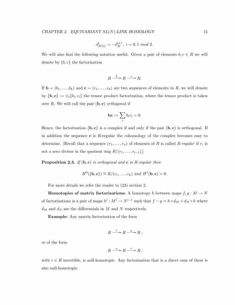
We will also find the following notation useful. Given a pair of elements b, c ∈ R we will
denote by b, c the factorization
Rb // R
c // R.
If b = (b1, . . . , bk) and c = (c1, . . . , ck) are two sequences of elements in R, we will denote
by b, c := ⊗ibi, ci the tensor product factorization, where the tensor product is taken
over R. We will call the pair (b, c) orthogonal if
bc :=∑i
bici = 0.
Hence, the factorization b, c is a complex if and only if the pair (b, c) is orthogonal. If
in addition the sequence c is R-regular the cohomology of the complex becomes easy to
determine. [Recall that a sequence (r1, . . . , rn) of elements of R is called R-regular if ri is
not a zero divisor in the quotient ring R/(r1, . . . , ri−1).]
Proposition 2.3. If (b, c) is orthogonal and c is R-regular then
H0(b, c) ∼= R/(c1, . . . , ck) and H1(b, c) = 0.
For more details we refer the reader to (23) section 2.
Homotopies of matrix factorizations: A homotopy h between maps f, g : M → N
of factorizations is a pair of maps hi : M i → N i−1 such that f − g = h dM + dN h where
dM and dN are the differentials in M and N respectively.
Example: Any matrix factorization of the form
Rr // R
ω // R ,
or of the form
Rω // R
r // R ,
with r ∈ R invertible, is null-homotopic. Any factorization that is a direct sum of these is
also null-homotopic.

CHAPTER 2. EQUIVARIANT SL(N)-LINK HOMOLOGY 16
Let HMF allω be the category with the same objects as MF allω but fewer morphisms:
HomHMF (M,N) := HomMF (M,N)/null − homotopic morphisms.
Consider the free R-module Hom(M,N) given by
Hom0(M,N) d // Hom1(M,N) d // Hom0(M,N) ,
where
Hom0(M,N) = Hom(M0, N0)⊕Hom(M1, N1),
Hom1(M,N) = Hom(M0, N1)⊕Hom(M1, N0),
and the differential given in the obvious way, i.e. for f ∈ Homi(M,N) and m ∈M
(df)(m) = dN (f(m)) + (−1)if(dM (m)).
It is easy to see that this is a 2-periodic complex, and following the notation of (23), we
denote its cohomology by
Ext(M,N) = Ext0(M,N)⊕ Ext1(M,N).
Notice that
Ext0(M,N) ∼= HomHMF (M,N),
Ext1(M,N) ∼= HomHMF (M,N〈1〉).
Tensor Products: As mentioned above, given two matrix factorizations M1 and M2
with potentials ω1 and ω2, respectively, their tensor product is given as the tensor product
of complexes, and a quick calculation shows that M1 ⊗M2 is a matrix factorization with
potential ω1 + ω2. Note that if ω1 + ω2 = 0 then M1 ⊗M2 becomes a 2-periodic complex.
To keep track of differentials of tensor products of factorizations we introduce the la-
belling scheme used in (23). Given a finite set I and a collection of matrix factorizations

CHAPTER 2. EQUIVARIANT SL(N)-LINK HOMOLOGY 17
Ma for a ∈ I, consider the Clifford ring Cl(I) of the set I. This ring has generators a ∈ I
and relations
a2 = 1, ab+ ba = 0, a 6= b.
As an abelian group it has rank 2|I| and a decomposition
Cl(I) =⊕J⊂I
ZJ ,
where ZJ has generators - all ways to order the set J and relations
a . . . bc . . . e+ a . . . cd . . . e = 0
for all orderings a . . . bc . . . e of J .
For each J ⊂ I not containing an element a there is a 2-periodic sequence
ZJra // ZJta
ra // ZJ ,
where ra is right multiplication by a in Cl(I) (note: r2a = 1).
Define the tensor product of factorizations Ma as the sum over all subsets J ⊂ I, of
(⊗a∈JM1a )⊗ (⊗b∈I\JM0
b )⊗Z ZJ ,
with differential
d =∑a∈I
da ⊗ ra,
where da is the differential of Ma. Denote this tensor product by ⊗a∈IMa. If we assign a
label a to a factorization M we write M as
M0(∅) // M1(a) // M0(∅).
An easy but useful exercise shows that if M has finite rank then Hom(M,N) ∼= N ⊗R
M∗−, where M∗− is the factorization
(M0)∗−(d1)∗// (M1)∗
(d0)∗ // (M0)∗.

CHAPTER 2. EQUIVARIANT SL(N)-LINK HOMOLOGY 18
Cohomology of matrix factorizations
Suppose now that R is a local ring with maximal ideal m and M a factorization over
R. If we impose the condition that the potential ω ∈m then
M0/mMd0 // M1/mM
d1 // M0/mM ,
is a 2 periodic complex, since d2 = ω ∈m. LetH(M) = H0(M)⊕H1(M) be the cohomology
of this complex.
Proposition 2.4. Let M be a matrix factorization over a local ring R, with potential ω
contained in the maximal ideal m, and let r ∈ R. The following are equivalent:
1)H(M) = 0.
2)H0(M) = 0.
3)H1(M) = 0.
4) M is null-homotopic.
5) M is isomorphic to a, possibly infinite, direct sum of
M = Rr // R
ω // R ,
and
M = Rω // R
r // R .
Proof: The proof is the same as in (23), and we only need to notice that it extends to
factorizations over any commutative, Noetherian, local ring. The idea is as follows: consider
a matrix representing one of the differentials and suppose that it has an entry not in the
maximal ideal, i.e. an invertible entry; then change bases and arrive at block-diagonal
matrices with blocks representing one of the two types of factorizations listed above (both
of which are null-homotpic). Using Zorn’s lemma we can decompose M as a direct sum
of Mes ⊕Mc where Mc is made up of the null-homotopic factorizations as above, i.e. the
“contractible” summand, and Mes the factor with corresponding submatrix containing no
invertible entries, i.e. the “essential” summand. Now it is easy to see that H(M) = 0 if
and only if Mes is trivial.

CHAPTER 2. EQUIVARIANT SL(N)-LINK HOMOLOGY 19
Proposition 2.5. If f : M → N is a homomorphism of factorizations over a local ring R
then the following are equivalent:
1) f is an isomorphism in HMF allω .
2) f induces an isomorphism on the cohomologies of M and N .
Proof: This is done in (23). Decompose M and N as in the proposition above and notice
that the cohomology of a matrix factorization is the cohomology of its essential part. Now
a map of two free R-modules L1 → L2 that induces an isomorphism on L1/m ∼= L2/m is
an isomorphism of R-modules.
Corollary 2.6. Let M be a matrix factorization over a local ring R. The decomposition
M ∼= Mes ⊕Mc is unique; moreover if M has finite-dimensional cohomology then it is the
direct sum of a finite rank factorization and a contractible factorization.
Let MFω be the category whose objects are factorizations with finite-dimensional coho-
mology and let HMFω be corresponding homotopy category.
Matrix factorizations over a graded ring
Let R = Q[a0, . . . , an−2][x1, . . . , xk], a graded ring of homogeneous polynomials in vari-
ables x1, . . . , xk with coefficients in Q[a0, . . . , an−2]. The gradings are as follows: deg(xi) = 2
and deg(ai) = 2(n− i) with i = 0, . . . n− 2. Furthermore let m = 〈a0, . . . , an−2, x1, . . . , xk〉
the maximal homogeneous ideal, and let a = 〈a0, . . . , an−2〉 the ideal generating the ring of
coefficients.
A matrix factorization M over R naturally becomes graded and we denote i the
grading shift up by i. Note that i commutes with the shift functor 〈1〉. All of the
categories introduced earlier have their graded counterparts which we denote with lower-
case. Let hmfallω is the homotopy category of graded matrix factorizations with the grading
bounded from below.
Proposition 2.7. Let f : M −→ N be a homomorphism of matrix factorizations over
R = Q[α0, . . . , αn−2][x1, . . . , xk] and let f : M/aM −→ N/aN be the induced map. Then f
is an isomorphism of factorizations if and only if f is.

CHAPTER 2. EQUIVARIANT SL(N)-LINK HOMOLOGY 20
Proof: One only needs to notice that modding out by the ideal a we arrive at factoriza-
tions over R = Q[x1, . . . , xk], the graded ring of homogeneous polynomials with coefficients
in Q and maximal ideal m′ = 〈x1, . . . , xk〉. Since a ⊂m and m′ ⊂m, H(M) = H(M/aM)
for any factorization and, hence, the induced maps on cohomology are the same, i.e.
H(f) = H(f). Since an isomorphism on cohomology implies an isomorphism of factor-
izations over R and R the proposition follows.
The matrix factorizations used to define the original link invariants in (23) were defined
over R. With the above proposition we will be able to bypass many of the calculations ness-
esary for MOY-type decompositions and Reidemeister moves, citing those from the original
paper. This simple observation will prove to be one of the most useful.
The category hmfω is Krull-Schmidt: In order to prove that the homology theory
we assign to links is indeed a topological invariant with Euler characteristic the quantum
sln-polynomial, we first need to show that the algebraic objects associated to each resolu-
tion, i.e. to a trivalent planar graph, satisfy the MOY relations (13). Since the objects in
question are complexes constructed from matrix factorizations, the MOY decompositions
are reflected by corresponding isomorphisms of complexes in the homotopy category. Hence,
in order for these relations to make sense, we need to know that if an object in our category
decomposes as a direct sum then it does so uniquely. In other words we need to show that
our category is Krull-Schmidt. The next subsection establishes this fact for hmfω, the ho-
motopy category of graded matrix factorizations over R = Q[a0, . . . , an−2][x1, . . . , xk] with
finite dimensional cohomology.
Given a homogeneous, finite rank, factorization M ∈ mfω, and a degree zero idempotent
e : M −→ M we can decompose M uniquely as the kernel and cokernel of e, i.e. we can
write M = eM ⊕ (1 − e)M . We need to establish this fact for hmfω; that is, we need to
know that given a degree zero idempotent e ∈ Homhmfω(M,M) we can decompose M as
above, and that this decomposition is unique up to homotopy.
Proposition 2.8. The category hmfω has the idempotents splitting property.

CHAPTER 2. EQUIVARIANT SL(N)-LINK HOMOLOGY 21
Proof: We follow (23) . Let I ⊂ Hommfω(M,M) be the ideal consisting of maps that
induce the trivial map on cohomology. Given any such map f ∈ I, we see that every entry
in the matrices representing f must be contained in m, i.e. the entries must be of non-zero
degree. Since a degree zero endomorphism of graded factorizations cannot have matrix
entries of arbitrarily large degree, we see that there exists an n ∈ N such that fn = 0 for
every f ∈ I, i.e. I is nilpotent.
Let K be the kernel of the map Hommfω(M,M) −→ Homhmfω(M,M). Clearly K ⊆ I
and, hence, K is also nilpotent. Since nilpotent ideals have the idempotents lifting property,
see for example (6) Thm. 1.7.3, we can lift any idempotent e ∈ Homhmfω(M,M) to
Hommfω(M,M) and decompose M = eM ⊕ (1− e)M .
Proposition 2.9. The category hmfω is Krull-Schmidt.
Proof: Proposition 8 and the fact that any object in hmfω is isomorphic to one of fi-
nite rank, having finite dimensional cohomology, imply that the endomorphism ring of any
indecomposable object is local. Hence, hmfω is Krull-Schmidt. See (6) for proofs of these
facts.
Planar Graphs and Matrix Factorizations
Our graphs are embedded in a disk and have two types of edges, unoriented and ori-
ented. Unoriented edges are called “thick” and drawn accordingly; each vertex adjoining a
thick edge has either two oriented edges leaving it or two entering. In figure 5.2 left x1, x2
are outgoing and x3, x4 are incoming. Oriented edges are allowed to have marks and we
also allow closed loops; points of the boundary are also referred to as marks. See for ex-
ample figure 2.4. To such a graph Γ we assign a matrix factorization in the following manner:
Let
P (x) =1
n+ 1xn+1 +
an−2
n− 1xn−1 + · · ·+ a1
2x2 + a0x.
Thick edges: To a thick edge t as in figure 5.2 left we assign a factorization Ct with po-
tential ωt = P (x1)+P (x2)−P (x3)−P (x4) over the ring Rt = Q[a0, . . . , an−2][x1, x2, x3, x4].
Since xk + yk lies in the ideal generated by x+ y and xy we can write it as a polynomial
gk(x+ y, xy). More explicitly,

CHAPTER 2. EQUIVARIANT SL(N)-LINK HOMOLOGY 22
gk(s1, s2) = sk1 + k∑
1≤i≤ k2
(−1)i
i
(k − 1− ii− 1
)si2s
k−2i1
Hence, xk1 + xk2 − xk3 − xk4 can be written as
xk1 + xk2 − xk3 − xk4 = (x1 + x2 − x3 − x4)u′k + (x1x2 − x3x4)u′′k
where
u′k =xk1 + xk2 − gk(x3 + x4, x1x2)
x1 + x2 − x3 − x4,
u′′k =gk(x3 + x4, x1x2)− xk3 − xk4
x1x2 − x3x4.
[Notice that our u′n+1 and u′′n+1 are the same as the u1 and u2 in (23), respectively.]
Let
U1 =1
n+ 1u′n+1 +
an−2
n− 1u′n−1 + · · ·+ a1
2u′2 + a0,
and
U2 =1
n+ 1u′′n+1 +
an−2
n− 1u′′n−1 + · · ·+ a1
2u′′2.
Define Ct to be the tensor product of graded factorizations
RtU1−→ Rt1− n
x1+x2−x3−x4−−−−−−−−−→ Rt,
and
RtU2−→ Rt3− n
x1x2−x3x4−−−−−−−→ Rt,
with the product shifted by −1.
Arcs: To an arc α bounded by marks oriented from j to i we assign the factorization
Lij
RαPij−−→ Rα
xi−xj−−−−→ Rα,
where Rα = Q[a0, . . . , an−2][xi, xj ] and

CHAPTER 2. EQUIVARIANT SL(N)-LINK HOMOLOGY 23
Pij =P (xi)− P (xj)
xi − xj.
Finally, to an oriented loop with no marks we assign the complex 0 → A → 0 = A〈1〉
where A = Q[a0, . . . , an−2][x]/(xn+an−2xn−2 + · · ·+a1x+a0). [Note: to a loop with marks
we assign the tensor product of Lij ’s as above, but this turns out to be isomorphic to A〈1〉
in the homotopy category.]
Figure 2.4: A planar graph
We define C(Γ) to be the tensor product of Ct over all thick edges t, Lij over all edges
α from j to i, and A〈1〉 over all oriented markless loops. This tensor product is taken
over appropriate rings such that C(Γ) is a free module over R = Q[a0, . . . , an−2][xi]
where the xi’s are marks. For example, to the graph in figure 2.4 we assign C(Γ) =
L74 ⊗ Ct1 ⊗ L3
6 ⊗ Ct2 ⊗ L108 ⊗ A〈1〉 tensored over Q[a0, . . . , an−2][x4], Q[a0, . . . , an−2][x3],
Q[a0, . . . , an−2][x6], Q[a0, . . . , an−2][x8] and Q[a0, . . . , an−2] respectively. C(Γ) becomes a
Z ⊕ Z2-graded complex with the Z2-grading coming from the matrix factorization. It has
potential ω =∑i∈∂Γ
±P (xi), where ∂Γ is the set of all boundary marks and the +, − is
determined by whether the direction of the edge corresponding to xi is towards or away
from the boundary. [Note: if Γ is a closed graph the potential is zero and we have an honest
2-complex.]

CHAPTER 2. EQUIVARIANT SL(N)-LINK HOMOLOGY 24
Example: Let us look at the factorization assigned to an oriented loop with two marks
x and y. We start out with the factorization Lyx assigned to an arc and then “close it off,”
which corresponds to moding out by the ideal generated by the relation x = y, see figure
2.5. We arrive at
Rxn+an−2xn−2+···+a1x+a0−−−−−−−−−−−−−−−−−→ R
0−→ R,
where R = Q[a0, . . . , an−2][x].
Figure 2.5: “Closing off” an arc
The homology of this complex is supported in degree 1, with
H1(Lyx/〈x = y〉) = Q[a0, . . . , an−2][x]/(xn + an−2xn−2 + · · ·+ a1x+ a0).
This is the algebra A we associated to an oriented loop with no marks. As we set out to
define a homology theory that assigns to the unkot the U(n)-equivariant cohomology of
CPn−1, this example illustrates the choice of potential P (x). Notice that A has a natural
Frobenius algebra structure with trace map ε and unit map ι.
ε : Q[a0, . . . , an−2][x]/(xn + an−2xn−2 + · · ·+ a1x+ a0) −→ Q[a0, . . . , an−2],
given by
ε(xn−1) = 1; ε(xi) = 0, i ≤ n− 2,
and
ι : Q[a0, . . . , an−2] −→ Q[a0, . . . , an−2][x]/(xn + an−2xn−2 + · · ·+ a1x+ a0),
ι(1) = 1.

CHAPTER 2. EQUIVARIANT SL(N)-LINK HOMOLOGY 25
Notice that ε(xi) is not equal to zero for i ≥ n but a homogeneous polynomial in the
ai’s. Many of the calculations in (23) necessary for the proofs of invariance would fail due
to this fact; proposition 4 will be key in getting around this difference. Of course, setting
ai = 0, for all i, gives us the same Frobenius algebra, unit and trace maps as in (23).
Figure 2.6: Maps χ0 and χ1
The maps χ0 and χ1: We now define maps between matrix factorizations associated
to a thick edge and two disjoint arcs as in figure 5.2. Let Γ0 correspond to the two disjoint
arcs and Γ1 to the thick edge.
C(Γ0) is the tensor product of L14 and L2
3. If we assign labels a, b to L14, L2
3 respectively,
the tensor product can be written as
R(∅)
R(ab)2− 2n
P0−→
R(a)1− n
R(b)1− n
P1−→
R(∅)
R(ab)2− 2n
,
where
P0 =
P14 x2 − x3
P23 x4 − x1
, P1 =
x1 − x4 x2 − x3
P23 −P14
,
and R = Q[a0, . . . , an−2][x1, x2, x3, x4].
Assigning labels a′ and b′ to the two factorizations in C(Γ1), we have that C(Γ1) is given
by
R(∅)−1
R(a′b′)3− 2n
Q0−→
R(a′)−n
R(b′)2− n
Q1−→
R(∅)−1
R(a′b′)3− 2n
,
where

CHAPTER 2. EQUIVARIANT SL(N)-LINK HOMOLOGY 26
Q0 =
U1 x1x2 − x3x4
U2 x3 + x4 − x1 − x2
, Q1 =
x1 + x2 − x3 − x4 x1x2 − x3x4
U2 −U1
.
A map between C(Γ0) and C(Γ1) can be given by a pair of 2 × 2 matrices. Define
χ0 : C(Γ0)→ C(Γ1) by
U0 =
x4 − x2 + µ(x1 + x2 − x3 − x4) 0
k1 1
, U1 =
x4 + µ(x1 − x4) µ(x2 − x3)− x2
−1 1
,
where
k1 = (µ− 1)U2 +U1 + x1U2 − P23
x1 − x4, for µ ∈ Z
and χ1 : C(Γ1)→ C(Γ0) by
V0 =
1 0
k2 k3
, V1 =
1 x3 + λ(x2 − x3)
1 x1 + λ(x4 − x1)
.
where
k2 = λU2 +U1 + x1U2 − P23
x4 − x1, k3 = λ(x3 + x4 − x1 − x2) + x1 − x3, for λ ∈ Z.
It is easy to see that different choices of µ and λ give homotopic maps. These maps are
degree 1. We encourage the reader to compare the above factorizations and maps to that of
(23), and notice the difference stemming from the fact that here we are working with new
potentials.
Just like in (23) we specialize to λ = 0 and µ = 1, and compute to see that the com-
position χ1χ0 = (x1 − x3)I, where I is the identity matrix, i.e. χ1χ0 is multiplication by
x1 − x3, which is homotopic to multiplication by x4 − x2 as an endomorphism of C(Γ0).
Similarly χ0χ1 = (x1 − x3)I, which is also homotopic to multiplication by x4 − x2 as an
endomorphism of C(Γ1).

CHAPTER 2. EQUIVARIANT SL(N)-LINK HOMOLOGY 27
Figure 2.7: Direct Sum Decomposition 0
Direct Sum Decomposition 0
where D0 =n−1∑i=0
xiι and D−10 =
n−1∑i=0
εxn−1−i.
By the pictures above, we really mean the complexes assigned to them, i.e. ∅〈1〉 is
the complex with Q[a0, . . . , an−2] sitting in homological grading 1 and the unknot is the
complex A〈1〉 as before. The map εxi is a composition of maps
A〈1〉 xi
−→ A〈1〉 ε−→ ∅〈1〉,
where xi is multiplication and ε is the trace map.
The map xiι is analogous. It is easy to check that the above maps are grading preserving
and their composition is an isomorphism in the homotopy category.
Direct Sum Decomposition I We follow (23) closely. Recall that here matrix factor-
izations are over the ring R = Q[a0, . . . , an−2].
Figure 2.8: Direct Sum Decomposition I
Proposition 2.10. The following two factorizations are isomorphic in hmfω.

CHAPTER 2. EQUIVARIANT SL(N)-LINK HOMOLOGY 28
C(Γ) ∼=n−2∑i=0
C(Γ1)〈1〉2− n+ 2i.
Proof: Define grading preserving maps αi and βi for 0 ≤ i ≤ n− 2, as in (23),
αi : C(Γ1)〈1〉 −→ C(Γ)n− 2− 2i,
αi =i∑
j=0
xj1xi−j2 α,
where α = χ0 ι′ is defined to be the composition in figure 5.3. [ι′ = ι ⊗ Id where Id
corresponds to the inclusion of the arc Γ1 into the disjoint union of the arc and circle, and
ι is the unit map.]
βi : C(Γ)n− 2− 2i −→ C(Γ1)〈1〉,
βi = βxn−i−21 ,
where β = ε′ χ1, see figure 5.4. [Similarly, ε′ = ε⊗ Id.]
Figure 2.9: The map α
Figure 2.10: The map β
Define maps:
α′ =n−2∑i=0
αi :n−2∑i=0
C(Γ1)〈1〉2− n+ 2i −→ C(Γ),

CHAPTER 2. EQUIVARIANT SL(N)-LINK HOMOLOGY 29
and
β′ =n−2∑i=0
βi : C(Γ) −→ C(Γ1)〈1〉2− n+ 2i.
In (23) it was shown that these maps are isomorphisms of factorizations over the ring
R = Q[x1, x2, x3, x4]. By Proposition 2.7 we are done.
Direct Sum Decomposition II
Figure 2.11: Direct Sum Decomposition II
Proposition 2.11. There is an isomorphism of factorizations in hmfω
C(Γ) ∼= C(Γ1)1 ⊕ C(Γ1)−1.
Proof: See (23).
Direct Sum Decomposition III
Proposition 2.12. There is an isomorphism of factorizations in hmfω
C(Γ) ∼= C(Γ2)⊕(⊕n−3i=0 C(Γ1)〈1〉3− n+ 2i
).
Proof: Define grading preserving maps αi, βi for 0 ≤ i ≤ n− 3
αi : C(Γ1)〈1〉3− n+ 2i −→ C(Γ)
αi = x5α,
where α = χ′0ι′, ι′ = Id⊗ι⊗Id with identity maps on the two arcs, and χ′0 the composition
of two χ0’s corresponding to merging the two arcs into the circle, see figure 2.13.

CHAPTER 2. EQUIVARIANT SL(N)-LINK HOMOLOGY 30
Figure 2.12: Direct Sum Decomposition III
Figure 2.13: The map α
βi : C(Γ) −→ C(Γ1)〈1〉3− n+ 2i
βi =n−3∑i=0
β∑
a+b+c=n−3−ixa2x
b4xc1,
where β is defined as in figure 5.5.
Figure 2.14: The map β
S : C(Γ) −→ C(Γ2).
In addition, let S be the map gotten by “merging” the thick edges together to form
two disjoint horizontal arcs, as in the top righ-hand corner above; an exact description of
CHAPTER 2. EQUIVARIANT SL(N)-LINK HOMOLOGY 31
S won’t really matter so we will not go into details and refer the interested reader to (23).
Let α′ =∑n−3
i=0 αi and β′ =∑n−3
i=0 βi. In (23) it shown that S ⊕ β′ is an isomorphism in
hmfω, with inverse S−1 ⊕ α′, so by Proposition 2.7 we are done. .
[Note: we abuse notation throughout by using a direct sum of maps to indicate a map
to or from a direct summand.]
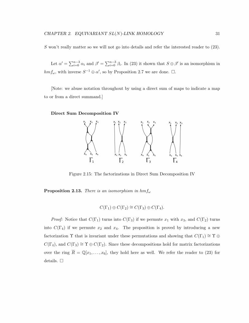
Direct Sum Decomposition IV
Figure 2.15: The factorizations in Direct Sum Decomposition IV
Proposition 2.13. There is an isomorphism in hmfω
C(Γ1)⊕ C(Γ2) ∼= C(Γ3)⊕ C(Γ4).
Proof: Notice that C(Γ1) turns into C(Γ3) if we permute x1 with x3, and C(Γ2) turns
into C(Γ4) if we permute x2 and x4. The proposition is proved by introducing a new
factorization Υ that is invariant under these permutations and showing that C(Γ1) ∼= Υ⊕
C(Γ4), and C(Γ3) ∼= Υ⊕ C(Γ2). Since these decompositions hold for matrix factorizations
over the ring R = Q[x1, . . . , x6], they hold here as well. We refer the reader to (23) for
details.
CHAPTER 2. EQUIVARIANT SL(N)-LINK HOMOLOGY 32
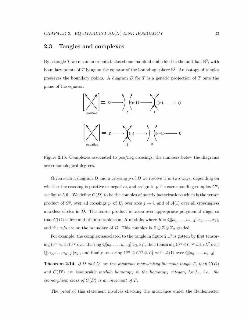
2.3 Tangles and complexes
By a tangle T we mean an oriented, closed one manifold embedded in the unit ball B3, with
boundary points of T lying on the equator of the bounding sphere S2. An isotopy of tangles
preserves the boundary points. A diagram D for T is a generic projection of T onto the
plane of the equator.
Figure 2.16: Complexes associated to pos/neg crossings; the numbers below the diagrams
are cohomological degrees.
Given such a diagram D and a crossing p of D we resolve it in two ways, depending on
whether the crossing is positive or negative, and assign to p the corresponding complex Cp,
see figure 5.6 . We define C(D) to be the comples of matrix factorizations which is the tensor
product of Cp, over all crossings p, of Lij over arcs j → i, and of A〈1〉 over all crossingless
markless circles in D. The tensor product is taken over appropriate polynomial rings, so
that C(D) is free and of finite rank as an R-module, where R = Q[a0, . . . , an−2][x1, . . . , xk],
and the xi’s are on the boundary of D. This complex is Z⊕ Z⊕ Z2 graded.
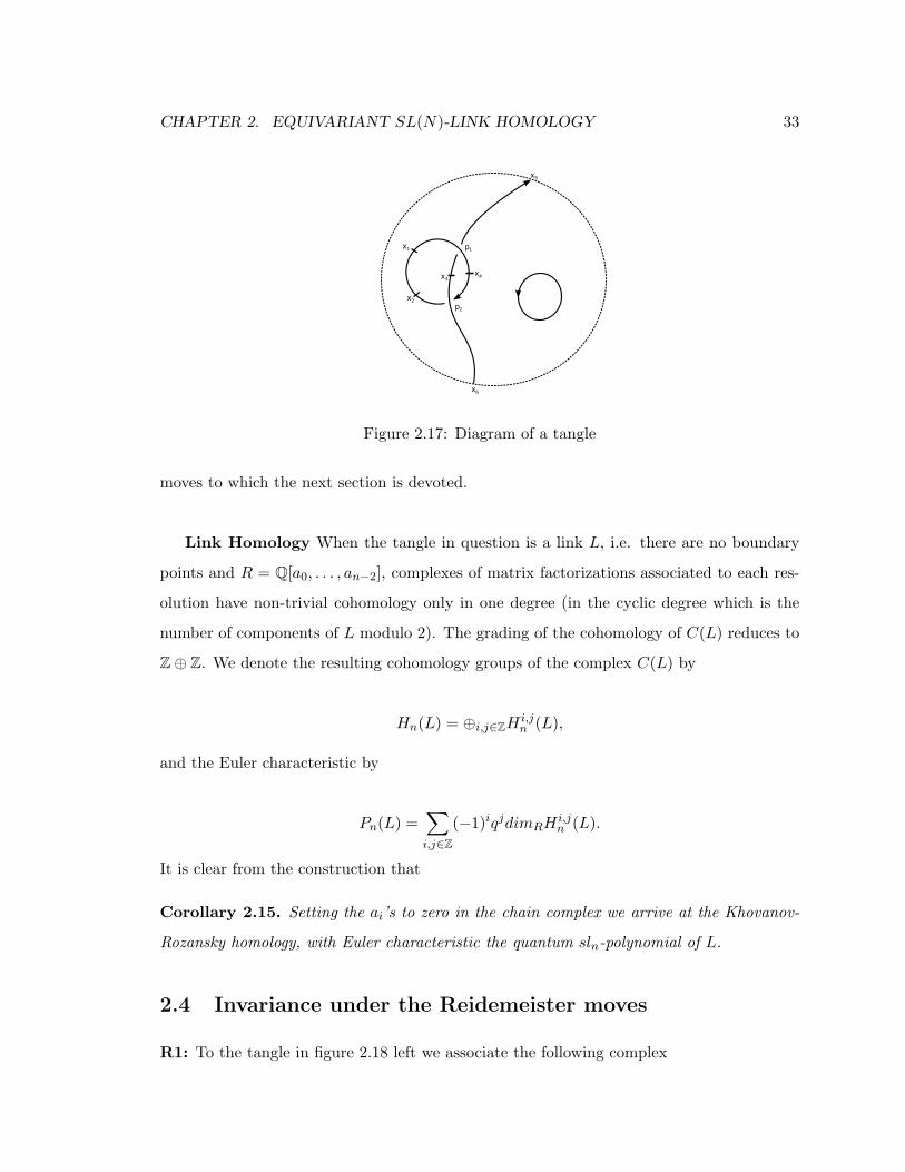
For example, the complex associated to the tangle in figure 2.17 is gotten by first tensor-
ing Cp1 with Cp2 over the ring Q[a0, . . . , an−2][x3, x4], then tensoring Cp1⊗Cp2 with L21 over
Q[a0, . . . , an−2][x2], and finally tensoring Cp1 ⊗ Cp2 ⊗ L21 with A〈1〉 over Q[a0, . . . , an−2].
Theorem 2.14. If D and D′ are two diagrams representing the same tangle T , then C(D)
and C(D′) are isomorphic modulo homotopy in the homotopy category hmfω, i.e. the
isomorphism class of C(D) is an invariant of T .
The proof of this statement involves checking the invariance under the Reidemeister
CHAPTER 2. EQUIVARIANT SL(N)-LINK HOMOLOGY 33
Figure 2.17: Diagram of a tangle
moves to which the next section is devoted.
Link Homology When the tangle in question is a link L, i.e. there are no boundary
points and R = Q[a0, . . . , an−2], complexes of matrix factorizations associated to each res-
olution have non-trivial cohomology only in one degree (in the cyclic degree which is the
number of components of L modulo 2). The grading of the cohomology of C(L) reduces to
Z⊕ Z. We denote the resulting cohomology groups of the complex C(L) by
Hn(L) = ⊕i,j∈ZHi,jn (L),
and the Euler characteristic by
Pn(L) =∑i,j∈Z
(−1)iqjdimRHi,jn (L).
It is clear from the construction that
Corollary 2.15. Setting the ai’s to zero in the chain complex we arrive at the Khovanov-
Rozansky homology, with Euler characteristic the quantum sln-polynomial of L.
2.4 Invariance under the Reidemeister moves
R1: To the tangle in figure 2.18 left we associate the following complex

CHAPTER 2. EQUIVARIANT SL(N)-LINK HOMOLOGY 34
Figure 2.18: Reidemeister I
0 // C(Γ1)1− n χ0 // C(Γ2)−n // 0.
Figure 2.19: Reidemeister 1 complex
Using direct decompositions 0 and I, and for a moment forgoing the overall grading
shifts, we see that this complex is isomorphic to
0 // ⊕n−1i=0 C(Γ)1− n+ 2i Φ //
⊕n−2j=0 C(Γ)1 + n− 2j // 0,
where
Φ = β′ χ0 n−1∑i=0
xi1ι′
=( n−2∑j=0
ε′ χ1xn−j−21
) χ0
n−1∑i=0
xi1ι′
=n−1∑i=0
n−2∑j=0
ε′ χ1 χ0xn−j+i−21 ι′
=n−1∑i=0
n−2∑j=0
ε′(x1 − x2)xn−j+i−21 ι′
= ε′( n−1∑i=0
n−2∑j=0
(xn−j+i−11 − x2x
n−j+i−21 )
)ι′.
Hence, Φ is an upper triangular matrix with 1’s on the diagonal, which implies that up
to homotopy the above complexes are isomorphic to

CHAPTER 2. EQUIVARIANT SL(N)-LINK HOMOLOGY 35
0 −→ C(Γ)n− 1 −→ 0.
Recalling that we left out the overall grading shift of −n+ 1 we arrive at the desired
conclusion:
0 // C(Γ1)1− n χ0 // C(Γ2)−n // 0
is homotopic to
0 −→ C(Γ)n− 1 −→ 0.
The other Reidemeister 1 move is proved analogously.
R2: The complex associated to the tangle in figure 2.20 left is
Figure 2.20: Reidemeister 2a
0 −→ C(Γ00)1 (f1,f3)t
−−−−−→
C(Γ01)
⊕
C(Γ10)
(f2,−f4)−−−−−→ C(Γ11)−1 −→ 0.
Using direct decomposition II we know that
C(Γ10) ∼= C(Γ1)1 ⊕ C(Γ1)−1.
Hence, the above complex is isomorphic to

CHAPTER 2. EQUIVARIANT SL(N)-LINK HOMOLOGY 36
Figure 2.21: Reidemeister 2a complex
0 −→ C(Γ00)1 (f1,f03,f13)t
−−−−−−−→
C(Γ01)
⊕
C(Γ1)1
⊕
C(Γ1)−1
(f2,−f04,−f14)−−−−−−−−−→ C(Γ11)−1 −→ 0,
where f03, f13, f04, f14 are the degreee 0 maps that give the isomorphism of decomposition
II. If we know that both f14 and f03 are isomorphisms then the subcomplex containing
C(Γ00), C(Γ10), and C(Γ11) is acyclic; moding out produces a complex homotopic to
0 −→ C(Γ0) −→ 0.
The next two lemmas establish the fact that f14 and f03 are indeed isomorphisms.
Lemma 2.16. The space of degree 0 endomorphisms of C(Γ1) is isomorphic to Q. The
space of degree 2 endomorphism is 3-dimensional spanned by x1, x2, x3, x4 with only relation
being x1 + x2 − x3 − x4 = 0 for n > 2, and 2-dimensional with the relations x1 + x2 = 0
and x3 + x4 = 0 for n = 2.
Proof: The complex Hom(C(Γ1), C(Γ1)) is isomorphic to the factorization of the pair

CHAPTER 2. EQUIVARIANT SL(N)-LINK HOMOLOGY 37
(b, c) where
b = (x1 +x2 +x3 +x4, x1x2−x3x4,−U1,−U2), c = (U1,U2, x1 +x2 +x3 +x4, x1x2−x3x4).
The pair (b, c) is orthogonal, since this is a complex, and it is easy to see that the
sequence c is regular (c is certainly regular when we set the ai’s equal to zero) and hence
the cohomology of this 2-complex is
Q[a0, . . . , an−2][x1, x2, x3, x4]/(x1 + x2 + x3 + x4, x1x2 − x3x4,U1,U2).
For n > 2 the last three terms of the above sequence are at least quadratic and, hence,
have degree at least 4 (recall that deg ai ≥ 4 for all i). For n = 2, U2 = u′′2 which is linear
and we get the relations x1 + x2 = 0, x3 + x4 = 0.
Lemma 2.17. f14 6= 0 and f03 6= 0.
Proof: With the above lemma the proof follows the lines of (23).
Hence, f14 and f03 are indeed isomorphisms and we arrive at the desired conclusion.
Figure 2.22:
R3: The complex assigned to the tangle on the left-hand side of figure 2.22 is
0 −→ C(Γ111) d−3
−−→
C(Γ011)−1
⊕
C(Γ101)−1
⊕
C(Γ110)−1
d−2
−−→
C(Γ100)−2
⊕
C(Γ010)−2
⊕
C(Γ001)−2
d−1
−−→ C(Γ000)−3 −→ 0.
Direct sum decompositions II and III show that

CHAPTER 2. EQUIVARIANT SL(N)-LINK HOMOLOGY 38
Figure 2.23: Reidemeister 3 complex
C(Γ101) ∼= C(Γ100)1 ⊕ C(Γ100)−1,
and
C(Γ111) ∼= C(Γ100)⊕Υ.
Inserting these and using arguments analogous to those used in the decomposition proofs
we reduce the original complex to
0 −→ Υ d−3
−−→
C(Γ011)−1
⊕
C(Γ110)−1
d−2
−−→
C(Γ010)−2
⊕
C(Γ100)−2
d−1
−−→ C(Γ000)−3 −→ 0.
Proposition 2.18. Assume n > 2, then for every arrow in 4.12 from object A to B the
space of grading-preserving morphisms
Homhmf (C(A), C(B)−1)

CHAPTER 2. EQUIVARIANT SL(N)-LINK HOMOLOGY 39
Figure 2.24: Reidemeister 3 complex reduced
is one dimensional. Moreover, the composition of any two arrows C(A) −→ C(B)−1 −→
C(C)−2 is nonzero.
Proof: Once again the maps in question are all of degree ≤ 2, and noticing that these
remain nonzero when we work over the ring Q[a0, . . . , an−2], we can revert to the calcula-
tions in (23).
Hence, this complex is invariant under the “flip” which takes x1 to x3 and x4 to x6.
This flip takes the complex associated to the braid on the left-hand side of figure 2.22 to
the one on the right-hand side.
2.5 Remarks
Given a diagram D of a link L let Cn(D) be the equivariant sln chain complex constructed
above. The homotopy class of Cn(D) is an invariant of L and consists of free Q[a0, . . . , an−2]-
modules where the ai’s are coefficients with deg(ai) = 2(n − i). The cohomology of this
complex Hn(D) is a graded Q[a0, . . . , an−2]-module. For a moment, let us consider the case
where all the ai = 0 for 1 ≤ i ≤ n−2, and denote by Cn,a(D) and Hn,a(D) the corresponding
complex and cohomology groups with a = a0. Here the cohomology Hn,a(D) is a finitely

CHAPTER 2. EQUIVARIANT SL(N)-LINK HOMOLOGY 40
generated Q[a]-module and we can decompose it as direct sum of torsion modules Q[a]/(ak)
for various k and free modules Q[a]. Let H ′n,a(D) = Hn,a(D)/Torn,a(D), where Torn,a(D)
is the torsion submodule. Just like in the sl2 case in (20) we have:
Proposition 2.19. H ′n,a(D) is a free Q[a]-module of rank nm, where m is the number of
components of L.
Proof: If we quotient Cn,a(D) by the subcomplex (a− 1)Cn,a(D) we arrive at the com-
plex studied by Gornik in (12), where he showed that its rank is nm. The ranks of our
complex and his are the same.
In some sense this specialization is isomorphic to n copies of the trivial link homology
which assigns to each link a copy of Q for each component, modulo grading shifts. In (29),
M. Mackaay and P. Vaz studied similar variants of the sl3-theory working over the Frobenius
algebra C[x]/(x3 +ax2 + bx+ c) with a, b, c ∈ C and arrived at three isomorphism classes of
homological complexes depending on the number of distinct roots of the polynomial x3 +
ax2 + bx+ c. They showed that multiplicity three corresponds to the sl3-homology of (18),
one root of multiplicity two is a modified version of the original sl2 or Khovanov homology,
and distinct roots correspond to the “Lee-type” deformation. We expect an interpretation
of their results in the equivariant version. Moreover, it would be interesting to understand
these specialization for higher n and we foresee similar decompositions, i.e. we expect the
homology theories to break up into isomorphism classes corresponding to the number of
distinct “roots” in the decomposition of the polynomial xn + an−2xn−2 + · · ·+ a1x+ a0.
The sl2-homology and sl3-homology for links, as well as their deformations, are defined
over Z; in chapter 4 we will present such an integral construction for all n.

Chapter 3 41
Chapter 3
Functoriality of Rouquier
complexes
3.1 Soergel bimodules in representation theory and link ho-
mology
For some time, the category of Soergel bimodules, here called SC, has played a significant
role in the study of representation theory, while more recently strong connections between
SC and knot theory have come to light. Originally introduced by Soergel in (39), SC is
an equivalent but more combinatorial description of a certain category of Harish-Chandra
modules over a semisimple lie algebra g. The added simplicity of this formulation comes
from the fact that SC is just a full monoidal subcategory of graded R-bimodules, where R
is a polynomial ring equipped with an action of the Weyl group of g. Among other things,
Soergel gave an isomorphism between the Grothendieck ring of SC and the Hecke algebra
H associated to g, where the Kazhdan-Lusztig generators bi of H lift to bimodules Bi which
are easily described. The full subcategory generated monoidally by these bimodules Bi is
here called SC1, and the category including all grading shifts and direct sums of objects
in SC1 is called SC2. It then turns out that SC is actually the idempotent closure of SC2,
which reduces the study of SC to the study of these elementary bimodules Bi and their
tensors. For more on Soergel bimodules and their applications to representation theory see

CHAPTER 3. FUNCTORIALITY OF ROUQUIER COMPLEXES 42
(37; 38; 40).
An important application of Soergel bimodules was discovered by Rouquier in (36),
where he observes that one can construct complexes in SC2 which satisfy the braid relations
modulo homotopy. To the i overcrossing (resp. undercrossing) in the braid group Rouquier
associates a complex, which has R in homological degree 0 and Bi in homological degree
−1 (resp. 1). Giving the homotopy equivalence classes of invertible complexes in SC2 the
obvious group structure under tensor product, this assignment extends to a homomorphism
from the braid group. Using this, one can define an action of the braid group on the
homotopy category of SC2, where the endofunctor associated to a crossing is precisely
taking the tensor product with its associated complex.
Following his work with L. Rozansky on matrix factorizations and link homology in (?
), Khovanov produced an equivalent categorification (21) of the HOMFLY-PT polynomial
utilizing Rouquier’s work. To a braid one associates its Rouquier complex, which naturally
has two gradings: the homological grading, and the internal grading of Soergel bimodules.
Then, taking the Hochschild homology of each term in the complex, one gets a complex
which is triply graded (the third grading is the Hochschild homological grading). Khovanov
showed that, up to degree shifts, this construction yields an equivalent triply-graded complex
to the one produced by the reduced version of the Khovanov-Rozansky HOMFLY-PT link
homology for the closure of the braid (see (21) and (22) for more details).
Many computations of HOMFLY-PT link homology were done by B. Webster (43), and
by J. Rasmussen in (33) and (35). In (33), Rasmussen showed that given a braid presentation
of a link, for every n ∈ N there exists a spectral sequence with E1-term its HOMFLY-PT
homology and the E∞-term its sl(n) homology. This was a spectacular development in
understanding the structural properties of these theories, and has also proven very useful
in computation (see for example (27)).
One key aspect of the original Khovanov-Rozansky theory is that it gives rise to a
projective functor. The braid group can actually be realized as the isomorphism classes
of objects in the category of braid cobordisms. This category, while having a topologi-
cal definition, is equivalent to a combinatorially defined category, whose objects are braid
diagrams, and whose morphisms are called movies (see Carter-Saito, (7)). For instance,

CHAPTER 3. FUNCTORIALITY OF ROUQUIER COMPLEXES 43
performing a Reidemeister 3 move on a braid diagram would give an equivalent element of
the braid group, but gives a distinct object in the braid cobordism category; however, the
R3 move itself is a movie which gives the isomorphism between those two objects. It was
shown in (22) that for each movie between braids one can associate a chain map between
their triply-graded complexes. This assignment was known to be projectively functorial,
meaning that the relations satisfied amongst movies in the braid cobordism category are
also satisfied by their associated chain maps, up to multiplication by a scalar. Scalars take
their value in Q, the ring over which Khovanov-Rozansky theory is defined. However, these
chain maps are not explicitly described even in the setting of Khovanov-Rozansky theory,
and the maps they correspond to in the Soergel bimodule context are even more obscure. A
more general discussion of braid group actions, including this categorification via Rouquier
complexes, and their extensions to projective actions on the category of braid cobordisms
can be found in (24).
Recently, in (1), B. Elias and Mikhail Khovanov gave a presentation of the category SC1
in terms of generators and relations. Moreover, it was shown that the entire category can
be drawn graphically, thanks to the biadjointness and cyclicity properties that the category
possesses. Each Bi is assigned a color, and a tensor product is assigned a sequence of
colors. Morphisms between tensor products can be drawn as certain colored graphs in the
plane, whose boundaries on bottom and top are the sequence of colors associated to the
source and target. Composition and tensor product of morphisms correspond to vertical and
horizontal concatenation, respectively. Morphisms are invariant under isotopy of the graph
embedding, and satisfy a number of other relations, as described herein. In addition to
providing a presentation, this graphical description is useful because one can use pictures to
encapsulate a large amount of information; complicated calculations involving compositions
of morphisms can be visualized intuitively and written down suffering only minor headaches.
Because of the simplicity of the diagrammatic calculus, we were able to calculate explic-
itly the chain maps which correspond to each generating cobordism in the braid cobordism
category, and check that these chain maps satisfy the same relations that braid cobordisms
do. The general proofs are straightforward and computationally explicit, performable by
any reader with patience, time, and colored chalk. While we use some slightly more so-

CHAPTER 3. FUNCTORIALITY OF ROUQUIER COMPLEXES 44
phisticated machinery to avoid certain incredibly lengthy computations, the machinery is
completely unnecessary. This makes the results of Rouquier and Khovanov that much more
concrete, and implies the following new result.
Theorem 3.1. There is a functor F from the category of combinatorial braid cobordisms
to the category of complexes in SC2 up to homotopy, lifting Rouquier’s construction (i.e.
such that F sends crossings to Rouquier complexes).
Soergel bimodules are generally defined over certain fields k in the literature, because
one is usually interested in Soergel bimodules as a categorification of the Hecke algebra, and
in relating indecomposable bimodules to the Kazhdan-Lusztig canonical basis. However,
we invite the reader to notice that the diagrammatic construction in (1) can be made over
any ring, and in particular over Z. In fact, all our proofs of functoriality still work over Z.
We discuss this in detail in section 3.5.2. In the subsequent paper, we plan to use the work
done here to define HOMFLY-PT and sl(n)-link homology theories over Z, a construction
which is long overdue. We also plan to investigate the Rasmussen spectral sequence in this
context.
At the given moment there does not exist a diagrammatic calculus for the higher
Hochschild homology of Soergel bimodules. Some insights have already been obtained,
although a full understanding had yet to emerge. We plan to develop the complete picture,
which should hopefully give an explicit and easily computable description of functoriality
in the link homology theories discussed above.
The organization of this chapter is as follows. In Section 3.2 we go over all the previous
constructions that are relevant to this paper. This includes the Hecke algebra, Soergel’s
categorification SC, the graphical presentation of SC, the combinatorial braid cobordism
category, and Rouquier’s complexes which link SC to braids. In Section 3.2.6 we describe
the conventions we will use in the remainder of the paper to draw Rouquier complexes
for movies. In Section 3.3 we define the functor from the combinatorial braid cobordism
category to the homotopy category of SC, and in Section 3.4 we check the movie move
relations to verify that our functor is well-defined. These checks are presented in numerical
order, not in logical order, but a discussion of the logical dependency of the proofs, and of
the simplifications that are used, can be found in Section 3.4.1. Section 3.5 contains some

CHAPTER 3. FUNCTORIALITY OF ROUQUIER COMPLEXES 45
useful statements for the interested reader, but is not strictly necessary. Some additional
light is shed on the generators and relations of SC in Section 3.5.1, where it is demonstrated
how the relations arise naturally from movie moves. In Section 3.5.2 we briefly describe
how one might construct the theory over Z, so that future papers may use this result to
define link homology theories over arbitrary rings.
3.2 Constructions
3.2.1 The Hecke Algebra
The Hecke algebra H of type A∞ has a presentation as an algebra over Z[t, t−1
]with
generators bi, i ∈ Z and the Hecke relations
b2i = (t+ t−1)bi (3.1)
bibj = bjbi for |i− j| ≥ 2 (3.2)
bibi+1bi + bi+1 = bi+1bibi+1 + bi. (3.3)
For any subset I ⊂ Z, we can consider the subalgebra H(I) ⊂ H generated by bi, i ∈ I,
which happens to have the same presentation as above. Usually only finite I are considered.
We write the monomial bi1bi2 · · · bid as bi where i = i1 . . . id is a finite sequence of indices;
by abuse of notation, we sometimes refer to this monomial simply as i . If i is as above, we
say the monomial has length d. We call a monomial non-repeating if ik 6= il for k 6= l. The
empty set is a sequence of length 0, and b∅ = 1.
Let ω be the t-antilinear anti-involution which fixes bi, i.e. ω(tabi ) = t−abσ(i) where σ
reverses the order of a sequence. Let ε : H → Z[t, t−1
]be the Z
[t, t−1
]-linear map which
is uniquely specified by ε(xy) = ε(yx) for all x, y ∈ H and ε(bi ) = td, whenever i is a
non-repeating sequence of length d. Let (, ) : H × H → Z[t, t−1
]be the map which sends
(x, y) 7→ ε(ω(x)y). Via the inclusion maps, these structures all descend to each H(I) as
well.
We say i, j ∈ Z are adjacent if |i− j| = 1, and are distant if |i− j| ≥ 2.
For more details on the Hecke algebra in this context, see (1).

CHAPTER 3. FUNCTORIALITY OF ROUQUIER COMPLEXES 46
3.2.2 The Soergel Categorification
In (39), Soergel introduced a monoidal category categorifying the Hecke algebra for a finite
Weyl group W of type A. We will denote this category by SC(I), or by SC when I is
irrelevant. Letting V be the geometric representation of W over a field k of characteristic 6=
2, and R its coordinate ring, the category SC is given as a full additive monoidal subcategory
of graded R-bimodules (whose objects are now commonly referred to as Soergel bimodules).
This category is not abelian, for it lacks images, kernels, and the like, but it is idempotent
closed. In fact, SC is given as the idempotent closure of another full additive monoidal
subcategory SC1, whose objects are called Bott-Samuelson modules. The category SC1 is
generated monoidally over R by objects Bi, i ∈ I, which satisfy
Bi ⊗Bi ∼= Bi1 ⊕Bi−1 (3.4)
Bi ⊗Bj ∼= Bj ⊗Bi for distant i, j (3.5)
Bi ⊗Bj ⊗Bi ⊕Bj ∼= Bj ⊗Bi ⊗Bj ⊕Bi for adjacent i, j. (3.6)
The Grothendieck group of SC(I) is isomorphic to H(I), with the class of Bi being sent
to bi, and the class of R1 being sent to t.
One useful feature of this categorification is that it is easy to calculate the dimension
of Hom spaces in each degree. Let HOM(M,N) def=⊕
m∈Z Hom(M,Nm) be the graded
vector space (actually an R-bimodule) generated by homogeneous morphisms of all degrees.
Let Bidef= Bi1 ⊗ · · · ⊗Bid . Then HOM(Bi , Bj ) is a free left R-module, and its graded rank
over R is given by (bi , bj ).
For two subsets I ⊂ I ′ ⊂ Z, the categories SC(I) and SC(I ′) are embedded in bimodule
categories over different rings R(I) and R(I ′), but there is nonetheless a faithful inclusion
of categories SC(I) → SC(I ′). This functor is not full: the size of R itself will grow, and
HOM(B∅, B∅) = R. However, the graded rank over R does not change, since the value of
ε and hence (, ) does not change over various inclusions. Effectively, the only difference in
Hom spaces under this inclusion functor is base change on the left, from R(I) to R(I ′).
As a result of this, most calculations involving morphisms between Soergel bimodules
will not depend on which I we work over. When I is infinite, the ring R is no longer
CHAPTER 3. FUNCTORIALITY OF ROUQUIER COMPLEXES 47
Noetherian, and we do not wish to deal with such cases. However, the categories SC(I)
over arbitrary finite I will all work essentially the same way. A slightly more rigorous
graphical statement of this property is forthcoming. In particular, the calculations we do
for the Braid group on m strands will also work for the braid group on m+ 1 strands, and
so forth.
3.2.3 Soergel Diagrammatics
In (1), the category SC1 was given a diagrammatic presentation by generators and relations,
allowing morphisms to be viewed as isotopy classes of certain graphs. We review this
presentation here, referring the reader to (1) for more details. We will first deal with the
case where W = Sn+1, or where I = 1, 2, . . . , n, and then discuss what the inclusions of
categories from the previous section imply for the general setting.
Remark 3.2. Technically, (1) gave the presentation for a slightly different category, which
we temporarily call SC′1. The category presented here is a quotient of SC′1 by the central
morphism corresponding to e1, the first symmetric polynomial. This is discussed briefly
in Section 4.5 of (1). Moreover, SC′1 is also a faithful extension of SC1, so that the main
results of this paper apply to the extension as well. We use SC1 instead because it is the
“minimal” category required for our results (no extensions are necessary), and because it
streamlines the presentation. We leave it as an exercise to see that the definition of SC1
below agrees with the e1 quotient of the category defined in (1).
The first subtlety to be addressed is that SC1 is only equivalent to the e1 quotient of SC′1when one is working over a base ring k where n + 1 is invertible. Otherwise, the quotient
of SC′1 is still a non-trivial faithful extension.
For a discussion of the advantages to using SC′1, see Section 3.5.2.
An object in SC1 is given by a sequence of indices i , which is visualized as d points on the
real line R, labelled or “colored” by the indices in order from left to right. Sometimes these
objects are also called Bi . Morphisms are given by pictures embedded in the strip R× [0, 1]
(modulo certain relations), constructed by gluing the following generators horizontally and
vertically:

CHAPTER 3. FUNCTORIALITY OF ROUQUIER COMPLEXES 48
For instance, if ”blue” corresponds to the index i and ”red” to j, then the lower right
generator is a morphism from jij to iji. The generating pictures above may exist in various
colors, although there are some restrictions based on of adjacency conditions.
We can view a morphism as an embedding of a planar graph, satisfying the following
properties:
1. Edges of the graph are colored by indices from 1 to n.
2. Edges may run into the boundary R×0, 1, yielding two sequences of colored points
on R, the top boundary i and the bottom boundary j . In this case, the graph is
viewed as a morphism from j to i .
3. Only four types of vertices exist in this graph: univalent vertices or “dots”, trivalent
vertices with all three adjoining edges of the same color, 4-valent vertices whose ad-
joining edges alternate in colors between i and j distant, and 6-valent vertices whose
adjoining edges alternate between i and j adjacent.
The degree of a graph is +1 for each dot and -1 for each trivalent vertex. 4-valent
and 6-valent vertices are of degree 0. The term graph henceforth refers to such a graph
embedding.
By convention, we color the edges with different colors, but do not specify which colors
match up with which i ∈ I. This is legitimate, as only the various adjacency relations
between colors are relevant for any relations or calculations. We will specify adjacency for
all pictures, although one can generally deduce it from the fact that 6-valent vertices only
join adjacent colors, and 4-valent vertices join only distant colors.
As usual in a diagrammatic category, composition of morphisms is given by vertical
concatenation, and the monoidal structure is given by horizontal concatenation.

CHAPTER 3. FUNCTORIALITY OF ROUQUIER COMPLEXES 49
In writing the relations, it will be useful to introduce a pictures for the “cup” and “cap”:
(3.7)
We then allow k-linear sums of graphs, and apply the relations below to obtain our
category SC1. Some of these relations are redundant. For a more detailed discussion of the
remarks in the remainder of this section, see (1).
(3.8)
(3.9)
(3.10)
(3.11)
(3.12)
Remark 3.3. The relations (3.8) through (3.12) together imply that the morphism specified
by a particular graph embedding is independent of the isotopy class of the embedding. We
could have described the category more simply by defining a morphism to be an isotopy
class of a certain kind of planar graph. However, it is useful to understand that these
“isotopy relations” exist, because they will appear naturally in the study of movie moves
(see Section 3.5.1).
Other relations are written in a format which already assumes that isotopy invariance is
given. Some of these relations contain horizontal lines, which cannot be constructed using
the generating pictures given; nonetheless, such a graph is isotopic to a number of different
pictures which are indeed constructible, and it is irrelevant which version you choose, so
the relation is unambiguous.

CHAPTER 3. FUNCTORIALITY OF ROUQUIER COMPLEXES 50
(3.13)
Remark 3.4. Relation (3.13) effectively states that a certain morphism is invariant under
90 degree rotation. To simplify drawings later on, we often draw this morphism as follows:
Note that morphisms will still be isotopy invariant with this convention.
Here are the remainder of the one color relations.
(3.14)
(3.15)
(3.16)
In the following relations, the two colors are distant.
(3.17)
(3.18)
(3.19)
(3.20)
In this relation, two colors are adjacent, and both distant to the third color.
(3.21)
In this relation, all three colors are mutually distant.

CHAPTER 3. FUNCTORIALITY OF ROUQUIER COMPLEXES 51
(3.22)
Remark 3.5. Relations (3.17) thru (3.22) indicate that any part of the graph colored i
and any part of the graph colored j “do not interact” for i and j distant. That is, one
may visualize sliding the j-colored part past the i-colored part, and it will not change the
morphism. We call this the distant sliding property.
In the following relations, the two colors are adjacent.
(3.23)
(3.24)
(3.25)
(3.26)
The last equality in (3.26) is implied by (3.16), so it is not necessary to include as a
relation. In this final relation, the colors have the same adjacency as 1, 2, 3.
(3.27)
Remark 3.6. Because of isotopy invariance, the object Bi in SC1 is self-biadjoint. In
particular, instead of viewing the graph in R × [0, 1] as a morphism from i to j , we could
twist it around and view it in the lower half plane (with no bottom boundary) as a morphism

CHAPTER 3. FUNCTORIALITY OF ROUQUIER COMPLEXES 52
from ∅ to iσ(j ). Thus, we need only investigate morphisms from ∅ to i , to determine all
Hom spaces.
Remark 3.7. There is a functor from this category into the category of R-bimodules,
sending a line colored i to Bi and each generator to an appropriate bimodule map. The
functor gives an equivalence of categories between this graphically defined category and the
subcategory SC1 of R-bimodules mentioned in the previous section, so the use of the same
name is legitimate.
We refer to any connected component of a graph which is a dot connected directly to
the boundary as a boundary dot, and to any component equal to two dots connected by an
edge as a double dot.
Remark 3.8. Relations (3.16), (3.20), and (3.26) are collectively called dot slides. They
indicate how one might attempt to move a double dot from one region of the graph to
another.
The following theorem and corollary are the most important results from (1), and the
crucial fact which allows all other proofs to work.
Theorem 3.9. Consider a morphism φ : i → ∅, and suppose that the index i appears in i
zero times (respectively, once). Then φ can be rewritten as a linear combination of graphs,
for which each graph has the following property: the only edges of the graph colored i are
included in double dots (respectively, as well as a single boundary dot connecting to i), and
moreover, all these double dots are in the leftmost region of the graph. This result may be
obtained simultaneously for multiple indices i. We could also have chosen the rightmost
region for the slide.
The space HOMSC1(∅, ∅) is the free commutative polynomial ring generated by fi, the
double dot colored i, for various i ∈ I. This is a graded ring, with the degree of fi is 2.
Remark 3.10. Another corollary of the more general results in (1) is that, when a color only
appears twice in the boundary one can (under certain conditions on other colors present)
reduce the graph to a form where that color only appears in a line connecting the two
boundary appearances (and double dots as usual). In particular, if no color appears more

CHAPTER 3. FUNCTORIALITY OF ROUQUIER COMPLEXES 53
than twice on the boundary, then under certain conditions one can reduce all graphs to a
form that has no trivalent vertices, and hence all morphisms have nonnegative degree. We
will use this fact to help check movie moves 8 and 9, in whose contexts the appropriate
conditions do hold.
The proof of this theorem involves using the relations to reduce a single color at a time
within a graph (while doing arbitrary things to the other colors). Once a color is reduced
to the above form, the remainder of the graph no longer interacts with that color. Then we
repeat the argument with another color on the rest of the graph, and so on and so forth.
Remark 3.11. There is a natural identification of the polynomial ring of double dots and
the coordinate ring R of the geometric representation. Because of this, a combination of
double dots is occasionally referred to as a polynomial. Placing double dots in the lefthand
or righthand region of a diagram will correspond to the left and right action of R on Hom
spaces.
Remark 3.12. Now we are in a position to see how the inclusion SC1(I) ⊂ SC1(I ′) behaves.
Let i and j be objects in SC1(I), and k an index in I ′\I. Applying Theorem 3.9 to the color
k, we can assume that in SC1(I ′) all morphisms from i to j will be (linear combinations
of) graphs where k only appears in double dots on the left. Doing this to each color in
I ′ \ I, we will have a collection of double dots next to a morphism which only uses colors
in I. Therefore the map HOMSC(I)(i , j )⊗ k[fk, k ∈ I ′ \ I]→ HOMSC(I′)(i , j ) is surjective.
In fact, it is an isomorphism. We say that the inclusion functor is fully faithful up to base
change. Of course, this result does not make it any easier to take a graph, which may have
an arbitrarily complicated k-colored part, and reduce it to the simple form where k only
appears in double dots on the left.
If we wished to define SC1(I) for some I ⊂ 1, . . . , n, the correct definition would be
to consider graphs which are only colored by indices in I. With this definition, inclusion
functors are still fully faithful up to base change.
Now we see where the isomorphisms (3.4) through (3.6) come from. To begin, we have
the following implication of (3.16):

CHAPTER 3. FUNCTORIALITY OF ROUQUIER COMPLEXES 54
(3.28)
We let SC2 be the category formally containing all direct sums and grading shifts of
objects in SC1, but whose morphisms are forced to be degree 0. Then (3.28) expresses the
direct sum decomposition
Bi ⊗Bi = Bi1 ⊕Bi−1
since it decomposes the identity idii as a sum of two orthogonal idempotents, each of which
is the composition of a projection and an inclusion map of the appropriate degree. If one
does not wish to use non-integral coefficients, and an adjacent color is present, then the
following implication of (3.26) can be used instead; this is again a decomposition of idii into
orthogonal idempotents.
(3.29)
Relation (3.17) expresses the isomorphism
Bi ⊗Bj = Bj ⊗Bi
for i and j distant.
The category SC is the Karoubi envelope, or idempotent completion, of the category
SC2. Recall that the Karoubi envelope of a category C has as objects pairs (B, e) where
B is an object in C and e an idempotent endomorphism of B. This object acts as though
it were the “image” of this projection e, and in an additive category behaves like a direct
summand. For more information on Karoubi envelopes, see Wikipedia.
The two color variants of relation (3.24) together express the direct sum decompositions
Bi ⊗Bi+1 ⊗Bi = Ci ⊕Bi (3.30)
Bi+1 ⊗Bi ⊗Bi+1 = Ci ⊕Bi+1. (3.31)
Again, the identity idi(i+1)i is decomposed into orthogonal idempotents, where the first
idempotent corresponds to a new object Ci in the idempotent completion, appearing as

CHAPTER 3. FUNCTORIALITY OF ROUQUIER COMPLEXES 55
a summand in both i(i + 1)i and (i + 1)i(i + 1). Technically, we get two new objects,
corresponding to the idempotent in Bi(i+1)i and the idempotent in B(i+1)i(i+1), but these
two objects are isomorphic, so by abuse of notation we call them both Ci.
We will primarily work within the category SC2. However, since this includes fully
faithfully into SC, all calculations work there as well.
3.2.4 Braids and Movies
In this paper we always use the combinatorial braid cobordism category as a replacement
for the topological braid cobordism category, since they are equivalent but the former is
more convenient for our purposes. See Carter and Saito (7) for more details.
The category of (n + 1)-stranded braid cobordisms can be defined as follows. The ob-
jects are arbitrary sequences of braid group generators Oi, 1 ≤ i ≤ n, and their inverses
Ui = O−1i . These sequences can be drawn using braid diagrams on the plane, where Oi is
an overcrossing (the i + 1st strand crosses over the i strand) and Ui is an undercrossing.
Objects have a monoidal structure given by concatenation of sequences. A movie is a finite
sequence of transformations of two types:
I. Reidemeister type moves, such as
τ1OiUiτ2 ↔ τ1τ2,
τ1OiOjτ2 ↔ τ1OjOiτ2 for distant i, j
τ1OiOi+1Oiτ2 ↔ τ1Oi+1OiOi+1τ2.
where τ1 and τ2 are arbitrary braid words.
II. Addition or removal of a single Oi or Ui from a braid word
τ1τ2 ↔ τ1O±1i τ2.

CHAPTER 3. FUNCTORIALITY OF ROUQUIER COMPLEXES 56
These transformations are known as movie generators. Morphisms in this category will
consist of movies modulo locality moves, which ensure that the category is a monoidal
category, and certain relations known as movie moves (it is common also to refer to locality
moves as movie moves). The movie moves can be found in figures 3.1 and 3.2. Movie moves
1− 10 are composed of type I transformations and 11− 14 each contains a unique type II
move. We denote the location of the addition or removal of a crossing in these last 4 movies
by little black triangles. There are many variants of each of these movies: one can change
the relative height of strands, can reflect the movie horizontally or vertically, or can run the
movie in reverse. We refer the reader to Carter and Saito (7), section 3.
Recall that the combinatorial cobordism category is monoidal. Locality moves merely
state that if two transformations are performed on a diagram in locations that do not
interact (they do not share any of the same crossings) then one may change the order in
which the transformations are performed. Any potential functor from the combinatorial
cobordism category to a monoidal category C which preserves the monoidal structure will
automatically satisfy the locality moves. Because of this, we need not mention the locality
moves again.
Given a braid diagram P (or an object in the cobordism category), the diagram P is given
by reversing the sequence defining P , and replacing all overcrossings with undercrossings
and vice versa.
Note that P is the inverse of P in the group generated freely by crossings, and hence in
the braid group as well.
Again, we refer the reader to (7) for more details on the combinatorial braid cobordism
category.

CHAPTER 3. FUNCTORIALITY OF ROUQUIER COMPLEXES 57
Figure 3.1: Braid movie moves 1− 8

CHAPTER 3. FUNCTORIALITY OF ROUQUIER COMPLEXES 58
Figure 3.2: Braid movie moves 9− 14
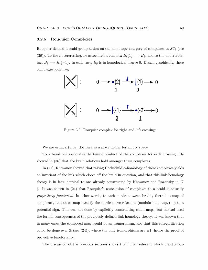
CHAPTER 3. FUNCTORIALITY OF ROUQUIER COMPLEXES 59
3.2.5 Rouquier Complexes
Rouquier defined a braid group action on the homotopy category of complexes in SC2 (see
(36)). To the i overcrossing, he associated a complex Bi1 −→ B∅, and to the undercross-
ing, B∅ −→ Bi−1. In each case, B∅ is in homological degree 0. Drawn graphically, these
complexes look like:
Figure 3.3: Rouquier complex for right and left crossings
We are using a (blue) dot here as a place holder for empty space.
To a braid one associates the tensor product of the complexes for each crossing. He
showed in (36) that the braid relations hold amongst these complexes.
In (21), Khovanov showed that taking Hochschild cohomology of these complexes yields
an invariant of the link which closes off the braid in question, and that this link homology
theory is in fact identical to one already constructed by Khovanov and Rozansky in (?
). It was shown in (24) that Rouquier’s association of complexes to a braid is actually
projectively functorial. In other words, to each movie between braids, there is a map of
complexes, and these maps satisfy the movie move relations (modulo homotopy) up to a
potential sign. This was not done by explicitly constructing chain maps, but instead used
the formal consequences of the previously-defined link homology theory. It was known that
in many cases the composed map would be an isomorphism, and that this categorification
could be done over Z (see (24)), where the only isomorphisms are ±1, hence the proof of
projective functoriality.
The discussion of the previous sections shows that it is irrelevant which braid group
CHAPTER 3. FUNCTORIALITY OF ROUQUIER COMPLEXES 60
we work in, because adding extra strands just corresponds to an inclusion functor which is
“fully faithful after base change”. In particular, when computing the space of chain maps
modulo homotopy between two complexes, we need not worry about the number of strands
available, except to keep track of our base ring. Hence calculations are effectively local.
3.2.6 Conventions
These are the conventions we use to draw Rouquier complexes henceforth.
We use a colored circle to indicate the empty graph, but maintain the color for reasons
of sanity. It is immediately clear that in the complex associated to a tensor product of
d Rouquier complexes, each summand will be a sequence of k lines where 0 ≤ k ≤ d
(interspersed with colored circles, but these represent the empty graph so could be ignored).
Each differential from one summand to another will be a “dot” map, with an appropriate
sign.
1. The dot would be a map of degree 1 if Bi had not been shifted accordingly. In SC2,
all maps must be homogeneous, so we could have deduced the degree shift in Bi
from the degree of the differential. Because of this, it is not useful to keep track of
various degree shifts of objects in a complex. We will draw all the objects without
degree shifts, and all differentials will therefore be maps of graded degree 1 (as well
as homological degree 1). It follows from this that homotopies will have degree -1, in
order to be degree 0 when the shifts are put back in. One could put in the degree
shifts later, noting that B∅ always occurs as a summand in a tensor product exactly
once, with degree shift 0.
2. Similarly, one need not keep track of the homological dimension. B∅ will always occur
in homological dimension 0.
3. We will use blue for the index associated to the leftmost crossing in the braid, then
red and dotted orange for other crossings, from left to right. The adjacency of these
various colors is determined from the braid.
4. We read tensor products in a braid diagram from bottom to top. That is, in the
following diagram, we take the complex for the blue crossing, and tensor by the

CHAPTER 3. FUNCTORIALITY OF ROUQUIER COMPLEXES 61
complex for the red crossing. Then we translate this into pictures by saying that
tensors go from left to right. In other words, in the complex associated to this braid,
blue always appears to the left of red.
5. One can deduce the sign of a differential between two summands using the Liebnitz
rule, d(ab) = d(a)b+(−1)|a|ad(b). In particular, since a line always occurs in the basic
complex in homological dimension ±1, the sign on a particular differential is exactly
given by the parity of lines appearing to the left of the map. For example,
6. When putting an order on the summands in the tensored complex, we use the fol-
lowing standardized order. Draw the picture for the object of smallest homological
degree, which we draw with lines and circles. In the next homological degree, the
first summand has the first color switched (from line to circle, or circle to line), the
second has the second color switched, and so forth. In the next homological degree,
two colors will be switched, and we use the lexicographic order: 1st and 2nd, then 1st
and 3rd, then 1st and 4th... then 2nd and 3rd, etc. This pattern continues.

CHAPTER 3. FUNCTORIALITY OF ROUQUIER COMPLEXES 62
3.3 Definition of the Functor
We extend Rouquier’s complexes to a functor F from the combinatorial braid cobordism
category to the category of chain complexes in SC2 modulo homotopy. Rouquier already
defined how the functor acts on objects, so it only remains to define chain maps for each of
the movie generators, and check the movie move relations.
There are four basic types of movie generators: birth/death of a crossing, slide, Reide-
meister 2 and Reidemeister 3.
• Birth and Death generators
Figure 3.4: Birth and Death of a crossing generators

CHAPTER 3. FUNCTORIALITY OF ROUQUIER COMPLEXES 63
• Reidemeister 2 generators
Figure 3.5: Reidemeister 2 type movie move generators

CHAPTER 3. FUNCTORIALITY OF ROUQUIER COMPLEXES 64
• Slide generators
Figure 3.6: Slide generators
• Reidemeister 3 generators There are 12 generators in all: 6 possibilities for the
height orders of the 3 strands (denoted by a number 1 through 6), and two directions
for the movie (denoted ”a” or ”b”). Thankfully, the color-switching symmetries of the
Soergel calculus allow us explicitly list only 6. The left-hand column lists the genera-
tors, and the chain complexes they correspond to; switching colors in the complexes
yields the corresponding generator listed on the right. Each of these variants has a
free parameter x, and the parameter used for each variant is actually independent
from the other variants.
Remark 3.13. Using sequences of R2-type generators and various movie moves we

CHAPTER 3. FUNCTORIALITY OF ROUQUIER COMPLEXES 65
could have abstained from ever defining certain R3-type variants or proving the movie
moves that use them. We never use this fact, and list all here for completeness.

CHAPTER 3. FUNCTORIALITY OF ROUQUIER COMPLEXES 66
Figure 3.7: Reidemeister 3 type movie move generators

CHAPTER 3. FUNCTORIALITY OF ROUQUIER COMPLEXES 67
Figure 3.8: Reidemeister 3 type movie move generators
CHAPTER 3. FUNCTORIALITY OF ROUQUIER COMPLEXES 68
Claim 3.14. Up to homotopy, each of the maps above is independent of x.
Proof. We prove the claim for generator 1a above; all the others follow from essentially
the same computation. One can easily observe that there are very few summands of the
source complex which admit degree -1 maps to summands of the target complex. In fact,
the unique (up to scalar) non-zero map of homological degree -1 and graded degree -1 is
a red trivalent vertex: a red fork which sends the single red line in the second row of the
source complex to the double red line in the second row of the target complex. Given two
chain maps, one with free variable x and one with say x′, the homotopy is given by the
above fork map, with coefficient (x−x′). The homotopies for the other variants are exactly
the same, save for the position, color, and direction of the fork (there is always a unique
map of homological and graded degree -1).
Remark 3.15. For all movie generators, there is a summand of both the source and the
target which is B∅. We have clearly used the convention that for Type I movie generators,
the induced map from the B∅ summand in the source to the B∅ summand in the target
is the identity map. It is true that, with this convention, the chain maps above are the
unique chain maps which would satisfy the movie move relations, where the only allowable
freedom is given by the choice of various parameters x (exercise). There is no choice up to
homotopy, so this is a unique solution.
Remark 3.16. Ignoring this convention, each of the above maps may be multiplied by an
invertible scalar. Some relations must be imposed between these scalars, which the reader
can determine easily by looking at the movie moves (each side must be multiplied by the
same scalar). Movie move 11 forces all slide generators to have scalar 1. Movie move 13
forces all R3 generators to have scalar 1. Movie move 14 and 2 combined force the scalar for
any R2 generator to be ±1, and then movie moves 2 and 5 force this sign to be the same for
all 4 variants. Movie move 12 shows that the scalar for the birth of an overcrossing and the
death of an undercrossing are related by the sign for the R2 generator. So the remaining
freedom in the definition of the functor is precisely a choice of one sign and one invertible
scalar.

CHAPTER 3. FUNCTORIALITY OF ROUQUIER COMPLEXES 69
3.4 Checking the Movie Moves
3.4.1 Simplifications
Given that the functor F has been defined explicitly, checking that the movie moves hold
up to homotopy can be done explicitly. One can write down the chain maps for both
complexes, and either check that they agree, or explicitly find the homotopy which gives
the difference. This is not difficult, and many computations of this form were done as sanity
checks. However, there are so many variants of each movie move that writing down every
one would take far too long.
Thanks to Morrison, Walker, and Clark (10), a significant amount of work can be
bypassed using a clever argument. The remainder of this section merely repeats results
from that paper.
Let P,Q, T designate braid diagrams. Hom(P,Q) will designate the hom space between
F (P ), F (Q) in the homotopy category of complexes in SC2. We write HOM for the graded
vector space of all morphisms of complexes (not necessarily in degree 0). Hom(Bi , Bj ) will
still designate the morphisms in SC1. Let 1 designate the crossingless braid diagram.
Lemma 3.17. (see (10)) Suppose that Movie Move 2 holds. Then there is an adjunction iso-
morphism Hom(POi, Q)→ Hom(P,QUi), or more generally Hom(PT,Q)→ Hom(P,QT ).
Similarly for other variations: Hom(OiP,Q)→ Hom(P,UiQ), Hom(P,QOi)→ Hom(PUi, Q),
etc.
Proof. Given a map f ∈ Hom(POi, Q), we get a map in Hom(P,QUi) as follows: take the
R2 movie from P to POiUi, then apply f ⊗ idUi to QUi. The reverse adjunction map is
similar, and the proof that these compose to the identity is exactly Movie Move 2.
For any braid P , Hom(P, P ) ∼= Hom(1, PP ).
Note that in the braid group, PP = 1.
Lemma 3.18. Suppose that Movie Moves 3, 5, 6, and 7 hold. Then if P and Q are two
braid diagrams which are equal in the braid group, then Hom(P, T ) ∼= Hom(Q,T ).
Proof. If two braid diagrams are equal in the braid group, one may be obtained from the
other by a sequence of R2, R3, and distant crossing switching moves. Put together, these

CHAPTER 3. FUNCTORIALITY OF ROUQUIER COMPLEXES 70
movie moves imply that all of the above yield isomorphisms of complexes. Thus P and Q
have isomorphic complexes.
Remark 3.19. Technically, we don’t even need these movie moves, only the resulting
isomorphisms, which were already shown by Rouquier. However, since these movie moves
are easy to prove and we desired the proofs in this paper to be self-contained, we show the
movie moves directly.
Now the complex associated to 1 is just B∅ in homological degree 0. So HOM(1, 1) =
HOM(B∅, B∅), which we have already calculated is the free polynomial ring generated by
double dots. In particular, the degree 0 morphisms are just multiples of the identity. Re-
member, this is a non-trivial fact in the graphical context! We will say more about this in
Section 3.5.1.
Putting it all together, we have
Suppose that Movie Moves 2,3,5,6,7 all hold. If P and Q are braid diagrams which are
equal in the braid group, then Hom(P,Q) ∼= k, a one-dimensional vector space.
The practical use of finding one-dimensional Hom spaces is to apply the following
method.
(See (10)) Consider two complexes A and B in an additive k-linear category. We say
that a summand of a term in A is homotopically isolated with respect to B if, for every
possible homotopy h from A to B, the map dh+hd : A→ B is zero when restricted to that
summand.
Lemma 3.20. Let φ and ψ be two chain maps from A to B, such that φ ≡ cψ up to
homotopy, for some scalar c ∈ k. Let X be a homotopically isolated summand of A. Then
the scalar c is determined on X, that is, φ = cψ on X.
The proof is trivial, see (10). The final result of this argument is the following corollary.
Suppose that Movie Moves 2,3,5,6,7 all hold. If P and Q are braid diagrams which are
equal in the braid group, and φ and ψ are two chain maps in Hom(P,Q) which agree on a
homotopically isolated summand of P , then φ and ψ are homotopic.
Proof. Because the Hom space modulo homotopy is one-dimensional, we know there exists

CHAPTER 3. FUNCTORIALITY OF ROUQUIER COMPLEXES 71
a constant c such that φ ≡ cψ. The agreement on the isolated summand implies that
c = 1.
Most of the movie generators are isomorphisms of complexes; only birth and death are
not. Hence, Movie Moves 1 through 10 all consist of morphisms P to Q, for P and Q equal
in the braid group. Finding a homotopically isolated summand and checking the map on
that summand alone will greatly reduce any work that needs to be done. Of course, one
must show Movie Moves 2,3,5,6,7 independently before this method can be used.
One final simplification, also found in Morrison, Walker and Clark, is that modulo Movie
Move 8 all variants of Movie Move 10 are equivalent. Hence we can prove Movie Move 10
by investigating solely the overcrossing-only variant.
These simplifications apply to any functorial theory of braid cobordisms, so long as
Hom(1, 1) is one-dimensional. Now we look at what we can say specifically about homo-
topically isolated summands for Rouquier complexes in SC2.
Any homotopy must be a map of degree -1 (if we ignore degree shifts on objects, as in our
conventions). There are very few maps of negative degree in SC2, a fact which immediately
forces most homotopies to be zero. For instance, there are no negative degree maps from B∅
to Bi, for any i. In an overcrossing-only braid, where B∅ occurs in the maximal homological
grading and various Bi show up in the penultimate homological grading, the B∅ summand
is homotopically isolated! Thus the overcrossing-only variant of Movie Move 10 will be easy.
In fact, because of the convention we use that all isomorphism movie generators will restrict
to multiplication by 1 from the B∅ summand to the B∅ summand, checking Movie Move 10
is immediate.
The only generators of negative degree are trivalent vertices. If each color appears no
more than once in a complex, then there can be no trivalent vertices, so no homotopies are
possible. This will apply to every variant of Movie Move 4, for instance.
Deducing possible homotopies is easy, as there are very few possibilities. For instance,
the only nonzero maps which occur in homotopies outside of Movie Move 10 are:

CHAPTER 3. FUNCTORIALITY OF ROUQUIER COMPLEXES 72
We will not use these simplifications to their maximal effect, since some checks are easy
enough to do without. For a discussion of other implications of checking the movie moves
by hand, see Section 3.5.1.
3.4.2 Movie Moves
NOTE:
(Logical sequence in the proofs of the movie moves.) We list the movie moves in nu-
merical order, as opposed to logical order of interdependence. To use the technical lemma
about homotopically isolated summands we first need to check movie moves 2,3,5,6,7. The
reader will see that we prove these through direct computation, relying on none of the other
moves.
• MM1 There are eight variants of this movie (sixteen if you count the horizontal flip,
which is just a color symmetry), of which we present two explicitly here. The key
fact is that every slide generator behaves the same way: chain maps on summands
have either a color crossing with a minus sign, the identity map with a plus sign,
or zero; these maps occur precisely between the only summands where they make
sense and, hence, have the same signs on both sides of the movie. Reversing direction
uniformly changes the sign on the cups or caps in the R2 move. The only interesting
part of the check uses a twist of relation (3.11). We describe in detail the movie
associated to the first generator in figure 3.9, and give the composition associated to
generator 3 in figure 3.10. Note that this check is trivial anyway since every summand
is homotopically isolated.

CHAPTER 3. FUNCTORIALITY OF ROUQUIER COMPLEXES 73
Figure 3.9: Movie Move 1 associated to slide generator 1

CHAPTER 3. FUNCTORIALITY OF ROUQUIER COMPLEXES 74
Figure 3.10: Movie Move 1 associated to slide generator 3
• MM2 There are 4 variants to deal with here; we describe only one, and similar
reasoning to that of MM1 will convince the reader that the other 3 are readily verified.
The composition has the following form:
Figure 3.11: Movie Move 2

CHAPTER 3. FUNCTORIALITY OF ROUQUIER COMPLEXES 75
• MM3 All 8 movie move 3 variants are essentially immediate after glancing at the
slide generators, but we list one for posterity:
Figure 3.12: Movie Move 3
• MM4 At this point the conscientious reader will find all 16 variants of movie move 4
quite easy, for the regularity of the slide chain maps allows one to write the composi-
tions for the left and right-hand side at once. The maps only differ at the triple-color
crossings, so we have to make use of relation (3.22).
Figure 3.13: Movie Move 4

CHAPTER 3. FUNCTORIALITY OF ROUQUIER COMPLEXES 76
• MM5 There are two variants of this movie, with the calculation for both almost
identical. We consider the move associated to the first generator. The compostion
has the following form:
Figure 3.14: Movie Move 5
• MM6 Again there are two variants and the calculation is almost as easy as the one
for MM5; the only difference is that here we actually have to produce a homotopy.
We check the variant associated to generator 1; left arrows are the identity, right the
composition, and dashed the homotopy. Checking that the homotopy works requires
playing with relation (3.16).
Figure 3.15: Movie Move 6

CHAPTER 3. FUNCTORIALITY OF ROUQUIER COMPLEXES 77
• MM7 There are 12 variants of MM7, one for each R3 generator, and color symmetry
will immediately reduce the number of different checks to 6; nevertheless, this is still
a bit a drudge as each one requires a homotopy and a minor exercise in the relations.
We display the movie associated to generator 1a and leave it to the very determined
reader to repeat a very similar computation the remaining 5 times. The chain maps
for the left-hand side of the movie are the following:
Figure 3.16: Movie Move 7

CHAPTER 3. FUNCTORIALITY OF ROUQUIER COMPLEXES 78
The composition and homotopy is:
Figure 3.17: Homotopy for Movie Move 7
To check that the prescribed maps actually give a homotopy between and composition
and the identity still requires some manipulation. The verification for the left-most
map is simply relation (3.24). The verification for the right-most map is immediate,
and for the third map is simple. This leaves us with the second map. Here dH+Hd =
which save for the central entry is precisely the identity minus the composition. Equal-
ity of the central entry follows from this computation:

CHAPTER 3. FUNCTORIALITY OF ROUQUIER COMPLEXES 79
NOTE: This computation was done using relation (3.26) numerous times.
• MM8 There are twelve variants of MM8: 3! possibilities for height order, and two
directions the movie can run. All twelve are dealt with by the same argument, using
a homotopically isolated summand. There are no degree −1 maps from B∅ to any
summand in the target, since there are at most two lines of a given color in the target,
so we can assume there are no trivalent vertices. Hence the B∅ summand of the source
is homotopically isolated, so we need only keep track of the homological degree 0 part,
which significantly simplifies the calculation. We present one variant in diagram 3.18.
Composing the chain maps for the two sides of MM8 we see that they agree on B∅.

CHAPTER 3. FUNCTORIALITY OF ROUQUIER COMPLEXES 80
Figure 3.18: Movie Move 8

CHAPTER 3. FUNCTORIALITY OF ROUQUIER COMPLEXES 81
• MM9 There are a frightful 96 versions of MM9, coming from all the different R3
moves that can be done (12 in all), the type of crossing that appears in the slide, and
horizontal and vertical flips. Once again, homotopically isolated summands come to
the rescue. Again, in each variant there are no more than two crossings of a given color,
so all maps from B∅ to each summand in the target have non-negative degree. Thus
the B∅ summand of the source is homotopically isolated. Three colors are involved,
the distant color and two adjacent colors. In the B∅ summand, the distant-colored
line does not appear, and no application of a distant slide or R3 move can make it
appear. When the distant-colored line does not appear, the distant slide move acts
by the identity. Thus both the right and left sides of the movie act the same way
on the B∅ summand, namely, they perform the R3 operation to it (sending it to the
appropriate summands of the target).
Figure 3.19: Movie Move 9
• MM10 The sheer burden of writing down the complexes and calculating the chain
maps for even one version of MM10 is best avoided at all costs. Despite at first
seeming the more complicated of the movie moves, it is in the end the easiest to
verify. We begin noting that, once one has shown MM8, all of the versions of MM10
are equivalent (see section 3.2.2 in (10)). So let us consider the variant with all left
crossings. We see immediately that the B∅ summand is homotopically isolated, that

CHAPTER 3. FUNCTORIALITY OF ROUQUIER COMPLEXES 82
it is the unique summand in homological degree 0 in every intermediate complex, and
that the chain maps all act by the identity in homological degree 0. Hence both sides
agree on a homotopically isolated summand.
• MM11 There are 32 variants of MM11: 2 choices of crossing, a vertical and a horizon-
tal flip, and the direction of the movie. Half of these have chain maps that compose
to zero on both sides, since the birth of a right crossing or the death of a left crossing
is the zero chain map. The rest are straightforward. We give an example below in
figure 3.20.
Figure 3.20: Movie Move 11
• MM12 There are 8 variants: a choice of R2 move, a vertical flip, and the direction of
the movie. Again, half of these are zero all around. Here are two variants; the other
two are extremely similar.

CHAPTER 3. FUNCTORIALITY OF ROUQUIER COMPLEXES 83
Figure 3.21: Movie Move 12
• MM13 There are 24 variants: 12 R3 generators and two directions. Half are zero,
and color symmetry for R3 generators reduces the number to check by half again. For
the 6 remaining variants, the check requires little more than just writing down the
composition, since the required homotopy in each instance is quite easy to guess. In
figure 3.22 we describe the variant associated to to the first R3 generator.

CHAPTER 3. FUNCTORIALITY OF ROUQUIER COMPLEXES 84
Figure 3.22: Movie Move 13

CHAPTER 3. FUNCTORIALITY OF ROUQUIER COMPLEXES 85
• MM14 Since none of the R3 generators of type 1 or 2 is compatible with MM14, we
are left with 16 variants: 8 R3 generators and 2 directions. As usual, there are only 4
to check. In addition to this, the initial frame of the movie corresponds to a complex
supported in homological degree 0 only, so we only need write down what happens
there. In figure 3.23 we describe the variant associated to the R3 generator 3a.
Figure 3.23: Movie Move 14

CHAPTER 3. FUNCTORIALITY OF ROUQUIER COMPLEXES 86
3.5 Additional Comments
3.5.1 The Benefits of Brute Force
We have now shown that there is a functor from the braid cobordism category into the
homotopy category of complexes in SC2. Our method of proof used homotopically isolated
summands, and hence relied on the fact that Hom(B∅, B∅) was 1-dimensional. This is a
trivial fact in the context of R-bimodules, amounting to the statement that HOM(R,R) =
R. However, it is a non-trivial fact to prove for the graphical definition of SC1, requiring
the more complicated graphical proofs in (1). Moreover, Hom(B∅, B∅) need not be 1-
dimensional in some arbitrary category C of which SC1 is a (non-full) subcategory, and we
may be interested in such categories C. For instance, it would be interesting to define such
a category C for which one would have all birth and death maps nontrivial (although the
authors have yet to find an interesting extension of this type).
Our method of proof, however, is irrelevant and the truth of Theorem 3.1 does not
depend on it. One could avoid any machinery by checking each movie move explicitly (in
fact, the only ones that remain to be checked are MM8, MM9, and MM10). Checking even
a single variant of MM10 by brute force is extremely tedious, since each complex has 64
summands, but it could be done. In addition, we have actually proven slightly more: for any
additive monoidal category C having objects Bi and morphisms satisfying the SC1 relations,
we can define a functor from the braid cobordism category into the homotopy category of
complexes in C. This is an obvious corollary, since that same data gives a functor from SC2
to C. If one chose to change the birth and death maps, the proof for movie moves 1 through
10 would be unchanged, and one would only need to check 11 through 14.
One other benefit to (theoretically) checking everything by hand is in knowing precisely
which coefficients are required, and thus understanding the dependence on the base ring k.
In all the movie moves we check in this paper, each differential, chain map, and homotopy
has integral coefficients (or free variables which may be chosen to be integral). In fact,
every nonzero coefficient that didn’t involve a free variable was ±1, and free variables may
be chosen such that every coefficient is 1,0, or −1. From our other calculations, the same
should be true for MM8 through MM10 as well (Khovanov and Thomas (24) already showed

CHAPTER 3. FUNCTORIALITY OF ROUQUIER COMPLEXES 87
that Rouquier complexes lift over Z to a projective functor, which implies the existence of
homotopy maps over Z). The next section discusses the definition of this functor in a
Z-linear category.
As an additional bonus, checking the movie moves does provide some intuition as to
why SC1 has the relations that it does. One might wonder why these particular relations
should be correct: in (1) we know they are correct because they hold in the R-bimodule
category and because they are sufficient to reduce all graphs to a simple form. There should
be a more intuitive explanation.
As an illustrative example, consider the overcrossing-only variation of Movie Move 10
and the unique summand of lowest (leftmost) homological degree: it is a sequence of 6 lines.
Then the left hand movie and the right hand movie correspond to the following maps on
this summand:
Thus equality of these two movies on the highest term, modulo relation (3.17), is exactly
relation (3.27).
Similarly, the highest terms in various other movie move variants utilize the other rela-
tions, as in the chart below.
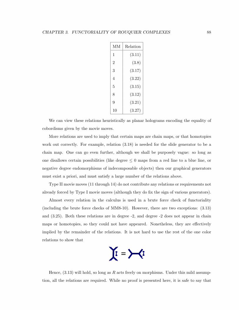
CHAPTER 3. FUNCTORIALITY OF ROUQUIER COMPLEXES 88
MM Relation
1 (3.11)
2 (3.8)
3 (3.17)
4 (3.22)
5 (3.15)
8 (3.12)
9 (3.21)
10 (3.27)
We can view these relations heuristically as planar holograms encoding the equality of
cobordisms given by the movie moves.
More relations are used to imply that certain maps are chain maps, or that homotopies
work out correctly. For example, relation (3.18) is needed for the slide generator to be a
chain map. One can go even further, although we shall be purposely vague: so long as
one disallows certain possibilities (like degree ≤ 0 maps from a red line to a blue line, or
negative degree endomorphisms of indecomposable objects) then our graphical generators
must exist a priori, and must satisfy a large number of the relations above.
Type II movie moves (11 through 14) do not contribute any relations or requirements not
already forced by Type I movie moves (although they do fix the sign of various generators).
Almost every relation in the calculus is used in a brute force check of functoriality
(including the brute force checks of MM8-10). However, there are two exceptions: (3.13)
and (3.25). Both these relations are in degree -2, and degree -2 does not appear in chain
maps or homotopies, so they could not have appeared. Nonetheless, they are effectively
implied by the remainder of the relations. It is not hard to use the rest of the one color
relations to show that
Hence, (3.13) will hold, so long as R acts freely on morphisms. Under this mild assump-
tion, all the relations are required. While no proof is presented here, it is safe to say that

CHAPTER 3. FUNCTORIALITY OF ROUQUIER COMPLEXES 89
the category SC1 is universal amongst all categories for which Rouquier complexes could be
defined functorially up to Type I movie moves (under suitable conditions on color symmetry
and torsion-free double dot actions), and that these relations are effectively predetermined.
3.5.2 Working over Z
Knot theorists should be interested in a Z-linear version of the Soergel bimodule story,
because it could theoretically yield a functorial link homology theory over Z. We describe
the Z-linear version below. Because defining things over Z is not really the focus of this
paper, and because a thorough discussion would require poring over (1) for coefficients, we
do not provide rigorous proofs of the statements in this section.
Ignoring the second equality in (3.26), which is equivalent to (3.16) after multiplication
by 2, every relation given has coefficients in Z. One could use these relations to define a
Z-linear version of SC1 and SC2, and then use base extension to define the category over
any other ring. The functor can easily be defined over Z, as we have demonstrated, and all
the brute force checks work without resorting to other coefficients. Theorem 3.1 still holds
for the Z-linear version of SC2.
In fact, the same method of proof (using homotopically isolated summands) will work
over Z in most contexts. One begins by checking the isomorphisms (3.4) through (3.6). The
only one which is in doubt is Bi ⊗Bi ∼= Bi−1 ⊕Bi1. So long as, for each i, there is an
adjacent color in I, we may use (3.29) to check this isomorphism. Otherwise, we are forced
to use (3.28), which does not have integral coefficients.
For now, assume that adjacent colors are present; we will discuss the other case below.
One still has a map of algebras from H to the additive Grothendieck group of SC1. A close
examination of the methods used in the last chapter of (1) will show that the graphical
proofs which classify HOM(∅, i) still work over Z in this context. Boundary dots with a
polynomial will be a spanning set for morphisms. One can still define a functor into a
bimodule category to show that this spanning set is in fact a basis. Therefore, the Hom
space pairing on SC1 will induce a semi-linear pairing on H, and it will be the same pairing
as before. Hom spaces will be free Z-modules of the appropriate graded rank, and this
knowledge suffices to use all the homotopically isolated arguments.

CHAPTER 3. FUNCTORIALITY OF ROUQUIER COMPLEXES 90
Remark 3.21. This statement does not imply that SC will categorify the Hecke algebra
when defined over Z. There may be missing idempotents, or extra non-isomorphic idem-
potents, so that the Grothendieck ring of the idempotent completion may be too big or
small.
If adjacent colors are not present, the easiest thing to do to prove Theorem 3.1 is
to include SC1(I) into a larger SC1(I ′) for which adjacent colors are present. Since this
inclusion is faithful, all movie move checks which hold for I ′ will hold for I. Alternatively,
one could use an extension of the category SC1(I), extending the generating set by adding
more polynomials, either as originally done in (1), or by formally adding 12 times the double
dot. Both of these should give an integral version of the category where the isomorphism
(3.4) holds, and where the graphical proofs of (1) still work. Finally, if one does not mind
ignoring 2-torsion, defining the category over Z[12 ] will also work.
Chapter 4 91
Chapter 4
Intergral HOMFLY-PT and
sl(n)-link homology
4.1 Background for diagrammatics of Soergel bimodules and
Rouquier Complexes
We extend the work in the last chapter on functoriality of Rouquier complexes to the con-
text of HOMFLY-PT and sl(n)-link homology. As there has yet to be seen an integral
version of either HOMFLY-PT or sl(n) homology for n > 3, with the original Khovanov
homology being defined over Z and torsion playing an interesting role, a natural question
arose as to whether this graphical calculus could be used to define these. The definition
of such integral theories is precisely the purpose of this chapter. The one immediate dis-
advantage to the graphical approach is that at the present moment there does not exist a
diagrammatic calculus for the Hochschild homology of Soergel bimodules. Hence, to define
integral HOMFLY-PT homology, our path takes a rather roundabout way, jumping between
matrix factorizations and diagrammatic Rouquier complexes whenever one is deemed more
advantageous than the other. For the sl(n) version of the story, we add the Rasmussen
spectral sequence into the mix and essentially repeat his construction in our context.
The organization of the chapter is the following: in section 4.2 we give a brief ac-
count of the necessary tools (matrix factorizations, Soergel bimodules, Hochschild homol-

CHAPTER 4. INTERGRAL HOMFLY-PT AND SL(N)-LINK HOMOLOGY 92
ogy, Rouquier complexes, and corresponding diagrammatics) - the emphasis here is brevity
and we refer the reader to more original sources for particulars and details; in sections
4.3 and 4.4 we describe the integral HOMFLY-PT complex and prove the Reidemeister
moves, utilizing all of the background in 4.2; section 4.5 is devoted to the Rasmussen spec-
tral sequence and integral sl(n)-link homology, and we conclude it with some remarks and
questions.
Throughout this chapter we will refer to a positive crossing as the one labelled D+ and
negative crossing as the one labelled D− in figure 4.1. For resolutions of a crossing we will
refer to Do and Ds of figure 4.1 as the “oriented” and “singular” resolutions, respectively.
We will use the following conventions for the HOMLFY-PT polynomial
aP (D−)− a−1P (D+) = (q − q−1)P (Do),
with P of the unknot being 1. Substituting a = qn we arrive at the quantum sl(n)-link
polynomial.
Figure 4.1: Crossings and resolutions
4.2 The toolkit
We will require some knowledge of matrix factorizations, Soergel bimodules and Rouquier
complexes, as well as the corresponding diagrammatic calculus of Elias and Khovanov (1).
In this section the reader will find a brief survey of the necessary tools, and for more details
we refer him to the following papers: for matrix factorizations (23), (33), for Soergel bi-

CHAPTER 4. INTERGRAL HOMFLY-PT AND SL(N)-LINK HOMOLOGY 93
modules and Rouquier complexes and diagrammatics (1), (2), (21), (36), and for Hochschild
homology (15), (21).
4.2.1 Matrix factorizations
Let R be a Noetherian commutative ring, w ∈ R, and C∗, ∗ ∈ Z, a free graded R-module.
A Z-graded matrix factorization with potential w consists of C∗ and a pair of differentials
d± : C∗ → C∗±1, such that (d+ + d−)2 = wIdC∗ .
A morphism of two matrix factorizations C∗ and D∗ is a homomorphism of graded R-
modules f : C∗ → D∗ that commutes with both d+ and d−. The tensor product C∗⊗D∗ is
taken as the regular tensor product of complexes, and is itself a matrix factorization with
differentials d+ and d−. A useful and easy exercise is the following:
Lemma 4.1. Given two matrix factorizations C∗ and D∗ with potentials wc and wd, re-
spectively, the tensor product C∗ ⊗D∗ is a matrix factorization with potential wc + wd.
Remark 4.2. Following Rasmussen (33), we work with Z-graded, rather than Z/2Z-graded,
matrix factorizations as in (22). The Z-grading implies that (d+ + d−)2 = wIdC∗ is equiv-
alent to
d2+ = d2
− = 0
and
d+d− + d−d+ = wIdC∗ .
In the case that w = 0, we acquire a new Z/2Z-graded chain complex structure with
differential d+ +d−. Suppressing the underlying ring R and potential w, we will denote the
category of graded matrix factorizations by mf .
We also need the notion of complexes of matrix factorizations. If we visualize a collec-
tion of matrix factorizations as sitting horizontally in the plane at each integer level, with
differentials d+ and d− running right and left, respectively, we can think of morphisms dv
between these as running in the vertical direction. If d2v = 0 we get a complex, i.e. all
together we have that
d± : Ci,j → Ci±1,j , dv : Ci,j → Ci,j+1,
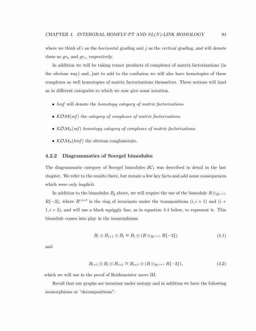
CHAPTER 4. INTERGRAL HOMFLY-PT AND SL(N)-LINK HOMOLOGY 94
where we think of i as the horizontal grading and j as the vertical grading, and will denote
these as grh and grv, respectively.
In addition we will be taking tensor products of complexes of matrix factorizations (in
the obvious way) and, just to add to the confusion we will also have homotopies of these
complexes as well homotopies of matrix factorizations themselves. These notions will land
us in different categories to which we now give some notation.
• hmf will denote the homotopy category of matrix factorizations
• KOM(mf ) the category of complexes of matrix factorizations
• KOMh(mf ) homotopy category of complexes of matrix factorizations
• KOMh(hmf ) the obvious conglomerate.
4.2.2 Diagrammatics of Soergel bimodules
The diagrammatic category of Soergel bimodules SC1 was described in detail in the last
chapter. We refer to the results there, but restate a few key facts and add some consequences
which were only implicit.
In addition to the bimodules Bi above, we will require the use of the bimodule R⊗Ri,i+1
R−3, where Ri,i+1 is the ring of invariants under the transpositions (i, i + 1) and (i +
1, i + 2), and will use a black squiggly line, as in equation 4.4 below, to represent it. This
bimodule comes into play in the isomorphisms
Bi ⊗Bi+1 ⊗Bi ∼= Bi ⊕ (R⊗Ri,i+1 R−3) (4.1)
and
Bi+1 ⊗Bi ⊗Bi+1∼= Bi+1 ⊕ (R⊗Ri,i+1 R−3), (4.2)
which we will use in the proof of Reidemeister move III.
Recall that our graphs are invariant under isotopy and in addition we have the following
isomorphisms or “decompositions”:

CHAPTER 4. INTERGRAL HOMFLY-PT AND SL(N)-LINK HOMOLOGY 95
(4.3)
Note that this relation is precisely that of Bi ⊗ Bi ∼= Bi1 ⊕ BI−1 described dia-
grammatically.
(4.4)
Here we have the graphical counterpart of 4.1 and 4.2.
Primarily we will work in another category denoted SC2, the category formally contain-
ing all direct sums and grading shifts of objects in SC1, but whose morphisms are forced
to be degree 0. In addition, we let SC be the Karoubi envelope, or idempotent completion,
of the category SC2. Recall that the Karoubi envelope of a category C has as objects pairs
(B, e) where B is an object in C and e an idempotent endomorphism of B. This object acts
as though it were the “image” of this projection e, and in an additive category behaves like
a direct summand. For more information on Karoubi envelopes, see Wikipedia. It is really
here that the object R⊗Ri,i+1 R−3 of 4.1 and 4.2 resides. In practice all our calculations
will be done in SC2, but since this includes fully faithfully into SC they will be valid there
as well.
4.2.3 Hochschild (co)homology
Let A be a k algebra and M an A-A-bimodule, or equivalently a left A⊗ Aop-module or a
right Aop ⊗A-module. The definitions of the Hochschild (co)homology groups HH∗(A,M)
(HH∗(A,M)) are the following:

CHAPTER 4. INTERGRAL HOMFLY-PT AND SL(N)-LINK HOMOLOGY 96
HH∗(A,M) := TorA⊗Aop
∗ (M,A) HH∗(A,M) := Ext∗A⊗Aop(A,M). (4.5)
To compute this we take a projective resolution of the A-bimodule A, with the natural
left and right action, by projective A-bimodules
· · · → P2 → P1 → P0 → 0,
and tensor this with M over A⊗Aop to get
· · · → P2 ⊗A⊗Aop M → P1 ⊗A⊗Aop M → P0 ⊗A⊗Aop M → 0.
The homology of this complex is isomorphic to HH∗(A,M).
Example: For any bimodule M , we have
HH0(A,M) ∼= M/[A,M ] HH0(A,M) ∼= MA,
where [A,M ] is the subspace of M generated by all elements of the form am−ma, a ∈ A
and m ∈M , and MA = m ∈M | am = ma for all a ∈ A. We leave this as an exercise or
refer the reader to (15).
If we take the polynomial algebra A = k[x1, . . . , xn], with k commutative, then we can
use a much smaller, “Koszul,” resolution of A by free A ⊗ A-modules. This is gotten by
taking the tensor product of the following complexes
0 // A⊗Axi⊗1−1⊗xi // A⊗A // 0,
for 1 ≥ i ≥ n. This resolution has length n, and its total space is naturally isomorphic to the
exterior algebra on n generators tensored with A ⊗ A. Hence, we get that the Hochschild
homology of a bimodule M over A is made up of 2n copies of M , with the differentials
coming from multiplication by xi ⊗ 1− 1⊗ xi, i.e.
0→ Cn(M)→ · · · → C1(M)→ C0(M)→ 0,
with

CHAPTER 4. INTERGRAL HOMFLY-PT AND SL(N)-LINK HOMOLOGY 97
Cj(M) =⊕
I⊂1,...,n,|I|=j
M ⊗Z Z[I],
where Z[I] is the rank 1 free abelian group generated by the symbol [I] (i.e. it’s there to
keep track where exactly we are in the complex). Here, the differential takes the form
d(m⊗ [I]) =∑i∈I±(xim−mxi)⊗ [I\i],
and the sign is taken as negative if I contains an odd number of elements less than i.
Remark 4.3. For the polynomial algebra, the Hochschild homology and cohomology are
isomorphic,
HHi(A,M) ∼= HHn−i(A,M),
for any bimodule M . This comes from self-duality of the Koszul resolution for such algebras.
Hence, we will be free to use either homology or cohomology groups in the constructions
below.
For us, taking Hochschild homology will come into play when looking at closed braid
diagrams. To a given resolution of a braid diagram we will assign a Soergel bimodule;
“closing off” this diagram will correspond to taking Hochschild homology of the associated
bimodule. More details of this below in section 4.3.2.
4.3 The integral HOMFLY-PT complex
4.3.1 The matrix factorization construction
As stated above we will work with Z-graded, rather than Z/2Z-graded, matrix factoriza-
tions and follow closely the conventions laid out in (33). We begin by first assigning the
appropriate complex to a single crossing and then extend this to general braids.
Gradings: Our complex will be triply graded, coming from the internal or “quan-
tum” grading of the underlying ring, the homological grading of the matrix factorizations,
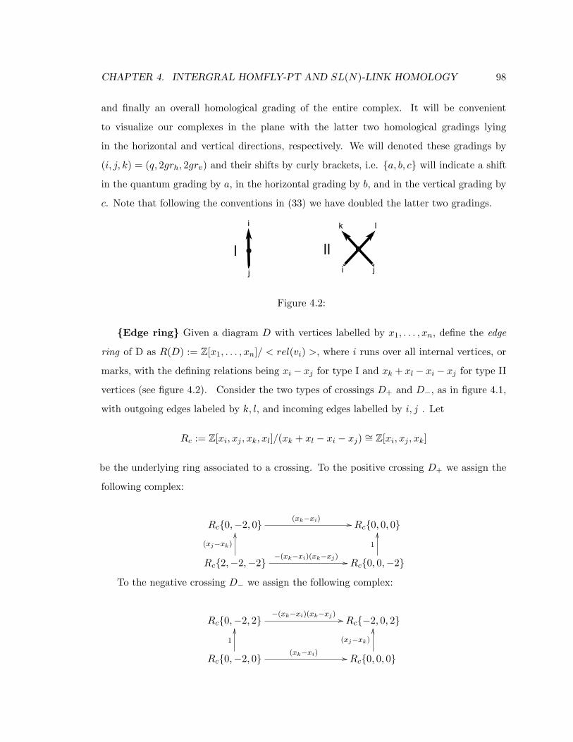
CHAPTER 4. INTERGRAL HOMFLY-PT AND SL(N)-LINK HOMOLOGY 98
and finally an overall homological grading of the entire complex. It will be convenient
to visualize our complexes in the plane with the latter two homological gradings lying
in the horizontal and vertical directions, respectively. We will denoted these gradings by
(i, j, k) = (q, 2grh, 2grv) and their shifts by curly brackets, i.e. a, b, c will indicate a shift
in the quantum grading by a, in the horizontal grading by b, and in the vertical grading by
c. Note that following the conventions in (33) we have doubled the latter two gradings.
Figure 4.2:
Edge ring Given a diagram D with vertices labelled by x1, . . . , xn, define the edge
ring of D as R(D) := Z[x1, . . . , xn]/ < rel(vi) >, where i runs over all internal vertices, or
marks, with the defining relations being xi − xj for type I and xk + xl − xi − xj for type II
vertices (see figure 4.2). Consider the two types of crossings D+ and D−, as in figure 4.1,
with outgoing edges labeled by k, l, and incoming edges labelled by i, j . Let
Rc := Z[xi, xj , xk, xl]/(xk + xl − xi − xj) ∼= Z[xi, xj , xk]
be the underlying ring associated to a crossing. To the positive crossing D+ we assign the
following complex:
Rc0,−2, 0(xk−xi) // Rc0, 0, 0
Rc2,−2,−2−(xk−xi)(xk−xj) //
(xj−xk)
OO
Rc0, 0,−2
1
OO
To the negative crossing D− we assign the following complex:
Rc0,−2, 2−(xk−xi)(xk−xj) // Rc−2, 0, 2
Rc0,−2, 0(xk−xi) //
1
OO
Rc0, 0, 0
(xj−xk)
OO

CHAPTER 4. INTERGRAL HOMFLY-PT AND SL(N)-LINK HOMOLOGY 99
A few useful things to note: The horizontal and vertical differentials d+ and dv are
homogeneous of degrees (2, 2, 0) and (0, 0, 2), respectively. For those more familiar with
(22) and hoping to reconcile the differences, note that in Rc multiplication by xkxl−xixj =
−(xk − xi)(xk − xj), so up to some grading shifts we are really working with the same
underlying complex as in the original construction, but of course now over Z, not Q.
To write down the complex for a general braid we tensor the above for every crossing,
keeping track of markings, and then replace the underlying ring with a copy of the edge
ring R(D). More precisely, given a diagram D of a braid let
C(D) :=⊗
crossings
(C(Dc)⊗Rc R(D)).
HOMFLY-PT homology Given a braid diagram D of a link L we define its
HOMFLY-PT homology to be the group
H(L) := H(H(C(D), d+), d∗v)−w + b, w + b− 1, w − b+ 1,
where w and b are the writhe and the number of strands of D, respectively.
Remark 4.4. In (33), this is what J. Rasmussen calls the “middle HOMFLY homology.”
The relation between this link homology theory and the HOMFLY-PT polynomial is that
for any link L ⊂ S3
∑i,j,k
(−1)(k−j)/2ajqidimH i,j,k(L) =−P (L)q − q−1
.
The reduced complex: There is a natural subcomplex C(D) ⊂ C(D) defined as
follows: let R(D) ⊂ R(D) to be the subring generated by xi − xj where i, j run over all
edges of D and let C(D) be the subcomplex gotten by replacing in C(D) each copy of R(D)
by one of R(D). A quick glance at the complexes C(D+) and C(D−) will reassure the
reader that this is indeed a subcomplex, as the coefficients of both dv and d+ lie in R(D).
We will refer to C(D) as the reduced complex for D.
• If i is an edge of D we can also define the complex C(D, i) := C(D)/(xi). It is not
hard to see that C(D, i) ∼= C(D) and is, hence, independent of the choice of edge i.
See (33) section 2.8 for a discussion as well as (22).

CHAPTER 4. INTERGRAL HOMFLY-PT AND SL(N)-LINK HOMOLOGY 100
Below we will work primarily with the reduced complex C(D), and will stick with the
grading conventions of (33), which are different than that of (22).
reduced homologyGiven a braid diagram D of a link L we define its reduced
HOMFLY-PT homology to be the group
H(L) := H(H(C(D), d+), d∗v)−w + b− 1, w + b− 1, w − b+ 1,
where w and b are the writhe and the number of strands of D, respectively.
Remark 4.5. For any link L ⊂ S3 we have
∑i,j,k
(−1)(k−j)/2ajqidimHi,j,k(L) = P (L).
We can look at the complex C(D) in two essential ways: either as the tensor product, over
appropriate rings, of C(D+) and C(D−) for every crossing in our diagram D (as described
above), or as a tensor product of corresponding complexes over all resolutions of the diagram.
Although this is really just a matter of point of view, the latter approach is what we find
in the original construction of Khovanov and Rozansky, as well as in the Soergel bimodule
construction to be described below. To clarify this approach, consider the oriented Do and
singular Ds resolution of a crossing as in diagram 4.1. Assign to Do the complex
0 // Rc(xk−xi) // Rc // 0
and to Ds the complex
0 // Rc−(xk−xi)(xk−xj) // Rc // 0.
Then we have
C(D+) : 0→ C(Ds) −→ C(Do)→ 0,
C(D−) : 0→ C(Do) −→ C(Ds)→ 0,
where the maps are given by dv as defined above. [For simplicity we leave out the internal
grading shifts.] Let a resolution of a link diagram D be a resolution of each crossing in

CHAPTER 4. INTERGRAL HOMFLY-PT AND SL(N)-LINK HOMOLOGY 101
either of the two ways above, and let the complex assigned to each resolution be the tensor
product of the corresponding complexes for each resolved crossing. Then, modulo grading
shifts, our total complex can be viewed as
C(D) =⊕
resolutions
C(Dres),
where Dres is the diagram of a given resolution. This closely mimics the “state-sum model”
for the Jones polynomial, due to Kauffman (16), or the MOY calculus of (13) for other
quantum polynomials.
4.3.2 The Soergel bimodule construction
We now turn to the Soergel bimodule construction for the HOMLFY-PT homology of (21).
Recall from section 4.2.2 that the Soergel bimodule Bi = R ⊗Ri R−1 where R = Z[x1 −
x2, . . . , xn−1−xn] is the ring generated by consecutive differences in variables x1, . . . , xn (n
is the number of strands in the braid diagram), and Ri ⊂ R is the subring of S2-invariants
corresponding to the permutation action xi ↔ xi+1. Furthermore define the map Bi → R
by 1⊗ 1 7−→ 1, and the map R→ Bi by 1 7−→ (xi − xi+1)⊗ 1 + 1⊗ (xi − xi+1). We resolve
a crossing in position [i, i+ 1] in the either of the two ways, as in figure 4.1, assigning R to
the oriented resolution and Bi to the singular resolution. For a positive crossing we have
the complex
C(D+) : 0→ R2 −→ Bi1 → 0,
and for a negative crossing the complex
C(D−) : 0→ Bi−1 −→ R−2 → 0.
We place Bi in homological grading 0 and increase/decrease by 1, i.e. in the complex for
D+, R2 is in homological grading −1. Note, this grading convention differs from (21),
and is the convention used in (2). The complexes above are known as Rouquier complexes,
due to R. Rouquier who studied braid group actions with relation to the category of Soergel
bimodules; for more information we refer the reader to (2), (21), and (36).
Given a braid diagram D we tensor the above complexes for each crossing, arriving
at a total complex of length k, where k is the number of crossings of D, or equivalently

CHAPTER 4. INTERGRAL HOMFLY-PT AND SL(N)-LINK HOMOLOGY 102
Figure 4.3:
the length of the corresponding braid word. Each entry in the complex can be thought of
as a resolution of the diagram consisting of the tensor product of the appropriate Soergel
bimodules. For example, to the graph in 4.3.2 we assign the bimodule B1 ⊗B2 ⊗B1. That
is, modulo grading shifts, we can view our total complex as
C(D) =⊕
resolutions
C(Dres).
To proceed, we take Hochschild homology HH(C(Dres)) for each resolution of D and arrive
at the complex
HH(C(D)) =⊕
resolutions
HH(C(Dres)),
with the induced differentials. Finally, taking homology of HH(C(D)) with respect to these
differentials gives us our link homology.
reduced homology Given a braid diagram D of a link L we define its reduced
HOMFLY-PT homology to be the group
H(HH(C(D))).
Of course, now that we have defined reduced HOMFLY-PT homology in two different
ways, it would be nice to reconcile the fact that they are indeed the same.
Claim 4.6. Up to grading shifts the two definitions of reduced HOMFLY-PT homology
agree, i.e. H(H(C(D), d+), d∗v) ∼= H(HH(C(D))) for a diagram D of a link L.
Proof. The proof in (21) works without any changes for matrix factorizations and Soergel
bimodules over Z. We sketch it here for completeness and the fact that we will be refer-
ring to some of its details a bit later. Lets first look at the matrix factorization C(Ds)

CHAPTER 4. INTERGRAL HOMFLY-PT AND SL(N)-LINK HOMOLOGY 103
(unreduced version) associated to a singular resolution Ds. Now C(Ds) can be though of
as a Koszul complex of the sequence (xk + xl − xi − xj , xkxl − xixj) in the polynomial ring
Z[xi, xj , xk, xl] (don’t forget that in Rc multiplication by xkxl−xixj = −(xk−xi)(xk−xj)).
Now this sequence is regular and the complex has cohomology in the right-most degree. The
cohomology is the quotient ring
Z[xi, xj , xk, xl]/(xi + xj − xk − xl, xkxl − xixj).
This is naturally isomorphic to the Soergel bimodule B′i (notice that this is the “unreduced”
Soergel bimodule) over the polynomial ring Z[xi, xj ]. The left and right action of R′ on
B′i corresponds to multiplication by xi, xj and xk, xl, respectively. Quotienning out by
xk + xl − xi − xj and xkxl − xixj agrees with the definition of B′i as the tensor product
R′ ⊗R′i R′ over the subalgebra R′ of symmetric polynomials in x1, x2.
Now lets consider a general resolution Dres. The matrix factorization for Dres is, once
again, just a Koszul complex corresponding to a sequence of two types of elements. The
first ones are as above, i.e. they are of the form xk + xl− xi− xj and xkxl− xixj and come
from the singular resolutions Ds, and the remaining are of the form xi−xj that come from
“closing off” our braid diagram D, which in turn means equating the corresponding marks
at the top and bottom the diagram. Now it is pretty easy to see that the polynomials of
the first type, coming from the Ds’s form a regular sequence and we can quotient out by
them immediately, just like above. The quotient ring we get is naturally isomorphic to the
Soergel bimodule B′(Dres) associated to the resolution Dres. At this point all we have left
is to deal with the remaining elements of the form xi − xj coming from closing off D; to
be more concrete, the Koszul complex we started with for Dres is quasi-isomorphic to the
Koszul complex of the ring B′(Dres) corresponding to these remaining elements. This in
turn precisely computes the Hochschild homology of B′(Dres).
Finally if we downsize from B′i to Bi and from C(Dres) to C(Dres) we get the required
isomorphism. For more details we refer the reader to (21).
Gradings et al: We come to the usual rigmarole of grading conventions, which seems
to be evepresent in link homology. Perhaps when using the Rouquier complexes above we
could have picked conventions that more closely matched those of 4.3.1. However, we chose

CHAPTER 4. INTERGRAL HOMFLY-PT AND SL(N)-LINK HOMOLOGY 104
not to for a couple of reasons: first there would inevitably be some grading conversion to
be done either way due to the inherent difference in the nature of the constructions, and
second we use Rouquier complexes to aid us in just a few results (namely the proof of
Reidemeister moves II and III), and leave them shortly after attaining these; hence, it is
convenient for us, as well as for the reader familiar with the Soergel bimodule construction of
(21) and the diagrammatic construction of (1), to adhere to the conventions of the former
and the subsequent results in (2). For completeness, we describe the conversion rules.
Recall that in the matrix factorization construction of 4.3.1 we denoted the gradings as
(i, j, k) = (q, 2grh, 2grv).
• To get the cohomological grading in the Soergel construction take (j−k)/2 from 4.3.1.
• The Hochschild here matches the “horizontal” or j grading of 4.3.1.
• To get the “quantum” grading i of 4.3.1 of an element x, take Hochschild grading of
x minus deg(x), i.e. deg(x) = j(x)− i(x).
4.3.2.1 Diagrammatic Rouquier complexes
We now restate the last section in the diagrammatic landuage of (2), i.e. that of chapter
3, as outlined above in 4.2.2. The main advantage of doing this is the inherent ability of
the graphical calculus developed by Elias and Khovanov in (1) to hide and, hence, simplify
the complexity of the calculations at hand. Recall that we work in the integral version of
Soergel category SC2 as defined in section 2.3 of (2), which allows for constructions over
Z without adjoining inverses (see section 5.2 in (2) for a discussion of these facts). Recall,
that an object of SC2 is given by a sequence of indices i , visualized as d points on the real
line and morhisms are given by pictures or graphs embedded in the strip R × [0, 1]. We
think of the indices as “colors,” and depict them accordingly. The Soergel bimodule Bi is
represented by a vertical line of “color” i (i.e. by the identity morphism from Bi to itself)
and the maps we find in the Rouquier complexes above, section 4.3.2, are given by those
referred to as “start-dot” and “end-dot.” More precisely, the complexes C(D−) and C(D+)
become

CHAPTER 4. INTERGRAL HOMFLY-PT AND SL(N)-LINK HOMOLOGY 105
Figure 4.4: Diagrammatic Rouquier complex for right and left crossings
We refer the reader to the “Conventions” section 3.2.6 of the last chapter for details of
how to go from a braid to diagrammatic Rouquier complex.
4.4 Checking the Reidemeister moves
We will use the matrix factorization construction of section 4.3.1 to check Reidemeister
move I, as it is not very difficult to verify even over Z that this goes through, and the
diagrammatic calculus of section 4.3.2.1 for the remaining moves. There are two main
reasons for the interplay: first, checking Reidemeister II and III over Z using the matrix
factorization approach is rather computationally intensive (it was already quite so over
Q in (22) with all the algebraic advantages of working over a field at hand); second, at
this moment there does not exist a full diagrammatic description of Hochschild homology
of Soergel bimodules, which prevents us from using a pictorial calculus to compute link
homology from closed braid diagrams. Of course, for Reidemeister II and III we could have
used the computations of (2), where we prove the stronger result that Rouquier complexes
are functorial over braid cobordisms, but the proofs we exhibit below use essentially the
same strategy as the original paper (22), but are so much simpler and more concise that
they underline well the usefulness of the diagrammatic calculus for computations. With
that said, we digress...
A small lemma from linear algebra, which Bar-Natan refers to as “Gaussian Elimination
for Complexes” in (5), will be very helpfull to us.
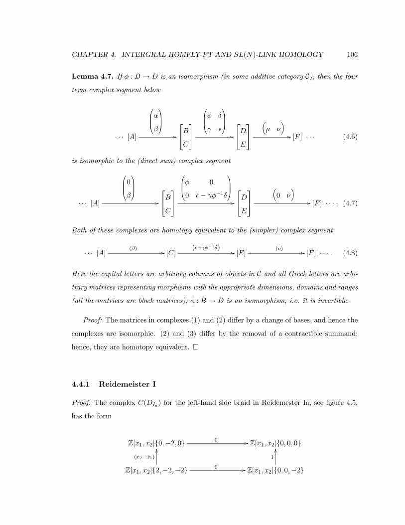
CHAPTER 4. INTERGRAL HOMFLY-PT AND SL(N)-LINK HOMOLOGY 106
Lemma 4.7. If φ : B → D is an isomorphism (in some additive category C), then the four
term complex segment below
· · · [A]
0BB@αβ
1CCA//
BC
0BB@φ δ
γ ε
1CCA//
DE
„µ ν
«// [F ] · · · (4.6)
is isomorphic to the (direct sum) complex segment
· · · [A]
0BB@0
β
1CCA//
BC
0BB@φ 0
0 ε− γφ−1δ
1CCA//
DE
„
0 ν«
// [F ] · · · . (4.7)
Both of these complexes are homotopy equivalent to the (simpler) complex segment
· · · [A](β) // [C]
(ε−γφ−1δ)// [E]
(ν) // [F ] · · · . (4.8)
Here the capital letters are arbitrary columns of objects in C and all Greek letters are arbi-
trary matrices representing morphisms with the appropriate dimensions, domains and ranges
(all the matrices are block matrices); φ : B → D is an isomorphism, i.e. it is invertible.
Proof: The matrices in complexes (1) and (2) differ by a change of bases, and hence the
complexes are isomorphic. (2) and (3) differ by the removal of a contractible summand;
hence, they are homotopy equivalent.
4.4.1 Reidemeister I
Proof. The complex C(DIa) for the left-hand side braid in Reidemester Ia, see figure 4.5,
has the form
Z[x1, x2]0,−2, 0 0 // Z[x1, x2]0, 0, 0
Z[x1, x2]2,−2,−2 0 //
(x2−x1)
OO
Z[x1, x2]0, 0,−2
1
OO

CHAPTER 4. INTERGRAL HOMFLY-PT AND SL(N)-LINK HOMOLOGY 107
Figure 4.5: The Reidemeister moves

CHAPTER 4. INTERGRAL HOMFLY-PT AND SL(N)-LINK HOMOLOGY 108
Up to homotopy, the right-hand side of the complex dissappears and only the top left
corner survives after quotioning out by the relation x2 − x1. Note that the overall degree
shifts of the total complex make sure that the left-over entry sits in the correct tri-grading.
Similarly, the complex C(DIb) for the left-hand side braid in Reidemester Ib, has the
form
Z[x1, x2]0,−2, 2 0 // Z[x1, x2]−2, 0, 2
Z[x1, x2]0,−2, 0 0 //
1
OO
Z[x1, x2]0, 0, 0
(x2−x1)
OO
The left-hand side is annihilated and the upper-right corner remains modulo the relation
x2 − x1.
4.4.2 Reidemeister II
Proof. Let’s first consider the braid diagrams for Reidemeister type IIa in figure 4.5. Recall
the decomposition Bi⊗Bi ∼= Bi−1⊕Bi1 in SC2 and its pictorial counterpart 4.3. The
complex we are interested in is
Figure 4.6: Reidemeister IIa complex with decomposition 4.3
Inserting the decomposed Bi⊗Bi and the corresponding maps, we find two isomorphisms
staring at us; we pick the left most one and mark it for removal.

CHAPTER 4. INTERGRAL HOMFLY-PT AND SL(N)-LINK HOMOLOGY 109
Figure 4.7: Reidemeister IIa complex, removing one of the acyclic subcomplexes
After changing basis and removing the acyclic complex, as in Lemma 4.7, we arrive at
the complex below with two more entries marked for removal.
Figure 4.8: Reidemeister IIa complex, removing a second acyclic subcomplex
With the marked acyclic subcomplex removed, we arrive at our desired result, the
complex assigned to the no crossing braid of two strands as in figure 4.5. The computation
for Reidemeister IIb is virtually identical.
4.4.3 Reidemeister III
Proof. Luckily, we only have to check one version of Reidemeister move III, but as the reader
will see below even that is pretty easy and not much harder than that of Reidemeister II
above. We follow closely the structure of the proof in (22), utilizing the bimodule R⊗Ri,i+1
R−3 and decomposition 4.4 to reduce the complex for one of the RIII braids to that
which is invariant under the move or, equivalently in our case, invariant under color flip.
We start with the braid on the left-hand side of III in figure 4.5; the corresponding complex,
with decomposition 4.3 and 4.4 given by dashed/yellow arrows, is
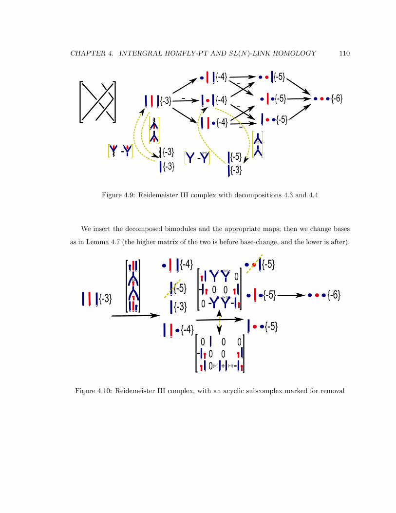
CHAPTER 4. INTERGRAL HOMFLY-PT AND SL(N)-LINK HOMOLOGY 110
Figure 4.9: Reidemeister III complex with decompositions 4.3 and 4.4
We insert the decomposed bimodules and the appropriate maps; then we change bases
as in Lemma 4.7 (the higher matrix of the two is before base-change, and the lower is after).
Figure 4.10: Reidemeister III complex, with an acyclic subcomplex marked for removal

CHAPTER 4. INTERGRAL HOMFLY-PT AND SL(N)-LINK HOMOLOGY 111
We strike out the acyclic subcomplex and mark another one for removal; yet again we
change bases (the lower matrix is the one after base change).
Figure 4.11: Reidemeister III complex, with another acyclic subcomplex marked for removal
Now we are almost done; if we can prove that the maps
are invariant under color change, we would arrive at a complex that is invariant under
Reidemeister move III. To do this we must stop for a second, go back to the source and
examine the original, algebraic, definitions of the morphisms in (1); upon doing so we are
relieved to see that the maps we are interested in are actually equal to zero (they are defined
by sending 1⊗ 1 7−→ 1⊗ 1⊗ 1⊗ 1 7−→ 1⊗ 1⊗ 1 7−→ 0). In all, we have arrived at

CHAPTER 4. INTERGRAL HOMFLY-PT AND SL(N)-LINK HOMOLOGY 112
Figure 4.12: Reidemeister III complex - the end result, after removal of all acyclic subcom-
plexes
Repeating the calculation for the braid on the right-hand side of RIII, figure 4.5, amounts
to the above calculation with the colors switched - a quick glance will convince the reader
that the end result is the same complex rotated about the x-axis.
4.4.4 Observations
Having seen this interplay between the different constructions, perhaps it is a good moment
to highlight exactly what categories we do need to work in so as to arrive at a genuine
link invariant, or a braid invariant at that. Well, let us start with the latter: we can take
the category of complexes of Soergel bimodules KOM(SC) (either the diagrammatic or
“original” version) and construct Rouquier complexes; if we mod out by homotopies and
work in KOMh(SC), we arrive at something that is not only an invariant of braids but
of braid cobordisms as well (over Z or Q if we wish). Now if we repeat the construction
in the category of complexes of graded matrix factorizations KOM(mf ), we have some
choices of homotopies to quotient out by. First, we can quotient out by the homotopies
in the category of graded matrix factorizations and work in KOM(hmf ) and second, we
can quotient in the category of the complexes and work in KOMh(mf ), or we can do
both and work in KOMh(hmf ). It is immediate that working in KOMh(mf ) is necessary,
but one could hope that it is also sufficient. A close look at the argument of Claim 4.6,
where the two constructions are proven equivalent, shows that if we start with the Koszul
complex associated to the resolution of a braid Dres the polynomial relations coming from
the singular vertices in Dres form a regular sequence and, hence, the homology of this
complex is the quotient of the edge ring R(Dres) by these relations and is supported in

CHAPTER 4. INTERGRAL HOMFLY-PT AND SL(N)-LINK HOMOLOGY 113
the right-most degree. It is this quotient that is isomorphic to the corresponding Soergel
bimodule, i.e. the Koszul complex is quasi-isomorphic, as a bimodule, to B′(Dres). Hence,
we really do need to work in KOMh(hmf ), to have a braid invariant or an invariant of
braid cobordisms, or a link invariant.
Anyone, who has suffered through the proofs of, say, Reidemeister III in (22) would
probably find the above a relief. Of course, much of the ease in computation using this
pictorial language is founded upon the intimate understanding and knowledge of hom spaces
between objects in SC, which is something that is only available to us due to the labors
Elias and Khovanov in (1). With that said, it would not be surprising if this diagrammatic
calculus would aid other calculations of link homology in the future.
All in all we have arrived at an integral version of HOMFLY-PT link homology; com-
bining with the results of (2) we have the following:
Theorem 4.8. Given a link L ⊂ S3, the groups H(L) and H(L) are invariants of L and
when tensored with Q are isomorphic to the unreduced and reduced versions, respectively,
of the Khovanov-Rozansky HOMFLY-PT link homology. Moreover, these integral homol-
ogy theories give rise to functors from the category of braid cobordisms to the category of
complexes of graded R-bimodules.
4.5 Rasmussen’s spectral sequence and integral sl(n)-link ho-
mology
It is time for us to look more closely at Rasmussen’s spectral sequence from HOMFLY-PT to
sl(n)-link homology. For this we need an extra “horizontal” differential d− in our complex,
and here is the first time we encounter matrix factorizations with a non-zero potential; as
before, to a link diagram D we will associate the tensor product of complexes of matrix
factorizations with potential for each crossing. These will be complexes over the ring
Rc = Z[xi, xj , xk, xl]/(xk + xl − xi − xj) ∼= Z[xi, xj , xk],
with total potential

CHAPTER 4. INTERGRAL HOMFLY-PT AND SL(N)-LINK HOMOLOGY 114
Wp[xi, xj , xk, xl] = p(xk) + p(xl)− p(xi)− p(xj),
where the p(x) ∈ Z[x]. We do not specify the potential p(x) at the moment as the spectral
sequence works for any choice; later on when looking at sl(n)-link homology we will set
p(x) = xn+1.
To define d−, let pi = Wp/(xk − xi) and pij = −Wp/(xk − xi)(xk − xj) (recall that in
Rc, (xk − xi)(xk − xj) = xixj − xkxl, and note that these polynomials are actually in Rc).
To the positive crossing D+ we assign the following complex:
Rc0,−2, 0(xk−xi) // Rc0, 0, 0
pi
oo
Rc2,−2,−2−(xk−xi)(xk−xj) //
(xj−xk)
OO
Rc0, 0,−2pij
oo
1
OO
To the negative crossing D− we assign the following complex:
Rc0,−2, 2−(xk−xi)(xk−xj) // Rc−2, 0, 2
pij
oo
Rc0,−2, 0(xk−xi) //
1
OO
Rc0, 0, 0pi
oo
(xj−xk)
OO
The total complex for a link L with diagram D will be defined analagously to the one
above, i.e.
Cp(D) :=⊗
crossings
(C(Dc)⊗Rc R(D)),
as will be the reduced Hp(L, i) and unreduced Hp(L) versions of link homology.
The main result of (33) is the following:
Theorem 4.9. Rasmussen, (33) Suppose L ⊂ S3 is a link, and let i be a marked com-
ponent of L. For each p(x) ∈ Q[x], there is a spectral sequence Ek(p) with E1(p) ∼= H(L)
and E∞(p) ∼= Hp(L, i). For all k > 0, the isomorphism type of Ek(p) is an invariant of the
pair (L, i).

CHAPTER 4. INTERGRAL HOMFLY-PT AND SL(N)-LINK HOMOLOGY 115
In particular setting p(x) = xn+1 one would arrive at a spectral sequence from the
HOMFLY-PT to the sl(n)-link homology. Rasmussen’s result pertains to rational link ho-
mology with matrix factorizations defined over the ring Q[x1, . . . , xn] and potentials polyno-
mials in Q[x]. We will essentially repeat his construction in our setting and, for the benefit
of those familiar with the results of (33), will stay as close as possible to the notation and
conventions therein. This will be a rather condensed version of the story and we refer the
reader to the original paper for more details.
We will work primarily with reduced link homology (although all the results follow
through for both versions) and with closed link diagrams, where all three differentials dv,
d+, and d− anticommute. We have some choices as to the order of running the differentials,
so let us define
H+(D, i) = H(C(D, i), d+).
Here, H+(D, i) inherits a pair of anticommuting differentials d∗− and d∗v, where d∗−
lowers grh by 1 while preserving grv and d∗v raises grv by 1 while preserving grh. Hence,
(H+p (D, i), d∗v, d
∗−) defines a double complex with total differential dv− := d∗v + d∗−.
Let Ek(p) be the spectral sequence induced by the horizontal filtration on the complex
(H+p (D, i), dv−).
After shifting the triple grading of Ek(p) by −w + b − 1, w + b − 1, w − b + 1 it is
immediate that the first page of the spectral sequence is isomorphic to H(L, i) (the part of
the differential d∗v + d∗− which preserves horizontal grading on E0(p) = H+(D, i)−w + b−
1, w + b− 1, w − b+ 1 is precisely d∗v, i.e. d0(p) = d∗v and
E1(p) = H(H+(D, i), d∗v)−w + b− 1, w + b− 1, w − b+ 1 ∼= H(L, i),
where D is a diagram for L). It also follows that dk(p) is homogenous of degree −k with
respect to grh and degree 1− k with respect to grv, and in the case that p(x) = xn+1 it is
also homogeneous of degree 2nk with respect to the q-grading.
Claim 4.10. Suppose L ⊂ S3 is a link, and let i be a marked component of L. For each
p(x) ∈ Z[x], the spectral sequence Ek(p) has E1(p) ∼= H(L, i) and E∞(p) ∼= Hp(L, i). For
all k > 0, the isomorphism type of Ek(p) is an invariant of the pair (L, i).

CHAPTER 4. INTERGRAL HOMFLY-PT AND SL(N)-LINK HOMOLOGY 116
Proof. We argue as in (33) section 5.4. Suppose that we have two closed diagrams Dj and
D′j that are related by the j’th Reidemeister move, and suppose that there is a morphism
σj : H+p (Dj , i)→ H
+p (D′j , i)
in the category KOM(mf ) that extends to a homotopy equivalence in the category of
modules over the edge ring R. Then σj induces a morphism of spectral sequences (σj)k :
Ek(Dj , i, p)→ Ek(D′j , i, p) which is an isomorphism for k > 0. See (33) for more details and
discussion. Hence, in practice we have to exhibit morphisms and prove invariance for the
first page of the spectral sequence, i.e. for the HOMLFY-PT homology, which is basically
already done. However, we ought to be a bit careful, of course, as here we are working with
H+p (D, i) and not with the complex C(D, i) defined in section 4.4.
Reidemeister I is done, as in this case d+ = 0 and, hence, the complex H+p (D, i) =
Cp(D, i) and the same argument as the one in section 4.4.1 works here.
For Reidemesiter II and III, we have to observe that for a closed diagram we have
morphisms σj : Cp(Dj , i) → Cp(D′j , i) for j = II, III, which are homotopy equivalences
of complexes (these can be extrapolated from section 4.4 above, or from (2), where all
chain maps are exhibited concretely). Therefore we get induced maps (σj)k on the spectral
sequence with the property that (σj)1 = σj∗ is an isomorphism.
To get the last part of the claim, i.e. that the reduced homology depends only on the
link component and not on the edge therein we refer the reader to (33), as the arguments
from there are valid verbatum.
Setting p(x) = xn+1, we get that the differentials dk(p) preserve q + 2ngrh and, hence,
the graded Euler characteristic of H(H+p (D, i), dv−) with respect to this quantity is the
same as that of E1(xn+1). Tensoring with Q, to get rid of torsion elements, and computing
we see that the Euler characteristic of the E∞(xn+1) is the quantum sl(n)-link polynomial
PL(qn, q) of L. See (33) section 5.1 for details. We have arrived at:
Theorem 4.11. The E∞(xn+1) of the spectral sequence defined in 4.5 is an invariant of L
and categorifies the quantum sl(n)-link polynomial PL(qn, q).
Remark 4.12. Well, we have a categorification over Z of the quantum sl(n)-link polyno-
mial, but what homology theory exactly are we dealing with? Is it isomorphic to

CHAPTER 4. INTERGRAL HOMFLY-PT AND SL(N)-LINK HOMOLOGY 117
H(H(H(Cxn+1(D, i), d+), d∗−), d∗v) or to H(H(Cxn+1(D, i), d+ + d−), d∗v) and are these two
isomorphic here? The answer is not immediate. In (33), Rasmussen bases the corresponding
results on a lemma that utilizes the Kunneth formula, which is much more manageable in
this context when looked at over Q. Of course, for certain classes of knots things are easier.
For example, if we take the class of knots that are KR-thin, then the spectral sequence
converges at the E1 term, as this statement only depends on the degrees of the differentials,
and we have that E∞(xn+1) ∼= H(H(Cxn+1(D, i), d+), d∗v). However, that’s a bit of a ‘red
herring’ as stated.

Chapter 5 118
Chapter 5
A particular example in sl(n)-link
homology
5.1 Introduction
For the duration of this chapter we return to the original Khovanov-Rozansky sl(n)-link
homology and explore the complex associated to a particular class of tangles. Using ideas
from (4) we show that for these tangles, and hence for knots and links composed from them,
the Khovanov-Rozansky complex reduces to one that is quite simple, i.e. one without any
“thick” edges. In particular we consider the tangle in figure 5.1 and show that its associated
complex is homotopic to the one below, with some grading shifts and basic maps which we
leave out for now.
Figure 5.1: Our main tangle and its reduced complex
The complexes for these knots and links are entirely “local,” and to calculate the homol-
ogy we only need to exploit the Frobenius structure of the underlying algebra assigned to
the unknot. Hence, here the calculations and complexity is similar to that of sl2-homology.
We also discuss a general algorithm, basically the one described in (4), to compute these

CHAPTER 5. A PARTICULAR EXAMPLE IN SL(N)-LINK HOMOLOGY 119
homology groups in a more time-efficient manner. We compare our results with similar
computations in the version of sl3-homology found in (17), which we refer to as the ”foam”
version (foams are certain types of cobordisms described in this paper), and giving an ex-
plicit isomorphism between the two versions. A very similar calculation in the sl3-homology,
that for the (2, n) torus knots, was first done in (30). Althought the construction of sl(n)
homology is essentially a specialization of its equivariant counterpart, for the sake of clar-
ity and completeness, we restate explicitly the relevant details. The bulk of the chapter
deals with the main calculation, and we finish with a discussion of an algorithm to compute
such links, compare the results with similar computations in the “foam” version of sl(3)
homology, and discuss general properties of relating to our examples.
5.2 A Review of Khovanov-Rozansky Homology
Our graphs are embedded in a disk and have two types of edges, unoriented and oriented.
Unoriented edges are called “thick” and drawn accordingly; each vertex adjoining a thick
edge has either two oriented edges leaving it or two entering. In figure 5.2 left x1, x2 are
outgoing and x3, x4 are incoming. As before oriented edges are allowed to have marks and
we also allow closed loops; points of the boundary are also referred to as marks. To such a
graph Γ we assign a matrix factorization in the following manner:
To a thick edge t as in figure 5.2 left we assign a factorization Ct with potential ωt =
xn+11 + xn+1
2 − xn+13 − xn+1
4 over the ring Rt = Q[x1, x2, x3, x4]. Since xn+1 + yn+1 lies in
the ideal generated by x + y and xy we can write it as a polynomial g(x + y, xy). Hence,
ωt can be written as
ωt = (x1 + x2 − x3 − x4)u1 + (x1x2 − x3x4)u2
where
u1 =xn+1
1 + xn+12 − g(x3 + x4, x1x2)
x1 + x2 − x3 − x4,

CHAPTER 5. A PARTICULAR EXAMPLE IN SL(N)-LINK HOMOLOGY 120
u2 =g(x3 + x4, x1x2)− xn+1
3 − xn+14
x1x2 − x3x4.
Ct is the tensor product of graded factorizations
Rtu1−→ Rt1− n
x1+x2−x3−x4−−−−−−−−−→ Rt
and
Rtu2−→ Rt3− n
x1x2−x3x4−−−−−−−→ Rt.
To an arc α bounded by marks oriented from j to i we assign the factorization Lij
Rαπij−−→ Rα
xi−xj−−−−→ Rα,
where Rα = Q[xi, xj ] and
πij =xn+1i − xn+1
j
xi − xj.
Finally, to an oriented loop with no marks we assign the complex 0 → A → 0 = A〈1〉
where A = Q[x]/(xn). [Note: to a loop with marks we assign the tensor product of Lij ’s as
above, but this turns out to be isomorphic to A〈1〉 in the homotopy category.]
Figure 5.2: Maps χ0 and χ1
We define C(Γ) to be the tensor product of Ct over all thick edges t, Lij over all edges
α from i to j, and A〈1〉 over all oriented markless loops. This tensor product is taken over
appropriate rings such that C[Γ] is a free module over R = Q[xi] where the xi’s are marks.
C(Γ) becomes a Z⊕Z2-graded complex with the Z2-grading coming from the factorization.
It has potential ω =∑i∈∂Γ
±xn+1i , where ∂Γ is the set of all boundary marks and the +, −
is determined by whether the direction of the edge corresponding to xi is towards or away
from the boundary. [Note: if Γ is a closed graph the potential is zero.]

CHAPTER 5. A PARTICULAR EXAMPLE IN SL(N)-LINK HOMOLOGY 121
The maps χ0 and χ1
We now define maps between matrix factorizations associated to the thick edge and two
disjoint arcs as in figure 5.2. Let Γ0 correspond to the two disjoint arcs and Γ1 to the thick
edge.
C(Γ0) is the tensor product of L14 and L2
3. If we assign labels a, b to L14, L2
3 respectively,
the tensor product can be written as
R(∅)
R(ab)2− 2n
P0−→
R(a)1− n
R(b)1− n
P1−→
R(∅)
R(ab)2− 2n
,
where
P0 =
π14 x2 − x3
π23 x4 − x1
, P1 =
x1 − x4 x2 − x3
π23 −π14
,
πij =n∑k=0
xki xn−kj .
Assigning labels a′ and b′ to the two factorizations in C(Γ1), we have that C(Γ1) is given
by
R(∅)−1
R(a′b′)3− 2n
Q1−→
R(a′)n
R(b′)2− n
Q2−→
R(∅)−1
R(a′b′)3− 2n
,
where
Q1 =
u1 x1x2 − x3x4
u2 x3 + x4 − x1 − x2
, Q2 =
x1 + x2 − x3 − x4 x1x2 − x3x4
u2 −u1
.
A map between C(Γ0) and C(Γ1) can be given by a pair of 2 × 2 matrices. Define
χ0 : C(Γ0)→ C(Γ1) by
U0 =
x1 − x3 0u1+x1u2−π23
x1−x41
, U1 =
x1 −x3
−1 1
,
and χ1 : C(Γ1)→ C(Γ0) by

CHAPTER 5. A PARTICULAR EXAMPLE IN SL(N)-LINK HOMOLOGY 122
V0 =
1 0u1+x1u2−π23
x4−x1x1 − x3
, V1 =
1 x3
1 x1
.
These maps have degree 1. Computing we see that the composition χ1χ0 = (x1 − x3)I,
where I is the identity matrix, i.e. χ1χ0 is multiplication by x1 − x3. Similarly χ0χ1 =
(x4−x2)I. [Note: these are specializations of the maps χ0 and χ1 given in (22), with λ = 0
and µ = 1. As these maps are homotopic for any rational value of λ and µ we are free to
do so.]
Define the trace ε : Q[x]/(xn) −→ Q as ε(xi) = 0 for i 6= n − 1 and ε(xn−1) = 1. The
unit ι : Q −→ Q[x]/(xn) is defined by ι(1) = 1.
As before, the relations between C(Γ)’s mimic the graph skein relations, see for example
(22), and we list the ones needed below.
Direct Sum Decomposition 0:
where D0 =n−1∑i=0
xiι and D−10 =
n−1∑i=0
εxn−1−i.
By the pictures above, we really mean the complexes assigned to them, i.e. ∅〈1〉 is the
complex with Q sitting in homological grading 1 and the unknot is the complex A〈1〉 as
above. The map xiι is a composition of maps
A〈1〉 xi
−→ 〈1〉 ι−→ ∅〈1〉,
where xi is multiplication and ι is the unit map, i.e. xiι is the map
Q[x]/(xn) xi
−→ Q[x]/(xn) ι−→ Q.

CHAPTER 5. A PARTICULAR EXAMPLE IN SL(N)-LINK HOMOLOGY 123
Similar with εxn−1−i. It is easy to check that the above maps are grading preserving
and their composition is the identity.
Direct Sum Decomposition I:
where D1 =n−2∑i=0
βxn−i−21 and D−1
1 =n−2∑i=0
i∑j=0
xj1xi−j2 α with α := χ0 ι′ and β := ε′ χ1.
Here ι′ = ι ⊗ Id and ε′ = ε ⊗ Id; the Id corresponds to the arc with endpoints labeled by
x2, x3, i.e ι′ is the map that includes the single arc diagram into one with the unknot and
single arc disjoint, see figure 5.3. Similar with ε′ in the right half of figure 5.4.
Figure 5.3: The map α in Direct Sum Decomposition I
Figure 5.4: The map β in Direct Sum Decomposition I
Direct Sum Decomposition II:
where D2 = S ⊕n−3∑j=0
βj and βj =n−3∑j=0
β∑
a+b+c=n−3−jxa2x
b4xc1.
Here β is given by the composition of two χ1’s, corresponding to the two thick edges
on the left-hand side above, and the trace map ε, see figure 5.5. Finally S is gotten by
“merging” the thick edges together to form two disjoint horizontal arcs, as in the top right-
hand corner above; an exact description of S won’t really matter so we will not go into
details and refer the interested reader to (22).

CHAPTER 5. A PARTICULAR EXAMPLE IN SL(N)-LINK HOMOLOGY 124
Figure 5.5: The map β in Direct Sum Decomposition II
Tangles and complexes
We resolve a crossing p in the two ways and assign to it a complex Cp depending on
whether the crossing is positive or negative. To a diagram D representing a tangle L we
assign the complex C(D) of matrix factorization which is the tensor product of Cp, over
all crossings p, of Lij over arcs j → i, and of A〈1〉 over all crossingless markless circles in
D. The tensor product is taken as before so that C(D) is free and of finite rank as an
R-module. This complex is Z⊕ Z⊕ Z2 graded.
Figure 5.6: Complexes associated to pos/neg crossings; the numbers below the diagrams
are cohomological degrees.

CHAPTER 5. A PARTICULAR EXAMPLE IN SL(N)-LINK HOMOLOGY 125
Theorem 5.1. (Khovanov-Rozansky, (22)) The isomorphism class of C(D) up to homotopy
is an invariant of the tangle.
If L is a link the cohomology groups are nontrivial only in degree equal to the number
of components of L mod 2. Hence, the grading reduces to Z⊕Z. The resulting cohomology
groups are denoted by
Hn(D) =⊕i,j∈Z
H i,jn (D),
and the Euler characteristic of Hn(D) is the quantum link polynomial Pn(L), i.e.
Pn(L) =∑i,j∈Z
(−1)iqjdimQHi,jn (D).
The isomorphism classes of H i,jn (D) depend only on the link L and, hence, are invariants
of the link.
5.3 The Basic Calculation
We first consider the complex associated to the tangle T in figure 5.7 with the appropriate
maps χ0 and χ1 left out.
Figure 5.7: The tangle T and its complex
We first look at the following part of the complex and, for simplicity, leave out the
overall grading shifts until later:
We apply direct sum decompositions 0 and I and end up with the following where the
maps F1 and F2 are isomorphisms:

CHAPTER 5. A PARTICULAR EXAMPLE IN SL(N)-LINK HOMOLOGY 126
Figure 5.8: First part of the complex for T with decompositions
Explicitly, F1 =∑n−1
i=0 Id⊗ xi1ι⊗ Id and F2 =∑n−2
j=0 Id⊗ βjComposing the maps we get:
F2 (Id⊗ χ0) F1 = (n−2∑j=0
Id⊗ βj) (Id⊗ χ0) (n−1∑i=0
Id⊗ xi1ι⊗ Id)
= (n−2∑j=0
Id⊗ βj) (n−1∑i=0
Id⊗ (χ0 (xi1ι⊗ Id)))
=n−2∑j=0
n−1∑i=0
Id⊗ (βj χ0 (xi1ι⊗ Id))
=n−2∑j=0
n−1∑i=0
Id⊗ (ε′(x1 − x4)xn+i−j−21 )
=n−2∑j=0
n−1∑i=0
Id⊗ (ε′(xn+i−j−11 − x4x
n+i−j−21 ))
=n−2∑j=0
n−1∑i=0
Id⊗ (ε(xn+i−j−11 )− x4ε(x
n+i−j−21 ))︸ ︷︷ ︸
Θ
.
To go from line 3 to 4 and 4 to 5, recall that βj = ε′ χ1xn−j−21 and χ1 χ0 = x1−x4 =
x1 − x5. [Note: for lack of better notation, we use “∑
” to indicate both a map from a
direct sum and an actual sum, as seen above indexed i and j respectively.]
Now Θ = Id if i = j, −x4 if i = j + 1, and 0 otherwise, F2 (Id⊗ χ0) F1 is given by
the following (n− 1)× n− 1 matrix:

CHAPTER 5. A PARTICULAR EXAMPLE IN SL(N)-LINK HOMOLOGY 127
Id −x4 0 . . . . . . 0
0 Id −x4 0 . . . 0...
. . . . . ....
.... . . . . .
...
0 . . . 0 Id −x4
Using Gaussian Elimination for complexes 4.7 it is easy to see that, up to homotopy,
only the top degree term survives. By degree, we mean with respect to the above grading
shifts.
Now we look at the following subcomplex:
Including all the isomorphisms we have the complex in figure 5.9, withG1 =∑n−2
i=0 αi⊗Id
and G2 = S ⊕∑n−3
j=0 βj (S is the saddle map).
Figure 5.9: The second part of the complex for T with decompositions
Composing these maps we get:
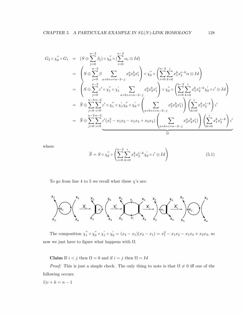
CHAPTER 5. A PARTICULAR EXAMPLE IN SL(N)-LINK HOMOLOGY 128
G2 χ′′0 G1 = (S ⊕
n−3∑j=0
βj) χ′′0 (
n−2∑i=0
αi ⊗ Id)
=
S ⊕ n−3∑j=0
β∑
a+b+c=n−3−jxa2x
b4xc1
χ′′0 (n−2∑i=0
i∑k=0
xk1xi−k2 α⊗ Id
)
=
S ⊕ n−3∑j=0
ε′ χ′′1 χ′1
∑a+b+c=n−3−j
xa2xb4xc1
χ′′0 (n−2∑i=0
i∑k=0
xk1xi−k2 χ
′0 ι′ ⊗ Id
)
= S ⊕n−3∑j=0
n−2∑i=0
ε′ χ′′1 χ′1χ′′0 χ
′0
∑a+b+c=n−3−j
xa2xb4xc1)
( i∑k=0
xk1xi−k2
)ι′
= S ⊕n−3∑j=0
n−2∑i=0
ε′(x21 − x1x2 − x1x4 + x2x4)
∑a+b+c=n−3−j
xa2xb4xc1)
( i∑k=0
xk1xi−k2
)ι′
︸ ︷︷ ︸Ω
where
S = S χ′′0
(n−2∑i=0
i∑k=0
xk1xi−k2 χ
′0 ι′ ⊗ Id
)(5.1)
To go from line 4 to 5 we recall what these χ’s are:
The composition χ′′1 χ
′′0 χ
′1 χ
′0 = (x4 − x1)(x2 − x1) = x2
1 − x1x2 − x1x4 + x2x4, so
now we just have to figure what happens with Ω.
Claim If i < j then Ω = 0 and if i = j then Ω = Id
Proof: This is just a simple check. The only thing to note is that Ω 6= 0 iff one of the
following occurs:
1)c+ k = n− 1

CHAPTER 5. A PARTICULAR EXAMPLE IN SL(N)-LINK HOMOLOGY 129
2)c+ k + 1 = n− 1
3)c+ k + 2 = n− 1
So i < j ⇒ k < j so say c+ k = n− 1. Then a+ b+ c = a+ b+n− 1− k = n− 3− j ⇒
a+ b = −2 + k − j < 0 contradiction, since a, b, c are nonnegative integers. The other two
cases are similar.
From above we see that we need k at least equal to j. So if i = j = k and c+ k + 2 =
n− 1⇒ a+ b+ c = a+ b+ n− 3− k = n− 3− j ⇒ a+ b = 0 and Ω = Id. The other two
cases force a+ b < 0.
So the matrix for Ω looks like:
Id ∗ ∗ ∗ ∗ ∗ ∗ ∗ ∗ ∗ ∗
0 Id ∗ ∗ ∗ ∗ ∗ ∗ ∗ ∗ ∗... 0
. . . . . ....
......
. . . . . ....
......
. . . ∗ ∗
0 . . . . . . 0 Id ∗
Using Gaussian Elimination 4.7 we see that only the entry corresponding to i = n − 2
survives and the original complex is homotopic to:
where A =

CHAPTER 5. A PARTICULAR EXAMPLE IN SL(N)-LINK HOMOLOGY 130
Id −x4 0 . . . . . . 0 0
0 Id −x4 0 . . . 0 0...
. . . . . ....
......
. . . . . ....
...... Id −x4 0
0 . . . . . . 0 Id −x4
0 . . . . . . 0 −Id x2
This is just our original matrix Θ but with one more row for the extra term, for which
the entries are computed identically as we have already done. We reduce the complex in
fig. 5.7, insert the overall grading shifts and arrive at our desired conclusion, i.e.:
Figure 5.10: The reduced complex for tangle T
Note: to convince ourselves that the map S above is indeed the “saddle” map as pre-
scribed, we need only to know that the hom-space of degree zero maps between the two
right-most diagrams above is 1-dimensional, in the homotopy category, and then argue that
the map is nonzero. This can be done by say closing off the two ends of the tangle above
such that we have a non-standard diagram of the unknot and looking at the cohomology of
the associated complex. We leave the details to the reader and refer to (23) for hom-space
calculations.

CHAPTER 5. A PARTICULAR EXAMPLE IN SL(N)-LINK HOMOLOGY 131
5.4 Basic Tensor Product Calculation
We now consider our tangle T composed with itself, i.e. the tangle gotten by taking two
copies of T and gluing the rightmost ends of one to the leftmost of the other. On the
complex level this corresponds to taking the tensor product of the complex for T with itself
while keeping track of the associated markings.
Figure 5.11: Complex for the tensor product
Note that when we take the tensor product we need to keep track of markings. For
example: in the left most entry of the tensored complex x2 = x′5 = x′4 = x3, which we
denote simply by x, etc.
As before, we decompose entries in the complex into direct sums of simpler objects,
compute the differentials and reduce using Gaussian Elimination 4.7. In a number of in-
stances we will restrict ourselves to the n = 3 case, as the general case works in exactly the
same way with the computation more cumbersome.
We break the computation up based on homological grading.

CHAPTER 5. A PARTICULAR EXAMPLE IN SL(N)-LINK HOMOLOGY 132
Degree 0:
Figure 5.12: Calculating degree 0 to 1
where M0 is: n−1∑i,j=0
Id⊗ ε(xn+i−j − xn−1+i−jx4)ι⊗ Id
n−1∑i,j=0
Id⊗ ε(x′2xn−1+i−j − xn+i−j)ι⊗ Id
For n = 3 we have the following:
−x4 0 0
Id −x4 0
0 Id −x4
x′2 0 0
−Id x′2 0
0 −Id x′2
reduce
Id −x4
−x24 0
x′2x4 0
x′2 − x4 0
−Id x′2
reduce
0
x′2x24
x′2x4 − x24
x′2 − x4
= M0
[Note: we first permute the rows in the first half of the matrix s.t. the Id maps appear
on the diagonal.]
The general case is exactly the same, i.e. in the left most matrix above, the upper and
lower 3×3 matrices become expanded to similar n×n matrices. Hence, the complex reduces
to:
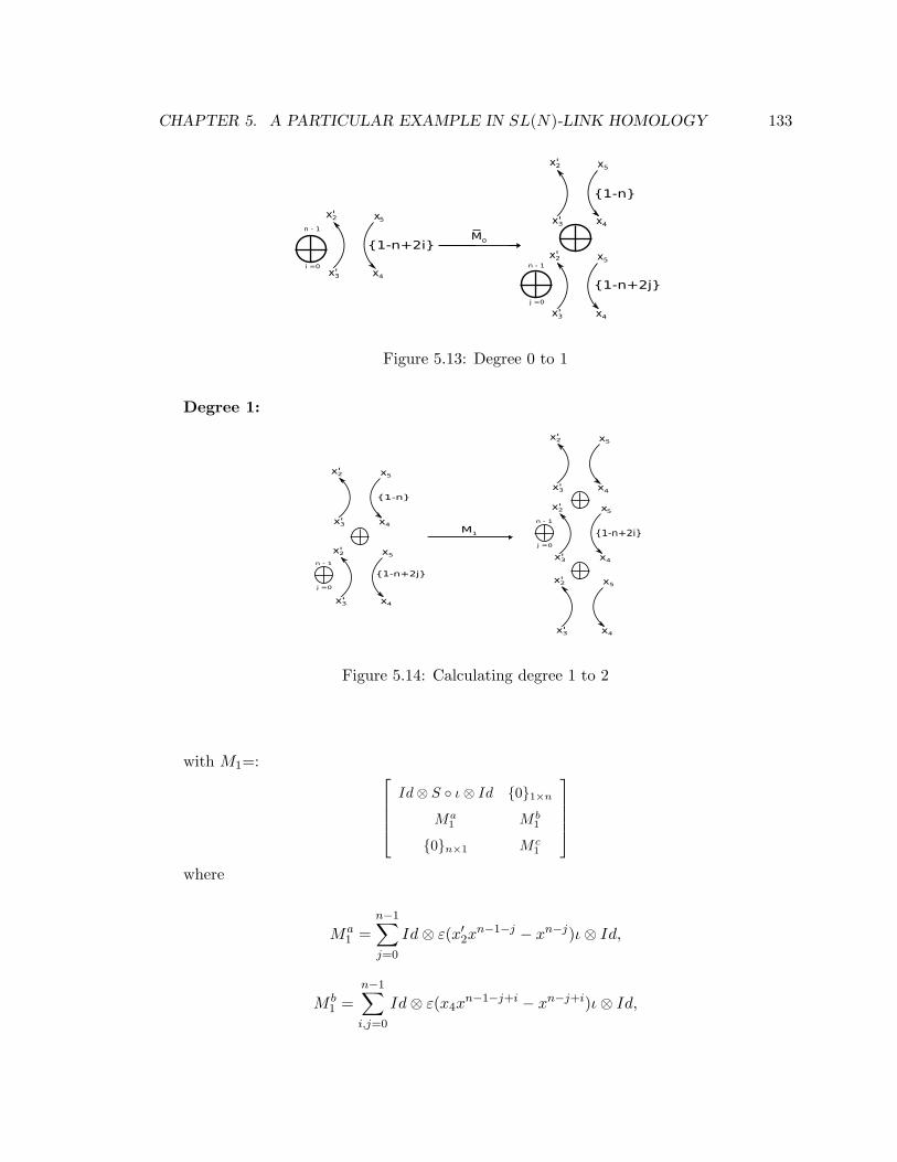
CHAPTER 5. A PARTICULAR EXAMPLE IN SL(N)-LINK HOMOLOGY 133
Figure 5.13: Degree 0 to 1
Degree 1:
Figure 5.14: Calculating degree 1 to 2
with M1=: Id⊗ S ι⊗ Id 01×n
Ma1 M b
1
0n×1 M c1
where
Ma1 =
n−1∑j=0
Id⊗ ε(x′2xn−1−j − xn−j)ι⊗ Id,
M b1 =
n−1∑i,j=0
Id⊗ ε(x4xn−1−j+i − xn−j+i)ι⊗ Id,
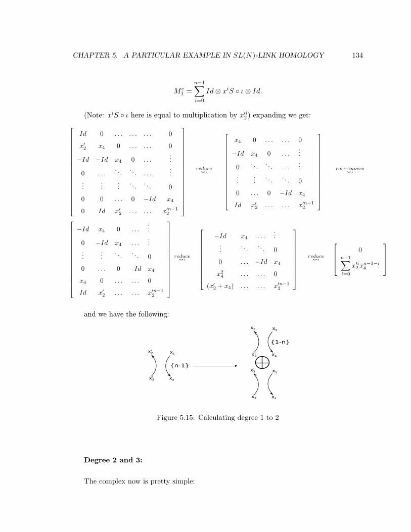
CHAPTER 5. A PARTICULAR EXAMPLE IN SL(N)-LINK HOMOLOGY 134
M c1 =
n−1∑i=0
Id⊗ xiS ι⊗ Id.
(Note: xiS ι here is equal to multiplication by x′i2 ) expanding we get:
Id 0 . . . . . . . . . 0
x′2 x4 0 . . . . . . 0
−Id −Id x4 0 . . ....
0 . . .. . . . . . . . .
......
......
. . . . . . 0
0 0 . . . 0 −Id x4
0 Id x′2 . . . . . . x′n−12
reduce
x4 0 . . . . . . 0
−Id x4 0 . . ....
0. . . . . . . . .
......
.... . . . . . 0
0 . . . 0 −Id x4
Id x′2 . . . . . . x′n−12
row−moves
−Id x4 0 . . ....
0 −Id x4 . . ....
......
. . . . . . 0
0 . . . 0 −Id x4
x4 0 . . . . . . 0
Id x′2 . . . . . . x′n−12
reduce
−Id x4 . . ....
.... . . . . . 0
0 . . . −Id x4
x24 . . . . . . 0
(x′2 + x4) . . . . . . x′n−12
reduce
0n−1∑i=0
x′i2xn−1−i4
and we have the following:
Figure 5.15: Calculating degree 1 to 2
Degree 2 and 3:
The complex now is pretty simple:

CHAPTER 5. A PARTICULAR EXAMPLE IN SL(N)-LINK HOMOLOGY 135
Figure 5.16: Calculating degree 2 and 3
M2 =
−(Id⊗ S ι)⊗ Id Id⊗ (S ι⊗ Id)
0 x′2 − x4
, M3 = [S S] .
All we have to do is note that Id⊗ S ι⊗ Id = Id reduce, insert the grading shifts and
arrive at the desired conclusion, i.e.:
Figure 5.17: The tensor complex
with A =n−1∑i=0
x′i2xn−1−i4 .

CHAPTER 5. A PARTICULAR EXAMPLE IN SL(N)-LINK HOMOLOGY 136
5.5 The General Case
Figure 5.18: Tensoring the complex with another copy of the basic tangle T
We suppose by induction that the k-fold tensor product of our basic complex has the
form as above in fig. 5.17 with alternating maps x′2−x4 and A, the last map being the saddle
cobordism S, and investigate what happens when we add one more iteration. As before,
this corresponds to tensoring with another copy of the reduced complex for tangle T , i.e.
the one in fig. 5.10, but as we will see below “most” of this new complex is null-homotopic
and it suffices to consider only the part depicted in fig. 5.18 directly above. Note that here
the bottom row is a subcomplex which is isomorphic to that of the top tangle and we claim
that, up to homotopy, this plus two more terms in leftmost homological degree is exactly
what survives. The remaining calculation is left to clear up this statement and we begin by
taking a look at the highlighted part of the complex depicted in fig. 5.18, i.e.:

CHAPTER 5. A PARTICULAR EXAMPLE IN SL(N)-LINK HOMOLOGY 137
Figure 5.19: Decomposing the entries of the general tensor product
...of course we have once again decomposed the complex and left out the overall grading
shifts until later.
The above composition of maps is:
Ma 0n×n 0n×1
M b M c 0n×1
01×n Md f0
Ma =n−1∑i,j=0
Id⊗ εf2xn−1−j+iι⊗ Id
M b =n−1∑i,j=0
Id⊗ εxn−1−j(x′2 − x)xiι⊗ Id
M c = −n−1∑i,j=0
Id⊗ εf1xn−1−j+iι⊗ Id
Md =n−1∑j=0
Id⊗ xn−1−jS ι⊗ Id
Expanding, with f0 = f2 = x − x4 and f1 =n−1∑m=0
xmxn−1−m4 we get the following
submatrices:
Ma =
−x4 0 . . . . . . 0
Id −x4 0 . . ....
0 Id −x4 . . ....
......
. . . . . . 0
0 . . . 0 Id −x4
M b =
x′2 0 . . . . . . 0
−Id x′2 0 . . ....
0 −Id x′2 . . ....
......
. . . . . . 0
0 . . . 0 −Id x′2

CHAPTER 5. A PARTICULAR EXAMPLE IN SL(N)-LINK HOMOLOGY 138
M c = −
xn−1xn−14 0 . . . . . . 0
∗ xn−1xn−14 0 . . . 0
... . . .. . . . . .
...
∗ . . . ∗ xn−1xn−14 0
Id ∗ . . . . . . xn−1xn−14
Now this might look like a mess to reduce, but the thing to notice is that, in the
corresponding summand in our decomposition, the first matrix above kills off all but the
topmost degree terms (with respect to the decomposition-induced grading shifts), whereas
the Id map found in the left-bottom corner of the second kills off precisely the topmost
degree term. As the maps alternate when we increase cohomological grading and none of
the reductions affect the bottom row (this is easy to see due to the 0’s found in the first
row), up to homotopy the bottom row remains altered only by a grading shift.
As far as the beginning and the end of the complex is concerned we have already done
those computations when we looked at the 2-fold tensor product. Hence, we arrive at our
desired conclusion:
Figure 5.20: The complex of the k-fold tensor product
where A =n−1∑i=0
x′i2xn−1−i4 .
Similarly we see that the tangle gotten by flipping all the crossings is
Figure 5.21: The complex of the k-fold tensor product

CHAPTER 5. A PARTICULAR EXAMPLE IN SL(N)-LINK HOMOLOGY 139
5.6 Remarks
Following (5) we can propose a similar “local” algorithm for computing Khovanov-Rozansky
homology. Start with a knot or link diagram and reduce it locally using the Direct Sum
Decompositions found. Then put all the pieces back together and end up with a complex
where the objects are are just circles, which we can further reduce to a complex of empty
sets with grading shifts, i.e. direct sums of Q the maps are matrices with rational entries.
Since a multiplication map Q→ Q is either an zero or an isomorphism we can use Gaussian
Elimination, as above, to further reduce this complex to one where all the differentials are
zero. The computational advantage of such an algorithm is described in more detail in (5).
Unfortunately no such program exists to our knowledge.
Furthermore, for the examples of tangles we consider here the computational complexity is
similar to that of sl2-homology. As there are no more “thick edges” in any resolution, only
Direct Sum Decomposition 0 is necessary to reduce the complex to Q vector spaces and
matrices between them. Potentially a modification of the existing programs could allow to
compute a large collection of examples composed from these tangles.
We have done a similar computation for the “foam” version of sl3-homology introduced
in (17). Here the nodes in the cube of resolutions are generated by maps from the empty
graph to the one at the corresponding node, with some relations, and the maps are given
by cobordisms between these trivalent graphs. The decompositions mimic the ones we find
here, when specializing to n = 3, as do the relations on the maps. Reducing the complex
as before we find that it is identical to the one found above when specialized to the n = 3
case. Hence, any link that can be decomposed into the above tangles has exactly the same
homology groups for the ”foam” and matrix-factorization version. This provides a rather
vast number of examples where the isomorphism between the two theories is completely
explicit.

Chapter 5 140
Bibliography
[1] Elias B. and M. Khovanov. Diagrammatics for Soergel categories. 2009,math.QA/0902.4700v1.
[2] Elias B. and D. Krasner. Rouquier complexes are functorial over braid cobordisms.2009, arXiv:0906.4761v2.
[3] J. Baldwin and O. Plamenevskaya. Khovanov homology, open books, and tight contactstructures. arXiv:0808.2336v2.
[4] Dror Bar-Natan. Khovanov’s homology for tangles and cobordisms. Geom. Topol.,9:1443–1499 (electronic), 2005.
[5] Dror Bar-Natan. Fast Khovanov homology computations. J. Knot Theory Ramifica-tions, 16(3), 2007.
[6] D.J. Benson. Representations and Cohomology I. Basic representation theory of fi-nite groups and associative algebras. Number 30 in Cambridge studies in advancedmathematics. Cambridge U. Press, 1995.
[7] J. Carter and M. Saito. Knotted surfaces and their diagrams,. Number 55 in Math.Surv. and Mon. AMS, 1998.
[8] S. Cautis and J. Kamnitzer. Knot homology via derived categories of coherent sheaves.i. the sl(2) case. Duke Math. J, 142.
[9] S. Cautis and J. Kamnitzer. Knot homology via derived categories of coherent sheaves.ii. the sl(m) case. Invent. Math., 174(1):165–232, 2008.
[10] S. Morrison D. Clark and K. Walker. Fixing the functoriality of Khovanov homology.arXiv:math/0701339v2.
[11] D. Eisenbud. Homological algebra on a complete intersection, with an application togroup representations. Trans. Amer. Math. Soc., 260:35–64, 1980.
[12] B. Gornik. Note on Khovanov link homology. 2004, math.QA/0402266.

BIBLIOGRAPHY 141
[13] T. Otsuki H. Murakami and S. Yamada. HOMFLY polynomial via an invariant ofcolored plane graphs. Enseign. Math., 44(3-4):325–360, 1998.
[14] V. F. R. Jones. A polynomial invariant for knots via von Neumann algebras. Bull.Amer. Math. Soc. (N.S.), (12):103–111, 1985.
[15] L. Kadison. New examples of Frobenius extensions. Number 14 in University LectureSeries. AMS, 1999.
[16] Louis H. Kauffman. State models and the Jones polynomial. Topology, 26(3):395–407,1987.
[17] Mikhail Khovanov. A categorification of the Jones polynomial. Duke Math. J.,101(3):359–426, 2000.
[18] Mikhail Khovanov. sl(3) link homology. Algebr. Geom. Topol., 4:1045–1081 (electronic),2004.
[19] Mikhail Khovanov. An invariant of tangle cobordisms. Trans. Amer. Math. Soc.,358(1):315–327 (electronic), 2006.
[20] Mikhail Khovanov. Link homology and Frobenius extensions. Fund. Math., 190:179–190, 2006.
[21] Mikhail Khovanov. Triply-graded link homology and Hochschild homology of Soergelbimodules. Internat. J. Math., 18(8):869–885, 2007.
[22] Mikhail Khovanov and Lev Rozansky. Matrix factorizations and link homology. Fund.Math., 199(1):1–91, 2008.
[23] Mikhail Khovanov and Lev Rozansky. Matrix factorizations and link homology. II.Geom. Topol., 12(3):1387–1425, 2008.
[24] Mikhail Khovanov and Richard Thomas. Braid cobordisms, triangulated categories,and flag varieties. Homology, Homotopy Appl., 9(2):19–94, 2007.
[25] E.S. Lee. An endomorphism of the Khovanov invariant. Adv. Math., 197:554–586,2005.
[26] A. Lauda M. Khovanov. A diagrammatic approach to categorification of quantumgroups i. Represent. Theory, 13:309–347, 2009.
[27] M. Mackaay and P. Vaz. The reduced HOMFLY-PT homology for the Conway andthe Kinoshita-Terasaka knots. Enseign. Math., arXiv:0812.1957v1.
BIBLIOGRAPHY 142
[28] Marco Mackaay and Pedro Vaz. The universal sl3-link homology. Algebr. Geom. Topol.,7:1135–1169, 2007.
[29] Marco Mackaay and Pedro Vaz. The foam and the matrix factorization sl3 link ho-mologies are equivalent. Algebr. Geom. Topol., 8(1):309–342, 2008.
[30] S. Morrison and A. Nieh. On Khovanov’s cobordism theory for su(3) knot homology.2006, math/0612754.
[31] Peter Ozsvath and Zoltan Szabo. On the Heegaard Floer homology of branched double-covers. Adv. Math., 194(1):1–33, 2005.
[32] O. Plamenevskaya. Transverse knots and Khovanov homology. Math. Res. Lett.,13(4):571–586, 2006.
[33] J. Rasmussen. Some differentials on Khovanov-Rozansky homology.arXiv:math/0607544v2.
[34] J. Rasmussen. Khovanov homology and the slice genus. 2004, math.GT/0402131.
[35] J. Rasmussen. Khovanov-Rozansky homology of two-bridge knots and links. DukeMath. J., 136(3):551–583, 2007.
[36] R. Rouquier. Categorification of the braid groups. math.RT/0409593.
[37] W. Soergel. Gradings on representation categories,. Proceedings of the ICM 1994 inZurich, pages 800–806.
[38] W. Soergel. Kazhdan-Lusztig-polynome und unzerlegbare bimoduln ”uber polynom-ringen. math.RT/0403496v2.
[39] W. Soergel. The combinatorics of Harish-Chandra bimodules. Journal Reine Angew.Math., 429:49–74, 1992.
[40] W. Soergel. Combinatorics of Harish-Chandra modules. Proceedings of the NATO ASI1997, Montreal, on Representation theories and Algebraic geometry, 1998.
[41] Catharina Stroppel. Categorification of the Temperley-Lieb category, tangles, andcobordisms via projective functors. Duke Math. J., 126(3):547–596, 2005.
[42] Catharina Stroppel. Parabolic category O, perverse sheaves on Grassmannians,Springer fibres and Khovanov homology. Compos. Math., 145(4):954–992, 2009.
[43] B. Webster. Kr.m2. 2005, http://katlas.math.toronto.edu/wiki/user:Ben/KRhomology.