Embed Size (px)
Citation preview

1
Computations for Vacuum Systems of
AcceleratorsR. Kersevan, CERN-TE-VSC-VSM
CERN Accelerator School – Vacuum Technology - Computations for Vacuum Systems of Accelerators – R Kersevan
2CERN Accelerator School – Vacuum Technology - Computations for Vacuum Systems of Accelerators – R Kersevan
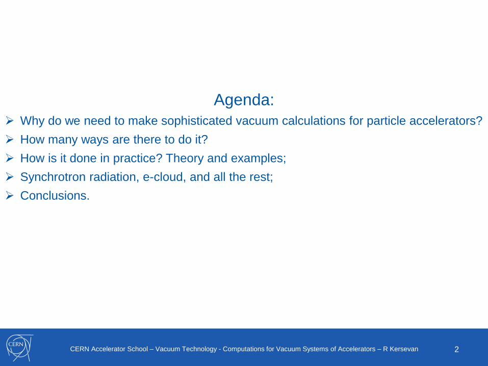
Agenda:
Why do we need to make sophisticated vacuum calculations for particle accelerators?
How many ways are there to do it?
How is it done in practice? Theory and examples;
Synchrotron radiation, e-cloud, and all the rest;
Conclusions.
3CERN Accelerator School – Vacuum Technology - Computations for Vacuum Systems of Accelerators – R Kersevan
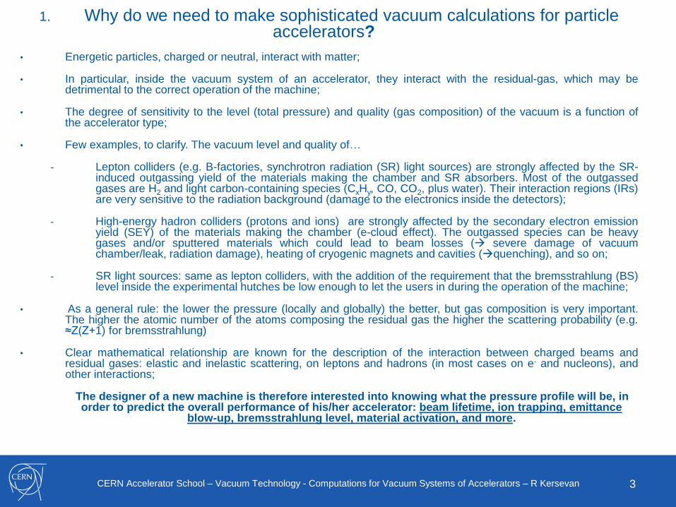
1. Why do we need to make sophisticated vacuum calculations for particle accelerators?
• Energetic particles, charged or neutral, interact with matter;
• In particular, inside the vacuum system of an accelerator, they interact with the residual-gas, which may bedetrimental to the correct operation of the machine;
• The degree of sensitivity to the level (total pressure) and quality (gas composition) of the vacuum is a function ofthe accelerator type;
• Few examples, to clarify. The vacuum level and quality of…
- Lepton colliders (e.g. B-factories, synchrotron radiation (SR) light sources) are strongly affected by the SR-induced outgassing yield of the materials making the chamber and SR absorbers. Most of the outgassedgases are H2 and light carbon-containing species (CxHy, CO, CO2, plus water). Their interaction regions (IRs)are very sensitive to the radiation background (damage to the electronics inside the detectors);
- High-energy hadron colliders (protons and ions) are strongly affected by the secondary electron emissionyield (SEY) of the materials making the chamber (e-cloud effect). The outgassed species can be heavygases and/or sputtered materials which could lead to beam losses ( severe damage of vacuumchamber/leak, radiation damage), heating of cryogenic magnets and cavities (quenching), and so on;
- SR light sources: same as lepton colliders, with the addition of the requirement that the bremsstrahlung (BS)level inside the experimental hutches be low enough to let the users in during the operation of the machine;
• As a general rule: the lower the pressure (locally and globally) the better, but gas composition is very important.The higher the atomic number of the atoms composing the residual gas the higher the scattering probability (e.g.≈Z(Z+1) for bremsstrahlung)
• Clear mathematical relationship are known for the description of the interaction between charged beams andresidual gases: elastic and inelastic scattering, on leptons and hadrons (in most cases on e- and nucleons), andother interactions;
The designer of a new machine is therefore interested into knowing what the pressure profile will be, in order to predict the overall performance of his/her accelerator: beam lifetime, ion trapping, emittance
blow-up, bremsstrahlung level, material activation, and more.
4CERN Accelerator School – Vacuum Technology - Computations for Vacuum Systems of Accelerators – R Kersevan
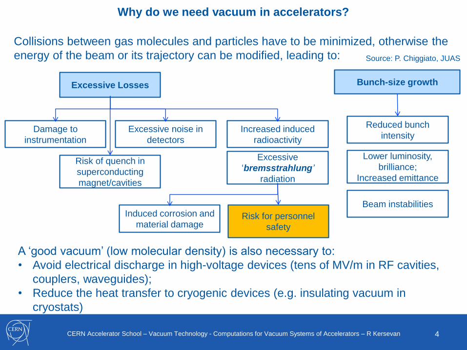
Why do we need vacuum in accelerators?
Excessive Losses
Collisions between gas molecules and particles have to be minimized, otherwise the
energy of the beam or its trajectory can be modified, leading to:
Bunch-size growth
Increased induced
radioactivity
Damage to
instrumentation
Risk of quench in
superconducting
magnet/cavities
Induced corrosion and
material damage
Beam instabilities
Reduced bunch
intensity
Lower luminosity,
brilliance;
Increased emittance
Excessive noise in
detectors
Excessive
‘bremsstrahlung’
radiation
Risk for personnel
safety
A ‘good vacuum’ (low molecular density) is also necessary to:
• Avoid electrical discharge in high-voltage devices (tens of MV/m in RF cavities,
couplers, waveguides);
• Reduce the heat transfer to cryogenic devices (e.g. insulating vacuum in
cryostats)
Source: P. Chiggiato, JUAS
5CERN Accelerator School – Vacuum Technology - Computations for Vacuum Systems of Accelerators – R Kersevan5
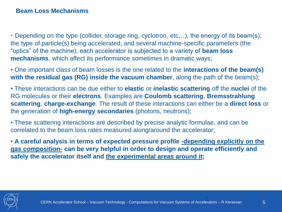
Beam Loss Mechanisms
• Depending on the type (collider, storage ring, cyclotron, etc…), the energy of its beam(s),
the type of particle(s) being accelerated, and several machine-specific parameters (the
“optics” of the machine), each accelerator is subjected to a variety of beam loss
mechanisms, which affect its performance sometimes in dramatic ways;
• One important class of beam losses is the one related to the interactions of the beam(s)
with the residual gas (RG) inside the vacuum chamber, along the path of the beam(s);
• These interactions can be due either to elastic or inelastic scattering off the nuclei of the
RG molecules or their electrons. Examples are Coulomb scattering, Bremsstrahlung
scattering, charge-exchange. The result of these interactions can either be a direct loss or
the generation of high-energy secondaries (photons, neutrons);
• These scattering interactions are described by precise analytic formulae, and can be
correlated to the beam loss rates measured along/around the accelerator;
• A careful analysis in terms of expected pressure profile -depending explicitly on the
gas composition- can be very helpful in order to design and operate efficiently and
safely the accelerator itself and the experimental areas around it;
6CERN Accelerator School – Vacuum Technology - Computations for Vacuum Systems of Accelerators – R Kersevan6
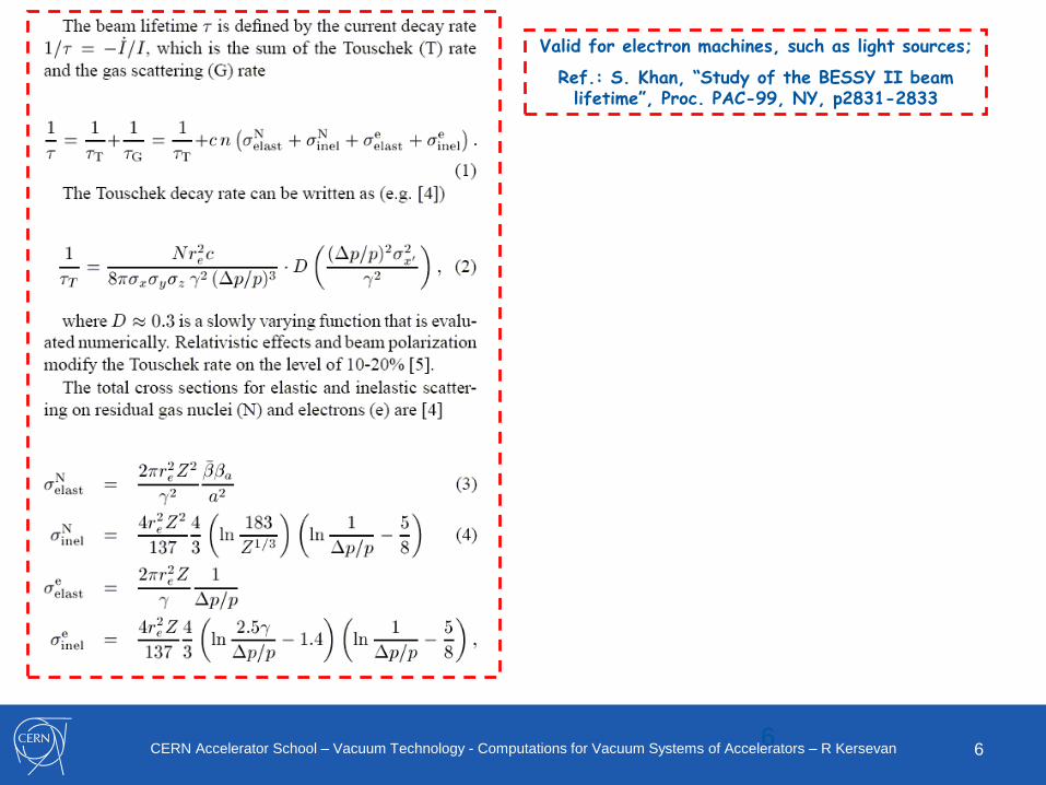
Valid for electron machines, such as light sources;
Ref.: S. Khan, “Study of the BESSY II beam lifetime”, Proc. PAC-99, NY, p2831-2833
7CERN Accelerator School – Vacuum Technology - Computations for Vacuum Systems of Accelerators – R Kersevan7
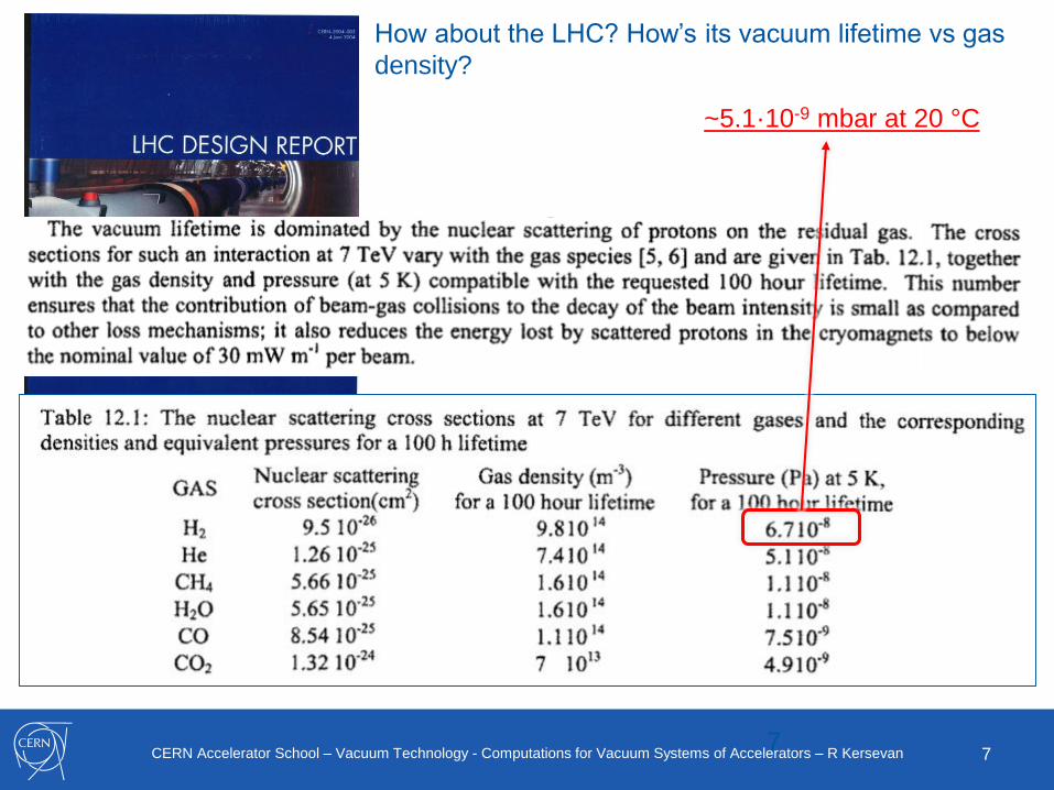
How about the LHC? How’s its vacuum lifetime vs gas
density?
~5.1·10-9 mbar at 20 °C
8CERN Accelerator School – Vacuum Technology - Computations for Vacuum Systems of Accelerators – R Kersevan8
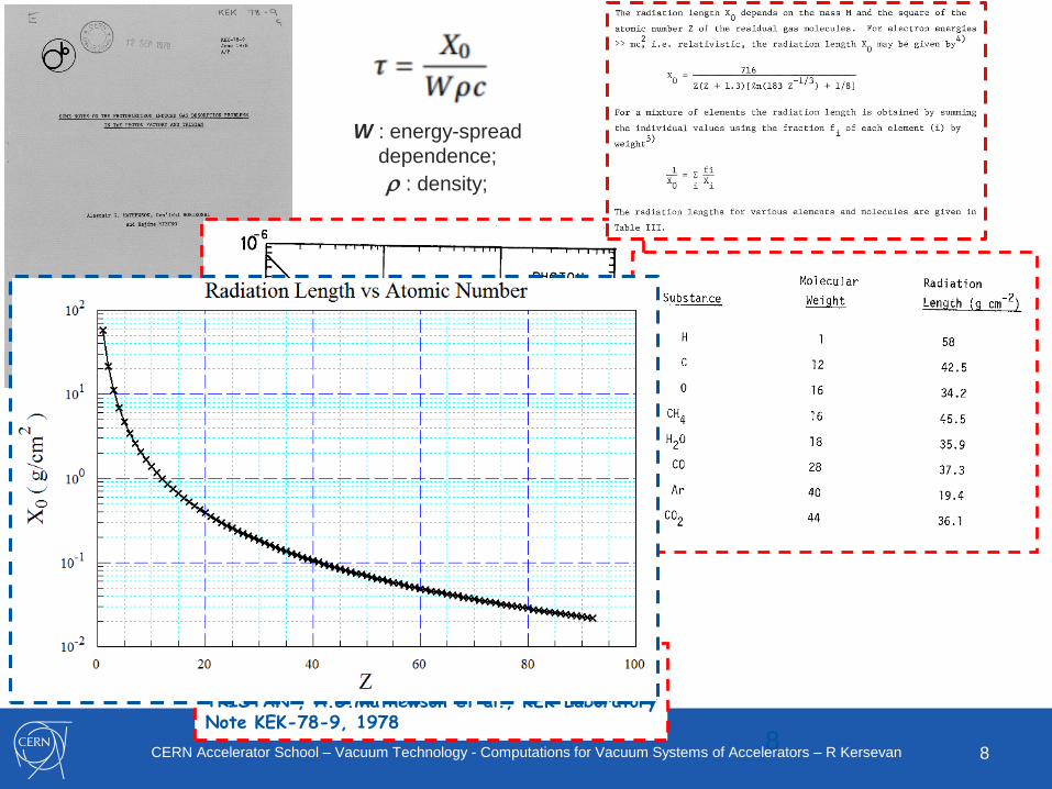
From: “Some notes on the photoelectron inducedgas desorption problems in the Photon Factory andTRISTAN”, A.G.Mathewson et al., KEK LaboratoryNote KEK-78-9, 1978
W : energy-spread
dependence;
r : density;
9CERN Accelerator School – Vacuum Technology - Computations for Vacuum Systems of Accelerators – R Kersevan
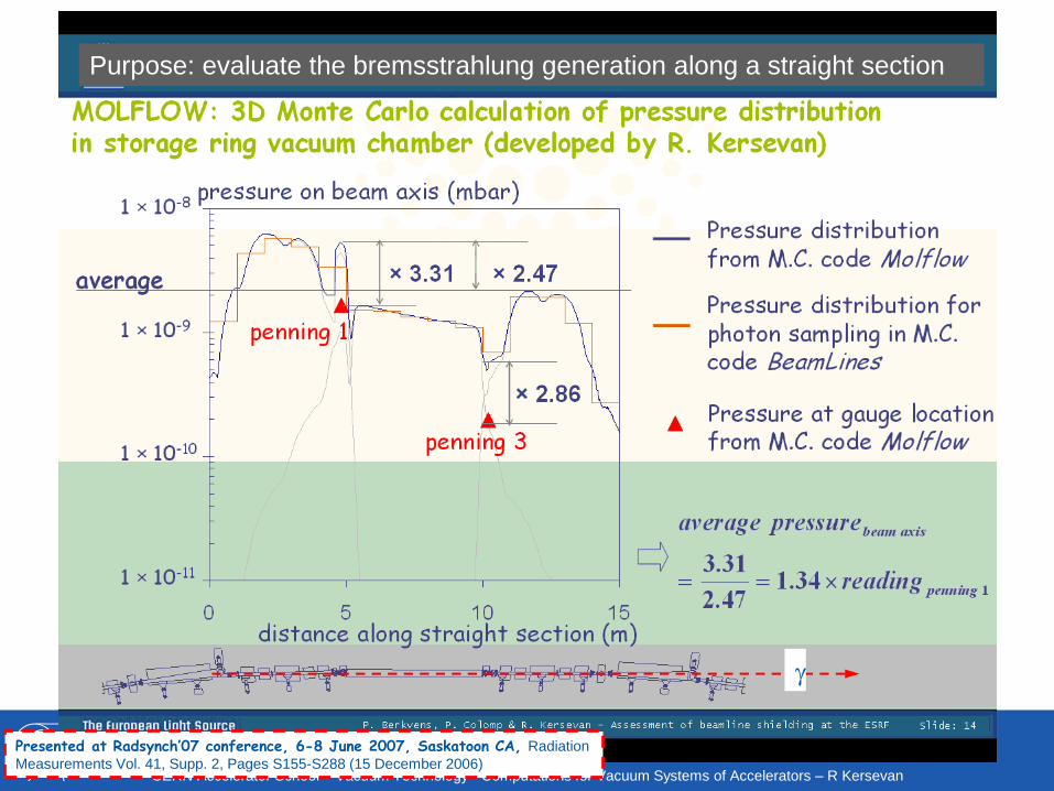
9Presented at Radsynch’07 conference, 6-8 June 2007, Saskatoon CA, Radiation
Measurements Vol. 41, Supp. 2, Pages S155-S288 (15 December 2006)
g
Purpose: evaluate the bremsstrahlung generation along a straight section
10CERN Accelerator School – Vacuum Technology - Computations for Vacuum Systems of Accelerators – R Kersevan
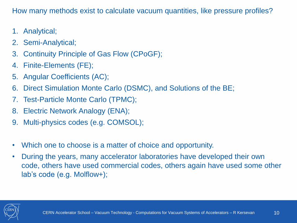
How many methods exist to calculate vacuum quantities, like pressure profiles?
1. Analytical;
2. Semi-Analytical;
3. Continuity Principle of Gas Flow (CPoGF);
4. Finite-Elements (FE);
5. Angular Coefficients (AC);
6. Direct Simulation Monte Carlo (DSMC), and Solutions of the BE;
7. Test-Particle Monte Carlo (TPMC);
8. Electric Network Analogy (ENA);
9. Multi-physics codes (e.g. COMSOL);
• Which one to choose is a matter of choice and opportunity.
• During the years, many accelerator laboratories have developed their own
code, others have used commercial codes, others again have used some other
lab’s code (e.g. Molflow+);
11CERN Accelerator School – Vacuum Technology - Computations for Vacuum Systems of Accelerators – R Kersevan
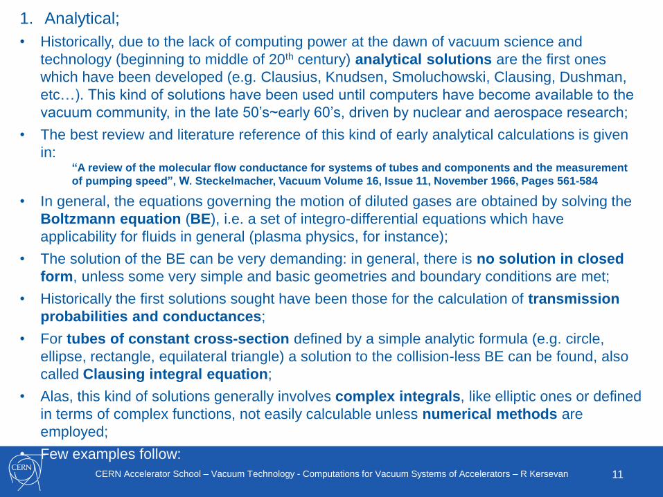
1. Analytical;
• Historically, due to the lack of computing power at the dawn of vacuum science and
technology (beginning to middle of 20th century) analytical solutions are the first ones
which have been developed (e.g. Clausius, Knudsen, Smoluchowski, Clausing, Dushman,
etc…). This kind of solutions have been used until computers have become available to the
vacuum community, in the late 50’s~early 60’s, driven by nuclear and aerospace research;
• The best review and literature reference of this kind of early analytical calculations is given
in:“A review of the molecular flow conductance for systems of tubes and components and the measurement
of pumping speed”, W. Steckelmacher, Vacuum Volume 16, Issue 11, November 1966, Pages 561-584
• In general, the equations governing the motion of diluted gases are obtained by solving the
Boltzmann equation (BE), i.e. a set of integro-differential equations which have
applicability for fluids in general (plasma physics, for instance);
• The solution of the BE can be very demanding: in general, there is no solution in closed
form, unless some very simple and basic geometries and boundary conditions are met;
• Historically the first solutions sought have been those for the calculation of transmission
probabilities and conductances;
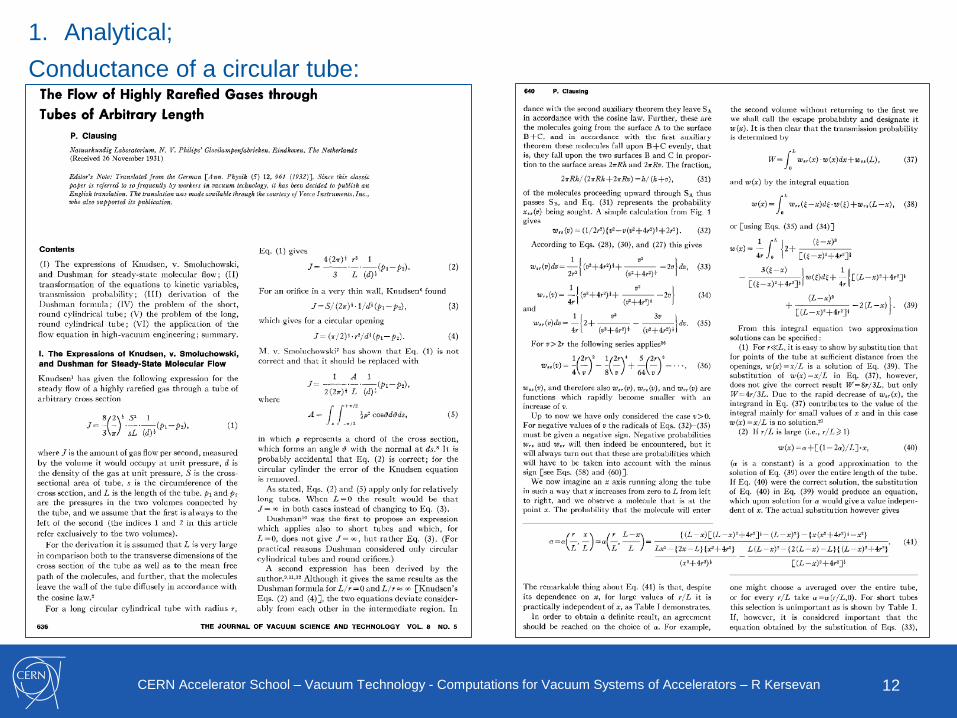
• For tubes of constant cross-section defined by a simple analytic formula (e.g. circle,
ellipse, rectangle, equilateral triangle) a solution to the collision-less BE can be found, also
called Clausing integral equation;
• Alas, this kind of solutions generally involves complex integrals, like elliptic ones or defined
in terms of complex functions, not easily calculable unless numerical methods are
employed;
• Few examples follow:
12CERN Accelerator School – Vacuum Technology - Computations for Vacuum Systems of Accelerators – R Kersevan
1. Analytical;
Conductance of a circular tube:
13CERN Accelerator School – Vacuum Technology - Computations for Vacuum Systems of Accelerators – R Kersevan
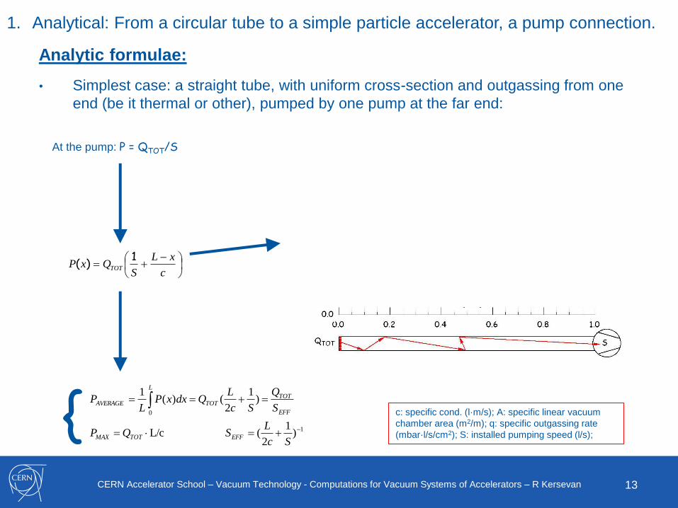
1. Analytical: From a circular tube to a simple particle accelerator, a pump connection.
Analytic formulae:
• Simplest case: a straight tube, with uniform cross-section and outgassing from one
end (be it thermal or other), pumped by one pump at the far end:
c
xL
SQxP TOT
1)(
1
0
)1
2( L/c
)1
2()(
1
Sc
LSQP
S
Q
Sc
LQdxxP
LP
EFFTOTMAX
EFF
TOT
L
TOTAVERAGE{
At the pump: P = QTOT/S
c: specific cond. (l·m/s); A: specific linear vacuum
chamber area (m2/m); q: specific outgassing rate
(mbar·l/s/cm2); S: installed pumping speed (l/s);
14CERN Accelerator School – Vacuum Technology - Computations for Vacuum Systems of Accelerators – R Kersevan
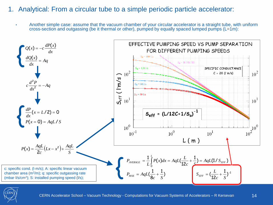
1. Analytical: From a circular tube to a simple periodic particle accelerator:
• Another simple case: assume that the vacuum chamber of your circular accelerator is a straight tube, with uniform cross-section and outgassing (be it thermal or other), pumped by equally spaced lumped pumps (L=1m):
Aqdx
Pdc
2
2
Aqdx
xdQ
dx
xdPcxQ
)(
)()(
{
SAqLxP
Lxdx
dP
/)0(
0)2/(
{
S
AqLxLx
c
AqLxP 2
2)(
1
0
)1
12( )
1
8
1(
)/1()1
12()(
1
Sc
LS
ScAqLP
SAqLSc
LAqLdxxP
LP
EFFMAX
EFF
L
AVERAGE{c: specific cond. (l·m/s); A: specific linear vacuum
chamber area (m2/m); q: specific outgassing rate
(mbar·l/s/cm2); S: installed pumping speed (l/s);
15CERN Accelerator School – Vacuum Technology - Computations for Vacuum Systems of Accelerators – R Kersevan
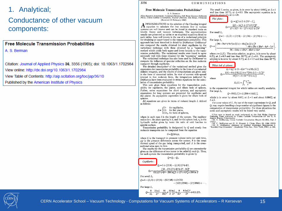
1. Analytical;
Conductance of other vacuum
components:
16CERN Accelerator School – Vacuum Technology - Computations for Vacuum Systems of Accelerators – R Kersevan
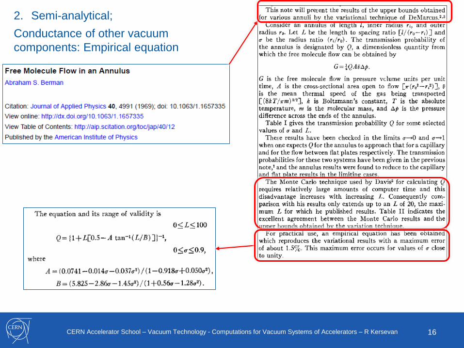
2. Semi-analytical;
Conductance of other vacuum
components: Empirical equation
17CERN Accelerator School – Vacuum Technology - Computations for Vacuum Systems of Accelerators – R Kersevan
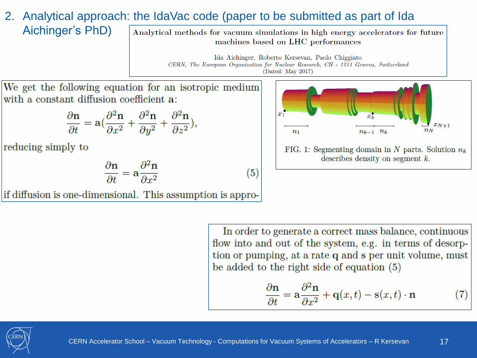
2. Analytical approach: the IdaVac code (paper to be submitted as part of Ida
Aichinger’s PhD)
18CERN Accelerator School – Vacuum Technology - Computations for Vacuum Systems of Accelerators – R Kersevan
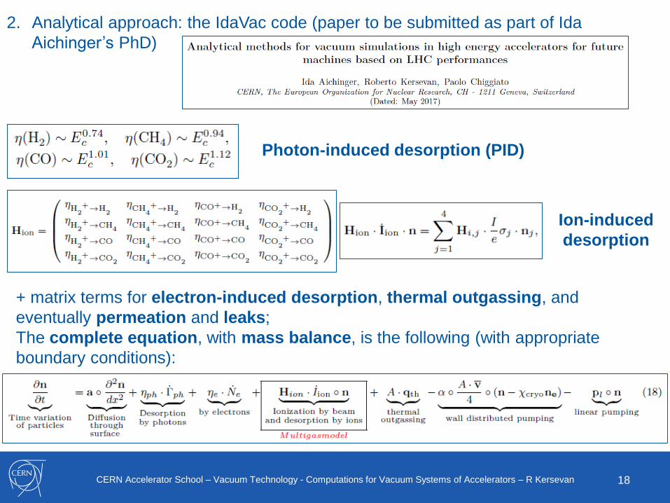
2. Analytical approach: the IdaVac code (paper to be submitted as part of Ida
Aichinger’s PhD)
Photon-induced desorption (PID)
Ion-induced
desorption
+ matrix terms for electron-induced desorption, thermal outgassing, and
eventually permeation and leaks;
The complete equation, with mass balance, is the following (with appropriate
boundary conditions):
19CERN Accelerator School – Vacuum Technology - Computations for Vacuum Systems of Accelerators – R Kersevan
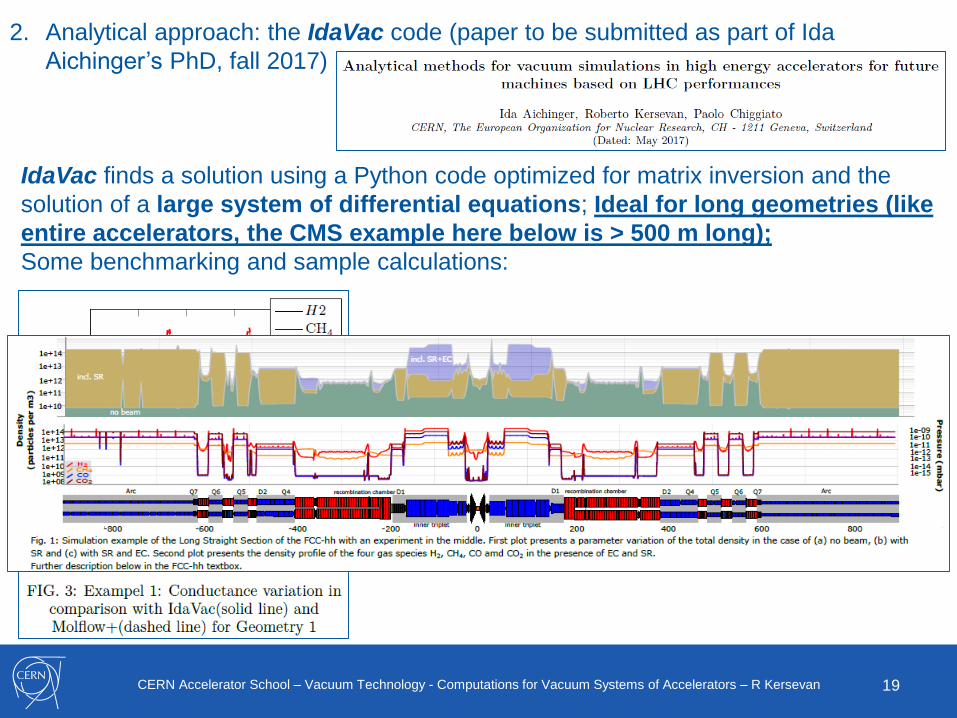
2. Analytical approach: the IdaVac code (paper to be submitted as part of Ida
Aichinger’s PhD, fall 2017)
IdaVac finds a solution using a Python code optimized for matrix inversion and the
solution of a large system of differential equations; Ideal for long geometries (like
entire accelerators, the CMS example here below is > 500 m long);
Some benchmarking and sample calculations:
20CERN Accelerator School – Vacuum Technology - Computations for Vacuum Systems of Accelerators – R Kersevan
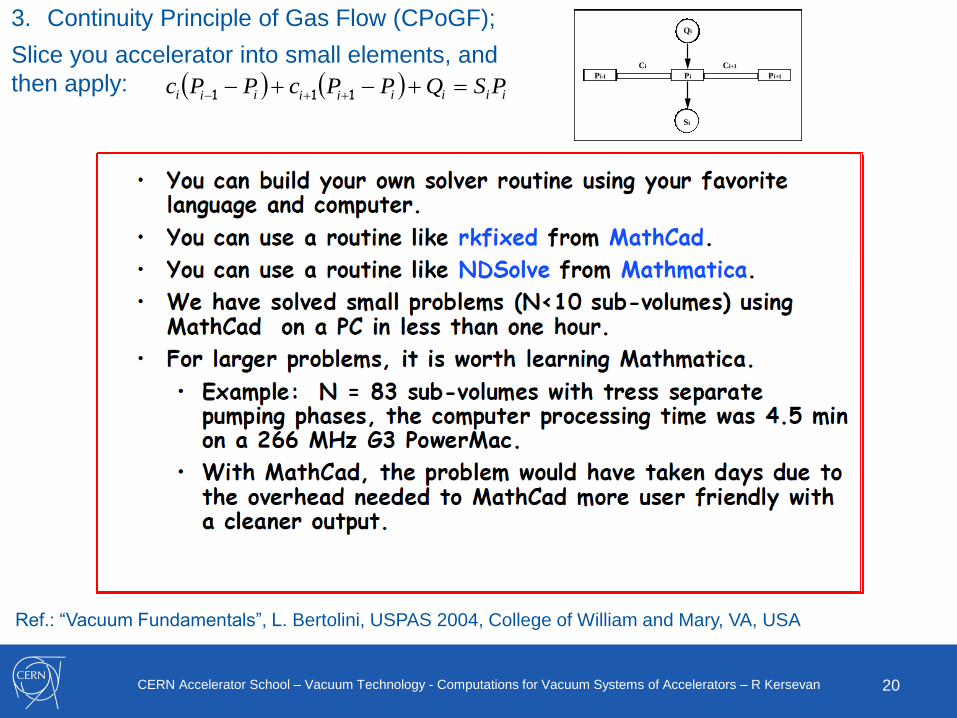
3. Continuity Principle of Gas Flow (CPoGF);
Slice you accelerator into small elements, and
then apply:
Ref.: “Vacuum Fundamentals”, L. Bertolini, USPAS 2004, College of William and Mary, VA, USA
Pi-1 Pi Pi+1
Ci Ci+1
Qi
Si
iiiiiiiii PSQPPcPPc 111
21CERN Accelerator School – Vacuum Technology - Computations for Vacuum Systems of Accelerators – R Kersevan
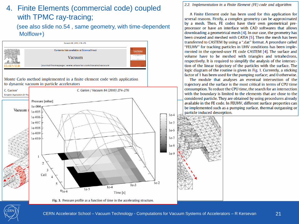
4. Finite Elements (commercial code) coupled
with TPMC ray-tracing;
(see also slide no.54 , same geometry, with time-dependent
Molflow+)
22CERN Accelerator School – Vacuum Technology - Computations for Vacuum Systems of Accelerators – R Kersevan
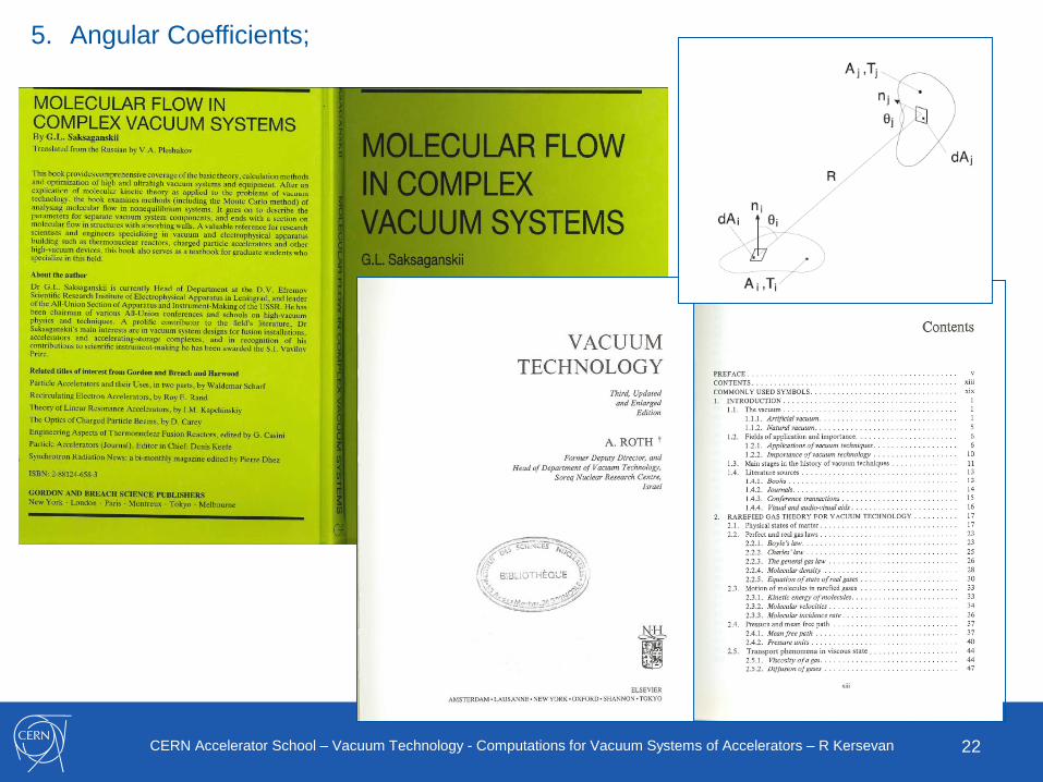
5. Angular Coefficients;
23CERN Accelerator School – Vacuum Technology - Computations for Vacuum Systems of Accelerators – R Kersevan
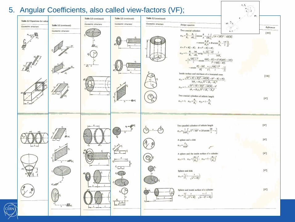
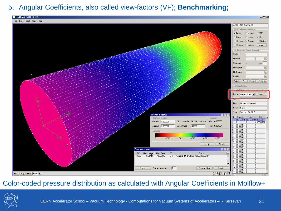
5. Angular Coefficients, also called view-factors (VF);
24CERN Accelerator School – Vacuum Technology - Computations for Vacuum Systems of Accelerators – R Kersevan
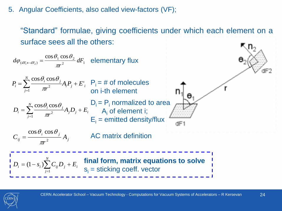
5. Angular Coefficients, also called view-factors (VF);
“Standard” formulae, giving coefficients under which each element on a
surface sees all the others:
12
21
)(
coscos21
dFr
d dFdF
iji
N
j
ji
i EPAr
P 'coscos
12
ijj
N
j
ji
i EDAr
D 1
2
coscos
j
ji
ij Ar
C2
coscos
i
N
j
jijii EDCsD 1
)1(
elementary flux
Pi = # of molecules
on i-th element
AC matrix definition
Di = Pi normalized to area
Ai of element i;
Ei = emitted density/flux
final form, matrix equations to solve
si = sticking coeff. vector
25CERN Accelerator School – Vacuum Technology - Computations for Vacuum Systems of Accelerators – R Kersevan
5. Angular Coefficients, also called view-factors (VF);
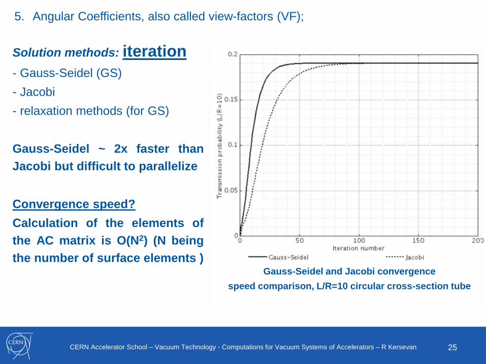
Solution methods: iteration
- Gauss-Seidel (GS)
- Jacobi
- relaxation methods (for GS)
Gauss-Seidel ~ 2x faster than
Jacobi but difficult to parallelize
Convergence speed?
Calculation of the elements of
the AC matrix is O(N2) (N being
the number of surface elements )Gauss-Seidel and Jacobi convergence
speed comparison, L/R=10 circular cross-section tube
26CERN Accelerator School – Vacuum Technology - Computations for Vacuum Systems of Accelerators – R Kersevan
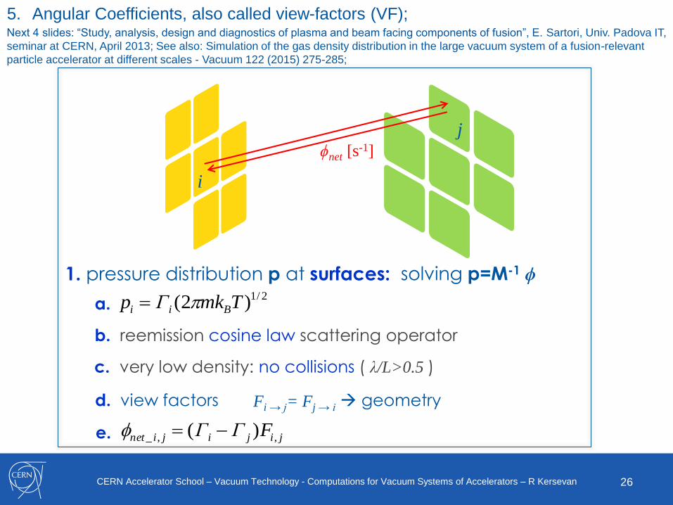
Γ [m-2 s-1]
b. reemission cosine law scattering operator
c. very low density: no collisions ( λ/L>0.5 )
Fi → j= Fj → id. view factors geometry
ϕnet [s-1]
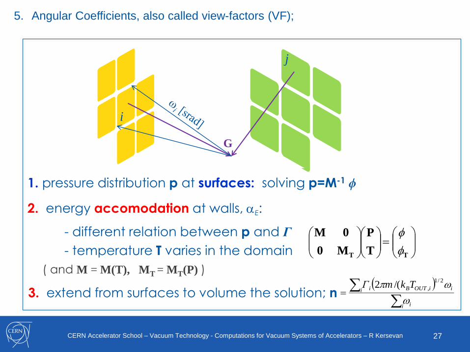
1. pressure distribution p at surfaces:
a.2/1)2( TmkΓp Bii
solving p=M-1 ϕ
e. jijijinet FΓΓ ,,_ )(
i
j
5. Angular Coefficients, also called view-factors (VF);Next 4 slides: “Study, analysis, design and diagnostics of plasma and beam facing components of fusion”, E. Sartori, Univ. Padova IT,
seminar at CERN, April 2013; See also: Simulation of the gas density distribution in the large vacuum system of a fusion-relevant
particle accelerator at different scales - Vacuum 122 (2015) 275-285;
27CERN Accelerator School – Vacuum Technology - Computations for Vacuum Systems of Accelerators – R Kersevan
2. energy accomodation at walls, aE:
- different relation between p and Γ
- temperature T varies in the domain
TT T
P
M0
0M
( and M = M(T), MT = MT(P) )
Ti [K]
1. pressure distribution p at surfaces: solving p=M-1 ϕ
Tr [K]
E
Wi
ri
TT
TTa
3. extend from surfaces to volume the solution; n
G
i
j
i i
i iiOUTBi TkmΓ
2/1
,/(2
5. Angular Coefficients, also called view-factors (VF);
28CERN Accelerator School – Vacuum Technology - Computations for Vacuum Systems of Accelerators – R Kersevan
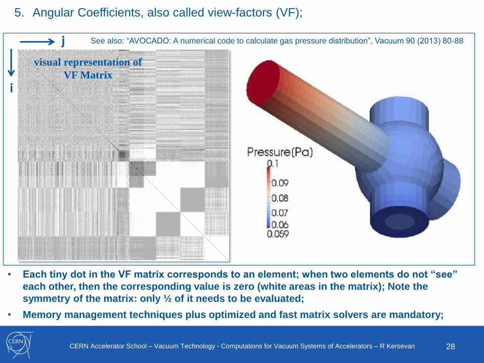
visual representation of
VF Matrix
i
j
• Each tiny dot in the VF matrix corresponds to an element; when two elements do not “see”
each other, then the corresponding value is zero (white areas in the matrix); Note the
symmetry of the matrix: only ½ of it needs to be evaluated;
• Memory management techniques plus optimized and fast matrix solvers are mandatory;
5. Angular Coefficients, also called view-factors (VF);
See also: “AVOCADO: A numerical code to calculate gas pressure distribution”, Vacuum 90 (2013) 80-88
29CERN Accelerator School – Vacuum Technology - Computations for Vacuum Systems of Accelerators – R Kersevan
5. Angular Coefficients, also called view-factors (VF);
Φ [m-2 s-1]
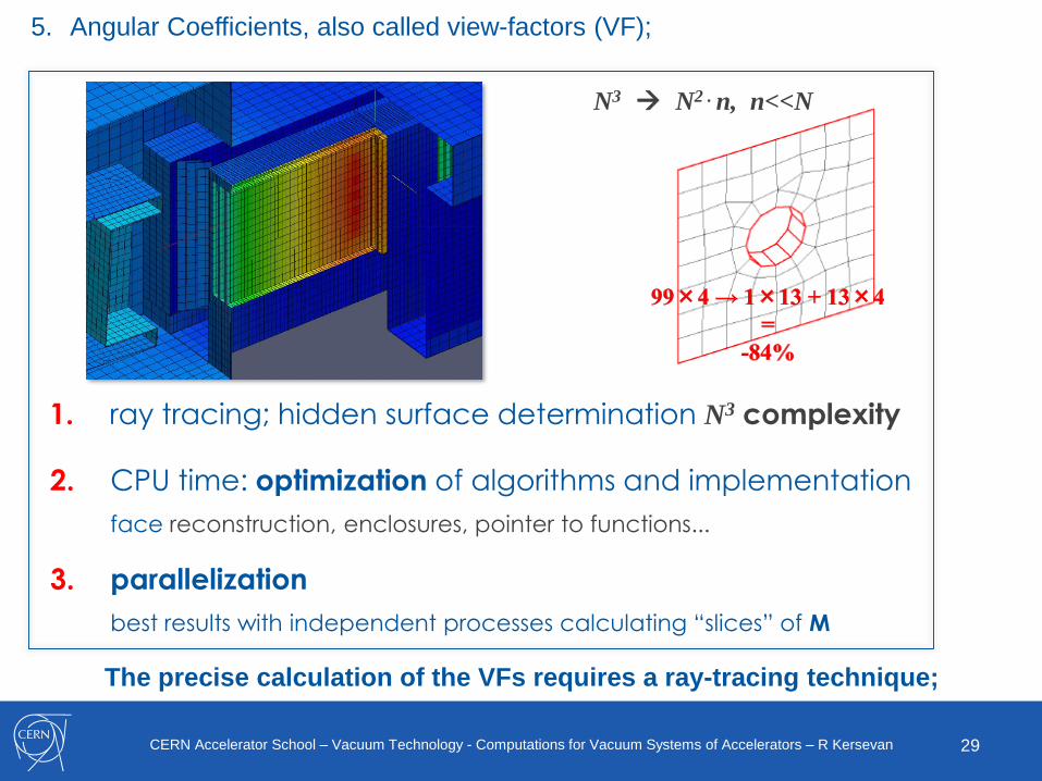
1. ray tracing; hidden surface determination N3 complexity
i jk
2. CPU time: optimization of algorithms and implementation
face reconstruction, enclosures, pointer to functions...
N3 N2 . n, n<<N
3. parallelization
best results with independent processes calculating “slices” of M
The precise calculation of the VFs requires a ray-tracing technique;
30CERN Accelerator School – Vacuum Technology - Computations for Vacuum Systems of Accelerators – R Kersevan
5. Angular Coefficients, also called view-factors (VF);
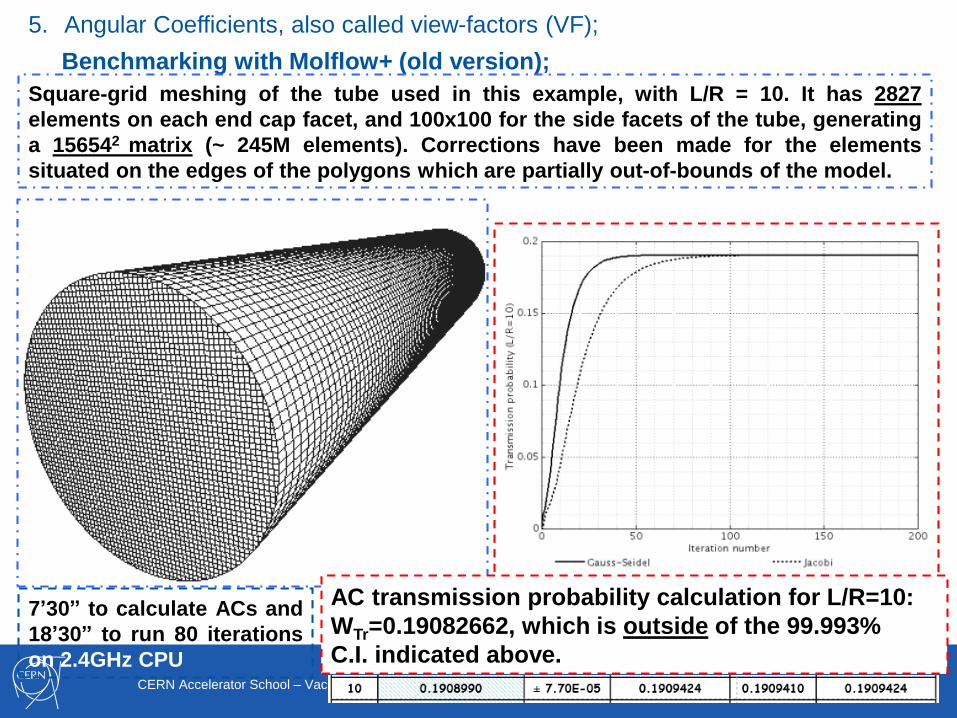
Benchmarking with Molflow+ (old version);
Square-grid meshing of the tube used in this example, with L/R = 10. It has 2827
elements on each end cap facet, and 100x100 for the side facets of the tube, generating
a 156542 matrix (~ 245M elements). Corrections have been made for the elements
situated on the edges of the polygons which are partially out-of-bounds of the model.
7’30” to calculate ACs and
18’30” to run 80 iterations
on 2.4GHz CPU
AC transmission probability calculation for L/R=10:
WTr=0.19082662, which is outside of the 99.993%
C.I. indicated above.
31CERN Accelerator School – Vacuum Technology - Computations for Vacuum Systems of Accelerators – R Kersevan
5. Angular Coefficients, also called view-factors (VF); Benchmarking;
Color-coded pressure distribution as calculated with Angular Coefficients in Molflow+
32CERN Accelerator School – Vacuum Technology - Computations for Vacuum Systems of Accelerators – R Kersevan
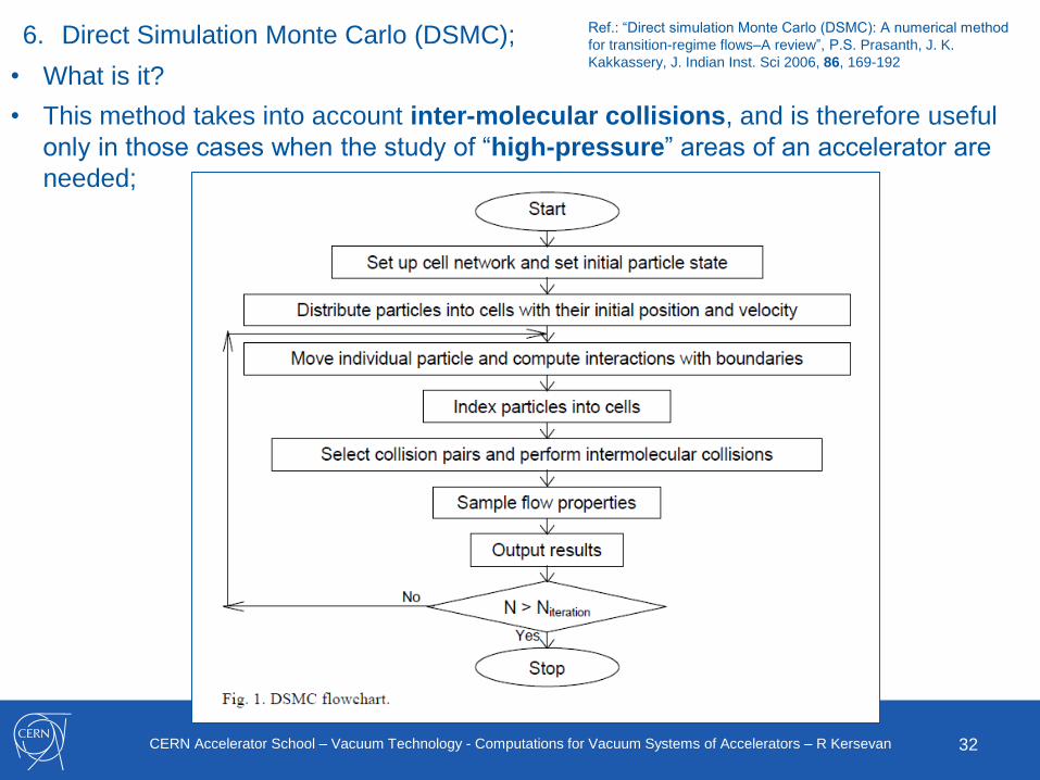
6. Direct Simulation Monte Carlo (DSMC);
• What is it?
• This method takes into account inter-molecular collisions, and is therefore useful
only in those cases when the study of “high-pressure” areas of an accelerator are
needed;
Ref.: “Direct simulation Monte Carlo (DSMC): A numerical method
for transition-regime flows–A review”, P.S. Prasanth, J. K.
Kakkassery, J. Indian Inst. Sci 2006, 86, 169-192
33CERN Accelerator School – Vacuum Technology - Computations for Vacuum Systems of Accelerators – R Kersevan
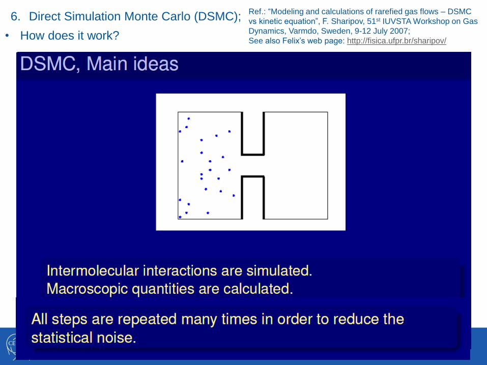
6. Direct Simulation Monte Carlo (DSMC);
• How does it work?
Ref.: “Modeling and calculations of rarefied gas flows – DSMC
vs kinetic equation”, F. Sharipov, 51st IUVSTA Workshop on Gas
Dynamics, Varmdo, Sweden, 9-12 July 2007;
See also Felix’s web page: http://fisica.ufpr.br/sharipov/
34CERN Accelerator School – Vacuum Technology - Computations for Vacuum Systems of Accelerators – R Kersevan
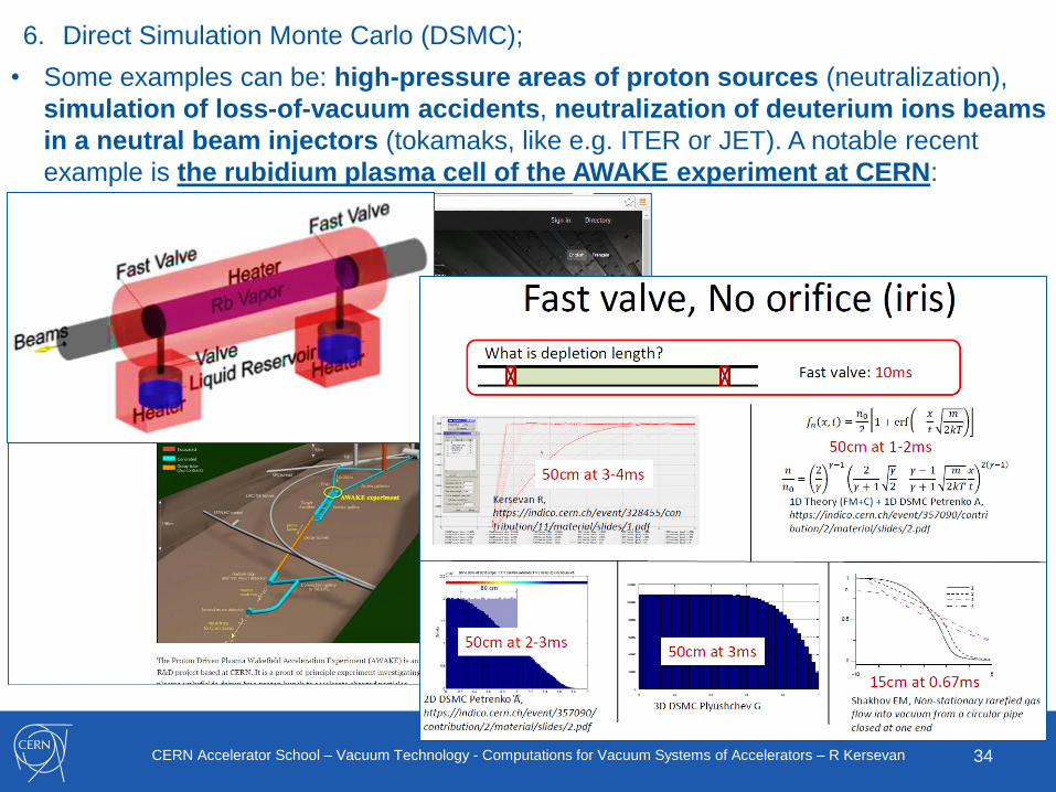
6. Direct Simulation Monte Carlo (DSMC);
• Some examples can be: high-pressure areas of proton sources (neutralization),
simulation of loss-of-vacuum accidents, neutralization of deuterium ions beams
in a neutral beam injectors (tokamaks, like e.g. ITER or JET). A notable recent
example is the rubidium plasma cell of the AWAKE experiment at CERN:
35CERN Accelerator School – Vacuum Technology - Computations for Vacuum Systems of Accelerators – R Kersevan
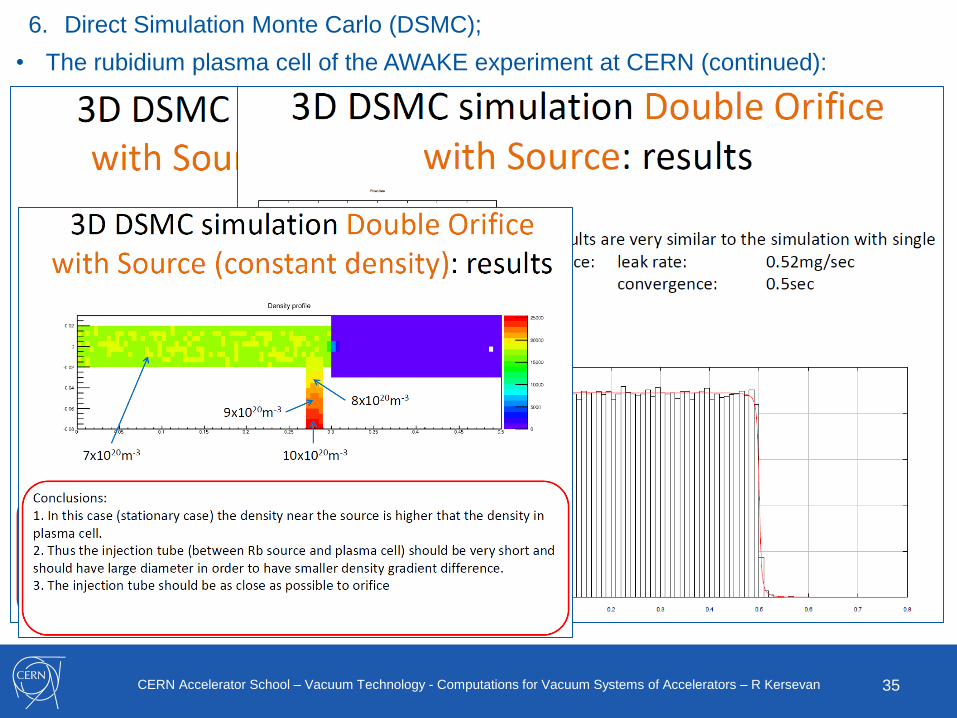
6. Direct Simulation Monte Carlo (DSMC);
• The rubidium plasma cell of the AWAKE experiment at CERN (continued):
36CERN Accelerator School – Vacuum Technology - Computations for Vacuum Systems of Accelerators – R Kersevan
6. Direct solutions of the Boltzmann equation;
• Another way of tackling the problem is to find the solution of the Boltzmann
equation; There exist a number of methods to solve it, and a short review of some of
them can be found in the excellent series of articles on the journal Vacuum Vol. 109,
Pages 1-424 (November 2014), « Advances in Vacuum Gas Dynamics », Guest
Editors: Felix Sharipov and Oleg B. Malyshev;
• It must be said at this point that this kind of solutions are very rarely applied to
solving practical problems of real accelerators’ vacuum systems, or their actual
design;
• The DSMC and other methods which include molecular collisions are widely used in
the analysis and design of vacuum pumps, such as Gaede pumps,
turbomolecular pumps, high-pressure vacuum gauges (e.g. Pirani), and more…
37CERN Accelerator School – Vacuum Technology - Computations for Vacuum Systems of Accelerators – R Kersevan
7. Test-Particle Monte Carlo (TPMC);
• The TPMC method is similar to the DSMC, but avoids the cumbersome and
sometimes overwhelming complexity of defining density and velocity fields in
order to correctly calculate the collision integral in the Boltzmann equation;
• Several vacuum scientists have developed their own code, but in the particle
accelerator community the Molflow+ code has become somewhat widespread,
and will therefore be used as a template for illustrating how the TPMC method
works, without loss of generality;
• The most complete and recent reference for Molflow+ and the companion
synchrotron radiation ray-tracing code SYNRAD+ is this:
Ref. “Monte Carlo Simulations of Ultra High Vacuum and Synchrotron Radiation for Particle Accelerators”,
M. Ady, PhD thesis EPFL/CERN, May 2016, http://cds.cern.ch/record/2157666/files/CERN-THESIS-2016-047.pdf
• Additional informations, tutorials given in the past, codes and files, and additional
documentation can be found here:
http://molflow.web.cern.ch/
• Please visit our web site and give us your feedback.
See also: https://www.dropbox.com/sh/1vt0x6212x5p5tb/AAD9zFMZ7BUSkww62nUp9wQ-a?dl=0
38CERN Accelerator School – Vacuum Technology - Computations for Vacuum Systems of Accelerators – R Kersevan
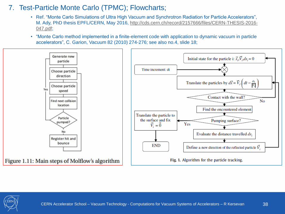
7. Test-Particle Monte Carlo (TPMC); Flowcharts;
• Ref. “Monte Carlo Simulations of Ultra High Vacuum and Synchrotron Radiation for Particle Accelerators”,
M. Ady, PhD thesis EPFL/CERN, May 2016, http://cds.cern.ch/record/2157666/files/CERN-THESIS-2016-
047.pdf;
• “Monte Carlo method implemented in a finite-element code with application to dynamic vacuum in particle
accelerators”, C. Garion, Vacuum 82 (2010) 274-276; see also no.4, slide 18;
39CERN Accelerator School – Vacuum Technology - Computations for Vacuum Systems of Accelerators – R Kersevan
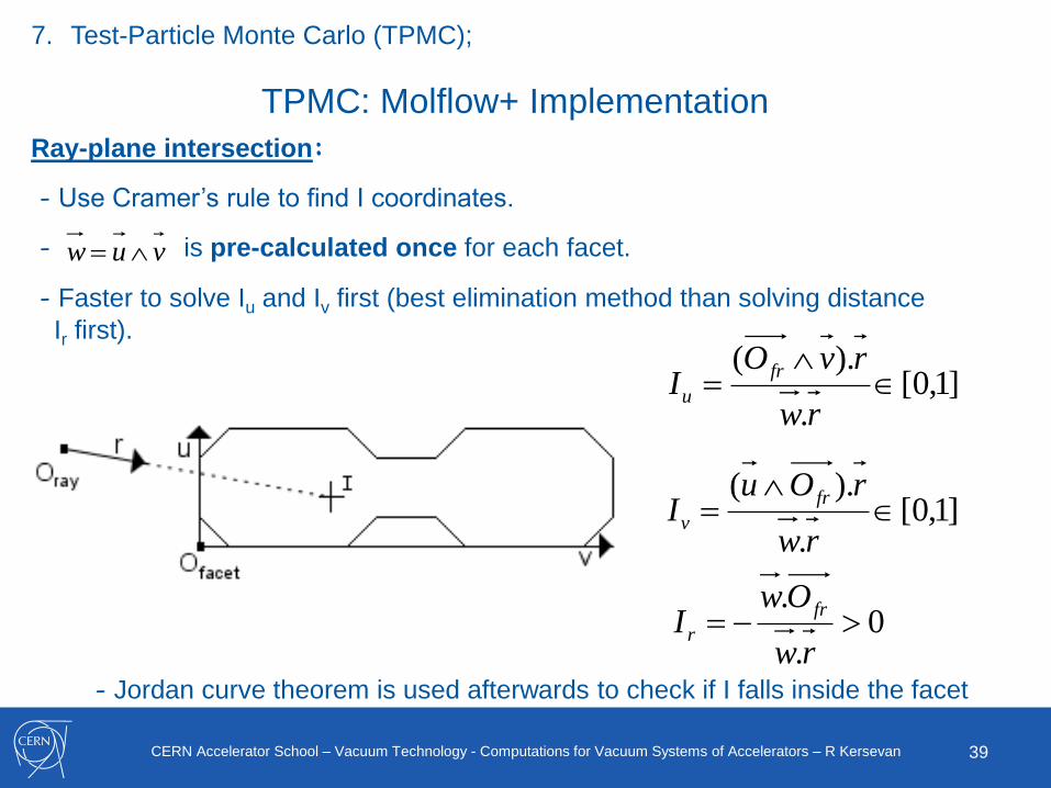
TPMC: Molflow+ Implementation
Ray-plane intersection:
- Use Cramer’s rule to find I coordinates.
vuw - is pre-calculated once for each facet.
]1,0[.
).(
rw
rvOI
fr
u
]1,0[.
).(
rw
rOuI
fr
v
0.
.
rw
OwI
fr
r
- Jordan curve theorem is used afterwards to check if I falls inside the facet
- Faster to solve Iu and Iv first (best elimination method than solving distance
Ir first).
7. Test-Particle Monte Carlo (TPMC);
40CERN Accelerator School – Vacuum Technology - Computations for Vacuum Systems of Accelerators – R Kersevan
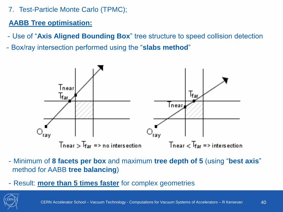
7. Test-Particle Monte Carlo (TPMC);
AABB Tree optimisation:
- Use of “Axis Aligned Bounding Box” tree structure to speed collision detection
- Box/ray intersection performed using the “slabs method”
- Minimum of 8 facets per box and maximum tree depth of 5 (using “best axis”
method for AABB tree balancing)
- Result: more than 5 times faster for complex geometries
41CERN Accelerator School – Vacuum Technology - Computations for Vacuum Systems of Accelerators – R Kersevan
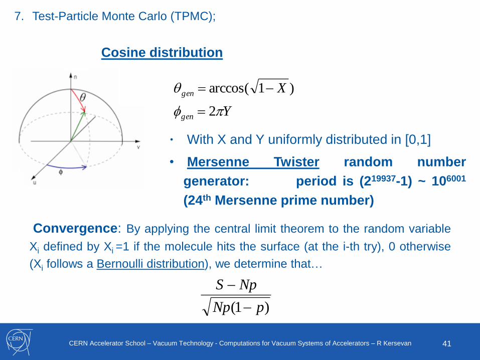
7. Test-Particle Monte Carlo (TPMC);
Cosine distribution
Y
X
gen
gen
2
)1arccos(
Convergence: By applying the central limit theorem to the random variable
Xi defined by Xi =1 if the molecule hits the surface (at the i-th try), 0 otherwise
(Xi follows a Bernoulli distribution), we determine that…
)1( pNp
NpS
• With X and Y uniformly distributed in [0,1]
• Mersenne Twister random number
generator: period is (219937-1) ~ 106001
(24th Mersenne prime number)
42CERN Accelerator School – Vacuum Technology - Computations for Vacuum Systems of Accelerators – R Kersevan
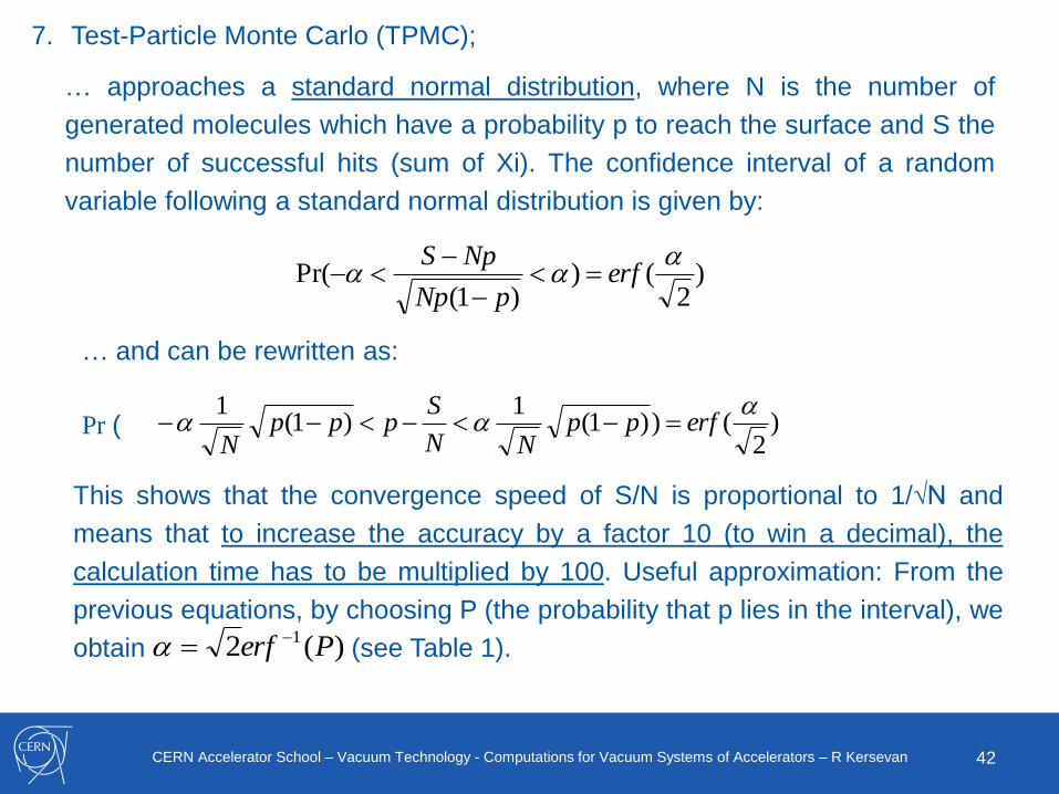
7. Test-Particle Monte Carlo (TPMC);
… approaches a standard normal distribution, where N is the number of
generated molecules which have a probability p to reach the surface and S the
number of successful hits (sum of Xi). The confidence interval of a random
variable following a standard normal distribution is given by:
)2
())1(
Pr(a
aa erfpNp
NpS
)2
())1(1
)1(1 a
aa erfppNN
Sppp
N
… and can be rewritten as:
Pr (
This shows that the convergence speed of S/N is proportional to 1/√N and
means that to increase the accuracy by a factor 10 (to win a decimal), the
calculation time has to be multiplied by 100. Useful approximation: From the
previous equations, by choosing P (the probability that p lies in the interval), we
obtain (see Table 1).)(2 1 Perf a
43CERN Accelerator School – Vacuum Technology - Computations for Vacuum Systems of Accelerators – R Kersevan
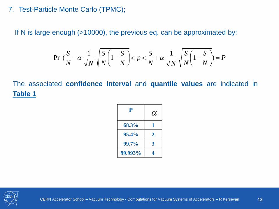
7. Test-Particle Monte Carlo (TPMC);
If N is large enough (>10000), the previous eq. can be approximated by:
PN
S
N
S
NN
Sp
N
S
N
S
NN
S
)1
11
1(Pr aa
The associated confidence interval and quantile values are indicated in
Table 1
aP
68.3% 1
95.4% 2
99.7% 3
99.993% 4
44CERN Accelerator School – Vacuum Technology - Computations for Vacuum Systems of Accelerators – R Kersevan
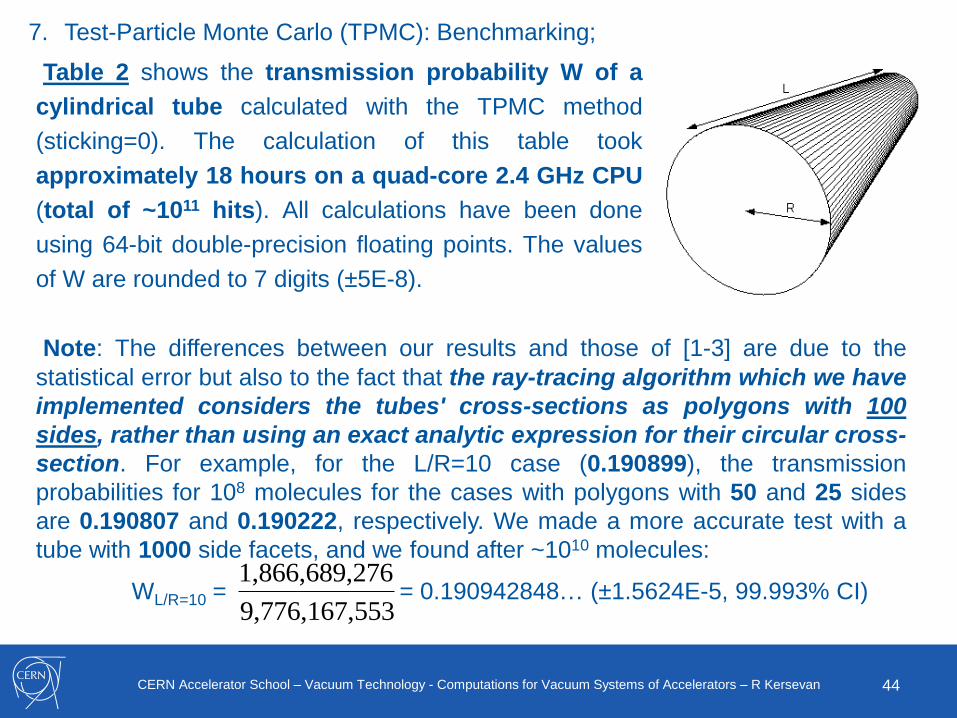
7. Test-Particle Monte Carlo (TPMC): Benchmarking;
Table 2 shows the transmission probability W of a
cylindrical tube calculated with the TPMC method
(sticking=0). The calculation of this table took
approximately 18 hours on a quad-core 2.4 GHz CPU
(total of ~1011 hits). All calculations have been done
using 64-bit double-precision floating points. The values
of W are rounded to 7 digits (±5E-8).
Note: The differences between our results and those of [1-3] are due to the
statistical error but also to the fact that the ray-tracing algorithm which we have
implemented considers the tubes' cross-sections as polygons with 100
sides, rather than using an exact analytic expression for their circular cross-
section. For example, for the L/R=10 case (0.190899), the transmission
probabilities for 108 molecules for the cases with polygons with 50 and 25 sides
are 0.190807 and 0.190222, respectively. We made a more accurate test with a
tube with 1000 side facets, and we found after ~1010 molecules:
WL/R=10 = = 0.190942848… (±1.5624E-5, 99.993% CI)5539,776,167,
2761,866,689,
45CERN Accelerator School – Vacuum Technology - Computations for Vacuum Systems of Accelerators – R Kersevan
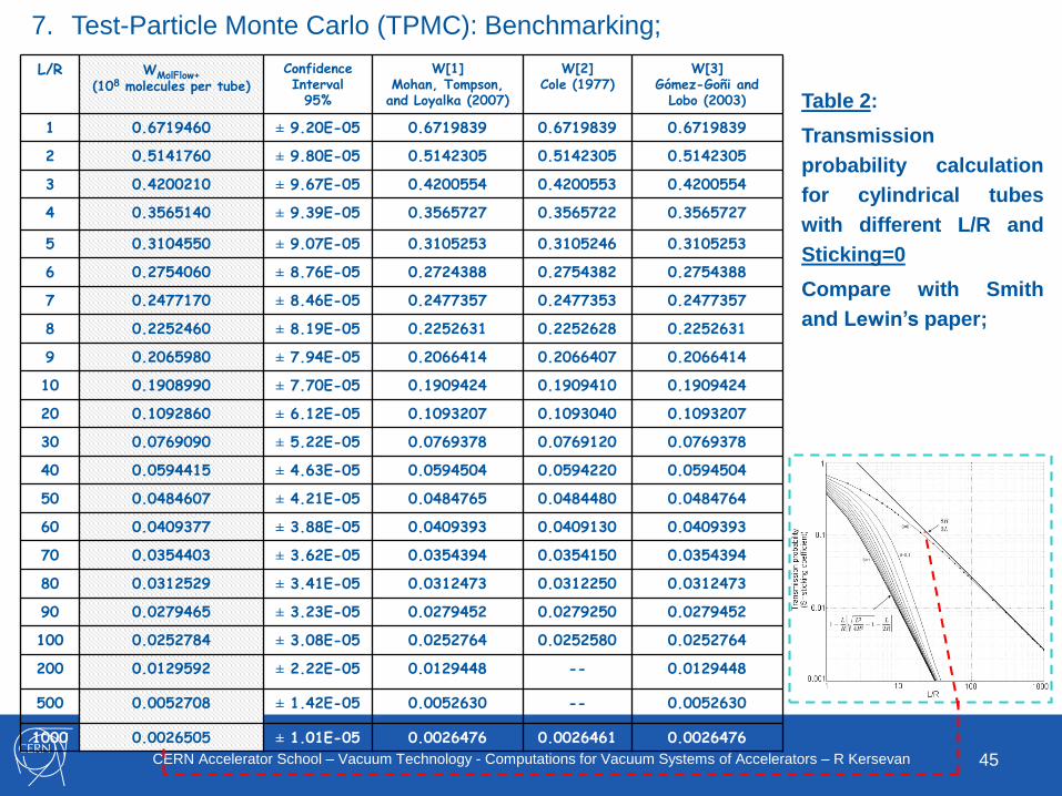
7. Test-Particle Monte Carlo (TPMC): Benchmarking;
L/R WMolFlow+(108 molecules per tube)
Confidence Interval
95%
W[1]Mohan, Tompson,and Loyalka (2007)
W[2]Cole (1977)
W[3]Gómez-Goñi and
Lobo (2003)
1 0.6719460 ± 9.20E-05 0.6719839 0.6719839 0.6719839
2 0.5141760 ± 9.80E-05 0.5142305 0.5142305 0.5142305
3 0.4200210 ± 9.67E-05 0.4200554 0.4200553 0.4200554
4 0.3565140 ± 9.39E-05 0.3565727 0.3565722 0.3565727
5 0.3104550 ± 9.07E-05 0.3105253 0.3105246 0.3105253
6 0.2754060 ± 8.76E-05 0.2724388 0.2754382 0.2754388
7 0.2477170 ± 8.46E-05 0.2477357 0.2477353 0.2477357
8 0.2252460 ± 8.19E-05 0.2252631 0.2252628 0.2252631
9 0.2065980 ± 7.94E-05 0.2066414 0.2066407 0.2066414
10 0.1908990 ± 7.70E-05 0.1909424 0.1909410 0.1909424
20 0.1092860 ± 6.12E-05 0.1093207 0.1093040 0.1093207
30 0.0769090 ± 5.22E-05 0.0769378 0.0769120 0.0769378
40 0.0594415 ± 4.63E-05 0.0594504 0.0594220 0.0594504
50 0.0484607 ± 4.21E-05 0.0484765 0.0484480 0.0484764
60 0.0409377 ± 3.88E-05 0.0409393 0.0409130 0.0409393
70 0.0354403 ± 3.62E-05 0.0354394 0.0354150 0.0354394
80 0.0312529 ± 3.41E-05 0.0312473 0.0312250 0.0312473
90 0.0279465 ± 3.23E-05 0.0279452 0.0279250 0.0279452
100 0.0252784 ± 3.08E-05 0.0252764 0.0252580 0.0252764
200 0.0129592 ± 2.22E-05 0.0129448 -- 0.0129448
500 0.0052708 ± 1.42E-05 0.0052630 -- 0.0052630
1000 0.0026505 ± 1.01E-05 0.0026476 0.0026461 0.0026476
Table 2:
Transmission
probability calculation
for cylindrical tubes
with different L/R and
Sticking=0
Compare with Smith
and Lewin’s paper;
46CERN Accelerator School – Vacuum Technology - Computations for Vacuum Systems of Accelerators – R Kersevan
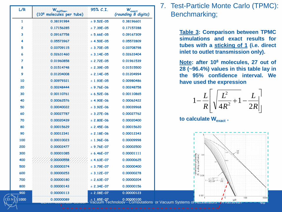
7. Test-Particle Monte Carlo (TPMC):
Benchmarking;
Table 3: Comparison between TPMC
simulations and exact results for
tubes with a sticking of 1 (i.e. direct
inlet to outlet transmission only).
Note: after 108 molecules, 27 out of
28 (~96.4%) values in this table lay in
the 95% confidence interval. We
have used the expression
to calculate Wexact .
R
L
R
L
R
L
21
41
2
2
L/R Wmolflow+
(108 molecules per tube)95% C.I. Wexact
(rounding 8 digits)
1 0.38191984 ± 9.52E-05 0.38196601
2 0.17156285 ± 7.39E-05 0.17157288
3 0.09167758 ± 5.66E-05 0.09167309
4 0.05573967 ± 4.50E-05 0.05572809
5 0.03709115 ± 3.70E-05 0.03708798
6 0.02631460 ± 3.14E-05 0.02633404
7 0.01960858 ± 2.72E-05 0.01961539
8 0.01514748 ± 2.39E-05 0.01515500
9 0.01204008 ± 2.14E-05 0.01204994
10 0.00979321 ± 1.93E-05 0.00980486
20 0.00248444 ± 9.76E-06 0.00248758
30 0.00110761 ± 6.52E-06 0.00110865
40 0.00062576 ± 4.90E-06 0.00062422
50 0.00040022 ± 3.92E-06 0.00039968
60 0.00027787 ± 3.27E-06 0.00027762
70 0.00020439 ± 2.80E-06 0.00020400
80 0.00015629 ± 2.45E-06 0.00015620
90 0.00012341 ± 2.18E-06 0.00012343
100 0.00010023 ± 1.96E-06 0.00009998
200 0.00002477 ± 9.76E-07 0.00002500
300 0.00001085 ± 6.46E-07 0.00001111
400 0.00000558 ± 4.63E-07 0.00000625
500 0.00000374 ± 3.79E-07 0.00000400
600 0.00000253 ± 3.12E-07 0.00000278
700 0.00000180 ± 2.63E-07 0.00000204
800 0.00000143 ± 2.34E-07 0.00000156
900 0.00000113 ± 2.08E-07 0.00000123
1000 0.00000089 ± 1.85E-07 0.00000100
47CERN Accelerator School – Vacuum Technology - Computations for Vacuum Systems of Accelerators – R Kersevan
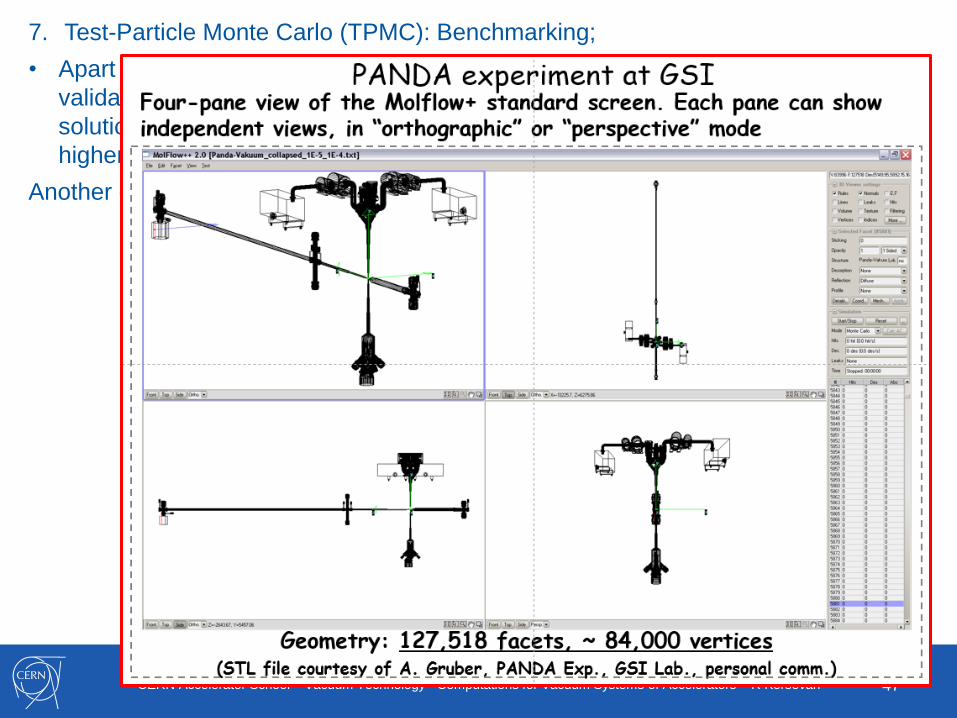
7. Test-Particle Monte Carlo (TPMC): Benchmarking;
• Apart from basic geometries having analytical solutions, Molflow+ has been
validated against the results of a lot of papers, both simulations, analytical
solutions, other calculation techniques, for geometries of the vacuum system of
higher levels of complexity, see M.Ady thesis for several examples;
Another example here:
48CERN Accelerator School – Vacuum Technology - Computations for Vacuum Systems of Accelerators – R Kersevan
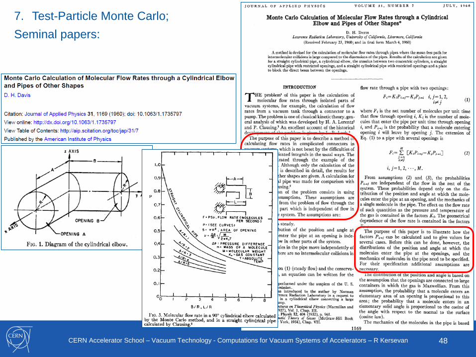
7. Test-Particle Monte Carlo;
Seminal papers:
49CERN Accelerator School – Vacuum Technology - Computations for Vacuum Systems of Accelerators – R Kersevan
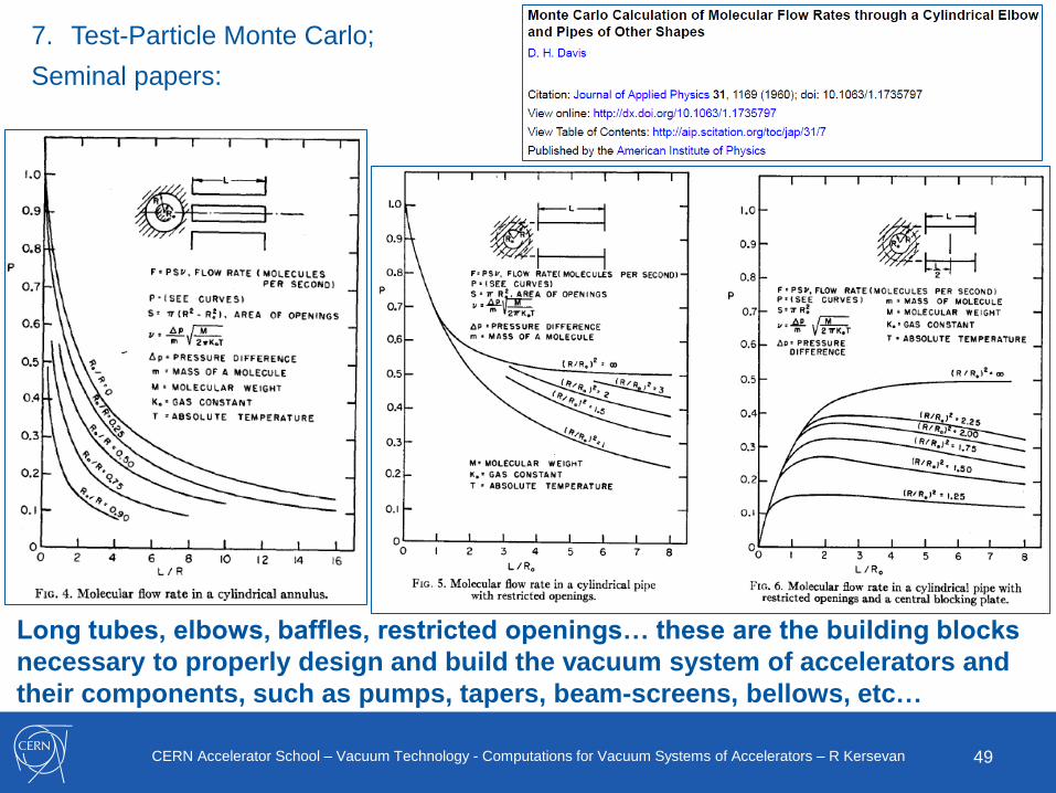
Long tubes, elbows, baffles, restricted openings… these are the building blocks
necessary to properly design and build the vacuum system of accelerators and
their components, such as pumps, tapers, beam-screens, bellows, etc…
7. Test-Particle Monte Carlo;
Seminal papers:
50CERN Accelerator School – Vacuum Technology - Computations for Vacuum Systems of Accelerators – R Kersevan
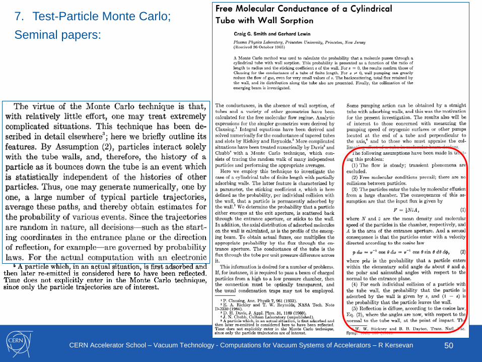
7. Test-Particle Monte Carlo;
Seminal papers:
51CERN Accelerator School – Vacuum Technology - Computations for Vacuum Systems of Accelerators – R Kersevan
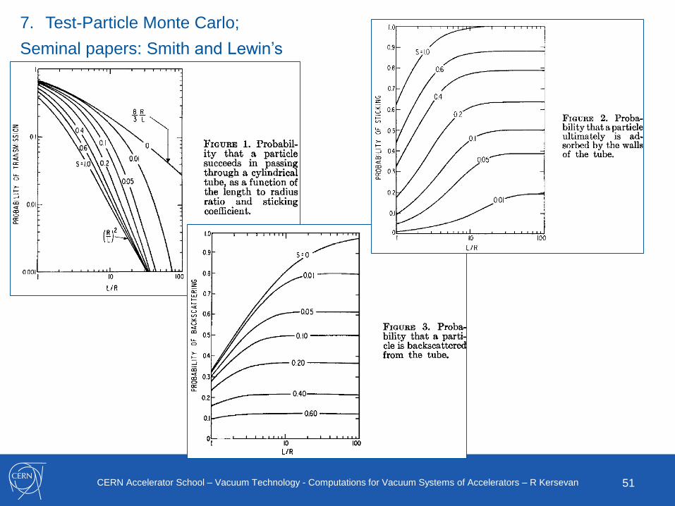
7. Test-Particle Monte Carlo;
Seminal papers: Smith and Lewin’s
52CERN Accelerator School – Vacuum Technology - Computations for Vacuum Systems of Accelerators – R Kersevan
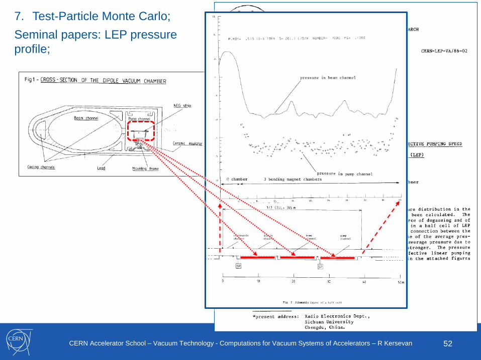
7. Test-Particle Monte Carlo;
Seminal papers: LEP pressure
profile;
53CERN Accelerator School – Vacuum Technology - Computations for Vacuum Systems of Accelerators – R Kersevan
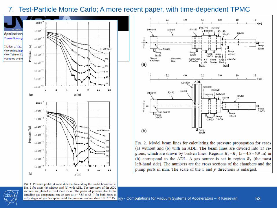
7. Test-Particle Monte Carlo; A more recent paper, with time-dependent TPMC
54CERN Accelerator School – Vacuum Technology - Computations for Vacuum Systems of Accelerators – R Kersevan
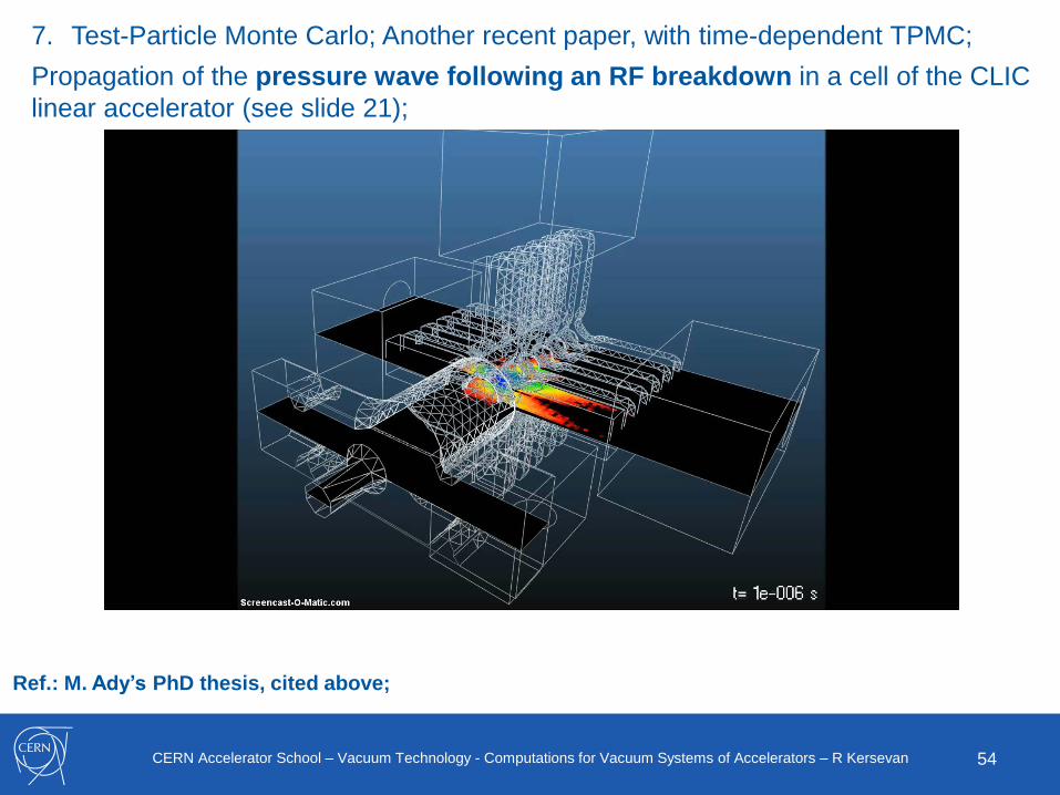
7. Test-Particle Monte Carlo; Another recent paper, with time-dependent TPMC;
Propagation of the pressure wave following an RF breakdown in a cell of the CLIC
linear accelerator (see slide 21);
Ref.: M. Ady’s PhD thesis, cited above;
55CERN Accelerator School – Vacuum Technology - Computations for Vacuum Systems of Accelerators – R Kersevan
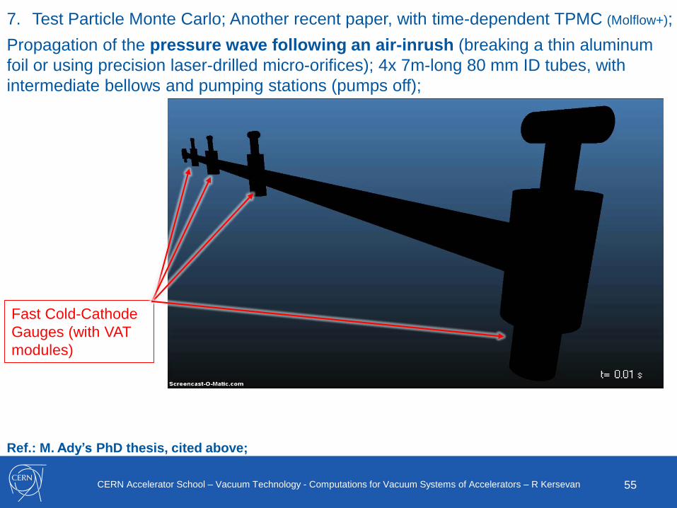
7. Test Particle Monte Carlo; Another recent paper, with time-dependent TPMC (Molflow+);
Propagation of the pressure wave following an air-inrush (breaking a thin aluminum
foil or using precision laser-drilled micro-orifices); 4x 7m-long 80 mm ID tubes, with
intermediate bellows and pumping stations (pumps off);
Ref.: M. Ady’s PhD thesis, cited above;
Fast Cold-Cathode
Gauges (with VAT
modules)
56CERN Accelerator School – Vacuum Technology - Computations for Vacuum Systems of Accelerators – R Kersevan
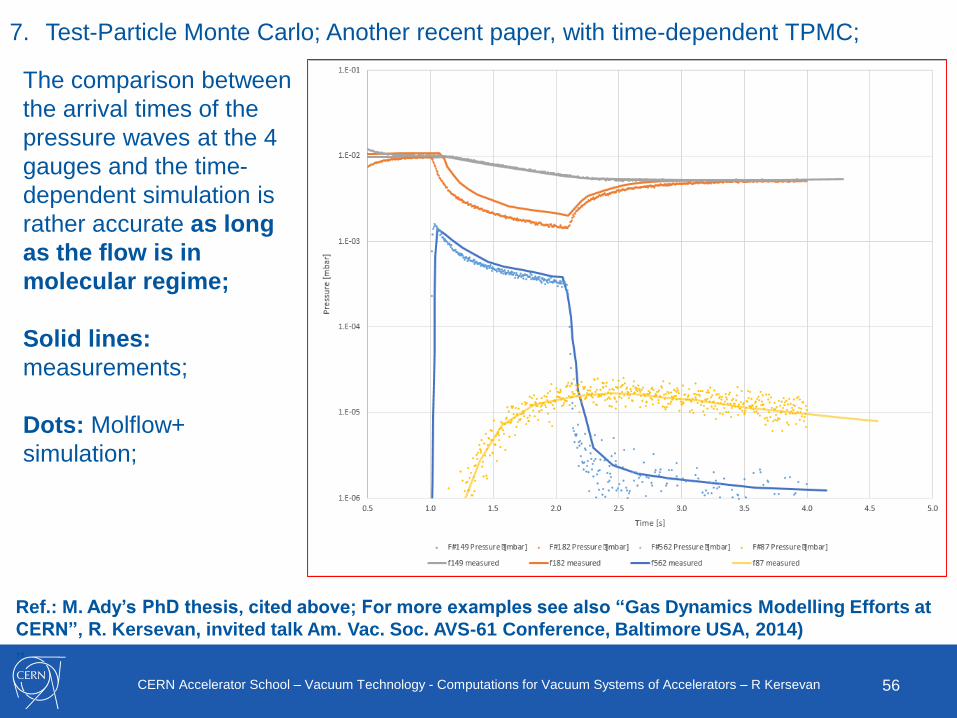
7. Test-Particle Monte Carlo; Another recent paper, with time-dependent TPMC;
Ref.: M. Ady’s PhD thesis, cited above; For more examples see also “Gas Dynamics Modelling Efforts at
CERN”, R. Kersevan, invited talk Am. Vac. Soc. AVS-61 Conference, Baltimore USA, 2014)
”
The comparison between
the arrival times of the
pressure waves at the 4
gauges and the time-
dependent simulation is
rather accurate as long
as the flow is in
molecular regime;
Solid lines:
measurements;
Dots: Molflow+
simulation;

57CERN Accelerator School – Vacuum Technology - Computations for Vacuum Systems of Accelerators – R Kersevan
7. Test-Particle Monte Carlo;
Conductance of other vacuum
components:
58CERN Accelerator School – Vacuum Technology - Computations for Vacuum Systems of Accelerators – R Kersevan
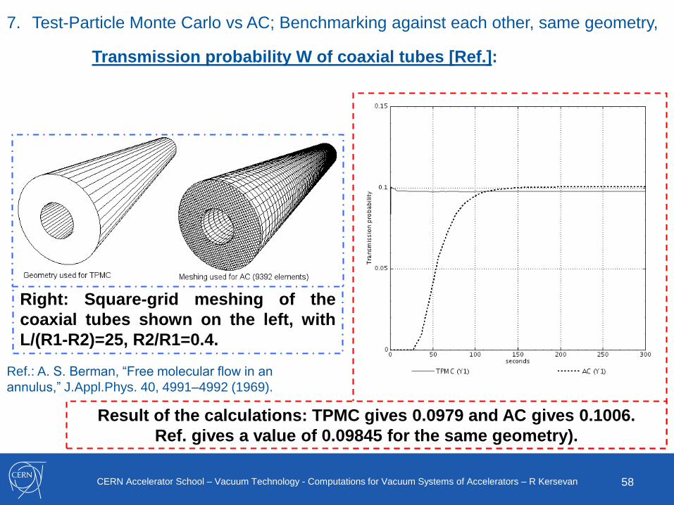
7. Test-Particle Monte Carlo vs AC; Benchmarking against each other, same geometry,
Right: Square-grid meshing of the
coaxial tubes shown on the left, with
L/(R1-R2)=25, R2/R1=0.4.
Transmission probability W of coaxial tubes [Ref.]:
Result of the calculations: TPMC gives 0.0979 and AC gives 0.1006.
Ref. gives a value of 0.09845 for the same geometry).
Ref.: A. S. Berman, “Free molecular flow in an
annulus,” J.Appl.Phys. 40, 4991–4992 (1969).
59CERN Accelerator School – Vacuum Technology - Computations for Vacuum Systems of Accelerators – R Kersevan
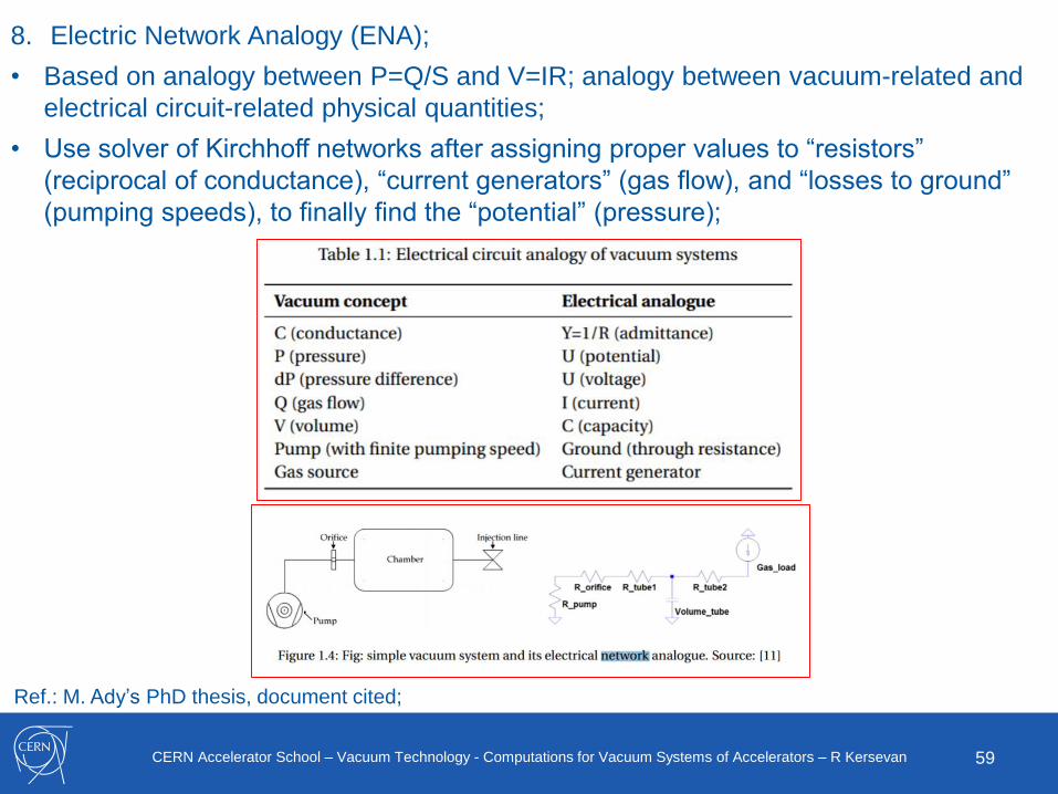
8. Electric Network Analogy (ENA);
• Based on analogy between P=Q/S and V=IR; analogy between vacuum-related and
electrical circuit-related physical quantities;
• Use solver of Kirchhoff networks after assigning proper values to “resistors”
(reciprocal of conductance), “current generators” (gas flow), and “losses to ground”
(pumping speeds), to finally find the “potential” (pressure);
Ref.: M. Ady’s PhD thesis, document cited;
60CERN Accelerator School – Vacuum Technology - Computations for Vacuum Systems of Accelerators – R Kersevan
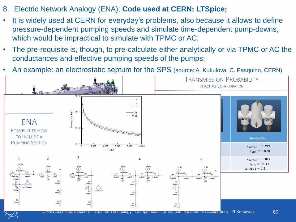
8. Electric Network Analogy (ENA); Code used at CERN: LTSpice;
• It is widely used at CERN for everyday’s problems, also because it allows to define
pressure-dependent pumping speeds and simulate time-dependent pump-downs,
which would be impractical to simulate with TPMC or AC;
• The pre-requisite is, though, to pre-calculate either analytically or via TPMC or AC the
conductances and effective pumping speeds of the pumps;
• An example: an electrostatic septum for the SPS (source: A. Kukulova, C. Pasquino, CERN)
61CERN Accelerator School – Vacuum Technology - Computations for Vacuum Systems of Accelerators – R Kersevan
Synchrotron radiation, e-cloud, and all the rest;
• Synchrotron radiation, and e-cloud, and other physical effects (impedance
instabilities leading to heating and thermal desorption, or ion-induced
desorption in large ion storage rings (e.g. GSI) also require sophisticated
and dedicated computational tools;
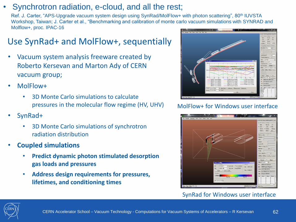
• For lack of time and space, we simply cite SYNRAD+, the ray-tracing
montecarlo code companion of Molflow+, which can be used “in series” in
order to simulate the vacuum environment of SR light sources;
• The most complete reference is, again, M. Ady’s PhD thesis and
bibliography therein;
• Here we use Jason Carter’s presentation at the 80th IUVSTA workshop in
Taiwan, to show the schematics of how SYNRAD+ and Molflow+, used in
sequence, can really help design and analyse the vacuum system of any
machine were SR is generated;
• This is a very compelling case, since most existing SR light sources are
under refurbishing phase or new construction (e.g. ESRF and APS upgrades
for the former, and MAX-IV for the latter), but also for hadron machines like
the LHC and the future high-energy colliders after it, like the FCC-h;
62CERN Accelerator School – Vacuum Technology - Computations for Vacuum Systems of Accelerators – R Kersevan
• Synchrotron radiation, e-cloud, and all the rest;Ref. J. Carter, “APS-Upgrade vacuum system design using SynRad/MolFlow+ with photon scattering”, 80th IUVSTA
Workshop, Taiwan; J. Carter et al., “Benchmarking and calibration of monte carlo vacuum simulations with SYNRAD and
Molflow+, proc. IPAC-16
SynRad for Windows user interface
MolFlow+ for Windows user interface
Use SynRad+ and MolFlow+, sequentially
• Vacuum system analysis freeware created by Roberto Kersevan and Marton Ady of CERN vacuum group;
• MolFlow+
• 3D Monte Carlo simulations to calculate pressures in the molecular flow regime (HV, UHV)
• SynRad+
• 3D Monte Carlo simulations of synchrotron radiation distribution
• Coupled simulations
• Predict dynamic photon stimulated desorption gas loads and pressures
• Address design requirements for pressures, lifetimes, and conditioning times
63CERN Accelerator School – Vacuum Technology - Computations for Vacuum Systems of Accelerators – R Kersevan
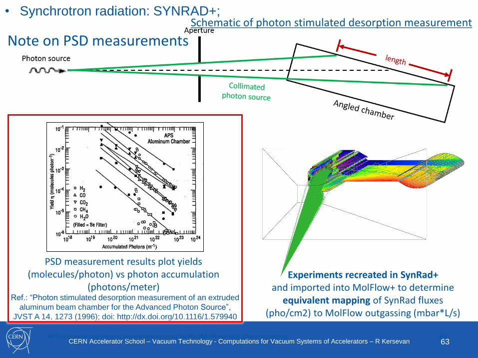
• Synchrotron radiation: SYNRAD+;
63
Schematic of photon stimulated desorption measurement
PSD measurement results plot yields (molecules/photon) vs photon accumulation
(photons/meter)Experiments recreated in SynRad+
and imported into MolFlow+ to determine equivalent mapping of SynRad fluxes
(pho/cm2) to MolFlow outgassing (mbar*L/s)
Note on PSD measurements
APS-U storage ring vacuum system design using SynRad/MolFlow+ with photon scattering
Ref.: “Photon stimulated desorption measurement of an extruded
aluminum beam chamber for the Advanced Photon Source”,
JVST A 14, 1273 (1996); doi: http://dx.doi.org/10.1116/1.579940
64CERN Accelerator School – Vacuum Technology - Computations for Vacuum Systems of Accelerators – R Kersevan
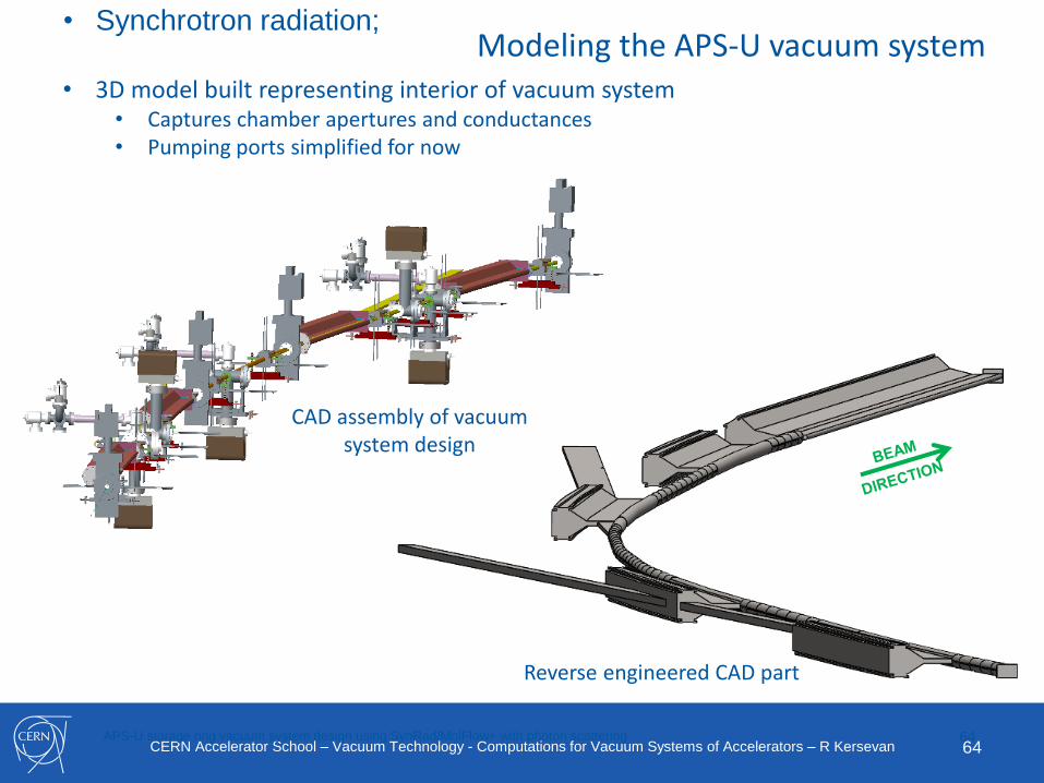
• Synchrotron radiation;
64APS-U storage ring vacuum system design using SynRad/MolFlow+ with photon scattering
Modeling the APS-U vacuum system
CAD assembly of vacuum system design
Reverse engineered CAD part
• 3D model built representing interior of vacuum system• Captures chamber apertures and conductances• Pumping ports simplified for now
65CERN Accelerator School – Vacuum Technology - Computations for Vacuum Systems of Accelerators – R Kersevan
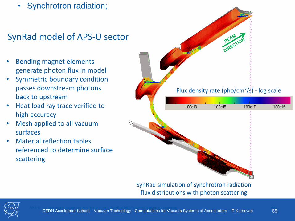
• Synchrotron radiation;
65APS-U storage ring vacuum system design using SynRad/MolFlow+ with photon scattering
Flux density rate (pho/cm2/s) - log scale
SynRad model of APS-U sector
SynRad simulation of synchrotron radiation flux distributions with photon scattering
• Bending magnet elements generate photon flux in model
• Symmetric boundary condition passes downstream photons back to upstream
• Heat load ray trace verified to high accuracy
• Mesh applied to all vacuum surfaces
• Material reflection tables referenced to determine surface scattering
66CERN Accelerator School – Vacuum Technology - Computations for Vacuum Systems of Accelerators – R Kersevan
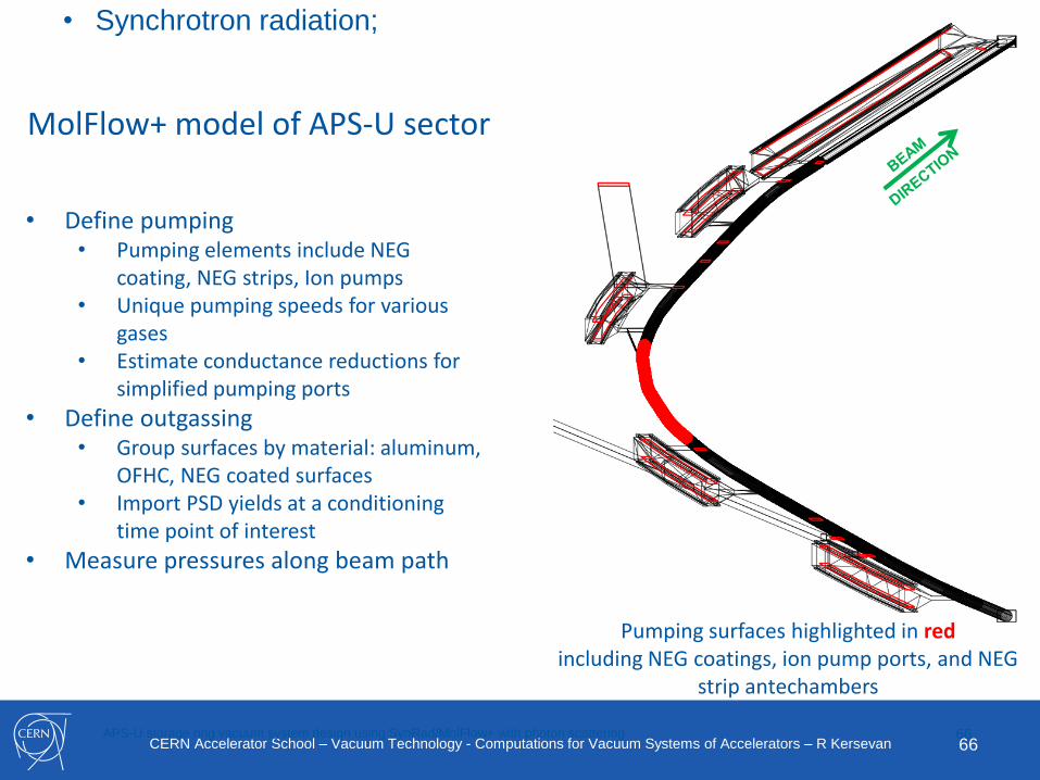
• Synchrotron radiation;
66APS-U storage ring vacuum system design using SynRad/MolFlow+ with photon scattering
Pumping surfaces highlighted in redincluding NEG coatings, ion pump ports, and NEG
strip antechambers
MolFlow+ model of APS-U sector
• Define pumping• Pumping elements include NEG
coating, NEG strips, Ion pumps• Unique pumping speeds for various
gases• Estimate conductance reductions for
simplified pumping ports
• Define outgassing• Group surfaces by material: aluminum,
OFHC, NEG coated surfaces• Import PSD yields at a conditioning
time point of interest
• Measure pressures along beam path
67CERN Accelerator School – Vacuum Technology - Computations for Vacuum Systems of Accelerators – R Kersevan
Conclusions:• Far from being an exhaustive document on all possible ways to calculate
vacuum quantities and pressure profiles for accelerators, for lack of time and
space, we have tried to show how some codes and algorithms work;
• It has been shown that there is a large number of computational tools which
allow the vacuum scientist/engineer to analyse and design the vacuum system
of new accelerators, or troubleshoot existing ones;
• The choice of the appropriate method and code depends on the type of
accelerator, the level of complexity to which the system has to be modelled and
simulated, and other factors, including personal habits like previous knowledge
of some code (e.g. ANSYS for FE calculations, LTSpice for electric networks,
etc…);
• The interpretation of the results of simulations must take into account the
physical basis implemented in the code of choice, and should preferably be
benchmarked with another code in case of doubt;
• Modern codes and methods allow a deep inspection of the physics behind the
creation of vacuum conditions: I urge every serious student of vacuum science
and technology to take the initiative and try to write his/her own code, even a
simple one based on some commercial software (e.g. MathCAD), because it is
only in doing that that a good understanding of how the vacuum system of an
accelerator works and should be designed, avoiding mistakes, and optimizing
the available resources (including financial) of the project;
Good luck to all of you!