Computations in quantum mechanics made easy · Computations in quantum mechanics made easy 4 0 2000 4000 6000 8000-4-2 0 2 4 t ... which are then applied alternately during

Computations in quantum mechanics made easy

H J Korsch1 and K Rapedius2

1 FB Physik, Universitat Kaiserslautern, D-67653 Kaiserslautern, Germany2 Karlsruhe Institute of Technology (KIT), Adenauerring 2, D-76131 Karlsruhe,

Germany

E-mail: [email protected], [email protected]

,

Abstract. Convenient and simple numerical techniques for performing quantum

computations based on matrix representations of Hilbert space operators are presented

and illustrated by various examples. The applications include the calculations of

spectral and dynamical properties for one-dimensional and two-dimensional single-

particle systems as well as bosonic many-particle and open quantum systems. Due to

their technical simplicity these methods are well suited as a tool for teaching quantum

mechanics to undergraduates and graduates. Explicit implementations of the presented

numerical methods in Matlab are given.

Submitted to: Eur. J. Phys.

1. Introduction

In [1] it was shown how to calculate the spectra of one-dimensional quantum systems in a

simple, convenient and effective way by means of matrix representations of Hilbert space

operators. Here we extend these techniques in various ways including the computation

of dynamical properties as well applications to higher dimensional systems, bosonic

many-particle and open quantum systems.

As discussed in [1] the basic building blocks for the discrete matrix representation

of operators used in the following programs are the operators a and a†, well known from

the harmonic oscillator, where they act as ladder operators on the harmonic oscillator

eigenstates |n〉, n = 0, 1, 2, . . . :

a |n+ 1〉 =√n+ 1 |n〉 , a†|n〉 =

√n+ 1 |n+ 1〉 , a†a |n〉 = n |n〉 . (1)

Motivated, e.g., by the application to the radiation field described by harmonic

oscillators with frequency ω0 these operators create or annihilate a photon of this

frequency or, more generally, a bosonic particle in second quantization. Therefore these

arX

iv:1

603.

0416

7v1

[qu

ant-

ph]

14

Mar

201

6

Computations in quantum mechanics made easy 2

operators are also known as creation and annihilation operators. Here we will mainly

use the matrix representation of these operators in the harmonic oscillator basis:

a =

0√

1 0 0 . . .

0 0√

2 0 . . .

0 0 0√

3 . . .

0 0 0 0 . . ....

......

.... . .

. (2)

As an introduction to the numerical applications presented below, the following shortMatlab code shows the construction of these matrices and their application to a basisvector

N = 4; Np=N+1; n = 1:N;

a = diag(sqrt(1:N),1); ad=a’;

n = [0 0 1 0 0]’;

a*n; ad*n; ad*a*n

where the properties (1) can be tested. It should be noted, however, that such numerical

matrix representations are necessarily finite, which causes numerical errors. The reader

may try for example to test the validity of the commutation relation [a, a†] = 1

numerically or to construct the eigenstates of the annihilation operator a, the coherent

states, numerically. In many cases these finite size errors can be reduced by increasing

the matrix size.

In addition, we will use the representation of the position and momentum operators

x = s√2

(a† + a) , p = is√

2(a† − a) (3)

where the scaling parameter is chosen as s = 1 in the following (see [1] for details).

These matrix representations of operators can now be used to construct in a simple way

matrix representations of other operators, such as the Hamiltonian or time-evolution

operators.

This paper is organized as follows: In section 2 we briefly review the calculation

of quantum eigenvalues for one-dimensional systems [1] and extend the analysis to

time-dependent calculations. The example applications include Bloch-oscillations in a

tilted periodic lattice. Section 3 illustrates the use of matrix representation for angular

momentum operators. In section 4 it is shown how to calculate the spectrum of a

two-dimensional quantum system. Applications to bosonic many-particle systems are

illustrated in section 5 by means of the Bose-Hubbard model. Finally, the dynamics

of an open quantum system described by a Lindblad master equation is calculated in

section 6.

2. One-dimensional systems

As a first example we consider the calculation of bound state energies for a single particle

in a one-dimensional potential described by the Hamiltonian

H =p2

2m+ V (x) , (4)


which has already been discussed in [1] for harmonic and quartic potentials. There

a simple program code can be found for computing the eigenvalues and, in addition,

also the corresponding wave functions. As an introduction we also list this code here,

however for a simple double-well potential

V (x) =1

2(|x| − x0)2 , (5)

a potential with harmonic minima at ±x0 separated by a barrier of height x20/2 at x = 0.

In the program code

N = 100; n = 1:N-1; x0 = 2.5;

m = sqrt(n);

x = 1/sqrt(2)*(diag(m,-1)+diag(m,1));

p = i/sqrt(2)*(diag(m,-1)-diag(m,1));

H = p^2/2+(sqrtm(x^2)-x0*eye(N))^2/2;

E = sort(eig(H)); E(1:8)

where ~ and the particle mass m are chosen as unity and x0 = 2.5. In addition itshould be noted that the matrix function |x| has been generated by taking the squarex^2 followed by the Matlab matrix function sqrtm(x^2). The output of the programis a listing of the first eight energy eigenvalues En, n = 0, . . . , 7, where the eigenvaluesbelow the potential barrier are arranged in doublets. Let us have a brief look at thetime dynamics for an initial state chosen as the ground state of the right potential well.This can be achieved by adding the lines

H1 = p^2/2 + (x-x0*eye(N))^2/2;

[V,Eig] = eig(H1);

psi = V(:,1);

tstep = 20; t(1) = 0; xav(1) = psi’*x*psi;

U = expm(-i*H*tstep);

for nt=1:400

t(nt+1) = t(nt)+tstep;

psi = U*psi;

xav(nt+1) = psi’*x*psi;

end

plot(t,xav); set(gca,’Fontsize’,20)

xlabel(’t’,’FontSize’,24); ylabel(’<x>’,’Rotation’,0,’FontSize’,24);

hold on

plot(t,x0*cos((E(2)-E(1))*t),’*r’)

to the program above. Then the time evolution operator U = exp−iH∆t/~ is used

to propagate the wave function over a sequence of 80 time steps ∆t = 20. At each

step the expectation value 〈x〉 is computed and finally plotted as a function of time in

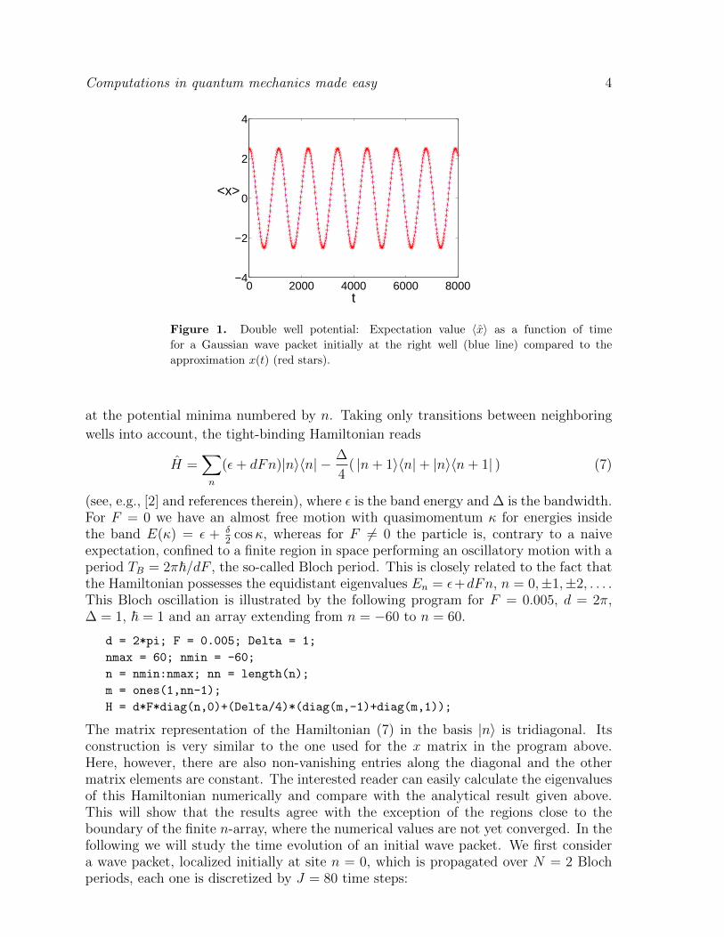
comparison with the approximation x(t) = x0 cos((E1 − E0)t) as shown in figure 1.

As a second application let us consider an extended one-dimensional system, a

particle in a periodic potential V0(x+ d) = V0(x) accelerated by a constant force F :

V (x) = V0(x) + Fx (6)

In the tight-binding approximation, the Hamiltonian is expressed in terms of the

Wannier states |n〉 of the lowest band of the periodic potential, which are localized


0 2000 4000 6000 8000−4

−2

0

2

4

t

<x>

Figure 1. Double well potential: Expectation value 〈x〉 as a function of time

for a Gaussian wave packet initially at the right well (blue line) compared to the

approximation x(t) (red stars).

at the potential minima numbered by n. Taking only transitions between neighboring

wells into account, the tight-binding Hamiltonian reads

H =∑n

(ε+ dFn)|n〉〈n| − ∆

4( |n+ 1〉〈n|+ |n〉〈n+ 1| ) (7)

(see, e.g., [2] and references therein), where ε is the band energy and ∆ is the bandwidth.For F = 0 we have an almost free motion with quasimomentum κ for energies insidethe band E(κ) = ε + δ

2cosκ, whereas for F 6= 0 the particle is, contrary to a naive

expectation, confined to a finite region in space performing an oscillatory motion with aperiod TB = 2π~/dF , the so-called Bloch period. This is closely related to the fact thatthe Hamiltonian possesses the equidistant eigenvalues En = ε+dFn, n = 0,±1,±2, . . . .This Bloch oscillation is illustrated by the following program for F = 0.005, d = 2π,∆ = 1, ~ = 1 and an array extending from n = −60 to n = 60.

d = 2*pi; F = 0.005; Delta = 1;

nmax = 60; nmin = -60;

n = nmin:nmax; nn = length(n);

m = ones(1,nn-1);

H = d*F*diag(n,0)+(Delta/4)*(diag(m,-1)+diag(m,1));

The matrix representation of the Hamiltonian (7) in the basis |n〉 is tridiagonal. Itsconstruction is very similar to the one used for the x matrix in the program above.Here, however, there are also non-vanishing entries along the diagonal and the othermatrix elements are constant. The interested reader can easily calculate the eigenvaluesof this Hamiltonian numerically and compare with the analytical result given above.This will show that the results agree with the exception of the regions close to theboundary of the finite n-array, where the numerical values are not yet converged. In thefollowing we will study the time evolution of an initial wave packet. We first considera wave packet, localized initially at site n = 0, which is propagated over N = 2 Blochperiods, each one is discretized by J = 80 time steps:


% initial state (gaussian)

psi = 0*n; psi(-nmin+1) = 1; % initial state (localized)

% time propagation (N Bloch periods, J steps each)

J = 80; N = 2;

Psi = zeros(nn,N*J+1);

Psi(:,1) = psi;

U = expm(-i*H*2*pi/d/F/J);

for nt = 1:N*J

Psi(:,nt+1) = U*Psi(:,nt);

end

t = 0:N*J; t = t/J;

imagesc(t,n,abs(Psi))

set(gca,’ydir’,’normal’,’FontSize’,20)

xlabel(’t/T_B’,’FontSize’,20)

ylabel(’n’,’rotation’,0,’FontSize’,20)

t/TB

n

0 0.5 1 1.5 2−60

−40

−20

0

20

40

60

t/TB

n

0 0.5 1 1.5 2−60

−40

−20

0

20

40

60

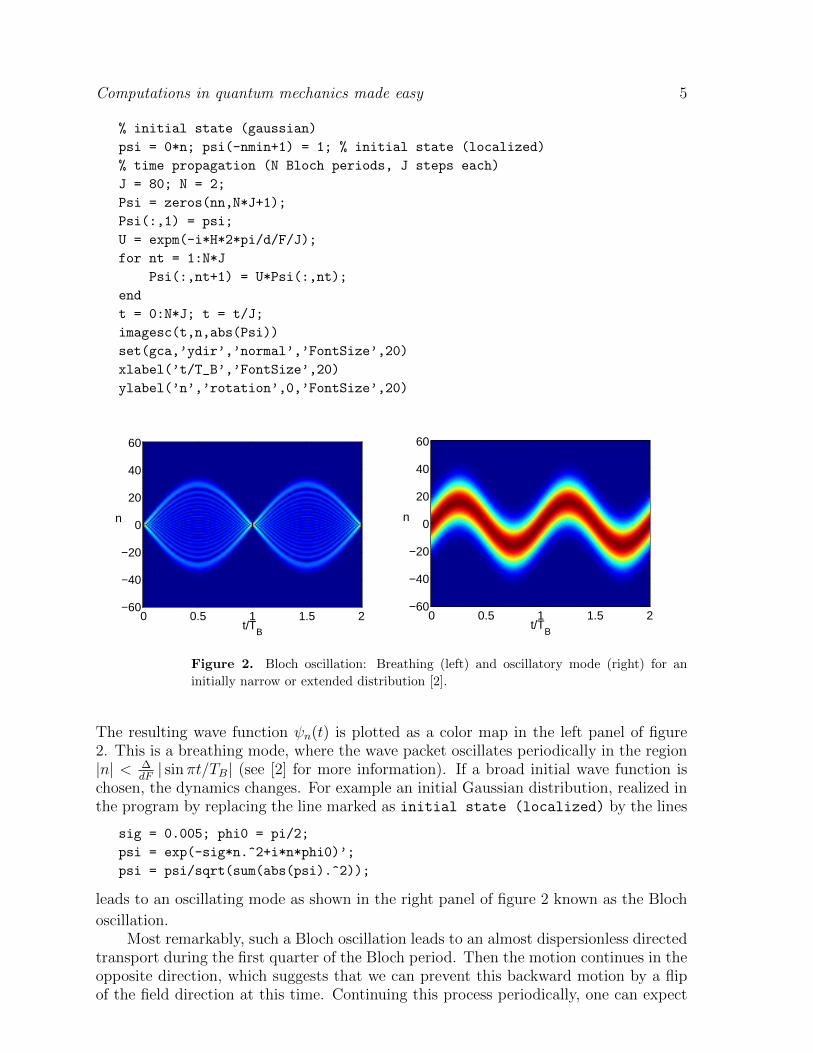
Figure 2. Bloch oscillation: Breathing (left) and oscillatory mode (right) for an

initially narrow or extended distribution [2].

The resulting wave function ψn(t) is plotted as a color map in the left panel of figure2. This is a breathing mode, where the wave packet oscillates periodically in the region|n| < ∆

dF| sinπt/TB| (see [2] for more information). If a broad initial wave function is

chosen, the dynamics changes. For example an initial Gaussian distribution, realized inthe program by replacing the line marked as initial state (localized) by the lines

sig = 0.005; phi0 = pi/2;

psi = exp(-sig*n.^2+i*n*phi0)’;

psi = psi/sqrt(sum(abs(psi).^2));

leads to an oscillating mode as shown in the right panel of figure 2 known as the Bloch

oscillation.Most remarkably, such a Bloch oscillation leads to an almost dispersionless directed

transport during the first quarter of the Bloch period. Then the motion continues in theopposite direction, which suggests that we can prevent this backward motion by a flipof the field direction at this time. Continuing this process periodically, one can expect


a directed dispersionless transport. To study such a field-flip system numerically, wefirst replace the second line in the program above by nmax = 160;nmin = -40; and theHamiltonian H by the two lines

Hp =+d*F*diag(n,0)+(Delta/4)*(diag(m,-1)+diag(m,1));

Hm =-d*F*diag(n,0)+(Delta/4)*(diag(m,-1)+diag(m,1));

defining Hamiltonians with different signs of F . As an initial state, a Gaussian is chosenand, for the time-propagation, the corresponding time-evolution operators are defined,which are then applied alternately during the subsequent Bloch periods:

Up = expm(-i*Hp*2*pi/d/F/J);

Um = expm(-i*Hm*2*pi/d/F/J);

nn = 0;

for nb = 1:2*N

for nt = 1:J/4

nn = nn+1;

Psi(:,nn+1) = Up*Psi(:,nn);

end

for nt = 1:J/4

nn = nn+1;

Psi(:,nn+1) = Um*Psi(:,nn);

end

end

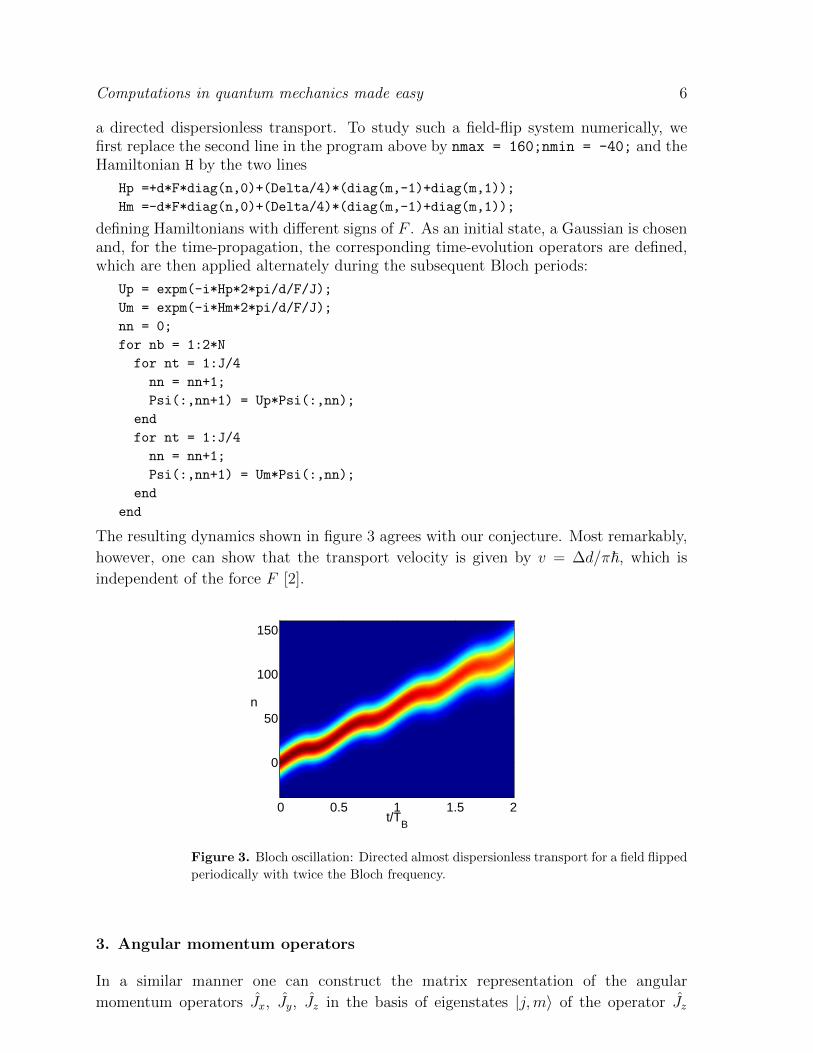
The resulting dynamics shown in figure 3 agrees with our conjecture. Most remarkably,

however, one can show that the transport velocity is given by v = ∆d/π~, which is

independent of the force F [2].

t/TB

n

0 0.5 1 1.5 2

0

50

100

150

Figure 3. Bloch oscillation: Directed almost dispersionless transport for a field flipped

periodically with twice the Bloch frequency.

3. Angular momentum operators

In a similar manner one can construct the matrix representation of the angular

momentum operators Jx, Jy, Jz in the basis of eigenstates |j,m〉 of the operator Jz


with eigenvalues m = −j, −j + 1, . . . ,+j, where j ≥ 0 is the total angular momentum,

which is an even or odd multiple of 12. First we construct the ladder operators J+ and

J− = J†+ with J+|j,m〉 =√j(j + 1)−m(m+ 1) |j,m+1〉 and the relations

Jx = 12

(J− + J+) , Jy = i2

(J− − J+) , Jz = 12[J+, J−] (8)

coded in the following program lines for j = 2:

j = 2; m = -j:j-1;

Jp = diag(sqrt(j*(j+1)-m.*(m+1)),1); Jm = Jp’;

Jx = (Jm+Jp)/2;

Jy = -i*(Jm-Jp)/2;

Jz = (Jp*Jm-Jm*Jp)/2;

If desired, one can check here the angular momentum commutation relations [Jx, Jy] =

iJz by means of Jx*Jy-Jy*Jx-i*Jz, which should yield the zero matrix. As an

application, one can calculate the energy eigenvalues of the rigid body Hamiltonian

(~ = 1)

H =J2x

2Ix+J2y

2Iy+J2z

2Iz, (9)

where the Ix, Iy and Iz are the principal moments of inertia. For a symmetric top, the

eigenvalues of the Hamiltonian are well known, namely

Ejk =j(j + 1)

2Ix+( 1

2Iz− 1

2Ix

)k2 , k = −j, . . . , j (10)

for Ix = Iy 6= Iz. For an asymmetric top, however, the eigenvalues for the special casesj = 1, 2, 3 are given in [3], but no general formula exists. This motivates, of course, anumerical approach, which is achieved by adding the program lines

Ix = 1/3; Iy = 1/2; Iz = 1;

H = Jx^2/2/Ix+Jy^2/2/Iy+Jz^2/2/Iz;

E = eig(H)’

in order to calculate the energy eigenvalues of an asymmetric top with Ix = 1/3,

Iy = 1/2 and Iz = 1 for j = 2. Note, however, that for this system body-fixed angular

momenta must be used with commutation relations [Jx, Jy] = −iJz (see, e.g., [3,4] for an

explanation). This can be achieved by changing the sign of the matrix representing Jy.

This subtlety does not affect the eigenvalues of the Hamiltonian (9) because it depends

only of the squares of the operators. The numerical eigenvalues

E = 4.2679 4.5000 6.0000 7.5000 7.7321

given by the program agree with the formulas in [3]:

E1 =2

Iz+

1

2Ix+

1

2Iy, E2 =

2

Iy+

1

2Iz+

1

2Ix, E3 =

2

Ix+

1

2Iy+

1

2Iz,

E4,5 =1

Ix+

1

Iy+

1

Iz±

√( 1

Ix+

1

Iy+

1

Iz

)2

− 3( 1

IxIy+

1

IyIz+

1

IzIx

). (11)

Such a small value as j = 2 is, of course, not a challenge for a computational

treatment. The interested reader may try, for instance, the larger angular momentum


0.5 1 1.50

20

40

60

80

100

E/j2

∆ N

/∆ E

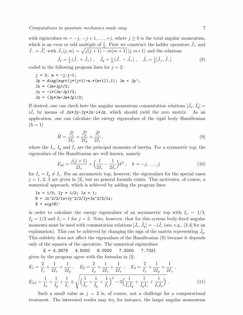
Figure 4. Asymmetric top: Histogram of the density of energy eigenvalues for

rotational momentum j = 1000 showing a pronounced spike at the classical energy

at the saddle point of the energy surface.

j = 1000 and analyze the distribution of the eigenvalues by plotting the state density

via hist(E/j^2,50). The resulting distribution in figure 4 shows a clear restriction to

an energy interval and a pronounced maximum. This structure can be understood by

the observation that for large angular momentum the system behaves almost classically.

Here the classical dynamics is restricted to a sphere with constant angular momentum

| ~J | = j and the energy function H = J2x

2Ix+

J2y

2Iy+ J2

z

2Izpossesses two minima, two maxima

and two saddle points on the angular momentum sphere. For the parameters used in

the program, the energy at the minima is Emin/j2 = 1/(2Iz) = 0.5, at the maxima

Emax/j2 = 1/(2Ix) = 1.5, and at the saddle point Esad/j

2 = 1/(2Iy) = 1. This

explains the restriction of the quantum energy eigenvalues to the classically allowed

region Emin < E < Emax. Furthermore, the quantum state density at the extrema is

approximately equal to the period of the classical orbits divided by 2π, which explains

the spike in the figure at the location of saddle point energy because the period at the

saddle point is infinite. Note that for j →∞ the quantum density also diverges at the

saddle point energy. An additional application of the angular momentum operators can

be found in section 5 below.

4. Two-dimensional systems

For a particle bound in a two-dimensional potential, the Hamiltonian

H =p2

1

2m+

p22

2m+ V (x1, x2) , (12)

can be conveniently expressed in the way described above by means of the tensor

product, i.e. the Kronecker product kron provided by Matlab . Denoting the position

operator for one degree of freedom as x and the corresponding identity operator as I,

the position operator for the two particles are x1 = x ⊗ I and x2 = I ⊗ x. The same


expressions appear for the momentum operators.

As an example the program described below computes the lowest energy eigenvalues

for the Pullen-Edmonds potential [5]

V (x1, x2) = 12x2

1 + 12x2

2 + αx21x

22 (13)

for α = 0.5. This potential has been employed in a number of studies related to

quantum chaos and also found applications to various molecular systems. The symmetry

group of the Hamiltonian is C4v and the eigenstates can be classified by the irreducible

representation A1,2, B1,2 and E [5]. The wave functions with symmetry A1 or B2 are

symmetric if x1 and x2 are interchanged, those with A2 or B1 symmetry antisymmetric.

If, on the other hand, the xj are changed to −xj, the A1 or B1 wave functions are

unaffected and the A2 or B2 wave functions change sign. In a harmonic oscillator

expansion

ϕ(x1, x2) =∞∑

n,m=0

Cnmϕn(x1)ϕm(x2) (14)

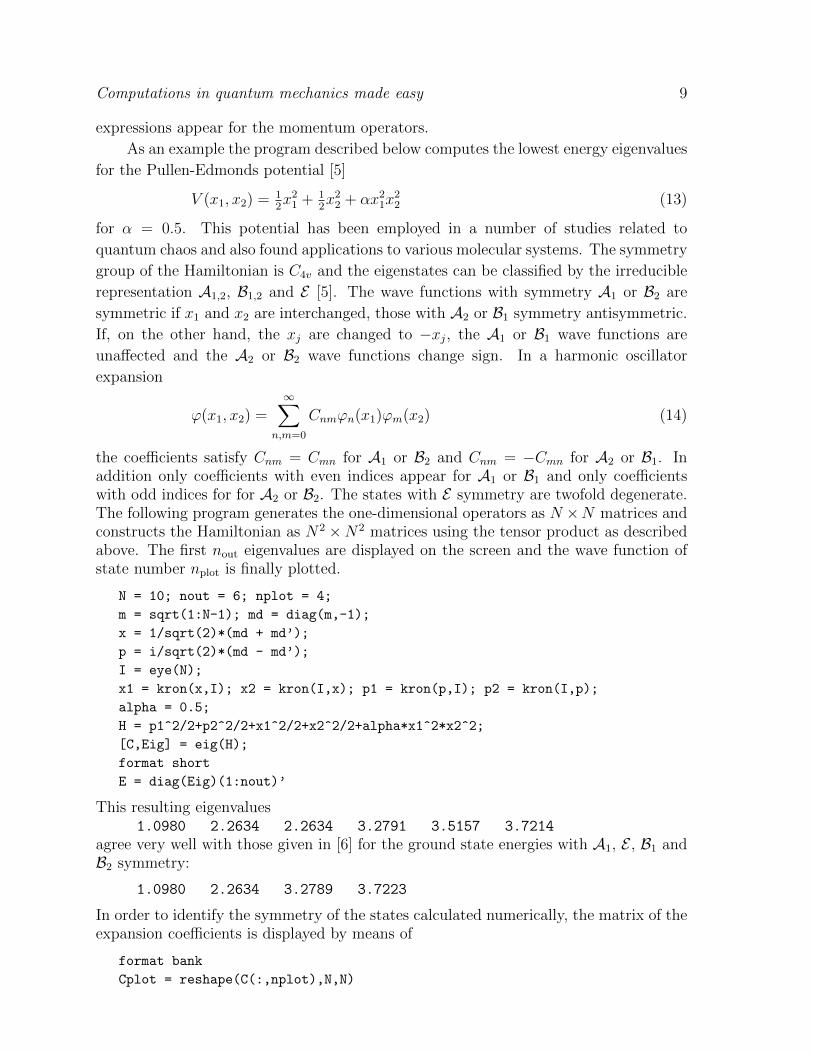
the coefficients satisfy Cnm = Cmn for A1 or B2 and Cnm = −Cmn for A2 or B1. Inaddition only coefficients with even indices appear for A1 or B1 and only coefficientswith odd indices for for A2 or B2. The states with E symmetry are twofold degenerate.The following program generates the one-dimensional operators as N ×N matrices andconstructs the Hamiltonian as N2 ×N2 matrices using the tensor product as describedabove. The first nout eigenvalues are displayed on the screen and the wave function ofstate number nplot is finally plotted.

N = 10; nout = 6; nplot = 4;

m = sqrt(1:N-1); md = diag(m,-1);

x = 1/sqrt(2)*(md + md’);

p = i/sqrt(2)*(md - md’);

I = eye(N);

x1 = kron(x,I); x2 = kron(I,x); p1 = kron(p,I); p2 = kron(I,p);

alpha = 0.5;

H = p1^2/2+p2^2/2+x1^2/2+x2^2/2+alpha*x1^2*x2^2;

[C,Eig] = eig(H);

format short

E = diag(Eig)(1:nout)’

This resulting eigenvalues1.0980 2.2634 2.2634 3.2791 3.5157 3.7214

agree very well with those given in [6] for the ground state energies with A1, E , B1 andB2 symmetry:

1.0980 2.2634 3.2789 3.7223

In order to identify the symmetry of the states calculated numerically, the matrix of theexpansion coefficients is displayed by means of

format bank

Cplot = reshape(C(:,nplot),N,N)


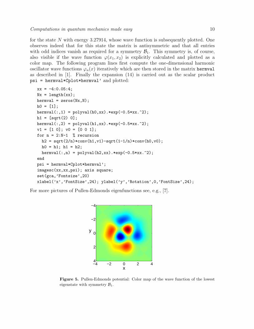
for the state N with energy 3.27914, whose wave function is subsequently plotted. Oneobserves indeed that for this state the matrix is antisymmetric and that all entrieswith odd indices vanish as required for a symmetry B1. This symmetry is, of course,also visible if the wave function ϕ(x1, x2) is explicitly calculated and plotted as acolor map. The following program lines first compute the one-dimensional harmonicoscillator wave functions ϕn(x) iteratively which are then stored in the matrix hermval

as described in [1]. Finally the expansion (14) is carried out as the scalar productpsi = hermval*Cplot*hermval’ and plotted:

xx = -4:0.05:4;

Nx = length(xx);

hermval = zeros(Nx,N);

h0 = [1];

hermval(:,1) = polyval(h0,xx).*exp(-0.5*xx.^2);

h1 = [sqrt(2) 0];

hermval(:,2) = polyval(h1,xx).*exp(-0.5*xx.^2);

v1 = [1 0]; v0 = [0 0 1];

for n = 2:N-1 % recursion

h2 = sqrt(2/n)*conv(h1,v1)-sqrt(1-1/n)*conv(h0,v0);

h0 = h1; h1 = h2;

hermval(:,n) = polyval(h2,xx).*exp(-0.5*xx.^2);

end

psi = hermval*Cplot*hermval’;

imagesc(xx,xx,psi); axis square;

set(gca,’Fontsize’,20)

xlabel(’x’,’FontSize’,24); ylabel(’y’,’Rotation’,0,’FontSize’,24);

For more pictures of Pullen-Edmonds eigenfunctions see, e.g., [7].

x

y

−4 −2 0 2 4

−4

−2

0

2

4

Figure 5. Pullen-Edmonds potential: Color map of the wave function of the lowest

eigenstate with symmetry B1.


5. Many-particle systems

A prominent example of a many-particle quantum system is the N -particle Bose-

Hubbard system [8], which is one of the basic models studied in theoretical investigations

of the dynamics of many particles on a lattice. Numbering the lattice sites by n, the

operators an and a†n with [an, a†n] = 1 describe annihilation and creation of a particle at

site n and a†nan is the particle number operator at site n. These operators for different

sites commute. Then the hermitian operators a†n+1an describe the destruction of a

particle at site n and the creation at site n + 1, and a†nan+1 + a†n+1an the hopping of

a particle between these sites. If the particles interact with each other the interaction

energy is proportional to the product of the particle number operators. In many cases

this interaction is short ranged, so that only the interaction of particles on the same

site must be taken into account. Let us confine ourselves here to the simple case of a

two-site system, the Bose-Hubbard dimer, with Hamiltonian

H = ε(a†1a1 − a†2a2) + v(a†1a2 + a†2a1) + c(a†1a1 − a†2a2)2 , (15)

where ±ε are the site energies, v the hopping and c the interaction strength. The

Hamiltonian commutes with the particle number operator N = a†1a1 + a†2a2, i.e. the

particle number N is conserved.

It is of interest to realize that the Bose-Hubbard dimer also appears naturally for a

collection of N bosonic atoms in a double-well potential, which is deep enough so that

only the lowest state in each well is populated. In this two-mode approximation the

system can be described by the Hamiltonian (15).The following Matlab program calculates the eigenvalues of the Hamiltonian (15).

First the creation and annihilation operators at the two sites are constructed by meansof the kron product as well as the Hamiltonian, whose eigenvalues and eigenstates arethen calculated for N = 24, i.e. a matrix dimension of Np = N + 1 = 25 for the singleparticle operators a:

N = 24; Np = N+1; Nout = 10; epsilon = 1; v = 1; c = 1;

a = diag(sqrt(1:N),1); ad = a’; I = eye(Np);

a1 = kron(a,I); ad1 = a1’;

a2 = kron(I,a); ad2 = a2’;

H = epsilon*(ad1*a1-ad2*a2)+v*(ad1*a2+ad2*a1)+c/2*(ad1*a1-ad2*a2)^2;

[C,E] = eig(H); E = diag(E);

One should be aware of the fact that the many-particle operators are represented byN2p × N2

p matrices and therefore one obtains N2p = 625 energy eigenvalues, however

not all of them are fully converged because of the restricted basis set |n1, n2〉, n1,2 =0, 1, . . . , N . All eigenstates populating only this restricted basis set are accuratelyrepresented, i.e. those with particle numbers up to N , a number of Np(Np + 1)/2 states.To illustrate this, the following program lines compute for all calculated eigenstates theexpectation values 〈N〉 of the number operator, which agree with the exact particle

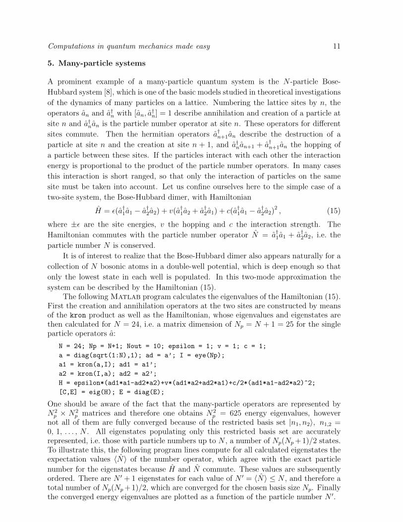
number for the eigenstates because H and N commute. These values are subsequentlyordered. There are N ′ + 1 eigenstates for each value of N ′ = 〈N〉 ≤ N , and therefore atotal number of Np(Np+ 1)/2, which are converged for the chosen basis size Np. Finallythe converged energy eigenvalues are plotted as a function of the particle number N ′.


Nav = diag(C’*(ad1*a1+ad2*a2)*C);

[Nav,index] = sort(Nav);

E = E(index);

plot(Nav(1:Np*(Np+1)/2),E(1:Np*(Np+1)/2),’b*’)

set(gca,’ydir’,’normal’,’FontSize’,20); axis([0 25 -50 350])

xlabel(’<N>’,’FontSize’,20); ylabel(’E_n’,’rotation’,0,’FontSize’,20)

0 5 10 15 20 25

0

100

200

300

<N>

En

Figure 6. Bose-Hubbard dimer: Energy eigenvalues as a function of the particle

number N .

In many applications, one is only interested in the eigenvalues and eigenstates ofthe Hamiltonian for a prescribed value N of the particle number. Then one can makeuse of the following trick: An extra term −λ(a†1a1 + a†2a2 − N) (λ ε, v) is added tothe Hamiltonian which does not affect the states with the given particle number N butwhich shifts the states with different particle numbers to high energies. The desiredeigenvalues can then be obtained by extracting the low-energy part of the spectrum ofthe resulting effective Hamiltonian as implemented in the following program:

N = 6; Np = N+1;

epsilon = 1; v = 1; c = 1;

a = diag(sqrt(1:Np-1),1); ad = a’; I = eye(Np);

a1 = kron(a,I); ad1 = a1’;

a2 = kron(I,a); ad2 = a2’;


% extraction of eigenvalues for particle number N

lambda = 10000;

H1 = H-lambda.*(ad1*a1+ad2*a2-N*kron(I,I));

E1 = eig(H1);

% filtering in two steps

E2 = E1.*(abs(E1)<10*epsilon.*N);

E = E2(find(E2))’

Calculated are the seven eigenvalues for N = 6 with the result

E = -4.792349 0.078611 4.347781 6.348595 12.731351 12.786011 24.500000


A more sophisticated alternative method leading to the same results for theeigenvalues consists in computing the Hamiltonian HN for a fixed particle numberN by projecting the original Hamiltonian H on the corresponding eigenstates of thenumber operator a†1a1 + a†2a2. Since the latter is a represented by a diagonal matrix, theimplementation is rather straightforward:

N_op = ad1*a1+ad2*a2;

iN=find(abs(diag(N_op)-N)<10^-6);

N_p=N_op(:,iN)./N;

H_N = N_p’*H*N_p;

E = eig(H_N)

For the Bose-Hubbard dimer, there is, however, a much more convenient way to

describe the system for a fixed particle number N . The Jordan-Schwinger representation

Jx = (a†1a2 + a†2a1)/2,

Jy = (a†1a2 − a†2a1)/2i, (16)

Jz = (a†1a1 − a†2a2)/2

transforms the system to angular momentum operators. The Hamiltonian (15) then

takes the form

H = 2εJz + 2vJx + 2cJ2z (17)

and the total angular momentum is J = N/2. Using the matrix representation ofangular momentum operators discussed in section 3, this Hamiltonian can be easilycoded in the following Matlab program:

N = 6; j = N/2; m = -j:j-1;

Jp = diag(sqrt(j*(j+1)-m.*(m+1)),1);

Jm = Jp’;

Jx = (Jm+Jp)/2;

Jy = i*(Jm-Jp)/2;

Jz = (Jp*Jm-Jm*Jp)/2;

epsilon = 1; v = 1; c = 1;

H = 2*epsilon*Jz+2*v*Jx+2*c*Jz^2;

E = eig(H)’

The results agree precisely with those given above for N = 6.

In the case of high matrix dimensions time and memory can be saved by using

sparse matrices. In Matlab this can be implemented straightforwardly, e.g. the

sparse matrix representation of the annihilation operator and the identity in an

N + 1-dimensional space are given by a = sparse(diag(sqrt(1:N),1)) and I =

speye(N+1) respectively. This automatically leads to a sparse matrix representation

of the Hamiltonian H. This already becomes relevant if the Bose-Hubbard dimer is

extended by an additional site. Such a Bose-Hubbard trimer, as described by the

Hamiltonian

H =3∑j=1

[− K

2

(eiΦ/3 a†j+1aj + e−iΦ/3 a†j aj+1

)+U

2a†j a†j aj aj

](18)


was considered in [9]. Here we identify site number 4 with site number 1, i.e. the three

sites form a triangular structure which constitutes a minimal model for a superfluid

circuit of a Bose-Einstein condensate. The additional phase factors in the hopping term

describe the influence of an applied magnetic flux Φ (in scaled dimensionless units) or

alternatively a rotation of the system with a frequency Ω ∝ Φ (see [9] for more details).The following program computes the eigenvalues En, eigenstates |n〉 and the

expectation values of the current Jn = 〈n|J |n〉 = 〈n|∂H∂Φ|n〉 and plots the results:

ND = 3*10+3; N = ND-1

K = 1; Phi = 0.8*pi; u = 0.5

U = K*u/N

u_qm = 3*u/N.^2

a = sparse(diag(sqrt(1:ND-1),1)); ad = a’; I=speye(ND);

a1 = kron(kron(a,I),I); ad1 = a1’;

a2 = kron(kron(I,a),I); ad2 = a2’;

a3 = kron(kron(I,I),a); ad3 = a3’;

N_op = ad1*a1+ad2*a2+ad3*a3;

iN = find(abs(diag(N_op)-N)<10^-6);

N_p = N_op(:,iN)./N;

H = -K/2*(exp(i*Phi/3)*(ad2*a1+ad3*a2+ad1*a3) ...

+exp(-i*Phi/3)*(ad1*a2+ad3*a1+ad2*a3)) ...

+U/2*(ad1^2*a1^2+ad2^2*a2^2+ad3^2*a3^2);

H_N = N_p’*H*N_p;

[C,E] = eig(full(H_N)); E = diag(E)/u;

dH_dPhi = -K/2*(-i/3*exp(i*Phi/3)*(ad2*a1+ad3*a2+ad1*a3) ...

+i/3*exp(-i*Phi/3)*(ad1*a2+ad3*a1+ad2*a3));

dH_dPhi_N = N_p’*dH_dPhi*N_p;

Jav = real(diag(C’*dH_dPhi_N*C));

plot(Jav,E,’o’,’markerfacecolor’,’r’,’markeredgecolor’,’r’)

set(gca,’ydir’,’normal’,’FontSize’,20);

xlabel(’<J>’,’FontSize’,20); ylabel(’E_n/u’,’rotation’,90,’FontSize’,20)

axis square

(depending on the Matlab version used it may be required to replace eig(H_N) by

eig(full(H_N)).)

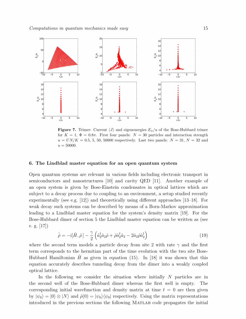
Figure 7 shows the distribution of the eigenstates with respect to the eigenenergies

and the currents. For noninteracting particles, u = UN/K = 0, the current J commutes

with the Hamiltonian and each eigenstate carries a quantized current, forming a triangle

in the energy-current plane as explained in [9]. For an integer filling N = 30 = 10 · 3of the trimer, the eigenstates are more and more redistributed along the line indicating

zero current with increasing interaction u. In the high interaction limit, even the ground

state becomes a zero current and thus an insulator state. This is a signature of a so-

called superfluid to Mott insulator transition, illustrated by the first four panels. In

contrast, for a non-integer filling per site the ground state always carries a current even

in the strong interaction limit as shown for N = 31 and N = 32 in the last two panels.

More about the rich behavior of this three site Bose-Hubbard system can be found in [9].


−10 −5 0 5 10−50

0

50

100

<J>

En/u

−10 −5 0 5 100

5

10

15

20

<J>

En/u

−10 −5 0 5 10

4

6

8

10

12

14

16

<J>

En/u

−10 −5 0 5 10

4

6

8

10

12

14

16

<J>

En/u

−10 −5 0 5 10

4

6

8

10

12

14

16

<J>

En/u

−10 −5 0 5 10

4

6

8

10

12

14

16

<J>

En/u

Figure 7. Trimer: Current 〈J〉 and eigenenergies En/u of the Bose-Hubbard trimer

for K = 1, Φ = 0.8π. First four panels: N = 30 particles and interaction strength

u = UN/K = 0.5, 5, 50, 50000 respectively. Last two panels: N = 31, N = 32 and

u = 50000.

6. The Lindblad master equation for an open quantum system

Open quantum systems are relevant in various fields including electronic transport in

semiconductors and nanostructures [10] and cavity QED [11]. Another example of

an open system is given by Bose-Einstein condensates in optical lattices which are

subject to a decay process due to coupling to an environment, a setup studied recently

experimentally (see e.g. [12]) and theoretically using different approaches [13–18]. For

weak decay such systems can be described by means of a Born-Markov approximation

leading to a Lindblad master equation for the system’s density matrix [19]. For the

Bose-Hubbard dimer of section 5 the Lindblad master equation can be written as (see

e. g. [17])

˙ρ = −i[H, ρ ]− γ

2

(a†2a2ρ+ ρa†2a2 − 2a2ρa

†2

)(19)

where the second term models a particle decay from site 2 with rate γ and the first

term corresponds to the hermitian part of the time evolution with the two site Bose-

Hubbard Hamiltonian H as given in equation (15). In [18] it was shown that this

equation accurately describes tunneling decay from the dimer into a weakly coupled

optical lattice.

In the following we consider the situation where initially N particles are in

the second well of the Bose-Hubbard dimer whereas the first well is empty. The

corresponding initial wavefunction and density matrix at time t = 0 are then given

by |ψ0〉 = |0〉 ⊗ |N〉 and ρ(0) = |ψ0〉〈ψ0| respectively. Using the matrix representations

introduced in the previous sections the following Matlab code propagates the initial


density matrix according to equation (19) by means of a predictor corrector integrator

[20]. The expectation values of the time-dependent site occupations are then obtained

via nj(t) = trace (ρ(t) a†j aj).

0 50 100Time t

0

0.5

1

Rel

ativ

e pa

rtic

le n

umbe

r

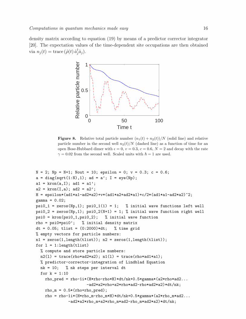
Figure 8. Relative total particle number (n1(t) + n2(t))/N (solid line) and relative

particle number in the second well n2(t)/N (dashed line) as a function of time for an

open Bose-Hubbard dimer with ε = 0, v = 0.3, c = 0.6, N = 2 and decay with the rate

γ = 0.02 from the second well. Scaled units with ~ = 1 are used.

N = 2; Np = N+1; Nout = 10; epsilon = 0; v = 0.3; c = 0.6;

a = diag(sqrt(1:N),1); ad = a’; I = eye(Np);

a1 = kron(a,I); ad1 = a1’;

a2 = kron(I,a); ad2 = a2’;


gamma = 0.02;

psi0_1 = zeros(Np,1); psi0_1(1) = 1; % initial wave functions left well

psi0_2 = zeros(Np,1); psi0_2(N+1) = 1; % initial wave function right well

psi0 = kron(psi0_1,psi0_2); % initial wave function

rho = psi0*psi0’; % initial density matrix

dt = 0.05; tlist = (0:2000)*dt; % time grid

% empty vectors for particle numbers:

n1 = zeros(1,length(tlist)); n2 = zeros(1,length(tlist));

for l = 1:length(tlist)

% compute and store particle numbers:

n2(l) = trace(rho*ad2*a2); n1(l) = trace(rho*ad1*a1);

% predictor-corrector-integration of Lindblad Equation

nk = 10; % nk steps per interval dt

for k = 1:10

rho_pred = rho-1i*(H*rho-rho*H)*dt/nk+0.5*gamma*(a2*rho*ad2...

-ad2*a2*rho+a2*rho*ad2-rho*ad2*a2)*dt/nk;

rho_m = 0.5*(rho+rho_pred);

rho = rho-1i*(H*rho_m-rho_m*H)*dt/nk+0.5*gamma*(a2*rho_m*ad2...

-ad2*a2*rho_m+a2*rho_m*ad2-rho_m*ad2*a2)*dt/nk;


end;

end;

figure(1) % plot of particle number expectation value (right well)

hold on

plot(tlist,n2/N,’r--’); plot(tlist,(n1+n2)/N,’b’);

box on

xlabel(’Time t’); ylabel(’Relative particle number’)

Figure 8 shows the resulting decay dynamics of the relative total particle number

(n1(t)+n2(t))/N (solid line) and the relative particle number in the second well n2(t)/N

for a symmetric double well with ε = 0, tunneling coefficient v = 0.3, interaction

constant c = 0.6, decay rate γ = 0.02 and an initial particle number N = 2.

In a non-interacting open dimer, the occupation n2(t)/N would yield exponentially

damped cosine-shaped Rabi oscillations. We clearly observe how this behavior is

modified by the interaction between the particles. Various Fourier components occur

which result from different excitation energies in the spectrum of the interacting bosonic

system.

7. Concluding remarks

Matrix representation techniques were presented and illustrated by a variety of different

examples demonstrating both their simplicity and wide applicability. These qualities

make them suitable for use in research projects as well as quantum mechanics courses

for undergraduate and graduate students.

Acknowledgments

The authors would like to thank Eva-Maria Graefe for careful reading of the manuscript

and for all valuable comments and suggestions.

References

[1] M. Gluck and H. J. Korsch, Eur. J. Phys. 23 (2002) 413

[2] T. Hartmann, F. Keck, H. J. Korsch, and S. Mossmann, New J. Phys. 6 (2004) 2

[3] L. D. Landau and E. M. Lifshitz, Quantum Mechanics, Pergamon Press, New York, 1977

[4] L. E. Ballentine, Quantum Mechanics – A Modern Development, World Scientific, Singapore, 2006

[5] R. A. Pullen and A. R. Edmonds, J. Phys. A 14 (1981) L477

[6] P. Amore and F. M. Fernandez, Phys. Scripta 80 (2009) 055002

[7] S. K. Joseph,, 2014. www.youtube.com/watch?v=gVAyZ47Iw7Q

[8] L. Pitaevskii and S. Stringari, Bose-Einstein Condensation, Oxford University Press, Oxford, 2003

[9] G. Arwas, A. Vardi, and D. Cohen, Phys. Rev. A 89 (2014) 013601

[10] M. Di Ventra, Electrical Transport in Nanoscale Systems, Cambridge University Press, Cambridge,

2008

[11] M. O. Scully and M. S. Zubairy, Quantum Optics, Cambridge University Press, Cambridge, 1997

[12] P. Wurtz, T. Langen, T. Gericke, A. Koglbauer, and H. Ott, Phys. Rev. Lett. 103 (2009) 80404


[13] K. Rapedius, C. Elsen, D. Witthaut, S. Wimberger, and H. J. Korsch, Phys. Rev. A 82 (2010)

063601

[14] A. U. J. Lode, A. I. Streltsov, O. E. Alon, H.-D. Meyer, and L. S. Cederbaum, J. Phys. B 42

(2009) 044018

[15] K. Rapedius and H. J. Korsch, Phys. Rev. A 86 (2012) 025601

[16] E. M. Graefe, H. J. Korsch, and A. E. Niederle, Phys. Rev. Lett 101 (2008) 150408

[17] D. Witthaut, F. Trimborn, and S. Wimberger, Phys. Rev. Lett. 101 (2008) 200402

[18] K. Rapedius, J. Phys. B 46 (2013) 125301

[19] H.-P. Breuer and F. Petruccione, The Theory of Open Quantum Systems, Oxford University Press,

Oxford, 2002

[20] W. H. Press, S. A. Teukolsky, W. T. Vetterling, and B. P. Flannery, Numerical Recipes, Cambridge

University Press, London, 3. edition, 2007

Documents

Computations in quantum mechanics made easy · Computations in quantum mechanics made easy 4 0 2000 4000 6000 8000-4-2 0 2 4 t ... which are then applied alternately during