Embed Size (px)
Citation preview
Joint Institute for Nuclear ResearchLaboratory of Information Technologies
E5,11-2001-279
COMPUTER ALGEBRAAND
ITS APPLICATION TO PHYSICS
CAAP-2001
Proceedings of International WorkshopDubna, Russia, June 28-30, 2001
Edited by V.P. Gerdt
Dubna 2002
Organizing Committee
Vladimir Gerdt (chairman)Sergue Vinitsky (vice-chairman)Alla Bogolubskaya (scientific secretary)Tatyana Donskova (secretary)Stanislav LukyanovVladimir KornyakYuri PaliiVitaly RostovtsevVasily SeveryanovAlexander ShevtsovAlla Zaikina
Computer Algebra and its Application to Physics. Proceedings of the Inter-national workshop (Dubna, June 28-30, 2001)/ Editor V.P.Gerdt.
This volume contains papers and abstracts of talks presented at the workshop oncomputer algebra algorithms, systems and software packages and their application tophysical and mathematical research and education. The collection consists of 34 fullpapers and 15 abstracts written by mathematicians, physicists and computer scientistsscientists who develop and use computer algebra methods and tools.
The material of the book appeals to readers from postgraduate students to researchersand university teachers of computational mathematics, physics and computer science.
2
Preface
The International workshop ”Computer Algebra and its Application to Physics”/CAAP-2001 took place at the Laboratory of Information Technologies of the Joint In-stitute for Nuclear Research (JINR) in Dubna, Russia, in June 28-30, 2001. This meetingwas supported by the Russian Foundation for Basic Research and the Scientific Center forApplied Research in JINR and brought together more than 70 scientists and researchersfrom Byelorussia, Bulgaria, Georgia, Germany, Canada, Poland, Russia, South Africa,Slovenia and Ukraine. Fifty two reports were presented at the workshop and their writ-ten forms as full papers or abstracts are contained in this volume.
This meeting was the fifth in a series of workshops on computer algebra and its ap-plication to physics were held in Dubna in 1979, 1982, 1985 and 1990. The workshopprovided a forum for researchers on computer algebra methods, algorithms and softwareand for those who use this tool in theoretical, mathematical and experimental physics,applied mathematics, engineering and education.
The CAAP-2001 workshop grew out of the recognition of the need for such a meet-ing based on the fact that, although there is a number of regular meetings of computeralgebraists and users of computer algebra systems, those meetings do not pay so much at-tention to specific needs of physical sciences as they did in 70th and 80th. We believe thatour workshop has helped to establish new links between algorithmic and software aspectsof computer algebra and those from research problems in natural sciences, especially inphysics.
It is my pleasure to acknowledge all contributors to these proceedings. Unfortunately,we did not received full papers for a number of interesting talks, and some full paperswere not accepted for the proceedings. For all these cases we decided to include abstractsof the talks.
Vladimir P. Gerdt
3
Contents
Abramov S.A., Petkovsek M.Minimal Multiplicative and Additive Decompositions of HypergeometricTerms in One Variable . . . . . . . . . . . . . . . . . . . . . . . . . . . . . . . . . . . . . . . . . . . . . 9
Altaisky M.V.On Some Algebraic Problems Arising in Quantum Mechanical Descrip-tion of Biological Systems . . . . . . . . . . . . . . . . . . . . . . . . . . . . . . . . . . . . . . . . . . 11
Bardin D., Passarino G., Kalinovskaya L., Christova P.,Andonov A., Bondarenko S., Nanava G.Project “CalcPHEP: Calculus for Precision High Energy Physics” . . . 12
Bochorishvili T., Grebenikov E.A.The Approximation of the Some Physical Processes by ExponentialFunctions . . . . . . . . . . . . . . . . . . . . . . . . . . . . . . . . . . . . . . . . . . . . . . . . . . . . . . . . . . 27
Czichowski G.Equivalence Transformations for Abel Equations - a PolynomialMethod . . . . . . . . . . . . . . . . . . . . . . . . . . . . . . . . . . . . . . . . . . . . . . . . . . . . . 30
Dimovski I., Spiridonova M.Numerical Solution of Boundary Value Problems for the Heat and Re-lated Equations . . . . . . . . . . . . . . . . . . . . . . . . . . . . . . . . . . . . . . . . . . . . . . . 32
Edneral V.F.On Families of Periodic Solutions of Low Resonant Case of the Gene-ralized Henon - Heiles System . . . . . . . . . . . . . . . . . . . . . . . . . . . . . . . . . . 43
Efimov G.B., Tshenkov I.B., Zueva E.Yu.Computer Algebra at KELDYSH Institute of Applied Mathematics . . . 52
Gareev F.A., Gareeva G.F.Conception of Universality of the Huygens Resonance SynchronizationPrinciple and Model for Structural Pecularities of Superconducting Sys-tems and Biomolecules . . . . . . . . . . . . . . . . . . . . . . . . . . . . . . . . . . . . . . . . 62
4
Galperin A.G., Dubovik V.M., Richvitsky V.S.Analytic Calculations for Some ODE with Quadratic Nonlinearity byContinuous-Group Methods and Vector-Field Analysis . . . . . . . . . . . . . 64
Gerdt V.P., Blinkov Yu.A.Janet Bases of Toric Ideals . . . . . . . . . . . . . . . . . . . . . . . . . . . . . . . . . . . . 71
Gerdt V.P., Khvedelidze A.M., Mladenov D.M.Analysis of Constraints in Light-Cone Version of SU(2) Yang-Mills Me-chanics . . . . . . . . . . . . . . . . . . . . . . . . . . . . . . . . . . . . . . . . . . . . . . . . . . . . . 83
Gerdt V.P., Yanovich D.A.Parallelism in Computing Janet Bases . . . . . . . . . . . . . . . . . . . . . . . . . . . 93
Glazunov N.M.On Algebraic Geometric and Computer Algebra Aspects of Mirror Sym-metry . . . . . . . . . . . . . . . . . . . . . . . . . . . . . . . . . . . . . . . . . . . . . . . . . . . . . . . 104
Golubitsky O.Differential Grobner Walk . . . . . . . . . . . . . . . . . . . . . . . . . . . . . . . . . . . . . 114
Govorukhin V.Application of Maple Package to Analysis of Fluid Dynamics and Ma-thematical Biology Problems . . . . . . . . . . . . . . . . . . . . . . . . . . . . . . . . . . . . 127
Grebenikov E.A., Jakubiak M., Kozak–Skoworodkin D.The Application of the Computing Algebra in Cosmic Dynamical Prob-lems . . . . . . . . . . . . . . . . . . . . . . . . . . . . . . . . . . . . . . . . . . . . . . . . . . . . . . . . 128
Grebenikov E.A., Olszanowski G., Siluszyk A.Stability of Equilibrium Points in Lagrange - Wintner Models . . . . . . . 137
Grebenikov E.A., Prokopenya A.N.Symbolic Computation Systems and the Many-Body Problem . . . . . . . 140
Grozin A.G.TEXmacs interfaces to Maxima, MuPAD and REDUCE . . . . . . . . . . . . . 149
5
Grozin A.Multiloop Calculations in Heavy Quark Effective Theory . . . . . . . . . . . 157
Gusev A., Samoilov V., Rostovtsev V. Vinitsky S.Maple Implementing Algebraic Perturbation Theory Algorithm: Hydro-gen Atom in Weak Electric Fields . . . . . . . . . . . . . . . . . . . . . . . . . . . . . . . 158
Hausdorf M., Seiler W.M.Completion to Involution and Symmetry Analysis . . . . . . . . . . . . . . . . . 169
Ivanov V.V.Chiral Lagrangian Approach to J/ψ + π → D + D∗ Process: ComputerAlgebra Calculations . . . . . . . . . . . . . . . . . . . . . . . . . . . . . . . . . . . . . . . . . . 180
Kalinina N.A., Prudnikov D.M.The FABULA System: Implementation on the Java Platform . . . . . . . 182
Kislenkov V.V.Iterative Evaluation of Functions over a Number of Points . . . . . . . . . 183
Komarova E.Computer Algebra Systems for Initial Boundary Value Problem withParameter . . . . . . . . . . . . . . . . . . . . . . . . . . . . . . . . . . . . . . . . . . . . . . . . . . . 184
Kondratieva M.V.Examples of Calculations of the Generators of Differential Ideal by ItsCharacteristic Set . . . . . . . . . . . . . . . . . . . . . . . . . . . . . . . . . . . . . . . . . . . . 185
Kornyak V.V.Extraction of “Minimal” Cochain Subcomplexes for Computing Coho-mologies of Lie Algebras and Superalgebras . . . . . . . . . . . . . . . . . . . . . . . 186
Makarevich N.A.Computation of the Characteristic Sets for the Euler Equations for Dif-ferent Rankings . . . . . . . . . . . . . . . . . . . . . . . . . . . . . . . . . . . . . . . . . . . . . . 196
6
Mechveliani S.D.Computer Algebra with Haskell: Applying Functional - Categorial-‘Lazy’Programming . . . . . . . . . . . . . . . . . . . . . . . . . . . . . . . . . . . . . . . . . . . . . . . . 203
Mitichkina A.M.On an Implementation of Desingularization of Linear Recurrence Ope-rators with Polynomial Coefficients . . . . . . . . . . . . . . . . . . . . . . . . . . . . . 212
Mityunin V.A., Zobnin A.I., Ovchinnikov A.I., Semyonov A.S.Involutive and Classical Grobner Bases Construction from The Compu-tational Viewpoint . . . . . . . . . . . . . . . . . . . . . . . . . . . . . . . . . . . . . . . . . . . . 221
Niukkanen A.W., Paramonova O.S.Computer Analysis of Hypergeometric Series: a Project of an Instruc-tion Set Duplicating Operations of the Factorization Method . . . . . . . . 231
Prokopenya A.N., Chichurin A.V.Investigation of Nonlinear Second and Third Orders Differential Equa-tions of P-Type with CAS MATHEMATICA . . . . . . . . . . . . . . . . . . . . . 245
Proskurin D., Pervushin V.N.Cosmological Creation of Vector Bosons and Integrals of Motion in Ge-neral Relativity . . . . . . . . . . . . . . . . . . . . . . . . . . . . . . . . . . . . . . . . . . . . . . . 253
Richvitsky V.S., Sapoznikov A.P., Galperin A.G.Analytical Design of SIMD Computer Application Software . . . . . . . . 254
Ryabenko A.Some Formal Solutions of LODE . . . . . . . . . . . . . . . . . . . . . . . . . . . . . . 260
Serdyukova S.I.Solving an Inverse Problem on Lattice by Using CAS REDUCE . . . . 261
Shapeev V.P.On Investigation of Involutivity of Differential Equation Systems in CASMATEMATICA . . . . . . . . . . . . . . . . . . . . . . . . . . . . . . . . . . . . . . . . . . . . . . 270
7
Sobolevsky S.Moveable Singularities of Polynomial Differential Equations . . . . . . . . 277
Suzko A.A.Bargmann-Darboux Transformations for Time-Dependent QuantumEquations . . . . . . . . . . . . . . . . . . . . . . . . . . . . . . . . . . . . . . . . . . . . . . . . . . . 291
Suzko A.A., Velicheva E.P.Analytic Modeling for Investigation of Quantum Systems in the Adia-batic Representation . . . . . . . . . . . . . . . . . . . . . . . . . . . . . . . . . . . . . . . . . . 301
Tchoupaeva I.J.Application of the Noncommutative Grobner Bases Method for ProvingGeometrical Statements in Coordinate-free Form . . . . . . . . . . . . . . . . . . 313
Tertychniy S.I.Program Package Intended for Internet-Based Access to Computer Al-gebra Resources . . . . . . . . . . . . . . . . . . . . . . . . . . . . . . . . . . . . . . . . . . . . . . 322
Vassiliev N.N., Kholshevnikov K.V.Geometry of Pairs of Keplerian Elliptic Orbits . . . . . . . . . . . . . . . . . . . 336
Vernov S.Yu.Exact and Asymptotic Solutions for the General Henon–HeilesSystem . . . . . . . . . . . . . . . . . . . . . . . . . . . . . . . . . . . . . . . . . . . . . . . . . . . . . . 337
Vinitsky S., Rostovtsev V., Gusev A.Extracting a Special Class of Integrable Systems with theBirkhoff-Gustavson Normalization of Polynomial Hamiltonians . . . . . 348
Zima E.V.On Numerical Stability of Polynomial Evaluation . . . . . . . . . . . . . . . . . 356
Index . . . . . . . . . . . . . . . . . . . . . . . . . . . . . . . . . . . . . . . . . . . . . . . . . . . . . . 357
8
Minimal Multiplicative and AdditiveDecompositions of Hypergeometric
Terms in One Variable
S. A. Abramova1, M. Petkovsekb2
a Computer Center of the Russian Academy of Science,Vavilova 40, Moscow 117967 Russia;
e-mail: [email protected] of Mathematics and Mechanics,
Faculty of Mathematics and Physics, University of Ljubljana,Jadranska 19, 1000 Ljubljana, Slovenia;
e-mail: [email protected]
In this talk we sum up our investigations [1, 2]. We describe a multiplicative nor-mal form for rational functions which exhibits the shift structure of the factors, andinvestigate its properties. On the basis of this form we propose an algorithm which,given a rational function R, extracts a rational part U from the indefinite product ofR:∏n
k=0 R(k) = U(n)∏n
k=0 V (k), where the numerator and denominator of the ratio-nal function V have the lowest possible degrees. This gives a minimal representation(or a minimal multiplicative decomposition) of the hypergeometric term
∏nk=0 R(k). For
example,
n−1∏k=0
(k + 3)(2k + 5)(3k + 1)(4k + 1)
(k + 1)(k + 4)(2k + 1)(3k + 4)= 4n (n + 1)(n + 2)(2n + 1)(2n + 3)
6(3n + 1)
n−1∏k=0
k + 14
k + 4.
We also present an algorithm which, given a hypergeometric term T (n), constructs hy-pergeometric terms T1(n) and T2(n) such that T (n) = ΔT1(n) + T2(n) (ΔT1(n) =T1(n + 1) − T1(n)) and T2(n) is minimal in some sense (see example below). This solvesthe decomposition problem for indefinite sums of hypergeometric terms: T1(n+1)−T1(n)is the “summable part” and T2(n) the “non-summable part” of T (n). In other words, weget a minimal additive decomposition of the hypergeometric term T (n). For example,(
−2n2 + 3n + 2
n2 + n
) n−1∏k=0
1
k + 2= Δ
(1
n
n−1∏k=0
1
k + 1
)− 1
n
n−1∏k=0
1
k + 1,
where the minimal representation 1n
∏n−1k=0
1k+1
of “non-summable” part has the rational
factor 1n
with the denominator of the lowest possible degree.
1Partially supported by the French-Russian Lyapunov Institute under grant 98-03.2Partially supported by MZT RS under grant J2-8549.
9

References
[1] S. A. Abramov and M. Petkovsek, Canonical representations of hypergeometricterms, In Proceedings FPSAC’01, 2001. To appear.
[2] S. A. Abramov and M. Petkovsek, Minimal decomposition of indefinite hypergeomet-ric sums, In Proceedings ISSAC’01, 2001. To appear.
10
On Some Algebraic ProblemsArising in Quantum MechanicalDescription of Biological Systems
M.V.Altaisky
Laboratory of Information Technologies,Joint Institute for Nuclear Research, Dubna, 141980 Russia;
The biological hierarchy and the differences between living and non-living matter areconsidered from the standpoint of quantum mechanics. Starting from the Schrodingerquestion “How the life can be understood from the standpoint of quantum mechanics?”,we analyze what algebraic constraints may be caused by a nontrivial “the part – thewhole” relation, when the state of a part is constrained by the state of the whole.
References
[1] M.V.Altaisky, quant-ph/0007023.
11
Project “CalcPHEP:Calculus for Precision High Energy
Physics”
D.Bardin, G.Passarino∗, L.Kalinovskaya, P.Christova, A.Andonov,S.Bondarenko, G.Nanava
Laboratory of Nuclear Problems, JINRJoliot-Curie, 6, Dubna, Moscow region, Russia;
e-mail: [email protected]∗ Dipartimento di Fisica Teorica, Universita di Torino, Italy
INFN, Sezione di Torino, Italy
Work supported by INTAS No00-00313 and by the European Union under contract HPRN-CT-2000-00149.
1 Introduction
The CalcPHEP collaboration joins the efforts of several groups of theorists known very wellin the field of theoretical support of various experiments in HEP, particularly at SLAC andLEP, (see, for instance [1], [2] and [3]). The first phase of the CalcPHEP system was realizedin the site http://brg.jinr.ru/ in 2000–2001. It is written mostly in FORM3, [4]. In this talk,we will describe the present status and our plans for the realization of next phases of theCalcPHEP project aimed at the theoretical support of experiments at modern and futureaccelerators: TEVATRON, LHC, electron Linear Colliders (LC’s) i.e. TESLA, NLC,CLIC, and muon factories. Within this project, we are creating a four-level computersystem which eventually must automatically calculate pseudo- and realistic observablesfor more and more complicated processes of elementary particle interactions, using theprinciple of knowledge storing. Upon completion of the second phase of the project,started January 2002 with duration of about three years, we plan to have a completeset of computer codes, accessible via an Internet-based environment and realizing thecomplete chain of calculations “from the Lagrangian to the realistic distributions” at theone-loop level precision including all 1 → 2 decays, 2 → 2 processes and certain classes of2 → 3 processes.
1.1 CalcPHEP group
The CalcPHEP group was formed in 2001 in sector No1 NEOVP LJAP.During the first phase of the project in 2000–2001, the CalcPHEP group created the
site brg.jinr.ru, where the development in two strategic directions is foreseen:
1. Creation of a softwear product, capable to compute HEP observables with one-loopprecision for complicated processes of elementary particle interactions, using theprinciple of knowledge storing. Application: LHC.
12
2. Works towards two-loop precision level control of simple processes: 1 → 2, 1 → 3and 2 → 2. Application: GigaZ option of electron LC’s.
1.2 A little bit of history
There are two historical sources of CalcPHEP project:1. From one side it roots back to many codes written by Dubna group aimed at a theo-retical support of HEP experiments in the past:1975 – 1986: support of CERN DIS experiments (BCDMS, EMC, NMC), creationof program TERAD; support of CERN neutrino experiments (CHARM-I, CDHSW andCHARM-II), creation of programs NUDIS, INVMUD, NUFITTER.1983 – 1989: Foundation of the DZRCG — “Dubna–Zeuthen Radiative CorrectionGroup”, creation of EW library DIZET; creation of the program ZBIZON — the fore-runnerof ZFITTER [5].1989 – 1997: support of the DIS experiments at HERA, creation of the program HECTOR;participation in SMC experiment at CERN with the program μela.1989 – 2001: Theoretical support of experiments at LEP, SLC (DELPHI, L3, ALEPH,OPAL and SLD).2. From the other side, a monograph “The Standard Model in the Making” was writ-ten [6]. While working on the book, the authors wrote hundreds of “book-supporting”form-codes, which comprised the proto-type of future CalcPHEP system.
Like well known codes of LEP era: TOPAZ0 [7], ZFITTER [5], KKMC [8], CalcPHEP issupposed to be a tool for precision calculations of pseudo- and realistic observables. Let’sremind these definitions that arose in depth of LEP community:
Definition 1. Realistic Observables are the (differential) cross-sections (more generalevent distributions) for a reaction, e.g.
e+e− → (γ, Z) → ff(nγ)
calculated with all available in the literature higher order corrections (QCD, EW), in-cluding real and virtual QED photonic corrections, possibly accounting for kinematicalcuts.
Definition 2. Pseudo-Observables are related to measured quantities by some de-convo-lution or unfolding procedure (e.g. undressing of QED corrections). The concept itself ofpseudo-observability is rather difficult to define. One way say that the experiments measuresome primordial distributions which are then reduced to secondary quantities under someset of specific assumptions (definitions).
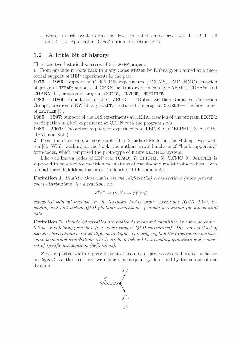
Z decay partial width represents typical example of pseudo-observables, i.e. it has tobe defined. At the tree level, we define it as a quantity described by the square of onediagram:
f
Z
f
13
2 LEP, Precision High Energy Physics and its Future
One may say that during recent years a new physical discipline was born. We call itPHEP, Precision High Energy Physics. Experimentally, it finally shaped in the result ofglorious 12 year LEP era: measurements at Z resonance in 1989 – 1995, and reachingan unprecedented experimental accuracy ≤ 10−3, and measurements above Z resonancein 1995 – 2000, at higher energies, where high enough experimental accuracy was alsoreached ≤ 1%. By 2/11/2000 LEP2 possibly saw hints of “God blessed” particle — Higgsboson, but was stopped, unfortunately, mainly due to lack of financing.
For the first time huge HEP facility challenged for theoreticians to perform calculationswith uncertainty better than experimental errors of O (10−3) and, eventually, efforts ofmany groups of theoreticians allowed the achievement of the theoretical precision of theorder 2.5 · 10−4 at the Z resonance and 2 − 3 · 10−4 at LEP2 energies.
This, in turn, greatly contributed to the success of precision tests of the SM, the mainresult of LEP era, which laid the foundation of the Precision High Energy Physics. Thisis why our project got this suffix PHEP.
2.1 Future of PHEP
PHEP has good perspectives and after the end of LEP. Several Input parameters of theStandard Model (SM) are expected to be improved in near future.
Recent discrepancy in the muon amm:
aSM
μ = 116591661(114) × 10−11
aEXP
μ (Average) = 116592023(151)
aEXP
μ − aSM
μ = 362(189) 2σ difference
exp. error (151) should be improved soon up to ∼ (50), (1)
necessitates an improvement of the knowledge of the hadronic contribution of Δα(5)h
(M2
Z
)to the running e.m. coupling. An experimental input for σ (e+e− → hadrons) at cmsenergies (1-4 GeV) is expected from BES-II, BEPC (Beijing), VEPP2000 (Novossibirsk)and DAFNE at cms energies around φ-meson.
Very important should be projected improvements of mass measurements: MW
, mt.LEP1 finished with indirect result for the top mass: mt = 169+10
−8 GeV; while LEP1 ⊕TEVATRON constraint yielded: mt = 174.5+4.4
−4.2 GeV.LEP2 reached for W mass M
W: M
W= 80.450 ± 0.039, in the direct measurements
and MW
= 80.373 ± 0.023 as indirect result.TEVATRON in RUN-I reached: M
W= 80.454 ± 0.060 GeV, mt = 174.3 ± 5.1 GeV.
Much better precision tags are expected to be reached at TEVATRON, RUN-II (re-cently started): ΔM
W∼ 20MeV, Δmt ∼ 2 GeV; and later at LHC (not so sooner than
in 2006, however): ΔMW
∼ 15 MeV, Δmt ∼ 1 GeV.Where, when and with which mass Higgs boson might be discovered?
− TEVATRON has a serious chance to see Higgs up to mass 180 GeV; however it willrequire very high integrated luminosity:
∫ L ≥ 5fb−1;
14
− LHC, will cover all allowed mass range up to 500 GeV (not so soon, after 2007);− LC’s and muon factories (after 2010–2012).
New horizon of PHEP will be opened with experiments at electron LC’s: TESLA(DESY) particularly with GigaZ option, i.e. coming back to Z resonance with statistics109; CLIC (CERN); JLC (KEK), NLC(SLAC, LNBL, LLNL, FNAL) and Muon StorageRings (Higgs Factory) — all that more than in ten years from now.
One expects fantastic precision tags there in:− Δ sin2 θeff ∼ 0.00002;− ΔM
W∼ 6 MeV, Δmt ∼ 100 − 200MeV;
− ΔMH∼ 100 MeV (from e+e− → ZH);
− and detail study of Higgs boson properties.Given our LEP1 experience one should definitely state that 2-loop precision level
control will be absolutely necessary for the analysis of these data!One may conclude that PHEP has a bright future: all future colliders — TEVATRON,
LHC, electron LC’s (TESLA, NLC, CLIC) and muon factories will be, actually, PHEPfacilities! For data analysis, they will surely require qualitatively new level of both theo-retical predictions and principally new computer codes.
3 Necessary notion
In order to understand the language of CalcPHEP one has to introduce many notions andnotations.
3.1 Input Parameter Set, IPS
The Minimal Standard Model (MSM), contains large number of Input Parameters:25 = 2 interaction constants α and α
S
⊕ 8 mixing angles (CKM and possible lepton analogs)⊕ 15 masses (12 fundamental fermions and 3 fundamental bosons Z, W, H).However, the number 25 is minimal. MSM is unable to compute its IPS from first
principles; MSM is able to compute any observable Oexpi in terms of its IPS:
Oexpi (measured) ↔ Otheor
i (calculated, as a function of IPS) . (2)
This is the way how precision measurements set constraints on IPS.
3.1.1 Number of free parameters in fits of Z resonance observables
At Z resonance, not all 25 parameters matter. Actually only 5 parameters:
Δα(5)h
(M2
Z
), α
S
(M2
Z
), mt , M
Z, M
H, (3)
which we call the Standard LEP1 IPS, matter.Using M
Z, measured at Z peak itself with the precision ∼ 2 × 10⁻⁵, and also reach
information from the other measurements for:
αS
(M2
Z
), mt , M
W, (4)
15
we approach one-parameter fit, with Higgs boson mass MH
being the only fitted parameter.The result of such a fit was shown in the Blue band figure, the most celebrated LEP erafigure, derived with the aid of TOPAZ0 [7] and ZFITTER [6] codes.
3.2 Quantum Fields of the SM
Here we sketch all fundamental quantum fields of the SM in one of the most generalgauges — Rξ, with three arbitrary gauge parameters ξ
A, ξ
Z, ξ.
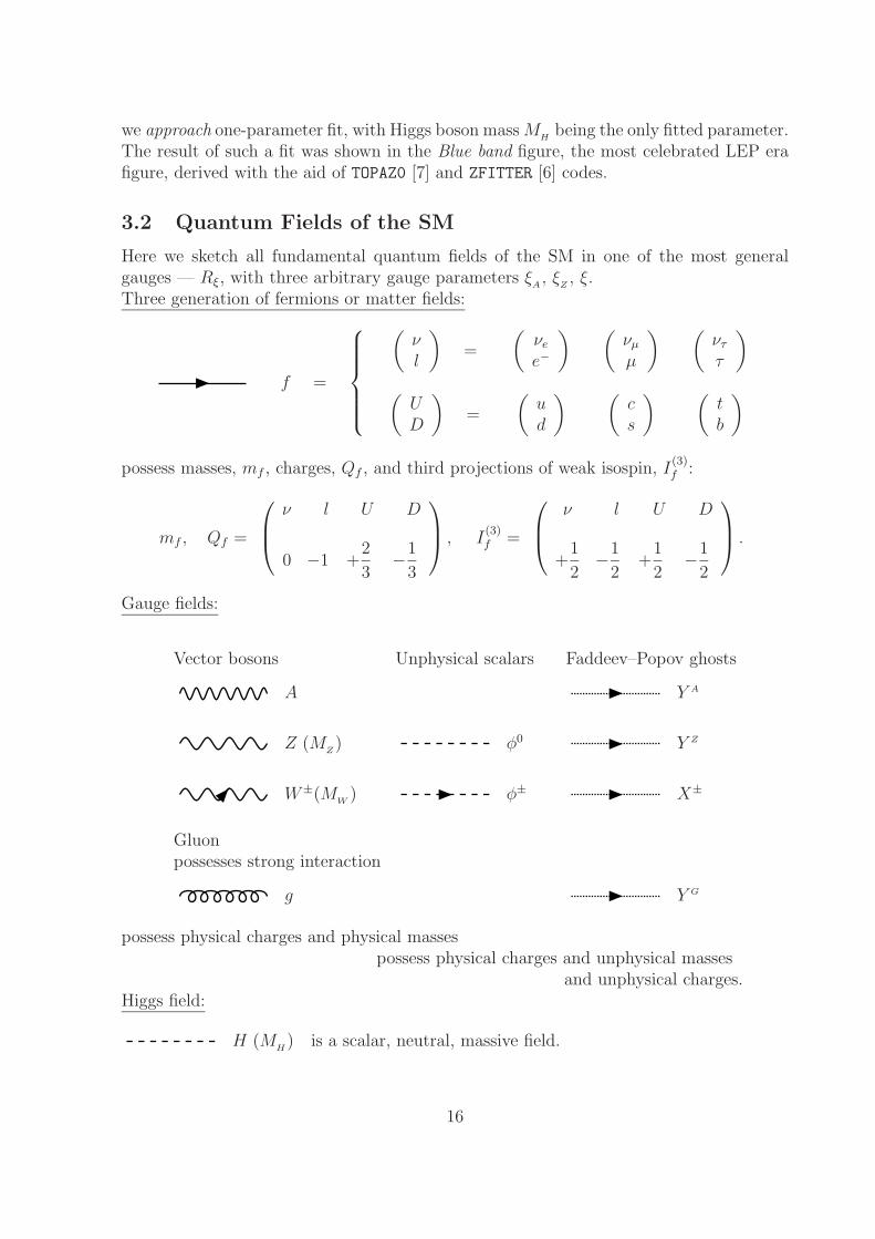
Three generation of fermions or matter fields:
f =
⎧⎪⎪⎪⎪⎨⎪⎪⎪⎪⎩
(νl
)=
(UD
)=
(νe
e−
)(
ud
)(
νμ
μ
)(
cs
)(
ντ
τ
)(
tb
)possess masses, mf , charges, Qf , and third projections of weak isospin, I
(3)f :
mf , Qf =
⎛⎜⎝ ν l U D
0 −1 +2
3−1
3
⎞⎟⎠ , I(3)f =
⎛⎜⎝ ν l U D
+1
2−1
2+
1
2−1
2
⎞⎟⎠ .
Gauge fields:
Vector bosons Unphysical scalars Faddeev–Popov ghosts
A Y A
Z (MZ) φ0 Y Z
W±(MW
) φ± X±
Gluonpossesses strong interaction
g Y G
possess physical charges and physical massespossess physical charges and unphysical masses
and unphysical charges.Higgs field:
H (MH) is a scalar, neutral, massive field.
16

3.2.1 The Lagrangian in Rξ gauge, Feynman Rules
At the ground level of CalcPHEP system one has this Lagrangian
L = L(IPS of 25 parameters, 17 fields, 3 gauge parameters), (5)
from which one derives primary Feynman rules for vertices.
3.2.2 Propagators in Rξ gauge
Here we list propagators in Rξ gauge, the other important bricks of CalcPHEP system.Propagator of a fermion, f :
f
−i/p + mf
p2 + m2f
Vector boson propagators:
A1
p2
{δμν +
(ξ2
A− 1) pμpν
p2
}Z
1
p2 + M2Z
{δμν +
(ξ2
Z− 1) pμpν
p2 + ξ2ZM2
Z
}W± 1
p2 + M2W
{δμν +
(ξ2 − 1
) pμpν
p2 + ξ2M2W
}Propagators of unphysical fields:
Y A
ξA
p2
φ0
1
p2 + ξ2ZM2
Z
,Y Z
ξZ
p2 + ξ2ZM2
Z
φ±1
p2 + ξ2M2W
,X±
ξ
p2 + ξ2M2W
Propagator of the physical scalar field, H-boson
H
1
p2 + M2H
3.3 Scalar A0, B0, etc functions
For calculation of one-loop integrals CalcPHEP uses the standard scalar A0, B0, C0 andD0 functions [6].One-point integrals or A0 functions, are met in tadpoles diagrams:
m
17
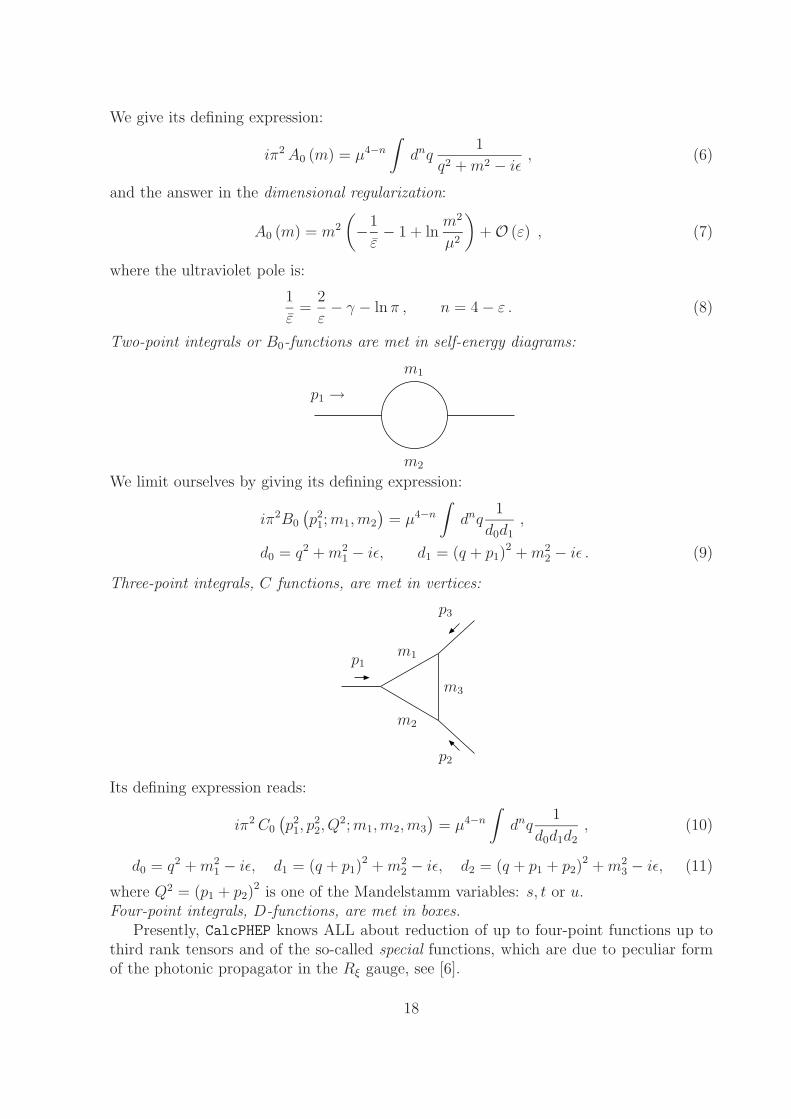
We give its defining expression:
iπ2 A0 (m) = μ4−n
∫dnq
1
q2 + m2 − iε, (6)
and the answer in the dimensional regularization:
A0 (m) = m2
(−1
ε− 1 + ln
m2
μ2
)+ O (ε) , (7)
where the ultraviolet pole is:
1
ε=
2
ε− γ − ln π , n = 4 − ε . (8)
Two-point integrals or B0-functions are met in self-energy diagrams:
p1 →m1
m2
We limit ourselves by giving its defining expression:
iπ2B0
(p2
1; m1,m2
)= μ4−n
∫dnq
1
d0d1
,
d0 = q2 + m21 − iε, d1 = (q + p1)
2 + m22 − iε . (9)
Three-point integrals, C functions, are met in vertices:
m1
m2
m3
p1
p3
p2
Its defining expression reads:
iπ2 C0
(p2
1, p22, Q
2; m1,m2,m3
)= μ4−n
∫dnq
1
d0d1d2
, (10)
d0 = q2 + m21 − iε, d1 = (q + p1)
2 + m22 − iε, d2 = (q + p1 + p2)
2 + m23 − iε, (11)
where Q2 = (p1 + p2)2 is one of the Mandelstamm variables: s, t or u.
Four-point integrals, D-functions, are met in boxes.Presently, CalcPHEP knows ALL about reduction of up to four-point functions up to
third rank tensors and of the so-called special functions, which are due to peculiar formof the photonic propagator in the Rξ gauge, see [6].
18
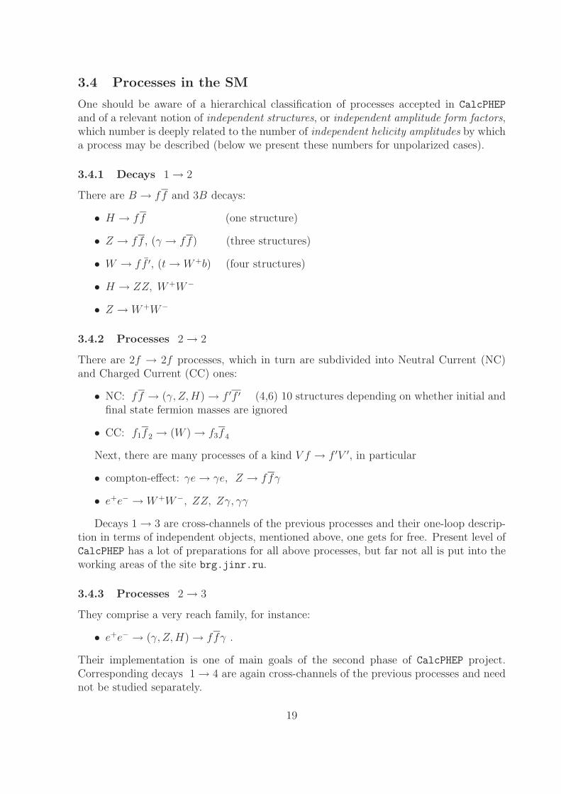
3.4 Processes in the SM
One should be aware of a hierarchical classification of processes accepted in CalcPHEP
and of a relevant notion of independent structures, or independent amplitude form factors,which number is deeply related to the number of independent helicity amplitudes by whicha process may be described (below we present these numbers for unpolarized cases).
3.4.1 Decays 1 → 2
There are B → ff and 3B decays:
• H → ff (one structure)
• Z → ff , (γ → ff) (three structures)
• W → ff ′, (t → W+b) (four structures)
• H → ZZ, W+W−
• Z → W+W−
3.4.2 Processes 2 → 2
There are 2f → 2f processes, which in turn are subdivided into Neutral Current (NC)and Charged Current (CC) ones:
• NC: ff → (γ, Z,H) → f ′f ′ (4,6) 10 structures depending on whether initial andfinal state fermion masses are ignored
• CC: f1f 2 → (W ) → f3f 4
Next, there are many processes of a kind V f → f ′V ′, in particular
• compton-effect: γe → γe, Z → ffγ
• e+e− → W+W−, ZZ, Zγ, γγ
Decays 1 → 3 are cross-channels of the previous processes and their one-loop descrip-tion in terms of independent objects, mentioned above, one gets for free. Present level ofCalcPHEP has a lot of preparations for all above processes, but far not all is put into theworking areas of the site brg.jinr.ru.
3.4.3 Processes 2 → 3
They comprise a very reach family, for instance:
• e+e− → (γ, Z,H) → ffγ .
Their implementation is one of main goals of the second phase of CalcPHEP project.Corresponding decays 1 → 4 are again cross-channels of the previous processes and neednot be studied separately.
19
3.4.4 Processes 2 → 4
To this family belongs 4 fermion processes of LEP2. Their study is not foreseen at thesecond phase of CalcPHEP project, but might be a subject of its third phase.
4 Building Blocks and knowledge storing
4.1 Simplest decay: Z → ff
4.1.1 Amplitude of Z → ff decay at tree level
Its tree level diagram was already presented at the end of Section 1.2; the correspondingamplitude reads:
V Zffμ = (2π)4 i
ig
2 cW
γμ
[I
(3)f
(1 + γ5
)− 2Qfs2W
], (12)
with vector and axial coupling constants: vf = I(3)f − 2Qfs
2W
, af = I(3)f . Note appearance
of the two structures in Eq. (12), which might be termed as L and Q structures, corre-spondingly. Note also, that Eq. (12) as well as all below, are written in Pauli metrics thatis used by CalcPHEP.
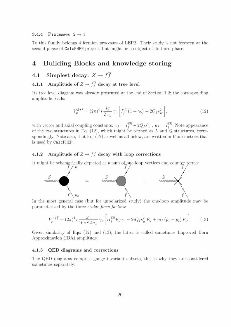
4.1.2 Amplitude of Z → ff decay with loop corrections
It might be schematically depicted as a sum of one-loop vertices and counter terms:f p1
Z
f p2
=
f
Z
f
+
f
Z
f
In the most general case (but for unpolarized study) the one-loop amplitude may beparameterized by the three scalar form factors:
V Zffμ = (2π)4 i
g3
16 π2 2 cW
γμ
[iI
(3)f FLγ+ − 2iQfs
2W
FQ + mf (p1 − p2) FD
]. (13)
Given similarity of Eqs. (12) and (13), the latter is called sometimes Improved BornApproximation (IBA) amplitude.
4.1.3 QED diagrams and corrections
The QED diagrams comprise gauge invariant subsets, this is why they are consideredsometimes separately:
20
f
Z
f
γ +
f
Z
f
γ+
f
Z
f
γ
Their contribution to the partial Z widths, in the case when no photon cuts are imposed,reads:
ΓQEDf = Γf
(1 +
3α
4πQ2
f
). (14)
4.2 Process e+e− → ff
Coming to a more complicated case of a 2f → 2f process, we will illustrate how buildingblocks, derived for a study of a lower level process, might be use at a higher level.
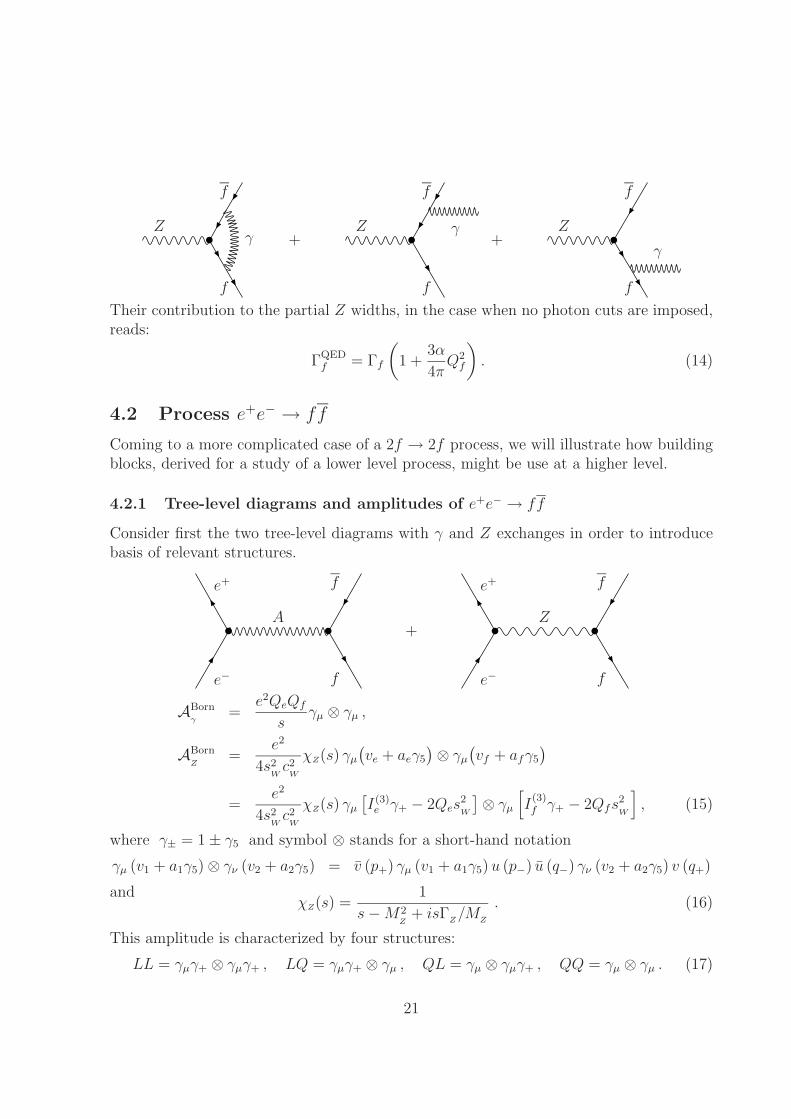
4.2.1 Tree-level diagrams and amplitudes of e+e− → ff
Consider first the two tree-level diagrams with γ and Z exchanges in order to introducebasis of relevant structures.
e+ f
A
e− f
+
e+ f
Z
e− f
ABornγ
=e2QeQf
sγμ ⊗ γμ ,
ABornZ
=e2
4s2W
c2W
χZ(s) γμ
(ve + aeγ5
)⊗ γμ
(vf + afγ5
)=
e2
4s2W
c2W
χZ(s) γμ
[I(3)e γ+ − 2Qes
2W
]⊗ γμ
[I
(3)f γ+ − 2Qfs
2W
], (15)
where γ± = 1 ± γ5 and symbol ⊗ stands for a short-hand notation
γμ (v1 + a1γ5) ⊗ γν (v2 + a2γ5) = v (p+) γμ (v1 + a1γ5) u (p−) u (q−) γν (v2 + a2γ5) v (q+)
andχZ(s) =
1
s − M2Z
+ isΓZ/M
Z
. (16)
This amplitude is characterized by four structures:
LL = γμγ+ ⊗ γμγ+ , LQ = γμγ+ ⊗ γμ , QL = γμ ⊗ γμγ+ , QQ = γμ ⊗ γμ . (17)
21
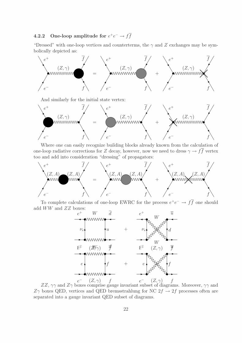
4.2.2 One-loop amplitude for e+e− → ff
“Dressed” with one-loop vertices and counterterms, the γ and Z exchanges may be sym-bolically depicted as:
e+ f
(Z, γ)
e− f
=
e+ f
(Z, γ)
e− f
+
e+ f
(Z, γ)
e− f
And similarly for the initial state vertex:
e+ f
(Z, γ)
e− f
=
e+ f
(Z, γ)
e− f
+
e+ f
(Z, γ)
e− f
Where one can easily recognize building blocks already known from the calculation ofone-loop radiative corrections for Z decay, however, now we need to dress γ → ff vertextoo and add into consideration “dressing” of propagators:
e+ f
(Z,A) (Z,A)
e− f
=
e+ f
(Z,A) (Z,A)
e− f
+
e+ f
(Z,A) (Z,A)
e− f
To complete calculations of one-loop EWRC for the process e+e− → ff one shouldadd WW and ZZ boxes:
e+ W d
νe u
e− W d
+
e+
Wu
νe d
e−W
ue+ (Z, γ) f
e f
e− (Z, γ) f
+
e+ (Z, γ) f
e f
e− (Z, γ) fZZ, γγ and Zγ boxes comprise gauge invariant subset of diagrams. Moreover, γγ and
Zγ boxes QED, vertices and QED bremsstrahlung for NC 2f → 2f processes often areseparated into a gauge invariant QED subset of diagrams.
22
Virtual QED one-loop diagrams together with four QED bremsstrahlung diagramsform an Infra-Red Divergence (IRD) free subset.
This example clearly shows how the principle of knowledge storing is implementedwithin CalcPHEP project: one starts from the simplest decays and collects all relevantbuilding blocks, BB’s (off-shell with respect to boson mass). Then one moves to nextlevel of complexity where all BB’s computed at the previous level are requested, but ontop one needs more complicated objects (here boxes).
This strategy was realized in our recent calculations of the EWRC to the e+e− → ffprocess, which are completely done with the aid of CalcPHEP system [9]. There is anotherstudy accomplished with CalcPHEP [10].
5 Status of the project
Before discussing what is already available at the site brg.jinr.ru, we present somegeneral information about CalcPHEP system.
5.1 Basic information about CalcPHEP, keywords
CalcPHEP is four-level computer system for automatic calculation of pseudo- andrealistic observables (decay rates, event distributions) for more and more complicatedprocesses of elementary particle interactions, using the principle of knowledge storing.
At each of the four levels there are:
1. Codes (written in FORM3), realizing full chain of analytic calculations from the SMLagrangian LSM to the Ultra Violet Free Amplitudes, UVFA, parameterized by aminimal set of scalar form factors;
2. Codes (written in FORM3), realizing analytic calculations of a minimal subset ofHelicity Amplitudes, HA’s, followed by an automatic procedure of generation ofcodes for numerical calculations of HA’s (presently FORTRAN codes, and in a nearperspective C++ codes).
3. Codes, realizing the so-called “infrared rearrangement” of HA’s. This is needed if themultiple photon emission is being exponentiated at the amplitude level. Currently,bremsstrahlung photons are added in the lowest order and the third level is skipped.
4. Codes, that use HA’s derived at the second (or third) level together with tree-levelHA’s for one-photon (or multiple-photon) emission, within a Monte Carlo eventgenerator, which is supposed to compute realistic distributions (presently FORTRAN
codes, and in a near perspective C++ codes.)
It is an Internet based and Database based system. The latter means that thereis a storage of source codes written in different languages, which talk to each other. Theyare placed into a homogeneous environment written in JAVA.
It follows Intermediate access principle i.e. full chain “from the Lagrangian torealistic distribution” should work out completely in real time, if someone requests this,however, it is supposed to have several “entries”, say after each level, or just providingthe user with its final product — a Monte Carlo event generator.
23
5.2 Some technical data about CalcPHEP
1. Address http://brg.jinr.ru/
2. For realization of the site one used:
− Apache web server under Linux,
− form3 compiler,
− mySQL server for relational databases.
3. In the current version, user-interface is realized with the use of PHP.
4. Nowadays, everything is being rewritten in JAVA in order to reach better “interac-tivity” and to use reach possibilities of already written in this language libraries.Main goal of this rewriting is to create a homogeneous environment bothfor accessing our codes from the database and for offering a possibility forsimultaneous work of several members of the group and external users.
5.3 Present and nearest versions of CalcPHEP system
In 2001, we released two test-versions of CalcPHEP:
1. v0.01 from March’01 realizes analytic calculations of one-loop UVFA for de-cays 1 → 2 (level-1).
2. v0.02 from September’01 returns numbers for one-loop decay widths (levels-1,2)via temporary bypass of level 4. It realizes also levels-1,2 for 2f → 2f NC process.
3. One has very many almost finished “preparations” for the other processes 2 → 2and decays 1 → 3 (level-1). All this should comprise v0.03 of Summer 2002.
4. An active work is being realized on implementation of level-4 for decays 1 → 2, thisshould complete full chain “from the SM Lagrangian to pseudo-observables” for thesimplest decays.
5. There are many problems to be solved at the second or later phases of the project.Among them one should mention:– automatic generation of Feynman Rules from a Lagrangian,– automatic generation of topologies of Feynman diagrams,– graphical representation of the results.
6 Conclusion
At a Symposium in honor of Professor Alberto Sirlin’s 70th Birthday was said: A newfrontier is as the horizon: most likely it is goodbye to the one man show. Running a newRadiative Correction project will be a little like running an experiment [11].
Indeed, projects of such a kind as CalcPHEP are definitely long term projects. Remem-ber, that ZFITTER took about 12 years, about the same time exists already FeynArts [12].
Our nearest goal is the realization of the second phase of the project upon completionof which we plan to have a complete software product, accessible via an Internet-basedenvironment, and realizing the chain of calculations “from the Lagrangian to the realistic
24
distributions” at the one-loop level precision including some processes 2 → 3 and decays1 → 4. Plans also assume to perform an R&D for the third phase of the project (seealso [13]–[16]) which should begin in 2004.
Second phase is basically oriented on a common work of theoreticians of the Dubnagroup and the Knoxville–Krakow collaboration [8].
United group proposes to realize in 2002-2004 an important phase of CalcPHEPproject: oriented toward a merger of analytic results to be produced by Dubna teamwith MC event generators to be developed by Knoxville–Krakow collaboration1.
Among most important milestones of first year, one should mention: realization of thelevels 2-4 for the simplest Z(H,W ) → ff decays; completion of level 1 for the radiativeZ decay, Z → ffγ, work on which is already under way; completion of levels 2-4 for theradiative Z decay.
References
[1] D. Bardin, G. Passarino, and W. Hollik (eds.), “Reports of the working group onprecision calculations for the Z resonance”, CERN Report, 95–03 (1995).
[2] D. Bardin, M. Gruenewald and G. Passarino, “Precision calculation project report”,February 1999, hep-ph/9902452.
[3] M.Kobel, Z. Was, C.Ainsley, A.Arbuzov, S.Arcelli, D.Bardin, I.Boyko,D.Bourilkov, P.Christova, J.Fujimoto, M.Grunewald, T.Ishikawa, M.Jack, S.Jadach,L.Kalinovskaya, Y.Kurihara, A.Leike, R.Mcpherson, M.-N.Minard, G.Montagna,M.Moretti, T.Munehisa, O.Nicrosini, A.Olchevski, F.Piccinini, B.Pietrzyk,W.Placzek, S.Riemann, T.Riemann, G.Taylor, Y.Shimizu, M.Skrzypek, S.Spagnolo,and B.Ward, “Two fermion production in electron positron collisions”, in Proc.of LEP2 Monte-Carlo Workshop, Geneva, Switzerland, 1999-2000, report hep-ph/0007180 (G.Passarino, R.Pittau, and S.Jadach, eds.), vol.1, pp.1–113, 2000.
[4] J. Vermaseren, “New features of form”, math-ph/0010025.
[5] D. Bardin, M. Bilenky, P. Christova, M. Jack, L. Kalinovskaya, A. Olchevski, S. Rie-mann, and T. Riemann, Comput. Phys. Commun. 133 (2001) 229.
[6] D. Bardin and G. Passarino, “The standard model in the making: Precision studyof the electroweak interactions”, Oxford, UK: Clarendon, 1999, 685p.
[7] G. Montagna, O. Nicrosini, F. Piccinini and G. Passarino, Comput. Phys. Commun.117 (1999) 278.
[8] S. Jadach, Z. Was and B.F.L. Ward, Comput. Phys. Commun. 124 (2000) 233;Comput. Phys. Commun. 130 (2000) 260.
1In this connection it is necessary to emphasize that any future code aimed at a com-parison of experimental data with theory predictions should be a MC generator, since theprocesses at very high energies will have multi-particle final states that make impossiblea semi-analytic approach used at LEP within ZFITTER project.
25
[9] D. Bardin and L. Kalinovskaya and G. Nanava, ”An electroweak library for thecalculation of EWRC to e+e− → ff within the CalcPHEP project”, hep-ph/0012080;revised version CERN-TH/308-2000, November 2001.
[10] D. Bardin, P. Christova, L. Kalinovskaya and G. Passarino, “Atomic Parity Violationand Precision Physics”, hep-ph/0102233, Eur.Phys.J. C22 (2001) 99.
[11] Giampiero Passarino, “Precision Physics Near LEP Shutdown and Evolutionary De-velopments” Presented at 50 Years of Electroweak Physics A symposium in honor ofProfessor Alberto Sirlin’s 70th Birthday October 27-28, 2000, hep-ph/0101299.
[12] T. Hahn, Comput. Phys. Commun. 140 (2001) 418.
[13] Dmitri Bardin, ”12 years of precision calculations for LEP. What’s next?”, Presentedat 50 Years of Electroweak Physics A symposium in honor of Professor Alberto Sirlin’s70th Birthday October 27-28, 2000, hep-ph/0101295.
[14] D. Yu. Bardin and L. V. Kalinovskaya and F. V. Tkachov, ”New algebraic-numeric methods for loop integrals: Some 1-loop experience”, QFTHEP-2000, Tver,September 2000. Eds.: V.I.Savrin and B.B.Levtchenko, SINP MSU, Moscow, 2001,hep-ph/0012209.
[15] G. Passarino, S. Uccirati, ”Algebraic-numerical evaluation of Feynman diagrams:Two-loop self-energies”, hep-ph/0112004.
[16] G. Passarino, Nucl.Phys. B619 (2001) 257, hep-ph/0108252.
26
The Approximation of the SomePhysical Processes by Exponential
Functions
T. Bochorishvili, E. A. Grebenikov
University of Podlasie, Siedlce, Poland;e-mail: [email protected]
The problem of the separation of radioactive substances from radioactive mixture isconnected with data processing obtained from the experimental measurements. The rules ofdecomposition of the radioactive chemical elements are described by exponential functions.It is natural that the problem of the best approximation of a finite set of measurementsby the exponential functions is adequate, which fundamental parameters are half-life ofunknown components of the radioactive mixture.
In 60-th XX century the known American mathematician C. Lanczos pointed in [1]two problems of great practical importance:
Problem 1. Find hidden periodicities in the polyharmonic processes, given in big setsof measurements.
Problem 2. It is necessary to determine the hidden exponents in processes of theradioactive disintegration, represented by massive measurements.
Both of these problems are related to so called ”ill posed problems” [2] and hence ifsolutions exist, there are several solutions.
The functional, that one has to minimize for determining the unknown parameters,is transcendental. More ever, the number of parameters also is unknown, which com-plicate one more the problem. C. Lanczos has solved both of these problems for thesimplest models: the measurements are realized on equidistant time grid and the numberof parameters is known [1].
The first problem for non-uniform division of time and with unknown number ofparameters has been solved by E.A. Grebenikov and S.V. Mironov[3]. They constructedthe so called method of two dimensional iteration, that has been successfully used inproblems of the cosmic dynamics.
In our paper is proposed a new algorithm of the pick-out of the exponential functions,based on the approximation discreet experimental measurements by exponent polynomi-als. It is possible to realize this algorithm on the non-equidistant time grid.
Let be done N points
(tk, yk) ∈ R2, 0 ≤ tk ≤ T, (k = 0, 1, 2, ..., N).
We are looking for a function f(t), t ∈ [0, T ] , the graph of which contains thesepoints. More ever, this function must be of the form:
27
f(t) =m∑
k=1
αkeλkt, t ∈ [0, T ] , (1)
where α = (α1, α2, ..., αm), λ = (λ1, λ2, ..., λm) the natural number m are to be deter-mined, usually m is much less then N , i.e. m << N . More ever, in order to solve thisproblem it is necessary to determine the lower and upper bound of m (m1 ≤ m ≤ m2).
To find the vectors α and λ, first of all we fix the natural number m = m0. In orderto use the method of least squares, we must construct the functional
Ψ (α,λ, f) =N∑
k=0
(yk −
m0∑i=1
αieλitk
)2
(2)
and we have to find the minimum of that
minα,λ
Ψ (α,λ, f) �−→ 0. (3)
Like this found solutions are supposed roots and require laborious analyses.The problem (3) is referred to as the problem of absolute (unconditional) minimization.
In such kind main difficulty consists in finding the initial point. In what follows we putin evidence an algorithm to solve this problem.
For this we generate a set of pseudo-random vectors:
{α,λ} = (αs1, α
s2, ..., α
sm, λs
1, λs2, ..., λ
sm) , s = 1, ..., N (4)
where N is big number about 106 − 107. We calculate the values of our functional inthese points, and so, we obtain a finite set of values of Ψ in the points (4). Let denotethem by Ψs, s = 1, ..., N . From this set we choose the minimal value Ψmin, and then wefilter the set (4) in such way, we drop out the points, which does not satisfy the followinginequality:
Ψs ≤ Ψmin + ε (5)
where ε is sufficiently small.On this way we select a subset of the set (4), on which the values of the functional
is small enough, and which accumulate in clusters around the points of minima. If thefunctional has at least one point of minimum, then there is at least one isolated cluster.We divide this cluster on other accumulations groups, enumerate them and denote byc1, c2, ..., cp, where p represents the number of these small clusters. Let l1, l2, ..., lp denotethe number of points in each cluster.
After this we find for each groups ci, (i = 1, 2, ..., p) the centroid (center of gravity) ofthe derivatives from the points of minimum and denote them by Xci
. This point can bedetermined by formula:
Xci=
li∑k=1
xk (Ψimax − Ψk)
31
li∑k=1
(Ψimax − Ψk)
31
(6)
28
where xk, (k = 1, 2, ..., li) are points of the cluster ci, Ψimax is the maximum value of the
functional on these points. The values of Xci, found in this way will, represent the first
approximation (initial point). The more exact solution will be determined by the methodof steepest descent. Each solution is probably one of the problem (3).
This construction has been purposed actually for that case, when one has a very bignumber of measurements, and to find a good first approximation (initial point) for one ofthe iteration algorithm for finding the points of minima of the quadratic functional. Tobe certain, that the obtain values of parameters {α,λ} give us the solution we have todo further analyses.
We proposed to divide the interval [0, T ] in to m0 parts and for each subinterval torepeat the above algorithm all over again. If the new values of the parameters are closeenough to previous one, then we can conclude, that the find solutions is the corrects one.If not, then we increase the number m0 (i.e. increases the number of exponential functionsin the term (1)) and we repeat the process for the new value of m0 from the beginning.
This process one has to repeat until:a) Either after some steps of iteration we obtain desired result;b) Either we continue the calculations until we achieve the maximal number m0.A numerical experiment was realized to estimate an efficiency of the suggested algo-
rithm. It was calculated the values of functional (2) at the 6 ·106 points and was obtainedgood approximations of a vector activity α and the coefficients of decomposition λ. Basedon made calculations we can conclude, that it is possible to use above algorithm for notonly numerical experiments.
References
[1] C. Lanczos, Applied Analysis, M, Goc. izdatelstvo fiz.-mat. literatury, 1961, p. 524.
[2] Tihonov A.N., Arsenin B.I., Metody reshenia nekorrektnyx zadach, M, Nauka,1986.
[3] Grebenikov E.A., Kiosa M.N., Mironov C.V., Chislenno-analiticheskie metody issle-dovania regularno vozmushennyx mnogochastotnyx system, M, Izd-vo MGU, 1986,p. 184.
29
Equivalence Transformations forAbel Equations - a Polynomial
Method
G. Czichowski
University of Greifswald;e-mail: [email protected]
We present a polynomial method for deciding the equivalence of two given Abel equa-tions and to compute then the corresponding equivalence transformation.
We consider the class of Abel differential equations
y′ = A0(x) + A1(x)y + A2(x)y2 + A3(x)y3,
which is invariant with respect to coordinate transformations (x, y) → (u, v) of the formu = F (x), v = G(x)y + H(x), which form the so called structure group G of this class.Structure groups of such classes of ODE’s may be computed effectively in terms of thecorresponding infinitesimal generators ∂ = ξ(x, y)∂x + η(x, y)∂y. In the above case thestructure group is given by generators ∂ with ξy = 0, ηyy = 0.
The question investigated here is to decide whether two Abel equations DE1 and DE2
are equivalent under the action of the structure group G. For polynomial computationswe restrict this problem at first to the case of rational function coefficients Ak(x), laterthe procedure may be generalized to the case of algebraic functions as coefficients.
The following method is based on ideas in of M.Berth and uses two differential invari-ants ABS1 and ABS2 for Abel equations with respect to the structure group G. For abbre-viation we give the corresponding values only for an Abel equation y′ = A0(x)+A1(x)y +A3(x)y3, that means A2(x) = 0. This form may be realized easily by a “Tschirnhaus”-transformation belonging to the structure group
ABS1 =(3A0A1A3 + A0A
′3 − A′
0A3)3
A50A
43
,
ABS2 =(3A2
0A3 − A′0A3y + A0A
′3y + 3A0A1A3y + 3A0A
23y
3)
A33y
6.
The polynomial method presented now works as follows: Write the Abel equationsDE1 and DE2 in variables x, y, z = y′ and u, v, w = v′ respectively. By evaluation ofABS1, ABS2 with respect to both ODE’s we get equations
G1(x, u) = 0, G2(x, y, u, v) = 0.
Elimination, Factorization and cancelling exponents of prime factors as well as nonessen-tial factors leads to several candidates for the equivalence transformation. These can-didates are then checked to realize an equivalence transformation from DE1 to DE2 ornot.
30
By corresponding calculations with minimal polynomials this method may be extendedto the case of algebraic coefficient functions.
Furthermore we consider examples from a special class of “Lie equations” of the form
y′′ = A0(x, y) + A1(x, a)y′ + A2(x, y)y′2
with corresponding invariants and analogous computations. Here the structure group isgiven by ξy = 0, ηyyy = 0 (fibre preserving transformations which are Moebius transfor-mations with respect to y).
31
Numerical Solution of BoundaryValue Problems for the Heat and
Related Equations
Ivan Dimovski, Margarita Spiridonova
Institute of Mathematics and Informatics,Bulgarian Academy of Sciences
G. Bonchev Str. Bl. 8, 1113 Sofia, Bulgaria;e-mail: [email protected]
1 Introduction
It is well known that the mathematical models of many problems in science and tech-nology are described by boundary value problems(BVP) for partial differential equations(PDEs) and most frequentely they can be solved only numerically. There are a num-ber of numerical methods for solution of PDEs and the most common of them are theFinite-Difference Methods (FDM). Some disadvantages of these methods are well knowntoo.
The solution of boundary-values problems is usually needed in numerical form. Theauthors propose an analytic approach for numerical solution of linear (local and nonlocal)BVP for the heat and related equations. It is based on an extension of the Duhamelprinciple from the time variable to space variables.
In order to remind the Duhamel principle, let us consider the simplest case of itsapplication. If we are looking for the solution of the BVP
ut = uxx
u(0, t) = 0, u(1, t) = ϕ(t)u(x, 0) = 0
(1)
in the strip 0≤x≤1, t≥0 , then we can reduce it to the same problem but for the specialchoice ϕ(t) ≡ 1. Denoting this special solution by U(x, t), the general solution of (1) isgiven by
u(x, t) =∂
∂t
∫ t
0
U(x, t − τ) ϕ(τ)dτ. (2)
In order to outline the idea of the following considerations, let us consider the BVP
ut = uxx
u(0, t) = 0, u(1, t) = 0u(x, 0) = f(x)
(3)
in the same strip 0≤x≤1, t≥0 .
32
Usually, this problem is solved by the Fourier method using the Fourier sine-transform.However, from the standpoint of the numerical analysis this method is not quite satis-factory, since it includes time-consuming operations, such as Fourier series expansion ofthe function f(x) and the numerical summation of the series obtained for u(x, t) in manypoints. It is well known that these series are very slow convergent. Using an analogue of(2) (see Example 1), it could be avoided the both time-consuming stages.
2 Extension of the Duhamel principle to space vari-
ables
In order to make clear the basic idea of the approach, we shell consider a rather generalnonlocal BVP with a Stieltjes boundary value condition of the following type.
Let P be a polynomial of one variable, and let us consider the evolution equation
ut = P
(∂2
∂x2
)u (4)
in the strip 0≤x≤1, t≥0. Let Φ be a non-zero linear functional in C1 [0, 1] . Then we arelooking for a solution of (4) satisfying the boundary values conditions
d2j
dx2ju(0, t) = 0, Φξ{ d2j
dx2ju(ξ, t)} = 0, (j = 0, 1, 2, . . . , deg P − 1) (5)
and the initial conditionu(x, 0) = χ(x),
where χ(x) is a given function from C1 [0, 1].As it is well known, each functional Φ in C1 [0, 1] can be represented in the form:
Φ {f} = af(0) +
∫ 1
0
f ′(ξ)dα(ξ),
where a is a constant and α is a function with bounded variation.Further we consider only the special cases:
Φ(f) = f(1) (local case) and Φ(f) =
∫ 1
0
f(ξ)dξ (nonlocal case) .
All our further considerations are based on the following
Theorem 1. Let Φ be a linear functional in C1 [0, 1] , such that Φξ {ξ} = 1. Then theoperation
(f � g)(x) = −1
2Φξ
{∫ ξ
0
h(x, ξ)dξ
}, (6)
33
where
h(x, ξ) =
∫ x
ξ
f(x + ξ − η)g(η)dη −∫ x
−ξ
f(|x − ξ − η|)g(|η|)sgn(x − ξ − η)ηdη (7)
is a bilinear, commutative and associative operation in C [0, 1] such that the right inverseoperator L of d2/dx2 which satisfies the boundary value conditions (Lf)(0) = 0, Φ(Lf) = 0has the form Lf = {x} � f.
Operation (6) bears the name convolution of the operator L .For a proof, see [Dim1] , pp. 176-177.By means of the convolution (7) it can be proposed the following extension of the
classical Duhamel principle for problem (4)-(5):
Theorem 2. Let U(x, t) be a solution of (4) for the special choice χ(x) ≡ x . Then
u(x, t) =∂2
∂x2(U(x, t) � χ(x)) (8)
is a solution of (4) provided χ satisfies the boundary value conditions of (4) .
The proof can be obtained either by a direct check, or using operational calculusapproach (see [Dim2], p. 140).
3 Examples
Examples illustrating the application of the presented approach are described. Allcomputations related to them are performed with the computer algebra system Mathe-matica [SW].
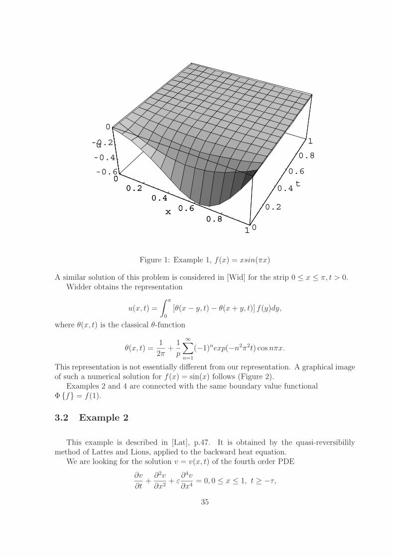
3.1 Example 1
We are looking for the solution of the BVP
ut = uxx, 0≤x≤1, t≥0u(0, t) = 0, u(1, t) = 0u(x, 0) = f(x).
From Theorem 2, when Φξ {u(ξ, t)} = u(1, t) we obtain
u(x, t) =
∫ 1
0
[U(1 − x − ξ, t) − U(1 + x − ξ, t)] f(ξ)dξ,
where
U(x, t) =∞∑
n=1
(−1)n exp(−n2π2t) cos nπx.
A numerical solution using the above formulas for f(x) = xsin(πx) has the followinggraphical image shown by Figure 1.
34
00.2
0.40.6
0.81
x
0
0.2
0.4
0.6
0.8
1
t-0.6
-0.4
-0.2
0
u
00.2
0.40.6
0.81
x
Figure 1: Example 1, f(x) = xsin(πx)
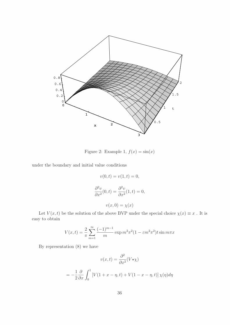
A similar solution of this problem is considered in [Wid] for the strip 0 ≤ x ≤ π, t > 0.Widder obtains the representation
u(x, t) =
∫ π
0
[θ(x − y, t) − θ(x + y, t)] f(y)dy,
where θ(x, t) is the classical θ-function
θ(x, t) =1
2π+
1
p
∞∑n=1
(−1)nexp(−n2π2t) cos nπx.
This representation is not essentially different from our representation. A graphical imageof such a numerical solution for f(x) = sin(x) follows (Figure 2).
Examples 2 and 4 are connected with the same boundary value functionalΦ {f} = f(1).
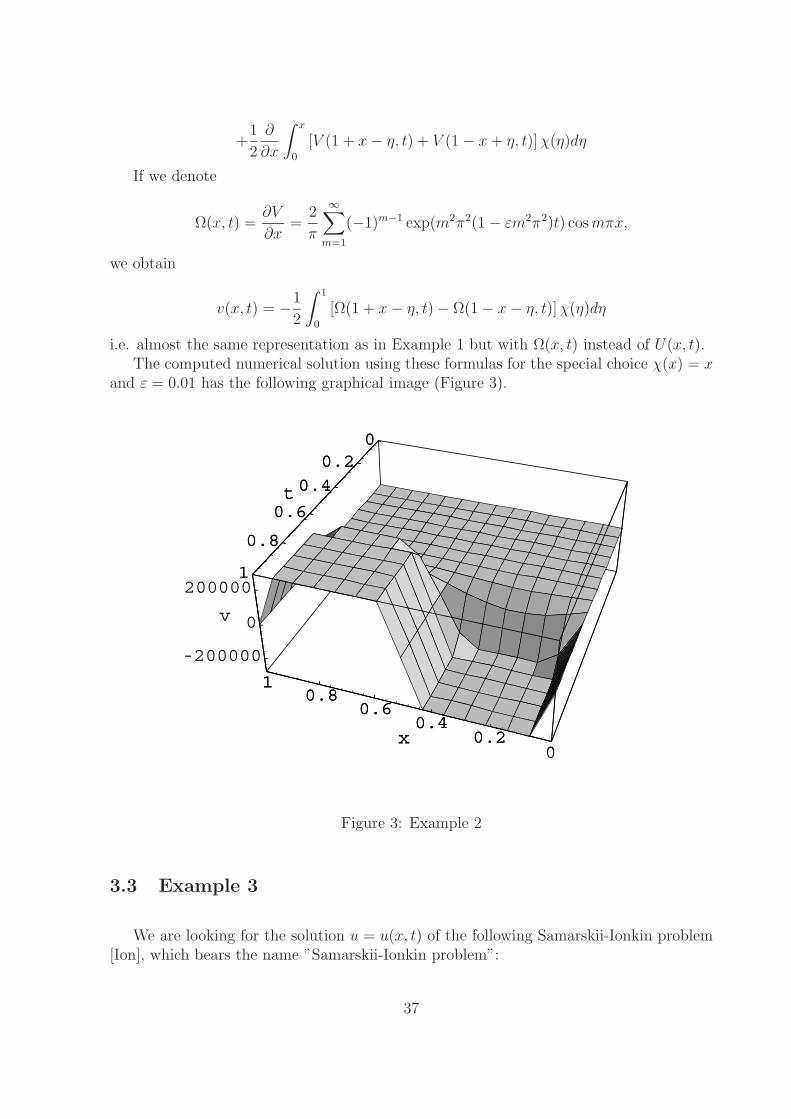
3.2 Example 2
This example is described in [Lat], p.47. It is obtained by the quasi-reversibililymethod of Lattes and Lions, applied to the backward heat equation.
We are looking for the solution v = v(x, t) of the fourth order PDE
∂v
∂t+
∂2v
∂x2+ ε
∂4v
∂x4= 0, 0 ≤ x ≤ 1, t ≥ −τ,
35
0
1
2
3
x0.5
1
1.5
2
t
0
0.2
0.4
0.6
0.8
0
1
2
3
x
Figure 2: Example 1, f(x) = sin(x)
under the boundary and initial value conditions
v(0, t) = v(1, t) = 0,
∂2v
∂x2(0, t) =
∂2v
∂x2(1, t) = 0,
v(x, 0) = χ(x)
Let V (x, t) be the solution of the above BVP under the special choice χ(x) ≡ x . It iseasy to obtain
V (x, t) =2
π
∞∑m=1
(−1)m−1
mexp m2π2(1 − εm2π2)t sin mπx
By representation (8) we have
v(x, t) =∂2
∂x2(V �χ)
= −1
2
∂
∂x
∫ 1
0
[V (1 + x − η, t) + V (1 − x − η, t)] χ(η)dη
36
+1
2
∂
∂x
∫ x
0
[V (1 + x − η, t) + V (1 − x + η, t)] χ(η)dη
If we denote
Ω(x, t) =∂V
∂x=
2
π
∞∑m=1
(−1)m−1 exp(m2π2(1 − εm2π2)t) cos mπx,
we obtain
v(x, t) = −1
2
∫ 1
0
[Ω(1 + x − η, t) − Ω(1 − x − η, t)] χ(η)dη
i.e. almost the same representation as in Example 1 but with Ω(x, t) instead of U(x, t).The computed numerical solution using these formulas for the special choice χ(x) = x
and ε = 0.01 has the following graphical image (Figure 3).
00.2
0.40.6
0.81
x
00.2
0.4
0.6
0.8
1
t
-200000
0
200000
v
00.2
0.40.6
0.81
x
00.2
0.4
0.6
0.8
1
t
Figure 3: Example 2
3.3 Example 3
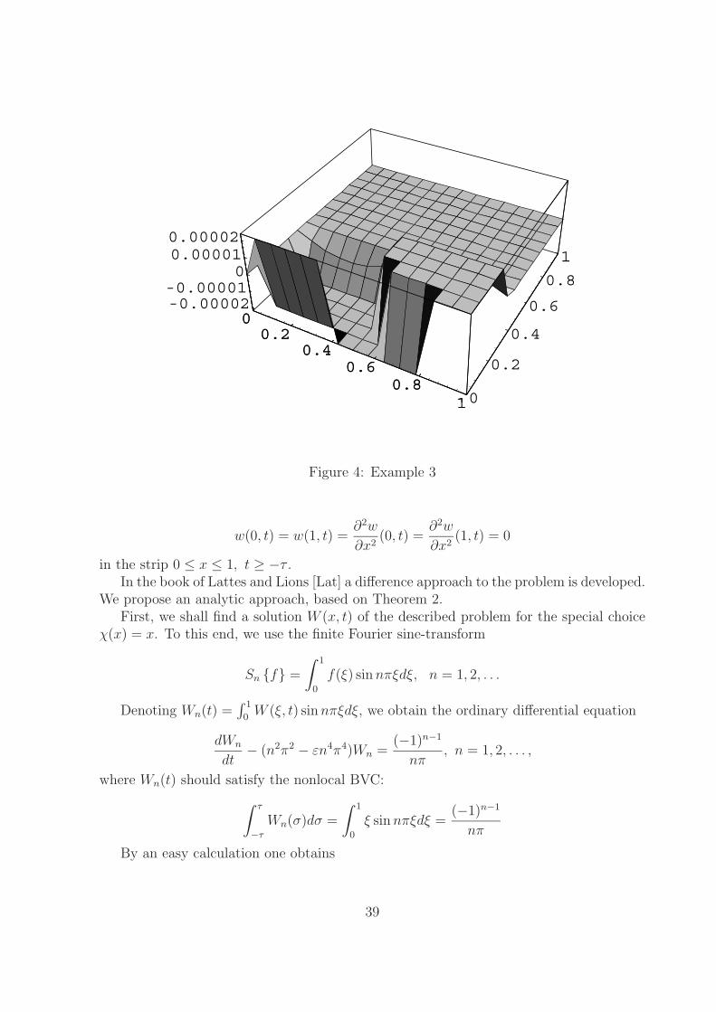
We are looking for the solution u = u(x, t) of the following Samarskii-Ionkin problem[Ion], which bears the name ”Samarskii-Ionkin problem”:
37
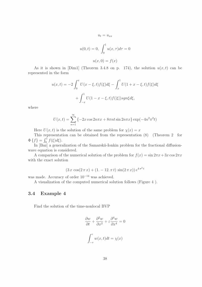
ut = uxx
u(0, t) = 0,
∫ 1
0
u(x, τ)dτ = 0
u(x, 0) = f(x)
As it is shown in [Dim1] (Theorem 3.4.8 on p. 174), the solution u(x, t) can berepresented in the form
u(x, t) = −2
∫ x
0
U(x − ξ, t)f(ξ)dξ −∫ 1
x
U(1 + x − ξ, t)f(ξ)dξ
+
∫ 1
−x
U(1 − x − ξ, t)f(|ξ|)sgnξdξ,
where
U(x, t) =∞∑
n=1
{−2x cos 2nπx + 8πnt sin 2nπx} exp(−4n2π2t)
Here U(x, t) is the solution of the same problem for χ(x) = xThis representation can be obtained from the representation (8) (Theorem 2 for
Φ {f} =∫ 1
0f(ξ)dξ).
In [Baz] a generalization of the Samarskii-Ionkin problem for the fractional diffusion-wave equation is considered.
A comparison of the numerical solution of the problem for f(x) = sin 2πx+3x cos 2πxwith the exact solution
(3 x cos(2 π x) + (1. − 12. π t) sin(2 π x)) e4 π2 t
was made. Accuracy of order 10−14 was achieved.A visualization of the computed numerical solution follows (Figure 4 ).
3.4 Example 4
Find the solution of the time-nonlocal BVP
∂w
∂t+
∂2w
∂x2+ ε
∂4w
∂x4= 0
∫ τ
−τ
w(x, t)dt = χ(x)
38
00.2
0.40.6
0.810
0.2
0.4
0.6
0.8
1
-0.00002-0.00001
00.000010.00002
00.2
0.40.6
0.81
Figure 4: Example 3
w(0, t) = w(1, t) =∂2w
∂x2(0, t) =
∂2w
∂x2(1, t) = 0
in the strip 0 ≤ x ≤ 1, t ≥ −τ .In the book of Lattes and Lions [Lat] a difference approach to the problem is developed.
We propose an analytic approach, based on Theorem 2.First, we shall find a solution W (x, t) of the described problem for the special choice
χ(x) = x. To this end, we use the finite Fourier sine-transform
Sn {f} =
∫ 1
0
f(ξ) sin nπξdξ, n = 1, 2, . . .
Denoting Wn(t) =∫ 1
0W (ξ, t) sin nπξdξ, we obtain the ordinary differential equation
dWn
dt− (n2π2 − εn4π4)Wn =
(−1)n−1
nπ, n = 1, 2, . . . ,
where Wn(t) should satisfy the nonlocal BVC:∫ τ
−τ
Wn(σ)dσ =
∫ 1
0
ξ sin nπξdξ =(−1)n−1
nπ
By an easy calculation one obtains
39
Wn(t) =(−1)n−1
nπ
n2π2 − εn4π4 + 2π
2 sinh(n2π2 − εn4π4)exp{(n2π2 − εu4π4)t} +
(−1)n−1
nπ(n2π2 − εu4π4)
Then the special solution W (x, t) has the following series expansion
W (x, t) = 2∞∑
n=1
Wn(t) sin nπx
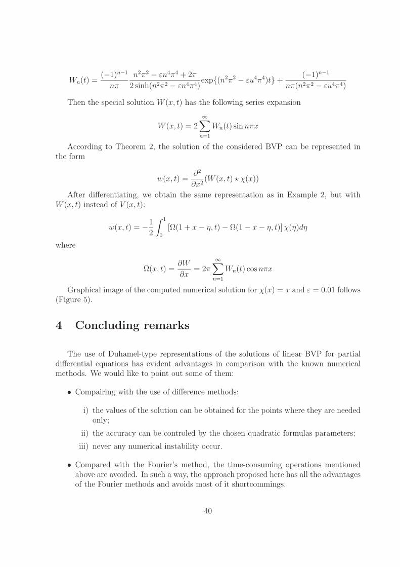
According to Theorem 2, the solution of the considered BVP can be represented inthe form
w(x, t) =∂2
∂x2(W (x, t) � χ(x))
After differentiating, we obtain the same representation as in Example 2, but withW (x, t) instead of V (x, t):
w(x, t) = −1
2
∫ 1
0
[Ω(1 + x − η, t) − Ω(1 − x − η, t)] χ(η)dη
where
Ω(x, t) =∂W
∂x= 2π
∞∑n=1
Wn(t) cos nπx
Graphical image of the computed numerical solution for χ(x) = x and ε = 0.01 follows(Figure 5).
4 Concluding remarks
The use of Duhamel-type representations of the solutions of linear BVP for partialdifferential equations has evident advantages in comparison with the known numericalmethods. We would like to point out some of them:
• Compairing with the use of difference methods:
i) the values of the solution can be obtained for the points where they are neededonly;
ii) the accuracy can be controled by the chosen quadratic formulas parameters;
iii) never any numerical instability occur.
• Compared with the Fourier’s method, the time-consuming operations mentionedabove are avoided. In such a way, the approach proposed here has all the advantagesof the Fourier methods and avoids most of it shortcommings.
40
0.20.4
0.60.8
1
x
0
0.2
0.4
0.6
0.8
1
t
00000
w
0.20.4
0.60.8
1
x
Figure 5: Example 4
• The performance of the computations related to the application of the presentedapproach in the environment of the computer algebra system Mathematica givesadditional advantages: high accuracy of the numerical computations, visualizationof the resuts and convenient use of the implemented approach.
References
[Dim1] Dimovski I., Convolutional Calculus, Kluwer Academic Publishers, Dordrecht,1990
[Dim2] Dimovski I., Duhamel-Type Representation of the Solutions of Non-Local Bound-ary Value Problems, Differential Equations and Applications (I), Proc. of the SecondConference, Rousse’81, Bulgaria, 1982, pp. 240-247
[Wid] Widder D.V., The Heat Equation, Academic Press, New York, 1975
[Lat] Lattes R. and J.-L. Lions, The Method of Quasi-Reversibility. Applications to Par-tial Differential Equations, American Elsevier Publ. Co., Inc., New York, 1969
[Ion] Ionkin N. I., Numerical Solution of a Nonclassical Boundary Value Problem for theHeat Equation, J. Differential Equations, V. 13, No 2, 1977, pp.294-304 (in Russian)
41

[SW] Wolfram S., Mathematica. A System for Doing Mathematics by Computer, SecondEdition, Addison-Wesley Publishing Co., Redwood City, California, 1991
[Baz] Bazhlekova E., Duhamel-type representation of the solutions of non-local boundaryvalue problems for the fractional diffusion-wave equation, Transform Methods &Special Functions, Proc. of the Second International Workshop, Varna, 1996, pp.32-40
42
On Families of Periodic Solutions ofLow Resonant Case of the
Generalized Henon - Heiles System
Victor F. Edneral1
Institute for Nuclear Physics of Moscow State University,Vorobievi Gori, Moscow, 119899 Russiae-mail: [email protected]
The paper describes the computer algebra application of the normal form method tobifurcation analysis of a low resonant case of the generalized Henon - Heiles system. Abehavior of all local families of periodic solutions in system parameters is determined.Corresponding approximated solutions were checked by a comparison with the numericalsolutions of the system.
1 Introduction
Normal form methods use a nonlinear change of variables to transform a nonlinear systemof ordinary differential equations to a simpler form. In this paper we use an algorithmbased on an approach developed by A.D. Bruno [1] for computing the resonant normalform. An important advantage of this approach is its algorithmic simplicity: there aredirect recurrence formulas for coefficients of the transformation and of the transformedsystem, and thus the storage of large intermediate results is not necessary. This approachdoes not require solving any intermediate systems and there are no restrictions on lowresonance cases.
2 The Generalized Henon–Heiles System
The generalized Henon–Heiles system is a couple of second order differential equations:
x + l1 · x + 2 · d · x · y = 0 ,y + l2 · y + d · x2 − c · y2 = 0 .
(1)
This system is known to be integrable [3] when:
1. l1 = l2, c/d = −1;
2. c/d = −6;
1Supported by the RFBR grant for the Scientific Schools support (the School by AcademicianA.A.Logunov)
43
3. 16l1 = l2, c/d = −16.
Below we discuss the case with the same pure imaginary eigenvalues of the linear partof (1). I.e. we suppose that l1 = l2 > 0. By changing the time variable we choosel1 = l2 = 1 and thus rewrite (1) to the ”low resonant form”.
Take into account the fact that if d = 0 the system can be integrated in an analyticalform because equations for x and y will be independent:
x + x = 0 , y + y − c · y2 = 0 .
The first equation above has an exponential solution and the second one has a solutionin terms of elliptic functions [9], example 6.10:
x(t) = C1 · exp(it) + C2 · exp(−it), C1, C2 ∈ C ,
t =
∫dt√
23· c · y3 − y2 + C3
, C3 ∈ R . (2)
Thus, let us assume that d = 0. Then with changing d · x → x, d · y → y and c/d → cwe obtain (1) in the form:
x + x + 2 · x · y = 0 ,y + y + x2 − c · y2 = 0 ,
(3)
with the Hamiltonian:
h =1
2[(x)2 + (y)2 + x2 + y2] + x2y − c
3y3 . (4)
A linear change of variables:
x = y1 + y2 , x = −i (y1 − y2)y = y3 + y4 , y = −i (y3 − y4) ,
(5)
transforms (3) to the form required by the method:
y1 = −i y1 − i (y1 + y2) (y3 + y4) ,y2 = i y2 + i (y1 + y2) (y3 + y4) ,y3 = −i y3 − i
2[(y1 + y2)
2 − c(y3 + y4)2] ,
y4 = i y4 + i2
[(y1 + y2)2 − c(y3 + y4)
2] ,
(6)
The eigenvalues of this system are two pairs of complex conjugate imaginary units: Λ =(−i, i,−i, i) 2. So this is a deeply resonant problem, i.e. the most difficult (and interesting)type of a problem.
2Remark that in paper [6] the other order of variables is used. The corresponding vector of eigenvaluesis Λ = (−i,−i, i, i) there. It corresponds to interchanging y2 ↔ y3 for agreement with notation of thepresent paper.
44
3 A Normal Form for the Generalized Henon–Heiles
System
For a pure resonance of the generalized Henon–Heiles system the ratios of all pairs ofeigenvalues are ±1 and the normal form for (6) is:
zk = zkGkdef= λkzk + zk
∑qk ≥ −1 ,
q1, . . . , qk−1, qk+1, . . . , q4 ≥ 0 ,q1 + q3 = q2 + q4 > 0
0 ≤ p ≤ q1 + q2 + q3 + q4
gk,q1,q2,q3,q4,p zq1
1 zq2
2 zq3
3 zq4
4 cp, k = 1, . . . , 4 . (7)
Gk = Gk(z, c) are series in z1, . . . , z4 and polynomials in c, gk,q1,q2,q3,q4,p are numericcoefficients which can be calculated by the LISP based program NORT [4].
The set A in a phase space of system (7) is defined by the system of equations [1], [7]:
A = {z1, z2, z3, z4 :λkzkω = λkzk + zk
∑gk,q1,q2,q3,q4,c zq1
1 zq2
2 zq3
3 zq4
4 cp}, k = 1, . . . , 4 ,(8)
where ω is a series in z1, . . . , z4 and polynomials in c. ω does not depend on index k alongthe set A.
Searching for all local periodic families of solutions of system (6) is equivalent tosearching for the set A which contains all of them. It is important that along the set Aformal series in formulae above have a basis which consists of convergent power series in zk
variables 3 [1]. So the families of periodic solutions of (8) can be expressed (approximated)in terms of convergent series.
Equations (8) can be recast (by eliminating ω which is non zero for non-trivial solu-tions) in the form:
P1def= z1z2 · [G1(z, c) + G2(z, c)] = 0 ,
P2def= z3z4 · [G3(z, c) + G4(z, c)] = 0 ,
P3def= z1z4 · [G1(z, c) + G4(z, c)] = 0 ,
P4def= z2z3 · [G2(z, c) + G3(z, c)] = 0 .
(9)
Of course no more than 3 equations above are independent, but the form (9) is symmetric.Because of (8) all families of periodic solutions of (7) have the form:
zj = aj exp(−iωt) , zj+1 = aj+1 exp(iωt) , j = 1, 3 . (10)
The aj above are integration constants and ω is time independent and plays the role offrequency. It depends on constants c and aj only.
With (10) we can rewrite (9) as an algebraic problem of solving a system of equations
3The parameter c is not supposed to be small.
45
over the ring of formal power series in ak:
P1def= a1a2 · [G1(a1, . . . , a4, c) + G2(a1, . . . , a4, c)] = 0 ,
P2def= a3a4 · [G3(a1, . . . , a4, c) + G4(a1, . . . , a4, c)] = 0 ,
P3def= a1a4 · [G1(a1, . . . , a4, c) + G4(a1, . . . , a4, c)] = 0 ,
P4def= a2a3 · [G2(a1, . . . , a4, c) + G3(a1, . . . , a4, c)] = 0 .
(11)
Searching for all local families of periodic solutions of system (7) is equivalent to deter-mining all solutions of system (11).
The original system (3) is real, thus real solutions of (7) satisfy the reality conditions:
zj+1 = zj, j = 1, 3oraj+1 = aj, j = 1, 3
(12)
so we can fix (by neglecting a trivial time shift) a2 = a1 as pure real.Because system 3 is even in time all families of solutions arise by couples.
4 Calculation of Results
By using our program NORT for system (6) we have calculated the normalizing transfor-mation and normal form till the 10th order in zk (i.e. till 12th in ak for Pk series). Wecalculated periodic solutions and compared them with corresponding numerical solutionsat different values of parameters. Below we discuss the bifurcation picture and the phaseportrait of system (3) following this analysis 4.
It is proved in [2] that for any reversible resonant system of the 4th order, both theseries P1 and P2 have the same factor:
P1(z) = (zr1z
s4 − zr
2zs3) · Q1(z) ,
P2(z) = (zr1z
s4 − zr
2zs3) · Q2(z) ,
where r and s are smallest positive integers which satisfy the equation λ1 · r = λ3 · s.For our case s = r = 1, but the system has an additional symmetry and we can find
by factoring that the P1 and P2 series calculated by the NORT program have a morecomplicated factor:
P1 = 2i· (a21a
24 − a2
2a23)·
·[1 +
1
6c +
(133
18− 95
108c − c2
)a1a2+
+
(4
9− 172
27c +
23
18c2 +
89
108c3
)a3a4 + O(a4)
],
P2 = −2i· (a21a
24 − a2
2a23)·
·[1 +
1
6c +
(13
2− 95
108c − 1
9c2
)a1a2+
+
(20
9− 148
27c − 1
2c2 − 7
108c3
)a3a4 + O(a4)
],
(13)
4All calculations below were carried out for the mechanical energy h = 1/12.
46
where (and in some places below) we adduce for simplicity first terms of the calculatedseries only.
Recall that we are interested only in local solutions, i.e. in such solutions of (11) whichcan include the stationary point ak = 0, k = 1, . . . , 4 as a particular case.
Thus, instead of the first pair of equations in (11), we have the equation:
a21a
24 − a2
2a23 = 0 ,
because the brackets in (13) cannot add any nontrivial local solution as they containconstant terms at c = −6, and at c = −6 these both brackets are proportional to a1a2 +4a3a4, which is a sum of squares of modules (see (12)).
So, if we now fix a1 = a2 = a as a pure real, then the first couple of equations (13)has two solutions:
1. a3 = a4 = b has a pure real value;
2. a3 = −a4 has a pure imaginary value. Let a3 = ib.
4.1 Case of Pure Real a3
In this case the second pair of equations (13) gives a single equation:
P3 = −P4 = α1 · a · b · [a2 − (c + 2)b2] ·[c − 1 −
(2431
180− 29
90c +
217
60c2
)a2−
−(
67
90− 1289
180c +
233
45c2 − 157
36c3
)b2 + O(a4) + O(b4) + O(a2b2)
]= 0 .
(14)
α1 here is a nonzero numerical constant. Let us discuss the families of periodic solutionswhich correspond to zeroing each factor of the product above.
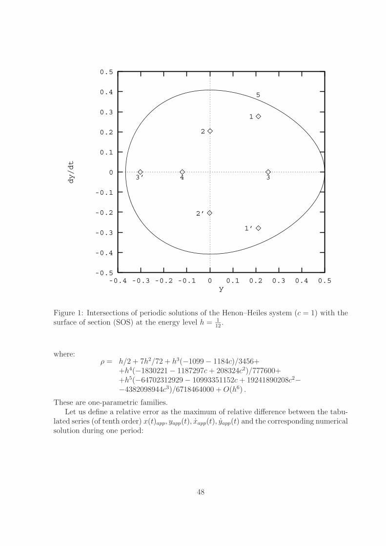
A couple of families of periodic solutions which corresponds to a = 0 exists at anyvalues of c and lies in the plane x = 0. This is a family with a single internal parameter.We choose the mechanical energy h from (4) as this parameter. At c = 1 this familycorresponds to family 5 of the classic Henon–Heiles system [8], see Fig. 1 and paper [6].
In Fig. 1, the intersections of periodic solutions of the Henon–Heiles system with Sur-face Of Section (SOS) [8], which is defined by equations SOS = {x = 0, x = x(x, y, y, h) >0}, are displayed in coordinates y, y. The periodic solutions of families 5 lie entirely inthe plane x = x = 0. For this case there is an analytical solution of type 2 in ellipticfunctions.
The families which correspond to b = 0 also exist at any values of c. They look likefamily 4 of the Henon – Heiles system (Fig. 1). The corresponding intersection flowsslowly from left to right at increasing c. The frequency of these periodic families is:
ω4 = 1 − 5ρ/3 + ρ2(−281 + 504c)/108++ρ3(−13913 + 645024c − 323488c2)/19440++ρ4(33903721 + 134318856c − 137045376c2 + 59393664c3)/699840+ρ5(103971857615 + 172223295216c − 402212367472c2++294216077568c3 − 105272265984c4)/220449600 + O(ρ6) ,
47
-0.5
-0.4
-0.3
-0.2
-0.1
0
0.1
0.2
0.3
0.4
0.5
-0.4 -0.3 -0.2 -0.1 0 0.1 0.2 0.3 0.4 0.5
dy/dt
y
1’
1
2’
2
3’ 34
5
Figure 1: Intersections of periodic solutions of the Henon–Heiles system (c = 1) with thesurface of section (SOS) at the energy level h = 1
12.
where:ρ = h/2 + 7h2/72 + h3(−1099 − 1184c)/3456+
+h4(−1830221 − 1187297c + 208324c2)/777600++h5(−64702312929 − 10993351152c + 19241890208c2−−4382098944c3)/6718464000 + O(h6) .
These are one-parametric families.Let us define a relative error as the maximum of relative difference between the tabu-
lated series (of tenth order) x(t)app, yapp(t), xapp(t), yapp(t) and the corresponding numericalsolution during one period:
48
ferrdef= supt ∈ [0, 2π/ωi]√
(xnum(t)−xapp(t))2+(ynum(t)−yapp(t))2+(xnum(t)−xapp(t))2+(ynum(t)−yapp(t))2
x2num(t)+y2
num(t)+x2num(t)+y2
num(t)
The relative error of the approximation of this case is about 6% at c = −1; 0.3% at c = 1and 0.23% at c = 2.
The next case is a2 = (c+2) · b2. At c = 1 it corresponds to 2 and 2’ families in fig. 1.The families are real if c ≥ −2 only. It is one parametric case also. With increasing c itslowly flows to the abscissa axis. At c = −2 it coincides with curve 5. The frequency is:
ω2 = 1 − 20h1/3 − 380h21/3 − 878960h3
1/243−−88121780h4
1/729 − 3203319760h51/729 + O(h6
1)
where h1 = h/(2(3 + c)). The relative error is about 4% at c = 0; 0.4% at c = 1 and0.06% at c = 2.
Zeroing the last brackets in (14) is possible near the point c = 1, when the corre-sponding distance c − 1 is about a square of amplitudes a or b, or, say, about energy h.So we can suppose that c = 1 + ε · h and the corresponding solution exists at least atε lower or about 1. This case agrees with families 1 and 1′ in Fig. 1. The intersectionwith SOS flows to the abscissa axis and from right to left with increasing ε. These areone parametric families. The frequency is: ω1 = 1−25εh/252+O(h2) . The relative errorhere is 0.09% at ε = −1; 0.09% at ε = 1 and 0.2% at ε = 2. A small value of error maysay about possibility of spreading this case into wider domain of the parameter ε.
4.2 Case of Pure Imaginary a3
Let a3 = ib. In this case the second pair of equations (13) also gives a single equation:
P3 = P4 = α2 · a · b · (c + 1)··[7a2 − (5c + 2)b2 + O(a4) + O(b4) + O(a2b2)] = 0 .
(15)
α2 here is a nonzero numerical constant. Let us one more discuss families of periodicsolutions, which correspond to zeroing factors of the product (15).
Cases a = 0 and b = 0 have been discussed. Case c = −1 is a specific one. It isan essential two parametric case, but it is better to choose parameters from a physicalmeaning. Let us introduce the energy as one of parameters. We will suppose that theamplitudes a and b connected with the energy h in this way:
a2 + b2 = p(h), a2 = β · p(h), β ∈ [0, 1] ,
where p(h) is the series:
p(h) = h/2 + 7h2/72 + 85h3/3456−−2173h4/3888 − 240679781h5/53747712 + O(h6) .
49
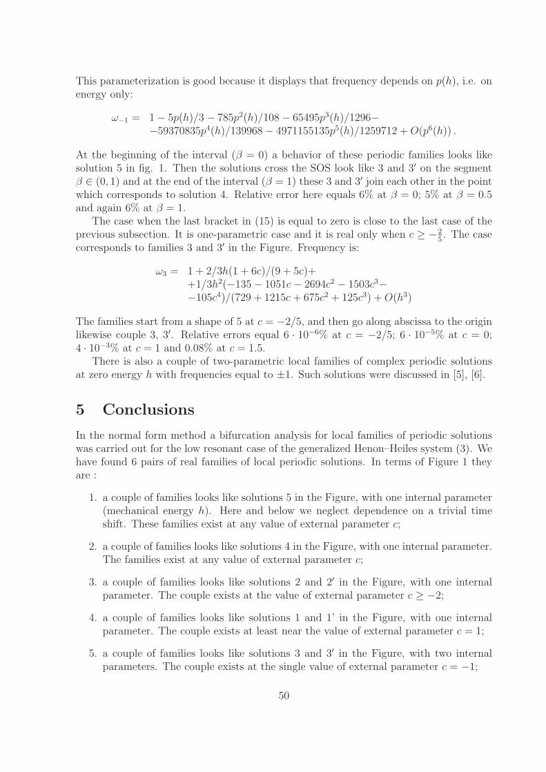
This parameterization is good because it displays that frequency depends on p(h), i.e. onenergy only:
ω−1 = 1 − 5p(h)/3 − 785p2(h)/108 − 65495p3(h)/1296−−59370835p4(h)/139968 − 4971155135p5(h)/1259712 + O(p6(h)) .
At the beginning of the interval (β = 0) a behavior of these periodic families looks likesolution 5 in fig. 1. Then the solutions cross the SOS look like 3 and 3′ on the segmentβ ∈ (0, 1) and at the end of the interval (β = 1) these 3 and 3′ join each other in the pointwhich corresponds to solution 4. Relative error here equals 6% at β = 0; 5% at β = 0.5and again 6% at β = 1.
The case when the last bracket in (15) is equal to zero is close to the last case of theprevious subsection. It is one-parametric case and it is real only when c ≥ −2
5. The case
corresponds to families 3 and 3′ in the Figure. Frequency is:
ω3 = 1 + 2/3h(1 + 6c)/(9 + 5c)++1/3h2(−135 − 1051c − 2694c2 − 1503c3−−105c4)/(729 + 1215c + 675c2 + 125c3) + O(h3)
The families start from a shape of 5 at c = −2/5, and then go along abscissa to the originlikewise couple 3, 3′. Relative errors equal 6 · 10−6% at c = −2/5; 6 · 10−5% at c = 0;4 · 10−3% at c = 1 and 0.08% at c = 1.5.
There is also a couple of two-parametric local families of complex periodic solutionsat zero energy h with frequencies equal to ±1. Such solutions were discussed in [5], [6].
5 Conclusions
In the normal form method a bifurcation analysis for local families of periodic solutionswas carried out for the low resonant case of the generalized Henon–Heiles system (3). Wehave found 6 pairs of real families of local periodic solutions. In terms of Figure 1 theyare :
1. a couple of families looks like solutions 5 in the Figure, with one internal parameter(mechanical energy h). Here and below we neglect dependence on a trivial timeshift. These families exist at any value of external parameter c;
2. a couple of families looks like solutions 4 in the Figure, with one internal parameter.The families exist at any value of external parameter c;
3. a couple of families looks like solutions 2 and 2′ in the Figure, with one internalparameter. The couple exists at the value of external parameter c ≥ −2;
4. a couple of families looks like solutions 1 and 1’ in the Figure, with one internalparameter. The couple exists at least near the value of external parameter c = 1;
5. a couple of families looks like solutions 3 and 3′ in the Figure, with two internalparameters. The couple exists at the single value of external parameter c = −1;
50
6. a couple of families looks like number 3 and 3′ in the Figure also, with one internalparameter. The couple exists at the value of external parameter c ≥ −2/5.
There are two local two-parametric complex families of periodic solutions at the energyh = 0 also.
Acknowledgements
The author is very grateful to Prof. R. I. Bogdanov and Dr. S. Yu. Vernov for interestingdiscussions and important advices.
References
[1] Bruno, A.D.: Local Method in Nonlinear Differential Equations, Springer-Verlag,Berlin (1989)
[2] Bruno, A.D., Soleev, A.: Local analysis of a singularity of a reversible ODE system.Complicated cases; Preprint # 47 of the Keldysh Institute of Applied Mathematicsof RAS, Moscow (1995)(in Russian)
[3] Chang, Y.F., Tabor, M. and Weiss, J.: Analytic structure of the Henon-Heiles Hamil-tonian in integrable and nonintegrable regimes. J. Math. Phys. 23 (1982) 531–538
[4] Edneral, V.F.: Computer generation of normalizing transformation for systems ofNonlinear ODE. In: Proceedings of the 1993 International Symposium on Symbolicand Algebraic Computation (Kiev, Ukraine, July 6-8, 1993), M. Bronstein (ed.),ACM Press, New York (1993) 14–19
[5] Edneral, V.F.: Complex periodic solutions of autonomous ODE systems with ana-lytical right-hand sides near an equilibrium point. Fundamentalnaya i prikladnayamatematika 1 (1995) #2 393–398 (in Russian)
[6] Edneral, V.F.: A symbolic approximation of periodic solutions of the Henon–Heilessystem by the normal form method. J.Mathematics and Computers in Simulation 45(1998) 445–463
[7] Edneral, V.F.: About normal form method. In: Proc. Second Workshop on ComputerAlgebra in Scientific Computing (CASC’99, Munich, Germany, 1999), Ganzha et al.(eds.), Springer (1999) 51–66
[8] Henon, M., Heiles, C.: The applicability of the third integral of motion: Some nu-merical experiments. Astronomical J. 69 (1964) 73–79
[9] Kamke, E.: Differentialgleichungen. I, Verbesserte Auflage, Leipzig (1959)
51
Computer Algebra at KELDYSHInstitute of Applied Mathematics
G.B.Efimov, I.B.Tshenkov, E.Yu.Zueva
Keldysh Institute of Applied Mathematics RAS, Moscow;e-mail: [email protected]
Brief retrospective review and main references concerned Computer Algebra (CA) re-searches and applications at famous Keldysh Institute of Applied Mathematics (RussiaAcademia of Science) are presented. At the Institute CA was used in various areas: Ap-plied Celestial Mechanics, Mathematics, Robotics, Hydromechanics, Applied CalculationMethods. Some original program sys-tems were elaborated. During several years the workdevoted to classification of existing systems and their possibilities was done. Conferencesand seminars concerned CA applications in mechanics were organized. A language ofrecur-sive functions, REFAL, was generated at the Institute. Later it was modified andintensively used in various fields, in particular CA. Many ideas and results, which onecan find in researches on CA and close fields implemented at Keldych Institute, are stillinteresting today. The work was supported by RFBI, grants No 01-01-00015 and No 00-15-96036.
Keldysh Institute of Applied Mathematics of Russian Academia of Science (RAS) wasfounded in 1952 by M.V.Keldysh for solving difficult scientific problems of national impor-tance, such as nuclear physics, cybernetics, space mechanics and others. At the Instituteexperts on different areas - mathematicians, physicists, mechanicians, computer scientists- were working together, in close contacts with each others. Such famous scientists asA.N.Tichonov, K.I.Babenko, I.M.Gelfand, A.A.Liapunov, I.B.Zeldovich,D.E.Okhozimsky,A.A.Samarsky, V.S.Yablonsky, M.R.Shura-Bura, A.N.Miamlin, M.L.Lidov, V.V.Beletsky,S.P.Kurdiumov, T.M.Eneev were among them.
Numerous difficult problems required various mathematical methods for their solution.Active pioneer’s using of first computers, enthusiasm caused by early successes in thisnew field - all this gave many interesting ideas. The idea of symbolic computations arosejust after computer’s appearance, as a will to learn computer to interact with the humanperson via ordinary mathematical language, to facilitate the job of physicist or mecanician.Reviews of early soviet researches on Computer Algebra (or Symbol Manipulations, asit was called initially) are presented in the publications [1-13]. These old works may beinteresting -not all of them were known sufficiently at the time when they were carriedout; some ideas are still valuable now.
First experiments with Symbol Manipulations were made in Russia as early as thebeginning of sixties. In 1956 at the first National Conference devoted to computer scienceA.A.Dorodnitcin formulated the task which we can consider as the beginning of SymbolManipulation in Soviet Union [14]. This task was concerned with the investigation of
52
nuclear explosion in the atmosphere. It was proposed to built the solution in the formof two asymptotic power series (near the center of the explosion and far from it). Theseassimptotics should be conjugated by common numerical solution in the regular area.Thus it was the combined analytical/numerical approach. D.E.Okhozimsky applied thisapproach to cosmodynamics problem [15]. He also built two assimptotics conjugated bycommon numerical part. Assimptotics construction on one of the first soviet computers”Strela” was pioneer too.
At the same time in Leningrad department of Steklov Mathematical Institute Nobellaureate L.V.Kantorovich investigated some types of symbolic notation for ComputerAlgebra. His follower T.N.Petrova created the program ”Polynomial Prorab”, used laterfor the tasks of theory of elasticity and others [16].
The formulation of Dorodnitcin is referred by A.A.Stogny [17], the follower of V.A.Glushkov in Kiev. He proposed an algorithm to obtain the polynomial solution of differ-ential equation. It was probably the first result of the famous Kiev Computer Algebraschool.
N.N.Yanenko investigated Cartan’s methods of analysis of compatibility of systems ofdifferential equations in partial derivations and realized it on computer ”Strela” [18].
Solutions in series of some problems of Celestial Mechanics were built in Leningradby V.A.Brumberg and his colleages [19]. This approach was elaborated and extendedlater. Similar work was done by I.B.Zadyhajlo and Z.P.Vlasova in KIAM, Moscow. Thesimilar approach to the tasks of the theory of elasticity was elaborated by the group ofL.V.Kantorovich in Leningrad and V.K.Kabulov in Tashkent [20].
Let us return to KIAM. Here the first attempts to use Symbol Manipulations were donein the area of Applied Celestial Mechanics. As it was mentioned above, manipulationswith trigonometric and power series were implemented on soviet computer ”Strela” byZ.P.Vlasova and I.B.Zadyhajlo (non-published). In 1964 D.E.Okhozimsky initiated thework on semi-analytical solution of one cosmodynamics problem, the low-thrust flight incentral field of gravitation [15]. G.B.Efimov realized this approach for simplest Poissonseries (1970) [21].
From 1970 A.P.Markeev used CA for Gamilton’s systems normalization and periodicsolution stability analysis [22]. The next steps in this direction were done by his fol-lower A.G.Sokolsky [23-25]. This work was continued by the same group in MAI andlater by A.G. Sokolsky in ITA RAS (Leningrad) [26-29], where the well known school ofV.A.Brumberg did work already. In MAI Computer Algebra applications to educationwere developed as well [30].
V.A.Saryshev and S.A.Gutnik used CA for the problem of sputnik equilibrium stability(1984) [31-32]. Some important results were obtained last years by A.D.Bruno and hisgroup (see below).
From 1963 M.L.Lidov with his group did numerous experiments concerned CA applica-tion to sputnik dynamics problems [33]. A method united both analytical and numericalapproaches was proposed [34-35]. For elliptic orbits and distortions of different sorts,analytical approach was used to construct the Hamilton disturbing function H*. Then,coordinate transformation and calculation of right parts of disturbed motion equations inevery step of integration, was done via Hamilton function differentiation. This approachprovides high accuracy method of motion calculation and allows to avoid labor-consuming
53
calculations [36-38]. Infortunately, requirements to CA systems to be used in this schemewere rather high, and available CA systems were not capable to satisfy them. Thus, thesevery interesting experiments didn’t produce practically usable integrated (analytically-numerical) system. From the other hand, it was impossible to use ready CA systemsof general purpose, very primitive at this time, to solve such complicated problems. Asa result, very sophisticated special algorithms and programs were elaborated, but theseinvestigations didn’t stimulate the development of CA systems for common usage.
The very interesting page in russian cybernetics is the history of REFAL. In 1969V.F.Tourchin created an original computer language REFAL based on new principle ofprogramming - associative text processing on the base of recursive function theory, withoutdirectly addressed control of the program [39-41]. From the beginning Computer Algebrawas among potential areas of REFAL applications [42]. However, first REFAL realiza-tion was rather ”scientific” then practical, since it was isolated and not compatible with”ordinary” software - numerical packages, library support, memory allocation and so on.Additional efforts of many people required to make REFAL modifications practically us-able, in particular for Computer Algebra Applications. S.N.Florentcev, S.A.Romanenko,A.V.Klimov were the first who wrote high-effective compiler from REFAL.
The first REFAL program realized some CA features was elaborated by V.F. Tourchinand others to solve some problems of Nuclear Physics in series [43]. I.B. Tshenkov elabo-rated general purpose SAM named SANTRA and later modified it [44-45]. On this basethe special applied system DISPLAN was made for processing non-standard differenceschemes, by I.B.Tshenkov and M.Yu.Shashkov [46]. M.L.Lidov and L.M. Bakuma wereamong the first REFAL’s users in applied area. They did some attempts to process Pois-son series. Analogous attempts in the group theory were done by H.C.Ibragimov andI.B.Tshenkov.
Some enthusiasts of REFAL were united by KIAM and worked in close contact with it.V.L.Topunov with his colleagues from Moscow Institute of Pedagogy used REFAL-basedCA system in differential geometry [47]. Together with V.P.Shapeev and the others fol-lowers of N.N.Yanenko (Novosibirsk) they realized method of H.Cartane and investigatedthe characteristics of difference schemes [48,17]. L.V.Provorov in N.Jukovsky CentralAir-Hydrodynamics Institute and in Bauman High Technology University used CA sys-tem ALCOR in large area applications in engineering [49]. In mechanics, O.M.Gorodeskiy(Grodno) and A.V.Korlyukov created CA system for simulation in dynamics of Gyroscopesystems (used by ac. D.M.Klimov) [50]. As a first stage of the work, the equations of themotion were automatically derived. Usage of REFAL allowed to present the equationsin convenient form near to human presentation. L.F.Belous and I.R.Akselrod (in Khar-cov) used REFAL for integration several different programming systems and numericalpackages into a united system, including in this system the well known REDUCE anddomestic Computer Algebra package SIRIUS [51].
In Keldysh Institute the possibilities to create REFAL-processor were investigated.A.N.Miamlin, I.B.Zadyhajlo and V.K.Smirnov were the leaders of the project [52-54].L.K. Eisymont analyzed REFAL efficiency for both program and apparatus realization,in particular from the CA application point of view [55,56]. REFAL processor EC-2702was simulated by V.K.Smirnov with his group on the computer EC-2635 with micropro-gramming [54,57-60]. This processor was compatible with EC-series computers, it was
54
used for CA problems as well as for translators [61].REFAL was initially planned as a ”meta language”. It was used indeed in wide scope
of textual tasks, more or less near to CA. V.A.Fisun, A.I.Choroshilov and others realizedcomputer languages Simula-1, DYNAMO [62,63], complex for cosmic training TRIKS,ALGOL-FORTRAN converter for physical packages - all based on REFAL. Yu.F.Golubevsimulated the work of on-board sputnik computer. In this direction the automate scalingof calculation was introduced, to compensate the lost of accuracy caused by fixed pointusage. This work was carried out by several authors, in particular L.K.Eisymont andI.B.Zadyhajlo. A.N.Andrianov and K.H. Efimkin automated the calculation of differenceschemes in NORMA system [64].
At the beginning of eighties, CA popularization and systems comparison became im-portant, in particular for mechanical tasks which required computer experiment for theirinvestigation and solution [5,7-8,65,66]. CA was successively used for difference schemesconstruction in the area of non-regularity [67]. The result of the last work was positivelyevaluated by A.A.Samarsky, leader in soviet mathematical modeling. With the aid ofA.A. Samarsky KIAM became one of the main organizer of the First National Conferenceon Computer Algebra Applications in Mechanics in Gorky (Nijniy Novgorod) in 1984 [6].The results of about 20 years research, as well as future plans and perspective directions,were discussed.
To generalize the experience of common work of mathematicians, mechanicians andprogrammers, some classification work was done by G.B.Efimov and M.V.Grosheva [68-71]. There were reviews of CA systems and CA applications for mechanical problems[5,7,8,66,72-75]. Tables of CA systems features were presented for users [5,8,68,69]. Thesereviews provided convenient tool for CA systems comparison and selection for potentialusers - experts in applied areas. Such analysis was useful for CA developers as well.First CA systems were usually specialized and elaborated for concrete task solution. Forexample, in the area of dynamics of multi-bodies systems many various CA systemswere created, so the classification and comparison of their features became important[69,71]. Later the well known modern universal systems, such as REDUCE and others,appeared and were used for various algorithms realization. For example, S.A.Gutnik,M.Yu.Shashkov and others used REDUCE [31,76,85-87,90]. Currently CA is used asnecessary standard tools in big program complex, often without any special mention.
A number of problems were investigated and solved in KIAM with aid of CA duringabout 25 years. The investigation of difference schemes was continued [45,67], partly incontact with the followers of N.N.Yanenko [75]. In the area of fluid and gas dynamics someworks were carried out. Several Hydrodynamics problems were resolved by I.B.Tshenkovand Ya.M. Kajdan with aid of REFAL-based CA program and by M.Yu.Shashkov andL.N.Platonova in REDUCE [76,77]. In the area of dynamics of complicated multi-bodiessystems (robotics, spacecraft) CA is used for deriving the equations of motion, stabilityinvestigation, automatic generation of program of numerical analysis, and others. ThePAS and others systems were created which was used for deriving the equations of mo-tion and for solving some problems of the theory of control [78-82]. Computer Algebraapplications to mechanical education were developed by D.Yu.Pogorelov, the follower ofV.V.Beletsky [83,84]. Reviews of the works, concerning CA application in mechanics,dynamics of multi-bodies systems and theory of control were issued [5,7,8,66,72-75].
55
Most important results of last years at Keldysh Institute are obtained by A.D.Brunoand his followers. It concerned some algorithms of normalization in Hamilton systems andNewton polyhedra investigation [85-90]. S.Yu.Sadov and V.P.Varin investigated stabilityof motion for celestial mechanics problems [86,87,90]. There are several publicationsdevoted to the history of CA and its applications in KIAM [13,91-93].
References
Almost all publications are in Russian, except noticed by ”*”. The ”Cosmic Research”and other Journals were translated in English since about 1975. At some numbers thereferences to Russian Reference Journal in Mathematics and Mechanics was done - RJMath., RJ Mech.
1. Calculus mathematics and computer facilities. All-Union seminar. - Inst. of LowTemperature Physics AS UkrSSR, 1972, N 3, 152 pp.
2. Analytical calculations on the Computer and their application in theoretical Physics.Materials of International conference. Dubna, 1979. - Dubna: JINR, 1980, 187 pp.1983, 260 pp. 1985, 420 pp.
3. Gerdt V.P., Tarasov O.V., Shirkov D.V.- Uspehi Phys. Nauk, 1980, v. 30, N 1,113-147.
4.∗ Miola A.M., Pottosin I.V. - A bibliography of soviet works in algebraic manipula-tions. - SIGSAM Bull., 1981, v. 15, N 1, 5-7.
5. Systems of analytical calculations on the Computer (Applied Analytical Packages).Materials of seminar of Institute Mechanics MSU, 1981. - Informator. KedyshInstitute of Applied Mathematics AS USSR, 1983, N 1, 65 pp.
6. Systems for Analytical Manipulation in Mechanics. Thesis the Reports of All-UnionConference. Gorky, 1984. - Gorky: GSU, 1984, 147 pp.
7. Applied Program Packages. Analitical manipulations. - M., Nauka, 1988. 156 pp.
8. Grosheva M.V., Efimov G.B. Systems for analytical calculation in Computer. - In:Applied programs pakages. Analytical manipulations. M., Nauka, 1988, 5-30.
9.∗ Brumberg V.A., Tarasevich S.V., Vasiliev N.N. Specialized Celestial Mechanics sys-tems for Symbolic Manipulations.- Celestial Mech., 1988/89, v. 45, N 1-3, 145-162.
10. Klimov D.M., Rudenko V.M. Computer Algebra Method’s in Mechanical problems.- M., Nauka, 1989. 215 pp.
11.∗ Computer Algebra in Physical Research. Int. Conf. Computer Algebra Phys. Res.,Dubna, USSR, 1990. Memorial Volume for N.N.Govorun. - World Scientific, 1991,453 p. Thesis, Dubna-1990. - Dubna: JINR, 1990.
56
12. Abramov S.A., Zima E.B., Rostovzev V.A. Computer Algebra. - Programirovanie,1992, N 5, 4-25.
13.∗ The History of Computer Algebra Applications. Session. 4-the Intern. IMACSconference on Applications of Computer Algebra.- IMACS ACA’98, Prage, Aug.9-11, 1998.- M., 1998, 35 pp.
14. A.A.Dorodnitcin. Solution of mathematical and logical tascs in computer. All-Uniom Confer. Moscow, 12-17 March 1956. Plenary reports. - VINITI. M., 1956.
15. Okhozimsky D.E. Cosmic Research. 1964, v.2, N 6, 817-842.-. - RJ Mech., 1965,11A29
16. Kantorovich L.V. About one mathematical symbolic system convinient for com-puter calculations. Doklady AS USSR, 1957, v. 113, N 4, 738-739; KantorovichL.V., Petrova L.T. 3th All-Union Mathemat. Congress. 1956. Rep. V.2, M., 151;Smirnova T.N. Trans. Steklov Mathematical Institute. - M.- L., 1962.; Pervozvan-skaya T.N. - Ibid.; Smirnova T.N. Polinomial PRPRAB. - L., Nauka. 1967.
17. Stogny A.A. In.: Problems of Cybernetic. - M., Nauka, 1962 N 7, 189-200.
18. Shurygin V.A., Yanenko N.N. In.: Problems of Cybernetic. - M., Nauka, 1961 N 6,33-43.- RJ Math., 1962, 7B332.
19. Brumberg V.A. Bull. ITA AS USSR, 1963, v.9, N 4, 234-256; Brumberg V.A.Reports of Inst. Theor. Astronomy (ITA AS USSR). L., 1966, N 11, 3-88; PolozovaN.G., Shor V.A. Probl. of motion artif. spacecrafts of Celestial bodies. - M., 1963.
20. Kabulov V.K. Doklady AS UzbekSSR, Tashkent, 1963, N 9; Tolok V.A. In.: Probl.comp. Math. & Thechn. Tashkent, 1964, N 3; Kabulov V.K. Algorithmizationin elasticity and deformational plasticity theory.- ”Fan” AS UsbekSSR, Tashkent,1966.
21. Efimov G.B. Cosmic Research.1970, v.8, N 1, 26-47.- RJ Mech., 1970, 7A28; KIAMPublication. 1970. 110 pp.
22. Markeev A.P. KIAM Publication. 1970. 163 pp.
23. Markeev A.P., Sokolsky A.G. KIAM Preprint N 10. 1975.
24. Markeev A.P., Sokolsky A.G. KIAM Preprint N 31. 1976. RJ Math., 1976, B1097.
25. Markeev A.P., Sokolsky A.G. Reports of Inst. Theor. Astronomy. L., 1978, N 17,62-68.
26. Sokolsky A.G., Shevchenko I.I. Preprint N 8 Inst. Theor. Astronomy. L., 1990.
27. Sokolsky A.G. Contemporant Problems of Computer Algebra in Celestial Mechanics- 7 All-Union Congress of Ther. & Applied Mechanics, M., 1991. Abstract. M.,1991, p. 323. RJ Mech., 1991, 12A125.
57
28.∗ Sokolsky A.G. On the Problems of Computerization of Celestial Mechanics.- Com-puter Algebra Applications. Intrn. Worcshop ISSAC Kiev, Ucrain, July 1993.-Abstract. S.-Peterburg. 1993. pp.41-45.
29.∗ Sokolsky A.G., Vakhidov A.A., Vasiliev N.N. Development of a Motion Theory forSatellites with large eccentricities by means of Computer Algebra.-Russia-RomaniaSimposium. Bucurest, 7-12 sent. 1995. Abstract., S.-Petersburg. 1995. 39.
30. Veretennikov V.G., Markeev A.P., Karpov I.I. et all. Theoretical Mechanics. Gen-eration and Analysis of equetion of motions.- M., ”Visshaya shkola”, 1990.
31. Sarychev V.A., Gutnik S.A. Cosmic Research.1984, v.22, N 3, 323-326.
32. Sarychev V.A., Gutnik S.A. KIAM Preprint N84 1990.
33. Dovjenko Z.P. Diploma. Moscow University (lided by Lidov M.L.) 1963.
34. Lidov M.L., Lyachva V.A., Solovyev A.A. Cosmic Research.1975, v.13, N 3, 335-346.- KIAM Preprint N 69-70. 1974.
35. Lidov M.L. Reports of Inst. Theor. Astronomy. Leningrad, 1978, N 17, 54-61.
36. Gordeeva Yu.F. KIAM Preprint N 26-27. Lidov M.L., Gordeeva Yu.F. CosmicResearch.1974, v.12, N 4, 491.
37. Lidov M.L., Solovyev A.A. Cosmic Research.1978, v.16, N 6, 806; Cosmic Re-search.1975, v.13, N 3, 303.- KIAM Preprint N 69-70. 1974.
38. Vashkovyak M.A. Cosmic Research.1972, v.10, N 2, 147-158; Cosmic Re-search.1983,v.21, N 6, 819. Cosmic Research.1985, v.23, N 3, 335-346.
39. Turchin V.F. Metaalgortmic Langvich. - Cybernetika. 1968, N4, 45-54. RJ Math.,1971, 2V86.
40. Turchin V.F., Serdobolsky V.I. - Cybernetika. 1969, N3, 58-62.
41. Turchin V.F. KIAM Preprint N41,43,44,48,49. 1971. RJ Math., 1972, 1V993-996.
42. Turchin V.F. - In.: Calculus mathematics and computer facilities. All-Union semi-nar. - Inst. of Low Temperature Physics AS UkrSSR, 1972, N 3, 28.
43. Budnik A.P., Turchin V.F., Tshenkov I.B. et all. Nuclear Phys., 1971, v.14, N2,304-314.
44. Tshenkov I.B. In.: Systems for Analytical Manipulation in Mechanics. Thesis theReports of All-Union Conference. Gorky, 1984. - Gorky: GSU, 1984, 47-49.
45. Tshenkov I.B. KIAM Preprints N 1, 7, 21 1989, N 14, 15 1991.
46. Shashkov M.Yu., Tshenkov I.B. KIAM Preprint N 48 1983, N 23 1985.
58
47. Topunov V.L. In.: Applied Math. and Math. Phys. M., 1975, N 2, 158-172, 148-152.
48. Arais E.A., Shapeev V.P., Yanenko N.N. Doklady AS USSR, 1974, v. 214, N 4, 737-738. RJ Math., 1974, 6V1149. Ganja V.J., Meleshko S.V., Murzin F.A., ShapeevV.P., Yanenko N.N. Doklady AS USSR, 1981, v. 261, N 5, 1044-1046. RJ Math.,1982, 4B1206.
49. Provorov L.V., Shtarkman V.S. KIAM Preprint N 61, 166 1982. Provorov L.V. etall. Bauman Moscow Technical University. M., 1985.
50. Klimov D.M., Gorodetsky O.M., Korlyukov O.M. Inst. Probl. Mach. AS USSR.Preprint N 233, 1985, 55 pp.
51. Belous L.F. In.: Systems for Analytical Manipulation in Mechanics. Thesis theReports of All-Union Conference. Gorky, 1984. - Gorky: GSU, 1984, 21-22.
52. Zadyhajlo I.B., Kamynin S.S., Lyubimsky E.Z. - KIAM Preprint N 1971.
53. Zadyhajlo I.B., Myamlin A.N., Smirnov V.K., Eisymont L.K. - In: Atificial In-telligence. Result & Perspective.- M. 1974. 157-165. Zadyhajlo I.B., Kotov E.I.,Krasovsky A.G., Myamlin A.N., Smirnov V.K. KIAM Preprint N 15 M., 1975.
54. Zadyhajlo I.B., Kotov E.I., Myamlin A.N., Pozdnyakov L.A., Smirnov V.K. - KIAMPreprint N 41 M., 1975.
55. Eisymont L.K. - Control Systems & Computers. 1977, N 2, 56-64.
56. Eisymont L.K., Platonova L.N. - In.: Analytical calculations on the Computerand their application in theoretical physics. Materials of International conference.Dubna, JINR, 1980, p. 19-33.
57. Myamlin A.N., Zadyhajlo I.B., Smirnov V.K. - In.: All-Union Conference. ParallelProgramming. Part 1. Novosibirsk: Comp.Centr.Sib. Dep. AS USSR.1980. 54-63.
58. Zadyhajlo I.B., Eisymont L.K. Systems for Analytical Manipulation in Mechanics.Thesis the Reports of All-Union Conference. Gorky, 1984. - Gorky: GSU, 1984,23-24.
59.∗ Myamlin A.N., Smirnov V.K., Golovkov S.L. A Specialized Symbol Processor. FifthGeneration Architecture. - Ed. by J.V.Woods. New-Holland, 1986.
60. Myamlin A.N., Smirnov V.K., Golovkov S.L. A specialized processor ES-2702. -In: Elaboration of Computer of new generation. - Ed. by A.P.Ershov, V.E.Kotov.Novosibirsk, Comp. Centr. Sib. Dep. AS USSR, 1986, p.39-47.
61. Smirnov V.K., Topunov V.L., Shishkov D.L. - KIAM Preprint N 62, 1991.
62. Bychkov S.P., Horoshilov A.I. et all. - KIAM Preprint N 118, 1975.
63. Bychkov S.P., Zelenetsky S.D., Fisun V.A., Horoshilov A.I. - KIAM Preprint N 118,1976.
59
64. Andrianov A.N., Efimkin K.N., Zadyhajlo I.B. - In: Langviche & parallele Comput-ers. M.: Nauka. 1990. 3-37; - Programmirovaniye. 1991, N2, pp. 80-94.
65. Samarsky A.A., Shashkov M.Yu. - In.: Systems for Analytical Manipulation inMechanics. Thesis the Reports of All-Union Conference. Gorky, 1984. - Gorky:GSU, 1984, 23-24; In: Optimization & Simulation in SAPR. Gorky, 1985, 33-41.
66. Efimov G.B. Analytical Manipulations in cycle of Computer experiments. - Ibid.58-63.
67. Efimov G.B., Tishkin V.F., Shashkov M.Yu., Tshenkov I.B. KIAM Preprint N 201982;- In.: Analytical calculations on the Computer and their application in the-oretical physics. Materials of International conference. Dubna, JINR, 1983. pp.74-84.
68. Grosheva M.V., Efimov G.B. In.: Applied Program Package. Nauka. Novosibirsk,1983. pp. 174-182.
69. Efimov G.B. Systems of Symbolic manipulations and it’s classification. - Preprintof Leningrad branch of Institute of Machines-management AS USSR, N 16,1989,pp. 5-6.
70. Efimov G.B., Zueva E.Yu. Computer analogy and Symbolic manipulations.- Algo-rithms and Programs in Celestial mechanics. Thesis reports of All-Union Work-shop.Leningrad. - Inst. of Theor. Astronomy, 1991, pp. 63-64.
71.∗ Efimov G.B., Grosheva M.V. - On Using Computer Algebra in Mechanics. -Computer Algebra in Scientific Computing. Intern. Conference, St.Petersburg,April 20-24,1998. Extended abstracts. St.Petrsb. 1998, 37-40.
72.∗ Grosheva M.V., Efimov G.B. On using symbolic manipulations in Mechanics.- Com-puter Algebra Applications. Intrn. Worcshop ISSAC Kiev, Ucrain, July 1993. Ab-stract. S.-Peterburg. 1993. P. 11-14.
73.∗ Grosheva M.V., Efimov G.B., Samsonov V.A. On using symbolic manipulations inMechanics.- Computer Algebra Applications. Intrn. Worcshop ISSAC Gamburg,Germany, Oct. 1995. Abstract. S.-Peterburg. 1995. p. 11-14.
74. Grosheva M.V., Efimov G.B., Samsonov V.A. - Simbolic Manipulations in ControlTheory. - Izvestiya Akademii Nauk. The Control Theory & Systems, 1998, N 3,80-91.
75. Valiullin A.N., Ganja V.J., Murzin F.A., Shapeev V.P., Yanenko N.N. Inst. Appl.& Theor.Mechanics. Sib.Dep. AS USSR, Preprint N 7, Novosibirsk, 1981. ValiullinA.N., Ganja V.J., Ilyin V.P., Shapeev V.P., Yanenko N.N. Doklady AS USSR, 1984,v. 275, N 3, 528-532. RJ Math., 1984, 3G341.
76. Platonova L.N., Shashkov M.Yu. - KIAM Preprint N 134 1983.
60
77. Kajdan Ya.M., Tshenkov I.B. - Jornal Appl.Mechan.& Technic Phys. (PMTF), N1(173), Novosibirsk, 1989, 41-49.
78. Sklyarenko (Zueva) E.Yu. Diploma. (leaded by Sadov Yu.A.). Moscow Phys.Technic. Inst., M., 1972.
79. Efimov G.B. Konikova N.S. Tes. 2-the All-Union Conference of Control Theory &Optimization in Mechanics. Kazan, 1977. 18.
80. Grosheva M.V., Efimov G.B., Konikova N.S., Samsonov V.A. Abstracts. Aii-UnionWork-shop in Robotic systems.Vladimir-1978. M., 1978, 196.
81. Klimov D.M., Efimov G.B., Rudenko V.M., Samsonov V.A. - In: Optimization &Simulation in SAPR. Gorky, 1985,3-33.
82. Grosheva M.V., Efimov G.B., Abdrahmanov A.T. - In.: Systems for AnalyticalManipulation in Mechanics. Thesis the Reports of All-Union Conference. Gorky,1984. - Gorky: GSU, 1984, 73-74.
83.∗ Pogorelov D. On Coding of Symbolic Expressions by Generation of Motion Equationsof Multibody Systems. - EUROMECH 343, Computer Symbolic Manipulation inMechanics. International Colloquium. Technical University Hamburg, Hamburg,Germany, October 9-13, 1995. Abstracts, p. 21.
84. Pogorelov D.Yu., Efimov G.B. KIAM Preprint N 72. 1993.
85. Soleev A., Aranson A.B. KIAM Preprint N 36 1994.
86. Bruno A.D., Varin V.P. KIAM Preprint N 124, 128 1995.
87.∗ Alexander D. Bruno, Victor P.Varin. The limit problems for equation of oscillationsof a satellite. - Celestial Mechanics and Dynamical Astronomy, 1997, v. 67.1-40.
88.∗ Bruno A.D., Edneral V.F., Stanly Steinberg. Foreword.- Mathematics and Com-puters in Simulation. 1998, v.45, p.409-411.
89.∗ Bruno A.D. Normal Forms. - Mathematics and Computers in Simulation. 1998,v.45, p.413-427.
90. Sadov S.Yu. KIAM Preprint N 37. 1998.
91. Grosheva M.V., Efimov G.B., Samsonov V.A. On the History of use the ComputerSymbolical Manipulation’s in Mechanics. - Inst.of Mech. Moscow Lomonosov Uni-versity, Preprint N 16-95, M., 1995. 44 pp.
92. Smirnov V.K. KIAM Preprint, M., 2001.
93. Efimov G.B., Zueva E.Yu., Tshenkov I.B. Computer Algebra in Keldysh Instituteof Applied Mathematics.- Mathematical Simulation. 2001, N 6.
61
Conception of Universality of theHuygens Resonance SynchronizationPrinciple and Model for Structural
Pecularities of SuperconductingSystems and Biomolecules
F.A. Gareeva, G.F. Gareevab
aBLTPH, bFLNPH JINR 141980 Dubna, Russiae-mail: [email protected]
Schrodinger wrote that an interaction between microscopic physical objects is con-trolled by specific resonance laws. According to these laws, the difference between twoeigenenergies (eigenfrequencies) in one system should be equal to each other: hν1−hν ′
1 =hν2−hν ′
2, ν1−ν ′1 = ν2−ν ′
2, which can be generalized for a complex system as∑
qijνj = 0(qij is the integer number matrix). Therefore, the eigenfrequencies are additive. In otherwords, the resonance condition is formulated in the following way: Oscillations partici-pating in an interaction process should be constituents of the same frequency. Thus, wecome to the conclusion: In a whole interacting self-consistent wave system the hierarchyof frequencies is established. So, the sum of all partial frequencies is an integral of motion.Any interaction in a microscopic hierarchic wave system exhibits the resonance charac-ter. Due to the above-said the corresponding partial motions are determinate. As theresonance condition arises from the fundamental energy conservation law, the rhythmsand synchronization of the majority of phenomena to be observed are the reflection ofthe universal property of self-organization of the Universe. The Huygens synchronizationprinciple is substantiated at the microscopic level and its universality is established. Theuniversal Huygens resonance synchronization principle is independent of substance, fields,matter and interactions for micro- and macrosystems. It is well known in optics (in quan-tum mechanics too) that the transition coefficient of light through the layer is equal toone if the following relations between the thickness d of layer and wave length λ exist
d = (n/4)λ, n = 1, 2, 3, ... (1)
It is interesting to note that: 1)the Tomasch quantization conditions for tunneling are thesame as (1), 2)the Bohr quantization conditions λN = Nλe for a hydrogen atom and thequantization conditions λN = Nλ4He for superfluid 4He coincide with (1) if N = n/4. Wecarry out a systematic analysis of interatomic distances for a huge number of systems using(1) in which λ = λe is the electron wave length in the ground state of hydrogen atoms. Wecome to the conclusion that the superconductivity can be explained by the assumption:channel motions in such systems and electron motion in the ground state of a hydrogenatom are exactly synchronous. Therefore, superconductive systems represent coherent
62
synchronized states — complex of coupled resonators with the commensurable frequencies.The parameter-free formula for interatomic distances in biomolecules, superconductorsand sizes of nanostructures has been obtained which establishes some bridge betweenthe structures of different phenomena (conductivity, superconductivity, insulator-metaltransitions, quantum Hall effect, superfluidity, quantization of nanostructure cluster sizes,sizes of biomolecules). This connection can be considered as indication of existence of thesame physical phenomena in the structures of the superconducting and living systems.The electron wave length in these systems plays a role of a standard one for distancesbetween atoms in such systems.
Interest of our results is not only in their closeness to experimental data, but alsoin the derivation of a formula from the fundamental laws of Nature — the conserva-tion law of energy-momentum and Huygens resonance synchronization principle. Theseobservations allow us to formulate a strategy of experimental searches for a new classof high-temperature superconductors. Thereby, we bring some arguments in favour tomechanism — ORDER from ORDER, declared by Schrodinger.
It means that our method can be used in a different fields of the fundamental re-search and also in applications: construction of a new materials, say, high-temperaturesuperconductors (control Tc), medicine, a new devices in analogy with biomolecules.
63
Analytic Calculations for Some ODEwith Quadratic Nonlinearity byContinuous-Group Methods and
Vector-Field Analysis
A.G. Galperin, V.M. Dubovik, V.S. Richvitsky
Laboratory of Information Technologies,Laboratory of High Energies,
Joint Institute for Nuclear Research, 141980 Dubna,Russia;e-mail: [email protected]
Analytic calculations allow a systematic analysis of various kinds of the Lotka-VolterraODE together with classical systems (the Euler top, etc.) by the continuous ODE groupcalculation and the vector field analysis. Owing to the equations being homogeneous (or byrestating the equation to a similar one), the analysis of a vector field leads to the graphicrepresentation of its behavior on a sphere at all the characteristic points.
1 The Model
The system of equationsx = x(az − by),y = y(bx − cz),z = z(cy − ax)
(1)
was introduced in the paper [1] as a model of the pre-election fight of two parties withparticipation of non-party people. As was discovered further, the system also describes thelines of the potential level in Henon-Hayles equations [8], the boundary of the 3-particledecay diagram [9], the formal kinetic [3] of chemical (abstract autocatalytic) reactions.
z + xa−→ 2x,
x + yb−→ 2y,
y + zc−→ 2z.
(2)
System (1) has essential features as compared with the Lotka-Volterra system ofpredator-prey on the one hand, and the Euler top equations on the other hand, in spiteof great external similarity. The conservation law for the sum of the components is builtin the system according to the sense of the model.
For instance, interpretation of the discussed model as that of the pre-election fight leadsus to recognition that the non-party electors could be considered as the third party. Wepostulate that the number of participants of the election campaign is constant, consideringthat the latter is short-term and without mortality.
64
We are interested in studying discrete and continuous symmetries of the system (1)and the full classification of its solutions in [5] (at the rate the authors succeeded in it). Itis noticeable that the considered system, unlike others (for example, the Lotka - Volterrasystem of predator-prey) could not have limit cycles, i.e. self-oscillating solutions, butcontains systems of cycles only.
2 First integrals and singular points
Further study of the system is based on the knowledge of the first integrals
I1 = x + y + z = A,I2 = xcyazb = C
(3)
and the analysis of its behavior in the vicinities of the singular points.The homogeneity of the system (1) in phase variables and parameters allows one to
determine the first continuous symmetry - the similarity of the phase curves (homothety)with the group generator
x ∂∂x
+ y ∂∂y
+ z ∂∂z (4)
and their independence of homothety of the space of parameters with the generator ofthe group
a ∂∂a
+ b ∂∂b
+ c ∂∂c
. (5)
This allows one to make two conclusions, leading to two different approaches.First, it is enough to consider phase space in two invariant planes: I1 = x + y + z = 1
and I1 = x + y + z = 0. Second, it is natural to switch to homogeneous coordinates inboth the spaces, i.e. to the projection spaces.
2.1 Evolution on the invariant planes
If we rewrite the system (1) as follows
r = F (r), (6)
wherer = (x, y, z)T ,
F (r) = (axz − bxy, byx − cyz, czy − azx)T (7)
is the list of the singular points, the solution of the system of equations
F (r) = 0 (8)
easily comes into the system of analytic calculations as well as the solution of the systemof the characteristic equations
det
(dF
dr− λI
)= 0, (9)
in the vicinities of the mentioned singularities.
65
The solutions of the characteristic equations
{x = A, y = 0, z = 0}, λ = {−a, b},{x = 0, y = A, z = 0}, λ = {−b, c},{x = 0, y = 0, z = A}, λ = {−c, a},
{x =c
a + b + c, y =
a
a + b + c, z =
b
a + b + c}, λ2 = − abc
a + b + c,
(10)
show us that there are always (in general) three singular points, two of which are of thenode type, and one is of the saddle type, and also the fourth point - the centre or thesaddle, which depends in what region of the state space it hits. According to this, in fact,space partition into the regions occurs. Since it is connected with the set of parameters,the space of parameters is divided into the regions exactly in the same way, and theconformity between the regions of these spaces is determined.
The knowledge of the first integrals allows us to calculate the generator of the dif-feomorphism group that transforms certain phase curves on the invariant plane into theothers when parameter values are constant, according to the formulae
(0, 1, 0) (F ,∇rI2,∇rI1)−1(
∂∂x , ∂
∂y ,∂∂z
)T
, (11)
It also allows one to calculate three generators of the diffeomorphism group thatconnect the change of the parameters a, b, c with the change of the phase curves
(0, ∂I2
∂a , 0) (F ,∇rI2,∇rI1)−1 ( ∂∂x , ∂
∂y ,∂∂z)
T + ∂∂a ,
(0, ∂I2
∂b , 0) (F ,∇rI2,∇rI1)−1 ( ∂∂x , ∂
∂y ,∂∂z)
T + ∂∂b ,
(0, ∂I2
∂c , 0) (F ,∇rI2,∇rI1)−1 ( ∂∂x , ∂
∂y ,∂∂z)
T + ∂∂c .
(12)
2.2 Evolution in the projection space
The equation (1) does not provide the consistent motion in the homogeneous coordinates,but the time rescaling (which depends on coordinates)
r = F 1(r) = 1√x2+y2+z2
F (r), (13)
allows us to coordinate them and thus to speak about the motion equations (13) in theprojection space.
The covering manifold of a 2-dimensional projection space is the 2-dimensional spherex2 + y2 + z2 = 1. The vector field projection of equations (13) onto a sphere results in aprojection onto a sphere of phase curves together with singularities to which fixed pointscorresponding to the solution asymptotes are added.
By means of analytic calculations there was obtained the vector field projection ontoa sphere
F s(r) = 1|r|(F 1(r) − rF 1(r)
rr r). (14)
Coordinates and types of singular points together with the figures of the vector fieldin the vicinity of each singularity (when a=1, b=1, c=1) are represented in Appendix A.
66
3 Classification of solutions
The most usual type of a manifest representation of the solution evolution on the phasespace is the phase portrait. It is obviously implied that other pictures are similar to thegiven one. It is most likely true only in the vicinity of the produced solution. Similarityrelation - the relation of equivalence - defines the partition of the phase space into theclasses of equivalence, i.e. regions, within which the phase trajectories are similar. Themeaning of the similarity conception will be defined while answering specific questions.
When the parameters are present, the similarity of the phase curves is asserted in thesame way, at least, for a certain vicinity of the parameter space. The mentioned similarityis also the ratio of equivalence in the space of parameters, and it divides the latter into theregions - classes of equivalence of the similar behavior of the system. Thus, the ensemblesof systems are chosen.
When looking at the system (1), one can notice that the discriminant set a,b,c, a+b+c1 of the population (10) of types of all the singular points gives the parameter spacepartition into the regions (it is easy to see that there are 14 of them).
The coordinates of the fourth singularity from the population (10) naturally set one-to-one correspondence between the space of parameters a:b:c and the phase space x:y:z.Thus, partition of the space of parameters into the regions is transferred on the phasespace.
One can notice that the phase curves in the phase space turn out to be kept withinone of the regions (i.e. there are no curves that proceed from one region to the other,which is not obvious because of the partition construction). The latter becomes clear byvirtue of that the boundaries between the regions themselves are phase curves, invariantunder any parameter changes (this is verified by the direct substitution).
When defining (see above) the meaning of the similarity, we notice that the curveswithin each region (of the phase space) are related in the sense that when the param-eters a:b:c are fixed, there exists the family of the diffeomorphisms with the generator(11), that transfers each phase curve of a certain (and each) region of the phase spaceinto a certain phase curve of the same region; when the set of the parameters a:b:c ischanged continuously within the region (of the parameters), there exists the family of thediffeomorphisms with the generator of the group (12).
The relationship of the phase curves of various regions is revealed in the sense that thediffeomorphism of the parameter space conserving the partitions will be the diffeomor-phism of the phase curves in case the latter is a composition of the permutation of phasespace regions and the diffeomorphisms of the phase curves within the regions describedearlier. In this case, the permutation of regions of the phase space is induced by one of theregions of the parameter space so that the singularity types remain constant in mapping.
There are fixed points corresponding to the asymptotes of the initial phase space inthe projection phase space x:y:z.
The vector field will be fully described if the plot of it in the vicinity of each point withthe indication of the characteristic curve leading to each adjacent singularity is given. Inthis case, the latter task is simplified by that the separatrixes are characteristic in the
1Each time when one of the variables a, b, c or the sum a+b+c alternates, the type of one of theparticular points is changed.
67
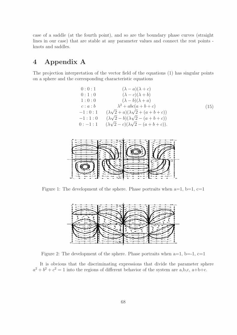
case of a saddle (at the fourth point), and so are the boundary phase curves (straightlines in our case) that are stable at any parameter values and connect the rest points -knots and saddles.
4 Appendix A
The projection interpretation of the vector field of the equations (1) has singular pointson a sphere and the corresponding characteristic equations
0 : 0 : 1 (λ − a)(λ + c)0 : 1 : 0 (λ − c)(λ + b)1 : 0 : 0 (λ − b)(λ + a)c : a : b λ2 + abc(a + b + c)
−1 : 0 : 1 (λ√
2 + a)(λ√
2 + (a + b + c))
−1 : 1 : 0 (λ√
2 − b)(λ√
2 − (a + b + c))
0 : −1 : 1 (λ√
2 − c)(λ√
2 − (a + b + c)).
(15)
Figure 1: The development of the sphere. Phase portraits when a=1, b=1, c=1
Figure 2: The development of the sphere. Phase portraits when a=1, b=-1, c=1
It is obvious that the discriminating expressions that divide the parameter spherea2 + b2 + c2 = 1 into the regions of different behavior of the system are a,b,c, a+b+c.
68
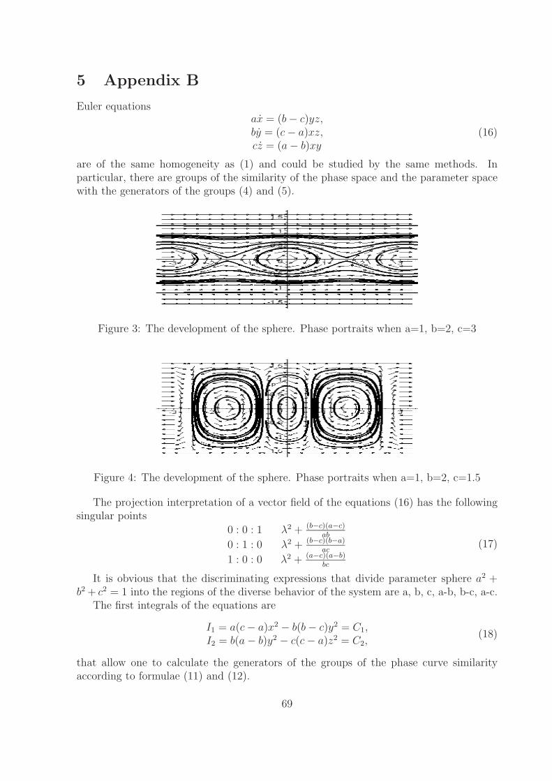
5 Appendix B
Euler equationsax = (b − c)yz,by = (c − a)xz,cz = (a − b)xy
(16)
are of the same homogeneity as (1) and could be studied by the same methods. Inparticular, there are groups of the similarity of the phase space and the parameter spacewith the generators of the groups (4) and (5).
Figure 3: The development of the sphere. Phase portraits when a=1, b=2, c=3
Figure 4: The development of the sphere. Phase portraits when a=1, b=2, c=1.5
The projection interpretation of a vector field of the equations (16) has the followingsingular points
0 : 0 : 1 λ2 + (b−c)(a−c)ab
0 : 1 : 0 λ2 + (b−c)(b−a)ac
1 : 0 : 0 λ2 + (a−c)(a−b)bc
(17)
It is obvious that the discriminating expressions that divide parameter sphere a2 +b2 + c2 = 1 into the regions of the diverse behavior of the system are a, b, c, a-b, b-c, a-c.
The first integrals of the equations are
I1 = a(c − a)x2 − b(b − c)y2 = C1,I2 = b(a − b)y2 − c(c − a)z2 = C2,
(18)
that allow one to calculate the generators of the groups of the phase curve similarityaccording to formulae (11) and (12).
69
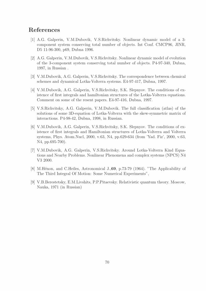
References
[1] A.G. Galperin, V.M.Dubovik, V.S.Richvitsky. Nonlinear dynamic model of a 3-component system conserving total number of objects. Int Conf. CMCP96, JINR,D5 11-96-300, p69, Dubna 1996.
[2] A.G. Galperin, V.M.Dubovik, V.S.Richvitsky. Nonlinear dynamic model of evolutionof the 3-component system conserving total number of objects. P4-97-340, Dubna,1997, in Russian .
[3] V.M.Dubovik, A.G. Galperin, V.S.Richvitsky. The correspondence between chemicalschemes and dynamical Lotka-Volterra systems. E4-97-417, Dubna, 1997.
[4] V.M.Dubovik, A.G. Galperin, V.S.Richvitsky, S.K. Slepnyov. The conditions of ex-istence of first integrals and hamiltonian structures of the Lotka-Volterra equations.Comment on some of the resent papers. E4-97-416, Dubna, 1997.
[5] V.S.Richvitsky, A.G. Galperin, V.M.Dubovik. The full classification (atlas) of thesolutions of some 3D-equation of Lotka-Volterra with the skew-symmetric matrix ofinteractions. P4-98-42, Dubna, 1998, in Russian.
[6] V.M.Dubovik, A.G. Galperin, V.S.Richvitsky, S.K. Slepnyov. The conditions of ex-istence of first integrals and Hamiltonian structures of Lotka-Volterra and Volterrasystems, Phys. Atom.Nucl, 2000, v.63, N4, pp.629-634 (from ’Yad. Fiz’, 2000, v.63,N4, pp.695-700).
[7] V.M.Dubovik, A.G. Galperin, V.S.Richvitsky. Around Lotka-Volterra Kind Equa-tions and Nearby Problems. Nonlinear Phenomena and complex systems (NPCS) N4V3 2000.
[8] M.Henon, and C.Heiles, Astronomical J.,69, p.73-79 (1964). ”The Applicability ofThe Third Integral Of Motion: Some Numerical Experiments”,
[9] V.B.Berestetsky, E.M.Livshits, P.P.Pitaevsky. Relativistic quantum theory. Moscow,Nauka, 1971 (in Russian)
70
Janet Bases of Toric Ideals
Vladimir P. Gerdta, Yuri A. Blinkovb
aLaboratory of Information Technologies,Joint Institute for Nuclear Research,
141980 Dubna, Russia;e-mail: [email protected]
bDepartment of Mathematics and Mechanics,Saratov State University,410071 Saratov, Russia;
e-mail: [email protected]
In this paper we present a version of the general polynomial involutive algorithm forcomputing Janet bases specialized to toric ideals. The relevant data structures are Janettrees which provide a very fast search for a Janet divisor. We broach also efficiency issuesin view of application of the algorithm presented to computation of toric ideals.
1 Introduction
We consider the problem of computing a Janet basis of a toric ideal IA in K[x] ≡K[x1, . . . , xn] generated by binomials of the form [1]
IA = { xu − xv | u,v ∈ Nn, π(u) = π(v), gcd(xu,xv) = 1 } .
Here u,v ∈ Nn and π is the semigroup homomorphism
π : Nn → Zd, u = {u1, . . . , un} → u1a1 + · · · + unan
where ai ∈ Zd (1 ≤ i ≤ n).Given a set of binomials generating a toric ideals, the problem of constructing its
Grobner basis is usually (except small problems) rather expensive from the computationalpoint of view [2]. In practice, for this particular problem, one typically deals with a largenumber n of variables and their degrees. If d is the maximal degree of the initial binomials,then the degree of a reduced Grobner basis is bounded by [3]
2 ·(
d2
2+ d
)2n−1
.
But for all that the reduced Grobner basis is also binomial since the binomial structure ispreserved during the Buchberger algorithm [4, 5]. Similarly, the involutive algorithms [6]based on the sequential multiplicative reductions of nonmultiplicative prolongations ofthe intermediate polynomials preserve the binomial structure. The output involutivebasis which is also a Grobner basis though generally redundant.
71
Thus, unlike construction of reduced Grobner bases or involutive bases for generalpolynomial ideals, the integer arithmetics which may take most of computing time is notimportant for binomial ideals. In this case a fast search of monomial divisors for perform-ing reductions of S-polynomials may become crucial in acceleration of computations.
Recently [8, 8] we designed and implemented involutive algorithms specialized to con-structing Janet bases of monomial and polynomial ideals. Janet division as well as anyother involutive division [6] provides uniqueness of an involutive divisor in a polynomialset with co-prime leading monomials. This allows one to organize a very fast search for aJanet divisor using special data structures for intermediate polynomial sets called Janettrees.
The main goal of this paper is to discuss the issue of practical efficiency in computingJanet bases of toric ideals based on the use of Janet trees. Since one of the most importantapplications of toric ideals is integer programming we shortly describe this application [9]in the next section.
2 Toric Ideals and Integer Programming
Let A be a matrix of dimension m×n with integer entries and b ∈ Zm, c ∈ Zn be vectors.The following optimization problem
min{ cTx | x ∈ Nn, Ax = b }
is called a problem of integer programming.We shall assume that c ∈ Nn. If there exists vector x0 satisfying Ax0 = b, x0 ∈ Nn,
then the problem of finding minimum of function cTx can be reduced to all kinds oftransformation of the initial vector state x0 using ker(A).
The problem of determining ker(A) can be formulated in terms of toric ideals. Indeed,every vector u ∈ ker(A) may be uniquely represented as u = u+−u− where both u+ andu− are nonnegative and have disjoint support. Associate symbol vi with the i-th columnof matrix A. Then the ideal
IA = { vu+ − vu− | u+ − u− = u ∈ ker(A) }
associated with ker(A) is toric. Given the initial solution x0, the optimal solution can befound as follows [9]:
1. Construct a basis of the toric ideal IA.
2. Construct a reduced Grobner basis or an involutive basis of IA with respect to theadmissible monomial ordering �c generated by vector c.
3. Reduce monomial vx0 modulo the constructed basis to obtain the optimal solution.
Therefore, the reduced Grobner basis or any involutive basis of the associated toric idealIA provide an algorithmic tool for solving the problem of integer programming.
72
3 Janet Bases of Toric Ideals
3.1 Definition of Janet Basis
In our papers [6] the Grobner bases of special type, called involutive and based on theconcept of involutive division were introduced. Given a set of coprime monomials andan involutive division, any monomial may have at most one involutive divisor in the set.This property of the involutive division allows one to design an efficient search for theinvolutive divisor using the method of separative monomials [10] for a general involutivedivision or Janet trees [7] for Janet division.
Because of a larger number of variables and unimportance of integer arithmeticaloperations over coefficients of the binomials, the practical complexity of an algorithm forconstruction of Grobner or Janet bases is caused by an enormous number of binomialsarising in computation of the basis. A faster search for divisors may accelerates thecomputation substantially.
By definition of Janet division [6] (which formalizes the pioneering ideas of Janet [11])induced by the order
x1 � x2 � . . . � xn (1)
on x, a polynomial set F is partitioned into the groups labeled by non-negative integersd1, . . . , di:
[d1, . . . , di] = { f ∈ F | dj = degj(lm(f)), 1 ≤ j ≤ i }where degi(u) denotes the degree of xi in monomial u and lm(f) denotes the leadingmonomial of f . A variable xi is called (Janet) multiplicative for f ∈ F if i = 1 and
deg1(lm(f)) = max{ deg1(lm(g)) | g ∈ F },or if i > 1, f ∈ [d1, . . . , di−1] and
degi(lm(f)) = max{ degi(lm(g)) | g ∈ [d1, . . . , di−1] } .
If a variable is not multiplicative for f ∈ F , it is called (Janet) nonmultiplicative for f .In the latter case we shall write xi ∈ NMJ(f, F ). u ∈ lm(F ) is a Janet divisor of w ∈ M,if u | w and monomial w/u contains only multiplicative variables for u. In this case wewrite u |J w.
Let lm(F ) = { lm(f) | f ∈ F }. Then a polynomial set F is called Janet autoreducedif each term in every f ∈ F has no Janet divisors among lm(F ) \ lm(f). A polynomial his said to be in the Janet normal form modulo F if every term in h has no Janet divisorsin lm(F ). In that follows NFJ(f, F ) denotes the Janet normal form f modulo F .
A Janet autoreduced set F is called a Janet basis if
(∀f ∈ F ) (∀x ∈ NMJ(f, F )) [ NFJ(f · x, F ) = 0 ] . (2)
A Janet basis G is called minimal if for any other Janet basis F of the same ideal theinclusion lm(G) ⊆ lm(F ) holds. If both G and F are monic this inclusion implies G ⊆ F .A Janet basis is a Grobner one, though generally not reduced. However, similarly to areduced Grobner basis, a monic minimal Janet basis is uniquely defined by an ideal anda monomial order. In that follows we deal with minimal Janet bases only and omit theword ”minimal”.
73
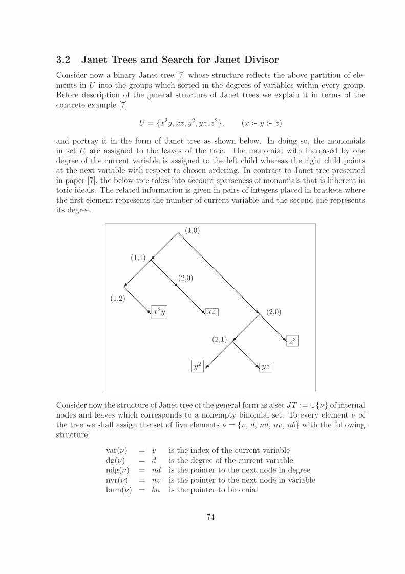
3.2 Janet Trees and Search for Janet Divisor
Consider now a binary Janet tree [7] whose structure reflects the above partition of ele-ments in U into the groups which sorted in the degrees of variables within every group.Before description of the general structure of Janet trees we explain it in terms of theconcrete example [7]
U = {x2y, xz, y2, yz, z2}, (x � y � z)
and portray it in the form of Janet tree as shown below. In doing so, the monomialsin set U are assigned to the leaves of the tree. The monomial with increased by onedegree of the current variable is assigned to the left child whereas the right child pointsat the next variable with respect to chosen ordering. In contrast to Janet tree presentedin paper [7], the below tree takes into account sparseness of monomials that is inherent intoric ideals. The related information is given in pairs of integers placed in brackets wherethe first element represents the number of current variable and the second one representsits degree.
��
���
��
����
��
�� x2y
��
���
��
��� xz
��
��
��
��
��
����
��
���
��
�� yz
��
���y2
��
��� z3
(1,0)
(1,1)
(1,2)
(2,0)
(2,0)
(2,1)
Consider now the structure of Janet tree of the general form as a set JT := ∪{ν} of internalnodes and leaves which corresponds to a nonempty binomial set. To every element ν ofthe tree we shall assign the set of five elements ν = {v, d, nd, nv, nb} with the followingstructure:
var(ν) = v is the index of the current variabledg(ν) = d is the degree of the current variablendg(ν) = nd is the pointer to the next node in degreenvr(ν) = nv is the pointer to the next node in variablebnm(ν) = bn is the pointer to binomial
74
In the absence of a child we shall assign the value nil to the corresponding pointer.Wherever it does not lead to misunderstanding we shall identify the pointers nd and nvwith the nodes they point out. To the root of JT we assign ν0 with var(ν0) = 1 inaccordance with labeling (1) and dg(ν0) = 0.The internal nodes and leaves of tree JT are characterized by the states:
Internal node: ((nv = nil ∧ v < var(nv)) ∨ (nd = nil ∧ d < dg(nd))∧ bn = nil
Leaf: nv = nil ∧ nd = nil ∧ bn = nil ∧ d = dg(lm(bn)).
For a fast search for Janet divisor in the given tree one can use the following algorithmJ-divisor which is an adaptation to the above structure of Janet tree of the algorithmdescribed in [7].
Algorithm: J-divisor(JT, w)
Input: JT , a Janet tree; w, monomialOutput: bn, a binomial such that lm(bn) |J w,
or nil, otherwise1: ν := ν0
2: while degvar(ν)(w) ≥ dg(ν) do3: while ndg(ν) and degvar(ndg(ν))(w) ≥ dg(ndg(ν)) do4: ν := ndg(ν)5: od6: if nvr(ν) then7: ν := nvr(ν)8: elif ndg(ν) then9: return nil
10: else11: return bnm(ν)12: fi13: od14: return nil
Apparently, the next theorem formulated and proved in [7] is valid for the adapted algo-rithm as well.
Theorem 1. Let d be the maximal total degree of the leading monomials of binomials inn variables which constitute the finite set U . Then the complexity bound of the algorithmJ − divisor and the binary search algorithm is given by
tJ−divisor = O(d + n),
tBinarySearch = O(n((d + n) log(d + n) − n log(n) − d log(d))).
Thus, the complexity bound for the search of Janet divisor is O(n + d) where n is thenumber of variables and d is the maximal degree of the leading monomials in the binomialbasis. Since this bound is even lower than that for the binary search algorithm, one canexpect that the involutive completion of binomial ideals may be faster than the reducedGrobner basis completion.
75
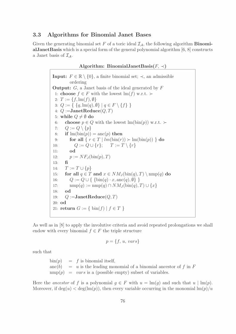
3.3 Algorithms for Binomial Janet Bases
Given the generating binomial set F of a toric ideal IA, the following algorithm Binomi-alJanetBasis which is a special form of the general polynomial algorithm [6, 8] constructsa Janet basis of IA.
Algorithm: BinomialJanetBasis(F, ≺)
Input: F ∈ R \ {0}, a finite binomial set; ≺, an admissibleordering
Output: G, a Janet basis of the ideal generated by F1: choose f ∈ F with the lowest lm(f) w.r.t. �2: T := {f, lm(f), ∅}3: Q := { {q, lm(q), ∅} | q ∈ F \ {f} }4: Q :=JanetReduce(Q, T )5: while Q = ∅ do6: choose p ∈ Q with the lowest lm(bin(p)) w.r.t. �7: Q := Q \ {p}8: if lm(bin(p)) = anc(p) then9: for all { r ∈ T | lm(bin(r)) � lm(bin(p)) } do
10: Q := Q ∪ {r}; T := T \ {r}11: od12: p := NFJ(bin(p), T )13: fi14: T := T ∪ {p}15: for all q ∈ T and x ∈ NMJ(bin(q), T ) \ nmp(q) do16: Q := Q ∪ { {bin(q) · x, anc(q), ∅} }17: nmp(q) := nmp(q) ∩ NMJ(bin(q), T ) ∪ {x}18: od19: Q :=JanetReduce(Q, T )20: od21: return G := { bin(f) | f ∈ T }
As well as in [8] to apply the involutive criteria and avoid repeated prolongations we shallendow with every binomial f ∈ F the triple structure
p = {f, u, vars}
such that
bin(p) = f is binomial itself,anc(b) = u is the leading monomial of a binomial ancestor of f in Fnmp(p) = vars is a (possible empty) subset of variables.
Here the ancestor of f is a polynomial g ∈ F with u = lm(g) and such that u | lm(p).Moreover, if deg(u) < deg(lm(p)), then every variable occurring in the monomial lm(p)/u
76
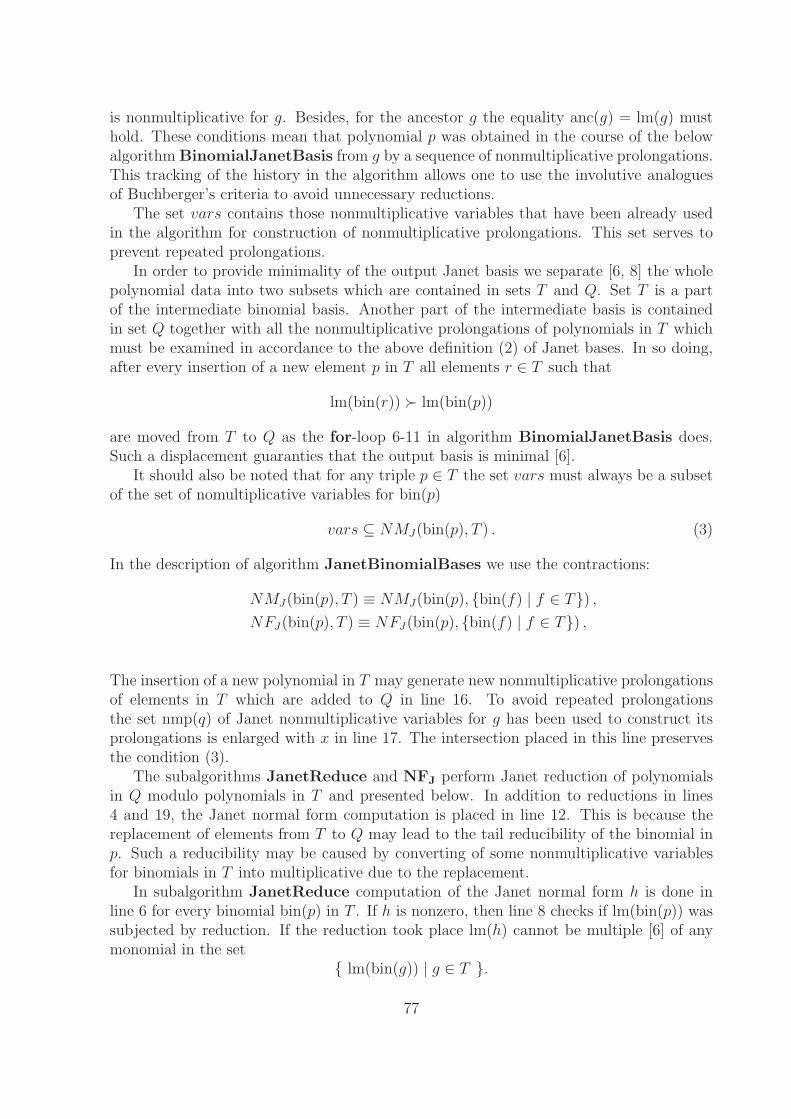
is nonmultiplicative for g. Besides, for the ancestor g the equality anc(g) = lm(g) musthold. These conditions mean that polynomial p was obtained in the course of the belowalgorithm BinomialJanetBasis from g by a sequence of nonmultiplicative prolongations.This tracking of the history in the algorithm allows one to use the involutive analoguesof Buchberger’s criteria to avoid unnecessary reductions.
The set vars contains those nonmultiplicative variables that have been already usedin the algorithm for construction of nonmultiplicative prolongations. This set serves toprevent repeated prolongations.
In order to provide minimality of the output Janet basis we separate [6, 8] the wholepolynomial data into two subsets which are contained in sets T and Q. Set T is a partof the intermediate binomial basis. Another part of the intermediate basis is containedin set Q together with all the nonmultiplicative prolongations of polynomials in T whichmust be examined in accordance to the above definition (2) of Janet bases. In so doing,after every insertion of a new element p in T all elements r ∈ T such that
lm(bin(r)) � lm(bin(p))
are moved from T to Q as the for-loop 6-11 in algorithm BinomialJanetBasis does.Such a displacement guaranties that the output basis is minimal [6].
It should also be noted that for any triple p ∈ T the set vars must always be a subsetof the set of nomultiplicative variables for bin(p)
vars ⊆ NMJ(bin(p), T ) . (3)
In the description of algorithm JanetBinomialBases we use the contractions:
NMJ(bin(p), T ) ≡ NMJ(bin(p), {bin(f) | f ∈ T}) ,
NFJ(bin(p), T ) ≡ NFJ(bin(p), {bin(f) | f ∈ T}) ,
The insertion of a new polynomial in T may generate new nonmultiplicative prolongationsof elements in T which are added to Q in line 16. To avoid repeated prolongationsthe set nmp(q) of Janet nonmultiplicative variables for g has been used to construct itsprolongations is enlarged with x in line 17. The intersection placed in this line preservesthe condition (3).
The subalgorithms JanetReduce and NFJ perform Janet reduction of polynomialsin Q modulo polynomials in T and presented below. In addition to reductions in lines4 and 19, the Janet normal form computation is placed in line 12. This is because thereplacement of elements from T to Q may lead to the tail reducibility of the binomial inp. Such a reducibility may be caused by converting of some nonmultiplicative variablesfor binomials in T into multiplicative due to the replacement.
In subalgorithm JanetReduce computation of the Janet normal form h is done inline 6 for every binomial bin(p) in T . If h is nonzero, then line 8 checks if lm(bin(p)) wassubjected by reduction. If the reduction took place lm(h) cannot be multiple [6] of anymonomial in the set
{ lm(bin(g)) | g ∈ T }.
77
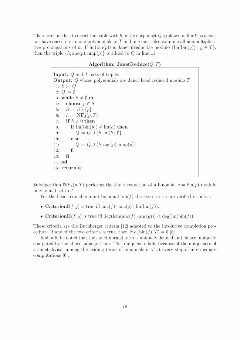
Therefore, one has to insert the triple with h in the output set Q as shown in line 9 as h can-not have ancestors among polynomials in T and one must also examine all nonmultiplica-tive prolongations of h. If lm(bin(p)) is Janet irreducible modulo {lm(bin(g)) | g ∈ T},then the triple {h, anc(p), nmp(p)} is added to Q in line 11.
Algorithm: JanetReduce(Q, T )
Input: Q and T , sets of triplesOutput: Q whose polynomials are Janet head reduced modulo T1: S := Q2: Q := ∅3: while S = ∅ do4: choose p ∈ S5: S := S \ {p}6: h := NFJ(p, T )7: if h = 0 then8: if lm(bin(p)) = lm(h) then9: Q := Q ∪ {h, lm(h), ∅}
10: else11: Q := Q ∪ {h, anc(p), nmp(p)}12: fi13: fi14: od15: return Q
Subalgorithm NFJ(p, T ) performs the Janet reduction of a binomial g = bin(p) modulopolynomial set in T .
For the head reducible input binomial bin(f) the two criteria are verified in line 5:
• CriterionI(f, g) is true iff anc(f) · anc(g) | lm(bin(f)).
• CriterionII(f, g) is true iff deg(lcm(anc(f) · anc(g))) < deg(lm(bin(f)).
These criteria are the Buchberger criteria [12] adapted to the involutive completion pro-cedure. If any of the two criteria is true, then NF (bin(f), T ) = 0 [8].
It should be noted that the Janet normal form is uniquely defined and, hence, uniquelycomputed by the above subalgorithm. This uniqueness hold because of the uniqueness ofa Janet divisor among the leading terms of binomials in T at every step of intermediatecomputations [6].
78
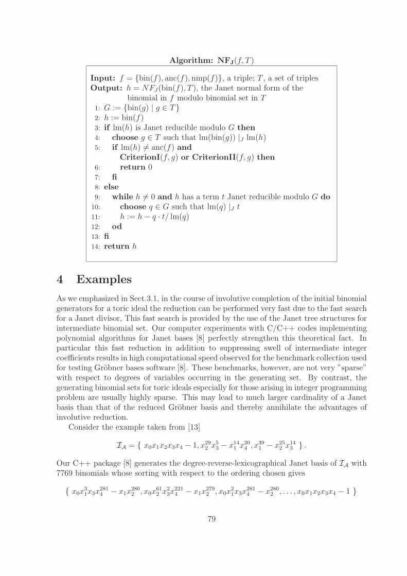
Algorithm: NFJ(f, T )
Input: f = {bin(f), anc(f), nmp(f)}, a triple; T , a set of triplesOutput: h = NFJ(bin(f), T ), the Janet normal form of the
binomial in f modulo binomial set in T1: G := {bin(g) | g ∈ T}2: h := bin(f)3: if lm(h) is Janet reducible modulo G then4: choose g ∈ T such that lm(bin(g)) |J lm(h)5: if lm(h) = anc(f) and
CriterionI(f, g) or CriterionII(f, g) then6: return 07: fi8: else9: while h = 0 and h has a term t Janet reducible modulo G do
10: choose q ∈ G such that lm(q) |J t11: h := h − q · t/ lm(q)12: od13: fi14: return h
4 Examples
As we emphasized in Sect.3.1, in the course of involutive completion of the initial binomialgenerators for a toric ideal the reduction can be performed very fast due to the fast searchfor a Janet divisor, This fast search is provided by the use of the Janet tree structures forintermediate binomial set. Our computer experiments with C/C++ codes implementingpolynomial algorithms for Janet bases [8] perfectly strengthen this theoretical fact. Inparticular this fast reduction in addition to suppressing swell of intermediate integercoefficients results in high computational speed observed for the benchmark collection usedfor testing Grobner bases software [8]. These benchmarks, however, are not very ”sparse”with respect to degrees of variables occurring in the generating set. By contrast, thegenerating binomial sets for toric ideals especially for those arising in integer programmingproblem are usually highly sparse. This may lead to much larger cardinality of a Janetbasis than that of the reduced Grobner basis and thereby annihilate the advantages ofinvolutive reduction.
Consider the example taken from [13]
IA = { x0x1x2x3x4 − 1, x292 x5
3 − x141 x20
4 , x391 − x25
2 x143 } .
Our C++ package [8] generates the degree-reverse-lexicographical Janet basis of IA with7769 binomials whose sorting with respect to the ordering chosen gives
{ x0x31x3x
2814 − x1x
2802 , x0x
612 x2
3x2214 − x1x
2792 , x0x
21x3x
2814 − x280
2 , . . . , x0x1x2x3x4 − 1 }
79
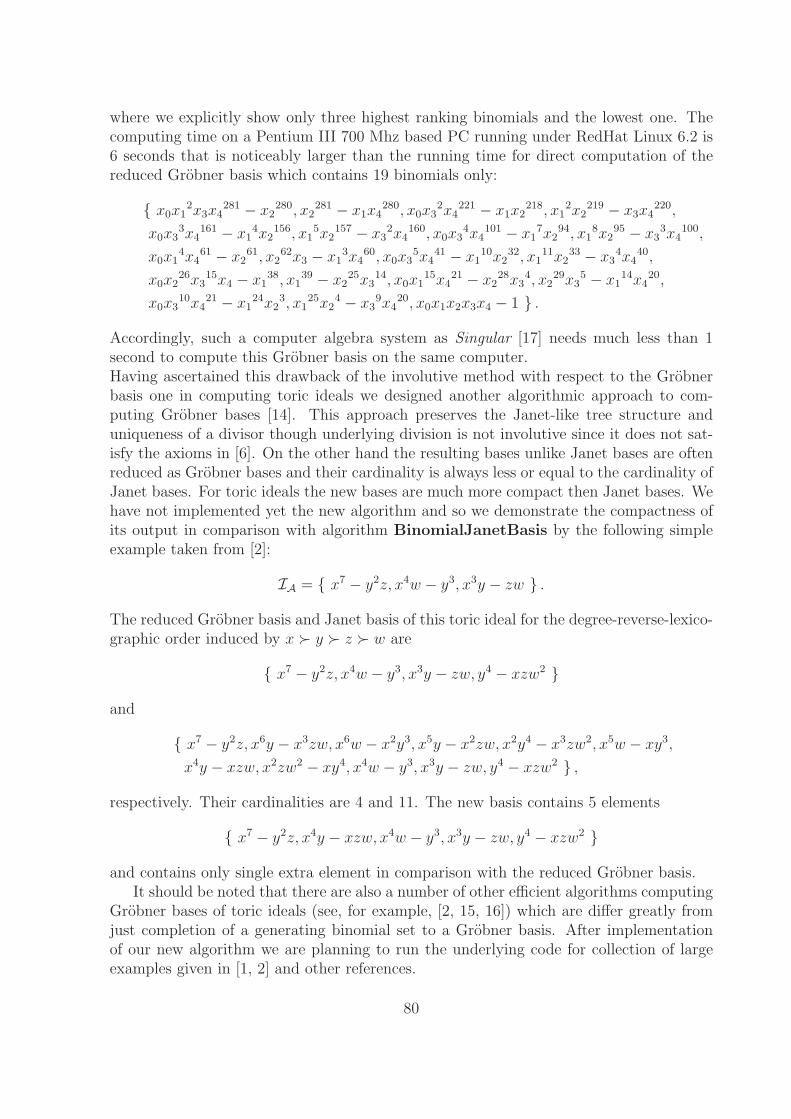
where we explicitly show only three highest ranking binomials and the lowest one. Thecomputing time on a Pentium III 700 Mhz based PC running under RedHat Linux 6.2 is6 seconds that is noticeably larger than the running time for direct computation of thereduced Grobner basis which contains 19 binomials only:
{ x0x12x3x4
281 − x2280, x2
281 − x1x4280, x0x3
2x4221 − x1x2
218, x12x2
219 − x3x4220,
x0x33x4
161 − x14x2
156, x15x2
157 − x32x4
160, x0x34x4
101 − x17x2
94, x18x2
95 − x33x4
100,
x0x14x4
61 − x261, x2
62x3 − x13x4
60, x0x35x4
41 − x110x2
32, x111x2
33 − x34x4
40,
x0x226x3
15x4 − x138, x1
39 − x225x3
14, x0x115x4
21 − x228x3
4, x229x3
5 − x114x4
20,
x0x310x4
21 − x124x2
3, x125x2
4 − x39x4
20, x0x1x2x3x4 − 1 } .
Accordingly, such a computer algebra system as Singular [17] needs much less than 1second to compute this Grobner basis on the same computer.Having ascertained this drawback of the involutive method with respect to the Grobnerbasis one in computing toric ideals we designed another algorithmic approach to com-puting Grobner bases [14]. This approach preserves the Janet-like tree structure anduniqueness of a divisor though underlying division is not involutive since it does not sat-isfy the axioms in [6]. On the other hand the resulting bases unlike Janet bases are oftenreduced as Grobner bases and their cardinality is always less or equal to the cardinality ofJanet bases. For toric ideals the new bases are much more compact then Janet bases. Wehave not implemented yet the new algorithm and so we demonstrate the compactness ofits output in comparison with algorithm BinomialJanetBasis by the following simpleexample taken from [2]:
IA = { x7 − y2z, x4w − y3, x3y − zw } .
The reduced Grobner basis and Janet basis of this toric ideal for the degree-reverse-lexico-graphic order induced by x � y � z � w are
{ x7 − y2z, x4w − y3, x3y − zw, y4 − xzw2 }
and
{ x7 − y2z, x6y − x3zw, x6w − x2y3, x5y − x2zw, x2y4 − x3zw2, x5w − xy3,
x4y − xzw, x2zw2 − xy4, x4w − y3, x3y − zw, y4 − xzw2 } ,
respectively. Their cardinalities are 4 and 11. The new basis contains 5 elements
{ x7 − y2z, x4y − xzw, x4w − y3, x3y − zw, y4 − xzw2 }
and contains only single extra element in comparison with the reduced Grobner basis.It should be noted that there are also a number of other efficient algorithms computing
Grobner bases of toric ideals (see, for example, [2, 15, 16]) which are differ greatly fromjust completion of a generating binomial set to a Grobner basis. After implementationof our new algorithm we are planning to run the underlying code for collection of largeexamples given in [1, 2] and other references.
80
Acknowledgements
The work was supported in part by the RFBR grants 00-15-96691, 01-01-00708 and bygrant Intas 99-1222.
References
[1] Sturmfels, B.: Grobner bases and convex polytopes. University Lecture Series 8, Prov-idence, RI, American Mathematical Society, 1996.
[2] Bigatti, A.M., La Scala, R., Robbiano, L.: Computing toric ideals. J. Symb. Comp.27 (1999) 351-365.
[3] Koppenhagen, U., Mayr, E.W.: An Optimal Algorithm for Constructing the ReducedGrobner Basis of Binomial Ideals. Proceedings of ISSAC’96, ACM Press, 1996, 55-62.
[4] Adams, W.W., Loustaunau, P.: An Introduction to Grobner Bases. Graduate Studiesin Mathematics 3, American Mathematical Society, 1994.
[5] Pottier, L.: Grobner Bases of Toric Ideals. Rapport de recherche 2224 (1997), INRIASophia Antipolis.
[6] Gerdt, V.P., Blinkov, Yu.A.: Involutive Bases of Polynomial Ideals. Math. Comp.Simul. 45 (1998) 519-542; Minimal Involutive Bases. Math. Comp. Simul. 45 (1998)543-560.
[7] Gerdt V.P., Blinkov Yu.A., Yanovich D.A. Construction of Janet Bases. I. Mono-mial Bases. In: Computer Algebra in Scientific Computing / CASC’01, V.G.Ganzha,E.W.Mayr and E.V.Vorozhtsov (Eds.), Springer-Verlag, Berlin, 2001, pp.233-247.
[8] Gerdt, V.P., Blinkov, Yu.A., Yanovich, D.A.: Construction of Janet Bases. II.Polynomial Bases. In: Computer Algebra in Scientific Computing / CASC’01,V.G.Ganzha, E.W.Mayr and E.V.Vorozhtsov (Eds.), Springer-Verlag, Berlin, 2001,pp.249-263.
[9] Conti, P., Traverso, C.: Buchberger algorithm and integer programming. Proceedingsof AAECC-9, Springer LNCS 539 (1991) 130-139.
[10] Blinkov, Yu.A.: Method of Separative Monomials for Involutive Divisions. Program-ming and Computer Software 3 (2001) 43-45.
[11] Janet, M.: Lecons sur les Systemes d’Equations aux Derivees Partielles, CahiersScientifiques IV, Gauthier-Villars, Paris, 1929.
[12] Buchberger, B.: Grobner Bases: an Algorithmic Method in Polynomial Ideal The-ory. In: Recent Trends in Multidimensional System Theory, N.K. Bose (ed.), Reidel,Dordrecht (1985) 184–232.
81
[13] Morales, M.: Equations des varietes monomiales. Preprint, Universite de Grenoble I,France.
[14] Gerdt, V.P., Blinkov, A.Yu.: Involutive-like Grobner Bases. In preparation.
[15] Di Biase, F., Urbanke, R.: An algorithm to calculate the kernel of certain polynomialring homomorphisms. Experimental Mathematics 4 (1995) 227-234.
[16] Hosten, S., Sturmfels, B.: GRIN: An implementation of Groebner basis for integerprogramming. In: Integer Programming and Combinatorial Optimization, Balas, E.,Clausen J., (Eds.), LNCS 920, Springer-Verlag, New York, 1995, pp.267-276.
[17] Greuel, G.-M., Pfister, G., Schoenemann, H.: Singular: A Computer Algebra Sys-tem for Polynomial Computation, Department of Mathematics, University of Keis-erslautern (2001) http://www.singular.uni-kl.de/Manual/2-0-0/.
82
Analysis of Constraints inLight-Cone Version of SU(2)
Yang-Mills Mechanics
V. P. Gerdt a, A. M. Khvedelidze a,b, D. M. Mladenov c
a Laboratory of Information Technologies,Joint Institute for Nuclear Research,
141980 Dubna, Russia;e-mail: [email protected]
b A.Razmadze Mathematical Institute,GE-380093 Tbilisi, Georgia;
e-mail: [email protected] Bogoliubov Laboratory of Theoretical Physics,
Joint Institute for Nuclear Research,141980 Dubna, Russia;
e-mail: [email protected]
We study the classical dynamics of mechanical model obtained from the light-coneversion of SU(2) Yang-Mills field theory under the supposition of the gauge potentialdependence only on “time” along the light-cone direction. The computer algebra systemMaple was used strongly to compute and separate the complete set of constraints. Incontrast to the instant form of the Yang-Mills mechanics the constraints here representa mixed form of first and second-class constraints and reduce the number of the physicaldegrees of freedom up to four canonical one.
1 Introduction
Notion of the evolution of observables is the key element in analyzing of the physicalproperties of any relativistic field theory. After Dirac’s famous work entitled “Formsof Relativistic Dynamics” [1] it has been recognized that the different choices of thetime evolution parameter can drastically change the content and interpretation of thetheory. The simplest and well-known example illustrated this observation is the light-conedynamics of free scalar field. In contrast to the corresponding instant time model, in thiscase, owing to the choice of time evolution parameter along the light-cone characteristics,theory becomes degenerate, the corresponding Hessian is zero [2]. Dealing with gaugetheories on the light-cone we encounter much more complicated description than for theordinary instant form dynamics (see e.g. recent reviews [3]-[7]).
In the present talk we would like to state some results concerning the light-cone de-scription of simple mechanical model originated from the SU(2) Yang-Mills theory underassumption of spatial homogeneity of the fields on the light-cone. This means that we
83
shall consider the light-cone action for SU(2) Yang-Mills model with the gauge potentialonly light-cone time depending. The dynamical system, obtained under such a supposi-tion contain finite number of degrees of freedom and possesses gauge invariance. Our aimis to study its Generalized Hamiltonian dynamics [2, 8, 9] and to compare it with thecorresponding instant form of the Yang-Mills mechanics, intensively studed during thelast decades (see e.g [11]-[17] and references therein).
Using the Generalized Hamiltonian formalism for degenerate systems [2, 8, 9] andexploiting the Maple package [10] implementing algorithm Dirac-Grobner for computationand separation of constraints we found the complete set of constraints and performed theirseparation into the sets of first and second-class constraints.
Our calculations demonstrate that the light-cone version of Yang-Mills mechanics dif-fers from its instant form counterpart in the character of the local gauge invariance andtherefore the corresponding unconstrained Hamiltonian systems describe different canon-ically non-equivalent models.
2 Description of the model
Let us start with a general formulation of the Yang-Mills theory on four-dimensionalMinkowski space M4, endowed with some arbitrary metric gP , tensor field of type (0, 2),
gP = gμν ωμ ⊗ ων . (1)
Here we use a basis ωμ , μ = 0, . . . , 3 of 1-forms in the cotangent space T ∗P (M4). The
metric defines a inner product between two vectors in the tangent space TP (M4) and ifone fixes a basis eμ in TP (M4), dual to the basis of 1-forms ωμ, the components of themetric tensor are given as
gμν = gP (eμ, eν) .
Using this geometric settings, the action of the Yang-Mills field theory can be repre-sented in coordinate free form
I :=1
g2
∫M4
tr F ∧ ∗F . (2)
Here the SU(2) algebra valued curvature 2-form
F := dA + A ∧ A
is constructed from the connection 1-form A = Aμ ωμ. The connection and curvature asLie algebra valued quantities are expressed in terms of the Pauli matrices σa , a = 1, 2, 3 1
A = Aa σa
2i, F = F a σa
2i.
1The Pauli matrices are defined to satisfy
[σa, σb] = 2 i εabc σc , trσaσb = 2 δab .
84
The metric g enters the action through the dual field strength tensor defined in accordanceto the Hodge star operation
∗Fμν =1
2εμναβ Fαβ .
If one fixes Lorentzian coordinates in Minkowski space M4 xμ = (x0, x1, x2, x3) andchoose a coordinate basis for the tangent vectors eμ = ∂
∂xμ , we have the conventionalMinkowskian metric g = ‖1,−1,−1,−1‖ and the corresponding action (2) will provideYang-Mills equations in the instant form with a time variable t = x0.
To formulate the light-cone version of the theory let us introduce basis vectors in thetangent space T ∗
P (M4)
e± :=1√2
(e0 ± e3) , e⊥ := (ek , k = 1, 2) .
The first two vectors are tangent to the light-cone and the corresponding coordinates arereferred usually as the light-cone coordinates xμ =
(x+, x−, x⊥) with
x± :=1√2
(x0 ± x3
), x⊥ :=
(xk , k = 1, 2
).
The light-cone basis vectors (e±, ek) determine, according to (1), the so-called light-conemetric, whose non-zero elements are
g+− = g−+ = −g11 = −g22 = 1
and thus the 1-form connection in the light-cone formulation is given as
A = A+ dx+ + A− dx+ + Ak dxk . (3)
Now we are ready to define the Lagrangian corresponding to the light-cone Yang-Mills mechanics. By definition the Lagrangian of Yang-Mills mechanics follows from theLagrangian of Yang-Mills theory if one suppose that 1-form connection A depends onlyon light-cone “time variable” x+
A = A(x+) .
Using the definition (2) and (3) we find the Lagrangian of the Yang-Mills light-conemechanics
L :=1
2g2
(F a
+− F a+− + 2 F a
+k F a−k − F a
12 F a12
), (4)
where the field-strength tensor light-cone components are⎧⎪⎪⎪⎪⎪⎨⎪⎪⎪⎪⎪⎩
F a+− =
∂Aa−
∂x+ + εabc Ab+ Ac
− ,
F a+k =
∂Aak
∂x+ + εabc Ab+ Ac
k ,
F a−k = εabc Ab
− Ack ,
F aij = εabc Ab
i Acj , i, j, k = 1, 2 .
(5)
85
3 Hamiltonian formulation of SU(2) Yang-Mills
mechanics on the light-cone
In this section we present the main results of this paper. The underlying computationswere done with the Maple package implementing algorithm Dirac-Grobner [10] for com-putation and separation of constraints for Lagrangian dynamical systems of polynomialtype. Some computational details are described in the next section.
The choice of the light-cone time variable
τ = x+
as the evolution parameter prescribes a certain Legendre transformation of the dynamicalvariables (A+, A−, Ak)
2⎧⎨⎩ π−a = ∂L
∂Aa−
= 1g2
(Aa− + εabc Ab
+ Ac−)
,
πka = ∂L
∂Aak
= 1g2 εabc Ab
− Ack .
(6)
Given this set of equations the Dirac-Grobner algorithm designed in [10] and leads to thethe primary constraints
ϕ(1)a := π+
a = 0 , (7)
χak := g2 πa
k + εabc Ab−Ac
k = 0 . (8)
Then, the canonical Hamiltonian is given by
HC =g2
2π−
a π−a − εabc Ab
+
(Ac
− π−a + Ac
k πka
)+ V (Ak) (9)
with a potential term in (9)
V (Ak) =1
2g2
[(Ab
1Ab1
)(Ac
2Ac2) −(Ab
1Ab2
)(Ac
1Ac2)]
.
The non vanishing Poisson brackets are
{Aa± , π±
b } = δab ,
{Aak , πl
b} = δlkδ
ab .
With respect to these fundamental Poisson brackets the primary constraints(ϕ
(1)a , χa
k
)obey the algebra
{ϕ(1)a , ϕ
(1)b } = 0 ,
{ϕ(1)a , χb
k} = 0 ,
{χai , χb
j} = −2 g2εabc Ac− gij .
2To simplify the formulas we shall use overdot to denote derivative of functions with respect to light-cone time variable x+. Further we shall treat in equal footing the up and down isotopic indexes, denotedwith a, b, c, d.
86
According to the Dirac’s prescription, the dynamics for degenerate theories is governed bythe total Hamiltonian which differs from the canonical one by linear combination of theprimary constraints. In case of the light-cone Yang-Mills mechanics the total Hamiltonianhas the form
HT = HC − 2 tr(U(τ) ϕ(1)
)− 2 tr (Vk(τ) χk) , (10)
where U(τ) and Vk(τ) are arbitrary SU(2) valued functions of the light-cone time τ =x+. Using this Hamiltonian it is necessary to check the dynamical self-consistence ofthe primary constraints. ¿From the requirement of conservation in time of the primaryconstraints ϕ
(1)a the following equations follows
0 = ϕ(1)a = {π+
a , HT} = εabc(Ab
−π−c + Ab
kπkc
).
It follows that there are three secondary constraints ϕ(2)a
ϕ(2)a := εabc
(Ab
−π−c + Ab
kπkc
)= 0 , (11)
which obey the SO(3, R) algebra
{ϕ(2)a , ϕ
(2)b } = εabc ϕ(2)
c .
The same procedure for the primary constraints χak gives
0 = χak = {χa
k , HC} − 2 g2 εabc V bk Ac
− . (12)
Because the matrix ‖εabc Ac−‖ is degenerate, its rank is
rank‖ εabc Ac− ‖ = 2 ,
one can determine among the Lagrange multipliers V kb only four ones. The unit null
vector of the matrix na‖ εabc Ac− ‖ = 0 is
na =Aa
−√(A1−)2 + (A2−)2 + (A3−)2
.
Using this null vector one can can decompose the six primary constraints χak
χak⊥ := χa
k −(nbχb
k
)na ,
ψk := naχak .
Constraints χak⊥ are functionally dependent due to the conditions
na χak⊥ = 0 (13)
and choosing among them any four independent constraints we are able to determine fourLagrange multipliers V k
b⊥. The two constraints ψk satisfy the Abelian algebra
{ψi , ψj} = 0 .
87
One can verify that the Poisson brackets of ψk and ϕ(2)a with the total Hamiltonian on
the constraint surface (CS) are zero
{ψk , HT} |CS = 0 , (14)
{ϕ(2)a , HT} |CS = 0 (15)
and thus there are no ternary constraints. One can now summarize: we arrive at the set
of constraints(ϕ
(1)a , ψk, ϕ
(2)a , χb
k⊥). The Poisson bracket algebra of the three first one is
{ϕ(1)a , ϕ(1)
a } = 0 , (16)
{ψi , ψj} = 0 , (17)
{ϕ(2)a , ϕ
(2)b } = εabc ϕ(2)
c , (18)
{ϕ(1)a , ψk} = {ϕ(1)
a , ϕ(2)b } = {ψk , ϕ(2)
a } = 0 . (19)
The constraints χbk⊥ satisfy the algebra
{χai⊥ , χb
j⊥} = −2 g2 εabc Ac− gij (20)
and the Poisson brackets between these two sets of constraints are
{ϕ(2)a , χb
k⊥} = εabc χck⊥ , (21)
{ϕ(1)a , χb
k⊥} = {ψi , χbj⊥} = 0 . (22)
From this algebra of constraints we conclude that we have eight first-class constraints(ϕ
(1)a , ψk, ϕ
(2)a
)and four second-class constraints χa
k⊥. According to counting of the de-
grees of freedom eliminated by all these constraints, after reduction to the unconstrainedphase space, instead of 24 degrees of freedom possessing the Yang-Mills mechanics on thelight-cone we arrive at 24 − 4 − 2(3 + 3 + 2) = 4 unconstrained degrees of freedom.
Thus one can conclude that in contrast to the instant form of the Yang-Mills mechanics,where the number of the unconstrained canonical pairs is 12, in the light-cone version wehave only 4 physical canonical variables. It is important to note that such a decreasingof the numbers of the physical coordinates has two reasons: as well as the presence ofthe second-class constraints as the additional first-class constraint. As it is well-knownthe presence of the first-class constraints in the theory means the existence of a certaingauge symmetry. Our analysis shows that in the light-cone Yang-Mills mechanics theoriginal SU(2) gauge symmetry of the field theory, after supposition of the gauge fieldshomogeneity, transforms into SU(2) × U(1) × U(1) symmetry.
4 Computational aspects
The system of Euler-Lagrange equations for the Lagrangian (4) with the generalizedcoordinates (5) as well as the system of Hamiltonian equations which are obtained by theLegendre transformation (6) is under-determined. Just under-determinacy is inherent inconstrained dynamical systems [1, 2, 8, 9], and to study such systems one has to compute
88
their ”hidden” constraints. For the quantization purposes one has also to separate theconstraints into disjoint sets of first-class and second-class constraints.
In the paper [10] a general algorithm for computing and separating constraints forpolynomial Lagrangians was devised. The algorithm combines the constructive ideas ofDirac [8] with the Grobner bases techniques and called Dirac-Grobner algorithm. Itsimplementation was done in Maple and in this section we characterize briefly the maincomputational steps one needs to obtain the results of the previous section as they weredone by the Maple code. In so doing the below described computational steps is nothingelse than concretization of the Dirac-Grobner algorithm to our model described in Sect.2.
Denote by qi and qi (1 ≤ i ≤ 12), respectively, the generalized Lagrangian coordinatesin (4) listed as
A1+, A2
+, A3+, A1
1, A21, A
31, A
12, A
22, A
32, A
1−, A2
−, A3−
and their velocities (time derivatives). Then momenta are
pi =∂L
∂qi
(1 ≤ i ≤ 12) . (23)
To compute the primary constraints it suffices to eliminate velocities qi from the system(23) polynomial in qi, qi, pi. The elimination are performed by computing a Grobnerbasis [18, 19] for the generating polynomial set
{ pi − ∂L
∂qi
| 1 ≤ i ≤ 12 }
for an ordering (in Maplelexdeg) eliminating velocities qi. In the obtained set all al-gebraically dependent constraints [18] are ruled out. Thus (7)-(8) is the algebraicallyindependent set.
The canonical Hamiltonian (9) is determined as reduction of
piqi − L
modulo the Grobner basis computed. Then computation of the Poisson brackets betweenthe Hamiltonian variables (generalized coordinates and momenta) as well as computationof the total Hamiltonian (10) is straightforward.
Next step is construction of the secondary constraints (11)-(12). It is done by reductionof the Poisson brackets of the primary constraints with the total Hamiltonian modulothe set of primary constraints. Again the Grobner basis technique provides the rightalgorithmic tool for doing such computations. Thus, the complete set of algebraicallyindependent constraints consists of twelve elements
F = { ϕ(1)a , ψk, ϕ
(2)a , χb
k⊥ } , (a, b = 1, 2, 3; k = 1, 2) , (24)
where from the six constraints χbk⊥ only four algebraically independent are included in
(24) in accordance with the two relations (13).Next, to separate the complete set of constraints into first and second classes one computesthe 12 × 12 Poisson bracket matrix on the constraint surface
M := ‖ {fi , fj} |CS ‖ ,
89
where fi, fj ∈ F . Since rank‖M‖ = 4 the complete constraint set F can be separated infour second-class constraints and eight first-class ones. To select the first-class constraintsit suffices to compute a basis
A = {a1, . . . , a8}of the null space for the matrix ‖M‖ and then construct the first-class constraints as
(ai)kfk (1 ≤ i ≤ 8) .
To extract the second-class constraints from F one constructs 8×12 matrix ‖ (ai)j ‖ fromthe components of the vectors in A and finds a basis
B = {b1, . . . ,b4}of the null space of the constructed matrix. Then every vector b ∈ B yields a second-classconstraint:
(bi)kfk (1 ≤ i ≤ 4) .
As a result, eight first-class constraints are(ϕ
(1)a , ψk, ϕ
(2)a
), whereas four algebraically
independent constraints from χak⊥ are of the second-class.
Relations (16)-(19) revealing the structure of the gauge group generated by the firstclass constraints can also be computed fully algorithmically. To do this we extended ofMaple package [10] with a general procedure that computes the Poisson bracket of any twofirst-class constraints fi and fj as linear combination of elements in the set of first-classconstraints:
{fi , fj} = ckij fk . (25)
With that end in view and in order to cope the most general case we implemented theextended Grobner basis algorithm [19]. Given a set of polynomials Q = {q1, . . . , qm}generating the polynomial ideal < Q >, this algorithm outputs the explicit representation
gi = hik qk (26)
of elements in a Grobner basis G = {g1 . . . , gn} of this ideal in terms of the polynomialsin Q. Having computed a Grobner basis G for the ideal generated by the first-classconstraints and the corresponding polynomial coefficients hik for the elements in G as givenin (26), the local group coefficients ck
ij (which may depend on the generalized coordinatesand momenta) in (25) are easily computed by reduction [18, 19] of the Poisson bracketsmodulo Grobner basis expressed in terms of the first-class constraints.
However, the use of this universal approach may be very expensive from the computa-tional point of view. For this reason our Maple package tries first to apply the multivariatepolynomial division algorithm [18] modulo the set of first-class constraints. Due to thespecial structure of the primary first-class constraints that usually include those linearin momenta as in (7), this algorithm often produces the right representation (26); butunlike the extended Grobner basis algorithm does it very fast. Correctness of the outputis easily verified by computing of the reminder. If the last vanishes, then the output of thedivision algorithm is correct. Otherwise the extended Grobner basis algorithm is applied.
In our case the division algorithm just produces the correct formulas (16)-(19) for the
Poisson brackets of the first-class constraints(ϕ
(1)a , ψk, ϕ
(2)a
). Similarly, one obtains the
formulas (20)-(22).
90
Acknowledgements
The work was supported in part by the RFBR grant 01-01-00708. Contribution of V.P.G.was also partially supported by the RFBR grant 00-15-96691 and by grant INTAS 99-1222.A.M.K. acknowledges INTAS for providing financial support, grant 00-00561.
References
[1] P.A.M. Dirac, Forms of relativistic dynamics, Rev. Mod. Phys. 21 (1949) 392-399.
[2] K. Sundermeyer, Constrained Dynamics, Lecture Notes in Physics 169,(Springer Verlag, Berlin-Heidelberg-New York, 1982).
[3] T. Heinzl, Light cone quantization: Foundations and applications, Lecture NotesPhysics 572 55-142, (Springer Verlag, Berlin-Heidelberg-New York, 2001). [arXiv:hep-th/0008096].
[4] G.A. Miller, Light front quantization: A technique for relativistic and realistic nuclearphysics, Prog. Part. Nucl. Phys. 45 (2000) 83-155 ; [arXiv: nucl-th/0002059].
[5] S.A. Paston, V.A. Franke and E.V. Prokhvatilov, Constructing the light front QCDHamiltonian, Theor. Math. Phys. 120 (1999) 1164-1181, (Teor. Mat. Fiz. 120 (1999)417-437); [arXiv: hep-th/0002062].
[6] H.C. Pauli, Discretized light cone quantization and the effective interaction inhadrons, AIP Conf. Proc. 494, (1999) 80-139; [arXiv: hep-ph/9910203].
[7] P.P. Srivastava, Perspectives of light front quantum field theory: Some new results,arXiv: hep-ph/9908492.
[8] P.A.M. Dirac, Lectures on Quantum Mechanics, Belfer Graduate School of Science,(Yeshiva University Press, New York, 1964).
[9] M. Henneaux, C. Teitelboim, Quantization of Gauge Systems,(Princeton University Press, Princeton, NJ, 1992).
[10] V.P. Gerdt and S.A. Gogilidze, Constrained Hamiltonian Systems and GrobnerBases. In: Computer Algebra in Scientific Computing / CASC’99, V.G. Ganzha,E.W. Mayr and E.V. Vorozhtsov (Eds.), pp. 139-146, (Springer-Verlag, Berlin, 1999).
[11] S.G. Matinyan, G.K. Savvidy, and N.G. Ter-Arutyunyan-Savvidy, Classical Yang-Mills mechanics. Nonlinear colour oscillations, Sov. Phys. JETP 53 (1981) 421-429.
[12] H.M. Asatryan and G.K. Savvidy, Configuration manifold of Yang-Mills classicalmechanics, Phys. Lett. A 99 (1983) 290-292.
[13] M.A. Soloviev, On the geometry of classical mechanics with nonabelian gauge sym-metry, Teor. Mat. Fyz. 73 (1987) 3-15.
91
[14] M.J. Gotay, Reduction of homogeneous Yang-Mills fields, J. Geom. Phys. 6 (1989)349-365.
[15] B. Dahmen and B. Raabe, Unconstrained SU(2) and SU(3) Yang-Mills classicalmechanics, Nucl. Phys. B 384 (1992) 352-380.
[16] S.A. Gogilidze, A.M. Khvedelidze, D.M. Mladenov, and H.-P. Pavel, Hamiltonianreduction of SU(2) Dirac-Yang-Mills mechanics, Phys. Rev. D 57 (1998) 7488-7500.
[17] A.M. Khvedelidze and D.M. Mladenov, Euler-Calogero-Moser system from SU(2)Yang-Mills theory, Phys. Rev. D 62, (2000) 125016(1-9) .
[18] D. Cox, J. Little, D. O’Shea, Ideals, Varieties and Algorithms, Second Edition,(Springer-Verlag, New York, 1996).
[19] T. Becker, V. Weispfenning, H. Kredel, Grobner Bases. A Computational Approachto Commutative Algebra. Graduate Texts in Mathematics 141,(Springer-Verlag, New York, 1993).
92
Parallelism in Computing JanetBases
Vladimir P. Gerdt, Denis A. Yanovich
Laboratory of Information Technologies,Joint Institute for Nuclear Research,
141980 Dubna, Russia;e-mail: [email protected] [email protected]
In this paper we show that the involutive algorithm for computation of Janet bases forpolynomial ideals admits an efficient parallelism based on the shared memory architecture.We present explicit computational results obtained for parallel modular computations on antwo-processor computer. As benchmarks we use those widely exploited for testing Grobnerbases software.
1 Introduction
The goal of this paper is to study efficiency of parallelism of the algorithm developed in [1]for computing Janet bases of polynomial ideals. Janet bases, whose structure goes backto the original Janet concept of involutive systems of partial differential equations [2], aretypical representatives of involutive bases [3, 4, 5, 6, 7]. They have found a number ofapplications to mathematics and physics [9].
As well as other involutive bases, Janet bases are (generally redundant) Grobnerbases [3] and, hence, have an exponential and even subexponential complexity bound [10].Though in practice, the modern computational algorithms for these bases terminate onmany problems much quicker than one might expect from the worst-case estimation, therunning time and storage space are still very high for polynomial systems of real practicalinterest. By this reason parallelization of these algorithms is a problem of great practicalimportance.
In the last decade quite a number of attempts have been made to parallelize (see, forexample [11, 12, 13]) the classical Buchberger algorithm for computing Grobner bases [15].It turned out that a reasonable scalability cannot be achieved. One of the main reasons isa very high sensitivity in the course of the Buchberger algorithm on the selection strategyfor critical pairs (S−polynomials). Such a strong dependence inhibits effectiveness of theparallelization.
In the present paper, by example of Janet bases, we argue that unlike the Buchbergeralgorithm, the involutive algorithm [1] admits an effective parallelism.
93
2 Polynomial Janet bases
In this paper we use notations and definitions given in [1, 8]: N is the set of non-negativeintegers; M = {xd1
1 · · ·xdnn | di ∈ N} is the set of monomials in the polynomial ring
R = K[x1, . . . , xn] over zero characteristic field K; degi(u) is the degree of xi in u ∈ M;deg(u) =
∑mi=1 degi(u) is the total degree of u; � is an admissible [10, 15] monomial
ordering compatible withx1 � x2 � · · · � xn .
If monomial u divides monomial v we write u | v. A divisor u of a monomial v is calleda proper divisor if deg(u) < deg(v). The leading monomial and the leading term of thepolynomial f ∈ R with respect to � are denoted by lm(f) and lt(f), respectively. IfF ⊂ R is a polynomial set, then lm(F ) denotes the leading monomial set for F , andId(F ) denotes the ideal in R generated by F .
Given a finite polynomial set F ⊂ R and a polynomial f ∈ F , the Janet separationof variables into multiplicative and nonmultiplicative with respect to f is done as follows.For each 1 ≤ i ≤ n divide F into groups labeled by non-negative integers d1, . . . , di:
[d1, . . . , di] = { f ∈ F | dj = degj(lm(f)), 1 ≤ j ≤ i }.A variable xi is called (Janet) multiplicative for f ∈ F if i = 1 and
deg1(lm(f)) = max{deg1(lm(g)) | g ∈ F},or if i > 1, f ∈ [d1, . . . , di−1] and
degi(lm(f)) = max{degi(lm(g)) | g ∈ [d1, . . . , di−1]}.If a variable is not multiplicative for f ∈ F , it is called (Janet) nonmultiplicative for f .In the latter case we shall write xi ∈ NMJ(f, F ). u ∈ lm(F ) is a Janet divisor of w ∈ M,if u | w and monomial w/u contains only multiplicative variables for u. In this case weshall write u |J w.
A finite polynomial set F is called Janet autoreduced if each term in every f ∈ F hasno Janet divisors among lm(F ) \ lm(f). A polynomial h ∈ R is said to be in the Janetnormal form modulo F if every term in h has no Janet divisors in lm(F ). In that followsNFJ(f, F ) denotes the Janet normal form of polynomial f modulo F . If the leadingmonomial lm(f) of f has no Janet divisors among elements in lm(F ), then we say that fis in the Janet head normal form modulo F and write f = HNFJ(f, F ).
A Janet autoreduced set F is called a Janet basis of Id(F ) if any nonmultiplicativeprolongation ( multiplication by a nonmultiplicative variable ) of any polynomial in F hasvanishing Janet normal form modulo F :
(∀f ∈ F ) (∀x ∈ NMJ(f, F )) [ NFJ(f · x, F ) = 0 ] . (1)
A Janet basis G of ideal Id(G) is called minimal if for any other Janet basis F of the idealthe inclusion lm(G) ⊆ lm(F ) holds. If both G and F are monic this inclusion impliesG ⊆ F . A Janet basis is a Grobner one, though generally not reduced. However, similarlyto a reduced Grobner basis a monic minimal Janet basis is uniquely defined by an ideal
94
and a monomial order. In that follows we deal with minimal Janet bases only and omitthe word ”minimal”.
The below described algorithm JanetBasis for computation of polynomial Janet basesderived from that described in [1], where one can find more algorithmic details. For pur-poses of parallelism we added one more input variable: a maximal number of simultaneousreductions to be done in parallel on an available environment.
As well as in [1] to apply the involutive criteria and avoid repeated prolongations weshall endow with every polynomial f ∈ F the triple structure
p = {f, u, vars}such that
pol(p) = f is polynomial f itself,anc(p) = u is the leading monomial of a polynomial ancestor of f in F,nmp(p) = vars is a (possible empty) subset of variables.
Here the ancestor of f is a polynomial g ∈ F with u = lm(g) and such that u | lm(p).Moreover, if deg(u) < deg(lm(p)), then every variable occurring in the monomial lm(p)/uis nonmultiplicative for g. Besides, for the ancestor g the equality anc(g) = lm(g) musthold. These conditions mean that polynomial p was obtained in the course of the belowalgorithm JanetBasis from g by a sequence of nonmultiplicative prolongations. Thistracking of the history in the algorithm allows one to use the involutive analogues ofBuchberger’s criteria to avoid unnecessary reductions.
The set vars contains those nonmultiplicative variables which have been already usedin the algorithm for construction of nonmultiplicative prolongations. This set serves toprevent repeated prolongations.
In order to provide minimality of the output Janet basis we separate [1, 4] the wholepolynomial data into two subsets which are contained in sets T and Q. Set T contains apart of the intermediate basis. Another part of the intermediate basis is contained in setQ together with all the nonmultiplicative prolongations of polynomials in T which mustbe examined in accordance to the above definition (1) of Janet bases. In so doing, afterevery insertion of a new element p in T all elements r ∈ T such that
lm(pol(r)) � lm(pol(p))
are moved from T to Q. Such a displacement guaranties that the output basis is mini-mal [4].
It should also be noted that for any triple p ∈ T the set vars must always be a subsetof the set of nomultiplicative variables of pol(p)
vars ⊆ NMJ(pol(p), T ) . (2)
In the description of algorithm JanetBases we use the following contractions
NMJ(pol(p), T ) ≡ NMJ(pol(p), {pol(f) | f ∈ T}) ,
NFJ(pol(p), T ) ≡ NFJ(pol(p), {pol(f) | f ∈ T}) ,
HNFJ(pol(p), T ) ≡ HNFJ(pol(p), {pol(f) | f ∈ T}) .
95
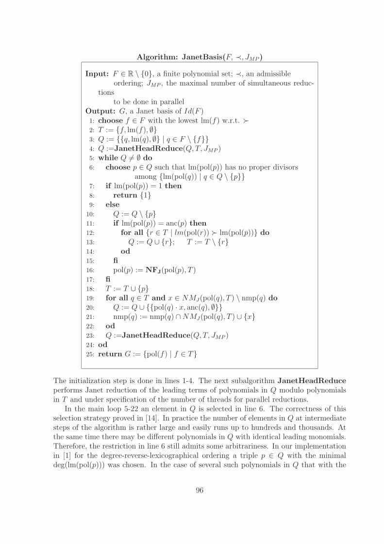
Algorithm: JanetBasis(F, ≺, JMP )
Input: F ∈ R \ {0}, a finite polynomial set; ≺, an admissibleordering; JMP , the maximal number of simultaneous reduc-
tionsto be done in parallel
Output: G, a Janet basis of Id(F )1: choose f ∈ F with the lowest lm(f) w.r.t. �2: T := {f, lm(f), ∅}3: Q := {{q, lm(q), ∅} | q ∈ F \ {f}}4: Q :=JanetHeadReduce(Q, T, JMP )5: while Q = ∅ do6: choose p ∈ Q such that lm(pol(p)) has no proper divisors
among {lm(pol(q)) | q ∈ Q \ {p}}7: if lm(pol(p)) = 1 then8: return {1}9: else
10: Q := Q \ {p}11: if lm(pol(p)) = anc(p) then12: for all {r ∈ T | lm(pol(r)) � lm(pol(p))} do13: Q := Q ∪ {r}; T := T \ {r}14: od15: fi16: pol(p) := NFJ(pol(p), T )17: fi18: T := T ∪ {p}19: for all q ∈ T and x ∈ NMJ(pol(q), T ) \ nmp(q) do20: Q := Q ∪ {{pol(q) · x, anc(q), ∅}}21: nmp(q) := nmp(q) ∩ NMJ(pol(q), T ) ∪ {x}22: od23: Q :=JanetHeadReduce(Q, T, JMP )24: od25: return G := {pol(f) | f ∈ T}
The initialization step is done in lines 1-4. The next subalgorithm JanetHeadReduceperforms Janet reduction of the leading terms of polynomials in Q modulo polynomialsin T and under specification of the number of threads for parallel reductions.
In the main loop 5-22 an element in Q is selected in line 6. The correctness of thisselection strategy proved in [14]. In practice the number of elements in Q at intermediatesteps of the algorithm is rather large and easily runs up to hundreds and thousands. Atthe same time there may be different polynomials in Q with identical leading monomials.Therefore, the restriction in line 6 still admits some arbitrariness. In our implementationin [1] for the degree-reverse-lexicographical ordering a triple p ∈ Q with the minimaldeg(lm(pol(p))) was chosen. In the case of several such polynomials in Q that with the
96
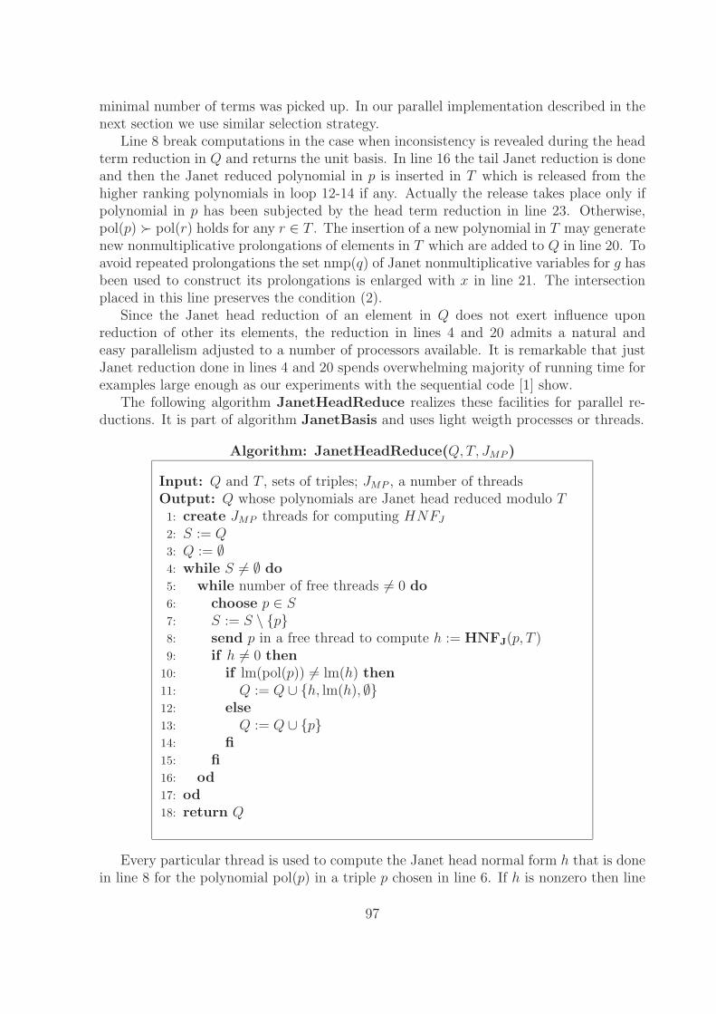
minimal number of terms was picked up. In our parallel implementation described in thenext section we use similar selection strategy.
Line 8 break computations in the case when inconsistency is revealed during the headterm reduction in Q and returns the unit basis. In line 16 the tail Janet reduction is doneand then the Janet reduced polynomial in p is inserted in T which is released from thehigher ranking polynomials in loop 12-14 if any. Actually the release takes place only ifpolynomial in p has been subjected by the head term reduction in line 23. Otherwise,pol(p) � pol(r) holds for any r ∈ T . The insertion of a new polynomial in T may generatenew nonmultiplicative prolongations of elements in T which are added to Q in line 20. Toavoid repeated prolongations the set nmp(q) of Janet nonmultiplicative variables for g hasbeen used to construct its prolongations is enlarged with x in line 21. The intersectionplaced in this line preserves the condition (2).
Since the Janet head reduction of an element in Q does not exert influence uponreduction of other its elements, the reduction in lines 4 and 20 admits a natural andeasy parallelism adjusted to a number of processors available. It is remarkable that justJanet reduction done in lines 4 and 20 spends overwhelming majority of running time forexamples large enough as our experiments with the sequential code [1] show.
The following algorithm JanetHeadReduce realizes these facilities for parallel re-ductions. It is part of algorithm JanetBasis and uses light weigth processes or threads.
Algorithm: JanetHeadReduce(Q, T, JMP )
Input: Q and T , sets of triples; JMP , a number of threadsOutput: Q whose polynomials are Janet head reduced modulo T1: create JMP threads for computing HNFJ
2: S := Q3: Q := ∅4: while S = ∅ do5: while number of free threads = 0 do6: choose p ∈ S7: S := S \ {p}8: send p in a free thread to compute h := HNFJ(p, T )9: if h = 0 then
10: if lm(pol(p)) = lm(h) then11: Q := Q ∪ {h, lm(h), ∅}12: else13: Q := Q ∪ {p}14: fi15: fi16: od17: od18: return Q
Every particular thread is used to compute the Janet head normal form h that is donein line 8 for the polynomial pol(p) in a triple p chosen in line 6. If h is nonzero then line
97
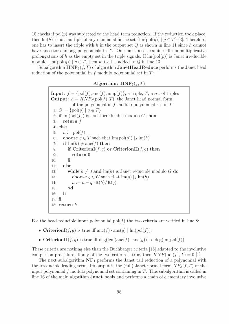
10 checks if pol(p) was subjected to the head term reduction. If the reduction took place,then lm(h) is not multiple of any monomial in the set {lm(pol(g)) | g ∈ T} [3]. Therefore,one has to insert the triple with h in the output set Q as shown in line 11 since h cannothave ancestors among polynomials in T . One must also examine all nonmultiplicativeprolongations of h as the empty set in the triple signals. If lm(pol(p)) is Janet irreduciblemodulo {lm(pol(g)) | g ∈ T , then p itself is added to Q in line 13.
Subalgorithm HNFJ(f, T ) of algorithm JanetHeadReduce performs the Janet headreduction of the polynomial in f modulo polynomial set in T :
Algorithm: HNFJ(f, T )
Input: f = {pol(f), anc(f), nmp(f)}, a triple; T , a set of triplesOutput: h = HNFJ(pol(f), T ), the Janet head normal form
of the polynomial in f modulo polynomial set in T1: G := {pol(g) | g ∈ T}2: if lm(pol(f)) is Janet irreducible modulo G then3: return f4: else5: h := pol(f)6: choose g ∈ T such that lm(pol(g)) |J lm(h)7: if lm(h) = anc(f) then8: if CriterionI(f, g) or CriterionII(f, g) then9: return 0
10: fi11: else12: while h = 0 and lm(h) is Janet reducible modulo G do13: choose q ∈ G such that lm(q) |J lm(h)14: h := h − q · lt(h)/ lt(q)15: od16: fi17: fi18: return h
For the head reducible input polynomial pol(f) the two criteria are verified in line 8:
• CriterionI(f, g) is true iff anc(f) · anc(g) | lm(pol(f)).
• CriterionII(f, g) is true iff deg(lcm(anc(f) · anc(g))) < deg(lm(pol(f)).
These criteria are nothing else than the Buchberger criteria [15] adapted to the involutivecompletion procedure. If any of the two criteria is true, then HNF (pol(f), T ) = 0 [1].
The next subalgorithm NFJ performs the Janet tail reduction of a polynomial withthe irreducible leading term. Its output is the (full) Janet normal form NFJ(f, T ) of theinput polynomial f modulo polynomial set containing in T . This subalgorithm is called inline 16 of the main algorithm Janet basis and performs a chain of elementary involutive
98
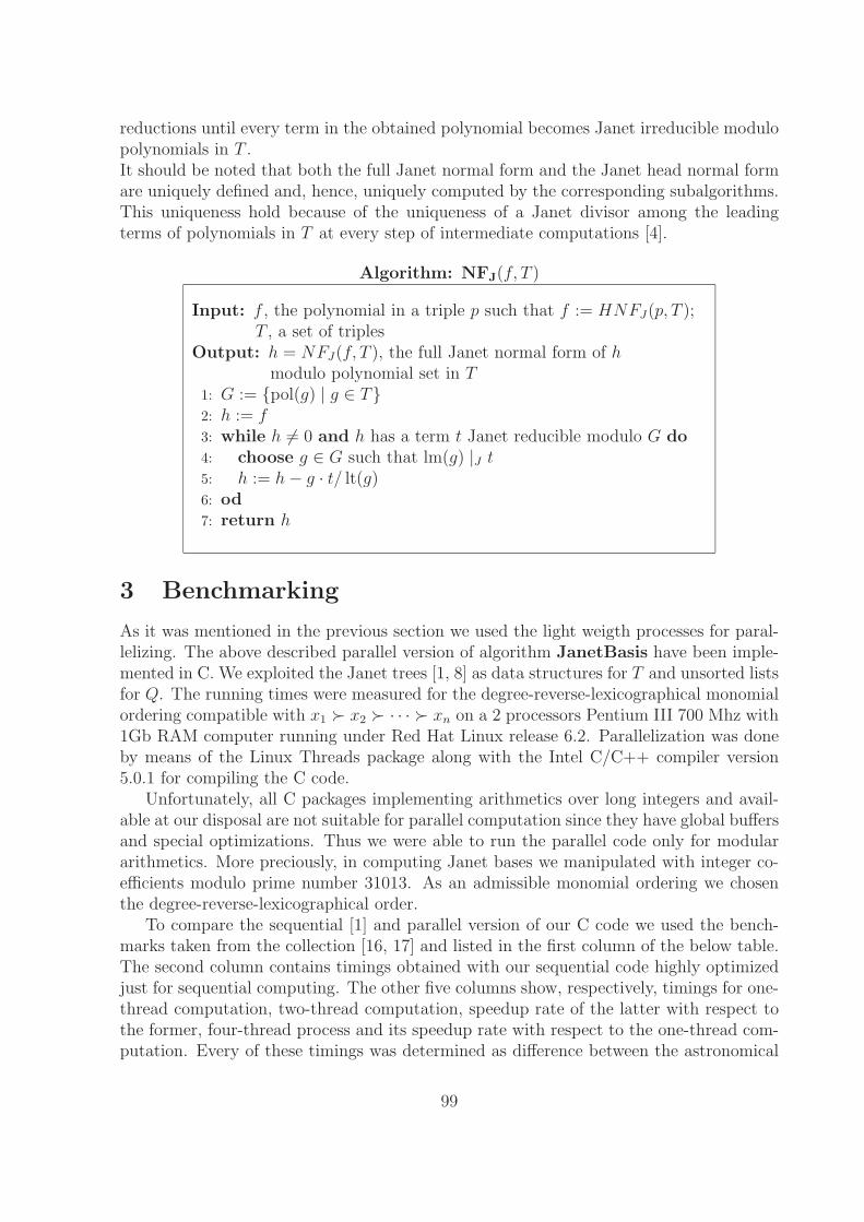
reductions until every term in the obtained polynomial becomes Janet irreducible modulopolynomials in T .It should be noted that both the full Janet normal form and the Janet head normal formare uniquely defined and, hence, uniquely computed by the corresponding subalgorithms.This uniqueness hold because of the uniqueness of a Janet divisor among the leadingterms of polynomials in T at every step of intermediate computations [4].
Algorithm: NFJ(f, T )
Input: f , the polynomial in a triple p such that f := HNFJ(p, T );T , a set of triples
Output: h = NFJ(f, T ), the full Janet normal form of hmodulo polynomial set in T
1: G := {pol(g) | g ∈ T}2: h := f3: while h = 0 and h has a term t Janet reducible modulo G do4: choose g ∈ G such that lm(g) |J t5: h := h − g · t/ lt(g)6: od7: return h
3 Benchmarking
As it was mentioned in the previous section we used the light weigth processes for paral-lelizing. The above described parallel version of algorithm JanetBasis have been imple-mented in C. We exploited the Janet trees [1, 8] as data structures for T and unsorted listsfor Q. The running times were measured for the degree-reverse-lexicographical monomialordering compatible with x1 � x2 � · · · � xn on a 2 processors Pentium III 700 Mhz with1Gb RAM computer running under Red Hat Linux release 6.2. Parallelization was doneby means of the Linux Threads package along with the Intel C/C++ compiler version5.0.1 for compiling the C code.
Unfortunately, all C packages implementing arithmetics over long integers and avail-able at our disposal are not suitable for parallel computation since they have global buffersand special optimizations. Thus we were able to run the parallel code only for modulararithmetics. More preciously, in computing Janet bases we manipulated with integer co-efficients modulo prime number 31013. As an admissible monomial ordering we chosenthe degree-reverse-lexicographical order.
To compare the sequential [1] and parallel version of our C code we used the bench-marks taken from the collection [16, 17] and listed in the first column of the below table.The second column contains timings obtained with our sequential code highly optimizedjust for sequential computing. The other five columns show, respectively, timings for one-thread computation, two-thread computation, speedup rate of the latter with respect tothe former, four-thread process and its speedup rate with respect to the one-thread com-putation. Every of these timings was determined as difference between the astronomical
99
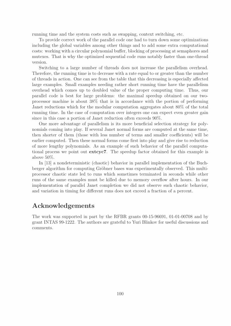
running time and the system costs such as swapping, context switching, etc.To provide correct work of the parallel code one had to turn down some optimizations
including the global variables among other things and to add some extra computationalcosts: working with a circular polynomial buffer, blocking of processing at semaphores andmutexes. That is why the optimized sequential code runs notably faster than one-threadversion.
Switching to a large number of threads does not increase the parallelism overhead.Therefore, the running time is to decrease with a rate equal to or greater than the numberof threads in action. One can see from the table that this decreasing is especially affectedlarge examples. Small examples needing rather short running time have the parallelismoverhead which comes up to doubled value of the proper computing time. Thus, ourparallel code is best for large problems: the maximal speedup obtained on our two-processor machine is about 38% that is in accordance with the portion of performingJanet reductions which for the modular computation aggregates about 80% of the totalrunning time. In the case of computation over integers one can expect even greater gainsince in this case a portion of Janet reduction often exceeds 90%.
One more advantage of parallelism is its more beneficial selection strategy for poly-nomials coming into play. If several Janet normal forms are computed at the same time,then shorter of them (those with less number of terms and smaller coefficients) will beearlier computed. Then these normal forms come first into play and give rise to reductionof more lengthy polynomials. As an example of such behavior of the parallel computa-tional process we point out extcyc7. The speedup factor obtained for this example isabove 50%.
In [13] a nondeterministic (chaotic) behavior in parallel implementation of the Buch-berger algorithm for computing Grobner bases was experimentally observed. This multi-processor chaotic state led to runs which sometimes terminated in seconds while otherruns of the same examples must be killed due to memory overflow after hours. In ourimplementation of parallel Janet completion we did not observe such chaotic behavior,and variation in timing for different runs does not exceed a fraction of a percent.
Acknowledgements
The work was supported in part by the RFBR grants 00-15-96691, 01-01-00708 and bygrant INTAS 99-1222. The authors are grateful to Yuri Blinkov for useful discussions andcomments.
100
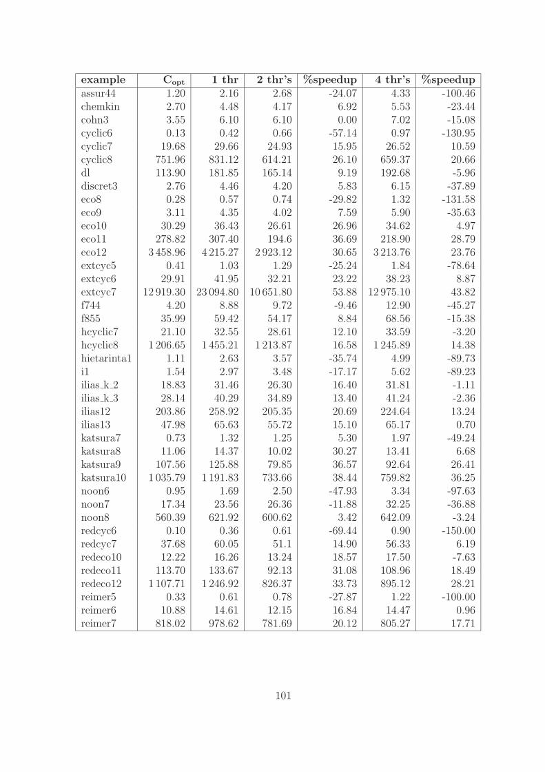
example Copt 1 thr 2 thr’s %speedup 4 thr’s %speedupassur44 1.20 2.16 2.68 -24.07 4.33 -100.46chemkin 2.70 4.48 4.17 6.92 5.53 -23.44cohn3 3.55 6.10 6.10 0.00 7.02 -15.08cyclic6 0.13 0.42 0.66 -57.14 0.97 -130.95cyclic7 19.68 29.66 24.93 15.95 26.52 10.59cyclic8 751.96 831.12 614.21 26.10 659.37 20.66dl 113.90 181.85 165.14 9.19 192.68 -5.96discret3 2.76 4.46 4.20 5.83 6.15 -37.89eco8 0.28 0.57 0.74 -29.82 1.32 -131.58eco9 3.11 4.35 4.02 7.59 5.90 -35.63eco10 30.29 36.43 26.61 26.96 34.62 4.97eco11 278.82 307.40 194.6 36.69 218.90 28.79eco12 3 458.96 4 215.27 2 923.12 30.65 3 213.76 23.76extcyc5 0.41 1.03 1.29 -25.24 1.84 -78.64extcyc6 29.91 41.95 32.21 23.22 38.23 8.87extcyc7 12 919.30 23 094.80 10 651.80 53.88 12 975.10 43.82f744 4.20 8.88 9.72 -9.46 12.90 -45.27f855 35.99 59.42 54.17 8.84 68.56 -15.38hcyclic7 21.10 32.55 28.61 12.10 33.59 -3.20hcyclic8 1 206.65 1 455.21 1 213.87 16.58 1 245.89 14.38hietarinta1 1.11 2.63 3.57 -35.74 4.99 -89.73i1 1.54 2.97 3.48 -17.17 5.62 -89.23ilias k 2 18.83 31.46 26.30 16.40 31.81 -1.11ilias k 3 28.14 40.29 34.89 13.40 41.24 -2.36ilias12 203.86 258.92 205.35 20.69 224.64 13.24ilias13 47.98 65.63 55.72 15.10 65.17 0.70katsura7 0.73 1.32 1.25 5.30 1.97 -49.24katsura8 11.06 14.37 10.02 30.27 13.41 6.68katsura9 107.56 125.88 79.85 36.57 92.64 26.41katsura10 1 035.79 1 191.83 733.66 38.44 759.82 36.25noon6 0.95 1.69 2.50 -47.93 3.34 -97.63noon7 17.34 23.56 26.36 -11.88 32.25 -36.88noon8 560.39 621.92 600.62 3.42 642.09 -3.24redcyc6 0.10 0.36 0.61 -69.44 0.90 -150.00redcyc7 37.68 60.05 51.1 14.90 56.33 6.19redeco10 12.22 16.26 13.24 18.57 17.50 -7.63redeco11 113.70 133.67 92.13 31.08 108.96 18.49redeco12 1 107.71 1 246.92 826.37 33.73 895.12 28.21reimer5 0.33 0.61 0.78 -27.87 1.22 -100.00reimer6 10.88 14.61 12.15 16.84 14.47 0.96reimer7 818.02 978.62 781.69 20.12 805.27 17.71
101
References
[1] Gerdt, V.P., Blinkov, Yu.A., Yanovich, D.A.: Construction of Janet Bases. II.Polynomial Bases. In: Computer Algebra in Scientific Computing / CASC’01,V.G.Ganzha, E.W.Mayr and E.V.Vorozhtsov (Eds.), Springer-Verlag, Berlin, 2001,pp.249-263.
[2] Janet, M.: Lecons sur les Systemes d’Equations aux Derivees Partielles, CahiersScientifiques, IV, Gauthier-Villars, Paris, 1929.
[3] Gerdt, V.P., Blinkov, Yu.A.: Involutive Bases of Polynomial Ideals. Math. Comp.Sim. 45 (1998) 519-542.
[4] Gerdt, V.P., Blinkov, Yu.A. Minimal Involutive Bases. Math. Comp. Simul. 45 (1998)543-560.
[5] Apel, J.: Theory of Involutive Divisions and an Application to Hilbert Function. J.Symb. Comp. 25 (1998) 683-704.
[6] Gerdt, V.P.: Completion of Linear Differential Systems to Involution. In: Com-puter Algebra in Scientific Computing / CASC’99, V.G.Ganzha, E.W.Mayr andE.V.Vorozhtsov (Eds.), Springer-Verlag, Berlin, 1999, pp. 115-137.
[7] Calmet, J., Hausdorf, M., Seiler, W.M.: A Constructive Introduction to Involution.Proc. Int. Symp. Applications of Computer Algebra - ISACA 2000, Allied Publishers,New Delhi, 2001, pp. 33-50.
[8] Gerdt V.P., Blinkov Yu.A., Yanovich D.A.: Construction of Janet Bases. I. Mono-mial Bases. In: Computer Algebra in Scientific Computing / CASC’01, V.G.Ganzha,E.W.Mayr and E.V.Vorozhtsov (Eds.), Springer-Verlag, Berlin, 2001, pp.233-247.
[9] Gerdt, V.P.: On the Relation Between Pommaret and Janet Bases. In: Com-puter Algebra in Scientific Computing / CASC’00, V.G.Ganzha, E.W.Mayr andE.V.Vorozhtsov (Eds.), Springer-Verlag, Berlin, 2000, pp.167-181.
[10] Cox, D., Little, J., O’Shea, D.: Ideals, Varieties and Algorithms. An Introduction toComputational Algebraic Geometry and Commutative Algebra. 2nd Edition, Springer-Verlag, New-York, 1996.
[11] Attardi, G., Traverso, C.: A Strategy-Accurate Parallel Buchberger Algorithm. In:PASCO’94, Lecture Notes Series in Computing 5, World Scientific, Singapore, 1994,pp. 49-54.
[12] Faugere, J.C.: Parallelization of Grobner Basis. In: PASCO’94, Lecture Notes Seriesin Computing 5, World Scientific, Singapore, 1994, pp. 124-132.
[13] Amrheim, B., Gloor, O., Kuchlin, W.: A Case Study of Multi-Threaded GrobnerBasis Completion. Proceedings of ISSAC’96, ACM Press, 1996, 95-102.
102
[14] Gerdt, V.P.: On an Algorithmic Optimization in Computation of Involutive Bases.Programming and Computer Software 2 (2002), to appear.
[15] Buchberger, B.: Grobner Bases: an Algorithmic Method in Polynomial Ideal The-ory. In: Recent Trends in Multidimensional System Theory, N.K. Bose (ed.), Reidel,Dordrecht (1985) 184–232.
[16] Bini, D., Mourrain, B.: Polynomial Test Suite, 1996.
http://www-sop.inria.fr/saga/POL.
[17] Verschelde, J.: The Database with Test Examples.
http://www.math.uic.edu/˜ jan/demo.html.
103
On Algebraic Geometric andComputer Algebra Aspects of
Mirror Symmetry
N.M. Glazunov
Glushkov Institute of Cybernetics NAS,03187 Glushkov prospect 40, Kiev-187 , Ukraine;
e-mail: [email protected]
We survey some algebraic geometric aspects of mirror symmetry and duality in stringtheory. Some applications of computer algebra to algebraic geometry and string theory areshortly reviewed.
1 Introduction
This paper aims to be accessible to those with no previous experience in algebraic ge-ometry; only some basic familiarity with linear and polynomial algebra, group theory,topology and category theory will be assumed.Development of theoretical physics in direction of string theory enlarged the context ofsymmetry considerations and included in it the notion of duality. String theory has fol-lowing ingredients: (i) base space (open or closed string) Σ; (ii) target space M ; (iii)fields: X → Σ → M ; (iv) action S =
∫ L(X,ϕ). where L is a Lagrangian [1]. Let Gbe a group such that G ⊃ SU(3) × SU(2) × U(1). Recall that if L(GΦ) = L(Φ) thenL is G−invariant, or G−symmetry. In string theory [1] one of the beautiful symmetriesis the radius symmetry R → 1/R of circle, known as T−duality [2, 3] and [4] and refer-ences there in. Authors of papers [5, 6] conjectured that a similar duality might exist inthe context of string propagation on Calabi-Yau (CY) manifolds, where the role of thecomplex deformation on one manifold get exchanged with the Kahler deformation on thedual manifold. A pair of manifolds satisfying this symmetry is called mirror pair, andthis duality is called mirror symmetry. From the point of view of physicists which didthe remarkable discovery mirror symmetry is a type of duality that means that we maytake two types of string theory and compactify them in two different ways and achieve”isomorphic” physics [7]. Or in the case of a pair of Calabi-Yau threefolds (X,Y ) P.Aspinwall are said [8] that X and Y to be a mirror pair if and only if the type IIA stringcompactified on X is ”isomorphic to” the E8 × E8 heterotic string compactified on Y. Ifin the case X is Calabi-Yau threefold then Y is the product of a K3 surface and ellipticcurve and the following data specifies the theory [8].
1. A Ricci-flat metric on Y.
2. A B−field ∈ H2(K3 × E,R/Z).
104
3. A vector bundle V → (K3×E) with a connection satisfying the Yang-Mills equationsand whose structure group ⊆ E8 × E8.
4. A dilation + axion, Φ ∈ C.
C. Vafa defines the notion of mirror of a Calabi-Yau manifold with a stable bundle.Lagrangian and special Lagrangian submanifolds appear in this situation. Mathemati-cians also work hard upon the problems of mirror symmetry, although it is difficult insome cases to attribute to a researcher the identifier ”mathematician” or ”physicist”.V. Batyrev gives construction of mirror pairs using Gorenstein toric Fano varieties andCalabi-Yau hypersurfaces in these varieties [9]. M. Kontsevich in his talk at the ICM’94gave a conjecturel interpratation of mirror symmetry as a ”shadow” of an equivalencebetween two triangulated categories associated with A∞− categories [10]. His conjecturewas proved in the case of elliptic curves by A. Polishchuk and E. Zaslow [11]. The aimof the paper is to provide a short and gentle survey of some algebraic aspects of mirrorsymmetry and duality with examples - without proofs, but with (a very restricted) guidesto the literature.
2 Algebraic geometric preliminaries
This section gives a basic introduction to algebraic geometric aspects of mirror symmetrybeginning with a description of how Calabi-Yau manifolds arise from ringed spaces. Amore detailed treatment of algebraic geometric material of this section may be foundin [12, 13], the terminology and notation of which will be followed here.Let X be a topological space and Cov(X) an open covering of X. It is well known [14]that Cov(X) forms the category. Let Cat be a category (of sets, abelian groups, rings,modules). The presheaf is a contravariant functor F from Cov(X) to Cat. If for exampleCat is the category Ab of abelian groups then F : Cov(X) → Ab is the presheaf of abeliangroups. Elements f ∈ F(U) is called sections of the presheaf F .If i : U ⊂ V then we shall denote by ρV
U the morphism F(i) : F(V ) → F(U). Functor Fis the contravariant and we apply morphisms from the left to the rigth. Hence for anyopen sets U ⊂ V ⊂ W
ρWU = ρV
UρWV .
Let U ⊂ X be any open subset of X and⋃
Uα = U it’s open covering. A presheaf F ona topological space X is called the sheaf if the following conditions are satisfied:1) if ρU
Uαs1 = ρU
Uαs2 for s1, s2 ∈ F(U) and for any Uα, then s1 = s2;
2) if sα ∈ F(Uα) are such that ρUα
Uα⋂
Uβsα = ρ
Uβ
Uα⋂
Uβsβ, then there exists s ∈ F(U) such
that sα = ρUUα
s for all Uα.The ringed space is the pair (X,O), where X is a topological space and O is a sheaf
of rings on X. A morphism of ringed spaces
ϕ : (X,OX) → (Y,OY )
is the class of maps (ϕ, ψU), where ϕ is the continuous map ϕ : X → Y, and ψU is ahomomorphism ψU : OY (U) → OX(ϕ−1(U)) for any open set U ⊂ Y such that the
105
diagram
OX(ϕ−1(V ))ρV
U−→ OX(ϕ−1(U))↓ ψV ↓ ψU
OY (V )ρV
U−→ OY (U)
is commutative for any U and V, U ⊂ V ⊂ Y. For a ringed space (X,OX) and an openU ⊂ X the restriction of the sheaf OX on U defines the ringed space (U,OX|U).Let OX be the sheaf of smooth functions on a topological space X. Then any smoothmanifold X with the sheaf OX is a ringed space (X,OX). Respectively let X be a Hausdorfftopological space and OX a sheaf on X. Let it satisfies conditions: (i) OX is the sheaf ofalgebras over C ; (ii) OX is a subsheaf of the sheaf of continuous complex valued functions.Let W be a domain in Cn and Oan the sheaf of analytical functions on W. The ringedspace (X,OX) is called the complex analytical manifold if for any point x ∈ X there existsa neighbourhood U � x such that (U,OX|U) � (W,Oan) (here � denotes the isomorphismof ringed spaces).
We shall use in contrast to [1] some another definition of Calabi-Yau (CY) manifold.The definition is based on the theorem of Yau who proved Calabi’s conjecture that acomplex Kahler manifold of vanishing first Chern class admits a Ricci-flat metric.
Definition 1. A complex Kahler manifold is called Calabi-Yau (CY) manifold if it hasvanishing first Chern class.
Examples of the CY-manifolds include, in particular, elliptic curves E, K3−surfacesand their products E × K3. Let (X,ω, Ω) be a complex manifold (real dimension =2n)with
ωn/n! = (−1)n(n−1)/2(i/2)n · Ω ∧ Ω.
It is said that a n−dimensional submanifold L ⊂ X is special Lagrangian (s-lag) ⇔
Re(Ω|L) = V ol|L ⇔ ω|L = 0, Im(Ω|L) = 0.
Example 1. Let X be an elliptic curve E. Then ω = c(i/2)dz∧dz, Ω = cdz. S-lag L ⊂ Eare straight lines with slope determined by arg c.
Let (U,OX|U) � SpecA for a commutative ring A. In the case the neighbourhoodU � x is called the affine neighbourhood of the point x.The scheme S is the ringed space (X,OX) with the condition: for any point x ∈ X thereis an affine neighbourhood V � x such that (V,OX|V ) � SpecA.
2.1 Blow-ups
Blowing up is a well known method of constructing complex manifolds M. There are pointson the manifolds that are not divisors on M. Blow up is the construction that transformspoints of complex manifolds to divisors. For instance in the case of two dimensionalcomplex manifolds (complex surface) N it consists of replacing a point p ∈ N by aprojective line CP(1) considered as the set of limit directions at p.
106
Example 2. Let π : M2 → C2 be the blow-up of C2 at the point 0 ∈ C2. Then M2 is atwo dimensional complex manifold that defined by two local charts. In coordinates C2 =(z1, z2),CP(1) = [l0, l1] the manifold M2 is defined in CP(1)×C2 by quadratic equationszilj = zjli. Thus M2 is a line bundle over Riemann sphere CP(1). π−1(0) = CP(1) iscalled the divisor of the blow up (the exceptional divisor).
Recently a large class of CY orbifolds in weighted projective spaces have been proposed.C. Vafa have predicted and S. Roan [17] have computed the Euler number of all theresolved CY hypersurfaces in a weighted projective space WCP(4).
3 Complexes, homotopy categories, cohomologies
and quasiisomorphisms
Here we recall the relevant properties of complexes, derived categories, cohomologies andquasimorphisms referring to [13, 20] for details and indication of proofs.Cochein complex
(K•, d) = {K0 d→ K1 d→ K2 d→ · · · }is the sequence of abelian groups and differentials d : Kp → Kp+1 with the conditiond ◦ d = 0. For a category Cat we denote by ObCat it’s objects and by Mor Cat it’smorphisms.
Let A be an abelian category, Kom(A) the category of complexes over A. Furthermore,there are various full subcategories of Kom(A) whose respective objects are the complexeswhich are bounded below, bounded above, bounded in both sides. Now recall (by [20])the notion of homotopy morphism.
Lemma-definition 1. (i) Let K•, L• be two complexes over abelian category A, k =ki, ki : Ki → Li−1 a sequence of morphisms between elements of the complexes.Then the maps
hi = ki+1diK + di−1
L ki : Ki → Li
form the morphism of complexes
h = kd + dk : K• → L•.
The morphism h is called homotopic to zero (h ∼ 0).(ii) morphisms f, g : K• → L• is called homotopic, if f − g = kd + dk ∼ 0 (f ∼ g), k iscalled homotopy.(iii) If f ∼ g, then H•(f) = H•(g), where the map H• is induced on cohomologies ofcomplexes.
The homotopy category K(A) is defined by the following way:
Ob K(A) = Ob Kom(A),
Mor K(A) = Mor Kom(A) by the module of homotopy equivalence.
107
Let X be a topological space and K•,L• be complexes of sheaves over X. Quasiisomor-phism is the map
f : K• → L•
which induces the isomorphism of cohomological sheaves
f∗ : Hq(K•) → Hq(L•), q ≥ 0.
4 Connections
Consider the connection in the context of algebraic geometry. Let S/k be the smoothscheme over field k, U an element of open covering of S, OS the structure sheaf on S,Γ(U,OS) the sections of OS on U . Let Ω1
S/k be the sheaf of germs of 1−dimension differ-entials, F be a coherent sheaf. The connection on the sheaf F is the sheaf homomorphism
∇ : F → Ω1S/k ⊗F ,
such that if f ∈ Γ(U,OS), g ∈ Γ(U,F) then
∇(fg) = f∇(g) + df ⊗ g.
There is the dual definition. Let F be the locally free sheaf, Θ1S/k the dual to sheaf Ω1
S/k,
∂ ∈ Γ(U, Θ1S/k). The connection is the homomorphism
ρ : Θ1S/k → EndOS
(F ,F),
ρ(∂)(fg) = ∂(f)g + fρ(∂).
4.1 Integration of connections
Let ΩiS/k be the sheaf of germs of i−dimensional differential forms on S. Particularly Ω1
S/k
is the cotangent bundle over S. Let ω ∈ ΩiS/k, f ∈ Γ and
∇i(ω ⊗ f) = dω ⊗ f + (−1)iω ∧∇(f).
Hence, ∇i define the sequence of homomorphisms of sheaves
F ∇−→ Ω1S/k ⊗F ∇1−→ Ω2
S/k ⊗F −→ · · ·The sequence is the complex if ∇ ◦∇1 = 0. In this case the connection ∇ is integrable.
Example 3. Let F = OS be the structural sheaf on S. Then
∇ : OS → Ω1S/k ⊗OS � Ω1
S/k.
Hence ∇(f) = df, ρ : ΘS/k → OS. This connection ∇ is integrable because it defines thede Rham complex
Ω•S/k : OS → Ω1
S/k → Ω2S/k → · · ·
108
Example 4. Let LC be a locally constant sheaf on S/k such that LC � kn (local coef-ficients) as sheaves. Let F = LC ⊗ OS, v ∈ Γ(U,LC), f ∈ Γ(U,F). Then there is acanonical connection ∇(v ⊗ f) = df ⊗ v:
∇ : F → Ω1S ⊗F .
For a connection ∇ : F → Ω1S ⊗F a section s ∈ Γ(U,F) is horizontal if ∇(s) = 0.
Let now S be a complex manifolds, ShC(S/k) the category of sheaves with a connec-tion and LC(S) the category of local coefficients over S. Let (F ,∇) ∈ ShC(S/k) be asheaf with connection. We can define the functor
Fn : (F ,∇) �→ {the sheaf of germs of horizontal sections of F}.and it’s inverse Fn−1.
Proposition 1. The functors Fn and Fn−1 give the equivalence of category ShC(S/k)and LC(S).
5 Moduli spaces in string theory
Mirror symmetry connects with geometrical deformations of complex and Kahler struc-tures on CY-manifolds. So we have to know moduli spaces of complex and Kahler struc-tures on CY-manifolds.
5.1 Moduli spaces
The theory of moduli spaces [15, 16] has, in recent years, become the meeting ground ofseveral different branches of mathematics and physics - algebraic geometry, instantons,differential geometry, string theory and arithmetics. Here we recall some underlieing alge-braic structures of the relation. In previous section we have reminded the situation withvector bundles on projective algebraic curves X. On X any first Chern class c1 ∈ H2(X,Z)can be realized as c1 of vector bundle of prescribed rank (dimension) r. How to classifyvector bundles over algebraic varieties of dimension more than 1? This is one of impor-tant problems of algebraic geometry and the problem has closed connections with gaugetheory in physics and differential geometry. Mamford [15] and others have formulatedthe problem about the determination of which cohomology classes on a projective varietycan be realized as Chern classes of vector bundles? Moduli spaces are appeared in theproblem. What is moduli? Classically Riemann claimed that 3g−3 (complex) parameterscould be for Riemann surface of genus g which would determine its conformal structure(for elliptic curves, when g = 1, it is needs one parameter). From algebraic point of viewwe have the following problem: given some kind of variety, classify the set of all varietieshaving something in common with the given one (same numerical invariants of some kind,belonging to a common algebraic family). For instance, for an elliptic curve the invariantis the modular invariant of the elliptic curve.
Let B be a class of objects. Let S be a scheme. A family of objects parametrized bythe S is the set of objects
109
Xs : s ∈ S,Xs ∈ B
equipped with an additional structure compatible with the structure of the base S. Pa-rameter varieties is a class of moduli spaces. These varieties is very convenient tool forcomputer algebra investigation of objects that parametrized by the parameter varieties.We have used the approach for investigation of rational points of hyperelliptic curves overprime finite fields [22].
Example 5. Let ω1, ω2 ∈ C, Im(ω1/ω2) > 0, Λ = nω1 + mω2, n,m ∈ Z be a lattice.Let H be the upper half plane. Then H/Λ = E be the elliptic curve. Let
y2 = x3 + ax + b = (x − e1)(x − e2)(x − e3), 4a3 + 27b2 = 0,
be the equation of E. Then the differential of first kind on E is defined by formula
ω = dx/y = dx/(x3 + ax + b)1/2.
Periods of E :
π1 = 2
∫ e2
e1
ω, π2 = 2
∫ e3
e2
ω.
The space of moduli of elliptic curves over C is A1(C). Its complation is CP(1).
For K3−surfaces the situation is more complicated but in some case is analogous [19]:
Theorem 1. The moduli space of complex structure on market K3−surface (includingorbifold points) is given by the space of possible periods.
Some computational aspects of periods and moduli spaces are considered in author’snote [23].
6 Some categorical constructions
Every compact symplectic manifold Y, ω with vanishing first Chern class, one can associatea A∞−category whose objects are essentially the Lagrangian submanifolds of Y, and whosemorphisms are determined by the intersections of pairs of submanifolds. This category iscalled Fukaya’s category and is denoted by F(Y ) [10]. Let (X,Y ) be a mirror pair. LetM be any element of the mirror pair. The bounded derived category Db(M) of coherentsheaves on M is obtained from the category of bounded complexes of coherent sheaves onM [20]. In the case of elliptic curves A. Poleshchuk and E. Zaslov have proved [11]:
Theorem 2. The categories Db(Eq) and F0(Eq) are equivalent.
Recently A. Kapustin and D. Orlov have suggested that Kontsevich’s conjecture mustbe modified: coherent sheaves must be replaced with modules over Azumaya algebras,and the Fukaya category must be ”twisted” by closed 2-form [21].
110
7 Computer algebra aspects
Computer algebra applications to classical algebraic geometry are well known. Most ofthem are based on the method of Grobner bases [24, 25]. They include the decompositionof algebraic varieties, rational parametrization of curves and surfaces [26, 27], inversion ofbirational maps [28], the normalization of affine rings [18]. Some computer algebra resultspresented on CAAP-2001 can be used for computations in algebraic geometry and stringtheory. These are results on computation of toric ideals presented by V. Gerdt [29] and oncomputation of cohomology presented by V. Kornyak [30]. Talks of V. Gerdt include alsoresult on computation in Yang-Mills mechanics [31]. Some recent papers include descrip-tion of efficient algorithms computing the homology of commutative differential gradedalgebras [32] and computing the complite Hopf algebra structure of the 1-homology ofpurely quadratic algebra [33].For the future research let us mention that it might be as well to have a tool, namelycomputer algebra for computation with (i) various moduli spaces; (ii) deformations (defor-mation of complex structure and deformation of Kahler structure); (iii) A∞−categories;(iv) geometric Fourier transform.
Conclusions
In the paper we tried to give an algebraic geometric framework for some aspects of mirrorsymmetry. This framework includes rather restricted context of mirror symmetry andstring theory. But it is based on a simple and unified mathematical base. Some applica-tions of computer algebra to algebraic geometry and string theory are shortly reviewed.
Acknowledgements
I would like to thanks the organizers of the CAAP’2001 (Dubna) and SAGP’99 (MirrorSymmetry in String Theory, CIRM, Luminy) for providing a very pleasent environmentduring the conferences.
References
[1] B. Greene, String theory on Calabi-Yau manifolds, Preprint, 1997, hep-th/9702155.
[2] L. Dixon, Lecture at the 1987 ICTP Summer Workshop in High Energy Physics andCosmology. Trieste, 1987.
[3] W. Lerche, C. Vafa, and N. Warner, Chiral rings in N=2 superconformal theories,Nucl. Phys., 1989, B324, pp. 421-430.
[4] A. Giveon, M. Porrati,E. Rabinovici, Target Space Duality in String Theory,Phys.Rept., 1994, N 244, pp. 77-202.
[5] P. Candelas, M. Lynker, R. Schimmrink. Nucl. Phys., 1990, B330, p. 49.
111
[6] B. Greene, R. Plesser, Nucl. Phys., 1990, B338, p. 15.
[7] C. Vafa, Geometric Physics, Proceedinds of ICM’98, Berlin, Documenta Math. J.DMV, 2000, pp. 430-439.
[8] P. Aspinwall, String theory and duality, ibid, pp. 229-238.
[9] V. Batyrev, Mirror symmetry and toric geometry, ibid, pp. 239-248.
[10] M. Kontsevich, Homological algebra of mirror symmetry, Proceedinds of ICM’94,Zurich, Birkhauser, 1995, pp. 120-139.
[11] A. Polishuk, E. Zaslow, Categorical mirror symmetry: the elliptic curves,Adv.Theor.Math.Phys., 1998, N 2, pp. 443-470.
[12] I.R. Shafarevitch. Foundations of Algebraic Geometry. Moscow: Nauka, 1988, v.1,v.2(in Russian).
[13] Ph. Griffiths, J. Harris. Principles of algebraic geometry. A Wiley Int. Pub. N.Y.,1978.
[14] R. Godement. Topologie algebrique et theorie des faisceaux. Hermann, Paris.
[15] D. Mamford, Towards an enumirative geometry of the moduli space of curves. Arith-metic and Geometry Vol.II, Progress in Math., 1983.
[16] J. Harris, J. Morrison, Moduli of curves, Berlin-N.Y, Springer, 1998.
[17] S. Roan, Algebraic geometry and physics, Preprint, 2000, math-ph/0011038
[18] W. Decker, T. de Jong, G. Greuel, G. Pfister, The normalization: A new algo-rithm, implementation and comparisons. ”Computational methods for representationsof groups and algebras”. Proceedings of the Euroconference, (April 1-5, 1997, Essen)Basel, Birkhauser, 1999, pp. 177-185
[19] W. Barth, C. Peters, and van der Ven., Compact complex surfaces, New York,Springer, 1984.
[20] S.I. Gelfand, Yu. I. Manin, Methods of homological algebra, Moscow, Nauka, 1988.
[21] A. Kapustin, D. Orlov, Remarks on A-branes, Mirror Symmetry, and the Fukayacategory, Preprint, 2001, hep-th/0109098
[22] N.M. Glazunov, On moduli spaces, equidistribution, bounds and rational points ofalgebraic curves. Ukrainian Math. Journ., 2001, N 9, pp. 1174-1183.
[23] N.M. Glazunov, Computation of Moduli, Periods and Modular Symbols. IMACS-ACA’98. Session ”Algebra and Geometry”. Prague, 1998.http://math.unm.edu/ACA/1998/sessions/geom/glazunov/index.html
112
[24] Buchberger B. An algerithm for finding a bases. PhD thesis, Universitst Innsbruck,Institut fur Mathematik, 1965.
[25] Buchberger B. Groebner bases: an algorithmic mathod in polynomial ideal theory.Recent Trends in Multidimensional Systems Theory, chapter 6. D. Riedel Publ. Comp,1985.
[26] J. Sendra, F. Winkler. Symbolic parametrization of curves. J. Symb. Comput., 1991,12, pp. 607-632.
[27] J. Schicho. Rational parametrization of surfaces. J. Symb. Comput., 1998, 26, pp. 1-29.
[28] J. Schicho. Inversion of Birational Maps with Grobner Bases. Lond. Math. Soc. Lect.Note Ser. Cambridge: Cambridge Univ. Press. 1998, 251, pp. 495-503.
[29] V.P. Gerdt, Yu.A. Blinkov. Janet trees in computing of toric ideals. Computer algebraand its applications to physics (CAAP-2001), Dubna, 2001, p. 19.
[30] V.V. Kornyak. Extraction of ”minimal” cochain subcomplexes. ibid, p. 10.
[31] V.P. Gerdt, A.M. Khvedelidze, D.M. Mladenov. On light-cone vertion of SU(2) Yang-Mills mechanics. ibid, p. 12.
[32] V. Alvarez, J. Armario, P. Real, B. Silva. Homological perturbation theory ond com-putability of Hochschild and cyclic homologies of CDGAS. Int. Conf. on Secondarycalculus and cohomological physics, Moscow, 1997, pp. 1-15.
[33] M. Jimenez, P. Real. ”Coalgebra” structures on 1-homological models for commuta-tive differential graded algebras. preprint, 2000, 15 p.
113
Differential Grobner walk
Oleg Golubitsky
Moscow State University,Laboratory of Computational Methods,
Faculty of Mechanics and Mathematics, MSU 119899e-mail: [email protected]
An algorithm which transforms a characteristic set of an ideal in the differential ringof differential polynomials w.r.t. one ranking into the characteristic set w.r.t. anotherranking is proposed. The algorithm is a generalization of the Grobner walk algorithm fortransformation of Grobner bases for polynomial ideals from one monomial ordering toanother.
The work was supported by INTAS, grant 99-1222.
1 Introduction
In this paper, we propose an algorithm which, given a characteristic set A of a prime differ-ential ideal I w.r.t. some ranking ≤1, and another ranking ≤2, constructs a characteristicset B of I w.r.t ≤2.
The problem addressed in this paper can be solved using either of the Rosenfeld-Grobner algorithm [19] or the Specialized Rosenfeld-Grobner algorithm [21]. In bothcases, however, the algorithms proceed by direct computation of the target characteristicset w.r.t. ranking ≤2. Since this may be very inefficient, especially in case when ≤2 is anelimination ranking, an algorithm (called DFGLM) based on an adaptation of the FGLMmethod [7] to differential algebra is proposed in [20]. However, as it is pointed out in [20],this algorithm is only applicable to differential systems whose solutions depend on finitelymany constants. The Kahler algorithm [20] is applicable to any differential systems but,as it is noticed in [20], it is less efficient than DFGLM.
The case when solutions of a differential system depend on finitely many constantsis completely analogous to the case of a zero-dimensional ideal in a polynomial ring R,to which the original FGLM algorithm is applicable. But even in this restricted case,the complexity of the algorithm grows with the dimension of quotient vector space R/I.Experiments in [9, 10] show that apart from very simple cases the Grobner walk algorithm[8] is at least as fast as FGLM, and as the dimension of R/I grows, the Grobner walkbecomes much faster. Besides, the Grobner walk approach is applicable to any polynomialideals.
The key concepts needed for Grobner walk are the ones of parametrization of allpossible monomial orders by weight matrices [3, 11], monomial preorders defined by weightvectors [3, 11, 18], and the Grobner fan [4, 11] of a polynomial ideal. In the differentialcase, the parametrization of rankings, in general, is very complex [18, 17]. Therefore, werestrict ourselves to the case of Riquier rankings [12, 18] which includes important cases
114
of orderly and elimination rankings [15, 20]. The Theorem of Mora and Robbiano aboutthe finiteness of the Grobner fan [4, 11] cannot be directly generalized to the differentialcase — in fact, the differential Grobner fan may be infinite. Despite that, we will showthat differential Grobner walk always terminates.
We generalize the key Grobner walk Lemmas [8, Lemmas 3.1–3.3] to the differentialcase, where they acquire a significantly different form. In particular, the polynomial idealgenerated by the set of initial forms plays a key role for the polynomial Grobner walk,but it cannot be generalized directly to the differential case. Instead, we consider the setsof initial forms themselves. However, the computation of characteristic sets for them isstill algorithmically possible.
In the end, we discuss some open problems which should be addressed before thedifferential Grobner walk can be implemented.
2 Differential algebra
Here we only give a short presentation of the basic concepts in differential algebra andrefer the reader to [13, 14, 15].
Let R be a commutative ring. A derivation over R is a mapping δ : R → R which forevery a, b ∈ R satisfies
δ(a + b) = δ(a) + δ(b), δ(ab) = δ(a)b + aδ(b).
A differential ring is a commutative ring endowed with a finite set of derivations Δ ={δ1, . . . , δm} which commute pairwise. The commutative monoid generated by the deriva-tions is denoted by Θ. Its elements are derivation operators θ = δi1
1 · · · δimm , where i1, . . . , im
are nonnegative integer numbers.A differential ideal I of differential ring R is an ideal of R stable under derivation, i.e.
∀A ∈ I, δ ∈ Δ δA ∈ I.
For a subset A ⊂ R, denote by [A] the smallest differential ideal containing A. ForA,B ∈ R, and differential ideal I, we shall write A ≡ B mod I, if A − B ∈ I.
Let U = {u1, . . . , un} be a finite set called the set of differential indeterminates.Derivation operators apply to differential indeterminates giving derivatives θu. We denoteby ΘU the set of all derivatives.
Let K be a differential field of characteristic zero. The differential ring of differentialpolynomials K{U} is the ring of polynomials of infinitely many variables K[ΘU ] endowedwith the set of derivations Δ.
3 Rankings
Let m be a nonnegative integer and n be a positive integer. Let
N = {0, 1, 2, . . .}, Nn = {1, . . . , n}.A ranking is a total order ≤ of Nm × Nn such that for all a, b, c ∈ Nm, i, j ∈ Nn,
115
• (a, i) ≤ (b, j) ⇐⇒ (a + c, i) ≤ (b + c, j)
• (a, i) ≥ (0, i).
Rankings on Nm × Nn correspond to those on the set of derivatives ΘU :
δi11 · · · δim
m uj ≤ δk11 · · · δkm
m ul ⇐⇒ (i1, . . . , im, j) ≤ (k1, . . . , km, l).
A ranking is a Riquier ranking, if for all a, b ∈ Nm, i, j ∈ Nn
(a, i) ≤ (b, i) ⇐⇒ (a, j) ≤ (b, j).
Note that Nm × Nn may be embedded into Nn+m by
(i1, . . . , im, j) �−→ (i1, . . . , im, 0, . . . ,(m+j)
1 , . . . , 0).
Using this embedding, we can characterize Riquier rankings.
Theorem 1. [18, Theorem 6] A Riquier ranking is a ranking ≤ for which there exists apositive integer s and an s × (m + n) real matrix M such that
• for k = 1, . . . ,m, kth column ck of M satisfies
ck ≥lex (0, . . . , 0) (1)
• (i1, . . . , im, j) ≤ (k1, . . . , km, l) if and only if
M(i1, . . . , im, 0, . . . ,
(m+j)
1 , . . . , 0) ≤lex M
(k1, . . . , km, 0, . . . ,
(m+l)
1 , . . . , 0).
Vice versa, any s×(m+n) real matrix M of rank m+n satisfying (1) defines a Riquierranking ≤M .
In a particular algorithm, for a ranking ≤, one makes finitely many comparisons w.r.t.≤. In this case, ranking ≤ may be defined by an integer matrix, since the followingtheorem holds.
Theorem 2. [18, Theorem 8] Let ≤ be a Riquier ranking on Nm × Nn, and let R be afinite subset of (Nm×Nn)2 such that for all (u, v) ∈ R, u ≤ v. Then there exists a positiveinteger s and an s× (m + n) integer matrix M satisfying (1) such that for all (u, v) ∈ R,u ≤M v.
116
4 Characteristic sets
Let ≤ be a Riquier ranking on the set of derivatives ΘU , A ∈ K{U}, A ∈ K. Thederivative θuj of highest rank present in A is called the leader of A (denoted as ld≤ A).
Let u = ld≤ A and d = degu A. Then A =∑d
i=0 Iiui, where I0, . . . , Id are uniquely defined
polynomials free of u. The differential polynomial IA = Id is called the initial of A, andthe differential polynomial SA =
∑di=1 iIiu
i−1 is called the separant of A. The leadingpolynomial lp≤ A is IA(ld≤ A)d.
Let A,B ∈ K{U}. We shall say that A has lower rank than B (and write A < B) ifeither A ∈ K, B ∈ K, or ld≤ A ≤ ld≤ B, or ld≤ A = ld≤ B = u and degu A < degu B. Incase when neither A < B, nor B < A, we will write rk≤ A = rk≤ B.
Let A,F ∈ K{U}, A ∈ K. The differential polynomial F is called partially reducedw.r.t. A, if F is free of every proper derivative θu of the leader u = ld≤ A of A. If Fis partially reduced w.r.t. A and degu F < degu A, then F is said to be reduced w.r.t.A. A nonempty subset A ⊂ K{U} is called autoreduced if any element of A is reducedw.r.t. any other element of A. Every autoreduced set is finite. If A = {A1, . . . , Ar} is anautoreduced set, then any two leaders ld≤ Ai, ld≤ Aj for 1 ≤ i = j ≤ r are distinct, andwe shall suppose that elements of any autoreduced set are arranged in order of increasingrank of their leaders ld≤ A1 < ld≤ A2 < · · · < ld≤ Ar.
Let A be an autoreduced subset of K{U} w.r.t. ≤. If F ∈ K{U}, then there exists adifferential polynomial F0 called the remainder of F (denoted rem≤(F,A)) and rA, tA ∈ N
(A ∈ A) such that F0 is reduced w.r.t. A, the rank of F0 is no higher than that of F , and∏A∈A IrA
A StAA F ≡ F0 mod [A]. For a subset B ⊂ K{U}, denote by rem≤(B,A) the set of
remainders of the differential polynomials in B w.r.t. A.Let A = {A1, . . . , Ar},B = {B1, . . . , Bs} be two autoreduced sets. We shall say
that A has lower rank than B and write A < B, if either there exists k ∈ N such thatrk≤ Ai = rk≤ Bi (1 ≤ i < k) and Ak < Bk, or r > s and rk≤ Ai = rk≤ Bi (1 ≤ i ≤ s).If r = s and rk≤ Ai = rk≤ Bi (1 ≤ i ≤ s), then A is said to have the same rank as B(rk≤A = rk≤ B). Any nonempty set of autoreduced subsets contains an autoreduced setof the lowest rank. For a subset I ⊂ K{U}, an autoreduced subset of I of the lowest rankis called a characteristic set of I. An autoreduced set A is a characteristic set of I if andonly if I contains no nonzero elements reduced w.r.t. A. If I is a differential ideal, andA is a characteristic set of I, then for each nonzero F ∈ I, lp≤ F is not reduced w.r.t. A.
5 Differential Grobner fan
At this point, we are interested in a description of all possible characteristic sets w.r.t. dif-ferent rankings. Contrary to the polynomial case, there are infinitely many characteristicsets of a differential ideal for a fixed ranking. However, the following lemma holds.
For a subset A ⊂ K{U}, let
ld≤(A) = {ld≤(A) | A ∈ A}
be the set of leaders of elements of A.
117
Lemma 1. Let ≤ be a (Riquier) ranking. Then all characteristic sets have the same setsof leaders.
Proof. Let A = {A1, . . . , Ar},B = {B1, . . . , Bs} be two characteristic sets of adifferential ideal I w.r.t. ≤. Then rk≤A = rk ≤ B, i.e. r = s and rk≤ Ai = rk≤ Bi
(1 ≤ i ≤ s). Thus, ld≤ Ai = ld≤ Bi (1 ≤ i ≤ s) and ld≤(A) = ld≤(B). �Let
Ld(I) = {ld≤(A) | ≤ is a Riquier ranking and A is a characteristic set of I w.r.t. ≤}.
Theorem 3. For each differential ideal I ⊂ K{U}, the set Ld(I) is finite.
Proof. Suppose that Ld(I) is an infinite set. For each N ∈ Ld(I), let ≤N be thecorresponding Riquier ranking. Then set Σ = {≤N | N ∈ Ld(I)} is infinite.
Let A0 ∈ I be a differential polynomial and A0 = {A0}. Since A0 contains only afinite number of terms, by the pigeonhole principle, there exists an infinite subset Σ1 ⊂ Σsuch that ld≤ A0 = ld≤1 A0 for all ≤,≤1∈ Σ1.
If A0 is a characteristic set of I w.r.t some ranking ≤1∈ Σ1, then A0 is a characteristicset of I w.r.t. every ≤∈ Σ1:
1. A0 is autoreduced w.r.t. ≤.
2. All differential polynomials in I are reduced w.r.t. A0, ≤.
However, this cannot be the case since the original set of rankings Σ was chosen so thatcharacteristic sets corresponding to distinct rankings in Σ have distinct sets of leaders.Hence, there must be some A1 ∈ I reduced w.r.t. A0 and ≤1. Note that A1 is also reducedw.r.t. A0 and any ≤∈ Σ1.
Let A1 = rem≤1(A0, {A1}). Then A1 is autoreduced. Now we apply the pigeonholeprinciple again to find an infinite subset Σ2 ⊆ Σ1 such that ld≤(A1) = ld≤2(A1) for all≤,≤2∈ Σ2. The above argument shows that A1 cannot be a characteristic set of I w.r.t.any of the rankings in Σ2 and there exists a differential polynomial A2 ∈ I reduced w.r.t.A1 and every ≤∈ Σ2. Note that A2 is also reduced w.r.t. {A0, A1} and any ≤∈ Σ2.
Proceeding in the same way, we construct an infinite sequence of differential polynomi-als A0, A1, A2, . . . and rankings ≤1,≤2, . . . such that Ai is reduced w.r.t. {A0, . . . , Ai−1}and ≤i (i > 0), and ld≤j
Ai = ld≤iAi for all j > i. Therefore, for all j > i, ld≤j Aj
| ld≤iAi.
One can find an infinite subsequence i1, i2, . . . such that ld≤i1Ai1 , ld≤i2
Ai2 , . . . arederivatives of the same differential indeterminate u ∈ U . Let θi1 , θi2 , . . . be the sequenceof derivation operators such that θiku is the leader of Aik (k > 0). Then for all 0 < k < l,we cannot have that θil|θik , and this contradicts the Dickson’s lemma. �
A marked characteristic set of a differential ideal I is a set of differential polynomialsA, together with identified leaders in each A ∈ A such that A is a characteristic set w.r.t.some ranking selecting those leaders. For a marked characteristic set A, the leader ofa polynomial A ∈ A will be denoted by ld A. The set of leaders of A will be denotedby ld A. Our next goal is to understand the set of all rankings for which A is a markedcharacteristic set of I.
118
By Theorem 1, each Riquier ranking ≤ is defined by some matrix M . Thus, when wedetermine the leader of a polynomial, we first compare the derivatives using the first rowof the matrix, i.e. a weight vector w.
Let w ∈ (Rm+n)+ be a weight vector. For a derivative u = δi11 · · · δim
m uj, let thew-degree of u be defined as the following inner product:
degw u = w · (i1, . . . , im, 0, . . . ,(m+j)
1 , . . . , 0).
For a differential monomial τ = c∏
α uα ∈ K, define
degw τ = maxα
degw uα.
Let A be a marked characteristic set of I. We define
CA = {w ∈ (Rm+n)+ | degw(ld A) ≥ degw u for all derivatives u present in A, A ∈ A}.
The elements of CA correspond to all possible first rows of matrices M defining rank-ings ≤M such that A is a marked characteristic set w.r.t. ≤M . It is easy to see from thedefinition that CA is an intersection of closed half-spaces in Rm+n, hence is a closed convexpolyhedral cone contained in the positive orthant. We will call CA a differential Grobnercone, and the set of all such cones for a differential ideal I the differential Grobner fan ofI.
Contrary to the polynomial case, a differential Grobner fan may be infinite. Forexample, let I = [∂u
∂x]. Then A0 = {∂u
∂x} is a characteristic set of I w.r.t. lexicographic
ranking with x > y. Also, for every i > 0,
Ai =
{∂iu
∂yi· ∂u
∂x
}is a marked characteristic set w.r.t. the same ranking, and
Ld(Ai) =
{∂u
∂x
}.
The differential Grobner cone for Ai is
CAi= {(w1, w2, w3) ∈ (R3)+ | w1 > w2i},
henceCA1
⊃ CA2⊃ . . . ,
where all inclusions are strict. In Section 8, we will see that despite the total number ofdifferential Grobner cones for a differential ideal may be infinite, the differential Grobnerwalk still terminates in finitely many steps.
119
6 Characteristic set conversion
We say that a weight vector w is compatible with a ranking ≤, if for all derivativesu1,u2 ∈ ΘU , degw u1 < degw u2 implies u1 < u2.
Let A = τ1 + . . . + τk be a differential polynomial represented as a sum of differentialmonomials. Let J = {i1, . . . , il} be a subset of {1, . . . , k} such that for all j, j′ ∈ J, i ∈{1, . . . , k} \ J ,
degw τj = degw τj′ , degw τj > degw τi.
We will call differential polynomial
inw A =∑j∈J
τj
the w-initial form of A. Intuitively, inw A is the sum of all differential monomials presentin A having the highest w-degree. For a subset A ⊂ K{U},
inw(A) = {inw(A) | A ∈ A}.
Lemma 2. If w is compatible with ≤ and A ∈ K{U} then
ld≤ A = ld≤(inw A) (2)
lp≤ A = lp≤(inw A) (3)
IA = Iinw A (4)
SA = Sinw A (5)
rk≤ A = rk≤(inw A) (6)
Proof. Let A = τ1+. . .+τk be a representation of A as a sum of differential monomialswhere τ1 contains the highest degree of ld≤ A. Then degw τ1 ≥ degw τi (i ∈ {1, . . . , k})since w is compatible with ≤. Hence τ1 is present in inw A and we obtain (2) and (6).Moreover, all differential monomials that contain ld≤ A are present in inw A, therefore(3), (4), and (5) hold. �
A differential polynomial A = τ1 + . . .+ τk is called w-homogeneous, if degw τ1 = . . . =degw τk, and by definition degw A = degw τ1. If A,B are two w-homogeneous differentialpolynomials such that degw A = degw B, and τ is a differential polynomial such thatdegw τ ≤ degw A, then A + B and τA are also w-homogeneous. However, θA, whereθ ∈ Θ, is not necessarily w-homogeneous. For example, let Δ = {δ}, A = uv ∈ K{u, v},w = (1, 1, 0). Then A is w-homogeneous, since A is a monomial, but δA = vδu + uδv isnot, since
degw(vδu) = max(degw(v), degw(δu)) = max(0, 2) = 2degw(uδv) = max(degw(u), degw(δv)) = max(1, 1) = 1
Lemma 3. Let ≤ be a ranking and let w be compatible with ≤. Let A = {A1, . . . , Ar} bea characteristic set for an ideal I w.r.t. ≤. Then inw(A) is a characteristic set of inw(I)w.r.t. ≤.
120
Proof. It follows from (2) that inw(A) is autoreduced.If F ∈ inw(A), then there exists F ∈ A such that inw F = F . According to (3),
lp≤ F = lp≤ F . Since A is a characteristic set for I w.r.t. ≤, lp≤ F is not reduced w.r.t.A, i.e. it is reducible by some A ∈ A. It follows from (2) that lp≤ F is then reducible byinw A, and hence F is reducible by inw A. �
We are now ready to introduce the differential Grobner walk. Assume that we havea characteristic set A0 for I w.r.t. some ranking ≤s. We call ≤s the starting ranking for
the walk, and we will assume that we have some matrix Ms =
(w0
N
)representing ≤s.
The goal is to compute a characteristic set for I w.r.t. some other given target ranking
≤t represented by matrix Mt =
(wt
N ′
). Consider the segment [w0,wt] = {ξwt + (1 −
ξ)w0 | ξ ∈ [0, 1]} — though that is not always the best choice and one might considermore complex “perturbed” paths from w0 to wt as in [10]. The Grobner walk consistsof a sequence of conversion steps performed each time the path crosses the boundary ofa differential Grobner cone, yielding a characteristic set of I corresponding to each newcone in turn. By the time we reach the end of the path we have the characteristic setw.r.t. the target ranking.
The conversion step is justified by the following Lemma.
Lemma 4. Let Aold be a characteristic set for a differential ideal I w.r.t. some ranking≤old. Let w be a weight vector compatible with ≤old satisfying the following condition: Forall A ∈ Aold, θ ∈ Θ, θ = 1,
degw(IA) < degw(ld≤oldA), degw(SA) < degw(θ ld≤old
A), (7)
where initial and separant are taken w.r.t. ≤old.1 Let ≤new be any other monomial or-
dering compatible with w. By Lemma 3, since w is compatible with ≤old, inw(Aold) is acharacteristic set for inw(I) w.r.t. ≤old. Let B = {B1, . . . , Bs} be a characteristic set forinw(I) w.r.t. ≤new.2 Then, one can efficiently compute a characteristic set Anew for Iw.r.t. ≤new.
Proof. For each i ∈ {1, . . . , s}, since inw(Aold) is a characteristic set for inw(I) w.r.t.≤old, Bi is reducible w.r.t. Aold, ≤old. So, there exists a differential monomial of theform τθ(ld≤old
A) present in Bi (θ ∈ Θ, τ is a differential monomial). There are two casespossible:
1. θ = 1. Take B′i = SABi − inw(τθA). Since by assumption (7) degw(SA) <
degw(θ ld≤oldA), we have that degw(SA) < degw Bi = degw(τθA). Since Bi ∈
inw(I), we have that Bi = inw Bi for some Bi ∈ I, and inw(SABi) = SABi. There-fore, B′
i = inw(SABi)− inw(τθA) and degw(SABi) = degw(τθA), hence B′i ∈ inw(I).
2. θ = 1. Take B′i = IABi − inw(τA). Since by (7) degw(IA) < degw(ld≤old
A), we havesimilarly that B′
i ∈ inw(I).
1If assumptions (7) do not hold, the conversion step cannot be performed as described below. Thenone can either compute the characteristic set w.r.t. ≤new directly and then proceed along the Grobnerwalk, or perturb the path and find another w such that conditions (7) hold.
2The question, how to compute B, will be briefly discussed in Section 9.
121
Continuing to “reduce” B′i in the same way, we finally obtain zero since every reduc-
tion chain is finite and zero is the only element in inw(I) irreducible w.r.t. Aold. There-fore, there exist polynomials q, pα, τα (α ∈ I) such that degw q < degw Bi, degw pα <degw(ταθαAα) and
qBi =∑
α∈I pα inw(ταθαAα)=∑
α∈I inw(pαταθαAα)= inw(
∑α∈I pαταθαAα).
(8)
TakeBi =
∑α
pαταθαAα, B = {B1, . . . , Bs}.
Then ld≤new Bi = ld≤new Bi, hence every polynomial in inw(I) is reducible w.r.t. B,≤new. Moreover, inw Bi is reduced w.r.t. B \ {Bi}, for each i ∈ {1, . . . , s}, since B isautoreduced. Hence, set
Anew = {rem≤new(Bi,B \ {Bi}) | 1 ≤ i ≤ s}is a characteristic set of I w.r.t. ≤new, and the conversion step is completed. �
The characteristic set Anew w.r.t. ≤new computed from characteristic set Aold w.r.t.≤old by the above procedure will be denoted by conv(Aold,≤old,≤new).
7 Differential Grobner walk
The differential Grobner walk consists of the following conversion steps.
First, let ≤1 be a ranking defined by the matrix
(w0
Mt
). Since both ≤1 and ≤0 are
compatible with w0, we can apply Lemma 4 and compute
A1 = conv(A0,≤0,≤1).
Each next step is performed as follows. Suppose, we have computed the characteristic
set Ai w.r.t. ≤i defined by matrix
(wi−1
Mt
). Let wi be the closest to wi−1 point on the
segment (wi−1,wt] such that the leader of some differential polynomial in Ai and someother derivative present in that polynomial have the same w-degree. Since Ai is finite,and every A ∈ Ai involves finitely many derivatives, there are finitely many (or zero)possibilities for wi, and one can always choose the minimal one out of them. If such apoint does not exist, Ai already is a characteristic set w.r.t. ≤t, and the algorithm stops.Otherwise, let ≤′
i be a ranking defined by the matrix⎛⎝ wi
wi−1
Mt
⎞⎠ .
Then ≤′i is compatible with w.
Lemma 5. Ai is a characteristic set of I w.r.t. ≤′i.
122
Proof. In order to prove that Ai is a characteristic set w.r.t. ≤′i, we shall prove that
for every A ∈ Ai, ld≤′i(A) = ld≤i
(A) and then use the fact that Ai is a characteristic setw.r.t. ≤i. Suppose, there exists A ∈ Ai such that u′ = ld≤′
i(A) = ld≤i
(A) = u. Then,
degwiu < degwi
u′ (9)
degwi−1u ≥ degwi−1
u′ (10)
There are two cases possible:
1. degwi−1u > degwi−1
u′. Then there exists a point w ∈ (wi−1,wi) such that degw u =degw u′ which contradicts to our choice of wi.
2. degwi−1u = degwi−1
u′. Then degwtu ≥ degwt
u′. Moreover, we cannot havedegwt
u = degwtu′ since there is at most one point w on the segment [wi−1,wt]
having the property degw u = degw u′. Thus degwtu > degwt
u′. Since degw u isa linear function of w, for every w ∈ (wi−1,wt], degw u > degwt
u′ which againcontradicts to our choice of wi.
�Let ≤i+1 be the ranking defined by the matrix
(wi
Mt
). Compute
Ai+1 = conv(Ai,≤′i,≤i+1),
and then proceed to the next step.In the next Section, we show that the Grobner walk algorithm always stops after a
finite number of conversion steps.
8 Termination of Grobner walk
During the Grobner walk procedure, we compute a sequence of characteristic setsA1,A2, . . . w.r.t. rankings ≤1,≤2, . . ., where ≤i are represented by matrices of the form(
wi−1
Mt
)(i > 0), and {wi} is a sequence of consecutive distinct points on the segment
(w0,wt].
Theorem 4. The sequences A1,A2, . . . and w1,w2, . . . are finite.
Proof. Assume that the sequences are infinite. For every i > 0, consider set
Ki = {k > 0 | ld≤i(Ai) = ld≤k
(Ak)}.
Obviously, for every i, j > 0, either Ki = Kj, or Ki ∩ Kj = ∅, and ∪∞i=1Ki = N \ {0}.
According to Theorem 3, the set {Kj}j∈N\{0} is finite. We shall prove that every Kj
(j ∈ N \ {0}) is also finite and thus show that our assumption about the infiniteness ofthe sequences above was wrong.
123
Take the minimal element i ∈ Kj. If Kj is infinite, then wi = wt and thus wi ∈(w0,wt). Then, for any k > i, k ∈ Kj, there exists differential polynomial Ak ∈ Ak, andderivative uk present in Ak such that
degwk(uk) = degwk
(ld≤kAk), (11)
and wk is the closest to wk−1 vector along the segment (wk−1,wt] such that the equality(11) holds. That is, for every w ∈ (wk−1,wk),
degw(uk) < degw(ld≤kAk). (12)
Since degw(uk) is a linear function of w, it follows from (11,12) that
degwi(uk) < degwi
(ld≤kAk). (13)
Let J = {j ∈ {1, . . . ,m + n} | wj0 = wj
t = 0}. For any point w ∈ (w0,wt),
wj = 0 ⇐⇒ j ∈ J.
The coordinates of wk that do not belong to J are uniquely determined by the corre-sponding components of the (n + m)-dimensional natural-valued vector representing uk,according to (11). But, according to (13), for every l ∈ J ,
|ulk| ≤
degwi(ld≤k
Ak)
wli
,
and wli = 0, since wi ∈ (w0,wt). So, there are finitely many choices for the components
of uk which do not belong to J , and hence, there are finitely many vectors wk. Since forj = k, wj = wk, we obtain that Ki is finite. �
9 Open problems
The first problem to solve before the differential Grobner walk can be implemented is howto compute efficiently the characteristic set B of inw(I) w.r.t. ≤new having a characteristicset inw(A) of inw(I) w.r.t. ≤old. This computation is possible despite inw(I) is nota differential ideal: one can compute a characteristic set B of I w.r.t. ≤new, then byLemma 3 inw(B) is a characteristic set of inw(I) w.r.t. ≤new. However, this argumentdoes not help from the practical point of view, since following this algorithm we wouldnot need consider inw(I) at all. Nevertheless, we hope that, as in case of a polynomialideal, there is an algorithm which computes B directly. Our future research is directedtowards the analysis of the Rosenfeld-Grobner algorithm and its adjustment for inw(I).
Second, one can extend the algorithm to arbitrary (non-Riquier) rankings, since theyalso have a matrix characterization [18, 17]. One will need to refine the notion of weightvector and initial form.
Finally, the choice of segment [w0,wt] as the Grobner walk path is not always thebest choice, as it follows from [9, 10]. One can either apply the path perturbation strat-egy described in these papers, or use pre-rankings [18] compatible with rankings whichgeneralize weight vectors.
124
References
[1] Buchberger B. An algorithm for finding a basis for the residue class ring of a zero-dimensional polynomial ideal (in German). PhD Thesis, Univ. of Insbruck, Inst. forMath, 1965.
[2] Becker T., Weispfenning V. with H. Kredel. Grobner Bases: a computational approachto Commutative Algebra, Springer-Verlag, 1993.
[3] Robbiano L. Term orderings on the polynomial ring. Proc. EUROCAL’85, 513–517,Linz, Austria, 1985.
[4] Mora T., Robbiano L. The Grobner fan of an ideal. JSC, 6:183–208, 1988.
[5] Schwarz F. Monomial orderings and Grobner bases. ACM SIGSAM Bulletin 25/1, pp.10–23, 1991.
[6] Carra-Ferro G., Sit W.Y. On term-orderings and rankings. Lecture notes in pure andapplied Math., Computational Algebra, Dekker, 151, 1992.
[7] Faugere J.C., Gianni P., Lazard D., Mora T. Efficient computation of zero-dimensionalGrobner bases by change of ordering. JSC, 16:329–344, 1993.
[8] Collart S., Kalkbrener M., Mall D. The Grobner walk. Dept. of Math., Swiss FederalInst. of Tech, 8092 Zurich, Switzerland, 1993.
[9] Amrhein B., Gloor O., Kuchlin W. How fast does the walk run. Proc. of RWCA’96,1996.
[10] Amrhein B., Gloor O., Kuchlin W. Walking faster. Proc. of DISCO’96, Karlsruhe,Germany, 1996.
[11] O’Shea D. Grobner fan and walk. Springer-Verlag electronic production, 2001.
[12] Riquier C. Les systemes d’equations aux derivees partielles. Gauthier-Villars, Paris,1910.
[13] Ritt J. Differential Algebra. Dover, 1950.
[14] Kolchin E.R. Differential Algebra and Algebraic Groups. Academic press, 1973.
[15] Kondratieva M.V., Levin A.B., Mikhalev A.V., Pankratiev E.V. Differential andDifference Dimension Polynomials. Kluver publishers, 1999.
[16] Mansfield E. Differential Grobner bases. Ph.D. Thesis, University of Sydney, 1991.
[17] Weispfenning V. Differential term-orders. Proc. of ISAAC’93. Kiev, ACM press, 1993.
[18] Rust C.J., Reid G.J. Rankings of partial derivatives. 1998.
125

[19] Boulier F., Lazard D., Ollivier F., Petitot M. Representation for the radical of afinitely generated differential ideal. Proc. ISAAC 1995, ACM Press, 158–166.
[20] Boulier F. Efficient computation of regular differential systems by change of rankingsusing Kahler differentials. Tech. rep., Universite Lille I, 1999.
[21] Boulier F., Lemaire F., Maza M.M. PARDI! Publication LIFL 2001-01, 2001.
126
Application of Maple Package toAnalysis of Fluid Dynamics andMathematical Biology Problems
V. Govorukhin
Rostov State University,e-mail: [email protected]
This talk is devoted to application of computer algebra package Maple for analysis ofplanar filtrational convection problem and ”active predator - prey” mathematical modelstudying. We use computer algebra manipulation to obtaining finite-dimensional approx-imation of PDE and for analysis of ODE-systems. Analytical form of approximationpermits to increase precision and rate of calculations. The possibilities of computer alge-bra allow to carry out the stability analysis of stationary regimes and to receive criticalvalues of bifurcation parameter only with an error of Galerkin or lines methods. Mapleis using for MATLAB and Pascal code generation with following numerical investigation.These two examples can be a sample for other scientific problem solution by Maple.
127
The Application of the ComputingAlgebra in Cosmic Dynamical
Problems
E.A. Grebenikov, M. Jakubiak, D. Kozak–Skoworodkin
University of Podlasie, Siedlce, Poland
In this paper we demonstrate the KAM–theory possibility to Lyapunov stability of newcosmic models by help methods of Computing Algebra.
Poincare Problem
Consider the 2n–dimensional Hamiltonian System
dp
dt= −∂H
∂q,
dq
dt=
∂H
∂p, (1)
where the Hamiltonian H(p, q) is of the type
H(p, q) ≡ H0(p) + μH1(p, q) , 0 ≤ μ < 1 , (2)
where H1 satisfies
H1(p, q) ≡ H1(p, q + (2π)). (3)
In addition we assume H(p, q) to be 2π–periodical on q1, q2, ..., qn and analytic on2n–dimensional symplectic manifold
G2n = {p ∈ Gn, ‖Imq‖ < ρ < 1, ‖Imq‖ =n∑
s=1
| Imqs |} , (4)
where Gn denotes a n–dimensional torus manifold in euclidean space. The variables (p, q)usually are refereed to as ”action – angle” coordinates.
The problem of integrability of the system (1), which means to find a nondegener-ate canonical mapping G2n → G∗
2n, (p, q) → (P,Q), that reduces the system (1) to thefollowing one:
dP
dt= 0 ,
dQ
dt=
∂H∗
∂P. (5)
It follows from this, that in G∗2n one has
H∗(P ) ≡ H(p, q) . (6)
128
Understanding the difficulty of this programme, Poincare considered the followingquestion to be solved first:
Problem. To find all the equilibrium points of the equations (1), to classify themand to investigate their orbital and Lyapunov stability.
We analyse two aspects of this problem, which can be solve by help Computing SymbolSystem (CSS) ”Mathematica”:
Aspect 1.1. The existence and linear stability problem of the equilibrium solutionsof the hamiltonian systems, describing the many – body (n > 3) restricted problems.
Aspect 1.2. The adaptability of KAM – theory ( in particularly, of Arnold – Mosertheorem ) for hamiltonian solution Lyapunov stability in restricted Newtonian many –body problem, in particularly.
Aspect 1.1.
One from property of symplectic phase marks, that linear hamiltonian systems in environ-ment of whichever equilibrium point (p0, q0) are describe by symplectic constant matrix.The basic property of such matrix is, that all eigenvalues have form ±α ± βi. Then thepoint (p0, q0) is stable, if all α ≡ 0. Therefore by methods of classical stability theory thestability of nonlinear systems is unsolvable and can be studied only in frames of KAM –theory.
In restricted newtonian problem of N(N = n + 2 > 3) bodies it is investigate themovement of zero – mass in symmetrical field, definited by gravitation powers of othermasses m1 = m2 = ... = mn = 0, creating the regular polygon, turning round centre m0 ofall masses. B. Elmabsout and E. Grebenicov showed, that similar configuration is exactparticular solution of newtonian problem of many bodies with equal masses. Similarlyas in classical restricted problem of three bodies, here also it can study the restrictedproblem of N–bodies: circular, elliptic, hyperbolic and parabolic.
The differential equations of restricted circular of N body problem in uniformly turningcoordinates system P0xyz have form:
d2x
dt2− 2ωn
dy
dt= −m0x
r3+
∂R
∂x,
d2y
dt2+ 2ωn
dy
dt= −m0y
r3+
∂R
∂y, (7)
d2z
dt2= −m0z
r3+
∂R
∂z,
R(x, y, z) =ω2
n
2(x2 + y2) + m
n∑k=1
[1
Δk
− xxk + yyk + zzk
r3k
], (8)
129
Δ2k = (x − xk)
2 + (y − yk)2 + (z − zk)
2 ,
r2 = x2 + y2 + z2, r2k = x2
k + y2k + z2
k, k = 1, ..., n ,
xk = a0 cos2π(k − 1)
n, yk = a0 sin
2π(k − 1)
n, zk = 0, k = 1, .., n , (9)
ωn =
√√√√ 1
a30
[m0 +
m
4
n∑k=2
(sin
π(k − 1)
n
)−1]
n = N − 2 ,
ωn–the angle speed of coordinate system P0xyz in relation to original inertial system, andalso is the angle speed of regular polygon P1P2...Pn in tops of which are masses m1 =m2 = ... = mn = 0, round central body P0 with mass m0. Using classical transformations,it is possible to write the equations (7) in form (1).
Determination of equilibrium positions of system (7) brings to solutions of non–linear,functional equation system:
dx
dt=
dy
dt=
dz
dt= 0 ,
(10)
−m0x
r3+
∂R
∂x= −m0y
r3+
∂R
∂y= −m0z
r3+
∂R
∂z= 0 ,
or
ω2nx − m0x
r3+ m
n∑k=1
[xk − x
Δ3k
− 1
a20
cos2π(k − 1)
n
]= 0 ,
ω2ny − m0y
r3+ m
n∑k=1
[yk − y
Δ3k
− 1
a20
sin2π(k − 1)
n
]= 0 , (11)
−m0z
r3+ m
n∑k=1
z
Δ3k
= 0 .
In (11) the sizes x, y, z are unknowns.Last equation from (11) for z = 0 is always realized. Then all equilibrium points of
system (7) are found in plane P0xy. It can show, that for any n ≥ 2 the system (11) isequivalent to system:
ω2nx − m0x
r3+ m
n∑k=1
xk − x
Δ3k
= 0 ,
(12)
ω2ny − m0y
r3+ m
n∑k=1
yk − y
Δ3k
= 0 .
130
In particularly, for famous restricted 3–body problem (n = 1) the equations (11) are form
ω21x − m0x
r3+ m
(1 − x
Δ31
− 1
)= 0 ,
(13)
ω21y − m0y
r3− my
Δ31
= 0 .
For y = 0 first equation has three Euler collinear solutions. For y = 0 the system (13) hastwo Lagrange solutions, which determinate two equilateral triangles P0P1P . It is known,that the collinear solutions are unstable in first approximation for arbitrary values of m.
Research of Lagrange triangle stability has 200–year history. At first G. Gascheau,E. Routh and A. Lyapunov studied the triangle stability in first approximation. Theconditions of this stability is
0 ≤ m < m∗ =9 −√
69
18= 0.0385209....
The stability in Lyapunov sense studied H. Poincare, A. Lyapunov, G. Birkhoff, C. Siegel,V. Arnold, A. Deprit, J. Moser, A. Leontovich, A. Markeev, A. Sokolski, V. Sebehely andultimate results were got on base of KAM–theory.
Using CSS ”Mathematica”, we count the coordinates of equilibrium positions in re-stricted problems 4, 5, 6, 7 – of bodies.
Here, the first algebraic problem, which appears at research of equilibrium positions, isthe determination of all solutions of nonlinear functional equations (12) for n = 2, 3, 4, 5.The next algebraic problem is the construction of linear hamiltonian system in environ-ment of the equilibrium points and research eigenvalues of the their matrices.
We demonstrated that the radial stationary points are unstable in first approximationfor all values m and the bisectorial stationary points are stable in first approximation for0 ≤ m < m∗.
We have the board
N 0 ≤ m < m∗
4 0 ≤ m < 0.085...
5 0 ≤ m < 0.023...
6 0 ≤ m < 0.0094...
7 0 ≤ m < 0.0047...
For all values 0 ≤ m < m∗ the eigenvalues of matrix of linear hamiltonian equationsare the numbers of type ±βi. Also one can prove, that all equilibrium positions are thehomografic solutions in Lagrange – Wintner sense of differntial equations (7).
Aspect 1.2.
For research of Lyapunov stability of stationary points, stable in first approximation, oneused Arnold – Moser theorem. In order to use this theorem, one should be realized the
131
operation of Birkhoff normalization of hamiltonians of these four problems with accuracyto fourth degree of local coordinates. All algebraic operations and calculations one realizedby help CSS ”Mathematica”. We will show, that in intervals 0 ≤ m < m∗ (with exceptionso-called of ”resonanse points”), the equilibrium positions of restricted problems are stablein Lyapunov sense.
If we will transfer the origin of coordinate system from point P0 to stable in firstapproximation stationary point with coordinates x∗, y∗ by help of expressions
X = x − x∗,
Y = y − y∗,
PX = px − px∗ ,
PY = py − py∗ ,
and we will pass to canonical variables (X,Y, PX , PY ), using classical transformations,we will receive, for example, hamiltonian H(7) of restricted problem of seven – bodies(n = 5) in form (14):
H(7) = ω5(ypx − xpy) +1
2(p2
x + p2y) − (x2 + y2)−1/2 − m
(((x − 1)2 + y2
)−1/2+
+
⎛⎝(1
4(1 +
√5) + x
)2
+
(−1
2
√1
2(5 −
√5) + y
)2⎞⎠−1/2
+
+
⎛⎝(1
4(1 +
√5) + x
)2
+
(1
2
√1
2(5 −
√5) + y
)2⎞⎠−1/2
+ (14)
+
⎛⎝(1
4(1 −
√5) + x
)2
+
(−1
2
√1
2(5 +
√5) + y
)2⎞⎠−1/2
+
+
⎛⎝(1
4(1 −
√5) + x
)2
+
(1
2
√1
2(5 +
√5) + y
)2⎞⎠−1/2
⎞⎟⎠ .
Hamiltonian differential equations have form (1). They have, of course, particular solution
X = Y = PX = PY = 0. (15)
Unfortunately they are not comfortable for research of Lyapunov stability, because thathamiltonian (14) is not positively definite function of phase variables (X,Y, PX , PY ). Inenough little environment of the coordinate origin (15) of hamiltonian (14) one can rep-resent by help of convergent power serie:
H = H2(X,Y, PX , PY ) + H3(X,Y ) + H4(X,Y ) + ..., (16)
where Hk–homogeneous form of k–degree.
132
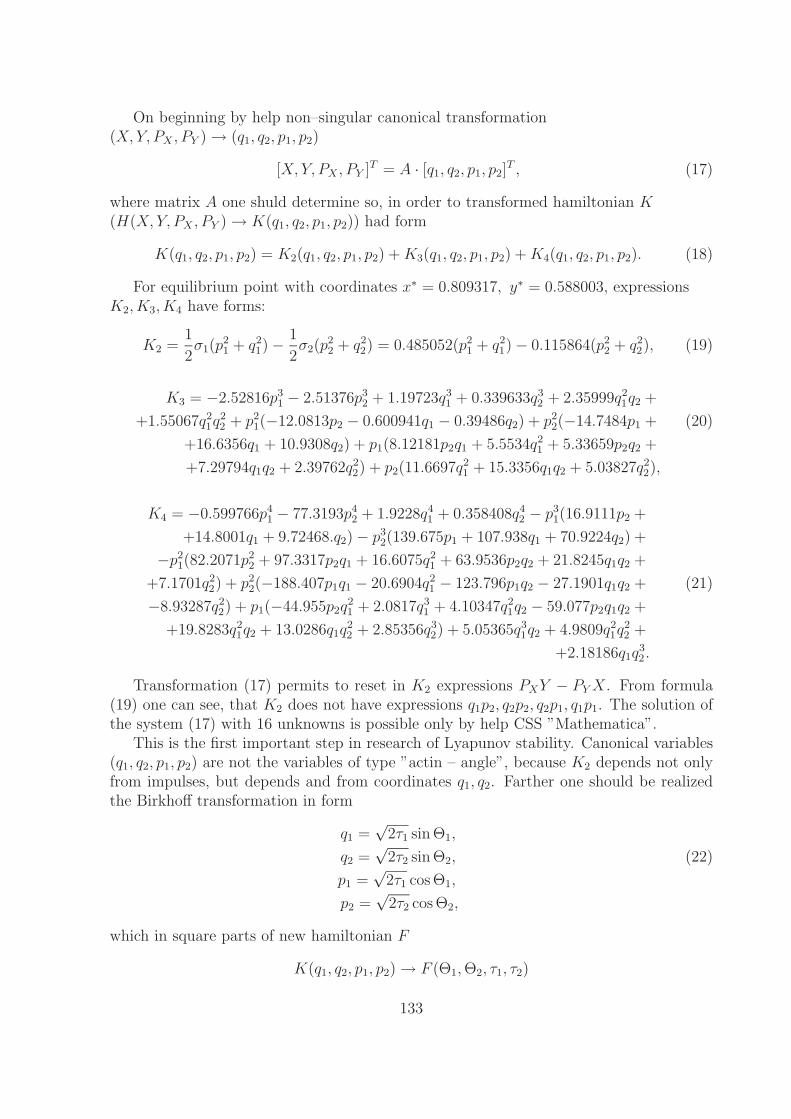
On beginning by help non–singular canonical transformation(X,Y, PX , PY ) → (q1, q2, p1, p2)
[X,Y, PX , PY ]T = A · [q1, q2, p1, p2]T , (17)
where matrix A one shuld determine so, in order to transformed hamiltonian K(H(X,Y, PX , PY ) → K(q1, q2, p1, p2)) had form
K(q1, q2, p1, p2) = K2(q1, q2, p1, p2) + K3(q1, q2, p1, p2) + K4(q1, q2, p1, p2). (18)
For equilibrium point with coordinates x∗ = 0.809317, y∗ = 0.588003, expressionsK2, K3, K4 have forms:
K2 =1
2σ1(p
21 + q2
1) −1
2σ2(p
22 + q2
2) = 0.485052(p21 + q2
1) − 0.115864(p22 + q2
2), (19)
K3 = −2.52816p31 − 2.51376p3
2 + 1.19723q31 + 0.339633q3
2 + 2.35999q21q2 +
+1.55067q21q
22 + p2
1(−12.0813p2 − 0.600941q1 − 0.39486q2) + p22(−14.7484p1 + (20)
+16.6356q1 + 10.9308q2) + p1(8.12181p2q1 + 5.5534q21 + 5.33659p2q2 +
+7.29794q1q2 + 2.39762q22) + p2(11.6697q2
1 + 15.3356q1q2 + 5.03827q22),
K4 = −0.599766p41 − 77.3193p4
2 + 1.9228q41 + 0.358408q4
2 − p31(16.9111p2 +
+14.8001q1 + 9.72468.q2) − p32(139.675p1 + 107.938q1 + 70.9224q2) +
−p21(82.2071p2
2 + 97.3317p2q1 + 16.6075q21 + 63.9536p2q2 + 21.8245q1q2 +
+7.1701q22) + p2
2(−188.407p1q1 − 20.6904q21 − 123.796p1q2 − 27.1901q1q2 + (21)
−8.93287q22) + p1(−44.955p2q
21 + 2.0817q3
1 + 4.10347q21q2 − 59.077p2q1q2 +
+19.8283q21q2 + 13.0286q1q
22 + 2.85356q3
2) + 5.05365q31q2 + 4.9809q2
1q22 +
+2.18186q1q32.
Transformation (17) permits to reset in K2 expressions PXY − PY X. From formula(19) one can see, that K2 does not have expressions q1p2, q2p2, q2p1, q1p1. The solution ofthe system (17) with 16 unknowns is possible only by help CSS ”Mathematica”.
This is the first important step in research of Lyapunov stability. Canonical variables(q1, q2, p1, p2) are not the variables of type ”actin – angle”, because K2 depends not onlyfrom impulses, but depends and from coordinates q1, q2. Farther one should be realizedthe Birkhoff transformation in form
q1 =√
2τ1 sin Θ1,
q2 =√
2τ2 sin Θ2, (22)
p1 =√
2τ1 cos Θ1,
p2 =√
2τ2 cos Θ2,
which in square parts of new hamiltonian F
K(q1, q2, p1, p2) → F (Θ1, Θ2, τ1, τ2)
133
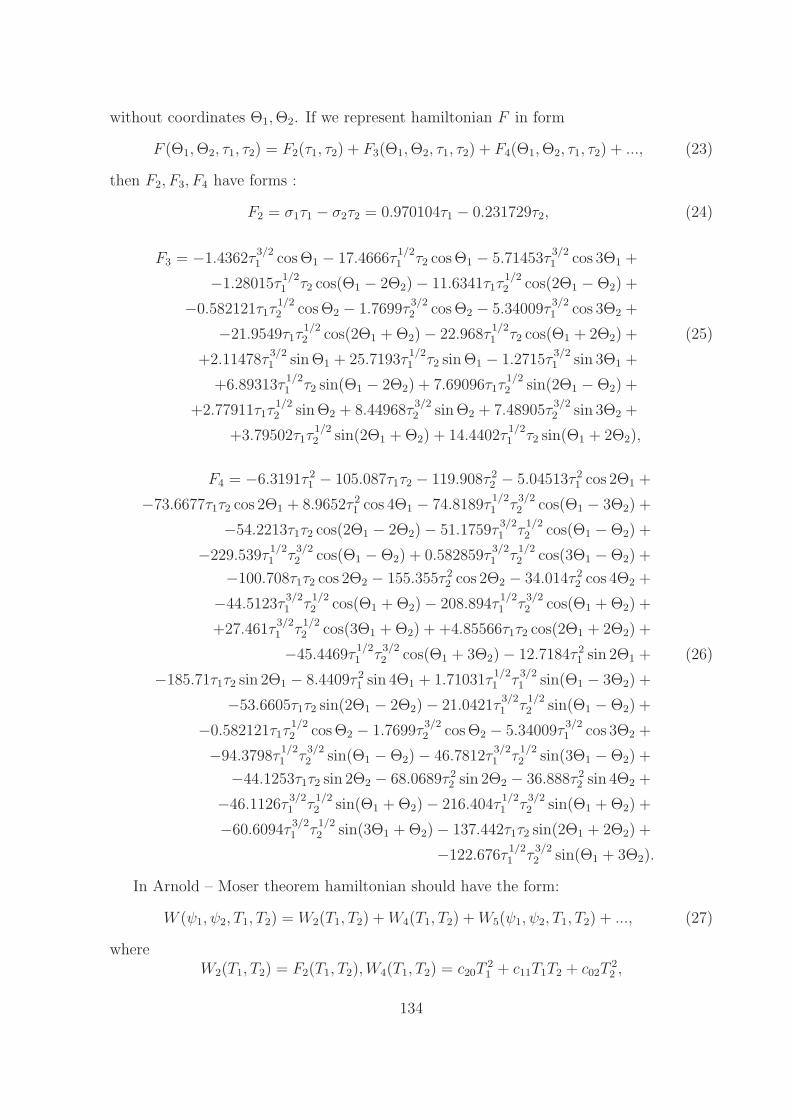
without coordinates Θ1, Θ2. If we represent hamiltonian F in form
F (Θ1, Θ2, τ1, τ2) = F2(τ1, τ2) + F3(Θ1, Θ2, τ1, τ2) + F4(Θ1, Θ2, τ1, τ2) + ..., (23)
then F2, F3, F4 have forms :
F2 = σ1τ1 − σ2τ2 = 0.970104τ1 − 0.231729τ2, (24)
F3 = −1.4362τ3/21 cos Θ1 − 17.4666τ
1/21 τ2 cos Θ1 − 5.71453τ
3/21 cos 3Θ1 +
−1.28015τ1/21 τ2 cos(Θ1 − 2Θ2) − 11.6341τ1τ
1/22 cos(2Θ1 − Θ2) +
−0.582121τ1τ1/22 cos Θ2 − 1.7699τ
3/22 cos Θ2 − 5.34009τ
3/21 cos 3Θ2 +
−21.9549τ1τ1/22 cos(2Θ1 + Θ2) − 22.968τ
1/21 τ2 cos(Θ1 + 2Θ2) + (25)
+2.11478τ3/21 sin Θ1 + 25.7193τ
1/21 τ2 sin Θ1 − 1.2715τ
3/21 sin 3Θ1 +
+6.89313τ1/21 τ2 sin(Θ1 − 2Θ2) + 7.69096τ1τ
1/22 sin(2Θ1 − Θ2) +
+2.77911τ1τ1/22 sin Θ2 + 8.44968τ
3/22 sin Θ2 + 7.48905τ
3/22 sin 3Θ2 +
+3.79502τ1τ1/22 sin(2Θ1 + Θ2) + 14.4402τ
1/21 τ2 sin(Θ1 + 2Θ2),
F4 = −6.3191τ 21 − 105.087τ1τ2 − 119.908τ 2
2 − 5.04513τ 21 cos 2Θ1 +
−73.6677τ1τ2 cos 2Θ1 + 8.9652τ 21 cos 4Θ1 − 74.8189τ
1/21 τ
3/22 cos(Θ1 − 3Θ2) +
−54.2213τ1τ2 cos(2Θ1 − 2Θ2) − 51.1759τ3/21 τ
1/22 cos(Θ1 − Θ2) +
−229.539τ1/21 τ
3/22 cos(Θ1 − Θ2) + 0.582859τ
3/21 τ
1/22 cos(3Θ1 − Θ2) +
−100.708τ1τ2 cos 2Θ2 − 155.355τ 22 cos 2Θ2 − 34.014τ 2
2 cos 4Θ2 +
−44.5123τ3/21 τ
1/22 cos(Θ1 + Θ2) − 208.894τ
1/21 τ
3/22 cos(Θ1 + Θ2) +
+27.461τ3/21 τ
1/22 cos(3Θ1 + Θ2) + +4.85566τ1τ2 cos(2Θ1 + 2Θ2) +
−45.4469τ1/21 τ
3/22 cos(Θ1 + 3Θ2) − 12.7184τ 2
1 sin 2Θ1 + (26)
−185.71τ1τ2 sin 2Θ1 − 8.4409τ 21 sin 4Θ1 + 1.71031τ
1/21 τ
3/21 sin(Θ1 − 3Θ2) +
−53.6605τ1τ2 sin(2Θ1 − 2Θ2) − 21.0421τ3/21 τ
1/22 sin(Θ1 − Θ2) +
−0.582121τ1τ1/22 cos Θ2 − 1.7699τ
3/22 cos Θ2 − 5.34009τ
3/21 cos 3Θ2 +
−94.3798τ1/21 τ
3/22 sin(Θ1 − Θ2) − 46.7812τ
3/21 τ
1/22 sin(3Θ1 − Θ2) +
−44.1253τ1τ2 sin 2Θ2 − 68.0689τ 22 sin 2Θ2 − 36.888τ 2
2 sin 4Θ2 +
−46.1126τ3/21 τ
1/22 sin(Θ1 + Θ2) − 216.404τ
1/21 τ
3/22 sin(Θ1 + Θ2) +
−60.6094τ3/21 τ
1/22 sin(3Θ1 + Θ2) − 137.442τ1τ2 sin(2Θ1 + 2Θ2) +
−122.676τ1/21 τ
3/22 sin(Θ1 + 3Θ2).
In Arnold – Moser theorem hamiltonian should have the form:
W (ψ1, ψ2, T1, T2) = W2(T1, T2) + W4(T1, T2) + W5(ψ1, ψ2, T1, T2) + ..., (27)
whereW2(T1, T2) = F2(T1, T2),W4(T1, T2) = c20T
21 + c11T1T2 + c02T
22 ,
134
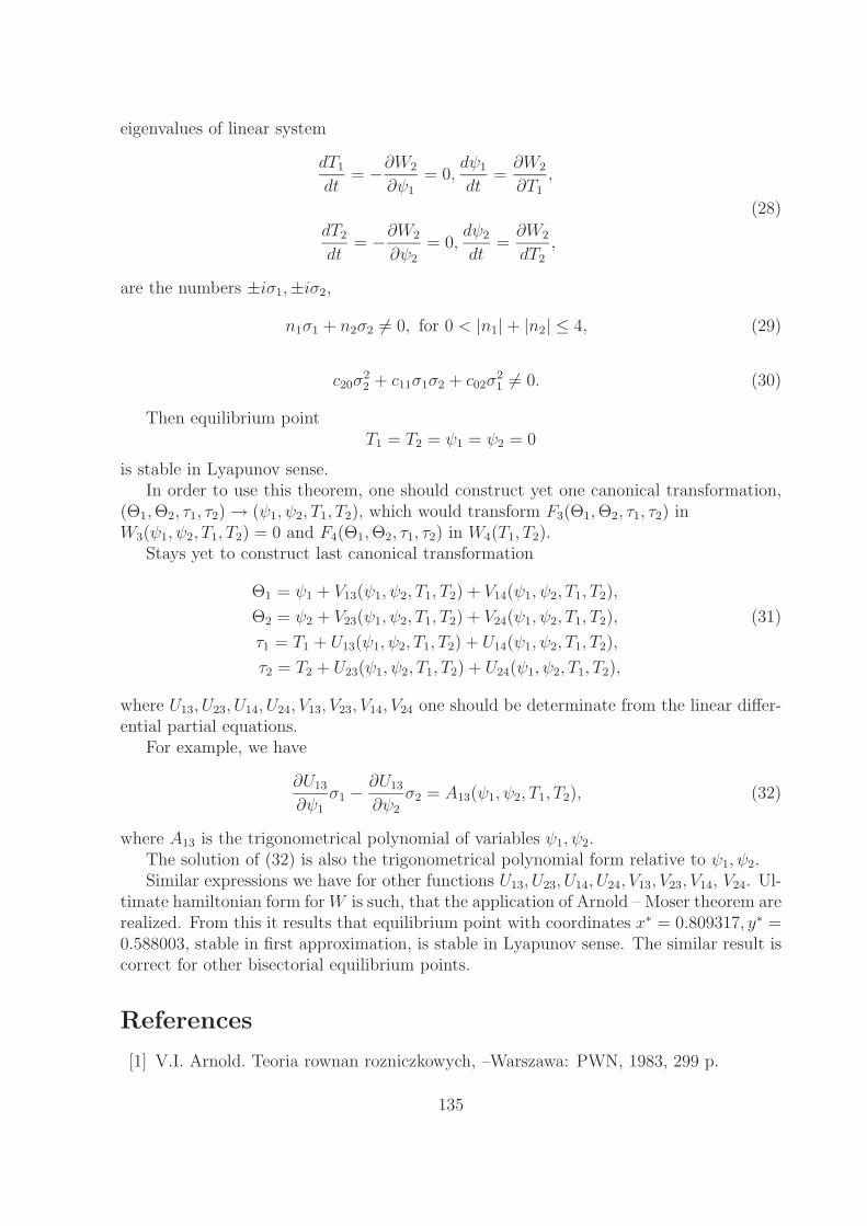
eigenvalues of linear system
dT1
dt= −∂W2
∂ψ1
= 0,dψ1
dt=
∂W2
∂T1
,
(28)
dT2
dt= −∂W2
∂ψ2
= 0,dψ2
dt=
∂W2
dT2
,
are the numbers ±iσ1,±iσ2,
n1σ1 + n2σ2 = 0, for 0 < |n1| + |n2| ≤ 4, (29)
c20σ22 + c11σ1σ2 + c02σ
21 = 0. (30)
Then equilibrium pointT1 = T2 = ψ1 = ψ2 = 0
is stable in Lyapunov sense.In order to use this theorem, one should construct yet one canonical transformation,
(Θ1, Θ2, τ1, τ2) → (ψ1, ψ2, T1, T2), which would transform F3(Θ1, Θ2, τ1, τ2) inW3(ψ1, ψ2, T1, T2) = 0 and F4(Θ1, Θ2, τ1, τ2) in W4(T1, T2).
Stays yet to construct last canonical transformation
Θ1 = ψ1 + V13(ψ1, ψ2, T1, T2) + V14(ψ1, ψ2, T1, T2),
Θ2 = ψ2 + V23(ψ1, ψ2, T1, T2) + V24(ψ1, ψ2, T1, T2), (31)
τ1 = T1 + U13(ψ1, ψ2, T1, T2) + U14(ψ1, ψ2, T1, T2),
τ2 = T2 + U23(ψ1, ψ2, T1, T2) + U24(ψ1, ψ2, T1, T2),
where U13, U23, U14, U24, V13, V23, V14, V24 one should be determinate from the linear differ-ential partial equations.
For example, we have
∂U13
∂ψ1
σ1 − ∂U13
∂ψ2
σ2 = A13(ψ1, ψ2, T1, T2), (32)
where A13 is the trigonometrical polynomial of variables ψ1, ψ2.The solution of (32) is also the trigonometrical polynomial form relative to ψ1, ψ2.Similar expressions we have for other functions U13, U23, U14, U24, V13, V23, V14, V24. Ul-
timate hamiltonian form for W is such, that the application of Arnold – Moser theorem arerealized. From this it results that equilibrium point with coordinates x∗ = 0.809317, y∗ =0.588003, stable in first approximation, is stable in Lyapunov sense. The similar result iscorrect for other bisectorial equilibrium points.
References
[1] V.I. Arnold. Teoria rownan rozniczkowych, –Warszawa: PWN, 1983, 299 p.
135
[2] S. Wolfram. The Mathematica – Book, –Cambridge: University Press, 1996, 1403 p.
[3] K.R. Meyer, G.R. Hall. Introduction to Hamiltonian Dynamical Systems and theN–Body Problem, –New York: Springer – Verlag, 1992, 292 p.
[4] J. Moser. On invariant curves of area preserving mappings of an Annulus, –Gottingen:Nachr. Wiss. Math -Phys, KI, I 1962.
[5] G.E.O. Giacaglia. Perturbation methods in non-linear systems, –New York: Springer– Verlag, 1972, 520 p.
[6] E. Grebenicov. Two New Dynamical Models in Celestial Machanics, –Bucharest:Rom. Astron. J., vol.8, Nr 1, 1998, pp. 13–19.
[7] D. Kozak, E. Onishk. Application of the ”Mathematica” computer system to the de-termination of the coordinates of equilibrium positions in the Grebenicov–Elmabsoutgravitation model of four bodies, –Kyiv: Nonlinear oscillations, 1999, pp.16–18.
[8] M. Jakubiak. Sufficient conditions of linear stability for equilibrium points in theNewtonian gravitational model of six bodies,–Kyiv: Nonlinear oscillations, 1999,pp.138–144.
[9] E. Grebienicov, D. Kozak, M. Jakubiak. The Algebraic Problems of the Normal-ization in Hamiltonian Theory, –Moscow: Proceeding of the Second InternationalWorkshop on Mathematica System in Teaching and Reserch, Siedlce’2000, 2000, pp.73–90.
[10] D. Kozak, M. Jakubiak. The Birkhoff Hamiltonian Normalization Using the ”Math-ematica”, –Odessa: Abstracts of ”DIFIN–2000”, p. 342.
136
Stability of Equilibrium Points inLagrange - Wintner Models
E. A. Grebenikov, G. Olszanowski, A. Siluszyk
University of Podlasie, Siedlce, Poland;e-mail: [email protected]
In the papers [1, 2, 3] it is demonstrated the existence of the equilibrium solutionsof differential equations for restricted Lagrange - Wintner gravitational models. In thesemodels it is studied the motion of the passive gravitate mass in Newtonian gravitationalfield, what is created by rotating gravitational regular polygon, in the vertices which thereare gravitational masses all equal m.
The numbers of vertices is arbitrary. Independently from of number of polygon verticesn the differential equations of the motion of passive gravitate mass in space R3 have sixorder and on the plane the order of this equation system is four. It is possible to prove,that all the equilibrium points in these models there are in the plane of regular polygon.
In this paper we prove, that the equilibrium points of circular restricted Lagrange -Wintner gravitational models for n = 7, ..., 20 are unstable. The differential equations ofthe motion of the point P in the gravitational field of the bodies Pk(k = 1, 2, .., n) in thebarycentric Cartesian system (Gxy) have the form [4]:⎧⎪⎪⎨⎪⎪⎩
d2xdt2
− 2ωndydt
− ω2nx = f m
n∑k=1
xk−xΔ3
k,
d2ydt2
+ 2ωndxdt
− ω2ny = f m
n∑k=1
yk−yΔ3
k,
(1)
where
ω2n =
m
4
n∑k=1
(sin
(π (k − 1)
n
))−1
, (2)
Δ2k = (x − xk)
2 + (y − yk)2 , (3)
f - gravitational constant (f = 1), m- mass of the body Pk.For determining of equilibrium points of system (1), after transformations we finally
have solving system of functional equations [4]:⎧⎪⎪⎨⎪⎪⎩Φ1 (x, y) ≡ ω2
nx +n∑
k=1
xk−xΔ3
k= 0,
Φ2 (x, y) ≡ ω2ny +
n∑k=1
yk−yΔ3
k= 0.
(4)
In the article [5] have been shown that for n = 3, 4, 5, 6 and for arbitrary mass m allthe equilibrium points (its number is equal 3n) are unstable. Our calculations show, that
137
for n = 7, .., 20 all the equilibrium points for arbitrary mass m also are unstable. Really,if to substitute in the equations (4) the expression (2) for ω2
n and to reduce the size of m,then we have the equations:⎧⎪⎪⎨⎪⎪⎩
m4
n∑k=1
(sin(
π(k−1)n
))−1
+n∑
k=1
xk−xΔ3
k= 0,
m4
n∑k=1
(sin(
π(k−1)n
))−1
+n∑
k=1
xk−xΔ3
k= 0.
(5)
These equations demonstrate, that the coordinates of equilibrium points do not de-pend from gravitational parameter m, but depend only from values n. We solved theequations (5) for n = 7, ..., 20 with the help of system Mathematica [6] and we found allthe equilibrium points of these models. The numbers of these points are 21, 24, 27, ..., 60.
The linearization of the system equations (1) in neighborhood of every equilibriumpoint gives the system of differential equation:
dx
dt= Ax, (6)
where A -matrix of the order 4 × 4 has the form:
A =
⎡⎢⎢⎣0 0 1 00 0 0 1
a31 a32 0 2a41 a42 −2 0
⎤⎥⎥⎦.
(7)
Here the elements a31, a32, a41, a42, are constants. The calculation show, that amongeigenvalues of matrix A for n = 7, .., 20 and for all the equilibrium points always existeigenvalues λ = ±a, where a-real number.
Hence, the equilibrium points of circular restricted Lagrange - Wintner gravitationalmodels for n = 7, 8, ..., 20 are unstable in the first approximation and it means, that thepoints are unstable in Lapunov sense[7].
References
[1] Kozak D., Oniszk E., Equilibrium Points in the Restricted Four - Body Problem:Sufficient Conditions for Linear Stability, -Bucharest: Rom. Astron. J., vol. 8, N◦ 1,1998, p. 27 -31.
[2] Olszanowski G., Maruszewski Z., A Restricted Four - Body Problem in Lagrange- Wintner Model, ”Mathematica” System in Teaching and Research, -M.:, 2000, p.205-211.
[3] Dziak A., The existence of Jacobi integral for averaging equations of restricted, ellipticthree-body problem, ”Mathematica” System in Teaching and Research, -M.:, 2000, p.191-194.
[4] Grebenicov E. A., Kozak-Skoworodkin D., Jakubiak M., The methods of computeralgebra in the many body problem, -M.:, Ed. RUDN, 2001,213p.
138

[5] Grebenicov E. A., Olszanowski G., Siluszyk A., On stability of symmetrical config-urations of many body problem,-Grodno: University VII International MathematicConference,28-30 May 2001,250p.
[6] Wolfram S., The Mathematica Book, - Cambridge University Press, 1996, p. 1403.
[7] Stepanov V.V., Kurs differencialnych uravnenii,-M.: Nauka, 1968.
139
Symbolic Computation Systems andthe Many-Body Problem
E.A. Grebenikova, A.N. Prokopenyab
a University of Podlasie, Siedlce, Polandb Brest Technical University, Belarus;e-mail: [email protected]
Usage of the computer algebra systems for solving the many-body problem is discussed.Stability of a new class of the exact symmetric solutions of the Newton’s gravitational (n+1)-body problem that are represented by regular, scale-similarly to itself varying polygon,rotating with variable angular velocity about its center is analyzed.
Introduction
The many-body problem is one of the most widely studied problems of classical mechanics.Many outstanding mathematicians and mechanicians starting from Newton have beendealing with this problem but only in the case of two interacting bodies the correspondinggeneral solution is found. Moreover, it turned out the differential equations of the many-body problem are in general not integrable. Thus, the problem formulated by Poincare- to find new classes of the exact particular solutions of the many-body problem and toinvestigate their stability - has retained a high degree of topicality.
Solving the first part of this problem is connected with a search of the central config-urations of the n-body system. The necessary and sufficient conditions of the existenceof central configurations of Newton’s gravitational n-body problem may be written as asystem of 3n nonlinear algebraic equations for 3n coordinates of the bodies with massesm1, ...,mn considered as parameters [1]. Analysis of a solvability of this system is verycomplicated algebraic problem and it has been completely fulfilled only for two and threeinteracting bodies. Nevertheless, there is a hypothesis proposed by A.Wintner [2] that inthe case of n > 3 the central configurations for the Newton’s n-body problem always existbut the amount of such configurations is restricted. This hypothesis in general form is notproved till present time. And it seems that for n > 3 this problem may be analyzed onlywith using modern symbolic computation systems, for example, Mathematica or Maplethat essentially increase our ability in doing both numerical and symbolic calculations.
When some exact particular solution of the many-body problem is found, the next stepis to investigate its stability. But this problem turned out to be the most complicatedproblem of the qualitative theory of differential equations. For example, solving thestability problem of the Lagrange triangular solutions has taken about 200 years, whereasstability of the homographic and homothetic solutions in the three-body problem still
140

remains unsolved. Analysis of this problem requires using both the methods of classicaltheory of stability and the KAM-theory. In the second case it is also necessary to constructthe Birkhoff transformation for the hamiltonian normalization. Realization both of theseapproaches is connected with doing a lot of tremendous analytical calculations that cannot be done by hands. So the further progress in solving the many-body problem andgenerally in the theory of dynamical systems is associated with using modern computeralgebra systems.
Linearization of the Equations of Motion
In [3] B. Elmabsout found a new exact particular solution of the plane Newton’s many-body problem where the n bodies P1, P2, ..., Pn of equal masses m are at the vertices of aregular polygon with n sides that rotates uniformly around the body P0 of a non-zero massm0 being at the center of polygon. Then it was shown [4, 5], that there exist a whole classof the exact symmetric solutions of the problem of (n + 1) bodies which are representedby regular, scale-similarly to self varying polygons, rotating with variable angular velocityaround their centers. Stability of the invariant polygon was completely investigated inlinear approximation in [6]. Here we study the stability problem in linear approximationin general case of the varying regular polygon with n sides. The corresponding equationsof motion of the bodies P1, P2, ..., Pn of equal masses m in relative Cartesian coordinatescan be written as [4] |
d2rj
dt2+ f (m0 + m)
rj
r3j
= f m
n∑i=1 (i=j)
( ri − rj
|ri − rj|3 − ri
ri3
)(j = 1, n), (1)
where m0 and f are a mass of the body P0 and gravitational constant respectively. It issupposed that the body P0 is in the origin of Cartesian frame P0 xyz.
Equations (1) can be written in cylindrical coordinates as
d2ρj
dt2− ρj
(dφj
dt
)2
+ f(m0 + m)ρj
rj3
=
= f m
n∑i=1 (i=j)
(cos(φi − φj)ρi − ρj
ri,j3
− cos(φi − φj)ρi
ri3
),
ρjd2φj
dt2+ 2
dρj
dt
dφj
dt= f m
n∑i=1 (i=j)
( 1
ri,j3− 1
ri3
)sin(φi − φj) ρi, (2)
d2zj
dt2+ f(m0 + m)
zj
r3j
= f m
n∑i=1 (i=j)
(zi − zj
ri,j3
− zi
ri3
)(j = 1, n)
where
r2i = ρ2
i + z2i , ri,j
2 = |ri − rj|2 = ρ2i + ρ2
j − 2ρiρj cos(φi − φj) + (zi − zj)2.
141
It is easy to check that equations (2) have a solution
ρj(t) = ρ1(t) ≡ ρ(t), φj(t) = φ(t) +2π
nj, zj(t) = 0 (j = 1, n), (3)
where the functions ρ(t) and φ(t) are connected with two relationships
ρ(φ) =p
1 + e cos φ, ρ2 dφ
dt= c ≡ const.
Parameter p is connected with the constant c according to the relationship
p =c2
f Mn
, Mn = m0 +m
4
n−1∑i=1
1
sin (π i/n).
Solution (3) determines the plane motion of the bodies on a similar trajectories beingin the P0 xy plane. The shape of the trajectories is completely determined with twoparameters p and e. And in the case of e = 0 all bodies move on the circle of radius pwith angular velocity
ω =
√f Mn
p3.
To investigate stability of solution (3) it is convenient to transform equations (2) intoNechvil’s phase space according to the rule
ρj(t) → p
1 + e cos φρj(φ), zj(t) → p
1 + e cos φzj(φ),
where p and e are some constants, and the polar angle φ is considered as a new independentvariable. Then we obtain the equations of motion in the form
d2ρj
dφ2− ρj
(dφj
dφ
)2
+e cos φ
1 + e cos φρj +
m0 + m
Mn(1 + e cos φ)
ρj
rj3
=
=m
Mn(1 + e cos φ)
n∑i=1 (i=j)
(cos(φi − φj)ρi − ρj
ri,j3
− cos(φi − φj)ρi
ri3
),
ρjd2φj
dφ2+ 2
dρj
dφ
dφj
dφ=
m
Mn(1 + e cos φ)
n∑i=1 (i=j)
( 1
ri,j3− 1
ri3
)sin(φi − φj) ρi,
d2zj
dφ2+
e cos φ
1 + e cos φzj +
m0 + m
Mn(1 + e cos φ)
zj
r3j
=
=m
Mn(1 + e cos φ)
n∑i=1 (i=j)
(zi − zj
ri,j3
− zi
ri3
)(j = 1, n), (4)
Solution (3) can be written in Nechvil’s variables as
ρj(φ) = ρ ≡ 1, φj(φ) = φ +2π
nj, zj(φ) = 0 (j = 1, n). (5)
142
In order to study the equations (4) at the neighborhood of solution (5) we put
ρj(φ) → 1 + uj(φ), φj(φ) → φ +2 π
nj + γj(φ).
Considering functions uj(φ), γj(φ), zj(φ) as small perturbations of solution (5) we expandequations (4) in powers of uj, γj, zj neglecting all terms of order superior or equal to 2.As a result we obtain a linearized system of differential equations in the form
d2uj
dφ2− 2
dγj
dφ=
8 + 12μ + S1
(1 + e cos φ)(4μ + S1)uj−
− 1
4(1 + e cos φ)(4μ + S1)
n∑i=1 (i=j)
1
| sin(π(i − j)/n)|3 ((−1 + 3 cos(2π
n(i − j)))uj+
+(−3 + cos(2π
n(i − j)) − 32 cos(
2π
n(i − j))| sin(
π
n(i − j))|3)ui−
−(1 + 16| sin(π
n(i − j))|3) sin(
2π
n(i − j))(γi − γj)),
d2γj
dφ2+ 2
duj
dφ= − 1
4(1 + e cos φ)(4μ + S1)
n∑i=1 (i=j)
1
| sin(π(i − j)/n)|3 ((1−
−32| sin(π
n(i − j))|3) sin
2π
n(i − j))ui + 3 sin
2π
n(i − j))uj+
+(3 + cos(2π
n(i − j)) + 16 cos(
2π
n(i − j))| sin(
π
n(i − j))|3)(γi − γj)),
d2zj
dφ2+
4(1 + μ) + (4μ + S1)e cos φ
(1 + e cos φ)(4μ + S1)zj = (6)
=1
2(1 + e cos φ)(4μ + S1)
n∑i=1(i=j)
1
| sin(π(i − j)/n)|3 ((1 − 8| sin(2π
n(i − j))|3) zi − zj),
where
μ =m0
m, S1 =
n−1∑j=1
1
sin(πj/n).
Now the problem of linear stability of solution (5) is reduced to studying stability of atrivial solution of the system (6) that is a linear system of differential equations withperiodic coefficients.
143
Studying Linear Stability of the Solutions for the Per-
pendicular Perturbations
According to system (6) the functions zj determining perturbations of the bodies trajec-tories in perpendicular to the plane P0xy direction do not depend on uj and γj . So inlinear approximation we can study stability of solution (5) in respect to the perpendicularperturbations zj and the perturbations uj and γj contained in the plane of orbits P0xyseparately. Let us start with studying linear stability of solutions (5) for perpendicularperturbations. It is convenient to rewrite the last equation of system (6) determiningthe functions zj in vector notations. So we introduce a n-dimensional vector Z withcomponents zj(φ) and n x n matrixes B and K that have the next elements:
Bjk =1
| sin(π(j − k)/n|3 for j = k and Bjj = −n∑
k=1( =j)
Bjk;
Kjk = 1 (j, k = 1, n).
Then we can rewrite the last equation of system (6) as
d2Z
dφ2=
1
2(1 + e cos φ)(4μ + S1)(B − 8K − 8μI − 2(4μ + S1)e cos φ I)Z, (7)
where I is an nxn identity matrix. It is easy to verify [6] that the matrix B has eigenvectorsEr with components
Ek,r =1√n
e2π r
ni k (k, r = 1, n) (8)
where i =√−1 and the first index k denotes the number of component. The correspond-
ing eigenvalues are (−λr) where
λr = 2n−1∑k=1
sin2(πrk/n)
sin3(πk/n).
Vectors (8) are also the eigenvectors of the matrix K that has two eigenvalues: 0 and n.Actually,
K Er = 0 for r = 1, n − 1 and K Er = n En.
So introducing the matrix Q with elements Qk,r = Ek,r we can easily diagonalize thematrixes B and K according to the transformation rules
B → Q+BQ, K → Q+KQ,
and reduce equation (7) to the normal form
d2z
dφ2= −a + e cos φ
1 + e cos φz, (9)
where
a =λr + 8μ + 8nδr,n
2(4μ + S1).
144
Equation (9) is the second order differential equation that is sometimes called a Hill’sequation. In the case of e = 0 it reduces to the equation of simple harmonic oscillatorof frequency
√a . It’s apparent that a > 0 for any r = 1, n and so in this case the
solution (5) is linearly stable for any perpendicular to the plane of the bodies trajectoriesperturbations.
Equation (9) is apparently equivalent to a linear system of two first order differentialequations with periodic matrix. General analysis of such systems shows that dependingon the values of parameters a and e its trivial solution may be stable or unstable [7].The boundaries between the domains of stability and instability in the ae-plane are somecurves a = a(e) which characterized by the presence of periodic solutions with period2π and 4π . Hence, we can attempt to determine these boundaries directly by seeking asolution of equation (9) in the form
z = c0 +∞∑
k=1
(ck cos(k
2φ) + dk sin(
k
2φ)). (10).
Although this is a Fourier series for the function z = z(φ) of period 4π, it can also beused to obtain the solution with period 2π by setting to zero the Fourier coefficientscorresponding to k being an odd integer. On substituting (10) into equation (9) andsetting coefficients of cos(k
2φ) and sin(k
2φ) to zero we have obtained the following infinite
sequence of equations determining coefficients of the Fourier series (10).
a c0 = 0,
ec0 + (a − 1)c2 − 3
2ec4 = 0,
. . . . . . . (11)
−k(k − 2)
2ec2k−2 + (a − k2)c2k − k(k + 2)
2ec2k+2 = 0.
(a − 1
4+
3
8e)c1 − 5
8ec3 = 0,
. . . . . . . (12)
−(2k − 5)(2k − 1)
8ec2k−3 + (a − (k − 1
2)2)c2k−1 − (2k − 1)(2k + 3)
8ec2k+1 = 0.
(a − 1) d2 − 3
2ed4 = 0,
. . . . . . . (13)
−k(k − 2)
2ed2k−2 + (a − k2)d2k − k(k + 2)
2ed2k+2 = 0.
(a − 1
4− 3
8e) d1 − 5
8e d3 = 0,
. . . . . . . (14)
145
−(2k − 5)(2k − 1)
8e d2k−3 + (a − (k − 1
2)2) d2k−1 − (2k − 1)(2k + 3)
8e d2k+1 = 0.
It can be seen that in fact there are four infinite subsequences of linear homogeneousequations. Two of these (11) and (13) are for the coefficients c0, c2, ... , c2k and d2, ... , d2k
respectively and represent solution (10) with period 2π. For a solution to exist, thecorresponding determinants of infinite systems (11), (13) must vanish, thus determiningthe stability boundaries in the ae-plane. These boundaries obviously reduce to a =(2k)2 (k = 0, 1, 2, ...) when e → 0. The remaining two subsequences of equations (12)and (14) are for c1, c3, ... , c2k+1 and d1, ... , d2k+1 , and correspond to those stability
boundaries which reduce to a = (2k−1)2
4(k = 1, 2, ...) when e → 0 .
Of course, it’s impossible to calculate a determinant of the infinite matrix. So to findthe stability boundaries a = a(e) we should truncate the infinite subsequences of equations(11)-(14) after the k-th term, where k is a suitably large number. The correspondingdeterminant of the system (11), for example, can be written as
Dk =
∣∣∣∣∣∣∣∣∣∣∣∣
a 0 0 0 ... 0c a − 1 −3
2e 0 ... 0
0 0 a − 4 −4e ... 00 0 −3
2e a − 9 ... 0
... ... ... ... ... ...
0 0 0 0 −k(k−2)2
e a − k2
∣∣∣∣∣∣∣∣∣∣∣∣. (15)
Setting determinant Dk to zero we obtain an algebraic equation giving us an approx-imation for the stability boundary ak = ak(e) . An exact expression for the boundary isobtained when k → ∞. Determinant (15) is best evaluated from the following recurrencerelation
Dk = (a − k2)Dk−1 − e2
2(k − 2)(k − 1)k(k + 1)Dk−2 (k = 3, 4, ...) (16)
which is readily established from (15). To start the iterative process we observe that
D1 = a, D2 = a(a − 1).
A similar procedure can be followed for the other systems (12)-(14). For instance, thedeterminant of system (13) is just the same as (15) with the first row and column deleted.The recurrence relation is again (16) for k ≥ 3 , but the starting values are now given by
D1 = a − 1, D2 = (a − 1)(a − 4).
The corresponding recurrence relation for the determinants of systems (12), (14) is
Dk = (a − (2k − 1)2
4) Dk−1 − e2
64(2k − 5)(2k − 3)(2k − 1)(2k + 1) Dk−2 (17)
with the starting values
D1 = a − 1
4± 3e
8, D2 = (a − 1
4± 3e
8)(a − 9
4) +
15e2
64.
146
It’s apparent from (16), (17) that in the case of e = 0 determinants of systems (11)-(14) will equal to zero when a = 1
4k2 (k = 0, 1, 2, ..). It means the stability boundaries
should cross the e = 0 axis in the ae-plane at these points. For sufficiently small e wecan represent the stability boundaries a = a(e) in the vicinity of the points a = 1
4k2 as a
power series in e. As a result we obtain the curves in the form
a = 0, a =1
4∓ 3
8e +
15
128e2 ∓ 45
2048e3 +
885
32768e4, a = 1,
a =9
4− 135
256e2 ∓ 45
2048e3 − 34695
262144e4, a = 4 − 6
5e2 − 39
125e4, ... (18)
where the error term is O(e5).It should be emphasized that zones of instability are bounded only by the curves
crossing the e = 0 axis in the points a = (2k−1)2
4(k = 1, 2 ... ) and these zones are quite
narrow. Besides, there are curves of instability crossing the e = 0 axis in the pointsa = k2 (k = 0, 1, 2, ... ) . Thus, if parameters a and e are in a zone of instability then thetrivial solution of equation (9) is unstable.
Conclusion
In present paper we have analyzed the linear stability of the exact particular solutions ofthe plane Newton’s many-body problem found in [4,5]. It was shown that stability of thesolutions in respect to the perpendicular perturbations and the perturbations containedin the plane of bodies orbits may be studied separately. Linear stability of the solutionsfor perpendicular perturbations depends on the ellipticity of the orbits e, the number onbodies n and parameter μ = m0/m because parameter a is determined with n and μaccording to (9). And if for a fixed value of e parameter a turns out to be in a zone ofinstability then the corresponding solution (5) is unstable. All calculations are done withcomputer algebra system Mathematica.
References
1. E.A.Grebenikov. About necessary and sufficient conditions of the existence of homo-graphic solutions of Newton’s many-body problem in noninertial frame of reference.Nonlinear Analysis and Homographic Dynamics, Iss. 1. Moscow, ComputerCenter RAS (1999) pp. 5-19.
2. A.Wintner. The Analytical Foundations of Celestial Mechanics. Princeton: Prince-ton Univ. Press, 1941.
3. B.Elmabsout. Sur l’existence de certaines configurations d’equilibre relatif dans leprobleme des N corps. Celestial Mechanics, 41 (1988), 131-151.
4. E.A.Grebenikov. The existence of the exact symmetric solutions in the plain New-ton’s problem of many bodies, Mathematical modeling, 10, No 8 (1998) pp. 74-80.
147

5. E.A.Grebenikov. New exact solutions in the planar symmetrical (n+1)-body prob-lem. Romanian Astronomical Journal, 7 (1997), No. 2, 151-156.
6. B.Elmabsout. Stability of some degenerate positions of relative equilibrium in then-body problem. Dynamics and Stability of Systems, 9 (1994), No. 4, 305-319.
7. R.Grimshaw. Nonlinear Ordinary Differential Equations, CRC Press, 2000, 328 pp.
148
In memoriam William Schelter
TEXmacs Interfaces to Maxima,MuPAD and REDUCE
A. G. Grozin
Budker Institute of Nuclear Physics,630090 Novosibirsk, Russia;
e-mail: [email protected]
GNU TEXmacs is a free wysiwyg word processor providing an excellent typesettingquality of texts and formulae. It can also be used as an interface to Computer AlgebraSystems (CASs). In the present work, interfaces to three general-purpose CASs have beenimplemented.
1 TEXmacs
GNU TEXmacs [1] is a free (GPL) word processor which
• typesets texts and mathematical formulae with very high quality (like LATEX),
• emphasizes the logical structure of a document rather than its appearance (likeLATEX),
• is easy to use and intuitive (like typical wysiwyg word processors),
• can be extended by a powerful programming language (like Emacs),
• can include PostScript figures (as well as other figures which can be converted toPostScript),
• can export LATEX, and import LATEX and html,
• supports a number of languages based on Latin and Cyrillic alphabets.
It uses TEX fonts both on screen and when printing documents. Therefore, it is trulywysiwyg, with equally good quality of on-screen and printed documents (in contrast toLyX which uses X fonts on screen and calls LATEX for printing). There is a similarcommercial program called Scientific Workplace (for Windows).
TEXmacs can also be used as an interface to any CAS which can generate LATEX output.It renders LATEX formulae on the fly, producing CAS output with highest typesettingquality (better than, e.g., Mathematica, which uses fixed-width fonts for formula output).A user can utilize editing facilities of TEXmacs: copy (a part of) a previous input into thenew one, edit it and sent to the CAS, copy a result derived using the CAS into a paper,
149
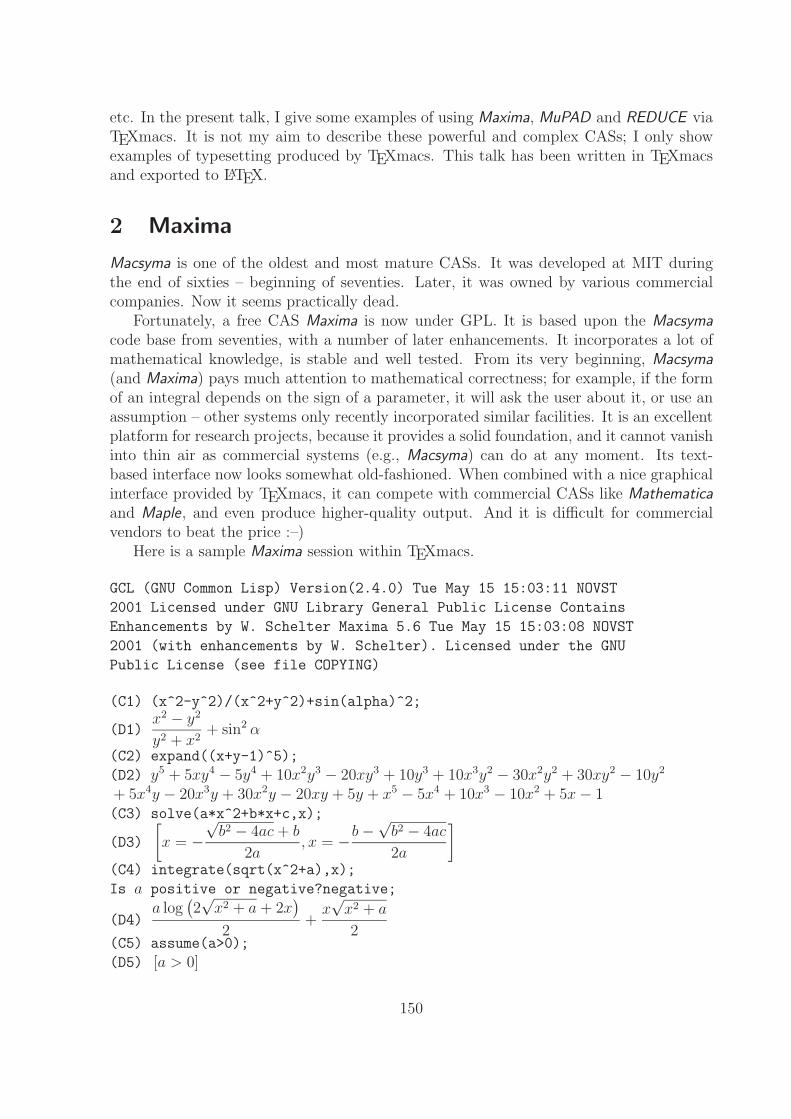
etc. In the present talk, I give some examples of using Maxima, MuPAD and REDUCE viaTEXmacs. It is not my aim to describe these powerful and complex CASs; I only showexamples of typesetting produced by TEXmacs. This talk has been written in TEXmacsand exported to LATEX.
2 Maxima
Macsyma is one of the oldest and most mature CASs. It was developed at MIT duringthe end of sixties – beginning of seventies. Later, it was owned by various commercialcompanies. Now it seems practically dead.
Fortunately, a free CAS Maxima is now under GPL. It is based upon the Macsymacode base from seventies, with a number of later enhancements. It incorporates a lot ofmathematical knowledge, is stable and well tested. From its very beginning, Macsyma(and Maxima) pays much attention to mathematical correctness; for example, if the formof an integral depends on the sign of a parameter, it will ask the user about it, or use anassumption – other systems only recently incorporated similar facilities. It is an excellentplatform for research projects, because it provides a solid foundation, and it cannot vanishinto thin air as commercial systems (e.g., Macsyma) can do at any moment. Its text-based interface now looks somewhat old-fashioned. When combined with a nice graphicalinterface provided by TEXmacs, it can compete with commercial CASs like Mathematicaand Maple, and even produce higher-quality output. And it is difficult for commercialvendors to beat the price :–)
Here is a sample Maxima session within TEXmacs.
GCL (GNU Common Lisp) Version(2.4.0) Tue May 15 15:03:11 NOVST
2001 Licensed under GNU Library General Public License Contains
Enhancements by W. Schelter Maxima 5.6 Tue May 15 15:03:08 NOVST
2001 (with enhancements by W. Schelter). Licensed under the GNU
Public License (see file COPYING)
(C1) (x^2-y^2)/(x^2+y^2)+sin(alpha)^2;
(D1)x2 − y2
y2 + x2+ sin2 α
(C2) expand((x+y-1)^5);
(D2) y5 + 5xy4 − 5y4 + 10x2y3 − 20xy3 + 10y3 + 10x3y2 − 30x2y2 + 30xy2 − 10y2
+ 5x4y − 20x3y + 30x2y − 20xy + 5y + x5 − 5x4 + 10x3 − 10x2 + 5x − 1(C3) solve(a*x^2+b*x+c,x);
(D3)
[x = −
√b2 − 4ac + b
2a, x = −b −√
b2 − 4ac
2a
](C4) integrate(sqrt(x^2+a),x);
Is a positive or negative?negative;
(D4)a log
(2√
x2 + a + 2x)
2+
x√
x2 + a
2(C5) assume(a>0);
(D5) [a > 0]
150
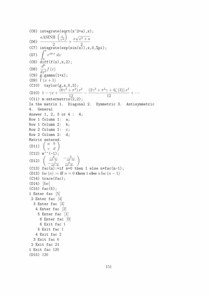
(C6) integrate(sqrt(x^2+a),x);
(D6)aASINH
(x√a
)2
+x√
x2 + a
2(C7) integrate(exp(sin(x)),x,0,%pi);
(D7)
∫ π
0
esin x dx
(C8) diff(f(x),x,2);
(D8)d2
dx2f (x)
(C9) g:gamma(1+x);
(D9) Γ (x + 1)(C10) taylor(g,x,0,3);
(D10) 1 − γx +(6γ2 + π2) x2
12− (2γ3 + π2γ + 4ζ (3)) x3
12+ · · ·
(C11) m:entermatrix(2,2);
Is the matrix 1. Diagonal 2. Symmetric 3. Antisymmetric
4. General
Answer 1, 2, 3 or 4 : 4;
Row 1 Column 1: a;
Row 1 Column 2: b;
Row 2 Column 1: c;
Row 2 Column 2: d;
Matrix entered.
(D11)
(a bc d
)(C12) m^^(-1);
(D12)
(d
ad−bc− b
ad−bc
− cad−bc
aad−bc
)(C13) fac(n):=if n=0 then 1 else n*fac(n-1);
(D13) fac (n) := if n = 0 then 1 else n fac (n − 1)(C14) trace(fac);
(D14) [fac](C15) fac(5);
1 Enter fac [5]2 Enter fac [4]3 Enter fac [3]4 Enter fac [2]5 Enter fac [1]6 Enter fac [0]6 Exit fac 1
5 Exit fac 14 Exit fac 2
3 Exit fac 62 Exit fac 24
1 Exit fac 120(D15) 120
151
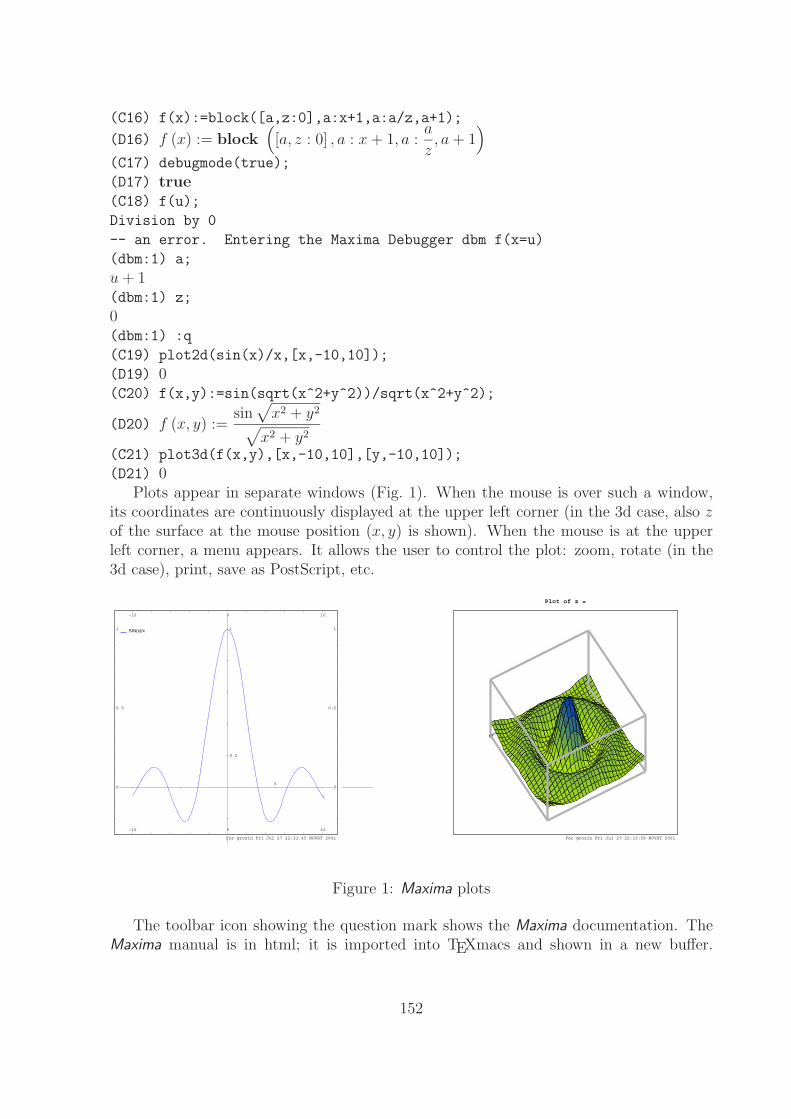
(C16) f(x):=block([a,z:0],a:x+1,a:a/z,a+1);
(D16) f (x) := block([a, z : 0] , a : x + 1, a :
a
z, a + 1
)(C17) debugmode(true);
(D17) true(C18) f(u);
Division by 0
-- an error. Entering the Maxima Debugger dbm f(x=u)
(dbm:1) a;
u + 1(dbm:1) z;
0(dbm:1) :q
(C19) plot2d(sin(x)/x,[x,-10,10]);
(D19) 0(C20) f(x,y):=sin(sqrt(x^2+y^2))/sqrt(x^2+y^2);
(D20) f (x, y) :=sin√
x2 + y2√x2 + y2
(C21) plot3d(f(x,y),[x,-10,10],[y,-10,10]);
(D21) 0Plots appear in separate windows (Fig. 1). When the mouse is over such a window,
its coordinates are continuously displayed at the upper left corner (in the 3d case, also zof the surface at the mouse position (x, y) is shown). When the mouse is at the upperleft corner, a menu appears. It allows the user to control the plot: zoom, rotate (in the3d case), print, save as PostScript, etc.
SIN(x)/x
5
0.2
1
−10
−10
0
0
10
10
0 0
0.5 0.5
1 1
For grozin Fri Jul 27 22:31:45 NOVST 2001
Plot of z =
For grozin Fri Jul 27 22:33:58 NOVST 2001
Figure 1: Maxima plots
The toolbar icon showing the question mark shows the Maxima documentation. TheMaxima manual is in html; it is imported into TEXmacs and shown in a new buffer.
152
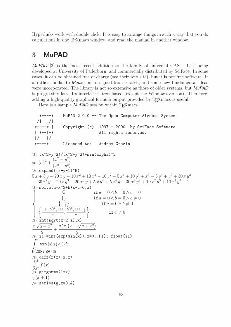
Hyperlinks work with double click. It is easy to arrange things in such a way that you docalculations in one TEXmacs window, and read the manual in another window.
3 MuPAD
MuPAD [3] is the most recent addition to the family of universal CASs. It is beingdeveloped at University of Paderborn, and commercially distributed by SciFace. In somecases, it can be obtained free of charge (see their web site), but it is not free software. Itis rather similar to Maple, but designed from scratch, and some new fundamental ideaswere incorporated. The library is not so extensive as those of older systems, but MuPADis progressing fast. Its interface is text-based (except the Windows version). Therefore,adding a high-quality graphical formula output provided by TEXmacs is useful.
Here is a sample MuPAD session within TEXmacs.
*----* MuPAD 2.0.0 -- The Open Computer Algebra System
/| /|
*----* | Copyright (c) 1997 - 2000 by SciFace Software
| *--|-* All rights reserved.
|/ |/
*----* Licensed to: Andrey Grozin
% (x^2-y^2)/(x^2+y^2)+sin(alpha)^2
sin (α)2 +(x2 − y2)
(x2 + y2)% expand((x+y-1)^5)
5 x + 5 y − 20 x y − 10 x2 + 10 x3 − 10 y2 − 5 x4 + 10 y3 + x5 − 5 y4 + y5 + 30 x y2
+ 30 x2 y − 20 x y3 − 20 x3 y + 5 x y4 + 5 x4 y − 30 x2 y2 + 10 x2 y3 + 10 x3 y2 − 1% solve(a*x^2+b*x+c=0,x)⎧⎪⎪⎪⎪⎨⎪⎪⎪⎪⎩
C if a = 0 ∧ b = 0 ∧ c = 0{} if a = 0 ∧ b = 0 ∧ c = 0{− c
b
}if a = 0 ∧ b = 0{
− b2−√
b2−4 a c2
a,
√b2−4 a c
2− b
2
a
}if a = 0
% int(sqrt(x^2+a),x)
x√
a + x2
2+
a ln(x +
√a + x2
)2% i1:=int(exp(sin(x)),x=0..PI); float(i1)∫ π
0
exp (sin (x)) dx
6.208758036% diff(f(x),x,x)∂2
∂x2f (x)
% g:=gamma(1+x)
γ (x + 1)% series(g,x=0,4)
153
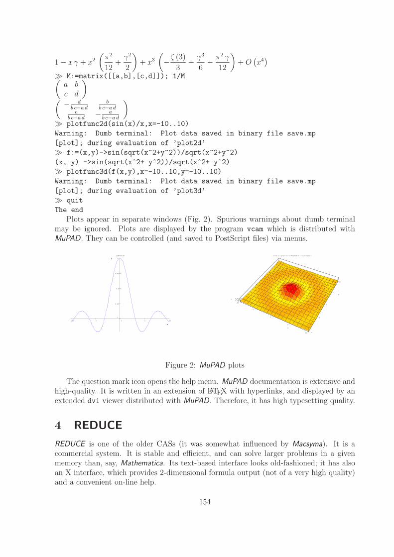
1 − x γ + x2
(π2
12+
γ2
2
)+ x3
(−ζ (3)
3− γ3
6− π2 γ
12
)+ O(x4)
% M:=matrix([[a,b],[c,d]]); 1/M(a bc d
)( − d
b c−a db
b c−a dc
b c−a d− a
b c−a d
)% plotfunc2d(sin(x)/x,x=-10..10)
Warning: Dumb terminal: Plot data saved in binary file save.mp
[plot]; during evaluation of ’plot2d’
% f:=(x,y)->sin(sqrt(x^2+y^2))/sqrt(x^2+y^2)
(x, y) ->sin(sqrt(x^2+ y^2))/sqrt(x^2+ y^2)
% plotfunc3d(f(x,y),x=-10..10,y=-10..10)
Warning: Dumb terminal: Plot data saved in binary file save.mp
[plot]; during evaluation of ’plot3d’
% quit
The end
Plots appear in separate windows (Fig. 2). Spurious warnings about dumb terminalmay be ignored. Plots are displayed by the program vcam which is distributed withMuPAD. They can be controlled (and saved to PostScript files) via menus.
1050-5-10
1
0.75
0.5
0.25
0
x
y
x
y
1/x*sin(x)
10
5
0
-5
-10
10
5
0
-5
-10
0.750.5
0.250
x
y
z
1/(x^2 + y^2)^(1/2)*sin((x^2 + y^2)^(1/2))
Figure 2: MuPAD plots
The question mark icon opens the help menu. MuPAD documentation is extensive andhigh-quality. It is written in an extension of LATEX with hyperlinks, and displayed by anextended dvi viewer distributed with MuPAD. Therefore, it has high typesetting quality.
4 REDUCE
REDUCE is one of the older CASs (it was somewhat influenced by Macsyma). It is acommercial system. It is stable and efficient, and can solve larger problems in a givenmemory than, say, Mathematica. Its text-based interface looks old-fashioned; it has alsoan X interface, which provides 2-dimensional formula output (not of a very high quality)and a convenient on-line help.
154
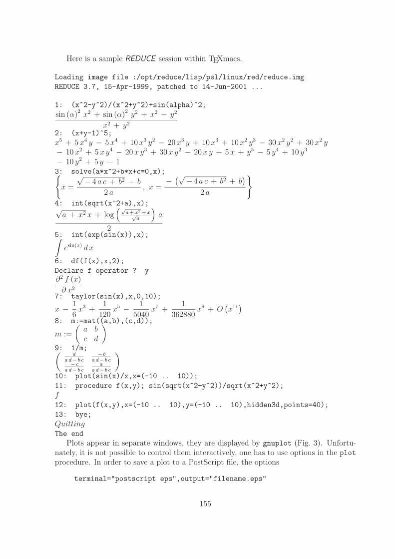
Here is a sample REDUCE session within TEXmacs.
Loading image file :/opt/reduce/lisp/psl/linux/red/reduce.img
REDUCE 3.7, 15-Apr-1999, patched to 14-Jun-2001 ...
1: (x^2-y^2)/(x^2+y^2)+sin(alpha)^2;
sin (α)2 x2 + sin (α)2 y2 + x2 − y2
x2 + y2
2: (x+y-1)^5;
x5 + 5 x4 y − 5 x4 + 10 x3 y2 − 20 x3 y + 10 x3 + 10 x2 y3 − 30 x2 y2 + 30 x2 y− 10 x2 + 5 x y4 − 20 x y3 + 30 x y2 − 20 x y + 5 x + y5 − 5 y4 + 10 y3
− 10 y2 + 5 y − 13: solve(a*x^2+b*x+c=0,x);{
x =
√− 4 a c + b2 − b
2 a, x =
− (√− 4 a c + b2 + b)
2 a
}4: int(sqrt(x^2+a),x);√
a + x2 x + log(√
a + x2 + x√a
)a
25: int(exp(sin(x)),x);∫
esin(x) d x
6: df(f(x),x,2);
Declare f operator ? y∂2 f (x)
∂ x2
7: taylor(sin(x),x,0,10);
x − 1
6x3 +
1
120x5 − 1
5040x7 +
1
362880x9 + O
(x11)
8: m:=mat((a,b),(c,d));
m :=
(a bc d
)9: 1/m;(
da d− b c
− ba d− b c− c
a d− b ca
a d− b c
)10: plot(sin(x)/x,x=(-10 .. 10));
11: procedure f(x,y); sin(sqrt(x^2+y^2))/sqrt(x^2+y^2);
f12: plot(f(x,y),x=(-10 .. 10),y=(-10 .. 10),hidden3d,points=40);
13: bye;
QuittingThe end
Plots appear in separate windows, they are displayed by gnuplot (Fig. 3). Unfortu-nately, it is not possible to control them interactively, one has to use options in the plot
procedure. In order to save a plot to a PostScript file, the options
terminal="postscript eps",output="filename.eps"
155
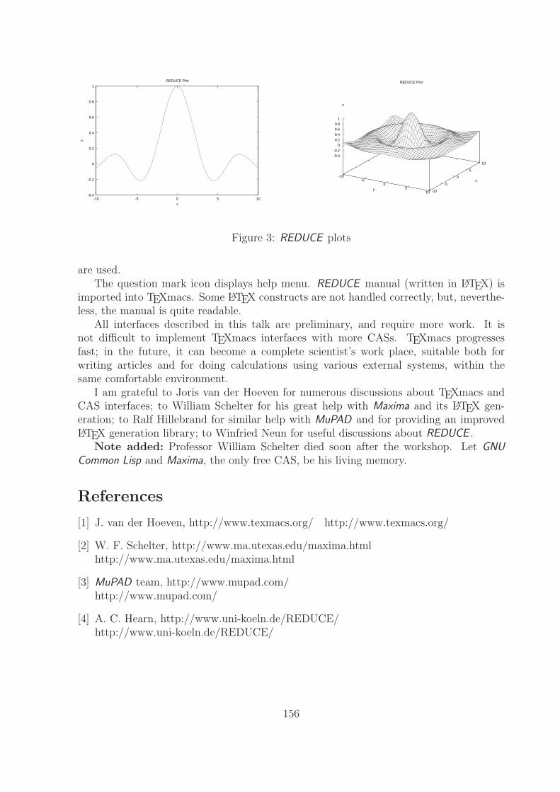
-0.4
-0.2
0
0.2
0.4
0.6
0.8
1
-10 -5 0 5 10
y
x
REDUCE Plot REDUCE Plot
-10-5
05
10y -10
-5
0
5
10
x
-0.4
-0.2
0
0.2
0.4
0.6
0.8
1
z
Figure 3: REDUCE plots
are used.The question mark icon displays help menu. REDUCE manual (written in LATEX) is
imported into TEXmacs. Some LATEX constructs are not handled correctly, but, neverthe-less, the manual is quite readable.
All interfaces described in this talk are preliminary, and require more work. It isnot difficult to implement TEXmacs interfaces with more CASs. TEXmacs progressesfast; in the future, it can become a complete scientist’s work place, suitable both forwriting articles and for doing calculations using various external systems, within thesame comfortable environment.
I am grateful to Joris van der Hoeven for numerous discussions about TEXmacs andCAS interfaces; to William Schelter for his great help with Maxima and its LATEX gen-eration; to Ralf Hillebrand for similar help with MuPAD and for providing an improvedLATEX generation library; to Winfried Neun for useful discussions about REDUCE .
Note added: Professor William Schelter died soon after the workshop. Let GNUCommon Lisp and Maxima, the only free CAS, be his living memory.
References
[1] J. van der Hoeven, http://www.texmacs.org/ http://www.texmacs.org/
[2] W. F. Schelter, http://www.ma.utexas.edu/maxima.htmlhttp://www.ma.utexas.edu/maxima.html
[3] MuPAD team, http://www.mupad.com/http://www.mupad.com/
[4] A. C. Hearn, http://www.uni-koeln.de/REDUCE/http://www.uni-koeln.de/REDUCE/
156
Multiloop Calculations in HeavyQuark Effective Theory
A. G. Grozin
Budker Institute of Nuclear Physics,630090 Novosibirsk, Russia;
e-mail: [email protected]
Heavy Quark Effective Theory (HQET) is a new approach to QCD problems witha single heavy quark, when all characteristic momenta are much less than its mass. Itsimplifies treatment of such problems, and reveals new symmetries hidden in QCD. Re-cently, an algorithm of calculation of arbitrary three-loop propagator diagrams in HQEThas been constructed, and implemented as a REDUCE package Grinder. It is about3000 lines long, and its testing required more than a CPU-month on good workstations.Large parts of this package were also ported to Axiom. Finding QCD/HQET matchingcoefficients requires calculation of on-shell diagrams with a massive quark in QCD. Analgorithm of three-loop calculations of single-mass on-shell propagator diagrams has alsobeen constructed, and implemented in FORM. A substantial progress was also achievedin calculation of diagrams with more than two legs in lower loops.
157
Maple Implementing AlgebraicPerturbation Theory Algorithm:Hydrogen Atom in Weak Electric
Fields
Alexander Gusev1, Valentin Samoilov1,Vitaly Rostovtsev2, Sergue Vinitsky3
1Scientific Center for Applied Research,2Laboratory of Information Technologies,
3Bogoliubov Laboratory of Theoretical Physics,Joint Institute for Nuclear Research,
141980 Dubna, Moscow Region, Russia;
Algorithms for evaluation of eigenvalues and eigenfunctions of a hydrogen atom inelectric fields in framework of perturbation theory is implemented on MAPLE. A programdescription as well as input and output files are represented.
1 Introduction
In articles [3, 4, 5] algorithms for calculating eigenfunctions and eigenvalues of hydrogenatom in the homogeneous electric field and in the field of distant charge were represented.They have been implemented by means of CAS REDUCE.
Algorithms of this sort are needed to construct of combined program package forcomputing both atomic systems properties in external fields and effective potentials inquantum mechanical three body problem [2, 1].
We have been generalizing our algorithms and implementing them in CAS Maple.In this case, we wrote the program without using rewrite rules. These algorithm andprogram are represented in the article. In addition, we perform a comparison of thepackages efficiency and results of calculation of energy spectrum up to 9 order by smallparameter.
2 Setting of the Problem
Concider Shroedinger equation of a hydrogen-like atom with the charge Za in weak electricfield (
1
2p2 − Za
r+ V (r, x3) − E
)|Φ〉 = 0, 〈Φ|Φ〉 = 1 (1)
158
where E is an energy and |Φ〉 are wave functions of hydrogen atom. V (r, x3) is potential,which can be represented as a series
V =∑k=1
εkVk, ε ( 1.
The wave function |Φ〉 and the energy E = E(R) are sought for in the form
|Φ〉 =∑k=0
εk|Φ(k)〉, E =∑k=0
εkE(k). (2)
Using these expansions we rewrite equation (1) in form(1
2rp2 − Za −
∑k=1
εkV (k)(x3, r) − rE(0)
)|Φ〉 = 0. (3)
Then we can write (3) in notations generators L56, A3 = L34, L3 = L12, x3 = L35 −L34, r = L56 − L46 of so(4,2) algebra [3]. Making use of the tilting transformation√√
−2E(0)
nU [3], we go over from the hydrogen states |Φ〉 to the basis states |Φ〉, we arrive
at the following equation:[L56 − Za√−2E(0)
− 1√−2E(0)
∑k=1
εkV (k)(x3√−2E(0)
,r√−2E(0)
)
]|Φ〉 = 0. (4)
The normalization condition for basis states |Φ〉 follows from(1) for states |Φ〉
〈Φ|Φ〉 =
√−2E(0)
n〈Φ|UrU−1|Φ〉 =
=
√−2E(0)
n〈Φ| r√−2E(0)
|Φ〉 =1
n〈Φ|r|Φ〉 = 1. (5)
Hence, it follows that in the course of the passage from the wave functions |Φ〉 to thebasis states |Φ〉, the first one should be normalized by the condition
〈Φ|r|Φ〉 = n, (6)
which becomes an identity for states |Φ(0)〉.
3 The Scheme of Perturbation Theory and Algo-
rithm
We look for a solution to equation (4) in the form of the perturbation series
|Φ〉 =kmax∑k=0
εk|Φ(k)〉. (7)
159
The unknown coefficients |Φ(k)〉 satisfy the system of inhomogeneous differential equations
L(n)|Φ(0)〉 = (L56 − n)|Φ(0)〉 = 0 ≡ f (0), (8)
L(n)|Φ(1)〉 =r
(−2E(0))[E(1) − Zb(Za − 1)]|Φ(0)〉 ≡ f (1), (8a)
L(n)|Φ(k)〉= r
(−2E(0))
k−1∑p=0
V (k−p)(x3√−2E(0)
,r√−2E(0)
)|Φ(p)〉≡f (k). (8b)
As the basis, which realizes the infinite-dimensional irreducible representation of the alge-bra so(4, 2) in x-space, we take the eigenfunctions 〈y|s, t〉 of commuting operators L56, A3
and L3 distinguished from the basis functions 〈y|n1 + s, n2 + t,m〉 only by the normaliza-tion factor and coincide with them at s = t = 0
〈y|s, t〉 =Cn1n2|m|
Cn1+s,n2+t,|m|〈y|n1 + s, n2 + t,m〉. (9)
The operators L56, x3, r and L3 on the functions 〈y|s, t〉 are defined by the relationswithout fractional powers of parabolic quantum numbers
L56|s, t〉 = (n1 + n2 + |m| + 1 + s + t)|s, t〉 = (n + s + t)|s, t〉, (10)
A3|s, t〉 = (−(n1 + s) + (n2 + t))|s, t〉, L3|s, t〉 = |m||s, t〉, (10a)
r|s, t〉 = (n + s + t)|s, t〉 − 12((n1 + s + |m|)|s − 1, t〉 + (n1 + s + 1)|s + 1, t〉
+(n2 + t + |m|)|s, t − 1〉 + (n2 + t + 1)|s, t + 1〉), (10c)
x3|s, t〉 = 12(−(n1 + s + |m|)|s − 1, t〉 − (n1 + s + 1)|s + 1t〉
+(n2 + t + |m|)|s, t − 1〉 + (n2 + t + 1)|s, t + 1〉) − (−(n1 + s) + (n2 + t))|s, t〉. (10d)
Suppose the azimutal quantum number m is positive m = |m|. Applying relations (10),we expand the right-hand side f (k) and solutions |Φ(k)〉 of the system (8) over basis states|s, t〉 (9):
f (k) =∑s,t
f(k)st |s, t〉, |Φ(k)〉 =
∑s,t
b(k)st |s, t〉. (11)
Substituting (11) into (8) and taking into account the relation
L(n)|s, t〉 = (s + t)|s, t〉and orthogonality condition (4) of basis (9), we obtain the system of linear algebraic
equations for unknown coefficients b(k)st and perturbation corrections E(k), for each k ≥ 1
(s + t)b(k)st − f
(k)st = 0, min(|s|, |t|, |s + t|) ≤ k. (12)
It enables us to find the coefficients b(k)st using known coefficients f
(k)st from the above
definitions. In the second order k = 2, we obtain the energy correction E(2) = 3ndZb/2Za
at s = t = 0 and eight coefficients b(2)st at s + t = 0:
b(2)0,∓1 = ∓n3Zb
8Z3a
(d ∓ m − n + 1)(d + 2n ∓ 2)),
160
b(2)0,∓2 = ∓n3Zb
32Z3a
(d ∓ m − n ∓ 1)(d ∓ m − n ± 3)),
b(1)1,−1 =
n
8Za
(d − m + n + 1)(d − m − n + 1)),
b(2)1,−1 = − n2
8Z2a
(d − m + n + 1)(d − m − n + 1)(d + 1)),
b(2)2,−2 =
n2
128Z2a
(d − m + n + 3)(d − m + n + 1)(d − m − n + 3)(d − m − n + 1)).
For Stark effect, coefficients b(1)1,−1, b
(1)−1,1 are equal to zero and b
(1)0,j are equal to correspond-
ing coefficients of hydrogen atom in the field of the distant charge b(2)0,j . The remaining
coefficients are obtained up to the sign by interchanging n1 by n2 (d = n2 − n1 → −d),
b(k)st (d) = (−1)k+1b
(k)ts (−d), b
(k)s,−s(d) = (−1)kb
(k)−s,s(−d). Indeed, at each k the functions
f(k)st depend on the unknown correction E(k) and known coefficients E(p) and b
(p)st for
p = 0, 1, · · · , k − 1, which are evaluated from previous k − 1 equations. The coeffi-cients b
(p)st also depend on the corrections E(q) and b
(q)st with q = 0, 1, · · · , p − 1, which
are evaluated from previous equations (12) by recurrence. Thus, in each order (k ≥ 1)
we calculate step-by-step the needed corrections E(k), b(k−2)s,−s , b
(k)s,t by solving the following
algebraic equations:
f(k)00
(E(k), E(p), b
(p)s′t′ , 0 ≤ p ≤ k − 1
)= 0 → E(k), (13)
f(k)s−s
(E(k), E(p), b
(p)s′,t′ , 1 ≤ p ≤ k − 1
)= 0 → b
(k−2)s−s , (13a)
b(k)s,t = (s + t)−1f
(k)st
(E(k), E(p), b
(p)s′,t′ , 0 ≤ p ≤ k − 1
). (13b)
The initial conditions for the recurrence procedure are given by
E(0) = − Z2a
2n2, b
(0)0,0 = 1, b
(0)s,t = 0 for s, t = 0, b
(k)0,0 = 0. (14)
To obtain the normalized wave function Φ by condition (6) up to the kth order, we must
redefine the coefficient b(k)0,0 by the following relation:
b(k)00 = − Za
2n2
k∑p=0
∑s′,t′
∑s,t
b(k−p)st 〈s, t| r√−2E(0)
|s′, t′〉b(p)s′t′ . (15)
In particularly, the coefficient b(1)0,0 = 0 and b
(2)0,0 is defined by
b(2)0,0 =
n2
64Z2a
(−d4+(2d2−m2)(m2+n2−3)+m2(3n2−1)−(n2−1)2)+3dn3Zb
4Z3a
. (16)
Then the algorithm is evaluated step by step as follows.1. ”Potential”. Coefficients of potential and energy expansions are calculated with
respond to (2). The step has two branch of calculations: in case of Stark effect and incase of point charge.
161
2. ”Action of potential by ket”. The results of actions of the operators r and x3 withrespect of (10c,10d) are defined in this step. Sequence of the calculations is described inthe next section.
3. Step ”finding eigenvalues” realizes the main goal of the calculations. Indeed, inthis step we are calculated the corrections to f (k) and E(k) by means of solving equations(13), (13a), (13b) up to preassigned order kmax.
4 Program MW3STARK and Results
In this Section we adduce the main program MW3STARK as a pilot implementationof the above algorithm in MAPLE VR5. First of all we defined next parameters:
• stark0_point1 – program switch: 0-stark, 1-point charge;
• kmax – a number of spectrum corrections;
• bbound – a boundary of summation range in expansions (11);
• -bbound≤ s, t ≤bbound;
• fdE,fdB are names of output files.
The program consists of blocks in respect to the algorithm described in previous sec-tion.
1. In block ”POTENTIAL”, we denote by V the potential multiplied by r and ee(k)and the energy E(k) (2). Program variables vr, vx3 and vr0, vx30 are the variablesr and x3 in (3). The Coice of calculation branch is realised by switch stark0_point1.
2. The block ”ACTION OF POTENTIAL BY KET” consist of the following parts.
(a) In block ”action r and x3 by ket” results of action of the operators r and x3
are defined.
(b) In block ”action v by ket” coefficients actket(k,x1,x2) of an expansion”V (k)ket(N1, N2,m) =
∑actket(k, x1, x2) ∗ ket(N1 + x1, N2 + x2,m)” are
defined and evaluated in following parts:
i. ”preparation”: set all actket(k,x1,x2) to zero. Then set actket(k,0,0)to value of potentials V(k,vx3,xr), and assign a degree of V(k,vx3,xr)over (vx3,vr) to a variable vmax(k);
ii. ”action of operator r by ket”: application of (10) for excluding r in cal-culation of potential action. In order that, we are using an auxiliary vari-able ketvspom. Terms containing the variable vr are transferred fromactket(k,x1,x2) to ketvspom. Then we factorized vr and act on ket,accordingly to step 2a. Boundaries of region (x1,x2) and a number of ap-plication of this procedure for k−th order are defined by means of variablevmax(k);
162
iii. ”action of operator x3 by ket”: An application of the formula (10d) toexclude the variable x3 is used under calculation of the potential action;
iv. ”test”: are transfer to new quantum numbers ”NN, ND”.
3. The subroutine ”finding eigenvalues realizes” consist of the following parts.
(a) ”Preparation”: the zero values are assigned to all b(k,js,jt) but b(0,0,0)=1;
(b) ”Calculations”: extracting eigenvalues and eigenfunctions. By means of loopunder k from sbros to kmax, we are accomplished the following actions:
i. ”calculating f”: by (8) and (11) we evaluate coefficients b(k,js,jt);
ii. ”calculating ee(k)”: we solve equation (13);
iii. ”calculating b(k-sbros,s,-s)”: an auxiliary block;
iv. ”add v(sbros)*b(k-sbros,s,-s)”: we are taking account over contribution ofthe action v(sbros) of the diagonal components b(k-sbros,js,-js);
v. calculating b(k,s,t): we solve equation (13b).
4. Print(b(k,s,t)).
5. Print time.
#program mw3stark;
restart;timestart:=time():
stark0_point1:=1; # 1 for atom in the field of the point charge,
#stark0_point1:=0; # 0 for stark effect
kmax:=11;
bbound:=20;
fdE:=open("e.out",WRITE): fdB:=open("b.out",WRITE):
#1. potential
if stark0_point1=0 then
V(1,vx3,vr):=expand(subs(vr0=vr*n/Za,vx30=vx3*n/Za
,(ee(1)*vr0-vr0*vx30)*n/Za));
for k from 2 to kmax do V(k,vx3,vr):=
expand(subs(vr0=vr*n/Za,vx30=vx3*n/Za,ee(k)*vr0*n/Za));
od:
fprintf(fdE,"Hydrogen atom in homogeneous
electric field\n kmax="):
fprintf(fdB,"Hydrogen atom in homogeneous
electric field\n kmax="):
fprintf(fdE,cat(convert(kmax,string),";\n")):
fprintf(fdB,cat(convert(kmax,string),";\n")):
sbros:=1;
fi:
if stark0_point1=1 then
163
V(1,vx3,vr):=expand(subs(vr0=vr*n/Za,vx30=vx3*n/Za
,n/Za*expand(vr0*(ee(1)-Zb*(Za-1)))));
for k from 2 to kmax do
V(k,vx3,vr):=expand(subs(vr0=vr*n/Za,vx30=vx3*n/Za
,n/Za*expand(vr0*(ee(k)+Zb*vr0^(k-1)
*orthopoly[P](k-1,-vx30/vr0)))));
od;
fprintf(fdE,"Hydrogen atom in the field
of the distant charge\n kmax="):
fprintf(fdB,"Hydrogen atom in the field
of the distant charge\n kmax="):
fprintf(fdE,cat(convert(kmax,string),";\n")):
fprintf(fdB,cat(convert(kmax,string),";\n")):
sbros:=2;
ee(1):=Zb*(Za-1);
fprintf(fdE,"ee(1) := "):
fprintf(fdE,cat(convert(ee(1),string),";\n")):
fi:
#2.actions of potential by ket #2a.action r and x3 by ket rul1:=
rket ( 0, 0):=(N1+N2+m+1): x3ket ( 0, 0):=-(-N1+N2):
rket (-1, 0):=-1/2*(N1+m): x3ket (-1, 0):=-1/2*(N1+m):
rket ( 1, 0):=-1/2*(N1+1): x3ket ( 1, 0):=-1/2*(N1+1):
rket ( 0,-1):=-1/2*(N2+m): x3ket ( 0,-1):=1/2*(N2+m):
rket ( 0, 1):=-1/2*(N2+1): x3ket ( 0, 1):=1/2*(N2+1):
#2b. action v by ket #2b1.podgotovka
for k from 0 to sbros-1 do vmax(k):=0 od:
for k from sbros to kmax do
vmax(k):=degree(subs(vx3=vx,vr=vx,V(k,vx3,vr)),vx);
for js from -vmax(k) to vmax(k) do
for jt from -vmax(k)+abs(js) to vmax(k)-abs(js) do
actket(k,js,jt):=0;
od od:
actket(k,0,0):=V(k,vx3,vr);
od:
#2b2. action of operator r by ket
for k from sbros to kmax do
for j from 0 to vmax(k)-1 do
for js from -j to j do
for jt from -j+abs(js) to j-abs(js) do
ketvspom:=simplify((actket(k,js,jt)
-subs(vr=0,actket(k,js,jt)))/vr);
actket(k,js,jt):=subs(vr=0,actket(k,js,jt));
for a in [0,0],[0,1],[1,0],[0,-1],[-1,0] do
164
as:=op(1,a);
at:=op(2,a);
actket(k,js+as,jt+at):=simplify(actket(k,js+as,jt+at)
+subs(N1=N1+js,N2=N2+jt,rket(as,at))*ketvspom);
od:od:od:od:od:
#2b3. action of operator x3 by ket
for k from sbros to kmax do
for j from 0 to vmax(k)-1 do
for js from -j to j do
for jt from -j+abs(js) to j-abs(js) do
ketvspom:=simplify((actket(k,js,jt)
-subs(vx3=0,actket(k,js,jt)))/vx3);
actket(k,js,jt):=subs(vx3=0,actket(k,js,jt));
for a in [0,0],[0,1],[1,0],[0,-1],[-1,0] do
as:=op(1,a); at:=op(2,a);
actket(k,js+as,jt+at):=simplify(actket(k,js+as,jt+at)
+subs(N1=N1+js,N2=N2+jt,x3ket(as,at))*ketvspom);
od:od:od:od:od:
#2b4. test
for k from sbros to kmax do
for js from -vmax(k) to vmax(k) do
for jt from -vmax(k)+abs(js) to vmax(k)-abs(js) do
actket(k,js,jt):=collect(subs(N1=(NN+ND-m-1)/2
,N2=(NN-ND-m-1)/2,actket(k,js,jt)),ee,simplify);
od:od:od:
#3. finding eigenvalues #3a. podgotovka
for k from 0 to kmax do
for js from -bbound to bbound do
for jt from -bbound to bbound do
b(k,js,jt):=0;
od:od:od: b(0,0,0):=1:
#3b. calculations
for k from sbros to kmax do
#3b1. calculating f (now b(k,s,t)=f(k,s,t))
for kpb from 0 to k-sbros do
for jsb from -bbound to bbound do
for jtb from -bbound to bbound do
if b(kpb,jsb,jtb)<>0 then
for js from -vmax(k-kpb) to vmax(k-kpb) do
for jt from -vmax(k-kpb)+abs(js) to vmax(k-kpb)-abs(js) do
if (abs(js+jsb)>bbound) or (abs(jt+jtb)>bbound)
165
then print("bbound is very small") fi:
b(k,js+jsb,jt+jtb):=collect(b(k,js+jsb,jt+jtb)
+b(kpb,jsb,jtb)*subs(NN=n+jsb+jtb,ND=d+jsb-jtb
,actket(k-kpb,js,jt)),ee,simplify);
od: od:
fi:
od:od:od:
#3b2. calculation ee(k):
ee(k):=
simplify(-coeff(b(k,0,0),ee(k),0)/coeff(b(k,0,0),ee(k),1)):
fprintf(fdE,cat( "\n ee(",convert(k,string)));
fprintf(fdE,cat( ") := ",convert(ee(k),string)));
fprintf(fdE,";\n ");
#3b3 calculation b(k-sbros, s,-s)
for js from 1 to bbound do
if((simplify(b(k,js,-js))<>0)or(simplify(b(k,-js,js)<>0)))
then
b(k-sbros, js,-js):=simplify(
-b(k,js,-js)/subs(NN=n,ND=d+2*js,actket(sbros,0,0))):
b(k-sbros, -js,js):=simplify(
-b(k,-js,js)/subs(NN=n,ND=d-2*js,actket(sbros,0,0))):
fi:
od:
#3b4. add v(sbros)*b(k-sbros...) to f(k,s,t)
for j from -bbound to bbound do
if simplify(b(k,j,-j))<>0 then
for js from -vmax(sbros) to vmax(sbros) do
for jt from -vmax(sbros)+abs(js) to vmax(sbros)-abs(js) do
if (abs(js+j)>bbound) or (abs(jt-j)>bbound)
then print("bbound is very small") fi:
b(k,js+j,jt-j):=simplify(b(k,js+j,jt-j)
+b(k-sbros,j,-j)*subs(NN=n,ND=d+2*j,actket(sbros,js,jt)));
od:od:
fi:
od:
#3b5. calculation b(k, s, t) (now b(k,s,t))
for js from -bbound to bbound do
for jt from -bbound to bbound do
if js<>-jt then
b(k,js,jt):=simplify(b(k,js,jt)/(js+jt)):
fi:
166
od:od:
print(k);
od:
#4. print(b);
for k from 0 to kmax-sbros do
for js from -bbound to bbound do
for jt from -bbound to bbound do
if b(k,js,jt)<>0 then
fprintf(fdB,cat( "\n b(",convert(k,string)));
fprintf(fdB,cat( ",",convert(js,string)));
fprintf(fdB,cat( ",",convert(jt,string)));
fprintf(fdB,cat( "):=",convert(b(k,js,jt),string)));
fprintf(fdB,";\n");
fi:
od:od:od:
#5.
fprintf(fdE,cat("\n\nTime:=",convert(time()-timestart,string))):
fprintf(fdE," s;\n"):
close(fdE):close(fdB):
To check the algorithm and program we have been calculating the corrections to b(k)st
and E(k) up to 11-th order. The results are very space consuming so we cannot adducethen here. This test was calculated on computer PC-2 350MHz 64MB memory. In theabove formulas, we use the following notations: n≡ n = n1 + n2 + |m| + 1, m≡ |m|,d≡ n1 −n2, za≡ Za, zb≡ Zb. Note that our results coincide up to the seventh order with[3, 4, 5] (the orders 8-11 was not calculated in the sited works because technical limits).
5 Conclusion
We have demonstrated the efficiency of the proposed recursive symbolic algorithm inthe framework of an algebraic version of the conventional perturbation theory withoutassumption on separation of independent variables in both parabolic and spherical repre-sentations, which are needed for applications [5]
Acknowledgements
We are grateful to Professor V.P. Gerdt for his support of this work and useful discussion.The authors (AG, SI) appreciate support of Russian Foundation for Basic Research (grantNo. 02-02-17617).
167
References
[1] Faifman, M.P., Ponomarev, L.I., Vinitsky, S.I.: Asymptotic form of effective potentialof the Coulomb three-body problem in the adiabatic representation J. Phys. B: Atom.Molec. Phys. 9 (1976) 2255–2268.
[2] Abrashkevich, A.G., Puzynin, I.V., Vinitsky, S.I.: ASYMPT: a program for calcu-lating asymptotics of hyperspherical potential curves and adiabatic potentials. Com-puter Physics Communications 125 (2000) 259–281.
[3] Gusev, A.A., Samoilov, V.N., Rostovtsev, V.A., Vinitsky, S.I.: Symbolic Algorithmof Algebraic Perturbation Theory of a Hydrogen Atom: the Stark effect. In: Com-puter Algebra in Scientific Computing, V.G.Ganzha, E.W. Mayr, E.V. Vorozhtsov(Eds.), Springer-Verlag, Berlin, 2000, pp. 219–231.
[4] A.A. Gusev, V.N. Samoilov, V.A. Rostovtsev, S.I. Vinitsky, Algebraic perturbationtheory for hydrogen atom in weak Electric Fields (in Russian) Programing v1, p27-31(2001).
[5] A.A. Gusev,V.N. Samoilov, V.A. Rostovtsev, S.I. Vinitsky: Symbolic Algorithmsof Algebraic Perturbation Theory: Hydrogen Atom in the Field of Distant ChargeProc. of Fourth Workshop on ”Computer Algebra in Scientific Computing”, (Kon-stanz, September 22 - 26, 2001), CASC-2001, Eds. V.G. Ganzha, E.W.Mayr, E.V.Vorozhtsov, Springer-Verlag, 2001, pp. 309-322.
168
Completion to Involutionand Symmetry Analysis
Marcus Hausdorf, Werner M. Seiler
Lehrstuhl fur Mathematik I, Universitat Mannheim,68131 Mannheim, Germany;
e-mail: {hausdorf,werner.seiler}@math.uni-mannheim.dehttp://www.math.uni-mannheim.de/~wms
We discuss some applications of the theory of involutive systems in the Lie symmetryanalysis of partial differential equations. Special emphasis is put on non-classical symme-tries.
Supported by Deutsche Forschungsgemeinschaft, Landesgraduiertenforderung Baden –Wurttemberg and INTAS grant 99-1222.
1 Introduction
Lie symmetry analysis represents one of the most important techniques for tackling dif-ferential equations, in particular non-linear ones. It often provides the only possibilityto find solutions in closed form. But many other applications exist, too; perhaps bestknown is the construction of conservation laws via Noether’s law. By now, a number oftextbooks on symmetry analysis are available (see e. g. [3, 9, 13]); a survey of computeralgebra tools for symmetry analysis was given by Hereman [5, 6].
The theory of involutive systems appears at many places in symmetry analysis. Thebest known application is, of course, the completion of the determining systems in orderto facilitate its integration in closed form. In fact, this problem has been a major impetusfor the renewal of interest in involution in the last, say, twenty years. In this article wewill, however, concentrate on other, less known applications.
In the literature one can find several different notions of involutive (or passive orcomplete) systems. We will use the so-called formal theory [14, 18]. It is a geometricapproach and may be formulated completely intrinsically. This makes its application insymmetry theory very natural.
This article is organised as follows. The next section briefly reviews some basic notionsof the formal theory. Then we study the role involution plays for the very definition ofsymmetries. Section 4 contains some formal results about measuring the size of thesolution space of differential equations. Then we analyze symmetry reductions; this leadsin a natural manner to non-classical symmetries. Finally, some conclusions are given.
169
2 Involution
For lack of space, we cannot give here a detailed introduction into the formal theory orthe underlying jet bundle formalism. Our presentation follows [18]; a general reference isthe book of Pommaret [14].
For simplicity, we will use local coordinates. Let x = (x1, . . . , xn) and u = (u1, . . . , um)be an adapted coordinate system on the fibred manifold π : E → X . Coordinates on theqth order jet bundle JqE are obtained by adding all derivatives
pαμ = ∂|μ|uα/∂(x1)μ1 · · · ∂(xn)μn
with |μ| ≤ q. Here μ = [μ1, . . . , μn] is a multi index and |μ| = μ1 + · · · + μn its length.Thus the jet bundle JqE may be interpreted as the space of all Taylor series truncated atorder q.
We define a differential equation1 of order q intrinsically as a fibred submanifold Rq ⊆JqE . Locally, Rq is described by a system of equations
Rq :{
Φτ (x,u,p) = 0 , τ = 1, . . . , p . (1)
A solution is a (local) section σ : X → E such that the image of its prolongation jqσ :X → JqE completely lies in Rq. Locally, a section is of the form σ(x) =
(x, s(x)
)with
some functions s = (s1, . . . , sm). For its prolongation we differentiate these functions andσ is a solution, if the substitution pα
μ = ∂|μ|sα/∂(x1)μ1 · · · ∂(xn)μn in (1) yields an identity.The prolongation Rq+1 ⊆ Jq+1E is obtained by formally differentiating every equation
in (1) with respect to all independent variables x, i. e. by adding the differential equations
DiΦτ =
∂Φτ
∂xi+
∂Φτ
∂uαpα
i +∂Φτ
∂pαμ
pαμ+1i
= 0 , i = 1, . . . , n . (2)
Iteration yields higher order prolongations Rq+r ⊆ Jq+rE . A (smooth) solution of Rq isautomatically also a solution of Rq+r and vice versa.
The symbol Mq of the differential equation Rq locally represented by the system (1) isthe solution space of the following linear system of (algebraic!) equations in the unknownsvα
μ
Mq :
⎧⎨⎩m∑
α=1
∑|μ|=q
(∂Φτ
∂pαμ
)vα
μ = 0 . (3)
(By abuse of language, we will refer to both the linear system and its solution space asthe symbol). The place-holders vα
μ are coordinates of a finite-dimensional vector space;we introduce one for each derivative of order q. For a linear differential equation, thesymbol is simply obtained by considering only the highest order or principal part andsubstituting vα
μ for pαμ.
Let us make a power series ansatz for the solutions of the differential equation Rq
expanding around some point x0 ∈ X . Substituting into (1) and evaluating at x = x0
1Note that we do not distinguish between scalar equations and systems!
170
yields a system of algebraic equations for the Taylor coefficients up to order q. Substitutingthe ansatz into Rq+r and evaluating again at x = x0 yields an inhomogeneous linearsystem for the coefficients of order q + r. Its homogeneous part is given by the matrix ofthe prolonged symbol Mq+r, i. e. the symbol of the prolonged equation Rq+r.
This order by order construction of a formal power series solution fails, if integrabilityconditions occur. They pose additional conditions on coefficients of lower order and mustall be known in order to pursue the above described procedure. A differential equationcontaining all its integrability conditions is called formally integrable, as it possesses aformal power series solution. Unfortunately, no finite criterion for formal integrability isknown.
For an intrinsic formulation of integrability conditions we exploit the natural projec-tion maps between jet bundles of different order (they simply forget the higher order
derivatives). For r > q we write πrq : JrE → JqE and define R(r)
q = πq+rq (Rq+r) ⊆ Rq, i. e.
we first prolong r times and then project back r times. Integrability conditions appearduring these prolongations, if and only if R(r)
q � Rq.
Definition 1. The differential equation Rq is formally integrable, if for all integers r > 0
the equality R(1)q+r = Rq+r holds.
It follows from the construction above that the arbitrariness of the general formalpower series solution is reflected by the dimensions of the prolonged symbols, becauseat each order dimMq+r coefficients are not determined by the differential equations butcan be chosen freely. Formal integrability does, however, not suffice to determine thesedimensions without explicitly constructing the prolonged symbols.
A jet variable pαμ is said to be of class k, if μk is the first non-vanishing entry of its
multi index. We order the columns of the symbol Mq by class (highest class first) andcompute a row echelon form. If vα
μ is the leading term of an equation in this solved formof the symbol, then pα
μ is a principal derivative. All other derivatives are parametric. We
define the indices β(k)q of the symbol Mq as the number of principal derivatives of class k.
Definition 2. The symbol Mq is called involutive, if
rankMq+1 =n∑
k=1
kβ(k)q . (4)
The differential equation Rq is involutive, if it is formally integrable and if its symbolMq is involutive.
In contrast to formal integrability, involution can be checked in a finite manner. Todecide whether a symbol is involutive requires only some linear algebra. For differentialequations we note the following very important criterion for involution that needs onlyone prolongation instead of infinitely many ones as the definition of formal integrability.
Theorem 1. Let Rq be a differential equation with involutive symbol Mq. Then Rq is
involutive, if and only if R(1)q = Rq.
171

Two important results on involutive equations are the Cartan–Kuranishi and theCartan–Kahler Theorem. The former one states that any (regular) differential equationRq can be completed in a finite number of steps to an equivalent differential equation
R(s)q+r that is involutive; discussions of the algorithmic realisation of this completion can
be found in [4, 17]. The latter is an existence and uniqueness theorem in the analyticcategory; if Rq is an analytic involutive differential equation, then a certain initial valueproblem for it has a unique analytic solution for analytic initial data. Thus it generalisesthe well-known Cauchy–Kovalevskaya Theorem.
3 Basic Symmetry Theory
Symmetry theory [3, 9, 13] provides us with some of the most important techniques forthe analysis of differential equations, in particular for non-linear equations. A somewhatsubtle and often overlooked point is the importance of the local solvability of the analyseddifferential equation. Essentially, this concerns the equivalence of two different definitionsof what a symmetry of a differential equation actually is.
Definition 3. A symmetry of a differential equation is a transformation that maps anyof its solutions into another solution.
This probably represents the most general definition of a symmetry of a differentialequation. It is still somewhat vague, as it is not clearly specified what kinds of transfor-mations or solutions are considered. We restrict in this article to point symmetries, i. e.to diffeomorphisms φ : E → E , and to formal power series solutions. Definition 3 is veryhard to apply in practice, as it requires the knowledge of the full solution space. Thususually the following, more geometric approach is taken.
Definition 4. A diffeomorphism φ : E → E is a point symmetry of the differentialequation Rq ⊆ JqE, if its prolongation φ(q) : JqE → JqE leaves the submanifold Rq
invariant.
The infinitesimal version of this definition forms the basis of all concrete computa-tions with Lie symmetries. One considers a one-parameter group of diffeomorphisms φε
generated by a vector field X over E . Given a local description of Rq in the form (1),a linearisation of the condition above leads to the well-known infinitesimal symmetrycriterion
X(q)Φτ
Rq= 0 (5)
where the prolonged vector field X(q) on JqE is the generator of φ(q)ε . X(q) and φ
(q)ε are
easily determined by the chain rule.With respect to our adapted coordinates, an arbitrary vector field X over E may be
locally written in the form X = ξi(x,u)∂xi + ηα(x,u)∂uα . Evaluation of the criterion (5)yields an overdetermined linear system of partial differential equations for the coefficientsξi and ηα, the determining system Dq (it has the same order as the equation Rq to beanalysed).
172
It is often assumed that Definitions 3 and 4 are equivalent, but this holds only undercertain assumptions on the differential equation Rq. We must assume that for every pointρ ∈ Rq at least one solution σ : X → E exists such that ρ ∈ jq(σ). This property is knownas local solvability. It is trivial for scalar equations or systems in Cauchy–Kovalevskayaform but becomes an issue for overdetermined systems.
We illustrate the problem with a very simple example. Consider the following firstorder equation:
R1 :
{uz + yux = 0 ,uy = 0 .
(6)
Since y appears explicitly, the manifold R1 does not remain invariant under y-translationsand thus they are not symmetries in the sense of Definition 4. Cross-differentiations showthat R(1)
1 is defined by the equations ux = uy = uz = 0. Hence the general solution of ourequation is u(x, y, z) = const and y-translations are symmetries in the sense of Definition3. The geometric approach “loses” this symmetry, as it requires that the whole manifoldR1 should remain invariant and not only its submanifold R(1)
1 . Since the image of any
prolonged solution j1σ lies in R(1)1 , the second definition imposes a stronger condition
than the first one.A less trivial example are the incompressible Navier–Stokes equations. They are not
formally integrable; the integrability condition is the well-known Poisson equation for thepressure. But in this special case, the hidden equation has no influence on the symmetryanalysis. Thus the classical results on the symmetry group of the Navier–Stokes equationsare correct, although their derivations neglect the integrability condition.
The problem disappears, as soon as we consider involutive differential equations. TheCartan–Kahler Theorem implies that any involutive equation is locally solvable. Notethat as we are only considering formal power series solutions, the analyticity assumptionsof this theorem play no role here.
4 Measuring the Size of Solution Spaces
It was already mentioned in Section 2 that the dimensions of the prolonged symbolsdimMq+r measure the size of the formal solution space. For involutive equations these
dimensions can be easily determined explicitly. Recall that the indices β(k)q count the
number of principal derivatives of order q and class k. Similarly, the Cartan characters
α(k)q = m
(q + n − k − 1
q − 1
)− β(k)
q , k = 1, . . . , n (7)
count the parametric derivatives of order q and class k.Associating with each equation whose principal derivative is of class k its multiplicative
variables x1, . . . , xk, one can show that if we prolong each equation with respect to itsmultiplicative variables only, we get algebraically independent equations. By (4), nofurther independent equations of order q+1 exist in the case of an involutive symbol. Thisimplies a simple way to compute the indices of the prolonged symbol: β
(k)q+1 =
∑ni=k β
(k)q
173
and correspondingly α(k)q+1 =
∑ni=k α
(k)q . Iteration yields
α(k)q+r =
n∑i=k
(r + i − k − 1
r − 1
)α(i)
q . (8)
Since dimMq+r =∑n
k=1 α(k)q+r, we see that if (and only if) the symbol Mq is involutive,
we can trivially determine the size of the formal solution space based on the Cartancharacters α
(k)q . For more details see [19].
A trivial application of these results consists in measuring the size of the symmetrygroup. As the dimension of a Lie group coincides with the dimension of its Lie algebra, weperform an involution analysis of the determining system Dq. The simplest case arises, ifthe symmetry group is finite-dimensional. It follows from the discussion above that thenall Cartan characters of the involutive completion D(s)
q+r must vanish and the dimension
of the group is simply dimD(s)q+r. In the case of an infinite-dimensional group, the Cartan
characters of D(s)q+r still encode much information about the size and, in particular, permit
an easy comparison of different groups. These results are not restricted to Lie pointsymmetries but may obviously be applied in the same manner to generalised symmetries.
A less trivial application, which we cannot discuss here, is that one may deduce notonly the size but also the structure of Lie symmetry algebra by a completely formalanalysis. In the case of a finite-dimensional algebra this is rather simple; for infinite-dimensional algebras one needs deeper results from their structure theory. More detailscan be found in [7, 16].
One interesting feature of this approach is the possibility to formally “subtract” someeffects. We will consider here only as a fairly trivial example superposition symmetries.A much more important application concerns gauge symmetries; formal methods allowfor a simple analysis of gauge fixing conditions or for an intrinsic definition of the numberof degrees of freedom. For lack of space we can only refer to the literature [21, 22].
All linear differential equations possess the superposition symmetry: if uα = fα(x)is any solution of Rq, then X = fα(x)∂uα is an infinitesimal symmetry. This reflectsthe elementary fact that linear combinations of solutions are again solutions; the solutionspace has the structure of a vector space. Thus one always finds an infinite-dimensionalsymmetry algebra for linear equations. But usually the other symmetries are of muchmore interest. Thus one would like to know the size of the remaining algebra.
We illustrate the procedure for the heat equation, although it is trivial to compute itssymmetries explicitly. The heat equation ut = uxx defines a five-dimensional submanifoldR2 in a six-dimensional jet bundle. Its Cartan characters are α
(2)2 = 0 and α
(1)2 = 2.
The determining system of the heat equation is also of second order:
D2 :
⎧⎨⎩τu = 0, τux + ξu = 0, ηuu − ξux = 0,τx = 0, τxx + 2ξx − τt = 0, ηux − 1
2ξxx + 1
2ξt = 0,
τuu = 0, ξuu = 0, ηxx − ηt = 0.(9)
Its involutive completion is D(4)3 and generated by the following equations (plus all their
174
prolongations up to third order):
D(4)3 :
⎧⎪⎪⎨⎪⎪⎩τttt = 0, ηxx − ηt = 0, ξu = 0,ηuu = 0, ξtt = 0, ξx − 1
2τt = 0,
ηux + 12ξt = 0, τu = 0, τx = 0,
ηut + 14τtt = 0.
(10)
Thus D(4)3 defines a 13-dimensional submanifold. Its Cartan characters are given by
α(3)3 = α
(2)3 = 0 and α
(1)3 = 2.
As the last character does not vanish, we have an infinite-dimensional symmetry group.The question is whether an infinite-dimensional subgroup besides the superposition sym-metry exists. But from a comparison of the Cartan characters of the determining systemand the heat equation, we see that the non-vanishing ones are identical. Hence the in-finiteness stems solely from the superposition symmetry.
In order to determine the number of remaining symmetries, we must compare thedimension of the heat equation and of its determining system as submanifolds, as thesuperposition symmetry manifests itself in the appearance of the equation ηxx − ηt = 0 inD(4)
3 . As the involutive completion of the determining system is of third order, we mustalso prolong the heat equation to third order.2 The number of remaining symmetries ishence given by dimD(4)
3 −dimR3 and one readily computes that this yields in our example13 − 7 = 6. Thus we recover the well-known result that besides superposition the heatequation has a six-dimensional symmetry group.
Another simple application of such formal considerations consists in measuring how“special” solutions are that have been obtained with symmetry methods. It is well-knownthat in the case of partial differential equations, it is not possible to construct the generalsolution using symmetry theory. Thus one would like to know how large the part of thesolution space is that one has constructed with the help of symmetry reductions.
For lack of space, we cannot go here into details. The basic idea is to perform aninvolution analysis of the combined system consisting of the original equation and therelevant invariant surface condition (see below). An example for the application of thistechnique to the case of generalised symmetries of a first order differential equation inCauchy–Kovalevskaya form can be found in [20] (see also [8]).
5 Symmetry Reductions
The fundamental idea behind symmetry reductions is to construct solutions of a givendifferential equation Rq that are invariant under the action of a group. Given a sym-metry of Rq, one usually rewrites the differential equation in terms of group invariants.Geometrically, this corresponds to “factoring” the submanifold Rq by the group action.Computationally, this leads to equations in a lower number of independent variables.
For our purposes another approach is more useful. A solution remains invariant underthe action of the one-parameter group generated by the vector field X = ξi(x,u)∂xi +
2In principle, such an adjustment of the order would also have been necessary for the above comparisonof the Cartan characters. In our example we could ignore this, as only the last Cartan character did notvanish and thus the Cartan characters are not affected by a prolongation.
175
ηα(x,u)∂uα , if and only if it is a solution of the corresponding invariant surface condition
ξi(x,u)∂uα
∂xi= ηα(x,u) , α = 1, . . . , m . (11)
Obviously, this represents a first order system of differential equations. In the sequelwe will assume ξn(x,u) ≡ 0, so that we can normalise it to one. As the numbering ofthe independent variables xi is arbitrary, this assumption amounts to a transversalitycondition: not all coefficients ξi may vanish identically or, equivalently, the action of thegroup generated by X must be transversal to the fibration of E .
If the differential equation Rq has the local representation (1), then any solution of itinvariant under the group generated by X must solve the augmented differential equationRq generated by the equations in (1) and in (11) (and the prolongations of the latter onesup to order q)
Rq :
{Φτ (x,u,p) = 0 , τ = 1, . . . , p ,ξi(x,u)pα
i = ηα(x,u) , α = 1, . . . , m .(12)
Even if Rq is a scalar equation or a system in Cauchy–Kovalevskaya form, the augmentedequation Rq will be an overdetermined equation. Hence the question whether it possessessolutions or equivalently whether Rq has group-invariant solution is non-trivial.
Following the discussion in Section 3, we assume throughout that Rq is an involutiveequation. It is easy to see that (under the made transversality assumption) the system(11) is involutive, too. Hence integrability conditions in (12) may only arise from cross-derivatives between equations of these two subsystems. In a straightforward calculationone shows [15, 21] that these conditions can be concisely expressed in the form X(q)Φτ = 0.
Assume now that the vector field X generates a one-parameter group of Lie pointsymmetries of Rq. Then (5) entails that all integrability conditions vanish modulo theequations contained in (1). Hence we always find group-invariant solutions for transversalpoint symmetries.
Obviously, more possibilities for group-invariant solutions exist. Assume for examplethat the integrability conditions X(q)Φτ = 0 do not vanish modulo (1) alone, thus X doesnot generate symmetries of Rq in the sense of Definition 4, but modulo (1) and (11).Then the augmented equation Rq is formally integrable and has at least formal powerseries solutions. Hence Rq does possess solutions invariant under the group generated byX, although Rq itself does not remain invariant under the group. In fact, this is nothingbut the non-classical method of Bluman and Cole [2].
But the non-classical method does not end here — in contrast to what is claimedin most articles on it. Olver and Rosenau [12] were probably the first to point this outintroducing the concept of a weak symmetry group as a group of transformations suchthat invariant solutions exist. Later, this observation was again emphasised by Pucciand Saccomandi [15] and one of the present authors [21]. In the language of the formaltheory we may formulate it as follows: it is not necessary that Rq is formally integrable(as required by Bluman and Cole), but it must be possible to complete Rq to a formallyintegrable equation without encountering inconsistencies.
We distinguish non-classical symmetries of different levels. The symmetries of level 0are the classical ones and those of Bluman–Cole; here Rq is already formally integrable.The vector field X generates a one-parameter group of symmetries of level s, if s is
176
the minimal number of projections required to render Rq formally integrable; i. e. the
completion leads to an equation of the form¯R(s)q+rs
.Let us consider a simple example of a non-classical symmetry of level 1 for the heat
equation (a number of further examples can be found in [12, 15]). It is generated by thevector field X = t∂t − x∂x − 3x3∂u. The augmented system (12) has now the followingform (we omit to write down the prolongations of the second equation to second order)
R2 :
{ut − uxx = 0 ,tut − xux + 3x3 = 0 .
(13)
R2 is not formally integrable because of the appearance of the integrability condition ut =6x (after simplification); hence X generates neither a classical point symmetry nor a non-classical symmetry in the sense of Bluman–Cole. Note that X(2)(ut−uxx) = 18x−ut−2uxx
and modulo the heat equation this is indeed equivalent to our integrability condition. As¯R(1)2 is formally integrable (in fact, even involutive), X generates a non-classical symmetry
of level 1. The direct integration of the completed system¯R(1)2 is trivial and yields the
corresponding group-invariant solutions of the heat equation: u(x, t) = x3 + 6xt + c withan arbitrary constant c.
6 Conclusions
The goal of this article was to exhibit some applications of the formal theory of differentialequations within the realm of symmetry methods. We demonstrated the importance ofcompleting a given differential equation before it is analysed, as otherwise one mightoverlook important symmetries. The formal analysis of the determining systems as studiedin Section 4 is probably of interest only in some special situations; symmetry methodslose a lot of their charm, if one is not able to explicitly determine the symmetries.
Any solution of a differential equation Rq is invariant under some Lie group of pointtransformations. Thus, in principle, any solution can be constructed via non-classicalsymmetry reductions [12, Theorem 5]. Unfortunately, in practice this seems hardly pos-sible. The determining systems of the non-classical method are non-linear and for higherlevels the systems comprise less equations which are, in addition, more complicated. Thusthe brute force approach of setting up the determining system and solving it explicitlywill almost always fail. Furthermore, it is a priori not clear up to which level one needsnon-classical symmetries.
Nevertheless, non-classical symmetries of higher level have already been applied suc-cessfully to compute explicit solutions. The method is probably most useful when one hasalready some ideas what groups might be of particular interest (for example for physicalreasons). Then one can impose strong restrictions on the form of the generator X andhas a chance to obtain manageable determining systems.
Apparently, the DETools library [1] of MuPAD represents currently the only avail-able computer algebra software for setting up the determining systems for non-classicalsymmetries of higher level. It allows for prescribing special ansatze for the symmetry gen-erators. The library also contains procedures for the completion to involution. Detaileddescriptions of these packages will appear elsewhere.
177
The non-classical method may be extended to generalised symmetries. The role of theinvariant surface condition is then played by the characteristic of the symmetry generator[12, Lemma 2]. Basically, this means that we augment Rq by some arbitrary differentialequations. Thus the non-classical method for generalised symmetries coincides with whatis often called the method of differential constraints (comprising also many other reductionmethods [10]). Again the practical applicability of the approach is greatly reduced by theunsolved problem of finding reasonable ansatze for the differential constraints.
Our analysis underlines again the correctness of a remark made already in 1986 byOlver and Rosenau [11]:
The most important conclusion to be drawn from this approach is that theunifying theme behind finding special solutions to partial differential equationsis not, as is commonly supposed, group theory, but rather the more analyticsubject of overdetermined systems of partial differential equations.
The importance of group theory lies in the fact that it permits the systematic constructionof “good” differential constraints.
References
[1] J. Belanger, M. Hausdorf, and W.M. Seiler. A MuPAD library for differential equa-tions. In V.G. Ghanza, E.W. Mayr, and E.V. Vorozhtsov, editors, Computer Algebrain Scientific Computing — CASC 2001, pages 25–42. Springer-Verlag, Berlin, 2001.
[2] G.W. Bluman and J.D. Cole. The general similarity solution of the heat equation.J. Math. Mech., 18:1025–1042, 1969.
[3] G.W. Bluman and S. Kumei. Symmetries and Differential Equations. Applied Math-ematical Sciences 81. Springer-Verlag, New York, 1989.
[4] M. Hausdorf and W.M. Seiler. An efficient algebraic algorithm for the geometriccompletion to involution. Preprint Universitat Mannheim, 2000.
[5] W. Hereman. Review of symbolic software for the computation of Lie symmetries ofdifferential equations. Euromath Bull., 2:45–82, 1994.
[6] W. Hereman. Symbolic software for Lie symmetry analysis. In N.H. Ibragimov,editor, CRC Handbook of Lie Group Analysis of Differential Equations, Volume 3:New Trends in Theoretical Development and Computational Methods, chapter 13.CRC Press, Boca Raton, Florida, 1995.
[7] I.G. Lisle, G.J. Reid, and A. Boulton. Algorithmic determination of structure ofinfinite Lie pseudogroups of symmetries of PDEs. In A.H.M. Levelt, editor, Proc.ISSAC ’95, pages 1–6. ACM Press, New York, 1995.
[8] S.V. Meleshko. Differential constraints and one-parameter Lie-Backlund transforma-tion groups. Sov. Math. Dokl., 28:37–41, 1983.
178
[9] P.J. Olver. Applications of Lie Groups to Differential Equations. Graduate Texts inMathematics 107. Springer-Verlag, New York, 1986.
[10] P.J. Olver. Direct reduction and differential constraints. Proc. Roy. Soc. Ser. A,444:509–523, 1994.
[11] P.J. Olver and P. Rosenau. The construction of special solutions to partial differentialequations. Phys. Lett. A, 114:107–112, 1986.
[12] P.J. Olver and P. Rosenau. Group-invariant solutions of differential equations. SIAMJ. Appl. Math., 47:263–278, 1987.
[13] L.V. Ovsiannikov. Group Analysis of Differential Equations. Academic Press, NewYork, 1982.
[14] J.F. Pommaret. Systems of Partial Differential Equations and Lie Pseudogroups.Gordon & Breach, London, 1978.
[15] E. Pucci and G. Saccomandi. On the weak symmetry groups of partial differentialequations. J. Math. Anal. Appl., 163:588–598, 1992.
[16] G.J. Reid. Finding abstract Lie symmetry algebras of differential equations withoutintegrating determining equations. Eur. J. Appl. Math., 2:319–340, 1991.
[17] J. Schu, W.M. Seiler, and J. Calmet. Algorithmic methods for Lie pseudogroups.In N. Ibragimov, M. Torrisi, and A. Valenti, editors, Proc. Modern Group Analysis:Advanced Analytical and Computational Methods in Mathematical Physics, pages337–344. Kluwer, Dordrecht, 1993.
[18] W.M. Seiler. Analysis and Application of the Formal Theory of Partial DifferentialEquations. PhD thesis, School of Physics and Materials, Lancaster University, 1994.
[19] W.M. Seiler. On the arbitrariness of the general solution of an involutive partialdifferential equation. J. Math. Phys., 35:486–498, 1994.
[20] W.M. Seiler. Arbitrariness of the general solution and symmetries. Acta Appl. Math.,41:311–322, 1995.
[21] W.M. Seiler. Involution and symmetry reductions. Math. Comp. Model., 25:63–73,1997.
[22] W.M. Seiler. Involution and constrained dynamics III: Intrinsic degrees of freedomcount. Tech. Mech., 20:137–146, 2000.
179
Chiral Lagrangian Approach toJ/ψ + π → D + D∗ Process: Computer
Algebra Calculations
Valery V. Ivanov
Laboratory of Information Technologies,Joint Institute for Nuclear Research,
141980 Dubna, Russia
The anomalous suppression of J/ψ in high-energy heavy-ion collisions may indicateon the quark-gluon plasma (QGP) formation in laboratory conditions [1]. This effectcan be explained both by the QGP formation [2] and by more conventional mechanismbased on J/ψ absorption by comoving hadrons [3]. In order to understand the anomalouscharmonium suppression, it is important to have better knowledge of the cross sectionsof the J/ψ absorption by hadrons.
Various approaches have been developed for the evaluation of the charmonium absorp-tion by hadrons [4]. However, all of them give significantly different values for σπψ (andfor σρψ).
In [5] the SU(4) chiral Lagrangian approach has been applied to the calculation ofJ/ψ breakup by hadrons impact together with specially chosen hadronic form factors.In this work we present the results of study of the J/ψ absorption by π and ρ mesonsapplying MATHEMATICA [6] and FORM [7] packages.
References
[1] T. Matsui and H. Satz, Phys. Lett. B 178 (1986) 416. Gonin M.et al(NA50 Collabo-ration) Nucl. Phys. A 610 (1996) 404; Abreu M. C.et al (NA50 Collaboration) Phys.Lett. B 450 (1999) 456.
[2] J.P. Blaizot and J.Y. Ollitrault, Phys. Rev. Lett. 77 (1996) 1703. C.Y. Wong, Nucl.Phys. A 630 (1998)487;
[3] W. Cassin and C.M. Ko, Phys. Lett. B 396 (1997) 39; N. Armesto and A. Capella,Phys. Lett. B 430 (1998) 23.
[4] C.Y. Wong, E.S. Swanson and T. Barnes, Phys. Rev. C 62, 045201 (2000). D.Kharzeev and H. Satz, Phys. Lett. B 334 (1994)155. S.G. Matinyan and B. Muller,Phys. Rev. C 58 (1998) 2994. K. Haglin, Phys. Rev. C 61 031902 (2000).
[5] V.V. Ivanov, Yu.L. Kalinovsky, D. Blaschke, G. Burau, Chiral Lagrangian approachto the J/ψ breakup cross section, In: Exporing Quark Matter, Proceedings of theWorkshops on ”Quark Matter in Astro- and Particle Physics”, Rostock (Germany),
180

November 2000 and ”Dynamical Aspects of the QCD Phase Transition” Trento(Italy) March 2001, pp. 149-164, Editors G.Burau, D.Blaschke, S.Schmidt, UniversityRostock, Rostock, 2001.
[6] Mathematica 3.0, Wolfram research.
[7] J.A.M. Vermaseren, FORM, November 21, 1989.
181
The FABULA System:Implementation on the Java
Platform
N.A. Kalinina, D.M. Prudnikov
Novosibirsk State University,Novosibirsk, Russia;
e-mail: [email protected]
The FABULA system [1] intended for solving transformation and optimization prob-lems of Boolean algebras is described.
The new implementation is carried out in language Java of the version JDK 1.2.The main rezult of modernization shows that Java has useful potential for providingpossibilities of algebra systems.
The FABULA system being the instrumental one oriented towards theoretical researchsupporting for decision making problem in conditions of interval and stochastic indefinite-ness. In particular the system suppose to be used in logic derivation procedure appliedto diagnostic expert system and when researching conditional and fuzzy events algebraicmodels.
The main function of FABULA system is analitical transformation of symbolic Booleanformulas and solving of optimization problems and systems of linear equations in Booleanalgebras.
The input language of FABULA system is an advanced programming one containingmeans for expressions, functions, equations and other language objects definition andoperating with them as well. The language has Pascal-like control constructions andrather wide toolkit for operating with Boolean functions.
The system is designed using traditional translator-systems design methods, the lat-est computer algebra system constructing methods and methods of the object-orientedprogramming.
The work is supported by Russian Foundation for Basic Research, grant N 00-07 90322.
References
[1] N.A.Kalinina, V.A.Klimov, M.I.Nechepurenko. Design and realization of computeralgebra system for Boolean algebra problems. In: Komputernaya logika, algebra iintellektnoe upravlenie. Problemy analiza i strategicheskoy stabilnosti. V.1, Irkutsk:IrVTs SORAN, 1994, pp.89-100.
182
Iterative Evaluation of Functionsover a Number of Points
V.V. Kislenkov
CMC dept., Moscow State Universitye-mail: [email protected]
A problem of evaluation of functions over a number of points is considered. Usualapproach, employed in many Computer Algebra applications, performs independent com-putation at each point. The approaches, described here, reduce the amount of operationsand allow to expedite such computations.
Using previously computed valueThis approach is based on substitution of an independent computation of function at
a new point xi with a simpler approximate computation, based on earlier computed valueof the function at point xj, where j < i and xi lies close enough to xj. Note that com-putation at xj is performed independently, using standard system routines and thereforehas standard accuracy. This approach allows to expedite computations (the experiments,comparing this approach with independent evaluation of elementary functions exp(x),ln(x), sin(x), tg(x) at all given points, indicate a 1.4-3.3 times speedup on PentiumII).Note that grid doesn’t need to be regular as it is required in some other optimizationapproaches, including application of chains of recurrences.
Configuring computational method w.r.t. the range of argument valuesMore general approach to evaluation of functions uses configurable methods. By
method configuration we assume a set of values of parameters, which adjust the method.When method receives an argument value at first time, it configures itself for a wholerange of argument values, which contains the received value. Being computed once, theconfiguration remains the same during computations until another argument value getsout of the range. At this point method generates a new configuration for a new range,containing the new argument value. Hence, after configuration has been done once, allfurther computations in the selected range can be performed faster. Moreover, a tran-sition to a new interval of argument values can be performed using data (e.g. polynomcoefficients) from previous configuration.
ImplementationThe approaches, described here, can be implemented as a library of procedures which
allows one to use grid-oriented procedures for evaluation of functions in addition to stan-dard computational means. Besides, such algorithms for computation of elementary func-tions, being implemented at microcode level and combined with knowledge about archi-tecture of the particular processor, could give a significant speedup for grid computationscomparing with traditional independent evaluation.
183
Computer Algebra Systems forInitial Boundary Value Problem
with Parameter
E. Komarova
Russian People’s Friendship University,Mathamatics and physics,
Moscow, Russia;e-mail: [email protected]
For parametric initial problem with parameter which takes on the values from 0 to 1it is constructed interpolation procedure of the solution with help of package Maple 6.
Consider the follow problem
εx = F (x, y, t), y = f(x, y, t), (1)
x(0, ε) = x0, y(0, ε) = y0 (2)
where x ∈ Rn, y ∈ Rm with ε ∈ [0, 1] and t ∈ [0, 1]. This work is the development of theresults made by M.G. Dmitriev and N.P. Belyaeva [1], [2]. The (1), (2) solution can befound in the following form
x[1/1] =a0(t) + a0(τ) + ε(a1(t) + a1(τ)) + ... + εn(an(t) + an(τ))
1 + εb1(t) + ... + bn(t)(3)
here τ = tε
and ε ∈ [0, 1]. The coefficients from (3) - are unknown smooth function ofthere arguments, which can be found from the asimptotical equality of the expression (3)to the series ε → 0 and to the ε → 1.
It was used mathematical package Maple version 6 which let to get formal solu-tion based on computer resources. After some computations we get the systems fora0(t), ..., an(t), a0(τ), ...an(τ) and for b1(t), ..., bn(t). To simplify it was used the casen = 2. Such order is enough to applications.
References
[1] Belyaeva N., Dmitriev M. Asimptotics joining of solution of initial boundary valueproblem with parameter based on Pade - approximation. // Programmnie sistemi(Russian edition), Moscow, 1999.
[2] Belyaeva N. The elaboration of algorithms for construction trajectory of dynamicsystems based on Pade - approximation and asymptotic expansions. // Abstract ofPh.D. thesis (Russian edition), 1999, Yaroslavl State university, 19 p.
[3] Vasil’eva A.B., Butuzov V.F. Asymptotic expanding solutions of singular perturba-tion equations//(Russian edition), Moscow, Nauka, 1973, 272 p.
184
Examples of Calculations of theGenerators of Differential Ideal by
Its Characteristic Set
M.V. Kondratieva
Moscow State UniversityFaculty of Mechanics and Mathematics, LCM;
e-mail: kondra [email protected]
An algorithm for representation of a radical differential ideal in a ring of differentialpolynomials as an intersection of a finite number of regular differential ideals was pro-posed in [2]. This algorithm is called the Rosenfeld-Grobner algorithm. However, therepresentation obtained by the above algorithm may not be minimal. This problem couldhave been solved if we could solve the following Ritt problem: given characteristic sets oftwo prime differential ideals, determine, whether one of the ideals is a subset of the otherone. (see [1]) The latter problem is currently far from being solved. The Ritt problem isa particular case of the problem of finding of the generators for a prime differential ideal:given P = [A] : H∞
A , where A is a characteristic set, find elements A1, . . . , An such thatP = {A1, . . . , An}.
In this paper we calculate the generators of some prime differential ideals. We supposethat the characteristic set consists of one irreducible ordinary differential equation (notethat even in this case the Ritt problem is non-trivial).
Using computer algebra system Maple-V.5, we calculated the generating system forprime differential ideals whose characteristic sets are y′′2 + 2y, y′′2y′ + 2y′2 + y + 1, yy′′ +y′2 + y. For these ideals the generating system consists of two elements. We suggest amethod which allows to obtain the generating system for some prime differential idealsand illustrate this method on ideals whose characteristic sets are y′′2 + y, y′′3 + y′′2y + y′
(and others).Also, a sufficient condition for a differential ideal to be generated by its characteristic
set is proved. This condition holds, for example, for ideals whose characteristic sets areyy′′ + y′ and yy′′ + y′ + y.
References
[1] E.R. Kolchin, Differential Algebra and Algebraic Groups, New York, Academic Press,1973.
[2] F. Boulier F., D. Lazard, F. Ollivier, M. Petitot, Representation for the radical of afinitely generated differential ideal. ISSAC’95, pp. 158–166.
185
Extraction of “Minimal” CochainSubcomplexes for Computing
Cohomologies of Lie Algebras andSuperalgebras
V. V. Kornyak
Laboratory of Information Technologies,Joint Institute for Nuclear Research,
141980 Dubna, Russia;email: [email protected]
A new algorithmic approach to computation of cohomologies of Lie (super)algebras isdescribed. The approach is based on splitting the full cochain complex into “minimal”subcomplexes in some non-invariant (i.e., dependent on the choice of coordinates) sense.Such splitting makes the computation much more efficient, because usually the dimensionsof cochain spaces included in the full cochain complex are very high. The pseudocode textsof algorithms are presented. The proposed approach is illustrated by two visually graspableexamples.
This work was partially supported by the grants RFBF 01-01-00708 and INTAS 99-1222.
1 Introduction
The dual constructions called homology and cohomology are the main tools for investiga-tion of different mathematical objects and physical models by means of algebraic topology.
Homological or cohomological theory arises if one can construct chain complex
0 ← C0∂0←− · · · ∂k−2←− Ck−1
∂k−1←− Ck∂k←− Ck+1
∂k+1←− · · · (1)
or cochain complex
0 → C0 d0−→ · · · dk−2−→ Ck−1 dk−1−→ Ck dk−→ Ck+1 dk+1−→ · · · , (2)
respectively. Here Ck and Ck are linear spaces (more generally, abelian groups), gradedby the integer number k, called dimension or degree (depending on the context). Theelements of the spaces Ck and Ck are called chains and cochains, respectively.
The linear mappings ∂k and dk are called boundary operator (or codifferential) anddifferential (or coboundary operator), correspondingly. The main property of these map-pings is “their squares are equal to zero”: ∂k−1 ◦ ∂k = dk ◦ dk−1 = 0. Note that thedifferential increases the dimension k, whereas the boundary operator decreases it.
186
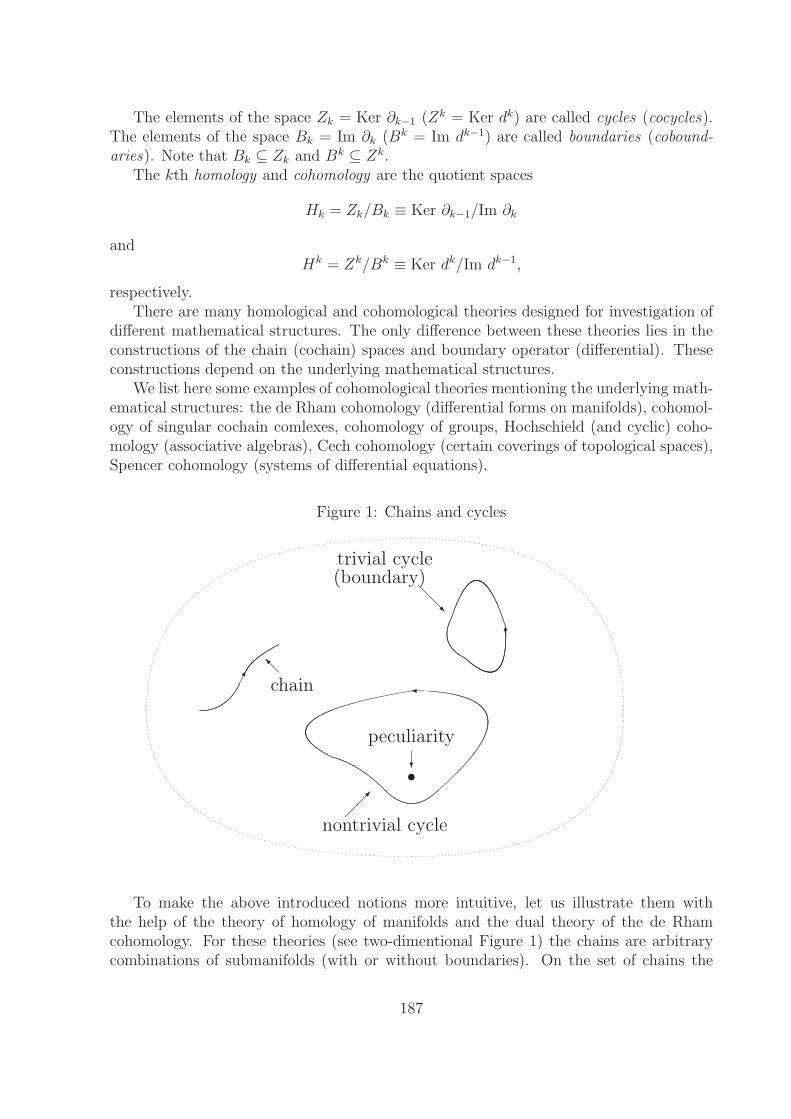
The elements of the space Zk = Ker ∂k−1 (Zk = Ker dk) are called cycles (cocycles).The elements of the space Bk = Im ∂k (Bk = Im dk−1) are called boundaries (cobound-aries). Note that Bk ⊆ Zk and Bk ⊆ Zk.
The kth homology and cohomology are the quotient spaces
Hk = Zk/Bk ≡ Ker ∂k−1/Im ∂k
andHk = Zk/Bk ≡ Ker dk/Im dk−1,
respectively.There are many homological and cohomological theories designed for investigation of
different mathematical structures. The only difference between these theories lies in theconstructions of the chain (cochain) spaces and boundary operator (differential). Theseconstructions depend on the underlying mathematical structures.
We list here some examples of cohomological theories mentioning the underlying math-ematical structures: the de Rham cohomology (differential forms on manifolds), cohomol-ogy of singular cochain comlexes, cohomology of groups, Hochschield (and cyclic) coho-mology (associative algebras), Cech cohomology (certain coverings of topological spaces),Spencer cohomology (systems of differential equations).
Figure 1: Chains and cycles
�� chain��
�
peculiarity
�
�
trivial cycle(boundary)
���
�
nontrivial cycle
To make the above introduced notions more intuitive, let us illustrate them withthe help of the theory of homology of manifolds and the dual theory of the de Rhamcohomology. For these theories (see two-dimentional Figure 1) the chains are arbitrarycombinations of submanifolds (with or without boundaries). On the set of chains the
187
structure of abelian group (and even of linear space) is imposed in some appropriateway. The cycles are combinations of submanifolds without boundaries. Some of thecycles contain peculiarities within. These cycles are called non-trivial and just they aretopologically interesting. To single out these non-trivial cycles up to the trivial ones(boundaries), one should construct the corresponding quotient space. The dual elementsto the chains, cochains, are exterior forms of different degrees on the manifold and thedifferential is the exterior differential acting on these forms. The duality for this pairof theories is provided by the generalized Stokes’ theorem stating that the integral ofdifferential of form over the manifold is equal to the integral of form over the boundaryof manifold:
∫M
dω =∫
∂Mω. (This theorem generalizes the well known theorems of the
integral calculus given by Newton–Leibniz, Stokes, Gauss-Ostrogradski etc.)The cohomology of the Lie (super)algebra A in the module X is defined via cochain
complex (2) in which (see, e. g., [1]) the cochain spaces Ck = Ck(A; X) consist ofsuperskewsymmetric k-linear mappings A × · · · × A → X, C0 = X by definition. Super-skewsymmetry means symmetry with respect to swapping of two adjacent odd cochainarguments and antisymmetry for any other combination of parities for adjacent pair.
The differential dk takes the form
(dkc)(a0, . . . , ak) = −∑
0≤i<j≤k
(−1)s(ai)+s(aj)+p(ai)p(aj)c([ai, aj], ao, . . . , ai, . . . , aj, . . . , ak)
−∑
0≤i≤k
(−1)s(ai)aic(ao, . . . , ai, . . . , ak), (3)
where the functions c(. . .) are elements of cochain spaces; ai ∈ A; p(ai) is the parity of ai;s(ai) = i, if ai is even element and s(ai) is equal to the number of even elements in thesequence a0, . . . , ai−1, if ai is odd element. In the case of trivial module (i.e., if ax = 0 forall a ∈ A and x ∈ X) one uses as a rule the notation Hk(A).
In papers [2, 3, 4, 5] we presented an algorithm for computation of Lie (super)algebracohomologies. These papers contain also description of its C implementation and someresults obtained with the help of codes designed. This algorithm computes cohomologyof Lie (super)algebra A over module X in a straightforward way, i. e., for cochain com-plex (2) the algorithm constructs the full set of basis monomials forming the space Ck,generates subsequently all basis monomials in the space Ck+1, computes the differentialscorresponding to these monomials to obtain the set of linear equations determining thespace of cocycles
Zk = Ker dk = {Ck | dCk = 0}, (4)
constructs the space of coboundaries
Bk = Im dk−1 = {Ck | Ck = dCk−1}. (5)
Finally, the algorithm constructs the basis elements of quotient space
Hk(A; X) = Zk/Bk. (6)
This last step is based on the Gauss elimination procedure.
188
The main difficulty in computing cohomology comes from the very high dimensions ofthe spaces Ck: for n-dimensional ordinary Lie algebra and p-dimensional module
dim Ck = p(n
k
),
and for (n|m)-dimensional Lie superalgebra
dim Ck = p(n
k
)+ p
k∑i=1
( nk − i
)(m + i − 1i
).
In many cases it is possibly to extract some easier to handle subcomplexes of the fullcochain complex (2). The partition of cochain complex for a graded algebra and moduleinto homogeneous components is a typical example. In many papers (see, e. g., [6, 7, 8])more special subcomplexes were used successfully to obtain new results in the theory ofcohomology of Lie (super)algebras.1
The main idea of the new algorithms presented in this paper is to extract the minimalpossible (in the sense explained below) subcomplexes from complex (2) and to carrycomputations within these subcomplexes.
2 Description of Algorithms
In this section we describe shortly two algorithms: ComputeCohomology and Search-Cohomology. The algorithm ComputeCohomology is applicable to the cases whenit is possible to handle the full space of cochains Ck, i. e., dim Ck should be moderateenough to keep the basis of Ck in the memory of a computer. This algorithm allows toobtain the full set of basis elements of cohomology for a given cochain complex.
On the other hand, the algorithm SearchCohomology allows to obtain partial in-formation about cohomology, i.e., to search for some cohomological classes, in high-dimensional complexes. In some cases this algorithm can be applied even to infinite-dimensional complexes.
The input data for both algorithms should include:
1. The Lie (super)algebra A over the module X. A and X should be presented as setsof basis elements, their commutator and action tables. Our C implementation of thealgorithms is able to construct these basis elements and tables for most importantalgebras and modules.
2. Integer non-negative number k, which is the degree (or dimension) of cohomology.
3. Integer number g giving the grade of cohomology. Most important algebras andmodules are graded (if not, one can always prescribe zero grade to all elements ofalgebra and module) and this grading induces grading in the cohomology.
1The main trick consists in imposing some restrictions on the elements of Ck and proving the invarianceof these restrictions with respect to the differential.
189
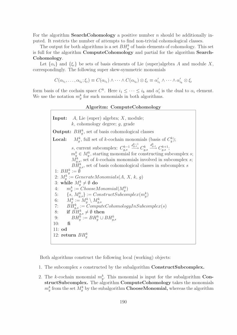
For the algorithm SearchCohomology a positive number n should be additionally in-puted. It restricts the number of attempts to find non-trivial cohomological classes.
The output for both algorithms is a set BHkg of basis elements of cohomology. This set
is full for the algorithm ComputeCohomology and partial for the algorithm Search-Cohomology.
Let {αi} and {ξι} be sets of basis elements of Lie (super)algebra A and module X,correspondingly. The following super skew-symmetric monomials
C(αi1 , . . . , αik ; ξι) ≡ C(αi1) ∧ · · · ∧ C(αik) ⊗ ξι ≡ α′i1∧ · · · ∧ α′
ik⊗ ξι
form basis of the cochain space Ck. Here i1 ≤ · · · ≤ ik and α′i is the dual to αi element.
We use the notation mkg for such monomials in both algorithms.
Algoritm: ComputeCohomology
Input: A, Lie (super) algebra; X, module;k, cohomology degree; g, grade
Output: BHkg , set of basis cohomological classes
Local: Mkg , full set of k-cochain monomials (basis of Ck
g );
s, current subcomplex: Ck−1g,s
dk−1g,s−→ Ck
g,s
dkg,s−→ Ck+1
g,s ;mk
g ∈ Mkg , starting monomial for constructing subcomplex s;
Mkg,s, set of k-cochain monomials involved in subcomplex s;
BHkg,s, set of basis cohomological classes in subcomplex s
1: BHkg := ∅
2: Mkg := GenerateMonomials(A, X, k, g)
3: while Mkg = ∅ do
4: mkg := ChooseMonomial(Mk
g )5: {s, Mk
g,s} := ConstructSubcomplex(mkg)
6: Mkg := Mk
g \ Mkg,s
7: BHkg,s := ComputeCohomologyInSubcomplex(s)
8: if BHkg,s = ∅ then
9: BHkg := BHk
g ∪ BHkg,s
10: fi11: od12: return BHk
g
Both algorithms construct the following local (working) objects:
1. The subcomplex s constructed by the subalgorithm ConstructSubcomplex.
2. The k-cochain monomial mkg . This monomial is input for the subalgorithm Con-
structSubcomplex. The algorithm ComputeCohomology takes the monomialsmk
g from the set Mkg by the subalgorithm ChooseMonomial, whereas the algorithm
190
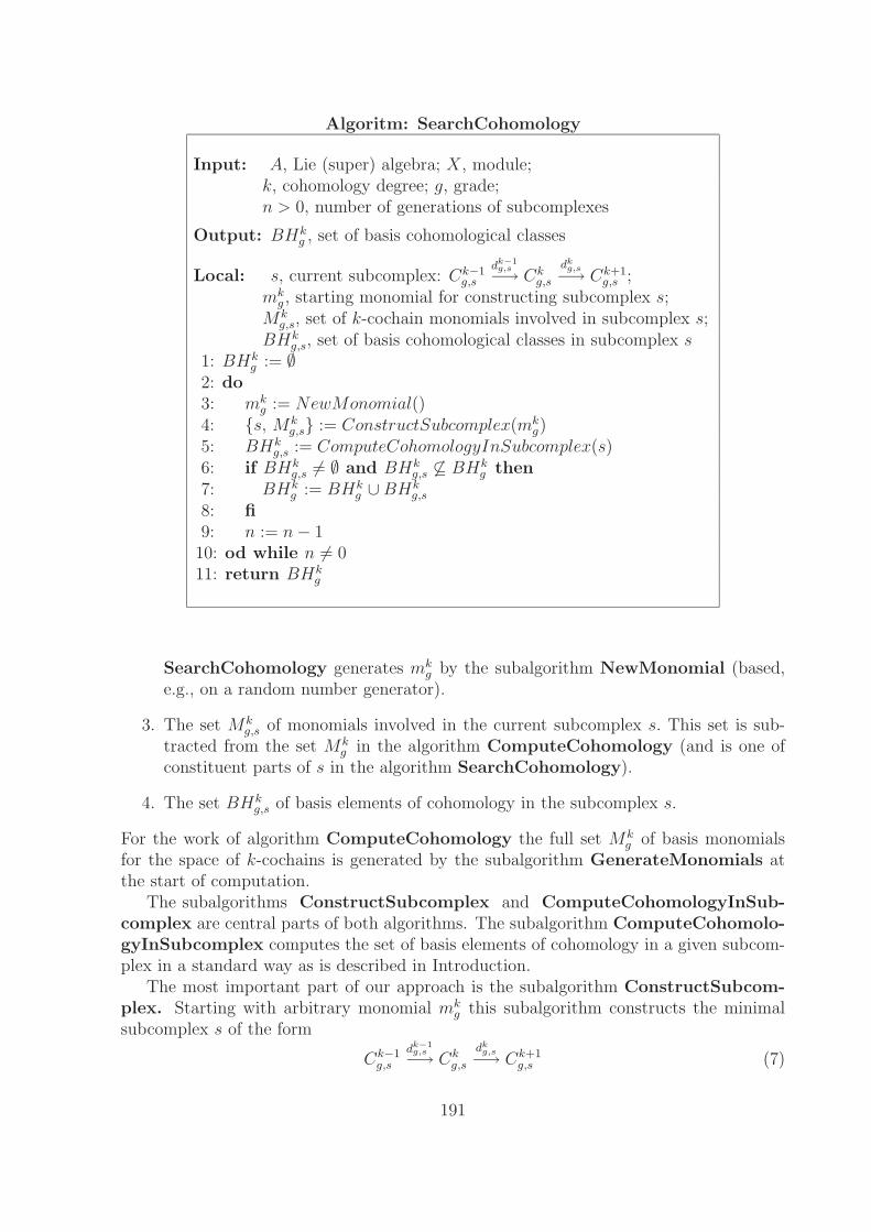
Algoritm: SearchCohomology
Input: A, Lie (super) algebra; X, module;k, cohomology degree; g, grade;n > 0, number of generations of subcomplexes
Output: BHkg , set of basis cohomological classes
Local: s, current subcomplex: Ck−1g,s
dk−1g,s−→ Ck
g,s
dkg,s−→ Ck+1
g,s ;mk
g , starting monomial for constructing subcomplex s;Mk
g,s, set of k-cochain monomials involved in subcomplex s;BHk
g,s, set of basis cohomological classes in subcomplex s1: BHk
g := ∅2: do3: mk
g := NewMonomial()4: {s, Mk
g,s} := ConstructSubcomplex(mkg)
5: BHkg,s := ComputeCohomologyInSubcomplex(s)
6: if BHkg,s = ∅ and BHk
g,s ⊆ BHkg then
7: BHkg := BHk
g ∪ BHkg,s
8: fi9: n := n − 1
10: od while n = 011: return BHk
g
SearchCohomology generates mkg by the subalgorithm NewMonomial (based,
e.g., on a random number generator).
3. The set Mkg,s of monomials involved in the current subcomplex s. This set is sub-
tracted from the set Mkg in the algorithm ComputeCohomology (and is one of
constituent parts of s in the algorithm SearchCohomology).
4. The set BHkg,s of basis elements of cohomology in the subcomplex s.
For the work of algorithm ComputeCohomology the full set Mkg of basis monomials
for the space of k-cochains is generated by the subalgorithm GenerateMonomials atthe start of computation.
The subalgorithms ConstructSubcomplex and ComputeCohomologyInSub-complex are central parts of both algorithms. The subalgorithm ComputeCohomolo-gyInSubcomplex computes the set of basis elements of cohomology in a given subcom-plex in a standard way as is described in Introduction.
The most important part of our approach is the subalgorithm ConstructSubcom-plex. Starting with arbitrary monomial mk
g this subalgorithm constructs the minimalsubcomplex s of the form
Ck−1g,s
dk−1g,s−→ Ck
g,s
dkg,s−→ Ck+1
g,s (7)
191
involving the monomial mkg . The subalgorithm ConstructSubcomplex is based on
formula (3) for the differential dk. This formula is a set of linear relations connecting k-and (k + 1)-monomials. The relations containing the monomial mk
g contains also othermonomials and we can add into consideration the relations for these monomials. Aftersuch connected relations for k-monomials are all constructed we should carry out ananalogous procedure with the differential dk−1. This can lead (in practice, fairly rare)to appearance of new k-monomials and then we should return to the procedure for thedifferential dk. This cyclic process terminates if any given basis element αi of algebraappears only in a finite number of the right hand parts of commutators and similarproperty (with respect to action of algebra on module) holds for basis elements of moduleξι. Note that the subalgorithm ConstructSubcomplex can construct finite-dimensionalsubcomplexes in some cases when grading does not allow finite-dimensional subcomplexes,e. g., when computing cohomology in adjoint module for infinite-dimensional gradedLie (super)algebras. Note also that the subcomplexes constructed by the subalgorithmConstructSubcomplex are not invariant, i. e., they depend on the choice of bases foralgebra and module, and they, apparently, not always can be extended to full sequence (2)in such a way that part (7) remains unchanged, but for our purposes this is not important.
3 Examples:
Computation of H3(Poincare(1, 3)) and H3(SH(0|4))
Both examples of computations in this section are carried out in zero grade complexes andwe shall omit subscripts g = 0 everywhere below. As the first example we consider com-putation of third cohomology in the trivial module for 10-dimensional Poincare algebra.The basis of this algebra contains the following generators of: translations P0, P1, P2, P3;rotations R1, R2, R3; Lorentz transformations L1, L2, L3. The commutator table for thePoincare algebra takes the form:
[Pμ, Pν ] = 0, μ, ν = 0, . . . , 3;
[P0, Li] = Pi, [Pi, Lj] = δijP0, [Pi, Rj] = εijkPk,
[Ri, Rj] = εijkRk, [Ri, Lj] = εijkLk, [Li, Lj] = −εijkRk, i, j, k = 1, . . . , 3.
Here εijk is the permutation symbol with ε123 = 1.We consider the part
C2 d2−→ C3 d3−→ C4 (8)
of cochain complex (2). The spaces of cochains have the following dimensions
dim C2 = 45, dim C3 = 120, dim C4 = 210.
The system of equations for 3-cocycles d3(C3) = 0 contains initially 187 equations for 120variables. The Gauss elimination process shows that the rank of this system is equal to83, i. e., the 3-cocycles form 37-dimensional subspace in 120-dimensional space C3. Theexpressions d2(C2) determine parametrically 35-dimensional subspace of coboundaries in
192
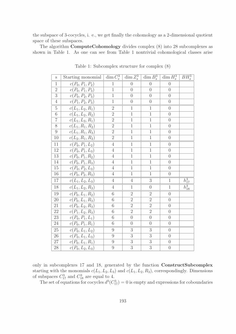
the subspace of 3-cocycles, i. e., we get finally the cohomology as a 2-dimensional quotientspace of these subspaces.
The algorithm ComputeCohomology divides complex (8) into 28 subcomplexes asshown in Table 1. As one can see from Table 1 nontrivial cohomological classes arise
Table 1: Subcomplex structure for complex (8)
s Starting monomial dim C3s dim Z3
s dim B3s dim H3
s BH3s
1 c(P0, P1, P2) 1 0 0 02 c(P0, P1, P3) 1 0 0 03 c(P0, P2, P3) 1 0 0 04 c(P1, P2, P3) 1 0 0 0
5 c(L1, L2, R1) 2 1 1 06 c(L1, L2, R2) 2 1 1 07 c(L1, L3, R1) 2 1 1 08 c(L1, R1, R2) 2 1 1 09 c(L1, R1, R3) 2 1 1 010 c(L2, R1, R2) 2 1 1 0
11 c(P0, P1, L2) 4 1 1 012 c(P0, P1, L3) 4 1 1 013 c(P0, P1, R2) 4 1 1 014 c(P0, P1, R3) 4 1 1 015 c(P0, P2, L3) 4 1 1 016 c(P0, P2, R3) 4 1 1 0
17 c(L1, L2, L3) 4 4 3 1 h317
18 c(L1, L2, R3) 4 1 0 1 h318
19 c(P0, L1, R2) 6 2 2 020 c(P0, L1, R3) 6 2 2 021 c(P0, L2, R3) 6 2 2 022 c(P1, L2, R3) 6 2 2 023 c(P0, P1, L1) 6 0 0 024 c(P0, P1, R1) 6 0 0 0
25 c(P0, L1, L2) 9 3 3 026 c(P0, L1, L3) 9 3 3 027 c(P0, L1, R1) 9 3 3 028 c(P0, L2, L3) 9 3 3 0
only in subcomplexes 17 and 18, generated by the function ConstructSubcomplexstarting with the monomials c(L1, L2, L3) and c(L1, L2, R3), correspondingly. Dimensionsof subspaces C3
17 and C318 are equal to 4.
The set of equations for cocycles d3(C317) = 0 is empty and expressions for coboundaries
193
d2(C217) take the form
c(L1, L2, L3) = −c(L1, R1) − c(L2, R2) − c(L3, R3),
c(L1, R2, R3) = c(L1, R1) − c(L2, R2) − c(L3, R3),
c(L2, R1, R3) = c(L1, R1) − c(L2, R2) + c(L3, R3),
c(L3, R1, R2) = −c(L1, R1) − c(L2, R2) + c(L3, R3),
where 2-cochains should be treated as arbitrary parameters. These relations determine3-dimensional subspace and basis element h3
17 of cohomology for subcomplex 17 can beexpressed in the form h3
17 = c(L1, L2, L3) − c(L1, R2, R3) + c(L2, R1, R3) − c(L3, R1, R2).For subcomplex 18 equations d3(C3
18) = 0 determining cocycles take the form
c(L1, L2, R1, R2) = −c(L1, L2, R3) − c(L1, L3, R2) + c(L2, L3, R1) + c(R1, R2, R3) = 0,
c(L1, L3, R1, R3) = c(L1, L2, R3) + c(L1, L3, R2) + c(L2, L3, R1) + c(R1, R2, R3) = 0,
c(L2, L3, R2, R3) = c(L1, L2, R3) − c(L1, L3, R2) − c(L2, L3, R1) + c(R1, R2, R3) = 0.
This system of equations determines 1-dimensional subspace. Expressions for cobound-aries d2(C2
18) determine 0-dimensional subspace taking the form
c(L1, L2, R3) = c(L1, L3, R2) = c(L2, L3, R1) = c(R1, R2, R3) = 0,
and basis element h318 of cohomology can be chosen as h3
18 = c(R1, R2, R3) or as linearcombination
h318 = αc(R1, R2, R3) + βc(L1, L2, R3) + γc(L1, L3, R2) + δc(L2, L3, R1),
with α − β + γ − δ = 0.Let us consider also an example of computation that is typical for Lie superalgebras.
Computation of the third cohomology in the trivial module and in zero grading for specialHamiltonian algebra SH(0|4) is a task of approximately the same complexity as in theabove example with the Poincare algebra. The (6|8)-dimensional superalgebra SH(0|4) hasthe following even E1 = θ1θ2, E2 = θ1θ3, E3 = θ2θ3, E4 = θ1θ4, E5 = θ2θ4, E6 = θ3θ4
and odd O1 = θ1, O2 = θ2, O3 = θ3, O4 = θ4, O5 = θ1θ2θ3, O6 = θ1θ2θ4, O7 =θ1θ3θ4, O8 = θ2θ3θ4 basis elements. Here θ1, θ2, θ3, θ4 are Grassmann variables andLie product coincides with Poisson bracket {·, ·}Pb. For this particular case {f, g}Pb =−(−1)p(f)Σ4
i=1∂f/∂θi∂g/∂θi, where f and g are functions of θ1, . . . θ4 and p(f) is parityof function f . In the case of Lie superalgebra cochain complex can be split into twosubcomplexes, even and odd. In our example only even subspace of C3 contains nontrivialcocycle. The spaces of even subcomplex have the following dimensions
dim C2 = 31, dim C3 = 116, dim C4 = 355.
The initial number of determining equations for 3-cocycles is equal to 351. This system ofequations determines 25-dimensional space of cocycles. The expressions for coboundariesdescribe 24-dimensional subspace, hence the cohomology is 1-dimensional.
194
The algorithm ComputeCohomology generates eight subcomplexes. Six of themhave the following characteristics:
dim C3s = 14, dim Z3
s = dim B3s = 3, dim H3
s = 0.
There are also two subcomplexes with dimC3s = 16, one of them has dim Z3
s = dim B3s =
dim H3s = 0. And finally, the remaining subcomplex (with 30 equations for 3-cocycles)
contains 1-dimensional cohomology: dimZ3s = 7, dim B3
s = 6, dim H3s = 1. We do not
present here the basis element of this cohomology explicitly because its expression israther long.
4 Conclusion
As one can see from the two above, chosen at random, examples, cochain complexescan be effectively divided into smaller subcomplexes. One can show that generally theefficiency of such division grows with increase of cochain degree k, i. e., the dimensionsof subcomplexes grow slower than the dimension of full complex. We are implementingthe algorithms ComputeCohomology and SearchCohomology as different regimes ofone C program.
References
[1] Fuks, D.B.: Cohomology of Infinite Dimensional Lie Algebras. Consultants Bureau,New York, 1987.
[2] Kornyak, V.V.: A program for Computing Cohomologies of Lie Superalgebras ofVector Fields. Zapiski nauchnyh seminarov POMI. St.Petersburg. 258 (1999) 148-160.
[3] Kornyak, V.V.: Cohomology of Lie Superalgebras of Hamiltonian Vector Fields:Computer Analysis. In: Computer Algebra in Scientific Computing / CASC’99,V.G.Ganzha, E.W.Mayr and E.V.Vorozhtsov (Eds.), Springer-Verlag, Berlin, 1999,pp. 241-249; math.SC/9906046.
[4] Kornyak, V.V.: Computation of Cohomology of Lie Superalgebras of Vector Fields.Int. J. of Mod. Phys. C. 11 (2000) 397-414; arXiv: math.SC/0002210.
[5] Kornyak, V.V.: Computation of Cohomology of Lie Superalgebras: Algorithm and Im-plementation. Russian Journal for Computer Science (“Programmirovanie”). 3 (2001)46-50 (in Russian).
[6] Gel’fand, I.M., Kalinin, D.I., Fuks, D.B.: On Cohomology of Lie Algebra of Hamilto-nian Formal Vector Fields. Funkts. Anal. Prilozhen. 6 (1972) 25-29 (in Russian).
[7] Perchik, J.: Cohomology of Hamiltonian and related formal vector fields Lie algebras.Topology. 15, 4 (1976) 395-404.
[8] Guillemin, V.M., Shnider, S.D.: Some stable results on the cohomology of classicalinfinite dimensional Lie algebras. Trans. Amer. Math. Soc. 179 (1973) 275-280.
195
Computation of the CharacteristicSets for the Euler Equations for
Different Rankings
N.A. Makarevich
Moscow State University,Faculty of Mechanics and Mathematics, MSU, 119899
e-mail: makarevich−[email protected]
The aim of this study is to investigate the dependence of the characteristic set ofthe system of the Euler equations on the number of the variables and on the ranking.This system is of interest for computation due to a number of reasons. It is one oftreatable systems of nonlinear differential equations and the corresponding differential idealis prime.
At the same time, the results obtained for various rankings are very different. The com-putations were made by the Rosenfeld—Grobner algorithm implemented in CAS MAPLE.This algorithm represents the least radical differential ideal containing initial ideal set bya finite number of differential polynomials as a finite intersection of regular differentialideals Ji:
{Σ} = J1 ∩ · · · ∩ Js
1 Some definitions and notations
Let K be a differential field of characteristic zero with a set of derivationsΔ = {d1, . . . , dm}. Consider the differential ring R = K{y1, . . . , yn}. The order of anoperator θ = d1
i1 . . . dmim is equal to the sum of the exponents ij. We call the yi by letters
and the θyi by derivatives. The degree of a polynomial f ∈ R or deg f is the degree of fas a polynomial in an infinite number of variables θyi and its order ord f is the maximalorder of the derivatives that are present in f .
Let I be an ideal and T be a multiplicatively stable family of R = K{y1, . . . , yn}. Thesymbol I : T stands for the ideal of all elements p of R such as for some t ∈ T the elementtp belongs to I.
A differential ideal I of R = K{y1, . . . , yn}, I = R is said to be prime if for anyp1, p2 ∈ R the inclusion p1p2 ∈ I implies either p1 ∈ I or p2 ∈ I.
A differential ideal I of R = K{y1, . . . , yn} is called radical if the inclusion pn ∈ I(p ∈ R, n is a positive integer) implies the inclusion p ∈ I. The least radical differentialideal containing a finite set Σ ⊂ R is denoted by {Σ}.
A total order R on the set of the derivatives yj is said to be a ranking if the followingconditions hold:
196
1. diθyj >R θyj for all derivations di, all operators θ and all letters yj;
2. θ1yi >R θ2yj ⇒ dkθ1yi >R dkθ2yj for all derivations dk, all operators θ1, θ2 and allletters yi, yj.
Let p ∈ K{y1, . . . , yn}, p /∈ K and R be a ranking. The leader u of p is defined asthe highest derivative with respect to the ranking R that appears in p. Let d denote thedegree of u in p. The initial Ip of p is the coefficient of ud in p. The separant Sp is thepartial derivative of p with respect to u.
Let p and q be two polynomials, u be the leader of p, and d be its degree in p. Thepolynomial q is said to be partially reduced with respect to p if no proper derivative ofu appears in q. The polynomial q is said to be reduced with respect to p if q is partiallyreduced with respect to p and its degree in u is less than d.
A set of polynomials is said to be autoreduced if each element of the set is reducedwith respect to every other its element. Let A be an autoreduced set. Let HA be theproduct of all initials and separants of A. The symbol H∞
A denotes the set of all powersof the element HA.
An autoreduced subset C of a set A of polynomials is called a characteristic set of Aif A contains no non-zero elements reduced with respect to C. A characteristic set C ofan ideal I reduces to zero all elements of I. If the ideal is prime, then C reduces to zeroonly the elements of I and we have I = [C] : H∞
C .Let p and q be two polynomials in an autoreduced set A, whose leaders θ1yi and θ2yi
are derivatives of one and the same letter yi. Let θ be the operator of minimal order,φ1 and φ2 be two derivation operators such that φ1θ1 = φ2θ2 = θ. The Δ-polynomialbetween p and q is the polynomial Δ = Sqφ1p − Spφ2q. A set A is said to be coherent ifit reduces to zero all Δ-polynomials between any two elements of A.
Let Σ be a differential polynomial system of equations and inequations {p1 = 0, . . . ,pk = 0, q1 = 0, . . . , ql = 0}, where pi, qj ∈ K{y1, . . . , yn} for i = 1 . . . k and j = 1 . . . l. Adifferential model of Σ is a morphism of the differential K-algebras K{y1, . . . , yn} → Linto a differential field L that annihilates the equations but not the inequations of Σ.
A system of differential equations and inequations is said to be regular with respectto a ranking R, if the set of its equations is autoreduced and coherent, the initial andseparant of each equation appear among the inequations and if its other inequations arepartially reduced with respect to the equations:
Ω
⎧⎪⎪⎪⎪⎪⎪⎪⎪⎪⎨⎪⎪⎪⎪⎪⎪⎪⎪⎪⎩
p1 = 0... A = {p1, . . . , ps} is autoreduced and coherent
ps = 0I1 = 0
... the initials and separants of pi
Ss = 0q = 0 q is partially reduced w.r.t. A
A differential ideal J is said to be regular if there exists a regular system Ω such asJ = [A] : H∞
Ω , where A is the set of equations of Ω.
197
The input data for the Rosenfeld–Grobner package are a system of differential equa-tions and inequations Σ and a ranking R. Its output is a finite family (Ωi) of consistent(with models) regular systems whose differential models form a partition of the differentialmodels of Σ. Let Ai denote the set of equations for each Ωi and HΩi
be the product ofall inequations of Ωi. Denoting by H∞
Ωithe set of all powers of the HΩi
, we can representthe result of the run of the program as
{Σ} = [A1] : H∞Ω1
∩ · · · ∩ [As] : H∞Ωs
2 Computations
In the case of three space variables, the system of the Euler equations is:
p1 := v1 x1 + v2 x2 + v3 x3
p2 := v1 t + v1 v1 x1 + v2 v1 x2 + v3 v1 x3 + px1
p3 := v2 t + v1 v2 x1 + v2 v2 x2 + v3 v2 x3 + px2
p4 := v3 t + v1 v3 x1 + v2 v3 x2 + v3 v3 x3 + px3
Theorem 1. If A is a coherent autoreduced set such that the ideal (A) : H∞A of
K{y1, . . . , yn} is prime and contains no nonzero elements reduced with respect to A, thenA is a characteristic set of a prime Δ-ideal of the ring K{y1, . . . , yn}.
The proof of this theorem can be found in [2].For t > x1 > x2 > x3, v1 > v2 > v3 > p, and the ordering of total degree then
lexicographic, the set A
p1 := v1 x1 + v2 x2 + v3 x3
p2 := v1 t + v2 v1 x2 + v3 v1 x3 + px1 − v1 v2 x2 − v1 v3 x3
p3 := v2 t + v1 v2 x1 + v2 v2 x2 + v3 v2 x3 + px2
p4 := v3 t + v1 v3 x1 + v2 v3 x2 + v3 v3 x3 + px3
p5 := px1 , x1 + px2 , x2 + px3 , x3 + v2 x1 v1 x2 + 2 v3 x1 v1 x3 + 2 v2 x22
+2 v3 x2 v2 x3 + 2 v3 x32 + 2 v2 x2 v3 x3
satisfies the conditions of the theorem; hence, the ideal corresponding to the system ofthe Euler equations is prime.
For some rankings, the program computes not only the required system whose set ofequations forms the characteristic set of the ideal, but also some redundant components.In this case and in some situations when the direct computations fail, the program allowsone to compute this system using the results obtained for another ranking.
So, the possible situations are the following:
198
1. the characteristic set can be computed directly;
2. the program stops the computation because the arguments of some intermediatefunctions become too large, but the characteristic set can be determined using theresult obtained for another ranking;
3. both attempts of computing the characteristic set fail.
When the initials and separants of a charasteristic set belong to the field of constant,I = [A] and in this case A is an analogue of the Grobner basis, in particular, the elementsof A and their derivatives generate the ideal.
Three cases of the Euler equations are considered: with one, two, and three spacevariables. It is natural that the first case is the simplest one. The initial system is:
vx, vt + vvx + px.
After reducing the second equation with respect to the first one, the system becomeslinear and the program computes the Grobner basis of the system. Due to its specialform, the basis can be obtained for any ranking and it is equal either to
vx, vt + px, pxx
or tovx, px + vt.
The cases of two and three space variables are much more complicated. For two spacevariables, the initial system is:
p1 := v1 t + v1 v1 x + v2 v1 y + px
p2 := v2 t + v1 v2 x + v2 v2 y + py
p3 := v1 x + v2 y
The system is symmetric with respect to the space variables; therefore, we can excludesome orders on the letters and derivations from consideration. For the order of total degreethen lexicographic, the results are obtained directly. Nevertheless, they depend on theorder of derivatives. If t > x > y, then in both cases p > v1 > v2 and v1 > v2 > predundant components appear.
If x > y > t, v1 > v2 > p, then we obtain
P := [regular , regular , regular ]
[[v1 v2 px, x + v1 v2 py, y + 2 v2 t v1 t + 2 v2 t px − 2 v2 t v2 y v1 + 2 v2 v2 y v1 t
+ 2 v2 v2 y px + 2 py v1 t + 2 py px − 2 py v2 y v1 , v1 x + v2 y,
v1 t + v2 v1 y + px − v2 y v1 , v2 t + v1 v2 x + v2 v2 y + py],
[px, x, v1 x, v1 t + px, py, v2 ], [py, y, v2 y, v2 t + py, px, v1 ]]
199
However, if t > x > y and v1 > v2 > p, then we have only one component
[[2 v2 x v1 y + px, x + 2 v2 y2 + py, y, v1 t + v2 v1 y + px − v2 y v1 , v1 x + v2 y,
v2 t + v1 v2 x + v2 v2 y + py]]
For the ranking where the derivatives di11 . . . din
n yj are ordered in the lexicographicalorder of the vectors (i1, . . . , in, j), the situation is the same. If t > x > y, then wedirectly obtain the characteristic sets which are quite simple. If x > y > t, then we obtainredundant components.
1. The case x > y > t and p > v1 > v2:
J := [regular , regular ]
[[v1 t + v2 v1 y + px − v2 y v1 , v1 x + v2 y, v2 t + v1 v2 x + v2 v2 y + py],
[v2 x, t, px, v2 t + py, v2 y, v1 ]]
2. The case t > x > y and p > v1 > v2:
[[v1 t + v2 v1 y + px − v2 y v1 , v2 t + v1 v2 x + v2 v2 y + py,
2 v2 x v1 y + px, x + 2 v2 y2 + py, y, v1 x + v2 y]]
The worst case is the case of the lexicographical order. Neither direct computations,nor computations using previous results can handle this system.
In the case of three space variables, one of the simplest sets corresponds to the orderof total degree then lexicographic, t > x1 > x2 > x3 and v1 > v2 > v3 > p. This casewas considered earlier. The output of the program is
[[2 v2 x1 v1 x2 + 2 v3 x1 v1 x3 + px1 , x1 + 2 v2 x22 + 2 v3 x2 v2 x3 + px2 , x2 + 2 v3 x3
2
+px3 , x3 + 2 v2 x2 v3 x3 , v1 t + v2 v1 x2 + v3 v1 x3 + px1 − v1 v2 x2 − v1 v3 x3 ,v1 x1 + v2 x2 + v3 x3 , v2 t + v1 v2 x1 + v2 v2 x2 + v3 v2 x3 + px2 ,v3 t + v1 v3 x1 + v2 v3 x2 + v3 v3 x3 + px3 ]]
Unlike the case of two space variables, if we change the order of derivatives for x1 >x2 > x3 > t, then the characteristic sets cannot be obtained directly, but can be computedwith the help of the previous results:
[[2 v2 v3 v1 x3 v2 x2 − 2 v1 v2 t v2 x2 − 2 v2 v3 v3 x3 v1 x3 + 2 v2 v1 t v2 x2
− 2 v1 v3 v2 x3 v3 x3 + 2 v2 v1 v3 x2 v2 x3 − 2 v1 v3 v2 x3 v2 x2
− 2 v1 px2 v3 x3 + 2 v2 v1 v3 x32 + v2 v1 px2 , x2 + 2 v3 2 v2 x3 v1 x3
+ 2 v3 v2 x3 px1 + 2 px2 v3 v1 x3 + 2 v2 t v3 v1 x3 − 2 v1 px2 v2 x2
+ v2 v1 px3 , x3 − 2 v1 v2 t v3 x3 − 2 v2 v1 x3 px3 + 2 v3 v2 x3 v1 t
+ 2 v2 v2 x2 px1 + v2 v1 px1 , x1 − 2 v2 v3 t v1 x3 − 2 v2 2 v3 x2 v1 x3 + 2 px2 px1
+ 2 px2 v1 t + 2 v2 t px1 + 2 v2 t v1 t, v1 x1 + v2 x2 + v3 x3 ,v1 t + v2 v1 x2 + v3 v1 x3 + px1 − v1 v2 x2 − v1 v3 x3 ,v2 t + v1 v2 x1 + v2 v2 x2 + v3 v2 x3 + px2 ,v3 t + v1 v3 x1 + v2 v3 x2 + v3 v3 x3 + px3 ]]
200
The result in the case, where p > v1 > v2 > v3 and t > x1 > x2 > x3, just as in thefirst case, can be obtained directly; however, its size is quite large:
[[−v2 x1 v3 x1 , x3 − v2 x1 v1 x2 , x2 + v1 v2 x1 , x2 , x2 − v2 x2 v2 x1 , x1 − v2 x2 v2 x2 , x2
− v2 x2 v3 x2 , x3
+ v1 v2 x1 , x1 , x1 + v1 v3 x1 , x2 , x3 + v3 v2 x1 , x1 , x3 + v1 x2 v3 x1 , x3 + 2 v3 x1 v2 x1 , x3
+ v3 x1 , x1 v2 x3 − 2 v2 x1 , x1 v3 x3 + v2 x1 v2 x1 , x2 − v3 x1 v1 x2 , x3 − 2 v3 x3 v2 x2 , x2
+ v2 v2 x2 , x2 , x2 + v3 x2 v2 x2 , x3 + v2 v3 x2 , x2 , x3 + v3 v2 x2 , x2 , x3 + v3 v3 x2 , x3 , x3
+ v2 v2 x1 , x1 , x2 − 2 v3 x3 v3 x2 , x3 − v3 x1 , x2 v1 x3 + v3 x2 v3 x3 , x3 + v2 t, x2 , x2
+v2 t, x1 , x1
+ v3 t, x2 , x3 , v3 x1 v1 x2 , x2 + v2 v3 x2 , x3 , x3 + v3 x1 v3 x1 , x3 + v3 t, x2 , x2 + v3 t, x1 , x1
+ v3 t, x3 , x3 + v3 x2 , x2 v3 x3 − v3 x2 v2 x3 , x3 − v3 x3 v3 x3 , x3 − v3 x3 v3 x1 , x1
+v3 v3 x3 , x3 , x3
− 4 v2 x2 , x3 v2 x2 − 2 v2 x2 v3 x3 , x3 + v2 x1 , x1 v3 x2 − v3 x1 v2 x1 , x2 − 2 v3 x1 , x1 v2 x2
− v3 x1 v1 x3 , x3 − 2 v2 x1 v1 x2 , x3 + v2 v3 x1 , x1 , x2 + 2 v2 x1 v3 x1 , x2 − 2 v2 x1 , x3 v1 x2
+ v1 v3 x1 , x3 , x3 + v1 v3 x1 , x1 , x1 + v3 v3 x1 , x1 , x3 + 2 v2 x2 v3 x2 , x2
+ v2 v3 x2 , x2 , x2 − 2 v3 x3 v2 x2 , x3 + v1 v3 x1 , x2 , x2 + v3 v3 x2 , x2 , x3 + 2 v3 x2 v3 x2 , x3
+ 2 v3 x1 , x2 v1 x2 + v2 x2 , x2 v3 x2 , v1 t, x2 + v2 v1 x2 , x2 + v3 x2 v1 x3 + v3 v1 x2 , x3
− v1 v2 x2 , x2 − v1 x2 v3 x3 − v1 v3 x2 , x3 − v2 t, x1 − v1 v2 x1 , x1 − v2 v2 x1 , x2
− v3 x1 v2 x3 − v3 v2 x1 , x3 + v2 x1 v3 x3 , v1 t, x3 + v2 x3 v1 x2 + v2 v1 x2 , x3
+ v3 v1 x3 , x3 − v1 x3 v2 x2 − v1 v2 x2 , x3 − v1 v3 x3 , x3 − v3 t, x1 − v1 v3 x1 , x1
− v2 x1 v3 x2 − v2 v3 x1 , x2 − v3 v3 x1 , x3 + v3 x1 v2 x2 , v2 t, x3 + v1 x3 v2 x1
+ v1 v2 x1 , x3 + v2 x3 v2 x2 + v2 v2 x2 , x3 + v3 x3 v2 x3 + v3 v2 x3 , x3 − v3 t, x2
− v3 x1 v1 x2 − v1 v3 x1 , x2 − v2 x2 v3 x2 − v2 v3 x2 , x2 − v3 x2 v3 x3 − v3 v3 x2 , x3 ,v1 t + v2 v1 x2 + v3 v1 x3 + px1 − v1 v2 x2 − v1 v3 x3 ,v2 t + v1 v2 x1 + v2 v2 x2 + v3 v2 x3 + px2 ,v3 t + v1 v3 x1 + v2 v3 x2 + v3 v3 x3 + px3 , v1 x1 + v2 x2 + v3 x3 ]]
Changing the order t > x1 > x2 > x3 for x1 > x2 > x3 > t, we obtain themost difficult case among the computable ones. It cannot be computed directly. Thecharacteristic set consists of only 9 differential polynomials, but they have 81, 34, 14, 13,6, 5, 5, and 3 terms, respectively, and occupy about three pages and a half.
For the ranking where the derivatives di11 . . . din
n yj are ordered in the lexicographicalorder of the vectors (i1, . . . , in, j), the computations are quite similar to the case of twospace variables; i.e., the same as for the order of total degree then lexicographic. Thecomputation complexity depends only on the order of the derivatives: if t > x1 > x2 > x3,then the basis is obtained directly; if x1 > x2 > x3 > t, then results for another rankingshould be used. But, in this case, the set itself has a very simple form, even simpler thanin the first case considered. However, in that case the computation time is short and theresults can be obtained directly. If x1 > x2 > x3 > t and p > v1 > v2 > v3, then the setconsists only of the reduced initial polinomials:
[[v1 t + v2 v1 x2 + v3 v1 x3 + px1 − v1 v2 x2 − v1 v3 x3 , v1 x1 + v2 x2 + v3 x3 ,v2 t + v1 v2 x1 + v2 v2 x2 + v3 v2 x3 + px2 ,v3 t + v1 v3 x1 + v2 v3 x2 + v3 v3 x3 + px3 ]]
201
However, it cannot be obtained directly.Finally, for the lexicographical order, we did not manage to obtain any results even in
the case of two space variables.In conclusion I would like to express my gratitude to my scientific adviser E.V.
Pankratiev for valuable remarks while preparing this paper.
References
[1] F. Boulier, D. Lazard, F. Ollivier, M. Petitot ”Representation for the radical of afinitely generated differential ideal”, ISSAC 1995, AMC Press, 158-166
[2] M.V. Kondratieva, A.B. Levin, A.V. Mikhalev, E.V. Pankratiev ”Differential andDifference Dimension Polynomials”, 1999, Kluwer Academic Publishers
202
Computer Algebra with Haskell:Applying
Functional-Categorial-‘Lazy’Programming
Serge D. Mechveliani
Program Systems Institute,Pereslavl-Zalessky, Russia;e-mail: [email protected]
We give an outline of a computer algebra program written in a functional languageHaskell and implementing certain piece of commutative algebra.
1 Introduction
The project of algebraic Domain Constructor DoCon [Me1] has grown into somewhatan advanced system: permutations, linear algebra, polynomial arithmetics, GCD, factor-ization, Grobner bases, symmetric functions package, and some other tools.
It is written in Haskell language [Ha] (Miranda family), which we declare as sup-porting the FTCL approach: Functional-Typeful-Categorial-LazyEvaluation style in pro-gramming.
Also certain simplified version is presented as the BAL program [Me2] — basic algebralibrary for Haskell. For anyone going to deal with DoCon we recommend to read first thepaper [Me2] discussing the main points of Haskell’s relation to computer algebra.
Why designing another CA system, is not the Axiom program [Je] sufficient?I experimented with the FTCL approach because (a) of importance of pure func-
tionality, (b) of ‘lazy’ evaluation elegance, (c) I aimed to study the question of fitnessto programming of mathematics of several known languages: Refal, ML, Haskell, term-rewriting logical languages . . . (d) for maintainability, free-with-source program tools,described at all levels, are preferable.
And Haskell does provide several free-with-source implementations, among which therecent DoCon exploits GHC [GH].
DoCon is a program package. The general notions of a class, instance, polymor-phic type, and such — are of the Haskell language. And DoCon is a library of particularalgebraic categories, their instances and other items.
The functionality feature allows to treat a program (brought to internal form) assymbolic expression, like say, a polynomial in mathematics. This enables (in principle)the compiler to simplify such a program symbolically.
But it was often said that functional programming reduces the efficiency, that thereis a necessity to use a pointer, a mutable array, and so on.
203
DoCon tries to shows that pure functionality and ‘lazy’ evaluation are practicable.The benchmarks reveal a good performance. These tests are described in the Section’pe’ of DoCon Manual [Me1]; they compare the CA programs DoCon-2.02, Axiom-2.2,MuPAD-1.4.2 on several algorithmically complex tasks.
We also discuss the design difficulties (Section 6). The most important one is, prob-ably, common to all ‘typeful’ systems and concerns modelling a domain depending ona dynamic value. With existing Haskell, we find certain way out in a sample argumentapproach — see Section 4.
Acknowledgements. The author is grateful to Dr. S.V.Duzhin for his administra-tive support of the project, Russian Foundation for Basic Research (grant 98-01-00980)andINTAS foundation (coordinator Professor B.Jacob) — for some part of DoCon was sup-ported by these grants, CA center MEDICIS <http//www.medicis.polytechnique.fr>
for making it possible to compare the chosen CA systems on one computer.
2 Mathematics implemented in DoCon-2.02
DoCon-2.02 includes in its functionality:Methods:
Permutation group: composition, inversion, decomposition to cycles.Fraction field over a gcd-ring: its arithmetic.Linear algebra over an Euclidean domain: vector, matrix arithmetic (dense form), reduc-tion to staircase and diagonal form of matrix, solving a system.Polynomial arithmetic and g.c.d. in P = R[x1, . . . , xn], R a commutative ring. Fourpossible representations for P , free module over P and symmetric functions are given bythe constructors UPol, Pol, RPol, EPol, SymPol; factorization in k[x, y], k a finitefield.Grobner basis, normal form, syzygy generators functions for P = R[x1, . . . , xn], R anEuclidean ring, and in a free module over P [Bu, Mo, MoM].Symmetric function package: decomposition into elementary symmetrics, to other bases,operations with partitions [16].
Category hierarchy expressed partially via the data classes of Haskell:Set, Semigroup, Group, Ring, LinSolvRing . . . LeftModule . . . ,some operations with the description terms of Subset, Subgroup, Subring, Ideal.
Domain constructors: Permutation; Fraction field for a gcd-ring, Residue ringby the ideal, and others.
Property processing: evaluation of certain small number of important algebraicdomain property values is supported: Finite, IsCyclicGroup, FactorialRing, and thesuch. They serve as the correctness conditions for various methods, besides, present animportant information by themself.
But many users need to do approximate computations, compute with differential op-erators, integration, and so on. With this respect, we point out that DoCon-2.02 is afree-with-source program that can be taken as basis and developed by adding user li-braries.
204
3 About Haskell language
The main Haskell features are:(F) pure functionality and high-order functions, (L) ‘lazy’ model of evaluation,(M) evaluation by pattern matching is widely usable,(T) recursive polymorphic parametric types with user-defined constructors, polymorphicfunctions, Hindley-Milner type system with static type resolution,(C) categorial approach to types.
We could provide many examples on the ‘lazy’ programming elegance. But let uspoint it out: sometimes ‘laziness’ leads to expenses. In the worst case, it increasesthe cost from ‘N steps of time + constant memory’ to ‘N steps of time + N cells ofmemory’.
The recursive polymorphic types are good becauseThey reflect the mathematical need to describe a domain of a map preventing senseless
computations. The types describe certain part of the correctness conditions which isrelatively easy for the compiler to check.
What is categorial programming.Haskell provides the type classes and their instances to express the idea somewhat
similar to object programming and to algebraic categories. For example, the declaration
class CommutativeRing a => GCDRing a where gcd : a -> a -> acanAssoc : a -> a
describes abstractly all the domains (types) ‘a’ supplied with the operations gcd,canAssoc, these operations having the specified types. Also it puts that the operationsof the category CommutativeRing (defined earlier) are inherited. The compiler controlsthe types and instance match for the data but not the properties of operations, such asassociativity, opposite existence, and so on. Further, the instance declaration
instance GCDRing Integer where canAssoc n = if n < 0 then -n else ngcd n 0 = ngcd n m = gcd m (mod n m)
tells the compiler in what way Integer is an instance of GCDRing. Then, the declarations
data Fraction a = a :/ a ...instance GCDRing a => AdditiveSemigroup (Fraction a)where(x :/ y) + (x’ :/ y’) = ... usual way to sum fractions
instance GCDRing a => Field (Fraction a) where ...
define the arithmetic of a domain Fraction a via arbitrary instance GCDRing a. Afterthis, our program is ready to operate uniformly with the fractions of integers, of integerpolynomials and such.
4 Particular points of DoCon design
These are
205
(sa) sample argument (SA) approach to representing domain depending on a value,
(ic) implicit categories given by attribute values (see Item (bo) and Section 5),
(bo) ‘base’ operations (related to SA),
(ct) casting to domain of sample via class Cast a b,
(gx) so-called gx-ring method to operate with ideals given by generator lists
(dt) possibility to transform domains isomorphically by means of instances,
Here follow some comments.Item (sa). The SA approach puts that an algebraic domain D = D(s) inside a type
T is defined by any data element s :: T. The meaning of D(s) is defined individuallyfor each known constructor C applied to form s. D(s) is defined according to C andthe parameter values contained in s. D(s) does not depend on the choice of s in thesame domain. For example, the vectors
s = Vec [0,1], Vec [0,0], Vec [-1,3,0] :: Vector Integer
define the vector domains D, D, D’ respectively, where D is the 2-dimensional vectordomain over Integer, D’ — the 3-dimensional one.
Each created element can be used further as a sample denoting a domain. With theSA approach, the correctness conditions provided by a sample are not checked by thecompiler, they can be checked on demand by the user program. Ignoring such valuedependent domains would make many computation methods impossible. For example,a natural design for the popular Chinese remainder method for the polynomial g.c.d.requires operating in different residue domains R/(p), the needed set of the elementsp ∈ R is determined at the run-time. We could give other important examples.
Item (bo). The ‘base’ operations relate closely to the SA approach. Most ex-plicit algebraic categories in DoCon export the corresponding ‘base’ operation: baseSet,baseRing, and others. Given any domain element s :: T, a ‘base’ operation buildsthe domain description term tD = tD(s) which gathers several attributes of a domain.
Item (ct). If s is an element of a certain domain, then one can use the constructioncast s x to convert various data x to corresponding canonical values in the domain
defined by s. For example, if s ∈ Z[x] is a polynomial over Integer, then theexpressions
cast s 2, cast s (2,3)
give the constant 2, considered as a polynomial, and a one-term polynomial equal to2 ∗ x3.
Items (gx), (dt). The gx operations generalize the structures of the Grobner basisand Grobner reduction operations, Euclidean extended g.c.d and remainder division andalso include the syzygy module generators finding. For example, one cannot computethe arithmetics and the ideal inclusion in a ring P = (Integer/(4))[x, y, z] by, say,direcly appying Grobner basis or Grobner reduction. Instead, DoCon has the categoryinstances for defining first the gx operations for Integer via the extended Euclidean
206
g.c.d. algorithm. Also the arithmetic and gx operations are defined for the domainP ′ = Integer[x, y, z], as the generic LinSolvRing instance for E[x1, . . . , xn], the latterbasing on the (weak) Grobner basis method over an Euclidean ring E. Further, the gxstructure is defined for the domain R = P ′/(4). This is done via the Grobner reductionin P ′ by the ideal (4) and via the correspondence of the ideals in P ′/(4) to theircounter-images in P ′. And it remains to exploit the computable isomorphism
P = (Integer/(4))[x, y, z] ←→ R = (Integer[x, y, z])/(4)
This scheme has to work for the domains of kind (R/I)[x1, . . . , xn]. But DoCon hasnot yet implemented the above isomorhism. We tried first to use such kind of domaintransformations for setting the gx operations for the domain P = a[x1, . . . , xn][y],where a is any domain qualified by the instance LinSolvRing (Pol a) — this assertsthat the domain a[x1, . . . , xn] has a gx structure. And in this case, DoCon uses success-fully the isomorphism P ←→ P ′ = a[y, x1, . . . , xn]to port the LinSolvRing instance from the ring P ′ to P .
5 Example of programming
Given two polynomials f, g with coefficients in Z = Integer, find the list of thegreatest common divisors for f, g, when their coefficients are reduced modulo severaldifferent integers m belonging to a list ms:
[gcd(f’m,g’m) | m <- ms], ms :: [Z]
Here f’m denotes f with coefficients projected modulo m.Let us program this in the BAL library. Its type denotations for this example are
f,g :: UPol Z, <--> Z[x]f’m, g’m :: UPol (ResidueE Z) <--> (Z/(m))[x]
The idea is that for different m the domain of the coefficients of f’m is different.Below, the items UPol, ResidueE, gcd, mapCoef, cast, rse, upol, smParse are of
BAL.
gcdMods :: EuclideanRing a => UPol a-> UPol a-> [a]-> [UPol (ResidueE a)]gcdMods f g ms =
[gcd [mapCoef (cast r) f, mapCoef (cast r) g] | r <- resSamples]whereresSamples = [rse ’f’ un m [] | m <- ms] -- :: [ResidueE a]un = unity $ head ms -- sample for ‘a’
-- Example of usage:let x1 = upol [(1,0)] "x" :: UPol Z -- unity polynomial: serves
-- also as a sample for Z[x]f = smParse x1 "(x^2 +2*x +3)*(3*x +1)" -- parse value from stringg = smParse x1 "(x^2 +2*x +3)*(x +2)^3" -- using x1 as sample
207
-- defining destination domaingcs = gcdMods f g [2,3,5]gl = last gcs --look into domain description(pS,pR) = (justBaseSet gl, justBaseRing gl) -- of gl -for curiosity
in (gcs, (osetCard pS, subringProps pR))
This expression is output as
( [x^2 + 1, x^2 + 2*x, x^3 + 4*x^2 + 2*x + 1],
( Infinity, [(IsField,No),(Factorial,Yes),...] )
)
Here are some explanations: first on the Haskell programming in general, then — onthis particular example.
X :: T denotes that data X is of type T. [] is the type constructor for List. ‘:’is a data constructor of prepending an element to a list. (x,y) is a pair, it has a type(a,b) for x :: a, y :: b.
f x y === ((f x) y) denotes a function application f(x,y). So, the above cast
is a function of two arguments, cast r is a function of one argument,[gcd (f r) (g r) | r <- resSamples] is the list of gcd-s when r runs through thelist resSamples.
Haskell also uses the $ denotation to save the parentheses in the function applica-tions. For example, the expression f x $ g y $ h z converts to f x (g y (h z)).
Certain indentation agreement on the program lines serves to save the program struc-tural parentheses (; { } (‘begin’,‘end’)).
The second line of the output of this program displays several attributes of the domainrelated to gl. ResidueE is an abstract data type. Some initial residue element
r :: EuclideanRing a => ResidueE a
can be created by the function rse.For example, rse ’c’ 4 3 [(3,1)] :: ResidueE Z creates the residue of 4 in the
domain Z/(3), 4 is being reduced modulo 3 to the internal representation 1; 3 goes tointernal representation and is called a ‘base’. Here rse treats the list [(3,1)] as thegiven factorization of the base; its usage is shown at the page 209. Another example: (rse’c’ 2 3 []), (rse ’c’ 4 3 []) create the two elements of the domain Z/(3) that lookinternally as Rse 2 3 [], Rse 1 3 [].
The mode ’c’ makes the rse function to reduce canonically the first argument bythe base. The mode ’f’ instructs it to apply ’c’ and also to prepare the factorizationof the base — taking it as ready if it is given in the argument. The factorization canbe skipped by setting it with the empty list []. The parts of r can be extracted bythe functions rseRepr, rseBase, rseFt. Once the programmer created any elements :: ResidueE a, other elements x :: a can be ‘projected’ standardly to the domain
of s by applying (cast s x).The operation mapCoef is of the BAL class PolLike. (mapCoef f p) applies the
function f to each coefficient of polynomial p bringing the result to the canonical formand returning a polynomial.
The library supplies the constructor ResidueE with
208
instance EuclideanRing a => Additive (ResidueE a) where ...
and other instances, up to CommutativeRing — with usual instances for the operations+, *, . . . The library also defines the instances
instance EuclideanRing a => GCDRing (ResidueE a) where ...instance EuclideanRing a => Field (ResidueE a)
The above instances support the arithmetic in R= Z/(m). And since the proposedstandard instance GCDRing (UPol a) defines gcd in R[x] via the arithmetic of R, allthis enables automatically the above program to computegcd [f’m, g’m] :: UPol (ResidueE Z).
The expression (osetCard pS, subringProps pR) shows explicitly the two attributes ofthe domain R[x] given by the last of gcd’s as by the sample. To find these attributes,BAL analyses the domain tower Z -- Z/(m) -- (Z/(m))[x] deducing the attributes ofeach domain from the ones of simpler domains.
Now suppose that we append the base 4 to the list in the above program:
gcs = gcdMods f g [2,3,5,4]
The program passes the compilation, starts running, prints the result for 2,3,5, and thenbreaks reporting
Error: gcd [f,g] <- R[x], R = Z/(4) R is not a GCD Ring
This is because we model the algebraic domain R = R(m) = Z/(m) depending on theparameter m :: Z. To compute gcd in R[x] a meaningful gcd algorithm in R is needed.For R = Z/(m), such algorithm has sense only for a prime m. In such case Z/(m) is afield and a GCDRing, and (gcd f’m g’m) computes by the method ‘over a GCDRing’. Toreflect all this, the library provides the instances
instance EuclideanRing a => GCDRing (ResidueE a) where ...instance EuclideanRing a => Field (ResidueE a)
The elements resSamples :: [ResidueE Z] belong to the domains Z/(m1), Z/(m2), . . .inside the same type ResidueE Z. The instances GCDRing, Field match formally eachdomain Z/(m), but these instances are valid only for a prime m.
The function call gcdMods f g [2,3,5,4] applies (gcd f’m g’m). Then, the op-eration gcd extracts a coefficient sample r from f’m and tests (detectGCDRing r).If it is not Yes, gcd sets the error break. In general, the programmer may skip anydetectCategory test. But then, it is up to the user to apply the related methods only tothe domains with meaningful parameters.
Each category in BAL is accompanied by its ‘detect’ function. For example, GCDRing
has the detector detectGCDRing :: GCDRing a => a -> PropValue
The sample r is a residue element, it defines the current domain R = Z/(m), itcontains a parameter ft = rseFt r. The operation gcd applies detectGCDRing
to test whether Z/(m) is really a GCD ring. The function detectGCDRing appliesbaseGCDRing . . . and looks into the above factorization part ft. At the fourth application
209
in our example, it finds ft = [(2,2)], showing that m is not prime, and gcd sets thebreak.
The domains like Z, (Z, UPol Z) are modelled by static type instances. In ourexample, however, Z/(m) cannot be expressed so. The SA approach by DoCon recognisesa category instance partially by class instances and partially by analysing the parametersin a sample element.
This is illustrated by the behavior of our example program on the list ms=[2,3,5,4].
6 Difficulties
The main problems encountered in the project concern(ul) cases of unneeded ‘laziness’ (Section 3), (sa) domain depending on a value,(le) language standard and implementation, (ct) implicit casting between domains.
Item (sa) was discussed earlier. Maybe, the dependent types feature ([Au]) can helpthe compiler to understand more of the value dependent domains.Item (le). DoCon is written not precisely in the standard Haskell-98 but in a languageincluding certain version of overlapping instances and some minor extensions. Mathemat-ical needs require some further extension. But there arises a question of the standardagreement.Item(ct). Casting between domains via the instances of class Cast a b
is not sufficient for really nice transformations. Some other function has to set auto-matically the operation cast of this class in appropriate places with the appropriatesamples.
References
[Au] L. Augustsson. Cayenne — a language with dependent types.In Proceedings of International Conference on Functional Programming (ICFP’98).ACM Press, September 1998.
[Bu] B. Buchberger. Grobner Bases: An Algorithmic Method in Polynomial Ideal The-ory. CAMP. Publ. No.83–29.0 November 1983.
[GH] The Glasgow Haskell Compiler. <http://haskell.org>
[Ha] Haskell 98: A Non-strict, Purely Functional Language. Report of February 1999.<http://www.haskell.org>
[Je] R. D. Jenks, R. S. Sutor, et al. Axiom, the Scientific Computation System.Springer-Verlag, New York–Heidelberg–Berlin (1992).
[Ma] I. G. Macdonald. Symmetric Functions and Hall Polynomials.Clarendon Press, Oxford, 1979.
210
[Me1] S. D. Mechveliani. DoCon the Algebraic Domain Constructor. Manual and programPereslavl-Zalessky, 1998-2000,<ftp.botik.ru:/pub/local/Mechveliani/docon/>
[Me2] S. D. Mechveliani. BAL — basic algebra library for Haskell. (paper manuscriptand source program) Pereslavl-Zalessky (2000-2001).<http://www.botik.ru/pub/local/Mechveliani/basAlgPropos/>
[Mo] H. M. Moeller. On the Construction of Grobner Bases Using Syzygies.Journal of Symbolic Computation (1988), Vol. 6.
[MoM] H. M. Moeller, F. Mora. New Constructive Methods in Classical Ideal Theory.Journal of Algebra, v 100, pp.138-178 (1986)
[Mu] MuPAD the Multi Processing Algebra Data Tool. <http://www.mupad.de>
211
On an Implementation ofDesingularization of LinearRecurrence Operators with
Polynomial Coefficients
A. M. Mitichkina
Moscow State University,Dept. of Computational Mathematics and Cybernetics,
Russia, Moscow 119899;e-mail [email protected]
We present in this paper an implementation of the algorithms to desingularize lineardifference operators with polynomial coefficients of the form
P = fd(n)Ed + · · · + f1(n)E + f0(n), fi(n) ∈ |Q[n], n ∈ ZZ, i = 0 . . . d
where the trailing and the leading coefficients f0(n) and fd(n) are not identically zero andhave integer roots. The algorithms to solve the problem for the case where the trailingcoefficient f0(n) vanishes for some integer n are presented in [1]. Based on the relationbetween the desingularization of the leading and the trailing coefficients, we present analgorithm to solve the problem for the case where the leading coefficient fd(n) have integerroots. We also describe an implementation of the algorithms [1] to extend a sequencewhich satisfies a given operator. This can be used to compute any element of the sequenceincluding those in the set of the integer roots of the trailing and/or the leading coefficients.
1 Introduction
For a given linear difference operator with polynomial coefficients
P = fd(n)Ed + · · · + f1(n)E + f0(n), fi(n) ∈ |Q[n], n ∈ ZZ, i = 0 . . . d, (1)
where E denotes the shift operator, defined by E(f(n)) = f(n + 1), the problem pointsof P is the set of all integer roots of either the trailing coefficient f0(n) or the leadingcoefficient fd(n) of P, and the desingularization of the operator P involves the eliminationof the problem points for either f0(n) or fd(n). This is attained via the construction ofan operator Q ∈ |Q[n,E] which is “similar” to P and which does not contain the problempoints.
The algorithms as presented in [1] allow one to construct the operator Q which is acomposition of a difference operator H ∈ |Q(n)[E] and the given operator P, i.e.,
Q = H ◦ P, (2)
212
where the integer roots of the trailing coefficient f0(n) in (1) are excluded.The process of constructing such an operator where the problem points are eliminated
is named the desingularization (either by the trailing or by the leading coefficient) of thegiven operator P, and the operator Q in (2) is named the desingularizing operator forP . A description of the implementation of these algorithms is presented in section 2.1.In section 2.2, we describe an algorithm to construct the operator Q which excludesthe integer roots of the leading coefficient. The algorithm consists of the application ofsome transformations to the input operator P in order to reduce the problem to that ofexcluding the integer roots of the trailing coefficient. Section 3 shows description of aprogram to desingularize a given sequence, i.e., to extend the sequence based on somegiven elements. For a given sequence, the problem elements are defined to be the elementswith the number from the set of the integer roots of either the trailing coefficient or theleading coefficient, and the remaining elements are named regular elements. One can usethe program to compute both the problem and the regular elements of the sequence.
2 Desingularization of Operators
2.1 An implementation of the algorithms to desingularize oper-ators and the ε-criterion.
For a given linear difference operator with polynomial coefficients P of the form (1), thealgorithm for the desingularization by the trailing coefficient of P [1] returns an answerin one of the following three forms:
1) a desingularizing operator where all integer roots of the trailing coefficient f0(n) areexcluded;
2) a desingularizing operator where at least one integer root of f0(n) is excluded;
3) no operator, i.e., it is not possible to exclude even one root of f0(n).
The ε-criterion as established in [1] determines if the operator Q of the form (2)exists. It also helps to determine the number of integer roots and which roots can beexcluded during the construction of Q. The main idea of the ε-criterion consists of thesubstitution of n by n + ε where ε is an indeterminate parameter, the application ofsome transformations, and finally, the back substitution of ε by 0 and the analysis of theresulting operator. The procedure IsDesingularizable is an implementation of boththe ε-criterion and of the algorithm to construct the desingularizing operator. It has thecalling sequence
IsDesingularizable(P,E, n,Q);
where P is a linear difference operator of the form (1), E is the shift operator w.r.t. n,and Q is an optional argument which can be any unassigned name. The output is theresult of applying the ε-criterion, i.e., it returns true if the desingularizing operator Q canbe constructed and all the integer roots in the trailing coefficient of P can be excluded,false if it is not possible to exlude any integer root, and FAIL(ints) if it is possible to
213
exclude at least one integer root. In the last case, ints is a sequence of integers specifyingthe integer roots which cannot be excluded. If the optional argument Q is specified, theconstructed desingularizing operator will be assigned to Q, provided that it exists.
Example 1. Consider the operator
> P := (n-3)*(n-2)*E+n*(n-1);
P := (n − 3)(n − 2)E + n(n − 1)
> IsDesingularizable(P,E,n);
true
This means that all integer roots of the trailing coefficient can be excluded during theconstruction of the desingularizing operator.
Example 2. Consider the operator
> P := (n-5)*(n-2)*E+n*(n-1)^2;
P := (n − 5)(n − 2)E + n(n − 1)2
> IsDesingularizable(P,E,n,’Q’);
FAIL(0)
The above result shows that the integer roots will be partially excluded during the con-struction of the desingularizing operator Q in (2). To be more specific, it is possible toexclude the root at n = 1. However, it is not possible to exclude the root at n = 0.
> Q;
1
12nE3 −
(1
12n2 − 43
12n +
59
6
)E2 + (4 n2 + 7 n + 6) E + n
The constructed operator Q can be written as Q = H ◦ P where
H =1
1440
1
n − 1E4 − 1
36
1
n − 1E3 − 1
2
1
n − 1E2 +
1
2
15 n − 19
n2 − 2 n + 1E +
1
n2 − 2 n + 1.
Note that the operator H in (2) should not have polynomial coefficients.
2.2 The desingularization of the operators by the leading coef-ficient
Consider the problem of excluding the integer roots of the leading coefficients of theoperator P in (1). An algorithm to solve this problem which is analogous to the one for thetrailing coefficient is discussed in [1]. This requires the development of two independentprograms. Therefore, it would be desirable if we are able to transform the problem forthe leading coefficient to that for the trailing coefficient.
Denote by ∗ the transformation to linear difference operators with polynomial coeffi-cients, defined by the substitution of n by −n, and of Ea by E−a, a ∈ ZZ. The followingproperties are needed subsequently. The proofs are simple and hence omitted.
214
Proposition 1. For all P, P1, P2 ∈ |Q[n,E],
1) (P1 + P2)∗ = P ∗
1 + P ∗2 ,
2) (P ∗)∗ = P ,
3) (P1 ◦ P2)∗ = P ∗
1 ◦ P ∗2 .
Applying the transformation ∗ to (1) results in
P ∗ = fd(−n)E−d + · · · + f1(−n)E−1 + f0(−n). (3)
Define the operator P1 as follow.
P ∗ = P1 ◦ E−d, P1 = fd(−n) + · · · + f1(−n)Ed−1 + f0(−n)Ed. (4)
Notice that the polynomial fd(−n) is the trailing coefficient of the operator P1. If weestablish a relationship between the problem of excluding the integer roots of the poly-nomial fd(−n) in P1 and that of the polynomial fd(n) in P , which we are interested in,we can reduce the problem of desingularization by the leading coefficient of the operatorP to the problem of desingularization by the trailing coefficient of the operator P1.
Recall that the application of the algorithm for the desingularization by the trailingcoefficient to P1 gives two possible results: the exclusion of some roots of the trailingcoefficients (all or at least one), and the exclusion of no root (no desigularizing operatorexists). Both cases are considered in the following theorem.
Theorem 1. For a given operator P ∈ |Q[n,E] of the form (1), ord P = d, let {l1, . . . , lm},l1 > · · · > lm be the integer roots of the leading coefficient fd(n) of P. Let the operatorP1 be as defined in (4). For 1 ≤ k ≤ m, let W ∈ |Q[n,E] be a desingularizing operatorfor P where the integer roots of the leading coefficients {lk, ..., lm} are excluded, and U ∈|Q[n,E], ord U = d1 be a desingularizing operator for P1 where the integer roots of thetrailing coefficient {−lk + d1 − d, . . . ,−lm + d1 − d} are excluded. Then the existence ofW is equivalent to the existence of U.
Proof: Suppose that the operator U exists, and can be written as
U = ud(−n) + ud−1(−n)E + · · · + u0(n)Ed + · · · + ud1(−n)Ed1 , d1 > d.
Since U is a desingularizing operator for P1, U = S ◦P1 for some S ∈ |Q(n)[E]. Therefore,U ◦ E−d = S ◦ P1 ◦ E−d. It follows from (4) that
U ◦ E−d = S ◦ P ∗. (5)
Applying the transformation ∗ to both sides of (5) yields H = U∗ ◦ Ed = S∗ ◦ P, whichcan be written in the form
H = ud1(n)Ed−d1 + · · · + u0(n) + · · · + ud−1(n)Ed−1 + ud(n)Ed.
215
Since d1 > d, the coefficients of some terms Ej, j < 0 in H might not vanish. They can beremoved by multiplying H from the left by Ed1−d. This yields Ed1−d ◦H = Ed1−d ◦S∗ ◦P.Set W = Ed1−d ◦ S∗ ◦ P. It is easy to see that W is a desingularizing operator for P, and
W = ud1(n+d1−d)+· · ·+u0(n+d1−d)Ed1−d+· · ·+ud−1(n+d1−d)Ed1−1+ud(n+d1−d)Ed1 .
Since the desingularizing operator U for P1 does not have in the trailing coefficient ud(−n)the roots {−lk+d1−d, . . . ,−lm+d1−d}, by definition of the transformation ∗, the leadingcoefficient of U∗ does not have the roots {lk − d1 + d, . . . , lm − d1 + d}. Consequently, theleading coefficient of H does not have these roots either. Since W is obtained by applyingEd1−d to H, by definition of the shift operator E, the leading coefficient of W does nothave the roots {lk, ..., lm}.
Suppose that the operator W exists, and can be written as
W = w0(n) + w1(n)E + · · · + wd(n)Ed + · · · + wd2(n)Ed2 , d2 > d.
Since W is a desingularizing operator for P, W = T ◦P for some T ∈ |Q(n)[E]. Therefore,
W ◦ E−d = T ◦ P ◦ E−d. (6)
Applying the transformation ∗ to both sides of (6) yields W ∗◦Ed = T ∗◦P ∗◦Ed. It followsfrom (4) that H = W ∗ ◦ Ed = T ∗ ◦ P1, which can be written as
w0(−n)Ed + w1(−n)Ed−1 + · · · + wd(−n) + · · · + wd2(−n)Ed−d2 .
Since d2 > d, the coefficients of some terms Ej, j < 0 in H might not vanish. Theycan be removed by multiplying H from the left by Ed2−d. This yields Ed2−d ◦ W ∗ ◦ Ed =Ed2−d ◦ T ∗ ◦ P1. Set U = Ed2−d ◦ W ∗ ◦ Ed. U is right divisible by P1, and has the form
wd2(−n+d2−d)+· · ·+wd(−n+d2−d)Ed2−d+· · ·+w1(−n+d2−d)Ed2−1+w0(−n+d2−d)Ed2 .(7)
Since the desingularizing operator W for P does not have in the leading coefficient wd2 theroots {lk, . . . , lm}, by definition of the the transformation ∗, the trailing coefficient of W ∗
does not have the roots {−lk, . . . ,−lm}. Consequently, the trailing coefficient of H doesnot have these roots either. Since U is obtained by applying Ed2−d to H, by definitionof the shift operator E, the trailing coefficient wd2(−n + d2 − d) of U does not have theroots {−lk − d2 + d, . . . ,−lm − d2 + d}. It follows from (7) that U has the order d2.Therefore, U is a desingularizing operator for P1.
Note that the function IsDesingularizable also accepts an optional argument whichis a name and has the value either lead or trail. This argument is used to determinewhether the desingularization should be done to the leading or the trailing coefficient.The default if trail.
Example 3.
> P := (n-2)*(n^3+2)*E+n;
P := (n − 2) (n3 + 2) E + n
216
> IsDesingularizable(P,E,n,Q,’lead’);
true
> Q;
− (n3 + 6 n2 + 12 n + 10) E3 −(
2
3n3 +
4
3n2 + 1
)E2 −
(1
6n3 − 1
3n2 + 1
)E − 1
6
Note that Q can be written as H ◦ P where
H =6
nE2 +
4
nE +
1
n.
2.3 On the construction of the multipliers
The algorithm of desingularization builds the resulting operator based on a set S ofconstructed operators each of which excludes one root in the leading or trailing coefficientcoeff. If coeff has only one root or it is possible to exclude only one root from the whole setof the roots of coeff, the operator constructed after the first step is the final result. In thecase when coeff has more than one roots, and it is possible to exclude m roots, m > 1, i.e.,the set S consists of m operators T1, . . . , Tm each of which is right divisible by the givenoperator and each of which has one root being excluded from coeff, then the resultingoperator with m roots in coeff being excluded is constructed as a linear combination ofthe m constructed operators, i.e.,
T = μ1T1 + μ2T2 + · · · + μmTm. (8)
The construction of the multipliers μi in (8) is based on the condition in [1] which relatesto the absence of integer roots in the polynomial
m∑j=1
μj(n − l1)γ1 · · · (n − lj−1)
γj−1(n − lj+1)γj+1 · · · (n − lm)γm , (9)
where {l1, . . . , lm} is the set of integer roots being excluded, and γi is the multiplicityof the root li, 1 ≤ i ≤ m. If γi = 1 for 1 ≤ i ≤ m, we can compute the multipliers bysetting the sum in (9) to 1. Otherwise, we use the method of random fitting multipliers,i.e., assigning an arbitrary value to μi and checking the condition on the absence of theinteger roots. In this case, it is possible that the computed operators are different for thesame input.
Example 4. In this example, the multipliers were computed by setting the sum in (9)to 1.
> P := (n-5)^2*(n-9)*E^3+n*(n+1);
P := (n − 5)2 (n − 9)E3 + n(n + 1)
> IsDesingularizable(P,E,n,H); H;
217
true
− 5
14(n + 4)2 E12 +
(807
7n2 − 3383
14n − 4637
14
)E9
+
(165
4n2 − 5001
14n +
22314
7
)E6 +
(161
4n +
995
4
)E3 − 1.
Example 5. In this example, the multipliers were selected at random.
> P := (n-3)*(n-2)*(n-1)*E+n^2*(n-1);
P := (n − 3)(n − 2)(n − 1)E + n2(n − 1)
> IsDesingularizable(P,E,n,H);
true
> H;(1
28n − 1
7
)E12 +
(165
28n − 547
28
)E9 −
(9
28n − 1821
14
)E6 −
(25
4n +
139
4
)E3 − 1
Second call to IsDesingularizable with the same input.
> IsDesingularizable(P,E,n,H);
true
> H;
− 5
222(n + 1)(n + 2)E4 +
(655
222n2 − 65
111n − 255
74
)E3
+
(110
37n2 +
420
37n +
1180
37
)E2 +
(99
67n2 − 25685
2479n +
6568
2479
)E
+
(99
67n2 +
5
37n − 5
37
)
3 Desingularization of Sequences
The second program is for desingularization of sequences. For the given several terms of asequence which satisfy a given operator of the form (1), the main problem is to constructthe extension of the sequence. Of most interest is the case where the direction of exten-sion passes through the problem points. Note that the construction of a desingularizingoperator for (1) is a variant of the solution to this problem. It is shown in [1] that eventhough there might exist different desingularizing operators, the sequence and its exten-sions, obtained by the construction of new operators, will satisfy the given operator, andthe extensions from different operators will be the same.
In order to make the extension, there is no need to use the expensive algorithm toconstruct the desingularizing operator. The ε-criterion clearly allows one to determine
218
if it is possible to construct the desingularizing operators, and in terms of sequence,which members we can pass through and continue the sequence. Some modification ofthe ε-criterion allows one to continue the sequence (if it is possible) without the need toconstruct the operator Q in (2).
It is obvious that the members of the sequence starting from α + 1 where
α = maxn∈ZZ
{n|fd(n) = 0}
to the direction of the increasing indices do not pose any problem. It is also well-knownthat if we have d elements of the sequence, we can calculate any regular element. Theidea of the ε-criterion helps to remove the problem elements temporarily if we make thetransition from the given operator P to the operator Pε by replacing n by n + ε. Afterthat we can compute elements of the sequence as rational functions of ε, evaluate theunknown terms step by step via c(α + 1), . . . , c(α + d + 1). After the transformations wemake the substitution ε = 0.
The procedure DesingularizedExtensionSequence is an implementation of this al-gorithm. It has the calling sequence
DesingularizedExtensionSequence(P,E, n, ini sys, c,N);
where P is a linear difference operator with polynomial coefficients, E is the shift operatorw.r.t. n, ini sys is a set of several terms of the given sequence that satisfy P, c is the nameof the sequence, and N is an integer denoting the last/first term of the desirable extension.The output from DesingularizedExtensionSequence is a list of the computed terms ofthe sequence.
Example 6. Consider the operator P from Example 1.
P := (n − 3)(n − 2)E + n(n − 1)
We would like to compute the elements of the sequence from −4 to 4 from the value ofone element of the sequence (note that the order of the operator P is 1).
> DesingularizedExtensionSequence(P,E,n,{c(4)=1},c,-4);
[c(−4) = 105, c(−3) = −50, c(−2) = 20, c(−1) = −6,
c(0) = 1, c(1) = 0, c(2) = 0, c(3) = 0, c(4) = 1]
Notice that the problem terms c(0) and c(1) are computed. Since the regular elementsare on the right of the roots of the trailing coefficients in the positive direction of theabscissa line, the problem points are encountered only in the case of extending the se-quence to the left, i.e. when N < α. Obviously, the described algorithm is correct for thecase of extending the sequence to the right, i.e., when N > α without problem terms. Ifα < N < minn∈ZZ{n|f0(n) = 0}, we calculate the elements analogously. The difference isthat the calculation will be to the direction of the decreasing indices.
Example 7. Let us return one more time to the operator P from Example 1.
219
> DesingularizedExtensionSequence(P,E,n,{c(-1)=1},c,4);
[c(−1) = −6, c(0) = 1, c(1) = 0, c(2) = 0, c(3) = 0, c(4) = 1]
Note that the algorithm gives a result without any error only in the case when
• the ε-criterion gives the positive answer concerning the calculation of the problemterms;
• the elements of the sequence from α + 1 to α + d + 1 are given.
In the remaining cases, the procedure can be invoked; however, there is no guaranteeof success.
If a user provides fewer than d elements, then the remaining elements will be repre-sented symbolically such as c(n) where n is an integer, and c is the name of the sequence.
Example 9. Consider the operator
> P := (n-1)*E^2+(1/2-n^2)*E+(1/4)*n*(2*n-1);
P := (n − 1)E2 +
(1
2− n2
)E +
1
4n (2 n − 1)
The order of the operator is 2. However, we provide only 1 element of the sequence.
> DesingularizedExtensionSequence(P,E,n,{c(5)=a},c,0);
[c(0) = − 8
13a +
53
13c(2), c(1) = 2 c(2), c(2) = c(2), c(3) =
51
104c(2) +
1
13a,
c(4) =45
208c(2) +
7
26a, c(5) = a]
In this example c(2) was chosen by the system as the parameter.
References
[1] S.A. Abramov, M. van Hoeij, Desingularization of Linear Difference Operators withPolynomial Coefficients. Proceedings ISSAC’99, 1999, pp. 269-275 .
220
Involutive and Classical GrobnerBases Construction from
the Computational Viewpoint
V.A. Mityunin, A.I. Zobnin, A.I. Ovchinnikov, A.S.Semyonov
Moscow State University,Department of Mechanics and Mathematics,
Russia, Moscow 119899;e-mail: [email protected] al [email protected]
[email protected] [email protected]
It is known that standard basis computation is a problem of great computational com-plexity both in time and in space. Modern computer algebra systems and software forcomputation of standard bases are able to compute only rather small systems. There areat least two obstacles that prohibit the us from moving further. The first problem in thestandard bases computation is the coefficient growth. The second one consist in the diffi-culty of parallelization of the known algorithms. There are two well-known approaches tocomputation of standard bases: the classical Buchberger and the involutive basis construc-tion algorithm. They have some obvious advantages and disadvantages but the nature ofthis difference can hardly be understood. We have developed and implemented an interpre-tation of the classical Buchberger and involutive bases computation algorithms using theC++ and investigated the bases sizes, computational times and some other parameters ofthe algorithms. From our point of view such a comparison is useful for a better under-standing of the algorithms. We have also developed a parallel version of this interpretationof the Buchberger algorithm.
The work was supported by INTAS( project no. 99-1222 ).
1 Introduction
There is some freedom of choice of some parameters in the Buchberger algorithm. Themost important parameter is the selection strategy. Probably, the best choice is the sugarone, which was presented and discussed in the [1]. Another good step is to homogenizethe basis. Both approaches have some disadvantages. The sugar strategy often works notvery well. Homogenizing basis, however, is good for strategy, but not so good for the basisto be computed, as it was noticed in [1]. We combine these options of algorithm avoid-ing the explicit homogenization of the basis by simulating the homogeneous algorithmdescribed below. This version of the algorithm was never published before. The resultsobtained were compared with the best freely available implementation of the Buchbergeralgorithm in CAS Singular and show better computational time in many examples. Wealso compare the results with the implementation of the involutive basis construction al-gorithm implemented by prof. V.P.Gerdt and collaborators, for detailed description see
221
[2]. Parallelization of pseudo-homogeneous version is also presented. There are numerouspapers described parallelization of the Bucheberger algorithm, see for example [3], [4], [5],[6], but the results were never very good. J.C.Fauger showed that the Buchberger algo-rithm is very sequentional one. In our parallelization we tried not to break the strategybecause it is very important task as was noticed by C.Traverso and introduced some wayto estimate the parallelization quality in addition to the computational time.
2 Buchberger algorithm
There are many interpretations of the Buchberger algorithm. We will consider the versiondescribed by Buchberger, see [7], [8]. The principal (and essential) improvement in thisalgorithm was the use of the criteria for avoiding useless S-pairs computation. There is anice version of the algorithm one can use in the homogeneous case. This modification isnot so well known. One can refer to paper [5] for detailed description of the homogeneousversion of the Buchberger algorithm. The main idea is to slowly rise the total degree ofpolynomials and S-pairs. Experiments have shown that the coefficient growth is not sorapid in the homogeneous case for most examples. We combine these strategies. Here wepresent our interpretation of this algorithm applied to the inhomogeneous case, Pseudo-Homogeneous Grobner basis. As one can see, we use sugar for simulating homogeneouscomputational process while not explicitly homogenizing the ideal. We slowly rise thetotal degree of the polynomials and S-pairs w.r.t. their sugar. From the definition ofsugar, it is obvious, that the prove of the correctness and termination of the algorithm isthe same as for the homogeneous version.
As the criteria for avoiding unnecessary reductions in the the algorithm we usedGebauer-Moller (see [9] and [10]), implemented as procedure syzBasis(). When com-puting the normal form, we chose double-sugar strategy described in [1]. The main ideabehind is to perform the reduction only if it does not rise the sugar of the polynomial.This strategy was implemented in the sugarnormalf() procedure. We tried to avoid in-termediate basis autoreductions due to the time complexity. Instead of this we just addevery new non-zero normal form to the intermediate basis and apply procedure finalre-duce() after the computation of the basis to find redundant polynomials. This procedureis very simple, it just discards polynomials with the leading monomial that is a multipleof the leading monomial of any other polynomial from the basis , and then performs fullautoreduction, which is usually very fast. Beside this, the basis before finalreduce() oftencontains exactly the same number of elements as the true Grobner basis, and is nevermuch more, and from our viewpoint this proves that the computation is efficient.
For detailed description of other auxiliary procedures like sugar computation, autore-ducing and S-polynomial computations refer to [8] and [1].
We also implemented the involutive basis construction algorithm as it was describedin [11], [12], [13] and [14]. Currently there is a much more efficient version, for detaileddescription refer to [2]. Our goal was to investigate the number of reductions as well asthe computation time of this algorithm compared with classical Buchberger algorithm.
222
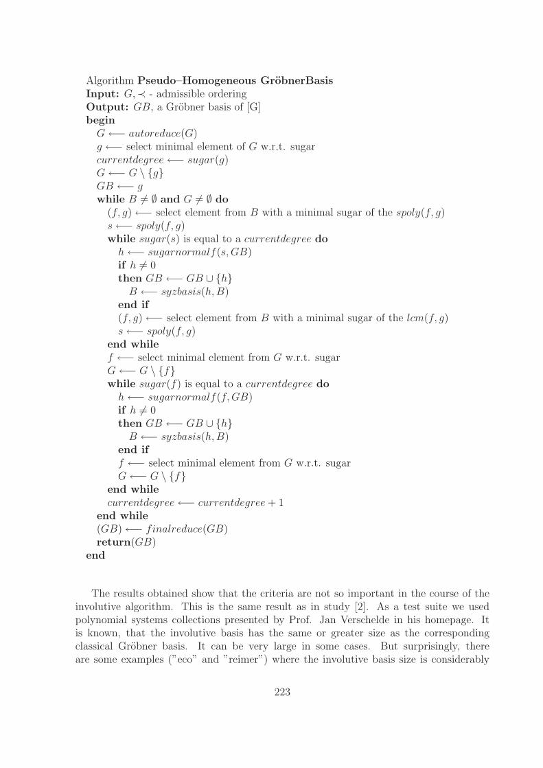
Algorithm Pseudo–Homogeneous GrobnerBasisInput: G,≺ - admissible orderingOutput: GB, a Grobner basis of [G]begin
G ←− autoreduce(G)g ←− select minimal element of G w.r.t. sugarcurrentdegree ←− sugar(g)G ←− G \ {g}GB ←− gwhile B = ∅ and G = ∅ do
(f, g) ←− select element from B with a minimal sugar of the spoly(f, g)s ←− spoly(f, g)while sugar(s) is equal to a currentdegree do
h ←− sugarnormalf(s,GB)if h = 0then GB ←− GB ∪ {h}
B ←− syzbasis(h,B)end if(f, g) ←− select element from B with a minimal sugar of the lcm(f, g)s ←− spoly(f, g)
end whilef ←− select minimal element from G w.r.t. sugarG ←− G \ {f}while sugar(f) is equal to a currentdegree do
h ←− sugarnormalf(f,GB)if h = 0then GB ←− GB ∪ {h}
B ←− syzbasis(h,B)end iff ←− select minimal element from G w.r.t. sugarG ←− G \ {f}
end whilecurrentdegree ←− currentdegree + 1
end while(GB) ←− finalreduce(GB)return(GB)
end
The results obtained show that the criteria are not so important in the course of theinvolutive algorithm. This is the same result as in study [2]. As a test suite we usedpolynomial systems collections presented by Prof. Jan Verschelde in his homepage. Itis known, that the involutive basis has the same or greater size as the correspondingclassical Grobner basis. It can be very large in some cases. But surprisingly, thereare some examples (”eco” and ”reimer”) where the involutive basis size is considerably
223
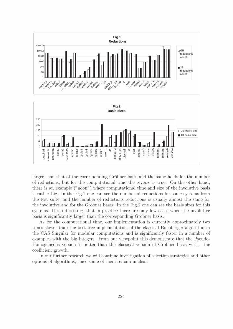
Fig.1Reductions
1
10
100
1000
10000
100000
1000000
butch
er8
cam
era1
s
chan
dra6
cohn
2
cohn
3
com
b300
0
cpdm
5
cycli
c2
cycli
c3
cycli
c4
cycli
c5
cycli
c6
haire
r_1 d1
des1
8_3
des2
2_24
discr
et3 i1
kin1
kinem
a
noon
3
noon
4
noon
5
reim
er4
reim
er5
reim
er6
viras
oro
GBreductionscount
JBreductionscount
Fig.2Basis sizes
0
50
100
150
200
250
butc
her8
cam
era1
s
chan
dra6
cohn
2
cohn
3
com
b300
0
cpdm
5
cycl
ic2
cycl
ic3
cycl
ic4
cycl
ic5
cycl
ic6
cycl
ic7
haire
r_1
d1
des1
8_3
des2
2_24
disc
ret3 i1
kin1
kine
ma
noon
3
noon
4
noon
5
reim
er4
reim
er5
reim
er6
vira
soro
GB basis size
JB basis size
larger than that of the corresponding Grobner basis and the same holds for the numberof reductions, but for the computational time the reverse is true. On the other hand,there is an example (”noon”) where computational time and size of the involutive basisis rather big. In the Fig.1 one can see the number of reductions for some systems fromthe test suite, and the number of reductions reductions is usually almost the same forthe involutive and for the Grobner bases. In the Fig.2 one can see the basis sizes for thissystems. It is interesting, that in practice there are only few cases when the involutivebasis is significantly larger than the corresponding Grobner basis.
As for the computational time, our implementation is currently approximately twotimes slower than the best free implementation of the classical Buchberger algorithm inthe CAS Singular for modular computations and is significantly faster in a number ofexamples with the big integers. From our viewpoint this demonstrate that the Pseudo-Homogeneous version is better than the classical version of Grobner basis w.r.t. thecoefficient growth.
In our further research we will continue investigation of selection strategies and otheroptions of algorithms, since some of them remain unclear.
224
3 Parallelization
It is not easy to parallelize the classical Grobner basis algorithm. It seems that thealgorithm described above can be parallelized with better quality. The most successfulattempt to parallelize the classical Buchberger algorithm was made by J.C.Faugere in hisFGb software. The parallel version of the involutive basis construction algorithm wasdescribed in [15], and the results were better w.r.t. classical version.
In this paper we present two attempts to parallelize the Pseudo-Homogeneous Buch-berger algorithm of computation of Grobner bases. As Faugere has showed, the problemof Grobner basis computation is very sequential and, therefore, every attempt to paral-lelize essentially breaks the original algorithm. The main reason is that the result of thepolynomial reduction often heavily depends on the previously found basis polynomials.Nevertheless, modifying a reduction strategy we can achieve some acceleration.
We explore two principle ideas. Assume, that at a current step we have a polynomialp to be reduced. Let us denote the list of previously reduced (and added to the basis)polynomials by P . The sequential version reduces p by P at this step and adds it to Pin the non-zero case.
What can we do? The list P can be divided into some parts, which can be distributedon different workstations. Let us denote these portions by P1, . . . , Pn. Thus we can sendp to the first workstation and reduce it by P1. At the next step we can send the result tothe workstation, that keeps P2. And at the same time we can send the next polynomialto be reduced, q, to P1. This is the main idea of the Pipeline algorithm (Fig.3).
The second idea is just the opposite. We distribute the whole P to all workstationsand simultaneously reduce the queue of polynomials p1, . . . , pn by P . This is the Conveyerstrategy (Fig.4).
Main ideas of the Pipeline strategy were developed in [4], and these of the Conveyerstrategy - in [5]. Of course, this brief discussion leaves many questions to be clearedfurther. Experiments show that the Conveyer version is much more rapid than the Pipelineis. Nevertheless, the Pipeline should be studied, as some questions of the character of itsoperation remain unclear.
Algorithm processpipelineInput: GB - polynomials list, B - the set of critical pairsOutput: modified set GB and Bbegin
h ←− receive polynomial from the pipelineif h = 0 then
if h was modified by reductions thenadd h to the pendinglist
elseGB ←− GB ∪ {h}, B ←− syzbasis(h,B)select the next slave and send h to it as new basis element
end ifend ifreturn (GB,B)
end
225
Algorithm Pipeline GrobnerBasisInput: G,≺ - admissible orderingOutput: GB, a Grobner basis of [G]begin
G ←− autoreduce(G)g ←− select minimal element of G w.r.t. sugarcurrentdegree ←− sugar(g)G ←− G \ {g}GB ←− gselect the first slave and send g to it as new basis elementpendinglist ←− {}while B = ∅ and G = ∅ do
(f, g) ←− select element from B with a minimal sugar of the spoly(f, g)s ←− spoly(f, g)while sugar(s) is equal to a currentdegree and pendinglist is not empty do
if pendinglist is not empty thenselect element from the pendinglist and send it to the pipeline
elsesend s to the pipeline
end if(GB,B) ←− processpipeline(GB,B)(f, g) ←− select element from B with a minimal sugar of the lcm(f, g)s ←− spoly(f, g)
end whilef ←− select minimal element from G w.r.t. sugarG ←− G \ {f}while sugar(f) is equal to a currentdegree and pendinglist is not empty do
if pendinglist is not empty thenselect element from the pendinglist and send it to the pipeline
elsesend f to the pipeline
end if(GB,B) ←− processpipeline(GB,B)f ←− select minimal element from G w.r.t. sugarG ←− G \ {f}
end whilecurrentdegree ←− currentdegree + 1
end while(GB) ←− finalreduce(GB)return(GB)
end
Algorithm Reductors Conveyer GrobnerBasisInput: G,≺ - admissible orderingOutput: GB, a Grobner basis of [G]
226
beginG ←− autoreduce(G), g ←− select minimal element of G w.r.t. sugarcurrentdegree ←− sugar(g), G ←− G \ {g}, GB ←− g, pendinglist ←− {}send g to slaves as new basis elementwhile B = ∅ and G = ∅ do
(f, g) ←− select element from B with a minimal sugar of the spoly(f, g)s ←− spoly(f, g)while sugar(s) is equal to a currentdegree and pendinglist is not empty do
send the next S-polynomials with degree(lcm(f, g)) = currentdegree to slavesR ←− receive reduced S-polynomials from slaveswhile R = ∅ do
h ←− select element from R with a minimal sugarR ←− R \ {h}if h = 0 then
B ←− syzbasis(h,B) and send h to slaves as new basis elementend if
end while(f, g) ←− select element from B with a minimal sugar of the spoly(f, g)s ←− spoly(f, g)
end whilef ←− select minimal element from G w.r.t. sugar, G ←− G \ {f}while sugar(f) is equal to a currentdegree and pendinglist is not empty do
send the next polynomials from G with degree(f) = currentdegree to slavesR ←− receive reduced polynomials from slaveswhile R = ∅ do
h ←− select element from R with a minimal sugarR ←− R \ {h}if h = 0 then
B ←− syzbasis(h,B) and send h to slaves as new basis elementend if
end whilef ←− select minimal element from G w.r.t. sugar, G ←− G \ {f}
end whilecurrentdegree ←− currentdegree + 1
end while(GB) ←− finalreduce(GB)return(GB)
end
227
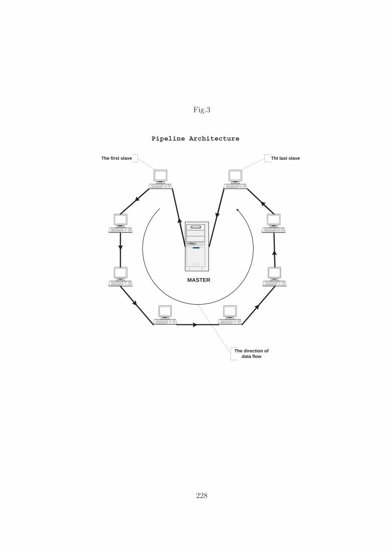
Fig.3
Pipeline Architecture
MASTER
Tht last slaveThe first slave
The direction ofdata flow
228
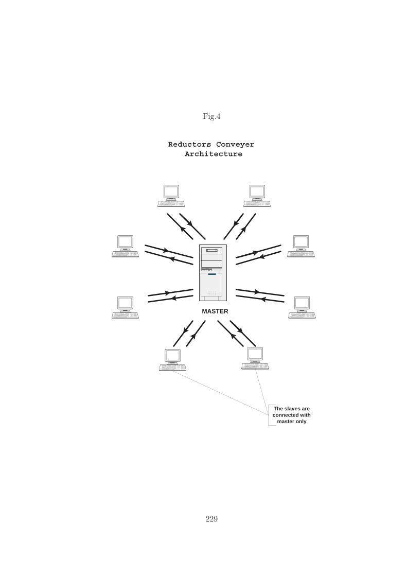
Fig.4
Reductors Conveyer Architecture
MASTER
The slaves areconnected with
master only
229
References
[1] A.Giovanni, T.Mora, G. Niesi, L. Robbiano, C. Traverso, One sugar cube, please orSelection Strategies in Buchberger Algorithm, Proceedings of ISSAC ’91, ACM, 1991,49-54
[2] Gerdt, V.P., Blinkov, Yu.A., Yanovich, D.A.: Construction of Janet Bases. II. Poly-nomial Bases. In: Computer Algebra in Scientific Computing / CASC’01
[3] J.C.Fauger, Parallelization of Grobner Basis, Proceedings of PASCO’94
[4] Kurt Siegl, A Parallel Factorization Tree Grobner Basis Algorithm, Proceedings ofPASCO’94
[5] Alyson A. Reeves, A Parallel Implementation of Buchberger’s Algorithm over Zp forp ≤ 31991, J.Symbolic Computation, 1998, 229-244
[6] Giuseppe Attardi, Carlo Traverso, A strategy-accurate parallel Buchberger algo-rithm, Proceedings of PASCO’94
[7] B. Buchberger, A Criterion for Detecting Unnecessary Reductions in the Construc-tion of Grobner Bases, Proceedings of the 1979 European Symposium on Symbolicand Algebraic Computation, Lecture Notes in Computer Science 72, Springer-Verlag,Berlin, Heidelberg, 3–21, 1979
[8] B. Buchberger, Grobner Bases : An Algorithmic Method in Polynomial Ideal Theory,In N. K. Bose, editor, Multidimensional Systems Theory , pages 184–232. D. ReidelPublishing Company, 1985
[9] T.Mora, G.Pfister, C.Traverso, An introduction to the tangent cone algorithm, Ad-vances in Computing research, Issues in Robotics and nonlinear geometry , 1992, 6,199-270
[10] R.Gebauer, H.M.Moller, On an Installation of Buchberger’s Algorithm, J. SymbolicComputation, (1988) 6, 275-286.
[11] V.P.Gerdt, Yu.A.Blinkov, Involutive Polynomial Bases, Publication IT-271, Labora-toire d’Informatique Fondamentale de Lille, Lille, 1995
[12] V.P.Gerdt, Yu.A.Blinkov, Involutive Bases of Polynomial Ideals, Mathematics andComputers in Simulation 45, 1998, 519-542.
[13] V.P.Gerdt, Yu.A.Blinkov, Minimal Involutive Bases, Mathematics and Computers inSimulation 45, 1998, 543-560
[14] Vladimir P. Gerdt, Involutive Division Technique: Some Generalizations and Opti-mizations, submitted to International Conference ”Computer Algebra in ScientificComputing” (April 20-24, St.Petersburg, Russia).
[15] Denis A. Yanovich, On Parallelization of Involutive Janet Bases Construction Algo-rithm, 2001, submitted to journal Programmirovanie
230
Computer Analysis ofHypergeometric Series: a Project of
an Instruction Set DuplicatingOperations of the Factorization
Method
A.W.Niukkanen, O.S.Paramonova
Vernadsky Institute (GEOKHI),RAS, Kossygin st. 19, 117975 Moscow, Russia;
e - mail: [email protected]; [email protected]
The operator factorization method (see, e.g., [1]) greatly facilitating the study of mul-tiple, including simple, hypergeometric series is the main object of our further interest.
The main goal of the paper is to outline a project of a universal ”formula sythesizer”in the theory of hypergeometric series. The main idea of the project is to convert the basicoperations of the operator factorization method into a complete set of commands servingus as a symbolic manipulation superstructure over a computer algebra system. Presentlywe do not try to carry out a program implementation of this part of the project (otherparts are well underway; see Sec. 1.5 and 4). Our only intention is to present, explicitly,a complete list of the main operations inherent in the factorization method.
The research has been supported by Russian Foundation for Basic Research, grant01-01-00380.
1 Computer analysis and the factorization method
1.1. Computer algebra or computer analysis? Being related to mathematical physicsby origin and to a great number of problems in a variety of sciences, by application,the hypergeometric series do have most direct relation to mathematical analysis, by themethods used for their study. Computer – aided approach to the study of hypergeometricseries relates, obviously, to computer analysis rather than to computer algebra.
Analysis is the heart of mathematics and the concept of function is the heart ofanalysis. Functions in pure mathematics are the immaterial entities which are deprivedof all properties except those endowed at will of mathematician. As to applied analysisthe hypergeometric series serve as a universal substitute for what we call a function. Incontrast to their ”pure analogs” they show a fantastic abundance of properties endowedby their explicit structure. Therefore any algorithm efficient enough to tackle multiplehypergeometric series of arbitrarily complicated structure can be looked upon as a versatilesolver capable to handle with almost any problem relating to functions of practical interest.
231
1.2.The central idea of the operator method is connected with an introduction of a newsimple differential operation of ”Ω-multiplication” w = u ∗ v over the functions u =u(x1, . . . , xN) and v = v(x1, . . . , xN):
〈u ∗ v|x1, . . . , xN〉 = u (d/ds1, . . . , d/dsN) v(x1s1, . . . , xNsN) |∀sn=0 (1)
The fundamental importance of the Ω-multiplication is that it allows any series havingcomplicated structure to be directly expressed through simpler series thus permitting us touse the properties of the simple series to analyze any property of the initial complicated se-ries. Let NF [A; x1, . . . , xN ], NF [B; x1, . . . , xN ] and NF [A,B; x1, . . . , xN ] be the seriesof the power functions xi1
1 . . . xiNN /(i1! . . . iN !) with coefficients A(i1, . . . , iN), B(i1, . . . , iN)
and A(i1, . . . , iN)B(i1, . . . , iN), respectively. The in(n = 1, . . . , N) are summation in-dices of the series (in = 0, 1, 2, . . .).
The general factorization formula for the series NF [A,B] reads
F N [A,B; x1, . . . , xN ] = 〈NF [A] ∗N F [B]|x1, . . . , xN〉 (2)
In short, F [A×B] = F [A]∗F [B]. This formula conveys the property of Ω - representablilityof multiplication operation over coeffifients of an arbitrary power series. It shows also thatthe factorization method can be looked upon as a disguised form of algebraization of thetheory of hypergeometric series.1.3. Conceptual basics of the method. First, any hypergeometric series is expressed onlythrough hypergeometric series (closure property). No necessity in employment of anyother auxiliary representation is arisen.
Second, the functional relation f ∗ f1 = f ∗ f2 will be called Ω-equivalent to therelation f1(x1, . . . , xN)=f2(x1, . . . , xN). The concept of Ω-equivalence allows classes ofΩ-equivalent relations to be introduced. In each class a simplest relation which will becalled a proto-relation can be chosen. Having proved the proto-relation we thus prove allformulas belonging to the class.
Third, using Ω-multiplication Ω-equivalent operators F1 ⇔ F2 can be introduced.They defined by
F1 (d/ds, s) Ψ(xs)∣∣s=0
= F2 (d/ds, s) Ψ(xs)∣∣s=0
, (3)
where Ψ is an arbitrary function. Note that F1 and F2 are not necessarily identical to oneanother. The possibility to substitute F1 for F2 in an Ω-product is an inportant technicalexpedient of the method.
Fourth, by analogy with arithmetically identical expressions the algebraic expressionsconnected by finite number of arithmetic operations and Ω-multiplication operations willbe called Ω-identical expressions. Transformation of an expression to an Ω-identical formis another important technical expedient.1.4. Three approaches to the use of factorization method. Altogether we can see threeapproaches. The first one is to derive all formulas manually being dispensed completelywith the necessity of working with computer. Even in this case the factorization methodoffers great advantages over traditional methods. The second approach implies the manualderivation of basis sets of formulas with subsequent application of symbolic computerprograms for exaustive search of all different combinations of the basis formulas. The thirdway consists in full–scale computerization of all operations inherent in the factorization
232
method which would open up the possibility for computer–aided derivation of any formularelating to the theory of hypergeometric functions. One of the goals of the present paperis to substantiate, theoretically, the feasibility of the third approach.1.5. An experience in development of symbolic computer programs. All programs devel-oped so far [2, 3] are based on the second (intermediate) approach. These programs utilizenot the factorization method per se, but the result of its application to a certain class offormulas with the aim to derive manually, without using a computer, a set of basic rela-tionships playing the role of building blocks for a chosen class of formulas. Applying sucha ”bounded–universal” procedure to one or another of several score classes of formulasmaking up the backbone of the theory of hypergeometric series one can obtain, in prin-ciple, sufficiently complete computerized version of the theory indirectly connected withthe factorization method. The initial steps in this direction covering the transformationtheory of hypergeometric series are made, with sufficient completeness, in the programsannounced in [2, 3].
The notable success of this approach was corroborated by the computer–aided deriva-tion [4] of an important reduction formula given by Gelfand at al. [5] and its numerousnon-trivial generalizations.1.6. An outline of the project. The accumulated experience suggests the desirability ofexpanding the programs’ potentialities, in the spirit of the third approach (see Section 1.4).
The central part of the core (CPC) of the projected program complex is conceived toperform, directly, all operations of the operator factorization method thus placing at theuser’s disposal a sort of a universal interactive ”formula synthesizer”.
The peripheral part of the core (PPC) is planned to consist of macro-commands im-plementing the sets of basic relations obtained with the help of the CPC. Many of theserelations have been already obtained manually [4, 6]. Very large sets of relations can beobtained with the help of the PPC in an automatic mode.
If the relations presenting little interest for derivation of new formulas are considedto be valuable on their own they will be placed at date base surrounding (DBS). TheDBS will play the role of an information reference system. The DBS is expected to be ofmoderate size for the main bulk of relations will be generated in PPC.1.7. How the method would work in the program. The functionality of the method inthe program would not differ much from the work using hand and pencil. There aretwo general schemes for carrying out calculations with the help of operator factorizationmethod.
The first scheme consists of four steps.Step 1 (analysis) breaks up a series into an Ω-product of simpler series. Step 2 (simpleseries transformations) utilizes the known properties of the simpler series for trans-formation of factorized terms. Step 3 (auxiliary transformations) uses a finite set ofauxiliary identities converting the resultant expression into a form allowing applicationof a (possible new) factirization formula. Step 4 (synthesis) transforms the operatorexpression into an algebraic form with the help of a suitable factorization formula.
The second scheme is based on the concept of Ω-equivalence (see Section 1.3). Intro-ducing a simple relation we can multiply its both sides by an Ω-factor thus obtaining anew relation.
Despite the seemingly exotic nature of these approaches, they prove in practice to be
233
quite simple, universal and effective, and thus fairly suitable for the role of a superstructureover one of the existing analytical manipulation systems.
2 Instruction set underlying the central part of the
core (CPC) of the proposed program complex
The instruction set duplicates the main operations of the factorization method. Eachdefinition of a formula giving us a project of a future entry of the instruction set is suppliedwith capital boldface label. Sometimes mnemonic synonyms of the instructions names areindicated in parentheses. The numbers attached to the labels of kindred formulas are tobe subsituted, in course of the program implementation, by exact specific indications ofthe commands formats.
The references to the definitions will be denoted by lower case boldface labels. Thewhole set of formulas given below constitutes a project of a specialized algorithmic lan-guage. This language may give an origin to a program complex aimed at a full-scalecomputerization of a substantial part of applied mathematical analysis. For convenience,all formulas are subdivided into several classes.
Sometimes, if a formula written for the case of one variable can be extended directlyto the case of several variables we do not present the latter explicitly.
For notation see Refs. [1] and [13].2.1. Factorization formulasFACT1. Factorization of the series F [d; x]
F [d1 ; x1 d(s)] F [d2; x2s]|s=0 = F [d1,d2 ; x1 x2] , d(s) = d/ds (4)
FACT2. Factorization of the series in one variable containing compound parameter
F [d1 ; x1 d(s)] F [d2; x2sm]|s=0 = F [< d1 | m >, d2 ; xm
1 x2] (5)
FACT3. General factorization of the series NF
NF [L1, L2 ; x1, . . . , xN ]
=N F[L1 ; d(s1), . . . , d(sN)] NF [L2 ; x1s1, . . . , xNsN
] ∣∣∀sn=0
(6)
FACT4. Special factorization of the series NF
NF [< d | m1, . . . ,mN >, L ; x1, . . . , xN ]
= F [d ; d(s)] NF [L ; x1sm1 , . . . , xNsmN ]
∣∣s=0
(7)
FACT5. Factorization of NF containing the glueing operator F [d0 ; xdm(s)]
F [d0 ; xdm(s)] F [d1 ; x1sm] · · ·F [dN ; xNsm]|s=0
= F
[d0,
1
m, . . . ,
m − 1
m: d1 ; . . . ; dN ; xx1m
m, . . . , xxNmm
](8)
234
FACT6. Factorization of multiple series containing constant arguments
Ω =N+P F [〈d|m1, . . . ,mN+P 〉, . . . : x1d
ds1
, . . . , xNd
dsN
, u1, . . . , uP ]
×N+QF [〈d′|l1, . . . , lN+Q〉, . . . : y1s1, . . . , yNsN , v1, . . . , vQ] | ∀sn=0 (9)
=N+P+Q F [〈d|m1, . . . ,mN ,mN+1, . . . ,mN+P , 0, . . . , 0︸ ︷︷ ︸Q
〉,
〈d′|l1, . . . , lN ,
P︷ ︸︸ ︷0, . . . , 0, lN+1, . . . , lN+Q〉, . . . :
x1y1, . . . , xNyN , u1, . . . , uP , v1, . . . , vQ] (10)
2.2. General properties of the Ω-multiplication operationOMEGA 1. Commutativity property u ∗ v = v ∗ u (COMM)
u(d(s))v(xs)|s=0 = v(d(s))u(xs)|s=0 (11)
OMEGA 2. Coupling rule (COUP)
u(d(s))v(xs)|s=0 = u(xd(s))v(s)|s=0 (12)
OMEGA 3. Associativity property (ASSOC)
< w ∗ (u ∗ v)|x >=< (w ∗ u) ∗ v|x > (13)
OMEGA 4. exp(x) plays the role of Ω-unit (OMUN) that is exp ∗f = f ∗ exp = f ,or
exp(d(s))f(xs)|s=0 = f(d(s)) exp(xs)s=0 = f(x) (14)
OMEGA 5. The Ω-”unitarity” can be interpreted as ”renaming” (s for x) property(REN)
exp xd(s)f(s)|s=0 = f(x) = f(x)|s⇒x (15)
2.3. Ω-equivalent operatorsThe case of EQUIV1. an arbitrary operator multiplied by power function
F (d(s))sn Ψ(s)|s=0 = F (n)(d(s)) Ψ(s)|s=0 (16)
The case of EQUIV2. an arbitrary operator multiplied by exponential function
F (d(s))exs Ψ(s)|s=0 = F (d(s) + x) Ψ(s)|s=0 (17)
The case of EQUIV3. the binomial operator multiplied by exponential function
F 10 [a; d(s)]exs Ψ(s)|s=0 = (1 − x)−aF 1
0 [a; d(s)/1 − x] Ψ(s)∣∣s=0
(18)
2.4. Relationships containing operators (without setting differentiation variable to zero)OPER1. Shift operator identity (SHIFT)
exp(u d(x))f(x) = f(x + u) (19)
235
OPER2. Similarity transformation (F and f are arbitrary functions, A is an arbitraryoperator) (SIMIL)
f−1 F (A) f = F (f−1Af ) = F (A + f−1[A, f ] ) (20)
OPER3. Operator argument displacement formula (DISP)
exp(−vx)F [d(x)] exp(vx) = F [d(x) + v] (21)
OPER4. Applying of a differential operator to exp(x) (OPEXP)
F (d(x)) exp(ux) = F (u) exp(ux) (22)
OPER5. Generalized Leibnitz rule (LEIB)
F (d(x)) f1(x)f2(x) = F (d(x1) + d(x2))f1(x1)f2(x2)|x1=x2=x (23)
OPER6. Differentiation of simple hypergeometric series (DIFHYP)
dn(x) F [d; ux] = un(d, n) F [d + n; ux] (24)
2.5. Elementary reduction formulasRED1. Reduction of the exponential series F 0
0 (REDEXP)
F 00 [∗//∗; x] = exp(x) (25)
RED2. Reduction of the binomial series F 10 (REDBIN)
F 10 [a//∗; x] ≡ F [a; x] = (1 − x)−a (26)
RED3. Reduction of an infinite geometrical progression (GEOINF)
1 + x + x2 + · · · ≡ F 10 [1; x] = (1 − x)−1 (27)
RED4. Reduction of the finite geometrical progression (GEOFIN)
1 + x + x2 + · · · + xN = (1 − xN+1)/(1 − x) (28)
RED5. Reduction of the series NF with empty glueing set
NF [∗//∗ : d1 ; . . . ; dN ; x1, . . . , xN ] = F [d1; x1] · · ·F [dN ; xN ] (29)
RED6. Reduction of the series NF with empty individual sets
NF [d : ∗ ; . . . ; ∗ ; x1, . . . , xN ] = F [d ; x1 + · · · + xN ] (30)
2.6. Auxiliary algebraic identitiesALG1 Gauss-Legendre multiplication formula for the Pochhammer symbol
(MULT(m))
(α,m i) = mm i( α
m, i)(α + 1
m, i
)· · ·(
α + m − 1
m, i
)(31)
236
ALG2. Inversion formula for Pochhammer symbol (INVER)
(a, −I) = (−1)I (1 − a, I)−1 (32)
ALG3. Cancellation or, vica versa, introduction of equal parameters in numerator anddenominator of a series (CANC, INTRO)
F [d; x] = F [a, d//a; x] (33)
ALG4. Vertical transfer of parameters (VERT)
NF [〈a|m1, . . . ,mN〉, L; x] =N F [L//〈1 − a|m1, . . . , mN〉; (−1)m x] , (34)
x = [x1, . . . , xN ], (−1)m x = [(−1)m1x1, . . . , (−1)mN xN ]ALG5. Any series NF is symmetric with respect to simultaneous permutation of argu-ments xi � xj, individual sets of parameters di � dj and all corresponding spectralnumbers mi � mi, li � lj, etc. (PERM)
ALG6. Uniformization of the argument of the binomial series F 10 [a; x + u] (UNIF)
F 10 [a; x + u] = (1 − x − u)−a = (1 − u)−a F 1
0 [a; x/(1 − u)] (35)
ALG7. Factorization of geometrical progression F 10 [1; x] into a product of two progres-
sions (PROG)
F 10 [1; x] =
(N−1∑r=0
xr
)F 1
0 [1; xN ] (36)
ALG8. Decomposition of ex into a sum of N series F 0N−1(x
N) (DEXP(N))
ex =N−1∑r=0
xr
r!F
[1 ; xN
〈1 + r|N〉]
=N−1∑r=0
xr
r!F
[ ∗ ; (x/N)N
1+rN
, · · · , N−1N
, N+1N
, · · · , N+rN
](37)
ALG9. Addition formula for binimial series (ADDBIN)
F 10 [a; x1 + x2] =
∞∑n=0
(a, n)
n!xn
1 F 10 [a + n; x1] x
n2 F 1
0 [a + n; x2] (38)
3 Examples suggestive of functionality specifics of
the proposed CPC commands
3.1. An elementary example can be seen from comparison between relationships prog anddexp(N) which prove to be Ω-equivalent one to another! The elementary formula progfollows from the formulas geofin and geoinf. Thus it is just the prog plays the role ofproto-relation (see Sec. 1.3). Applying the operator F 0
1 [∗//1; z d(x)]|x=0 to the both partsof prog we use the operations fact1, canc and redexp in the left-hand part and theoperations equiv1, difhyp, fact2, mult(m) and canc in the right-hand part. Thenthe dexp(N) follows immediately. More general relations belonging to this class can be
237
obtained in analogous way if we apply F [d; zd(x)]|x=0, instead of the F 01 , to the both
parts of prog.3.2. Already published examples. In fact, we are delivered from the necessity of givingmany examples of how the method could work in practice. Numerous examples of thekind are given in the already published papers [1], [7]-[13]. Many simple examples illus-trating application of operations (4) - (38) are given is Ref. [1]. The same operations wereemlpoyed for derivation of new recurrence relations [7]. Some new generating functionsfor the Laguerre polynomials were presented in Ref. [8]. More general generating func-tions, as well as a complete set of Meixner-type formulas and a new class of Lagrangeanpolynomials were introduced in [9]. Very important special transformations of the AppelF4 and the Horn H1 and G2 functions were obtained in [10]. A new approach to derivationand generalization of involved Burchnall and Chaundy expansions playing a particularlyimportant role in the theory of double hypergeometric series was found in [11]. A sophis-ticated analysis of many particular problems originated from contemplation of a classicalrelation between Bessel functions was given in [12]. A heavy use of the operations (4) -(38) was made in [13] for analysis of linearization relations and addition formulas includinga generaliztion of an important Koornwinder formula of the Jacobi polynomials. Specialattention has been given in Ref. [13] to the details of the new technology of analyticaltransformations based on the operations (4) - (38).3.3. An additional example. The references given in Sec. 3.2 relate mostly to the mainscheme involving the four steps mentioned in Sec. 1.7. The second scheme based onthe concept of Ω-equivalency was paid lesser attention in the above examples and needstherefore a little bit more substantiation. To this end we introduce the notation
u1 = 1 − z + ξ1z, u2 = 1 − z + ξ2zand consider the elementary relationship
L ≡ F 10 [c; (1 − ξ1)(1 − ξ2)z] = (1 − z)c(u1u2)
−c F 10 [c; ξ1ξ2z/u1u2] ≡ R. (39)
which is readily verified by using the reduction rule redbin. We then transform the proto-relation (39) to an Ω-identical form facilitating transition to Ω-equivalent relations. Usingtwice the operation fact1 we get the preliminary Ω-identical (see Sec. 1.3) transformation
F 10
[c;
ξ1ξ2z
u1u2
]=∏2
n=1F 1
0
[c;
ξn(1 − z)
un
d
dsn
]F 0
1
[∗;c
s1s1z
(1 − z)2
]∣∣∣∣s1=s2=0
(40)
To simplify dependence on ξ1, ξ2 we multiply eq. (40) by u−c1 u−c
2 (see eq. (39)), transformthe both operator series F 1
0 with the help of redbin, allow for definitions of u1, u2, makesome elementary algebraic manipulations, use, inversely, the redbin and employ equiv2.Thus we have
u−cn F 1
0
[c;
ξn(1 − z)
un
d
dsn
]= (1 − z)−c F 1
0
[c; ξn
(d
dsn
+z
z − 1
)]⇔ (1 − z)−c F 1
0 [c; ξnd(sn)] exp[zsn(z − 1)−1]. (41)
Inserting (40) and (41) into (39) we finally have the desired Ω-identical representation of
238
R:
R = (1 − z)−c F 10 [c; ξ1d(s1)]F
10 [c; ξ2d(s2)]
× exp
(zs1
z − 1
)exp
(zs2
z − 1
)F 0
1
[∗c
; s1s2z
(1 − z)2
]∣∣∣∣s1=s2=0
. (42)
With the help of redbin the left-hand side L can be writhen as:
L =∑∞
n=0
(c, n
n!F 1
0 [−n, ξ1]F10 [−n, ξ2] z
n . (43)
Then we apply the operator
F 01 [∗//c; x1d(ξ1)]F
01 [∗//c; x2d(ξ2)] |ξ1=ξ2=0
to the both sides of the identity L = R where L and R are given by eqs. (42) and (43)respectevely. In case of the L the only operation fact1 is needed. In case of the R weapply fact1, canc, redexp and ren, consecutively. The result∑∞
n=0
(c, n)
n!F 1
1
[−n
c
; x1
]F 1
1
[−n
c
; x2
]zn
= (1 − z)−c exp
[(x1 + x2)z
z − 1
]F 0
1
[∗c
; x1x2z
(1 − z)2
](44)
is equivalent to the Hille-Hardi bilinear generating function for Laguerre polynomials (see[14], vol.1).
Applying to the both sides of eq. (44) the operator product
F 10 [a1; ξ1d(x1)]F
10 [a2; ξ2d(x2)]|x1=x2 ,
using twice fact1 on the left and equiv3 (see eq. (41)) and fact1 on the right we obtainthe apparently new bilinear generating functions for Gaussian polynomials F [−n, a//c; ξ]:∑∞
n=0
(c, n)
n!F 2
1
[−n, a1
c
; ξ1
]F 2
1
[−n, a2
c
; ξ2
]zn
= (1 − z)a1+a2−c u−a11 u−a2
2 F [a1, a2//c; ξ1ξ2z/u1u2] . (45)
An attempt to apply eq.(45) to the Gegenbauer polynomials Cλn(x) may seem to make no
sense whatever because any of the known hypergeometric representations of Cλn(x) in the
form of F 21 contains two parameters dependent on n whereas each of the F 2
1 in eq. (45)contains only one such parameter. Being sure that the list of representations for theCλ
n(x) given in literature is not complete we looked into a question of how many differentformulas for the Cλ
n(x) may exist. We used the linear (x → x−1, x → 1−x, x → x/(x−1))and quadratic transformations (see [14], vol. 2 and the Sec. 4.2 below) conserving thepolynomial structure of the transformed functions. We found altogether 18 differentrepresentations. The formula
Cλn(x) =
(2λ, n)
n![x + (x2 − 1)1/2]n F 2
1
[−n, λ ;
2λ
2(x2 − 1)1/2
x + (x2 − 1)1/2
](46)
239
which is incidentally absent in literature is of prime interest for applications.This formula is remarkable for that the dependence on the order n of the polyn-
jmial F [−n, λ//2λ] in the definition (46) in the same as in the case of the polynomialsF [−n//α + 1] occuring in the definition of the Laguerre polynomials. The structuralsimilarity of the Cλ
n(x) and Lαn shows that solution of the problems where dependence
on n plays an essential role would have, formally, much in common for the Cλn(x) and
Lαn despite the fact that the Gegenbauer polynomials are a natural particular case of the
Jacobi polynomials which have nothing to do with the Laguerre polynomials. Beyond thefactorization method this formal observation would hardly be of any significance. On thecontrary, within the factorization method the simple observation gives us a powerful toolfor obtaining new interesting results. For example, letting a1 = a2 = λ, c = 2λ in eq. (45)and using eq. (46) to express the resultant F 2
1 polynomials through Cλn(x) we can read-
ily obtain a seemingly new bilinear generating function for the Gegenbauer polynomials.Derivation of bilateral, for the Lα
n and Cλn(x), generating function can be also performed
with ease.
4 Examples of macro-commands constituiting
the peripheral part of the core (PPC) of the pro-
posed program complex
As was already mentioned above (see Sec. 1.5 and 1.6) along with the universal set of”low-level” derivation rules (4) - (38) we are going to use the generators of formula classesconsisting of a few specialized ”high-level” basic relationships. In distinction to the CPCoperations many of the PPC macro-commands have been already programmed [2, 3] andapplied for analysis of multiple hypergeometric series [4, 15].
We first give typical instances of macro-commands and then present some examplesof using these macro-commands (all necessary definitions and notation are given in therefs. [1, 13]).4.1. Linear transformationsLIN(K). Linear transformation connecting two series having the Kummer type (1//1)with respect to x0 (the L∗ symbolizes the coefficients independent of summation indexi0):
F
[ 〈ν1|1,m1〉 , L∗ ; x0,x〈ν0|1,m0〉
]= ex0 F
[ 〈ν01|1,m01〉, 〈ν1|0,m1〉, L∗ ; −x0,x〈ν0|1,m0〉 , 〈ν01|0,m01〉
](47)
LIN(G). Three linear transformations linking the series having the Gauss type (2//1)with respect to x0. For each series we use a canonical representation [1, 13], where allspectral numbers connected with x0 are equal to 1. The three transformations change,consecutively, the first (G01), the second (G02) and the both (G00) numerator parameters.The symbol following G in (GOQ) is the number of argument.
F
[ 〈ν1|1,m1〉 , 〈ν2|1,m2〉 , L∗ ; x0,x〈ν0|1,m0〉
]=
240
LIN(G01) = L01F ≡ (1 − x0)
−ν2 ×
×F
[〈ν01|1,m01〉 , 〈ν2|1,m2〉 , 〈ν1|0,m1〉 , L∗ ;
x0
x0 − 1,
x
(1 − x0)m2
〈ν0|1,m0〉 , 〈ν01|0,m01〉
](48)
LIN(G02) = L02F ≡ (1 − x0)
−ν1 ×
×F
[〈ν1|1,m1〉 , 〈ν02|1,m02〉 , 〈ν2|0,m2〉 , L∗ ;
x0
x0 − 1,
x
(1 − x0)m1
〈ν0|1,m0〉 , 〈ν02|0,m02〉
](49)
LIN(G00) = L00F ≡ (1 − x0)
ν012 ×
×F
[ 〈ν01|1,m01〉, 〈ν02|1,m02〉, 〈ν1|0,m1〉 , 〈ν2|0,m2〉 , L∗ ; x0,X〈ν0|1,m0〉, 〈ν01|0,m01〉, 〈ν02|0,m02〉
], (50)
X = x(1 − x0)−m012 .
4.2. Quadratic transformationsThe ”classical” theory of quadratic transfornations even in case of simple series lackssimplicity and transparency of structure to say nothing of multiple case. The relationshipswhich follow are applicable to any multiple series satisfying some necessary conditions.Moreover instead of 9 functions we can confine ourselves, at the first step, but to 3functions:
F1 ≡ F1[〈ν1|1,m1〉, 〈ν1 + 1/2|1,m1〉, L∗//〈ν0|1,m0〉; x0,x], (51)
F2 ≡ F2[〈ν1|1,m1〉, 〈ν2|1,m2〉, L∗//〈1 + ν12|1,m12〉; x0,x], (52)
F3 ≡ F3[〈ν1|1,m1〉, 〈ν2|1,m2〉, L∗//〈2ν2|1, 2m2〉; x0,x]. (53)
Just these functions occur in the following three basic quadratic transformations:QUAD32. The transformation relating F3 to F2 is
F3 = [(2/(2 − x0)]ν1F1
[ 〈ν1
2
∣∣1, m1
2〉, 〈ν1+1
2
∣∣1, m1
2〉, L∗; x13,x13
〈ν2 + 1/2|1,m2〉]
(54)
x13 = x20(2 − x0)
−2, x13 = 4m12 x (2 − x0)−m1 .
QUAD21. The transformation linking F2 and F1 has the form
F2 = (1 + x0)−ν1F1
[ 〈ν1
2
∣∣1, m1
2〉, 〈ν1+1
2
∣∣1, m1
2〉, 〈ν2|0,m2〉, L∗; x12,x12
〈1 + ν1 − ν2|1,m1 − m2〉]
(55)
x12 = 4x0(1 + x0)−2, x12 = 2m1x(1 + x0)
−m1 .QUAD32. The transformation expressing F3 through F2 is
F3 = [2/(1 +√
1 − x0)]2ν1F2
[ 〈ν1|1,m1〉, 〈ν12 + 12|1,m12〉, L∗; x23,x23
〈ν2 + 1/2|1,m2〉〈ν12 + 12|0,m12〉
](56)
x23 = (1 −√1 − x0)
2(1 +√
1 − x0)−2, x23 = 4m12x(1 +
√1 − x0)
−2m1 .All other quadratic transformations follow from eqs. (54)-(56) by using the three oper-ations lin(G) for F1, F2, F3 occuring in (54)-(56). This adds 6 new functions. Letting
241
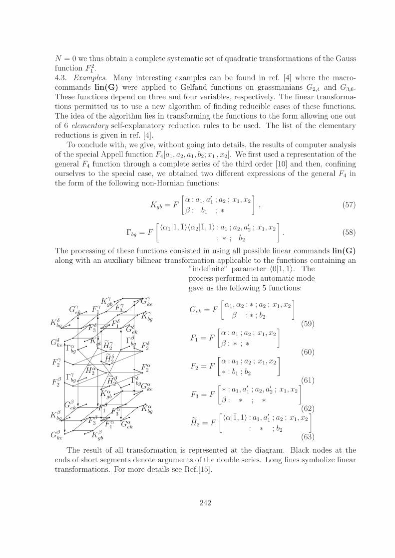
N = 0 we thus obtain a complete systematic set of quadratic transformations of the Gaussfunction F 2
1 .4.3. Examples. Many interesting examples can be found in ref. [4] where the macro-commands lin(G) were applied to Gelfand functions on grassmanians G2,4 and G3,6.These functions depend on three and four variables, respectively. The linear transforma-tions permitted us to use a new algorithm of finding reducible cases of these functions.The idea of the algorithm lies in transforming the functions to the form allowing one outof 6 elementary self-explanatory reduction rules to be used. The list of the elementaryreductions is given in ref. [4].
To conclude with, we give, without going into details, the results of computer analysisof the special Appell function F4[a1, a2, a1, b2; x1 , x2]. We first used a representation of thegeneral F4 function through a complete series of the third order [10] and then, confiningourselves to the special case, we obtained two different expressions of the general F4 inthe form of the following non-Hornian functions:
Kgb = F
[α
β
:
:
a1, a′1
b1
;
;
a2
∗; x1, x2
], (57)
Γbg = F
[〈α1|1, 1〉〈α2|1, 1〉 :
:
a1
∗;
;
a2, a′2
b2
; x1, x2
]. (58)
The processing of these functions consisted in using all possible linear commands lin(G)along with an auxiliary bilinear transformation applicable to the functions containing an
� �� �
� � � �� � � �
� � � �� � � �
� �� �
���
����
���
���
���
���
���
��
�� ��
�� �� �� ��
�� �� �� ��
�� ��
� �� �
� � � �� � � �
� � � �� � � �
� �� �
���
����
���
���
���
���
���
��
�� ��
�� �� �� ��
�� �� �� ��
�� ��
��
��
��
��
��
��
��
��
��
��
��
��
�
�
�����
�����
�����
�����
�� ��
������ ��
����
������
�
�
��
��
�
�
��
�
�
�
��
�� ��
��
�
�
�
�
Kδbg
Gδke
F γ2
F β2
Kβbg
Gβke
Kγgb
Gγek F γ
1F γ
3Kγ
bg
Gγke
F δ2
Fα2
Kαbg
Gαke
Hβ2
Hδ2
Γδbg
F δ3
F δ1
Kδgb
Gδek
Hγ2Γα
bg
Γβbg
Hα2
Γγbg
Kαgb
Gβek F β
1
Fα1
Kβgb
Gαek
Fα3
F β3
”indefinite” parameter 〈0|1, 1〉. Theprocess performed in automatic modegave us the following 5 functions:
Gek = F
[α1, α2
β
:
:
∗∗
;
;
a2
b2
; x1, x2
](59)
F1 = F
[α
β
:
:
a1
∗;
;
a2
∗; x1, x2
](60)
F2 = F
[α
∗:
:
a1
b1
;
;
a2
b2
; x1, x2
](61)
F3 = F
[ ∗β
:
:
a1, a′1
∗;
;
a2, a′2
∗; x1, x2
](62)
H2 = F
[〈α|1, 1〉 :
:
a1, a′1
∗;
;
a2
b2
; x1, x2
](63)
The result of all transformation is represented at the diagram. Black nodes at theends of short segments denote arguments of the double series. Long lines symbolize lineartransformations. For more details see Ref.[15].
242
5 Concluding remarks
The program implementation of the ”central part of the core” (see Sec. 2) would allowus, instead of using a ”manual”, with pen and paper, calculation technique, to performall analytical transformations with the help of computer in an interactive mode, in thisway relieving the researcher of the tedious copying of cumbersome formulas and placingat his disposal a universal ”formula synthesizer” of a sort.
An addition of new macro-commands to the ”peripheral part of the core” (see Sec. 4)would give us an access to hundreds and thousands of new relationships, whose publicationin the traditional form of books and periodicals would hardly have been practicable.
An inappropriately cumbersome user interface may well happen to become a sub-stantial practical obstacle to the effective program realization of the global approach. Adetailed look at the work with the formulas’ ”screen images” and sophisticated investi-gation of different variants of its organization seems to be obligatory condition for theeffective man–machine formula interface. We hope that recourse to ”semantics-oriented”tools, like XML, OpenMath, etc., may help us to solve the problem.
References
[1] A.W.Niukkanen A new theory of multiple hypergeometric series and its prospectsfor computer algebra programming (in Russian), Fundamentalnaya i prikladnayamatematika, 1999, 5, 1–29.
[2] O.S.Paramonova, A.W.Niukkanen, Analytical transformations of hypergeometric se-ries (in Russian), Programmirovanie, 1998, No 6, 25–26.
[3] O.S.Paramonova, A.W.Niukkanen, New algorithms of finding reduction formulas ofmultiple hypergeometric series (in Russian), Programmirovanie, 2000, No 1, 62–63.
[4] A.W.Niukkanen, O.S.Paramonova, Computer generation of complicated transforma-tions for multiple hypergeometric series, Comput. Phys. Commun., 2000, 126, 141–148.
[5] I.M. Gel’fand, M.I. Graev, V.S. Retakh, General hypergeometric equations systemsand hypergeometric type series (in Russian), Uspekhi Matem. Nauk , 1992, 47, 3–82.
[6] A. W. Niukkanen, Transformation theory of multiple hypergeometric series and com-puter aided symbolic calculations, Proceedings of the 9th Conference on Computa-tional modelling and computing in physics , Dubna, 1997, 219–223.
[7] A.W.Niukkanen, Factorization method and recurrence relations (in Russian), Integraltransforms and special functions. Computer center, 1997, 1, No 2, 10-15.
[8] A. W. Niukkanen, A new method in the theory of the hypergeometric series (inRussian), Uspekhi Matematicheskikh Nauk , 1988, 43, 191–193.
[9] A. W. Niukkanen, A new approach to the theory of the hypergeometric series (inRussian), Russian Matematicheskie zametki, 1991, 50, 65–73.
243
[10] A.W.Niukkanen, Factorization method and special transformations of the functionsF4, H1 and G2 (in Russian), Uspekhi Matem. Nauk , 1999, 54, 169–170.
[11] A.W.Niukkanen, New algoritms for the hypergeometric series and the Burchnall andChaundy expansions (in Russian), Programmirovanie, 2000, No 2, 67–69.
[12] A.W.Niukkanen, I.V.Perevozchikov, V.A.Lurie, A generalization of a classical rela-tion between Jν+n(z), Jν(z) and Jν−1(z), Fractional calculus and applied analysis,2000, 3, No 2, 119-132.
[13] A.W.Niukkanen, Operator factorization method and addition formulas for hyperge-ometric functions, Integral transforms and special functions, 2001, 11, 25-48.
[14] A. Erdelyi, W. Magnus, F. Oberhettinger, F. Tricomi, Higer transcendental func-tions , (McGraw-Hill, N.-Y., 1953).
[15] O.S.Paramonova, A.W.Niukkanen, Computer analysis of transformation formulas ofthe Appell and the Horn functions, submitted to Programmirovanie.
244
Investigation of Nonlinear Secondand Third Orders Differential
Equations of P-Type withCAS MATHEMATICA
A.N.Prokopenyaa, A.V.Chichurinb
aBrest Technical University, Belarus;bBrest State University, Belarus;
e-mail: [email protected]
Usage of the computer algebra system Mathematica for solving some problems ofanalytical and general theory of nonlinear ordinary differ ential equation of the secondand the third orders is discussed.
Introduction
There are some problems arising on investigating of the nonlinear second and third ordersordinary differential equations of P-type (solutions of such equations have not movablecritical singular points) that can be successfully solved with computer algebra systemMathematica ([1,2]). In present paper we’ll consider several such problems and showhow they can be solved using the corresponding Mathematica codes. In the case ofthe second order differential equations of P-type it is possible to make refer to the nextproblems.
Problem 1. Construction the systems that are equivalent to thesix non - reducible Painleve equations.
We start from construction of the equivalent system for the third Painleve equation (P3)that can be defined as
eq = w′′[z] ==w′[z]
w[z]− w′[z]
z+
1
z(α w[z]2 + β) + γ w[z]3 +
δ
w[z];
If such system would be constructed then we could build the Baklund’s transformationfor this equation. Let us seek this system in the form ([3])
eq1 = w′[z] == a0[z] + a1[z]w[z] + a3[z]w[z]2 + a6[z]w[z]2v[z];
eq2 = v′[z] == b0[z] + b1[z]w[z] + b2[z]v[z] + b4[z]w[z]v[z] + b6[z]v[z]2w[z];
where aj(z), bi(z) (j = 0, 1, 3, 6; i = 0, 1, 2, 4, 6) are some functions. Solving eq1 on v(z)and substituting the result into eq2 we obtain the next second order differential equation:
sol1 = DSolve[eq1,v, z]//Flatten;
245
eq3 = w′′[z] == (w′′[z]/.Solve[eq2/.sol1,w′′[z]][[1]]);
In order the system of equations eq1, eq2 to be equivalent to the second order differentialequation of P-type eq3 should coincide with (P3)-equation. To satisfy this requirementwe should introduce some restrictions on coefficients aj(z) and bi(z). First we equalizedenominators of the right sides of eq3 and eq.
eq4 = Denominator[Together[eq3[[2]] == Denominator[Together[eq[[2]]
w[z] a6[z] == z w[z]
Solving equation eq4 we obtain the function a6(z) (sol4 = DSolve[eq4, a6, z][[1]] {a6 →(#1&)}). Then we define numerators of the right sides of eq3 and eq taking into accountthe solution sol4.
eq5 = Collect[Numerator[Together[eq3[[2]]/.sol4]], {w′[z],w[z]}];eq6 = Numerator[Together[eq[[2]]]];
Equalizing coefficients of w′(z)2 in eq5 and eq6 we can find the function b6(z).
eq7 = Coefficient[eq5,w′[z],2] == Coefficient[eq6,w′[z],2]
2 z + b6[z] == z
sol7 = DSolve[eq7,b6, z]//Flatten
{b6 → (−#1 &)}Then we equalize coefficients of w′(z)w(z)2 in eq5 and eq6 and obtain the function b4(z).
eq8 = Coefficient[eq5/.sol7,w′[z]w[z]2] == Coefficient[eq6,w′[z]w[z]2]
2 z a3[z] + z b4[z] == 0
sol8 = DSolve[eq8,b4, z][[1]]
{b4 → (−2 a3[#1 ] &)}Substituting functions b4 and b6 determined in sol7 and sol8 into expression eq5 andequalizing the corresponding coefficients of w′w, wn (n = 0, 4) in eq5 and eq6 we can findfunctions b2, b1, b0 a0 and a1. This algorithm is realized below.
eq9 = Coefficient[eq5/.sol7/.sol8,w′[z]w[z]] == Coefficient[eq6,w′[z]w[z]]
1 + z a1[z] + z b2[z] == −1
sol9 = DSolve[eq9,b2, z][[1]]
{ b2 → (−2 + # 1 a1[# 1]
# 1& ) }
eq10 = Coefficient[eq5/.sol7/.sol8/.sol9,w[z]4] == Coefficient[eq6,w[z]4]
z a3[z]2 + z2 b1[z] == z γ
246
sol10 = DSolve[eq10,b1, z][[1]]
{ b1 → (−−γ + a3[# 1]2
# 1& ) }
eq11 = (eq5/.w → (0 &)/.sol7) == (eq6/.w → (0 &)) {−za0[z]2 == z δ}sol11 = DSolve[eq11, a0, z][[1]]
{ a0 → (−I√
δ & ) }eq12 = Coefficient[eq5/.sol7/.sol8/.sol9/.sol10/.sol11,w[z]3] =
Coefficient[eq6,w[z]3]
−a3[z] + (2 + z a1[z]) a3[z] + z2 b0[z] + z a′3[z] == α
sol12 = DSolve[eq12,b0, z][[1]]
{ b0 → (−−α + a3[# 1] + #1 a1[#] a3[#] + #1 a′3 [#1]
# 12& ) }
eq13 = Coefficient[eq5/.sol7/.sol8/.sol9/.sol10/.sol11/.sol12,w[z]2] =
= Coefficient[eq6,w[z]2]
−a1[z] − z a1[z]2 + a1[z] (2 + z a1[z]) + z a′1[z] == 0
sol13 = DSolve[eq13, a1, z][[1]]
{ a1 → (C[1]
#1& ) }
eq14 = Coefficient[eq5/.sol7/.sol8/.sol9/.sol10/.sol11/.sol12/.sol13,w[z]] =
= Coefficient[eq6,w[z]]/.w′[z] → 0
I√
δ + 2I√
δ C[1] − I√
δ (2 + C[1]) == β
sol14 = DSolve[eq14,C[1]][[1]]
{ C[1] → −I (β + I√
δ)√δ
}
Now we can substitute all functions found above into eq3 and rewrite it as
w′′[z] = (eq3[[2]]/.sol4/.sol7/.sol8/.sol9/.sol10/.sol11
/.sol12/.sol13/.sol14//Collect[#, w′[z],w[z], Simplify] &)
w′′[z] ==β
z+
δ
w[z]+
α w[z]2
z+ γ w[z]3 − w′[z]
z+
w′[z]2
w[z]
We see that this equation exactly coincides with the third Painleve equation. So thesystem of equations eq1, eq2 with functions aj(z), bi(z) found above is equivalent to (P3)equation and its generalizes the corresponding system obtained in [3].
With functions aj(z), bi(z) found above we can rewrite this system as
{eq1, eq2}/.sol4/.sol7/.sol8/.sol9/.sol10/.sol11
247
/.sol12/.sol13/.sol14///Simplify
{w′[z] == −I√
δ + (1 − Iβ√δ)
w[z]
z+ (z v[z] + a3[z])w[z]2, v′[z] ==
1
z2(α − z3v[z]2w[z] − 2a3[z] +
Iβ a3[z]√δ
+
+ z v[z] (−3 +Iβ√
δ− 2z w[z] a3[z]) + z w[z](γ − a3[z]2) − z a′
3[z]) }
Now let us consider the sixth Painleve equation (P6) [4]. To investigate characteristicsof non-movable singular points and also to solve some other problems it is better to usean equivalent system instead of (P6) equation. Such system consists of two differentialequations of the first order. Let the first equation has a form
w′ = F1(z, w) + F2(z, w)v. (P6)
The second equation is determinated with the form of equation (P6). Differentiatingequation (P6) and equating the right part of the equation obtained to the right part of(P6) (that is given in a normal form) after some transformations we have obtained thesecond equation of the equivalent system in the next form
F2 v′ + φ0 + φ1 v + φ2 v2 = 0,
where φ2 = ( ∂ F2
∂ w− l(z, w) F2) F2,
φ1 =∂ F2
∂ z− m(z, w) F2 − 2 l(z, w) F1 F2 + F2 +
∂ F1
∂ w+ F1
∂ F2
∂ w,
φ0 =∂ F1
∂ z− n(z, w) − m(z, w) F1 − l(z, w) F 2
1 + F1∂ F1
∂ w,
l(w, z) =1
2(1
w+
1
w − 1+
1
w − z), m(z, w) = − (
1
z+
1
z − 1+
1
w − z),
n(z, w) =w(w − 1)(w − z)
z2(z − 1)2(α + β
z
w2+ γ
z − 1
(w − 1)2+ δ
z(z − 1)
(w − z)2),
where α, β, γ, δ are some constants. In general case functions F1 and F2 may bearbitrary. Consequently realization of this algorithm is very complicated. It requires alot of calculations, which can not be done without CAS (for example, Mathematica)([4]).Thus, using Mathematica it’s easy to build an equivalent system for the equation (P6).
Using the results obtained for problem 1 the next two problems can be solved.
Problem 2. Reduction of the system obtained to the correspond-ing equation of geodesic lines and investigation of geometricalproperties of its solution ([5,6])
Let us solve the problem for the more general system that include the equivalent to (P6)system as partial. We define the system in the form
ur1 = z(z − 1)w′[z] == a[w[z],v[z]]z + b[w[z],v[z]]; (1)
248
ur2 = z(z − 1)v′[z] == c[w[z],v[z]]z + d[w[z],v[z]]; (2)
From equation (2) we have found v′[z]: sol2 = Solve[ur2,v′[z]][[1]]
{v′[z] → −−zc[w[z], v[z]] − d[w[z], v[z]]
z(z − 1).}
Dividing equation (1) on (2) and considering v as a new independent variable we havefound dw
dvin the form
ur3 = w′[v] == (ur1[[2]]/ur2[[2]]/. φ [z] → φ)
{w′[v] ==z a[w, v] + b[w, v]
z c[w, v] + d[w, v]} (3)
Let us find z solving equation (3): sol3 = Solve[ur3, z][[1]]
{z → −b[w, v] + d[w, v] w′[v]
a[w, v] − c[w, v] w′[v]} (4)
The right part of (4) is a function of three variables, i.e. f(w, v, dwdv
). And we can calculatea derivative v′[z]: φ[v ] = z/.sol3/.φ [w,v] → φ[w[v],v];
dv = v′[z]/.sol2/.φ [w[z],v[z]] → φ[w[v],v]/.z → φ[v]//Simplify
(b[w[v], v] c[w[v], v] − a[w[v], v] d[w[v], v])(−a[w[v], v] + c[w[v], v]w′[v])
(b[w[v], v] − d[w[v], v] w′[v])(a[w[v], v] + b[w[v], v] − (c[w[v], v] + d[w[v], v])w′[v]))
Now let us consider the main equation eq4 = dv ∂v φ[v] == 1;
sol4 = Solve[eq4,w′′[v]][[1]]//Simplify;
From the equation obtained we can find the coefficient k(w, v)
k[w ,v ] = −1/((w′′[v]/.sol4//Factor)[[2]])/.w[v] → w
−(b[w, v] c[w, v] − a[w, v] d[w, v])2
In a similar way we can find other coefficients e[w, v], f [w, v], g[w, v], h[w, v]
rest = (w′′[v]/.sol4//Factor)[[3]]//Collect[#,w′[v],Simplify]&;
e[w ,v ] = Coefficient[rest,w′[v],3]/.w[v] → w//Simplify
(a[w, v] d[w, v]2c(1,0)[w, v] + c[w, v]d[w, v](d[w, v] − b[w, v]c(1,0)[w, v]−−a[w, v] d(1,0[w, v]) + c[w, v]2(d[w, v] + b[w, v]d(1,0)[w, v])
f [w ,v ] = Coefficient[rest,w′[v],2]/.w[v] → w//Simplify
b[w, v]2c[w, v]c(1,0)[w, v] + a[w, v]d[w, v](d[w, v](−1 + c(0,1) − a(1,0)[w, v])+
+c[w, v](−2 − d(0,1)[w, v] + b(1,0)[w, v]) + a[w, v]d(1,0)[w, v])+
249
+b[w, v](c[w, v]2(−1 + d(0,1)[w, v] − b(1,0)[w, v]) − a[w, v]d[w, v]c(1,0)[w, v]−−c[w, v](d[w, v](2 + c(0,1)[w, v] − a(1,0)[w, v]) + a[w, v]d[w, v]c(1,0)[w, v]−
−c[w, v](d[w, v](2 + c(0,1)[w, v] − a(1,0)[w, v]) + a[w, v]d(1,0)[w, v]))
g[w ,v ] = Coefficient[rest,w′[v],1]/.w[v] → w//Simplify
b[w, v]c[w, v](d[w, v]a(0,1)[w, v] − c[w, v]b(0,1)[w, v] + b[w, v](1 + c(0,1) − a(1, 0)[w, v]))+
+a[w, v]2d[w, v](1 + d(0,1)[w, v] − b(1,0)[w, v]) + a[w, v](d[w, v]
(−d[w, v]a(0,1)[w, v] + c[w, v]b(0,1)[w, v]) + b[w, v](d[w, v](2 − c(0,1)[w, v]+
+a(1,0)[w, v]) + c[w, v](2 − d(0,1)[w, v] + b(1,0)[w, v])))
h[w ,v ] = Coefficient[rest,w′[v],0]/.w[v] → w//Simplify
−b[w, v]2c[w, v]a(0,1)[w, v] + a[w, v]b[w, v](−b[w, v] + d[w, v]a(0,1)[w, v]+
+c[w, v]b(0,1)[w, v]) − a[w, v]2(b[w, v] + d[w, v]b(0,1)[w, v])
Thus we have built the second order differential equation of geodesic lines of the nextkind
k[w, v]d2w
dv2= e[w, v](
dw
dv)3 + f [w, v](
dw
dv)2 + g[w, v]
dw
dv+ h[w, v]. (5)
Let us substitute now the values of a[w, v]z + b[w, v], c[w, v]z + d[w, v] for (P6)
a[w,v]z + b[w,v] = λz +((r−λ)z − (1 +λ +q))w+c2w2 + c1w(w−1)(w−z)v;
c[w,v]z+ d[w,v]= μ−((r−λ)z−(1+λ+q))v−2c2wv− c1
2(3w2−2zv−2w+z)v2;
where μ ≡ 2α−c222c1
, α, λ, r, c1, c2 are constants ([7]). Then coefficients of equation (5) for P6
are determined as e[w, v], f [w, v], g[w, v], h[w, v], k[w, v]. For example, k[w, v] has a form
k[w, v] = −1
4(vw(−2r + 2λ + c1v(2v − 1))(−1 − q − λ + c1vw(w − 1) + c2w)+
+(rw + λ − λw − c1vw(w − 1))(v2w(3w − 2)c1 − 2(v + qv + λv + μ − 2c2vw)))2.
Problem 3. Construction Backlund’s transformation for Painleveequations
Using the functions a0(z), a1(z), a3(z), a6(z), b0(z), b1(z), b2(z), b4(z), b6(z) obtained abovewe can introduce the next transformations for equation P3:
H : w → v =w′ − a0 − a1 w − a3 w2
a6 w2;
G : v → w =v′ − b0 − b1 v
b1 + b4 v + b6 v2,
T : w → σ1 wk1 , z → σ2 zk2 (σ1, σ2, k1, k2 = 0).
250
Choosing parameters σ1, σ2 (k1 = k2 = 1) we can fix two nonzero parameters in (P3)equation. Let φ(z) is a solution of (P3). Then we can construct new solutions of (P3)using the next transformations ([7])
T1 : φ → σ1 φ(σ2z, α σ−11 σ2, β σ1 σ2, γ σ−2
1 σ22, δ σ2
1 σ22),
T2 : φ → φ−1(z,−β,−α, −δ, −γ),
T3 : φ(z, α, β, 0, 0) → φ1/2(z2, 0, 0, 2 α, 2 − β),
Actually, these new solutions w(z, α, β, γ, δ) can be built according to the scheme:
wH→ v
Tj→ vG→ w (j = 1, 2, 3).
Each transformation Tj gives us the corresponding Baklund’s transformation. Such proce-dure may be also realized for (P6) equation ([7]). In the case of the third order differentialequations of P-type let us consider
Problem 4.
To find one-parametrical family of solutions (for example, in the form of solutions ofRiccati equation) for differential equation of the third order with six singular points
y′′′ =6∑
k=1
(y′ − a′k)(y
′′ − a′′k) + Ak(y
′ − a′k)
3 + Bk(w′ − a′
k)2 + Ck(y
′ − a′k)
y − ak
+
+Dy′′ + Ey′ +6∏
i=1
(y − ak)6∑
k=1
Fk
y − ak
, (7)
where Ak, Bk, Ck, Fk (k = 1, 6), D, E are functions of x and ak (k = 1, 6) are constants.J.Chazy found the necessary and sufficient conditions of the solution of equation (7) tohave no movable singular critical points, namely, functions Ak, Bk, Ck, Fk D, E andak (k = 1, 6) have to satisfy the system of 31 algebraic and differential equations. Usingthis result we rewrite equation (7) in the form ([8])
p(y)(y′′′ − Dy′′ − Ey′) =6∑
i=1
qi(y)vi(y′′, y′) + p(y)
6∑i=1
qi(y) Fi, (8)
where p(y) = y6 + σ2y4 − σ3y
3 + σ4y2 + σ6,
qi(y) = y5 + aiy4 + ω2iy
3 − ω3iy2 + ω4i(y + ai),
ω2i = σ2 + a2i , ω3i = σ3 − aiσ2 − a3
i , ω4i = σ4 − aiσ3 + a2i σ2 + a4
i ,
vi(y′′, y′) = y′y′′ − 1
ai
y′3 + Bi y′2 + Ci y′ (i = 1, 6),
σj (j = 2, 3, 4, 6) are elementary symmetric polynomial composed of the elements ak (k =1, 6). We double differentiate an expression y′ = α(x) y2 + β(x) y + γ(x) and substitute
251
y′, y′′, y′′′ into equation (8). Comparing the coefficients of powers yn (n = 0, 11) we obtaina system of equations for determination of the unknown functions α(x), β(x), γ(x).
For example, for certain coefficients conditions of equation (8) the equations
y′ = α(y2 ± 1
6σ2
(∓4σ22 + 6σ4 +
√4σ4
2 − 27σ2σ23 − 24σ2
2σ4 + 36σ24))
determine one-parametric family of the equation (8) solutions.The authors would like to thank Prof. N.A.Lukashevich for the interesting discussion
of the considered problems.
References
1. Prokopenya A. N., Chichurin A. V. Usage of the System Mathematica for SolvingOrdinary Differential Equations. Minsk, BSU, 1999. - 265 p.
2. Prokopenya A. N., Chichurin A. V. Computer algebra system Mathematica andsolving of ordinary differential equations // Procedings of second international sci-entific conference CAS-99, Minsk, 20-24.09.1999. - Minsk, BSU, 1999. P. 96-98.
3. Prokopenya A. N., Chichurin A. V. Baklund’s Transformation Search with Com-puter Algebra System Mathematica // Proceedings of the Second InternationalWorkshop on Mathematica System in Teaching and Research, Siedlce, Poland, Jan.28-30, 2000. - Moscow, Publ. S. Lavrova, 2000. P.165-177.
4. Prokopenya A. N., Chichurin A. V. Construction of the systems that are equivalentto the equation // Proceedings of International Mathematical Conf. ”VIII Byelorus-sian Mathematical Conference”, Minsk, June 19-24, 2000. - Minsk, IM NASB, 2000.V. 3. P. 176.
5. Lukashevich N. A., Chichurin A. V. About one transformation III and V Painleveequations // Proc. of the Acad. of Sc. of Belarus. 1995. No 2, P.9-12.
6. Prokopenya A. N., Chichurin A. V. Investigation of the equation of geodesic linescorresponding to the third Painleve equation // Proc. of Int. Conf. ”The ThirdScientific Readings on Ordinary Differential Equations on the 80th Anniversary ofYu.S.Bogdanov Birth”, Minsk, Feb. 26-March 1, 2001. - Minsk, BSU, 2001. P.14-15.
7. Gromak V. I., Lukashevich N. A. The Analytic Solutions of the Painleve equations.Minsk. Universitetskoye, 1990.
8. Chichurin A. V. Third Order P-type Equations with Six Poles // Vestnik BrestUniversity, 2001. No 2. P. 55-61.
252
Cosmological Creation of VectorBosons and Integrals of Motion in
General Relativity
D. Proskurin, V.N. Pervushin
Bogoliubov Laboratory of Theoretical Physics,Joint Institute for Nuclear Research,
Dubna, Russia
The cosmological creation of primordial vector bosons and fermions is described inthe Standard Model of strong and electro-weak interactions given in a space-time withthe relative standard of measurement of geometric intervals. Using the reparametrization- invariant perturbation theory and the holomorphic representation of quantized fieldswe derive equations for the Bogoliubov coefficients and distribution functions of createdparticles. The main result is the intensive cosmological creation of longitudinal Z and Wbosons (due to their mass singularity) by the universe in the rigid state. We introducethe hypothesis that the decay of the primordially created vector bosons is the origin ofthe Cosmic Microwave Background radiation.
253
Analytical Design of SIMDComputer Application Software
V.S. Richvitsky, A.P. Sapoznikov, A.G. Galperin
Laboratory of Information Technologies,Laboratory of High Energies,
Joint Institute for Nuclear Research,141980 Dubna, Russia;
e-mail: [email protected]
1 APE-100 supercomputer
One of the aim of the APE100 group [2, 3] is the realization of a supercomputer speciallydesigned to solve specific problem arising from QCD community, but suitable also forother applications.
The family of computers APE is array-parallel computing systems with distributedmemory and SIMD architecture. The basic distinctive feature of architecture SIMD (Sin-gle Instruction, Multiple Data) is the fact, that all processors, included in structure ofthe computing system, synchronously carry out the same program, and each processorprocesses the complete set of local data.
To the present time APE-100 is successfully maintained in Italy, Great Britain andGermany. A 32-processor complete set (the configuration 8x2x2) is established and inJINR [1].
The basic programming language in APE-100 is language TAO of a high level withfortran-like syntax and built-in support of parallel architecture of the machine.
2 APE-100 programming
The programming of computers with SIMD architecture is very difficult. Some Fortrancompilers has regimes of automatic parallelization of usual programs. The present articlegives another approach.
The original mathematical problem is to be solved must seemed contain some prop-erties to be parallelizable. For example, if may be the set of processes with the identicalprogram over data of the same structure, that are not communicate each other, such asMonte-Carlo simulation.
In other cases the processes may be parallel and execute the identical instructionstream but communicate at some points. If some big row of data is distributed amongthe number of processors for summation, the total sum will be obtained when processorscommunicate their partners their partial sums and after that each of them can calculatetotal sum.
254
Task of data distribution is may be solvable due to some symmetries in calculationssuch as some permutation group of assignments, that not affect on results. Mentionedgroup property is thought be more the property of the original mathematical task, thanof the numerical method or the derived algorithm in language of programming.
So, if the formulas of task solution derived with analytical tools such as Maple, thisanalytical tool can find the symmetries for distribution the data among processors andsuch methods of their communications that give the total results.
Usually, the programmer mentions, that each method of programming may be givenby some macro, so that the task from initial formulation on some formal language usingformal syntax and formal context rules may be decomposed into sequence of applicationsof macro to primitive objects and to the preceding ones. The primitive objects are thedata distribution and the programming forms.
Our approach is to discover the symmetries in the original task formulation, thatpreserving in derived formulas and programming statements. Then the analytical toolmay fill the structures of data distribution in memory with additional structures, thatdistribute the data among processors, parallelize calculations and collect results of them.
The Maple power is enough for analyzing the structure of formulas, the relationsbetween and assignments ’producer-consumer’, group calculations and writing the text ofoutput program in some suitable language of parallel programming to file.
2.1 Program control
The control of the program may be global and local. The usual control operators -branching and cycles - concern to global, i.e. work simultaneously on all processors (sincea flow of teams one).
The local branching is carried out on each processor individually. Actually, the branch,which should not be run, running on all the processors, but the results of calculations arenot writing down to a memory.
Local conditions is usual logic expression. The global condition will be formed fromlocal with the some specific logic functions.
2.2 Data control
Every processing node can access data stored on the nodes at its right, left, up, down, frontand rear. The RIGHT, LEFT, UP, DOWN, FRONT and REAR keywords can be addedto the address of an array in order to access the data stored in one of the neighbouringnodes.
Example 1. The procedure summarizes same variable s1 on all processors and leavesa copy of a sum in variable sum also on each processor.
subroutine SumAllLocals(real s1, real sum) real t[1] !! must be
declared as array because we use "indexes"
t[0]=s1
sum=s1 !! start from own local value
do i=2,imachinelx !! summation in x-direction
255
t[0]=t[left]+sum
enddo
sum=t[0]
do j=2,imachinely !! summation in y-direction
t[0]=t[back]+sum
enddo
sum=t[0]
do k=2,imachinelz !! summation in z-direction
t[0]=t[up]+sum
enddo
sum=t[0] !! final result
end
3 Analytical calculations in automatic program con-
struction
The problem of SIMD is such distribution of data between processors, that it ”was dividedwithout reminder”.
Methods of data distribution must be packed into Maple procedures, that analyze thevariable dependence and try any possible allocations of them including division arrays onparts and duplication of simple variables in memories of different processor nodes.
Example 2. Scalar product of vectors v1 [160] and v2 [160] is calculated which areplaced on sixteen processors, connected in a cyclically closed square (i.e. torus). Theknown way of summation is divided into two parts: local summation and summationbetween processors.
real v1[10],v2[10] real s[1] sum=0. do i=1,10
sum=sum+v1[i]*v2[i]
enddo s[0]=sum do i=2,4
s[0]=s[left]+sum
enddo sum=s[0] do i=2,4
s[0]=s[down]+sum
sum=s[0] enddo
Backtracking algorithms for retrieve combinatorial schemes are known in Prologuelanguage [5, 6], where backtracking is fundamental mechanism of proof.
4 The analysis of structure of calculations and pro-
gram construction
We shall assume, that the problem is described by the disordered list of calculations of akind
var = formula, ....
256
It is required to determine dependence between variables and to order assignments,by receiving thus program.
4.1 Ordering calculations
Each calculation creates the relation of preceding between variables. Variable X directlyprecedes variable Y (X ¡ Y), if the formula for calculation Y contains X. The relation X ¡Y is transitive closure of direct precedence.
The precedence derives a lattice with operations ∨ and ∧: Z = X ∧Y , if Z is greatestsuch, that Z < X and Z < Y . Similarly Z = X ∨ Y , if Z is least such, that X < Zand Y < Z. If the lattice is incomplete, it should be filled up with greatest and least (bydefinition) symbols.
An ideal in a lattice U is a set B, that a) if x ∈ B and y ∈ U , than x ∨ y ∈ B, b) ifx ∈ B and y < x, than y ∈ B.
The greatest ideal in U will be set {z = x ∨ y : x, y ∈ U}.Ordering calculations is reached by executing of the following algorithm:
U:=set of all variables;
While U <> {} do
B:=greatest ideal in U;
Print out calculations of variables of U-B;
U:= B
End.
It is the not most effective algorithm, but it is useful, as it is a basis of all further circuitsof calculations.
The procedure Symlist builds for each expression the list variable, from which it de-pends:
Symlist:=proc(x) local s,i,a,b,t:
if type(x,symbol) then {x} else
if type(x,atomic) and whattype(x)<>indexed then {} else
if op(0,x)=‘::‘then
i:=op(1,op(1,x)): a:=op(1,op(2,op(1,x))):
b:=op(2,op(2,op(1,x))): t:=op(2,x):
Symlist(t) union Symlist(a) union Symlist(b) minus {i}
else
s:={}: for i from 1 to nops(x) do:
s:=s union Symlist(op(i,x)):
od:
s
fi
fi
fi
end:
257
Example 3.Symlist(2 ∗ cos(phi)/d + r ∗ sin(phi))
results{r, d, phi}.
The procedure Stream orders calculations:
Stream:=proc(s) local rr,rl,rp,ru,r0,re,rs,rv,r:
rr:=Union(map(x->Symlist(rhs(x)),s));
rl:=Union(map(x->Symlist(lhs(x)),s));
rp:=rr minus rl; ru:=rr union rl minus rp;
r0:=s: r:=[]: rs:=[]; while ru <> {} do:
re:=select(x->(Symlist(rhs(x)) intersect ru)={},r0);
r:=[r,re]; rv:=map(x->lhs(x),re);
r0:=r0 minus re; ru:=ru minus rv;
od:
List(r)
end:
List:=proc(s) local i:
if type(s,set) or type(s,list) then seq(List(s[i]),i=1..nops(s))
else s
fi
end:
Example 4.Stream({a = b + c, c = d/e, b = e})
resultsc = d/e, b = e, a = b + c.
The procedure Translate builds the program under the list of the formulas:
Translate:=proc(S) local i,a,b,t:
if op(0,S)=‘::‘ then
i:=op(1,op(1,S)):
a:=op(1,op(2,op(1,S))):
b:=op(2,op(2,op(1,S))):
t:=op(2,S):
print(cat(‘for ‘,i,‘:=‘,a,‘ to ‘,b,‘ do begin‘));
Translate(t);
print(‘end;‘);
else
if type(S,list) then
for i from 1 to nops(S) do:
Translate(S[i]);
od:
258
else
if type(S,set) then
Translate([Stream(S)]);
else
print(S);
fi
fi
fi
end:
Example 5.
S := {(i = 0..3) :: z[i] = r[i] − b, r[i] = f [i] + i, b = c/d} : Translate(S);
results
b = c/d do i=0,3 r[i] = f[i] + i z[i] = r[i] - b enddo
References
[1] Sapojnikov A.P., ” APE Project in JINR ”, Second International Conference ” Mod-ern Trends in Computational Physics ”, July 24-29, 2000, Dubna, Russia. D11-2000-155, p144. Http : //www.jinr.ru/ tsap/Koi/ape/ape conf.htm
[2] The Ape Project: a Gigaflop Parallel Processor for Lattice Calculations, P. Bacilieriet al., L.O. Hertzberger and W. Hoogland (Editors), Computing in High EnergyPhysics 85. Elsevier Science Publishers B.V., North-Holland, 1986.
[3] The Ape Computer: an Array Processor Optimized for Lattice Gauge Theory Sim-ulations, M. Albanese et al., Comp. Phys. Comm. 45(1987)345.
[4] Burow B.D., ” DRAFT: Task System and Item Architecture (TSIA) ”, DESY 99-066June 1999.
[5] Language a Prologue in the fifth generation the COMPUTER. The collection of thearticles, translation with English. Moscow, ”World”, 1988.
[6] Hogger K. ” Introduction in logic programming ”. Moscow, World, 1988.
259
Some Formal Solutions of LODE
A. Ryabenko1
Computing Center of the Russian Academy of ScienceVavilova 40, Moscow 117967 Russia;
e-mail: [email protected]
Let be given a linear homogeneous ordinary differential equation Ly(x) = 0 withcoefficients which are polynomial over a field K of characteristic 0. There is a method [3] tobuild a local fundamental system of formal solutions for the equation in a neighbourhoodof x = x0.
A formal solution has the form
y(t) = eQ(1/t)tλΦ(t), x(t) − x0 = Λtp,
where the regular part Φ(t) = Φs(t)+Φs−1(t) log(t)+ · · ·+Φ0(t) logs(t) can be built by the
well known Frobenius’ algorithm. The power series Φ0(t) =∑∞
n=0 c(0)n tn has coefficients
which satisfy a linear homogeneous recurrence Rc(0) = 0 with polynomial coefficients. Theothers series Φi(t) =
∑∞n=0 c
(i)n tn, 1 ≤ i ≤ s, have coefficients which satisfy homogeneous
or inhomogeneous recurrences: Rc(i) = fi(n). Using these recurrences, we can computeformal solutions with arbitrary accuracy.
We present a method to select a subspace of formal solutions that content onlysuch power series which are polynomial (i.e. c
(i)n = 0 for all large enought n) or m-
hypergeometric (i.e. c(i)n+m/c
(i)n ∈ K(n), m ≥ 1, for all large enought n). In this case we
can write series from formal solutions in the closed form. To arrive at our goal we use thealgorithms from [1] and [2] for finding all m-hypergeometric solutions of the homogeneousand inhomogeneous recurrence.
References
[1] M. Petkovsek, Hypergeometric solutions of linear recurrences with polynomial coef-ficients. J. Symb. Comput., 1992, vol. 14, pp. 243-264.
[2] M. Petkovsek, B. Salvy, Finding all hypergeometric solutions of linear differentialequations, Proc. ISSAC’93, 1993, pp. 27-33.
[3] E. Pflugel, DESIR-II, RT 154, IMAG Grenoble, 1996.
1Supported in part by grant from the French-Russian Lyapunov Institute, Project No 98-03
260
Solving an Inverse Problem onLattice by Using CAS REDUCE
S.I. Serdyukova
JINR, Dubna, Russia;e-mail: [email protected]
An algorithm of numerical solution of the inverse problem for two-dimensional Shrodingerequation had been worked out [1]. The problem reduces to reconstruction of five-diagonalM ×N matrix with given spectrum and given first N components for each of basic eigen-vectors. But all N components can’t be chosen arbitrary. It’s stated that they must satisfy(N −1)2(M −1) additional conditions and N conditions of compatibility. We succeeded toclear the statement of the problem to the end in the process of concrete calculating. It hadbeen shown that the lacking components can be determined by solving the system of thepolynomial equations. Deriving and solving huge polynomial system had been performedon SPP by using CAS REDUCE 3.6. This time we succeeded to overcome difficulties[1], arising in solving, by choosing proper variables and proper initial data. In our reportwe discuss as well the inverse problem, when symmetry of basic eigenvectors is reserved.Then the problem reduces to solving polynomial system not so big order (36 instead 62 inconcrete example). But additional difficulties connected with the statement of the problemarise. The symmetry of basic eigenvectors leads to symmetry of blocks of found matrix.As result we can’t even disturb spectrum arbitrarily. First N components must satisfy ad-ditionally some ”symmetry conditions”. In our report we show how such inverse problemis stated and solved in concrete case.
1 General statement of the problem
Wave motion on the lattices in discrete quantum mechanics is described [2] by finite-difference Schrodinger equation:
−ψi−1,j − 2ψi,j + ψi+1,j
h2x
− ψi,j−1 − 2ψi,j + ψi,j+1
h2y
+ Uijψij = λψi,j.
We consider the problem in rectangle 1 ≤ i ≤ M, 1 ≤ j ≤ N, with zero boundaryconditions: ψ0,j = ψM+1,j = ψi,0 = ψi,N+1 = 0.
In the case of zero potential (Ui,j = 0) the eigenvalues and basic eigenvectors aredetermined by formulae
λm,n ==4
h2x
sin2 πm
2(M + 1)+
4
h2y
sin2 πn
2(N + 1),
Vm,n = ||vm,n(i, j)|| = 2√
hxhy|| sin πmi
M + 1sin
πnj
N + 1||,
261
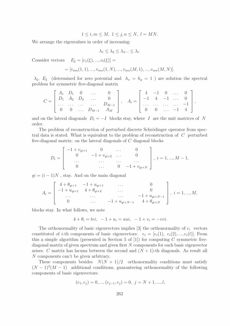
1 ≤ i,m ≤ M, 1 ≤ j, n ≤ N, l = MN.
We arrange the eigenvalues in order of increasing:
λ1 ≤ λ2 ≤ λ3... ≤ λl.
Consider vectors Eξ = [e1(ξ), ..., el(ξ)] =
= [vmn(1, 1), ..., vmn(1, N), ..., vmn(M, 1), ..., vmn(M,N)].
λξ, Eξ (determined for zero potential and hx = hy = 1 ) are solution the spectralproblem for symmetric five-diagonal matrix
C =
⎡⎢⎢⎣A1 D1 0 . . . 0D1 A2 D2 . . . 0. . . . . . . . . . . . DM−1
0 0 . . . DM−1 AM
⎤⎥⎥⎦ , Ai =
⎡⎢⎢⎣4 −1 0 . . . 0−1 4 −1 . . . 0. . . . . . . . . . . . −10 0 . . . −1 4
⎤⎥⎥⎦ ,
and on the lateral diagonals Di = −I blocks stay, where I are the unit matrices of Norder.
The problem of reconstruction of perturbed discrete Schrodinger operator from spec-tral data is stated. What is equivalent to the problem of reconstruction of C perturbedfive-diagonal matrix: on the lateral diagonals of C diagonal blocks
Di =
⎡⎢⎢⎣−1 + vqi+1 0 . . . 0
0 −1 + vqi+2 . . . 0. . . . . . . . . . . .0 . . . 0 −1 + vqi+N
⎤⎥⎥⎦ , i = 1, ...,M − 1,
qi = (i − 1)N , stay. And on the main diagonal
Ai =
⎡⎢⎢⎣4 + θqi+1 −1 + uqi+1 . . . 0−1 + uqi+1 4 + θqi+2 . . . 0
. . . . . . . . . −1 + uqi+N−1
0 . . . −1 + uqi+N−1 4 + θqi+N
⎤⎥⎥⎦ , i = 1, ...,M,
blocks stay. In what follows, we note
4 + θi = tei, − 1 + ui = uui, − 1 + vi = −vvi.
The orthonormality of basic eigenvectors implies [3] the orthonormality of ei vectorsconstituted of i-th components of basic eigenvectors: ei = [ei(1), ei(2), ..., ei(l)]. Fromthis a simple algorithm (presented in Section 5 of [1]) for computing C symmetric five-diagonal matrix of given spectrum and given first N components for each basic eigenvectorarises. C matrix has lacuna between the second and (N + 1)-th diagonals. As result allN components can’t be given arbitrary.
These components besides N(N + 1)/2 orthonormality conditions must satisfy(N − 1)2(M − 1) additional conditions, guaranteeing orthonormality of the followingcomponents of basic eigenvectors:
(e1, ej) = 0, ..., (ej−1, ej) = 0, j = N + 1, ..., l,
262
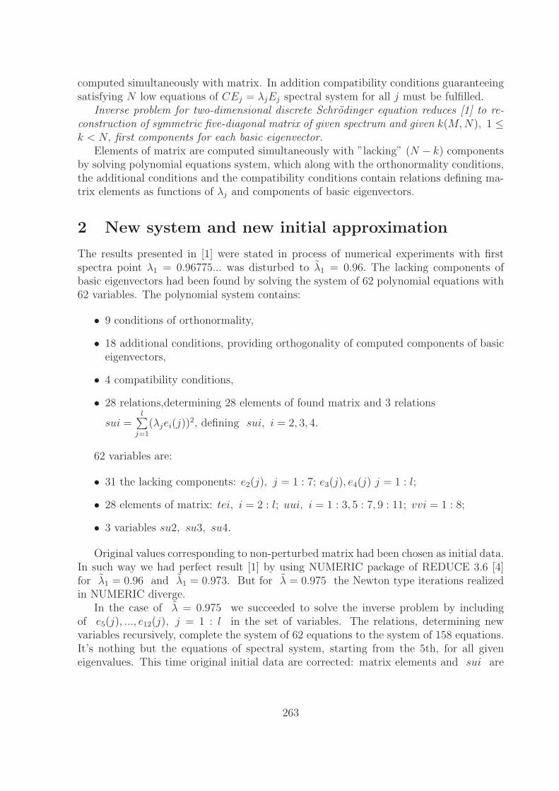
computed simultaneously with matrix. In addition compatibility conditions guaranteeingsatisfying N low equations of CEj = λjEj spectral system for all j must be fulfilled.
Inverse problem for two-dimensional discrete Schrodinger equation reduces [1] to re-construction of symmetric five-diagonal matrix of given spectrum and given k(M,N), 1 ≤k < N, first components for each basic eigenvector.
Elements of matrix are computed simultaneously with ”lacking” (N − k) componentsby solving polynomial equations system, which along with the orthonormality conditions,the additional conditions and the compatibility conditions contain relations defining ma-trix elements as functions of λj and components of basic eigenvectors.
2 New system and new initial approximation
The results presented in [1] were stated in process of numerical experiments with firstspectra point λ1 = 0.96775... was disturbed to λ1 = 0.96. The lacking components ofbasic eigenvectors had been found by solving the system of 62 polynomial equations with62 variables. The polynomial system contains:
• 9 conditions of orthonormality,
• 18 additional conditions, providing orthogonality of computed components of basiceigenvectors,
• 4 compatibility conditions,
• 28 relations,determining 28 elements of found matrix and 3 relations
sui =l∑
j=1
(λjei(j))2, defining sui, i = 2, 3, 4.
62 variables are:
• 31 the lacking components: e2(j), j = 1 : 7; e3(j), e4(j) j = 1 : l;
• 28 elements of matrix: tei, i = 2 : l; uui, i = 1 : 3, 5 : 7, 9 : 11; vvi = 1 : 8;
• 3 variables su2, su3, su4.
Original values corresponding to non-perturbed matrix had been chosen as initial data.In such way we had perfect result [1] by using NUMERIC package of REDUCE 3.6 [4]for λ1 = 0.96 and λ1 = 0.973. But for λ = 0.975 the Newton type iterations realizedin NUMERIC diverge.
In the case of λ = 0.975 we succeeded to solve the inverse problem by includingof e5(j), ..., e12(j), j = 1 : l in the set of variables. The relations, determining newvariables recursively, complete the system of 62 equations to the system of 158 equations.It’s nothing but the equations of spectral system, starting from the 5th, for all giveneigenvalues. This time original initial data are corrected: matrix elements and sui are
263
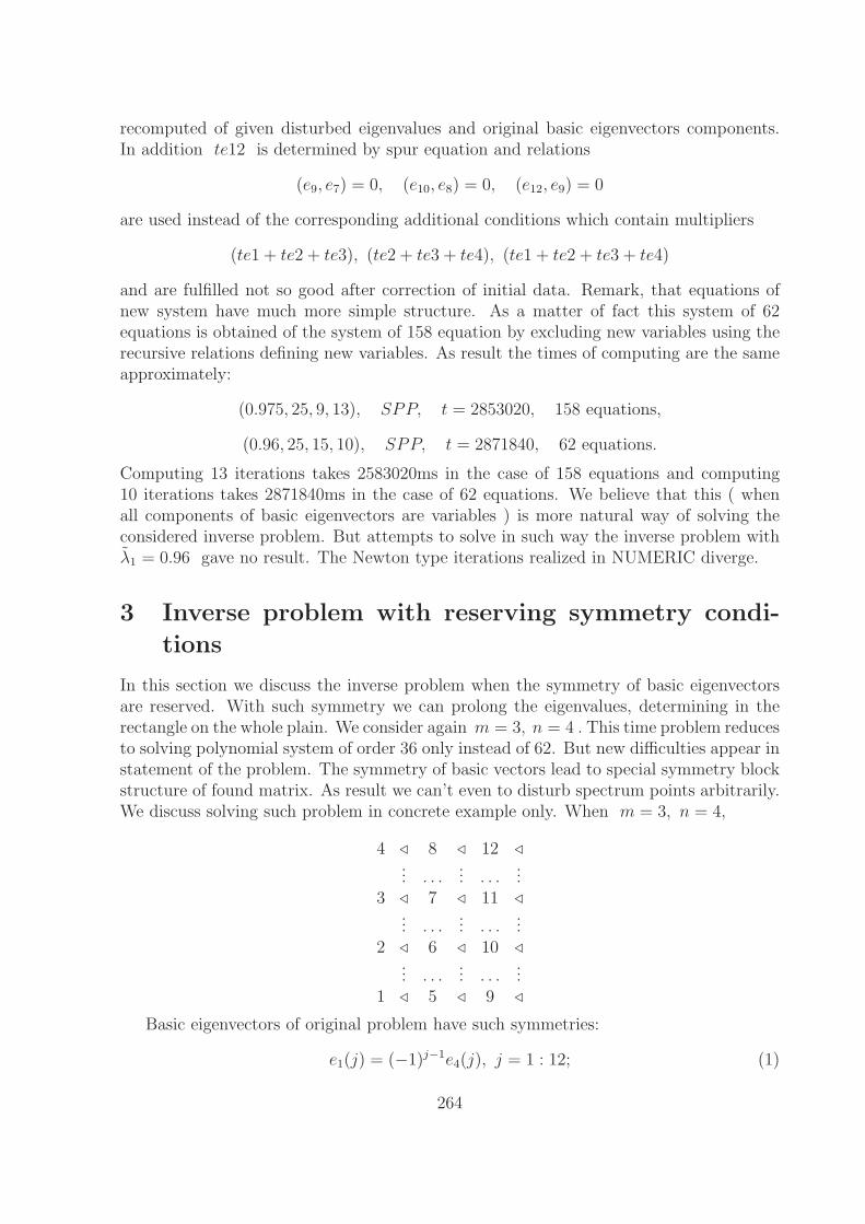
recomputed of given disturbed eigenvalues and original basic eigenvectors components.In addition te12 is determined by spur equation and relations
(e9, e7) = 0, (e10, e8) = 0, (e12, e9) = 0
are used instead of the corresponding additional conditions which contain multipliers
(te1 + te2 + te3), (te2 + te3 + te4), (te1 + te2 + te3 + te4)
and are fulfilled not so good after correction of initial data. Remark, that equations ofnew system have much more simple structure. As a matter of fact this system of 62equations is obtained of the system of 158 equation by excluding new variables using therecursive relations defining new variables. As result the times of computing are the sameapproximately:
(0.975, 25, 9, 13), SPP, t = 2853020, 158 equations,
(0.96, 25, 15, 10), SPP, t = 2871840, 62 equations.
Computing 13 iterations takes 2583020ms in the case of 158 equations and computing10 iterations takes 2871840ms in the case of 62 equations. We believe that this ( whenall components of basic eigenvectors are variables ) is more natural way of solving theconsidered inverse problem. But attempts to solve in such way the inverse problem withλ1 = 0.96 gave no result. The Newton type iterations realized in NUMERIC diverge.
3 Inverse problem with reserving symmetry condi-
tions
In this section we discuss the inverse problem when the symmetry of basic eigenvectorsare reserved. With such symmetry we can prolong the eigenvalues, determining in therectangle on the whole plain. We consider again m = 3, n = 4 . This time problem reducesto solving polynomial system of order 36 only instead of 62. But new difficulties appear instatement of the problem. The symmetry of basic vectors lead to special symmetry blockstructure of found matrix. As result we can’t even to disturb spectrum points arbitrarily.We discuss solving such problem in concrete example only. When m = 3, n = 4,
4 � 8 � 12 �... . . .
... . . ....
3 � 7 � 11 �... . . .
... . . ....
2 � 6 � 10 �... . . .
... . . ....
1 � 5 � 9 �
Basic eigenvectors of original problem have such symmetries:
e1(j) = (−1)j−1e4(j), j = 1 : 12; (1)
264
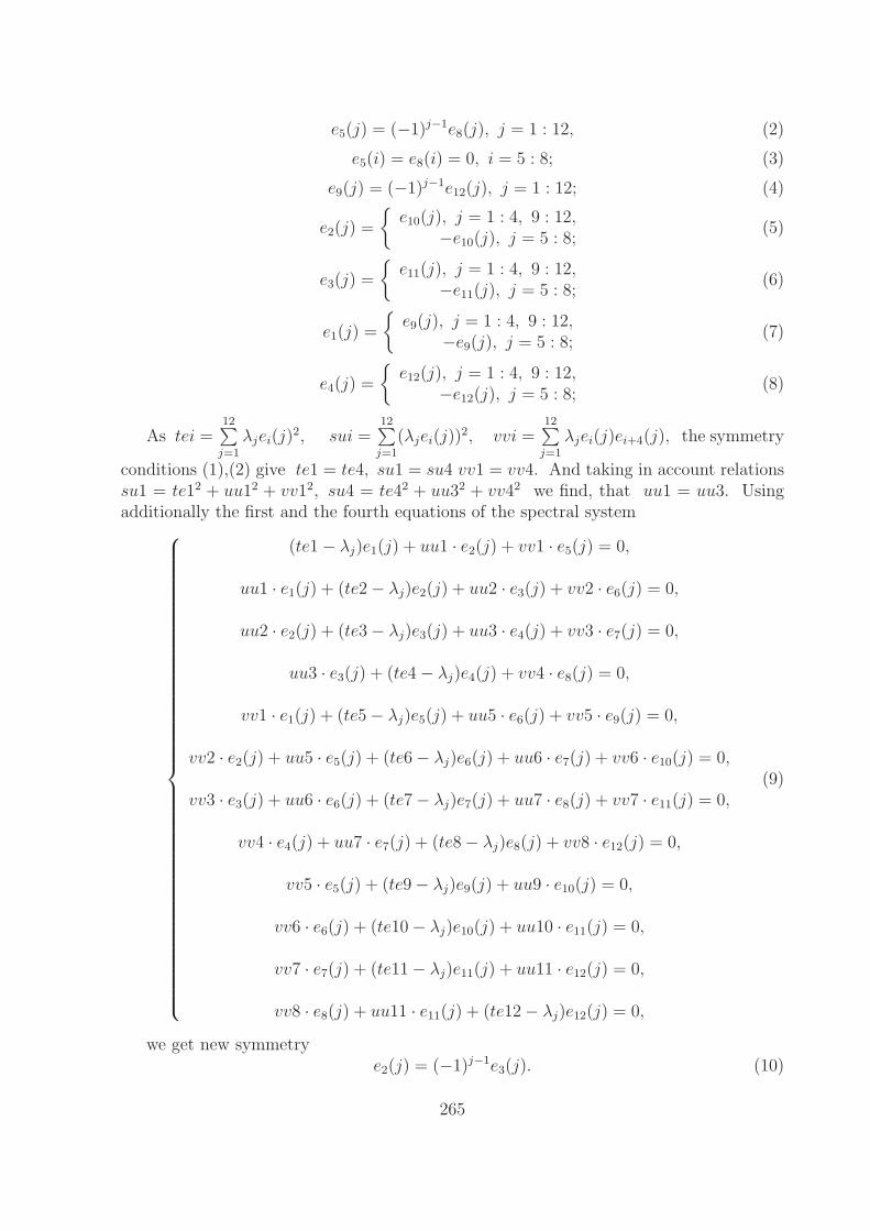
e5(j) = (−1)j−1e8(j), j = 1 : 12, (2)
e5(i) = e8(i) = 0, i = 5 : 8; (3)
e9(j) = (−1)j−1e12(j), j = 1 : 12; (4)
e2(j) =
{e10(j), j = 1 : 4, 9 : 12,
−e10(j), j = 5 : 8;(5)
e3(j) =
{e11(j), j = 1 : 4, 9 : 12,
−e11(j), j = 5 : 8;(6)
e1(j) =
{e9(j), j = 1 : 4, 9 : 12,
−e9(j), j = 5 : 8;(7)
e4(j) =
{e12(j), j = 1 : 4, 9 : 12,
−e12(j), j = 5 : 8;(8)
As tei =12∑
j=1
λjei(j)2, sui =
12∑j=1
(λjei(j))2, vvi =
12∑j=1
λjei(j)ei+4(j), the symmetry
conditions (1),(2) give te1 = te4, su1 = su4 vv1 = vv4. And taking in account relationssu1 = te12 + uu12 + vv12, su4 = te42 + uu32 + vv42 we find, that uu1 = uu3. Usingadditionally the first and the fourth equations of the spectral system⎧⎪⎪⎪⎪⎪⎪⎪⎪⎪⎪⎪⎪⎪⎪⎪⎪⎪⎪⎪⎪⎪⎪⎪⎪⎪⎪⎪⎪⎪⎪⎪⎪⎪⎪⎪⎪⎪⎪⎪⎪⎨⎪⎪⎪⎪⎪⎪⎪⎪⎪⎪⎪⎪⎪⎪⎪⎪⎪⎪⎪⎪⎪⎪⎪⎪⎪⎪⎪⎪⎪⎪⎪⎪⎪⎪⎪⎪⎪⎪⎪⎪⎩
(te1 − λj)e1(j) + uu1 · e2(j) + vv1 · e5(j) = 0,
uu1 · e1(j) + (te2 − λj)e2(j) + uu2 · e3(j) + vv2 · e6(j) = 0,
uu2 · e2(j) + (te3 − λj)e3(j) + uu3 · e4(j) + vv3 · e7(j) = 0,
uu3 · e3(j) + (te4 − λj)e4(j) + vv4 · e8(j) = 0,
vv1 · e1(j) + (te5 − λj)e5(j) + uu5 · e6(j) + vv5 · e9(j) = 0,
vv2 · e2(j) + uu5 · e5(j) + (te6 − λj)e6(j) + uu6 · e7(j) + vv6 · e10(j) = 0,
vv3 · e3(j) + uu6 · e6(j) + (te7 − λj)e7(j) + uu7 · e8(j) + vv7 · e11(j) = 0,
vv4 · e4(j) + uu7 · e7(j) + (te8 − λj)e8(j) + vv8 · e12(j) = 0,
vv5 · e5(j) + (te9 − λj)e9(j) + uu9 · e10(j) = 0,
vv6 · e6(j) + (te10 − λj)e10(j) + uu10 · e11(j) = 0,
vv7 · e7(j) + (te11 − λj)e11(j) + uu11 · e12(j) = 0,
vv8 · e8(j) + uu11 · e11(j) + (te12 − λj)e12(j) = 0,
(9)
we get new symmetrye2(j) = (−1)j−1e3(j). (10)
265
So it’s natural, when we find the lacking of 4 first components, to suppose that theysatisfying (1) and (10). This leads immediately to the following relations te1 = te4, te2 =te3, uu1 = uu3, su1 = su4, su2 = su3, vv1 = vv4, vv2 = vv3, e5(j) = (−1)j−1e8(j).Taken in account additionally and the second and the third equations of the spectralsystem (9), we get one more symmetry e6(j) = (−1)j−1e7(j) . This and the symmetrycondition (2) give te5 = te8, te6 = te7, uu5 = uu7, su5 = su8, su6 = su7.
These, the previous found relations and
su5 = vv12 + te52 + uu52 + vv52, su8 = vv42 + uu72 + te82 + vv82
su6 = vv22 + te52 + uu52 + te62 + uu62 + vv62, su7 = vv32 + uu62 + te72 + uu72 + vv72
give vv5 = vv8, vv6 = vv7. Using 5th and 8th equations of (9) we have, that
e9(j) = (−1)j−1e12(j), te9 = te12 = te1. (11)
With additional request (3) and symmetry conditions (5), (7) we obtain, that vv1 =vv5. Using the fifth equation of the spectral system (9) we find, that e6(j) = 0, j = 5 : 8,which implies vv2 = vv6. Using 6th and 7th equations of the spectral system (9), relationsvv2 = vv3, uu5 = uu7, te6 = te7, vv6 = vv7 and symmetries:
e2(j) = (−1)j−1e3(j), e5(j) = (−1)j−1e8(j), e6(j) = (−1)j−1e7(j)
we get, that e11 = (−1)j−1e10(j). The last and (11) imply te10 = te11, uu9 = uu11.As result we proved, that disturbed matrix, whose basic eigenvectors satisfy the sym-
metry conditions (1),(5),(7) and additional request (3), has special symmetric block-diagonal structure:
M =
⎡⎣ A W 0W B W0 W A
⎤⎦ , A =
⎡⎢⎢⎣a1 b1 0 0b1 a2 b2 00 b2 a2 b1
0 0 b1 a1
⎤⎥⎥⎦ , B =
⎡⎢⎢⎣α1 β1 0 0β1 α2 β2 00 β2 α2 β1
0 0 β1 α1
⎤⎥⎥⎦and W = diag(d1, d2, d3, d4). Eigenvalues of M are solutions of
Det[−(A − λI)(2 − W−1(B − λI)W−1(A − λI))] = 0,
where I is the unit matrix of order 4. The spectrum of such matrix can’t be arbitrary.We can’t to disturb the spectrum of original matrix arbitrarily and hope to find matrixhaving given disturbed spectrum and reserving the symmetric block-diagonal structure.
The eigenvectors E = [E1, E2, E3, E4]T , Ei − column-vectors of order 4, satisfy a
system ⎧⎪⎪⎪⎪⎨⎪⎪⎪⎪⎩(A − λI)E1 + WE2 = 0,
WE1 + (B − λI)E2 + WE3 = 0,
WE2 + (A − λI)E3 = 0.
266
By subtracting the third equation from the first we get
(A − λI)E1 = (A − λI)E3.
So, if λ is not eigenvalue of A, then E1 = E3. For original matrix λ5, λ6, λ7, λ8 formthe spectrum of A. We succeeded to solve the inverse problem for two disturbed spectra.
First we put δ = 0.003, Δa1 = Δa2 = δ, Δa3 = 1 − √1 + δ − δ2, Δa4 = 2δ, the
other elements of matrix stay nonperturbed. Then λi with odd i are disturbed and witheven i stay nonperturbed.
Second we put δ = 0.001, Δa1 = δ, Δa2 = 3δ, Δa3 = −δ,Δa4 = −2δ, Δb1 = 2δ, Δb3 = 2δ, Δb4 = 3δ, Δc1 = −2δ, Δc2 = −3δ,Δc3 = −2δ, Δb4 = −3δ, the other elements of matrix stay nonperturbed. Then all λi
were disturbed.In both cases perturbed matrix M, whose basic eigenvectors reserve the symmetry,
was reconstructed of given spectrum by solving a system of 36 polynomial equations with36 variables:
e1(j), e2(j), j = 1 : 12; te1, te2, te5, te6, uu1, uu2, uu5, uu6, vv1, vv2; su1, su2.
The system consists of 6 orthonormality conditions, 6 additional conditions (instead of 18in [1]), 4 compatibility conditions and 8 symmetry conditions.
Orthonormality conditions are
||e1|| = 1,12∑
j=1
e1(j)2 = 1; ||e2|| = 1,
12∑j=1
e2(j)2 = 1;
(e1, e2) = 0,12∑
j=1
e1(j)e2(j) = 0; (e1, e3) = 0,12∑
j=1
e1(j)e2(j)(−1)j = 0;
(e1, e4) = 0,12∑
j=1
e1(j)2(−1)j = 0; (e2, e3) = 0,
12∑j=1
e2(j)2(−1)j = 0.
Additional conditions are
e5 ⊥ e3,
12∑j=1
λje1(j)e3(j) = 0; e5 ⊥ e4,
12∑j=1
λje1(j)e4(j) = 0;
e6 ⊥ e5,
12∑j=1
λ2je1(j)e2(j) = uu1(te1 + te2);
e7 ⊥ e5,12∑
j=1
λ2je1(j)e3(j) = uu1 · uu2;
e7 ⊥ e6,
12∑j=1
λ2je2(j)e3(j) = uu2(te2 + te3); e8 ⊥ e5,
12∑j=1
λ2je1(j)e4(j) = 0.
267
Compatibility conditions are e5(j) = 0, j = 5 : 8. Symmetry conditions are e1(j) =e9(j), j = 1 : 4; e2(j) = e10(j), j = 1 : 4. The rest 12 equations of the systemdetermine matrix elements and su1, su2. The first 8 equations (9) determine recursivelyei(j), i = 5 : 12, as functions of chosen 36 variables. The corresponding functions aresubstituted in the right parts of
tei =12∑
j=1
λjei(j)2; uui =
12∑j=1
λjei(j) · ei+1(j); sui =12∑
j=1
(λjei(j))2.
The obtained system of 36 equations is solved by using NUMERIC, REDUCE 3.6.The original values of variables, corresponding to nonperturbed matrix are used as initialdata. We have perfect results in both cases: when all eigenvalues are disturbed and whenonly λi with odd i are disturbed.
Inverse problem on lattice, odd eigenvalues are disturbed$ Time:
42340 ms plus GC time: 180 ms la1; {0.973752448877015,15,9,10}$
Given spectrum. Found spectrum. Original spectrum. spi
:= { sp := { spo:={ 0.973752448877015,
la=0.973752448877015, 0.9677524488770101029937243,
1.96775244887701, la=1.96775244887_677,
1.967752448877010102993724, 3.2098204263768,
la=2.38796601125_285, 3.203820426376799799402898,
4.2038204263768, la=3.20982042_594845,
4.203820426376799799402898, 2.38796601125011,
la=3.38196601_231218, 2.381966011250105151795413,
3.38196601125011, la=3.80217957_13511,
3.381966011250105151795413, 4.6240339887499,
la=4.2038204_3090632, 4.618033988749894848204587,
5.61803398874989, la=4.6240339_7973626,
5.618033988749894848204587, 3.80217957362321,
la=4.7961795_8022541, 3.796179573623200200597102,
4.7961795736232, la=5.618033988_01261,
4.796179573623200200597102, 6.038247551123,
la=6.038247551_38763, 6.032247551122989897006276,
7.03224755112299}$ la=7.0322475511_1343}$
7.032247551122989897006276}$ rsys := {0.0240180000000204,18}$
Here rsys - result of substitution of initial data into the system. The maximum ofabsolute value of errors is in the 18th equation. 10 iterations were produced. Precisionwas 15, accuracy - 9. The found 4 first components of basic eigenvectors were used tocompute by primitive algorithm matrix with given spectrum presented in first column.The spectrum of found matrix is presented in the second column. The given and foundspectra coincide in 7 digits after the point. In the third column the spectrum of originalnonperturbed matrix is presented.
Inverse problem on lattice, all eigenvalues are disturbed$ Time:
268
60120 ms plus GC time: 330 ms la1;
{0.9665691027195753794729945,25,15,10}$ Given spectrum.
Found spectrum. spi := { sp := {
0.9665691027195753794729945, la=0.9665691027195753794729_854,
1.966479843598617085136807, la=1.966479843598617085136_768,
2.382071494687886682758795, la=2.38207149468788668275_9047,
3.201930178484952829213039, la=3.2019301784849528291_82246,
3.383176353169839514484215, la=3.383176353169839514_559909,
3.802704231391624853279469, la=3.802704231391624853_128874,
4.201014526413978981566726, la=4.201014526413978981_837853,
4.619928505312113317241205, la=4.61992850531211331_6772882,
4.801348034174387164076531, la=4.801348034174387164_400907,
5.622823646830160485515785, la=5.622823646830160485_484107,
6.036796487403846938034527, la=6.0367964874038469380_44792,
7.037157595813016769219905}$ la=7.037157595813016769219_662}$
rsys := {0.02630705693190862570881944,23}$
This time maximum of absolute value of errors is in the 23th equation. 10 iterationswere produced. Precision was 25, accuracy - 15. The given and found spectra coincide in18 digits after the point. The calculations had been produced on SPP.
4 References
1. Serdyukova S.I., Russ.J. Numer. Anal. Math. Modelling, Vol.15, No.5, pp. 455-468(2000)).
2. B.N.Zakhariev, A.A.Suzko - Direct and Inverse Problems. Potentials in QuantumScattering. Springer, Heidelberg,1990, Sec.2.4.
3. F.R.Gantmakher - Matrix Theory. Nauka, Moscow, 1967 (in Russian)
4. Hearn A.C. - REDUCE User’s Manual. Version 3.6. Rand, Santa Monica, 1995.CA 90707-2138.
269
On Investigation ofInvolutivity of Differential EquationSystems in CAS ‘MATEMATICA’
V.P. Shapeev1
ITAM SB RAS,630090, Novosibirsk, Russia;
e-mail: [email protected]
Compatibility analysis of partial differential equation systems is a kind of problemwhere Computer Algebra Systems (CAS) can be very helpful [4, 5, 6, 7, 8, 9, 10, 11].There is mathematical definition of two equivalent algorithms in this problem: Cartan’sone [1, 2] and one of Janet-Spencer-Kuranishi) [3]. In applications this problem demandslong symbolic computations.
In terms of symbolic computations, compatibility analysis consists of a certain se-quence of algebraic differential procedures. Given system PDE (S) we differentiate it byall independent variables and add to it all differential consequences, thus constructing theprolonged system (PS) (prolongation operation). Then, we calculate dimensions of theembedded linear spaces sequence, related to ranks of matrices of coefficients (PS). Coordi-nates in these spaces are dependent and independent variables in (S) and all derivatives ofthe latter in (PS). Then, we use the Cartan criterion that is expressed numerically throughdimensions of the embedded spaces sequence. If Cartan criterion is not fulfilled, (PS) istaken for the given system and the next prolongation is made. It continues this way untilCartan criterion is fulfilled (system (PS) in involution) or contradiction is obtained inthe form of equation of independent variables (system (S) is contradictory). The theoryguarantees that one of these results is reached within a finite number of prolongations.Only solutions of system in involution (PS) are solutions of system (S).
Realisation in CAS of an algorithm, which would be suitable for analysis in a generalcase, is a very complicated problem. The main difficulty is that in a nonlinear case, whilecalculating ranks of the matrices, one has to make assumptions, that should be tested ona variety defined by (PS) in the space of all variables and derivatives. Here, in a nonlinearcase the algorithm can branch out into many cases, and it is difficult to describe themall formally. However, particular cases show that the last difficulty can be overcome inthe dialogue mode, because in practice the number of subcases can be small. Analysis ofPDE compatibility as one of the algorithm’s steps is a part of the Differential ConstraintsMethod (DCM) or non-classical symmetries and of group analysis method for systemsof partial differential equations (PDE). If the initial system (S) contains equations whoseforms are indefinite because of the ”indefinite elements” in them (for example, the form of
1This work was partially supported by the Russian Foundation for Basic Research (grants 99-01-00515and 00-01-00370) and INTAS (proposal 1222).
270
quasi-linear equation coefficients is indefinite), then the Cartan criterion can be fulfilledby applying restrictions to the ranks of corresponding matrices of (PS) coefficients. Ingeneral case this will be expressed in the form of differential equations on the indefiniteelements. If one manages to find solutions for such equations, thus he finds the form forthe indefinite elements, which make the initial system (S) compatible. This form has tobe defined in the differential constraints method while looking for constraints compatiblewith a given system, and also in the method of intermediate integral.
In the present paper MATHEMATICA is used first of all for formulating the compat-ibility conditions, whose operator form can be obtained before using CAS. For example,in the case of overdetermined systems of quasi-linear hyperbolic equations, the form ofthe compatibility conditions is shown in the terms of full differentiation operators [7]. Asimilar situation can take place in the case of overdetermined systems of linear equations.
Compatibility analysis of overdetermined uniform linear systems of partial differentialequations of one unknown function is carried out with help of the well known Poissonbrackets algorithm. Despite the relatively simple form, its applications lead to hugesymbolic computations. In the present paper a program in MATHEMATICA system isrealised, whose input data is the number of equations, number and designation of thevariables, the form of the equations. It uses the standard functions of the system. Theprogram makes one prolongation and finds number of algebraically independent equationsin the prolonged system (PS) by calculating the ranks of the corresponding matrices. Inthe dialogue mode the number of prolongations is limited by the computer resources only.If system (S) has indefinite elements, then by demanding the corresponding matricesdeterminants to be zero, one can obtain conditions for the indefinite elements, whichwould make the prolonged system complete (i.e. in involution).
The following is a sample problem solved by the program. One-dimensional equationsof polytropic gas dynamics in Lagrangian variables
ut + px = 0, ψ(x)p−kpt + ux = 0, ψt = 0 (1)
by introducing potential φ by formulas u = −φx, p = φt, are reduced to equation
ψ(x)(φt)−kφtt − φxx = 0. (2)
We seek intermediate integral for it in the form (variable t is not among the coefficients(2))
F (x, φ, φt, φx) = C. (3)
Equation (2) contains indefinite element ψ(x) that is a function pertaining to the entropyand defining its gas particle distribution as a function of Lagrangian variable x. It followsfrom the known definition that intermediate integral (3) for equation (2) exists if in respectto function F (x, φ, φt, φx) two linear equations are fulfilled
L1 = Fφx ± φk/2t (ψ(x)−1/2)Fφt = 0,
L2 = Fxφk/2−1t ψ(x)−1/2 ± (1 ± φ
k/2−1t ψ(x)−1/2φx)Fφ = 0.
(4)
In the dialogue mode two system prolongations are made (4). From the demand ofthe prolonged system involution (corresponding determinants equal zero) we obtain an
271
ordinary differential equation of the second order on indefinite element ψ(x) with generalsolution ψ = (c1x + c2)
k−4. Taken the latter into account, we can solve system (PS) andthus obtain intermediate integral (3). Moreover, in this case one can obtain solutions ofequation (3). These solutions will have one-functional arbitrariness of the initial equation(2) and thus they will be solutions of gas dynamics equations (1). They generalize theknown isoentropic Riemann waves on the case of non-isoentropic flows with two constantsarbitrariness in entropy distribution on Lagrangian variable x. We do not have enoughspace here to go into details of this example.
As the other examples in the present paper, we sought conditions for existence ofone and a system of intermediate integrals for equations of the second order with threeindependent variables. Similar to the definition in the two-dimensional case in the classicaltheory of differential equations, by intermediate integral for equation of the second order
F (x1, x2, x3, u, u1, u2, u3, u11, ..., u33) = 0 (5)
in the three-dimensional case we will call differential equation of the first order
V (x1, x2, x3, u, u1, u2, u3) = c1, (6)
whose any non-special solution is a solution of equation (5). Here u(x1, x2, x3) is anunknown function, ui = ∂u
∂xi, uij = ∂ui
∂xj, c1 is an arbitrary constant. System of equations
(5), (6) is overdetermined and needs to be analysed for compatibility. Let us differentiate(6) once by each variable x1, x2, x3:
vx1 + u1vu + vu1u11 + vu2u21 + vu3u31 = 0,vx2 + u2vu + vu1u12 + vu2u22 + vu3u32 = 0,vx3 + u3vu + vu1u13 + vu2u23 + vu3u33 = 0.
(7)
On non-special solution intermediate integral (6) can be resolved in respect to ui0 whichis one of ui (i=1,2,3), while system (7) can be resolved in respect to three correspondingui0j, (j=1,2,3). By definition, substitution of found ui in (5) turns it to identity.
Consider quasi-linear equation
3∑i,j=1
aijuij + l = 0 (aij = aji), (8)
where coefficients aij, l are functions of x1, x2, x3, u, u1, u2, u3. In order to turn (8) toidentity due to equations (6), all minors of the fourth order in the matrix of secondderivative coefficients and free terms in system (7), (8)⎛⎜⎜⎝
vu1 vu2 vu3 0 0 0 vx1 + u1vu
0 vu1 0 vu2 vu3 0 vx2 + u2vu
0 0 vu1 0 vu2 vu3 vx3 + u3vu
a11 2a12 2a13 a22 2a23 a33 l
⎞⎟⎟⎠must equal zero. Hence, we obtain four proportions between vui
, vxi, that can be formu-
lated in the following way
μ21vu2 = vu1 , μ31vu3 = vu1 , μ32vu3 = vu2 ,a11vx1 + a22μ21vx2 + a33μ31vx3 + (a11u1 + a22μ21u2 + a33μ31u3)vu − lvu1 ,
(9)
272
where μij = (aij ±√
a2ij − aiiajj)/aii. Moreover, from this we obtain μ31 = μ32μ21 —
restriction on coefficients aij, (i, j = 1, 2, 3). Equation system (9) is linear and uniform inrespect to function v. Its compatibility is investigated with help of Poisson brackets. Indoing this, the program in MATHEMATICA system described above essentially helps amathematician to carry out the symbolic computations. Example. For equation
a(z)u11 + 2b(z)(u12 + u13) + c(z)(u22 + 2u23 + u33) = 0, z = u2 + u3
after one prolongation system (9) becomes complete (in involution). By its integrationwe find intermediate integral
v ≡ u1 +
∫cdz
b ±√b2 − ac
= c1.
In two-dimensional case a separate intermediate integral selects for an equation ofthe second order a class of solutions with one arbitrary function of one argument. Inthe three-dimensional case a separate intermediate integral selects for an equation of thesecond order a class of solution with one arbitrary function of two arguments. But a moreessential distinction of the three-dimensional case from the two-dimensional one consistsof the fact that an equation of the second order with three independent variables can havesystem of two intermediate integrals, which selects a class of solutions with one arbitraryfunction of one argument.
By a system of intermediate integrals for equations of the second order (5) we will callsystem of differential equations of the first order
Ψ(x1, x2, x3, u, u1, u2, u3) = c1, Ω(x1, x2, x3, u, u1, u2, u3) = c2, (10)
whose any non-special solution is a solution of equation (5).Equation system (5), (10) is overdetermined. Its compatibility should be investigated
by a general algorithm with use of Cartan criterion. A part of the analysis can be carriedout before using CAS. Let us differentiate equations (10) by all independent variables.The obtained equations can be written in the form
AY = t, (11)
where Y = (u11, u12, u13, u22, u23, u33, )′ and t = (t1, t2, ..., t6)
′ are column vectors. Fromcalculations we obtain that det(A) ≡ 0, therefore matrix A rank is less than six. It can beproved that A rank equals five. At that for compatibility of (10) it is necessary that rankof the extended matrix of system (11) also equals five. If the last condition is fulfilled inthe space of variables (x1, x2, x3, u, u1, u2, u3, ) on variety (10) identically, then accordingto Cartan criterion it can be shown that system (10) is in involution with arbitrariness inone function of one argument. The last condition can be reduced to the form
(t1Ψu1 + t2Ψu2 + t3Ψu3 − t4Ωu1 − t5Ωu2 − t6Ωu6). (12)
In the non-linear case it is difficult to obtain a definite answer, whether equations(10) are a system of intermediate integrals for (5). Such an investigation is easier in the
273
case of quasi-linear and linear equations. With help of the program it is possible to carryout complete investigation in more simple cases, because the further investigations arereduced to substitution of some expressions into others, obtaining coefficients at certainvariables in the problem, and to some other operations which can be easily programmedin MATHEMATICA. For example it is found out that there is a wide class of weaklynonlinear equations
∑3i,j=1 aijuij +
∑3i=1 aiui + l = 0, aij = aji, which have weakly
nonlinear intermediate integrals Ψ ≡ u1 − du3 − f = 0, Ω ≡ u2 − gu3 − h = 0, whereaij, ai, d, g are functions of x, l, f, h are functions of x, u.
For wave equationu11 − a2(u22 + u33) = 0, (13)
where a = const, we have managed with the help of CAS to complete all sequence of thedescribed algorithm’s steps and obtain solutions, which are known functionally invariantsolutions in a particular case. It is shown that among solutions of the intermediateintegrals there are those which are not functionally invariant.
As another example, CAS MATHEMATICA was applied to investigation of invo-lution of overdetermined systems, which appear in result of the differential constraintsmethod (non-classical symmetries) application to one-dimensional gas dynamics equa-tions [8]. Compared to the old version in REDUCE the new program version has newfeatures: deduction of characteristic equations and of proportions along the characteris-tics for overdetermined systems under consideration, transition to different notations ofinitial equations and results in order to obtain them in a convenient form for subsequentprocessing.
We will mention here some peculiarities that we have found while solving this problemin CAS.
1) There are two essentially different ways in MATHEMATICA to differentiate com-plicated expressions. The first one is to apply differentiation functions available in thelanguage. The second one is to reduce differentiation operation to rules of replacement ofone expression by another. The first way is easier for new users. Programming the secondway is similar in both CASs and are more labour-intensive, because it is easy to make amistake in complicated cases, so a thorough program testing is needed.
In problems of compatibility analysis the first way leads to overgrowth of intermediateoperations, because there can be many function arguments. For example, intermediateintegral (6) has seven of them. In space of second derivatives indefinite elements will havethirteen arguments. The number of arguments essentially increases if we consider equationsystems. In MATHEMATICA a particular function is written with all arguments to allowthe system differentiate by a given argument. Of course, in end of solving problem, whendifferentiation is not needed anymore, we can set transformation rules, which rewrite theobtained expressions without function arguments. However, it leads to overgrowth of theprogram itself.
In using the second way, one can go without ascribing arguments to the functiondescriptor. Moreover, in CAS REDUCE function arguments can be mentioned only onetime. The second way allows one to obtain shorter expressions, thus making process ofpreliminary analysis and integration of differential equations in the dialogue mode easier.
2) The transformation mentioned above, pertaining to removing arguments of com-plicated functions, demand description of different transformation rules in the program.
274
There is an opportunity in MATHEMATICA to write all necessary consequence of trans-formation as one compound operator with help of embeded simple operators. However,in this case such a compound operator often works much slower than in the case whenseparate transformations are realised by consequence of commands with simple operatorsof needed quantity. In the latter case the program is bigger. It has to be mentioned alsothat one compound transformation operator may be unable to make all transformationswritten in simple transformations, that is in the first case additional result transformationsmay be needed. This makes it of little use in solving the problems under consideration.
3) In application of operators (functions) with similar purposes to operations with frac-tional rational functions REDUCE often provides more simple expressions than MATHE-MATICA. The latter for similar simplifications demands use of other additional functions,in particular function Simplify[].
4) Application of CAS to problems, whose solution is not guaranteed without reali-sation in the program of complete algorithm, demands that the user knows the completealgorithm of its solution and understands the results he can obtain, that is that he knowsthe problem and ways of its solving. Simple example. Characteristic matrix Ch(λ) fortwo-dimensional equations of gas dynamics in plain (ν = 0) and axisymmetric (ν = 1)cases:
uτx + vτy − τux − τvy = ν τvy
, uux + vuy + τpx = 0,
uvx + vvy + τpy = 0, upx + vpy + A(ux + vy) = −ν Avy
.(14)
has four proper values λi, (i = 1, ..., 4). Here, λ ≡ y′ = dy/dx, (u, v) are coordinates ofthe velocity vector along axes x, y; p is pressure, τ is specific volume, c is sound speed,A = c2/τ .
MATHEMATICA could not solve the characteristic equation in symbolic form. Twocharacteristic directions y′
2,3 = v/u are known to coincide with direction of gas particlesvelocity. If we eliminate consequently these two roots with help of command
Chp3[λ] = Together[Ch[λ]/(x − v/u)]//Simplify,
Chp2[λ] = Together[Chp3[λ]/(x − v/u)]//Simplify,
then in result command Solve[Chp2[x] == 0, λ] produces two other (of a more compli-cated form) roots of the characteristic equation.
In more difficult cases CAS user can act in a similar way: to apply it only to a partof operations in a complicated algorithm of symbolic computations. The rest part of theoperations can be realised in the dialogue mode, using knowledge of the problem specifics.Thus, the technique used here of applying CAS only to a part of calculations needed forcomplete involution analysis can be justified.
References
[1] Cartan E. Les systemes differentiels exterieurs et leurs applications geometriques.Paris: Hermann, 1945. 215 p.
275
[2] Finikov S.P. Cartan exterior forms method in differential geometry. M.; L.: Gostekhiz-dat, 1948. 432 p, (Russian).
[3] Kuranishi M. Lectures on involutive systems of partial differential equations. SaoPaulo: Publ. Soc. Math., 1967. 77 p.
[4] Shurygin V.A., Yanenko N.N., On computer realization of algebraic/differential algo-rithms, in: Problemy Kibernetiki, 6, 1961, (Russian).
[5] Arais E.A., Shapeev V.P. and Yanenko N.N. Computer realization of Cartan’s externalforms, Dokl. AN SSSR. 1974, 214 (4), 737–738, (Russian).
[6] Peter A. Clarkson and Elizabeth L. Mansfield, Shwarz F. Symmetries and involutionsystems: Some experiments in Computer algebra // Topics in Soliton theory and Ex-actly solvable Nonlinear equations. Proceeding of Conf. on Nonlinear Evolution Equa-tions, Solitons and Inverse scattering Transform. - 1978. - p. 290-299.
[7] Sidorov A.F., Shapeev V.P., and Yanenko N.N. The Method of Differential Constraintsand its Application in Gas Dynamics. Nauka, Novosibirsk. 1984 – 272 p., (Russian).
[8] Meleshko S.V., Shapeev V.P. Application of computer algebra to analysis of differentialequations systems compatibility // 6th International IMACS Conference on Applica-tions of Computer Algebra IMACS ACA - June, 25-28, 2000, St. Petersburg, Russia -Abstracts, pp. 37-38.
[9] Ganzha V.G., Meleshko S.V., Murzin F.A., Shapeev V.P., Yanenko N.N. Computerrealization of the algorithm for the investigation of compatibility of systems of partialdifferential equations, Doklady Akademii Nauk SSSR, 261(5), 1044-1046, 1981, (Rus-sian).
[10] Ganzha V.G., Meleshko S.V., Shapeev V.P.. Automation of Compatibility Analysisof Quasilinear PDE Systems with the Aid of the REDUSE System. Computer Algebraand Its Applications to Mechanics. Nova Science Publishers, New York, 1993, p. 89-96.
[11] Meleshko S.V., Shapeev V.P.. An application of the differential constraints methodfor the two-dimensional equations of gas dynamics. Prikladnaya Matematikai Mekhanika, 63(6), 909-916, 1999, (Russian).
276
Moveable Singularities of PolynomialDifferential Equations
S. Sobolevsky
Minsk, Belarus
Solutions of ordinary differential equations in complex domain can admit singularitiesof two types: fixed (depending on the coefficients singularities) and movable (which locationvaries from one solution to another). The investigation of ordinary differential equationssolutions movable singularities has been started by the remarkable series of papers by Fuchs[1] (concerning the first-order equations), Painleve [2,3] and Gambier [4] (concerning thesecond-order equations). The main results are summarized in Ince [5]. Further, Chazy[6], Garnier [7], and Bereau [8] have obtained partial results concerning the rational third-order differential equations.
In the present paper we consider the arbitrary-order polynomial differential equationsof the form
w(n) = P (w(n−1), w(n−2), . . . , w, z), (1)
where n is an entire positive number and P is a nonlinear polynomial on w and itsderivatives with coefficients, analytic on z in a certain domain U ⊂ C.
We shall prove that every equation of class (1) admits movable singular points, i.e.not all of its solutions are analytic in U . Further we’ll present an algorithm and thecorresponding Mathematica program for investigation of these singularities.
Let us rewrite the equation (1) in the following form
w(n) =∑χ∈S
aχ(z)n−1∏j=0
(w(j))χj , (2)
where S is a certain set of n-vectors with nonnegative integer coordinatesχ = (χ0, χ1, . . . , χn−1) and aχ are functions, analytic in domain U . For each χ ∈ S let usassume
|χ| =n−1∑j=0
χj, ν(χ) =n−1∑j=1
jχj.
Consider two cases: I. maxχ∈S
ν(χ) < n and II. maxχ∈S
ν(χ) ≥ n.
I. First, consider a case maxχ∈S
ν(χ) < n. For all real t let us assume
ϕ(t) = minχ∈S
{t(|χ| − 1) − ν(χ) + n}, S(t) = {χ : χ ∈ S, t(|χ| − 1) − ν(χ) + n = ϕ(t)}.
277
It’s easy to see that function ϕ has at least one negative real root t = t0 because ϕ is acontinuous on the real axe function, lim
t→−∞= −∞, ϕ(0) = n−max
χ∈Sν(χ) > 0. This root is
rational because t0 = (n − ν(χ))/(|χ| − 1) for all χ ∈ St0 .Then after introducing the parametric variable replacement w = αt0v, z = z0 + αx for
z0 ∈ U we’ll transform the equation (2) to the following form
v(n) =∑χ∈S0
aχ(z0)n−1∏j=0
(v(j))χj + o(α), (3)
where S0 = S(t0) and o(α) denotes the sum of terms with positive rational degrees of α.For the equation (1) to be free of movable critical singular points it is necessary that theequation (3) for α = 0 would admit no solutions with critical singularities in zero as wellas the reduced equation
v(n) =∑χ∈S0
aχ(z0)n−1∏j=0
(v(j))χj . (4)
Let us call the value t0 the Bureau number for the equation (4).The equation (4) admits solutions of the form
v = λxt0 ,
where λ satisfies an equation
t0(t0 − 1) . . . (t0 − n + 1)λ =∑χ∈S0
aχ(z0)
[n−1∏j=0
t0(t0 − 1) . . . (t0 − j + 1)
]λ|χ|. (5)
Let us call the equation (4) regular if the equation (5) admits nonzero roots andirregular in the opposite case. The regular equations (4) with noninteger Bureau sym-bol obviously admit solutions with critical algebraic singular point in zero. The regularequations (4) with integer Bureau symbol admit solutions with pole in zero.
Let us show that the irregular equations (4) always admit solutions with critical sin-gularities in zero.
Consider the irregular equation (4). In this case the right side of the equation (4)admits parametric family of solutions v = λxt0 for arbitrary λ. Variable replacementx = es/α1/M
, v = xt0u, α = εM for sufficiently great positive integer M reduces theequation (4) to the form
εmu(n) = F (u(n−1), u(n−2), . . . , u, ε), (6)
where m is a natural number; F is a polynomial on all variables, and F (0Cn−1 , u, 0) ≡ 0
and F (0Cn−1 , u, ε) ≡ 0.
We’ll need the followingT h e o r e m 1. Consider an equation
αmw(n) = F (w(n−1), w(n−2), . . . , w, z, α) (7)
278
where m and n are natural numbers and F is function, analytic in a neighborhood of somepoint (wn−1
0 , wn−20 , . . . , w0, z0, 0) ∈ Cn+2. Let w = ϕ0(z) be a solution of the equation (7)
for α = 0 satisfying the initial conditions ϕ(j)(z0) = wj0, j = 0, n − 1.
Then in every neighborhood of z0 there exists such a point z1 and a sequence w = ϕα(z)of solutions of the equation (7) for real positive α which, for α → +0, uniformly convergesto ϕ0(z) in some neighborhood of z1.
To prove theorem 1 we’ll need the following two lemma.L e m m a 1. Consider the system⎧⎨⎩ αkgu′
g =s∑
l=1
Agl(z)ul + Fg(αu, αv, z, α), g = 1, s
v′ = B(z)u + C(z)v,(8)
where u = (ug, g = 1, s), ug ∈ Cng , ng ∈ N; v ∈ Cm; z, α ∈ C; kg ∈ N, k1 > k2 > . . . >ks; Agl, B(z), C(z) are correspondingly the ng × nl-, m × n- and m × m-matrixes withcoefficients, analytic on z in the certain domain U ⊂ C; F is a mapping from Cn+m+2
to Cn, analytic in a neighborhood of a set {(0Cn+m , z, 0) : z ∈ U}, where n =
s∑g=1
ng, and
F (0Cn+m , z, 0) ≡ 0. Let us assume that in the domain U the determinants of matrixes(
Agl, l = 1, θ
l = 1, θ
)for θ = 1, s are nonzero.
Than for every positive real α there exists a solution u = ϕα(z), v = φα(z) of thesystem (8) such that for α → +0 the sequences ϕα(z), φα(z) uniformly converge to zeroin some closed subdomain V ⊂ U .
Proof of the lemma 1. We may consider Agl ≡ 0 for g < l, because in the oppositecase it is sufficient to introduce the following replacements:
u0g = u0
g, j = 1, s, A0gl = Agl, j, l = 1, s,
uθg = uθ−1
g − αkθ−kgAθ−1gθ (z)(Aθ−1
θθ (z))−1u1, g = θ + 1, s,
Aθgl = Aθ−1
gl − Aθ−1gθ (Aθ−1
θθ )−1Aθ−1θl , g = θ + 1, s, l = 1, s,
θ = 1, s − 1.
The correctness of these replacements implies from that fact, that for θ = 1, s takes place
0 = det
(Agl(z), l = 1, θ
l = 1, θ
)= det
(Ag−1
gl (z), l = 1, θ
l = 1, θ
)=
s∏g=1
Ag−1gg (z), ∀z ∈ U.
In this case, on a lemma condition, for all g = 1, s and z ∈ U we have detAgg(z) = 0.We may also consider, that Agl ≡ 0 for g > l, because in the opposite case it is sufficientto introduce the following replacements:
ug = ug + A−1gg
(s∑
l=g+1
Agl(z)ul
).
279
It is easy to see, that there exists such a point z0 ∈ U , in which neighborhood matrixesAgg, g = 1, s could be represented as Agg(z) = Qg(z)Jg(z)Q−1
g (z), where Qg(z) arematrixes with analytic in a neighborhood of z0 coefficients and nonzero in a neighborhoodof z0 determinant, Jg(z) = diag(Jg
j (z), j = 1, τg), τg ∈ N, Jgj (z) is a Jordan cell of
dimension ζgj with analytic in a neighborhood of z0 diagonal element μg
j (z), andτ∑
j=1
ζgj =
ng.Having made in (8) a variable replacement ug = Qg(z)xg, g = 1, s, we’ll obtain{
αkgx′g = Jg(z)xg + Fg(αx, αv, z, α), g = 1, s,
v′ = B(z)Q(z)x + C(z)v,(9)
where Fg(a, b, z, α) ≡ Q−1(z)Fg(Q(z)a, b, z, α)−αkQ(z)−1Q′(z)a, Q(z) = diag(Qj(z), j =1, s).
We will need the following propositionP r o p o s i t i o n 1. Consider a linear differential system
du
dz= J(z)u + b(z), (10)
Where u is an n-vector function, τ ∈ N, J(z) is a Jordan cell of dimension n withanalytic in the convex closed area V ⊂ C diagonal element μ(z), b is an analytic in Vn-vector function. Let’s also assume that for some point z0 ∈ V and every point z ∈ Vthe inequalities
||b(z)|| < M,Re[μ(z)(z − z0)/|z − z0|] < −σ, z = z0,
(11)
where M,σ > 0, take place. Then the system (10) admits a private solution u = ξV,J,b(z)such, that for all z ∈ V , the inequality
|ξV,a,b(z)| < M(n∑
l=1
σ−l)
takes place.P r o o f of the proposition 1. Let’s rewrite the system (10) in the following form{
duj
dz= μ(z)uj + uj+1 + bj(z), j = 1, n − 1,
dun
dz= μ(z)un + bn(z),
(12)
where u = (u1, u2, . . . , un), b = (b1, b2, . . . , bn).In the case n = 1 the required solution ξV,a,b may be found in the following way:
u(z) =z − z0
|z − z0|
|z−z0|∫0
exp{ z − z0
|z − z0|
|z−z0|∫s
a(z0 + τz − z0
|z − z0|)dτ}
b(s)ds.
For this solution the required inequality
|u(z)| < M
|z−z0|∫0
exp{ |z−z0|∫
s
Re[a(z0 + τz − z0
|z − z0|)z − z0
|z − z0| ]dτ}
ds <
280
M
|z−z0|∫0
exp{−
|z−z0|∫s
σdτ}
ds =< M
t∫0
exp {σ(s − t)}ds =M
σ(1 − e−t) < M/σ
holds.Then the system (12) admits a solution
un = ϕn(z) = ξV,μ(z),bn(z)(z),
uj = ϕj(z) = ξV,μ(z),bj(z)+ϕj+1(z)(z), j = n − 1, 1,
which satisfies inequalities
|un| ≤ M/σ, |uj| ≤ (M + |uj+1|)/σ = M(
j∑l=1
σ−l), j = n − 1, 1
i.e. is the required one. The propositon 1 proof in comlete.Let’s choose a complex number r such, that |r| = 1, and for all g, j an inequality
Re[rμgj (z0)] = 0 takes place (it is obvious, that such r exists). As a required area V we
shall choose the closed neighborhood of point z0 in a form of a rhomb with the center inz0 and vertexes z0 +pr, z0−pr, z0 +pri, z0−qpri, where p, q are positive real numbers. Itis easy to see, that choosing p and q small enough, it is always possible to achieve, that forany point z ∈ V \ {z0 + pr, z0 − pr} and any g, j inequalities Re[(z − (z0 + pr))μg
j (z)] = 0would take place, Re[(z − (z0 − pr))μg
j (z)] = 0. Then there will be σ > 0 such, that forany g, j either Re[(z−(z0 +pr))μg
j (z)] < −σ for all z ∈ V or Re[(z−(z0−pr))μgj (z)] < −σ
for all z ∈ V . We shall also consider q small enough, such that diamV = 2pr.Let’s build solutions ϕα(z) = (ϕg
α, g = 1, s), φα(z) in the closed area V as limits ofthe following sequences. Let’s assume
ϕα,1(z) ≡ 0Cn , φα,1(z) ≡ 0C
m .
For any j ∈ N, j > 1 let’s assume
ϕgα,j(z) = ξV,Jg ,hg
j (z)(z), z ∈ V, g = s, 1
where hgj (z) =
s∑l=g+1
Agl(z)ϕgα,j(z) + Fg(αϕα,j−1(z), αφα,j−1(z), z, α), and as φα,j we shall
choose a solution of a linear system
dv
dz= C(z)v + B(z)Q(z)ϕα,j−1(z)
with initial conditions v(z0 − pr) = 0.Let’s consider ε, δ,M,N, σ > 0, such that for every n + m-vector which component
modulo it is less than n-vector δ, 0 < α < ε and all z ∈ V , inequalities take place
||∂F
∂a(a, z, α)||, ||∂F
∂α(a, z, α)|| < M,⇒ ||F (a, z, α)|| < (|α| + ||a||)M
281
||B(z)Q(z)|| < N, ||C(z)|| < T, ||diag(Jj(z), j = 1, τ)|| < N.
Let’s assume + =
max1≤q≤s,1≤κ≤τq
ζqκ∑
l=1
σ−l.
By induction on j in view of proposition 1 it is simple to show, that at all j ∈ N, z ∈ Vand 0 < α < χ = min{1, ε, δ/(1+ δ)/M/+, δT/(N+(e2prT − 1), 1/(2M+(1+2δ(N(e2prT −1)/T )))} the inequalities
||ϕqα,j(z)|| < α(1 + δ)M+ < δ, q = 1, s,
||φα,j(z)|| < α(1 + δ)MN+(e2prT − 1)/T,||ϕq
α,j+1(z) − ϕqα,j(z)|| < α(1 + max{N(e2prT − 1)/T ||ϕα,j−1(z) − ϕα,j−2(z)||,
||ϕqα,j(z) − ϕq
α,j−1(z)||})M+ < ||ϕqα,j(z) − ϕq
α,j−1(z)||/2, q = 1, s,||φα,j+1(z) − φα,j(z)|| < N(e2prT − 1)/T ||ϕα,j(z) − ϕα,j−1(z)||.
(13)
take place.From inequalities (13), for every fixed α ∈ (0, χ) the sequences {ϕα,j(z), j ∈ N},
{φα,j(z), j ∈ N} uniformly on V converge to some limiting vector-functions ϕα(z), φα(z),and the pair ϕα(z), φα(z) is a private solution of the system (9), satisfying the inequalities
||ϕα(z)|| ≤ α(1 + δ)M+, ||φα(z)|| ≤ α(1 + δ)MN+(e2prT − 1)/T.
Thus sequences ϕα(z), φα(z) are the required ones. The proof of lemma 1 is now complete.L e m m a 2. Consider an equation
αmw(n) = F (αkiw(i), i = 0, n − 1, z, αr) (14)
where m, r, ki are nonnegative rational numbers such that m > kn−1 ≥ kn−2 ≥ . . . ≥ k0 = 0and r > 0; F is a function, analytic in a neighborhood of a set {(0C
n , z, 0) : z ∈ U} forsome domain U ⊂ C, and F (0C
n , z, 0) ≡ 0. Let us also assume that for τ = maxki=0
i the
condition ∂F∂w(τ) (0C
n , z, 0) ≡ 0 holds.Then for every positive real α there exists a solution w = ϕα(z) of the equation (14)
such that for α → +0 the sequence ϕα(z) uniformly converges to zero in some closedsubdomain V ⊂ U .
Proof of lemma 2. Let us take rational numbers 0 < ρτ+1 < ρτ+2 < . . . < ρn = m suchthat there exist indexes τ = i0 < i1 < i2 < . . . < is = n and positive rational numbers0 < d0 < d1 < d2 < . . . < ds−1 such that ∂F
∂w(ij) (0Cn , z, 0) ≡ 0 and for ij < k ≤ ij+1 the
condition ρk = ρij + dj(k − ij) holds.
Then lemma 2 follows from lemma 1 after a replacement w(i) = αρiui, i = τ + 1, n − 1,
w(i) = ui, i = 0, τ − 1, w(i∗) = ui∗ −(
τ∑i=0
∂F∂w(i) (0C
n , z, 0)ui
)/ ∂F
∂w(τ) (0Cn , z, 0), α = εM ,
where M is a sufficiently great natural number.R e m a r k 1. For every natural N , one may represent the solutions ϕα(z) in the
following form
ϕα(z) =N∑
j=1
αj/Mφj(z) + αN/M ϕα(z), (15)
282
where M is a number from lemma 2 proof, φj are analytic in V functions and the sequenceϕα(z) uniformly in V converges to zero for α → +0.
The representation (15) can be obtained by repeated application of the replacementv = α1/M(φ(z) + v) which does not change the form of the equation (14) for certain φ.
Now theorem 1 implies from the obvious proposition, that every equation (7) may betransformed either to the form (14) or to the form (7) with m = 0 with the help of thereplacement
w = ϕ0(z) +s∑
j=1
αkjφj(z) + αkv,
where k > kj > kj−1 . . . k1 > 0 are rational numbers, φj are some function, analytic insome point z1 from a neighborhood of z0.
From the proposition above and the remark 1 one can obtainR e m a r k 2. For certain natural M and every natural N , one may represent the
solutions ϕα(z) in theorem 1 in the following form
ϕα(z) = ϕ0(z) +N∑
j=1
αj/Mφj(z) + αN/M ϕα(z)
where φj are analytic in a certain neighborhood V of the point z1 functions and the se-quence ϕα(z) uniformly in V converge to zero for α → +0.
Now from the theorem 1 and remark 2 for arbitrary constant C and positive real αand arbitrary natural N there exist solutions u = ϕα(z) of the equation (6) of the form
ϕε(s) = C +N∑
j=1
εj/Kφj(s) + εN/Kϕα(s),
where φj(s) are analytic in a certain neighborhood V of some point z1 which in spite of theequation (6) autonomy may be considered to be zero, and the sequence ϕα(s) uniformlyin V converges to zero for ε → +0. It is simple to see that for sufficiently great N not allφj are constant, because F (0C
n−1 , u, ε) ≡ 0.
Then the equation (4) admits a solution of the form
w = ζα(x) = C +N∑
j=1
αj/KMφj(α1/M ln x) + αN/M ϕα1/M (α1/M ln x),
where some φj are nonconstant and therefore admits movable critical singular points.From the aforesaid we have the followingP r o p e r t y 1. The solutions of regular equation (4) with Bureau number p always
admit poles or critical poles of order p in zero. The solutions of irregular equation (4)always admit critical singularities in zero.
II. Now let us consider the equation (2) in the case maxχ∈S
ν(χ) ≥ n. Assume
|χ|τ =n−1∑j=τ
χj, ν(χ) =n−1∑
j=τ+1
(j − τ)χj.
283
Consider two cases: 1) there exists such a τ ∗ that maxχ∈S
ντ∗(χ) = n− τ ∗, 2) there does not
exist such a τ ∗.1) In this case let us apply a variable replacement
z = z0 + αx, w(j) = wj0 + αwj, j = 0, τ ∗ − 1, w(τ∗) = u
for arbitrary constant z0, wj0. For α = 0 we’ll obtain a reduced equation of the form
u(m) =∑χ∈H
cχ(u)m−1∏j=1
(u(j))χj , (16)
where m = n−τ ∗; H is a certain set of m−1-vectors with nonnegative integer coordinates
χ = (χ1, . . . , χm−1) such thatm−1∑j=1
jχj = m; cχ are not identically equal to zero polynomials
on u with constant coefficients. One can choose z0, wj0 so that the set H would not be
empty. Let us denote the degree and the senior coefficient of polynomial cχ by dχ and kχ
correspondingly, and |χ| =m−1∑j=1
χj.
The replacementx = αx,u = v/α,u′ = αt−1p
for positive rational t reduces an equation (2) to a system{p(m−1) =
∑χ∈H
αt(|χ|−1)−dχkχ(p(m−2))χm−1(p(m−3))χm−2 . . . pχ1vdχ + o(α1/M),
v′ = pαt+1,(17)
where M is a sufficiently great natural number. For t = maxχ∈H
dχ/(|χ| − 1) > 0 and
H0 = {χ ∈ H : dχ = t(|χ| − 1)} the reduced at α = 0 system (17) takes form{p(m−1) =
∑χ∈H0
kχ(p(m−2))χm−1(p(m−3))χm−2 . . . pχτ+1vdχ ,
v′ = 0.(18)
For constant v the first equation of this system is a (4)-type equation with Bureau number−1. Thus, from the property 1, p in the system (18) admits movable simple poles or criticalsingular points. Let p = p0(x), v = v0 be a solution of the system (18) where p0 admits apole or a critical singularity. Then the system (17) admits a solution of the form
p = p0(x) + o(α1/M ), v = v0 +
(∫p0(x)dx + o(α1/M )
)αt+1,
i.e. admits movable critical singular points. It means that the equation (2) in the consid-ered case admits them.
284
2) In this case let us denote τ ∗ = maxmaxχ∈S
ντ∗(χ)>n−ττ , m = n − τ ∗. Consider a function
ϕ(t) = minχ∈S
{t(|χ|τ∗+1 − 1) − ντ∗(χ) + m}. This function is obviously continuous on the
segment [0, 1], while ϕ(0) = s − mτ < 0 and ϕ(1) = s − 1 − mτ+1 > 0. Hence thefunction ϕ has at least one root t = t0 on an interval (0, 1). Assume S0 = {χ : χ ∈S, t0(|χ|τ∗+1 − 1) − ντ∗(χ) + m = 0.
Then after introducing in the equation (2) the replacement
z = z0 + αx, w(j) = wj0 + αwj, j = 0, τ ∗ − 1, w(τ∗) = wτ∗
0 + αt0u,
with constant wj0, z0 one can obtain at α = 0 the reduced equation of the form
u(m) =∑χ∈S0
(aχ(z0)
τ∗∏j=0
(wj0)
χj
)(u(m−1))χn−1(u(m−2))χn−2 . . . (u′)χτ∗+1 . (19)
One can choose constants z0, wj0 so that the right side of the equation (19) would be not
identically equal to zero. Then the equation (19) would be the (4)-type equation withnoninteger Bureau number t0. According to the property 1 it means that the reducedequation (19) as well as the initial equation (2) admits movable critical singular points.
From the aforesaid we have the followingP r o p e r t y 2. The (2) satisfying an inequality max
χ∈Sν(χ) ≥ n always admits
movable critical singular points.From properties 1,2 the following theorem follows.T h e o r e m 2. The equation (1) always admits movable singular points. It can be
free of movable critical singular points only if for equation (2) the inequality maxχ∈S
ν(χ) < n
holds and the corresponding equation (4) is regular with an integer Bureau number.Let us continue the investigation of the equation (1) under the necessary for the
absence of movable critical singular points conditions of theorem 2. After reducing it tothe form (3) its solution can be found in the form
v(x) =∞∑
j=0
vj(x), (20)
where the function v0 satisfies the equation (4); the function v1 satisfies the equation (4)
v(n) =n−1∑j=0
Lj(v0)v(j), (21)
where Lj(v0) =∑
χ∈S0
aχ(z0)χj
(n−1∏i=0
(v(i)0 (x))χi
)/v
(j)0 (x); and vj for j > 1 satisfy linear
differential equations of the form
v(n) =n−1∑j=0
Lj(v0)v(j) + f(v0, v1, . . . , vj−1),
285
which homogeneous part coincides with (21) and f is a function which polynomiallydepends on v0, v1, . . . , vj−1.
The equation (21) is called the Euler equation for the equation (3). It can be alsodirectly obtained from the equation (3) as a reduced equation after introducing the re-placement v = v0 + αv and assuming α = 0.
The necessary condition for the equation (3) to be free of solutions with critical sin-gularities in zero is that its Euler equation for any v0 satisfying the equation (4) mustadmit no solutions with critical singularity in zero. The numerical test for the absenceof movable critical singular points for the equation (3) can be obtained by considerationEuler equations for v0 = λxt0 where λ is an arbitrary nonzero solution of the algebraicequation (5). For this v0 Euler equation takes form
v(n) =n−1∑j=0
lj(λ)v(j)xj−n, (22)
where lj are polynomials on λ with constant coefficients. This equation admits solutionsof the form v = xr where r is an arbitrary solution of an equation
n−1∏i=0
(r − i) =n−1∑j=0
lj
j−1∏i=0
(r − i). (23)
Furthermore if the equation (23) admits multiple roots then the considered Euler equation(22) admits solution with logarithmic branch points. So the solution of the equation (22)admit no critical singularities in zero if and only if the equation (23) roots are integer andpairwise different.
The special case when l0 = l1 = . . . = ln−1 = 0 needs special consideration. In thiscase the equation (4) admits solutions with critical singularities in zero. Really, the afterintroducing the replacement v = v0 + αv we’ll find the obtained equation’s solution inthe form v = C + αkg(x) + o(αk) where C is a constant, k is a natural number and gsatisfied an equation g(n) = h(x) where h admits a pole of order less than n, i.e. g admitslogarithmic branch point in zero.
From aforesaid one can obtain the followingP r o p e r t y 3. For the equation (2) satisfying an inequality max
χ∈Sν(χ) < n to be free
of movable critical singular points it is necessary that for any λ satisfying the equation (5)the equation (22) has not identically equal to zero right side and the equation (23) rootsare integer and pairwise different.
If the condition of property 3 holds the further investigation of the equation (3) con-sists of sequential determination of v2, v3, . . . for all v0 and λ and investigation of theresingularities in zero.
From property 3 one can obtain the following corollary concerning the special class ofequations (1).
T h e o r e m 3. The equation (1) which right side does not essentially depend onw(n−1) and w(n−2) always admits movable critical singular points.Proof of theorem 3. Let us denote the corresponding equation (23) roots by r1, r2, . . . , rn.According to the property 3 for the equation (1) to be free of movable critical singularpoints it is necessary that r1, r2, . . . , rn would be integer and pairwise different. Let it be.
286
Under the theorem 3 conditions the equality ln−1 = ln−2 = 0 for the equation (23)holds. It means that r1 + r2 + . . . + rn = 0 + 1 + . . . + n − 1 and r2
1 + r22 + . . . + r2
n =02 +12 + . . .+(n−1)2. One can easily sea that it is possible only if r1, r2, . . . , rn are equalto 0, 1, . . . , n− 1. But this is possible only in the case l0 = l1 = . . . = ln−1 = 0 which doesnot satisfy the condition of proposition 3. The proof of theorem 3 is now complete.
From theorem 3 one can sea that for equations (1) free of movable critical points thecorresponding equation (4) would essentially depend on v(n−1) or v(n−2) and so its Bureaunumber would be −1 or −2.
From aforesaid we obtain the following algorithm of equation (1) movable singularitiesinvestigation.
Step 1. Check the inequality maxχ∈S
ν(χ) < n. If it does not hold the original equation
admits movable critical points.Step 2. Compute the Bureau number and check whether it is equal to −1 or −2. If
it does not hold the original equation admits movable critical points.Step 3. For any nonzero λ satisfying the equation (5) check whether at least one of
lj(λ) is nonzero and whether the roots of equation (23) are integer and pairwise different.If it does not hold the original equation admits movable critical points.
This program realization of this algorithm has been obtained using the Mathematica4 system in the form of the following module
BeginPackage[”ADE‘”]Diffinst::usage = ”evalutes substitution in ODE”Check1::usage = ”check of condition 1”Check2::usage = ”check of condition 2”Evalute::usage= ”Evaluates the investigation of a given equation eq of order n in the givenor arbitrary point z0”Begin[”‘Private‘”]Diffinst[de , u , x , u1 , x2 , x1 ] := {Module[{},
de[[1]] /. {de[[2]] -> Function[{z}, u1[u[x1[z]], x1[z]]],de[[3]] -> x2[x]}], u, x}Check1[de , n ] := Module[{u,x,a,z0},((Expand[aˆn*
Diffinst[de, u, x, Function[{u, x}, u], Function[{x}, z0 + a*x],Function[{z}, (z - z0)/a]][[1]]]) /. a -> 0 )=== 0]
Check2[de , n ,u ,x ,a ,z0 ] := Module[{de0,b},de0:=Expand[aˆ(n+1)*Diffinst[de, u, x, Function[{u, x}, u/a], Function[{x}, z0 +
a*x],Function[{z}, (z - z0)/a]][[1]]];b=If[((de0/.a->0)=!=0)&&((de0/.a->0)=!=ComplexInfinity),1,de0:=Expand[aˆ(n+2)*Diffinst[de, u, x, Function[{u, x}, u/aˆ2], Function[{x}, z0
+ a*x],Function[{z}, (z - z0)/a]][[1]]];If[((de0/.a->0)=!=0)&&((de0/.a->0)=!=ComplexInfinity),2,0]];{b,de0}]
Evalute[de ,n ,z0 ]:=Module[{de0,d0,re,a,i,j,l,k,ks,eul,reul,r,r0,dec,dec0},Off[Power::infy];If[Not[Check1[de,n]],Print[”Weight-power condition doesn’t hold, so the considered
287
equation admits movable critical singularities”],Print[”Weight-power condition holds”]; de0=Check2[de,n,de[[2]],de[[3]],a,z0];If[de0[[1]]==0,Print[”Bureau number is different from 1 or 2, so the considered equa-
tion admits movable critical singularities”],Print[”Bureau number is ”,-de0[[1]]]; d0=de0[[2]]/.a->0; Print[”The reduced equa-
tion is ”,D[de[[2]][de[[3]]],{de[[3]],n}]==d0];re=Expand[de[[3]]ˆ(de0[[1]]+n)*Diffinst[{D[de[[2]][de[[3]]],{de[[3]],n}]
-d0,de[[2]],de[[3]]}, de[[2]],de[[3]],Function[{u,x},k*xˆ(-de0[[1]])],Function[{x},x],Function[{x},x]][[1]]];
ks=Solve[re==0,k]; If[Length[ks]< =1,Print[”The considered equation is irregular and admits movable critical singularities”],
ks=NSolve[re==0,k]; dec0=True;For[l=1;j=1,l¡=Length[ks],l++,If[(k/.ks[[l]])=!=0.,Print[j,”]. ”,de[[2]]==(k/.ks[[l]])*de[[3]]ˆ(-de0[[1]])];j++;Print[”The corresponding Euler equation”];eul=Sum[(D[d0,D[de[[2]][de[[3]]],{de[[3]],i}]]/.{de[[2]]->Function[{z},
(k/.ks[[l]])*zˆ(-de0[[1]])]})*D[de[[2]][de[[3]]],{de[[3]],i}],{i,0,n-1}];If[eul===0.,Print[”Euler equation is degenerative”];dec0=False,Print[D[de[[2]][de[[3]]],{de[[3]],n}]==eul];Print[”admits roots”];reul=Expand[de[[3]]ˆ(-r+n)*Diffinst[{D[de[[2]][de[[3]]],{de[[3]],n}]
-eul,de[[2]],de[[3]]},de[[2]],de[[3]],Function[{u,x},xˆr],Function[{x},x],Function[{x},x]][[1]]];
r0=r/.NSolve[reul==0,r];Print[r0];dec=True; For[i=1,i¡=Length[r0],i++,
dec=(dec && (Abs[FractionalPart[r0[[i]]]]<0.0005))];If[dec,Print[”Euler numbers seem to be integer”],Print[”Some of the Euler numbers
are noninteger”]]; dec0=(dec0 && dec)]]];If[dec0,Print[”All necessary conditions for the considered equation to be free of mov-
able critical singularities hold”],Print[”The considered equation amdits movable critical singularities”]];]]]]
End[];EndPackage[]
The module provides a function ”Evalute” which checks the conditions necessary forthe given equation to be free of movable critical singularities. The syntax is following:
Evalute[rhs, w, z, n, z0], where rhs is the equation’s right-hand side, w is a dependant
variable, z is an independant variable, n is the equation’s order, and z0 is a point z0
in which the investigation is being carried out. Here are the examples of this functionapplications.
Example 1. Second order equation w′′ = w′3:Input: Evalute[w’[z]ˆ3, w, z, 2, z0]Output: Weight-power condition doesn’t hold, so the considered equation admits movable
288
critical singularitiesExample 2. Abel equation w′ = w3:
Input: Evalute[w[z]ˆ3, w, z, 1, z0]Output: Weight-power condition holds Bureau number is different from 1 or 2, so theconsidered equation admits movable critical singularities
Example 3. Second order equation class w′′ = 2w′w+w3 +a(z)w2 +b(z)w′+c(z)w+d(z):Input: Evalute[2*w’[z]*w[z] + w[z]ˆ3 + a[z]*w[z]ˆ2 + b[z]*w’[z] + c[z]*w[z] + d[z], w, z,2, z0]Output: Weight-power condition holdsBureau number is -1The reduced equation is w”[z]=w[z]ˆ3+2w[z]w’[z]1]. w==-0.732051/zThe corresponding Euler equationw”[z]==3.0718w[z]/zˆ2-1.4641w’[z]/zadmits roots{-2,1.5359}Some of the Euler numbers are noninteger2]. w==2.73205/zThe corresponding Euler equationw”[z]==16.9282w[z]/zˆ2+5.4641w’[z]/zadmits roots{-2,8.4641}Some of the Euler numbers are nonintegerThe considered equation amdits movable critical singularities
Example 4. Chazy barrier equation [6] w′′′ = ww′′ − 2w′2:Input: Evalute[w[z]*w”[z] - 2*w’[z]ˆ2, w, z, 3, z0]Output: Weight-power condition holdsBureau number is -1The reduced equation is w”’[z]==-2w’[z]ˆ2+w[z]w”[z]The considered equation is irregular and admits movable critical singularities
Example 5. First Painleve equation w′′ = 6w2 + z:Input: Evalute[6*w[z]ˆ2 + z, w, z, 2, z0]Output: Weight-power condition holdsBureau number is -2The reduced equation is w”[z]==6w[z]ˆ21]. w==1/zˆ2The corresponding Euler equationw”[z]=12w[z]/zˆ2admits roots{-3,4}Euler numbers seem to be integerAll necessary conditions for the considered equation to be free of movable critical singu-larities hold
289
Summary
In the present paper the nonlinear arbitrary-order polynomial differential equations areconsidered. It is shown that there solutions always admit movable singularities and thealgorithm of these singularities investigation is given. The program realization of thisalgorithm in Mathematica 4 system is presented.
References
1. L. Fuchs. Uber Differentialgleichungen deren Integrale feste Verzweigungspunktebesitzen, Sitz. Akad. Wiss. Berlin 32:699-710 (1884).
2. P. Painleve. Memoire sur les equations differentielles dont l’integrale generale estuniforme, Bull. Soc. Math. France 28:201-261 (1900).
3. P. Painleve. Sur les equations differentielles du second ordre et d’ordre superieurdont l’integrale generale est uniforme, Acta. Math. 25:1-85 (1902).
4. B. Gambier. Sur les equations differentielles du second ordre et du premier degredont l’integrale generale est a points critiques fixes, Acta. Math. 33:1-55 (1910).
5. E.L. Ince. Ordinary differential equations, Dover Publications, New York, 1956(originally published by Longmans & Green, London and New York, 1926).
6. J. Chazy. Sur les equations differentielles du troisieme ordre et d’ordre superier dontl’integrale generale a ses points critiques fixes, Acta. Math. 34:317-385 (1911).
7. R. Garnier. Sur des equations differentielles du troisieme ordre dont l’integralegenerale est uniforme et sur une classe dequations nouvelles d’ordre superier dontl’integrale generale a ses points critiques fixes, Ann. Sci. Ecole Norm. Sup. 29:1-126(1912).
8. F. Bureau. Differential equations with fixed critical points, Ann. di Math. 66:1-116(1964).
290
Bargmann-Darboux Transformationsfor Time-Dependent Quantum
Equations
A.A. Suzko 1
Joint Institute for Nuclear Research,Dubna, Russia
A procedure is elaborated of constructing a time-dependent periodic Hamiltonian forwhich Schrodinger equations admit analytic solutions. The method is based on the trans-formation of time-independent soluble problems into time-dependent ones by a set of uni-tary time-dependent transformations and a proper choice of initial states. A class of 2×2periodic time-dependent potential matrices with cyclic matrix solutions is constructed ina closed explicit form. The expectation value of Hamiltonian, total, dynamical, and geo-metric phases are derived in terms of the obtained solutions.
1 Introduction
Extensive study of time-dependent quantum oscillators [1]–[5], the study of quantumsystems with a dynamical semisimple Lie group [6] have shown that an algebraic approachis a very useful tool for investigation of the evolution of dynamic quantum systems. Themethod of separation of variables [7], and the supersymmetry method [8] were suggestedfor construction of time-dependent exactly solvable potentials. In this paper, we elaboratethe technique of constructing a periodic time-dependent Hamiltonian admitting exactsolutions with the use of an exactly soluble time-independent Hamiltonian, unitary time-dependent transformations and a proper choice of initial states.
The technique of Bargmann-Darboux transformations and the supersymmetry methodin quantum mechanics yield a variety of soluble stationary models [9, 10, 11]. Each ofthese models, to our mind, can be generalized to obtain the corresponding family of time-dependent exactly soluble Hamiltonians. Our main findings are as follows. First, weexplicitly show how to construct exactly soluble time-dependent generalizations of anyexactly soluble time-independent model for a 2 × 2 Hamiltonian. We do this by usingunitary time-dependent transformations which change time-independent problems intotime-dependent ones and by choosing initial states so that to derive cyclic solutions whichrequire the initial states to be eigenstates of a time-independent Hamiltonian. We showhow to generate a large family of time-dependent models from one time-independent modelby employing a family of special time-dependent operators of transformation. Finally, asan application of our method, we present explicit expression of an expectation value of
1Permanent address: Radiation Physics and Chemistry Problems Institute, Academy of Sciences ofBelarus, Minsk
291
Hamiltonian, the nonadiabatic geometric phase, total and dynamical phases which arederived in terms of the obtained cyclic solutions. In particular, we demonstrate how toconstruct a set of periodic time-dependent Hamiltonians whose expectation values do notdepend on time. This procedure can be used for modeling quantum wells and wires.
Low-dimensional physical systems have attracted considerable attention as from the-oretical and as well as from the practical point of view. Recent achievements in micro-fabrication technology give opportunities to construct two-dimensional quantum wells,superlattices, quantum wires and dots with properties of particle confinement. As it wasshown in [12] and [13] that under definite conditions a particle can be localized in a nonuni-form high frequency electromagnetic field. Recently Tralle [14] following Cook et.al. [15]considered a particle motion in a rapidly oscillating field of the form V (r, t) = V (r) cos ωtin terms of the Shcrodinger equations with periodic and aperiodic V (r), correspond-ingly. The main result of these authors is that for a sufficiently high frequency ω thetime-dependent potential is, in a sense, equivalent to the time-independent effective po-tential and as a sequence a particle can be confined. This result is equivalent to theresult [13] where the classical movement was considered. Here we generate more com-plicate time-dependent potentials which with special initial functions give the effect liketime-independent potentials, in particular, the expectation values of the time-dependentHamiltonian for cyclic solutions do not dependent on time. It means that these statesbehave equivalent stationary states with conserve energy.
2 Construction of a time-dependent Hamiltonian
To simplify the description below, we give a scheme of generation of a time-dependentHamiltonian with corresponding solutions from a time-independent one [16]. Supposethat the state |Ψ(t) > of a dynamical system evolves according to the matrix Schrodingerequation
i∂|Ψ(r, t) >
∂t= H(r, t)|Ψ(r, t) > (1)
with � = 1 and T periodic time-dependent Hamiltonian, H(t) = H(t + T ),
H(r, t) = −∇2r + V (r, t), (2)
the potential matrix V (r, t) = {Vij(r, t)} is Hermitian. Our goal is to give the procedureof obtaining a wide class of time-dependent Hamiltonians H(t) for which exact solutionsof (1) can be found. To this end, we use the time-independent Hamiltonian
H(r) = −∇2r + V (r) (3)
with a real symmetric potential matrix V (r) and �2/2m = 1, and a unitary time-dependent transformation S(t) [6, 16]
|Ψ(r, t) >= S(t)|Φ(r, t) >, (4)
292
by means of which the known time-independent Hamiltonian (3) is changed into thetime-dependent one
H(t) = S(t)HS†(t) + iS(t)S†(t). (5)
Here |Φ(r, t) > satisfies the equation of motion with the time-independent Hamiltonian
H(r)
i∂|Φ(r, t) >
∂t= H(r)|Φ(r, t) > (6)
and it is of the form
|Φ(r, t) >= exp(−iH(r)t)|Φ(r, 0) > . (7)
It is evident, the solutions |Ψ(r, t) > and |Φ(r, t) > can be defined, at correspondingchoice of initial functions, by solutions of the time-independent problem
H|Φ(E) >= E |Φ(E) > . (8)
If the system of Schrodinger equations (8) with some known time-independent Hamil-
tonian H(r) is exactly soluble, the system of equations (1) with the time-dependentHamiltonian (5) admits exact solutions too.
2.1 Construction of a 2 × 2 T -periodic Hamiltonian H(t)
Now consider reconstruction of the 2 × 2 periodic time-dependent Hamiltonian taken inthe form (2). We start with the time-independent Hamiltonian (3) with the 2 × 2 realsymmetric potential matrix V (r), V12(r) = V21(r). By means of a unitary time-dependenttransformation taken in the form
S(t) = exp(−is · h(t)) = exp(−i3∑
i=1
sihi(t)) (9)
the time-independent Hamiltonian (3) with regard to equations (1) and (5) turns into thetime-dependent Hamiltonian
H(r, t) = −∇2r + exp(−is · h(t))V (r) exp(is · h(t)) + (s · h(t)). (10)
Here s = (1/2)σ is the spin operator, σ = (σ1, σ2, σ3) and σi are the Pauli matrices anda dot means a time-derivative. The solutions of (1) with Hamiltonian (10), according to(4), are represented as
|Ψ(r, t) >= exp(−is · h(t) exp(−iH(r)t)|Φ(r, t = 0) > . (11)
It is convenient to present the 2 × 2 Hamiltonian (3) by the sum of diagonal and zerotrace matrices as
H(r) = −∇2r +
(V11(r) V12(r)V21(r) V22(r)
)=(−∇2
r + q(r))I + 2(s · B(r)), (12)
293
with the evident notations : q(r) = (V11(r) + V22(r))/2, B1(r) = V12(r), B2(r) = 0,B3(r) = (V11(r) − V22(r))/2 and I is the identity matrix. Then the time-dependentHamiltonian (10) can be represented as
H(r, t) =(−∇2
r + q(r))I + 2 exp(−is · h(t))(s · B(r)) exp(is · h(t)) + (s · h(t)). (13)
Obviously, the transformation (9) does not change the first term of (12) and transforms thesecond term. It is evident that the Hamiltonian for the two coupled system of equationscorresponds to the three- or two-dimensional problem with coordinates Bi(r) dependenton the extra parameter r. Such a Hamiltonian may be considered as an analog of theinhomogeneous magnetic field B(r) or a model Hamiltonian for describing a two-levelatom.
In terms of the evolution operator U(t) = U(t, 0), the solution |Ψ(r, t) > is
|Ψ(r, t) >= U(t)|Ψ(r, 0) >, U(0) = 1. (14)
In the case when |Ψ(r, 0) >= |Φ(r, 0) >, it is easy to find from (11) and (14) a veryimportant relationship between the operators U(t) and S(t)
U(t) = S(t)) exp−iHt = exp(−is · h(t)) exp(−iHt). (15)
The evolution operator in one period is written as
U(T ) = exp(−is · h(T )) exp(−iHT ). (16)
In assumption that S(T ) and H commute [S(T )H] = 0, we easily obtain that U(T ) and
H commute. Indeed,
U †(T )HU(T ) = S†(T ) exp(−iHT )H exp(iHT )S(T ) = S†(T )HS(T ) = H,
i.e.,
[U(T )H] = 0 (17)
and therefore U(T ) and H have common eigenvectors |Φν >.Now consider cyclic solutions that after one period T (T = 2π/ω) are recovered up to
the phase, i.e., initial states |Ψν(0) > are eigenvectors of U(T ) and because of (17) they
are eigenvectors of the effective Hamiltonian H. This leads to
|Ψν(r, T ) >= U(T )|Ψν(r, 0) >= exp(−iβν)|Ψν(r, 0) >, (18)
|Ψν(0) >= |Φν >, (19)
where βν is the total phase. From this, the matrix representation of U(T ) can be writtenas
U(T ) =∑
ν
exp(−iβν)|Φν >< Φν |
294
and U(T ) has a set of linearly independent eigenvectors |Φν > with eigenvalues exp(−iβν).With allowance for (11) the recurrent solutions at any time are written as
|Ψν(r, t) >= exp(−is · h(t)) exp(−iEνt)|Φν(r) > . (20)
It is evident now, to determine the cyclic solutions we need time-independent solutions.Thus, whenever H(r) is an exactly soluble time-independent Hamiltonian, the properlygenerated time-dependent system of equations has cyclic exact solutions. The evolutionof an arbitrary initial state |Ψ(r, 0) >=
∑ν αν |Ψν(r, 0) > can be represented as a su-
perposition of a basis set of recurrent linearly independent vector solutions, |Ψ(r, t) >=∑ν αν |Ψν(r, t) > .Now we can proceed to calculations of geometric phase, associated with the evolution
of cyclic solutions, dynamical phase and the expectation value of Hamiltonian. To findthe dynamical phase δν , we need the expectation value εν(t) of H(t),
δν =
∫ T
0
εν(t)dt =
∫ T
0
< Ψν(r, t)|H(t)|Ψν(r, t) > dt
=
∫ T
0
< Ψν(r, 0)|U †(t)H(t)U(t)|Ψν(r, 0) > dt. (21)
By using (15) and (5) we have
U †(t)H(t)U(t) = eiH(r)t(H(r) − iS†(t)S(t)
)e−iH(r)t.
Since for cyclic solutions |Ψν(r, 0) >= |Φν(r) > and |Φν(r) > is an eigenstate vector of
H(r) with an eigenvalue Eν we express the expectation value εν(t) and the dynamicalphase δν as
εν(t) = Eν− < Φν(r)|iS†(t)S(t)|Φν(r) >, (22)
δν = EνT −∫ T
0
< Φν(r)|iS†(t)S(t)|Φν(r) > dt. (23)
Hence, the geometric phase ϕν , given by removing the dynamical phase from the totalphase βν , is
ϕν = βν − δν = βν − EνT +
∫ T
0
< Φν(r)|iS†(t)S(t)|Φν(r) > dt. (24)
It should be noted that for a time-periodic and unitary S(t), the expression (24) forthe geometric phase is simplified
ϕν =
∫ T
0
< Φν(r)|iS†(t)S(t)|Φν(r) > dt. (25)
Really, in this case in contrast with (16) the time evolution operator after one period
is U(T ) = exp(−iH(r)T ). Since |Ψν(0, r) > is an eigenstate of U(T ) with eigenvalue
295
exp(−iβν) then |Ψν(0, r) > is also eigenstate of H with eigenvalue βν/T . At the same
time, since eigenvalues of H are Eν , then βν/T = Eν and (25) is valid.
Examples. Consider some particular examples of constructing a time-dependentHamiltonian (13) with the corresponding solutions by using SU(2) transformation (9) inwhich the components of h(t) are linear functions of time, hi(t) = ωit
S(t) =3∏
i=1
Si(t) = exp(−is · wt).
1 case. Let S(t) = S3(t) = exp(−iσ3ωt/2) where ω is some constant angular velocity.Then, in accordance with (5) or (13) the time-independent Hamiltonian (12) is trans-formed into the time-dependent one as
H(r, t) =(−∇2
r + q(r))I +
(V11(r)−V22(r)+ω
2V12(r) exp(−iωt)
V21(r) exp(iωt) −V11(r)−V22(r)+ω2
). (26)
It is evident that H(r, t) is time-periodic, H(r, t = 0) = H(r, t = T ), T = 2π/ω. Its
Routhian is H(r) connected with H(r, t = 0) by H(r, 0) = H(r) + ω2σ3. By using (20) the
cyclic solutions can be written as
|Ψν(r, t) >=
(exp(−i(Eν
1 + ω3/2)t) 0
0 exp(−i(Eν2 − ω3/2)t)
)|Φν(r) >, (27)
where Eνα = (Eν − Δα) and Δα can be the energy of inner structure (threshold).
2 case. If S(t) is chosen as an operator of rotation around y-axis
S2(t) = exp(−iσ2ω2t/2) =
(cos(ω2t/2) − sin(ω2t/2)sin(ω2t/2) cos(ω2t/2)
), (28)
then in accordance with (13) the time-dependent Hamiltonian H(t) takes another form
H(r, t) = (−∇2r + q(r))I + (29)
+
(V11−V22
2cos ω2t − V12 sin ω2t V12 cos ω2t + V11−V22
2sin ω2t − iω2/2
V12 cos ω2t + V11−V22
2sin ω2t + iω2/2 −(V11−V22
2cos ω2t − V12 sin ω2t)
).
In accordance with (20) the recurrent solutions of equation (1) are immediately writtenas
|Ψν(r, t) >=
(cos(ω2t/2) exp(−iEν
1 t) − sin(ω2t/2) exp(−iEν2 t)
sin(ω2t/2) exp(−iEν1 t) cos(ω2t/2) exp(−iEν
2 t)
)|Φν(r) > . (30)
3 case. Let S(t) be chosen as an operator of rotation around x-axis
S1(t) = exp(−iσ1ω1t/2) =
(cos(ω1t/2) −i sin(ω1t/2)
−i sin(ω1t/2) cos(ω1t/2)
). (31)
296
Then, from (13) the time-dependent Hamiltonian H(t) is
H(r, t) =(−∇2
r + q(r))I (32)
+
(V11−V22
2cos(ω1t) V12 − ω1
2+ iV11−V22
2sin(ω1t)
V12 − ω1
2− iV11−V22
2sin(ω1t) −V11−V22
2cos(ω1t)
).
The cyclic solutions of (1) with account of (20) are written as
|Ψν(r, t) =
(cos(ω1t/2) exp(−iEν
1 t) −i sin(ω1t/2) exp(−iEν2 t)
−i sin(ω1t/2) exp(−iEν1 t) cos(ω1t/2) exp(−iEν
2 t)
)|Φν(r) > . (33)
Now we show that for all the considered examples with hi(t) = ωit the expectationvalues of H(t) for corresponding cyclic solutions are independent on time. Really, therelation (22), with account of expressions for potentials and cyclic solutions (26)–(33),gives the expectation values of H(t) as
εiν =< Φν(r)|H(r)|Φν(r) > +
ωi
2< Φν(r)|σi|Φν(r) >= Eν +
ωi
2¯σi
ν . (34)
It means that equation (1), for obtained family of time-dependent potential matrices,possesses solutions and properties like time-independent ones. Note, the spin-expectationvalue
¯σiν =< Ψν(t, r)|σi|Ψν(t, r) >=< Φν(r)|σi|Φν(r) >
is none other than spin-alignment along the rotating axis and does not depend on timein this case. For the dynamical phase δν from (34) we get
δiν =
T∫0
εiν(t)dt = EνT + π ¯σi
ν . (35)
Removing the dynamical phase (35) from the total phase
βν = π + EνT. (36)
we get the geometric phase ϕiν
ϕiν = (βν − δi
ν) = π(1 − ¯σiν). (37)
One can easily see that the geometric phase is determined by the spin-expectation value¯σi
ν along the rotating axis. It is evident, in all considered cases the Hamiltonian (26),(29), (32) is T -periodic, T = 2π/ω, and the solutions (27), (30) and (33) are are 2T -periodic and change sign after one period. As one can easily seen, if S(t) is chosen to beT -periodic then the Hamiltonian becomes T/2-periodic, and the solutions are T -periodic.In this case, the total phase is multiply of 2π, and the geometric phase is determined by(25).
Thus, by means of a different choice of transformation operators Si(t), i = 1, 2, 3, threefamilies of time-dependent potential matrices with the corresponding cyclic solutions are
297
generated in a closed form from one family of time-independent potential matrices. It isevident that a more general transformation can be taken and can be used to change time-independent Hamiltonian H into time-dependent H(t). For example, S(t) can be taken asa direct product of the Si(t), S(t) =
∏3i=1 Si(t), or with a more complicated dependence of
S on time. So, whenever V (r) is an exactly soluble potential matrix for the ordinary time-independent system of Schrodinger equations, a family of exactly soluble time-dependentpotential matrices for the system of Schrodinger equations (1) can be generated.
Let V (r) be a Bargmann potential matrix for which the system of equations (8) hasexact solutions. For example, the matrix elements of the transparent potential and therelevant Jost solutions are [10]
Vαα′(r) = 2d
dr
∑νλ
exp(−κναr)γν
αP−1νλ (r)γλ
α′ exp(−κλα′r), (38)
F±αα′(k, r) = exp(±ikαr)δαα′ (39)
−∑νλ
γνα exp(−κν
αr)P−1νλ (r)
∫ ∞
r
γλα′ exp(−(κλ
α′ ± ikα′)r′)dr′,
where
Pνλ(r) = δνλ +m∑α′
γνα′γλ
α′
κνα′ + κλ
α′exp(−(κν
α′ + κλα′)r).
The normalized solution for the vector function of the bound state is immediately ex-pressed through the matrix Jost solutions taken at the energy of the bound state, k = iκν ,(iκν)
2 = −Eν , kα = (E − Δα)1/2,
Φα(Eν , r) =m∑α′
Fαα′(k = iκν , r)γνα′ , α, α′ = 1, 2. (40)
Here, the indices ν and λ correspond to the bound states characterized by the energies Eν
and amplitudes |γν > determine normalizing matrices |γνα >< γν
α′ | and the channel indicesare labeled as α, α′. Substitution (38) into (26), (29), (32) and (40) into (27), (30), (33)allows determination of three families of potential matrices and pertinent cyclic solutionsin an closed analytical form. Let us take another exactly solvable example, the potentialmatrix and corresponding regular solutions within the radial Gelfand-Levitan approach,when the spectral matrix for H(r) coincides with one for free Hamiltonian at E > 0, canbe written as
Vαα′(r) = 2d
dr
∑νλ
sinh[κναr]/κν
α)cνα′P−1
νλ (r)cλα′(sinh[κλ
α′r]/κλα′ , (41)
φαα′(k, r) =sin[kαr]
kα
δαα′ −∑νλ
cνα
sinh[κναr]
κνα
P−1νλ (r)cλ
α′
∫ r
0
sinh[κλα′r]
κλα′
sin[kα′r′]kα′
dr′, (42)
298
where cνα determine normalizing matrices Cν = |cν
α >< cνα| and
Pνλ(r) = δνλ +m∑α′
cνα′cλ
α′
∫ r
0
(sinh[κνα′r]/κν
α′)(sinh[κλj′r
′]/κλα′)dr′.
The normalized solution for the vector function of the bound state is given as
Φα(Eν , r) =m∑α′
φαα′(k = iκν , r)cνα′ . (43)
Substituting (41) into (26), (29), (32) and (43) into (27), (30), (33) we readily obtainanother three families potentials and corresponding periodic solutions in an explicit form.It is worth noting that the class of exactly solvable stationary problems is very wide. Al-gebraic Bargmann-Darboux transformations give multiple examples of problems that canbe used to generate a large class of explicit time–dependent potential matrices admittingexact solutions of the Schrodinger equation (1). We consider 2 × 2 matrix equations asexamples. In principle, this procedure can be used for the generation of an exactly solublepotential matrix for systems of N coupled time-dependent equations.
3 Conclusion
We have developed the method of solving a system of coupled time-dependent Schrodingerequations in an explicit form by using unitary time-dependent transformations whichchange time-independent problems into time-dependent ones. In distinction to earlierstudies, the method is based on soluble time-independent equations and a special choice ofinitial functions. This approach yields a large class of previously unknown exactly solvablenonstationary models and can be used for investigation of two- and three–dimensionalobjects. The family of time-dependent soluble potential matrices, for which a system oftwo-coupled Schrodinger equations has exact solutions, is generated. As an application ofthe suggested method, we have presented explicit expressions of the expectation value ofH(t), the nonadiabatic geometric phase, total, and dynamical phases, which are derived interms of obtained cyclic solutions. Time-dependent models, for which expectation valuesdon’t dependent on time, are given.
Acknowledgments
The author is grateful for useful discussions and hospitality to Professor H.V. Von Geramb.The paper was supported in part by the BRFFI, grant No.F99R-162/641.
References
[1] H.R. Levis, J. Math. Phys., 1962, vol. 3, p. 806; H.R. Levis and W.B. Riesenfeld, J.Math. Phys., 1969, vol. 10, p. 1458.
299
[2] I.A. Malkin and V.I., Man’ko Dynamical Symmetries and Coherent States of Quan-tum Systems (Moscow, Nauka, 1979)
[3] C.F., Lo, Phys.Rev.A 1992, vol. 45, p. 5262.
[4] M. Maamache, Phys. Rev.A, 1995, vol. 52, p. 936.
[5] K. Bay, W. Lay, A. Akopyan, J. Phys.A: Math Gen., 1997, vol. 30, p. 3057.
[6] Wang, Shun-Jin, Phys. Rev.A, 1990, vol. 42, p. 5107; ibid p. 5103.
[7] C.J. Efthimiou and D. Spector, Phys. Rev.A, 1994, vol. 49, p. 2301.
[8] B.F. Samsonov, J.Phys.A:Math.Gen., 2000, vol.33, p.591.
[9] K. Chadan and P.C. Sabatier, Inverse Problems in Quantum Scattering Theory(Springer-Verlag. Berlin Heidelberg/New York, 1989, 493p. 2-nd ed.)
[10] B.N. Zakhariev and A.A. Suzko, Direct and Inverse Problems. (Potentials in Quan-tum Scattering) (Springer-Verlag. Berlin Heidelberg/New York, 1990, 223p. 2-nd ed.)
[11] G. Junker, Supersymmetric Method in Quantum and Statistical Physics, (Springer-Verlag. Berlin Heidelberg/New York, 1996).
[12] W.Paul and M.Raether Z.Phys., 1955, vol.140, p.262.
[13] A.V. Gaponov and M.A. Miller J.Eksper.Teor.Fiz., 1958, vol.43, p. 242.
[14] I.E. Tralle, Phys.Stat.Sol. 1994, vol.181, p.97.
[15] R. Cook et.al., Phys.Rev., 1985, vol. A31, p.564.
[16] E. Velicheva, A. Suzko, Theor. and Math.Physics 1998, vol.115, p.687.
300
Analytic Modeling for Investigationof Quantum Systems in theAdiabatic Representation
A.A. Suzko, E.P. Velicheva
Joint Institute for Nuclear Research,Laboratory of Information Technology,
JINR, Dubna, Russiaand Radiation Physics and Chemistry Problems Institute,
National Academy of Sciences of Belarus, Minske-mail: [email protected]
Complex dynamical systems with some degrees of freedom are analyzed on the basisof the inverse scattering problem in the adiabatic representation. Matrix elements of anexchange interaction determining the ”slow” subsystem are calculated and studied in termsof exact solutions obtained within the parametric inverse problem for the ”fast” subsystem.The main characteristics of the slow subsystem Hamiltonian depend on the statement ofthe parametric inverse problem: namely, the fast subsystem is given on the semi-axisor on the entire axis. It is shown that in the case of the radial parametric problem orparametric problem specified on the semi-axis, matrix elements of the induced vector andscalar potentials and eigenfunctions are singular at the degeneration points of two levels.The opposite occurs in the case of the parametric problem specified on the entire axis, theyare regular at the degeneration points of two levels. The influence of parametric spectralcharacteristics of the fast subsystem on the behavior of the slow subsystem is studied. Inparticular, it is shown that the choice of normalizing functions determining the transparentsymmetric potential in fast variables leads to the zero coupling between states for two-levelsystems, (even at the point of degeneration), while another choice of normalization factorsleads to nonsymmetric potentials and nonzero coupling for the same energy levels. Ourapproach suggested allows the investigation of adiabatically driven quantum systems witha prescribed dependence on parametric adiabatic variables.
1 Introduction
Consider the system evolving according to the Schrodinger equation
i�∂|Ψ(t) >
∂t= H(x(t))|Ψ(t) >, (1)
where the Hamiltonian H(x(t)) is given in the form
H(x(t)) = −∂2/∂x2 + h(x(t)), h(x(t)) = −∂2/∂y2 + V (x(t), y). (2)
301
If ψn(x(t); y) are solutions to the equation
h(x(t))|ψn(x(t); y) >= En(x(t))|ψn(x(t); y) > (3)
and form a complete orthonormal set |ψn(x; y) >< ψn(x; y′)| = δ(y − y′), < ψn(x; y) |ψm(x; y) >= δnm ∀x, with elements depending on x = x(t) parametrically. Then Ψ canbe expressed by the expansion
|Ψ(x(t), y) >=∑
n
|n >< n|Ψ >=∑
n
∫ψn(x(t); y)Fn(x(t)) (4)
over the eigenstates of the self-adjoint parametric Hamiltonian (3). Upon substitutingthe expansion (4) into the initial Schrodinger equation (1) and using the relations oforthonormalization, we arrive at a multichannel system of gauge equations
i�∂
∂tF (x(t)) = [−(∇x + A(x))2 + V (x)]F (x(t)). (5)
Here A(x) and V (x) are the effective vector and scalar potentials, respectively, the matrixelements of which are induced by the basis functions ψ(x; y) of the parametric problem(3)
Anm(x) =< ψn(x; y)|∇x|ψm(x; y) >, (6)
Vnm(x) = < ψn(x; y)|h(x)|ψm(x; y) > −i� < ψn(x; y)|∂tψm(x; y) >
≡ En(x)δnm − i�Bnm(x). (7)
In the case of a slow and smooth evolution in time of the collective coordinates x(t), thesecond derivative is neglected in (2), H(x(t)) → h(x(t)), and the solution of equation (1)is sought in the form of an expansion (see, for instance, [1],
|Ψ(x(t), y) >=∑
n
cn(x(t)) exp(− i
�
∫ t
0
En(x(t′))dt′)|ψn(x(t); y) > . (8)
With account of (8) and (3) in (1), we find that the system of equations for cn(t) can bewritten in the form
∂tcn(t) =∑m
Bnm(x(t)) exp[− i
�
∫ t
0
(En(t′) − Em(t′))dt′]cm(t) . (9)
The matrix elements of the exchange interaction Bnm(x(t)) are generated by the basisfunctions |n > of the ”instantaneous” Hamiltonian (3)
Bnm(x(t)) =< n|m >= Anm(x(t)) · x(t), (10)
where the dot denotes the time derivative. Thus, the initial problem in the adiabaticapproach is reduced to the consistent solution of two problems: a parametric one (3) anda multichannel one for the system of gauge-type equations (5) or (9). Here, we assume
302
that H(x(t)) is real, limited, and continuous in x. Because, for each x, the eigenfunctionsare real valued and orthonormal then the nonadiabatic couplings Anm = −Amn in (6) arereal and antisymmetric in n and m. The matrix elements of (6) of the induced connectionA can be computed in terms of the analytic eigenfunctions of parametric equations (3)for the given functional dependence of scattering data {S(x, k),M2(x), E(x)} on the slowcoordinate variable x(t).
In accordance with the general definition of the inverse scattering problem [2] and[3], the parametric inverse problem [4] consist of the reconstruction of the potential andcorresponding solutions from the known scattering data {S(x, k),M2(x), E(x)} (in theMarchenko approach) or the spectral data {ρ(x, k), N2(x), E(x)} (Gelfand-Levitan ap-proach) parametrically depending on the coordinate variable x. This dependence reflectsthe peculiarity of the nonstandard parametric inverse problem. Specifying this depen-dence and employing the algebraic methods of the inverse scattering problem, we presenta wide class of potentials for which one can construct exactly solvable models and, conse-quently, derive solutions in a closed analytic form. These generalized Bargmann potentialsare defined by the rational Jost functions f ≡ f+,
f(x; k) =◦f (k)
∏ k − iα(x)
k + iβ(x)(11)
parametrically depending on the ”slow” dynamical variables x through the dependence ofspectral parameters on these variables. This situation is, to a certain extent, analogousto the theory of nonlinear evolution equations. The parametric Jost function (11) has Ncurves k = −iβj(x), j = 1, 2, ...N of simple poles and N curves of simple zeros k = iαj(x)defined as functions of the parametric variable x.
For real potentials, the curves iαj(x) and −iβj(x) must be situated symmetrically withrespect to the imaginary axis in the complex k plane. In α(x), there are not only zeros onthe imaginary semi-axis corresponding to the bound states Re κj(x) = 0, Im κj(x) > 0for each value of x, but, also, zeros in the lower k half-plane with Im νj(x) < 0 (thenumber of simple pole curves of βj(x) equals the total number of κj(x) and νj(x)). Inthis case, the scattering matrix and the spectral function assume the form
S(x; k) =◦S (k)
∏ (k + iα(x))(k + iβ(x))
(k − iβ(x))(k − iα(x)), ρ(x; k) =
◦ρ (k)
∏ (k − iβ(x))(k + iβ(x))
(k + iα(x))(k − iα(x)).(12)
For such S(x; k) and ρ(x; k), the kernels of the integral equations of the parametric inverseproblem can be represented as the sums of terms with a factorized dependence on thefast variable y: Q(x; y, y′) =
∑Ni Bi(x; y)Bi(x; y′). When the kernel Q is inserted into the
base parametric equation of the inverse problem,
K(x; y, y′) + Q(x; y, y′) +
∞(y)∫y(0)
K(x; y, y′′)Q(x; y′′, y′)dy′ = 0, (13)
it is evident that the kernel of the generalized shift K(x; y, y′) also becomes degenerate:K(x; y, y′) =
∑Ni Ki(x; y)Bi(x; y′). As a consequence, the system of integral equations of
the inverse problem is reduced to a system of algebraic equations. Then, the spherically
303
nonsymmetric potential and solutions corresponding to it can be expressed in a closedanalytic form in terms of the known solutions and spectral characteristics by using thegeneralized equations of the parametric inverse problem,
V (x, y) =◦V (y) ∓ 2
d
dyK(x; y, y), (14)
φ(x; k, y) =◦φ (k, y) +
∞(y)∫y(0)
K(x; y, y′)◦φ (k, y′)dy′. (15)
Integration limits in (13), (15), and the signs in (14) depend on the particular approachto the inverse problem. The limits from y to ∞ and the minus sign correspond to theMarchenko approach. Limits [0, y] and plus sign represent the Gelfand–Levitan approach.
Within the generalized Marchenko approach [5], the integral kernels Q(x; y, y′), de-pendent on x as a parameter
Q(x; y, y′) =1
2π
∞∫−∞
[◦S (k) − S(x; k)]
◦f (k, y)
◦f (k, y′)dk (16)
+m∑n
M2n(x)
◦f (iκn(x), y)
◦f (iκn(x), y′) −
◦m∑n
◦M
2
n
◦f (i
◦κn, y)
◦f (i
◦κn, y
′) ,
are constructed by using two sets of the scattering data. These are the set {S(x; k),En(x), M2
n(x)}, corresponding to equation (2) for every value of parameter x, and the
ordinary scattering data { ◦S (k),
◦En,
◦M
2
n}, corresponding to (2) with V (x; y) = 0 and◦V (y) = 0. The functions
◦f (k, y) are standard Jost solutions with the known potential
◦V (y). Potentials (14) and Jost solutions (15) are determined from K(x; y, y′), withrespect to which, the linear integral equation (13) is solved for every fixed x.
2 Exactly solvable models within the parametric in-
verse problem on the semi-axis
For the parametric inverse problem, radial or on a semi-axis, when◦V (y) = 0 and,
correspondingly,◦S (k) = 1, the kernel of the basic integral equation (13) in the Marchenko
approach,
Q(x; (y + y′)) =1
2π
∞∫−∞
[1 − S(x; k)] exp[ik(y + y′)] dk (17)
+N∑n
M2n(x) exp[−κn(x)(y + y′)] ,
304
with the scattering matrix (12), can be rewritten as
Q(x; (y + y′)) = −iN∑n
Res S(k = iβn(x)) exp[−βn(x)(y + y′)] (18)
+N∑n
{−iRes S(k = iκn(x)) exp[−κn(x)(y + y′)] + M2n(x) exp[−κn(x)(y + y′)]} .
Following the procedure of constructing phase–equivalent potentials suggested in [6] forthe one-dimensional problem and in [4] for the parametric problem, we shall reduce so-lution of the inverse problem to the successive applications of two procedures. First, onecan cancel out the second summation in the right-hand side of (18) if the normalization
functions M2n(x) =
◦M
2
n (x) are chosen to be equal to i Res S(k) at k = iκn(x),
◦M
2
n (x) = i Res S(k)|k=iκn(x) (19)
= −2κn(x)(κn(x) + βn(x))
(κn(x) − βn(x))
N∏n′ =n
(κn(x) + βn′(x))(κn(x) + κn′(x))
(κn(x) − βn′(x))(κn(x) − κn′(x)).
As a result, we obtain a simpler expression for the kernel Q =◦Q,
◦Q (x; y, y′) =
N∑n
An(x) exp[−βn(x)(y + y′)], (20)
where
An(x) =2βn(x)(βn(x) + κn(x))
(βn(x) − κn(x))
N∏n′ =n
(βn(x) + κn′(x))(βn(x) + βn′(x))
(βn(x) − βn′(x))(βn(x) − κn′(x)). (21)
Inserting the kernel◦Q (x; y, y′) (20) into the parametric Marchenko equation (13), we
obtain
◦K (x; y, y′) +
N∑n
An(x){
e−βn(x)y +
∞∫y
◦K (x; y, y′′)e−βn(x)y′′
dy′′}
e−βn(x)y′= 0,
where the expression in braces is the Jost solution◦f (k = iβn(x), y) for the sought
potential◦V (x; y). Such that
◦K (x; y, y′) has a form similar to that of
◦Q (x; y, y′) from
(20) with a separabilized dependence on y and y′ and with a parametric dependence onx,
◦K (x; y, y′) = −
N∑n
An(x)◦f (iβn(x), y) exp[−βn(x)y′]. (22)
305
Substituting this kernel of the generalized shift from the free wave to the Jost solutioninto the triangular integral equation
◦f (x; k, y) = exp(iky) +
∞∫y
◦K (x; y, y′) exp(iky′)dy′ (23)
we get, at k = iβn(x), a set of equations for◦f (iβn(x), y),
◦f (iβn(x), y) =
N∑n′
exp[−(βn′(x)y]P−1n′n(x; y),
where Pnn′(x; y) is defined as follows:
Pnn′(x; y) = δnn′ + An(x)exp[−(βn(x) + βn′(x))y]
βn(x) + βn′(x).
Then, by substituting (22) into the parametric equations of the inverse problem (13) –(15), we obtain
◦V (x; y) = −2
d2
dy2ln det ||P (x; y)||, (24)
◦f± (x; k, y) = exp(±iky) +
N∑nn′
An(x)P−1nn′(x; y)
exp[−(βn(x) + βn′(x) ∓ ik)y]
(βn(x) ∓ ik). (25)
A similar situation is obtained in the Gelfand–Levitan approach, only, there, thenormalizing functions N2
n(x) are expressed through Res [f+(x; k)f−(x; k)]−1 at the pointsk = iκn(x):
N2n(x) = 4iκ2
n(x)[(df+(x; k)/dk)|k=iκn(x)f−(iκn(x))]−1.
The corresponding algebraic formulae for the one-dimensional Bargmann potentials andtheir solutions [6] can be obtained directly if we set κn(x) ≡ κn and βn(x) ≡ βn.
At the second stage, by using the corresponding◦f (x; k, y) as the initial solutions,
we obtain a family of potentials and solutions for arbitrary normalizing functions M2n(x)
that do not obey the condition (19):◦
M2
n (x) < M2n(x). Since the scattering S(x; k)–
function is independent of the choice of the normalization functions M2n(x), we have
S(x; k) =◦S (x; k). As a result, the integral term in a generalized expression such as (16)
for Q(x; y, y′) vanishes. Since, on the other hand, both V (x; y) and◦V (x; y) possess the
same potential curves (curves of bound states) En(x) =◦En (x) but different normalization
factors M2n(x) and
◦M
2
n (x), respectively, we find that
Q(x; y, y′) =N∑n
(M2n(x)− ◦
M2
n (x))◦f (iκn(x), y)
◦f (iκn(x), y′). (26)
306
And similarly, the kernel of the generalized shift K(x; y, y′) is written as
K(x; y, y′) = −N∑n
(M2n(x)− ◦
M2
n (x))f(iκn(x), y)◦f (iκn(x), y′). (27)
Inserting K(x; y, y′) and Q(x; y, y′) into the basic parametric Marchenko equations (13)–(15), we derive the following relations for the potential and Jost solutions:
V (x; y) =◦V (x; y) + 2
d2
dy2ln det ||P (x; y)|| , (28)
f±(x; k, y) =◦f± (x; k, y)−
−N∑nm
(M2n(x)− ◦
M2
n (x))◦f (iκn(x), y)P−1
nm(x; y)
∫ ∞
y
◦f (iκm(x), y′)
◦f± (k, y′)dy′.
The explicit dependence on the fast variables is defined by the Jost solutions (25) deter-mined at k = iκn(x), i.e., on the level-energy curves depending on the parametric variablex. Here we employed the notation
Pnm(x; y) = δnm + (M2n(x)− ◦
M2
n (x))
∫ ∞
y
◦f (iκn(x), y′)
◦f (iκm(x), y′)dy′.
Since S(x; k), corresponding to the two-dimensional potentials V (x; y) (28), is inde-
pendent of the normalizations M2n(x), S(x; k) =
◦S (x; k), the formula (28) represents a
parametric family of potentials depending on N parametric functions M2n(x). A change
of the normalization functions M2n(x) of the parametric eigenstates leads to a change in
the potentials, the Jost, regular, and basis solutions of the parametric Hamiltonian, andthe matrix elements of the exchange interaction, and, therefore, strongly influences thebehavior of the dynamical quantum systems.
2.1 Bargmann potentials with two potential curves
Let us now present the case with two potential curves in the problem on the semi-axis.The Jost function (11) can be written in the form
f(x; k) =(k − iκ1(x))(k − iκ2(x))
(k + iβ1(x))(k + iβ2(x)); Im {κj(x)} = Im {βj(x)} = 0, j = 1, 2 (29)
and
S(x; k) =(k + iκ1(x))(k + iβ1(x))
(k − iβ1(x))(k − iκ1(x))
(k + iκ2(x))(k + iβ2(x))
(k − iβ2(x))(k − iκ2(x)). (30)
Two pole curves correspond to the zero curves k = iκj(x) of the parametric Jost functionf+(x; k)), the other pole curves correspond to the pole trajectories k = iβj(x) of theparametric Jost function f−(x; k).
307
We have, necessarily, βj(x) > 0 (for the Jost function f+(x; k) to be analytic in theupper half-plane k for all x). When κj(x) > 0, we have the bound state curves (thepotential curves of bound states Ej(x) = −κ2
j(x)); when κj(x) < 0, we do not have anybound states. In principle, the functions α(x) in (11), (12) can change from negativevalues α(x) = −ν(x) (antibound state trajectory) to positive values α(x) = κ(x). Ifαj(x) = −νj(x) < 0 ∀x, the potential is not deep and wide enough to produce boundstates and the potential corresponds to S(x, k) with pole curves at k = iβj(x). Herewe assume that κj(x) > 0, to provide for the existence of two bound state curves. Theordering of the potential curves Ei < Ei+1 is assumed. To simplify the investigation of theproblem, we take the normalizations of the bound state wave functions in the form (19)
◦M
2
1 (x) = −2κ1(x)(κ1(x) + β1(x))
(κ1(x) − β1(x))
(κ1(x) + β2(x))(κ1(x) + κ2(x))
(κ1(x) − β2(x))(κ1(x) − κ2(x)),
◦M
2
2 (x) = −2κ2(x)(κ2(x) + β2(x))
(κ2(x) − β2(x))
(κ2(x) + β1(x))(κ2(x) + κ1(x))
(κ2(x) − β1(x))(κ2(x) − κ1(x)). (31)
Thus, the potential V (x, y) is determined only by the spectral data κj(x) and βj(x), j =1, 2, and corresponds to one of the family of potentials characterized by the same en-ergy levels Ej(x) and the same parametric S(x; k) (30) with four pole curves. From therelations (24), (25), we obtain the two–dimensional potential V (x, y) and the correspond-
ing normalized wave functions ψj(x, y) =◦
M j (x)◦f (iκj(x), y), j = 1, 2 (Fig.1b,c) of the
self-energy curves E1,2(x). The matrix element A12(x) =∫
ψ1(x; y)∂xψ2(x; y)dy of thenonadiabatic connection (6) is computed in terms of the analytic functions ψ1,2(x; y).
From the normalizations M2j (x) being positive definite, the conditions β2(x) ≥ κ2(x)
and β1(x) ≥ κ1(x) ≥ β2(x) follow. This means that E2(x) ≥ β22(x) ≥ E1(x). If the levels
E1(x) and E2(x) move towards each other, one or both of them would be equal to β22(x) at
any point of x = x′. It can be easily seen from the relations (31) that the correspondingnormalizing function M2
1 (x) or M22 (x) becomes singular when κ1(x
′) = β2(x′) or κ2(x
′) =β2(x
′). If κ1(x′) = β2(x
′) = κ2(x′), both normalization functions M2
1 (x) and M22 (x) have
double poles at the point of the degeneracy x = x′. It can be seen from the relations (21)and (24) that the potential V (x; y) with the pertinent normalized functions ψ1,2(x, y)has a double pole at this point x = x′ somewhere on the positive y-axis, but it has nophysical meaning from the point of standard scattering theory. One can see from (19)that the same investigations with singular behaviors of normalizing functions are validfor potentials with an arbitrary number of levels when two levels move closer together.Remind of the investigations of normalizations in [7] at avoided level crossings.
3 Transparent Potentials
The one-dimensional inverse problem on the entire axis −∞ < y < ∞ with the zero-threflection coefficient, Sref (k) = 0, describes transparent (reflectionless) potentials alongthe variable y. If the reflection function Sref (x; k) is chosen to be equal to zero at allenergies and at all values of the parametric variable x, then the integral in the relation forQ(x; y, y′) vanishes and only the sum over the bound states remains. The transmission
308
coefficient Str, with an absolute value equal to unity, is a rational function,
Str(x; k) =∏ k + iκ(x)
k − iκ(x), (32)
depending on the dynamical parametric variable x = x(t).The relations for the potentials and solutions can be expressed in terms of normalized
eigenfunctions and represented in a most symmetric and convenient form. Following [8],introduce the function
λn(x; y) = γn(x) exp(−κn(x)y).
Then the formula for K(x; y, y′) can be written as
K(x; y, y′) = −N∑n
γn(x)ψn(x; y) exp(−κn(x)y′) = −N∑n
ψn(x; y)λn(x; y′). (33)
For the normalized eigenfunctions ψn(x; y) from (15), we obtain
ψn(x; y) =N∑j
λj(x; y)A−1jn (x; y), (34)
with the matrix Ajn(x; y) given by
Ajn(x; y) = δjn +λj(x; y)λn(x; y)
κn(x) + κj(x). (35)
Finally, the kernel K(x; y, y′) and the potential can be represented as
K(x; y, y′) = −N∑n
N∑j
λj(x; y)A−1jn (x; y)λn(x; y′),
V (x; y) = −4m∑n
κn(x)ψ2n(x; y). (36)
Recall that these relations are obtained for the specific case of the zero reflection functionSref (x; k) = 0 ∀x.
Exactly solvable models with time-dependent symmetric in y potentials.Note that the symmetric transparent potentials for each fixed value of x and the perti-nent wave functions are completely defined by the energy levels, since in this case thenormalizations of the bound state functions are expressed as
γ2n(x) = 2κn(x)
∏m=n
∣∣∣κm(x) + κn(x)
κm(x) − κn(x)
∣∣∣ . (37)
Consider the simple example of two-dimensional exactly solvable models for two-levelsystems with symmetric in y potentials. Taking the equation (34) for the normalized
309
eigenfunctions ψ1(x; y) and ψ2(x; y) and carrying out some simplifications, we obtain
ψ1(x; y) =
√2κ1(x)b(x) cosh(κ1(x)y)
cosh[(κ1(x) + κ2(x))y] + b(x) cosh[(κ1(x) − κ2(x))y],
ψ2(x; y) =
√2κ2(x)b(x) sinh(κ2(x)y)
cosh[(κ1(x) + κ2(x))y] + b(x) cosh[(κ1(x) − κ2(x))y](38)
with b(x) = |(κ1(x) + κ2(x))/(κ1(x) − κ2(x))|. Taking an account of (38) for V (x; y) in(36), we get the potential in an explicit form convenient for analysis:
V (x; y) == −8b(x)κ2
1(x) cosh2(κ1(x)y) + κ22(x) sinh2(κ2(x)y)
{cosh[(κ1(x) + κ2(x))y] + b(x) cosh[(κ1(x) − κ2(x))y]}2. (39)
Obviously, the potential V (x; y) is symmetric in y for each value of the parametric variablex. It is also easily seen from (38) that the eigenfunction of the ground state ψ1(x; y) issymmetric and ψ2(x; y) is antisymmetric in y for each fixed value of x, as it is requiredfor the problem on the entire axis −∞ < y < ∞ with a potential V (x; y) symmetric in yfor each fixed x.
As a limiting case, we can consider κ2(x) → κ1(x). It can be seen from (39) and (38)that if κ2(x) = κ1(x) at any point of x = x′, the limiting values of the potential and thewave functions are equal to zero, V (x′; y) = ψ1(x
′; y) = ψ2(x′; y) = 0 ∀y, while in the
above considered problem on the half axis 0 ≤ y < ∞, the potential, together with itseigenfunctions, are singular at x = x′.
Matrix elements of the exchange interaction A12(x), induced by basis functions of theparametric instantaneous Hamiltonian, can be written in the form
A12(x) = 2b(x)√
κ1(x)κ2(x)[∫ ∞
−∞
y(∂κ2(x)/∂x) cosh(κ1(x)y) cosh(κ2(x)y)
G2(x; y),
− cosh(κ1(x)y) sinh(κ2(x)y)(∂G(x; y)/∂x)
G3(x; y)dy]
(40)
with G(x; y) = cosh[(κ1(x) + κ2(x))y] + b(x) cosh[(κ1(x) − κ2(x))y]. Since G(x; y) and∂xG(x; y) are even functions in y, it can be easily shown that this integral vanishes, sinceboth integrands are odd functions of y, i.e., A12(x) = 0 ∀x. This means that thereis no coupling between the eigenstates ψ1(x; y) and ψ2(x; y) for any moment t and anypoint of the adiabatic variable x for transparent symmetric in y potentials. The transitionamplitude between the bound state functions ψ1(x; y) and ψ2(x; y) is equal to zero becauseit is defined by the zero matrix elements A12(x) = 0 ∀x.
The choice of normalizing functions γ2n(x) of the energy-level states, which do not obey
the condition (37), leads to loss of symmetry in y of potentials, and to another behaviorof the parametric basis functions. As a result, the matrix elements of the exchangeinteraction A12(x) = 0, that is the coupling between neighboring states takes place,A1,2(x) = 0, and the transitions take place, as well.
As a consequence of our analysis, we can conclude that the choice of normalizationfunctions of the parametric Hamiltonian eigenstates strongly influences the behavior ofthe dynamical quantum systems.
310
4 Conclusions
The method presented permits one to construct a wide class of potentials and correspon-ding solutions of the parametric equation (3) in a closed analytical form and, after that,to calculate the matrix elements of the exchange interaction. The first procedure is analgebraic one, but the second step is, in general, numerical. Therefore, the method issemi-analytical. This approach allows one to investigate the influence of the parametricspectral data on the behavior of the potentials, of the basis functions of the parametricHamiltonian, and of the matrix elements of the exchange interaction. It was shown thatthe main features of the exchange interaction determining the slow subsystem Hamiltonianessentially depend on the character of the parametric (fast) Hamiltonian: namely, thefast subsystem Hamiltonian is given on the semi–axis 0 ≤ y < ∞ or on the entire axis−∞ < y < ∞. As a consequence, the problems of level crossing are different in bothcases. The matrix elements Anm(x) have no singularities at the degeneracy points oftwo-levels if the consideration is made within the parametric problem on the entire lineand Anm(x) are singular at the degeneracy points if the consideration is made within theparametric problem on the half-axis. It was shown that in the case of the parametricproblem on the entire axis the potentials, the basis functions and the matrix elementsof the coupling are not singular at the degeneracy points of the two states, while in theparametric problem on the half-axis, the potential, together with its eigenfunctions andmatrix elements of the exchange interaction, are singular at these points. We studied theeffect of the normalizing functions on the properties of dynamical systems. In particular,we have found that in the parametric problem on the entire axis for a special choice ofthe normalization functions (37), the exchange interaction between the bound states fortwo-level systems are equal to zero for all values of the adiabatic variables, even at thepoint of the degeneracy. In fact, we can trace the behavior of the matrix elements of theexchange interaction (6) at any moment of time. We can recommend our approach forthe investigation of the Landau–Zener transitions and level crossing problems.
Acknowledgments
The authors are grateful to Professor H. von Geramb for valuable discussions. The paperwas supported in part by the BRFFI, grant No.F99R-162/641.
References
[1] J.T. Hwang, J. T. and Ph. Pechukas, J. Chem. Phys., 1977, vol. 67, p. 4640.
[2] L.M. Gelfand and B.M. Levitan, On the determination of a differential equation byits spectral function, Sov.Izv.AN USSR, ser.Math., 1951, vol.15, No.4, 309-360.
[3] V.M. Marchenko Sturm-Liouville Operators and their Applications (Naukova Dumka,Kiev) 1977;Z.S. Agranovich and V.A. Marchenko The inverse Problem of Scattering Theory (Gor-don and Breach, New York) 1963.
311
[4] A.A. Suzko, ”Multidimensional and three-particle scattering problems in the adiabaticrepresentation”, Phys. Part. Nucl. 1993, vol.24, 485-516; Proc. Int.Conf. ” QuantumInversion Theory and Applications”, in Lecture Notes in Physics, ed. H.V.von GerambVol. 427, (Springer-Verlag, Heidelberg, 1993), 67-106.
[5] H.E. Moses, J.Math.Phys., 1979, vol.20, 2047-2053.V.N. Pivovarchik V.N and A.A. Suzko, In Proc. Heat-and Mass Transfer Inst. AN BSSR”Evolutional Problems of Energy Transfer in Inhomogeneous Mediums” Minsk, (1982)168-177.
[6] B.N. Zakhariev, A.A. Suzko, Potentials and Quantum Scattering: Direct and InverseProblems (Springer-Verlag, New York, Berlin, Heidelberg) 1990.
[7] E.A. Solov’ev, Usp. Fiz. Nauk. 1989, vol.157, 437.
[8] E.P. Velicheva and A.A. Suzko, ”Exactly Solvable Models and Dynamical QuantumSystems”, Teor. Math. Phys. 1998, vol. 115, No.1, p.106-131.
312
Application of the NoncommutativeGrobner Bases Method for Proving
Geometrical Statements inCoordinate-free Form
Irina J. Tchoupaeva
Moscow, MSU, mech-mathe-mail: [email protected]
In this paper we consider the application of the noncommutative Grobner bases methodfor proving theorems in algebraic geometry. Geometrical statements of constructive typeshould be given in the coordinate-free form.
1 Coordinate-free representation of points and state-
ments
We consider theorems of elementary geometry (two-dimensional and three-dimensional).Let A1, A2, A3, . . . , An be points in a finite-dimensional space. We treat these points asvectors drawn from the origin 0. Then, geometrically, the outer product of two vectors Aand B is a bivector corresponding to the parallelogram obtained by sweeping the vectorA along the vector B. The parallelogram obtained by sweeping B along A differs fromthe parallelogram obtained by sweeping A along B only in the orientation.
Consider the Grassman algebra generated by points A1, A2, A3, . . . , An, i.e., the freealgebra with an external product A∧B, which is associative and anticommutative: A∧B =−B ∧ A.
Consider a finite-dimensional space and task-space embedded in this space. For ex-ample, in the case of a two-dimensional task we consider a plane in the enveloping space.
2 Grassman algebra
It is known that the Grassman algebra is an associative free algebra with a finite set ofrelations corresponding to the anticommutativity of multiplication on the generators:
Gr = 〈A1, . . . , An‖Ai ∧ Aj = −Aj ∧ Ai∀i, j ∈ {1, . . . , n}〉 .
The conditions of anticommutativity Ai ∧ Aj = −Aj ∧ Ai∀i, j ∈ {1 . . . n} on thegenerators allow us to permute the neighboring factors in any product Ai1 ∧ · · · ∧Aik . Asa result, the product changes the sign.
313
So, any of these products in the Grassman algebra is equal up to the sign either to zeroor to a product of generators with strictly increasing indices. It follows that any elementof the Grassman algebra can be represented as a linear combination of such products
X =∑
(i1,...,ik), i1<i2<···<ik
α(i1,...,ik)Ai1 ∧ · · · ∧ Aik .
Then, the dimension of the Grassman algebra is equal to 2n, where n is the numberof the generators. Thus, all ideals of this algebra are finite dimensional and have finiteGrobner bases.
3 Statements of the constructive type
In Chou’s collection of examples [2] of two-dimensional geometrical tasks, there are anumber of statements of the constructive type, which can be written in the coordinate-free form.
The following assertions can be written as some relations in the Grassman algebra:
1) three points A1, A2, A3 are collinear iff (A1 − A2) ∧ (A1 − A3) = 0;
2) the lines A1A2 and A3A4 are parallel iff (A1 − A2) ∧ (A3 − A4) = 0;
3) a point A3 divides an interval [A1; A2] in the ratio n : m iff m(A3 − A1) = n(A2 −A3) = 0.
Moreover, some additional relations can be added to this list.
1) two points A1 and A2 are equal iff A1 − A2 = 0;
2) two bivectors A1 ∧ A2 and B1 ∧ B2 are collinear iff αA1 ∧ A2 = βB1 ∧ B2;
3) a point P lies on a plane {A1, A2, A3} iff (A1 − P ) ∧ (A2 − P ) ∧ (A3 − P ) = 0,
etc.
4 Noncommutative Grobner bases
Let us consider an associative noncommutative free algebra with unit 1 over the field Fwith generators a1, . . . , ak. Each element of this algebra can be represented in the form∑
(j1,...,jl)k(j1,...,jl)aj1 . . . ajl
. Introducing an order on the generators and an admissible
order on the monomials, we can define the leading monomials lm(u) = k(j1,...,jlu )u aj1 . . . ajlu
and lm(v) = k(i1,...,ilv )v ai1 . . . ailv
for any polynomials u =∑
(j1,...,jlu ) k(j1,...,jlu )u aj1 . . . ajlu
and
v =∑
(i1,...,ilv ) k(i1,...,ilv )v ai1 . . . ailv
.Since we consider a free algebra over a field, we can normalize these polynomials so
that the leading coefficients become equal to unit. So, we assume that lm(u) = aj1 . . . ajlu
and lm(v) = ai1 . . . ailv.
314
Now, we can consider all compositions of two monomials lm(u) and lm(v).Two monomials have a composition f(u, v), iff the end of the first monomial is equal
to the beginning of the second one, namely, in our case there exists an integer m > 0and a set of indices p1, . . . , pm such that lm(u) = aj1 . . . ajlu−m
ap1 . . . apm and lm(v) =ap1 . . . apmaim+1 . . . ailv
.Then, the composition is equal to
f(u, v) = aj1 . . . ajlu−map1 . . . apmaim+1 . . . ailv
= lm(u)v1 = u1 lm(v),
where v1 = aim+1 . . . ailvand u1 = aj1 . . . ajlu−m
.Since any monomial can be represented as a finite noncommutative product of the
generators, there exist at most a finite set of compositions for each pair of monomials.Having obtained all compositions of leading monomials of two polynomials, one can writea finite number of noncommutative S -polynomials, which can be constructed as S(u, v) =u1v − uv1.
A monomial x = as1 . . . asn is divisible by a monomial y = at1 . . . atm iff the monomialy is the substring of the monomial x so that x = yleftyyright.
A polynomial p1 with the unit leading coefficient is reducible with respect to a polyno-mial p2 with the unit leading coefficient iff the leading monomial lm(p1) is divided by theleading monomial lm(p2) so that lm(p1) = α lm(p2)β, where α and β are some monomials.The result of reduction is the polynomial p′1 = p1 − αp2β.
Noncommutative Grobner bases of an ideal I are determined by analogy with thecommutative case, as a complete system of relations, which generate this ideal.
The Buchberger algorithm is the same, however, the definitions of division, reductionand S -polynomial are changed.
5 Example of a theorem
Example 1. (Gauss’ line).Let A1, A2, B1, B2 be arbitrary points. Construct the complete quadrilateral A1A2B1B2
and diagonals A1A2, B1B2, A1B2 and B1A2. Let A1A2 intersect B1B2 at A3, A1B2
intersect B1A2 at B3. Let M1 be the midpoint of A1B1, M2 be the midpoint of A2B2 andM3 be the midpoint of A3B3. Then, the points M1, M2 and M3 lie on one straight line.
Now, we can formulate the following statements of the constructive type for thistheorem:
1) col(A1, A2, A3): (A1 − A2) ∧ (A1 − A3) = 0
2) col(B1, B2, A3): (B1 − B2) ∧ (B1 − A3) = 0
3) col(B1, A2, B3): (B1 − A2) ∧ (B1 − B3) = 0
4) col(A1, B2, B3): (A1 − B2) ∧ (A1 − B3) = 0
5) midp(A1, B1,M1): (M1 − A1) = (B1 − M1) = 0
6) midp(A2, B2,M2): (M2 − A2) = (B2 − M2) = 0
315
7) midp(A1, B1,M1): (M3 − A3) = (B3 − M3) = 0
The conclusion is the following: col(M1,M2,M3): (M1 − M2) ∧ (M1 − M3) = 0.
6 Description of Grobner Bases method for the proof
of the theorems which are true universally (com-
mutative and anticommutative case)
Some geometrical theorems can be formulated in these terms. To prove these theorems,the theory of noncommutative Grobner bases can be applied. The system of polynomialscorresponding to the hypotheses of the theorem and anticommutativity relations for thegenerators of the Grassman algebra are considered as generators of an ideal in a freeassociative algebra. The assertion of the theorem (written as a polynomial in this algebra)is valid if it belongs to this ideal. This is equivalent to zero reducibility of this polynomial.
Implementation of the algorithm for obtaining noncommutative Grobner bases in thering of noncommutative polynomials with integer coefficients are being developed.
In the commutative case, we have the same idea, but for the description of hypothesesand conclusions we use the equations for the coordinates of the points.
7 Calculation of Grobner Bases on a systems with
identities. Equivalence of identities on a whole set
and relations on bases elements
In the general case, a polynomial identity is not equivalent to a system of equation ongenerators. However, in our case, the anticommutativity of homogeneous linear polyno-mials is equivalent to anticommutativity relations on the generators. There is a finitenumber of such relations.
For example, the property A ∧ B = −B ∧ A for all homogeneous linear polynomialsA,B ∈ Gr is equivalent to the finite set of relations on the generators Ai ∧ Aj = −Aj ∧Ai∀i, j ∈ {1, . . . , n}.
The conditions of anticommutativity can also be written as A∧A = 0 for all homoge-neous linear polynomials A from the Grassman algebra. However, in this case the finitesystem of relations on the generators Ai ∧ Ai = 0, i ∈ {1, . . . , n} is not equivalent tothe previous statement.
8 Description of the implemented algorithm
The algorithm for computing the anticommutative Grobner bases with integer coefficientshas been implemented.
The main algorithm in the program is the following:
1) Input the number of the variables and hypotheses.
316
2) Input the name of the variables in the increasing order.
3) Input the hypotheses and the conclusion.
4) Convert all the statements into the internal format.
5) Add the conditions of anticommutativity to the system.
6) Calculate the noncommutative Grobner basis of the system.
7) Calculate the normal form of the conclusion of the theorem with respect to theGrobner basis.
8) If the result is equal to zero, then the theorem is true universally, otherwise thetheorem is not true universally.
The kernel of the program processes the general case of noncommutative Grobnerbases; however, the current interface is oriented to proving a specific class of geometricaltheorems which can be formulated in terms of statements (1)–(3) in the Grassman algebra.
In CAS Maple V, functions which are able to make similar calculations are not revealed.The program is written in Php 4.0 and uses possibilities of the web interface. Php
4.0 is a platform-free programming language. On the one hand, there is a possibility toinclude HTML-code into the texts of the programs for simple testing; on the other hand,this language enables us to use its resources as an object-oriented language.
9 An example of calculation of anticommutative
Grobner bases by the program
As an example, consider the operation of the program on the theorem on the Gauss lineformulated above.
Determine the noncommutative Grobner basis and the normal form of the conclusionof the theorem for the reverse lexicographical order on the monomials under the conditionA1 < A2 < A3 < B1 < B2 < B3 < M1 < M2 < M3.
The hypotheses of the theorem are
P [0] : 1 ∗ A2 ∧ A3 − 1 ∗ A1 ∧ A3 − 1 ∗ A2 ∧ A1 + 1 ∗ A1 ∧ A1
P [1] : 1 ∗ B2 ∧ B1 − 1 ∗ B1 ∧ B1 − 1 ∗ B2 ∧ A3 + 1 ∗ B1 ∧ A3
P [2] : 1 ∗ B2 ∧ B3 − 1 ∗ A1 ∧ B3 − 1 ∗ B2 ∧ A1 + 1 ∗ A1 ∧ A3
P [3] : 1 ∗ B1 ∧ B3 − 1 ∗ A2 ∧ B3 − 1 ∗ B1 ∧ B1 + 1 ∗ A2 ∧ B1
P [4] : 2 ∗ M1 − 1 ∗ B1 − 1 ∗ A1
P [5] : 2 ∗ M2 − 1 ∗ B2 − 1 ∗ A2
P [6] : 2 ∗ M3 − 1 ∗ B3 − 1 ∗ A3
The conclusion of the theorem is
1 ∗ M1 ∧ M1 − 1 ∗ M1 ∧ M3 − 1 ∗ M2 ∧ M1 + 1 ∗ M2 ∧ M3
317
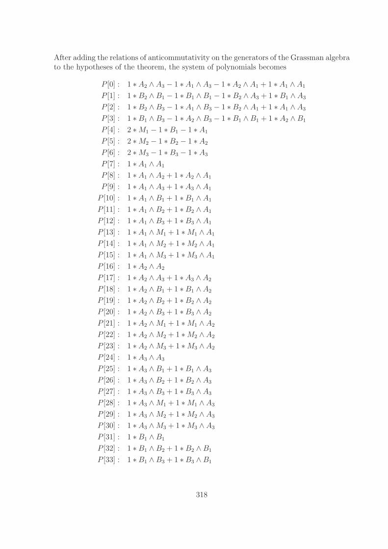
After adding the relations of anticommutativity on the generators of the Grassman algebrato the hypotheses of the theorem, the system of polynomials becomes
P [0] : 1 ∗ A2 ∧ A3 − 1 ∗ A1 ∧ A3 − 1 ∗ A2 ∧ A1 + 1 ∗ A1 ∧ A1
P [1] : 1 ∗ B2 ∧ B1 − 1 ∗ B1 ∧ B1 − 1 ∗ B2 ∧ A3 + 1 ∗ B1 ∧ A3
P [2] : 1 ∗ B2 ∧ B3 − 1 ∗ A1 ∧ B3 − 1 ∗ B2 ∧ A1 + 1 ∗ A1 ∧ A3
P [3] : 1 ∗ B1 ∧ B3 − 1 ∗ A2 ∧ B3 − 1 ∗ B1 ∧ B1 + 1 ∗ A2 ∧ B1
P [4] : 2 ∗ M1 − 1 ∗ B1 − 1 ∗ A1
P [5] : 2 ∗ M2 − 1 ∗ B2 − 1 ∗ A2
P [6] : 2 ∗ M3 − 1 ∗ B3 − 1 ∗ A3
P [7] : 1 ∗ A1 ∧ A1
P [8] : 1 ∗ A1 ∧ A2 + 1 ∗ A2 ∧ A1
P [9] : 1 ∗ A1 ∧ A3 + 1 ∗ A3 ∧ A1
P [10] : 1 ∗ A1 ∧ B1 + 1 ∗ B1 ∧ A1
P [11] : 1 ∗ A1 ∧ B2 + 1 ∗ B2 ∧ A1
P [12] : 1 ∗ A1 ∧ B3 + 1 ∗ B3 ∧ A1
P [13] : 1 ∗ A1 ∧ M1 + 1 ∗ M1 ∧ A1
P [14] : 1 ∗ A1 ∧ M2 + 1 ∗ M2 ∧ A1
P [15] : 1 ∗ A1 ∧ M3 + 1 ∗ M3 ∧ A1
P [16] : 1 ∗ A2 ∧ A2
P [17] : 1 ∗ A2 ∧ A3 + 1 ∗ A3 ∧ A2
P [18] : 1 ∗ A2 ∧ B1 + 1 ∗ B1 ∧ A2
P [19] : 1 ∗ A2 ∧ B2 + 1 ∗ B2 ∧ A2
P [20] : 1 ∗ A2 ∧ B3 + 1 ∗ B3 ∧ A2
P [21] : 1 ∗ A2 ∧ M1 + 1 ∗ M1 ∧ A2
P [22] : 1 ∗ A2 ∧ M2 + 1 ∗ M2 ∧ A2
P [23] : 1 ∗ A2 ∧ M3 + 1 ∗ M3 ∧ A2
P [24] : 1 ∗ A3 ∧ A3
P [25] : 1 ∗ A3 ∧ B1 + 1 ∗ B1 ∧ A3
P [26] : 1 ∗ A3 ∧ B2 + 1 ∗ B2 ∧ A3
P [27] : 1 ∗ A3 ∧ B3 + 1 ∗ B3 ∧ A3
P [28] : 1 ∗ A3 ∧ M1 + 1 ∗ M1 ∧ A3
P [29] : 1 ∗ A3 ∧ M2 + 1 ∗ M2 ∧ A3
P [30] : 1 ∗ A3 ∧ M3 + 1 ∗ M3 ∧ A3
P [31] : 1 ∗ B1 ∧ B1
P [32] : 1 ∗ B1 ∧ B2 + 1 ∗ B2 ∧ B1
P [33] : 1 ∗ B1 ∧ B3 + 1 ∗ B3 ∧ B1
318
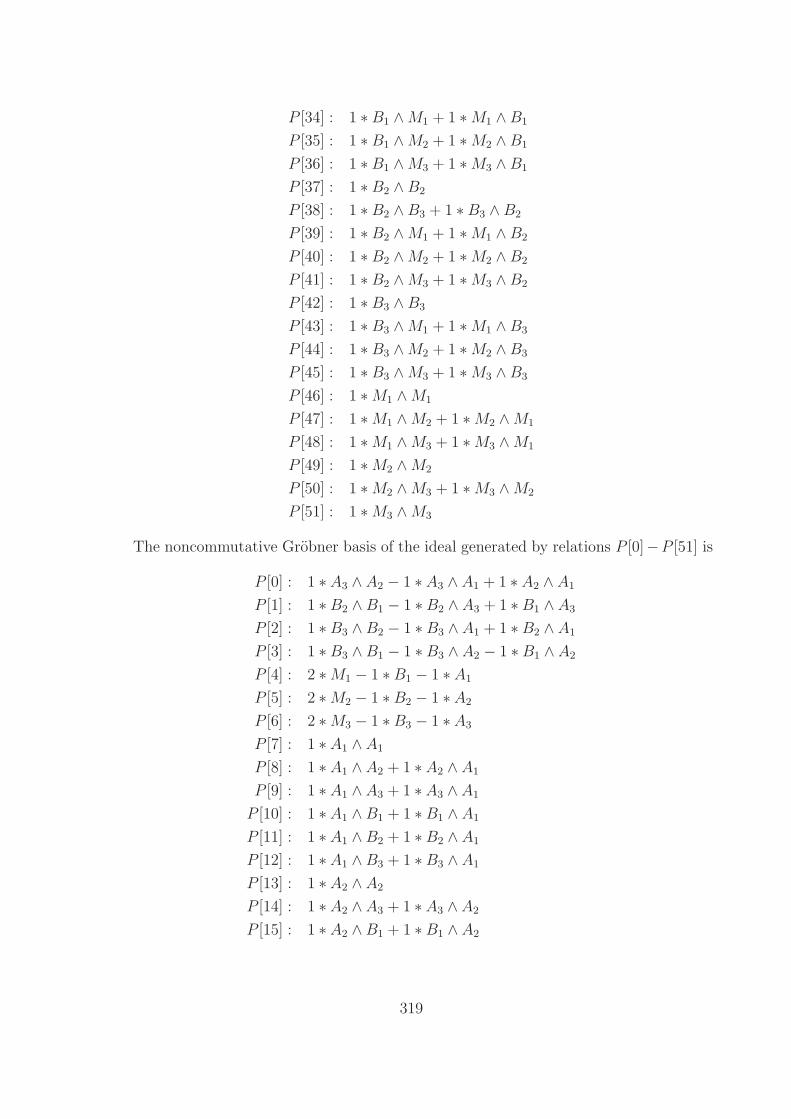
P [34] : 1 ∗ B1 ∧ M1 + 1 ∗ M1 ∧ B1
P [35] : 1 ∗ B1 ∧ M2 + 1 ∗ M2 ∧ B1
P [36] : 1 ∗ B1 ∧ M3 + 1 ∗ M3 ∧ B1
P [37] : 1 ∗ B2 ∧ B2
P [38] : 1 ∗ B2 ∧ B3 + 1 ∗ B3 ∧ B2
P [39] : 1 ∗ B2 ∧ M1 + 1 ∗ M1 ∧ B2
P [40] : 1 ∗ B2 ∧ M2 + 1 ∗ M2 ∧ B2
P [41] : 1 ∗ B2 ∧ M3 + 1 ∗ M3 ∧ B2
P [42] : 1 ∗ B3 ∧ B3
P [43] : 1 ∗ B3 ∧ M1 + 1 ∗ M1 ∧ B3
P [44] : 1 ∗ B3 ∧ M2 + 1 ∗ M2 ∧ B3
P [45] : 1 ∗ B3 ∧ M3 + 1 ∗ M3 ∧ B3
P [46] : 1 ∗ M1 ∧ M1
P [47] : 1 ∗ M1 ∧ M2 + 1 ∗ M2 ∧ M1
P [48] : 1 ∗ M1 ∧ M3 + 1 ∗ M3 ∧ M1
P [49] : 1 ∗ M2 ∧ M2
P [50] : 1 ∗ M2 ∧ M3 + 1 ∗ M3 ∧ M2
P [51] : 1 ∗ M3 ∧ M3
The noncommutative Grobner basis of the ideal generated by relations P [0]−P [51] is
P [0] : 1 ∗ A3 ∧ A2 − 1 ∗ A3 ∧ A1 + 1 ∗ A2 ∧ A1
P [1] : 1 ∗ B2 ∧ B1 − 1 ∗ B2 ∧ A3 + 1 ∗ B1 ∧ A3
P [2] : 1 ∗ B3 ∧ B2 − 1 ∗ B3 ∧ A1 + 1 ∗ B2 ∧ A1
P [3] : 1 ∗ B3 ∧ B1 − 1 ∗ B3 ∧ A2 − 1 ∗ B1 ∧ A2
P [4] : 2 ∗ M1 − 1 ∗ B1 − 1 ∗ A1
P [5] : 2 ∗ M2 − 1 ∗ B2 − 1 ∗ A2
P [6] : 2 ∗ M3 − 1 ∗ B3 − 1 ∗ A3
P [7] : 1 ∗ A1 ∧ A1
P [8] : 1 ∗ A1 ∧ A2 + 1 ∗ A2 ∧ A1
P [9] : 1 ∗ A1 ∧ A3 + 1 ∗ A3 ∧ A1
P [10] : 1 ∗ A1 ∧ B1 + 1 ∗ B1 ∧ A1
P [11] : 1 ∗ A1 ∧ B2 + 1 ∗ B2 ∧ A1
P [12] : 1 ∗ A1 ∧ B3 + 1 ∗ B3 ∧ A1
P [13] : 1 ∗ A2 ∧ A2
P [14] : 1 ∗ A2 ∧ A3 + 1 ∗ A3 ∧ A2
P [15] : 1 ∗ A2 ∧ B1 + 1 ∗ B1 ∧ A2
319
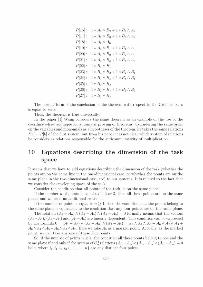
P [16] : 1 ∗ A2 ∧ B2 + 1 ∗ B2 ∧ A2
P [17] : 1 ∗ A2 ∧ B3 + 1 ∗ B3 ∧ A2
P [18] : 1 ∗ A3 ∧ A3
P [19] : 1 ∗ A3 ∧ B1 + 1 ∗ B1 ∧ A3
P [20] : 1 ∗ A3 ∧ B2 + 1 ∗ B2 ∧ A3
P [21] : 1 ∗ A3 ∧ B3 + 1 ∗ B3 ∧ A3
P [22] : 1 ∗ B1 ∧ B1
P [23] : 1 ∗ B1 ∧ B2 + 1 ∗ B2 ∧ B1
P [24] : 1 ∗ B1 ∧ B3 + 1 ∗ B3 ∧ B1
P [25] : 1 ∗ B2 ∧ B2
P [26] : 1 ∗ B2 ∧ B3 + 1 ∗ B3 ∧ B2
P [27] : 1 ∗ B3 ∧ B3
The normal form of the conclusion of the theorem with respect to the Grobner basisis equal to zero.
Thus, the theorem is true universally.In the paper [1] Wang considers the same theorem as an example of the use of the
coordinate-free technique for automatic proving of theorems. Considering the same orderon the variables and monomials as a hypotheses of the theorem, he takes the same relationsP [0]−P [6] of the first system, but from his paper it is not clear which system of relationshe considers as relations responsible for the anticommutativity of multiplication.
10 Equations describing the dimension of the task
space
It seems that we have to add equations describing the dimension of the task (whether thepoints are on the same line in the one-dimensional case, or whether the points are on thesame plane in the two-dimensional case, etc) to our systems. It is related to the fact thatwe consider the enveloping space of the task.
Consider the condition that all points of the task lie on the same plane.If the number n of points is equal to 1, 2 or 3, then all these points are on the same
plane, and we need no additional relations.If the number of points is equal to n ≥ 4, then the condition that the points belong to
the same plane is equivalent to the condition that any four points are on the same plane.The relation (A1 − A0) ∧ (A2 − A0) ∧ (A3 − A0) = 0 formally means that the vectors
(A3−A0), (A2−A0) and (A1−A0) are linearly dependent. This condition can be expressedby the formula 0 = (A1 − A0) ∧ (A2 − A0) ∧ (A3 − A0) = A1 ∧ A2 ∧ A3 − A0 ∧ A2 ∧ A3 +A0 ∧A1 ∧A3 −A0 ∧A1 ∧A2. Here we take A0 as a marked point. Actually, as the markedpoint, we can take any one of these four points.
So, if the number of points n ≥ 4, the condition all these points belong to one and thesame plane if and only if the system of C4
n relations (Ai1−Ai0)∧(Ai2−Ai0)∧(Ai3−Ai0) = 0hold, where i0, i1, i2, i3 ∈ {1, . . . , n} are any distinct four points.
320
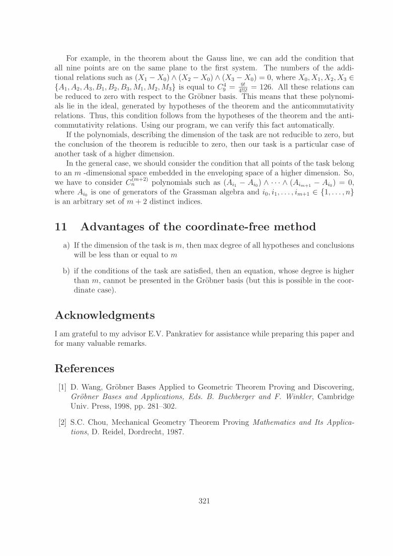
For example, in the theorem about the Gauss line, we can add the condition thatall nine points are on the same plane to the first system. The numbers of the addi-tional relations such as (X1 − X0) ∧ (X2 − X0) ∧ (X3 − X0) = 0, where X0, X1, X2, X3 ∈{A1, A2, A3, B1, B2, B3,M1,M2,M3} is equal to C4
9 = 9!4!5!
= 126. All these relations canbe reduced to zero with respect to the Grobner basis. This means that these polynomi-als lie in the ideal, generated by hypotheses of the theorem and the anticommutativityrelations. Thus, this condition follows from the hypotheses of the theorem and the anti-commutativity relations. Using our program, we can verify this fact automatically.
If the polynomials, describing the dimension of the task are not reducible to zero, butthe conclusion of the theorem is reducible to zero, then our task is a particular case ofanother task of a higher dimension.
In the general case, we should consider the condition that all points of the task belongto an m -dimensional space embedded in the enveloping space of a higher dimension. So,we have to consider C
(m+2)n polynomials such as (Ai1 − Ai0) ∧ · · · ∧ (Aim+1 − Ai0) = 0,
where Ai0 is one of generators of the Grassman algebra and i0, i1, . . . , im+1 ∈ {1, . . . , n}is an arbitrary set of m + 2 distinct indices.
11 Advantages of the coordinate-free method
a) If the dimension of the task is m, then max degree of all hypotheses and conclusionswill be less than or equal to m
b) if the conditions of the task are satisfied, then an equation, whose degree is higherthan m, cannot be presented in the Grobner basis (but this is possible in the coor-dinate case).
Acknowledgments
I am grateful to my advisor E.V. Pankratiev for assistance while preparing this paper andfor many valuable remarks.
References
[1] D. Wang, Grobner Bases Applied to Geometric Theorem Proving and Discovering,Grobner Bases and Applications, Eds. B. Buchberger and F. Winkler, CambridgeUniv. Press, 1998, pp. 281–302.
[2] S.C. Chou, Mechanical Geometry Theorem Proving Mathematics and Its Applica-tions, D. Reidel, Dordrecht, 1987.
321
Program PackageIntended for Internet-Based Accessto Computer Algebra Resources
S.I. Tertychniy
VNIIFTRI, Mendeleevo,e-mail: [email protected]
General structure and major features of the package GRGnetwork intended for remoteaccess to software based on the universal computer algebra system Reduce making use ofInternet communication media are discussed.
Introduction
Objectives
The work discussed below constitutes a part of the long-term programme intended forthe developing of program computational tools incorporating the methods of ComputerAlgebra (CA) and the modern communication technologies based on the Internet infras-tructure. In the most general setting, the corresponding software is intended to renderassistance in the solving of certain classes of problems in theoretical physics — first of all,the theory of gravity — with the help of modern computational tools. It is designed toprovide Internet-based access to the consolidated computational resources of ComputerAlgebra Systems (CAS), universal or/and specialized, in conjunction with a number ofadditional services enhancing the efficiency and convenience of this form of their usage.
Assuming more narrow frameworks, we outline here the basic points and main featuresof the package GRGnetwork, constituting one of the components of the software intendedto address the problem declared above but being also of a notable interest in its own right.
Before the discussing the very content of the work an outline of its starting points hasto be given.
Approach
The approach implemented on GRGnetwork is based on the client-server method andmakes use of the object-oriented (OO) programming technique. The latter point impliesthe wide application of the platform independent OO Java technology, playing here therole of the universal environment and basic programming tool.
322
Advantages versus shortcomings
The choice indicated above is a priori distinguished by some potential advantages appar-ently enabling one to efficiently settle a number of subsidiary problems which constitutein fact the core of the problem to be solved. These include in particular the followingnoteworthy points:
• Inheriting specific feature of the Java technology, the software developed on its baseautomatically possesses the important property of independence on the computerplatform (often called portability property).
• The incorporation of a Java Virtual Machine (JVM) in majority of the most popularand widely used www-browsers releases a potential user of Java-based softwareof concern about the providing and installing any specific background software.This circumstance makes access to Java-based software fairly straightforward foreverybody interested in its capabilities. In particular, this concerns non-experiencedbeginners as well, that is evidently the point of significant importance.
• The constituent of Java environment called Abstract Window Toolkit (AWT) enablesone to realize a portable graphical multi-window user/system interface (GUI) on auniform, platform independent base.
• The facility of Java applets enables one to achieve a properly secure implementationof the remote access to common integrated computational resources through theInternet communication media.
This list of attractive features of Java-based technique of program development shouldseem sufficient for some substantiating of the choice adopted. However, at the same time,it might be perhaps argued that all the matter above looks rather as a fine theory andcannot really play role of practical guidelines.
Indeed, dealing closer with the issue of a brute reality, the approach outlined turns outbe also associated, simultaneously with evident advantages, with a number of drawbacks,many of the latter being, in a sense, close companions of the former, though. Pursuing tomaintain a reasonable balance of pluses and minuses in these speculations, the followingremarks somewhat contravening with the ones just made are now in order:
• The existing realizations of Java environment and their implementations into www-browsers prove not be free of some apparently buggy behavior or specific improperpeculiarities. This is currently true, to a great extent, for all the widely practicedsoftware of this class, essentially. Additionally, there are still no corresponding suffi-ciently detailed documented or, say, practical standards which one could refer to inthe developing of Java-based software on a stable ground. Most of the ‘pathologies’specific Java realizations reveal, either apparent or actual, can only be captured bymeans of laborious testing, making use of the notorious ‘trial and error method’.Moreover, in these studies, some vague deviations from the available standards areobserved, unfortunately. Such violations of a standard usually prove computer plat-form and Java version dependent. Hence they claim in each concrete case a specific
323
treatment, sometimes fairly laborious, that does not promote the final software qual-ity. Sometimes, in spite of all the efforts of a programmer, Java-based software maynot manifest all the capabilities promised by the relevant Java specifications.
• The realization of graphical interface tools in Java’ graphical engine AWT is cur-rently difficult to qualify advantageous in many respects. In particular, it doesnot support some graphical facilities which are, in principle, ensured by graphicsengines of the operating systems (OS) of interest. Additionally, in practice, theexecution of some dynamical operations seems to be realized in a way which is farof perfectness and manifests some apparently improper visual effects. As a result,in certain cases, it turns out problematic for AWT-based interfaces to compete withthe system-dependent GUI realizations.
It may be supposed that such sort shortcomings are partially connected with theportability property lying in the base of the Java technology.
Nevertheless, the above does not mean, of course, that Java-based software cannotturn out an efficient and useful tool. Besides, fortunately, it can be noted that some ob-servations give evidence that the general situation concerning the shortcomings mentionedabove tends to gradually improve.
Basic ingredients of the package background
Let us now characterize the basic ingredients of the software complex GRGnetwork isbased upon. These include in particular the following elements:
Graphical interface tools
The source of constructive elements used for the development of GRGnetworkinvolves the collection of platform independent graphical interface tools im-plemented in the form of Java’s Abstract Window Toolkit (AWT). It providesa variety of graphical primitives allowing to construct a platform-independentfriendly graphical user interface (GUI).
Basic networking tools
A substantial advantage of the Java concept is the integrating into Java en-vironment all the necessary network communication capabilities. Making useof this feature, the communication between the ‘client’ and ‘server’ compo-nents of GRGnetwork is realized on the base of TCP/IP protocol and employsInternet communication channels, the local networking based on TCP/IP (in-tranets) being supported on the identical ground. The two sub-componentsof the ‘server’ component of the package (called GRGmediator and GRGslave,see below) also communicate making use of TCP/IP protocol, the specificrealization of this data transport bus being irrelevant.
324
Computer algebra server
The next point of significant importance is the implementation of ComputerAlgebra (CA) facilities in GRGnetwork. Introducing no own low level CAprimitives and algorithms, GRGnetwork leans on the general purposes CAsystem Reduce [1]. The latter is regarded here as the primary tool for theperforming manipulations with symbolic mathematical data of a general kind.The routines realizing the processing of the specifically structured mathemat-ical data (the subject going beyond the scope of the present notes) are alsobased on the Reduce capabilities, mostly those intended for the handling oflow level symbolic data.
It is worth noting the following features of Reduce which are crucial for theselection of this system as CA server in GRGnetwork:
• Reduce is an open system allowing easy and efficiently realized extensionsand/or modifications on the both ‘top level’ (handling of mathematicalstructured data) and ‘bottom level’ (handling of symbolic data primitivesof a general kind).
• Reduce performs calculations in a maximally automatic way, assumingminimum of intervenience of a user at intermediate stages of a calculation.
• Reduce is a portable system which has been implemented in all computerplatforms of practical interest, essentially.
• Reduce system includes the portable compiler allowing to build fairlycompact efficient executable codes of high performance.
Although CAS Reduce is not free of some own (fairly essential) shortcomings,currently one sees no satisfactory alternative to it among the other universalCASs (Mathematica, Maple, Macsima, Maxima, muPad), at least, as far as theclass of problems considered in the present work is concerned.
Security managing
The next point of high importance, the security issue, is one of the mostsubstantial problems concerning any software making use of the contemporaryInternet communication media. Considering its relation to GRGnetwork, asystem based on the ‘client-server’ method, it has to be noted that there areobviously two its branches. Namely, these are the problem of secure run of theclient component on the user’ computer and the security of the functioning ofthe server component.
Concerning the latter side of the security problem, the important element of itssolution in GRGnetwork is the assignment of all the communication functionsto a special server component called GRGmediator. One of its main functionsis the filtering out any possible detrimental intervention outwards.
325
Further, the loading/startup of client components of GRGnetwork and furthertheir communication with network server (i.e., ‘physically’, with GRGmedia-tor) is realized making use of the Java applet facility. The latter is known asbasically safe way of the data exchange and the handling of the codes trans-ported through the Internet communication media. The point is that thecode of a Java applet is not immediately executed by computer hardware butis interpreted by the so called Java Virtual Machine (JVM) integrated with(or ‘plugged in’) the web-browser which runs on the user’ computer. Variousmeasures ensuring safe execution of downloaded applet codes are implementedin JVM. Hence, a necessary security level is automatically ensured as long asthe appropriate integrity and authenticity of web-browser itself is being kept.This strategy constitutes the main ingredient of the service responsible for thesecure functioning of the client component of GRGnetwork.
Finally, the communication of a user with the CA package Reduce, playing roleof CA server, is managed by the so called PSL Security Guard (PSLguard).The point is that PSL (Portable Standard Lisp), the lower layer Reduce isbased upon, takes no care about the issue of a secure functioning in an opennetwork environment. PSLguard is intended to compensate for this shortcom-ing, shielding the server against possible hostile attacks through the securityholes lurked in the CAS background.
Issue of a practical realization
The concretizing and practical realization of the approaches sketched above prove torequire simultaneous solution of a variety of interrelated problems of quite different kinds.This, in turn, requires fulfillment of a number of conditions which are outlined below.
Run-time environment
The solution implemented in GRGnetwork is based on the following decisions.
• The server part of GRGnetwork, i.e. the sub-components named GRGmediatorand GRGslave, are realized as Java applications which run on sufficiently pow-erful (preferable distinct) computers within Java Run-time Environment (JRE) (orin framework of more recent equivalent packages abbreviated by their developers asJDK and J2SKD which contain JRE as their subsets).
• The computers where GRGmediator and GRGslave reside at have to be connectedby a fast IP channel of a sufficient carrying capacity.
• GRGslave has to be able to run the processes of CA Reduce (the more ones simul-taneously, the better).
• The client component startup procedure implies the making use of http server.
• The realization of the functioning of the client component of the package assumes
326
– the making use of www-browser with graphical interface and Java support.
Currently, such browsers are available for all the computer platforms, essentially. Theirincomplete list includes various releases of Netscape Communicator/Navigator and Mi-crosoft Internet Explorer (excluding the latest ones), Opera, Mozilla, Konqueror , etc.Some of them consume comparatively moderate computer resources to be able to run onpersonal computers of fairly moderate capabilities and performance rate.
– The access to Internet is the second (and last) condition necessary for thefunctioning of the client component; the making use of a local network insteadis also feasible.
The existence and availability of the software mentioned above is a crucial point mak-ing the goal of the project potentially achievable.
Developer workplace
Another point of crucial importance is the structure and, accordingly, feasibility of re-alization of the hard/software complex which is natural to name a developer workplace.Essentially, the capabilities and efficiency of this necessary tool affects all the route of thesubsequent work and, essentially, determines the total feasibility of the project.
It has to be emphasized that the problem to be solved implies the development of areal time multi-thread assemblage of ‘spatially distributed’ asynchronously run programscommunicated via TCP/IP Internet channels , the latter maying reveal variable carryingcapability (including low one) and limited overall reliability. It is also worth also notingthat the work on the project was being carried out under rather unfavorable conditionswith minimal support in the country with crisis economy. In reality, the last circumstanceproved the next point strictly conditioned the way of the realization of the project. Thelatter can be summarized as follows:
Hardware: The work of the ‘spatially distributed’ multi-component package communi-cating with the help of TCP/IP protocol mentioned above is emulated on a single personal(‘IBM PC-compatible’) computer.
Operating system: The most important ‘constructive element’ consolidating all thesoftware utilized is OS Linux. A number of releases of Slackware, RedHat, Mandrake(currently ALTLinux) distributions were tested and utilized.
This choice of OS immediately implies a number of advantages. The most importantones are the following:
TCP/IP support: This function is incorporated in the OS kernel. The correspondingutilities necessary for the maintaining TCP/IP connections are ensured as OS constituentsas well.
Network emulation: Inter-computer TCP/IP communication is emulated on a singlecomputer by OS facilities available defaults.
327
Java developer tools: Java programs are coded, tested, and run making use of JavaDevelopment Kit (JDK, further transformed to J2SKD package) of several subsequentreleases supported by Sun Microsystems; another clone of similar software of comparablecapabilities utilized was developed and distributed by IBM Corporation.
Http server: The well known http-server Apache (included in all the recent Linuxdistributions) is used for the emulating of the startup procedure of the client component ofGRGnetwork. The help subsystem and support of online documenting are also maintainedwith its assistance.
www-browsers: Several www-browsers with graphical interface and Java support areused as hosts for the client component, most notable packages are Netscape Communicatorclone (currently developed under the name Mozilla Communicator) and Microsoft InternetExplorer (in the case of client component running over OS Windows).
Algebraic processor: General purpose CA Reduce system of releases 3.6 and 3.7 run-ning upon PSL package is used as the algebraic processor.
etc. . . A lot of auxiliary software some of which is, essentially, indispensable for thepackage development (various editors, documenting tools, graphics handling tools, etc.)are utilized.
Remark: A crucial circumstance allowing the practical development of GRGnetwork isthe existence, availability, and ability to be consistently integrated of all the functionalcomponents of developer workplace listed above within the common shell running on asingle computer of a moderate performance rate assembled from standard components.
After the formal characteristic of the package given above, more informative descrip-tion of its very structure and the functioning is now in order.
GRGnetwork structure
In active state, GRGnetwork consists of a single server component and some (one ormore) client components functioning asynchronously and running, generally speaking, ondifferent computers. It is assumed that each client component lives on an own computer(in most typical case, on a personal user’ computer) connected by TCP/IP channel withInternet. Through the latter, the client component can (and does) communicate withserver computer of GRGnetwork.
Concerning the server component of GRGnetwork software, it has to be reminded thatit actually consists of the two relatively independent sub-components called GRGmediatorand GRGslave. This is GRGmediator which runs on the ‘server computer’ mentionedabove and plays the role of a common interface communicating via Internet with clientcomponents, if there are active any.
328
The second server component, GRGslave, runs, preferably, on a computer distinctfrom the one where GRGmediator resides at (for the sake of performance decoupling).It is assumed that GRGslave is also connected with GRGmediator by TCP/IP channel,being at the same time, as far as one concerns the functioning of GRGnetwork, isolatedof the other connections. This channel is assumed to be a sufficiently fast and ‘absolutelyreliable’ because no special provisions is made for the data losses or significant transmittingdelays in it. Note that no such limitations on the channels connecting GRGmediator andGRGclients are assumed.
Therefore, the graph of TCP/IP ‘links’ connecting the components of GRGnetworkconstitute a star-like figure with GRGmediator situated in its vertex.
More about GRGnetwork components
Let us consider the functions of GRGnetwork components in more details.
GRGmediator: communication center
The main function of GRGmediator is the maintaining TCP/IP connection withGRGclient and GRGslave, receiving and dispatching the data and command streams,simple specific top-layer protocols being implemented for such a purpose. GRGmediatoroccupies a separate port and effectively filters outward calls coming in through it. Thelatter point is substantial for the ensuring the secure functioning of the server component.
GRGslave: application server
In a sense, GRGslave is the ‘genuine’ server in GRGnetwork. In particular, it managesthe logical connections with client components, carries out the registration of new clients,starts and controls the CA server (CAS Reduce), maintains the remote file systems ofclients (which point will be discussed below), performing all the operations over them‘on the physical level’, etc. GRGslave also handles the necessary information concerningthe registered clients, updates and stores the statistics characterizing their activity andconsumption of the shared resources etc.
GRGclient: user interface
First of all, GRGclient plays the role of a friendly interface with a ‘final user’. It alsoperforms some useful service tricks specific for the work with CA systems. Hence, as faras one concerns the apparent convenience of the package use, this it is perhaps the mostimportant component. GRGclient is realized in the graphical multi-window format andmakes use of the major active control facilities typical for window-based GUI (buttons,various menus, etc.).
Another function of GRGclient, less apparent but definitely not less important, is themaintaining stable connection with the server component (‘physically’, with GRGmedi-ator) in accordance with the corresponding protocol. The latter includes some facilities
329
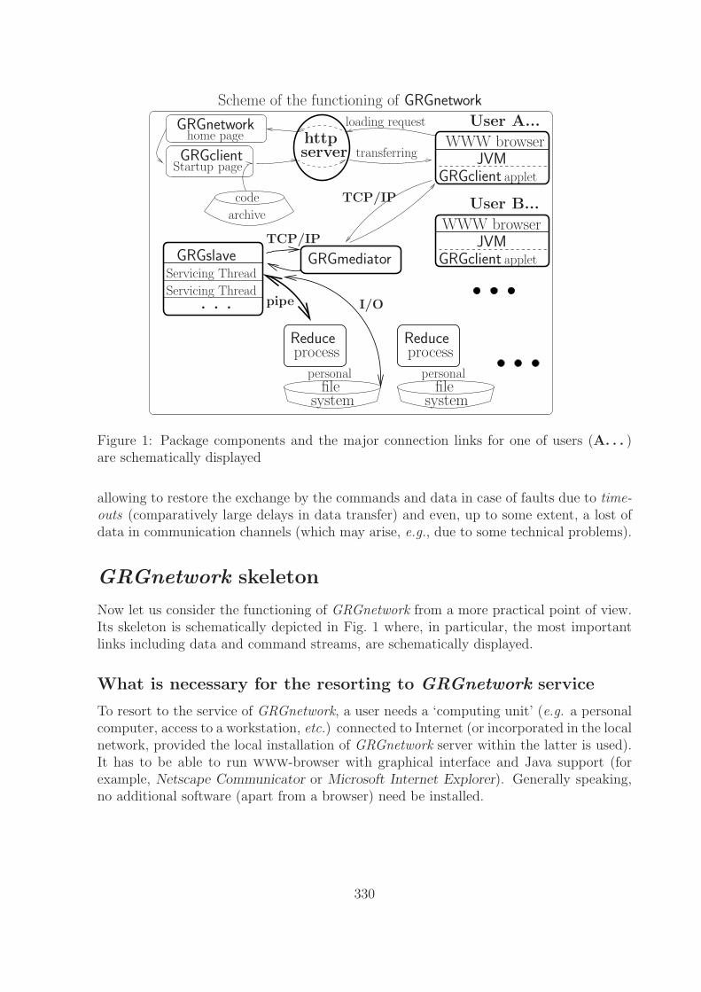
loading request
archive
code
GRGclientStartup
GRGnetworkhome page WWW browser
User A...
GRGclientJVM
applet
GRGclientJVM
applet
User B...
WWW browser
transferring
processReduce
GRGnetwork
page
filesystem
personalfile
personal
system
GRGslave
. . .
Servicing Thread
Servicing Thread
GRGmediator
processReduce
I/Opipe
TCP/IP
TCP/IP
serverhttp
Scheme of the functioning of
Figure 1: Package components and the major connection links for one of users (A. . . )are schematically displayed
allowing to restore the exchange by the commands and data in case of faults due to time-outs (comparatively large delays in data transfer) and even, up to some extent, a lost ofdata in communication channels (which may arise, e.g., due to some technical problems).
GRGnetwork skeleton
Now let us consider the functioning of GRGnetwork from a more practical point of view.Its skeleton is schematically depicted in Fig. 1 where, in particular, the most importantlinks including data and command streams, are schematically displayed.
What is necessary for the resorting to GRGnetwork service
To resort to the service of GRGnetwork, a user needs a ‘computing unit’ (e.g. a personalcomputer, access to a workstation, etc.) connected to Internet (or incorporated in the localnetwork, provided the local installation of GRGnetwork server within the latter is used).It has to be able to run www-browser with graphical interface and Java support (forexample, Netscape Communicator or Microsoft Internet Explorer). Generally speaking,no additional software (apart from a browser) need be installed.
330
Work session: start up and run
Having the above things at his/her disposal, a user begins the work with GRGnetworkwith the opening the homepage of GRGnetwork (see [2]), that implicitly assumes thecontact with the corresponding http-server.
This page contains, apart from some appropriate introductory elucidations and thereferences (links) to the auxiliary documenting matter etc., the link leading to startuppage containing the ‘button’ which enables one to issue the command to start the Javaapplet executing GRGclient code.
It has to be mentioned that in response to the command above, the code of GRGclientis automatically transferred from the same website by the browser. Hence, as it has beennoted, no specific actions by user or, say, preliminary installation of additional software(apart from the browser itself) are required.
Having been started, after the initialization, GRGclient opens the window of the socalled ControlPanel. Making use of the latter, the user may adjust some working pa-rameters (in particular, to specify the ‘name’ under which he or she will be registeredin GRGnetwork, provided the ‘personalized’ access is implied), to consult with the helpnotes, etc. However, at this stage, the main action ControlPanel enables one to carry out,is the establishing connection with GRGmediator.
It is also worth noting here that before the establishing connection with GRGmediator(which is carried out by means of a special procedure whose details are unseen for theuser), GRGclient lives quite autonomously ‘in the user’s computer’ (‘inside the browser’)and, essentially, is of no relation to GRGnetwork. Only after the establishing connectionwith GRGmediator, GRGclient turns out incorporated in GRGnetwork. Note also that theconnection between GRGclient and GRGmediator is independent on the one establishedby the browser during the loading the content of GRGnetwork homepage. In particular, itis not serviced by the http-server (transferring the content of homepage to the browser).GRGmediator plays here the role of a communication server itself.
GRGmediator runs on the GRGnetwork server computer and maintains, apart fromtemporary connections with one or more GRGclients, the permanent connection withGRGslave which performs the major part of actual ‘service work’ in GRGnetwork. Theseactions are usually explicitly requested by client components. Making use of the graph-ical interface (GUI) ensured by GRGclient, the user directs appropriate commands toGRGmediator which dispatches them to GRGslave for subsequent execution. In responseto these commands, GRGslave performs the actions requested. In particular, it starts(or stops, or restarts) CA Reduce processes, catching and linking (again resorting to theassistance of GRGmediator) the output data stream to the corresponding client, trans-ports the Reduce input commands (constituting the program code written in the Reduceinput language) to Reduce process, performs the file handling operations. The outputof the application processes (e.g. CA Reduce), other information and control commandsare received by the GRGclient applet through the reverse data transport bus ensured byGRGmediator. Finally, having get data generated by application, GRGclient usually putthem into the corresponding window displayed on the computer monitor, making availablefor the user.
331
Some noteworthy features
Now we would like to outline some selected features of GRGnetwork. This matter shouldmake the subject of our discussion more clear and definite.
Balancing rates of data generating and data use
It has to be noted that there is a substantial distinction in the remote interactive runof applied programs (including CAS) from the same work carried out with the help ofa ‘local’ computer. This is the issue of the balancing of the rates of the ‘generating’ ofoutput data by applied program (running on the remote server, in our case by GRGslave)and the ‘consumption’ of these data by the client component — finally, their utilizing, inone way or another, by the user.
A priori, the rates of these two processes may be very different. Especially oftenone encounters a situation where the data stream produced by a ‘loose’ applied programis, during some period of time, much more intensive than the maximal rate of the dataprocessing the agent situated on the opposite side of the communication channel is able toensure. In practice, the amount of data generated by an application can prove enormousin quite innocent working situations. For example, this can occur in the case of a logicalmistake in the applied program leading to interminable data generating loop. One easilyimagines also circumstances when the rate of the ‘utilizing’ of data by the network clientpractically vanishes becoming incompatible with fairly moderate rate of their generating.
A natural claim to any tool of remote application control including GRGnetwork isthe ability to stably handle such situations. The essence of the problem is obvious: it isnecessary to do something with data of volume permanently enhancing with time whichhad been produced by application but, in view of some reasons, still cannot be ‘takenaway’ by the client component.
The method of the settling the problem indicated above which is adopted in GRGnet-work makes use of the ‘quantization’ of the both output (concerning the server component)and input (concerning the client component, respectively) data streams. Its idea is quitestraightforward. Specifically, when the output data quantum (e.g. certain amount of textlines) received from application process by GRGslave is exceeded, it stops (‘freezes’) theapplication (provided the latter is generating further output data). Simultaneously, theclient component is notified on such an event. Another reason of the ‘freezing’ of ap-plication may be the corresponding explicit command issued by the client component.It is generated, for example, if the user needs to suspend the reception of new output.Application run is continued (application output ‘is melted’) in response to the ‘opposite’command of the client component (which can be either automatic or initiated by theuser).
It turn, the client component stops to fill in the screen (i.e. some TextArea in thewindow of ApplicationControlPanel) with the new data either in the case of the filling upof the input buffer of certain volume or in response to the explicit user command (when the‘freeze’ item in the appropriate menu is clicked). Then GRGclient directs to the GRGslavethe directive to also ‘freeze’. Since this action needs some time to be performed, clientcomponent is further collecting the messages such as those which have already been issued
332
and are being transported through the network, if any, without displaying them on thescreen. This ‘frozen’ state of GRGclient continues until the user allows GRGclient to runfurther (i.e. to proceed to display the new data on the screen, removing the ‘oldest’ ones)by means of the corresponding command.
It is worth noting that the user may also disable this ‘freezing/melting’ mechanism.Then there will be no apparent pauses initiated by the client and the new data auto-matically ousts the ‘most early’ portions of data from the screen. At the same time,the quantization of the application output by GRGslave is still carried out, enabling theserver to synchronize the the process of data transfer between GRGnetwork components.
The user is therefore provided with necessary tools (controlled with the help of GUIof the client component) enabling him or her to efficiently control the intensity of thestream of output data produced by application and its displaying on the monitor screen.
Remote libraries
A useful service worth noting here which is provided by GRGnetwork is an easy access tosome ‘standard’ data libraries situated on the server. Currently, the library of the standardtests (samples of usage in fact) of numerous Reduce applied packages is supported.
On the screen, the structure of data libraries is represented in the form of tree-likecollection of specifically linked menus. Having chosen some ‘leave’ (representing a con-crete file), a user can either elicit its content, putting it ‘to the screen’, or submit to CASReduce as the input code for the processing. In the latter case the output generated byReduce is returned to the screen. The interactive programs, such as Reduce Lessons byD.R. Stoutemyer, for example, are executed in a usual way, just like on a ‘local’ com-puter (if one ignores the facility of the freezing/melting the output data stream discussedabove). Additionally, the system inspects the library of compiled codes of the standardpackages (another ‘standard library’ with a distinct form of access) searching for the onecorresponding to the test file (i.e. the package) chosen and, if there is any, enables theuser to load this package by means of a ‘single mouse click’.
Anonymous and personalized access
Generally speaking, the main service of GRGnetwork is the ensuring of the remote accessfrom an ‘arbitrary computer’ to the capabilities of CA system which is, currently, theCAS Reduce; the interfaces to some specialized packages running over Reduce (see, inparticular, [3],[4]) are planned to be implemented.
It has to be noted that there are two modes of such an access. It is convenient tocall them anonymous and personalized, respectively. Formally, these modes are distinctby the necessity, in the case of personalized access, to submit to GRGnetwork server the‘personal’ name of the user and the associated password. The procedure of the establishing‘personalized’ connection claims these data from the user (while connecting as anonymousclient, a user introduces no identifying – or any other – information).
Commenting this point, it has to be noted that, technically, in the case of personalizedaccess, there appears feasibility for the server to properly attribute subsequent sessions of
333
the same user. This ability enables it to ensure such ‘named’ users with some ‘long-term’(multi-session) resources.
On the contrary, various ‘anonymous’ work sessions of the same user cannot be at-tributed to their actual ‘author’. All the anonymous users (there may be many of themsimultaneously connected to GRGnetwork at each moment of time while the named usermay simultaneously lead the only session alone) are treated on the equal ground beingconsidered, on the one hand, as unrelated ones, while, on the other hand, they are pro-vided with the common long-term resources alone. This distinction is substantial in thehandling of the file systems which are supplied by GRGnetwork to any registered user,both named and anonymous, which point will be outlined below.
Remote file systems
GRGnetwork supplies users with remote file systems constituted of directories (folders)and data files. These are realized in the standard way as multiple-branching trees withnodes-folders and leaves-files which are created in response to user commands. All thesedata ‘physically’ reside on GRGnetwork server and are maintained by GRGslave.
All the anonymous clients are endowed with the common file system and possessidentical rights on all its resources. In this case, in view of impossibility of the ‘personal’attributing of concrete data sets to any ‘specific anonymous user’, the natural restrictionson the set of allowable file operations over the data files and folders are imposed. Inparticular, any operation which potentially could deteriorate for anybody the access tosome data (for example, the altering in some way the path to it) is not allowed. Theserestrictions include in particular any removing or renaming files or directories, etc.
On the contrary, every named client (i.e. the one making use of personalized accessmode) is supplied with own, ‘individual’, file system. The access to this system is protectedby a password. In such a case, the full set of operations with the files and directoriesis allowed (and the corresponding executive tools are provided). The only substantiallimitation worth mentioning is the restriction imposed on the overall data volume. Thequota-based rule (regulated by system administrator) to the providing of the data storageresources to named users is followed.
The file operations with remote personal file systems provided to named users allowsthe following:
• to store textual data get from Input TextArea of ApplicationControlPanel to a namedfile;
• to reproduce the content of the file in the Output TextArea of the same window;
• to create named folders;
• to copy, to remove, to rename, and to move separate files and folders with all theircontent;
• to process the content of files by CAS Reduce, sending output to the monitor screen(to Output TextArea);
334
• to search for files and folders in the filesystem tree by their names;
• and more. . .
Conclusion
The outcome of the work reported is currently (June 2001) the software package consistingof the three main components called GRGclient, GRGmediator, GRGslave with associateddocumentation (currently not accomplished, will be enhanced). GRGclient componentwith the corresponding startup facilities and the draft of User’ guide are available (in thedemonstrative mode) on URL [2].
It has to be noted that this software should not be considered as a finalized product.The further enhancing of its capabilities is planned, some additional debugging still retainsto be performed. Nevertheless in its recent state of development GRGnetwork alreadybecomes an efficient tool able to provide valuable assistance in solution of problems bythe methods of Computer Algebra.
Acknowledgments
This work was partially supported by Intas in frames of the grant 961-842. The authoris grateful to Yu.N. Obukhov for the valuable collaboration in the test exploitation of thepackage under OS Solaris and useful discussions.
References
[1] A.C. Hearn, REDUCE User’s Manual. Version 3.6. Rand publication CP78 (Rev.7/95) (RAND, Santa Monica, CA 90407-2138, USA, 1995).
[2] S.I. Tertychniy, GRGnetwork homesite, http://www.thp.uni-koeln.de/~yo/GR_
ALGEBRA/html/index.html, 2001 (in progress).
[3] S.I. Tertychniy, I.G. Obukhova, GRGEC: Computer Algebra System for Applicationsto Gravity Theory, SIGSAM Bulletin 31 (1997) 6
[4] S.I. Tertychniy, Searching for electrovac solutions to Einstein–Maxwell equations withthe help of computer algebra system GRG-EC (LANL archive, gr-qc/9810057, 1998).
335
Geometry of Pairs of KeplerianElliptic Orbits
N.N. Vassiliev, K.V. Kholshevnikov
Steklov Mathematical Institute,St.Petersburg State University
We study using computer algebra methods a class of problems connected with mutualconfigaration of two Keplerian elliptic orbits. The first one is the problem of findingcritical points of the distance function between two keplerian elliptic orbits. We reduceit to determination of all real roots of a trigonometric polynomial of degree eight. Thecoefficients of the polynomial are rational functions of orbital parameters. Using Groebnerbases technigue we show that a polynomial of smaller degree with such properties doesnot exist. This fact shows that our result cannot be improved and allows us to constructan optimal algorithm to find the minimal distance between two keplerian orbits. Wedefine also a function on the set of pairs of Keplerian ellipses so that sign of the functionwould be a topological invariant of their configuration. The sign is negative if and onlyif the related ellipses are linked. Explicit formulae representing the linking coefficientsas functions of orbital elements are deduced. We suggest different ways to use thesecoefficients for determining exact intersections of pairs of osculating Keplerian orbits.Also we study different metrizations for the space of pairs of Keplerian elliptic orbits.
336
Exact and Asymptotic Solutions forthe General Henon–Heiles System
S.Yu. Vernov
Institute of Nuclear Physics,Moscow State University,
Vorobievy Gory, Moscow, 119899, Russia;e-mail: [email protected]
1 The Henon–Heiles system
Let us consider a three-dimensional galaxy with an axial symmetric and time-independentpotential function. The equations of galactic motion admit of two well-known integrals:energy and angular momentum. If we know also the third integral of motion then we cansolve the motion equations by the method of quadratures. However, the third integral aspolynomial function does not exist in general case.
In the 1960s, numerical [1] and asymptotic methods [2, 3] have been developed to showexistence or absence of the third integral for some polynomial potentials.
In [1] (1964) Henon and Heiles wrote: ”In order to have more freedom of experi-mentation, we forgot momentarily the astronomical origin of the problem and considerits general form: does an axisymmetrical potential admit a third isolating integral ofmotion ?”. They chose Hamiltonian
H =1
2
(x2
t + y2t + x2 + y2
)+ x2y − 1
3y3,
because: (a) it is analytically simple; this makes the numerical computations oftrajectories easy; (b) at the same time, it is sufficiently complicated to give trajectorieswhich are far from trivial. Indeed, Henon and Heiles found that for low energies thissystem appeared to be integrable, in so much as trajectories (numerically integrated)always lay on well defined two-dimensional surfaces. On the other hand, they also obtainedthat for high energies many of these integral surfaces were destroyed and that phase spaceacquired large ergodic regions. The Henon–Heiles system became a paradigm of chaoticHamiltonian dynamics.
Let us consider the Henon–Heiles Hamiltonian in the general form:
H =1
2
(x2
t + y2t + λx2 + y2
)+ x2y − C
3y3, (1)
where C and λ are numerical parameters.Investigations of the general Henon–Heiles system:{
xtt = −λx − 2xy,
ytt = −y − x2 + Cy2,(2)
337
can be separated on the following ways:1. The solutions of (2) have been investigated in the complex time plane using
numerical integration techniques [4, 5]. Numerical investigations of the Henon–Heilessystem are continued up to now [6, 7].
2. The second integral as formal power series in phase variables x, xt, y andyt (Gustavson integral) has been constructed for the Henon–Heiles system both in theoriginal (λ = 1, C = 1) [3] (see also [8]) and in the general forms [9]. To obtain the secondintegral Gustavson has constructed the normal form of Hamiltonian (1). Using the Brunoalgorithm [10] V.F. Edneral has constructed the Poincare–Dulac normal form and found(provided the energy is small) local families of periodic solutions of Henon–Heiles systemboth in the original [11] and in the general [12] forms.
3. The singularities at the fixed points in phase space are locally analyzed vianormal form theory, whereas the singularities in the complex (time) plane are studied bythe Painleve analysis. Using this analysis three integrable cases of the general Henon–Heiles system have been found:
(i) C = −1, λ = 1,(ii) C = −6, λ is an arbitrary number,(iii) C = −16, λ = 1
16.
The nontrivial cases are (ii) and (iii), case (i) is separable. In the nontrivial integrable casesfour parameter solutions [13] and the second integrals [14–17] have been found1. Furtherdevelopment in the Painleve approach has led to finding of Backlund transformation [13]and Lax pairs [19] for the case (ii). The three integrable cases of the Henon–Heiles systemcorrespond precisely to the stationary flows of the only three integrable cases of fifth-order polynomial nonlinear evolution equations of scale weight 7 (respectively the Sawada–Kotega, the fifth-order Korteweg–de Vries and the Kaup–Kupershmidt equations) [20].
4. It is known that the variable y as a solution of the Henon–Heiles system has tosatisfy the following fourth-order equation:
ytttt = (2C − 8)ytty − (4λ + 1)ytt + 2(C + 1)y2t +
20C
3y3 + (4Cλ − 6)y2 − λy − 4H. (3)
To find a partial solution of this equation one can assume that y satisfies some moresimple equation. For example, it is well-known that the Henon–Heiles system and, hence,equation (3) have solutions in terms of Weierstrass elliptic functions satisfying the first-order differential equation:
y2t = Ay3 + By2 + Cy + D, (4)
where A, B, C and D are some constants.E.I. Timoshkova [21] considered the following equation:
y2t = Ay3 + By2 + Cy + D + Gy5/2 + Ey3/2 (5)
1An geometrical interpretation of the second integral in the case (ii) is presented in [18]
338
instead of equation (4) and found new one parameter sets of solutions of the Henon–Heilessystem in nonintegrable cases (C = −4
3or C = −16
5, λ is arbitrary number).
In present paper I use the Painleve method to find an asymptotic solutions of Henon–Heiles system in the case C = −16
5.
2 The Painleve property
The Painleve property for ordinary differential equations (ODE’s) is defined as follows.The solutions of a system of ODE’s are regarded as analytic functions of a complex (time)variable [22, 23]. The movable singularity of the solution is the singularity, locationof which depends on initial conditions.
Definition. A system of ODE’s is said to have the Painleve property if all movablesingularities of its general solution are single-valued (simple poles) [24].
All solutions of such systems (systems of P-type) are expressible as simple Laurentseries. As known a Hamiltonian system in a 2s–dimensional phase space is called com-pletely integrable if it possesses s independent integrals which commute with respect tothe associated Poisson bracket. When this is the case, the equations of motion are (inprincipal at least) separable and solutions can be obtained by the method of quadratures.Since the work of S.V. Kovalevskaya [25] (see also [26]) on the motion of a rigid bodyabout fixed point, the Painleve property has been proposed as a criterion for complete in-tegrability [27, 28]. If the system misses the Painleve property (has complex or irrational”resonances”), then the system cannot be ”algebraically integrable” [29] (see also [30] andreferences there in). N. Ercolani and E.D. Siggia [31, 32] advance arguments as to why thePainleve test works, i.e. they showed how to exploit the singular analysis to yield the in-tegrals. They proved a theorem which demonstrates that the singularity analysis providesbounds on the degrees of polynomial integrals for a large class of separable systems.
3 The Painleve test
3.1 Various algorithms of the Painleve test
The Painleve test is any algorithm designed to determine necessary conditions for a dif-ferential equation to have the Painleve property. The original algorithm developed byPainleve [24] is known as the α-method. The method of S.V. Kovalevskaya [25] is not asgeneral as the α-method but is more simple than it is. In 1980, motivated by the work ofS.V. Kovalevskaya, M.J. Ablowitz, A. Ramani and H. Segur [33] developed a new algo-rithm of the Painleve test for ODE’s2. Using this algorithm one can determine whether
2In [33] Ablowitz et al. have proven that if a partial differential equation (PDE) is solvable by theinverse scattering transform then a system of ODE’s is obtained from this PDE by the exact similarityreduction the solutions (of this system of ODE’s) associated with Gel’fand–Levitan–Marchenko equationwill possess the Painleve property. Furthermore, they conjecture that, when all the ODE’s obtainedby exact similarity transforms from a given PDE have the Painleve property, perhaps after a change ofvariables, then PDE will be ”integrable”. A powerful generalization of the Painleve test for both nonlinearordinary and partial differential equations was developed by J.Weiss, M.Tabor and G.Carnevale [34, 35]
339
a system of ODE’s admits movable branch points, either algebraic or logarithmic. Thisalgorithm can be used not only to isolate values of parameters of integrable cases, butalso to find asymptotic partial solutions in nonintegrable cases. The test consists of threelevels, if the system passes some level then it means that the system may be a system ofP-type and we have to check the system on the following level.
3.2 The first level: find the dominant behavior
We assume that the dominant behavior of solutions in a sufficiently small neighborhoodof the singularity is algebraic. To find the dominant behavior we look for solutions in theform
x = d1(t − t0)α and y = d2(t − t0)
β, (6)
where t0 is arbitrary. Substitution (6) into (2) shows that for certain values of α and β,two or more terms in the equations of (2) may balance (these terms have the same powers),and the rest can be ignored as t −→ t0. For each choice of α and β the terms which canbalance are called the leading terms. For the Henon–Heiles system in the general formthere exist two possible dominant behaviors [5, 37]:
Case 1: Case 2: (β < +e(α) < 0)
α = −2, β = −2 α =1±√
1−48/C
2, β = −2
d1 = ±3√
2 + C, d2 = −3 d1 = arbitrary, d2 = − 6C
It is possible that an original system is not of P-type, but after change of variablesthe obtained system is of P-type3. For C = − 16
5in Case 2 we obtain α = − 3
2and to
continue the Painleve test we have to introduce new variables z = x2 and to consider thefollowing system instead of system (2):{
zttz = 12z2
t − 2λz2 − 4z2y,
ytt = −y − z − 165y2.
(7)
3.3 The second level: find the resonances
For each obtained pair of values of α ≡ 2α and β we construct the simplified system thatretains only the leadings terms of equations of the original system (7).
For α = −4, β = −2 the simplified system is{zttz = 1
2z2
t − 4z2y,
ytt = −z − 165y2.
(8.1)
Substituting
z = − 54
5(t − t0)
−4 + b1(t − t0)−4+r and y = −3(t − t0)
−2 + b2(t − t0)−2+r
(see also [19, 36, 37]). The Painleve test for both ODE’s and PDE’s which is based on perturbationtheory is presented in [38].
3In this case the original system is said to have the weak Painleve property. For example, in theintegrable case (iii) system (2) has the weak Painleve property.
340
in system (8.1), we obtain that to leading order in (t−t0) {(t−t0)2r−8 for the first equation
and (t − t0)r−4 for the second equation} this system reduces to a system of two linear
algebraic equations:Q(r)b = 0, (9)
where Q(r) is 2×2 matrix, which elements depend on r, and b ≡ (b1, b2). Determinantdet(Q(r)) is a polynomial of order 4. Equation (9) has nonzero solution only if
det(Q(r)) = 0. (10)
The roots of equation (10):
r1 = −1, r2 = 6, r3 =5 +
√53.8
2, r4 =
5 −√53.8
2
determine resonances (one root is always (−1), it represents the arbitrariness of t0). Someroots of (10) are not integer. This result means, that the Henon–Heiles system withC = −16
5is a nonintegrable system. There is no algorithm to find the general solution for
a nonintegrable system.To find a partial asymptotic solutions let us consider the dominant behavior in the
case of α = −3 and β = −2. The simplified system is4{zttz = 1
2z2
t − 4z2y,
ytt = − 165y2.
(8.2)
Substituting
z = d1(t − t0)−3 + b1(t − t0)
−3+r and y = − 15
8(t − t0)
−2 + b2(t − t0)−2+r
into (8.2) we repeat calculations and obtain that resonances and corresponding arbitraryparameters can arise in terms proportional to (t − t0)
−2+r, where r = −1, 0, 4, 6. Rootr = −1 corresponds to arbitrary parameter t0, root r = 0 corresponds to arbitraryparameter d1, other roots correspond to new arbitrary parameters, i.e. new constants ofintegration5.
3.4 The third level: find the constants of integration
The third (and the last) level of the Painleve test is a substitution into the original (notsimplified) system (7) the following series:
z = d1(t − t0)−3 +
rmax∑j=1
czj−3(t − t0)j−3 and y = − 15
8(t − t0)
−2 +rmax∑j=1
cyj−2(t − t0)j−2,
where rmax = 6, cyj and czj are unknown constants.
4The simplified systems (8.1) and (8.2) are different.5Values of roots r in the case of arbitrary C see in [5, 37].
341
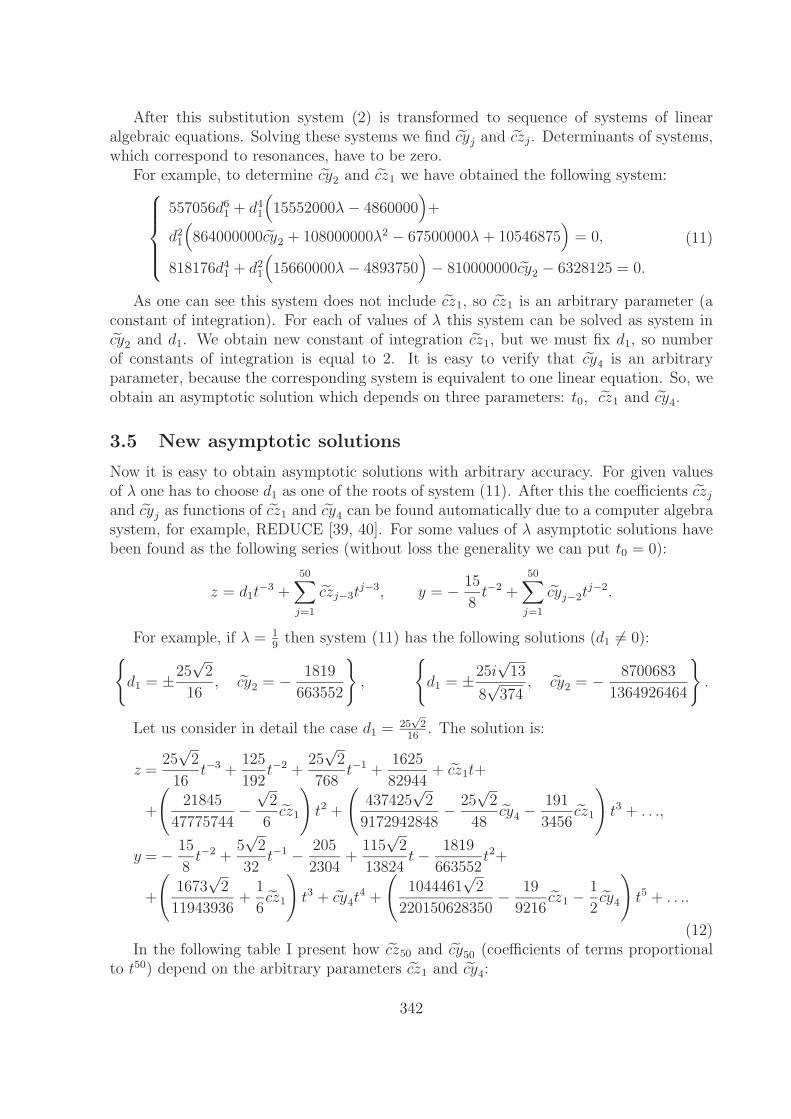
After this substitution system (2) is transformed to sequence of systems of linearalgebraic equations. Solving these systems we find cyj and czj. Determinants of systems,which correspond to resonances, have to be zero.
For example, to determine cy2 and cz1 we have obtained the following system:⎧⎪⎪⎪⎨⎪⎪⎪⎩557056d6
1 + d41
(15552000λ − 4860000
)+
d21
(864000000cy2 + 108000000λ2 − 67500000λ + 10546875
)= 0,
818176d41 + d2
1
(15660000λ − 4893750
)− 810000000cy2 − 6328125 = 0.
(11)
As one can see this system does not include cz1, so cz1 is an arbitrary parameter (aconstant of integration). For each of values of λ this system can be solved as system incy2 and d1. We obtain new constant of integration cz1, but we must fix d1, so numberof constants of integration is equal to 2. It is easy to verify that cy4 is an arbitraryparameter, because the corresponding system is equivalent to one linear equation. So, weobtain an asymptotic solution which depends on three parameters: t0, cz1 and cy4.
3.5 New asymptotic solutions
Now it is easy to obtain asymptotic solutions with arbitrary accuracy. For given valuesof λ one has to choose d1 as one of the roots of system (11). After this the coefficients czj
and cyj as functions of cz1 and cy4 can be found automatically due to a computer algebrasystem, for example, REDUCE [39, 40]. For some values of λ asymptotic solutions havebeen found as the following series (without loss the generality we can put t0 = 0):
z = d1t−3 +
50∑j=1
czj−3tj−3, y = − 15
8t−2 +
50∑j=1
cyj−2tj−2.
For example, if λ = 19
then system (11) has the following solutions (d1 = 0):{d1 = ±25
√2
16, cy2 = − 1819
663552
},
{d1 = ±25i
√13
8√
374, cy2 = − 8700683
1364926464
}.
Let us consider in detail the case d1 = 25√
216
. The solution is:
z =25√
2
16t−3 +
125
192t−2 +
25√
2
768t−1 +
1625
82944+ cz1t+
+
(21845
47775744−
√2
6cz1
)t2 +
(437425
√2
9172942848− 25
√2
48cy4 −
191
3456cz1
)t3 + . . .,
y = − 15
8t−2 +
5√
2
32t−1 − 205
2304+
115√
2
13824t − 1819
663552t2+
+
(1673
√2
11943936+
1
6cz1
)t3 + cy4t
4 +
(1044461
√2
220150628350− 19
9216cz1 − 1
2cy4
)t5 + . . ..
(12)In the following table I present how cz50 and cy50 (coefficients of terms proportional
to t50) depend on the arbitrary parameters cz1 and cy4:
342
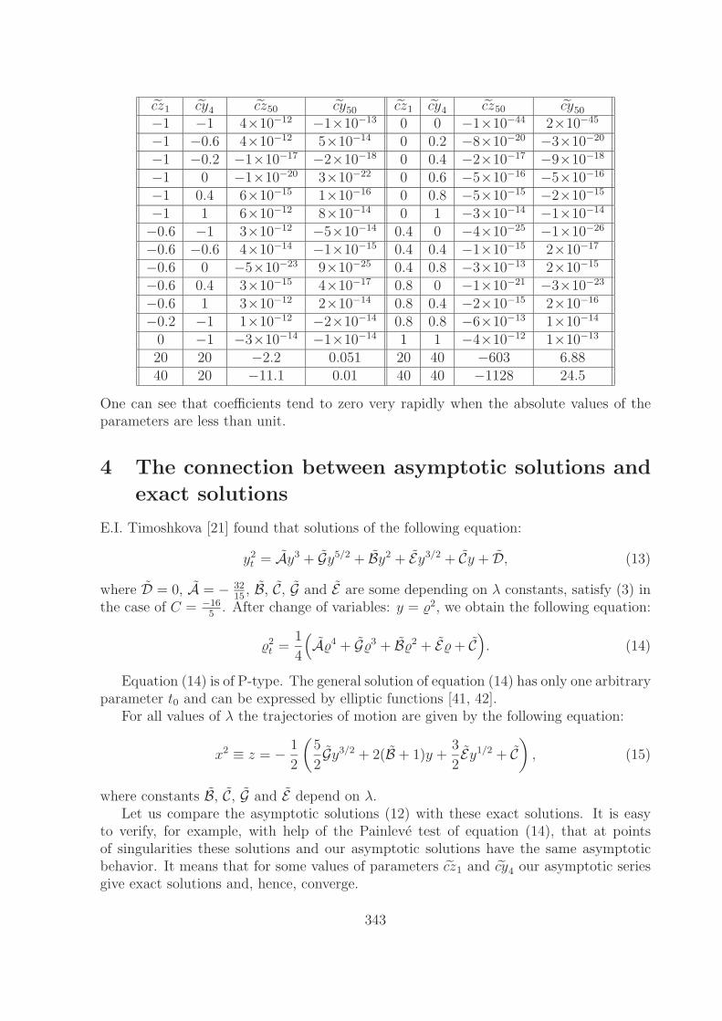
cz1 cy4 cz50 cy50 cz1 cy4 cz50 cy50
−1 −1 4×10⁻¹² −1×10⁻¹³ 0 0 −1×10−44 2×10−45
−1 −0.6 4×10⁻¹² 5×10⁻¹⁴ 0 0.2 −8×10⁻²⁰ −3×10⁻²⁰
−1 −0.2 −1×10⁻¹⁷ −2×10⁻¹⁸ 0 0.4 −2×10⁻¹⁷ −9×10⁻¹⁸
−1 0 −1×10⁻²⁰ 3×10⁻²² 0 0.6 −5×10⁻¹⁶ −5×10⁻¹⁶
−1 0.4 6×10⁻¹⁵ 1×10⁻¹⁶ 0 0.8 −5×10⁻¹⁵ −2×10⁻¹⁵
−1 1 6×10⁻¹² 8×10⁻¹⁴ 0 1 −3×10⁻¹⁴ −1×10⁻¹⁴
−0.6 −1 3×10⁻¹² −5×10⁻¹⁴ 0.4 0 −4×10⁻²⁵ −1×10⁻²⁶
−0.6 −0.6 4×10⁻¹⁴ −1×10⁻¹⁵ 0.4 0.4 −1×10⁻¹⁵ 2×10⁻¹⁷
−0.6 0 −5×10⁻²³ 9×10⁻²⁵ 0.4 0.8 −3×10⁻¹³ 2×10⁻¹⁵
−0.6 0.4 3×10⁻¹⁵ 4×10⁻¹⁷ 0.8 0 −1×10⁻²¹ −3×10⁻²³
−0.6 1 3×10⁻¹² 2×10⁻¹⁴ 0.8 0.4 −2×10⁻¹⁵ 2×10⁻¹⁶
−0.2 −1 1×10⁻¹² −2×10⁻¹⁴ 0.8 0.8 −6×10⁻¹³ 1×10⁻¹⁴
0 −1 −3×10⁻¹⁴ −1×10⁻¹⁴ 1 1 −4×10⁻¹² 1×10⁻¹³
20 20 −2.2 0.051 20 40 −603 6.8840 20 −11.1 0.01 40 40 −1128 24.5
One can see that coefficients tend to zero very rapidly when the absolute values of theparameters are less than unit.
4 The connection between asymptotic solutions and
exact solutions
E.I. Timoshkova [21] found that solutions of the following equation:
y2t = Ay3 + Gy5/2 + By2 + Ey3/2 + Cy + D, (13)
where D = 0, A = − 3215
, B, C, G and E are some depending on λ constants, satisfy (3) inthe case of C = −16
5. After change of variables: y = �2, we obtain the following equation:
�2t =
1
4
(A�4 + G�3 + B�2 + E� + C
). (14)
Equation (14) is of P-type. The general solution of equation (14) has only one arbitraryparameter t0 and can be expressed by elliptic functions [41, 42].
For all values of λ the trajectories of motion are given by the following equation:
x2 ≡ z = − 1
2
(5
2Gy3/2 + 2(B + 1)y +
3
2Ey1/2 + C
), (15)
where constants B, C, G and E depend on λ.Let us compare the asymptotic solutions (12) with these exact solutions. It is easy
to verify, for example, with help of the Painleve test of equation (14), that at pointsof singularities these solutions and our asymptotic solutions have the same asymptoticbehavior. It means that for some values of parameters cz1 and cy4 our asymptotic seriesgive exact solutions and, hence, converge.
343
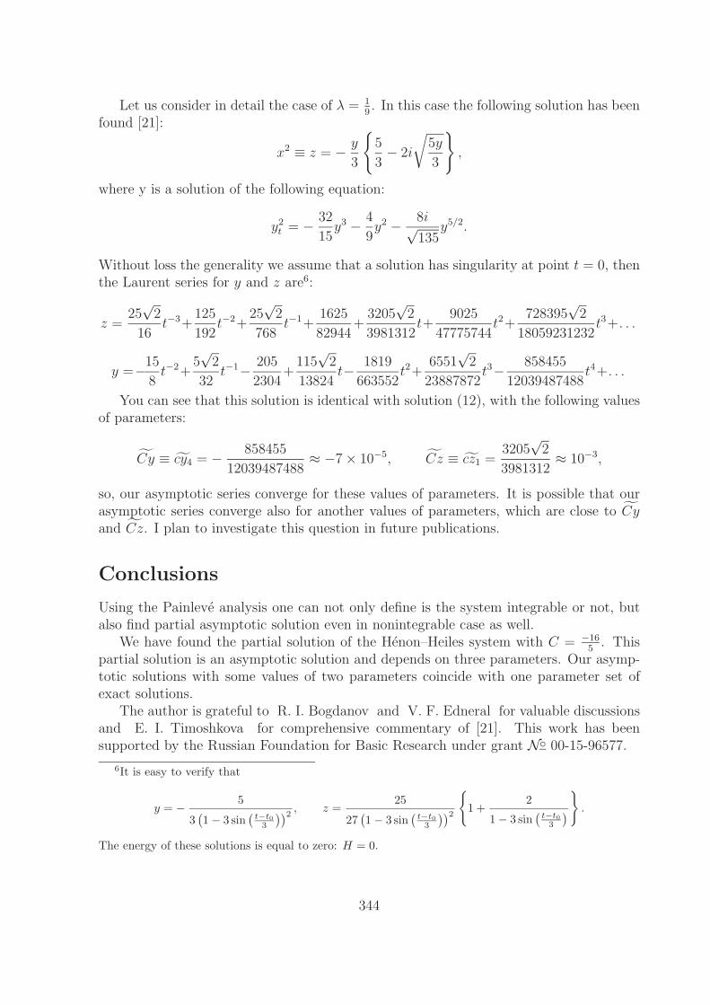
Let us consider in detail the case of λ = 19. In this case the following solution has been
found [21]:
x2 ≡ z = − y
3
{5
3− 2i
√5y
3
},
where y is a solution of the following equation:
y2t = − 32
15y3 − 4
9y2 − 8i√
135y5/2.
Without loss the generality we assume that a solution has singularity at point t = 0, thenthe Laurent series for y and z are6:
z =25√
2
16t−3+
125
192t−2+
25√
2
768t−1+
1625
82944+
3205√
2
3981312t+
9025
47775744t2+
728395√
2
18059231232t3+. . .
y =−15
8t−2+
5√
2
32t−1− 205
2304+
115√
2
13824t− 1819
663552t2+
6551√
2
23887872t3− 858455
12039487488t4+. . .
You can see that this solution is identical with solution (12), with the following valuesof parameters:
Cy ≡ cy4 = − 858455
12039487488≈ −7 × 10⁻⁵, Cz ≡ cz1 =
3205√
2
3981312≈ 10−3,
so, our asymptotic series converge for these values of parameters. It is possible that ourasymptotic series converge also for another values of parameters, which are close to Cyand Cz. I plan to investigate this question in future publications.
Conclusions
Using the Painleve analysis one can not only define is the system integrable or not, butalso find partial asymptotic solution even in nonintegrable case as well.
We have found the partial solution of the Henon–Heiles system with C = −165
. Thispartial solution is an asymptotic solution and depends on three parameters. Our asymp-totic solutions with some values of two parameters coincide with one parameter set ofexact solutions.
The author is grateful to R. I. Bogdanov and V. F. Edneral for valuable discussionsand E. I. Timoshkova for comprehensive commentary of [21]. This work has beensupported by the Russian Foundation for Basic Research under grant N◦ 00-15-96577.
6It is easy to verify that
y = − 5
3(1 − 3 sin
(t−t0
3
))2 , z =25
27(1 − 3 sin
(t−t0
3
))2{
1 +2
1 − 3 sin(
t−t03
)} .
The energy of these solutions is equal to zero: H = 0.
344
References
[1] M. Henon, C. Heiles, The Applicability of the Third Integral of Motion: Some Nu-merical Experiments, Astronomical J., 1964, vol. 69, pp. 73–79.
[2] G. Contopoulos, A Third Integral of Motion in a Galaxy, Zeitschrift fur Asrtophysik,1960, vol. 49, pp. 273–291; On the Existence of a Third Integral of Motion, Astro-nomical J., 1963, vol. 68, pp. 1–14; Resonance Cases and a Small Divisors in a ThirdIntegral of Motion, Astronomical J., 1963, vol. 68, pp. 763–779.
[3] A.G. Gustavson, On Constructing Formal Integrals of a Hamiltonian System Nearan Equilibrium Point, Astronomical J., 1966, vol. 71, pp. 670–686.
[4] Y.F. Chang, M. Tabor, J. Weiss, G. Corliss, On the Analytic Structure of the Henon–Heiles System, Phys. Lett. A, 1981, vol. 85, pp. 211–213.
[5] Y.F. Chang, M. Tabor, J. Weiss, Analytic Structure of the Henon–Heiles Hamiltonianin integrable and nonintegrable regimes, J. Math. Phys., 1982, vol. 23, pp. 531–538.
[6] J.C.B. de Figueiredo, C.G. Ragazzo, C.P. Malta, Two Important Numbers in theHenon–Heiles System, Phys. Lett. A, 1998, vol. 241, pp. 35–40.
[7] A.P.S. de Moura, P.S. Letelier, Fractal basins in Henon–Heiles and other PolynomialPotentials, Phys. Lett. A, 1999, vol. 256, pp. 362–368.
[8] J.K. Moser, Lecture on Hamiltonian Systems, Memoirs of the AMS, 1968, vol. 81,pp. 1–60, {in English}, 1973, ”Mir”, Moscow, {in Russian}.
[9] M. Braun, On the Applicability of the Third Integral of Motion, J. of DifferentialEquations, 1973, vol. 13, pp. 300–318.
[10] A.D. Bruno, Local method in Nonlinear Differential Equations, Springer Series inSoviet Mathematics, ISBN-3-540-18926-2, 1989; Power Geometry in Algebraic andDifferential Equations, Moscow, Nayka, 1998, {in Russian}.
[11] V.F. Edneral, A Symbolic Approximation of Periodic Solutions of the Henon–HeilesSystem by the Normal Form Method, Mathematics and Computers in Simulations,1998, vol. 45, pp. 445–463.
[12] V.F. Edneral, Bifurcation Analysis of Low Resonant Case of the Generalized Henon–Heiles System, Proc. of CASC 2001 (Konstanz, Germany, 2001), ed. by Ganzha etal., 2001, Springer, pp. 167–176.
[13] J. Weiss, Backlund Transformation and Linearizations of the Henon–Heiles System,Phys. Lett. A, 1984, vol. 102, pp. 329–331; Backlund Transformation and the Henon–Heiles System, Phys. Lett. A, 1984, vol. 105, pp. 387–389.
[14] J. Greene, Preprint La Jolla Institute LJI-TN-81-122, 1981.
[15] B. Grammaticos, B. Dorizzi, R. Padjen, Painleve Property and Integrals of Motionfor the Henon–Heiles System, Phys. Lett. A, 1982, vol. 89, pp. 111–113.
[16] L.S. Hall, A Theory of Exact and Approximate Configurational Invariants, PhysicaD, 1983, vol. 8, pp. 90–106.
[17] A.P. Fordy, Hamiltonian Symmetries of the Henon–Heiles System, Phys. Lett. A,1983, vol. 97, pp. 21–23.
345
[18] C. Clementi, M. Pettini, A Geometric Interpretation of Integrable Motions,arXiv:astro-ph/0105364, 2001.
[19] A.C. Newell, M. Tabor, Y.B. Zeng, A Unified Approach to Painleve Expansions,Physica D, 1987, vol. 29, pp. 1–68.
[20] A.P. Fordy, The Henon–Heiles System Revisited, Physica D, 1991, vol. 52, pp. 204–210.
[21] E.I. Timoshkova, A New Class of Trajectories of Motion in the Henon–Heiles Poten-tial Field, Rus. Astron. J., 1999, vol. 76, pp. 470–475, {in Russian}, Astron. Rep.,1999, vol. 43, p. 406, {in English}.
[22] V.V. Golubev, Lectures on Analytical Theory of Differential Equations, Gostekhiz-dat, Moscow–Leningrad, 1950, {in Russian}.
[23] E. Hille, Ordinary Differential Equations on the Complex Plane, Wiley, New York,1976.
[24] P. Painleve, Lecons sur la theorie analytique des equations differentelles (Leconsde Stockholm, 1895), Paris, 1896; Memoire sur les equations differentelles dontl’integrale generale est uniforme, Bull Soc. Math. France, 1900, vol. 28, pp. 201–261;Sur les equations differentelles du second order d’ordre superieur dont l’integralegenerale est uniforme, Acta Mathematica, 1902, vol. 25, pp. 1–85; reprinted in:Oeuvres de P. Painleve, vol. 1, ed. du CNRS, Paris, 1973.
[25] S.V. Kovalevskaya, Sur le probleme de la rotation d’un corps solide autour d’unpoint fixe, Acta Mathematica, 1889, vol. 12, pp. 177–232; Sur une properiete dususteme d’equations differentielles qui definit la rotation d’un corps solide autourd’un point fixe, Acta Mathematica, 1890, vol. 14, pp. 81–93, {in French}; ScientificWorks, Moscow, 1948, {in Russian}.
[26] V.V. Golubev, Lectures on the Integration of the Equation of Motion of a RigidBody, State Pub. House, Moscow, 1953, {in Russian}.
[27] T. Bountis, H. Segur, F. Vivaldi, Integrable Hamiltonian Systems and the PainleveProperty, Physical Review A, 1982, vol. 25, pp. 1257–1264.
[28] A. Ramani, B. Grammaticos, T. Bountis, The Painleve Property and SingularityAnalysis of Integrable and Nonintegrable Systems, Physics Reports, 1989, vol. 180,pp. 159–245.
[29] H. Yoshida, Necessary Conditions for the Existence of Algebraic First Integrals. I &II, Celestial Mechanics, 1983, vol. 31, pp. 363–379; pp. 381–399.
[30] H. Yoshida, A new Necessary Condition for the Integrability of Hamiltonian Systemswith a Two-dimensional Homogeneous Potential, Physica D, 1999, vol. 128, pp. 53–69.
[31] N. Ercolani, E.D. Siggia, Painleve Property and Integrability, Phys. Lett. A, 1986,vol. 119, pp. 112–116.
[32] N. Ercolani, E.D. Siggia, Painleve Property and Geometry, Physica D, 1989, vol. 34,pp. 303–346.
346
[33] M.J. Ablowitz, A. Ramani, H. Segur, A Connection between Nonlinear EvolutionEquations and Ordinary Differential Equations of P-type. I & II, J. Math. Phys.,1980, vol. 21, pp. 715–721; pp. 1006–1015.
[34] J. Weiss, M. Tabor, G. Carnevale, The Painleve Property for Partial DifferentialEquations, J. Math. Phys., 1983, vol. 24, pp. 522–526.
[35] J Weiss, The Painleve Property for Partial Differential Equations. II: Backlund Trans-formation, Lax Pairs and the Schwarzian derivative, J. Math. Phys., 1983, vol. 24,pp. 1405–1413.
[36] R. Conte, The Painleve Analysis of nonlinear PDE and related topics: a computeralgebra program, preprint, 1988; Invariant Painleve Analysis of Partial DifferentialEquations, Phys. Lett. A, 1989, vol. 140, pp. 383–390.
[37] M. Tabor, Chaos and Integrability in Nonlinear Dynamics, 1989, Wiles, New York,{in English}, 2001, URSS, Moscow, {in Russian}.
[38] R. Conte, A.P. Fordy, A. Pickering, A Perturbative Painleve Approach to NonlinearDifferential Equations, Physica D, 1993, vol. 69, pp. 33–58.
[39] A.C. Hearn, REDUCE.User’s Manual. Vers. 3.6, RAND Publ. CP78, 1995.
[40] V.F. Edneral, A.P. Kryukov, A.Ya. Rodionov, The Language for Algebraic Compu-tation REDUCE, Moscow, MSU Publ. House, 1989, {in Russian}.
[41] Ed. by H. Bateman, A. Erdelyi, Higher Transcendental Functions. Vol. 3, MC Graw-Hill Book Company, New York, Toronto, London, 1955, {in English}, ”Nauka”,Moscow, 1967, {in Russian}.
[42] I.A. Gerasimov, Weierstrass functions and these Applications in Mechanics and As-tronomy, MSU Publ. House, Moscow, 1990, {in Russian}.
347
Extracting a Special Class ofIntegrable Systems with the
Birkhoff-Gustavson Normalization ofPolynomial Hamiltonians
Sergue Vinitsky, Vitaly Rostovtsev, Alexander Gusev
Joint Institute for Nuclear Research,Dubna 141980 Moscow Region, Russia
A new procedure of extracting a special class of polynomial Hamiltonians under Bertrand -Darboux integrability condition using the ordinary Birkhoff - Gustavson normalizationis proposed. Typical examples corresponding to the integral of motion contained onlyquadratic form of momenta are examined with help of this procedure implemented as asymbolic computer algebra algorithm on REDUCE 3.6.
Thanks to RFBR for supporting by Grant No. 02-02-16716.
1 Introduction
The ordinary and inverse Birkhoff-Gustavson (BG) normalization procedures have beenapplied very effectively in studies of the polynomial Hamiltonian systems [1-4]. Recently,for example, the inverse BG normalization procedure applied to the perturbed harmonicoscillators with homogeneous-cubic polynomial potentials (PHOCPs) and to those withhomogeneous-quartic polynomial potentials (PHOQPs) has succeeded to find a new deeprelation the Bertrand-Darboux integrability condition (BDIC) for PHOCPs and that forPHOQPs [4]. Further, in [4], the validity of the same relation is conjectured as abovebetween the BDIC of the perturbed harmonic oscillators with homogeneous-polynomialpotentials of degree-k (k-PHOs) and that of 2(k − 1)-PHOs. In this paper a variant ofthe above conjecture [4] is posed and the proved to be true. The proof is accomplishedby analyzing the vanishing condition for the BGNF of a given PHO. The condition isdescribed as a system of algebraic equations of the coefficients in the given polynomialpotential. Since both the BG normalization and the analysis of the vanish condition fitcomputer algebra, a procedure for this purpose is newly implemented on REDUCE 3.6.As a simple but an interesting application the relation conjectured in [4] between theBDIC for k-PHOs and that for 2(k − 1)-PHOs is proved to be true at least in the case ofk = 5 besides k = 3. Integrals of motion are calculated for those PHOs, too.
348
2 The Ordinary Normalization Problem
In this section, we review the ordinary and inverse problems of the BGNF expansion verybriefly following1. Let us consider the Hamiltonian systems with n degrees of freedom onthe phase space +n ×+n, which admits a stable equilibrium point in a resonance of equalfrequencies. Without a loss of generality, such an equilibrium point can be put at theorigin of the phase space. So the Hamiltonian of such a system is assumed to be expandedinto a formal power series, up to degree-2ρ, it takes the polynomial in (q, p) of the form
K(q, p) =1
2
n∑j=1
(p2
j + q2j
)+
2ρ∑k=3
Kk(q, p), (1)
where Kk(q, p) denotes k (k = 3, 4, · · · ) the homogeneous part of degree-k.The ordinary normalization problem is the conversion of a given K into a polynomial
(i.e. power series) G(ξ, η) BGNF through a local canonical transformation, (q, p) → (ξ, η),which is associated with generating function of second type,
W (q, η) =n∑
j=1
qjηj +
2ρ∑k=3
Wk(q, η) (2)
on writing down G(ξ, η) as
G(ξ, η) =1
2
n∑j=1
(η2
j + ξ2j
)+
2ρ∑k=3
Gk(ξ, η), (3)
in the degree-2ρ case, G(ξ, η) is said to be in BGNF if every homogeneous part Gk(ξ, η)(k = 3, 4, . . . , 2ρ) in G(ξ, η) satisfies the Poisson-commuting relation,{
1
2
n∑j=1
(η2
j + ξ2j
), Gk(ξ, η)
}=
(n∑
j=1
(ξj
∂
∂ηj
− ηj∂
∂ξj
))Gk(ξ, η) = 0. (4)
Indeed such as conversion G(ξ, η) is determined uniquely through
G(∂W
∂η, η) = K(q,
∂W
∂q), (5)
together with W (q, η) [4].
3 A background of the algorithm
Theorem 1.(Bertrand-Darboux) The hamiltonian
K(q, p) =1
2(p2
1 + p22) + V, V = V2 + V ′(q1, q2), V2 =
1
2(q2
1 + q22) (6)
1Those who are interested in the inverse problem, see[4]
349
has the quadratic-velocity integral of motion
I = (aq22 + bq2 + c)p2
1 + (aq21 + b′q1 + c′)p2
2
+(−2aq1q2 − bq1 − b′q2 + c1)p1p2 + K ′(q1, q2),(7)
if the potential correction V ′ satisfy BDIC
(∂2V ′
∂q22
− ∂2V ′
∂q21
)(−2aq1q2 − b′q2 − bq1 + c1) +∂V ′
∂q1
(6aq2 + 3b) (8)
+2∂2V ′
∂q1q2
(a(q22 − q2
1) + bq2 − b′q1 + c − c′) +∂V ′
∂q2
(−6aq1 − 3b′) = 0,
where a, b, b′, c, c′, c1 are real-valued constants.Non-velocity part of integral K ′ meet the conditions
∂K ′
∂q1
= 2(aq22 + bq2 + c)
∂V
∂q1
+ (−2aq1q2 − bq1 − b′q2 + c1)∂V
∂q2
, (9)
∂K ′
∂q2
= 2(aq21 + b′q1 + c′)
∂V
∂q2
+ (−2aq1q2 − bq1 − b′q2 + c1)∂V
∂q1
.
Assertion 1. Let Kn,M−1(q, p) and KM(q, p) be the perturbed harmonic oscillatorHamiltonians of the form
Kn,M−1(q, p) = K2(q, p) + Vn(q) +M−1∑m=1
V(2n−4)m+2(q), (10)
andKM(q, p) = K2(q, p) + V(2n−4)M+2(q),
with n = 3, 5, 7, · · · and M = 1, 2, 3, · · · , where
K2(q, p) =1
2(q2
1 + q22 + p2
1 + p22),
and Vk(q) for every k is a homogeneous polynomial in q of degree-k. The perturbedoscillators with the Hamiltonian Kn,M−1(q, p) and with KM(q, p) share the same Birkhoff-Gustavson normal form (BGNF) up to degree-(2n − 4)M + 2 if both oscillators satisfythe Bertrand-Darboux integrability condition. The proof can be done from the followingassertion.
Assertion 2. If the hamiltonian Kn,M(q, p) has normal form
Gn,M(ξ, η) = G2(ξ, η) +M∑
m=1
G(2n−4)m+2(ξ, η), (11)
G2(ξ, η) =1
2(ξ2
1 + ξ22 + η2
1 + η22)
such that Gn,M(ξ, η) − G2(ξ, η) = 0 then oscillators with polynomial hamiltoniansKn,M−1(q, p) and KM(q, p) are satisfy the BDIC. Assertion 2 follows from the next theo-rem.
350
Theorem 2. If polynomial hamiltonian
K(p, q) = K2(p, q) +∑m
Vm(q), K2(p, q) =1
2
n∑j=1
(p2j + q2
j ) (12)
admits an integral of motion in a polynomial form
I(p, q) = I2(p, q) +∑m
Im(q), I2(p, q) =n∑
j,k=1
(ajkpjpk + a′jkqjqk),
where ajk are real-valued parameters, then so does the polynomial hamiltonian
K∗(p, q) = K2(p, q) +∑m
amVm(q),
for the same parameters am in K the integral of motion
I∗(p, q) = I2(p, q) +∑m
amIm(q).
Proof. Since Vm(q) and Im(q) are independent of p, then Poisson bracket of K and Iresults in
[K(p, q), I(p, q)] = [K2(p, q), I2(p, q)] +∑m
([Vm(q), I2(p, q)] + [K2(p, q), Im(q)]).
Hence under condition [K(p, q), I(p, q)] = 0, we have
[K2(p, q), I2(p, q)] = 0, [Vm(q), I2(p, q)] + [K2(p, q), Im(q)] = 0, (13)
by equating each homogeneous part in (2ρ) in [K, I]. The equation (13) leads the vanish-ment of the Poisson bracket,
[K∗(p, q), I∗(p, q)]=[K2(p, q), I2(p, q)] +∑m
am([Vm(q), I2(p, q)]+[K2(p, q), Im(q)])
which proves own assertion.
4 Algorithm
The procedure of extracting the integrable class of the polynomial Hamiltonians underconsideration is realized by the following algorithm implemented by REDUCE 3.6:
1. For polynomial Hamiltonian Kn,M(q, p) (10), where Vk =∑k
j=0 ckjqj1q
k−j2 we find
BGNF Gn,M(ξ, η) (11) with help of GITA program [6].2. We put G(2k−4)m+2(ξ, η) for m = 1 term of normal form (11) equal zero.3. Using standard procedure coeff we have the list of equations for real-value param-
eters c(2k−4)m+2 j′ (each equation contains one of these parameters in first order) and ckj
(0 ≤ j ≤ k, 0 ≤ j′ ≤ (2k − 4)m + 2). After that we exclude the identical equations.
351
4.For each derived equations with help of the standard procedure part we extract suchcoefficient c(2k−4)m+2 j′ , which is contained in this(the) equation (under consideration) andexpress c(2k−4)m+2 j′ via coefficients ckj.
If any coefficient c(2k−4)m+2 j′ is kept in few equations, then we chose one of theseequations and by subtraction of the chosen equation from the above equations we arriveto requirements, i.e., equations which pose some constrain conditions on these coefficientsckj(in other words equations keeping only such set of coefficients ckj which satisfies tothese equations).
5. We make substitution of c(2k−4)m+2 j′ expressed via ckj which has been received onprevious step in the normal form and in the initial Hamiltonian.
6. We realize steps 2.-5. at m = 2...M .7. We solve a system of equations, composed from the requirement equations between
the set of coefficients ckj and for each of the founded solutions of such system, we calculatea set coefficients c(2k−4)m+2 j′ (m = 2...M)versus the above mentioned set of coefficientsckj.
Further we calculate such real-valued parametersa, b, b′, c, c′, c1 for which BDIC (8)keeps for each of potentials V ′ = Vk and V ′ = V(2k−4)m+2, separately .
Then we calculate non-velocity part of integrals K ′ = Ik and K ′ = I(2k−4)m+2 from (9)and corresponding integrals of motion I from (7).
At that we have, that quadratic part of integrals of the motion for different potentials(but definite solution of the system of equations described on this step 7.) can be reducedto the same form. Therefore, Hamiltonian (10)coefficients of which satisfy to the all abovederived conditions has a integral in the form I = I2 + Ik +
∑Mm=1 I(2k−4)m+2.
5 Examples
5.1 (n, M) = (3, 2)
For hamiltonian
K3,2(q, p) =1
2
2∑j=1
(p2
j + q2j
)+ V3 + V4 + V6, Vk =
k∑j=0
ckjqj1q
k−j2 , k ≥ 3 (14)
where ckj are parameters chosen arbitrary, we find the normal form
G3,2(ξ, η) =1
2
2∑j=1
(η2
j + ξ2j
)+ G3(ξ, η) + G4(ξ, η) + G6(ξ, η), (15)
where Gk(ξ, η) are homogeneous polynomial of degree k
352
G3(ξ, η) = 0,
G4(ξ, η) = (ξ22 + η2
2)2(−15
16c230 −
5
48c231 +
3
8c40)
+(ξ22 + η2
2)(ξ1ξ2 + η1η2)(−5
4c30c31 − 5
12c31c32 +
3
8c41)
+(ξ21 + η2
1)(ξ22 + η2
2)(−7
8c30c32 +
1
12c231 −
7
8c31c33 +
1
12c232 +
1
8c42)
+(ξ1ξ2 + η1η2)2(
1
4c30c32 − 1
2c231 +
1
4c31c33 − 1
2c232+
1
4c42)
+(ξ22 + η2
2)(ξ1ξ2 + η1η2)(− 5
12c31c32 − 5
4c32c33 +
3
8c43)
+(ξ21 + η2
1)2(− 5
48c232 −
15
16c233 +
3
8c44),
(16)
correction G6(ξ, η) is presented by 6-order polynomial of coordinates ξ, η with the coef-ficients depended on the parameters c3j, c4j, c6j. Under condition G4(ξ, η) = 0, we find,that the parameters c4k must be depend on the parameters c3j
c44 =5
18c232 +
5
2c233, c43 =
10
9c31c32 +
10
3c32c33,
c42 = −c30c32 + 2c231 − c31c33 + 2c2
32
c41 =10
3c30c31 +
10
9c31c32, c40 =
5
2c230 +
5
18c231.
(17)
Here, the parameters c3k are satisfy by next relation
c231 + c2
32 − 3(c30c32 + c31c33) = 0. (18)
Under condition G6(ξ, η) = 0, after substitution (17), we find no new relations betweenparameters c3j and parameters c6j dependent from c3j
c66 = (306c30c332−242c2
31c232−534c31c
232c33−242c4
32−3780c232c
233−11340c4
33)/405,c65 = (96c30c31c
232 + 324c30c
232c33 − 312c3
31c32 − 852c231c32c33
−592c31c332 − 2196c31c32c
233 − 1788c3
32c33 − 7560c32c333)/135,
c64 = (72c230c
232 − 228c30c
231c32 + 468c30c31c32c33 + 156c30c
332
+270c30c32c233 − 72c4
31 − 336c331c33 − 412c2
31c232 + 306c2
31c233
−792c31c232c33 + 270c31c
333 − 200c4
32 − 1350c232c
233)/27,
c63 = (792c230c31c32 − 540c2
30c32c33 − 1944c30c331 + 972c30c
231c33
+2892c30c31c232 − 540c30c31c
233 + 972c30c
232c33 − 2732c3
31c32
+2892c231c32c33 − 2732c31c
332 + 792c31c32c
233 − 1944c3
32c33)/81,c62 = (270c3
30c32 − 1350c230c
231 + 270c2
30c31c33 + 306c230c
232
−792c30c231c32 + 468c30c31c32c33 − 336c30c
332 − 200c4
31 + 156c331c33
−412c231c
232 + 72c2
31c233 − 228c31c
232c33 − 72c4
32)/27,c61 = (−7560c3
30c31 − 2196c230c31c32 − 1788c30c
331 + 324c30c
231c33
−852c30c31c232 − 592c3
31c32 + 96c231c32c33 − 312c31c
332)/135,
c60 = (−11340c430−3780c2
30c231−534c30c
231c32−242c4
31+306c331c33−242c2
31c232)/405.
(19)
We go back to the equation (18) to solve it. Three types of solution can be obtained
1) c31 = 0, c32 = 0; 2) c31 = 0, c32 = 0, c33 = c31/3;
353
3) c32 = 0, c30 =(c2
31 + c232 − 3c31c33)
3c32
. (20)
We remark here that, in the case 1, we find that the hamiltonian (14) takes the formseparated in the variables. Further the case 2 reduces to the case 3 by changing the pairsof variables (q1, p1) ↔ (q2, p2) in the hamiltonian (14).
In fact, that the hamiltonian (14) in which the parameters ckj are satisfied to conditions(17), (19) and 3) from (20) has the integral of motion in form
I3,2(q, p) = (c31 − 3c33)(p12 + q2
1) − 2c32(p1p2 + q1q2) + I3 + I4 + I6, (21)
where Ik = Ik(q1, q2) are k-degree homogeneous polynomial functions of coordinates.
5.2 (n, M) = (5, 1)
Let us consider the hamiltonian K5,1(q, p) and finding normal form G5,1(ξ, η)
K5,1(q, p) =1
2
2∑j=1
(p2
j + q2j
)+ V5 + V8, G5,1(ξ, η) =
1
2
2∑j=1
(η2
j + ξ2j
)+ G8(ξ, η).
Under conditionG8(ξ, η)=0, we find that the parameters c8j are depended on c5j
c88 = (9c254 + 225c2
55)/50, c87 = (18c53c54 + 180c54c55)/25,c86 = (49c52c54 + 70c2
53 + 245c53c55 + 280c254)/75,
c85 = (−28c51c54 + 70c52c53 − 70c52c55 + 140c53c54)/25,c84 = (−2c50c54−16c51c53−2c51c55+27c2
52−16c52c54+27c253)/6,
c83 = (−70c50c53 + 140c51c52 − 28c51c54 + 70c52c53)/25,c82 = (245c50c52 + 280c2
51 + 49c51c53 + 70c252)/75,
c81 = (180c50c51 + 18c51c52)/25, c80 = (225c250 + 9c2
51)/50.
(22)
Here the parameters c5j are satisfy by next conditions
−2c52c54 + c253 − 10c53c55 + 4c2
54 = 0,−4c51c54 + c52c53 − 10c52c55 + 2c53c54 = 0,20c50c54 − 92c51c53 + 20c51c55 + 45c2
52 − 92c52c54 + 45c253 = 0,
−20c50c54 − 20c51c53 − 20c51c55 + 11c252 − 20c52c54 + 11c2
53 = 0,−10c50c53 + 2c51c52 − 4c51c54 + c52c53 = 0,−10c50c52 + 4c2
51 − 2c51c53 + c252 = 0.
(23)
If parameter c53 = 0 then the system of equations (23) has next solution
c50 = (c352 − 4c2
52c54 + 2c52c253 + 4c52c
254 − 2c2
53c54)/(10c253),
c51 = (c252 − 2c52c54 + c2
53)/(2c53), c55 = (−2c52c54 + c253 + 4c2
54)/(10c53)
and the integral of motion takes form
I5,1(q, p) = (c52 − 2c54)(p12 + q1
2) − 2c53(q2q1 + p2p1) + I5 + I8.
354
References
[1] Y.Uwano, N.A.Chekanov, V.A.Rostovtsev and S.I.Vinitsky, Computer Algebra in Sci-entific Computing, V.Ganzha et.al. eds., 441–61 (Springer-Verlag, 1999).
[2] N.A.Chekanov, M.Hongo, V.A.Rostovtsev, Y.Uwano and S.I.Vinitsky,Phys. Atom. Nucl. 61, 1918-22 (1998).
[3] N.Chekanov, V.Rostovtsev, Y.Uwano and S.Vinitsky, Comp. Phys. Commun. 126,47–50 (2000).
[4] Y.Uwano, J. Phys. A 33, 6635-6653 (2000)
[5] J.K.Moser. Lectures of hamiltonian system. Memories of AMS No.81,1-60 AMS,Providence (1968).
[6] V.Basios, N.A.Chekanov, B.L.Markovski, V.A.Rostovtsev, Y.Uwano and S.I.Vinitsky,Comp. Phys. Commun. 90, 355–368 (1995).
355
On Numerical Stability ofPolynomial Evaluation
Eugene V. ZimaDepartment of Computer Science
University of Waterloo, Waterloo, Canadae-mail: [email protected]
The section “Tabulating polynomial values” in [4] gives a caution on the accumulationof rounding errors when tables of finite differences are used for the evaluation of polynomialvalues. However it does not indicate the accumulative error effect quantitatively. On theother hand, very pessimistic bounds for the accumulated error of this kind of polynomialevaluation are given in [1] and repeated in [2]. These bounds involve, for example, thedegree of the evaluated polynomial. We will analyze different schemes for polynomialevaluation (forward and backward differencing [5]) and will show that the accumulatederror does not depend on the degree of a polynomial (as in the case of Horner method [3]).This means that the numeric stability of finite differences based polynomial evaluation ismuch better than it was previously thought.
We will also consider examples of applications of differencing technique to such prob-lems as 2D and 3D plotting (in particular, algebraic curves plotting) and discuss ourimplementation.
References
[1] O. Bachmann, Chains of recurrences, PhD thesis, Kent State Univ., Kent, OH -44240, USA, December 1996.
[2] R. van Engelen, Symbolic Evaluation of Chains of Recurrences for Loop Optimiza-tion, Technical Report TR-000102, Department of Computer Science, Florida StateUniversity, 2000.
[3] N.J. Higham, Accuracy and stability of numerical algorithms, SIAM, 1996.
[4] D.E. Knuth, The art of computer programming. V.2. Seminumerical Algorithms,Second edition. Addison-Wesley, 1981.
[5] E.V. Zima, On computational properties of chains of recurrences. In InternationalSymposium on Symbolic and Algebraic Computation (2001), London, Canada, ACMPress (to appear).
356

Index
Abramov S.A. 9Altaisky M.V. 11Andonov A. 12Bardin D. 12Blinkov Yu.A. 71Bochorishvili T. 27Bondarenko S. 12Chichurin A.V. 245Christova P. 12Czichowski G. 30Dimovski I. 32Dubovik V.M. 64Edneral V.F. 43Efimov G.B. 52Gareev F.A. 62Gareeva G.F. 62Galperin A.G. 64,254Gerdt V.P. 71,83,93Glazunov N.M. 104Golubitsky O. 114Govorukhin V. 127Grebenikov E.A. 27,128, 137,140Grozin A.G. 149,157Gusev A. 158,348Hausdorf M. 169Ivanov V.V. 180Jakubiak M. 128Kalinina N.A. 182Kalinovskaya L. 12Kholshevnikov K.V. 336Khvedelidze A.M. 83Kislenkov V.V. 183Komarova E. 184Kondratieva M.V. 185Kornyak V.V. 186Kozak–Skoworodkin D. 128Makarevich N.A. 196Mechveliani S.D. 203Mitichkina A.M. 212Mityunin V.A. 221Mladenov D.M. 83Nanava G. 12
Niukkanen A.W. 231Olszanowski G. 137Ovchinnikov A.I. 221Paramonova O.S. 231Passarino G. 12Pervushin V.N. 253Petkovsek M. 9Prokopenya A.N. 140,245Proskurin D. 253Prudnikov D.M. 182Richvitsky V.S. 64,254Rostovtsev V. 158,348Ryabenko A. 260Samoilov V. 158Sapoznikov A.P. 254Seiler W.M. 169Semyonov A.S. 221Serdyukova S.I. 261Shapeev V.P. 270Siluszyk A. 137Sobolevsky S. 277Spiridonova M. 32Suzko A.A. 291,301Tchoupaeva I.J. 313Tertychniy S.I. 322Tshenkov I.B. 52Vassiliev N.N. 336Velicheva E.P. 301Vernov S.Yu. 337Vinitsky S. 158,348Yanovich D.A. 93Zima E.V. 356Zobnin A.I. 221Zueva E.Yu. 52
357


![Computer Algebra using Maple Part IV: [Numerical] Linear Algebra](https://img.pdfslide.net/doc/110x75/6210ccc2e095ed73887ee0c5/computer-algebra-using-maple-part-iv-numerical-linear-algebra.jpg)