Embed Size (px)
Citation preview
Computer Animation
• In its simplest form, computer animation simply mean: using a standard renderer to produce
consecutive frames wherein the animation consists of relative
movement between rigid bodies and possibly movement of the view point or virtual camera
• This is completely analogous to model animation where scale models are photographed by special cameras
Computer Animation
• An animation system may be high-level, low-level, or somewhere in between High-level animation systems allow the
animator to specify the motion in abstract general terms
Low-level systems requires the animator to specify individual moving parameters
High-level commands describe behavior implicitly in terms of events and relationships
Computer Animation
• Animating one rigid object with 6 degrees of freedom for 5 seconds at 30 frames per second requires 9000 numbers
• A fully defined human figure will have more than 200 degrees of freedom
• A control hierarchy reduces the amount of numbers that the animator has to specify High-level constructs are mapped to lower-
level data
Medium-Level Animation
• Medium-level animation techniques may generally be placed in one or more of the following categories
• Procedural animation control over motion specification achieved
through use of procedures that explicitly define the movement as a function of time
• Representational animation not only can an object move through space,
but the shape of the object itself may change
Medium-Level Animation
• There are two subsections of this category: The animation of articulated objects
An articulated object is made up of connected segments or links whose motion relative to each other is somewhat restricted
Soft object animation This includes the more general techniques
for deforming and animating the deformation of objects
Medium-Level Animation
• Stochastic animation controls the general features of the animation by invoking stochastic processes that generate large amounts of low-level detail This approach is particularly suited to particle
systems.
• In behavioral animation, the animator exerts control by defining how objects behave or interact with their environment
Low-Level Control
• We now examine some of the techniques that, under the paradigm of animation as hierarchy of control, corresponds to the different ways of imposing the first level of abstraction on the task of motion control
Keyframing
• Keyframe systems take their name from the traditional hierarchical production system first developed by Walt Disney
• Skilled animators would design or choreograph a particular sequence by drawing frames that established the animation - the so-called keyframes
• The production of the complete sequence was then passed on to less skilled artists who used the keyframes to produce ‘in-between’ frames
Keyframing
• The emulation of this system by the computer, whereby interpolation replaces the inbetween artist, was one of the first computer animation tools to be developed.
• This technique was quickly generalized to allow for the interpolation of any parameter affecting the motion
• Care must be taken when parameterizing the system, since interpolating naive, semantically inappropriate parameters can yield inferior motion
Keyframing
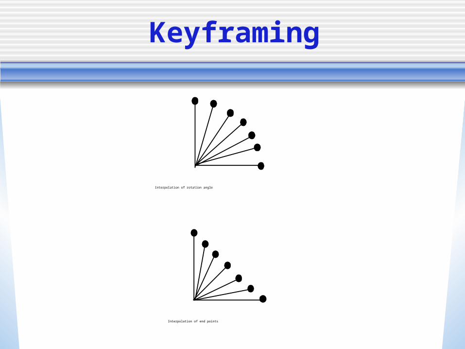
Interpolation of rotation angle
Interpolation of end points
Keyframing
• The keyframing approach carries certain disadvantages First, it is only really suitable for simple
motion of rigid bodies Second, care must be taken to ensure
that no unwanted motion excursions are introduced by the interpolant
None the less, interpolation of key frames remains fundamental to most animation systems
Spline-Driven Animation
• Spline-driven animation means the explicit specification of the motion characteristic of an object by using cubic splines
• Cubic B-splines are composite curves made up of several curve segments
• The curve possesses second order continuity
• These cubes are commonly used in computer graphics.
Spline-Driven Animation
• Consider a single segment of the curve defined over the interval 0≤u≤1
• The curve is a cubic polynomial which can be specified interactively by defining four control points
• The particular curve that passes through these points is constrained by the need for second order continuity at the end points of the curve segments Adjacent curve segments share three control
points
Spline-Driven Animation
• Using this information we can derive mathematically the exact form of each of the curve segments as follows:
Qi(u) = sum from k=0 to 3 pi+kBk(u)
• where the pi’s are the control points, and the Bi’s are defined as follows:
B0(u) = (1+u)3/6
B1(u) = (3u3-6u2+4)/6
B2(u) = (-3u3+3u2+3u+1)/6
B3(u) = u3/6
Spline-Driven Animation
• Then the curve is reparameterized in terms of a global variable U
• If the ends of the curve segments occur at equal intervals with respect to the curve parameter, the curve is known as a uniform B-spline
Spline-Driven Animation
• Suppose we have interactively specified a spline Q(u) (by giving four control points) that we wish to use as the path for the motion of an object
• To generate an animation sequence, we need to find the position of the object along the path at equal intervals in time
Spline-Driven Animation
• In order to do this, we need to reparameterize the curve in terms of arclength Without the arclength parameter, it is not
possible to have an object move with uniform speed along a spline
The reparameterization is nontrivial and will not be given here
Once this has been done, an object positioned on a curve Q(u) can be driven by a velocity curve V(u) = (t(u), s(u)) that plots the arclength s, or
distance traveled, against time
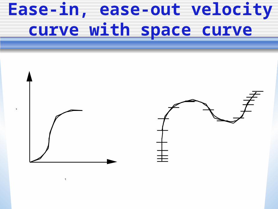
Ease-in, ease-out velocity curve with space curve
s
t
Spline-Driven Animation
• The velocity curve can be generalized to drive any motion parameter The term ‘motion parameter’ then
encompasses anything that moves in the animation sequence apart from the usual kinetic variables such as position and orientation
Movement could also include color and transparency, for example
This methodology is known as general kinetic control
Animating Articulated Structures
• Older animation systems keyframe based
• Newer animation systems use forward kinematics and inverse kinematics to specify and control motion
• The characters themselves are constructed out of skeletons which resemble the articulated structures found in robotics
Animating Articulated Structures
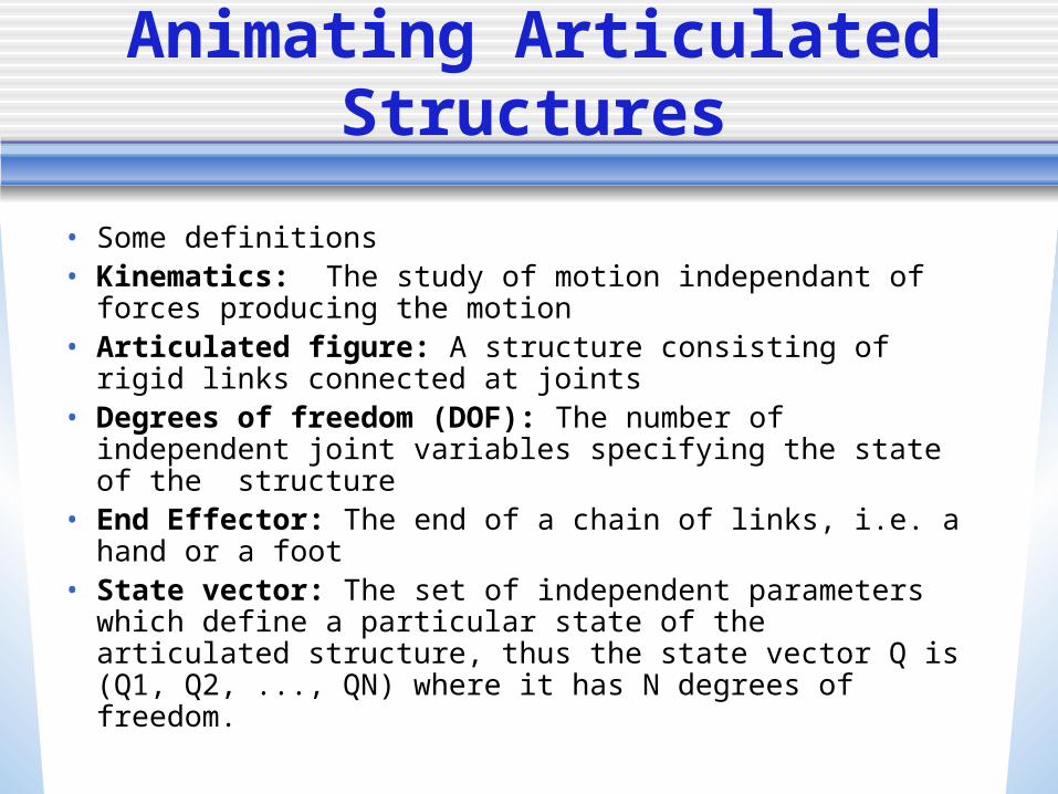
• Some definitions• Kinematics: The study of motion independant of
forces producing the motion• Articulated figure: A structure consisting of rigid
links connected at joints• Degrees of freedom (DOF): The number of
independent joint variables specifying the state of the structure
• End Effector: The end of a chain of links, i.e. a hand or a foot
• State vector: The set of independent parameters which define a particular state of the articulated structure, thus the state vector Q is (Q1, Q2, ..., QN) where it has N degrees of freedom.
Forward and Inverse Kinematics
• In forward kinematics the motion of all the joints in the structure are explicitly specified which yields the end effector position
• The end effector position X is a function of the state vector of the structure, or: X = f ( Q )
Forward and Inverse Kinematics
• In inverse kinematics (also known as "goal directed motion") the end effector's position is all that is defined
• Given the end effector position, we must derive the state vector of the structure which produced that end effector position
• Thus the state vector is given by Q = f-1( X )
Forward Kinematics
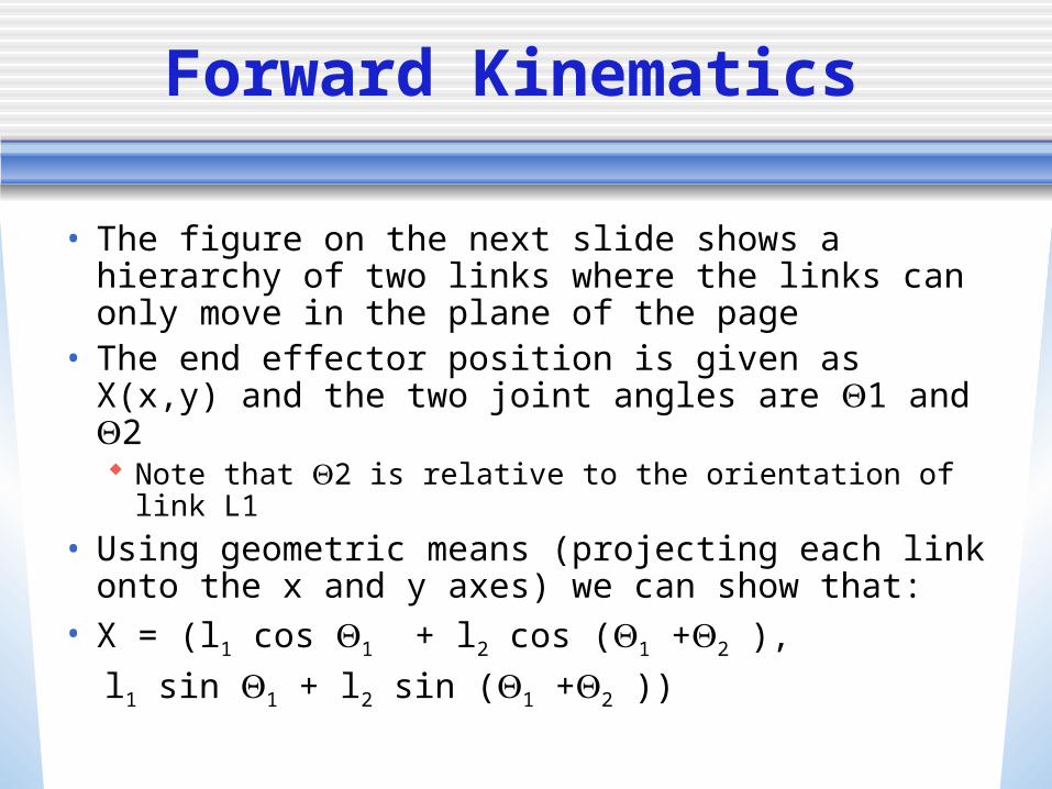
• The figure on the next slide shows a hierarchy of two links where the links can only move in the plane of the page
• The end effector position is given as X(x,y) and the two joint angles are 1 and 2 Note that 2 is relative to the orientation of link L1
• Using geometric means (projecting each link onto the x and y axes) we can show that:
• X = (l1 cos 1 + l2 cos (1 +2 ),
l1 sin 1 + l2 sin (1 +2 ))
Forward Kinematics
QuickTime™ and aTIFF (Uncompressed) decompressorare needed to see this picture.
Inverse Kinematics
• Given the end-effector position (x,y) we can find the joint angles 1 and 2 Once again use simple geometry
• Increasing degrees of freedom allows more motion, but makes the geometry more difficult (for inverse kinematics, there will be multiple solutions)
The Jacobian
• Given X = f(Q) where X is of dimension n and Q is of dimension m, the Jacobian is the n x m matrix of partial derivatives relating differential changes of Q (dQ) to differential changes in X (dX) dX = J(Q) dQ
• For use in computer graphics we usually divide everything by dt dotX = J(Q) dotQ
The Jacobian
• Where dotX is velocity of the end effector which is itself a vector of six dimensions that include linear velocity and angular velocity, and where dotQ is time derivative of the state vector
• Thus the Jacobian maps velocities in state space to velocities in cartesian space
• Thus at any time these quantities are related via the linear transformation J which itself changes through time as Q changes
The Jacobian
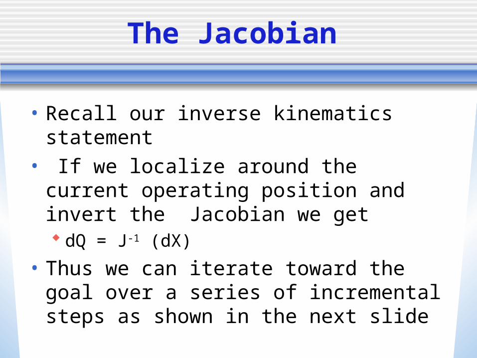
• Recall our inverse kinematics statement
• If we localize around the current operating position and invert the Jacobian we get dQ = J-1 (dX)
• Thus we can iterate toward the goal over a series of incremental steps as shown in the next slide
The Jacobian
QuickTime™ and aTIFF (Uncompressed) decompressorare needed to see this picture.
The Jacobian
• Rather than doing the actual differentiation we need another way to construct the Jacobian
• This is done by developing a system for referencing the chain of links (not developed here)
Example
QuickTime™ and aTIFF (Uncompressed) decompressorare needed to see this picture.
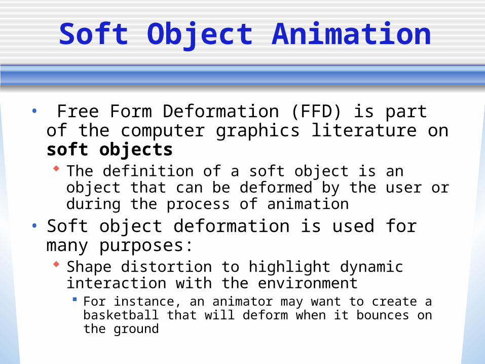
Soft Object Animation
• Free Form Deformation (FFD) is part of the computer graphics literature on soft objects The definition of a soft object is an object that
can be deformed by the user or during the process of animation
• Soft object deformation is used for many purposes: Shape distortion to highlight dynamic interaction
with the environment For instance, an animator may want to create a
basketball that will deform when it bounces on the ground
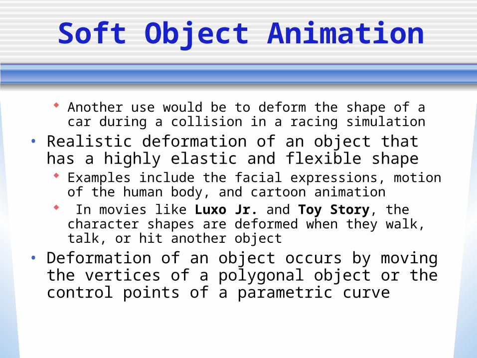
Soft Object Animation
Another use would be to deform the shape of a car during a collision in a racing simulation
• Realistic deformation of an object that has a highly elastic and flexible shape Examples include the facial expressions, motion of the
human body, and cartoon animation In movies like Luxo Jr. and Toy Story, the character
shapes are deformed when they walk, talk, or hit another object
• Deformation of an object occurs by moving the vertices of a polygonal object or the control points of a parametric curve
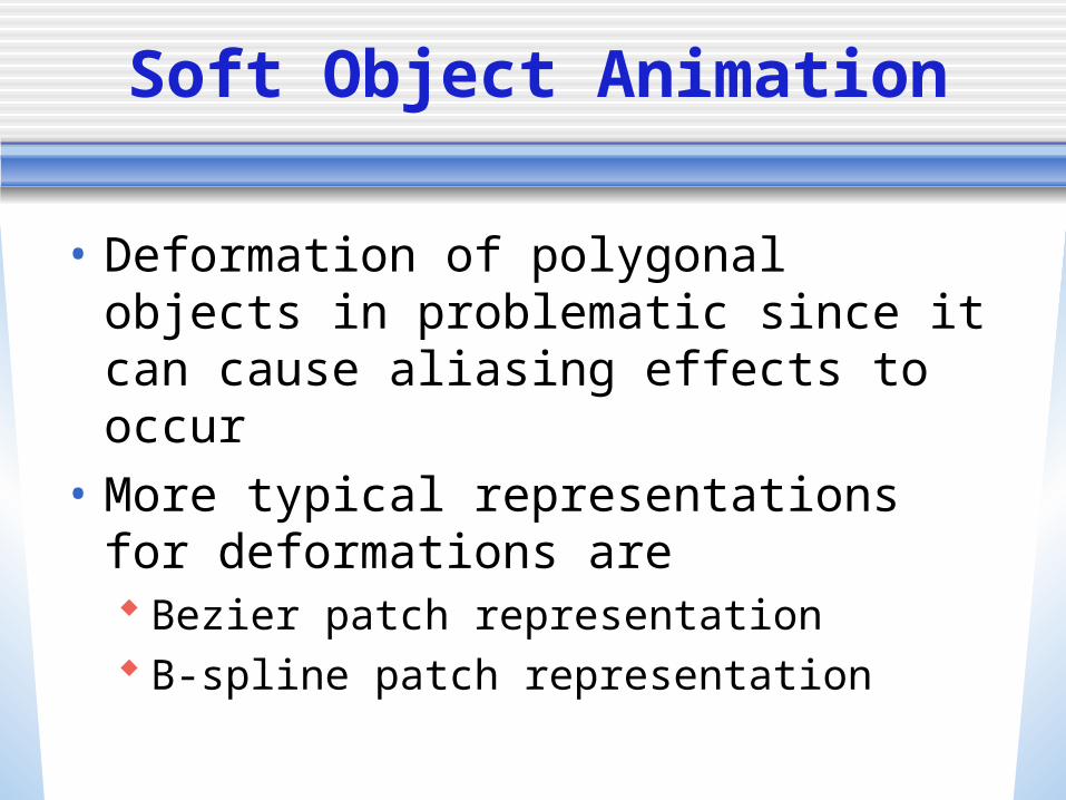
Soft Object Animation
• Deformation of polygonal objects in problematic since it can cause aliasing effects to occur
• More typical representations for deformations are Bezier patch representation B-spline patch representation
Bezier Patch
QuickTime™ and aTIFF (Uncompressed) decompressorare needed to see this picture.


![Computer Animation - Princeton University Computer … · Pixar 3-D and 2-D animation Homer 3-D Homer 2-D ... Disney Computer Animation Animation pipeline ... 18-animation.ppt [Read-Only]](https://img.pdfslide.net/doc/110x75/5b40ec327f8b9a4b3f8db714/computer-animation-princeton-university-computer-pixar-3-d-and-2-d-animation.jpg)