FYTN05Spring 2018

Computer Assignment 1: Depletion Forces

Supervisor: Daniel Nilsson(+46 222 9347 , daniel.nilsson@thep.lu.se)

Deadline: Monday, February 19 10:15

This document and the java-program can be downloaded fromhttp://home.thep.lu.se/˜carl/fytn05/assignments.html

1 Introduction

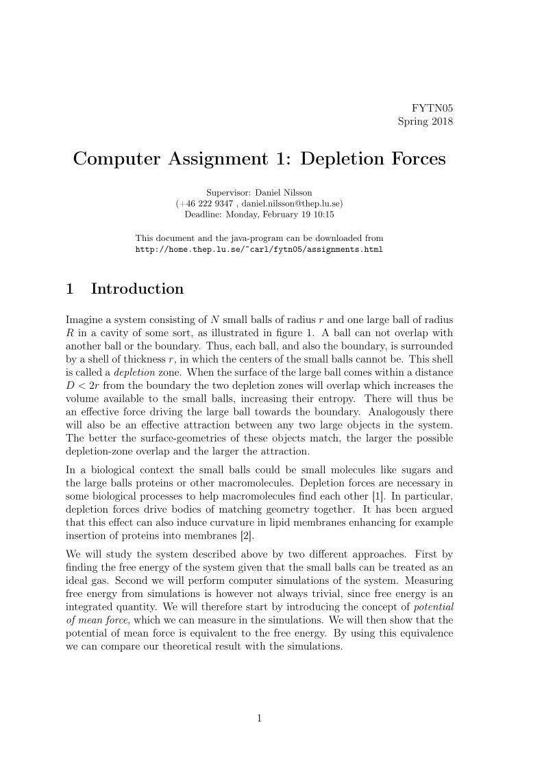
Imagine a system consisting of N small balls of radius r and one large ball of radiusR in a cavity of some sort, as illustrated in figure 1. A ball can not overlap withanother ball or the boundary. Thus, each ball, and also the boundary, is surroundedby a shell of thickness r, in which the centers of the small balls cannot be. This shellis called a depletion zone. When the surface of the large ball comes within a distanceD < 2r from the boundary the two depletion zones will overlap which increases thevolume available to the small balls, increasing their entropy. There will thus bean effective force driving the large ball towards the boundary. Analogously therewill also be an effective attraction between any two large objects in the system.The better the surface-geometries of these objects match, the larger the possibledepletion-zone overlap and the larger the attraction.

In a biological context the small balls could be small molecules like sugars andthe large balls proteins or other macromolecules. Depletion forces are necessary insome biological processes to help macromolecules find each other [1]. In particular,depletion forces drive bodies of matching geometry together. It has been arguedthat this effect can also induce curvature in lipid membranes enhancing for exampleinsertion of proteins into membranes [2].

We will study the system described above by two different approaches. First byfinding the free energy of the system given that the small balls can be treated as anideal gas. Second we will perform computer simulations of the system. Measuringfree energy from simulations is however not always trivial, since free energy is anintegrated quantity. We will therefore start by introducing the concept of potentialof mean force, which we can measure in the simulations. We will then show that thepotential of mean force is equivalent to the free energy. By using this equivalencewe can compare our theoretical result with the simulations.

1

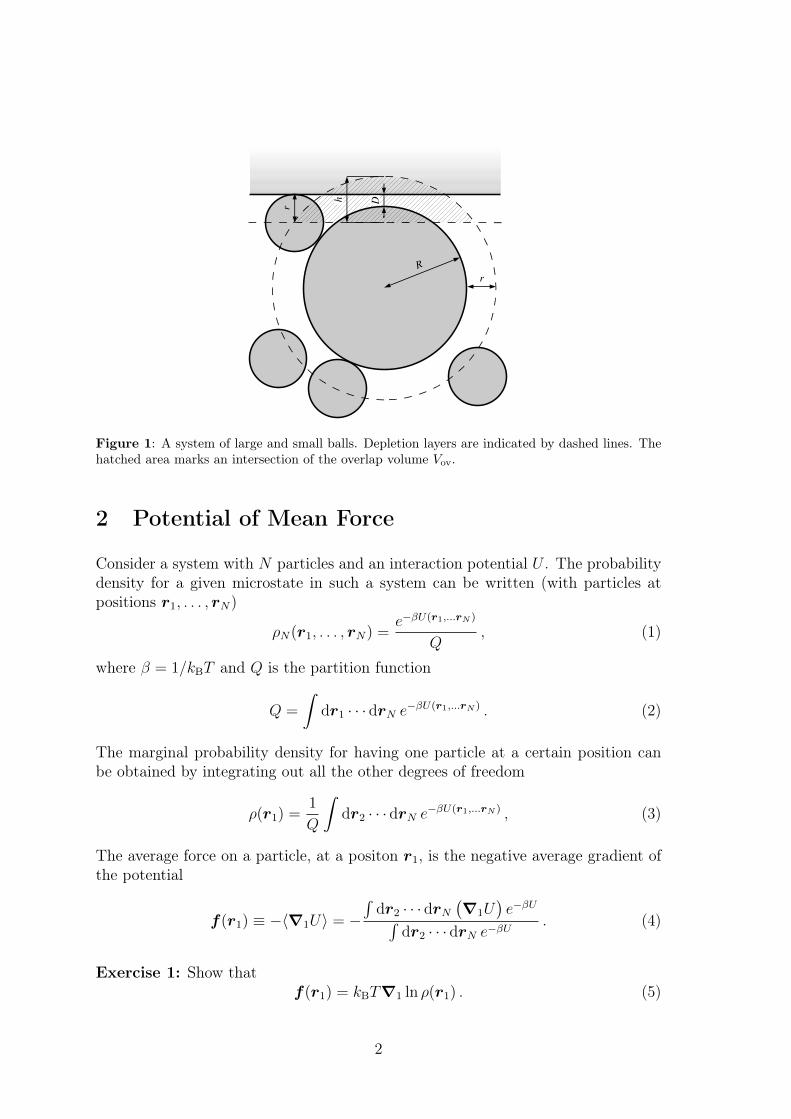
Figure 1: A system of large and small balls. Depletion layers are indicated by dashed lines. Thehatched area marks an intersection of the overlap volume Vov.

2 Potential of Mean Force

Consider a system with N particles and an interaction potential U . The probabilitydensity for a given microstate in such a system can be written (with particles atpositions r1, . . . , rN)

ρN(r1, . . . , rN) =e−βU(r1,...rN )

Q, (1)

where β = 1/kBT and Q is the partition function

Q =

∫dr1 · · · drN e−βU(r1,...rN ) . (2)

The marginal probability density for having one particle at a certain position canbe obtained by integrating out all the other degrees of freedom

ρ(r1) =1

Q

∫dr2 · · · drN e−βU(r1,...rN ) , (3)

The average force on a particle, at a positon r1, is the negative average gradient ofthe potential

f(r1) ≡ −〈∇1U〉 = −∫

dr2 · · · drN(∇1U

)e−βU∫

dr2 · · · drN e−βU. (4)

Exercise 1: Show thatf(r1) = kBT∇1 ln ρ(r1) . (5)

2

Equation 5 states that the function

w(r1) = −kBT ln ρ(r1) (6)

acts as an average potential on our particle. If we replace all the other particles inour system by the potential w(r1), the probability density function ρ(r1) will bethe same for the remaining particle1. This potential is usually called the potentialof mean force (PMF), or the reversible work. Furthermore, the energy difference

∆w = w(r(f)1 )− w(r

(i)1 ) (7)

describes the work needed to translate the considered particle from r(i)1 to r(f)

1 with allthe other particles in equilibrium during the process. If we consider r1 an externalparameter, the two states can be treated as two different macrostates. In thisinterpretation ∆w is equivalent to the free energy difference ∆F between two givenmacrostates. From here on we will treat free energy and PMF equivalently. Moregenerally we can define a PMF for any parameter, λ, describing a macrostate, as

w(λ) = −kBT ln ρ(λ) . (8)

Spherically symmetric systems

Suppose the probability density ρ(r) is spherically symmetric, ρ(r) = g(r). Theprobability density as a function of r, ρ(r), is obtained by integrating over a shell ofwidth dr at distance r from the origin,

ρ(r)dr = dr

∫g(r)r2 sin θdθdϕ = 4πr2g(r)dr . (9)

Correspondingly, the PMF can be studied as a function of r. This PMF is given by

w(r) = −kBT ln ρ(r) = −kBT ln(4πr2g(r)) = −kBT ln g(r)− kBT ln 4πr2 . (10)

3 Free energy in an ideal gas approximation

Now return to the system introduced in section 1. For a given microstate, ρ(r0, r1, . . . , rN)is either 0 or 1/Q, depending on if there is an overlap or not. Given that the volumefraction of the small balls is small, such a system is described well as an ideal gas.Given a position, r0, of the big ball, the free energy of the system is then

F = −NkBT lnV ′ ( + terms independent of volume), (11)

where V ′ is the volume available to the small balls, i. e.

V ′ = V − Vbig + Vov . (12)1Because in such a system ρ ∝ exp (−w(r1)/kBT ), which is basically an inversion of (6).

3

Figure 2: 3D view of the overlap volume Vov. The base of the spherical cap of heigth h has radiusa and area A.

V is the available volume of the cavity, (4π(RS − r)3), Vbig the volume of the bigball (including its depletion layer), 4π(R+ r)3/3, and Vov the volume of the overlapbetween the depletion zones of the big ball and the cavity. Here we will mainlystudy a spherical cavity of radius RS, which gives V = 4π(RS − r)3/3.

We want to determine how the free energy depends on the position of the big ball.Without loss of generality, we may assume that the ball is constrained to move in onedimension. The free energy is then a function of the distance r0 between the center ofthe ball and the center of the cavity, or equivalently the distance D between the balland the sphere (D = RS − R− r0). Denote this free energy F (D). The free energyfor an unconstrained big ball, moving freely in the cavity, is F (D) − kBT ln 4πr20(compare equation 10).

To calculate F (D) it is convenient to first determine the entropic force

f(D) = −∂F∂D

=NkBT

V ′(D)· ∂Vov

∂D. (13)

If one assumes V ′(D) ≈ V

f(D) ≈ N

VkBT ·

∂Vov

∂D= ckBT ·

∂Vov

∂D, (14)

where c = N/V is the concentration of small balls.

Flat boundary

The simplest case we can study is a system where the boundary is a flat wall (asin figure 1). The derivative of Vov with respect to D is equal to the negative of thearea where the depletion zones meet (the base area of the spherical cap which Vov

measures, see figure 2)∂Vov

∂D= −A(D) . (15)

4

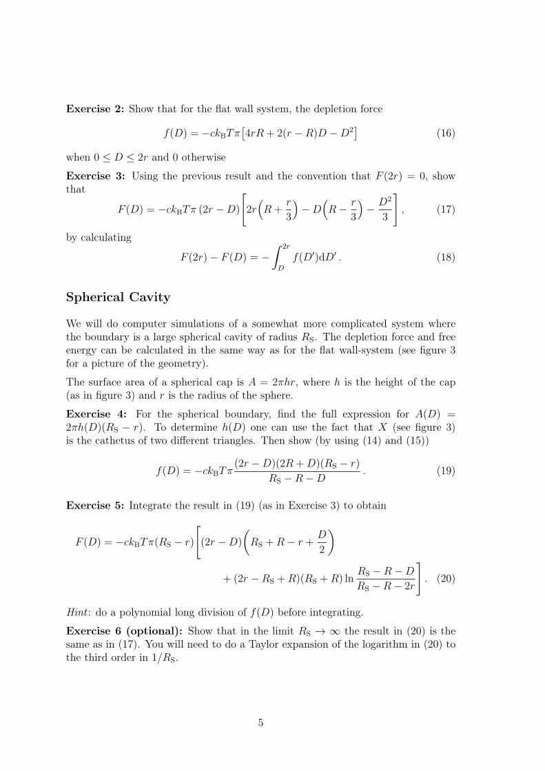
Exercise 2: Show that for the flat wall system, the depletion force

f(D) = −ckBTπ[4rR + 2(r −R)D −D2

](16)

when 0 ≤ D ≤ 2r and 0 otherwise

Exercise 3: Using the previous result and the convention that F (2r) = 0, showthat

F (D) = −ckBTπ (2r −D)

[2r(R +

r

3

)−D

(R− r

3

)− D2

3

], (17)

by calculating

F (2r)− F (D) = −∫ 2r

D

f(D′)dD′ . (18)

Spherical Cavity

We will do computer simulations of a somewhat more complicated system wherethe boundary is a large spherical cavity of radius RS. The depletion force and freeenergy can be calculated in the same way as for the flat wall-system (see figure 3for a picture of the geometry).

The surface area of a spherical cap is A = 2πhr, where h is the height of the cap(as in figure 3) and r is the radius of the sphere.

Exercise 4: For the spherical boundary, find the full expression for A(D) =2πh(D)(RS − r). To determine h(D) one can use the fact that X (see figure 3)is the cathetus of two different triangles. Then show (by using (14) and (15))

f(D) = −ckBTπ(2r −D)(2R +D)(RS − r)

RS −R−D. (19)

Exercise 5: Integrate the result in (19) (as in Exercise 3) to obtain

F (D) = −ckBTπ(RS − r)

[(2r −D)

(RS +R− r +

D

2

)

+ (2r −RS +R)(RS +R) lnRS −R−DRS −R− 2r

]. (20)

Hint : do a polynomial long division of f(D) before integrating.

Exercise 6 (optional): Show that in the limit RS → ∞ the result in (20) is thesame as in (17). You will need to do a Taylor expansion of the logarithm in (20) tothe third order in 1/RS.

5

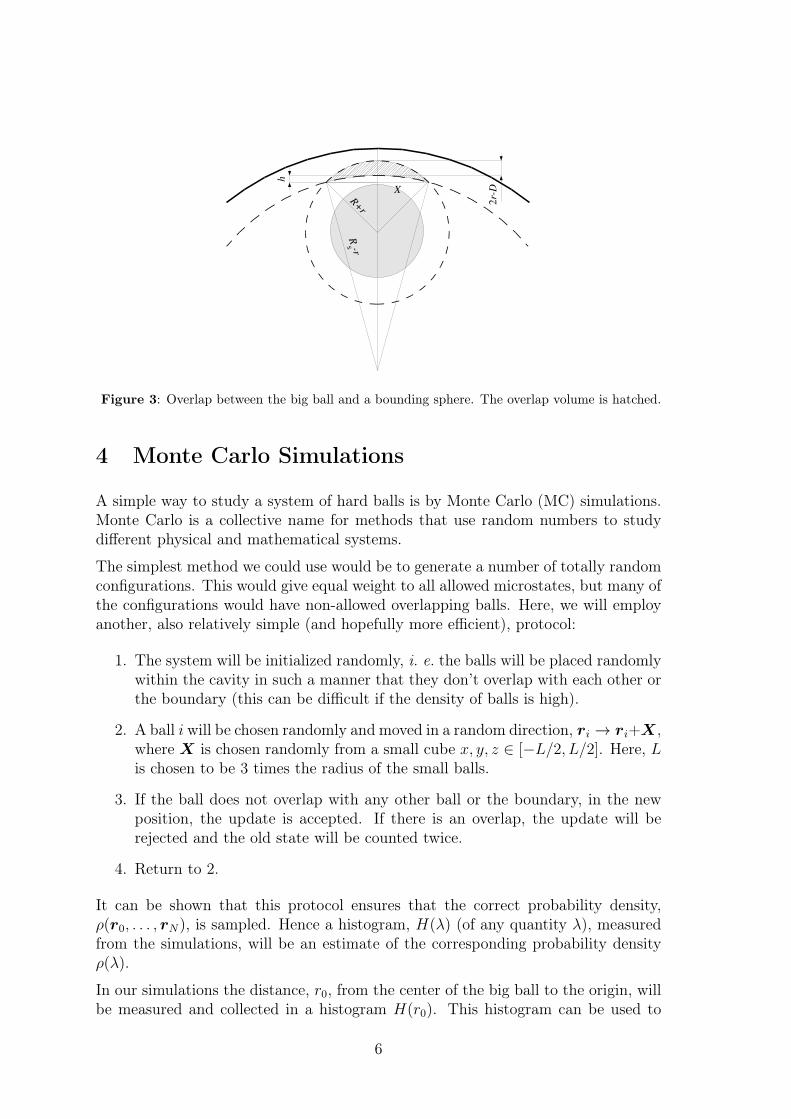
Figure 3: Overlap between the big ball and a bounding sphere. The overlap volume is hatched.

4 Monte Carlo Simulations

A simple way to study a system of hard balls is by Monte Carlo (MC) simulations.Monte Carlo is a collective name for methods that use random numbers to studydifferent physical and mathematical systems.

The simplest method we could use would be to generate a number of totally randomconfigurations. This would give equal weight to all allowed microstates, but many ofthe configurations would have non-allowed overlapping balls. Here, we will employanother, also relatively simple (and hopefully more efficient), protocol:

1. The system will be initialized randomly, i. e. the balls will be placed randomlywithin the cavity in such a manner that they don’t overlap with each other orthe boundary (this can be difficult if the density of balls is high).

2. A ball i will be chosen randomly and moved in a random direction, ri → ri+X,where X is chosen randomly from a small cube x, y, z ∈ [−L/2, L/2]. Here, Lis chosen to be 3 times the radius of the small balls.

3. If the ball does not overlap with any other ball or the boundary, in the newposition, the update is accepted. If there is an overlap, the update will berejected and the old state will be counted twice.

4. Return to 2.

It can be shown that this protocol ensures that the correct probability density,ρ(r0, . . . , rN), is sampled. Hence a histogram, H(λ) (of any quantity λ), measuredfrom the simulations, will be an estimate of the corresponding probability densityρ(λ).

In our simulations the distance, r0, from the center of the big ball to the origin, willbe measured and collected in a histogram H(r0). This histogram can be used to

6

check the free energy estimate F (D) obtained above under the ideal gas assumption.If this assumption holds, H(r0) and F (D) will be related by

−kBT lnH(r0) = F (D)− kBT ln 4πr20 , 0 ≤ D ≤ 2r . (21)

Running the program

The program you will use is a java-program that can be downloaded from the web.There will be supervised sessions in the computer rooms at the astronomy depart-ment, but if you prefer working at home the program should run on Windows andMac machines as well (neither has been tested though), provided you have Java1.6 installed. You will also need some software that can plot curves and data, likegnuplot. After you have logged in at the astronomy department you should firstcreate a directory with your name. You can do this by opening a terminal and usingthe linux-command mkdir, i. e. type

mkdir yourname

Then download the program depletion.jar, using a web browser, to that directory.To enter the directory write

cd yourname

and to run the program type

java -jar depletion.jar

After you have finished the exercise, and have made sure that you have copies of allthe files you need for writing the report, remove your directory with the command

rm -r yourname

The program has several options, you can set the number of balls, the size of thesmall ball, the big ball and the cavity. You can choose if you want to simulatea two- or three-dimensional system, and if you want the cavity to be spherical orellipsoidal. You can also decide how long the simulation will be, by two paramaters:cycle length and number of cycles. Cycle length is the number of individual MCsteps that are performed in one cycle. Dividing the simulation into cycles is simplyfor convenience. The number of steps in a cycle is roughly the same as the numberof balls, thus ensuring that after a cycle the position of most balls has been changed,i. e. a significantly changed state has been reached.

During the simulation, two files are written, one corresponding to the PMF (calledPMF file), which contains − lnH(r0), and one with run-time snap shots of theposition of the large ball (Runtime data file). You can set the sample rate for thehistogram H(r0) and how often the files should be updated. All the settings thatwere used in the simulation will be written to both files.

When you have selected the settings the simulation can be started. The time neededper MC step increases approximately linearly with the number of balls N . If youdouble the number of balls you will need a twice as long simulation for the same

7

number of steps. But the complexity of the simulations increases a lot for densesystem, the number of MC steps needed to obtain adequate sampling increasesrapidly with N when N gets large.

5 Problems

Problem 1: The ideal gas approximation

Run a simulation with the default values. The simulation will have statistical errors,but is not biased by any approximation. Compare the PMF obtained from thesimulation with the free energy we found under the ideal gas assumption (using(21)). Also check how the omission of Vbig in (14) affects your result (we alsoomitted Vov, but that has a smaller effect). Do this for some different values of theparameters. Remember that the comparison is only valid in the range 0 ≤ D ≤ 2r.The histogram is not normalized so an additive constant should be included in (21).

Problem 2: Dense systems

An experimental study of this type of system is can be found in [2]. In that studyR = 474 nm, r = 42 nm, RS ≈ 1 700 nm and the volume fraction of small balls,φV = Nr3/R3

S, was 0.3. Simulating such a dense system in 3D is outside the scopeof this exercise however (too many balls are needed). But you can try to simulatea 2D system with a similar area fraction of small balls, φA ∼ 0.1− 0.3. Even in the2D system you will need 400–500 balls if you take the numbers directly from theexperiment. Therefore, use a smaller RS so that the number of balls is less than200. You will still need longer simulation times than the default value to get clearresults. Our ideal gas approximation doesn’t apply to these dense systems, the freeenergy is more complicated.2 In particular there is more than one minimum in thePMF, why?

Problem 3: Curvature

In the experiment the dependence of the depletion force on the boundary curvaturewas studied [2]. An ellipsoid cavity is a simple example of a system with varyingcurvature along the boundary. Simulate a 2D elliptical system for some differentdensities. The program uses the value from the option Size of cavity for the semimi-nor axis, and sets the semimajor axis of the ellipsoid to two times that value. F (r0)is not displayed in these simulations because r0 is not a good coordinate in an el-lipse, instead you should look at the runtime snapshots to get a qualitative pictureof what is going on. Explain what you see!

2When you plot − lnH(r0) for a two-dimensional system, the geometric correction term will beln(2πr0) instead of ln(4πr20).

8

6 Report

The report should consist of four main parts, it’s up to you how you want to organizeyour text, but the following should be included in one way or another:

• Introduction – describe the problem in general terms, give background infor-mation, etc.

• Theory – discuss the theory that describes the problem, including answers toexercises. To get the highest grade this part should be a continuous text, notjust a list of answers to the exercises.

• Results and discussion – describe your results from the different simulations,discuss them and try to explain them as far as possible. If you prefer, resultsand discussion can be two separate sections.

• Conclusions – summarize what you have done and present any general discus-sion or conclusions you want to include.

The report should be submitted through Live@Lund, preferably as a pdf-file. Thecorrected reports can be found in the bookshelf outside the HUB lecture hall.

You are encouraged to collaborate when doing the exercise but the reports shouldbe individual. In the report you are allowed to use information from any sourceyou like, but a reference should be given for each statement. Any material that isnot originally yours, i. e. text from the internet or other students, and not correctlyreferenced, will be recognized and reported to the university disciplinary council.Past experience has shown that the vast majority of students understand this, butthere have been exceptions.

References

[1] Phillips, R.; Kondev, J.; Therot, J.; Garcia, H.G. Physical Biology of the Cell, secondedition. 2013. Garland Science

[2] Dinsmore, A. D.; Wong, D. T.; Nelson, P.; Yodh, A. G. Hard Spheres in Vesicles:Curvature-Induced Forces and Particle-Induced Curvature. 1998. Physical Review Letters80: 409–412.

[3] Chandler, David. Introduction to Modern Statistical Mechanics. 1987. Oxford Univer-sity Press, Oxford.

[4] Dickman, Ronald; Attard, Phil; Simonian, Veronika. Entropic forces in binary hardsphere mixtures: Theory and simulation. 1997. Journal of Chemical Physics 107: 205–213.

9

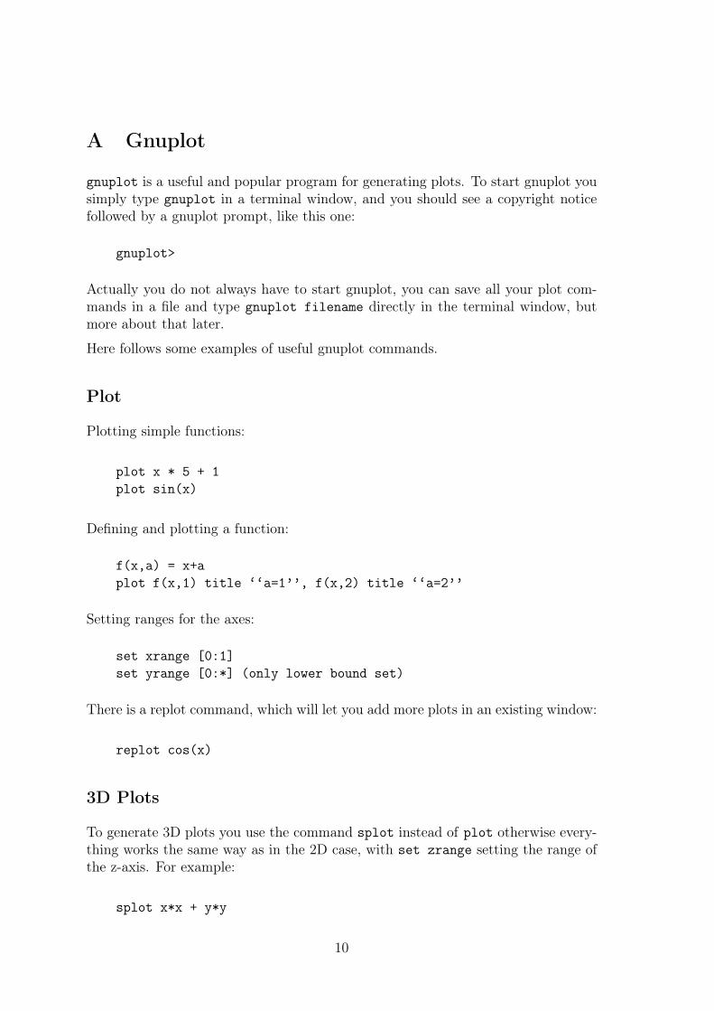
A Gnuplot

gnuplot is a useful and popular program for generating plots. To start gnuplot yousimply type gnuplot in a terminal window, and you should see a copyright noticefollowed by a gnuplot prompt, like this one:

gnuplot>

Actually you do not always have to start gnuplot, you can save all your plot com-mands in a file and type gnuplot filename directly in the terminal window, butmore about that later.

Here follows some examples of useful gnuplot commands.

Plot

Plotting simple functions:

plot x * 5 + 1plot sin(x)

Defining and plotting a function:

f(x,a) = x+aplot f(x,1) title ‘‘a=1’’, f(x,2) title ‘‘a=2’’

Setting ranges for the axes:

set xrange [0:1]set yrange [0:*] (only lower bound set)

There is a replot command, which will let you add more plots in an existing window:

replot cos(x)

3D Plots

To generate 3D plots you use the command splot instead of plot otherwise every-thing works the same way as in the 2D case, with set zrange setting the range ofthe z-axis. For example:

splot x*x + y*y

10

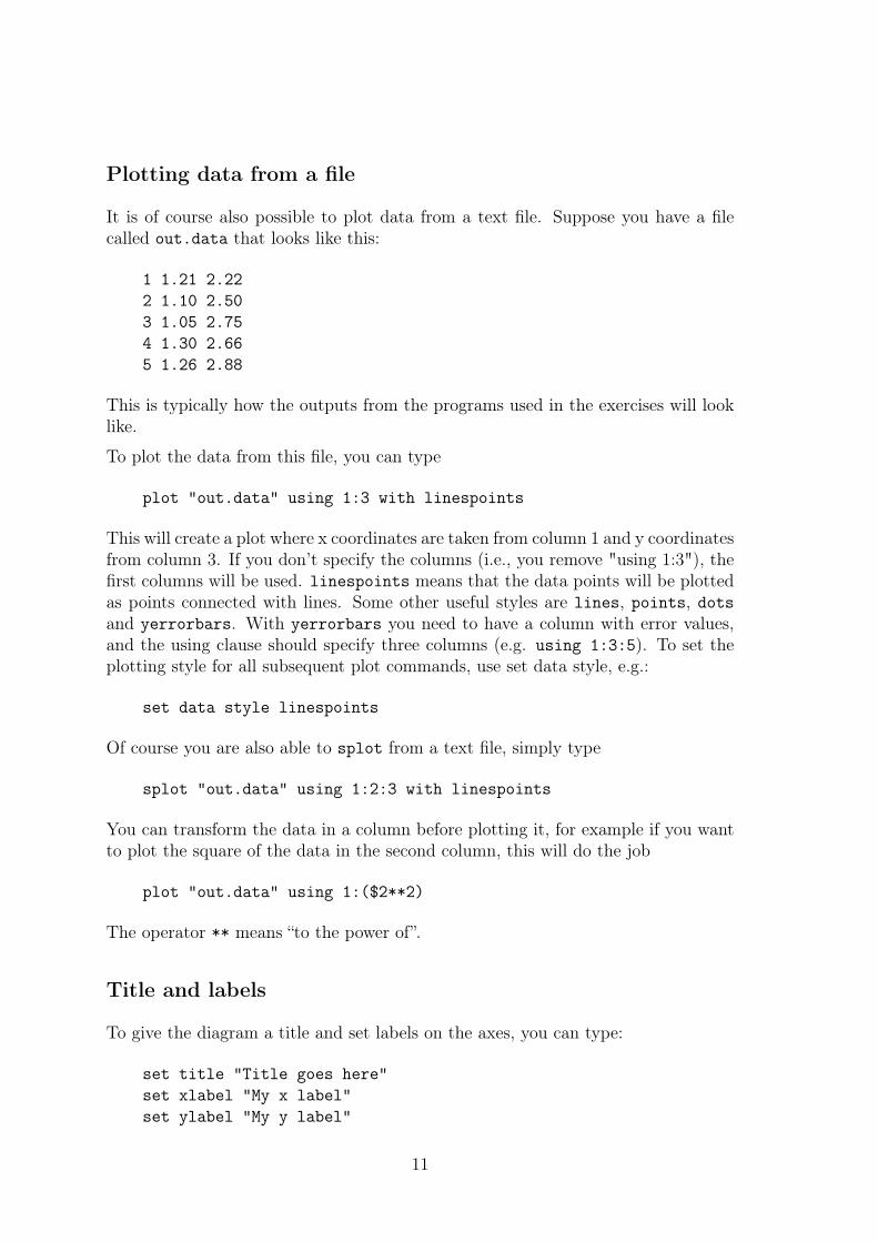
Plotting data from a file

It is of course also possible to plot data from a text file. Suppose you have a filecalled out.data that looks like this:

1 1.21 2.222 1.10 2.503 1.05 2.754 1.30 2.665 1.26 2.88

This is typically how the outputs from the programs used in the exercises will looklike.

To plot the data from this file, you can type

plot "out.data" using 1:3 with linespoints

This will create a plot where x coordinates are taken from column 1 and y coordinatesfrom column 3. If you don’t specify the columns (i.e., you remove "using 1:3"), thefirst columns will be used. linespoints means that the data points will be plottedas points connected with lines. Some other useful styles are lines, points, dotsand yerrorbars. With yerrorbars you need to have a column with error values,and the using clause should specify three columns (e.g. using 1:3:5). To set theplotting style for all subsequent plot commands, use set data style, e.g.:

set data style linespoints

Of course you are also able to splot from a text file, simply type

splot "out.data" using 1:2:3 with linespoints

You can transform the data in a column before plotting it, for example if you wantto plot the square of the data in the second column, this will do the job

plot "out.data" using 1:($2**2)

The operator ** means “to the power of”.

Title and labels

To give the diagram a title and set labels on the axes, you can type:

set title "Title goes here"set xlabel "My x label"set ylabel "My y label"

11

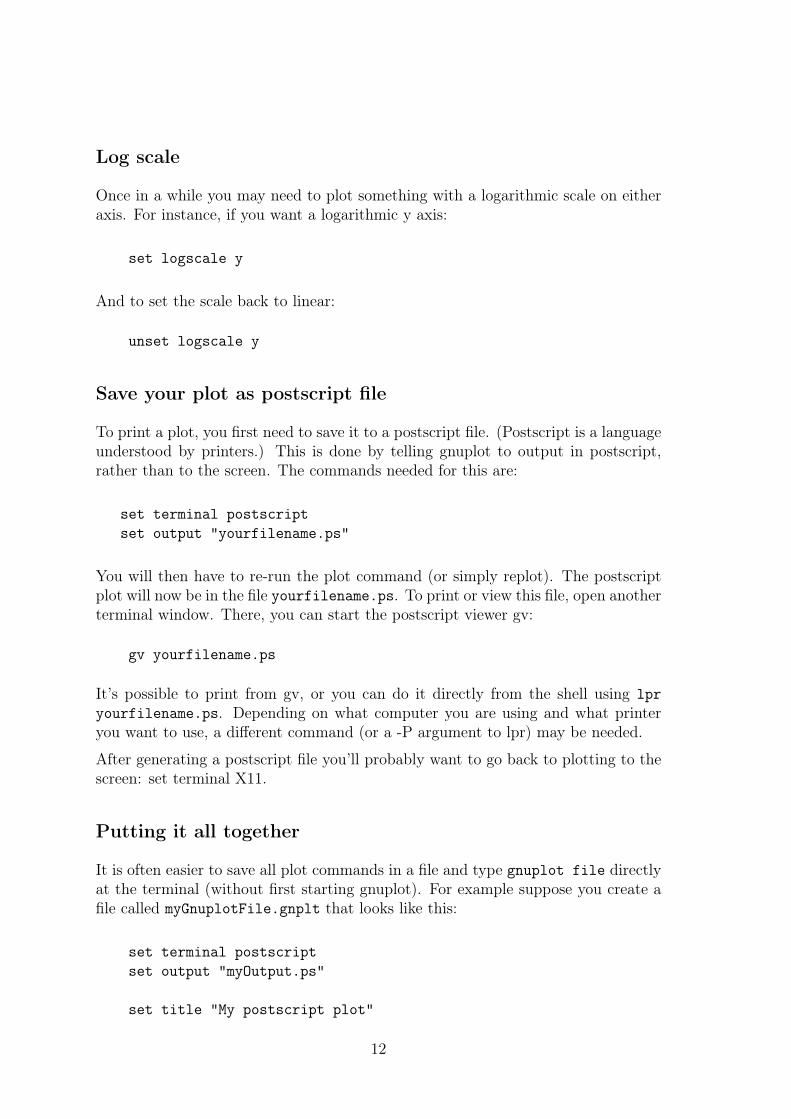
Log scale

Once in a while you may need to plot something with a logarithmic scale on eitheraxis. For instance, if you want a logarithmic y axis:

set logscale y

And to set the scale back to linear:

unset logscale y

Save your plot as postscript file

To print a plot, you first need to save it to a postscript file. (Postscript is a languageunderstood by printers.) This is done by telling gnuplot to output in postscript,rather than to the screen. The commands needed for this are:

set terminal postscriptset output "yourfilename.ps"

You will then have to re-run the plot command (or simply replot). The postscriptplot will now be in the file yourfilename.ps. To print or view this file, open anotherterminal window. There, you can start the postscript viewer gv:

gv yourfilename.ps

It’s possible to print from gv, or you can do it directly from the shell using lpryourfilename.ps. Depending on what computer you are using and what printeryou want to use, a different command (or a -P argument to lpr) may be needed.

After generating a postscript file you’ll probably want to go back to plotting to thescreen: set terminal X11.

Putting it all together

It is often easier to save all plot commands in a file and type gnuplot file directlyat the terminal (without first starting gnuplot). For example suppose you create afile called myGnuplotFile.gnplt that looks like this:

set terminal postscriptset output "myOutput.ps"

set title "My postscript plot"

12

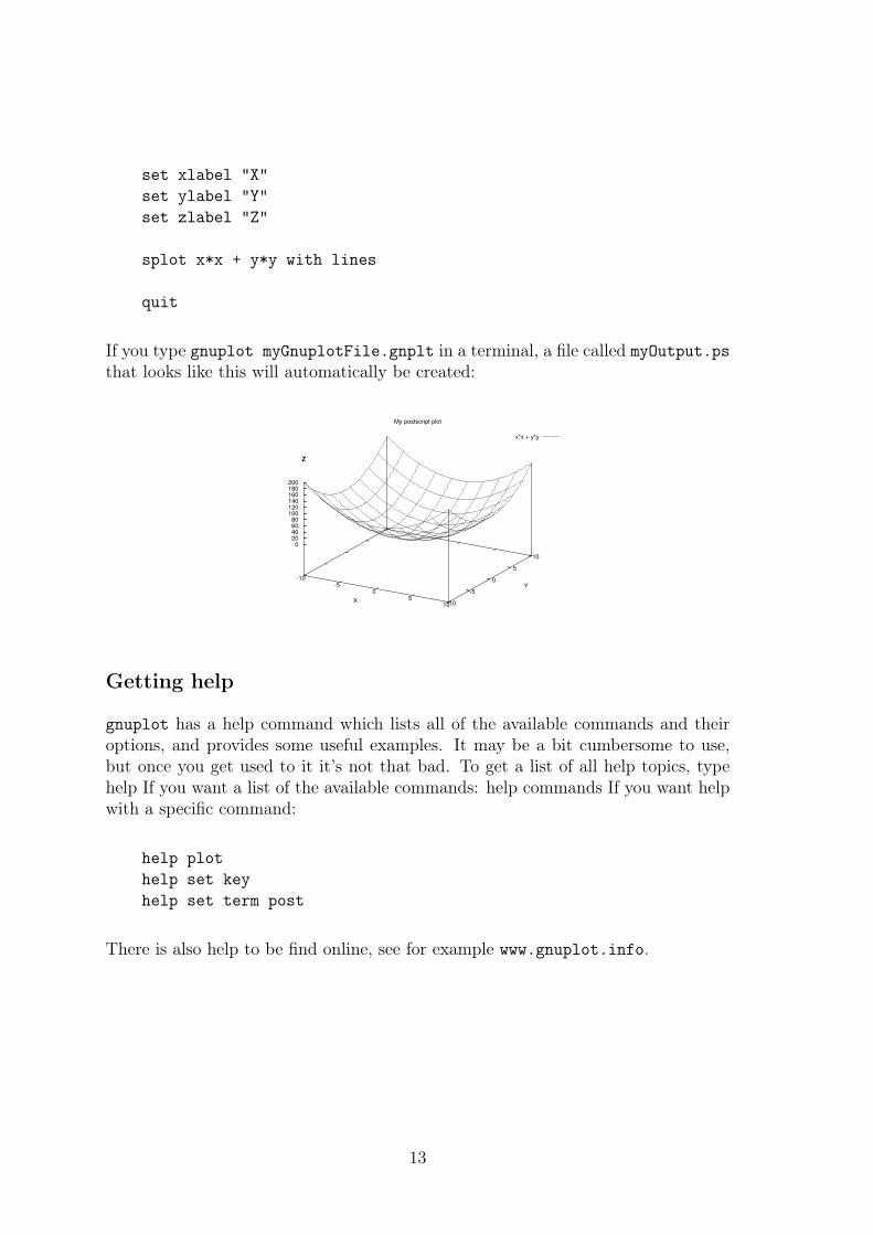
set xlabel "X"set ylabel "Y"set zlabel "Z"

splot x*x + y*y with lines

quit

If you type gnuplot myGnuplotFile.gnplt in a terminal, a file called myOutput.psthat looks like this will automatically be created:

-10-5

0 5

10-10

-5

0

5

10

0 20 40 60 80

100 120 140 160 180 200

Z

My postscript plot

x*x + y*y

X

Y

Z

Getting help

gnuplot has a help command which lists all of the available commands and theiroptions, and provides some useful examples. It may be a bit cumbersome to use,but once you get used to it it’s not that bad. To get a list of all help topics, typehelp If you want a list of the available commands: help commands If you want helpwith a specific command:

help plothelp set keyhelp set term post

There is also help to be find online, see for example www.gnuplot.info.

13