Embed Size (px)
Citation preview

Paul A. Jenkins
Computer Intensive Statistics
APTS 2020–21 Supporting Notes
July 9, 2021
apts.ac.ukAcademyforPhDTraininginStatistics

2

Table of Contents
1. Introduction . . . . . . . . . . . . . . . . . . . . . . . . . . . . . . . . . . . . . . . . . . . . . . . . . . . . . . . . . . . . . . . . . . . . . . . 5
1.1 Three Views of Sample Approximation . . . . . . . . . . . . . . . . . . . . . . . . . . . . . . . . . . . . . . . . . . . . . 5
1.2 The Usefulness of Sample Approximation . . . . . . . . . . . . . . . . . . . . . . . . . . . . . . . . . . . . . . . . . . . 7
1.3 Further Reading . . . . . . . . . . . . . . . . . . . . . . . . . . . . . . . . . . . . . . . . . . . . . . . . . . . . . . . . . . . . . . . . . 7
2. Simulation-Based Inference . . . . . . . . . . . . . . . . . . . . . . . . . . . . . . . . . . . . . . . . . . . . . . . . . . . . . . . . 9
2.1 Simulation . . . . . . . . . . . . . . . . . . . . . . . . . . . . . . . . . . . . . . . . . . . . . . . . . . . . . . . . . . . . . . . . . . . . . . 9
2.2 Monte Carlo Testing . . . . . . . . . . . . . . . . . . . . . . . . . . . . . . . . . . . . . . . . . . . . . . . . . . . . . . . . . . . . . 15
2.3 The Bootstrap . . . . . . . . . . . . . . . . . . . . . . . . . . . . . . . . . . . . . . . . . . . . . . . . . . . . . . . . . . . . . . . . . . 15
2.4 Monte Carlo Integration . . . . . . . . . . . . . . . . . . . . . . . . . . . . . . . . . . . . . . . . . . . . . . . . . . . . . . . . . . 18
3. Markov chain Monte Carlo . . . . . . . . . . . . . . . . . . . . . . . . . . . . . . . . . . . . . . . . . . . . . . . . . . . . . . . . 25
3.1 The Basis of Markov chain Monte Carlo (MCMC) . . . . . . . . . . . . . . . . . . . . . . . . . . . . . . . . . . . 25
3.2 Constructing MCMC Algorithms . . . . . . . . . . . . . . . . . . . . . . . . . . . . . . . . . . . . . . . . . . . . . . . . . . 28
3.3 Composing kernels: Mixtures and Cycles . . . . . . . . . . . . . . . . . . . . . . . . . . . . . . . . . . . . . . . . . . . 49
3.4 Diagnosing Convergence . . . . . . . . . . . . . . . . . . . . . . . . . . . . . . . . . . . . . . . . . . . . . . . . . . . . . . . . . . 51
3.5 Optimisation with MCMC . . . . . . . . . . . . . . . . . . . . . . . . . . . . . . . . . . . . . . . . . . . . . . . . . . . . . . . . 61
4. Augmentation: Extending the Space . . . . . . . . . . . . . . . . . . . . . . . . . . . . . . . . . . . . . . . . . . . . . . . 67
4.1 Composition Sampling . . . . . . . . . . . . . . . . . . . . . . . . . . . . . . . . . . . . . . . . . . . . . . . . . . . . . . . . . . . 67
4.2 Rejection Revisited . . . . . . . . . . . . . . . . . . . . . . . . . . . . . . . . . . . . . . . . . . . . . . . . . . . . . . . . . . . . . . 68
4.3 Data Augmentation . . . . . . . . . . . . . . . . . . . . . . . . . . . . . . . . . . . . . . . . . . . . . . . . . . . . . . . . . . . . . . 68
4.4 Multiple Augmentation for Optimisation . . . . . . . . . . . . . . . . . . . . . . . . . . . . . . . . . . . . . . . . . . . 69
4.5 Approximate Bayesian Computation . . . . . . . . . . . . . . . . . . . . . . . . . . . . . . . . . . . . . . . . . . . . . . . 74
5. Current and Future Directions . . . . . . . . . . . . . . . . . . . . . . . . . . . . . . . . . . . . . . . . . . . . . . . . . . . . . 77
5.1 Ensemble-based Methods and Sequential Monte Carlo . . . . . . . . . . . . . . . . . . . . . . . . . . . . . . . . 77
5.2 Pseudomarginal Methods and Particle MCMC . . . . . . . . . . . . . . . . . . . . . . . . . . . . . . . . . . . . . . 78
5.3 Approximate Approximate Methods . . . . . . . . . . . . . . . . . . . . . . . . . . . . . . . . . . . . . . . . . . . . . . . 78
5.4 Quasi-Monte Carlo . . . . . . . . . . . . . . . . . . . . . . . . . . . . . . . . . . . . . . . . . . . . . . . . . . . . . . . . . . . . . . 78
5.5 Hamiltonian/Hybrid MCMC . . . . . . . . . . . . . . . . . . . . . . . . . . . . . . . . . . . . . . . . . . . . . . . . . . . . . . 78
5.6 Methods for Big Data . . . . . . . . . . . . . . . . . . . . . . . . . . . . . . . . . . . . . . . . . . . . . . . . . . . . . . . . . . . . 79

4
A. Some Markov Chain Concepts . . . . . . . . . . . . . . . . . . . . . . . . . . . . . . . . . . . . . . . . . . . . . . . . . . . . . 87
A.1 Stochastic Processes . . . . . . . . . . . . . . . . . . . . . . . . . . . . . . . . . . . . . . . . . . . . . . . . . . . . . . . . . . . . . 87
A.2 Discrete State Space Markov Chains . . . . . . . . . . . . . . . . . . . . . . . . . . . . . . . . . . . . . . . . . . . . . . . 88
A.3 General State Space Markov Chains . . . . . . . . . . . . . . . . . . . . . . . . . . . . . . . . . . . . . . . . . . . . . . . 94
A.4 Selected Theoretical Results . . . . . . . . . . . . . . . . . . . . . . . . . . . . . . . . . . . . . . . . . . . . . . . . . . . . . . 99
A.5 Further Reading . . . . . . . . . . . . . . . . . . . . . . . . . . . . . . . . . . . . . . . . . . . . . . . . . . . . . . . . . . . . . . . . . 100

1. Introduction
These notes were intended to supplement the Computer Intensive Statistics lectures and laboratory ses-
sions rather than to replace or directly accompany them. As such, material is presented here in an order
which is logical for reference purposes after the week and not precisely the order in which it was to be
discussed during the week. There is much more information in these notes concerning some topics than
would have been covered during the week itself. One of their main functions is to provide pointers to the
relevant literature for anyone wanting to learn more about these topics.
Acknowledgement. These notes are based on a set developed by Adam Johansen, which can be traced
back to a lecture course given by him and Ludger Evers in Bristol in 2007–08. Many of the bet-
ter figures were originally prepared by Ludger Evers. Any errors are mine and should be directed to
1.1 Three Views of Sample Approximation
Many of the techniques described in these notes are simulation-based or otherwise make use of sample
approximations of quantities. In the preliminary notes there is some discussion of the approximation of
π, for example, by representing it in terms of an expectation that can be approximated using a sample
average.
In general there are three increasingly abstract ways of viewing the justification of this type of approach.
Thinking in these terms can be very helpful when trying to understand what these techniques are aiming
to do and why we might expect them to work, and so it’s worth thinking about this even before getting
in to the details of particular algorithms.
1.1.1 Direct Approximation
This is a definition of Monte Carlo methods due to Halton (1970):
Representing the solution of a problem as a parameter of a hypothetical population, and using
a random sequence of numbers to construct a sample of the population, from which statistical
estimates of the parameter can be obtained.
Recalling the approximation of π in the preliminary material, we constructed a simple random sample
from a population described by a Bernoulli distribution with parameter π/4 and then used a simple
estimate of the population parameter as an estimate of π/4.

6 1. Introduction
Although in one sense this is the simplest view of a simulation-based approach to inference, it requires
a specific construction for each problem we want to address.
1.1.2 Approximation of Integrals
The next level of indirection is to view Monte Carlo methods as algorithms for approximation of integrals.
The quantity we wish to estimate is written as an expectation with respect to a probability distribution
and a large sample from that population is then used to approximate that expectation; we can easily
justify this via the (strong) law of large numbers and the central limit theorem.
That is, given I =∫ϕ(x)f(x)dx, we sample a collection,X1, . . . , Xn, of n independent random variables
with distribution f and use the sample mean of ϕ(Xi) as an approximation of I:
In =1
n
n∑
i=1
ϕ(Xi).
The strong law of large numbers tells us that Ina.s.→ I, and the central limit theorem (CLT) tells us that,
provided that ϕ(X) has finite variance,√nVar [ϕ(X)][In − I]
D→ Z, where X ∼ f and Z is a standard
normal random variable. The CLT tells us something about the rate at which the estimate converges.
Notice that this rate is independent of the space in which the Xi live: this is the basis of the (slightly
misleading) claim that the Monte Carlo method beats the curse of dimensionality. Although the rate is
independent of dimension (Z is scaled by a quantity which decreases at a rate of√n, independent of
dimension), the associated constants typically do depend on the dimension of the sampling space (in this
simple case, this is because Var [ϕ(X)] is typically larger when X takes values in a larger space). . .
In the case of the estimation of π, we can let Xi = (Xxi , X
yi ) with Xx
iiid∼ U[−1,+1], Xy
iiid∼ U[−1,+1],
and Xxi , X
yi independent of one another. So we have f(x, y) = 1
4 I[−1,+1](x)I[−1,+1](y), where IA(x) denotes
the indicator function on a set A evaluated at the point x, i.e. it takes the value 1 if x ∈ A and 0 otherwise.
We consider the points which land within a disc of unit radius centred at the origin, S1 = {(x, y) :
x2 +y2 ≤ 1}, and the proportion of points drawn from f which lie within S1. The population value of this
quantity (i.e. the probability that a particular point lies within the circle) is clearly the expectation of a
function taking the value 1 within S1 and 0 outside it: π/4 =∫IS1
(x, y)f(x, y)dx.
Note that this is just a particular case of the useful fact that the probability of any event A is equal
to the expectation of an indicator function on that set.
1.1.3 Approximation of Distributions
The most abstract view of the Monte Carlo method, and indeed other approaches to simulation-based
inference, is through the lens of distributional approximation. Rather than constructing an approximation
of the quantity of interest directly, or of an integral representation of that quantity of interest, we could
consider the method as providing an approximation of the distribution of interest itself.
If we are interested in some property of a probability distribution—a probability, an expectation, a
quantile,. . . , then a natural approach would be to obtain an approximation of that distribution and to use
the corresponding property of that approximation as an approximation of the quantity of interest. The
natural simulation-based approach is to use the empirical distribution associated with a (large) sample
from the distribution of interest. That is, we consider a discrete distribution which places mass 1/n on
each of n points obtained by sampling from f , and then use this distribution as an approximation to f
itself.

1.2 The Usefulness of Sample Approximation 7
The (measure-theoretic) way of writing such an approximation is:
fn =1
n
n∑
i=1
δxi ,
where x1, . . . , xn are realisations of X1, . . . , Xniid∼ π and δx denotes the probability distribution (i.e.
measure) which places mass 1 at x. In the case in which π is a distribution over the real numbers we can
think in terms of its distribution function and write
Fn(x) =
n∑
i=1
1
nI(−∞,x](xi),
which just tells us that we approximate P(X ≤ x) with the proportion of the sampled values which lie
below x.
In the case of the estimation of π, we saw in the previous section that we can represent π as an
expectation with respect to f(x, y) = 14 I[−1,+1](x)I[−1,+1](y). We immediately recover our approximation
of π by taking the expectation under fn rather than f .
This may seem like an unnecessarily complicated or abstract view of the approach, but it is very general
and encompasses many ostensibly different approaches to Monte Carlo estimation.
1.2 The Usefulness of Sample Approximation
It may seem surprising at first, but it is often possible to obtain samples from distributions with respect to
which it is not possible to compute expectations explicitly. Sampling is a different problem from integrating,
and one may be soluble while the other is not. We can use the approximation provided by artificial samples
in these cases to approximate quantities of interest that we might not be able to approximate adequately
by other means.
In some other situations we will see, we may have to deal with settings in which we have access to
a sample whose distribution we don’t know; in such settings we can still use the approximation of the
distribution provided by the sample itself.
1.3 Further Reading
A great many books have been written on the material discussed here, but it might be useful to identify
some examples with particular strengths:
– An elementary self-contained introduction written from a similar perspective to these notes is provided
by Voss (2013).
– A more in-depth study of Monte Carlo methods, particularly Markov chain Monte Carlo, is provided
by Robert and Casella (2004).
– A slightly more recent collection of MCMC topics, including chapters on Hamiltonian Monte Carlo, is
given by Brooks et al. (2011).
– A book with many examples from the natural sciences, which might be more approachable to those
with a background in those sciences, is given by Liu (2001).
Where appropriate, references to both primary literature and good tutorials are provided throughout these
notes.

8 1. Introduction

2. Simulation-Based Inference
2.1 Simulation
Much of what we will consider in this module involves sampling from distributions; simulate some gener-
ative process to obtain realisations of random variables. A natural question to ask is: how can we actually
do this? What does it mean to sample from a distribution, and how can we actually implement such a
procedure using a computer?
2.1.1 Pseudorandom Number Generation
This material is included for completeness, but isn’t actually covered in this module; a good summary
was provided in the Statistical Computing module.
Actually, strictly speaking, we can’t generally obtain realisations of random variables of a specified
distribution using standard hardware. We settle for sequences of numbers which have the same relevant
statistical properties as random numbers and, more particularly, we will see that given a sequence of
standard uniform (i.e. U[0, 1]) random variables, we can use some simple techniques to transform them to
obtain random variables with other distributions of interest.
A pseudorandom number generator is a deterministic procedure which, when applied to some internal
state, produces a value that can be used as a proxy for a realisation of a U[0, 1] random variable and a new
internal state. Such a procedure is initialised by the supply of some seed value and then applied iteratively
to produce a sequence of realisations. Of course, these numbers are not in any meaningful sense random,
indeed, to quote von Neumann:
Any one who considers artithmetical methods of reproducing random digits is, of course, in a
state of sin. . . . there is no such thing as a random number—there are only methods of producing
random numbers, and a strict arithmetic procedure is of course not such a method.
There are some very bad pseudorandom number generators in which there are very obvious patterns
in the output and their use could seriously bias the conclusions of any statistical method based around
simulation. So-called linear congruential generators were very popular for a time—but thankfully that time
has largely passed, and unless you’re involved with legacy code or hardware you’re unlikely to encounter
such things.
We don’t have time to go into the details and intricacies of the PRNG in this module and as long as
we’re confident that we’re using a PRNG which is good enough for our purposes then we needn’t worry

10 2. Simulation-Based Inference
too much about its precise inner workings. Thankfully, a great deal of time and energy has gone into
developing and testing PRNGs, including the Mersenne-twister-19937 (Matsumoto and Nishimura, 1998)
used by default in the current implementation of R (R Core Team, 2013).
Parallel Computing and PRNGs. Parallel implementation of Monte Carlo algorithms requires access
to parallel sources of random numbers. Of course, we really need to avoid simulating streams of random
numbers in parallel with unintended relationships between the variables in the different streams. This is
not at all trivial. Thankfully, some good solutions to the problem do exist—see Salmon et al. (2011) for
an example.
Quasi-Random Numbers. Quasi-random numbers, like pseudo-random numbers, are deterministic se-
quences of numbers which are intended to have, in an appropriate sense, similar statistical properties to
pseudorandom numbers, but that is the limit of the similarities between these two things. Quasi-random
number sequences (QRNS) are intended to have a particular maximum discrepancy property. See Morokoff
and Caflisch (1995) for an introduction to the Quasi Monte Carlo technique based around such numbers;
or Niederreiter (1992) for a book-length introduction.
Real Random Numbers. Although standard computers don’t have direct access to any mechanism for
generating truly random numbers; dedicated hardware devices that provide such a generator do exist.
There exist sequences of numbers obtained by transformations of physical noise sources; see www.random.
org for example. Surprisingly, the benefits of using such numbers—rather than those obtained from a
good PRNG—do not necessarily outweigh the disadvantages (greater difficulty in replicating the results;
difficulties associated with characterising the distribution of the input noise and hence the output random
variables. . . ). We won’t discuss these sources any further in these notes.
Finite Precision. Although the focus of this section has been noting that the real random numbers
employed in computational algorithms are usually not random, it is also worthwhile noting that they
are also, typically, not really real numbers either. Most computations are performed using finite precision
arithmetic. There is some discussion of simulation from the perspective of finite precision arithmetic as
far back as (Devroye, 1986, Chapter 15). Again, we won’t generally concern ourself with this detail here;
some of this was covered in the Statistical Computing module.
2.1.2 Transformation Methods
Having established that sources (of numbers which have similar properties to those of) random numbers
uniformly distributed over the unit interval are available, we now turn our attention to turning random
variables with such a distribution into random variables with other distributions. In principle, applying
such transformations to realisations of U[0, 1] random variables will provide us with realisations of random
variables of interest.
One of the simplest methods of generating random samples from a distribution with some cumulative
distribution function (CDF) F (x) = P(X ≤ x) is based on the inverse of that CDF. Although the CDF
is, by definition, an increasing function, it is not necessarily strictly increasing or continuous and so may
not be invertible. To address this we define the generalised inverse F−(u) := inf{x : F (x) ≥ u}. (In some
fields this is also called the quantile function.) Figure 2.1 illustrates its definition. If F is continuous and
strictly increasing, then F−(u) = F−1(u). That is, the generalised inverse of a distribution function is a
genuine generalisation of the inverse in that when F is invertible, F− coincides with its inverse and when
F is not invertible F− is well defined nonetheless.

2.1 Simulation 11
F−(u) x
1
u
F (x)
Fig. 2.1. Illustration of the definition of the generalised inverse F− of a CDF F
Theorem 2.1 (Inversion Method). Let U ∼ U[0, 1] and F be a CDF. Then F−(U) has the CDF F .
Proof. It is easy to see (e.g. in Figure 2.1) that F−(u) ≤ x is equivalent to u ≤ F (x). Thus for U ∼ U. [0, 1],
P(F−(U) ≤ x) = P(U ≤ F (x)) = F (x),
thus F is the CDF of X = F−(U). �
Example 2.1 (Exponential Distribution). The exponential distribution with rate λ > 0 has the CDF
Fλ(x) = 1− exp(−λx) for x ≥ 0. Thus F−λ (u) = F−1λ (u) = − log(1− u)/λ, and we can generate random
samples from Exp (λ) by applying the transformation − log(1−U)/λ to a uniform U[0, 1] random variable
U .
As U and 1 − U , of course, have the same distribution we can instead use − log(U)/λ to save a
subtraction operation. /
When the generalised inverse of the CDF of a distribution of interest is available in closed form,
the Inversion Method can be a very efficient tool for generating random numbers. However very few
distributions possess a CDF whose (generalised) inverse can be evaluated efficiently. Take, for example,
the Normal distribution, whose CDF is not even available in closed form.
The generalised inverse of the CDF is just one possible transformation. Might there be other transfor-
mations that yield samples from the desired distribution? An example of such a method is the Box-Muller
method for generating Normal random variables. Such specialised methods can be very efficient, but
typically come at the cost of considerable case-specific implementation effort (aside from the difficulties
associated with devising such methods in the first place).
Example 2.2 (Box-Muller Method for Normal Simulation (Box and Muller, 1958)). Using the transformation-
of-density formula, one can show that X1, X2iid∼ N (0, 1) iff their polar coordinates (R, θ) with
X1 = R · cos(θ), X2 = R · sin(θ),
are independent, θ ∼ U[0, 2π], and R2 ∼ Exp (1/2). Using U1, U2iid∼ U[0, 1] and Example 2.1 we can
generate R and θ by
R =√−2 log(U1), θ = 2πU2,
and thus
X1 =√−2 log(U1) · cos(2πU2), X2 =
√−2 log(U1) · sin(2πU2)
are two independent realisations from a N (0, 1) distribution. /

12 2. Simulation-Based Inference
The idea of transformation methods like the Inversion Method was to generate random samples from a
distribution other than the target distribution and to transform them such that they come from the desired
target distribution. Transformation methods such as those described here are typically extremely efficient
but it can be difficult to find simple transformations to produce samples from complicated distributions,
especially in multivariate settings.
Many ingenious transformation schemes have been devised for specific classes of distributions (see
Devroye (1986) for a good summary of these), but there are many interesting distributions for which no
such transformation scheme has been devised. In these cases we have to proceed differently. One option
is to sample from a distribution other than that of interest, in which case we have to find other ways of
correcting for the fact that we sample from the “wrong” distribution. One method for doing exactly this
is described in the next section; at the end of this chapter we see an alternative way of using samples from
‘proposal’ distributions to approximate integrals with respect to another distribution (Section 2.4.2).
2.1.3 Rejection Sampling
The basic idea of rejection sampling is to sample from a proposal distribution (sometimes referred to as
an instrumental distribution) and to reject samples that are “unlikely” under the target distribution in
a principled way. Assume that we want to sample from a target distribution whose density f is known
to us. The simple idea underlying rejection sampling (and several other Monte Carlo algorithms) is the
following rather trivial identity:
f(x) =
∫ f(x)
0
1 du =
∫ ∞
0
I[0,f(x)](u)︸ ︷︷ ︸f(x,u):=
du.
Thus f(x) =∫∞
0f(x, u)du can be interpreted as the marginal density of a uniform distribution on the
area under the density f(x), {(x, u) : 0 ≤ u ≤ f(x)}. This equivalence is very important in simulation,
and has been referred to as the fundamental theorem of simulation. Figure 2.2 illustrates this idea.
10
2.4
u
x
Fig. 2.2. Illustration of Example 2.3. Sampling from the area under the curve (dark grey) corresponds
to sampling from the Beta (3, 5) density. In Example 2.3 we use a uniform distribution over the light grey
rectangle as as proposal distribution. Empty circles denote rejected values, filled circles denote accepted
values.
This suggests that we can generate a sample from f by sampling from the area under the curve—but
it doesn’t tell us how to sample uniformly from this area, which may be quite complicated (especially if
we try to extend the idea to sampling from the distribution of a multivariate random variable).
2.1 Simulation 13
Example 2.3 (Sampling from a Beta distribution). The Beta (a, b) distribution (a, b > 0) has the density
f(x) =Γ (a+ b)
Γ (a)Γ (b)xa−1(1− x)b−1, for 0 < x < 1,
where Γ (a) =∫∞
0ta−1 exp(−t) dt is the Gamma function. For a, b > 1 the Beta (a, b) density is unimodal
with mode (a − 1)/(a + b − 2). Figure 2.2 shows the density of a Beta (3, 5) distribution. It attains its
maximum of 1680/729 ≈ 2.305 at x = 1/3.
Using the above identity we can draw from Beta (3, 5) by drawing from a uniform distribution on the area
under the density {(x, u) : 0 < u < f(x)} (the area shaded in dark gray in Figure 2.2). In order to sample
from the area under the density, we will use a similar trick to that used in the estimation of π in the
preliminary material. We will sample from the light grey rectangle and and keep only the samples that
fall in the area under the curve. Figure 2.2 illustrates this idea.
Mathematically speaking, we sample independently X ∼ U[0, 1] and U ∼ U[0, 2.4]. We keep the pair
(X,U) if U < f(X), otherwise we reject it. The conditional probability that a pair (X,U) is kept if X = x
is
P(U < f(X)|X = x) = P(U < f(x)) =f(x)
2.4.
As X and U were drawn independently, we can rewrite our algorithm as: Draw X from U[0, 1] and accept
X with probability f(X)/2.4, otherwise reject X. /
The method proposed in Example 2.3 is based on bounding the density of the Beta distribution by
a box. Whilst this is a powerful idea, it cannot be applied directly to many other distributions, as many
probability densities are either unbounded or have unbounded support (the whole real line, for example).
However, we might be able to bound the density of f(x) by M · g(x), where g(x) is a density from which
we can easily sample and M is a finite constant.
Algorithm 2.1 (Rejection sampling). Given two densities f , g, with f(x) ≤M ·g(x) for all x, we can
generate a sample from f as follows.
1. Draw X ∼ g.
2. Accept X as a sample from f with probability
f(X)
M · g(X),
otherwise go back to step 1.
Proof. Denote by E the set of all possible values X can take (for our purposes it can be assumed to be
some subset of Rd but can, in principle, be a much more general space and f and g can be densities with
respect to essentially any common reference measure). We have, for any (measurable) X ⊆ E,
P(X ∈ X and is accepted) =
∫
Xg(x)
f(x)
M · g(x)︸ ︷︷ ︸=P(X is accepted|X=x)
dx =
∫X f(x) dx
M, (2.1)
and thus
P(X is accepted) = P(X ∈ E and is accepted) =1
M, (2.2)
yielding
P(x ∈ X |X is accepted) =P(X ∈ X and is accepted)
P(X is accepted)=
∫X f(x) dx/M
1/M=
∫
Xf(x) dx. (2.3)
Thus the density of the values accepted by the algorithm is f . �

14 2. Simulation-Based Inference
Remark 2.1. If we know f only up to a multiplicative constant, i.e. if we only know f(x), where f(x) =
C · f(x), we can carry out rejection sampling using
f(X)
M · g(X)
as the probability of rejecting X, provided f(x) ≤M ·g(x) for all x. Then by essentially the same argument
as was used in (2.1)–(2.3) we have
P(X ∈ X and is accepted) =
∫
Xg(x)
f(x)
M · g(x)dx =
∫X f(x) dx
M=
∫X f(x) dx
C ·M ,
P(X is accepted) = 1/(C ·M), and thus
P(x ∈ X |X is accepted) =
∫X f(x) dx/(C ·M)
1/(C ·M)=
∫
Xf(x) dx.
Example 2.4 (Rejection sampling from the N (0, 1) distribution using a Cauchy proposal). Assume we want
to sample from the N (0, 1) distribution with density
f(x) =1√2π
exp
(−x
2
2
)
using a Cauchy distribution with density
g(x) =1
π(1 + x2)
as proposal distribution. Of course, there is not much point is using this method is practice: the Box-Muller
method is more efficient. The smallest M we can choose such that f(x) ≤Mg(x) is M =√
2π ·exp(−1/2).
Figure 2.3 illustrates the results. As before, filled circles correspond to accepted values whereas open circles
correspond to rejected values.
1 2 3 4 5 6−1−2−3−4−5−6
M · g(x)
f(x)
Fig. 2.3. Illustration of Example 2.3. Sampling from the area under the density f(x) (dark grey) corre-
sponds to sampling from the N (0, 1) density. The proposal g(x) is a Cauchy (0, 1).
Note that it is impossible to do rejection sampling the other way round: sampling from a Cauchy
distribution using a N (0, 1) distribution as proposal distribution. There is no M ∈ R such that
1
π(1 + x2)≤M · 1√
2πσ2exp
(−x
2
2
);
the Cauchy distribution has heavier tails than the Normal distribution. This illustrates a general principle
that rejection sampling requires a proposal with heavier tails than the target distribution and the still
more general principle that tail behaviour is often critical to the performance (or even correctness) of
Monte Carlo algorithms. /

2.2 Monte Carlo Testing 15
2.2 Monte Carlo Testing
One of the simplest forms of simulation-based inference goes under the name of Monte Carlo Testing or,
sometimes, randomized testing. The idea is appealingly simple and rather widely applicable.
Recall the basic idea of testing (or null hypothesis significance testing to be a little more precise).
Given a null hypothesis about the data, compute some test statistic (i.e. a real valued summary function
of the observed data) whose distribution is known under the null hypothesis and would be expected to
deviate systematically from this under the alternative hypothesis. If a value of the test statistic shows a
deviation which would be expected no more than α% of the time when the null hypothesis is true (but
which is expected to be more common under the alternative hypothesis), then one concludes that there is
evidence which justifies rejecting the null hypothesis at the α% level.
In principle this is reasonably straightforward, but there are often practical difficulties with following
such a procedure. In particular, what if we do not know the distribution of the test statistic under the null
hypothesis? The classical solution is to appeal to asymptotic theory for large samples to characterise the
distribution of this statistic. This has two drawbacks: it is only approximately correct for finite samples,
and it can be extremely difficult to do.
One simple solution which seems to have been first suggested formally by Barnard (1963) is to use
simulation. This approach has taken a little while to gain popularity, despite some far-sighted early work
(Besag and Diggle, 1977, for example), perhaps in part because of limited computational resources and in
part because of perceived difficulties with replication.
If T denotes the test statistic obtained from the actual data and T1, T2, . . . denote those obtained from
repeated sampling under the null hypothesis, then, if the null hypothesis is true, (T1, . . . , Tk, T ) comprises a
collection of k+ 1 iid replicates of the test statistic. The probability that T is the largest of (T1, . . . , Tk, T )
is exactly 1/(k + 1) (by symmetry) and the probability that T is in the largest l of (T1, . . . , Tk, T ) is,
similarly, l/(k + 1).
By this reasoning, we can construct a hypothesis test at the 5% significance level by drawing k = 19
realisations of the test statistic and rejecting the null hypothesis if and only if T? is greater than any of
those synthetic replicates. This test is clearly exact : the probability of rejection if the null hypothesis is
true is exactly as is specified. However, there is a loss of power as a result of the randomization, and there
is no guarantee that two people presented with the same data will reach the same conclusion (if they
both simulate different artificial replicates then one may reject and the other may not). However, for a
“large enough” value of k these departures from the exact idealised test which this Monte Carlo procedure
mimics are very small.
Although this idea might seem slightly arcane and removed from the other ideas we’ve been discussing
in this section, it really is motivated by the same ideas. The empirical distribution of the artificial sample
of test statistics converges to the true sampling distribution as the sample size becomes large, and we’re
then just using the empirical quantiles as a proxy for the quantiles of the true distribution. With a little
bit of care, as seen here, this can be done in such a way that the false positive (“type I”, if you insist)
error probability is exactly that specified by the level of the test.
2.3 The Bootstrap
The bootstrap is based around a similar idea: if we want to characterise the distribution of an estimator
then one option would be to simulate many replicates of it, and to use the resulting empirical distribution

16 2. Simulation-Based Inference
function as a proxy for the actual distribution function of the estimator. However, we don’t typically know
the distribution of the estimator1.
If we knew that our dataset comprised realisations from some specific, known, distribution then it would
be straightforward to simulate the distribution of a statistic by generating a large number of synthetic
data sets and computing the statistic associated with each synthetic data set. In practice, however, we
generally don’t even know that distribution (after all, if we did there wouldn’t be much statistics left to
do. . . ).
The idea behind the bootstrap is that the empirical distribution of a large (simple random) sample
from some distribution is typically very close to the distribution itself (in various senses which we won’t
make precise here). In order to exploit this, we draw many replicates of the entire data set by sampling
with replacement from that data set (i.e. by sampling from the associated empirical distribution) to obtain
so-called bootstrap replicates. The statistic is then calculated for each of these replicates, and the resulting
empirical distribution of the resulting statistic values, which we will term the bootstrap distribution, is used
as a proxy for the true sampling distribution of that statistic.
If we’re interested in some particular property of the sampling distribution of the test statistic (such
as the variance of the statistic which might be useful in the construction of an approximate confidence
interval), then we can simply: estimate that property of the estimator under the true sampling distribution
with the property of that estimator under the bootstrap distribution, and use simulation get the latter.
A little more precisely, let T = h(X1, . . . , Xn) denote a quantity calculated as a function of the original
simple random sample of size n, X1, . . . , Xn (i.e. T is a statistic calculated as a function h of some actually
observed data). In order to approximate the sampling distribution of T we do the following:
Obtain Bootstrap Samples For i = 1, . . . , B:
– Sample X?i,1, . . . , X
?i,n
iid∼ 1n
∑nj=1 δXj
End For
Compute Summaries For i = 1, . . . , B:
– Set T ?i = h(X?i,1, . . . , X
?i,n).
End For
Compute Empirical Distribution
– Set f?T = 1B
∑Bi=1 δT?i .
– Set F ?T (t) = 1B
∑Bi=1 I(−∞,t](T ?i ).
Computer Approximations of Interest e.g. Sampling variance of T is VarfT [T ]; approximate
with
Varf?T [T ] =1
B
N∑
i=1
(T ?i )2 −
[1
B
B∑
i=1
T ?i
]2
,
which is none other than the sample variance of the
statistic obtained from the bootstrap sample.
1 Actually, an algorithm known as the parametric bootstrap does consider exactly this case, essentially resulting
in an importance sampling estimate.

2.3 The Bootstrap 17
2.3.1 Bootstrap Confidence Intervals
One major use of the bootstrap is in the construction of (approximate) confidence intervals for statistics
for which it might be difficult to construct exact confidence intervals.
Asymptotic Approach. We saw in the previous section that we can obtain approximations of the
variance of an estimator using bootstrap techniques. The simplest method for constructing an approximate
confidence interval using the bootstrap is to use such a variance estimate together with an assumption of
approximate (or asymptotic) normality in order to arrive at an approximate (or asymptotic) confidence
interval.
Taking this approach, we would arrive at an interval with endpoints of
Tn(X1, . . . , Xn)± zα/2√VarfT ? [Tn],
where zα denotes the level α critical points of the standard normal distribution.
Although this approach may seem appealing in its simplicity, it can be expected to perform well
only when the sampling distribution of the summary statistic is approximately normal. Imposing this
additional assumption rather defeats the object of using bootstrap methods rather than employing simpler
approximations directly.
Bootstrap Percentile Intervals. The next level of sophistication is to use the empirical distribution of
the bootstrap realisations as a proxy for the sampling distribution of the statistic of interest. We arrive
directly at an approximate confidence interval of the form [t?1−α/2, t?α/2] where t?α denotes the level α
critical value of the bootstrap distribution.
Again this is a nice simple approach, but it does depend rather strongly on the quality of the approx-
imation of the sampling distribution of T by the bootstrap distribution, and this is determined by the
original sample size, amongst other factors.
Approximate Pivotal Quantity Approach. Another common approach to the problem has better
asymptotic properties than that of the previous section and should generally be preferred in practice.
Assume that T is an estimator of some real population parameter, θ, and that the quantity R = T − θis pivotal. (Recall that if X is drawn from a distribution parametrised by θ then R = R(X, θ) is pivotal
for θ if its distribution is independent of θ.) As before, assume that we are able to obtain a large number
of bootstrap replicates of T , denoted T ?1 , . . . , T?B .
Let FR denote the distribution function of R, so that: FR(r) := P(R ≤ r). It’s a matter of straightfor-
ward algebra to establish that:
P(L ≤ θ ≤ U) = P(L− T ≤ θ − T ≤ U − T ) = P(T − U ≤ R ≤ T − L) = FR(T − L)− FR(T − U).
If we seek a confidence interval at level α it would be natural, therefore, to insist that T−L = F−1R (1−α/2)
and that T − U = F−1R (α/2) (assuming that FR is invertible, of course).
Defining L and U in this way, we arrive at coverage of 1 − α for the interval [L,U ] with L = T −F−1R (1−α/2) and U = T −F−1
R (α/2). Unfortunately, we can’t use this interval directly because we don’t
know FR and we certainly don’t know F−1R .
This is where we invoke the usual bootstrap argument. If we are able to assume that the bootstrap
replicates are to T as T is to θ then we can obtain a collection of bootstrap replicates of the pivotal
quantity which we may define as: R?i = T ?i − T . We can then go on to define the associated empirical
distribution function and, more importantly, we can obtain the quantiles of this distribution. Letting r?α

18 2. Simulation-Based Inference
denote the level α quantile of our bootstrap distribution, we obtain a bootstrap pivotal confidence interval
of the form [L?, U?] with:
L? = T − r?1−α/2, U? = T + r?α/2.
Such confidence intervals can be shown to be asymptotically correct under fairly weak regularity
conditions.
Remark 2.2. Although this approach may seem somewhat more complicated and less transparent than the
methods discussed previously, it can be seen that the rate of convergence of bootstrap approximations of
pivotal quantities can be O(1/n), in contrast to the O(1/√n) obtained by appeals to asymptotic normality
or the use of bootstrap approximations of non-pivotal quantities. See Young (1994) for a concise argument
based around Edgeworth expansions for an illustration of statistical asymptotics in practice.
A more extensive theoretical consideration of these, and several other, approaches to the construction of
bootstrap confidence intervals is provided by Hall (1986). A readable survey of developments in bootstrap
methodology was provided by Davison et al. (2003).
2.4 Monte Carlo Integration
Perhaps the most common application of simulation based inference is to the approximation of (intractable)
integrals. We’ll consider the approximation of expectations of the form Ih = Ef [h] =∫h(x)f(x)dx, noting
that more general integrals can always be written in this form by decomposing the integrand as the product
of a probability density and whatever remains.
2.4.1 Simple / Perfect / Naıve Monte Carlo
The canonical approach to Monte Carlo estimation of Ih is to draw X1, . . . , Xniid∼ f and to employ the
estimator:
Inh =1
n
n∑
i=1
h(Xi).
The strong law of large numbers tells us (provided that Ih exists) that limn→∞ Inh = Ih. Furthermore,
provided that Varf [h] = σ2 <∞, the Central Limit Theorem can be invoked to tell us that:
√n[Inh − I]
D→ N(0, σ2
),
providing a rate of convergence.
If this were all there was to say about the topic then this could be a very short module. In fact, there
are two reasons that we must go beyond this perfect Monte Carlo approach:
1. Often, if we wish to evaluate expectations with respect to some distribution π then we can’t just
simulate directly from π. Indeed, this is likely to be the case if we require sophisticated simulation-
based methods to approximate the integral.
2. Even if we can sample from π, in some situations we obtain better estimates of Ih if we instead sample
from another carefully selected distribution and correct for the discrepancy.
In Section 2.1 we saw some algorithms for sampling from some distributions; in Chapter 3 we will see
another technique which will allow us to work with more challenging distributions. But first we turn our
attention to a technique which can be used both to allow us to employ samples from distributions simpler
than π to approximate Ih, and to provide better estimators than the perfect Monte Carlo approach if we
are able to sample from a distribution tuned to both f and h.

2.4 Monte Carlo Integration 19
2.4.2 Importance Sampling
In rejection sampling we compensated for the fact that we sampled from the proposal distribution g(x)
instead of f(x) by rejecting some of the proposed values. Importance sampling is based on the idea of
instead using weights to correct for the fact that we sample from the proposal distribution g(x) instead
of the target distribution f(x).
Indeed, importance sampling is based on the elementary identity
P(X ∈ X ) =
∫
Xf(x) dx =
∫
Xg(x)
f(x)
g(x)︸ ︷︷ ︸=:w(x)
dx =
∫
Xg(x)w(x) dx (2.4)
for all measurable X ⊆ E and g(·), such that g(x) > 0 for (almost) all x with f(x) > 0. We can generalise
this identity by considering the expectation Ef [h(X)] of a measurable function h:
Ef [h(X)] =
∫f(x)h(x) dx =
∫g(x)
f(x)
g(x)︸ ︷︷ ︸=:w(x)
h(x) dx =
∫g(x)w(x)h(x) dx = Eg [w(X) · h(X)] , (2.5)
if g(x) > 0 for (almost) all x with f(x) · h(x) 6= 0.
Assume we have a sample X1, . . . , Xn ∼ g. Then, provided Eg [|w(X) · h(X)|] exists,
1
n
n∑
i=1
w(Xi)h(Xi)a.s.n→∞−→ Eg [w(X) · h(X)] ,
and thus by (2.5)
1
n
n∑
i=1
w(Xi)h(Xi)a.s.n→∞−→ Ef [h(X)] .
In other words, we can estimate µ := Ef [h(X)] by using
µ :=1
n
n∑
i=1
w(Xi)h(Xi)
Note that whilst Eg [w(X)] =∫Ef(x)g(x) g(x) dx =
∫Ef(x) = 1, the weights w1(X), . . . , wn(X) do not
necessarily sum up to n, so one might want to consider the self-normalised version
µ :=1∑n
i=1 w(Xi)
n∑
i=1
w(Xi)h(Xi).
This gives rise to the following algorithm:
Algorithm 2.2 (Importance Sampling). Choose g such that supp(g) ⊇ supp(f · h).
1. For i = 1, . . . , n:
i. Generate Xi ∼ g.
ii. Set w(Xi) = f(Xi)g(Xi)
.
2. Return either
µ =
∑ni=1 w(Xi)h(Xi)∑n
i=1 w(Xi)
or
µ =
∑ni=1 w(Wi)h(Xi)
n.
The following theorem gives the bias and the variance of importance sampling.
Theorem 2.2 (Bias and Variance of Importance Sampling).

20 2. Simulation-Based Inference
(a) Eg [µ] = µ,
(b) Varg [µ] =Varg [w(X) · h(X)]
n,
(c) Eg [µ] = µ+µVarg [w(X)]− Cov [[, g]]w(X), w(X) · h(X)
n+O(n−2),
(d) Varg [µ] =Varg [w(X) · h(X)]− 2µCov [[, g]]w(X), w(X) · h(X) + µ2Varg [w(X)]
n+O(n−2).
Proof. (a) Eg
[1
n
n∑
i=1
w(Xi)h(Xi)
]=
1
n
n∑
i=1
Eg [w(Xi)h(Xi)] = Ef [h(X)].
(b) Varg
[1
n
n∑
i=1
w(Xi)h(Xi)
]=
1
n2
n∑
i=1
Varg [w(Xi)h(Xi)] =Varg [w(X)h(X)]
n.
For (c) and (d) see (Liu, 2001, p. 35) �
Note that the theorem implies that, contrary to µ, the self-normalised estimator µ is biased. The self-
normalised estimator µ, however, might have a lower variance. In addition, it has another advantage: we
only need to know the density up to a multiplicative constant, as is often the case in Bayesian modelling,
for example. Assume f(x) = C · f(x), then
µ =
∑ni=1 w(Xi)h(Xi)∑n
i=1 w(Xi)=
∑ni=1
f(Xi)g(Xi)
h(Xi)∑ni=1
f(Xi)g(Xi)
=
∑ni=1
C·f(Xi)g(Xi)
h(Xi)∑ni=1
C·f(Xi)g(Xi)
=
∑ni=1
f(Xi)g(Xi)
h(Xi)∑ni=1
f(Xi)g(Xi)
,
i.e. the self-normalised estimator µ does not depend on the normalisation constant C. By a closely anal-
ogous argument, one can show that is also enough to know g only up to a multiplicative constant. On
the other hand, as demonstrated by the proof of Theorem 2.2 it is a lot harder to analyse the theoretical
properties of the self-normalised estimator µ.
Although the above equations (2.4) and (2.5) hold for every g with supp(g) ⊇ supp(f · h) and the
importance sampling algorithm converges for a large choice of such g, one typically only considers choices
of g that lead to finite variance estimators. The following two conditions are each sufficient (albeit rather
restrictive; see Geweke (1989) for some other possibilities) to ensure that µ has finite variance:
– f(x) ≤M · g(x) and Varf [h(X)] <∞.
– E is compact, f is bounded above on E, and g is bounded below on E.
So far we have only studied whether a g is an appropriate proposal distribution, i.e. whether the
variance of the estimator µ (or µ) is finite. This leads to the question which proposal distribution is
optimal, i.e. for which choice Var [µ] is minimal. The following theorem, variants of which date back at
least to Goertzel (1949), answers this question:
Theorem 2.3 (Optimal proposal). The proposal distribution g that minimises the variance of µ is
g∗(x) =|h(x)|f(x)∫
E|h(t)|f(t) dt
.
Proof. We have from Theorem 2.2 (b) that
n·Varg [µ] = Varg [w(X) · h(X)] = Varg
[h(X) · f(X)
g(X)
]= Eg
[(h(X) · f(X)
g(X)
)2]−(Eg[h(X) · f(X)
g(X)
]
︸ ︷︷ ︸=Eg [µ]=µ
)2
.
The second term is independent of the choice of proposal distribution, thus we need minimise only
Eg[(
h(X)·f(X)g(X)
)2]. Substituting g? into this expression we obtain:

2.4 Monte Carlo Integration 21
Eg?[(
h(X) · f(X)
g?(X)
)2]
=
∫
E
h(x)2 · f(x)2
g?(x)dx =
(∫
E
h(x)2 · f(x)2
|h(x)|f(x)dx
)·(∫
E
|h(t)|f(t) dt
)
=
(∫
E
|h(x)|f(x) dx
)2
On the other hand, we can apply Jensen’s inequality to Eg[(
h(X)·f(X)g(X)
)2], yielding
Eg
[(h(X) · f(X)
g(X)
)2]≥(Eg[ |h(X)| · f(X)
g(X)
])2
=
(∫
E
|h(x)|f(x) dx
)2
i.e. the estimator obtained by using an importance sampler employing proposal distribution g? attains the
minimal possible variance amongst the class of importance sampling estimators. �
An important corollary of Theorem 2.3 is that importance sampling can be super-efficient : when using
the optimal g? from Theorem 2.3 the variance of µ is less than the variance obtained when sampling
directly from f :
n · Varf
[h(X1) + · · ·+ h(Xn)
n
]= Ef
[h(X)2
]− µ2
≥ (Ef [|h(X)|])2 − µ2 =
(∫
E
|h(x)|f(x) dx
)2
− µ2 = n · Varg? [µ]
where the inequality follows from Jensen’s inequality. Unless h is (almost surely) constant, the inequality
is strict. There is an intuitive explanation to the super-efficiency of importance sampling. Using g? instead
of f causes us to focus on regions which balance both high probability density, f , and substantial values
of the function, where |h| is large, which contribute the most to the integral Ef [h(X)].
Theorem 2.3 is, however, a rather formal optimality result. When using µ we need to know the nor-
malisation constant of g?, which if h is everywhere positive is exactly the integral we are attempting to
approximate—and is likely to be equally difficult to evaluate even when that is not the case! Furthermore,
we need to be able to draw samples from g? efficiently. The practically important implication of Theorem
2.3 is that we should choose an instrumental distribution g whose shape is close to the one of f · |h|.
Example 2.5 (Computing Ef [|X|] for X ∼ t3). Assume we want to compute Ef [|X|] for X from a t-
distribution with 3 degrees of freedom (t3) using a Monte Carlo method. Consider three different schemes.
– Sampling X1, . . . , Xn directly from t3 and estimating Ef [|X|] by
1
n
n∑
i=1
|Xi|.
– Alternatively we could use importance sampling using a t1 (which is nothing other than a Cauchy
distribution) as proposal distribution. The idea behind this choice is that the density gt1(x) of a t1
distribution is closer to f(x)|x|, where f(x) is the density of a t3 distribution, as Figure 2.4 shows.
– Third, we will consider importance sampling using a N (0, 1) distribution as proposal distribution.
Note that the third choice yields weights of infinite variance, as the proposal distribution (N (0, 1)) has
lighter tails than the distribution we want to sample from (t3). The right-hand panel of Figure 2.5 illustrates
that this choice yields a very poor estimate of the integral∫|x|f(x) dx. Sampling directly from the t3
distribution can be seen as importance sampling with all weights wi ≡ 1; this choice clearly minimises the
variance of the weights. However, minimizing the variance of the weights does not imply that this yields
an estimate of the integral∫|x|f(x) dx of minimal variance. Indeed, after 1500 iterations the empirical

22 2. Simulation-Based Inference
-4 -2 0 2 4
0.0
0.1
0.2
0.3
0.4
x
|x| · f(x) (Target)f(x) (direct sampling)gt1(x) (IS t1)gN(0,1)(x) (IS N (0, 1))
Fig. 2.4. Illustration of the different instrumental distributions in Example 2.5.
standard deviation (over 100 realisations) of the direct estimate is 0.0345, which is larger than the empirical
standard deviation of µ when using a t1 distribution as proposal distribution, which is 0.0182. This suggests
that using a t1 distribution as proposal distribution is super-efficient (see Figure 2.5), although we should
always be careful when assuming that empirical standard deviations are a good approximation of the true
standard deviation.
Figure 2.6 somewhat explains why the t1 distribution is a far better choice than the N (0, 1) distribution.
As the N (0, 1) distribution does not have heavy enough tails, the weight tends to infinity as |x| → +∞.
Thus large |x| can receive very large weights, causing the jumps of the estimate µ shown in Figure 2.5.
The t1 distribution has heavy enough tails, to ensure that the weights are small for large values of |x|,explaining the small variance of the estimate µ when using a t1 distribution as proposal distribution. /

2.4 Monte Carlo Integration 23
000 500500500 100010001000 150015001500
0.0
0.5
1.0
1.5
2.0
2.5
3.0
ISestimateover
time
Iteration
Sampling directly from t3 IS with t1 instrumental dist. IS with N (0, 1) instrumental dist.
Fig. 2.5. Estimates of E [|X|] for X ∼ t3 obtained after 1 to 1500 iterations. The three panels correspond
to the three different sampling schemes used. The areas shaded in grey correspond to the range of 100
replications.
000 -2-2-2 -4-4-4 222 444
0.0
0.5
1.0
1.5
2.0
2.5
3.0
Weigh
tsW
i
Sample Xi from the instrumental distribution
Sampling directly from t3 IS (t1 instrumental) IS (N (0, 1) instrumental)
Fig. 2.6. Weights Wi obtained for 20 realisations Xi from the different proposal distributions.

24 2. Simulation-Based Inference

3. Markov chain Monte Carlo
The focus of this chapter is on one class of simulation-based algorithms for approximating complex distribu-
tions without having to sample directly from those distributions. These methods have been tremendously
successful in modern computational statistics.
Discrete time Markov processes on general state spaces, or Markov chains as we shall call such processes
here, are described in some detail in the Applied Stochastic Processes module. Here, we investigate one
particular use of these processes, as a mechanism for obtaining samples suitable for approximating complex
distributions of interest.
Some definitions, background and useful results on Markov chains are provided in Appendix A.
3.1 The Basis of Markov chain Monte Carlo (MCMC)
In Chapter 2 we saw various methods for obtaining samples from distributions as well as some uses for
such samples. The range of situations in which we like to make use of samples from distributions is,
unfortunately, somewhat wider than the range of situations in which we can obtain such samples (easily,
efficiently, or at all in some cases).
As the earlier Applied Stochastic Processes course will have provided a sound introduction to Markov
chains for anyone able to attend it and not already familiar with them, we don’t repeat that introduction
here. Appendix A may provide a useful reference if these things are new to you (or, indeed, if it’s some
time since you’ve thought about them) and here we confine ourselves to a few essential definitions.
There are various conventions in the literature, but we will use the term Markov chain to refer to any
discrete time Markov process, whatever may be its state space. (Sometimes the state space is also assumed
to be discrete.) We’ll assume here that the target distribution f is a continuous distribution over E ⊆ Rd
for definiteness and for compact notation, but it should be realised that these techniques can be used in
much greater generality.
For definiteness, we’ll let K denote the density of the transition kernel of a Markov chain and we’ll
look for f -invariant Markov kernels, i.e. those for which:
∫
x∈E
∫
x′∈Af(x)K(x,x′)dxdx′ =
∫
x∈Af(x)dx
for every measurable set A. We have assumed here that f admits a density and K(x, ·) admits a
density for any x, and we can of course simplify this slightly and write the invariance condition as

26 3. Markov chain Monte Carlo
∫Ef(x)K(x,x′)dx = f(x′). Intuitively, an f -invariant Markov kernel is one which preserves the distribu-
tion f in the sense that if one samples X ∼ f and then conditional upon X taking the value x, sample
X ′ ∼ K(x, ·) then, marginally, X ′ ∼ f .
If X0,X1, . . . is a Markov chain with some initial distribution µ0 and f -invariant transition K then
its clear that if at any time s that Xs ∼ f , then for every t > s we have Xt ∼ f . That is, if the marginal
distribution of the state of the Markov chain is f at any time then the marginal distribution of the state
of the Markov chain at any later time is also f . This encourages us to consider using as an estimator of
Ih =∫h(x)f(x)dx the sample path average of the function of interest:
IMCMCh =
1
t
t∑
i=1
h(Xi)
which is of exactly the same form as the simple Monte Carlo estimator—except that it makes use of the
trajectory of a Markov chain with f its invariant distribution instead of a collection of iid realisations
from f itself.
However, there are two other issues which we need to consider before we could expect this estimator
to have good properties:
– Is any Xt ∼ f? We know that if this is ever true it remains true for all subsequent times but we don’t
know that this situation is ever achieved.
– How does the dependence between consecutive states influence the estimator? Consider X1 ∼ f and
Xi = Xi−1 for all i > 1. This is a Markov chain whose states are all marginally distributed according
to f , but we wouldn’t expect IMCMCh to behave well if we used such a chain.
Next we’ll briefly consider some problems which could arise and what behaviour we might need in
order to have some confidence in an MCMC estimator before seeing some results which formally justify
the approach.
3.1.1 Selected Properties and Potential Failure Modes
Not all f -invariant Markov kernels are suitable for use in Monte Carlo simulation. In addition to preserving
the correct distribution, we need some notion of mixing or forgetting : we need the chain to move around
the space in such a way that serial dependencies decay over time. The identity transition which sets
Xt = Xt−1 with probability one is f -invariant for every f , but is of little use for MCMC purposes.
There are certain properties of Markov chains that are important because we can use them to ensure
that various pathological things don’t happen in the course of our simulations. We give a very brief
summary here; see Appendix A for a slightly more formal presentation and some references.
Periodicity. A Markov chain is periodic if the state space can be partitioned by a collection of more than
one disjoint sets in such a way that the chain moves cyclically between elements of this partition. If such a
partition exists then the number of elements in it is known as the period of the Markov chain; otherwise,
the chain is termed aperiodic. In Markov chain Monte Carlo algorithms we generally require that the
simulated chains are aperiodic (otherwise it’s clear that the chain cannot ever forget in which element of
the partition it started and, if initialised at some value, x0, will have disjoint support at time t and t+ 1
for all t and hence can never reach distribution f).

3.1 The Basis of Markov chain Monte Carlo (MCMC) 27
Reducibility. A discrete space Markov chain is reducible if a chain cannot evolve from (almost) any point
in the state space to any other; otherwise it is irreducible. In the case of chains defined on continuous
spaces it is necessary to introduce a reference distribution, say φ, and to term the chain φ-irreducible if
any set of positive probability under φ can be reached with positive probability from any starting point. In
MCMC applications we require that the chains we use are f -irreducible; otherwise, the parts of the space
that would be explored by the evolution of the chain would depend strongly on the starting value—and
this would remain true even if the chain were run for an infinitely long time.
Transience. Another significant type of undesirable behaviour is transience. Loosely speaking, a Markov
chain is transient if it is expected to visit sets of positive probability under its invariant distribution only
finitely often, even if permitted to run for infinite time. This means that in some sense the chain tends
to drift off to infinity. In order for results like the law of large numbers to be adapted to the Markov
chain setting, we require that sets of positive probability would in principle be visited arbitrarily often if
the chain were to run for long enough. A φ-irreducible Markov chain is recurrent if the expected number
of returns to any set of positive φ-probability is infinite. We’ll focus on chains which have a stronger
property. A φ-irreducible Markov chain is Harris recurrent if the probability that any set which has
positive probability under φ is visited infinitely often by the chain (over an infinite time period) is one for
all starting values.
3.1.2 A Few Theoretical Results
Formally, we justify Markov chain Monte Carlo by considering the asymptotic properties of the Markov
chain (actually, in some situations it’s possible to deal with finite sample properties but these are rather
specialised settings). The following two results are two (amongst many similar theorems with subtly
different conditions) which are to MCMC as the strong law of large numbers and the central limit theorem
are to simple Monte Carlo.
Theorem 3.1 (An Ergodic Theorem). If (Xi)i∈N is an f -invariant, Harris recurrent Markov chain,
then the following strong law of large numbers holds (convergence is with probability 1) for any integrable
function h : E → R:
limt→∞
1
t
t∑
i=1
h(Xi)a.s.=
∫h(x)f(x)dx.
Theorem 3.2 (A Markov Chain Central Limit Theorem). Under technical regularity conditions
(see (Jones, 2004) for a summary of various combinations of conditions) it is possible to obtain a central
limit theorem for the ergodic averages of a Harris recurrent, f -invariant Markov chain, and a function
h : E → R which has at least two finite moments (depending upon the combination of regularity conditions
assumed, it may be necessary to have a finite moment of order 2 + δ for some δ > 0):
limt→∞
√t
[1
t
t∑
i=1
h(Xi)−∫h(x)f(x)dx
]D= N
(0, σ2(h)
),
σ2(h) = E[(h(X1)− h)2
]+ 2
∞∑
k=2
E[(h(X1)− h)(h(Xk)− h)
],
where h =∫h(x)µ(x)dx.
Although the variance is not a straightforward thing to calculate in practice (it’s rarely possible) this
expression is informative. It quantifies what we would expect intuitively, that the stronger the (positive1)
1 In principle, if we could arrange for negative correlation we could improve upon the independent case but in
practice this isn’t feasible.

28 3. Markov chain Monte Carlo
relationship between successive elements of the chain the higher the variance of the resulting estimates.
If K(x, ·) = f(·) so that we obtain a sequence of iid samples form the target distribution then we recover
the variance of the simple Monte Carlo estimator.
3.2 Constructing MCMC Algorithms
So, having established that we can in principle employ Markov chains with f -invariant kernels to approx-
imate expectations with respect to f , a natural question is how can we construct an f -invariant Markov
kernel? Fortunately, there are some general methods which are very widely applicable.
3.2.1 Gibbs Samplers
We begin with a motivating example which shows that for realistic problems it may be possible to char-
acterise and sample from the full conditional distributions associated with each variable separately; that
is, the conditional distribution of any one variable given any particular value for all of the other variables,
even when it is not possible to sample directly form their joint distribution. We’ll use this to motivate a
strategy of sampling iteratively from these full conditional distributions in order to obtain a realisation
of a Markov chain, before going on to demonstrate that this approach falls within the MCMC framework
described above.
Example 3.1 (Poisson change point model). Assume the following Poisson model of two regimes for n
random variables Y1, . . . , Yn.
Yi ∼ Poi(λ1) for i = 1, . . . ,M,
Yi ∼ Poi(λ2) for i = M + 1, . . . , n.
A conjugate prior distribution for λj is the Gamma (αj , βj) distribution with density
f(λj) =1
Γ (αj)λαj−1j β
αjj exp(−βjλj).
The joint distribution of Y1, . . . , Yn, λ1, λ2, and M is
f(y1, . . . , yn, λ1, λ2,M) =
(M∏
i=1
exp(−λ1)λyi1
yi!
)·(
n∏
i=M+1
exp(−λ2)λyi2
yi!
)
· 1
Γ (α1)λα1−1
1 βα11 exp(−β1λ1) · 1
Γ (α2)λα2−1
2 βα22 exp(−β2λ2).
If M is known, the posterior distribution of λ1 has the density
f(λ1 | Y1, . . . , Yn,M) ∝ λα1−1+∑Mi=1 yi
1 exp(−(β1 +M)λ1),
so
λ1 | Y1, . . . Yn,M ∼ Gamma
(α1 +
M∑
i=1
yi, β1 +M
), (3.1)
λ2 | Y1, . . . Yn,M ∼ Gamma
(α2 +
n∑
i=M+1
yi, β2 + n−M). (3.2)
Now assume that we do not know the change point M and that we assume a uniform prior on the set
{1, . . . ,M − 1}. It is easy to compute the distribution of M given the observations Y1, . . . Yn, and λ1 and
λ2. It is a discrete distribution with probability density function proportional to

3.2 Constructing MCMC Algorithms 29
p(M) ∝ λ∑Mi=1 yi
1 · λ∑ni=M+1 yi
2 · exp((λ2 − λ1) ·M). (3.3)
The conditional distributions in (3.1) to (3.3) are all easy to sample from. It is however rather difficult to
sample from the joint posterior of (λ1, λ2,M). /
The example above suggests the strategy of alternately sampling from the (full) conditional distribu-
tions ((3.1) to (3.3) in the example). This tentative strategy however raises some questions.
– Is the joint distribution uniquely specified by the conditional distributions? We know that it is not
determined by the collection of marginal distributions and so this is an important question (an algorithm
which makes use of only these distributions could only be expected to provide information about the
joint distribution if these conditionals do characterise that distribution).
– Sampling alternately from the conditional distributions yields a Markov chain: the newly proposed
values only depend on the present values, not the past values. Will this approach yield a Markov chain
with the correct invariant distribution? Will the Markov chain converge to the invariant distribution?
The Hammersley–Clifford Theorem. We begin by addressing the first of these questions via a rather
elegant result known as the Hammersley–Clifford Theorem, although Hammersley and Clifford never
actually published the result.
Definition 3.1 (Positivity condition). A distribution with density f(x1, . . . , xp) and marginal densi-
ties fXi(xi) is said to satisfy the positivity condition if f(x1, . . . , xp) > 0 for all x1, . . . , xp with fXi(xi) > 0.
The positivity condition thus implies that the support of the joint density f is the Cartesian product
of the support of the marginals fXi .
Theorem 3.3 (Hammersley–Clifford). Let (X1, . . . , Xp) satisfy the positivity condition and have joint
density f(x1, . . . , xp). Then for all (ξ1, . . . , ξp) ∈ supp(f)
f(x1, . . . , xp) ∝p∏
j=1
fXj |X−j (xj | x1, . . . , xj−1, ξj+1, . . . , ξp)
fXj |X−j (ξj | x1, . . . , xj−1, ξj+1, . . . , ξp).
Proof. We have
f(x1, . . . , xp−1, xp) = fXp|X−p(xp | x1, . . . , xp−1)f(x1, . . . , xp−1) (3.4)
and by exactly the same argument
f(x1, . . . , xp−1, ξp) = fXp|X−p(ξp | x1, . . . , xp−1)f(x1, . . . , xp−1), (3.5)
thus
f(x1, . . . , xp)(3.4)= f(x1, . . . , xp−1)︸ ︷︷ ︸
(3.5)= f(x1,...,,xp−1,ξp)/fXp|X−p (ξp|x1,...,xp−1)
fXp|X−p(xp | x1, . . . , xp−1)
= f(x1, . . . , xp−1, ξp)fXp|X−p(xp | x1, . . . , xp−1)
fXp|X−p(ξp | x1, . . . , xp−1)= . . .
= f(ξ1, . . . , ξp)fX1|X−1
(x1 | ξ2, . . . , ξp)fX1|X−1
(ξ1 | ξ2, . . . , ξp)· · · fXp|X−p(xp | x1, . . . , xp−1)
fXp|X−p(ξp | x1, . . . , xp−1).
The positivity condition guarantees that the conditional densities are non-zero. �

30 3. Markov chain Monte Carlo
Note that the Hammersley–Clifford theorem does not guarantee the existence of a joint probability
distribution for every choice of conditionals, as the following example shows. In Bayesian modelling such
problems arise most often when using improper prior distributions.
Example 3.2. Consider the following “model”
X1 | X2 ∼ Exp (λX2) ,
X2 | X1 ∼ Exp (λX1) ,
for which it would be easy to design a Gibbs sampler. Trying to apply the Hammersley–Clifford theorem,
we obtain
f(x1, x2) ∝ fX1|X2(x1 | ξ2) · fX2|X1
(x2 | x1)
fX1|X2(ξ1 | ξ2) · fX2|X1
(ξ2 | x1)=λξ2 exp(−λx1ξ2) · λx1 exp(−λx1x2)
λξ2 exp(−λξ1ξ2) · λx1 exp(−λx1ξ2)∝ exp(−λx1x2)
The integral∫ ∫
exp(−λx1x2) dx1 dx2, however, is not finite: there is no two-dimensional probability
distribution with f(x1, x2) as its density. /
Gibbs Sampling Algorithm. The generic Gibbs sampler is widely accepted as being first proposed
by Geman and Geman (1984) and popularised within the general statistical community by Gelfand and
Smith (1990). Denote x−i := (x1, . . . , xi−1, xi+1, . . . , xp).
Algorithm 3.1 ((Systematic sweep) Gibbs sampler). Starting with (X(0)1 , . . . , X
(0)p ) iterate for t =
1, 2, . . .
1. Draw X(t)1 ∼ fX1|X−1
(· | X(t−1)2 , . . . , X
(t−1)p ).
...
j. Draw X(t)j ∼ fXj |X−j (· | X
(t)1 , . . . , X
(t)j−1, X
(t−1)j+1 , . . . , X
(t−1)p ).
...
p. Draw X(t)p ∼ fXp|X−p(· | X(t)
1 , . . . , X(t)p−1).
Figure 3.1 illustrates the Gibbs sampler. The conditional distributions used in the Gibbs sampler are
often referred to as full conditionals (being conditional upon everything except the variable being sampled
at each step). Note that the Gibbs sampler is not reversible. Liu et al. (1995) proposed the following
algorithm that yields a reversible chain.
Algorithm 3.2 (Random sweep Gibbs sampler). Starting with (X(0)1 , . . . , X
(0)p ) iterate or t = 1, 2, . . .
1. Draw an index j from a distribution on {1, . . . , p} (e.g. uniform).
2. Draw X(t)j ∼ fXj |X−j (· | X
(t−1)1 , . . . , X
(t−1)j−1 , X
(t−1)j+1 , . . . , X
(t−1)p ), and set X
(t)ι := X
(t−1)ι for all ι 6= j.
Convergence of Gibbs Samplers. First we must establish whether that joint distribution f(x1, . . . , xp)
is indeed the stationary distribution of the Markov chain generated by the Gibbs sampler. All the results
in this section will be derived for the systematic scan Gibbs sampler (Algorithm 3.1). Very similar results
hold for the random scan Gibbs sampler (Algorithm 3.2).
To proceed with such an analysis, we first have to determine the transition kernel corresponding to
the Gibbs sampler.
Lemma 3.1. The transition kernel of the Gibbs sampler is
K(x(t−1),x(t)) = fX1|X−1(x
(t)1 | x
(t−1)2 , . . . , x(t−1)
p ) · fX2|X−2(x
(t)2 | x
(t)1 , x
(t−1)3 , . . . , x(t−1)
p ) · . . .·fXp|X−p(x(t)
p | x(t)1 , . . . , x
(t)p−1)

3.2 Constructing MCMC Algorithms 31
X(t)1
X(t)
2
(X(0)1 , X
(0)2 )
(X(1)1 , X
(0)2 )
(X(1)1 , X
(1)2 )
(X(2)1 , X
(1)2 )
(X(2)1 , X
(2)2 )(X
(3)1 , X
(2)2 )
(X(3)1 , X
(3)2 ) (X
(4)1 , X
(3)2 )
(X(4)1 , X
(4)2 ) (X
(5)1 , X
(4)2 )
(X(5)1 , X
(5)2 )(X
(6)1 , X
(5)2 )
(X(6)1 , X
(6)2 )
Fig. 3.1. Illustration of the Gibbs sampler for a two-dimensional distribution
Proof. We have, for any (measurable X ):
P(x(t) ∈ X | x(t−1) = x(t−1)) =
∫
Xf(xt|x(t−1))(x
(t) | x(t−1)) dx(t)
=
∫
XfX1|X−1
(x(t)1 | x
(t−1)2 , . . . , x(t−1)
p )︸ ︷︷ ︸corresponds to step 1. of the algorithm
· fX2|X−2(x
(t)2 | x
(t)1 , x
(t−1)3 , . . . , x(t−1)
p )︸ ︷︷ ︸
corresponds to step 2. of the algorithm
· . . .
· fXp|X−p(x(t)p | x(t)
1 , . . . , x(t)p−1)
︸ ︷︷ ︸corresponds to step p. of the algorithm
dx(t) �
�

32 3. Markov chain Monte CarloP
rop
osi
tion
3.1
.T
he
join
tdis
trib
uti
onf
(x1,...,xp)
isin
dee
dth
ein
vari
an
tdis
trib
uti
on
of
the
Mark
ov
chain
(x(0
),x
(1),...
)ge
ner
ate
dby
the
Gib
bssa
mple
r.
Pro
of.
Ass
um
eth
atx
(t−
1)∼f
,th
en
P(x
(t)∈X
)=
∫ X
∫f
(x(t−
1))K
(x(t−
1),x
(t))dx
(t−
1)dx
(t)
=
∫ X
∫···∫
f(x
(t−
1)
1,...,x
(t−
1)
p)dx
(t−
1)
1
︸︷︷
︸=f
(x(t−
1)
2,...,x
(t−
1)
p)
f X1|X−
1(x
(t)
1|x
(t−
1)
2,...,x
(t−
1)
p)
︸︷︷
︸=f
(x(t)
1,x
(t−
1)
2,...,x
(t−
1)
p)
···fXp|X−p(x
(t)
p|x
(t)
1,...,x
(t)
p−
1)dx
(t−
1)
2...dx
(t−
1)
pdx
(t)
=
∫ X
∫···∫
f(x
(t)
1,x
(t−
1)
2,...,x
(t−
1)
p)dx
(t−
1)
2
︸︷︷
︸=f
(x(t)
1,x
(t−
1)
3,...,x
(t−
1)
p)
f X2|X−
2(x
(t)
2|x
(t)
1,x
(t−
1)
3,...,x
(t−
1)
p)
︸︷︷
︸=f
(x(t)
1,x
(t)
2,x
(t−
1)
3,...,x
(t−
1)
p)
···fXp|X−p(x
(t)
p|x
(t)
1,...,x
(t)
p−
1)dx
(t−
1)
3...dx
(t−
1)
pdx
(t)
=...
=
∫ X
∫f
(x(t
)1,...,x
(t)
p−
1,x
(t−
1)
p)dx
(t−
1)
p
︸︷︷
︸=f
(x(t)
1,...,x
(t)
p−
1)
f Xp|X−p(x
(t)
p|x
(t)
1,...,x
(t)
p−
1)
︸︷︷
︸=f
(x(t)
1,...,x
(t)
p)
dx
(t)
=
∫ Xf
(x(t
)1,...,x
(t)
p)dx
(t)
Thu
sf
isth
ed
ensi
tyofx
(t)
(ifx
(t−
1)∼f
).�

3.2 Constructing MCMC Algorithms 33
So far we have established that f is indeed the invariant distribution of the Gibbs sampler. Next, we have
to analyse under which conditions the Markov chain generated by the Gibbs sampler will converge to f .
First of all we have to study under which conditions the resulting Markov chain is irreducible (really,
we mean f -irreducible, of course, here and in the following we mean “irreducibility” with respect to the
target distribution f). The following example shows that such irreducibility does not hold for every possible
target distribution.
Example 3.3 (Reducible Gibbs sampler). Consider Gibbs sampling from the uniform distribution on C1 ∪C2 with C1 := {(x1, x2) : ‖(x1, x2)− (1, 1)‖ ≤ 1} and C2 := {(x1, x2) : ‖(x1, x2)− (−1,−1)‖ ≤ 1}, i.e.
f(x1, x2) =1
2πIC1∪C2(x1, x2).
Figure 3.2 shows the density as well the first few samples obtained by starting a Gibbs sampler with
X(0)1 < 0 and X
(0)2 < 0. It is easy to that when the Gibbs sampler is started in C1 it will stay there and
-2
-2
-1
-1
0
0
1
1
2
2
X(t)1
X(t)
2
Fig. 3.2. Illustration of a Gibbs sampler failing to sample from a distribution with unconnected support
(uniform distribution on {(x1, x2) : ‖(x1, x2)− (1, 1)‖ ≤ 1|} ∪ {(x1, x2) : ‖(x1, x2)− (−1,−1)‖ ≤ 1|})
never reach C2. The reason for this is that the conditional distribution X2 | X1 (X1 | X2) is for X1 < 0
(X2 < 0) entirely concentrated on C1. /
The following proposition gives a sufficient condition for irreducibility (and thus the recurrence) of
the Markov chain generated by the Gibbs sampler. There are less strict conditions for the irreducibility
and aperiodicity of the Markov chain generated by the Gibbs sampler (see e.g. Robert and Casella, 2004,
Lemma 10.11).
Proposition 3.2. If the joint distribution f(x1, . . . , xp) satisfies the positivity condition, the Gibbs sam-
pler yields an f -irreducible, recurrent Markov chain.
Proof. Let X ⊆ supp(f) be a set with∫X f(x
(t)1 , . . . , x
(t)p )d(x
(t)1 , . . . , x
(t)p ) > 0. Then

34 3. Markov chain Monte Carlo
∫
XK(x(t−1),x(t))dx(t) =
∫
XfX1|X−1
(x(t)1 | x
(t−1)2 , . . . , x(t−1)
p )︸ ︷︷ ︸>0 (on a set of non-zero measure)
· · · fXp|X−p(x(t)p | x(t)
1 , . . . , x(t)p−1)
︸ ︷︷ ︸>0 (on a set of non-zero measure)
dx(t) > 0.
Thus the Markov Chain (x(t))t is strongly f -irreducible. As f is the invariant distribution of the Markov
chain, it is recurrent. �
If the transition kernel is absolutely continuous with respect to the dominating measure, then recurrence
even implies Harris recurrence (see e.g. Robert and Casella, 2004, Lemma 10.9).
Now we have established all the necessary ingredients to state an ergodic theorem for the Gibbs
sampler, which is a direct consequence of Theorems A.1 and A.2.
Theorem 3.4. If the Markov chain generated by the Gibbs sampler is irreducible and recurrent (which is
e.g. the case when the positivity condition holds), then for any integrable function h : E → R:
limn→∞
1
n
n∑
t=1
h(x(t))→ Ef [h(X)]
for almost every starting value x(0). If the chain is Harris recurrent, then the above result holds for every
starting value x(0).
Theorem 3.4 guarantees that we can approximate expectations Ef [h(x)] by their empirical counterparts
using a single Markov chain.
Example 3.4. Assume that we want to use a Gibbs sampler to estimate P(X1 ≥ 0, X2 ≥ 0) for a
N
((µ1
µ2
),
(σ2
1 σ12
σ12 σ22
))distribution. The marginal distributions are
X1 ∼ N(µ1, σ
21
)and X2 ∼ N
(µ2, σ
22
).
In order to construct a Gibbs sampler, we need the conditional distributions X1 | X2 = x2 and X2 | X1 =
x1. We have2
f(x1, x2) ∝ exp
−1
2
((x1
x2
)−(µ1
µ2
))′(σ2
1 σ12
σ12 σ22
)−1((x1
x2
)−(µ1
µ2
))
∝ exp
(− (x1 − (µ1 + σ12/σ
222(x2 − µ2)))2
2(σ21 − (σ12)2/σ2
2)
),
2 We make use of ((x1
x2
)−
(µ1
µ2
))′(σ21 σ12
σ12 σ22
)−1((x1
x2
)−
(µ1
µ2
))
=1
σ21σ
22 − (σ12)2
((x1
x2
)−
(µ1
µ2
))′(σ22 −σ12
−σ12 σ21
)((x1
x2
)−
(µ1
µ2
))
=1
σ21σ
22 − (σ12)2
(σ22(x1 − µ1)2 − 2σ12(x1 − µ1)(x2 − µ2)
)+ const
=1
σ21σ
22 − (σ12)2
(σ22x
21 − 2σ2
2x1µ1 − 2σ12x1(x2 − µ2))
+ const
=1
σ21 − (σ12)2/σ2
2
(x21 − 2x1(µ1 + σ12/σ
22(x2 − µ2))
)+ const
=1
σ21 − (σ12)2/σ2
2
(x1 − (µ1 + σ12/σ
22(x2 − µ2)
)2+ const

3.2 Constructing MCMC Algorithms 35
i.e.
(X1 | X2 = x2) ∼ N(µ1 + σ12/σ
22(x2 − µ2), σ2
1 − (σ12)2/σ22
).
Thus the Gibbs sampler for this problem consists of iterating for t = 1, 2, . . .
1. Draw X(t)1 ∼ N
(µ1 + σ12/σ
22(X
(t−1)2 − µ2), σ2
1 − (σ12)2/σ22
).
2. Draw X(t)2 ∼ N
(µ2 + σ12/σ
21(X
(t)1 − µ1), σ2
2 − (σ12)2/σ21
).
Now consider the special case µ1 = µ2 = 0, σ21 = σ2
2 = 1 and σ12 = 0.3. Figure 3.4 shows the sample paths
of this Gibbs sampler.
Using Theorem 3.4 we can estimate P(X1 ≥ 0, X2 ≥ 0) by the proportion of samples (X(t)1 , X
(t)2 ) with
X(t)1 ≥ 0 and X
(t)2 ≥ 0. Figure 3.3 shows this estimate. /
0 2000 4000 6000 8000 10000
0.1
0.2
0.3
0.4
0.5
t
|{(X
(τ)
1,X
(τ)
2):τ≤
t,X
(τ)
1≥
0,X
(τ)
2≥
0}|/t
Fig. 3.3. Estimate of the P(X1 ≥ 0, X2 ≥ 0) obtained using a Gibbs sampler. The area shaded in grey
corresponds to the range of 100 replications.
A Gibbs sampler is of course not the optimal way to sample from a N (µ,Σ) distribution. A more
efficient way is: draw Z1, . . . , Zpiid∼ N (0, 1) and set (X1, . . . , Xp)
′ = Σ1/2(Z1, . . . , Zp)′ + µ. As we shall
see, in some instances the loss of efficiency arising from Gibbs sampling can be very severe.
Note that the realisations (x(0),x(1), . . . ) form a Markov chain, and are thus not independent, but
typically positively correlated. The correlation between the x(t) is larger if the Markov chain moves only
slowly (the chain is then said to be slowly mixing). For the Gibbs sampler this is typically the case if the
variables Xj are strongly (positively or negatively) correlated, as the following example shows.
Example 3.5 (Sampling from a highly correlated bivariate Gaussian). Figure 3.5 shows the results ob-
tained when sampling from a bivariate Normal distribution as in Example 3.4, however with σ12 = 0.99.
This yields a correlation of ρ(X1, X2) = 0.99. This Gibbs sampler is a lot slower mixing than the one
considered in Example 3.4 (and displayed in Figure 3.4): due to the strong correlation the Gibbs sampler
can only perform very small movements. This makes subsequent samples X(t−1)j and X
(t)j highly correlated
and this leads to slower convergence, as the plot of the estimated densities show (panels (b) and (c) of
Figures 3.4 and 3.5). /

36 3. Markov chain Monte Carlo
-2.0
-2.0
2.0
2.0
-1.0
-1.0
1.0
1.0
0.0
0.0
X(t)1
X(t)
2
(a) First 50 iterations of (X(t)1 , X
(t)2 )
MCMC sampleX
(t)1
fX1(x1)
(b) Path of X(t)1 and estimated density of X after
1,000 iterations
MCMC sampleX(t)2
fX2(x2)
(c) Path of X(t)2 and estimated density of X2 after
1,000 iterations
Fig. 3.4. Gibbs sampler for a bivariate standard normal distribution (correlation ρ(X1, X2) = 0.3)
3.2 Constructing MCMC Algorithms 37
3.2.2 Metropolis and Beyond
Although the Gibbs sampler is appealing and appears generally applicable, there are some difficulties with
it. In particular, it requires that the full conditional distributions are known and can be sampled from (and
in order to be efficient these need to be the full conditional distributions of groups of highly-dependent
subsets of the random variables which can further complicate the problem). We turn our attention now
to a still more broadly-applicable class of MCMC algorithms based around an accept/reject mechanism.
The Metropolis–Hastings algorithm dates back to Metropolis et al. (1953) and Hastings (1970). Like
rejection sampling (Algorithm 2.1), the Metropolis–Hastings algorithm is based on proposing values sam-
pled from a proposal distribution, which are then accepted with a certain probability that reflects how
likely it is that they are from the target distribution f .
The main drawback of the rejection sampling algorithm is that it is often very difficult to come up
with a suitable proposal distribution that leads to an efficient algorithm. One way around this problem is
to allow for “local updates”, i.e. let the proposed value depend on the last accepted value. This makes it
easier to come up with a suitable (conditional) proposal, however at the price of yielding a Markov chain
instead of a sequence of independent realisations.
Algorithm 3.3 (Metropolis–Hastings). Starting withX(0) := (X(0)1 , . . . , X
(0)p ) iterate for t = 1, 2, . . .
1. Draw X ∼ q(· |X(t−1)).
2. Compute
α(X |X(t−1)) = min
{1,
f(X) · q(X(t−1) |X)
f(X(t−1)) · q(X |X(t−1))
}. (3.6)
3. With probability α(X |X(t−1)) set X(t) = X, otherwise set X(t) = X(t−1).
Figure 3.6 illustrates the Metropolis–Hastings algorithm. Note that if the algorithm rejects the newly
proposed value (open disks joined by dotted lines in figure 3.6) it accepts its current value X(t−1) in-
stead. (The Metropolis–Hastings algorithm never rejects.) The probability that the Metropolis–Hastings
algorithm accepts the newly proposed state X given that it currently is in state X(t−1) is
a(x(t−1)) =
∫α(x | x(t−1))q(x | x(t−1)) dx. (3.7)
Just like the Gibbs sampler, the Metropolis–Hastings algorithm generates a Markov chain, whose properties
will be discussed in the next section.
Remark 3.1. The probability of acceptance (3.6) does not depend on the normalisation constant: if f(x) =
C · π(x), then
f(x) · q(x(t−1) | x)
f(x(t−1)) · q(x | x(t−1))=
Cπ(x) · q(x(t−1) | x)
Cπ(x(t−1)) · q(x | x(t−1))=
π(x) · q(x(t−1) | x)
π(x(t−1)) · q(x | x(t−1)).
Thus f only needs to be known up to normalisation constant. Similarly, it is enough to know q(x(t−1) | x)
up to a multiplicative constant independent of x(t−1) and x.
3.2.3 Convergence of Metropolis–Hastings
Lemma 3.2. The transition kernel3 of the Metropolis–Hastings algorithm is
3 Note that, despite the slight abuse of notation, the transition kernel (3.8) is not absolutely continuous with
respect to the Lebesgue measure (i.e. it doesn’t have a simple density).

38 3. Markov chain Monte Carlo
-1.5
-1.5
-1.0
-1.0
-0.5
-0.5
0.0
0.0
0.5
0.5
1.0
1.0
1.5
1.5
X(t)1
X(t)
2
(a) First 50 iterations of (X(t)1 , X
(t)2 )
MCMC sampleX(t)1
fX1(x1)
(b) Path of X(t)1 and estimated density of X1 after
1,000 iterations
MCMC sampleX(t)2
fX2(x2)
(c) Path of X(t)2 and estimated density of X2 after
1,000 iterations
Fig. 3.5. Gibbs sampler for a bivariate normal distribution with correlation ρ(X1, X2) = 0.99
X(t)1
X(t)
2
x(0)=x(1)=x(2)
x(3)=x(4)=x(5)=x(6)=x(7)
x(8)
x(9)x(10)
x(11)=x(12)=x(13)=x(14)
x(15)
Fig. 3.6. Illustration of the Metropolis–Hastings algorithm. Filled dots denote accepted states, open
circles rejected values.

3.2 Constructing MCMC Algorithms 39
K(x(t−1),x(t)) = α(x(t) | x(t−1))q(x(t) | x(t−1)) + (1− a(x(t−1)))δx(t−1)(x(t)), (3.8)
where δx(t−1)(·) denotes a probability distribution which places a mass of one at x(t−1).
Proof. We have
P(x(t) ∈ X | x(t−1) = x(t−1)) = P(x(t) ∈ X ,new value accepted | x(t−1) = x(t−1))
+P(x(t) ∈ X ,new value rejected | x(t−1) = x(t−1))
=
∫
Xα(x(t) | x(t−1))q(x(t) | x(t−1)) dx(t)
+ IX (x(t−1))︸ ︷︷ ︸=∫X δx(t−1) (dx(t))
P(new value rejected | x(t−1) = x(t−1))︸ ︷︷ ︸=1−a(x(t−1))
︸ ︷︷ ︸=∫X (1−a(x(t−1)))δ
x(t−1) (dx(t))
=
∫
Xα(x(t) | x(t−1))q(x(t) | x(t−1)) dx(t) +
∫
X(1− a(x(t−1)))δx(t−1)(dx(t)).
�
Proposition 3.3. The Metropolis–Hastings kernel (3.8) satisfies the detailed balance condition
K(x(t−1),x(t))f(x(t−1)) = K(x(t),x(t−1))f(x(t))
and thus f(x) is the invariant distribution of the Markov chain (x(0),x(1), . . . ) generated by the Metropolis–
Hastings sampler. Furthermore the Markov chain is reversible.
Proof. We have that
α(x(t) | x(t−1))q(x(t) | x(t−1))f(x(t−1)) = min
{1,
f(x(t))q(x(t−1) | x(t))
f(x(t−1))q(x(t) | x(t−1))
}q(x(t) | x(t−1))f(x(t−1))
= min{f(x(t−1))q(x(t) | x(t−1)), f(x(t))q(x(t−1) | x(t))
}
= min
{f(x(t−1))q(x(t) | x(t−1))
f(x(t))q(x(t−1) | x(t)), 1
}q(x(t−1) | x(t))f(x(t))
= α(x(t−1) | x(t))q(x(t−1) | x(t))f(x(t)),
and thus
K(x(t−1),x(t))f(x(t−1)) = α(x(t) | x(t−1))q(x(t) | x(t−1))f(x(t−1))︸ ︷︷ ︸=α(x(t−1)|x(t))q(x(t−1)|x(t))f(x(t))
+ (1− a(x(t−1))) δx(t−1)(x(t))︸ ︷︷ ︸=0 if x(t) 6= x(t−1)
f(x(t−1))
︸ ︷︷ ︸(1−a(x(t)))δ
x(t) (x(t−1))f(x(t))
= K(x(t),x(t−1))f(x(t)).
The other conclusions follow by proposition A.2, suitably adapted to the continuous case (i.e. replacing
the sums by integrals). �
Next we need to examine whether the Metropolis–Hastings algorithm yields an irreducible chain. As
with the Gibbs sampler, this is not necessarily the case, as the following example shows.
Example 3.6 (Reducible Metropolis–Hastings). Consider using a Metropolis–Hastings algorithm for sam-
pling from a uniform distribution on [0, 1] ∪ [2, 3] and a U[x(t−1) − δ, x(t−1) + δ
]distribution as proposal
distribution q(· | x(t−1)). Figure 3.7 illustrates this example. It is easy to see that the resulting Markov
chain is not irreducible if δ ≤ 1: in this case the chain either stays in [0, 1] or [2, 3]. /

40 3. Markov chain Monte Carlo
x(t−1)
1/(2δ) q(· | x(t−1))
δδ
f(·)
1 2 3
1/2
Fig. 3.7. Illustration of example 3.6
Under mild assumptions on the proposal q(· | x(t−1)) one can however establish the irreducibility of
the resulting Markov chain:
– If q(x(t) | x(t−1)) is positive for all x(t−1),x(t) ∈ supp(f), then it is easy to see that we can reach any
set of non-zero probability under f within a single step. The resulting Markov chain is thus strongly
irreducible. Even though this condition seems rather restrictive, many popular choices of q(· | x(t−1))
like multivariate Gaussian or t-distributions fulfil this condition.
– Roberts and Tweedie (1996, Theorem 2.2) gives a more general condition for the irreducibility of the
resulting Markov chain: they only require that
∃ ε > 0, δ > 0 : q(x(t) | x(t−1)) > ε if ‖x(t−1) − x(t)‖ < δ
together with the boundedness (away from both zero and infinity) of f on any compact set.
The Markov chain (x(0),x(1), . . . ) is further aperiodic if there is positive probability that the chain
remains in the current state, i.e. P(x(t) = x(t−1)) > 0, which is the case if
P(f(x(t−1))q(x | x(t−1)) > f(x)q(x(t−1) | x)
)> 0.
Note that this condition is not met if we use a “perfect” proposal which has f as invariant distribution:
in this case we accept every proposed value with probability 1 (see e.g. Remark 3.2).
Proposition 3.4. The Markov chain generated by the Metropolis–Hastings algorithm is Harris-recurrent
if it is irreducible.
Proof. Recurrence follows (using the result stated on page 98) from the irreducibility and the fact that f
is the invariant distribution. For a proof of Harris recurrence see (Tierney, 1994, Corollary 2). �
As we have now established (Harris-)recurrence, we are now ready to state an ergodic theorem (using
Theorems A.1 and A.2).
Theorem 3.5. If the Markov chain generated by the Metropolis–Hastings algorithm is irreducible, then
for any integrable function h : E → R:
limn→∞
1
n
n∑
t=1
h(x(t))→ Ef [h(X)]
for every starting value x(0).
As with the Gibbs sampler, the above ergodic theorem allows for inference using a single Markov chain.

3.2 Constructing MCMC Algorithms 41
3.2.4 The random walk Metropolis algorithm
In this section we will focus on an important special case of the Metropolis–Hastings algorithm: the random
walk Metropolis–Hastings algorithm. Assume that we generate the newly proposed state X not using the
fairly general
X ∼ q(· |X(t−1)), (3.9)
from algorithm 3.3, but rather
X = X(t−1) + ε, ε ∼ g, (3.10)
with g being a symmetric distribution. It is easy to see that (3.10) is a special case of (3.9) using q(x |x(t−1)) = g(x− x(t−1)). When using (3.10) the probability of acceptance simplifies to
min
{1,
f(X) · q(X(t−1) |X)
f(X(t−1)) · q(X |X(t−1))
}= min
{1,
f(X)
f(X(t−1))
},
as q(X | X(t−1)) = g(X −X(t−1)) = g(X(t−1) −X) = q(X(t−1) | X) using the symmetry of g. This
yields the following algorithm, a special case of Algorithm 3.3, which is actually the original algorithm
proposed by Metropolis et al. (1953).
Algorithm 3.4 (Random walk Metropolis). Starting withX(0) := (X(0)1 , . . . , X
(0)p ) and using a sym-
metric distribution g, iterate for t = 1, 2, . . .
1. Draw ε ∼ g and set X = X(t−1) + ε.
2. Compute
α(X |X(t−1)) = min
{1,
f(X)
f(X(t−1))
}. (3.11)
3. With probability α(X |X(t−1)) set X(t) = X, otherwise set X(t) = X(t−1).
Example 3.7 (Bayesian probit model). In a medical study on infections resulting from birth by Cæsarean
section (taken from Fahrmeir and Tutz, 2001) three influence factors have been studied: an indicator
whether the Cæsarian was planned or not (zi1), an indicator of whether additional risk factors were
present at the time of birth (zi2), and an indicator of whether antibiotics were given as a prophylaxis
(zi3). The response Yi is the number of infections that were observed amongst ni patients having the same
influence factors (covariates). The data is given in Table 3.1.
Number of births planned risk factors antibiotics
with infection total
yi ni zi1 zi2 zi3
11 98 1 1 1
1 18 0 1 1
0 2 0 0 1
23 26 1 1 0
28 58 0 1 0
0 9 1 0 0
8 40 0 0 0
Table 3.1. Data used in example 3.7
The data can be modelled by assuming that
Yi ∼ Bin(ni, πi), π = Φ(z′iβ),
42 3. Markov chain Monte Carlo
where zi = (1, zi1, zi2, zi3) and Φ(·) being the CDF of the N(0, 1) distribution. Note that Φ(t) ∈ [0, 1] for
all t ∈ R.
A suitable prior distribution for the parameter of interest β is β ∼ N(0, I/λ). The posterior density
of β is
f(β | y1, . . . , yn) ∝(
N∏
i=1
Φ(z′iβ)yi · (1− Φ(z′iβ))ni−yi
)· exp
−λ
2
3∑
j=0
β2j
.
We can sample from the above posterior distribution using the following random walk Metropolis algo-
rithm. Starting with any β(0) iterate for t = 1, 2, . . . :
1. Draw ε ∼ N(0,Σ) and set β = β(t−1) + ε.
2. Compute
α(β | β(t−1)) = min
{1,
f(β | Y1, . . . , Yn)
f(β(t−1) | Y1, . . . , Yn)
}.
3. With probability α(β | β(t−1)) set β(t) = β, otherwise set β(t) = β(t−1).
To keep things simple, we choose the covariance Σ of the proposal to be 0.08 · I.Figure 3.8 and Table 3.2 show the results obtained using 50,000 samples (you might want to consider a
Posterior mean 95% credible interval
intercept β0 -1.0952 -1.4646 -0.7333
planned β1 0.6201 0.2029 1.0413
risk factors β2 1.2000 0.7783 1.6296
antibiotics β3 -1.8993 -2.3636 -1.471
Table 3.2. Parameter estimates obtained for the Bayesian probit model from example 3.7
longer chain in practice). Note that the convergence of the β(t)j is to a distribution, whereas the cumulative
averages∑tτ=1 β
(τ)j /t converge, as the ergodic theorem implies, to a value. For Figure 3.8 and Table 3.2
the first 10,000 samples have been discarded (“burn-in”). /
Choosing the proposal distribution. The efficiency of a Metropolis–Hastings sampler depends on
the choice of the proposal distribution q(· | x(t−1)). An ideal choice of proposal would lead to a small
correlation of subsequent realisations X(t−1) and X(t). This correlation has two sources:
– the correlation between the current state X(t−1) and the newly proposed value X ∼ q(· |X(t−1)), and
– the correlation introduced by retaining a value X(t) = X(t−1) because the newly generated value X
has been rejected.
Thus we would ideally want a proposal distribution that both allows for fast changes in the X(t) and yields
a high probability of acceptance. Unfortunately these are two competing goals. If we choose a proposal
distribution with a small variance, the probability of acceptance will be high, however the resulting Markov
chain will be highly correlated, as the X(t) change only very slowly. If, on the other hand, we choose a
proposal distribution with a large variance, the X(t) can potentially move very fast, however the probability
of acceptance will be rather low.
Example 3.8. Assume we want to sample from a N(0, 1) distribution using a random walk Metropolis–
Hastings algorithm with ε ∼ N(0, σ2). At first sight, we might think that setting σ2 = 1 is the optimal
choice, this is however not the case. In this example we examine the choices: σ2 = 0.1, σ2 = 1, σ2 = 2.382,
and σ2 = 102. Figure 3.9 shows the sample paths of a single run of the corresponding random walk

3.2 Constructing MCMC Algorithms 43
00
00
1000010000
1000010000
2000020000
2000020000
3000030000
3000030000
4000040000
4000040000
5000050000
5000050000
0.5
0.5
1.0
1.5
1.5
-2.0
-2.0
-1.5
-1.0
-1.0
-0.5
-0.5
0.0
0.0
-3.0
β(t)0
β(t)
0
β(t)1
β(t)
1
β(t)2
β(t)
2
β(t)3
β(t)
3(a) Sample paths of the β
(t)j
00
00
1000010000
1000010000
2000020000
2000020000
3000030000
3000030000
4000040000
4000040000
5000050000
5000050000
-1.0
-1.0
-0.6
-0.2
samplesample
samplesample
∑tτ=1 β
(τ)0 /t
∑t τ=1β(τ
)0
/t
0.20.30.4
0.5
0.50.60.7
∑tτ=1 β
(τ)1 /t
∑t τ=1β(τ
)1
/t
0.0
1.0
∑tτ=1 β
(τ)2 /t
∑t τ=1β(τ
)2
/t
-2.0
-1.5
-0.5
∑tτ=1 β
(τ)3 /t
∑t τ=1β(τ
)3
/t
(b) Cumulative averages∑tτ=1 β
(τ)j /t
den
sity
den
sity
den
sity
den
sity
-2.0
-2.0
-1.5
-1.5
-1.0
-1.0 -0.5
0.0
0.0
0.0
0.0
0.0
0.5
0.5
0.5
0.5
0.5
0.5
1.0
1.0
1.0
1.0
1.0
1.0
1.5
1.5
1.5
1.5
1.5
1.5
β0β1
2.0
β2
-3.0 -2.5
β3
(c) Posterior distributions of the βj
Fig. 3.8. Results obtained for the Bayesian probit model from example 3.7

44 3. Markov chain Monte Carlo
Metropolis–Hastings algorithm. Rejected values are drawn as grey open circles. Table 3.3 shows the average
correlation ρ(X(t−1), X(t)) as well as the average probability of acceptance α(X | X(t−1)) averaged over
100 runs of the algorithm. Choosing σ2 too small yields a very high probability of acceptance, however at
the price of a chain that is hardly moving. Choosing σ2 too large allows the chain to make large jumps;
however, most of the proposed values are rejected, so the chain remains for a long time at each accepted
value. The results suggest that σ2 = 2.382 is the optimal choice. This corresponds to the theoretical results
of Gelman et al. (1995) and the many papers which have extended the original result. /
Autocorrelation ρ(X(t−1), X(t)) Probability of acceptance α(X,X(t−1))
Mean 95% CI Mean 95% CI
σ2 = 0.12 0.9901 (0.9891,0.9910) 0.9694 (0.9677,0.9710)
σ2 = 1 0.7733 (0.7676,0.7791) 0.7038 (0.7014,0.7061)
σ2 = 2.382 0.6225 (0.6162,0.6289) 0.4426 (0.4401,0.4452)
σ2 = 102 0.8360 (0.8303,0.8418) 0.1255 (0.1237,0.1274)
Table 3.3. Average correlation ρ(X(t−1), X(t)) and average probability of acceptance α(X | X(t−1)) found
in example 3.8 for different choices of the proposal variance σ2.
Finding the ideal proposal distribution q(· | x(t−1)) is an art. The optimal proposal would be sam-
pling directly from the target distribution. The very reason for using a Metropolis–Hastings algorithm
is, however, that we cannot sample directly from the target! This difficulty is the price we have to pay
for the generality of the Metropolis–Hastings algorithm. Popular choices for random walk proposals are
multivariate Gaussian or t-distributions. The latter have heavier tails, making them a safer choice. The
covariance structure of the proposal distribution should ideally reflect the covariance of the target dis-
tribution. Roberts et al. (1997) propose to adjust the proposal such that the acceptance rate is around
1/2 for one- or two dimensional target distributions, and around 1/4 for larger dimensions, which is in
line with the results we obtained in the above simple example and the guidelines which motivate them.
Remember, however, that these are just rough guidelines and there is little to be gained from fine-tuning
acceptance rates to several decimal places.
Example 3.9 (Bayesian probit model (continued)). In the Bayesian probit model we studied in example
3.7 we drew
ε ∼ N (0,Σ)
with Σ = 0.08 · I, i.e. we modelled the components of ε to be independent. The proportion of accepted
values we obtained in example 3.7 was 13.9%. Table 3.4 (a) shows the corresponding autocorrelation. The
resulting Markov chain can be made faster mixing by using a proposal distribution that represents the
covariance structure of the posterior distribution of β. This can be done by resorting to the frequentist
theory of generalised linear models (GLM): it suggests that the asymptotic covariance of the maximum
likelihood estimate β is (z′Dz)−1, where z is the matrix of the covariates, and D is a suitable diagonal
matrix. When using Σ = 2 · (z′Dz)−1 in the algorithm presented in Section 3.7 we can obtain better
mixing performance: the autocorrelation is reduced (see Table 3.4 (b)), and the proportion of accepted
values obtained increases to 20.0%. Note that the determinant of both choices of Σ was chosen to be
the same, so the improvement of the mixing behaviour is due to a difference in the structure of the the
covariance. /

3.2 Constructing MCMC Algorithms 45
-6-6
-6-6
-4-4
-4-4
-2-2
-2-2
0
0
00
02
22
24
44
46
66
6
σ2=
0.12
σ2=
1σ2=
2.38
2
200 400 600 800 1000
σ2=
102
Fig. 3.9. Sample paths for example 3.8 for different choices of the proposal variance σ2. Open grey discs
represent rejected values.

46 3. Markov chain Monte Carlo
(a) Σ = 0.08 · I
β0 β1 β2 β3
Autocorrelation ρ(β(t−1)j , β
(t)j ) 0.9496 0.9503 0.9562 0.9532
(b) Σ = 2 · (z′Dz)−1
β0 β1 β2 β3
Autocorrelation ρ(β(t−1)j , β
(t)j ) 0.8726 0.8765 0.8741 0.8792
Table 3.4. Autocorrelation ρ(β(t−1)j , β
(t)j ) between subsequent samples for the two choices of the covari-
ance Σ.
3.2.5 The (Metropolised) Independence Sampler
The random walk proposals considered thus far are appealing because we can in principle employ them
without detailed knowledge of the structure of the target distribution nor dedicating considerable effort
to their design. However, if we do have information about the target distribution we may wish to use it
to design global rather than local proposals and hence, we might hope, to reduce the autocorrelation of
the chain.
This is indeed possible and if we can construct proposal distributions which have a similar form to the
target distribution we can obtain good performance within an MCMC algorithm.
Choosing proposals of the form q(x(t) | x(t−1)) = q(x(t)) (i.e. which are independent of the current state)
leads to what is known as the Metropolised Independence Sampler or, sometimes, just the Independence
Sampler. This name is potentially a little misleading, as this algorithm does not yield independent samples;
it simply employs proposals which are themselves independent of the current state of the chain.
Algorithm 3.5 (Metropolised Independence Sampler). Starting with X(0) := (X(0)1 , . . . , X
(0)p ) it-
erate for t = 1, 2, . . .
1. Draw X ∼ q(·).2. Compute
α(X |X(t−1)) = min
{1,f(X) · q(X(t−1))
f(X(t−1)) · q(X)
}= min
{1,
f(X)/q(X)
f(X(t−1))/q(X(t−1))
}. (3.12)
3. With probability α(X |X(t−1)) set X(t) = X, otherwise set X(t) = X(t−1).
The form of the acceptance probability given in Equation 3.12 is highly suggestive: the ratio within
the minimum is exactly a ratio of importance weights. If we sampled independently from q and used those
samples to approximate expectations with respect to f by importance sampling, we’d be using exactly the
numerator of this ratio as the importance weight. If we used the same strategy within a rejection sampling
setting, assuming this ratio to be bounded, then we’d need an acceptance probability proportional to this
ratio.
Later we will see that under those conditions in which the independence sampler proposal would be a
good rejection sampling proposal it will also be a good proposal within a MCMC setting. First, however,
it’s interesting to consider the relationship between the independence sampler and its rejection-sampling
counterpart.
Proposition 3.5 (Acceptance Rates). If f(x)/q(x) ≤M <∞ the acceptance rate of the independence
sampler is at least as high as that of the corresponding rejection sampler.

3.2 Constructing MCMC Algorithms 47
Proof. Simply expanding the acceptance probability at any point x we establish that:
a(x) =
∫q(y)α(x, y)dy =
∫q(y) min
(1,f(y)/q(y)
f(x)/q(x)
)dy =
∫min
(q(y),
f(y)
f(x)/q(x)
)dy
≥∫
min (f(y)/M, f(y)/M) dy ≥ 1/M,
and as this holds for any M which bounds f/q, the acceptance rate of the independence sampler is lower
bounded by the best possible acceptance rate for any rejection sampler. �
However, this comes at a cost: with rejection sampling one obtains independent samples from the
target; with the independence sampler this is not the case.
Ergodicity and the Independence Sampler. One method of assessing the convergence of Markov
chains is to look at how far away from the invariant distribution it is possible for the marginal distribution
of the chain to remain after a certain number of iterations. In order to make such an assessment it is
necessary to define a distance on the space of probability measures.
Definition 3.2 (Total Variation). The total variation distance between two probability distributions, f
and g, may be defined as:
||f − g||TV :=2 supA
∣∣∣∣∫
A
f(x)− g(x)dx
∣∣∣∣ .
Actually, in the case of probability densities, this is exactly the L1 distance between those densities and
you may find this formulation easier to interpret:
Proposition 3.6. For any pair of probability densities defined on a common space E:
||f − g||TV =
∫|f(x)− g(x)|dx.
Proof. Let A? = {x : f(x) > g(x)}. It is clear that for all A:∣∣∣∣∫
A
(f(x)− g(x))dx
∣∣∣∣ ≤∣∣∣∣∫
A?f(x)− g(x)dx
∣∣∣∣ .
Noting further that∫A∪Ac(f(x)− g(x))dx = 0, we can establish that for any (measurable) A:
∫
A
(f(x)− g(x))dx = −∫
Ac(f(x)− g(x))dx
and so
2
∣∣∣∣∫
A
f(x)− g(x)dx
∣∣∣∣ =
∣∣∣∣∫
A
f(x)− g(x)dx
∣∣∣∣+
∣∣∣∣∫
Acf(x)− g(x)dx
∣∣∣∣ .
On A?, f(x) > g(x) while on (A?)c the reverse is true, so:∣∣∣∣∫
A?f(x)− g(x)dx
∣∣∣∣ =
∫
A?f(x)− g(x)dx =
∫
A?|f(x)− g(x)|dx
and ∣∣∣∣∣
∫
(A?)cf(x)− g(x)dx
∣∣∣∣∣ = −∫
(A?)cf(x)− g(x)dx =
∫
(A?)c|f(x)− g(x)|dx.
Combining everything, we establish that:
||f − g||TV := 2 supA
∣∣∣∣∫
A
f(x)− g(x)dx
∣∣∣∣ = 2
∣∣∣∣∫
A?f(x)− g(x)dx
∣∣∣∣
=
∣∣∣∣∫
A?f(x)− g(x)dx
∣∣∣∣+
∣∣∣∣∣
∫
(A?)cf(x)− g(x)dx
∣∣∣∣∣
=
∫
A?|f(x)− g(x)|dx+
∫
(A?)c|f(x)− g(x)|dx
=
∫|f(x)− g(x)|dx.

48 3. Markov chain Monte Carlo
�
Having defined total variation, we can define three forms of ergodicity.
Definition 3.3 (Forms of Ergodicity). An f -invariant Markov kernel, K, is said to be ergodic if
limn→∞
||Kn(x, ·)− f(·)||TV = 0
where ||Kn(x, ·)− f(·)||TV =∫|Kn(x, y)− f(y)|dy.
If this statement can be strengthened to:
||Kn(x, ·)− f(·)||TV ≤M(x)ρn
for some M(x) <∞ and ρ < 1 then the kernel is said to be geometrically ergodic and if it can be further
strengthened to:
||Kn(x, ·)− f(·)||TV ≤Mρn
for some M < ∞ which does not depend upon x then it is said to be uniformly geometrically ergodic or
simply uniformly ergodic.
These are useful because they tell us something about the qualitative rate of convergence of the Markov
chain to stationarity. However, we should bear in mind that if we don’t know the constants M and ρ then
even a uniformly ergodic chain can in practice converge rather slowly (see Roberts and Rosenthal (2011)
for some examples).
We’re now in a position to state and prove one celebrated result about independence samplers.
Proposition 3.7. If an independence sampler uses proposal q and target f and f(y)/q(y) ≤M <∞ then
the associated Markov kernel is uniformly ergodic.
Proof. We follow the argument of (Robert and Casella, 2004, Exercise 7.11). First we show that
f(y)/q(y) ≤M ⇒ K(x, y) ≥ f(y)/M :
K(x, y) = q(y)α(x, y) + (1− a(x))δx(y) ≥ q(y)α(x, y) ≥ q(y) min
(f(y)/q(y)
f(x)/q(x), 1
)= min
(f(y)
f(x)/q(x), q(y)
).
Under the assumptions of the proposition we have that f(x)/q(x) ≤M and q(y) ≥ f(y)/M and so:
K(x, y) ≥ min
(f(y)
M,f(y)/M
)= f(y)/M. (3.13)
Now we establish a preliminary result, defining A?(x) = {y : f(y) > K(x, y)}:
supA
∣∣∣∣∫
A
K(x, y)− f(y)dy
∣∣∣∣ =
∣∣∣∣∣
∫
A?(x)
K(x, y)− f(y)dy
∣∣∣∣∣
=
∫
A?(x)
f(y)−K(x, y)dy
≤∫
A?(x)
f(y)− (1/M)f(y)dy = 1− 1
M,
using Equation 3.13 to bound the negative term from below. We use this as a base case for induc-
tion. We have (by substituting this bound into the definition of the total variation norm) for n = 1:
||Kn(x, ·)− f(·)||TV ≤ 2(1− 1/M)n.
We now turn to the induction step, and assume that the hypothesis ||Kn(x, ·)− f(·)||TV ≤ 2(1−1/M)n
holds for some n and write, for any (measurable) A:

3.3 Composing kernels: Mixtures and Cycles 49
∫
A
(Kn+1(x, y)− f(y))dy =
∫
A
∫
A
(Kn(u, y)− f(y))dy(K(x, u)− f(u))du
(you can check this by remembering that K is f -invariant and expanding the right hand side explicitly).
The induction hypothesis tells us that the integral over y is bounded by (1 − 1/M)n (it’s easy to
establish that the integral over any set of the difference between any pair of probability densities is at
most half of the total variation distance between those densities), and a similar argument to that used to
prove the base case establishes that the integral over u can then be bounded by (1− 1/M):∫
A
(Kn+1(x, y)− f(y))dy =
∫
A
∫
A
(Kn(u, y)− f(y))dy(K(x, u)− f(u))du
≤∫
(1− 1/M)n(K(x, u)− f(u))du ≤ (1− 1/M)n+1
Writing the total variation as twice the supremum over A of quantities of this form completes the
argument. �
3.3 Composing kernels: Mixtures and Cycles
It can be advantageous, especially in the case of more complex distributions, to combine different
Metropolis–Hastings updates into a single algorithm. Each of the different Metropolis–Hastings updates
corresponds to a transition kernel K(j). As with the substeps of Gibbs sampler there are two simple and
valid ways of combining the transition kernels K(1), . . . ,K(r):
– As in the systematic scan Gibbs sampler, we can cycle through the kernels in a deterministic order, i.e.
first carry out the Metropolis–Hastings update corresponding the the kernel K(1), then carry out the
one corresponding to K(2), etc. until we start again with K(1). The transition kernel of this composite
chain is
K◦(x(t−1),x(t)) =
∫· · ·∫K(1)(x(t−1), ξ(1))K(2)(ξ(1), ξ(2)) · · ·K(r)(ξ(r−1),x(t)) dξ(r−1) · · · dξ(1).
If each of the transition kernels K(j) has the invariant distribution f ; i.e.∫f(x(t−1))K(x(t−1),x(t)) dx(t−1) = f(x(t)),
then K◦ has f as invariant distribution, too, as∫f(x(t−1))K◦(x(t−1),x(t)) dx(t−1)
=
∫· · ·∫ ∫
K(1)(x(t−1), ξ(1))f(x(t−1))dx(t−1)
︸ ︷︷ ︸=f(ξ(1))
K(2)(ξ(1), ξ(2))dξ(1)
︸ ︷︷ ︸f(ξ(2))
· · · dξ(r−2)
︸ ︷︷ ︸=f(ξ(r−1))
K(r)(ξ(r−1),x(t))dξ(r−1)
= f(x(t)).
– Alternatively, we can, as in the random scan Gibbs sampler, choose each time at random which of
the kernels should be used, i.e. use the kernel K(j) with probability wj > 0 (∑rι=1 wι = 1). The
corresponding kernel of the composite chain is the mixture
K+(x(t−1),x(t)) =
r∑
ι=1
wιK(ι)(x(t−1),x(t)).

50 3. Markov chain Monte Carlo
Once again, if each of the transition kernels K(j) has the invariant distribution f , then K+ has f as
invariant distribution:
∫f(x(t−1))K+(x(t−1),x(t)) dx(t−1) =
r∑
ι=1
wι
∫f(x(t−1))K(ι)(x(t−1),x(t)) dx(t−1)
︸ ︷︷ ︸=f(x(t))
= f(x(t)).
Example 3.10 (One-at-a-time Metropolis–Hastings). One example of a method using composite kernels is
the so-called one-at-a-time Metropolis–Hastings algorithm. Consider the case of a p-dimensional random
variable X = (X1, . . . , Xp). The Metropolis–Hastings algorithms 3.3 and 3.4 update all components at a
time. It can, however, be difficult to come up with a suitable proposal distribution q(· | x(t−1)) (or g) for
all variables. Alternatively, we could, as in the Gibbs sampler, update each component separately. For this
we need p proposal distributions q1, . . . , qp for updating each of the Xj . The j-th proposal qj (and thus
the j-th kernel K(j)) corresponds to updating the Xj .
As mentioned above we can cycle deterministically through the kernels (corresponding to the kernel K◦),
yielding the following algorithm. Starting with X(0) = (X(0)1 , . . . , X
(0)p ) iterate
1. i. Draw X1 ∼ q1(· | X(t−1)2 , . . . , X
(t−1)p ).
ii. Compute α1 = min
{1,
f(X1,X(t−1)2 ,...,X(t−1)
p )·q1(X(t−1)1 |X1,X
(t−1)2 ,...,X(t−1)
p )
f(X(t−1)1 ,X
(t−1)2 ,...,X
(t−1)p )·q1(X1|X(t−1)
1 ,X(t−1)2 ,...,X
(t−1)p )
}.
iii. With probability α1 set X(t)1 = X1, otherwise set X
(t)1 = X
(t−1)1 .
. . .
j. i. Draw Xj ∼ qj(· | X(t)1 , . . . , X
(t)j−1, X
(t−1)j , . . . , X
(t−1)p ).
ii. Compute αj = min
{1,
f(X(t)1 ,...,X
(t)j−1,Xj ,X
(t−1)j+1 ,...,X(t−1)
p )·qj(X(t−1)j |X(t)
1 ,...,X(t)j−1,Xj ,X
(t−1)j+1 ,...,X(t−1)
p )
f(X(t)1 ,...,X
(t)j−1,X
(t−1)j ,X
(t−1)j+1 ,...,X
(t−1)p )·qj(Xj |X(t)
1 ,...,X(t)j−1,X
(t−1)j ,X
(t−1)j+1 ,...,X
(t−1)p )
}.
iii. With probability αj set X(t)j = Xj , otherwise set X
(t)j = X
(t−1)j .
. . .
p. i. Draw Xp ∼ qp(· | X(t)1 , . . . , X
(t)p−1, X
(t−1)p ).
ii. Compute αp = min
{1,
f(X(t)1 ,...,X
(t)p−1,Xp)·qp(X(t−1)
p |X(t)1 ,...,X
(t)p−1,Xp)
f(X(t)1 ,...,X
(t)p−1,X
(t−1)p )·qp(Xp|X(t)
1 ,...,X(t)p−1,X
(t−1)p )
}.
iii. With probability αp set X(t)p = Xp, otherwise set X
(t)p = X
(t−1)p .
The corresponding random sweep algorithm (corresponding toK+) is: Starting withX(0) = (X(0)1 , . . . , X
(0)p )
iterate
1. Draw an index j from a distribution on {1, . . . , p} (e.g. uniform)
2. Draw Xj ∼ qj(· | X(t−1)1 , . . . , X
(t−1)p ).
3. Compute αj = min
{1,
f(X(t−1)1 ,...,X
(t−1)j−1 ,Xj ,X
(t−1)j+1 ,...,X(t−1)
p )·qj(X(t−1)j |X(t−1)
1 ,...,X(t−1)j−1 ,Xj ,X
(t−1)j+1 ,...,X(t−1)
p )
f(X(t−1)1 ,...,X
(t−1)j−1 ,X
(t−1)j ,X
(t−1)j+1 ,...,X
(t−1)p )·qj(Xj |X(t−1)
1 ,...,X(t−1)j−1 ,X
(t−1)j ,X
(t−1)j+1 ,...,X
(t−1)p )
}.
4. With probability αj set X(t)j = Xj , otherwise set X
(t)j = X
(t−1)j .
5. Set X(t)ι := X
(t−1)ι for all ι 6= j.
Note the similarity to the Gibbs sampler. Indeed, the Gibbs sampler is a special case of a one-at-a-time
Metropolis–Hastings algorithm as the following remark shows. /
Remark 3.2. The Gibbs sampler for a p-dimensional distribution is a special case of a one-at-a-time
Metropolis–Hastings algorithm: the (systematic scan) Gibbs sampler (Algorithm 3.1) is a cycle of p ker-
nels, whereas the random scan Gibbs sampler (Algorithm 3.2) is a mixture of these kernels. The proposal
qj corresponding to the j-th kernel consists of drawing X(t)j ∼ fXj |X−j . The corresponding probability of
acceptance is uniformly equal to 1.

3.4 Diagnosing Convergence 51
Proof. The update of the j-th component of the Gibbs sampler consists of sampling from Xj | X−j , i.e.
it has the proposal
qj(xj | x(t−1)) = fXj |X−j (xj | x(t)1 , . . . , x
(t)j−1, x
(t−1)j+1 , . . . , x(t−1)
p ).
We obtain for the j-th kernel that
f(x(t)1 , . . . , x
(t)j−1, xj , x
(t−1)j+1 , . . . , x
(t−1)p )qj(x
(t−1)j | x(t)
1 , . . . , x(t)j−1, xj , x
(t−1)j+1 , . . . , x
(t−1)p )
f(x(t)1 , . . . , x
(t)j−1, x
(t−1)j , x
(t−1)j+1 , . . . , x
(t−1)p )qj(xj | x(t)
1 , . . . , x(t)j−1, x
(t−1)j , x
(t−1)j+1 , . . . , x
(t−1)p )
=f(x
(t)1 , . . . , x
(t)j−1, xj , x
(t−1)j+1 , . . . , x
(t−1)p )fXj |X−j (x
(t−1)j | x(t)
1 , . . . , x(t)j−1, x
(t−1)j+1 , . . . , x
(t−1)p )
f(x(t)1 , . . . , x
(t)j−1, x
(t−1)j , x
(t−1)j+1 , . . . , x
(t−1)p )fXj |X−j (xj | x
(t)1 , . . . , x
(t)j−1, x
(t−1)j+1 , . . . , x
(t−1)p )
=
f(x(t)1 , . . . , x
(t)j−1, xj , x
(t−1)j+1 , . . . , x
(t−1)p )
f(x(t)1 ,...,x
(t)j−1,x
(t−1)j ,x
(t−1)j+1 ,...,x(t−1)
p )
f(x(t)1 ,...,x
(t)j−1,x
(t−1)j+1 ,...,x
(t−1)p )
f(x(t)1 , . . . , x
(t)j−1, x
(t−1)j , x
(t−1)j+1 , . . . , x
(t−1)p )
f(x(t)1 ,...,x
(t)j−1,xj ,x
(t−1)j+1 ,...,x
(t−1)p )
f(x(t)1 ,...,x
(t)j−1,
(t−1)j+1 ,...,x
(t−1)p )
= 1,
thus αj ≡ 1. �
As explained above, the composite kernels K+ and K◦ have the invariant distribution f , if all kernels
K(j) have f as invariant distribution. Similarly, it is sufficient for the irreducibility of the kernels K+ and
K◦ that all kernels K(j) are irreducible. This is however not a very useful condition, nor is it a necessary
condition. Often, some of the kernels K(j) focus on certain subspaces, and thus cannot be irreducible for
the entire space. The kernels K(j) corresponding to the Gibbs sampler are not irreducible themselves: the
j-th Gibbs kernel K(j) only updates Xj , not the other Xι (ι 6= j).
3.4 Diagnosing Convergence
3.4.1 Practical considerations
The theory of Markov chains guarantees that a Markov chain that is irreducible and has invariant distribu-
tion f converges to the invariant distribution. The ergodic theorems allow for approximating expectations
Ef [h(X)] by their corresponding empirical means
1
T
T∑
t=1
h(X(t)) −→ Ef [h(X)]
using the entire chain. In practice, however, often only a subset of the chain (X(t))t is used:
Burn-in Depending on howX(0) is chosen, the distribution of (X(t))t for small t might still be far from the
stationary distribution f . Thus it might be beneficial to discard the first iterations X(t), t = 1, . . . , T0.
This early stage of the sampling process is often referred to as burn-in period. How large T0 has to be
chosen depends on how fast mixing the Markov chain (X(t))t is. Figure 3.10 illustrates the idea of a
burn-in period.
Thinning Markov chain Monte Carlo methods typically yield a Markov chain with positive autocorrela-
tion, i.e. ρ(X(t)k , X
(t+τ)k ) is positive for small τ . This suggests building a subchain by only keeping
every m-th value (m > 1), i.e. we consider a Markov chain (Y (t))t with Y (t) = X(m·t) instead of
(X(t))t. If the correlation ρ(X(t),X(t+τ)) decreases monotonically in τ , then
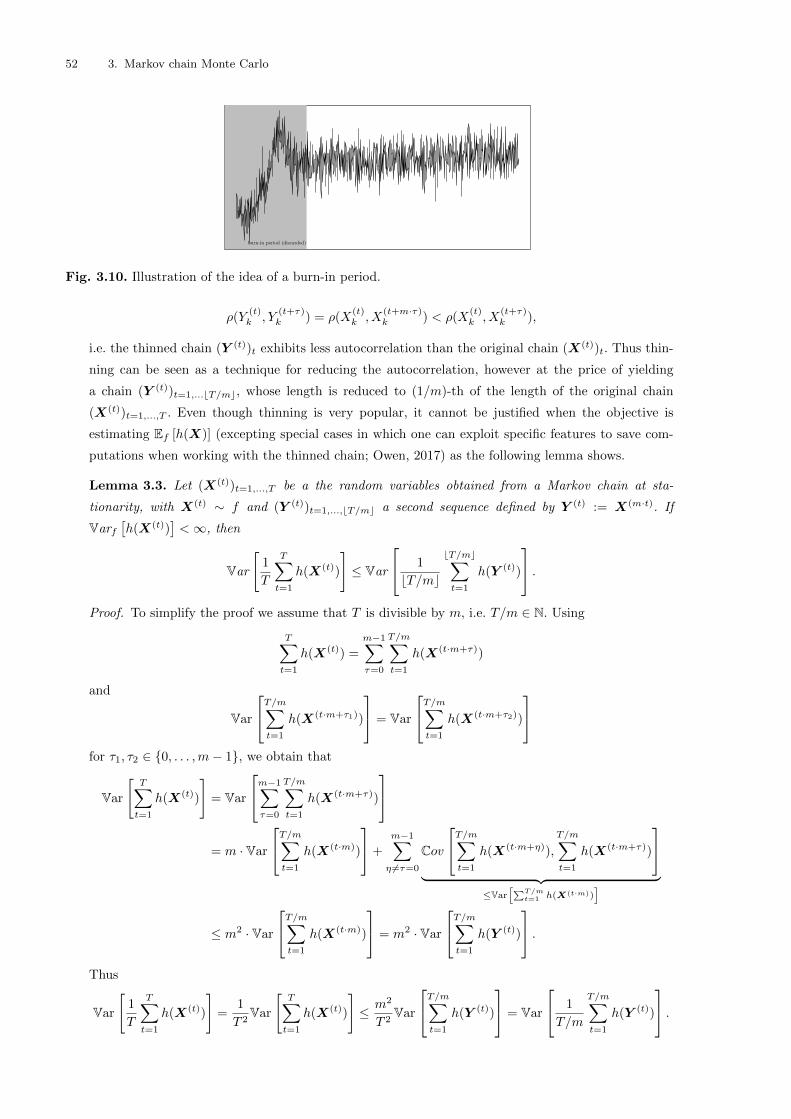
52 3. Markov chain Monte Carlo
burn-in period (discarded)
Fig. 3.10. Illustration of the idea of a burn-in period.
ρ(Y(t)k , Y
(t+τ)k ) = ρ(X
(t)k , X
(t+m·τ)k ) < ρ(X
(t)k , X
(t+τ)k ),
i.e. the thinned chain (Y (t))t exhibits less autocorrelation than the original chain (X(t))t. Thus thin-
ning can be seen as a technique for reducing the autocorrelation, however at the price of yielding
a chain (Y (t))t=1,...bT/mc, whose length is reduced to (1/m)-th of the length of the original chain
(X(t))t=1,...,T . Even though thinning is very popular, it cannot be justified when the objective is
estimating Ef [h(X)] (excepting special cases in which one can exploit specific features to save com-
putations when working with the thinned chain; Owen, 2017) as the following lemma shows.
Lemma 3.3. Let (X(t))t=1,...,T be a the random variables obtained from a Markov chain at sta-
tionarity, with X(t) ∼ f and (Y (t))t=1,...,bT/mc a second sequence defined by Y (t) := X(m·t). If
Varf[h(X(t))
]<∞, then
Var
[1
T
T∑
t=1
h(X(t))
]≤ Var
1
bT/mc
bT/mc∑
t=1
h(Y (t))
.
Proof. To simplify the proof we assume that T is divisible by m, i.e. T/m ∈ N. Using
T∑
t=1
h(X(t)) =
m−1∑
τ=0
T/m∑
t=1
h(X(t·m+τ))
and
Var
T/m∑
t=1
h(X(t·m+τ1))
= Var
T/m∑
t=1
h(X(t·m+τ2))
for τ1, τ2 ∈ {0, . . . ,m− 1}, we obtain that
Var
[T∑
t=1
h(X(t))
]= Var
m−1∑
τ=0
T/m∑
t=1
h(X(t·m+τ))
= m · Var
T/m∑
t=1
h(X(t·m))
+
m−1∑
η 6=τ=0
Cov
T/m∑
t=1
h(X(t·m+η)),
T/m∑
t=1
h(X(t·m+τ))
︸ ︷︷ ︸≤Var
[∑T/mt=1 h(X(t·m))
]
≤ m2 · Var
T/m∑
t=1
h(X(t·m))
= m2 · Var
T/m∑
t=1
h(Y (t))
.
Thus
Var
[1
T
T∑
t=1
h(X(t))
]=
1
T 2Var
[T∑
t=1
h(X(t))
]≤ m2
T 2Var
T/m∑
t=1
h(Y (t))
= Var
1
T/m
T/m∑
t=1
h(Y (t))
.

3.4 Diagnosing Convergence 53
�
The concept of thinning can be useful for other reasons. If storage is limited it may not be possible
to store all of an arbitrarily long chain; in this context, it can be much better to store the thinned
skeleton of a long chain than to consider the entire sample path of a shorter chain. Furthermore, it
can be easier to assess the convergence of the thinned chain (Y (t))t as opposed to entire chain (X(t))t.
3.4.2 Tools for monitoring convergence
Although the theory presented in the preceding chapters guarantees the convergence of the Markov chains
to the required distributions, this does not imply that a finite sample from such a chain yields a good
approximation to the target distribution. As with all approximating methods this must be confirmed in
practice.
This section tries to give a brief overview over various approaches to diagnosing convergence. A more
detailed review with many practical examples can be found in (Guihennec-Jouyaux et al., 1998) or (Robert
and Casella, 2004, Chapter 12). There are numerous R packages (CODA is well known; mcmcse provides
useful tools for assessing some aspects of performance) that provides a vast selection of tools for diagnosing
convergence.
Diagnosing convergence is an art. The techniques presented in the following are no more than ex-
ploratory tools that help you judge whether the chain has reached its stationary regime. This section
contains several cautionary examples where the different tools for diagnosing convergence fail.
Broadly speaking, convergence assessment can be split into the following three categories, each of which
considers the assessment of a different aspect of convergence:
Convergence to the target distribution. The first, and most important, question is whether (X(t))t yields
a sample from the target distribution? In order to answer this question we need to assess . . .
– whether (X(t))t has reached a stationary regime, and
– whether (X(t))t covers the entire support of the target distribution.
Convergence of the averages. Does∑Tt=1 h(X(t))/T provide a good approximation to the expectation
Ef [h(X)] under the target distribution?
Comparison to i.i.d. sampling. How much information is contained in the sample from the Markov chain
compared to i.i.d. sampling?
3.4.3 Basic plots
The most basic approach to diagnosing the output of a Markov Chain Monte Carlo algorithm is to plot
the sample path (X(t))t. Note that the convergence of (X(t))t is in distribution, i.e. the sample path is
not supposed to converge to a single value. Ideally, the plot should be oscillating very fast and show very
little structure or trend. In general terms, the smoother such a plot seems, the slower the mixing of the
associated chain.
Note however that this plot suffers from the “you’ve only seen where you’ve been” problem. It is
impossible to see from a plot of the sample path whether the chain has explored the entire support of the
distribution (without additional information).
Example 3.11 (A simple mixture of two Gaussians). Consider sampling from a mixture of two well-separated
Gaussians
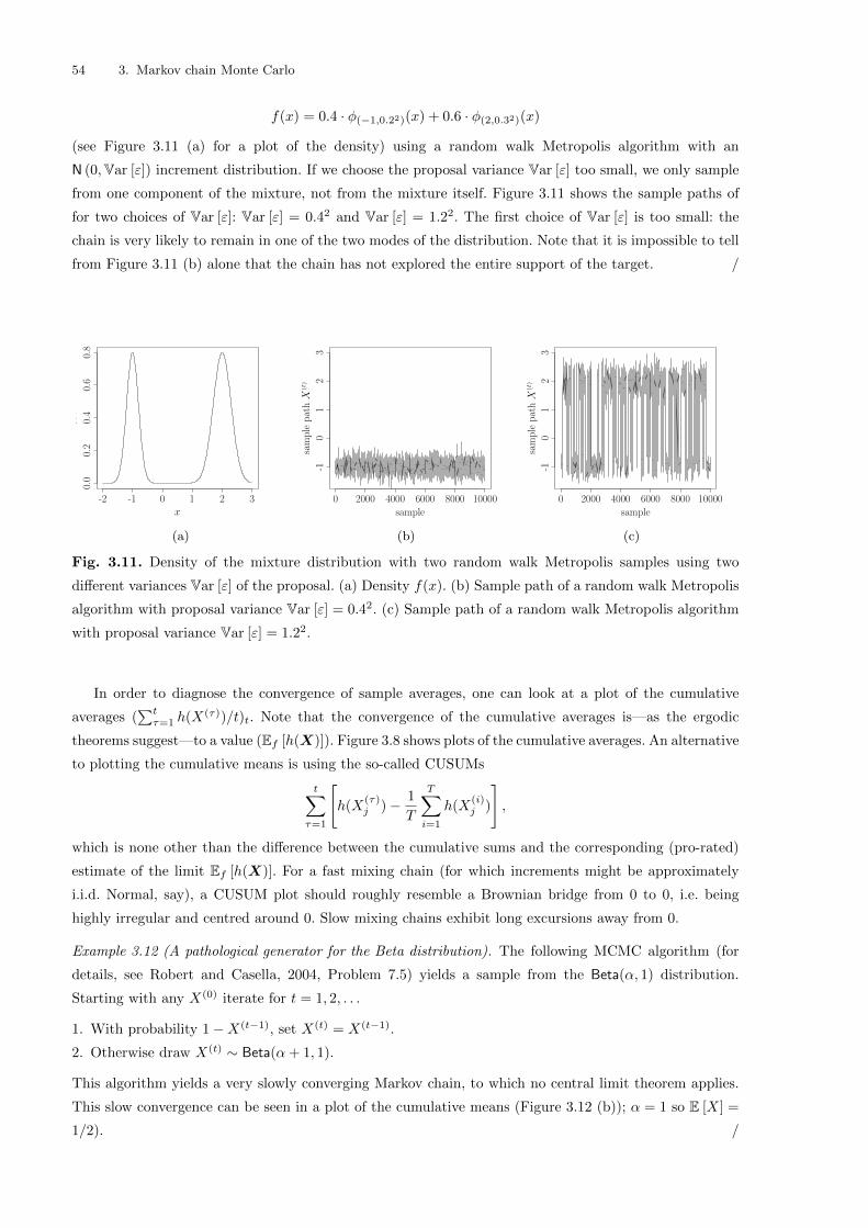
54 3. Markov chain Monte Carlo
f(x) = 0.4 · φ(−1,0.22)(x) + 0.6 · φ(2,0.32)(x)
(see Figure 3.11 (a) for a plot of the density) using a random walk Metropolis algorithm with an
N (0,Var [ε]) increment distribution. If we choose the proposal variance Var [ε] too small, we only sample
from one component of the mixture, not from the mixture itself. Figure 3.11 shows the sample paths of
for two choices of Var [ε]: Var [ε] = 0.42 and Var [ε] = 1.22. The first choice of Var [ε] is too small: the
chain is very likely to remain in one of the two modes of the distribution. Note that it is impossible to tell
from Figure 3.11 (b) alone that the chain has not explored the entire support of the target. /
-2 -1 0 1 2 3
0.0
0.2
0.4
0.6
0.8
x
f(x)
(a)
2000 4000 6000 8000 10000
-10
0
12
3
sample
samplepathX
(t)
(b)
2000 4000 6000 8000 10000
-10
0
12
3
sample
samplepathX
(t)
(c)
Fig. 3.11. Density of the mixture distribution with two random walk Metropolis samples using two
different variances Var [ε] of the proposal. (a) Density f(x). (b) Sample path of a random walk Metropolis
algorithm with proposal variance Var [ε] = 0.42. (c) Sample path of a random walk Metropolis algorithm
with proposal variance Var [ε] = 1.22.
In order to diagnose the convergence of sample averages, one can look at a plot of the cumulative
averages (∑tτ=1 h(X(τ))/t)t. Note that the convergence of the cumulative averages is—as the ergodic
theorems suggest—to a value (Ef [h(X)]). Figure 3.8 shows plots of the cumulative averages. An alternative
to plotting the cumulative means is using the so-called CUSUMs
t∑
τ=1
[h(X
(τ)j )− 1
T
T∑
i=1
h(X(i)j )
],
which is none other than the difference between the cumulative sums and the corresponding (pro-rated)
estimate of the limit Ef [h(X)]. For a fast mixing chain (for which increments might be approximately
i.i.d. Normal, say), a CUSUM plot should roughly resemble a Brownian bridge from 0 to 0, i.e. being
highly irregular and centred around 0. Slow mixing chains exhibit long excursions away from 0.
Example 3.12 (A pathological generator for the Beta distribution). The following MCMC algorithm (for
details, see Robert and Casella, 2004, Problem 7.5) yields a sample from the Beta(α, 1) distribution.
Starting with any X(0) iterate for t = 1, 2, . . .
1. With probability 1−X(t−1), set X(t) = X(t−1).
2. Otherwise draw X(t) ∼ Beta(α+ 1, 1).
This algorithm yields a very slowly converging Markov chain, to which no central limit theorem applies.
This slow convergence can be seen in a plot of the cumulative means (Figure 3.12 (b)); α = 1 so E [X] =
1/2). /

3.4 Diagnosing Convergence 55
0 2000 4000 6000 8000 10000
0.0
0.2
0.4
0.6
0.8
1.0
sample
sample
pathX
(t)
(a) Sample path X(t)
0 2000 4000 6000 8000 10000
0.2
0.4
0.6
0.8
1.0
sample
cumulative
average∑
t τ=1X
(τ)/t
(b) Cumulative means∑tτ=1X
(τ)/t
Fig. 3.12. Sample paths and cumulative means obtained for the pathological Beta generator, α = 1.
Note that it is impossible to tell from a plot of the cumulative means whether the Markov chain has
explored the entire support of the target distribution.
3.4.4 Non-parametric tests of stationarity
A variety of nonparametric tests can be employed to establish whether the samples from a Markov chain
behave in particular ways. This section presents an illustration of the (informal, approximate) use of the
Kolmogorov-Smirnov test to assess whether there is evidence that a Markov chain has not yet reached
stationarity.
In its simplest version, it is based on splitting the chain into three parts: (X(t))t=1,...,bT/3c,
(X(t))t=bT/3c+1,...,2bT/3c, and (X(t))t=2bT/3c+1,...,T . The first block is considered to be the burn-in pe-
riod. If the Markov chain has reached its stationary regime after bT/3c iterations, the second and third
block should be from the same distribution. Thus we should be able to tell whether the chain has converged
by comparing the distribution of (X(t))t=bT/3c+1,...,2bT/3c to the distribution of (X(t))t=2bT/3c+1,...,T using
suitable nonparametric two-sample tests. One such test is the Kolmogorov-Smirnov test.
Definition 3.4 (Kolmogorov-Smirnov Statistic). The two-sample Kolmogorov-Smirnov test for com-
paring two i.i.d. samples Z1,1, . . . , Z1,n and Z2,1, . . . , Z2,n is based on comparing their empirical CDFs
Fk(z) =1
n
n∑
i=1
I(−∞,z](Zk,i).
The Kolmogorov-Smirnov test statistic is the maximum difference between the two empirical CDFs:
K = supz∈R|F1(z)− F2(z)|.
For n→∞ the CDF of√n ·K converges to the CDF
R(k) = 1−∞∑
i=1
(−1)i−1 exp(−2i2k2).

56 3. Markov chain Monte Carlo
As the Kolmogorov-Smirnov test is designed for i.i.d. samples, we do not apply it to the (X(t))t directly,
but to a thinned chain (Y (t))t with Y (t) = X(m·t): the thinned chain is less correlated and thus closer to
being an i.i.d. sample. This, of course, still formally violates the conditions under which the Kolmogorov-
Smirnov test is exact but one can still hope to obtain useful information when the conditions are close to
being satisfied.
We can now use the Kolmogorov-Smirnov statistics to compare the distribution of the second block,
(Y (t))t=bT/(3m)c+1,...,2bT/(3m)c, with that of the third, (Y (t))t=2bT/(3m)c+1,...,bT/mc:
K = supx∈R
∣∣∣F(Y (t))t=bT/(3m)c+1,...,2bT/(3m)c(x)− F(Y (t))t=2bT/(3m)c+1,...,bT/mc
(x)∣∣∣ .
As the thinned chain is not an i.i.d. sample, we cannot use the Kolmogorov-Smirnov test as a formal
statistical test (besides, we would run into problems of multiple testing). However, we can use it as an
informal tool by monitoring the standardised statistic√tKt as a function of t., where Kt denotes the
Kolmogorov-Smirnov statistic obtained from the sample consisting of the first t observations only. If a
significant proportion of the values of this standardised statistic are above the corresponding quantile of
the asymptotic distribution, it is safe to assume that the chain has not yet reached its stationary regime.
Example 3.13 (Gibbs sampling from a bivariate Gaussian (continued)). In this example we consider sam-
pling from a bivariate Gaussian distribution, once with ρ(X1, X2) = 0.3 and once with ρ(X1, X2) = 0.99.
The former leads to a fast mixing chain, the latter to a very slowly mixing chain. Figure 3.13 shows the
plots of the standardised Kolmogorov-Smirnov statistic. It suggests that the sample size of 10,000 is large
enough for the low-correlation setting, but not large enough for the high-correlation setting. /
0 2000 4000 6000 8000 10000
0.6
0.8
1.0
1.2
1.4
1.6
1.8
sample
Standardised
KSstatistic√tK
t
(a) ρ(X1, X2) = 0.3
0 2000 4000 6000 8000 10000
12
34
56
7
sample
Standardised
KSstatistic√tK
t
(b) ρ(X1, X2) = 0.99
Fig. 3.13. Standardised Kolmogorov-Smirnov statistic for X(5·t)1 from the Gibbs sampler from the bivari-
ate Gaussian for two different correlations.
Note that this use of the Kolmogorov-Smirnov test suffers from the “you’ve only seen where you’ve
been” problem, as it is based on comparing (Y (t))t=bT/(3m)c+1,...,2bT/(3m)c and (Y (t))t=2bT/(3m)c+1,...,bT/mc.
A plot of the Kolmogorov-Smirnov statistic for the chain with Var [ε] = 0.4 from Example 3.11 would not
reveal anything unusual.

3.4 Diagnosing Convergence 57
3.4.5 Riemann sums and control variates
A simple tool for diagnosing convergence of a one-dimensional Markov chain can be based on the fact that∫
E
f(x) dx = 1.
We can estimate this integral using the Riemann sum
T∑
t=2
(X [t] −X [t−1])f(X [t]), (3.14)
where X [1] ≤ · · · ≤ X [T ] is the ordered sample from the Markov chain. If the Markov chain has explored
all the support of f , then (3.14) should be around 1 (as it is an estimate of the integral of a probability
density). Note that this method, often referred to as Riemann sums (Philippe and Robert, 2001), requires
that the density f is known inclusive of normalisation constants (and thus to apply this technique to a
univariate marginal of a multivariate problem would require that at least one univariate marginal of the
target distributions is known exactly).
Example 3.14 (A simple mixture of two Gaussians (continued)). In Example 3.11 we considered two random-
walk Metropolis algorithms: one (Var [ε] = 0.42) failed to explore the entire support of the target distri-
bution, whereas the other one (Var [ε] = 1.22) managed to. The corresponding Riemann sums are 0.598
and 1.001, clearly indicating that the first algorithm does not explore the entire support. /
Riemann sums can be seen as a special case of a technique called control variates. The idea of control
variates is essentially to compare several ways of estimating the same quantity using the same collection
of samples. If the different estimates disagree, the chain has not yet converged. Note that the technique of
control variates is only useful if the different estimators converge about as fast as the quantity of interest—
otherwise we would obtain an overly optimistic, or an overly conservative estimate of whether the chain
has converged. In the special case of the Riemann sum we compare two quantities: the constant 1 and the
Riemann sum (3.14).
3.4.6 Comparing multiple chains
A family of convergence diagnostics (see e.g. Gelman and Rubin, 1992; Brooks and Gelman, 1998) is based
on running L > 1 chains—which we will denote by (X(1,t))t, . . . , (X(L,t))t—with overdispersed starting
values X(1,0), . . . ,X(L,0) (in the sense that the variance of the starting values should be larger than the
variance of the target distribution). These starting values should in principle be chosen to give reasonable
coverage of the support of the target distribution.
All L chains should converge to the same distribution, so comparing the plots described in Section
3.4.3 for the L different chains should not reveal any difference. A more formal approach to diagnosing
whether the L chains are all from the same distribution can be based on comparing the inter-quantile
distances.
We can estimate the inter-quantile distances in two ways. The first consists of estimating the inter-
quantile distance for each of the L chains and averaging over these results, i.e. our estimate is∑Ll=1 δ
(l)γ /L,
where δ(l)γ is the distance between the γ and (1− γ) quantile of the l-th chain (X
(l,t)k )t. Alternatively, we
can pool the data first, and then compute the distance, δγ , between the γ and (1 − γ) quantile of the
pooled data. If all chains are a sample from the same distribution, both estimates should be roughly the
same, so their ratio

58 3. Markov chain Monte Carlo
Sintervalγ =
∑Ll=1 δ
(l)γ /L
δγ
can be used as a tool to diagnose whether all chains sampled from the same distribution, in which case
the ratio should be around 1.
Alternatively, one could compare the variances within the L chains to the pooled estimate of the
variance (see Brooks and Gelman, 1998, for more details).
Example 3.15 (A simple mixture of two Gaussians (continued)). In the example of the mixture of two
Gaussians we will consider L = 8 chains initialised with iid samples from a N(0, 102
)distribution. Figure
3.14 shows the sample paths of the 8 chains for both choices of Var [ε]. The corresponding values of Sinterval0.05
are:
Var [ε] = 0.42 : Sinterval0.05 =
0.9789992
3.630008= 0.2696962
Var [ε] = 1.22 : Sinterval0.05 =
3.634382
3.646463= 0.996687.
/
2000 4000 6000 8000 10000
-2-1
0
0
12
3
sample
sample
pathsX
(l,t)
(a) Var [ε] = 0.42
2000 4000 6000 8000 10000
-2-1
0
0
12
3
sample
sample
pathsX
(l,t)
(b) Var [ε] = 1.22
Fig. 3.14. Comparison of the sample paths for L = 8 chains for the mixture of two Gaussians.
Note that this method depends crucially on the choice of initial values X(1,0), . . . ,X(L,0), and thus
can easily fail, as the following example shows.
Example 3.16 (Witch’s hat distribution). Consider a distribution with the following density:
f(x1, x2) ∝{
(1− δ)φ(µ,σ2·I)(x1, x2) + δ if x1, x2 ∈ (0, 1),
0 otherwise,
which is a mixture of a Gaussian and a uniform distribution, both truncated to (0, 1)× (0, 1). Figure 3.15
illustrates the density. For very small σ2, the Gaussian component is concentrated in a very small area
around µ.
The conditional distribution of X1 | X2 is

3.4 Diagnosing Convergence 59
f(x1 | x2) =
{(1− δx2
)φ(µ,σ2·I)(x1, x2) + δx2for x1 ∈ (0, 1)
0 otherwise
with δx2=
δ
δ + (1− δ)φ(µ2,σ2)(x2).
Assume we want to estimate P (0.49 < X1, X2 ≤ 0.51) for δ = 10−3, µ = (0.5, 0.5)′, and σ = 10−5
using a Gibbs sampler. Note that 99.9% of the mass of the distribution is concentrated in a very small
area around (0.5, 0.5), i.e. P (0.49 < X1, X2 ≤ 0.51) ≈ 0.999.
Nonetheless, it is very unlikely that the Gibbs sampler visits this part of the distribution. This is due
to the fact that unless x2 (or x1) is very close to µ2 (or µ1), δx2(or δx1
) is almost 1, i.e. the Gibbs
sampler only samples from the uniform component of the distribution. Figure 3.15 shows the samples
obtained from 15 runs of the Gibbs sampler (first 100 iterations only) all using different initialisations.
On average only 0.04% of the sampled values lie in (0.49, 0.51) × (0.49, 0.51) yielding an estimate of
P (0.49 < X1, X2 ≤ 0.51) = 0.0004 (as opposed to P (0.49 < X1, X2 ≤ 0.51) = 0.999).
It is however close to impossible to detect this problem with any technique based on multiple initiali-
sations. The Gibbs sampler shows this behaviour for practically all starting values. In Figure 3.15 all 15
starting values yield a Gibbs sampler that is stuck in the “brim” of the witch’s hat and thus misses 99.9%
of the probability mass of the target distribution. /
x 1
x2
density
f(x
1 , x2 )
(a) Density for δ = 0.2, µ =
(0.5, 0.5)′, and σ = 0.05
0.0
0.0
0.2
0.2
0.4
0.4
0.6
0.6
0.8
0.8
1.0
1.0
x1
x2
(b) First 100 values from 15 samples using different
starting values.
(δ = 10−3, µ = (0.5, 0.5)′, and σ = 10−5)
Fig. 3.15. Density and sample from the witch’s hat distribution.
3.4.7 Comparison to i.i.d. sampling and the effective sample size
MCMC algorithms typically yield a positively correlated sample (X(t))t=1,...,T , which contains less infor-
mation than an i.i.d. sample of size T . If the (X(t))t=1,...,T are positively correlated, then the variance of
the average
Var
[1
T
T∑
t=1
h(X(t))
](3.15)
is larger than the variance we would obtain from an i.i.d. sample, which is Var[h(X(t))
]/T .

60 3. Markov chain Monte Carlo
The effective sample size (ESS) attempts to quantify the loss of information caused by this positive
correlation. The effective sample size is the size an i.i.d. sample would have to have in order to obtain the
same variance (3.15) as the estimate from the Markov chain (X(t))t=1,...,T .
As the exact computation of this quantity is generally impossible, a number of simplifying approxi-
mations are often made in order to obtain a computationally tractable proxy for this quantity. Slightly
confusingly, the approximate equivalent independent sample size arrived at following this chain of ap-
proximations is also referred to as the ESS. More sophisticated approximations are used to obtain better
approximations of the ESS in some settings, but we focus here on one simple and widely-applicable option.
In order to compute the variance (3.15) we make the simplifying assumption that (h(X(t)))t=1,...,T is
from a second-order stationary time series, i.e. Var[h(X(t))
]= σ2, and ρ(h(X(t)), h(X(t+τ))) = ρ(τ).
Then
Var
[1
T
T∑
t=1
h(X(t))
]=
1
T 2
T∑
t=1
Var[h(X(t))
]
︸ ︷︷ ︸=σ2
+2∑
1≤s<t≤TCov
[h(X(s)), h(X(t))
]
︸ ︷︷ ︸=σ2·ρ(t−s)
=σ2
T 2
(T + 2
T−1∑
τ=1
(T − τ)ρ(τ)
)=σ2
T
(1 + 2
T−1∑
τ=1
(1− τ
T
)ρ(τ)
).
If∑∞τ=1 |ρ(τ)| <∞, then we can obtain from the dominated convergence theorem (see e.g. Brockwell and
Davis, 1991, Theorem 7.1.1 for details) that
T · Var
[1
T
T∑
t=1
h(X(t))
]−→ σ2
(1 + 2
∞∑
τ=1
ρ(τ)
)
as T →∞. Note that the variance of the simple Monte Carlo estimate of Ef [h(X)] would be σ2/TESS if
we were to use an i.i.d. sample of size TESS. We can now obtain the effective sample size TESS by equating
these two variances and solving for TESS, yielding
TESS =1
1 + 2∑∞τ=1 ρ(τ)
· T.
If we assume that (h(X(t)))t=1,...,T is a first-order autoregressive time series (AR(1)), i.e. ρ(τ) =
ρ(h(X(t)), h(X(t+τ))) = ρ|τ |, then we obtain using 1 + 2∑∞τ=1 ρ
τ = (1 + ρ)/(1− ρ) that
TESS =1− ρ1 + ρ
· T.
Example 3.17 (Gibbs sampling from a bivariate Gaussian (continued)). In examples 3.4 and 3.5 we ob-
tained for the low-correlation setting that ρ(X(t−1)1 , X
(t)1 ) = 0.078, thus the effective sample size is
TESS =1− 0.078
1 + 0.078· 10000 = 8547.
For the high-correlation setting we obtained ρ(X(t−1)1 , X
(t)1 ) = 0.979, thus the effective sample size is
considerably smaller:
TESS =1− 0.979
1 + 0.979· 10000 = 105. /
Note that there are other more sophisticated ways of estimating ESS which do not require this crude
autoregressive approximation. The mcmcse package provides an implementation of the method of Gong
and Flegal (2016) which has somewhat better properties than the method employed by coda.

3.5 Optimisation with MCMC 61
3.5 Optimisation with MCMC
So far we have studied various methods that allow for approximating expectations E [h(X)] by ergodic
averages 1T
∑Tt=1 h(X
(t)i ). This section presents an algorithm for finding the (global) mode(s) of a distri-
bution. For definiteness, in this chapter we define the mode(s) of a distribution to be the set of global
maxima of the density, i.e. {ξ : f(ξ) ≥ f(x) ∀x}. In Section 3.5.1 we will extend this idea to finding
global extrema of arbitrary functions.
We could estimate the mode of a distribution by theX(t) with maximal density f(X(t)); this is however
a not very efficient strategy. A sample from a Markov chain with invariant distribution f(·) samples from
the whole distribution and not only from the mode(s).
This suggests modifying the distribution such that it is more concentrated around the mode(s). One
way of achieving this is to consider
f(β)(x) ∝ (f(x))β
for very large values of β.
Example 3.18 (Normal distribution). Consider the N(µ, σ2
)distribution with density
f(µ,σ2)(x) =1√
2πσ2exp
(− (x− µ)2
2σ2
)∝ exp
(− (x− µ)2
2σ2
).
It is easy to see that the mode of the N(µ, σ2
)distribution is µ. We have that
(f(µ,σ2)(x)
)β ∝(
exp
(− (x− µ)2
2σ2
))β= exp
(− (x− µ)2
2σ2/β
)∝ f(µ,σ2/β)(x).
In other words, the larger β is chosen, the more concentrated the distribution will be around the mode µ.
Figure 3.16 illustrates this idea. /
-2-2-2-2 -1-1-1-1 1111 000
0
0 222
2
2
46
810
12
xxxx
den
sity
φ(0,1)(x)(φ(0,1)(x)
)10 ∝ φ(0,1/10)(x)(φ(0,1)(x)
)100 ∝ φ(0,1/100)(x)(φ(0,1)(x)
)1000 ∝ φ(0,1/1000)(x)
Fig. 3.16. Density of the N (0, 1) raised to increasing powers. The areas shaded in grey represent 90% of
the probability mass.

62 3. Markov chain Monte Carlo
-2-2-2-2 -1-1-1-1 1111 0000 2222
f(x) (f(x))3
(f(x))9
(f(x))27
xxxx
Fig. 3.17. An arbitrary multimodal density raised to increasing powers. The areas shaded in grey reach
from the 5% to the 95% quantiles.
The result we have obtained for the Gaussian distribution in the above example actually holds in
general. For β → ∞ the distribution defined by the density f(β)(x) converges to a distribution that has
all mass on the mode(s) of f (see Figure 3.17 for an example). It is instructive to see informally why this
is the case when considering a discrete random variable with probability density function p(·) and finite
support E. Denote with E∗ the set of modes of p, i.e. p(ξ) ≥ p(x) for all ξ ∈ E∗ and x ∈ E, and with
m := p(ξ) with ξ ∈ E∗. Then
p(β)(x)=(p(x))β∑
y∈E∗(p(y))β +∑y∈E\E∗(p(y))β
=(p(x)/m)β∑
y∈E∗ 1 +∑y∈E\E∗(p(y)/m)β
β→∞−→{
1/|E∗| if x ∈ E∗
0 if x 6∈ E∗
In general in the continuous case the distribution is not uniform on the modes and depends on the
curvature around each mode (see Hwang, 1980, for details). An outline of the argument is:
−20 −10 0 10 20
05
00
10
00
15
00
20
00
25
00
x
y
Take x? ∈ arg maxx f(x) and let:
E1 = {x : f(x) ≥ f(x?)− ε}.E2 = {x : f(x) ≥ f(x?)− 2ε} \ E1.
D = Rd \ (E1 ∪ E2).
Consider:
limβ→∞
P(β)(E1 ∪ E2)/P(β)(D)
Use:
P(β)(D)/P(β)(E1)→ 0.
Under slightly stronger regularity conditions one can employ an elementary argument along the same
lines as the one described in the discrete case above.
We can use a random-walk Metropolis algorithm to sample from f(β)(·). The probability of accepting
a move from X(t−1) to X would be
min
{1,
f(β)(X)
f(β)(X(t−1))
}= min
{1,
(f(X)
f(X(t−1))
)β}.
Note that this probability does not depend on the (generally unknown) normalisation constant of f(β)(·).It is however difficult to directly sample from f(β) for large values of β: for β → ∞ the probability of
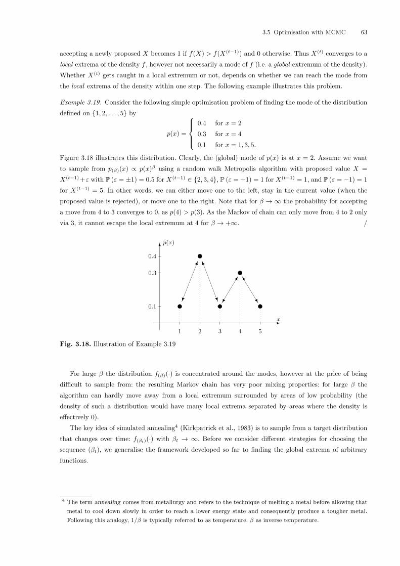
3.5 Optimisation with MCMC 63
accepting a newly proposed X becomes 1 if f(X) > f(X(t−1)) and 0 otherwise. Thus X(t) converges to a
local extrema of the density f , however not necessarily a mode of f (i.e. a global extremum of the density).
Whether X(t) gets caught in a local extremum or not, depends on whether we can reach the mode from
the local extrema of the density within one step. The following example illustrates this problem.
Example 3.19. Consider the following simple optimisation problem of finding the mode of the distribution
defined on {1, 2, . . . , 5} by
p(x) =
0.4 for x = 2
0.3 for x = 4
0.1 for x = 1, 3, 5.
Figure 3.18 illustrates this distribution. Clearly, the (global) mode of p(x) is at x = 2. Assume we want
to sample from p(β)(x) ∝ p(x)β using a random walk Metropolis algorithm with proposed value X =
X(t−1) +ε with P (ε = ±1) = 0.5 for X(t−1) ∈ {2, 3, 4}, P (ε = +1) = 1 for X(t−1) = 1, and P (ε = −1) = 1
for X(t−1) = 5. In other words, we can either move one to the left, stay in the current value (when the
proposed value is rejected), or move one to the right. Note that for β →∞ the probability for accepting
a move from 4 to 3 converges to 0, as p(4) > p(3). As the Markov of chain can only move from 4 to 2 only
via 3, it cannot escape the local extremum at 4 for β → +∞. /
1 2 3 4 5
0.1
0.3
0.4
x
p(x)
Fig. 3.18. Illustration of Example 3.19
For large β the distribution f(β)(·) is concentrated around the modes, however at the price of being
difficult to sample from: the resulting Markov chain has very poor mixing properties: for large β the
algorithm can hardly move away from a local extremum surrounded by areas of low probability (the
density of such a distribution would have many local extrema separated by areas where the density is
effectively 0).
The key idea of simulated annealing4 (Kirkpatrick et al., 1983) is to sample from a target distribution
that changes over time: f(βt)(·) with βt → ∞. Before we consider different strategies for choosing the
sequence (βt), we generalise the framework developed so far to finding the global extrema of arbitrary
functions.
4 The term annealing comes from metallurgy and refers to the technique of melting a metal before allowing that
metal to cool down slowly in order to reach a lower energy state and consequently produce a tougher metal.
Following this analogy, 1/β is typically referred to as temperature, β as inverse temperature.

64 3. Markov chain Monte Carlo
3.5.1 Minimising an arbitrary function
Consider that we want to find the global minimum of a function h : E → R. Finding the global minimum
of H(x) is equivalent to finding the mode of a distribution
f(x) ∝ exp(−H(x)) for x ∈ E,
if such a distribution exists. In this framework, finding the mode of a density f corresponds to finding the
minimum of − log(f(x)). As in the previous section we can raise f to large powers to obtain a distribution
f(βt)(x) = (f(x))βt ∝ exp(−βt ·H(x)) for x ∈ E.
We hope to find the (global) minimum of H(x), which is the (global) mode of the distribution defined
by fβt(x), by sampling from a Metropolis–Hastings algorithm. As suggested above we let βt → ∞. This
yields the following algorithm:
Algorithm 3.6 (Simulated Annealing). Starting with X(0) := (X(0)1 , . . . , X
(0)p ) and β(0) > 0 iterate
for t = 1, 2, . . .
1. Increase β(t−1) to β(t) (see below for different annealing schedules).
2. Draw X ∼ q(· |X(t−1)).
3. Compute
α(X |X(t−1)) = min
{1, exp
(−βt(H(X)−H(X(t−1)))
)· q(X
(t−1) |X)
q(X |X(t−1))
}.
4. With probability α(X |X(t−1)) set X(t) = X, otherwise set X(t) = X(t−1).
If a random walk Metropolis update is used (i.e. X = X(t−1) + ε with ε ∼ g(·) for a symmetric g),
then the probability of acceptance becomes
α(X |X(t−1)) = min{
1, exp(−βt(H(X)−H(X(t−1)))
)}.
Using the same arguments as in the previous section, it is easy to see that the simulated annealing
algorithm converges to a local minimum of H(·). Whether it will be able to find the global minimum
depends on how slowly we let the inverse temperature β go to infinity.
Logarithmic tempering When choosing βt = log(1+t)β0
, the inverse temperature increases slow enough that
global convergence results can be established for certain special cases. Hajek (1988) established global
convergence when H(·) is optimised over a finite set using a proposal which is uniform over E and loga-
rithmic tempering with a suitably large β0. Andrieu et al. (2001) use Foster-Lyapunov type arguments
to establish convergence on more general spaces (under appropriate conditions).
Assume we choose β0 = ∆H with ∆H := maxx,x′∈E |H(x)−H(x′)|. Then the probability of reaching
state x in the t-th step is
P(X(t) = x
)=∑
ξ
P(X(t) = x | X(t−1) = ξ
)
︸ ︷︷ ︸≥exp(−βt∆H)/|E|
P(X(t−1) = ξ
)≥ exp(−βt∆H)/|E|
Using the logarithmic tempering schedule we obtain P(X(t) = x
)≥ 1/ ((1 + t)|E|) and thus the
expected number of visits to state x is
∞∑
t=0
P(X(t) = x
)≥∞∑
t=0
[(1 + t)|E|]−1 =∞.

3.5 Optimisation with MCMC 65
Thus every state is recurrent. As β increases we however spend an ever increasing amount of time in
the global minima of x.
On the one hand visiting very state x infinitely often implies that we can escape from local minima.
On the other hand, this implies as well that we visit every state x (regardless of how large H(x)
is) infinitely often. In other words, the reason why simulated annealing with logarithmic tempering
works, is that it still behaves very much like an exhaustive search. However the only reason why we
consider simulated annealing is that exhaustive search would be too slow! For this reason, logarithmic
tempering has little practical relevance.
Geometric tempering A popular choice is βt = αt · β0 for some α > 1.
Example 3.20. Assume we want to find the maximum of the function
H(x) =((x− 1)2 − 1
)2+ 3 · s(11.56 · x2), with s(x) =
{|x| mod 2 for 2k ≤ |x| ≤ 2k + 1
2− |x| mod 2 for 2k + 1 ≤ |x| ≤ 2(k + 1)
for k ∈ N0. Figure 3.19 (a) shows H(x) for x ∈ [−1, 3]. The global minimum of H(x) is at x = 0.
We simulated annealing with a geometric tempering with β0 = 1 and βt = 1.001βt−1 and a random
walk Metropolis algorithm with ε ∼ Cauchy(0,√
0.1). Figure 3.19 (b) shows the first 1,000 iterations
of the Markov chain yielded by the simulated annealing algorithm. Note that when using a Gaussian
distribution with small enough a variance the simulated annealing algorithm is very likely to remain in
the local minimum at x ≈ 1.8. /
Note that there is no guarantee that the simulated annealing algorithm converges to the global mini-
mum of H(x) in finite time. In practice, it would be unrealistic to expect simulated annealing to converge
to a global minimum, however in most cases it will find a “good” local minimum.

66 3. Markov chain Monte Carlo
-1 1 3
0
0
2
2
46
810
x
H(x)
(a) Objective function
0.0
0.0
0.5
0.5
1.0
1.0
1.5
1.5
2.0
2.0
2.5
X(t)
0 200 400 600 800 1000
t
H(X
(t))
(b) Resulting Markov chain (X(t)) and sequence H(X(t))
Fig. 3.19. Objective function H(x) from Example 3.20 and first 1,000 iterations of the Markov chain
yielded by simulated annealing.

4. Augmentation: Extending the Space
A very general technique in the field of simulation based inference is to augment the space on which
simulation is done with auxiliary variables whose presence makes the problem easier. It may seem coun-
terintuitive that making the space on which one must sample larger can make the sampling easier, but
as we shall see in this chapter their are many techniques in the literature which can be seen as particular
cases of this general strategy.
4.1 Composition Sampling
Consider the problem of drawing samples from a mixture distribution, i.e. one with a density of the form
fX(x) =
k∑
i=1
wifi(x)
where w = (w1, . . . , wk) is a vector of non-negative real numbers which sum to one. These correspond to
component weights and {fi}ki=1 corresponds to a family of k different probability densities.
In principle one can readily develop techniques for sampling from such densities using the ideas de-
scribed in Section 2.1. However, it’s convenient to have a simple generic method which can be used
whenever we have techniques for sampling from the fi individually.
Consider introducing an auxiliary variable Z which has a discrete distribution over {1, . . . , k} with
associated vector of probability masses w. The joint distribution
fX,Z(x, z) =
k∑
i=1
wiδi,zfz(x),
admits the marginal over x:
k∑
z=1
fX,Z(x, z) =
k∑
z=1
k∑
i=1
wiδi,zfz(x) =
k∑
i=1
wi
k∑
z=1
δi,zfz(x) =
k∑
i=1
wifi(x) = fX(x),
as required.
The basis of composition sampling is that fX,Z also admits a straightforward marginal distribution
over z, by construction, fZ(z) =∑ki=1 wiδi,z and the conditional distribution of X given Z = z is simply
fX|Z(x|z) = fz(x).
Combining these ideas, we conclude that we can sample from fX,Z by sampling Z ∼ Cat (w), sampling
X from its conditional distribution given the realized value of Z: X|{Z = z} ∼ fz and then discarding
the auxiliary variable z.

68 4. Augmentation: Extending the Space
4.2 Rejection Revisited
We can also look at rejection sampling through the lens of spatial extension. Consider the following
scenario. We are interested in obtaining samples from fX , know that supx fX(x)/gX(x) ≤ M < ∞ for
some density gX from which we can sample and some real constant M . We extend the space by introducing
an additional U which takes its values in R+ and define the joint distributions:
gX,U (x, u) ∝ IGM ((x, u)), fX,U (x, u) ∝ IF((x, u)),
where GM := {(x, u) ∈ X ⊗ R+ : u ≤ Mg(x)} and F := {(x, u) ∈ X ⊗ R : u ≤ f(x)} are simply the sets
of points beneath Mg and f , respectively.
If gX is tractable then we can straightforwardly sample from gX,U by sampling X ∼ gx and U |X =
x ∼ U[0,Mg(x)]. We could then imagine conducting importance sampling to approximate expectations
under fX,U , which would lead us to an estimator for I =∫fX,U (x, u)ϕ(x, u)dxdu of the form
Inϕ =
∑ni=1
IF((Xi,Ui))IGM ((Xi,Ui))
ϕ(Xi)∑ni=1
IF((Xi,Ui))IGM ((Xi,Ui))
noting that F ⊆ GM and that the probability (under the sampling mechanism by which we have just
described for simulating these random variables which amounts to sampling from the uniform distribution
over GM ) that Xi 6∈ GM is 0 allowing us to adopt the convention that 0/0 = 0 here, we obtain:
Inϕ =
∑ni=1 IF((Xi, Ui))ϕ(Xi, U)∑n
i=1 IF((Xi, Ui))=
∑{i:(Xi,Ui)∈F} ϕ(Xi, U)∑{i:(Xi,Ui)∈F} 1
.
Note that this is simply the sample average of the function ϕ over those points which fell within F. If
we restrict our attention to ϕ(x, u) = ϕ(x) (i.e. we consider functions which depend only upon x) it is
clear that we’ve recast the simple Monte Carlo estimate of the expectation of a function under fX using a
sample obtained using n proposals from g within a rejection sampler as an importance sampling estimate
on an extended space.
The relationship between rejection and importance sampling is well known and has been studied by
many authors (Chen, 2005; Perron, 1999).
4.3 Data Augmentation
Perhaps the most widely known spatial extension technique is that known as data augmentation, intro-
duced by Tanner and Wong (1987).
Consider a latent variable model : a statistical model in which one has unknown parameters about
which one wishes to performance inference, θ, observations which are known, y, and a collection of hidden
(latent) variables, z. Typically, the joint distribution of all these quantities, say, fY ,Z,θ is known but
integrating out the latent variables is not feasible. Without access to fY ,θ it’s not possible to implement,
directly, an MCMC algorithm with the associated marginal posterior distribution fθ|Y as its target.
The basis of data augmentation is to augment the vector of parameters θ with these latent variables,
z and to run an MCMC algorithm (or other Monte Carlo algorithm of your choice) which instead targets
the joint posterior distribution fθ,Z|Y noting that this distribution admits as its marginal in θ exactly
the marginal posterior distribution which was the original object of inference. A mixture model is the
canonical example of a model which can be susceptible to this approach.

4.4 Multiple Augmentation for Optimisation 69
4.4 Multiple Augmentation for Optimisation
A closely related idea used in optimisation is based around “multiple augmentation”, introducing several
replicates of unobserved quantities in order to allow the maximisation of a marginal quantity which it may
not be possible to evaluate. We focus here on the State Augmentation for Maximisation of Expectations
algorithm of Doucet et al. (2002); similar methods are also described by others including Gaetan and
Yao (2003); Jacquier et al. (2007). These schemes all employ MCMC; the alternative of employing a
population-based sampling method known as Sequential Monte Carlo was explored by Johansen et al.
(2008).
Two common optimisation problems arise in the evaluation of statistical estimators: Maximum Likeli-
hood Estimation: Given L(θ;x) = fx(x; θ), compute θML = arg maxθ∈Θ L(θ;x) and Maximum a Posteriori
Estimation: Given L(θ;x) = fx(x; θ) and prior fprior(θ), compute θMAP = arg maxθ∈Θ fprior(θ)L(θ;x).
Both can fit our simple optimisation framework, and we can see a further illustration of the workings
of the annealing method by considering the sequence of distributions obtained for simple problems.
Example 4.1 (Gaussian MAP Estimation). – If L(µ;x) =∏ni=1 φµ,σ2(xi) with σ2 known,
– and π(µ) = φµ0,σ20(µ), then
– the posterior is
fpost(µ) = N
(µ,σ2µ+ nσ2
0 x
σ2 + nσ20
,σ2σ2
0
σ2 + nσ20
),
– and we could aim to sample from
fMAP(β) (µ) ∝ (fpost(µ))β ∝ N
(µ,σ2µ+ nσ2
0 x
σ2 + nσ20
,σ2σ2
0
β(σ2 + nσ20)
).
Example 4.2 (Example: Normal ML Estimation). – If L(µ;x) =∏ni=1 φµ,σ2(xi) with σ2 known,
– we could view the likelihood as being proportional to a distribution over µ:
f(µ) = N(µ; x, σ2/n
),
– and we could aim to sample from
fMLE(β) (µ) ∝ (f(µ))β ∝ N
(µ; x, σ2/βn
).
In both of these cases, the sequence of distributions concentrates on the maximiser of the original
objective function, and so any algorithm able to sample from these distributions (for large enough β) will
provide good approximations of the optimiser of the objective function. These methods involve target
distributions that resemble the posterior distribution (either a real posterior, or one obtained using an
instrumental prior for the purposes of approximating the MLE) which would have been obtained if there
were many copies of the data, so the approach is sometimes referred to as “data cloning”.
Two closely related problems often arise when dealing with complicated statistical models. Marginal
Maximum Likelihood Estimation: Given L(θ;x) =∫fx,z(x, z; θ)dz, compute θML = arg maxθ∈Θ L(θ;x);
and Marginal Maximum a Posteriori Estimation: Given L(θ;x) =∫fx,z(x, z; θ)dz and prior fprior(θ),
compute θMMAP = arg maxθ∈Θ fprior(θ)L(θ;x). Such problems often arise when one can write down a
complete generative model for the process by which the data arose in terms of the parameters, but one
only observes a subset of the random quantities generated within that model. For example, consider a
mixture model in which we don’t observe the association of observations with mixture components or a
genetic model in which we observe the DNA sequences of only the current generation of individuals: we
don’t observe the sequences of their ancestors or their genealogical trees (Stephens, 2007). If it is possible

70 4. Augmentation: Extending the Space
to integrate out the unobserved random quantities then we can proceed as usual, but unfortunately we
can’t typically evaluate the marginal likelihoods.
Recall the demarginalisation technique for sampling from fx(x) by defining a convenient joint distri-
bution fx,z(x, z) which admits the distribution of interest as a marginal. In order to do this, we saw that
we could introduce a set of auxiliary random variables Z1, . . . , Zr such that fx is the marginal density of
(X1, . . . , Xp) under the joint distribution of (X1, . . . , Xp, Z1, . . . , Zr), i.e.
f(x1, . . . , xp) =
∫f(x1, . . . , xn, z1, . . . , zr) d(z1, . . . , zr).
The idea of introducing some auxiliary random variables in such a way that f(β)(x) is the marginal
distribution seems a natural extension of this idea.
In order to do this, we consider
L(x, z|θ) = fX,Z(x, z|θ) = fZ(z|θ)fX(x|z, θ),
and introduce a whole collection of vectors of auxiliary variables:
fMMAPβ (θ,z1, . . . ,zβ |x) ∝
β∏
i=1
[π(θ)fZ(zi)fX(x|zi, θ)] .
We can easily establish that, by exploiting the conditional independence structure of our augmented
likelihood:
fMMAPβ (θ|x) ∝
∫fMMAPβ (θ,z1, . . . ,zβ |x)dz1, . . . dzβ
∝ π(θ)βfX(x|θ)β = fpost(θ|x)β
This idea is the basis of the State Augmentation for Maximisation of Expectations (SAME) algorithm
(Doucet et al., 2002).
In the case of maximising the likelihood rather than the posterior we need to be slightly more careful.
The likelihood is a probability density over the data, but need not even be integrable if viewed as a function
of the parameters. We can address this problem by introducing an instrumental prior distribution (one
used exclusively for computational reasons which is not intended to have any influence on the resulting
inference.
Considering
L(θ;x, z) = fX,Z(x, z|θ) = fZ(z|θ)fX(x|z, θ),
we can again consider multiple augmentation—this time for MMLE estimation—by setting
fMMLEβ (θ,z1, . . . ,zβ |x) ∝ π(θ)
β∏
i=1
[fZ(zi)fX(x|zi, θ)] ,
which ensures that
fMMLEβ (θ|x) ∝
∫fMMLEβ (θ,z1, . . . ,zβ |x)dz1, . . . dzβ
∝[π(θ)(1/β)fX(x|θ)
]β≈ L(θ;x)β
for large enough β under support and regularity conditions on π(·), the instrumental prior.
Both of these augmentation strategies can give rise to a sequence of target distributions if we replace
β with βt, a non-decreasing sequence of numbers of replicates of the augmenting variables. (In the SAME

4.4 Multiple Augmentation for Optimisation 71
case it can be sensible to keep βt fixed at a particular value for several iterations to give the chain time
to reach equilibrium before further increasing it.) And given such a sequence of target distributions, we
can apply MCMC kernels for which each is invariant in essentially the same manner as we did when
considering simulated annealing. In the particular case in which we can sample from all of the relevant
full conditional distributions, this gives rise to Algorithm 4.1; more general cases can be dealt with via
obvious extensions.
Algorithm 4.1 (The SAME Gibbs Sampler). Starting with θ(0) iterate for t = 1, 2, . . .
1. Increase β(t−1) to β(t) (if necessary).
2. For k = 1, . . . , βt, sample:
z(t)k ∼ fZ(z
(t)k |x,θ(t−1))
3. Sample:
θ(t) ∼ f ...(βt)(θ|x, z(t)
1 , . . . ,z(t)βt
)
The following toy example shows the SAME Gibbs sampler in action.
Example 4.3. Consider finding the parameters which maximise the likelihood in a setting in which the
likelihood is a student t-distribution of unknown location parameter θ with 0.05 degrees of freedom. Four
observations are available, x = (−20, 1, 2, 3).
In this case, the marginal likelihood is known (and we can use this knowledge to verify that the
algorithm works as expected):
log p(x|θ) = −0.525
4∑
i=1
log(0.05 + (xi − θ)2
).
This marginal likelihood is illustrated in Figure 4.1.
p(x|θ)
θ
−12
−10
−10−20−30 2010
−8
−6
−4
−2
0
student t: log Marginal Likelihood
fMML
(5)
(θ)
θ
0.0
0.5
1.0
1.5
2.0
2.5
54321−1 0
student t: associated target (β = 5)
Fig. 4.1. The log marginal likelihood (left) and the target distribution obtained by the annealing approach
at β = 5 (right) for Example 4.3.
However, it is also possible to write down an augmented complete likelihood admitting this as a
marginal distribution, by exploiting the fact that the student t-distribution may be written as a scale
mixture of normal densities:
72 4. Augmentation: Extending the Space
log p(x, z|θ) = −4∑
i=1
[0.475 log zi + 0.025zi + 0.5zi(xi − θ)2
],
p(βt)(z1:βt |θ,x) =
βt∏
i=1
4∏
j=1
Gamma
(zi,j ; 0.525, 0.025 +
(xj − θ)2
2
),
p(βt)(θ|z1:βt) ∝ N(θ;µ
(θ)t , Σ
(θ)t
),
where the parameters are
Σ(θ)t =
βt∑
i=1
4∑
j=1
zi,j
−1
, µ(θ)t = Σ
(θ)t
βt∑
i=1
yT zi.
We can straightforwardly implement the SAME Gibbs sampler for this problem.
It is perhaps more interesting to return to the familiar mixture model for which we have already
considered several forms of inference. Lets apply the data augmentation approach to the problem of
maximising the posterior density. (Note that one cannot use maximum likelihood estimation, at least
directly, in this setting as the likelihood is not bounded above: if a cluster mean coincides exactly with
an observation then making the variance of that component arbitrarily small leads to an arbitrarily high
likelihood!)
Example 4.4 (MAP Estimation for a Gaussian Mixture Model). Consider again the Gaussian mixture model
in which we assume that the density of yi is a mixture of Gaussians
f(yi|π1, . . . , πk, µ1, . . . , µk, τ1, . . . , τk) =
k∑
κ=1
πκφ(µκ,1/τκ)(yi).
Suitable prior distributions are a Dirichlet distribution for (π1, . . . , πk), a Gaussian for µκ, and a Gamma
distribution for τκ. In order to ensure identifiability we assume the µκ are ordered, i.e. µ1 < · · · < µk and
make the corresponding change to the posterior density (in order to compensate for setting the density
to zero for all configurations which fail to satisfy the ordering constraint, the density of all configurations
compatible with the constraint must be increased by a factor of k!). Here we assume that k is known, and
have:
– n iid observations, x1, . . . , xn.
– Likelihood fX,Z(xi, zi|ω, µ, σ) = ωziN(xi;µzi , σ
2zi
).
– Marginal likelihood fX(xi|ω, µ, σ) =K∑j=1
ωjN(xi;µj , σ
2j
).
– Diffuse conjugate priors:
ω ∼ Dirichlet (χ, . . . , χ) ,
σ2i ∼ IG
(λi + 3
2,bi2
),
µi|σ2i ∼ N
(ai, σ
2i /λi
).
All full conditional distributions of interest are available, which allows us to use our Gibbs sampling
strategy. This gives rise to an iterative algorithm in which step t comprises the following steps:
– Sample:

4.4 Multiple Augmentation for Optimisation 73
ω ← Dirichlet (βt(χ− 1) + 1 + n1(βt), . . . , βt(χ− 1) + 1 + nK(βt)) ,
σ2i ← IG (Ai, Bi) ,
µi|σ2i ← N
(βtλiai + xβti
βtλi + nβti,
σ2i
βtλi + nβti
),
where
nβti =
βt∑
l=1
n∑
p=1
Ii(Z(t−1)l,p ), xβti =
βt∑
l=1
n∑
p=1
Ii(Z(t−1)l,p )xj , x2
βti =
βt∑
l=1
n∑
p=1
Ii(Zl,p)x2j ,
– and
Ai =βt(λi + 1) + nβti
2+ 1,
Bi =1
2
(βt(bi + λia
2i ) + x2βt
i −βt∑
g=1
(xgi − xg−1i + λiai)
2
λi + ngi − ng−1i
).
– Sample, for j = 1, . . . , βt:
z(t)j ∼ fposterior(z|x, π(t), σ(t), µ(t)).
The marginal posterior can be calculated (which means that we don’t need such a complicated algo-
rithm to deal with this problem, although it does perform well; the advantage of using such an example
is that it allows us to assess the performance of the algorithm).
First we compare the performance of 50 runs of the algorithm with 50 (differently initialised) runs of
a deterministic algorithm (expectation maximisation; EM) which is widely used to deal with problems of
this type. Cost gives a rough indication of the computational cost of running each algorithm once.
Algorithm T Cost Mean Std. Dev. Min Max
EM 500 500 -158.06 3.23 -166.39 -153.85
EM 5000 5000 -157.73 3.83 -165.81 -153.83
SAME(6) 4250 8755 -155.32 0.87 -157.35 -154.03
SAME(50) 4250 112522 -155.05 0.82 -156.11 -153.98
Two different sequences of the annealing parameter were considered:
SAME(6): Set βt = 1 for the first half of the iterations and then increasing linearly to a final maximum
value of 6.
SAME(50): Set βt = 1 for the first 250 iterations, and then increasing linearly to 50.
The log posterior density of the generating parameters was -155.87. These parameters were:
π = [0.2, 0.3, 0.5] , µ = [0, 2, 3] , and σ =
[1,
1
4,
1
16
].
Although the EM algorithm occasionally produces good results, for this clean simulated data, some
runs of the algorithm totally fail to find anything close to the global mode. The SAME algorithm is
computationally more costly, but does behave more robustly. In real marginal optimisation problems, one
typically cannot evaluate the objective function and so robust methods that can be relied upon to produce
good solutions are required.
Next we turn to the much celebrated Galaxy data set of (Roeder, 1990). This data set consists of
the velocities of 82 galaxies, and it has been suggested that it consists of a mixture of between 3 and 7
distinct components—for example, see Roeder and Wasserman (1997) and Escobar and West (1995). For
our purposes we have estimated the parameters of a 3 component Gaussian mixture model from which we

74 4. Augmentation: Extending the Space
assume the data was drawn. The following table summarises the marginal posterior of the solutions found
by 50 runs of each algorithm, comparing the same algorithm with the EM algorithm. Cost gives a rough
indication of the computational cost of running each algorithm once.
Algorithm T Cost Mean Std. Dev. Min Max
EM 500 500 -46.54 2.92 -54.12 -44.32
EM 5000 5000 -46.91 3.00 -56.68 -44.34
SAME(6) 4250 8755 -45.18 0.54 -46.61 -44.17
SAME(50) 4250 112522 -44.93 0.21 -45.52 -44.47
Again, two different sequences of annealing schedule were considered:
SAME(6) set βt = 1 for the first half of the iterations and then increasing linearly to a final maximum
value of 6,
SAME(50) set βt = 1 for the first 250 iterations, and then increasing linearly to 50,
and again, good robustness is demonstrated by the same algorithm. A slightly more sophisticated algorithm
(Johansen et al., 2008) finds solutions broadly consistent with the −43.96± 0.03 found here.
4.5 Approximate Bayesian Computation
The Approximate Bayesian Computation (ABC) approach to inference has become extremely popular for
performing inference for models whose likelihood is not tractable (either in the sense that we can’t evaluate
it pointwise or that such evaluation is prohibitively expensive). Such models abound in some areas, such
as ecology and phylogenetics, and these methods have consequently received a great deal of attention in
recent years.
It was Pritchard et al. (1999) who introduced the method, although there are some connections to
earlier work such as Diggle and Gratton (1984); Tavare et al. (1997). It is not always viewed as a spatial
extension technique, but it can be quite helpful to think about it in these terms.
Before moving on to consider ABC itself, think about a simple case in which one has a target distribu-
tion fX|Y (x|y) which will typically be a Bayesian posterior distribution (and y the observed data). This
distribution is written, via Bayes rule as:
fX|Y (x|y) =fY |X(y|x)fX(x)
fY (y).
If both fX(x) and fY |X(y|x) can be evaluated pointwise then we can use standard simulation techniques to
obtain samples which we can use to approximate our target distribution, and to approximate expectations
with respect to it.
If we cannot evaluate fY |X even pointwise, then we can’t directly use the techniques which we’ve
described previously. To address this, we can invoke a clever data augmentation trick which requires only
that we can sample from fY |X . First let’s consider the case in which Y is a discrete random variable. We
can define the extended distribution, with Z taking it values in the space space as Y :
fX,Z|Y (x, z|y) ∝ fY |X(z|x)fX(x)δy,z
and note that it has as a marginal distribution, our target:
∑
z
fX,Z|Y (x, z|y) ∝∑
z
fY |X(z|x)fX(x)δy,z = fY |X(y|x)fX(x).
4.5 Approximate Bayesian Computation 75
In the simplest case, we can sample (X,Z) ∼ fY |X(z|x)fX(x) using this as a rejection sampling
proposal for our target distribution, keeping samples with probability proportional to
fX,Z|Y (x, z|y)/fY |X(z|x)fX(x).
This probability can easily be seen to be proportional to δy,z. So this rejection sampling algorithm amounts
to sampling X from its prior distribution; sampling an artificial set of data from the model fY |X and
keeping the sample as a sample from the posterior only if the artificial data set exactly matches the
observed one.
Thus far, this clever algorithm has made no approximations. However, the probability of a sample
being accepted is exactly the probability that a data set drawn by sampling a parameter value from
the prior and a data set from the data-generating model with that parameter value exactly matches the
observed data. In the case of very small discrete data sets this might be acceptable, but typically it will
be vanishingly small. That’s why approximation becomes necessary.
The approximate part of ABC arises first of all by relaxing the requirement that the simulated data
exactly matches the observed data and keeping any sample for which the simulated data falls within some
tolerance, ε, of the observed data. This leads to a different target distribution:
fABCX,Z|Y ∝ fY |X(z|x)fX(x)IB(y,ε)(z),
where B(y, ε) := {x : |x− y| ≤ ε}, for which the marginal is no longer correct but may be approximately
so under regularity conditions:
fABCx|Y ∝
∫fY |X(z|x)fX(x)IB(y,ε)(z)dz
∝ fX(x)
∫fY |X(z|x)IB(y,ε)(z)dz ∝ fX(x)
∫
z∈B(y,ε)
fY |X(z|x)dz.
This approximation amounts to a smoothing of the likelihood function.
Often a further approximation is introduced by considering not the data itself but some low dimensional
summary. If that low dimensional summary does not constitute a sufficient statistic for the inferential
task at hand, this induces an additional approximation error which doesn’t vanish even if the tolerance
parameter, ε, is reduced to zero. We won’t consider this further here, but it is important to be aware of
the impact of such approximation if you employ this type of technique in real inferential situations.
Using simple rejection sampling with such a target distribution leads to the ABC algorithm of Pritchard
et al. (1999), while using this target distribution within a standard MCMC algorithm was proposed by
Marjoram et al. (2003) with various approaches based around other Monte Carlo schemes, especially
Sequential Monte Carlo also being proposed by various authors including Sisson et al. (2007); Del Moral
et al. (2012); Peters et al. (2012).
It is important to be aware that ABC makes use of both finite tolerances and summary statistics. If
the latter lack the sufficiency property this also introduces approximation error which does not go away
with increased simulation effort and which can be extremely difficult to quantify or understand. Although
the method is appealing in its simplicity and broad applicability, as statisticians we should be careful to
understand any approximations involved in our computations.
There has recently been some work on the use of ABC within a model selection context. Early algo-
rithms include those of Del Moral et al. (2012). Characterisation of sufficient statistics for model choice
by ABC can be found in Grelaud et al. (2009); Didelot et al. (2011); Robert et al. (2011) while Marin
et al. (2014) characterises the properties required in order for insufficient summary statistics to provide
asymptotically consistent Bayes factor (and hence model selection).

76 4. Augmentation: Extending the Space

5. Current and Future Directions
Monte Carlo methodology is being actively developed. Indeed it is is likely that many of the students
attending this module will themselves be working on aspects of computer intensive statistics. No module
of this sort can hope to start from the beginning of the discipline and reach all of the frontiers of current
research. This chapter contains a very few words about some current research directions and attempts to
provide references so that the interested reader can easily find out more. It isn’t an exhaustive summary
of interesting directions in this area, but I have attempted to provide a little information about at least
the most widespread such topics (and, of course, those in which I am myself particularly interested).
5.1 Ensemble-based Methods and Sequential Monte Carlo
Ensemble- (or particle-) based methods use a collection of samples to approximate a distribution within
an algorithm. Operations are performed on the ensemble rather than considering only a single sample
at a time as for MCMC algorithms. Many of these methods come originally from the signal-processing
literature, in which a class of algorithms known as particle filters were introduced by Gordon et al. (1993)
to approximate the solution of the discrete time filtering problem. Consider the problem of inferring the
location of an object using noisy radar measurements taken at regular times. The filtering problem in this
setting asks for the posterior distribution of the true location of the object (which is treated as a hidden
or latent variable) at a time t given the noisy observations up to time t. A particle filter approximates this
distribution by simulating a collection of particles whose weighted empirical distribution hopefully provides
a good approximation to this filtering distribution. Particles are evolved through time and reweighted in
order to update the filtering distribution as new observations arrive. See Doucet and Johansen (2011) for
a recent survey of these and some related techniques.
Amongst others, Neal (2001) and Chopin (2001) proposed algoriothms based around this type of
methodology (from quite different perspectives) which are applicable to more general problems. The
particle filtering framework can be generalised to a rather more abstract problem of sampling from a
growing collection of measures, in which case the algorithm is known as Sequential Monte Carlo. See Del
Moral et al. (2006) for an important special case known as Sequential Monte Carlo samplers, and Del
Moral (2004, 2013) for book-length studies of the theoretical behaviour of this type of algorithm.

78 5. Current and Future Directions
5.2 Pseudomarginal Methods and Particle MCMC
One area which has attracted a lot of recent attention is that in which one has access to a joint distribution
but is interested in inference for only a (relatively low-dimensional) marginal of that distribution. It
was demonstrated in Beaumont (2003) that with a clever spatial-extension scheme one could justify an
approximation to the ideal marginal scheme. Such an approach was further analysed by Andrieu and
Roberts (2009) (and there is a trail of more recent work) who termed them pseudo-marginal methods.
The idea is motivated as follows. Suppose you wanted to run an MCMC algorithm on a model parameter
but you could not compute the acceptance probability at each step because the likelihoods appearing in the
numerator and denominator of the Metropolis-Hastings ratio are intractable. However, at some additional
cost you are able to obtain a Monte Carlo estimate for each likelihood. If you were to simply plug in
those estimates into the Metropolis-Hastings ratio, you have no guarantees that the MCMC algorithm
still has the correct target distribution. The essence of the pseudo-marginal method is to view the act of
doing Monte Carlo estimation as an instance of data augmentation; the augmentation comes from all the
extra randomness you need to do the Monte Carlo step. By writing down this augmentation explicitly
and treating the randomness associated with the Monte Carlo steps carefully, one is able to show that the
MCMC algorithm still has the correct target.
A closely related idea is the particle MCMC (PMCMC) approach of Andrieu et al. (2010). Here, SMC
algorithms are used within an MCMC algorithm to integrate out large collections of latent variables. A
number of schemes can be justified based upon a common extended-space view of these algorithms.
5.3 Approximate Approximate Methods
Pseudomarginal and related methods are often referred to as exact approximate methods: they are ap-
proximate in the sense that they emulate an idealised algorithm by invoking additional randomness, but
are exact in the sense that they retain the correct target distribution. In recent years there has been some
interest in making still further approximations and considering approximation schemes which also affect
the target distribution. There is some weak theoretical support that such methods can work under certain
circumstances (Alquier et al., 2016; Medina-Aguayo et al., 2016; Everitt et al., 2017, for example) but it
remains difficult to justify their use in realistic settings.
5.4 Quasi-Monte Carlo
In Section 2.1.1 the idea of quasi-random number generators was briefly mentioned. The use of quasi-
random numbers within simulation procedures has received a burst of recent attention in large part due to
the recent paper of Gerber and Chopin (2015) which presented an elegant approach to their incorporation
within the SMC framework. See also Gerber et al. (2019) for further connections between quasi-Monte
Carlo and SMC.
5.5 Hamiltonian/Hybrid MCMC
Hamiltonian Monte Carlo (HMC) is another approach to constructing MCMC chains which gives the
evolution of those chains a physical interpretation. We augment the state space to incorporate a momentum

5.6 Methods for Big Data 79
variable and use some clever numerical technology borrowed from the physics literature—like the HMC
method itself—in order to produce transitions which can exhibit much better mixing than the small steps
allowed by Metropolis-Hastings type algorithms in high dimensions. Techniques adapted to a statistical
setting in order to make use of higher order spatial structure was developed by Girolami and Calderhead
(2011). See Neal (2011) for an introduction to these methods.
5.6 Methods for Big Data
An enormous research effort is currently being dedicated to the development of methods which scale
sufficiently well with the size of a set of data that they allow inference with truly enormous data sets.
This is too large, and too specialised, an area to dedicate much space to here, but Bardenet et al. (2017)
provide an excellent comparative summary of the current state of the art.
Standard MCMC algorithms suffer in high-dimensions partly because their reversible nature slows down
exploration of the state space. There has been a flurry of recent work developing non-reversible MCMC
algorithms with good scaling properties. Often they are best expressed as continuous-time algorithms in
contrast to the discrete updates of standard MCMC. This has something of the flavour of HMC but they
rely heavily on proposals driven by piecewise deterministic Markov processes; see Fearnhead et al. (2018)
for an introduction.

80 5. Current and Future Directions

Bibliography
Alquier, P., Friel, N., Everitt, R. and Boland, A. (2016) Noisy Monte Carlo: convergence of Markov chains
with approximate transition kernels. Statistics and Computing, 26, 29–47.
Andrieu, C., Breyer, L. and Doucet, A. (2001) Convergence of simulated annealing using foster-lyapunov
criteria. Journal of Applied Probability, 38, 975–994.
Andrieu, C., Doucet, A. and Holenstein, R. (2010) Particle Markov chain Monte Carlo. Journal of the
Royal Statistical Society B, 72, 269–342.
Andrieu, C. and Roberts, G. O. (2009) The pseudo-marginal approach for efficient Monte Carlo compu-
tations. Annals of Statistics, 37, 697–725.
Bardenet, R., Doucet, A. and Holmes, C. (2017) On Markov chain Monte Carlo methods for tall data.
The Journal of Machine Learning Research, 18, 1515–1557.
Barnard, G. A. (1963) Discussion of Prof. Bartlett’s paper. Journal of the Royal Statistical Society B, 25,
294.
Beaumont, M. (2003) Estimation of population growth or decline in genetically monitored populations.
Genetics, 164, 1139–1160.
Besag, J. and Diggle, P. (1977) Simple Monte Carlo tests for spatial pattern. Journal of the Royal Statistical
Society C, 26, 327–333.
Box, G. E. P. and Muller, M. E. (1958) A note on the generation of normal random deviates. Annals of
Mathematical Statistics, 29, 610–611.
Brockwell, P. J. and Davis, R. A. (1991) Time series: theory and methods. New York: Springer, 2 edn.
Brooks, S. and Gelman, A. (1998) General methods for monitoring convergence of iterative simulations.
Journal of Computational and Graphical Statistics, 7, 434–455.
Brooks, S., Gelman, A., Jones, G. L. and Meng, X.-L. (eds.) (2011) Handbook of Markov Chain Monte
Carlo. CRC Press.
Chen, Y. (2005) Another look at rejection sampling through importance sampling. Statistics & probability
letters, 72, 277–283.
Chopin, N. (2001) Sequential inference and state number determination for discrete state-space models
through particle filtering. Working Paper 2001-34, CREST, Laboratoire de Statistique, CREST, INSEE,
Timbre J120, 75675 Paris cedex 14, France.
Davison, A. C., Hinkley, D. V. and Young, G. A. (2003) Recent developments in bootstrap methodology.
Statistical Science, 18, 141–157.
Del Moral, P. (2004) Feynman-Kac formulae: genealogical and interacting particle systems with applica-
tions. Probability and Its Applications. New York: Springer Verlag.

82 BIBLIOGRAPHY
— (2013) Mean Field Integration. Chapman Hall.
Del Moral, P., Doucet, A. and Jasra, A. (2006) Sequential Monte Carlo samplers. Journal of the Royal
Statistical Society B, 63, 411–436.
— (2012) An adaptive sequential Monte Carlo method for approximate Bayesian computation. Statistics
and Computing, 22, 1009–1020.
Devroye, L. (1986) Non-Uniform Random Variate Generation. New York: Springer Verlag.
Didelot, X., Everitt, R. G., Johansen, A. M. and Lawson, D. J. (2011) Likelihood-free estimation of model
evidence. Bayesian Analysis, 6, 49–76.
Diggle, P. J. and Gratton, R. J. (1984) Monte Carlo methods of inference for implicit statistical models.
Journal of the Royal Statistical Society B, 46, 193–227.
Doucet, A., Godsill, S. J. and Robert, C. P. (2002) Marginal maximum a posteriori estimation using
Markov chain Monte Carlo. Statistics and Computing, 12, 77–84.
Doucet, A. and Johansen, A. M. (2011) A tutorial on particle filtering and smoothing: Fiteen years later.
In The Oxford Handbook of Nonlinear Filtering (eds. D. Crisan and B. Rozovsky), 656–704. Oxford
University Press.
Escobar, M. D. and West, M. (1995) Bayesian density estimation and inference using mixtures. Journal
of the American Statistical Association, 90, 577–588.
Everitt, R. G., Johansen, A. M., Rowing, E. and Evdemon-Hogan, M. (2017) Bayesian model selection
with un-normalised likelihoods. Statistics and Computing, 27, 403–422.
Fahrmeir, L. and Tutz, G. (2001) Multivariate Statistical Modelling Based on Generalised Linear Models.
New York: Springer, 2 edn.
Fearnhead, P., Bierkens, J., Pollock, M. and Roberts, G. O. (2018) Piecewise deterministic Markov pro-
cesses for continuous-time Monte Carlo. Statistical Science, 33, 386–412.
Gaetan, C. and Yao, J.-F. (2003) A multiple-imputation Metropolis version of the EM algorithm.
Biometrika, 90, 643–654.
Gelfand, A. E. and Smith, A. F. M. (1990) Sampling based approaches to calculating marginal densities.
Journal of the American Statistical Association, 85, 398–409.
Gelman, A., Roberts, G. O. and Gilks, W. R. (1995) Efficient Metropolis jumping rules, vol. 5, 599–607.
Oxford: Oxford University Press.
Gelman, A. and Rubin, B. D. (1992) Inference from iterative simulation using multiple sequences. Statis-
tical Science, 7, 457–472.
Geman, S. and Geman, D. (1984) Stochastic relaxation, Gibbs distributions, and the Bayesian restoration
of images. IEEE Transactions on Pattern Analysis and Machine Intelligence, 6, 721–741.
Gerber, M. and Chopin, N. (2015) Sequential quasi monte carlo. Journal of the Royal Statistical Society:
Series B (Statistical Methodology), 77, 509–579.
Gerber, M., Chopin, N. and Whiteley, N. (2019) Negative association, ordering and convergence of resam-
pling methods. Annals of Statistics, 47, 2236–2260.
Geweke, J. (1989) Bayesian inference in econometrics models using Monte Carlo integration. Econometrica,
57, 1317–1339.
Gilks, W. R., Richardson, S. and Spiegelhalter, D. J. (eds.) (1996) Markov Chain Monte Carlo In Practice.
Chapman and Hall, first edn.
Girolami, M. and Calderhead, B. (2011) Riemann manifold Langevin and Hamiltonian Monte Carlo meth-
ods. Journal of the Royal Statistical Society B, 73, 123–214.

BIBLIOGRAPHY 83
Goertzel, G. (1949) Quota sampling and importance functions in stochastic solution of particle prob-
lems. Technical Report ORNL-434, Oak Ridge National Laboratory, Oak Ridge National Laboratory,
Tennessee, USA.
Gong, L. and Flegal, J. M. (2016) A practical sequential stopping rule for high- dimensional Markov chain
Monte Carlo. Journal of Computational and Graphical Statistics, 25, 684–700.
Gordon, N. J., Salmond, S. J. and Smith, A. F. M. (1993) Novel approach to nonlinear/non-Gaussian
Bayesian state estimation. IEE Proceedings-F, 140, 107–113.
Grelaud, A., Robert, C. P., Marin, J.-M., Rodolphe, F. and Taly, J.-F. (2009) ABC likelihood-free method-
ology for model choice in gibbs random fields. Bayesian Analysis, 4, 317–336.
Guihennec-Jouyaux, C., Mengersen, K. L. and Robert, C. P. (1998) MCMC convergence diagnostics: A
“reviewww”. Tech. Rep. 9816, Institut National de la Statistique et des Etudes Economiques.
Hajek, B. (1988) Cooling schedules for optimal annealing. Mathematics of Operations Research, 13, 311–
329.
Hall, P. (1986) On the bootstrap and confidence intervals. The Annals of Statistics, 1431–1452.
Halton, J. H. (1970) A retrospective and prospective survey of the Monte Carlo method. SIAM Review,
12, 1–63.
Hastings, W. K. (1970) Monte Carlo sampling methods using Markov Chains and their applications.
Biometrika, 52, 97–109.
Hwang, C.-R. (1980) Laplace’s method revisited: Weak convergence of probability measures. Annals of
Probability, 8, 1177–1182.
Jacquier, E., Johannes, M. and Polson, N. (2007) MCMC maximum likelihood for latent state models.
Journal of Econometrics, 137, 615–640.
Johansen, A. M. (2009) Markov Chains. In Encyclopaedia of Computer Science and Engineering (ed.
B. W. Wah), vol. 4, 1800–1808. 111 River Street, MS 8-02, Hoboken, NJ 07030-5774: John Wiley and
Sons, Inc.
Johansen, A. M., Doucet, A. and Davy, M. (2008) Particle methods for maximum likelihood parameter
estimation in latent variable models. Statistics and Computing, 18, 47–57.
Jones, G. L. (2004) On the Markov chain central limit theorem. Probability Surveys, 1, 299–320.
Kirkpatrick, S., Gelatt, Jr., C. D. and Vecchi, M. P. (1983) Optimization by simulated annealing. Science,
270, 671–680.
Liu, J. S. (2001) Monte Carlo Strategies in Scientific Computing. Springer Series in Statistics. New York:
Springer Verlag.
Liu, J. S., Wong, W. H. and Kong, A. (1995) Covariance structure and convergence rate of the Gibbs
sampler with various scans. Journal of the Royal Statistical Society B, 57, 157–169.
Marin, J.-M., Pillai, N., Robert, C. P. and Rousseau, J. (2014) Relevant statistics for Bayesian model
choice. Journal of the Royal Statistical Society B. To appear.
Marjoram, P., Molitor, J., Plagnol, V. and Tavare, S. (2003) Markov chain Monte Carlo without likelihoods.
Proceedings of the National Academy of Sciences (U.S.A.), 100, 15324–15328.
Matsumoto, M. and Nishimura, T. (1998) Mersenne twister: a 623-dimensionally equidistributed uniform
pseudo-random number generator. ACM Transactions on Modeling and Computer Simulation, 8, 3–30.
Medina-Aguayo, F. J., Lee, A. and Roberts, G. O. (2016) Stability of noisy Metropolis-Hastings. Statistics
and Computing, 26, 1187–1211.
Metropolis, N., Rosenbluth, A. W., Rosenbluth, M. N. and Teller, A. H. (1953) Equation of state calcu-
lations by fast computing machines. Journal of Chemical Physics, 21, 1087–1092.

84 BIBLIOGRAPHY
Meyn, S. P. and Tweedie, R. L. (1993) Markov Chains and Stochastic Stability. Springer Verlag.
Morokoff, W. J. and Caflisch, R. E. (1995) Quasi-Monte Carlo integration. J. Comp. Phys., 122, 218–230.
Neal, R. (2011) MCMC using Hamiltonian dynamics. In Brooks et al. (2011), 113–162.
Neal, R. M. (2001) Annealed importance sampling. Statistics and Computing, 11, 125–139.
Niederreiter, H. (1992) Random Number Generation and Quasi-Monte Carlo Methods. Society for Indus-
trial and Applied Mathematics.
Nummelin, E. (1984) General Irreducible Markov Chains and Non-Negative Operators. No. 83 in Cam-
bridge Tracts in Mathematics. Cambridge University Press, 1st paperback edn.
Owen, A. O. (2017) Statistically efficient thinning of a Markov chain sampler. Journal of Computational
and Graphical Statistics, 26, 738–744.
Perron, F. (1999) Beyond accept-reject sampling. Biometrika, 86, 803–813.
Peters, G. W., Fan, Y. and Sisson, S. (2012) On Sequential Monte Carlo, partial rejection control and
Approximate Bayesian Computation. Statistics and Computing, 22, 1209–1222.
Philippe, A. and Robert, C. P. (2001) Riemann sums for MCMC estimation and convergence monitoring.
Statistics and Computing, 11, 103–115.
Pritchard, J. K., Seielstad, M. T., Perez-Lezaun, A. and Feldman, M. W. (1999) Population growth of
human Y chromosomes: a study of Y chromosome microsatellites. Mol Biol Evol, 16, 1791–1798.
R Core Team (2013) R: A Language and Environment for Statistical Computing. R Foundation for
Statistical Computing, Vienna, Austria.
Robert, C. P. and Casella, G. (2004) Monte Carlo Statistical Methods. New York: Springer Verlag, second
edn.
Robert, C. P., Cornuet, J. M., Marin, J. M. and Pillai, N. S. (2011) Lack of confidence in approximate
Bayesian computational (ABC) model choice. Proceedings of the National Academy of Science, USA,
108, 15112–15117.
Roberts, G. (1996) Markov Chain concepts related to sampling algorithms. In Gilks et al. (1996), chap. 3,
45–54.
Roberts, G. and Tweedie, R. (1996) Geometric convergence and central limit theorems for multivariate
Hastings and Metropolis algorithms. Biometrika, 83, 95–110.
Roberts, G. O., Gelman, A. and Gilks, W. (1997) Weak convergence and optimal scaling of random walk
Metropolis algorithms. Annals of Applied Probability, 7, 110–120.
Roberts, G. O. and Rosenthal, J. S. (2004) General state space Markov chains and MCMC algorithms.
Probability Surveys, 1, 20–71.
— (2011) Quantitative non-geometric convergence bounds for independence samplers. Methodology and
Computing in Applied Probability, 13, 391–403.
Roeder, K. (1990) Density estimation with cofidence sets exemplified by superclusters and voids in galaxies.
Journal of the American Statistical Association, 85, 617–624.
Roeder, K. and Wasserman, L. (1997) Practical Bayesian density estimation using mixtures of normals.
Journal of the American Statistical Association, 92, 894–902.
Salmon, J. K., Moraes, M. A., Dror, R. O. and Shaw, D. E. (2011) Parallel random numbers: As easy as
1, 2, 3. In Proceedings of 2011 International Conference for High Performance Computing, Networking,
Storage and Analysis.
Sisson, S. A., Fan, Y. and Tanaka, M. M. (2007) Sequential Monte Carlo without likelihoods. Proceedings
of the National Academy of Science, USA, 104, 1760–1765.

BIBLIOGRAPHY 85
Stephens, M. (2007) Inference under the coalescent. In Handbook of Statistical Genetics (eds. D. Balding,
M. Bishop and C. Cannings), chap. 26, 878–908. Wiley, Chichester, UK.
Tanner, M. A. and Wong, W. H. (1987) The calculation of posterior distributions by data augmentation.
Journal of the American Statistical Association, 82, 528–540.
Tavare, S., Balding, D. J., Griffiths, R. C. and Donnelly, P. (1997) Inferring coalescence times from DNA
sequence data. Geneetics, 145, 505–518.
Tierney, L. (1994) Markov Chains for exploring posterior distributions. Annals of Statistics, 22, 1701–1762.
— (1996) Introduction to general state space Markov Chain theory. In Gilks et al. (1996), chap. 4, 59–74.
Voss, J. (2013) An Introduction to Statistical Computing: A Simulation-based Approach. Wiley.
Young, G. A. (1994) Bootstrap: More than a stab in the dark? Statistical Science, 9, 382–395.

86 BIBLIOGRAPHY

A. Some Markov Chain Concepts
This appendix is provided largely to make these notes self contained and to provide a little context and
some details for those who want them. The notion of a stochastic process in general and Markov chains
in particular are, of course, explored in more depth during the Applied Stochastic Processes module. No
significant amount of lecture time will be dedicated to this material, and if this is all unfamiliar to you
then you’ll be able to engage with the lectures and the module without becoming intimately acquainted
with the fine details of this material.
I’ve attempted to balance the need for technical rigour with accessibility and have avoided making
much explicit reference to the theory of measure. If you aren’t familiar with measure theory then you
should be able to read this appendix by simply ignoring any reference to measurability but be aware that
should you go on to use these concepts in the wild that we do need to be careful about such things.
A.1 Stochastic Processes
For our purposes we can define an E-valued process as a function ξ : I → E which maps values in some
index set I to some other space E. The evolution of the process is described by considering the variation
of ξ(i) with i. An E-valued stochastic process (or random process) can be viewed as a process in which,
for each i ∈ I, ξ(i) is a random variable taking values in E.
Although a rich literature on more general situations exists, we will consider only the case of discrete
time stochastic processes in which the index set I is N (of course, any index set isomorphic to N can be
used in the same framework by simple relabeling). We will use the notation ξi to indicate the value of the
process at time i (note that there need be no connection between the index set and real time, but this
terminology is both convenient and standard).
We will begin with an extremely brief description of a general stochastic process, before moving on to
discuss the particular classes of process in which we will be interested. In order to characterise a stochastic
process of the sort in which we are interested, it is sufficient to know all of its finite-dimensional distribu-
tions, the joint distributions of the process at any collection of finitely many times. For any collection of
times i1, i2, . . . , it and any measurable collection of subsets of E, Ai1 , Ai2 , . . . , Ait we are interested in the
probability:
P (ξi1 ∈ Ai1 , ξi2 ∈ Ai2 , . . . , ξit ∈ Ait) .
For such a collection of probabilities to define a stochastic process, we require that they meet a certain
consistency criterion. We require the marginal distribution of the values taken by the process at any

88 A. Some Markov Chain Concepts
collection of times to be the same under any finite-dimensional distribution which includes the process at
those time points, so, defining any second collection of times j1, . . . , js with the property that jk 6= il for
any k ≤ t, l ≤ s, we must have that:
P (ξi1 ∈ Ai1 , ξi2 ∈ Ai2 , . . . , ξit ∈ Ait) = P (ξi1 ∈ Ai1 , ξi2 ∈ Ai2 , . . . , ξit ∈ Ait , ξj1 ∈ E, . . . , ξjs ∈ E) .
This is just an expression of the intuitive concept that any finite-dimensional distribution which describes
the process at the times of interest should provide the same description if we neglect any information it
provides about the process at other times. Or, to put it another way, they must all be marginal distributions
of the same distribution.
In the case of real-valued stochastic processes, in which E = R, we may express this concept in terms
of the joint distribution functions (the multivariate analogue of the distribution function). Defining the
joint distribution functions according to:
Fi1,...,it(x1, x2, . . . , xt) = P (ξi1 ≤ x1, ξi2 ≤ x2, . . . , ξit ≤ xt) ,
our consistency requirement may now be expressed as:
Fi1,...,it,j1,...,js(x1, x2, . . . , xt,∞, . . . ,∞) = Fi1,...,it(x1, x2, . . . , xt).
Having established that we can specify a stochastic process if we are able to specify its finite-dimensional
distributions, we might wonder how to specify these distributions. In the next two sections, we proceed to
describe a class of stochastic processes which can be described constructively and whose finite-dimensional
distributions may be easily established. The Markov processes which we are about to introduce represent
the most widely used class of stochastic processes, and the ones which will be of most interest in the
context of Monte Carlo methods.
A.2 Discrete State Space Markov Chains
A.2.1 Basic Notions
We begin by turning our attention to the discrete state space case which is somewhat easier to deal with
than the general case which will be of interest later. In the case of discrete state spaces, in which |E|is either finite, or countably infinite, we can work with the actual probability of the process having a
particular value at any time (you’ll recall that in the case of continuous random variables more subtlety
is generally required as the probability of any continuous random variable defined by a density (with
respect to Lebesgue measure, in particular) taking any particular value is zero). This simplifies things
considerably, and we can consider defining the distribution of the process of interest over the first t time
points by employing the following decomposition:
P (ξ1 = x1, ξ2 = x2, . . . , ξt = xt)
= P (ξ1 = x1, ξ2 = x2, . . . , ξt−1 = xt−1)P (ξt = xt|ξ1 = x1, . . . , ξt−1 = xt−1) .
Looking at this decomposition, it’s clear that we could construct all of the distributions of interest from an
initial distribution from which ξ1 is assumed to be drawn and then a sequence of conditional distributions
for each t, leading us to the specification:

A.2 Discrete State Space Markov Chains 89
P (ξ1 = x1, ξ2 = x2, . . . , ξt = xt) = P (ξ1 = x1)
t∏
i=2
P (ξi = xi|ξ1 = x1, . . . , ξi−1 = xi−1) . (A.1)
From this specification we can trivially construct all of the finite-dimensional distributions using no more
than the sum and product rules of probability.
So, we have a method for constructing finite-dimensional distributions for a discrete state space stochas-
tic process, but it remains a little formal as the conditional distributions seem likely to become increasingly
complex as the time index increases. The conditioning present in decomposition (A.1) is needed to capture
any relationship between the distribution at time t and any previous time. In many situations of interest,
we might expect interactions to exist on only a much shorter time-scale. Indeed, one could envisage a
memoryless process in which the distribution of the state at time t + 1 depends only upon its state at
time t, ξt, regardless of the path by which it reached ξt. Formally, we could define such a process as:
P (ξ1 = x1, ξ2 = x2, . . . , ξt = xt) =P (ξ1 = x1)
t∏
i=2
P (ξi = xi|ξi−1 = xi−1) . (A.2)
It is clear that (A.2) is a particular case of (A.1) in which this lack of memory property is captured
explicitly, as:
P (ξt = xt|ξ1 = x1, . . . , ξt−1 = xt−1) = P (ξt = xt|ξt−1 = xt−1) .
We will take this as the defining property of a collection of processes which we will refer to as discrete time
Markov processes or, as they are more commonly termed in the Monte Carlo literature, Markov chains.
There is some debate in the literature as to whether the term “Markov chain” should be reserved for those
Markov processes which take place on a discrete state space, those which have a discrete index set (the
only case we will consider here) or both. As is common in the field of Monte Carlo simulation, we will use
the terms Markov chain and Markov process interchangeably.
When dealing with discrete state spaces, it is convenient to associate a row vector1 with any probability
distribution. We assume, without loss of generality, that the state space, E, is N. Now, given a random
variable X on E, we say that X has distribution µ, often written as X ∼ µ for some vector µ with the
property that:
∀x ∈ E : P (X = x) = µx.
Homogeneous Markov Chains. The term homogeneous Markov Chain is used to describe a Markov
process of the sort just described with the additional caveat that the conditional probabilities do not
depend explicitly on the time index, so:
∀m ∈ N : P (ξt = y|ξt−1 = x) ≡ P (ξt+m = y|ξt+m−1 = x) .
In this setting, it is particular convenient to define a function corresponding to the transition probability
(as the probability distribution at time t+ 1 conditional upon the state of the process at time t) or kernel
as it is often known, which may be written as a two argument function or, in the discrete case as a matrix,
K(i, j) = Kij = P (ξt = j|ξt−1 = i).
Having so expressed things, we are able to describe the dynamic structure of a discrete state space,
discrete time Markov chain in a particularly simple form. If we allow µt to describe the distribution of
the chain at time t, so that µt,i = P (ξt = i), then we have by applying the sum and product rules of
probability, that:
1 Formally, much of the time this will be an infinite-dimensional vector but this need not concern us here.

90 A. Some Markov Chain Concepts
µt+1,j =∑
i
µt,iKij .
We may recognise this as standard vector-matrix multiplication and write simply that µt+1 = µtK and,
proceeding inductively it’s straightforward to verify that µt+m = µtKm where Km denotes the usual mth
matrix power of K. We will make some use of this object, as it characterises the m-step ahead condition
distribution:
Kmij := (Km)ij = P (ξt+m = j|ξt = i) .
In fact, the initial distribution µ1, together with K tells us the full distribution of the chain over any finite
time horizon:
P (ξ1 = x1, . . . , ξt = xt) = µ1,x1
t∏
i=2
Kxi−1xi .
A general stochastic processes is said to possess the weak Markov property if, for any deterministic
time, t and any finite integer p, we may write that for any integrable function ϕ : E → R:
E [ϕ(ξt+p)|ξ1 = x1, . . . ξt = xt] = E [ϕ(ξt+p)|ξt = xt] .
Inhomogeneous Markov Chains. Note that it is perfectly possible to define Markov Chains whose
behaviour does depend explicitly upon the time index. Although such processes are more complex to
analyse than their homogeneous counterparts, they do play a role in Monte Carlo methodology—in both
established algorithms such as simulated annealing (see Section 3.5) and in more recent developments
such as adaptive Markov Chain Monte Carlo and the State Augmentation for Maximising Expectations
(SAME) algorithm of Doucet et al. (2002). In the interests of simplicity, what follows is presented for
homogeneous Markov Chains.
Examples. Before moving on to introduce some theoretical properties of discrete state space Markov
chains we will present a few simple examples. Whilst there are innumerable examples of homogeneous
discrete state space Markov chains, we confined ourselves here to some particular simple cases which will
be used to illustrate some properties below, and which will probably be familiar to you.
We begin with an example which is apparently simple, and rather well known, but which exhibits some
interesting properties.
Example A.1 (the simple random walk over the integers). Given a process ξt whose value at time t+ 1 is
ξt+1 with probability p+ and ξt−1 with probability p− = 1−p+, we obtain the familiar random walk. We
may write this as a Markov chain by setting E = Z and noting that the transition kernel may be written
as:
Kij =
p− if j = i− 1
p+ if j = i+ 1
0 otherwise.
p+p+p+p+
p−p−p−p−t− 2 t− 1 t t+ 1 t+ 2
Fig. A.1. A simple random walk on Z.
/

A.2 Discrete State Space Markov Chains 91
Example A.2. It will be interesting to look at a slight extension of this random walk, in which there
is some probability p0 of remaining in the present state at the next time step, so p+ + p− < 0 and
p0 = 1− (p+ + p−). In this case we may write the transition kernel as:
Kij =
p− if j = i− 1
p0 if j = i
p+ if j = i+ 1
0 otherwise.
p+p+p+p+
p−p−p−p−
p0p0p0p0p0
t− 2 t− 1 t t+ 1 t+ 2
Fig. A.2. A random walk on Z with Ktt > 0.
/
Example A.3 (Random Walk on a Triangle). A third example which we will consider below could be
termed a “random walk on a triangle”. In this case, we set E = {1, 2, 3} and define a transition ker-
nel of the form:
K =
0 p+ p−
p− 0 p+
p+ p− 0
.
p+
p+p+
p−p−p−1
2
3
Fig. A.3. A random walk on a triangle.
/
Example A.4 (One-sided Random Walk). Finally, we consider the rather one-sided random walk on the
positive integers, illustrated in figure A.4, and defined by transition kernel:
Kij =
p0 if j = i
p+ = 1− p0 if j = i+ 1
0 otherwise.
/
A.2.2 Important Properties
In this section we introduce some important properties in the context of discrete state space Markov
chains and attempt to illustrate their importance within the field of Monte Carlo simulation. As is the

92 A. Some Markov Chain Concepts
p+p+p+p+
p0p0p0p0p0
t t+ 1 t+ 2 t+ 3 t+ 4
Fig. A.4. A random walk on the positive integers.
usual practice when dealing with this material, we will restrict our study to the homogeneous case. As
you will notice, it is the transition kernel which is most important in characterising a Markov chain.
We begin by considering how the various states that a Markov chain may be reached from one another.
In particular, the notion of states which communicate is at the heart of the study of Markov chains.
Definition A.1 (Accessibility). A state y is accessible from a state x, sometimes written as x→ y if,
for a discrete state space Markov chain,
inf {t : P (ξt = y|ξ1 = x) > 0} <∞.
We can alternatively write this condition in terms of the transition matrix as inf{t : Kt
xy > 0}<∞.
This concept tells us which states one can reach at some finite time in the future, if one starts from a
particular state and then moves, at each time, according to the transition kernel, K. That is, if x → y,
then there is a positive probability of reaching y at some finite time in the future, if we start from a state
x and then “move” according to the Markov kernel K. It is now useful to consider cases in which one can
traverse the entire space, or some subset of it, starting from any point.
Definition A.2 (Communication). Two states x, y ∈ E are said to communicate (written, by some
authors as x↔ y) if each is accessible from the other, that is:
x↔ y ⇔ x→ y and y → x.
We’re now in a position to describe the relationship, under the action of a Markov kernel, between two
states. This allows us to characterise something known as the communication structure of the associated
Markov chain to some degree, noting which points its possible to travel both to and back from. We now
go on to introduce a concept which will allow us to describe the properties of the full state space, or
significant parts of it, rather than individual states.
Definition A.3 (Irreducibility). A Markov Chain is said to be irreducible if all states communicate,
so ∀x, y ∈ E : x → y. Given a distribution φ on E, the term φ-irreducible is used to describe a Markov
chain for which every state with positive probability under φ communicates with every other such state:
∀x, y ∈ supp(φ) : x→ y
where the support of the discrete distribution φ is defined as supp(φ) = {x ∈ E : φ(x) > 0}. It is said to
be strongly irreducible if any state can be reached from any point in the space in a single step and strongly
φ-irreducible if all states (except for a collection with probability 0 under φ) may be reached in a single
step.
This will prove to be important for the study of Monte Carlo methods based upon Markov chains as a
chain with this property can somehow explore the entire space rather than being confined to some portion
of it, perhaps one which depends upon the initial state.

A.2 Discrete State Space Markov Chains 93
It is also important to consider the type of routes which it is possible to take between a state, x, and
itself as this will tell us something about the presence of long-range correlation between the states of the
chain.
Definition A.4 (Period). A state x in a discrete state space Markov chain has period d(x) defined as:
d(x) = gcd {s ≥ 1 : Ksxx > 0} ,
where gcd denotes the greatest common denominator. A chain possessing such a state is said to have a
cycle of length d.
Proposition A.1. All states which communicate have the same period and hence, in an irreducible
Markov chain, all states have the same period.
Proof. Assume that x ↔ y. Let there exist paths of lengths r, s and t, respectively from x → y, y → x
and y → y, respectively.
There are paths of length r + s and r + s + t from x to x, hence d(x) must be a divisor of r + s and
r + s+ t and consequently of their difference, t. This holds for any t corresponding to a path from y → y
and so d(x) is a divisor of the length of any path from y → y: as d(y) is the greatest common divisor of
all such paths, we have that d(x) ≤ d(y).
By symmetry, we also have that d(y) ≤ d(x), and this completes the proof. �
In the context of irreducible Markov chains, the term periodic is used to describe those chains whose states
have some common period great than 1, whilst those chains whose period is 1 are termed aperiodic.
One further quantity needs to be characterised in order to study the Markov chains which will arise
later. Some way of describing how many times a state is visited if a Markov chain is allowed to run for
infinite time still seems required. In order to do this it is useful to define an additional random quantity,
the number of times that a state is visited:
ηx :=
∞∑
k=1
Ix(ξk).
We will also adopt the convention, common in the Markov chain literature that, given any function of the
path of a Markov chain, ϕ, Ex [ϕ] is the expectation of that function under the law of the Markov chain
initialised with ξ1 = x. Similarly, if µ is some distribution over E, then Eµ [ϕ] should be interpreted as the
expectation of φ under the law of the process initialised with ξ1 ∼ µ.
Definition A.5 (Transience and Recurrence). In the context of discrete state space Markov chains,
we describe a state, x, as transient if:
Ex [ηx] <∞,
whilst, if we have that,
Ex [ηx] =∞,
then that state will be termed recurrent.
In the case of irreducible Markov chains, transience and recurrence are properties of the chain itself,
rather than its individual states: if any state is transient (or recurrent) then all states have that property.
Indeed, for an irreducible Markov chain either all states are recurrent or all are transient.
We will be particularly concerned in this course with Markov kernels which admit an invariant distri-
bution.

94 A. Some Markov Chain Concepts
Definition A.6 (Invariant Distribution). A distribution, µ is said to be invariant or stationary for a
Markov kernel, K, if µK = µ.
If a Markov chain has any single time marginal distribution which corresponds to its stationary distri-
bution, ξt ∼ µ, then all of its future time marginals are the same as, ξt+s ∼ µKs = µ. A Markov chain
is said to be in its stationary regime once this has occurred. Note that this tells us nothing about the
correlation between the states or their joint distribution. One can also think of the invariant distribution
µ of a Markov kernel, K as the left eigenvector with unit eigenvalue.
Definition A.7 (Reversibility). A stationary stochastic process is said to be reversible if the statistics
of the time-reversed version of the process match those of the process in the forward distribution, so that
reversing time makes no discernible difference to the sequence of distributions which are obtained, that
is the distribution of any collection of future states given any past history must match the conditional
distribution of the past conditional upon the future being the reversal of that history.
Reversibility is a condition which, if met, simplifies the analysis of Markov chains. It is normally verified
by checking the detailed balance condition, (A.3). If this condition holds for a distribution, then it also
tells us that this distribution is the stationary distribution of the chain, another property which we will
be interested in.
Proposition A.2. If a Markov kernel satisfies the detailed balance condition for some distribution µ,
∀x, y ∈ E : µxKxy = µyKyx (A.3)
then:
1. µ is the invariant distribution of the chain.
2. The chain is reversible with respect to µ.
Proof. To demonstrate that K is µ-invariant, consider summing both sides of the detailed balance equation
over x:
∑
x∈EµxKxy =
∑
x∈EµyKyx,
(µK)y = µy,
and as this holds for all y, we have µK = µ.
In order to verify that the chain is reversible we proceed directly:
P (ξt = x|ξt+1 = y) =P (ξt = x, ξt+1 = y)
P (ξt+1 = y)=
P (ξt = x)Kxy
P (ξt+1 = y)=µxKxy
µy=µyKyx
µy= Kyx
= P (ξt = x|ξt−1 = y) ,
in the case of a Markov chain it is clear that if the transitions are time-reversible then the process must
be time reversible. �
A.3 General State Space Markov Chains
A.3.1 Basic Concepts
The study of general state space Markov chains is a complex and intricate business. To do so entirely
rigorously requires a degree of technical sophistication which lies somewhat outside the scope of this

A.3 General State Space Markov Chains 95
course. Here, we will content ourselves with explaining how the concepts introduced in the context of
discrete state spaces in the previous section might be extended to continuous domains via the use of
probability densities. We will not consider more complex cases—such as mixed continuous and discrete
spaces, or distributions over uncountable spaces which may not be described by a density. Nor will we
provide proofs of results for this case, but will provide suitable references for the interested reader.
Although the guiding principles are the same, the study of Markov chains with continuous state spaces
requires considerably more subtlety as it is necessary to introduce concepts which correspond to those
which we introduced in the discrete case, describe the same properties and are motivated by the same
intuition but which remain meaningful when we are dealing with densities rather than probabilities. As
always, the principal complication is that the probability of any random variable distributed according to
a non-degenerate density on a continuous state space taking any particular value is formally zero.
We will begin by considering how to emulate the decomposition we used to define a Markov chain on a
discrete state space, Equation (A.2), when E is a continuous state space. In this case, what we essentially
require is that the probability of any range of possible values, given the entire history of the process
depends only upon its most recent value in the sense that, for any measurable At ⊆ E:
P (ξt ∈ At|ξ1 = x1, . . . , ξt−1 = xt−1) = P (ξt ∈ At|ξt−1 = xt−1) .
In the case which we are considering, it is convenient to describe the distribution of a random variable
over E in terms of some probability density, µ : E → R which has the property that, if integrated over
any measurable set, it tells us the probability that the random variable in question lies within that set,
i.e. if X ∼ µ, we have that for any measurable set A that:
P (X ∈ A) =
∫
A
µ(x)dx.
We will consider only the homogeneous case here, although the generalisation to inhomogeneous Markov
chains follows in the continuous setting in precisely the same manner as the discrete one. In this context,
we may describe the conditional probabilities of interest as a function K : E × E → R which has the
property that for all measurable sets A ⊆ E and all points x ∈ E:
P (ξt ∈ A|Xt−1 = x) =
∫
A
K(x, y)dy.
We note that, as in the discrete case the law of a Markov chain evaluated at any finite number of
points may be completely specified by the initial distribution, call it µ, and a transition kernel, K. We
have, for any suitable collection of sets A1, . . . , that the following holds:
P (ξ1 ∈ A1, . . . , ξt ∈ At) =
∫
A1×···×At
µ(x1)
t∏
k=2
Kk(xk−1, xk)dx1 . . . dxt.
And, again, it is useful to be able to consider the s-step ahead conditional distributions,
P (ξt+s ∈ A|ξt = xt) =
∫
Es−1×A
k=t+s∏
k=t+1
K(xk−1, xk)dxt+1 . . . dxt+s,
and it is useful to define an s-step ahead transition kernel in the same manner as it is in the discrete case,
here matrix multiplication is replaced by a convolution operation but the intuition remains the same.
Defining

96 A. Some Markov Chain Concepts
Ks(xt, xt+s) :=
∫
Es−1
k=t+s∏
k=t+1
K(xk−1, xk)dxt+1 . . . dxt+s−1,
we are able to write
P (ξt+s ∈ A|ξt = xt) =
∫
A
Ks(xt, xt+s)dxt+s.
A.3.2 Important Properties
In this section we will introduce properties which fulfill the same role in context of continuous state spaces
as those introduced in section A.2.2 do in the discrete setting.
Whilst it is possible to define concepts similar to communication and accessibility in a continuous state
space context, this isn’t especially productive. We are more interested in the property of irreducibility : we
want some way of determining what class of states are reachable from one another and hence what part of
E might be explored, with positive probability, starting from a point within such a class. We will proceed
directly to a continuous state space definition of this concept.
Definition A.8 (Irreducibility). Given a distribution, µ, over E, a Markov chain is said to be µ-
irreducible if for all points x ∈ E and all measurable sets A such that µ(A) > 0 there exists some t such
that: ∫
A
Kt(x, y)dy > 0.
If this condition holds with t = 1, then the chain is said to be strongly µ-irreducible.
This definition has the same character as that employed in the discrete case, previously, but is well defined
for more general state spaces. It still tells us whether a chain is likely to be satisfactory if we are interested
in approximation of some property of a measure µ by using a sample of the evolution of that chain: if it is
not µ-irreducible then there are some points in the space from which we cannot reach all of the support
of µ, and this is likely to be a problem. In the sequel we will be interested more of less exclusively with
Markov chains which are irreducible with respect to some measure of interest.
We need a little more subtlety in extending some of the concepts introduced in the case of discrete
Markov chains to the present context. In order to do this, it will be necessary to introduce the concept of
the small set ; these function as a replacement for the individual states of a discrete space Markov chain
as we will see shortly.
A first attempt might be to consider the following sets which have the property that the distribution of
taken by the Markov chain at time t+ 1 is the same if it starts at any point in this set—so the conditional
distribution function is constant over this set.
Definition A.9 (Atoms). A Markov chain with transition kernel K is said to have an atom, α ⊆ E, if
there is some probability distribution, ν, such that:
∀x ∈ α,A ⊆ E :
∫
A
K(x, y)dy =
∫
A
ν(y)dy.
If the Markov chain in question is ν-irreducible, then α is termed an accessible atom.
Whilst the concept of atoms starts to allow us to introduce some sort of structure similar to that
seen in discrete chains—it provides us with a set of positive probability which, if the chain ever enters it,
we know the distribution of the subsequent state. Note that this is much stronger than knowledge of the

A.3 General State Space Markov Chains 97
transition kernel, K, as in general all points in the space have zero probability. Most interesting continuous
state spaces do not possess atoms. The condition that the distribution of the next state is precisely the
same, wherever the current state is rather strong. Another approach would be to require only that the
conditional distribution has a common component, and that is the intuition behind a much more useful
concept which underlies much of the analysis of general state space Markov chains.
Definition A.10 (Small Sets). A set, C ⊆ E, is termed small for a given Markov chain (or, when one
is being precise, (ν, s, ε)-small) if there exists some positive integer s, some ε > 0 and some non-trivial
probability distribution, ν, such that:
∀x ∈ C,A ⊆ E :
∫
A
Ks(x, y)dy ≥ ε∫
A
ν(y)dy.
This tells us that the distribution s-steps after the chain enters the small set has a component of size
at least ε of the distribution ν, wherever it was within that set. In this sense, small sets are not “too big”:
there is potentially some commonality of all paths emerging from them. Although we have not proved
that such sets exist for any particular class of Markov chains it is, in fact, the case that they do for
many interesting Markov chain classes and their existence allows for a number of sophisticated analytic
techniques to be applied
In order to define cycles (and hence the notion of periodicity) in the general case, we require the
existence of a small set. We need some group of “sufficiently similar” points in the state space which have
a finite probability of being reached. We then treat this collection of points in the same manner as an
individual state in the discrete case, leading to the following definitions.
Definition A.11 (Cycles). A µ-irreducible Markov chain has a cycle of length d if there exists a
(ν,M, ε)-small set C, such that:
d = gcd {s ≥ 1 : C is (ν, s, δsε)-small for some δs > 0} .
This provides a reasonable concept of periodicity within a general state space Markov chain as it gives
us a way of characterising the existence of regions of the space with the property that, wherever you start
within that region you have positive probability of returning to that set after any multiple of d steps and
this does not hold for any number of steps which is not a multiple of d. We are able to define periodicity
and aperiodicity in the same manner as for discrete chains, but using this definition of a cycle. As in the
discrete space, all states within the support of µ in a µ-irreducible chain must have the same period (see
Proposition A.1) although we will not prove this here.
Considering periodicity from a different viewpoint, we are able to characterise it in a manner which is
rather easier to interpret but somewhat difficult to verify in practice. The following definition of period
is equivalent to that given above (Nummelin, 1984): a Markov chain has a period d if there exists some
partition of the state space, E1, . . . , Ed with the properties that:
– ∀i 6= j : Ei ∩ Ej = ∅,–
d⋃i=1
Ei = E,
–
∀i, j, t, s : P (Xt+s ∈ Ej |Xt ∈ Ei) =
{1 j = i+ s mod d
0 otherwise.
What this actually tells us is that a Markov chain with a period of d has associated with it a disjoint
partition of the state space, E1, . . . , Ed and that we know that the chain moves with probability 1 from

98 A. Some Markov Chain Concepts
set E1 to E2, E2 to E3, Ed−1 to Ed and Ed to E1 (assuming that d ≥ 3, of course). Hence the chain will
visit a particular element of the partition with a period of d.
We also require some way of characterising how often a continuous state space Markov chain visits
any particular region of the state space in order to obtain concepts analogous to those of transience and
recurrence in the discrete setting. In order to do this we define a collection of random variables ηA for any
subset A of E, which correspond to the number of times the set A is visited, i.e. ηA :=∑∞l=1 IA(ξk) and,
once again we use Ex [·] to denote the expectation under the law of the Markov chain with initial state x.
We note that if a chain is not µ-irreducible for some distribution µ, then there is no guarantee that it is
either transient or recurrent, however, the following definitions do hold:
Definition A.12 (Transience and Recurrence). We begin by defining uniform transience and recur-
rence for sets A ⊆ E for µ-irreducible general state space Markov chains. Such a set is recurrent if:
∀x ∈ A : Ex [ηA] =∞.
A set is uniformly transient if there exists some M <∞ such that:
∀x ∈ A : Ex [ηA] ≤M.
The weaker concept of transience of a set may then be introduced. A set, A ⊆ E, is transient if it may be
expressed as a countable union of uniformly transient sets, i.e.:
∃ {Bi ⊆ E}∞i=1 : A ⊆∞⋃
i=1
Bi
∀i ∈ N, ∀x ∈ Bi : Ex [ηBi ] ≤Mi <∞.
A general state space Markov chain is recurrent if the following two conditions are satisfied:
– The chain is µ-irreducible for some distribution µ,
– For every measurable set A ⊆ E such that∫Aµ(y)dy > 0, Ex [ηA] =∞ for every x ∈ A;
whilst it is transient if it is µ-irreducible for some distribution µ and the entire space is transient.
As in the discrete setting, in the case of irreducible chains, transience and recurrence are properties of
the chain rather than individual states: all states within the support of the irreducibility distribution are
either transient or recurrent. It is useful to note that any µ-irreducible Markov chain which has stationary
distribution µ is positive recurrent (Tierney, 1994).
A slightly stronger form of recurrence is widely employed in the proof of many theoretical results which
underlie many applications of Markov chains to statistical problems, this form of recurrence is known as
Harris recurrence and may be defined as follows:
Definition A.13 (Harris Recurrence). A set A ⊆ E is Harris recurrent if Px (ηA =∞) = 1 for every
x ∈ A.
A Markov chain is Harris recurrent if there exists some distribution µ with respect to which it is
irreducible and every set A such that∫Aµ(x)dx > 0 is Harris recurrent.
The concepts of invariant distribution, reversibility and detailed balance are essentially unchanged
from the discrete setting. It’s necessary to consider integrals with respect to densities rather than sums
over probability distributions, but no fundamental differences arise here.

A.4 Selected Theoretical Results 99
A.4 Selected Theoretical Results
The probabilistic study of Markov chains dates back more than fifty years and comprises an enormous
literature, much of it rather technically sophisticated. We don’t intend to summarise that literature here,
nor to provide proofs of the results which we present here. This section serves only to motivate the material
presented in the subsequent chapters.
These two theorems fill the role which the law of large numbers and the central limit theorem for
independent, identically distributed random variables fill in the case of simple Monte Carlo methods.
They tell us, roughly speaking, that if we take the sample averages of a function at the points of a Markov
chain which satisfies suitable regularity conditions and possesses the correct invariant distribution, then
we have convergence of those averages to the integral of the function of interest under the invariant
distribution and, furthermore, under stronger regularity conditions we can obtain a rate of convergence.
There are two levels of strength of law of large numbers which it is useful to be aware of. The first
tells us that for most starting points of the chain a law of large numbers will hold. Under slightly stronger
conditions (which it may be difficult to verify in practice) it is possible to show the same result holds for
all starting points.
Theorem A.1 (A Simple Ergodic Theorem). If (ξi)i∈N is a µ-irreducible, recurrent Rd-valued Markov
chain which admits µ as a stationary distribution, then the following strong law of large numbers holds
(convergence is with probability 1) for any integrable function ϕ : Rd → R:
limt→∞
1
t
t∑
i=1
ϕ(ξi)a.s.=
∫ϕ(x)µ(x)dx.
for almost every starting value x (i.e. for any x except perhaps for a set of bad starting value, N , which
has the property that∫N µ(x)dx = 0).
An outline of the proof of this theorem is provided by (Roberts and Rosenthal, 2004, Fact 5.).
Theorem A.2 (A Stronger Ergodic Theorem). If (ξi)i∈N is a µ-invariant, Harris recurrent Markov
chain, then the following strong law of large numbers holds (convergence is with probability 1) for any
integrable function ϕ : E → R:
limt→∞
1
t
t∑
i=1
ϕ(ξi)a.s.=
∫ϕ(x)µ(x)dx.
A proof of this result is beyond the scope of the course. This is a particular case of (Robert and Casella,
2004, p. 241, Theorem 6.63), and a proof of the general theorem is given there. The same theorem is also
presented with proof in (Meyn and Tweedie, 1993, p. 433, Theorem 17.3.2).
Theorem A.3 (A Central Limit Theorem). Under technical regularity conditions (see (Jones, 2004)
for a summary of various combinations of conditions) it is possible to obtain a central limit theorem for
the ergodic averages of a Harris recurrent, µ-invariant Markov chain, and a function ϕ : E → R which
has at least two finite moments (depending upon the combination of regularity conditions assumed, it may
be necessary to have a finite moment of order 2 + δ).
limt→∞
√t
[1
t
t∑
i=1
ϕ(ξi)−∫ϕ(x)µ(x)dx
]D= N
(0, σ2(ϕ)
),
σ2(ϕ) = E[(f(ξ1)− ϕ)2
]+ 2
∞∑
k=2
E [(ϕ(ξ1)− ϕ)(ϕ(ξk)− ϕ)] ,
where ϕ =∫ϕ(x)µ(x)dx.

100 A. Some Markov Chain Concepts
A.5 Further Reading
We conclude this chapter by noting that innumerable tutorials on the subject of Markov chains have been
written, particularly with reference to their use in the field of Monte Carlo simulation. Some which might
be of interest include the following:
– Roberts (1996) provides an elementary introduction to some Markov chain concepts required to under-
stand their use in Monte Carlo algorithms.
– In the same volume, Tierney (1996) provides a more technical look at the same concepts; a more
in-depth, but similar approach is taken by the earlier paper Tierney (1994).
– An alternative, elementary formulation of some of the material presented here together with some
additional background material, aimed at an engineering audience, can be found in Johansen (2009).
– Robert and Casella (2004, chapter 6). This is a reasonably theoretical treatment intended for those
interest in Markov chain Monte Carlo; it is reasonably technical in content, without dwelling on proofs.
Those familiar with measure theoretic probability might find this a reasonably convenient place to start.
– Those of you interested in technical details might like to consult (Meyn and Tweedie, 1993). This is the
definitive reference work on stability, convergence and theoretical analysis of Markov chains and it is
now possible to download it, free of charge from the website of one of the authors.
– A less detailed, but more general and equally rigorous, look at Markov chains is provided by the seminal
work of (Nummelin, 1984). This covers some material outside of the field of probability, but remains a
concise work and presents only a few of the simpler results. It is perhaps a less intimidating starting
point than (Meyn and Tweedie, 1993), although opinions on this vary.
– A recent survey of theoretical results relevant to Monte Carlo is provided by (Roberts and Rosenthal,
2004). Again, this is necessarily somewhat technical.