Embed Size (px)
Citation preview
STES’S
SMT. KASHIBAI NAVALE COLLEGE OF ENGINEERING, VADGAON (BK), PUNE
Department of Computer Engineering SEMESTER-II
[AY 2015 - 2016]
LABORATORY MANUAL
Computer Laboratory- IV
TEACHING SCHEME: EXAMINATION SCHEME:
Practical: 4 Hrs/Week Oral Assessment: 50 Marks
Term work Assessment: 50 Marks
Prepared by:
1. Prof. D.H.Kulkarni
2. Prof. P.M.Kakade
3. Prof. S.R.Suryavanshi
4. Prof. M.M.Dharanguttikar
Computer Laboratory IV B.E.C.E(Sem-II) [2015-16]
2 Department of Computer Engineering, SKNCOE, Pune
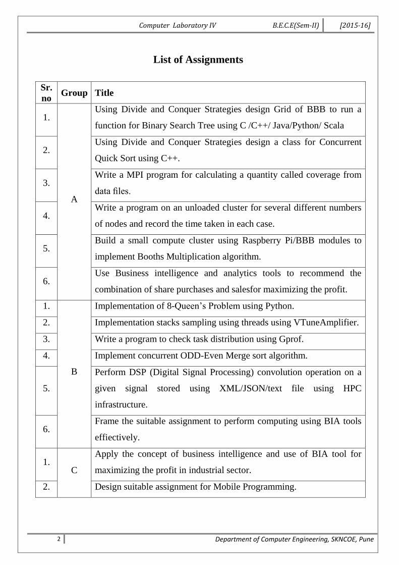
List of Assignments
Sr.
no Group Title
1.
A
Using Divide and Conquer Strategies design Grid of BBB to run a
function for Binary Search Tree using C /C++/ Java/Python/ Scala
2. Using Divide and Conquer Strategies design a class for Concurrent
Quick Sort using C++.
3. Write a MPI program for calculating a quantity called coverage from
data files.
4. Write a program on an unloaded cluster for several different numbers
of nodes and record the time taken in each case.
5. Build a small compute cluster using Raspberry Pi/BBB modules to
implement Booths Multiplication algorithm.
6. Use Business intelligence and analytics tools to recommend the
combination of share purchases and salesfor maximizing the profit.
1.
B
Implementation of 8-Queen’s Problem using Python.
2. Implementation stacks sampling using threads using VTuneAmplifier.
3. Write a program to check task distribution using Gprof.
4. Implement concurrent ODD-Even Merge sort algorithm.
5.
Perform DSP (Digital Signal Processing) convolution operation on a
given signal stored using XML/JSON/text file using HPC
infrastructure.
6. Frame the suitable assignment to perform computing using BIA tools
effiectively.
1. C
Apply the concept of business intelligence and use of BIA tool for
maximizing the profit in industrial sector.
2. Design suitable assignment for Mobile Programming.

Computer Laboratory IV B.E.C.E(Sem-II) [2015-16]
3 Department of Computer Engineering, SKNCOE, Pune
Group A
Assignments
Computer Laboratory IV B.E.C.E(Sem-II) [2015-16]
4 Department of Computer Engineering, SKNCOE, Pune
Assignment No. 1
Title
Using Divide and Conquer Strategies design a cluster/Grid of
BBB to run a function for Binary Search Tree using C /C++/
Java/Python/ Scala.
Roll No.
Class B.E. (C.E.)
Date
Subject Computer Lab IV
Signature
Computer Laboratory IV B.E.C.E(Sem-II) [2015-16]
5 Department of Computer Engineering, SKNCOE, Pune
Assignment No:1
Title: Using Divide and Conquer Strategies design a cluster/Grid of BBB to run a
function for Binary Search Tree(BST) using C /C++/ Java/Python/ Scala
Objectives:
To learn the concept that how to execute BST on cluster/Grid of BBB
To study the representation and implementation of Divide and Conquer Strategies
for Binary Search Tree on cluster/Grid of BBB.
Theory:
Divide and conquer strategy:
In computer science, divide and conquer (DandC) is an algorithm design paradigm based on multi-
branched recursion. A divide and conquer algorithm works by recursively breaking down a problem
into two or more sub-problems of the same (or related) type (divide), until these become simple
enough to be solved directly (conquer). The solutions to the sub-problems are then combined to give
a solution to the original problem. This divide and conquer technique is the basis of efficient
algorithms for all kinds of problems, such as sorting (e.g., quicksort, merge sort), multiplying large
numbers (e.g. Karatsuba), syntactic analysis (e.g., top-down parsers), and computing the discrete
Fourier transform (FFTs).
Understanding and designing DandC algorithms is a complex skill that requires a good
understanding of the nature of the underlying problem to be solved. As when proving a theorem by
induction, it is often necessary to replace the original problem with a more general or complicated
problem in order to initialize the recursion, and there is no systematic method for finding the proper
generalization. These DandC complications are seen when optimizing the calculation of a Fibonacci
number with efficient double recursion. The correctness of a divide and conquer algorithm is usually
proved by mathematical induction, and its computational cost is often determined by solving
recurrence relations. Divide-and-conquer is a top-down technique for designing algorithms that
consists of dividing the problem into smaller sub problems hoping that the solutions of the sub
problems are easier to find and then composing the partial solutions into the solution of the original
problem.
Little more formally, divide-and-conquer paradigm consists of following major phases:
Computer Laboratory IV B.E.C.E(Sem-II) [2015-16]
6 Department of Computer Engineering, SKNCOE, Pune
1. Breaking the problem into several sub-problems that are similar to the original problem but
smaller in size,
2. Solve the sub-problem recursively (successively and independently), and then
3. Combine these solutions to sub problems to create a solution to the original problem.
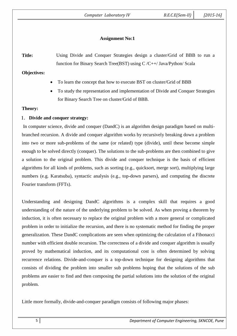
Binary Search tree:
Binary Search tree is a binary tree in which each internal node x stores an element such that the
element stored in the left subtree of x are less than or equal to x and elements stored in the right
subtree of x are greater than or equal to x. This is called binary-search-tree property. The basic
operations on a binary search tree take time proportional to the height of the tree. For a complete
binary tree with node n, such operations run in (log n) worst-case time. If the tree is a linear chain
of n nodes, however, the same operations takes (n) worst-case time.
Fig 1.Binary Search Tree
The height of the Binary Search Tree equals the number of links from the root node to deepest node.
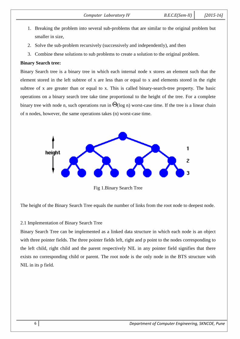
2.1 Implementation of Binary Search Tree
Binary Search Tree can be implemented as a linked data structure in which each node is an object
with three pointer fields. The three pointer fields left, right and p point to the nodes corresponding to
the left child, right child and the parent respectively NIL in any pointer field signifies that there
exists no corresponding child or parent. The root node is the only node in the BTS structure with
NIL in its p field.
Computer Laboratory IV B.E.C.E(Sem-II) [2015-16]
7 Department of Computer Engineering, SKNCOE, Pune
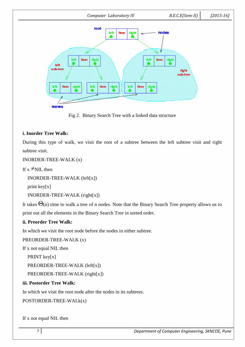
Fig 2. Binary Search Tree with a linked data structure
i. Inorder Tree Walk:
During this type of walk, we visit the root of a subtree between the left subtree visit and right
subtree visit.
INORDER-TREE-WALK (x)
If x NIL then
INORDER-TREE-WALK (left[x])
print key[x]
INORDER-TREE-WALK (right[x])
It takes (n) time to walk a tree of n nodes. Note that the Binary Search Tree property allows us to
print out all the elements in the Binary Search Tree in sorted order.
ii. Preorder Tree Walk:
In which we visit the root node before the nodes in either subtree.
PREORDER-TREE-WALK (x)
If x not equal NIL then
PRINT key[x]
PREORDER-TREE-WALK (left[x])
PREORDER-TREE-WALK (right[x])
iii. Postorder Tree Walk:
In which we visit the root node after the nodes in its subtrees.
POSTORDER-TREE-WALk(x)
If x not equal NIL then

Computer Laboratory IV B.E.C.E(Sem-II) [2015-16]
8 Department of Computer Engineering, SKNCOE, Pune
POSTORDER-TREE-WALK (left[x])
PREORDER-TREE-WALK (right[x])
PRINT key [x]
It takes O(n) time to walk (inorder, preorder and pastorder) a tree of n nodes.
2.2 Operations on BST:
2.2.1 Insertion
To insert a node into a BST
Find a leaf node the appropriate place and
Connect the node to the parent of the leaf.
2.2.2 Sorting
We can sort a given set of n numbers by first building a binary search tree containing these number
by using TREE-INSERT (x) procedure repeatedly to insert the numbers one by one and then
printing the numbers by an inorder tree walk
2.2.3 Deletion
Removing a node from a BST is a bit more complex, since we do not want to create any "holes" in
the tree. If the node has one child then the child is spliced to the parent of the node. If the node has
two children then its successor has no left child; copy the successor into the node and delete the
successor instead TREE-DELETE (T, z) removes the node pointed to by z from the tree T. IT
returns a pointer to the node removed so that the node can be put on a free-node list, etc.
3. What is Beagle Bone Black?
BeagleBone Black is a low-cost, community-supported development platform for developers and
hobbyists. Boot Linux in under 10 seconds and get started on development in less than 5 minutes
with just a single USB cable.
Processor: AM335x 1GHz ARM® Cortex-A8
512MB DDR3 RAM
4GB 8-bit eMMC on-board flash storage
3D graphics accelerator
NEON floating-point accelerator
2x PRU 32-bit microcontrollers
Connectivity
USB client for power and communications
USB host
Computer Laboratory IV B.E.C.E(Sem-II) [2015-16]
9 Department of Computer Engineering, SKNCOE, Pune
Ethernet
HDMI
2x 46 pin headers
Software Compatibility
Debian
Android
Ubuntu
Cloud9 IDE on Node.js w/ BoneScript library.
Mathematical Model:
Let S be system used to perform binary search using divide and conquer strategy.
S={I,O,F,fail,success}
Where,
Inputs:
I={I1,I2,I3}
I1=is array size supplied by user.
I2=array element equal to size specified.
I3= element to be searched.
Output:
O={position array elements searched}
Success: Successful execution of binary search function if element searched is found in array.
Failure: If searched element is not present in array then function fails.
Function set: F={main(),binary search()}
Where, main()- main function which is binary search
Binary search () - function to perform search using divide and conquer strategy.
Computer Laboratory IV B.E.C.E(Sem-II) [2015-16]
10 Department of Computer Engineering, SKNCOE, Pune
Venn diagram:
Input Output
Conclusion:
Hence, we have successfully studied cluster/Grid of BBB to run a function for Binary Search Tree.
A1
A2
.
.
An
A1
A2
.
.
An
Computer Laboratory IV B.E.C.E(Sem-II) [2015-16]
11 Department of Computer Engineering, SKNCOE, Pune
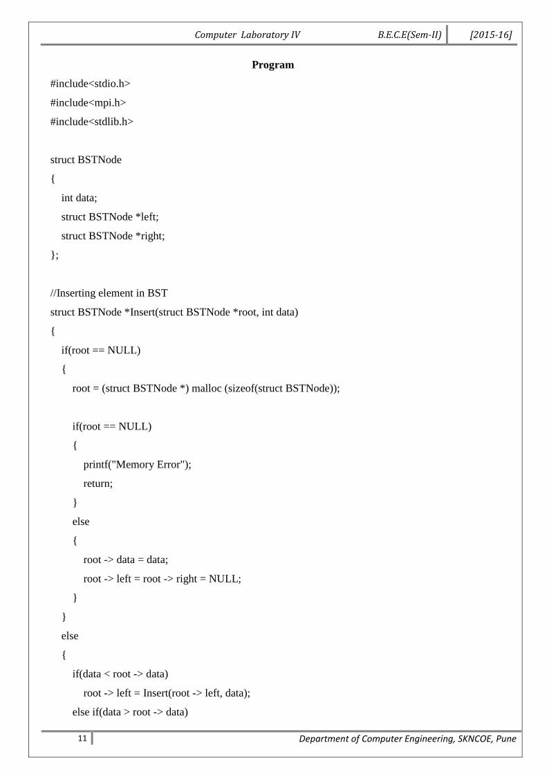
Program
#include<stdio.h>
#include<mpi.h>
#include<stdlib.h>
struct BSTNode
{
int data;
struct BSTNode *left;
struct BSTNode *right;
};
//Inserting element in BST
struct BSTNode *Insert(struct BSTNode *root, int data)
{
if(root == NULL)
{
root = (struct BSTNode *) malloc (sizeof(struct BSTNode));
if(root == NULL)
{
printf("Memory Error");
return;
}
else
{
root -> data = data;
root -> left = root -> right = NULL;
}
}
else
{
if(data < root -> data)
root -> left = Insert(root -> left, data);
else if(data > root -> data)
Computer Laboratory IV B.E.C.E(Sem-II) [2015-16]
12 Department of Computer Engineering, SKNCOE, Pune
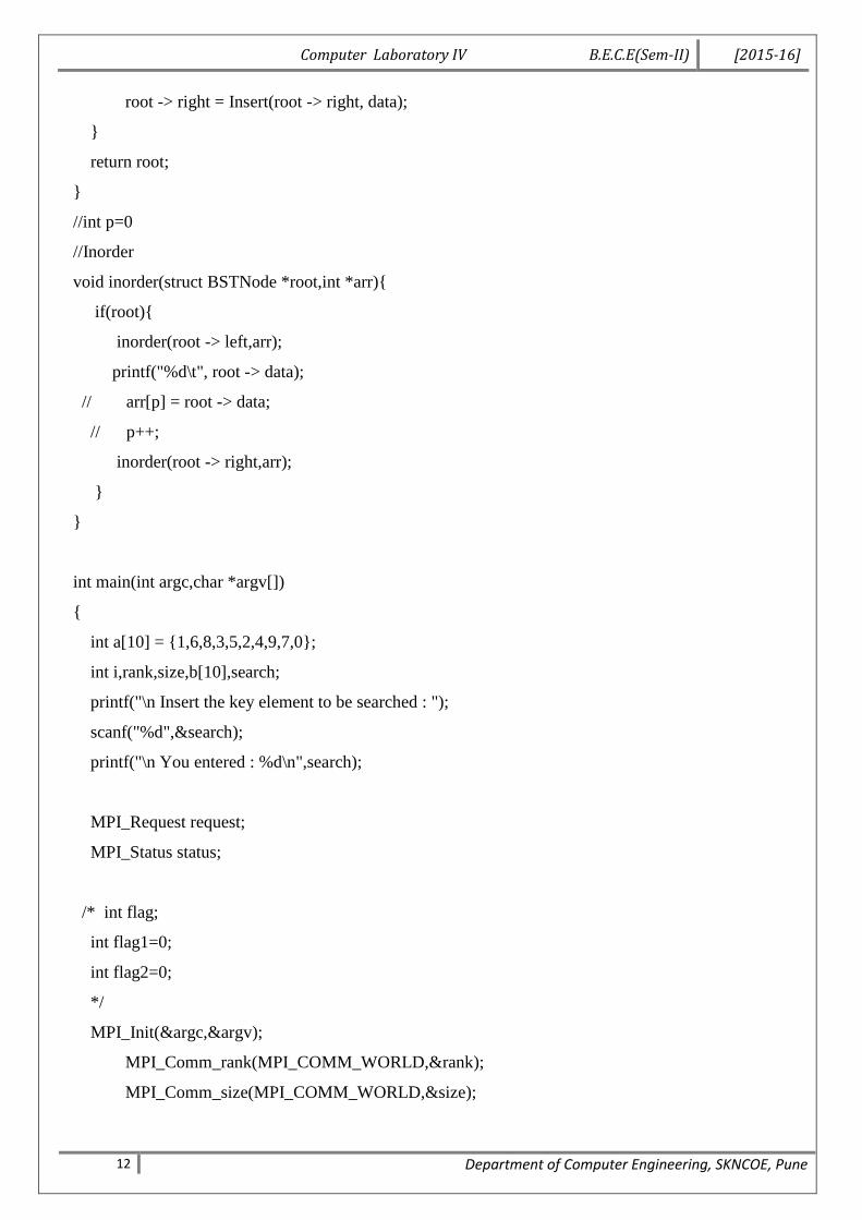
root -> right = Insert(root -> right, data);
}
return root;
}
//int p=0
//Inorder
void inorder(struct BSTNode *root,int *arr){
if(root){
inorder(root -> left,arr);
printf("%d\t", root -> data);
// arr[p] = root -> data;
// p++;
inorder(root -> right,arr);
}
}
int main(int argc,char *argv[])
{
int a[10] = {1,6,8,3,5,2,4,9,7,0};
int i,rank,size,b[10],search;
printf("\n Insert the key element to be searched : ");
scanf("%d",&search);
printf("\n You entered : %d\n",search);
MPI_Request request;
MPI_Status status;
/* int flag;
int flag1=0;
int flag2=0;
*/
MPI_Init(&argc,&argv);
MPI_Comm_rank(MPI_COMM_WORLD,&rank);
MPI_Comm_size(MPI_COMM_WORLD,&size);
Computer Laboratory IV B.E.C.E(Sem-II) [2015-16]
13 Department of Computer Engineering, SKNCOE, Pune
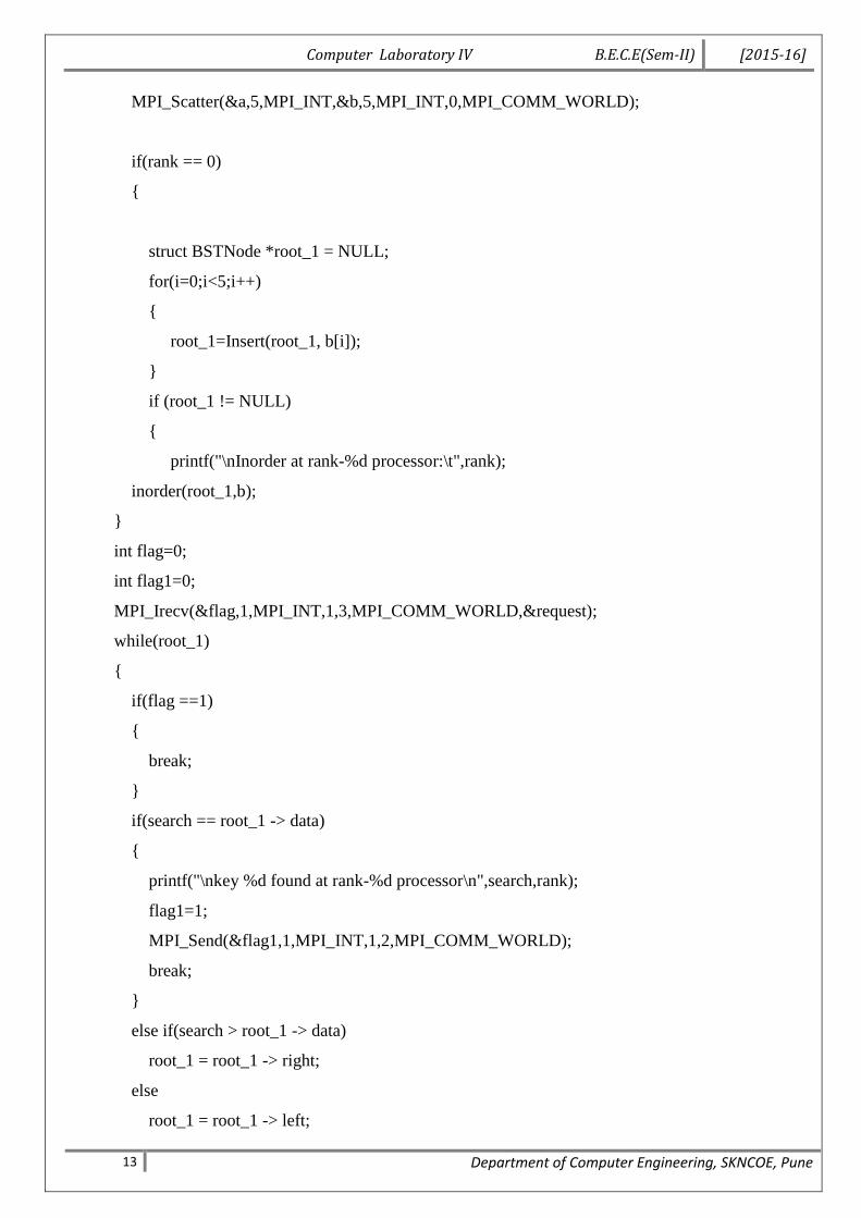
MPI_Scatter(&a,5,MPI_INT,&b,5,MPI_INT,0,MPI_COMM_WORLD);
if(rank == 0)
{
struct BSTNode *root_1 = NULL;
for(i=0;i<5;i++)
{
root_1=Insert(root_1, b[i]);
}
if (root_1 != NULL)
{
printf("\nInorder at rank-%d processor:\t",rank);
inorder(root_1,b);
}
int flag=0;
int flag1=0;
MPI_Irecv(&flag,1,MPI_INT,1,3,MPI_COMM_WORLD,&request);
while(root_1)
{
if(flag ==1)
{
break;
}
if(search == root_1 -> data)
{
printf("\nkey %d found at rank-%d processor\n",search,rank);
flag1=1;
MPI_Send(&flag1,1,MPI_INT,1,2,MPI_COMM_WORLD);
break;
}
else if(search > root_1 -> data)
root_1 = root_1 -> right;
else
root_1 = root_1 -> left;
Computer Laboratory IV B.E.C.E(Sem-II) [2015-16]
14 Department of Computer Engineering, SKNCOE, Pune
}
MPI_Send(&flag1,1,MPI_INT,1,2,MPI_COMM_WORLD);
MPI_Wait(&request,&status);
if(flag ==0 && flag1 ==0)
{
printf("\nKey %d not found\n",search);
}
}
if(rank == 1)
{
struct BSTNode *root_2 = NULL;
for(i=0;i<5;i++)
{
root_2=Insert(root_2, b[i]);
}
if (root_2 != NULL)
{
printf("\nInorder at rank-%d processor:\t",rank);
inorder(root_2,b);
}
int flag=0;
int flag1=0;
MPI_Irecv(&flag,1,MPI_INT,0,2,MPI_COMM_WORLD,&request);
while(root_2)
{
if(flag ==1)
{
break;
}
if(search == root_2 -> data)
{
printf("\nkey %d found at rank-%d processor\n",search,rank);
flag1=1;
MPI_Send(&flag1,1,MPI_INT,0,3,MPI_COMM_WORLD);
Computer Laboratory IV B.E.C.E(Sem-II) [2015-16]
15 Department of Computer Engineering, SKNCOE, Pune
break;
}
else if(search > root_2 -> data)
root_2 = root_2 -> right;
else
root_2 = root_2 -> left;
}
MPI_Send(&flag1,1,MPI_INT,0,3,MPI_COMM_WORLD);
}
MPI_Finalize();
return 0;
}
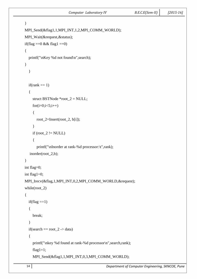
Output
root@beaglebone1:/hpcuser# vim bst_mpi.c
root@beaglebone1:/hpcuser# mpicc bst__mpi.c
root@beaglebone1:/hpcuser# mpiexec -n 2 -f machines.txt ./a.out
Insert the key element to be searched : 5
You entered : 5
Inorder at rank-0 processor: 1 3 5 6 8
Inorder at rank-1 processor: 0 2 4 7 9
key 5 found at rank-0 processor
root@beaglebone1:/hpcuser#
Computer Laboratory IV B.E.C.E(Sem-II) [2015-16]
16 Department of Computer Engineering, SKNCOE, Pune
Assignment No. 2
Title Using Divide and Conquer Strategies design a class for
Concurrent Quick Sort using C++.
Roll No.
Class B.E. (C.E.)
Date
Subject Computer Lab IV
Signature
Computer Laboratory IV B.E.C.E(Sem-II) [2015-16]
17 Department of Computer Engineering, SKNCOE, Pune
Assignment No:2
Title: Using Divide and Conquer Strategies design a class for Concurrent Quick Sort
using C++.
Objectives:
To learn the concept of Concurrent Quick Sort.
To study the representation and implementation of Divide and Conquer Strategies
for Concurrent Quick Sort using C++.
Theory:
Concurrent quick sort:
Like merge sort, quicksort uses divide-and-conquer, and so it's a recursive algorithm. The way that
quicksort uses divide-and-conquer is a little different from how merge sort does. In merge sort, the
divide step does hardly anything, and all the real work happens in the combine step. Quicksort is the
opposite: all the real work happens in the divide step. In fact, the combine step in quicksort does
absolutely nothing.
Quicksort has a couple of other differences from merge sort. Quicksort works in place. And its
worst-case running time is as bad as selection sort's and insertion sort's: Θ(n2)Θ(n2). But its
average-case running time is as good as merge sort's: Θ(nlgn)Θ(nlgn). So why think about quicksort
when merge sort is at least as good? That's because the constant factor hidden in the big-Θ notation
for quicksort is quite good. In practice, quicksort outperforms merge sort, and it significantly
outperforms selection sort and insertion sort.
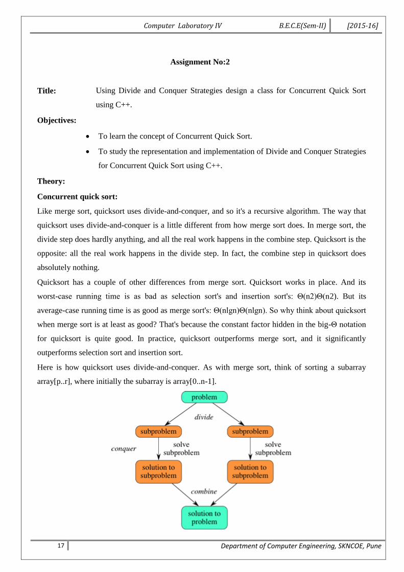
Here is how quicksort uses divide-and-conquer. As with merge sort, think of sorting a subarray
array[p..r], where initially the subarray is array[0..n-1].
Computer Laboratory IV B.E.C.E(Sem-II) [2015-16]
18 Department of Computer Engineering, SKNCOE, Pune
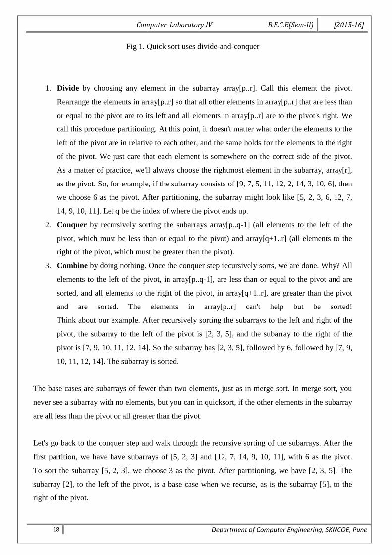
Fig 1. Quick sort uses divide-and-conquer
1. Divide by choosing any element in the subarray array[p..r]. Call this element the pivot.
Rearrange the elements in array[p..r] so that all other elements in array[p..r] that are less than
or equal to the pivot are to its left and all elements in array[p..r] are to the pivot's right. We
call this procedure partitioning. At this point, it doesn't matter what order the elements to the
left of the pivot are in relative to each other, and the same holds for the elements to the right
of the pivot. We just care that each element is somewhere on the correct side of the pivot.
As a matter of practice, we'll always choose the rightmost element in the subarray, array[r],
as the pivot. So, for example, if the subarray consists of [9, 7, 5, 11, 12, 2, 14, 3, 10, 6], then
we choose 6 as the pivot. After partitioning, the subarray might look like [5, 2, 3, 6, 12, 7,
14, 9, 10, 11]. Let q be the index of where the pivot ends up.
2. Conquer by recursively sorting the subarrays array[p..q-1] (all elements to the left of the
pivot, which must be less than or equal to the pivot) and array[q+1..r] (all elements to the
right of the pivot, which must be greater than the pivot).
3. Combine by doing nothing. Once the conquer step recursively sorts, we are done. Why? All
elements to the left of the pivot, in array[p..q-1], are less than or equal to the pivot and are
sorted, and all elements to the right of the pivot, in array[q+1..r], are greater than the pivot
and are sorted. The elements in array[p..r] can't help but be sorted!
Think about our example. After recursively sorting the subarrays to the left and right of the
pivot, the subarray to the left of the pivot is [2, 3, 5], and the subarray to the right of the
pivot is [7, 9, 10, 11, 12, 14]. So the subarray has [2, 3, 5], followed by 6, followed by [7, 9,
10, 11, 12, 14]. The subarray is sorted.
The base cases are subarrays of fewer than two elements, just as in merge sort. In merge sort, you
never see a subarray with no elements, but you can in quicksort, if the other elements in the subarray
are all less than the pivot or all greater than the pivot.
Let's go back to the conquer step and walk through the recursive sorting of the subarrays. After the
first partition, we have have subarrays of [5, 2, 3] and [12, 7, 14, 9, 10, 11], with 6 as the pivot.
To sort the subarray [5, 2, 3], we choose 3 as the pivot. After partitioning, we have [2, 3, 5]. The
subarray [2], to the left of the pivot, is a base case when we recurse, as is the subarray [5], to the
right of the pivot.
Computer Laboratory IV B.E.C.E(Sem-II) [2015-16]
19 Department of Computer Engineering, SKNCOE, Pune
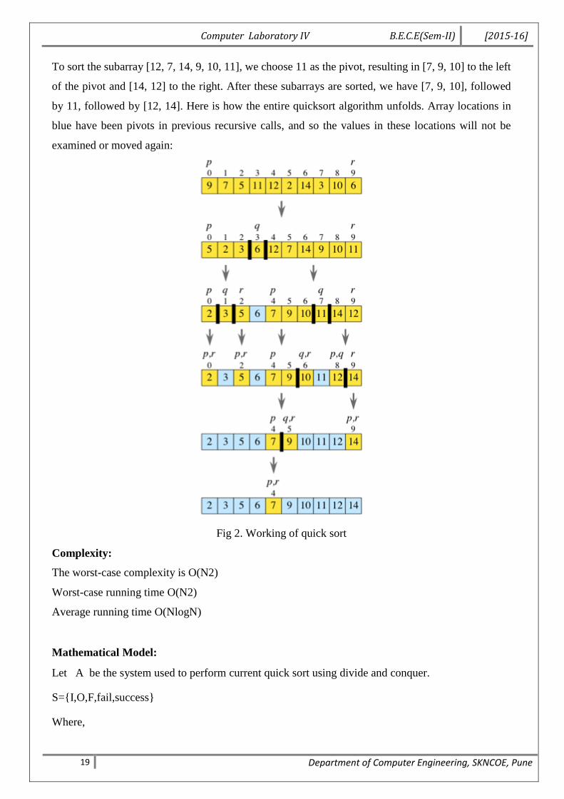
To sort the subarray [12, 7, 14, 9, 10, 11], we choose 11 as the pivot, resulting in [7, 9, 10] to the left
of the pivot and [14, 12] to the right. After these subarrays are sorted, we have [7, 9, 10], followed
by 11, followed by [12, 14]. Here is how the entire quicksort algorithm unfolds. Array locations in
blue have been pivots in previous recursive calls, and so the values in these locations will not be
examined or moved again:
Fig 2. Working of quick sort
Complexity:
The worst-case complexity is O(N2)
Worst-case running time O(N2)
Average running time O(NlogN)
Mathematical Model:
Let A be the system used to perform current quick sort using divide and conquer.
S={I,O,F,fail,success}
Where,
Computer Laboratory IV B.E.C.E(Sem-II) [2015-16]
20 Department of Computer Engineering, SKNCOE, Pune
Input:
I={I1,I2,I3....}
I1={N}
N=size of an array.
I2={A1,A2,A3,A4,......,An}
is array element equal to array size specified.
Output:
O={A1,A2,A3,........,An}
sorted array element using quick sort.
Success: Successful execution of quick sort 1 to n and array elements are sorted.
Function set:
p={main(), partition(),quick sort()}
where,
main(): main function which calls quick sort function.
partition(): to separate array list into two sublist and return pivot position.
quick sort(): to sort array elements.
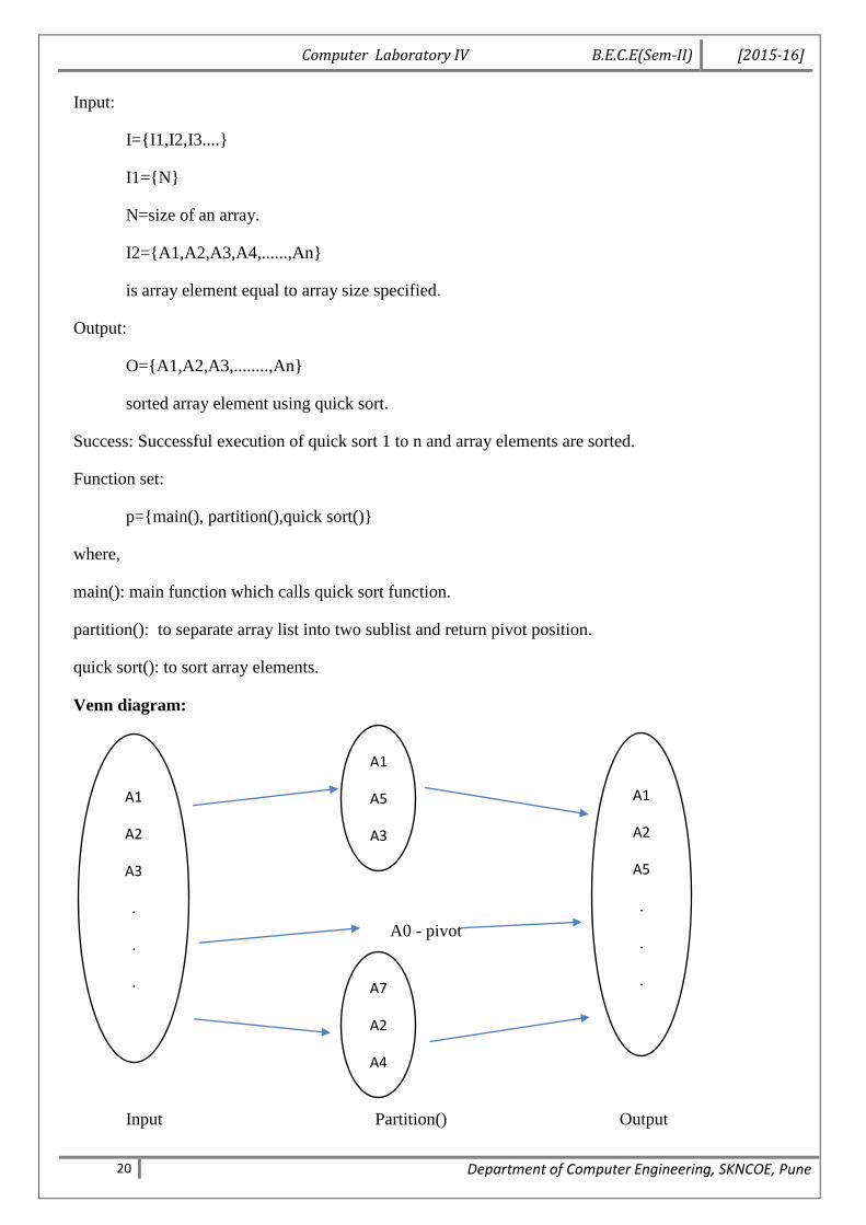
Venn diagram:
A0 - pivot
Input Partition() Output
A1
A2
A3
.
.
.
An
A1
A2
A5
.
.
.
Am
A1
A5
A3
A7
A2
A4

Computer Laboratory IV B.E.C.E(Sem-II) [2015-16]
21 Department of Computer Engineering, SKNCOE, Pune
Conclusion:
Hence, we have successfully studied and implemented Concurrent Quick Sort using C++..
Computer Laboratory IV B.E.C.E(Sem-II) [2015-16]
22 Department of Computer Engineering, SKNCOE, Pune
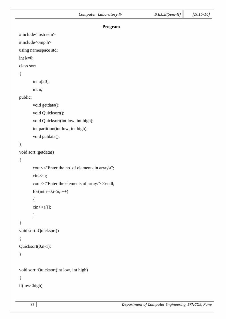
Program
#include<iostream>
#include<omp.h>
using namespace std;
int k=0;
class sort
{
int a[20];
int n;
public:
void getdata();
void Quicksort();
void Quicksort(int low, int high);
int partition(int low, int high);
void putdata();
};
void sort::getdata()
{
cout<<"Enter the no. of elements in array\t";
cin>>n;
cout<<"Enter the elements of array:"<<endl;
for(int i=0;i<n;i++)
{
cin>>a[i];
}
}
void sort::Quicksort()
{
Quicksort(0,n-1);
}
void sort::Quicksort(int low, int high)
{
if(low<high)
Computer Laboratory IV B.E.C.E(Sem-II) [2015-16]
23 Department of Computer Engineering, SKNCOE, Pune
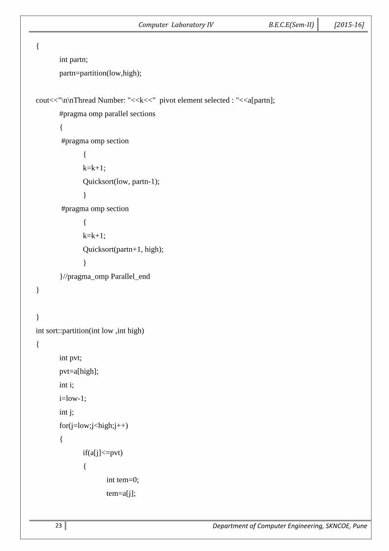
{
int partn;
partn=partition(low,high);
cout<<"\n\nThread Number: "<<k<<" pivot element selected : "<<a[partn];
#pragma omp parallel sections
{
#pragma omp section
{
k=k+1;
Quicksort(low, partn-1);
}
#pragma omp section
{
k=k+1;
Quicksort(partn+1, high);
}
}//pragma_omp Parallel_end
}
}
int sort::partition(int low ,int high)
{
int pvt;
pvt=a[high];
int i;
i=low-1;
int j;
for(j=low;j<high;j++)
{
if(a[j]<=pvt)
{
int tem=0;
tem=a[j];
Computer Laboratory IV B.E.C.E(Sem-II) [2015-16]
24 Department of Computer Engineering, SKNCOE, Pune
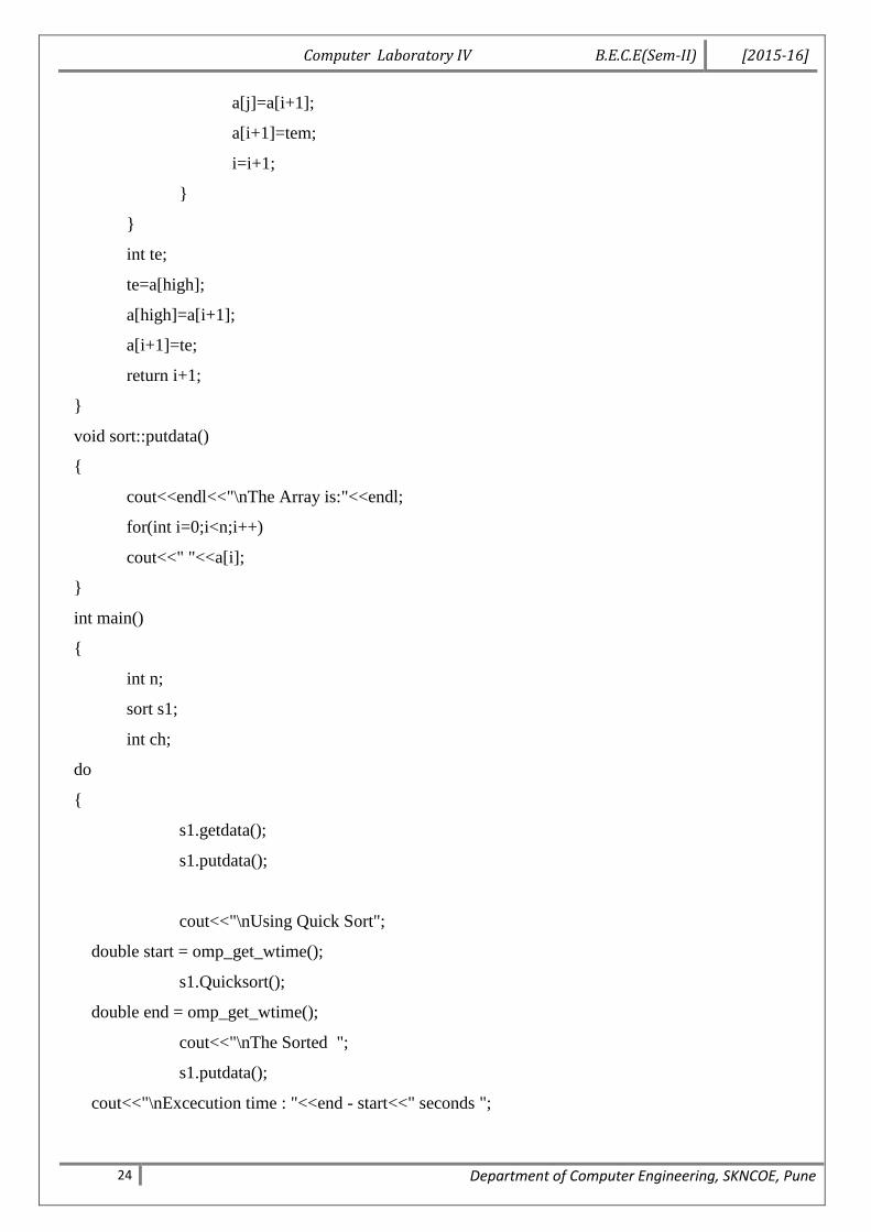
a[j]=a[i+1];
a[i+1]=tem;
i=i+1;
}
}
int te;
te=a[high];
a[high]=a[i+1];
a[i+1]=te;
return i+1;
}
void sort::putdata()
{
cout<<endl<<"\nThe Array is:"<<endl;
for(int i=0;i<n;i++)
cout<<" "<<a[i];
}
int main()
{
int n;
sort s1;
int ch;
do
{
s1.getdata();
s1.putdata();
cout<<"\nUsing Quick Sort";
double start = omp_get_wtime();
s1.Quicksort();
double end = omp_get_wtime();
cout<<"\nThe Sorted ";
s1.putdata();
cout<<"\nExcecution time : "<<end - start<<" seconds ";
Computer Laboratory IV B.E.C.E(Sem-II) [2015-16]
25 Department of Computer Engineering, SKNCOE, Pune
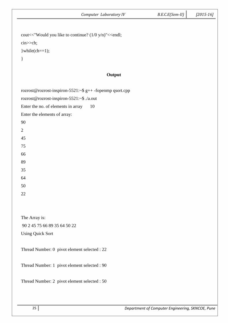
cout<<"Would you like to continue? (1/0 y/n)"<<endl;
cin>>ch;
}while(ch==1);
}
Output
rozrost@rozrost-inspiron-5521:~$ g++ -fopenmp qsort.cpp
rozrost@rozrost-inspiron-5521:~$ ./a.out
Enter the no. of elements in array 10
Enter the elements of array:
90
2
45
75
66
89
35
64
50
22
The Array is:
90 2 45 75 66 89 35 64 50 22
Using Quick Sort
Thread Number: 0 pivot element selected : 22
Thread Number: 1 pivot element selected : 90
Thread Number: 2 pivot element selected : 50
Computer Laboratory IV B.E.C.E(Sem-II) [2015-16]
26 Department of Computer Engineering, SKNCOE, Pune
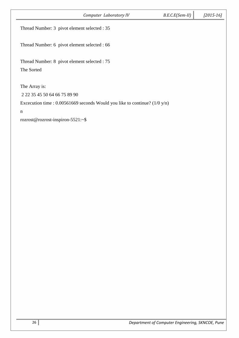
Thread Number: 3 pivot element selected : 35
Thread Number: 6 pivot element selected : 66
Thread Number: 8 pivot element selected : 75
The Sorted
The Array is:
2 22 35 45 50 64 66 75 89 90
Excecution time : 0.00561669 seconds Would you like to continue? (1/0 y/n)
n
rozrost@rozrost-inspiron-5521:~$
Computer Laboratory IV B.E.C.E(Sem-II) [2015-16]
27 Department of Computer Engineering, SKNCOE, Pune
Assignment No. 3
Title Write a MPI program for calculating a quantity called coverage
from data files.
Roll No.
Class B.E. (C.E.)
Date
Subject Computer Lab IV
Signature
Computer Laboratory IV B.E.C.E(Sem-II) [2015-16]
28 Department of Computer Engineering, SKNCOE, Pune
Assignment No:3
Title:
Write a MPI program for calculating a quantity called coverage from data files.
Objectives:
To learn the concept that how to execute MPI methods.
To study the representation and implementation of MPI methodology for parallel
computing.
Theory:-
Message Passing Interface (MPI) is a standardized and portable message-passing system designed by a
group of researchers from academia and industry to function on a wide variety of parallel computers. The
standard defines the syntax and semantics of a core of library routines useful to a wide range of users
writing portable message-passing programs in different computer programming languages such as Fortran,
C, C++ and Java. There are several well-tested and efficient implementations of MPI, including some that
are free or in the public domain. These fostered the development of a parallel software industry, and
encouraged development of portable and scalable large-scale parallel applications.
Functions of MPI:-
1. MPI_INIT :-
This method MPI_INIT is used to initialize the execution environnment.
Syntax:-
int MPI_Init(int *argc, char ***argv)
Input Parameters:-
1. argc – Pointer to the number of arguments.
2. argv – pointer to the argument vector.
2. MPI_Scatter
Sends data from one process to all other processes in a communicator.
Syntax :- int MPI_Scatter(const void *sendbuf, int send_count, MPI_Data type sendtype, void
*recbuf, int rev_count, MPI_Datatype recvtype, int root, MPI_Comm comm)
Input Parameters :-
sendbuff- address of send buffer(choice, significant only at root)
sendcount – number of elements send to each processes.
Sendtype – datatype of sendbuf elements.
Computer Laboratory IV B.E.C.E(Sem-II) [2015-16]
29 Department of Computer Engineering, SKNCOE, Pune
Recvcount – number of elements in recv buffer(int).
Recvtype – datatype of recv buffer elements
root – rank of sending process(int).
Comm – communicator
Output Parameters:-
recvbuf – address of recv buffer.
3. MPI_Comm_rank :-
determines the rank of the calling process in the communicator.
Syntax :-
int MPI_Comm_rank(MPI_Comm comm, int *rank)
Input Parameters :-
comm – communicator(handle)
Output Parameters :-
rank – rank of the calling process in the group of comm(int)
4. MPI_Finalize :-
Terminates MPI execution environment.
Syntax :-
int MPI_Finalize(void)
5. MPI_Gather :-
Gathers together values from a group of processes.
Syntax :-
int MPI_Gather(const void *sendbuf, int send_count, MPI_Data type sendtype, void
*recbuf, int rev_count, MPI_Datatype recvtype, int root, MPI_Comm comm)
Mathematical Model:
Let M be the system.
M = {I, P, O, S, F}
Let I be the input.
I = {k}
k = any number.
Let P be the process.
Computer Laboratory IV B.E.C.E(Sem-II) [2015-16]
30 Department of Computer Engineering, SKNCOE, Pune
P = {n, q, r}
n=squaring the number.
q=calculating the run time
r= plotting the graph
Let O be the Output.
O = {c}
c =square of the number and run time.
Let S be the case of Success.
S = {l}
l = Satisfied all conditions.
Let F be the case of Failure.
F = {f}
f = Satisfied result not generated.
Conclusion:
Hence, we have successfully studied MPI methodology for high performance parallel computing.
Computer Laboratory IV B.E.C.E(Sem-II) [2015-16]
31 Department of Computer Engineering, SKNCOE, Pune
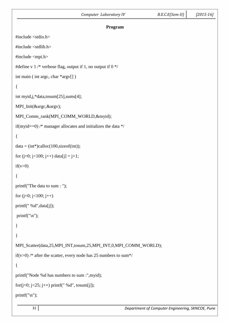
Program
#include <stdio.h>
#include <stdlib.h>
#include <mpi.h>
#define v 1 /* verbose flag, output if 1, no output if 0 */
int main ( int argc, char *argv[] )
{
int myid,j,*data,tosum[25],sums[4];
MPI_Init(&argc,&argv);
MPI_Comm_rank(MPI_COMM_WORLD,&myid);
if(myid==0) /* manager allocates and initializes the data */
{
data = (int*)calloc(100,sizeof(int));
for (j=0; j<100; j++) data[j] = j+1;
if(v>0)
{
printf("The data to sum : ");
for (j=0; j<100; j++)
printf(" %d",data[j]);
printf("\n");
}
}
MPI_Scatter(data,25,MPI_INT,tosum,25,MPI_INT,0,MPI_COMM_WORLD);
if(v>0) /* after the scatter, every node has 25 numbers to sum*/
{
printf("Node %d has numbers to sum :",myid);
for(j=0; j<25; j++) printf(" %d", tosum[j]);
printf("\n");
Computer Laboratory IV B.E.C.E(Sem-II) [2015-16]
32 Department of Computer Engineering, SKNCOE, Pune
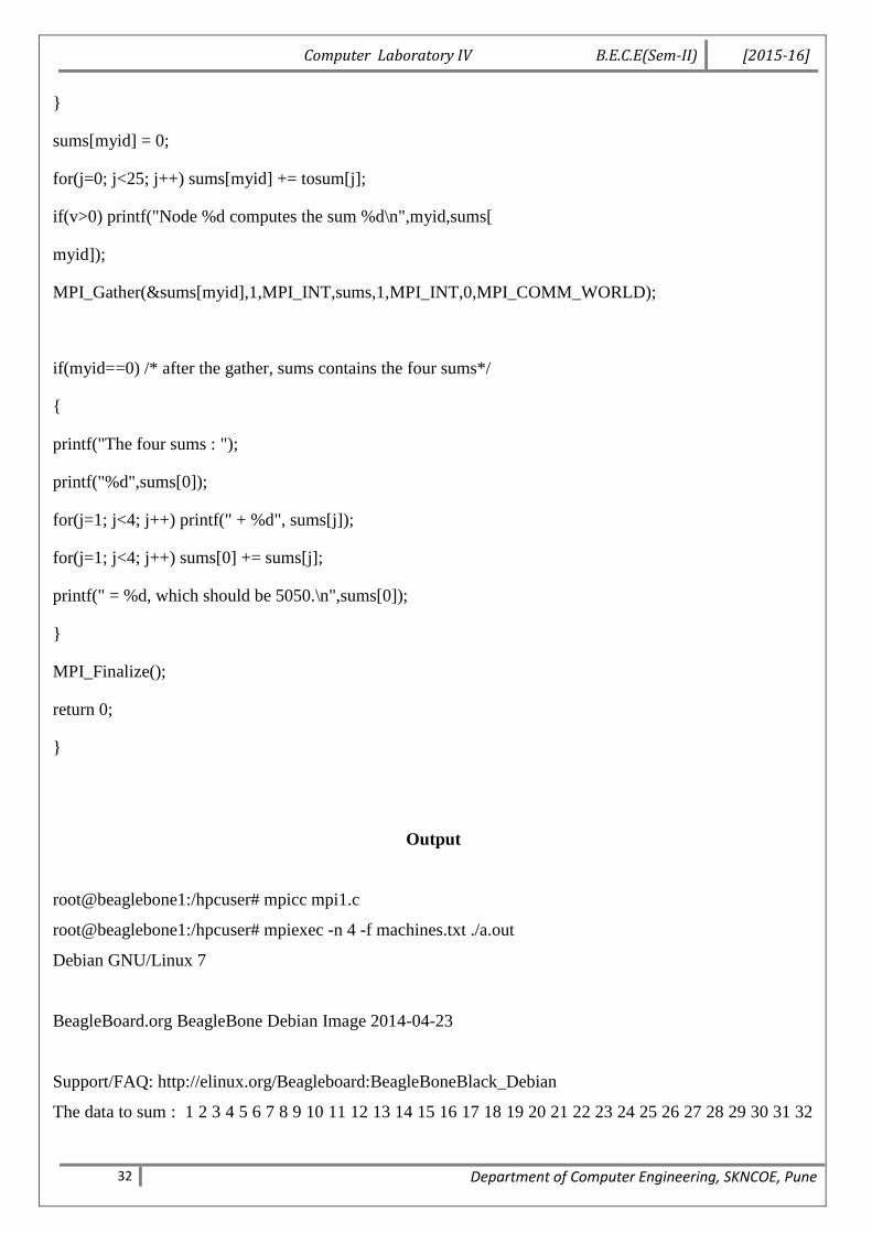
}
sums[myid] = 0;
for(j=0; j<25; j++) sums[myid] += tosum[j];
if(v>0) printf("Node %d computes the sum %d\n",myid,sums[
myid]);
MPI_Gather(&sums[myid],1,MPI_INT,sums,1,MPI_INT,0,MPI_COMM_WORLD);
if(myid==0) /* after the gather, sums contains the four sums*/
{
printf("The four sums : ");
printf("%d",sums[0]);
for(j=1; j<4; j++) printf(" + %d", sums[j]);
for(j=1; j<4; j++) sums[0] += sums[j];
printf(" = %d, which should be 5050.\n",sums[0]);
}
MPI_Finalize();
return 0;
}
Output
root@beaglebone1:/hpcuser# mpicc mpi1.c
root@beaglebone1:/hpcuser# mpiexec -n 4 -f machines.txt ./a.out
Debian GNU/Linux 7
BeagleBoard.org BeagleBone Debian Image 2014-04-23
Support/FAQ: http://elinux.org/Beagleboard:BeagleBoneBlack_Debian
The data to sum : 1 2 3 4 5 6 7 8 9 10 11 12 13 14 15 16 17 18 19 20 21 22 23 24 25 26 27 28 29 30 31 32
Computer Laboratory IV B.E.C.E(Sem-II) [2015-16]
33 Department of Computer Engineering, SKNCOE, Pune
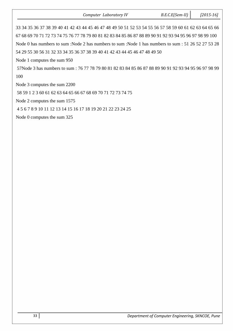
33 34 35 36 37 38 39 40 41 42 43 44 45 46 47 48 49 50 51 52 53 54 55 56 57 58 59 60 61 62 63 64 65 66
67 68 69 70 71 72 73 74 75 76 77 78 79 80 81 82 83 84 85 86 87 88 89 90 91 92 93 94 95 96 97 98 99 100
Node 0 has numbers to sum :Node 2 has numbers to sum :Node 1 has numbers to sum : 51 26 52 27 53 28
54 29 55 30 56 31 32 33 34 35 36 37 38 39 40 41 42 43 44 45 46 47 48 49 50
Node 1 computes the sum 950
57Node 3 has numbers to sum : 76 77 78 79 80 81 82 83 84 85 86 87 88 89 90 91 92 93 94 95 96 97 98 99
100
Node 3 computes the sum 2200
58 59 1 2 3 60 61 62 63 64 65 66 67 68 69 70 71 72 73 74 75
Node 2 computes the sum 1575
4 5 6 7 8 9 10 11 12 13 14 15 16 17 18 19 20 21 22 23 24 25
Node 0 computes the sum 325
Computer Laboratory IV B.E.C.E(Sem-II) [2015-16]
34 Department of Computer Engineering, SKNCOE, Pune
Assignment No. 4
Title
Write a program on an unloaded cluster for several different
numbers of nodes and record the time taken in each case. Draw
a graph of execution time against the number of nodes.
Roll No.
Class B.E. (C.E.)
Date
Subject Computer Lab IV
Signature
Computer Laboratory IV B.E.C.E(Sem-II) [2015-16]
35 Department of Computer Engineering, SKNCOE, Pune
Assignment No:4
Title : Write a program on an unloaded cluster for several different numbers of nodes and record
the time taken in each case. Draw a graph of execution time against the number of nodes.
Objectives:
To learn the concept that how to implement unloaded cluster for several nodes.
To study the representation and implementation of unloaded cluster in MPI
environment.
Theory:
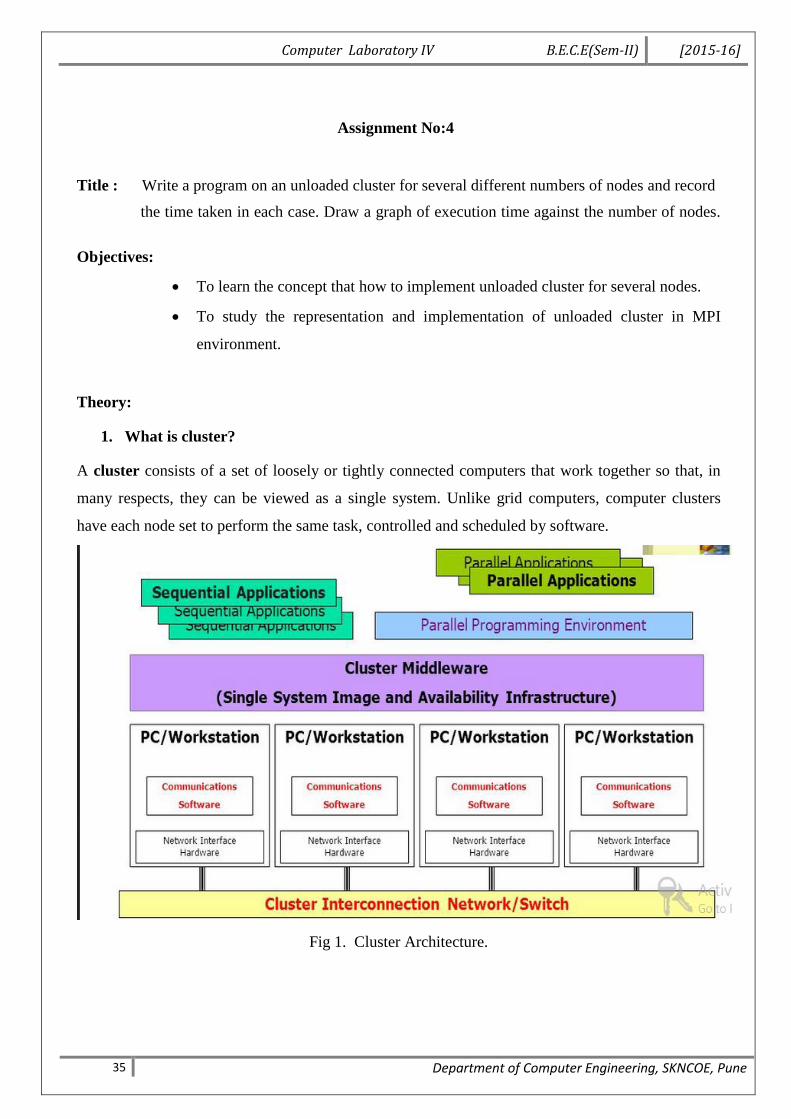
1. What is cluster?
A cluster consists of a set of loosely or tightly connected computers that work together so that, in
many respects, they can be viewed as a single system. Unlike grid computers, computer clusters
have each node set to perform the same task, controlled and scheduled by software.
Fig 1. Cluster Architecture.
Computer Laboratory IV B.E.C.E(Sem-II) [2015-16]
36 Department of Computer Engineering, SKNCOE, Pune
2.Data sharing and communication over Cluster by
1. Message passing intertface-(MPI)
Two widely used approaches for communication between cluster nodes are MPI, the Message
Passing Interface and PVM, the Parallel Virtual Machine.
PVM was developed at the Oak Ridge National Laboratory around 1989 before MPI was available.
PVM must be directly installed on every cluster node and provides a set of software libraries that
paint the node as a "parallel virtual machine". PVM provides a run-time environment for message-
passing, task and resource management, and fault notification. PVM can be used by user programs
written in C, C++, or Fortran, etc.
MPI emerged in the early 1990s out of discussions among 40 organizations. The initial effort was
supported by ARPA and National Science Foundation. Rather than starting anew, the design of MPI
drew on various features available in commercial systems of the time. The MPI specifications then
gave rise to specific implementations. MPI implementations typically use TCP/IP and socket
connections.
Output Parameters
Rank- rank of the calling process in the group of comm (integer)
Thread and Interrupt Safety
This routine is both thread- and interrupt-safe. This means that this routine may safely be used by
multiple threads and from within a signal handler.
2. MPI_Send-
Performs a blocking send
Synopsis
int MPI_Send(const void *buf, int count, MPI_Datatype datatype, int dest, int tag,
MPI_Comm comm)
Input Parameters
Buf- initial address of send buffer (choice)
Computer Laboratory IV B.E.C.E(Sem-II) [2015-16]
37 Department of Computer Engineering, SKNCOE, Pune
count- number of elements in send buffer (nonnegative integer)
datatype- datatype of each send buffer element (handle)
dest- rank of destination (integer)
tag- message tag (integer)
comm- communicator (handle)
3. MPI_Recv
Blocking receive for a message
Synopsis
int MPI_Recv(void *buf, int count,Two widely used approaches for communication between cluster
nodes are MPI, the Message Passing Interface and PVM, the Parallel Virtual Machine.
PVM was developed at the Oak Ridge National Laboratory around 1989 before MPI was available.
PVM must be directly installed on every cluster node and provides a set of software libraries that
paint the node as a "parallel virtual machine". PVM provides a run-time environment for message-
passing, task and resource management, and fault notification. PVM can be used by user programs
written in C, C++, or Fortran, etc.
MPI emerged in the early 1990s out of discussions among 40 organizations. The initial effort was
supported by ARPA and National Science Foundation. Rather than starting anew, the design of MPI
drew on various features available in commercial systems of the time. The MPI specifications then
gave rise to specific implementations. MPI implementations typically use TCP/IP and socket
connections.
Output Parameters
Rank- rank of the calling process in the group of comm (integer)
Thread and Interrupt Safety
This routine is both thread- and interrupt-safe. This means that this routine may safely be used by
multiple threads and from within a signal handler.
4. MPI_Send-
Performs a blocking send
Computer Laboratory IV B.E.C.E(Sem-II) [2015-16]
38 Department of Computer Engineering, SKNCOE, Pune
Synopsis
int MPI_Send(const void *buf, int count, MPI_Datatype datatype, int dest, int tag,
MPI_Comm comm)
Input Parameters
Buf- initial address of send buffer (choice)
count- number of elements in send buffer (nonnegative integer)
datatype- datatype of each send buffer element (handle)
dest- rank of destination (integer)
tag- message tag (integer)
comm- communicator (handle)
5. MPI_Recv-
Blocking receive for a message
Synopsis MPI_Datatype datatype, int source, int tag,
MPI_Comm comm, MPI_Status *status)
Output Parameters
buf -initial address of receive buffer (choice)
status- status object (Status)
Input Parameters
count -maximum number of elements in receive buffer (integer)
datatype- datatype of each receive buffer element (handle)
source- rank of source (integer)
tag- message tag (integer)
comm-communicator (handle)
6. MPI_Wtime()-
Returns an elapsed time on the calling processor
Synopsis
double MPI_Wtime( void )
Return value
Time in seconds since an arbitrary time in the past.
Computer Laboratory IV B.E.C.E(Sem-II) [2015-16]
39 Department of Computer Engineering, SKNCOE, Pune
7. MPI_Finalize()-
Terminates MPI execution environment
Synopsis
int MPI_Finalize( void )
Notes
All processes must call this routine before exiting. The number of processes running after this
routine is called is undefined; it is best not to perform much more than a return rc after calling
MPI_Finalize.
Mathematical Model:
Let M be the system.
M = {I, P, O, S, F}
Let I be the input.
I = {k}
k = any number.
Let P be the process.
P = {n, q, r}
n=squaring the number.
q=calculating the run time
r= plotting the graph
Let O be the Output.
O = {c}
c =square of the number and run time.
Let S be the case of Success.
S = {l}
l = Satisfied all conditions.
Let F be the case of Failure.
F = {f}
f = Satisfied result not generated.
Computer Laboratory IV B.E.C.E(Sem-II) [2015-16]
40 Department of Computer Engineering, SKNCOE, Pune
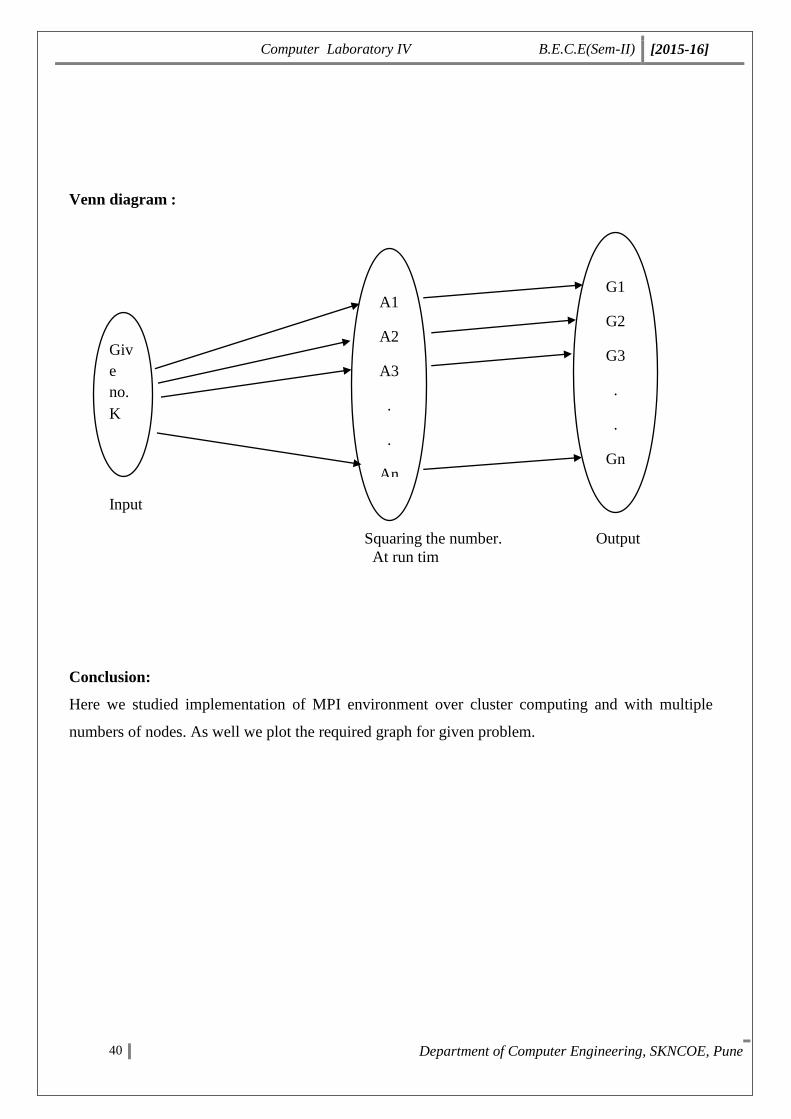
Venn diagram :
Input
Squaring the number. Output
At run tim
Conclusion:
Here we studied implementation of MPI environment over cluster computing and with multiple
numbers of nodes. As well we plot the required graph for given problem.
Giv
e
no.
K
A1
A2
A3
.
.
An
An
G1
G2
G3
.
.
Gn
An
Computer Laboratory IV B.E.C.E(Sem-II) [2015-16]
41 Department of Computer Engineering, SKNCOE, Pune
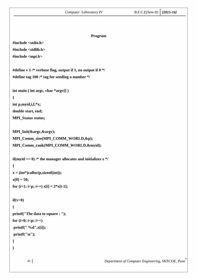
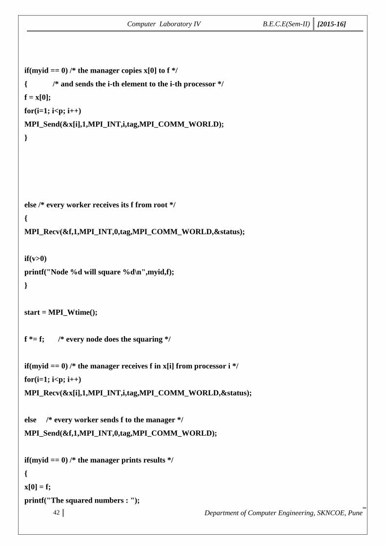
Program
#include <stdio.h>
#include <stdlib.h>
#include <mpi.h>
#define v 1 /* verbose flag, output if 1, no output if 0 */
#define tag 100 /* tag for sending a number */
int main ( int argc, char *argv[] )
{
int p,myid,i,f,*x;
double start, end;
MPI_Status status;
MPI_Init(&argc,&argv);
MPI_Comm_size(MPI_COMM_WORLD,&p);
MPI_Comm_rank(MPI_COMM_WORLD,&myid);
if(myid == 0) /* the manager allocates and initializes x */
{
x = (int*)calloc(p,sizeof(int));
x[0] = 50;
for (i=1; i<p; i++) x[i] = 2*x[i-1];
if(v>0)
{
printf("The data to square : ");
for (i=0; i<p; i++)
printf(" %d",x[i]);
printf("\n");
}
}
Computer Laboratory IV B.E.C.E(Sem-II) [2015-16]
42 Department of Computer Engineering, SKNCOE, Pune
if(myid == 0) /* the manager copies x[0] to f */
{ /* and sends the i-th element to the i-th processor */
f = x[0];
for(i=1; i<p; i++)
MPI_Send(&x[i],1,MPI_INT,i,tag,MPI_COMM_WORLD);
}
else /* every worker receives its f from root */
{
MPI_Recv(&f,1,MPI_INT,0,tag,MPI_COMM_WORLD,&status);
if(v>0)
printf("Node %d will square %d\n",myid,f);
}
start = MPI_Wtime();
f *= f; /* every node does the squaring */
if(myid == 0) /* the manager receives f in x[i] from processor i */
for(i=1; i<p; i++)
MPI_Recv(&x[i],1,MPI_INT,i,tag,MPI_COMM_WORLD,&status);
else /* every worker sends f to the manager */
MPI_Send(&f,1,MPI_INT,0,tag,MPI_COMM_WORLD);
if(myid == 0) /* the manager prints results */
{
x[0] = f;
printf("The squared numbers : ");

Computer Laboratory IV B.E.C.E(Sem-II) [2015-16]
43 Department of Computer Engineering, SKNCOE, Pune
for(i=0; i<p; i++)
printf(" %d",x[i]);
printf("\n");
end = MPI_Wtime();
printf("Runtime = %f\n", end-start);
}
MPI_Finalize();
return 0;
}
Output
root@beaglebone1:/hpcuser# mpicc mpi1.c
root@beaglebone1:/hpcuser# mpiexec -n 2 -f machines.txt ./a.out
Debian GNU/Linux 7
BeagleBoard.org BeagleBone Debian Image 2014-04-23
Support/FAQ: http://elinux.org/Beagleboard:BeagleBoneBlack_Debian
The data to square : 50 100
Node 1 will square 100
The squared numbers : 2500 10000
Runtime = 0.011505
root@beaglebone1:/hpcuser#
Computer Laboratory IV B.E.C.E(Sem-II) [2015-16]
44 Department of Computer Engineering, SKNCOE, Pune
Assignment No. 5
Title Build a small compute cluster using Raspberry Pi/BBB
modules to implement Booths Multiplication algorithm
Roll No.
Class B.E. (C.E.)
Date
Subject Computer Lab IV
Signature
Computer Laboratory IV B.E.C.E(Sem-II) [2015-16]
45 Department of Computer Engineering, SKNCOE, Pune
Assignment No:5
Title: Build a small compute cluster using Raspberry Pi/BBB modules to implement
Booths Multiplication algorithm
Objectives:
To learn the concept that how to execute Boots Algorithm on cluster/Grid of BBB
To study the representation and implementation of Boots Algorithm on cluster/Grid
BBB.
Theory:
1. Booths Algorithm strategy:
Booth's multiplication algorithm is a multiplication algorithm that multiplies two signed binary
numbers in two's complement notation. The algorithm was invented by Andrew Donald Booth in 1950
while doing research on crystallography at Birkbeck College in Bloomsbury, London. Booth used
desk calculators that were faster at shifting than adding and created the algorithm to increase their
speed. Booth's algorithm is of interest in the study of computer architecture.
Booths Multiplication Algorithm:
Booth's algorithm can be implemented by repeatedly adding (with ordinary unsigned binary addition)
one of two predetermined values A and S to a product P, then performing a rightward arithmetic shift
on P. Let m and r be the multiplicand and multiplier, respectively; and let x and y represent the
number of bits in m and r.
1. Determine the values of A and S, and the initial value of P. All of these numbers should have a
length equal to (x + y + 1).
1. A: Fill the most significant (leftmost) bits with the value of m. Fill the remaining (y + 1) bits
with zeros.
2. S: Fill the most significant bits with the value of (-m) in two's complement notation. Fill the
remaining (y + 1) bits with zeros.
3. P: Fill the most significant x bits with zeros. To the right of this, append the value of r. Fill the
least significant (rightmost) bit with a zero.
2. Determine the two least significant (rightmost) bits of P.
1. If they are 01, find the value of P + A. Ignore any overflow.
Computer Laboratory IV B.E.C.E(Sem-II) [2015-16]
46 Department of Computer Engineering, SKNCOE, Pune
2. If they are 10, find the value of P + S. Ignore any overflow.
3. If they are 00, do nothing. Use P directly in the next step.
4. If they are 11, do nothing. Use P directly in the next step.
3. Arithmetically shift the value obtained in the 2nd step by a single place to the right. Let P now
equal this new value.
4. Repeat steps 2 and 3 until they have been done y times.
5. Drop the least significant (rightmost) bit from P. This is the product of m and r.
Example of Boots Multiplication:
Find 3 × (-4), with m = 3 and r = -4, and x = 4 and y = 4:
m = 0011, -m = 1101, r = 1100
A = 0011 0000 0
S = 1101 0000 0
P = 0000 1100 0
Perform the loop four times:
P = 0000 1100 0. The last two bits are 00.
P = 0000 0110 0. Arithmetic right shift.
P = 0000 0110 0. The last two bits are 00.
P = 0000 0011 0. Arithmetic right shift.
P = 0000 0011 0. The last two bits are 10.
P = 1101 0011 0. P = P + S.
P = 1110 1001 1. Arithmetic right shift.
P = 1110 1001 1. The last two bits are 11.
P = 1111 0100 1. Arithmetic right shift.

Computer Laboratory IV B.E.C.E(Sem-II) [2015-16]
47 Department of Computer Engineering, SKNCOE, Pune
The product is 1111 0100, which is -12
2. What is BeagleBone Black?
Launched in 2008, the original BeagleBoard was developed by Texas Instruments as an open source
computer. It featured a 720 MHz Cortex A8 arm chip and 256MB of memory. The BeagleBoard-xm
and BeagleBone were released in subsequent years leading to the BeagleBone Black as the most
recent release. Though its $45 price tag is a little higher than a Raspberry Pi, it has a faster 1GHz
Cortex 8 chip, 512 MB of RAM and extra USB connections. In addition to 2GB of onboard memory
that comes with a pre-installed Linux distribution, there is a micro SD card slot allowing you to load
additional versions of Linux and boot to them instead. Thanks to existing support for multiple Linux
distributions such as Debian and Ubuntu, BeagleBone Black looked to me like a great inexpensive
starting point for creating my very own home server cluster.
BeagleBone Black is a low-cost, community-supported development platform for developers and
hobbyists. Boot Linux in under 10 seconds and get started on development in less than 5 minutes with
just a single USB cable.
3. Building a Compute Cluster with the BeagleBone Black:
3.1 Setting up the Cluster:
For the personal cluster we decided to start small and try it out with just three machines. The list of
equipment that I bought is as follows:
1x 8 port gigabit switch
3x beaglebone blacks
3x ethernet cables
3x 5V 2 amp power supplys
3x 4 GB microSD cards
To keep it simple, we decided to build a command line cluster that I would control through my laptop
or desktop. The BeagleBone Black supports HDMI output so you can use them as standalone
computers but I figured that would not be necessary for my needs. The simplest way to get the
BeagleBone Black running is to use the supplied USB cable to hook it up to an existing computer and
SSH to the pre-installed OS. We have to first load a version of Linux on to each of the three SD
cards.
sudo ./setup_sdcard.sh --probe-mmc
Computer Laboratory IV B.E.C.E(Sem-II) [2015-16]
48 Department of Computer Engineering, SKNCOE, Pune
On the machine the SD card was listed as /dev/sdb with its main partition showing as /dev/sdb1. If
you see the partition listed as I did, you need to unmount it before you can install the image on it.
Once the card was ready, run the following command:
sudo ./setup_sdcard.sh --mmc /dev/sdb --uboot bone
This command took care of the full install of the OS on to the SD card. Once it was finished repeat it
for the other two SD cards. The default user name for the installed distribution is ubuntu with
password temppwd. Insert the SD cards in to the BeagleBones and then connected them to the
ethernet switch.
The last step was to power them up and boot them using the micro SD cards. Doing this required
holding down the user boot button while connecting the 5V power connector. The button is located on
a little raised section near the usb port and tells the device to read from the SD card. Once you see the
lights flashing repeatedly you can release the button. Since each instance will have the same default
hostname when initially booting, it is advisable to power them on one at a time and follow the steps
below to set the IP and hostname before powering up the next one.
Mathematical Model:
Let S be system used to to implement Booths Multiplication algorithm.
S={I,O,F,fail,success}
Where,
Inputs:
I={I1,I2,I3}
I1=is array size supplied by user.
I2=is array size supplied by user.
I3=array element equal to size specified.
Output:
O={multiplication of array elements provided by user}
Success: Successful multiplication of array elements provided by user.
Failure: If provided elements are not match with array size then function fails.
Function set: F={main(),set() ,multiply()}
Computer Laboratory IV B.E.C.E(Sem-II) [2015-16]
49 Department of Computer Engineering, SKNCOE, Pune
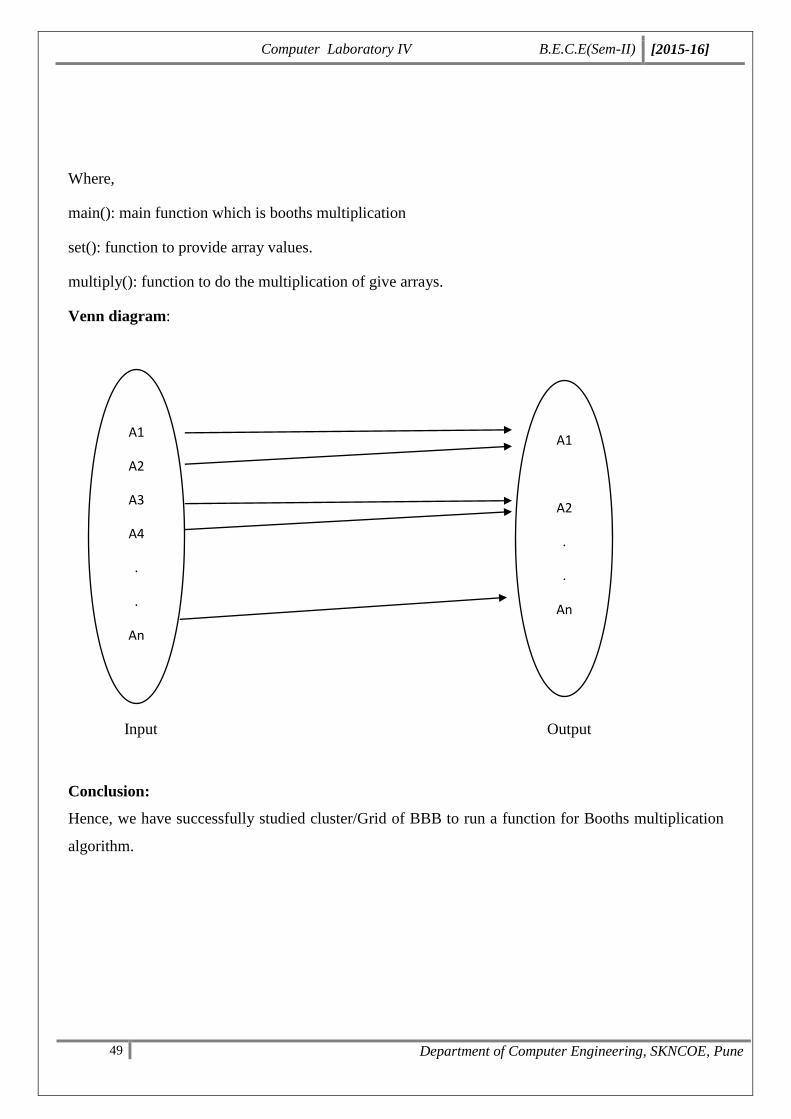
Where,
main(): main function which is booths multiplication
set(): function to provide array values.
multiply(): function to do the multiplication of give arrays.
Venn diagram:
Input Output
Conclusion:
Hence, we have successfully studied cluster/Grid of BBB to run a function for Booths multiplication
algorithm.
A1
A2
A3
A4
.
.
An
A1
A2
.
.
An
Computer Laboratory IV B.E.C.E(Sem-II) [2015-16]
50 Department of Computer Engineering, SKNCOE, Pune
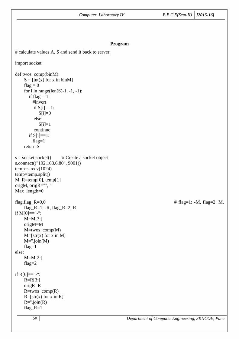
Program
# calculate values A, S and send it back to server.
import socket
def twos_comp(binM):
S = [int(x) for x in binM]
flag = 0
for i in range(len(S)-1, -1, -1):
if flag==1:
#invert
if S[i]==1:
S[i]=0
else:
S[i]=1
continue
if S[i]==1:
flag=1
return S
s = socket.socket() # Create a socket object
s.connect(("192.168.6.80", 9001))
temp=s.recv(1024)
temp=temp.split()
M, R=temp[0], temp[1]
origM, origR="", ""
Max_length=0
flag,flag_R=0,0 # flag=1: -M, flag=2: M.
flag_R=1: -R, flag_R=2: R
if M[0]=="-":
M=M[3:]
origM=M
M=twos_comp(M)
M=[str(x) for x in M]
M=''.join(M)
flag=1
else:
M=M[2:]
flag=2
if R[0]=="-":
R=R[3:]
origR=R
R=twos_comp(R)
R=[str(x) for x in R]
R=''.join(R)
flag_R=1
Computer Laboratory IV B.E.C.E(Sem-II) [2015-16]
51 Department of Computer Engineering, SKNCOE, Pune
else:
R=R[2:]
flag_R=2
if len(M)>= len(R):
padding=len(M)-len(R)+1 #+1 for sign bit
if flag==1:
M="1"+M
else:
M="0"+M
for i in range (padding):
if flag_R==1:
R="1"+R
else:
R="0"+R
Max_length=len(M)
else:
padding=len(R)-len(M)+1
if flag_R==1:
R="1"+R
else:
R="0"+R
for i in range (padding):
if flag==1:
M="1"+M
else:
M="0"+M
Max_length=len(R)
print M, R
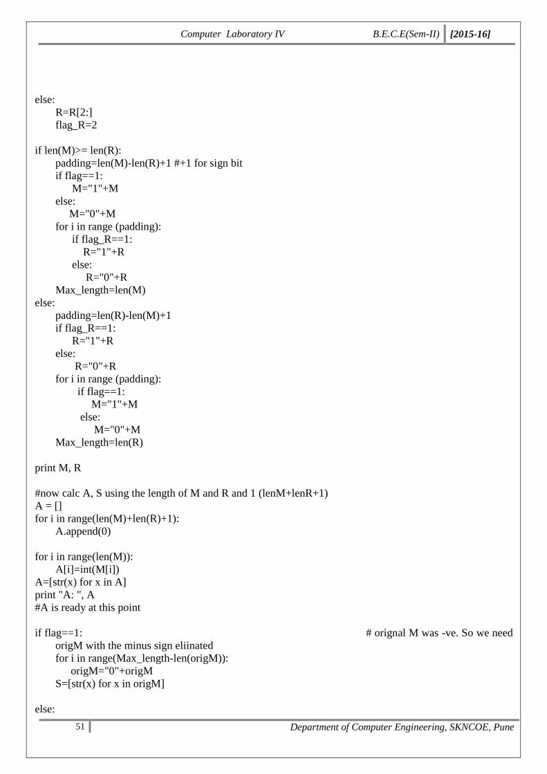
#now calc A, S using the length of M and R and 1 (lenM+lenR+1)
A = []
for i in range(len(M)+len(R)+1):
A.append(0)
for i in range(len(M)):
A[i]=int(M[i])
A=[str(x) for x in A]
print "A: ", A
#A is ready at this point
if flag==1: # orignal M was -ve. So we need
origM with the minus sign eliinated
for i in range(Max_length-len(origM)):
origM="0"+origM
S=[str(x) for x in origM]
else:
Computer Laboratory IV B.E.C.E(Sem-II) [2015-16]
52 Department of Computer Engineering, SKNCOE, Pune
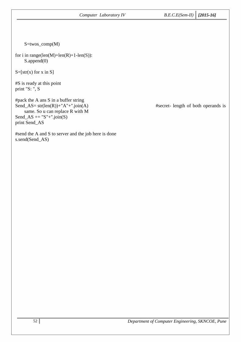
S=twos_comp(M)
for i in range(len(M)+len(R)+1-len(S)):
S.append(0)
S=[str(x) for x in S]
#S is ready at this point
print "S: ", S
#pack the A ans S in a buffer string
Send_AS= str(len(R))+"A"+''.join(A) #secret- length of both operands is
same. So u can replace R with M
Send_AS += "S"+''.join(S)
print Send_AS
#send the A and S to server and the job here is done
s.send(Send_AS)
Computer Laboratory IV B.E.C.E(Sem-II) [2015-16]
53 Department of Computer Engineering, SKNCOE, Pune
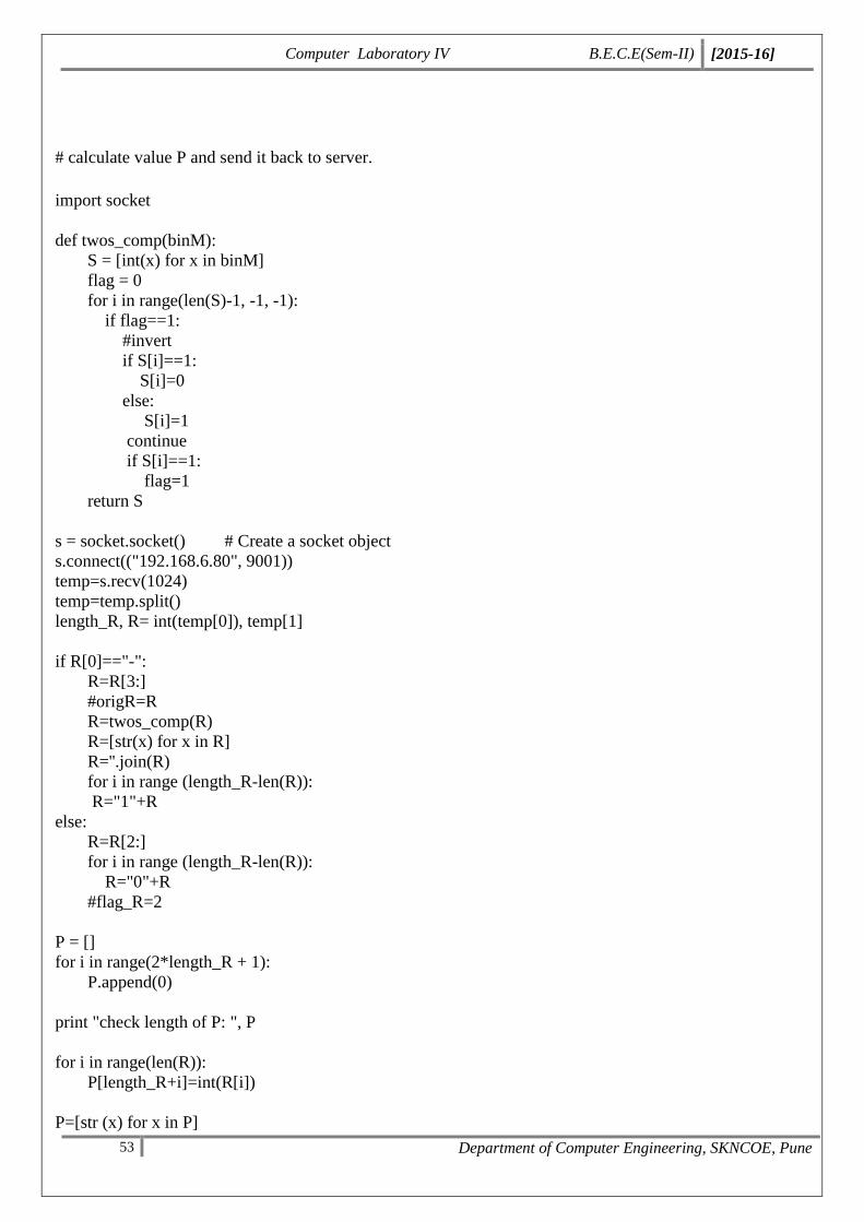
# calculate value P and send it back to server.
import socket
def twos_comp(binM):
S = [int(x) for x in binM]
flag = 0
for i in range(len(S)-1, -1, -1):
if flag==1:
#invert
if S[i]==1:
S[i]=0
else:
S[i]=1
continue
if S[i]==1:
flag=1
return S
s = socket.socket() # Create a socket object
s.connect(("192.168.6.80", 9001))
temp=s.recv(1024)
temp=temp.split()
length_R, R= int(temp[0]), temp[1]
if R[0]=="-":
R=R[3:]
#origR=R
R=twos_comp(R)
R=[str(x) for x in R]
R=''.join(R)
for i in range (length_R-len(R)):
R="1"+R
else:
R=R[2:]
for i in range (length_R-len(R)):
R="0"+R
#flag_R=2
P = []
for i in range(2*length_R + 1):
P.append(0)
print "check length of P: ", P
for i in range(len(R)):
P[length_R+i]=int(R[i])
P=[str (x) for x in P]

Computer Laboratory IV B.E.C.E(Sem-II) [2015-16]
54 Department of Computer Engineering, SKNCOE, Pune
P="".join(P)
print P
s.send("P"+P)
Computer Laboratory IV B.E.C.E(Sem-II) [2015-16]
55 Department of Computer Engineering, SKNCOE, Pune
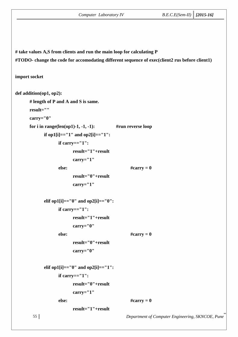
# take values A,S from clients and run the main loop for calculating P
#TODO- change the code for accomodating different sequence of exec(client2 rus before client1)
import socket
def addition(op1, op2):
# length of P and A and S is same.
result=""
carry="0"
for i in range(len(op1)-1, -1, -1): #run reverse loop
if op1[i]=="1" and op2[i]=="1":
if carry=="1":
result="1"+result
carry="1"
else: #carry = 0
result="0"+result
carry="1"
elif op1[i]=="0" and op2[i]=="0":
if carry=="1":
result="1"+result
carry="0"
else: #carry = 0
result="0"+result
carry="0"
elif op1[i]=="0" and op2[i]=="1":
if carry=="1":
result="0"+result
carry="1"
else: #carry = 0
result="1"+result
Computer Laboratory IV B.E.C.E(Sem-II) [2015-16]
56 Department of Computer Engineering, SKNCOE, Pune
carry="0"
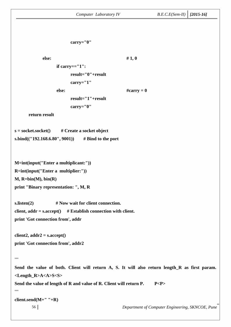
else: # 1, 0
if carry=="1":
result="0"+result
carry="1"
else: #carry = 0
result="1"+result
carry="0"
return result
s = socket.socket() # Create a socket object
s.bind(("192.168.6.80", 9001)) # Bind to the port
M=int(input("Enter a multiplicant:"))
R=int(input("Enter a multiplier:"))
M, R=bin(M), bin(R)
print "Binary representation: ", M, R
s.listen(2) # Now wait for client connection.
client, addr = s.accept() # Establish connection with client.
print 'Got connection from', addr
client2, addr2 = s.accept()
print 'Got connection from', addr2
'''
Send the value of both. Client will return A, S. It will also return length_R as first param.
<Length_R>A<A>S<S>
Send the value of length of R and value of R. Client will return P. P<P>
'''
client.send(M+" "+R)
Computer Laboratory IV B.E.C.E(Sem-II) [2015-16]
57 Department of Computer Engineering, SKNCOE, Pune
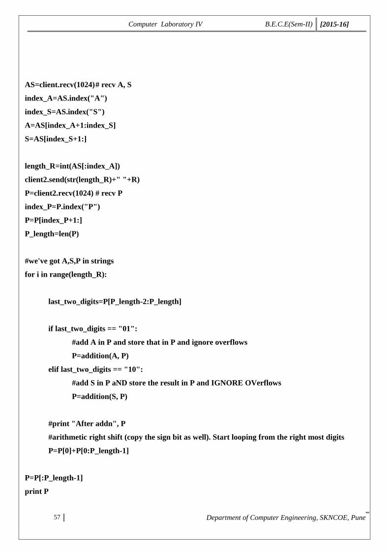
AS=client.recv(1024) # recv A, S
index_A=AS.index("A")
index_S=AS.index("S")
A=AS[index_A+1:index_S]
S=AS[index_S+1:]
length_R=int(AS[:index_A])
client2.send(str(length_R)+" "+R)
P=client2.recv(1024) # recv P
index_P=P.index("P")
P=P[index_P+1:]
P_length=len(P)
#we've got A,S,P in strings
for i in range(length_R):
last_two_digits=P[P_length-2:P_length]
if last_two_digits == "01":
#add A in P and store that in P and ignore overflows
P=addition(A, P)
elif last_two_digits == "10":
#add S in P aND store the result in P and IGNORE OVerflows
P=addition(S, P)
#print "After addn", P
#arithmetic right shift (copy the sign bit as well). Start looping from the right most digits
P=P[0]+P[0:P_length-1]
P=P[:P_length-1]
print P
Computer Laboratory IV B.E.C.E(Sem-II) [2015-16]
58 Department of Computer Engineering, SKNCOE, Pune
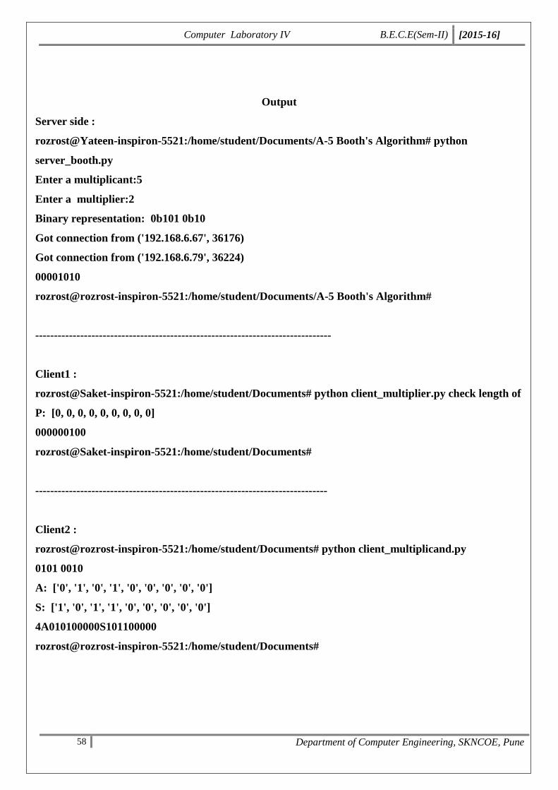
Output
Server side :
rozrost@Yateen-inspiron-5521:/home/student/Documents/A-5 Booth's Algorithm# python
server_booth.py
Enter a multiplicant:5
Enter a multiplier:2
Binary representation: 0b101 0b10
Got connection from ('192.168.6.67', 36176)
Got connection from ('192.168.6.79', 36224)
00001010
rozrost@rozrost-inspiron-5521:/home/student/Documents/A-5 Booth's Algorithm#
-------------------------------------------------------------------------------
Client1 :
rozrost@Saket-inspiron-5521:/home/student/Documents# python client_multiplier.py check length of
P: [0, 0, 0, 0, 0, 0, 0, 0, 0]
000000100
rozrost@Saket-inspiron-5521:/home/student/Documents#
------------------------------------------------------------------------------
Client2 :
rozrost@rozrost-inspiron-5521:/home/student/Documents# python client_multiplicand.py
0101 0010
A: ['0', '1', '0', '1', '0', '0', '0', '0', '0']
S: ['1', '0', '1', '1', '0', '0', '0', '0', '0']
4A010100000S101100000
rozrost@rozrost-inspiron-5521:/home/student/Documents#
Computer Laboratory IV B.E.C.E(Sem-II) [2015-16]
59 Department of Computer Engineering, SKNCOE, Pune
Assignment No. 6
Title
Use Business intelligence and analytics tools to recommend
the combination of share purchases and salesfor maximizing
the profit.
Roll No.
Class B.E. (C.E.)
Date
Subject Computer Lab IV
Signature
Computer Laboratory IV B.E.C.E(Sem-II) [2015-16]
60 Department of Computer Engineering, SKNCOE, Pune
Assignment No: 6
Title: Use Business intelligence and analytics tools to recommend the combination of share
purchases and sales for maximizing the profit.
Objectives:
To study different types of BI analytics tools.
To study the representation and implementation of BI tools for maximizing shares profit.
Theory:
Business Intelligence: -
Business intelligence (BI) is a technology-driven process for analyzing data and presenting actionable
information to help corporate executives, business managers and other end users make more informed
business decisions. BI encompasses a variety of tools, applications and methodologies that enable
organizations to collect data from internal systems and external sources, prepare it for analysis, develop
and run queries against the data, and create reports, dashboards and data visualizations to make the
analytical results available to corporate decision makers as well as operational workers.
The potential benefits of business intelligence programs include accelerating and improving decision
making; optimizing internal business processes; increasing operational efficiency; driving new
revenues; and gaining competitive advantages over business rivals. BI systems can also help companies
identify market trends and spot business problems that need to be addressed.
Business intelligence combines a broad set of data analysis applications, including ad hoc analysis and
querying, enterprise reporting, online analytical processing (OLAP), mobile BI, real-time BI,
operational BI, cloud and software as a service BI, open source BI, collaborative BI and location
intelligence. BI technology also includes data visualization software for designing charts and other
infographics, as well as tools for building BI dashboards and performance scorecards that display
visualized data on business metrics and key performance indicators in an easy-to-grasp way. BI
applications can be bought separately from different vendors or as part of a unified BI platform from a
single vendor.
Computer Laboratory IV B.E.C.E(Sem-II) [2015-16]
61 Department of Computer Engineering, SKNCOE, Pune
BI Programs:
BI programs can also incorporate forms of advanced analytics, such as data mining, predictive analytics,
text mining, statistical analysis and big data analytics. In many cases though, advanced analytics
projects are conducted and managed by separate teams of data scientists, statisticians, predictive
modelers and other skilled analytics professionals, while BI teams oversee more straightforward
querying and analysis of business data.
BI Data:
Business intelligence data typically is stored in a data warehouse or smaller data marts that hold subsets
of a company's information. In addition, Hadoop systems are increasingly being used within BI
architectures as repositories or landing pads for BI and analytics data, especially for unstructured data,
log files, sensor data and other types of big data. Before it's used in BI applications, raw data from
different source systems must be integrated, consolidated and cleansed using data integration and data
quality tools to ensure that users are analyzing accurate and consistent information.
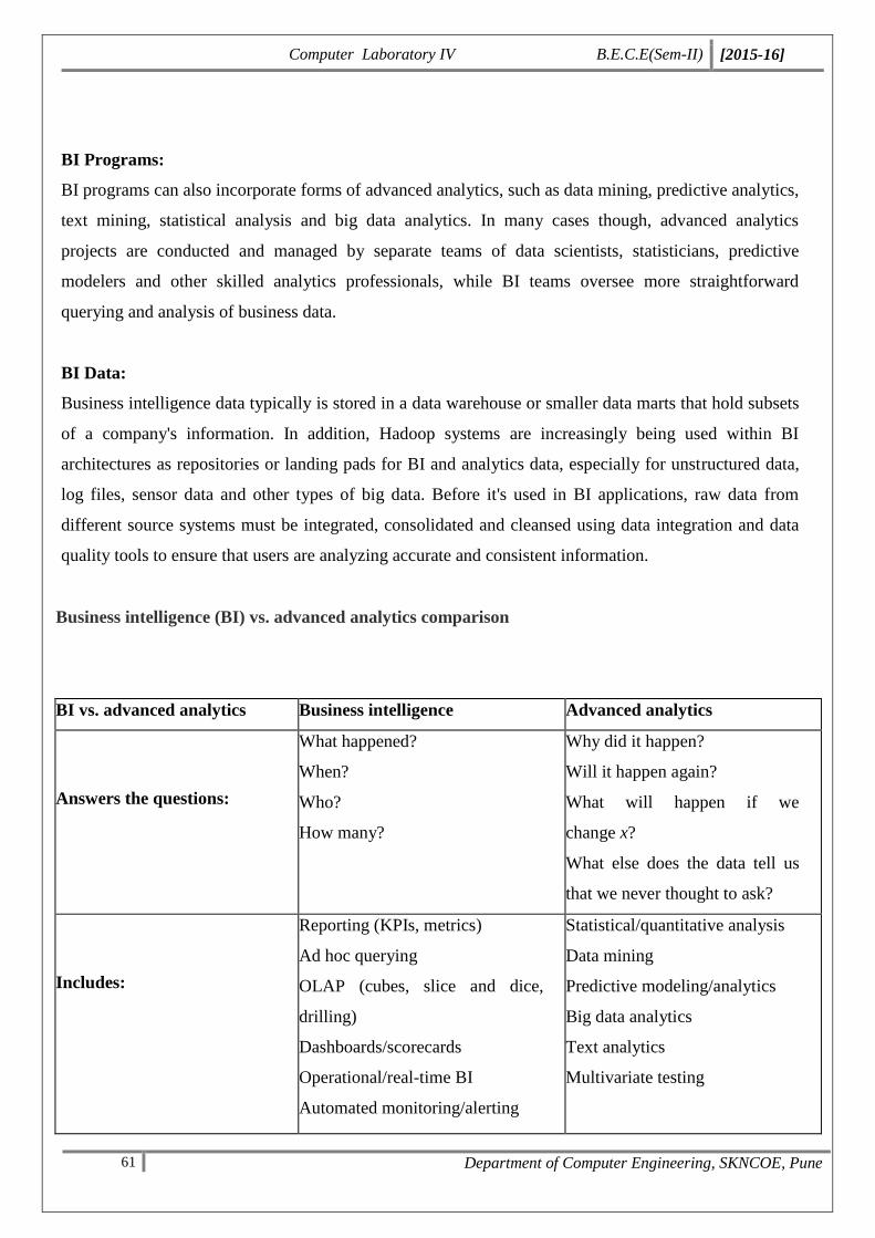
Business intelligence (BI) vs. advanced analytics comparison
BI vs. advanced analytics Business intelligence Advanced analytics
Answers the questions:
What happened?
When?
Who?
How many?
Why did it happen?
Will it happen again?
What will happen if we
change x?
What else does the data tell us
that we never thought to ask?
Includes:
Reporting (KPIs, metrics)
Ad hoc querying
OLAP (cubes, slice and dice,
drilling)
Dashboards/scorecards
Operational/real-time BI
Automated monitoring/alerting
Statistical/quantitative analysis
Data mining
Predictive modeling/analytics
Big data analytics
Text analytics
Multivariate testing
Computer Laboratory IV B.E.C.E(Sem-II) [2015-16]
62 Department of Computer Engineering, SKNCOE, Pune
BI Tools:
Business Intelligence tools provide companies reliable information and true insights in order to improve
decision making and social collaboration. With business intelligence you’ll be able to produce much
better company results. The BI tools provide the means for efficient reporting, thorough analysis of
(big) data, statistics and analytics and dashboards displaying KPIs.
Bring your company data to life with BI tools
Bring your company data to life by combining, analyzing and visualizing all that data very easily. The
tools will help you to see and understand the success factors of your business more quickly.
And where things (might) go wrong and where you need to make adjustments. They give employees and
managers the possibility to improve business processes on a daily basis by using correct information and
relevant insights.
Selecting the wrong tool might hurt
Companies who are not successful often have an issue with their information infrastructure. They may
have selected the wrong Business Intelligence tool or perhaps they don’t use business intelligence-tools
at all.They have not been able to implement BI and are still in the dark and that hurts company results.
What are the biggest benefits of BI tools?
√ Improve the overall performance of your organization, departments and teams.
√ Make fact-based decisions without neglecting the intuition of experienced employees.
√ Enhance the business processes in the organization using the right visualizations.
√ Easy monitoring and reporting of your genuine KPIs using role-based dashboards.
How can you easily select one of the tools for your organization? Step 1:
Define the key bi tool selection criteria, both the user and IT requirements.
Step 2:
With a list of questions you need to contact all the vendors to get the answers.
Step 3:
Validate and analyze all the information from the Business Intelligence vendors.
Step 4:
Make a short list for a proof-of-concept (POC) and perform the POC.
Computer Laboratory IV B.E.C.E(Sem-II) [2015-16]
63 Department of Computer Engineering, SKNCOE, Pune
Step 5:
Choose the tool / platform that suits your needs and price criteria best.
How can you compare BI tools very quickly?
Business Intelligence tools come in many different flavors. All the tools run on the Windows platform
for example, but only a few support the different flavors of Unix and Linux. Some have excellent
functionality for pixel perfect reporting and others do better in dash-boarding and predictive analytics.
KPIs
What are Key Performance Indicators (KPIs) and how do you choose which ones to use? It is difficult
to determine what are genuine KPIs, a little like looking for a needle in a haystack. The problem being
that we are trying to shed light on is the (future) performance of our most critical internal processes
which will allow us to achieve the organization’s (strategic) goals within the chosen policies.A KPI
should be important enough that achieving it will have a huge impact on the total performance of the
organization (or part of the organization).
The King of KPIs, David Parmenter, said once “Key performance indicators (KPIs), while used
commonly around the world, have never until now been clearly defined.” This is the reason that it is
essential to understand which types of (performance) indicators actually exist:
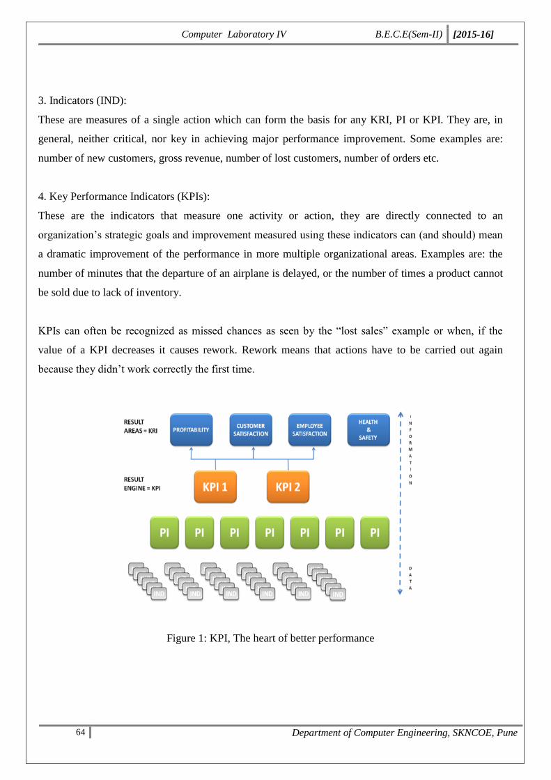
1. Key Results Indicators (KRIs):
These are complex indicators based on the total achievement of a broad range of actions, for example,
the profitability of a company, the level of satisfaction of the employees, or customer satisfaction levels.
2. Performance Indicators (PIs):
These are very specific indicators, they tell us what we need to achieve in a given area and are not
particularly “key” to achieving efficient performance in the organization’s internal processes. Examples
are: the profit achieved from the company’s 10 largest customers or the revenue growth percentage for a
given product or service. These can, of course, be very useful things to measure, but in general they are
not critical for achieving better performance in multiple result areas of the organization at the same
time. By concentrating solely on performance in terms of, for example, revenue growth we often miss
the fact that we are no longer making any profit because the customers and employees have become
dissatisfied.
Computer Laboratory IV B.E.C.E(Sem-II) [2015-16]
64 Department of Computer Engineering, SKNCOE, Pune
3. Indicators (IND):
These are measures of a single action which can form the basis for any KRI, PI or KPI. They are, in
general, neither critical, nor key in achieving major performance improvement. Some examples are:
number of new customers, gross revenue, number of lost customers, number of orders etc.
4. Key Performance Indicators (KPIs):
These are the indicators that measure one activity or action, they are directly connected to an
organization’s strategic goals and improvement measured using these indicators can (and should) mean
a dramatic improvement of the performance in more multiple organizational areas. Examples are: the
number of minutes that the departure of an airplane is delayed, or the number of times a product cannot
be sold due to lack of inventory.
KPIs can often be recognized as missed chances as seen by the “lost sales” example or when, if the
value of a KPI decreases it causes rework. Rework means that actions have to be carried out again
because they didn’t work correctly the first time.
Figure 1: KPI, The heart of better performance
Computer Laboratory IV B.E.C.E(Sem-II) [2015-16]
65 Department of Computer Engineering, SKNCOE, Pune
Proprietary Products:
ActiveReports, Actuate Corporation, ApeSoft, Diamond Financial Management System, Birst,
BOARD, ComArch, Data Applied, Decision Support Panel, Dexon Business, Intelligence, Domo,
Dundas Data Visualization, Inc., Dimensional Insight, Dynamic AI,
Entalysis, Grapheur, GoodData - Cloud Based, InfoCaptor Dashboard, IBM CognosicCube. IDV
Solutions Visual FusionInetSoft, RubyReport, Information Builders,InfoZoom, Jackbe, Jaspersoft (now
TIBCO, iReport,Jasper Studio, Jasper Analysis, Jasper ETL, Jasper Library), Jedox, JReport (from
Jinfonet Software), Klipfolio Dashboard,Lavastorm, LIONsolver, List and Label, Logi Analytics,
Looker, Lumalytics, Manta Tools,Microsoft, SQL Server Reporting Services, SQL Server Analysis
Services, PerformancePoint Server 2007, Proclarity, Power Pivot, MicroStrategy, myDIALS,
NextAction, Numetric, Oracle, Hyperion Solutions Corporation, Business Intelligence Suite Enterprise
Edition, Panorama Software, Pentaho (now Hitachi Data Systems),Pervasive DataRush, PRELYTIS,
Qlik, Quantrix, RapidMiner, Roambi, SAP NetWeaver, SiSense, SAS, Siebel Systems, Spotfire (now
Tibco), Sybase IQ, Tableau Software, TARGIT Business Intelligence, Teradata, Lighthouse,
VeroAnalytics, XLCubed, Yellowfin Business Intelligence, Zoho Reports (as part of the Zoho Office
Suite).
Tableau Software:
It is an American computer software company headquartered in Seattle, Washington. It produces a
family of interactive data visualization products focused on business intelligence.
Tableau offers five main products:
1. Tableau Desktop,
2. Tableau Server,
3. Tableau Online,
4. Tableau Reader and
5. Tableau Public.
Tableau Public and Tableau Reader are free to use, while both Tableau Server and Tableau Desktop
come with a 14-day fully functional free trial period, after which the user must pay for the software.

Computer Laboratory IV B.E.C.E(Sem-II) [2015-16]
66 Department of Computer Engineering, SKNCOE, Pune
Tableau Desktop comes in both a Professional and a lower cost Personal edition. Tableau Online is
available with an annual subscription for a single user, and scales to support thousands of users.
See what you can create
With Tableau, you’ll not only analyze data faster, but you’ll also create interactive visualizations,
identify trends and discover new insights. You’ll be answering your own questions as fast as you can
think of them. See how others transformed their data from numbers on a spreadsheet to informative
presentations in these dashboards from the Tableau Visualization Gallery.
Sports Comparison Storm Tracking iPhone TweetsCrime Spotting
Following Stock Market KPI’s can be created based on share market data:
• Who are Market Gainers :(Top 5) Which stocks show max gain from opening value
• Who are Market Losers (bottom 5): Which stocks show max loss from opening value
• How one stock is comparing with other stocks based on Gain or loss.
• % Change in Stock Value---Gain Or loss
• The volume of stocks.
• Sector Wise Performance (Stock market sectors are a way of classifying stocks, wherein stocks in
similar industries are grouped together.)

Computer Laboratory IV B.E.C.E(Sem-II) [2015-16]
67 Department of Computer Engineering, SKNCOE, Pune
Similar experience is available at :
http://www.tableau.com/solutions/real-estate-analysis
Conclusion:
Hence, we studies BI analytical tools.
Computer Laboratory IV B.E.C.E(Sem-II) [2015-16]
68 Department of Computer Engineering, SKNCOE, Pune
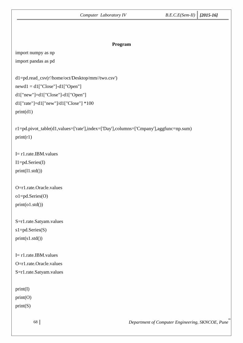
Program
import numpy as np
import pandas as pd
d1=pd.read_csv(r'/home/oct/Desktop/mm//two.csv')
newd1 = d1["Close"]-d1["Open"]
d1["new"]=d1["Close"]-d1["Open"]
d1["rate"]=d1["new"]/d1["Close"] *100
print(d1)
r1=pd.pivot_table(d1,values=['rate'],index=['Day'],columns=['Cmpany'],aggfunc=np.sum)
print(r1)
I= r1.rate.IBM.values
I1=pd.Series(I)
print(I1.std())
O=r1.rate.Oracle.values
o1=pd.Series(O)
print(o1.std())
S=r1.rate.Satyam.values
s1=pd.Series(S)
print(s1.std())
I= r1.rate.IBM.values
O=r1.rate.Oracle.values
S=r1.rate.Satyam.values
print(I)
print(O)
print(S)

Computer Laboratory IV B.E.C.E(Sem-II) [2015-16]
69 Department of Computer Engineering, SKNCOE, Pune
s1=S.sum()
o1=O.sum()
i1=I.sum()
print(s1)
print(o1)
print(i1)
max(s1,o1,i1)
print("You may Purchase Oracle Share as its rate of profit is high")

Computer Laboratory IV B.E.C.E(Sem-II) [2015-16]
70 Department of Computer Engineering, SKNCOE, Pune
Output
Day,Cmpany,Open,Close
1,IBM,250,200
1,Oracle,300,302
1,Satyam,150,151
2,IBM,252,252
2,Oracle,305,310
2,Satyam,152,151
3,IBM,255,251
3,Oracle,301,302
3,Satyam,151,151
4,IBM,251,252
4,Oracle,300,302
4,Satyam,152,155

Computer Laboratory IV B.E.C.E(Sem-II) [2015-16]
71 Department of Computer Engineering, SKNCOE, Pune
Group B
Assignments
Computer Laboratory IV B.E.C.E(Sem-II) [2015-16]
72 Department of Computer Engineering, SKNCOE, Pune
Assignment No. 1
Title
8-Queens Matrix is Stored using JSON/XML having first Queen
placed, use back-tracking to place remaining Queens to generate
final 8-queen’s Matrix using Python. Create a backtracking
scenario and use HPC architecture (Preferably BBB) for
computation of next placement of a queen.
Roll No.
Class B.E. (C.E.)
Date
Subject Computer Lab IV
Signature
Computer Laboratory IV B.E.C.E(Sem-II) [2015-16]
73 Department of Computer Engineering, SKNCOE, Pune
Assignment No: 1
Title: 8-Queens Matrix is Stored using JSON/XML having first Queen placed, use back-
tracking to place remaining Queens to generate final 8-queen’s Matrix using Python.
Create a backtracking scenario and use HPC architecture (Preferably BBB) for
computation of next placement of a queen.
Objectives:
To develop problem solving abilities using HPC
To study the representation, implementation of IP Spoofing and Web Spoofing.
Theory:
1. Eight queens’ puzzle
The eight queens’ puzzle is the problem of placing eight chess queens on an 8×8 chessboard so that no
two queens threaten each other. Thus, a solution requires that no two queens share the same row,
column, or diagonal. The eight queens puzzle is an example of the more general n-queens problem of
placing n queens on an n×n chessboard, where solutions exist for all natural numbers n with the
exception of n=2 and n=3.
The problem can be quite computationally expensive as there are 4,426,165,368 (i.e., 64C8) possible
arrangements of eight queens on an 8×8 board, but only 92 solutions. It is possible to use shortcuts
that reduce computational requirements or rules of thumb that avoids brute-force computational
techniques. For example, just by applying a simple rule that constrains each queen to a single column
(or row), though still considered brute force, it is possible to reduce the number of possibilities to just
16,777,216 (that is, 88) possible combinations. Generating permutations further reduces the
possibilities to just 40,320 (that is, 8!), which are then checked for diagonal attacks.
2. Backtracking :
Backtracking is a general algorithm for finding all (or some) solutions to some computational
problems, notably constraint satisfaction problems that incrementally builds candidates to the
solutions, and abandons each partial candidate c ("backtracks") as soon as it determines that c cannot
possibly be completed to a valid solution.
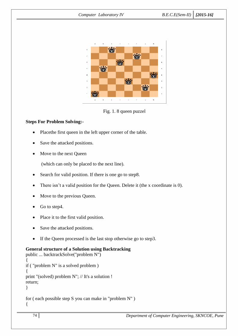
Computer Laboratory IV B.E.C.E(Sem-II) [2015-16]
74 Department of Computer Engineering, SKNCOE, Pune
Fig. 1. 8 queen puzzel
Steps For Problem Solving:-
Placethe first queen in the left upper corner of the table.
Save the attacked positions.
Move to the next Queen
(which can only be placed to the next line).
Search for valid position. If there is one go to step8.
There isn’t a valid position for the Queen. Delete it (the x coordinate is 0).
Move to the previous Queen.
Go to step4.
Place it to the first valid position.
Save the attacked positions.
If the Queen processed is the last stop otherwise go to step3.
General structure of a Solution using Backtracking
public ... backtrackSolve("problem N")
{
if ( "problem N" is a solved problem )
{
print "(solved) problem N"; // It's a solution !
return;
}
for ( each possible step S you can make in "problem N" )
{
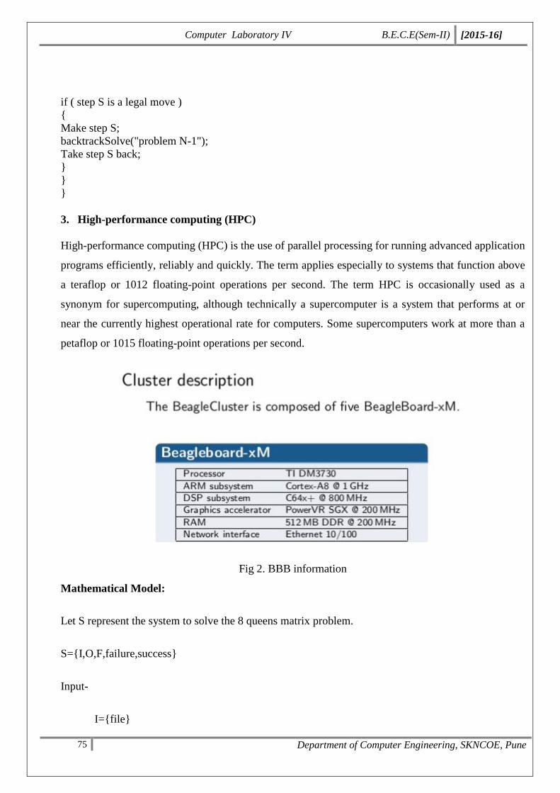
Computer Laboratory IV B.E.C.E(Sem-II) [2015-16]
75 Department of Computer Engineering, SKNCOE, Pune
if ( step S is a legal move )
{
Make step S;
backtrackSolve("problem N-1");
Take step S back;
}
}
}
3. High-performance computing (HPC)
High-performance computing (HPC) is the use of parallel processing for running advanced application
programs efficiently, reliably and quickly. The term applies especially to systems that function above
a teraflop or 1012 floating-point operations per second. The term HPC is occasionally used as a
synonym for supercomputing, although technically a supercomputer is a system that performs at or
near the currently highest operational rate for computers. Some supercomputers work at more than a
petaflop or 1015 floating-point operations per second.
Fig 2. BBB information
Mathematical Model:
Let S represent the system to solve the 8 queens matrix problem.
S={I,O,F,failure,success}
Input-
I={file}
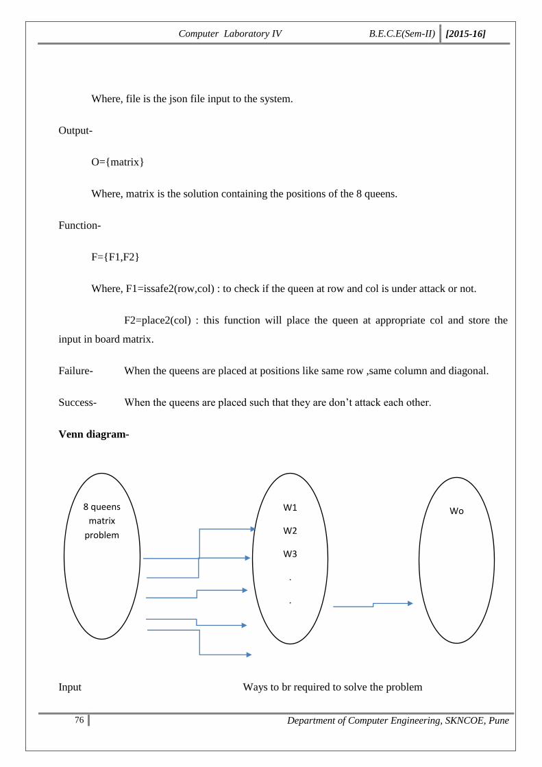
Computer Laboratory IV B.E.C.E(Sem-II) [2015-16]
76 Department of Computer Engineering, SKNCOE, Pune
Where, file is the json file input to the system.
Output-
O={matrix}
Where, matrix is the solution containing the positions of the 8 queens.
Function-
F={F1,F2}
Where, F1=issafe2(row,col) : to check if the queen at row and col is under attack or not.
F2=place2(col) : this function will place the queen at appropriate col and store the
input in board matrix.
Failure- When the queens are placed at positions like same row ,same column and diagonal.
Success- When the queens are placed such that they are don’t attack each other.
Venn diagram-
Input Ways to br required to solve the problem
8 queens
matrix
problem
W1
W2
W3
.
.
Wn
Wo

Computer Laboratory IV B.E.C.E(Sem-II) [2015-16]
77 Department of Computer Engineering, SKNCOE, Pune
Conclusion:
Hence we studied and implemented 8 Queen’s algorithm.
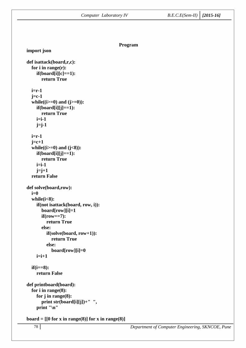
Computer Laboratory IV B.E.C.E(Sem-II) [2015-16]
78 Department of Computer Engineering, SKNCOE, Pune
Program
import json
def isattack(board,r,c):
for i in range(r):
if(board[i][c]==1):
return True
i=r-1
j=c-1
while((i>=0) and (j>=0)):
if(board[i][j]==1):
return True
i=i-1
j=j-1
i=r-1
j=c+1
while((i>=0) and (j<8)):
if(board[i][j]==1):
return True
i=i-1
j=j+1
return False
def solve(board,row):
i=0
while(i<8):
if(not isattack(board, row, i)):
board[row][i]=1
if(row==7):
return True
else:
if(solve(board, row+1)):
return True
else:
board[row][i]=0
i=i+1
if(i==8):
return False
def printboard(board):
for i in range(8):
for j in range(8):
print str(board[i][j])+" ",
print "\n"
board = [[0 for x in range(8)] for x in range(8)]
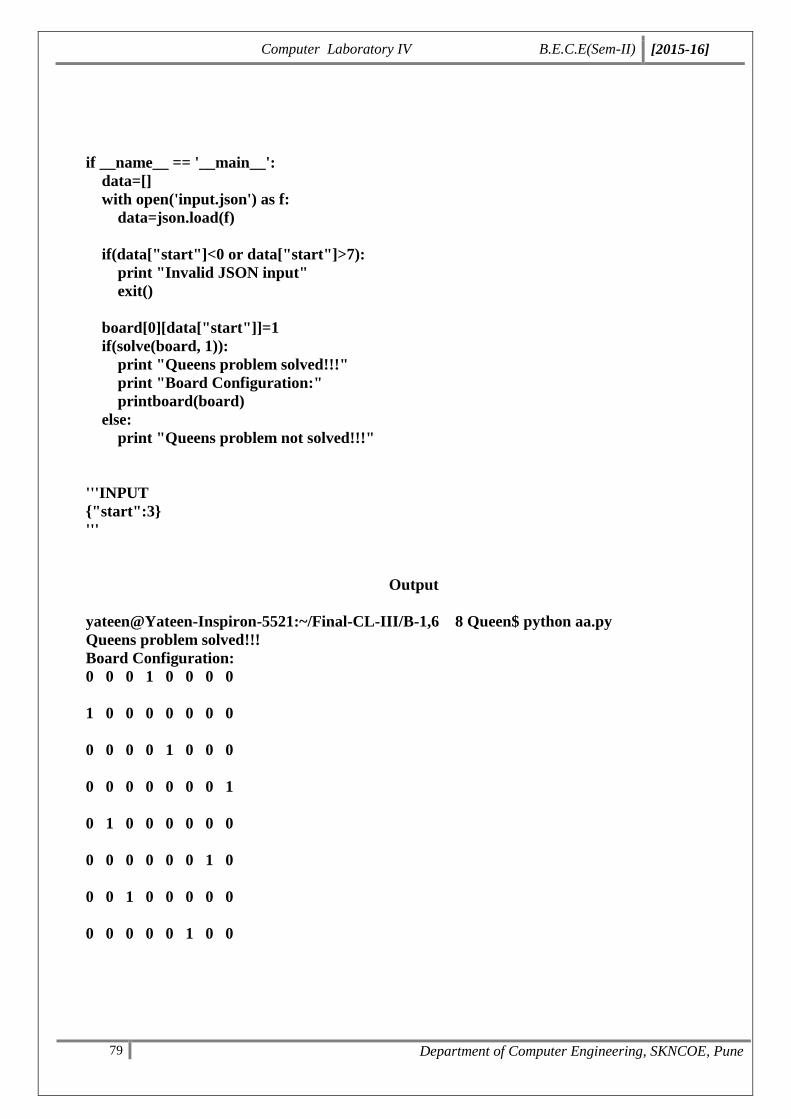
Computer Laboratory IV B.E.C.E(Sem-II) [2015-16]
79 Department of Computer Engineering, SKNCOE, Pune
if __name__ == '__main__':
data=[]
with open('input.json') as f:
data=json.load(f)
if(data["start"]<0 or data["start"]>7):
print "Invalid JSON input"
exit()
board[0][data["start"]]=1
if(solve(board, 1)):
print "Queens problem solved!!!"
print "Board Configuration:"
printboard(board)
else:
print "Queens problem not solved!!!"
'''INPUT
{"start":3}
'''
Output
yateen@Yateen-Inspiron-5521:~/Final-CL-III/B-1,6 8 Queen$ python aa.py
Queens problem solved!!!
Board Configuration:
0 0 0 1 0 0 0 0
1 0 0 0 0 0 0 0
0 0 0 0 1 0 0 0
0 0 0 0 0 0 0 1
0 1 0 0 0 0 0 0
0 0 0 0 0 0 1 0
0 0 1 0 0 0 0 0
0 0 0 0 0 1 0 0
Computer Laboratory IV B.E.C.E(Sem-II) [2015-16]
80 Department of Computer Engineering, SKNCOE, Pune
Assignment No.
2
Title Develop a stack sampling using threads using VTune
Amplifier.
Roll No.
Class B.E. (C.E.)
Date
Subject Computer Lab IV
Signature
Computer Laboratory IV B.E.C.E(Sem-II) [2015-16]
81 Department of Computer Engineering, SKNCOE, Pune
Assignment No:2
Title: Develop a stack sampling using threads using VTune Amplifier.
Objectives:
To understand sampling and VTune Amplifier.
Theory:
Intel VTune Amplifier is a commercial application for software performance analysis for 32 and
64-bit x86 based machines, and has both GUI and command line interfaces. It is available for
both Linux and Microsoft Windows operating systems. Although basic features work on both Intel
and AMD hardware, advanced hardware-based sampling requires an Intel-manufactured CPU. It is
available as part of Intel Parallel Studio or as a stand-alone product.
VTune Amplifier assists in various kinds of code profiling including stack sampling, thread
profiling and hardware event sampling. The profiler result consists of details such as time spent in
each sub routine which can be drilled down to the instruction level. The time taken by the
instructions is indicative of any stalls in the pipeline during instruction execution. The tool can be
also used to analyze thread performance. The new GUI can filter data based on a selection in the
timeline.
Features:
Software sampling
Works on x86 compatible processors and gives both the locations where time is spent and
the call stack used.
JIT profiling support
Profiles dynamically generated code.
Locks and waits analysis
Finds long synchronization waits that occur when cores are underutilized.
Threading timeline
Shows thread relationships to identify load balancing and synchronization issues. It can also
be used to select a region of time and filter the results. This can remove the clutter of data
gathered during uninteresting times like application start-up.
Source view
Sampling results are displayed line by line on the source / assembly code.
Hardware event sampling
Computer Laboratory IV B.E.C.E(Sem-II) [2015-16]
82 Department of Computer Engineering, SKNCOE, Pune
This uses the on chip performance monitoring unit and requires an Intel processor. It can
find specific tuning opportunities like cache misses and branch mispredictions.
Performance Profiling with Intel VTune Amplifier XE
System Requirements
Processor requirements
The list of supported processors is constantly being extended. Here is a partial list of
processors where the EBS analysis is enabled:
Mobile Processors
Intel® Atom™ Processor
Intel® Core™ i7 Mobile Processor Extreme Edition (including 2nd, 3rd, 4th and 5th
Generation Intel® Core™ processors)
Intel® Core™ i7, i5, i3 Mobile Processors (including 2nd, 3rd, 4th, 5th and 6th Generation
Intel® Core™ processors)
Intel® Core™2 Extreme Mobile Processor
Intel® Core™2 Quad Mobile Processor
Intel® Core™2 Duo Mobile Processor
Intel® Pentium® Mobile Processor
Desktop Processors
Intel® Atom™ Processor
Intel® Core™ i7 Desktop Processor Extreme Edition (including 2nd, 3rd, 4th and 5th
Generation Intel® Core™ processors)
Intel® Core™ i7, i5, i3 Desktop Processors (including 2nd, 3rd, 4th, 5th and 6th Generation
Intel® Core™ processors)
Intel® Core™2 Quad Desktop Processor
Intel® Core™2 Extreme Desktop Processor
Intel® Core™2 Duo Desktop Processor
Computer Laboratory IV B.E.C.E(Sem-II) [2015-16]
83 Department of Computer Engineering, SKNCOE, Pune
Server and Workstation Processors
Intel® Xeon® processors E7 family (including v2 and v3)
Intel® Xeon® processor E5 family (including v2 and v3)
Intel® Xeon® processors E3 family (including v2, v3 and v4)
Intel® Xeon® Processor D family
Intel® Xeon® Processor 7000 Sequence
Intel® Xeon® Processor 6000 Sequence
Intel® Xeon® Processor 5000 Sequence
Intel® Xeon® Processor 3000 Sequence
Intel® Xeon Phi™ Coprocessors
Quad-Core Intel® Xeon® processors 7xxx, 5xxx, and 3xxx series
Dual-Core Intel® Xeon® processors 7xxx, 5xxx, and 3xxx series
System Memory Requirements
At least 2 GB of RAM
Disk Space Requirements
900 MB free disk space required for all product features and all architectures
Software Requirements
Supported Linux distributions:
Red Hat* Enterprise Linux 5, 6 and 7 [1]
CentOS* versions equivalent to Red Hat* Enterprise Linux* versions listed above
SUSE* Linux* Enterprise Server (SLES) 11 and 12
Fedora* 221 and 232
Ubuntu* 12.04, 14.04 and 15.1004
Debian* 7.0 and 8.0
Supported compilers:
Intel® C/C++ Compiler 11 and higher
Intel® Fortran Compiler 11 and higher
GNU C/C++ Compiler 3.4.6 and higher
Computer Laboratory IV B.E.C.E(Sem-II) [2015-16]
84 Department of Computer Engineering, SKNCOE, Pune
Application coding requirements
Supported programming languages:
Fortran
C
C++
Java*
OpenCL*
Concurrency and Locks and Waits analysis types interpret the use of constructs from the
following threading methodologies:
Intel® Threading Building Blocks
Posix* Threads on Linux*
OpenMP* [2]
Intel's C/C++ Parallel Language Extensions
Supported Java* environments
Oracle* JVM 6, 7 and 8 – Hotspots and Hardware event-based analysis types
IBM* J9 – Hardware event-based analysis types only
Supported OpenCL* environments:
Intel® SDK for OpenCL Applications XE 2013
Hardware event-based sampling analysis with stacks requirements
Linux kernel version 2.6.32 or above
Driverless hardware event-based sampling analysis:
Linux kernel version 2.6.32 or above, exporting CPU PMU programming details over
/sys/bus/event_source/devices/cpu/format file system
Supported Intel® Manycore Platform Software Stack (Intel® MPSS) versions for Intel®
Xeon Phi™ co-processor profiling:
Hardware event-based sampling analysis: the MPSS 2.1, 3.3.*, 3.4.*, 3.5.* and 3.6*
Hardware event-based sampling analysis with stacks: the MPSS 3.3.5, 3.4, 3.4.1, 3.4.2,
3.4.3, 3.4.4, 3.4.5, 3.5.2, 3.6
Computer Laboratory IV B.E.C.E(Sem-II) [2015-16]
85 Department of Computer Engineering, SKNCOE, Pune
Issues and Limitations
Running time is attributed to the next instruction
1. To collect the data about time-consuming running regions of the target, the VTune™
Amplifier XE interrupts executing target threads and attributes the time to the context IP
address.
2. Due to the collection mechanism, the captured IP address points to an instruction AFTER
the one that is actually consuming most of the time. This leads to the running time being
attributed to the next instruction (or, rarely to one of the subsequent instructions) in the
Assembly view. In rare cases, this can also lead to wrong attribution of running time in the
source - the time may be erroneously attributed to the source line AFTER the actual hot line.
3. In case the inline mode is ON and the program has small functions inlined at the hotspots,
this can cause the running time to be attributed to a wrong function since the next instruction
can belong to a different function in tightly inlined code.
An application that allocates massive chunks of memory may fail to work under VTune
Amplifier XE (200083850)
1. If a 32-bit application allocates massive chunks of memory (close to 2 GB) in the heap, it
may fail to launch under the VTune Amplifier XE while running fine on its own. This
happens because the VTune Amplifier XE requires additional memory when profiling an
application. The workaround could be in using larger address space (for example, converting
the project to 64-bit).
2. Hardware event-based analysis may crash certain Intel® Core™ i7 processor-based systems
when deep sleep states are enabled (200149603)
3. On some Intel® Core™ i7 processor-based (code named Nehalem) systems with C-states
enabled, sampling may cause system hanging due to a known hardware issue To avoid this,
disable the “Cn(ACPI Cn) report to OS” BIOS option before sampling with the VTune
Amplifier XE analyzer on Intel Core i7 processor-based systems .
1. Red Hat Enterprise Linux 5* is deprecated. Support for this operating system version is
deprecated and may be removed in a future release.

Computer Laboratory IV B.E.C.E(Sem-II) [2015-16]
86 Department of Computer Engineering, SKNCOE, Pune
2. VTune Amplifier XE supports analysis of OpenMP* applications built with Intel® Fortran
Compiler Professional Edition version 11.0 or higher, Intel® C++ Compiler Professional Edition
version 11.0 or higher, or GNU* C/C++ Compiler 4.2 or higher.
3. 32-bit graphical host deprecated. The 32-bit VTune Amplifier graphical host is deprecated and
may be removed in a future release. Thus, in the future release, a 64-bit OS host will be required to
graphically analyze collected profile data. Command line profiling and reporting on 32-bit OS hosts
will still be supported.
Conclusion:
Hence we studied unloaded stack sampling using threads and using VTune.
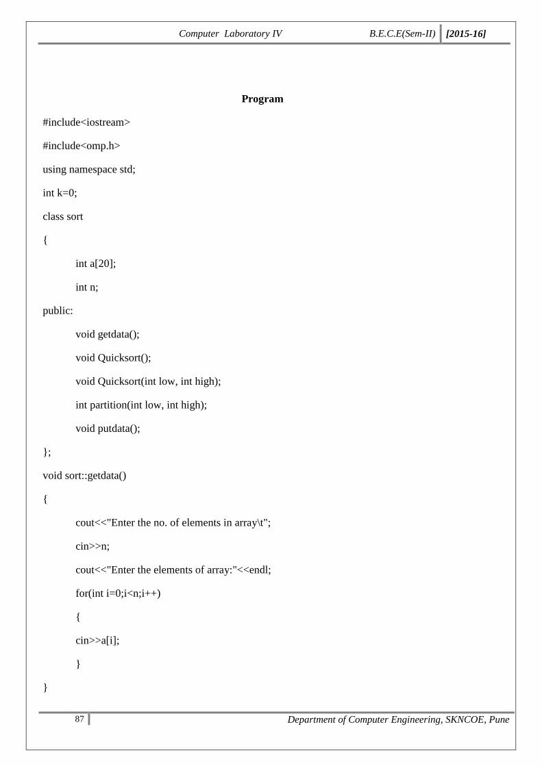
Computer Laboratory IV B.E.C.E(Sem-II) [2015-16]
87 Department of Computer Engineering, SKNCOE, Pune
Program
#include<iostream>
#include<omp.h>
using namespace std;
int k=0;
class sort
{
int a[20];
int n;
public:
void getdata();
void Quicksort();
void Quicksort(int low, int high);
int partition(int low, int high);
void putdata();
};
void sort::getdata()
{
cout<<"Enter the no. of elements in array\t";
cin>>n;
cout<<"Enter the elements of array:"<<endl;
for(int i=0;i<n;i++)
{
cin>>a[i];
}
}
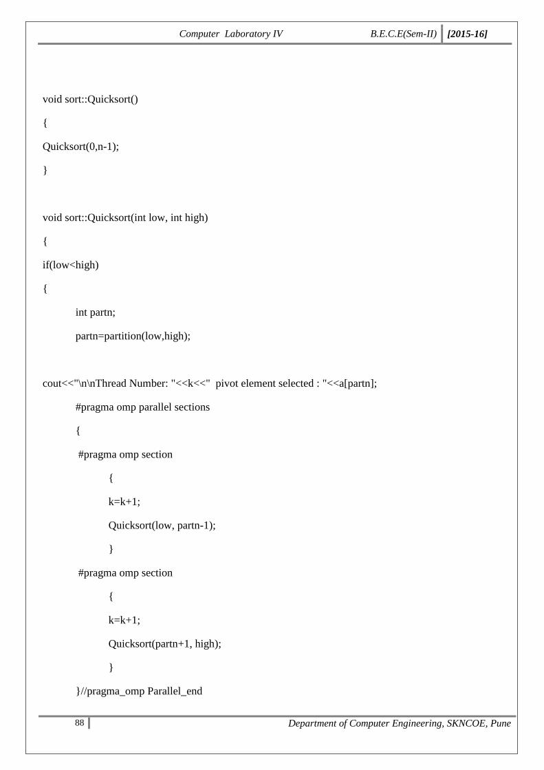
Computer Laboratory IV B.E.C.E(Sem-II) [2015-16]
88 Department of Computer Engineering, SKNCOE, Pune
void sort::Quicksort()
{
Quicksort(0,n-1);
}
void sort::Quicksort(int low, int high)
{
if(low<high)
{
int partn;
partn=partition(low,high);
cout<<"\n\nThread Number: "<<k<<" pivot element selected : "<<a[partn];
#pragma omp parallel sections
{
#pragma omp section
{
k=k+1;
Quicksort(low, partn-1);
}
#pragma omp section
{
k=k+1;
Quicksort(partn+1, high);
}
}//pragma_omp Parallel_end
Computer Laboratory IV B.E.C.E(Sem-II) [2015-16]
89 Department of Computer Engineering, SKNCOE, Pune
}
}
int sort::partition(int low ,int high)
{
int pvt;
pvt=a[high];
int i;
i=low-1;
int j;
for(j=low;j<high;j++)
{
if(a[j]<=pvt)
{
int tem=0;
tem=a[j];
a[j]=a[i+1];
a[i+1]=tem;
i=i+1;
}
}
int te;
te=a[high];
a[high]=a[i+1];
a[i+1]=te;
return i+1;
Computer Laboratory IV B.E.C.E(Sem-II) [2015-16]
90 Department of Computer Engineering, SKNCOE, Pune
}
void sort::putdata()
{
cout<<endl<<"\nThe Array is:"<<endl;
for(int i=0;i<n;i++)
cout<<" "<<a[i];
}
int main()
{
int n;
sort s1;
int ch;
do
{
s1.getdata();
s1.putdata();
cout<<"\nUsing Quick Sort";
double start = omp_get_wtime();
s1.Quicksort();
double end = omp_get_wtime();
cout<<"\nThe Sorted ";
s1.putdata();
cout<<"\nExcecution time : "<<end - start<<" seconds ";
cout<<"Would you like to continue? (1/0 y/n)"<<endl;

Computer Laboratory IV B.E.C.E(Sem-II) [2015-16]
91 Department of Computer Engineering, SKNCOE, Pune
cin>>ch;
}while(ch==1);
}
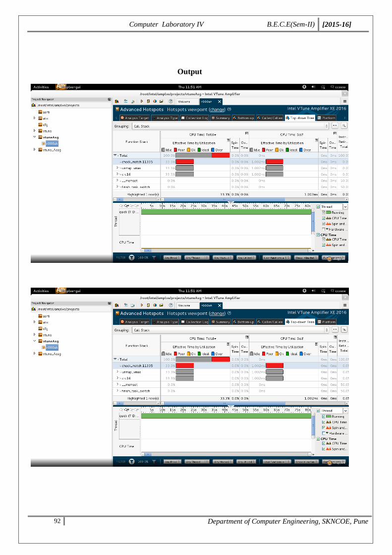
Computer Laboratory IV B.E.C.E(Sem-II) [2015-16]
92 Department of Computer Engineering, SKNCOE, Pune
Output
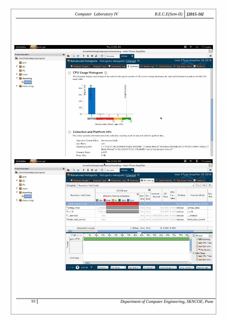
Computer Laboratory IV B.E.C.E(Sem-II) [2015-16]
93 Department of Computer Engineering, SKNCOE, Pune

Computer Laboratory IV B.E.C.E(Sem-II) [2015-16]
94 Department of Computer Engineering, SKNCOE, Pune
Assignment No.
3
Title
Write a program to check task distribution using Gprof.l
Roll No.
Class B.E. (C.E.)
Date
Subject Computer Lab IV
Signature
Computer Laboratory IV B.E.C.E(Sem-II) [2015-16]
95 Department of Computer Engineering, SKNCOE, Pune
Assignment No: 3
Title: Write a program to check task distribution using Gprof.l
Objectives:
To understand and task distribution using Gprof.l
Theory:
Gprof is a performance analysis tool for Unix applications. It uses a hybrid of instrumentation and
sampling and was created as extended version of the older "prof" tool. Unlike prof, gprof is capable of
limited call graph collecting and printing.
GPROF was originally written by a group led by Susan L. Graham at the University of California,
Berkeley for Berkeley Unix (4.2BSD). Another implementation was written as part of the GNU
project for GNU Binutils in 1988 by Jay Fenlason.
Profiling is an important aspect of software programming. Through profiling one can determine the
parts in program code that are time consuming and need to be re-written. This helps make your
program execution faster which is always desired.
In very large projects, profiling can save your day by not only determining the parts in your program
which are slower in execution than expected but also can help you find many other statistics through
which many potential bugs can be spotted and sorted out.
How to use gprof ?
Using the gprof tool is not at all complex. You just need to do the following on a high-level:
Have profiling enabled while compiling the code
Execute the program code to produce the profiling data
Run the gprof tool on the profiling data file (generated in the step above).
The last step above produces an analysis file which is in human readable form. This file contains a
couple of tables (flat profile and call graph) in addition to some other information. While flat profile
Computer Laboratory IV B.E.C.E(Sem-II) [2015-16]
96 Department of Computer Engineering, SKNCOE, Pune
gives an overview of the timing information of the functions like time consumption for the execution of
a particular function, how many times it was called etc. On the other hand, call graph focuses on each
function like the functions through which a particular function was called, what all functions were
called from within this particular function etc So this way one can get idea of the execution time spent
in the sub-routines too..
Gprof Setup and Usage
Here are some of the steps required for downloading and setting environment for gprof :
If not installed already, download and install gprof by executing apt-get install binutils
To check that gprof is installed properly, execute the gprof command and it should give some error
likea.out: No such file or directory.
Assuming that the compiler being used it gcc or cc, compile your code with the option -pg so that
the executable includes extra code for profiling purpose.
Run the program in a normal way. When the program terminates, a file named gmon.out (profiler
data) would be produced in the same directory from which the program was run.
Use the gprof profiler to process this profiler data (gmon.out) and produce human readable
performance analysis and statistics of the program.
Steps for execution
1. First, compile your application as you normally would, but be sure to include the -pg flag.
Note that if you compile and link as separate steps in your application built, you will need to
include -pg in both steps.
2. For parallel applications only: if you want each parallel process to produce its own output
file, you will need to set the undocumented environment variable GMON_OUT_PRFIX to
some non-null string. For example
% gcc -03 -pg -o myprog myprog.c
% setenv GMON_OUT_PREFIX ‘gmon.out’
Computer Laboratory IV B.E.C.E(Sem-II) [2015-16]
97 Department of Computer Engineering, SKNCOE, Pune
3. Run your application as usual. The example below shown a 16 task MPI application running
in the pdebug partition.
4. View the results: use the gprof command to convert the output file into human readable
report. Several examples shown below:
a. Serial
b. Parallel – one process only
c. Parallel – multiple processes
d. Parallel – all processes
Another option for parallel programs is to sum all output files into single gmon.sum file which can
then be viewed with gprof. For eample
Conclusion:
Hence, we studied and implemented the gprof concept.
% srun -n16 -ppdebug myprog
1 % gprof myprog gmon.out
2 % gprof myprog gmon.out.18302
3 % gprof myprog gmon.out.18297 gmon.out.18300 gmon.out.9097
4 % gprof myprog gmon.out.*
% gprof myprog -s gmon.out.*
% gprof myprog gmon.sum
Computer Laboratory IV B.E.C.E(Sem-II) [2015-16]
98 Department of Computer Engineering, SKNCOE, Pune
Program
#include <stdio.h>
void func2()
{
int count = 0;
for(count=0; count < 0XFFFFF; count++);
return;
}
void func1(void)
{
int count = 0;
for(count=0; count < 0XFF; count++)
func2();
return;
}
int main(void)
{
printf("\n Hello World! \n");
func1();
func2();
return 0;
}
Output
/*
student@student-OptiPlex-3010:~$ gedit test.c
student@student-OptiPlex-3010:~$ gcc -Wall -pg test.c -o test
student@student-OptiPlex-3010:~$ ./test
Hello World!
student@student-OptiPlex-3010:~$ gprof test gmon.out > prof_output
student@student-OptiPlex-3010:~$
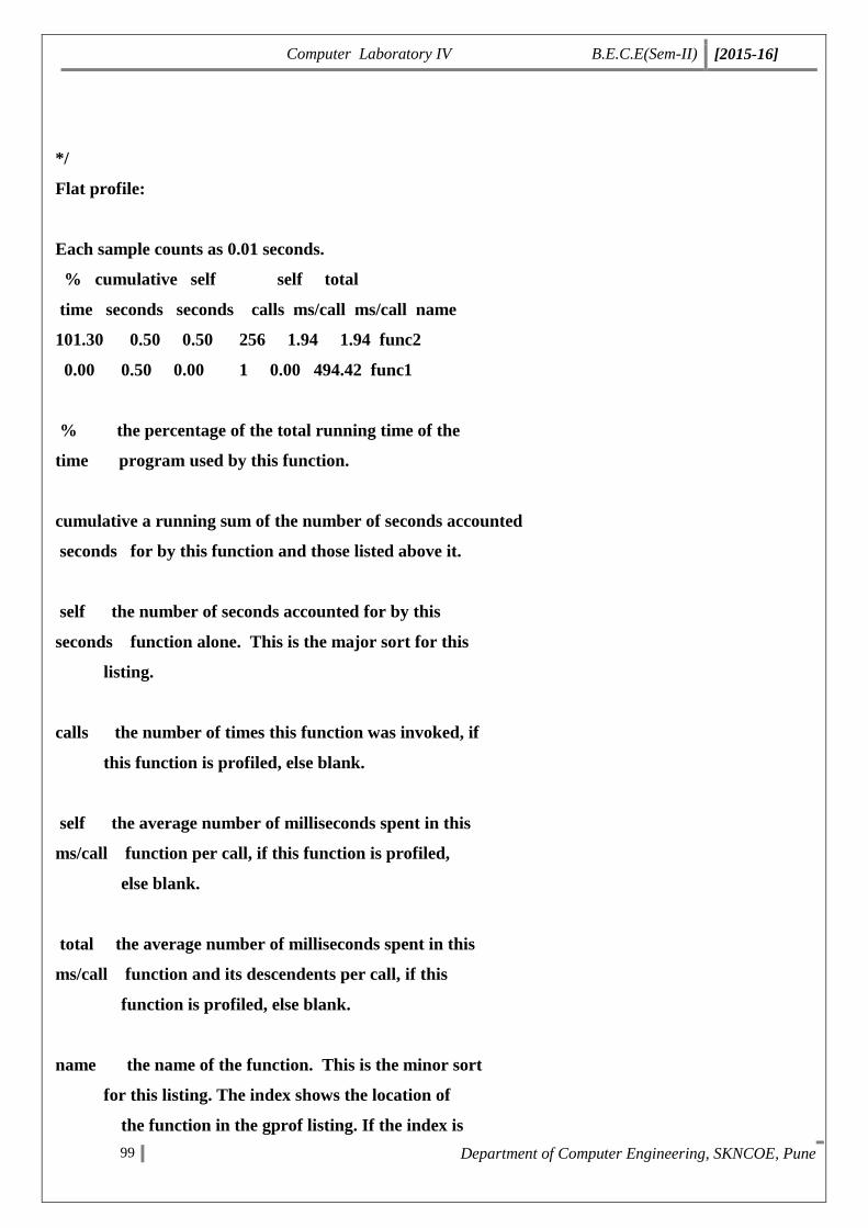
Computer Laboratory IV B.E.C.E(Sem-II) [2015-16]
99 Department of Computer Engineering, SKNCOE, Pune
*/
Flat profile:
Each sample counts as 0.01 seconds.
% cumulative self self total
time seconds seconds calls ms/call ms/call name
101.30 0.50 0.50 256 1.94 1.94 func2
0.00 0.50 0.00 1 0.00 494.42 func1
% the percentage of the total running time of the
time program used by this function.
cumulative a running sum of the number of seconds accounted
seconds for by this function and those listed above it.
self the number of seconds accounted for by this
seconds function alone. This is the major sort for this
listing.
calls the number of times this function was invoked, if
this function is profiled, else blank.
self the average number of milliseconds spent in this
ms/call function per call, if this function is profiled,
else blank.
total the average number of milliseconds spent in this
ms/call function and its descendents per call, if this
function is profiled, else blank.
name the name of the function. This is the minor sort
for this listing. The index shows the location of
the function in the gprof listing. If the index is
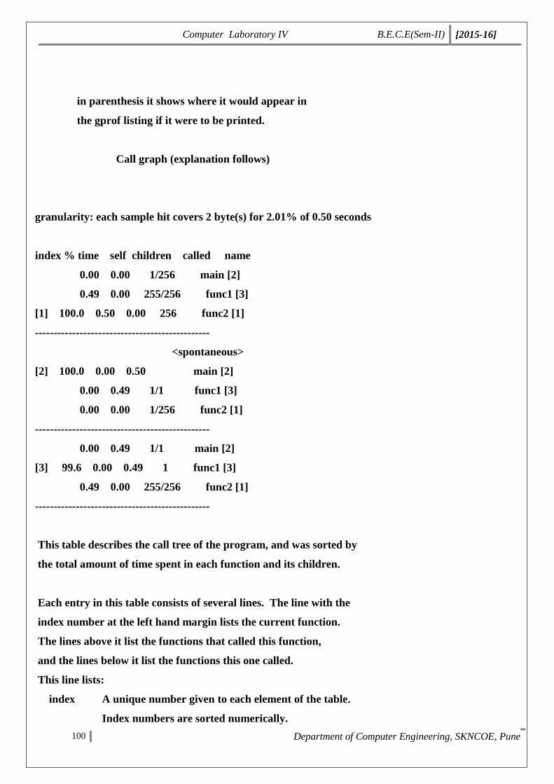
Computer Laboratory IV B.E.C.E(Sem-II) [2015-16]
100 Department of Computer Engineering, SKNCOE, Pune
in parenthesis it shows where it would appear in
the gprof listing if it were to be printed.
Call graph (explanation follows)
granularity: each sample hit covers 2 byte(s) for 2.01% of 0.50 seconds
index % time self children called name
0.00 0.00 1/256 main [2]
0.49 0.00 255/256 func1 [3]
[1] 100.0 0.50 0.00 256 func2 [1]
-----------------------------------------------
<spontaneous>
[2] 100.0 0.00 0.50 main [2]
0.00 0.49 1/1 func1 [3]
0.00 0.00 1/256 func2 [1]
-----------------------------------------------
0.00 0.49 1/1 main [2]
[3] 99.6 0.00 0.49 1 func1 [3]
0.49 0.00 255/256 func2 [1]
-----------------------------------------------
This table describes the call tree of the program, and was sorted by
the total amount of time spent in each function and its children.
Each entry in this table consists of several lines. The line with the
index number at the left hand margin lists the current function.
The lines above it list the functions that called this function,
and the lines below it list the functions this one called.
This line lists:
index A unique number given to each element of the table.
Index numbers are sorted numerically.

Computer Laboratory IV B.E.C.E(Sem-II) [2015-16]
101 Department of Computer Engineering, SKNCOE, Pune
The index number is printed next to every function name so
it is easier to look up where the function is in the table.
% time This is the percentage of the `total' time that was spent
in this function and its children. Note that due to
different viewpoints, functions excluded by options, etc,
these numbers will NOT add up to 100%.
self This is the total amount of time spent in this function.
children This is the total amount of time propagated into this
function by its children.
called This is the number of times the function was called.
If the function called itself recursively, the number
only includes non-recursive calls, and is followed by
a `+' and the number of recursive calls.
name The name of the current function. The index number is
printed after it. If the function is a member of a
cycle, the cycle number is printed between the
function's name and the index number.
For the function's parents, the fields have the following meanings:
self This is the amount of time that was propagated directly
from the function into this parent.
children This is the amount of time that was propagated from
the function's children into this parent.
called This is the number of times this parent called the

Computer Laboratory IV B.E.C.E(Sem-II) [2015-16]
102 Department of Computer Engineering, SKNCOE, Pune
function `/' the total number of times the function
was called. Recursive calls to the function are not
included in the number after the `/'.
name This is the name of the parent. The parent's index
number is printed after it. If the parent is a
member of a cycle, the cycle number is printed between
the name and the index number.
If the parents of the function cannot be determined, the word
`<spontaneous>' is printed in the `name' field, and all the other
fields are blank.
For the function's children, the fields have the following meanings:
self This is the amount of time that was propagated directly
from the child into the function.
children This is the amount of time that was propagated from the
child's children to the function.
called This is the number of times the function called
this child `/' the total number of times the child
was called. Recursive calls by the child are not
listed in the number after the `/'.
name This is the name of the child. The child's index
number is printed after it. If the child is a
member of a cycle, the cycle number is printed
between the name and the index number.
If there are any cycles (circles) in the call graph, there is an
entry for the cycle-as-a-whole. This entry shows who called the

Computer Laboratory IV B.E.C.E(Sem-II) [2015-16]
103 Department of Computer Engineering, SKNCOE, Pune
cycle (as parents) and the members of the cycle (as children.)
The `+' recursive calls entry shows the number of function calls that
were internal to the cycle, and the calls entry for each member shows,
for that member, how many times it was called from other members of
the cycle.
Index by function name
[3] func1 [1] func2
Computer Laboratory IV B.E.C.E(Sem-II) [2015-16]
104 Department of Computer Engineering, SKNCOE, Pune
Assignment No.
4
Title
Perform DSP(Digital Signal Processing) convolution operation
on a given signal stored using XML/JSON/ text file using HPC
infrastructure.
Roll No.
Class B.E. (C.E.)
Date
Subject Computer Lab IV
Signature
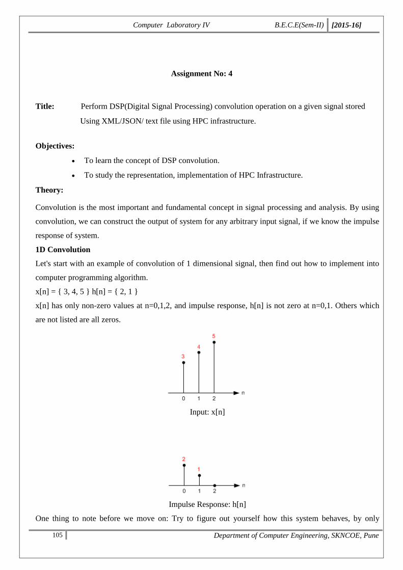
Computer Laboratory IV B.E.C.E(Sem-II) [2015-16]
105 Department of Computer Engineering, SKNCOE, Pune
Assignment No: 4
Title: Perform DSP(Digital Signal Processing) convolution operation on a given signal stored
Using XML/JSON/ text file using HPC infrastructure.
Objectives:
To learn the concept of DSP convolution.
To study the representation, implementation of HPC Infrastructure.
Theory:
Convolution is the most important and fundamental concept in signal processing and analysis. By using
convolution, we can construct the output of system for any arbitrary input signal, if we know the impulse
response of system.
1D Convolution
Let's start with an example of convolution of 1 dimensional signal, then find out how to implement into
computer programming algorithm.
x[n] = { 3, 4, 5 } h[n] = { 2, 1 }
x[n] has only non-zero values at n=0,1,2, and impulse response, h[n] is not zero at n=0,1. Others which
are not listed are all zeros.
Input: x[n]
Impulse Response: h[n]
One thing to note before we move on: Try to figure out yourself how this system behaves, by only
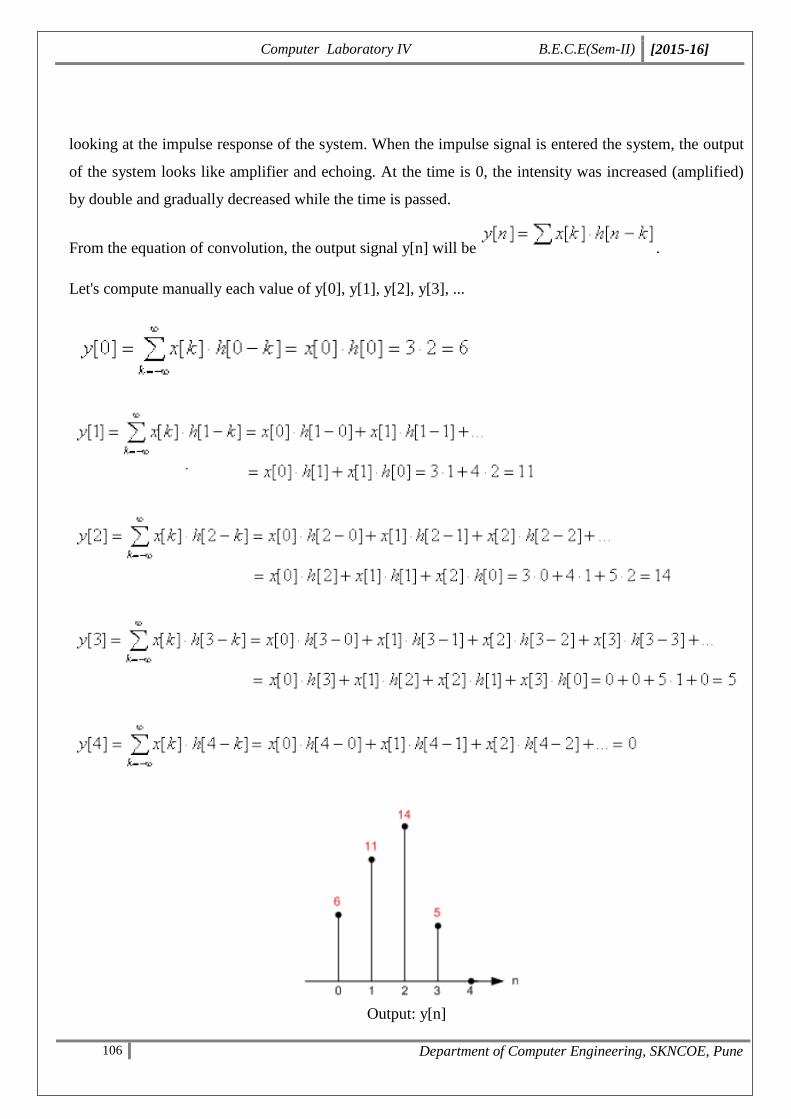
Computer Laboratory IV B.E.C.E(Sem-II) [2015-16]
106 Department of Computer Engineering, SKNCOE, Pune
looking at the impulse response of the system. When the impulse signal is entered the system, the output
of the system looks like amplifier and echoing. At the time is 0, the intensity was increased (amplified)
by double and gradually decreased while the time is passed.
From the equation of convolution, the output signal y[n] will be .
Let's compute manually each value of y[0], y[1], y[2], y[3], ...
Output: y[n]
Computer Laboratory IV B.E.C.E(Sem-II) [2015-16]
107 Department of Computer Engineering, SKNCOE, Pune
Notice that y[0] has only one component, x[0]h[0], and others are omitted, because others are all zeros at
k ≠ 0. In other words, x[1]h[-1] = x[2]h[-2] = 0. The above equations also omit the terms if they are
obviously zeros. If n is larger than and equal to 4, y[n] will be zeros. So we stop here to compute y[n]and
adding these 4 signals (y[0], y[1], y[2], y[3]) produces the output signal y[n] = {6, 11, 14, 5}.
Let's look more closely the each output. In order to see a pattern clearly, the order of addition is swapped.
The last term comes first and the first term goes to the last. And, all zero terms are ignored.
y[0] = x[0]·h[0]
y[1] = x[1]·h[0] + x[0]·h[1]
y[2] = x[2]·h[0] + x[1]·h[1]
y[3] = x[3]·h[0] + x[2]·h[1]
Can you see the pattern? For example, y[2] is calculated from 2 input samples; x[2] and x[1], and 2
impulse response samples; h[0] and h[1]. The input sample starts from 2, which is same as the sample
point of output, and decreased. The impulse response sample starts from 0 and increased.
Based on the pattern that we found, we can write an equation for any sample of the output;
where i is any sample point and k is the number of samples in impulse response. For instance, if an
impulse response has 4 samples, the sample of output signal at 9 is;
y[9] = x[9]·h[0] + x[8]·h[1] + x[7]·h[2] + x[6]·h[3] Notice the first sample, y[0] has only one term.
Based on the pattern that we found, y[0] is calculated as: y[0] = x[0]·h[0] + x[-1]·h[1]. Because x[-1] is
not defined, we simply pad it to zero.
Implementation:
Implementation Convolution is the treatment of a matrix by another one called the kernel. The
convolution matrix filter uses the image to be treated as the first matrix. The image is a bi dimensional
collection of pixels in rectangular coordinates.
Only 3*3 matrices will be considered as they are mostly used and are enough for all the effects we want.
The second matrix has a variable size. Then the matrices are converted to 1-D array and the two array of
numbers, which are generally of different sizes bu multiplied. It produces a third array of numbers of the
same dimensionality. This can be used in image processing to implement operators whose output values
are simple linear combinations of certain pixel values.
Message Passing Interface (MPI) In this code we multiply an n*n matrix with an m*m matrix using
Computer Laboratory IV B.E.C.E(Sem-II) [2015-16]
108 Department of Computer Engineering, SKNCOE, Pune
convolution theorem. m+2 processes are there that compute each elements of final matrix in parallel.
Initialization MPI_Init (&argc,&argv):This function message passing interface by passing arguments
on command line. They are 0 by default.
MPI_Comm_size(MPI_COMM_WORLD,&totalnodes):
This function gives total number of processes. First parameter is communicator. Second parameter
contains the t of processes. MPI_Comm_rank(MPI_COMM_WORLD function gives the rank of the
process, which is 1 less than total number of processes. (2) Steps Two matrices are input in process 0 of
rank 0. Then the size of padded matrix c is sent to process 1 using MPI_Send method. This initializes all
elements of c to 0, which is (m+2) * (m+2) matrix. This is received by the 0
MPI_Recv method, which adds the elements of matrix b to matrix c. Hence only outer elements of c are 0.
m*m size output matrix d using same procedure as given above. Then find out each element of the resultant
matrix. First send the size of the output matrix & padded matrix (using MPI_Send) to all the processes.
Different processes calculate the elements of output matrix and return the result to process 0, using
MPI_Recv. That is how output will be received from m processes concurrently.
Commands Syntax
(a)MPI_Send()
It performs a blocking send. Synopsis:intMPI_Send(void *buf, MPI_Datatypedatatype, intdest, int
tag,MPI_Commcomm) Input Parameters: buf: initial address of send buffer (choice) Implementation
Convolution is the treatment of a matrix by another one called the kernel. The convolution matrix filter
uses the image to be treated as the first matrix. The image is a bidimensional collection of pixels in
rectangular coordinates.3 *3 matrices will be considered as they are mostly used and are enough for all
the effects we want. The second matrix has a variable size. Then the matrices are converted D array and
the two array of numbers, which are generally of different sizes but of the same dimension are multiplied.
It produces a third array of numbers of the same dimensionality. This can be used in image processing to
implement operators whose output values are simple linear combinations of certain pixel values.
Passing Interface (MPI) In this code we multiply an n*n matrix with an m*m matrix using convolution
theorem. m+2 processes are there that compute each elements of final matrix in parallel.
MPI_Init (&argc,&argv): This function initializes the message passing interface by passing arguments
on command line. They are 0 by default.
MPI_Comm_size(MPI_COMM_WORLD,&totalnodes): Thi s function gives total number of
processes. First parameter is communicator. Second parameter contains the total number
MPI_Comm_rank(MPI_COMM_WORLD & mynode): This function gives the rank of the process,
Computer Laboratory IV B.E.C.E(Sem-II) [2015-16]
109 Department of Computer Engineering, SKNCOE, Pune
which is 1 less than Two matrices are input in process 0 of rank 0. Then the size sent to process 1 using
MPI_Send method. This initializes all elements of c to 0, which is (m+2) * (m+2) matrix. This is
received by the 0th process by MPI_Recv method, which adds the elements of matrix b to matrix c.
Hence only outer elements of c are 0. Initialize the m*m size output matrix d using same procedure as
given Then find out each element of the resultant matrix. First send the size of the output matrix &
padded matrix (using MPI_Send) to all the processes. Different processes he elements of output matrix
and return the result to process 0, using MPI_Recv. That is how output will be received from m processes
intMPI_Send(void *buf, int count, intdest, int initial address of send buffer .
count: number of elements in send buffer (nonnegative integer) datatype: datatype of each send buffer
element (handle) dest: rank of destination (integer) tag:message tag (integer) comm.: communicator
(handle)
(b)MPI_Recv()
It is a blocking receives for a message. intMPI_Recv(void *buf, int count, MPI_Datatypedatatype, int
source, inttag,MPI_Comm comm, MPI_Status *status) Output Parameters: buf: initial address of receive
buffer (choice) status: status object (Status) Input Parameters count: maximum number of elements in
receive buffer (integer) datatype: datatype of each receive buffer element (handle) source: rank of source
(integer) tag: message tag (integer) comm: communicator (handle).
(c) MPI_Finalize()
This function tests if work of a process is finished.
Mathematical Model:
Let A be the system used to perform DSP(Digital Signal Processing) convolution operation on a given
signal stored.
S={I,O,F,fail,success}
where
I={I1,I2,I3....}
I1={N} ,where N=size of an array.
I2={N+1} ,kernel count.
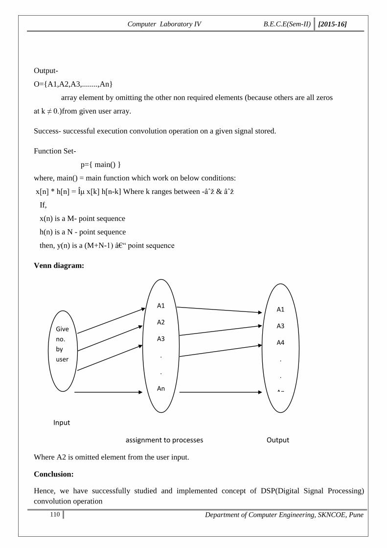
Computer Laboratory IV B.E.C.E(Sem-II) [2015-16]
110 Department of Computer Engineering, SKNCOE, Pune
Output-
O={A1,A2,A3,........,An}
array element by omitting the other non required elements (because others are all zeros
at k ≠ 0.)from given user array.
Success- successful execution convolution operation on a given signal stored.
Function Set-
p={ main() }
where, main() = main function which work on below conditions:
x[n] * h[n] = Îμ x[k] h[n-k] Where k ranges between -∞ & ∞
If,
x(n) is a M- point sequence
h(n) is a N - point sequence
then, y(n) is a (M+N-1) – point sequence
Venn diagram:
Input
assignment to processes Output
Where A2 is omitted element from the user input.
Conclusion:
Hence, we have successfully studied and implemented concept of DSP(Digital Signal Processing)
convolution operation
Give
no.
by
user
A1
A2
A3
.
.
An
An
A1
A3
A4
.
.
An
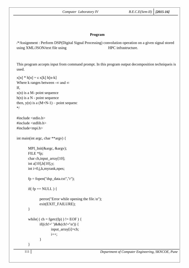
Computer Laboratory IV B.E.C.E(Sem-II) [2015-16]
111 Department of Computer Engineering, SKNCOE, Pune
Program
/*Assignment : Perform DSP(Digital Signal Processing) convolution operation on a given signal stored
using XML/JSON/text file using HPC infrastructure.
This program accepts input from command prompt. In this program output decomposition techniqueis is
used.
x[n] * h[n] = ε x[k] h[n-k]
Where k ranges between -∞ and ∞
If,
x(n) is a M- point sequence
h(n) is a N - point sequence
then, y(n) is a (M+N-1) – point sequenc
*/
#include <stdio.h>
#include <stdlib.h>
#include<mpi.h>
int main(int argc, char **argv) {
MPI_Init(&argc, &argv);
FILE *fp;
char ch,input_array[10];
int a[10],b[10],y;
int i=0,j,k,myrank,npes;
fp = fopen("dsp_data.txt","r");
if( fp == NULL ) {
perror("Error while opening the file.\n");
exit(EXIT_FAILURE);
}
while( ( ch = fgetc(fp) ) != EOF ) {
if((ch!=' ')&&(ch!='\n')) {
input_array[i]=ch;
i++;
}
}
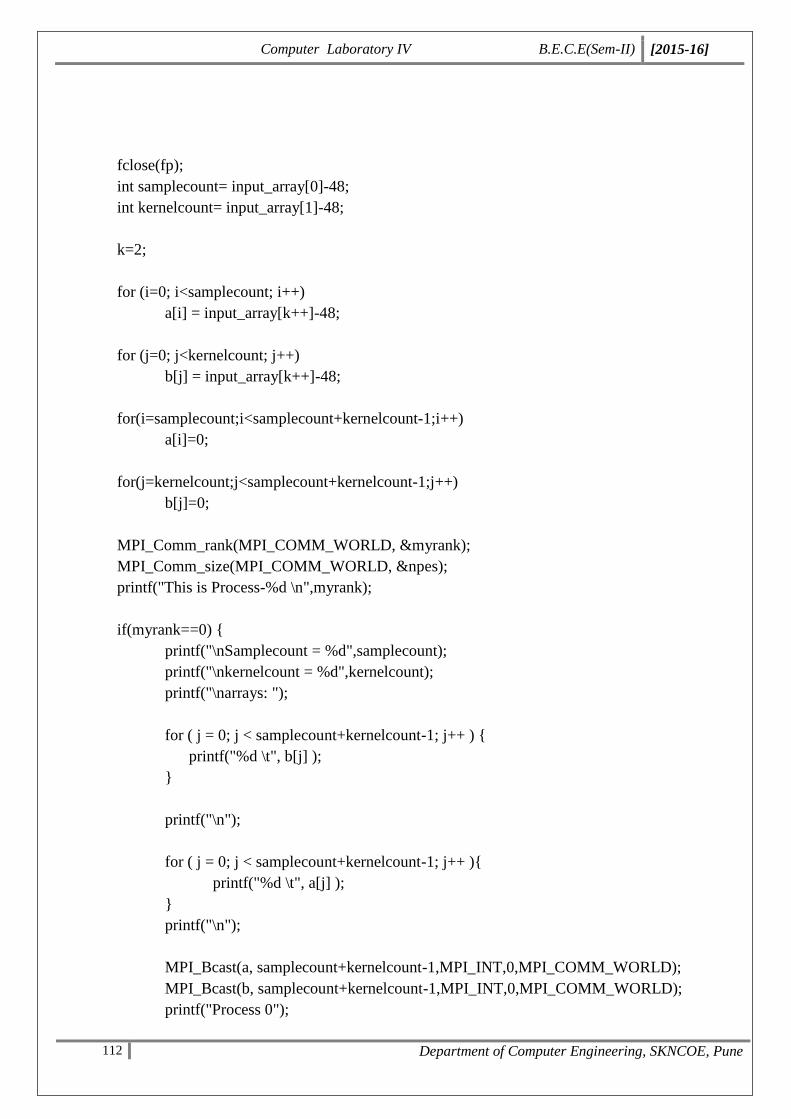
Computer Laboratory IV B.E.C.E(Sem-II) [2015-16]
112 Department of Computer Engineering, SKNCOE, Pune
fclose(fp);
int samplecount= input_array[0]-48;
int kernelcount= input_array[1]-48;
k=2;
for (i=0; i<samplecount; i++)
a[i] = input_array[k++]-48;
for (j=0; j<kernelcount; j++)
b[j] = input_array[k++]-48;
for(i=samplecount;i<samplecount+kernelcount-1;i++)
a[i]=0;
for(j=kernelcount;j<samplecount+kernelcount-1;j++)
b[j]=0;
MPI_Comm_rank(MPI_COMM_WORLD, &myrank);
MPI_Comm_size(MPI_COMM_WORLD, &npes);
printf("This is Process-%d \n",myrank);
if(myrank==0) {
printf("\nSamplecount = %d",samplecount);
printf("\nkernelcount = %d",kernelcount);
printf("\narrays: ");
for ( j = 0; j < samplecount+kernelcount-1; j++ ) {
printf("%d \t", b[j] );
}
printf("\n");
for ( j = 0; j < samplecount+kernelcount-1; j++ ){
printf("%d \t", a[j] );
}
printf("\n");
MPI_Bcast(a, samplecount+kernelcount-1,MPI_INT,0,MPI_COMM_WORLD);
MPI_Bcast(b, samplecount+kernelcount-1,MPI_INT,0,MPI_COMM_WORLD);
printf("Process 0");
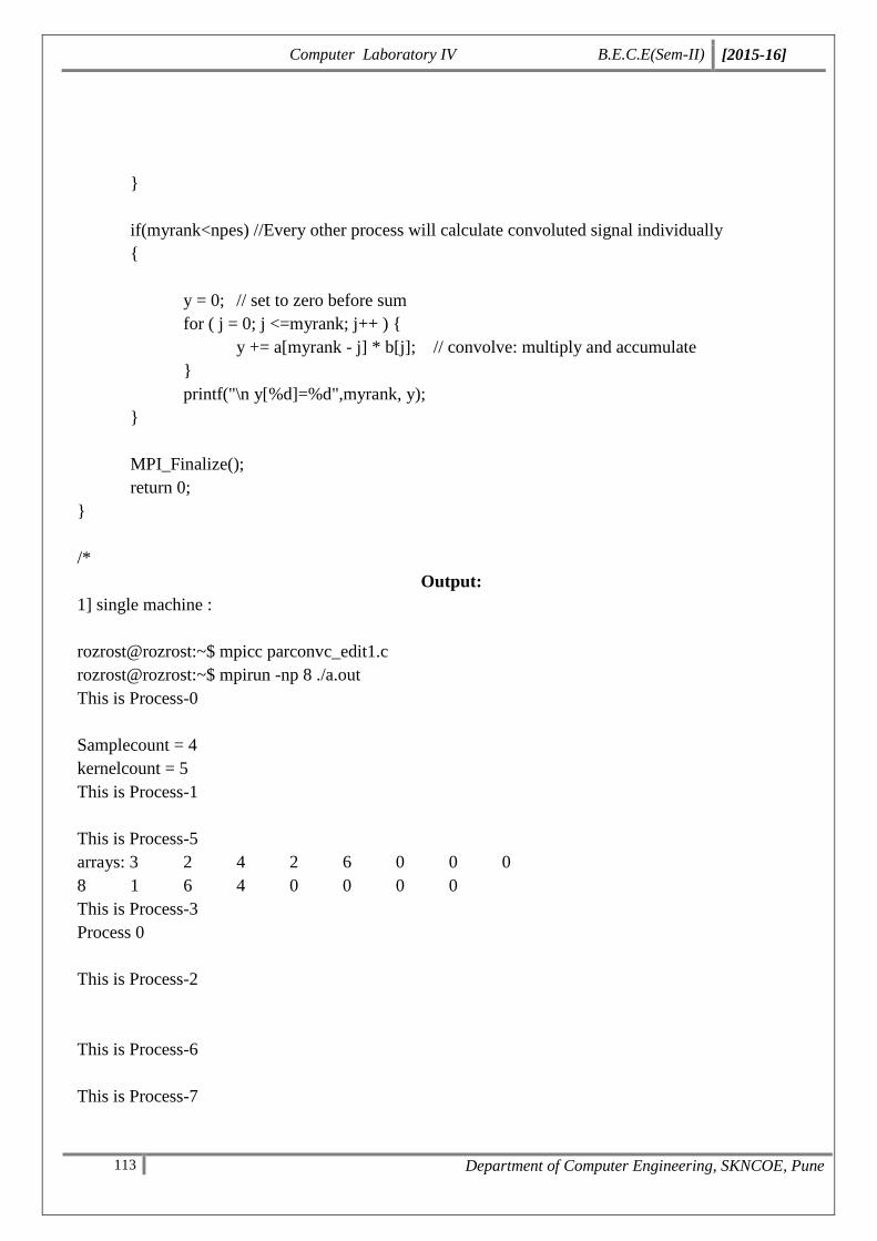
Computer Laboratory IV B.E.C.E(Sem-II) [2015-16]
113 Department of Computer Engineering, SKNCOE, Pune
}
if(myrank<npes) //Every other process will calculate convoluted signal individually
{
y = 0; // set to zero before sum
for ( j = 0; j <=myrank; j++ ) {
y += a[myrank - j] * b[j]; // convolve: multiply and accumulate
}
printf("\n y[%d]=%d",myrank, y);
}
MPI_Finalize();
return 0;
}
/*
Output:
1] single machine :
rozrost@rozrost:~$ mpicc parconvc_edit1.c
rozrost@rozrost:~$ mpirun -np 8 ./a.out
This is Process-0
Samplecount = 4
kernelcount = 5
This is Process-1
This is Process-5
arrays: 3 2 4 2 6 0 0 0
8 1 6 4 0 0 0 0
This is Process-3
Process 0
This is Process-2
This is Process-6
This is Process-7
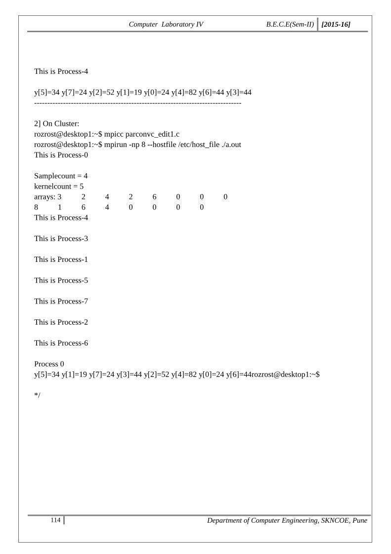
Computer Laboratory IV B.E.C.E(Sem-II) [2015-16]
114 Department of Computer Engineering, SKNCOE, Pune
This is Process-4
y[5]=34 y[7]=24 y[2]=52 y[1]=19 y[0]=24 y[4]=82 y[6]=44 y[3]=44
-------------------------------------------------------------------------------
2] On Cluster:
rozrost@desktop1:~$ mpicc parconvc_edit1.c
rozrost@desktop1:~$ mpirun -np 8 --hostfile /etc/host_file ./a.out
This is Process-0
Samplecount = 4
kernelcount = 5
arrays: 3 2 4 2 6 0 0 0
8 1 6 4 0 0 0 0
This is Process-4
This is Process-3
This is Process-1
This is Process-5
This is Process-7
This is Process-2
This is Process-6
Process 0
y[5]=34 y[1]=19 y[7]=24 y[3]=44 y[2]=52 y[4]=82 y[0]=24 y[6]=44rozrost@desktop1:~$
*/
Computer Laboratory IV B.E.C.E(Sem-II) [2015-16]
115 Department of Computer Engineering, SKNCOE, Pune
Assignment No.
5
Title
Perform concurrent ODD - Even Mearge sort Using HPC
infrastructure (preferably BBB using Python/scala/Java/C++)
Roll No.
Class B.E. (C.E.)
Date
Subject Computer Lab IV
Signature
Computer Laboratory IV B.E.C.E(Sem-II) [2015-16]
116 Department of Computer Engineering, SKNCOE, Pune
Assignment No:5
Title: Perform concurrent ODD - Even Mearge sort Using HPC infrastructure (preferably BBB
using Python/scala/Java/C++)
Objectives:
To learn the concept of ODD - Even Mearge sort
To study the representation, implementation of concurrent ODD - Even Mearge sort
Using HPC infrastructure
Theory:
The odd-even merge sort algorithm was developed by K.E. Batcher . It is based on a merge algorithm
that merges two sorted halves of a sequence to a completely sorted sequence.
Building a Compute Cluster with the BeagleBone Black
Configuring the BeagleBones
Once the hardware is set up and a machine is connected to the network, Putty or any other SSH client can
be used to connect to the machines. The default hostname to connect to using the above image is ubuntu-
armhf. My first task was to change the hostname. I chose to name mine beaglebone1, beaglebone2 and
beaglebone3. First I used the hostname command:
sudo hostname beaglebone1
Next I edited /etc/hostname and placed the new hostname in the file. The next step was to hard code the
IP address for so I could probably map it in the hosts file. I did this by editing /etc/network/interfaces to
tell it to use static IPs. In my case I have a local network with a router at 192.168.1.1. I decided to start
the IP addresses at 192.168.1.51 so the file on the first node looked like this:
iface eth0 inet static
address 192.168.1.51
netmask 255.255.255.0
network 192.168.1.0
broadcast 192.168.1.255
gateway 192.168.1.1
Computer Laboratory IV B.E.C.E(Sem-II) [2015-16]
117 Department of Computer Engineering, SKNCOE, Pune
It is usually a good idea to pick something outside the range of IPs that your router might assign if you
are going to have a lot of devices. Usually you can configure this range on your router. With this done,
the final step to perform was to edit /etc/hosts and list the name and IP address of each node that would
be in the cluster. My file ended up looking like this on each of them:
127.0.0.1 localhost
192.168.1.51 beaglebone1
192.168.1.52 beaglebone2
192.168.1.53 beaglebone3
Creating a Compute Cluster With MPI
After setting up all 3 BeagleBones, I was ready to tackle my first compute project. I figured a good
starting point for this was to set up MPI. MPI is a standardized system for passing messages between
machines on a network. It is powerful in that it distributes programs across nodes so each instance has
access to the local memory of its machine and is supported by several languages such as C, Python and
Java. There are many versions of MPI available so I chose MPICH which I was already familiar with.
Installation was simple, consisting of the following three steps:
sudo apt-get update
sudo apt-get install gcc
sudo apt-get install libcr-dev mpich2 mpich2-doc
MPI works by using SSH to communicate between nodes and using a shared folder to share data. The
first step to allowing this was to install NFS. I picked beaglebone1 to act as the master node in the MPI
cluster and installed NFS server on it:
sudo apt-get install nfs-client
With this done, I installed the client version on the other two nodes:
sudo apt-get install nfs-server
Next I created a user and folder on each node that would be used by MPI. I decided to call mine hpcuser
and started with its folder:
sudomkdir /hpcuser
Once it was created on all the nodes, I synced up the folders by issuing this on the master node:
echo "/hpcuser *(rw,sync)" | sudo tee -a /etc/exports
Then I mounted the master's node on each slave so they can see any files that are added to the master
node:
Computer Laboratory IV B.E.C.E(Sem-II) [2015-16]
118 Department of Computer Engineering, SKNCOE, Pune
sudo mount beaglebone1:/hpcuser /hpcuser
To make sure this is mounted on reboots I edited /etc/fstab and added the following:
beaglebone1:/hpcuser /hpcusernfs
Finally I created the hpcuser and assigned it the shared folder:
sudouseradd -d /hpcuserhpcuser
With network sharing set up across the machines, I installed SSH on all of them so that MPI could
communicate with each:
sudo apt-get install openssh-server
The next step was to generate a key to use for the SSH communication. First I switched to the hpcuser
and then used ssh-keygen to create the key.
su - hpcuser
sshkeygen-t rsa
When performing this step, for simplicity you can keep the passphrase blank. When asked for a location,
you can keep the default. If you want to use a passphrase, you will need to take extra steps to prevent
SSH from prompting you to enter the phrase. You can use ssh-agent to store the key and prevent this.
Once the key is generated, you simply store it in our authorized keys collection:
cd .ssh
cat id_rsa.pub >>authorized_keys
I then verified that the connections worked using ssh:
ssh hpcuser@beaglebone2
Testing MPI
Once the machines were able to successfully connect to each other, I wrote a simple program on the
master node to try out. While logged in as hpcuser, I created a simple program in its root directory
/hpcuser called mpi1.c. MPI needs the program to exist in the shared folder so it can run on each
machine. The program below simply displays the index number of the current process, the total number
of processes running and the name of the host of the current process. Finally, the main node receives a
sum of all the process indexes from the other nodes and displays it:
#include <mpi.h>
#include <stdio.h>
int main(intargc, char* argv[])
Computer Laboratory IV B.E.C.E(Sem-II) [2015-16]
119 Department of Computer Engineering, SKNCOE, Pune
{
int rank, size, total;
char hostname[1024];
gethostname(hostname, 1023);
MPI_Init(&argc, &argv);
MPI_Comm_rank (MPI_COMM_WORLD, &rank);
MPI_Comm_size (MPI_COMM_WORLD, &size);
MPI_Reduce(&rank, &total, 1, MPI_INT, MPI_SUM, 0, MPI_COMM_WORLD);
printf("Testing MPI index %d of %d on hostname %s\n", rank, size, hostname);
if (rank==0)
{
printf("Process sum is %d\n", total);
}
MPI_Finalize();
return 0;
}
Next I created a file called machines.txt in the same directory and placed the names of the nodes in the
cluster inside, one per line. This file tells MPI where it should run:
beaglebone1
beaglebone2
beaglebone3
With both files created, I finally compiled the program using mpicc and ran the test:
mpicc mpi1.c -o mpiprogram
mpiexec -n 8 -f machines.txt. /mpiprogram
This resulted in the following output demonstrating it ran on all 3 nodes:
Testing MPI index 4 of 8 on hostname beaglebone2
Testing MPI index 7 of 8 on hostname beaglebone2
Testing MPI index 5 of 8 on hostname beaglebone3
Testing MPI index 6 of 8 on hostname beaglebone1
Testing MPI index 1 of 8 on hostname beaglebone2
Testing MPI index 3 of 8 on hostname beaglebone1
Testing MPI index 2 of 8 on hostname beaglebone3

Computer Laboratory IV B.E.C.E(Sem-II) [2015-16]
120 Department of Computer Engineering, SKNCOE, Pune
Testing MPI index 0 of 8 on hostname beaglebone1
Process sum is 28
ODD-Even Merge sort algorithm:
In computing, an odd–even sort or odd–even transposition sort is a relatively simple sorting algorithm,
developed originally for use on parallel processors with local interconnections. It is a comparison sort
related to bubble sort, with which it shares many characteristics. It functions by comparing all odd/even
indexed pairs of adjacent elements in the list and, if a pair is in the wrong order (the first is larger than the
second) the elements are switched. The next step repeats this for even/odd indexed pairs (of adjacent
elements). Then it alternates between odd/even and even/odd steps until the list is sorted.
Sorting on processor arrays
On parallel processors, with one value per processor and only local left–right neighbor connections, the
processors all concurrently do a compare–exchange operation with their neighbors, alternating between
odd–even and even–odd pairings. This algorithm was originally presented, and shown to be efficient on
such processors, by Habermann in 1972.
The algorithm extends efficiently to the case of multiple items per processor. In the Baudet–Stevenson
odd–even merge-splitting algorithm, each processor sorts its own sublist at each step, using any efficient
sort algorithm, and then performs a merge splitting, or transposition–merge, operation with its neighbor,
with neighbor pairing alternating between odd–even and even–odd on each step. 1. It starts by
distributing n/p sub-lists (p is the number of processors and n the size of the array to sort) to all the
processors.
2. Each processor then sequentially sorts its sub-list.
3. The algorithm then operates by alternating between an odd and an even phase :
1. In the even phase, even numbered processors (processor i) communicate with the next odd numbered
processors (processor i+1). In this communication process, the two sub-lists for each 2 communicating
processes are merged together. The upper half of the list is then kept in the higher number processor and
the lower half is put in the lower number processor.
2. In the odd phase, odd number processors (processor i) communicate with the previous even number
processors (i-1) in exactly the same way as in the even phase.
Mathematical Model:
Odd-Even Merge sort is used for sorting of given data. Following parameters are used for Odd-Even
Merge sort:
Computer Laboratory IV B.E.C.E(Sem-II) [2015-16]
121 Department of Computer Engineering, SKNCOE, Pune
M= {s, e, i, o, n, F, Success, Failure}
Where,
s = Start state = inserting numbers to array to be sorted.
e = End state = Sorted list displayed.
i is the set of input element.
o is the set of required output.
n = Number of processors = {host names of processors in a file}
F is the set of functions required for Odd-Even Merge sort. = {f1, f2}
f1 = {Odd-Even Cycle}
f2 = {Even-Odd Cycle}
i= {a1, a2, a3,…….., an}. = Array of elements to be sorted.
o={Sorted list of elements by Odd-Even Merge sort}
Success – Sorted list of elements by Odd-Even Merge sort.
Failure-ɸ
Conclusion:
Hence, we have successfully studied concept of concurrent ODD - Even Merge sort Using
HPC infrastructure
Computer Laboratory IV B.E.C.E(Sem-II) [2015-16]
122 Department of Computer Engineering, SKNCOE, Pune
Program
#include <stdio.h>
#include <stdlib.h>
#include <mpi.h>
int merge(double *ina, int lena, double *inb, int lenb, double *out) {
int i,j;
int outcount=0;
for (i=0,j=0; i<lena; i++) {
while ((inb[j] < ina[i]) && j < lenb) {
out[outcount++] = inb[j++];
}
out[outcount++] = ina[i];
}
while (j<lenb)
out[outcount++] = inb[j++];
return 0;
}
int domerge_sort(double *a, int start, int end, double *b) {
if ((end - start) <= 1) return 0;
int mid = (end+start)/2;
domerge_sort(a, start, mid, b);
domerge_sort(a, mid, end, b);
merge(&(a[start]), mid-start, &(a[mid]), end-mid, &(b[start]));
int i;
for (i=start; i<end; i++)
a[i] = b[i];
return 0;
}
int merge_sort(int n, double *a) {
double b[n];
domerge_sort(a, 0, n, b);
return 0;
}
void printstat(int rank, int iter, char *txt, double *la, int n) {
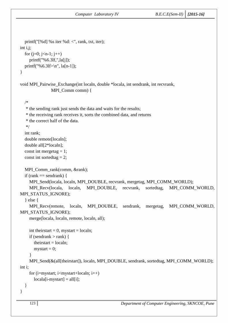
Computer Laboratory IV B.E.C.E(Sem-II) [2015-16]
123 Department of Computer Engineering, SKNCOE, Pune
printf("[%d] %s iter %d: <", rank, txt, iter);
int i,j;
for (j=0; j<n-1; j++)
printf("%6.3lf,",la[j]);
printf("%6.3lf>\n", la[n-1]);
}
void MPI_Pairwise_Exchange(int localn, double *locala, int sendrank, int recvrank,
MPI_Comm comm) {
/*
* the sending rank just sends the data and waits for the results;
* the receiving rank receives it, sorts the combined data, and returns
* the correct half of the data.
*/
int rank;
double remote[localn];
double all[2*localn];
const int mergetag = 1;
const int sortedtag = 2;
MPI_Comm_rank(comm, &rank);
if (rank == sendrank) {
MPI_Send(locala, localn, MPI_DOUBLE, recvrank, mergetag, MPI_COMM_WORLD);
MPI_Recv(locala, localn, MPI_DOUBLE, recvrank, sortedtag, MPI_COMM_WORLD,
MPI_STATUS_IGNORE);
} else {
MPI_Recv(remote, localn, MPI_DOUBLE, sendrank, mergetag, MPI_COMM_WORLD,
MPI_STATUS_IGNORE);
merge(locala, localn, remote, localn, all);
int theirstart = 0, mystart = localn;
if (sendrank > rank) {
theirstart = localn;
mystart = 0;
}
MPI_Send(&(all[theirstart]), localn, MPI_DOUBLE, sendrank, sortedtag, MPI_COMM_WORLD);
int i;
for (i=mystart; i<mystart+localn; i++)
locala[i-mystart] = all[i];
}
}
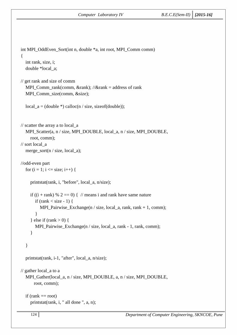
Computer Laboratory IV B.E.C.E(Sem-II) [2015-16]
124 Department of Computer Engineering, SKNCOE, Pune
int MPI_OddEven_Sort(int n, double *a, int root, MPI_Comm comm)
{
int rank, size, i;
double *local_a;
// get rank and size of comm
MPI_Comm_rank(comm, &rank); //&rank = address of rank
MPI_Comm_size(comm, &size);
local_a = (double *) calloc(n / size, sizeof(double));
// scatter the array a to local_a
MPI_Scatter(a, n / size, MPI_DOUBLE, local_a, n / size, MPI_DOUBLE,
root, comm);
// sort local_a
merge_sort(n / size, local_a);
//odd-even part
for (i = 1; i <= size; i++) {
printstat(rank, i, "before", local_a, n/size);
if ((i + rank) % 2 == 0) { // means i and rank have same nature
if (rank < size - 1) {
MPI_Pairwise_Exchange(n / size, local_a, rank, rank + 1, comm);
}
} else if (rank > 0) {
MPI_Pairwise_Exchange(n / size, local_a, rank - 1, rank, comm);
}
}
printstat(rank, i-1, "after", local_a, n/size);
// gather local_a to a
MPI_Gather(local_a, n / size, MPI_DOUBLE, a, n / size, MPI_DOUBLE,
root, comm);
if (rank == root)
printstat(rank, i, " all done ", a, n);
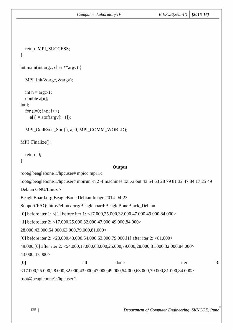
Computer Laboratory IV B.E.C.E(Sem-II) [2015-16]
125 Department of Computer Engineering, SKNCOE, Pune
return MPI_SUCCESS;
}
int main(int argc, char **argv) {
MPI_Init(&argc, &argv);
int n = argc-1;
double a[n];
int i;
for (i=0; i<n; i++)
a[i] = atof(argv[i+1]);
MPI_OddEven_Sort(n, a, 0, MPI_COMM_WORLD);
MPI_Finalize();
return 0;
}
Output
root@beaglebone1:/hpcuser# mpicc mpi1.c
root@beaglebone1:/hpcuser# mpirun -n 2 -f machines.txt ./a.out 43 54 63 28 79 81 32 47 84 17 25 49
Debian GNU/Linux 7
BeagleBoard.org BeagleBone Debian Image 2014-04-23
Support/FAQ: http://elinux.org/Beagleboard:BeagleBoneBlack_Debian
[0] before iter 1: <[1] before iter 1: <17.000,25.000,32.000,47.000,49.000,84.000>
[1] before iter 2: <17.000,25.000,32.000,47.000,49.000,84.000>
28.000,43.000,54.000,63.000,79.000,81.000>
[0] before iter 2: <28.000,43.000,54.000,63.000,79.000,[1] after iter 2: <81.000>
49.000,[0] after iter 2: <54.000,17.000,63.000,25.000,79.000,28.000,81.000,32.000,84.000>
43.000,47.000>
[0] all done iter 3:
<17.000,25.000,28.000,32.000,43.000,47.000,49.000,54.000,63.000,79.000,81.000,84.000>
root@beaglebone1:/hpcuser#

Computer Laboratory IV B.E.C.E(Sem-II) [2015-16]
126 Department of Computer Engineering, SKNCOE, Pune
Assignment No. 6
Title Frame the suitable assignment to perform computing using
BIA tools effectively.
Roll No.
Class B.E. (C.E.)
Date
Subject Computer Lab IV
Signature
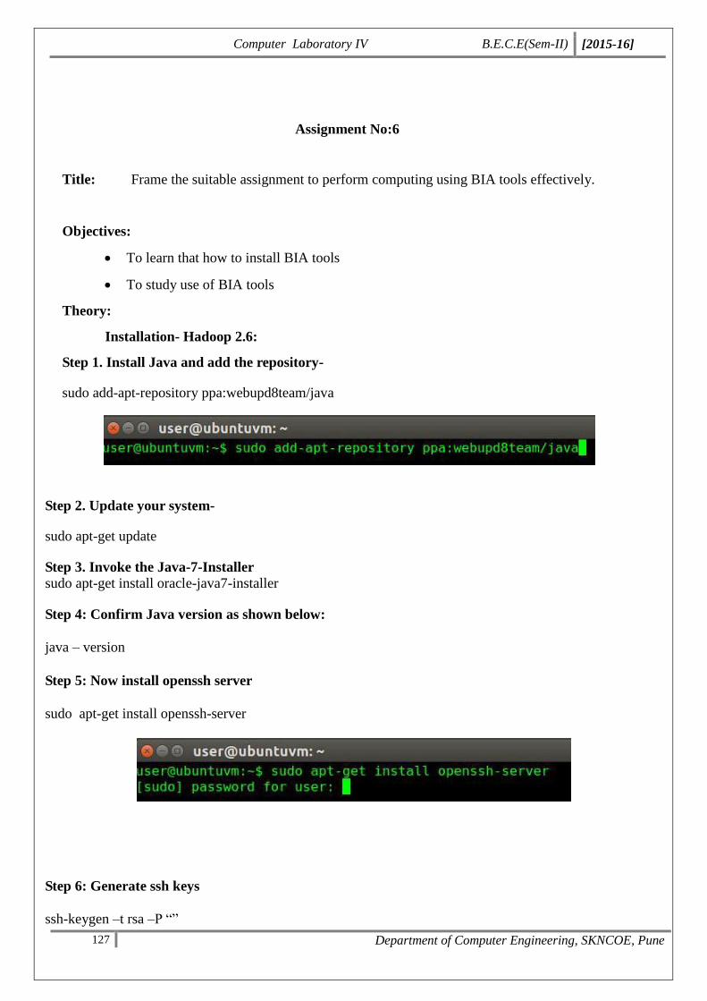
Computer Laboratory IV B.E.C.E(Sem-II) [2015-16]
127 Department of Computer Engineering, SKNCOE, Pune
Assignment No:6
Title: Frame the suitable assignment to perform computing using BIA tools effectively.
Objectives:
To learn that how to install BIA tools
To study use of BIA tools
Theory:
Installation- Hadoop 2.6:
Step 1. Install Java and add the repository-
sudo add-apt-repository ppa:webupd8team/java
sudo apt-get update
Step 3. Invoke the Java-7-Installer
sudo apt-get install oracle-java7-installer
Step 4: Confirm Java version as shown below:
java – version
Step 5: Now install openssh server
sudo apt-get install openssh-server
Step 6: Generate ssh keys
ssh-keygen –t rsa –P “”
Step 7: Just press enter for password, don’t enter any password by yourself. Once done it will
look like below:
Step 2. Update your system-
sudo apt-get update
Step 3. Invoke the Java-7-Installer
sudo apt-get install oracle-java7-installer
Step 4: Confirm Java version as shown below:
java – version
Step 5: Now install openssh server
sudo apt-get install openssh-server
Step 6: Generate ssh keys
ssh-keygen –t rsa –P “”
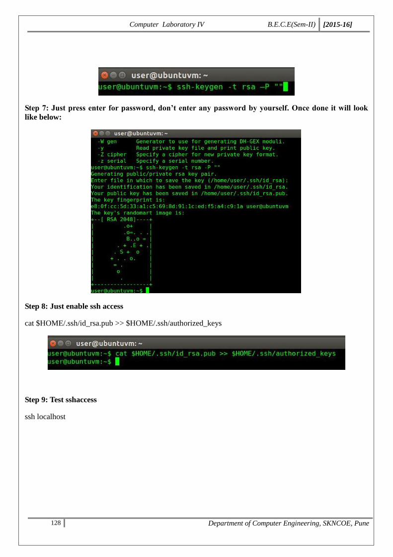
Computer Laboratory IV B.E.C.E(Sem-II) [2015-16]
128 Department of Computer Engineering, SKNCOE, Pune
Step 7: Just press enter for password, don’t enter any password by yourself. Once done it will look
like below:
Step 8: Just enable ssh access
cat $HOME/.ssh/id_rsa.pub >> $HOME/.ssh/authorized_keys
Step 9: Test sshaccess
ssh localhost
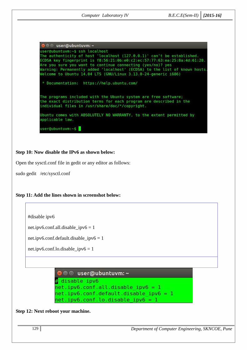
Computer Laboratory IV B.E.C.E(Sem-II) [2015-16]
129 Department of Computer Engineering, SKNCOE, Pune
Step 10: Now disable the IPv6 as shown below:
Open the sysctl.conf file in gedit or any editor as follows:
sudo gedit /etc/sysctl.conf
Step 11: Add the lines shown in screenshot below:
#disable ipv6
net.ipv6.conf.all.disable_ipv6 = 1
net.ipv6.conf.default.disable_ipv6 = 1
net.ipv6.conf.lo.disable_ipv6 = 1
Step 12: Next reboot your machine.
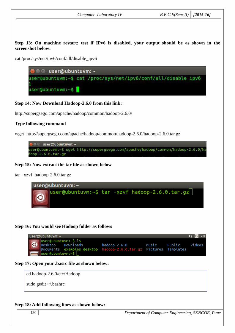
Computer Laboratory IV B.E.C.E(Sem-II) [2015-16]
130 Department of Computer Engineering, SKNCOE, Pune
Step 13: On machine restart; test if IPv6 is disabled, your output should be as shown in the
screenshot below:
cat /proc/sys/net/ipv6/conf/all/disable_ipv6
Step 14: Now Download Hadoop-2.6.0 from this link:
http://supergsego.com/apache/hadoop/common/hadoop-2.6.0/
Type following command
wget http://supergsego.com/apache/hadoop/common/hadoop-2.6.0/hadoop-2.6.0.tar.gz
Step 15: Now extract the tar file as shown below
tar -xzvf hadoop-2.6.0.tar.gz
Step 16: You would see Hadoop folder as follows
Step 17: Open your .basrc file as shown below:
cd hadoop-2.6.0/etc/Hadoop
sudo gedit ~/.bashrc
Step 18: Add following lines as shown below:
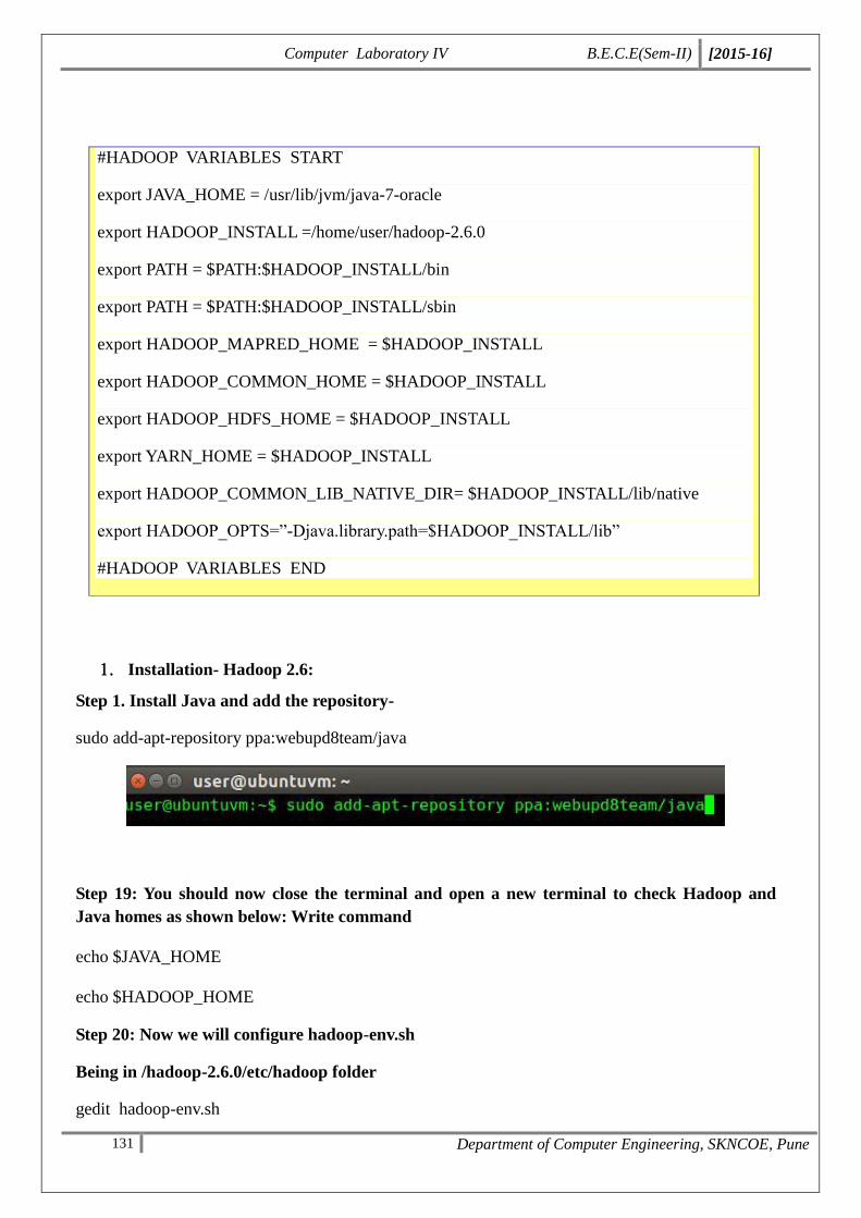
Computer Laboratory IV B.E.C.E(Sem-II) [2015-16]
131 Department of Computer Engineering, SKNCOE, Pune
#HADOOP VARIABLES START
export JAVA_HOME = /usr/lib/jvm/java-7-oracle
export HADOOP_INSTALL =/home/user/hadoop-2.6.0
export PATH = $PATH:$HADOOP_INSTALL/bin
export PATH = $PATH:$HADOOP_INSTALL/sbin
export HADOOP_MAPRED_HOME = $HADOOP_INSTALL
export HADOOP_COMMON_HOME = $HADOOP_INSTALL
export HADOOP_HDFS_HOME = $HADOOP_INSTALL
export YARN_HOME = $HADOOP_INSTALL
export HADOOP_COMMON_LIB_NATIVE_DIR= $HADOOP_INSTALL/lib/native
export HADOOP_OPTS=”-Djava.library.path=$HADOOP_INSTALL/lib”
#HADOOP VARIABLES END
Installation- Hadoop 2.6:
Step 1. Install Java and add the repository-
sudo add-apt-repository ppa:webupd8team/java
Step 19: You should now close the terminal and open a new terminal to check Hadoop and
Java homes as shown below: Write command
echo $JAVA_HOME
echo $HADOOP_HOME
Step 20: Now we will configure hadoop-env.sh
Being in /hadoop-2.6.0/etc/hadoop folder
gedit hadoop-env.sh
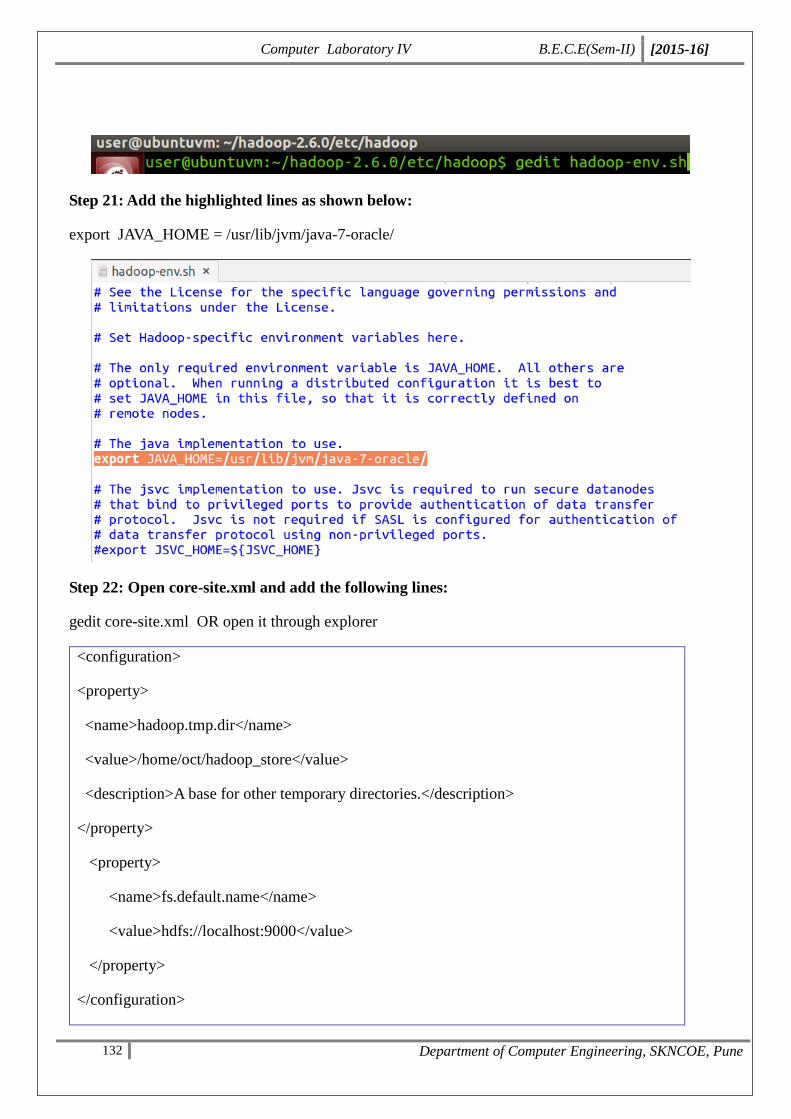
Computer Laboratory IV B.E.C.E(Sem-II) [2015-16]
132 Department of Computer Engineering, SKNCOE, Pune
Step 21: Add the highlighted lines as shown below:
export JAVA_HOME = /usr/lib/jvm/java-7-oracle/
Step 22: Open core-site.xml and add the following lines:
gedit core-site.xml OR open it through explorer
<configuration>
<property>
<name>hadoop.tmp.dir</name>
<value>/home/oct/hadoop_store</value>
<description>A base for other temporary directories.</description>
</property>
<property>
<name>fs.default.name</name>
<value>hdfs://localhost:9000</value>
</property>
</configuration>
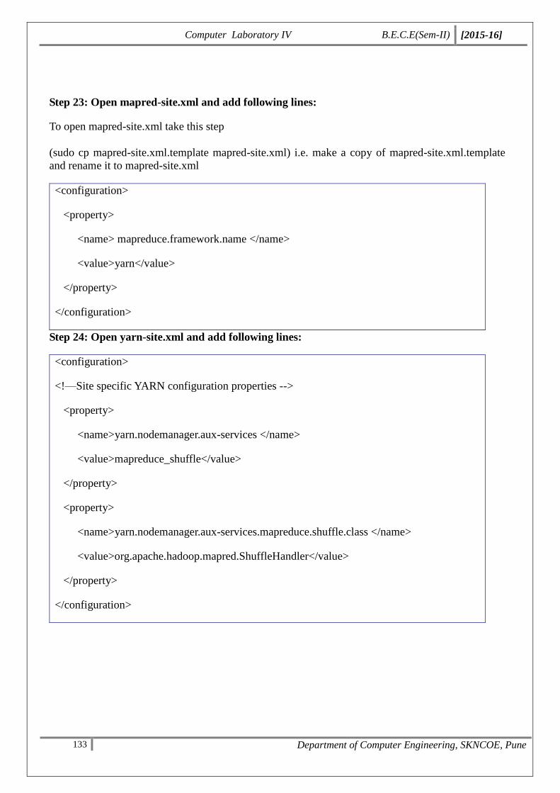
Computer Laboratory IV B.E.C.E(Sem-II) [2015-16]
133 Department of Computer Engineering, SKNCOE, Pune
Step 23: Open mapred-site.xml and add following lines:
To open mapred-site.xml take this step
(sudo cp mapred-site.xml.template mapred-site.xml) i.e. make a copy of mapred-site.xml.template
and rename it to mapred-site.xml
<configuration>
<property>
<name> mapreduce.framework.name </name>
<value>yarn</value>
</property>
</configuration>
Step 24: Open yarn-site.xml and add following lines:
<configuration>
<!—Site specific YARN configuration properties -->
<property>
<name>yarn.nodemanager.aux-services </name>
<value>mapreduce_shuffle</value>
</property>
<property>
<name>yarn.nodemanager.aux-services.mapreduce.shuffle.class </name>
<value>org.apache.hadoop.mapred.ShuffleHandler</value>
</property>
</configuration>
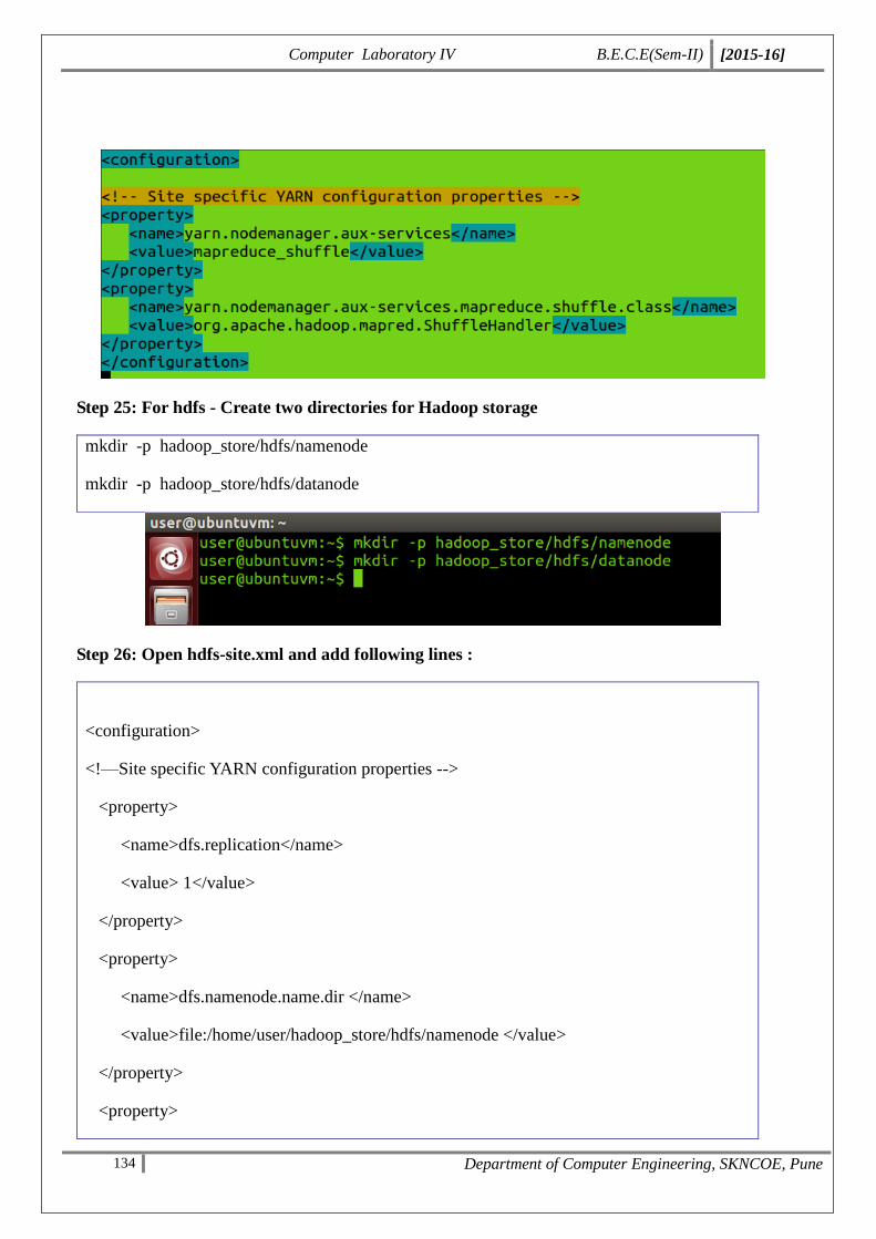
Computer Laboratory IV B.E.C.E(Sem-II) [2015-16]
134 Department of Computer Engineering, SKNCOE, Pune
Step 25: For hdfs - Create two directories for Hadoop storage
mkdir -p hadoop_store/hdfs/namenode
mkdir -p hadoop_store/hdfs/datanode
Step 26: Open hdfs-site.xml and add following lines :
<configuration>
<!—Site specific YARN configuration properties -->
<property>
<name>dfs.replication</name>
<value> 1</value>
</property>
<property>
<name>dfs.namenode.name.dir </name>
<value>file:/home/user/hadoop_store/hdfs/namenode </value>
</property>
<property>

Computer Laboratory IV B.E.C.E(Sem-II) [2015-16]
135 Department of Computer Engineering, SKNCOE, Pune
<name> dfs.namenode.data.dir </name>
<value> file:/home/user/hadoop_store/hdfs/datanode </value>
</property>
</configuration>
Step 27: Change folder permission
Write this command
sudo chown user:user -R /home/user/hadoop
sudo chown user:user -R /home/user/hadoop_store
Step 28: Give the folder the full permission
sudo chmod -R 777 /home/user/hadoop
sudo chmod -R 777 /home/user/hadoop_store
Step 29: Format namenode:
hdfs namenode –format
Step 30: Start all the services of Hadoop as shown below:
start-dfs.sh --- jps ---Namenode, Datanode and SecondaryNN
start-yarn.sh
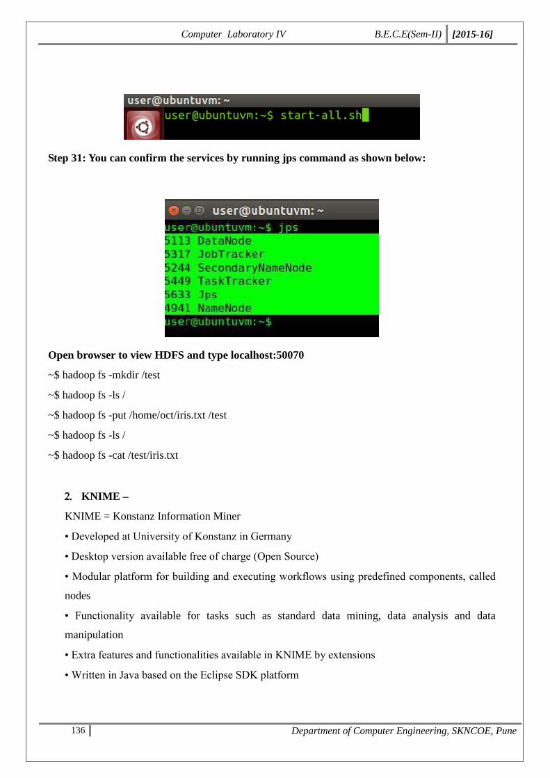
Computer Laboratory IV B.E.C.E(Sem-II) [2015-16]
136 Department of Computer Engineering, SKNCOE, Pune
Step 31: You can confirm the services by running jps command as shown below:
Open browser to view HDFS and type localhost:50070
~$ hadoop fs -mkdir /test
~$ hadoop fs -ls /
~$ hadoop fs -put /home/oct/iris.txt /test
~$ hadoop fs -ls /
~$ hadoop fs -cat /test/iris.txt
KNIME –
KNIME = Konstanz Information Miner
• Developed at University of Konstanz in Germany
• Desktop version available free of charge (Open Source)
• Modular platform for building and executing workflows using predefined components, called
nodes
• Functionality available for tasks such as standard data mining, data analysis and data
manipulation
• Extra features and functionalities available in KNIME by extensions
• Written in Java based on the Eclipse SDK platform
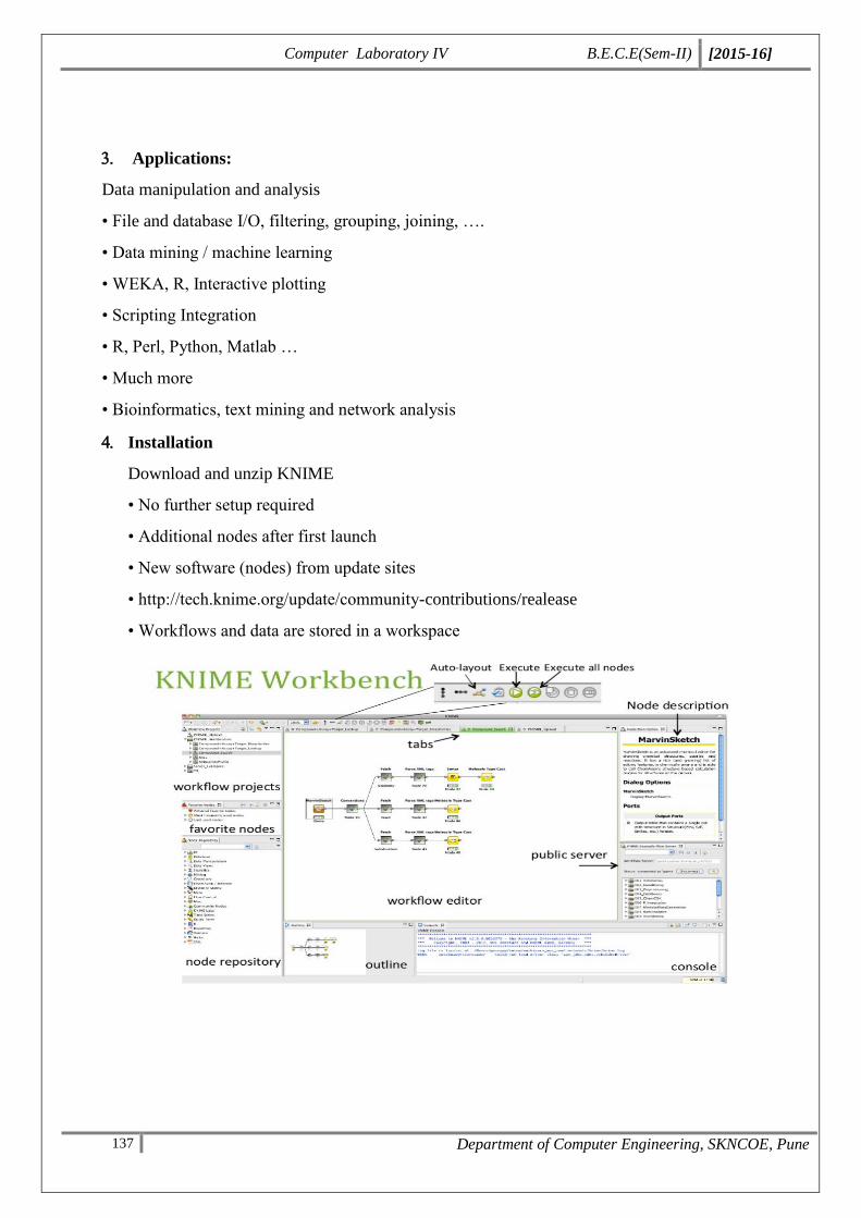
Computer Laboratory IV B.E.C.E(Sem-II) [2015-16]
137 Department of Computer Engineering, SKNCOE, Pune
Applications:
Data manipulation and analysis
• File and database I/O, filtering, grouping, joining, ….
• Data mining / machine learning
• WEKA, R, Interactive plotting
• Scripting Integration
• R, Perl, Python, Matlab …
• Much more
• Bioinformatics, text mining and network analysis
Installation
Download and unzip KNIME
• No further setup required
• Additional nodes after first launch
• New software (nodes) from update sites
• http://tech.knime.org/update/community-contributions/realease
• Workflows and data are stored in a workspace
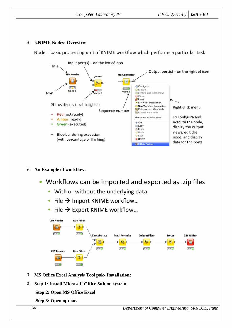
Computer Laboratory IV B.E.C.E(Sem-II) [2015-16]
138 Department of Computer Engineering, SKNCOE, Pune
KNIME Nodes: Overview
An Example of workflow:
MS Office Excel Analysis Tool pak- Installation:
Step 1: Install Microsoft Office Suit on system.
Step 2: Open MS Office Excel
Step 3: Open options
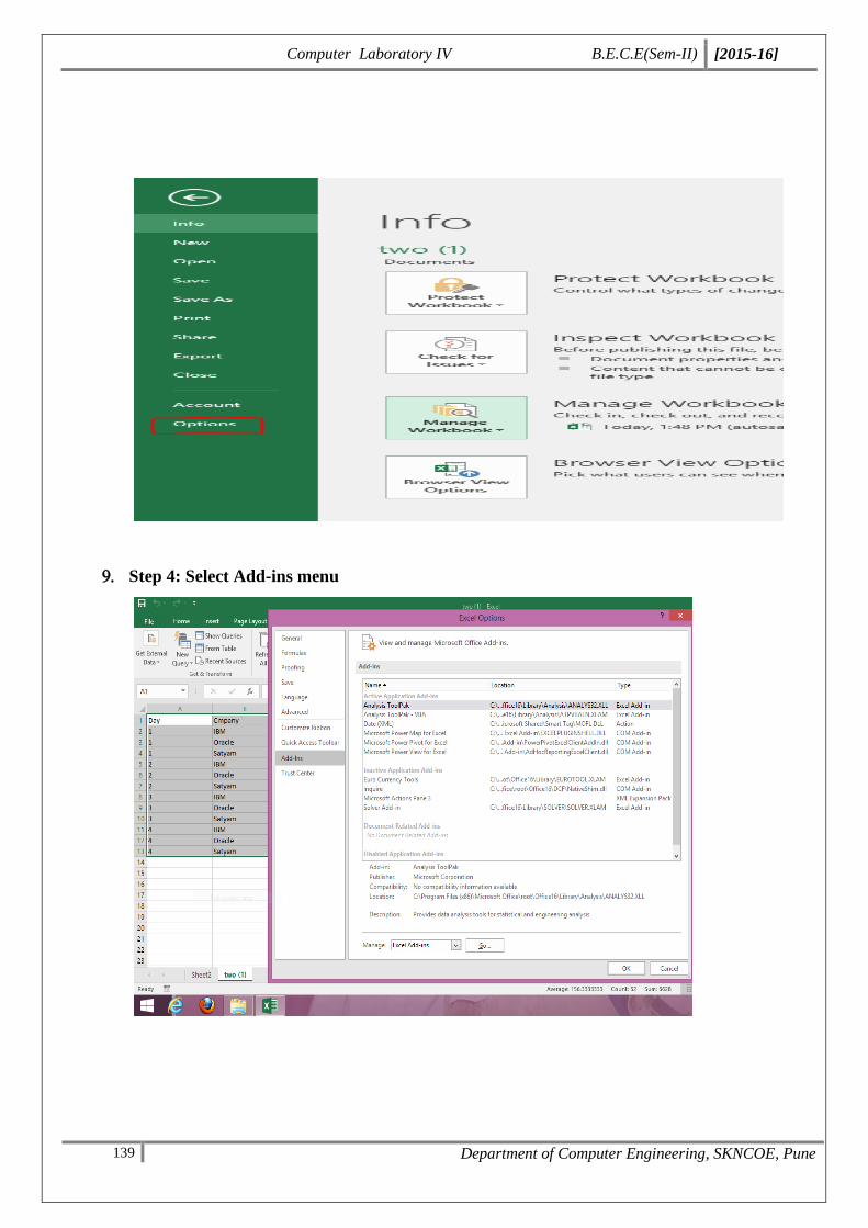
Computer Laboratory IV B.E.C.E(Sem-II) [2015-16]
139 Department of Computer Engineering, SKNCOE, Pune
Step 4: Select Add-ins menu
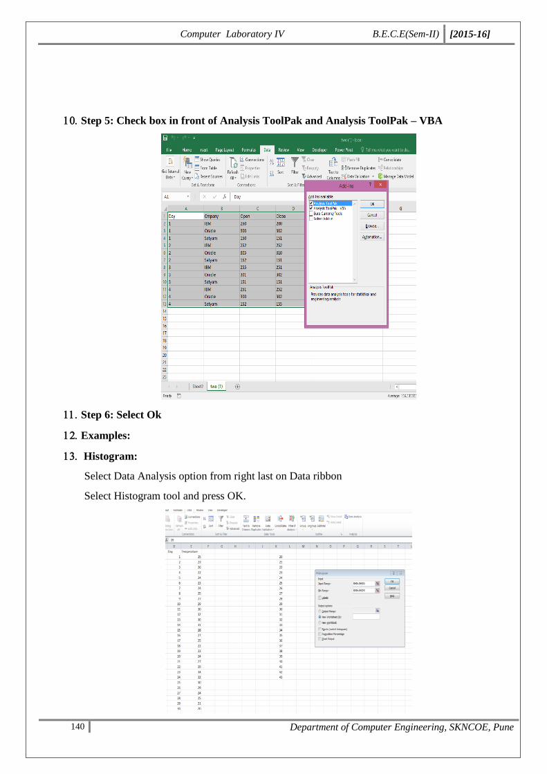
Computer Laboratory IV B.E.C.E(Sem-II) [2015-16]
140 Department of Computer Engineering, SKNCOE, Pune
Step 5: Check box in front of Analysis ToolPak and Analysis ToolPak – VBA
Step 6: Select Ok
Examples:
Histogram:
Select Data Analysis option from right last on Data ribbon
Select Histogram tool and press OK.

Computer Laboratory IV B.E.C.E(Sem-II) [2015-16]
141 Department of Computer Engineering, SKNCOE, Pune
Enter input range and Bin values by selecting appropriate cells from excel sheet
Covariance:
Select Data Analysis option from right last on Data ribbon
Select covariance tool and press OK.
Enter input range values by selecting appropriate cells from excel sheet
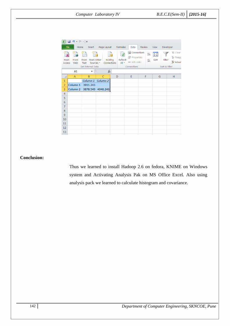
Computer Laboratory IV B.E.C.E(Sem-II) [2015-16]
142 Department of Computer Engineering, SKNCOE, Pune
Conclusion:
Thus we learned to install Hadoop 2.6 on fedora, KNIME on Windows
system and Activating Analysis Pak on MS Office Excel. Also using
analysis pack we learned to calculate histogram and covariance.

Computer Laboratory IV B.E.C.E(Sem-II) [2015-16]
143 Department of Computer Engineering, SKNCOE, Pune
Group C
Assignment
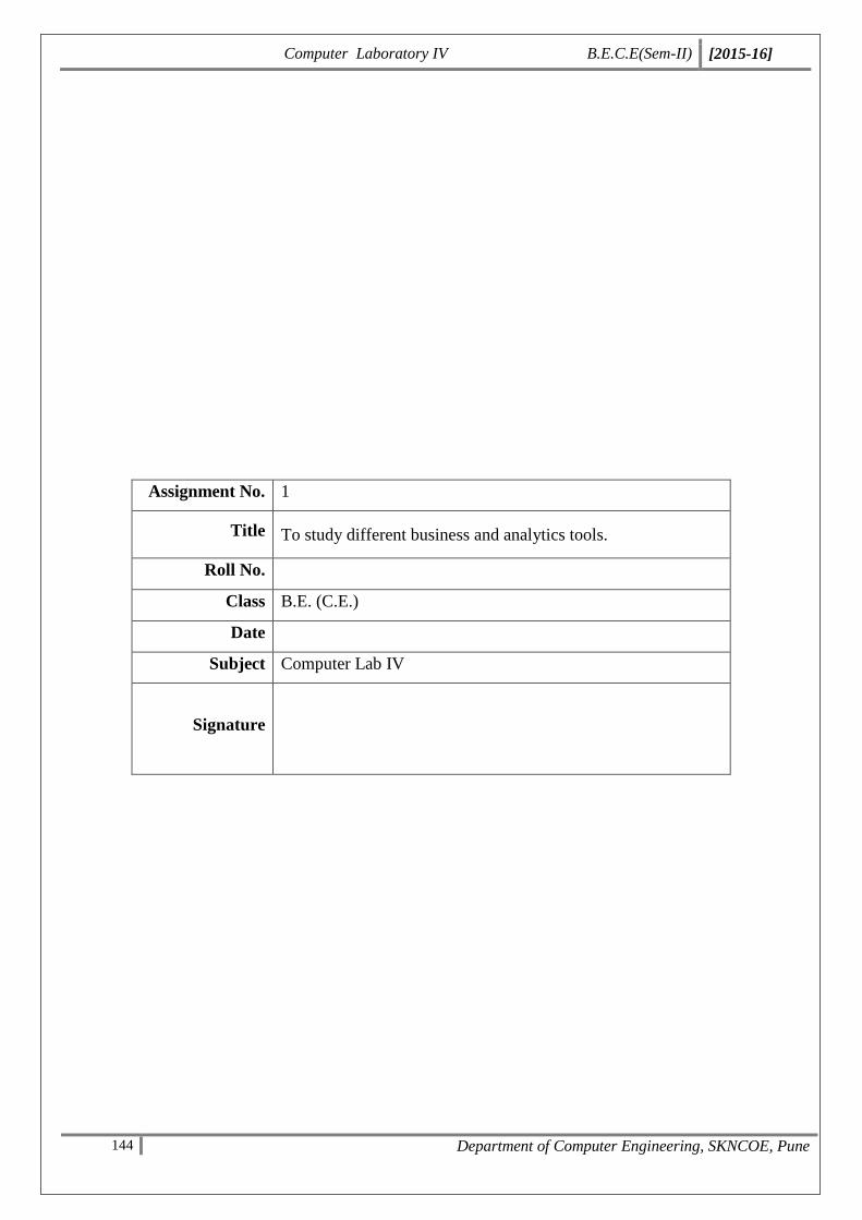
Computer Laboratory IV B.E.C.E(Sem-II) [2015-16]
144 Department of Computer Engineering, SKNCOE, Pune
Assignment No. 1
Title
To study different business and analytics tools.
Roll No.
Class B.E. (C.E.)
Date
Subject Computer Lab IV
Signature
Computer Laboratory IV B.E.C.E(Sem-II) [2015-16]
145 Department of Computer Engineering, SKNCOE, Pune
Assignment no.: 1
BIA:
Business intelligence (BI) can be described as "a set of techniques and tools for the acquisition and
transformation of raw data into meaningful and useful information for business analysis purposes".
The term "data surfacing" is also more often associated with BI functionality. BI technologies are
capable of handling large amounts of unstructured data to help identify, develop and otherwise
create new strategic business opportunities. The goal of BI is to allow for the easy interpretation of
these large volumes of data. Identifying new opportunities and implementing an effective strategy
based on insights can provide businesses with a competitive market advantage and long-term
stability.
BI technologies provide historical, current and predictive views of business operations. Common
functions of business intelligence technologies are reporting, online analytical processing, analytics,
data mining, process mining, complex event processing, business performance management,
benchmarking, text mining, predictive analytics and prescriptive analytics.
BI can be used to support a wide range of business decisions ranging from operational to strategic.
Basic operating decisions include product positioning or pricing. Strategic business decisions
include priorities, goals and directions at the broadest level. In all cases, BI is most effective when it
combines data derived from the market in which a company operates (external data) with data from
company sources internal to the business such as financial and operations data (internal data). When
combined, external and internal data can provide a more complete picture which, in e_ect, creates an
"intelligence" that cannot be derived by any singular set of data.
Business intelligence is made up of an increasing number of components including:
Multidimensional aggregation and allocation Denormalization, tagging and standardization Real-
Title: To study different business and analytics tools.
Objectives:
To study the the Business intelligence. Select an Industrial sector and write a BIA
tool for maximizing the profit.
Theory
Computer Laboratory IV B.E.C.E(Sem-II) [2015-16]
146 Department of Computer Engineering, SKNCOE, Pune
time reporting with analytical alert A method of interfacing with unstructured data sources Group
consolidation, budgeting and rolling forecasts Statistical inference and probabilistic simulation Key
performance in dicators optimization Version control and process management Open item
management.
BIA tool
Business intelligence tools are a type of application software designed to retrieve, analyze,
transform and report data for business intelligence. The tools generally read data that have been
previously stored, often, though not necessarily, in a data warehouse or data mart.
Types of business intelligence tools:
The key general categories of business intelligence tools are:
Spreadsheets
Reporting and querying software: tools that extract, sort, summarize present selected data
OLAP: Online analytical processing
Digital dashboards
Data mining
Process Visualization
Data warehousing
Local information systems
Except for spreadsheets, these tools are provided as standalone tools, suites of tools, components of
ERP systems, or as components of software targeted to a specific industry. The tools are sometimes
packaged into data warehouse appliances.
KNN:
The K Nearest Neighbor (k-NN) is a very intuitive method that classifies unlabeled examples based
on their similarity with examples in the training set.k-NN is a type of instance-based learning, or
lazy learning, where the function is only approximated locally and all computation is deferred until
classification. The k-NN algorithm is among the simplest of all machine learning algorithms.
Computer Laboratory IV B.E.C.E(Sem-II) [2015-16]
147 Department of Computer Engineering, SKNCOE, Pune
k-NN advantages
1. The cost of the learning process is zero
2. No assumptions about the characteristics of the concepts to learn have to be done
3. Complex concepts can be learned by local approximation using simple procedures
4. Robust to noisy training data.
Algorithm
1. start
2. Determine parameter K = number of nearest neighbors
3. Calculate the distance between the query instance and all the training samples
4. Sort the distance and determine nearest neighbors based on the K-th minimum distance
5. Gather the category Y of the nearest neighbors
6. Use simple majority of the category of nearest neighbors as the prediction value of the query
instance
Conclusion: We have successfully implemented BIA tools.
Computer Laboratory IV B.E.C.E(Sem-II) [2015-16]
148 Department of Computer Engineering, SKNCOE, Pune
Assignment No. 2
Title
Design suitable assignment for mobile programming
Roll No.
Class B.E. (C.E.)
Date
Subject Computer Lab IV
Signature
Computer Laboratory IV B.E.C.E(Sem-II) [2015-16]
149 Department of Computer Engineering, SKNCOE, Pune
Assignment No:2
Title: Design suitable assignment for mobile programming
Objectives:
To learn the concept that how to create mobile application
To study the representation and implementation of java and android studio
Theory:
1. Linux Kernel
The basic layer is the Linux Kernel. The whole Android OS is built on top of the Linux Kernel with
some further architectural changes. Please don’t get confused by the terms Linux and Linux Kernel.
The term Kernel means the core of any Operating System. By saying Android is based upon Linux
Kernel, it doesn’t mean that it is another Linux distribution. It is not like that. It simply means,
Android at its core is Linux. But you can’t run any linux packages on Android. It is a totally
different OS. It is this Linux kernel that interacts with the hardware and it contains all the essential
hardware drivers. Drivers are programs that control and communicate with the hardware. For
example, consider the Bluetooth function. All devices has a Bluetooth hardware in it. Therefore the
kernel must include a Bluetooth driver to communicate with the Bluetooth hardware. The Linux
kernel also acts as an abstraction layer between the hardware and other software layers. As the
Android is built on a most popular and proven foundation, the porting of Android to variety of
hardware became a relatively painless task.
2. Libraries
The next layer is the Android’s native libraries. It is this layer that enables the device to handle
different types of data. These libraries are written in c or c++ language and are specific for a
particular hardware.
Some of the important native libraries include the following:
Surface Manager: It is used for compositing window manager with off-screen buffering. Off-
screen buffering means the apps can’t directly draw into the screen, instead the drawings go to the
off-screen buffer. There it is combined with other drawings and form the final screen the user will
Computer Laboratory IV B.E.C.E(Sem-II) [2015-16]
150 Department of Computer Engineering, SKNCOE, Pune
see. This off screen buffer is the reason behind the transparency of windows.
Media framework: Media framework provides different media codecs allowing the recording and
playback of different media formats
SQLite: SQLite is the database engine used in android for data storage purposes
WebKit: It is the browser engine used to display HTML content
OpenGL: Used to render 2D or 3D graphics content to the screen
3. Android Runtime
Android Runtime consists of Dalvik Virtual machine and Core Java libraries.
Dalvik Virtual Machine
It is a type of JVM used in android devices to run apps and is optimized for low processing power
and low memory environments. Unlike the JVM, the Dalvik Virtual Machine doesn’t run .class
files, instead it runs .dex files. .dex files are built from .class file at the time of compilation and
provides hifger efficiency in low resource environments. The Dalvik VM allows multiple instance
of Virtual machine to be created simultaneously providing security, isolation, memory management
and threading support.
ART
Google has introduced a new virtual machine known as ART (Android Runtime) in their newer
releases of Android. In Lollipop, the Dalvik Virtual Machine is completely replaced by ART. ART
has many advantages over Dalvik VM such as AOT (Ahead Of Time) compilation and improved
garbage collection which boost the performance of apps significantly.
Core Java Libraries
These are different from Java SE and Java ME libraries. However these libraries provides most of
the functionalities defined in the Java SE libraries.
4. Application Framework
These are the blocks that our applications directly interacts with. These programs manage the basic
functions of phone like resource management, voice call management etc. As a developer, you just
consider these are some basic tools with which we are building our applications.
Computer Laboratory IV B.E.C.E(Sem-II) [2015-16]
151 Department of Computer Engineering, SKNCOE, Pune
Important blocks of Application framework are:
Activity Manager: Manages the activity life cycle of applications
Content Providers: Manage the data sharing between applications
Telephony Manager: Manages all voice calls. We use telephony manager if we want to access
voice calls in our application.
Location Manager: Location management, using GPS or cell tower
Resource Manager: Manage the various types of resources we use in our Application
5. Application
Applications are the top layer in the Android architecture and this is where our applications are
gonna fit into. Several standard applications comes pre-installed with every device, such as:
SMS client app
Dialer
Web browser
Contact manager
As a developer we are able to write an app which replaces any existing system app. That is, you are
not limited in accessing any particular feature. You are practically limitless and can whatever you
want to do with the android.
Conclusion:
Hence, we have successfully studied and implemented a simple application in mobile programming
Computer Laboratory IV B.E.C.E(Sem-II) [2015-16]
152 Department of Computer Engineering, SKNCOE, Pune
Program
import android.app.Activity;
import android.net.wifi.WifiInfo;
import android.net.wifi.WifiManager;
import android.os.Build;
import android.os.Bundle;
import android.view.Menu;
import android.widget.TextView;
public class MainActivity extends Activity {
@Override
protected void onCreate(Bundle savedInstanceState) {
super.onCreate(savedInstanceState);
// setContentView(R.layout.activity_main);
TextView infoView = new TextView(this);
setContentView(infoView);
WifiManager myWifiManager = (WifiManager) getSystemService(WIFI_SERVICE);
WifiInfo myWifiInfo = myWifiManager.getConnectionInfo();
int ipAddress = myWifiInfo.getIpAddress();
System.out.println("WiFi address is "
+ android.text.format.Formatter.formatIpAddress(ipAddress));
String info = "System Info:\n".toUpperCase();
info += "BOARD: " + Build.BOARD + "\n" + "BOOTLOADER: "
+ Build.BOOTLOADER + "\n" + "BRAND: " + Build.BRAND + "\n"
+ "CPU_ABI: " + Build.CPU_ABI + "\n" + "CPU_ABI2: "
+ Build.CPU_ABI2 + "\n" + "DEVICE: " + Build.DEVICE + "\n"
+ "DISPLAY: " + Build.DISPLAY + "\n" + "FINGERPRINT: "
+ Build.FINGERPRINT + "\n" + "HARDWARE: " + Build.HARDWARE
+ "\n" + "HOST: " + Build.HOST + "\n" + "ID: " + Build.ID
Computer Laboratory IV B.E.C.E(Sem-II) [2015-16]
153 Department of Computer Engineering, SKNCOE, Pune
+ "\n" + "MANUFACTURER: " + Build.MANUFACTURER + "\n"
+ "MODEL: " + Build.MODEL + "\n" + "PRODUCT: " + Build.PRODUCT
+ "\n" + "SERIAL: " + Build.SERIAL + "\n" + "TAGS: "
+ Build.TAGS + "\n" + "TIME: " + Build.TIME + "\n" + "TYPE: "
+ Build.TYPE + "\n" + "USER: " + Build.USER + "\n"
+ "My IP Address:" + ipAddress + "\n" + "Network ID: "
+ myWifiInfo.getNetworkId() + "\n" + "Mac Address: "
+ myWifiInfo.getMacAddress() + "\n" + "SSID: "
+ myWifiInfo.getSSID() + "\n"
+ "RadioVersion: " + Build.getRadioVersion() + "\n" + " \n";
infoView.setText(info);
}
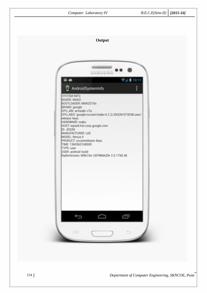
Computer Laboratory IV B.E.C.E(Sem-II) [2015-16]
154 Department of Computer Engineering, SKNCOE, Pune
Output
![Finale 2000a - [Gershwin Sax Med 11 x 17.MUS] · 2016. 4. 23. · B?? bbb bbb bbb bb b b bbb b b bb bb b b bbb bbb bbb bbb bbb bbb bbb bbb bbb bbb bbb bbb bbb 1 2 3 1 2 Eng. Hrn](https://img.pdfslide.net/doc/110x75/60fc438ee202e771cc70576b/finale-2000a-gershwin-sax-med-11-x-17mus-2016-4-23-b-bbb-bbb-bbb-bb.jpg)


![Finale 2005 - [Maestro Lázaro.mus]rede.cultura.ce.gov.br/banco-de-partituras/wp... · ã ã bbbbb bb bbb bbb bbb bbb bb bb bbb bbb bbb bbb bbb bb bb bb bbbbb bbbbb bbbbb bbbbb bb](https://img.pdfslide.net/doc/110x75/5fb08cc40d00c529e931a7d6/finale-2005-maestro-lzaromusrede-bbbbb-bb-bbb-bbb-bbb-bbb-bb-bb-bbb.jpg)