Computer Methods in Applied Mechanics and Engineeringcrm.sns.it/media/course/3060/miehe+hofacker+welschinger10.pdf · maximum reference energy obtained in the deformation history,

Computer Methods in Applied Mechanics and Engineering 199 (2010) 2765–

Contents lists available at ScienceDirect

Computer Methods in Applied Mechanics and Engineering

j ourna l homepage: www.e lsev ie r.com/ locate /cma

2778

A phase field model for rate-independent crack propagation: Robust algorithmicimplementation based on operator splits

Christian Miehe ⁎, Martina Hofacker, Fabian WelschingerInstitute of Applied Mechanics (CE) Chair I, University of Stuttgart, Pfaffenwaldring 7, 70550 Stuttgart, Germany

⁎ Corresponding author. Tel.: +49 711 685 66379.E-mail address: [email protected]: http://www.mechbau.uni-stuttgart.de/ls1/ (C.

0045-7825/$ – see front matter © 2010 Elsevier B.V. Aldoi:10.1016/j.cma.2010.04.011

a b s t r a c t
a r t i c l e i n f o
Article history:Received 4 January 2010Received in revised form 14 April 2010Accepted 15 April 2010Available online 7 May 2010

Keywords:FractureCrack propagationPhase fieldsGradient-type damageIncremental variational principlesFinite elementsCoupled multi-field problem

The computational modeling of failure mechanisms in solids due to fracture based on sharp crackdiscontinuities suffers in situations with complex crack topologies. This can be overcome by a diffusive crackmodeling based on the introduction of a crack phase field. Following our recent work [C. Miehe, F.Welschinger, M. Hofacker, Thermodynamically-consistent phase field models of fracture: Variationalprinciples and multi-field fe implementations, International Journal for Numerical Methods in EngineeringDOI:10.1002/nme.2861] on phase-field-type fracture, we propose in this paper a new variational frameworkfor rate-independent diffusive fracture that bases on the introduction of a local history field. It contains amaximum reference energy obtained in the deformation history, which may be considered as a measure forthe maximum tensile strain obtained in history. It is shown that this local variable drives the evolution of thecrack phase field. The introduction of the history field provides a very transparent representation of thebalance equation that governs the diffusive crack topology. In particular, it allows for the construction of anew algorithmic treatment of diffusive fracture. Here, we propose an extremely robust operator split schemethat successively updates in a typical time step the history field, the crack phase field and finally thedisplacement field. A regularization based on a viscous crack resistance that even enhances the robustness ofthe algorithm may easily be added. The proposed algorithm is considered to be the canonically simplescheme for the treatment of diffusive fracture in elastic solids. We demonstrate the performance of the phasefield formulation of fracture by means of representative numerical examples.

art.de (C. Miehe).Miehe).

l rights reserved.

© 2010 Elsevier B.V. All rights reserved.

1. Introduction

The prediction of failure mechanisms due to crack initiation andpropagation in solids is of great importance for engineering applica-tions. Following the classical treatments of Griffith [2] and Irwin [3],cracks propagate if the energy release rate reaches a critical value. TheGriffith theory provides a criterion for crack propagation but isinsufficient to determine curvilinear crack paths, crack kinking andbranching angles. In particular, such a theory is unable to predict crackinitiation. These defects of the classical Griffith-type theory of brittlefracture can be overcome by variational methods based on energyminimization as suggested by Francfort &Marigo [4], see also Bourdin,Francfort & Marigo [5], Dal Maso & Toader [6] and Buliga [7]. Theregularized setting of their framework, considered in Bourdin,Francfort & Marigo [8,5], is obtained by Γ-convergence inspired bythe work on image segmentation by Mumford & Shah [9]. We refer toAmbrosio & Tortorelli [10] and the reviews of Dal Maso [11] andBraides [12,13] for details on Γ-convergent approximations of freediscontinuity problems. The approximation regularizes a sharp crack

surface topology in the solid by diffusive crack zones governed by ascalar auxiliary variable. This variable can be considered as a phasefield which interpolates between the unbroken and the broken stateof the material. Conceptually similar are recently outlined phase fieldapproaches to brittle fracture based on the classical Ginzburg-Landautype evolution equation as reviewed in Hakim & Karma [14], see alsoKarma, Kessler & Levine [15] and Eastgate et al. [16]. In contrast to theabove mentioned rate-independent approach, these models are fullyviscous in nature and mostly applied to dynamic fracture. The phasefield approaches to fracture offer important new perspectives towardsthe theoretical and computational modeling of complex cracktopologies. Recall that finite-element-based numerical implementa-tions of sharp crack discontinuities, such as interface elementformulations, element and nodal enrichment strategies suffer in thecase of three-dimensional applications with crack branching. Ad-vanced XFEM-basedmethods for sharp crack propagation are outlinedin Belytschko et al. [17,18] We also refer to the adaptive interfacemethods by Gürses & Miehe [19] and Miehe & Gürses [20,21] for themodeling of configurational-force-driven sharp crack propagation. Incontrast, phase-field-type diffusive crack approaches avoid themodeling of discontinuities and can be implemented in a straightfor-ward manner by coupled multi-field finite element solvers. In therecent workMiehe,Welschinger & Hofacker [1], we outlined a general

mailto:[email protected]

http://www.mechbau.uni-stuttgart.de/ls1/

http://dx.doi.org/10.1016/j.cma.2010.04.011

http://www.sciencedirect.com/science/journal/00457825



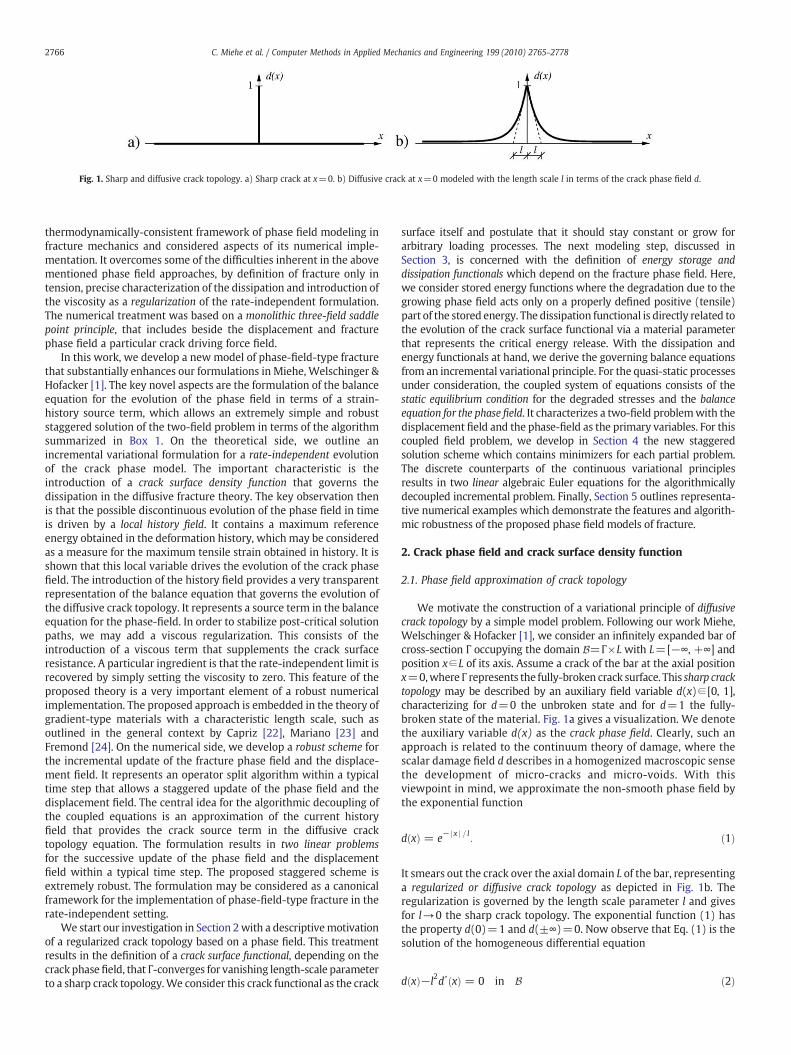
Fig. 1. Sharp and diffusive crack topology. a) Sharp crack at x=0. b) Diffusive crack at x=0 modeled with the length scale l in terms of the crack phase field d.

2766 C. Miehe et al. / Computer Methods in Applied Mechanics and Engineering 199 (2010) 2765–2778

thermodynamically-consistent framework of phase field modeling infracture mechanics and considered aspects of its numerical imple-mentation. It overcomes some of the difficulties inherent in the abovementioned phase field approaches, by definition of fracture only intension, precise characterization of the dissipation and introduction ofthe viscosity as a regularization of the rate-independent formulation.The numerical treatment was based on a monolithic three-field saddlepoint principle, that includes beside the displacement and fracturephase field a particular crack driving force field.

In this work, we develop a newmodel of phase-field-type fracturethat substantially enhances our formulations in Miehe, Welschinger &Hofacker [1]. The key novel aspects are the formulation of the balanceequation for the evolution of the phase field in terms of a strain-history source term, which allows an extremely simple and robuststaggered solution of the two-field problem in terms of the algorithmsummarized in Box 1. On the theoretical side, we outline anincremental variational formulation for a rate-independent evolutionof the crack phase model. The important characteristic is theintroduction of a crack surface density function that governs thedissipation in the diffusive fracture theory. The key observation thenis that the possible discontinuous evolution of the phase field in timeis driven by a local history field. It contains a maximum referenceenergy obtained in the deformation history, which may be consideredas a measure for the maximum tensile strain obtained in history. It isshown that this local variable drives the evolution of the crack phasefield. The introduction of the history field provides a very transparentrepresentation of the balance equation that governs the evolution ofthe diffusive crack topology. It represents a source term in the balanceequation for the phase-field. In order to stabilize post-critical solutionpaths, we may add a viscous regularization. This consists of theintroduction of a viscous term that supplements the crack surfaceresistance. A particular ingredient is that the rate-independent limit isrecovered by simply setting the viscosity to zero. This feature of theproposed theory is a very important element of a robust numericalimplementation. The proposed approach is embedded in the theory ofgradient-type materials with a characteristic length scale, such asoutlined in the general context by Capriz [22], Mariano [23] andFremond [24]. On the numerical side, we develop a robust scheme forthe incremental update of the fracture phase field and the displace-ment field. It represents an operator split algorithm within a typicaltime step that allows a staggered update of the phase field and thedisplacement field. The central idea for the algorithmic decoupling ofthe coupled equations is an approximation of the current historyfield that provides the crack source term in the diffusive cracktopology equation. The formulation results in two linear problemsfor the successive update of the phase field and the displacementfield within a typical time step. The proposed staggered scheme isextremely robust. The formulation may be considered as a canonicalframework for the implementation of phase-field-type fracture in therate-independent setting.

We start our investigation in Section 2with a descriptivemotivationof a regularized crack topology based on a phase field. This treatmentresults in the definition of a crack surface functional, depending on thecrack phasefield, that Γ-converges for vanishing length-scale parameterto a sharp crack topology.We consider this crack functional as the crack

surface itself and postulate that it should stay constant or grow forarbitrary loading processes. The next modeling step, discussed inSection 3, is concerned with the definition of energy storage anddissipation functionals which depend on the fracture phase field. Here,we consider stored energy functions where the degradation due to thegrowing phase field acts only on a properly defined positive (tensile)part of the stored energy. The dissipation functional is directly related tothe evolution of the crack surface functional via a material parameterthat represents the critical energy release. With the dissipation andenergy functionals at hand, we derive the governing balance equationsfrom an incremental variational principle. For the quasi-static processesunder consideration, the coupled system of equations consists of thestatic equilibrium condition for the degraded stresses and the balanceequation for the phase field. It characterizes a two-field problemwith thedisplacement field and the phase-field as the primary variables. For thiscoupled field problem, we develop in Section 4 the new staggeredsolution scheme which contains minimizers for each partial problem.The discrete counterparts of the continuous variational principlesresults in two linear algebraic Euler equations for the algorithmicallydecoupled incremental problem. Finally, Section 5 outlines representa-tive numerical examples which demonstrate the features and algorith-mic robustness of the proposed phase field models of fracture.

2. Crack phase field and crack surface density function

2.1. Phase field approximation of crack topology

We motivate the construction of a variational principle of diffusivecrack topology by a simple model problem. Following our work Miehe,Welschinger & Hofacker [1], we consider an infinitely expanded bar ofcross-section Γ occupying the domain B=Γ×L with L=[−∞, +∞] andposition x∈L of its axis. Assume a crack of the bar at the axial positionx=0,where Γ represents the fully-broken crack surface. This sharp cracktopology may be described by an auxiliary field variable d(x)∈[0, 1],characterizing for d=0 the unbroken state and for d=1 the fully-broken state of the material. Fig. 1a gives a visualization. We denotethe auxiliary variable d(x) as the crack phase field. Clearly, such anapproach is related to the continuum theory of damage, where thescalar damage field d describes in a homogenized macroscopic sensethe development of micro-cracks and micro-voids. With thisviewpoint in mind, we approximate the non-smooth phase field bythe exponential function

dðxÞ = e− jx j = l: ð1Þ

It smears out the crack over the axial domain L of the bar, representinga regularized or diffusive crack topology as depicted in Fig. 1b. Theregularization is governed by the length scale parameter l and givesfor l→0 the sharp crack topology. The exponential function (1) hasthe property d(0)=1 and d(±∞)=0. Now observe that Eq. (1) is thesolution of the homogeneous differential equation

dðxÞ−l2d″ðxÞ = 0 in B ð2Þ


Fig. 2. Sharp and diffusive crack topology. a) Sharp crack surface Γ embedded into the solid B. b) The regularized crack surface Γl(d) is a functional of the crack phase field d.

1 Convergence to Sharp Crack Discontinuities. The Γ–limit Γl→Γ of the functionalEq. (6) for vanishing length scale l→0 to the sharp crack surface Γ:=∫

ΓdA is considered

in Braides [12], see Fig. 3 for a visualization. The functional Eq. (4) provides the basisfor an elliptic regularization of the free discontinuity problem of brittle fracture. It hasalready been used in Bourdin, Francfort and Marigo [8] for the definition of aregularized surface energy. In contrast, we introduce the functional in the purelygeometric context with regard to the subsequent definition of a dissipation potential.

C. Miehe et al. / Computer Methods in Applied Mechanics and Engineering 199 (2010) 2765–2778 2767

subject to the above Dirichlet-type boundary conditions. Thisdifferential equation is the Euler equation of the variational principle

d = Arg infd∈WIðdÞf g with IðdÞ = 12∫B d2 + l2d′2

n odV ð3Þ

and W={d|d(0)=1, d(±∞)=0}. The functional I(d) can easily beconstructed by integrating a Galerkin-typeweak form of the differentialEq. (2). Now observe, that the evaluation of the functional for thesolution (1) gives with dV=Γdx the identification I(d=e−|x|/l)= lΓ,which relates the functional I to the crack surface Γ. As a consequence,we may introduce the functional

ΓlðdÞ : =1lIðdÞ = 1

2l∫B d2 + l2d′2

n odV ð4Þ

alternatively to Eq. (3)2. Clearly, the minimization of this scaledfunctional also gives the regularized crack topology (1) depicted inFig. 1b. However, the scaling by the length-scale parameter l has theconsequence that the functional Γl(d) may be considered as the cracksurface itself. In the one-dimensional problem under consideration, theevaluation of Γl(d) at the solution point gives for arbitrary length scalesl the crack surface Γ. This property characterizes the functional Γl as animportant ingredient of the subsequent constitutive modeling ofdiffusive crack propagation.

2.2. Introduction of a crack surface density function

The one-dimensional description of a diffusive crack topology canbe extended to multi-dimensional solids in a straightforward manner.Let B⊂Rδ, be the reference configuration of a material body withdimension δ∈ [1–3] in space and ∂B⊂Rδ−1 its surface as depicted inFig. 2. In the subsequent treatment, we intend to study cracks in thesolid evolving in the range T ⊂R of time. To this end, we introducethe time-dependent crack phase field

d : B × T →½0;1�ðx; tÞ↦dðx; tÞ

�ð5Þ

defined on the solid B. Then, a multi-dimensional extension of theone-dimensional regularized crack functional Eq. (4), derived inAppendix A, reads

ΓlðdÞ = ∫B γðd;∇dÞdV ; ð6Þ

where we have introduced the crack surface density function per unitvolume of the solid

γ d;∇dð Þ = 12l

d2 +l2j∇dj2 ð7Þ

This function, which depends on the crack phase field d and its spatialgradient ∇d, plays a critical role in the subsequent modeling ofcrack propagation. Assuming a given sharp crack surface topology

γ d;∇dð Þ = 12l

d2 +l2j∇dj2

Γ(t)⊂Rδ−1 inside the solid B at time t, as depicted in Fig. 2a, weobtain in analogy to Eq. (3) the regularized crack phase field d(x, t) onB, visualized in Fig. 2b, from the minimization principle

dðx; tÞ = Arg infd∈WΓðtÞ

ΓlðdÞ( )

ð8Þ

subject to theDirichlet-type constraintsWΓ(t)={d|d(x, t)=1atx∈Γ(t)}.The Euler equations of the above variational principle are

d−l2Δd = 0 in B and ∇d·n = 0 on ∂B; ð9Þ

whereΔd is the Laplacianof thephasefield andn theoutwardnormal on∂B. Fig. 3 depicts a numerical solution of the variational problem (8) ofdiffusive crack topology and demonstrates the influence of the lengthscale l. We refer to the recentworkMiehe,Welschinger & Hofacker [12],for a more detailed derivation.1

3. A framework of rate-independent diffusive fracture

With the idea of a diffusive crack topology at hand, we developin this section a constitutive framework of phase-field-type fracturefor the rate-independent setting. The subsequent formulation interms of a history field is motivated in Appendix A by a simple one-dimensional structure of local damage mechanics. Fig. 4 provides avisual guide to the subsequent developments.

3.1. Degrading strain energy functional due to fracture

3.1.1. Displacement and strain fieldsIn the small-strain context, we describe the response of the

fracturing solid by the displacement field

u : B × T →Rδ

ðx; tÞ↦uðx; tÞ

�ð10Þ

in addition to the phase field d introduced in Eq. (5). u(x, t)∈Rδ is thedisplacement of the material point x∈B at time t∈T . The strains areassumed to be small. Thus, the norm of the macroscopic displacement


Fig. 3. Solutions of the variational problem (8) of diffusive crack topology for a quadratic specimen with a horizontal sharp crack Γ, taken from [1]. Regularized crack surfaces Γl(d)governed by the crack phase field d for different length scales laN lbN lcN ld. The sequence of pictures visualizes the Γ-limit Γl→Γ of the crack surface functional Eq. (6).


gradient ||∇u||b � is bounded by a small number �. The displacementgradient defines the small strain tensor

εðuÞ = ∇su :=12½∇u + ∇Tu�: ð11Þ

In order to account for a stress degradation only in tension, wedecompose the strain tensor into positive and negative parts

ε = εþ + ε− ð12Þ

describing tensile and compressive modes. These contributions aredefined based on the spectral decomposition of the strain tensorε=∑i=1

δ εini⊗ni, where {εi}i=1...δ are the principal strains and{ni}i=1...δ the principal strain directions. We set

εþ := ∑δi = 1 ⟨ε

i⟩ + ni⊗ ni and ε− := ∑δ

i = 1 ⟨εi⟩−ni⊗ ni ð13Þ

in terms of the bracket operators ⟨x⟩+:=(x+|x|)/2 and ⟨x⟩−:= (x− |x|)/2, respectively. The derivative of Eq. (12) with respect to the totalstrains defines the two projection tensors

ℙþ : = ∂ε½εþðεÞ� and ℙ− := I−ℙþ; ð14Þ

which are isotropic tensor functions of ε. These fourth-order tensorsproject the total strains onto its positive and negative parts, i.e. ε+=P+:ε and ε−=P−:ε. The computation of these objects is performedby the algorithms outlined in Miehe [25] and Miehe & Lambrecht[26].

Fig. 4. Amulti-field approach of phase-field-type crack propagation in deformable solids. Thesolid domain B. a) The displacement field is constrained by the Dirichlet- and Neumann-tyfracture phase field is constrained by the possible Dirichlet-type boundary condition d=1 odefined in Eq. (40) contains a maximum local strain energy obtained within the fracture pr

3.1.2. Constitutive free energy functionalWe focus on the standard linear theory of elasticity for isotropic

solids by considering the global energy storage functional

Eðu; dÞ = ∫BψðεðuÞ; dÞdV ð15Þ

that depends on the displacement u and the fracture phase field d. Theenergy storage function ψ describes the energy stored in the bulk of thesolid per unit volume. A fully isotropic constitutive assumption for thedegradation of energy due to fracture may have the form

ψ ε; dð Þ = g dð Þ + k½ �ψþ0 εð Þ + ψ−

0 εð Þ: ð16Þ

In thismultiplicative ansatz,ψ0 is an isotropic reference energy functionassociated with the undamaged elastic solid, i.e.

ψ0ðεÞ = λtr2½ε�= 2 + μtr½ε2� ð17Þ

with elastic constants λN0 and μN0, which we additively decompose

ψðεÞ = ψþ0 ðεÞ + ψ−

0 ðεÞ ð18Þ

into a positive part ψ0+ due to tension and a negative part ψ0

− due tocompression. Here, we assume the definitions

ψþ0 ðεÞ = λ⟨tr½ε�⟩2þ = 2 + μtr½ε2þ� and ψ−

0 ðεÞ = λ⟨tr½ε�⟩2− = 2 + μtr½ε2−�ð19Þ

with the above definitions of the brackets ⟨x⟩+ and ⟨x⟩_ and thepositive and negative strain tensors ε+ and ε−, respectively. Note thatboth terms are positive. Furthermore, observe that the volumetric

ψ ε;dð Þ = g dð Þ + k½ �ψþ0 εð Þ + ψ−

0 εð Þ:

displacement field u, the fracture phase field d and the history fieldH are defined on thepe boundary conditions u=uD on ∂Bu and σ⋅n= tN on ∂Bt with ∂B=∂Bu∪∂Bt. b) Then Γ and the Neumann condition ∇d⋅n=0 on the full surface ∂B. c) The history field Hocess. It drives the evolution of the fracture phase field d via Eq. (41).


Box 1Staggered Scheme for Phase Field Fracture in [tn, tn+1].

1. Initialization. The displacement, fracture phase and history fields un, dn and Hn at time tn are known. Update prescribed loads γ, ū, t atcurrent time tn+1.

2. Compute History. Determine maximum reference energy obtained in history

H =ψþ0 ð∇sunÞ for ψþ

0 ð∇sunÞ N Hn

Hn otherwise

(

in the domain B and store it as a history variable field.3. Compute Fracture Phase Field. Determine the current fracture phase field d from the minimization problem of crack topology

d = Arg infd

∫B gcγðd;∇dÞ + η2τ

ðd−dnÞ2−ð1−dÞ2H

h idV

n o

with the crack surface density function

γðd;∇dÞ = 12l

d2 +l2j∇d j2:

4. Compute Displacement Field. Determine the current displacement u at frozen fracture phase field d from the minimization problem ofelasticity

u = Arg infu

∫B ψð∇su;dÞ−γ·u½ �dV−∫∂Btt⋅udA

n o

with the free energy density function

ψðε;dÞ = ½ð1−dÞ2 + k�ψþ0 ðεÞ + ψ−

0 ðεÞ

with ψ0±(ε)=λ ⟨ tr[ε] ⟩±2 /2+μtr[ε±2 ] for the Dirichlet-type boundary condition u=ū on ∂Bu.


contribution is chosen either positive or negative according to the signof the volume dilatation e=tr[ε], which cannot be expressed in termsof the positive and negative strain tensors ε+ and ε−. Themonotonically decreasing degradation function g(d) describes thedegradation of the positive (tensile) part of the stored energy withevolving damage. It is assumed to have the properties

gð0Þ = 1 ; gð1Þ = 0 ; g′ð1Þ = 0: ð20Þ

The first two conditions include the limits for the unbroken and thefully-broken case. As shown below, the latter constraint ensures thatthe energetic fracture force converges to a finite value if the damageconverges to the fully-broken state d=1. A simple function that hasthe above properties is

gðdÞ = ð1−dÞ2: ð21Þ

The small positive parameter k≈0 in Eq. (16) circumvents the fulldegradation of the energy by leaving the artificial elastic rest energydensity kψ0(ε) at a fully-broken state d=1. It is chosen as small aspossible such that the algebraic conditioning number of the appliednumerical discretization method remains well-posed for partly-broken systems.

3.1.3. Rate of energy functionalTaking the time derivative of Eq. (15), we obtain the rate of energy

which we consider to be a functional of the rates {u, ḋ}

Eðu; d;u; dÞ = ∫B ½σ : ∇s u−f d �dV ð22Þ

at given state {u, d}. Here, we introduced per definition the stresstensor

σ := ∂εψðε; dÞ = ½ð1−dÞ2 + k�½λ⟨tr½ε�⟩þ1 + 2μεþ� + ½λ⟨tr½ε�⟩−1 + 2με−�ð23Þ

and the energetic force

f := −∂dψðε;dÞ = 2ð1−dÞψþ0 ðεÞ: ð24Þ

Note that the energetic force f is positive and bounded by a finite valuefor the limit ψ0

+(ε)→∞. As shown below this property ensures thatthe phase field variable is bounded by its maximum value d=1. Thekey term that drives the crack evolution is the positive part ψ0

+(ε) ofthe reference energy, that may be considered to describe locally theintensity of the tensile part of the deformation.

3.2. Dissipation functional due to fracture

3.2.1. Dissipation due to crack propagationFor a given fracture surface functional Γ(d) introduced in Eq. (6),

we define the work needed to create a diffusive fracture topology by

WcðdÞ : = ∫B gcγðd;∇dÞdV ; ð25Þ

where gc is the Griffith-type critical energy release rate and γ(d, ∇d)the crack surface density function defined in Eq. (7). The rate of thework functional Wc defines the crack dissipation

Wcðd;dÞ = ∫B ðgcδdγÞddV ; ð26Þ



which is considered to be a functional of the rate {d} of the crack phasefield at given state {d}. Here, we introduced the variational orfunctional derivative

δdγðdÞ := ∂dγ−Div½∂∇dγ� =1l½d−l2Δd� ð27Þ

of the crack density function. Based on thermodynamical arguments,we demand

Wcðd;dÞ≥ 0 ð28Þ

as the basic ingredient of our framework, enforcing a growth of thefracture workWc defined in Eq. (25). Observe that we may satisfy thisglobal irreversibility constraint of crack evolution by ensuring locally apositive variational derivative of the crack surface function and apositive evolution of the crack phase field

δdγ ≥ 0 and d ≥ 0: ð29Þ

The former condition is ensured in the subsequent treatment by aconstitutive assumption that relates the functional derivative to apositive energetic driving force. The latter constraint is a naturalassumption that relates the fracture phase field for the non-reversibleevolution of micro-cracks and micro-voids.

3.2.2. Rate-independent evolution of the phase fieldIn order to satisfy the local constraints Eq. (29) within a possibly

discontinuous, rate-independent evolution, we introduce the localthreshold function

tcðβ; dÞ = β−gcδdγðdÞ ≤ 0 ð30Þ

formulated in terms of the variable β dual to d, in what followsdenoted as the driving force field. Then, as shown below, the abovelocal constraints Eq. (29) can be satisfied by the definition

Wcðd;dÞ = supβ;λ≥0

Dλðd;β;λ; dÞ ð31Þ

in terms of the extended dissipation functional

Dλðd;β;λ;dÞ = ∫B ½β d−λtcðβ;dÞ�dV ð32Þ

that includes the threshold function (30). λ is a Lagrange multiplierfield.

3.3. Incremental variational principle and governing equations

3.3.1. An incremental variational principleWith the rate of the energy functional Eq. (22) and the extended

dissipation functional Eq. (32) at hand, we introduce the incrementalpotential

Πλðu; d;β;λ;u; dÞ = Eðu; d;u;dÞ + Dλðd;β;λ;dÞ−PðuÞ; ð33Þ

that balances the internal power Ė+Dλ with the power due toexternal loading

PðuÞ = ∫Bγ·udV + ∫∂Bt

t· udA: ð34Þ

Here, γ is a prescribed volume force in B and t a surface traction on ∂Bt.We then obtain the basic field equations of the problem from theargument of virtual power that we base on the variational statement

fu; d;β;λg = Argf statu ; d;β;λ≥0

Πλðu; d;β;λ;u; dÞg: ð35Þ

The variation of the functional with respect to the four field variables,taking into account δu=0 on ∂Bu, yields the coupled field equations

ð1Þ : Div½σ� + Pγ = 0;ð2Þ : β−f = 0;ð3Þ : d−λ = 0;ð4Þ : λ ≥ 0;ð5Þ : β−gcδdγ ≤ 0;ð6Þ : λðβ−gcδdγÞ = 0

ð36Þ

in the domain B along with the boundary conditions

σ·n = t on ∂Bt and ∇d·n = 0 on ∂B: ð37Þ

Note that we have introduced per definition the stress tensor σand the energetic force f defined in Eqs. (23) and (24). The lastthree equations in Eq. (36) are the Kuhn-Tucker-type equationsassociated with the optimization problem with inequality con-straints. From Eq. (36)2,3, elimination of β= f and λ=ḋ yields thereduced system

ð1Þ : Div½σ� + Pγ = 0;ð2Þ : d ≥ 0;ð3Þ : f−gcδdγ ≤ 0;ð4Þ : dðf−gcδdγÞ = 0:

ð38Þ

Note that Eq. (38)2 satisfies explicitly the desired thermodynamicconsistency condition (29)2. The first condition gcδdγ≥0 in (29)1 isalso satisfied. This may be seen if the damage field is computed in thecase of loading from Eq. (38)3, which results into

gcδdγ :=gcl½d−l2Δd� = 2ð1−dÞψþ

0 ðεÞ for d N 0: ð39Þ

Note that the right hand side is positive which proves thecondition (29)1. Thus the proposed model of rate-independentdiffusive crack evolution is consistent with the thermodynamicaxiom of positive dissipation. Note furthermore, that Eq. (39) hasthe desired property d→1 for ψ0

+(ε)→∞.

3.3.2. Compact history-field-based formulationIt is clear that the ‘load term’ ψ0

+(ε) in Eq. (39) determines theamount of the phase field variable d. Hence, motivated by Eq. (A.7) ofthe local damagemodel outlined in Appendix A, wemay introduce thelocal history field of maximum positive reference energy

Hðx; tÞ := maxs∈½0;t�

ψþ0 ðεðx; sÞÞ ð40Þ

obtained in a typical, possibly cyclical loading process. Replacing ψ0+ in

Eq. (39) by this field, we obtain the equation

gcl

d−l2Δdh i

= 2 1−dð ÞH ð41Þ

which determines the phase field in the case of loading and unloading.Note that this equation equips the crack topology Eq. (9)1 by the localcrack source on the right hand side. With this notion at hand, theproposed fracture phase field model may be reduced to the compactsystem of only two equations

ð1Þ : Div½σðu;dÞ� + Pγ = 0;ð2Þ : gcδdγðdÞ−2ð1−dÞH = 0;

ð42Þ

which determine the current displacement and phase fields u and d interms of the definitions (23), (40), (19) and (27) for the stresses σ,

gcl

d−l2Δdh i

= 2 1−dð ÞH



the history field H of maximum reference energy ψ0+ and the

variational derivative δdγ of the crack density function. This isconsidered to be the most simple representation of rate-independentdiffusive fracture, associated with the multi-field scenario visualizedin Fig. 4.

3.4. Viscous regularization of the rate-independent problem

As commented on in Section 5, a viscous regularization of theabove rate-independent formulation may stabilize the numericaltreatment. It can be formulated in terms of a variational principlebased on the potential

Πηðu; d;β;u;dÞ = Eðu; d;u; dÞ + Dηðd;β;dÞ−PðuÞ; ð43Þ

that includes a modified extended dissipation functional

Dηðd;β;dÞ = ∫B ½β d−1η⟨tcðβ;dÞ⟩

2þ�dV ; ð44Þ

where η≥0 is a viscosity parameter. The modified variationalprinciple

fu; d;βg = Argf statu ; d; β

Πηðu; d;β;u;dÞg ð45Þ

then results in the coupled set of local equations

ð1Þ : Div½σ� + Pγ = 0;

ð2Þ : d−1η⟨f−gcδdγ⟩þ = 0;

ð46Þ

where the field β has been eliminated. Note that the evolution ḋ of thephase field is now governed by a viscous equation governed by the‘over-force’ ⟨f−gcδdγ⟩+. As a consequence, Eq. (41) may be recast intothe viscous regularized format

gcl

d−l2Δdh i

+ ηd = 2 1−dð ÞH ð47Þ

again driven by the local history field H of maximum positivereference energy defined in Eq. (40). This equation equips the cracktopology Eq. (9)1 by the viscous resistance term on the left hand sideand the crack source term on the right hand side. Thus the viscousregularization of the system (42) reads

ð1Þ : Div½σðu;dÞ� + Pγ = 0;ð2Þ : gcδdγðdÞ + η d−2ð1−dÞH = 0:

ð48Þ

The model is thermodynamically consistent by satisfying theconstraints

δdγ + η d ≥ 0 and d ≥ 0; ð49Þ

which contain in addition to Eq. (29) a contribution to the dissipation dueto the viscous resistance of the phase field evolution. Observe that therate-independent case is recovered by simply setting η=0. This feature isa very convenient ingredient of a robust numerical implementation.

4. Staggered solution of incremental multi-field problem

We construct in this section a robust solution procedure of themulti-field problem visualized in Fig. 4 based on convenientalgorithmic operator splits of the evolution equations.

gcl

d−l2Δdh i

+ ηd = 2 1−dð ÞH

4.1. Staggered update scheme of time-discrete fields

4.1.1. Time-discrete fieldsWe now consider field variables at the discrete times 0, t1, t2,…, tn,

tn+1, …, T of the process interval [0, T]. In order to advance thesolution within a typical time step, we focus on the finite timeincrement [tn, tn+1], where

τn+1 := tn+1−tn N 0 ð50Þ

denotes the step length. In the subsequent treatment, all fieldvariables at time tn are assumed to be known. The goal then is todetermine the fields at time tn+1 based on variational principles validfor the time increment under consideration. In order to obtain acompact notation, we drop in what follows the subscript n+1 andconsider all variables without subscript to be evaluated at time tn+1.In particular, we write

uðxÞ := uðx; tn+1Þ and dðxÞ := dðx; tn+1Þ ð51Þ

for the displacement and fracture phase field at the current time tn+1

and

unðxÞ := uðx; tnÞ and dnðxÞ := dðx; tnÞ ð52Þ

for the fields at time tn. As a consequence, the rates of thedisplacement and the fracture phase field are considered to beconstant in the time increment Eq. (50) under consideration, definedby u=(u−un)/τ and ḋ:=(d−dn)/τ. Note that, due to the givenfields at time tn, the above rates associated with the time incrementEq. (50) are linear functions of the variables (Eq. (51)) at the currenttime tn+1.

4.1.2. Update of history fieldWe consider an operator split algorithmwithin the typical time step

[tn, tn+1] that allows a staggered update of the fracture phase field andthe displacement field. The central idea for an algorithmic decoupling ofthe coupled equations is an approximated formulation of the currenthistory field H:=H(x, tn+1) in terms of the displacement field un attime tn defined in Eq. (52). Starting from the initial condition

H0 := Hðx; t = t0Þ = 0; ð53Þ

we assume the current value of maximum reference energy obtainedin history to be determined by

H =ψþ0 ð∇ sunÞ for ψþ

0 ð∇sunÞ N Hn;

Hn otherwise:

(ð54Þ

As a consequence of this simple definition, the energy H that drivesthe current fracture phase field d at time tn+1 is in the case of damageloading dependent on the displacement un at time tn. With thisalgorithmic definition at hand, we may define two decoupledvariational problems which define the phase field d and thedisplacement u at the current time tn+1.

4.1.3. Update of phase fieldConsidering the energetic historyHdefined inEq. (54) tobe constant

in the time interval [tn, tn+1], we introduce the algorithmic functional

ΠτdðdÞ = ∫B ½gcγðd;∇dÞ + η

2τðd−dnÞ

2−ð1−dÞ2H�dV ð55Þ

where γ is the crack surface density function introduced in Eq. (7). Thecurrent fracture phase field is then computed from the algorithmicvariational problem

d = Argfinfd

ΠτdðdÞg: ð56Þ


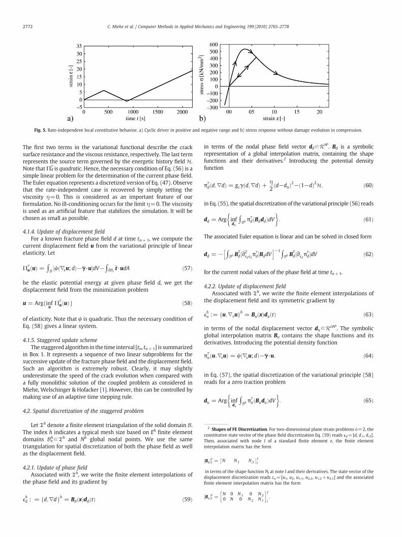
Fig. 5. Rate-independent local constitutive behavior. a) Cyclic driver in positive and negative range and b) stress response without damage evolution in compression.

2 Shapes of FE Discretization. For two-dimensional plane strain problems δ=2, theconstitutive state vector of the phase field discretization Eq. (59) reads cd=[d, d,1, d,2].Then, associated with node I of a standard finite element e, the finite elementinterpolation matrix has the form

½Bd�eI = N N;1 N;2

� �TI

in terms of the shape function NI at note I and their derivatives. The state vector of thedisplacement discretization reads cu=[u1, u2, u1,1, u2,2, u1,2+u2,1] and the associatedfinite element interpolation matrix has the form

½Bu�eI =

N 0 N;1 0 N;20 N 0 N;2 N;1

� �TI:


The first two terms in the variational functional describe the cracksurface resistance and the viscous resistance, respectively. The last termrepresents the source term governed by the energetic history field H.Note thatΠd

τ is quadratic. Hence, the necessary condition of Eq. (56) is asimple linear problem for the determination of the current phase field.The Euler equation represents a discretized version of Eq. (47). Observethat the rate-independent case is recovered by simply setting theviscosity η=0. This is considered as an important feature of ourformulation. No ill-conditioning occurs for the limit η=0. The viscosityis used as an artificial feature that stabilizes the simulation. It will bechosen as small as possible.

4.1.4. Update of displacement fieldFor a known fracture phase field d at time tn+1, we compute the

current displacement field u from the variational principle of linearelasticity. Let

ΠτuðuÞ = ∫B ½ψð∇su; dÞ−γ·u�dV−∫∂Bt

t·udA ð57Þ

be the elastic potential energy at given phase field d, we get thedisplacement field from the minimization problem

u = Argfinfu

ΠτuðuÞg ð58Þ

of elasticity. Note that ψ is quadratic. Thus the necessary condition ofEq. (58) gives a linear system.

4.1.5. Staggered update schemeThe staggered algorithm in the time interval [tn, tn+1] is summarized

in Box 1. It represents a sequence of two linear subproblems for thesuccessive update of the fracture phase field and the displacement field.Such an algorithm is extremely robust. Clearly, it may slightlyunderestimate the speed of the crack evolution when compared witha fully monolithic solution of the coupled problem as considered inMiehe, Welschinger & Hofacker [1]. However, this can be controlled bymaking use of an adaptive time stepping rule.

4.2. Spatial discretization of the staggered problem

Let Th denote a finite element triangulation of the solid domain B.The index h indicates a typical mesh size based on Eh finite elementdomains Be

h∈Th and Nh global nodal points. We use the sametriangulation for spatial discretization of both the phase field as wellas the displacement field.

4.2.1. Update of phase fieldAssociated with Th, we write the finite element interpolations of

the phase field and its gradient by

chd : = fd;∇dgh = BdðxÞddðtÞ ð59Þ

in terms of the nodal phase field vector dd∈RNh

. Bd is a symbolicrepresentation of a global interpolation matrix, containing the shapefunctions and their derivatives.2 Introducing the potential densityfunction

πτdðd;∇dÞ = gcγðd;∇dÞ + η

2ðd−dnÞ

2−ð1−dÞ2H; ð60Þ

in Eq. (55), the spatial discretization of the variational principle (56) reads

dd = Arg infdd

∫Bh πτdðBdddÞdV

� �: ð61Þ

The associated Euler equation is linear and can be solved in closed form

dd = − ∫Bh BTd ½∂

2cdcd

πτd�BddV

h i−1∫Bh BTd ½∂cdπ

τd�dV ð62Þ

for the current nodal values of the phase field at time tn+1.

4.2.2. Update of displacement fieldAssociated with Th, we write the finite element interpolations of

the displacement field and its symmetric gradient by

chu := u;∇suf gh = BuðxÞduðtÞ ð63Þ

in terms of the nodal displacement vector du∈RδNh

. The symbolicglobal interpolation matrix Bu contains the shape functions and itsderivatives. Introducing the potential density function

πτuðu;∇suÞ = ψð∇su;dÞ−γ·u; ð64Þ

in Eq. (57), the spatial discretization of the variational principle (58)reads for a zero traction problem

du = Arg infdu

∫Bh πτuðBuduÞdV

� �: ð65Þ


Fig. 6. Single edge notched specimen. Geometry and boundary conditions. a) Tensiontest treated in Section 5.1 and b) shear test treated in Section 5.2.


The associated Euler equation of linear elasticity yields the closedform solution

du = − ∫Bh BTu½∂

2cucu

πτu�BudV

h i−1∫Bh BTu½∂cuπ

τu�dV ð66Þ

for the current nodal values of the phase field at time tn+1.

Fig. 7. Single edge notched tension test. Load-deflection curves for a length scale a) l1=0.015

Fig. 8. Single edge notched tension test. Crack pattern for η=1×10−6 kN s/mm2 at a displacescale of l1=0.0150 mm and d) u=5.7×10−3 mm, e) u=5.9×10−3 mm, and f) u=6.3×1

5. Representative numerical examples

We now demonstrate the modeling capability of the proposedapproach to diffusive fracture bymeans of numerical model problems.The proposed staggered scheme outlined in Box 1 based on the localhistory field is much faster than the monolithic three-field formula-tion outlined in Miehe, Welschinger & Hofacker [1]. As shown below,it allows performing rate-independent problems in a straightforwardmanner. We demonstrate this for a spectrum of standard benchmarkproblems such as a single edge notched specimen subjected to tensileand pure shear loadings, a symmetric and an asymmetric notchedthree point bending test. The characteristic of the local materialresponse for a cyclic loading process is demonstrated in Fig. 5. Theresult is obtained by a local driving of the constitutive model. It showsthe basic properties of a rate-independent hysteresis due to localdamagemechanismswhich occur only in the tensile range. There is nodiffusive fracture evolution in the compressive range.

5.1. Single edge notched tension test

Consider a squared plate with horizontal notch which is placed atmiddle height from the left outer surface to the center of thespecimen. The geometric setup is depicted in Fig. 6. In order to capture

0mm and b) l2=0.0075mm obtained for η=1×10−6 kN s/mm2 and η=0 kN s/mm2.

ment of a) u=5.7×10−3 mm, b) u=5.9×10−3 mm, c) u=6.1×10−3 mm for a length0−3 mm for a length scale of l2=0.0075 mm.


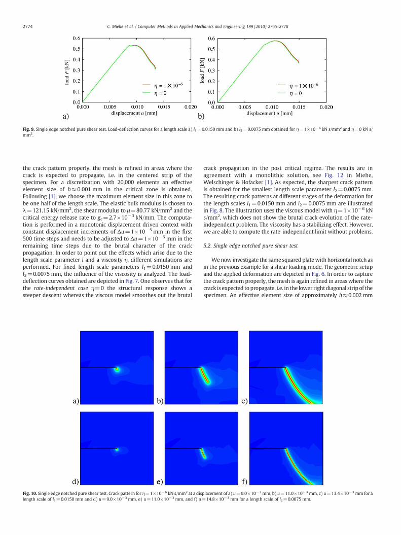
Fig. 9. Single edge notched pure shear test. Load-deflection curves for a length scale a) l1=0.0150 mm and b) l2=0.0075 mm obtained for η=1×10−6 kN s/mm2 and η=0 kN s/mm2.


the crack pattern properly, the mesh is refined in areas where thecrack is expected to propagate, i.e. in the centered strip of thespecimen. For a discretization with 20,000 elements an effectiveelement size of h≈0.001 mm in the critical zone is obtained.Following [1], we choose the maximum element size in this zone tobe one half of the length scale. The elastic bulk modulus is chosen toλ=121.15 kN/mm2, the shear modulus to μ=80.77 kN/mm2 and thecritical energy release rate to gc=2.7×10−3 kN/mm. The computa-tion is performed in a monotonic displacement driven context withconstant displacement increments of Δu=1×10−5 mm in the first500 time steps and needs to be adjusted to Δu=1×10−6 mm in theremaining time steps due to the brutal character of the crackpropagation. In order to point out the effects which arise due to thelength scale parameter l and a viscosity η, different simulations areperformed. For fixed length scale parameters l1=0.0150 mm andl2=0.0075 mm, the influence of the viscosity is analyzed. The load-deflection curves obtained are depicted in Fig. 7. One observes that forthe rate-independent case η=0 the structural response shows asteeper descent whereas the viscous model smoothes out the brutal

Fig. 10. Single edge notched pure shear test. Crack pattern for η=1×10−6 kN s/mm2 at a dislength scale of l1=0.0150 mm and d) u=9.0×10−3 mm, e) u=11.0×10−3 mm, and f) u=

crack propagation in the post critical regime. The results are inagreement with a monolithic solution, see Fig. 12 in Miehe,Welschinger & Hofacker [1]. As expected, the sharpest crack patternis obtained for the smallest length scale parameter l2=0.0075 mm.The resulting crack patterns at different stages of the deformation forthe length scales l1=0.0150 mm and l2=0.0075 mm are illustratedin Fig. 8. The illustration uses the viscous model with η=1×10−6 kNs/mm2, which does not show the brutal crack evolution of the rate-independent problem. The viscosity has a stabilizing effect. However,we are able to compute the rate-independent limit without problems.

5.2. Single edge notched pure shear test

Wenow investigate the same squared platewith horizontal notch asin the previous example for a shear loading mode. The geometric setupand the applied deformation are depicted in Fig. 6. In order to capturethe crack pattern properly, the mesh is again refined in areas where thecrack is expected to propagate, i.e. in the lower rightdiagonal strip of thespecimen. An effective element size of approximately h≈0.002 mm

placement of a) u=9.0×10−3 mm, b) u=11.0×10−3 mm, c) u=13.4×10−3 mm for a14.8×10−3 mm for a length scale of l2=0.0075 mm.


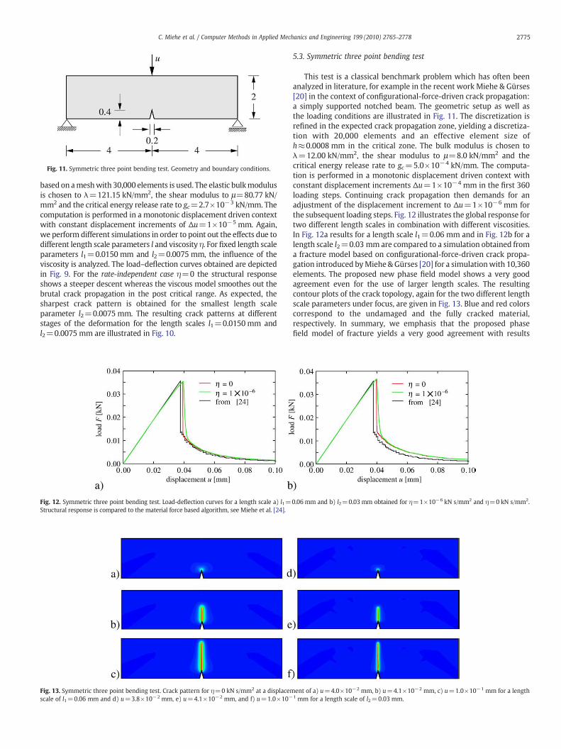
Fig. 11. Symmetric three point bending test. Geometry and boundary conditions.


based on ameshwith 30,000 elements is used. The elastic bulkmodulusis chosen to λ=121.15 kN/mm2, the shear modulus to μ=80.77 kN/mm2 and the critical energy release rate to gc=2.7×10−3 kN/mm. Thecomputation is performed in a monotonic displacement driven contextwith constant displacement increments of Δu=1×10−5 mm. Again,we perform different simulations in order to point out the effects due todifferent length scale parameters l and viscosity η. For fixed length scaleparameters l1=0.0150 mm and l2=0.0075 mm, the influence of theviscosity is analyzed. The load–deflection curves obtained are depictedin Fig. 9. For the rate-independent case η=0 the structural responseshows a steeper descent whereas the viscous model smoothes out thebrutal crack propagation in the post critical range. As expected, thesharpest crack pattern is obtained for the smallest length scaleparameter l2=0.0075 mm. The resulting crack patterns at differentstages of the deformation for the length scales l1=0.0150mm andl2=0.0075 mm are illustrated in Fig. 10.

Fig. 12. Symmetric three point bending test. Load-deflection curves for a length scale a) l1=Structural response is compared to the material force based algorithm, see Miehe et al. [24].

Fig. 13. Symmetric three point bending test. Crack pattern for η=0 kN s/mm2 at a displacemscale of l1=0.06 mm and d) u=3.8×10−2 mm, e) u=4.1×10−2 mm, and f) u=1.0×10−

5.3. Symmetric three point bending test

This test is a classical benchmark problem which has often beenanalyzed in literature, for example in the recent work Miehe & Gürses[20] in the context of configurational-force-driven crack propagation:a simply supported notched beam. The geometric setup as well asthe loading conditions are illustrated in Fig. 11. The discretization isrefined in the expected crack propagation zone, yielding a discretiza-tion with 20,000 elements and an effective element size ofh≈0.0008 mm in the critical zone. The bulk modulus is chosen toλ=12.00 kN/mm2, the shear modulus to μ=8.0 kN/mm2 and thecritical energy release rate to gc=5.0×10−4 kN/mm. The computa-tion is performed in a monotonic displacement driven context withconstant displacement increments Δu=1×10−4 mm in the first 360loading steps. Continuing crack propagation then demands for anadjustment of the displacement increment to Δu=1×10−6 mm forthe subsequent loading steps. Fig. 12 illustrates the global response fortwo different length scales in combination with different viscosities.In Fig. 12a results for a length scale l1=0.06 mm and in Fig. 12b for alength scale l2=0.03 mm are compared to a simulation obtained froma fracture model based on configurational-force-driven crack propa-gation introduced byMiehe & Gürses [20] for a simulationwith 10,360elements. The proposed new phase field model shows a very goodagreement even for the use of larger length scales. The resultingcontour plots of the crack topology, again for the two different lengthscale parameters under focus, are given in Fig. 13. Blue and red colorscorrespond to the undamaged and the fully cracked material,respectively. In summary, we emphasis that the proposed phasefield model of fracture yields a very good agreement with results

0.06 mm and b) l2=0.03 mm obtained for η=1×10−6 kN s/mm2 and η=0 kN s/mm2.

ent of a) u=4.0×10−2 mm, b) u=4.1×10−2 mm, c) u=1.0×10−1 mm for a length1 mm for a length scale of l2=0.03 mm.


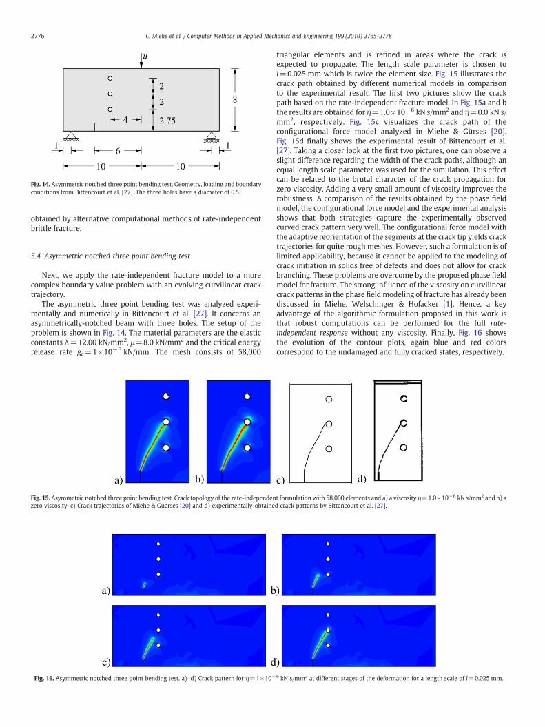
Fig. 14. Asymmetric notched three point bending test. Geometry, loading and boundaryconditions from Bittencourt et al. [27]. The three holes have a diameter of 0.5.


obtained by alternative computational methods of rate-independentbrittle fracture.

5.4. Asymmetric notched three point bending test

Next, we apply the rate-independent fracture model to a morecomplex boundary value problem with an evolving curvilinear cracktrajectory.

The asymmetric three point bending test was analyzed experi-mentally and numerically in Bittencourt et al. [27]. It concerns anasymmetrically-notched beam with three holes. The setup of theproblem is shown in Fig. 14. The material parameters are the elasticconstants λ=12.00 kN/mm2, μ=8.0 kN/mm2 and the critical energyrelease rate gc=1×10−3 kN/mm. The mesh consists of 58,000

Fig. 15. Asymmetric notched three point bending test. Crack topology of the rate-independenzero viscosity. c) Crack trajectories of Miehe & Guerses [20] and d) experimentally-obtaine

Fig. 16. Asymmetric notched three point bending test. a)–d) Crack pattern for η=1×10−

triangular elements and is refined in areas where the crack isexpected to propagate. The length scale parameter is chosen tol=0.025 mm which is twice the element size. Fig. 15 illustrates thecrack path obtained by different numerical models in comparisonto the experimental result. The first two pictures show the crackpath based on the rate-independent fracture model. In Fig. 15a and bthe results are obtained for η=1.0×10−6 kN s/mm2 and η=0.0 kN s/mm2, respectively. Fig. 15c visualizes the crack path of theconfigurational force model analyzed in Miehe & Gürses [20].Fig. 15d finally shows the experimental result of Bittencourt et al.[27]. Taking a closer look at the first two pictures, one can observe aslight difference regarding the width of the crack paths, although anequal length scale parameter was used for the simulation. This effectcan be related to the brutal character of the crack propagation forzero viscosity. Adding a very small amount of viscosity improves therobustness. A comparison of the results obtained by the phase fieldmodel, the configurational force model and the experimental analysisshows that both strategies capture the experimentally observedcurved crack pattern very well. The configurational force model withthe adaptive reorientation of the segments at the crack tip yields cracktrajectories for quite rough meshes. However, such a formulation is oflimited applicability, because it cannot be applied to the modeling ofcrack initiation in solids free of defects and does not allow for crackbranching. These problems are overcome by the proposed phase fieldmodel for fracture. The strong influence of the viscosity on curvilinearcrack patterns in the phase fieldmodeling of fracture has already beendiscussed in Miehe, Welschinger & Hofacker [1]. Hence, a keyadvantage of the algorithmic formulation proposed in this work isthat robust computations can be performed for the full rate-independent response without any viscosity. Finally, Fig. 16 showsthe evolution of the contour plots, again blue and red colorscorrespond to the undamaged and fully cracked states, respectively.

t formulation with 58,000 elements and a) a viscosity η=1.0×10−6 kN s/mm2 and b) ad crack patterns by Bittencourt et al. [27].

6 kN s/mm2 at different stages of the deformation for a length scale of l=0.025 mm.



6. Conclusion

We outlined a thermodynamically consistent framework for rate-independent diffusive crack propagation in elastic solids. To this end,we proposed a new incremental variational framework for rate-independent diffusive fracture that bases on the introduction of a localhistory field. It contains a maximum reference energy obtained in thedeformation history, which may be considered as a measure for themaximum tensile strain obtained in history. It was shown that thislocal variable drives the evolution of the fracture phase field. Itallowed the construction of an extremely robust operator splitscheme that successively updates in a typical time step the historyfield, the crack phase field and finally the displacement field. Anartificial viscous regularization stabilizes the overall performance. Theproposed algorithm is considered to be the canonically simple schemefor the treatment of diffusive fracture. We demonstrated theperformance of the proposed phase field formulations of fracture bymeans of representative numerical examples.

Acknowledgment

Support for this research was provided by the German ResearchFoundation (DFG) under grant Mi 295/11-2.

Appendix A. Introduction of a damage-driving history field

In order to motivate the structure of the diffusive fracture modeloutlined in Section 3, we consider a local damage model in a one-dimensional setting. It is governed by a free energy function

ψðε; dÞ = gðdÞψ0ðεÞ with gðdÞ = ð1−dÞ2 and ψ0ðεÞ =12Eε

2

ðA:1Þ

in terms of the convex reference energy function ψ0(ε)=ψ(ε, 0) andthe degrading function g(d), which depend on the strain ε and theinternal damage variable d. E is the elastic stiffness. The degradingfunction is positive g≥0, monotonic decreasing g′≤0 and has theproperties g(0)=1, g(1)=0 and g′(1)=0. From Eq. (A.1), we obtainby a standard exploitation method of the second axiom of thermo-dynamics, often referred to as Coleman's method, the constitutiveexpression for the stresses

σðε;dÞ := ∂εψðε;dÞ = ð1−dÞ2Eε ðA:2Þ

and the reduced dissipation inequality

D = f d≥ 0 with f ðε;dÞ := −∂dψðε;dÞ = 2ð1−dÞψ0ðεÞ: ðA:3Þ

A rate-independent, discontinuous evolution of the internalvariable can be based on the threshold function

tð f ; dÞ = f−cd: ðA:4Þ

Here, the constant c=1 N/m2 has the value one and the unit of anenergy density. With this function at hand, a rate-independentevolution of damage is defined by the equations

d ≥ 0; tð f ;dÞ ≤ 0; dtð f ;dÞ = 0: ðA:5Þ

Considering damage loading, ḋN0, we may compute the currentdamage variable d from the condition t(f; d)=0 in Eq. (71)2, yieldingthe closed form solution

d =hðεÞ

c + hðεÞ for d N 0 with hðεÞ = 2ψ0ðεÞ = jε j2E ; ðA:6Þ

where the function h(ε) is directly related to the reference energyψ0(ε). As outlined in Eq. (A.6)3, the convex reference free energy is aquadratic function of the norm |ε|E of the strain ε with regard to ametric provided by the elasticity modulus E. It obviously drives theaccumulation of the damage variable d. Note that Eq. (A.6)1 providesthe desired property d→1 for h(ε)→∞ or |ε|E→∞. Furthermore,observe that damage accumulation d N0 takes place only if the functionh(ε) defined in Eq. (A.6)3 grows. DefiningH(t) as the maximum valueof h(ε(t)) obtained in time history, wemay replace system (A.5) for therate-independent evolution of the damage variable d by the simpleclosed-form equation

dðtÞ = HðtÞc + HðtÞ with HðtÞ := maxs∈½0;t� hðεðsÞÞf g: ðA:7Þ

See for example Miehe [28] for an analogous definition of a historyfield in rate-independent, discontinuous damage mechanics. The twoEqs. (A.2) and (A.7) then govern exclusively a damage-type degradingstress response in an elastic solid. Note that in this model due to EN0the current damage variable d is in a one-to-one relationship to themaximum strain norm obtained in time history

εmaxðtÞ := maxs∈½0;t�

f jεðsÞ jg =ffiffiffiffiffiffiffiffiffiffiffiffiffiffiffiffiffiHðtÞ= E

p: ðA:8Þ

References

[1] C. Miehe, F. Welschinger, M. Hofacker, Thermodynamically-consistent phase fieldmodels of fracture: Variational principles and multi-field fe implementations,International Journal forNumericalMethods inEngineeringDOI:10.1002/nme.2861.

[2] A.A. Griffith, The phenomena of rupture and flow in solids, PhilosophicalTransactions of the Royal Society London A 221 (1921) 163–198.

[3] G.R. Irwin, Fracture, in: S. Flügge (Ed.), Elasticity and Plasticity, Encyclopedia ofPhysics, Vol. 6, Springer, 1958, pp. 551–590.

[4] G.A. Francfort, J.J. Marigo, Revisiting brittle fracture as an energy minimizationproblem, Journal of the Mechanics and Physics of Solids 46 (1998) 1319–1342.

[5] B. Bourdin, G.A. Francfort, J.J. Marigo, The Variational Approach to Fracture,Springer Verlag, Berlin, 2008.

[6] G. Dal Maso, R. Toader, A model for the quasistatic growth of brittle fractures:Existence and approximation results, Archive for Rational Mechanics and Analysis162 (2002) 101–135.

[7] M. Buliga, Energy minimizing brittle crack propagation, Journal of Elasticity 52(1999) 201–238.

[8] B. Bourdin, G.A. Francfort, J.J. Marigo, Numerical experiments in revisited brittlefracture, Journal of the Mechanics and Physics of Solids 48 (2000) 797–826.

[9] D. Mumford, J. Shah, Optimal approximations by piecewise smooth functions andassociated variational problems, Communications on Pure and Applied Mathe-matics 42 (1989) 577–685.

[10] L. Ambrosio, V.M. Tortorelli, Approximation of functionals depending on jumps byelliptic functionals via γ-convergence, Communications on Pure and AppliedMathematics 43 (1990) 999–1036.

[11] G. Dal Maso, An Introduction to Γ-Convergence, Birkhäuser, Boston, 1993.[12] D.P. Braides, Approximation of Free Discontinuity Problems, Springer Verlag,

Berlin, 1998.[13] D.P. Braides, Γ-Convergence for Beginners, Oxford University Press, New York,

2002.[14] V. Hakim, A. Karma, Laws of crack motion and phase-field models of fracture,

Journal of the Mechanics and Physics of Solids 57 (2009) 342–368.[15] A. Karma, D.A. Kessler, H. Levine, Phase-field model of mode iii dynamic fracture,

Physical Review Letters 92 (2001) 8704.045501.[16] L.O. Eastgate, J.P. Sethna, M. Rauscher, T. Cretegny, C.-S. Chen, C.R. Myers, Fracture

in mode i using a conserved phase-field model, Physical Review E 65 (2002)036117-1-10.

[17] T. Belytschko, H. Chen, J. Xu, G. Zi, Dynamic crack propagation based on loss ofhyperbolicity and a new discontinuous enrichment, International Journal forNumerical Methods in Engineering 58 (2003) 1873–1905.

[18] J.-H. Song, T. Belytschko, Cracking node method for dynamic fracture with finiteelements, International Journal for Numerical Methods in Engineering 77 (2009)360–385.

[19] E. Gürses, C. Miehe, A computational framework of three-dimensional configu-rational-force-driven brittle crack propagation, Computer Methods in AppliedMechanics and Engineering 198 (2009) 1413–1428.

[20] C. Miehe, E. Gürses, A robust algorithm for configurational-force-driven brittlecrack propagation with r-adaptive mesh alignment, International Journal forNumerical Methods in Engineering 72 (2007) 127–155.

[21] C. Miehe, E. Gürses, M. Birkle, A computational framework of configurational-force-driven brittle fracture based on incremental energy minimization, Interna-tional Journal of Fracture 145 (2007) 245–259.

[22] G. Capriz, Continua with Microstructure, Springer Verlag, 1989.



[23] P.M. Mariano, Multifield theories in mechanics of solids, Advances in AppliedMechanics 38 (2001) 1–93.

[24] M. Frémond, Non-Smooth Thermomechanics, Springer Verlag, 2002.[25] C. Miehe, Comparison of two algorithms for the computation of fourth-order

isotropic tensor functions, Computers & Structures 66 (1998) 37–43.[26] C. Miehe, M. Lambrecht, Algorithms for computation of stresses and elasticity

moduli in terms of Seth–Hill's family of generalized strain tensors, Communica-tions in Numerical Methods in Engineering 17 (2001) 337–353.

[27] T.N. Bittencourt, P.A. Wawrzynek, A.R. Ingraffea, J.L. Sousa, Quasi-automaticsimulation of crack propagation for 2d lefm problems, Engineering FractureMechanics 55 (1996) 321–334.

[28] C. Miehe, Discontinuous and continuous damage evolution in Ogden-type large-strain elastic materials, European Journal of Mechanics A / Solids 14 (1995)697–720.


Documents

Computer Methods in Applied Mechanics and Engineeringcrm.sns.it/media/course/3060/miehe+hofacker+welschinger10.pdf · maximum reference energy obtained in the deformation history,