Embed Size (px)
Citation preview
Computer Network Routing with a Fuzzy Neural Network
Julia K. Brande
Dissertation submitted to the Faculty of theVirginia Polytechnic Institute and State University
in partial fulfillment of the requirements for the degree of
Doctor of Philosophyin
Management Science
Terry R. Rakes, ChairEdward R. ClaytonLaurence J. MooreLoren Paul Rees
Robert T. Sumichrast
November 7, 1997Blacksburg, Virginia
Keywords: Network Routing, Fuzzy Reasoning, Neural Networks, Wide Area Networks
Copyright 1997, Julia K. Brande
ii
Computer Network Routing with a Fuzzy Neural Network
Julia K. Brande
(ABSTRACT)
The growing usage of computer networks is requiring improvements in network technologies
and management techniques so users will receive high quality service. As more individuals
transmit data through a computer network, the quality of service received by the users begins
to degrade. A major aspect of computer networks that is vital to quality of service is data
routing. A more effective method for routing data through a computer network can assist with
the new problems being encountered with today’s growing networks.
Effective routing algorithms use various techniques to determine the most appropriate route
for transmitting data. Determining the best route through a wide area network (WAN),
requires the routing algorithm to obtain information concerning all of the nodes, links, and
devices present on the network. The most relevant routing information involves various
measures that are often obtained in an imprecise or inaccurate manner, thus suggesting that
fuzzy reasoning is a natural method to employ in an improved routing scheme. The neural
network is deemed as a suitable accompaniment because it maintains the ability to learn in
dynamic situations. Once the neural network is initially designed, any alterations in the
computer routing environment can easily be learned by this adaptive artificial intelligence
method. The capability to learn and adapt is essential in today’s rapidly growing and
changing computer networks. These techniques, fuzzy reasoning and neural networks, when
combined together provide a very effective routing algorithm for computer networks.
Computer simulation is employed to prove the new fuzzy routing algorithm outperforms the
Shortest Path First (SPF) algorithm in most computer network situations. The benefits
increase as the computer network migrates from a stable network to a more variable one. The
advantages of applying this fuzzy routing algorithm are apparent when considering the
dynamic nature of modern computer networks.

iii
Dedication
This dissertation is dedicated to my parents, Charles and Norma Brande. Their unconditional
love and support has helped me achieve my goals and I offer them my heartfelt gratitude.

iv
Acknowledgements
I express my sincere thanks to Professor Terry Rakes, my dissertation chairman. I am
extremely fortunate to have had the opportunity to work with him and value this collaboration
greatly. Thank you for all your work, enthusiasm, and commitment to this research and to me.
I could not have achieved this goal without you.
The guidance and support of my committee members are also deeply appreciated. Dr. Edward
R. Clayton, Dr. Laurence J. Moore, Dr. Loren Paul Rees, and Dr. Robert T. Sumichrast, you
have all been excellent mentors. Thank you for your contributions to my dissertation.
I would also like to thank Ronald Earp, Jr. He has joined me in enduring many challenging
years of graduate and undergraduate studies, has supported me in hundreds of ways, and has
recently become my husband. Thank you for being a loving and caring companion throughout
the doctoral process.
v
Table of Contents
Chapter 1 : Introduction ........................................................................................................1
Statement of the Problem.................................................................................................................. 3
Objective of the Study ....................................................................................................................... 5
Research Methodology ...................................................................................................................... 6
Scope and Limitations ....................................................................................................................... 7
Contributions of the Research .......................................................................................................... 8
Plan of Presentation........................................................................................................................... 8
Chapter 2 : Literature Review................................................................................................9
Introduction........................................................................................................................................ 9
Network Routing................................................................................................................................ 9
Conclusion ........................................................................................................................................ 17
Chapter 3 : Background and Methodology.........................................................................19
Introduction...................................................................................................................................... 19
Fuzzy Reasoning............................................................................................................................... 19Introduction................................................................................................................................................... 19Fuzzy Sets ..................................................................................................................................................... 20Manipulating Fuzzy Sets ............................................................................................................................... 24
Neural Networks .............................................................................................................................. 25Learning and Recall....................................................................................................................................... 27Fuzzy Neural Networks................................................................................................................................. 29
Methodology ..................................................................................................................................... 29Introduction................................................................................................................................................... 29Fuzzy Sets in Routing.................................................................................................................................... 32Fuzzy Neural Network for Routing ............................................................................................................... 36Neural Network Training .............................................................................................................................. 38
Performance Comparison ............................................................................................................... 40
Summary........................................................................................................................................... 40
Chapter 4 : Fuzzy Routing...................................................................................................42
Introduction...................................................................................................................................... 42
Simulation Design ............................................................................................................................ 42
Algorithm Development .................................................................................................................. 51Neural Network Training Set ........................................................................................................................ 51Fuzzy Routing Sets........................................................................................................................................ 54Neural Network Training and Design............................................................................................................ 56Algorithm Simulation.................................................................................................................................... 56
Experimental Design........................................................................................................................ 57
vi
Simulation and Analysis.................................................................................................................. 58Scenario One ................................................................................................................................................. 59Scenario Two ................................................................................................................................................ 63Scenario Three .............................................................................................................................................. 66Scenario Four ................................................................................................................................................ 68
Conclusion ........................................................................................................................................ 71
Chapter 5 : Conclusions.......................................................................................................72
Summary........................................................................................................................................... 72
Future Research............................................................................................................................... 74
References ................................................................................................................................76
APPENDIX A: Fuzzy rule-based reasoning..........................................................................81
APPENDIX B: AweSim Simulation Variables .....................................................................88
APPENDIX C: Simulation model for the new algorithm.....................................................90
APPENDIX D: C code used in simulations.........................................................................100
Vita..........................................................................................................................................132

vii
Table of Figures
Figure 3.1: Boolean sets of tall and not tall people............................................................................................. 21Figure 3.2: Fuzzy sets of tall and not tall people................................................................................................. 21Figure 3.3: Gaussian membership function......................................................................................................... 23Figure 3.4: Trapezoidal membership functions ................................................................................................... 23Figure 3.5: Triangular membership functions..................................................................................................... 23Figure 3.6: Neural network architecture ............................................................................................................. 26Figure 3.7: Structure of neurode j ....................................................................................................................... 28Figure 3.8: Distance membership sets................................................................................................................. 34Figure 3.9: Throughput membership sets ............................................................................................................ 34Figure 3.10: Failure membership sets ................................................................................................................. 35Figure 3.11: Congestion membership sets........................................................................................................... 35Figure 3.12: Example computer network............................................................................................................. 37Figure 3.13: Neural network design .................................................................................................................... 39Figure 4.1: Example WAN ................................................................................................................................... 45Figure 4.2 : A second variation of the example network ...................................................................................... 46Figure 4.3: A third variation of the example network........................................................................................... 47Figure 4.4: Packets at node 1 .............................................................................................................................. 51Figure 4.5: Packet creation module for node 1 ................................................................................................... 52Figure 4.6: Module for destination check............................................................................................................ 52Figure 4.7: Distance (hops) ................................................................................................................................. 54Figure 4.8: Congestion (packets)......................................................................................................................... 54Figure 4.9: Throughput (bps) .............................................................................................................................. 54Figure 4.10: Failure (seconds) ............................................................................................................................ 55Figure 4.11: Sigmoid function y = (1 + e-I)-1...................................................................................................... 56Figure 4.12: Distribution of difference values..................................................................................................... 61Figure 4.13: Normal probability plot of difference data ..................................................................................... 62Figure 4.14: Distribution of scenario two data ................................................................................................... 65Figure 4.15: Normal probability plot of scenario two data................................................................................. 65Figure 4.16: Distribution of scenario three ......................................................................................................... 67Figure 4.17: Normal probability plot for scenario three..................................................................................... 68Figure 4.18: Distribution of scenario four........................................................................................................... 70Figure 4.19: Normal probability plot for scenario four ...................................................................................... 70Figure A.1: Rs Matrix........................................................................................................................................... 82Figure A.2: Example membership functions ........................................................................................................ 86Figure A.3: Membership function “Expand” resulting from correlation minimum ............................................ 87Figure A.4: Final Expand membership function................................................................................................... 87
viii
Table of Tables
Table 3.1: Membership grades ............................................................................................................................. 24Table 3.2: Discrete distance membership set....................................................................................................... 34Table 3.3 : Twelve fuzzy sets ................................................................................................................................ 37Table 4.1: Experimental design ........................................................................................................................... 57Table 4.2: Average transmission times in scenario one....................................................................................... 59Table 4.3: Average transmission times in scenario two........................................................................................ 64Table 4.4: Average transmission times in scenario three ..................................................................................... 67Table 4.5: Average transmission times in scenario four....................................................................................... 69Table 4.6: P-values for all tests ........................................................................................................................... 71Table 5.1: Significant P-values............................................................................................................................ 73
1
Chapter 1 : Introduction
Computer networks are rapidly becoming a necessity in today’s business organizations,
leading to an increase in the number of computer networks and network users. As networks
become more abundant, it becomes increasingly necessary to focus on the quality of service
that is being provided to the users of the network. The responsibility of this issue lies with the
network management.
Network management involves the monitoring, analysis, control, and planning of activities
and resources of a computer network in order to provide the users with a certain quality of
service (Znaty and Sclavos 1994). The idea is to ensure that the system is operating
effectively and efficiently at all times, so there are no short-term or long-term service
problems.
The proliferation of computer networks increases the need for improved network
management techniques. As computer networks expand, they become more complex as they
attempt to support a more diverse selection of applications and users. The problems
associated with supporting more users are exposed when the network seeks to provide each
user with an expected quality of service. Problems concerning congestion, unacceptable
throughput, bottlenecks, security, equipment failure and poor response times are immediate
results of growing networks that can represent an unacceptable quality of service. It has
become a necessary and challenging task to provide efficient utilization by ensuring that the
network remains accessible and uncrowded.
The International Organization for Standardization (ISO) has defined five areas as the key
areas of network management: fault management, accounting management, configuration
management, security management and performance management (Stallings and Van Slyke
1994). Fault management is the collection of services that enables the detection, isolation and
correction of abnormal operations transpiring in the managed network (Znaty and Sclavos
1994). The absence of fault management causes the network to become vulnerable to
additional operational irregularities. A variety of tools is currently available to assist the
network manager in fault management tasks, the majority of which automate the discovering
2
of a fault by determining communication or lack of communication with the network devices.
The remaining tasks of fault management are usually performed by the network manager.
Accounting management tracks network resource utilization for each individual and each
group in order for the network manager to provide the appropriate quantity of resources
(Leinwand and Fang 1993). It is also used to establish metrics, check quotas, determine costs,
and bill users (Leinwand and Fang 1993). The information gathered in accounting
management can also help determine if users are abusing their privileges or transmitting data
in such a way that diminishes performance.
Security management controls access to information on the network (Stallings 1990). This
provides protection for sensitive information that may exist in the system. Without this part
of network management, there is no systematic manner to distribute, store and authorize
passwords. Having the ability to maintain secure access to restricted information is necessary
in most computer networks.
Performance management monitors the network to ensure its accessibility so that users
may utilize it efficiently (Leinwand and Fang 1993). Two processes are involved in
performance management: monitoring and controlling. Monitoring traces activities occurring
on the network while the controlling function provides a way to adjust the network in order to
improve performance. The activities that are monitored provide the network manager with
measures such as capacity usage, amount of traffic, throughput levels, and response times
(Stallings and Van Slyke 994).
Configuration management involves obtaining data from the network in order to manage
the setup of the network devices (Leinwand and Fang 1993). It includes the processes of
network planning, resource planning and service planning. It also includes traffic
management, the process of routing data correctly through a network. The process of
configuration management provides an organized approach to changing and updating
segments and devices on the network.
The five network management areas differ in intricacy, depending on the type of network.
A computer network can be categorized into one of three categories: local area networks,
metropolitan area networks, or wide area networks. The overall concept of each type is
virtually the same; the difference lies within the size of the network.

3
Local area networks (LANs) are networks that connect equipment within a single building
or a group of neighboring buildings. Metropolitan area networks (MANs) are used to connect
computer systems within an area the size of a city. A MAN is commonly developed by
combining many LANs with a public telecommunication provider. A wide area network
(WAN) connects many smaller networks, either metropolitan or local area networks. There is
no specified distance that must lie between the smaller networks. A WAN connects smaller
networks that are in different parts of a city, different cities, or different countries.
Such large amounts of time and money are being invested into computer networks today
that it has become both desirable and cost-effective to automate parts of the network
management process. Applying artificial intelligence to specific areas of network
management allows the network engineer to dedicate additional time and effort to the more
specialized and intricate details of the system. Many forms of artificial intelligence have
previously been introduced to network management; however, it appears that one of the more
applicable areas, fuzzy reasoning, has been somewhat overlooked.
Computer network managers are often challenged with decision-making based on vague or
partial information. Similarly, computer networks frequently perform operational adjustments
based on this same vague or partial information. The imprecise nature of this information can
lead to difficulties and inaccuracies when automating network management using currently
applied artificial intelligence techniques. Fuzzy reasoning will allow this type of imprecise
information to be dealt with in a precise and well-defined manner, providing a more flawless
method of automating the network management decision making process.
Statement of the Problem
The overall goal of network management is to provide network users with an acceptable
quality of service. To reach this goal, network managers are trying to automate as many
network operations tasks as possible. Many currently available network management systems
are automated in order to assist managers in obtaining vital information necessary to achieve
the desired quality-of-service. As a result, network managers are discovering that measurable
productivity improvements can be obtained through automation of the straightforward
management tasks (Cikoski 1995).
4
Recent attempts at automation include integrating artificial intelligence into network
management systems using neural networks, expert systems, and genetic algorithms. These
methods have successfully diminished the time and effort required of the network manager by
reducing the amount of interaction that is needed.
One important issue that is encountered when attempting to automate segments of the
network management process involves the inaccuracy of the results because of imprecise data.
Many factors involved in network management cannot easily be described in a precise manner
because they are either descriptors concerning the unknown future of the network, or ones that
are quantified into groups having no definite boundaries. For example, when analyzing the
performance of a network, we can characterize the network as being either reliable or
unreliable. However, it is evident that there will be no single point that defines the cutoff
between reliable and unreliable. Instead, there will be a fuzzy area between the two that
describes a network as being somewhat reliable and somewhat unreliable. This type of
imprecise information is very prominent in network management tasks. If methods can be
developed to take into account this imprecise information, more meaningful results can be
reported.
The literature currently indicates the successful application of artificial intelligence
techniques to the five areas of network management. However, there is very little
acknowledgment that the information required for network management is such that it cannot
be accurately defined with an exact descriptor. This has caused many inaccurate assumptions
when attempting to automate the network management system. Applying fuzzy reasoning to
these automation processes could alleviate the problem of inaccuracy and allow for more
flawless results and analyses.
An issue that is burdening many computer network managers is increasing traffic. All
types of networks are experiencing this problem to some degree. For example, frame relay
usage is experiencing massive growth and corresponding traffic problems. Three of the major
frame relay communications corporations, MCI Communications, Sprint and LDDS
WorldCom have all confirmed their traffic levels are growing monthly by fifteen to twenty
percent (Wickre 1997). The growth seen by these companies is analogous to the growth being
experienced by all types of computer networks around the globe.
5
Increasing traffic loads will naturally lead to network delays, which will lead to other
problems as well. These network delays can easily cause dropped sessions or lost data, not to
mention dissatisfied users. It is impossible to stem this increasing traffic load. However,
optimal routing of messages within a network can mitigate some of the difficulties of heavy
traffic. Therefore, a more efficient method of routing needs to be developed to combat
network delays.
Objective of the Study
The objective of this research is to explore the use of fuzzy reasoning in one area of
network management, namely the routing aspect of configuration management. A more
effective method for routing data through a computer network needs to be discovered to assist
with the new problems being encountered on today’s networks. Although traffic management
is only one aspect of configuration management, at this time it is one of the most visible
networking issues. This becomes apparent as consideration is given to the increasing number
of network users and the tremendous growth driven by Internet-based multimedia
applications.
Because of the number of users and the distances between WAN users, efficient routing is
more critical in wide area networks than in LANs (also, many LAN architectures such as
token ring do not allow any flexibility in the nature of message passing). In order to
determine the best route over the WAN, it is necessary to obtain information concerning all of
the nodes, links, and LANs present in the wide area network. The most relevant routing
information involves various measures regarding each link. These measures include the
distance a message will travel, bandwidth available for transmitting that message (maximum
signal frequency), packet size used to segment the message (size of the data group being sent),
and the likelihood of a link failure. These are often measured in an imprecise or inaccurate
manner, thus suggesting that fuzzy reasoning is a natural method to employ in an improved
routing scheme.
Utilizing fuzzy reasoning should assist in expressing these imprecise network measures;
however, there still remains the massive growth issue concerning traffic levels. Most routing
algorithms currently being implemented as a means of transmitting data from a source node to
6
a destination node cannot effectively handle this large traffic growth. Most network routing
methods are designed to be efficient for a current network situation; therefore, when the
network deviates from the original situation, the methods begin to lose efficiency. This
suggests that an effective routing method should also be capable of learning how to
successfully adapt to network growth. Neural networks are extremely capable of adapting to
system changes, and thus will be applied as a second artificial intelligence technique to the
proposed routing method in this research.
The proposed routing approach incorporates fuzzy reasoning in order to prepare a more
accurate assessment of the network’s traffic conditions, and hence provide a faster, more
reliable, or more efficient route for data exchange. Neural networks will be incorporated into
the routing method as a means for the routing method to adapt and learn how to successfully
handle network traffic growth. The combination of these two tools is expected to produce a
more effective routing method than is currently available.
In order to achieve the primary objective of more efficient routing, several minor
objectives also need to be accomplished. A method of data collection is needed throughout
the different phases of the study. Data collection will be accomplished through the use of
simulation methods; therefore, a simulation model must be accurately designed before
proceeding with experimenting or analysis. Additional requirements include building and
training the neural network and defining the fuzzy system. The simulation model, neural
network and fuzzy system will be discussed in full detail in chapter four.
The remaining areas of network management, security management, accounting
management, fault management and performance management, may also lend themselves to
fuzzy analysis, but will not be addressed in this study. The objective of this research is to
demonstrate the effective applicability of fuzzy reasoning to only one area of network
management, traffic routing.
Research Methodology
This research is divided into three phases. The initial phase involves designing the
simulation model to be used for obtaining data. The simulation will mimic a given computer
7
network and its routing process. Once developed, the fuzzy algorithm will be applied to the
given scenario and then simulated in order to analyze the proposed methods.
The second phase consists of developing the specifics of the routing algorithm. This
involves devising the fuzzy logic details as well as the details pertaining to the neural network.
This phase is the focus of the study and therefore requires the most detail and explanation.
Finally, the proposed method will be analyzed and compared to a current method that does
not involve fuzzy reasoning. The comparison will involve the simulation model being applied
to an example network situation. The complete methodology will be described in detail in
chapter four.
Scope and Limitations
The specific results of this research will be constrained by certain characteristics of the
research methodology. The first of these involves the simulation to be used for testing the
routing algorithm. The simulation model will be designed to imitate a given computer
network; therefore, results obtained from the simulation will be directly related to that specific
network design. This will not prevent any generalized conclusions from being developed
since the network dependencies involved are consistent between networks. For example, any
type of network will degrade in performance as failures increase. Similarly, an increase in
congestion will eventually cause performance degradation no matter what type of network is
concerned. Although the results of this research will not guarantee universal results, it will
provide results that may easily be generalized to relate to most routing situations.
A second limiting characteristic of the research methodology pertains to the fuzzy sets
being utilized in the routing algorithm as they are defined with specific shapes and refer to
certain network metrics. The specific metrics and fuzzy set shapes that will be used in this
research are not definitive for the algorithm but seem most appropriate in this dissertation.
All networks differ in some respect and therefore, current routing algorithms require
appropriate parameters to be established when initiating a network. Therefore, the shapes of
the fuzzy sets and the metrics used in the algorithm can easily be altered to reflect the
individual features of the network. These details will be explained explicitly in chapter four.
8
Contributions of the Research
The purpose of this research is to illustrate the potential of applying fuzzy reasoning to a
network management technique, namely, traffic management. This will not include designing
a new routing protocol, but will instead provide a new algorithm that can easily be employed
by a current routing protocol.
Routing algorithms differ from routing protocols in that a routing protocol implements a
particular routing algorithm. Routing protocols define the metric(s) to be used for optimal
route calculations by the algorithm. The protocols also define the size, contents, exchange
frequency, and exchange pattern of routing updates and other messages (Cisco 1996). The
sole purpose of the routing algorithm is to implement a specific process to determine the
appropriate route.
The traffic routing prototype will be developed under assumptions common to many
different computer networks. This will also allow for more emphasis on the fuzzy reasoning
concept rather than the development of a generalized routing simulation. The detailed
descriptions of the assumptions will be presented in chapter four along with the routing
model.
Plan of Presentation
This chapter has served as an introduction to the idea of applying fuzzy reasoning to the
traffic discipline of network management. This area has been selected to demonstrate the
specific applicability of fuzzy reasoning to network management.
The next chapter surveys the literature in network routing, performance monitoring and
network design. The purpose of chapter two is to establish the lack of research in the area of
fuzzy reasoning applied to traffic management. Chapter three presents the necessary
background information and methodology. Chapter four presents the fuzzy model for routing
data through a computer network. Finally, chapter five will provide some concluding
comments.
9
Chapter 2 : Literature Review
Introduction
Various approaches for more efficiently routing data through a computer network have been
proposed in recent literature. Although there have been some proposed methods that use
artificial intelligence techniques, very few of these apply fuzzy reasoning. The following
literature review has been abridged to include the most recent methods and any literature that
has applied artificial intelligence or fuzzy logic to data routing.
Network Routing
Delivering data efficiently through a wide area network can be a difficult task when many
nodes are present. Transmission would be virtually effortless if every node on the network
had a direct link to every other node. This would provide for simple transmissions between
two stations on the network; however, it is an impractical solution. The necessary method of
handling this task is to employ the specialties of a network router. A router is an
internetworking device that transmits data between two computer networks. It operates much
like a small computer in that it executes a special software program that determines the best
route for the data to reach its destination. The stations on a WAN can also provide the same
kinds of functions as a router. There are two categories of routing algorithms that are used to
determine the optimal route: deterministic routing and adaptive routing (Van Norman 1992).
Deterministic routing uses predefined tables as the basis of the routing process. Routing
tables retain the addresses and additional information concerning other bridges, routers and
links on the WAN. Because the routing tables are pre-determined, these algorithms do not
reflect the dynamic status of the network, but have a fixed set of procedures for the incoming
data to follow. The limited amount of research for deterministic routing suggests that this
type of routing is straightforward and sufficiently developed. However, Pirkul and
Narasimhan (1994) have proposed a mathematical programming approach for deterministic
10
routing, and other modest improvements in routing table construction is also suggested to be
possible.
Adaptive routing uses frequently updated information to determine an appropriate route
while considering traffic conditions on the WAN. Every node on an asynchronous transfer
mode (ATM) or packet switched network performs adaptive traffic routing. Thus far, many
different schemes have been proposed to address adaptive routing. Among the more common
approaches are neural networks (Hiramatsu 1989; Rauch and Winarske 1988; Matsumoto
1992; Jensen, Eshera and Barash 1990; Wang and Weissler 1995) expert systems (Flikop
1993) and math programming (Hashida and Kodaira 1976; Key and Cope 1990).
Two very common and simple criterion used in selecting a WAN route are the minimum-
hop route and the least-cost route. Both of these methods are applied to adaptive routing
situations as well as deterministic approaches that usea static routing table. The minimum-
hop method uses routing tables to determine the route having the least number of hops to
reach the destination node. A hop refers to a data packet traveling from one device to the next
and represents a single link between two devices. The least-cost method finds the route
having the least cost, where cost is based on data rate (Stallings 1990). Other metrics are also
commonly used, such as reliability, travel delay, available bandwidth, load of the resources,
allowable packet size and communication cost (Cisco 1995).
Efficient routing schemes have been thoroughly researched in regard to traditional
telephone networks. Therefore, much of the literature concerning network routing is specific
to telephone networks. Although the routing process for telephone networks is similar to that
of computer networks, there are characteristics specific to computer networks that need to be
considered.
Mitra and Seery (1991) analyze some of the more popular telephone routing techniques
based on alternate routing. These techniques are similar in that each call is provided with a
list of possible routes to use. The differences are found in the algorithms used to select
alternate routes when the first choice is unavailable.
Krasniewski (1984) suggests a fuzzy approach to alternate routing in a telephone network.
A fuzzy membership function is used to assign each alternate path a value between 0 and 1 to
indicate the relative selection order of the path.
11
Huang, Wu and Wu (1994) discuss the concept of a virtual path in computer networks.
They follow this discussion with the reluctance for computer networks to cooperate with
traditional centralized routing schemes for telephone networks.
During the past thirty years, Markov processes have been thoroughly applied to routing
processes in telephone networks. V. E. Benes (1966) initiated the research in the application
of Markov processes by describing the routing problem as a Markov process. The interest in
this area is depicted in the references and descriptions given by K. R. Krishnan (1990) for
various routing algorithms based on a Markov process. However, the extensive amount of
computational power required for these algorithms suggests they cannot be used without
certain assumptions being made. More recent research by Kolarov and Hui (1994) indicates
that Markov theory has also been applied to networks with consideration to different types of
traffic (e.g. voice, facsimile, file transfer and video). Once again, this algorithm is suboptimal
because of the computational complexity and the resulting simplifying assumptions.
The shortest-feasible path scheme is a routing scheme that attempts to locate the shortest
feasible path between the source and destination nodes. This category of routing schemes
consists of most routing schemes applied to public telephone networks worldwide. The least-
loaded scheme is one that selects the path having the largest free capacity. Huang, Wu and
Wu (1994) proposed a heuristic method that compromises between these two existing
methods by applying concepts from both to arrive at a more efficient route selection.
A mathematical model for selecting primary and secondary routes was proposed by Pirkul
and Narasimhan (1994). The model attempts to minimize the mean delay encountered by
messages traveling through a network. A secondary route is determined in the event of
excessive delays or failures of the primary route. Although the only major problem with this
scheme is seen when both primary and secondary routes have delays or failures, this continues
to hold the disadvantage of all deterministic approaches; specifically, lack of accuracy due to
ignorance of recent network changes and fluctuations.
Another deterministic routing approach was proposed by Qi (1993). The scheme uses
routing tables developed from a probabilistic model of the network instead of an estimated
constant.
12
Lee, Hluchyj and Hublet (1993) have recently proposed a routing scheme that uses the
current state of the network to efficiently determine an acceptable path for each individual
call. This strategy combines three distinct methods to obtain one that is both adaptive and
compromising to user needs. The three strategies used are call-by-call, source, and fallback
routing.
Upon arrival of each call, the call-by-call routing strategy determines a route that satisfies
the quality of service demanded by the user. Source routing determines a route exclusively at
the source. This is accomplished by using a global network configuration and status that are
updated to express the current status of the entire network. Fallback routing computes an
initial route based on the user’s most preferred criteria for that call. It is then determined
whether or not this initial route will satisfy the user’s other requirements. If all requirements
are satisfied and the path is feasible, then it is used. Otherwise, the fallback rules are invoked
to determine an alternate route. This process is repeated until a feasible route is obtained.
The strategy proposed by Lee, Hluchyj and Humblet (1993) combines all three of these
methods. An initial route based on the connection state and the user’s quality of service
requirements is found. This is done individually for each call, thus employing the underlying
concepts of the call-by-call strategy. If this initial path is feasible, then an attempt is made to
route the data along this path. If this is not a feasible path, then a set of rules are invoked to
see if a fallback computation is needed. If so, then the next alternate path is computed. This
is an iterative process that continues until a feasible and acceptable route is found. Fallback is
good for prioritized multicriteria routing.
Lee et al. apply a rule-based strategy that uses topology information that is updated often.
The idea is to try and satisfy the most important constraint first, then see if the selected route
will concurrently satisfy the other constraints as well. Essentially, this is a hierarchical source,
call-by-call routing scheme that uses fallback. By combining all these together, an improved
method is developed that provides call specific routes and is adaptable to individual calls.
This economy of scope is especially useful considering the increasing variety in traffic types
due to multimedia applications.
Stach (1987) proposed one of the few rule-based routing schemes that monitors and
predicts a network’s configuration to determine the path to use for each new call. The routes
13
are assigned based on delay tolerance. If a call has a high delay tolerance, then it is assigned
to one of the poorest acceptable paths, whereas a call having a low delay tolerance is assigned
to the best available path.
Matsumoto (1992) proposed an adaptive routing scheme, Neuroutin, which uses analog
neural networks to determine the optimal routing path through a communications network.
Because of the high processing speed of an analog neural network, this method is suggested to
be ideal for high-speed networks using ATM. The method uses two different neural networks
for each routing decision.
The first neural network is installed in every node of the communications network and acts
as a communications network simulator. Every node of the communications network sends
information concerning delays to the other nodes and eventually the optimum routing scheme
is determined. As signals propagate through the network, a second neural network is
employed to determine the route that used the least amount of time to receive the delay
signals. Consider the situation where a source node, S, wants to send a message to destination
node, D. The delay information that has been distributed throughout the communications
network becomes available to the neural network in node S and is used to obtain the optimum
route. The neural network simulator present in node S is representative of the
communications network and operates from the specified destination node representative back
to the source node representative. The route that receives the delay signal first is determined
to be the route that can send the message fastest at that specific time. Hence, each time a
message needs to be sent, the sending node uses its neural network to simulate the
communications network and determines the optimum route for that message at that particular
time. This appears to be an appropriate idea for high-speed networks but no evidence of
successful implementation has yet been exhibited.
Jensen, Eshera, and Barash (1990) proposed another neural network approach. They
proposed using a standard, two-layer, feedforward network located in every node on the
network. The first layer of the neural network contains neurons for each possible message
destination while the second layer contains neurons for each directly connected neighbor of
the current node. Training of the neural networks is accomplished through Hebbian learning
and transpires every time a message is received at the corresponding communication node.
14
The training process can be summarized as follows. A node desiring to send a message
signals its corresponding neural network. The neural network updates itself based on
incoming information that accompanies the traveling message. Next, it selects the optimum
neighboring node to which the message should be sent. This process is repeated at each node
as the message travels through the network from source to destination. This method was
tested against more common methods and performed better than random routing, but slightly
worse than a standard lookup table method.
The proposed method has two obvious problems. First, the neural network at each node
receives information concerning other nodes in the communication network only when it is
being used. Hence, if a communications node is located such that it receives no messages
over a long period of time, then that particular node will be unaware of recent changes and
problems in the entire network. Second, this method only looks one step ahead when
selecting a path, suggesting that this would not be an appropriate method for a large
communications network. A solution to the first problem, and others not mentioned above,
has been proposed by Wang and Weissler (1995). However, the second problem still remains.
A message can easily get caught in a trap and become blocked from its operable path.
Wang and Weissler (1995) also suggested that a Hopfield neural network can be used
instead, if the routing problem is thought of as a traveling salesman problem. The underlying
similarity is that both situations are searching for the optimal route between source and
destination nodes, which could be computers or cities. The Hopfield network, the JEB
network (updated by Wang and Weissler 1995), and three common routing algorithms
(Bellman-Ford, Dijkstra, and Floyd-Warshall), were compared. Although each of these
methods has its own disadvantages and advantages, Wang and Weissler fulfilled their desire
of showing that neural networks can be used for message routing.
An expert system approach to network routing was proposed by Flikop (1993). The expert
system is unique in that it does not require feedback, thus decreasing reaction time during the
routing process.
Computer network routing is such a contemporary issue that limited information on the
topic is currently available, coming primarily from a few recent textbooks and “white papers”
written by the companies that manufacture routers. For this reason, much of the routing
15
literature surveyed in this chapter deals with telephone routing. To some extent, telephone
routing is relevant to computer routing; however, there are additional concerns that are not
addressed when routing in a telephone network. The quality of service required for different
applications requires computer networks to focus on attributes such as available bandwidth
and necessary data rates. Again, issues such as these are being addressed at conferences, in
the proprietary company papers mentioned above, and some of the more recent computer
network texts.
Adaptive traffic routing in computer networks is usually accomplished by using one or
more metrics. A metric, in the context of network routing, is an attribute used to measure the
desirability of a route. As previously mentioned, reliability, delay, bandwidth, load, MTU
(Maximum Transfer Unit), and communication cost are all metrics that are being successfully
used today (Cisco 1995). The routing protocols being employed today can be divided into two
categories, interdomain routing protocols and intradomain routing protocols. A routing
protocol running within a routing domain is considered to be an intradomain routing protocol,
while a routing protocol to interconnect routing domains is an interdomain routing protocol
(Perlman 1992).
RIP (Routing Information Protocol) is an intradomain protocol that was initially associated
with UNIX and TCP/IP (Transmission Control Protocol / Internet Protocol) in 1982. RIP was
the foundation for the protocols employed by companies such as Novell, 3Com and Apple.
Since the establishment of this protocol, there have been many significant limitations defined.
Most obvious is the limited network size it can handle. Whatever metric is being used, its
value is restricted to have a maximum value of sixteen. Consequently, the metric commonly
used for RIP is a simple hop count that is limited to computing only sixteen hops or less
(Perlman 1992). A hop refers to a data packet traveling from one device to the next;
therefore, sixteen hops represent a data packet traveling along sixteen different links between
various devices on the network. RIP is also deficient in that real-time parameters, such as
delay and load, cannot be considered in the routing process. These two massive limitations
are causing limited instances of RIP utilization (Cisco 1995).
IGRP (Interior Gateway Routing Protocol) is also an intradomain routing protocol, but
it has the capability to be used in larger, more complex networks. It has the additional benefit
16
of using multiple metrics to determine the route to be used. Internetwork delay, bandwidth,
reliability, MTU, and load are all weighted and considered in the routing decision (Cisco
1995).
IS-IS (Intermediate System to Intermediate System) is a standard intradomain protocol for
routing CLNP (Connectionless Network Protocol) in DECnet. This protocol uses packets
generated by each router, called link state packets, that specify the neighbors of that particular
router. This allows an indirect method for all routers to find the desired paths (Perlman 1992).
OSPF (Open Shortest Path First) is a more recent intradomain protocol that was derived
from IS-IS. It utilizes a resource intensive algorithm to consider multiple metrics in defining
the necessary route to use. Based on the type of service needed, the algorithm defines the
levels for each of the metrics and calculates routes to the destinations. A routing table is
created for every combination of each level of each metric (e.g. low delay, high throughput,
high reliability). As the number of metrics and their corresponding levels increase, the
computational power needed is going to grow tremendously.
EGP (Exterior Gateway Protocol) is the primary interdomain protocol used in the Internet,
and it was the first interdomain routing protocol established. The design of this protocol is
quite simple, and thus has many problems. The absence of metrics in the routing decision, the
problematic creation of routing loops and the cumbersome updates to the routing tables are all
strong reasons that EGP is slowly being phased out of use (Cisco 1995).
The primary attempt to improve EGP is through the interdomain protocol, BGP (Border
Gateway Protocol). The specifications of BGP can be found in Internet RFC 1163. The
metric used by BGP is an arbitrary unit specifying the “degree of preference” for a particular
route. Degree of preference is a metric that is determined through information of criteria such
as domain count (the number of routers, or equivalent devices, that will be visited as data
travels from source to destination) and type of link.
Adaptive traffic routing focuses on the current state of the network, thus attempting to
satisfy the quality of service needed by the users. The methods that have been proposed thus
far base their routes on network performance information, which is often inaccurate due to the
time needed for the information to reach necessary devices. Since this information is based
upon vague observations, fuzzy logic seems to be the natural method to use in network
17
routing. For example, in the BGP algorithm, a fuzzy membership value in the set of “best
routes” might be much better than existing methods for determining the “degree of
preference” for a particular route.
In earlier work, Brande (1995) suggested employing fuzzy reasoning to determine network
data routes. Other research applying fuzzy reasoning to data routing appears to have been
addressed by only two papers (Khalfet and Chemouil 1994, Arnold et al. 1997). The approach
suggested by Khalfet and Chemouil contains ideas that are directly related to the circuit
switched telephone system in France, and therefore has limited applicability for the type of
computer network routing addressed in this research. Their underlying concept is similar to
that which will be proposed in this dissertation. However, their method excludes many
important considerations of a modern computer network. The criteria for packet switched
WAN routing are more detailed than those for telephone routing. Khalfet and Chemouil
(1994) address only two criteria in their adaptive telephone routing scheme; quality and
availability. Although these are both important to a computer network, there are many
additional factors that need to be considered when routing data through a packet switched
WAN (Stallings 1990).
The second and more relevant paper is that of Arnold et al (1997). They suggest a
computer data routing method that applies fuzzy reasoning directly to the routing decision.
The algorithm operates similar to a shortest route algorithm, except the measures used in
defining the shortest route are assumed to be part of a fuzzy system. That portion of their
algorithm is similar to the one developed in this dissertation. The major distinction is found
in the manner that fuzzy reasoning is employed to make the final routing decision. Arnold et
al. utilize a rulebased system, whereas this dissertation integrates a neural network into the
algorithm. The neural network provides the advantage of allowing the algorithm to adapt to
changes in the computer network, and does not require the assistance of an expert to articulate
the often complex and detailed rules necessary to determine good routes.
Conclusion
This chapter has provided a review of the literature concerning the area of computer data
routing. The majority of the literature comes from the more mature domain of telephone

18
routing. Although the two have some common characteristics and requirements, there still
remain enough differences to suggest a need for more research in the area of computer
routing. Some of the more prominent routing protocols being used in computer networks
today employ the fuzzy concept of describing characteristics in degree. However, there is no
evidence of fuzzy reasoning being directly applied to computer network routing. The next
chapter will provide a review of fuzzy reasoning and neural network concepts, which will lead
into an overview of the methodology to be used in the study. The following chapter provides
details of the methodology and analysis observed in this research.
19
Chapter 3 : Background and Methodology
Introduction
Fuzzy reasoning provides the foundation upon which the research in this dissertation is
established. A second tool, neural networks, will be used to enhance the capabilities of the
fuzzy reasoning process; therefore, it is important to provide thorough explanations of fuzzy
reasoning and neural networks before presenting the routing methodology. The first section
of this chapter provides a brief introduction to fuzzy reasoning and how it differs from more
common reasoning approaches. The second section discusses neural networks and how they
are designed. This background information leads into the third section that provides an
overview of the methodology to be implemented in this research. Finally, the fourth section
provides a brief conclusion and summary.
Fuzzy Reasoning
Introduction
Fuzzy reasoning refers to the superset of classical reasoning (Boolean logic) that has been
augmented to recognize and manage imprecise information. This is accomplished through the
use of fuzzy sets or fuzzy rules. A non-fuzzy (Boolean) set is a set that categorizes objects or
information as either completely belonging to the set, or not belonging at all. A set of this
nature has a precise boundary that defines what belongs to the set and what does not. A fuzzy
set is one whose members either belong completely, partially, or not at all. The boundary that
defines membership and non-membership in a fuzzy set is imprecise, thus allowing an object,
or piece of information, to partially belong to a set. The concept of a fuzzy set was initially
introduced in 1965 by Lotfi A. Zadeh (Zadeh 1965). He developed the methodology for
solving problems having uncertain, imprecise or vague descriptions. Because few people are
comfortable defining exact set definitions for descriptive classifications, fuzzy reasoning has
been a popular concept in the literature.

20
Expert systems have been a popular vehicle for applying fuzzy reasoning. Traditional
expert systems use Boolean logic to reason through a decision-making process. The rules in a
typical expert system are of the form: If x is low and y is high then z is medium. Using
Boolean logic, x is a variable whose value is defined as either completely low or absolutely
not low, and y is a variable that is defined as either completely high or not high at all. Based
on the precise values of x and y, Boolean logic will determine whether or not z is a member of
the set “medium” or the set “not medium”.
Fuzzy expert systems use fuzzy reasoning as the underlying logic to analyze a particular
situation. A fuzzy system once again applies rules of the form: If x is low and y is high then z
is medium. However, using fuzzy reasoning, x is a variable defined as being completely low,
not low at all, or somewhere in between those two extremes. Similarly, y is a variable defined
as being completely high, not high at all, or somewhere in between the two extremes.
Depending on the strength of membership of x and y in their respective sets, z will be inferred
to belong, to some extent, to the set “medium.” Although fuzzy reasoning uses fuzzy sets to
represent imprecise concepts, it does so in a very precise and well-defined manner (Masters
1993) and hence, results in consistent and logical conclusions.
Fuzzy Sets
The term “fuzzy” refers to the situation where the boundaries of a set of observations are
not well defined. Examples of fuzzy sets include the set of “expensive automobiles,” “large
houses”, “effective medicines,” and “successful businesses.” A classic example refers to the
set of tall people. Traditional Boolean logic maintains that the set of tall people is mutually
exclusive to the set of not tall people. This notion implies that every person is either tall or
not tall, but not both. Attempting to define a precise dividing line between the set of tall
people and the set of not tall people exposes the primary problem associated with this logic.
Figure 3.1 suggests that it is impossible to define this dividing point without disregard to
common sense.
It is easy to say that a seven foot tall person is a member of the set of tall people. What
about a person who is six feet tall? Or five feet tall? There is obviously a vague, or fuzzy,

21
Not Tall Tall
3 4 5 6 7 8 9
Height (feet)
Figure 3.1: Boolean sets of tall and not tall people
boundary between the set of tall people and that of not tall people. Like most properties in the
world, tallness is a matter of degree (Kosko 1993). Every person has a certain degree of
tallness. Every person also has a certain degree of being not tall. Sets of this kind cannot be
accurately represented using classical set theory, where an object is either a member or not a
member. Fuzzy sets allow an object to partially belong to a set while still belonging to
another set. This idea is applied to the set of tall people in Figure 3.2.
1
Grade of 0.5_ Not Tall TallMembership
0 | | | | | |3 4 5 6 7 8
Height (feet)
Figure 3.2: Fuzzy sets of tall and not tall people
Fuzzy sets are based on a continuum of membership grades. A membership function that
assigns grades of membership is associated with each fuzzy set. The membership grades are
typically represented in the interval [0,1]; however, unlike probabilities, this is not a

22
requirement. An object having a membership grade of zero is definitely not in the set,
whereas an object having a membership grade of one is absolutely in the set. For example, the
fuzzy set of tall people (Figure 3.2) assigns a membership grade of 1 to all people that are 6½
feet tall or taller. Also, people that are 4½ feet tall or shorter are definitely not tall. Cases
that are not certain to fall either in or out of the set are given grades between zero and one.
The set of tall people assigns a membership grade of 0.5 to all people that are 5½ feet tall.
These same people also have a membership grade of 0.5 in the set of not tall people. Explicit
membership grades do not disclose any definite significance, but are context dependent and
can be subjectively determined.
At this point it is necessary to distinguish between fuzzy theory and probability theory.
The primary difference between the two coincides with the difference between a probability
and a membership grade. A probability describes the likelihood of a particular event
occurring and thus, not occurring. This concept is valid when referring to events that are
either going to occur or not occur. If someone selects an integer between one and one million,
that integer is either going to be an odd number or an even number. In this example, it makes
sense to use probabilities to define the likelihood of selecting an even number and the
likelihood of selecting an odd number. A membership grade contributes a different type of
information in relation to a probability. A membership grade specifies to what extent the
event occurs, where probability assumes that it will either occur or not occur.
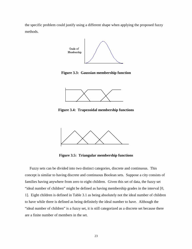
Determining the shape of the membership function that will represent the fuzzy set is an
important step that can have a large impact on the reasoning process. Gaussian functions
(Figure 3.3) are popular for representing single numbers; however, simple membership
functions provide a more straightforward approach to the fuzzy process. Two of the more
commonly used simple shapes are trapezoids (Figure 3.4) and triangles (Figure 3.5) (Masters
1993). A trapezoidal membership function is appropriate when a range of values of the fuzzy
variables share the maximum membership value (as represented by the flat top of the
trapezoid). A triangle shape is appropriate when only a single value at the apex enjoys the
maximum grade of membership. Trapezoid shaped membership functions are used in the
network management applications suggested in this proposal. However, the characteristics of
23
the specific problem could justify using a different shape when applying the proposed fuzzy
methods.
Figure 3.3: Gaussian membership function
Figure 3.4: Trapezoidal membership functions
Figure 3.5: Triangular membership functions
Fuzzy sets can be divided into two distinct categories, discrete and continuous. This
concept is similar to having discrete and continuous Boolean sets. Suppose a city consists of
families having anywhere from zero to eight children. Given this set of data, the fuzzy set
“ideal number of children” might be defined as having membership grades in the interval [0,
1]. Eight children is defined in Table 3.1 as being absolutely not the ideal number of children
to have while three is defined as being definitely the ideal number to have. Although the
“ideal number of children” is a fuzzy set, it is still categorized as a discrete set because there
are a finite number of members in the set.

24
Table 3.1: Membership grades
Number ofChildren
Membership in “IdealNumber of Children”
0 0.31 0.72 0.83 1.04 0.75 0.46 0.37 0.18 0.0
A continuous fuzzy set is likewise analogous to a continuous Boolean set. Suppose
someone is interested in the speed of a particular set of automobiles. These automobiles can
travel between 0 and 130 miles per hour. Given this information, the fuzzy set “too fast”
might be defined in the following manner. Traveling at 25 miles per hour might belong to the
“too fast” set with a membership grade of 0. Traveling at 60 miles per hour might belong
with a membership grade of 0.3, and traveling at 90 miles per hour might belong with a
membership grade of 0.8. The possible speeds at which the automobile can travel is an
infinite set of numbers in the interval [0, 130], hence making this fuzzy set a continuous fuzzy
set.
Manipulating Fuzzy Sets
Once the fuzzy sets have been defined, several approaches are available for manipulating
those sets. The first and most common is a rule based approach. This approach was
employed in the previous attempt of fuzzy reasoning applied to network routing (Arnold et al.
1995). The second approach involves using neural networks to process the information
obtained from fuzzy sets. Neural networks are utilized in this study; therefore, an explanation
for processing fuzzy sets with neural networks is provided in the next section. Appendix A
contains a discussion of the rule based approach for the interested reader.
25
Neural Networks
A neural network is an artificial intelligence technique originally designed to mimic the
functionality of the human brain. It is a non-algorithmic procedure that has a strong capability
of learning and adapting to changes in its operating environment. The ability to successfully
modify itself indicates neural networks could be a beneficial tool in managing volatile
networks. Hence, this study chose this method to process the information obtained by the
fuzzy sets.
A neural network is composed of many simple and highly interconnected processors called
neurodes. These are analogous to the biological neurons in the human brain. The artificial
neurodes are connected by links that carry signals between one another, similar to biological
neurons. The neurodes receive input stimuli that are translated into an output stimulus.
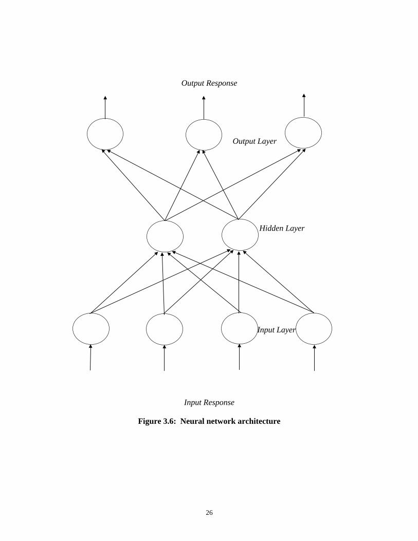
A neural network consists of many neurodes connected together as in Figure 3.6. This
illustrates a three layer neural network, which is the type that will be designed for this study.
However, it is possible to have more than (or less than) three layers and more than (or less
than) nine neurodes in a neural network.
Processing begins when information (input response) enters the input layer of neurodes.
Inputs entering any neurode in the neural network will follow the same basic process. This is
a two step process that uses two different mathematical expressions for evaluation. The first
step utilizes a summation function to combine all input values to a neurode into a weighted
input value. The second step utilizes a different mathematical expression, known as a transfer
function, that describes the translation of the weighted input pattern to an output response.
This two step process operates identically for all neurodes in the neural network.
The summation function controls how the neurode will compute the net weighted input
from the single inputs it has received. Although the summation function operates identically
for all layers, summation outcomes for the input layer will be more direct than at the other
layers. This is because each neurode in the input layer receives a single input value. Since the
sum of a single value is equal to that original value, the net weighted inputs for these neurodes
will be the original input values. Neurodes in the other two layers require some computation
to obtain their net weighted inputs. This is accomplished using the following summation
formula.
26
Output Response
Output Layer
Hidden Layer
Input Layer
Input Response
Figure 3.6: Neural network architecture
27
I w xj ij ii
n
��
�1
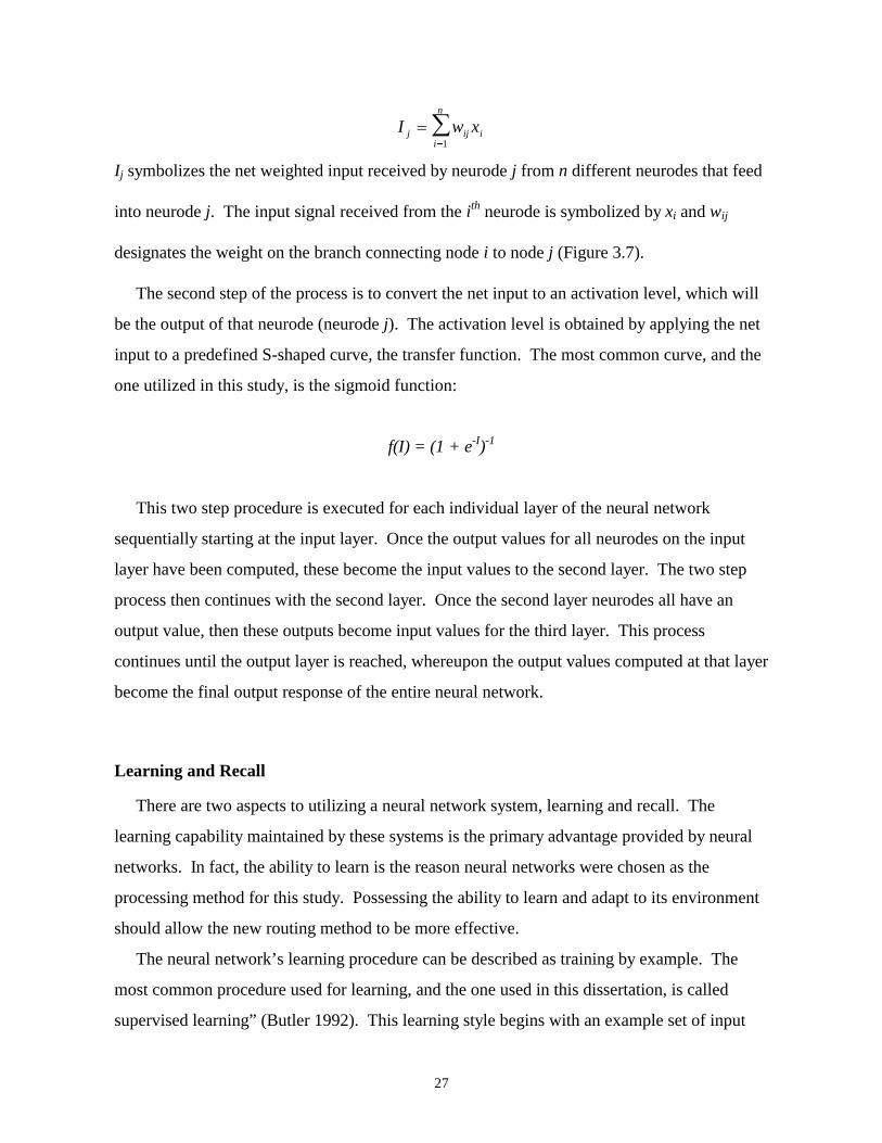
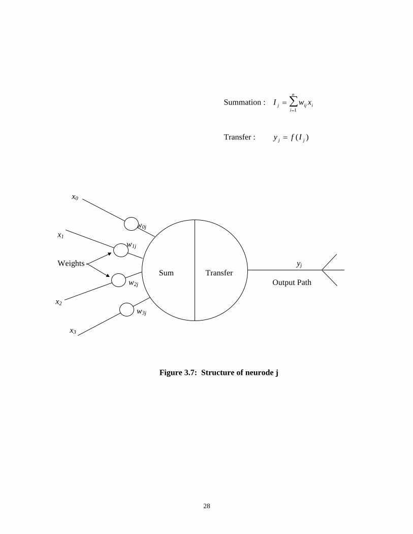
Ij symbolizes the net weighted input received by neurode j from n different neurodes that feed
into neurode j. The input signal received from the ith neurode is symbolized by xi and wij
designates the weight on the branch connecting node i to node j (Figure 3.7).
The second step of the process is to convert the net input to an activation level, which will
be the output of that neurode (neurode j). The activation level is obtained by applying the net
input to a predefined S-shaped curve, the transfer function. The most common curve, and the
one utilized in this study, is the sigmoid function:
f(I) = (1 + e-I)-1
This two step procedure is executed for each individual layer of the neural network
sequentially starting at the input layer. Once the output values for all neurodes on the input
layer have been computed, these become the input values to the second layer. The two step
process then continues with the second layer. Once the second layer neurodes all have an
output value, then these outputs become input values for the third layer. This process
continues until the output layer is reached, whereupon the output values computed at that layer
become the final output response of the entire neural network.
Learning and Recall
There are two aspects to utilizing a neural network system, learning and recall. The
learning capability maintained by these systems is the primary advantage provided by neural
networks. In fact, the ability to learn is the reason neural networks were chosen as the
processing method for this study. Possessing the ability to learn and adapt to its environment
should allow the new routing method to be more effective.
The neural network’s learning procedure can be described as training by example. The
most common procedure used for learning, and the one used in this dissertation, is called
supervised learning” (Butler 1992). This learning style begins with an example set of input
28
Summation : I w xj ij ii
n
��
�1
Transfer : y f Ij j� ( )
x0
w0j
x1
w1j
Weights yj
Sum Transfer w2j Output Path
x2
w3j
x3
Figure 3.7: Structure of neurode j
29
and corresponding output patterns. These input/output pairs are exposed to the neural
network, which eventually learns the distinct type of output to expect upon receiving certain
inputs. This training causes learning to occur by reducing the error produced when the neural
network predicts an output from a given set of input values. The error reduction is
accomplished by modifying the weights that connect the neurodes to one another. This is
analogous to biological learning where the brain’s synapses strengthen their connections
between neurons upon learning. The weights of the artificial network are adapted according
to a specified learning rule, which in this study is known as the delta learning rule (Butler
1992).
The recall operation of neural networks occurs only after the learning process has been
completed. At that time, the neural network should be sufficiently trained to generate the
appropriate output for a given set of inputs. Recall is essentially the process of employing a
trained network to provide usable predictions.
Fuzzy Neural Networks
Fuzzy sets were initially introduced into neural networks in 1974 (Lee 1974), but has not
experienced much development until recently. Since 1991, much attention has been focused
on incorporating fuzzy reasoning into neural networks (Chan 1993).
A neural network is considered a fuzzy neural network if the signals and/or the weights in
the system are based around fuzzy sets (Buckley 1994). This research will employ fuzzy
neural networks whose signals are membership grades generated from fuzzy sets. This
alteration of the neural network inputs will not affect the neural network operations previously
described.
Methodology
Introduction
Delivering data through a wide area network can be a difficult task when many nodes are
present. Transmission would be virtually effortless if every node on the network had a direct
link to every other node. This would provide for simple transmissions between two stations
on the network; however, it is an impractical solution. The necessary method of handling this
30
problem is to employ the specialties of a network router so data can be effectively transmitted
through other devices on the network. As described earlier, a router is an internetworking
device that transmits data between two computer networks. It operates much like a small
computer in that it executes a special software program that determines the best route for the
data to reach its destination.
Adaptive traffic routing focuses on the current state of the network, thus attempting to
satisfy quality of service needed by the users. The methods that have been proposed thus far
base their routes on network performance information, which is often inaccurate due to the
time needed for the information to travel. Since this information is based upon vague
observations, fuzzy logic seems to be the natural method to use in network routing.
The criteria for packet switched WAN routing is more detailed than those for telephone
routing. Khalfet and Chemouil (1994) address only two criteria in their adaptive telephone
routing scheme; quality and availability. Stallings (1990) suggests that there are many
requirements for a routing function in a packet switched WAN. These requirements include
correctness, simplicity, robustness, stability, fairness, and optimality. As discussed earlier,
two common, and simple, criterion used in selecting a WAN route are the minimum-hop route
and the least-cost route, where cost is based on data rate (Stallings 1990). Data rate is a
concept that is not addressed with circuit switched networks, as packet switched networks can
have different data rates on different links. Two additional considerations, according to
Stallings (1990), that help fulfill the above requirements are failures and congestion.
This research will present an application of fuzzy neural network control to adaptive traffic
routing in a packet switched WAN. There currently exist three non-neural network protocols
that use similar (but not fuzzy) criteria to determine an appropriate data route, namely OSPF,
IGRP and BGP. These three routing protocols were briefly discussed in chapter two, but will
be explained in more detail here.
The “open shortest path first” algorithm (OSPF) is so called because open refers to being
not proprietary and shortest path first is another phrase meaning “link state routing algorithm”
(Perlman 1992). A link state routing algorithm distributes the responsibility of defining the
network link topology to all routers on the network. Each router is responsible for learning
information about its neighbors and constructs a link state packet (LSP) to contain and
31
transmit this information. The LSP is transmitted to all other routers that in turn, store the
received LSPs for computing appropriate routes to each destination.
Each router is configured with a cost for each link that is attached to it. Links can be
configured with up to four different costs concerning the link: bandwidth, amount of delay,
amount of money, and frailty. Each cost defines a different route; therefore, the router
calculates routes to all destinations based on the different possible combinations of metrics to
be used. In addition to being extremely resource intensive (Cisco 1995), this requires the user
to know which metric they would like to employ for computing the route to the destination.
The desired “quality of service” (QOS) option found in the data packet header is responsible
for declaring which metric should be used (Perlman 1992). The basic idea behind OSPF is
that it uses LSPs to determine a set of routing tables for each router. Depending on the
desired quality of service, one of the routing tables is selected as an appropriate one for
transmitting the data packet. Once again, this is a routing protocol currently being used.
IGRP (Interior Gateway Routing Protocol), similar to OSPF, uses a combination of metrics
to make a routing decision. However, IGRP always considers all its metrics when computing
a route. Network delay, bandwidth, reliability, MTU (the maximum size of a packet that can
traverse a particular network link) and delay, all play a role in determining the routing path for
data transmission (Cisco 1995). Each metric is assigned a certain weight that represents its
level of importance in transmitting data throughout the network. IGRP also provides a second
routing path that will be employed in the case of faults in a link. This routing protocol is also
one that is currently being implemented in modern computer networks.
BGP (Border Gateway Protocol) is a routing protocol that is slowly beginning to be
implemented in the Internet (Cisco 1995). The basis of BGP, like OSPF and IGRP, focuses
on a metric; however, the BGP metric is very different from those found in OSPF and IGRP.
BGP utilizes a metric to rank all of the feasible routes to a destination. This metric is an
arbitrary unit that specifies the “degree of preference” for a particular path. The degree of
preference is based on metrics that are defined by the network administrator. These metrics
usually include domain counts, speed, reliability, stability and other factors.
The BGP idea of declaring the optimal route based on a degree of preference is parallel to
the concept of fuzzy routing. The BGP metrics (domain count, speed, reliability, stability,
32
etc.) are difficult to characterize in a precise manner. For example, it is impossible to give a
precise level of reliability or stability of a network link. This imprecision suggests that the
degree of preference for a network link might be more accurately determined if the deciding
metrics are defined as fuzzy sets.
This proposal of a fuzzy routing algorithm will not include the development of a new
routing protocol. Instead, it will just be an addition to an existing protocol such as BGP. The
current usage of the proposed routing metrics implies that this idea enjoys a substantial
foundation in current practice.
The criterion used to satisfy Stallings’ (1990) requirements include such properties as
distance, throughput, failures, congestion and others. A selection of the most critical
characteristics will be used to create and define the proposed fuzzy routing control. The fuzzy
routing process, once fully developed, will be validated by comparison to existing protocols in
a simulation environment.
Fuzzy Sets in Routing
A routing table consists of a set of fixed details concerning aspects such as the different
possible routes and the data rates for the different links. Dynamic information that is reported
from the other nodes is included as well. The combination of all this information is used to
make efficient routing decisions at each node in the WAN. In order to address the necessary
requirements for routing through a packet switched WAN, the following criteria will be used
in this example: distance, throughput, failures and congestion. Each of these criteria will have
associated with them a group of fuzzy membership functions. Trapezoid shaped membership
functions, as discussed previously are used in the explanations below, but the characteristics
of the specific problem could justify using a different shape.
Distance is an important factor because it is directly related to transmission time. Each
node has the ability to store information such as the optimal number of hops to the destination
under favorable conditions. This information, referred to as distance, should be viewed in an
inexact manner because of the possibility that network failures (and subsequent re-routings)
might occur before packet transmission is complete. Every outgoing link of the node will
have associated with it a fuzzy distance value of short, medium, or long, which will have
problem-dependent values.

33
Defining the fuzzy membership sets for distance requires additional explanation because
distance, as number of hops, is a discrete measure. A possible discrete representation of the
distance membership sets is illustrated in Table 3.2 with an explanation of discrete fuzzy
reasoning found in Appendix A. The complication with this definition arises when the
number of nodes in the WAN begins to increase. As this happens the number of possible
hops will also increase, thus expanding the size and complexity of the table. Since the
continuous membership definition will outline a description similar to the discrete, it is
possible to represent the fuzzy distance membership sets as continuous. Although the WAN
referenced in this research is not very large, this research will apply the continuous distance
membership sets since it is a viable option and enjoys the added benefit of consistency with
the other fuzzy membership sets, as they are all continuous as well. The fuzzy membership
sets to be utilized with the distance metric are shown in Figure 3.8.
Throughput is related to data rate and should be as high as possible. Data rates of the
outgoing links on a node can be stored as variable information at that node. Differing
amounts of traffic can affect these data rates in distinct manners; therefore, it is necessary to
classify these rates into fuzzy groups; low, medium, and high. The numerical values
corresponding to these sets will depend on the specific WAN being modeled. The
membership sets associated with the throughput characteristic are shown in Figure 3.9. While
the fuzzy variable utilized here is data rate in megabytes per second, another logical measure
might be the percentage of packets successfully delivered.
Similar to all electronic equipment, a WAN is subject to occasional failures. Many
different types of failures can occur, each of which has a differing degree of severity. Some
failures, such as a break in the cable, will be more severe than failures such as a temporary
power failure. Level of failure is information that is reported by other nodes; therefore, a
certain amount of travel time is needed to receive the information. Because of this time delay,
the information concerning failures may be inaccurate at times, resulting in fuzzy knowledge.
The fuzzy groups specifying severity of failure are mild, severe and very severe. The severity
of a failure is usually directly correlated with the estimated time to repair; therefore, the failure
membership set will be measured by estimated time to repair. The specific types of possible
failures depend on the hardware that is being used in the WAN. Another possible measure of
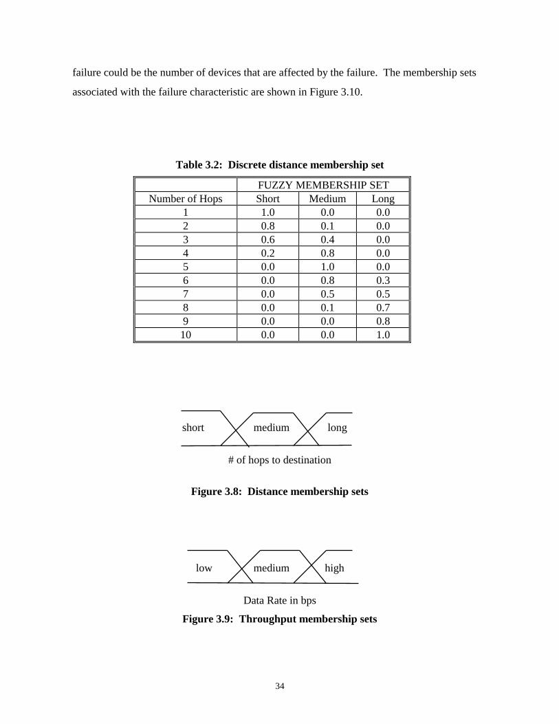
34
failure could be the number of devices that are affected by the failure. The membership sets
associated with the failure characteristic are shown in Figure 3.10.
Table 3.2: Discrete distance membership set
FUZZY MEMBERSHIP SETNumber of Hops Short Medium Long
1 1.0 0.0 0.02 0.8 0.1 0.03 0.6 0.4 0.04 0.2 0.8 0.05 0.0 1.0 0.06 0.0 0.8 0.37 0.0 0.5 0.58 0.0 0.1 0.79 0.0 0.0 0.810 0.0 0.0 1.0
short medium long
# of hops to destination
Figure 3.8: Distance membership sets
low medium high
Data Rate in bps
Figure 3.9: Throughput membership sets

35
mild severe very severe
Time to repair
Figure 3.10: Failure membership sets
Users of a WAN expect a certain service quality that is affected significantly by
congestion. Similar to failures, different levels of congestion can occur as well. Level of
congestion is also information that is reported by other nodes; therefore, travel time can cause
this information to be inaccurate at times. Also, there is no one point that could be considered
the transition point from low to medium congestion. The fuzzy groups characterizing
congestion are low, medium and high, with values based on the average amount of traffic
traveling through the WAN. Although number of packets may seem like a discrete measure, it
is defined with a continuous membership set because the numbers encompass such a large
range. This reasoning is analogous to that of the distance membership set. Another logical
fuzzy descriptor, that is continuous, might be traffic as a percentage of the maximum possible
throughput. The membership sets associated with the congestion characteristic are shown in
Figure 3.11.
low medium high
Number of Packets
Figure 3.11: Congestion membership sets
These four criteria all have descriptions with inaccurate boundaries, hence they are all
represented best through the use of a fuzzy controller. The controller is responsible for
determining the level of efficiency for all possible routing decisions. For example, if a
deciding node has three possible outgoing routes, it will need to determine the level of
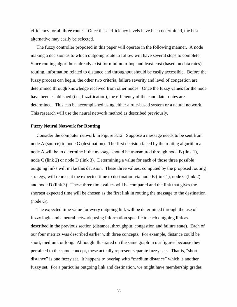
36
efficiency for all three routes. Once these efficiency levels have been determined, the best
alternative may easily be selected.
The fuzzy controller proposed in this paper will operate in the following manner. A node
making a decision as to which outgoing route to follow will have several steps to complete.
Since routing algorithms already exist for minimum-hop and least-cost (based on data rates)
routing, information related to distance and throughput should be easily accessible. Before the
fuzzy process can begin, the other two criteria, failure severity and level of congestion are
determined through knowledge received from other nodes. Once the fuzzy values for the node
have been established (i.e., fuzzification), the efficiency of the candidate routes are
determined. This can be accomplished using either a rule-based system or a neural network.
This research will use the neural network method as described previously.
Fuzzy Neural Network for Routing
Consider the computer network in Figure 3.12. Suppose a message needs to be sent from
node A (source) to node G (destination). The first decision faced by the routing algorithm at
node A will be to determine if the message should be transmitted through node B (link 1),
node C (link 2) or node D (link 3). Determining a value for each of those three possible
outgoing links will make this decision. These three values, computed by the proposed routing
strategy, will represent the expected time to destination via node B (link 1), node C (link 2)
and node D (link 3). These three time values will be compared and the link that gives the
shortest expected time will be chosen as the first link in routing the message to the destination
(node G).
The expected time value for every outgoing link will be determined through the use of
fuzzy logic and a neural network, using information specific to each outgoing link as
described in the previous section (distance, throughput, congestion and failure state). Each of
our four metrics was described earlier with three concepts. For example, distance could be
short, medium, or long. Although illustrated on the same graph in our figures because they
pertained to the same concept, these actually represent separate fuzzy sets. That is, “short
distance” is one fuzzy set. It happens to overlap with “medium distance” which is another
fuzzy set. For a particular outgoing link and destination, we might have membership grades
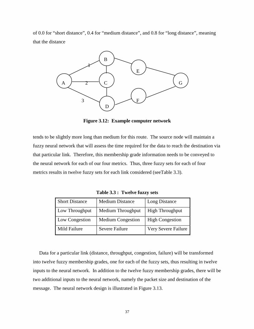
37
of 0.0 for “short distance”, 0.4 for “medium distance”, and 0.8 for “long distance”, meaning
that the distance
B 1
E
A 2 C G
3 F D
Figure 3.12: Example computer network
tends to be slightly more long than medium for this route. The source node will maintain a
fuzzy neural network that will assess the time required for the data to reach the destination via
that particular link. Therefore, this membership grade information needs to be conveyed to
the neural network for each of our four metrics. Thus, three fuzzy sets for each of four
metrics results in twelve fuzzy sets for each link considered (seeTable 3.3).
Table 3.3 : Twelve fuzzy sets
Short Distance Medium Distance Long Distance
Low Throughput Medium Throughput High Throughput
Low Congestion Medium Congestion High Congestion
Mild Failure Severe Failure Very Severe Failure
Data for a particular link (distance, throughput, congestion, failure) will be transformed
into twelve fuzzy membership grades, one for each of the fuzzy sets, thus resulting in twelve
inputs to the neural network. In addition to the twelve fuzzy membership grades, there will be
two additional inputs to the neural network, namely the packet size and destination of the
message. The neural network design is illustrated in Figure 3.13.
38
When node A’s controller (Figure 3.12) determines the best link to use from among link1,
link 2 or link 3, the neural network will be invoked three different times using three sets of
inputs to get three expected time values. These three time values are then compared to find
the link that will give the lowest expected time to reach the destination. That will be the link
chosen to send the message along. When the message arrives at the next node, the same
process will be repeated using a similar neural network for all outgoing links of that particular
node. This procedure continues until the destination node is reached. A similar, but not
identical, neural network will be present at each node of the computer network. This
dissertation will establish the advantages of this routing strategy by testing it at a single source
node. Results obtained with this neural network can easily be generalized to all nodes on the
computer network.
Neural Network Training
Training the neural network will be the most time consuming phase of the study and will
require that a simulation model first be designed. The training process will operate in the
following manner.
I. Design the neural network with fourteen input nodes, one bias node and one output
node that represents the expected time to reach the destination. The appropriate
number of hidden nodes will be determined by applying common rules of thumb (i.e.
number of input nodes and number of output nodes divided by 2). The input and
output nodes are defined as seen in Figure 3.13.
II. Build a simulation model to represent a hypothetical computer network. Two details
will remain constant throughout the simulation process: the network topology and the
source node of interest.
III. A large number of simulations will be run to develop a sufficient training set. Each
simulation will consist of transmitting a message from a source node along each of the
possible outgoing links using a data profile. Each profile for node one will consist of
the following information:
A. destination node
B. packet size
C. distance from the current node to the destination via the link in question
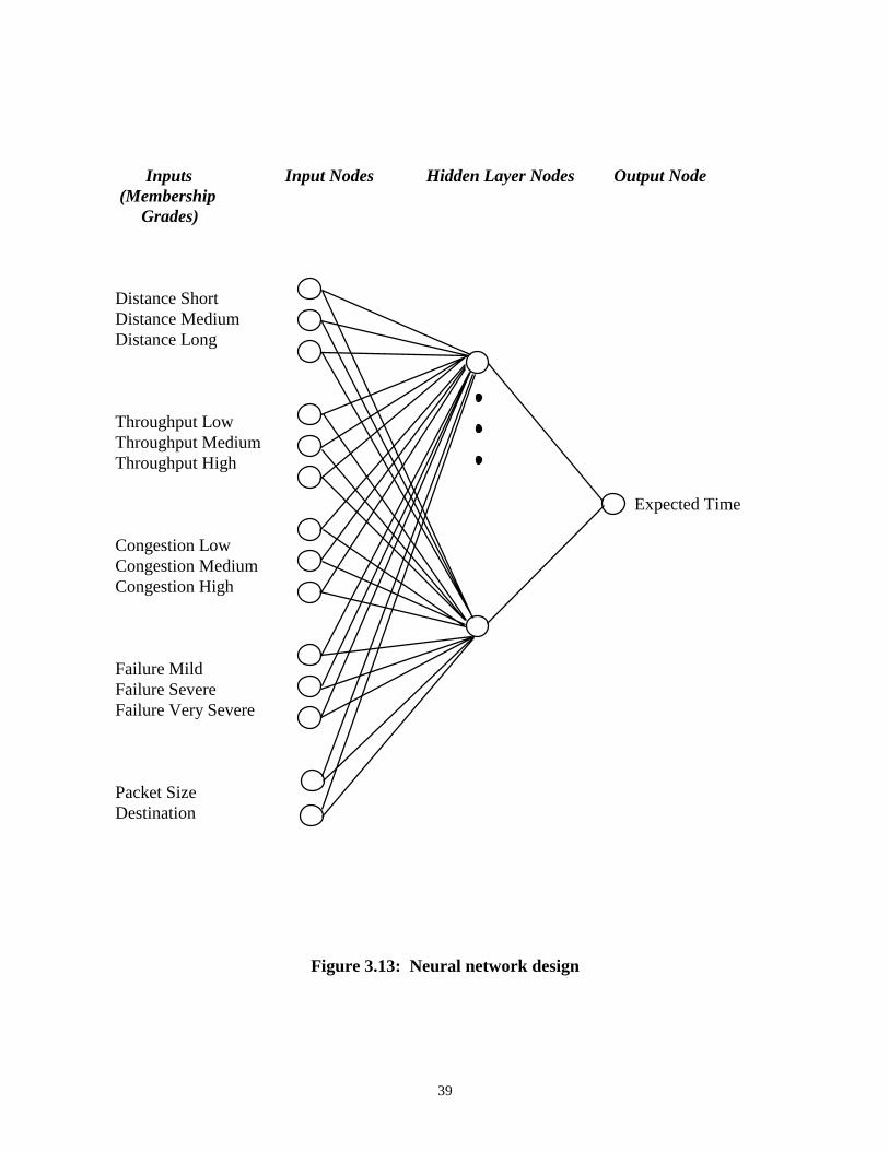
39
Inputs Input Nodes Hidden Layer Nodes Output Node (Membership Grades)
Distance ShortDistance MediumDistance Long
Throughput LowThroughput MediumThroughput High
Expected Time
Congestion LowCongestion MediumCongestion High
Failure MildFailure SevereFailure Very Severe
Packet SizeDestination
Figure 3.13: Neural network design
40
D. throughput on the link
E. number of packets traveling on that link
F. type of failure present on that link.
By varying the values of these six characteristics and repeating the simulation, we will
generate a database of operating characteristics and the resulting transmission time along each
of the links leaving the source node. The operating characteristics will be the input portion of
the training set for the neural network. The time to complete the transmission using that
particular link will be the output portion of the training set.
As the six inputs vary between simulations, there remains an additional detail concerning
routing through the remaining portion of the network (subsequent routing after the first link
leaving the transmission node). Once the simulation uses a profile regarding each possible
outgoing link to travel from the source node to the next node, there needs to be an appropriate
algorithm to send the message through the remainder of the computer network. Random
routing was chosen to avoid preferences for any of the input measures. For example, if
shortest path routing was used in the remainder of the network, then the distance metric would
be unfairly weighted.
Performance Comparison
Once the neural network has been trained and is ready to be used for routing messages,
performance of the new method must be compared to an existing method. Through the use of
simulations, the fuzzy-neural method will be compared to a current shortest route algorithm
and the comparative performances will be analyzed statistically. As a further step, it would be
desirable to compare the fuzzy-neural method to the fuzzy-rule based method developed by
Arnold et al. (1997) as described in chapter two. However, such comparisons are not possible
due to incomplete details of that algorithm and its performance.
Summary
Fuzzy sets are most useful when dealing with human thoughts and processes. Suppose that
an antique dealer is asked to establish a collection of furniture as being rare or common.
41
Defining a precise boundary between the two categories, rare and common, would be a
difficult task for the dealer; therefore, in his mind, he will probably view each piece in a fuzzy
manner. Fuzzy reasoning is a form of artificial intelligence that attempts to mimic the human
reasoning process. According to the expectation of Zadeh, the historical task of fuzzy theory
is making computers resemble the human brain more closely (Wang and Loe 1993). Neural
networks address a related but different aspect of human cognition. Fuzzy reasoning is used
to mimic the human reasoning process while neural networks are used to mimic the human
learning process. Combined together, these two artificial intelligence tools should result in a
successful and effective routing algorithm. This chapter has outlined briefly the methodology
that will be used to develop the new routing method and to gauge its performance. The next
chapter presents more methodological details in context as the experiments and analysis of the
results are presented.
42
Chapter 4 : Fuzzy Routing
Introduction
This chapter contains the new routing algorithm and an analysis concerning the strengths
and capabilities of the new design. This entire process can be divided into tasks and
sufficiently described in four sections. The initial task, and topic of the first section, involves
designing a simulation model to represent the detailed routing process found in a computer
network. The second section presents details concerning the development of the new routing
algorithm as applied to the hypothetical network described in section one. The third and fourth
sections describe the experimental design and analysis of the new algorithm.
Simulation Design
Before developing a simulation model for analyzing the new routing algorithm, a
hypothetical network must be established. This is an essential portion of the development
process due to the network dependency of the new algorithm. Although the basic concepts of
the new algorithm will remain constant from network to network, there will exist some
variations in the specific network parameters. These variations depend on many factors
including the capacity of the transmission media, size of the network and types of devices
present. This will be true for most adaptive algorithms as they are employed on different
types of networks. Network limitations vary such that a high data rate in one computer
network could potentially be considered a low data rate in another network.
The hypothetical computer network referred to throughout this chapter is illustrated in
Figure 4.1. This network represents twelve local area networks interconnected to form a wide
area network. Each of the twelve LANs in the diagram is considered to be a single node in
this study, and will be referred to as nodes one through twelve. Furthermore, each LAN is
assumed to possess its own designated routing device (probably a packet switch) for

43
transmitting data to other LANs. Hence, when a LAN node is referred to in this chapter, the
reference is actually directed toward the routing device for that particular LAN. This is
illustrated in Figure 4.2, which displays possible details of the upper left corner of the
example network. The symbols inside the boxes represent packet switches (i.e. P1 is packet
switch one corresponding to LAN one).
WANs involve not only interconnected LANs. For example, Figure 4.2 indicates that each
of the twelve nodes of the example network represents a combination of computers and
routing devices. Node 1 of the example network could symbolize a LAN and its packet
switching device. Node 2, node 4 and node 7 could also represent a LAN and packet
switching device. However, node 3 is illustrated as a packet switching device attached to
three other computing devices that do not form a LAN.
Another possible interpretation of the example network is illustrated in Figure 4.3. This
description of the example network involves a different setup; wide area networks and their
designated routers. The symbols inside the boxes represent the routers (i.e. R1 for router one).
Either description is appropriate for implementing the routing algorithm. Although details of
the situations appear extremely different, the routing process will operate similarly for each.
This suggests that much information regarding the individual LANs will not be needed to
simulate the WAN’s routing process.
Each of the twelve nodes represents the routing center for that particular network. The
details of the twelve individual networks are not needed for this simulation study because
knowing how many devices are in each network will not affect the simulation. Knowing
exactly what kind of device is sending the data will not matter either. Many characteristics
and occurrences will be analogous under either routing algorithm during the comparison later
in this chapter. Therefore, occurrences while sending data from the originating device to that
network’s routing device would also be insignificant in this study.
An extensive list of details could easily be generated to express the specifications of the
WAN as the two routing algorithms are simulated; however, such details will not be necessary
given the comparative nature of the study. For example, it might be true that the routing
device at node 1 handles a network with fifteen workstations while the LAN at node 2
maintains only twelve workstations. Details such as these can distinguish the illustrated
44
WAN from others but are unnecessary in a comparative study as this. The different routing
methods will be compared using identical networks under identical circumstances, causing
only a portion of the network’s descriptive details to be relevant.
The twelve routing centers are interconnected with seventeen different links. It is assumed
that the same type of transmission media, a T-1 circuit using twisted pair, is utilized for each
link. Telephone carriers offer this common media with 24 channels, for an aggregate digital
transmission rate of 1.544 Mbps (million bits per second) on each link (Stallings 1993). This
assumption will not affect the generalization of the final results since the fuzzy metrics (e.g.
low congestion, high throughput, etc.) are defined relative to the specific network structure.
The T-1 transmission media was chosen because it is commonly used for data transmissions.
Once again, the transmission media and transmission rate will be identical in simulating both
algorithms. Therefore, simulating a different transmission media or rate should not have
affected the final results of this comparison.
A T-1 communications link is created by multiplexing twenty-four 8000 bytes per second
(bps) lines (Stamper 1995). The 8000 bps rate is the base throughput level for each link,
while the size and number of packets traversing the link will determine the manner by which
throughput will change. As more packets begin traversing a specific link, the throughput of
that link will begin decreasing at a proportional rate.
If a problem occurs on a link and the number of packets desiring to traverse that link
becomes excessive, the model does not refuse packets to the link. Those packets, instead,
would be placed in a queue to wait until their turn for transmission. This is another
characteristic that remains acceptable because it appears on both sides of the comparison.
The messages generated from node one will be no larger than 100,000 bytes each.
However, a message that large cannot be transmitted as one single packet. Any message
larger than 1500 bytes must be segmented into multiple packets of 1500 bytes each or less.
This maximum packet size was chosen because popular ethernet packets maintain a maximum
packet size of 1500 bytes (Hardy 1995). Although the networks in this study are not specified
as ethernet networks, choice of maximum packet size is not critical because it will be held
constant when comparing the new and existing algorithms.
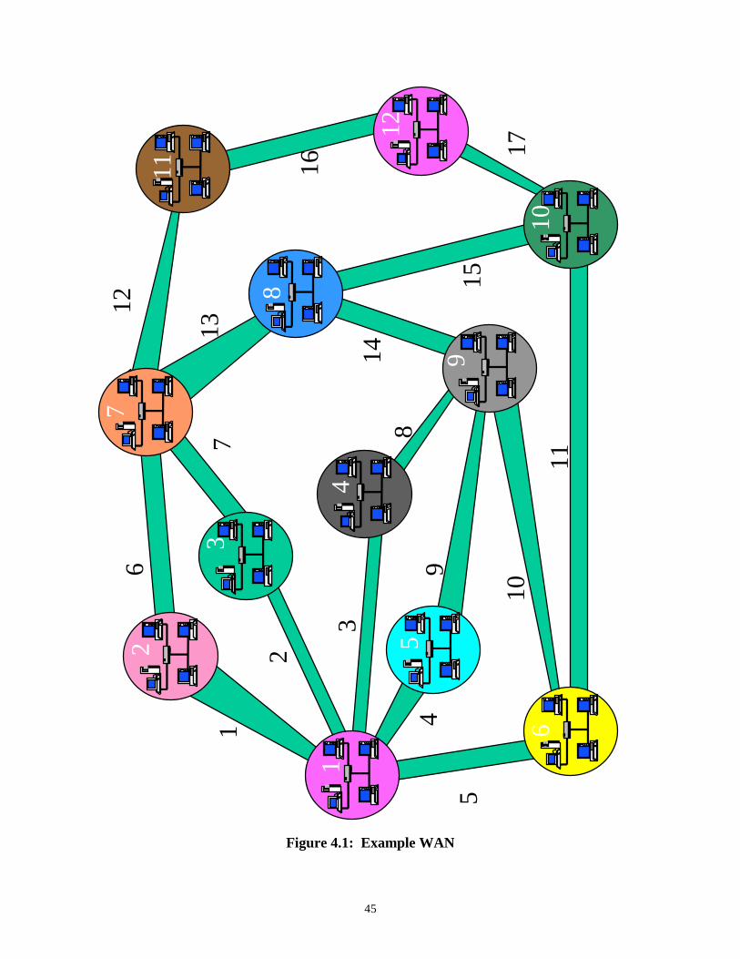
45
1
2
3
5
6
4
9
8
7
11
12
10
6
4
5
1
3
2
14
7
12
9
11
16
15
17
8
10
13
Figure 4.1: Example WAN

46
LAN 7
LAN 2P7
P2
P3
LAN 1 P1
P4
LAN 4
Figure 4.2 : A second variation of the example network

47
WAN 7
WAN 2R7
R2
R3 WAN 3
WAN 1 R1
R4
WAN 4
Figure 4.3: A third variation of the example network
48
This comparative study will observe the variations that result from applying different
routing algorithms to routing node one. This will be done while all other details remain
consistent between the two algorithms. The primary objects of interest are routing node one
and the links connecting node one to the remaining nodes, links one through five. This
routing node is the one that will control the routing algorithm being studied. All other routing
nodes use a randomly generated fixed routing table to determine how to route their packets.
As node one generates and receives packets, the routing algorithm will select one of links one
through five as the link upon which the packet will travel. Therefore, information regarding
routing node one and links one through five must be known during the simulation. Packets
will be generated at other nodes and sent along other links as well in order to create realistic
congestion levels; however, specific details concerning the other links and nodes are not
needed to accurately perform the simulation study.
The open shortest path first (OSPF) protocol is a common protocol used in TCP/IP
networks (Stallings 1997) which efficiently implements shortest path routing. The simulation
model was designed to route packets at node one using two different algorithms: the new
algorithm and an OSPF (shortest-path) algorithm. These two will be compared to establish
the significant advantage of applying the new algorithm.
OSPF uses link state routing to obtain information describing the entire computer network.
The basic idea is that each routing device on the network is responsible for meeting its
neighbors and learning their situations (Perlman 1992). Each routing device forms a “link
state packet” (LSP) which contains information regarding that device. This LSP is transmitted
to the neighboring routers just as any other packet would be sent. The receiving routers store
the LSP and use the contained information to update their routing tables.
LSPs are generated periodically and when a noticed change occurs. The simulation model
in this study collects information for table updates every 60 seconds, but actual LSPs are not
transmitted during the simulation. Having LSPs travel during the simulation would affect the
study by simply adding more congestion and would not affect the final results of the
comparison. The LSPs, if included, would alter both sides of the study in an identical manner
because the LSPs would be analogous for both routing algorithms. Transmitting and
receiving information to and from the network nodes will not affect anything in this study

49
because it is done the same way for either algorithm. Essentially, the LSPs are omitted
because they operate identically regardless of which algorithm is used.
OSPF uses an algorithm that computes the route incurring the least cost where cost is a
measure defined by the user. It most often refers to the number of hops from source to
destination (distance) but can be expressed as a function of delay, data rate, dollar cost,
different distance measure or another factor delivered by the LSPs (Stallings 1997). The
OSPF algorithm used against the new algorithm considers the measured cost to be the number
of hops to the destination.
The least-cost routing algorithm employed by OSPF was originally proposed by Dijkstra
(Dijkstra 1959). It is a common algorithm used in many shortest route situations where
objects need to be transported. Examples include data on computer networks, vehicles on
highways, trains and railroads, etc. Dijkstra’s algorithm finds the shortest path from a starting
point, or source node, to all other points, or nodes, on the network. The entire procedure takes
a number of stages, equal to the number of nodes in the system. The new algorithm will be
compared to Dijkstra’s algorithm using number of hops as the metric defining cost. The
simulation model was similarly designed for both circumstances with the sole difference being
the algorithm employed to update the routing table at node one.
The simulation model was developed using AweSim (version 1.4), by Pritsker
Corporation, with many of the detailed processes being controlled through user written C
functions. The AweSim model consists of many small modules, each representing an
individual portion of the networking processes.
The core of the simulation model involves the details of generating packets originating at
node one. These are the packets of interest since they will begin traveling as a result of the
new or OSPF routing algorithm. As these packets continue through the network, they will
encounter other routing nodes. These nodes are of little concern to the study, and therefore,
will operate in a consistent manner between the two situations, involving the new algorithm
and the shortest route algorithm. This consistency is established by giving the other routing
nodes a fixed routing table that was randomly generated and has no algorithm for updates.
Figure 4.4 illustrates the steps used in generating and routing packets from node one. The
first step is to generate messages, which will be segmented into smaller packets. The source
50
node of these packets is known to be node one, but the destination node is randomly chosen
for each message. Before the packet begins traveling, its associated “Current Node”
characteristic is set to node 1. The packet’s “Current Node” is its location at the present time.
The “Current Node” and “Destination Node” corresponding to the packet are used as inputs to
the routing table to determine the “Next Node” to visit. The packet then travels to the “Next
Node” and the new “Current Node” becomes the old “Next Node.” Upon inspection of the
packet’s location at this point, it must be determined if the packet has reached its destination
node. If it has not, then another routing table is used to direct the packet to the next node.
This continues until the packet does reach its destination node. At that instance, statistics are
collected and the packet is terminated.
Other modules of the simulation model include one to generate other packets at other
nodes. These packets serve only one purpose, to provide additional traffic throughout the
network. Another module generates random failures on some of the network links. These
failures are not extremely severe, as the simulation model declares them to persist to a
maximum of only 100 seconds. The model was designed in such a manner because replicated
samples of short time periods will be collected, suggesting lengthy failures would not exhibit
their full effect. A 10-minute sample containing a 30-minute failure would provide less
meaningful results because it would be impossible to observe what happens during the node’s
recovery period. A situation such as that would guarantee that failure related changes would
not be seen, and thus would not be useful. The hypothesis that the new algorithm will
dominate in the presence of network fluctuations suggests that we need to observe before,
after, and during failures, even if the failures are short.
Portions of the AweSim modules are illustrated to provide a brief explanation. Figure 4.5
represents the creation of packets at node 1 and their segmentation as needed. Figure 4.6
represents the process that occurs when a packet arrives at another node. This module
determines if the packet came from node 1 and whether the packet has reached its final
destination. At this point, statistics are collected or the routing table at that node is accessed.
The entire AweSim model is provided in Appendix B. The supporting C code is provided in
Appendix C.
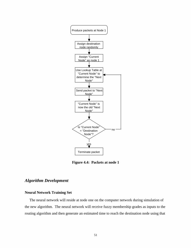
51
Produce packets at Node 1
Assign destinationnode randomly
Use Lookup Table at"Current Node" to
determine the "NextNode"
Assign "CurrentNode" as node 1
Send packet to "NextNode"
"Current Node" isnow the old "Next
Node"
Is "Current Node"= "Destination
Node"?
Terminate packet
yes
no
Figure 4.4: Packets at node 1
Algorithm Development
Neural Network Training Set
The neural network will reside at node one on the computer network during simulation of
the new algorithm. The neural network will receive fuzzy membership grades as inputs to the
routing algorithm and then generate an estimated time to reach the destination node using that
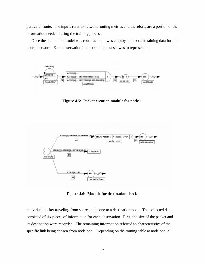
52
particular route. The inputs refer to network routing metrics and therefore, are a portion of the
information needed during the training process.
Once the simulation model was constructed, it was employed to obtain training data for the
neural network. Each observation in the training data set was to represent an
Figure 4.5: Packet creation module for node 1
Figure 4.6: Module for destination check
individual packet traveling from source node one to a destination node. The collected data
consisted of six pieces of information for each observation. First, the size of the packet and
its destination were recorded. The remaining information referred to characteristics of the
specific link being chosen from node one. Depending on the routing table at node one, a
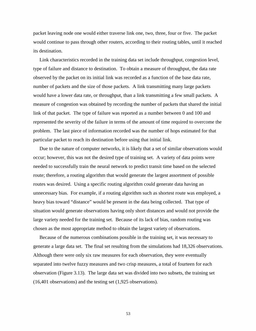
53
packet leaving node one would either traverse link one, two, three, four or five. The packet
would continue to pass through other routers, according to their routing tables, until it reached
its destination.
Link characteristics recorded in the training data set include throughput, congestion level,
type of failure and distance to destination. To obtain a measure of throughput, the data rate
observed by the packet on its initial link was recorded as a function of the base data rate,
number of packets and the size of those packets. A link transmitting many large packets
would have a lower data rate, or throughput, than a link transmitting a few small packets. A
measure of congestion was obtained by recording the number of packets that shared the initial
link of that packet. The type of failure was reported as a number between 0 and 100 and
represented the severity of the failure in terms of the amount of time required to overcome the
problem. The last piece of information recorded was the number of hops estimated for that
particular packet to reach its destination before using that initial link.
Due to the nature of computer networks, it is likely that a set of similar observations would
occur; however, this was not the desired type of training set. A variety of data points were
needed to successfully train the neural network to predict transit time based on the selected
route; therefore, a routing algorithm that would generate the largest assortment of possible
routes was desired. Using a specific routing algorithm could generate data having an
unnecessary bias. For example, if a routing algorithm such as shortest route was employed, a
heavy bias toward “distance” would be present in the data being collected. That type of
situation would generate observations having only short distances and would not provide the
large variety needed for the training set. Because of its lack of bias, random routing was
chosen as the most appropriate method to obtain the largest variety of observations.
Because of the numerous combinations possible in the training set, it was necessary to
generate a large data set. The final set resulting from the simulations had 18,326 observations.
Although there were only six raw measures for each observation, they were eventually
separated into twelve fuzzy measures and two crisp measures, a total of fourteen for each
observation (Figure 3.13). The large data set was divided into two subsets, the training set
(16,401 observations) and the testing set (1,925 observations).
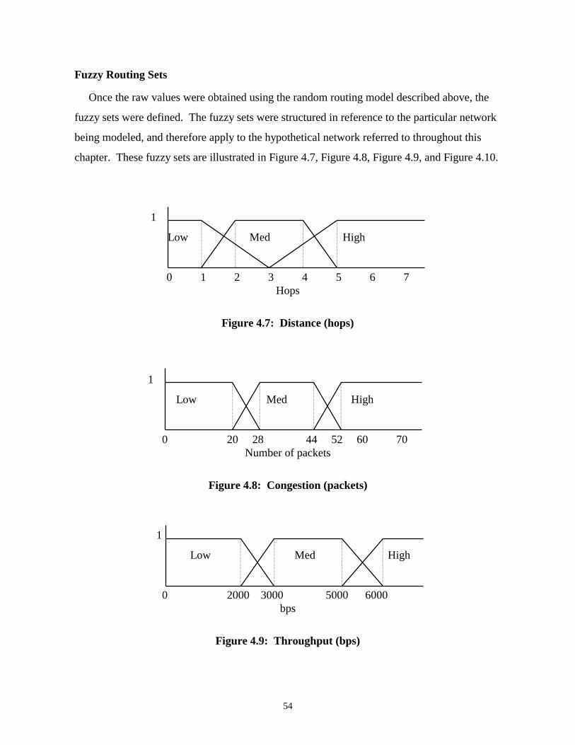
54
Fuzzy Routing Sets
Once the raw values were obtained using the random routing model described above, the
fuzzy sets were defined. The fuzzy sets were structured in reference to the particular network
being modeled, and therefore apply to the hypothetical network referred to throughout this
chapter. These fuzzy sets are illustrated in Figure 4.7, Figure 4.8, Figure 4.9, and Figure 4.10.
1
Low Med High
0 1 2 3 4 5 6 7Hops
Figure 4.7: Distance (hops)
1
Low Med High
0 20 28 44 52 60 70Number of packets
Figure 4.8: Congestion (packets)
1
Low Med High
0 2000 3000 5000 6000bps
Figure 4.9: Throughput (bps)
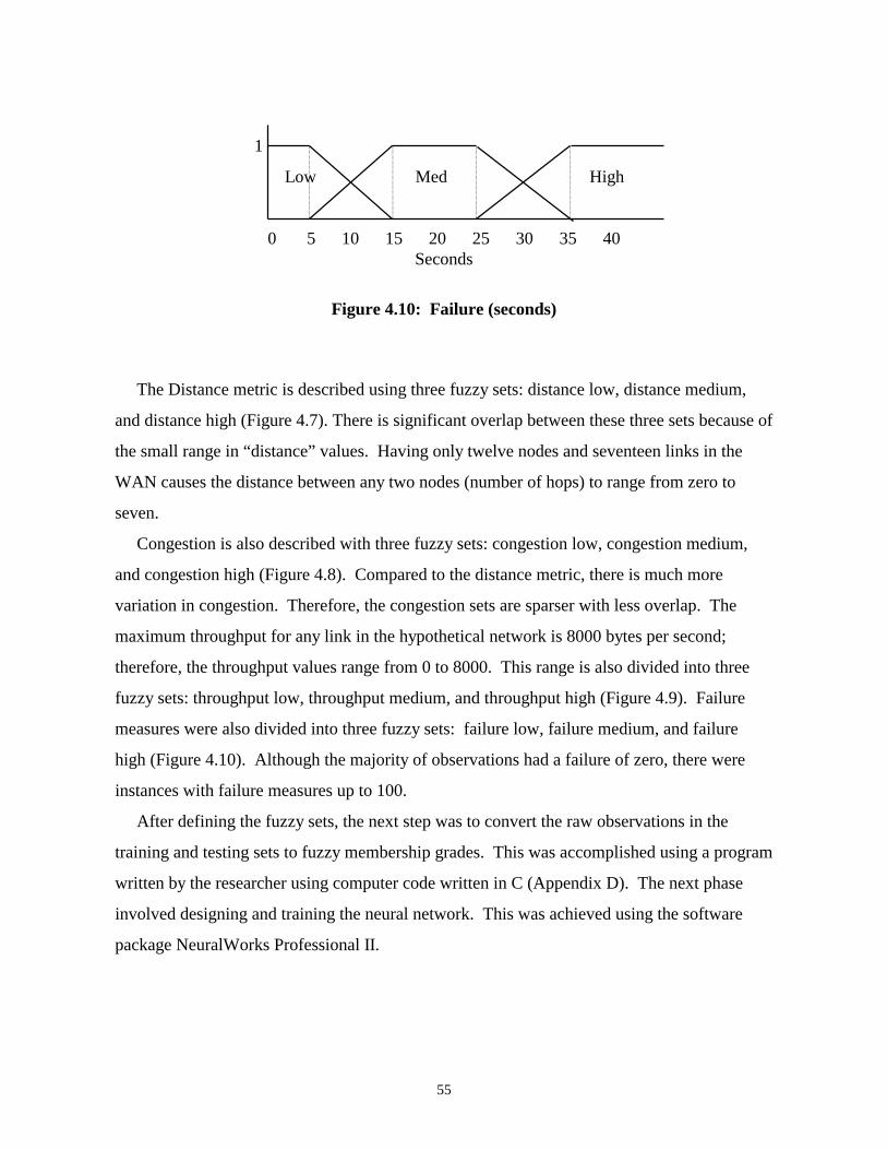
55
1
Low Med High
0 5 10 15 20 25 30 35 40Seconds
Figure 4.10: Failure (seconds)
The Distance metric is described using three fuzzy sets: distance low, distance medium,
and distance high (Figure 4.7). There is significant overlap between these three sets because of
the small range in “distance” values. Having only twelve nodes and seventeen links in the
WAN causes the distance between any two nodes (number of hops) to range from zero to
seven.
Congestion is also described with three fuzzy sets: congestion low, congestion medium,
and congestion high (Figure 4.8). Compared to the distance metric, there is much more
variation in congestion. Therefore, the congestion sets are sparser with less overlap. The
maximum throughput for any link in the hypothetical network is 8000 bytes per second;
therefore, the throughput values range from 0 to 8000. This range is also divided into three
fuzzy sets: throughput low, throughput medium, and throughput high (Figure 4.9). Failure
measures were also divided into three fuzzy sets: failure low, failure medium, and failure
high (Figure 4.10). Although the majority of observations had a failure of zero, there were
instances with failure measures up to 100.
After defining the fuzzy sets, the next step was to convert the raw observations in the
training and testing sets to fuzzy membership grades. This was accomplished using a program
written by the researcher using computer code written in C (Appendix D). The next phase
involved designing and training the neural network. This was achieved using the software
package NeuralWorks Professional II.
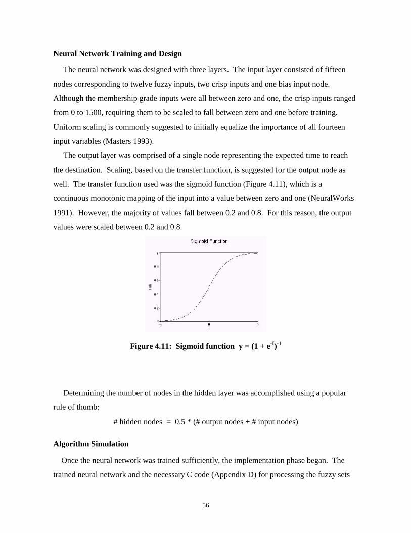
56
Neural Network Training and Design
The neural network was designed with three layers. The input layer consisted of fifteen
nodes corresponding to twelve fuzzy inputs, two crisp inputs and one bias input node.
Although the membership grade inputs were all between zero and one, the crisp inputs ranged
from 0 to 1500, requiring them to be scaled to fall between zero and one before training.
Uniform scaling is commonly suggested to initially equalize the importance of all fourteen
input variables (Masters 1993).
The output layer was comprised of a single node representing the expected time to reach
the destination. Scaling, based on the transfer function, is suggested for the output node as
well. The transfer function used was the sigmoid function (Figure 4.11), which is a
continuous monotonic mapping of the input into a value between zero and one (NeuralWorks
1991). However, the majority of values fall between 0.2 and 0.8. For this reason, the output
values were scaled between 0.2 and 0.8.
Figure 4.11: Sigmoid function y = (1 + e-I)-1
Determining the number of nodes in the hidden layer was accomplished using a popular
rule of thumb:
# hidden nodes = 0.5 * (# output nodes + # input nodes)
Algorithm Simulation
Once the neural network was trained sufficiently, the implementation phase began. The
trained neural network and the necessary C code (Appendix D) for processing the fuzzy sets
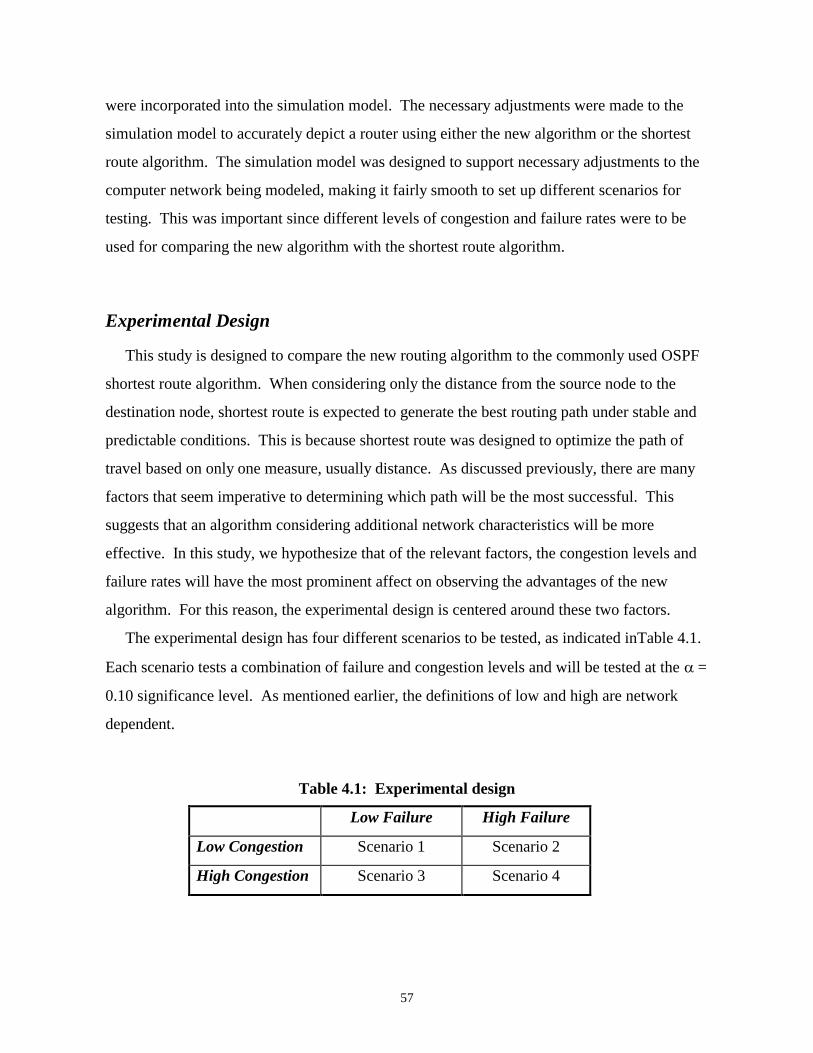
57
were incorporated into the simulation model. The necessary adjustments were made to the
simulation model to accurately depict a router using either the new algorithm or the shortest
route algorithm. The simulation model was designed to support necessary adjustments to the
computer network being modeled, making it fairly smooth to set up different scenarios for
testing. This was important since different levels of congestion and failure rates were to be
used for comparing the new algorithm with the shortest route algorithm.
Experimental Design
This study is designed to compare the new routing algorithm to the commonly used OSPF
shortest route algorithm. When considering only the distance from the source node to the
destination node, shortest route is expected to generate the best routing path under stable and
predictable conditions. This is because shortest route was designed to optimize the path of
travel based on only one measure, usually distance. As discussed previously, there are many
factors that seem imperative to determining which path will be the most successful. This
suggests that an algorithm considering additional network characteristics will be more
effective. In this study, we hypothesize that of the relevant factors, the congestion levels and
failure rates will have the most prominent affect on observing the advantages of the new
algorithm. For this reason, the experimental design is centered around these two factors.
The experimental design has four different scenarios to be tested, as indicated inTable 4.1.
Each scenario tests a combination of failure and congestion levels and will be tested at the � =
0.10 significance level. As mentioned earlier, the definitions of low and high are network
dependent.
Table 4.1: Experimental design
Low Failure High Failure
Low Congestion Scenario 1 Scenario 2
High Congestion Scenario 3 Scenario 4
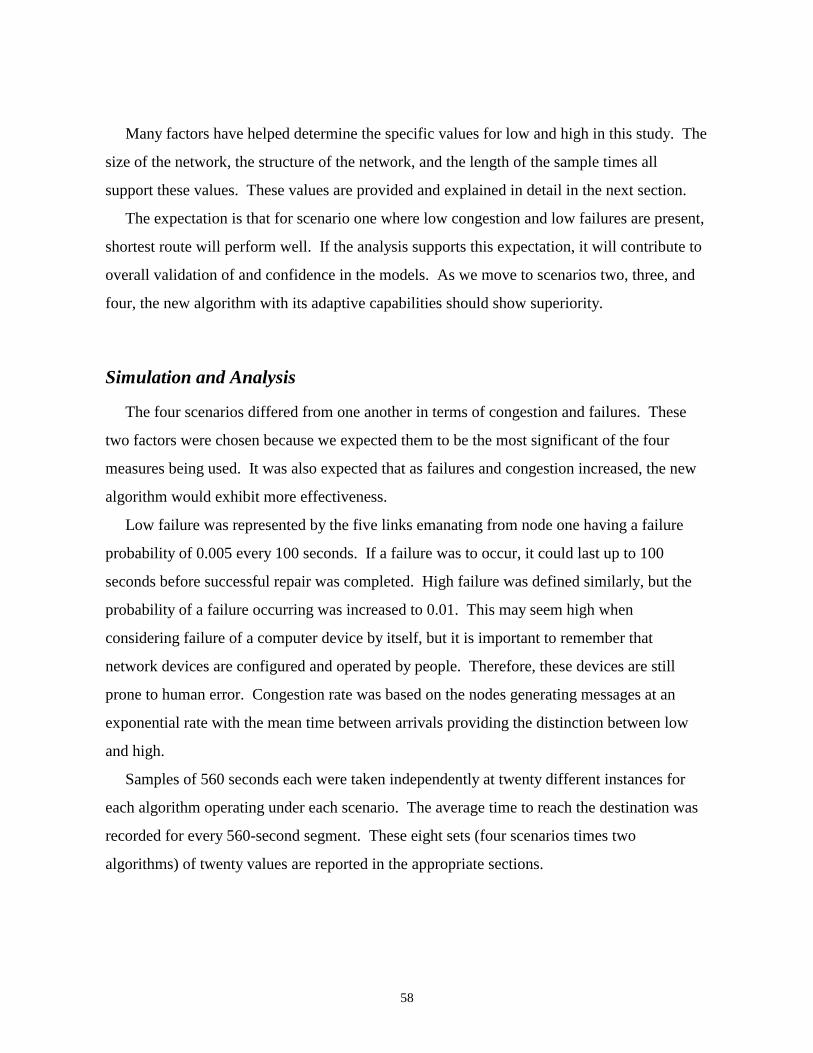
58
Many factors have helped determine the specific values for low and high in this study. The
size of the network, the structure of the network, and the length of the sample times all
support these values. These values are provided and explained in detail in the next section.
The expectation is that for scenario one where low congestion and low failures are present,
shortest route will perform well. If the analysis supports this expectation, it will contribute to
overall validation of and confidence in the models. As we move to scenarios two, three, and
four, the new algorithm with its adaptive capabilities should show superiority.
Simulation and Analysis
The four scenarios differed from one another in terms of congestion and failures. These
two factors were chosen because we expected them to be the most significant of the four
measures being used. It was also expected that as failures and congestion increased, the new
algorithm would exhibit more effectiveness.
Low failure was represented by the five links emanating from node one having a failure
probability of 0.005 every 100 seconds. If a failure was to occur, it could last up to 100
seconds before successful repair was completed. High failure was defined similarly, but the
probability of a failure occurring was increased to 0.01. This may seem high when
considering failure of a computer device by itself, but it is important to remember that
network devices are configured and operated by people. Therefore, these devices are still
prone to human error. Congestion rate was based on the nodes generating messages at an
exponential rate with the mean time between arrivals providing the distinction between low
and high.
Samples of 560 seconds each were taken independently at twenty different instances for
each algorithm operating under each scenario. The average time to reach the destination was
recorded for every 560-second segment. These eight sets (four scenarios times two
algorithms) of twenty values are reported in the appropriate sections.
59
Scenario One
The first scenario was designed to be the most stable configuration having low congestion
as well as low failure. This scenario depicts the most steady of the three; therefore, it is
expected that the new algorithm will have no significant advantages over shortest route in this
initial scenario. The mean transit times collected for each algorithm under this arrangement
are listed in Table 4.2.
Table 4.2: Average transmission times in scenario one
Run ShortRt(Xi)
New(Yi)
Difference(Zi)
1 1.96803 1.47507 0.4929632 2.92071 2.92071 0.0000003 2.17437 2.06283 0.1115484 4.94895 5.16149 -0.2125415 1.70533 1.18618 0.5191486 2.68648 2.63175 0.0547347 2.98919 2.98919 0.0000008 3.26343 3.26343 0.0000009 5.45248 5.45248 0.00000010 1.28048 1.26822 0.01225811 5.14172 5.19462 -0.05289212 2.83256 3.15188 -0.31932613 1.58977 1.44055 0.14922214 2.43743 2.43743 0.00000015 2.73254 2.73254 0.00000016 1.42578 1.42578 0.00000017 4.75493 4.86279 -0.10785118 2.10527 2.25102 -0.14575319 2.83925 3.15180 -0.31254320 2.11343 2.18450 -0.071072
Average 2.86811 2.86221 0.005895
The sampling process was conducted such that both sets of runs utilized an identical
ordering of message creation; therefore, the forty means collected are actually twenty pairs.
This suggests the presence of paired differences. There are two sets of statistical tests that can

60
be used for paired data; parametric and nonparametric. However, before any statistical testing
could begin the normality of the data needed to be established to determine which tests would
be most appropriate.

61
The graphs of Figure 4.12 and Figure 4.13 illustrate the lack of normality in the difference
data. The frequency histogram illustrates the skewed nature of the data and contradicts a
normal distribution. The normal probability plot was generated using Minitab (Release 9.2).
The horizontal axis displays a scale of the actual data while the vertical axis displays a
probability scale. The least-squares line on the graph was calculated to fit the points and
estimates the cumulative distribution function for the population of the difference data. Upon
viewing the frequency histogram, the observations appear to exhibit a skewed distribution.
This suggests that the data is not symmetric and therefore, not normal.
The Anderson-Darling test for normality was performed by Minitab as a default test of the
following hypothesis:
H0: the Difference data comes from a normally distributed population.
Ha: the Difference data does not comes from a normally distributed population.
The test resulted in a significant p-value that was less than 0.003 and strongly supports the
rejection of the null hypothesis.
The hypothesis test, normal probability plot, and frequency histogram all suggest that
nonparametric procedures would be most appropriate for testing significance of the difference
data. The appropriate nonparametric tests are the sign test and the Wilcoxon signed rank test.
These tests consider the population medians instead of their means.
0.50.30.1-0.1-0.3
10
5
0
Diff
Fre
quen
cy
Figure 4.12: Distribution of difference values
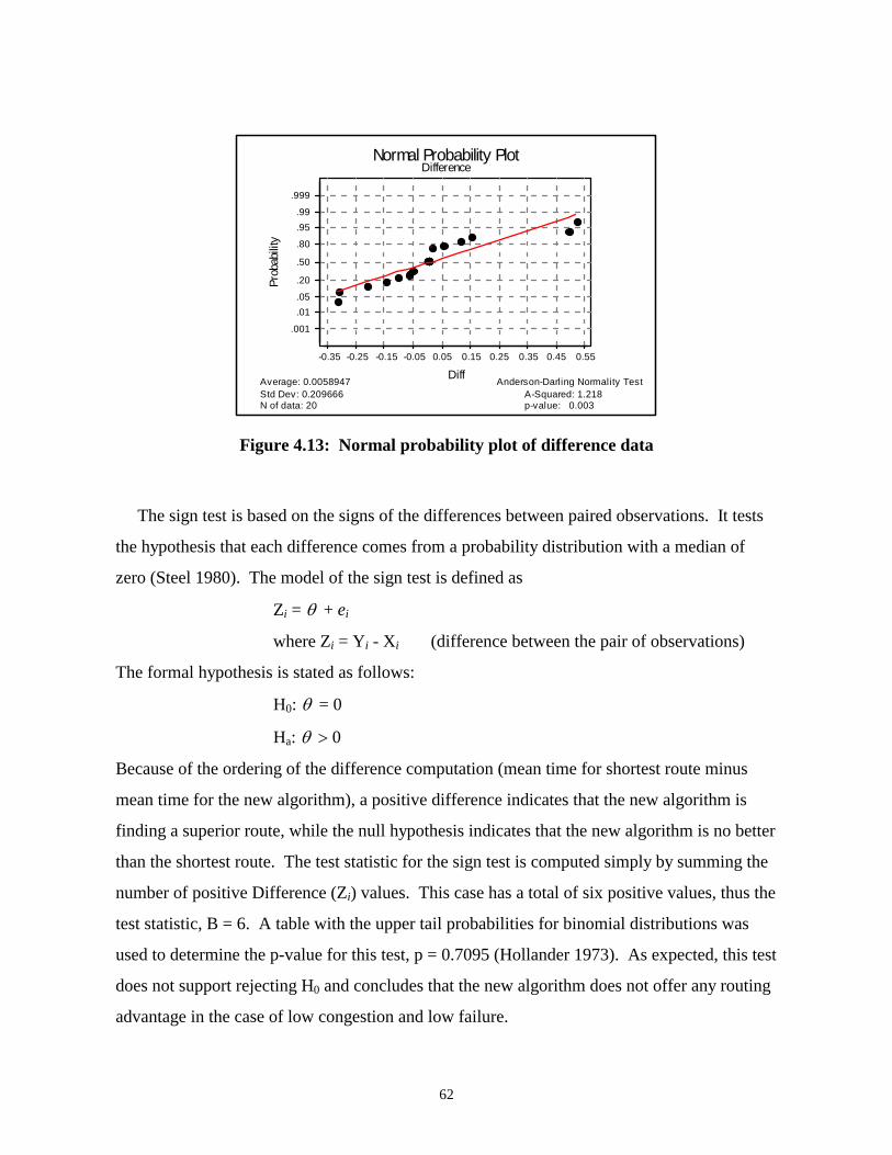
62
p-value: 0.003A-Squared: 1.218
Anderson-Darling Normality Test
N of data: 20Std Dev: 0.209666Average: 0.0058947
0.550.450.350.250.150.05-0.05-0.15-0.25-0.35
.999
.99
.95
.80
.50
.20
.05
.01
.001
Pro
babi
lity
Diff
Normal Probability PlotDifference
Figure 4.13: Normal probability plot of difference data
The sign test is based on the signs of the differences between paired observations. It tests
the hypothesis that each difference comes from a probability distribution with a median of
zero (Steel 1980). The model of the sign test is defined as
Zi = � + ei
where Zi = Yi - Xi (difference between the pair of observations)
The formal hypothesis is stated as follows:
H0: � = 0
Ha: � � 0
Because of the ordering of the difference computation (mean time for shortest route minus
mean time for the new algorithm), a positive difference indicates that the new algorithm is
finding a superior route, while the null hypothesis indicates that the new algorithm is no better
than the shortest route. The test statistic for the sign test is computed simply by summing the
number of positive Difference (Zi) values. This case has a total of six positive values, thus the
test statistic, B = 6. A table with the upper tail probabilities for binomial distributions was
used to determine the p-value for this test, p = 0.7095 (Hollander 1973). As expected, this test
does not support rejecting H0 and concludes that the new algorithm does not offer any routing
advantage in the case of low congestion and low failure.
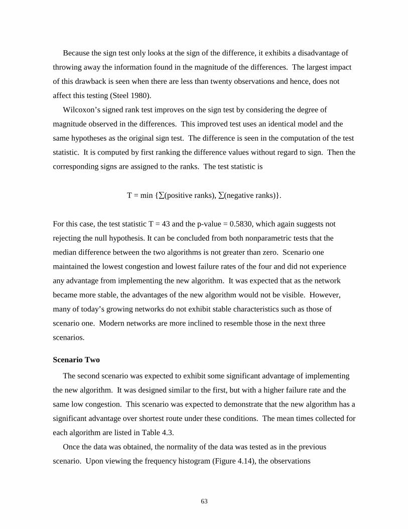
63
Because the sign test only looks at the sign of the difference, it exhibits a disadvantage of
throwing away the information found in the magnitude of the differences. The largest impact
of this drawback is seen when there are less than twenty observations and hence, does not
affect this testing (Steel 1980).
Wilcoxon’s signed rank test improves on the sign test by considering the degree of
magnitude observed in the differences. This improved test uses an identical model and the
same hypotheses as the original sign test. The difference is seen in the computation of the test
statistic. It is computed by first ranking the difference values without regard to sign. Then the
corresponding signs are assigned to the ranks. The test statistic is
T = min {�(positive ranks), �(negative ranks)}.
For this case, the test statistic T = 43 and the p-value = 0.5830, which again suggests not
rejecting the null hypothesis. It can be concluded from both nonparametric tests that the
median difference between the two algorithms is not greater than zero. Scenario one
maintained the lowest congestion and lowest failure rates of the four and did not experience
any advantage from implementing the new algorithm. It was expected that as the network
became more stable, the advantages of the new algorithm would not be visible. However,
many of today’s growing networks do not exhibit stable characteristics such as those of
scenario one. Modern networks are more inclined to resemble those in the next three
scenarios.
Scenario Two
The second scenario was expected to exhibit some significant advantage of implementing
the new algorithm. It was designed similar to the first, but with a higher failure rate and the
same low congestion. This scenario was expected to demonstrate that the new algorithm has a
significant advantage over shortest route under these conditions. The mean times collected for
each algorithm are listed in Table 4.3.
Once the data was obtained, the normality of the data was tested as in the previous
scenario. Upon viewing the frequency histogram (Figure 4.14), the observations
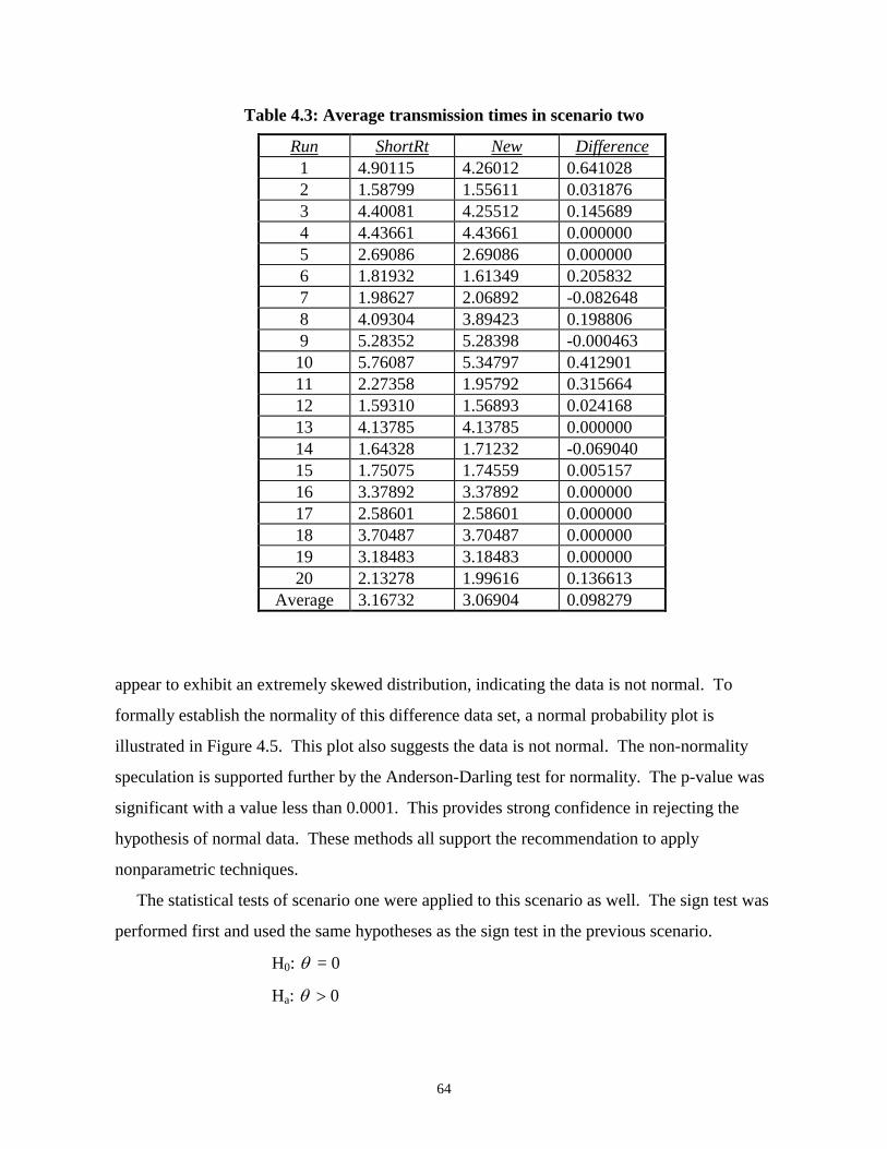
64
Table 4.3: Average transmission times in scenario two
Run ShortRt New Difference1 4.90115 4.26012 0.6410282 1.58799 1.55611 0.0318763 4.40081 4.25512 0.1456894 4.43661 4.43661 0.0000005 2.69086 2.69086 0.0000006 1.81932 1.61349 0.2058327 1.98627 2.06892 -0.0826488 4.09304 3.89423 0.1988069 5.28352 5.28398 -0.00046310 5.76087 5.34797 0.41290111 2.27358 1.95792 0.31566412 1.59310 1.56893 0.02416813 4.13785 4.13785 0.00000014 1.64328 1.71232 -0.06904015 1.75075 1.74559 0.00515716 3.37892 3.37892 0.00000017 2.58601 2.58601 0.00000018 3.70487 3.70487 0.00000019 3.18483 3.18483 0.00000020 2.13278 1.99616 0.136613
Average 3.16732 3.06904 0.098279
appear to exhibit an extremely skewed distribution, indicating the data is not normal. To
formally establish the normality of this difference data set, a normal probability plot is
illustrated in Figure 4.5. This plot also suggests the data is not normal. The non-normality
speculation is supported further by the Anderson-Darling test for normality. The p-value was
significant with a value less than 0.0001. This provides strong confidence in rejecting the
hypothesis of normal data. These methods all support the recommendation to apply
nonparametric techniques.
The statistical tests of scenario one were applied to this scenario as well. The sign test was
performed first and used the same hypotheses as the sign test in the previous scenario.
H0: � = 0
Ha: � � 0
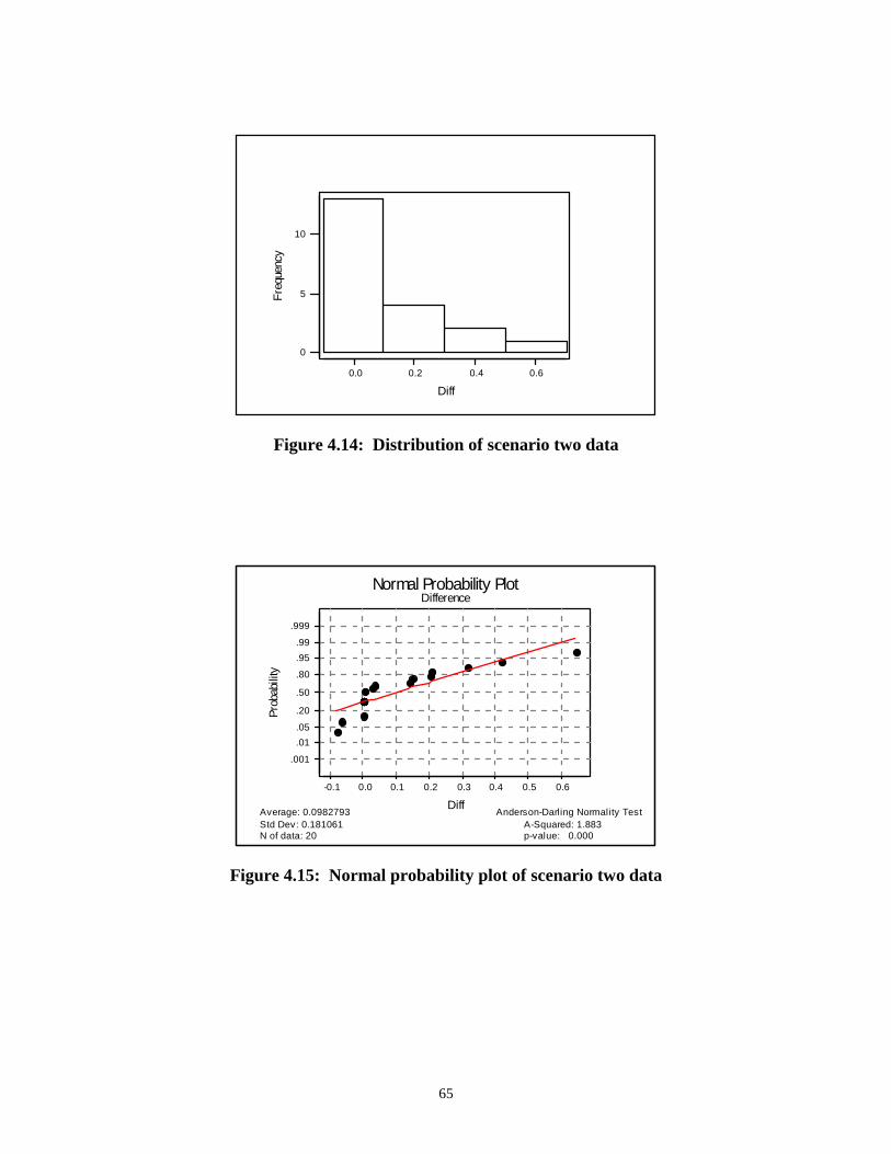
65
0.60.40.20.0
10
5
0
Diff
Fre
quen
cy
Figure 4.14: Distribution of scenario two data
p-value: 0.000A-Squared: 1.883
Anderson-Darling Normality Test
N of data: 20Std Dev: 0.181061Average: 0.0982793
0.60.50.40.30.20.10.0-0.1
.999
.99
.95
.80
.50
.20
.05
.01
.001
Pro
babi
lity
Diff
Normal Probability PlotDifference
Figure 4.15: Normal probability plot of scenario two data
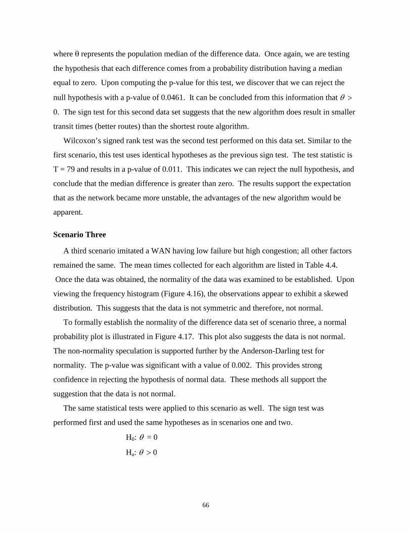
66
where � represents the population median of the difference data. Once again, we are testing
the hypothesis that each difference comes from a probability distribution having a median
equal to zero. Upon computing the p-value for this test, we discover that we can reject the
null hypothesis with a p-value of 0.0461. It can be concluded from this information that � �
0. The sign test for this second data set suggests that the new algorithm does result in smaller
transit times (better routes) than the shortest route algorithm.
Wilcoxon’s signed rank test was the second test performed on this data set. Similar to the
first scenario, this test uses identical hypotheses as the previous sign test. The test statistic is
T = 79 and results in a p-value of 0.011. This indicates we can reject the null hypothesis, and
conclude that the median difference is greater than zero. The results support the expectation
that as the network became more unstable, the advantages of the new algorithm would be
apparent.
Scenario Three
A third scenario imitated a WAN having low failure but high congestion; all other factors
remained the same. The mean times collected for each algorithm are listed in Table 4.4.
Once the data was obtained, the normality of the data was examined to be established. Upon
viewing the frequency histogram (Figure 4.16), the observations appear to exhibit a skewed
distribution. This suggests that the data is not symmetric and therefore, not normal.
To formally establish the normality of the difference data set of scenario three, a normal
probability plot is illustrated in Figure 4.17. This plot also suggests the data is not normal.
The non-normality speculation is supported further by the Anderson-Darling test for
normality. The p-value was significant with a value of 0.002. This provides strong
confidence in rejecting the hypothesis of normal data. These methods all support the
suggestion that the data is not normal.
The same statistical tests were applied to this scenario as well. The sign test was
performed first and used the same hypotheses as in scenarios one and two.
H0: � = 0
Ha: � � 0
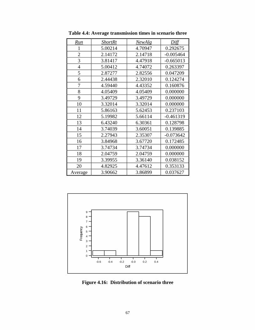
67
Table 4.4: Average transmission times in scenario three
Run ShortRt NewAlg Diff1 5.00214 4.70947 0.2926752 2.14172 2.14718 -0.0054643 3.81417 4.47918 -0.6650134 5.00412 4.74072 0.2633975 2.87277 2.82556 0.0472096 2.44438 2.32010 0.1242747 4.59440 4.43352 0.1608768 4.05409 4.05409 0.0000009 3.49729 3.49729 0.00000010 3.32014 3.32014 0.00000011 5.86163 5.62453 0.23710312 5.19982 5.66114 -0.46131913 6.43240 6.30361 0.12879814 3.74039 3.60051 0.13988515 2.27943 2.35307 -0.07364216 3.84968 3.67720 0.17248517 3.74734 3.74734 0.00000018 2.04759 2.04759 0.00000019 3.39955 3.36140 0.03815220 4.82925 4.47612 0.353133
Average 3.90662 3.86899 0.037627
0.40.2-0.0-0.2-0.4-0.6
9
8
7
6
5
4
3
2
1
0
Diff
Fre
quen
cy
Figure 4.16: Distribution of scenario three

68
p-value: 0.002A-Squared: 1.302
Anderson-Darling Normality Test
N of data: 20Std Dev: 0.238313Average: 0.0376274
0.4-0.1-0.6
.999
.99
.95
.80
.50
.20
.05
.01
.001
Pro
babi
lity
Diff
Normal Probability PlotDifference
Figure 4.17: Normal probability plot for scenario three
where � represents the population median of the difference data. Once again, we are testing
the hypothesis that each difference comes from a probability distribution having a median
equal to zero. Upon computing the p-value for this test, we discover that we can confidently
reject the null hypothesis at a minimum alpha level of 0.0592. Although this is not as strong
as the p-value in scenario two, it is still significant. It can be concluded from this information
that � � 0.
Wilcoxon’s signed rank test was the second test performed on this data set. Similar to the
first scenarios, this test uses identical hypotheses as the previous sign test. The test statistic is
T = 86 and results in a p-value = 0.074. This suggests rejecting the null hypothesis, but at a
much weaker level than the second scenario. At a minimum � level of 0.074, it can be
concluded that the median difference is greater than zero. It was expected that even as failure
remained low, but congestion increased, the advantages of the new algorithm would increase.
Scenario Four
The last scenario depicted the network during a very hectic time period having a high
failure probability and a high congestion rate. The data collected is given in Table 4.5.
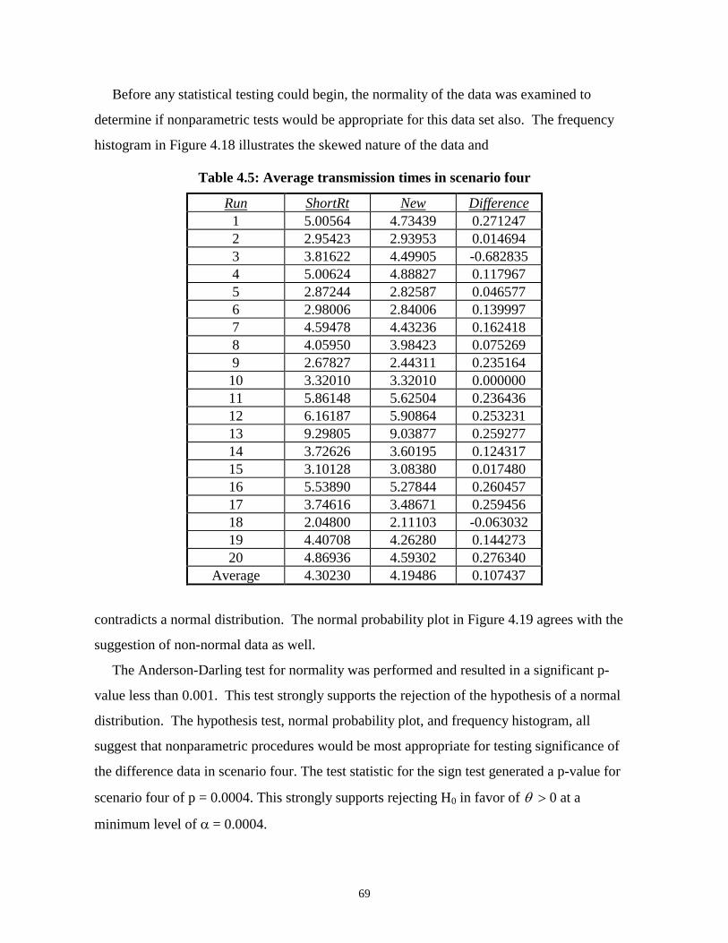
69
Before any statistical testing could begin, the normality of the data was examined to
determine if nonparametric tests would be appropriate for this data set also. The frequency
histogram in Figure 4.18 illustrates the skewed nature of the data and
Table 4.5: Average transmission times in scenario four
Run ShortRt New Difference1 5.00564 4.73439 0.2712472 2.95423 2.93953 0.0146943 3.81622 4.49905 -0.6828354 5.00624 4.88827 0.1179675 2.87244 2.82587 0.0465776 2.98006 2.84006 0.1399977 4.59478 4.43236 0.1624188 4.05950 3.98423 0.0752699 2.67827 2.44311 0.23516410 3.32010 3.32010 0.00000011 5.86148 5.62504 0.23643612 6.16187 5.90864 0.25323113 9.29805 9.03877 0.25927714 3.72626 3.60195 0.12431715 3.10128 3.08380 0.01748016 5.53890 5.27844 0.26045717 3.74616 3.48671 0.25945618 2.04800 2.11103 -0.06303219 4.40708 4.26280 0.14427320 4.86936 4.59302 0.276340
Average 4.30230 4.19486 0.107437
contradicts a normal distribution. The normal probability plot in Figure 4.19 agrees with the
suggestion of non-normal data as well.
The Anderson-Darling test for normality was performed and resulted in a significant p-
value less than 0.001. This test strongly supports the rejection of the hypothesis of a normal
distribution. The hypothesis test, normal probability plot, and frequency histogram, all
suggest that nonparametric procedures would be most appropriate for testing significance of
the difference data in scenario four. The test statistic for the sign test generated a p-value for
scenario four of p = 0.0004. This strongly supports rejecting H0 in favor of � � 0 at a
minimum level of � = 0.0004.
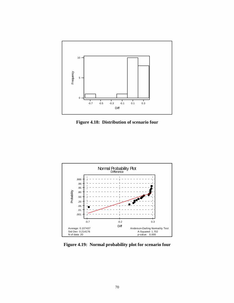
70
0.30.1-0.1-0.3-0.5-0.7
10
5
0
Diff
Fre
quen
cy
Figure 4.18: Distribution of scenario four
p-value: 0.000A-Squared: 1.702
Anderson-Darling Normality Test
N of data: 20Std Dev: 0.214176Average: 0.107437
0.3-0.2-0.7
.999
.99
.95
.80
.50
.20
.05
.01
.001
Pro
babi
lity
Diff
Normal Probability PlotDifference
Figure 4.19: Normal probability plot for scenario four
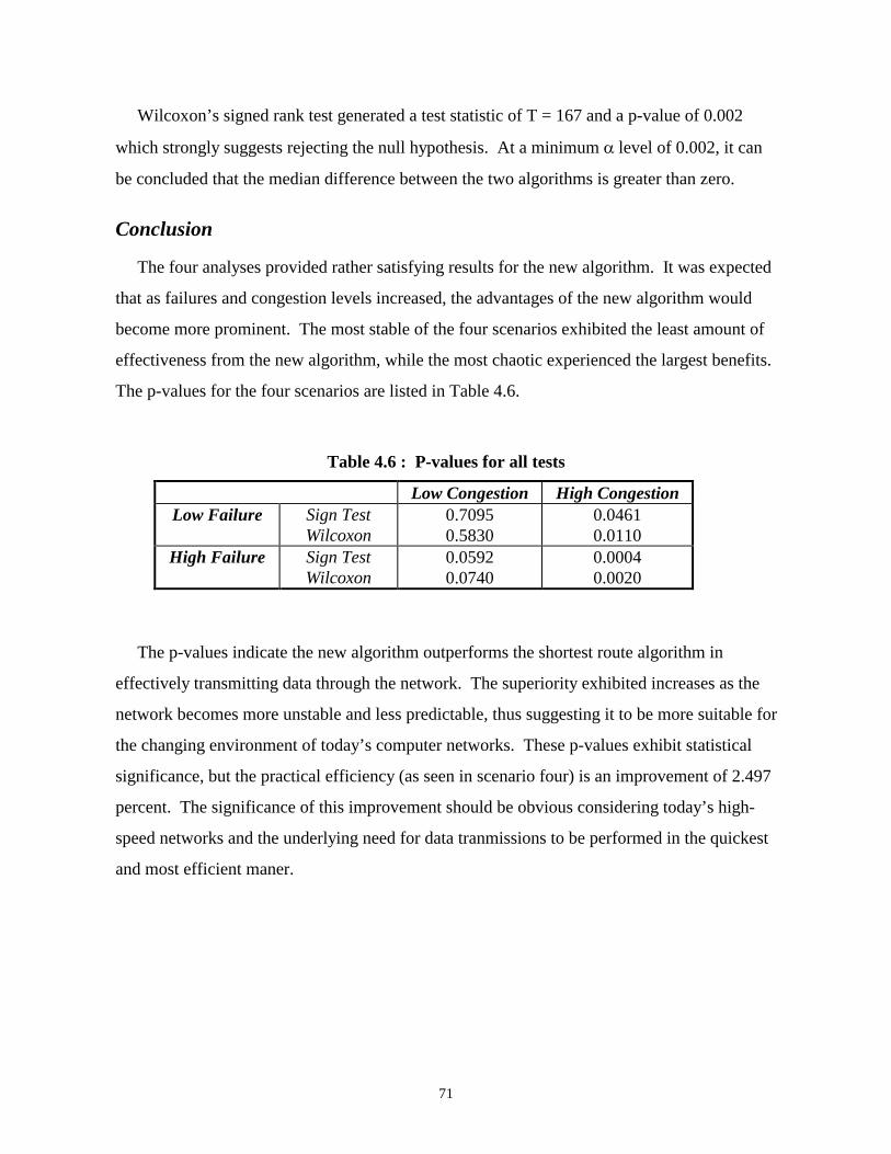
71
Wilcoxon’s signed rank test generated a test statistic of T = 167 and a p-value of 0.002
which strongly suggests rejecting the null hypothesis. At a minimum � level of 0.002, it can
be concluded that the median difference between the two algorithms is greater than zero.
Conclusion
The four analyses provided rather satisfying results for the new algorithm. It was expected
that as failures and congestion levels increased, the advantages of the new algorithm would
become more prominent. The most stable of the four scenarios exhibited the least amount of
effectiveness from the new algorithm, while the most chaotic experienced the largest benefits.
The p-values for the four scenarios are listed in Table 4.6.
Table 4.6 : P-values for all tests
Low Congestion High CongestionLow Failure Sign Test
Wilcoxon0.70950.5830
0.04610.0110
High Failure Sign TestWilcoxon
0.05920.0740
0.00040.0020
The p-values indicate the new algorithm outperforms the shortest route algorithm in
effectively transmitting data through the network. The superiority exhibited increases as the
network becomes more unstable and less predictable, thus suggesting it to be more suitable for
the changing environment of today’s computer networks. These p-values exhibit statistical
significance, but the practical efficiency (as seen in scenario four) is an improvement of 2.497
percent. The significance of this improvement should be obvious considering today’s high-
speed networks and the underlying need for data tranmissions to be performed in the quickest
and most efficient maner.
72
Chapter 5 : Conclusions
Summary
Computer networks are becoming more abundant in today’s business environments as they
play a central role in maintaining and transmitting information. Many organizations have
realized that ease of access to information is a critical need that can also build a competitive
advantage if it is easily accessible. Networks play a central role in this concept for many
reasons, with the most important being that they can help geographically dispersed
organizations overcome the geographic obstacle.
The growing usage of computer networks is requiring improvements in network
technologies and management techniques so that users will still be provided with high quality
service. A major aspect of computer networks that is vital to quality of service is data routing.
As more individuals transmit data through a computer network, the quality of service received
by the users begins to degrade. This indicates that more effective and adaptive measures must
be developed for routing data through computer networks. The essence of this dissertation
was based on developing an improved method for data routing.
The primary tool applied in the routing method of this research was fuzzy reasoning. This
was argued to be an appropriate technique for routing due to the imprecise measures currently
used in present routing algorithms. Many of today’s algorithms use various network
measures, known as metrics, to establish the best path through a computer network. Few
people have yet to recognize the nontrivial inaccuracies present in the measures. Increasing
complexities and growth of computer networks is accelerating the significance of this notion.
To combat these inaccurate metrics, fuzzy reasoning was applied as the basis of the new
algorithm presented in this dissertation.
A secondary technique utilized was a neural network. The neural network was deemed
suitable because it has the ability to learn. Once the neural network is designed, any
alterations in the computer routing environment can easily be learned by this adaptive
artificial intelligence method. The capability to learn and adapt is essential in today’s rapidly
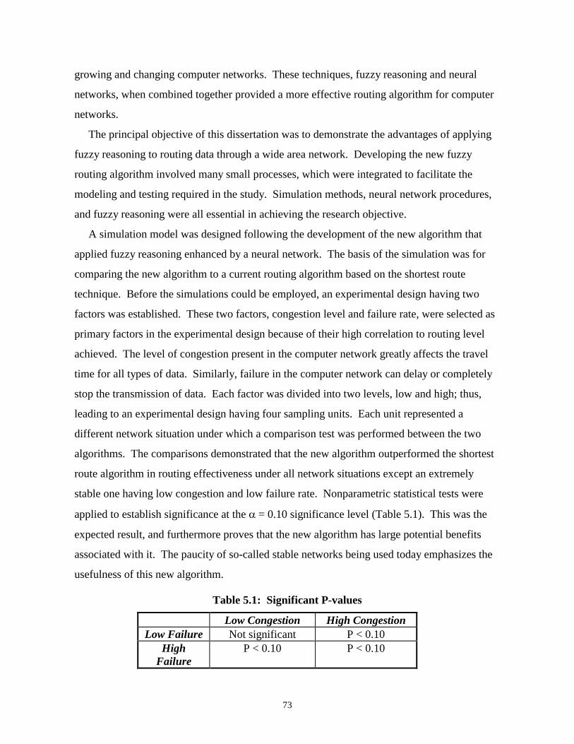
73
growing and changing computer networks. These techniques, fuzzy reasoning and neural
networks, when combined together provided a more effective routing algorithm for computer
networks.
The principal objective of this dissertation was to demonstrate the advantages of applying
fuzzy reasoning to routing data through a wide area network. Developing the new fuzzy
routing algorithm involved many small processes, which were integrated to facilitate the
modeling and testing required in the study. Simulation methods, neural network procedures,
and fuzzy reasoning were all essential in achieving the research objective.
A simulation model was designed following the development of the new algorithm that
applied fuzzy reasoning enhanced by a neural network. The basis of the simulation was for
comparing the new algorithm to a current routing algorithm based on the shortest route
technique. Before the simulations could be employed, an experimental design having two
factors was established. These two factors, congestion level and failure rate, were selected as
primary factors in the experimental design because of their high correlation to routing level
achieved. The level of congestion present in the computer network greatly affects the travel
time for all types of data. Similarly, failure in the computer network can delay or completely
stop the transmission of data. Each factor was divided into two levels, low and high; thus,
leading to an experimental design having four sampling units. Each unit represented a
different network situation under which a comparison test was performed between the two
algorithms. The comparisons demonstrated that the new algorithm outperformed the shortest
route algorithm in routing effectiveness under all network situations except an extremely
stable one having low congestion and low failure rate. Nonparametric statistical tests were
applied to establish significance at the � = 0.10 significance level (Table 5.1). This was the
expected result, and furthermore proves that the new algorithm has large potential benefits
associated with it. The paucity of so-called stable networks being used today emphasizes the
usefulness of this new algorithm.
Table 5.1: Significant P-values
Low Congestion High CongestionLow Failure Not significant P < 0.10
HighFailure
P < 0.10 P < 0.10
74
An additional advantage of the new algorithm that was discussed but not simulated is the
neural network’s ability to learn. The simulation provided data to train a neural network that
was trained only once. If implemented in an actual computer network, the algorithm would
likely perform even better due to its learning capability. This is because the neural network
would understand how to manage various modifications in the network as it grows. This is a
notable feature as computer networks are not designed to be static systems, but instead are
dynamic systems that are constantly changing.
The conclusions of this research are obviously limited to some extent in that a specific
network structure and certain metrics were employed. However, we believe this network
exhibits general characteristics that help intuitively conclude that our results can be
generalized over most wide area networks. Utilizing fuzzy sets and a neural network that are
defined relative to the specific computer network assists in generalizing with these results. A
computer network having altered characteristics would employ fuzzy sets with different
domain ranges and a different neural network. Future research involving other network
configurations and metrics will also help support these generalizations.
Future Research
The positive results encountered in this dissertation suggest that additional experiments
may provide further insight into the benefits of fuzzy routing. This dissertation research
studied the benefits of a single network node applying the new fuzzy routing algorithm while
all other nodes applied a standard routing algorithm. Future research could employ the new
algorithm at all network nodes and possibly demonstrate additional improvements to the
routing process.
Another modification that could prove beneficial lies with combining the two routing
algorithms that were employed in this study. It was discovered that the new algorithm did not
exhibit any advantages during network situations having low failures and low congestion.
This suggests that a hybrid routing scheme might improve routing efficiency. The hybrid
routing algorithm would conditionally utilize the fuzzy routing scheme during chaotic
instances and the shortest path scheme during more stable periods.
75
As advancements continue in the technical realm of computers and computer networks, the
popularity of these systems will continue to increase. This will cause more people to crowd
onto the already crowded networks. Although computer networks are becoming more
automated, there is still some human interaction and control that will be needed. For this
reason, additional research will be needed in the field of managing computer networks.
Fuzzy reasoning might also lend itself to further research, primarily due to the past
reluctance of researchers in the United States to apply this artificial intelligence technique and
the resulting scarcity of published research in the area. This research, as well as other recent
articles, has assisted in developing a more stable foundation of the technique in this country.
The hesitation by so many researchers in the past to explore fuzzy techniques has caused the
application area of fuzzy reasoning to remain an extremely open area of research.
Performance management is another network management area that is conducive to the
application of fuzzy reasoning. The performance of a network (response time, amount of
traffic, throughput, etc.) is not simply acceptable or unacceptable, but instead has a fuzzy
region where the performance begins to decline into unacceptability. Future research in this
area would require a methodology for determining a network’s performance level based upon
a set of fuzzy criteria (Brande 1996). This would provide the network manager a more
accurate description of the network when monitoring its performance.
In summary, an in-depth review of research in the network management area suggests there
has yet to be any substantial application of fuzzy reasoning toward any form of network
management. However, the abundance of imperfect information involved in managing a
computer network indicates this as a natural area for fuzzy reasoning. The novelty of
combining these two areas together has yet to be realized by many people; however, as was
established in this dissertation, the combination can be an extremely effective one.
76
References
Ani, C. I. and F. Halsall, “Simulation Technique for Evaluating Cell-Loss Rate in ATMNetworks,” Simulation, May (1995), 320-329.
Arnold, W., H. Hellendoorn, R. Seiseng, C. Thomas and A. Weitzel, “Fuzzy Routing,” FuzzySets and Systems, 85, (1997), 131-153.
Benes, V. E., “Programming and Control Problems Arising from Optimal Routing inTelephone Networks,” Bell Syst. Tech. J., 45, 9, Nov (1966), 1373-1438.
Brande, J. K., “Network Performance Management Using Fuzzy Logic”, Proceedings of theSE DSI meeting, (1996), 321-323.
Brande, J. K., “Fuzzy Adaptive Traffic Routing in a Packet Switched WAN”, Proceedings ofthe SE INFORMS Meeting, (1995), 434-436.
Buckley, J. J, and Y. Hayashi, “Fuzzy Neural Networks,” Fuzzy Sets, Neural Networks andSoft Computing, ed. R. R. Yager and L. A. Zadeh, Van Nostrand Reinhold, NY, (1994),233-249.
Caudill, M. and C. Butler, Understanding Neural Networks: Computer Explorations, Volume1: Basic Networks, The MIT Press, Massachusetts, (1994).
Cebulka, K. D., M. J. Muller and C. A. Riley, “Applications of Artificial Intelligence forMeeting Network Management Challenges in the 1990’s,” Proceedings of GLOBECOM,(1989), 501-506.
Ceri, S. and L. Tanca, “Expert Design of Local Area Networks,” IEEE Expert Magazine,October, (1990), 23-33.
Chan, S. C., L. S. U. Hsu and K. F. Loe, “Fuzzy Neural-Logic Networks,” Between Mind andComputer, Fuzzy Science and Engineering, ed. P. Z. Wang and K. F. Loe, World ScientificPub. Co. Pte. Ltd., (1993).
Cikoski, T.R., “Getting Prepared for Rule-based Integrated Network Management,”Telecommunications (America’s Edition), March, (1995), 46-50.
Cisco Systems, Inc., “Routing Procedures,”http://www.cisco.com/warp/public/732/Tech/rtrp_pc.html, (1995).
Comer, D. E., Internetworking with TCP/IP, Volume 1: Principles, Protocols, andArchitecture, Second Edition, Prentice Hall, New Jersey, (1991).
77
Dijkstra, E. “A Note on Two Problems in Connection with Graphs.” NumericalMathematics, October, (1959).
Fahmy, H. and C. Douligeris, “END: An Expert System Designer,” IEEE Network, Nov/Dec(1995), 18-27.
Flikop, Z., “Traffic Management in Packet Switching Networks,” Proceedings of IEEEInternational Conference on Communications, 1, (1993), 25-29.
Hamersma, B. and M. S. Chodos, “Availability and Maintenance Considerations inTelecommunications Network Design and the use of Simulation Tools,” Proceedings of the3D Africon Conference, (1992), 267-270.
Hamilton, J. A., G. R. Ratteree and U. W. Pooch, “A Toolkit for Monitoring the Utilizationand Performance of Computer Networks,” Simulation, 64, 5 (1995) 297-301.
Hardy, J. K., Inside Networks, Prentice Hall, New Jersey, (1995).
Harris, R. J., “Reliable Design of Communication Networks,” Proceedings of the 14th
International Teletraffic Congress, 2 (1994), 1331-1340.
Hashida, O. and K. Kodaira, “Digital Data Switching Network Configurations,” Rev. of Elect.Comm. Labs, 24, 1-2 (1976), 85-96.
Havel, O. and A. Patel, “Design and Implementation of a Composite Performance EvaluationModel for Heterogenous Network Management Applications,” International Journal ofNetwork Management, Jan/Feb (1995), 25-46.
Hiramatsu, A., “ATM Communications Network Control by Neural Network,” Proceedingsof IJCNN, (1989), 251-259.
Hollander, M. and D. A. Wolfe, Nonparametric Statistical Methods, John Wiley and Sons,New York, (1973).
Huang, N., C. Wu and Y. Wu, “Some Routing Problems on Broadband ISDN,” ComputerNetworks and ISDN Systems, 27 (1994), 101-116.
Jensen, J. E., M. A. Eshera and S. C. Barash, “Neural Network Controller For AdaptiveRouting in Survivable Communications Networks,” Proceedings of IJCNN, (1990), 29-36.
Key, P. B. and G. A. Cope, “Distributed Dynamic Routing Schemes,” IEEE CommunicationsMagazine, Oct (1990), 54-64.
78
Khalfet, J. and P Chemouil, “Application of Fuzzy Control to Adaptive Traffic Routing inTelephone Networks,” Information and Decision Technologies, 19 (1994), 339-348.
Kolarov, A. and J. Hui, “Least Cost Routing in Multiple-Service Networks,” Proceedings ofIEEE INFOCOM, 3 (1994), 1482-1489.
Kosko, Bart, Fuzzy Thinking: The New Science of Fuzzy Logic, Hyperion, NY, (1993)
Krasniewski, A., “Fuzzy Automata as Adaptive Algorithms for Telephone Traffic Routing,”Proceedings of the IEEE ICC 1984, May (1984), 61-66.
Krishnan, K. R., “Markov Decision Algorithms for Dynamic Routing,” IEEECommunications Magazine, Oct (1990), 66-69.
Kumar, A., R. M. Pathak, Y. P. Gupta and H. R. Parsael, “A Genetic Algorithm forDistributed System Topology Design,” Computers and Industrial Engineering, 28, 3, July(1995), 659-670.
Lee, W., M. Hluchyj and P. Humblet, “Rule-Based Call-by-Call Source Routing for IntegratedCommunication Networks,” Proceedings of the IEEE INFOCOM (1993), 987-993.
Leinwand, A. and K. Fang, Network Management: A Practical Perspective, Addison-WesleyPublishing Company, Inc., (1993), 77-94.
Lirov, Y., “Fuzzy logic for distributed systems troubleshooting,” Second IEEE InternationalConference on Fuzzy Systems, (1993), 986-991.
Masters, T., Practical Neural Network Recipes in C++, Academic Press Inc, San Diego, CA,(1993), 279-326.
Matsumoto, T., “Neuroutin: A Novel High-Speed Adaptive-Routing Scheme Using a NeuralNetwork as a Communications Network Simulator,” IEEE ICC, (1992), 1568-1572.
Mitra, D., J. B. Seery, “Comparative Evaluations of Randomized and Dynamic RoutingStrategies for Circuit-Switched Networks,” IEEE Transactions on Communications, 39, 1,Jan (1991), 102-116.
Nakata, H., T. Wakahara, T. Kayano and K. Sugita, “Network Integration ConsultationEnvironment (NICE),” NTT Review, 7, 2, March (1995), 82-89.
Nedvidek, M. N. and H. T. Mouftah, “A Network Performance Advisor for ComputerNetworks,” IEEE ICC, (1989), 1443-1447.
NeuralWorks Professional II, Neural Computing, NeuralWare, Inc., 1991.
79
Nikloaidou, D. Lelis, D. Mouzakis and P. Georgiadis, “Distributed System IntelligentDesign,” Proceedings of the 5th International Conference of Database and Expert SystemsApplications (DEXA), (1994), 498-508.
Perlman, R., Interconnections: Bridges and Routers, Addison-Wesley Publishing Company,Massachusetts, (1992).
Pirkul, H. and S. Narasimhan, “Primary and Secondary Route Selection in BackboneComputer Networks,” ORSA Journal on Computing, 6, Winter (1994), 50-60.
Qi, R., “A New Method for Network Routing: A Preliminary Report,” Proceedings of theIEEE Pacific Rim Conference on Communications, Computers and Signal Processing, 2,(1993), 553-556.
Rakes, T. R., Lecture Notes, Foundations of Decision Support Systems I, Virginia Tech,(1994).
Ramadas, K., “Performance Tools: A Case Study,” WESCON 92 Conference Record, (1992),206-210.
Rauch, H.E. and T. Winarske, “Neural Networks for Routing Communication Traffic,” IEEECS Magazine, 8, 2 (1988), 26-31.
Reynolds, P. L., P. W. Sanders and C. T. Stockel, “Uncertainty in TelecommunicationNetwork Design,” Expert Systems, 12, 3, August (1995) 219-229.
Rolston, D. W., Principles of Artificial Intelligence and Expert Systems Development,McGraw-Hill Book Company, New York, (1988).
Stach, J. F., “Expert Systems Find a New Place in Data Networks for Optimal MessageRouting,” in Networking Software, Ungaro, ed., Data Communication Book Series,McGraw Hill, (1987), 75-83.
Stallings, W. Business Data Communications, New York: Macmillan, (1990).
Stallings, W. and R. Van Slyke, Business Data Communications, 2nd ed., Macmillan CollegePublishing Co., New York, (1994).
Stallings, W. Local and Metropolitan Area Networks, 4th ed., Macmillan Publishing Co., NewYork, (1993).
Stallings, W. Local and Metropolitan Area Networks, 5th ed., Prentice Hall, New Jersey,(1997).
Stamper, D. A., Business Data Communications, 4th ed., Benjamin Cummings, (1994).

80
Steel, R. G. D. and J. H. Torrie, Principles and Procedures of Statistics: A BiometricalApproach, 2nd ed., McGraw-Hill, (1980).
Terplan, K., Effective Management of Local Area Networks: Functions, Instruments, andPeople, McGraw Hill Series on Computer Communications, New York, (1992).
Van Norman, H. LAN/WAN Optimization Techniques, Boston: Artech House, (1992).
Wang, C. and P. N. Weissler, “The Use of Artificial Neural Networks for Optimal MessageRouting,” IEEE Network, March/April (1995), 16-24.
Wang, Loe, Between Mind and Computer: Fuzzy Science and Engineering, Advances inFuzzy Systems - Applications and Theory Volume 1, World Scientific, (1993).
Warfield, B. and P. Sember, “Prospects for the Use of SArtificial Intelligence in Real-TimeNetwork Traffic Management,” Computer Networks and ISDN Systems Journal, Dec(1990), 163-169.
Whay C. L., M. G. Hluchyi and P. A. Humblet, “Routing Subject to Quality of ServiceConstraints in Integrated Communication Networks,” IEEE Network, July/August (1995),46-55.
Wickre, P. K., “Frame Relay Traffic Snarls,” Network World, 14, 25, June 23 (1997), 55-56.
Yagyu, T., “Support System to Construct Distributed Communication Networks,”Proceedings of the 1993 International Conference on Fuzzy Systems, 2, (1993), 1004-1008.
Zadeh, L. A., “Fuzzy Sets,” Information and Control, 8, (1965), 338-353.
Znaty, S. and J. Sclavos, “Annotated Bibliography on Network Management,” ComputerCommunication Review, 24, 1, Jan (1994), 37-56.
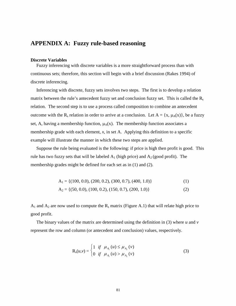
81
APPENDIX A: Fuzzy rule-based reasoning
Discrete Variables Fuzzy inferencing with discrete variables is a more straightforward process than with
continuous sets; therefore, this section will begin with a brief discussion (Rakes 1994) of
discrete inferencing.
Inferencing with discrete, fuzzy sets involves two steps. The first is to develop a relation
matrix between the rule’s antecedent fuzzy set and conclusion fuzzy set. This is called the Rs
relation. The second step is to use a process called composition to combine an antecedent
outcome with the Rs relation in order to arrive at a conclusion. Let A = {x, �A(x)}, be a fuzzy
set, A, having a membership function, �A(x). The membership function associates a
membership grade with each element, x, in set A. Applying this definition to a specific
example will illustrate the manner in which these two steps are applied.
Suppose the rule being evaluated is the following: if price is high then profit is good. This
rule has two fuzzy sets that will be labeled A1 (high price) and A2 (good profit). The
membership grades might be defined for each set as in (1) and (2).
A1 = {(100, 0.0), (200, 0.2), (300, 0.7), (400, 1.0)} (1)
A2 = {(50, 0.0), (100, 0.2), (150, 0.7), (200, 1.0)} (2)
A1 and A2 are now used to compute the Rs matrix (Figure A.1) that will relate high price to
good profit.
The binary values of the matrix are determined using the definition in (3) where u and v
represent the row and column (or antecedent and conclusion) values, respectively.
Rs(u,v) = 1
0
��
if
if � �
� �
A A
A A
u v
u v1 2
1 2
( ) ( )
( ) ( )
�(3)
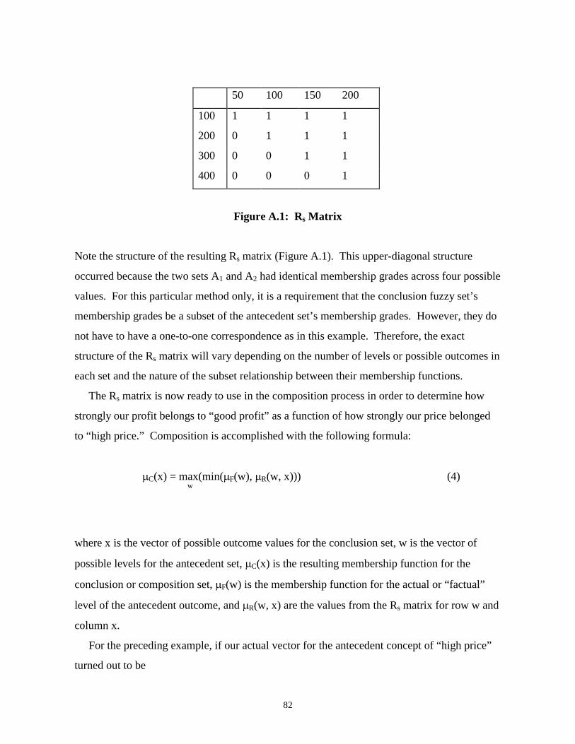
82
50 100 150 200
100 1 1 1 1
200 0 1 1 1
300 0 0 1 1
400 0 0 0 1
Figure A.1: Rs Matrix
Note the structure of the resulting Rs matrix (Figure A.1). This upper-diagonal structure
occurred because the two sets A1 and A2 had identical membership grades across four possible
values. For this particular method only, it is a requirement that the conclusion fuzzy set’s
membership grades be a subset of the antecedent set’s membership grades. However, they do
not have to have a one-to-one correspondence as in this example. Therefore, the exact
structure of the Rs matrix will vary depending on the number of levels or possible outcomes in
each set and the nature of the subset relationship between their membership functions.
The Rs matrix is now ready to use in the composition process in order to determine how
strongly our profit belongs to “good profit” as a function of how strongly our price belonged
to “high price.” Composition is accomplished with the following formula:
�C(x) = max(min(�F(w), �R(w, x))) (4) w
where x is the vector of possible outcome values for the conclusion set, w is the vector of
possible levels for the antecedent set, �C(x) is the resulting membership function for the
conclusion or composition set, �F(w) is the membership function for the actual or “factual”
level of the antecedent outcome, and �R(w, x) are the values from the Rs matrix for row w and
column x.
For the preceding example, if our actual vector for the antecedent concept of “high price”
turned out to be
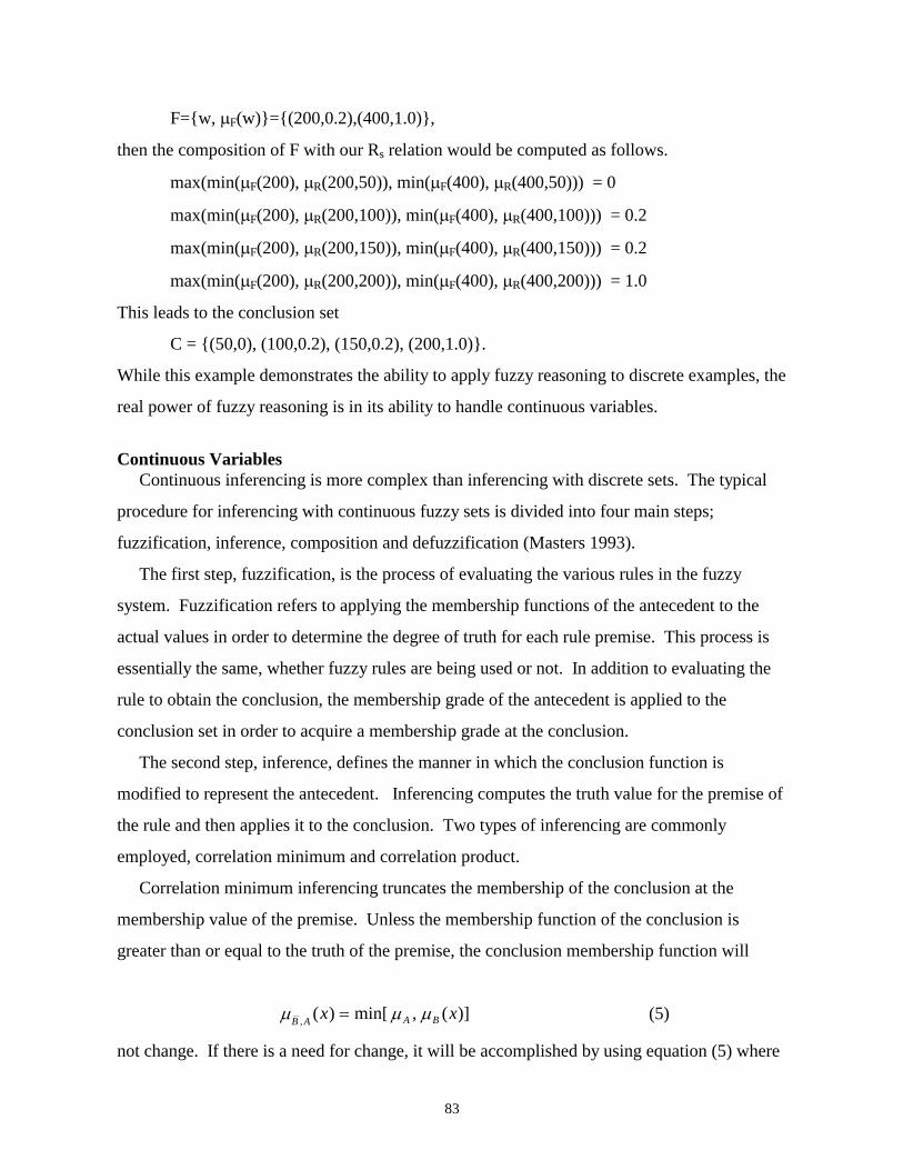
83
F={w, �F(w)}={(200,0.2),(400,1.0)},
then the composition of F with our Rs relation would be computed as follows.
max(min(�F(200), �R(200,50)), min(�F(400), �R(400,50))) = 0
max(min(�F(200), �R(200,100)), min(�F(400), �R(400,100))) = 0.2
max(min(�F(200), �R(200,150)), min(�F(400), �R(400,150))) = 0.2
max(min(�F(200), �R(200,200)), min(�F(400), �R(400,200))) = 1.0
This leads to the conclusion set
C = {(50,0), (100,0.2), (150,0.2), (200,1.0)}.
While this example demonstrates the ability to apply fuzzy reasoning to discrete examples, the
real power of fuzzy reasoning is in its ability to handle continuous variables.
Continuous Variables Continuous inferencing is more complex than inferencing with discrete sets. The typical
procedure for inferencing with continuous fuzzy sets is divided into four main steps;
fuzzification, inference, composition and defuzzification (Masters 1993).
The first step, fuzzification, is the process of evaluating the various rules in the fuzzy
system. Fuzzification refers to applying the membership functions of the antecedent to the
actual values in order to determine the degree of truth for each rule premise. This process is
essentially the same, whether fuzzy rules are being used or not. In addition to evaluating the
rule to obtain the conclusion, the membership grade of the antecedent is applied to the
conclusion set in order to acquire a membership grade at the conclusion.
The second step, inference, defines the manner in which the conclusion function is
modified to represent the antecedent. Inferencing computes the truth value for the premise of
the rule and then applies it to the conclusion. Two types of inferencing are commonly
employed, correlation minimum and correlation product.
Correlation minimum inferencing truncates the membership of the conclusion at the
membership value of the premise. Unless the membership function of the conclusion is
greater than or equal to the truth of the premise, the conclusion membership function will
� � �B A A Bx x, ( ) min[ , ( )]� (5)
not change. If there is a need for change, it will be accomplished by using equation (5) where
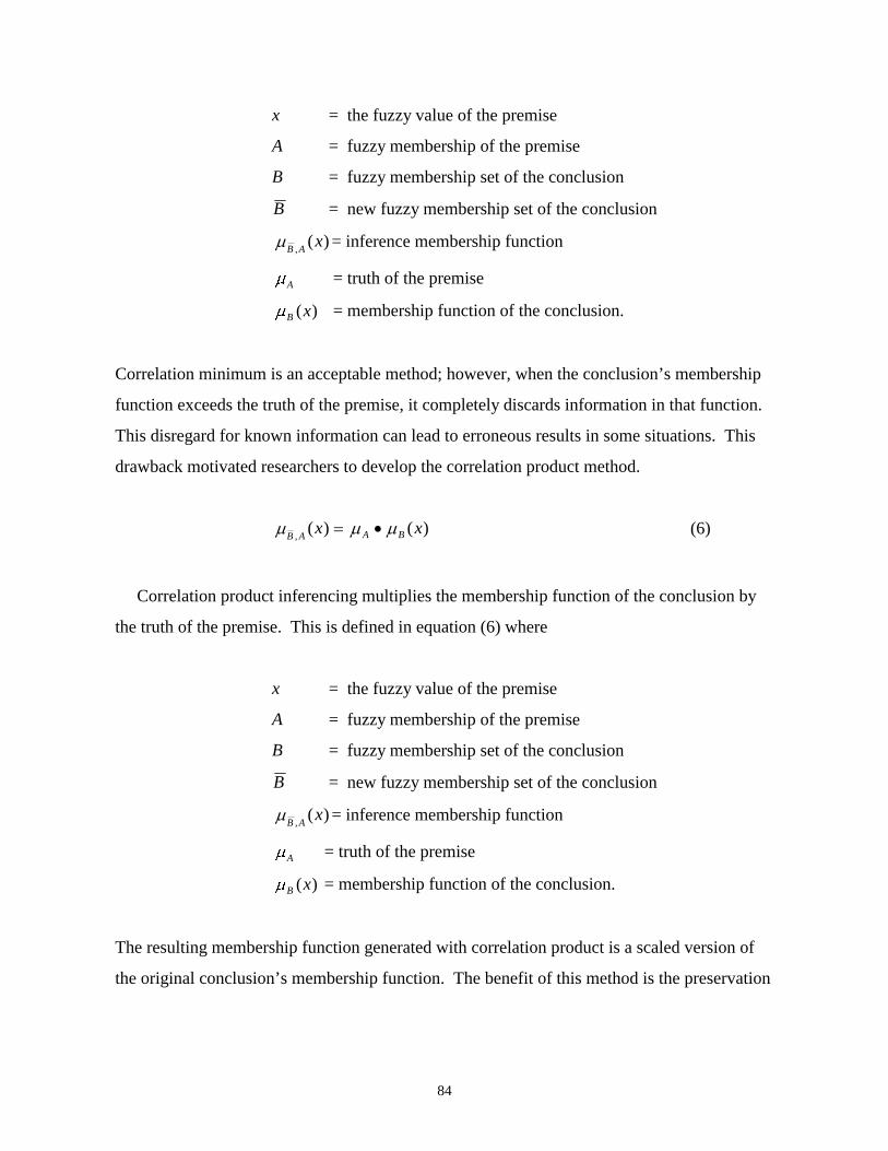
84
x = the fuzzy value of the premise
A = fuzzy membership of the premise
B = fuzzy membership set of the conclusion
B = new fuzzy membership set of the conclusion
�B Ax
,( ) = inference membership function
�A = truth of the premise
�B x( ) = membership function of the conclusion.
Correlation minimum is an acceptable method; however, when the conclusion’s membership
function exceeds the truth of the premise, it completely discards information in that function.
This disregard for known information can lead to erroneous results in some situations. This
drawback motivated researchers to develop the correlation product method.
� � �B A A Bx x,
( ) ( )� � (6)
Correlation product inferencing multiplies the membership function of the conclusion by
the truth of the premise. This is defined in equation (6) where
x = the fuzzy value of the premise
A = fuzzy membership of the premise
B = fuzzy membership set of the conclusion
B = new fuzzy membership set of the conclusion
�B A
x,
( ) = inference membership function
�A = truth of the premise
�B x( ) = membership function of the conclusion.
The resulting membership function generated with correlation product is a scaled version of
the original conclusion’s membership function. The benefit of this method is the preservation
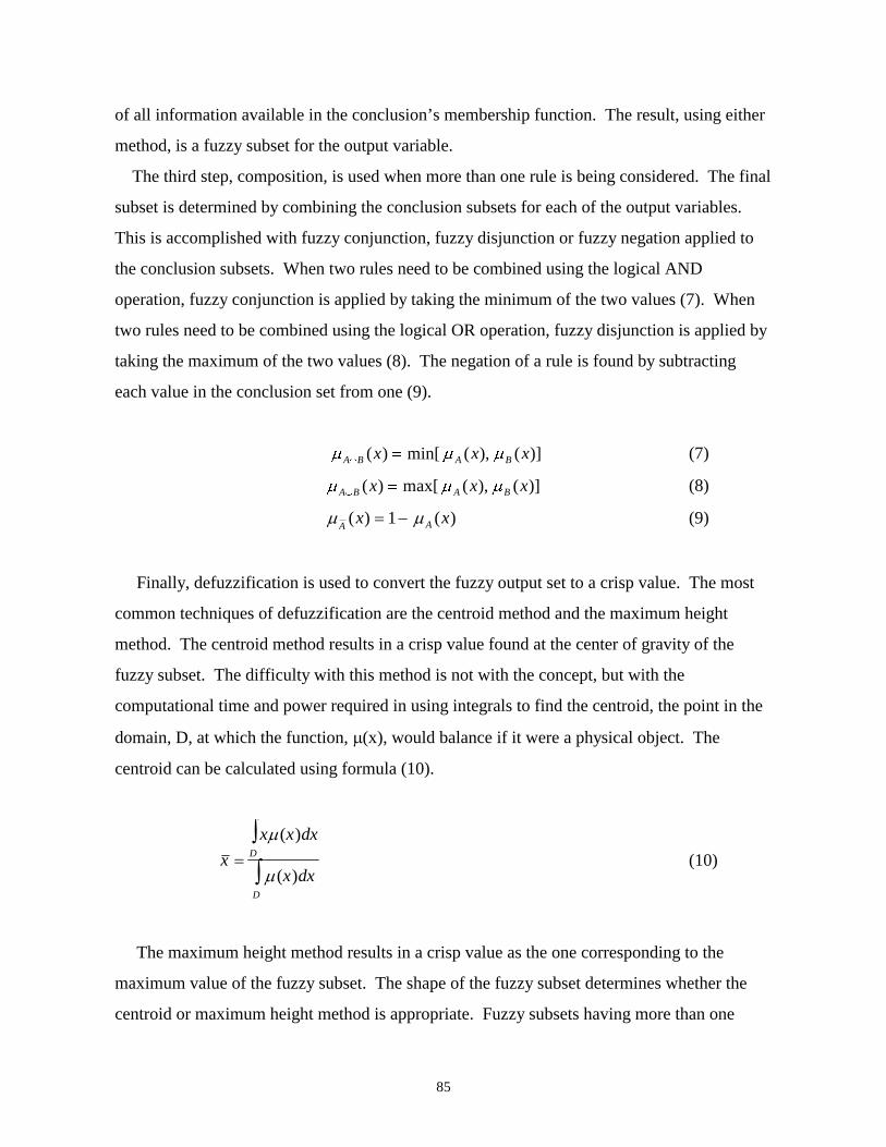
85
of all information available in the conclusion’s membership function. The result, using either
method, is a fuzzy subset for the output variable.
The third step, composition, is used when more than one rule is being considered. The final
subset is determined by combining the conclusion subsets for each of the output variables.
This is accomplished with fuzzy conjunction, fuzzy disjunction or fuzzy negation applied to
the conclusion subsets. When two rules need to be combined using the logical AND
operation, fuzzy conjunction is applied by taking the minimum of the two values (7). When
two rules need to be combined using the logical OR operation, fuzzy disjunction is applied by
taking the maximum of the two values (8). The negation of a rule is found by subtracting
each value in the conclusion set from one (9).
� � �A B A Bx x x�
�( ) min[ ( ), ( )] (7)
� � �A B A Bx x x�
�( ) max[ ( ), ( )] (8)
� �A Ax x( ) ( )� �1 (9)
Finally, defuzzification is used to convert the fuzzy output set to a crisp value. The most
common techniques of defuzzification are the centroid method and the maximum height
method. The centroid method results in a crisp value found at the center of gravity of the
fuzzy subset. The difficulty with this method is not with the concept, but with the
computational time and power required in using integrals to find the centroid, the point in the
domain, D, at which the function, �(x), would balance if it were a physical object. The
centroid can be calculated using formula (10).
x
x x dx
x dx
D
D
�
�
�
( )
( )(10)
The maximum height method results in a crisp value as the one corresponding to the
maximum value of the fuzzy subset. The shape of the fuzzy subset determines whether the
centroid or maximum height method is appropriate. Fuzzy subsets having more than one
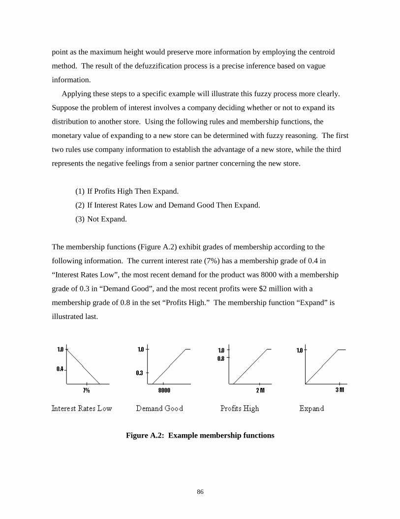
86
point as the maximum height would preserve more information by employing the centroid
method. The result of the defuzzification process is a precise inference based on vague
information.
Applying these steps to a specific example will illustrate this fuzzy process more clearly.
Suppose the problem of interest involves a company deciding whether or not to expand its
distribution to another store. Using the following rules and membership functions, the
monetary value of expanding to a new store can be determined with fuzzy reasoning. The first
two rules use company information to establish the advantage of a new store, while the third
represents the negative feelings from a senior partner concerning the new store.
(1) If Profits High Then Expand.
(2) If Interest Rates Low and Demand Good Then Expand.
(3) Not Expand.
The membership functions (Figure A.2) exhibit grades of membership according to the
following information. The current interest rate (7%) has a membership grade of 0.4 in
“Interest Rates Low”, the most recent demand for the product was 8000 with a membership
grade of 0.3 in “Demand Good”, and the most recent profits were $2 million with a
membership grade of 0.8 in the set “Profits High.” The membership function “Expand” is
illustrated last.
Figure A.2: Example membership functions
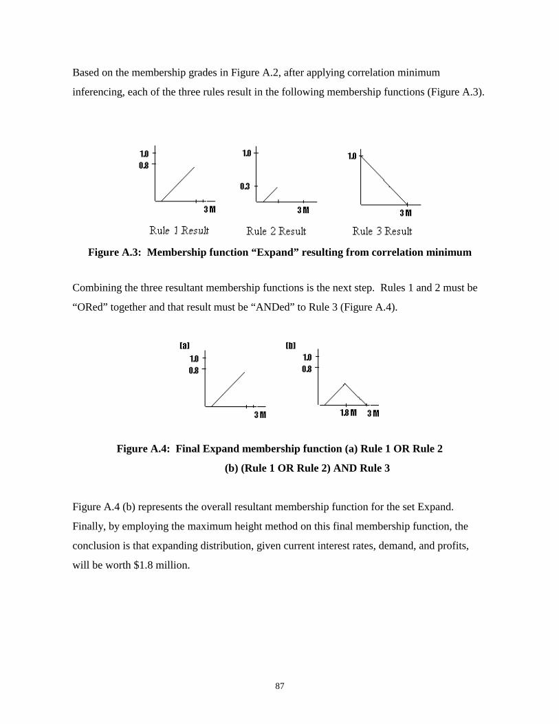
87
Based on the membership grades in Figure A.2, after applying correlation minimum
inferencing, each of the three rules result in the following membership functions (Figure A.3).
Figure A.3: Membership function “Expand” resulting from correlation minimum
Combining the three resultant membership functions is the next step. Rules 1 and 2 must be
“ORed” together and that result must be “ANDed” to Rule 3 (Figure A.4).
Figure A.4: Final Expand membership function (a) Rule 1 OR Rule 2
(b) (Rule 1 OR Rule 2) AND Rule 3
Figure A.4 (b) represents the overall resultant membership function for the set Expand.
Finally, by employing the maximum height method on this final membership function, the
conclusion is that expanding distribution, given current interest rates, demand, and profits,
will be worth $1.8 million.

88
APPENDIX B: AweSim Simulation Variables
Two types of variables were used in the AweSim simulation model, global variables andentity attributes. The global variables are present throughout the entire simulation and can beaccessed from any module in the entire simulation. The global variables and their meaningsare listed below. Entity attributes are more localized. Every entity that is created throughoutthe simulation has a set of entity attributes. These attributes refer to that specific entity.Although seven Create nodes exist in the simulation, only three of these require its entities tohave attributes. The three sets of entity attributes appear following the global variables.
Global VariablesName DefinitionXX(1) Number of packets on link 1XX(2) Number of packets on link 2XX(3) Number of packets on link 3XX(4) Number of packets on link 4XX(5) Number of packets on link 5XX(11) Throughput on link 1XX(12) Throughput on link 2XX(13) Throughput on link 3XX(14) Throughput on link 4XX(15) Throughput on link 5XX(21) Failure on link 1XX(22) Failure on link 2XX(23) Failure on link 3XX(24) Failure on link 4XX(25) Failure on link 5XX(26) - XX(37) Failure on links 6 - 17
Entity Variables (associated with every packet originating at node one)Name MeaningATRIB(1) Time of creationATRIB(2) Current node idATRIB(3) Destination node idATRIB(4) Packet sizeATRIB(5) Next link the packet will traverseATRIB(6) Next node the packet will visitATRIB(7) Number of additional packets on the first link traversedATRIB(8) Throughput on the first link traversedATRIB(9) Failure (if any) experienced on the first link traversed

89
Entity Variables (associated with every packet created at nodes 2 - 12)Name MeaningATRIB(1) Creation timeATRIB(3) Indicates the origin node is not node 1ATRIB(5) Next link the packet will traverseATRIB(6) Indicates the origin node is not node 1
Entity VariablesName MeaningATRIB(1) Creation timeATRIB(2) Subscript corresponding to the global variable for the link to fail (26 -
37)
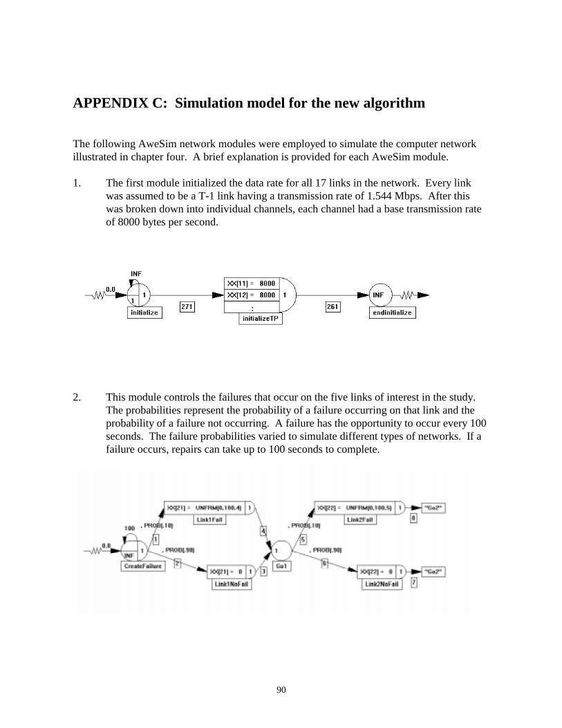
90
APPENDIX C: Simulation model for the new algorithm
The following AweSim network modules were employed to simulate the computer networkillustrated in chapter four. A brief explanation is provided for each AweSim module.
1. The first module initialized the data rate for all 17 links in the network. Every linkwas assumed to be a T-1 link having a transmission rate of 1.544 Mbps. After thiswas broken down into individual channels, each channel had a base transmission rateof 8000 bytes per second.
2. This module controls the failures that occur on the five links of interest in the study.The probabilities represent the probability of a failure occurring on that link and theprobability of a failure not occurring. A failure has the opportunity to occur every 100seconds. The failure probabilities varied to simulate different types of networks. If afailure occurs, repairs can take up to 100 seconds to complete.
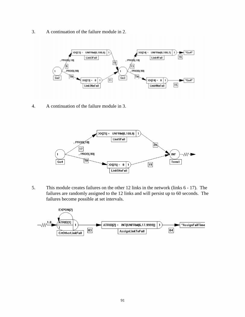
91
3. A continuation of the failure module in 2.
4. A continuation of the failure module in 3.
5. This module creates failures on the other 12 links in the network (links 6 - 17). Thefailures are randomly assigned to the 12 links and will persist up to 60 seconds. Thefailures become possible at set intervals.
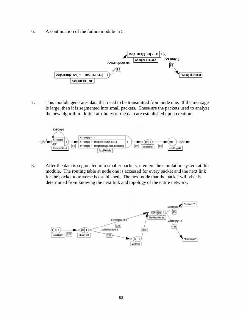
92
6. A continuation of the failure module in 5.
7. This module generates data that need to be transmitted from node one. If the messageis large, then it is segmented into small packets. These are the packets used to analyzethe new algorithm. Initial attributes of the data are established upon creation.
8. After the data is segmented into smaller packets, it enters the simulation system at thismodule. The routing table at node one is accessed for every packet and the next linkfor the packet to traverse is established. The next node that the packet will visit isdetermined from knowing the next link and topology of the entire network.

93
9. Packets that originate at other nodes (nodes 2-12) need to be generated also. Thesepackets are of no statistical interest to the study; therefore, they are assigned flagvalues to avoid collecting travel information.
10. This large module represents a packet traveling on links 1, 2, 3, 4 or 5. Data regardingthe traveled link is also collected here. That data was used for training the neuralnetwork, and for obtaining information to update the routing table.
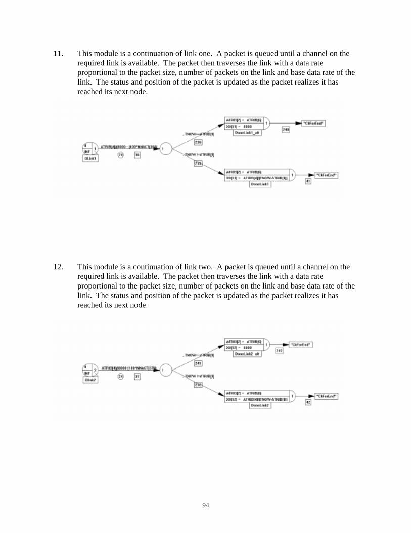
94
11. This module is a continuation of link one. A packet is queued until a channel on therequired link is available. The packet then traverses the link with a data rateproportional to the packet size, number of packets on the link and base data rate of thelink. The status and position of the packet is updated as the packet realizes it hasreached its next node.
12. This module is a continuation of link two. A packet is queued until a channel on therequired link is available. The packet then traverses the link with a data rateproportional to the packet size, number of packets on the link and base data rate of thelink. The status and position of the packet is updated as the packet realizes it hasreached its next node.
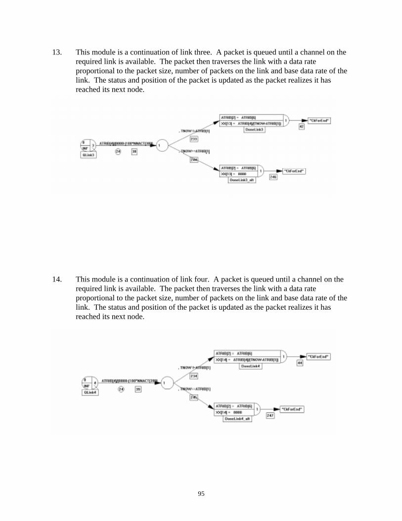
95
13. This module is a continuation of link three. A packet is queued until a channel on therequired link is available. The packet then traverses the link with a data rateproportional to the packet size, number of packets on the link and base data rate of thelink. The status and position of the packet is updated as the packet realizes it hasreached its next node.
14. This module is a continuation of link four. A packet is queued until a channel on therequired link is available. The packet then traverses the link with a data rateproportional to the packet size, number of packets on the link and base data rate of thelink. The status and position of the packet is updated as the packet realizes it hasreached its next node.
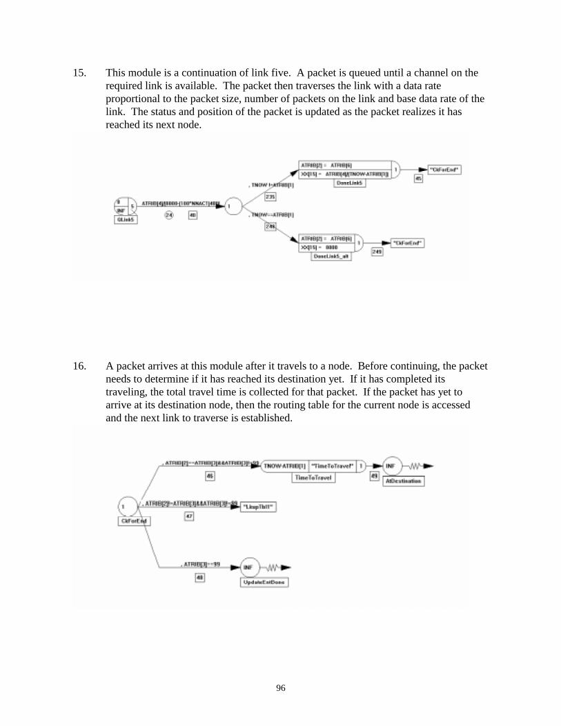
96
15. This module is a continuation of link five. A packet is queued until a channel on therequired link is available. The packet then traverses the link with a data rateproportional to the packet size, number of packets on the link and base data rate of thelink. The status and position of the packet is updated as the packet realizes it hasreached its next node.
16. A packet arrives at this module after it travels to a node. Before continuing, the packetneeds to determine if it has reached its destination yet. If it has completed itstraveling, the total travel time is collected for that packet. If the packet has yet toarrive at its destination node, then the routing table for the current node is accessedand the next link to traverse is established.
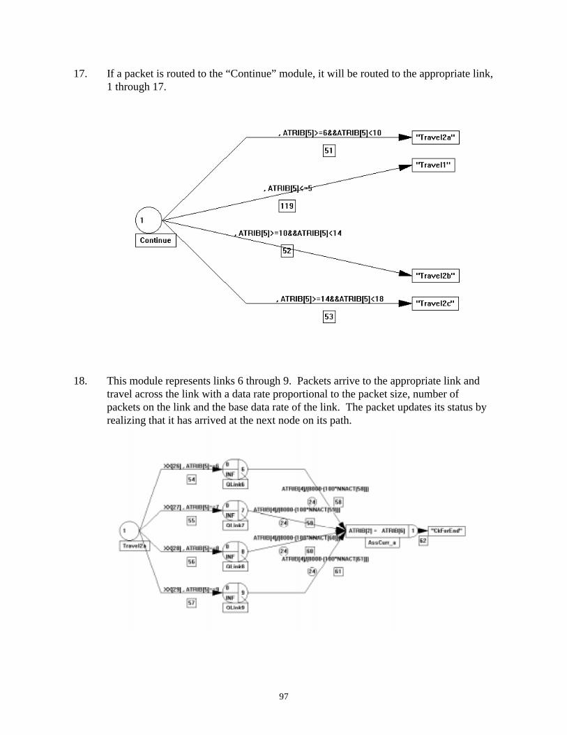
97
17. If a packet is routed to the “Continue” module, it will be routed to the appropriate link,1 through 17.
18. This module represents links 6 through 9. Packets arrive to the appropriate link andtravel across the link with a data rate proportional to the packet size, number ofpackets on the link and the base data rate of the link. The packet updates its status byrealizing that it has arrived at the next node on its path.
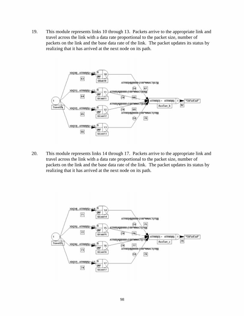
98
19. This module represents links 10 through 13. Packets arrive to the appropriate link andtravel across the link with a data rate proportional to the packet size, number ofpackets on the link and the base data rate of the link. The packet updates its status byrealizing that it has arrived at the next node on its path.
20. This module represents links 14 through 17. Packets arrive to the appropriate link andtravel across the link with a data rate proportional to the packet size, number ofpackets on the link and the base data rate of the link. The packet updates its status byrealizing that it has arrived at the next node on its path.

99
21. Every 60 seconds, the routing table at node one is updated. The updating is performedby a set of C-code commands found in appendix D.
22. Random updates were needed during data collection for training the neural network.This module provided the necessary code to complete those random updates.
100
APPENDIX D: C code used in simulations
This appendix contains the C code written for simulation purposes. It is divided into twosections. The first (Appendix D.1) provides the code used in simulating the new algorithm,while the second (Appendix D.2) provides the code to simulate the shortest route algorithm.
Appendix D.1: C code used to simulate the new algorithm.
#include "vslam.h"#include "stdio.h "#include "math.h"#include "string.h"#include "math.h"#include "conio.h"#include "ctype.h"#include "stdlib.h"
struct FuzzySet{ double x0; double x1; double x2; double x3; double y0; double y1; double y2; double y3; int n; double *x; double *y;};/* Each fuzzy membership set is trapezoidal and has 4 significant points associated with its shape. *//* These points are (x0, y0), (x1, y1), (x2, y2) and (x3, y3). */
static void LkupTbl1(ENTITY * peUser);/* LkupTbl1 carries out the process of accessing the lookup table at node 1. *//* When a packet at node 1 needs to be routed to another node, this lookup table *//* determines which link the packet will traverse next. */
static void GetNextNode1(ENTITY * peUser);static void GetNextNode2(ENTITY * peUser);static void GetNextNode3(ENTITY * peUser);static void GetNextNode4(ENTITY * peUser);static void GetNextNode5(ENTITY * peUser);static void GetNextNode6(ENTITY * peUser);static void GetNextNode7(ENTITY * peUser);static void GetNextNode8(ENTITY * peUser);static void GetNextNode9(ENTITY * peUser);static void GetNextNode10(ENTITY * peUser);static void GetNextNode11(ENTITY * peUser);static void GetNextNode12(ENTITY * peUser);

101
/* GetNextNode1 – GetNextNode12 are used to access the lookup tables at nodes 1 – 12 and *//* determine the next node the packet will travel to. */
static void UpdateDistance(ENTITY * peUser);/* UpdateDistance is used as a part of the simulation program to change the routing table at node 1. *//* This is necessary for data as it provides a larger variety of situations for data collection. */
static void GetTrainingData(ENTITY * peUser);/* GetTrainingData collects data and stores it for future use in training the neural network. */
static void SegmentPacket(ENTITY * peUser);/* SegmentPacket takes an originating packet being transmitted and breaks it up into smaller packets *//* that the transmission media of the network will accept. This must be done before any part of that *//* data can be sent. */
static void GetDistance(ENTITY * peUser);/* GetDistance is not a part of the routing algorithm, but is used for data collection. */
static void RandTableChange(ENTITY * peUser);/* RandTableChange was a function that provided random network changes but was later omitted. */
static void UpdateTable(ENTITY * peUser);/* This is the code used to update the lookup table using the new fuzzy algorithm. */
BOOL SWFUNC INTLC(UINT uiRun){ BOOL bReturn = TRUE;
/* Initialize the NEXTLINK Routing table for current nodes 1 through 12 */ PUTARY(1,1,0); PUTARY(2,1,6); PUTARY(3,1,7); PUTARY(4,1,8); PUTARY(1,2,1); PUTARY(2,2,0); PUTARY(3,2,7); PUTARY(4,2,8); PUTARY(1,3,2); PUTARY(2,3,6); PUTARY(3,3,0); PUTARY(4,3,8); PUTARY(1,4,3); PUTARY(2,4,6); PUTARY(3,4,7); PUTARY(4,4,0); PUTARY(1,5,4); PUTARY(2,5,6); PUTARY(3,5,7); PUTARY(4,5,8); PUTARY(1,6,5); PUTARY(2,6,6); PUTARY(3,6,7); PUTARY(4,6,8); PUTARY(1,7,1); PUTARY(2,7,6); PUTARY(3,7,7); PUTARY(4,7,8); PUTARY(1,8,2); PUTARY(2,8,6); PUTARY(3,8,7); PUTARY(4,8,8); PUTARY(1,9,3); PUTARY(2,9,6); PUTARY(3,9,7); PUTARY(4,9,8); PUTARY(1,10,4); PUTARY(2,10,6); PUTARY(3,10,7); PUTARY(4,10,8); PUTARY(1,11,5); PUTARY(2,11,6); PUTARY(3,11,7); PUTARY(4,11,8); PUTARY(1,12,5); PUTARY(2,12,6); PUTARY(3,12,7); PUTARY(4,12,8);
PUTARY(5,1,9); PUTARY(6,1,10); PUTARY(7,1,12); PUTARY(8,1,15); PUTARY(5,2,9); PUTARY(6,2,10); PUTARY(7,2,12); PUTARY(8,2,15); PUTARY(5,3,9); PUTARY(6,3,10); PUTARY(7,3,12); PUTARY(8,3,15); PUTARY(5,4,9); PUTARY(6,4,10); PUTARY(7,4,12); PUTARY(8,4,15); PUTARY(5,5,0); PUTARY(6,5,10); PUTARY(7,5,12); PUTARY(8,5,15); PUTARY(5,6,9); PUTARY(6,6,0); PUTARY(7,6,12); PUTARY(8,6,15); PUTARY(5,7,9); PUTARY(6,7,10); PUTARY(7,7,0); PUTARY(8,7,15); PUTARY(5,8,9); PUTARY(6,8,10); PUTARY(7,8,12); PUTARY(8,8,0); PUTARY(5,9,9); PUTARY(6,9,10); PUTARY(7,9,12); PUTARY(8,9,15); PUTARY(5,10,9); PUTARY(6,10,10); PUTARY(7,10,12); PUTARY(8,10,15); PUTARY(5,11,9); PUTARY(6,11,10); PUTARY(7,11,12); PUTARY(8,11,15); PUTARY(5,12,9); PUTARY(6,12,10); PUTARY(7,12,12); PUTARY(8,12,15);
102
PUTARY(9,1,14); PUTARY(10,1,11); PUTARY(11,1,16); PUTARY(12,1,17); PUTARY(9,2,14); PUTARY(10,2,11); PUTARY(11,2,16); PUTARY(12,2,17); PUTARY(9,3,14); PUTARY(10,3,11); PUTARY(11,3,16); PUTARY(12,3,17); PUTARY(9,4,14); PUTARY(10,4,11); PUTARY(11,4,16); PUTARY(12,4,17); PUTARY(9,5,14); PUTARY(10,5,11); PUTARY(11,5,16); PUTARY(12,5,17); PUTARY(9,6,14); PUTARY(10,6,11); PUTARY(11,6,16); PUTARY(12,6,17); PUTARY(9,7,14); PUTARY(10,7,11); PUTARY(11,7,16); PUTARY(12,7,17); PUTARY(9,8,14); PUTARY(10,8,11); PUTARY(11,8,16); PUTARY(12,8,17); PUTARY(9,9,0); PUTARY(10,9,11); PUTARY(11,9,16); PUTARY(12,9,17); PUTARY(9,10,14); PUTARY(10,10,0); PUTARY(11,10,16); PUTARY(12,10,17); PUTARY(9,11,14); PUTARY(10,11,17); PUTARY(11,11,0); PUTARY(12,11,16); PUTARY(9,12,14); PUTARY(10,12,11); PUTARY(11,12,16); PUTARY(12,12,0);
/* Initialize Distance (#hops to destination using links 1-5) matrix */
PUTARY(21,22,1); PUTARY(22,22,3); PUTARY(23,22,5); PUTARY(24,22,5); PUTARY(25,22,5); PUTARY(21,23,3); PUTARY(22,23,1); PUTARY(23,23,5); PUTARY(24,23,5); PUTARY(25,23,5); PUTARY(21,24,5); PUTARY(22,24,5); PUTARY(23,24,1); PUTARY(24,24,3); PUTARY(25,24,3); PUTARY(21,25,5); PUTARY(22,25,5); PUTARY(23,25,3); PUTARY(24,25,1); PUTARY(25,25,3); PUTARY(21,26,5); PUTARY(22,26,5); PUTARY(23,26,3); PUTARY(24,26,3); PUTARY(25,26,1); PUTARY(21,27,2); PUTARY(22,27,2); PUTARY(23,27,4); PUTARY(24,27,4); PUTARY(25,27,4); PUTARY(21,28,3); PUTARY(22,28,3); PUTARY(23,28,3); PUTARY(24,28,3); PUTARY(25,28,3); PUTARY(21,29,4); PUTARY(22,29,4); PUTARY(23,29,2); PUTARY(24,29,2); PUTARY(25,29,2); PUTARY(21,30,4); PUTARY(22,30,4); PUTARY(23,30,4); PUTARY(24,30,4); PUTARY(25,30,2); PUTARY(21,31,3); PUTARY(22,31,3); PUTARY(23,31,5); PUTARY(24,31,5); PUTARY(25,31,4); PUTARY(21,32,4); PUTARY(22,32,4); PUTARY(23,32,5); PUTARY(24,32,5); PUTARY(25,32,3);
return(bReturn);}
void SWFUNC EVENT(int iCode, ENTITY * peUser){ switch (iCode) { case 1: /* arrive to event node 1 */ GetNextNode1(peUser); break; case 2: /* arrive to event node 2 */ GetNextNode2(peUser); break; case 3: /* arrive to event node 3 */ GetNextNode3(peUser); break; case 4: /* arrive to event node 4 */ GetNextNode4(peUser); break; case 5: /* arrive to event node 5 */ GetNextNode5(peUser); break; case 6: /* arrive to event node 6 */ GetNextNode6(peUser); break; case 7: /* arrive to event node 7 */ GetNextNode7(peUser); break;
103
case 8: /* arrive to event node 8 */ GetNextNode8(peUser); break; case 9: /* arrive to event node 9 */ GetNextNode9(peUser); break; case 10: /* arrive to event node 10 */ GetNextNode10(peUser); break; case 11: /* arrive to event node 11 */ GetNextNode11(peUser); break; case 12: /* arrive to event node 12 */ GetNextNode12(peUser); break; case 17: /* arrive to event node 17 */ GetDistance(peUser); break; case 18: /* arrive to event node 18 */ RandTableChange(peUser); break; case 19: /* arrive to event node 19 */ SegmentPacket(peUser); break; case 20: /* arrive to event node 20 */ LkupTbl1(peUser); break; case 23: /* arrive to event node 23 */ UpdateDistance(peUser); break; case 24: /* arrive to event node 24 */ GetTrainingData(peUser); break; default: su_error(1,"Unknown event code"); break; }}
double SWFUNC USERF(int iCode, ENTITY * peUser){ double dReturn; switch (iCode) { case 26: UpdateTable(peUser); break; }dReturn = 987;return dReturn;}
static void SWFUNC LkupTbl1(ENTITY * peUser){ int NextLink = GETARY(peUser->ATRIB[2],peUser->ATRIB[3]); peUser->ATRIB[5] = NextLink;
104
}
static void SWFUNC GetNextNode1(ENTITY * peUser){ int NextNode = 0; if (peUser->ATRIB[5]==1.0) NextNode = 2; else if (peUser->ATRIB[5]==2.0) NextNode = 3; else if (peUser->ATRIB[5]==3.0) NextNode = 4; else if (peUser->ATRIB[5]==4.0) NextNode = 5; else if (peUser->ATRIB[5]==5.0) NextNode = 6; peUser->ATRIB[6] = NextNode;}
static void SWFUNC GetNextNode2(ENTITY * peUser){ int NextNode = 0; if (peUser->ATRIB[5]==1.0) NextNode = 1; else if (peUser->ATRIB[5]==6.0) NextNode = 7; peUser->ATRIB[6] = NextNode;}
static void SWFUNC GetNextNode3(ENTITY * peUser){ int NextNode = 0; if (peUser->ATRIB[5]==2.0) NextNode = 1; else if (peUser->ATRIB[5]==7.0) NextNode = 7; peUser->ATRIB[6] = NextNode;}
static void SWFUNC GetNextNode4(ENTITY * peUser){ int NextNode = 0; if (peUser->ATRIB[5]==3.0) NextNode = 1; else if (peUser->ATRIB[5]==8.0) NextNode = 9; peUser->ATRIB[6] = NextNode;}
static void SWFUNC GetNextNode5(ENTITY * peUser){ int NextNode = 0; if (peUser->ATRIB[5]==4.0) NextNode = 1; else if (peUser->ATRIB[5]==9.0) NextNode = 9; peUser->ATRIB[6] = NextNode;}
static void SWFUNC GetNextNode6(ENTITY * peUser){ int NextNode = 0; if (peUser->ATRIB[5]==5.0) NextNode = 1; else if (peUser->ATRIB[5]==10.0) NextNode = 9; else if (peUser->ATRIB[5]==11.0) NextNode = 10; peUser->ATRIB[6] = NextNode;}
static void SWFUNC GetNextNode7(ENTITY * peUser)

105
{ int NextNode = 0; if (peUser->ATRIB[5]==6.0) NextNode = 2; else if (peUser->ATRIB[5]==7.0) NextNode = 3; else if (peUser->ATRIB[5]==12.0) NextNode = 11; else if (peUser->ATRIB[5]==13.0) NextNode = 8; peUser->ATRIB[6] = NextNode;}
static void SWFUNC GetNextNode8(ENTITY * peUser){ int NextNode = 0; if (peUser->ATRIB[5]==13.0) NextNode = 7; else if (peUser->ATRIB[5]==14.0) NextNode = 9; else if (peUser->ATRIB[5]==15.0) NextNode = 10; peUser->ATRIB[6] = NextNode;}
static void SWFUNC GetNextNode9(ENTITY * peUser){ int NextNode = 0; if (peUser->ATRIB[5]==8.0) NextNode = 4; else if (peUser->ATRIB[5]==9.0) NextNode = 5; else if (peUser->ATRIB[5]==10.0) NextNode = 6; else if (peUser->ATRIB[5]==14.0) NextNode = 8; peUser->ATRIB[6] = NextNode;}
static void SWFUNC GetNextNode10(ENTITY * peUser){ int NextNode = 0; if (peUser->ATRIB[5]==11.0) NextNode = 6; else if (peUser->ATRIB[5]==15.0) NextNode = 8; else if (peUser->ATRIB[5]==17.0) NextNode = 12; peUser->ATRIB[6] = NextNode;}
static void SWFUNC GetNextNode11(ENTITY * peUser){ int NextNode = 0; if (peUser->ATRIB[5]==12.0) NextNode = 7; else if (peUser->ATRIB[5]==16.0) NextNode = 12; peUser->ATRIB[6] = NextNode;}
static void SWFUNC GetNextNode12(ENTITY * peUser){ int NextNode = 0; if (peUser->ATRIB[5]==16.0) NextNode = 11; else if (peUser->ATRIB[5]==17.0) NextNode = 10; peUser->ATRIB[6] = NextNode;}
static void UpdateDistance(ENTITY * peUser){
106
if (XX[26] != 0.0) { PUTARY(21,23,99); PUTARY(21,26,99); PUTARY(21,28,99); PUTARY(21,24,99); PUTARY(21,27,99); PUTARY(21,29,99); PUTARY(21,25,99); PUTARY(22,22,99); PUTARY(21,30,99); PUTARY(21,31,99); PUTARY(21,32,99); PUTARY(23,22,99); PUTARY(24,22,99); PUTARY(25,22,99); }
if (XX[27] != 0.0) { PUTARY(21,23,99); PUTARY(22,22,99); PUTARY(22,28,99); PUTARY(23,23,99); PUTARY(22,24,99); PUTARY(22,29,99); PUTARY(24,23,99); PUTARY(22,25,99); PUTARY(22,30,99); PUTARY(25,23,99); PUTARY(21,26,99); PUTARY(22,31,99); PUTARY(22,32,99); PUTARY(22,27,99); }
if (XX[28] != 0.0) { PUTARY(23,22,99); PUTARY(23,23,99); PUTARY(24,24,99); PUTARY(22,24,99); PUTARY(23,30,99); PUTARY(25,24,99); PUTARY(23,26,99); PUTARY(23,32,99); PUTARY(23,25,99); PUTARY(23,29,99); PUTARY(23,27,99); PUTARY(23,31,99); PUTARY(21,24,99); PUTARY(23,28,99); }
if (XX[29] != 0.0) { PUTARY(24,22,99); PUTARY(23,25,99); PUTARY(24,29,99); PUTARY(24,23,99); PUTARY(25,25,99); PUTARY(24,30,99); PUTARY(24,24,99); PUTARY(24,26,99); PUTARY(24,31,99); PUTARY(21,25,99); PUTARY(24,27,99); PUTARY(22,25,99); PUTARY(24,28,99); PUTARY(24,32,99); }
if (XX[30] != 0.0) { PUTARY(25,24,5); PUTARY(23,26,5); PUTARY(25,25,5); PUTARY(24,26,5); PUTARY(25,29,4); }
if (XX[31] != 0.0) { PUTARY(25,30,4); PUTARY(25,31,5); PUTARY(25,32,5); }
if (XX[32] != 0.0) { PUTARY(21,31,6); PUTARY(24,31,6); PUTARY(22,31,6); PUTARY(23,31,6); PUTARY(21,32,5); PUTARY(22,32,5); } if (XX[33] != 0.0) { PUTARY(23,22,8); PUTARY(23,23,8); PUTARY(21,24,8); PUTARY(24,22,8); PUTARY(24,23,8); PUTARY(22,24,8); PUTARY(25,22,6); PUTARY(25,23,6); PUTARY(21,25,8); PUTARY(22,26,6); PUTARY(22,25,8); PUTARY(21,26,6); PUTARY(21,29,7); PUTARY(23,27,7); PUTARY(21,28,6); PUTARY(22,29,7); PUTARY(24,27,7); PUTARY(22,28,6); PUTARY(21,30,5); PUTARY(25,27,5); PUTARY(24,31,6); PUTARY(22,30,5); PUTARY(23,31,6); }
107
if (XX[34] != 0.0) { PUTARY(21,24,7); PUTARY(23,22,7); PUTARY(23,23,7); PUTARY(22,24,7); PUTARY(24,22,7); PUTARY(24,23,7); PUTARY(23,28,5); PUTARY(21,25,7); PUTARY(23,27,6); PUTARY(21,29,6); PUTARY(22,25,7); PUTARY(24,27,6); PUTARY(22,29,6); PUTARY(24,28,5); PUTARY(23,31,6); PUTARY(24,31,6); }
if (XX[35] != 0.0) { PUTARY(21,30,5); PUTARY(22,30,5); }
if (XX[36] != 0.0) { PUTARY(25,31,5); PUTARY(21,32,5); PUTARY(22,32,5); }
if (XX[37] != 0.0) { PUTARY(25,31,5); PUTARY(23,32,6); PUTARY(24,32,6); PUTARY(25,32,6); }}
static void GetTrainingData(ENTITY * peUser){ FILE *fp; double time; time = TNOW - peUser->ATRIB[1]; fp = fopen("simdata", "a"); fprintf(fp, "%4.0f", peUser->ATRIB[4]); /*PACKET SIZE*/ fprintf(fp, "\t%6.0f", peUser->ATRIB[3]); /*DESTINATION*/ fprintf(fp, "\t%6.0f", peUser->ATRIB[19]); /*DISTANCE*/ fprintf(fp, "\t%4.0f", peUser->ATRIB[7]); /*#PKTS ON INITIAL LINK USED*/ fprintf(fp, "\t\t%8.4f", peUser->ATRIB[8]); /*THROUGHPUT ON INITIAL LINK USED*/ fprintf(fp, "\t\t%6.0f", peUser->ATRIB[5]); /*link*/ fprintf(fp, "\t\t%f\n", time); /*TIME TO REACH DESTINATION*/ fclose(fp);}
static void SegmentPacket(ENTITY * peUser){ ENTITY *peNew; int NumOfSegs; int count; if (peUser->ATRIB[4] > 1500) { NumOfSegs = peUser->ATRIB[4]/1500; count = NumOfSegs; while (count > 0) { peNew = su_entnew(0,NULL,NULL,NULL); peNew->ATRIB[1] = TNOW; peNew->ATRIB[2] = peUser->ATRIB[2]; peNew->ATRIB[3] = peUser->ATRIB[3]; peNew->ATRIB[4] = 1500; peNew->ATRIB[18] = 1; ENTER(1,peNew);
108
count = count-1; } peNew = su_entnew(0,NULL,NULL,NULL); peNew->ATRIB[1] = TNOW; peNew->ATRIB[2] = peUser->ATRIB[2]; peNew->ATRIB[3] = peUser->ATRIB[3]; peNew->ATRIB[4] = peUser->ATRIB[4]-(1500*NumOfSegs); peNew->ATRIB[18] = 1; ENTER(1,peNew); } if (peUser->ATRIB[4] <= 1500) { peNew = su_entnew(0,NULL,NULL,NULL); peNew->ATRIB[1] = TNOW; peNew->ATRIB[2] = peUser->ATRIB[2]; peNew->ATRIB[3] = peUser->ATRIB[3]; peNew->ATRIB[4] = peUser->ATRIB[4]; peNew->ATRIB[18] = 1; ENTER(1,peNew); }}
static void GetDistance(ENTITY * peUser){ peUser->ATRIB[19] = GETARY(peUser->ATRIB[5] + 20,peUser->ATRIB[3] + 20); peUser->ATRIB[18] = 0;}
void UpdateTable(){ double dxval, txval, fxval, cxval;/* The x value membership grades calculated for distance, throughput, failure and congestion. */
double dyvallo, dyvalmd, dyvalhi, tyvallo, tyvalmd, tyvalhi; double fyvallo, fyvalmd, fyvalhi, cyvallo, cyvalmd, cyvalhi;/* The y values for the 12 fuzzy sets. */
double PktSz, Dest, Dist, Pkts, Tput, Fail;/* These 4 vars hold the actual values for the packetsize, destination, and 4 metrics of the packet. */
double I1, I2, I3, I4, I5, I6, I7, I8, I9, I10, I11, I12, I13, I14, I15; double I16, I17, I18, I19, I20, I21, I22, I23; double y16, y17, y18, y19, y20, y21, y22, y23; double W1_16, W1_17, W1_18, W1_19, W1_20, W1_21, W1_22, W1_23; double W2_16, W2_17, W2_18, W2_19, W2_20, W2_21, W2_22; double W3_16, W3_17, W3_18, W3_19, W3_20, W3_21, W3_22; double W4_16, W4_17, W4_18, W4_19, W4_20, W4_21, W4_22; double W5_16, W5_17, W5_18, W5_19, W5_20, W5_21, W5_22; double W6_16, W6_17, W6_18, W6_19, W6_20, W6_21, W6_22; double W7_16, W7_17, W7_18, W7_19, W7_20, W7_21, W7_22; double W8_16, W8_17, W8_18, W8_19, W8_20, W8_21, W8_22; double W9_16, W9_17, W9_18, W9_19, W9_20, W9_21, W9_22; double W10_16, W10_17, W10_18, W10_19, W10_20, W10_21, W10_22; double W11_16, W11_17, W11_18, W11_19, W11_20, W11_21, W11_22; double W12_16, W12_17, W12_18, W12_19, W12_20, W12_21, W12_22;

109
double W13_16, W13_17, W13_18, W13_19, W13_20, W13_21, W13_22; double W14_16, W14_17, W14_18, W14_19, W14_20, W14_21, W14_22; double W15_16, W15_17, W15_18, W15_19, W15_20, W15_21, W15_22; double W16_23, W17_23, W18_23, W19_23, W20_23, W21_23, W22_23;/* The I, y, and W variables all refer to numbers used in the forward pass of the neural network. */
double HiPredTime, PredTime;/* Predicted time using that route. HiPredTime is used to store the highest during comparisons. */
int LinkNumber, LinkToUse, curr, dst;int lo, mid, hi ;double yyy ;
struct FuzzySet DistLo = {0,0.5,1,3,1,1,1,0,0,0,0};struct FuzzySet DistMd = {1,2,4,5,0,1,1,0,0,0,0};struct FuzzySet DistHi = {3,5,7,8,0,1,1,1,0,0,0};struct FuzzySet CongLo = {0,8,20,28,1,1,1,0,0,0,0};struct FuzzySet CongMd = {20,28,44,52,0,1,1,0,0,0,0};struct FuzzySet CongHi = {44,52,72,84,0,1,1,1,0,0,0};struct FuzzySet TputLo = {0,1000,2000,3000,1,1,1,0,0,0,0};struct FuzzySet TputMd = {2000,3000,5000,6000,0,1,1,0,0,0,0};struct FuzzySet TputHi = {5000,6000,8000,20000,0,1,1,1,0,0,0};struct FuzzySet FailLo = {0,1,5,15,1,1,1,0,0,0,0};struct FuzzySet FailMd = {5,15,25,35,0,1,1,0,0,0,0};struct FuzzySet FailHi = {25,35,45,100,0,1,1,1,0,0,0};/* The above declarations define the fuzzy sets for this particular simulated network. */
double xx[4], yy[4] ;
/* The following is divided into 12 sections, one for each membership set. *//* Memory is allocated and the fuzzy sets are prepared so the membership grades can be obtained. */
/* --------------------Distance Low-------------------*/ xx[0] = DistLo.x0 ; yy[0] = DistLo.y0 ; DistLo.n = 1 ; if ((DistLo.x1 != DistLo.x0) || (DistLo.y1 != DistLo.y0)) { xx[DistLo.n] = DistLo.x1 ; yy[DistLo.n] = DistLo.y1 ; ++DistLo.n ; } if ((DistLo.x2 != DistLo.x1) || (DistLo.y2 != DistLo.y1)) { xx[DistLo.n] = DistLo.x2 ; yy[DistLo.n] = DistLo.y2 ; ++DistLo.n ; } if ((DistLo.x3 != DistLo.x2) || (DistLo.y3 != DistLo.y2)) { xx[DistLo.n] = DistLo.x3 ; yy[DistLo.n] = DistLo.y3 ; ++DistLo.n ; } DistLo.x = (double *) malloc ( 2 * DistLo.n * sizeof(double) ) ; if (DistLo.x == NULL) { DistLo.n = 0 ; // Flag as invalid return ; } DistLo.y = DistLo.x + DistLo.n ; // This saves a call to malloc memcpy ( DistLo.x , xx , DistLo.n * sizeof(double) ) ; memcpy ( DistLo.y , yy , DistLo.n * sizeof(double) ) ;
110
/* --------------------Distance Medium-------------------*/ xx[0] = DistMd.x0 ; yy[0] = DistMd.y0 ; DistMd.n = 1 ; if ((DistMd.x1 != DistMd.x0) || (DistMd.y1 != DistMd.y0)) { xx[DistMd.n] = DistMd.x1 ; yy[DistMd.n] = DistMd.y1 ; ++DistMd.n ; } if ((DistMd.x2 != DistMd.x1) || (DistMd.y2 != DistMd.y1)) { xx[DistMd.n] = DistMd.x2 ; yy[DistMd.n] = DistMd.y2 ; ++DistMd.n ; } if ((DistMd.x3 != DistMd.x2) || (DistMd.y3 != DistMd.y2)) { xx[DistMd.n] = DistMd.x3 ; yy[DistMd.n] = DistMd.y3 ; ++DistMd.n ; } DistMd.x = (double *) malloc ( 2 * DistMd.n * sizeof(double) ) ; if (DistMd.x == NULL) { DistMd.n = 0 ; // Flag as invalid return ; } DistMd.y = DistMd.x + DistMd.n ; // This saves a call to malloc memcpy ( DistMd.x , xx , DistMd.n * sizeof(double) ) ; memcpy ( DistMd.y , yy , DistMd.n * sizeof(double) ) ;
/* --------------------Distance High-------------------*/ xx[0] = DistHi.x0 ; yy[0] = DistHi.y0 ; DistHi.n = 1 ; if ((DistHi.x1 != DistHi.x0) || (DistHi.y1 != DistHi.y0)) { xx[DistHi.n] = DistHi.x1 ; yy[DistHi.n] = DistHi.y1 ; ++DistHi.n ; } if ((DistHi.x2 != DistHi.x1) || (DistHi.y2 != DistHi.y1)) { xx[DistHi.n] = DistHi.x2 ; yy[DistHi.n] = DistHi.y2 ; ++DistHi.n ; } if ((DistHi.x3 != DistHi.x2) || (DistHi.y3 != DistHi.y2)) { xx[DistHi.n] = DistHi.x3 ; yy[DistHi.n] = DistHi.y3 ; ++DistHi.n ; } DistHi.x = (double *) malloc ( 2 * DistHi.n * sizeof(double) ) ; if (DistHi.x == NULL) { DistHi.n = 0 ; // Flag as invalid return ; } DistHi.y = DistHi.x + DistHi.n ; // This saves a call to malloc memcpy ( DistHi.x , xx , DistHi.n * sizeof(double) ) ; memcpy ( DistHi.y , yy , DistHi.n * sizeof(double) ) ;
/* --------------------Congestion Low-------------------*/ xx[0] = CongLo.x0 ; yy[0] = CongLo.y0 ; CongLo.n = 1 ; if ((CongLo.x1 != CongLo.x0) || (CongLo.y1 != CongLo.y0)) { xx[CongLo.n] = CongLo.x1 ;
111
yy[CongLo.n] = CongLo.y1 ; ++CongLo.n ; } if ((CongLo.x2 != CongLo.x1) || (CongLo.y2 != CongLo.y1)) { xx[CongLo.n] = CongLo.x2 ; yy[CongLo.n] = CongLo.y2 ; ++CongLo.n ; } if ((CongLo.x3 != CongLo.x2) || (CongLo.y3 != CongLo.y2)) { xx[CongLo.n] = CongLo.x3 ; yy[CongLo.n] = CongLo.y3 ; ++CongLo.n ; } CongLo.x = (double *) malloc ( 2 * CongLo.n * sizeof(double) ) ; if (CongLo.x == NULL) { CongLo.n = 0 ; // Flag as invalid return ; } CongLo.y = CongLo.x + CongLo.n ; // This saves a call to malloc memcpy ( CongLo.x , xx , CongLo.n * sizeof(double) ) ; memcpy ( CongLo.y , yy , CongLo.n * sizeof(double) ) ;
/* --------------------Congestion Medium-------------------*/ xx[0] = CongMd.x0 ; yy[0] = CongMd.y0 ; CongMd.n = 1 ; if ((CongMd.x1 != CongMd.x0) || (CongMd.y1 != CongMd.y0)) { xx[CongMd.n] = CongMd.x1 ; yy[CongMd.n] = CongMd.y1 ; ++CongMd.n ; } if ((CongMd.x2 != CongMd.x1) || (CongMd.y2 != CongMd.y1)) { xx[CongMd.n] = CongMd.x2 ; yy[CongMd.n] = CongMd.y2 ; ++CongMd.n ; } if ((CongMd.x3 != CongMd.x2) || (CongMd.y3 != CongMd.y2)) { xx[CongMd.n] = CongMd.x3 ; yy[CongMd.n] = CongMd.y3 ; ++CongMd.n ; } CongMd.x = (double *) malloc ( 2 * CongMd.n * sizeof(double) ) ; if (CongMd.x == NULL) { CongMd.n = 0 ; // Flag as invalid return ; } CongMd.y = CongMd.x + CongMd.n ; // This saves a call to malloc memcpy (CongMd.x , xx , CongMd.n * sizeof(double) ) ; memcpy (CongMd.y , yy , CongMd.n * sizeof(double) ) ;
/* --------------------Congestion High-------------------*/ xx[0] = CongHi.x0 ; yy[0] = CongHi.y0 ; CongHi.n = 1 ; if ((CongHi.x1 != CongHi.x0) || (CongHi.y1 != CongHi.y0)) { xx[CongHi.n] = CongHi.x1 ; yy[CongHi.n] = CongHi.y1 ; ++CongHi.n ; }
112
if ((CongHi.x2 != CongHi.x1) || (CongHi.y2 != CongHi.y1)) { xx[CongHi.n] = CongHi.x2 ; yy[CongHi.n] = CongHi.y2 ; ++CongHi.n ; } if ((CongHi.x3 != CongHi.x2) || (CongHi.y3 != CongHi.y2)) { xx[CongHi.n] = CongHi.x3 ; yy[CongHi.n] = CongHi.y3 ; ++CongHi.n ; } CongHi.x = (double *) malloc ( 2 * CongHi.n * sizeof(double) ) ; if (CongHi.x == NULL) { CongHi.n = 0 ; // Flag as invalid return ; } CongHi.y = CongHi.x + CongHi.n ; // This saves a call to malloc memcpy (CongHi.x , xx , CongHi.n * sizeof(double) ) ; memcpy (CongHi.y , yy , CongHi.n * sizeof(double) ) ;
/* --------------------Failure Low-------------------*/ xx[0] = FailLo.x0 ; yy[0] = FailLo.y0 ; FailLo.n = 1 ; if ((FailLo.x1 != FailLo.x0) || (FailLo.y1 != FailLo.y0)) { xx[FailLo.n] = FailLo.x1 ; yy[FailLo.n] = FailLo.y1 ; ++FailLo.n ; } if ((FailLo.x2 != FailLo.x1) || (FailLo.y2 != FailLo.y1)) { xx[FailLo.n] = FailLo.x2 ; yy[FailLo.n] = FailLo.y2 ; ++FailLo.n ; } if ((FailLo.x3 != FailLo.x2) || (FailLo.y3 != FailLo.y2)) { xx[FailLo.n] = FailLo.x3 ; yy[FailLo.n] = FailLo.y3 ; ++FailLo.n ; } FailLo.x = (double *) malloc ( 2 * FailLo.n * sizeof(double) ) ; if (FailLo.x == NULL) { FailLo.n = 0 ; // Flag as invalid return ; } FailLo.y = FailLo.x + FailLo.n ; // This saves a call to malloc memcpy (FailLo.x , xx , FailLo.n * sizeof(double) ) ; memcpy (FailLo.y , yy , FailLo.n * sizeof(double) ) ;
/* --------------------Failure Medium-------------------*/ xx[0] = FailMd.x0 ; yy[0] = FailMd.y0 ; FailMd.n = 1 ;
if ((FailMd.x1 != FailMd.x0) || (FailMd.y1 != FailMd.y0)) { xx[FailMd.n] = FailMd.x1 ; yy[FailMd.n] = FailMd.y1 ;
113
++FailMd.n ; } if ((FailMd.x2 != FailMd.x1) || (FailMd.y2 != FailMd.y1)) { xx[FailMd.n] = FailMd.x2 ; yy[FailMd.n] = FailMd.y2 ; ++FailMd.n ; } if ((FailMd.x3 != FailMd.x2) || (FailMd.y3 != FailMd.y2)) { xx[FailMd.n] = FailMd.x3 ; yy[FailMd.n] = FailMd.y3 ; ++FailMd.n ; } FailMd.x = (double *) malloc ( 2 * FailMd.n * sizeof(double) ) ; if (FailMd.x == NULL) { FailMd.n = 0 ; // Flag as invalid return ; } FailMd.y = FailMd.x + FailMd.n ; // This saves a call to malloc memcpy (FailMd.x , xx , FailMd.n * sizeof(double) ) ; memcpy (FailMd.y , yy , FailMd.n * sizeof(double) ) ;
/* --------------------Failure High-------------------*/ xx[0] = FailHi.x0 ; yy[0] = FailHi.y0 ; FailHi.n = 1 ; if ((FailHi.x1 != FailHi.x0) || (FailHi.y1 != FailHi.y0)) { xx[FailHi.n] = FailHi.x1 ; yy[FailHi.n] = FailHi.y1 ; ++FailHi.n ; } if ((FailHi.x2 != FailHi.x1) || (FailHi.y2 != FailHi.y1)) { xx[FailHi.n] = FailHi.x2 ; yy[FailHi.n] = FailHi.y2 ; ++FailHi.n ; } if ((FailHi.x3 != FailHi.x2) || (FailHi.y3 != FailHi.y2)) { xx[FailHi.n] = FailHi.x3 ; yy[FailHi.n] = FailHi.y3 ; ++FailHi.n ; } FailHi.x = (double *) malloc ( 2 * FailHi.n * sizeof(double) ) ; if (FailHi.x == NULL) { FailHi.n = 0 ; // Flag as invalid return ; } FailHi.y = FailHi.x + FailHi.n ; // This saves a call to malloc memcpy (FailHi.x , xx , FailHi.n * sizeof(double) ) ; memcpy (FailHi.y , yy , FailHi.n * sizeof(double) ) ;
/* --------------------Throughput Low-------------------*/ xx[0] = TputLo.x0 ; yy[0] = TputLo.y0 ; TputLo.n = 1 ; if ((TputLo.x1 != TputLo.x0) || (TputLo.y1 != TputLo.y0)) { xx[TputLo.n] = TputLo.x1 ;

114
yy[TputLo.n] = TputLo.y1 ; ++TputLo.n ; } if ((TputLo.x2 != TputLo.x1) || (TputLo.y2 != TputLo.y1)) { xx[TputLo.n] = TputLo.x2 ; yy[TputLo.n] = TputLo.y2 ; ++TputLo.n ; } if ((TputLo.x3 != TputLo.x2) || (TputLo.y3 != TputLo.y2)) { xx[TputLo.n] = TputLo.x3 ; yy[TputLo.n] = TputLo.y3 ; ++TputLo.n ; } TputLo.x = (double *) malloc ( 2 * TputLo.n * sizeof(double) ) ; if (TputLo.x == NULL) { TputLo.n = 0 ; // Flag as invalid return ; } TputLo.y = TputLo.x + TputLo.n ; // This saves a call to malloc memcpy (TputLo.x , xx , TputLo.n * sizeof(double) ) ; memcpy (TputLo.y , yy , TputLo.n * sizeof(double) ) ;
/* --------------------Throughput Medium-------------------*/ xx[0] = TputMd.x0 ; yy[0] = TputMd.y0 ; TputMd.n = 1 ; if ((TputMd.x1 != TputMd.x0) || (TputMd.y1 != TputMd.y0)) { xx[TputMd.n] = TputMd.x1 ; yy[TputMd.n] = TputMd.y1 ; ++TputMd.n ; } if ((TputMd.x2 != TputMd.x1) || (TputMd.y2 != TputMd.y1)) { xx[TputMd.n] = TputMd.x2 ; yy[TputMd.n] = TputMd.y2 ; ++TputMd.n ; } if ((TputMd.x3 != TputMd.x2) || (TputMd.y3 != TputMd.y2)) { xx[TputMd.n] = TputMd.x3 ; yy[TputMd.n] = TputMd.y3 ; ++TputMd.n ; } TputMd.x = (double *) malloc ( 2 * TputMd.n * sizeof(double) ) ; if (TputMd.x == NULL) { TputMd.n = 0 ; // Flag as invalid return ; } TputMd.y = TputMd.x + TputMd.n ; // This saves a call to malloc memcpy (TputMd.x , xx , TputMd.n * sizeof(double) ) ; memcpy (TputMd.y , yy , TputMd.n * sizeof(double) ) ;
/* --------------------Throughput High-------------------*/ xx[0] = TputHi.x0 ; yy[0] = TputHi.y0 ; TputHi.n = 1 ; if ((TputHi.x1 != TputHi.x0) || (TputHi.y1 != TputHi.y0)) {
115
xx[TputHi.n] = TputHi.x1 ; yy[TputHi.n] = TputHi.y1 ; ++TputHi.n ; } if ((TputHi.x2 != TputHi.x1) || (TputHi.y2 != TputHi.y1)) { xx[TputHi.n] = TputHi.x2 ; yy[TputHi.n] = TputHi.y2 ; ++TputHi.n ; } if ((TputHi.x3 != TputHi.x2) || (TputHi.y3 != TputHi.y2)) { xx[TputHi.n] = TputHi.x3 ; yy[TputHi.n] = TputHi.y3 ; ++TputHi.n ; } TputHi.x = (double *) malloc ( 2 * TputHi.n * sizeof(double) ) ; if (TputHi.x == NULL) { TputHi.n = 0 ; // Flag as invalid return ; } TputHi.y = TputHi.x + TputHi.n ; // This saves a call to malloc memcpy ( TputHi.x , xx , TputHi.n * sizeof(double) ) ; memcpy ( TputHi.y , yy , TputHi.n * sizeof(double) ) ;
/* The following assignments refer to the weights in the neural network. */W1_16 = -0.2658;W2_16 = -.1093 ;W3_16 = -.0814 ;W4_16 = -.2235 ;W5_16 = -.1709;W6_16 = -.1731;W7_16 = -.0865;W8_16 = -.3571;W9_16 = -.0425;W10_16 = .1920;W11_16 = -.4797;W12_16 = -.1209;W13_16 = -.1083;W14_16 = -.1608;W15_16 = -.1552;
W1_17 = -.3235;W2_17 = .0788;W3_17 = -.3092;W4_17 = -.1294;W5_17 = -.1033;W6_17 = -.0566;W7_17 = -.1034;W8_17 = -.5290;W9_17 = -.1377;W10_17 = .3448;W11_17 = -.7552 ;W12_17 = -.5474 ;W13_17 = .2303;W14_17 = -.0865;W15_17 = -.1237;

116
W1_18 = -.3747;W2_18 = -.0809;W3_18 = -.1509 ;W4_18 = -.1616 ;W5_18 = -.2034 ;W6_18 = -.0664;W7_18 = .0279;W8_18 = -.3565;W9_18 = -.0362;W10_18 = .0083;W11_18 = -.2084;W12_18 = -.2058;W13_18 = -.0547;W14_18 = -.1766;W15_18 = -.1396;
W1_19 = -.3223;W2_19 = -.0520;W3_19 = -.0430;W4_19 = -.2494;W5_19 = -.2542;W6_19 = -.0259;W7_19 = .0229;W8_19 = -.3310;W9_19 = -.0712;W10_19 = .0369;W11_19 = -.2589;W12_19 = -.2234;W13_19 = -.0791;W14_19 = -.1826;W15_19 = -.1444;
W1_20 = -.3240;W2_20 = .0208;W3_20 = -.0767 ;W4_20 = -.2089 ;W5_20 = -.2069 ;W6_20 = -.0717 ;W7_20 = -.0715 ;W8_20 = -.3397;W9_20 = .0180;W10_20 = -.0177;W11_20 = -.3236;W12_20 = -.2400;W13_20 = -.0875;W14_20 = -.2936 ;W15_20 = -.0905;
W1_21 = -.2627;W2_21 = .0134;W3_21 = -.0082;W4_21 = -.1378;W5_21 = -.1775;W6_21 = -.1727;
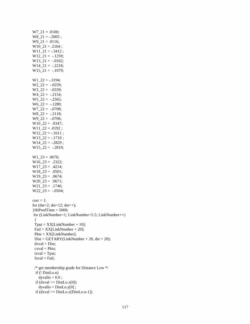
117
W7_21 = .0100;W8_21 = -.5005 ;W9_21 = .0116;W10_21 = .2164 ;W11_21 = -.3412 ;W12_21 = -.1259;W13_21 = -.0162;W14_21 = -.2218;W15_21 = -.1079;
W1_22 = -.3194;W2_22 = -.0259;W3_22 = -.0339;W4_22 = -.2154;W5_22 = -.2565;W6_22 = -.1280;W7_22 = -.0708;W8_22 = -.2118;W9_22 = -.0706;W10_22 = .0347;W11_22 = .0192 ;W12_22 = -.1611 ;W13_22 = -.1710 ;W14_22 = -.2829 ;W15_22 = -.2819;
W1_23 = .0676;W16_23 = .2322;W17_23 = .4214;W18_23 = .0501;W19_23 = .0674;W20_23 = .0671;W21_23 = .1746;W22_23 = -.0504;
curr = 1;for (dst=2; dst<12; dst++);{HiPredTime = 5000; for (LinkNumber=1; LinkNumber<5.5; LinkNumber++) { Tput = XX[LinkNumber + 10]; Fail = XX[LinkNumber + 20]; Pkts = XX[LinkNumber]; Dist = GETARY(LinkNumber + 20, dst + 20); dxval = Dist; cxval = Pkts; txval = Tput; fxval = Fail;
/* get membership grade for Distance Low */ if (! DistLo.n) dyvallo = 0.0 ; if (dxval <= DistLo.x[0]) dyvallo = DistLo.y[0] ; if (dxval >= DistLo.x[DistLo.n-1])

118
dyvallo = DistLo.y[DistLo.n-1] ; lo = 0 ; // We will keep x[lo] strictly less than dxval hi = DistLo.n-1 ; // and x[hi] greater or equal to dxval for (;;) { // Cuts interval in half each time mid = (lo + hi) / 2 ; // Center of interval if (mid == lo) // Happens when lo and hi adjacent break ; // So then we are done if (DistLo.x[mid] < dxval) // Replace appropriate interval end with mid lo = mid ; else hi = mid ; }
yyy = (dxval - DistLo.x[hi-1])/(DistLo.x[hi]-DistLo.x[hi-1])*(DistLo.y[hi]-DistLo.y[hi-1]); dyvallo = yyy + DistLo.y[hi-1] ;
/* get membership grade for Distance Medium */ if (! DistMd.n) dyvalmd = 0.0 ; if (dxval <= DistMd.x[0]) dyvalmd = DistMd.y[0] ; if (dxval >= DistMd.x[DistMd.n-1]) dyvalmd = DistMd.y[DistMd.n-1] ; lo = 0 ; // We will keep x[lo] strictly less than dxval hi = DistMd.n-1 ; // and x[hi] greater or equal to dxval for (;;) { // Cuts interval in half each time mid = (lo + hi) / 2 ; // Center of interval if (mid == lo) // Happens when lo and hi adjacent break ; // So then we are done if (DistMd.x[mid] < dxval) // Replace appropriate interval end with mid lo = mid ; else hi = mid ; } yyy = (dxval - DistMd.x[hi-1])/(DistMd.x[hi]-DistMd.x[hi-1])*(DistMd.y[hi]-DistMd.y[hi-1]); dyvalmd = yyy + DistMd.y[hi-1] ;
/* get membership grade for Distance High */ if (! DistHi.n) dyvalhi = 0.0 ;
if (dxval <= DistHi.x[0]) dyvalhi = DistHi.y[0] ;
if (dxval >= DistHi.x[DistHi.n-1]) dyvalhi = DistHi.y[DistHi.n-1] ;
lo = 0 ; // We will keep x[lo] strictly less than dxval hi = DistHi.n-1 ; // and x[hi] greater or equal to dxval for (;;) { // Cuts interval in half each time mid = (lo + hi) / 2 ; // Center of interval if (mid == lo) // Happens when lo and hi adjacent break ; // So then we are done if (DistHi.x[mid] < dxval) // Replace appropriate interval end with mid lo = mid ;
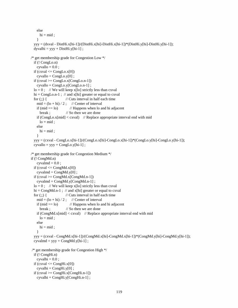
119
else hi = mid ; } yyy = (dxval - DistHi.x[hi-1])/(DistHi.x[hi]-DistHi.x[hi-1])*(DistHi.y[hi]-DistHi.y[hi-1]); dyvalhi = yyy + DistHi.y[hi-1] ;
/* get membership grade for Congestion Low */ if (! CongLo.n) cyvallo = 0.0 ; if (cxval <= CongLo.x[0]) cyvallo = CongLo.y[0] ; if (cxval >= CongLo.x[CongLo.n-1]) cyvallo = CongLo.y[CongLo.n-1] ; lo = 0 ; // We will keep x[lo] strictly less than cxval hi = CongLo.n-1 ; // and x[hi] greater or equal to cxval for (;;) { // Cuts interval in half each time mid = (lo + hi) / 2 ; // Center of interval if (mid == lo) // Happens when lo and hi adjacent break ; // So then we are done if (CongLo.x[mid] < cxval) // Replace appropriate interval end with mid lo = mid ; else hi = mid ; } yyy = (cxval - CongLo.x[hi-1])/(CongLo.x[hi]-CongLo.x[hi-1])*(CongLo.y[hi]-CongLo.y[hi-1]); cyvallo = yyy + CongLo.y[hi-1] ;
/* get membership grade for Congestion Medium */if (! CongMd.n) cyvalmd = 0.0 ; if (cxval <= CongMd.x[0]) cyvalmd = CongMd.y[0] ; if (cxval >= CongMd.x[CongMd.n-1]) cyvalmd = CongMd.y[CongMd.n-1] ; lo = 0 ; // We will keep x[lo] strictly less than cxval hi = CongMd.n-1 ; // and x[hi] greater or equal to cxval for (;;) { // Cuts interval in half each time mid = (lo + hi) / 2 ; // Center of interval if (mid == lo) // Happens when lo and hi adjacent break ; // So then we are done if (CongMd.x[mid] < cxval) // Replace appropriate interval end with mid lo = mid ; else hi = mid ; } yyy = (cxval - CongMd.x[hi-1])/(CongMd.x[hi]-CongMd.x[hi-1])*(CongMd.y[hi]-CongMd.y[hi-1]); cyvalmd = yyy + CongMd.y[hi-1] ;
/* get membership grade for Congestion High */ if (! CongHi.n) cyvalhi = 0.0 ; if (cxval <= CongHi.x[0]) cyvalhi = CongHi.y[0] ; if (cxval >= CongHi.x[CongHi.n-1]) cyvalhi = CongHi.y[CongHi.n-1] ;
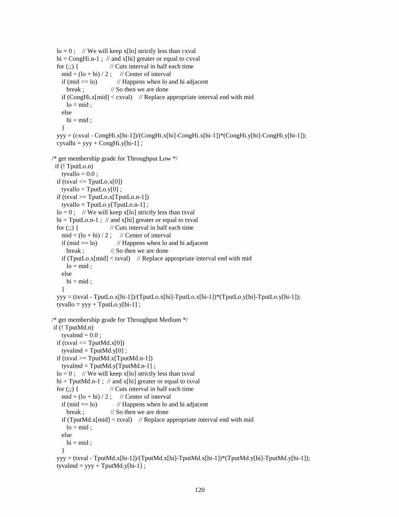
120
lo = 0 ; // We will keep x[lo] strictly less than cxval hi = CongHi.n-1 ; // and x[hi] greater or equal to cxval for (;;) { // Cuts interval in half each time mid = (lo + hi) / 2 ; // Center of interval if (mid == lo) // Happens when lo and hi adjacent break ; // So then we are done if (CongHi.x[mid] < cxval) // Replace appropriate interval end with mid lo = mid ; else hi = mid ; } yyy = (cxval - CongHi.x[hi-1])/(CongHi.x[hi]-CongHi.x[hi-1])*(CongHi.y[hi]-CongHi.y[hi-1]); cyvalhi = yyy + CongHi.y[hi-1] ;
/* get membership grade for Throughput Low */ if (! TputLo.n) tyvallo = 0.0 ; if (txval <= TputLo.x[0]) tyvallo = TputLo.y[0] ; if (txval >= TputLo.x[TputLo.n-1]) tyvallo = TputLo.y[TputLo.n-1] ; lo = 0 ; // We will keep x[lo] strictly less than txval hi = TputLo.n-1 ; // and x[hi] greater or equal to txval for (;;) { // Cuts interval in half each time mid = (lo + hi) / 2 ; // Center of interval if (mid == lo) // Happens when lo and hi adjacent break ; // So then we are done if (TputLo.x[mid] < txval) // Replace appropriate interval end with mid lo = mid ; else hi = mid ; } yyy = (txval - TputLo.x[hi-1])/(TputLo.x[hi]-TputLo.x[hi-1])*(TputLo.y[hi]-TputLo.y[hi-1]); tyvallo = yyy + TputLo.y[hi-1] ;
/* get membership grade for Throughput Medium */ if (! TputMd.n) tyvalmd = 0.0 ; if (txval <= TputMd.x[0]) tyvalmd = TputMd.y[0] ; if (txval >= TputMd.x[TputMd.n-1]) tyvalmd = TputMd.y[TputMd.n-1] ; lo = 0 ; // We will keep x[lo] strictly less than txval hi = TputMd.n-1 ; // and x[hi] greater or equal to txval for (;;) { // Cuts interval in half each time mid = (lo + hi) / 2 ; // Center of interval if (mid == lo) // Happens when lo and hi adjacent break ; // So then we are done if (TputMd.x[mid] < txval) // Replace appropriate interval end with mid lo = mid ; else hi = mid ; } yyy = (txval - TputMd.x[hi-1])/(TputMd.x[hi]-TputMd.x[hi-1])*(TputMd.y[hi]-TputMd.y[hi-1]); tyvalmd = yyy + TputMd.y[hi-1] ;

121
/* get membership grade for Throughput High */ if (! TputHi.n) tyvalhi = 0.0 ; if (txval <= TputHi.x[0]) tyvalhi = TputHi.y[0] ; if (txval >= TputHi.x[TputHi.n-1]) tyvalhi = TputHi.y[TputHi.n-1] ; lo = 0 ; // We will keep x[lo] strictly less than txval hi = TputHi.n-1 ; // and x[hi] greater or equal to txval for (;;) { // Cuts interval in half each time mid = (lo + hi) / 2 ; // Center of interval if (mid == lo) // Happens when lo and hi adjacent break ; // So then we are done if (TputHi.x[mid] < txval) // Replace appropriate interval end with mid lo = mid ; else hi = mid ; } yyy = (txval - TputHi.x[hi-1])/(TputHi.x[hi]-TputHi.x[hi-1])*(TputHi.y[hi]-TputHi.y[hi-1]); tyvalhi = yyy + TputHi.y[hi-1] ;
/* get membership grade for Failure Low */ if (! FailLo.n) fyvallo = 0.0 ; if (fxval <= FailLo.x[0]) fyvallo = FailLo.y[0] ; if (fxval >= FailLo.x[FailLo.n-1]) fyvallo = FailLo.y[FailLo.n-1] ; lo = 0 ; // We will keep x[lo] strictly less than fxval hi = FailLo.n-1 ; // and x[hi] greater or equal to fxval for (;;) { // Cuts interval in half each time mid = (lo + hi) / 2 ; // Center of interval if (mid == lo) // Happens when lo and hi adjacent break ; // So then we are done if (FailLo.x[mid] < fxval) // Replace appropriate interval end with mid lo = mid ; else hi = mid ; } yyy = (fxval - FailLo.x[hi-1])/(FailLo.x[hi]-FailLo.x[hi-1])*(FailLo.y[hi]-FailLo.y[hi-1]); fyvallo = yyy + FailLo.y[hi-1] ;
/* get membership grade for Failure Medium */if (! FailMd.n) fyvalmd = 0.0 ; if (fxval <= FailMd.x[0]) fyvalmd = FailMd.y[0] ; if (fxval >= FailMd.x[FailMd.n-1]) fyvalmd = FailMd.y[FailMd.n-1] ; lo = 0 ; // We will keep x[lo] strictly less than fxval hi = FailMd.n-1 ; // and x[hi] greater or equal to fxval for (;;) { // Cuts interval in half each time mid = (lo + hi) / 2 ; // Center of interval if (mid == lo) // Happens when lo and hi adjacent

122
break ; // So then we are done if (FailMd.x[mid] < fxval) // Replace appropriate interval end with mid lo = mid ; else hi = mid ; } yyy = (fxval - FailMd.x[hi-1])/(FailMd.x[hi]-FailMd.x[hi-1])*(FailMd.y[hi]-FailMd.y[hi-1]); fyvalmd = yyy + FailMd.y[hi-1] ;
/* get membership grade for Failure High */ if (! FailHi.n) fyvalhi = 0.0 ; if (fxval <= FailHi.x[0]) fyvalhi = FailHi.y[0] ; if (fxval >= FailHi.x[FailHi.n-1]) fyvalhi = FailHi.y[FailHi.n-1] ; lo = 0 ; // We will keep x[lo] strictly less than fxval hi = FailHi.n-1 ; // and x[hi] greater or equal to fxval for (;;) { // Cuts interval in half each time mid = (lo + hi) / 2 ; // Center of interval if (mid == lo) // Happens when lo and hi adjacent break ; // So then we are done if (FailHi.x[mid] < fxval) // Replace appropriate interval end with mid lo = mid ; else hi = mid ; } yyy = (fxval - FailHi.x[hi-1])/(FailHi.x[hi]-FailHi.x[hi-1])*(FailHi.y[hi]-FailHi.y[hi-1]); fyvalhi = yyy+FailHi.y[hi-1] ;
/* The next statements establish the input into the neural network. */ I1= 1.0; //bias I2 = tyvallo; I3 = tyvalmd; I4 = tyvalhi; I5 = cyvallo; I6 = cyvalmd; I7 = cyvalhi; I8 = fyvallo; I9 = fyvalmd; I10 = fyvalhi; I11 = dyvallo; I12 = dyvalmd; I13 = dyvalhi; I14 = (PktSz-1)/1499; I15 = (Dest-2)/10;
/* The next statements calculate values at the hidden layer in the neural network. */ I16 = (I1*W1_16)+(I2*W2_16)+(I3*W3_16)+(I4*W4_16)+(I5*W5_16)+(I6*W6_16); I16 = I16 + (I7*W7_16)+(I8*W8_16)+(I9*W9_16)+(I10*W10_16)+(I11*W11_16); I16 = I16 + (I12*W12_16)+(I13*W13_16)+(I14*W14_16)+(I15*W15_16);
I17 = (I1*W1_17)+(I2*W2_17)+(I3*W3_17)+(I4*W4_17)+(I5*W5_17)+(I6*W6_17); I17 = I17 + (I7*W7_17)+(I8*W8_17)+(I9*W9_17)+(I10*W10_17)+(I11*W11_17); I17 = I17 + (I12*W12_17)+(I13*W13_17)+(I14*W14_17)+(I15*W15_17);
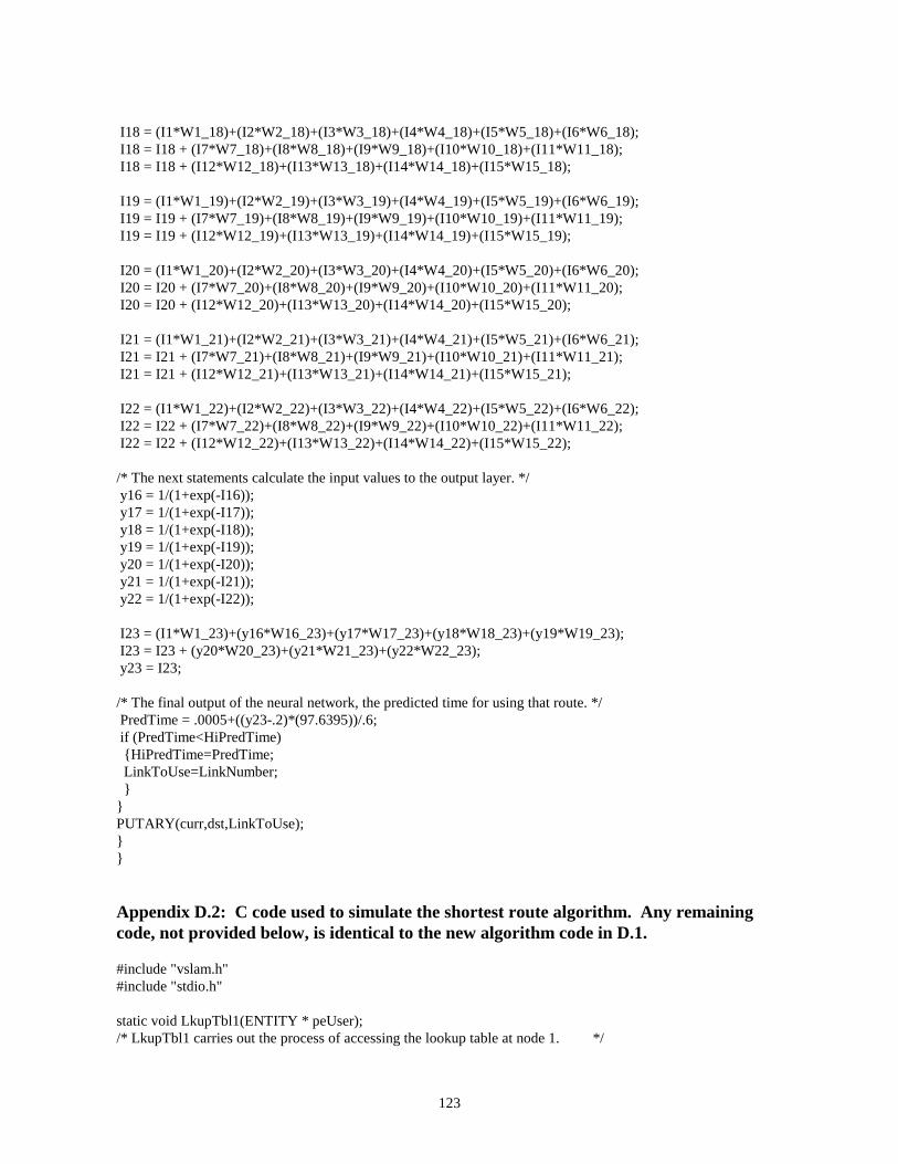
123
I18 = (I1*W1_18)+(I2*W2_18)+(I3*W3_18)+(I4*W4_18)+(I5*W5_18)+(I6*W6_18); I18 = I18 + (I7*W7_18)+(I8*W8_18)+(I9*W9_18)+(I10*W10_18)+(I11*W11_18); I18 = I18 + (I12*W12_18)+(I13*W13_18)+(I14*W14_18)+(I15*W15_18);
I19 = (I1*W1_19)+(I2*W2_19)+(I3*W3_19)+(I4*W4_19)+(I5*W5_19)+(I6*W6_19); I19 = I19 + (I7*W7_19)+(I8*W8_19)+(I9*W9_19)+(I10*W10_19)+(I11*W11_19); I19 = I19 + (I12*W12_19)+(I13*W13_19)+(I14*W14_19)+(I15*W15_19);
I20 = (I1*W1_20)+(I2*W2_20)+(I3*W3_20)+(I4*W4_20)+(I5*W5_20)+(I6*W6_20); I20 = I20 + (I7*W7_20)+(I8*W8_20)+(I9*W9_20)+(I10*W10_20)+(I11*W11_20); I20 = I20 + (I12*W12_20)+(I13*W13_20)+(I14*W14_20)+(I15*W15_20);
I21 = (I1*W1_21)+(I2*W2_21)+(I3*W3_21)+(I4*W4_21)+(I5*W5_21)+(I6*W6_21); I21 = I21 + (I7*W7_21)+(I8*W8_21)+(I9*W9_21)+(I10*W10_21)+(I11*W11_21); I21 = I21 + (I12*W12_21)+(I13*W13_21)+(I14*W14_21)+(I15*W15_21);
I22 = (I1*W1_22)+(I2*W2_22)+(I3*W3_22)+(I4*W4_22)+(I5*W5_22)+(I6*W6_22); I22 = I22 + (I7*W7_22)+(I8*W8_22)+(I9*W9_22)+(I10*W10_22)+(I11*W11_22); I22 = I22 + (I12*W12_22)+(I13*W13_22)+(I14*W14_22)+(I15*W15_22);
/* The next statements calculate the input values to the output layer. */ y16 = 1/(1+exp(-I16)); y17 = 1/(1+exp(-I17)); y18 = 1/(1+exp(-I18)); y19 = 1/(1+exp(-I19)); y20 = 1/(1+exp(-I20)); y21 = 1/(1+exp(-I21)); y22 = 1/(1+exp(-I22));
I23 = (I1*W1_23)+(y16*W16_23)+(y17*W17_23)+(y18*W18_23)+(y19*W19_23); I23 = I23 + (y20*W20_23)+(y21*W21_23)+(y22*W22_23); y23 = I23;
/* The final output of the neural network, the predicted time for using that route. */ PredTime = .0005+((y23-.2)*(97.6395))/.6; if (PredTime<HiPredTime) {HiPredTime=PredTime; LinkToUse=LinkNumber; }}PUTARY(curr,dst,LinkToUse);}}
Appendix D.2: C code used to simulate the shortest route algorithm. Any remainingcode, not provided below, is identical to the new algorithm code in D.1.
#include "vslam.h"#include "stdio.h"
static void LkupTbl1(ENTITY * peUser);/* LkupTbl1 carries out the process of accessing the lookup table at node 1. */
124
/* When a packet at node 1 needs to be routed to another node, this lookup table *//* determines which link the packet will traverse next. */
static void GetNextNode1(ENTITY * peUser);static void GetNextNode2(ENTITY * peUser);static void GetNextNode3(ENTITY * peUser);static void GetNextNode4(ENTITY * peUser);static void GetNextNode5(ENTITY * peUser);static void GetNextNode6(ENTITY * peUser);static void GetNextNode7(ENTITY * peUser);static void GetNextNode8(ENTITY * peUser);static void GetNextNode9(ENTITY * peUser);static void GetNextNode10(ENTITY * peUser);static void GetNextNode11(ENTITY * peUser);static void GetNextNode12(ENTITY * peUser);/* GetNextNode1 – GetNextNode12 are used to access the lookup tables at nodes 1 – 12 and *//* determine the next node the packet will travel to. */
static void UpdateDistance(ENTITY * peUser);/* UpdateDistance is used as a part of the simulation program to change the routing table at node 1. *//* This is necessary for data as it provides a larger variety of situations for data collection. */
static void SegmentPacket(ENTITY * peUser);/* SegmentPacket takes an originating packet being transmitted and breaks it up into smaller packets *//* that the transmission media of the network will accept. This must be done before any part of that *//* data can be sent. */
static void UpdateTable(ENTITY * peUser);/* This is the code used to update the lookup table using the shortest route algorithm. */
static void GetDistance(ENTITY * peUser);
BOOL SWFUNC INTLC(UINT uiRun){ BOOL bReturn = TRUE;
/* Initialize the NEXTLINK table for current nodes 1 through 12 */ PUTARY(1,1,0); PUTARY(2,1,6); PUTARY(3,1,7); PUTARY(4,1,8); PUTARY(1,2,1); PUTARY(2,2,0); PUTARY(3,2,7); PUTARY(4,2,8); PUTARY(1,3,2); PUTARY(2,3,6); PUTARY(3,3,0); PUTARY(4,3,8); PUTARY(1,4,3); PUTARY(2,4,6); PUTARY(3,4,7); PUTARY(4,4,0); PUTARY(1,5,4); PUTARY(2,5,6); PUTARY(3,5,7); PUTARY(4,5,8); PUTARY(1,6,5); PUTARY(2,6,6); PUTARY(3,6,7); PUTARY(4,6,8); PUTARY(1,7,1); PUTARY(2,7,6); PUTARY(3,7,7); PUTARY(4,7,8); PUTARY(1,8,2); PUTARY(2,8,6); PUTARY(3,8,7); PUTARY(4,8,8); PUTARY(1,9,3); PUTARY(2,9,6); PUTARY(3,9,7); PUTARY(4,9,8); PUTARY(1,10,4); PUTARY(2,10,6); PUTARY(3,10,7); PUTARY(4,10,8); PUTARY(1,11,5); PUTARY(2,11,6); PUTARY(3,11,7); PUTARY(4,11,8); PUTARY(1,12,5); PUTARY(2,12,6); PUTARY(3,12,7); PUTARY(4,12,8);
PUTARY(5,1,9); PUTARY(6,1,10); PUTARY(7,1,12); PUTARY(8,1,15); PUTARY(5,2,9); PUTARY(6,2,10); PUTARY(7,2,12); PUTARY(8,2,15); PUTARY(5,3,9); PUTARY(6,3,10); PUTARY(7,3,12); PUTARY(8,3,15); PUTARY(5,4,9); PUTARY(6,4,10); PUTARY(7,4,12); PUTARY(8,4,15); PUTARY(5,5,0); PUTARY(6,5,10); PUTARY(7,5,12); PUTARY(8,5,15);
125
PUTARY(5,6,9); PUTARY(6,6,0); PUTARY(7,6,12); PUTARY(8,6,15); PUTARY(5,7,9); PUTARY(6,7,10); PUTARY(7,7,0); PUTARY(8,7,15); PUTARY(5,8,9); PUTARY(6,8,10); PUTARY(7,8,12); PUTARY(8,8,0); PUTARY(5,9,9); PUTARY(6,9,10); PUTARY(7,9,12); PUTARY(8,9,15); PUTARY(5,10,9); PUTARY(6,10,10); PUTARY(7,10,12); PUTARY(8,10,15); PUTARY(5,11,9); PUTARY(6,11,10); PUTARY(7,11,12); PUTARY(8,11,15); PUTARY(5,12,9); PUTARY(6,12,10); PUTARY(7,12,12); PUTARY(8,12,15);
PUTARY(9,1,14); PUTARY(10,1,11); PUTARY(11,1,16); PUTARY(12,1,17); PUTARY(9,2,14); PUTARY(10,2,11); PUTARY(11,2,16); PUTARY(12,2,17); PUTARY(9,3,14); PUTARY(10,3,11); PUTARY(11,3,16); PUTARY(12,3,17); PUTARY(9,4,14); PUTARY(10,4,11); PUTARY(11,4,16); PUTARY(12,4,17); PUTARY(9,5,14); PUTARY(10,5,11); PUTARY(11,5,16); PUTARY(12,5,17); PUTARY(9,6,14); PUTARY(10,6,11); PUTARY(11,6,16); PUTARY(12,6,17); PUTARY(9,7,14); PUTARY(10,7,11); PUTARY(11,7,16); PUTARY(12,7,17); PUTARY(9,8,14); PUTARY(10,8,11); PUTARY(11,8,16); PUTARY(12,8,17); PUTARY(9,9,0); PUTARY(10,9,11); PUTARY(11,9,16); PUTARY(12,9,17); PUTARY(9,10,14); PUTARY(10,10,0); PUTARY(11,10,16); PUTARY(12,10,17); PUTARY(9,11,14); PUTARY(10,11,17); PUTARY(11,11,0); PUTARY(12,11,16); PUTARY(9,12,14); PUTARY(10,12,11); PUTARY(11,12,16); PUTARY(12,12,0);
/* Initialize Distance (#hops to destination using links 1-5) matrix */
PUTARY(21,22,1); PUTARY(22,22,3); PUTARY(23,22,5); PUTARY(24,22,5); PUTARY(25,22,5); PUTARY(21,23,3); PUTARY(22,23,1); PUTARY(23,23,5); PUTARY(24,23,5); PUTARY(25,23,5); PUTARY(21,24,5); PUTARY(22,24,5); PUTARY(23,24,1); PUTARY(24,24,3); PUTARY(25,24,3); PUTARY(21,25,5); PUTARY(22,25,5); PUTARY(23,25,3); PUTARY(24,25,1); PUTARY(25,25,3); PUTARY(21,26,5); PUTARY(22,26,5); PUTARY(23,26,3); PUTARY(24,26,3); PUTARY(25,26,1); PUTARY(21,27,2); PUTARY(22,27,2); PUTARY(23,27,4); PUTARY(24,27,4); PUTARY(25,27,4); PUTARY(21,28,3); PUTARY(22,28,3); PUTARY(23,28,3); PUTARY(24,28,3); PUTARY(25,28,3); PUTARY(21,29,4); PUTARY(22,29,4); PUTARY(23,29,2); PUTARY(24,29,2); PUTARY(25,29,2); PUTARY(21,30,4); PUTARY(22,30,4); PUTARY(23,30,4); PUTARY(24,30,4); PUTARY(25,30,2); PUTARY(21,31,3); PUTARY(22,31,3); PUTARY(23,31,5); PUTARY(24,31,5); PUTARY(25,31,4); PUTARY(21,32,4); PUTARY(22,32,4); PUTARY(23,32,5); PUTARY(24,32,5); PUTARY(25,32,3);
return(bReturn);}
void SWFUNC EVENT(int iCode, ENTITY * peUser){ switch (iCode) { case 1: /* arrive to event node 1 - GetNextNode1 */ GetNextNode1(peUser); break; case 2: /* arrive to event node 2 – GetNextNode2 */ GetNextNode2(peUser); break; case 3: /* arrive to event node 3 – GetNextNode3 */ GetNextNode3(peUser); break; case 4: /* arrive to event node 4 – GetNextNode4 */ GetNextNode4(peUser); break; case 5: /* arrive to event node 5 – GetNextNode5 */
126
GetNextNode5(peUser); break; case 6: /* arrive to event node 6 – GetNextNode6 */ GetNextNode6(peUser); break; case 7: /* arrive to event node 7 – GetNextNode7 */ GetNextNode7(peUser); break; case 8: /* arrive to event node 8 – GetNextNode8 */ GetNextNode8(peUser); break; case 9: /* arrive to event node 9 – GetNextNode9 */ GetNextNode9(peUser); break; case 10: /* arrive to event node 10 - GetNextNode10 */ GetNextNode10(peUser); break; case 11: /* arrive to event node 11 - GetNextNode11 */ GetNextNode11(peUser); break; case 12: /* arrive to event node 12 - GetNextNode12 */ GetNextNode12(peUser); break; case 17: /* arrive to event node 17 */ GetDistance(peUser); break; case 19: /* arrive to event node 19 */ SegmentPacket(peUser); break; case 20: /* arrive to event node 20 - LkupTbl1 */ LkupTbl1(peUser); break; case 23: /* arrive to event node 23 */ UpdateDistance(peUser); break; case 26: /* arrive to event node 26 */ UpdateTable(peUser); break; default: su_error(1,"Unknown event code"); break; }}
static void SWFUNC LkupTbl1(ENTITY * peUser){ int NextLink = GETARY(peUser->ATRIB[2],peUser->ATRIB[3]); peUser->ATRIB[5] = NextLink;}
static void SWFUNC GetNextNode1(ENTITY * peUser){ int NextNode = 0; if (peUser->ATRIB[5]==1.0) NextNode = 2; else if (peUser->ATRIB[5]==2.0) NextNode = 3;
127
else if (peUser->ATRIB[5]==3.0) NextNode = 4; else if (peUser->ATRIB[5]==4.0) NextNode = 5; else if (peUser->ATRIB[5]==5.0) NextNode = 6; peUser->ATRIB[6] = NextNode;}
static void SWFUNC GetNextNode2(ENTITY * peUser){ int NextNode = 0; if (peUser->ATRIB[5]==1.0) NextNode = 1; else if (peUser->ATRIB[5]==6.0) NextNode = 7; peUser->ATRIB[6] = NextNode;}
static void SWFUNC GetNextNode3(ENTITY * peUser){ int NextNode = 0; if (peUser->ATRIB[5]==2.0) NextNode = 1; else if (peUser->ATRIB[5]==7.0) NextNode = 7; peUser->ATRIB[6] = NextNode;}
static void SWFUNC GetNextNode4(ENTITY * peUser){ int NextNode = 0; if (peUser->ATRIB[5]==3.0) NextNode = 1; else if (peUser->ATRIB[5]==8.0) NextNode = 9; peUser->ATRIB[6] = NextNode;}
static void SWFUNC GetNextNode5(ENTITY * peUser){ int NextNode = 0; if (peUser->ATRIB[5]==4.0) NextNode = 1; else if (peUser->ATRIB[5]==9.0) NextNode = 9; peUser->ATRIB[6] = NextNode;}
static void SWFUNC GetNextNode6(ENTITY * peUser){ int NextNode = 0; if (peUser->ATRIB[5]==5.0) NextNode = 1; else if (peUser->ATRIB[5]==10.0) NextNode = 9; else if (peUser->ATRIB[5]==11.0) NextNode = 10; peUser->ATRIB[6] = NextNode;}
static void SWFUNC GetNextNode7(ENTITY * peUser){ int NextNode = 0; if (peUser->ATRIB[5]==6.0) NextNode = 2; else if (peUser->ATRIB[5]==7.0) NextNode = 3; else if (peUser->ATRIB[5]==12.0) NextNode = 11; else if (peUser->ATRIB[5]==13.0) NextNode = 8; peUser->ATRIB[6] = NextNode;
128
}
static void SWFUNC GetNextNode8(ENTITY * peUser){ int NextNode = 0; if (peUser->ATRIB[5]==13.0) NextNode = 7; else if (peUser->ATRIB[5]==14.0) NextNode = 9; else if (peUser->ATRIB[5]==15.0) NextNode = 10; peUser->ATRIB[6] = NextNode;}
static void SWFUNC GetNextNode9(ENTITY * peUser){ int NextNode = 0; if (peUser->ATRIB[5]==8.0) NextNode = 4; else if (peUser->ATRIB[5]==9.0) NextNode = 5; else if (peUser->ATRIB[5]==10.0) NextNode = 6; else if (peUser->ATRIB[5]==14.0) NextNode = 8; peUser->ATRIB[6] = NextNode;}
static void SWFUNC GetNextNode10(ENTITY * peUser){ int NextNode = 0; if (peUser->ATRIB[5]==11.0) NextNode = 6; else if (peUser->ATRIB[5]==15.0) NextNode = 8; else if (peUser->ATRIB[5]==17.0) NextNode = 12; peUser->ATRIB[6] = NextNode;}
static void SWFUNC GetNextNode11(ENTITY * peUser){ int NextNode = 0; if (peUser->ATRIB[5]==12.0) NextNode = 7; else if (peUser->ATRIB[5]==16.0) NextNode = 12; peUser->ATRIB[6] = NextNode;}
static void SWFUNC GetNextNode12(ENTITY * peUser){ int NextNode = 0; if (peUser->ATRIB[5]==16.0) NextNode = 11; else if (peUser->ATRIB[5]==17.0) NextNode = 10; peUser->ATRIB[6] = NextNode;}
static void UpdateDistance(ENTITY * peUser){ if (XX[26] != 0.0) { PUTARY(21,23,99); PUTARY(21,26,99); PUTARY(21,28,99); PUTARY(21,24,99); PUTARY(21,27,99); PUTARY(21,29,99); PUTARY(21,25,99); PUTARY(22,22,99); PUTARY(21,30,99); PUTARY(21,31,99); PUTARY(21,32,99); PUTARY(23,22,99); PUTARY(24,22,99); PUTARY(25,22,99); }
129
if (XX[27] != 0.0) { PUTARY(21,23,99); PUTARY(22,22,99); PUTARY(22,28,99); PUTARY(23,23,99); PUTARY(22,24,99); PUTARY(22,29,99); PUTARY(24,23,99); PUTARY(22,25,99); PUTARY(22,30,99); PUTARY(25,23,99); PUTARY(21,26,99); PUTARY(22,31,99); PUTARY(22,32,99); PUTARY(22,27,99); }
if (XX[28] != 0.0) { PUTARY(23,22,99); PUTARY(23,23,99); PUTARY(24,24,99); PUTARY(22,24,99); PUTARY(23,30,99); PUTARY(25,24,99); PUTARY(23,26,99); PUTARY(23,32,99); PUTARY(23,25,99); PUTARY(23,29,99); PUTARY(23,27,99); PUTARY(23,31,99); PUTARY(21,24,99); PUTARY(23,28,99); }
if (XX[29] != 0.0) { PUTARY(24,22,99); PUTARY(23,25,99); PUTARY(24,29,99); PUTARY(24,23,99); PUTARY(25,25,99); PUTARY(24,30,99); PUTARY(24,24,99); PUTARY(24,26,99); PUTARY(24,31,99); PUTARY(21,25,99); PUTARY(24,27,99); PUTARY(22,25,99); PUTARY(24,28,99); PUTARY(24,32,99); }
if (XX[30] != 0.0) { PUTARY(25,24,5); PUTARY(23,26,5); PUTARY(25,25,5); PUTARY(24,26,5); PUTARY(25,29,4); }
if (XX[31] != 0.0) { PUTARY(25,30,4); PUTARY(25,31,5); PUTARY(25,32,5); }
if (XX[32] != 0.0) { PUTARY(21,31,6); PUTARY(24,31,6); PUTARY(22,31,6); PUTARY(23,31,6); PUTARY(21,32,5); PUTARY(22,32,5); } if (XX[33] != 0.0) { PUTARY(23,22,8); PUTARY(23,23,8); PUTARY(21,24,8); PUTARY(24,22,8); PUTARY(24,23,8); PUTARY(22,24,8); PUTARY(25,22,6); PUTARY(25,23,6); PUTARY(21,25,8); PUTARY(22,26,6); PUTARY(22,25,8); PUTARY(21,26,6); PUTARY(21,29,7); PUTARY(23,27,7); PUTARY(21,28,6); PUTARY(22,29,7); PUTARY(24,27,7); PUTARY(22,28,6); PUTARY(21,30,5); PUTARY(25,27,5); PUTARY(24,31,6); PUTARY(22,30,5); PUTARY(23,31,6); }
if (XX[34] != 0.0) { PUTARY(21,24,7); PUTARY(23,22,7); PUTARY(23,23,7); PUTARY(22,24,7); PUTARY(24,22,7); PUTARY(24,23,7); PUTARY(23,28,5); PUTARY(21,25,7); PUTARY(23,27,6); PUTARY(21,29,6); PUTARY(22,25,7); PUTARY(24,27,6); PUTARY(22,29,6); PUTARY(24,28,5); PUTARY(23,31,6);

130
PUTARY(24,31,6); }
if (XX[35] != 0.0) { PUTARY(21,30,5); PUTARY(22,30,5); }
if (XX[36] != 0.0) { PUTARY(25,31,5); PUTARY(21,32,5); PUTARY(22,32,5); }
if (XX[37] != 0.0) { PUTARY(25,31,5); PUTARY(23,32,6); PUTARY(24,32,6); PUTARY(25,32,6); }}
static void SegmentPacket(ENTITY * peUser){ ENTITY *peNew; int NumOfSegs; int count; if (peUser->ATRIB[4] > 1500) { NumOfSegs = peUser->ATRIB[4]/1500; count = NumOfSegs; while (count > 0) { peNew = su_entnew(0,NULL,NULL,NULL); peNew->ATRIB[1] = TNOW; peNew->ATRIB[2] = peUser->ATRIB[2]; peNew->ATRIB[3] = peUser->ATRIB[3]; peNew->ATRIB[4] = 1500; peNew->ATRIB[18] = 1; ENTER(1,peNew); count = count-1; } peNew = su_entnew(0,NULL,NULL,NULL); peNew->ATRIB[1] = TNOW; peNew->ATRIB[2] = peUser->ATRIB[2]; peNew->ATRIB[3] = peUser->ATRIB[3]; peNew->ATRIB[4] = peUser->ATRIB[4]-(1500*NumOfSegs); peNew->ATRIB[18] = 1; ENTER(1,peNew); } if (peUser->ATRIB[4] <= 1500) { peNew = su_entnew(0,NULL,NULL,NULL); peNew->ATRIB[1] = TNOW; peNew->ATRIB[2] = peUser->ATRIB[2]; peNew->ATRIB[3] = peUser->ATRIB[3]; peNew->ATRIB[4] = peUser->ATRIB[4]; peNew->ATRIB[18] = 1; ENTER(1,peNew); }}
static void UpdateTable(ENTITY * peUser)
131
{ int curr, dest, y, dist, link,x; curr=1; for (dest=2; dest<13; dest++) { y = dest + 20; dist = 100; link = 1; for (x=21; x<26; x++) { if (GETARY(x,y)<dist) { dist = GETARY(x,y); link = x-20; } } }}
static void GetDistance(ENTITY * peUser){ peUser->ATRIB[19] = GETARY(peUser->ATRIB[5] + 20,peUser->ATRIB[3] + 20); peUser->ATRIB[18] = 0; }

132
VitaJulia K. Brande
Julia was born on October 8, 1969 in Greensboro, North Carolina. She resided in North
Carolina throughout most of her school years.
In 1987, Julia enrolled in North Carolina State University where she spent four years
pursuing two degrees. She graduated in 1991 with a BS in Statistics as well as a BS in
Applied Mathematics. While waiting to begin her graduate studies, she worked as a statistical
computer programmer at Quintiles, Inc. in Research Triangle Park, North Carolina.
Julia chose to continue her education at Virginia Tech while continuing her work at
Quintiles when classes would permit. She completed her MS in Statistics in 1992 and
remained at Virginia Tech as a member of the Ph.D. program in the Department of
Management Science and Information Technology. She began the program in 1993 where she
served as a lecturer in the department while working on her dissertation.
Now that Julia has completed her Ph.D. work, she has returned to North Carolina State
University where she is currently an Assistant Professor of Management Information Systems
under the name Julia Brande Earp.