Embed Size (px)
Citation preview
Computer Network-1 10CS55
Dept of CSE, GCEM 1
SYLLABUS
COMPUTER NETWORKS – I
Subject Code: 10CS55 I.A. Marks : 25
Hours/Week : 04 Exam Hours: 03
Total Hours : 52 Exam Marks: 100
PART – A
UNIT - 1 7 Hours Introduction: Data Communications, Networks, The Internet, Protocols & Standards, Layered
Tasks, The OSI model, Layers in OSI model, TCP/IP Protocol suite, Addressing
UNIT- 2 7 Hours Physical Layer-1: Analog & Digital Signals, Transmission Impairment, Data Rate limits,
Performance, Digital-digital conversion (Only Line coding: Polar, Bipolar and Manchester
coding), Analog-to-digital conversion (only PCM), Transmission Modes, Digital-to-analog
conversion
UNIT- 3 6 Hours Physical Layer-2 and Switching: Multiplexing, Spread Spectrum, Introduction to switching,
Circuit Switched Networks, Datagram Networks, Virtual Circuit Networks
UNIT- 4 6 Hours Data Link Layer-1: Error Detection & Correction: Introduction, Block coding, Linear block
codes, Cyclic codes, Checksum.
PART - B
UNIT- 5 6 Hours Data Link Layer-2: Framing, Flow and Error Control, Protocols, Noiseless Channels, Noisy
channels, HDLC, PPP (Framing, Transition phases only)
UNIT- 6 7 Hours Multiple Access & Ethernet: Random access, Controlled Access, Channelization, Ethernet:
IEEE standards, Standard Ethernet, Changes in the standard, Fast Ethernet, Gigabit Ethernet
UNIT – 7 6 Hours
Wireless LANs and Cellular Networks: Introduction, IEEE 802.11, Bluetooth, Connecting
devices, Cellular Telephony
UNIT - 8: 7 Hours Network Layer: Introduction, Logical addressing, IPv4 addresses, IPv6 addresses,
Internetworking basics, IPv4, IPv6, Comparison of IPv4 and IPv6 Headers.
Computer Network-1 10CS55
Dept of CSE, GCEM 2
Text Books:
1. Behrouz A. Forouzan,: Data Communication and Networking, 4th Edition Tata McGraw-Hill,
2006.
(Chapters 1.1 to 1.4, 2.1 to 2.5, 3.1 To 3.6, 4.1 to 4.3, 5.1, 6.1, 6.2, 8.1 to 8.3, 10.1 to 10.5, 11.1
to 11.7, 12.1 to 12.3, 13.1 to 13.5, 14.1, 14.2, 15.1, 16.1, 19.1, 19.2, 20.1 to 20.3)
Reference Books: 1. Alberto Leon-Garcia and Indra Widjaja: Communication Networks - Fundamental Concepts
and Key architectures, 2nd Edition Tata McGraw-Hill, 2004.
2. William Stallings: Data and Computer Communication, 8th Edition, Pearson Education, 2007.
3. Larry L. Peterson and Bruce S. Davie: Computer Networks – A Systems Approach, 4th
Edition, Elsevier, 2007.
4. Nader F. Mir: Computer and Communication Networks, Pearson Education, 2007.

Computer Network-1 10CS55
Dept of CSE, GCEM 3
TABLE OF CONTENTS
SL NO PARTICULARS PAGE NO 1 Introduction to networks 6
1.1 Data Communications, 1.2 Networks
1.3 The Internet,
1.4 Protocols & Standards
1.5 Layered Tasks
1.6 The OSI model
1.7 TCP/IP Protocol suite, Addressing
2 Physical Layer-1 37
2.1 Analog & Digital Signals 2.2 Transmission Impairment
2.3 Data Rate limits
2.4 Data Rate limits
2.5 Analog-to-digital conversion
2.6 Transmission Modes
2.7 Digital-to-analog conversion
3 Physical Layer-2 and Switching 71
3.1 Multiplexing
3.2 Spread Spectrum
3.3 Introduction to switching
3.4 Circuit Switched Networks
3.5 Datagram Networks
3.6 Virtual Circuit Networks
4 Data Link Layer-1 108
4.1 Error Detection & Correction 4.2 Introduction
4.3 Block coding
4.4 Linear block codes
4.5 Cyclic codes
4.6 Checksum
5 Data Link Layer-2 153
5.1 Framing 5.2 Flow and Error Control
5.3 Protocols
5.4 Noiseless Channels
5.5 Noisy channels
5.6 HDLC, PPP (Framing, Transition phases only)

Computer Network-1 10CS55
Dept of CSE, GCEM 4
6 Multiple Access & Ethernet 224
6.1 Random access 6.2 Controlled Access
6.3 Channelization,
6.4 Ethernet: IEEE standards
6.5 Standard Ethernet
6.6 Changes in the standard, Fast Ethernet, Gigabit Ethernet
7 Wireless LANs and Cellular Networks 198
7.1 Introduction,
7.2 IEEE 802.11
7.3 Bluetooth
7.4 Connecting devices,
7.5 Cellular Telephony
8 Network Layer 263
8.1 Introduction
8.2 Logical addressing
8.3 IPv4 addresses
8.4, IPv6 addresses
8.5 Internetworking basics, IPv4, IPv6
8.6, Comparison of IPv4 and IPv6 Headers.
Computer Network-1 10CS55
Dept of CSE, GCEM 5
COMPUTER NETWORKS – I
Subject Code: 10CS55 I.A. Marks : 25
Hours/Week : 04 Exam Hours: 03
Total Hours : 52 Exam Marks: 100
PART – A
UNIT - 1 7 Hours
Introduction:
- Data Communications,
- Networks,
- The Internet,
- Protocols & Standards,
- Layered Tasks,
- The OSI model,
- Layers in OSI model,
- TCP/IP Protocol suite, Addressing
Computer Network-1 10CS55
Dept of CSE, GCEM 6
UNIT – I
Introduction
1.1 DATA COMMUNICATIONS
Data communications are the exchange of data between two devices via some form of
transmission medium such as a wire cable. For data communications to occur, the
communicating devices must be part of a communication system made up of a combination of
hardware (physical equipment) and software (programs). The effectiveness of a data
communications system depends on four fundamental characteristics: delivery, accuracy,
timeliness, and jitter.
1. Delivery. The system must deliver data to the correct destination. Data must be received by
the intended device or user and only by that device or user.
2. Accuracy. The system must deliver the data accurately. Data that have been altered in
transmission and left uncorrected are unusable.
3. Timeliness. The system must deliver data in a timely manner. Data delivered late are useless.
In the case of video and audio, timely delivery means delivering data as they are produced, in the
same order that they are produced, and without significant delay. This kind of delivery is called
real-time transmission.
4. Jitter. Jitter refers to the variation in the packet arrival time. It is the uneven delay in the
delivery of audio or video packets. For example, let us assume that video packets are sent every
30 ms. If some of the packets arrive with 30-ms delay and others with 40-ms delay, an uneven
quality in the video is the result.
Components
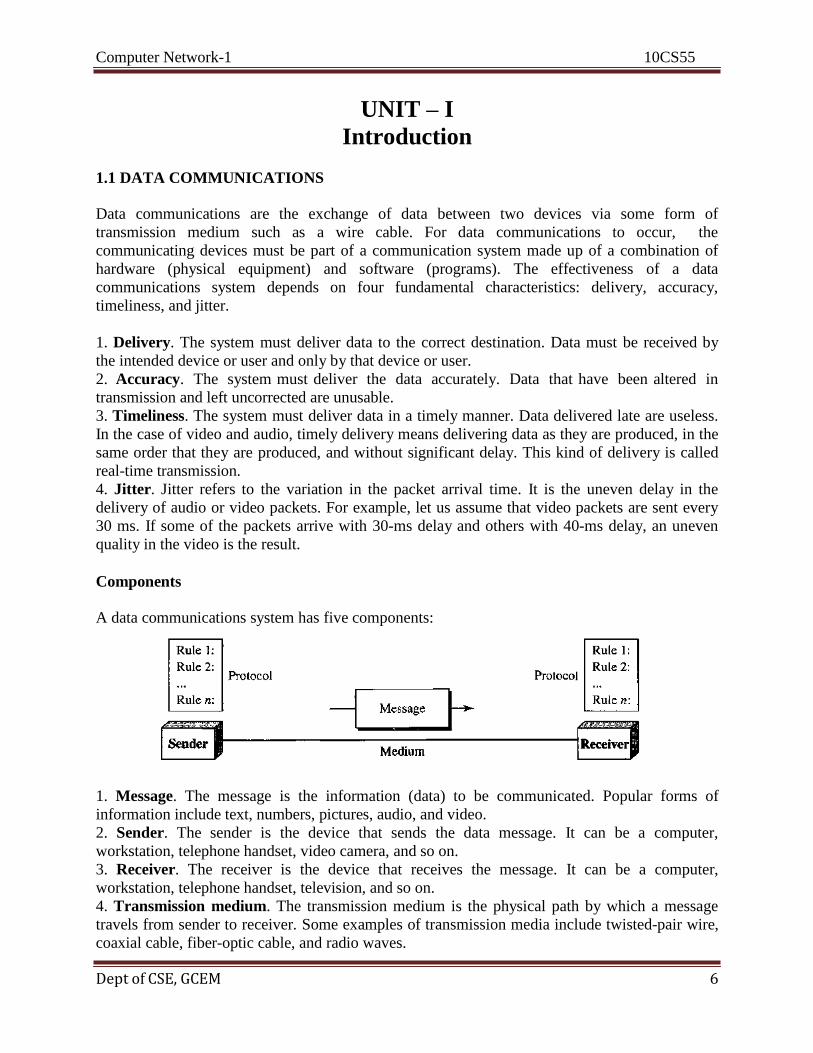
A data communications system has five components:
1. Message. The message is the information (data) to be communicated. Popular forms of
information include text, numbers, pictures, audio, and video.
2. Sender. The sender is the device that sends the data message. It can be a computer,
workstation, telephone handset, video camera, and so on.
3. Receiver. The receiver is the device that receives the message. It can be a computer,
workstation, telephone handset, television, and so on.
4. Transmission medium. The transmission medium is the physical path by which a message
travels from sender to receiver. Some examples of transmission media include twisted-pair wire,
coaxial cable, fiber-optic cable, and radio waves.
Computer Network-1 10CS55
Dept of CSE, GCEM 7
5. Protocol. A protocol is a set of rules that govern data communications. It represents an
agreement between the communicating devices. Without a protocol, two devices may be
connected but not communicating.
Data Representation
Information today comes in different forms such as text, numbers, images, audio, and
video.
Text In data communications, text is represented as a bit pattern, a sequence of bits (0s or 1s).
Different sets of bit patterns have been designed to represent text symbols. Each set is called a
code, and the process of representing symbols is called coding. Today, the prevalent coding
system is called Unicode, which uses 32 bits to represent a symbol or character used in any
language in the world.
Numbers Numbers are also represented by bit patterns. However, a code such as ASCII is not used to
represent numbers; the number is directly converted to a binary number to simplify mathematical
operations.
Images Images are also represented by bit patterns. In its simplest form, an image is composed of a
matrix of pixels (picture elements), where each pixel is a small dot. The size of the pixel depends
on the resolution. For example, an image can be divided into 1000 pixels or 10,000 pixels. In the
second case, there is a better representation of the image (better resolution), but more memory is
needed to store the image.
After an image is divided into pixels, each pixel is assigned a bit pattern. The size and the
value of the pattern depend on the image. For an image made of only black- and-white dots (e.g.,
a chessboard), a 1-bit pattern is enough to represent a pixel.
There are several methods to represent color images. One method is called RGB, so called
because each color is made of a combination of three primary colors: red, green, and blue.
Audio Audio refers to the recording or broadcasting of sound or music. Audio is by nature different
from text, numbers, or images. It is continuous, not discrete. Even when we use a microphone to
change voice or music to an electric signal, we create a continuous signal.
Video Video refers to the recording or broadcasting of a picture or movie. Video can either be produced
as a continuous entity (e.g., by a TV camera), or it can be a combination of images, each a
discrete entity, arranged to convey the idea of motion.

Computer Network-1 10CS55
Dept of CSE, GCEM 8
Data Flow
Communication between two devices can be simplex, half-duplex, or full-duplex as shown in
figure.
Simplex In simplex mode, the communication is unidirectional, as on a one-way street. Only one of the
two devices on a link can transmit; the other can only receive. Keyboards and traditional
monitors are examples of simplex devices. The keyboard can only introduce input; the monitor
can only accept output. The simplex mode can use the entire capacity of the channel to send data
in one direction.
Half-Duplex In half-duplex mode, each station can both transmit and receive, but not at the same time. When
one device is sending, the other can only receive, and vice versa. In a half-duplex transmission,
the entire capacity of a channel is taken over by whichever of the two devices is transmitting at
the time. Walkie-talkies and CB (citizens band) radios are both half-duplex systems.
The half-duplex mode is used in cases where there is no need for communication in both
directions at the same time; the entire capacity of the channel can be utilized for each direction.
Full-Duplex In full-duplex made (also, called duplex), both stations can transmit and receive simultaneously.
In full-duplex mode, signals going in one direction share the capacity of the link with signals
going in the other direction. This sharing can occur in two ways: Either the link must contain two
physically separate transmission paths, one for sending and the other for receiving; or the
capacity of the channel is divided between signals travelling in both directions.
One common example of full-duplex communication is the telephone network. The full-
duplex mode is used when communication in both directions is required all the time. The
capacity of the channel, however, must be divided between the two directions.

Computer Network-1 10CS55
Dept of CSE, GCEM 9
1.2 NETWORKS
A network is a set of devices (often referred to as nodes) connected by communication links. A
node can be a computer, printer, or any other device capable of sending and/or receiving data
generated by other nodes on the network.
Distributed Processing
Most networks use distributed processing, in which a task is divided among multiple computers.
Instead of one single large machine being responsible for all aspects of a process, separate
computers (usually a personal computer or workstation) handle a subset.
Network Criteria
A network must be able to meet a certain number of criteria. The most important of these are
performance, reliability, and security.
Performance Performance can be measured in many ways, including transit time and response time. Transit
time is the amount of time required for a message to travel from one device to another. Response
time is the elapsed time between an inquiry and a response. The performance of a network
depends on a number of factors, including the number of users, the type of transmission medium,
the capabilities of the connected hardware, and the efficiency of the software. Performance is
often evaluated by two networking metrics: throughput and delay.
We often need more throughput and less delay.
Reliability In addition to accuracy of delivery, network reliability is measured by the frequency of failure,
the time it takes a link to recover from a failure, and the network's robustness in a catastrophe.
Security Network security issues include protecting data from unauthorized access, protecting data from
damage and development, and implementing policies and procedures for recovery from breaches
and data losses.
Physical Structures
Type of Connection
A network is two or more devices connected through links. A link is a communications pathway
that transfers data from one device to another. For communication to occur, two devices must be
connected in some way to the same link at the same time. There are two possible types of
connections: point-to-point and multipoint.
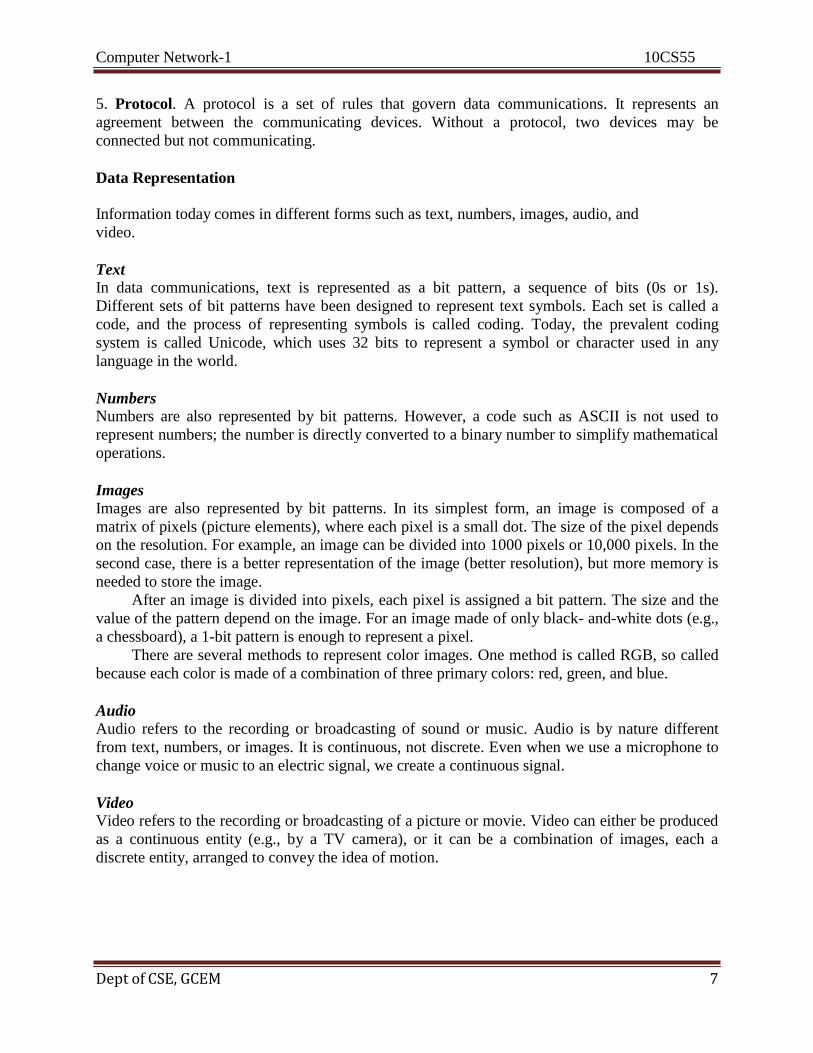
Point-to-Point A point-to-point connection provides a dedicated link between two devices. The
entire capacity of the link is reserved for transmission between those two devices. Most point-to-
Computer Network-1 10CS55
Dept of CSE,GCEM 10
point connections use an actual length of wire or cable to connect the two ends, but other
options, such as microwave or satellite links, are also possible.
Multipoint A multipoint (also called multidrop) connection is one in which more than two
specific devices share a single link. In a multipoint environment, the capacity of the channel is
shared, either spatially or temporally. If several devices can use the link simultaneously, it is a
spatially shared connection. If users must take turns, it is a timeshared connection.
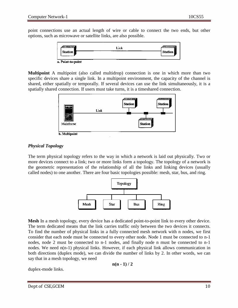
Physical Topology
The term physical topology refers to the way in which a network is laid out physically. Two or
more devices connect to a link; two or more links form a topology. The topology of a network is
the geometric representation of the relationship of all the links and linking devices (usually
called nodes) to one another. There are four basic topologies possible: mesh, star, bus, and ring.
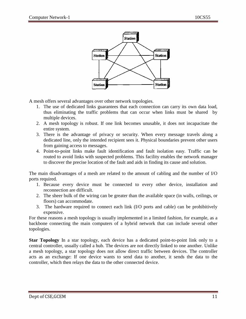
Mesh In a mesh topology, every device has a dedicated point-to-point link to every other device.
The term dedicated means that the link carries traffic only between the two devices it connects.
To find the number of physical links in a fully connected mesh network with n nodes, we first
consider that each node must be connected to every other node. Node 1 must be connected to n-1
nodes, node 2 must be connected to n-1 nodes, and finally node n must be connected to n-1
nodes. We need n(n-1) physical links. However, if each physical link allows communication in
both directions (duplex mode), we can divide the number of links by 2. In other words, we can
say that in a mesh topology, we need
duplex-mode links. n(n - 1) / 2
Computer Network-1 10CS55
Dept of CSE,GCEM 11
A mesh offers several advantages over other network topologies.
1. The use of dedicated links guarantees that each connection can carry its own data load,
thus eliminating the traffic problems that can occur when links must be shared by
multiple devices.
2. A mesh topology is robust. If one link becomes unusable, it does not incapacitate the
entire system.
3. There is the advantage of privacy or security. When every message travels along a
dedicated line, only the intended recipient sees it. Physical boundaries prevent other users
from gaining access to messages.
4. Point-to-point links make fault identification and fault isolation easy. Traffic can be
routed to avoid links with suspected problems. This facility enables the network manager
to discover the precise location of the fault and aids in finding its cause and solution.
The main disadvantages of a mesh are related to the amount of cabling and the number of I/O
ports required.
1. Because every device must be connected to every other device, installation and
reconnection are difficult.
2. The sheer bulk of the wiring can be greater than the available space (in walls, ceilings, or
floors) can accommodate.
3. The hardware required to connect each link (I/O ports and cable) can be prohibitively
expensive.
For these reasons a mesh topology is usually implemented in a limited fashion, for example, as a
backbone connecting the main computers of a hybrid network that can include several other
topologies.
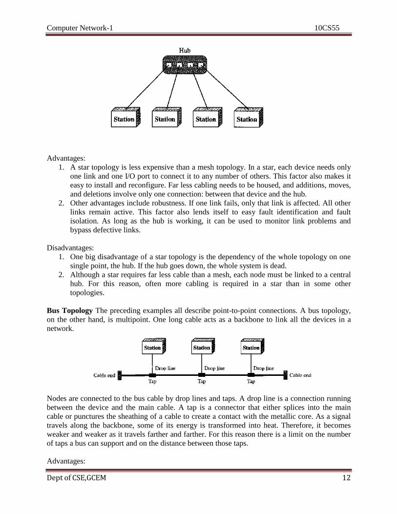
Star Topology In a star topology, each device has a dedicated point-to-point link only to a
central controller, usually called a hub. The devices are not directly linked to one another. Unlike
a mesh topology, a star topology does not allow direct traffic between devices. The controller
acts as an exchange: If one device wants to send data to another, it sends the data to the
controller, which then relays the data to the other connected device.
Computer Network-1 10CS55
Dept of CSE,GCEM 12
Advantages:
1. A star topology is less expensive than a mesh topology. In a star, each device needs only
one link and one I/O port to connect it to any number of others. This factor also makes it
easy to install and reconfigure. Far less cabling needs to be housed, and additions, moves,
and deletions involve only one connection: between that device and the hub.
2. Other advantages include robustness. If one link fails, only that link is affected. All other
links remain active. This factor also lends itself to easy fault identification and fault
isolation. As long as the hub is working, it can be used to monitor link problems and
bypass defective links.
Disadvantages:
1. One big disadvantage of a star topology is the dependency of the whole topology on one
single point, the hub. If the hub goes down, the whole system is dead.
2. Although a star requires far less cable than a mesh, each node must be linked to a central
hub. For this reason, often more cabling is required in a star than in some other
topologies.
Bus Topology The preceding examples all describe point-to-point connections. A bus topology,
on the other hand, is multipoint. One long cable acts as a backbone to link all the devices in a
network.
Nodes are connected to the bus cable by drop lines and taps. A drop line is a connection running
between the device and the main cable. A tap is a connector that either splices into the main
cable or punctures the sheathing of a cable to create a contact with the metallic core. As a signal
travels along the backbone, some of its energy is transformed into heat. Therefore, it becomes
weaker and weaker as it travels farther and farther. For this reason there is a limit on the number
of taps a bus can support and on the distance between those taps.
Advantages:
Computer Network-1 10CS55
Dept of CSE,GCEM 13
1. Advantages of a bus topology include ease of installation. Backbone cable can be laid
along the most efficient path, then connected to the nodes by drop lines of various
lengths. In this way, a bus uses less cabling than mesh or star topologies.
2. In a bus, redundancy is eliminated. Only the backbone cable stretches through the entire
facility. Each drop line has to reach only as far as the nearest point on the backbone.
Disadvantages:
1. Disadvantages include difficult reconnection and fault isolation. A bus is usually
designed to be optimally efficient at installation. It can therefore be difficult to add new
devices.
2. Signal reflection at the taps can cause degradation in quality. This degradation can be
controlled by limiting the number and spacing of devices connected to a given length of
cable. Adding new devices may therefore require modification or replacement of the
backbone.
3. a fault or break in the bus cable stops all transmission, even between devices on the same
side of the problem. The damaged area reflects signals back in the direction of origin,
creating noise in both directions.
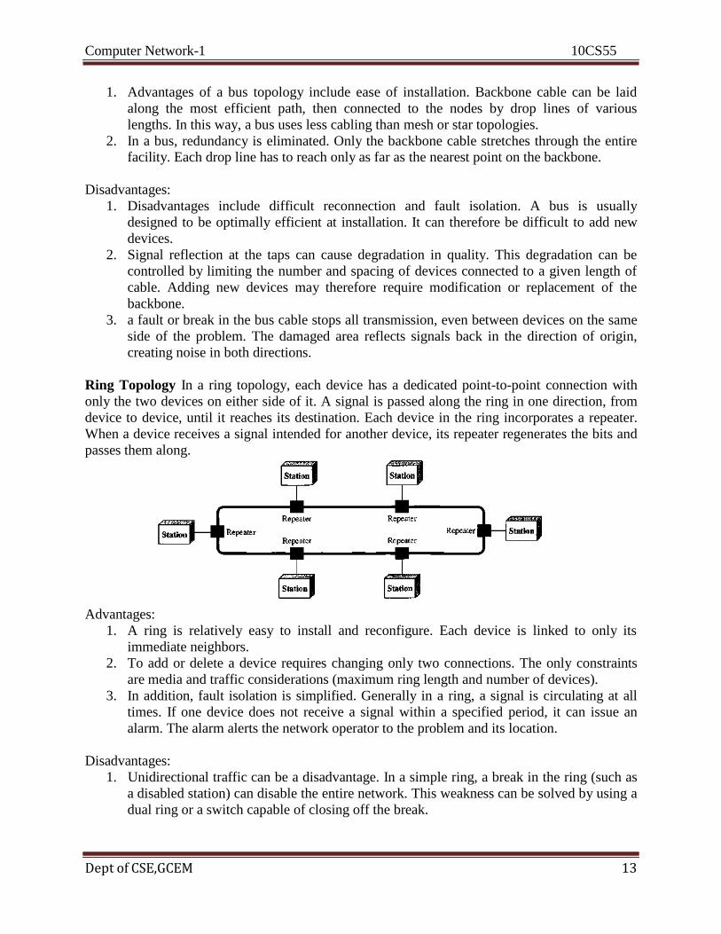
Ring Topology In a ring topology, each device has a dedicated point-to-point connection with
only the two devices on either side of it. A signal is passed along the ring in one direction, from
device to device, until it reaches its destination. Each device in the ring incorporates a repeater.
When a device receives a signal intended for another device, its repeater regenerates the bits and
passes them along.
Advantages:
1. A ring is relatively easy to install and reconfigure. Each device is linked to only its
immediate neighbors.
2. To add or delete a device requires changing only two connections. The only constraints
are media and traffic considerations (maximum ring length and number of devices).
3. In addition, fault isolation is simplified. Generally in a ring, a signal is circulating at all
times. If one device does not receive a signal within a specified period, it can issue an
alarm. The alarm alerts the network operator to the problem and its location.
Disadvantages:
1. Unidirectional traffic can be a disadvantage. In a simple ring, a break in the ring (such as
a disabled station) can disable the entire network. This weakness can be solved by using a
dual ring or a switch capable of closing off the break.

Computer Network-1 10CS55
Dept of CSE,GCEM 14
Hybrid Topology A network can be hybrid. For example, we can have a main star topology with
each branch connecting several stations in a bus topology as shown:
Network Models
Computer networks are created by different entities. Standards are needed so that these
heterogeneous networks can communicate with one another. The two best-known standards are
the OSI model and the Internet model. The OSI (Open Systems Interconnection) model defines a
seven-layer network; the Internet model defines a five-layer network.
Categories of Networks
Local Area Network
A local area network (LAN) is usually privately owned and links the devices in a single office,
building, or campus. Depending on the needs of an organization and the type of technology used,
a LAN can be as simple as two PCs and a printer in someone's home office; or it can extend
throughout a company and include audio and video peripherals. Currently, LAN size is limited to
a few kilometers.
LANs are designed to allow resources to be shared between personal computers or
workstations. The resources to be shared can include hardware (e.g., a printer), software (e.g., an
application program), or data. A common example of a LAN, found in many business
environments, links a workgroup of task-related computers, for example, engineering
workstations or accounting PCs. One of the computers may be given a large capacity disk drive
and may become a server to clients. Software can be stored on this central server and used as
needed by the whole group.
In addition to size, LANs are distinguished from other types of networks by their
transmission media and topology. In general, a given LAN will use only one type of transmission
medium. The most common LAN topologies are bus, ring, and star.

Computer Network-1 10CS55
Dept of CSE,GCEM 15
Wide Area Network
A wide area network (WAN) provides long-distance transmission of data, image, audio, and
video information over large geographic areas that may comprise a country, a continent, or even
the whole world.
A WAN can be as complex as the backbones that connect the Internet or as simple as a dial-up
line that connects a home computer to the Internet. We normally refer to the first as a switched
WAN and to the second as a point-to-point WAN. The switched WAN connects the end systems,
which usually comprise a router (internet-working connecting device) that connects to another
LAN or WAN. The point-to-point
WAN is normally a line leased from a telephone or cable TV provider that connects a home
computer or a small LAN to an Internet service provider (ISP). This type of WAN is often used
to provide Internet access.
Computer Network-1 10CS55
Dept of CSE,GCEM 16
Metropolitan Area Networks
A metropolitan area network (MAN) is a network with a size between a LAN and a WAN. It
normally covers the area inside a town or a city. It is designed for customers who need a high-
speed connectivity, normally to the Internet, and have endpoints spread over a city or part of city.
A good example of a MAN is the part of the telephone company network that can provide a
high-speed DSL line to the customer.
Interconnection of Networks: Internetwork
Today, it is very rare to see a LAN, a MAN, or a LAN in isolation; they are connected to one
another. When two or more networks are connected, they become an internetwork, or internet.
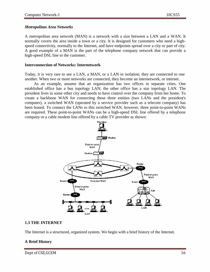
As an example, assume that an organization has two offices in separate cities. One
established office has a bus topology LAN; the other office has a star topology LAN. The
president lives in some other city and needs to have control over the company from her home. To
create a backbone WAN for connecting these three entities (two LANs and the president's
computer), a switched WAN (operated by a service provider such as a telecom company) has
been leased. To connect the LANs to this switched WAN, however, three point-to-point WANs
are required. These point-to-point WANs can be a high-speed DSL line offered by a telephone
company or a cable modem line offered by a cable TV provider as shown:
1.3 THE INTERNET
The Internet is a structured, organized system. We begin with a brief history of the Internet.
A Brief History
Computer Network-1 10CS55
Dept of CSE,GCEM 17
In the mid-1960s, mainframe computers in research organizations were stand-alone devices.
Computers from different manufacturers were unable to communicate with one another. The
Advanced Research Projects Agency (ARPA) in the Department of Defense (DoD) was
interested in finding a way to connect computers so that the researchers they funded could share
their findings, thereby reducing costs and eliminating duplication of effort.
In 1967, at an Association for Computing Machinery (ACM) meeting, ARPA presented its
ideas for ARPANET, a small network of connected computers. The idea was that each host
computer (not necessarily from the same manufacturer) would be attached to a specialized
computer, called an interface message processor (IMP). The IMPs, in turn, would be connected
to one another. Each IMP had to be able to communicate with other IMPs as well as with its own
attached host.
By 1969, ARPANET was a reality. Four nodes, at the University of California at Los
Angeles (UCLA), the University of California at Santa Barbara (UCSB), Stanford Research
Institute (SRI), and the University of Utah, were connected via the IMPs to form a network.
Software called the Network Control Protocol (NCP) provided communication between the
hosts.
In 1972, Vint Cerf and Bob Kahn, both of whom were part of the core ARPANET group,
collaborated on what they called the Internetting Project. Cerf and Kahn's land-mark 1973 paper
outlined the protocols to achieve end-to-end delivery of packets. This paper on Transmission
Control Protocol (TCP) included concepts such as encapsulation, the datagram, and the functions
of a gateway.
Shortly thereafter, authorities made a decision to split TCP into two protocols:
Transmission Control Protocol (TCP) and Internetworking Protocol (IP). IP would handle
datagram routing while TCP would be responsible for higher-level functions such as
segmentation, reassembly, and error detection. The internetworking protocol became known as
TCP/IP.
The Internet Today
The Internet today is not a simple hierarchical structure. It is made up of many wide- and local-
area networks joined by connecting devices and switching stations. It is difficult to give an
accurate representation of the Internet because it is continually changing--new networks are
being added, existing networks are adding addresses, and networks of defunct companies are
being removed. Today most end users who want Internet connection use the services of Internet
service providers (ISPs). There are international service providers, national service providers,
regional service providers, and local service providers. The Internet today is run by private
companies, not the government. The figure shows a conceptual (not geographic) view of the
Internet.

Computer Network-1 10CS55
Dept of CSE,GCEM 18
International Internet Service Providers
At the top of the hierarchy are the international service providers that connect nations together.
National Internet Service Providers The national Internet service providers are backbone networks created and maintained by
specialized companies. To provide connectivity between the end users, these backbone networks
are connected by complex switching stations (normally run by a third party) called network
access points (NAPs). Some national ISP networks are also connected to one another by private
switching stations called peering points. These normally operate at a high data rate.
Regional Internet Service Providers Regional intemet service providers or regional ISPs are smaller ISPs that are connected to one or
more national ISPs. They are at the third level of the hierarchy with a smaller data rate.
Local Internet Service Providers Local Internet service providers provide direct service to the end users. The local ISPs can be
connected to regional ISPs or directly to national ISPs. Most end users are connected to the local
ISPs.
1.4 PROTOCOLS AND STANDARDS
Protocols
Computer Network-1 10CS55
Dept of CSE,GCEM 19
In computer networks, communication occurs between entities in different systems. An entity is
anything capable of sending or receiving information. However, two entities cannot simply send
bit streams to each other and expect to be understood. For communication to occur, the entities
must agree on a protocol. A protocol is a set of rules that govern data communications. A
protocol defines what is communicated, how k is communicated, and when it is communicated.
The key elements of a protocol are syntax, semantics, and timing.
• Syntax. The term syntax refers to the structure or format of the data, meaning the order in
which they are presented. For example, a simple protocol might expect the first 8 bits of data to
be the address of the sender, the second 8 bits to be the address of the receiver, and the rest of the
stream to be the message itself.
• Semantics. The word semantics refers to the meaning of each section of bits. How is a
particular pattern to be interpreted, and what action is to be taken based on that interpretation?
• Timing. The term timing refers to two characteristics: when data should be sent and how fast
they can be sent. For example, if a sender produces data at 100 Mbps but the receiver can process
data at only 1 Mbps, the transmission will overload the receiver and some data will be lost.
Standards
Standards are essential in creating and maintaining an open and competitive market for
equipment manufacturers and in guaranteeing national and international interoperability of data
and telecommunications technology and processes. Standards provide guidelines to
manufacturers, vendors, government agencies, and other service providers to ensure the kind of
interconnectivity necessary in today's marketplace and in international communications. Data
communication standards fall into two categories: de facto (meaning
"by fact" or "by convention") and de jure (meaning "by law" or "by regulation").
• De facto. Standards that have not been approved by an organized body but have been adopted
as standards through widespread use are de facto standards. De facto standards are often
established originally by manufacturers who seek to define the functionality of a new product or
technology.
• De jure. Those standards that have been legislated by an officially recognized body are de jure
standards.
Standards Organizations
Standards are developed through the cooperation of standards creation committees, forums, and
government regulatory agencies.
Standards Creation Committees
While many organizations are dedicated to the establishment of standards, data
telecommunications in North America rely primarily on those published by the following:
• International Organization for Standardization (ISO). The ISO is a multinational body
whose membership is drawn mainly from the standards creation committees of various

Computer Network-1 10CS55
Dept of CSE,GCEM 20
governments throughout the world. The ISO is active in developing cooperation in the realms of
scientific, technological, and economic activity.
• International Telecommunication Elnion Telecommunication Standards Sector (ITEl-T).
By the early 1970s, a number of countries were defining national standards for
telecommunications, but there was still little international compatibility. The United Nations
responded by forming, as part of its International Telecommunication Union (ITU), a committee,
the Consultative Committee for International Telegraphy and Telephony (CCITT). This
committee was devoted to the research and establishment of standards for telecommunications in
general and for phone and data systems in particular. On March 1, 1993, the name
of this committee was changed to the International Telecommunication Union -
Telecommunication Standards Sector (ITU-T).
• American National Standards Institute (ANSI). Despite its name, the American National
Standards Institute is a completely private, nonprofit corporation not affiliated with the U.S.
federal government. However, all ANSI activities are undertaken with the welfare of the United
States and its citizens occupying primary importance.
• Institute of Electrical and Electronics Engineers (IEEE). The Institute of Electrical and
Electronics Engineers is the largest professional engineering society in the world. International in
scope, it aims to advance theory, creativity, and product quality in the fields of electrical
engineering, electronics, and radio as well as in all related branches of engineering. As one of its
goals, the IEEE oversees the development and adoption of international standards for computing
and communications.
• Electronic Industries Association (EIA). Aligned with ANSI, the Electronic Industries
Association is a nonprofit organization devoted to the promotion of electronics manufacturing
concerns. Its activities include public awareness education and lobbying efforts in addition to
standards development. In the field of information technology, the EIA has made significant
contributions by defining physical connection interfaces and electronic signaling specifications
for data communication.
Forums
Telecommunications technology development is moving faster than the ability of stan-dards
committees to ratify standards. Standards committees are procedural bodies and by nature slow-
moving. To accommodate the need for working models and agreements and to facilitate the
standardization process, many special-interest groups have developed forums made up of
representatives from interested corporations. The forums
work with universities and users to test, evaluate, and standardize new technologies. By
concentrating their efforts on a particular technology, the forums are able to speed acceptance
and use of those technologies in the telecommunications community. The forums present their
conclusions to the standards bodies.
Regulatory Agencies
All communications technology is subject to regulation by government agencies such as the
Federal Communications Commission (FCC) in the United States. The purpose of these agencies
is to protect the public interest by regulating radio, television, and wire/cable communications.
Computer Network-1 10CS55
Dept of CSE,GCEM 21
The FCC has authority over interstate and international commerce as it relates to
communications.
Internet Standards
An Internet standard is a thoroughly tested specification that is useful to and adhered to by those
who work with the Internet. It is a formalized regulation that must be followed. There is a strict
procedure by which a specification attains Internet standard status. A specification begins as an
Internet draft. An Internet draft is a working document (a work in progress) with no official
status and a 6-month lifetime. Upon recommendation from the Internet authorities, a draft may
be published as a Request for Comment (RFC). Each RFC is edited, assigned a number, and
made available to all interested parties. RFCs go through maturity levels and are categorized
according to their requirement level.
Chapter 2
Network Models
2.1 LAYERED TASKS
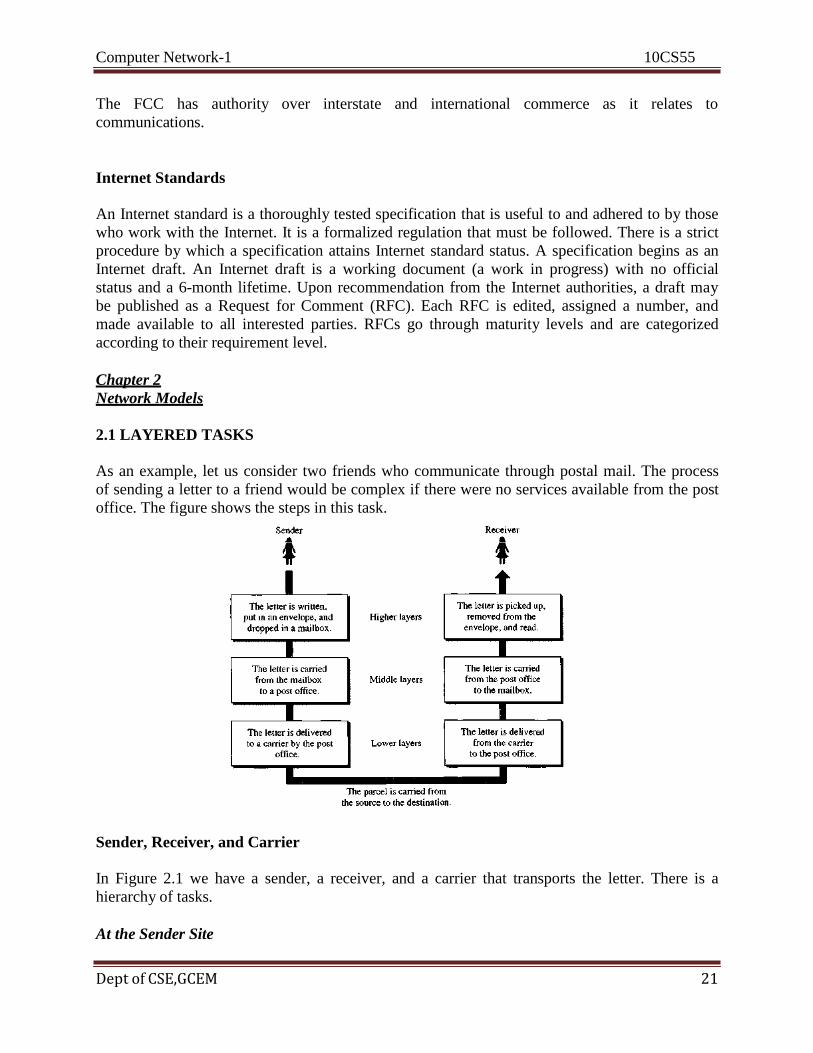
As an example, let us consider two friends who communicate through postal mail. The process
of sending a letter to a friend would be complex if there were no services available from the post
office. The figure shows the steps in this task.
Sender, Receiver, and Carrier
In Figure 2.1 we have a sender, a receiver, and a carrier that transports the letter. There is a
hierarchy of tasks.
At the Sender Site

Computer Network-1 10CS55
Dept of CSE,GCEM 22
The activities that take place at the sender site, in order, are:
Higher layer. The sender writes the letter, inserts the letter in an envelope, writes the
sender and receiver addresses, and drops the letter in a mailbox.
Middle layer. The letter is picked up by a letter carrier and delivered to the post office.
Lower layer. The letter is sorted at the post office; a carder transports the letter.
On the Way The letter is then on its way to the recipient. On the way to the recipient's local post office, the
letter may actually go through a central office. In addition, it may be trans- ported by truck, train,
airplane, boat, or a combination of these.
At the Receiver Site
Lower layer. The carrier transports the letter to the post office.
Middle layer. The letter is sorted and delivered to the recipient's mailbox.
Higher layer. The receiver picks up the letter, opens the envelope, and reads it.
Hierarchy
According to our analysis, there are three different activities at the sender site and another three
activities at the receiver site. The task of transporting the letter between the sender and the
receiver is done by the carrier. Something that is not obvious immediately is that the tasks must
be done in the order given in the hierarchy. At the sender site, the letter must be written and
dropped in the mailbox before being picked up by the letter carrier and delivered to the post
office. At the receiver site, the letter must be dropped in the recipient mailbox before being
picked up and read by the recipient.
Services Each layer at the sending site uses the services of the layer immediately below it. The sender at
the higher layer uses the services of the middle layer. The middle layer uses the services of the
lower layer. The lower layer uses the services of the carrier. The layered model that dominated
data communications and networking literature before 1990 was the Open Systems
Interconnection (OSI) model.
2.2 THE OSI MODEL
The OSI model is a layered framework for the design of network systems that allows
communication between all types of computer systems. It consists of seven separate but related
layers, each of which defines a part of the process of moving information across a network.
Computer Network-1 10CS55
Dept of CSE,GCEM 23
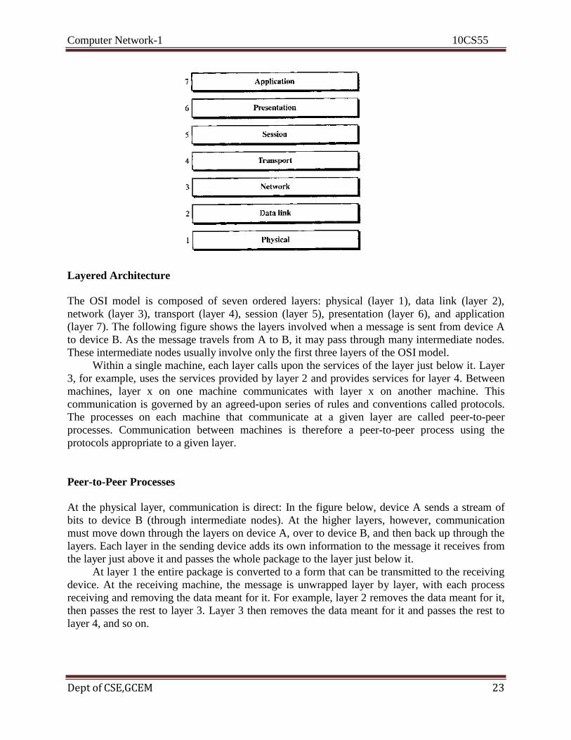
Layered Architecture
The OSI model is composed of seven ordered layers: physical (layer 1), data link (layer 2),
network (layer 3), transport (layer 4), session (layer 5), presentation (layer 6), and application
(layer 7). The following figure shows the layers involved when a message is sent from device A
to device B. As the message travels from A to B, it may pass through many intermediate nodes.
These intermediate nodes usually involve only the first three layers of the OSI model.
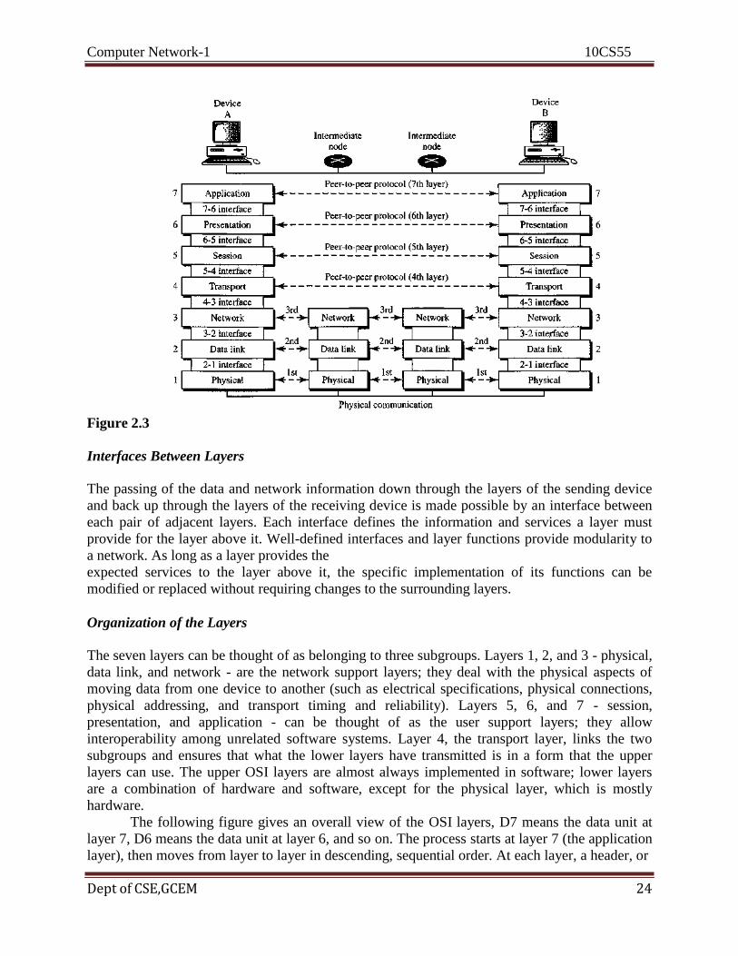
Within a single machine, each layer calls upon the services of the layer just below it. Layer
3, for example, uses the services provided by layer 2 and provides services for layer 4. Between
machines, layer x on one machine communicates with layer x on another machine. This
communication is governed by an agreed-upon series of rules and conventions called protocols.
The processes on each machine that communicate at a given layer are called peer-to-peer
processes. Communication between machines is therefore a peer-to-peer process using the
protocols appropriate to a given layer.
Peer-to-Peer Processes
At the physical layer, communication is direct: In the figure below, device A sends a stream of
bits to device B (through intermediate nodes). At the higher layers, however, communication
must move down through the layers on device A, over to device B, and then back up through the
layers. Each layer in the sending device adds its own information to the message it receives from
the layer just above it and passes the whole package to the layer just below it.
At layer 1 the entire package is converted to a form that can be transmitted to the receiving
device. At the receiving machine, the message is unwrapped layer by layer, with each process
receiving and removing the data meant for it. For example, layer 2 removes the data meant for it,
then passes the rest to layer 3. Layer 3 then removes the data meant for it and passes the rest to
layer 4, and so on.
Computer Network-1 10CS55
Dept of CSE,GCEM 24
Figure 2.3
Interfaces Between Layers
The passing of the data and network information down through the layers of the sending device
and back up through the layers of the receiving device is made possible by an interface between
each pair of adjacent layers. Each interface defines the information and services a layer must
provide for the layer above it. Well-defined interfaces and layer functions provide modularity to
a network. As long as a layer provides the
expected services to the layer above it, the specific implementation of its functions can be
modified or replaced without requiring changes to the surrounding layers.
Organization of the Layers
The seven layers can be thought of as belonging to three subgroups. Layers 1, 2, and 3 - physical,
data link, and network - are the network support layers; they deal with the physical aspects of
moving data from one device to another (such as electrical specifications, physical connections,
physical addressing, and transport timing and reliability). Layers 5, 6, and 7 - session,
presentation, and application - can be thought of as the user support layers; they allow
interoperability among unrelated software systems. Layer 4, the transport layer, links the two
subgroups and ensures that what the lower layers have transmitted is in a form that the upper
layers can use. The upper OSI layers are almost always implemented in software; lower layers
are a combination of hardware and software, except for the physical layer, which is mostly
hardware.
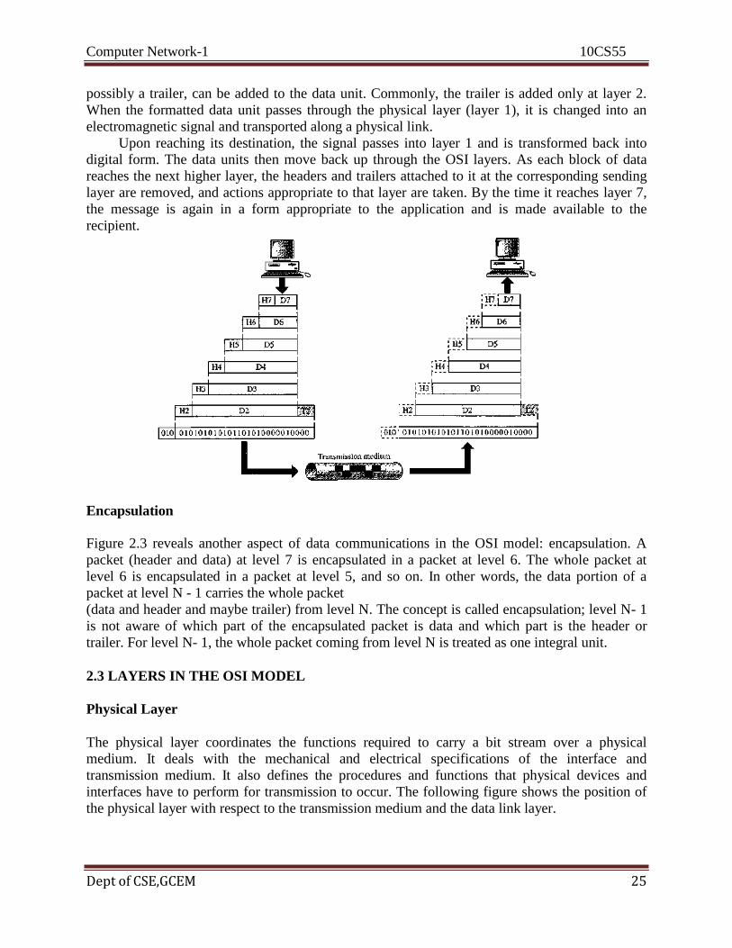
The following figure gives an overall view of the OSI layers, D7 means the data unit at
layer 7, D6 means the data unit at layer 6, and so on. The process starts at layer 7 (the application
layer), then moves from layer to layer in descending, sequential order. At each layer, a header, or
Computer Network-1 10CS55
Dept of CSE,GCEM 25
possibly a trailer, can be added to the data unit. Commonly, the trailer is added only at layer 2.
When the formatted data unit passes through the physical layer (layer 1), it is changed into an
electromagnetic signal and transported along a physical link.
Upon reaching its destination, the signal passes into layer 1 and is transformed back into
digital form. The data units then move back up through the OSI layers. As each block of data
reaches the next higher layer, the headers and trailers attached to it at the corresponding sending
layer are removed, and actions appropriate to that layer are taken. By the time it reaches layer 7,
the message is again in a form appropriate to the application and is made available to the
recipient.
Encapsulation
Figure 2.3 reveals another aspect of data communications in the OSI model: encapsulation. A
packet (header and data) at level 7 is encapsulated in a packet at level 6. The whole packet at
level 6 is encapsulated in a packet at level 5, and so on. In other words, the data portion of a
packet at level N - 1 carries the whole packet
(data and header and maybe trailer) from level N. The concept is called encapsulation; level N- 1
is not aware of which part of the encapsulated packet is data and which part is the header or
trailer. For level N- 1, the whole packet coming from level N is treated as one integral unit.
2.3 LAYERS IN THE OSI MODEL
Physical Layer
The physical layer coordinates the functions required to carry a bit stream over a physical
medium. It deals with the mechanical and electrical specifications of the interface and
transmission medium. It also defines the procedures and functions that physical devices and
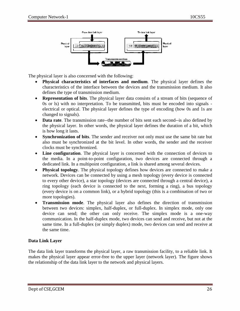
interfaces have to perform for transmission to occur. The following figure shows the position of
the physical layer with respect to the transmission medium and the data link layer.
Computer Network-1 10CS55
Dept of CSE,GCEM 26
The physical layer is also concerned with the following:
Physical characteristics of interfaces and medium. The physical layer defines the
characteristics of the interface between the devices and the transmission medium. It also
defines the type of transmission medium.
Representation of bits. The physical layer data consists of a stream of bits (sequence of
0s or ls) with no interpretation. To be transmitted, bits must be encoded into signals -
electrical or optical. The physical layer defines the type of encoding (how 0s and 1s are
changed to signals).
Data rate. The transmission rate--the number of bits sent each second--is also defined by
the physical layer. In other words, the physical layer defines the duration of a bit, which
is how long it lasts.
Synchronization of bits. The sender and receiver not only must use the same bit rate but
also must be synchronized at the bit level. In other words, the sender and the receiver
clocks must be synchronized.
Line configuration. The physical layer is concerned with the connection of devices to
the media. In a point-to-point configuration, two devices are connected through a
dedicated link. In a multipoint configuration, a link is shared among several devices.
Physical topology. The physical topology defines how devices are connected to make a
network. Devices can be connected by using a mesh topology (every device is connected
to every other device), a star topology (devices are connected through a central device), a
ring topology (each device is connected to the next, forming a ring), a bus topology
(every device is on a common link), or a hybrid topology (this is a combination of two or
more topologies).
Transmission mode. The physical layer also defines the direction of transmission
between two devices: simplex, half-duplex, or full-duplex. In simplex mode, only one
device can send; the other can only receive. The simplex mode is a one-way
communication. In the half-duplex mode, two devices can send and receive, but not at the
same time. In a full-duplex (or simply duplex) mode, two devices can send and receive at
the same time.
Data Link Layer
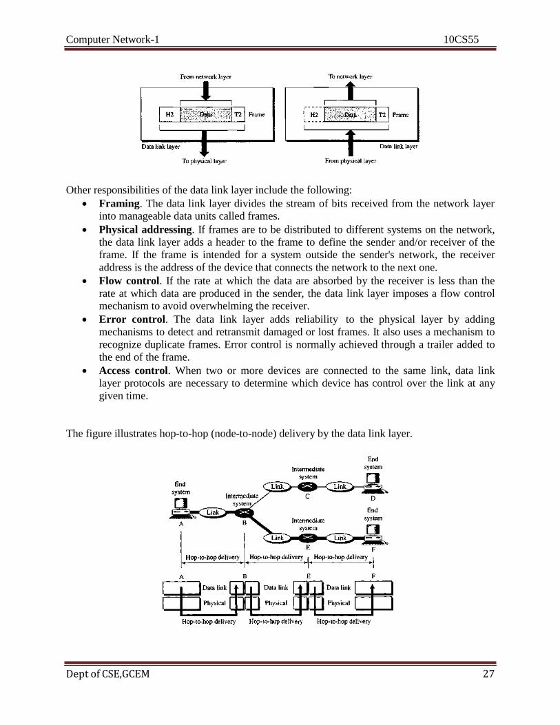
The data link layer transforms the physical layer, a raw transmission facility, to a reliable link. It
makes the physical layer appear error-free to the upper layer (network layer). The figure shows
the relationship of the data link layer to the network and physical layers.
Computer Network-1 10CS55
Dept of CSE,GCEM 27
Other responsibilities of the data link layer include the following:
Framing. The data link layer divides the stream of bits received from the network layer
into manageable data units called frames.
Physical addressing. If frames are to be distributed to different systems on the network,
the data link layer adds a header to the frame to define the sender and/or receiver of the
frame. If the frame is intended for a system outside the sender's network, the receiver
address is the address of the device that connects the network to the next one.
Flow control. If the rate at which the data are absorbed by the receiver is less than the
rate at which data are produced in the sender, the data link layer imposes a flow control
mechanism to avoid overwhelming the receiver.
Error control. The data link layer adds reliability to the physical layer by adding
mechanisms to detect and retransmit damaged or lost frames. It also uses a mechanism to
recognize duplicate frames. Error control is normally achieved through a trailer added to
the end of the frame.
Access control. When two or more devices are connected to the same link, data link
layer protocols are necessary to determine which device has control over the link at any
given time.
The figure illustrates hop-to-hop (node-to-node) delivery by the data link layer.
Computer Network-1 10CS55
Dept of CSE,GCEM 28
Communication at the data link layer occurs between two adjacent nodes. To send data from A
to F, three partial deliveries are made. First, the data link layer at A sends a frame to the data link
layer at B (a router). Second, the data link layer at B sends a new frame to the data link layer at
E. Finally, the data link layer at E sends a new frame to the data link layer at F.
Network Layer
The network layer is responsible for the source-to-destination delivery of a packet, possibly
across multiple networks (links). Whereas the data link layer oversees the delivery of the packet
between two systems on the same network (links), the network layer ensures that each packet
gets from its point of origin to its final destination.
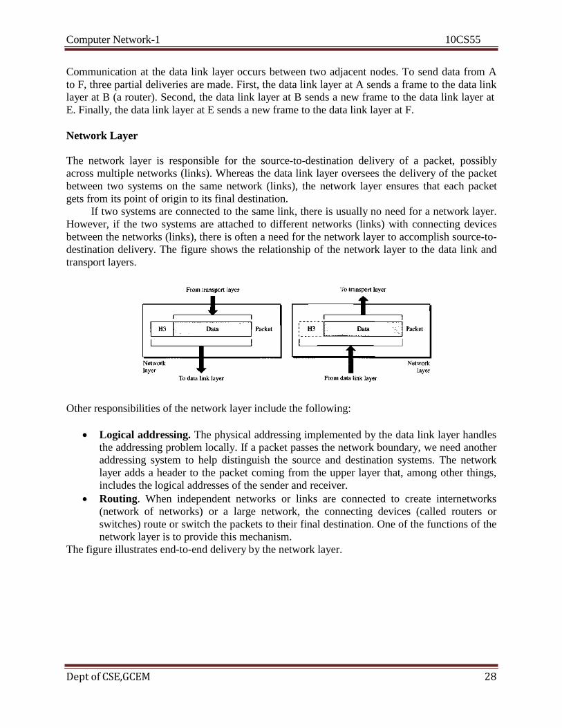
If two systems are connected to the same link, there is usually no need for a network layer.
However, if the two systems are attached to different networks (links) with connecting devices
between the networks (links), there is often a need for the network layer to accomplish source-to-
destination delivery. The figure shows the relationship of the network layer to the data link and
transport layers.
Other responsibilities of the network layer include the following:
Logical addressing. The physical addressing implemented by the data link layer handles
the addressing problem locally. If a packet passes the network boundary, we need another
addressing system to help distinguish the source and destination systems. The network
layer adds a header to the packet coming from the upper layer that, among other things,
includes the logical addresses of the sender and receiver.
Routing. When independent networks or links are connected to create internetworks
(network of networks) or a large network, the connecting devices (called routers or
switches) route or switch the packets to their final destination. One of the functions of the
network layer is to provide this mechanism.
The figure illustrates end-to-end delivery by the network layer.

Computer Network-1 10CS55
Dept of CSE,GCEM 29
The network layer at A sends the packet to the network layer at B. When the packet arrives at
router B, the
router makes a decision based on the final destination (F) of the packet. As we will see in later
chapters, router B uses its routing table to find that the next hop is router E. The network layer at
B, therefore, sends the packet to the network layer at E. The network layer at E, in turn, sends the
packet to the network layer at F.
Transport Layer
The transport layer is responsible for process-to-process delivery of the entire message. A
process is an application program running on a host. Whereas the network layer oversees source-
to-destination delivery of individual packets, it does not recognize any relationship between
those packets. It treats each one independently, as though each piece belonged to a separate
message, whether or not it does. The transport layer, on the other hand, ensures that the whole
message arrives intact and in order, overseeing both error control and flow control at the source-
to-destination level. The figure shows the relationship of the transport layer to the network and
session layers.
Other responsibilities of the transport layer include the following:

Computer Network-1 10CS55
Dept of CSE,GCEM 30
Service-point addressing. Computers often run several programs at the same time. For
this reason, source-to-destination delivery means delivery not only from one computer to
the next but also from a specific process (running program) on one computer to a specific
process (running program) on the other. The transport layer header must therefore include
a type of address called a service-point address (or port address). The network layer gets
each packet to the correct computer; the transport layer gets the entire message to the
correct process on that computer.
Segmentation and reassembly. A message is divided into transmittable segments, with
each segment containing a sequence number. These numbers enable the transport layer to
reassemble the message correctly upon arriving at the destination and to identify and
replace packets that were lost in transmission.
Connection control. The transport layer can be either connectionless or connection-
oriented. A connectionless transport layer treats each segment as an independent packet
and delivers it to the transport layer at the destination machine. A connection-oriented
transport layer makes a connection with the transport layer at the destination machine
first before delivering the packets. After all the data are transferred, the connection is
terminated.
Flow control. Like the data link layer, the transport layer is responsible for flow control.
However, flow control at this layer is performed end to end rather than across a single
link.
Error control. Like the data link layer, the transport layer is responsible for error
control. However, error control at this layer is performed process-to-process rather than
across a single link. The sending transport layer makes sure that the entire message
arrives at the receiving transport layer without error (damage, loss, or duplication). Error
correction is usually achieved through retransmission.
The figure illustrates process-to-process delivery by the transport layer.
Session Layer
The services provided by the first three layers (physical, data link, and network) are not
sufficient for some processes. The session layer is the network dialog controller. It establishes,
maintains, and synchronizes the interaction among communicating systems.
Specific responsibilities of the session layer include the following:
Computer Network-1 10CS55
Dept of CSE,GCEM 31
Dialog control. The session layer allows two systems to enter into a dialog. It allows the
communication between two processes to take place in either half- duplex (one way at a
time) or full-duplex (two ways at a time) mode.
Synchronization. The session layer allows a process to add checkpoints, or
synchronization points, to a stream of data. For example, if a system is sending a file of
2000 pages, it is advisable to insert checkpoints after every 100 pages to ensure that each
100-page unit is received and acknowledged independently. In this case, if a crash
happens during the transmission of page 523, the only pages that need to be resent after
system recovery are pages 501 to 523. Pages previous to 501 need not be resent.
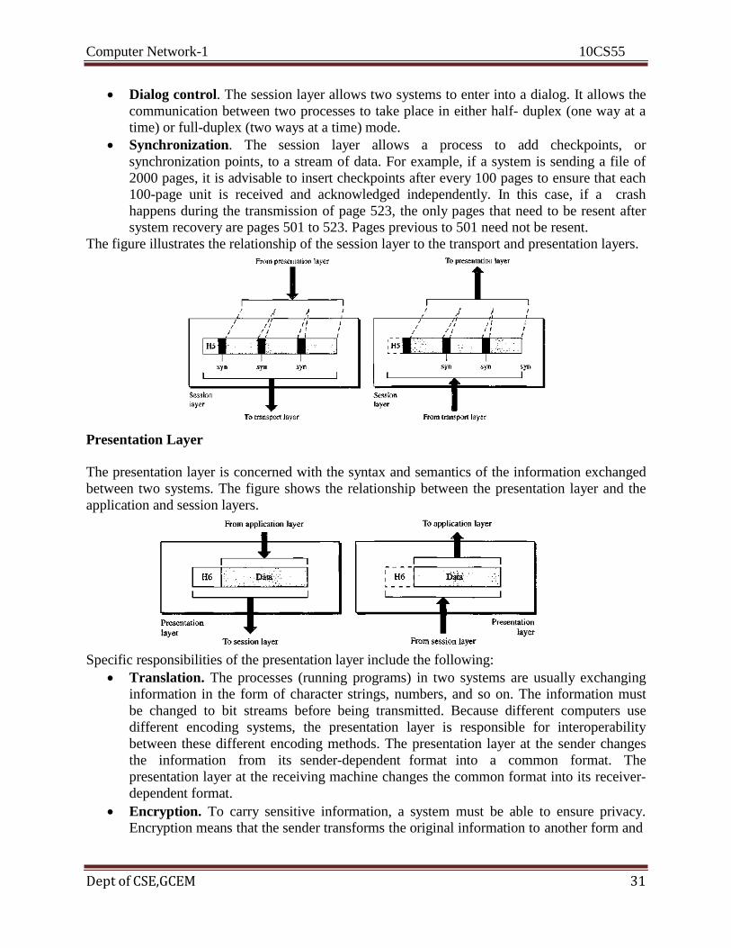
The figure illustrates the relationship of the session layer to the transport and presentation layers.
Presentation Layer
The presentation layer is concerned with the syntax and semantics of the information exchanged
between two systems. The figure shows the relationship between the presentation layer and the
application and session layers.
Specific responsibilities of the presentation layer include the following:
Translation. The processes (running programs) in two systems are usually exchanging
information in the form of character strings, numbers, and so on. The information must
be changed to bit streams before being transmitted. Because different computers use
different encoding systems, the presentation layer is responsible for interoperability
between these different encoding methods. The presentation layer at the sender changes
the information from its sender-dependent format into a common format. The
presentation layer at the receiving machine changes the common format into its receiver-
dependent format.
Encryption. To carry sensitive information, a system must be able to ensure privacy.
Encryption means that the sender transforms the original information to another form and
Computer Network-1 10CS55
Dept of CSE,GCEM 32
sends the resulting message out over the network. Decryption reverses the original
process to transform the message back to its original form.
Compression. Data compression reduces the number of bits contained in the
information. Data compression becomes particularly important in the transmission of
multimedia such as text, audio, and video.
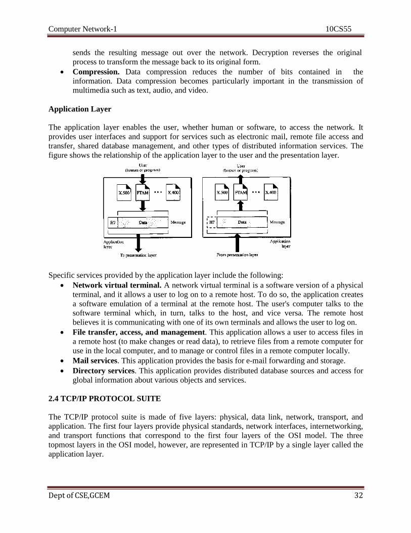
Application Layer
The application layer enables the user, whether human or software, to access the network. It
provides user interfaces and support for services such as electronic mail, remote file access and
transfer, shared database management, and other types of distributed information services. The
figure shows the relationship of the application layer to the user and the presentation layer.
Specific services provided by the application layer include the following:
Network virtual terminal. A network virtual terminal is a software version of a physical
terminal, and it allows a user to log on to a remote host. To do so, the application creates
a software emulation of a terminal at the remote host. The user's computer talks to the
software terminal which, in turn, talks to the host, and vice versa. The remote host
believes it is communicating with one of its own terminals and allows the user to log on.
File transfer, access, and management. This application allows a user to access files in
a remote host (to make changes or read data), to retrieve files from a remote computer for
use in the local computer, and to manage or control files in a remote computer locally.
Mail services. This application provides the basis for e-mail forwarding and storage.
Directory services. This application provides distributed database sources and access for
global information about various objects and services.
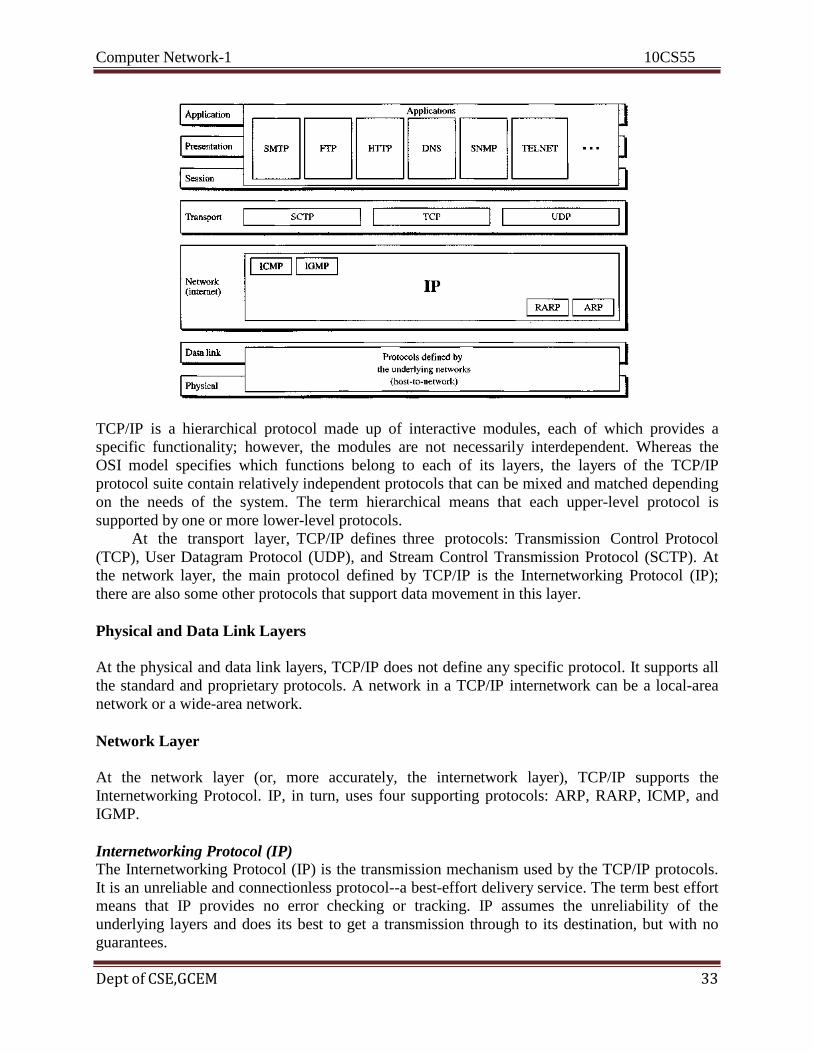
2.4 TCP/IP PROTOCOL SUITE
The TCP/IP protocol suite is made of five layers: physical, data link, network, transport, and
application. The first four layers provide physical standards, network interfaces, internetworking,
and transport functions that correspond to the first four layers of the OSI model. The three
topmost layers in the OSI model, however, are represented in TCP/IP by a single layer called the
application layer.
Computer Network-1 10CS55
Dept of CSE,GCEM 33
TCP/IP is a hierarchical protocol made up of interactive modules, each of which provides a
specific functionality; however, the modules are not necessarily interdependent. Whereas the
OSI model specifies which functions belong to each of its layers, the layers of the TCP/IP
protocol suite contain relatively independent protocols that can be mixed and matched depending
on the needs of the system. The term hierarchical means that each upper-level protocol is
supported by one or more lower-level protocols.
At the transport layer, TCP/IP defines three protocols: Transmission Control Protocol
(TCP), User Datagram Protocol (UDP), and Stream Control Transmission Protocol (SCTP). At
the network layer, the main protocol defined by TCP/IP is the Internetworking Protocol (IP);
there are also some other protocols that support data movement in this layer.
Physical and Data Link Layers
At the physical and data link layers, TCP/IP does not define any specific protocol. It supports all
the standard and proprietary protocols. A network in a TCP/IP internetwork can be a local-area
network or a wide-area network.
Network Layer
At the network layer (or, more accurately, the internetwork layer), TCP/IP supports the
Internetworking Protocol. IP, in turn, uses four supporting protocols: ARP, RARP, ICMP, and
IGMP.
Internetworking Protocol (IP) The Internetworking Protocol (IP) is the transmission mechanism used by the TCP/IP protocols.
It is an unreliable and connectionless protocol--a best-effort delivery service. The term best effort
means that IP provides no error checking or tracking. IP assumes the unreliability of the
underlying layers and does its best to get a transmission through to its destination, but with no
guarantees.
Computer Network-1 10CS55
Dept of CSE,GCEM 34
IP transports data in packets called datagrams, each of which is transported separately.
Datagrams can travel along different routes and can arrive out of sequence or be duplicated. IP
does not keep track of the routes and has no facility for reordering datagrams once they arrive at
their destination.
Address Resolution Protocol The Address Resolution Protocol (ARP) is used to associate a logical address with a physical
address. On a typical physical network, such as a LAN, each device on a link is identified by a
physical or station address, usually imprinted on the network interface card (NIC). ARP is used
to find the physical address of the node when its Internet address is known.
Reverse Address Resolution Protocol The Reverse Address Resolution Protocol (RARP) allows a host to discover its Internet address
when it knows only its physical address. It is used when a computer is connected to a network
for the first time or when a diskless computer is booted.
Internet Control Message Protocol The Internet Control Message Protocol (ICMP) is a mechanism used by hosts and gateways to
send notification of datagram problems back to the sender. ICMP sends query and error reporting
messages.
Internet Group Message Protocol The Internet Group Message Protocol (IGMP) is used to facilitate the simultaneous transmission
of a message to a group of recipients.
Transport Layer
Traditionally the transport layer was represented in TCP/IP by two protocols: TCP and UDP. IP
is a host-to-host protocol, meaning that it can deliver a packet from one physical device to
another. UDP and TCP are transport level protocols responsible for delivery of a message from a
process (running program) to another process. A new transport layer protocol, SCTP, has been
devised to meet the needs of some newer applications.
User Datagram Protocol The User Datagram Protocol (UDP) is the simpler of the two standard TCP/IP transport
protocols. It is a process-to-process protocol that adds only port addresses, checksum error
control, and length information to the data from the upper layer.
Transmission Control Protocol The Transmission Control Protocol (TCP) provides full transport-layer services to applications.
TCP is a reliable stream transport protocol. The term stream, in this context, means connection-
oriented: A connection must be established between both ends of a transmission before either can
transmit data.
At the sending end of each transmission, TCP divides a stream of data into smaller units
called segments. Each segment includes a sequence number for reordering after receipt, together
with an acknowledgment number for the segments received. Segments are carried across the
Computer Network-1 10CS55
Dept of CSE,GCEM 35
internet inside of IP datagrams. At the receiving end, TCP collects each datagram as it comes in
and reorders the transmission based on sequence numbers.
Stream Control Transmission Protocol The Stream Control Transmission Protocol (SCTP) provides support for newer applications such
as voice over the Internet. It is a transport layer protocol that combines the best features of UDP
and TCP.
Application Layer
The application layer in TCP/IP is equivalent to the combined session, presentation, and
application layers in the OSI model. Many protocols are defined at this layer.
Recommended Questions
1. Identify the five components of a data communications system.
2. What are the advantages of distributed processing?
3. What are the two types of line configuration?
4. What is an internet? What is the Internet? 5. What is the difference between half-duplex and full-duplex transmission
modes?
6. Why are protocols needed?
Computer Network-1 10CS55
Dept of CSE,GCEM 36
COMPUTER NETWORKS – I
Subject Code: 10CS55 I.A. Marks : 25
Hours/Week : 04 Exam Hours: 03
Total Hours : 52 Exam Marks: 100
UNIT- 2 7 Hours
Physical Layer-1:
- Analog & Digital Signals,
- Transmission Impairment,
- Data Rate limits, Performance,
- Digital-digital conversion (Only Line coding: Polar, Bipolar and Manchester coding),
- Analog-to-digital conversion (only PCM),
- Transmission Modes, - Digital-to-analog conversion
Computer Network-1 10CS55
Dept of CSE,GCEM 37
UNIT – II
Chapter 3
Data and Signals
3.1 ANALOG AND DIGITAL
Analog and Digital Data
Data can be analog or digital. The term analog data refers to information that is Continuous;
digital data refers to information that has discrete states. For example, an analog clock that has
hour, minute, and second hands gives information in a continuous form; the movements of the
hands are continuous.
Analog data, such as the sounds made by a human voice, take on continuous values. When
someone speaks, an analog wave is created in the air. This can be captured by a microphone and
converted to an analog signal or sampled and converted to a digital signal.
Digital data take on discrete values. For example, data are stored in computer memory in the
form of Os and 1 s. They can be converted to a digital signal or modulated into an analog signal
for transmission across a medium.
Analog and Digital Signals
Like the data they represent, signals can be either analog or digital. An analog signal has
infinitely many levels of intensity over a period of time. As the wave moves from value A to
value B, it passes through and includes an infinite number of values along its path. A digital
signal, on the other hand, can have only a limited number of defined values. Although each value
can be any number, it is often as simple as 1 and 0.
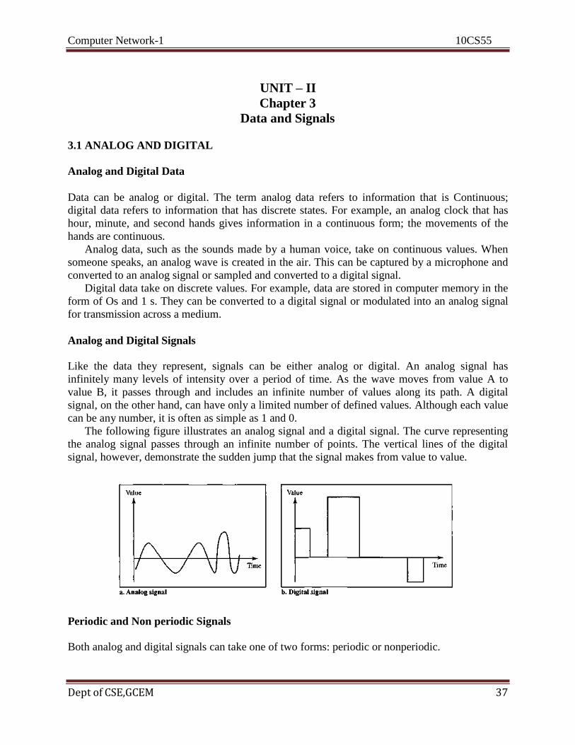
The following figure illustrates an analog signal and a digital signal. The curve representing
the analog signal passes through an infinite number of points. The vertical lines of the digital
signal, however, demonstrate the sudden jump that the signal makes from value to value.
Periodic and Non periodic Signals
Both analog and digital signals can take one of two forms: periodic or nonperiodic.
Computer Network-1 10CS55
Dept of CSE,GCEM 38
A periodic signal completes a pattern within a measurable time frame, called a period, and
repeats that pattern over subsequent identical periods. The completion of one full pattern is
called a cycle. A nonperiodic signal changes without exhibiting a pattern or cycle that repeats
over time.
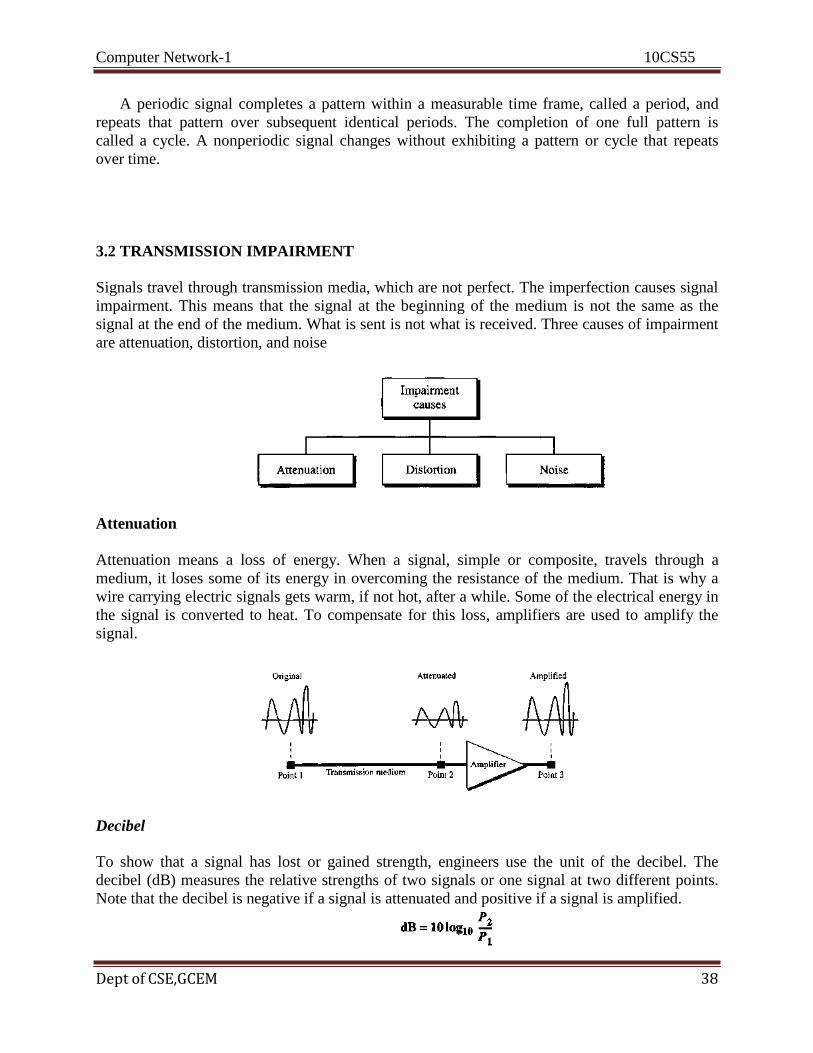
3.2 TRANSMISSION IMPAIRMENT
Signals travel through transmission media, which are not perfect. The imperfection causes signal
impairment. This means that the signal at the beginning of the medium is not the same as the
signal at the end of the medium. What is sent is not what is received. Three causes of impairment
are attenuation, distortion, and noise
Attenuation
Attenuation means a loss of energy. When a signal, simple or composite, travels through a
medium, it loses some of its energy in overcoming the resistance of the medium. That is why a
wire carrying electric signals gets warm, if not hot, after a while. Some of the electrical energy in
the signal is converted to heat. To compensate for this loss, amplifiers are used to amplify the
signal.
Decibel
To show that a signal has lost or gained strength, engineers use the unit of the decibel. The
decibel (dB) measures the relative strengths of two signals or one signal at two different points.
Note that the decibel is negative if a signal is attenuated and positive if a signal is amplified.
Computer Network-1 10CS55
Dept of CSE,GCEM 39
Variables P1 and P2 are the powers of a signal at points 1 and 2, respectively.
Distortion
Distortion means that the signal changes its form or shape. Distortion can occur in a composite
signal made of different frequencies. Each signal component has its own propagation speed (see
the next section) through a medium and, therefore, its own delay in arriving at the final
destination. Differences in delay may create a difference in phase if the delay is not exactly the
same as the period duration. In other words, signal components at the receiver have phases
different from what they had at the sender. The shape of the composite signal is therefore not the
same.
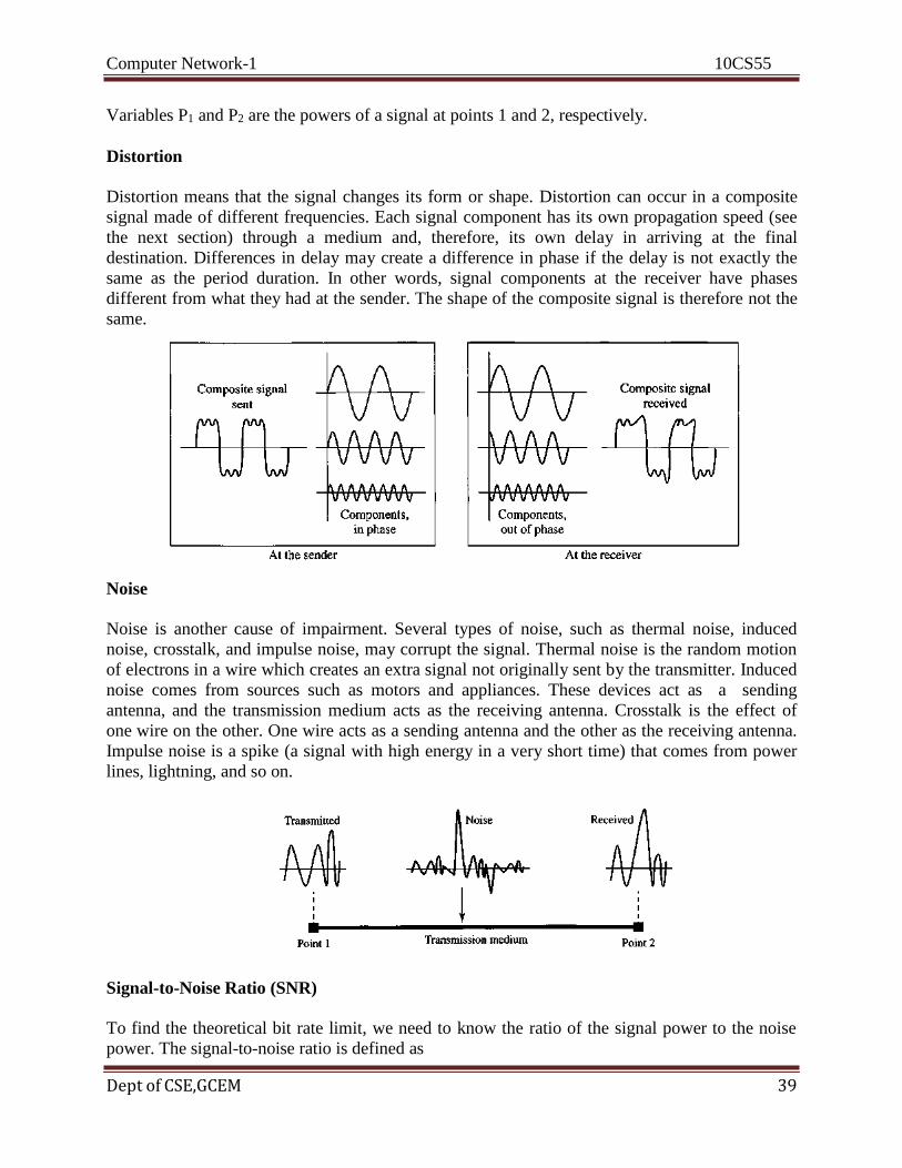
Noise
Noise is another cause of impairment. Several types of noise, such as thermal noise, induced
noise, crosstalk, and impulse noise, may corrupt the signal. Thermal noise is the random motion
of electrons in a wire which creates an extra signal not originally sent by the transmitter. Induced
noise comes from sources such as motors and appliances. These devices act as a sending
antenna, and the transmission medium acts as the receiving antenna. Crosstalk is the effect of
one wire on the other. One wire acts as a sending antenna and the other as the receiving antenna.
Impulse noise is a spike (a signal with high energy in a very short time) that comes from power
lines, lightning, and so on.
Signal-to-Noise Ratio (SNR)
To find the theoretical bit rate limit, we need to know the ratio of the signal power to the noise
power. The signal-to-noise ratio is defined as
Computer Network-1 10CS55
Dept of CSE,GCEM 40
SNR is actually the ratio of what is wanted (signal) to what is not wanted (noise). A high SNR
means the signal is less corrupted by noise; a low SNR means the signal is more corrupted by
noise.
Because SNR is the ratio of two powers, it is often described in decibel units, SNRdB, defined as
3.3 DATA RATE LIMITS
Data rate depends on three factors:
1. The bandwidth available
2. The level of the signals we use
3. The quality of the channel (the level of noise)
Two theoretical formulas were developed to calculate the data rate: one by Nyquist for
a noiseless channel, another by Shannon for a noisy channel.
Noiseless Channel: Nyquist Bit Rate
For a noiseless channel, the Nyquist bit rate formula defines the theoretical maximum bit rate
BitRate = 2 x bandwidth x log2L
In this formula, bandwidth is the bandwidth of the channel, L is the number of signal levels used
to represent data, and BitRate is the bit rate in bits per second.
According to the formula, we might think that, given a specific bandwidth, we can have any bit
rate we want by increasing the number of signal levels. Although the idea is theoretically correct,
practically there is a limit. When we increase the number of signal levels, we impose a burden on
the receiver. If the number of levels in a signal is just 2, the receiver can easily distinguish
between a 0 and a 1. If the level of a signal is 64, the receiver must be very sophisticated to
distinguish between 64 different levels. In other words, increasing the levels of a signal reduces
the reliability of the system.
Noisy Channel: Shannon Capacity
In reality, we cannot have a noiseless channel; the channel is always noisy. In 1944, Claude
Shannon introduced a formula, called the Shannon capacity, to determine the theoretical highest
data rate for a noisy channel:
Capacity = bandwidth x log2(1+SNR)
Computer Network-1 10CS55
Dept of CSE,GCEM 41
In this formula, bandwidth is the bandwidth of the channel, SNR is the signal-to-noise ratio, and
capacity is the capacity of the channel in bits per second. Note that in the Shannon formula there
is no indication of the signal level, which means that no matter how many levels we have, we
cannot achieve a data rate higher than the capacity of the channel. In other words, the formula
defines a characteristic of the channel, not the method of transmission.
3.4 PERFORMANCE
Bandwidth
One characteristic that measures network performance is bandwidth. However, the term can be
used in two different contexts with two different measuring values: bandwidth in hertz and
bandwidth in bits per second.
Bandwidth in Hertz
Bandwidth in hertz is the range of frequencies contained in a composite signal or the range of
frequencies a channel can pass. For example, we can say the bandwidth of a subscriber telephone
line is 4 kHz.
Bandwidth in Bits per Seconds
The term bandwidth can also refer to the number of bits per second that a channel, a link, or even
a network can transmit. For example, one can say the bandwidth of a Fast Ethernet network (or
the links in this network) is a maximum of 100 Mbps. This means that this network can send 100
Mbps.
Relationship
There is an explicit relationship between the bandwidth in hertz and bandwidth in bits per
seconds. Basically, an increase in bandwidth in hertz means an increase in bandwidth in bits per
second. The relationship depends on whether we have baseband transmission or transmission
with modulation.
Throughput
The throughput is a measure of how fast we can actually send data through a network. Although,
at first glance, bandwidth in bits per second and throughput seem the same, they are different. A
link may have a bandwidth of B bps, but we can only send T bps through this link with T always
less than B. In other words, the bandwidth is a potential measurement of a link; the throughput is
an actual measurement of how fast we can send data. For example, we may have a link with a
bandwidth of 1 Mbps, but the devices connected to the end of the link may handle only 200 kbps.
This means that we cannot send more than 200 kbps through this link.

Computer Network-1 10CS55
Dept of CSE,GCEM 42
Latency (Delay)
The latency or delay defines how long it takes for an entire message to completely arrive at the
destination from the time the first bit is sent out from the source. We can say that latency is made
of four components: propagation time, transmission time, queuing time and processing delay.
Latency = propagation time + transmission time + queuing time + processing delay
Propagation Time
Propagation time measures the time required for a bit to travel from the source to the destination.
The propagation time is calculated by dividing the distance by the propagation speed.
The propagation speed of electromagnetic signals depends on the medium and on the frequency
of the signal.
Transmission Time
In data communications we don't send just 1 bit, we send a message. The first bit may take a time
equal to the propagation time to reach its destination; the last bit also may take the same amount
of time. However, there is a time between the first bit leaving the sender and the last bit arriving
at the receiver. The first bit leaves earlier and arrives earlier; the last bit leaves later and arrives
later. The time required for transmission of a message depends on the size of the message and the
bandwidth of the channel.
Queuing Time
The third component in latency is the queuing time, the time needed for each intermediate or end
device to hold the message before it can be processed. The queuing time is not a fixed factor; it
changes with the load imposed on the network. When there is heavy traffic on the network, the
queuing time increases. An intermediate device, such as a router, queues the arrived messages
and processes them one by one. If there are many messages, each message will have to wait.
Bandwidth-Delay Product
Bandwidth and delay are two performance metrics of a link. What is very important in data
communications is the product of the two, the bandwidth-delay product. Let us elaborate on this
issue, using two hypothetical cases as examples.
Case 1. The following figure shows case 1.

Computer Network-1 10CS55
Dept of CSE,GCEM 43
Let us assume that we have a link with a bandwidth of 1 bps Also assume that the delay of the
link is 5 s We want to see what the bandwidth-delay product means in this case. From the figure,
it can be said that this product 1 x 5 is the maximum number of bits that can fill the link. There
can be no more than 5 bits at any time on the link.
Case 2. Now assume we have a bandwidth of 4 bps. The figure shows that there can be
maximum 4 x 5 = 20 bits on the line. The reason is that, at each second, there are 4 bits on the
line; the duration of each bit is 0.25s.
The above two cases show that the product of bandwidth and delay is the number of bits that can
fill the link. This measurement is important if we need to send data in bursts and wait for the
acknowledgment of each burst before sending the next one. To use the maximum capability of
the link, we need to make the size of our burst 2 times the product of bandwidth and delay; we
need to fill up the full-duplex channel (two directions). The sender should send a burst of data of
(2 x bandwidth x delay) bits. The sender then waits for receiver acknowledgment for part of the
burst before sending another burst. The amount 2 x bandwidth x delay is the number of bits that
can be in transition at any time.
Jitter
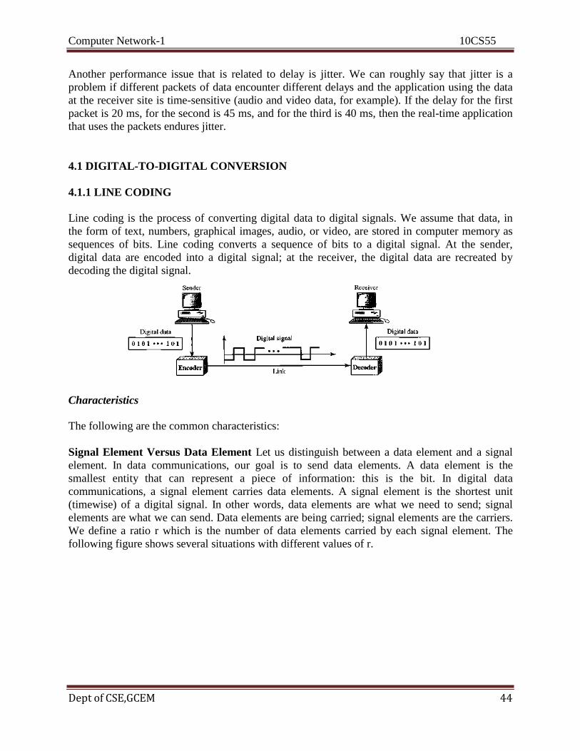
Computer Network-1 10CS55
Dept of CSE,GCEM 44
Another performance issue that is related to delay is jitter. We can roughly say that jitter is a
problem if different packets of data encounter different delays and the application using the data
at the receiver site is time-sensitive (audio and video data, for example). If the delay for the first
packet is 20 ms, for the second is 45 ms, and for the third is 40 ms, then the real-time application
that uses the packets endures jitter.
4.1 DIGITAL-TO-DIGITAL CONVERSION
4.1.1 LINE CODING
Line coding is the process of converting digital data to digital signals. We assume that data, in
the form of text, numbers, graphical images, audio, or video, are stored in computer memory as
sequences of bits. Line coding converts a sequence of bits to a digital signal. At the sender,
digital data are encoded into a digital signal; at the receiver, the digital data are recreated by
decoding the digital signal.
Characteristics
The following are the common characteristics:
Signal Element Versus Data Element Let us distinguish between a data element and a signal
element. In data communications, our goal is to send data elements. A data element is the
smallest entity that can represent a piece of information: this is the bit. In digital data
communications, a signal element carries data elements. A signal element is the shortest unit
(timewise) of a digital signal. In other words, data elements are what we need to send; signal
elements are what we can send. Data elements are being carried; signal elements are the carriers.
We define a ratio r which is the number of data elements carried by each signal element. The
following figure shows several situations with different values of r.
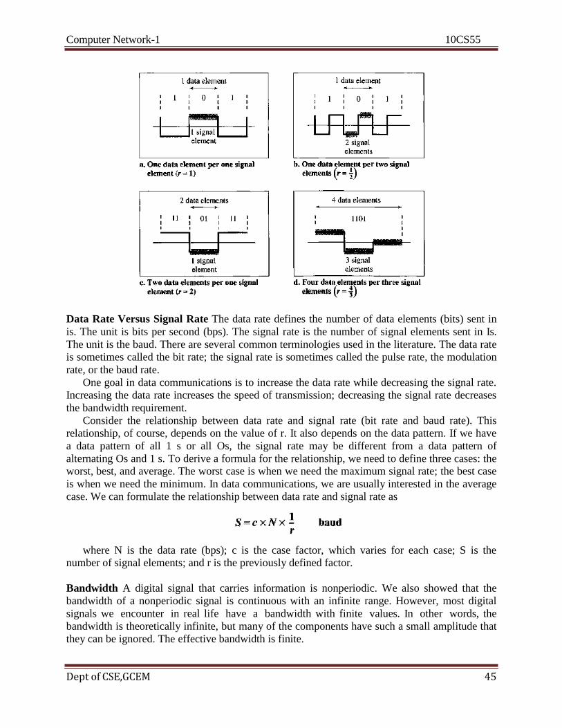
Computer Network-1 10CS55
Dept of CSE,GCEM 45
Data Rate Versus Signal Rate The data rate defines the number of data elements (bits) sent in
is. The unit is bits per second (bps). The signal rate is the number of signal elements sent in Is.
The unit is the baud. There are several common terminologies used in the literature. The data rate
is sometimes called the bit rate; the signal rate is sometimes called the pulse rate, the modulation
rate, or the baud rate.
One goal in data communications is to increase the data rate while decreasing the signal rate.
Increasing the data rate increases the speed of transmission; decreasing the signal rate decreases
the bandwidth requirement.
Consider the relationship between data rate and signal rate (bit rate and baud rate). This
relationship, of course, depends on the value of r. It also depends on the data pattern. If we have
a data pattern of all 1 s or all Os, the signal rate may be different from a data pattern of
alternating Os and 1 s. To derive a formula for the relationship, we need to define three cases: the
worst, best, and average. The worst case is when we need the maximum signal rate; the best case
is when we need the minimum. In data communications, we are usually interested in the average
case. We can formulate the relationship between data rate and signal rate as
where N is the data rate (bps); c is the case factor, which varies for each case; S is the
number of signal elements; and r is the previously defined factor.
Bandwidth A digital signal that carries information is nonperiodic. We also showed that the
bandwidth of a nonperiodic signal is continuous with an infinite range. However, most digital
signals we encounter in real life have a bandwidth with finite values. In other words, the
bandwidth is theoretically infinite, but many of the components have such a small amplitude that
they can be ignored. The effective bandwidth is finite.
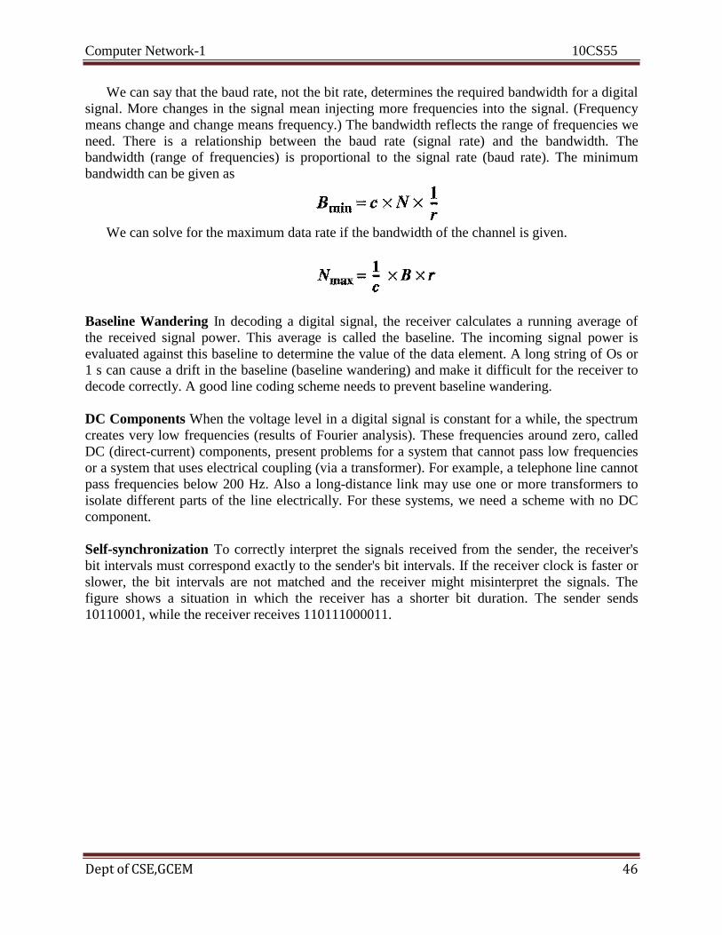
Computer Network-1 10CS55
Dept of CSE,GCEM 46
We can say that the baud rate, not the bit rate, determines the required bandwidth for a digital
signal. More changes in the signal mean injecting more frequencies into the signal. (Frequency
means change and change means frequency.) The bandwidth reflects the range of frequencies we
need. There is a relationship between the baud rate (signal rate) and the bandwidth. The
bandwidth (range of frequencies) is proportional to the signal rate (baud rate). The minimum
bandwidth can be given as
We can solve for the maximum data rate if the bandwidth of the channel is given.
Baseline Wandering In decoding a digital signal, the receiver calculates a running average of
the received signal power. This average is called the baseline. The incoming signal power is
evaluated against this baseline to determine the value of the data element. A long string of Os or
1 s can cause a drift in the baseline (baseline wandering) and make it difficult for the receiver to
decode correctly. A good line coding scheme needs to prevent baseline wandering.
DC Components When the voltage level in a digital signal is constant for a while, the spectrum
creates very low frequencies (results of Fourier analysis). These frequencies around zero, called
DC (direct-current) components, present problems for a system that cannot pass low frequencies
or a system that uses electrical coupling (via a transformer). For example, a telephone line cannot
pass frequencies below 200 Hz. Also a long-distance link may use one or more transformers to
isolate different parts of the line electrically. For these systems, we need a scheme with no DC
component.
Self-synchronization To correctly interpret the signals received from the sender, the receiver's
bit intervals must correspond exactly to the sender's bit intervals. If the receiver clock is faster or
slower, the bit intervals are not matched and the receiver might misinterpret the signals. The
figure shows a situation in which the receiver has a shorter bit duration. The sender sends
10110001, while the receiver receives 110111000011.
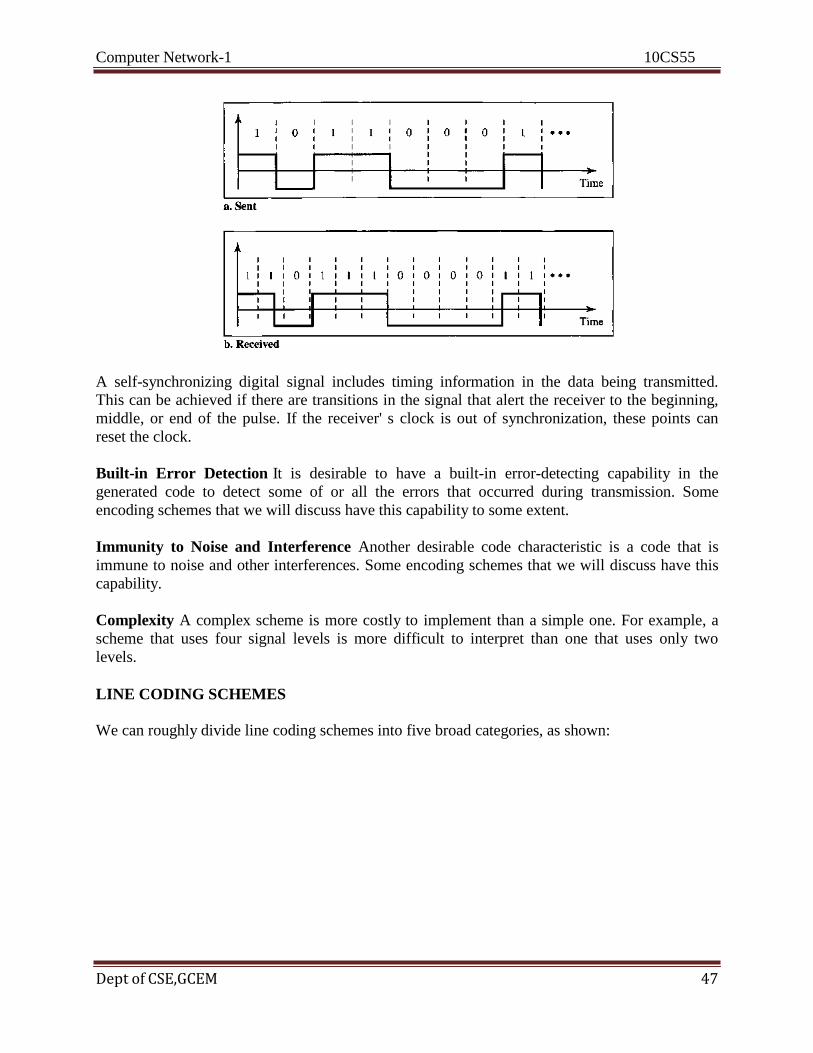
Computer Network-1 10CS55
Dept of CSE,GCEM 47
A self-synchronizing digital signal includes timing information in the data being transmitted.
This can be achieved if there are transitions in the signal that alert the receiver to the beginning,
middle, or end of the pulse. If the receiver' s clock is out of synchronization, these points can
reset the clock.
Built-in Error Detection It is desirable to have a built-in error-detecting capability in the
generated code to detect some of or all the errors that occurred during transmission. Some
encoding schemes that we will discuss have this capability to some extent.
Immunity to Noise and Interference Another desirable code characteristic is a code that is
immune to noise and other interferences. Some encoding schemes that we will discuss have this
capability.
Complexity A complex scheme is more costly to implement than a simple one. For example, a
scheme that uses four signal levels is more difficult to interpret than one that uses only two
levels.
LINE CODING SCHEMES
We can roughly divide line coding schemes into five broad categories, as shown:
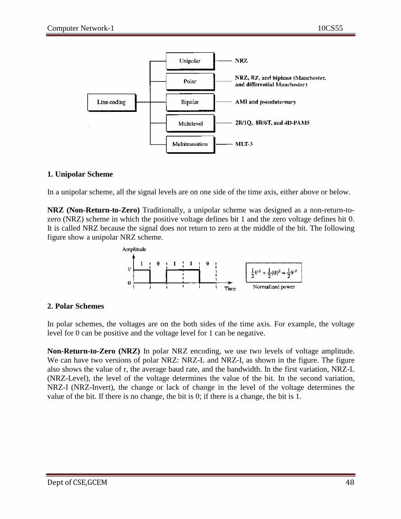
Computer Network-1 10CS55
Dept of CSE,GCEM 48
1. Unipolar Scheme
In a unipolar scheme, all the signal levels are on one side of the time axis, either above or below.
NRZ (Non-Return-to-Zero) Traditionally, a unipolar scheme was designed as a non-return-to-
zero (NRZ) scheme in which the positive voltage defines bit 1 and the zero voltage defines bit 0.
It is called NRZ because the signal does not return to zero at the middle of the bit. The following
figure show a unipolar NRZ scheme.
2. Polar Schemes
In polar schemes, the voltages are on the both sides of the time axis. For example, the voltage
level for 0 can be positive and the voltage level for 1 can be negative.
Non-Return-to-Zero (NRZ) In polar NRZ encoding, we use two levels of voltage amplitude.
We can have two versions of polar NRZ: NRZ-L and NRZ-I, as shown in the figure. The figure
also shows the value of r, the average baud rate, and the bandwidth. In the first variation, NRZ-L
(NRZ-Level), the level of the voltage determines the value of the bit. In the second variation,
NRZ-I (NRZ-Invert), the change or lack of change in the level of the voltage determines the
value of the bit. If there is no change, the bit is 0; if there is a change, the bit is 1.
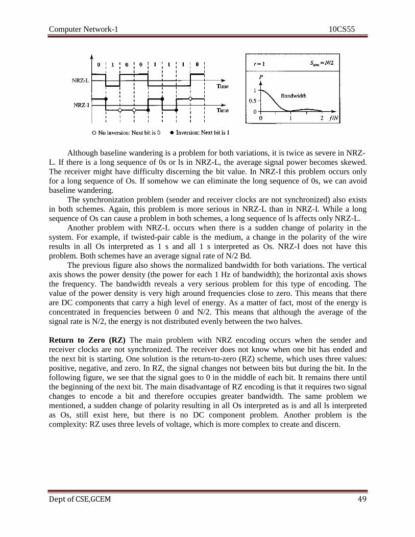
Computer Network-1 10CS55
Dept of CSE,GCEM 49
Although baseline wandering is a problem for both variations, it is twice as severe in NRZ-
L. If there is a long sequence of 0s or ls in NRZ-L, the average signal power becomes skewed.
The receiver might have difficulty discerning the bit value. In NRZ-I this problem occurs only
for a long sequence of Os. If somehow we can eliminate the long sequence of 0s, we can avoid
baseline wandering.
The synchronization problem (sender and receiver clocks are not synchronized) also exists
in both schemes. Again, this problem is more serious in NRZ-L than in NRZ-I. While a long
sequence of Os can cause a problem in both schemes, a long sequence of ls affects only NRZ-L.
Another problem with NRZ-L occurs when there is a sudden change of polarity in the
system. For example, if twisted-pair cable is the medium, a change in the polarity of the wire
results in all Os interpreted as 1 s and all 1 s interpreted as Os. NRZ-I does not have this
problem. Both schemes have an average signal rate of N/2 Bd.
The previous figure also shows the normalized bandwidth for both variations. The vertical
axis shows the power density (the power for each 1 Hz of bandwidth); the horizontal axis shows
the frequency. The bandwidth reveals a very serious problem for this type of encoding. The
value of the power density is very high around frequencies close to zero. This means that there
are DC components that carry a high level of energy. As a matter of fact, most of the energy is
concentrated in frequencies between 0 and N/2. This means that although the average of the
signal rate is N/2, the energy is not distributed evenly between the two halves.
Return to Zero (RZ) The main problem with NRZ encoding occurs when the sender and
receiver clocks are not synchronized. The receiver does not know when one bit has ended and
the next bit is starting. One solution is the return-to-zero (RZ) scheme, which uses three values:
positive, negative, and zero. In RZ, the signal changes not between bits but during the bit. In the
following figure, we see that the signal goes to 0 in the middle of each bit. It remains there until
the beginning of the next bit. The main disadvantage of RZ encoding is that it requires two signal
changes to encode a bit and therefore occupies greater bandwidth. The same problem we
mentioned, a sudden change of polarity resulting in all Os interpreted as is and all ls interpreted
as Os, still exist here, but there is no DC component problem. Another problem is the
complexity: RZ uses three levels of voltage, which is more complex to create and discern.

Computer Network-1 10CS55
Dept of CSE, GCEM 51
Biphase: Manchester and Differential Manchester The idea of RZ (transition at the middle of
the bit) and the idea of NRZ-L are combined into the Manchester scheme. In Manchester
encoding, the duration of the bit is divided into two halves. The voltage remains at one level
during the first half and moves to the other level in the second half. The transition at the middle
of the bit provides synchronization. Differential Manchester, on the other hand, combines the
ideas of RZ and NRZ-I. There is always a transition at the middle of the bit, but the bit values are
determined at the beginning of the bit. If the next bit is 0, there is a transition; if the next bit is 1,
there is none.
The Manchester scheme overcomes several problems associated with NRZ-L, and
differential Manchester overcomes several problems associated with NRZ-I. First, there is no
baseline wandering. There is no DC component because each bit has a positive and negative
voltage contribution. The only drawback is the signal rate. The signal rate for Manchester and
differential Manchester is double that for NRZ. The reason is that there is always one transition
at the middle of the bit and maybe one transition at the end of each bit.
3. Bipolar Schemes
In bipolar encoding (sometimes called multilevel binary), there are three voltage levels: positive,
negative, and zero. The voltage level for one data element is at zero, while the voltage level for
the other element alternates between positive and negative.

Computer Network-1 10CS55
Dept of CSE, GCEM 52
AMI and Pseudoternary The figure shows two variations of bipolar encoding: AMI and
pseudoternary. A common bipolar encoding scheme is called bipolar alternate mark inversion
(AMI). AMI means alternate 1 inversion. A neutral zero voltage represents binary 0. Binary ls
are represented by alternating positive and negative voltages. A variation of AMI encoding is
called pseudoternary in which the 1 bit is encoded as a zero voltage and the 0 bit is encoded as
alternating positive and negative voltages.
The bipolar scheme was developed as an alternative to NRZ. The bipolar scheme has the
same signal rate as NRZ, but there is no DC component. The NRZ scheme has most of its energy
concentrated near zero frequency, which makes it unsuitable for transmission over channels with
poor performance around this frequency. The concentration of the energy in bipolar encoding is
around frequency N/2.
If we have a long sequence of 1 s, the voltage level alternates between positive and
negative; it is not constant. Therefore, there is no DC component. For a long sequence of Os, the
voltage remains constant, but its amplitude is zero, which is the same as having no DC
component. In other words, a sequence that creates a constant zero voltage does not have a DC
component.
AMI is commonly used for long-distance communication, but it has a synchronization
problem when a long sequence of Os is present in the data.
4. Multilevel Schemes
The goal is to increase the number of bits per baud by encoding a pattern of m data elements into a pattern of n signal elements. We only have two types of data elements (0s and ls), which means
that a group of m data elements can produce a combination of 2m data patterns. We can have different types of signal elements by allowing different signal levels. If we have L different
levels, then we can produce Ln combinations of signal patterns. If 2m = Ln, then each data pattern
is encoded into one signal pattern. If 2m< Ln, data patterns occupy only a subset of signal patterns. The subset can be carefully designed to prevent baseline wandering, to provide synchronization, and to detect errors that occurred during data transmission. Data encoding is not
possible if 2m > Ln because some of the data patterns cannot be encoded.
The code designers have classified these types of coding as mBnL, where m is the length of
the binary pattern, B means binary data, n is the length of the signal pattern, and L is the number
of levels in the signalling. A letter is often used in place of L: B (binary) for L = 2, T (ternary)
for L = 3, and Q (quaternary) for L = 4. Note that the first two letters define the data pattern, and
the second two define the signal pattern.

Computer Network-1 10CS55
Dept of CSE, GCEM 53
2B1Q The first mBnL scheme we discuss, two binary, one quaternary (2B1Q), uses data patterns
of size 2 and encodes the 2-bit patterns as one signal element belonging to a four-level signal. In
this type of encoding m = 2, n = 1, and L = 4 (quaternary). The figure shows an example of a
2B1Q signal.
The average signal rate of 2B1Q is S = N/4. This means that using 2B1Q, we can send data
2 times faster than by using NRZ-L. However, 2B1Q uses four different signal levels, which
means the receiver has to discern four different thresholds. The reduced bandwidth comes with a
price. There are no redundant signal patterns in this scheme because 22 = 41.
8B6T A very interesting scheme is eight binary, six ternary (8B6T). This code is used with
100BASE-4T cable. The idea is to encode a pattern of 8 bits as a pattern of 6 signal elements,
where the signal has three levels (ternary). In this type of scheme, we can have 28 = 256 different
data patterns and 36 = 478 different signal patterns. There are 478 - 256 = 222 redundant signal
elements that provide synchronization and error detection. Part of the redundancy is also used to
provide DC balance. Each signal pattern has a weight of 0 or +1 DC values. This means that
there is no pattern with the weight -1. To make the whole stream DC-balanced, the sender keeps
track of the weight. If two groups of weight 1 are encountered one after another, the first one is
sent as is, while the next one is totally inverted to give a weight of -1. The figure shows an example of three data patterns encoded as three signal patterns. The
three possible signal levels are represented as -, 0, and +. The first 8-bit pattern 00010001 is
encoded as the signal pattern -0-0++ with weight 0; the second 8-bit pattern 01010011 is
encoded as - + - + + 0 with weight +1. The third bit pattern should be encoded as + - - + 0 + with
weight +1. To create DC balance, the sender inverts the actual signal. The receiver can easily
recognize that this is an inverted pattern because the weight is -1. The pattern is inverted before
decoding.
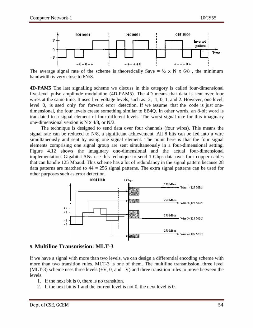
Computer Network-1 10CS55
Dept of CSE, GCEM 54
The average signal rate of the scheme is theoretically Save = ½ x N x 6/8 , the minimum bandwidth is very close to 6N/8.
4D-PAM5 The last signalling scheme we discuss in this category is called four-dimensional
five-level pulse amplitude modulation (4D-PAM5). The 4D means that data is sent over four
wires at the same time. It uses five voltage levels, such as -2, -1, 0, 1, and 2. However, one level,
level 0, is used only for forward error detection. If we assume that the code is just one-
dimensional, the four levels create something similar to 8B4Q. In other words, an 8-bit word is
translated to a signal element of four different levels. The worst signal rate for this imaginary
one-dimensional version is N x 4/8, or N/2.
The technique is designed to send data over four channels (four wires). This means the
signal rate can be reduced to N/8, a significant achievement. All 8 bits can be fed into a wire
simultaneously and sent by using one signal element. The point here is that the four signal
elements comprising one signal group are sent simultaneously in a four-dimensional setting.
Figure 4.12 shows the imaginary one-dimensional and the actual four-dimensional
implementation. Gigabit LANs use this technique to send 1-Gbps data over four copper cables
that can handle 125 Mbaud. This scheme has a lot of redundancy in the signal pattern because 28
data patterns are matched to 44 = 256 signal patterns. The extra signal patterns can be used for
other purposes such as error detection.
5. Multiline Transmission: MLT-3
If we have a signal with more than two levels, we can design a differential encoding scheme with
more than two transition rules. MLT-3 is one of them. The multiline transmission, three level
(MLT-3) scheme uses three levels (+V, 0, and –V) and three transition rules to move between the
levels.
1. If the next bit is 0, there is no transition.
2. If the next bit is 1 and the current level is not 0, the next level is 0.
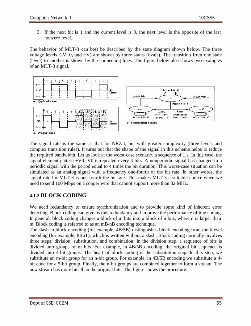
Computer Network-1 10CS55
Dept of CSE, GCEM 55
3. If the next bit is 1 and the current level is 0, the next level is the opposite of the last
nonzero level.
The behavior of MLT-3 can best be described by the state diagram shown below. The three
voltage levels (-V, 0, and +V) are shown by three states (ovals). The transition from one state
(level) to another is shown by the connecting lines. The figure below also shows two examples
of an MLT-3 signal.
The signal rate is the same as that for NRZ-I, but with greater complexity (three levels and
complex transition rules). It turns out that the shape of the signal in this scheme helps to reduce
the required bandwidth. Let us look at the worst-case scenario, a sequence of 1 s. In this case, the
signal element pattern +V0 -V0 is repeated every 4 bits. A nonperiodic signal has changed to a
periodic signal with the period equal to 4 times the bit duration. This worst-case situation can be
simulated as an analog signal with a frequency one-fourth of the bit rate. In other words, the
signal rate for MLT-3 is one-fourth the bit rate. This makes MLT-3 a suitable choice when we
need to send 100 Mbps on a copper wire that cannot support more than 32 MHz.
4.1.2 BLOCK CODING
We need redundancy to ensure synchronization and to provide some kind of inherent error
detecting. Block coding can give us this redundancy and improve the performance of line coding.
In general, block coding changes a block of m bits into a block of n bits, where n is larger than
m. Block coding is referred to as an mB/nB encoding technique.
The slash in block encoding (for example, 4B/5B) distinguishes block encoding from multilevel
encoding (for example, 8B6T), which is written without a slash. Block coding normally involves
three steps: division, substitution, and combination. In the division step, a sequence of bits is
divided into groups of m bits. For example, in 4B/5B encoding, the original bit sequence is
divided into 4-bit groups. The heart of block coding is the substitution step. In this step, we
substitute an m-bit group for an n-bit group. For example, in 4B/5B encoding we substitute a 4-
bit code for a 5-bit group. Finally, the n-bit groups are combined together to form a stream. The
new stream has more bits than the original bits. The figure shows the procedure.

Computer Network-1 10CS55
Dept of CSE, GCEM 56
4B/5B
The four binary/five binary (4B/5B) coding scheme was designed to be used in combination with
NRZ-I. Recall that NRZ-I has a good signal rate, one-half that of the biphase, but it has a
synchronization problem. A long sequence of 0s can make the receiver clock lose
synchronization. One solution is to change the bit stream, prior to encoding with NRZ-I, so that
it does not have a long stream of 0s. The 4B/5B scheme achieves this goal. The block-coded
stream does not have more that three consecutive 0s, as we will see later. At the receiver, the
NRZ-I encoded digital signal is first decoded into a stream of bits and then decoded to remove
the redundancy. The figure shows the idea.
In 4B/5B, the 5-bit output that replaces the 4-bit input has no more than one leading zero
(left bit) and no more than two trailing zeros (right bits). So when different groups are combined
to make a new sequence, there are never more than three consecutive 0s.
Note that the first two columns pair a 4-bit group with a 5-bit group. A group of 4 bits can
have only 16 different combinations while a group of 5 bits can have 32 different combinations.
This means that there are 16 groups that are not used for 4B/5B encoding. Some of these unused
groups are used for control purposes; the others are not used at all. The latter provide a kind of
error detection. If a 5-bit group arrives that belongs to the unused portion of the table, the
receiver knows that there is an error in the transmission.

Computer Network-1 10CS55
Dept of CSE, GCEM 57
The figure shows an example of substitution in 4B/5B coding. 4B/5B encoding solves the
problem of synchronization and overcomes one of the deficiencies of NRZ-I. However, we need
to remember that it increases the signal rate of NRZ-I. The redundant bits add 20 percent more
baud. Still, the result is less than the biphase scheme which has a signal rate of 2 times that of
NRZ-I. However, 4B/5B block encoding does not solve the DC component problem of NRZ-I. If
a DC component is unacceptable, we need to use biphase or bipolar encoding.
8B/10B
The eight binary/ten binary (8B/10B) encoding is similar to 4B/5B encoding except that a group
of 8 bits of data is now substituted by a 10-bit code. It provides greater error detection capability
than 4B/5B. The 8B/10B block coding is actually a combination of 5B/6B and 3B/4B encoding,
as shown in the figure.

Computer Network-1 10CS55
Dept of CSE, GCEM 58
The most five significant bits of a 10-bit block is fed into the 5B/6B encoder; the least 3
significant bits is fed into a 3B/4B encoder. The split is done to simplify the mapping table. To
prevent a long run of consecutive 0s or ls, the code uses a disparity controller which keeps track
of excess 0s over ls (or ls over 0s). If the bits in the current block create a disparity that contributes to the previous disparity (either direction), then each bit in the code is complemented
(a 0 is changed to a 1 and a 1 is changed to a 0). The coding has 210 - 28 = 768 redundant groups
that can be used for disparity checking and error detection. In general, the technique is superior to 4B/5B because of better built-in error-checking capability and better synchronization.
4.1.3 SCRAMBLING
Biphase schemes that are suitable for dedicated links between stations in a LAN are not
suitable for long-distance communication because of their wide bandwidth requirement. The
combination of block coding and NRZ line coding is not suitable for long-distance encoding
either, because of the DC component. Bipolar AMI encoding, on the other hand, has a narrow
bandwidth and does not create a DC component. However, a long sequence of Os upsets the
synchronization. If we can find a way to avoid a long sequence of 0s in the original stream, we
can use bipolar AMI for long distances. We are looking for a technique that does not increase the
number of bits and does provide synchronization. We are looking for a solution that substitutes
long zero-level pulses with a combination of other levels to provide synchronization. One
solution is called scrambling. We modify part of the AMI rule to include scrambling, as shown in
the figure. Note that scrambling, as opposed to block coding, is done at the same time as
encoding. The system needs to insert the required pulses based on the defined scrambling rules.
Two common scrambling techniques are B8ZS and HDB3.
B8ZS
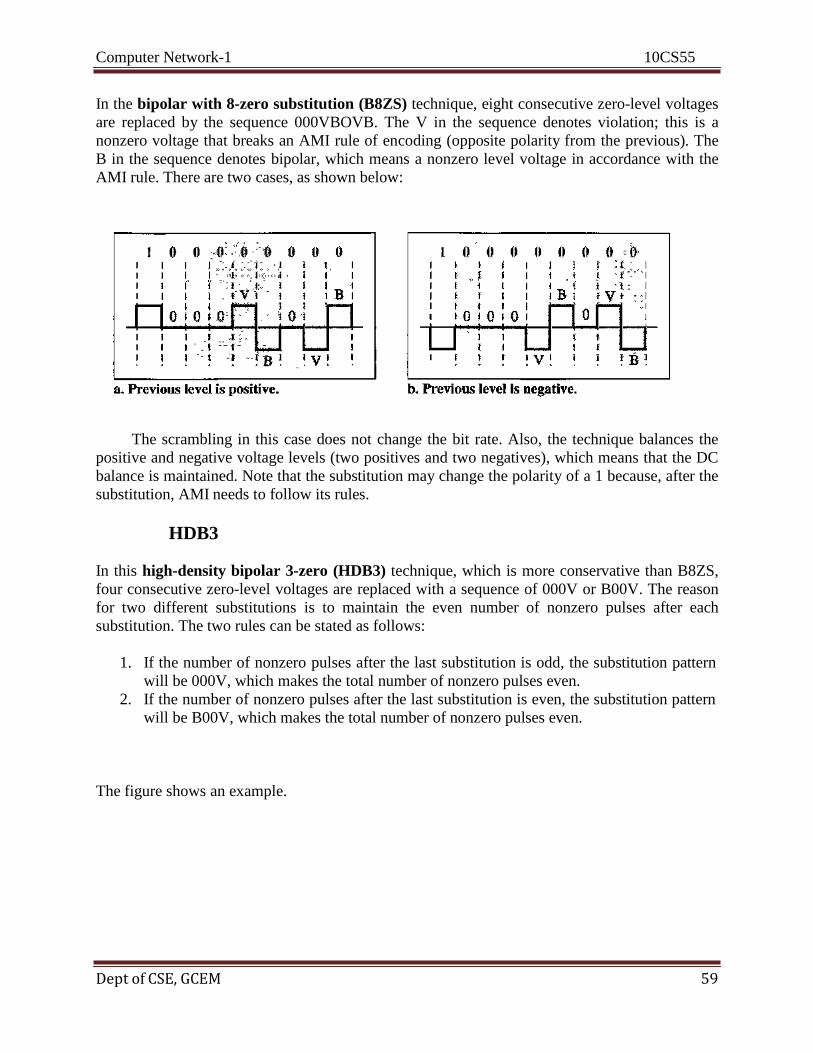
Computer Network-1 10CS55
Dept of CSE, GCEM 59
In the bipolar with 8-zero substitution (B8ZS) technique, eight consecutive zero-level voltages
are replaced by the sequence 000VBOVB. The V in the sequence denotes violation; this is a
nonzero voltage that breaks an AMI rule of encoding (opposite polarity from the previous). The
B in the sequence denotes bipolar, which means a nonzero level voltage in accordance with the
AMI rule. There are two cases, as shown below:
The scrambling in this case does not change the bit rate. Also, the technique balances the
positive and negative voltage levels (two positives and two negatives), which means that the DC
balance is maintained. Note that the substitution may change the polarity of a 1 because, after the
substitution, AMI needs to follow its rules.
HDB3
In this high-density bipolar 3-zero (HDB3) technique, which is more conservative than B8ZS,
four consecutive zero-level voltages are replaced with a sequence of 000V or B00V. The reason
for two different substitutions is to maintain the even number of nonzero pulses after each
substitution. The two rules can be stated as follows:
1. If the number of nonzero pulses after the last substitution is odd, the substitution pattern
will be 000V, which makes the total number of nonzero pulses even.
2. If the number of nonzero pulses after the last substitution is even, the substitution pattern
will be B00V, which makes the total number of nonzero pulses even.
The figure shows an example.
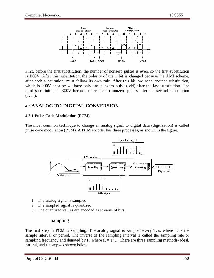
Computer Network-1 10CS55
Dept of CSE, GCEM 60
First, before the first substitution, the number of nonzero pulses is even, so the first substitution
is B00V. After this substitution, the polarity of the 1 bit is changed because the AMI scheme,
after each substitution, must follow its own rule. After this bit, we need another substitution,
which is 000V because we have only one nonzero pulse (odd) after the last substitution. The
third substitution is B00V because there are no nonzero pulses after the second substitution
(even).
4.2 ANALOG-TO-DIGITAL CONVERSION
4.2.1 Pulse Code Modulation (PCM)
The most common technique to change an analog signal to digital data (digitization) is called
pulse code modulation (PCM). A PCM encoder has three processes, as shown in the figure.
1. The analog signal is sampled.
2. The sampled signal is quantized.
3. The quantized values are encoded as streams of bits.
Sampling
The first step in PCM is sampling. The analog signal is sampled every Ts s, where Ts is the
sample interval or period. The inverse of the sampling interval is called the sampling rate or
sampling frequency and denoted by fs, where fs = 1/Ts. There are three sampling methods- ideal,
natural, and flat-top -as shown below.
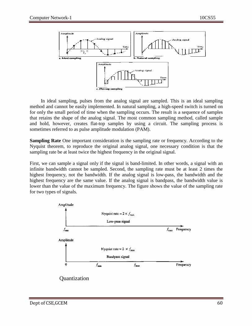
Computer Network-1 10CS55
Dept of CSE,GCEM 60
In ideal sampling, pulses from the analog signal are sampled. This is an ideal sampling
method and cannot be easily implemented. In natural sampling, a high-speed switch is turned on
for only the small period of time when the sampling occurs. The result is a sequence of samples
that retains the shape of the analog signal. The most common sampling method, called sample
and hold, however, creates flat-top samples by using a circuit. The sampling process is
sometimes referred to as pulse amplitude modulation (PAM).
Sampling Rate One important consideration is the sampling rate or frequency. According to the
Nyquist theorem, to reproduce the original analog signal, one necessary condition is that the
sampling rate be at least twice the highest frequency in the original signal.
First, we can sample a signal only if the signal is band-limited. In other words, a signal with an
infinite bandwidth cannot be sampled. Second, the sampling rate must be at least 2 times the
highest frequency, not the bandwidth. If the analog signal is low-pass, the bandwidth and the
highest frequency are the same value. If the analog signal is bandpass, the bandwidth value is
lower than the value of the maximum frequency. The figure shows the value of the sampling rate
for two types of signals.
Quantization

Computer Network-1 10CS55
Dept of CSE,GCEM 61
The result of sampling is a series of pulses with amplitude values between the maximum and
minimum amplitudes of the signal. The set of amplitudes can be infinite with nonintegral values
between the two limits. These values cannot be used in the encoding process. The following are
the steps in quantization:
1. We assume that the original analog signal has instantaneous amplitudes between Vmin and
Vmax.
2. We divide the range into L zones, each of height Δ(delta).
3. We assign quantized values of 0 to L - 1 to the midpoint of each zone. 4. We approximate the value of the sample amplitude to the quantized values.
As a simple example, assume that we have a sampled signal and the sample amplitudes are
between -20 and +20 V. We decide to have eight levels (L = 8). This means that Δ = 5 V. The
figure shows this example.
The value at the top of each sample in the graph shows the actual amplitude. In the chart, the first
row is the normalized value for each sample (actual amplitude/ Δ). The quantization process
selects the quantization value from the middle of each zone. This means that the normalized
quantized values (second row) are different from the normalized amplitudes. The difference is
called the normalized error (third row). The fourth row is the quantization code for each sample

Computer Network-1 10CS55
Dept of CSE,GCEM 62
based on the quantization levels at the left of the graph. The encoded words (fifth row) are the
final products of the conversion.
Quantization Levels The choice of L, the number of levels, depends on the range of the
amplitudes of the analog signal and how accurately we need to recover the signal. If the
amplitude of a signal fluctuates between two values only, we need only two levels; if the signal,
like voice, has many amplitude values, we need more quantization levels. In audio digitizing, L
is normally chosen to be 256; in video it is normally thousands. Choosing lower values of L
increases the quantization error if there is a lot of fluctuation in the signal.
Quantization Error Quantization is an approximation process. The input values to the quantizer
are the real values; the output values are the approximated values. The output values are chosen
to be the middle value in the zone. If the input value is also at the middle of the zone, there is no
quantization error; otherwise, there is an error. In the previous example, the normalized
amplitude of the third sample is 3.24, but the normalized quantized value is 3.50. This means that
there is an error of +0.26. The value of the error for any sample is less than Δ/2. In other words,
we have - Δ/2 ≤ error ≤ Δ/2.
The quantization error changes the signal-to-noise ratio of the signal, which in turn reduces the
upper limit capacity according to Shannon.
The contribution of the quantization error to the SNRdB of the signal depends on the number of
quantization levels L, or the bits per sample nb, as shown in the following formula:
Uniform Versus Non-uniform Quantization For many applications, the distribution of the
instantaneous amplitudes in the analog signal is not uniform. Changes in amplitude often occur
more frequently in the lower amplitudes than in the higher ones. For these types of applications it
is better to use nonuniform zones. In other words, the height of Δ is not fixed; it is greater near
the lower amplitudes and less near the higher amplitudes. Nonuniform quantization can also be
achieved by using a process called companding and expanding. The signal is companded at the
sender before conversion; it is expanded at the receiver after conversion. Companding means
reducing the instantaneous voltage amplitude for large values; expanding is the opposite process.
Companding gives greater weight to strong signals and less weight to weak ones. It has been
proved that nonuniform quantization effectively reduces the SNRdB of quantization.
Encoding
The last step in PCM is encoding. After each sample is quantized and the number of bits per
sample is decided, each sample can be changed to an nb-bit code word. A quantization code of 2
is encoded as 010; 5 is encoded as 101; and so on. Note that the number of bits for each sample
is determined from the number of quantization levels. If the number of quantization levels is L,
the number of bits is n b = log 2 L. The bit rate can be found from the formula:
Bit rate = sampling rate x number of bits per sample = fs x nb
Original Signal Recovery
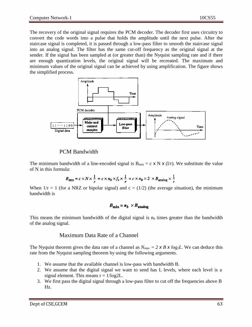
Computer Network-1 10CS55
Dept of CSE,GCEM 63
The recovery of the original signal requires the PCM decoder. The decoder first uses circuitry to
convert the code words into a pulse that holds the amplitude until the next pulse. After the
staircase signal is completed, it is passed through a low-pass filter to smooth the staircase signal
into an analog signal. The filter has the same cut-off frequency as the original signal at the
sender. If the signal has been sampled at (or greater than) the Nyquist sampling rate and if there
are enough quantization levels, the original signal will be recreated. The maximum and
minimum values of the original signal can be achieved by using amplification. The figure shows
the simplified process.
PCM Bandwidth
The minimum bandwidth of a line-encoded signal is Bmin = c x N x (l/r). We substitute the value
of N in this formula:
When 1/r = 1 (for a NRZ or bipolar signal) and c = (1/2) (the average situation), the minimum
bandwidth is
This means the minimum bandwidth of the digital signal is nb times greater than the bandwidth
of the analog signal.
Maximum Data Rate of a Channel
The Nyquist theorem gives the data rate of a channel as Nmax = 2 x B x log2L. We can deduce this rate from the Nyquist sampling theorem by using the following arguments.
1. We assume that the available channel is low-pass with bandwidth B.
2. We assume that the digital signal we want to send has L levels, where each level is a
signal element. This means r = 1/log2L.
3. We first pass the digital signal through a low-pass filter to cut off the frequencies above B
Hz.

Computer Network-1 10CS55
Dept of CSE,GCEM 64
4. We treat the resulting signal as an analog signal and sample it at 2 x B samples per
second and quantize it using L levels. Additional quantization levels are useless because
the signal originally had L levels.
5. The resulting bit rate is N =fs x nb = 2 x B x log2L. This is the maximum bandwidth; if the case factor c increases, the data rate is reduced.
Minimum Required Bandwidth
The previous argument can give us the minimum bandwidth if the data rate and the number of
signal levels are fixed. We can say
4.2.2 Delta Modulation (DM)
PCM finds the value of the signal amplitude for each sample; DM finds the change from the
previous sample. The figure shows the process. Note that there are no code words here; bits are
sent one after another.
Modulator
The modulator is used at the sender site to create a stream of bits from an analog signal. The
process records the small positive or negative changes, called delta δ. If the delta is positive, the
process records a 1; if it is negative, the process records a 0. However, the process needs a base
against which the analog signal is compared. The modulator builds a second signal that
resembles a staircase. Finding the change is then reduced to comparing the input signal with the
gradually made staircase signal. The figure shows a diagram of the process.
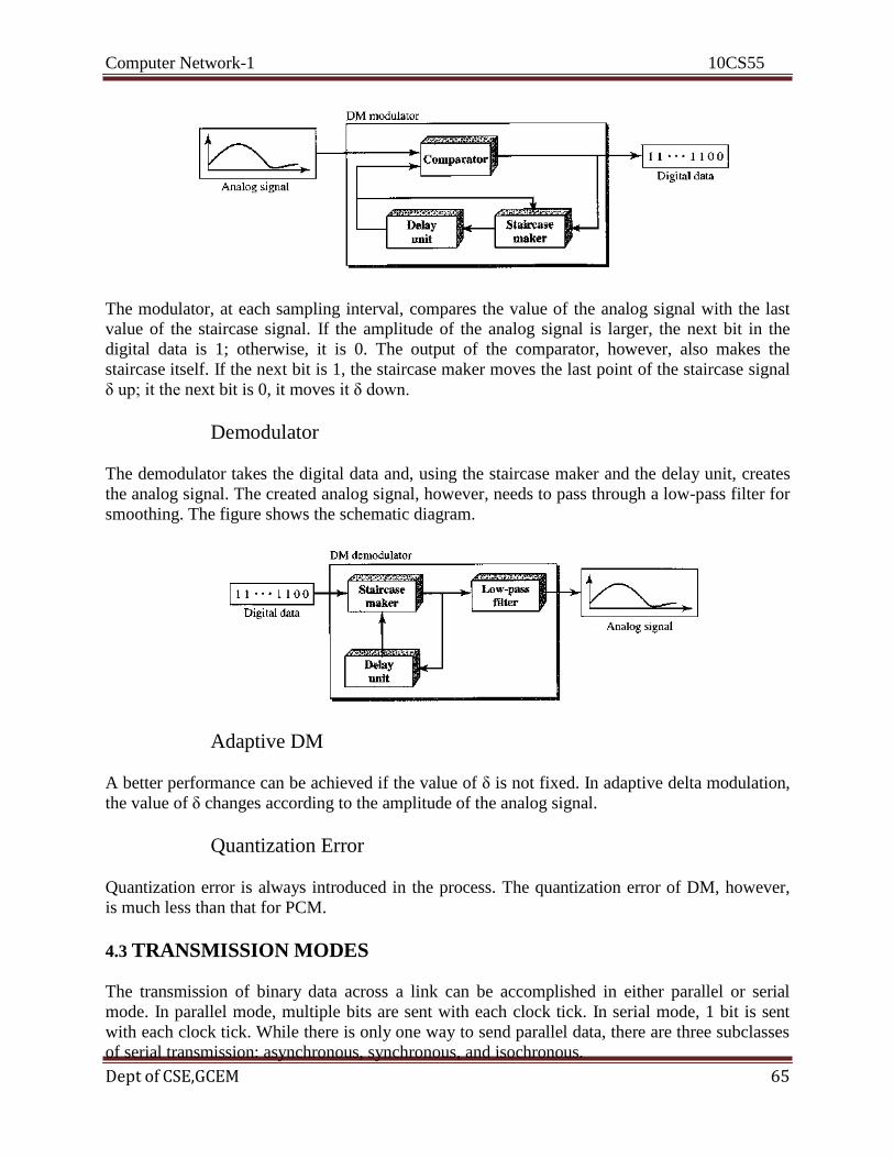
Computer Network-1 10CS55
Dept of CSE,GCEM 65
The modulator, at each sampling interval, compares the value of the analog signal with the last
value of the staircase signal. If the amplitude of the analog signal is larger, the next bit in the
digital data is 1; otherwise, it is 0. The output of the comparator, however, also makes the
staircase itself. If the next bit is 1, the staircase maker moves the last point of the staircase signal
δ up; it the next bit is 0, it moves it δ down.
Demodulator
The demodulator takes the digital data and, using the staircase maker and the delay unit, creates
the analog signal. The created analog signal, however, needs to pass through a low-pass filter for
smoothing. The figure shows the schematic diagram.
Adaptive DM
A better performance can be achieved if the value of δ is not fixed. In adaptive delta modulation,
the value of δ changes according to the amplitude of the analog signal.
Quantization Error
Quantization error is always introduced in the process. The quantization error of DM, however,
is much less than that for PCM.
4.3 TRANSMISSION MODES
The transmission of binary data across a link can be accomplished in either parallel or serial
mode. In parallel mode, multiple bits are sent with each clock tick. In serial mode, 1 bit is sent
with each clock tick. While there is only one way to send parallel data, there are three subclasses
of serial transmission: asynchronous, synchronous, and isochronous.
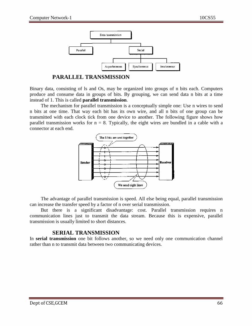
Computer Network-1 10CS55
Dept of CSE,GCEM 66
PARALLEL TRANSMISSION
Binary data, consisting of ls and Os, may be organized into groups of n bits each. Computers
produce and consume data in groups of bits. By grouping, we can send data n bits at a time
instead of 1. This is called parallel transmission.
The mechanism for parallel transmission is a conceptually simple one: Use n wires to send
n bits at one time. That way each bit has its own wire, and all n bits of one group can be
transmitted with each clock tick from one device to another. The following figure shows how
parallel transmission works for n = 8. Typically, the eight wires are bundled in a cable with a
connector at each end.
The advantage of parallel transmission is speed. All else being equal, parallel transmission
can increase the transfer speed by a factor of n over serial transmission.
But there is a significant disadvantage: cost. Parallel transmission requires n
communication lines just to transmit the data stream. Because this is expensive, parallel
transmission is usually limited to short distances.
SERIAL TRANSMISSION In serial transmission one bit follows another, so we need only one communication channel
rather than n to transmit data between two communicating devices.

Computer Network-1 10CS55
Dept of CSE,GCEM 67
The advantage of serial over parallel transmission is that with only one communication
channel, serial transmission reduces the cost of transmission over parallel by roughly a factor of
n.
Since communication within devices is parallel, conversion devices are required at the
interface between the sender and the line (parallel-to-serial) and between the line and the receiver
(serial-to-parallel).
Serial transmission occurs in one of three ways: asynchronous, synchronous, and
isochronous.
Asynchronous Transmission
Asynchronous transmission is so named because the timing of a signal is unimportant. Instead,
information is received and translated by agreed upon patterns. As long as those patterns are
followed, the receiving device can retrieve the information without regard to the rhythm in which
it is sent. Patterns are based on grouping the bit stream into bytes. Each group, usually 8 bits, is
sent along the link as a unit. The sending system handles each group independently, relaying it to
the link whenever ready, without regard to a timer.
Without synchronization, the receiver cannot use timing to predict when the next group
will arrive. To alert the receiver to the arrival of a new group, therefore, an extra bit is added to
the beginning of each byte. This bit, usually a 0, is called the start bit. To let the receiver know
that the byte is finished, 1 or more additional bits are appended to the end of the byte. These bits,
usually 1 s, are called stop bits. By this method, each byte is increased in size to at least 10 bits,
of which 8 bits is information and 2 bits or more are signals to the receiver. In addition, the
transmission of each byte may then be followed by a gap of varying duration. This gap can be
represented either by an idle channel or by a stream of additional stop bits.
The start and stop bits and the gap alert the receiver to the beginning and end of each byte
and allow it to synchronize with the data stream. This mechanism is called asynchronous
because, at the byte level, the sender and receiver do not have to be synchronized. But within
each byte, the receiver must still be synchronized with the incoming bit stream. That is, some
synchronization is required, but only for the duration of a single byte. The receiving device
resynchronizes at the onset of each new byte. When the receiver detects a start bit, it sets a timer
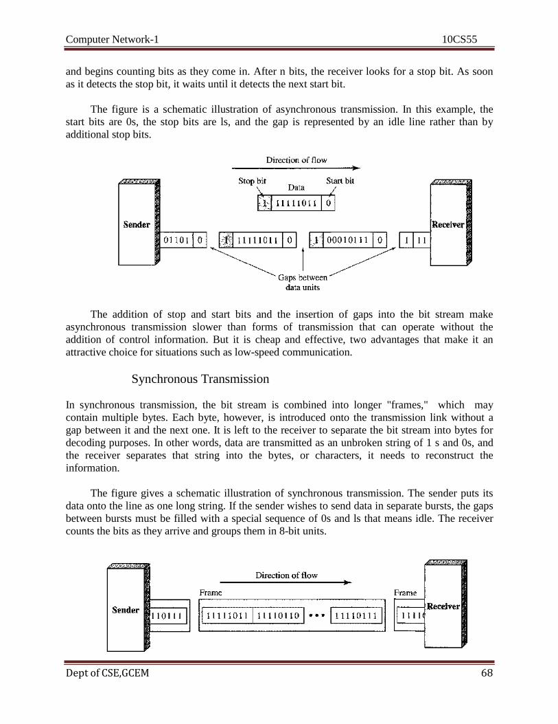
Computer Network-1 10CS55
Dept of CSE,GCEM 68
and begins counting bits as they come in. After n bits, the receiver looks for a stop bit. As soon
as it detects the stop bit, it waits until it detects the next start bit.
The figure is a schematic illustration of asynchronous transmission. In this example, the
start bits are 0s, the stop bits are ls, and the gap is represented by an idle line rather than by
additional stop bits.
The addition of stop and start bits and the insertion of gaps into the bit stream make
asynchronous transmission slower than forms of transmission that can operate without the
addition of control information. But it is cheap and effective, two advantages that make it an
attractive choice for situations such as low-speed communication.
Synchronous Transmission
In synchronous transmission, the bit stream is combined into longer "frames," which may
contain multiple bytes. Each byte, however, is introduced onto the transmission link without a
gap between it and the next one. It is left to the receiver to separate the bit stream into bytes for
decoding purposes. In other words, data are transmitted as an unbroken string of 1 s and 0s, and
the receiver separates that string into the bytes, or characters, it needs to reconstruct the
information.
The figure gives a schematic illustration of synchronous transmission. The sender puts its
data onto the line as one long string. If the sender wishes to send data in separate bursts, the gaps
between bursts must be filled with a special sequence of 0s and ls that means idle. The receiver
counts the bits as they arrive and groups them in 8-bit units.
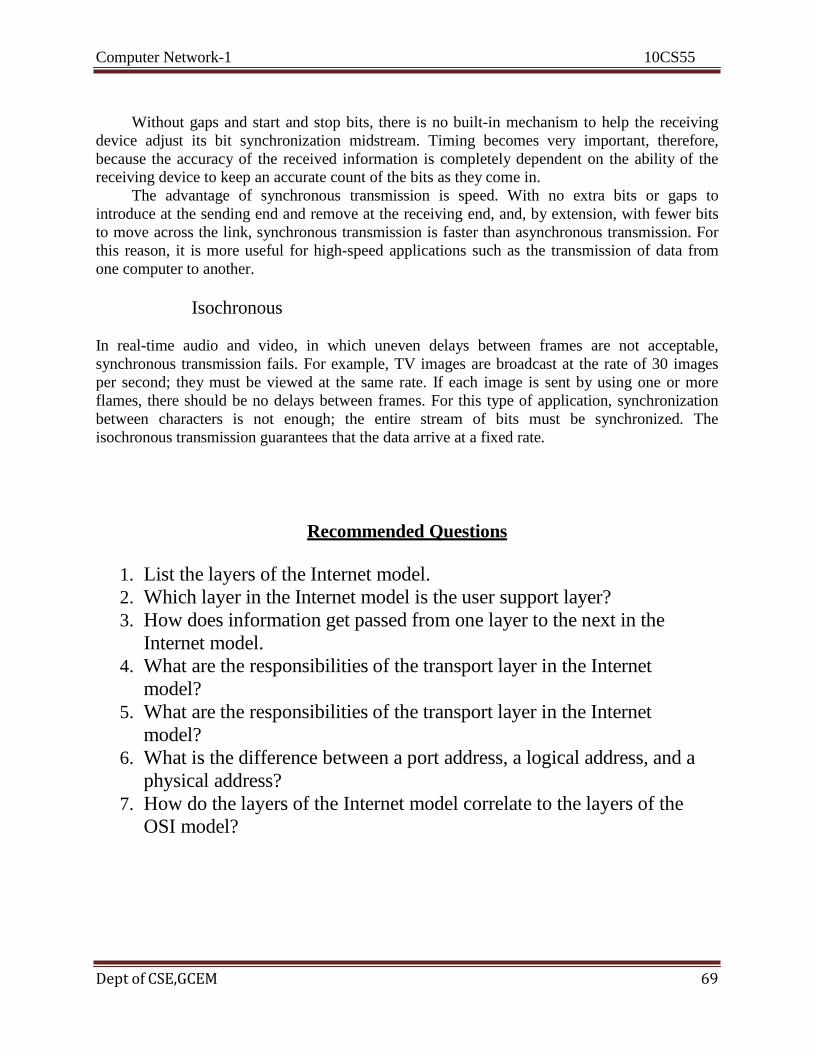
Computer Network-1 10CS55
Dept of CSE,GCEM 69
Without gaps and start and stop bits, there is no built-in mechanism to help the receiving
device adjust its bit synchronization midstream. Timing becomes very important, therefore,
because the accuracy of the received information is completely dependent on the ability of the
receiving device to keep an accurate count of the bits as they come in.
The advantage of synchronous transmission is speed. With no extra bits or gaps to
introduce at the sending end and remove at the receiving end, and, by extension, with fewer bits
to move across the link, synchronous transmission is faster than asynchronous transmission. For
this reason, it is more useful for high-speed applications such as the transmission of data from
one computer to another.
Isochronous
In real-time audio and video, in which uneven delays between frames are not acceptable,
synchronous transmission fails. For example, TV images are broadcast at the rate of 30 images
per second; they must be viewed at the same rate. If each image is sent by using one or more
flames, there should be no delays between frames. For this type of application, synchronization
between characters is not enough; the entire stream of bits must be synchronized. The
isochronous transmission guarantees that the data arrive at a fixed rate.
Recommended Questions
1. List the layers of the Internet model.
2. Which layer in the Internet model is the user support layer?
3. How does information get passed from one layer to the next in the
Internet model.
4. What are the responsibilities of the transport layer in the Internet
model?
5. What are the responsibilities of the transport layer in the Internet
model?
6. What is the difference between a port address, a logical address, and a
physical address?
7. How do the layers of the Internet model correlate to the layers of the
OSI model?
Computer Network-1 10CS55
Dept of CSE,GCEM 70
COMPUTER NETWORKS – I
Subject Code: 10CS55 I.A. Marks : 25 Hours/Week : 04 Exam Hours: 03
Total Hours : 52 Exam Marks: 100
UNIT- 3 6 Hours Physical Layer-2 and Switching:
- Multiplexing,
- Spread Spectrum,
- Introduction to switching,
- Circuit Switched Networks,
- Datagram Networks,
- Virtual Circuit Networks
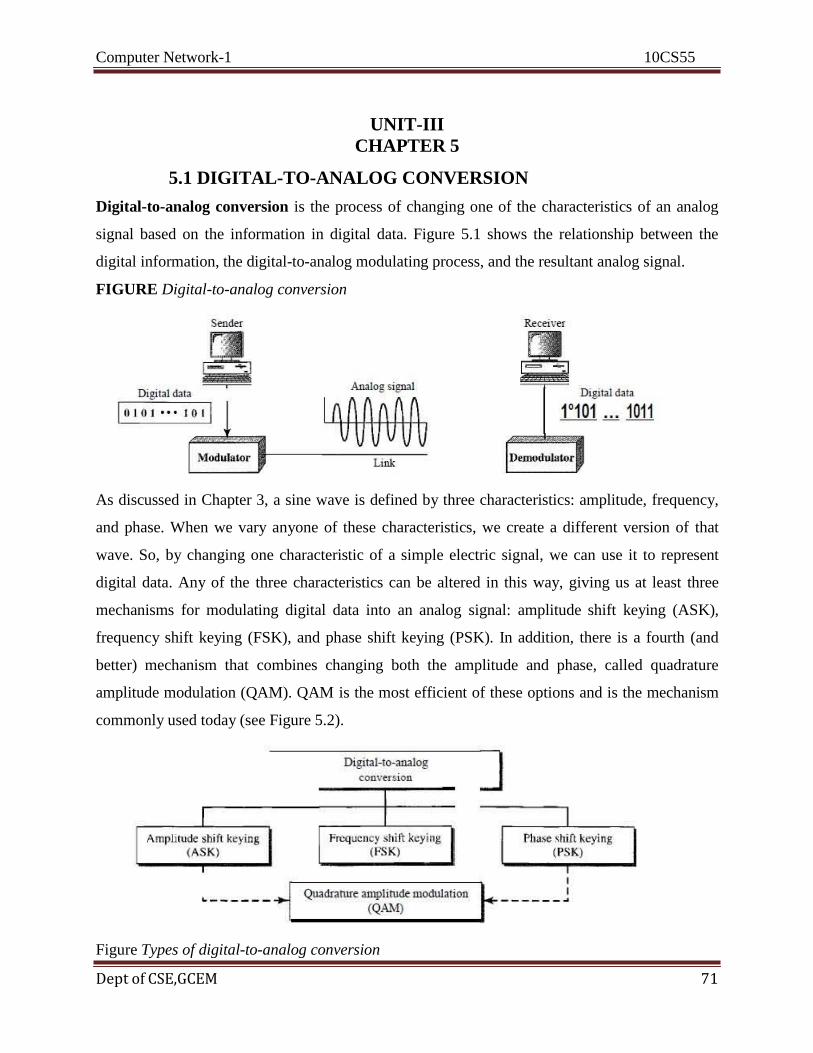
Computer Network-1 10CS55
Dept of CSE,GCEM 71
UNIT-III
CHAPTER 5
5.1 DIGITAL-TO-ANALOG CONVERSION
Digital-to-analog conversion is the process of changing one of the characteristics of an analog
signal based on the information in digital data. Figure 5.1 shows the relationship between the
digital information, the digital-to-analog modulating process, and the resultant analog signal.
FIGURE Digital-to-analog conversion
As discussed in Chapter 3, a sine wave is defined by three characteristics: amplitude, frequency,
and phase. When we vary anyone of these characteristics, we create a different version of that
wave. So, by changing one characteristic of a simple electric signal, we can use it to represent
digital data. Any of the three characteristics can be altered in this way, giving us at least three
mechanisms for modulating digital data into an analog signal: amplitude shift keying (ASK),
frequency shift keying (FSK), and phase shift keying (PSK). In addition, there is a fourth (and
better) mechanism that combines changing both the amplitude and phase, called quadrature
amplitude modulation (QAM). QAM is the most efficient of these options and is the mechanism
commonly used today (see Figure 5.2).
Figure Types of digital-to-analog conversion
Computer Network-1 10CS55
Dept of CSE,GCEM 72
Aspects of Digital-to-Analog Conversion
Before we discuss specific methods of digital-to-analog modulation, two basic issues must be
reviewed: bit and baud rates and the carrier signal.
Data Element Versus Signal Element
In Chapter 4, we discussed the concept of the data element versus the signal element. We defined
a data element as the smallest piece of information to be exchanged, the bit. We also defined a
signal element as the smallest unit of a signal that is constant. Although we continue to use the
same terms in this chapter, we will see that the nature of the signal element is a little bit different
in analog transmission
Data Rate Versus Signal Rate
We can define the data rate (bit rate) and the signal rate (baud rate) as we did for digital
transmission. The relationship between them is
S=Nxi/r! baud
where N is the data rate (bps) and r is the number of data elements carried in one signal element.
The value of r in analog transmission is r =log2 L, where L is the type of signal element, not the
level. The same nomenclature is used to simplify the comparisons.
The same analogy we used in Chapter 4 for bit rate and baud rate applies here. In transportation,
a baud is analogous to a vehicle, and a bit is analogous to a passenger. We need to maximize the
number of people per car to reduce the traffic.
Example1
An analog signal carries 4 bits per signal element. If 1000 signal elements are sent per second,
find the bit rate.
Solution
In this case, r = 4, S = 1000, and N is unknown. We can find the value ofN from
S=Nx!r
or N=Sxr= 1000 x 4 =4000 bps

Computer Network-1 10CS55
Dept of CSE,GCEM 73
Example 5.2
An analog signal has a bit rate of 8000 bps and a baud rate of 1000 baud. How many data
elements are carried by each signal element? How many signal elements do we need?
Solution
In this example, S = 1000, N =8000, and rand L are unknown. We find first the value of rand
then the value of L.
S=Nx1r
r= logzL
N 8000 .
r = - =-- =8 bltslbaud
S 1000
L= y= 28 = 256
Bandwidth
The required bandwidth for analog transmission of digital data is proportional to the signal rate
except for FSK, in which the difference between the carrier signals needs to be added. We
discuss the bandwidth for each technique.
Carrier Signal
In analog transmission, the sending device produces a high-frequency signal that acts as a base
for the information signal. This base signal is called the carrier signal or carrier frequency. The
receiving device is tuned to the frequency of the carrier signal that it expects from the sender.
Digital information then changes the carrier signal by modifying one or more of its
characteristics (amplitude, frequency, or phase). This kind of modification is called modulation
(shift keying).
Amplitude Shift Keying
In amplitude shift keying, the amplitude of the carrier signal is varied to create signal elements.
Both frequency and phase remain constant while the amplitude changes. Binary
ASK (BASK)
Although we can have several levels (kinds) of signal elements, each with a different amplitude,
ASK is normally implemented using only two levels. This is referred to as binary amplitude shift
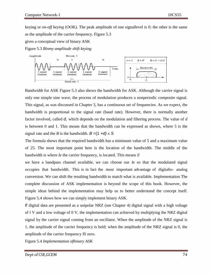
Computer Network-1 10CS55
Dept of CSE,GCEM 74
keying or on-off keying (OOK). The peak amplitude of one signallevel is 0; the other is the same
as the amplitude of the carrier frequency. Figure 5.3
gives a conceptual view of binary ASK
Figure 5.3 Binmy amplitude shift keying
Bandwidth for ASK Figure 5.3 also shows the bandwidth for ASK. Although the carrier signal is
only one simple sine wave, the process of modulation produces a nonperiodic composite signal.
This signal, as was discussed in Chapter 3, has a continuous set of frequencies. As we expect, the
bandwidth is proportional to the signal rate (baud rate). However, there is normally another
factor involved, called d, which depends on the modulation and filtering process. The value of d
is between 0 and 1. This means that the bandwidth can be expressed as shown, where 5 is the
signal rate and the B is the bandwidth. B =(1 +d) x S
The formula shows that the required bandwidth has a minimum value of 5 and a maximum value
of 25. The most important point here is the location of the bandwidth. The middle of the
bandwidth is where Ie the carrier frequency, is located. This means if
we have a bandpass channel available, we can choose our Ie so that the modulated signal
occupies that bandwidth. This is in fact the most important advantage of digitalto- analog
conversion. We can shift the resulting bandwidth to match what is available. Implementation The
complete discussion of ASK implementation is beyond the scope of this book. However, the
simple ideas behind the implementation may help us to better understand the concept itself.
Figure 5.4 shows how we can simply implement binary ASK.
If digital data are presented as a unipolar NRZ (see Chapter 4) digital signal with a high voltage
of I V and a low voltage of 0 V, the implementation can achieved by multiplying the NRZ digital
signal by the carrier signal coming from an oscillator. When the amplitude of the NRZ signal is
1, the amplitude of the carrier frequency is held; when the amplitude of the NRZ signal is 0, the
amplitude of the carrier frequency IS zero.
Figure 5.4 Implementation ofbinary ASK

Computer Network-1 10CS55
Dept of CSE,GCEM 75
Example 5.3
We have an available bandwidth of 100 kHz which spans from 200 to 300 kHz. What are the
carrier
frequency and the bit rate if we modulated our data by using ASK with d =I?
Solution
The middle of the bandwidth is located at 250 kHz. This means that our carrier frequency can be
atfe =250 kHz. We can use the formula for bandwidth to find the bit rate (with d =1 and r =1).
B =(l +d) x S=2 x N X! =2 XN =100 kHz ...... N =50 kbps
Example 5.4
In data communications, we normally use full-duplex links with communication in both
directions. We need to divide the bandwidth into two with two carrier frequencies, as shown in
Figure 5.5. The figure shows the positions of two carrier frequencies and the bandwidths.The
available bandwidth for each direction is now 50 kHz, which leaves us with a data rate of 25
kbps in each direction.
Figure 5.5 Bandwidth offull-duplex ASK used in Example 5.4
Multilevel ASK
The above discussion uses only two amplitude levels. We can have multilevel ASK in which
there are more than two levels. We can use 4,8, 16, or more different amplitudes for the signal
and modulate the data using 2, 3, 4, or more bits at a time. In these cases, r = 2, r = 3, r =4, and
so on. Although this is not implemented with pure ASK, it is implemented with QAM (as we
will see later).

Computer Network-1 10CS55
Dept of CSE,GCEM 76
Frequency Shift Keying
In frequency shift keying, the frequency of the carrier signal is varied to represent data. The
frequency of the modulated signal is constant for the duration of one signal element,
but changes for the next signal element if the data element changes. Both peak amplitude and
phase remain constant for all signal elements
Binary FSK (BFSK)
One way to think about binary FSK (or BFSK) is to consider two carrier frequencies. In Figure
5.6, we have selected two carrier frequencies,f} and12. We use the first carrier if the data
element is 0; we use the second if the data element is 1. However, note that this is an unrealistic
example used only for demonstration purposes. Normally the carrier frequencies are very high,
and the difference between them is very small.
Figure 5.6 Binary frequency shift keying
As Figure 5.6 shows, the middle of one bandwidth isJI and the middle of the other is h. Both JI
and12 are il/ apart from the midpoint between the two bands. The difference between the two
frequencies is 211f Bandwidth for BFSK Figure 5.6 also shows the bandwidth of FSK. Again the
carrier signals are only simple sine waves, but the modulation creates a nonperiodic composite
signal with continuous frequencies. We can think of FSK as two ASK signals, each with its own
carrier frequency Cil or h). If the difference between the two frequencies is 211j, then the
required bandwidth is B=(l+d)xS+2iij What should be the minimum value of 211/? In Figure
5.6, we have chosen a value greater than (l + d)S. It can be shown that the minimum value
should be at least S for the proper operation of modulation and demodulation
Example 5.5
We have an available bandwidth of 100 kHz which spans from 200 to 300 kHz. What should be
the carrier frequency and the bit rate if we modulated our data by using FSK with d =1?

Computer Network-1 10CS55
Dept of CSE,GCEM 77
Solution
This problem is similar to Example 5.3, but we are modulating by using FSK. The midpoint of
the band is at 250 kHz. We choose 2~f to be 50 kHz; this means B =(1 + d) x S + 28f =100 -. 2S
=50 kHz S = 25 kbaud N;;;; 25 kbps Compared to Example 5.3, we can see the bit rate for ASK
is 50 kbps while the bit rate for FSK is 25 kbps. Implementation There are two implementations
of BFSK: noncoherent and coherent. In noncoherent BFSK, there may be discontinuity in the
phase when one signal element ends and the next begins. In coherent BFSK, the phase continues
through the boundary of two signal elements. Noncoherent BFSK can be implemented by
treating BFSK as two ASK modulations and using two carrier frequencies. Coherent BFSK can
be implemented by using one voltage-controlled oscillator (VeO) that changes its frequency
according to the input voltage. Figure 5.7 shows the simplified idea behind the second
implementation. The input to the oscillator is the unipolar NRZ signal. When the amplitude of
NRZ is zero, the oscillator keeps its regular frequency; when the amplitude is positive, the
frequency is increased.
Figure 5.7 Implementation ofBFSK
Multilevel FSK
Multilevel modulation (MFSK) is not uncommon with the FSK method. We can use more than
two frequencies. For example, we can use four different frequenciesfIJ2,!3, and 14 to send 2 bits
at a time. To send 3 bits at a time, we can use eight frequencies. And so on. However, we need to
remember that the frequencies need to be 2~1 apart. For the proper operation of the modulator
and demodulator, it can be shown that the minimum value of 2~lneeds to be S. We can show
that the bandwidth with d =0 is B;;;; (l +d) x S + (L - 1)24{ -. B =Lx S
Example 5.6

Computer Network-1 10CS55
Dept of CSE,GCEM 78
We need to send data 3 bits at a time at a bit rate of 3 Mbps. The carrier frequency is 10 MHz.
Calculate the number of levels (different frequencies), the baud rate, and the
bandwidth.
Solution
We can have L =23 =8. The baud rate is S =3 MHz/3 =1000 Mbaud. This means that the carrier
frequencies must be 1MHz apart (211f =1 MHz). The bandwidth is B=8 x 1000 =8000. Figure
5.8 shows the allocation of frequencies and bandwidth.
Figure 5.8 Bandwidth ofMFSK used in Example 5.6
Phase Shift Keying
In phase shift keying, the phase of the carrier is varied to represent two or more different signal
elements. Both peak amplitude and frequency remain constant as the phase changes. Today, PSK
is more common than ASK or FSK. However, we will see Sh0l1ly that QAM, which combines
ASK and PSK, is the dominant method of digitalto- analog modulation.
Binary PSK (BPSK)
The simplest PSK is binary PSK, in which we have only two signal elements, one with a phase
of 0°, and the other with a phase of 180°. Figure 5.9 gives a conceptual view of PSK. Binary
PSK is as simple as binary ASK with one big advantage-it is less
susceptible to noise. In ASK, the criterion for bit detection is the amplitude of the signal; in PSK,
it is the phase. Noise can change the amplitude easier than it can change the phase. In other
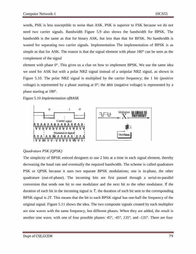
Computer Network-1 10CS55
Dept of CSE,GCEM 79
words, PSK is less susceptible to noise than ASK. PSK is superior to FSK because we do not
need two carrier signals. Bandwidth Figure 5.9 also shows the bandwidth for BPSK. The
bandwidth is the same as that for binary ASK, but less than that for BFSK. No bandwidth is
wasted for separating two carrier signals. Implementation The implementation of BPSK is as
simple as that for ASK. The reason is that the signal element with phase 180° can be seen as the
complement of the signal
element with phase 0°. This gives us a clue on how to implement BPSK. We use the same idea
we used for ASK but with a polar NRZ signal instead of a unipolar NRZ signal, as shown in
Figure 5.10. The polar NRZ signal is multiplied by the carrier frequency; the 1 bit (positive
voltage) is represented by a phase starting at 0°; the abit (negative voltage) is represented by a
phase starting at 180°.
Figure 5.10 Implementation ofBASK
Quadrature PSK (QPSK)
The simplicity of BPSK enticed designers to use 2 bits at a time in each signal element, thereby
decreasing the baud rate and eventually the required bandwidth. The scheme is called quadrature
PSK or QPSK because it uses two separate BPSK modulations; one is in-phase, the other
quadrature (out-of-phase). The incoming bits are first passed through a serial-to-parallel
conversion that sends one bit to one modulator and the next bit to the other modulator. If the
duration of each bit in the incoming signal is T, the duration of each bit sent to the corresponding
BPSK signal is 2T. This means that the bit to each BPSK signal has one-half the frequency of the
original signal. Figure 5.11 shows the idea. The two composite signals created by each multiplier
are sine waves with the same frequency, but different phases. When they are added, the result is
another sine wave, with one of four possible phases: 45°, -45°, 135°, and -135°. There are four
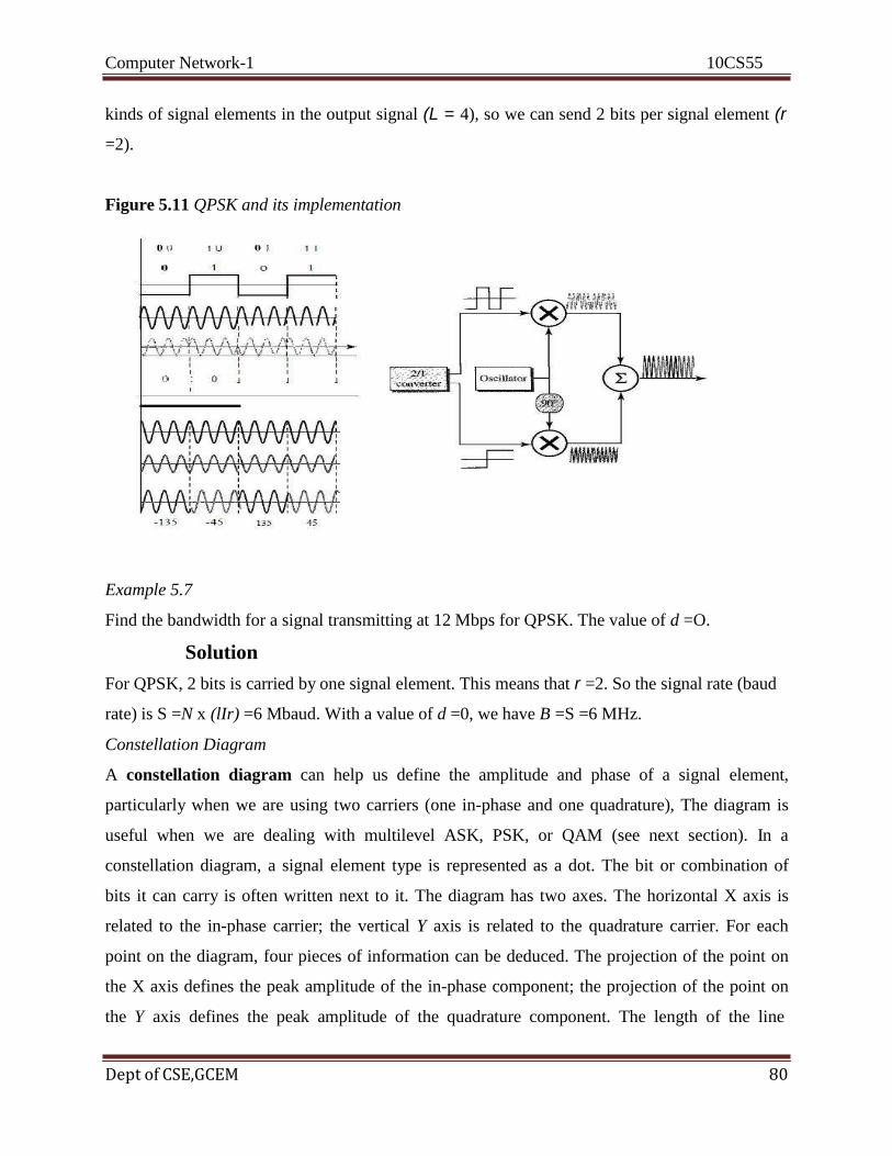
Computer Network-1 10CS55
Dept of CSE,GCEM 80
kinds of signal elements in the output signal (L = 4), so we can send 2 bits per signal element (r
=2).
Figure 5.11 QPSK and its implementation
Example 5.7
Find the bandwidth for a signal transmitting at 12 Mbps for QPSK. The value of d =O.
Solution
For QPSK, 2 bits is carried by one signal element. This means that r =2. So the signal rate (baud
rate) is S =N x (lIr) =6 Mbaud. With a value of d =0, we have B =S =6 MHz.
Constellation Diagram
A constellation diagram can help us define the amplitude and phase of a signal element,
particularly when we are using two carriers (one in-phase and one quadrature), The diagram is
useful when we are dealing with multilevel ASK, PSK, or QAM (see next section). In a
constellation diagram, a signal element type is represented as a dot. The bit or combination of
bits it can carry is often written next to it. The diagram has two axes. The horizontal X axis is
related to the in-phase carrier; the vertical Y axis is related to the quadrature carrier. For each
point on the diagram, four pieces of information can be deduced. The projection of the point on
the X axis defines the peak amplitude of the in-phase component; the projection of the point on
the Y axis defines the peak amplitude of the quadrature component. The length of the line

Computer Network-1 10CS55
Dept of CSE,GCEM 81
(vector) that connects the point to the origin is the peak amplitude of the signal element
(combination of the X and Y components); the angle the line makes with the X axis is the phase
of the signal element. All the information we need, can easily be found on a constellation
diagram. Figure 5.12 shows a constellation diagram.
Figure 5.12 Concept ofa constellation diagram
Example 5.8
Show the constellation diagrams for an ASK (OOK), BPSK, and QPSK signals.
Solution
Figure 5.13 shows the three constellation diagrams
Figure 5.13 Three constellation diagrams
Let us analyze each case separately: a. For ASK, we are using only an in-phase carrier.
Therefore, the two points should be on the X axis. Binary 0 has an amplitude of 0 V; binary 1 has
an amplitude of 1V (for example). The points are located at the origin and at 1 unit. h. BPSK also

Computer Network-1 10CS55
Dept of CSE,GCEM 82
uses only an in-phase carrier. However, we use a polar NRZ signal for modulation. It creates two
types of signal elements, one with amplitude 1 and the other with amplitude -1. This can be
stated in other words: BPSK creates two different signal elements, one with amplitude I V and in
phase and the other with amplitude 1V and 1800 out of phase. c. QPSK uses two carriers, one in-
phase and the other quadrature. The point representing 11 is made of two combined signal
elements, both with an amplitude of 1 V. One element is represented by an in-phase carrier, the
other element by a quadrature carrier. The amplitude of the final signal element sent for this 2-bit
data element is 2112, and the phase is 45°. The argument is similar for the other three points. All
signal elements have an amplitude of 2112, but their phases are different (45°, 135°, -135°, and -
45°). Of course, we could have chosen the amplitude of the carrier to be 1/(21/2) to make the
final amplitudes 1 V.
Quadrature Amplitude Modulation
PSK is limited by the ability of the equipment to distinguish small differences in phase. This
factor limits its potential bit rate. So far, we have been altering only one of the three
characteristics of a sine wave at a time; but what if we alter two? Why not combine ASK and
PSK? The idea of using two carriers, one in-phase and the other quadrature, with different
amplitude levels for each carrier is the concept behind quadrature amplitude modulation (QAM).
The possible variations of QAM are numerous. Figure 5.14 shows some of these schemes. Figure
5.14a shows the simplest 4-QAM scheme (four different signal element
types) using a unipolar NRZ signal to modulate each carrier. This is the same mechanism we
used for ASK (OOK). Part b shows another 4-QAM using polar NRZ, but this is exactly the
same as QPSK. Part c shows another QAM-4 in which we used a signal with two positive levels
to modulate each of the two carriers. Finally, Figure 5.14d shows a 16-QAM constellation of a
signal with eight levels, four positive and four negative.
Figure 5.14 Constellation diagrams for some QAMs

Computer Network-1 10CS55
Dept of CSE,GCEM 83
Bandwidth for QAM
The minimum bandwidth required for QAM transmission is the same as that required
for ASK and PSK transmission. QAM has the same advantages as PSK over ASK.
5.2 ANALOG-TO-ANALOG CONVERSION
Analog-to-analog conversion, or analog modulation, is the representation of analog information
by an analog signal. One may ask why we need to modulate an analog signal; it is already
analog. Modulation is needed if the medium is bandpass in nature or if only a bandpass channel
is available to us. An example is radio. The government assigns a narrow bandwidth to each
radio station. The analog signal produced by each station is a low-pass signal, all in the same
range. To be able to listen to different stations, the low-pass signals need to be shifted, each to a
different range. Analog-to-analog conversion can be accomplished in three ways: amplitude
modulation (AM), frequency modulation (FM), and phase modulation (PM). FM and PM are
usually categorized together. See Figure 5.15
Figure 5.15 Types ofanalog-to-analog modulation
Amplitude Modulation
In AM transmission, the carrier signal is modulated so that its amplitude varies with the changing
amplitudes of the modulating signal. The frequency and phase of the carrier remain the same;
only the amplitude changes to follow variations in the information. Figure 5.16 shows how this
concept works. The modulating signal is the envelope of the carrier.
Figure 5.16 Amplitude modulation

Computer Network-1 10CS55
Dept of CSE,GCEM 84
As Figure 5.16 shows, AM is normally implemented by using a simple multiplier because the
amplitude of the carrier signal needs to be changed according to the amplitude of the modulating
signal.
AM Bandwidth
Figure 5.16 also shows the bandwidth of an AM signal. The modulation creates a bandwidth that
is twice the bandwidth of the modulating signal and covers a range centered on the carrier
frequency. However, the signal components above and below the carrier frequency carry exactly
the same information. For this reason, some implementations discard one-half of the signals and
cut the bandwidth in half.
Stalldard Balldwidth Allocatioll for AiH l(adio
The bandwidth of an audio signal (speech and music) is usually 5 kHz. Therefore, an AM radio
station needs a bandwidth of 10kHz. In fact, the Federal Communications Commission (FCC)
allows 10 kHz for each AM station. AM stations are allowed carrier frequencies anywhere
between 530 and 1700 kHz (1.7 MHz). However, each station's carrier frequency must be
separated from those on either side of it by at least 10 kHz (one AM bandwidth) to avoid
interference. If one station uses a carrier frequency of 1100 kHz, the next station's carrier
frequency cannot be lower than 1110 kHz (see Figure 5.17).
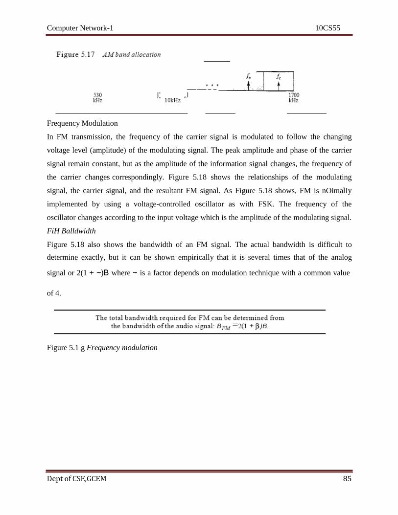
Computer Network-1 10CS55
Dept of CSE,GCEM 85
Frequency Modulation
In FM transmission, the frequency of the carrier signal is modulated to follow the changing
voltage level (amplitude) of the modulating signal. The peak amplitude and phase of the carrier
signal remain constant, but as the amplitude of the information signal changes, the frequency of
the carrier changes correspondingly. Figure 5.18 shows the relationships of the modulating
signal, the carrier signal, and the resultant FM signal. As Figure 5.18 shows, FM is nOimalIy
implemented by using a voltage-controlled oscillator as with FSK. The frequency of the
oscillator changes according to the input voltage which is the amplitude of the modulating signal.
FiH Balldwidth
Figure 5.18 also shows the bandwidth of an FM signal. The actual bandwidth is difficult to
determine exactly, but it can be shown empirically that it is several times that of the analog
signal or 2(1 + ~)B where ~ is a factor depends on modulation technique with a common value
of 4.
Figure 5.1 g Frequency modulation
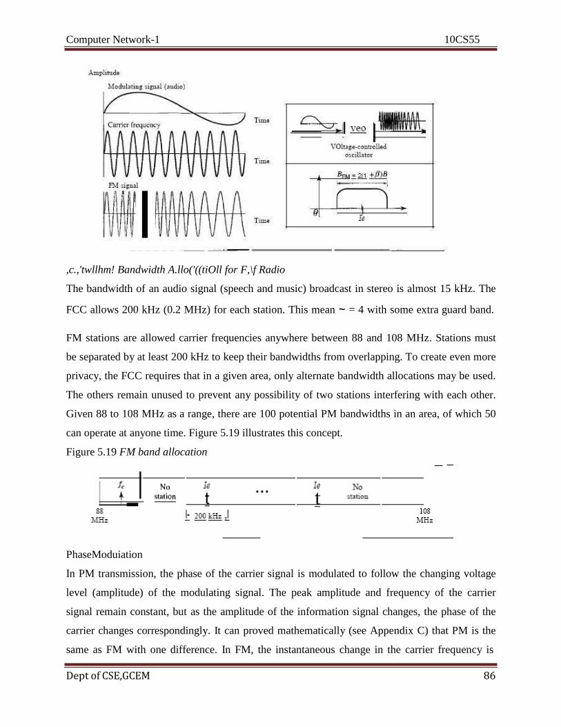
Computer Network-1 10CS55
Dept of CSE,GCEM 86
,c.,'twllhm! Bandwidth A.llo('((tiOll for F,\f Radio
The bandwidth of an audio signal (speech and music) broadcast in stereo is almost 15 kHz. The
FCC allows 200 kHz (0.2 MHz) for each station. This mean ~ = 4 with some extra guard band.
FM stations are allowed carrier frequencies anywhere between 88 and 108 MHz. Stations must
be separated by at least 200 kHz to keep their bandwidths from overlapping. To create even more
privacy, the FCC requires that in a given area, only alternate bandwidth allocations may be used.
The others remain unused to prevent any possibility of two stations interfering with each other.
Given 88 to 108 MHz as a range, there are 100 potential PM bandwidths in an area, of which 50
can operate at anyone time. Figure 5.19 illustrates this concept.
Figure 5.19 FM band allocation
PhaseModuiation
In PM transmission, the phase of the carrier signal is modulated to follow the changing voltage
level (amplitude) of the modulating signal. The peak amplitude and frequency of the carrier
signal remain constant, but as the amplitude of the information signal changes, the phase of the
carrier changes correspondingly. It can proved mathematically (see Appendix C) that PM is the
same as FM with one difference. In FM, the instantaneous change in the carrier frequency is
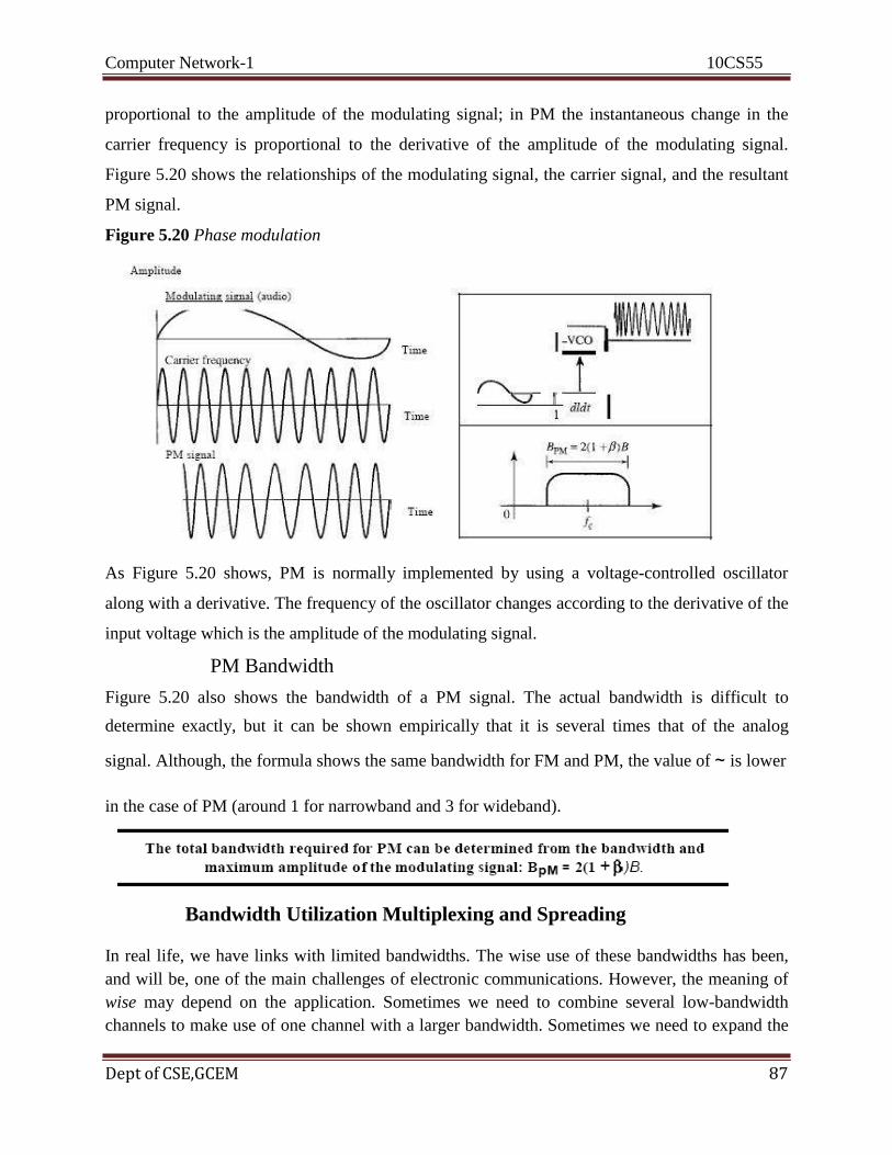
Computer Network-1 10CS55
Dept of CSE,GCEM 87
proportional to the amplitude of the modulating signal; in PM the instantaneous change in the
carrier frequency is proportional to the derivative of the amplitude of the modulating signal.
Figure 5.20 shows the relationships of the modulating signal, the carrier signal, and the resultant
PM signal.
Figure 5.20 Phase modulation
As Figure 5.20 shows, PM is normally implemented by using a voltage-controlled oscillator
along with a derivative. The frequency of the oscillator changes according to the derivative of the
input voltage which is the amplitude of the modulating signal.
PM Bandwidth
Figure 5.20 also shows the bandwidth of a PM signal. The actual bandwidth is difficult to
determine exactly, but it can be shown empirically that it is several times that of the analog
signal. Although, the formula shows the same bandwidth for FM and PM, the value of ~ is lower
in the case of PM (around 1 for narrowband and 3 for wideband).
Bandwidth Utilization Multiplexing and Spreading
In real life, we have links with limited bandwidths. The wise use of these bandwidths has been,
and will be, one of the main challenges of electronic communications. However, the meaning of
wise may depend on the application. Sometimes we need to combine several low-bandwidth
channels to make use of one channel with a larger bandwidth. Sometimes we need to expand the

Computer Network-1 10CS55
Dept of CSE,GCEM 88
bandwidth of a channel to achieve goals such as privacy and ant jamming. In this chapter, we

Computer Network-1 10CS55
Dept of CSE,GCEM 89
explore these two broad categories of bandwidth utilization: multiplexing and spreading. In
multiplexing, our goal is efficiency; we combine several channels into one. In spreading, our
goals are privacy and ant jamming; we expand the bandwidth of a channel to insert redundancy,
which is necessary to achieve these goals.
6.1 MULTIPLEXING
Whenever the bandwidth of a medium linking two devices is greater than the bandwidth needs of
the devices, the link can be shared. Multiplexing is the set of techniques that allows the
simultaneous transmission of multiple signals across a single data link. As data and
telecommunications use increases, so does traffic. We can accommodate this increase by
continuing to add individual links each time a new channel is needed; or we can install higher-
bandwidth links and use each to carry multiple signals. As described in Chapter 7, today's
technology includes high-bandwidth media such as optical fiber and terrestrial and satellite
microwaves. Each has a bandwidth far in excess of that needed for the average transmission
signal. If the bandwidth of a link is greater than the bandwidth needs of the devices connected to
it, the bandwidth is wasted. An efficient system maximizes the utilization of all resources;
bandwidth is one of the most precious resources we have in data communications. In a
multiplexed system, n lines share the bandwidth of one link. Figure 6.1 shows the basic format of
a multiplexed system. The lines on the left direct their transmission streams to a multiplexer
(MUX), which combines them into a single stream (many-toone). At the receiving end, that
stream is fed into a demultiplexer (DEMUX), which separates the stream back into its
component transmissions (one-to-many) and directs them to their corresponding lines. In the
figure, the word link refers to the physical path. The word channel refers to the portion of a link
that carries a transmission between a given pair of lines. One link can have many (n) channels.
Figure 6.1 Dividing a link into channels
There are three basic multiplexing techniques: frequency-division multiplexing, wavelength-
division multiplexing, and time-division multiplexing. The first two are techniques designed for
analog signals, the third, for digital signals (see Figure 6.2).
Figure 6.2 Categories of multiplexing
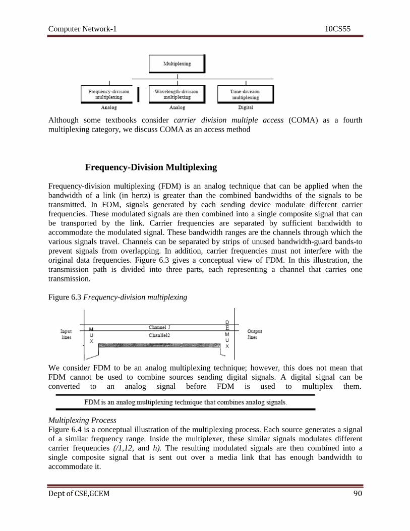
Computer Network-1 10CS55
Dept of CSE,GCEM 90
Although some textbooks consider carrier division multiple access (COMA) as a fourth
multiplexing category, we discuss COMA as an access method
Frequency-Division Multiplexing
Frequency-division multiplexing (FDM) is an analog technique that can be applied when the
bandwidth of a link (in hertz) is greater than the combined bandwidths of the signals to be
transmitted. In FOM, signals generated by each sending device modulate different carrier
frequencies. These modulated signals are then combined into a single composite signal that can
be transported by the link. Carrier frequencies are separated by sufficient bandwidth to
accommodate the modulated signal. These bandwidth ranges are the channels through which the
various signals travel. Channels can be separated by strips of unused bandwidth-guard bands-to
prevent signals from overlapping. In addition, carrier frequencies must not interfere with the
original data frequencies. Figure 6.3 gives a conceptual view of FDM. In this illustration, the
transmission path is divided into three parts, each representing a channel that carries one
transmission.
Figure 6.3 Frequency-division multiplexing
We consider FDM to be an analog multiplexing technique; however, this does not mean that
FDM cannot be used to combine sources sending digital signals. A digital signal can be
converted to an analog signal before FDM is used to multiplex them.
Multiplexing Process
Figure 6.4 is a conceptual illustration of the multiplexing process. Each source generates a signal
of a similar frequency range. Inside the multiplexer, these similar signals modulates different
carrier frequencies (/1,12, and h). The resulting modulated signals are then combined into a
single composite signal that is sent out over a media link that has enough bandwidth to
accommodate it.

Computer Network-1 10CS55
Dept of CSE,GCEM 91
Figure 6.4 FDM process
Demultiplexing Process
The demultiplexer uses a series of filters to decompose the multiplexed signal into its constituent
component signals. The individual signals are then passed to a demodulator that separates them
from their carriers and passes them to the output lines. Figure 6.5 is a conceptual illustration of
demultiplexing process.
Figure 6.5 FDM demultiplexing example
The Analog Carrier System
To maximize the efficiency of their infrastructure, telephone companies have traditionally
multiplexed signals from lower-bandwidth lines onto higher-bandwidth lines. In this way, many
switched or leased lines can be combined into fewer but bigger channels. For analog lines, FDM
is used. One of these hierarchical systems used by AT&T is made up of groups, super groups,
master groups, and jumbo groups
Figure 6.9 Analog hierarchy
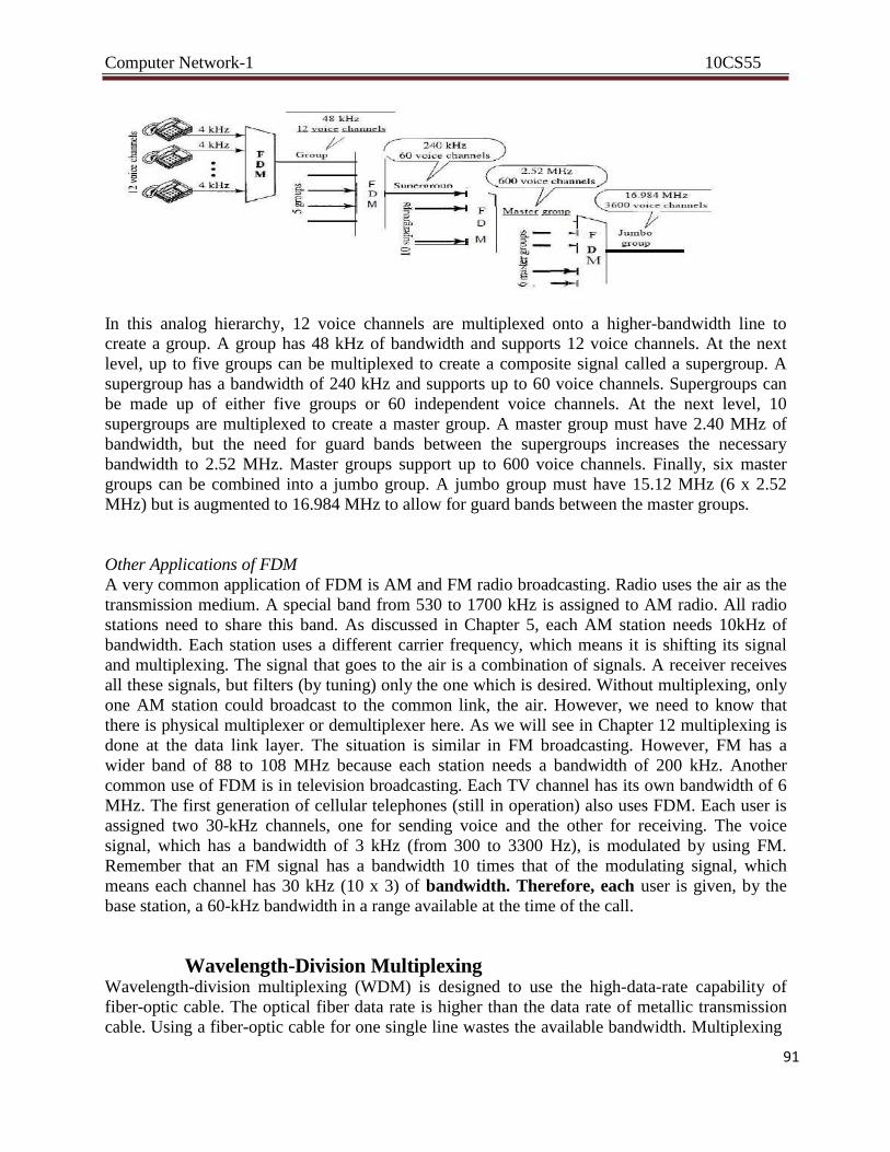
Computer Network-1 10CS55
91
In this analog hierarchy, 12 voice channels are multiplexed onto a higher-bandwidth line to
create a group. A group has 48 kHz of bandwidth and supports 12 voice channels. At the next
level, up to five groups can be multiplexed to create a composite signal called a supergroup. A
supergroup has a bandwidth of 240 kHz and supports up to 60 voice channels. Supergroups can
be made up of either five groups or 60 independent voice channels. At the next level, 10
supergroups are multiplexed to create a master group. A master group must have 2.40 MHz of
bandwidth, but the need for guard bands between the supergroups increases the necessary
bandwidth to 2.52 MHz. Master groups support up to 600 voice channels. Finally, six master
groups can be combined into a jumbo group. A jumbo group must have 15.12 MHz (6 x 2.52
MHz) but is augmented to 16.984 MHz to allow for guard bands between the master groups.
Other Applications of FDM
A very common application of FDM is AM and FM radio broadcasting. Radio uses the air as the
transmission medium. A special band from 530 to 1700 kHz is assigned to AM radio. All radio
stations need to share this band. As discussed in Chapter 5, each AM station needs 10kHz of
bandwidth. Each station uses a different carrier frequency, which means it is shifting its signal
and multiplexing. The signal that goes to the air is a combination of signals. A receiver receives
all these signals, but filters (by tuning) only the one which is desired. Without multiplexing, only
one AM station could broadcast to the common link, the air. However, we need to know that
there is physical multiplexer or demultiplexer here. As we will see in Chapter 12 multiplexing is
done at the data link layer. The situation is similar in FM broadcasting. However, FM has a
wider band of 88 to 108 MHz because each station needs a bandwidth of 200 kHz. Another
common use of FDM is in television broadcasting. Each TV channel has its own bandwidth of 6
MHz. The first generation of cellular telephones (still in operation) also uses FDM. Each user is
assigned two 30-kHz channels, one for sending voice and the other for receiving. The voice
signal, which has a bandwidth of 3 kHz (from 300 to 3300 Hz), is modulated by using FM.
Remember that an FM signal has a bandwidth 10 times that of the modulating signal, which
means each channel has 30 kHz (10 x 3) of bandwidth. Therefore, each user is given, by the
base station, a 60-kHz bandwidth in a range available at the time of the call.
Wavelength-Division Multiplexing Wavelength-division multiplexing (WDM) is designed to use the high-data-rate capability of
fiber-optic cable. The optical fiber data rate is higher than the data rate of metallic transmission
cable. Using a fiber-optic cable for one single line wastes the available bandwidth. Multiplexing
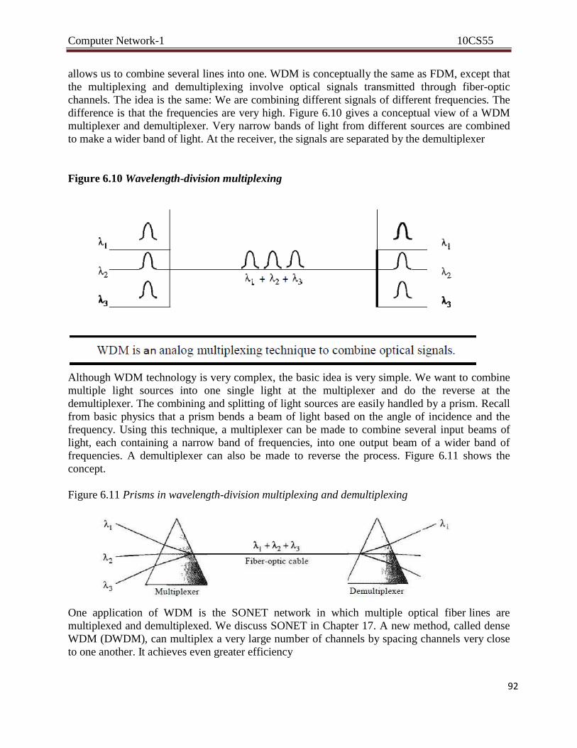
Computer Network-1 10CS55
92
allows us to combine several lines into one. WDM is conceptually the same as FDM, except that
the multiplexing and demultiplexing involve optical signals transmitted through fiber-optic
channels. The idea is the same: We are combining different signals of different frequencies. The
difference is that the frequencies are very high. Figure 6.10 gives a conceptual view of a WDM
multiplexer and demultiplexer. Very narrow bands of light from different sources are combined
to make a wider band of light. At the receiver, the signals are separated by the demultiplexer
Figure 6.10 Wavelength-division multiplexing
Although WDM technology is very complex, the basic idea is very simple. We want to combine
multiple light sources into one single light at the multiplexer and do the reverse at the
demultiplexer. The combining and splitting of light sources are easily handled by a prism. Recall
from basic physics that a prism bends a beam of light based on the angle of incidence and the
frequency. Using this technique, a multiplexer can be made to combine several input beams of
light, each containing a narrow band of frequencies, into one output beam of a wider band of
frequencies. A demultiplexer can also be made to reverse the process. Figure 6.11 shows the
concept.
Figure 6.11 Prisms in wavelength-division multiplexing and demultiplexing
One application of WDM is the SONET network in which multiple optical fiber lines are
multiplexed and demultiplexed. We discuss SONET in Chapter 17. A new method, called dense
WDM (DWDM), can multiplex a very large number of channels by spacing channels very close
to one another. It achieves even greater efficiency
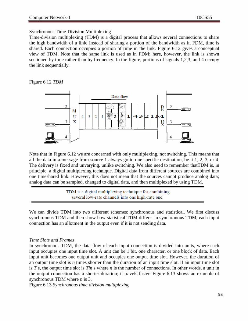
Computer Network-1 10CS55
93
Synchronous Time-Division Multiplexing
Time-division multiplexing (TDM) is a digital process that allows several connections to share
the high bandwidth of a linle Instead of sharing a portion of the bandwidth as in FDM, time is
shared. Each connection occupies a portion of time in the link. Figure 6.12 gives a conceptual
view of TDM. Note that the same link is used as in FDM; here, however, the link is shown
sectioned by time rather than by frequency. In the figure, portions of signals 1,2,3, and 4 occupy
the link sequentially.
Figure 6.12 TDM
Note that in Figure 6.12 we are concerned with only multiplexing, not switching. This means that
all the data in a message from source 1 always go to one specific destination, be it 1, 2, 3, or 4.
The delivery is fixed and unvarying, unlike switching. We also need to remember thatTDM is, in
principle, a digital multiplexing technique. Digital data from different sources are combined into
one timeshared link. However, this does not mean that the sources cannot produce analog data;
analog data can be sampled, changed to digital data, and then multiplexed by using TDM.
We can divide TDM into two different schemes: synchronous and statistical. We first discuss
synchronous TDM and then show how statistical TDM differs. In synchronous TDM, each input
connection has an allotment in the output even if it is not sending data.
Time Slots and Frames
In synchronous TDM, the data flow of each input connection is divided into units, where each
input occupies one input time slot. A unit can be 1 bit, one character, or one block of data. Each
input unit becomes one output unit and occupies one output time slot. However, the duration of
an output time slot is n times shorter than the duration of an input time slot. If an input time slot
is T s, the output time slot is Tin s where n is the number of connections. In other words, a unit in
the output connection has a shorter duration; it travels faster. Figure 6.13 shows an example of
synchronous TDM where n is 3.
Figure 6.13 Synchronous time-division multiplexing
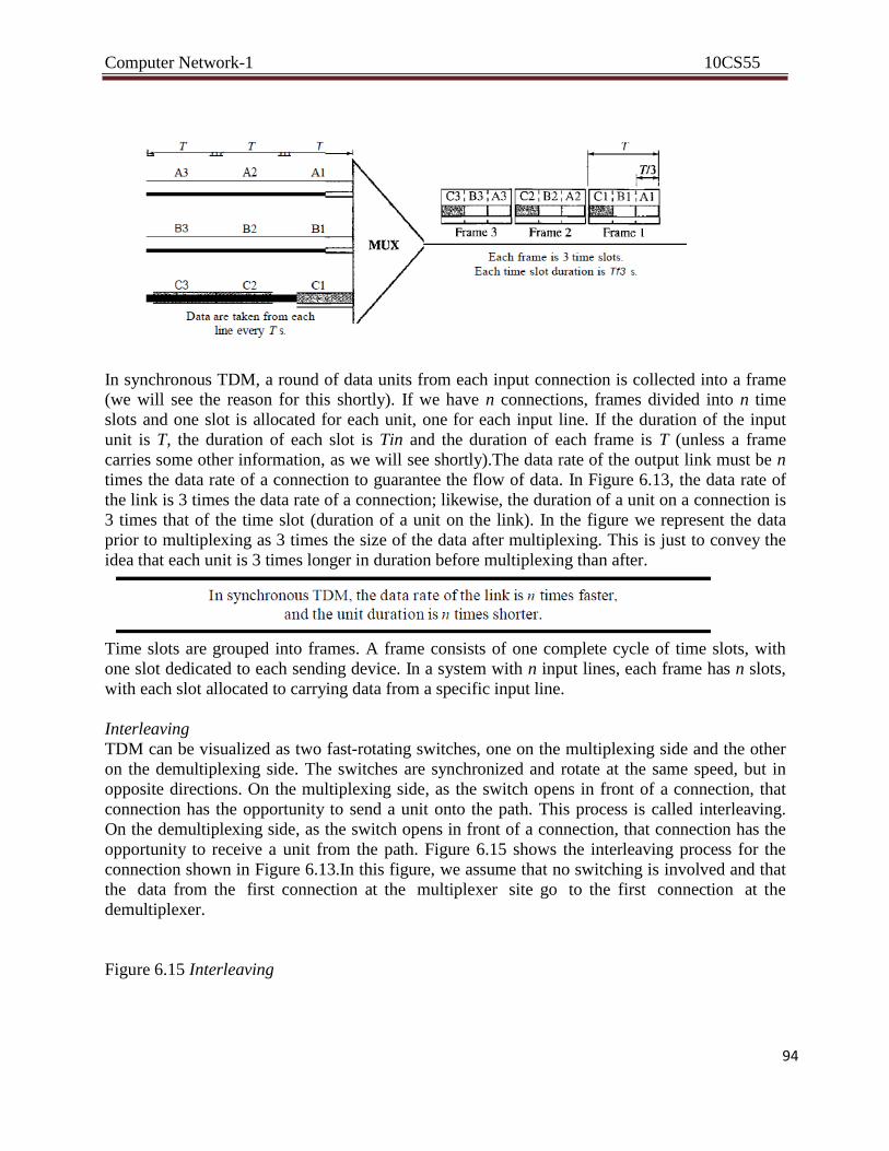
Computer Network-1 10CS55
94
In synchronous TDM, a round of data units from each input connection is collected into a frame
(we will see the reason for this shortly). If we have n connections, frames divided into n time
slots and one slot is allocated for each unit, one for each input line. If the duration of the input
unit is T, the duration of each slot is Tin and the duration of each frame is T (unless a frame
carries some other information, as we will see shortly).The data rate of the output link must be n
times the data rate of a connection to guarantee the flow of data. In Figure 6.13, the data rate of
the link is 3 times the data rate of a connection; likewise, the duration of a unit on a connection is
3 times that of the time slot (duration of a unit on the link). In the figure we represent the data
prior to multiplexing as 3 times the size of the data after multiplexing. This is just to convey the
idea that each unit is 3 times longer in duration before multiplexing than after.
Time slots are grouped into frames. A frame consists of one complete cycle of time slots, with
one slot dedicated to each sending device. In a system with n input lines, each frame has n slots,
with each slot allocated to carrying data from a specific input line.
Interleaving
TDM can be visualized as two fast-rotating switches, one on the multiplexing side and the other
on the demultiplexing side. The switches are synchronized and rotate at the same speed, but in
opposite directions. On the multiplexing side, as the switch opens in front of a connection, that
connection has the opportunity to send a unit onto the path. This process is called interleaving.
On the demultiplexing side, as the switch opens in front of a connection, that connection has the
opportunity to receive a unit from the path. Figure 6.15 shows the interleaving process for the
connection shown in Figure 6.13.In this figure, we assume that no switching is involved and that
the data from the first connection at the multiplexer site go to the first connection at the
demultiplexer.
Figure 6.15 Interleaving

Computer Network-1 10CS55
95
Empty Slots
Synchronous TDM is not as efficient as it could be. If a source does not have data tosend, the
corresponding slot in the output frame is empty. Figure 6.18 shows a case inwhich one of the
input lines has no data to send and one slot in another input line has discontinuous data.
Figure 6.18 Empty slots
The first output frame has three slots filled, the second frame has two slots filled, and the third
frame has three slots filled. No frame is full. We learn in the next sectionthat statistical TDM can
improve the efficiency by removing the empty slots from theframe.
Data Rate Management
One problem with TDM is how to handle a disparity in the input data rates. In all our discussion
so far, we assumed that the data rates of all input lines were the same. However, if data rates are
not the same, three strategies, or a combination of them, can be used. We call these three
strategies multilevel multiplexing, multiple-slot allocation, and pulse stuffing.
Multilevel Multiplexing Multilevel multiplexing is a technique used when the data rate of an
input line is a multiple of others. For example, in Figure 6.19, we have two inputs of 20 kbps and
three inputs of 40 kbps. The first two input lines can be multiplexed together to provide a data
rate equal to the last three. A second level of multiplexing can create an output of 160 kbps.
Figure 6.19 Multilevel multiplexing
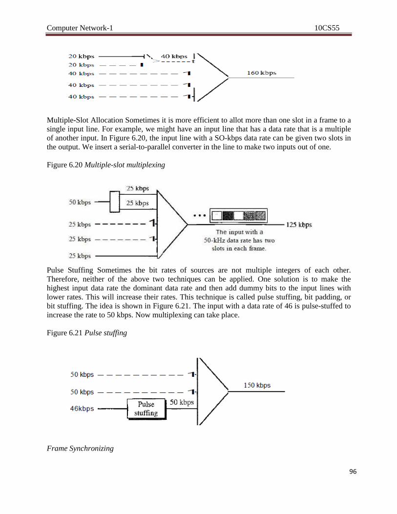
Computer Network-1 10CS55
96
Multiple-Slot Allocation Sometimes it is more efficient to allot more than one slot in a frame to a
single input line. For example, we might have an input line that has a data rate that is a multiple
of another input. In Figure 6.20, the input line with a SO-kbps data rate can be given two slots in
the output. We insert a serial-to-parallel converter in the line to make two inputs out of one.
Figure 6.20 Multiple-slot multiplexing
Pulse Stuffing Sometimes the bit rates of sources are not multiple integers of each other.
Therefore, neither of the above two techniques can be applied. One solution is to make the
highest input data rate the dominant data rate and then add dummy bits to the input lines with
lower rates. This will increase their rates. This technique is called pulse stuffing, bit padding, or
bit stuffing. The idea is shown in Figure 6.21. The input with a data rate of 46 is pulse-stuffed to
increase the rate to 50 kbps. Now multiplexing can take place.
Figure 6.21 Pulse stuffing
Frame Synchronizing
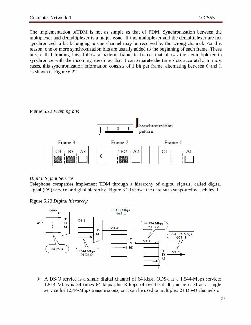
Computer Network-1 10CS55
97
The implementation ofTDM is not as simple as that of FDM. Synchronization between the
multiplexer and demultiplexer is a major issue. If the. multiplexer and the demultiplexer are not
synchronized, a bit belonging to one channel may be received by the wrong channel. For this
reason, one or more synchronization bits are usually added to the beginning of each frame. These
bits, called framing bits, follow a pattern, frame to frame, that allows the demultiplexer to
synchronize with the incoming stream so that it can separate the time slots accurately. In most
cases, this synchronization information consists of 1 bit per frame, alternating between 0 and I,
as shown in Figure 6.22.
Figure 6.22 Framing bits
Digital Signal Service
Telephone companies implement TDM through a hierarchy of digital signals, called digital
signal (DS) service or digital hierarchy. Figure 6.23 shows the data rates supportedby each level
Figure 6.23 Digital hierarchy
A DS-O service is a single digital channel of 64 kbps. ODS-I is a 1.544-Mbps service;
1.544 Mbps is 24 times 64 kbps plus 8 kbps of overhead. It can be used as a single
service for 1.544-Mbps transmissions, or it can be used to multiplex 24 DS-O channels or
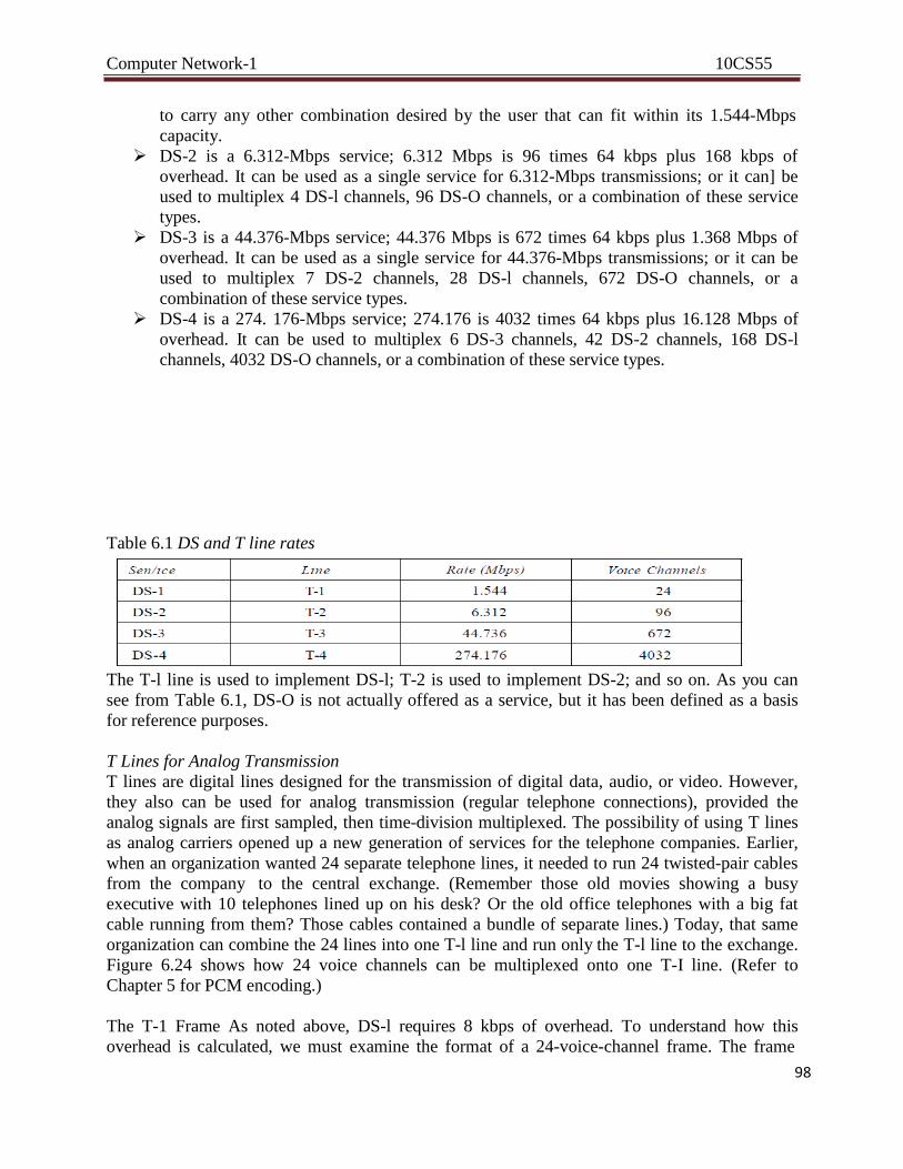
Computer Network-1 10CS55
98
to carry any other combination desired by the user that can fit within its 1.544-Mbps
capacity.
DS-2 is a 6.312-Mbps service; 6.312 Mbps is 96 times 64 kbps plus 168 kbps of
overhead. It can be used as a single service for 6.312-Mbps transmissions; or it can] be
used to multiplex 4 DS-l channels, 96 DS-O channels, or a combination of these service
types.
DS-3 is a 44.376-Mbps service; 44.376 Mbps is 672 times 64 kbps plus 1.368 Mbps of
overhead. It can be used as a single service for 44.376-Mbps transmissions; or it can be
used to multiplex 7 DS-2 channels, 28 DS-l channels, 672 DS-O channels, or a
combination of these service types.
DS-4 is a 274. 176-Mbps service; 274.176 is 4032 times 64 kbps plus 16.128 Mbps of
overhead. It can be used to multiplex 6 DS-3 channels, 42 DS-2 channels, 168 DS-l
channels, 4032 DS-O channels, or a combination of these service types.
Table 6.1 DS and T line rates
The T-l line is used to implement DS-l; T-2 is used to implement DS-2; and so on. As you can
see from Table 6.1, DS-O is not actually offered as a service, but it has been defined as a basis
for reference purposes.
T Lines for Analog Transmission
T lines are digital lines designed for the transmission of digital data, audio, or video. However,
they also can be used for analog transmission (regular telephone connections), provided the
analog signals are first sampled, then time-division multiplexed. The possibility of using T lines
as analog carriers opened up a new generation of services for the telephone companies. Earlier,
when an organization wanted 24 separate telephone lines, it needed to run 24 twisted-pair cables
from the company to the central exchange. (Remember those old movies showing a busy
executive with 10 telephones lined up on his desk? Or the old office telephones with a big fat
cable running from them? Those cables contained a bundle of separate lines.) Today, that same
organization can combine the 24 lines into one T-l line and run only the T-l line to the exchange.
Figure 6.24 shows how 24 voice channels can be multiplexed onto one T-I line. (Refer to
Chapter 5 for PCM encoding.)
The T-1 Frame As noted above, DS-l requires 8 kbps of overhead. To understand how this
overhead is calculated, we must examine the format of a 24-voice-channel frame. The frame

Computer Network-1 10CS55
99
used on a T-l line is usually 193 bits divided into 24 slots of 8 bits each plus 1 extra bit for
synchronization (24 x 8 + 1 = 193); see Figure 6.25. In other words,
Figure 6.24 T-l line for multiplexing telephone lines
Figure 6.25 T-l frame structure
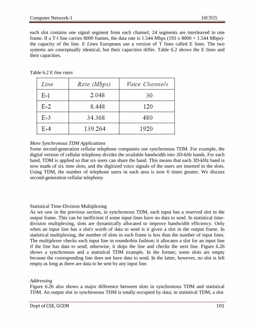
Computer Network-1 10CS55
Dept of CSE, GCEM 101
each slot contains one signal segment from each channel; 24 segments are interleaved in one
frame. If a T-l line carries 8000 frames, the data rate is 1.544 Mbps (193 x 8000 = 1.544 Mbps)-
the capacity of the line. E Lines Europeans use a version of T lines called E lines. The two
systems are conceptually identical, but their capacities differ. Table 6.2 shows the E lines and
their capacities.
Table 6.2 E line rates
More Synchronous TDM Applications
Some second-generation cellular telephone companies use synchronous TDM. For example, the
digital version of cellular telephony divides the available bandwidth into 3D-kHz bands. For each
band, TDM is applied so that six users can share the band. This means that each 3D-kHz band is
now made of six time slots, and the digitized voice signals of the users are inserted in the slots.
Using TDM, the number of telephone users in each area is now 6 times greater. We discuss
second-generation cellular telephony
Statistical Time-Division Multiplexing
As we saw in the previous section, in synchronous TDM, each input has a reserved slot in the
output frame. This can be inefficient if some input lines have no data to send. In statistical time-
division multiplexing, slots are dynamically allocated to improve bandwidth efficiency. Only
when an input line has a slot's worth of data to send is it given a slot in the output frame. In
statistical multiplexing, the number of slots in each frame is less than the number of input lines.
The multiplexer checks each input line in roundrobin fashion; it allocates a slot for an input line
if the line has data to send; otherwise, it skips the line and checks the next line. Figure 6.26
shows a synchronous and a statistical TDM example. In the former, some slots are empty
because the corresponding line does not have data to send. In the latter, however, no slot is left
empty as long as there are data to be sent by any input line.
Addressing
Figure 6.26 also shows a major difference between slots in synchronous TDM and statistical
TDM. An output slot in synchronous TDM is totally occupied by data; in statistical TDM, a slot
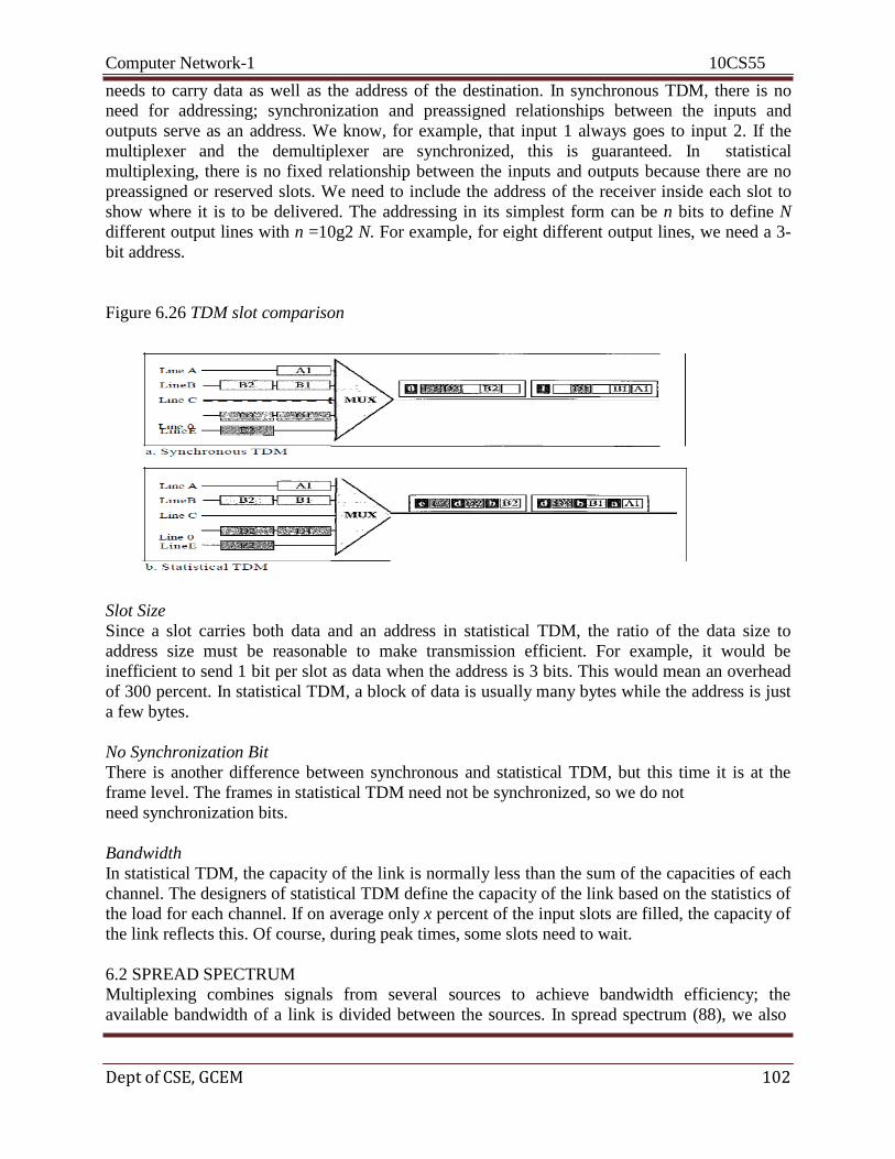
Computer Network-1 10CS55
Dept of CSE, GCEM 102
needs to carry data as well as the address of the destination. In synchronous TDM, there is no
need for addressing; synchronization and preassigned relationships between the inputs and
outputs serve as an address. We know, for example, that input 1 always goes to input 2. If the
multiplexer and the demultiplexer are synchronized, this is guaranteed. In statistical
multiplexing, there is no fixed relationship between the inputs and outputs because there are no
preassigned or reserved slots. We need to include the address of the receiver inside each slot to
show where it is to be delivered. The addressing in its simplest form can be n bits to define N
different output lines with n =10g2 N. For example, for eight different output lines, we need a 3-
bit address.
Figure 6.26 TDM slot comparison
Slot Size
Since a slot carries both data and an address in statistical TDM, the ratio of the data size to
address size must be reasonable to make transmission efficient. For example, it would be
inefficient to send 1 bit per slot as data when the address is 3 bits. This would mean an overhead
of 300 percent. In statistical TDM, a block of data is usually many bytes while the address is just
a few bytes.
No Synchronization Bit
There is another difference between synchronous and statistical TDM, but this time it is at the
frame level. The frames in statistical TDM need not be synchronized, so we do not
need synchronization bits.
Bandwidth
In statistical TDM, the capacity of the link is normally less than the sum of the capacities of each
channel. The designers of statistical TDM define the capacity of the link based on the statistics of
the load for each channel. If on average only x percent of the input slots are filled, the capacity of
the link reflects this. Of course, during peak times, some slots need to wait.
6.2 SPREAD SPECTRUM
Multiplexing combines signals from several sources to achieve bandwidth efficiency; the
available bandwidth of a link is divided between the sources. In spread spectrum (88), we also
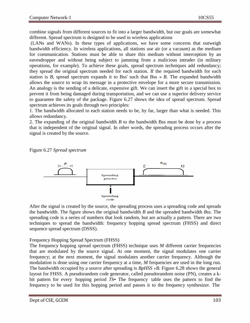
Computer Network-1 10CS55
Dept of CSE, GCEM 103
combine signals from different sources to fit into a larger bandwidth, but our goals are somewhat
different. Spread spectrum is designed to be used in wireless applications
(LANs and WANs). In these types of applications, we have some concerns that outweigh
bandwidth efficiency. In wireless applications, all stations use air (or a vacuum) as the medium
for communication. Stations must be able to share this medium without interception by an
eavesdropper and without being subject to jamming from a malicious intruder (in military
operations, for example). To achieve these goals, spread spectrum techniques add redundancy;
they spread the original spectrum needed for each station. If the required bandwidth for each
station is B, spread spectrum expands it to Bss' such that Bss » B. The expanded bandwidth
allows the source to wrap its message in a protective envelope for a more secure transmission.
An analogy is the sending of a delicate, expensive gift. We can insert the gift in a special box to
prevent it from being damaged during transportation, and we can use a superior delivery service
to guarantee the safety of the package. Figure 6.27 shows the idea of spread spectrum. Spread
spectrum achieves its goals through two principles:
1. The bandwidth allocated to each station needs to be, by far, larger than what is needed. This
allows redundancy.
2. The expanding of the original bandwidth B to the bandwidth Bss must be done by a process
that is independent of the original signal. In other words, the spreading process occurs after the
signal is created by the source.
Figure 6.27 Spread spectrum
After the signal is created by the source, the spreading process uses a spreading code and spreads
the bandwidth. The figure shows the original bandwidth B and the spreaded bandwidth Bss. The
spreading code is a series of numbers that look random, but are actually a pattern. There are two
techniques to spread the bandwidth: frequency hopping spread spectrum (FHSS) and direct
sequence spread spectrum (DSSS).
Frequency Hopping Spread Spectrum (FHSS)
The frequency hopping spread spectrum (FHSS) technique uses M different carrier frequencies
that are modulated by the source signal. At one moment, the signal modulates one carrier
frequency; at the next moment, the signal modulates another carrier frequency. Although the
modulation is done using one carrier frequency at a time, M frequencies are used in the long run.
The bandwidth occupied by a source after spreading is BpHSS »B. Figure 6.28 shows the general
layout for FHSS. A pseudorandom code generator, called pseudorandom noise (PN), creates a k-
bit pattern for every hopping period Th• The frequency table uses the pattern to find the
frequency to be used for this hopping period and passes it to the frequency synthesizer. The
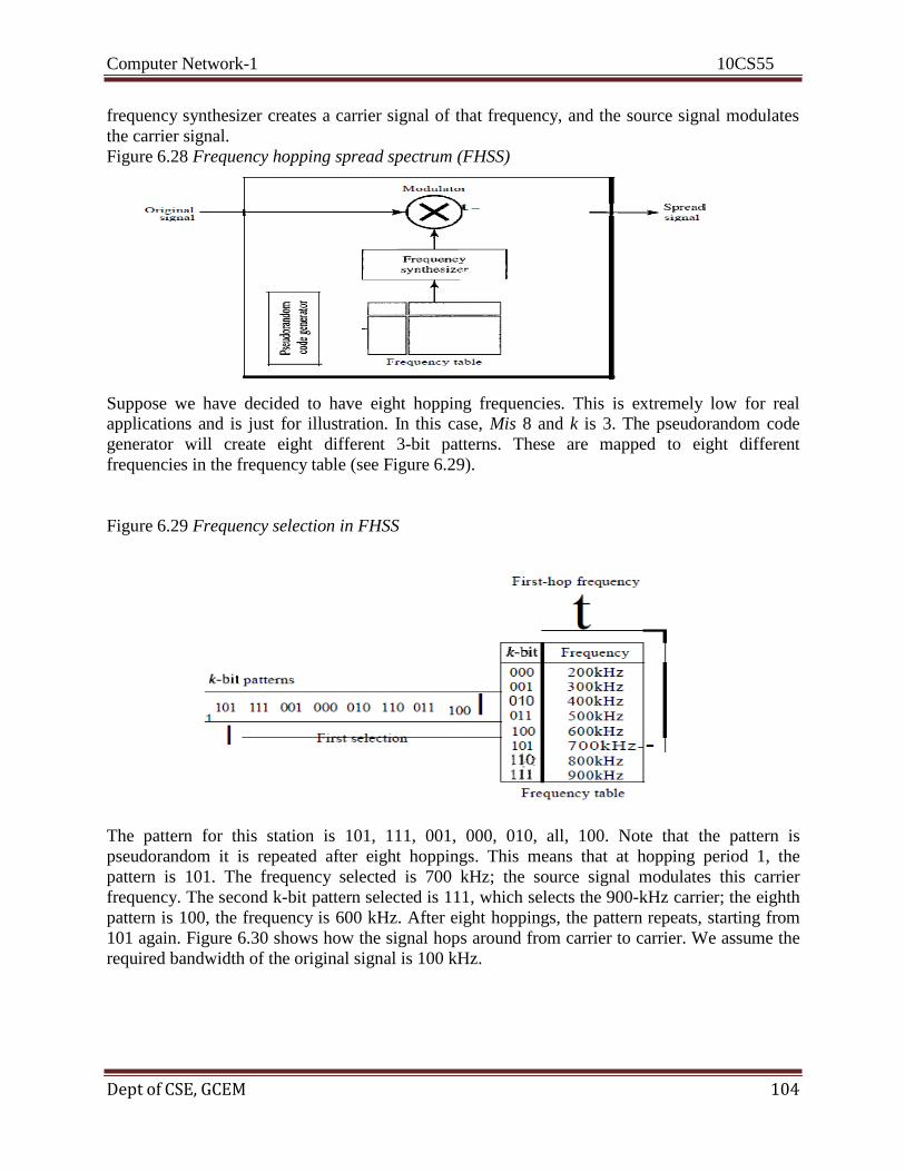
Computer Network-1 10CS55
Dept of CSE, GCEM 104
frequency synthesizer creates a carrier signal of that frequency, and the source signal modulates
the carrier signal.
Figure 6.28 Frequency hopping spread spectrum (FHSS)
Suppose we have decided to have eight hopping frequencies. This is extremely low for real
applications and is just for illustration. In this case, Mis 8 and k is 3. The pseudorandom code
generator will create eight different 3-bit patterns. These are mapped to eight different
frequencies in the frequency table (see Figure 6.29).
Figure 6.29 Frequency selection in FHSS
The pattern for this station is 101, 111, 001, 000, 010, all, 100. Note that the pattern is
pseudorandom it is repeated after eight hoppings. This means that at hopping period 1, the
pattern is 101. The frequency selected is 700 kHz; the source signal modulates this carrier
frequency. The second k-bit pattern selected is 111, which selects the 900-kHz carrier; the eighth
pattern is 100, the frequency is 600 kHz. After eight hoppings, the pattern repeats, starting from
101 again. Figure 6.30 shows how the signal hops around from carrier to carrier. We assume the
required bandwidth of the original signal is 100 kHz.
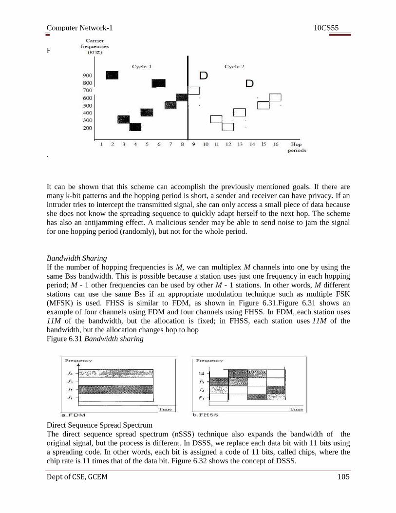
Computer Network-1 10CS55
Dept of CSE, GCEM 105
Figure 6.30 FHSS cycles
.
It can be shown that this scheme can accomplish the previously mentioned goals. If there are
many k-bit patterns and the hopping period is short, a sender and receiver can have privacy. If an
intruder tries to intercept the transmitted signal, she can only access a small piece of data because
she does not know the spreading sequence to quickly adapt herself to the next hop. The scheme
has also an antijamming effect. A malicious sender may be able to send noise to jam the signal
for one hopping period (randomly), but not for the whole period.
Bandwidth Sharing
If the number of hopping frequencies is M, we can multiplex M channels into one by using the
same Bss bandwidth. This is possible because a station uses just one frequency in each hopping
period; M - 1 other frequencies can be used by other M - 1 stations. In other words, M different
stations can use the same Bss if an appropriate modulation technique such as multiple FSK
(MFSK) is used. FHSS is similar to FDM, as shown in Figure 6.31.Figure 6.31 shows an
example of four channels using FDM and four channels using FHSS. In FDM, each station uses
11M of the bandwidth, but the allocation is fixed; in FHSS, each station uses 11M of the
bandwidth, but the allocation changes hop to hop
Figure 6.31 Bandwidth sharing
Direct Sequence Spread Spectrum
The direct sequence spread spectrum (nSSS) technique also expands the bandwidth of the
original signal, but the process is different. In DSSS, we replace each data bit with 11 bits using
a spreading code. In other words, each bit is assigned a code of 11 bits, called chips, where the
chip rate is 11 times that of the data bit. Figure 6.32 shows the concept of DSSS.

Computer Network-1 10CS55
Dept of CSE, GCEM 106
Figure 6.32 DSSS
As an example, let us consider the sequence used in a wireless LAN, the famous Barker
sequence where 11 is 11. We assume that the original signal and the chips in the chip generator
use polar NRZ encoding. Figure 6.33 shows the chips and the result of multiplying the original
data by the chips to get the spread signal. In Figure 6.33, the spreading code is 11 chips having
the pattern 10110111000 (in this case). If the original signal rate is N, the rate of the spread
signal is lIN. This means that the required bandwidth for the spread signal is 11 times larger than
the bandwidth of the original signal. The spread signal can provide privacy if the intruder does
not know the code. It can also provide immunity against interference if each station uses a
different code.
Figure 6.33 DSSS example
Bandwidth Sharing
Can we share a bandwidth in DSSS as we did in FHSS? The answer is no and yes. If we use a
spreading code that spreads signals (from different stations) that cannot be combined and
separated, we cannot share a bandwidth. For example, as we will see in Chapter 14, some
wireless LANs use DSSS and the spread bandwidth cannot be shared. However, if we use a
special type of sequence code that allows the combining and separating of spread signals, we can
share the bandwidth. As we will see in Chapter 16, a special spreading code allows us to use
DSSS in cellular telephony and share a bandwidth between several users.
Recommended Questions
1. List three main multiplexing techniques mentioned in this chapter. 2. Define the analog hierarchy used by telephone companies and list
different levels of the hierarchy.

Computer Network-1 10CS55
Dept of CSE, GCEM 107
3. Which of the three multiplexing techniques is common for fiber optic
links?
4. Distinguish between multilevel TDM, multiple slot TDM, and pulse-
stuffed TDM
5. Describe the goals of multiplexing
Computer Network-1 10CS55
Dept of CSE, GCEM 108
COMPUTER NETWORKS – I
Subject Code: 10CS55 I.A. Marks : 25 Hours/Week : 04 Exam Hours: 03
Total Hours : 52 Exam Marks: 100
UNIT- 4 6 Hours
Data Link Layer-1:
-Error Detection & Correction:
- Introduction,
-Block coding,
-Linear block codes,
-Cyclic codes, -Checksum.
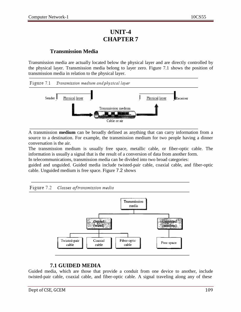
Computer Network-1 10CS55
Dept of CSE, GCEM 109
UNIT-4
CHAPTER 7
Transmission Media
Transmission media are actually located below the physical layer and are directly controlled by
the physical layer. Transmission media belong to layer zero. Figure 7.1 shows the position of
transmission media in relation to the physical layer.
A transmission medium can be broadly defined as anything that can carry information from a
source to a destination. For example, the transmission medium for two people having a dinner
conversation is the air.
The transmission medium is usually free space, metallic cable, or fiber-optic cable. The
information is usually a signal that is the result of a conversion of data from another form.
In telecommunications, transmission media can be divided into two broad categories:
guided and unguided. Guided media include twisted-pair cable, coaxial cable, and fiber-optic
cable. Unguided medium is free space. Figure 7.2 shows
7.1 GUIDED MEDIA Guided media, which are those that provide a conduit from one device to another, include
twisted-pair cable, coaxial cable, and fiber-optic cable. A signal traveling along any of these

Computer Network-1 10CS55
Dept of CSE, GCEM 110
media is directed and contained by the physical limits of the medium. Twisted-pair and coaxial
cable use metallic (copper) conductors that accept and transport signals in the form of electric
current. Optical fiber is a cable that accepts and transports signals in the form of light.
Twisted-Pair Cable
A twisted pair consists of two conductors (normally copper), each with its own plastic
insulation, twisted together, as shown in Figure 7.3.
One of the wires is used to carry signals to the receiver, and the other is used only as a ground
reference. The receiver uses the difference between the two. One of the wires is used to carry
signals to the receiver, and the other is used only as a ground reference. The receiver uses the
difference between the two. In addition to the signal sent by the sender on one of the wires,
interference (noise) and crosstalk may affect both wires and create unwanted signals.
If the two wires are parallel, the effect of these unwanted signals is not the same in both wires
because they are at different locations relative to the noise or crosstalk sources
(e,g., one is closer and the other is farther). This results in a difference at the receiver. By
twisting the pairs, a balance is maintained.
Unshielded Versus Shielded Twisted-Pair Cable
The most common twisted-pair cable used in communications is referred to as unshielded
twisted-pair (UTP). IBM has also produced a version of twisted-pair cable
for its use called shielded twisted-pair (STP). STP cable has a metal foil or braidedmesh
covering that encases each pair of insulated conductors. Although metal casing improves the
quality of cable by preventing the penetration of noise or crosstalk, it is bulkier and more
expensive. Figure 7.4 shows the difference between UTP and STP.
Categories
The Electronic Industries Association (EIA) has developed standards to classify
unshielded twisted-pair cable into seven categories. Categories are determined by cable
quality, with 1 as the lowest and 7 as the highest. Each EIA category is suitable for
specific uses. Table 7. 1 shows these categories.
Connectors
The most common UTP connector is RJ45 (RJ stands for registered jack), as shown
in Figure 7.5. The RJ45 is a keyed connector, meaning the connector can be inserted in
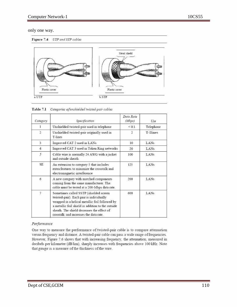
Computer Network-1 10CS55
Dept of CSE,GCEM 110
only one way.

Computer Network-1 10CS55
Dept of CSE,GCEM 111
Applications
Twisted-pair cables are used in telephone lines to provide voice and data channels. The
local loop-the line that connects subscribers to the central telephone office commonly
consists of unshielded twisted-pair cables.
The DSL lines that are used by the telephone companies to provide high-data-rate
connections also use the high-bandwidth capability of unshielded twisted-pair cables.
Local-area networks, such as 10Base-T and l00Base-T, also use twisted-pair cables.
Coaxial Cable Coaxial cable (or coax) carries signals of higher frequency ranges than those in
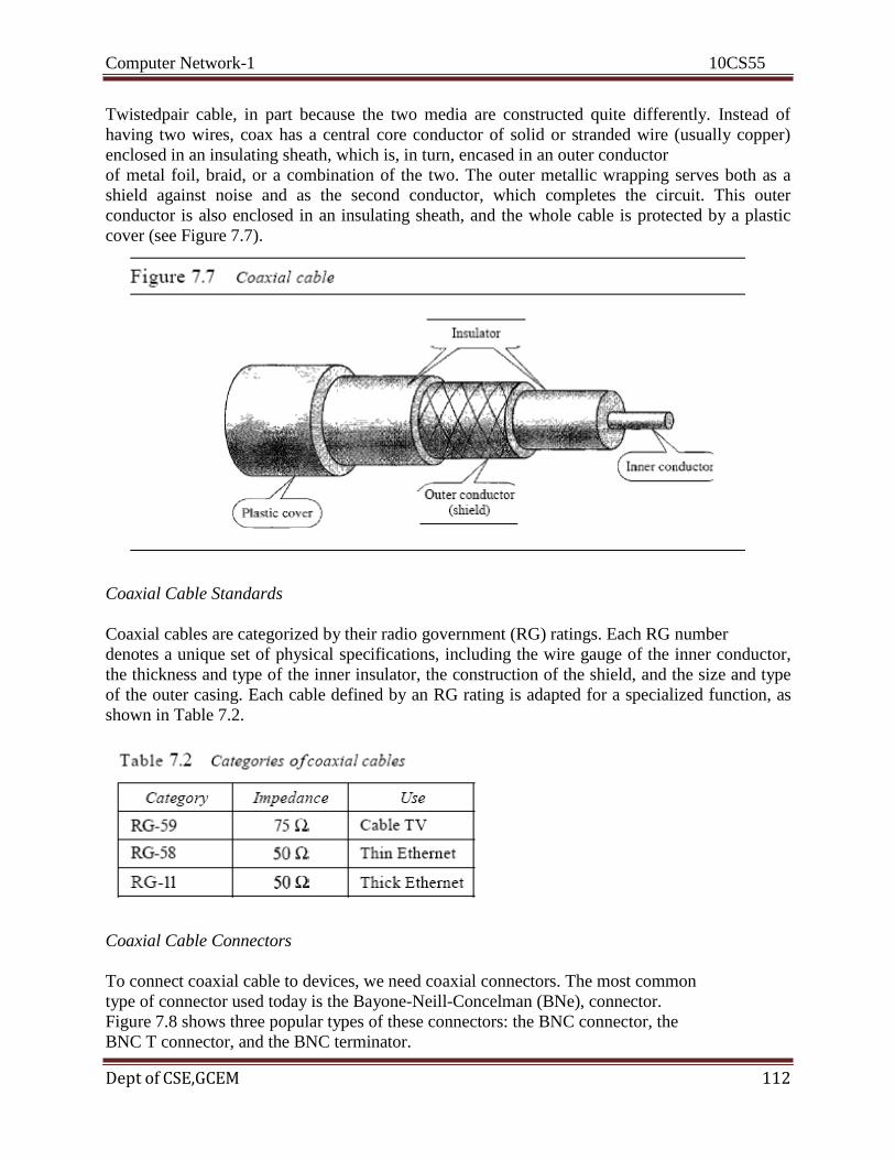
Computer Network-1 10CS55
Dept of CSE,GCEM 112
Twistedpair cable, in part because the two media are constructed quite differently. Instead of
having two wires, coax has a central core conductor of solid or stranded wire (usually copper)
enclosed in an insulating sheath, which is, in turn, encased in an outer conductor
of metal foil, braid, or a combination of the two. The outer metallic wrapping serves both as a
shield against noise and as the second conductor, which completes the circuit. This outer
conductor is also enclosed in an insulating sheath, and the whole cable is protected by a plastic
cover (see Figure 7.7).
Coaxial Cable Standards
Coaxial cables are categorized by their radio government (RG) ratings. Each RG number
denotes a unique set of physical specifications, including the wire gauge of the inner conductor,
the thickness and type of the inner insulator, the construction of the shield, and the size and type
of the outer casing. Each cable defined by an RG rating is adapted for a specialized function, as
shown in Table 7.2.
Coaxial Cable Connectors
To connect coaxial cable to devices, we need coaxial connectors. The most common
type of connector used today is the Bayone-Neill-Concelman (BNe), connector.
Figure 7.8 shows three popular types of these connectors: the BNC connector, the
BNC T connector, and the BNC terminator.
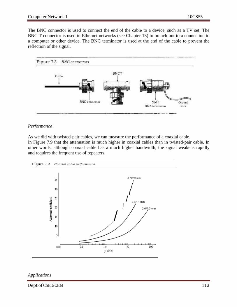
Computer Network-1 10CS55
Dept of CSE,GCEM 113
The BNC connector is used to connect the end of the cable to a device, such as a TV set. The
BNC T connector is used in Ethernet networks (see Chapter 13) to branch out to a connection to
a computer or other device. The BNC terminator is used at the end of the cable to prevent the
reflection of the signal.
Performance
As we did with twisted-pair cables, we can measure the performance of a coaxial cable.
In Figure 7.9 that the attenuation is much higher in coaxial cables than in twisted-pair cable. In
other words, although coaxial cable has a much higher bandwidth, the signal weakens rapidly
and requires the frequent use of repeaters.
Applications

Computer Network-1 10CS55
Dept of CSE,GCEM 114
Coaxial cable was widely used in analog telephone networks where a single coaxial network
could carry 10,000 voice signals. Later it was used in digital telephone networks
where a single coaxial cable could carry digital data up to 600 Mbps. However, coaxial
cable in telephone networks has largely been replaced today with fiber-optic cable.
Cable TV networks also use coaxial cables. In the traditional cable TV network, the entire
network used coaxial cable. Later, however, cable TV providers replaced most of the media with
fiber-optic cable; hybrid networks use coaxial cable only at the network boundaries, near the
consumer premises. Cable TV uses RG-59 coaxial cable.
Another common application of coaxial cable is in traditional Ethernet LANs Because of its
high bandwidth, and consequently high data rate, coaxial cable was chosen for digital
transmission in early Ethernet LANs. The 10Base-2, or Thin Ethernet, uses RG-58 coaxial cable
with BNe connectors to transmit data at 10 Mbps with a range of 185 m. The lOBase5, or Thick
Ethernet, uses RG-11 (thick coaxial cable) to transmit 10 Mbps with a range of 5000 m. Thick
Ethernet has specialized connectors.
Fiber-Optic Cable
A fiber-optic cable is made of glass or plastic and transmits signals in the form of light.
To understand optical fiber, we first need to explore several aspects of the nature of light.
Light travels in a straight line as long as it is moving through a single uniform substance.
If a ray of light traveling through one substance suddenly enters another substance (of a different
density), the ray changes direction. Figure 7.10 shows how a ray of light changes direction when
going from a more dense to a less dense substance.
As the figure shows, if the angle of incidence I (the arIgle the ray makes with the
line perpendicular to the interface between the two substances) is less than the critical
angle, the ray refracts and moves closer to the surface. If the angle of incidence is equal to the
critical angle, the light bends along the interface. If the angle is greater than the critical angle, the
ray reflects (makes a turn) and travels again in the denser substance.
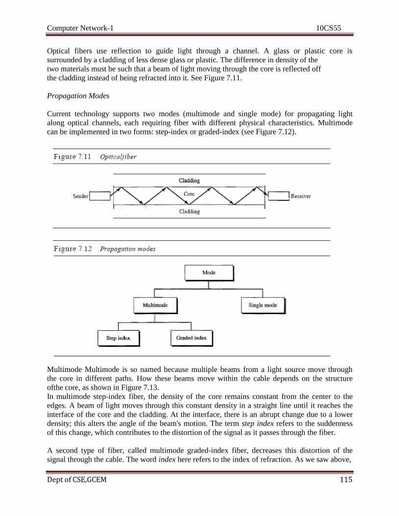
Computer Network-1 10CS55
Dept of CSE,GCEM 115
Optical fibers use reflection to guide light through a channel. A glass or plastic core is
surrounded by a cladding of less dense glass or plastic. The difference in density of the
two materials must be such that a beam of light moving through the core is reflected off
the cladding instead of being refracted into it. See Figure 7.11.
Propagation Modes
Current technology supports two modes (multimode and single mode) for propagating light
along optical channels, each requiring fiber with different physical characteristics. Multimode
can be implemented in two forms: step-index or graded-index (see Figure 7.12).
Multimode Multimode is so named because multiple beams from a light source move through
the core in different paths. How these beams move within the cable depends on the structure
ofthe core, as shown in Figure 7.13.
In multimode step-index fiber, the density of the core remains constant from the center to the
edges. A beam of light moves through this constant density in a straight line until it reaches the
interface of the core and the cladding. At the interface, there is an abrupt change due to a lower
density; this alters the angle of the beam's motion. The term step index refers to the suddenness
of this change, which contributes to the distortion of the signal as it passes through the fiber.
A second type of fiber, called multimode graded-index fiber, decreases this distortion of the
signal through the cable. The word index here refers to the index of refraction. As we saw above,

Computer Network-1 10CS55
Dept of CSE,GCEM 116
the index of refraction is related to density. A graded-index fiber, therefore, is one with varying
densities. Density is highest at the center of the core and decreases gradually to its lowest at the
edge. Figure 7.13 shows the impact of this variable density on the propagation of light beams.
Single-Mode Single-mode uses step-index fiber and a highly focused source of light that limits
beams to a small range of angles, all close to the horizontal. The single mode fiber itself is
manufactured with a much smaller diameter than that of multimode fiber, and with substantially
lower density (index of refraction). The decrease in density results in a critical angle that is close
enough to 90° to make the propagation of beams almost horizontal. In this case, propagation of
different beams is almost identical, and delays are negligible. All the beams arrive at the
destination "together" and can be recombined with little distortion to the signal (see Figure 7.13).
Fiber Sizes
Optical fibers are defined by the ratio of the diameter of their core to the diameter of
their cladding, both expressed in micrometers. The common sizes are shown in Table 7.3.
Note that the last size listed is for single-mode only.

Computer Network-1 10CS55
Dept of CSE,GCEM 117
Cable Composition
Figure 7.14 shows the composition of a typical fiber-optic cable. The outer jacket is made
of either PVC or Teflon. Inside the jacket are Kevlar strands to strengthen the cable. Kevlar
is a strong material used in the fabrication of bulletproof vests. Below the Kevlar is another
plastic coating to cushion the fiber. The fiber is at the center of the cable, and it consists of
cladding and core.
Fiber-Optic Cable Connectors
There are three types of connectors for fiber-optic cables, as shown in Figure 7.15.
The subscriber channel (SC) connector is used for cable TV. It uses a push/pull locking
system. The straight-tip (ST) connector is used for connecting cable to networking devices. It
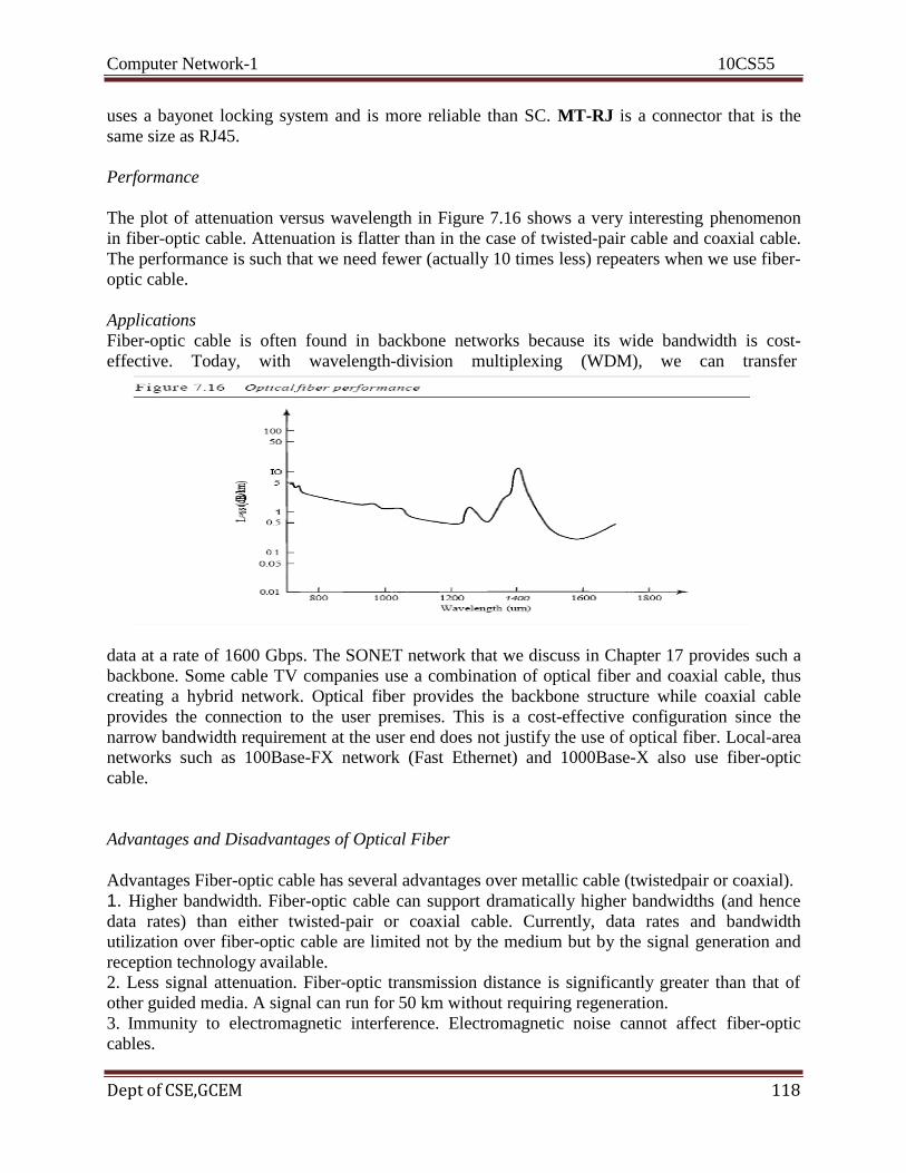
Computer Network-1 10CS55
Dept of CSE,GCEM 118
uses a bayonet locking system and is more reliable than SC. MT-RJ is a connector that is the
same size as RJ45.
Performance
The plot of attenuation versus wavelength in Figure 7.16 shows a very interesting phenomenon
in fiber-optic cable. Attenuation is flatter than in the case of twisted-pair cable and coaxial cable.
The performance is such that we need fewer (actually 10 times less) repeaters when we use fiber-
optic cable.
Applications
Fiber-optic cable is often found in backbone networks because its wide bandwidth is cost-
effective. Today, with wavelength-division multiplexing (WDM), we can transfer
data at a rate of 1600 Gbps. The SONET network that we discuss in Chapter 17 provides such a
backbone. Some cable TV companies use a combination of optical fiber and coaxial cable, thus
creating a hybrid network. Optical fiber provides the backbone structure while coaxial cable
provides the connection to the user premises. This is a cost-effective configuration since the
narrow bandwidth requirement at the user end does not justify the use of optical fiber. Local-area
networks such as 100Base-FX network (Fast Ethernet) and 1000Base-X also use fiber-optic
cable.
Advantages and Disadvantages of Optical Fiber
Advantages Fiber-optic cable has several advantages over metallic cable (twistedpair or coaxial).
1. Higher bandwidth. Fiber-optic cable can support dramatically higher bandwidths (and hence
data rates) than either twisted-pair or coaxial cable. Currently, data rates and bandwidth
utilization over fiber-optic cable are limited not by the medium but by the signal generation and
reception technology available.
2. Less signal attenuation. Fiber-optic transmission distance is significantly greater than that of
other guided media. A signal can run for 50 km without requiring regeneration.
3. Immunity to electromagnetic interference. Electromagnetic noise cannot affect fiber-optic
cables.

Computer Network-1 10CS55
Dept of CSE,GCEM 119
4. Resistance to corrosive materials. Glass is more resistant to corrosive materials than copper.
6.Light weight. Fiber-optic cables are much lighter than copper cables. 7. Greater immunity to tapping. Fiber-optic cables are more immune to tapping than copper
cables. Copper cables create antenna effects that can easily be tapped. Disadvantages There are
some disadvantages in the use of optical fiber.
8. Installation and maintenance. Fiber-optic cable is a relatively new technology. Its installation
and maintenance require expertise that is not yet available everywhere.
9. Unidirectional light propagation. Propagation of light is unidirectional. If we need
bidirectional communication, two fibers are needed.
10. Cost. The cable and the interfaces are relatively more expensive than those of other guided
media. If the demand for bandwidth is not high, often the use of optical fiber
cannot be justified.
7.2 UNGUIDED MEDIA: WIRELESS
Unguided media transport electromagnetic waves without using a physical conductor. This type
of communication is often referred to as wireless communication. Signals are normally broadcast
through free space and thus are available to anyone who has a device capable of receiving them.
Figure 7.17 shows the part of the electromagnetic spectrum, ranging from 3 kHz to 900 THz,
used for wireless communication.
Unguided signals can travel from the source to destination in several ways: ground
propagation, sky propagation, and line-of-sight propagation, as shown in Figure 7.18.
In ground propagation, radio waves travel through the lowest portion of the atmosphere, hugging
the earth. These low-frequency signals emanate in all directions from the transmitting antenna
and follow the curvature of the planet. Distance depends on the amount of power in the signal:
The greater the power, the greater the distance. In sky propagation, higher-frequency radio waves
radiate upward into the ionosphere (the layer of atmosphere where particles exist as ions) where
they are reflected back to earth. This type of transmission allows for greater distances with lower
output power. In line-or-sight propagation, very high-frequency signals are transmitted in
straight lines directly from antenna to antenna. Antennas must be directional, facing each other,
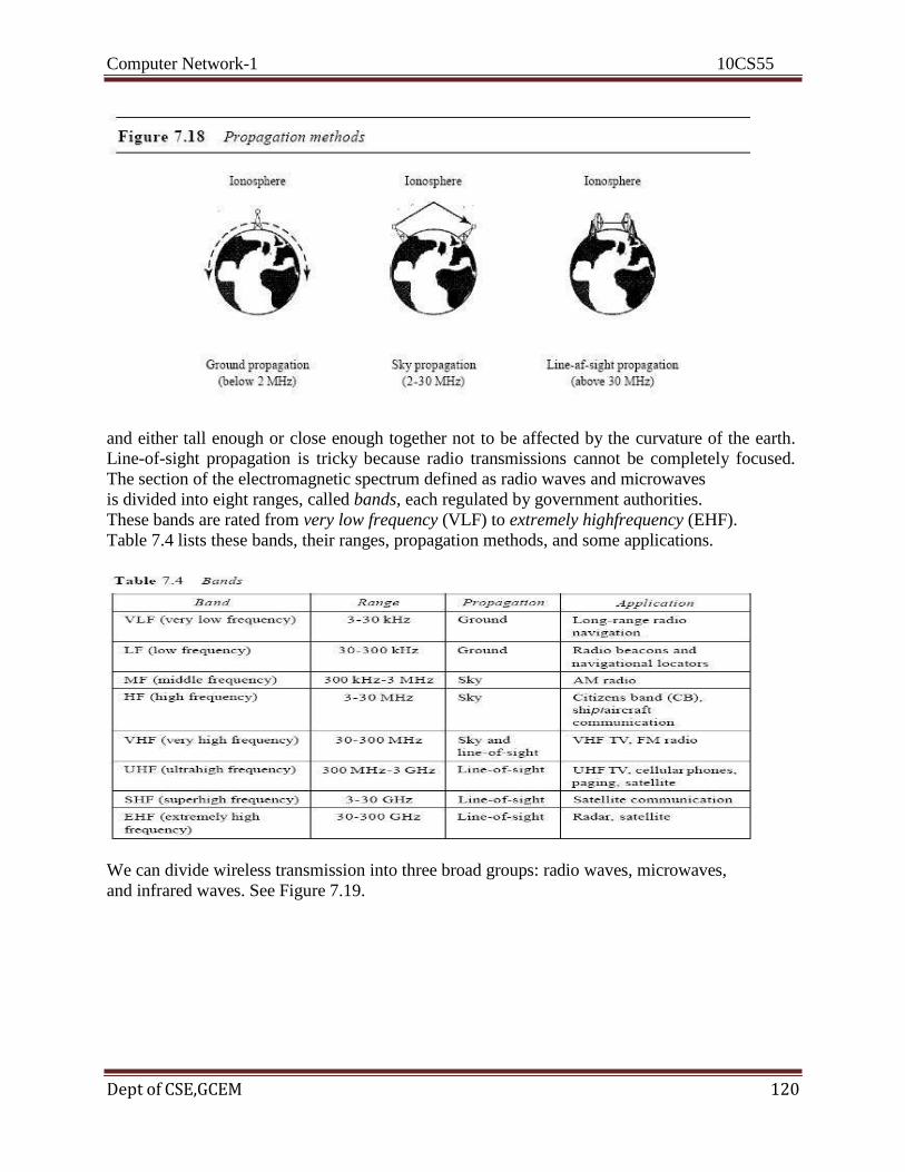
Computer Network-1 10CS55
Dept of CSE,GCEM 120
and either tall enough or close enough together not to be affected by the curvature of the earth.
Line-of-sight propagation is tricky because radio transmissions cannot be completely focused.
The section of the electromagnetic spectrum defined as radio waves and microwaves
is divided into eight ranges, called bands, each regulated by government authorities.
These bands are rated from very low frequency (VLF) to extremely highfrequency (EHF).
Table 7.4 lists these bands, their ranges, propagation methods, and some applications.
We can divide wireless transmission into three broad groups: radio waves, microwaves,
and infrared waves. See Figure 7.19.

Computer Network-1 10CS55
Dept of CSE,GCEM 121
Radio Waves
Electromagnetic waves ranging in frequencies between 3 kHz and 1 GHz are normally called
radio waves; waves ranging in frequencies between 1 and 300 GHz are called microwaves.
However, the behavior of the waves, rather than the frequencies, is a better
criterion for classification. Radio waves, for the most part, are omnidirectional. When an antenna
transmits radio waves, they are propagated in all directions. This means that the sending and
receiving antennas do not have to be aligned. A sending antenna sends waves that can be
received by any receiving antenna. The omnidirectional property has a disadvantage, too. The
radio waves transmitted by one antenna are susceptible to interference by another antenna that
may send signals using the same frequency or band.
Radio waves, particularly those waves that propagate in the sky mode, can travel long distances.
This makes radio waves a good candidate for long-distance broadcasting
such as AM radio.
Radio waves, particularly those of low and medium frequencies, can penetrate walls.
This characteristic can be both an advantage and a disadvantage. It is an advantage because, for
example, an AM radio can receive signals inside a building. It is a disadvantage because we
cannot isolate a communication to just inside or outside a building. The radio wave band is
relatively narrow, just under 1 GHz, compared to the microwave band. When this band is divided
into subbands, the subbands are also narrow, leading to a low data rate for digital
communications.
Almost the entire band is regulated by authorities (e.g., the FCC in the United States). Using any
part of the band requires permission from the authorities.
Omnidirectional Antenna
Radio waves use omnidirectional antennas that send out signals in all directions. Based on the
wavelength, strength, and the purpose of transmission, we can have several types of antennas.
Figure 7.20 shows an omnidirectional antenna.
Applications
The omnidirectional characteristics of radio waves make them useful for multicasting,
in which there is one sender but many receivers. AM and FM radio, television, maritime radio,
cordless phones, and paging are examples of multicasting.
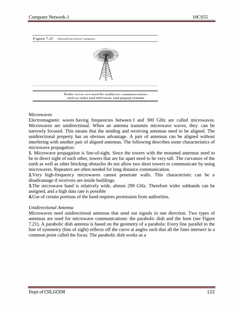
Computer Network-1 10CS55
Dept of CSE,GCEM 122
Microwaves
Electromagnetic waves having frequencies between I and 300 GHz are called microwaves.
Microwaves are unidirectional. When an antenna transmits microwave waves, they can be
narrowly focused. This means that the sending and receiving antennas need to be aligned. The
unidirectional property has an obvious advantage. A pair of antennas can be aligned without
interfering with another pair of aligned antennas. The following describes some characteristics of
microwave propagation:
1. Microwave propagation is line-of-sight. Since the towers with the mounted antennas need to
be in direct sight of each other, towers that are far apart need to be very tall. The curvature of the
earth as well as other blocking obstacles do not allow two short towers to communicate by using
microwaves. Repeaters are often needed for long distance communication.
2.Very high-frequency microwaves cannot penetrate walls. This characteristic can be a
disadvantage if receivers are inside buildings.
3.The microwave band is relatively wide, almost 299 GHz. Therefore wider subbands can be
assigned, and a high data rate is possible
4.Use of certain portions of the band requires permission from authorities.
Unidirectional Antenna
Microwaves need unidirectional antennas that send out signals in one direction. Two types of
antennas are used for microwave communications: the parabolic dish and the hom (see Figure
7.21). A parabolic dish antenna is based on the geometry of a parabola: Every line parallel to the
line of symmetry (line of sight) reflects off the curve at angles such that all the lines intersect in a
common point called the focus. The parabolic dish works as a

Computer Network-1 10CS55
Dept of CSE,GCEM 123
funnel, catching a wide range of waves and directing them to a common point. In this way, more
of the signal is recovered than would be possible with a single-point receiver. Outgoing
transmissions are broadcast through a horn aimed at the dish. The microwaves hit the dish and
are deflected outward in a reversal of the receipt path.
A horn antenna looks like a gigantic scoop. Outgoing transmissions are broadcast up a stem
(resembling a handle) and deflected outward in a series of narrow parallel beams by the curved
head. Received transmissions are collected by the scooped shape of the horn, in a manner similar
to the parabolic dish, and are deflected down into the stem.
Applications
Microwaves, due to their unidirectional properties, are very useful when unicast (one-to-one)
communication is needed between the sender and the receiver. They are used in cellular phones ,
satellite networks , and wireless LANs
Infrared
Infrared waves, with frequencies from 300 GHz to 400 THz (wavelengths from 1 mm to 770
nm), can be used for short-range communication. Infrared waves, having high frequencies,
cannot penetrate walls. This advantageous characteristic prevents interference between one
system and another; a short-range communication system in one room cannot be affected by
another system in the next room. When we use our infrared remote control, we do not interfere
with the use of the remote by our neighbors. However, this same characteristic makes infrared
signals useless for long-range communication. In addition, we cannot use infrared waves outside
a building because the sun's rays contain infrared waves that can interfere with the
communication.
Applications
The infrared band, almost 400 THz, has an excellent potential for data transmission. Such a wide
bandwidth can be used to transmit digital data with a very high data rate. The Infrared Data
Association (IrDA), an association for sponsoring the use of infrared waves, has established
standards for using these signals for communication between devices such as keyboards, mice,
PCs, and printers. For example, some manufacturers provide a special port called the IrDA port
that allows a wireless keyboard to communicate with a PC. The standard originally defined a
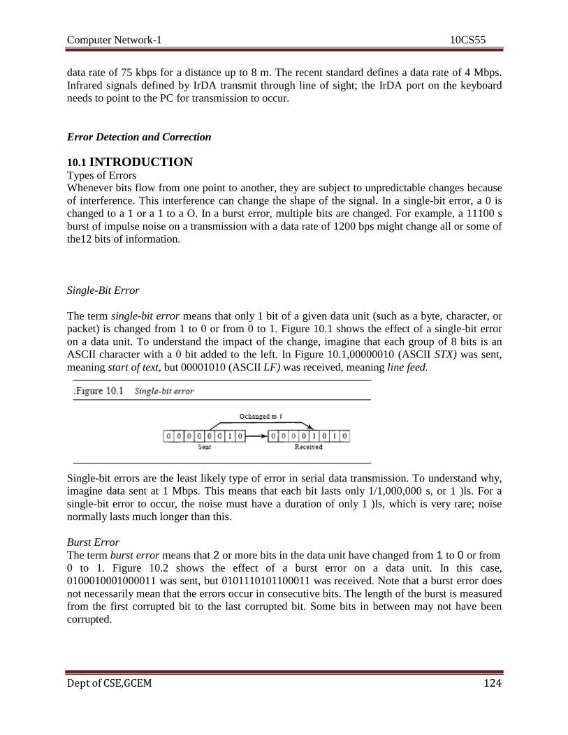
Computer Network-1 10CS55
Dept of CSE,GCEM 124
data rate of 75 kbps for a distance up to 8 m. The recent standard defines a data rate of 4 Mbps.
Infrared signals defined by IrDA transmit through line of sight; the IrDA port on the keyboard
needs to point to the PC for transmission to occur.
Error Detection and Correction
10.1 INTRODUCTION Types of Errors Whenever bits flow from one point to another, they are subject to unpredictable changes because
of interference. This interference can change the shape of the signal. In a single-bit error, a 0 is
changed to a 1 or a 1 to a O. In a burst error, multiple bits are changed. For example, a 11100 s
burst of impulse noise on a transmission with a data rate of 1200 bps might change all or some of
the12 bits of information.
Single-Bit Error
The term single-bit error means that only 1 bit of a given data unit (such as a byte, character, or
packet) is changed from 1 to 0 or from 0 to 1. Figure 10.1 shows the effect of a single-bit error
on a data unit. To understand the impact of the change, imagine that each group of 8 bits is an
ASCII character with a 0 bit added to the left. In Figure 10.1,00000010 (ASCII STX) was sent,
meaning start of text, but 00001010 (ASCII LF) was received, meaning line feed.
Single-bit errors are the least likely type of error in serial data transmission. To understand why,
imagine data sent at 1 Mbps. This means that each bit lasts only 1/1,000,000 s, or 1 )ls. For a
single-bit error to occur, the noise must have a duration of only 1 )ls, which is very rare; noise
normally lasts much longer than this.
Burst Error
The term burst error means that 2 or more bits in the data unit have changed from 1 to 0 or from
0 to 1. Figure 10.2 shows the effect of a burst error on a data unit. In this case,
0100010001000011 was sent, but 0101110101100011 was received. Note that a burst error does
not necessarily mean that the errors occur in consecutive bits. The length of the burst is measured
from the first corrupted bit to the last corrupted bit. Some bits in between may not have been
corrupted.
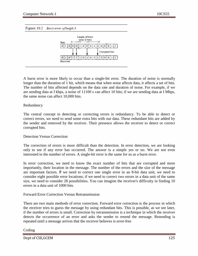
Computer Network-1 10CS55
Dept of CSE,GCEM 125
A burst error is more likely to occur than a single-bit error. The duration of noise is normally
longer than the duration of 1 bit, which means that when noise affects data, it affects a set of bits.
The number of bits affected depends on the data rate and duration of noise. For example, if we
are sending data at I kbps, a noise of 11100 s can affect 10 bits; if we are sending data at I Mbps,
the same noise can affect 10,000 bits.
Redundancy
The central concept in detecting or correcting errors is redundancy. To be able to detect or
correct errors, we need to send some extra bits with our data. These redundant bits are added by
the sender and removed by the receiver. Their presence allows the receiver to detect or correct
corrupted bits.
Detection Versus Correction
The correction of errors is more difficult than the detection. In error detection, we are looking
only to see if any error has occurred. The answer is a simple yes or no. We are not even
interested in the number of errors. A single-bit error is the same for us as a burst error.
In error correction, we need to know the exact number of bits that are corrupted and more
importantly, their location in the message. The number of the errors and the size of the message
are important factors. If we need to correct one single error in an 8-bit data unit, we need to
consider eight possible error locations; if we need to correct two errors in a data unit of the same
size, we need to consider 28 possibilities. You can imagine the receiver's difficulty in finding 10
errors in a data unit of 1000 bits.
Forward Error Correction Versus Retransmission
There are two main methods of error correction. Forward error correction is the process in which
the receiver tries to guess the message by using redundant bits. This is possible, as we see later,
if the number of errors is small. Correction by retransmission is a technique in which the receiver
detects the occurrence of an error and asks the sender to resend the message. Resending is
repeated until a message arrives that the receiver believes is error-free
Coding

Computer Network-1 10CS55
Dept of CSE,GCEM 126
Redundancy is achieved through various coding schemes. The sender adds redundant bits
through a process that creates a relationship between the redundant bits and the actual data bits.
The receiver checks the relationships between the two sets of bits to detect or correct the errors.
The ratio of redundant bits to the data bits and the robustness of the process are important factors
in any coding scheme. Figure 10.3 shows the general idea of coding.
We can divide coding schemes into two broad categories:
block coding and convolution coding..
Modular Arithmetic
In modular arithmetic, use only a limited range of integers. An upper limit, called a modulus N then use only the integers 0 to N - I, inclusive. This is modulo-N arithmetic.
For example, if the modulus is 12, we use only the integers 0 to 11, inclusive. An example of
modulo arithmetic is our clock system. It is based on modulo-12 arithmetic, substituting the
number 12 for O. In a modulo-N system, if a number is greater than N, it is divided by N and
the remainder is the result. If it is negative, as many Ns as needed are added to make it positive.
Modulo-2 Arithmetic
Of particular interest is modulo-2 arithmetic. In this arithmetic, the modulus N is 2. We can use
only 0 and 1. Operations in this
Notice particularly that addition and subtraction give the same results. In this arithmetic we use
the XOR (exclusive OR) operation for both addition and subtraction. The result of an XOR
operation is 0 if two bits are the same; the result is I if two bits are different. Figure 10.4 shows
this operation.
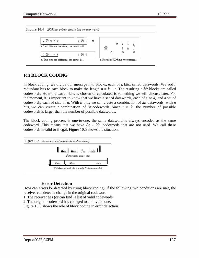
Computer Network-1 10CS55
Dept of CSE,GCEM 127
10.2 BLOCK CODING
In block coding, we divide our message into blocks, each of k bits, called datawords. We add r
redundant bits to each block to make the length n = k + r. The resulting n-bit blocks are called
codewords. How the extra r bits is chosen or calculated is something we will discuss later. For
the moment, it is important to know that we have a set of datawords, each of size k, and a set of
codewords, each of size of n. With k bits, we can create a combination of 2k datawords; with n
bits, we can create a combination of 2n codewords. Since n > k, the number of possible
codewords is larger than the number of possible datawords.
The block coding process is one-to-one; the same dataword is always encoded as the same
codeword. This means that we have 2n - 2k codewords that are not used. We call these
codewords invalid or illegal. Figure 10.5 shows the situation.
Error Detection
How can errors be detected by using block coding? If the following two conditions are met, the
receiver can detect a change in the original codeword.
1. The receiver has (or can find) a list of valid codewords.
2. The original codeword has changed to an invalid one.
Figure 10.6 shows the role of block coding in error detection.
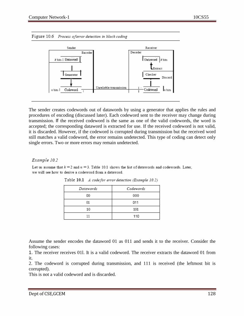
Computer Network-1 10CS55
Dept of CSE,GCEM 128
The sender creates codewords out of datawords by using a generator that applies the rules and
procedures of encoding (discussed later). Each codeword sent to the receiver may change during
transmission. If the received codeword is the same as one of the valid codewords, the word is
accepted; the corresponding dataword is extracted for use. If the received codeword is not valid,
it is discarded. However, if the codeword is corrupted during transmission but the received word
still matches a valid codeword, the error remains undetected. This type of coding can detect only
single errors. Two or more errors may remain undetected.
Assume the sender encodes the dataword 01 as 011 and sends it to the receiver. Consider the
following cases:
1. The receiver receives 01l. It is a valid codeword. The receiver extracts the dataword 01 from
it. 2. The codeword is corrupted during transmission, and 111 is received (the leftmost bit is
corrupted).
This is not a valid codeword and is discarded.
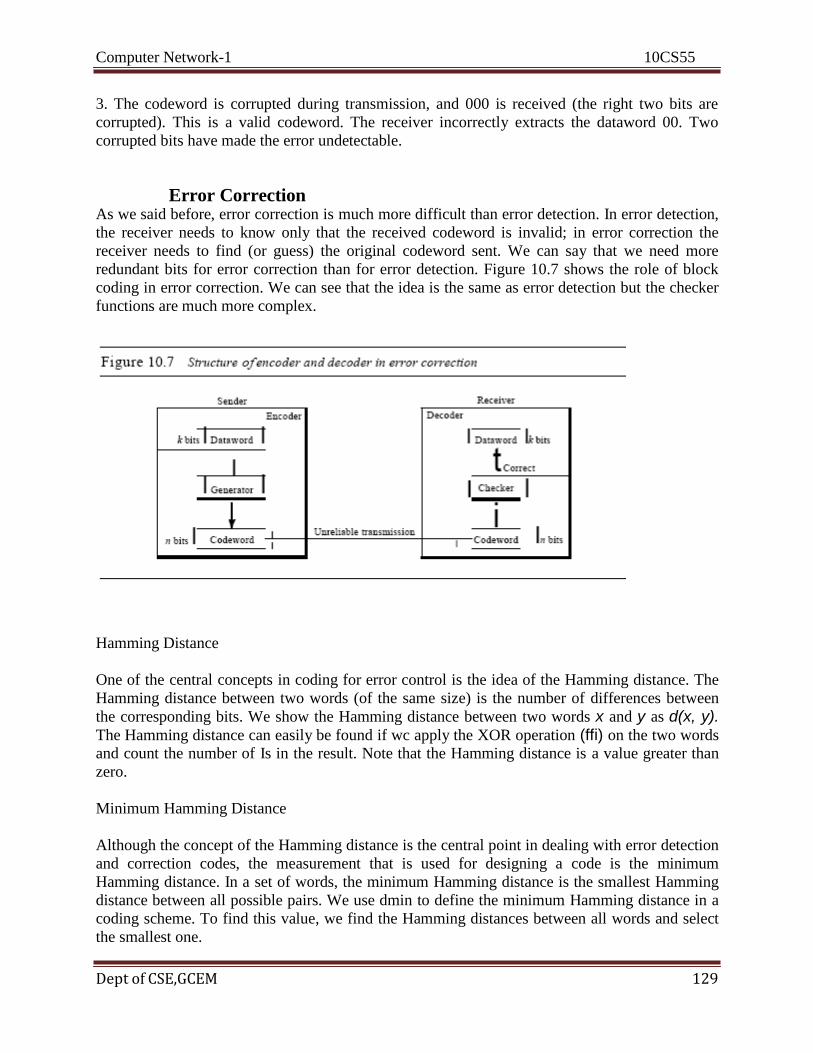
Computer Network-1 10CS55
Dept of CSE,GCEM 129
3. The codeword is corrupted during transmission, and 000 is received (the right two bits are
corrupted). This is a valid codeword. The receiver incorrectly extracts the dataword 00. Two
corrupted bits have made the error undetectable.
Error Correction As we said before, error correction is much more difficult than error detection. In error detection,
the receiver needs to know only that the received codeword is invalid; in error correction the
receiver needs to find (or guess) the original codeword sent. We can say that we need more
redundant bits for error correction than for error detection. Figure 10.7 shows the role of block
coding in error correction. We can see that the idea is the same as error detection but the checker
functions are much more complex.
Hamming Distance
One of the central concepts in coding for error control is the idea of the Hamming distance. The
Hamming distance between two words (of the same size) is the number of differences between
the corresponding bits. We show the Hamming distance between two words x and y as d(x, y). The Hamming distance can easily be found if wc apply the XOR operation (ffi) on the two words
and count the number of Is in the result. Note that the Hamming distance is a value greater than
zero.
Minimum Hamming Distance
Although the concept of the Hamming distance is the central point in dealing with error detection
and correction codes, the measurement that is used for designing a code is the minimum
Hamming distance. In a set of words, the minimum Hamming distance is the smallest Hamming
distance between all possible pairs. We use dmin to define the minimum Hamming distance in a
coding scheme. To find this value, we find the Hamming distances between all words and select
the smallest one.
Computer Network-1 10CS55
Dept of CSE,GCEM 130
Three Parameters
Before we continue with our discussion, we need to mention that any coding scheme needs to
have at least three parameters: the codeword size n, the dataword size k, and the minimum
Hamming distance dmin. A coding scheme C is written as C(n, k) with a separate expression for
dmin- For example, we can call our first coding scheme C(3, 2) with dmin =2 and our second
coding scheme C(5, 2) with dmin ::= 3.
Hamming Distance and Error
Before we explore the criteria for error detection or correction, let us discuss the relationship
between the Hamming distance and errors occurring during transmission. When a codeword is
corrupted during transmission, the Hamming distance between the sent and received codewords
is the number of bits affected by the error. In other words, the Hamming distance between the
received codeword and the sent codeword is the number ofbits that are corrupted during
transmission. For example, if the codeword 00000 is sent and 01101 is received, 3 bits are in
error and the Hamming distance between the two is d(OOOOO, 01101) =3.
Minimum Distance for Error Detection

Computer Network-1 10CS55
Dept of CSE,GCEM 131
Now let us find the minimum Hamming distance in a code if we want to be able to detect up to s
errors. If s errors occur during transmission, the Hamming distance between the sent codeword
and received codeword is s. If our code is to detect up to s errors, the minimum distance between
the valid codes must be s + 1, so that the received codeword does not match a valid codeword. In
other words, if the minimum distance between all valid codewords is s + 1, the received
codeword cannot be erroneously mistaken for another codeword. The distances are not enough (s
+ 1) for the receiver to accept it as valid. The error will be detected. We need to clarify a point
here: Although a code with dmin =s + 1
Minimum Distance for Error Correction
Error correction is more complex than error detection; a decision is involved. When a received
codeword is not a valid codeword, the receiver needs to decide which valid codeword was
actually sent. The decision is based on the concept of territory, an exclusive area surrounding the
codeword. Each valid codeword has its own territory. We use a geometric approach to define
each territory. We assume that each valid codeword has a circular territory with a radius of t and
that the valid codeword is at the center. For example, suppose a codeword x is corrupted by t bits
or less. Then this corrupted codeword is located either inside or on the perimeter of this circle. If the receiver receives a codeword that belongs to this territory, it decides that the original
codeword is the one at the center. Note that we assume that only up to t errors have occurred;
otherwise, the decision is wrong. Figure 10.9 shows this geometric interpretation. Some texts use
a sphere to show the distance between all valid block codes.
10.3 LINEAR BLOCK CODES
Almost all block codes used today belong to a subset called linear block codes. The use of
nonlinear block codes for error detection and correction is not as widespread because their
Computer Network-1 10CS55
Dept of CSE,GCEM 132
structure makes theoretical analysis and implementation difficult. We therefore concentrate on
linear block codes. The formal definition of linear block codes requires the knowledge of
abstract algebra (particularly Galois fields), which is beyond the scope of this book. We therefore
give an informal definition. For our purposes, a linear block code is a code in which the
exclusive OR (addition modulo-2) of two valid codewords creates another valid codeword.
Minimum Distance for Linear Block Codes
It is simple to find the minimum Hamming distance for a linear block code. The minimum
Hamming distance is the number of Is in the nonzero valid codeword with the smallest number
of 1s.
Some Linear Block Codes
Let us now show some linear block codes. These codes are trivial because we can easily find the
encoding and decoding algorithms and check their performances.
Simple Parity-Check Code
Perhaps the most familiar error-detecting code is the simple parity-check code. In this code, a k- bit dataword is changed to an n-bit codeword where n = k + 1. The extra bit, called the parity bit,
is selected to make the total number of Is in the codeword even. Although some implementations
specify an odd number of Is, we discuss the even case. The minimum Hamming distance for this
category is dmin =2, which means that the code is a single-bit error-detecting code; it cannot
correct any error.
Our first code (Table 10.1) is a parity-check code with k -= 2 and n =3. The code in Table 10.3 is
also a parity-check code with k =4 and n =5.
Figure 10.10 shows a possible structure of an encoder (at the sender) and a decoder (at the
receiver).
The encoder uses a generator that takes a copy of a 4-bit dataword (ao, aI' a2' and a3) and
generates a parity bit roo The dataword bits and the parity bit create the 5-bit codeword. The
parity bit that is added makes the number of Is in the codeword even.

Computer Network-1 10CS55
Dept of CSE,GCEM 133
This is normally done by adding the 4 bits of the dataword (modulo-2); the result is the parity bit.
In other words,
If the number of 1s is even, the result is 0; if the number of 1s is odd, the result is 1. In both
cases, the total number of 1s in the codeword is even. The sender sends the codeword which may
be corrupted during transmission. The receiver receives a 5-bit word. The checker at the receiver
does the same thing as the generator in the sender with one exception: The addition is done over
all 5 bits. The result, which is called the syndrome, is just 1 bit. The syndrome is 0 when the
number of 1s in the received codeword is even; otherwise, it is 1.
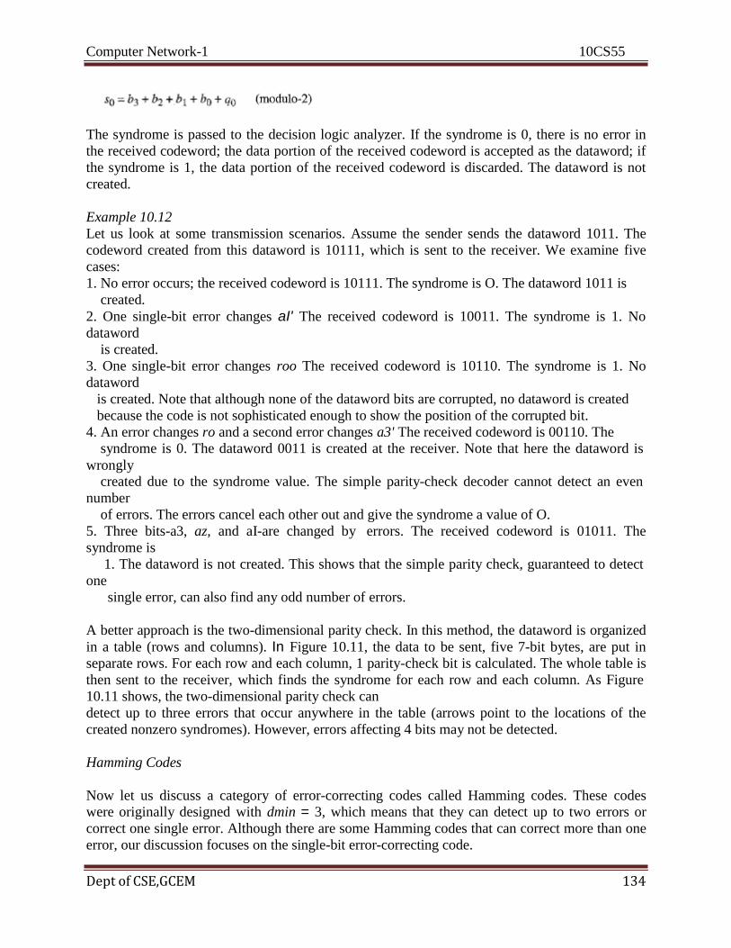
Computer Network-1 10CS55
Dept of CSE,GCEM 134
The syndrome is passed to the decision logic analyzer. If the syndrome is 0, there is no error in
the received codeword; the data portion of the received codeword is accepted as the dataword; if
the syndrome is 1, the data portion of the received codeword is discarded. The dataword is not
created.
Example 10.12
Let us look at some transmission scenarios. Assume the sender sends the dataword 1011. The
codeword created from this dataword is 10111, which is sent to the receiver. We examine five
cases:
1. No error occurs; the received codeword is 10111. The syndrome is O. The dataword 1011 is
created.
2. One single-bit error changes aI' The received codeword is 10011. The syndrome is 1. No
dataword
is created.
3. One single-bit error changes roo The received codeword is 10110. The syndrome is 1. No
dataword
is created. Note that although none of the dataword bits are corrupted, no dataword is created
because the code is not sophisticated enough to show the position of the corrupted bit.
4. An error changes ro and a second error changes a3' The received codeword is 00110. The
syndrome is 0. The dataword 0011 is created at the receiver. Note that here the dataword is
wrongly created due to the syndrome value. The simple parity-check decoder cannot detect an even
number
of errors. The errors cancel each other out and give the syndrome a value of O.
5. Three bits-a3, az, and aI-are changed by errors. The received codeword is 01011. The
syndrome is
1. The dataword is not created. This shows that the simple parity check, guaranteed to detect
one
single error, can also find any odd number of errors.
A better approach is the two-dimensional parity check. In this method, the dataword is organized
in a table (rows and columns). In Figure 10.11, the data to be sent, five 7-bit bytes, are put in
separate rows. For each row and each column, 1 parity-check bit is calculated. The whole table is
then sent to the receiver, which finds the syndrome for each row and each column. As Figure
10.11 shows, the two-dimensional parity check can
detect up to three errors that occur anywhere in the table (arrows point to the locations of the
created nonzero syndromes). However, errors affecting 4 bits may not be detected.
Hamming Codes
Now let us discuss a category of error-correcting codes called Hamming codes. These codes
were originally designed with dmin = 3, which means that they can detect up to two errors or
correct one single error. Although there are some Hamming codes that can correct more than one
error, our discussion focuses on the single-bit error-correcting code.

Computer Network-1 10CS55
Dept of CSE,GCEM 135
First let us find the relationship between n and k in a Hamming code. We need to choose an
integer m >= 3. The values of nand k are then calculated from mas n = 2m – 1 and k ::: n - m.
The number of check bits r =m.
For example, ifm =3, then n ::: 7 and k::: 4. This is a Hamming code C(7, 4) with dmin=3. Table
10.4 shows the datawords and codewords for this code.
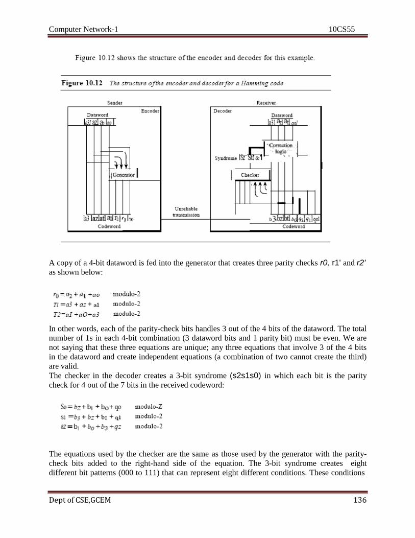
Computer Network-1 10CS55
Dept of CSE,GCEM 136
A copy of a 4-bit dataword is fed into the generator that creates three parity checks r0, r1' and r2' as shown below:
In other words, each of the parity-check bits handles 3 out of the 4 bits of the dataword. The total
number of 1s in each 4-bit combination (3 dataword bits and 1 parity bit) must be even. We are
not saying that these three equations are unique; any three equations that involve 3 of the 4 bits
in the dataword and create independent equations (a combination of two cannot create the third)
are valid.
The checker in the decoder creates a 3-bit syndrome (s2s1s0) in which each bit is the parity
check for 4 out of the 7 bits in the received codeword:
The equations used by the checker are the same as those used by the generator with the parity-
check bits added to the right-hand side of the equation. The 3-bit syndrome creates eight
different bit patterns (000 to 111) that can represent eight different conditions. These conditions

Computer Network-1 10CS55
Dept of CSE,GCEM 137
define a lack of error or an error in 1 of the 7 bits of the received codeword, as shown in Table
10.5.
Performance
A Hamming code can only correct a single error or detect a double error. However, there is a
way to make it detect a burst error, as shown in Figure 10.13. The key is to split a burst error
between several codewords, one error for each codeword. In data communications, we normally
send a packet or a frame of data. To make the Hamming code respond to a burst error of size N, we need to make N codewords out of our frame. Then, instead of sending one codeword at a
time, we arrange the codewords in a table and send the bits in the table a column at a time. In Figure 10.13, the bits are sent column by column (from the left). In each column, the bits are sent
from the bottom to the top. In this way, a frame is made out of the four codewords and sent to the
receiver. Figure 10.13 shows
10.4 CYCLIC CODES
Cyclic codes are special linear block codes with one extra property. In a cyclic code, if a
codeword is cyclically shifted (rotated), the result is another codeword. For example, if 1011000
is a codeword and we cyclically left-shift, then 0110001 is also a codeword.
Computer Network-1 10CS55
Dept of CSE,GCEM 138
In this case, if we call the bits in the first word ao to a6' and the bits in the second word
B0 to b6, we can shift the bits by using the following:
In the rightmost equation, the last bit of the first word is wrapped around and becomes the first
bit of the second word.
Cyclic Redundancy Check
We can create cyclic codes to correct errors. However, the theoretical background required is
beyond the scope of this book. In this section, we simply discuss a category of cyclic codes
called the cyclic redundancy check (CRC) that is used in networks such as LANs and WANs
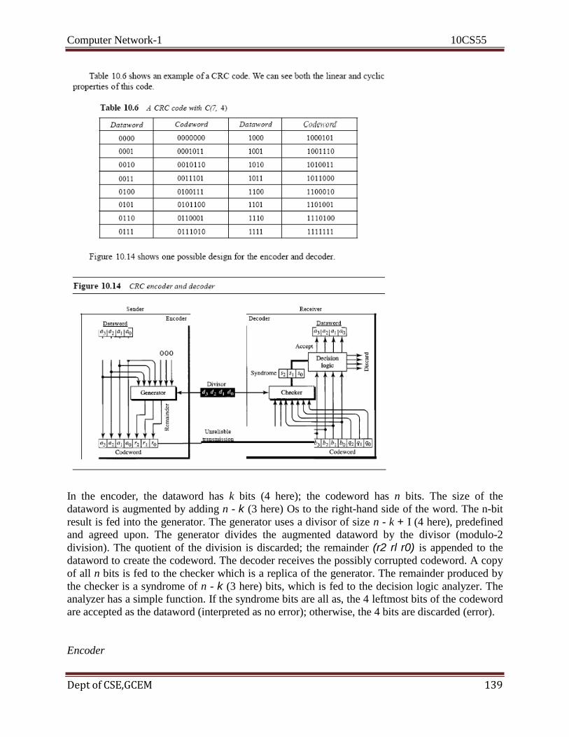
Computer Network-1 10CS55
Dept of CSE,GCEM 139
In the encoder, the dataword has k bits (4 here); the codeword has n bits. The size of the
dataword is augmented by adding n - k (3 here) Os to the right-hand side of the word. The n-bit
result is fed into the generator. The generator uses a divisor of size n - k + I (4 here), predefined
and agreed upon. The generator divides the augmented dataword by the divisor (modulo-2
division). The quotient of the division is discarded; the remainder (r2 rl r0) is appended to the
dataword to create the codeword. The decoder receives the possibly corrupted codeword. A copy
of all n bits is fed to the checker which is a replica of the generator. The remainder produced by
the checker is a syndrome of n - k (3 here) bits, which is fed to the decision logic analyzer. The
analyzer has a simple function. If the syndrome bits are all as, the 4 leftmost bits of the codeword
are accepted as the dataword (interpreted as no error); otherwise, the 4 bits are discarded (error).
Encoder

Computer Network-1 10CS55
Dept of CSE,GCEM 140
Let us take a closer look at the encoder. The encoder takes the dataword and augments it with n -
k number of as. It then divides the augmented dataword by the divisor, as shown in Figure 10.15.
The process of modulo-2 binary division is the same as the familiar division process we use for
decimal numbers. However, as mentioned at the beginning of the chapter, in this case addition
and subtraction are the same. We use the XOR operation to do both. As in decimal division, the
process is done step by step. In each step, a copy of the divisor is XORed with the 4 bits of the
dividend. The result of the XOR operation (remainder) is 3 bits (in this case), which is used for
the next step after 1 extra bit is pulled down to make it 4 bits long. There is one important point
we need to remember in this type of division. If the leftmost bit of the dividend (or the part used
in each step) is 0, the step cannot use the regular divisor; we need to use an all-0s divisor. When
there are no bits left to pull down, we have a result. The 3-bit remainder forms the check bits (r2'
rl' and ro). They are appended to the dataword to create the codeword.
Decoder
The codeword can change during transmission. The decoder does the same division process as
the encoder. The remainder of the division is the syndrome. If the syndrome is all 0s, there is no
error; the dataword is separated from the received codeword and accepted. Otherwise, everything
is discarded. Figure 10.16 shows two cases: The left hand figure shows the value of syndrome
when no error has occurred; the syndrome is 000. The right-hand part of the figure shows the
case in which there is one single error. The syndrome is not all 0s (it is 01l).
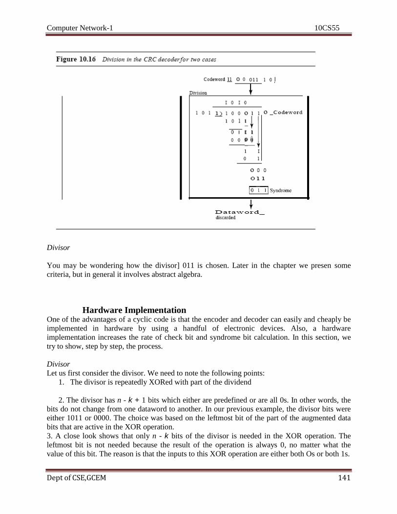
Computer Network-1 10CS55
Dept of CSE,GCEM 141
Divisor
You may be wondering how the divisor] 011 is chosen. Later in the chapter we presen some
criteria, but in general it involves abstract algebra.
Hardware Implementation One of the advantages of a cyclic code is that the encoder and decoder can easily and cheaply be
implemented in hardware by using a handful of electronic devices. Also, a hardware
implementation increases the rate of check bit and syndrome bit calculation. In this section, we
try to show, step by step, the process.
Divisor
Let us first consider the divisor. We need to note the following points:
1. The divisor is repeatedly XORed with part of the dividend
2. The divisor has n - k + 1 bits which either are predefined or are all 0s. In other words, the
bits do not change from one dataword to another. In our previous example, the divisor bits were
either 1011 or 0000. The choice was based on the leftmost bit of the part of the augmented data
bits that are active in the XOR operation.
3. A close look shows that only n - k bits of the divisor is needed in the XOR operation. The
leftmost bit is not needed because the result of the operation is always 0, no matter what the
value of this bit. The reason is that the inputs to this XOR operation are either both Os or both 1s.

Computer Network-1 10CS55
Dept of CSE,GCEM 142
In our previous example, only 3 bits, not 4, is actually used in the XOR operation. Using these
points, we can make a fixed (hardwired) divisor that can be used for a cyclic code if we know the
divisor pattern. Figure 10.17 shows such a design for our previous example. We have also shown
the XOR devices used for the operation.
Note that if the leftmost bit of the part of dividend to be used in this step is 1, the divisor bits
(d2d1do) are all; if the leftmost bit is 0, the divisor bits arc 000. The design provides the right
choice based on the leftmost bit.
Augmented Dataword
In our paper-and-pencil division process in Figure 10.15, we show the augmented dataword as
fixed in position with the divisor bits shifting to the right, 1 bit in each step. The divisor bits are
aligned with the appropriate part of the augmented dataword. Now that our divisor is fixed, we
need instead to shift the bits of the augmented dataword to the left (opposite direction) to align
the divisor bits with the appropriate part. There is no need to store the augmented dataword bits.
Remainder
In our previous example, the remainder is 3 bits (n - k bits in general) in length. We can use three
registers (single-bit storage devices) to hold these bits. To find the final remainder of the
division, we need to modify our division process. The following is the step-by-step process that
can be used to simulate the division process in hardware (or even in software).
1.We assume that the remainder is originally all 0s (000 in our example).
2. At each time click (arrival of 1 bit from an augmented dataword), we repeat the following two
actions:
a. We use the leftmost bit to make a decision about the divisor (011 or 000).
b. The other 2 bits of the remainder and the next bit from the augmented dataword (total
of 3 bits) are XORed with the 3-bit divisor to create the next remainder. Figure 10.18 shows
this simulator, but note that this is not the final design; there will be more improvements
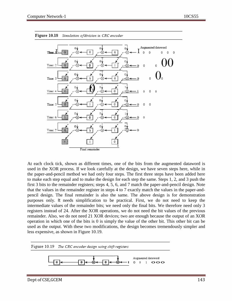
Computer Network-1 10CS55
Dept of CSE,GCEM 143
At each clock tick, shown as different times, one of the bits from the augmented dataword is
used in the XOR process. If we look carefully at the design, we have seven steps here, while in
the paper-and-pencil method we had only four steps. The first three steps have been added here
to make each step equal and to make the design for each step the same. Steps 1, 2, and 3 push the
first 3 bits to the remainder registers; steps 4, 5, 6, and 7 match the paper-and-pencil design. Note
that the values in the remainder register in steps 4 to 7 exactly match the values in the paper-and-
pencil design. The final remainder is also the same. The above design is for demonstration
purposes only. It needs simplification to be practical. First, we do not need to keep the
intermediate values of the remainder bits; we need only the final bits. We therefore need only 3
registers instead of 24. After the XOR operations, we do not need the bit values of the previous
remainder. Also, we do not need 21 XOR devices; two are enough because the output of an XOR
operation in which one of the bits is 0 is simply the value of the other bit. This other bit can be
used as the output. With these two modifications, the design becomes tremendously simpler and
less expensive, as shown in Figure 10.19.
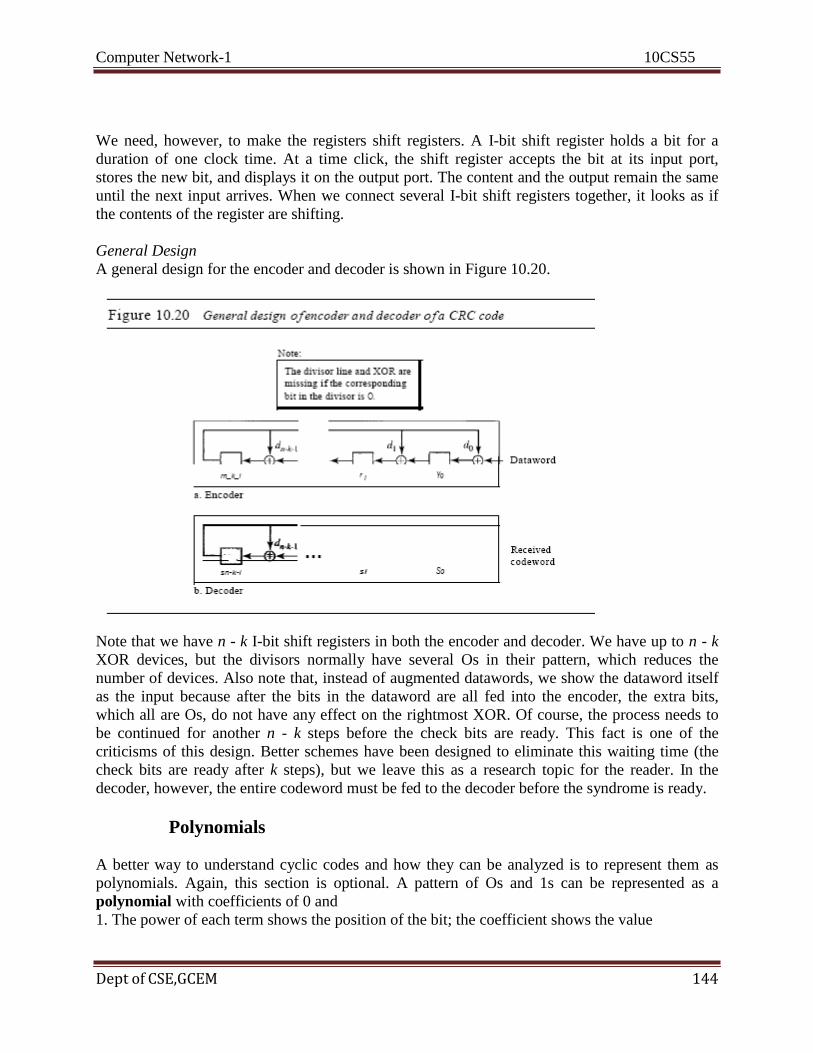
Computer Network-1 10CS55
Dept of CSE,GCEM 144
We need, however, to make the registers shift registers. A I-bit shift register holds a bit for a
duration of one clock time. At a time click, the shift register accepts the bit at its input port,
stores the new bit, and displays it on the output port. The content and the output remain the same
until the next input arrives. When we connect several I-bit shift registers together, it looks as if
the contents of the register are shifting.
General Design
A general design for the encoder and decoder is shown in Figure 10.20.
Note that we have n - k I-bit shift registers in both the encoder and decoder. We have up to n - k
XOR devices, but the divisors normally have several Os in their pattern, which reduces the
number of devices. Also note that, instead of augmented datawords, we show the dataword itself
as the input because after the bits in the dataword are all fed into the encoder, the extra bits,
which all are Os, do not have any effect on the rightmost XOR. Of course, the process needs to
be continued for another n - k steps before the check bits are ready. This fact is one of the
criticisms of this design. Better schemes have been designed to eliminate this waiting time (the
check bits are ready after k steps), but we leave this as a research topic for the reader. In the
decoder, however, the entire codeword must be fed to the decoder before the syndrome is ready.
Polynomials
A better way to understand cyclic codes and how they can be analyzed is to represent them as
polynomials. Again, this section is optional. A pattern of Os and 1s can be represented as a
polynomial with coefficients of 0 and
1. The power of each term shows the position of the bit; the coefficient shows the value

Computer Network-1 10CS55
Dept of CSE,GCEM 145
of the bit. Figure 10.21 shows a binary pattern and its polynomial representation. In Figure
10.21a we show how to translate a binary pattern to a polynomial; in Figure 1O.21b we show
how the polynomial can be shortened by removing all terms with zero coefficients and replacing
xl by x and xO by 1.
Figure 10.21 shows one immediate benefit; a 7-bit pattern can be replaced by three terms. The
benefit is even more conspicuous when we have a polynomial such as x23 + X3 + 1. Here the bit
pattern is 24 bits in length (three Is and twenty-one Os) while the polynomial is just three terms.
Degree of a Polynomial
The degree of a polynomial is the highest power in the polynomial. For example, the degree of
the polynomial x6 + x + 1 is 6. Note that the degree of a polynomial is 1 less that the number of
bits in the pattern. The bit pattern in this case has 7 bits.
Adding and Subtracting Polynomials
Adding and subtracting polynomials in mathematics are done by adding or subtracting the
coefficients of terms with the same power. In our case, the coefficients are only 0 and 1, and
adding is in modulo-2. This has two consequences. First, addition and subtraction are the same.
Second, adding or subtracting is done by combining terms and deleting pairs of identical terms.
For example, adding x5 + x4 + x2 and x6 + x4 + x2 gives just x6 + x5. The terms x4 and x2 are
deleted. However, note that if we add, for example, three polynomials and we get x2 three times,
we delete a pair of them and keep the third.
Multiplying or Dividing Terms
In this arithmetic, multiplying a term by another term is very simple; we just add the powers. For
example, x3 x x4 is x7 , For dividing, we just subtract the power of the second term from the
power of the first. For example, x51x2 is x3.
Multiplying Two Polynomials

Computer Network-1 10CS55
Dept of CSE,GCEM 146
Multiplying a polynomial by another is done term by term. Each term of the first polynomial
must be multiplied by all terms of the second. The result, of course, is then simplified, and pairs
of equal terms are deleted. The following is an example:
Dividing One Polynomial by Another
Division of polynomials is conceptually the same as the binary division we discussed for an
encoder. We divide the first term of the dividend by the first term of the divisor to get the first
term of the quotient. We multiply the term in the quotient by the divisor and subtract the result
from the dividend. We repeat the process until the dividend degree is less than the divisor degree.
We will show an example of division later in this chapter.
Shifting
A binary pattern is often shifted a number of bits to the right or left. Shifting to the left means
adding extra Os as rightmost bits; shifting to the right means deleting some rightmost bits.
Shifting to the left is accomplished by multiplying each term of the polynomial by xn, where m is
the number of shifted bits; shifting to the right is accomplished by dividing each term of the
polynomial by xn. The following shows shifting to the left and to the right. Note that we do not
have negative powers in the polynomial representation.
When we augmented the dataword in the encoder of Figure 10.15, we actually shifted the bits to
the left. Also note that when we concatenate two bit patterns, we shift the first polynomial to the
left and then add the second polynomial.
Cyclic Code Encoder Using Polynomials
Now that we have discussed operations on polynomials, we show the creation of a codeword
from a dataword. Figure 10.22 is the polynomial version of Figure 10.15. We can see that the
process is shorter. The dataword 1001 is represented as x3 + 1. The divisor 1011 is represented
as x3 + x + 1. To find the augmented dataword, we have left-shifted the dataword 3 bits
(multiplying by x\ The result is x6 + x3 . Division is straightforward. We divide the first term of
the dividend, x6, by the first term of the divisor, x3. The first term of the quotient is then x6/x3,
or x3. Then we multiply x3 by the divisor and subtract (according to our previous definition of
subtraction) the result from the dividend. The result is x4, with a degree greater than the divisor's

Computer Network-1 10CS55
Dept of CSE,GCEM 147
degree; we continue to divide until the degree of the remainder is less than the degree of the
divisor.
It can be seen that the polynomial representation can easily simplify the operation of division in
this case, because the two steps involving all-Os divisors are not needed here. (Of course, one
could argue that the all-Os divisor step can also be eliminated in binary division.) In a
polynomial representation, the divisor is normally referred to as the generator polynomial t(x).
Cyclic Code Analysis
We can analyze a cyclic code to find its capabilities by using polynomials. We define the
following, wheref(x) is a polynomial with binary coefficients.
Dataword: d(x) Syndrome: sex)
Codeword: c(x) Error: e(x) Generator: g(x) If sex) is not zero, then one or more bits is corrupted. However, if sex) is zero, either no bit is
corrupted or the decoder failed to detect any errors.
In our analysis we want to find the criteria that must be imposed on the generator, g(x) to detect
the type of error we especially want to be detected. Let us first find the relationship among the
sent codeword, error, received codeword, and the generator. We can say

Computer Network-1 10CS55
Dept of CSE,GCEM 148
In other words, the received codeword is the sum of the sent codeword and the error. The
receiver divides the received codeword by g(x) to get the syndrome. We can write this as
The first term at the right-hand side of the equality does not have a remainder (according to the
definition of codeword). So the syndrome is actually the remainder of the second term on the
right-hand side. If this term does not have a remainder (syndrome =0), either e(x) is 0 or e(x) is
divisible by g(x). We do not have to worry about the first case (there is no error); the second case
is very important. Those errors that are divisible by g(x) are not caught. Let us show some
specific errors and see how they can be caught by a welldesigned g(x).
Single-Bit Error
What should be the structure of g(x) to guarantee the detection of a single-bit error? A single-bit
error is e(x) =xi, where i is the position of the bit. If a single-bit error is caught, then xi is not
divisible by g(x). (Note that when we say not divisible, we mean that there is a remainder.) If
g(x) ha~ at least two terms (which is normally the case) and the coefficient of x0 is not zero
(the rightmost bit is 1), then e(x) cannot be divided by g(x).
Two Isolated Single-Bit Errors
Now imagine there are two single-bit isolated errors. Under what conditions can this type of
error be caught? We can show this type of error as e(x) =: xl + xi. The values of I and j define
the positions of the errors, and the difference j - i defines the distance between the two errors, as
shown in Figure 10.23.
Odd Numbers of Errors
A generator with a factor of x + 1 can catch all odd numbers of errors. This means that we need
to make x + 1 a factor of any generator. Note that we are not saying that the generator itself
should be x + 1; we are saying that it should have a factor of x + 1. If it is only x + 1, it cannot
catch the two adjacent isolated errors (see the previous section). For example, x4 + x2 + X + 1
can catch all odd-numbered errors since it can be written as a product of the two polynomials x + 1 and x3 + x2 + 1.
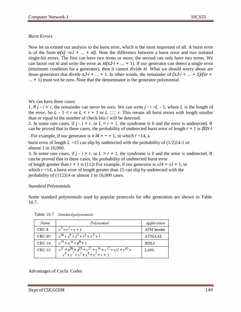
Computer Network-1 10CS55
Dept of CSE,GCEM 149
Burst Errors
Now let us extend our analysis to the burst error, which is the most important of all. A burst error
is of the form e(x) =eJ + ... + xi). Note the difference between a burst error and two isolated
single-bit errors. The first can have two terms or more; the second can only have two terms. We
can factor out xi and write the error as xi(xJ-i + ... + 1). If our generator can detect a single error
(minimum condition for a generator), then it cannot divide xi. What we should worry about are
those generators that divide xJ-i + ... + 1. In other words, the remainder of (xJ-i + ... + 1)/(xr + ... + 1) must not be zero. Note that the denominator is the generator polynomial.
We can have three cases:
1. If j - i < r, the remainder can never be zero. We can write j - i =L - 1, where L is the length of
the error. So L - 1 < r or L < r + 1 or L :::;: r. This means all burst errors with length smaller
than or equal to the number of check bits r will be detected.
2. In some rare cases, if j - i = r, or L = r + 1, the syndrome is 0 and the error is undetected. It can be proved that in these cases, the probability of undetected burst error of length r + 1 is (ll2r-l
. For example, if our generator is x l4 + ~ + 1, in which r =14, a
burst error of length L =15 can slip by undetected with the probability of (1/2)14-1 or
almost 1 in 10,000.
3. In some rare cases, if j - i > r, or L > r + 1, the syndrome is 0 and the error is undetected. It can be proved that in these cases, the probability of undetected burst error
of length greater than r + 1 is (112t For example, if our generator is x14 + x3 + 1, in
which r =14, a burst error of length greater than 15 can slip by undetected with the
probability of (112)14 or almost 1 in 16,000 cases.
Standard Polynomials
Some standard polynomials used by popular protocols for eRe generation are shown in Table
10.7.
Advantages of Cyclic Codes
Computer Network-1 10CS55
Dept of CSE, GCEM 151
We have seen that cyclic codes have a very good performance in detecting single-bit errors,
double errors, an odd number of errors, and burst errors. They can easily be implemented in
hardware and software. They are especially fast when implemented in hardware. This has made
cyclic codes a good candidate for many networks.
Other Cyclic Codes
The cyclic codes we have discussed in this section are very simple. The check bits and
syndromes can be calculated by simple algebra. There are, however, more powerful polynomials
that are based on abstract algebra involving Galois fields. These are beyond the scope of this
book. One of the most interesting of these codes is the Reed-Solomon code used today for both
detection and correction.
10.5 CHECKSUM
The last error detection method we discuss here is called the checksum. The checksum is used in
the Internet by several protocols although not at the data link layer. However,we briefly discuss
it here to complete our discussion on error checking. Like linear and cyclic codes, the checksum
is based on the concept of redundancy. Several protocols still use the checksum for error
detection although the tendency is to replace it with a CRC. This means that the CRC is also
used in layers other than the data link layer.
Idea
The concept of the checksum is not difficult. Let us illustrate it with a few examples. One's
Complement The previous example has one major drawback. All of our data can be written as a
4-bit word (they are less than 15) except for the checksum. One solution is to use one's
complement arithmetic. In this arithmetic, we can represent unsigned numbers between 0 and 2n
- 1 using only n bits. t If the number has more than n bits, the extra leftmost bits need to be added
to the n rightmost bits (wrapping). In one's complement arithmetic, a negative number can be
represented by inverting all bits (changing a 0 to a 1 and a 1 to a 0). This is the same as
subtracting the number from 2n - 1.
Internet Checksum
Traditionally, the Internet has been using a 16-bit checksum. The sender calculates the checksum
by following these steps.
Sender site:
1. The message is divided into 16-bit words.
2. The value of the checksum word is set to O.
3. All words including the checksum are added ushtg one's complement addition.
4. The sum is complemented and becomes the checksum.
5. The checksum is sent with the data.
Receiver site:
1. The message (including checksum) is divided into 16-bit words.

Computer Network-1 10CS55
Dept of CSE, GCEM 152
2. All words are added using one's complement addition.
3. The sum is complemented and becomes the new checksum.
4. If the value of checksum is 0, the message is accepted; otherwise, it is rejected.
The nature of the checksum (treating words as numbers and adding and complementing them) is
well-suited for software implementation. Short programs can be written to calculate the
checksum at the receiver site or to check the validity of the message at the receiver site.
Recommended Questions
1. How does a single-bit error differ from a burst error? 2. Distinguish between forward error correction versus error correction by
retransmission.
3. What is the definition of a linear block code? What is the definition of a
cyclic code?
4. What is the Hamming distance? What is the minimum Hamming
distance?
5. How is the simple parity check related to the two-dimensional parity
check?
6. Discuss the concept of redundancy in error detection and correction.
Computer Network-1 10CS55
Dept of CSE, GCEM 153
COMPUTER NETWORKS – I
Subject Code: 10CS55 I.A. Marks : 25
Hours/Week : 04 Exam Hours: 03
Total Hours : 52 Exam Marks: 100
PART - B
UNIT- 5 6 Hours
Data Link Layer-2:
-Framing,
-Flow and Error Control,
-Protocols, Noiseless Channels,
-Noisy channels,
-HDLC, -PPP (Framing, Transition phases only)

Computer Network-1 10CS55
Dept of CSE, GCEM 154
UNIT-5
Data Link Control
11.1 FRAMING
Data transmission in the physical layer means moving bits in the form of a signal from the source
to the destination. The physical layer provides bit synchronization to ensure that the sender and
receiver use the same bit durations and timing.
The data link layer, on the other hand, needs to pack bits into frames, so that each frame is
distinguishable from another. Our postal system practices a type of framing. The simple act of
inserting a letter into an envelope separates one piece of information from another; the envelope
serves as the delimiter. In addition, each envelope defines the sender and receiver addresses since
the postal system is a many-to-many carrier facility.
Framing in the data link layer separates a message from one source to a destination, or from
other messages to other destinations, by adding a sender address and a destination address. The
destination address defines where the packet is to go; the sender address helps the recipient
acknowledge the receipt. Although the whole message could be packed in one frame, that is not
normally done. One reason is that a frame can be very large, making flow and error control very
inefficient. When a message is carried in one very large frame, even a single-bit error would
require the retransmission of the whole message. When a message is divided into smaller frames,
a single-bit error affects only that small frame.
Fixed-Size Framing
Frames can be of fixed or variable size. In fixed-size framing, there is no need for defining the
boundaries of the frames; the size itself can be used as a delimiter. An example of this type of
framing is the ATM wide-area network, which uses frames of fixed size called cells.
Variable-Size Framing
Our main discussion in this chapter concerns variable-size framing, prevalent in local area
networks. In variable-size framing, we need a way to define the end of the frame and the
beginning of the next.
Character-Oriented Protocols
In a character-oriented protocol, data to be carried are 8-bit characters from a coding system such
as ASCII (see Appendix A). The header, which normally carries the source and destination
addresses and other control information, and the trailer, which carries error detection or error
correction redundant bits, are also multiples of 8 bits. To separate one frame from the next, an 8-
bit (I-byte) flag is added at the beginning and the end of a frame. The flag, composed of
protocol-dependent special characters, signals the start or end of a frame. Figure 11.1 shows the
format of a frame in a character-oriented protocol.
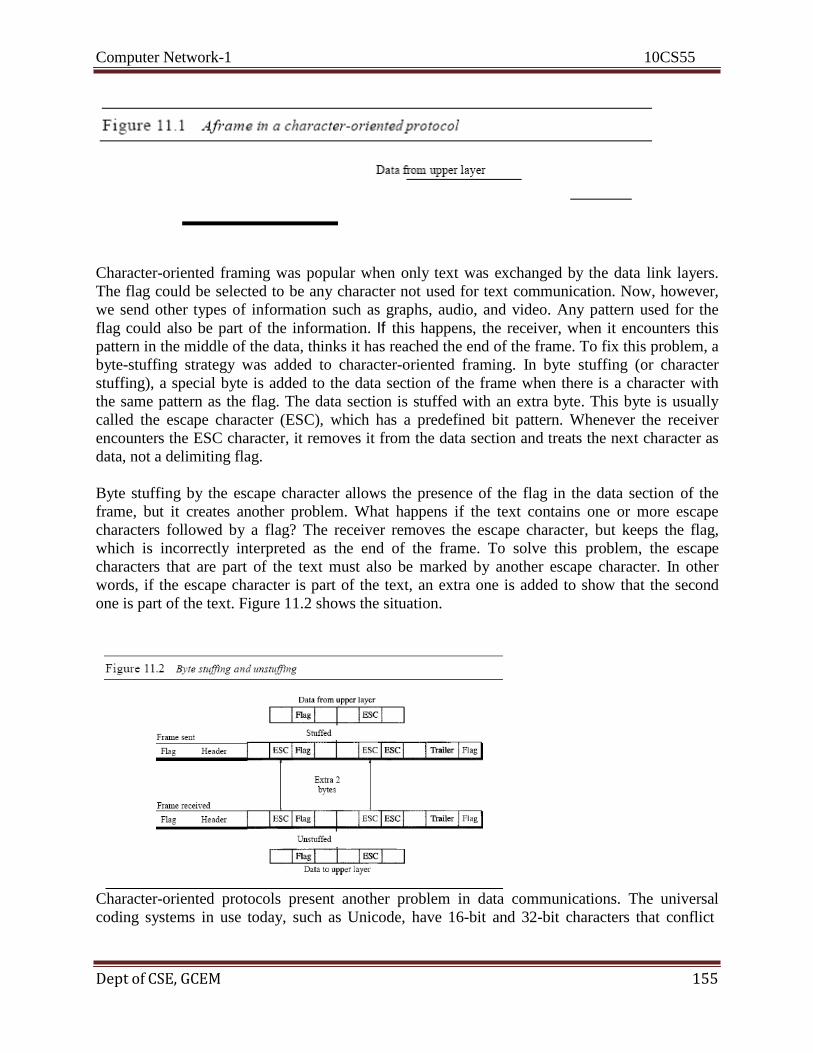
Computer Network-1 10CS55
Dept of CSE, GCEM 155
Character-oriented framing was popular when only text was exchanged by the data link layers.
The flag could be selected to be any character not used for text communication. Now, however,
we send other types of information such as graphs, audio, and video. Any pattern used for the
flag could also be part of the information. If this happens, the receiver, when it encounters this
pattern in the middle of the data, thinks it has reached the end of the frame. To fix this problem, a
byte-stuffing strategy was added to character-oriented framing. In byte stuffing (or character
stuffing), a special byte is added to the data section of the frame when there is a character with
the same pattern as the flag. The data section is stuffed with an extra byte. This byte is usually
called the escape character (ESC), which has a predefined bit pattern. Whenever the receiver
encounters the ESC character, it removes it from the data section and treats the next character as
data, not a delimiting flag.
Byte stuffing by the escape character allows the presence of the flag in the data section of the
frame, but it creates another problem. What happens if the text contains one or more escape
characters followed by a flag? The receiver removes the escape character, but keeps the flag,
which is incorrectly interpreted as the end of the frame. To solve this problem, the escape
characters that are part of the text must also be marked by another escape character. In other
words, if the escape character is part of the text, an extra one is added to show that the second
one is part of the text. Figure 11.2 shows the situation.
Character-oriented protocols present another problem in data communications. The universal
coding systems in use today, such as Unicode, have 16-bit and 32-bit characters that conflict

Computer Network-1 10CS55
Dept of CSE, GCEM 156
with 8-bit characters. We can say that in general, the tendency is moving toward the bit-oriented
protocols that we discuss next.
Bit-Oriented Protocols
In a bit-oriented protocol, the data section of a frame is a sequence of bits to be interpreted by the
upper layer as text, graphic, audio, video, and so on. However, in addition to headers (and
possible trailers), we still need a delimiter to separate one frame from the other. Most protocols
use a special 8-bit pattern flag 01111110 as the delimiter to define the beginning and the end of
the frame, as shown in Figure 11.3.
This flag can create the same type of problem we saw in the byte-oriented protocols.
That is, if the flag pattern appears in the data, we need to somehow inform the receiver that this
is not the end of the frame. We do this by stuffing 1 single bit (instead
of I byte) to prevent the pattern from looking like a flag. The strategy is called bit stuffing. In bit
stuffing, if a 0 and five consecutive I bits are encountered, an extra 0 is
added. This extra stuffed bit is eventually removed from the data by the receiver. Figure 11.4
shows bit stuffing at the sender and bit removal at the receiver. Note that even if we have a 0
after five 1s, we still stuff a 0. The 0 will be removed by the receiver.

Computer Network-1 10CS55
Dept of CSE, GCEM 157
This means that if the flag like pattern 01111110 appears in the data, it will change to 011111010
(stuffed) and is not mistaken as a flag by the receiver. The real flag 01111110 is not stuffed by
the sender and is recognized by the receiver.
11.2 FLOW AND ERROR CONTROL
Data communication requires at least two devices working together, one to send and the other to
receive. Even such a basic arrangement requires a great deal of coordination for an intelligible
exchange to occur. The most important responsibilities of the data link layer are flow control and
error control. Collectively, these functions are known as data link control.
Flow Control
Flow control coordinates the amount of data that can be sent before receiving an
acknowledgment and is one of the most important duties of the data link layer. In most protocols,
flow control is a set of procedures that tells the sender how much data it can transmit before it
must wait for an acknowledgment from the receiver. The flow of data must not be allowed to
overwhelm the receiver. Any receiving device has a limited speed at which it can process
incoming data and a limited amount of memory in which to store incoming data. The receiving
device must be able to inform the sending device before those limits are reached and to request
that the transmitting device send fewer frames or stop temporarily. Incoming data must be
checked and processed before they can be used. The rate of such processing is often slower than
the rate of transmission. For this reason,
each receiving device has a block of memory, called a buffer, reserved for storing incoming data
until they are processed. If the buffer begins to fill up, the receiver must be able to tell the sender
to halt transmission until it is once again able to receive.
Error Control
Error control is both error detection and error correction. It allows the receiver to inform the
sender of any frames lost or damaged in transmission and coordinates the retransmission of those
frames by the sender. In the data link layer, the term error control
refers primarily to methods of error detection and retransmission. Error control in the data link
layer is often implemented simply: Any time an error is detected in an exchange, specified
frames are retransmitted. This process is called automatic repeat request (ARQ).
11.3 PROTOCOLS
Now let us see how the data link layer can combine framing, flow control, and error control to
achieve the delivery of data from one node to another. The protocols are normally implemented
in software by using one of the common programming languages. To make our discussions
language-free, we have written in pseudocode a version of each protocol that concentrates mostly
on the procedure instead of delving into the details of language rules. The protocols in the first
category cannot be used in real life, but they serve as a basis for understanding the protocols of
noisy channels. Figure 11.5 shows the classifications.

Computer Network-1 10CS55
Dept of CSE, GCEM 158
There is a difference between the protocols we discuss here and those used in real networks. All
the protocols we discuss are unidirectional in the sense that the data frames travel from one node,
called the sender, to another node, called the receiver. Although special frames, called
acknowledgment (ACK) and negative acknowledgment (NAK) can flow in the opposite
direction for flow and error control purposes, data flow in only one direction.
In a real-life network, the data link protocols are implemented as bidirectional; data flow in both
directions. In these protocols the flow and error control information such as ACKs and NAKs is
included in the data frames in a technique called piggybacking. Because bidirectional protocols
are more complex than unidirectional ones, we chose the latter for our discussion. If they are
understood, they can be extended to bidirectional protocols.
11.4 NOISELESS CHANNELS
The first is a protocol that does not use flow control; the second is the one that does. Of course,
neither has error control because we have assumed that the channel is a perfect noiseless channel.
Simplest Protocol
Our first protocol, which we call the Simplest Protocol for lack of any other name, is one that has
no flow or error control. Like other protocols we will discuss in this chapter, it is a unidirectional
protocol in which data frames are traveling in only one direction-from the sender to receiver. We
assume that the receiver can immediately handle any frame it receives with a processing time
that is small enough to be negligible. The data link layer of the receiver immediately removes the
header from the frame and hands the data packet to its network layer, which can also accept the
packet immediately. In other words, the receiver can never be overwhelmed with incoming
frames.
Design
There is no need for flow control in this scheme. The data link layer at the sender site gets data
from its network layer, makes a frame out of the data, and sends it. The data link layer at the
receiver site receives a frame from its physical layer, extracts data from the frame, and delivers

Computer Network-1 10CS55
Dept of CSE, GCEM 159
the data to its network layer. The data link layers of the sender and receiver provide transmission
services for their network layers. The data link layers use the services provided by their physical
layers (such as signaling, multiplexing, and so on) for the physical transmission of bits. Figure
11.6 shows a design.
The sender site cannot send a frame until its network layer has a data packet to send. The
receiver site cannot deliver a data packet to its network layer until a frame arrives. If the protocol
is implemented as a procedure, we need to introduce the idea of events in the protocol. The
procedure at the sender site is constantly running; there is no action until there is a request from
the network layer. The procedure at the receiver site is also constantly rulming, but there is no
action until notification from the physical layer arrives. Both procedures are constantly running
because they do not know when the corresponding events will occur.
Algorithms
Algorithm 11.1 shows the procedure at the sender site.
Analysis The algorithm has an infinite loop, which means lines 3 to 9 are repeated forever once
the program starts. The algorithm is an event-driven one, which means that it sleeps (line 3) until
an event wakes it up (line 4). This means that there may be an undefined span of time between
the execution of line 3 and line 4; there is a gap between these actions. When the event, a request
from the network layer, occurs, lines 6 though 8 are executed. The program then repeats the loop
and again sleeps at line 3 until the next occurrence of the event. We have written

Computer Network-1 10CS55
Dept of CSE, GCEM 160
pseudocode for the main process and SendFrame. GetData takes a data packet from the network
layer, Make Frame0 adds a header and delimiter flags to the data packet to make a frame, and
SendFrame0 delivers the frame to the physical layer for transmission.
Algorithm 11.2 shows the procedure at the receiver site.
Analysis This algorithm has the same format as Algorithm 11.1, except that the direction of the
frames and data is upward. The event here is the arrival of a data frame. After the event occurs,
the data link layer receives the frame from the physical layer using the ReceiveFrame process,
extracts the data from the frame using the ExtractData process, and delivers the data to the
network layer using the DeliverData process. Here, we also have an event-driven algorithm
because the algorithm never knows when the data frame will arrive.
Stop-and-Wait Protocol
If data frames arrive at the receiver site faster than they can be processed, the frames must be
stored until their use. Normally, the receiver does not have enough storage space, especially if it
is receiving data from many sources. This may result in either the discarding of frames or denial
of service. To prevent the receiver from becoming overwhelmed with frames. There must be
feedback from the receiver to the sender. The protocol we discuss now is called the Stop-and-
Wait Protocol because the sender sends one frame, stops until it receives confirmation from the
receiver (okay to go ahead), and then sends the next frame.
Design
Figure 11.8 illustrates the mechanism. Comparing this figure with Figure 11.6, can see the traffic
on the forward channel (from sender to receiver) and the reverse channel. At any time, there is
either one data frame on the forward channel or one ACK frame on the reverse channel. We
therefore need a half-duplex link.
Algorithms
Algorithm 11.3 is for the sender site.
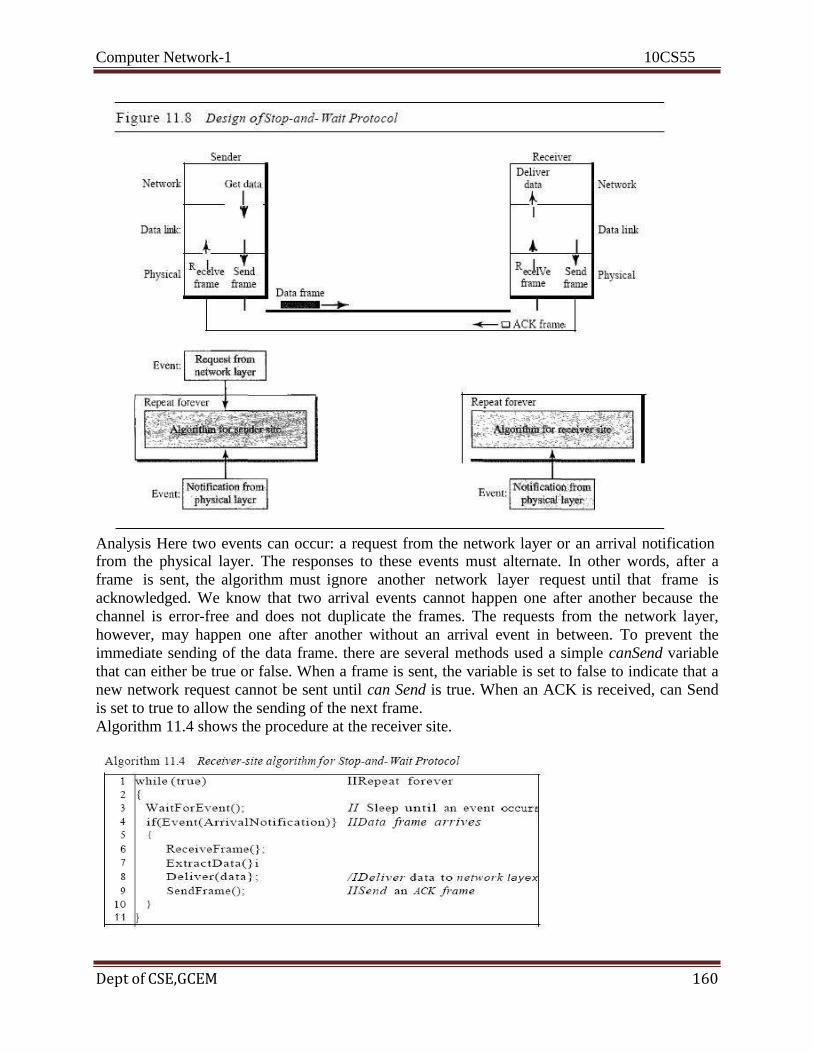
Computer Network-1 10CS55
Dept of CSE,GCEM 160
Analysis Here two events can occur: a request from the network layer or an arrival notification from the physical layer. The responses to these events must alternate. In other words, after a
frame is sent, the algorithm must ignore another network layer request until that frame is
acknowledged. We know that two arrival events cannot happen one after another because the
channel is error-free and does not duplicate the frames. The requests from the network layer,
however, may happen one after another without an arrival event in between. To prevent the
immediate sending of the data frame. there are several methods used a simple canSend variable
that can either be true or false. When a frame is sent, the variable is set to false to indicate that a
new network request cannot be sent until can Send is true. When an ACK is received, can Send
is set to true to allow the sending of the next frame.
Algorithm 11.4 shows the procedure at the receiver site.

Computer Network-1 10CS55
Dept of CSE,GCEM 161
Analysis This is very similar to Algorithm 11.2 with one exception. After the data frame arrives,
the receiver sends an ACK frame (line 9) to acknowledge the receipt and allow the sender
to send the next frame.
11.5 NOISY CHANNELS
Stop-and-Wait Automatic Repeat Request Our first protocol, called the Stop-and-Wait Automatic Repeat Request (Stop-and Wait ARQ),
adds a simple error control mechanism to the Stop-and-Wait Protocol. Let us see how this
protocol detects and corrects errors. To detect and correct corrupted frames, we need to add
redundancy bits to our data frame. When the frame arrives at the receiver site, it is checked and if
it is corrupted, it is silently discarded. The detection of errors in this protocol is manifested by
the silence of the receiver.
Lost frames are more difficult to handle than corrupted ones. In our previous protocols, there was
no way to identify a frame. The received frame could be the correct one, or a duplicate, or a
frame out of order. The solution is to number the frames. When the receiver receives a data
frame that is out of order, this means that frames were either lost or duplicated.
The completed lost frames need to be resent in this protocol. If the receiver does not respond
when there is an error, how can the sender know which frame to resend? To remedy this
problem, the sender keeps a copy of the sent frame. At the same time, it starts a timer. If the
timer expires and there is no ACK for the sent frame, the frame is resent, the copy is held, and
the timer is restarted. Since the protocol uses the stop-and-wait mechanism, there is only one
specific frame that needs an ACK even though several copies of the same frame can be in the
network.
Since an ACK frame can also be corrupted and lost, it too needs redundancy bits and a sequence
number. The ACK frame for this protocol has a sequence number field. In this protocol, the
sender simply discards a corrupted ACK frame or ignores an out-of-order one.
Sequence Numbers
As we discussed, the protocol specifies that frames need to be numbered. This is done by using
sequence numbers. A field is added to the data frame to hold the sequence number of that frame.
One important consideration is the range of the sequence numbers. Since we want to minimize
the frame size, we look for the smallest range that provides unambiguous communication. The
sequence numbers of course can wrap around. Decide that the field is m bits long, the sequence
numbers start from 0, go to 2m - 1, and then are repeated.
Let us reason out the range of sequence numbers we need. Assume we have used x as a sequence
number; we only need to use x + 1 after that. There is no need for x + 2. To show this, assume
that the sender has sent the frame numbered x. Three things can happen.
1. The frame arrives safe and sound at the receiver site; the receiver sends an acknowledgment.
The acknowledgment arrives at the sender site, causing the sender to send
the next frame numbered x + 1.
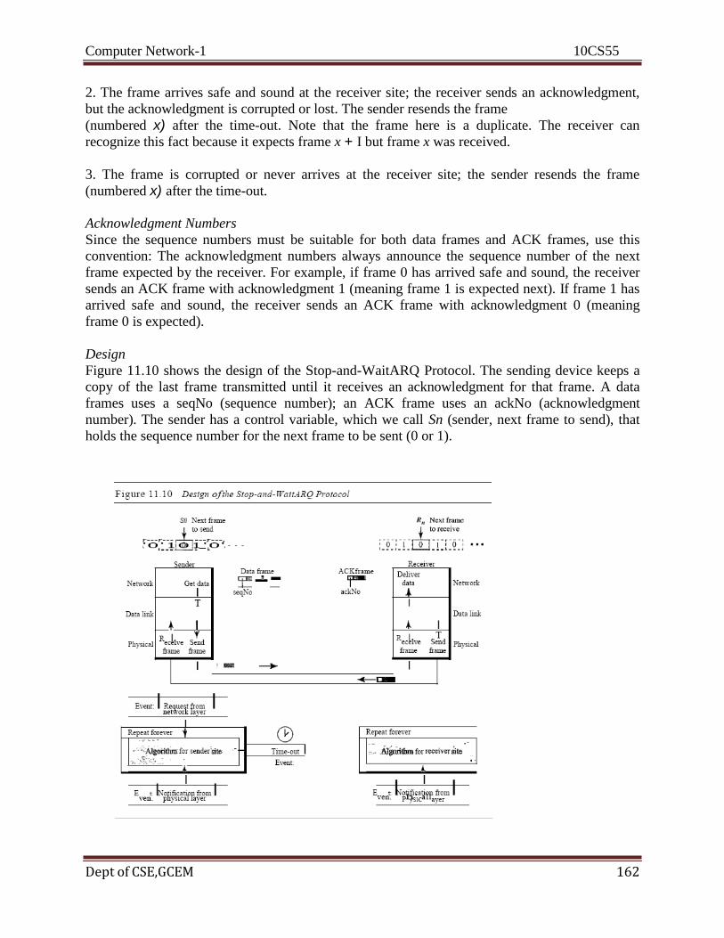
Computer Network-1 10CS55
Dept of CSE,GCEM 162
2. The frame arrives safe and sound at the receiver site; the receiver sends an acknowledgment,
but the acknowledgment is corrupted or lost. The sender resends the frame
(numbered x) after the time-out. Note that the frame here is a duplicate. The receiver can
recognize this fact because it expects frame x + I but frame x was received.
3. The frame is corrupted or never arrives at the receiver site; the sender resends the frame
(numbered x) after the time-out.
Acknowledgment Numbers
Since the sequence numbers must be suitable for both data frames and ACK frames, use this
convention: The acknowledgment numbers always announce the sequence number of the next
frame expected by the receiver. For example, if frame 0 has arrived safe and sound, the receiver
sends an ACK frame with acknowledgment 1 (meaning frame 1 is expected next). If frame 1 has
arrived safe and sound, the receiver sends an ACK frame with acknowledgment 0 (meaning
frame 0 is expected).
Design
Figure 11.10 shows the design of the Stop-and-WaitARQ Protocol. The sending device keeps a
copy of the last frame transmitted until it receives an acknowledgment for that frame. A data
frames uses a seqNo (sequence number); an ACK frame uses an ackNo (acknowledgment
number). The sender has a control variable, which we call Sn (sender, next frame to send), that
holds the sequence number for the next frame to be sent (0 or 1).

Computer Network-1 10CS55
Dept of CSE,GCEM 163
The receiver has a control variable, which we call Rn (receiver, next frame expected), that holds
the number of the next frame expected. When a frame is sent, the value of Sn is incremented
(modulo-2), which means if it is 0, it becomes 1 and vice versa. When a frame is received, the
value of Rn is incremented (modulo-2), which means if it is 0, it becomes 1 and vice versa. Three
events can happen at the sender site; one event can happen at the receiver site. Variable Sn points
to the slot that matches the sequence number of the frame that has been sent, but not
acknowledged; Rn points to the slot that matches the sequence number of the expected frame.

Computer Network-1 10CS55
Dept of CSE,GCEM 164
Analysis We first notice the presence of Sn' the sequence number of the next frame to be sent.
This variable is initialized once (line 1), but it is incremented every time a frame is sent (line 13)
in preparation for the next frame. However, since this is modulo-2 arithmetic, the sequence
numbers are
0, 1,0, 1, and so on. Note that the processes in the first event (SendFrame, StoreFrame, and Purge
Frame) use an Sn defining the frame sent out. We need at least one buffer to hold this frame until
we are sure that it is received safe and sound. Line 10 shows that before the frame is sent, it is
stored.
The copy is used for resending a corrupt or lost frame. We are still using the canSend variable to
prevent the network layer from making a request before the previous frame is received safe and
sound. If the frame is not corrupted and the ackNo of theACK frame matches the sequence
number of the next frame to send, we stop the timer and purge the copy of the data frame we
saved. Otherwise, we just ignore this event and wait for the next event to happen. After each
frame is sent, a timer is started.
When the timer expires (line 28), the frame is resent and the timer is restarted.
Algorithm 11.6 shows the procedure at the receiver site.
Analysis This is noticeably different from Algorithm 11.4. First, all arrived data frames that are
corrupted are ignored. If the SeqNo of the frame is the one that is expected (Rn ), the frame is
accepted, the data are delivered to the network layer, and the value of Rn is incremented.
However, there is one subtle point here. Even if the sequence number of the data frame does not
match the next frame expected, an ACK is sent to the sender. This ACK, however, just
reconfirms the previous ACK instead of confirming the frame received. This is done because the
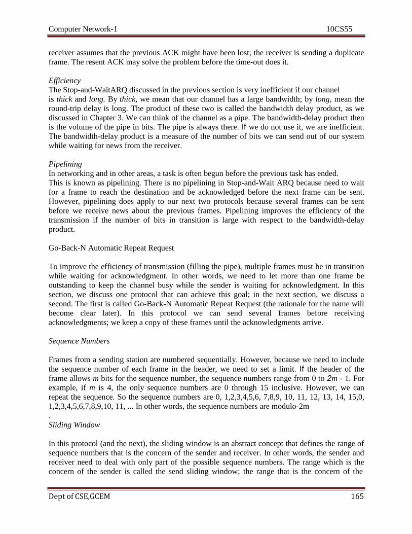
Computer Network-1 10CS55
Dept of CSE,GCEM 165
receiver assumes that the previous ACK might have been lost; the receiver is sending a duplicate
frame. The resent ACK may solve the problem before the time-out does it.
Efficiency
The Stop-and-WaitARQ discussed in the previous section is very inefficient if our channel
is thick and long. By thick, we mean that our channel has a large bandwidth; by long, mean the
round-trip delay is long. The product of these two is called the bandwidth delay product, as we
discussed in Chapter 3. We can think of the channel as a pipe. The bandwidth-delay product then
is the volume of the pipe in bits. The pipe is always there. If we do not use it, we are inefficient.
The bandwidth-delay product is a measure of the number of bits we can send out of our system
while waiting for news from the receiver.
Pipelining
In networking and in other areas, a task is often begun before the previous task has ended.
This is known as pipelining. There is no pipelining in Stop-and-Wait ARQ because need to wait
for a frame to reach the destination and be acknowledged before the next frame can be sent.
However, pipelining does apply to our next two protocols because several frames can be sent
before we receive news about the previous frames. Pipelining improves the efficiency of the
transmission if the number of bits in transition is large with respect to the bandwidth-delay
product.
Go-Back-N Automatic Repeat Request
To improve the efficiency of transmission (filling the pipe), multiple frames must be in transition
while waiting for acknowledgment. In other words, we need to let more than one frame be
outstanding to keep the channel busy while the sender is waiting for acknowledgment. In this
section, we discuss one protocol that can achieve this goal; in the next section, we discuss a
second. The first is called Go-Back-N Automatic Repeat Request (the rationale for the name will
become clear later). In this protocol we can send several frames before receiving
acknowledgments; we keep a copy of these frames until the acknowledgments arrive.
Sequence Numbers
Frames from a sending station are numbered sequentially. However, because we need to include
the sequence number of each frame in the header, we need to set a limit. If the header of the
frame allows m bits for the sequence number, the sequence numbers range from 0 to 2m - 1. For
example, if m is 4, the only sequence numbers are 0 through 15 inclusive. However, we can
repeat the sequence. So the sequence numbers are 0, 1,2,3,4,5,6, 7,8,9, 10, 11, 12, 13, 14, 15,0,
1,2,3,4,5,6,7,8,9,10, 11, ... In other words, the sequence numbers are modulo-2m
. Sliding Window
In this protocol (and the next), the sliding window is an abstract concept that defines the range of
sequence numbers that is the concern of the sender and receiver. In other words, the sender and
receiver need to deal with only part of the possible sequence numbers. The range which is the
concern of the sender is called the send sliding window; the range that is the concern of the

Computer Network-1 10CS55
Dept of CSE,GCEM 166
receiver is called the receive sliding window. We discuss both here. The send window is an
imaginary box covering the sequence numbers of the data frames which can be in transit. In each
window position, some of these sequence numbers define the frames that have been sent; others
define those that can be sent. The maximum size of the window is 2m - 1 for reasons that we
discuss later. In this chapter, we let the size be fixed and set to the maximum value, but we will
see in future chapters that some protocols may have a variable window size. Figure 11.12 shows
a sliding window of size 15 (m =4). The window at any time divides the possible sequence
numbers into four regions. The first region, from the far left to the left wall of the window,
defines the sequence
numbers belonging to frames that are already acknowledged. The sender does not worry about
these frames and keeps no copies of them. The second region, colored in Figure 11.12a, defines
the range of sequence numbers belonging to the frames that are sent and have an unknown status.
The sender needs to wait to find out if these frames have been received or were lost. We call
these outstanding frames. The third range, white in the figure, defines the range of sequence
numbers for frames that can be sent; however, the corresponding data packets have not yet been
received from the network layer. Finally, the fourth region defines sequence numbers that cannot
be used until the window slides, as we see next.
The window itself is an abstraction; three variables define its size and location at any time. We
call these variables Sf(send window, the first outstanding frame), Sn (send window, the next
frame to be sent), and Ssize (send window, size). The variable Sf defines the sequence number of
the first (oldest) outstanding frame. The variable Sn holds the sequence number that will be
assigned to the next frame to be sent. Finally, the variable Ssize defines the size of the window,
which is fixed in our protocol.

Computer Network-1 10CS55
Dept of CSE,GCEM 167
Figure 11.12b shows how a send window can slide one or more slots to the right when an
acknowledgment arrives from the other end. As we will see shortly, theacknowledgments
in this protocol are cumulative, meaning that more than one frame can be acknowledged by an
ACK frame. In Figure 11.12b, frames 0, I, and 2 are acknowledged,
so the window has slid to the right three slots. Note that the value ofSf is 3 because frame 3 is
now the first outstanding frame. The receive window makes sure that the correct data frames are
received and that the correct acknowledgments are sent. The size of the receive window is
always 1. The receiver is always looking for the arrival of a specific frame. Any frame arriving
out of order is discarded and needs to be resent. Figure 11.13 shows the receive window.
Note that we need only one variable Rn (receive window, next frame expected) to define this
abstraction. The sequence numbers to the left of the window belong to the frames already
received and acknowledged; the sequence numbers to the right of this window define the frames
that cannot be received. Any received frame with a sequence number in these two regions is
discarded. Only a frame with a sequence number matching the value of Rn is accepted and
acknowledged. The receive window also slides, but only one slot at a time. When a correct frame
is received (and a frame is received only one at a time), the window slides.
Timers
Although there can be a timer for each frame that is sent, in our protocol we use only
one. The reason is that the timer for the first outstanding frame always expires first; we
send all outstanding frames when this timer expires.
Acknowledgment
The receiver sends a positive acknowledgment if a frame has arrived safe and sound
and in order. If a frame is damaged or is received out of order, the receiver is silent and
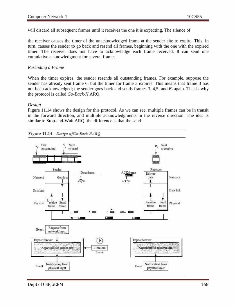
Computer Network-1 10CS55
Dept of CSE,GCEM 168
will discard all subsequent frames until it receives the one it is expecting. The silence of
the receiver causes the timer of the unacknowledged frame at the sender site to expire. This, in
turn, causes the sender to go back and resend all frames, beginning with the one with the expired
timer. The receiver does not have to acknowledge each frame received. It can send one
cumulative acknowledgment for several frames.
Resending a Frame
When the timer expires, the sender resends all outstanding frames. For example, suppose the
sender has already sent frame 6, but the timer for frame 3 expires. This means that frame 3 has
not been acknowledged; the sender goes back and sends frames 3, 4,5, and 6\ again. That is why
the protocol is called Go-Back-N ARQ.
Design
Figure 11.14 shows the design for this protocol. As we can see, multiple frames can be in transit
in the forward direction, and multiple acknowledgments in the reverse direction. The idea is
similar to Stop-and-Wait ARQ; the difference is that the send

Computer Network-1 10CS55
Dept of CSE,GCEM 169
Window allows us to have as many frames in transition as there are slots in the send window.
Send Window Size
We can now show why the size of the send window must be less than 2m. As an example, we
choose m =2, which means the size of the window can be 2m - 1, or 3. Figure 11.15 compares a
window size of 3 against a window size of 4. If the size of the window is (less than 22) and all
three acknowledgments are lost, the frame timer expires and all three frames are resent. The
receiver =is now expecting frame 3, not frame 0, so the duplicate frame is correctly discarded.
On the other hand, if the size of the window is 4 (equal to 22) and all acknowledgments are lost,
the sender will send a duplicate of frame 0. However, this time the window of the receiver
expects to receive frame 0, so it accepts frame 0, not as a duplicate, but as the first frame in the
next cycle. This is an error.
Algorithms
Algorithm 11.7 shows the procedure for the sender in this protocol

Computer Network-1 10CS55
Dept of CSE,GCEM 170
Analysis This algorithm first initializes three variables. Unlike Stop-and-Wait ARQ, this
protocol allows several requests from the network layer without the need for other events to
occur; we just need to be sure that the window is not full (line 12). In our approach, if the
window is full, the request is just ignored and the network layer needs to try again. Some
implementations use other methods such as enabling or disabling the network layer. The
handling of the arrival event is more complex than in the previous protocol. If we receive a
corrupted ACK, we ignore it. If the ade Na belongs to one of the outstanding frames, we use a
loop to purge the buffers and move the left wall to the right. The time-out event is also more
complex.
Algorithm 11.8 is the procedure at the receiver site.
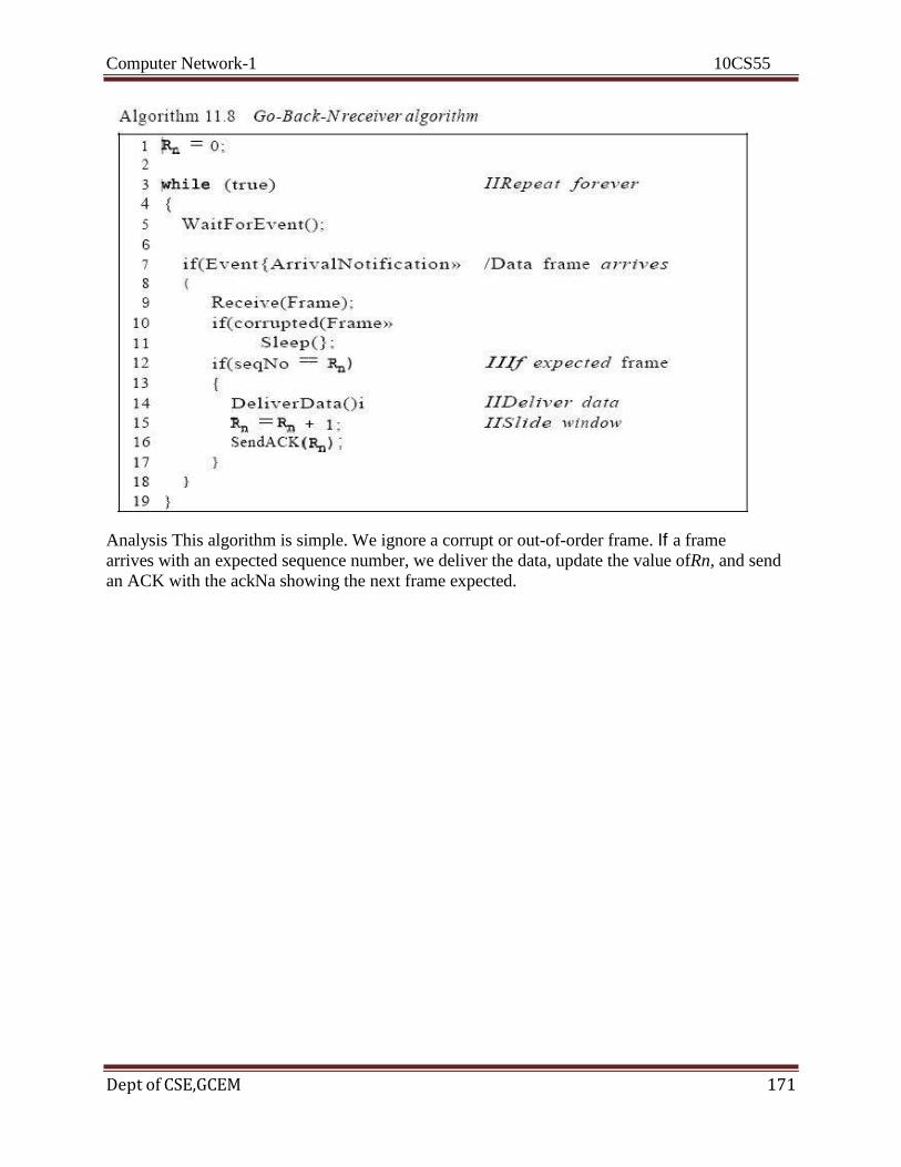
Computer Network-1 10CS55
Dept of CSE,GCEM 171
Analysis This algorithm is simple. We ignore a corrupt or out-of-order frame. If a frame
arrives with an expected sequence number, we deliver the data, update the value ofRn, and send
an ACK with the ackNa showing the next frame expected.
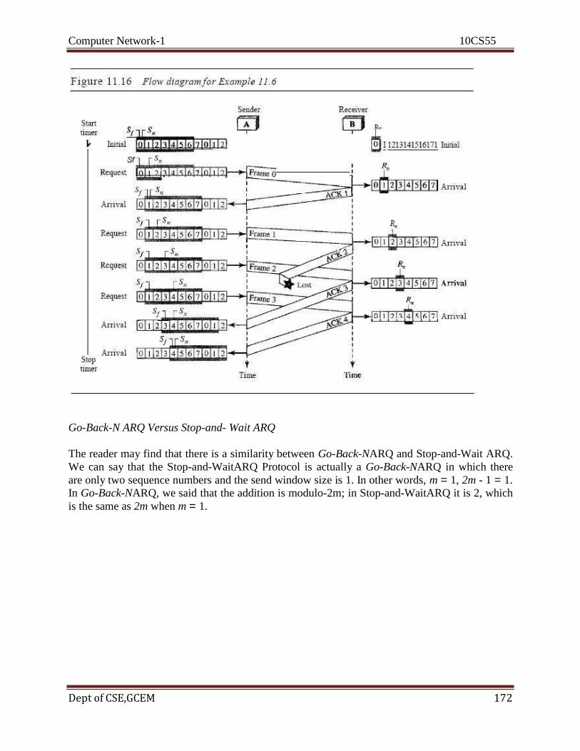
Computer Network-1 10CS55
Dept of CSE,GCEM 172
Go-Back-N ARQ Versus Stop-and- Wait ARQ
The reader may find that there is a similarity between Go-Back-NARQ and Stop-and-Wait ARQ.
We can say that the Stop-and-WaitARQ Protocol is actually a Go-Back-NARQ in which there
are only two sequence numbers and the send window size is 1. In other words, m = 1, 2m - 1 = 1.
In Go-Back-NARQ, we said that the addition is modulo-2m; in Stop-and-WaitARQ it is 2, which
is the same as 2m when m = 1.

Computer Network-1 10CS55
Dept of CSE,GCEM 173
Selective Repeat Automatic Repeat Request
Go-Back-N ARQ simplifies the process at the receiver site. The receiver keeps track of only one
variable, and there is no need to buffer out-of-order frames; they are simply discarded. However,
this protocol is very inefficient for a noisy link. In a noisy link a frame has a higher probability of
damage, which means the resending of multiple frames. This resending uses up the bandwidth
and slows down the transmission. For noisy links, there is another mechanism that does not
resend N frames when just one frame is damaged; only the damaged frame is resent. This
mechanism is called Selective RepeatARQ. It is more efficient for noisy links, but the processing
at the receiver is more complex.

Computer Network-1 10CS55
Dept of CSE,GCEM 174
Windows
The Selective Repeat Protocol also uses two windows: a send window and a receive window.
However, there are differences between the windows in this protocol and the ones in Go-Back-N.
First, the size of the send window is much smaller; it is 2m- I . The reason for this will be
discussed later. Second, the receive window is the same size as the send window. The send
window maximum size can be 2m- I . For example, if m = 4, the sequence numbers go from 0 to
15, but the size of the window is just 8 (it is 15 in the Go-Back-N Protocol). The smaller window
size means less efficiency in filling the pipe, but the fact that there are fewer duplicate frames
can compensate for this.
The protocol uses the same variables as we discussed for Go-Back-N. We show the Selective
Repeat send window in Figure 11.18 to emphasize the size. Compare it with Figure 11.12.
The receive window in Selective Repeat is totally different from the one in GoBack- N. First, the
size of the receive window is the same as the size of the send window (2m- I ). The Selective
Repeat Protocol allows as many frames as the size of the receive window to arrive out of order
and be kept until there is a set of in-order frames to be delivered to the network layer. Because
the sizes of the send window and receive window are the same, all the frames in the send frame
can arrive out of order and be stored until they can be delivered. We need, however, to mention
that the receiver never delivers packets out of order to the network layer. Figure 11.19 shows the
receive window in this

Computer Network-1 10CS55
Dept of CSE,GCEM 175
protocol. Those slots inside the window that are colored define frames that have arrived out of
order and are waiting for their neighbors to arrive before delivery to the network layer.
Design
The design in this case is to some extent similar to the one we described for the 00Back-N, but
more complicated, as shown in Figure 11.20
Window Sizes
Windows must be at most one half of 2m. For an example, we choose m = 2, which means the
size of the window is 2m/2, or 2. Figure 11.21 compares a window size of 2 with a window size
of 3. If the size of the window is 2 and all acknowledgments are lost, the timer for frame 0
expires and frame 0 is resent. However, the window of the receiver is now expecting

Computer Network-1 10CS55
Dept of CSE,GCEM 176
frame 2, not frame 0, so this duplicate frame is correctly discarded. When the size of the window
is 3 and all acknowledgments are lost, the sender sends a duplicate of frame 0. However, this
time, the window of the receiver expects to receive frame 0 (0 is part of the window), so it
accepts frame 0, not as a duplicate, but as the first frame in the next cycle. This is clearly an
error.
Algorithms
Algorithm 11.9 shows the procedure for the sender

Computer Network-1 10CS55
Dept of CSE,GCEM 177
Analysis The handling of the request event is similar to that of the previous protocol except that
one timer is started for each frame sent. The arrival event is more complicated here. An ACK or
a NAK frame may arrive. If a valid NAK frame arrives, we just resend the corresponding frame.
If a valid ACK arrives, we use a loop to purge the buffers, stop the corresponding timer and
move the left wall of the window. The time-out event is simpler here; only the frame which times
out is resent

Computer Network-1 10CS55
Dept of CSE,GCEM 178
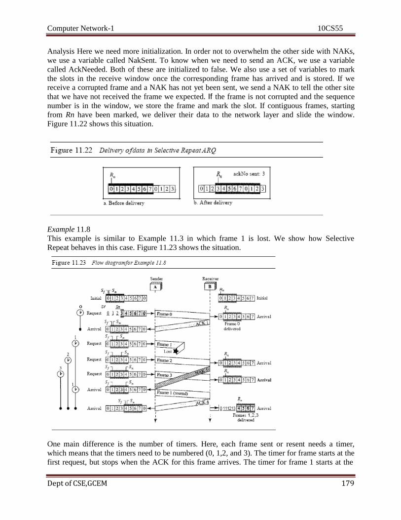
Computer Network-1 10CS55
Dept of CSE,GCEM 179
Analysis Here we need more initialization. In order not to overwhelm the other side with NAKs,
we use a variable called NakSent. To know when we need to send an ACK, we use a variable
called AckNeeded. Both of these are initialized to false. We also use a set of variables to mark
the slots in the receive window once the corresponding frame has arrived and is stored. If we
receive a corrupted frame and a NAK has not yet been sent, we send a NAK to tell the other site
that we have not received the frame we expected. If the frame is not corrupted and the sequence
number is in the window, we store the frame and mark the slot. If contiguous frames, starting
from Rn have been marked, we deliver their data to the network layer and slide the window.
Figure 11.22 shows this situation.
Example 11.8
This example is similar to Example 11.3 in which frame 1 is lost. We show how Selective
Repeat behaves in this case. Figure 11.23 shows the situation.
One main difference is the number of timers. Here, each frame sent or resent needs a timer,
which means that the timers need to be numbered (0, 1,2, and 3). The timer for frame starts at the
first request, but stops when the ACK for this frame arrives. The timer for frame 1 starts at the
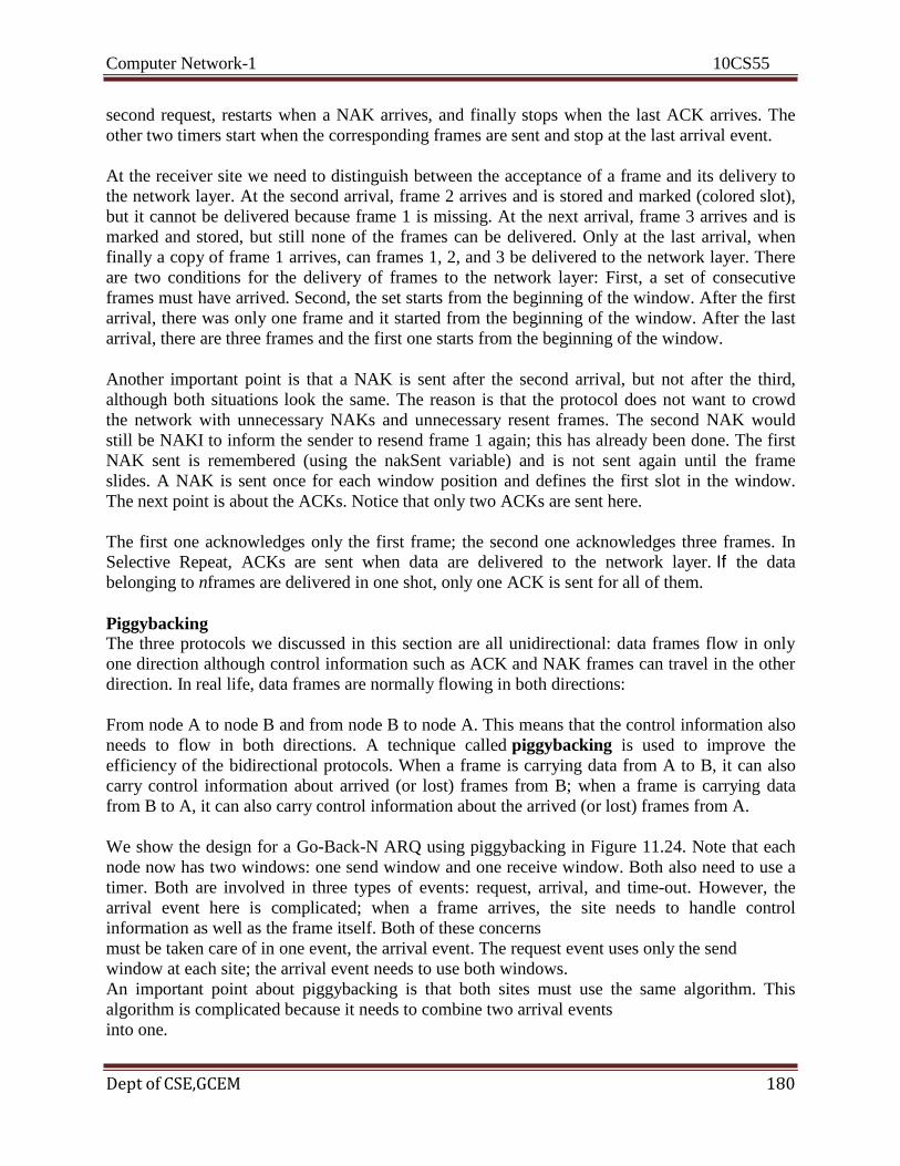
Computer Network-1 10CS55
Dept of CSE,GCEM 180
second request, restarts when a NAK arrives, and finally stops when the last ACK arrives. The
other two timers start when the corresponding frames are sent and stop at the last arrival event.
At the receiver site we need to distinguish between the acceptance of a frame and its delivery to
the network layer. At the second arrival, frame 2 arrives and is stored and marked (colored slot),
but it cannot be delivered because frame 1 is missing. At the next arrival, frame 3 arrives and is
marked and stored, but still none of the frames can be delivered. Only at the last arrival, when
finally a copy of frame 1 arrives, can frames 1, 2, and 3 be delivered to the network layer. There
are two conditions for the delivery of frames to the network layer: First, a set of consecutive
frames must have arrived. Second, the set starts from the beginning of the window. After the first
arrival, there was only one frame and it started from the beginning of the window. After the last
arrival, there are three frames and the first one starts from the beginning of the window.
Another important point is that a NAK is sent after the second arrival, but not after the third,
although both situations look the same. The reason is that the protocol does not want to crowd
the network with unnecessary NAKs and unnecessary resent frames. The second NAK would
still be NAKI to inform the sender to resend frame 1 again; this has already been done. The first
NAK sent is remembered (using the nakSent variable) and is not sent again until the frame
slides. A NAK is sent once for each window position and defines the first slot in the window.
The next point is about the ACKs. Notice that only two ACKs are sent here.
The first one acknowledges only the first frame; the second one acknowledges three frames. In
Selective Repeat, ACKs are sent when data are delivered to the network layer. If the data
belonging to nframes are delivered in one shot, only one ACK is sent for all of them.
Piggybacking The three protocols we discussed in this section are all unidirectional: data frames flow in only
one direction although control information such as ACK and NAK frames can travel in the other
direction. In real life, data frames are normally flowing in both directions:
From node A to node B and from node B to node A. This means that the control information also
needs to flow in both directions. A technique called piggybacking is used to improve the
efficiency of the bidirectional protocols. When a frame is carrying data from A to B, it can also
carry control information about arrived (or lost) frames from B; when a frame is carrying data
from B to A, it can also carry control information about the arrived (or lost) frames from A.
We show the design for a Go-Back-N ARQ using piggybacking in Figure 11.24. Note that each
node now has two windows: one send window and one receive window. Both also need to use a
timer. Both are involved in three types of events: request, arrival, and time-out. However, the
arrival event here is complicated; when a frame arrives, the site needs to handle control
information as well as the frame itself. Both of these concerns
must be taken care of in one event, the arrival event. The request event uses only the send
window at each site; the arrival event needs to use both windows.
An important point about piggybacking is that both sites must use the same algorithm. This
algorithm is complicated because it needs to combine two arrival events
into one.
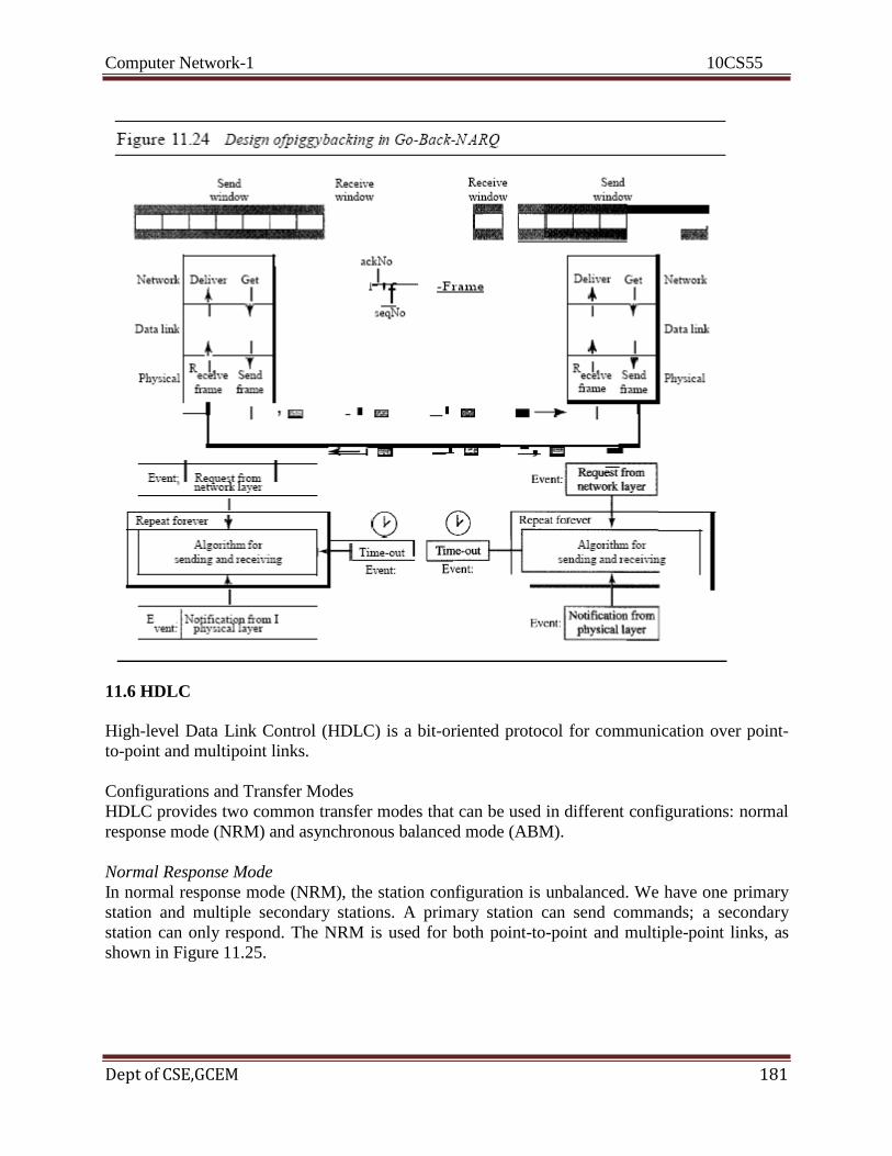
Computer Network-1 10CS55
Dept of CSE,GCEM 181
11.6 HDLC
High-level Data Link Control (HDLC) is a bit-oriented protocol for communication over point-
to-point and multipoint links.
Configurations and Transfer Modes
HDLC provides two common transfer modes that can be used in different configurations: normal
response mode (NRM) and asynchronous balanced mode (ABM).
Normal Response Mode
In normal response mode (NRM), the station configuration is unbalanced. We have one primary
station and multiple secondary stations. A primary station can send commands; a secondary
station can only respond. The NRM is used for both point-to-point and multiple-point links, as
shown in Figure 11.25.

Computer Network-1 10CS55
Dept of CSE,GCEM 182
Asynchronous Balanced Mode
In asynchronous balanced mode (ABM), the configuration is balanced. The link is point-to-point,
and each station can function as a primary and a secondary (acting as peers), as shown in Figure
11.26. This is the common mode today.
Frames
To provide the flexibility necessary to support all the options possible in the modes and
configurations just described, HDLC defines three types of frames: information frames (I-
frames), supervisory frames (S-frames), and unnumbered frames (V-frames). Each type of frame
serves as an envelope for the transmission of a different type of message. I-frames are used to
transport user data and control information relating to user data (piggybacking). S-frames are
used only to transport control information. V-frames are reserved for system management.
Information carried by V-frames is intended for managing the link itself.
Frame Format
Each frame in HDLC may contain up to six fields, as shown in Figure 11.27: a beginning flag
field, an address field, a control field, an information field, a frame check sequence (FCS) field,
and an ending flag field. In multiple-frame transmissions, the ending flag of one frame can serve
as the beginning flag of the next frame.

Computer Network-1 10CS55
Dept of CSE,GCEM 183
Fields
Let us now discuss the fields and their use in different frame types.
o Flag field. The flag field of an HDLC frame is an 8-bit sequence with the bit pattern 01111110
that identifies both the beginning and the end of a frame and serves as a synchronization pattern
for the receiver.
o Address field. The second field of an HDLC frame contains the address of the secondary
station. If a primary station created the frame, it contains a to address. If a secondary creates the
frame, it contains afrom address. An address field can be 1 byte or several bytes long, depending
on the needs of the network. One byte can identify up to 128 stations (l bit is used for another
purpose). Larger networks require multiple-byte address fields. If the address field is only 1 byte,
the last bit is always a 1. If the address is more than 1 byte, all bytes but the last one will end
with 0; only the last will end with 1. Ending each intermediate byte with 0 indicates to the
receiver that there are more address bytes to come.
o Control field. The control field is a 1- or 2-byte segment of the frame used for flow and error
control. The interpretation of bits in this field depends on the frame type. We discuss this field
later and describe its format for each frame type.
o Information field. The information field contains the user's data from the network layer or
management information. Its length can vary from one network to another.
o FCS field. The frame check sequence (FCS) is the HDLC error detection field. It can contain
either a 2- or 4-byte ITU-T CRC.
Control Field The control field determines the type of frame and defines its functionality. So let us discuss the
format of this field in greater detail. The format is specific for the type of frame, as shown in
Figure 11.28.

Computer Network-1 10CS55
Dept of CSE,GCEM 184
Control Field for I-Frames
I-frames are designed to carry user data from the network layer. In addition, they can include
flow and error control information (piggybacking). The subfields in the control field are used to
define these functions. The first bit defines the type. If the first bit of the control field is 0, this
means the frame is an I-frame. The next 3 bits, called N(S), define the sequence number of the
frame. Note that with 3 bits, we can define a sequence number between and 7; but in the
extension format, in which the control field is 2 bytes, this field is larger. The last 3 bits, called
N(R), correspond to the acknowledgment number when piggybacking is used. The single bit
between N(S) and N(R) is called the PIF bit. The PIP field is a single bit with a dual purpose. It has meaning only when it is set (bit = 1) and can mean poll or final. It means poll when the
frame is sent by a primary station to a secondary (when the address field contains the address of
the receiver). It means final when the frame is sent by a secondary to a primary (when the
address field contains the address of the sender).
Control Field for S-Frames
Supervisory frames are used for flow and error control whenever piggybacking is either
impossible or inappropriate (e.g., when the station either has no data of its own to send or needs
to send a command or response other than an acknowledgment). S-frames do not have
information fields. If the first 2 bits of the control field is 10, this means the frame is an S-frame.
The last 3 bits, called N(R), corresponds to the acknowledgment number (ACK) or negative
acknowledgment number (NAK) depending on the type of S-frame. The 2 bits called code is
used to define the type of S-frame itself. With 2 bits, we can have four types of S-frames, as
described below:
o Receive ready (RR). If the value of the code subfield is 00, it is an RR S-frame. This kind of
frame acknowledges the receipt of a safe and sound frame or group of frames. In this case, the
value N(R) field defines the acknowledgment number. Receive not ready (RNR). If the value of
the code subfield is 10, it is an RNR S-frame. This kind of frame is an RR frame with additional
functions. It acknowledges the receipt of a frame or group of frames, and it announces that the
receiver is busy and cannot receive more frames. It acts as a kind of congestion control
mechanism by asking the sender to slow down. The value of NCR) is the acknowledgment
number.

Computer Network-1 10CS55
Dept of CSE,GCEM 185
o Reject (REJ). If the value of the code subfield is 01, it is a REJ S-frame. This is a NAK frame,
but not like the one used for Selective Repeat ARQ. It is a NAK that can be used in Go-Back-N
ARQ to improve the efficiency of the process by informing the sender, before the sender time
expires, that the last frame is lost or damaged. The value of NCR) is the negative
acknowledgment number.
o Selective reject (SREJ). If the value of the code subfield is 11, it is an SREJ S-frame. This is a
NAK frame used in Selective Repeat ARQ. Note that the HDLC Protocol uses the term selective
reject instead of selective repeat. The value of N(R) is the negative acknowledgment number.
Control Field for V-Frames
Unnumbered frames are used to exchange session management and control information between
connected devices. Unlike S-frames, U-frames contain an information field, but one used for
system management information, not user data. As with S-frames, however, much of the
information carried by U-frames is contained in codes included in the control field. U-frame
codes are divided into two sections: a 2-bit prefix before the PtF bit and a 3-bit suffix after the
PtF bit. Together, these two segments (5 bits) can be used to create up to 32 different types of U-
frames. Some of the more common types are shown in Table 11.1.
Example 11.9: Connection/Disconnection
Figure 11.29 shows how V-frames can be used for connection establishment and connection
release. Node A asks for a connection with a set asynchronous balanced mode = (SABM) frame;
node B gives a positive response with an unnumbered acknowledgment (VA) frame. After these
two exchanges, data can be transferred between the two nodes (not shown in the figure). After
data transfer, node A sends a DISC (disconnect) frame to release the connection; it is confirmed
by node B responding with a VA (unnumbered acknowledgment).

Computer Network-1 10CS55
Dept of CSE,GCEM 186
Example 11.10: Piggybacking without Error
Figure 11.30 shows an exchange using piggybacking. Node A begins the exchange of
information with an I-frame numbered 0 followed by another I-frame numbered 1. Node B
piggybacks its acknowledgment of both frames onto an I-frame of its own. Node B's first I-frame
is also numbered 0 [N(S) field] and contains a 2 in its N(R) field, acknowledging the receipt of
Ns frames 1 and 0 and indicating that it expects frame 2 to arrive next. Node B transmits its
second and third I-frames (numbered 1 and 2) before accepting further frames from node A. Its
N(R) information, therefore, has not changed: B frames 1 and 2 indicate that node B is still
expecting Ns frame 2 to arrive next. Node A has sent all its data. Therefore, it cannot piggyback
an acknowledgment onto an I-frame and sends an S-frame
instead. The RR code indicates that A is still ready to receive. The number 3 in the N(R) field
tells B that frames 0, 1, and 2 have all been accepted and that A is now expecting frame number
3.

Computer Network-1 10CS55
Dept of CSE,GCEM 187
Example 11.11: Piggybacking with Error
Figure 11.31 shows an exchange in which a frame is lost. Node B sends three data frames (0, 1,
and 2), but frame 1 is lost. When node A receives frame 2, it discards it and sends a REI frame
for frame 1. Note that the protocol being used is Go-Back-N with the special use of an REI frame
as a NAK frame. The NAK frame does two things here: It confirms the receipt of frame and
declares that frame 1 and any following frames must be resent. Node B, after receiving the REI
frame, resends frames 1 and 2. Node A acknowledges the receipt by sending an RR frame (ACK)
with acknowledgment number 3.
11.7 POINT-TO-POINT PROTOCOL
Although HDLC is a general protocol that can be used for both point-to-point and multipoint
configurations, one of the most common protocols for point-to-point access is the Point-to-Point
Protocol (PPP). Today, millions of Internet users who need to connect their home computers to

Computer Network-1 10CS55
Dept of CSE,GCEM 188
the server of an Internet service provider use PPP. The majority of these users have a traditional
modem; they are connected to the Internet through a telephone line, which provides the services
of the physical layer. But to control and
manage the transfer of data, there is a need for a point-to-point protocol at the data link
layer. PPP is by far the most common. PPP provides several services:
1. PPP defines the format of the frame to be exchanged between devices.
2. PPP defines how two devices can negotiate the establishment of the link and the
exchange of data.
3. PPP defines how network layer data are encapsulated in the data link frame.
4. PPP defines how two devices can authenticate each other.
5. PPP provides multiple network layer services supporting a variety of network layer

Computer Network-1 10CS55
Dept of CSE,GCEM 189
protocols.
6. PPP provides connections over multiple links.
7. PPP provides network address configuration. This is particularly useful when a home
user needs a temporary network address to connect to the Internet.
On the other hand, to keep PPP simple, several services are missing:
I. PPP does not provide flow control. A sender can send several frames one after another
with no concern about overwhelming the receiver. 2. PPP has a very simple mechanism for error control. A CRC field is used to detect
errors. If the frame is corrupted, it is silently discarded; the upper-layer protocol needs
to take care of the problem. Lack of error control and sequence numbering may cause a
packet to be received out of order.
3. PPP does not provide a sophisticated addressing mechanism to handle frames in a
multipoint configuration.
Framing
PPP is a byte-oriented protocol. Framing is done according to the discussion of byte oriented
protocols at the beginning of this chapter.
Frame Format
Figure 11.32 shows the format of a PPP frame. The description of each field follows:
o Flag. A PPP frame starts and ends with a I-byte flag with the bit pattern 01111110. Although
this pattern is the same as that used in HDLC, there is a big difference. PPP is a byte-oriented
protocol; HDLC is a bit-oriented protocol. The flag is treated as a byte, as we will explain later.
o Address. The address field in this protocol is a constant value and set to 11111111 (broadcast
address). During negotiation (discussed later), the two parties may agree to omit this byte. o Control. This field is set to the constant value 11000000 (imitating unnumbered frames in
HDLC). As we will discuss later, PPP does not provide any flow control. Error control is also
limited to error detection. This means that this field is not needed at all, and again, the two
parties can agree, during negotiation, to omit this byte. o Protocol. The protocol field defines
what is being carried in the data field: either user data or other information. We discuss this field
in detail shortly. This field is by default 2 bytes long, but the two parties can agree to use only 1
byte. o Payload field. This field carries either the user data or other information that we will
discuss shortly. The data field is a sequence of bytes with the default of a maximum of 1500
bytes; but this can be changed during negotiation. The data field is byte stuffed if the flag byte
pattern appears in this field. Because there is no field defining the size of the data field, padding
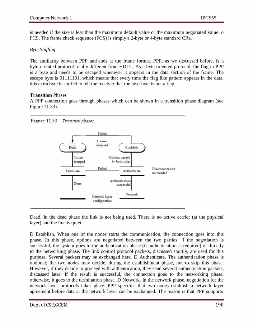
Computer Network-1 10CS55
Dept of CSE,GCEM 190
is needed if the size is less than the maximum default value or the maximum negotiated value. o
FCS. The frame check sequence (FCS) is simply a 2-byte or 4-byte standard CRe.
Byte Stuffing
The similarity between PPP and ends at the frame format. PPP, as we discussed before, is a
byte-oriented protocol totally different from HDLC. As a byte-oriented protocol, the flag in PPP
is a byte and needs to be escaped whenever it appears in the data section of the frame. The
escape byte is 01111101, which means that every time the flag like pattern appears in the data,
this extra byte is stuffed to tell the receiver that the next byte is not a flag.
Transition Phases
A PPP connection goes through phases which can be shown in a transition phase diagram (see
Figure 11.33).
Dead. In the dead phase the link is not being used. There is no active carrier (at the physical
layer) and the line is quiet.
D Establish. When one of the nodes starts the communication, the connection goes into this
phase. In this phase, options are negotiated between the two parties. If the negotiation is
successful, the system goes to the authentication phase (if authentication is required) or directly
to the networking phase. The link control protocol packets, discussed shortly, are used for this
purpose. Several packets may be exchanged here. D Authenticate. The authentication phase is
optional; the two nodes may decide, during the establishment phase, not to skip this phase.
However, if they decide to proceed with authentication, they send several authentication packets,
discussed later. If the result is successful, the connection goes to the networking phase;
otherwise, it goes to the termination phase. D Network. In the network phase, negotiation for the
network layer protocols takes place. PPP specifies that two nodes establish a network layer
agreement before data at the network layer can be exchanged. The reason is that PPP supports

Computer Network-1 10CS55
Dept of CSE,GCEM 191
multiple protocols at the network layer. If a node is running multiple protocols simultaneously at
the network layer, the receiving node needs to know which protocol will receive the data.
o Open. In the open phase, data transfer takes place. When a connection reaches this phase, the
exchange of data packets can be started. The connection remains in this phase until one of the
endpoints wants to terminate the connection.
o Terminate. In the termination phase the connection is terminated. Several packets
are exchanged between the two ends for house cleaning and closing the link.
Multiplexing
Although PPP is a data link layer protocol, PPP uses another set of other protocols to establish
the link, authenticate the parties involved, and carry the network layer data. Three sets of
protocols are defined to make PPP powetful: the Link Control Protocol (LCP), two
Authentication Protocols (APs), and several Network Control Protocols (NCPs). At any moment,
a PPP packet can carry data from one of these protocols in its data field, as shown in Figure
11.34. Note that there is one LCP, two APs, and several NCPs. Data may also come from several
different network layers.
Link Control Protocol
The Link Control Protocol (LCP) is responsible for establishing, maintaining, configuring, and
terminating links. It also provides negotiation mechanisms to set options between the two
endpoints. Both endpoints of the link must reach an agreement about the options before the link
can be established. See Figure 11.35. All LCP packets are carried in the payload field of the PPP
frame with the protocol field set to C021 in hexadecimal.
The code field defines the type of LCP packet. There are 11 types of packets as shown in Table
11.2
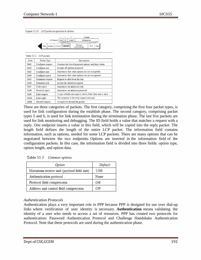
Computer Network-1 10CS55
Dept of CSE,GCEM 192
There are three categories of packets. The first category, comprising the first four packet types, is
used for link configuration during the establish phase. The second category, comprising packet
types 5 and 6, is used for link termination during the termination phase. The last five packets are
used for link monitoring and debugging. The ID field holds a value that matches a request with a
reply. One endpoint inserts a value in this field, which will be copied into the reply packet. The
length field defines the length of the entire LCP packet. The information field contains
information, such as options, needed for some LCP packets. There are many options that can be
negotiated between the two endpoints. Options are inserted in the information field of the
configuration packets. In this case, the information field is divided into three fields: option type,
option length, and option data.
Authentication Protocols
Authentication plays a very important role in PPP because PPP is designed for use over dial-up
links where verification of user identity is necessary. Authentication means validating the
identity of a user who needs to access a set of resources. PPP has created two protocols for
authentication: Password Authentication Protocol and Challenge Handshake Authentication
Protocol. Note that these protocols are used during the authentication phase.
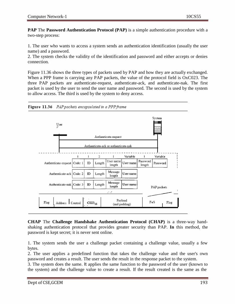
Computer Network-1 10CS55
Dept of CSE,GCEM 193
PAP The Password Authentication Protocol (PAP) is a simple authentication procedure with a
two-step process:
1. The user who wants to access a system sends an authentication identification (usually the user
name) and a password.
2. The system checks the validity of the identification and password and either accepts or denies
connection.
Figure 11.36 shows the three types of packets used by PAP and how they are actually exchanged.
When a PPP frame is carrying any PAP packets, the value of the protocol field is OxC023. The
three PAP packets are authenticate-request, authenticate-ack, and authenticate-nak. The first
packet is used by the user to send the user name and password. The second is used by the system
to allow access. The third is used by the system to deny access.
CHAP The Challenge Handshake Authentication Protocol (CHAP) is a three-way hand-
shaking authentication protocol that provides greater security than PAP. In this method, the
password is kept secret; it is never sent online.
1. The system sends the user a challenge packet containing a challenge value, usually a few
bytes.
2. The user applies a predefined function that takes the challenge value and the user's own
password and creates a result. The user sends the result in the response packet to the system.
3. The system does the same. It applies the same function to the password of the user (known to
the system) and the challenge value to create a result. If the result created is the same as the

Computer Network-1 10CS55
Dept of CSE,GCEM 194
result sent in the response packet, access is granted; otherwise, it is denied. CHAP is more secure
than PAP, especially if the system continuously changes the challenge value. Even if the intruder
learns the challenge value and the result, the password is still secret. Figure 11.37 shows the
packets and how they are used.
CHAP packets are encapsulated in the PPP frame with the protocol value C223 in hexadecimal.
There are four CHAP packets: challenge, response, success, and failure. The first packet is used
by the system to send the challenge value. The second is used by the user to return the result of
the calculation. The third is used by the system to allow access to the system. The fourth is used
by the system to deny access to the system.
Network Control Protocols
PPP is a multiple-network layer protocol. It can carry a network layer data packet from
protocols defined by the Internet, OSI, Xerox, DECnet, AppleTalk, Novel, and so on. To do this,
PPP has defined a specific Network Control Protocol for each network protocol. For example,
IPCP (Internet Protocol Control Protocol) configures the link for carrying IP data packets. Xerox
CP does the same for the Xerox protocol data packets, and so on. Note that none of the NCP
packets carry network layer data; they just configure the link at the network layer for the
incoming data. IPCP One NCP protocol is the Internet Protocol Control Protocol (IPCP). This
protocol configures the link used to carry IP packets in the Internet. IPCP is especially of interest

Computer Network-1 10CS55
Dept of CSE,GCEM 195
to us. The format of an IPCP packet is shown in Figure 11.38. Note that the value of the protocol
field in hexadecimal is 8021.
Other Protocols There are other NCP protocols for other network layer protocols. The OSI
Network Layer Control Protocol has a protocol field value of 8023; the Xerox NS IDP Control
Protocol has a protocol field value of 8025; and so on. The value of the code and the format of
the packets for these other protocols are the same as shown in Table 11.4.
Data/rom the Network Layer
After the network layer configuration is completed by one of the NCP protocols, the users can
exchange data packets from the network layer. Here again, there are different protocol fields for
different network layers. For example, if PPP is carrying data from the IP network layer, the field
value is 0021 (note that the three rightmost digits are the same as for IPCP). If PPP is carrying
data from the OSI network layer, the value of the protocol field is 0023, and so on. Figure 11.39
shows the frame for IP.

Computer Network-1 10CS55
Dept of CSE,GCEM 196
Multilink PPP
PPP was originally designed for a single-channel point-to-point physical link. The availability of
multiple channels in a single point-to-point link motivated the development of
Multilink PPP. In this case, a logical PPP frame is divided into several actual PPP
frames. A segment of the logical frame is carried in the payload of an actual PPP frame,
as shown in Figure 11.40. To show that the actual PPP frame is carrying a fragment of a
logical PPP frame, the protocol field is set to Ox003d. This new development adds complexity.
For example, a sequence number needs to be added to the actual PPP frame to show a fragment's
position in the logical frame.
Example 11.12
Let us go through the phases followed by a network layer packet as it is transmitted through a
PPP connection. Figure 11.41 shows the steps. For simplicity, we assume unidirectional
movement of data from the user site to the system site (such as sending an e-mail through an
ISP).

Computer Network-1 10CS55
Dept of CSE,GCEM 197

Computer Network-1 10CS55
Dept of CSE,GCEM 198
The first two frames show link establishment. We have chosen two options (not shown in the
figure): using PAP for authentication and suppressing the address control fields Frames 3 and 4
are for authentication. Frames 5 and 6 establish the network layer connection using IPCP. The
next several frames show that some IP packets are encapsulated in the PPP frame. The system
(receiver) may have been running several network layer protocols, but it knows that the
incoming data must be delivered to the IP protocol because the NCP protocol used before the
data transfer was IPCP. After data transfer, the user then terminates the data link connection,
which is acknowledged by the system. of Course the user or the system could have chosen to
terminate the network layer IPCP and keep the data link layer running if it wanted to run another
NCP protocol. The example is trivial, but it points out the similarities of the packets in LCP, AP,
and NCP. It also shows the protocol field values and code numbers for particular protocols
Recommended Questions
1. Define framing and the reason for its need
2. Compare and contrast flow control and error control 3. What are the two protocols we discussed for noiseless channels in this
chapter?
4. Explain the reason for moving from the Stop-and-Wait ARQ Protocol to
the 00Back NARQ Protocol
5. Compare and contrast the Go-Back-NARQ Protocol with Selective-
RepeatARQ
6. ompare and contrast HDLC with PPP. Which one is byte-oriented;
which one is bit oriented.
7. Define piggybacking and its usefulness
8. Which of the protocols described in this chapter utilize pipelining?
Computer Network-1 10CS55
Dept of CSE,GCEM 199
COMPUTER NETWORKS – I
Subject Code: 10CS55 I.A. Marks : 25
Hours/Week : 04 Exam Hours: 03
Total Hours : 52 Exam Marks: 100
UNIT- 6 7 Hours Multiple Access & Ethernet:
- Random access,
- Controlled Access,
- Channelization,
- Ethernet: IEEE standards,
- Standard Ethernet,
- Changes in the standard,
- Fast Ethernet, - Gigabit Ethernet
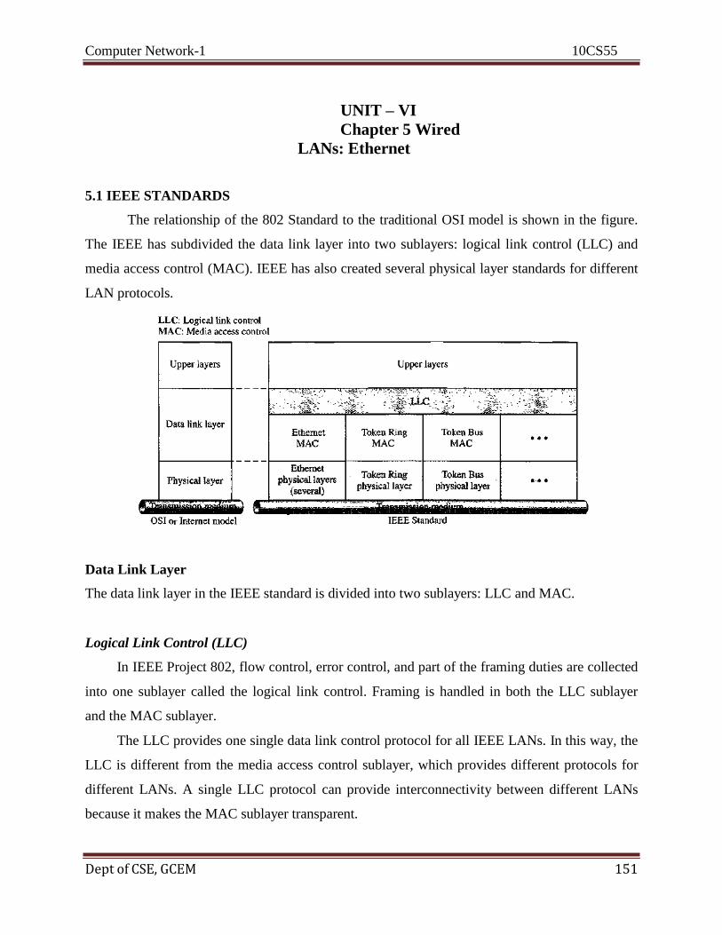
Computer Network-1 10CS55
Dept of CSE, GCEM 151
UNIT – VI
Chapter 5 Wired
LANs: Ethernet
5.1 IEEE STANDARDS
The relationship of the 802 Standard to the traditional OSI model is shown in the figure.
The IEEE has subdivided the data link layer into two sublayers: logical link control (LLC) and
media access control (MAC). IEEE has also created several physical layer standards for different
LAN protocols.
Data Link Layer
The data link layer in the IEEE standard is divided into two sublayers: LLC and MAC.
Logical Link Control (LLC)
In IEEE Project 802, flow control, error control, and part of the framing duties are collected
into one sublayer called the logical link control. Framing is handled in both the LLC sublayer
and the MAC sublayer.
The LLC provides one single data link control protocol for all IEEE LANs. In this way, the
LLC is different from the media access control sublayer, which provides different protocols for
different LANs. A single LLC protocol can provide interconnectivity between different LANs
because it makes the MAC sublayer transparent.

Computer Network-1 10CS55
Dept of CSE, GCEM 152
5. All words are added using one's complement addition.
6. The sum is complemented and becomes the new checksum.
7. If the value of checksum is 0, the message is accepted; otherwise, it is rejected.
The nature of the checksum (treating words as numbers and adding and complementing them) is
well-suited for software implementation. Short programs can be written to calculate the
checksum at the receiver site or to check the validity of the message at the receiver site.
Recommended Questions
1. How does a single-bit error differ from a burst error? 2. Distinguish between forward error correction versus error correction by
retransmission.
3. What is the definition of a linear block code? What is the definition of a
cyclic code?
4. What is the Hamming distance? What is the minimum Hamming
distance?
5. How is the simple parity check related to the two-dimensional parity
check?
6. Discuss the concept of redundancy in error detection and correction.

Computer Network-1 10CS55
Dept of CSE, GCEM 153
COMPUTER NETWORKS – I
Subject Code: 10CS55 I.A. Marks : 25
Hours/Week : 04 Exam Hours: 03
Total Hours : 52 Exam Marks: 100
PART - B
UNIT- 5 6 Hours
Data Link Layer-2:
-Framing,
-Flow and Error Control,
-Protocols, Noiseless Channels,
-Noisy channels,
-HDLC, -PPP (Framing, Transition phases only)

Computer Network-1 10CS55
Dept of CSE, GCEM 154
UNIT-5
Data Link Control
11.1 FRAMING
Data transmission in the physical layer means moving bits in the form of a signal from the source
to the destination. The physical layer provides bit synchronization to ensure that the sender and
receiver use the same bit durations and timing.
The data link layer, on the other hand, needs to pack bits into frames, so that each frame is
distinguishable from another. Our postal system practices a type of framing. The simple act of
inserting a letter into an envelope separates one piece of information from another; the envelope
serves as the delimiter. In addition, each envelope defines the sender and receiver addresses since
the postal system is a many-to-many carrier facility.
Framing in the data link layer separates a message from one source to a destination, or from
other messages to other destinations, by adding a sender address and a destination address. The
destination address defines where the packet is to go; the sender address helps the recipient
acknowledge the receipt. Although the whole message could be packed in one frame, that is not
normally done. One reason is that a frame can be very large, making flow and error control very
inefficient. When a message is carried in one very large frame, even a single-bit error would
require the retransmission of the whole message. When a message is divided into smaller frames,
a single-bit error affects only that small frame.
Fixed-Size Framing
Frames can be of fixed or variable size. In fixed-size framing, there is no need for defining the
boundaries of the frames; the size itself can be used as a delimiter. An example of this type of
framing is the ATM wide-area network, which uses frames of fixed size called cells.
Variable-Size Framing
Our main discussion in this chapter concerns variable-size framing, prevalent in local area
networks. In variable-size framing, we need a way to define the end of the frame and the
beginning of the next.
Character-Oriented Protocols
In a character-oriented protocol, data to be carried are 8-bit characters from a coding system such
as ASCII (see Appendix A). The header, which normally carries the source and destination
addresses and other control information, and the trailer, which carries error detection or error
correction redundant bits, are also multiples of 8 bits. To separate one frame from the next, an 8-
bit (I-byte) flag is added at the beginning and the end of a frame. The flag, composed of
protocol-dependent special characters, signals the start or end of a frame. Figure 11.1 shows the
format of a frame in a character-oriented protocol.

Computer Network-1 10CS55
Dept of CSE, GCEM 155
Character-oriented framing was popular when only text was exchanged by the data link layers.
The flag could be selected to be any character not used for text communication. Now, however,
we send other types of information such as graphs, audio, and video. Any pattern used for the
flag could also be part of the information. If this happens, the receiver, when it encounters this
pattern in the middle of the data, thinks it has reached the end of the frame. To fix this problem, a
byte-stuffing strategy was added to character-oriented framing. In byte stuffing (or character
stuffing), a special byte is added to the data section of the frame when there is a character with
the same pattern as the flag. The data section is stuffed with an extra byte. This byte is usually
called the escape character (ESC), which has a predefined bit pattern. Whenever the receiver
encounters the ESC character, it removes it from the data section and treats the next character as
data, not a delimiting flag.
Byte stuffing by the escape character allows the presence of the flag in the data section of the
frame, but it creates another problem. What happens if the text contains one or more escape
characters followed by a flag? The receiver removes the escape character, but keeps the flag,
which is incorrectly interpreted as the end of the frame. To solve this problem, the escape
characters that are part of the text must also be marked by another escape character. In other
words, if the escape character is part of the text, an extra one is added to show that the second
one is part of the text. Figure 11.2 shows the situation.
Character-oriented protocols present another problem in data communications. The universal
coding systems in use today, such as Unicode, have 16-bit and 32-bit characters that conflict
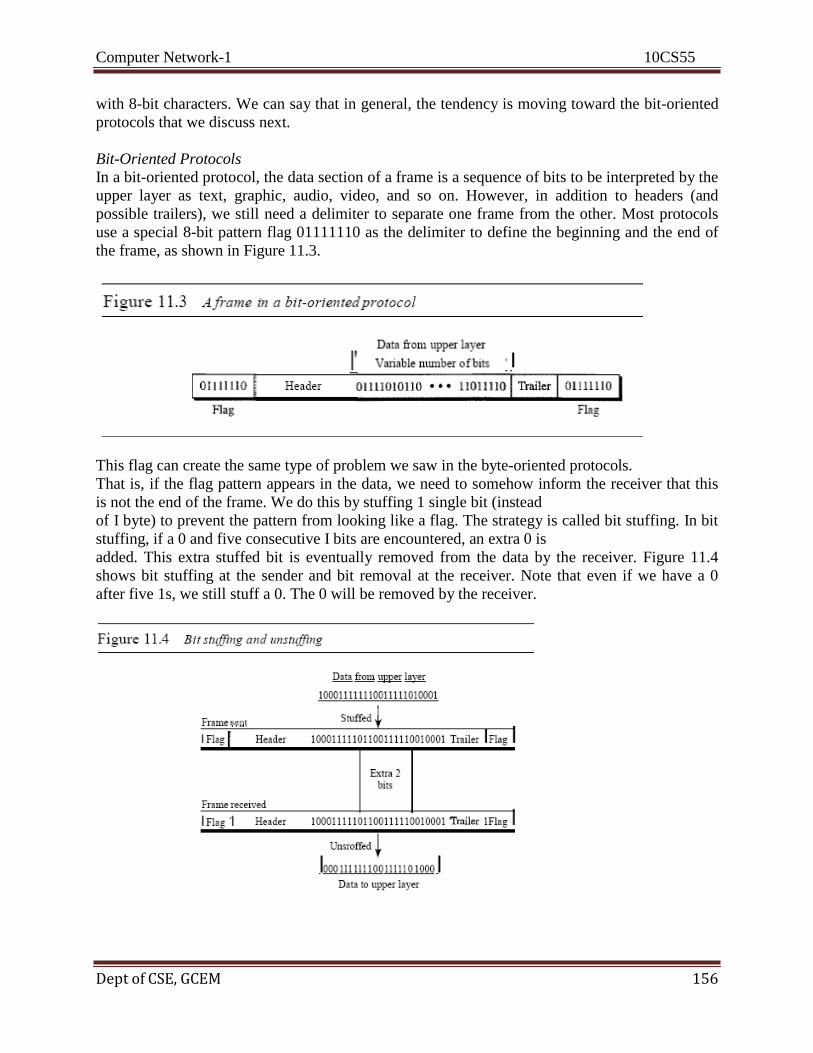
Computer Network-1 10CS55
Dept of CSE, GCEM 156
with 8-bit characters. We can say that in general, the tendency is moving toward the bit-oriented
protocols that we discuss next.
Bit-Oriented Protocols
In a bit-oriented protocol, the data section of a frame is a sequence of bits to be interpreted by the
upper layer as text, graphic, audio, video, and so on. However, in addition to headers (and
possible trailers), we still need a delimiter to separate one frame from the other. Most protocols
use a special 8-bit pattern flag 01111110 as the delimiter to define the beginning and the end of
the frame, as shown in Figure 11.3.
This flag can create the same type of problem we saw in the byte-oriented protocols.
That is, if the flag pattern appears in the data, we need to somehow inform the receiver that this
is not the end of the frame. We do this by stuffing 1 single bit (instead
of I byte) to prevent the pattern from looking like a flag. The strategy is called bit stuffing. In bit
stuffing, if a 0 and five consecutive I bits are encountered, an extra 0 is
added. This extra stuffed bit is eventually removed from the data by the receiver. Figure 11.4
shows bit stuffing at the sender and bit removal at the receiver. Note that even if we have a 0
after five 1s, we still stuff a 0. The 0 will be removed by the receiver.
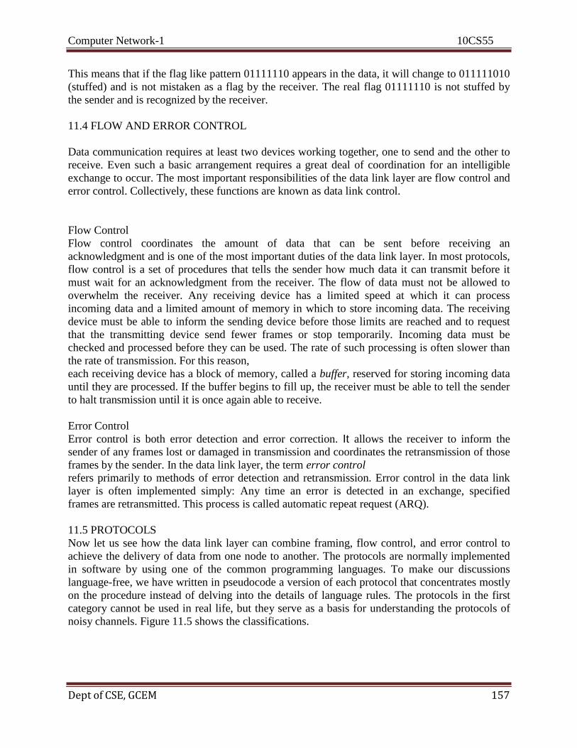
Computer Network-1 10CS55
Dept of CSE, GCEM 157
This means that if the flag like pattern 01111110 appears in the data, it will change to 011111010
(stuffed) and is not mistaken as a flag by the receiver. The real flag 01111110 is not stuffed by
the sender and is recognized by the receiver.
11.4 FLOW AND ERROR CONTROL
Data communication requires at least two devices working together, one to send and the other to
receive. Even such a basic arrangement requires a great deal of coordination for an intelligible
exchange to occur. The most important responsibilities of the data link layer are flow control and
error control. Collectively, these functions are known as data link control.
Flow Control
Flow control coordinates the amount of data that can be sent before receiving an
acknowledgment and is one of the most important duties of the data link layer. In most protocols,
flow control is a set of procedures that tells the sender how much data it can transmit before it
must wait for an acknowledgment from the receiver. The flow of data must not be allowed to
overwhelm the receiver. Any receiving device has a limited speed at which it can process
incoming data and a limited amount of memory in which to store incoming data. The receiving
device must be able to inform the sending device before those limits are reached and to request
that the transmitting device send fewer frames or stop temporarily. Incoming data must be
checked and processed before they can be used. The rate of such processing is often slower than
the rate of transmission. For this reason,
each receiving device has a block of memory, called a buffer, reserved for storing incoming data
until they are processed. If the buffer begins to fill up, the receiver must be able to tell the sender
to halt transmission until it is once again able to receive.
Error Control
Error control is both error detection and error correction. It allows the receiver to inform the
sender of any frames lost or damaged in transmission and coordinates the retransmission of those
frames by the sender. In the data link layer, the term error control
refers primarily to methods of error detection and retransmission. Error control in the data link
layer is often implemented simply: Any time an error is detected in an exchange, specified
frames are retransmitted. This process is called automatic repeat request (ARQ).
11.5 PROTOCOLS
Now let us see how the data link layer can combine framing, flow control, and error control to
achieve the delivery of data from one node to another. The protocols are normally implemented
in software by using one of the common programming languages. To make our discussions
language-free, we have written in pseudocode a version of each protocol that concentrates mostly
on the procedure instead of delving into the details of language rules. The protocols in the first
category cannot be used in real life, but they serve as a basis for understanding the protocols of
noisy channels. Figure 11.5 shows the classifications.
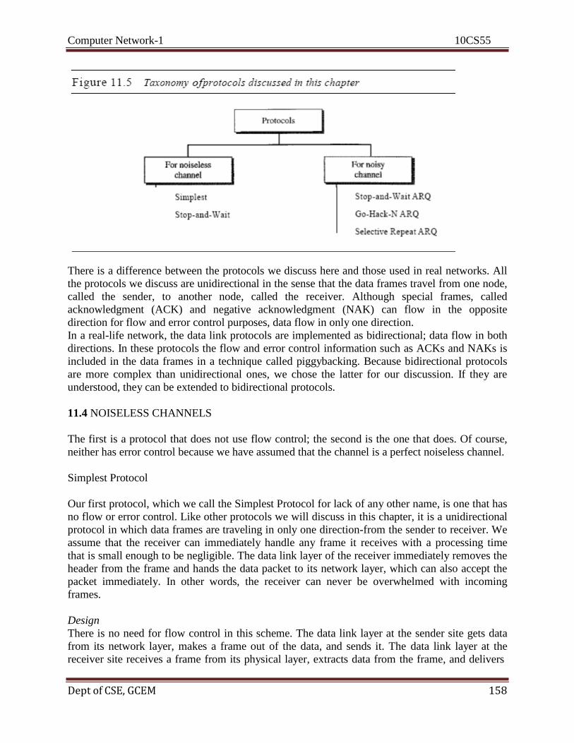
Computer Network-1 10CS55
Dept of CSE, GCEM 158
There is a difference between the protocols we discuss here and those used in real networks. All
the protocols we discuss are unidirectional in the sense that the data frames travel from one node,
called the sender, to another node, called the receiver. Although special frames, called
acknowledgment (ACK) and negative acknowledgment (NAK) can flow in the opposite
direction for flow and error control purposes, data flow in only one direction.
In a real-life network, the data link protocols are implemented as bidirectional; data flow in both
directions. In these protocols the flow and error control information such as ACKs and NAKs is
included in the data frames in a technique called piggybacking. Because bidirectional protocols
are more complex than unidirectional ones, we chose the latter for our discussion. If they are
understood, they can be extended to bidirectional protocols.
11.4 NOISELESS CHANNELS
The first is a protocol that does not use flow control; the second is the one that does. Of course,
neither has error control because we have assumed that the channel is a perfect noiseless channel.
Simplest Protocol
Our first protocol, which we call the Simplest Protocol for lack of any other name, is one that has
no flow or error control. Like other protocols we will discuss in this chapter, it is a unidirectional
protocol in which data frames are traveling in only one direction-from the sender to receiver. We
assume that the receiver can immediately handle any frame it receives with a processing time
that is small enough to be negligible. The data link layer of the receiver immediately removes the
header from the frame and hands the data packet to its network layer, which can also accept the
packet immediately. In other words, the receiver can never be overwhelmed with incoming
frames.
Design
There is no need for flow control in this scheme. The data link layer at the sender site gets data
from its network layer, makes a frame out of the data, and sends it. The data link layer at the
receiver site receives a frame from its physical layer, extracts data from the frame, and delivers
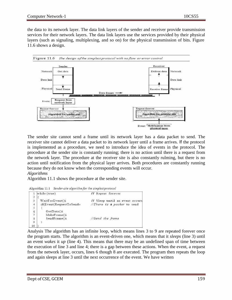
Computer Network-1 10CS55
Dept of CSE, GCEM 159
the data to its network layer. The data link layers of the sender and receiver provide transmission
services for their network layers. The data link layers use the services provided by their physical
layers (such as signaling, multiplexing, and so on) for the physical transmission of bits. Figure
11.6 shows a design.
The sender site cannot send a frame until its network layer has a data packet to send. The
receiver site cannot deliver a data packet to its network layer until a frame arrives. If the protocol
is implemented as a procedure, we need to introduce the idea of events in the protocol. The
procedure at the sender site is constantly running; there is no action until there is a request from
the network layer. The procedure at the receiver site is also constantly rulming, but there is no
action until notification from the physical layer arrives. Both procedures are constantly running
because they do not know when the corresponding events will occur.
Algorithms
Algorithm 11.1 shows the procedure at the sender site.
Analysis The algorithm has an infinite loop, which means lines 3 to 9 are repeated forever once
the program starts. The algorithm is an event-driven one, which means that it sleeps (line 3) until
an event wakes it up (line 4). This means that there may be an undefined span of time between
the execution of line 3 and line 4; there is a gap between these actions. When the event, a request
from the network layer, occurs, lines 6 though 8 are executed. The program then repeats the loop
and again sleeps at line 3 until the next occurrence of the event. We have written

Computer Network-1 10CS55
Dept of CSE, GCEM 160
pseudocode for the main process and SendFrame. GetData takes a data packet from the network
layer, Make Frame0 adds a header and delimiter flags to the data packet to make a frame, and
SendFrame0 delivers the frame to the physical layer for transmission.
Algorithm 11.2 shows the procedure at the receiver site.
Analysis This algorithm has the same format as Algorithm 11.1, except that the direction of the
frames and data is upward. The event here is the arrival of a data frame. After the event occurs,
the data link layer receives the frame from the physical layer using the ReceiveFrame process,
extracts the data from the frame using the ExtractData process, and delivers the data to the
network layer using the DeliverData process. Here, we also have an event-driven algorithm
because the algorithm never knows when the data frame will arrive.
Stop-and-Wait Protocol
If data frames arrive at the receiver site faster than they can be processed, the frames must be
stored until their use. Normally, the receiver does not have enough storage space, especially if it
is receiving data from many sources. This may result in either the discarding of frames or denial
of service. To prevent the receiver from becoming overwhelmed with frames. There must be
feedback from the receiver to the sender. The protocol we discuss now is called the Stop-and-
Wait Protocol because the sender sends one frame, stops until it receives confirmation from the
receiver (okay to go ahead), and then sends the next frame.
Design
Figure 11.8 illustrates the mechanism. Comparing this figure with Figure 11.6, can see the traffic
on the forward channel (from sender to receiver) and the reverse channel. At any time, there is
either one data frame on the forward channel or one ACK frame on the reverse channel. We
therefore need a half-duplex link.
Algorithms
Algorithm 11.3 is for the sender site.

Computer Network-1 10CS55
Dept of CSE,GCEM 160
Analysis Here two events can occur: a request from the network layer or an arrival notification from the physical layer. The responses to these events must alternate. In other words, after a
frame is sent, the algorithm must ignore another network layer request until that frame is
acknowledged. We know that two arrival events cannot happen one after another because the
channel is error-free and does not duplicate the frames. The requests from the network layer,
however, may happen one after another without an arrival event in between. To prevent the
immediate sending of the data frame. there are several methods used a simple canSend variable
that can either be true or false. When a frame is sent, the variable is set to false to indicate that a
new network request cannot be sent until can Send is true. When an ACK is received, can Send
is set to true to allow the sending of the next frame.
Algorithm 11.4 shows the procedure at the receiver site.

Computer Network-1 10CS55
Dept of CSE,GCEM 161
Analysis This is very similar to Algorithm 11.2 with one exception. After the data frame arrives,
the receiver sends an ACK frame (line 9) to acknowledge the receipt and allow the sender
to send the next frame.
11.5 NOISY CHANNELS
Stop-and-Wait Automatic Repeat Request Our first protocol, called the Stop-and-Wait Automatic Repeat Request (Stop-and Wait ARQ),
adds a simple error control mechanism to the Stop-and-Wait Protocol. Let us see how this
protocol detects and corrects errors. To detect and correct corrupted frames, we need to add
redundancy bits to our data frame. When the frame arrives at the receiver site, it is checked and if
it is corrupted, it is silently discarded. The detection of errors in this protocol is manifested by
the silence of the receiver.
Lost frames are more difficult to handle than corrupted ones. In our previous protocols, there was
no way to identify a frame. The received frame could be the correct one, or a duplicate, or a
frame out of order. The solution is to number the frames. When the receiver receives a data
frame that is out of order, this means that frames were either lost or duplicated.
The completed lost frames need to be resent in this protocol. If the receiver does not respond
when there is an error, how can the sender know which frame to resend? To remedy this
problem, the sender keeps a copy of the sent frame. At the same time, it starts a timer. If the
timer expires and there is no ACK for the sent frame, the frame is resent, the copy is held, and
the timer is restarted. Since the protocol uses the stop-and-wait mechanism, there is only one
specific frame that needs an ACK even though several copies of the same frame can be in the
network.
Since an ACK frame can also be corrupted and lost, it too needs redundancy bits and a sequence
number. The ACK frame for this protocol has a sequence number field. In this protocol, the
sender simply discards a corrupted ACK frame or ignores an out-of-order one.
Sequence Numbers
As we discussed, the protocol specifies that frames need to be numbered. This is done by using
sequence numbers. A field is added to the data frame to hold the sequence number of that frame.
One important consideration is the range of the sequence numbers. Since we want to minimize
the frame size, we look for the smallest range that provides unambiguous communication. The
sequence numbers of course can wrap around. Decide that the field is m bits long, the sequence
numbers start from 0, go to 2m - 1, and then are repeated.
Let us reason out the range of sequence numbers we need. Assume we have used x as a sequence
number; we only need to use x + 1 after that. There is no need for x + 2. To show this, assume
that the sender has sent the frame numbered x. Three things can happen.
4. The frame arrives safe and sound at the receiver site; the receiver sends an acknowledgment.
The acknowledgment arrives at the sender site, causing the sender to send
the next frame numbered x + 1.
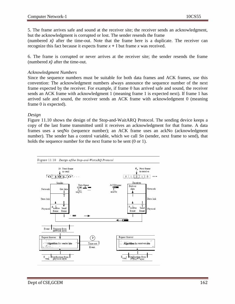
Computer Network-1 10CS55
Dept of CSE,GCEM 162
5. The frame arrives safe and sound at the receiver site; the receiver sends an acknowledgment,
but the acknowledgment is corrupted or lost. The sender resends the frame
(numbered x) after the time-out. Note that the frame here is a duplicate. The receiver can
recognize this fact because it expects frame x + I but frame x was received.
6. The frame is corrupted or never arrives at the receiver site; the sender resends the frame
(numbered x) after the time-out.
Acknowledgment Numbers
Since the sequence numbers must be suitable for both data frames and ACK frames, use this
convention: The acknowledgment numbers always announce the sequence number of the next
frame expected by the receiver. For example, if frame 0 has arrived safe and sound, the receiver
sends an ACK frame with acknowledgment 1 (meaning frame 1 is expected next). If frame 1 has
arrived safe and sound, the receiver sends an ACK frame with acknowledgment 0 (meaning
frame 0 is expected).
Design
Figure 11.10 shows the design of the Stop-and-WaitARQ Protocol. The sending device keeps a
copy of the last frame transmitted until it receives an acknowledgment for that frame. A data
frames uses a seqNo (sequence number); an ACK frame uses an ackNo (acknowledgment
number). The sender has a control variable, which we call Sn (sender, next frame to send), that
holds the sequence number for the next frame to be sent (0 or 1).
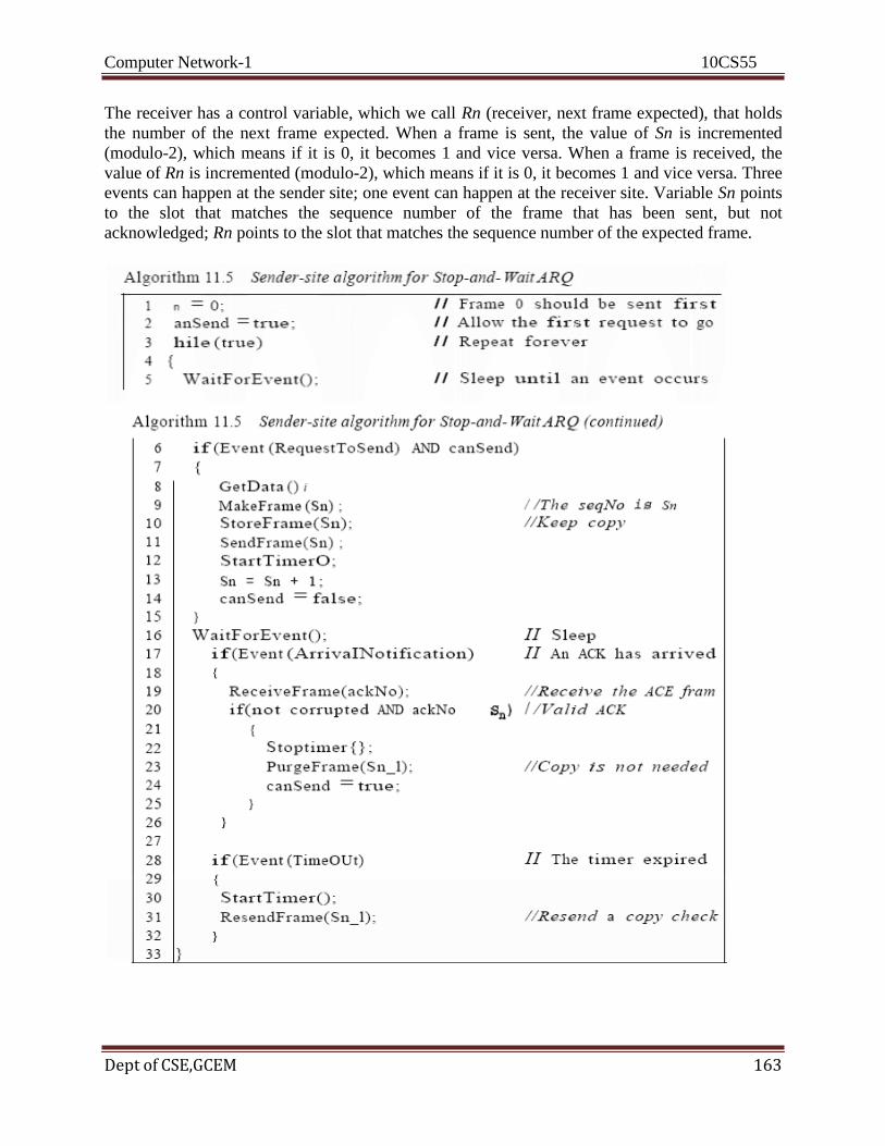
Computer Network-1 10CS55
Dept of CSE,GCEM 163
The receiver has a control variable, which we call Rn (receiver, next frame expected), that holds
the number of the next frame expected. When a frame is sent, the value of Sn is incremented
(modulo-2), which means if it is 0, it becomes 1 and vice versa. When a frame is received, the
value of Rn is incremented (modulo-2), which means if it is 0, it becomes 1 and vice versa. Three
events can happen at the sender site; one event can happen at the receiver site. Variable Sn points
to the slot that matches the sequence number of the frame that has been sent, but not
acknowledged; Rn points to the slot that matches the sequence number of the expected frame.
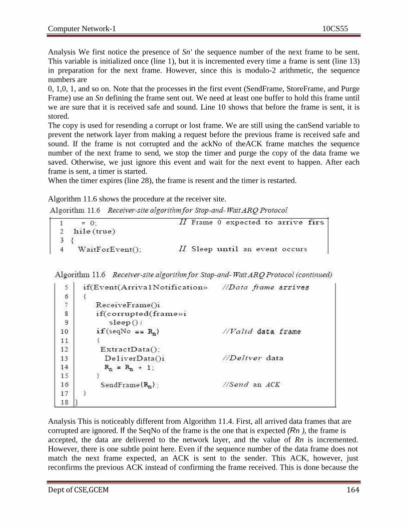
Computer Network-1 10CS55
Dept of CSE,GCEM 164
Analysis We first notice the presence of Sn' the sequence number of the next frame to be sent.
This variable is initialized once (line 1), but it is incremented every time a frame is sent (line 13)
in preparation for the next frame. However, since this is modulo-2 arithmetic, the sequence
numbers are
0, 1,0, 1, and so on. Note that the processes in the first event (SendFrame, StoreFrame, and Purge
Frame) use an Sn defining the frame sent out. We need at least one buffer to hold this frame until
we are sure that it is received safe and sound. Line 10 shows that before the frame is sent, it is
stored.
The copy is used for resending a corrupt or lost frame. We are still using the canSend variable to
prevent the network layer from making a request before the previous frame is received safe and
sound. If the frame is not corrupted and the ackNo of theACK frame matches the sequence
number of the next frame to send, we stop the timer and purge the copy of the data frame we
saved. Otherwise, we just ignore this event and wait for the next event to happen. After each
frame is sent, a timer is started.
When the timer expires (line 28), the frame is resent and the timer is restarted.
Algorithm 11.6 shows the procedure at the receiver site.
Analysis This is noticeably different from Algorithm 11.4. First, all arrived data frames that are
corrupted are ignored. If the SeqNo of the frame is the one that is expected (Rn ), the frame is
accepted, the data are delivered to the network layer, and the value of Rn is incremented.
However, there is one subtle point here. Even if the sequence number of the data frame does not
match the next frame expected, an ACK is sent to the sender. This ACK, however, just
reconfirms the previous ACK instead of confirming the frame received. This is done because the

Computer Network-1 10CS55
Dept of CSE,GCEM 165
receiver assumes that the previous ACK might have been lost; the receiver is sending a duplicate
frame. The resent ACK may solve the problem before the time-out does it.
Efficiency
The Stop-and-WaitARQ discussed in the previous section is very inefficient if our channel
is thick and long. By thick, we mean that our channel has a large bandwidth; by long, mean the
round-trip delay is long. The product of these two is called the bandwidth delay product, as we
discussed in Chapter 3. We can think of the channel as a pipe. The bandwidth-delay product then
is the volume of the pipe in bits. The pipe is always there. If we do not use it, we are inefficient.
The bandwidth-delay product is a measure of the number of bits we can send out of our system
while waiting for news from the receiver.
Pipelining
In networking and in other areas, a task is often begun before the previous task has ended.
This is known as pipelining. There is no pipelining in Stop-and-Wait ARQ because need to wait
for a frame to reach the destination and be acknowledged before the next frame can be sent.
However, pipelining does apply to our next two protocols because several frames can be sent
before we receive news about the previous frames. Pipelining improves the efficiency of the
transmission if the number of bits in transition is large with respect to the bandwidth-delay
product.
Go-Back-N Automatic Repeat Request
To improve the efficiency of transmission (filling the pipe), multiple frames must be in transition
while waiting for acknowledgment. In other words, we need to let more than one frame be
outstanding to keep the channel busy while the sender is waiting for acknowledgment. In this
section, we discuss one protocol that can achieve this goal; in the next section, we discuss a
second. The first is called Go-Back-N Automatic Repeat Request (the rationale for the name will
become clear later). In this protocol we can send several frames before receiving
acknowledgments; we keep a copy of these frames until the acknowledgments arrive.
Sequence Numbers
Frames from a sending station are numbered sequentially. However, because we need to include
the sequence number of each frame in the header, we need to set a limit. If the header of the
frame allows m bits for the sequence number, the sequence numbers range from 0 to 2m - 1. For
example, if m is 4, the only sequence numbers are 0 through 15 inclusive. However, we can
repeat the sequence. So the sequence numbers are 0, 1,2,3,4,5,6, 7,8,9, 10, 11, 12, 13, 14, 15,0,
1,2,3,4,5,6,7,8,9,10, 11, ... In other words, the sequence numbers are modulo-2m
. Sliding Window
In this protocol (and the next), the sliding window is an abstract concept that defines the range of
sequence numbers that is the concern of the sender and receiver. In other words, the sender and
receiver need to deal with only part of the possible sequence numbers. The range which is the
concern of the sender is called the send sliding window; the range that is the concern of the

Computer Network-1 10CS55
Dept of CSE,GCEM 166
receiver is called the receive sliding window. We discuss both here. The send window is an
imaginary box covering the sequence numbers of the data frames which can be in transit. In each
window position, some of these sequence numbers define the frames that have been sent; others
define those that can be sent. The maximum size of the window is 2m - 1 for reasons that we
discuss later. In this chapter, we let the size be fixed and set to the maximum value, but we will
see in future chapters that some protocols may have a variable window size. Figure 11.12 shows
a sliding window of size 15 (m =4). The window at any time divides the possible sequence
numbers into four regions. The first region, from the far left to the left wall of the window,
defines the sequence
numbers belonging to frames that are already acknowledged. The sender does not worry about
these frames and keeps no copies of them. The second region, colored in Figure 11.12a, defines
the range of sequence numbers belonging to the frames that are sent and have an unknown status.
The sender needs to wait to find out if these frames have been received or were lost. We call
these outstanding frames. The third range, white in the figure, defines the range of sequence
numbers for frames that can be sent; however, the corresponding data packets have not yet been
received from the network layer. Finally, the fourth region defines sequence numbers that cannot
be used until the window slides, as we see next.
The window itself is an abstraction; three variables define its size and location at any time. We
call these variables Sf(send window, the first outstanding frame), Sn (send window, the next
frame to be sent), and Ssize (send window, size). The variable Sf defines the sequence number of
the first (oldest) outstanding frame. The variable Sn holds the sequence number that will be
assigned to the next frame to be sent. Finally, the variable Ssize defines the size of the window,
which is fixed in our protocol.
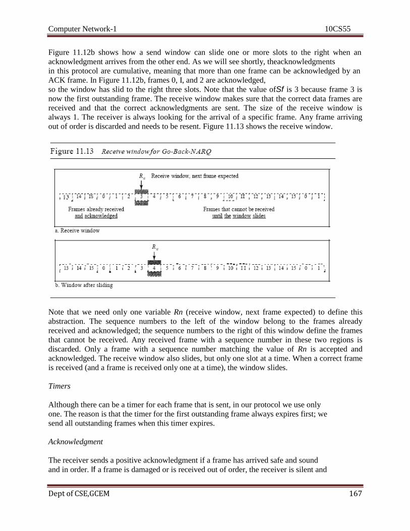
Computer Network-1 10CS55
Dept of CSE,GCEM 167
Figure 11.12b shows how a send window can slide one or more slots to the right when an
acknowledgment arrives from the other end. As we will see shortly, theacknowledgments
in this protocol are cumulative, meaning that more than one frame can be acknowledged by an
ACK frame. In Figure 11.12b, frames 0, I, and 2 are acknowledged,
so the window has slid to the right three slots. Note that the value ofSf is 3 because frame 3 is
now the first outstanding frame. The receive window makes sure that the correct data frames are
received and that the correct acknowledgments are sent. The size of the receive window is
always 1. The receiver is always looking for the arrival of a specific frame. Any frame arriving
out of order is discarded and needs to be resent. Figure 11.13 shows the receive window.
Note that we need only one variable Rn (receive window, next frame expected) to define this
abstraction. The sequence numbers to the left of the window belong to the frames already
received and acknowledged; the sequence numbers to the right of this window define the frames
that cannot be received. Any received frame with a sequence number in these two regions is
discarded. Only a frame with a sequence number matching the value of Rn is accepted and
acknowledged. The receive window also slides, but only one slot at a time. When a correct frame
is received (and a frame is received only one at a time), the window slides.
Timers
Although there can be a timer for each frame that is sent, in our protocol we use only
one. The reason is that the timer for the first outstanding frame always expires first; we
send all outstanding frames when this timer expires.
Acknowledgment
The receiver sends a positive acknowledgment if a frame has arrived safe and sound
and in order. If a frame is damaged or is received out of order, the receiver is silent and

Computer Network-1 10CS55
Dept of CSE,GCEM 168
will discard all subsequent frames until it receives the one it is expecting. The silence of
the receiver causes the timer of the unacknowledged frame at the sender site to expire. This, in
turn, causes the sender to go back and resend all frames, beginning with the one with the expired
timer. The receiver does not have to acknowledge each frame received. It can send one
cumulative acknowledgment for several frames.
Resending a Frame
When the timer expires, the sender resends all outstanding frames. For example, suppose the
sender has already sent frame 6, but the timer for frame 3 expires. This means that frame 3 has
not been acknowledged; the sender goes back and sends frames 3, 4,5, and 6\ again. That is why
the protocol is called Go-Back-N ARQ.
Design
Figure 11.14 shows the design for this protocol. As we can see, multiple frames can be in transit
in the forward direction, and multiple acknowledgments in the reverse direction. The idea is
similar to Stop-and-Wait ARQ; the difference is that the send

Computer Network-1 10CS55
Dept of CSE,GCEM 169
Window allows us to have as many frames in transition as there are slots in the send window.
Send Window Size
We can now show why the size of the send window must be less than 2m. As an example, we
choose m =2, which means the size of the window can be 2m - 1, or 3. Figure 11.15 compares a
window size of 3 against a window size of 4. If the size of the window is (less than 22) and all
three acknowledgments are lost, the frame timer expires and all three frames are resent. The
receiver =is now expecting frame 3, not frame 0, so the duplicate frame is correctly discarded.
On the other hand, if the size of the window is 4 (equal to 22) and all acknowledgments are lost,
the sender will send a duplicate of frame 0. However, this time the window of the receiver
expects to receive frame 0, so it accepts frame 0, not as a duplicate, but as the first frame in the
next cycle. This is an error.
Algorithms
Algorithm 11.7 shows the procedure for the sender in this protocol
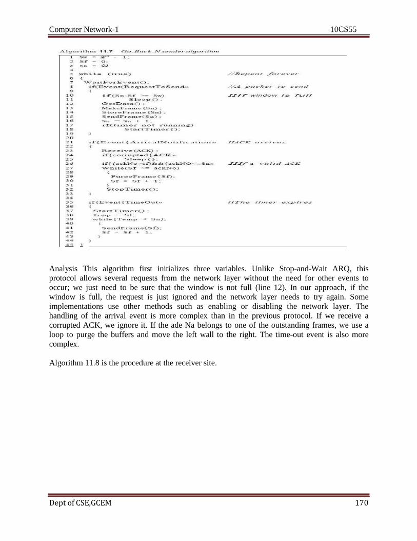
Computer Network-1 10CS55
Dept of CSE,GCEM 170
Analysis This algorithm first initializes three variables. Unlike Stop-and-Wait ARQ, this
protocol allows several requests from the network layer without the need for other events to
occur; we just need to be sure that the window is not full (line 12). In our approach, if the
window is full, the request is just ignored and the network layer needs to try again. Some
implementations use other methods such as enabling or disabling the network layer. The
handling of the arrival event is more complex than in the previous protocol. If we receive a
corrupted ACK, we ignore it. If the ade Na belongs to one of the outstanding frames, we use a
loop to purge the buffers and move the left wall to the right. The time-out event is also more
complex.
Algorithm 11.8 is the procedure at the receiver site.

Computer Network-1 10CS55
Dept of CSE,GCEM 171
Analysis This algorithm is simple. We ignore a corrupt or out-of-order frame. If a frame
arrives with an expected sequence number, we deliver the data, update the value ofRn, and send
an ACK with the ackNa showing the next frame expected.

Computer Network-1 10CS55
Dept of CSE,GCEM 172
Go-Back-N ARQ Versus Stop-and- Wait ARQ
The reader may find that there is a similarity between Go-Back-NARQ and Stop-and-Wait ARQ.
We can say that the Stop-and-WaitARQ Protocol is actually a Go-Back-NARQ in which there
are only two sequence numbers and the send window size is 1. In other words, m = 1, 2m - 1 = 1.
In Go-Back-NARQ, we said that the addition is modulo-2m; in Stop-and-WaitARQ it is 2, which
is the same as 2m when m = 1.
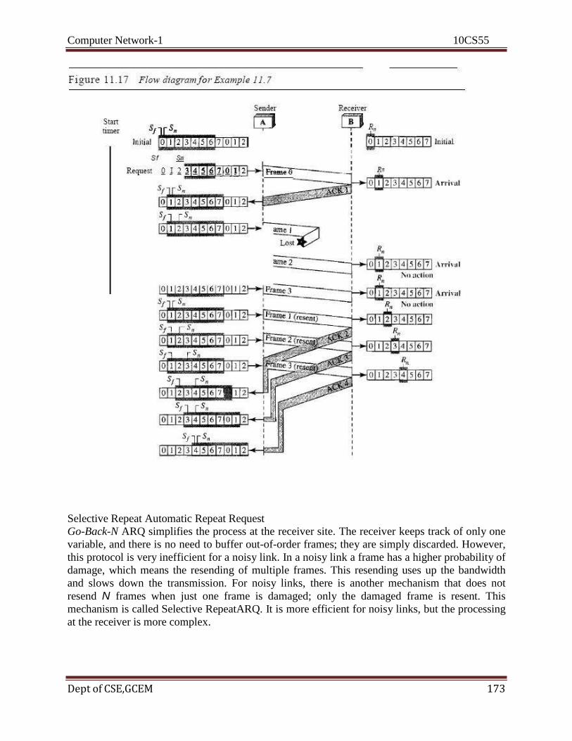
Computer Network-1 10CS55
Dept of CSE,GCEM 173
Selective Repeat Automatic Repeat Request
Go-Back-N ARQ simplifies the process at the receiver site. The receiver keeps track of only one
variable, and there is no need to buffer out-of-order frames; they are simply discarded. However,
this protocol is very inefficient for a noisy link. In a noisy link a frame has a higher probability of
damage, which means the resending of multiple frames. This resending uses up the bandwidth
and slows down the transmission. For noisy links, there is another mechanism that does not
resend N frames when just one frame is damaged; only the damaged frame is resent. This
mechanism is called Selective RepeatARQ. It is more efficient for noisy links, but the processing
at the receiver is more complex.
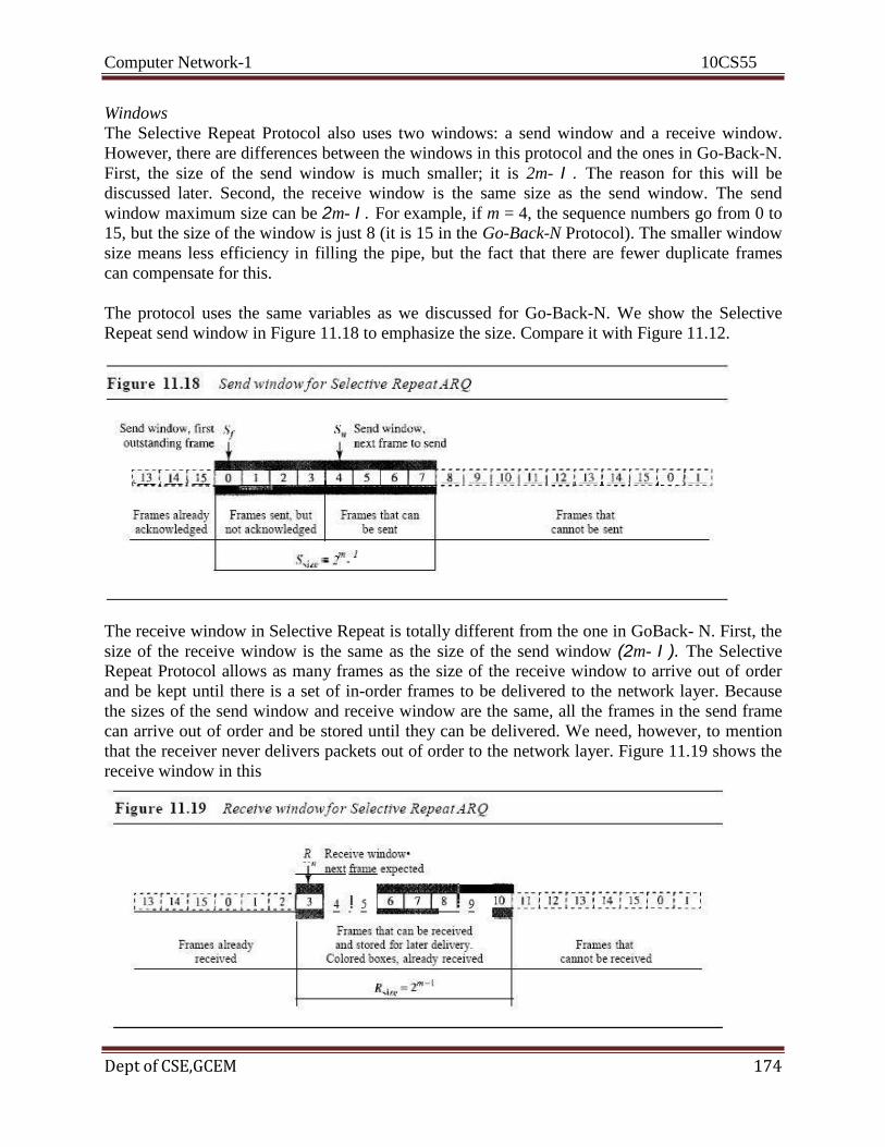
Computer Network-1 10CS55
Dept of CSE,GCEM 174
Windows
The Selective Repeat Protocol also uses two windows: a send window and a receive window.
However, there are differences between the windows in this protocol and the ones in Go-Back-N.
First, the size of the send window is much smaller; it is 2m- I . The reason for this will be
discussed later. Second, the receive window is the same size as the send window. The send
window maximum size can be 2m- I . For example, if m = 4, the sequence numbers go from 0 to
15, but the size of the window is just 8 (it is 15 in the Go-Back-N Protocol). The smaller window
size means less efficiency in filling the pipe, but the fact that there are fewer duplicate frames
can compensate for this.
The protocol uses the same variables as we discussed for Go-Back-N. We show the Selective
Repeat send window in Figure 11.18 to emphasize the size. Compare it with Figure 11.12.
The receive window in Selective Repeat is totally different from the one in GoBack- N. First, the
size of the receive window is the same as the size of the send window (2m- I ). The Selective
Repeat Protocol allows as many frames as the size of the receive window to arrive out of order
and be kept until there is a set of in-order frames to be delivered to the network layer. Because
the sizes of the send window and receive window are the same, all the frames in the send frame
can arrive out of order and be stored until they can be delivered. We need, however, to mention
that the receiver never delivers packets out of order to the network layer. Figure 11.19 shows the
receive window in this

Computer Network-1 10CS55
Dept of CSE,GCEM 175
protocol. Those slots inside the window that are colored define frames that have arrived out of
order and are waiting for their neighbors to arrive before delivery to the network layer.
Design
The design in this case is to some extent similar to the one we described for the 00Back-N, but
more complicated, as shown in Figure 11.20
Window Sizes
Windows must be at most one half of 2m. For an example, we choose m = 2, which means the
size of the window is 2m/2, or 2. Figure 11.21 compares a window size of 2 with a window size
of 3. If the size of the window is 2 and all acknowledgments are lost, the timer for frame 0
expires and frame 0 is resent. However, the window of the receiver is now expecting

Computer Network-1 10CS55
Dept of CSE,GCEM 176
frame 2, not frame 0, so this duplicate frame is correctly discarded. When the size of the window
is 3 and all acknowledgments are lost, the sender sends a duplicate of frame 0. However, this
time, the window of the receiver expects to receive frame 0 (0 is part of the window), so it
accepts frame 0, not as a duplicate, but as the first frame in the next cycle. This is clearly an
error.
Algorithms
Algorithm 11.9 shows the procedure for the sender
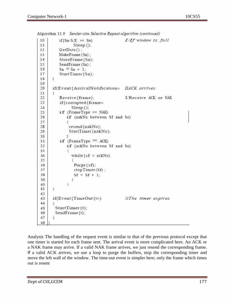
Computer Network-1 10CS55
Dept of CSE,GCEM 177
Analysis The handling of the request event is similar to that of the previous protocol except that
one timer is started for each frame sent. The arrival event is more complicated here. An ACK or
a NAK frame may arrive. If a valid NAK frame arrives, we just resend the corresponding frame.
If a valid ACK arrives, we use a loop to purge the buffers, stop the corresponding timer and
move the left wall of the window. The time-out event is simpler here; only the frame which times
out is resent
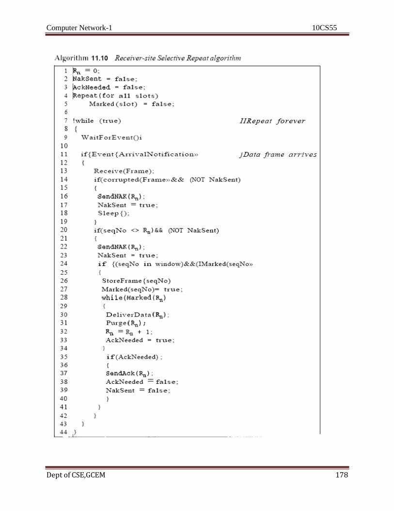
Computer Network-1 10CS55
Dept of CSE,GCEM 178

Computer Network-1 10CS55
Dept of CSE,GCEM 179
Analysis Here we need more initialization. In order not to overwhelm the other side with NAKs,
we use a variable called NakSent. To know when we need to send an ACK, we use a variable
called AckNeeded. Both of these are initialized to false. We also use a set of variables to mark
the slots in the receive window once the corresponding frame has arrived and is stored. If we
receive a corrupted frame and a NAK has not yet been sent, we send a NAK to tell the other site
that we have not received the frame we expected. If the frame is not corrupted and the sequence
number is in the window, we store the frame and mark the slot. If contiguous frames, starting
from Rn have been marked, we deliver their data to the network layer and slide the window.
Figure 11.22 shows this situation.
Example 11.8
This example is similar to Example 11.3 in which frame 1 is lost. We show how Selective
Repeat behaves in this case. Figure 11.23 shows the situation.
One main difference is the number of timers. Here, each frame sent or resent needs a timer,
which means that the timers need to be numbered (0, 1,2, and 3). The timer for frame starts at the
first request, but stops when the ACK for this frame arrives. The timer for frame 1 starts at the

Computer Network-1 10CS55
Dept of CSE,GCEM 180
second request, restarts when a NAK arrives, and finally stops when the last ACK arrives. The
other two timers start when the corresponding frames are sent and stop at the last arrival event.
At the receiver site we need to distinguish between the acceptance of a frame and its delivery to
the network layer. At the second arrival, frame 2 arrives and is stored and marked (colored slot),
but it cannot be delivered because frame 1 is missing. At the next arrival, frame 3 arrives and is
marked and stored, but still none of the frames can be delivered. Only at the last arrival, when
finally a copy of frame 1 arrives, can frames 1, 2, and 3 be delivered to the network layer. There
are two conditions for the delivery of frames to the network layer: First, a set of consecutive
frames must have arrived. Second, the set starts from the beginning of the window. After the first
arrival, there was only one frame and it started from the beginning of the window. After the last
arrival, there are three frames and the first one starts from the beginning of the window.
Another important point is that a NAK is sent after the second arrival, but not after the third,
although both situations look the same. The reason is that the protocol does not want to crowd
the network with unnecessary NAKs and unnecessary resent frames. The second NAK would
still be NAKI to inform the sender to resend frame 1 again; this has already been done. The first
NAK sent is remembered (using the nakSent variable) and is not sent again until the frame
slides. A NAK is sent once for each window position and defines the first slot in the window.
The next point is about the ACKs. Notice that only two ACKs are sent here.
The first one acknowledges only the first frame; the second one acknowledges three frames. In
Selective Repeat, ACKs are sent when data are delivered to the network layer. If the data
belonging to nframes are delivered in one shot, only one ACK is sent for all of them.
Piggybacking The three protocols we discussed in this section are all unidirectional: data frames flow in only
one direction although control information such as ACK and NAK frames can travel in the other
direction. In real life, data frames are normally flowing in both directions:
From node A to node B and from node B to node A. This means that the control information also
needs to flow in both directions. A technique called piggybacking is used to improve the
efficiency of the bidirectional protocols. When a frame is carrying data from A to B, it can also
carry control information about arrived (or lost) frames from B; when a frame is carrying data
from B to A, it can also carry control information about the arrived (or lost) frames from A.
We show the design for a Go-Back-N ARQ using piggybacking in Figure 11.24. Note that each
node now has two windows: one send window and one receive window. Both also need to use a
timer. Both are involved in three types of events: request, arrival, and time-out. However, the
arrival event here is complicated; when a frame arrives, the site needs to handle control
information as well as the frame itself. Both of these concerns
must be taken care of in one event, the arrival event. The request event uses only the send
window at each site; the arrival event needs to use both windows.
An important point about piggybacking is that both sites must use the same algorithm. This
algorithm is complicated because it needs to combine two arrival events
into one.

Computer Network-1 10CS55
Dept of CSE,GCEM 181
11.8 HDLC
High-level Data Link Control (HDLC) is a bit-oriented protocol for communication over point-
to-point and multipoint links.
Configurations and Transfer Modes
HDLC provides two common transfer modes that can be used in different configurations: normal
response mode (NRM) and asynchronous balanced mode (ABM).
Normal Response Mode
In normal response mode (NRM), the station configuration is unbalanced. We have one primary
station and multiple secondary stations. A primary station can send commands; a secondary
station can only respond. The NRM is used for both point-to-point and multiple-point links, as
shown in Figure 11.25.

Computer Network-1 10CS55
Dept of CSE,GCEM 182
Asynchronous Balanced Mode
In asynchronous balanced mode (ABM), the configuration is balanced. The link is point-to-point,
and each station can function as a primary and a secondary (acting as peers), as shown in Figure
11.26. This is the common mode today.
Frames
To provide the flexibility necessary to support all the options possible in the modes and
configurations just described, HDLC defines three types of frames: information frames (I-
frames), supervisory frames (S-frames), and unnumbered frames (V-frames). Each type of frame
serves as an envelope for the transmission of a different type of message. I-frames are used to
transport user data and control information relating to user data (piggybacking). S-frames are
used only to transport control information. V-frames are reserved for system management.
Information carried by V-frames is intended for managing the link itself.
Frame Format
Each frame in HDLC may contain up to six fields, as shown in Figure 11.27: a beginning flag
field, an address field, a control field, an information field, a frame check sequence (FCS) field,
and an ending flag field. In multiple-frame transmissions, the ending flag of one frame can serve
as the beginning flag of the next frame.

Computer Network-1 10CS55
Dept of CSE,GCEM 183
Fields
Let us now discuss the fields and their use in different frame types.
o Flag field. The flag field of an HDLC frame is an 8-bit sequence with the bit pattern 01111110
that identifies both the beginning and the end of a frame and serves as a synchronization pattern
for the receiver.
o Address field. The second field of an HDLC frame contains the address of the secondary
station. If a primary station created the frame, it contains a to address. If a secondary creates the
frame, it contains afrom address. An address field can be 1 byte or several bytes long, depending
on the needs of the network. One byte can identify up to 128 stations (l bit is used for another
purpose). Larger networks require multiple-byte address fields. If the address field is only 1 byte,
the last bit is always a 1. If the address is more than 1 byte, all bytes but the last one will end
with 0; only the last will end with 1. Ending each intermediate byte with 0 indicates to the
receiver that there are more address bytes to come.
o Control field. The control field is a 1- or 2-byte segment of the frame used for flow and error
control. The interpretation of bits in this field depends on the frame type. We discuss this field
later and describe its format for each frame type.
o Information field. The information field contains the user's data from the network layer or
management information. Its length can vary from one network to another.
o FCS field. The frame check sequence (FCS) is the HDLC error detection field. It can contain
either a 2- or 4-byte ITU-T CRC.
Control Field The control field determines the type of frame and defines its functionality. So let us discuss the
format of this field in greater detail. The format is specific for the type of frame, as shown in
Figure 11.28.
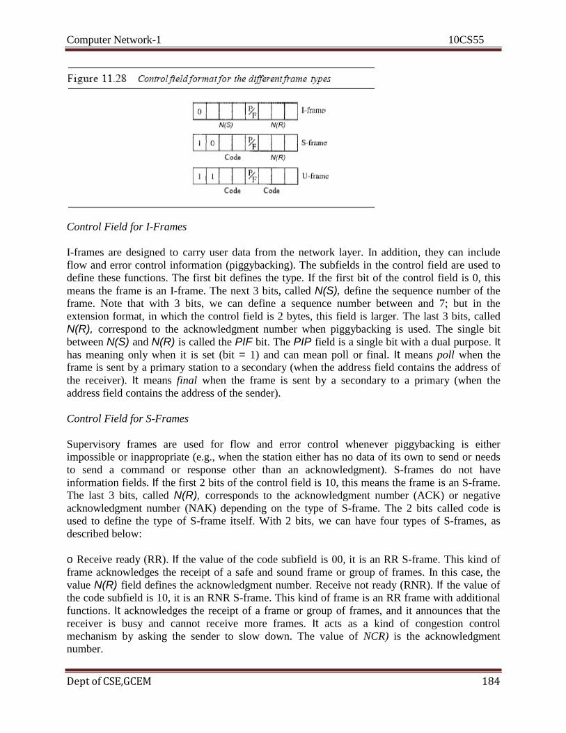
Computer Network-1 10CS55
Dept of CSE,GCEM 184
Control Field for I-Frames
I-frames are designed to carry user data from the network layer. In addition, they can include
flow and error control information (piggybacking). The subfields in the control field are used to
define these functions. The first bit defines the type. If the first bit of the control field is 0, this
means the frame is an I-frame. The next 3 bits, called N(S), define the sequence number of the
frame. Note that with 3 bits, we can define a sequence number between and 7; but in the
extension format, in which the control field is 2 bytes, this field is larger. The last 3 bits, called
N(R), correspond to the acknowledgment number when piggybacking is used. The single bit
between N(S) and N(R) is called the PIF bit. The PIP field is a single bit with a dual purpose. It has meaning only when it is set (bit = 1) and can mean poll or final. It means poll when the
frame is sent by a primary station to a secondary (when the address field contains the address of
the receiver). It means final when the frame is sent by a secondary to a primary (when the
address field contains the address of the sender).
Control Field for S-Frames
Supervisory frames are used for flow and error control whenever piggybacking is either
impossible or inappropriate (e.g., when the station either has no data of its own to send or needs
to send a command or response other than an acknowledgment). S-frames do not have
information fields. If the first 2 bits of the control field is 10, this means the frame is an S-frame.
The last 3 bits, called N(R), corresponds to the acknowledgment number (ACK) or negative
acknowledgment number (NAK) depending on the type of S-frame. The 2 bits called code is
used to define the type of S-frame itself. With 2 bits, we can have four types of S-frames, as
described below:
o Receive ready (RR). If the value of the code subfield is 00, it is an RR S-frame. This kind of
frame acknowledges the receipt of a safe and sound frame or group of frames. In this case, the
value N(R) field defines the acknowledgment number. Receive not ready (RNR). If the value of
the code subfield is 10, it is an RNR S-frame. This kind of frame is an RR frame with additional
functions. It acknowledges the receipt of a frame or group of frames, and it announces that the
receiver is busy and cannot receive more frames. It acts as a kind of congestion control
mechanism by asking the sender to slow down. The value of NCR) is the acknowledgment
number.

Computer Network-1 10CS55
Dept of CSE,GCEM 185
o Reject (REJ). If the value of the code subfield is 01, it is a REJ S-frame. This is a NAK frame,
but not like the one used for Selective Repeat ARQ. It is a NAK that can be used in Go-Back-N
ARQ to improve the efficiency of the process by informing the sender, before the sender time
expires, that the last frame is lost or damaged. The value of NCR) is the negative
acknowledgment number.
o Selective reject (SREJ). If the value of the code subfield is 11, it is an SREJ S-frame. This is a
NAK frame used in Selective Repeat ARQ. Note that the HDLC Protocol uses the term selective
reject instead of selective repeat. The value of N(R) is the negative acknowledgment number.
Control Field for V-Frames
Unnumbered frames are used to exchange session management and control information between
connected devices. Unlike S-frames, U-frames contain an information field, but one used for
system management information, not user data. As with S-frames, however, much of the
information carried by U-frames is contained in codes included in the control field. U-frame
codes are divided into two sections: a 2-bit prefix before the PtF bit and a 3-bit suffix after the
PtF bit. Together, these two segments (5 bits) can be used to create up to 32 different types of U-
frames. Some of the more common types are shown in Table 11.1.
Example 11.9: Connection/Disconnection
Figure 11.29 shows how V-frames can be used for connection establishment and connection
release. Node A asks for a connection with a set asynchronous balanced mode = (SABM) frame;
node B gives a positive response with an unnumbered acknowledgment (VA) frame. After these
two exchanges, data can be transferred between the two nodes (not shown in the figure). After
data transfer, node A sends a DISC (disconnect) frame to release the connection; it is confirmed
by node B responding with a VA (unnumbered acknowledgment).
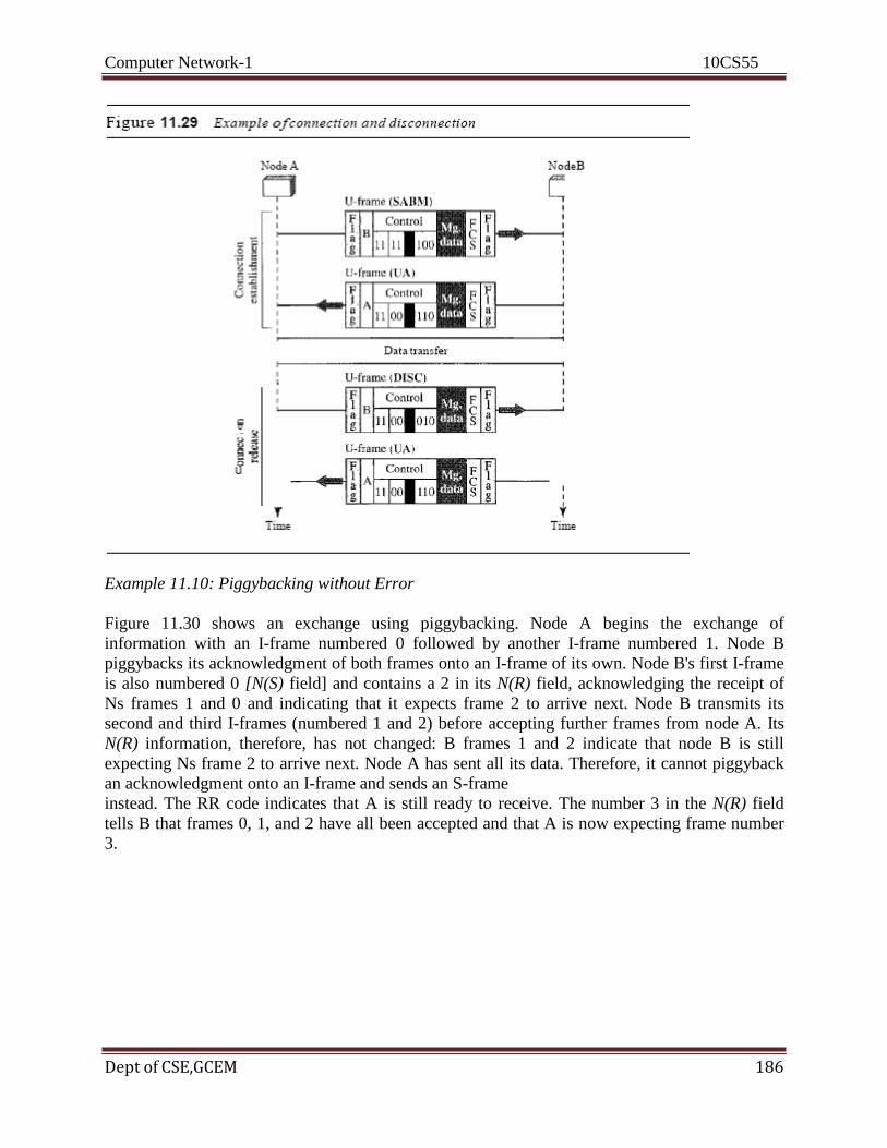
Computer Network-1 10CS55
Dept of CSE,GCEM 186
Example 11.10: Piggybacking without Error
Figure 11.30 shows an exchange using piggybacking. Node A begins the exchange of
information with an I-frame numbered 0 followed by another I-frame numbered 1. Node B
piggybacks its acknowledgment of both frames onto an I-frame of its own. Node B's first I-frame
is also numbered 0 [N(S) field] and contains a 2 in its N(R) field, acknowledging the receipt of
Ns frames 1 and 0 and indicating that it expects frame 2 to arrive next. Node B transmits its
second and third I-frames (numbered 1 and 2) before accepting further frames from node A. Its
N(R) information, therefore, has not changed: B frames 1 and 2 indicate that node B is still
expecting Ns frame 2 to arrive next. Node A has sent all its data. Therefore, it cannot piggyback
an acknowledgment onto an I-frame and sends an S-frame
instead. The RR code indicates that A is still ready to receive. The number 3 in the N(R) field
tells B that frames 0, 1, and 2 have all been accepted and that A is now expecting frame number
3.
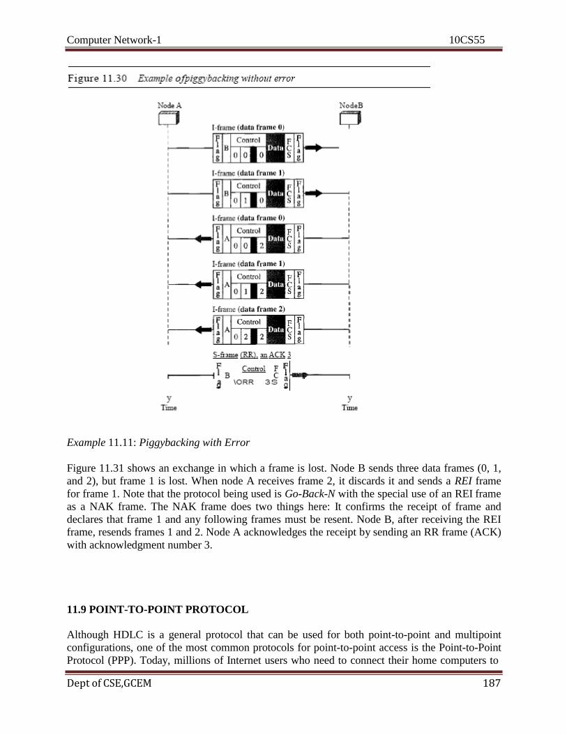
Computer Network-1 10CS55
Dept of CSE,GCEM 187
Example 11.11: Piggybacking with Error
Figure 11.31 shows an exchange in which a frame is lost. Node B sends three data frames (0, 1,
and 2), but frame 1 is lost. When node A receives frame 2, it discards it and sends a REI frame
for frame 1. Note that the protocol being used is Go-Back-N with the special use of an REI frame
as a NAK frame. The NAK frame does two things here: It confirms the receipt of frame and
declares that frame 1 and any following frames must be resent. Node B, after receiving the REI
frame, resends frames 1 and 2. Node A acknowledges the receipt by sending an RR frame (ACK)
with acknowledgment number 3.
11.9 POINT-TO-POINT PROTOCOL
Although HDLC is a general protocol that can be used for both point-to-point and multipoint
configurations, one of the most common protocols for point-to-point access is the Point-to-Point
Protocol (PPP). Today, millions of Internet users who need to connect their home computers to

Computer Network-1 10CS55
Dept of CSE,GCEM 188
the server of an Internet service provider use PPP. The majority of these users have a traditional
modem; they are connected to the Internet through a telephone line, which provides the services
of the physical layer. But to control and
manage the transfer of data, there is a need for a point-to-point protocol at the data link
layer. PPP is by far the most common. PPP provides several services:
5. PPP defines the format of the frame to be exchanged between devices.
6. PPP defines how two devices can negotiate the establishment of the link and the
exchange of data.
7. PPP defines how network layer data are encapsulated in the data link frame.
8. PPP defines how two devices can authenticate each other.
5. PPP provides multiple network layer services supporting a variety of network layer

Computer Network-1 10CS55
Dept of CSE,GCEM 189
protocols.
8. PPP provides connections over multiple links.
9. PPP provides network address configuration. This is particularly useful when a home
user needs a temporary network address to connect to the Internet.
On the other hand, to keep PPP simple, several services are missing:
I. PPP does not provide flow control. A sender can send several frames one after another
with no concern about overwhelming the receiver. 4. PPP has a very simple mechanism for error control. A CRC field is used to detect
errors. If the frame is corrupted, it is silently discarded; the upper-layer protocol needs
to take care of the problem. Lack of error control and sequence numbering may cause a
packet to be received out of order.
5. PPP does not provide a sophisticated addressing mechanism to handle frames in a
multipoint configuration.
Framing
PPP is a byte-oriented protocol. Framing is done according to the discussion of byte oriented
protocols at the beginning of this chapter.
Frame Format
Figure 11.32 shows the format of a PPP frame. The description of each field follows:
o Flag. A PPP frame starts and ends with a I-byte flag with the bit pattern 01111110. Although
this pattern is the same as that used in HDLC, there is a big difference. PPP is a byte-oriented
protocol; HDLC is a bit-oriented protocol. The flag is treated as a byte, as we will explain later.
o Address. The address field in this protocol is a constant value and set to 11111111 (broadcast
address). During negotiation (discussed later), the two parties may agree to omit this byte. o Control. This field is set to the constant value 11000000 (imitating unnumbered frames in
HDLC). As we will discuss later, PPP does not provide any flow control. Error control is also
limited to error detection. This means that this field is not needed at all, and again, the two
parties can agree, during negotiation, to omit this byte. o Protocol. The protocol field defines
what is being carried in the data field: either user data or other information. We discuss this field
in detail shortly. This field is by default 2 bytes long, but the two parties can agree to use only 1
byte. o Payload field. This field carries either the user data or other information that we will
discuss shortly. The data field is a sequence of bytes with the default of a maximum of 1500
bytes; but this can be changed during negotiation. The data field is byte stuffed if the flag byte
pattern appears in this field. Because there is no field defining the size of the data field, padding

Computer Network-1 10CS55
Dept of CSE,GCEM 190
is needed if the size is less than the maximum default value or the maximum negotiated value. o
FCS. The frame check sequence (FCS) is simply a 2-byte or 4-byte standard CRe.
Byte Stuffing
The similarity between PPP and ends at the frame format. PPP, as we discussed before, is a
byte-oriented protocol totally different from HDLC. As a byte-oriented protocol, the flag in PPP
is a byte and needs to be escaped whenever it appears in the data section of the frame. The
escape byte is 01111101, which means that every time the flag like pattern appears in the data,
this extra byte is stuffed to tell the receiver that the next byte is not a flag.
Transition Phases
A PPP connection goes through phases which can be shown in a transition phase diagram (see
Figure 11.33).
Dead. In the dead phase the link is not being used. There is no active carrier (at the physical
layer) and the line is quiet.
D Establish. When one of the nodes starts the communication, the connection goes into this
phase. In this phase, options are negotiated between the two parties. If the negotiation is
successful, the system goes to the authentication phase (if authentication is required) or directly
to the networking phase. The link control protocol packets, discussed shortly, are used for this
purpose. Several packets may be exchanged here. D Authenticate. The authentication phase is
optional; the two nodes may decide, during the establishment phase, not to skip this phase.
However, if they decide to proceed with authentication, they send several authentication packets,
discussed later. If the result is successful, the connection goes to the networking phase;
otherwise, it goes to the termination phase. D Network. In the network phase, negotiation for the
network layer protocols takes place. PPP specifies that two nodes establish a network layer
agreement before data at the network layer can be exchanged. The reason is that PPP supports

Computer Network-1 10CS55
Dept of CSE,GCEM 191
multiple protocols at the network layer. If a node is running multiple protocols simultaneously at
the network layer, the receiving node needs to know which protocol will receive the data.
o Open. In the open phase, data transfer takes place. When a connection reaches this phase, the
exchange of data packets can be started. The connection remains in this phase until one of the
endpoints wants to terminate the connection.
o Terminate. In the termination phase the connection is terminated. Several packets
are exchanged between the two ends for house cleaning and closing the link.
Multiplexing
Although PPP is a data link layer protocol, PPP uses another set of other protocols to establish
the link, authenticate the parties involved, and carry the network layer data. Three sets of
protocols are defined to make PPP powetful: the Link Control Protocol (LCP), two
Authentication Protocols (APs), and several Network Control Protocols (NCPs). At any moment,
a PPP packet can carry data from one of these protocols in its data field, as shown in Figure
11.34. Note that there is one LCP, two APs, and several NCPs. Data may also come from several
different network layers.
Link Control Protocol
The Link Control Protocol (LCP) is responsible for establishing, maintaining, configuring, and
terminating links. It also provides negotiation mechanisms to set options between the two
endpoints. Both endpoints of the link must reach an agreement about the options before the link
can be established. See Figure 11.35. All LCP packets are carried in the payload field of the PPP
frame with the protocol field set to C021 in hexadecimal.
The code field defines the type of LCP packet. There are 11 types of packets as shown in Table
11.2

Computer Network-1 10CS55
Dept of CSE,GCEM 192
There are three categories of packets. The first category, comprising the first four packet types, is
used for link configuration during the establish phase. The second category, comprising packet
types 5 and 6, is used for link termination during the termination phase. The last five packets are
used for link monitoring and debugging. The ID field holds a value that matches a request with a
reply. One endpoint inserts a value in this field, which will be copied into the reply packet. The
length field defines the length of the entire LCP packet. The information field contains
information, such as options, needed for some LCP packets. There are many options that can be
negotiated between the two endpoints. Options are inserted in the information field of the
configuration packets. In this case, the information field is divided into three fields: option type,
option length, and option data.
Authentication Protocols
Authentication plays a very important role in PPP because PPP is designed for use over dial-up
links where verification of user identity is necessary. Authentication means validating the
identity of a user who needs to access a set of resources. PPP has created two protocols for
authentication: Password Authentication Protocol and Challenge Handshake Authentication
Protocol. Note that these protocols are used during the authentication phase.

Computer Network-1 10CS55
Dept of CSE,GCEM 193
PAP The Password Authentication Protocol (PAP) is a simple authentication procedure with a
two-step process:
3. The user who wants to access a system sends an authentication identification (usually the user
name) and a password.
4. The system checks the validity of the identification and password and either accepts or denies
connection.
Figure 11.36 shows the three types of packets used by PAP and how they are actually exchanged.
When a PPP frame is carrying any PAP packets, the value of the protocol field is OxC023. The
three PAP packets are authenticate-request, authenticate-ack, and authenticate-nak. The first
packet is used by the user to send the user name and password. The second is used by the system
to allow access. The third is used by the system to deny access.
CHAP The Challenge Handshake Authentication Protocol (CHAP) is a three-way hand-
shaking authentication protocol that provides greater security than PAP. In this method, the
password is kept secret; it is never sent online.
4. The system sends the user a challenge packet containing a challenge value, usually a few
bytes.
5. The user applies a predefined function that takes the challenge value and the user's own
password and creates a result. The user sends the result in the response packet to the system.
6. The system does the same. It applies the same function to the password of the user (known to
the system) and the challenge value to create a result. If the result created is the same as the

Computer Network-1 10CS55
Dept of CSE,GCEM 194
result sent in the response packet, access is granted; otherwise, it is denied. CHAP is more secure
than PAP, especially if the system continuously changes the challenge value. Even if the intruder
learns the challenge value and the result, the password is still secret. Figure 11.37 shows the
packets and how they are used.
CHAP packets are encapsulated in the PPP frame with the protocol value C223 in hexadecimal.
There are four CHAP packets: challenge, response, success, and failure. The first packet is used
by the system to send the challenge value. The second is used by the user to return the result of
the calculation. The third is used by the system to allow access to the system. The fourth is used
by the system to deny access to the system.
Network Control Protocols
PPP is a multiple-network layer protocol. It can carry a network layer data packet from
protocols defined by the Internet, OSI, Xerox, DECnet, AppleTalk, Novel, and so on. To do this,
PPP has defined a specific Network Control Protocol for each network protocol. For example,
IPCP (Internet Protocol Control Protocol) configures the link for carrying IP data packets. Xerox
CP does the same for the Xerox protocol data packets, and so on. Note that none of the NCP
packets carry network layer data; they just configure the link at the network layer for the
incoming data. IPCP One NCP protocol is the Internet Protocol Control Protocol (IPCP). This
protocol configures the link used to carry IP packets in the Internet. IPCP is especially of interest
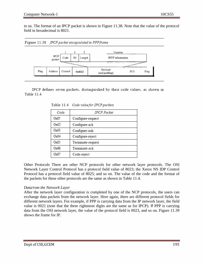
Computer Network-1 10CS55
Dept of CSE,GCEM 195
to us. The format of an IPCP packet is shown in Figure 11.38. Note that the value of the protocol
field in hexadecimal is 8021.
Other Protocols There are other NCP protocols for other network layer protocols. The OSI
Network Layer Control Protocol has a protocol field value of 8023; the Xerox NS IDP Control
Protocol has a protocol field value of 8025; and so on. The value of the code and the format of
the packets for these other protocols are the same as shown in Table 11.4.
Data/rom the Network Layer
After the network layer configuration is completed by one of the NCP protocols, the users can
exchange data packets from the network layer. Here again, there are different protocol fields for
different network layers. For example, if PPP is carrying data from the IP network layer, the field
value is 0021 (note that the three rightmost digits are the same as for IPCP). If PPP is carrying
data from the OSI network layer, the value of the protocol field is 0023, and so on. Figure 11.39
shows the frame for IP.

Computer Network-1 10CS55
Dept of CSE,GCEM 196
Multilink PPP
PPP was originally designed for a single-channel point-to-point physical link. The availability of
multiple channels in a single point-to-point link motivated the development of
Multilink PPP. In this case, a logical PPP frame is divided into several actual PPP
frames. A segment of the logical frame is carried in the payload of an actual PPP frame,
as shown in Figure 11.40. To show that the actual PPP frame is carrying a fragment of a
logical PPP frame, the protocol field is set to Ox003d. This new development adds complexity.
For example, a sequence number needs to be added to the actual PPP frame to show a fragment's
position in the logical frame.
Example 11.12
Let us go through the phases followed by a network layer packet as it is transmitted through a
PPP connection. Figure 11.41 shows the steps. For simplicity, we assume unidirectional
movement of data from the user site to the system site (such as sending an e-mail through an
ISP).
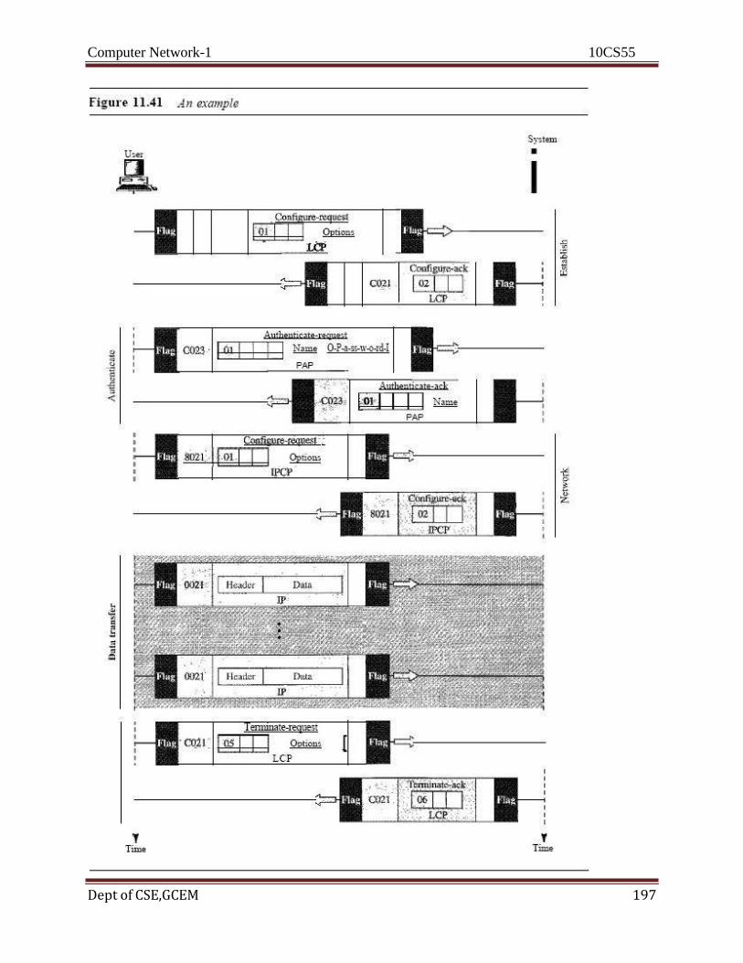
Computer Network-1 10CS55
Dept of CSE,GCEM 197
Computer Network-1 10CS55
Dept of CSE,GCEM 198
The first two frames show link establishment. We have chosen two options (not shown in the
figure): using PAP for authentication and suppressing the address control fields Frames 3 and 4
are for authentication. Frames 5 and 6 establish the network layer connection using IPCP. The
next several frames show that some IP packets are encapsulated in the PPP frame. The system
(receiver) may have been running several network layer protocols, but it knows that the
incoming data must be delivered to the IP protocol because the NCP protocol used before the
data transfer was IPCP. After data transfer, the user then terminates the data link connection,
which is acknowledged by the system. of Course the user or the system could have chosen to
terminate the network layer IPCP and keep the data link layer running if it wanted to run another
NCP protocol. The example is trivial, but it points out the similarities of the packets in LCP, AP,
and NCP. It also shows the protocol field values and code numbers for particular protocols
Recommended Questions
1. Define framing and the reason for its need
2. Compare and contrast flow control and error control 3. What are the two protocols we discussed for noiseless channels in this
chapter?
4. Explain the reason for moving from the Stop-and-Wait ARQ Protocol to
the 00Back NARQ Protocol
5. Compare and contrast the Go-Back-NARQ Protocol with Selective-
RepeatARQ
6. ompare and contrast HDLC with PPP. Which one is byte-oriented;
which one is bit oriented.
7. Define piggybacking and its usefulness
8. Which of the protocols described in this chapter utilize pipelining?

Computer Network-1 10CS55
Dept of CSE,GCEM 199
COMPUTER NETWORKS – I
Subject Code: 10CS55 I.A. Marks : 25
Hours/Week : 04 Exam Hours: 03
Total Hours : 52 Exam Marks: 100
UNIT- 6 7 Hours Multiple Access & Ethernet:
- Random access,
- Controlled Access,
- Channelization,
- Ethernet: IEEE standards,
- Standard Ethernet,
- Changes in the standard,
- Fast Ethernet, - Gigabit Ethernet

Computer Network-1 10CS55
Dept of CSE, GCEM 200
UNIT – VI
Chapter 5 Wired
LANs: Ethernet
5.1 IEEE STANDARDS
The relationship of the 802 Standard to the traditional OSI model is shown in the figure.
The IEEE has subdivided the data link layer into two sublayers: logical link control (LLC) and
media access control (MAC). IEEE has also created several physical layer standards for different
LAN protocols.
Data Link Layer
The data link layer in the IEEE standard is divided into two sublayers: LLC and MAC.
Logical Link Control (LLC)
In IEEE Project 802, flow control, error control, and part of the framing duties are collected
into one sublayer called the logical link control. Framing is handled in both the LLC sublayer
and the MAC sublayer.
The LLC provides one single data link control protocol for all IEEE LANs. In this way, the
LLC is different from the media access control sublayer, which provides different protocols for
different LANs. A single LLC protocol can provide interconnectivity between different LANs
because it makes the MAC sublayer transparent.

Computer Network-1 10CS55
Dept of CSE, GCEM 201
UNIT – VI Chapter 5 Wired
LANs: Ethernet
5.1 IEEE STANDARDS
The relationship of the 802 Standard to the traditional OSI model is shown in the figure.
The IEEE has subdivided the data link layer into two sublayers: logical link control (LLC) and
media access control (MAC). IEEE has also created several physical layer standards for different
LAN protocols.
Data Link Layer
The data link layer in the IEEE standard is divided into two sublayers: LLC and MAC.
Logical Link Control (LLC)
In IEEE Project 802, flow control, error control, and part of the framing duties are collected
into one sublayer called the logical link control. Framing is handled in both the LLC sublayer
and the MAC sublayer.
The LLC provides one single data link control protocol for all IEEE LANs. In this way, the
LLC is different from the media access control sublayer, which provides different protocols for
different LANs. A single LLC protocol can provide interconnectivity between different LANs
because it makes the MAC sublayer transparent.
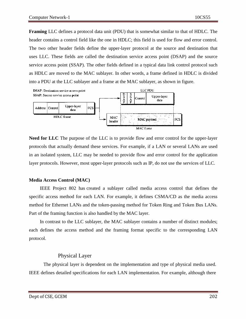
Computer Network-1 10CS55
Dept of CSE, GCEM 202
Framing LLC defines a protocol data unit (PDU) that is somewhat similar to that of HDLC. The
header contains a control field like the one in HDLC; this field is used for flow and error control.
The two other header fields define the upper-layer protocol at the source and destination that
uses LLC. These fields are called the destination service access point (DSAP) and the source
service access point (SSAP). The other fields defined in a typical data link control protocol such
as HDLC are moved to the MAC sublayer. In other words, a frame defined in HDLC is divided
into a PDU at the LLC sublayer and a frame at the MAC sublayer, as shown in figure.
Need for LLC The purpose of the LLC is to provide flow and error control for the upper-layer
protocols that actually demand these services. For example, if a LAN or several LANs are used
in an isolated system, LLC may be needed to provide flow and error control for the application
layer protocols. However, most upper-layer protocols such as IP, do not use the services of LLC.
Media Access Control (MAC)
IEEE Project 802 has created a sublayer called media access control that defines the
specific access method for each LAN. For example, it defines CSMA/CD as the media access
method for Ethernet LANs and the token-passing method for Token Ring and Token Bus LANs.
Part of the framing function is also handled by the MAC layer.
In contrast to the LLC sublayer, the MAC sublayer contains a number of distinct modules;
each defines the access method and the framing format specific to the corresponding LAN
protocol.
Physical Layer
The physical layer is dependent on the implementation and type of physical media used.
IEEE defines detailed specifications for each LAN implementation. For example, although there
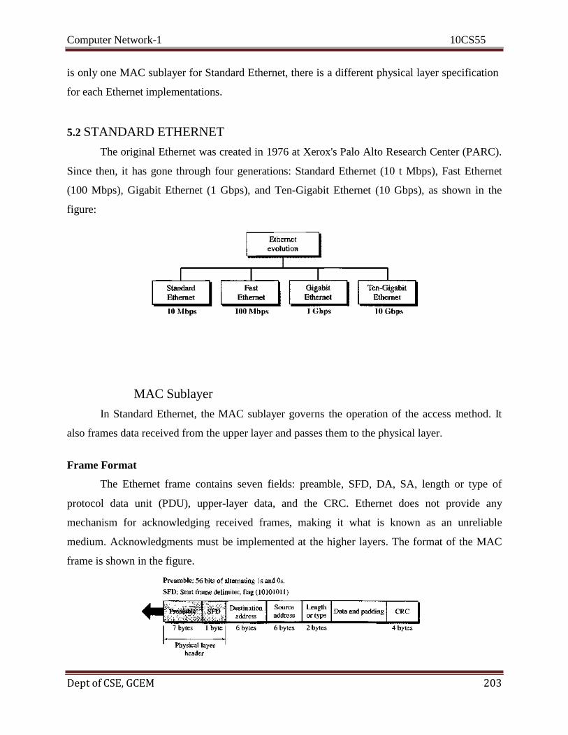
Computer Network-1 10CS55
Dept of CSE, GCEM 203
is only one MAC sublayer for Standard Ethernet, there is a different physical layer specification
for each Ethernet implementations.
5.2 STANDARD ETHERNET
The original Ethernet was created in 1976 at Xerox's Palo Alto Research Center (PARC).
Since then, it has gone through four generations: Standard Ethernet (10 t Mbps), Fast Ethernet
(100 Mbps), Gigabit Ethernet (1 Gbps), and Ten-Gigabit Ethernet (10 Gbps), as shown in the
figure:
MAC Sublayer
In Standard Ethernet, the MAC sublayer governs the operation of the access method. It
also frames data received from the upper layer and passes them to the physical layer.
Frame Format
The Ethernet frame contains seven fields: preamble, SFD, DA, SA, length or type of
protocol data unit (PDU), upper-layer data, and the CRC. Ethernet does not provide any
mechanism for acknowledging received frames, making it what is known as an unreliable
medium. Acknowledgments must be implemented at the higher layers. The format of the MAC
frame is shown in the figure.

Computer Network-1 10CS55
Dept of CSE, GCEM 204
Preamble. The first field of the 802.3 frame contains 7 bytes (56 bits) of alternating 0s
and 1s that alerts the receiving system to the coming frame and enables it to synchronize
its input timing. The pattern provides only an alert and a timing pulse. The 56-bit pattern
allows the stations to miss some bits at the beginning of the frame. The preamble is
actually added at the physical layer and is not (formally) part of the frame.
Start frame delimiter (SFD). The second field (1 byte: 10101011) signals the beginning
of the frame. The SFD warns the station or stations that this is the last chance for
synchronization. The last 2 bits is 11 and alerts the receiver that the next field is the
destination address.
Destination address (DA). The DA field is 6 bytes and contains the physical address of
the destination station or stations to receive the packet.
Source address (SA). The SA field is also 6 bytes and contains the physical address of
the sender of the packet.
Length or type. This field is defined as a type field or length field. The original Ethernet
used this field as the type field to define the upper-layer protocol using the MAC frame.
The IEEE standard used it as the length field to define the number of bytes in the data
field.
Data. This field carries data encapsulated from the upper-layer protocols. It is a
minimum of 46 and a maximum of 1500 bytes.
CRC. The last field contains error detection information, in this case a CRC-32.
Frame Length
Ethernet has imposed restrictions on both the minimum and maximum lengths of a frame,
as shown in figure.

Computer Network-1 10CS55
Dept of CSE, GCEM 205
The minimum length restriction is required for the correct operation of CSMA/CD. An Ethernet
frame needs to have a minimum length of 512 bits or 64 bytes. Part of this length is the header
and the trailer. If we count 18 bytes of header and trailer (6 bytes of source address, 6 bytes of
destination address, 2 bytes of length or type, and 4 bytes of CRC), then the minimum length of
data from the upper layer is 64 - 18 = 46 bytes. If the upper-layer packet is less than 46 bytes,
padding is added to make up the difference.
The standard defines the maximum length of a frame (without preamble and SFD field) as
1518 bytes. If we subtract the 18 bytes of header and trailer, the maximum length of the payload
is 1500 bytes. The maximum length restriction has two historical reasons. First, memory was
very expensive when Ethernet was designed: a maximum length restriction helped to reduce the
size of the buffer. Second, the maximum length restriction prevents one station from
monopolizing the shared medium, blocking other stations that have data to send.
Addressing
Each station on an Ethernet network (such as a PC, workstation, or printer) has its own
network interface card (NIC). The NIC fits inside the station and provides the station with a 6-
byte physical address. As shown in the figure, the Ethernet address is 6 bytes (48 bits), normally
written in hexadecimal notation, with a colon between the bytes.
Unicast, Multicast, and Broadcast Addresses A source address is always a unicast address--the
frame comes from only one station. The destination address, however, can be unicast, multicast,
or broadcast. The following figure shows how to distinguish a unicast address from a multicast
address. If the least significant bit of the first byte in a destination address is 0, the address is
unicast; otherwise, it is multicast.

Computer Network-1 10CS55
Dept of CSE, GCEM 206
A unicast destination address defines only one recipient; the relationship between the sender and
the receiver is one-to-one. A multicast destination address defines a group of addresses; the
relationship between the sender and the receivers is one4o-many. The broadcast address is a
special case of the multicast address; the recipients are all the stations on the LAN. A broadcast
destination address is forty-eight ls.
Access Method: CSMA/CD
Standard Ethernet uses 1-persistent CSMA/CD
Slot Time In an Ethernet network, the round-trip time required for a frame to travel from one
end of a maximum-length network to the other plus the time needed to send the jam sequence is
called the slot time.
Slot time = round-trip time + time required to send the jam sequence
The slot time in Ethernet is defined in bits. It is the time required for a station to send 512 bits.
This means that the actual slot time depends on the data rate; for traditional 10-Mbps Ethernet it
is 51.2µs.
Slot Time and Collision The choice of a 512-bit slot time was not accidental. It was chosen to
allow the proper functioning of CSMA/CD. To understand the situation, let us consider two
cases.
In the first case, we assume that the sender sends a minimum-size packet of 512 bits.
Before the sender can send the entire packet out, the signal travels through the network and
reaches the end of the network. If there is another signal at the end of the network (worst case), a
collision occurs. The sender has the opportunity to abort the sending of the frame and to send a
jam sequence to inform other stations of the collision. The roundtrip time plus the time required
to send the jam sequence should be less than the time needed for the sender to send the minimum
frame, 512 bits. The sender needs to be aware of the collision before it is too late, that is, before
it has sent the entire frame.
In the second case, the sender sends a frame larger than the minimum size (between 512
and 1518 bits). In this case, if the station has sent out the first 512 bits and has not heard a
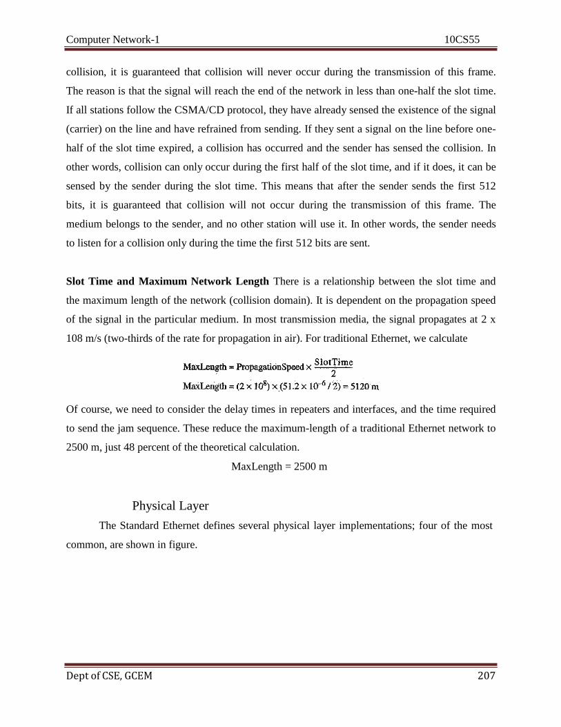
Computer Network-1 10CS55
Dept of CSE, GCEM 207
collision, it is guaranteed that collision will never occur during the transmission of this frame.
The reason is that the signal will reach the end of the network in less than one-half the slot time.
If all stations follow the CSMA/CD protocol, they have already sensed the existence of the signal
(carrier) on the line and have refrained from sending. If they sent a signal on the line before one-
half of the slot time expired, a collision has occurred and the sender has sensed the collision. In
other words, collision can only occur during the first half of the slot time, and if it does, it can be
sensed by the sender during the slot time. This means that after the sender sends the first 512
bits, it is guaranteed that collision will not occur during the transmission of this frame. The
medium belongs to the sender, and no other station will use it. In other words, the sender needs
to listen for a collision only during the time the first 512 bits are sent.
Slot Time and Maximum Network Length There is a relationship between the slot time and
the maximum length of the network (collision domain). It is dependent on the propagation speed
of the signal in the particular medium. In most transmission media, the signal propagates at 2 x
108 m/s (two-thirds of the rate for propagation in air). For traditional Ethernet, we calculate
Of course, we need to consider the delay times in repeaters and interfaces, and the time required
to send the jam sequence. These reduce the maximum-length of a traditional Ethernet network to
2500 m, just 48 percent of the theoretical calculation.
MaxLength = 2500 m
Physical Layer
The Standard Ethernet defines several physical layer implementations; four of the most
common, are shown in figure.

Computer Network-1 10CS55
Dept of CSE, GCEM 208
Encoding and Decoding
All standard implementations use digital signaling (baseband) at 10 Mbps. At the sender, data
are converted to a digital signal using the Manchester scheme; at the receiver, the received signal
is interpreted as Manchester and decoded into data. The figure shows the encoding scheme for
Standard Ethernet.
10Base5: Thick Ethernet
10Base5 was the first Ethernet specification to use a bus topology with an external transceiver
(transmitter/receiver) connected via a tap to a thick coaxial cable. The transceiver is responsible
for transmitting, receiving, and detecting collisions.
The transceiver is connected to the station via a transceiver cable that provides separate paths for
sending and receiving. This means that collision can only happen in the coaxial cable.
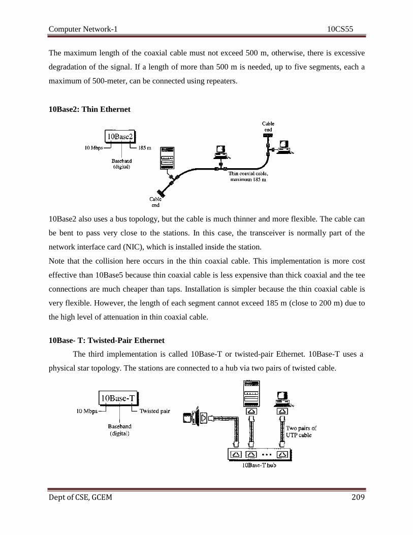
Computer Network-1 10CS55
Dept of CSE, GCEM 209
The maximum length of the coaxial cable must not exceed 500 m, otherwise, there is excessive
degradation of the signal. If a length of more than 500 m is needed, up to five segments, each a
maximum of 500-meter, can be connected using repeaters.
10Base2: Thin Ethernet
10Base2 also uses a bus topology, but the cable is much thinner and more flexible. The cable can
be bent to pass very close to the stations. In this case, the transceiver is normally part of the
network interface card (NIC), which is installed inside the station.
Note that the collision here occurs in the thin coaxial cable. This implementation is more cost
effective than 10Base5 because thin coaxial cable is less expensive than thick coaxial and the tee
connections are much cheaper than taps. Installation is simpler because the thin coaxial cable is
very flexible. However, the length of each segment cannot exceed 185 m (close to 200 m) due to
the high level of attenuation in thin coaxial cable.
10Base- T: Twisted-Pair Ethernet
The third implementation is called 10Base-T or twisted-pair Ethernet. 10Base-T uses a
physical star topology. The stations are connected to a hub via two pairs of twisted cable.
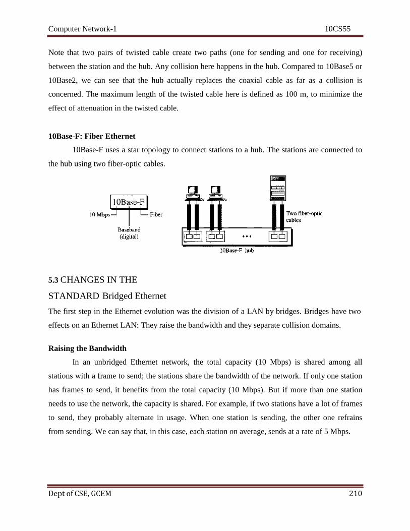
Computer Network-1 10CS55
Dept of CSE, GCEM 210
Note that two pairs of twisted cable create two paths (one for sending and one for receiving)
between the station and the hub. Any collision here happens in the hub. Compared to 10Base5 or
10Base2, we can see that the hub actually replaces the coaxial cable as far as a collision is
concerned. The maximum length of the twisted cable here is defined as 100 m, to minimize the
effect of attenuation in the twisted cable.
10Base-F: Fiber Ethernet
10Base-F uses a star topology to connect stations to a hub. The stations are connected to
the hub using two fiber-optic cables.
5.3 CHANGES IN THE
STANDARD Bridged Ethernet
The first step in the Ethernet evolution was the division of a LAN by bridges. Bridges have two
effects on an Ethernet LAN: They raise the bandwidth and they separate collision domains.
Raising the Bandwidth
In an unbridged Ethernet network, the total capacity (10 Mbps) is shared among all
stations with a frame to send; the stations share the bandwidth of the network. If only one station
has frames to send, it benefits from the total capacity (10 Mbps). But if more than one station
needs to use the network, the capacity is shared. For example, if two stations have a lot of frames
to send, they probably alternate in usage. When one station is sending, the other one refrains
from sending. We can say that, in this case, each station on average, sends at a rate of 5 Mbps.

Computer Network-1 10CS55
Dept of CSE,GCEM 210
A bridge divides the network into two or more networks. Bandwidth-wise, each network is
independent. For example, in the figure below, a network with 12 stations is divided into two
networks, each with 6 stations. Now each network has a capacity of 10 Mbps. The 10-Mbps
capacity in each segment is now shared between 6 stations (actually 7 because the bridge acts as
a station in each segment), not 12 stations. In a network with a heavy load, each station
theoretically is offered 10/6 Mbps instead of 10/12 Mbps, assuming that the traffic is not going
through the bridge.
Separating Collision Domains
Another advantage of a bridge is the separation of the collision domain. The figure below shows
the collision domains for an unbridged and a bridged network. You can see that the collision
domain becomes much smaller and the probability of collision is reduced tremendously. Without
bridging, 12 stations contend for access to the medium; with bridging only 3 stations contend for
access to the medium.

Computer Network-1 10CS55
Dept of CSE,GCEM 211
Switched Ethernet
The idea of a bridged LAN can be extended to a switched LAN. Instead of having two to
four networks, why not have N networks, where N is the number of stations on the LAN? In
other words, if we can have a multiple-port bridge, why not have an N-port switch? In this way,
the bandwidth is shared only between the station and the switch (5 Mbps each). In addition, the
collision domain is divided into N domains.
A layer 2 switch is an N-port bridge with additional sophistication that allows faster handling of
the packets. Evolution from a bridged Ethernet to a switched Ethernet was a big step that opened
the way to an even faster Ethernet.
Full-Duplex Ethernet
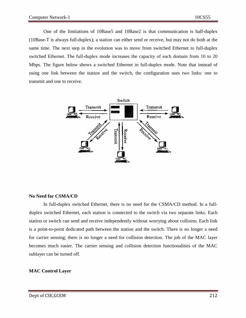
Computer Network-1 10CS55
Dept of CSE,GCEM 212
One of the limitations of 10Base5 and 10Base2 is that communication is half-duplex
(10Base-T is always full-duplex); a station can either send or receive, but may not do both at the
same time. The next step in the evolution was to move from switched Ethernet to full-duplex
switched Ethernet. The full-duplex mode increases the capacity of each domain from 10 to 20
Mbps. The figure below shows a switched Ethernet in full-duplex mode. Note that instead of
using one link between the station and the switch, the configuration uses two links: one to
transmit and one to receive.
No Need for CSMA/CD
In full-duplex switched Ethernet, there is no need for the CSMA/CD method. In a full-
duplex switched Ethernet, each station is connected to the switch via two separate links. Each
station or switch can send and receive independently without worrying about collision. Each link
is a point-to-point dedicated path between the station and the switch. There is no longer a need
for carrier sensing; there is no longer a need for collision detection. The job of the MAC layer
becomes much easier. The carrier sensing and collision detection functionalities of the MAC
sublayer can be turned off.
MAC Control Layer

Computer Network-1 10CS55
Dept of CSE,GCEM 213
Standard Ethernet was designed as a connectionless protocol at the MAC sublayer. There
is no explicit flow control or error control to inform the sender that the frame has arrived at the
destination without error. When the receiver receives the frame, it does not send any positive or
negative acknowledgment.
To provide for flow and error control in full-duplex switched Ethernet, a new sublayer, called the
MAC control, is added between the LLC sublayer and the MAC sublayer.
5.4 FAST ETHERNET
Fast Ethernet was designed to compete with LAN protocols such as FDDI or Fiber Channel
(or Fibre Channel, as it is sometimes spelled). IEEE created Fast Ethernet under the name
802.3u. Fast Ethernet is backward-compatible with Standard Ethernet, but it can transmit data 10
times faster at a rate of 100 Mbps. The goals of Fast Ethernet can be summarized as follows:
1. Upgrade the data rate to 100 Mbps.
2. Make it compatible with Standard Ethernet.
3. Keep the same 48-bit address.
4. Keep the same frame format.
5. Keep the same minimum and maximum frame lengths.
MAC Sublayer
A main consideration in the evolution of Ethernet from 10 to 100 Mbps was to keep the
MAC sublayer untouched. However, a decision was made to drop the bus topologies and keep
only the star topology. For the star topology, there are two choices, as we saw before: half duplex
and full duplex. In the half-duplex approach, the stations are connected via a hub; in the full-
duplex approach, the connection is made via a switch with buffers at each port.
The access method is the same (CSMA/CD) for the half-duplex approach; for full-duplex Fast
Ethernet, there is no need for CSMA/CD. However, the implementations keep CSMA/CD for
backward compatibility with Standard Ethernet.
Autonegotiation
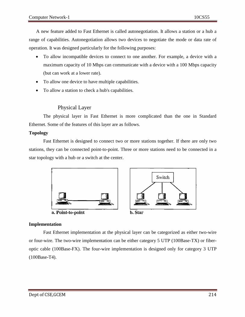
Computer Network-1 10CS55
Dept of CSE,GCEM 214
A new feature added to Fast Ethernet is called autonegotiation. It allows a station or a hub a
range of capabilities. Autonegotiation allows two devices to negotiate the mode or data rate of
operation. It was designed particularly for the following purposes:
To allow incompatible devices to connect to one another. For example, a device with a
maximum capacity of 10 Mbps can communicate with a device with a 100 Mbps capacity
(but can work at a lower rate).
To allow one device to have multiple capabilities.
To allow a station to check a hub's capabilities.
Physical Layer
The physical layer in Fast Ethernet is more complicated than the one in Standard
Ethernet. Some of the features of this layer are as follows.
Topology
Fast Ethernet is designed to connect two or more stations together. If there are only two
stations, they can be connected point-to-point. Three or more stations need to be connected in a
star topology with a hub or a switch at the center.
Implementation
Fast Ethernet implementation at the physical layer can be categorized as either two-wire
or four-wire. The two-wire implementation can be either category 5 UTP (100Base-TX) or fiber-
optic cable (100Base-FX). The four-wire implementation is designed only for category 3 UTP
(100Base-T4).

Computer Network-1 10CS55
Dept of CSE,GCEM 215
Encoding
Manchester encoding needs a 200-Mbaud bandwidth for a data rate of 100 Mbps, which
makes it unsuitable for a medium such as twisted-pair cable. For this reason, the Fast Ethernet
designers sought some alternative encoding/decoding scheme. However, it was found that one
scheme would not perform equally well for all three implementations. Therefore, three different
encoding schemes were chosen.
100Base-TX uses two pairs of twisted-pair cable (either category 5 UTP or STP). For this
implementation, the MLT-3 scheme was selected since it has good bandwidth performance.
However, since MLT-3 is not a self-synchronous line coding scheme, 4B/5B block coding is
used to provide bit synchronization by preventing the occurrence of a long sequence of 0s and ls.
This creates a data rate of 125 Mbps, which is fed into MLT-3 for encoding.

Computer Network-1 10CS55
Dept of CSE,GCEM 216
100Base-FX uses two pairs of fiber-optic cables. Optical fiber can easily handle high bandwidth
requirements by using simple encoding schemes. The designers of 100Base-FX selected the
NRZ-I encoding scheme for this implementation. However, NRZ-I has a bit synchronization
problem for long sequences of 0s (or 1s, based on the encoding). To overcome this problem, the
designers used 4B/5B block encoding as we described for 100Base-TX. The block encoding
increases the bit rate from 100 to 125 Mbps, which can easily be handled by fiber-optic cable.
100Base-T4, was designed to use category 3 or higher UTP. The implementation uses four pairs
of UTP for
transmitting 100 Mbps. Encoding/decoding in 100Base-T4 is more complicated. As this
implementation uses category 3 UTP, each twisted-pair cannot easily handle more than 25
Mbaud. In this design, one pair switches between sending and receiving. Three pairs of UTP
category 3, however, can handle only 75 Mbaud (25 Mbaud) each. We need to use an encoding
scheme that converts 100 Mbps to a 75 Mbaud signal. 8B/6T satisfies this requirement. In
8B/6T, eight data elements are encoded as six signal elements. This means that 100 Mbps uses
only (6/8) x 100 Mbps, or 75 Mbaud.
Summary
5.5 GIGABIT ETHERNET

Computer Network-1 10CS55
Dept of CSE,GCEM 217
The need for an even higher data rate resulted in the design of the Gigabit Ethernet protocol
(1000 Mbps). The IEEE committee calls the Standard 802.3z. The goals of the Gigabit Ethernet
design can be summarized as follows:
1. Upgrade the data rate to 1 Gbps.
2. Make it compatible with Standard or Fast Ethernet.
3. Use the same 48-bit address.
4. Use the same frame format.
5. Keep the same minimum and maximum frame lengths.
6. To support autonegotiation as defined in Fast Ethernet.
MAC Sublayer
Gigabit Ethernet has two distinctive approaches for medium access: half-duplex and full-
duplex. Almost all implementations of Gigabit Ethernet follow the full-duplex approach.
Full-Duplex Mode
In full-duplex mode, there is a central switch connected to all computers or other
switches. In this mode, each switch has buffers for each input port in which data are stored until
they are transmitted. There is no collision in this mode. This means that CSMA/CD is not used.
Lack of collision implies that the maximum length of the cable is determined by the signal
attenuation in the cable, not by the collision detection process.
Half-Duplex Mode
Gigabit Ethernet can also be used in half-duplex mode, although it is rare. In this case, a
switch can be replaced by a hub, which acts as the common cable in which a collision might
occur. The half-duplex approach uses CSMA/CD. The maximum length of the network in this
approach is totally dependent on the minimum frame size. Three methods have been defined:
traditional, carder extension, and frame bursting.
Traditional In the traditional approach, we keep the minimum length of the frame as in
traditional Ethernet (512 bits). However, because the length of a bit is 1/100 shorter in Gigabit
Ethernet than in 10-Mbps Ethernet, the slot time for Gigabit Ethernet is 512 bits x 1/1000 gs,

Computer Network-1 10CS55
Dept of CSE,GCEM 218
which is equal to 0.512 gs. The reduced slot time means that collision is detected 100 times
earlier. This means that the maximum length of the network is
25 m. This length may be suitable if all the stations are in one room, but it may not even be long
enough to connect the computers in one single office.
Carrier Extension To allow for a longer network, we increase the minimum frame length. The
carrier extension approach defines the minimum length of a frame as 512 bytes (4096 bits). This
means that the minimum length is 8 times longer. This method forces a station to add extension
bits (padding) to any frame that is less than 4096 bits. In this way, the maximum length of the
network can be increased 8 times to a length of 200 m. This allows a length of 100 m from the
hub to the station.
Frame Bursting Carrier extension is very inefficient if we have a series of short frames to send;
each frame carries redundant data. To improve efficiency, frame bursting was proposed. Instead
of adding an extension to each frame, multiple frames are sent. However, to make these multiple
frames look like one frame, padding is added between the frames (the same as that used for the
carrier extension method) so that the channel is not idle.
Physical Layer
The physical layer in Gigabit Ethernet is more complicated than that in Standard or Fast
Ethernet. Some features of this layer are:
Topology
Gigabit Ethernet is designed to connect two or more stations. If there are only two
stations, they can be connected point-to-point. Three or more stations need to be connected in a
star topology with a hub or a switch at the center. Another possible configuration is to connect
several star topologies or let a star topology be part of another as shown.
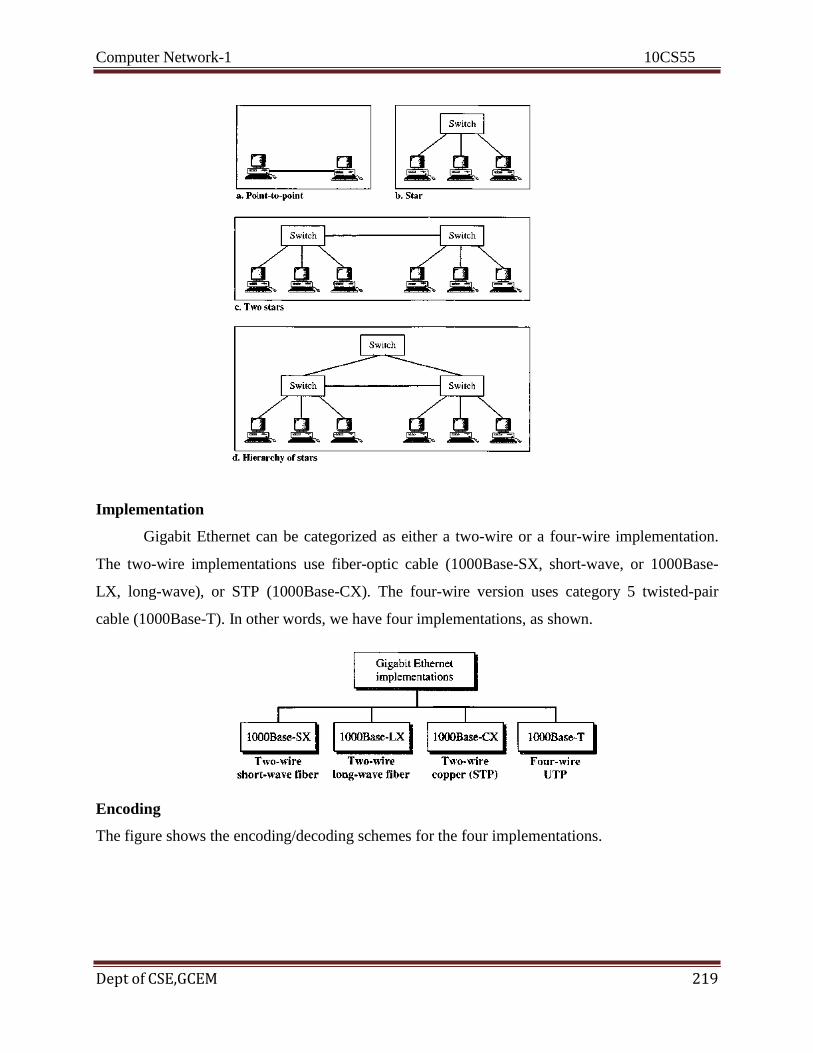
Computer Network-1 10CS55
Dept of CSE,GCEM 219
Implementation
Gigabit Ethernet can be categorized as either a two-wire or a four-wire implementation.
The two-wire implementations use fiber-optic cable (1000Base-SX, short-wave, or 1000Base-
LX, long-wave), or STP (1000Base-CX). The four-wire version uses category 5 twisted-pair
cable (1000Base-T). In other words, we have four implementations, as shown.
Encoding
The figure shows the encoding/decoding schemes for the four implementations.
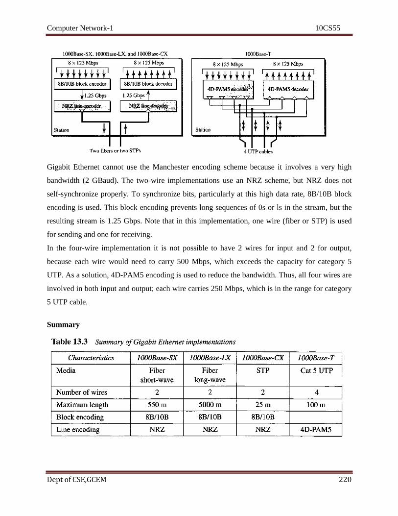
Computer Network-1 10CS55
Dept of CSE,GCEM 220
Gigabit Ethernet cannot use the Manchester encoding scheme because it involves a very high
bandwidth (2 GBaud). The two-wire implementations use an NRZ scheme, but NRZ does not
self-synchronize properly. To synchronize bits, particularly at this high data rate, 8B/10B block
encoding is used. This block encoding prevents long sequences of 0s or ls in the stream, but the
resulting stream is 1.25 Gbps. Note that in this implementation, one wire (fiber or STP) is used
for sending and one for receiving.
In the four-wire implementation it is not possible to have 2 wires for input and 2 for output,
because each wire would need to carry 500 Mbps, which exceeds the capacity for category 5
UTP. As a solution, 4D-PAM5 encoding is used to reduce the bandwidth. Thus, all four wires are
involved in both input and output; each wire carries 250 Mbps, which is in the range for category
5 UTP cable.
Summary

Computer Network-1 10CS55
Dept of CSE,GCEM 221
Ten-Gigabit Ethernet
The IEEE committee created Ten-Gigabit Ethernet and called it Standard 802.3ae. The goals
of the Ten-Gigabit Ethernet design can be summarized as follows:
1. Upgrade the data rate to 10 Gbps.
2. Make it compatible with Standard, Fast, and Gigabit Ethernet.
3. Use the same 48-bit address.
4. Use the same frame format.
5. Keep the same minimum and maximum frame lengths.
6. Allow the interconnection of existing LANs into a metropolitan area network (MAN) or a
wide area network (WAN).
7. Make Ethernet compatible with technologies such as Frame Relay and ATM.
MAC Sublayer
Ten-Gigabit Ethernet operates only in full duplex mode which means there is no need for
contention; CSMA/CD is not used in Ten-Gigabit Ethernet.
Physical Layer
The physical layer in Ten-Gigabit Ethernet is designed for using fiber-optic cable over long
distances. Three implementations are the most common: 10GBase-S, 10GBase-L, and 10GBase-
E.
Recommended Questions
1. What is the advantage of controlled access over random access.
2. What is the purpose of jam signal in CSMA/CD
3. How do the two persistent strategies differ.
4. How does CSMA/CD differ from CSMA/CA.
5. Discuss the difference between polling and selecting. 6. What is the purpose of a NIC.

Computer Network-1 10CS55
Dept of CSE,GCEM 222
7. What is the difference between multicast and broadcast address.
8. What are the common Ethernet traditional applications. 9. What are the common fast Ethernet and gigabit Ethernet applications.
Computer Network-1 10CS55
Dept of CSE,GCEM 223
COMPUTER NETWORKS – I
Subject Code: 10CS55 I.A. Marks : 25 Hours/Week : 04 Exam Hours: 03
Total Hours : 52 Exam Marks: 100
UNIT – 7 6 Hours Wireless LANs and Cellular Networks:
- Introduction,
- IEEE 802.11,
- Bluetooth,
- Connecting devices, - Cellular Telephony
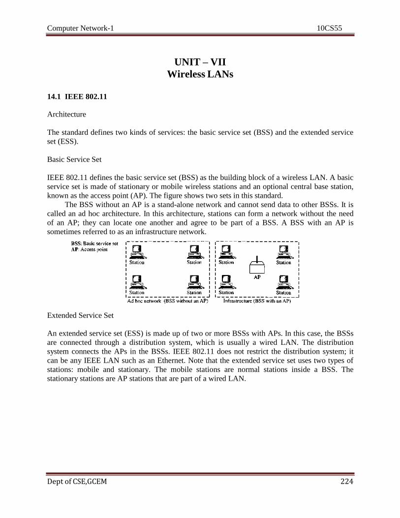
Computer Network-1 10CS55
Dept of CSE,GCEM 224
UNIT – VII
Wireless LANs
14.1 IEEE 802.11
Architecture
The standard defines two kinds of services: the basic service set (BSS) and the extended service
set (ESS).
Basic Service Set
IEEE 802.11 defines the basic service set (BSS) as the building block of a wireless LAN. A basic
service set is made of stationary or mobile wireless stations and an optional central base station,
known as the access point (AP). The figure shows two sets in this standard.
The BSS without an AP is a stand-alone network and cannot send data to other BSSs. It is
called an ad hoc architecture. In this architecture, stations can form a network without the need
of an AP; they can locate one another and agree to be part of a BSS. A BSS with an AP is
sometimes referred to as an infrastructure network.
Extended Service Set
An extended service set (ESS) is made up of two or more BSSs with APs. In this case, the BSSs
are connected through a distribution system, which is usually a wired LAN. The distribution
system connects the APs in the BSSs. IEEE 802.11 does not restrict the distribution system; it
can be any IEEE LAN such as an Ethernet. Note that the extended service set uses two types of
stations: mobile and stationary. The mobile stations are normal stations inside a BSS. The
stationary stations are AP stations that are part of a wired LAN.
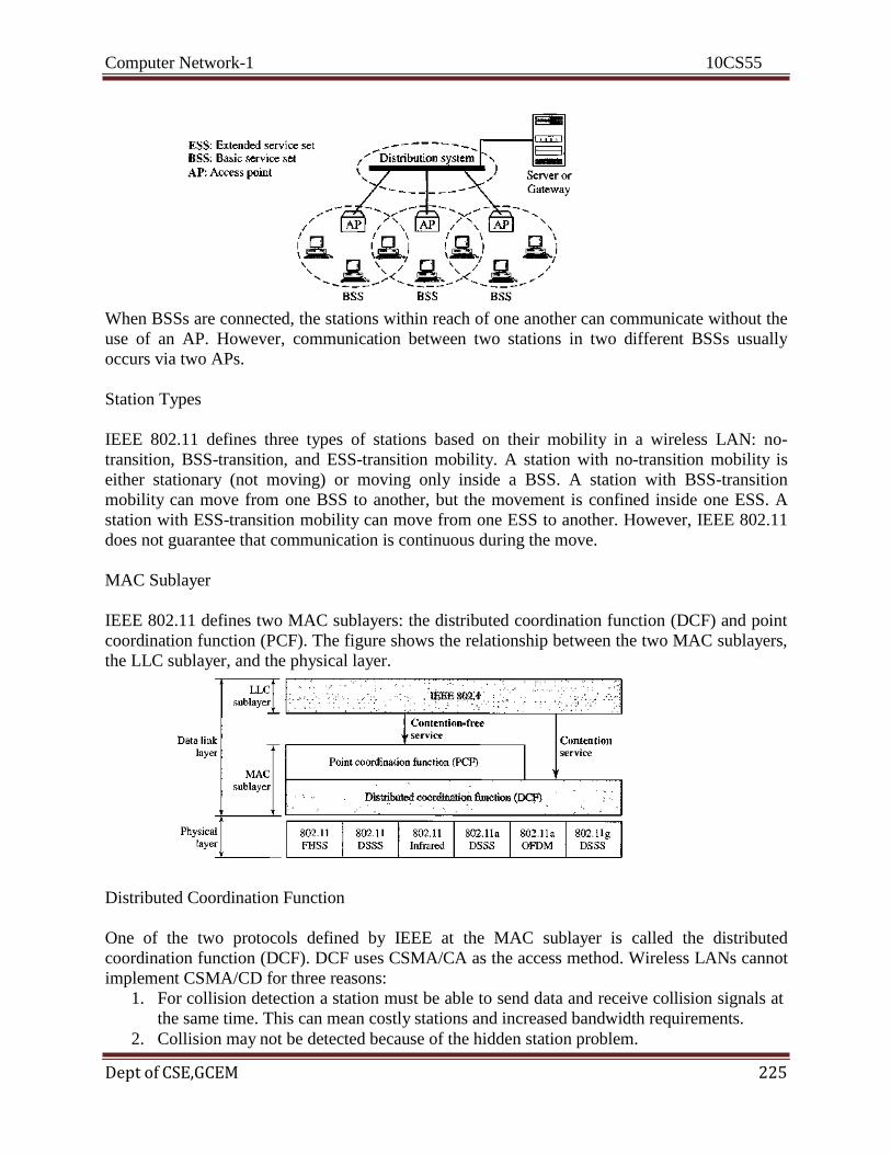
Computer Network-1 10CS55
Dept of CSE,GCEM 225
When BSSs are connected, the stations within reach of one another can communicate without the
use of an AP. However, communication between two stations in two different BSSs usually
occurs via two APs.
Station Types
IEEE 802.11 defines three types of stations based on their mobility in a wireless LAN: no-
transition, BSS-transition, and ESS-transition mobility. A station with no-transition mobility is
either stationary (not moving) or moving only inside a BSS. A station with BSS-transition
mobility can move from one BSS to another, but the movement is confined inside one ESS. A
station with ESS-transition mobility can move from one ESS to another. However, IEEE 802.11
does not guarantee that communication is continuous during the move.
MAC Sublayer
IEEE 802.11 defines two MAC sublayers: the distributed coordination function (DCF) and point
coordination function (PCF). The figure shows the relationship between the two MAC sublayers,
the LLC sublayer, and the physical layer.
Distributed Coordination Function
One of the two protocols defined by IEEE at the MAC sublayer is called the distributed
coordination function (DCF). DCF uses CSMA/CA as the access method. Wireless LANs cannot
implement CSMA/CD for three reasons:
1. For collision detection a station must be able to send data and receive collision signals at
the same time. This can mean costly stations and increased bandwidth requirements.
2. Collision may not be detected because of the hidden station problem.

Computer Network-1 10CS55
Dept of CSE,GCEM 226
3. The distance between stations can be great. Signal fading could prevent a station at one
end from hearing a collision at the other end.
Process Flowchart The figure shows the process flowchart for CSMA/CA as used in wireless
LANs.
Frame Exchange Time Line The figure shows the exchange of data and control frames in time.
1. Before sending a frame, the source station senses the medium by checking the energy
level at the carrier frequency.
a. The channel uses a persistence strategy with back-off until the channel is idle.

Computer Network-1 10CS55
Dept of CSE,GCEM 227
b. After the station is found to be idle, the station waits for a period of time called
the distributed interframe space (DIFS); then the station sends a control frame
called the request to send (RTS).
2. After receiving the RTS and waiting a period of time called the short interframe space
(SIFS), the destination station sends a control frame, called the clear to send (CTS), to the
source station. This control frame indicates that the destination station is ready to receive
data.
3. The source station sends data after waiting an amount of time equal to SIFS.
4. The destination station, after waiting an amount of time equal to SIFS, sends an
acknowledgment to show that the frame has been received. Acknowledgment is needed
in this protocol because the station does not have any means to check for the successful
arrival of its data at the destination. On the other hand, the lack of collision in CSMA/CD
is a kind of indication to the soume that data have arrived.
Network Allocation Vector When a station sends an RTS frame, it includes the duration of time
that it needs to occupy the channel. The stations that are affected by this transmission create a
timer called a network allocation vector (NAV) that shows how much time must pass before
these stations are allowed to check the channel for idleness. Each time a station accesses the
system and sends an RTS frame, other stations start their NAV. In other words, each station,
before sensing the physical medium to see if it is idle, first checks its NAV to see if it has
expired.
Collision During Handshaking What happens if there is collision during the time when RTS or
CTS control frames are in transition, often called the handshaking period? Two or more stations
may try to send RTS frames at the same time. These control frames may collide. However,
because there is no mechanism for collision detection, the sender assumes there has been a
collision if it has not received a CTS frame from the receiver. The back-off strategy is employed,
and the sender tries again.
Point Coordination Function (PCF)
The point coordination function (PCF) is an optional access method that can be implemented in
an infrastructure network (not in an ad hoc network). It is implemented on top of the DCF and is
used mostly for time-sensitive transmission. PCF has a centralized, contention-free polling
access method. The AP performs polling for stations that are capable of being polled. The
stations are polled one after another, sending any data they have to the AP. To give priority to
PCF over DCF, another set of interframe spaces has been defined: PIFS and SIFS. The SIFS is
the same as that in DCF, but the PIFS (PCF IFS) is shorter than the DIFS. This means that if, at
the same time, a station wants to use only DCF and an AP wants to use PCF, the AP has priority.
Due to the priority of PCF over DCF, stations that only use DCF may not gain access to the
medium. To prevent this, a repetition interval has been designed to cover both contention-free
(PCF) and contention-based (DCF) traffic. The repetition interval, which is repeated
continuously, starts with a special control frame, called a beacon frame. When the stations hear
the beacon frame, they start their NAV for the duration of the contention-free period of the
repetition interval. The figure shows an example of a repetition interval.

Computer Network-1 10CS55
Dept of CSE,GCEM 228
During the repetition interval, the PC (point controller) can send a poll frame, receive data, send
an ACK, receive an ACK, or do any combination of these (802.11 uses piggybacking). At the
end of the contention-free period, the PC sends a CF end (contention-free end) frame to allow the
contention-based stations to use the medium.
Fragmentation
The wireless environment is very noisy; a corrupt frame has to be retransmitted. The protocol,
therefore, recommends fragmentation--the division of a large frame into smaller ones. It is more
efficient to resend a small frame than a large one.
Frame Format
The MAC layer frame consists of nine fields, as shown.
Frame control (FC). The FC field is 2 bytes long and defines the type of frame and some control
information. The table describes the subfields.
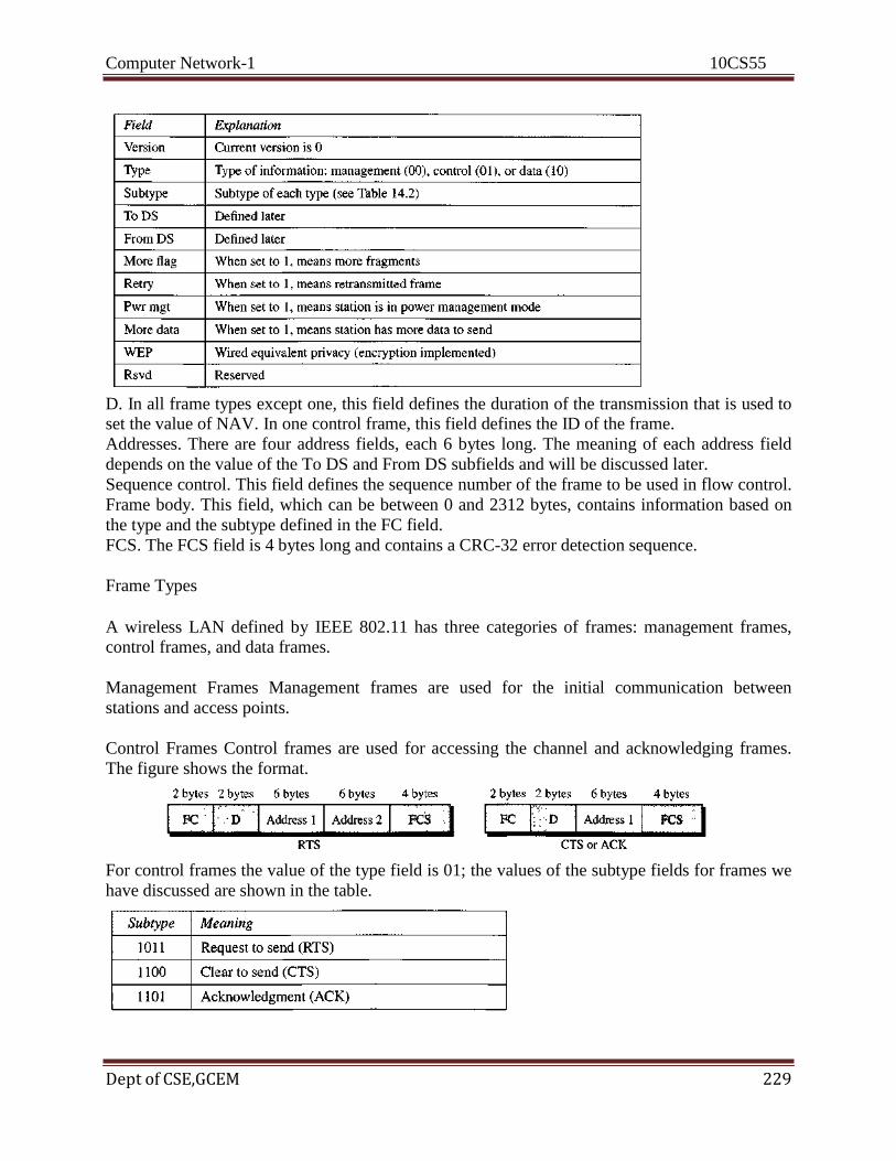
Computer Network-1 10CS55
Dept of CSE,GCEM 229
D. In all frame types except one, this field defines the duration of the transmission that is used to set the value of NAV. In one control frame, this field defines the ID of the frame.
Addresses. There are four address fields, each 6 bytes long. The meaning of each address field
depends on the value of the To DS and From DS subfields and will be discussed later.
Sequence control. This field defines the sequence number of the frame to be used in flow control.
Frame body. This field, which can be between 0 and 2312 bytes, contains information based on
the type and the subtype defined in the FC field.
FCS. The FCS field is 4 bytes long and contains a CRC-32 error detection sequence.
Frame Types
A wireless LAN defined by IEEE 802.11 has three categories of frames: management frames,
control frames, and data frames.
Management Frames Management frames are used for the initial communication between
stations and access points.
Control Frames Control frames are used for accessing the channel and acknowledging frames.
The figure shows the format.
For control frames the value of the type field is 01; the values of the subtype fields for frames we
have discussed are shown in the table.
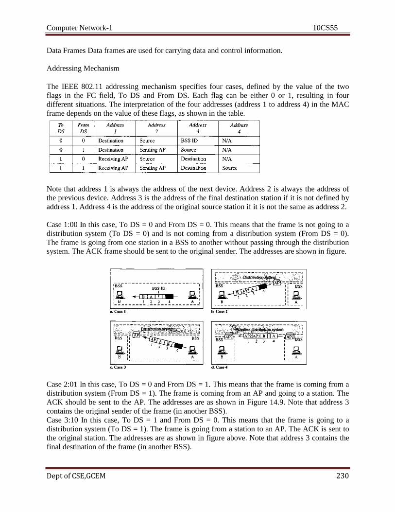
Computer Network-1 10CS55
Dept of CSE,GCEM 230
Data Frames Data frames are used for carrying data and control information.
Addressing Mechanism
The IEEE 802.11 addressing mechanism specifies four cases, defined by the value of the two
flags in the FC field, To DS and From DS. Each flag can be either 0 or 1, resulting in four
different situations. The interpretation of the four addresses (address 1 to address 4) in the MAC
frame depends on the value of these flags, as shown in the table.
Note that address 1 is always the address of the next device. Address 2 is always the address of
the previous device. Address 3 is the address of the final destination station if it is not defined by
address 1. Address 4 is the address of the original source station if it is not the same as address 2.
Case 1:00 In this case, To DS = 0 and From DS = 0. This means that the frame is not going to a
distribution system (To DS = 0) and is not coming from a distribution system (From DS = 0).
The frame is going from one station in a BSS to another without passing through the distribution
system. The ACK frame should be sent to the original sender. The addresses are shown in figure.
Case 2:01 In this case, To DS = 0 and From DS = 1. This means that the frame is coming from a
distribution system (From DS = 1). The frame is coming from an AP and going to a station. The
ACK should be sent to the AP. The addresses are as shown in Figure 14.9. Note that address 3
contains the original sender of the frame (in another BSS).
Case 3:10 In this case, To DS = 1 and From DS = 0. This means that the frame is going to a
distribution system (To DS = 1). The frame is going from a station to an AP. The ACK is sent to
the original station. The addresses are as shown in figure above. Note that address 3 contains the
final destination of the frame (in another BSS).
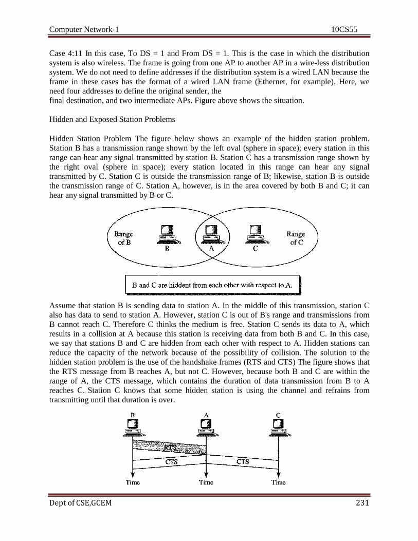
Computer Network-1 10CS55
Dept of CSE,GCEM 231
Case 4:11 In this case, To DS = 1 and From DS = 1. This is the case in which the distribution
system is also wireless. The frame is going from one AP to another AP in a wire-less distribution
system. We do not need to define addresses if the distribution system is a wired LAN because the
frame in these cases has the format of a wired LAN frame (Ethernet, for example). Here, we
need four addresses to define the original sender, the
final destination, and two intermediate APs. Figure above shows the situation.
Hidden and Exposed Station Problems
Hidden Station Problem The figure below shows an example of the hidden station problem.
Station B has a transmission range shown by the left oval (sphere in space); every station in this
range can hear any signal transmitted by station B. Station C has a transmission range shown by
the right oval (sphere in space); every station located in this range can hear any signal
transmitted by C. Station C is outside the transmission range of B; likewise, station B is outside
the transmission range of C. Station A, however, is in the area covered by both B and C; it can
hear any signal transmitted by B or C.
Assume that station B is sending data to station A. In the middle of this transmission, station C
also has data to send to station A. However, station C is out of B's range and transmissions from
B cannot reach C. Therefore C thinks the medium is free. Station C sends its data to A, which
results in a collision at A because this station is receiving data from both B and C. In this case,
we say that stations B and C are hidden from each other with respect to A. Hidden stations can
reduce the capacity of the network because of the possibility of collision. The solution to the
hidden station problem is the use of the handshake frames (RTS and CTS) The figure shows that
the RTS message from B reaches A, but not C. However, because both B and C are within the
range of A, the CTS message, which contains the duration of data transmission from B to A
reaches C. Station C knows that some hidden station is using the channel and refrains from
transmitting until that duration is over.

Computer Network-1 10CS55
Dept of CSE,GCEM 232
Exposed Station Problem Now consider a situation that is the inverse of the previous one: the
exposed station problem. In this problem a station refrains from using a channel when it is, in
fact, available. In the figure, station A is transmitting to station B. Station C has some data to
send to station D, which can be sent without interfering with the transmission from A to B.
However, station C is exposed to transmission from
A; it hears what A is sending and thus refrains from sending. In other words, C is too
conservative and wastes the capacity of the channel.
The handshaking messages RTS and CTS cannot help in this case, despite what you might think.
Station C hears the RTS from A, but does not hear the CTS from B. Station C, after hearing the
RTS from A, can wait for a time so that the CTS from B reaches A; it then sends an RTS to D to
show that it needs to communicate with D. Both stations B and A may hear this RTS, but station
A is in the sending state, not the receiving state. Station B, however, responds with a CTS. The
problem is here. If station A has started sending its data, station C cannot hear the CTS from
station D because of the collision; it cannot send its data to D. It remains exposed until A finishes
sending its data as the figure shows.
Physical Layer
Table Physical layers

Computer Network-1 10CS55
Dept of CSE,GCEM 233
All implementations, except the infrared, operate in the industrial, scientific, and medical (ISM)
band, which defines three unlicensed bands in the three ranges 902-928 MHz, 2.400--4.835 GHz,
and 5.725-5.850 GHz, as shown in Figure 14.14.
Figure 14.14 industrial, scientific, and medical (ISM) band
IEEE 802.11 FHSS
IEEE 802.11 FHSS uses the frequency-hopping spread spectrum (FHSS) method FHSS uses the
2.4-GHz ISM band. The band is divided into 79 subbands of 1 MHz (and some guard bands). A
pseudorandom number generator selects the hopping sequence. The modulation technique in this
specification is either two-level FSK or four-level FSK with I or 2 bitslbaud, which results in a
data rate of 1 or 2 Mbps, as shown in Figure 14.15.
IEEE 802.11 DSSS
IEEE 802.11 DSSS uses the direct sequence spread spectrum (DSSS) method. DSSS uses the
2.4-GHz ISM band. The modulation technique in this specification is PSK at 1 Mbaud/s. The
system allows 1 or 2 bitslbaud (BPSK or QPSK), which results in a data rate of 1 or 2 Mbps, as
shown in Figure 14.16.
IEEE 802.11 Infrared
IEEE 802.11 infrared uses infrared light in the range of 800 to 950 nm. The modulation
technique is called pulse position modulation (PPM). For a I-Mbps data rate, a 4-bit
Figure 14.15 Physical layer ofIEEE 802.11 FHSS

Computer Network-1 10CS55
Dept of CSE,GCEM 234
Figure 14.16 Physical layer ofIEEE 802.11 DSSS
sequence is first mapped into a 16-bit sequence in which only one bit is set to 1 and the rest are
set to O. For a 2-Mbps data rate, a 2-bit sequence is first mapped into a 4-bit sequence in which
only one bit is set to 1 and the rest are set to O. The mapped sequences are then converted to
optical signals; the presence of light specifies 1, the absence of light specifies O. See Figure
14.17.
Figure 14.17 Physical layer of IEEE 802.11 infrared
IEEE 802.lla OFDM
IEEE 802.Ila OFDM describes the orthogonal frequency-division multiplexing (OFDM) method
for signal generation in a 5-GHz ISM band. OFDM is similar to FDM as discussed in Chapter 6,
with one major difference: All the subbands are used by one source at a given time. Sources
contend with one another at the data link layer for access. The band is divided into 52 subbands,
with 48 subbands for sending 48 groups of bits at a time and 4 subbands for control information.
The scheme is similar
to ADSL, as discussed in Chapter 9. Dividing the band into subbands diminishes the effects of
interference. If the subbands are used randomly, security can also be increased. OFDM uses PSK
and QAM for modulation. The common data rates are 18 Mbps (PSK) and 54 Mbps (QAM).
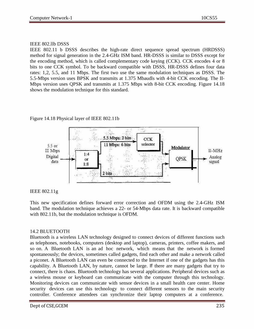
Computer Network-1 10CS55
Dept of CSE,GCEM 235
IEEE 802.llb DSSS
IEEE 802.11 b DSSS describes the high-rate direct sequence spread spectrum (HRDSSS)
method for signal generation in the 2.4-GHz ISM band. HR-DSSS is similar to DSSS except for
the encoding method, which is called complementary code keying (CCK). CCK encodes 4 or 8
bits to one CCK symbol. To be backward compatible with DSSS, HR-DSSS defines four data
rates: 1,2, 5.5, and 11 Mbps. The first two use the same modulation techniques as DSSS. The
5.5-Mbps version uses BPSK and transmits at 1.375 Mbaudls with 4-bit CCK encoding. The II-
Mbps version uses QPSK and transmits at 1.375 Mbps with 8-bit CCK encoding. Figure 14.18
shows the modulation technique for this standard.
Figure 14.18 Physical layer of IEEE 802.11b
IEEE 802.11g
This new specification defines forward error correction and OFDM using the 2.4-GHz ISM
band. The modulation technique achieves a 22- or 54-Mbps data rate. It is backward compatible
with 802.11b, but the modulation technique is OFDM.
14.2 BLUETOOTH
Bluetooth is a wireless LAN technology designed to connect devices of different functions such
as telephones, notebooks, computers (desktop and laptop), cameras, printers, coffee makers, and
so on. A Bluetooth LAN is an ad hoc network, which means that the network is formed
spontaneously; the devices, sometimes called gadgets, find each other and make a network called
a piconet. A Bluetooth LAN can even be connected to the Internet if one of the gadgets has this
capability. A Bluetooth LAN, by nature, cannot be large. If there are many gadgets that try to
connect, there is chaos. Bluetooth technology has several applications. Peripheral devices such as
a wireless mouse or keyboard can communicate with the computer through this technology.
Monitoring devices can communicate with sensor devices in a small health care center. Home
security devices can use this technology to connect different sensors to the main security
controller. Conference attendees can synchronize their laptop computers at a conference.

Computer Network-1 10CS55
Dept of CSE,GCEM 236
Bluetooth was originally started as a project by the Ericsson Company. It is named for Harald
Blaatand, the king of Denmark (940-981) who united Denmark and Norway. Blaatand translates
to Bluetooth in English. Today, Bluetooth technology is the implementation of a protocol
defined by the IEEE 802.15 standard. The standard defines a wireless personal-area network
(PAN) operable in an area the size of a room or a hall.
Architecture
Bluetooth defines two types of networks: piconet and scatternet.
Piconets
A Bluetooth network is called a piconet, or a small net. A piconet can have up to eight stations,
one of which is called the primary;t the rest are called secondaries. All the secondary stations
synchronize their clocks and hopping sequence with the primary. Note that a piconet can have
only one primary station. The communication between the primary and the secondary can be
one-to-one or one-to-many. Figure 14.19 shows a piconet.
Figure 14.19 Piconet
Although a piconet can have a maximum of seven secondaries, an additional eight secondaries
can be in the parked state. A secondary in a parked state is synchronized with the primary, but
cannot take part in communication until it is moved from the parked state. Because only eight
stations can be active in a piconet, activating a station from the parked state means that an active
station must go to the parked state.
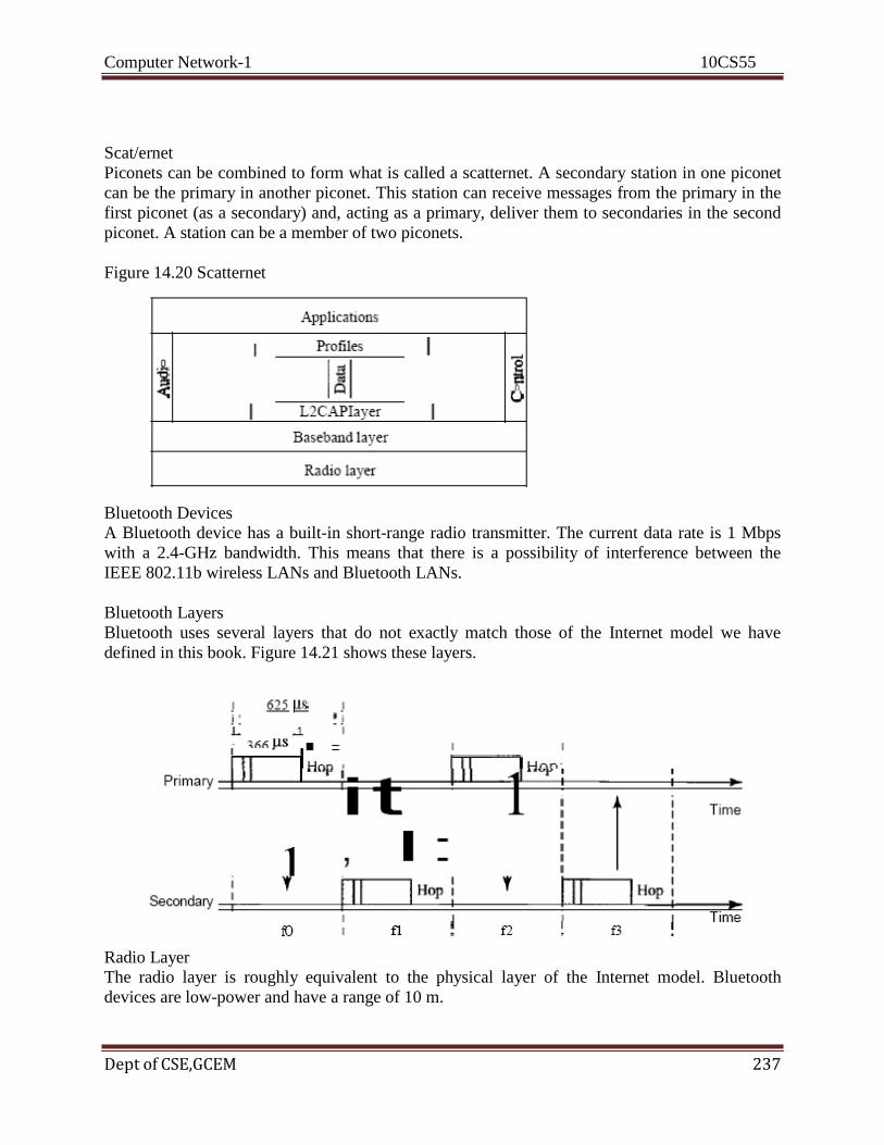
Computer Network-1 10CS55
Dept of CSE,GCEM 237
Scat/ernet
Piconets can be combined to form what is called a scatternet. A secondary station in one piconet
can be the primary in another piconet. This station can receive messages from the primary in the
first piconet (as a secondary) and, acting as a primary, deliver them to secondaries in the second
piconet. A station can be a member of two piconets.
Figure 14.20 Scatternet
Bluetooth Devices
A Bluetooth device has a built-in short-range radio transmitter. The current data rate is 1 Mbps
with a 2.4-GHz bandwidth. This means that there is a possibility of interference between the
IEEE 802.11b wireless LANs and Bluetooth LANs.
Bluetooth Layers
Bluetooth uses several layers that do not exactly match those of the Internet model we have
defined in this book. Figure 14.21 shows these layers.
Radio Layer
The radio layer is roughly equivalent to the physical layer of the Internet model. Bluetooth
devices are low-power and have a range of 10 m.
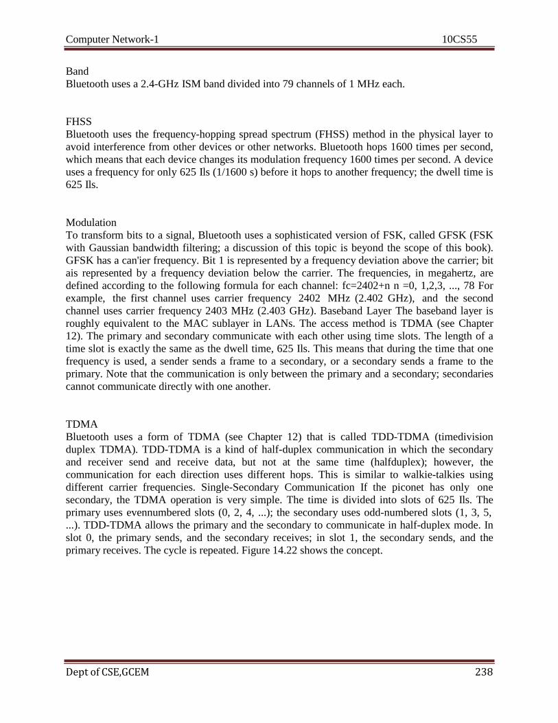
Computer Network-1 10CS55
Dept of CSE,GCEM 238
Band
Bluetooth uses a 2.4-GHz ISM band divided into 79 channels of 1 MHz each.
FHSS
Bluetooth uses the frequency-hopping spread spectrum (FHSS) method in the physical layer to
avoid interference from other devices or other networks. Bluetooth hops 1600 times per second,
which means that each device changes its modulation frequency 1600 times per second. A device
uses a frequency for only 625 Ils (1/1600 s) before it hops to another frequency; the dwell time is
625 Ils.
Modulation
To transform bits to a signal, Bluetooth uses a sophisticated version of FSK, called GFSK (FSK
with Gaussian bandwidth filtering; a discussion of this topic is beyond the scope of this book).
GFSK has a can'ier frequency. Bit 1 is represented by a frequency deviation above the carrier; bit
ais represented by a frequency deviation below the carrier. The frequencies, in megahertz, are
defined according to the following formula for each channel: fc=2402+n n =0, 1,2,3, ..., 78 For
example, the first channel uses carrier frequency 2402 MHz (2.402 GHz), and the second
channel uses carrier frequency 2403 MHz (2.403 GHz). Baseband Layer The baseband layer is
roughly equivalent to the MAC sublayer in LANs. The access method is TDMA (see Chapter
12). The primary and secondary communicate with each other using time slots. The length of a
time slot is exactly the same as the dwell time, 625 Ils. This means that during the time that one
frequency is used, a sender sends a frame to a secondary, or a secondary sends a frame to the
primary. Note that the communication is only between the primary and a secondary; secondaries
cannot communicate directly with one another.
TDMA
Bluetooth uses a form of TDMA (see Chapter 12) that is called TDD-TDMA (timedivision
duplex TDMA). TDD-TDMA is a kind of half-duplex communication in which the secondary
and receiver send and receive data, but not at the same time (halfduplex); however, the
communication for each direction uses different hops. This is similar to walkie-talkies using
different carrier frequencies. Single-Secondary Communication If the piconet has only one
secondary, the TDMA operation is very simple. The time is divided into slots of 625 Ils. The
primary uses evennumbered slots (0, 2, 4, ...); the secondary uses odd-numbered slots (1, 3, 5,
...). TDD-TDMA allows the primary and the secondary to communicate in half-duplex mode. In
slot 0, the primary sends, and the secondary receives; in slot 1, the secondary sends, and the
primary receives. The cycle is repeated. Figure 14.22 shows the concept.

Computer Network-1 10CS55
Dept of CSE,GCEM 239
Let us elaborate on the figure. 1. In slot 0, the primary sends a frame to secondary 1.
2. In slot 1, only secondary I sends a frame to the primary because the previous frame was
addressed to secondary 1; other secondaries are silent.
3. In slot 2, the primary sends a frame to secondary 2.
4. In slot 3, only secondary 2 sends a frame to the primary because the previous frame was
addressed to secondary 2; other secondaries are silent.
5. The cycle continues. We can say that this access method is similar to a poll/select operation
with reservations. When the primary selects a secondary, it also polls it. The next time slot is
reserved for
the polled station to send its frame. If the polled secondary has no frame to send, the channel is
silent.
Physical Links
Two types of links can be created between a primary and a secondary: SCQ links and ACL links.
sca A synchronous connection-oriented (SeQ) link is used when avoiding latency (delay in data
delivery) is more important than integrity (error-free delivery). In an SCQ link, a physical link is
created between the primary and a secondary by reserving specific slots at regular intervals. The
basic unit of connection is two slots, one for each direction. If a packet is damaged, it is never
retransmitted. SCQ is used for real-time audio where avoiding delay is all-important. A
secondary can create up to three SCQ links with the primary, sending digitized audio (PCM) at
64 kbps in each link. ACL An asynchronous connectionless link (ACL) is used when data
integrity is more important than avoiding latency. In this type of link, if a payload encapsulated
in the frame is corrupted, it is retransmitted. A secondary returns an ACL frame in the available
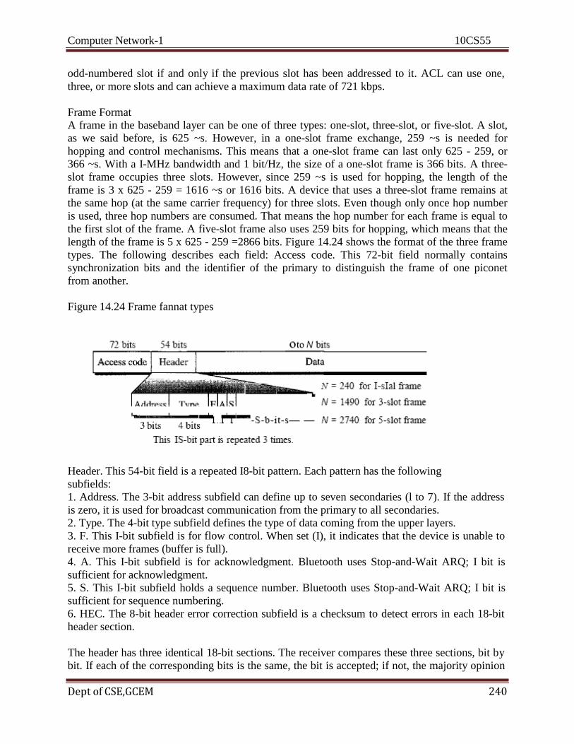
Computer Network-1 10CS55
Dept of CSE,GCEM 240
odd-numbered slot if and only if the previous slot has been addressed to it. ACL can use one,
three, or more slots and can achieve a maximum data rate of 721 kbps.
Frame Format
A frame in the baseband layer can be one of three types: one-slot, three-slot, or five-slot. A slot,
as we said before, is 625 ~s. However, in a one-slot frame exchange, 259 ~s is needed for
hopping and control mechanisms. This means that a one-slot frame can last only 625 - 259, or
366 ~s. With a I-MHz bandwidth and 1 bit/Hz, the size of a one-slot frame is 366 bits. A three-
slot frame occupies three slots. However, since 259 ~s is used for hopping, the length of the
frame is 3 x 625 - 259 = 1616 ~s or 1616 bits. A device that uses a three-slot frame remains at
the same hop (at the same carrier frequency) for three slots. Even though only once hop number
is used, three hop numbers are consumed. That means the hop number for each frame is equal to
the first slot of the frame. A five-slot frame also uses 259 bits for hopping, which means that the
length of the frame is 5 x 625 - 259 =2866 bits. Figure 14.24 shows the format of the three frame
types. The following describes each field: Access code. This 72-bit field normally contains
synchronization bits and the identifier of the primary to distinguish the frame of one piconet
from another.
Figure 14.24 Frame fannat types
Header. This 54-bit field is a repeated I8-bit pattern. Each pattern has the following
subfields:
1. Address. The 3-bit address subfield can define up to seven secondaries (l to 7). If the address
is zero, it is used for broadcast communication from the primary to all secondaries.
2. Type. The 4-bit type subfield defines the type of data coming from the upper layers.
3. F. This I-bit subfield is for flow control. When set (I), it indicates that the device is unable to
receive more frames (buffer is full).
4. A. This I-bit subfield is for acknowledgment. Bluetooth uses Stop-and-Wait ARQ; I bit is
sufficient for acknowledgment.
5. S. This I-bit subfield holds a sequence number. Bluetooth uses Stop-and-Wait ARQ; I bit is
sufficient for sequence numbering.
6. HEC. The 8-bit header error correction subfield is a checksum to detect errors in each 18-bit
header section.
The header has three identical 18-bit sections. The receiver compares these three sections, bit by
bit. If each of the corresponding bits is the same, the bit is accepted; if not, the majority opinion
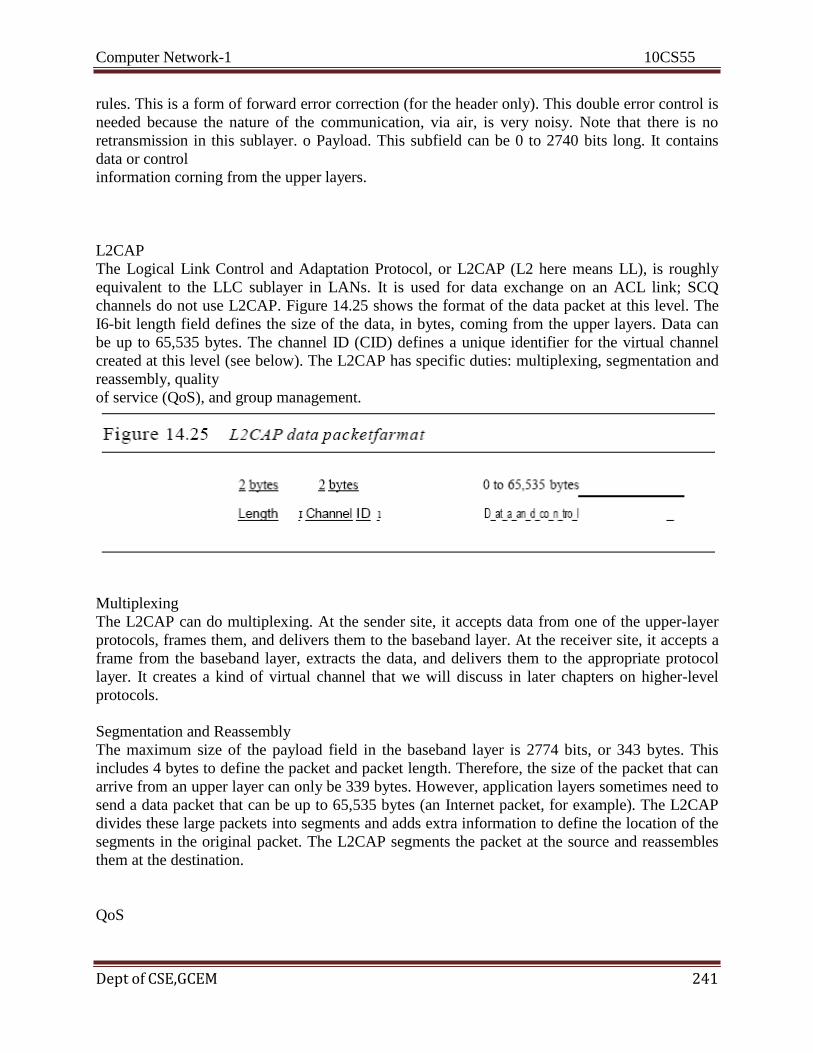
Computer Network-1 10CS55
Dept of CSE,GCEM 241
rules. This is a form of forward error correction (for the header only). This double error control is
needed because the nature of the communication, via air, is very noisy. Note that there is no
retransmission in this sublayer. o Payload. This subfield can be 0 to 2740 bits long. It contains
data or control
information corning from the upper layers.
L2CAP
The Logical Link Control and Adaptation Protocol, or L2CAP (L2 here means LL), is roughly
equivalent to the LLC sublayer in LANs. It is used for data exchange on an ACL link; SCQ
channels do not use L2CAP. Figure 14.25 shows the format of the data packet at this level. The
I6-bit length field defines the size of the data, in bytes, coming from the upper layers. Data can
be up to 65,535 bytes. The channel ID (CID) defines a unique identifier for the virtual channel
created at this level (see below). The L2CAP has specific duties: multiplexing, segmentation and
reassembly, quality
of service (QoS), and group management.
Multiplexing
The L2CAP can do multiplexing. At the sender site, it accepts data from one of the upper-layer
protocols, frames them, and delivers them to the baseband layer. At the receiver site, it accepts a
frame from the baseband layer, extracts the data, and delivers them to the appropriate protocol
layer. It creates a kind of virtual channel that we will discuss in later chapters on higher-level
protocols.
Segmentation and Reassembly
The maximum size of the payload field in the baseband layer is 2774 bits, or 343 bytes. This
includes 4 bytes to define the packet and packet length. Therefore, the size of the packet that can
arrive from an upper layer can only be 339 bytes. However, application layers sometimes need to
send a data packet that can be up to 65,535 bytes (an Internet packet, for example). The L2CAP
divides these large packets into segments and adds extra information to define the location of the
segments in the original packet. The L2CAP segments the packet at the source and reassembles
them at the destination.
QoS

Computer Network-1 10CS55
Dept of CSE,GCEM 242
Bluetooth allows the stations to define a quality-of-service level. We discuss quality of service in
Chapter 24. For the moment, it is sufficient to know that if no quality-of-service level is defined,
Bluetooth defaults to what is called best-effort service; it will do its best under the circumstances.
Group Management
Another functionality of L2CAP is to allow devices to create a type of logical addressing
between themselves. This is similar to multicasting. For example, two or three secondary devices
can be part of a multicast group to receive data from the primary. Other Upper Layers Bluetooth
defines several protocols for the upper layers that use the services of L2CAP; these protocols are
specific for each purpose.
15 CONNECTING DEVICES
In this section, we divide connecting devices into five different categories based on the layer in
which they operate in a network, as shown in Figure 15.1.
Figure 15.1 Five categories ofconnecting devices
The five categories contain devices which can be defined as
1. Those which operate below the physical layer such as a passive hub.
2. Those which operate at the physical layer (a repeater or an active hub).
3. Those which operate at the physical and data link layers (a bridge or a two-layer switch).
4. Those which operate at the physical, data link, and network
5. Those which can operate at all five layers (a gateway).
Passive Hubs
A passive hub is just a connector. It connects the wires coming from different branches. In a star-
topology Ethernet LAN, a passive hub is just a point where the signals coming from different
stations collide; the hub is the collision point. This type of a hub is part of the media; its location
in the Internet model is below the physical layer.
Repeaters
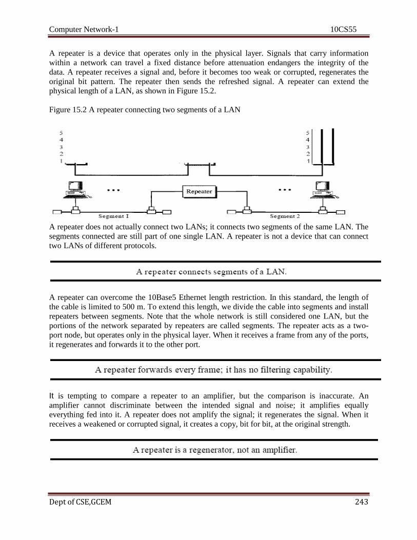
Computer Network-1 10CS55
Dept of CSE,GCEM 243
A repeater is a device that operates only in the physical layer. Signals that carry information
within a network can travel a fixed distance before attenuation endangers the integrity of the
data. A repeater receives a signal and, before it becomes too weak or corrupted, regenerates the
original bit pattern. The repeater then sends the refreshed signal. A repeater can extend the
physical length of a LAN, as shown in Figure 15.2.
Figure 15.2 A repeater connecting two segments of a LAN
A repeater does not actually connect two LANs; it connects two segments of the same LAN. The
segments connected are still part of one single LAN. A repeater is not a device that can connect
two LANs of different protocols.
A repeater can overcome the 10Base5 Ethernet length restriction. In this standard, the length of
the cable is limited to 500 m. To extend this length, we divide the cable into segments and install
repeaters between segments. Note that the whole network is still considered one LAN, but the
portions of the network separated by repeaters are called segments. The repeater acts as a two-
port node, but operates only in the physical layer. When it receives a frame from any of the ports,
it regenerates and forwards it to the other port.
It is tempting to compare a repeater to an amplifier, but the comparison is inaccurate. An
amplifier cannot discriminate between the intended signal and noise; it amplifies equally
everything fed into it. A repeater does not amplify the signal; it regenerates the signal. When it
receives a weakened or corrupted signal, it creates a copy, bit for bit, at the original strength.

Computer Network-1 10CS55
Dept of CSE,GCEM 244
The location of a repeater on a link is vital. A repeater must be placed so that a signal reaches it
before any noise changes the meaning of any of its bits. A little noise can alter the precision of a
bit's voltage without destroying its identity (see Figure 15.3). If the corrupted bit travels much
farther, however, accumulated noise can change its meaning completely. At that point, the
original voltage is not recoverable, and the error needs to be corrected. A repeater placed on the
line before the legibility of the signal becomes lost can still read the signal well enough to
determine the intended voltages and replicate them in their original form.
Figure 15.3 Function ofa repeater
Active Hubs
An active hub is actually a multipart repeater. It is normally used to create connections between
stations in a physical star topology. We have seen examples of hubs in some Ethernet
implementations (lOBase-T, for example). However, hubs can also be used to create multiple
levels of hierarchy, as shown in Figure 15.4. The hierarchical use of hubs removes the length
limitation of 10Base-T (100 m).
Bridges
A bridge operates in both the physical and the data link layer. As a physical layer device, it
regenerates the signal it receives. As a data link layer device, the bridge can check the physical
(MAC) addresses (source and destination) contained in the frame.
Figure 15.4 A hierarchy of hubs
Filtering
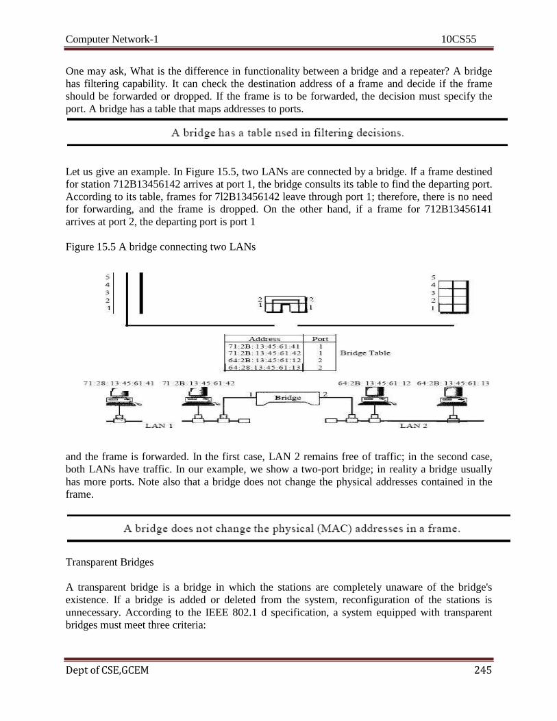
Computer Network-1 10CS55
Dept of CSE,GCEM 245
One may ask, What is the difference in functionality between a bridge and a repeater? A bridge
has filtering capability. It can check the destination address of a frame and decide if the frame
should be forwarded or dropped. If the frame is to be forwarded, the decision must specify the
port. A bridge has a table that maps addresses to ports.
Let us give an example. In Figure 15.5, two LANs are connected by a bridge. If a frame destined
for station 712B13456142 arrives at port 1, the bridge consults its table to find the departing port.
According to its table, frames for 7l2B13456142 leave through port 1; therefore, there is no need
for forwarding, and the frame is dropped. On the other hand, if a frame for 712B13456141
arrives at port 2, the departing port is port 1
Figure 15.5 A bridge connecting two LANs
and the frame is forwarded. In the first case, LAN 2 remains free of traffic; in the second case,
both LANs have traffic. In our example, we show a two-port bridge; in reality a bridge usually
has more ports. Note also that a bridge does not change the physical addresses contained in the
frame.
Transparent Bridges
A transparent bridge is a bridge in which the stations are completely unaware of the bridge's
existence. If a bridge is added or deleted from the system, reconfiguration of the stations is
unnecessary. According to the IEEE 802.1 d specification, a system equipped with transparent
bridges must meet three criteria:

Computer Network-1 10CS55
Dept of CSE,GCEM 246
I. Frames must be forwarded from one station to another.
2. The forwarding table is automatically made by learning frame movements in the network.
3. Loops in the system must be prevented.
Forwarding A transparent bridge must correctly forward the frames, as discussed in the previous
section. Learning The earliest bridges had forwarding tables that were static. The systems
administrator would manually enter each table entry during bridge setup. Although the process
was simple, it was not practical. If a station was added or deleted, the table had to be modified
manually. The same was true if a station's MAC address changed, which is not a rare event. For
example, putting in a new network card means a new MAC address.
A better solution to the static table is a dynamic table that maps addresses to ports automatically.
To make a table dynamic, we need a bridge that gradually learns from the frame movements. To
do this, the bridge inspects both the destination and the source addresses. The destination address
is used for the forwarding decision (table lookup); the source address is used for adding entries to
the table and for updating purposes.
Let us elaborate on this process by using Figure 15.6.
1. When station A sends a frame to station D, the bridge does not have an entry for either D or A.
The frame goes out from all three ports; the frame floods the network. However, by looking at
the source address, the bridge learns that station A must be located on the LAN connected to port
1. This means that frames destined for A, in the future, must be sent out through port 1. The
bridge adds this entry to its table. The table has its first entry now.
2. When station E sends a frame to station A, the bridge has an entry for A, so it forwards the
frame only to port 1. There is no flooding. In addition, it uses the source address of the frame, E,
to add a second entry to the table.
3. When station B sends a frame to C, the bridge has no entry for C, so once again it floods the
network and adds one more entry to the table.
4. The process of learning continues as the bridge forwards frames.
Figure 15.6 A learning bridge and the process of learning

Computer Network-1 10CS55
Dept of CSE,GCEM 247
Loop Problem Transparent bridges work fine as long as there are no redundant bridges in the
system. Systems administrators, however, like to have redundant bridges (more than one bridge
between a pair of LANs) to make the system more reliable. If a bridge fails, another bridge takes
over until the failed one is repaired or replaced. Redundancy can create loops in the system,
which is very undesirable. Figure 15.7 shows a very simple example of a loop created in a
system with two LANs connected by two bridges.
1. Station A sends a frame to station D. The tables of both bridges are empty. Both forward the
frame and update their tables based on the source address A.
2. Now there are two copies of the frame on LAN 2. The copy sent out by bridge 1 is received by
bridge 2, which does not have any information about the destination address D; it floods the
bridge. The copy sent out by bridge 2 is received by bridge 1 and is sent out for lack of
information about D. Note that each frame is handled separately because bridges, as two nodes
on a network sharing the medium, use an access method such as CSMA/CD. The tables of both
bridges are updated, but still there is no information for destination D.
3. Now there are two copies of the frame on LAN 1. Step 2 is repeated, and both copies flood the
network.
4. The process continues on and on. Note that bridges are also repeaters and regenerate frames.
So in each iteration, there are newly generated fresh copies of the frames. To solve the looping

Computer Network-1 10CS55
Dept of CSE,GCEM 248
problem, the IEEE specification requires that bridges use the spanning tree algorithm to create a
loopless topology.
Figure 15.7 Loop problem in a learning bridge
Spanning Tree
In graph theory, a spanning tree is a graph in which there is no loop. In a bridged LAN, this
means creating a topology in which each LAN can be reached from any other LAN through one
path only (no loop). We cannot change the physical topology of the system because of physical
connections between cables and bridges, but we can create a logical topology that overlays the
physical one. Figure 15.8 shows a system with four LANs and five bridges. We have shown the
physical system and its representation in graph theory. Although some textbooks represent the
LANs as nodes and the bridges as the connecting arcs, we have shown both LANs and bridges as
nodes. The connecting arcs show the connection of a LAN to a bridge and vice versa. To find the
spanning tree, we need to assign a cost (metric) to each arc. The interpretation of the cost is left
up to the systems administrator. It may be the path with minimum hops (nodes), the path with
minimum delay, or the path with maximum bandwidth. If two ports have the same shortest value,
the systems administrator just chooses one. We have chosen the minimum hops. However, as we
will see in Chapter 22, the hop count is normally 1 from a bridge to the LAN and 0 in the reverse
direction.
The process to find the spanning tree involves three steps:

Computer Network-1 10CS55
Dept of CSE, GCEM 250
1. Every bridge has a built-in ID (normally the serial number, which is unique). Each bridge
broadcasts this ID so that all bridges know which one has the smallest ID. The bridge with the
smallest ID is selected as the root bridge (root of the tree). We assume that bridge B1 has the
smallest ID. It is, therefore, selected as the root bridge.
Figure 15.8 A system ofconnected LANs and its graph representation
2. The algorithm tries to find the shortest path (a path with the shortest cost) from the root bridge
to every other bridge or LAN. The shortest path can be found by examining the total cost from
the root bridge to the destination. Figure 15.9 shows the shortest paths.
3. The combination of the shortest paths creates the shortest tree
.
4. Based on the spanning tree, we mark the ports that are part of the spanning tree, the
forwarding ports, which forward a frame that the bridge receives. We also mark those ports that
are not part of the spanning tree, the blocking ports, which block the frames received by the
bridge. Figure 15.10 shows the physical systems of LANs with forwarding points (solid lines)
and blocking ports (broken lines).
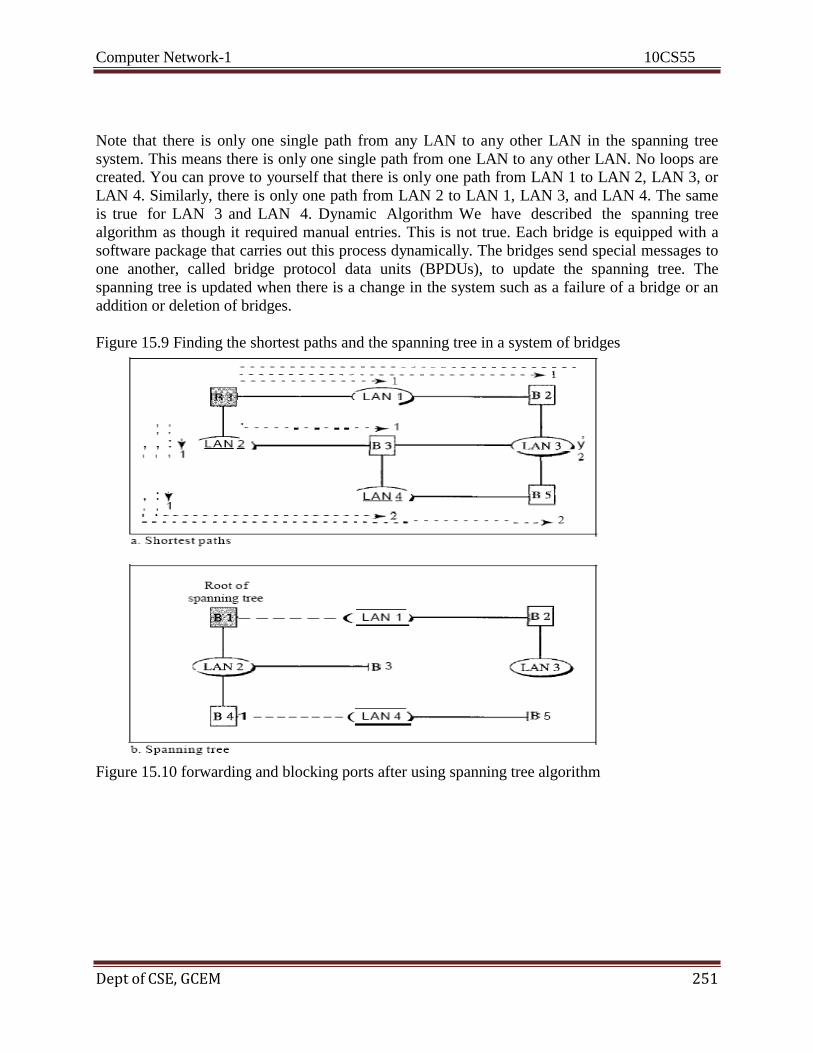
Computer Network-1 10CS55
Dept of CSE, GCEM 251
Note that there is only one single path from any LAN to any other LAN in the spanning tree
system. This means there is only one single path from one LAN to any other LAN. No loops are
created. You can prove to yourself that there is only one path from LAN 1 to LAN 2, LAN 3, or
LAN 4. Similarly, there is only one path from LAN 2 to LAN 1, LAN 3, and LAN 4. The same
is true for LAN 3 and LAN 4. Dynamic Algorithm We have described the spanning tree
algorithm as though it required manual entries. This is not true. Each bridge is equipped with a
software package that carries out this process dynamically. The bridges send special messages to
one another, called bridge protocol data units (BPDUs), to update the spanning tree. The
spanning tree is updated when there is a change in the system such as a failure of a bridge or an
addition or deletion of bridges.
Figure 15.9 Finding the shortest paths and the spanning tree in a system of bridges
Figure 15.10 forwarding and blocking ports after using spanning tree algorithm
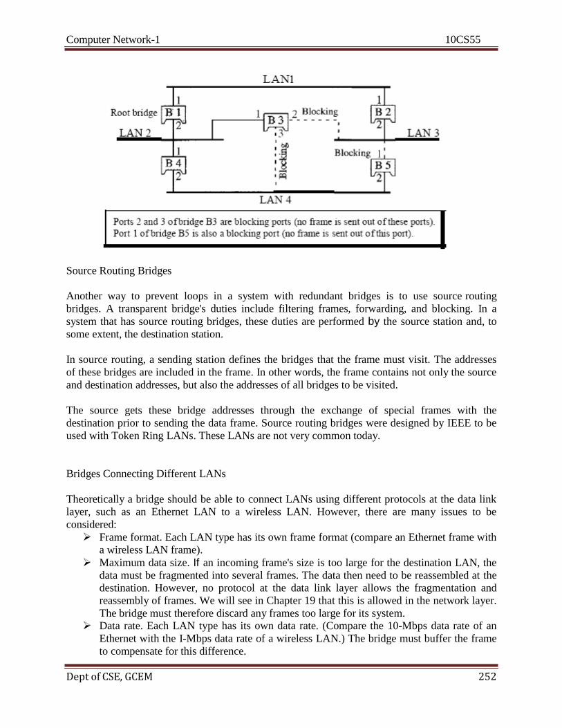
Computer Network-1 10CS55
Dept of CSE, GCEM 252
Source Routing Bridges
Another way to prevent loops in a system with redundant bridges is to use source routing
bridges. A transparent bridge's duties include filtering frames, forwarding, and blocking. In a
system that has source routing bridges, these duties are performed by the source station and, to
some extent, the destination station.
In source routing, a sending station defines the bridges that the frame must visit. The addresses
of these bridges are included in the frame. In other words, the frame contains not only the source
and destination addresses, but also the addresses of all bridges to be visited.
The source gets these bridge addresses through the exchange of special frames with the
destination prior to sending the data frame. Source routing bridges were designed by IEEE to be
used with Token Ring LANs. These LANs are not very common today.
Bridges Connecting Different LANs
Theoretically a bridge should be able to connect LANs using different protocols at the data link
layer, such as an Ethernet LAN to a wireless LAN. However, there are many issues to be
considered:
Frame format. Each LAN type has its own frame format (compare an Ethernet frame with
a wireless LAN frame).
Maximum data size. If an incoming frame's size is too large for the destination LAN, the
data must be fragmented into several frames. The data then need to be reassembled at the
destination. However, no protocol at the data link layer allows the fragmentation and
reassembly of frames. We will see in Chapter 19 that this is allowed in the network layer.
The bridge must therefore discard any frames too large for its system.
Data rate. Each LAN type has its own data rate. (Compare the 10-Mbps data rate of an
Ethernet with the I-Mbps data rate of a wireless LAN.) The bridge must buffer the frame
to compensate for this difference.
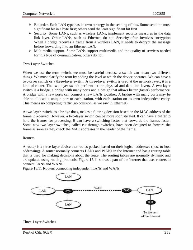
Computer Network-1 10CS55
Dept of CSE, GCEM 253
Bit order. Each LAN type has its own strategy in the sending of bits. Some send the most
significant bit in a byte first; others send the least significant bit first.
Security. Some LANs, such as wireless LANs, implement security measures in the data
link layer. Other LANs, such as Ethernet, do not. Security often involves encryption
When a bridge receives a frame from a wireless LAN, it needs to decrypt the message
before forwarding it to an Ethernet LAN.
Multimedia support. Some LANs support multimedia and the quality of services needed
for this type of communication; others do not.
Two-Layer Switches
When we use the term switch, we must be careful because a switch can mean two different
things. We must clarify the term by adding the level at which the device operates. We can have a
two-layer switch or a three-layer switch. A three-layer switch is used at the network layer; it is a
kind of router. The two-layer switch performs at the physical and data link layers. A two-layer
switch is a bridge, a bridge with many ports and a design that allows better (faster) performance.
A bridge with a few ports can connect a few LANs together. A bridge with many ports may be
able to allocate a unique port to each station, with each station on its own independent entity.
This means no competing traffic (no collision, as we saw in Ethernet).
A two-layer switch, as a bridge does, makes a filtering decision based on the MAC address of the
frame it received. However, a two-layer switch can be more sophisticated. It can have a buffer to
hold the frames for processing. It can have a switching factor that forwards the frames faster.
Some new two-layer switches, called cut-through switches, have been designed to forward the
frame as soon as they check the MAC addresses in the header of the frame.
Routers
A router is a three-layer device that routes packets based on their logical addresses (host-to-host
addressing). A router normally connects LANs and WANs in the Internet and has a routing table
that is used for making decisions about the route. The routing tables are normally dynamic and
are updated using routing protocols. Figure 15.11 shows a part of the Internet that uses routers to
connect LANs and WANs.
Figure 15.11 Routers connecting independent LANs and WANs
Three-Layer Switches

Computer Network-1 10CS55
Dept of CSE, GCEM 254
A three-layer switch is a router, but a faster and more sophisticated. The switching fabric in a
three-layer switch allows faster table lookup and forwarding. In this book, we use the terms
router and three-layer switch interchangeably.
Gateway
Although some textbooks use the terms gateway and router interchangeably, most of the
literature distinguishes between the two. A gateway is normally a computer that operates in all
five layers of the Internet or seven layers of OSI model. A gateway takes an application message,
reads it, and interprets it. This means that it can be used as a connecting device between two
internetworks that use different models. For example, a network designed to use the OSI model
can be connected to another network using the Internet model. The gateway connecting the two
systems can take a frame as it arrives from the first system, move it up to the OSI application
layer, and remove the
message. Gateways can provide security.
15.2 BACKBONE NETWORKS
Some connecting devices discussed in this chapter can be used to connect LANs in a backbone
network. A backbone network allows several LANs to be connected. In a backbone network, no
station is directly connected to the backbone; the stations are part of a LAN, and the backbone
connects the LANs. The backbone is itself a LAN that uses a LAN protocol such as Ethernet;
each connection to the backbone is itself another LAN. Although many different architectures
can be used for a backbone, we discuss only the two most common: the bus and the star.
Bus Backbone
In a bus backbone, the topology of the backbone is a bus. The backbone itself can use one of the
protocols that support a bus topology such as lOBase5 or lOBase2.
Bus backbones are normally used as a distribution backbone to connect different buildings in an
organization. Each building can comprise either a single LAN or another backbone (normally a
star backbone). A good example of a bus backbone is one that connects single- or multiple-floor
buildings on a campus. Each single-floor building usually has a single LAN. Each multiple-floor
building has a backbone (usually a star) that connects each LAN on a floor. A bus backbone can
interconnect these LANs and backbones. Figure 15.12 shows an example of a bridge-based
backbone with four LANs
Figure 15.12 Bus backbone
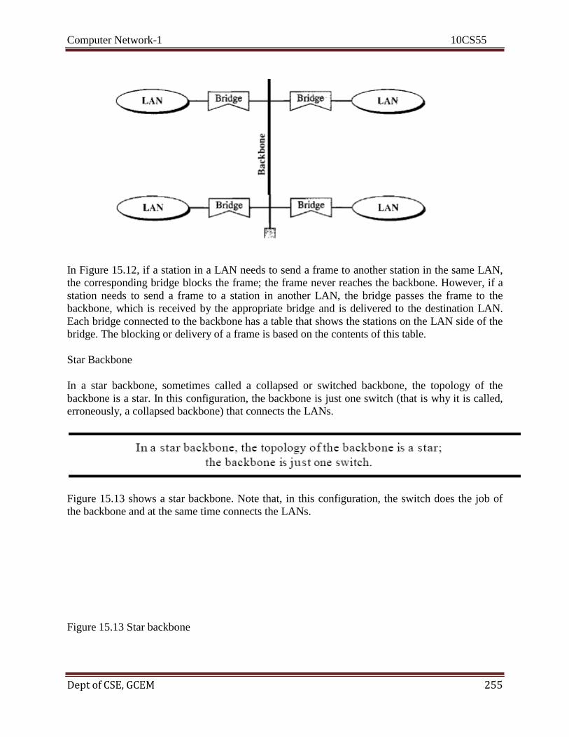
Computer Network-1 10CS55
Dept of CSE, GCEM 255
In Figure 15.12, if a station in a LAN needs to send a frame to another station in the same LAN,
the corresponding bridge blocks the frame; the frame never reaches the backbone. However, if a
station needs to send a frame to a station in another LAN, the bridge passes the frame to the
backbone, which is received by the appropriate bridge and is delivered to the destination LAN.
Each bridge connected to the backbone has a table that shows the stations on the LAN side of the
bridge. The blocking or delivery of a frame is based on the contents of this table.
Star Backbone
In a star backbone, sometimes called a collapsed or switched backbone, the topology of the
backbone is a star. In this configuration, the backbone is just one switch (that is why it is called,
erroneously, a collapsed backbone) that connects the LANs.
Figure 15.13 shows a star backbone. Note that, in this configuration, the switch does the job of
the backbone and at the same time connects the LANs.
Figure 15.13 Star backbone

Computer Network-1 10CS55
Dept of CSE, GCEM 256
Star backbones are mostly used as a distribution backbone inside a building. In a multifloor
building, we usually find one LAN that serves each particular floor. A star backbone connects
these LANs. The backbone network, which is just a switch, can be installed in the basement or
the first floor, and separate cables can run from the switch to each LAN. If the individual LANs
have a physical star topology, either the hubs (or switches) can be installed in a closet on the
corresponding floor, or all can be installed close to the switch. We often find a rack or chassis in
the basement where the backbone switch and all hubs or switches are installed.
Connecting Remote LANs
Another common application for a backbone network is to connect remote LANs. This type of
backbone network is useful when a company has several offices with LANs and needs to connect
them. The connection can be done through bridges, sometimes called remote bridges. The
bridges act as connecting devices connecting LANs and point-to-point networks, such as leased
telephone lines or ADSL lines. The point-to-point network in this case is considered a LAN
without stations. The point-to-point link can use a protocol such as PPP. Figure 15.14 shows a
backbone connecting remote LANs.
Figure 15.14 Connecting remote IANs with bridges

Computer Network-1 10CS55
Dept of CSE, GCEM 257
15.3 VIRTUAL LANs
A station is considered part of a LAN if it physically belongs to that LAN. The criterion of
membership is geographic. What happens if we need a virtual connection between two stations
belonging to two different physical LANs? We can roughly define a virtual local area network
(VLAN) as a local area network configured by software, not by physical wiring.
Let us use an example to elaborate on this definition. Figure 15.15 shows a switched LAN in an
engineering firm in which 10 stations are grouped into three LANs that are connected by a
switch. The first four engineers work together as the first group, the next three engineers work
together as the second group, and the last three engineers work together as the third group. The
LAN is configured to allow this arrangement. But what would happen if the administrators
needed to move two engineers from the first group to the third group, to speed up the project
being done by the third group? The LAN configuration would need to be changed. The network
technician must rewire. The problem is repeated if, in another week, the two engineers move
back to their previous group. In a switched LAN, changes in the work group mean physical
changes in the network configuration.
Figure 15.15 A switch connecting three LANs
Figure 15.16 shows the same switched LAN divided into VLANs. The whole idea of VLAN
technology is to divide a LAN into logical, instead of physical, segments. A LAN can be divided
into several logical LANs called VLANs. Each VLAN is a work group in the organization. If a
person moves from one group to another, there is no need to change the physical configuration.
The group membership in VLANs is defined by software, not hardware. Any station can be
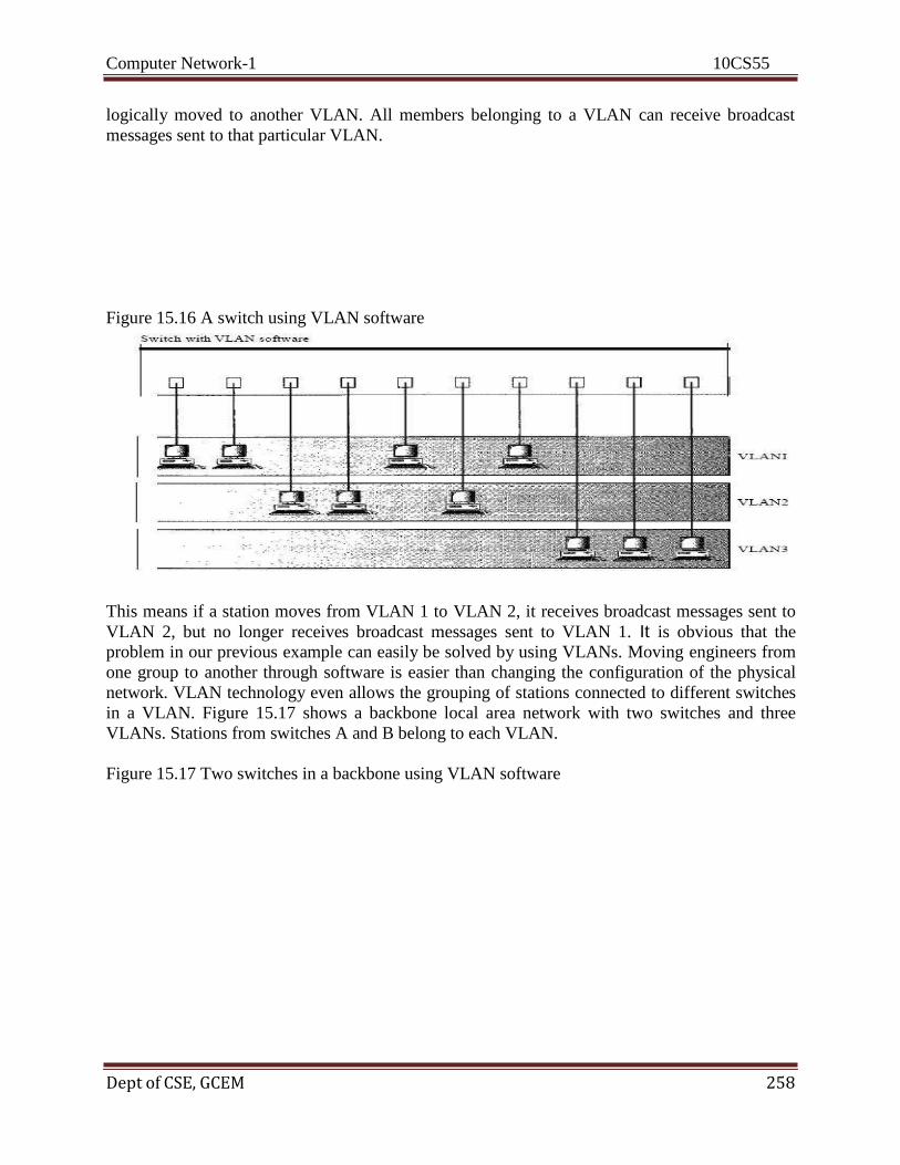
Computer Network-1 10CS55
Dept of CSE, GCEM 258
logically moved to another VLAN. All members belonging to a VLAN can receive broadcast
messages sent to that particular VLAN.
Figure 15.16 A switch using VLAN software
This means if a station moves from VLAN 1 to VLAN 2, it receives broadcast messages sent to
VLAN 2, but no longer receives broadcast messages sent to VLAN 1. It is obvious that the
problem in our previous example can easily be solved by using VLANs. Moving engineers from
one group to another through software is easier than changing the configuration of the physical
network. VLAN technology even allows the grouping of stations connected to different switches
in a VLAN. Figure 15.17 shows a backbone local area network with two switches and three
VLANs. Stations from switches A and B belong to each VLAN.
Figure 15.17 Two switches in a backbone using VLAN software
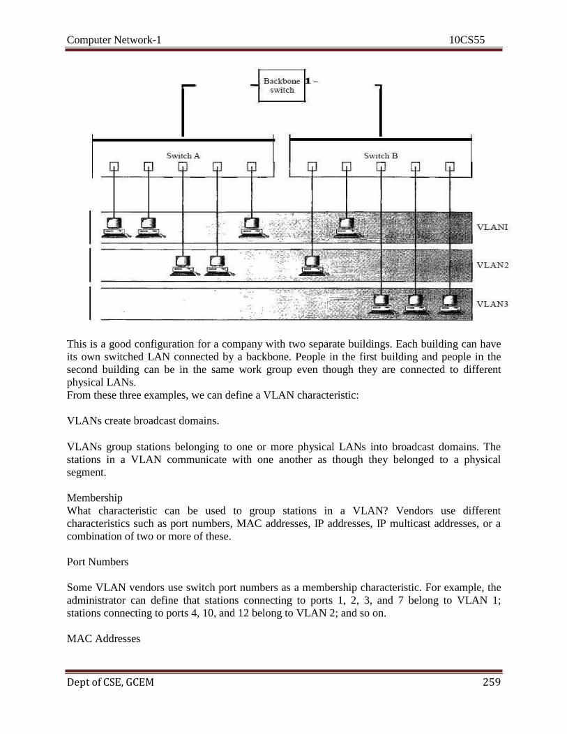
Computer Network-1 10CS55
Dept of CSE, GCEM 259
This is a good configuration for a company with two separate buildings. Each building can have
its own switched LAN connected by a backbone. People in the first building and people in the
second building can be in the same work group even though they are connected to different
physical LANs.
From these three examples, we can define a VLAN characteristic:
VLANs create broadcast domains.
VLANs group stations belonging to one or more physical LANs into broadcast domains. The
stations in a VLAN communicate with one another as though they belonged to a physical
segment.
Membership
What characteristic can be used to group stations in a VLAN? Vendors use different
characteristics such as port numbers, MAC addresses, IP addresses, IP multicast addresses, or a
combination of two or more of these.
Port Numbers
Some VLAN vendors use switch port numbers as a membership characteristic. For example, the
administrator can define that stations connecting to ports 1, 2, 3, and 7 belong to VLAN 1;
stations connecting to ports 4, 10, and 12 belong to VLAN 2; and so on.
MAC Addresses

Computer Network-1 10CS55
Dept of CSE, GCEM 260
Some VLAN vendors use the 48-bit MAC address as a membership characteristic. For example,
the administrator can stipulate that stations having MAC addresses E21342A12334 and
F2A123BCD341belong to VLAN 1.
IP Addresses
Some VLAN vendors use the 32-bit IP address (see Chapter 19) as a membership characteristic.
For example, the administrator can stipulate that stations having IP addresses 181.34.23.67,
181.34.23.72, 181.34.23.98, and 181.34.23.112 belong to VLAN 1. Multicast IP Addresses
Some VLAN vendors use the multicast IP address (see Chapter 19) as a membership
characteristic. Multicasting at the IP layer is now translated to multicasting at the data link layer.
Combination Recently, the software available from some vendors allows all these characteristics
to be combined. The administrator can choose one or more characteristics when installing the
software. In addition, the software can be reconfigured to change the settings.
Configuration
How are the stations grouped into different VLANs? Stations are configured in one of three
ways: manual, semiautomatic, and automatic.
Manual Configuration
In a manual configuration, the network administrator uses the VLAN software to manually
assign the stations into different VLANs at setup. Later migration from one VLAN to another is
also done manually. Note that this is not a physical configuration; it is a logical configuration.
The term manually here means that the administrator types the port numbers, the IP addresses, or
other characteristics, using the VLAN software.
Automatic Configuration
In an automatic configuration, the stations are automatically connected or disconnected from a
VLAN using criteria defined by the administrator. For example, the administrator can define the
project number as the criterion for being a member of a group. When a user changes the project,
he or she automatically migrates to a new VLAN.
Semiautomatic Configuration
A semiautomatic configuration is somewhere between a manual configuration and an automatic
configuration. Usually, the initializing is done manually, with migrations done automatically.
Communication between Switches
In a multiswitched backbone, each switch must know not only which station belongs to which
VLAN, but also the membership of stations connected to other switches. For example, in Figure
15.17, switch A must know the membership status of stations connected to switch B, and switch
B must know the same about switch A. Three methods have been devised for this purpose: table
maintenance, frame tagging, and time-division multiplexing.

Computer Network-1 10CS55
Dept of CSE,GCEM 260
Table Maintenance
In this method, when a station sends a broadcast frame to its group members, the switch creates
an entry in a table and records station membership. The switches send their tables to one another
periodically for updating.
Frame Tagging
In this method, when a frame is traveling between switches, an extra header is added to the MAC
frame to define the destination VLAN. The frame tag is used by the receiving switches to
determine the VLANs to be receiving the broadcast message.
Time-Division Multiplexing (TDM)
In this method, the connection (trunk) between switches is divided into timeshared channels (see
TDM in Chapter 6). For example, if the total number of VLANs in a backbone is five, each trunk
is divided into five channels. The traffic destined for VLAN 1 travels in channell, the traffic
destined for VLAN 2 travels in channel 2, and so on. The receiving switch determines the
destination VLAN by checking the channel from which the frame arrived.
IEEE Standard
In 1996, the IEEE 802.1 subcommittee passed a standard called 802.1Q that defines the format
for frame tagging. The standard also defines the format to be used in multiswitched backbones
and enables the use of multivendor equipment in VLANs. IEEE 802.1Q has opened the way for
further standardization in other issues related to VLANs. Most vendors have already accepted the
standard.
Advantages
There are several advantages to using VLANs.
Cost and Time Reduction
VLANs can reduce the migration cost of stations going from one group to another. Physical
reconfiguration takes time and is costly. Instead of physically moving one station to another
segment or even to another switch, it is much easier and quicker to move it by using software.
Creating Virtual Work Groups
VLANs can be used to create virtual work groups. For example, in a campus environment,
professors working on the same project can send broadcast messages to one another without the
necessity of belonging to the same department. This can reduce traffic if the multicasting
capability of IP was previously used. Security
Computer Network-1 10CS55
Dept of CSE,GCEM 261
VLANs provide an extra measure of security. People belonging to the same group can send
broadcast messages with the guaranteed assurance that users in other groups will not receive
these messages
Recommended Questions
1. What is the relationship between a base station and a
mobile switching center?
2. What are the functions of a mobile switching center? 3. What is the difference between a hard handoff and a soft
handoff?
4. What is the relationship between D-AMPS and AMPS?
5. What are the three types of orbits? 6. Which type of orbit does a GEO satellite have? Explain
your answer
7. What is the relationship between the Van Allen belts and
satellites?
8. What is the relationship between the Van Allen belts and
satellites?
Computer Network-1 10CS55
Dept of CSE,GCEM 262
COMPUTER NETWORKS – I
Subject Code: 10CS55 I.A. Marks : 25 Hours/Week : 04 Exam Hours: 03
Total Hours : 52 Exam Marks: 100
UNIT - 8: 7 Hours Network Layer:
- Introduction,
- Logical addressing,
- IPv4 addresses,
- Internetworking basics,
- IPv4, IPv6,
- Comparison of IPv4 and IPv6 Headers.

Computer Network-1 10CS55
Dept of CSE,GCEM 263
Unit-8
NETWORK LAYER
Logical Addressing Logical Address, which is assigned during configuration of the network, refers to the virtual
address or logical location of the machine. This concept is similar to a person’s mailing address.
Usually Two types of logical addressing are used in the Network layer. IP addresses and IPX
addresses. IP addresses are used in all TCP/IP based networks where as IPX addresses are used
in Novel Netware environment.
IP Addresses IP address is the 32 BIT identifier used to identify the host or some interface. IP address consists
of two parts Network ID (high order bits), that represents the Network for the particular host or
interface. Host ID (low order bits), that represents the logical host identification number. IP
addresses are divided into 5 classes:
• Class A addresses start with a `0' in the most significant bit, followed by a 7-bit network
address and a 24-bit local part.
• Class B addresses start with a `10' in the two most significant bits, followed by a 14-bit network
number and a 16-bit local part.
• Class C addresses start with a `110' in the three most significant bits, followed by a 21-bit
network number and an 8-bit local part
. Class D addresses start with a `1110' in the four most significant bits, followed by a 28-bit
group number. Used for multicast.
• Class E addresses start with a ‘11110’ and are reserved for future use.
Classful addressing:
• Inefficient use of address space, address space exhaustion
• e.g., class B net allocated enough addresses for 65K hosts, even if only
2K hosts in that network
CIDR: Classless InterDomain Routing
• Network portion of address of arbitrary length
• Address format: a.b.c.d/x, where x is # bits in network portion of address
11001000 00010111 00010000 00000000
An Internet Protocol address (IP address) is a numerical label assigned to each device (e.g.,
computer, printer) participating in a computer network that uses the Internet Protocol for
communication.[1] An IP address serves two principal functions: host or network
interface identification and location addressing. Its role has been characterized as follows:
"A name indicates what we seek. An address indicates where it is. A route indicates how to get
there."[2]
The designers of the Internet Protocol defined an IP address as a 32-bit number[1] and this
system, known as Internet Protocol Version 4 (IPv4), is still in use today. However, due to the
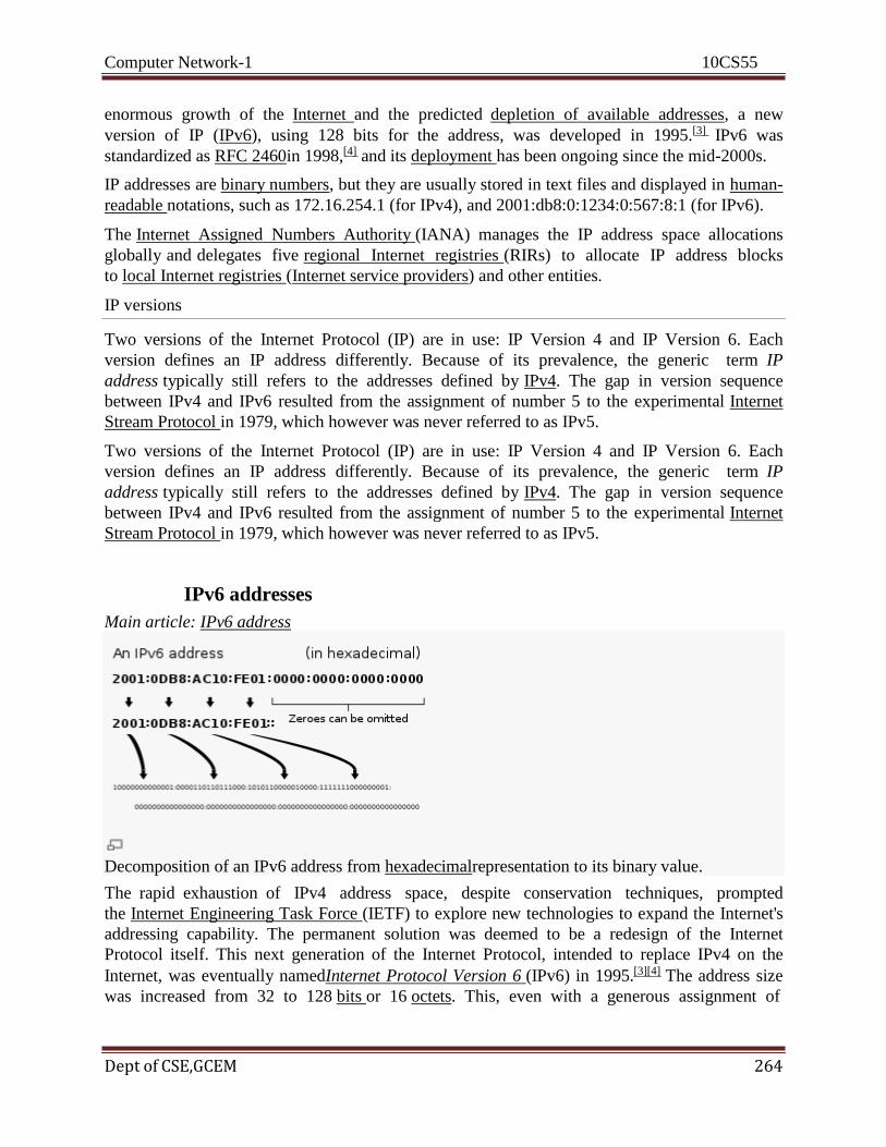
Computer Network-1 10CS55
Dept of CSE,GCEM 264
enormous growth of the Internet and the predicted depletion of available addresses, a new
version of IP (IPv6), using 128 bits for the address, was developed in 1995.[3] IPv6 was
standardized as RFC 2460in 1998,[4] and its deployment has been ongoing since the mid-2000s.
IP addresses are binary numbers, but they are usually stored in text files and displayed in human-
readable notations, such as 172.16.254.1 (for IPv4), and 2001:db8:0:1234:0:567:8:1 (for IPv6).
The Internet Assigned Numbers Authority (IANA) manages the IP address space allocations
globally and delegates five regional Internet registries (RIRs) to allocate IP address blocks
to local Internet registries (Internet service providers) and other entities.
IP versions
Two versions of the Internet Protocol (IP) are in use: IP Version 4 and IP Version 6. Each
version defines an IP address differently. Because of its prevalence, the generic term IP
address typically still refers to the addresses defined by IPv4. The gap in version sequence
between IPv4 and IPv6 resulted from the assignment of number 5 to the experimental Internet
Stream Protocol in 1979, which however was never referred to as IPv5.
IPv6 addresses
The rapid exhaustion of IPv4 address space, despite conservation techniques, prompted
the Internet Engineering Task Force (IETF) to explore new technologies to expand the Internet's
addressing capability. The permanent solution was deemed to be a redesign of the Internet
Protocol itself. This next generation of the Internet Protocol, intended to replace IPv4 on the
Internet, was eventually namedInternet Protocol Version 6 (IPv6) in 1995.[3][4] The address size
was increased from 32 to 128 bits or 16 octets. This, even with a generous assignment of
Main article: IPv6 address
Decomposition of an IPv6 address from hexadecimalrepresentation to its binary value.
Computer Network-1 10CS55
Dept of CSE,GCEM 265
network blocks, is deemed sufficient for the foreseeable future. Mathematically, the new address
space provides the potential for a maximum of 2128, or about 3.403×1038 unique addresses.
The new design is not intended to provide a sufficient quantity of addresses on its own, but rather
to allow efficient aggregation of subnet routing prefixes to occur at routing nodes. As a result,
routing table sizes are smaller, and the smallest possible individual allocation is a subnet for
264 hosts, which is the square of the size of the entire IPv4 Internet. At these levels, actual
address utilization rates will be small on any IPv6 network segment. The new design also
provides the opportunity to separate the addressing infrastructure of a network segment — that is
the local administration of the segment's available space — from the addressing prefix used to
route external traffic for a network. IPv6 has facilities that automatically change the routing
prefix of entire networks, should the global connectivity or the routing policy change, without
requiring internal redesign or renumbering.
The large number of IPv6 addresses allows large blocks to be assigned for specific purposes and,
where appropriate, to be aggregated for efficient routing. With a large address space, there is not
the need to have complex address conservation methods as used in Classless Inter-Domain
Routing (CIDR).
Many modern desktop and enterprise server operating systems include native support for the
IPv6 protocol, but it is not yet widely deployed in other devices, such as home networking
routers,voice over IP (VoIP) and multimedia equipment, and network peripherals.
IPv6 private addresses
Just as IPv4 reserves addresses for private or internal networks, blocks of addresses are set aside
in IPv6 for private addresses. In IPv6, these are referred to as unique local addresses (ULA).RFC
4193 sets aside the routing prefix fc00::/7 for this block which is divided into two /8 blocks with
different implied policies. The addresses include a 40-bit pseudorandom number that minimizes
the risk of address collisions if sites merge or packets are misrouted.[8]
Early designs used a different block for this purpose (fec0::), dubbed site-local
addresses.[9] However, the definition of what constituted sites remained unclear and the poorly
defined addressing policy created ambiguities for routing. This address range specification was
abandoned and must not be used in new systems.[10]
Addresses starting with fe80:, called link-local addresses, are assigned to interfaces for
communication on the link only. The addresses are automatically generated by the operating
system for each network interface. This provides instant and automatic network connectivity for
any IPv6 host and means that if several hosts connect to a common hub or switch, they have a
communication path via their link-local IPv6 address. This feature is used in the lower layers of
IPv6 network administration (e.g. Neighbor Discovery Protocol).
None of the private address prefixes may be routed on the public Internet.
IP subnetworks
IP networks may be divided into subnetworks in both IPv4 and IPv6. For this purpose, an IP
address is logically recognized as consisting of two parts: the network prefix and the host
identifier, orinterface identifier (IPv6). The subnet mask or the CIDR prefix determines how the
IP address is divided into network and host parts.
Computer Network-1 10CS55
Dept of CSE,GCEM 266
The term subnet mask is only used within IPv4. Both IP versions however use the Classless
Inter-Domain Routing (CIDR) concept and notation. In this, the IP address is followed by a slash
and the number (in decimal) of bits used for the network part, also called the routing prefix. For
example, an IPv4 address and its subnet mask may be 192.0.2.1 and 255.255.255.0, respectively.
TheCIDR notation for the same IP address and subnet is 192.0.2.1/24, because the first 24 bits of
the IP address indicate the network and subnet.
IP address assignment
Internet Protocol addresses are assigned to a host either anew at the time of booting, or
permanently by fixed configuration of its hardware or software. Persistent configuration is also
known as using a static IP address. In contrast, in situations when the computer's IP address is
assigned newly each time, this is known as using a dynamic IP address.
Methods
Static IP addresses are manually assigned to a computer by an administrator. The exact
procedure varies according to platform. This contrasts with dynamic IP addresses, which are
assigned either by the computer interface or host software itself, as in Zeroconf, or assigned by a
server using Dynamic Host Configuration Protocol (DHCP). Even though IP addresses assigned
using DHCP may stay the same for long periods of time, they can generally change. In some
cases, a network administrator may implement dynamically assigned static IP addresses. In this
case, a DHCP server is used, but it is specifically configured to always assign the same IP
address to a particular computer. This allows static IP addresses to be configured centrally,
without having to specifically configure each computer on the network in a manual procedure.
In the absence or failure of static or stateful (DHCP) address configurations, an operating system
may assign an IP address to a network interface using state-less auto-configuration methods,
such as Zeroconf.
Uses of dynamic addressing
Dynamic IP addresses are most frequently assigned on LANs and broadband networks
by Dynamic Host Configuration Protocol (DHCP) servers. They are used because it avoids the
administrative burden of assigning specific static addresses to each device on a network. It also
allows many devices to share limited address space on a network if only some of them will be
online at a particular time. In most current desktop operating systems, dynamic IP configuration
is enabled by default so that a user does not need to manually enter any settings to connect to a
network with a DHCP server. DHCP is not the only technology used to assign dynamic IP
addresses. Dialup and some broadband networks use dynamic address features of the Point-to-
Point Protocol.
Sticky dynamic IP address
A sticky dynamic IP address is an informal term used by cable and DSL Internet access
subscribers to describe a dynamically assigned IP address which seldom changes. The addresses
are usually assigned with DHCP. Since the modems are usually powered on for extended periods
of time, the address leases are usually set to long periods and simply renewed. If a modem is
turned off and powered up again before the next expiration of the address lease, it will most
likely receive the same IP address.
Computer Network-1 10CS55
Dept of CSE,GCEM 267
Address autoconfiguration
RFC 3330 defines an address block, 169.254.0.0/16, for the special use in link-local
addressing for IPv4 networks. In IPv6, every interface, whether using static or dynamic address
assignments, also receives a local-link address automatically in the block fe80::/10.
These addresses are only valid on the link, such as a local network segment or point-to-point
connection, that a host is connected to. These addresses are not routable and like private
addresses cannot be the source or destination of packets traversing the Internet.
When the link-local IPv4 address block was reserved, no standards existed for mechanisms of
address autoconfiguration. Filling the void, Microsoft created an implementation that is called
Automatic Private IP Addressing (APIPA). Due to Microsoft's market power, APIPA has been
deployed on millions of machines and has, thus, become a de facto standard in the industry.
Many years later, the IETF defined a formal standard for this functionality, RFC 3927,
entitled Dynamic Configuration of IPv4 Link-Local Addresses.
Uses of static addressing
Some infrastructure situations have to use static addressing, such as when finding the Domain
Name System (DNS) host that will translate domain names to IP addresses. Static addresses are
also convenient, but not absolutely necessary, to locate servers inside an enterprise. An address
obtained from a DNS server comes with a time to live, or caching time, after which it should be
looked up to confirm that it has not changed. Even static IP addresses do change as a result of
network administration (RFC 2072).
Public addresses
A public IP address, in common parlance, is synonymous with a globally routable unicast IP address.[citation needed]
Both IPv4 and IPv6 define address ranges that are reserved for private networks and link-local
addressing. The term public IP address often used excludes these types of addresses.
Modifications to IP addressing
IP blocking and firewalls
Firewalls perform Internet Protocol blocking to protect networks from unauthorized access. They
are common on today's Internet. They control access to networks based on the IP address of a
client computer. Whether using a blacklist or a whitelist, the IP address that is blocked is the
perceived IP address of the client, meaning that if the client is using a proxy server or network
address translation, blocking one IP address may block many individual computers.
IP address translation
Multiple client devices can appear to share IP addresses: either because they are part of a shared
hosting web server environment or because an IPv4 network address translator (NAT) or proxy
server acts as an intermediary agent on behalf of its customers, in which case the real originating
IP addresses might be hidden from the server receiving a request. A common practice is to have
a NAT hide a large number of IP addresses in a private network. Only the "outside" interface(s)
of the NAT need to have Internet-routable addresses.[11]
Dept of CSE,GCEM 268
Computer Network-1 10CS55
Most commonly, the NAT device maps TCP or UDP port numbers on
the outside to individual private addresses on the inside. Just as a
telephone number may have site-specific extensions, the port numbers
are site-specific extensions to an IP address.
In small home networks, NAT functions usually take place in a residential gateway device,
typically one marketed as a "router". In this scenario, the computers connected to the router
would have 'private' IP addresses and the router would have a 'public' address to communicate
with the Internet. This type of router allows several computers to share one public IP address.
Recommended Questions
1. What is the name of the packet in IP layer. 2. Why does the IP checksum just cover the header.
3. What is the function of ICMP.
4. Name and explain three types of IPv6 addresses. 5. What strategies are devised for transition of IPV4 to IPV6.
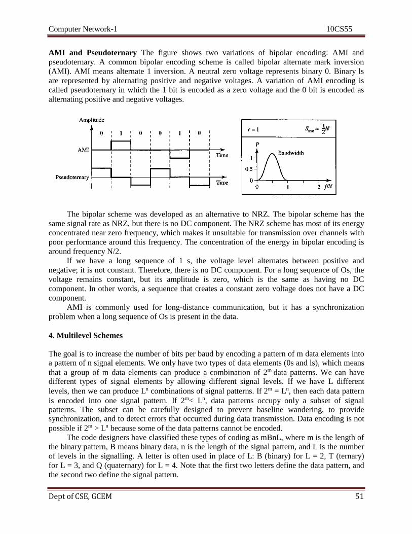
Computer Network-1 10CS55
Dept of CSE, GCEM 51
AMI and Pseudoternary The figure shows two variations of bipolar encoding: AMI and
pseudoternary. A common bipolar encoding scheme is called bipolar alternate mark inversion
(AMI). AMI means alternate 1 inversion. A neutral zero voltage represents binary 0. Binary ls
are represented by alternating positive and negative voltages. A variation of AMI encoding is
called pseudoternary in which the 1 bit is encoded as a zero voltage and the 0 bit is encoded as
alternating positive and negative voltages.
The bipolar scheme was developed as an alternative to NRZ. The bipolar scheme has the
same signal rate as NRZ, but there is no DC component. The NRZ scheme has most of its energy
concentrated near zero frequency, which makes it unsuitable for transmission over channels with
poor performance around this frequency. The concentration of the energy in bipolar encoding is
around frequency N/2.
If we have a long sequence of 1 s, the voltage level alternates between positive and
negative; it is not constant. Therefore, there is no DC component. For a long sequence of Os, the
voltage remains constant, but its amplitude is zero, which is the same as having no DC
component. In other words, a sequence that creates a constant zero voltage does not have a DC
component.
AMI is commonly used for long-distance communication, but it has a synchronization
problem when a long sequence of Os is present in the data.
4. Multilevel Schemes
The goal is to increase the number of bits per baud by encoding a pattern of m data elements into a pattern of n signal elements. We only have two types of data elements (0s and ls), which means
that a group of m data elements can produce a combination of 2m data patterns. We can have different types of signal elements by allowing different signal levels. If we have L different
levels, then we can produce Ln combinations of signal patterns. If 2m = Ln, then each data pattern
is encoded into one signal pattern. If 2m< Ln, data patterns occupy only a subset of signal patterns. The subset can be carefully designed to prevent baseline wandering, to provide synchronization, and to detect errors that occurred during data transmission. Data encoding is not
possible if 2m > Ln because some of the data patterns cannot be encoded.
The code designers have classified these types of coding as mBnL, where m is the length of
the binary pattern, B means binary data, n is the length of the signal pattern, and L is the number
of levels in the signalling. A letter is often used in place of L: B (binary) for L = 2, T (ternary)
for L = 3, and Q (quaternary) for L = 4. Note that the first two letters define the data pattern, and
the second two define the signal pattern.
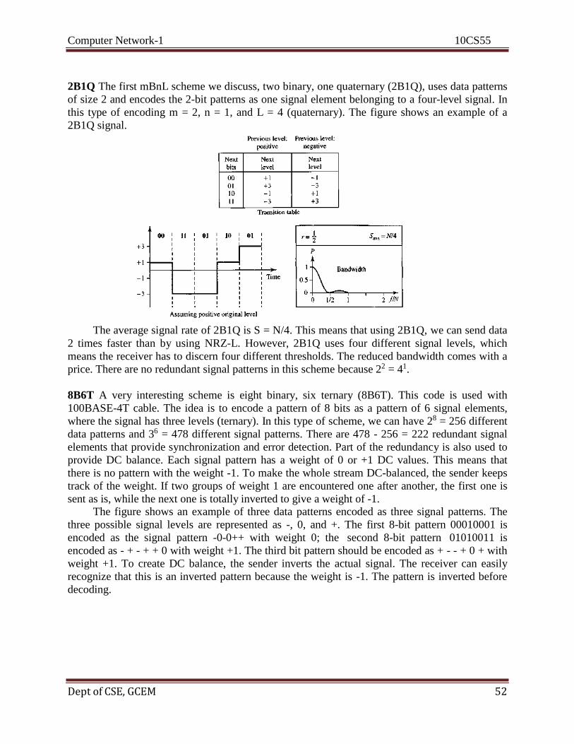
Computer Network-1 10CS55
Dept of CSE, GCEM 52
2B1Q The first mBnL scheme we discuss, two binary, one quaternary (2B1Q), uses data patterns
of size 2 and encodes the 2-bit patterns as one signal element belonging to a four-level signal. In
this type of encoding m = 2, n = 1, and L = 4 (quaternary). The figure shows an example of a
2B1Q signal.
The average signal rate of 2B1Q is S = N/4. This means that using 2B1Q, we can send data
2 times faster than by using NRZ-L. However, 2B1Q uses four different signal levels, which
means the receiver has to discern four different thresholds. The reduced bandwidth comes with a
price. There are no redundant signal patterns in this scheme because 22 = 41.
8B6T A very interesting scheme is eight binary, six ternary (8B6T). This code is used with
100BASE-4T cable. The idea is to encode a pattern of 8 bits as a pattern of 6 signal elements,
where the signal has three levels (ternary). In this type of scheme, we can have 28 = 256 different
data patterns and 36 = 478 different signal patterns. There are 478 - 256 = 222 redundant signal
elements that provide synchronization and error detection. Part of the redundancy is also used to
provide DC balance. Each signal pattern has a weight of 0 or +1 DC values. This means that
there is no pattern with the weight -1. To make the whole stream DC-balanced, the sender keeps
track of the weight. If two groups of weight 1 are encountered one after another, the first one is
sent as is, while the next one is totally inverted to give a weight of -1. The figure shows an example of three data patterns encoded as three signal patterns. The
three possible signal levels are represented as -, 0, and +. The first 8-bit pattern 00010001 is
encoded as the signal pattern -0-0++ with weight 0; the second 8-bit pattern 01010011 is
encoded as - + - + + 0 with weight +1. The third bit pattern should be encoded as + - - + 0 + with
weight +1. To create DC balance, the sender inverts the actual signal. The receiver can easily
recognize that this is an inverted pattern because the weight is -1. The pattern is inverted before
decoding.
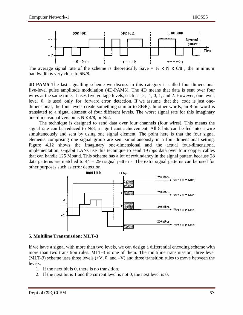
Computer Network-1 10CS55
Dept of CSE, GCEM 53
The average signal rate of the scheme is theoretically Save = ½ x N x 6/8 , the minimum bandwidth is very close to 6N/8.
4D-PAM5 The last signalling scheme we discuss in this category is called four-dimensional
five-level pulse amplitude modulation (4D-PAM5). The 4D means that data is sent over four
wires at the same time. It uses five voltage levels, such as -2, -1, 0, 1, and 2. However, one level,
level 0, is used only for forward error detection. If we assume that the code is just one-
dimensional, the four levels create something similar to 8B4Q. In other words, an 8-bit word is
translated to a signal element of four different levels. The worst signal rate for this imaginary
one-dimensional version is N x 4/8, or N/2.
The technique is designed to send data over four channels (four wires). This means the
signal rate can be reduced to N/8, a significant achievement. All 8 bits can be fed into a wire
simultaneously and sent by using one signal element. The point here is that the four signal
elements comprising one signal group are sent simultaneously in a four-dimensional setting.
Figure 4.12 shows the imaginary one-dimensional and the actual four-dimensional
implementation. Gigabit LANs use this technique to send 1-Gbps data over four copper cables
that can handle 125 Mbaud. This scheme has a lot of redundancy in the signal pattern because 28
data patterns are matched to 44 = 256 signal patterns. The extra signal patterns can be used for
other purposes such as error detection.
5. Multiline Transmission: MLT-3
If we have a signal with more than two levels, we can design a differential encoding scheme with
more than two transition rules. MLT-3 is one of them. The multiline transmission, three level
(MLT-3) scheme uses three levels (+V, 0, and –V) and three transition rules to move between the
levels.
1. If the next bit is 0, there is no transition.
2. If the next bit is 1 and the current level is not 0, the next level is 0.
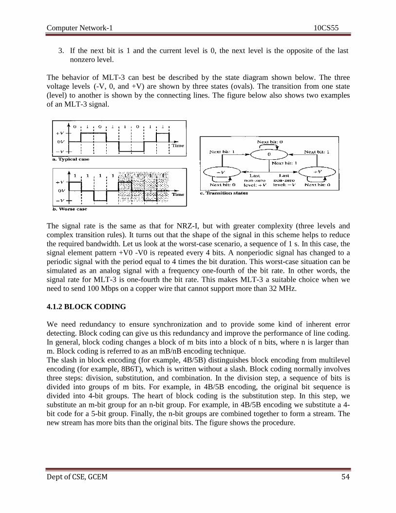
Computer Network-1 10CS55
Dept of CSE, GCEM 54
3. If the next bit is 1 and the current level is 0, the next level is the opposite of the last
nonzero level.
The behavior of MLT-3 can best be described by the state diagram shown below. The three
voltage levels (-V, 0, and +V) are shown by three states (ovals). The transition from one state
(level) to another is shown by the connecting lines. The figure below also shows two examples
of an MLT-3 signal.
The signal rate is the same as that for NRZ-I, but with greater complexity (three levels and
complex transition rules). It turns out that the shape of the signal in this scheme helps to reduce
the required bandwidth. Let us look at the worst-case scenario, a sequence of 1 s. In this case, the
signal element pattern +V0 -V0 is repeated every 4 bits. A nonperiodic signal has changed to a
periodic signal with the period equal to 4 times the bit duration. This worst-case situation can be
simulated as an analog signal with a frequency one-fourth of the bit rate. In other words, the
signal rate for MLT-3 is one-fourth the bit rate. This makes MLT-3 a suitable choice when we
need to send 100 Mbps on a copper wire that cannot support more than 32 MHz.
4.1.2 BLOCK CODING
We need redundancy to ensure synchronization and to provide some kind of inherent error
detecting. Block coding can give us this redundancy and improve the performance of line coding.
In general, block coding changes a block of m bits into a block of n bits, where n is larger than
m. Block coding is referred to as an mB/nB encoding technique.
The slash in block encoding (for example, 4B/5B) distinguishes block encoding from multilevel
encoding (for example, 8B6T), which is written without a slash. Block coding normally involves
three steps: division, substitution, and combination. In the division step, a sequence of bits is
divided into groups of m bits. For example, in 4B/5B encoding, the original bit sequence is
divided into 4-bit groups. The heart of block coding is the substitution step. In this step, we
substitute an m-bit group for an n-bit group. For example, in 4B/5B encoding we substitute a 4-
bit code for a 5-bit group. Finally, the n-bit groups are combined together to form a stream. The
new stream has more bits than the original bits. The figure shows the procedure.
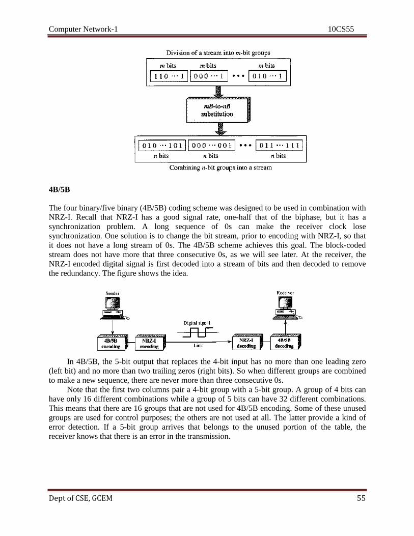
Computer Network-1 10CS55
Dept of CSE, GCEM 55
4B/5B
The four binary/five binary (4B/5B) coding scheme was designed to be used in combination with
NRZ-I. Recall that NRZ-I has a good signal rate, one-half that of the biphase, but it has a
synchronization problem. A long sequence of 0s can make the receiver clock lose
synchronization. One solution is to change the bit stream, prior to encoding with NRZ-I, so that
it does not have a long stream of 0s. The 4B/5B scheme achieves this goal. The block-coded
stream does not have more that three consecutive 0s, as we will see later. At the receiver, the
NRZ-I encoded digital signal is first decoded into a stream of bits and then decoded to remove
the redundancy. The figure shows the idea.
In 4B/5B, the 5-bit output that replaces the 4-bit input has no more than one leading zero
(left bit) and no more than two trailing zeros (right bits). So when different groups are combined
to make a new sequence, there are never more than three consecutive 0s.
Note that the first two columns pair a 4-bit group with a 5-bit group. A group of 4 bits can
have only 16 different combinations while a group of 5 bits can have 32 different combinations.
This means that there are 16 groups that are not used for 4B/5B encoding. Some of these unused
groups are used for control purposes; the others are not used at all. The latter provide a kind of
error detection. If a 5-bit group arrives that belongs to the unused portion of the table, the
receiver knows that there is an error in the transmission.
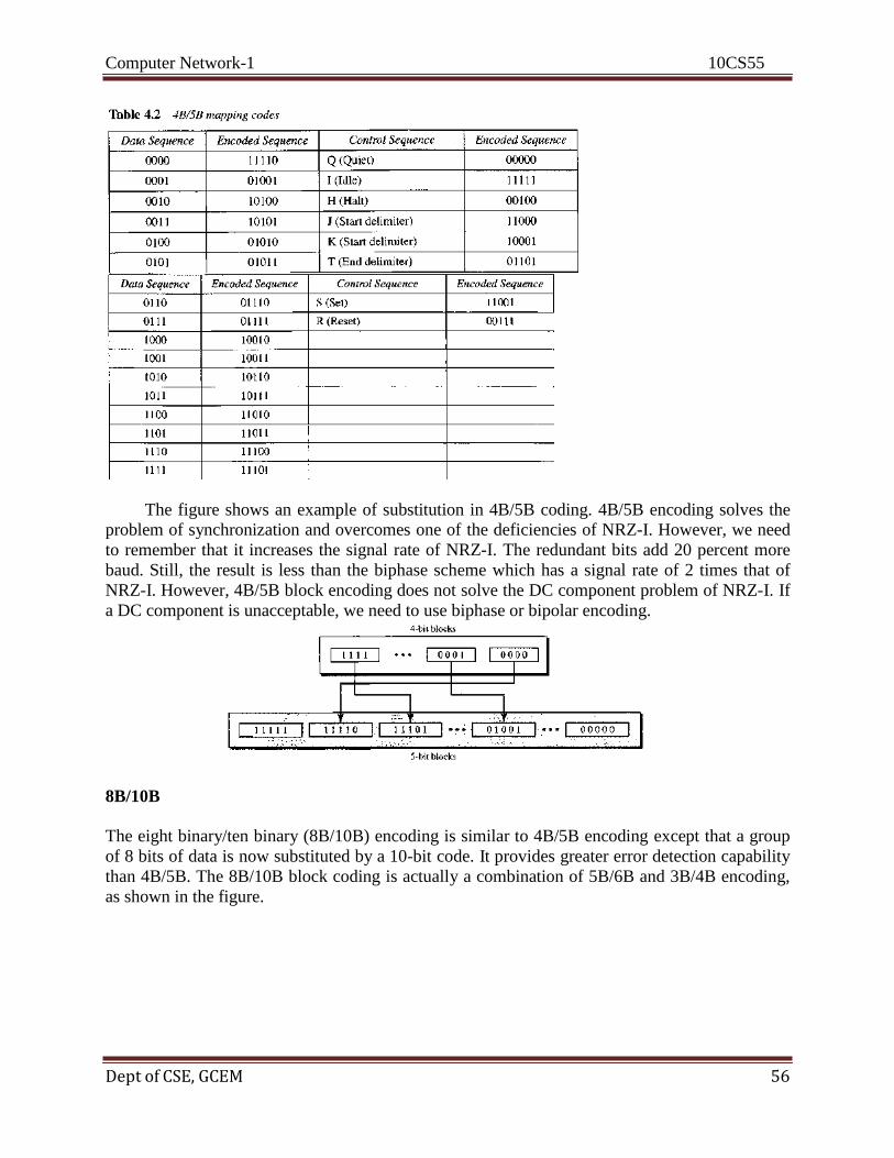
Computer Network-1 10CS55
Dept of CSE, GCEM 56
The figure shows an example of substitution in 4B/5B coding. 4B/5B encoding solves the
problem of synchronization and overcomes one of the deficiencies of NRZ-I. However, we need
to remember that it increases the signal rate of NRZ-I. The redundant bits add 20 percent more
baud. Still, the result is less than the biphase scheme which has a signal rate of 2 times that of
NRZ-I. However, 4B/5B block encoding does not solve the DC component problem of NRZ-I. If
a DC component is unacceptable, we need to use biphase or bipolar encoding.
8B/10B
The eight binary/ten binary (8B/10B) encoding is similar to 4B/5B encoding except that a group
of 8 bits of data is now substituted by a 10-bit code. It provides greater error detection capability
than 4B/5B. The 8B/10B block coding is actually a combination of 5B/6B and 3B/4B encoding,
as shown in the figure.
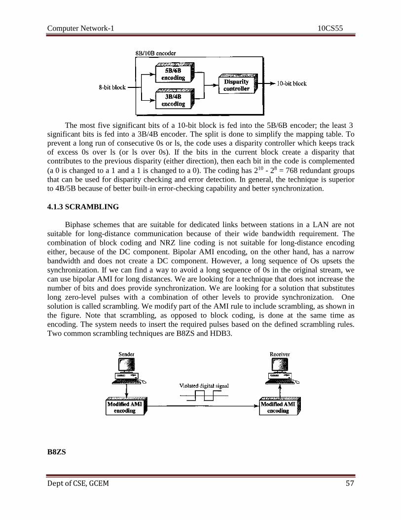
Computer Network-1 10CS55
Dept of CSE, GCEM 57
The most five significant bits of a 10-bit block is fed into the 5B/6B encoder; the least 3
significant bits is fed into a 3B/4B encoder. The split is done to simplify the mapping table. To
prevent a long run of consecutive 0s or ls, the code uses a disparity controller which keeps track
of excess 0s over ls (or ls over 0s). If the bits in the current block create a disparity that contributes to the previous disparity (either direction), then each bit in the code is complemented
(a 0 is changed to a 1 and a 1 is changed to a 0). The coding has 210 - 28 = 768 redundant groups
that can be used for disparity checking and error detection. In general, the technique is superior to 4B/5B because of better built-in error-checking capability and better synchronization.
4.1.3 SCRAMBLING
Biphase schemes that are suitable for dedicated links between stations in a LAN are not
suitable for long-distance communication because of their wide bandwidth requirement. The
combination of block coding and NRZ line coding is not suitable for long-distance encoding
either, because of the DC component. Bipolar AMI encoding, on the other hand, has a narrow
bandwidth and does not create a DC component. However, a long sequence of Os upsets the
synchronization. If we can find a way to avoid a long sequence of 0s in the original stream, we
can use bipolar AMI for long distances. We are looking for a technique that does not increase the
number of bits and does provide synchronization. We are looking for a solution that substitutes
long zero-level pulses with a combination of other levels to provide synchronization. One
solution is called scrambling. We modify part of the AMI rule to include scrambling, as shown in
the figure. Note that scrambling, as opposed to block coding, is done at the same time as
encoding. The system needs to insert the required pulses based on the defined scrambling rules.
Two common scrambling techniques are B8ZS and HDB3.
B8ZS

Computer Network-1 10CS55
Dept of CSE, GCEM 58
In the bipolar with 8-zero substitution (B8ZS) technique, eight consecutive zero-level voltages
are replaced by the sequence 000VBOVB. The V in the sequence denotes violation; this is a
nonzero voltage that breaks an AMI rule of encoding (opposite polarity from the previous). The
B in the sequence denotes bipolar, which means a nonzero level voltage in accordance with the
AMI rule. There are two cases, as shown below:
The scrambling in this case does not change the bit rate. Also, the technique balances the
positive and negative voltage levels (two positives and two negatives), which means that the DC
balance is maintained. Note that the substitution may change the polarity of a 1 because, after the
substitution, AMI needs to follow its rules.
HDB3
In this high-density bipolar 3-zero (HDB3) technique, which is more conservative than B8ZS,
four consecutive zero-level voltages are replaced with a sequence of 000V or B00V. The reason
for two different substitutions is to maintain the even number of nonzero pulses after each
substitution. The two rules can be stated as follows:
1. If the number of nonzero pulses after the last substitution is odd, the substitution pattern
will be 000V, which makes the total number of nonzero pulses even.
2. If the number of nonzero pulses after the last substitution is even, the substitution pattern
will be B00V, which makes the total number of nonzero pulses even.
The figure shows an example.

Computer Network-1 10CS55
Dept of CSE, GCEM 59
First, before the first substitution, the number of nonzero pulses is even, so the first substitution
is B00V. After this substitution, the polarity of the 1 bit is changed because the AMI scheme,
after each substitution, must follow its own rule. After this bit, we need another substitution,
which is 000V because we have only one nonzero pulse (odd) after the last substitution. The
third substitution is B00V because there are no nonzero pulses after the second substitution
(even).
4.2 ANALOG-TO-DIGITAL CONVERSION
4.2.1 Pulse Code Modulation (PCM)
The most common technique to change an analog signal to digital data (digitization) is called
pulse code modulation (PCM). A PCM encoder has three processes, as shown in the figure.
1. The analog signal is sampled.
2. The sampled signal is quantized.
3. The quantized values are encoded as streams of bits.
Sampling
The first step in PCM is sampling. The analog signal is sampled every Ts s, where Ts is the
sample interval or period. The inverse of the sampling interval is called the sampling rate or
sampling frequency and denoted by fs, where fs = 1/Ts. There are three sampling methods- ideal,
natural, and flat-top -as shown below.
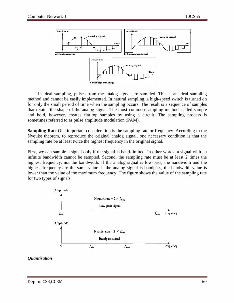
Computer Network-1 10CS55
Dept of CSE,GCEM 60
In ideal sampling, pulses from the analog signal are sampled. This is an ideal sampling
method and cannot be easily implemented. In natural sampling, a high-speed switch is turned on
for only the small period of time when the sampling occurs. The result is a sequence of samples
that retains the shape of the analog signal. The most common sampling method, called sample
and hold, however, creates flat-top samples by using a circuit. The sampling process is
sometimes referred to as pulse amplitude modulation (PAM).
Sampling Rate One important consideration is the sampling rate or frequency. According to the
Nyquist theorem, to reproduce the original analog signal, one necessary condition is that the
sampling rate be at least twice the highest frequency in the original signal.
First, we can sample a signal only if the signal is band-limited. In other words, a signal with an
infinite bandwidth cannot be sampled. Second, the sampling rate must be at least 2 times the
highest frequency, not the bandwidth. If the analog signal is low-pass, the bandwidth and the
highest frequency are the same value. If the analog signal is bandpass, the bandwidth value is
lower than the value of the maximum frequency. The figure shows the value of the sampling rate
for two types of signals.
Quantization
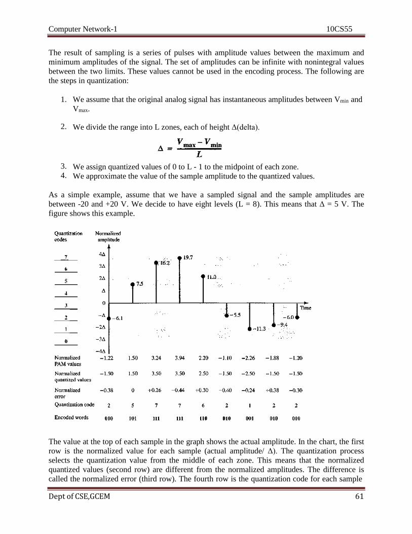
Computer Network-1 10CS55
Dept of CSE,GCEM 61
The result of sampling is a series of pulses with amplitude values between the maximum and
minimum amplitudes of the signal. The set of amplitudes can be infinite with nonintegral values
between the two limits. These values cannot be used in the encoding process. The following are
the steps in quantization:
1. We assume that the original analog signal has instantaneous amplitudes between Vmin and
Vmax.
2. We divide the range into L zones, each of height Δ(delta).
3. We assign quantized values of 0 to L - 1 to the midpoint of each zone. 4. We approximate the value of the sample amplitude to the quantized values.
As a simple example, assume that we have a sampled signal and the sample amplitudes are
between -20 and +20 V. We decide to have eight levels (L = 8). This means that Δ = 5 V. The
figure shows this example.
The value at the top of each sample in the graph shows the actual amplitude. In the chart, the first
row is the normalized value for each sample (actual amplitude/ Δ). The quantization process
selects the quantization value from the middle of each zone. This means that the normalized
quantized values (second row) are different from the normalized amplitudes. The difference is
called the normalized error (third row). The fourth row is the quantization code for each sample
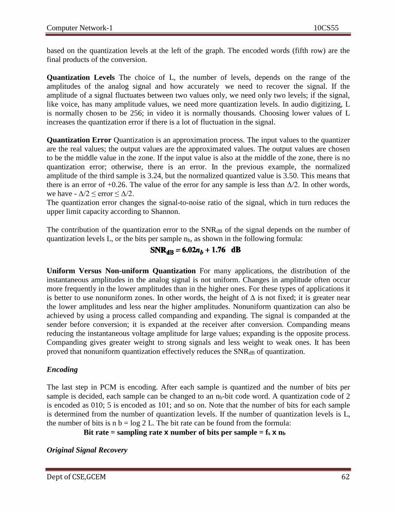
Computer Network-1 10CS55
Dept of CSE,GCEM 62
based on the quantization levels at the left of the graph. The encoded words (fifth row) are the
final products of the conversion.
Quantization Levels The choice of L, the number of levels, depends on the range of the
amplitudes of the analog signal and how accurately we need to recover the signal. If the
amplitude of a signal fluctuates between two values only, we need only two levels; if the signal,
like voice, has many amplitude values, we need more quantization levels. In audio digitizing, L
is normally chosen to be 256; in video it is normally thousands. Choosing lower values of L
increases the quantization error if there is a lot of fluctuation in the signal.
Quantization Error Quantization is an approximation process. The input values to the quantizer
are the real values; the output values are the approximated values. The output values are chosen
to be the middle value in the zone. If the input value is also at the middle of the zone, there is no
quantization error; otherwise, there is an error. In the previous example, the normalized
amplitude of the third sample is 3.24, but the normalized quantized value is 3.50. This means that
there is an error of +0.26. The value of the error for any sample is less than Δ/2. In other words,
we have - Δ/2 ≤ error ≤ Δ/2.
The quantization error changes the signal-to-noise ratio of the signal, which in turn reduces the
upper limit capacity according to Shannon.
The contribution of the quantization error to the SNRdB of the signal depends on the number of
quantization levels L, or the bits per sample nb, as shown in the following formula:
Uniform Versus Non-uniform Quantization For many applications, the distribution of the
instantaneous amplitudes in the analog signal is not uniform. Changes in amplitude often occur
more frequently in the lower amplitudes than in the higher ones. For these types of applications it
is better to use nonuniform zones. In other words, the height of Δ is not fixed; it is greater near
the lower amplitudes and less near the higher amplitudes. Nonuniform quantization can also be
achieved by using a process called companding and expanding. The signal is companded at the
sender before conversion; it is expanded at the receiver after conversion. Companding means
reducing the instantaneous voltage amplitude for large values; expanding is the opposite process.
Companding gives greater weight to strong signals and less weight to weak ones. It has been
proved that nonuniform quantization effectively reduces the SNRdB of quantization.
Encoding
The last step in PCM is encoding. After each sample is quantized and the number of bits per
sample is decided, each sample can be changed to an nb-bit code word. A quantization code of 2
is encoded as 010; 5 is encoded as 101; and so on. Note that the number of bits for each sample
is determined from the number of quantization levels. If the number of quantization levels is L,
the number of bits is n b = log 2 L. The bit rate can be found from the formula:
Bit rate = sampling rate x number of bits per sample = fs x nb
Original Signal Recovery
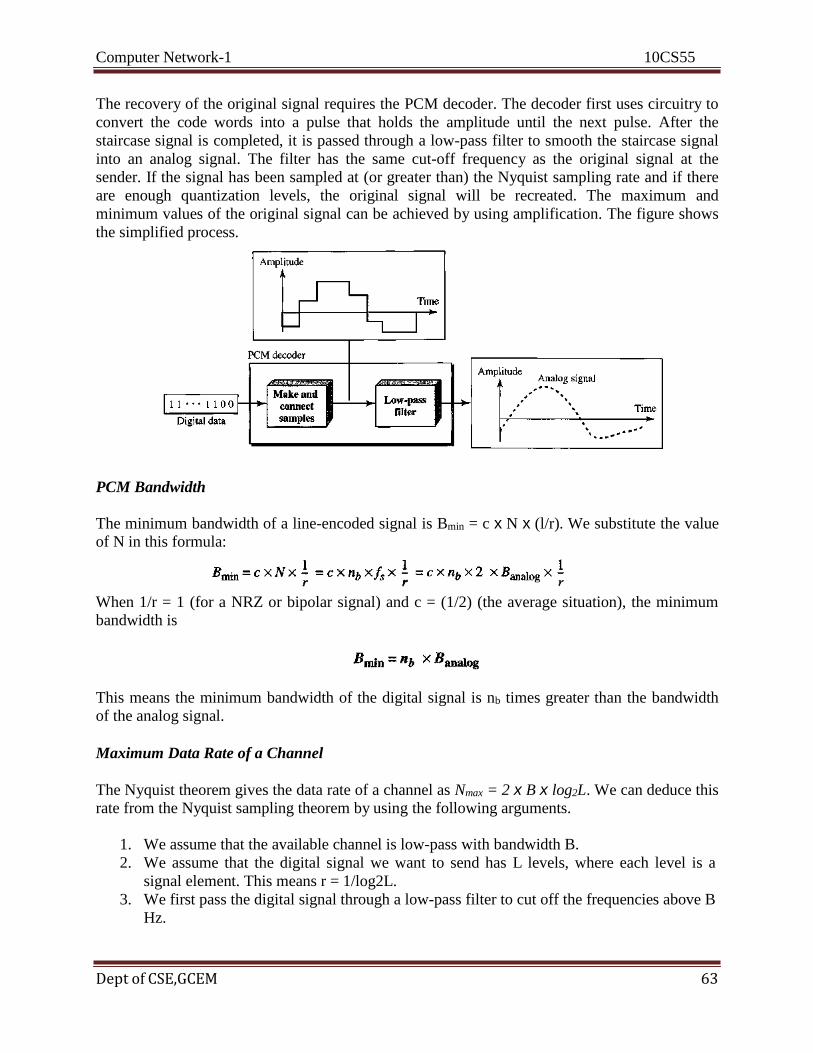
Computer Network-1 10CS55
Dept of CSE,GCEM 63
The recovery of the original signal requires the PCM decoder. The decoder first uses circuitry to
convert the code words into a pulse that holds the amplitude until the next pulse. After the
staircase signal is completed, it is passed through a low-pass filter to smooth the staircase signal
into an analog signal. The filter has the same cut-off frequency as the original signal at the
sender. If the signal has been sampled at (or greater than) the Nyquist sampling rate and if there
are enough quantization levels, the original signal will be recreated. The maximum and
minimum values of the original signal can be achieved by using amplification. The figure shows
the simplified process.
PCM Bandwidth
The minimum bandwidth of a line-encoded signal is Bmin = c x N x (l/r). We substitute the value
of N in this formula:
When 1/r = 1 (for a NRZ or bipolar signal) and c = (1/2) (the average situation), the minimum
bandwidth is
This means the minimum bandwidth of the digital signal is nb times greater than the bandwidth
of the analog signal.
Maximum Data Rate of a Channel
The Nyquist theorem gives the data rate of a channel as Nmax = 2 x B x log2L. We can deduce this
rate from the Nyquist sampling theorem by using the following arguments.
1. We assume that the available channel is low-pass with bandwidth B.
2. We assume that the digital signal we want to send has L levels, where each level is a
signal element. This means r = 1/log2L.
3. We first pass the digital signal through a low-pass filter to cut off the frequencies above B
Hz.

Computer Network-1 10CS55
Dept of CSE,GCEM 64
4. We treat the resulting signal as an analog signal and sample it at 2 x B samples per
second and quantize it using L levels. Additional quantization levels are useless because
the signal originally had L levels.
5. The resulting bit rate is N =fs x nb = 2 x B x log2L. This is the maximum bandwidth; if the case factor c increases, the data rate is reduced.
Minimum Required Bandwidth
The previous argument can give us the minimum bandwidth if the data rate and the number of
signal levels are fixed. We can say
4.2.2 Delta Modulation (DM)
PCM finds the value of the signal amplitude for each sample; DM finds the change from the
previous sample. The figure shows the process. Note that there are no code words here; bits are
sent one after another.
Modulator
The modulator is used at the sender site to create a stream of bits from an analog signal. The
process records the small positive or negative changes, called delta δ. If the delta is positive, the
process records a 1; if it is negative, the process records a 0. However, the process needs a base
against which the analog signal is compared. The modulator builds a second signal that
resembles a staircase. Finding the change is then reduced to comparing the input signal with the
gradually made staircase signal. The figure shows a diagram of the process.
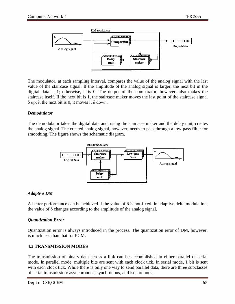
Computer Network-1 10CS55
Dept of CSE,GCEM 65
The modulator, at each sampling interval, compares the value of the analog signal with the last
value of the staircase signal. If the amplitude of the analog signal is larger, the next bit in the
digital data is 1; otherwise, it is 0. The output of the comparator, however, also makes the
staircase itself. If the next bit is 1, the staircase maker moves the last point of the staircase signal
δ up; it the next bit is 0, it moves it δ down.
Demodulator
The demodulator takes the digital data and, using the staircase maker and the delay unit, creates
the analog signal. The created analog signal, however, needs to pass through a low-pass filter for
smoothing. The figure shows the schematic diagram.
Adaptive DM
A better performance can be achieved if the value of δ is not fixed. In adaptive delta modulation,
the value of δ changes according to the amplitude of the analog signal.
Quantization Error
Quantization error is always introduced in the process. The quantization error of DM, however,
is much less than that for PCM.
4.3 TRANSMISSION MODES
The transmission of binary data across a link can be accomplished in either parallel or serial
mode. In parallel mode, multiple bits are sent with each clock tick. In serial mode, 1 bit is sent
with each clock tick. While there is only one way to send parallel data, there are three subclasses
of serial transmission: asynchronous, synchronous, and isochronous.
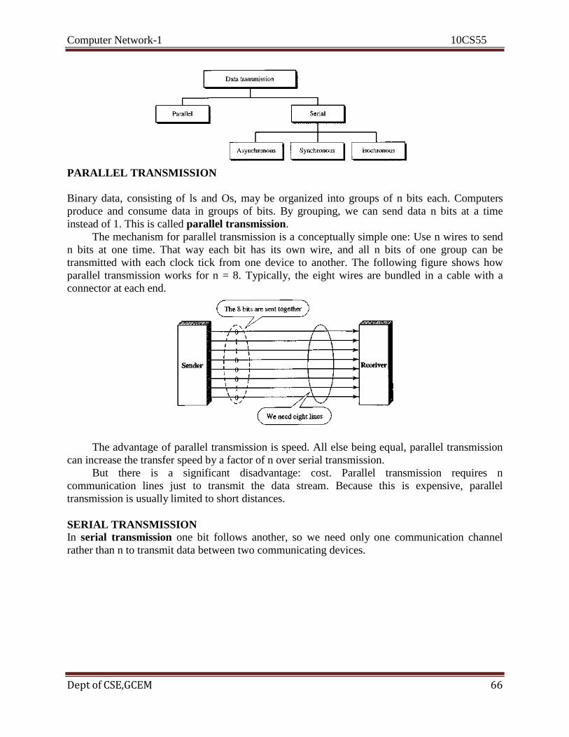
Computer Network-1 10CS55
Dept of CSE,GCEM 66
PARALLEL TRANSMISSION
Binary data, consisting of ls and Os, may be organized into groups of n bits each. Computers
produce and consume data in groups of bits. By grouping, we can send data n bits at a time
instead of 1. This is called parallel transmission.
The mechanism for parallel transmission is a conceptually simple one: Use n wires to send
n bits at one time. That way each bit has its own wire, and all n bits of one group can be
transmitted with each clock tick from one device to another. The following figure shows how
parallel transmission works for n = 8. Typically, the eight wires are bundled in a cable with a
connector at each end.
The advantage of parallel transmission is speed. All else being equal, parallel transmission
can increase the transfer speed by a factor of n over serial transmission.
But there is a significant disadvantage: cost. Parallel transmission requires n
communication lines just to transmit the data stream. Because this is expensive, parallel
transmission is usually limited to short distances.
SERIAL TRANSMISSION In serial transmission one bit follows another, so we need only one communication channel
rather than n to transmit data between two communicating devices.

Computer Network-1 10CS55
Dept of CSE,GCEM 67
The advantage of serial over parallel transmission is that with only one communication
channel, serial transmission reduces the cost of transmission over parallel by roughly a factor of
n.
Since communication within devices is parallel, conversion devices are required at the
interface between the sender and the line (parallel-to-serial) and between the line and the receiver
(serial-to-parallel).
Serial transmission occurs in one of three ways: asynchronous, synchronous, and
isochronous.
Asynchronous Transmission
Asynchronous transmission is so named because the timing of a signal is unimportant. Instead,
information is received and translated by agreed upon patterns. As long as those patterns are
followed, the receiving device can retrieve the information without regard to the rhythm in which
it is sent. Patterns are based on grouping the bit stream into bytes. Each group, usually 8 bits, is
sent along the link as a unit. The sending system handles each group independently, relaying it to
the link whenever ready, without regard to a timer.
Without synchronization, the receiver cannot use timing to predict when the next group
will arrive. To alert the receiver to the arrival of a new group, therefore, an extra bit is added to
the beginning of each byte. This bit, usually a 0, is called the start bit. To let the receiver know
that the byte is finished, 1 or more additional bits are appended to the end of the byte. These bits,
usually 1 s, are called stop bits. By this method, each byte is increased in size to at least 10 bits,
of which 8 bits is information and 2 bits or more are signals to the receiver. In addition, the
transmission of each byte may then be followed by a gap of varying duration. This gap can be
represented either by an idle channel or by a stream of additional stop bits.
The start and stop bits and the gap alert the receiver to the beginning and end of each byte
and allow it to synchronize with the data stream. This mechanism is called asynchronous
because, at the byte level, the sender and receiver do not have to be synchronized. But within
each byte, the receiver must still be synchronized with the incoming bit stream. That is, some
synchronization is required, but only for the duration of a single byte. The receiving device
resynchronizes at the onset of each new byte. When the receiver detects a start bit, it sets a timer

Computer Network-1 10CS55
Dept of CSE,GCEM 68
and begins counting bits as they come in. After n bits, the receiver looks for a stop bit. As soon
as it detects the stop bit, it waits until it detects the next start bit.
The figure is a schematic illustration of asynchronous transmission. In this example, the
start bits are 0s, the stop bits are ls, and the gap is represented by an idle line rather than by
additional stop bits.
The addition of stop and start bits and the insertion of gaps into the bit stream make
asynchronous transmission slower than forms of transmission that can operate without the
addition of control information. But it is cheap and effective, two advantages that make it an
attractive choice for situations such as low-speed communication.
Synchronous Transmission
In synchronous transmission, the bit stream is combined into longer "frames," which may
contain multiple bytes. Each byte, however, is introduced onto the transmission link without a
gap between it and the next one. It is left to the receiver to separate the bit stream into bytes for
decoding purposes. In other words, data are transmitted as an unbroken string of 1 s and 0s, and
the receiver separates that string into the bytes, or characters, it needs to reconstruct the
information.
The figure gives a schematic illustration of synchronous transmission. The sender puts its
data onto the line as one long string. If the sender wishes to send data in separate bursts, the gaps
between bursts must be filled with a special sequence of 0s and ls that means idle. The receiver
counts the bits as they arrive and groups them in 8-bit units.
Computer Network-1 10CS55
Dept of CSE,GCEM 69
Without gaps and start and stop bits, there is no built-in mechanism to help the receiving
device adjust its bit synchronization midstream. Timing becomes very important, therefore,
because the accuracy of the received information is completely dependent on the ability of the
receiving device to keep an accurate count of the bits as they come in.
The advantage of synchronous transmission is speed. With no extra bits or gaps to
introduce at the sending end and remove at the receiving end, and, by extension, with fewer bits
to move across the link, synchronous transmission is faster than asynchronous transmission. For
this reason, it is more useful for high-speed applications such as the transmission of data from
one computer to another.
Isochronous
In real-time audio and video, in which uneven delays between frames are not acceptable,
synchronous transmission fails. For example, TV images are broadcast at the rate of 30 images
per second; they must be viewed at the same rate. If each image is sent by using one or more
flames, there should be no delays between frames. For this type of application, synchronization
between characters is not enough; the entire stream of bits must be synchronized. The
isochronous transmission guarantees that the data arrive at a fixed rate.
Recommended Questions
1. List the layers of the Internet model.
2. Which layer in the Internet model is the user support layer?
3. How does information get passed from one layer to the next in the
Internet model.
4. What are the responsibilities of the transport layer in the Internet
model?
5. What are the responsibilities of the transport layer in the Internet
model?
6. What is the difference between a port address, a logical address, and a
physical address?
7. How do the layers of the Internet model correlate to the layers of the
OSI model?
Computer Network-1 10CS55
Dept of CSE,GCEM 70
COMPUTER NETWORKS – I
Subject Code: 10CS55 I.A. Marks : 25
Hours/Week : 04 Exam Hours: 03
Total Hours : 52 Exam Marks: 100
UNIT- 3 6 Hours Physical Layer-2 and Switching:
- Multiplexing,
- Spread Spectrum,
- Introduction to switching,
- Circuit Switched Networks,
- Datagram Networks, - Virtual Circuit Networks

Computer Network-1 10CS55
Dept of CSE,GCEM 71
UNIT-III
CHAPTER 5
5.1 DIGITAL-TO-ANALOG CONVERSION
Digital-to-analog conversion is the process of changing one of the characteristics of an analog
signal based on the information in digital data. Figure 5.1 shows the relationship between the
digital information, the digital-to-analog modulating process, and the resultant analog signal.
FIGURE Digital-to-analog conversion
As discussed in Chapter 3, a sine wave is defined by three characteristics: amplitude, frequency,
and phase. When we vary anyone of these characteristics, we create a different version of that
wave. So, by changing one characteristic of a simple electric signal, we can use it to represent
digital data. Any of the three characteristics can be altered in this way, giving us at least three
mechanisms for modulating digital data into an analog signal: amplitude shift keying (ASK),
frequency shift keying (FSK), and phase shift keying (PSK). In addition, there is a fourth (and
better) mechanism that combines changing both the amplitude and phase, called quadrature
amplitude modulation (QAM). QAM is the most efficient of these options and is the mechanism
commonly used today (see Figure 5.2).
Figure Types of digital-to-analog conversion

Computer Network-1 10CS55
Dept of CSE,GCEM 72
Aspects of Digital-to-Analog Conversion
Before we discuss specific methods of digital-to-analog modulation, two basic issues must be
reviewed: bit and baud rates and the carrier signal.
Data Element Versus Signal Element
In Chapter 4, we discussed the concept of the data element versus the signal element. We defined
a data element as the smallest piece of information to be exchanged, the bit. We also defined a
signal element as the smallest unit of a signal that is constant. Although we continue to use the
same terms in this chapter, we will see that the nature of the signal element is a little bit different
in analog transmission
Data Rate Versus Signal Rate
We can define the data rate (bit rate) and the signal rate (baud rate) as we did for digital
transmission. The relationship between them is
S=Nxi/r! baud
where N is the data rate (bps) and r is the number of data elements carried in one signal element.
The value of r in analog transmission is r =log2 L, where L is the type of signal element, not the
level. The same nomenclature is used to simplify the comparisons.
The same analogy we used in Chapter 4 for bit rate and baud rate applies here. In transportation,
a baud is analogous to a vehicle, and a bit is analogous to a passenger. We need to maximize the
number of people per car to reduce the traffic.
Example1
An analog signal carries 4 bits per signal element. If 1000 signal elements are sent per second,
find the bit rate.
Solution
In this case, r = 4, S = 1000, and N is unknown. We can find the value ofN from
S=Nx!r
or N=Sxr= 1000 x 4 =4000 bps
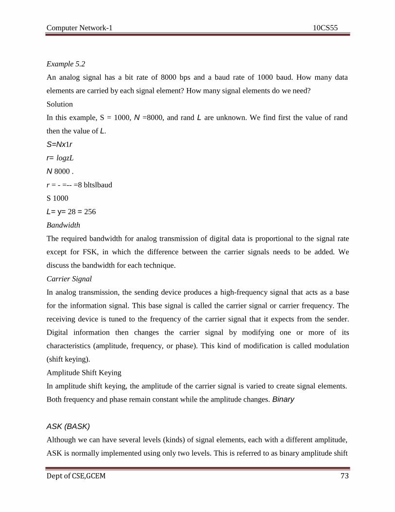
Computer Network-1 10CS55
Dept of CSE,GCEM 73
Example 5.2
An analog signal has a bit rate of 8000 bps and a baud rate of 1000 baud. How many data
elements are carried by each signal element? How many signal elements do we need?
Solution
In this example, S = 1000, N =8000, and rand L are unknown. We find first the value of rand
then the value of L.
S=Nx1r
r= logzL
N 8000 .
r = - =-- =8 bltslbaud
S 1000
L= y= 28 = 256
Bandwidth
The required bandwidth for analog transmission of digital data is proportional to the signal rate
except for FSK, in which the difference between the carrier signals needs to be added. We
discuss the bandwidth for each technique.
Carrier Signal
In analog transmission, the sending device produces a high-frequency signal that acts as a base
for the information signal. This base signal is called the carrier signal or carrier frequency. The
receiving device is tuned to the frequency of the carrier signal that it expects from the sender.
Digital information then changes the carrier signal by modifying one or more of its
characteristics (amplitude, frequency, or phase). This kind of modification is called modulation
(shift keying).
Amplitude Shift Keying
In amplitude shift keying, the amplitude of the carrier signal is varied to create signal elements.
Both frequency and phase remain constant while the amplitude changes. Binary
ASK (BASK)
Although we can have several levels (kinds) of signal elements, each with a different amplitude,
ASK is normally implemented using only two levels. This is referred to as binary amplitude shift

Computer Network-1 10CS55
Dept of CSE,GCEM 74
keying or on-off keying (OOK). The peak amplitude of one signallevel is 0; the other is the same
as the amplitude of the carrier frequency. Figure 5.3
gives a conceptual view of binary ASK
Figure 5.3 Binmy amplitude shift keying
Bandwidth for ASK Figure 5.3 also shows the bandwidth for ASK. Although the carrier signal is
only one simple sine wave, the process of modulation produces a nonperiodic composite signal.
This signal, as was discussed in Chapter 3, has a continuous set of frequencies. As we expect, the
bandwidth is proportional to the signal rate (baud rate). However, there is normally another
factor involved, called d, which depends on the modulation and filtering process. The value of d
is between 0 and 1. This means that the bandwidth can be expressed as shown, where 5 is the
signal rate and the B is the bandwidth. B =(1 +d) x S
The formula shows that the required bandwidth has a minimum value of 5 and a maximum value
of 25. The most important point here is the location of the bandwidth. The middle of the
bandwidth is where Ie the carrier frequency, is located. This means if
we have a bandpass channel available, we can choose our Ie so that the modulated signal
occupies that bandwidth. This is in fact the most important advantage of digitalto- analog
conversion. We can shift the resulting bandwidth to match what is available. Implementation The
complete discussion of ASK implementation is beyond the scope of this book. However, the
simple ideas behind the implementation may help us to better understand the concept itself.
Figure 5.4 shows how we can simply implement binary ASK.
If digital data are presented as a unipolar NRZ (see Chapter 4) digital signal with a high voltage
of I V and a low voltage of 0 V, the implementation can achieved by multiplying the NRZ digital
signal by the carrier signal coming from an oscillator. When the amplitude of the NRZ signal is
1, the amplitude of the carrier frequency is held; when the amplitude of the NRZ signal is 0, the
amplitude of the carrier frequency IS zero.
Figure 5.4 Implementation ofbinary ASK
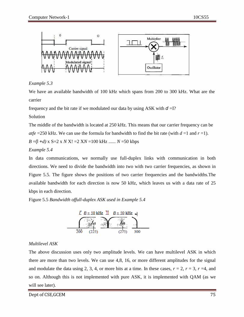
Computer Network-1 10CS55
Dept of CSE,GCEM 75
Example 5.3
We have an available bandwidth of 100 kHz which spans from 200 to 300 kHz. What are the
carrier
frequency and the bit rate if we modulated our data by using ASK with d =I?
Solution
The middle of the bandwidth is located at 250 kHz. This means that our carrier frequency can be
atfe =250 kHz. We can use the formula for bandwidth to find the bit rate (with d =1 and r =1).
B =(l +d) x S=2 x N X! =2 XN =100 kHz ...... N =50 kbps
Example 5.4
In data communications, we normally use full-duplex links with communication in both
directions. We need to divide the bandwidth into two with two carrier frequencies, as shown in
Figure 5.5. The figure shows the positions of two carrier frequencies and the bandwidths.The
available bandwidth for each direction is now 50 kHz, which leaves us with a data rate of 25
kbps in each direction.
Figure 5.5 Bandwidth offull-duplex ASK used in Example 5.4
Multilevel ASK
The above discussion uses only two amplitude levels. We can have multilevel ASK in which
there are more than two levels. We can use 4,8, 16, or more different amplitudes for the signal
and modulate the data using 2, 3, 4, or more bits at a time. In these cases, r = 2, r = 3, r =4, and
so on. Although this is not implemented with pure ASK, it is implemented with QAM (as we
will see later).
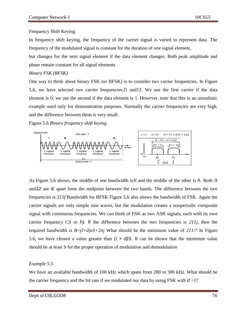
Computer Network-1 10CS55
Dept of CSE,GCEM 76
Frequency Shift Keying
In frequency shift keying, the frequency of the carrier signal is varied to represent data. The
frequency of the modulated signal is constant for the duration of one signal element,
but changes for the next signal element if the data element changes. Both peak amplitude and
phase remain constant for all signal elements
Binary FSK (BFSK)
One way to think about binary FSK (or BFSK) is to consider two carrier frequencies. In Figure
5.6, we have selected two carrier frequencies,f} and12. We use the first carrier if the data
element is 0; we use the second if the data element is 1. However, note that this is an unrealistic
example used only for demonstration purposes. Normally the carrier frequencies are very high,
and the difference between them is very small.
Figure 5.6 Binary frequency shift keying
As Figure 5.6 shows, the middle of one bandwidth isJI and the middle of the other is h. Both JI
and12 are il/ apart from the midpoint between the two bands. The difference between the two
frequencies is 211f Bandwidth for BFSK Figure 5.6 also shows the bandwidth of FSK. Again the
carrier signals are only simple sine waves, but the modulation creates a nonperiodic composite
signal with continuous frequencies. We can think of FSK as two ASK signals, each with its own
carrier frequency Cil or h). If the difference between the two frequencies is 211j, then the
required bandwidth is B=(l+d)xS+2iij What should be the minimum value of 211/? In Figure
5.6, we have chosen a value greater than (l + d)S. It can be shown that the minimum value
should be at least S for the proper operation of modulation and demodulation
Example 5.5
We have an available bandwidth of 100 kHz which spans from 200 to 300 kHz. What should be
the carrier frequency and the bit rate if we modulated our data by using FSK with d =1?
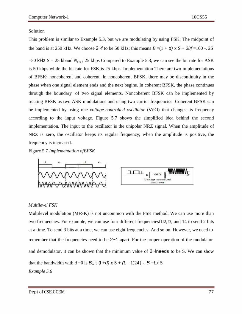
Computer Network-1 10CS55
Dept of CSE,GCEM 77
Solution
This problem is similar to Example 5.3, but we are modulating by using FSK. The midpoint of
the band is at 250 kHz. We choose 2~f to be 50 kHz; this means B =(1 + d) x S + 28f =100 -. 2S
=50 kHz S = 25 kbaud N;;;; 25 kbps Compared to Example 5.3, we can see the bit rate for ASK
is 50 kbps while the bit rate for FSK is 25 kbps. Implementation There are two implementations
of BFSK: noncoherent and coherent. In noncoherent BFSK, there may be discontinuity in the
phase when one signal element ends and the next begins. In coherent BFSK, the phase continues
through the boundary of two signal elements. Noncoherent BFSK can be implemented by
treating BFSK as two ASK modulations and using two carrier frequencies. Coherent BFSK can
be implemented by using one voltage-controlled oscillator (VeO) that changes its frequency
according to the input voltage. Figure 5.7 shows the simplified idea behind the second
implementation. The input to the oscillator is the unipolar NRZ signal. When the amplitude of
NRZ is zero, the oscillator keeps its regular frequency; when the amplitude is positive, the
frequency is increased.
Figure 5.7 Implementation ofBFSK
Multilevel FSK
Multilevel modulation (MFSK) is not uncommon with the FSK method. We can use more than
two frequencies. For example, we can use four different frequenciesfIJ2,!3, and 14 to send 2 bits
at a time. To send 3 bits at a time, we can use eight frequencies. And so on. However, we need to
remember that the frequencies need to be 2~1 apart. For the proper operation of the modulator
and demodulator, it can be shown that the minimum value of 2~lneeds to be S. We can show
that the bandwidth with d =0 is B;;;; (l +d) x S + (L - 1)24{ -. B =Lx S
Example 5.6
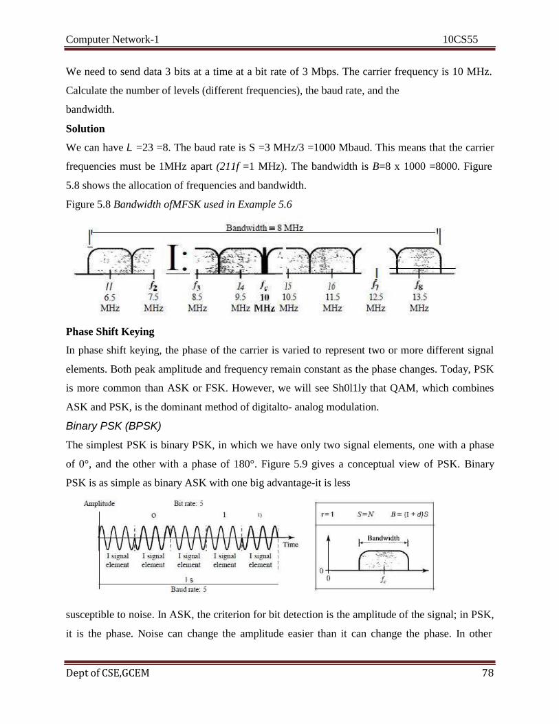
Computer Network-1 10CS55
Dept of CSE,GCEM 78
We need to send data 3 bits at a time at a bit rate of 3 Mbps. The carrier frequency is 10 MHz.
Calculate the number of levels (different frequencies), the baud rate, and the
bandwidth.
Solution
We can have L =23 =8. The baud rate is S =3 MHz/3 =1000 Mbaud. This means that the carrier
frequencies must be 1MHz apart (211f =1 MHz). The bandwidth is B=8 x 1000 =8000. Figure
5.8 shows the allocation of frequencies and bandwidth.
Figure 5.8 Bandwidth ofMFSK used in Example 5.6
Phase Shift Keying
In phase shift keying, the phase of the carrier is varied to represent two or more different signal
elements. Both peak amplitude and frequency remain constant as the phase changes. Today, PSK
is more common than ASK or FSK. However, we will see Sh0l1ly that QAM, which combines
ASK and PSK, is the dominant method of digitalto- analog modulation.
Binary PSK (BPSK)
The simplest PSK is binary PSK, in which we have only two signal elements, one with a phase
of 0°, and the other with a phase of 180°. Figure 5.9 gives a conceptual view of PSK. Binary
PSK is as simple as binary ASK with one big advantage-it is less
susceptible to noise. In ASK, the criterion for bit detection is the amplitude of the signal; in PSK,
it is the phase. Noise can change the amplitude easier than it can change the phase. In other

Computer Network-1 10CS55
Dept of CSE,GCEM 79
words, PSK is less susceptible to noise than ASK. PSK is superior to FSK because we do not
need two carrier signals. Bandwidth Figure 5.9 also shows the bandwidth for BPSK. The
bandwidth is the same as that for binary ASK, but less than that for BFSK. No bandwidth is
wasted for separating two carrier signals. Implementation The implementation of BPSK is as
simple as that for ASK. The reason is that the signal element with phase 180° can be seen as the
complement of the signal
element with phase 0°. This gives us a clue on how to implement BPSK. We use the same idea
we used for ASK but with a polar NRZ signal instead of a unipolar NRZ signal, as shown in
Figure 5.10. The polar NRZ signal is multiplied by the carrier frequency; the 1 bit (positive
voltage) is represented by a phase starting at 0°; the abit (negative voltage) is represented by a
phase starting at 180°.
Figure 5.10 Implementation ofBASK
Quadrature PSK (QPSK)
The simplicity of BPSK enticed designers to use 2 bits at a time in each signal element, thereby
decreasing the baud rate and eventually the required bandwidth. The scheme is called quadrature
PSK or QPSK because it uses two separate BPSK modulations; one is in-phase, the other
quadrature (out-of-phase). The incoming bits are first passed through a serial-to-parallel
conversion that sends one bit to one modulator and the next bit to the other modulator. If the
duration of each bit in the incoming signal is T, the duration of each bit sent to the corresponding
BPSK signal is 2T. This means that the bit to each BPSK signal has one-half the frequency of the
original signal. Figure 5.11 shows the idea. The two composite signals created by each multiplier
are sine waves with the same frequency, but different phases. When they are added, the result is
another sine wave, with one of four possible phases: 45°, -45°, 135°, and -135°. There are four
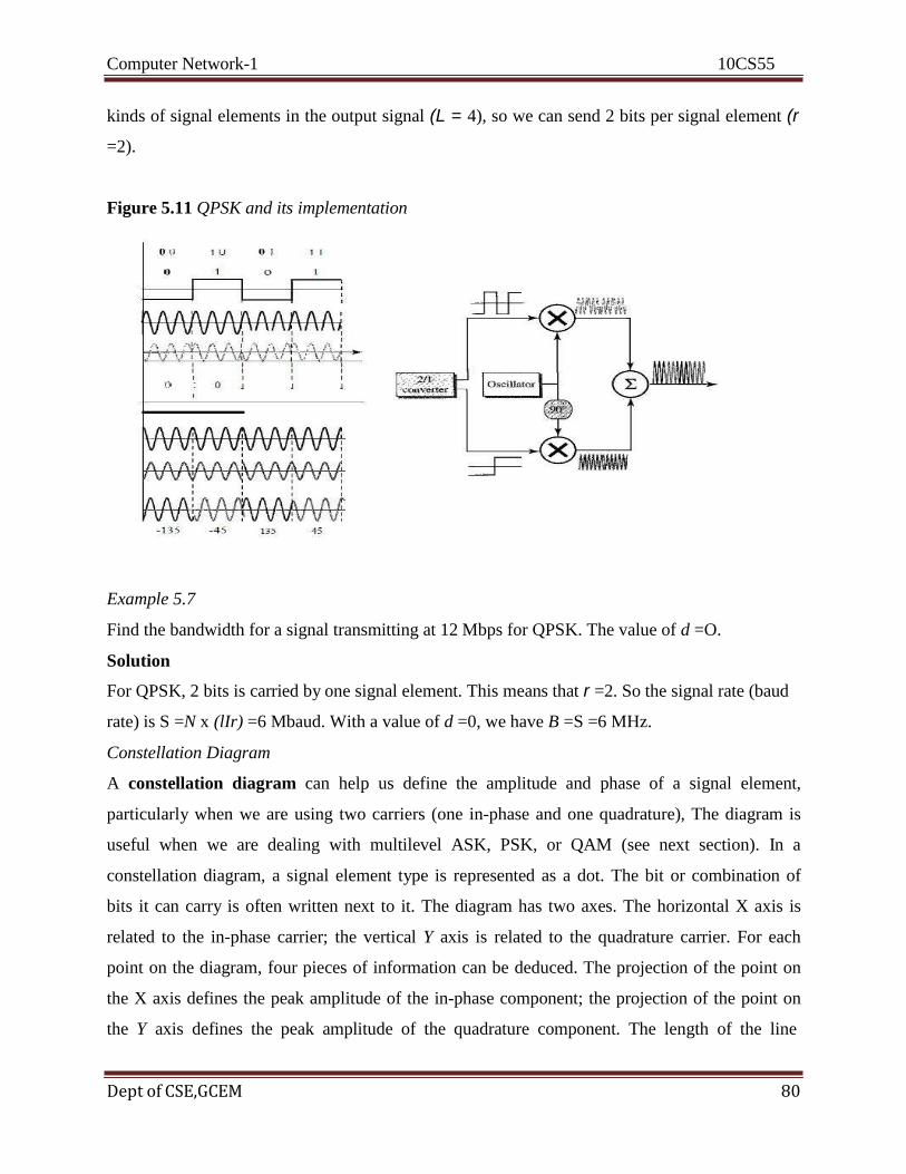
Computer Network-1 10CS55
Dept of CSE,GCEM 80
kinds of signal elements in the output signal (L = 4), so we can send 2 bits per signal element (r
=2).
Figure 5.11 QPSK and its implementation
Example 5.7
Find the bandwidth for a signal transmitting at 12 Mbps for QPSK. The value of d =O.
Solution
For QPSK, 2 bits is carried by one signal element. This means that r =2. So the signal rate (baud
rate) is S =N x (lIr) =6 Mbaud. With a value of d =0, we have B =S =6 MHz.
Constellation Diagram
A constellation diagram can help us define the amplitude and phase of a signal element,
particularly when we are using two carriers (one in-phase and one quadrature), The diagram is
useful when we are dealing with multilevel ASK, PSK, or QAM (see next section). In a
constellation diagram, a signal element type is represented as a dot. The bit or combination of
bits it can carry is often written next to it. The diagram has two axes. The horizontal X axis is
related to the in-phase carrier; the vertical Y axis is related to the quadrature carrier. For each
point on the diagram, four pieces of information can be deduced. The projection of the point on
the X axis defines the peak amplitude of the in-phase component; the projection of the point on
the Y axis defines the peak amplitude of the quadrature component. The length of the line
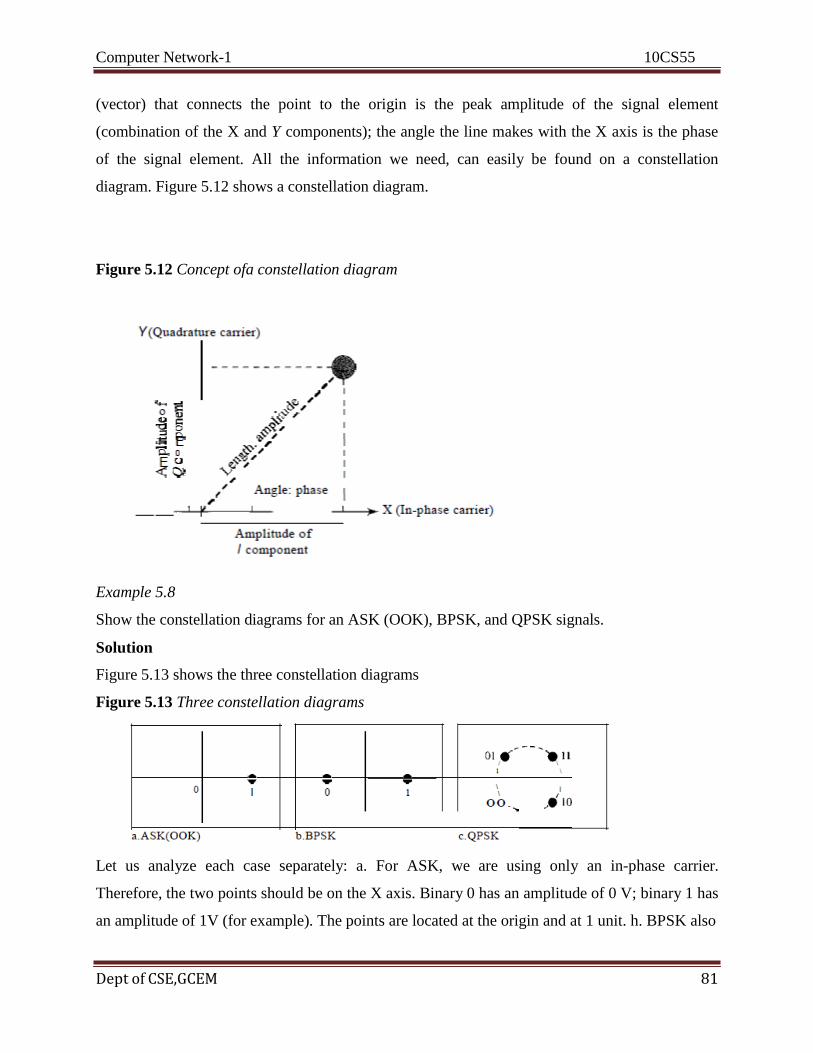
Computer Network-1 10CS55
Dept of CSE,GCEM 81
(vector) that connects the point to the origin is the peak amplitude of the signal element
(combination of the X and Y components); the angle the line makes with the X axis is the phase
of the signal element. All the information we need, can easily be found on a constellation
diagram. Figure 5.12 shows a constellation diagram.
Figure 5.12 Concept ofa constellation diagram
Example 5.8
Show the constellation diagrams for an ASK (OOK), BPSK, and QPSK signals.
Solution
Figure 5.13 shows the three constellation diagrams
Figure 5.13 Three constellation diagrams
Let us analyze each case separately: a. For ASK, we are using only an in-phase carrier.
Therefore, the two points should be on the X axis. Binary 0 has an amplitude of 0 V; binary 1 has
an amplitude of 1V (for example). The points are located at the origin and at 1 unit. h. BPSK also
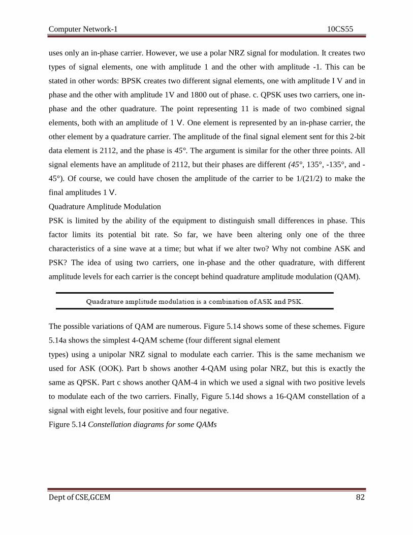
Computer Network-1 10CS55
Dept of CSE,GCEM 82
uses only an in-phase carrier. However, we use a polar NRZ signal for modulation. It creates two
types of signal elements, one with amplitude 1 and the other with amplitude -1. This can be
stated in other words: BPSK creates two different signal elements, one with amplitude I V and in
phase and the other with amplitude 1V and 1800 out of phase. c. QPSK uses two carriers, one in-
phase and the other quadrature. The point representing 11 is made of two combined signal
elements, both with an amplitude of 1 V. One element is represented by an in-phase carrier, the
other element by a quadrature carrier. The amplitude of the final signal element sent for this 2-bit
data element is 2112, and the phase is 45°. The argument is similar for the other three points. All
signal elements have an amplitude of 2112, but their phases are different (45°, 135°, -135°, and -
45°). Of course, we could have chosen the amplitude of the carrier to be 1/(21/2) to make the
final amplitudes 1 V.
Quadrature Amplitude Modulation
PSK is limited by the ability of the equipment to distinguish small differences in phase. This
factor limits its potential bit rate. So far, we have been altering only one of the three
characteristics of a sine wave at a time; but what if we alter two? Why not combine ASK and
PSK? The idea of using two carriers, one in-phase and the other quadrature, with different
amplitude levels for each carrier is the concept behind quadrature amplitude modulation (QAM).
The possible variations of QAM are numerous. Figure 5.14 shows some of these schemes. Figure
5.14a shows the simplest 4-QAM scheme (four different signal element
types) using a unipolar NRZ signal to modulate each carrier. This is the same mechanism we
used for ASK (OOK). Part b shows another 4-QAM using polar NRZ, but this is exactly the
same as QPSK. Part c shows another QAM-4 in which we used a signal with two positive levels
to modulate each of the two carriers. Finally, Figure 5.14d shows a 16-QAM constellation of a
signal with eight levels, four positive and four negative.
Figure 5.14 Constellation diagrams for some QAMs
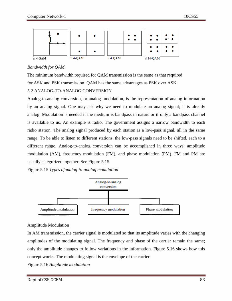
Computer Network-1 10CS55
Dept of CSE,GCEM 83
Bandwidth for QAM
The minimum bandwidth required for QAM transmission is the same as that required
for ASK and PSK transmission. QAM has the same advantages as PSK over ASK.
5.2 ANALOG-TO-ANALOG CONVERSION
Analog-to-analog conversion, or analog modulation, is the representation of analog information
by an analog signal. One may ask why we need to modulate an analog signal; it is already
analog. Modulation is needed if the medium is bandpass in nature or if only a bandpass channel
is available to us. An example is radio. The government assigns a narrow bandwidth to each
radio station. The analog signal produced by each station is a low-pass signal, all in the same
range. To be able to listen to different stations, the low-pass signals need to be shifted, each to a
different range. Analog-to-analog conversion can be accomplished in three ways: amplitude
modulation (AM), frequency modulation (FM), and phase modulation (PM). FM and PM are
usually categorized together. See Figure 5.15
Figure 5.15 Types ofanalog-to-analog modulation
Amplitude Modulation
In AM transmission, the carrier signal is modulated so that its amplitude varies with the changing
amplitudes of the modulating signal. The frequency and phase of the carrier remain the same;
only the amplitude changes to follow variations in the information. Figure 5.16 shows how this
concept works. The modulating signal is the envelope of the carrier.
Figure 5.16 Amplitude modulation

Computer Network-1 10CS55
Dept of CSE,GCEM 84
As Figure 5.16 shows, AM is normally implemented by using a simple multiplier because the
amplitude of the carrier signal needs to be changed according to the amplitude of the modulating
signal.
AM Bandwidth
Figure 5.16 also shows the bandwidth of an AM signal. The modulation creates a bandwidth that
is twice the bandwidth of the modulating signal and covers a range centered on the carrier
frequency. However, the signal components above and below the carrier frequency carry exactly
the same information. For this reason, some implementations discard one-half of the signals and
cut the bandwidth in half.
Stalldard Balldwidth Allocatioll for AiH l(adio
The bandwidth of an audio signal (speech and music) is usually 5 kHz. Therefore, an AM radio
station needs a bandwidth of 10kHz. In fact, the Federal Communications Commission (FCC)
allows 10 kHz for each AM station. AM stations are allowed carrier frequencies anywhere
between 530 and 1700 kHz (1.7 MHz). However, each station's carrier frequency must be
separated from those on either side of it by at least 10 kHz (one AM bandwidth) to avoid
interference. If one station uses a carrier frequency of 1100 kHz, the next station's carrier
frequency cannot be lower than 1110 kHz (see Figure 5.17).

Computer Network-1 10CS55
Dept of CSE,GCEM 85
Frequency Modulation
In FM transmission, the frequency of the carrier signal is modulated to follow the changing
voltage level (amplitude) of the modulating signal. The peak amplitude and phase of the carrier
signal remain constant, but as the amplitude of the information signal changes, the frequency of
the carrier changes correspondingly. Figure 5.18 shows the relationships of the modulating
signal, the carrier signal, and the resultant FM signal. As Figure 5.18 shows, FM is nOimalIy
implemented by using a voltage-controlled oscillator as with FSK. The frequency of the
oscillator changes according to the input voltage which is the amplitude of the modulating signal.
FiH Balldwidth
Figure 5.18 also shows the bandwidth of an FM signal. The actual bandwidth is difficult to
determine exactly, but it can be shown empirically that it is several times that of the analog
signal or 2(1 + ~)B where ~ is a factor depends on modulation technique with a common value
of 4.
Figure 5.1 g Frequency modulation

Computer Network-1 10CS55
Dept of CSE,GCEM 86
,c.,'twllhm! Bandwidth A.llo('((tiOll for F,\f Radio
The bandwidth of an audio signal (speech and music) broadcast in stereo is almost 15 kHz. The
FCC allows 200 kHz (0.2 MHz) for each station. This mean ~ = 4 with some extra guard band.
FM stations are allowed carrier frequencies anywhere between 88 and 108 MHz. Stations must
be separated by at least 200 kHz to keep their bandwidths from overlapping. To create even more
privacy, the FCC requires that in a given area, only alternate bandwidth allocations may be used.
The others remain unused to prevent any possibility of two stations interfering with each other.
Given 88 to 108 MHz as a range, there are 100 potential PM bandwidths in an area, of which 50
can operate at anyone time. Figure 5.19 illustrates this concept.
Figure 5.19 FM band allocation
PhaseModuiation
In PM transmission, the phase of the carrier signal is modulated to follow the changing voltage
level (amplitude) of the modulating signal. The peak amplitude and frequency of the carrier
signal remain constant, but as the amplitude of the information signal changes, the phase of the
carrier changes correspondingly. It can proved mathematically (see Appendix C) that PM is the
same as FM with one difference. In FM, the instantaneous change in the carrier frequency is
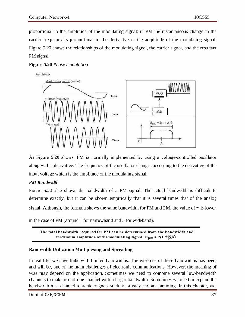
Computer Network-1 10CS55
Dept of CSE,GCEM 87
proportional to the amplitude of the modulating signal; in PM the instantaneous change in the
carrier frequency is proportional to the derivative of the amplitude of the modulating signal.
Figure 5.20 shows the relationships of the modulating signal, the carrier signal, and the resultant
PM signal.
Figure 5.20 Phase modulation
As Figure 5.20 shows, PM is normally implemented by using a voltage-controlled oscillator
along with a derivative. The frequency of the oscillator changes according to the derivative of the
input voltage which is the amplitude of the modulating signal.
PM Bandwidth
Figure 5.20 also shows the bandwidth of a PM signal. The actual bandwidth is difficult to
determine exactly, but it can be shown empirically that it is several times that of the analog
signal. Although, the formula shows the same bandwidth for FM and PM, the value of ~ is lower
in the case of PM (around 1 for narrowband and 3 for wideband).
Bandwidth Utilization Multiplexing and Spreading
In real life, we have links with limited bandwidths. The wise use of these bandwidths has been,
and will be, one of the main challenges of electronic communications. However, the meaning of
wise may depend on the application. Sometimes we need to combine several low-bandwidth
channels to make use of one channel with a larger bandwidth. Sometimes we need to expand the
bandwidth of a channel to achieve goals such as privacy and ant jamming. In this chapter, we
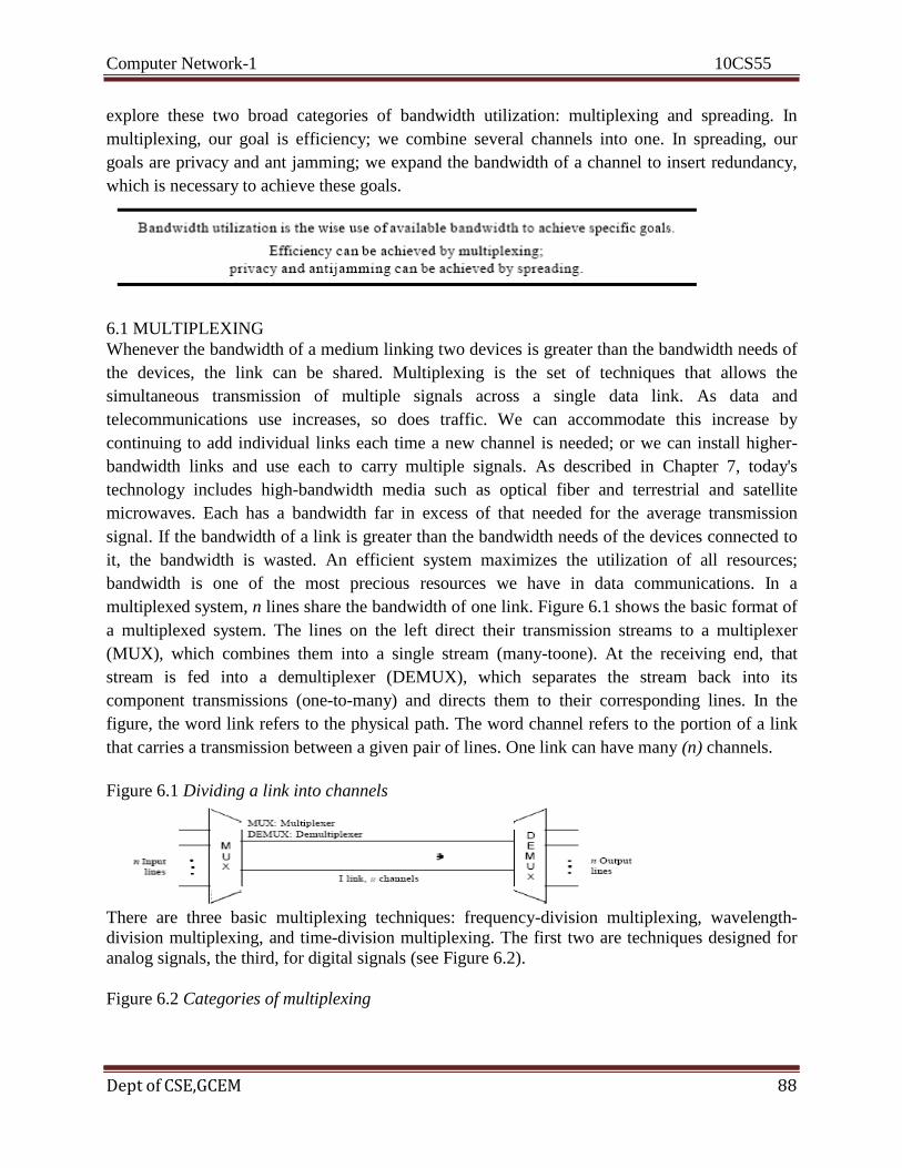
Computer Network-1 10CS55
Dept of CSE,GCEM 88
explore these two broad categories of bandwidth utilization: multiplexing and spreading. In
multiplexing, our goal is efficiency; we combine several channels into one. In spreading, our
goals are privacy and ant jamming; we expand the bandwidth of a channel to insert redundancy,
which is necessary to achieve these goals.
6.1 MULTIPLEXING
Whenever the bandwidth of a medium linking two devices is greater than the bandwidth needs of
the devices, the link can be shared. Multiplexing is the set of techniques that allows the
simultaneous transmission of multiple signals across a single data link. As data and
telecommunications use increases, so does traffic. We can accommodate this increase by
continuing to add individual links each time a new channel is needed; or we can install higher-
bandwidth links and use each to carry multiple signals. As described in Chapter 7, today's
technology includes high-bandwidth media such as optical fiber and terrestrial and satellite
microwaves. Each has a bandwidth far in excess of that needed for the average transmission
signal. If the bandwidth of a link is greater than the bandwidth needs of the devices connected to
it, the bandwidth is wasted. An efficient system maximizes the utilization of all resources;
bandwidth is one of the most precious resources we have in data communications. In a
multiplexed system, n lines share the bandwidth of one link. Figure 6.1 shows the basic format of
a multiplexed system. The lines on the left direct their transmission streams to a multiplexer
(MUX), which combines them into a single stream (many-toone). At the receiving end, that
stream is fed into a demultiplexer (DEMUX), which separates the stream back into its
component transmissions (one-to-many) and directs them to their corresponding lines. In the
figure, the word link refers to the physical path. The word channel refers to the portion of a link
that carries a transmission between a given pair of lines. One link can have many (n) channels.
Figure 6.1 Dividing a link into channels
There are three basic multiplexing techniques: frequency-division multiplexing, wavelength-
division multiplexing, and time-division multiplexing. The first two are techniques designed for
analog signals, the third, for digital signals (see Figure 6.2).
Figure 6.2 Categories of multiplexing
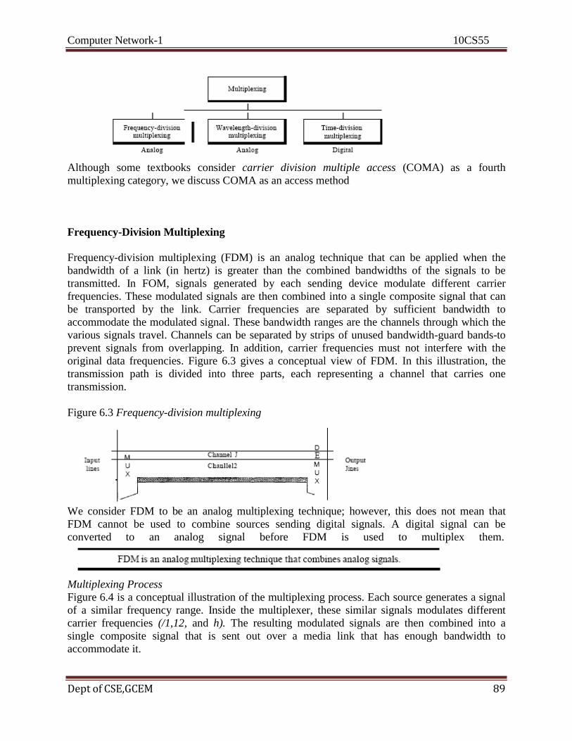
Computer Network-1 10CS55
Dept of CSE,GCEM 89
Although some textbooks consider carrier division multiple access (COMA) as a fourth
multiplexing category, we discuss COMA as an access method
Frequency-Division Multiplexing
Frequency-division multiplexing (FDM) is an analog technique that can be applied when the
bandwidth of a link (in hertz) is greater than the combined bandwidths of the signals to be
transmitted. In FOM, signals generated by each sending device modulate different carrier
frequencies. These modulated signals are then combined into a single composite signal that can
be transported by the link. Carrier frequencies are separated by sufficient bandwidth to
accommodate the modulated signal. These bandwidth ranges are the channels through which the
various signals travel. Channels can be separated by strips of unused bandwidth-guard bands-to
prevent signals from overlapping. In addition, carrier frequencies must not interfere with the
original data frequencies. Figure 6.3 gives a conceptual view of FDM. In this illustration, the
transmission path is divided into three parts, each representing a channel that carries one
transmission.
Figure 6.3 Frequency-division multiplexing
We consider FDM to be an analog multiplexing technique; however, this does not mean that
FDM cannot be used to combine sources sending digital signals. A digital signal can be
converted to an analog signal before FDM is used to multiplex them.
Multiplexing Process
Figure 6.4 is a conceptual illustration of the multiplexing process. Each source generates a signal
of a similar frequency range. Inside the multiplexer, these similar signals modulates different
carrier frequencies (/1,12, and h). The resulting modulated signals are then combined into a
single composite signal that is sent out over a media link that has enough bandwidth to
accommodate it.

Computer Network-1 10CS55
Dept of CSE,GCEM 90
Figure 6.4 FDM process
Demultiplexing Process
The demultiplexer uses a series of filters to decompose the multiplexed signal into its constituent
component signals. The individual signals are then passed to a demodulator that separates them
from their carriers and passes them to the output lines. Figure 6.5 is a conceptual illustration of
demultiplexing process.
Figure 6.5 FDM demultiplexing example
The Analog Carrier System
To maximize the efficiency of their infrastructure, telephone companies have traditionally
multiplexed signals from lower-bandwidth lines onto higher-bandwidth lines. In this way, many
switched or leased lines can be combined into fewer but bigger channels. For analog lines, FDM
is used. One of these hierarchical systems used by AT&T is made up of groups, super groups,
master groups, and jumbo groups
Figure 6.9 Analog hierarchy
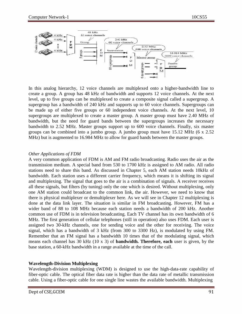
Computer Network-1 10CS55
Dept of CSE,GCEM 91
In this analog hierarchy, 12 voice channels are multiplexed onto a higher-bandwidth line to
create a group. A group has 48 kHz of bandwidth and supports 12 voice channels. At the next
level, up to five groups can be multiplexed to create a composite signal called a supergroup. A
supergroup has a bandwidth of 240 kHz and supports up to 60 voice channels. Supergroups can
be made up of either five groups or 60 independent voice channels. At the next level, 10
supergroups are multiplexed to create a master group. A master group must have 2.40 MHz of
bandwidth, but the need for guard bands between the supergroups increases the necessary
bandwidth to 2.52 MHz. Master groups support up to 600 voice channels. Finally, six master
groups can be combined into a jumbo group. A jumbo group must have 15.12 MHz (6 x 2.52
MHz) but is augmented to 16.984 MHz to allow for guard bands between the master groups.
Other Applications of FDM
A very common application of FDM is AM and FM radio broadcasting. Radio uses the air as the
transmission medium. A special band from 530 to 1700 kHz is assigned to AM radio. All radio
stations need to share this band. As discussed in Chapter 5, each AM station needs 10kHz of
bandwidth. Each station uses a different carrier frequency, which means it is shifting its signal
and multiplexing. The signal that goes to the air is a combination of signals. A receiver receives
all these signals, but filters (by tuning) only the one which is desired. Without multiplexing, only
one AM station could broadcast to the common link, the air. However, we need to know that
there is physical multiplexer or demultiplexer here. As we will see in Chapter 12 multiplexing is
done at the data link layer. The situation is similar in FM broadcasting. However, FM has a
wider band of 88 to 108 MHz because each station needs a bandwidth of 200 kHz. Another
common use of FDM is in television broadcasting. Each TV channel has its own bandwidth of 6
MHz. The first generation of cellular telephones (still in operation) also uses FDM. Each user is
assigned two 30-kHz channels, one for sending voice and the other for receiving. The voice
signal, which has a bandwidth of 3 kHz (from 300 to 3300 Hz), is modulated by using FM.
Remember that an FM signal has a bandwidth 10 times that of the modulating signal, which
means each channel has 30 kHz (10 x 3) of bandwidth. Therefore, each user is given, by the
base station, a 60-kHz bandwidth in a range available at the time of the call.
Wavelength-Division Multiplexing
Wavelength-division multiplexing (WDM) is designed to use the high-data-rate capability of
fiber-optic cable. The optical fiber data rate is higher than the data rate of metallic transmission
cable. Using a fiber-optic cable for one single line wastes the available bandwidth. Multiplexing
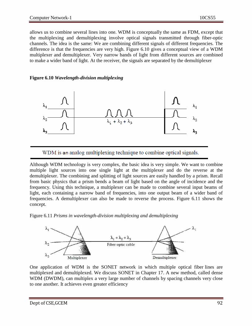
Computer Network-1 10CS55
Dept of CSE,GCEM 92
allows us to combine several lines into one. WDM is conceptually the same as FDM, except that
the multiplexing and demultiplexing involve optical signals transmitted through fiber-optic
channels. The idea is the same: We are combining different signals of different frequencies. The
difference is that the frequencies are very high. Figure 6.10 gives a conceptual view of a WDM
multiplexer and demultiplexer. Very narrow bands of light from different sources are combined
to make a wider band of light. At the receiver, the signals are separated by the demultiplexer
Figure 6.10 Wavelength-division multiplexing
Although WDM technology is very complex, the basic idea is very simple. We want to combine
multiple light sources into one single light at the multiplexer and do the reverse at the
demultiplexer. The combining and splitting of light sources are easily handled by a prism. Recall
from basic physics that a prism bends a beam of light based on the angle of incidence and the
frequency. Using this technique, a multiplexer can be made to combine several input beams of
light, each containing a narrow band of frequencies, into one output beam of a wider band of
frequencies. A demultiplexer can also be made to reverse the process. Figure 6.11 shows the
concept.
Figure 6.11 Prisms in wavelength-division multiplexing and demultiplexing
One application of WDM is the SONET network in which multiple optical fiber lines are
multiplexed and demultiplexed. We discuss SONET in Chapter 17. A new method, called dense
WDM (DWDM), can multiplex a very large number of channels by spacing channels very close
to one another. It achieves even greater efficiency
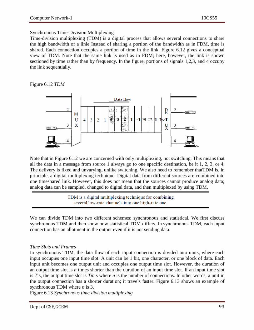
Computer Network-1 10CS55
Dept of CSE,GCEM 93
Synchronous Time-Division Multiplexing
Time-division multiplexing (TDM) is a digital process that allows several connections to share
the high bandwidth of a linle Instead of sharing a portion of the bandwidth as in FDM, time is
shared. Each connection occupies a portion of time in the link. Figure 6.12 gives a conceptual
view of TDM. Note that the same link is used as in FDM; here, however, the link is shown
sectioned by time rather than by frequency. In the figure, portions of signals 1,2,3, and 4 occupy
the link sequentially.
Figure 6.12 TDM
Note that in Figure 6.12 we are concerned with only multiplexing, not switching. This means that
all the data in a message from source 1 always go to one specific destination, be it 1, 2, 3, or 4.
The delivery is fixed and unvarying, unlike switching. We also need to remember thatTDM is, in
principle, a digital multiplexing technique. Digital data from different sources are combined into
one timeshared link. However, this does not mean that the sources cannot produce analog data;
analog data can be sampled, changed to digital data, and then multiplexed by using TDM.
We can divide TDM into two different schemes: synchronous and statistical. We first discuss
synchronous TDM and then show how statistical TDM differs. In synchronous TDM, each input
connection has an allotment in the output even if it is not sending data.
Time Slots and Frames
In synchronous TDM, the data flow of each input connection is divided into units, where each
input occupies one input time slot. A unit can be 1 bit, one character, or one block of data. Each
input unit becomes one output unit and occupies one output time slot. However, the duration of
an output time slot is n times shorter than the duration of an input time slot. If an input time slot
is T s, the output time slot is Tin s where n is the number of connections. In other words, a unit in
the output connection has a shorter duration; it travels faster. Figure 6.13 shows an example of
synchronous TDM where n is 3.
Figure 6.13 Synchronous time-division multiplexing
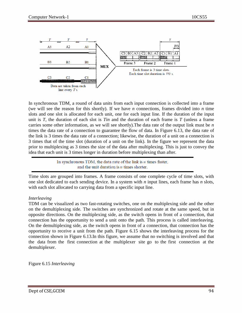
Computer Network-1 10CS55
Dept of CSE,GCEM 94
In synchronous TDM, a round of data units from each input connection is collected into a frame
(we will see the reason for this shortly). If we have n connections, frames divided into n time
slots and one slot is allocated for each unit, one for each input line. If the duration of the input
unit is T, the duration of each slot is Tin and the duration of each frame is T (unless a frame
carries some other information, as we will see shortly).The data rate of the output link must be n
times the data rate of a connection to guarantee the flow of data. In Figure 6.13, the data rate of
the link is 3 times the data rate of a connection; likewise, the duration of a unit on a connection is
3 times that of the time slot (duration of a unit on the link). In the figure we represent the data
prior to multiplexing as 3 times the size of the data after multiplexing. This is just to convey the
idea that each unit is 3 times longer in duration before multiplexing than after.
Time slots are grouped into frames. A frame consists of one complete cycle of time slots, with
one slot dedicated to each sending device. In a system with n input lines, each frame has n slots,
with each slot allocated to carrying data from a specific input line.
Interleaving
TDM can be visualized as two fast-rotating switches, one on the multiplexing side and the other
on the demultiplexing side. The switches are synchronized and rotate at the same speed, but in
opposite directions. On the multiplexing side, as the switch opens in front of a connection, that
connection has the opportunity to send a unit onto the path. This process is called interleaving.
On the demultiplexing side, as the switch opens in front of a connection, that connection has the
opportunity to receive a unit from the path. Figure 6.15 shows the interleaving process for the
connection shown in Figure 6.13.In this figure, we assume that no switching is involved and that
the data from the first connection at the multiplexer site go to the first connection at the
demultiplexer.
Figure 6.15 Interleaving
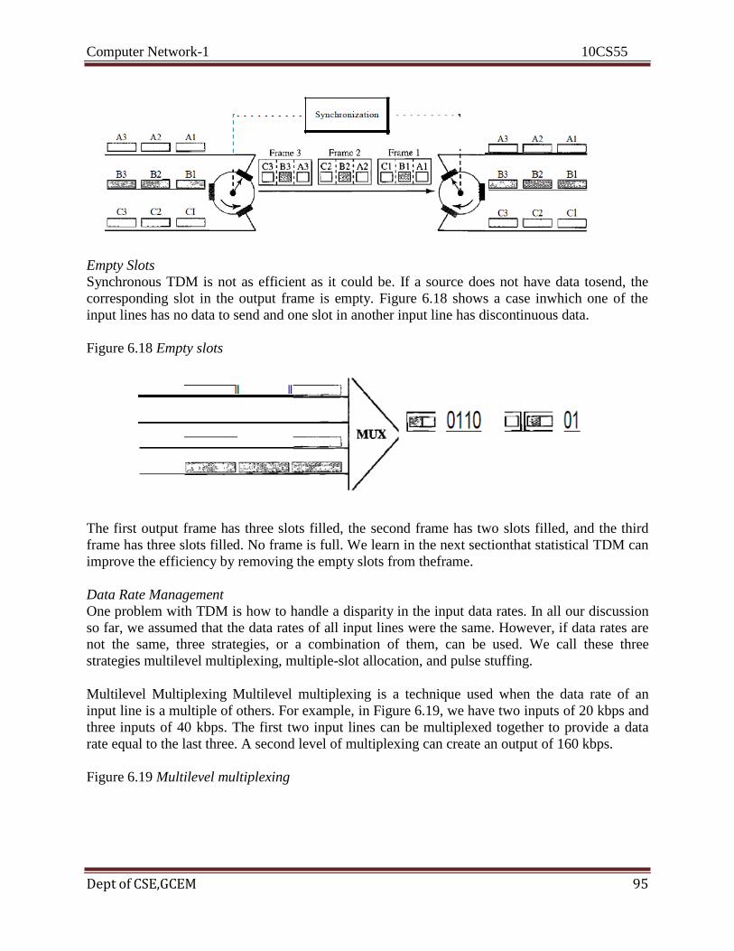
Computer Network-1 10CS55
Dept of CSE,GCEM 95
Empty Slots
Synchronous TDM is not as efficient as it could be. If a source does not have data tosend, the
corresponding slot in the output frame is empty. Figure 6.18 shows a case inwhich one of the
input lines has no data to send and one slot in another input line has discontinuous data.
Figure 6.18 Empty slots
The first output frame has three slots filled, the second frame has two slots filled, and the third
frame has three slots filled. No frame is full. We learn in the next sectionthat statistical TDM can
improve the efficiency by removing the empty slots from theframe.
Data Rate Management
One problem with TDM is how to handle a disparity in the input data rates. In all our discussion
so far, we assumed that the data rates of all input lines were the same. However, if data rates are
not the same, three strategies, or a combination of them, can be used. We call these three
strategies multilevel multiplexing, multiple-slot allocation, and pulse stuffing.
Multilevel Multiplexing Multilevel multiplexing is a technique used when the data rate of an
input line is a multiple of others. For example, in Figure 6.19, we have two inputs of 20 kbps and
three inputs of 40 kbps. The first two input lines can be multiplexed together to provide a data
rate equal to the last three. A second level of multiplexing can create an output of 160 kbps.
Figure 6.19 Multilevel multiplexing
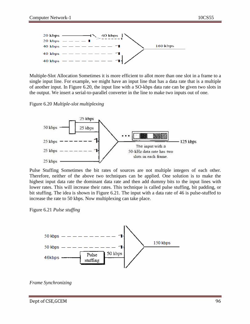
Computer Network-1 10CS55
Dept of CSE,GCEM 96
Multiple-Slot Allocation Sometimes it is more efficient to allot more than one slot in a frame to a
single input line. For example, we might have an input line that has a data rate that is a multiple
of another input. In Figure 6.20, the input line with a SO-kbps data rate can be given two slots in
the output. We insert a serial-to-parallel converter in the line to make two inputs out of one.
Figure 6.20 Multiple-slot multiplexing
Pulse Stuffing Sometimes the bit rates of sources are not multiple integers of each other.
Therefore, neither of the above two techniques can be applied. One solution is to make the
highest input data rate the dominant data rate and then add dummy bits to the input lines with
lower rates. This will increase their rates. This technique is called pulse stuffing, bit padding, or
bit stuffing. The idea is shown in Figure 6.21. The input with a data rate of 46 is pulse-stuffed to
increase the rate to 50 kbps. Now multiplexing can take place.
Figure 6.21 Pulse stuffing
Frame Synchronizing
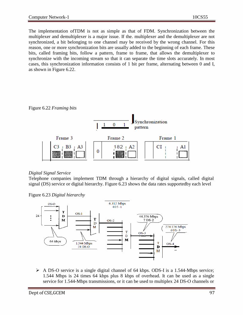
Computer Network-1 10CS55
Dept of CSE,GCEM 97
The implementation ofTDM is not as simple as that of FDM. Synchronization between the
multiplexer and demultiplexer is a major issue. If the. multiplexer and the demultiplexer are not
synchronized, a bit belonging to one channel may be received by the wrong channel. For this
reason, one or more synchronization bits are usually added to the beginning of each frame. These
bits, called framing bits, follow a pattern, frame to frame, that allows the demultiplexer to
synchronize with the incoming stream so that it can separate the time slots accurately. In most
cases, this synchronization information consists of 1 bit per frame, alternating between 0 and I,
as shown in Figure 6.22.
Figure 6.22 Framing bits
Digital Signal Service
Telephone companies implement TDM through a hierarchy of digital signals, called digital
signal (DS) service or digital hierarchy. Figure 6.23 shows the data rates supportedby each level
Figure 6.23 Digital hierarchy
A DS-O service is a single digital channel of 64 kbps. ODS-I is a 1.544-Mbps service;
1.544 Mbps is 24 times 64 kbps plus 8 kbps of overhead. It can be used as a single
service for 1.544-Mbps transmissions, or it can be used to multiplex 24 DS-O channels or
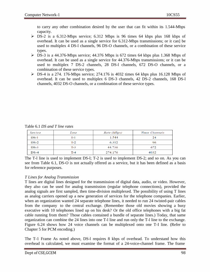
Computer Network-1 10CS55
Dept of CSE,GCEM 98
to carry any other combination desired by the user that can fit within its 1.544-Mbps
capacity.
DS-2 is a 6.312-Mbps service; 6.312 Mbps is 96 times 64 kbps plus 168 kbps of
overhead. It can be used as a single service for 6.312-Mbps transmissions; or it can] be
used to multiplex 4 DS-l channels, 96 DS-O channels, or a combination of these service
types.
DS-3 is a 44.376-Mbps service; 44.376 Mbps is 672 times 64 kbps plus 1.368 Mbps of
overhead. It can be used as a single service for 44.376-Mbps transmissions; or it can be
used to multiplex 7 DS-2 channels, 28 DS-l channels, 672 DS-O channels, or a
combination of these service types.
DS-4 is a 274. 176-Mbps service; 274.176 is 4032 times 64 kbps plus 16.128 Mbps of
overhead. It can be used to multiplex 6 DS-3 channels, 42 DS-2 channels, 168 DS-l
channels, 4032 DS-O channels, or a combination of these service types.
Table 6.1 DS and T line rates
The T-l line is used to implement DS-l; T-2 is used to implement DS-2; and so on. As you can
see from Table 6.1, DS-O is not actually offered as a service, but it has been defined as a basis
for reference purposes.
T Lines for Analog Transmission
T lines are digital lines designed for the transmission of digital data, audio, or video. However,
they also can be used for analog transmission (regular telephone connections), provided the
analog signals are first sampled, then time-division multiplexed. The possibility of using T lines
as analog carriers opened up a new generation of services for the telephone companies. Earlier,
when an organization wanted 24 separate telephone lines, it needed to run 24 twisted-pair cables
from the company to the central exchange. (Remember those old movies showing a busy
executive with 10 telephones lined up on his desk? Or the old office telephones with a big fat
cable running from them? Those cables contained a bundle of separate lines.) Today, that same
organization can combine the 24 lines into one T-l line and run only the T-l line to the exchange.
Figure 6.24 shows how 24 voice channels can be multiplexed onto one T-I line. (Refer to
Chapter 5 for PCM encoding.)
The T-1 Frame As noted above, DS-l requires 8 kbps of overhead. To understand how this
overhead is calculated, we must examine the format of a 24-voice-channel frame. The frame
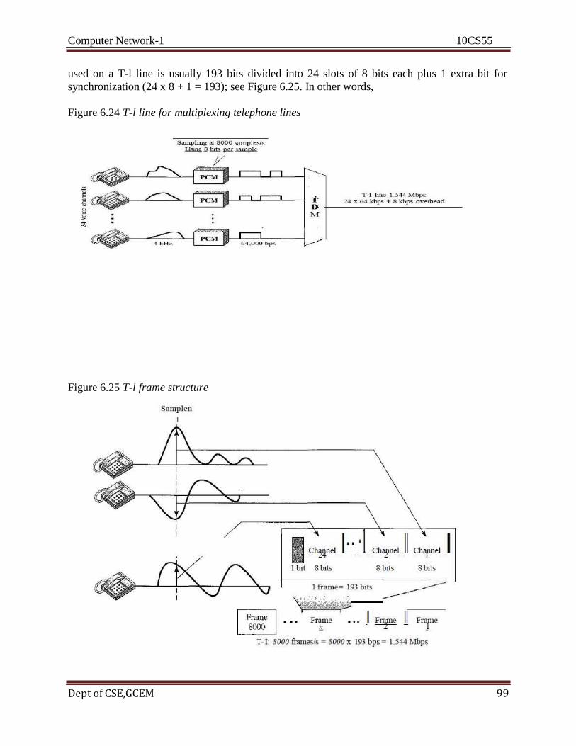
Computer Network-1 10CS55
Dept of CSE,GCEM 99
used on a T-l line is usually 193 bits divided into 24 slots of 8 bits each plus 1 extra bit for
synchronization (24 x 8 + 1 = 193); see Figure 6.25. In other words,
Figure 6.24 T-l line for multiplexing telephone lines
Figure 6.25 T-l frame structure
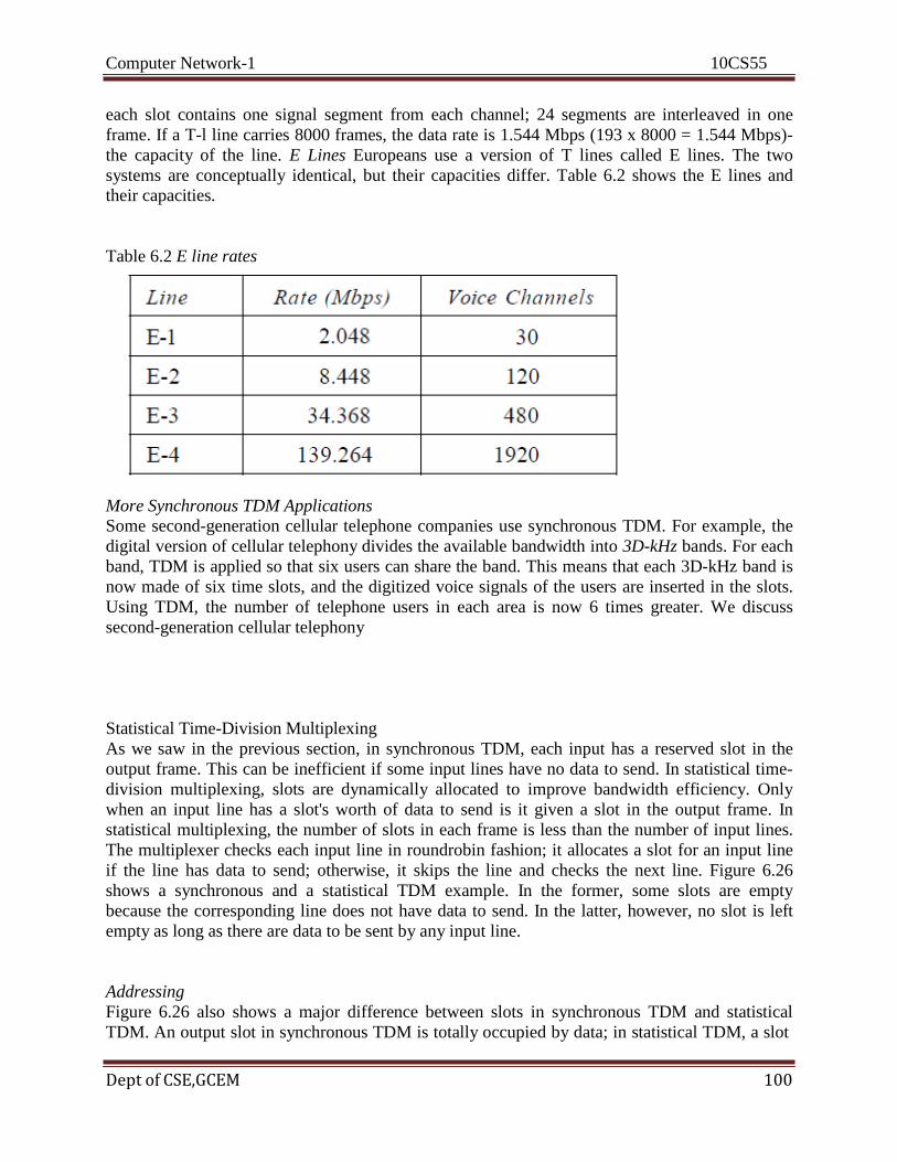
Computer Network-1 10CS55
Dept of CSE,GCEM 100
each slot contains one signal segment from each channel; 24 segments are interleaved in one
frame. If a T-l line carries 8000 frames, the data rate is 1.544 Mbps (193 x 8000 = 1.544 Mbps)-
the capacity of the line. E Lines Europeans use a version of T lines called E lines. The two
systems are conceptually identical, but their capacities differ. Table 6.2 shows the E lines and
their capacities.
Table 6.2 E line rates
More Synchronous TDM Applications
Some second-generation cellular telephone companies use synchronous TDM. For example, the
digital version of cellular telephony divides the available bandwidth into 3D-kHz bands. For each
band, TDM is applied so that six users can share the band. This means that each 3D-kHz band is
now made of six time slots, and the digitized voice signals of the users are inserted in the slots.
Using TDM, the number of telephone users in each area is now 6 times greater. We discuss
second-generation cellular telephony
Statistical Time-Division Multiplexing
As we saw in the previous section, in synchronous TDM, each input has a reserved slot in the
output frame. This can be inefficient if some input lines have no data to send. In statistical time-
division multiplexing, slots are dynamically allocated to improve bandwidth efficiency. Only
when an input line has a slot's worth of data to send is it given a slot in the output frame. In
statistical multiplexing, the number of slots in each frame is less than the number of input lines.
The multiplexer checks each input line in roundrobin fashion; it allocates a slot for an input line
if the line has data to send; otherwise, it skips the line and checks the next line. Figure 6.26
shows a synchronous and a statistical TDM example. In the former, some slots are empty
because the corresponding line does not have data to send. In the latter, however, no slot is left
empty as long as there are data to be sent by any input line.
Addressing
Figure 6.26 also shows a major difference between slots in synchronous TDM and statistical
TDM. An output slot in synchronous TDM is totally occupied by data; in statistical TDM, a slot

Computer Network-1 10CS55
Dept of CSE, GCEM 101
needs to carry data as well as the address of the destination. In synchronous TDM, there is no
need for addressing; synchronization and preassigned relationships between the inputs and
outputs serve as an address. We know, for example, that input 1 always goes to input 2. If the
multiplexer and the demultiplexer are synchronized, this is guaranteed. In statistical
multiplexing, there is no fixed relationship between the inputs and outputs because there are no
preassigned or reserved slots. We need to include the address of the receiver inside each slot to
show where it is to be delivered. The addressing in its simplest form can be n bits to define N
different output lines with n =10g2 N. For example, for eight different output lines, we need a 3-
bit address.
Figure 6.26 TDM slot comparison
Slot Size
Since a slot carries both data and an address in statistical TDM, the ratio of the data size to
address size must be reasonable to make transmission efficient. For example, it would be
inefficient to send 1 bit per slot as data when the address is 3 bits. This would mean an overhead
of 300 percent. In statistical TDM, a block of data is usually many bytes while the address is just
a few bytes.
No Synchronization Bit
There is another difference between synchronous and statistical TDM, but this time it is at the
frame level. The frames in statistical TDM need not be synchronized, so we do not
need synchronization bits.
Bandwidth
In statistical TDM, the capacity of the link is normally less than the sum of the capacities of each
channel. The designers of statistical TDM define the capacity of the link based on the statistics of
the load for each channel. If on average only x percent of the input slots are filled, the capacity of
the link reflects this. Of course, during peak times, some slots need to wait.
6.2 SPREAD SPECTRUM
Multiplexing combines signals from several sources to achieve bandwidth efficiency; the
available bandwidth of a link is divided between the sources. In spread spectrum (88), we also

Computer Network-1 10CS55
Dept of CSE, GCEM 102
combine signals from different sources to fit into a larger bandwidth, but our goals are somewhat
different. Spread spectrum is designed to be used in wireless applications
(LANs and WANs). In these types of applications, we have some concerns that outweigh
bandwidth efficiency. In wireless applications, all stations use air (or a vacuum) as the medium
for communication. Stations must be able to share this medium without interception by an
eavesdropper and without being subject to jamming from a malicious intruder (in military
operations, for example). To achieve these goals, spread spectrum techniques add redundancy;
they spread the original spectrum needed for each station. If the required bandwidth for each
station is B, spread spectrum expands it to Bss' such that Bss » B. The expanded bandwidth
allows the source to wrap its message in a protective envelope for a more secure transmission.
An analogy is the sending of a delicate, expensive gift. We can insert the gift in a special box to
prevent it from being damaged during transportation, and we can use a superior delivery service
to guarantee the safety of the package. Figure 6.27 shows the idea of spread spectrum. Spread
spectrum achieves its goals through two principles:
1. The bandwidth allocated to each station needs to be, by far, larger than what is needed. This
allows redundancy.
2. The expanding of the original bandwidth B to the bandwidth Bss must be done by a process
that is independent of the original signal. In other words, the spreading process occurs after the
signal is created by the source.
Figure 6.27 Spread spectrum
After the signal is created by the source, the spreading process uses a spreading code and spreads
the bandwidth. The figure shows the original bandwidth B and the spreaded bandwidth Bss. The
spreading code is a series of numbers that look random, but are actually a pattern. There are two
techniques to spread the bandwidth: frequency hopping spread spectrum (FHSS) and direct
sequence spread spectrum (DSSS).
Frequency Hopping Spread Spectrum (FHSS)
The frequency hopping spread spectrum (FHSS) technique uses M different carrier frequencies
that are modulated by the source signal. At one moment, the signal modulates one carrier
frequency; at the next moment, the signal modulates another carrier frequency. Although the
modulation is done using one carrier frequency at a time, M frequencies are used in the long run.
The bandwidth occupied by a source after spreading is BpHSS »B. Figure 6.28 shows the general
layout for FHSS. A pseudorandom code generator, called pseudorandom noise (PN), creates a k-
bit pattern for every hopping period Th• The frequency table uses the pattern to find the
frequency to be used for this hopping period and passes it to the frequency synthesizer. The

Computer Network-1 10CS55
Dept of CSE, GCEM 103
frequency synthesizer creates a carrier signal of that frequency, and the source signal modulates
the carrier signal.
Figure 6.28 Frequency hopping spread spectrum (FHSS)
Suppose we have decided to have eight hopping frequencies. This is extremely low for real
applications and is just for illustration. In this case, Mis 8 and k is 3. The pseudorandom code
generator will create eight different 3-bit patterns. These are mapped to eight different
frequencies in the frequency table (see Figure 6.29).
Figure 6.29 Frequency selection in FHSS
The pattern for this station is 101, 111, 001, 000, 010, all, 100. Note that the pattern is
pseudorandom it is repeated after eight hoppings. This means that at hopping period 1, the
pattern is 101. The frequency selected is 700 kHz; the source signal modulates this carrier
frequency. The second k-bit pattern selected is 111, which selects the 900-kHz carrier; the eighth
pattern is 100, the frequency is 600 kHz. After eight hoppings, the pattern repeats, starting from
101 again. Figure 6.30 shows how the signal hops around from carrier to carrier. We assume the
required bandwidth of the original signal is 100 kHz.

Computer Network-1 10CS55
Dept of CSE, GCEM 104
Figure 6.30 FHSS cycles
.
It can be shown that this scheme can accomplish the previously mentioned goals. If there are
many k-bit patterns and the hopping period is short, a sender and receiver can have privacy. If an
intruder tries to intercept the transmitted signal, she can only access a small piece of data because
she does not know the spreading sequence to quickly adapt herself to the next hop. The scheme
has also an antijamming effect. A malicious sender may be able to send noise to jam the signal
for one hopping period (randomly), but not for the whole period.
Bandwidth Sharing
If the number of hopping frequencies is M, we can multiplex M channels into one by using the
same Bss bandwidth. This is possible because a station uses just one frequency in each hopping
period; M - 1 other frequencies can be used by other M - 1 stations. In other words, M different
stations can use the same Bss if an appropriate modulation technique such as multiple FSK
(MFSK) is used. FHSS is similar to FDM, as shown in Figure 6.31.Figure 6.31 shows an
example of four channels using FDM and four channels using FHSS. In FDM, each station uses
11M of the bandwidth, but the allocation is fixed; in FHSS, each station uses 11M of the
bandwidth, but the allocation changes hop to hop
Figure 6.31 Bandwidth sharing
Direct Sequence Spread Spectrum
The direct sequence spread spectrum (nSSS) technique also expands the bandwidth of the
original signal, but the process is different. In DSSS, we replace each data bit with 11 bits using
a spreading code. In other words, each bit is assigned a code of 11 bits, called chips, where the
chip rate is 11 times that of the data bit. Figure 6.32 shows the concept of DSSS.
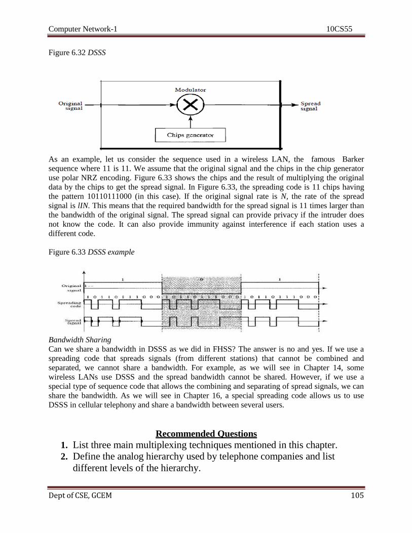
Computer Network-1 10CS55
Dept of CSE, GCEM 105
Figure 6.32 DSSS
As an example, let us consider the sequence used in a wireless LAN, the famous Barker
sequence where 11 is 11. We assume that the original signal and the chips in the chip generator
use polar NRZ encoding. Figure 6.33 shows the chips and the result of multiplying the original
data by the chips to get the spread signal. In Figure 6.33, the spreading code is 11 chips having
the pattern 10110111000 (in this case). If the original signal rate is N, the rate of the spread
signal is lIN. This means that the required bandwidth for the spread signal is 11 times larger than
the bandwidth of the original signal. The spread signal can provide privacy if the intruder does
not know the code. It can also provide immunity against interference if each station uses a
different code.
Figure 6.33 DSSS example
Bandwidth Sharing
Can we share a bandwidth in DSSS as we did in FHSS? The answer is no and yes. If we use a
spreading code that spreads signals (from different stations) that cannot be combined and
separated, we cannot share a bandwidth. For example, as we will see in Chapter 14, some
wireless LANs use DSSS and the spread bandwidth cannot be shared. However, if we use a
special type of sequence code that allows the combining and separating of spread signals, we can
share the bandwidth. As we will see in Chapter 16, a special spreading code allows us to use
DSSS in cellular telephony and share a bandwidth between several users.
Recommended Questions
1. List three main multiplexing techniques mentioned in this chapter. 2. Define the analog hierarchy used by telephone companies and list
different levels of the hierarchy.
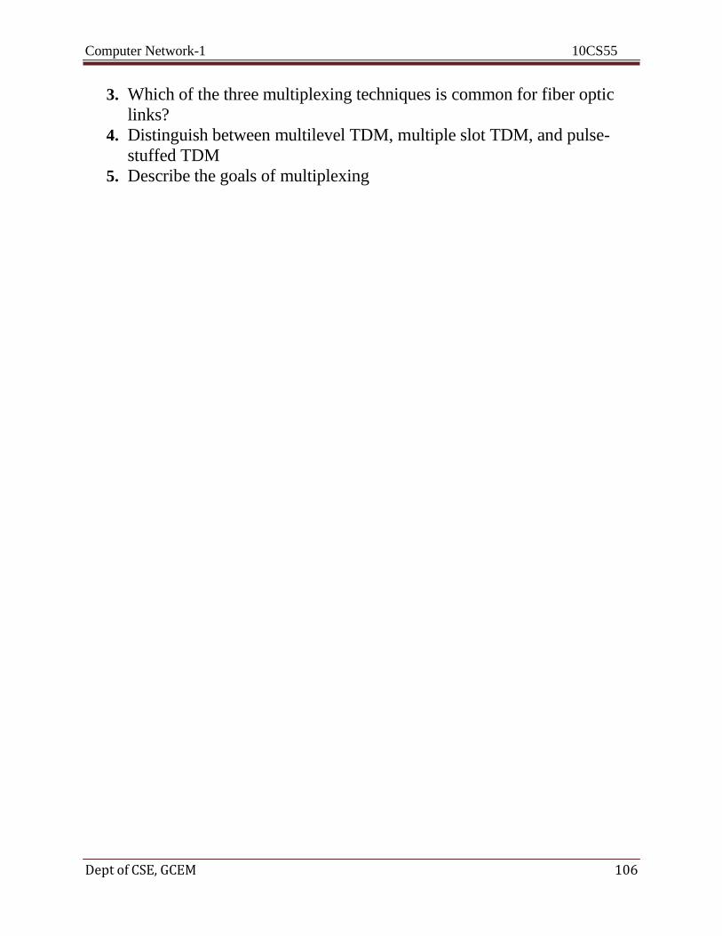
Computer Network-1 10CS55
Dept of CSE, GCEM 106
3. Which of the three multiplexing techniques is common for fiber optic
links?
4. Distinguish between multilevel TDM, multiple slot TDM, and pulse-
stuffed TDM
5. Describe the goals of multiplexing
Computer Network-1 10CS55
Dept of CSE, GCEM 107
COMPUTER NETWORKS – I
Subject Code: 10CS55 I.A. Marks : 25
Hours/Week : 04 Exam Hours: 03
Total Hours : 52 Exam Marks: 100
UNIT- 4 6 Hours
Data Link Layer-1:
-Error Detection & Correction:
- Introduction,
-Block coding,
-Linear block codes,
-Cyclic codes, -Checksum.
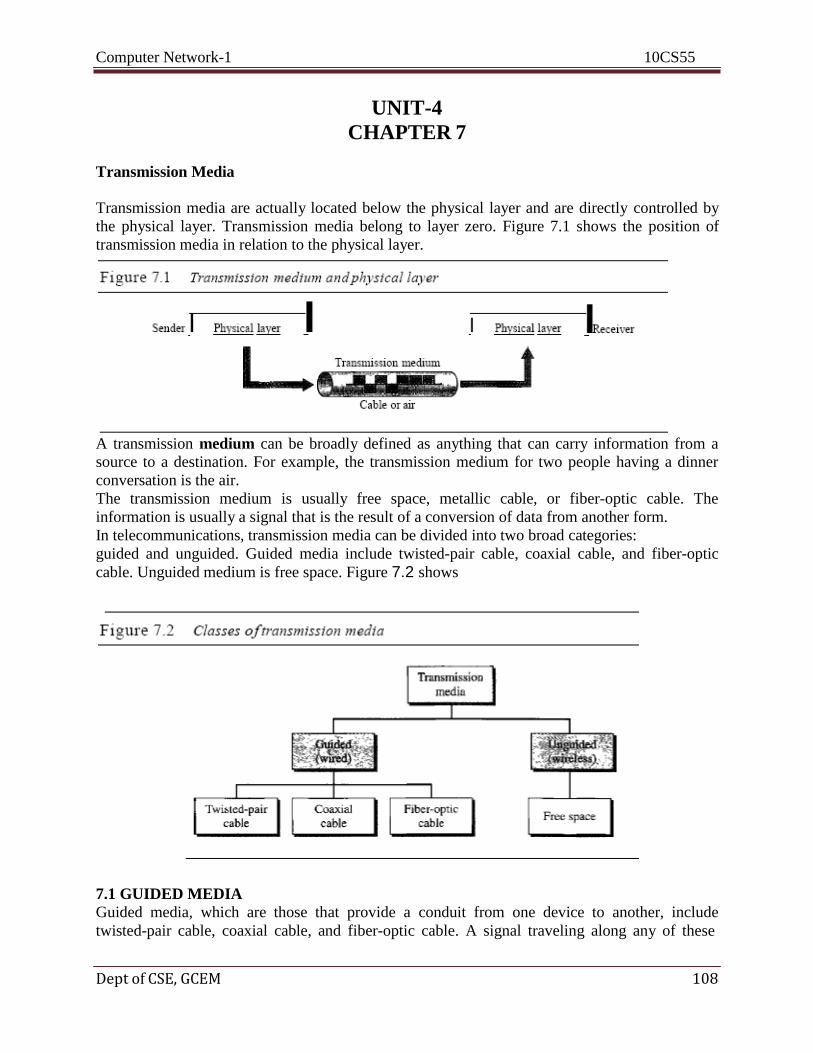
Computer Network-1 10CS55
Dept of CSE, GCEM 108
UNIT-4
CHAPTER 7
Transmission Media
Transmission media are actually located below the physical layer and are directly controlled by
the physical layer. Transmission media belong to layer zero. Figure 7.1 shows the position of
transmission media in relation to the physical layer.
A transmission medium can be broadly defined as anything that can carry information from a
source to a destination. For example, the transmission medium for two people having a dinner
conversation is the air.
The transmission medium is usually free space, metallic cable, or fiber-optic cable. The
information is usually a signal that is the result of a conversion of data from another form.
In telecommunications, transmission media can be divided into two broad categories:
guided and unguided. Guided media include twisted-pair cable, coaxial cable, and fiber-optic
cable. Unguided medium is free space. Figure 7.2 shows
7.1 GUIDED MEDIA
Guided media, which are those that provide a conduit from one device to another, include
twisted-pair cable, coaxial cable, and fiber-optic cable. A signal traveling along any of these

Computer Network-1 10CS55
Dept of CSE, GCEM 109
media is directed and contained by the physical limits of the medium. Twisted-pair and coaxial
cable use metallic (copper) conductors that accept and transport signals in the form of electric
current. Optical fiber is a cable that accepts and transports signals in the form of light.
Twisted-Pair Cable
A twisted pair consists of two conductors (normally copper), each with its own plastic
insulation, twisted together, as shown in Figure 7.3.
One of the wires is used to carry signals to the receiver, and the other is used only as a ground
reference. The receiver uses the difference between the two. One of the wires is used to carry
signals to the receiver, and the other is used only as a ground reference. The receiver uses the
difference between the two. In addition to the signal sent by the sender on one of the wires,
interference (noise) and crosstalk may affect both wires and create unwanted signals.
If the two wires are parallel, the effect of these unwanted signals is not the same in both wires
because they are at different locations relative to the noise or crosstalk sources
(e,g., one is closer and the other is farther). This results in a difference at the receiver. By
twisting the pairs, a balance is maintained.
Unshielded Versus Shielded Twisted-Pair Cable
The most common twisted-pair cable used in communications is referred to as unshielded
twisted-pair (UTP). IBM has also produced a version of twisted-pair cable
for its use called shielded twisted-pair (STP). STP cable has a metal foil or braidedmesh
covering that encases each pair of insulated conductors. Although metal casing improves the
quality of cable by preventing the penetration of noise or crosstalk, it is bulkier and more
expensive. Figure 7.4 shows the difference between UTP and STP.
Categories
The Electronic Industries Association (EIA) has developed standards to classify
unshielded twisted-pair cable into seven categories. Categories are determined by cable
quality, with 1 as the lowest and 7 as the highest. Each EIA category is suitable for
specific uses. Table 7. 1 shows these categories.
Connectors
The most common UTP connector is RJ45 (RJ stands for registered jack), as shown
in Figure 7.5. The RJ45 is a keyed connector, meaning the connector can be inserted in

Computer Network-1 10CS55
Dept of CSE,GCEM 110
only one way.
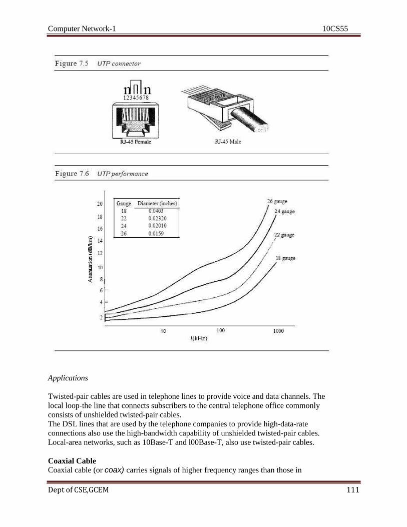
Computer Network-1 10CS55
Dept of CSE,GCEM 111
Applications
Twisted-pair cables are used in telephone lines to provide voice and data channels. The
local loop-the line that connects subscribers to the central telephone office commonly
consists of unshielded twisted-pair cables.
The DSL lines that are used by the telephone companies to provide high-data-rate
connections also use the high-bandwidth capability of unshielded twisted-pair cables.
Local-area networks, such as 10Base-T and l00Base-T, also use twisted-pair cables.
Coaxial Cable Coaxial cable (or coax) carries signals of higher frequency ranges than those in

Computer Network-1 10CS55
Dept of CSE,GCEM 112
Twistedpair cable, in part because the two media are constructed quite differently. Instead of
having two wires, coax has a central core conductor of solid or stranded wire (usually copper)
enclosed in an insulating sheath, which is, in turn, encased in an outer conductor
of metal foil, braid, or a combination of the two. The outer metallic wrapping serves both as a
shield against noise and as the second conductor, which completes the circuit. This outer
conductor is also enclosed in an insulating sheath, and the whole cable is protected by a plastic
cover (see Figure 7.7).
Coaxial Cable Standards
Coaxial cables are categorized by their radio government (RG) ratings. Each RG number
denotes a unique set of physical specifications, including the wire gauge of the inner conductor,
the thickness and type of the inner insulator, the construction of the shield, and the size and type
of the outer casing. Each cable defined by an RG rating is adapted for a specialized function, as
shown in Table 7.2.
Coaxial Cable Connectors
To connect coaxial cable to devices, we need coaxial connectors. The most common
type of connector used today is the Bayone-Neill-Concelman (BNe), connector.
Figure 7.8 shows three popular types of these connectors: the BNC connector, the
BNC T connector, and the BNC terminator.

Computer Network-1 10CS55
Dept of CSE,GCEM 113
The BNC connector is used to connect the end of the cable to a device, such as a TV set. The
BNC T connector is used in Ethernet networks (see Chapter 13) to branch out to a connection to
a computer or other device. The BNC terminator is used at the end of the cable to prevent the
reflection of the signal.
Performance
As we did with twisted-pair cables, we can measure the performance of a coaxial cable.
In Figure 7.9 that the attenuation is much higher in coaxial cables than in twisted-pair cable. In
other words, although coaxial cable has a much higher bandwidth, the signal weakens rapidly
and requires the frequent use of repeaters.
Applications
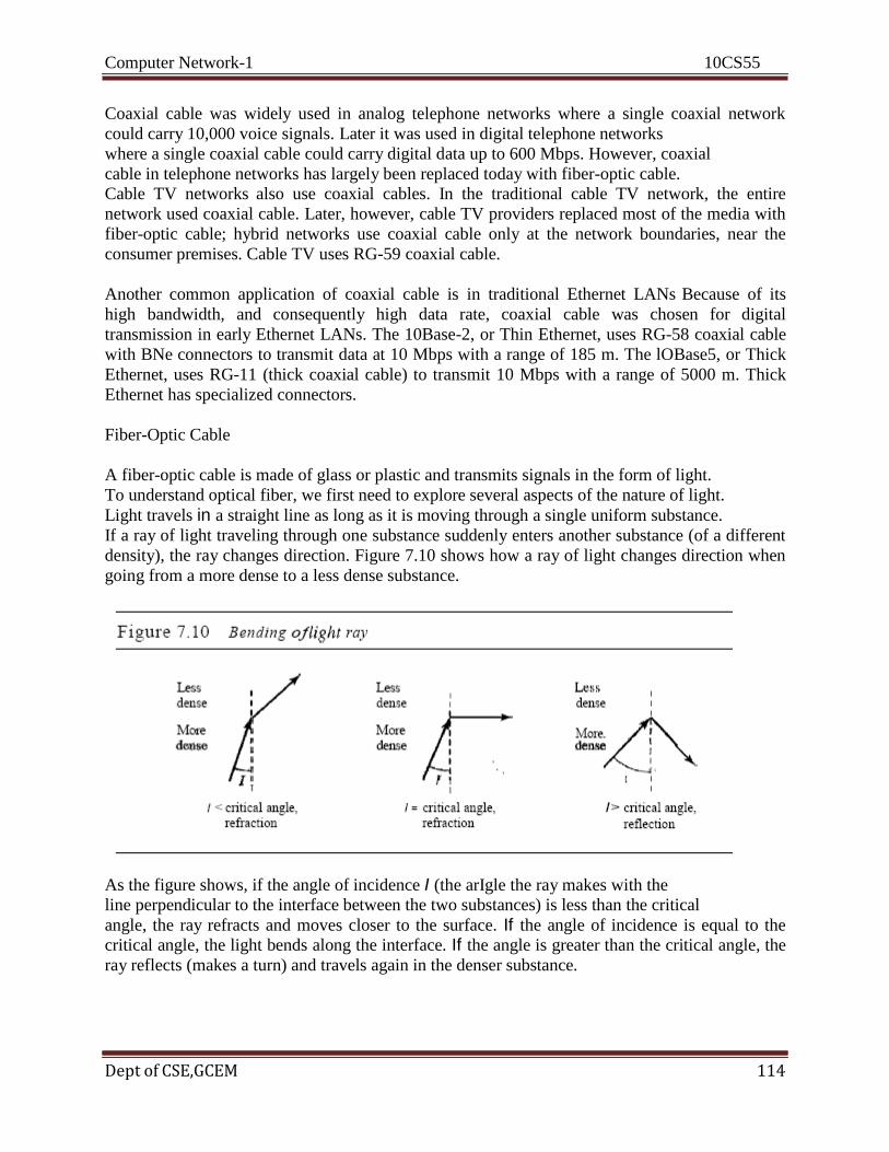
Computer Network-1 10CS55
Dept of CSE,GCEM 114
Coaxial cable was widely used in analog telephone networks where a single coaxial network
could carry 10,000 voice signals. Later it was used in digital telephone networks
where a single coaxial cable could carry digital data up to 600 Mbps. However, coaxial
cable in telephone networks has largely been replaced today with fiber-optic cable.
Cable TV networks also use coaxial cables. In the traditional cable TV network, the entire
network used coaxial cable. Later, however, cable TV providers replaced most of the media with
fiber-optic cable; hybrid networks use coaxial cable only at the network boundaries, near the
consumer premises. Cable TV uses RG-59 coaxial cable.
Another common application of coaxial cable is in traditional Ethernet LANs Because of its
high bandwidth, and consequently high data rate, coaxial cable was chosen for digital
transmission in early Ethernet LANs. The 10Base-2, or Thin Ethernet, uses RG-58 coaxial cable
with BNe connectors to transmit data at 10 Mbps with a range of 185 m. The lOBase5, or Thick
Ethernet, uses RG-11 (thick coaxial cable) to transmit 10 Mbps with a range of 5000 m. Thick
Ethernet has specialized connectors.
Fiber-Optic Cable
A fiber-optic cable is made of glass or plastic and transmits signals in the form of light.
To understand optical fiber, we first need to explore several aspects of the nature of light.
Light travels in a straight line as long as it is moving through a single uniform substance.
If a ray of light traveling through one substance suddenly enters another substance (of a different
density), the ray changes direction. Figure 7.10 shows how a ray of light changes direction when
going from a more dense to a less dense substance.
As the figure shows, if the angle of incidence I (the arIgle the ray makes with the
line perpendicular to the interface between the two substances) is less than the critical
angle, the ray refracts and moves closer to the surface. If the angle of incidence is equal to the
critical angle, the light bends along the interface. If the angle is greater than the critical angle, the
ray reflects (makes a turn) and travels again in the denser substance.

Computer Network-1 10CS55
Dept of CSE,GCEM 115
Optical fibers use reflection to guide light through a channel. A glass or plastic core is
surrounded by a cladding of less dense glass or plastic. The difference in density of the
two materials must be such that a beam of light moving through the core is reflected off
the cladding instead of being refracted into it. See Figure 7.11.
Propagation Modes
Current technology supports two modes (multimode and single mode) for propagating light
along optical channels, each requiring fiber with different physical characteristics. Multimode
can be implemented in two forms: step-index or graded-index (see Figure 7.12).
Multimode Multimode is so named because multiple beams from a light source move through
the core in different paths. How these beams move within the cable depends on the structure
ofthe core, as shown in Figure 7.13.
In multimode step-index fiber, the density of the core remains constant from the center to the
edges. A beam of light moves through this constant density in a straight line until it reaches the
interface of the core and the cladding. At the interface, there is an abrupt change due to a lower
density; this alters the angle of the beam's motion. The term step index refers to the suddenness
of this change, which contributes to the distortion of the signal as it passes through the fiber.
A second type of fiber, called multimode graded-index fiber, decreases this distortion of the
signal through the cable. The word index here refers to the index of refraction. As we saw above,
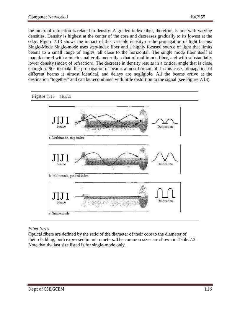
Computer Network-1 10CS55
Dept of CSE,GCEM 116
the index of refraction is related to density. A graded-index fiber, therefore, is one with varying
densities. Density is highest at the center of the core and decreases gradually to its lowest at the
edge. Figure 7.13 shows the impact of this variable density on the propagation of light beams.
Single-Mode Single-mode uses step-index fiber and a highly focused source of light that limits
beams to a small range of angles, all close to the horizontal. The single mode fiber itself is
manufactured with a much smaller diameter than that of multimode fiber, and with substantially
lower density (index of refraction). The decrease in density results in a critical angle that is close
enough to 90° to make the propagation of beams almost horizontal. In this case, propagation of
different beams is almost identical, and delays are negligible. All the beams arrive at the
destination "together" and can be recombined with little distortion to the signal (see Figure 7.13).
Fiber Sizes
Optical fibers are defined by the ratio of the diameter of their core to the diameter of
their cladding, both expressed in micrometers. The common sizes are shown in Table 7.3.
Note that the last size listed is for single-mode only.
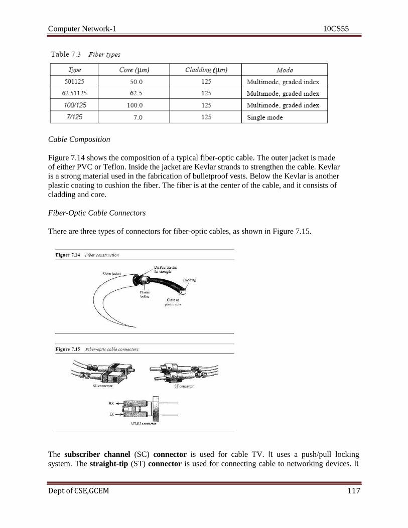
Computer Network-1 10CS55
Dept of CSE,GCEM 117
Cable Composition
Figure 7.14 shows the composition of a typical fiber-optic cable. The outer jacket is made
of either PVC or Teflon. Inside the jacket are Kevlar strands to strengthen the cable. Kevlar
is a strong material used in the fabrication of bulletproof vests. Below the Kevlar is another
plastic coating to cushion the fiber. The fiber is at the center of the cable, and it consists of
cladding and core.
Fiber-Optic Cable Connectors
There are three types of connectors for fiber-optic cables, as shown in Figure 7.15.
The subscriber channel (SC) connector is used for cable TV. It uses a push/pull locking
system. The straight-tip (ST) connector is used for connecting cable to networking devices. It

Computer Network-1 10CS55
Dept of CSE,GCEM 118
uses a bayonet locking system and is more reliable than SC. MT-RJ is a connector that is the
same size as RJ45.
Performance
The plot of attenuation versus wavelength in Figure 7.16 shows a very interesting phenomenon
in fiber-optic cable. Attenuation is flatter than in the case of twisted-pair cable and coaxial cable.
The performance is such that we need fewer (actually 10 times less) repeaters when we use fiber-
optic cable.
Applications
Fiber-optic cable is often found in backbone networks because its wide bandwidth is cost-
effective. Today, with wavelength-division multiplexing (WDM), we can transfer
data at a rate of 1600 Gbps. The SONET network that we discuss in Chapter 17 provides such a
backbone. Some cable TV companies use a combination of optical fiber and coaxial cable, thus
creating a hybrid network. Optical fiber provides the backbone structure while coaxial cable
provides the connection to the user premises. This is a cost-effective configuration since the
narrow bandwidth requirement at the user end does not justify the use of optical fiber. Local-area
networks such as 100Base-FX network (Fast Ethernet) and 1000Base-X also use fiber-optic
cable.
Advantages and Disadvantages of Optical Fiber
Advantages Fiber-optic cable has several advantages over metallic cable (twistedpair or coaxial).
1. Higher bandwidth. Fiber-optic cable can support dramatically higher bandwidths (and hence
data rates) than either twisted-pair or coaxial cable. Currently, data rates and bandwidth
utilization over fiber-optic cable are limited not by the medium but by the signal generation and
reception technology available.
2. Less signal attenuation. Fiber-optic transmission distance is significantly greater than that of
other guided media. A signal can run for 50 km without requiring regeneration.
3. Immunity to electromagnetic interference. Electromagnetic noise cannot affect fiber-optic
cables.

Computer Network-1 10CS55
Dept of CSE,GCEM 119
4. Resistance to corrosive materials. Glass is more resistant to corrosive materials than copper.
6.Light weight. Fiber-optic cables are much lighter than copper cables. 7. Greater immunity to tapping. Fiber-optic cables are more immune to tapping than copper
cables. Copper cables create antenna effects that can easily be tapped. Disadvantages There are
some disadvantages in the use of optical fiber.
8. Installation and maintenance. Fiber-optic cable is a relatively new technology. Its installation
and maintenance require expertise that is not yet available everywhere.
9. Unidirectional light propagation. Propagation of light is unidirectional. If we need
bidirectional communication, two fibers are needed.
10. Cost. The cable and the interfaces are relatively more expensive than those of other guided
media. If the demand for bandwidth is not high, often the use of optical fiber
cannot be justified.
7.2 UNGUIDED MEDIA: WIRELESS
Unguided media transport electromagnetic waves without using a physical conductor. This type
of communication is often referred to as wireless communication. Signals are normally broadcast
through free space and thus are available to anyone who has a device capable of receiving them.
Figure 7.17 shows the part of the electromagnetic spectrum, ranging from 3 kHz to 900 THz,
used for wireless communication.
Unguided signals can travel from the source to destination in several ways: ground
propagation, sky propagation, and line-of-sight propagation, as shown in Figure 7.18.
In ground propagation, radio waves travel through the lowest portion of the atmosphere, hugging
the earth. These low-frequency signals emanate in all directions from the transmitting antenna
and follow the curvature of the planet. Distance depends on the amount of power in the signal:
The greater the power, the greater the distance. In sky propagation, higher-frequency radio waves
radiate upward into the ionosphere (the layer of atmosphere where particles exist as ions) where
they are reflected back to earth. This type of transmission allows for greater distances with lower
output power. In line-or-sight propagation, very high-frequency signals are transmitted in
straight lines directly from antenna to antenna. Antennas must be directional, facing each other,

Computer Network-1 10CS55
Dept of CSE,GCEM 120
and either tall enough or close enough together not to be affected by the curvature of the earth.
Line-of-sight propagation is tricky because radio transmissions cannot be completely focused.
The section of the electromagnetic spectrum defined as radio waves and microwaves
is divided into eight ranges, called bands, each regulated by government authorities.
These bands are rated from very low frequency (VLF) to extremely highfrequency (EHF).
Table 7.4 lists these bands, their ranges, propagation methods, and some applications.
We can divide wireless transmission into three broad groups: radio waves, microwaves,
and infrared waves. See Figure 7.19.
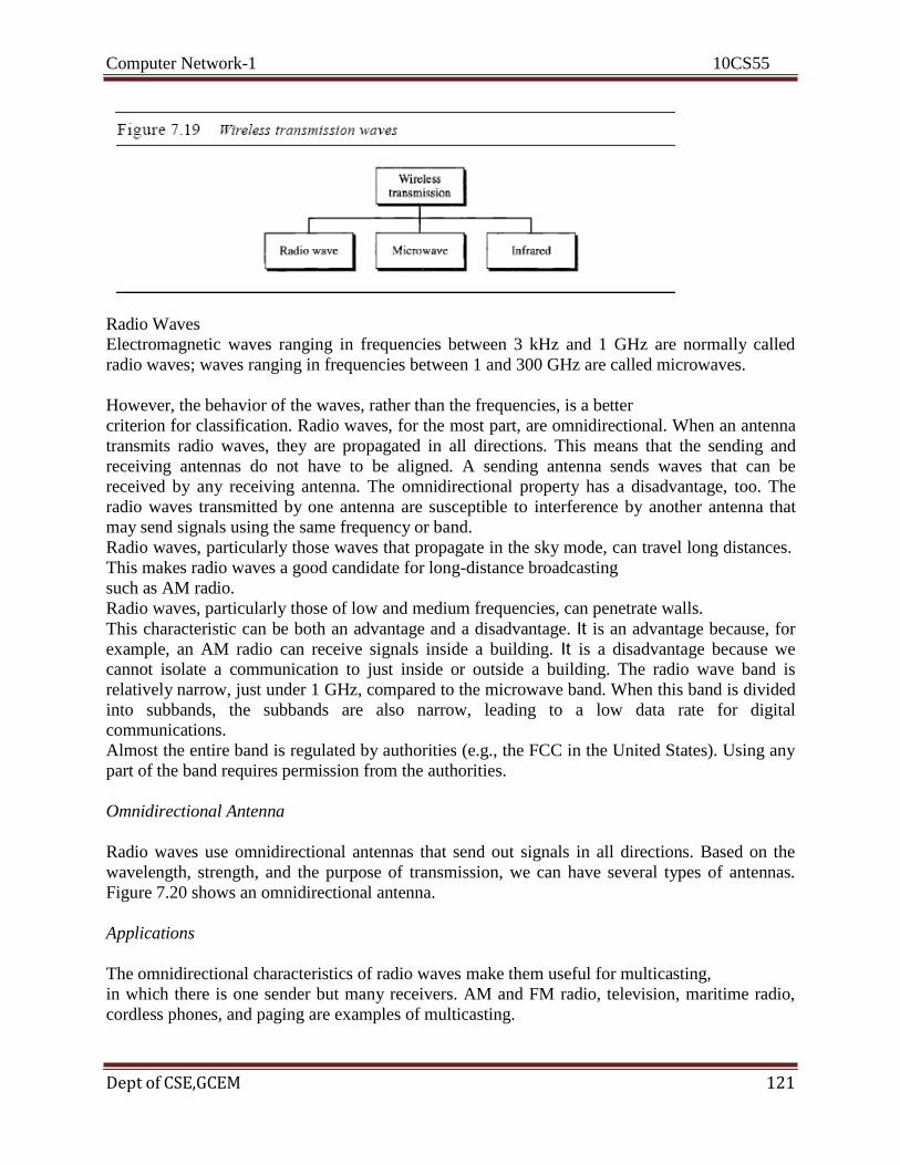
Computer Network-1 10CS55
Dept of CSE,GCEM 121
Radio Waves
Electromagnetic waves ranging in frequencies between 3 kHz and 1 GHz are normally called
radio waves; waves ranging in frequencies between 1 and 300 GHz are called microwaves.
However, the behavior of the waves, rather than the frequencies, is a better
criterion for classification. Radio waves, for the most part, are omnidirectional. When an antenna
transmits radio waves, they are propagated in all directions. This means that the sending and
receiving antennas do not have to be aligned. A sending antenna sends waves that can be
received by any receiving antenna. The omnidirectional property has a disadvantage, too. The
radio waves transmitted by one antenna are susceptible to interference by another antenna that
may send signals using the same frequency or band.
Radio waves, particularly those waves that propagate in the sky mode, can travel long distances.
This makes radio waves a good candidate for long-distance broadcasting
such as AM radio.
Radio waves, particularly those of low and medium frequencies, can penetrate walls.
This characteristic can be both an advantage and a disadvantage. It is an advantage because, for
example, an AM radio can receive signals inside a building. It is a disadvantage because we
cannot isolate a communication to just inside or outside a building. The radio wave band is
relatively narrow, just under 1 GHz, compared to the microwave band. When this band is divided
into subbands, the subbands are also narrow, leading to a low data rate for digital
communications.
Almost the entire band is regulated by authorities (e.g., the FCC in the United States). Using any
part of the band requires permission from the authorities.
Omnidirectional Antenna
Radio waves use omnidirectional antennas that send out signals in all directions. Based on the
wavelength, strength, and the purpose of transmission, we can have several types of antennas.
Figure 7.20 shows an omnidirectional antenna.
Applications
The omnidirectional characteristics of radio waves make them useful for multicasting,
in which there is one sender but many receivers. AM and FM radio, television, maritime radio,
cordless phones, and paging are examples of multicasting.

Computer Network-1 10CS55
Dept of CSE,GCEM 122
Microwaves
Electromagnetic waves having frequencies between I and 300 GHz are called microwaves.
Microwaves are unidirectional. When an antenna transmits microwave waves, they can be
narrowly focused. This means that the sending and receiving antennas need to be aligned. The
unidirectional property has an obvious advantage. A pair of antennas can be aligned without
interfering with another pair of aligned antennas. The following describes some characteristics of
microwave propagation:
1. Microwave propagation is line-of-sight. Since the towers with the mounted antennas need to
be in direct sight of each other, towers that are far apart need to be very tall. The curvature of the
earth as well as other blocking obstacles do not allow two short towers to communicate by using
microwaves. Repeaters are often needed for long distance communication.
2.Very high-frequency microwaves cannot penetrate walls. This characteristic can be a
disadvantage if receivers are inside buildings.
3.The microwave band is relatively wide, almost 299 GHz. Therefore wider subbands can be
assigned, and a high data rate is possible
4.Use of certain portions of the band requires permission from authorities.
Unidirectional Antenna
Microwaves need unidirectional antennas that send out signals in one direction. Two types of
antennas are used for microwave communications: the parabolic dish and the hom (see Figure
7.21). A parabolic dish antenna is based on the geometry of a parabola: Every line parallel to the
line of symmetry (line of sight) reflects off the curve at angles such that all the lines intersect in a
common point called the focus. The parabolic dish works as a
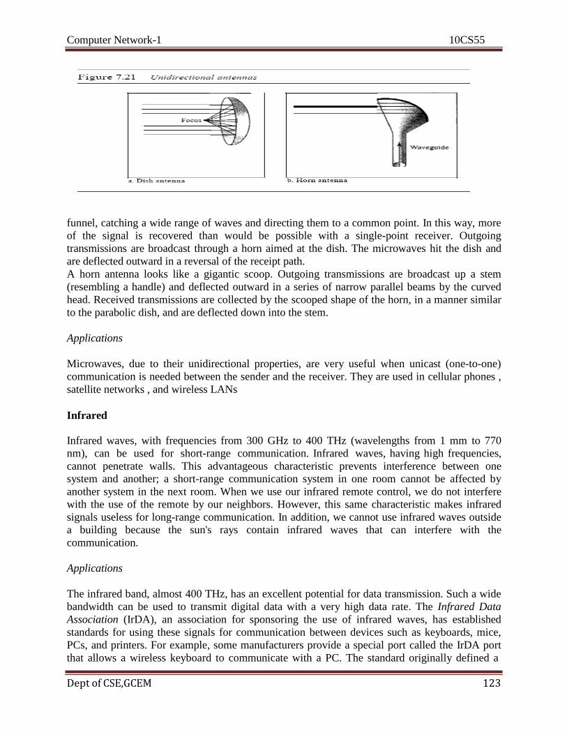
Computer Network-1 10CS55
Dept of CSE,GCEM 123
funnel, catching a wide range of waves and directing them to a common point. In this way, more
of the signal is recovered than would be possible with a single-point receiver. Outgoing
transmissions are broadcast through a horn aimed at the dish. The microwaves hit the dish and
are deflected outward in a reversal of the receipt path.
A horn antenna looks like a gigantic scoop. Outgoing transmissions are broadcast up a stem
(resembling a handle) and deflected outward in a series of narrow parallel beams by the curved
head. Received transmissions are collected by the scooped shape of the horn, in a manner similar
to the parabolic dish, and are deflected down into the stem.
Applications
Microwaves, due to their unidirectional properties, are very useful when unicast (one-to-one)
communication is needed between the sender and the receiver. They are used in cellular phones ,
satellite networks , and wireless LANs
Infrared
Infrared waves, with frequencies from 300 GHz to 400 THz (wavelengths from 1 mm to 770
nm), can be used for short-range communication. Infrared waves, having high frequencies,
cannot penetrate walls. This advantageous characteristic prevents interference between one
system and another; a short-range communication system in one room cannot be affected by
another system in the next room. When we use our infrared remote control, we do not interfere
with the use of the remote by our neighbors. However, this same characteristic makes infrared
signals useless for long-range communication. In addition, we cannot use infrared waves outside
a building because the sun's rays contain infrared waves that can interfere with the
communication.
Applications
The infrared band, almost 400 THz, has an excellent potential for data transmission. Such a wide
bandwidth can be used to transmit digital data with a very high data rate. The Infrared Data
Association (IrDA), an association for sponsoring the use of infrared waves, has established
standards for using these signals for communication between devices such as keyboards, mice,
PCs, and printers. For example, some manufacturers provide a special port called the IrDA port
that allows a wireless keyboard to communicate with a PC. The standard originally defined a

Computer Network-1 10CS55
Dept of CSE,GCEM 124
data rate of 75 kbps for a distance up to 8 m. The recent standard defines a data rate of 4 Mbps.
Infrared signals defined by IrDA transmit through line of sight; the IrDA port on the keyboard
needs to point to the PC for transmission to occur.
Error Detection and Correction
10.1 INTRODUCTION
Types of Errors Whenever bits flow from one point to another, they are subject to unpredictable changes because
of interference. This interference can change the shape of the signal. In a single-bit error, a 0 is
changed to a 1 or a 1 to a O. In a burst error, multiple bits are changed. For example, a 11100 s
burst of impulse noise on a transmission with a data rate of 1200 bps might change all or some of
the12 bits of information.
Single-Bit Error
The term single-bit error means that only 1 bit of a given data unit (such as a byte, character, or
packet) is changed from 1 to 0 or from 0 to 1. Figure 10.1 shows the effect of a single-bit error
on a data unit. To understand the impact of the change, imagine that each group of 8 bits is an
ASCII character with a 0 bit added to the left. In Figure 10.1,00000010 (ASCII STX) was sent,
meaning start of text, but 00001010 (ASCII LF) was received, meaning line feed.
Single-bit errors are the least likely type of error in serial data transmission. To understand why,
imagine data sent at 1 Mbps. This means that each bit lasts only 1/1,000,000 s, or 1 )ls. For a
single-bit error to occur, the noise must have a duration of only 1 )ls, which is very rare; noise
normally lasts much longer than this.
Burst Error
The term burst error means that 2 or more bits in the data unit have changed from 1 to 0 or from
0 to 1. Figure 10.2 shows the effect of a burst error on a data unit. In this case,
0100010001000011 was sent, but 0101110101100011 was received. Note that a burst error does
not necessarily mean that the errors occur in consecutive bits. The length of the burst is measured
from the first corrupted bit to the last corrupted bit. Some bits in between may not have been
corrupted.

Computer Network-1 10CS55
Dept of CSE,GCEM 125
A burst error is more likely to occur than a single-bit error. The duration of noise is normally
longer than the duration of 1 bit, which means that when noise affects data, it affects a set of bits.
The number of bits affected depends on the data rate and duration of noise. For example, if we
are sending data at I kbps, a noise of 11100 s can affect 10 bits; if we are sending data at I Mbps,
the same noise can affect 10,000 bits.
Redundancy
The central concept in detecting or correcting errors is redundancy. To be able to detect or
correct errors, we need to send some extra bits with our data. These redundant bits are added by
the sender and removed by the receiver. Their presence allows the receiver to detect or correct
corrupted bits.
Detection Versus Correction
The correction of errors is more difficult than the detection. In error detection, we are looking
only to see if any error has occurred. The answer is a simple yes or no. We are not even
interested in the number of errors. A single-bit error is the same for us as a burst error.
In error correction, we need to know the exact number of bits that are corrupted and more
importantly, their location in the message. The number of the errors and the size of the message
are important factors. If we need to correct one single error in an 8-bit data unit, we need to
consider eight possible error locations; if we need to correct two errors in a data unit of the same
size, we need to consider 28 possibilities. You can imagine the receiver's difficulty in finding 10
errors in a data unit of 1000 bits.
Forward Error Correction Versus Retransmission
There are two main methods of error correction. Forward error correction is the process in which
the receiver tries to guess the message by using redundant bits. This is possible, as we see later,
if the number of errors is small. Correction by retransmission is a technique in which the receiver
detects the occurrence of an error and asks the sender to resend the message. Resending is
repeated until a message arrives that the receiver believes is error-free
Coding
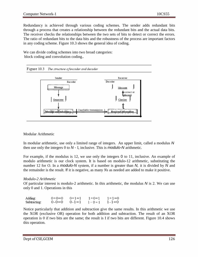
Computer Network-1 10CS55
Dept of CSE,GCEM 126
Redundancy is achieved through various coding schemes. The sender adds redundant bits
through a process that creates a relationship between the redundant bits and the actual data bits.
The receiver checks the relationships between the two sets of bits to detect or correct the errors.
The ratio of redundant bits to the data bits and the robustness of the process are important factors
in any coding scheme. Figure 10.3 shows the general idea of coding.
We can divide coding schemes into two broad categories:
block coding and convolution coding..
Modular Arithmetic
In modular arithmetic, use only a limited range of integers. An upper limit, called a modulus N then use only the integers 0 to N - I, inclusive. This is modulo-N arithmetic.
For example, if the modulus is 12, we use only the integers 0 to 11, inclusive. An example of
modulo arithmetic is our clock system. It is based on modulo-12 arithmetic, substituting the
number 12 for O. In a modulo-N system, if a number is greater than N, it is divided by N and
the remainder is the result. If it is negative, as many Ns as needed are added to make it positive.
Modulo-2 Arithmetic
Of particular interest is modulo-2 arithmetic. In this arithmetic, the modulus N is 2. We can use
only 0 and 1. Operations in this
Notice particularly that addition and subtraction give the same results. In this arithmetic we use
the XOR (exclusive OR) operation for both addition and subtraction. The result of an XOR
operation is 0 if two bits are the same; the result is I if two bits are different. Figure 10.4 shows
this operation.

Computer Network-1 10CS55
Dept of CSE,GCEM 127
10.2 BLOCK CODING
In block coding, we divide our message into blocks, each of k bits, called datawords. We add r
redundant bits to each block to make the length n = k + r. The resulting n-bit blocks are called
codewords. How the extra r bits is chosen or calculated is something we will discuss later. For
the moment, it is important to know that we have a set of datawords, each of size k, and a set of
codewords, each of size of n. With k bits, we can create a combination of 2k datawords; with n
bits, we can create a combination of 2n codewords. Since n > k, the number of possible
codewords is larger than the number of possible datawords.
The block coding process is one-to-one; the same dataword is always encoded as the same
codeword. This means that we have 2n - 2k codewords that are not used. We call these
codewords invalid or illegal. Figure 10.5 shows the situation.
Error Detection How can errors be detected by using block coding? If the following two conditions are met, the
receiver can detect a change in the original codeword.
1. The receiver has (or can find) a list of valid codewords.
2. The original codeword has changed to an invalid one.
Figure 10.6 shows the role of block coding in error detection.

Computer Network-1 10CS55
Dept of CSE,GCEM 128
The sender creates codewords out of datawords by using a generator that applies the rules and
procedures of encoding (discussed later). Each codeword sent to the receiver may change during
transmission. If the received codeword is the same as one of the valid codewords, the word is
accepted; the corresponding dataword is extracted for use. If the received codeword is not valid,
it is discarded. However, if the codeword is corrupted during transmission but the received word
still matches a valid codeword, the error remains undetected. This type of coding can detect only
single errors. Two or more errors may remain undetected.
Assume the sender encodes the dataword 01 as 011 and sends it to the receiver. Consider the
following cases:
1. The receiver receives 01l. It is a valid codeword. The receiver extracts the dataword 01 from
it. 2. The codeword is corrupted during transmission, and 111 is received (the leftmost bit is
corrupted).
This is not a valid codeword and is discarded.
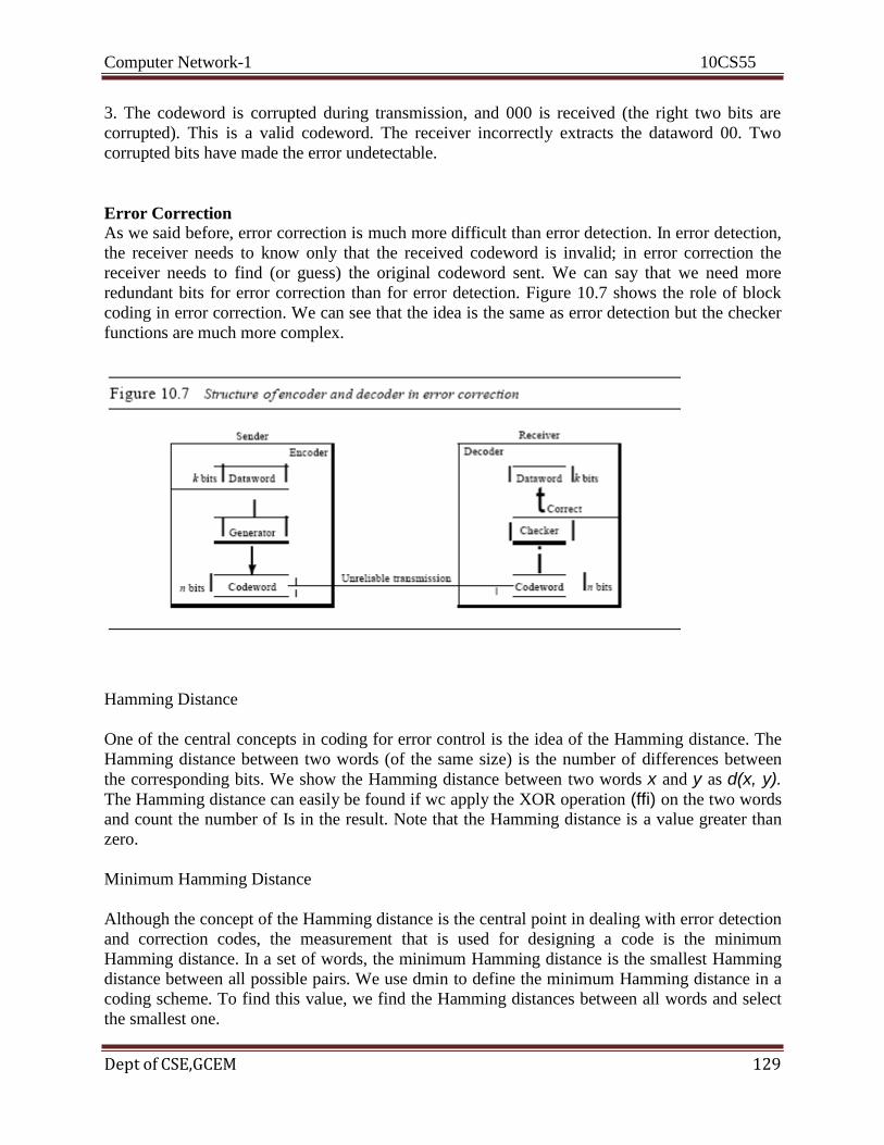
Computer Network-1 10CS55
Dept of CSE,GCEM 129
3. The codeword is corrupted during transmission, and 000 is received (the right two bits are
corrupted). This is a valid codeword. The receiver incorrectly extracts the dataword 00. Two
corrupted bits have made the error undetectable.
Error Correction As we said before, error correction is much more difficult than error detection. In error detection,
the receiver needs to know only that the received codeword is invalid; in error correction the
receiver needs to find (or guess) the original codeword sent. We can say that we need more
redundant bits for error correction than for error detection. Figure 10.7 shows the role of block
coding in error correction. We can see that the idea is the same as error detection but the checker
functions are much more complex.
Hamming Distance
One of the central concepts in coding for error control is the idea of the Hamming distance. The
Hamming distance between two words (of the same size) is the number of differences between
the corresponding bits. We show the Hamming distance between two words x and y as d(x, y). The Hamming distance can easily be found if wc apply the XOR operation (ffi) on the two words
and count the number of Is in the result. Note that the Hamming distance is a value greater than
zero.
Minimum Hamming Distance
Although the concept of the Hamming distance is the central point in dealing with error detection
and correction codes, the measurement that is used for designing a code is the minimum
Hamming distance. In a set of words, the minimum Hamming distance is the smallest Hamming
distance between all possible pairs. We use dmin to define the minimum Hamming distance in a
coding scheme. To find this value, we find the Hamming distances between all words and select
the smallest one.

Computer Network-1 10CS55
Dept of CSE,GCEM 130
Three Parameters
Before we continue with our discussion, we need to mention that any coding scheme needs to
have at least three parameters: the codeword size n, the dataword size k, and the minimum
Hamming distance dmin. A coding scheme C is written as C(n, k) with a separate expression for
dmin- For example, we can call our first coding scheme C(3, 2) with dmin =2 and our second
coding scheme C(5, 2) with dmin ::= 3.
Hamming Distance and Error
Before we explore the criteria for error detection or correction, let us discuss the relationship
between the Hamming distance and errors occurring during transmission. When a codeword is
corrupted during transmission, the Hamming distance between the sent and received codewords
is the number of bits affected by the error. In other words, the Hamming distance between the
received codeword and the sent codeword is the number ofbits that are corrupted during
transmission. For example, if the codeword 00000 is sent and 01101 is received, 3 bits are in
error and the Hamming distance between the two is d(OOOOO, 01101) =3.
Minimum Distance for Error Detection
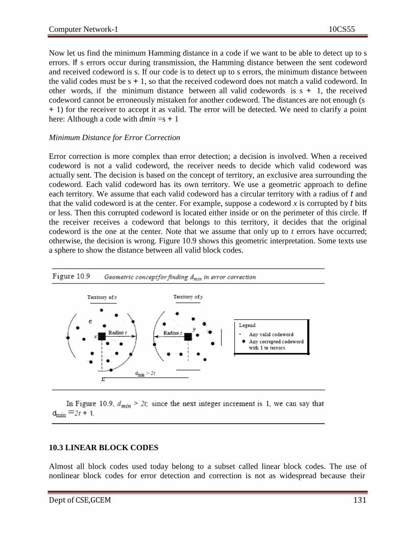
Computer Network-1 10CS55
Dept of CSE,GCEM 131
Now let us find the minimum Hamming distance in a code if we want to be able to detect up to s
errors. If s errors occur during transmission, the Hamming distance between the sent codeword
and received codeword is s. If our code is to detect up to s errors, the minimum distance between
the valid codes must be s + 1, so that the received codeword does not match a valid codeword. In
other words, if the minimum distance between all valid codewords is s + 1, the received
codeword cannot be erroneously mistaken for another codeword. The distances are not enough (s
+ 1) for the receiver to accept it as valid. The error will be detected. We need to clarify a point
here: Although a code with dmin =s + 1
Minimum Distance for Error Correction
Error correction is more complex than error detection; a decision is involved. When a received
codeword is not a valid codeword, the receiver needs to decide which valid codeword was
actually sent. The decision is based on the concept of territory, an exclusive area surrounding the
codeword. Each valid codeword has its own territory. We use a geometric approach to define
each territory. We assume that each valid codeword has a circular territory with a radius of t and
that the valid codeword is at the center. For example, suppose a codeword x is corrupted by t bits
or less. Then this corrupted codeword is located either inside or on the perimeter of this circle. If the receiver receives a codeword that belongs to this territory, it decides that the original
codeword is the one at the center. Note that we assume that only up to t errors have occurred;
otherwise, the decision is wrong. Figure 10.9 shows this geometric interpretation. Some texts use
a sphere to show the distance between all valid block codes.
10.3 LINEAR BLOCK CODES
Almost all block codes used today belong to a subset called linear block codes. The use of
nonlinear block codes for error detection and correction is not as widespread because their

Computer Network-1 10CS55
Dept of CSE,GCEM 132
structure makes theoretical analysis and implementation difficult. We therefore concentrate on
linear block codes. The formal definition of linear block codes requires the knowledge of
abstract algebra (particularly Galois fields), which is beyond the scope of this book. We therefore
give an informal definition. For our purposes, a linear block code is a code in which the
exclusive OR (addition modulo-2) of two valid codewords creates another valid codeword.
Minimum Distance for Linear Block Codes
It is simple to find the minimum Hamming distance for a linear block code. The minimum
Hamming distance is the number of Is in the nonzero valid codeword with the smallest number
of 1s.
Some Linear Block Codes
Let us now show some linear block codes. These codes are trivial because we can easily find the
encoding and decoding algorithms and check their performances.
Simple Parity-Check Code
Perhaps the most familiar error-detecting code is the simple parity-check code. In this code, a k- bit dataword is changed to an n-bit codeword where n = k + 1. The extra bit, called the parity bit,
is selected to make the total number of Is in the codeword even. Although some implementations
specify an odd number of Is, we discuss the even case. The minimum Hamming distance for this
category is dmin =2, which means that the code is a single-bit error-detecting code; it cannot
correct any error.
Our first code (Table 10.1) is a parity-check code with k -= 2 and n =3. The code in Table 10.3 is
also a parity-check code with k =4 and n =5.
Figure 10.10 shows a possible structure of an encoder (at the sender) and a decoder (at the
receiver).
The encoder uses a generator that takes a copy of a 4-bit dataword (ao, aI' a2' and a3) and
generates a parity bit roo The dataword bits and the parity bit create the 5-bit codeword. The
parity bit that is added makes the number of Is in the codeword even.

Computer Network-1 10CS55
Dept of CSE,GCEM 133
This is normally done by adding the 4 bits of the dataword (modulo-2); the result is the parity bit.
In other words,
If the number of 1s is even, the result is 0; if the number of 1s is odd, the result is 1. In both
cases, the total number of 1s in the codeword is even. The sender sends the codeword which may
be corrupted during transmission. The receiver receives a 5-bit word. The checker at the receiver
does the same thing as the generator in the sender with one exception: The addition is done over
all 5 bits. The result, which is called the syndrome, is just 1 bit. The syndrome is 0 when the
number of 1s in the received codeword is even; otherwise, it is 1.

Computer Network-1 10CS55
Dept of CSE,GCEM 134
The syndrome is passed to the decision logic analyzer. If the syndrome is 0, there is no error in
the received codeword; the data portion of the received codeword is accepted as the dataword; if
the syndrome is 1, the data portion of the received codeword is discarded. The dataword is not
created.
Example 10.12
Let us look at some transmission scenarios. Assume the sender sends the dataword 1011. The
codeword created from this dataword is 10111, which is sent to the receiver. We examine five
cases:
1. No error occurs; the received codeword is 10111. The syndrome is O. The dataword 1011 is
created.
2. One single-bit error changes aI' The received codeword is 10011. The syndrome is 1. No
dataword
is created.
3. One single-bit error changes roo The received codeword is 10110. The syndrome is 1. No
dataword
is created. Note that although none of the dataword bits are corrupted, no dataword is created
because the code is not sophisticated enough to show the position of the corrupted bit.
4. An error changes ro and a second error changes a3' The received codeword is 00110. The
syndrome is 0. The dataword 0011 is created at the receiver. Note that here the dataword is
wrongly created due to the syndrome value. The simple parity-check decoder cannot detect an even
number
of errors. The errors cancel each other out and give the syndrome a value of O.
5. Three bits-a3, az, and aI-are changed by errors. The received codeword is 01011. The
syndrome is
1. The dataword is not created. This shows that the simple parity check, guaranteed to detect
one
single error, can also find any odd number of errors.
A better approach is the two-dimensional parity check. In this method, the dataword is organized
in a table (rows and columns). In Figure 10.11, the data to be sent, five 7-bit bytes, are put in
separate rows. For each row and each column, 1 parity-check bit is calculated. The whole table is
then sent to the receiver, which finds the syndrome for each row and each column. As Figure
10.11 shows, the two-dimensional parity check can
detect up to three errors that occur anywhere in the table (arrows point to the locations of the
created nonzero syndromes). However, errors affecting 4 bits may not be detected.
Hamming Codes
Now let us discuss a category of error-correcting codes called Hamming codes. These codes
were originally designed with dmin = 3, which means that they can detect up to two errors or
correct one single error. Although there are some Hamming codes that can correct more than one
error, our discussion focuses on the single-bit error-correcting code.
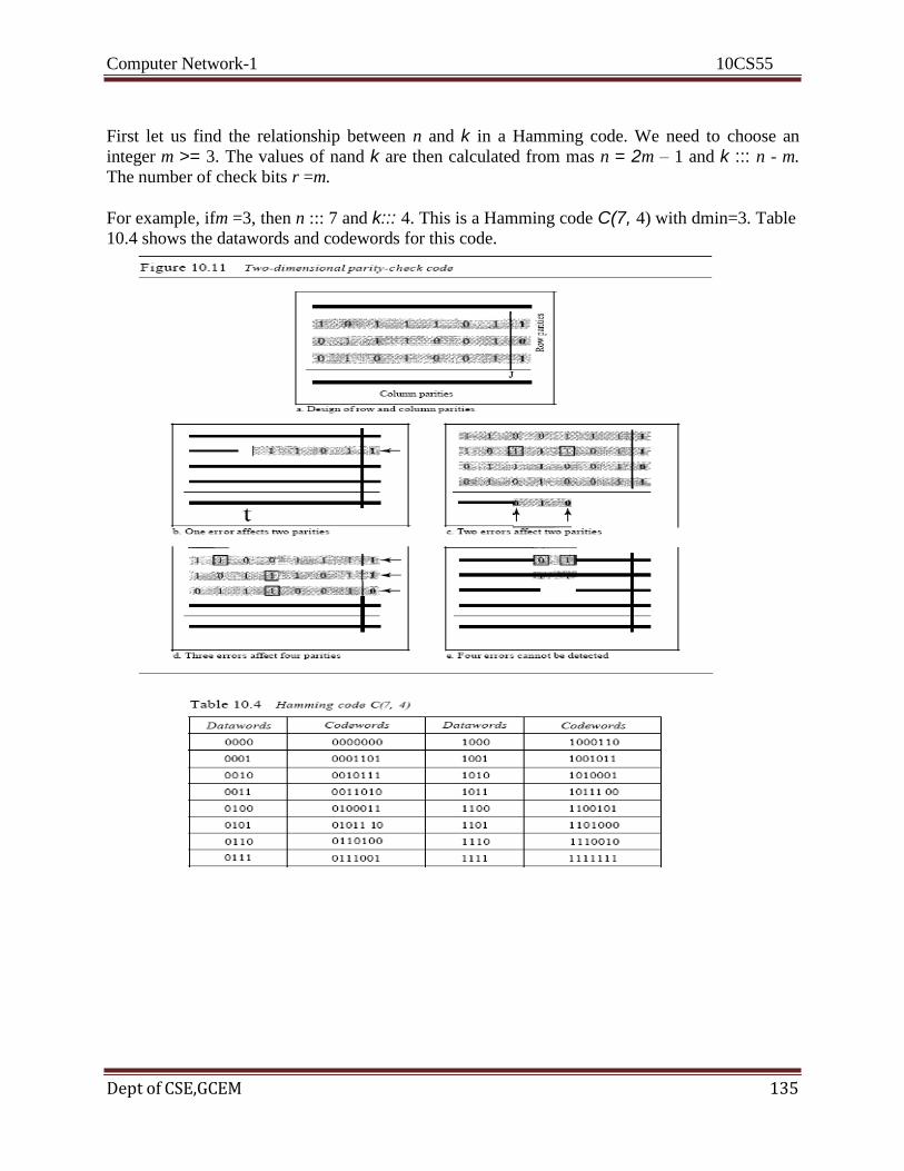
Computer Network-1 10CS55
Dept of CSE,GCEM 135
First let us find the relationship between n and k in a Hamming code. We need to choose an
integer m >= 3. The values of nand k are then calculated from mas n = 2m – 1 and k ::: n - m.
The number of check bits r =m.
For example, ifm =3, then n ::: 7 and k::: 4. This is a Hamming code C(7, 4) with dmin=3. Table
10.4 shows the datawords and codewords for this code.

Computer Network-1 10CS55
Dept of CSE,GCEM 136
A copy of a 4-bit dataword is fed into the generator that creates three parity checks r0, r1' and r2' as shown below:
In other words, each of the parity-check bits handles 3 out of the 4 bits of the dataword. The total
number of 1s in each 4-bit combination (3 dataword bits and 1 parity bit) must be even. We are
not saying that these three equations are unique; any three equations that involve 3 of the 4 bits
in the dataword and create independent equations (a combination of two cannot create the third)
are valid.
The checker in the decoder creates a 3-bit syndrome (s2s1s0) in which each bit is the parity
check for 4 out of the 7 bits in the received codeword:
The equations used by the checker are the same as those used by the generator with the parity-
check bits added to the right-hand side of the equation. The 3-bit syndrome creates eight
different bit patterns (000 to 111) that can represent eight different conditions. These conditions
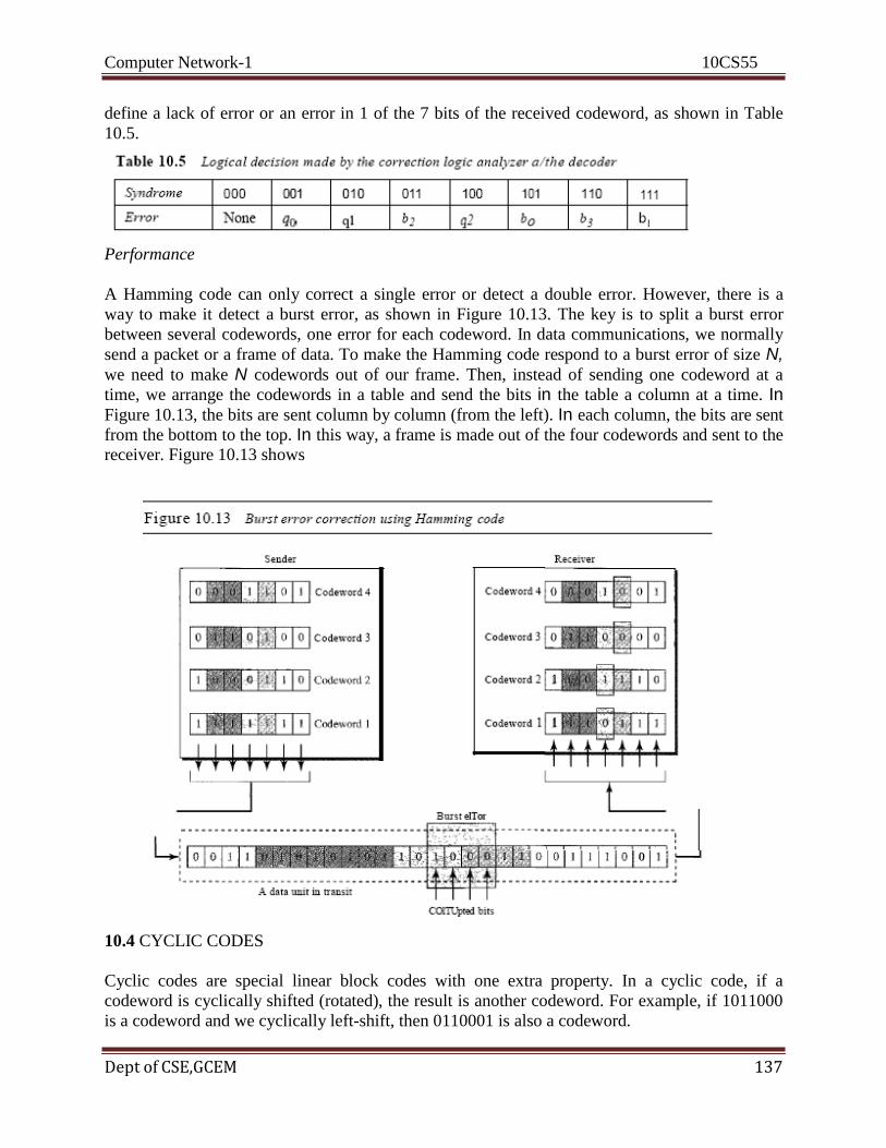
Computer Network-1 10CS55
Dept of CSE,GCEM 137
define a lack of error or an error in 1 of the 7 bits of the received codeword, as shown in Table
10.5.
Performance
A Hamming code can only correct a single error or detect a double error. However, there is a
way to make it detect a burst error, as shown in Figure 10.13. The key is to split a burst error
between several codewords, one error for each codeword. In data communications, we normally
send a packet or a frame of data. To make the Hamming code respond to a burst error of size N, we need to make N codewords out of our frame. Then, instead of sending one codeword at a
time, we arrange the codewords in a table and send the bits in the table a column at a time. In Figure 10.13, the bits are sent column by column (from the left). In each column, the bits are sent
from the bottom to the top. In this way, a frame is made out of the four codewords and sent to the
receiver. Figure 10.13 shows
10.4 CYCLIC CODES
Cyclic codes are special linear block codes with one extra property. In a cyclic code, if a
codeword is cyclically shifted (rotated), the result is another codeword. For example, if 1011000
is a codeword and we cyclically left-shift, then 0110001 is also a codeword.

Computer Network-1 10CS55
Dept of CSE,GCEM 138
In this case, if we call the bits in the first word ao to a6' and the bits in the second word
B0 to b6, we can shift the bits by using the following:
In the rightmost equation, the last bit of the first word is wrapped around and becomes the first
bit of the second word.
Cyclic Redundancy Check
We can create cyclic codes to correct errors. However, the theoretical background required is
beyond the scope of this book. In this section, we simply discuss a category of cyclic codes
called the cyclic redundancy check (CRC) that is used in networks such as LANs and WANs

Computer Network-1 10CS55
Dept of CSE,GCEM 139
In the encoder, the dataword has k bits (4 here); the codeword has n bits. The size of the
dataword is augmented by adding n - k (3 here) Os to the right-hand side of the word. The n-bit
result is fed into the generator. The generator uses a divisor of size n - k + I (4 here), predefined
and agreed upon. The generator divides the augmented dataword by the divisor (modulo-2
division). The quotient of the division is discarded; the remainder (r2 rl r0) is appended to the
dataword to create the codeword. The decoder receives the possibly corrupted codeword. A copy
of all n bits is fed to the checker which is a replica of the generator. The remainder produced by
the checker is a syndrome of n - k (3 here) bits, which is fed to the decision logic analyzer. The
analyzer has a simple function. If the syndrome bits are all as, the 4 leftmost bits of the codeword
are accepted as the dataword (interpreted as no error); otherwise, the 4 bits are discarded (error).
Encoder
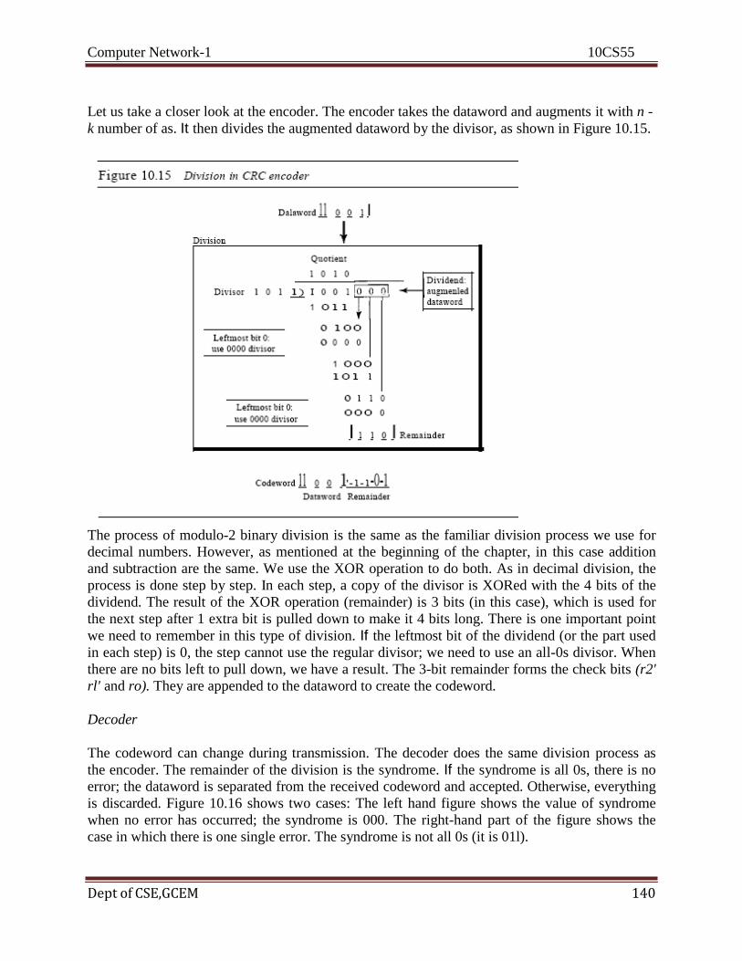
Computer Network-1 10CS55
Dept of CSE,GCEM 140
Let us take a closer look at the encoder. The encoder takes the dataword and augments it with n -
k number of as. It then divides the augmented dataword by the divisor, as shown in Figure 10.15.
The process of modulo-2 binary division is the same as the familiar division process we use for
decimal numbers. However, as mentioned at the beginning of the chapter, in this case addition
and subtraction are the same. We use the XOR operation to do both. As in decimal division, the
process is done step by step. In each step, a copy of the divisor is XORed with the 4 bits of the
dividend. The result of the XOR operation (remainder) is 3 bits (in this case), which is used for
the next step after 1 extra bit is pulled down to make it 4 bits long. There is one important point
we need to remember in this type of division. If the leftmost bit of the dividend (or the part used
in each step) is 0, the step cannot use the regular divisor; we need to use an all-0s divisor. When
there are no bits left to pull down, we have a result. The 3-bit remainder forms the check bits (r2'
rl' and ro). They are appended to the dataword to create the codeword.
Decoder
The codeword can change during transmission. The decoder does the same division process as
the encoder. The remainder of the division is the syndrome. If the syndrome is all 0s, there is no
error; the dataword is separated from the received codeword and accepted. Otherwise, everything
is discarded. Figure 10.16 shows two cases: The left hand figure shows the value of syndrome
when no error has occurred; the syndrome is 000. The right-hand part of the figure shows the
case in which there is one single error. The syndrome is not all 0s (it is 01l).
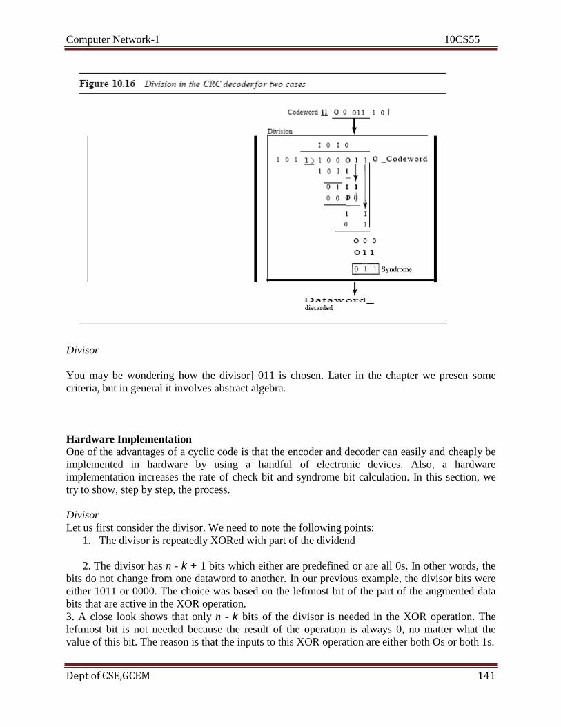
Computer Network-1 10CS55
Dept of CSE,GCEM 141
Divisor
You may be wondering how the divisor] 011 is chosen. Later in the chapter we presen some
criteria, but in general it involves abstract algebra.
Hardware Implementation One of the advantages of a cyclic code is that the encoder and decoder can easily and cheaply be
implemented in hardware by using a handful of electronic devices. Also, a hardware
implementation increases the rate of check bit and syndrome bit calculation. In this section, we
try to show, step by step, the process.
Divisor
Let us first consider the divisor. We need to note the following points:
1. The divisor is repeatedly XORed with part of the dividend
2. The divisor has n - k + 1 bits which either are predefined or are all 0s. In other words, the
bits do not change from one dataword to another. In our previous example, the divisor bits were
either 1011 or 0000. The choice was based on the leftmost bit of the part of the augmented data
bits that are active in the XOR operation.
3. A close look shows that only n - k bits of the divisor is needed in the XOR operation. The
leftmost bit is not needed because the result of the operation is always 0, no matter what the
value of this bit. The reason is that the inputs to this XOR operation are either both Os or both 1s.
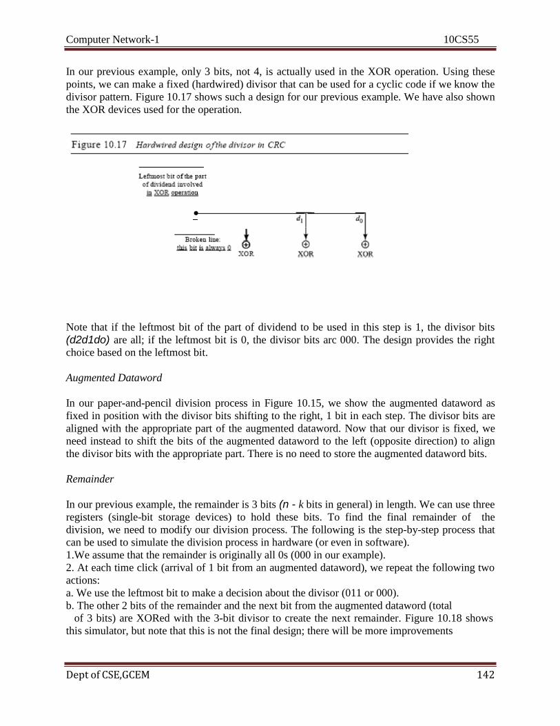
Computer Network-1 10CS55
Dept of CSE,GCEM 142
In our previous example, only 3 bits, not 4, is actually used in the XOR operation. Using these
points, we can make a fixed (hardwired) divisor that can be used for a cyclic code if we know the
divisor pattern. Figure 10.17 shows such a design for our previous example. We have also shown
the XOR devices used for the operation.
Note that if the leftmost bit of the part of dividend to be used in this step is 1, the divisor bits
(d2d1do) are all; if the leftmost bit is 0, the divisor bits arc 000. The design provides the right
choice based on the leftmost bit.
Augmented Dataword
In our paper-and-pencil division process in Figure 10.15, we show the augmented dataword as
fixed in position with the divisor bits shifting to the right, 1 bit in each step. The divisor bits are
aligned with the appropriate part of the augmented dataword. Now that our divisor is fixed, we
need instead to shift the bits of the augmented dataword to the left (opposite direction) to align
the divisor bits with the appropriate part. There is no need to store the augmented dataword bits.
Remainder
In our previous example, the remainder is 3 bits (n - k bits in general) in length. We can use three
registers (single-bit storage devices) to hold these bits. To find the final remainder of the
division, we need to modify our division process. The following is the step-by-step process that
can be used to simulate the division process in hardware (or even in software).
1.We assume that the remainder is originally all 0s (000 in our example).
2. At each time click (arrival of 1 bit from an augmented dataword), we repeat the following two
actions:
a. We use the leftmost bit to make a decision about the divisor (011 or 000).
b. The other 2 bits of the remainder and the next bit from the augmented dataword (total
of 3 bits) are XORed with the 3-bit divisor to create the next remainder. Figure 10.18 shows
this simulator, but note that this is not the final design; there will be more improvements

Computer Network-1 10CS55
Dept of CSE,GCEM 143
At each clock tick, shown as different times, one of the bits from the augmented dataword is
used in the XOR process. If we look carefully at the design, we have seven steps here, while in
the paper-and-pencil method we had only four steps. The first three steps have been added here
to make each step equal and to make the design for each step the same. Steps 1, 2, and 3 push the
first 3 bits to the remainder registers; steps 4, 5, 6, and 7 match the paper-and-pencil design. Note
that the values in the remainder register in steps 4 to 7 exactly match the values in the paper-and-
pencil design. The final remainder is also the same. The above design is for demonstration
purposes only. It needs simplification to be practical. First, we do not need to keep the
intermediate values of the remainder bits; we need only the final bits. We therefore need only 3
registers instead of 24. After the XOR operations, we do not need the bit values of the previous
remainder. Also, we do not need 21 XOR devices; two are enough because the output of an XOR
operation in which one of the bits is 0 is simply the value of the other bit. This other bit can be
used as the output. With these two modifications, the design becomes tremendously simpler and
less expensive, as shown in Figure 10.19.
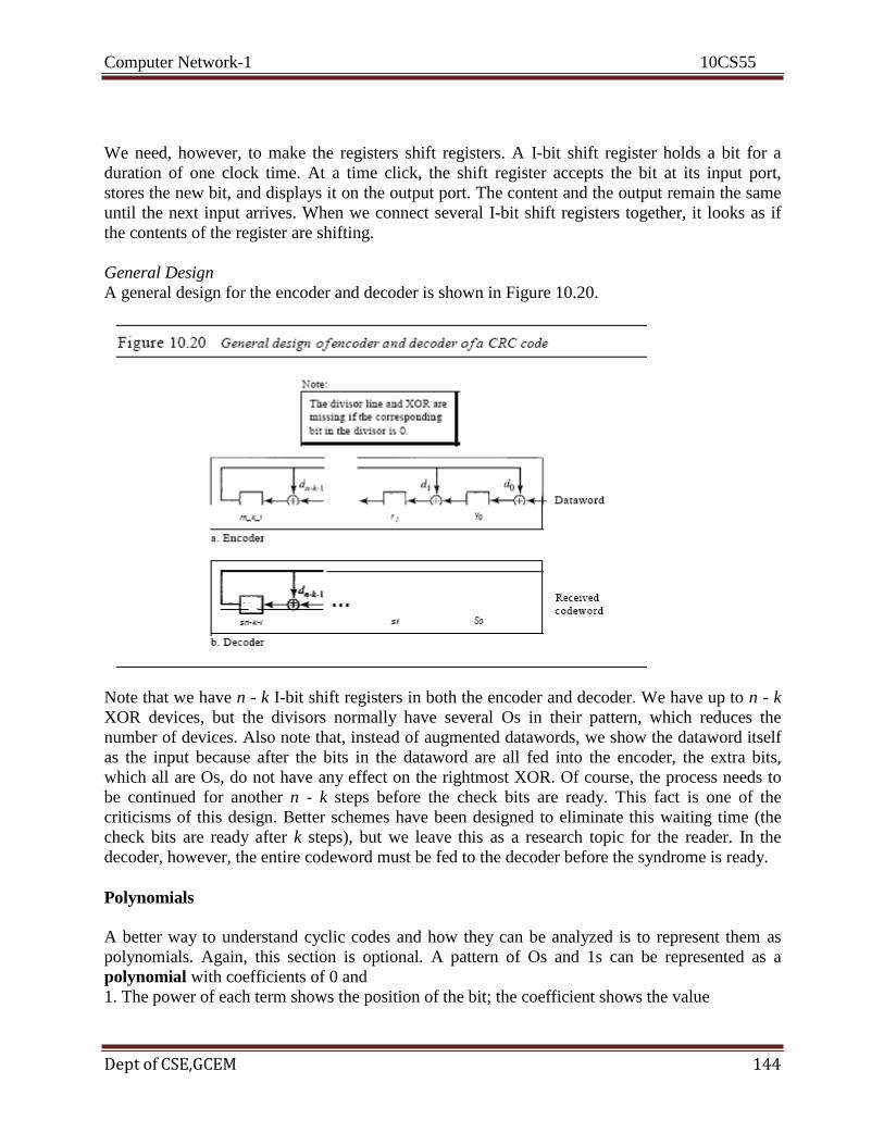
Computer Network-1 10CS55
Dept of CSE,GCEM 144
We need, however, to make the registers shift registers. A I-bit shift register holds a bit for a
duration of one clock time. At a time click, the shift register accepts the bit at its input port,
stores the new bit, and displays it on the output port. The content and the output remain the same
until the next input arrives. When we connect several I-bit shift registers together, it looks as if
the contents of the register are shifting.
General Design
A general design for the encoder and decoder is shown in Figure 10.20.
Note that we have n - k I-bit shift registers in both the encoder and decoder. We have up to n - k
XOR devices, but the divisors normally have several Os in their pattern, which reduces the
number of devices. Also note that, instead of augmented datawords, we show the dataword itself
as the input because after the bits in the dataword are all fed into the encoder, the extra bits,
which all are Os, do not have any effect on the rightmost XOR. Of course, the process needs to
be continued for another n - k steps before the check bits are ready. This fact is one of the
criticisms of this design. Better schemes have been designed to eliminate this waiting time (the
check bits are ready after k steps), but we leave this as a research topic for the reader. In the
decoder, however, the entire codeword must be fed to the decoder before the syndrome is ready.
Polynomials
A better way to understand cyclic codes and how they can be analyzed is to represent them as
polynomials. Again, this section is optional. A pattern of Os and 1s can be represented as a
polynomial with coefficients of 0 and
1. The power of each term shows the position of the bit; the coefficient shows the value
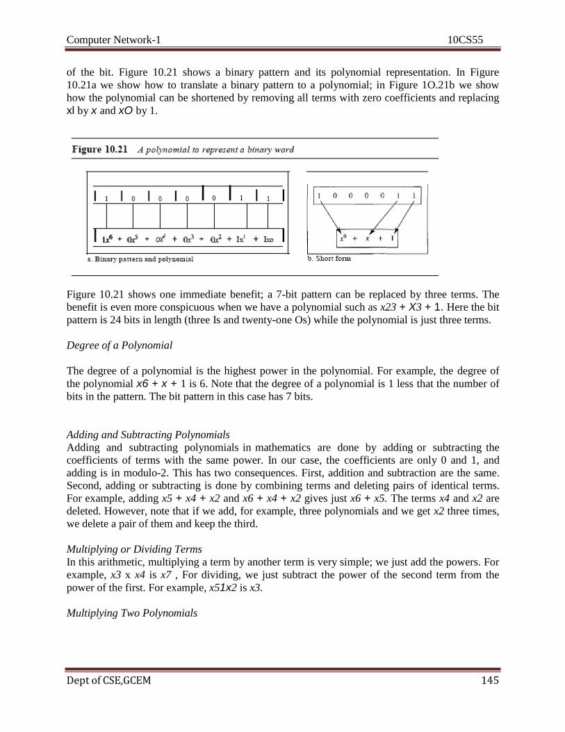
Computer Network-1 10CS55
Dept of CSE,GCEM 145
of the bit. Figure 10.21 shows a binary pattern and its polynomial representation. In Figure
10.21a we show how to translate a binary pattern to a polynomial; in Figure 1O.21b we show
how the polynomial can be shortened by removing all terms with zero coefficients and replacing
xl by x and xO by 1.
Figure 10.21 shows one immediate benefit; a 7-bit pattern can be replaced by three terms. The
benefit is even more conspicuous when we have a polynomial such as x23 + X3 + 1. Here the bit
pattern is 24 bits in length (three Is and twenty-one Os) while the polynomial is just three terms.
Degree of a Polynomial
The degree of a polynomial is the highest power in the polynomial. For example, the degree of
the polynomial x6 + x + 1 is 6. Note that the degree of a polynomial is 1 less that the number of
bits in the pattern. The bit pattern in this case has 7 bits.
Adding and Subtracting Polynomials
Adding and subtracting polynomials in mathematics are done by adding or subtracting the
coefficients of terms with the same power. In our case, the coefficients are only 0 and 1, and
adding is in modulo-2. This has two consequences. First, addition and subtraction are the same.
Second, adding or subtracting is done by combining terms and deleting pairs of identical terms.
For example, adding x5 + x4 + x2 and x6 + x4 + x2 gives just x6 + x5. The terms x4 and x2 are
deleted. However, note that if we add, for example, three polynomials and we get x2 three times,
we delete a pair of them and keep the third.
Multiplying or Dividing Terms
In this arithmetic, multiplying a term by another term is very simple; we just add the powers. For
example, x3 x x4 is x7 , For dividing, we just subtract the power of the second term from the
power of the first. For example, x51x2 is x3.
Multiplying Two Polynomials

Computer Network-1 10CS55
Dept of CSE,GCEM 146
Multiplying a polynomial by another is done term by term. Each term of the first polynomial
must be multiplied by all terms of the second. The result, of course, is then simplified, and pairs
of equal terms are deleted. The following is an example:
Dividing One Polynomial by Another
Division of polynomials is conceptually the same as the binary division we discussed for an
encoder. We divide the first term of the dividend by the first term of the divisor to get the first
term of the quotient. We multiply the term in the quotient by the divisor and subtract the result
from the dividend. We repeat the process until the dividend degree is less than the divisor degree.
We will show an example of division later in this chapter.
Shifting
A binary pattern is often shifted a number of bits to the right or left. Shifting to the left means
adding extra Os as rightmost bits; shifting to the right means deleting some rightmost bits.
Shifting to the left is accomplished by multiplying each term of the polynomial by xn, where m is
the number of shifted bits; shifting to the right is accomplished by dividing each term of the
polynomial by xn. The following shows shifting to the left and to the right. Note that we do not
have negative powers in the polynomial representation.
When we augmented the dataword in the encoder of Figure 10.15, we actually shifted the bits to
the left. Also note that when we concatenate two bit patterns, we shift the first polynomial to the
left and then add the second polynomial.
Cyclic Code Encoder Using Polynomials
Now that we have discussed operations on polynomials, we show the creation of a codeword
from a dataword. Figure 10.22 is the polynomial version of Figure 10.15. We can see that the
process is shorter. The dataword 1001 is represented as x3 + 1. The divisor 1011 is represented
as x3 + x + 1. To find the augmented dataword, we have left-shifted the dataword 3 bits
(multiplying by x\ The result is x6 + x3 . Division is straightforward. We divide the first term of
the dividend, x6, by the first term of the divisor, x3. The first term of the quotient is then x6/x3,
or x3. Then we multiply x3 by the divisor and subtract (according to our previous definition of
subtraction) the result from the dividend. The result is x4, with a degree greater than the divisor's
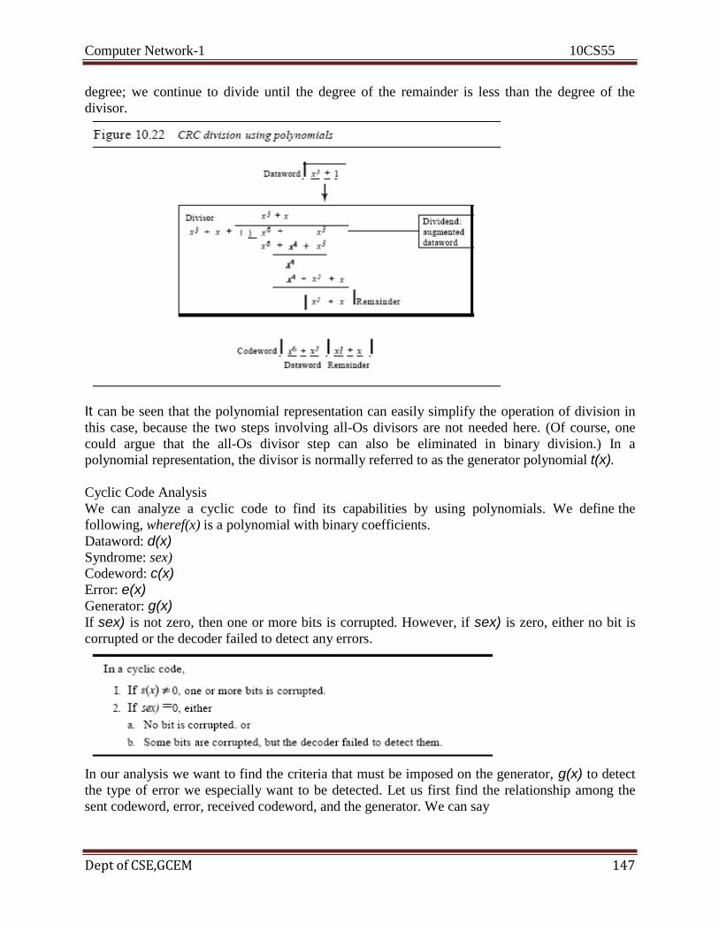
Computer Network-1 10CS55
Dept of CSE,GCEM 147
degree; we continue to divide until the degree of the remainder is less than the degree of the
divisor.
It can be seen that the polynomial representation can easily simplify the operation of division in
this case, because the two steps involving all-Os divisors are not needed here. (Of course, one
could argue that the all-Os divisor step can also be eliminated in binary division.) In a
polynomial representation, the divisor is normally referred to as the generator polynomial t(x).
Cyclic Code Analysis
We can analyze a cyclic code to find its capabilities by using polynomials. We define the
following, wheref(x) is a polynomial with binary coefficients.
Dataword: d(x) Syndrome: sex)
Codeword: c(x) Error: e(x) Generator: g(x) If sex) is not zero, then one or more bits is corrupted. However, if sex) is zero, either no bit is
corrupted or the decoder failed to detect any errors.
In our analysis we want to find the criteria that must be imposed on the generator, g(x) to detect
the type of error we especially want to be detected. Let us first find the relationship among the
sent codeword, error, received codeword, and the generator. We can say
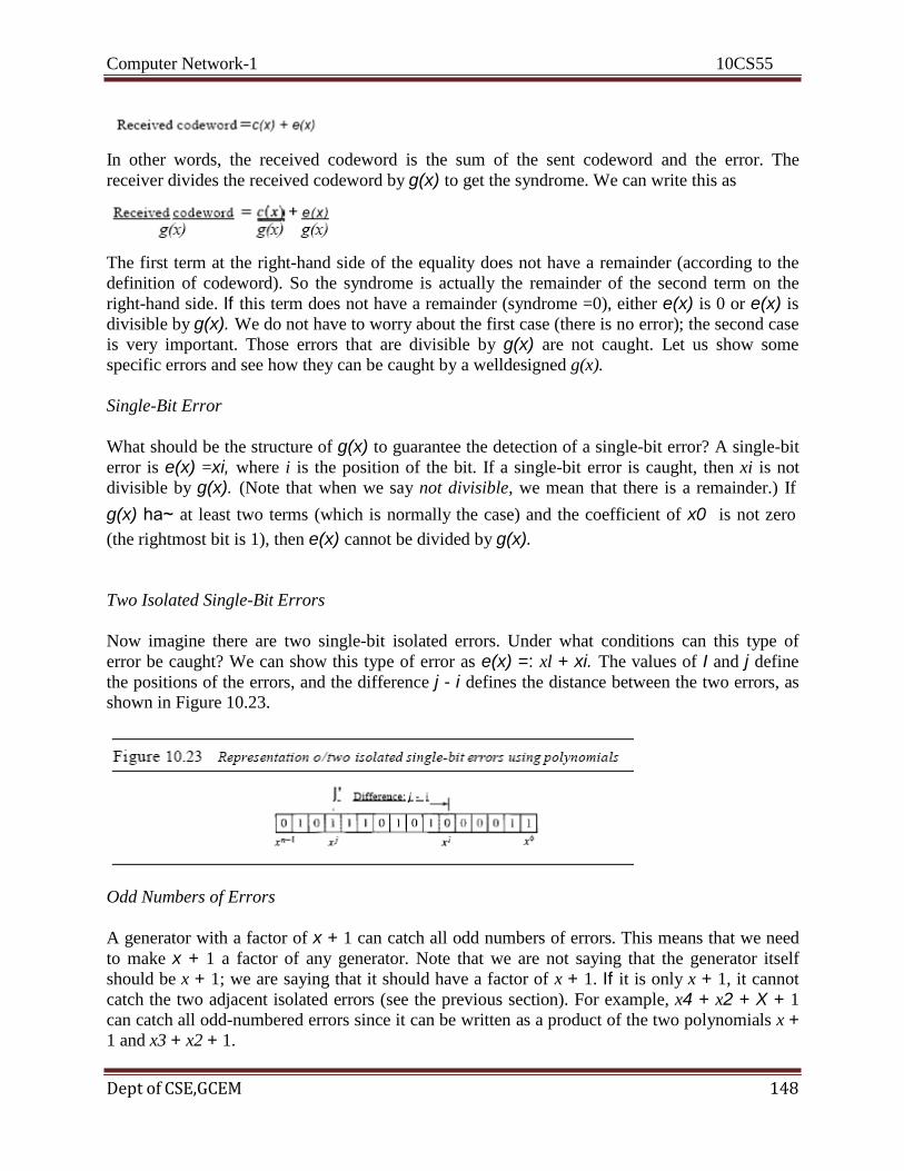
Computer Network-1 10CS55
Dept of CSE,GCEM 148
In other words, the received codeword is the sum of the sent codeword and the error. The
receiver divides the received codeword by g(x) to get the syndrome. We can write this as
The first term at the right-hand side of the equality does not have a remainder (according to the
definition of codeword). So the syndrome is actually the remainder of the second term on the
right-hand side. If this term does not have a remainder (syndrome =0), either e(x) is 0 or e(x) is
divisible by g(x). We do not have to worry about the first case (there is no error); the second case
is very important. Those errors that are divisible by g(x) are not caught. Let us show some
specific errors and see how they can be caught by a welldesigned g(x).
Single-Bit Error
What should be the structure of g(x) to guarantee the detection of a single-bit error? A single-bit
error is e(x) =xi, where i is the position of the bit. If a single-bit error is caught, then xi is not
divisible by g(x). (Note that when we say not divisible, we mean that there is a remainder.) If
g(x) ha~ at least two terms (which is normally the case) and the coefficient of x0 is not zero
(the rightmost bit is 1), then e(x) cannot be divided by g(x).
Two Isolated Single-Bit Errors
Now imagine there are two single-bit isolated errors. Under what conditions can this type of
error be caught? We can show this type of error as e(x) =: xl + xi. The values of I and j define
the positions of the errors, and the difference j - i defines the distance between the two errors, as
shown in Figure 10.23.
Odd Numbers of Errors
A generator with a factor of x + 1 can catch all odd numbers of errors. This means that we need
to make x + 1 a factor of any generator. Note that we are not saying that the generator itself
should be x + 1; we are saying that it should have a factor of x + 1. If it is only x + 1, it cannot
catch the two adjacent isolated errors (see the previous section). For example, x4 + x2 + X + 1
can catch all odd-numbered errors since it can be written as a product of the two polynomials x + 1 and x3 + x2 + 1.

Computer Network-1 10CS55
Dept of CSE,GCEM 149
Burst Errors
Now let us extend our analysis to the burst error, which is the most important of all. A burst error
is of the form e(x) =eJ + ... + xi). Note the difference between a burst error and two isolated
single-bit errors. The first can have two terms or more; the second can only have two terms. We
can factor out xi and write the error as xi(xJ-i + ... + 1). If our generator can detect a single error
(minimum condition for a generator), then it cannot divide xi. What we should worry about are
those generators that divide xJ-i + ... + 1. In other words, the remainder of (xJ-i + ... + 1)/(xr + ... + 1) must not be zero. Note that the denominator is the generator polynomial.
We can have three cases:
1. If j - i < r, the remainder can never be zero. We can write j - i =L - 1, where L is the length of
the error. So L - 1 < r or L < r + 1 or L :::;: r. This means all burst errors with length smaller
than or equal to the number of check bits r will be detected.
2. In some rare cases, if j - i = r, or L = r + 1, the syndrome is 0 and the error is undetected. It can be proved that in these cases, the probability of undetected burst error of length r + 1 is (ll2r-l
. For example, if our generator is x l4 + ~ + 1, in which r =14, a
burst error of length L =15 can slip by undetected with the probability of (1/2)14-1 or
almost 1 in 10,000.
3. In some rare cases, if j - i > r, or L > r + 1, the syndrome is 0 and the error is undetected. It can be proved that in these cases, the probability of undetected burst error
of length greater than r + 1 is (112t For example, if our generator is x14 + x3 + 1, in
which r =14, a burst error of length greater than 15 can slip by undetected with the
probability of (112)14 or almost 1 in 16,000 cases.
Standard Polynomials
Some standard polynomials used by popular protocols for eRe generation are shown in Table
10.7.
Advantages of Cyclic Codes

Computer Network-1 10CS55
Dept of CSE,GCEM 150
We have seen that cyclic codes have a very good performance in detecting single-bit errors,
double errors, an odd number of errors, and burst errors. They can easily be implemented in
hardware and software. They are especially fast when implemented in hardware. This has made
cyclic codes a good candidate for many networks.
Other Cyclic Codes
The cyclic codes we have discussed in this section are very simple. The check bits and
syndromes can be calculated by simple algebra. There are, however, more powerful polynomials
that are based on abstract algebra involving Galois fields. These are beyond the scope of this
book. One of the most interesting of these codes is the Reed-Solomon code used today for both
detection and correction.
10.5 CHECKSUM
The last error detection method we discuss here is called the checksum. The checksum is used in
the Internet by several protocols although not at the data link layer. However,we briefly discuss
it here to complete our discussion on error checking. Like linear and cyclic codes, the checksum
is based on the concept of redundancy. Several protocols still use the checksum for error
detection although the tendency is to replace it with a CRC. This means that the CRC is also
used in layers other than the data link layer.
Idea
The concept of the checksum is not difficult. Let us illustrate it with a few examples. One's
Complement The previous example has one major drawback. All of our data can be written as a
4-bit word (they are less than 15) except for the checksum. One solution is to use one's
complement arithmetic. In this arithmetic, we can represent unsigned numbers between 0 and 2n
- 1 using only n bits. t If the number has more than n bits, the extra leftmost bits need to be added
to the n rightmost bits (wrapping). In one's complement arithmetic, a negative number can be
represented by inverting all bits (changing a 0 to a 1 and a 1 to a 0). This is the same as
subtracting the number from 2n - 1.
Internet Checksum
Traditionally, the Internet has been using a 16-bit checksum. The sender calculates the checksum
by following these steps.
Sender site:
1. The message is divided into 16-bit words.
2. The value of the checksum word is set to O.
3. All words including the checksum are added ushtg one's complement addition.
4. The sum is complemented and becomes the checksum.
5. The checksum is sent with the data.
Receiver site:
1. The message (including checksum) is divided into 16-bit words.
Computer Network-1 10CS55
Dept of CSE, GCEM 151
2. All words are added using one's complement addition.
3. The sum is complemented and becomes the new checksum.
4. If the value of checksum is 0, the message is accepted; otherwise, it is rejected.
The nature of the checksum (treating words as numbers and adding and complementing them) is
well-suited for software implementation. Short programs can be written to calculate the
checksum at the receiver site or to check the validity of the message at the receiver site.
Recommended Questions
1. How does a single-bit error differ from a burst error? 2. Distinguish between forward error correction versus error correction by
retransmission.
3. What is the definition of a linear block code? What is the definition of a
cyclic code?
4. What is the Hamming distance? What is the minimum Hamming
distance?
5. How is the simple parity check related to the two-dimensional parity
check?
6. Discuss the concept of redundancy in error detection and correction.

Computer Network-1 10CS55
Dept of CSE, GCEM 152
COMPUTER NETWORKS – I
Subject Code: 10CS55 I.A. Marks : 25
Hours/Week : 04 Exam Hours: 03
Total Hours : 52 Exam Marks: 100
PART - B
UNIT- 5 6 Hours
Data Link Layer-2:
-Framing,
-Flow and Error Control,
-Protocols, Noiseless Channels,
-Noisy channels,
-HDLC, -PPP (Framing, Transition phases only)
Computer Network-1 10CS55
Dept of CSE, GCEM 153
UNIT-5
Data Link Control
11.1 FRAMING
Data transmission in the physical layer means moving bits in the form of a signal from the source
to the destination. The physical layer provides bit synchronization to ensure that the sender and
receiver use the same bit durations and timing.
The data link layer, on the other hand, needs to pack bits into frames, so that each frame is
distinguishable from another. Our postal system practices a type of framing. The simple act of
inserting a letter into an envelope separates one piece of information from another; the envelope
serves as the delimiter. In addition, each envelope defines the sender and receiver addresses since
the postal system is a many-to-many carrier facility.
Framing in the data link layer separates a message from one source to a destination, or from
other messages to other destinations, by adding a sender address and a destination address. The
destination address defines where the packet is to go; the sender address helps the recipient
acknowledge the receipt. Although the whole message could be packed in one frame, that is not
normally done. One reason is that a frame can be very large, making flow and error control very
inefficient. When a message is carried in one very large frame, even a single-bit error would
require the retransmission of the whole message. When a message is divided into smaller frames,
a single-bit error affects only that small frame.
Fixed-Size Framing
Frames can be of fixed or variable size. In fixed-size framing, there is no need for defining the
boundaries of the frames; the size itself can be used as a delimiter. An example of this type of
framing is the ATM wide-area network, which uses frames of fixed size called cells.
Variable-Size Framing
Our main discussion in this chapter concerns variable-size framing, prevalent in local area
networks. In variable-size framing, we need a way to define the end of the frame and the
beginning of the next.
Character-Oriented Protocols
In a character-oriented protocol, data to be carried are 8-bit characters from a coding system such
as ASCII (see Appendix A). The header, which normally carries the source and destination
addresses and other control information, and the trailer, which carries error detection or error
correction redundant bits, are also multiples of 8 bits. To separate one frame from the next, an 8-
bit (I-byte) flag is added at the beginning and the end of a frame. The flag, composed of
protocol-dependent special characters, signals the start or end of a frame. Figure 11.1 shows the
format of a frame in a character-oriented protocol.

Computer Network-1 10CS55
Dept of CSE, GCEM 154
Character-oriented framing was popular when only text was exchanged by the data link layers.
The flag could be selected to be any character not used for text communication. Now, however,
we send other types of information such as graphs, audio, and video. Any pattern used for the
flag could also be part of the information. If this happens, the receiver, when it encounters this
pattern in the middle of the data, thinks it has reached the end of the frame. To fix this problem, a
byte-stuffing strategy was added to character-oriented framing. In byte stuffing (or character
stuffing), a special byte is added to the data section of the frame when there is a character with
the same pattern as the flag. The data section is stuffed with an extra byte. This byte is usually
called the escape character (ESC), which has a predefined bit pattern. Whenever the receiver
encounters the ESC character, it removes it from the data section and treats the next character as
data, not a delimiting flag.
Byte stuffing by the escape character allows the presence of the flag in the data section of the
frame, but it creates another problem. What happens if the text contains one or more escape
characters followed by a flag? The receiver removes the escape character, but keeps the flag,
which is incorrectly interpreted as the end of the frame. To solve this problem, the escape
characters that are part of the text must also be marked by another escape character. In other
words, if the escape character is part of the text, an extra one is added to show that the second
one is part of the text. Figure 11.2 shows the situation.
Character-oriented protocols present another problem in data communications. The universal
coding systems in use today, such as Unicode, have 16-bit and 32-bit characters that conflict

Computer Network-1 10CS55
Dept of CSE, GCEM 155
with 8-bit characters. We can say that in general, the tendency is moving toward the bit-oriented
protocols that we discuss next.
Bit-Oriented Protocols
In a bit-oriented protocol, the data section of a frame is a sequence of bits to be interpreted by the
upper layer as text, graphic, audio, video, and so on. However, in addition to headers (and
possible trailers), we still need a delimiter to separate one frame from the other. Most protocols
use a special 8-bit pattern flag 01111110 as the delimiter to define the beginning and the end of
the frame, as shown in Figure 11.3.
This flag can create the same type of problem we saw in the byte-oriented protocols.
That is, if the flag pattern appears in the data, we need to somehow inform the receiver that this
is not the end of the frame. We do this by stuffing 1 single bit (instead
of I byte) to prevent the pattern from looking like a flag. The strategy is called bit stuffing. In bit
stuffing, if a 0 and five consecutive I bits are encountered, an extra 0 is
added. This extra stuffed bit is eventually removed from the data by the receiver. Figure 11.4
shows bit stuffing at the sender and bit removal at the receiver. Note that even if we have a 0
after five 1s, we still stuff a 0. The 0 will be removed by the receiver.

Computer Network-1 10CS55
Dept of CSE, GCEM 156
This means that if the flag like pattern 01111110 appears in the data, it will change to 011111010
(stuffed) and is not mistaken as a flag by the receiver. The real flag 01111110 is not stuffed by
the sender and is recognized by the receiver.
11.2 FLOW AND ERROR CONTROL
Data communication requires at least two devices working together, one to send and the other to
receive. Even such a basic arrangement requires a great deal of coordination for an intelligible
exchange to occur. The most important responsibilities of the data link layer are flow control and
error control. Collectively, these functions are known as data link control.
Flow Control
Flow control coordinates the amount of data that can be sent before receiving an
acknowledgment and is one of the most important duties of the data link layer. In most protocols,
flow control is a set of procedures that tells the sender how much data it can transmit before it
must wait for an acknowledgment from the receiver. The flow of data must not be allowed to
overwhelm the receiver. Any receiving device has a limited speed at which it can process
incoming data and a limited amount of memory in which to store incoming data. The receiving
device must be able to inform the sending device before those limits are reached and to request
that the transmitting device send fewer frames or stop temporarily. Incoming data must be
checked and processed before they can be used. The rate of such processing is often slower than
the rate of transmission. For this reason,
each receiving device has a block of memory, called a buffer, reserved for storing incoming data
until they are processed. If the buffer begins to fill up, the receiver must be able to tell the sender
to halt transmission until it is once again able to receive.
Error Control
Error control is both error detection and error correction. It allows the receiver to inform the
sender of any frames lost or damaged in transmission and coordinates the retransmission of those
frames by the sender. In the data link layer, the term error control
refers primarily to methods of error detection and retransmission. Error control in the data link
layer is often implemented simply: Any time an error is detected in an exchange, specified
frames are retransmitted. This process is called automatic repeat request (ARQ).
11.3 PROTOCOLS
Now let us see how the data link layer can combine framing, flow control, and error control to
achieve the delivery of data from one node to another. The protocols are normally implemented
in software by using one of the common programming languages. To make our discussions
language-free, we have written in pseudocode a version of each protocol that concentrates mostly
on the procedure instead of delving into the details of language rules. The protocols in the first
category cannot be used in real life, but they serve as a basis for understanding the protocols of
noisy channels. Figure 11.5 shows the classifications.

Computer Network-1 10CS55
Dept of CSE, GCEM 157
There is a difference between the protocols we discuss here and those used in real networks. All
the protocols we discuss are unidirectional in the sense that the data frames travel from one node,
called the sender, to another node, called the receiver. Although special frames, called
acknowledgment (ACK) and negative acknowledgment (NAK) can flow in the opposite
direction for flow and error control purposes, data flow in only one direction.
In a real-life network, the data link protocols are implemented as bidirectional; data flow in both
directions. In these protocols the flow and error control information such as ACKs and NAKs is
included in the data frames in a technique called piggybacking. Because bidirectional protocols
are more complex than unidirectional ones, we chose the latter for our discussion. If they are
understood, they can be extended to bidirectional protocols.
11.4 NOISELESS CHANNELS
The first is a protocol that does not use flow control; the second is the one that does. Of course,
neither has error control because we have assumed that the channel is a perfect noiseless channel.
Simplest Protocol
Our first protocol, which we call the Simplest Protocol for lack of any other name, is one that has
no flow or error control. Like other protocols we will discuss in this chapter, it is a unidirectional
protocol in which data frames are traveling in only one direction-from the sender to receiver. We
assume that the receiver can immediately handle any frame it receives with a processing time
that is small enough to be negligible. The data link layer of the receiver immediately removes the
header from the frame and hands the data packet to its network layer, which can also accept the
packet immediately. In other words, the receiver can never be overwhelmed with incoming
frames.
Design
There is no need for flow control in this scheme. The data link layer at the sender site gets data
from its network layer, makes a frame out of the data, and sends it. The data link layer at the
receiver site receives a frame from its physical layer, extracts data from the frame, and delivers

Computer Network-1 10CS55
Dept of CSE, GCEM 158
the data to its network layer. The data link layers of the sender and receiver provide transmission
services for their network layers. The data link layers use the services provided by their physical
layers (such as signaling, multiplexing, and so on) for the physical transmission of bits. Figure
11.6 shows a design.
The sender site cannot send a frame until its network layer has a data packet to send. The
receiver site cannot deliver a data packet to its network layer until a frame arrives. If the protocol
is implemented as a procedure, we need to introduce the idea of events in the protocol. The
procedure at the sender site is constantly running; there is no action until there is a request from
the network layer. The procedure at the receiver site is also constantly rulming, but there is no
action until notification from the physical layer arrives. Both procedures are constantly running
because they do not know when the corresponding events will occur.
Algorithms
Algorithm 11.1 shows the procedure at the sender site.
Analysis The algorithm has an infinite loop, which means lines 3 to 9 are repeated forever once
the program starts. The algorithm is an event-driven one, which means that it sleeps (line 3) until
an event wakes it up (line 4). This means that there may be an undefined span of time between
the execution of line 3 and line 4; there is a gap between these actions. When the event, a request
from the network layer, occurs, lines 6 though 8 are executed. The program then repeats the loop
and again sleeps at line 3 until the next occurrence of the event. We have written

Computer Network-1 10CS55
Dept of CSE, GCEM 159
pseudocode for the main process and SendFrame. GetData takes a data packet from the network
layer, Make Frame0 adds a header and delimiter flags to the data packet to make a frame, and
SendFrame0 delivers the frame to the physical layer for transmission.
Algorithm 11.2 shows the procedure at the receiver site.
Analysis This algorithm has the same format as Algorithm 11.1, except that the direction of the
frames and data is upward. The event here is the arrival of a data frame. After the event occurs,
the data link layer receives the frame from the physical layer using the ReceiveFrame process,
extracts the data from the frame using the ExtractData process, and delivers the data to the
network layer using the DeliverData process. Here, we also have an event-driven algorithm
because the algorithm never knows when the data frame will arrive.
Stop-and-Wait Protocol
If data frames arrive at the receiver site faster than they can be processed, the frames must be
stored until their use. Normally, the receiver does not have enough storage space, especially if it
is receiving data from many sources. This may result in either the discarding of frames or denial
of service. To prevent the receiver from becoming overwhelmed with frames. There must be
feedback from the receiver to the sender. The protocol we discuss now is called the Stop-and-
Wait Protocol because the sender sends one frame, stops until it receives confirmation from the
receiver (okay to go ahead), and then sends the next frame.
Design
Figure 11.8 illustrates the mechanism. Comparing this figure with Figure 11.6, can see the traffic
on the forward channel (from sender to receiver) and the reverse channel. At any time, there is
either one data frame on the forward channel or one ACK frame on the reverse channel. We
therefore need a half-duplex link.
Algorithms
Algorithm 11.3 is for the sender site.

Computer Network-1 10CS55
Dept of CSE,GCEM 160
Analysis Here two events can occur: a request from the network layer or an arrival notification from the physical layer. The responses to these events must alternate. In other words, after a
frame is sent, the algorithm must ignore another network layer request until that frame is
acknowledged. We know that two arrival events cannot happen one after another because the
channel is error-free and does not duplicate the frames. The requests from the network layer,
however, may happen one after another without an arrival event in between. To prevent the
immediate sending of the data frame. there are several methods used a simple canSend variable
that can either be true or false. When a frame is sent, the variable is set to false to indicate that a
new network request cannot be sent until can Send is true. When an ACK is received, can Send
is set to true to allow the sending of the next frame.
Algorithm 11.4 shows the procedure at the receiver site.
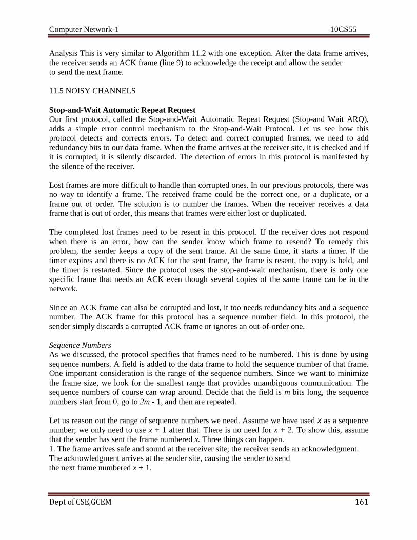
Computer Network-1 10CS55
Dept of CSE,GCEM 161
Analysis This is very similar to Algorithm 11.2 with one exception. After the data frame arrives,
the receiver sends an ACK frame (line 9) to acknowledge the receipt and allow the sender
to send the next frame.
11.5 NOISY CHANNELS
Stop-and-Wait Automatic Repeat Request Our first protocol, called the Stop-and-Wait Automatic Repeat Request (Stop-and Wait ARQ),
adds a simple error control mechanism to the Stop-and-Wait Protocol. Let us see how this
protocol detects and corrects errors. To detect and correct corrupted frames, we need to add
redundancy bits to our data frame. When the frame arrives at the receiver site, it is checked and if
it is corrupted, it is silently discarded. The detection of errors in this protocol is manifested by
the silence of the receiver.
Lost frames are more difficult to handle than corrupted ones. In our previous protocols, there was
no way to identify a frame. The received frame could be the correct one, or a duplicate, or a
frame out of order. The solution is to number the frames. When the receiver receives a data
frame that is out of order, this means that frames were either lost or duplicated.
The completed lost frames need to be resent in this protocol. If the receiver does not respond
when there is an error, how can the sender know which frame to resend? To remedy this
problem, the sender keeps a copy of the sent frame. At the same time, it starts a timer. If the
timer expires and there is no ACK for the sent frame, the frame is resent, the copy is held, and
the timer is restarted. Since the protocol uses the stop-and-wait mechanism, there is only one
specific frame that needs an ACK even though several copies of the same frame can be in the
network.
Since an ACK frame can also be corrupted and lost, it too needs redundancy bits and a sequence
number. The ACK frame for this protocol has a sequence number field. In this protocol, the
sender simply discards a corrupted ACK frame or ignores an out-of-order one.
Sequence Numbers
As we discussed, the protocol specifies that frames need to be numbered. This is done by using
sequence numbers. A field is added to the data frame to hold the sequence number of that frame.
One important consideration is the range of the sequence numbers. Since we want to minimize
the frame size, we look for the smallest range that provides unambiguous communication. The
sequence numbers of course can wrap around. Decide that the field is m bits long, the sequence
numbers start from 0, go to 2m - 1, and then are repeated.
Let us reason out the range of sequence numbers we need. Assume we have used x as a sequence
number; we only need to use x + 1 after that. There is no need for x + 2. To show this, assume
that the sender has sent the frame numbered x. Three things can happen.
1. The frame arrives safe and sound at the receiver site; the receiver sends an acknowledgment.
The acknowledgment arrives at the sender site, causing the sender to send
the next frame numbered x + 1.

Computer Network-1 10CS55
Dept of CSE,GCEM 162
2. The frame arrives safe and sound at the receiver site; the receiver sends an acknowledgment,
but the acknowledgment is corrupted or lost. The sender resends the frame
(numbered x) after the time-out. Note that the frame here is a duplicate. The receiver can
recognize this fact because it expects frame x + I but frame x was received.
3. The frame is corrupted or never arrives at the receiver site; the sender resends the frame
(numbered x) after the time-out.
Acknowledgment Numbers
Since the sequence numbers must be suitable for both data frames and ACK frames, use this
convention: The acknowledgment numbers always announce the sequence number of the next
frame expected by the receiver. For example, if frame 0 has arrived safe and sound, the receiver
sends an ACK frame with acknowledgment 1 (meaning frame 1 is expected next). If frame 1 has
arrived safe and sound, the receiver sends an ACK frame with acknowledgment 0 (meaning
frame 0 is expected).
Design
Figure 11.10 shows the design of the Stop-and-WaitARQ Protocol. The sending device keeps a
copy of the last frame transmitted until it receives an acknowledgment for that frame. A data
frames uses a seqNo (sequence number); an ACK frame uses an ackNo (acknowledgment
number). The sender has a control variable, which we call Sn (sender, next frame to send), that
holds the sequence number for the next frame to be sent (0 or 1).

Computer Network-1 10CS55
Dept of CSE,GCEM 163
The receiver has a control variable, which we call Rn (receiver, next frame expected), that holds
the number of the next frame expected. When a frame is sent, the value of Sn is incremented
(modulo-2), which means if it is 0, it becomes 1 and vice versa. When a frame is received, the
value of Rn is incremented (modulo-2), which means if it is 0, it becomes 1 and vice versa. Three
events can happen at the sender site; one event can happen at the receiver site. Variable Sn points
to the slot that matches the sequence number of the frame that has been sent, but not
acknowledged; Rn points to the slot that matches the sequence number of the expected frame.

Computer Network-1 10CS55
Dept of CSE,GCEM 164
Analysis We first notice the presence of Sn' the sequence number of the next frame to be sent.
This variable is initialized once (line 1), but it is incremented every time a frame is sent (line 13)
in preparation for the next frame. However, since this is modulo-2 arithmetic, the sequence
numbers are
0, 1,0, 1, and so on. Note that the processes in the first event (SendFrame, StoreFrame, and Purge
Frame) use an Sn defining the frame sent out. We need at least one buffer to hold this frame until
we are sure that it is received safe and sound. Line 10 shows that before the frame is sent, it is
stored.
The copy is used for resending a corrupt or lost frame. We are still using the canSend variable to
prevent the network layer from making a request before the previous frame is received safe and
sound. If the frame is not corrupted and the ackNo of theACK frame matches the sequence
number of the next frame to send, we stop the timer and purge the copy of the data frame we
saved. Otherwise, we just ignore this event and wait for the next event to happen. After each
frame is sent, a timer is started.
When the timer expires (line 28), the frame is resent and the timer is restarted.
Algorithm 11.6 shows the procedure at the receiver site.
Analysis This is noticeably different from Algorithm 11.4. First, all arrived data frames that are
corrupted are ignored. If the SeqNo of the frame is the one that is expected (Rn ), the frame is
accepted, the data are delivered to the network layer, and the value of Rn is incremented.
However, there is one subtle point here. Even if the sequence number of the data frame does not
match the next frame expected, an ACK is sent to the sender. This ACK, however, just
reconfirms the previous ACK instead of confirming the frame received. This is done because the

Computer Network-1 10CS55
Dept of CSE,GCEM 165
receiver assumes that the previous ACK might have been lost; the receiver is sending a duplicate
frame. The resent ACK may solve the problem before the time-out does it.
Efficiency
The Stop-and-WaitARQ discussed in the previous section is very inefficient if our channel
is thick and long. By thick, we mean that our channel has a large bandwidth; by long, mean the
round-trip delay is long. The product of these two is called the bandwidth delay product, as we
discussed in Chapter 3. We can think of the channel as a pipe. The bandwidth-delay product then
is the volume of the pipe in bits. The pipe is always there. If we do not use it, we are inefficient.
The bandwidth-delay product is a measure of the number of bits we can send out of our system
while waiting for news from the receiver.
Pipelining
In networking and in other areas, a task is often begun before the previous task has ended.
This is known as pipelining. There is no pipelining in Stop-and-Wait ARQ because need to wait
for a frame to reach the destination and be acknowledged before the next frame can be sent.
However, pipelining does apply to our next two protocols because several frames can be sent
before we receive news about the previous frames. Pipelining improves the efficiency of the
transmission if the number of bits in transition is large with respect to the bandwidth-delay
product.
Go-Back-N Automatic Repeat Request
To improve the efficiency of transmission (filling the pipe), multiple frames must be in transition
while waiting for acknowledgment. In other words, we need to let more than one frame be
outstanding to keep the channel busy while the sender is waiting for acknowledgment. In this
section, we discuss one protocol that can achieve this goal; in the next section, we discuss a
second. The first is called Go-Back-N Automatic Repeat Request (the rationale for the name will
become clear later). In this protocol we can send several frames before receiving
acknowledgments; we keep a copy of these frames until the acknowledgments arrive.
Sequence Numbers
Frames from a sending station are numbered sequentially. However, because we need to include
the sequence number of each frame in the header, we need to set a limit. If the header of the
frame allows m bits for the sequence number, the sequence numbers range from 0 to 2m - 1. For
example, if m is 4, the only sequence numbers are 0 through 15 inclusive. However, we can
repeat the sequence. So the sequence numbers are 0, 1,2,3,4,5,6, 7,8,9, 10, 11, 12, 13, 14, 15,0,
1,2,3,4,5,6,7,8,9,10, 11, ... In other words, the sequence numbers are modulo-2m
. Sliding Window
In this protocol (and the next), the sliding window is an abstract concept that defines the range of
sequence numbers that is the concern of the sender and receiver. In other words, the sender and
receiver need to deal with only part of the possible sequence numbers. The range which is the
concern of the sender is called the send sliding window; the range that is the concern of the
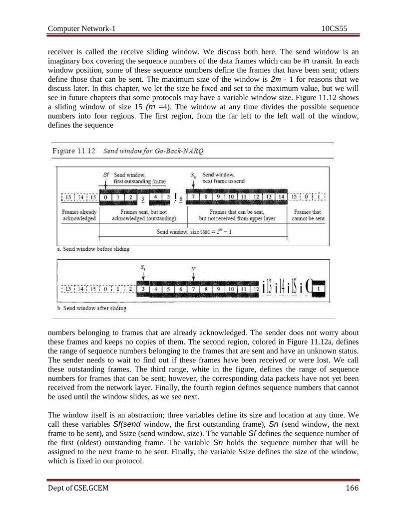
Computer Network-1 10CS55
Dept of CSE,GCEM 166
receiver is called the receive sliding window. We discuss both here. The send window is an
imaginary box covering the sequence numbers of the data frames which can be in transit. In each
window position, some of these sequence numbers define the frames that have been sent; others
define those that can be sent. The maximum size of the window is 2m - 1 for reasons that we
discuss later. In this chapter, we let the size be fixed and set to the maximum value, but we will
see in future chapters that some protocols may have a variable window size. Figure 11.12 shows
a sliding window of size 15 (m =4). The window at any time divides the possible sequence
numbers into four regions. The first region, from the far left to the left wall of the window,
defines the sequence
numbers belonging to frames that are already acknowledged. The sender does not worry about
these frames and keeps no copies of them. The second region, colored in Figure 11.12a, defines
the range of sequence numbers belonging to the frames that are sent and have an unknown status.
The sender needs to wait to find out if these frames have been received or were lost. We call
these outstanding frames. The third range, white in the figure, defines the range of sequence
numbers for frames that can be sent; however, the corresponding data packets have not yet been
received from the network layer. Finally, the fourth region defines sequence numbers that cannot
be used until the window slides, as we see next.
The window itself is an abstraction; three variables define its size and location at any time. We
call these variables Sf(send window, the first outstanding frame), Sn (send window, the next
frame to be sent), and Ssize (send window, size). The variable Sf defines the sequence number of
the first (oldest) outstanding frame. The variable Sn holds the sequence number that will be
assigned to the next frame to be sent. Finally, the variable Ssize defines the size of the window,
which is fixed in our protocol.

Computer Network-1 10CS55
Dept of CSE,GCEM 167
Figure 11.12b shows how a send window can slide one or more slots to the right when an
acknowledgment arrives from the other end. As we will see shortly, theacknowledgments
in this protocol are cumulative, meaning that more than one frame can be acknowledged by an
ACK frame. In Figure 11.12b, frames 0, I, and 2 are acknowledged,
so the window has slid to the right three slots. Note that the value ofSf is 3 because frame 3 is
now the first outstanding frame. The receive window makes sure that the correct data frames are
received and that the correct acknowledgments are sent. The size of the receive window is
always 1. The receiver is always looking for the arrival of a specific frame. Any frame arriving
out of order is discarded and needs to be resent. Figure 11.13 shows the receive window.
Note that we need only one variable Rn (receive window, next frame expected) to define this
abstraction. The sequence numbers to the left of the window belong to the frames already
received and acknowledged; the sequence numbers to the right of this window define the frames
that cannot be received. Any received frame with a sequence number in these two regions is
discarded. Only a frame with a sequence number matching the value of Rn is accepted and
acknowledged. The receive window also slides, but only one slot at a time. When a correct frame
is received (and a frame is received only one at a time), the window slides.
Timers
Although there can be a timer for each frame that is sent, in our protocol we use only
one. The reason is that the timer for the first outstanding frame always expires first; we
send all outstanding frames when this timer expires.
Acknowledgment
The receiver sends a positive acknowledgment if a frame has arrived safe and sound
and in order. If a frame is damaged or is received out of order, the receiver is silent and

Computer Network-1 10CS55
Dept of CSE,GCEM 168
will discard all subsequent frames until it receives the one it is expecting. The silence of
the receiver causes the timer of the unacknowledged frame at the sender site to expire. This, in
turn, causes the sender to go back and resend all frames, beginning with the one with the expired
timer. The receiver does not have to acknowledge each frame received. It can send one
cumulative acknowledgment for several frames.
Resending a Frame
When the timer expires, the sender resends all outstanding frames. For example, suppose the
sender has already sent frame 6, but the timer for frame 3 expires. This means that frame 3 has
not been acknowledged; the sender goes back and sends frames 3, 4,5, and 6\ again. That is why
the protocol is called Go-Back-N ARQ.
Design
Figure 11.14 shows the design for this protocol. As we can see, multiple frames can be in transit
in the forward direction, and multiple acknowledgments in the reverse direction. The idea is
similar to Stop-and-Wait ARQ; the difference is that the send
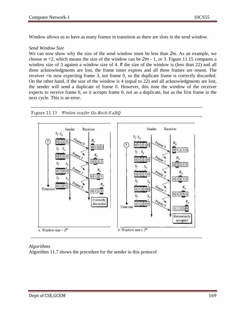
Computer Network-1 10CS55
Dept of CSE,GCEM 169
Window allows us to have as many frames in transition as there are slots in the send window.
Send Window Size
We can now show why the size of the send window must be less than 2m. As an example, we
choose m =2, which means the size of the window can be 2m - 1, or 3. Figure 11.15 compares a
window size of 3 against a window size of 4. If the size of the window is (less than 22) and all
three acknowledgments are lost, the frame timer expires and all three frames are resent. The
receiver =is now expecting frame 3, not frame 0, so the duplicate frame is correctly discarded.
On the other hand, if the size of the window is 4 (equal to 22) and all acknowledgments are lost,
the sender will send a duplicate of frame 0. However, this time the window of the receiver
expects to receive frame 0, so it accepts frame 0, not as a duplicate, but as the first frame in the
next cycle. This is an error.
Algorithms
Algorithm 11.7 shows the procedure for the sender in this protocol

Computer Network-1 10CS55
Dept of CSE,GCEM 170
Analysis This algorithm first initializes three variables. Unlike Stop-and-Wait ARQ, this
protocol allows several requests from the network layer without the need for other events to
occur; we just need to be sure that the window is not full (line 12). In our approach, if the
window is full, the request is just ignored and the network layer needs to try again. Some
implementations use other methods such as enabling or disabling the network layer. The
handling of the arrival event is more complex than in the previous protocol. If we receive a
corrupted ACK, we ignore it. If the ade Na belongs to one of the outstanding frames, we use a
loop to purge the buffers and move the left wall to the right. The time-out event is also more
complex.
Algorithm 11.8 is the procedure at the receiver site.

Computer Network-1 10CS55
Dept of CSE,GCEM 171
Analysis This algorithm is simple. We ignore a corrupt or out-of-order frame. If a frame
arrives with an expected sequence number, we deliver the data, update the value ofRn, and send
an ACK with the ackNa showing the next frame expected.

Computer Network-1 10CS55
Dept of CSE,GCEM 172
Go-Back-N ARQ Versus Stop-and- Wait ARQ
The reader may find that there is a similarity between Go-Back-NARQ and Stop-and-Wait ARQ.
We can say that the Stop-and-WaitARQ Protocol is actually a Go-Back-NARQ in which there
are only two sequence numbers and the send window size is 1. In other words, m = 1, 2m - 1 = 1.
In Go-Back-NARQ, we said that the addition is modulo-2m; in Stop-and-WaitARQ it is 2, which
is the same as 2m when m = 1.

Computer Network-1 10CS55
Dept of CSE,GCEM 173
Selective Repeat Automatic Repeat Request
Go-Back-N ARQ simplifies the process at the receiver site. The receiver keeps track of only one
variable, and there is no need to buffer out-of-order frames; they are simply discarded. However,
this protocol is very inefficient for a noisy link. In a noisy link a frame has a higher probability of
damage, which means the resending of multiple frames. This resending uses up the bandwidth
and slows down the transmission. For noisy links, there is another mechanism that does not
resend N frames when just one frame is damaged; only the damaged frame is resent. This
mechanism is called Selective RepeatARQ. It is more efficient for noisy links, but the processing
at the receiver is more complex.

Computer Network-1 10CS55
Dept of CSE,GCEM 174
Windows
The Selective Repeat Protocol also uses two windows: a send window and a receive window.
However, there are differences between the windows in this protocol and the ones in Go-Back-N.
First, the size of the send window is much smaller; it is 2m- I . The reason for this will be
discussed later. Second, the receive window is the same size as the send window. The send
window maximum size can be 2m- I . For example, if m = 4, the sequence numbers go from 0 to
15, but the size of the window is just 8 (it is 15 in the Go-Back-N Protocol). The smaller window
size means less efficiency in filling the pipe, but the fact that there are fewer duplicate frames
can compensate for this.
The protocol uses the same variables as we discussed for Go-Back-N. We show the Selective
Repeat send window in Figure 11.18 to emphasize the size. Compare it with Figure 11.12.
The receive window in Selective Repeat is totally different from the one in GoBack- N. First, the
size of the receive window is the same as the size of the send window (2m- I ). The Selective
Repeat Protocol allows as many frames as the size of the receive window to arrive out of order
and be kept until there is a set of in-order frames to be delivered to the network layer. Because
the sizes of the send window and receive window are the same, all the frames in the send frame
can arrive out of order and be stored until they can be delivered. We need, however, to mention
that the receiver never delivers packets out of order to the network layer. Figure 11.19 shows the
receive window in this

Computer Network-1 10CS55
Dept of CSE,GCEM 175
protocol. Those slots inside the window that are colored define frames that have arrived out of
order and are waiting for their neighbors to arrive before delivery to the network layer.
Design
The design in this case is to some extent similar to the one we described for the 00Back-N, but
more complicated, as shown in Figure 11.20
Window Sizes
Windows must be at most one half of 2m. For an example, we choose m = 2, which means the
size of the window is 2m/2, or 2. Figure 11.21 compares a window size of 2 with a window size
of 3. If the size of the window is 2 and all acknowledgments are lost, the timer for frame 0
expires and frame 0 is resent. However, the window of the receiver is now expecting
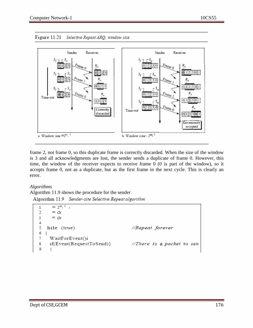
Computer Network-1 10CS55
Dept of CSE,GCEM 176
frame 2, not frame 0, so this duplicate frame is correctly discarded. When the size of the window
is 3 and all acknowledgments are lost, the sender sends a duplicate of frame 0. However, this
time, the window of the receiver expects to receive frame 0 (0 is part of the window), so it
accepts frame 0, not as a duplicate, but as the first frame in the next cycle. This is clearly an
error.
Algorithms
Algorithm 11.9 shows the procedure for the sender

Computer Network-1 10CS55
Dept of CSE,GCEM 177
Analysis The handling of the request event is similar to that of the previous protocol except that
one timer is started for each frame sent. The arrival event is more complicated here. An ACK or
a NAK frame may arrive. If a valid NAK frame arrives, we just resend the corresponding frame.
If a valid ACK arrives, we use a loop to purge the buffers, stop the corresponding timer and
move the left wall of the window. The time-out event is simpler here; only the frame which times
out is resent

Computer Network-1 10CS55
Dept of CSE,GCEM 178

Computer Network-1 10CS55
Dept of CSE,GCEM 179
Analysis Here we need more initialization. In order not to overwhelm the other side with NAKs,
we use a variable called NakSent. To know when we need to send an ACK, we use a variable
called AckNeeded. Both of these are initialized to false. We also use a set of variables to mark
the slots in the receive window once the corresponding frame has arrived and is stored. If we
receive a corrupted frame and a NAK has not yet been sent, we send a NAK to tell the other site
that we have not received the frame we expected. If the frame is not corrupted and the sequence
number is in the window, we store the frame and mark the slot. If contiguous frames, starting
from Rn have been marked, we deliver their data to the network layer and slide the window.
Figure 11.22 shows this situation.
Example 11.8
This example is similar to Example 11.3 in which frame 1 is lost. We show how Selective
Repeat behaves in this case. Figure 11.23 shows the situation.
One main difference is the number of timers. Here, each frame sent or resent needs a timer,
which means that the timers need to be numbered (0, 1,2, and 3). The timer for frame starts at the
first request, but stops when the ACK for this frame arrives. The timer for frame 1 starts at the

Computer Network-1 10CS55
Dept of CSE,GCEM 180
second request, restarts when a NAK arrives, and finally stops when the last ACK arrives. The
other two timers start when the corresponding frames are sent and stop at the last arrival event.
At the receiver site we need to distinguish between the acceptance of a frame and its delivery to
the network layer. At the second arrival, frame 2 arrives and is stored and marked (colored slot),
but it cannot be delivered because frame 1 is missing. At the next arrival, frame 3 arrives and is
marked and stored, but still none of the frames can be delivered. Only at the last arrival, when
finally a copy of frame 1 arrives, can frames 1, 2, and 3 be delivered to the network layer. There
are two conditions for the delivery of frames to the network layer: First, a set of consecutive
frames must have arrived. Second, the set starts from the beginning of the window. After the first
arrival, there was only one frame and it started from the beginning of the window. After the last
arrival, there are three frames and the first one starts from the beginning of the window.
Another important point is that a NAK is sent after the second arrival, but not after the third,
although both situations look the same. The reason is that the protocol does not want to crowd
the network with unnecessary NAKs and unnecessary resent frames. The second NAK would
still be NAKI to inform the sender to resend frame 1 again; this has already been done. The first
NAK sent is remembered (using the nakSent variable) and is not sent again until the frame
slides. A NAK is sent once for each window position and defines the first slot in the window.
The next point is about the ACKs. Notice that only two ACKs are sent here.
The first one acknowledges only the first frame; the second one acknowledges three frames. In
Selective Repeat, ACKs are sent when data are delivered to the network layer. If the data
belonging to nframes are delivered in one shot, only one ACK is sent for all of them.
Piggybacking The three protocols we discussed in this section are all unidirectional: data frames flow in only
one direction although control information such as ACK and NAK frames can travel in the other
direction. In real life, data frames are normally flowing in both directions:
From node A to node B and from node B to node A. This means that the control information also
needs to flow in both directions. A technique called piggybacking is used to improve the
efficiency of the bidirectional protocols. When a frame is carrying data from A to B, it can also
carry control information about arrived (or lost) frames from B; when a frame is carrying data
from B to A, it can also carry control information about the arrived (or lost) frames from A.
We show the design for a Go-Back-N ARQ using piggybacking in Figure 11.24. Note that each
node now has two windows: one send window and one receive window. Both also need to use a
timer. Both are involved in three types of events: request, arrival, and time-out. However, the
arrival event here is complicated; when a frame arrives, the site needs to handle control
information as well as the frame itself. Both of these concerns
must be taken care of in one event, the arrival event. The request event uses only the send
window at each site; the arrival event needs to use both windows.
An important point about piggybacking is that both sites must use the same algorithm. This
algorithm is complicated because it needs to combine two arrival events
into one.

Computer Network-1 10CS55
Dept of CSE,GCEM 181
11.6 HDLC
High-level Data Link Control (HDLC) is a bit-oriented protocol for communication over point-
to-point and multipoint links.
Configurations and Transfer Modes
HDLC provides two common transfer modes that can be used in different configurations: normal
response mode (NRM) and asynchronous balanced mode (ABM).
Normal Response Mode
In normal response mode (NRM), the station configuration is unbalanced. We have one primary
station and multiple secondary stations. A primary station can send commands; a secondary
station can only respond. The NRM is used for both point-to-point and multiple-point links, as
shown in Figure 11.25.
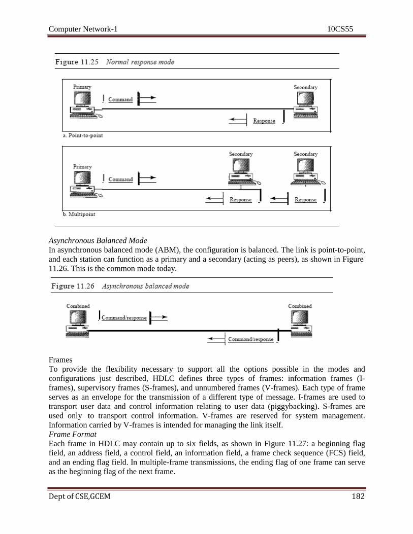
Computer Network-1 10CS55
Dept of CSE,GCEM 182
Asynchronous Balanced Mode
In asynchronous balanced mode (ABM), the configuration is balanced. The link is point-to-point,
and each station can function as a primary and a secondary (acting as peers), as shown in Figure
11.26. This is the common mode today.
Frames
To provide the flexibility necessary to support all the options possible in the modes and
configurations just described, HDLC defines three types of frames: information frames (I-
frames), supervisory frames (S-frames), and unnumbered frames (V-frames). Each type of frame
serves as an envelope for the transmission of a different type of message. I-frames are used to
transport user data and control information relating to user data (piggybacking). S-frames are
used only to transport control information. V-frames are reserved for system management.
Information carried by V-frames is intended for managing the link itself.
Frame Format
Each frame in HDLC may contain up to six fields, as shown in Figure 11.27: a beginning flag
field, an address field, a control field, an information field, a frame check sequence (FCS) field,
and an ending flag field. In multiple-frame transmissions, the ending flag of one frame can serve
as the beginning flag of the next frame.
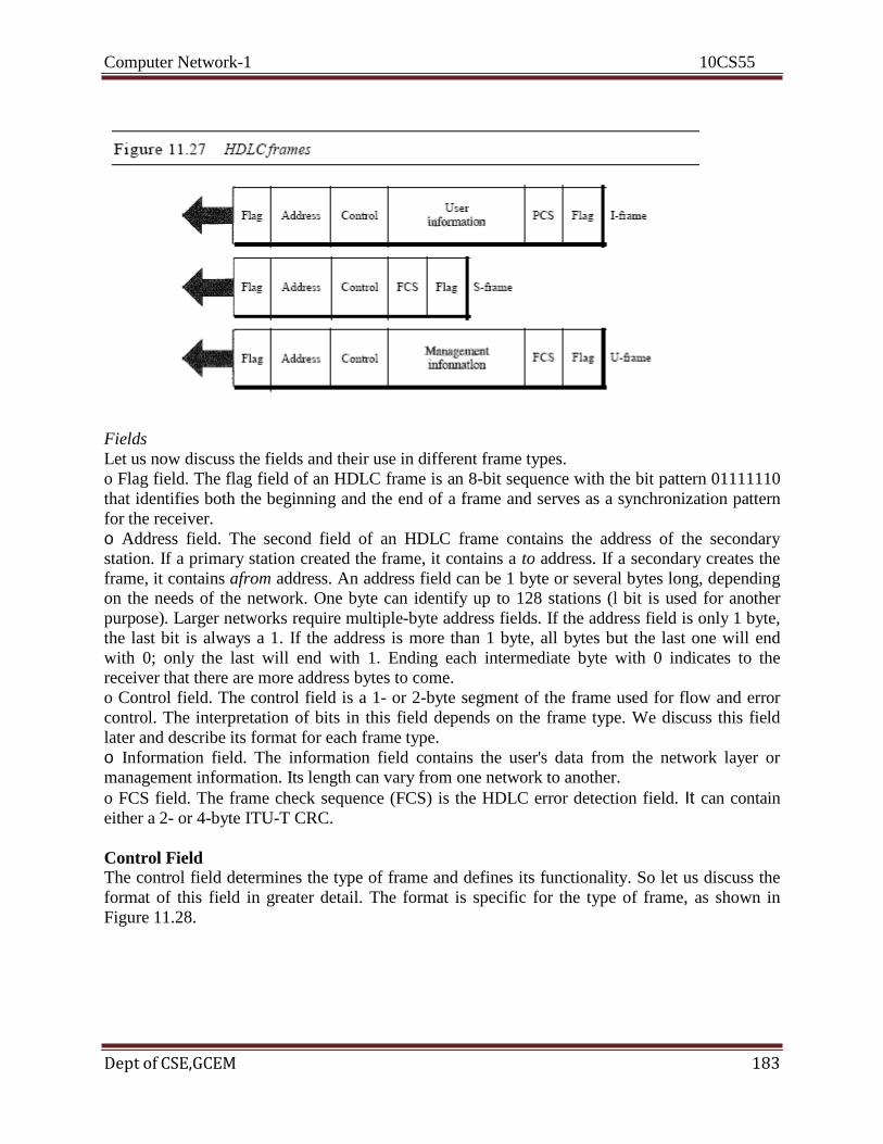
Computer Network-1 10CS55
Dept of CSE,GCEM 183
Fields
Let us now discuss the fields and their use in different frame types.
o Flag field. The flag field of an HDLC frame is an 8-bit sequence with the bit pattern 01111110
that identifies both the beginning and the end of a frame and serves as a synchronization pattern
for the receiver.
o Address field. The second field of an HDLC frame contains the address of the secondary
station. If a primary station created the frame, it contains a to address. If a secondary creates the
frame, it contains afrom address. An address field can be 1 byte or several bytes long, depending
on the needs of the network. One byte can identify up to 128 stations (l bit is used for another
purpose). Larger networks require multiple-byte address fields. If the address field is only 1 byte,
the last bit is always a 1. If the address is more than 1 byte, all bytes but the last one will end
with 0; only the last will end with 1. Ending each intermediate byte with 0 indicates to the
receiver that there are more address bytes to come.
o Control field. The control field is a 1- or 2-byte segment of the frame used for flow and error
control. The interpretation of bits in this field depends on the frame type. We discuss this field
later and describe its format for each frame type.
o Information field. The information field contains the user's data from the network layer or
management information. Its length can vary from one network to another.
o FCS field. The frame check sequence (FCS) is the HDLC error detection field. It can contain
either a 2- or 4-byte ITU-T CRC.
Control Field The control field determines the type of frame and defines its functionality. So let us discuss the
format of this field in greater detail. The format is specific for the type of frame, as shown in
Figure 11.28.

Computer Network-1 10CS55
Dept of CSE,GCEM 184
Control Field for I-Frames
I-frames are designed to carry user data from the network layer. In addition, they can include
flow and error control information (piggybacking). The subfields in the control field are used to
define these functions. The first bit defines the type. If the first bit of the control field is 0, this
means the frame is an I-frame. The next 3 bits, called N(S), define the sequence number of the
frame. Note that with 3 bits, we can define a sequence number between and 7; but in the
extension format, in which the control field is 2 bytes, this field is larger. The last 3 bits, called
N(R), correspond to the acknowledgment number when piggybacking is used. The single bit
between N(S) and N(R) is called the PIF bit. The PIP field is a single bit with a dual purpose. It has meaning only when it is set (bit = 1) and can mean poll or final. It means poll when the
frame is sent by a primary station to a secondary (when the address field contains the address of
the receiver). It means final when the frame is sent by a secondary to a primary (when the
address field contains the address of the sender).
Control Field for S-Frames
Supervisory frames are used for flow and error control whenever piggybacking is either
impossible or inappropriate (e.g., when the station either has no data of its own to send or needs
to send a command or response other than an acknowledgment). S-frames do not have
information fields. If the first 2 bits of the control field is 10, this means the frame is an S-frame.
The last 3 bits, called N(R), corresponds to the acknowledgment number (ACK) or negative
acknowledgment number (NAK) depending on the type of S-frame. The 2 bits called code is
used to define the type of S-frame itself. With 2 bits, we can have four types of S-frames, as
described below:
o Receive ready (RR). If the value of the code subfield is 00, it is an RR S-frame. This kind of
frame acknowledges the receipt of a safe and sound frame or group of frames. In this case, the
value N(R) field defines the acknowledgment number. Receive not ready (RNR). If the value of
the code subfield is 10, it is an RNR S-frame. This kind of frame is an RR frame with additional
functions. It acknowledges the receipt of a frame or group of frames, and it announces that the
receiver is busy and cannot receive more frames. It acts as a kind of congestion control
mechanism by asking the sender to slow down. The value of NCR) is the acknowledgment
number.
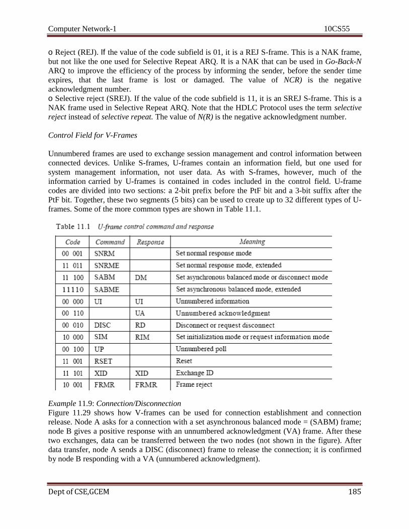
Computer Network-1 10CS55
Dept of CSE,GCEM 185
o Reject (REJ). If the value of the code subfield is 01, it is a REJ S-frame. This is a NAK frame,
but not like the one used for Selective Repeat ARQ. It is a NAK that can be used in Go-Back-N
ARQ to improve the efficiency of the process by informing the sender, before the sender time
expires, that the last frame is lost or damaged. The value of NCR) is the negative
acknowledgment number.
o Selective reject (SREJ). If the value of the code subfield is 11, it is an SREJ S-frame. This is a
NAK frame used in Selective Repeat ARQ. Note that the HDLC Protocol uses the term selective
reject instead of selective repeat. The value of N(R) is the negative acknowledgment number.
Control Field for V-Frames
Unnumbered frames are used to exchange session management and control information between
connected devices. Unlike S-frames, U-frames contain an information field, but one used for
system management information, not user data. As with S-frames, however, much of the
information carried by U-frames is contained in codes included in the control field. U-frame
codes are divided into two sections: a 2-bit prefix before the PtF bit and a 3-bit suffix after the
PtF bit. Together, these two segments (5 bits) can be used to create up to 32 different types of U-
frames. Some of the more common types are shown in Table 11.1.
Example 11.9: Connection/Disconnection
Figure 11.29 shows how V-frames can be used for connection establishment and connection
release. Node A asks for a connection with a set asynchronous balanced mode = (SABM) frame;
node B gives a positive response with an unnumbered acknowledgment (VA) frame. After these
two exchanges, data can be transferred between the two nodes (not shown in the figure). After
data transfer, node A sends a DISC (disconnect) frame to release the connection; it is confirmed
by node B responding with a VA (unnumbered acknowledgment).

Computer Network-1 10CS55
Dept of CSE,GCEM 186
Example 11.10: Piggybacking without Error
Figure 11.30 shows an exchange using piggybacking. Node A begins the exchange of
information with an I-frame numbered 0 followed by another I-frame numbered 1. Node B
piggybacks its acknowledgment of both frames onto an I-frame of its own. Node B's first I-frame
is also numbered 0 [N(S) field] and contains a 2 in its N(R) field, acknowledging the receipt of
Ns frames 1 and 0 and indicating that it expects frame 2 to arrive next. Node B transmits its
second and third I-frames (numbered 1 and 2) before accepting further frames from node A. Its
N(R) information, therefore, has not changed: B frames 1 and 2 indicate that node B is still
expecting Ns frame 2 to arrive next. Node A has sent all its data. Therefore, it cannot piggyback
an acknowledgment onto an I-frame and sends an S-frame
instead. The RR code indicates that A is still ready to receive. The number 3 in the N(R) field
tells B that frames 0, 1, and 2 have all been accepted and that A is now expecting frame number
3.

Computer Network-1 10CS55
Dept of CSE,GCEM 187
Example 11.11: Piggybacking with Error
Figure 11.31 shows an exchange in which a frame is lost. Node B sends three data frames (0, 1,
and 2), but frame 1 is lost. When node A receives frame 2, it discards it and sends a REI frame
for frame 1. Note that the protocol being used is Go-Back-N with the special use of an REI frame
as a NAK frame. The NAK frame does two things here: It confirms the receipt of frame and
declares that frame 1 and any following frames must be resent. Node B, after receiving the REI
frame, resends frames 1 and 2. Node A acknowledges the receipt by sending an RR frame (ACK)
with acknowledgment number 3.
11.7 POINT-TO-POINT PROTOCOL
Although HDLC is a general protocol that can be used for both point-to-point and multipoint
configurations, one of the most common protocols for point-to-point access is the Point-to-Point
Protocol (PPP). Today, millions of Internet users who need to connect their home computers to
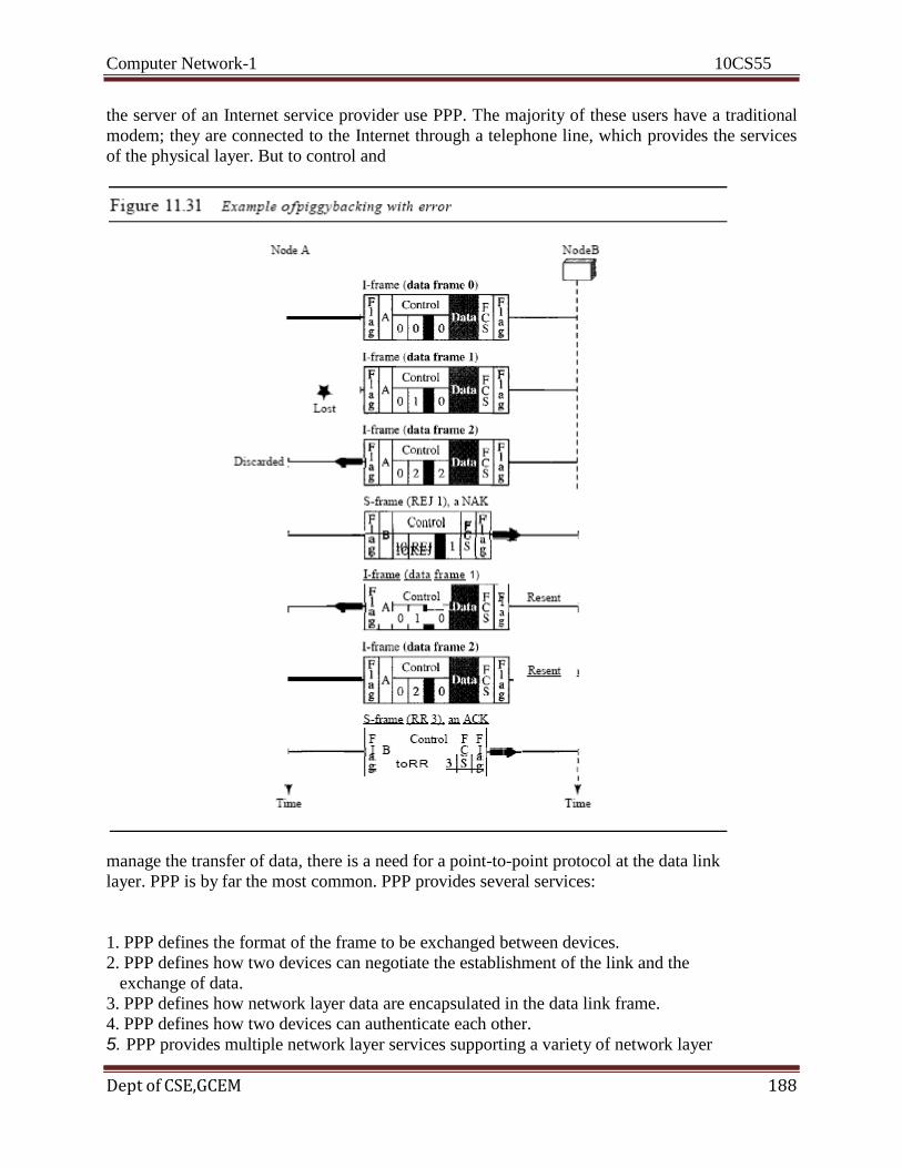
Computer Network-1 10CS55
Dept of CSE,GCEM 188
the server of an Internet service provider use PPP. The majority of these users have a traditional
modem; they are connected to the Internet through a telephone line, which provides the services
of the physical layer. But to control and
manage the transfer of data, there is a need for a point-to-point protocol at the data link
layer. PPP is by far the most common. PPP provides several services:
1. PPP defines the format of the frame to be exchanged between devices.
2. PPP defines how two devices can negotiate the establishment of the link and the
exchange of data.
3. PPP defines how network layer data are encapsulated in the data link frame.
4. PPP defines how two devices can authenticate each other.
5. PPP provides multiple network layer services supporting a variety of network layer
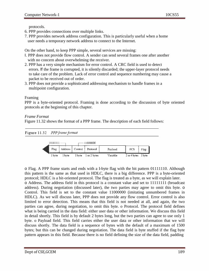
Computer Network-1 10CS55
Dept of CSE,GCEM 189
protocols.
6. PPP provides connections over multiple links.
7. PPP provides network address configuration. This is particularly useful when a home
user needs a temporary network address to connect to the Internet.
On the other hand, to keep PPP simple, several services are missing:
I. PPP does not provide flow control. A sender can send several frames one after another
with no concern about overwhelming the receiver. 2. PPP has a very simple mechanism for error control. A CRC field is used to detect
errors. If the frame is corrupted, it is silently discarded; the upper-layer protocol needs
to take care of the problem. Lack of error control and sequence numbering may cause a
packet to be received out of order.
3. PPP does not provide a sophisticated addressing mechanism to handle frames in a
multipoint configuration.
Framing
PPP is a byte-oriented protocol. Framing is done according to the discussion of byte oriented
protocols at the beginning of this chapter.
Frame Format
Figure 11.32 shows the format of a PPP frame. The description of each field follows:
o Flag. A PPP frame starts and ends with a I-byte flag with the bit pattern 01111110. Although
this pattern is the same as that used in HDLC, there is a big difference. PPP is a byte-oriented
protocol; HDLC is a bit-oriented protocol. The flag is treated as a byte, as we will explain later.
o Address. The address field in this protocol is a constant value and set to 11111111 (broadcast
address). During negotiation (discussed later), the two parties may agree to omit this byte. o Control. This field is set to the constant value 11000000 (imitating unnumbered frames in
HDLC). As we will discuss later, PPP does not provide any flow control. Error control is also
limited to error detection. This means that this field is not needed at all, and again, the two
parties can agree, during negotiation, to omit this byte. o Protocol. The protocol field defines
what is being carried in the data field: either user data or other information. We discuss this field
in detail shortly. This field is by default 2 bytes long, but the two parties can agree to use only 1
byte. o Payload field. This field carries either the user data or other information that we will
discuss shortly. The data field is a sequence of bytes with the default of a maximum of 1500
bytes; but this can be changed during negotiation. The data field is byte stuffed if the flag byte
pattern appears in this field. Because there is no field defining the size of the data field, padding

Computer Network-1 10CS55
Dept of CSE,GCEM 190
is needed if the size is less than the maximum default value or the maximum negotiated value. o
FCS. The frame check sequence (FCS) is simply a 2-byte or 4-byte standard CRe.
Byte Stuffing
The similarity between PPP and ends at the frame format. PPP, as we discussed before, is a
byte-oriented protocol totally different from HDLC. As a byte-oriented protocol, the flag in PPP
is a byte and needs to be escaped whenever it appears in the data section of the frame. The
escape byte is 01111101, which means that every time the flag like pattern appears in the data,
this extra byte is stuffed to tell the receiver that the next byte is not a flag.
Transition Phases
A PPP connection goes through phases which can be shown in a transition phase diagram (see
Figure 11.33).
Dead. In the dead phase the link is not being used. There is no active carrier (at the physical
layer) and the line is quiet.
D Establish. When one of the nodes starts the communication, the connection goes into this
phase. In this phase, options are negotiated between the two parties. If the negotiation is
successful, the system goes to the authentication phase (if authentication is required) or directly
to the networking phase. The link control protocol packets, discussed shortly, are used for this
purpose. Several packets may be exchanged here. D Authenticate. The authentication phase is
optional; the two nodes may decide, during the establishment phase, not to skip this phase.
However, if they decide to proceed with authentication, they send several authentication packets,
discussed later. If the result is successful, the connection goes to the networking phase;
otherwise, it goes to the termination phase. D Network. In the network phase, negotiation for the
network layer protocols takes place. PPP specifies that two nodes establish a network layer
agreement before data at the network layer can be exchanged. The reason is that PPP supports
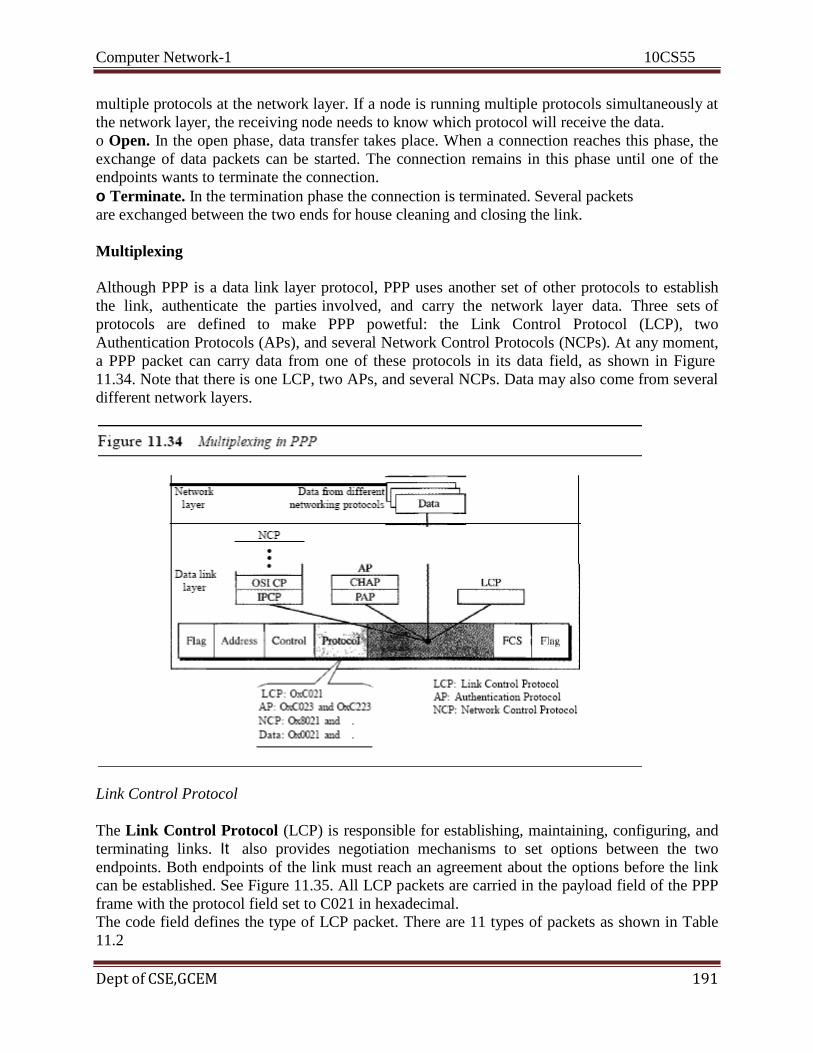
Computer Network-1 10CS55
Dept of CSE,GCEM 191
multiple protocols at the network layer. If a node is running multiple protocols simultaneously at
the network layer, the receiving node needs to know which protocol will receive the data.
o Open. In the open phase, data transfer takes place. When a connection reaches this phase, the
exchange of data packets can be started. The connection remains in this phase until one of the
endpoints wants to terminate the connection.
o Terminate. In the termination phase the connection is terminated. Several packets
are exchanged between the two ends for house cleaning and closing the link.
Multiplexing
Although PPP is a data link layer protocol, PPP uses another set of other protocols to establish
the link, authenticate the parties involved, and carry the network layer data. Three sets of
protocols are defined to make PPP powetful: the Link Control Protocol (LCP), two
Authentication Protocols (APs), and several Network Control Protocols (NCPs). At any moment,
a PPP packet can carry data from one of these protocols in its data field, as shown in Figure
11.34. Note that there is one LCP, two APs, and several NCPs. Data may also come from several
different network layers.
Link Control Protocol
The Link Control Protocol (LCP) is responsible for establishing, maintaining, configuring, and
terminating links. It also provides negotiation mechanisms to set options between the two
endpoints. Both endpoints of the link must reach an agreement about the options before the link
can be established. See Figure 11.35. All LCP packets are carried in the payload field of the PPP
frame with the protocol field set to C021 in hexadecimal.
The code field defines the type of LCP packet. There are 11 types of packets as shown in Table
11.2

Computer Network-1 10CS55
Dept of CSE,GCEM 192
There are three categories of packets. The first category, comprising the first four packet types, is
used for link configuration during the establish phase. The second category, comprising packet
types 5 and 6, is used for link termination during the termination phase. The last five packets are
used for link monitoring and debugging. The ID field holds a value that matches a request with a
reply. One endpoint inserts a value in this field, which will be copied into the reply packet. The
length field defines the length of the entire LCP packet. The information field contains
information, such as options, needed for some LCP packets. There are many options that can be
negotiated between the two endpoints. Options are inserted in the information field of the
configuration packets. In this case, the information field is divided into three fields: option type,
option length, and option data.
Authentication Protocols
Authentication plays a very important role in PPP because PPP is designed for use over dial-up
links where verification of user identity is necessary. Authentication means validating the
identity of a user who needs to access a set of resources. PPP has created two protocols for
authentication: Password Authentication Protocol and Challenge Handshake Authentication
Protocol. Note that these protocols are used during the authentication phase.

Computer Network-1 10CS55
Dept of CSE,GCEM 193
PAP The Password Authentication Protocol (PAP) is a simple authentication procedure with a
two-step process:
1. The user who wants to access a system sends an authentication identification (usually the user
name) and a password.
2. The system checks the validity of the identification and password and either accepts or denies
connection.
Figure 11.36 shows the three types of packets used by PAP and how they are actually exchanged.
When a PPP frame is carrying any PAP packets, the value of the protocol field is OxC023. The
three PAP packets are authenticate-request, authenticate-ack, and authenticate-nak. The first
packet is used by the user to send the user name and password. The second is used by the system
to allow access. The third is used by the system to deny access.
CHAP The Challenge Handshake Authentication Protocol (CHAP) is a three-way hand-
shaking authentication protocol that provides greater security than PAP. In this method, the
password is kept secret; it is never sent online.
1. The system sends the user a challenge packet containing a challenge value, usually a few
bytes.
2. The user applies a predefined function that takes the challenge value and the user's own
password and creates a result. The user sends the result in the response packet to the system.
3. The system does the same. It applies the same function to the password of the user (known to
the system) and the challenge value to create a result. If the result created is the same as the
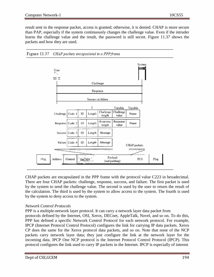
Computer Network-1 10CS55
Dept of CSE,GCEM 194
result sent in the response packet, access is granted; otherwise, it is denied. CHAP is more secure
than PAP, especially if the system continuously changes the challenge value. Even if the intruder
learns the challenge value and the result, the password is still secret. Figure 11.37 shows the
packets and how they are used.
CHAP packets are encapsulated in the PPP frame with the protocol value C223 in hexadecimal.
There are four CHAP packets: challenge, response, success, and failure. The first packet is used
by the system to send the challenge value. The second is used by the user to return the result of
the calculation. The third is used by the system to allow access to the system. The fourth is used
by the system to deny access to the system.
Network Control Protocols
PPP is a multiple-network layer protocol. It can carry a network layer data packet from
protocols defined by the Internet, OSI, Xerox, DECnet, AppleTalk, Novel, and so on. To do this,
PPP has defined a specific Network Control Protocol for each network protocol. For example,
IPCP (Internet Protocol Control Protocol) configures the link for carrying IP data packets. Xerox
CP does the same for the Xerox protocol data packets, and so on. Note that none of the NCP
packets carry network layer data; they just configure the link at the network layer for the
incoming data. IPCP One NCP protocol is the Internet Protocol Control Protocol (IPCP). This
protocol configures the link used to carry IP packets in the Internet. IPCP is especially of interest

Computer Network-1 10CS55
Dept of CSE,GCEM 195
to us. The format of an IPCP packet is shown in Figure 11.38. Note that the value of the protocol
field in hexadecimal is 8021.
Other Protocols There are other NCP protocols for other network layer protocols. The OSI
Network Layer Control Protocol has a protocol field value of 8023; the Xerox NS IDP Control
Protocol has a protocol field value of 8025; and so on. The value of the code and the format of
the packets for these other protocols are the same as shown in Table 11.4.
Data/rom the Network Layer
After the network layer configuration is completed by one of the NCP protocols, the users can
exchange data packets from the network layer. Here again, there are different protocol fields for
different network layers. For example, if PPP is carrying data from the IP network layer, the field
value is 0021 (note that the three rightmost digits are the same as for IPCP). If PPP is carrying
data from the OSI network layer, the value of the protocol field is 0023, and so on. Figure 11.39
shows the frame for IP.
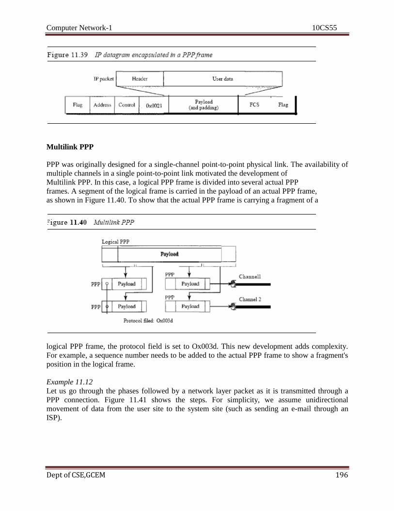
Computer Network-1 10CS55
Dept of CSE,GCEM 196
Multilink PPP
PPP was originally designed for a single-channel point-to-point physical link. The availability of
multiple channels in a single point-to-point link motivated the development of
Multilink PPP. In this case, a logical PPP frame is divided into several actual PPP
frames. A segment of the logical frame is carried in the payload of an actual PPP frame,
as shown in Figure 11.40. To show that the actual PPP frame is carrying a fragment of a
logical PPP frame, the protocol field is set to Ox003d. This new development adds complexity.
For example, a sequence number needs to be added to the actual PPP frame to show a fragment's
position in the logical frame.
Example 11.12
Let us go through the phases followed by a network layer packet as it is transmitted through a
PPP connection. Figure 11.41 shows the steps. For simplicity, we assume unidirectional
movement of data from the user site to the system site (such as sending an e-mail through an
ISP).

Computer Network-1 10CS55
Dept of CSE,GCEM 197

Computer Network-1 10CS55
Dept of CSE,GCEM 198
The first two frames show link establishment. We have chosen two options (not shown in the
figure): using PAP for authentication and suppressing the address control fields Frames 3 and 4
are for authentication. Frames 5 and 6 establish the network layer connection using IPCP. The
next several frames show that some IP packets are encapsulated in the PPP frame. The system
(receiver) may have been running several network layer protocols, but it knows that the
incoming data must be delivered to the IP protocol because the NCP protocol used before the
data transfer was IPCP. After data transfer, the user then terminates the data link connection,
which is acknowledged by the system. of Course the user or the system could have chosen to
terminate the network layer IPCP and keep the data link layer running if it wanted to run another
NCP protocol. The example is trivial, but it points out the similarities of the packets in LCP, AP,
and NCP. It also shows the protocol field values and code numbers for particular protocols
Recommended Questions
1. Define framing and the reason for its need
2. Compare and contrast flow control and error control 3. What are the two protocols we discussed for noiseless channels in this
chapter?
4. Explain the reason for moving from the Stop-and-Wait ARQ Protocol to
the 00Back NARQ Protocol
5. Compare and contrast the Go-Back-NARQ Protocol with Selective-
RepeatARQ
6. ompare and contrast HDLC with PPP. Which one is byte-oriented;
which one is bit oriented.
7. Define piggybacking and its usefulness
8. Which of the protocols described in this chapter utilize pipelining?

Computer Network-1 10CS55
Dept of CSE,GCEM 199
COMPUTER NETWORKS – I
Subject Code: 10CS55 I.A. Marks : 25
Hours/Week : 04 Exam Hours: 03
Total Hours : 52 Exam Marks: 100
UNIT- 6 7 Hours Multiple Access & Ethernet:
- Random access,
- Controlled Access,
- Channelization,
- Ethernet: IEEE standards,
- Standard Ethernet,
- Changes in the standard,
- Fast Ethernet, - Gigabit Ethernet

Computer Network-1 10CS55
Dept of CSE,GCEM 200
UNIT – VI
Chapter 5 Wired
LANs: Ethernet
5.1 IEEE STANDARDS
The relationship of the 802 Standard to the traditional OSI model is shown in the figure.
The IEEE has subdivided the data link layer into two sublayers: logical link control (LLC) and
media access control (MAC). IEEE has also created several physical layer standards for different
LAN protocols.
Data Link Layer
The data link layer in the IEEE standard is divided into two sublayers: LLC and MAC.
Logical Link Control (LLC)
In IEEE Project 802, flow control, error control, and part of the framing duties are collected
into one sublayer called the logical link control. Framing is handled in both the LLC sublayer
and the MAC sublayer.
The LLC provides one single data link control protocol for all IEEE LANs. In this way, the
LLC is different from the media access control sublayer, which provides different protocols for
different LANs. A single LLC protocol can provide interconnectivity between different LANs
because it makes the MAC sublayer transparent.

Computer Network-1 10CS55
Dept of CSE, GCEM 200
UNIT – VI
Chapter 5 Wired
LANs: Ethernet
5.1 IEEE STANDARDS
The relationship of the 802 Standard to the traditional OSI model is shown in the figure.
The IEEE has subdivided the data link layer into two sublayers: logical link control (LLC) and
media access control (MAC). IEEE has also created several physical layer standards for different
LAN protocols.
Data Link Layer
The data link layer in the IEEE standard is divided into two sublayers: LLC and MAC.
Logical Link Control (LLC)
In IEEE Project 802, flow control, error control, and part of the framing duties are collected
into one sublayer called the logical link control. Framing is handled in both the LLC sublayer
and the MAC sublayer.
The LLC provides one single data link control protocol for all IEEE LANs. In this way, the
LLC is different from the media access control sublayer, which provides different protocols for
different LANs. A single LLC protocol can provide interconnectivity between different LANs
because it makes the MAC sublayer transparent.
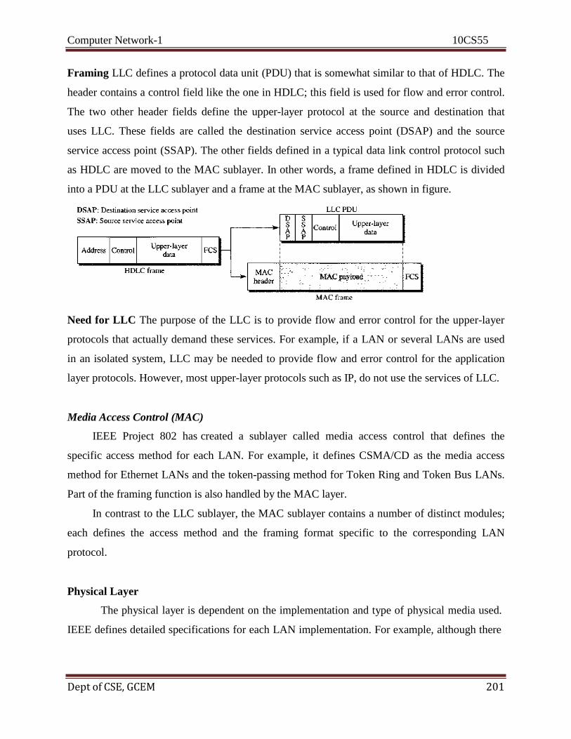
Computer Network-1 10CS55
Dept of CSE, GCEM 201
Framing LLC defines a protocol data unit (PDU) that is somewhat similar to that of HDLC. The
header contains a control field like the one in HDLC; this field is used for flow and error control.
The two other header fields define the upper-layer protocol at the source and destination that
uses LLC. These fields are called the destination service access point (DSAP) and the source
service access point (SSAP). The other fields defined in a typical data link control protocol such
as HDLC are moved to the MAC sublayer. In other words, a frame defined in HDLC is divided
into a PDU at the LLC sublayer and a frame at the MAC sublayer, as shown in figure.
Need for LLC The purpose of the LLC is to provide flow and error control for the upper-layer
protocols that actually demand these services. For example, if a LAN or several LANs are used
in an isolated system, LLC may be needed to provide flow and error control for the application
layer protocols. However, most upper-layer protocols such as IP, do not use the services of LLC.
Media Access Control (MAC)
IEEE Project 802 has created a sublayer called media access control that defines the
specific access method for each LAN. For example, it defines CSMA/CD as the media access
method for Ethernet LANs and the token-passing method for Token Ring and Token Bus LANs.
Part of the framing function is also handled by the MAC layer.
In contrast to the LLC sublayer, the MAC sublayer contains a number of distinct modules;
each defines the access method and the framing format specific to the corresponding LAN
protocol.
Physical Layer
The physical layer is dependent on the implementation and type of physical media used.
IEEE defines detailed specifications for each LAN implementation. For example, although there

Computer Network-1 10CS55
Dept of CSE, GCEM 202
is only one MAC sublayer for Standard Ethernet, there is a different physical layer specification
for each Ethernet implementations.
5.2 STANDARD ETHERNET
The original Ethernet was created in 1976 at Xerox's Palo Alto Research Center (PARC).
Since then, it has gone through four generations: Standard Ethernet (10 t Mbps), Fast Ethernet
(100 Mbps), Gigabit Ethernet (1 Gbps), and Ten-Gigabit Ethernet (10 Gbps), as shown in the
figure:
MAC Sublayer
In Standard Ethernet, the MAC sublayer governs the operation of the access method. It
also frames data received from the upper layer and passes them to the physical layer.
Frame Format
The Ethernet frame contains seven fields: preamble, SFD, DA, SA, length or type of
protocol data unit (PDU), upper-layer data, and the CRC. Ethernet does not provide any
mechanism for acknowledging received frames, making it what is known as an unreliable
medium. Acknowledgments must be implemented at the higher layers. The format of the MAC
frame is shown in the figure.
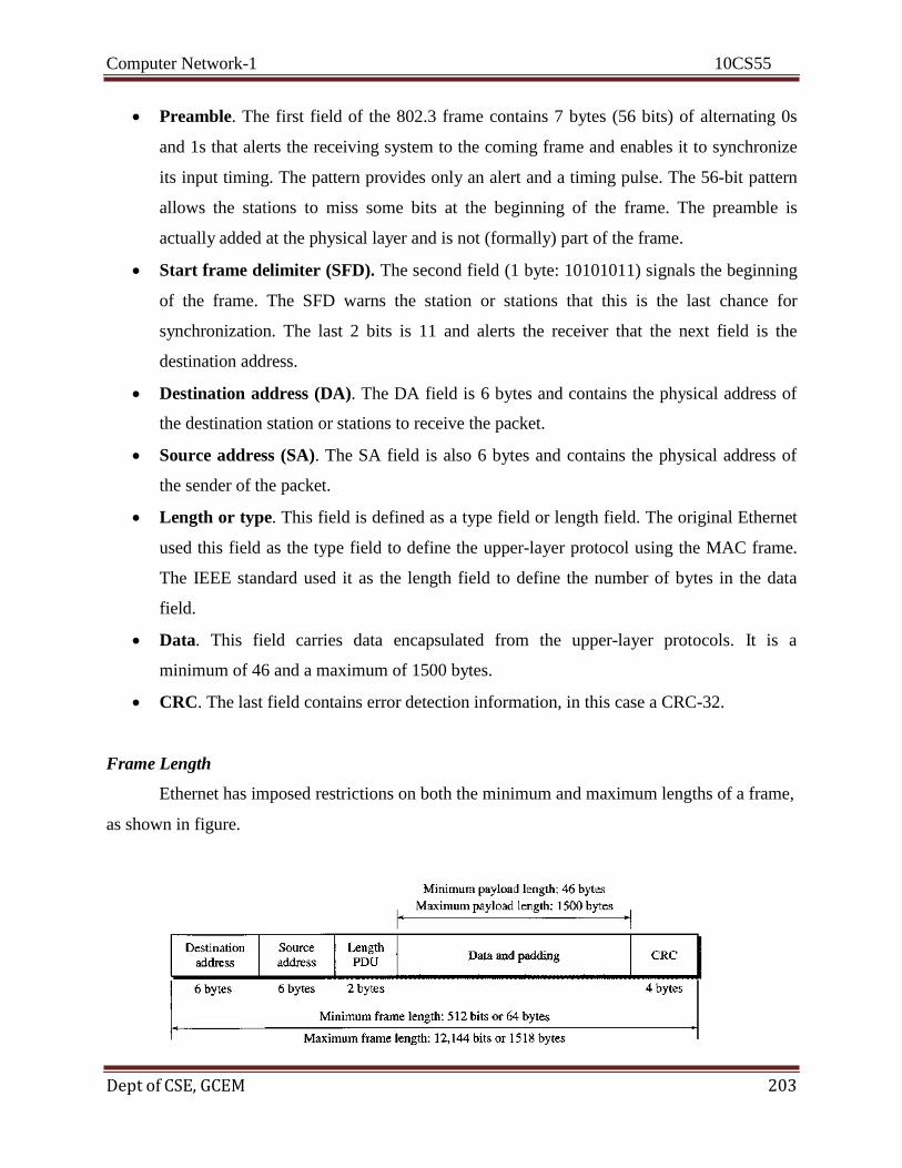
Computer Network-1 10CS55
Dept of CSE, GCEM 203
Preamble. The first field of the 802.3 frame contains 7 bytes (56 bits) of alternating 0s
and 1s that alerts the receiving system to the coming frame and enables it to synchronize
its input timing. The pattern provides only an alert and a timing pulse. The 56-bit pattern
allows the stations to miss some bits at the beginning of the frame. The preamble is
actually added at the physical layer and is not (formally) part of the frame.
Start frame delimiter (SFD). The second field (1 byte: 10101011) signals the beginning
of the frame. The SFD warns the station or stations that this is the last chance for
synchronization. The last 2 bits is 11 and alerts the receiver that the next field is the
destination address.
Destination address (DA). The DA field is 6 bytes and contains the physical address of
the destination station or stations to receive the packet.
Source address (SA). The SA field is also 6 bytes and contains the physical address of
the sender of the packet.
Length or type. This field is defined as a type field or length field. The original Ethernet
used this field as the type field to define the upper-layer protocol using the MAC frame.
The IEEE standard used it as the length field to define the number of bytes in the data
field.
Data. This field carries data encapsulated from the upper-layer protocols. It is a
minimum of 46 and a maximum of 1500 bytes.
CRC. The last field contains error detection information, in this case a CRC-32.
Frame Length
Ethernet has imposed restrictions on both the minimum and maximum lengths of a frame,
as shown in figure.
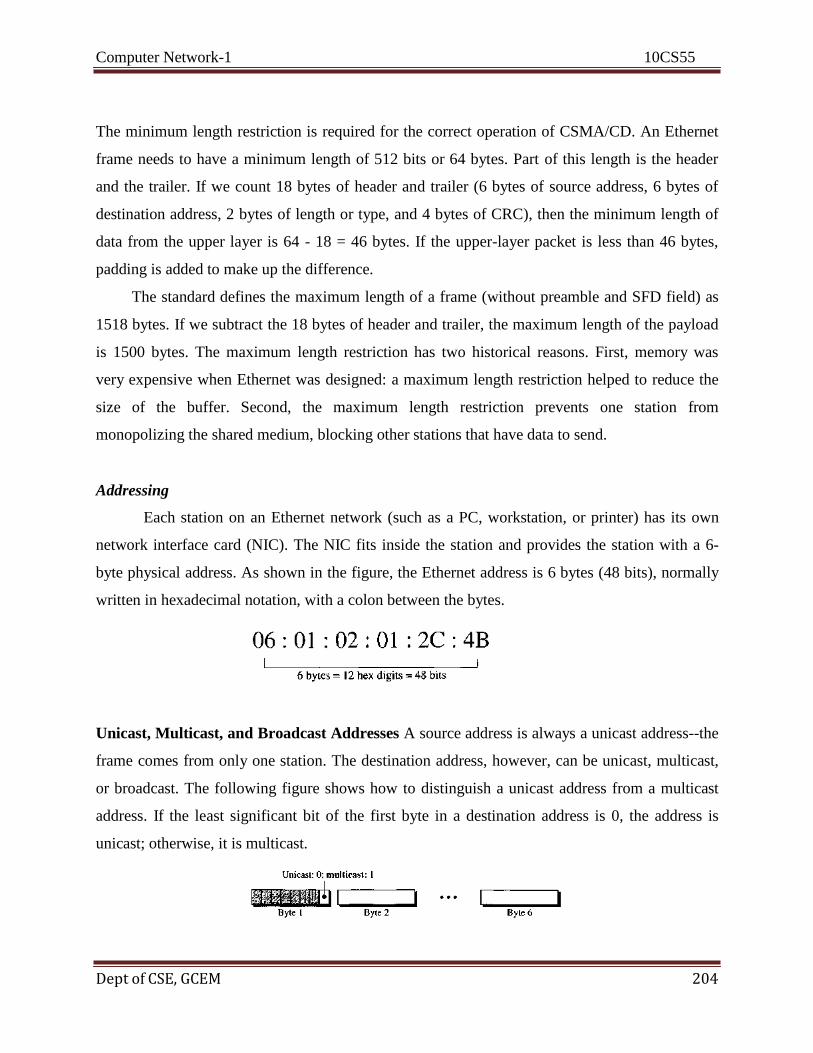
Computer Network-1 10CS55
Dept of CSE, GCEM 204
The minimum length restriction is required for the correct operation of CSMA/CD. An Ethernet
frame needs to have a minimum length of 512 bits or 64 bytes. Part of this length is the header
and the trailer. If we count 18 bytes of header and trailer (6 bytes of source address, 6 bytes of
destination address, 2 bytes of length or type, and 4 bytes of CRC), then the minimum length of
data from the upper layer is 64 - 18 = 46 bytes. If the upper-layer packet is less than 46 bytes,
padding is added to make up the difference.
The standard defines the maximum length of a frame (without preamble and SFD field) as
1518 bytes. If we subtract the 18 bytes of header and trailer, the maximum length of the payload
is 1500 bytes. The maximum length restriction has two historical reasons. First, memory was
very expensive when Ethernet was designed: a maximum length restriction helped to reduce the
size of the buffer. Second, the maximum length restriction prevents one station from
monopolizing the shared medium, blocking other stations that have data to send.
Addressing
Each station on an Ethernet network (such as a PC, workstation, or printer) has its own
network interface card (NIC). The NIC fits inside the station and provides the station with a 6-
byte physical address. As shown in the figure, the Ethernet address is 6 bytes (48 bits), normally
written in hexadecimal notation, with a colon between the bytes.
Unicast, Multicast, and Broadcast Addresses A source address is always a unicast address--the
frame comes from only one station. The destination address, however, can be unicast, multicast,
or broadcast. The following figure shows how to distinguish a unicast address from a multicast
address. If the least significant bit of the first byte in a destination address is 0, the address is
unicast; otherwise, it is multicast.
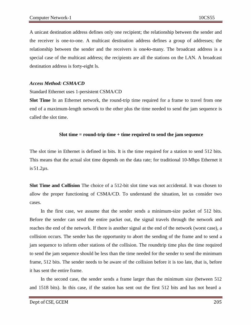
Computer Network-1 10CS55
Dept of CSE, GCEM 205
A unicast destination address defines only one recipient; the relationship between the sender and
the receiver is one-to-one. A multicast destination address defines a group of addresses; the
relationship between the sender and the receivers is one4o-many. The broadcast address is a
special case of the multicast address; the recipients are all the stations on the LAN. A broadcast
destination address is forty-eight ls.
Access Method: CSMA/CD
Standard Ethernet uses 1-persistent CSMA/CD
Slot Time In an Ethernet network, the round-trip time required for a frame to travel from one
end of a maximum-length network to the other plus the time needed to send the jam sequence is
called the slot time.
Slot time = round-trip time + time required to send the jam sequence
The slot time in Ethernet is defined in bits. It is the time required for a station to send 512 bits.
This means that the actual slot time depends on the data rate; for traditional 10-Mbps Ethernet it
is 51.2µs.
Slot Time and Collision The choice of a 512-bit slot time was not accidental. It was chosen to
allow the proper functioning of CSMA/CD. To understand the situation, let us consider two
cases.
In the first case, we assume that the sender sends a minimum-size packet of 512 bits.
Before the sender can send the entire packet out, the signal travels through the network and
reaches the end of the network. If there is another signal at the end of the network (worst case), a
collision occurs. The sender has the opportunity to abort the sending of the frame and to send a
jam sequence to inform other stations of the collision. The roundtrip time plus the time required
to send the jam sequence should be less than the time needed for the sender to send the minimum
frame, 512 bits. The sender needs to be aware of the collision before it is too late, that is, before
it has sent the entire frame.
In the second case, the sender sends a frame larger than the minimum size (between 512
and 1518 bits). In this case, if the station has sent out the first 512 bits and has not heard a
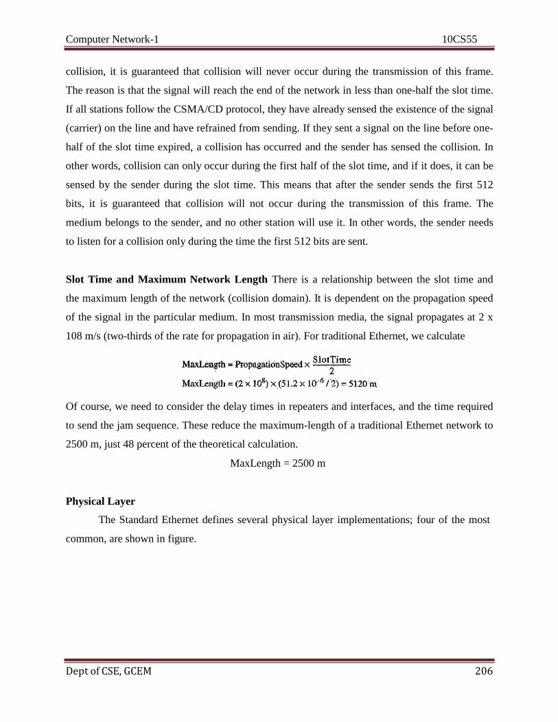
Computer Network-1 10CS55
Dept of CSE, GCEM 206
collision, it is guaranteed that collision will never occur during the transmission of this frame.
The reason is that the signal will reach the end of the network in less than one-half the slot time.
If all stations follow the CSMA/CD protocol, they have already sensed the existence of the signal
(carrier) on the line and have refrained from sending. If they sent a signal on the line before one-
half of the slot time expired, a collision has occurred and the sender has sensed the collision. In
other words, collision can only occur during the first half of the slot time, and if it does, it can be
sensed by the sender during the slot time. This means that after the sender sends the first 512
bits, it is guaranteed that collision will not occur during the transmission of this frame. The
medium belongs to the sender, and no other station will use it. In other words, the sender needs
to listen for a collision only during the time the first 512 bits are sent.
Slot Time and Maximum Network Length There is a relationship between the slot time and
the maximum length of the network (collision domain). It is dependent on the propagation speed
of the signal in the particular medium. In most transmission media, the signal propagates at 2 x
108 m/s (two-thirds of the rate for propagation in air). For traditional Ethernet, we calculate
Of course, we need to consider the delay times in repeaters and interfaces, and the time required
to send the jam sequence. These reduce the maximum-length of a traditional Ethernet network to
2500 m, just 48 percent of the theoretical calculation.
MaxLength = 2500 m
Physical Layer
The Standard Ethernet defines several physical layer implementations; four of the most
common, are shown in figure.
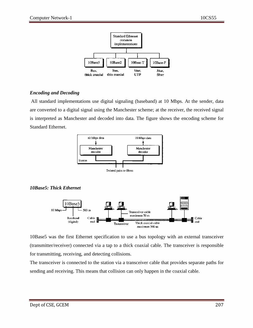
Computer Network-1 10CS55
Dept of CSE, GCEM 207
Encoding and Decoding
All standard implementations use digital signaling (baseband) at 10 Mbps. At the sender, data
are converted to a digital signal using the Manchester scheme; at the receiver, the received signal
is interpreted as Manchester and decoded into data. The figure shows the encoding scheme for
Standard Ethernet.
10Base5: Thick Ethernet
10Base5 was the first Ethernet specification to use a bus topology with an external transceiver
(transmitter/receiver) connected via a tap to a thick coaxial cable. The transceiver is responsible
for transmitting, receiving, and detecting collisions.
The transceiver is connected to the station via a transceiver cable that provides separate paths for
sending and receiving. This means that collision can only happen in the coaxial cable.
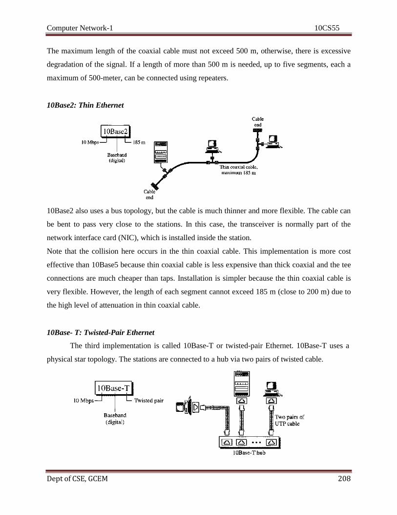
Computer Network-1 10CS55
Dept of CSE, GCEM 208
The maximum length of the coaxial cable must not exceed 500 m, otherwise, there is excessive
degradation of the signal. If a length of more than 500 m is needed, up to five segments, each a
maximum of 500-meter, can be connected using repeaters.
10Base2: Thin Ethernet
10Base2 also uses a bus topology, but the cable is much thinner and more flexible. The cable can
be bent to pass very close to the stations. In this case, the transceiver is normally part of the
network interface card (NIC), which is installed inside the station.
Note that the collision here occurs in the thin coaxial cable. This implementation is more cost
effective than 10Base5 because thin coaxial cable is less expensive than thick coaxial and the tee
connections are much cheaper than taps. Installation is simpler because the thin coaxial cable is
very flexible. However, the length of each segment cannot exceed 185 m (close to 200 m) due to
the high level of attenuation in thin coaxial cable.
10Base- T: Twisted-Pair Ethernet
The third implementation is called 10Base-T or twisted-pair Ethernet. 10Base-T uses a
physical star topology. The stations are connected to a hub via two pairs of twisted cable.
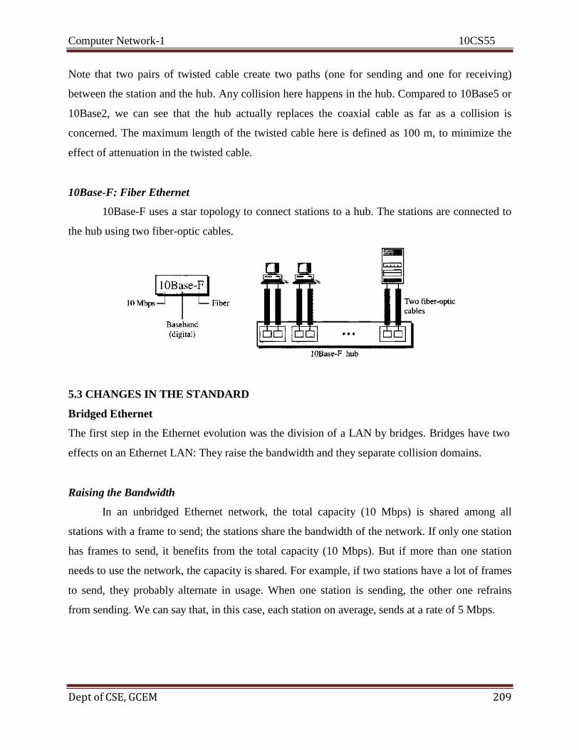
Computer Network-1 10CS55
Dept of CSE, GCEM 209
Note that two pairs of twisted cable create two paths (one for sending and one for receiving)
between the station and the hub. Any collision here happens in the hub. Compared to 10Base5 or
10Base2, we can see that the hub actually replaces the coaxial cable as far as a collision is
concerned. The maximum length of the twisted cable here is defined as 100 m, to minimize the
effect of attenuation in the twisted cable.
10Base-F: Fiber Ethernet
10Base-F uses a star topology to connect stations to a hub. The stations are connected to
the hub using two fiber-optic cables.
5.3 CHANGES IN THE STANDARD
Bridged Ethernet
The first step in the Ethernet evolution was the division of a LAN by bridges. Bridges have two
effects on an Ethernet LAN: They raise the bandwidth and they separate collision domains.
Raising the Bandwidth
In an unbridged Ethernet network, the total capacity (10 Mbps) is shared among all
stations with a frame to send; the stations share the bandwidth of the network. If only one station
has frames to send, it benefits from the total capacity (10 Mbps). But if more than one station
needs to use the network, the capacity is shared. For example, if two stations have a lot of frames
to send, they probably alternate in usage. When one station is sending, the other one refrains
from sending. We can say that, in this case, each station on average, sends at a rate of 5 Mbps.
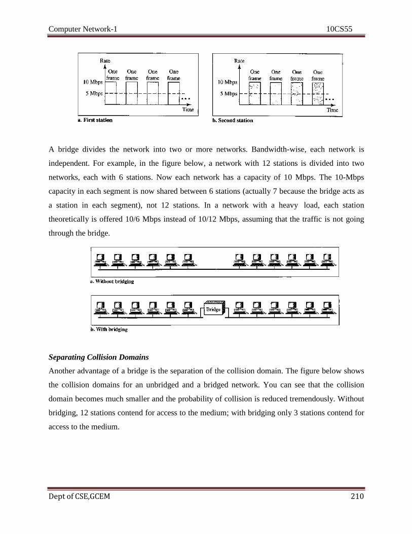
Computer Network-1 10CS55
Dept of CSE,GCEM 210
A bridge divides the network into two or more networks. Bandwidth-wise, each network is
independent. For example, in the figure below, a network with 12 stations is divided into two
networks, each with 6 stations. Now each network has a capacity of 10 Mbps. The 10-Mbps
capacity in each segment is now shared between 6 stations (actually 7 because the bridge acts as
a station in each segment), not 12 stations. In a network with a heavy load, each station
theoretically is offered 10/6 Mbps instead of 10/12 Mbps, assuming that the traffic is not going
through the bridge.
Separating Collision Domains
Another advantage of a bridge is the separation of the collision domain. The figure below shows
the collision domains for an unbridged and a bridged network. You can see that the collision
domain becomes much smaller and the probability of collision is reduced tremendously. Without
bridging, 12 stations contend for access to the medium; with bridging only 3 stations contend for
access to the medium.
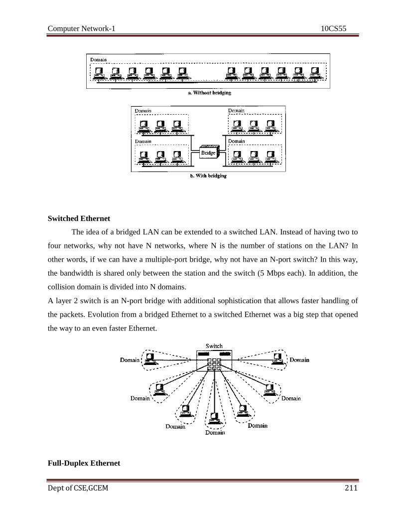
Computer Network-1 10CS55
Dept of CSE,GCEM 211
Switched Ethernet
The idea of a bridged LAN can be extended to a switched LAN. Instead of having two to
four networks, why not have N networks, where N is the number of stations on the LAN? In
other words, if we can have a multiple-port bridge, why not have an N-port switch? In this way,
the bandwidth is shared only between the station and the switch (5 Mbps each). In addition, the
collision domain is divided into N domains.
A layer 2 switch is an N-port bridge with additional sophistication that allows faster handling of
the packets. Evolution from a bridged Ethernet to a switched Ethernet was a big step that opened
the way to an even faster Ethernet.
Full-Duplex Ethernet

Computer Network-1 10CS55
Dept of CSE,GCEM 212
One of the limitations of 10Base5 and 10Base2 is that communication is half-duplex
(10Base-T is always full-duplex); a station can either send or receive, but may not do both at the
same time. The next step in the evolution was to move from switched Ethernet to full-duplex
switched Ethernet. The full-duplex mode increases the capacity of each domain from 10 to 20
Mbps. The figure below shows a switched Ethernet in full-duplex mode. Note that instead of
using one link between the station and the switch, the configuration uses two links: one to
transmit and one to receive.
No Need for CSMA/CD
In full-duplex switched Ethernet, there is no need for the CSMA/CD method. In a full-
duplex switched Ethernet, each station is connected to the switch via two separate links. Each
station or switch can send and receive independently without worrying about collision. Each link
is a point-to-point dedicated path between the station and the switch. There is no longer a need
for carrier sensing; there is no longer a need for collision detection. The job of the MAC layer
becomes much easier. The carrier sensing and collision detection functionalities of the MAC
sublayer can be turned off.
MAC Control Layer
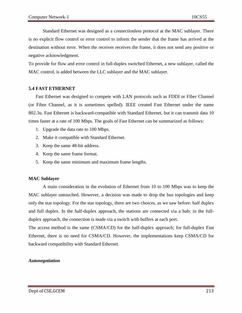
Computer Network-1 10CS55
Dept of CSE,GCEM 213
Standard Ethernet was designed as a connectionless protocol at the MAC sublayer. There
is no explicit flow control or error control to inform the sender that the frame has arrived at the
destination without error. When the receiver receives the frame, it does not send any positive or
negative acknowledgment.
To provide for flow and error control in full-duplex switched Ethernet, a new sublayer, called the
MAC control, is added between the LLC sublayer and the MAC sublayer.
5.4 FAST ETHERNET
Fast Ethernet was designed to compete with LAN protocols such as FDDI or Fiber Channel
(or Fibre Channel, as it is sometimes spelled). IEEE created Fast Ethernet under the name
802.3u. Fast Ethernet is backward-compatible with Standard Ethernet, but it can transmit data 10
times faster at a rate of 100 Mbps. The goals of Fast Ethernet can be summarized as follows:
1. Upgrade the data rate to 100 Mbps.
2. Make it compatible with Standard Ethernet.
3. Keep the same 48-bit address.
4. Keep the same frame format.
5. Keep the same minimum and maximum frame lengths.
MAC Sublayer
A main consideration in the evolution of Ethernet from 10 to 100 Mbps was to keep the
MAC sublayer untouched. However, a decision was made to drop the bus topologies and keep
only the star topology. For the star topology, there are two choices, as we saw before: half duplex
and full duplex. In the half-duplex approach, the stations are connected via a hub; in the full-
duplex approach, the connection is made via a switch with buffers at each port.
The access method is the same (CSMA/CD) for the half-duplex approach; for full-duplex Fast
Ethernet, there is no need for CSMA/CD. However, the implementations keep CSMA/CD for
backward compatibility with Standard Ethernet.
Autonegotiation

Computer Network-1 10CS55
Dept of CSE,GCEM 214
A new feature added to Fast Ethernet is called autonegotiation. It allows a station or a hub a
range of capabilities. Autonegotiation allows two devices to negotiate the mode or data rate of
operation. It was designed particularly for the following purposes:
To allow incompatible devices to connect to one another. For example, a device with a
maximum capacity of 10 Mbps can communicate with a device with a 100 Mbps capacity
(but can work at a lower rate).
To allow one device to have multiple capabilities.
To allow a station to check a hub's capabilities.
Physical Layer
The physical layer in Fast Ethernet is more complicated than the one in Standard
Ethernet. Some of the features of this layer are as follows.
Topology
Fast Ethernet is designed to connect two or more stations together. If there are only two
stations, they can be connected point-to-point. Three or more stations need to be connected in a
star topology with a hub or a switch at the center.
Implementation
Fast Ethernet implementation at the physical layer can be categorized as either two-wire
or four-wire. The two-wire implementation can be either category 5 UTP (100Base-TX) or fiber-
optic cable (100Base-FX). The four-wire implementation is designed only for category 3 UTP
(100Base-T4).
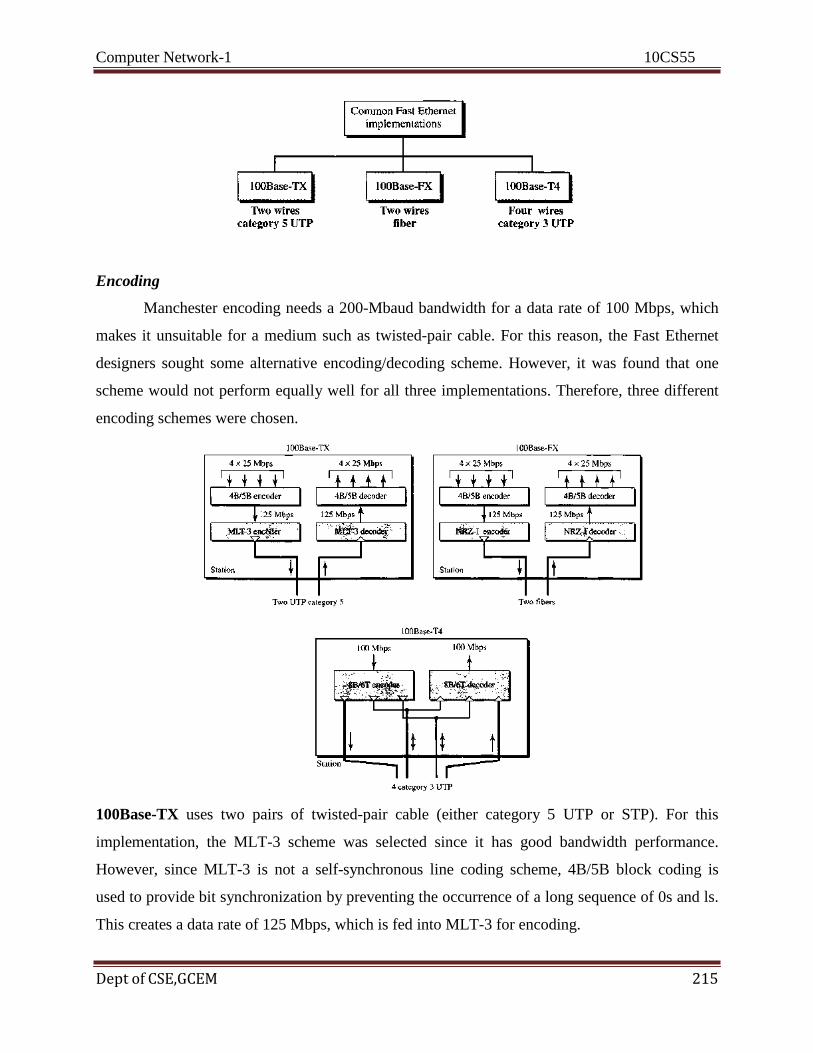
Computer Network-1 10CS55
Dept of CSE,GCEM 215
Encoding
Manchester encoding needs a 200-Mbaud bandwidth for a data rate of 100 Mbps, which
makes it unsuitable for a medium such as twisted-pair cable. For this reason, the Fast Ethernet
designers sought some alternative encoding/decoding scheme. However, it was found that one
scheme would not perform equally well for all three implementations. Therefore, three different
encoding schemes were chosen.
100Base-TX uses two pairs of twisted-pair cable (either category 5 UTP or STP). For this
implementation, the MLT-3 scheme was selected since it has good bandwidth performance.
However, since MLT-3 is not a self-synchronous line coding scheme, 4B/5B block coding is
used to provide bit synchronization by preventing the occurrence of a long sequence of 0s and ls.
This creates a data rate of 125 Mbps, which is fed into MLT-3 for encoding.
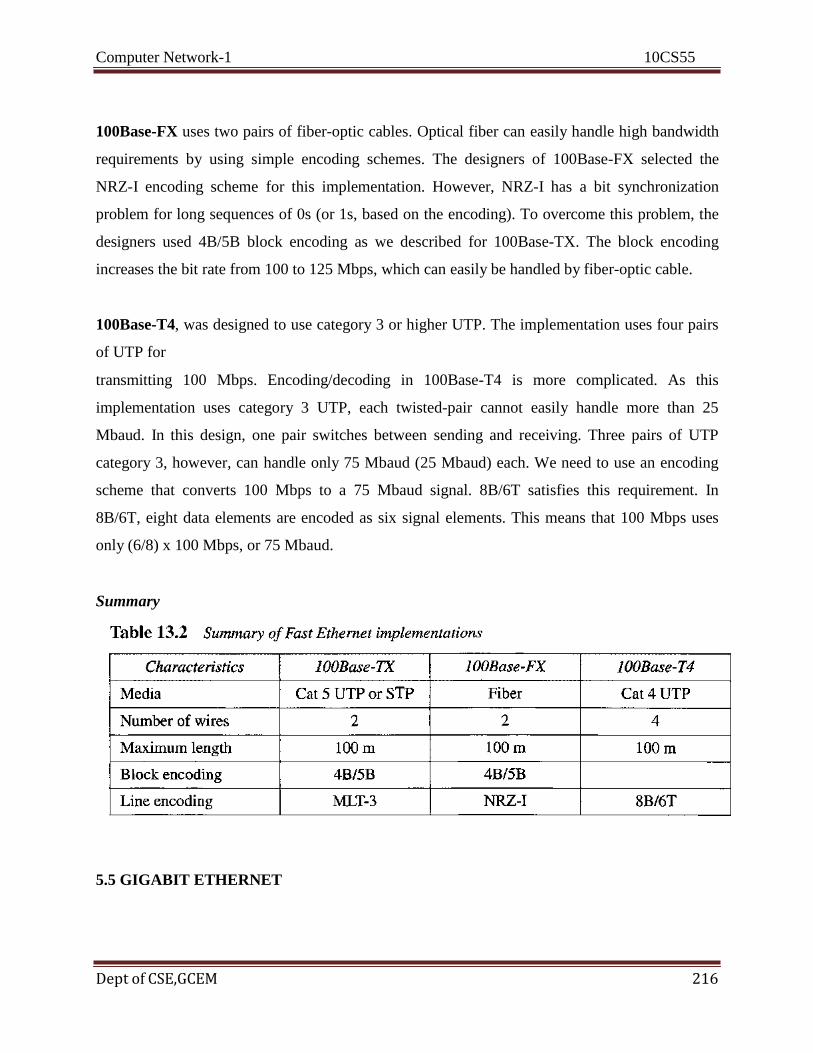
Computer Network-1 10CS55
Dept of CSE,GCEM 216
100Base-FX uses two pairs of fiber-optic cables. Optical fiber can easily handle high bandwidth
requirements by using simple encoding schemes. The designers of 100Base-FX selected the
NRZ-I encoding scheme for this implementation. However, NRZ-I has a bit synchronization
problem for long sequences of 0s (or 1s, based on the encoding). To overcome this problem, the
designers used 4B/5B block encoding as we described for 100Base-TX. The block encoding
increases the bit rate from 100 to 125 Mbps, which can easily be handled by fiber-optic cable.
100Base-T4, was designed to use category 3 or higher UTP. The implementation uses four pairs
of UTP for
transmitting 100 Mbps. Encoding/decoding in 100Base-T4 is more complicated. As this
implementation uses category 3 UTP, each twisted-pair cannot easily handle more than 25
Mbaud. In this design, one pair switches between sending and receiving. Three pairs of UTP
category 3, however, can handle only 75 Mbaud (25 Mbaud) each. We need to use an encoding
scheme that converts 100 Mbps to a 75 Mbaud signal. 8B/6T satisfies this requirement. In
8B/6T, eight data elements are encoded as six signal elements. This means that 100 Mbps uses
only (6/8) x 100 Mbps, or 75 Mbaud.
Summary
5.5 GIGABIT ETHERNET

Computer Network-1 10CS55
Dept of CSE,GCEM 217
The need for an even higher data rate resulted in the design of the Gigabit Ethernet protocol
(1000 Mbps). The IEEE committee calls the Standard 802.3z. The goals of the Gigabit Ethernet
design can be summarized as follows:
1. Upgrade the data rate to 1 Gbps.
2. Make it compatible with Standard or Fast Ethernet.
3. Use the same 48-bit address.
4. Use the same frame format.
5. Keep the same minimum and maximum frame lengths.
6. To support autonegotiation as defined in Fast Ethernet.
MAC Sublayer
Gigabit Ethernet has two distinctive approaches for medium access: half-duplex and full-
duplex. Almost all implementations of Gigabit Ethernet follow the full-duplex approach.
Full-Duplex Mode
In full-duplex mode, there is a central switch connected to all computers or other
switches. In this mode, each switch has buffers for each input port in which data are stored until
they are transmitted. There is no collision in this mode. This means that CSMA/CD is not used.
Lack of collision implies that the maximum length of the cable is determined by the signal
attenuation in the cable, not by the collision detection process.
Half-Duplex Mode
Gigabit Ethernet can also be used in half-duplex mode, although it is rare. In this case, a
switch can be replaced by a hub, which acts as the common cable in which a collision might
occur. The half-duplex approach uses CSMA/CD. The maximum length of the network in this
approach is totally dependent on the minimum frame size. Three methods have been defined:
traditional, carder extension, and frame bursting.
Traditional In the traditional approach, we keep the minimum length of the frame as in
traditional Ethernet (512 bits). However, because the length of a bit is 1/100 shorter in Gigabit
Ethernet than in 10-Mbps Ethernet, the slot time for Gigabit Ethernet is 512 bits x 1/1000 gs,
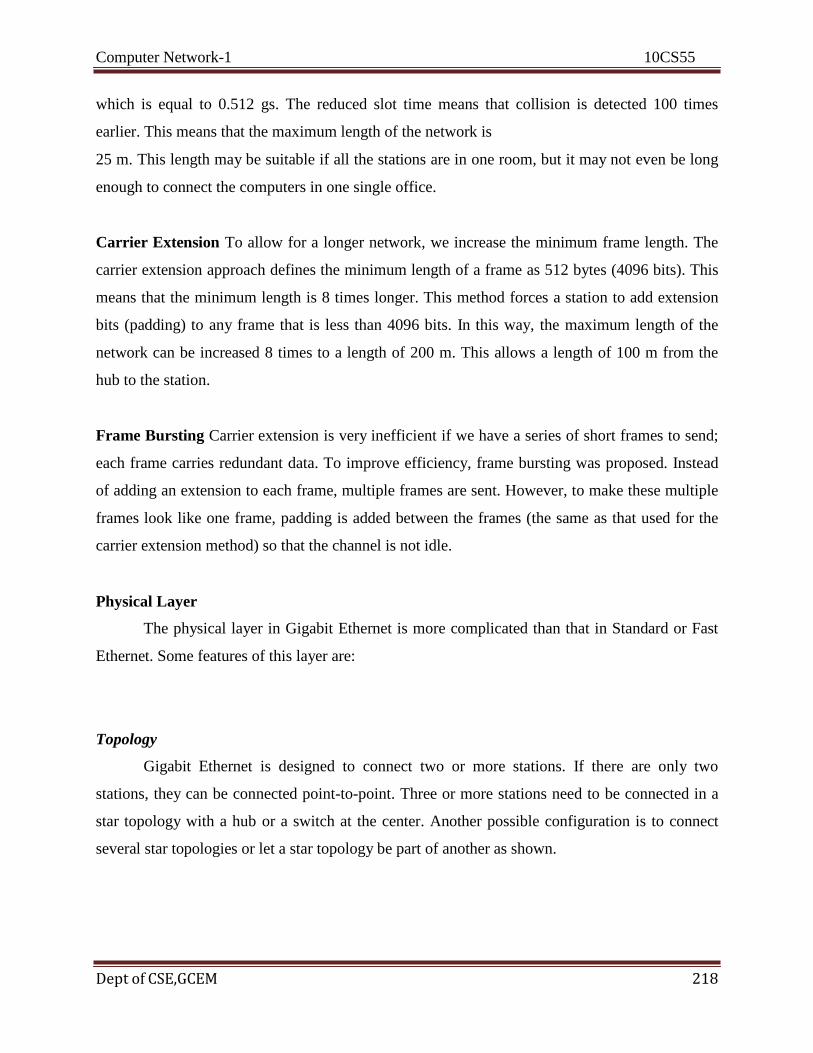
Computer Network-1 10CS55
Dept of CSE,GCEM 218
which is equal to 0.512 gs. The reduced slot time means that collision is detected 100 times
earlier. This means that the maximum length of the network is
25 m. This length may be suitable if all the stations are in one room, but it may not even be long
enough to connect the computers in one single office.
Carrier Extension To allow for a longer network, we increase the minimum frame length. The
carrier extension approach defines the minimum length of a frame as 512 bytes (4096 bits). This
means that the minimum length is 8 times longer. This method forces a station to add extension
bits (padding) to any frame that is less than 4096 bits. In this way, the maximum length of the
network can be increased 8 times to a length of 200 m. This allows a length of 100 m from the
hub to the station.
Frame Bursting Carrier extension is very inefficient if we have a series of short frames to send;
each frame carries redundant data. To improve efficiency, frame bursting was proposed. Instead
of adding an extension to each frame, multiple frames are sent. However, to make these multiple
frames look like one frame, padding is added between the frames (the same as that used for the
carrier extension method) so that the channel is not idle.
Physical Layer
The physical layer in Gigabit Ethernet is more complicated than that in Standard or Fast
Ethernet. Some features of this layer are:
Topology
Gigabit Ethernet is designed to connect two or more stations. If there are only two
stations, they can be connected point-to-point. Three or more stations need to be connected in a
star topology with a hub or a switch at the center. Another possible configuration is to connect
several star topologies or let a star topology be part of another as shown.
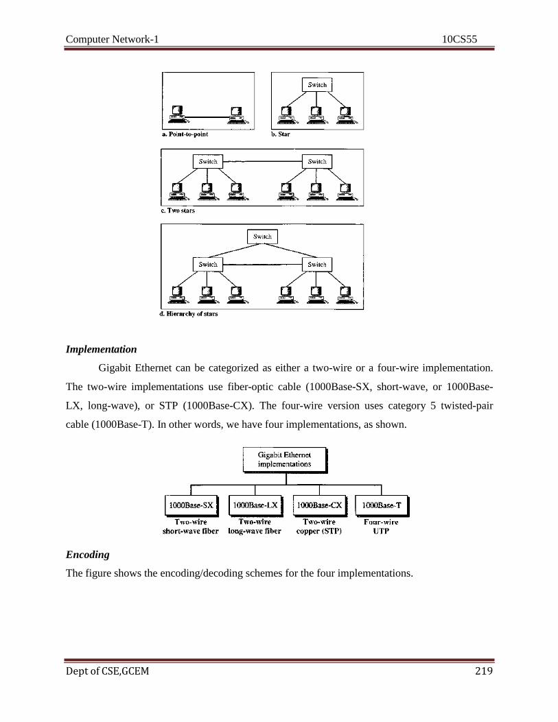
Computer Network-1 10CS55
Dept of CSE,GCEM 219
Implementation
Gigabit Ethernet can be categorized as either a two-wire or a four-wire implementation.
The two-wire implementations use fiber-optic cable (1000Base-SX, short-wave, or 1000Base-
LX, long-wave), or STP (1000Base-CX). The four-wire version uses category 5 twisted-pair
cable (1000Base-T). In other words, we have four implementations, as shown.
Encoding
The figure shows the encoding/decoding schemes for the four implementations.

Computer Network-1 10CS55
Dept of CSE,GCEM 220
Gigabit Ethernet cannot use the Manchester encoding scheme because it involves a very high
bandwidth (2 GBaud). The two-wire implementations use an NRZ scheme, but NRZ does not
self-synchronize properly. To synchronize bits, particularly at this high data rate, 8B/10B block
encoding is used. This block encoding prevents long sequences of 0s or ls in the stream, but the
resulting stream is 1.25 Gbps. Note that in this implementation, one wire (fiber or STP) is used
for sending and one for receiving.
In the four-wire implementation it is not possible to have 2 wires for input and 2 for output,
because each wire would need to carry 500 Mbps, which exceeds the capacity for category 5
UTP. As a solution, 4D-PAM5 encoding is used to reduce the bandwidth. Thus, all four wires are
involved in both input and output; each wire carries 250 Mbps, which is in the range for category
5 UTP cable.
Summary
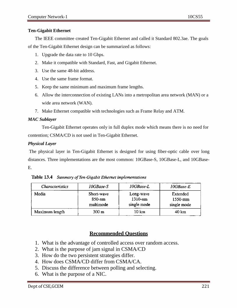
Computer Network-1 10CS55
Dept of CSE,GCEM 221
Ten-Gigabit Ethernet
The IEEE committee created Ten-Gigabit Ethernet and called it Standard 802.3ae. The goals
of the Ten-Gigabit Ethernet design can be summarized as follows:
1. Upgrade the data rate to 10 Gbps.
2. Make it compatible with Standard, Fast, and Gigabit Ethernet.
3. Use the same 48-bit address.
4. Use the same frame format.
5. Keep the same minimum and maximum frame lengths.
6. Allow the interconnection of existing LANs into a metropolitan area network (MAN) or a
wide area network (WAN).
7. Make Ethernet compatible with technologies such as Frame Relay and ATM.
MAC Sublayer
Ten-Gigabit Ethernet operates only in full duplex mode which means there is no need for
contention; CSMA/CD is not used in Ten-Gigabit Ethernet.
Physical Layer
The physical layer in Ten-Gigabit Ethernet is designed for using fiber-optic cable over long
distances. Three implementations are the most common: 10GBase-S, 10GBase-L, and 10GBase-
E.
Recommended Questions
1. What is the advantage of controlled access over random access.
2. What is the purpose of jam signal in CSMA/CD
3. How do the two persistent strategies differ.
4. How does CSMA/CD differ from CSMA/CA.
5. Discuss the difference between polling and selecting. 6. What is the purpose of a NIC.
Computer Network-1 10CS55
Dept of CSE,GCEM 222
7. What is the difference between multicast and broadcast address.
8. What are the common Ethernet traditional applications. 9. What are the common fast Ethernet and gigabit Ethernet applications.

Computer Network-1 10CS55
Dept of CSE,GCEM 223
COMPUTER NETWORKS – I
Subject Code: 10CS55 I.A. Marks : 25
Hours/Week : 04 Exam Hours: 03
Total Hours : 52 Exam Marks: 100
UNIT – 7 6 Hours Wireless LANs and Cellular Networks:
- Introduction,
- IEEE 802.11,
- Bluetooth,
- Connecting devices, - Cellular Telephony

Computer Network-1 10CS55
Dept of CSE,GCEM 224
UNIT – VII
Wireless LANs
14.1 IEEE 802.11
Architecture
The standard defines two kinds of services: the basic service set (BSS) and the extended service
set (ESS).
Basic Service Set
IEEE 802.11 defines the basic service set (BSS) as the building block of a wireless LAN. A basic
service set is made of stationary or mobile wireless stations and an optional central base station,
known as the access point (AP). The figure shows two sets in this standard.
The BSS without an AP is a stand-alone network and cannot send data to other BSSs. It is
called an ad hoc architecture. In this architecture, stations can form a network without the need
of an AP; they can locate one another and agree to be part of a BSS. A BSS with an AP is
sometimes referred to as an infrastructure network.
Extended Service Set
An extended service set (ESS) is made up of two or more BSSs with APs. In this case, the BSSs
are connected through a distribution system, which is usually a wired LAN. The distribution
system connects the APs in the BSSs. IEEE 802.11 does not restrict the distribution system; it
can be any IEEE LAN such as an Ethernet. Note that the extended service set uses two types of
stations: mobile and stationary. The mobile stations are normal stations inside a BSS. The
stationary stations are AP stations that are part of a wired LAN.

Computer Network-1 10CS55
Dept of CSE,GCEM 225
When BSSs are connected, the stations within reach of one another can communicate without the
use of an AP. However, communication between two stations in two different BSSs usually
occurs via two APs.
Station Types
IEEE 802.11 defines three types of stations based on their mobility in a wireless LAN: no-
transition, BSS-transition, and ESS-transition mobility. A station with no-transition mobility is
either stationary (not moving) or moving only inside a BSS. A station with BSS-transition
mobility can move from one BSS to another, but the movement is confined inside one ESS. A
station with ESS-transition mobility can move from one ESS to another. However, IEEE 802.11
does not guarantee that communication is continuous during the move.
MAC Sublayer
IEEE 802.11 defines two MAC sublayers: the distributed coordination function (DCF) and point
coordination function (PCF). The figure shows the relationship between the two MAC sublayers,
the LLC sublayer, and the physical layer.
Distributed Coordination Function
One of the two protocols defined by IEEE at the MAC sublayer is called the distributed
coordination function (DCF). DCF uses CSMA/CA as the access method. Wireless LANs cannot
implement CSMA/CD for three reasons:
1. For collision detection a station must be able to send data and receive collision signals at
the same time. This can mean costly stations and increased bandwidth requirements.
2. Collision may not be detected because of the hidden station problem.
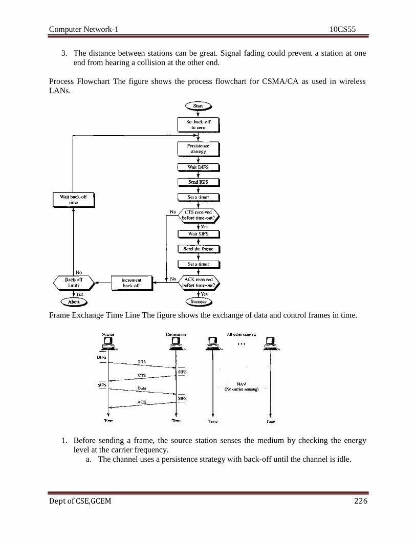
Computer Network-1 10CS55
Dept of CSE,GCEM 226
3. The distance between stations can be great. Signal fading could prevent a station at one
end from hearing a collision at the other end.
Process Flowchart The figure shows the process flowchart for CSMA/CA as used in wireless
LANs.
Frame Exchange Time Line The figure shows the exchange of data and control frames in time.
1. Before sending a frame, the source station senses the medium by checking the energy
level at the carrier frequency.
a. The channel uses a persistence strategy with back-off until the channel is idle.
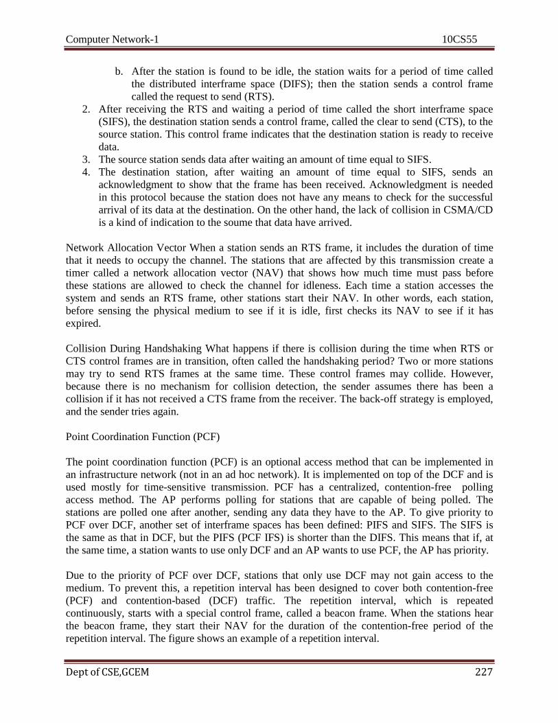
Computer Network-1 10CS55
Dept of CSE,GCEM 227
b. After the station is found to be idle, the station waits for a period of time called
the distributed interframe space (DIFS); then the station sends a control frame
called the request to send (RTS).
2. After receiving the RTS and waiting a period of time called the short interframe space
(SIFS), the destination station sends a control frame, called the clear to send (CTS), to the
source station. This control frame indicates that the destination station is ready to receive
data.
3. The source station sends data after waiting an amount of time equal to SIFS.
4. The destination station, after waiting an amount of time equal to SIFS, sends an
acknowledgment to show that the frame has been received. Acknowledgment is needed
in this protocol because the station does not have any means to check for the successful
arrival of its data at the destination. On the other hand, the lack of collision in CSMA/CD
is a kind of indication to the soume that data have arrived.
Network Allocation Vector When a station sends an RTS frame, it includes the duration of time
that it needs to occupy the channel. The stations that are affected by this transmission create a
timer called a network allocation vector (NAV) that shows how much time must pass before
these stations are allowed to check the channel for idleness. Each time a station accesses the
system and sends an RTS frame, other stations start their NAV. In other words, each station,
before sensing the physical medium to see if it is idle, first checks its NAV to see if it has
expired.
Collision During Handshaking What happens if there is collision during the time when RTS or
CTS control frames are in transition, often called the handshaking period? Two or more stations
may try to send RTS frames at the same time. These control frames may collide. However,
because there is no mechanism for collision detection, the sender assumes there has been a
collision if it has not received a CTS frame from the receiver. The back-off strategy is employed,
and the sender tries again.
Point Coordination Function (PCF)
The point coordination function (PCF) is an optional access method that can be implemented in
an infrastructure network (not in an ad hoc network). It is implemented on top of the DCF and is
used mostly for time-sensitive transmission. PCF has a centralized, contention-free polling
access method. The AP performs polling for stations that are capable of being polled. The
stations are polled one after another, sending any data they have to the AP. To give priority to
PCF over DCF, another set of interframe spaces has been defined: PIFS and SIFS. The SIFS is
the same as that in DCF, but the PIFS (PCF IFS) is shorter than the DIFS. This means that if, at
the same time, a station wants to use only DCF and an AP wants to use PCF, the AP has priority.
Due to the priority of PCF over DCF, stations that only use DCF may not gain access to the
medium. To prevent this, a repetition interval has been designed to cover both contention-free
(PCF) and contention-based (DCF) traffic. The repetition interval, which is repeated
continuously, starts with a special control frame, called a beacon frame. When the stations hear
the beacon frame, they start their NAV for the duration of the contention-free period of the
repetition interval. The figure shows an example of a repetition interval.
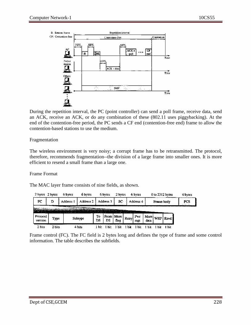
Computer Network-1 10CS55
Dept of CSE,GCEM 228
During the repetition interval, the PC (point controller) can send a poll frame, receive data, send
an ACK, receive an ACK, or do any combination of these (802.11 uses piggybacking). At the
end of the contention-free period, the PC sends a CF end (contention-free end) frame to allow the
contention-based stations to use the medium.
Fragmentation
The wireless environment is very noisy; a corrupt frame has to be retransmitted. The protocol,
therefore, recommends fragmentation--the division of a large frame into smaller ones. It is more
efficient to resend a small frame than a large one.
Frame Format
The MAC layer frame consists of nine fields, as shown.
Frame control (FC). The FC field is 2 bytes long and defines the type of frame and some control
information. The table describes the subfields.

Computer Network-1 10CS55
Dept of CSE,GCEM 229
D. In all frame types except one, this field defines the duration of the transmission that is used to set the value of NAV. In one control frame, this field defines the ID of the frame.
Addresses. There are four address fields, each 6 bytes long. The meaning of each address field
depends on the value of the To DS and From DS subfields and will be discussed later.
Sequence control. This field defines the sequence number of the frame to be used in flow control.
Frame body. This field, which can be between 0 and 2312 bytes, contains information based on
the type and the subtype defined in the FC field.
FCS. The FCS field is 4 bytes long and contains a CRC-32 error detection sequence.
Frame Types
A wireless LAN defined by IEEE 802.11 has three categories of frames: management frames,
control frames, and data frames.
Management Frames Management frames are used for the initial communication between
stations and access points.
Control Frames Control frames are used for accessing the channel and acknowledging frames.
The figure shows the format.
For control frames the value of the type field is 01; the values of the subtype fields for frames we
have discussed are shown in the table.

Computer Network-1 10CS55
Dept of CSE,GCEM 230
Data Frames Data frames are used for carrying data and control information.
Addressing Mechanism
The IEEE 802.11 addressing mechanism specifies four cases, defined by the value of the two
flags in the FC field, To DS and From DS. Each flag can be either 0 or 1, resulting in four
different situations. The interpretation of the four addresses (address 1 to address 4) in the MAC
frame depends on the value of these flags, as shown in the table.
Note that address 1 is always the address of the next device. Address 2 is always the address of
the previous device. Address 3 is the address of the final destination station if it is not defined by
address 1. Address 4 is the address of the original source station if it is not the same as address 2.
Case 1:00 In this case, To DS = 0 and From DS = 0. This means that the frame is not going to a
distribution system (To DS = 0) and is not coming from a distribution system (From DS = 0).
The frame is going from one station in a BSS to another without passing through the distribution
system. The ACK frame should be sent to the original sender. The addresses are shown in figure.
Case 2:01 In this case, To DS = 0 and From DS = 1. This means that the frame is coming from a
distribution system (From DS = 1). The frame is coming from an AP and going to a station. The
ACK should be sent to the AP. The addresses are as shown in Figure 14.9. Note that address 3
contains the original sender of the frame (in another BSS).
Case 3:10 In this case, To DS = 1 and From DS = 0. This means that the frame is going to a
distribution system (To DS = 1). The frame is going from a station to an AP. The ACK is sent to
the original station. The addresses are as shown in figure above. Note that address 3 contains the
final destination of the frame (in another BSS).

Computer Network-1 10CS55
Dept of CSE,GCEM 231
Case 4:11 In this case, To DS = 1 and From DS = 1. This is the case in which the distribution
system is also wireless. The frame is going from one AP to another AP in a wire-less distribution
system. We do not need to define addresses if the distribution system is a wired LAN because the
frame in these cases has the format of a wired LAN frame (Ethernet, for example). Here, we
need four addresses to define the original sender, the
final destination, and two intermediate APs. Figure above shows the situation.
Hidden and Exposed Station Problems
Hidden Station Problem The figure below shows an example of the hidden station problem.
Station B has a transmission range shown by the left oval (sphere in space); every station in this
range can hear any signal transmitted by station B. Station C has a transmission range shown by
the right oval (sphere in space); every station located in this range can hear any signal
transmitted by C. Station C is outside the transmission range of B; likewise, station B is outside
the transmission range of C. Station A, however, is in the area covered by both B and C; it can
hear any signal transmitted by B or C.
Assume that station B is sending data to station A. In the middle of this transmission, station C
also has data to send to station A. However, station C is out of B's range and transmissions from
B cannot reach C. Therefore C thinks the medium is free. Station C sends its data to A, which
results in a collision at A because this station is receiving data from both B and C. In this case,
we say that stations B and C are hidden from each other with respect to A. Hidden stations can
reduce the capacity of the network because of the possibility of collision. The solution to the
hidden station problem is the use of the handshake frames (RTS and CTS) The figure shows that
the RTS message from B reaches A, but not C. However, because both B and C are within the
range of A, the CTS message, which contains the duration of data transmission from B to A
reaches C. Station C knows that some hidden station is using the channel and refrains from
transmitting until that duration is over.
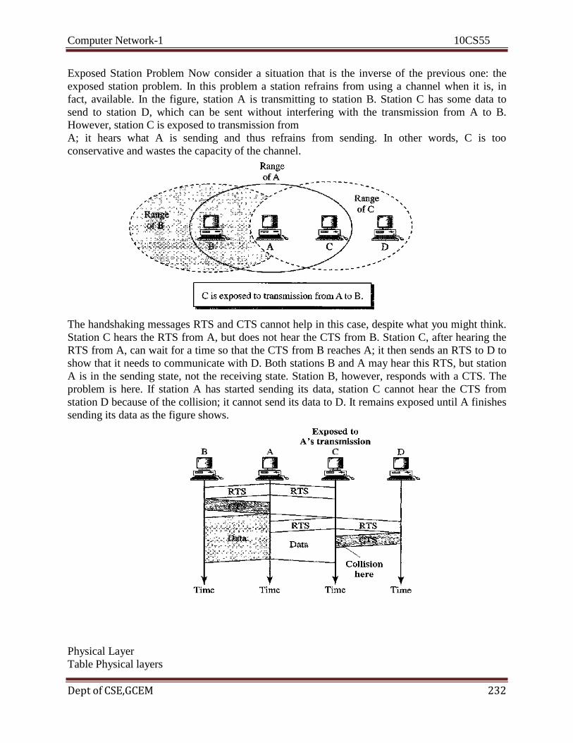
Computer Network-1 10CS55
Dept of CSE,GCEM 232
Exposed Station Problem Now consider a situation that is the inverse of the previous one: the
exposed station problem. In this problem a station refrains from using a channel when it is, in
fact, available. In the figure, station A is transmitting to station B. Station C has some data to
send to station D, which can be sent without interfering with the transmission from A to B.
However, station C is exposed to transmission from
A; it hears what A is sending and thus refrains from sending. In other words, C is too
conservative and wastes the capacity of the channel.
The handshaking messages RTS and CTS cannot help in this case, despite what you might think.
Station C hears the RTS from A, but does not hear the CTS from B. Station C, after hearing the
RTS from A, can wait for a time so that the CTS from B reaches A; it then sends an RTS to D to
show that it needs to communicate with D. Both stations B and A may hear this RTS, but station
A is in the sending state, not the receiving state. Station B, however, responds with a CTS. The
problem is here. If station A has started sending its data, station C cannot hear the CTS from
station D because of the collision; it cannot send its data to D. It remains exposed until A finishes
sending its data as the figure shows.
Physical Layer
Table Physical layers
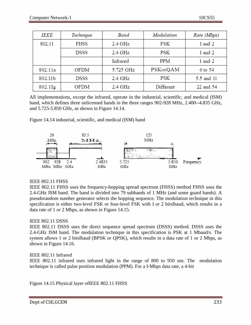
Computer Network-1 10CS55
Dept of CSE,GCEM 233
All implementations, except the infrared, operate in the industrial, scientific, and medical (ISM)
band, which defines three unlicensed bands in the three ranges 902-928 MHz, 2.400--4.835 GHz,
and 5.725-5.850 GHz, as shown in Figure 14.14.
Figure 14.14 industrial, scientific, and medical (ISM) band
IEEE 802.11 FHSS
IEEE 802.11 FHSS uses the frequency-hopping spread spectrum (FHSS) method FHSS uses the
2.4-GHz ISM band. The band is divided into 79 subbands of 1 MHz (and some guard bands). A
pseudorandom number generator selects the hopping sequence. The modulation technique in this
specification is either two-level FSK or four-level FSK with I or 2 bitslbaud, which results in a
data rate of 1 or 2 Mbps, as shown in Figure 14.15.
IEEE 802.11 DSSS
IEEE 802.11 DSSS uses the direct sequence spread spectrum (DSSS) method. DSSS uses the
2.4-GHz ISM band. The modulation technique in this specification is PSK at 1 Mbaud/s. The
system allows 1 or 2 bitslbaud (BPSK or QPSK), which results in a data rate of 1 or 2 Mbps, as
shown in Figure 14.16.
IEEE 802.11 Infrared
IEEE 802.11 infrared uses infrared light in the range of 800 to 950 nm. The modulation
technique is called pulse position modulation (PPM). For a I-Mbps data rate, a 4-bit
Figure 14.15 Physical layer ofIEEE 802.11 FHSS
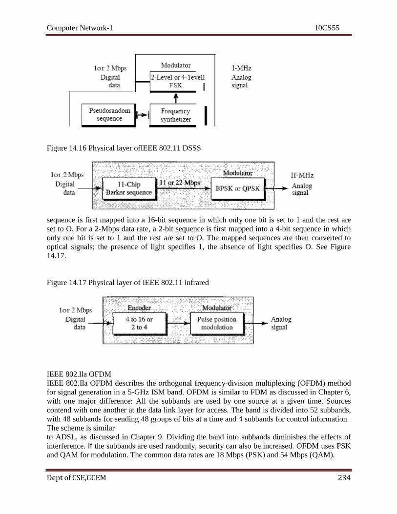
Computer Network-1 10CS55
Dept of CSE,GCEM 234
Figure 14.16 Physical layer ofIEEE 802.11 DSSS
sequence is first mapped into a 16-bit sequence in which only one bit is set to 1 and the rest are
set to O. For a 2-Mbps data rate, a 2-bit sequence is first mapped into a 4-bit sequence in which
only one bit is set to 1 and the rest are set to O. The mapped sequences are then converted to
optical signals; the presence of light specifies 1, the absence of light specifies O. See Figure
14.17.
Figure 14.17 Physical layer of IEEE 802.11 infrared
IEEE 802.lla OFDM
IEEE 802.Ila OFDM describes the orthogonal frequency-division multiplexing (OFDM) method
for signal generation in a 5-GHz ISM band. OFDM is similar to FDM as discussed in Chapter 6,
with one major difference: All the subbands are used by one source at a given time. Sources
contend with one another at the data link layer for access. The band is divided into 52 subbands,
with 48 subbands for sending 48 groups of bits at a time and 4 subbands for control information.
The scheme is similar
to ADSL, as discussed in Chapter 9. Dividing the band into subbands diminishes the effects of
interference. If the subbands are used randomly, security can also be increased. OFDM uses PSK
and QAM for modulation. The common data rates are 18 Mbps (PSK) and 54 Mbps (QAM).

Computer Network-1 10CS55
Dept of CSE,GCEM 235
IEEE 802.llb DSSS
IEEE 802.11 b DSSS describes the high-rate direct sequence spread spectrum (HRDSSS)
method for signal generation in the 2.4-GHz ISM band. HR-DSSS is similar to DSSS except for
the encoding method, which is called complementary code keying (CCK). CCK encodes 4 or 8
bits to one CCK symbol. To be backward compatible with DSSS, HR-DSSS defines four data
rates: 1,2, 5.5, and 11 Mbps. The first two use the same modulation techniques as DSSS. The
5.5-Mbps version uses BPSK and transmits at 1.375 Mbaudls with 4-bit CCK encoding. The II-
Mbps version uses QPSK and transmits at 1.375 Mbps with 8-bit CCK encoding. Figure 14.18
shows the modulation technique for this standard.
Figure 14.18 Physical layer of IEEE 802.11b
IEEE 802.11g
This new specification defines forward error correction and OFDM using the 2.4-GHz ISM
band. The modulation technique achieves a 22- or 54-Mbps data rate. It is backward compatible
with 802.11b, but the modulation technique is OFDM.
14.2 BLUETOOTH
Bluetooth is a wireless LAN technology designed to connect devices of different functions such
as telephones, notebooks, computers (desktop and laptop), cameras, printers, coffee makers, and
so on. A Bluetooth LAN is an ad hoc network, which means that the network is formed
spontaneously; the devices, sometimes called gadgets, find each other and make a network called
a piconet. A Bluetooth LAN can even be connected to the Internet if one of the gadgets has this
capability. A Bluetooth LAN, by nature, cannot be large. If there are many gadgets that try to
connect, there is chaos. Bluetooth technology has several applications. Peripheral devices such as
a wireless mouse or keyboard can communicate with the computer through this technology.
Monitoring devices can communicate with sensor devices in a small health care center. Home
security devices can use this technology to connect different sensors to the main security
controller. Conference attendees can synchronize their laptop computers at a conference.

Computer Network-1 10CS55
Dept of CSE,GCEM 236
Bluetooth was originally started as a project by the Ericsson Company. It is named for Harald
Blaatand, the king of Denmark (940-981) who united Denmark and Norway. Blaatand translates
to Bluetooth in English. Today, Bluetooth technology is the implementation of a protocol
defined by the IEEE 802.15 standard. The standard defines a wireless personal-area network
(PAN) operable in an area the size of a room or a hall.
Architecture
Bluetooth defines two types of networks: piconet and scatternet.
Piconets
A Bluetooth network is called a piconet, or a small net. A piconet can have up to eight stations,
one of which is called the primary;t the rest are called secondaries. All the secondary stations
synchronize their clocks and hopping sequence with the primary. Note that a piconet can have
only one primary station. The communication between the primary and the secondary can be
one-to-one or one-to-many. Figure 14.19 shows a piconet.
Figure 14.19 Piconet
Although a piconet can have a maximum of seven secondaries, an additional eight secondaries
can be in the parked state. A secondary in a parked state is synchronized with the primary, but
cannot take part in communication until it is moved from the parked state. Because only eight
stations can be active in a piconet, activating a station from the parked state means that an active
station must go to the parked state.

Computer Network-1 10CS55
Dept of CSE,GCEM 237
Scat/ernet
Piconets can be combined to form what is called a scatternet. A secondary station in one piconet
can be the primary in another piconet. This station can receive messages from the primary in the
first piconet (as a secondary) and, acting as a primary, deliver them to secondaries in the second
piconet. A station can be a member of two piconets.
Figure 14.20 Scatternet
Bluetooth Devices
A Bluetooth device has a built-in short-range radio transmitter. The current data rate is 1 Mbps
with a 2.4-GHz bandwidth. This means that there is a possibility of interference between the
IEEE 802.11b wireless LANs and Bluetooth LANs.
Bluetooth Layers
Bluetooth uses several layers that do not exactly match those of the Internet model we have
defined in this book. Figure 14.21 shows these layers.
Radio Layer
The radio layer is roughly equivalent to the physical layer of the Internet model. Bluetooth
devices are low-power and have a range of 10 m.

Computer Network-1 10CS55
Dept of CSE,GCEM 238
Band
Bluetooth uses a 2.4-GHz ISM band divided into 79 channels of 1 MHz each.
FHSS
Bluetooth uses the frequency-hopping spread spectrum (FHSS) method in the physical layer to
avoid interference from other devices or other networks. Bluetooth hops 1600 times per second,
which means that each device changes its modulation frequency 1600 times per second. A device
uses a frequency for only 625 Ils (1/1600 s) before it hops to another frequency; the dwell time is
625 Ils.
Modulation
To transform bits to a signal, Bluetooth uses a sophisticated version of FSK, called GFSK (FSK
with Gaussian bandwidth filtering; a discussion of this topic is beyond the scope of this book).
GFSK has a can'ier frequency. Bit 1 is represented by a frequency deviation above the carrier; bit
ais represented by a frequency deviation below the carrier. The frequencies, in megahertz, are
defined according to the following formula for each channel: fc=2402+n n =0, 1,2,3, ..., 78 For
example, the first channel uses carrier frequency 2402 MHz (2.402 GHz), and the second
channel uses carrier frequency 2403 MHz (2.403 GHz). Baseband Layer The baseband layer is
roughly equivalent to the MAC sublayer in LANs. The access method is TDMA (see Chapter
12). The primary and secondary communicate with each other using time slots. The length of a
time slot is exactly the same as the dwell time, 625 Ils. This means that during the time that one
frequency is used, a sender sends a frame to a secondary, or a secondary sends a frame to the
primary. Note that the communication is only between the primary and a secondary; secondaries
cannot communicate directly with one another.
TDMA
Bluetooth uses a form of TDMA (see Chapter 12) that is called TDD-TDMA (timedivision
duplex TDMA). TDD-TDMA is a kind of half-duplex communication in which the secondary
and receiver send and receive data, but not at the same time (halfduplex); however, the
communication for each direction uses different hops. This is similar to walkie-talkies using
different carrier frequencies. Single-Secondary Communication If the piconet has only one
secondary, the TDMA operation is very simple. The time is divided into slots of 625 Ils. The
primary uses evennumbered slots (0, 2, 4, ...); the secondary uses odd-numbered slots (1, 3, 5,
...). TDD-TDMA allows the primary and the secondary to communicate in half-duplex mode. In
slot 0, the primary sends, and the secondary receives; in slot 1, the secondary sends, and the
primary receives. The cycle is repeated. Figure 14.22 shows the concept.

Computer Network-1 10CS55
Dept of CSE,GCEM 239
Let us elaborate on the figure. 1. In slot 0, the primary sends a frame to secondary 1.
2. In slot 1, only secondary I sends a frame to the primary because the previous frame was
addressed to secondary 1; other secondaries are silent.
3. In slot 2, the primary sends a frame to secondary 2.
4. In slot 3, only secondary 2 sends a frame to the primary because the previous frame was
addressed to secondary 2; other secondaries are silent.
5. The cycle continues. We can say that this access method is similar to a poll/select operation
with reservations. When the primary selects a secondary, it also polls it. The next time slot is
reserved for
the polled station to send its frame. If the polled secondary has no frame to send, the channel is
silent.
Physical Links
Two types of links can be created between a primary and a secondary: SCQ links and ACL links.
sca A synchronous connection-oriented (SeQ) link is used when avoiding latency (delay in data
delivery) is more important than integrity (error-free delivery). In an SCQ link, a physical link is
created between the primary and a secondary by reserving specific slots at regular intervals. The
basic unit of connection is two slots, one for each direction. If a packet is damaged, it is never
retransmitted. SCQ is used for real-time audio where avoiding delay is all-important. A
secondary can create up to three SCQ links with the primary, sending digitized audio (PCM) at
64 kbps in each link. ACL An asynchronous connectionless link (ACL) is used when data
integrity is more important than avoiding latency. In this type of link, if a payload encapsulated
in the frame is corrupted, it is retransmitted. A secondary returns an ACL frame in the available

Computer Network-1 10CS55
Dept of CSE,GCEM 240
odd-numbered slot if and only if the previous slot has been addressed to it. ACL can use one,
three, or more slots and can achieve a maximum data rate of 721 kbps.
Frame Format
A frame in the baseband layer can be one of three types: one-slot, three-slot, or five-slot. A slot,
as we said before, is 625 ~s. However, in a one-slot frame exchange, 259 ~s is needed for
hopping and control mechanisms. This means that a one-slot frame can last only 625 - 259, or
366 ~s. With a I-MHz bandwidth and 1 bit/Hz, the size of a one-slot frame is 366 bits. A three-
slot frame occupies three slots. However, since 259 ~s is used for hopping, the length of the
frame is 3 x 625 - 259 = 1616 ~s or 1616 bits. A device that uses a three-slot frame remains at
the same hop (at the same carrier frequency) for three slots. Even though only once hop number
is used, three hop numbers are consumed. That means the hop number for each frame is equal to
the first slot of the frame. A five-slot frame also uses 259 bits for hopping, which means that the
length of the frame is 5 x 625 - 259 =2866 bits. Figure 14.24 shows the format of the three frame
types. The following describes each field: Access code. This 72-bit field normally contains
synchronization bits and the identifier of the primary to distinguish the frame of one piconet
from another.
Figure 14.24 Frame fannat types
Header. This 54-bit field is a repeated I8-bit pattern. Each pattern has the following
subfields:
1. Address. The 3-bit address subfield can define up to seven secondaries (l to 7). If the address
is zero, it is used for broadcast communication from the primary to all secondaries.
2. Type. The 4-bit type subfield defines the type of data coming from the upper layers.
3. F. This I-bit subfield is for flow control. When set (I), it indicates that the device is unable to
receive more frames (buffer is full).
4. A. This I-bit subfield is for acknowledgment. Bluetooth uses Stop-and-Wait ARQ; I bit is
sufficient for acknowledgment.
5. S. This I-bit subfield holds a sequence number. Bluetooth uses Stop-and-Wait ARQ; I bit is
sufficient for sequence numbering.
6. HEC. The 8-bit header error correction subfield is a checksum to detect errors in each 18-bit
header section.
The header has three identical 18-bit sections. The receiver compares these three sections, bit by
bit. If each of the corresponding bits is the same, the bit is accepted; if not, the majority opinion

Computer Network-1 10CS55
Dept of CSE,GCEM 241
rules. This is a form of forward error correction (for the header only). This double error control is
needed because the nature of the communication, via air, is very noisy. Note that there is no
retransmission in this sublayer. o Payload. This subfield can be 0 to 2740 bits long. It contains
data or control
information corning from the upper layers.
L2CAP
The Logical Link Control and Adaptation Protocol, or L2CAP (L2 here means LL), is roughly
equivalent to the LLC sublayer in LANs. It is used for data exchange on an ACL link; SCQ
channels do not use L2CAP. Figure 14.25 shows the format of the data packet at this level. The
I6-bit length field defines the size of the data, in bytes, coming from the upper layers. Data can
be up to 65,535 bytes. The channel ID (CID) defines a unique identifier for the virtual channel
created at this level (see below). The L2CAP has specific duties: multiplexing, segmentation and
reassembly, quality
of service (QoS), and group management.
Multiplexing
The L2CAP can do multiplexing. At the sender site, it accepts data from one of the upper-layer
protocols, frames them, and delivers them to the baseband layer. At the receiver site, it accepts a
frame from the baseband layer, extracts the data, and delivers them to the appropriate protocol
layer. It creates a kind of virtual channel that we will discuss in later chapters on higher-level
protocols.
Segmentation and Reassembly
The maximum size of the payload field in the baseband layer is 2774 bits, or 343 bytes. This
includes 4 bytes to define the packet and packet length. Therefore, the size of the packet that can
arrive from an upper layer can only be 339 bytes. However, application layers sometimes need to
send a data packet that can be up to 65,535 bytes (an Internet packet, for example). The L2CAP
divides these large packets into segments and adds extra information to define the location of the
segments in the original packet. The L2CAP segments the packet at the source and reassembles
them at the destination.
QoS
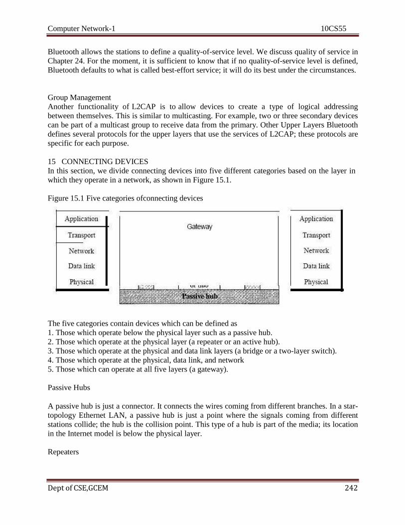
Computer Network-1 10CS55
Dept of CSE,GCEM 242
Bluetooth allows the stations to define a quality-of-service level. We discuss quality of service in
Chapter 24. For the moment, it is sufficient to know that if no quality-of-service level is defined,
Bluetooth defaults to what is called best-effort service; it will do its best under the circumstances.
Group Management
Another functionality of L2CAP is to allow devices to create a type of logical addressing
between themselves. This is similar to multicasting. For example, two or three secondary devices
can be part of a multicast group to receive data from the primary. Other Upper Layers Bluetooth
defines several protocols for the upper layers that use the services of L2CAP; these protocols are
specific for each purpose.
15 CONNECTING DEVICES
In this section, we divide connecting devices into five different categories based on the layer in
which they operate in a network, as shown in Figure 15.1.
Figure 15.1 Five categories ofconnecting devices
The five categories contain devices which can be defined as
1. Those which operate below the physical layer such as a passive hub.
2. Those which operate at the physical layer (a repeater or an active hub).
3. Those which operate at the physical and data link layers (a bridge or a two-layer switch).
4. Those which operate at the physical, data link, and network
5. Those which can operate at all five layers (a gateway).
Passive Hubs
A passive hub is just a connector. It connects the wires coming from different branches. In a star-
topology Ethernet LAN, a passive hub is just a point where the signals coming from different
stations collide; the hub is the collision point. This type of a hub is part of the media; its location
in the Internet model is below the physical layer.
Repeaters

Computer Network-1 10CS55
Dept of CSE,GCEM 243
A repeater is a device that operates only in the physical layer. Signals that carry information
within a network can travel a fixed distance before attenuation endangers the integrity of the
data. A repeater receives a signal and, before it becomes too weak or corrupted, regenerates the
original bit pattern. The repeater then sends the refreshed signal. A repeater can extend the
physical length of a LAN, as shown in Figure 15.2.
Figure 15.2 A repeater connecting two segments of a LAN
A repeater does not actually connect two LANs; it connects two segments of the same LAN. The
segments connected are still part of one single LAN. A repeater is not a device that can connect
two LANs of different protocols.
A repeater can overcome the 10Base5 Ethernet length restriction. In this standard, the length of
the cable is limited to 500 m. To extend this length, we divide the cable into segments and install
repeaters between segments. Note that the whole network is still considered one LAN, but the
portions of the network separated by repeaters are called segments. The repeater acts as a two-
port node, but operates only in the physical layer. When it receives a frame from any of the ports,
it regenerates and forwards it to the other port.
It is tempting to compare a repeater to an amplifier, but the comparison is inaccurate. An
amplifier cannot discriminate between the intended signal and noise; it amplifies equally
everything fed into it. A repeater does not amplify the signal; it regenerates the signal. When it
receives a weakened or corrupted signal, it creates a copy, bit for bit, at the original strength.
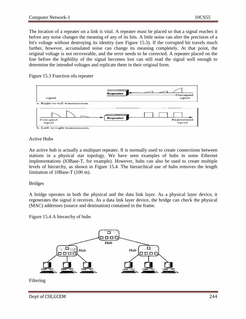
Computer Network-1 10CS55
Dept of CSE,GCEM 244
The location of a repeater on a link is vital. A repeater must be placed so that a signal reaches it
before any noise changes the meaning of any of its bits. A little noise can alter the precision of a
bit's voltage without destroying its identity (see Figure 15.3). If the corrupted bit travels much
farther, however, accumulated noise can change its meaning completely. At that point, the
original voltage is not recoverable, and the error needs to be corrected. A repeater placed on the
line before the legibility of the signal becomes lost can still read the signal well enough to
determine the intended voltages and replicate them in their original form.
Figure 15.3 Function ofa repeater
Active Hubs
An active hub is actually a multipart repeater. It is normally used to create connections between
stations in a physical star topology. We have seen examples of hubs in some Ethernet
implementations (lOBase-T, for example). However, hubs can also be used to create multiple
levels of hierarchy, as shown in Figure 15.4. The hierarchical use of hubs removes the length
limitation of 10Base-T (100 m).
Bridges
A bridge operates in both the physical and the data link layer. As a physical layer device, it
regenerates the signal it receives. As a data link layer device, the bridge can check the physical
(MAC) addresses (source and destination) contained in the frame.
Figure 15.4 A hierarchy of hubs
Filtering

Computer Network-1 10CS55
Dept of CSE,GCEM 245
One may ask, What is the difference in functionality between a bridge and a repeater? A bridge
has filtering capability. It can check the destination address of a frame and decide if the frame
should be forwarded or dropped. If the frame is to be forwarded, the decision must specify the
port. A bridge has a table that maps addresses to ports.
Let us give an example. In Figure 15.5, two LANs are connected by a bridge. If a frame destined
for station 712B13456142 arrives at port 1, the bridge consults its table to find the departing port.
According to its table, frames for 7l2B13456142 leave through port 1; therefore, there is no need
for forwarding, and the frame is dropped. On the other hand, if a frame for 712B13456141
arrives at port 2, the departing port is port 1
Figure 15.5 A bridge connecting two LANs
and the frame is forwarded. In the first case, LAN 2 remains free of traffic; in the second case,
both LANs have traffic. In our example, we show a two-port bridge; in reality a bridge usually
has more ports. Note also that a bridge does not change the physical addresses contained in the
frame.
Transparent Bridges
A transparent bridge is a bridge in which the stations are completely unaware of the bridge's
existence. If a bridge is added or deleted from the system, reconfiguration of the stations is
unnecessary. According to the IEEE 802.1 d specification, a system equipped with transparent
bridges must meet three criteria:
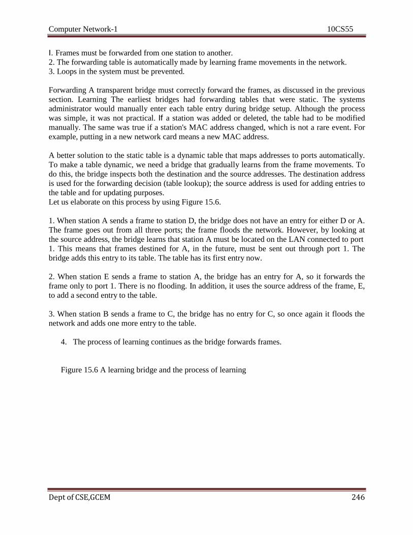
Computer Network-1 10CS55
Dept of CSE,GCEM 246
I. Frames must be forwarded from one station to another.
2. The forwarding table is automatically made by learning frame movements in the network.
3. Loops in the system must be prevented.
Forwarding A transparent bridge must correctly forward the frames, as discussed in the previous
section. Learning The earliest bridges had forwarding tables that were static. The systems
administrator would manually enter each table entry during bridge setup. Although the process
was simple, it was not practical. If a station was added or deleted, the table had to be modified
manually. The same was true if a station's MAC address changed, which is not a rare event. For
example, putting in a new network card means a new MAC address.
A better solution to the static table is a dynamic table that maps addresses to ports automatically.
To make a table dynamic, we need a bridge that gradually learns from the frame movements. To
do this, the bridge inspects both the destination and the source addresses. The destination address
is used for the forwarding decision (table lookup); the source address is used for adding entries to
the table and for updating purposes.
Let us elaborate on this process by using Figure 15.6.
1. When station A sends a frame to station D, the bridge does not have an entry for either D or A.
The frame goes out from all three ports; the frame floods the network. However, by looking at
the source address, the bridge learns that station A must be located on the LAN connected to port
1. This means that frames destined for A, in the future, must be sent out through port 1. The
bridge adds this entry to its table. The table has its first entry now.
2. When station E sends a frame to station A, the bridge has an entry for A, so it forwards the
frame only to port 1. There is no flooding. In addition, it uses the source address of the frame, E,
to add a second entry to the table.
3. When station B sends a frame to C, the bridge has no entry for C, so once again it floods the
network and adds one more entry to the table.
4. The process of learning continues as the bridge forwards frames.
Figure 15.6 A learning bridge and the process of learning

Computer Network-1 10CS55
Dept of CSE,GCEM 247
Loop Problem Transparent bridges work fine as long as there are no redundant bridges in the
system. Systems administrators, however, like to have redundant bridges (more than one bridge
between a pair of LANs) to make the system more reliable. If a bridge fails, another bridge takes
over until the failed one is repaired or replaced. Redundancy can create loops in the system,
which is very undesirable. Figure 15.7 shows a very simple example of a loop created in a
system with two LANs connected by two bridges.
1. Station A sends a frame to station D. The tables of both bridges are empty. Both forward the
frame and update their tables based on the source address A.
2. Now there are two copies of the frame on LAN 2. The copy sent out by bridge 1 is received by
bridge 2, which does not have any information about the destination address D; it floods the
bridge. The copy sent out by bridge 2 is received by bridge 1 and is sent out for lack of
information about D. Note that each frame is handled separately because bridges, as two nodes
on a network sharing the medium, use an access method such as CSMA/CD. The tables of both
bridges are updated, but still there is no information for destination D.
3. Now there are two copies of the frame on LAN 1. Step 2 is repeated, and both copies flood the
network.
4. The process continues on and on. Note that bridges are also repeaters and regenerate frames.
So in each iteration, there are newly generated fresh copies of the frames. To solve the looping
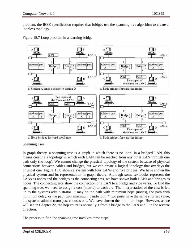
Computer Network-1 10CS55
Dept of CSE,GCEM 248
problem, the IEEE specification requires that bridges use the spanning tree algorithm to create a
loopless topology.
Figure 15.7 Loop problem in a learning bridge
Spanning Tree
In graph theory, a spanning tree is a graph in which there is no loop. In a bridged LAN, this
means creating a topology in which each LAN can be reached from any other LAN through one
path only (no loop). We cannot change the physical topology of the system because of physical
connections between cables and bridges, but we can create a logical topology that overlays the
physical one. Figure 15.8 shows a system with four LANs and five bridges. We have shown the
physical system and its representation in graph theory. Although some textbooks represent the
LANs as nodes and the bridges as the connecting arcs, we have shown both LANs and bridges as
nodes. The connecting arcs show the connection of a LAN to a bridge and vice versa. To find the
spanning tree, we need to assign a cost (metric) to each arc. The interpretation of the cost is left
up to the systems administrator. It may be the path with minimum hops (nodes), the path with
minimum delay, or the path with maximum bandwidth. If two ports have the same shortest value,
the systems administrator just chooses one. We have chosen the minimum hops. However, as we
will see in Chapter 22, the hop count is normally 1 from a bridge to the LAN and 0 in the reverse
direction.
The process to find the spanning tree involves three steps:

Computer Network-1 10CS55
Dept of CSE,GCEM 249
1. Every bridge has a built-in ID (normally the serial number, which is unique). Each bridge
broadcasts this ID so that all bridges know which one has the smallest ID. The bridge with the
smallest ID is selected as the root bridge (root of the tree). We assume that bridge B1 has the
smallest ID. It is, therefore, selected as the root bridge.
Figure 15.8 A system ofconnected LANs and its graph representation
2. The algorithm tries to find the shortest path (a path with the shortest cost) from the root bridge
to every other bridge or LAN. The shortest path can be found by examining the total cost from
the root bridge to the destination. Figure 15.9 shows the shortest paths.
3. The combination of the shortest paths creates the shortest tree
.
4. Based on the spanning tree, we mark the ports that are part of the spanning tree, the
forwarding ports, which forward a frame that the bridge receives. We also mark those ports that
are not part of the spanning tree, the blocking ports, which block the frames received by the
bridge. Figure 15.10 shows the physical systems of LANs with forwarding points (solid lines)
and blocking ports (broken lines).
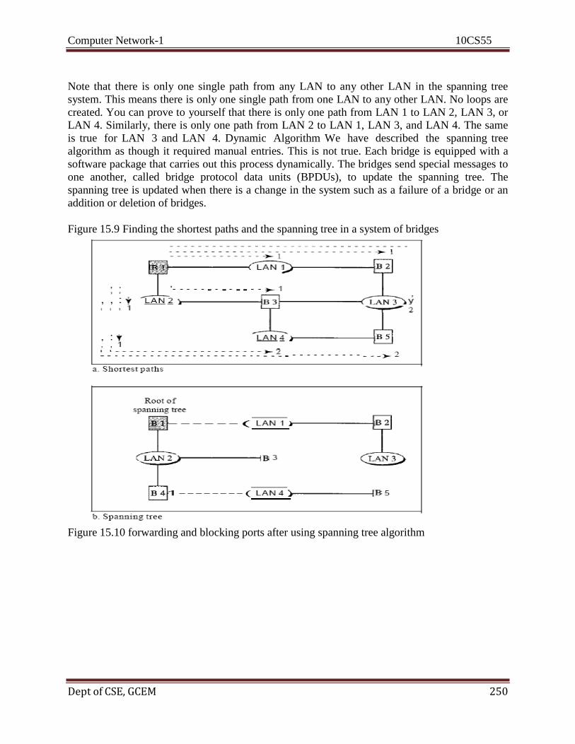
Computer Network-1 10CS55
Dept of CSE, GCEM 250
Note that there is only one single path from any LAN to any other LAN in the spanning tree
system. This means there is only one single path from one LAN to any other LAN. No loops are
created. You can prove to yourself that there is only one path from LAN 1 to LAN 2, LAN 3, or
LAN 4. Similarly, there is only one path from LAN 2 to LAN 1, LAN 3, and LAN 4. The same
is true for LAN 3 and LAN 4. Dynamic Algorithm We have described the spanning tree
algorithm as though it required manual entries. This is not true. Each bridge is equipped with a
software package that carries out this process dynamically. The bridges send special messages to
one another, called bridge protocol data units (BPDUs), to update the spanning tree. The
spanning tree is updated when there is a change in the system such as a failure of a bridge or an
addition or deletion of bridges.
Figure 15.9 Finding the shortest paths and the spanning tree in a system of bridges
Figure 15.10 forwarding and blocking ports after using spanning tree algorithm

Computer Network-1 10CS55
Dept of CSE, GCEM 251
Source Routing Bridges
Another way to prevent loops in a system with redundant bridges is to use source routing
bridges. A transparent bridge's duties include filtering frames, forwarding, and blocking. In a
system that has source routing bridges, these duties are performed by the source station and, to
some extent, the destination station.
In source routing, a sending station defines the bridges that the frame must visit. The addresses
of these bridges are included in the frame. In other words, the frame contains not only the source
and destination addresses, but also the addresses of all bridges to be visited.
The source gets these bridge addresses through the exchange of special frames with the
destination prior to sending the data frame. Source routing bridges were designed by IEEE to be
used with Token Ring LANs. These LANs are not very common today.
Bridges Connecting Different LANs
Theoretically a bridge should be able to connect LANs using different protocols at the data link
layer, such as an Ethernet LAN to a wireless LAN. However, there are many issues to be
considered:
Frame format. Each LAN type has its own frame format (compare an Ethernet frame with
a wireless LAN frame).
Maximum data size. If an incoming frame's size is too large for the destination LAN, the
data must be fragmented into several frames. The data then need to be reassembled at the
destination. However, no protocol at the data link layer allows the fragmentation and
reassembly of frames. We will see in Chapter 19 that this is allowed in the network layer.
The bridge must therefore discard any frames too large for its system.
Data rate. Each LAN type has its own data rate. (Compare the 10-Mbps data rate of an
Ethernet with the I-Mbps data rate of a wireless LAN.) The bridge must buffer the frame
to compensate for this difference.

Computer Network-1 10CS55
Dept of CSE, GCEM 252
Bit order. Each LAN type has its own strategy in the sending of bits. Some send the most
significant bit in a byte first; others send the least significant bit first.
Security. Some LANs, such as wireless LANs, implement security measures in the data
link layer. Other LANs, such as Ethernet, do not. Security often involves encryption
When a bridge receives a frame from a wireless LAN, it needs to decrypt the message
before forwarding it to an Ethernet LAN.
Multimedia support. Some LANs support multimedia and the quality of services needed
for this type of communication; others do not.
Two-Layer Switches
When we use the term switch, we must be careful because a switch can mean two different
things. We must clarify the term by adding the level at which the device operates. We can have a
two-layer switch or a three-layer switch. A three-layer switch is used at the network layer; it is a
kind of router. The two-layer switch performs at the physical and data link layers. A two-layer
switch is a bridge, a bridge with many ports and a design that allows better (faster) performance.
A bridge with a few ports can connect a few LANs together. A bridge with many ports may be
able to allocate a unique port to each station, with each station on its own independent entity.
This means no competing traffic (no collision, as we saw in Ethernet).
A two-layer switch, as a bridge does, makes a filtering decision based on the MAC address of the
frame it received. However, a two-layer switch can be more sophisticated. It can have a buffer to
hold the frames for processing. It can have a switching factor that forwards the frames faster.
Some new two-layer switches, called cut-through switches, have been designed to forward the
frame as soon as they check the MAC addresses in the header of the frame.
Routers
A router is a three-layer device that routes packets based on their logical addresses (host-to-host
addressing). A router normally connects LANs and WANs in the Internet and has a routing table
that is used for making decisions about the route. The routing tables are normally dynamic and
are updated using routing protocols. Figure 15.11 shows a part of the Internet that uses routers to
connect LANs and WANs.
Figure 15.11 Routers connecting independent LANs and WANs
Three-Layer Switches

Computer Network-1 10CS55
Dept of CSE, GCEM 253
A three-layer switch is a router, but a faster and more sophisticated. The switching fabric in a
three-layer switch allows faster table lookup and forwarding. In this book, we use the terms
router and three-layer switch interchangeably.
Gateway
Although some textbooks use the terms gateway and router interchangeably, most of the
literature distinguishes between the two. A gateway is normally a computer that operates in all
five layers of the Internet or seven layers of OSI model. A gateway takes an application message,
reads it, and interprets it. This means that it can be used as a connecting device between two
internetworks that use different models. For example, a network designed to use the OSI model
can be connected to another network using the Internet model. The gateway connecting the two
systems can take a frame as it arrives from the first system, move it up to the OSI application
layer, and remove the
message. Gateways can provide security.
15.2 BACKBONE NETWORKS
Some connecting devices discussed in this chapter can be used to connect LANs in a backbone
network. A backbone network allows several LANs to be connected. In a backbone network, no
station is directly connected to the backbone; the stations are part of a LAN, and the backbone
connects the LANs. The backbone is itself a LAN that uses a LAN protocol such as Ethernet;
each connection to the backbone is itself another LAN. Although many different architectures
can be used for a backbone, we discuss only the two most common: the bus and the star.
Bus Backbone
In a bus backbone, the topology of the backbone is a bus. The backbone itself can use one of the
protocols that support a bus topology such as lOBase5 or lOBase2.
Bus backbones are normally used as a distribution backbone to connect different buildings in an
organization. Each building can comprise either a single LAN or another backbone (normally a
star backbone). A good example of a bus backbone is one that connects single- or multiple-floor
buildings on a campus. Each single-floor building usually has a single LAN. Each multiple-floor
building has a backbone (usually a star) that connects each LAN on a floor. A bus backbone can
interconnect these LANs and backbones. Figure 15.12 shows an example of a bridge-based
backbone with four LANs
Figure 15.12 Bus backbone

Computer Network-1 10CS55
Dept of CSE, GCEM 254
In Figure 15.12, if a station in a LAN needs to send a frame to another station in the same LAN,
the corresponding bridge blocks the frame; the frame never reaches the backbone. However, if a
station needs to send a frame to a station in another LAN, the bridge passes the frame to the
backbone, which is received by the appropriate bridge and is delivered to the destination LAN.
Each bridge connected to the backbone has a table that shows the stations on the LAN side of the
bridge. The blocking or delivery of a frame is based on the contents of this table.
Star Backbone
In a star backbone, sometimes called a collapsed or switched backbone, the topology of the
backbone is a star. In this configuration, the backbone is just one switch (that is why it is called,
erroneously, a collapsed backbone) that connects the LANs.
Figure 15.13 shows a star backbone. Note that, in this configuration, the switch does the job of
the backbone and at the same time connects the LANs.
Figure 15.13 Star backbone
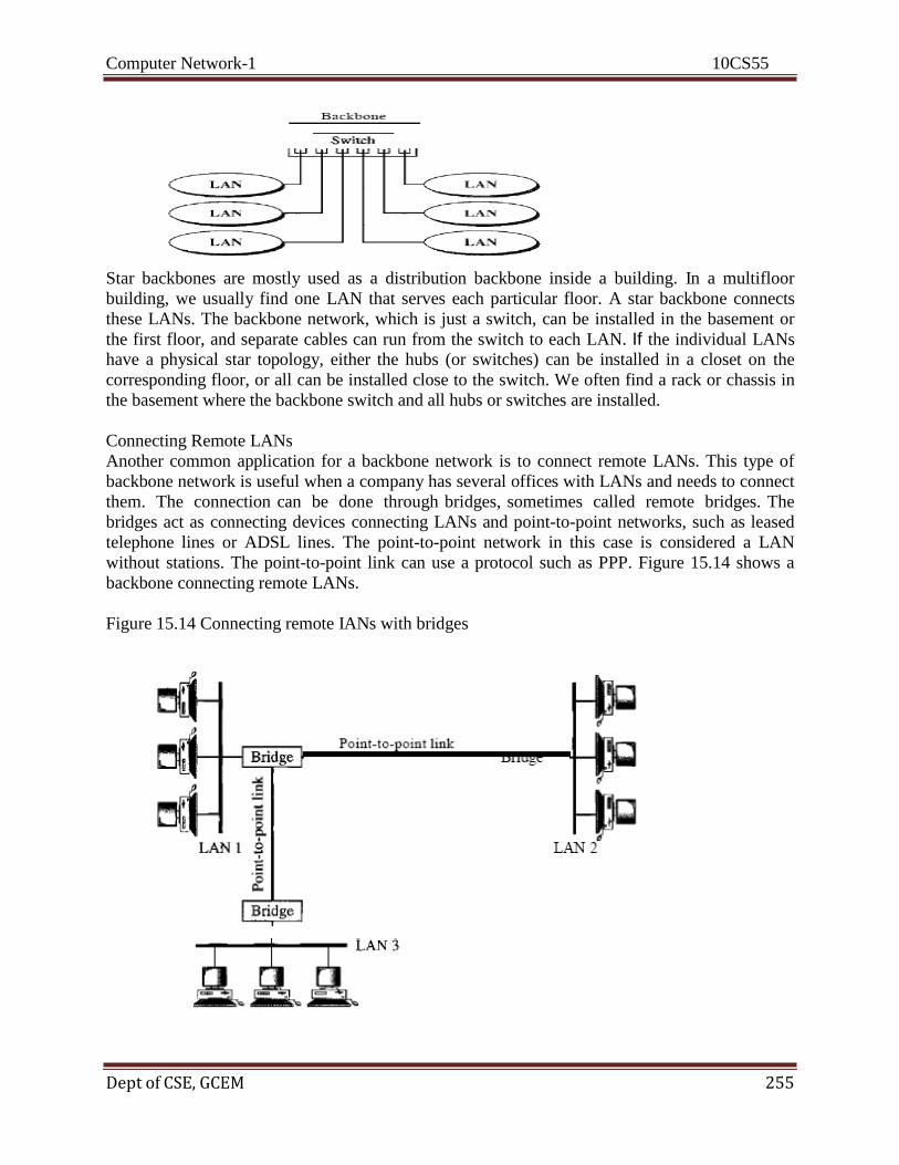
Computer Network-1 10CS55
Dept of CSE, GCEM 255
Star backbones are mostly used as a distribution backbone inside a building. In a multifloor
building, we usually find one LAN that serves each particular floor. A star backbone connects
these LANs. The backbone network, which is just a switch, can be installed in the basement or
the first floor, and separate cables can run from the switch to each LAN. If the individual LANs
have a physical star topology, either the hubs (or switches) can be installed in a closet on the
corresponding floor, or all can be installed close to the switch. We often find a rack or chassis in
the basement where the backbone switch and all hubs or switches are installed.
Connecting Remote LANs
Another common application for a backbone network is to connect remote LANs. This type of
backbone network is useful when a company has several offices with LANs and needs to connect
them. The connection can be done through bridges, sometimes called remote bridges. The
bridges act as connecting devices connecting LANs and point-to-point networks, such as leased
telephone lines or ADSL lines. The point-to-point network in this case is considered a LAN
without stations. The point-to-point link can use a protocol such as PPP. Figure 15.14 shows a
backbone connecting remote LANs.
Figure 15.14 Connecting remote IANs with bridges
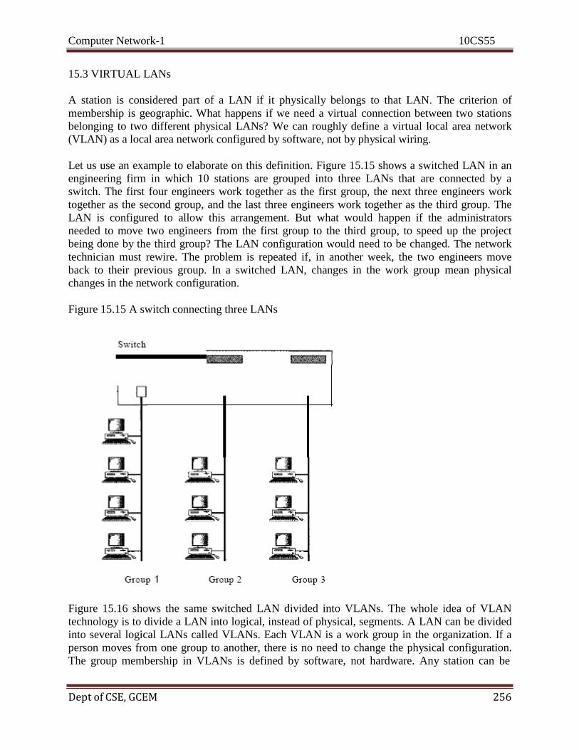
Computer Network-1 10CS55
Dept of CSE, GCEM 256
15.3 VIRTUAL LANs
A station is considered part of a LAN if it physically belongs to that LAN. The criterion of
membership is geographic. What happens if we need a virtual connection between two stations
belonging to two different physical LANs? We can roughly define a virtual local area network
(VLAN) as a local area network configured by software, not by physical wiring.
Let us use an example to elaborate on this definition. Figure 15.15 shows a switched LAN in an
engineering firm in which 10 stations are grouped into three LANs that are connected by a
switch. The first four engineers work together as the first group, the next three engineers work
together as the second group, and the last three engineers work together as the third group. The
LAN is configured to allow this arrangement. But what would happen if the administrators
needed to move two engineers from the first group to the third group, to speed up the project
being done by the third group? The LAN configuration would need to be changed. The network
technician must rewire. The problem is repeated if, in another week, the two engineers move
back to their previous group. In a switched LAN, changes in the work group mean physical
changes in the network configuration.
Figure 15.15 A switch connecting three LANs
Figure 15.16 shows the same switched LAN divided into VLANs. The whole idea of VLAN
technology is to divide a LAN into logical, instead of physical, segments. A LAN can be divided
into several logical LANs called VLANs. Each VLAN is a work group in the organization. If a
person moves from one group to another, there is no need to change the physical configuration.
The group membership in VLANs is defined by software, not hardware. Any station can be

Computer Network-1 10CS55
Dept of CSE, GCEM 257
logically moved to another VLAN. All members belonging to a VLAN can receive broadcast
messages sent to that particular VLAN.
Figure 15.16 A switch using VLAN software
This means if a station moves from VLAN 1 to VLAN 2, it receives broadcast messages sent to
VLAN 2, but no longer receives broadcast messages sent to VLAN 1. It is obvious that the
problem in our previous example can easily be solved by using VLANs. Moving engineers from
one group to another through software is easier than changing the configuration of the physical
network. VLAN technology even allows the grouping of stations connected to different switches
in a VLAN. Figure 15.17 shows a backbone local area network with two switches and three
VLANs. Stations from switches A and B belong to each VLAN.
Figure 15.17 Two switches in a backbone using VLAN software

Computer Network-1 10CS55
Dept of CSE, GCEM 258
This is a good configuration for a company with two separate buildings. Each building can have
its own switched LAN connected by a backbone. People in the first building and people in the
second building can be in the same work group even though they are connected to different
physical LANs.
From these three examples, we can define a VLAN characteristic:
VLANs create broadcast domains.
VLANs group stations belonging to one or more physical LANs into broadcast domains. The
stations in a VLAN communicate with one another as though they belonged to a physical
segment.
Membership
What characteristic can be used to group stations in a VLAN? Vendors use different
characteristics such as port numbers, MAC addresses, IP addresses, IP multicast addresses, or a
combination of two or more of these.
Port Numbers
Some VLAN vendors use switch port numbers as a membership characteristic. For example, the
administrator can define that stations connecting to ports 1, 2, 3, and 7 belong to VLAN 1;
stations connecting to ports 4, 10, and 12 belong to VLAN 2; and so on.
MAC Addresses
Computer Network-1 10CS55
Dept of CSE, GCEM 259
Some VLAN vendors use the 48-bit MAC address as a membership characteristic. For example,
the administrator can stipulate that stations having MAC addresses E21342A12334 and
F2A123BCD341belong to VLAN 1.
IP Addresses
Some VLAN vendors use the 32-bit IP address (see Chapter 19) as a membership characteristic.
For example, the administrator can stipulate that stations having IP addresses 181.34.23.67,
181.34.23.72, 181.34.23.98, and 181.34.23.112 belong to VLAN 1. Multicast IP Addresses
Some VLAN vendors use the multicast IP address (see Chapter 19) as a membership
characteristic. Multicasting at the IP layer is now translated to multicasting at the data link layer.
Combination Recently, the software available from some vendors allows all these characteristics
to be combined. The administrator can choose one or more characteristics when installing the
software. In addition, the software can be reconfigured to change the settings.
Configuration
How are the stations grouped into different VLANs? Stations are configured in one of three
ways: manual, semiautomatic, and automatic.
Manual Configuration
In a manual configuration, the network administrator uses the VLAN software to manually
assign the stations into different VLANs at setup. Later migration from one VLAN to another is
also done manually. Note that this is not a physical configuration; it is a logical configuration.
The term manually here means that the administrator types the port numbers, the IP addresses, or
other characteristics, using the VLAN software.
Automatic Configuration
In an automatic configuration, the stations are automatically connected or disconnected from a
VLAN using criteria defined by the administrator. For example, the administrator can define the
project number as the criterion for being a member of a group. When a user changes the project,
he or she automatically migrates to a new VLAN.
Semiautomatic Configuration
A semiautomatic configuration is somewhere between a manual configuration and an automatic
configuration. Usually, the initializing is done manually, with migrations done automatically.
Communication between Switches
In a multiswitched backbone, each switch must know not only which station belongs to which
VLAN, but also the membership of stations connected to other switches. For example, in Figure
15.17, switch A must know the membership status of stations connected to switch B, and switch
B must know the same about switch A. Three methods have been devised for this purpose: table
maintenance, frame tagging, and time-division multiplexing.
Computer Network-1 10CS55
Dept of CSE,GCEM 260
Table Maintenance
In this method, when a station sends a broadcast frame to its group members, the switch creates
an entry in a table and records station membership. The switches send their tables to one another
periodically for updating.
Frame Tagging
In this method, when a frame is traveling between switches, an extra header is added to the MAC
frame to define the destination VLAN. The frame tag is used by the receiving switches to
determine the VLANs to be receiving the broadcast message.
Time-Division Multiplexing (TDM)
In this method, the connection (trunk) between switches is divided into timeshared channels (see
TDM in Chapter 6). For example, if the total number of VLANs in a backbone is five, each trunk
is divided into five channels. The traffic destined for VLAN 1 travels in channell, the traffic
destined for VLAN 2 travels in channel 2, and so on. The receiving switch determines the
destination VLAN by checking the channel from which the frame arrived.
IEEE Standard
In 1996, the IEEE 802.1 subcommittee passed a standard called 802.1Q that defines the format
for frame tagging. The standard also defines the format to be used in multiswitched backbones
and enables the use of multivendor equipment in VLANs. IEEE 802.1Q has opened the way for
further standardization in other issues related to VLANs. Most vendors have already accepted the
standard.
Advantages
There are several advantages to using VLANs.
Cost and Time Reduction
VLANs can reduce the migration cost of stations going from one group to another. Physical
reconfiguration takes time and is costly. Instead of physically moving one station to another
segment or even to another switch, it is much easier and quicker to move it by using software.
Creating Virtual Work Groups
VLANs can be used to create virtual work groups. For example, in a campus environment,
professors working on the same project can send broadcast messages to one another without the
necessity of belonging to the same department. This can reduce traffic if the multicasting
capability of IP was previously used. Security

Computer Network-1 10CS55
Dept of CSE,GCEM 261
VLANs provide an extra measure of security. People belonging to the same group can send
broadcast messages with the guaranteed assurance that users in other groups will not receive
these messages
Recommended Questions
1. What is the relationship between a base station and a
mobile switching center?
2. What are the functions of a mobile switching center? 3. What is the difference between a hard handoff and a soft
handoff?
4. What is the relationship between D-AMPS and AMPS?
5. What are the three types of orbits? 6. Which type of orbit does a GEO satellite have? Explain
your answer
7. What is the relationship between the Van Allen belts and
satellites?
8. What is the relationship between the Van Allen belts and
satellites?
Computer Network-1 10CS55
Dept of CSE,GCEM 262
COMPUTER NETWORKS – I
Subject Code: 10CS55 I.A. Marks : 25
Hours/Week : 04 Exam Hours: 03
Total Hours : 52 Exam Marks: 100
UNIT - 8: 7 Hours Network Layer:
- Introduction,
- Logical addressing,
- IPv4 addresses,
- Internetworking basics,
- IPv4, IPv6, - Comparison of IPv4 and IPv6 Headers.
Computer Network-1 10CS55
Dept of CSE,GCEM 263
Unit-8
NETWORK LAYER
Logical Addressing Logical Address, which is assigned during configuration of the network, refers to the virtual
address or logical location of the machine. This concept is similar to a person’s mailing address.
Usually Two types of logical addressing are used in the Network layer. IP addresses and IPX
addresses. IP addresses are used in all TCP/IP based networks where as IPX addresses are used
in Novel Netware environment.
IP Addresses IP address is the 32 BIT identifier used to identify the host or some interface. IP address consists
of two parts Network ID (high order bits), that represents the Network for the particular host or
interface. Host ID (low order bits), that represents the logical host identification number. IP
addresses are divided into 5 classes:
• Class A addresses start with a `0' in the most significant bit, followed by a 7-bit network
address and a 24-bit local part.
• Class B addresses start with a `10' in the two most significant bits, followed by a 14-bit network
number and a 16-bit local part.
• Class C addresses start with a `110' in the three most significant bits, followed by a 21-bit
network number and an 8-bit local part
. Class D addresses start with a `1110' in the four most significant bits, followed by a 28-bit
group number. Used for multicast.
• Class E addresses start with a ‘11110’ and are reserved for future use.
Classful addressing:
• Inefficient use of address space, address space exhaustion
• e.g., class B net allocated enough addresses for 65K hosts, even if only
2K hosts in that network
CIDR: Classless InterDomain Routing
• Network portion of address of arbitrary length
• Address format: a.b.c.d/x, where x is # bits in network portion of address
11001000 00010111 00010000 00000000
An Internet Protocol address (IP address) is a numerical label assigned to each device (e.g.,
computer, printer) participating in a computer network that uses the Internet Protocol for
communication.[1] An IP address serves two principal functions: host or network
interface identification and location addressing. Its role has been characterized as follows:
"A name indicates what we seek. An address indicates where it is. A route indicates how to get
there."[2]
The designers of the Internet Protocol defined an IP address as a 32-bit number[1] and this
system, known as Internet Protocol Version 4 (IPv4), is still in use today. However, due to the

Computer Network-1 10CS55
Dept of CSE,GCEM 264
enormous growth of the Internet and the predicted depletion of available addresses, a new
version of IP (IPv6), using 128 bits for the address, was developed in 1995.[3] IPv6 was
standardized as RFC 2460in 1998,[4] and its deployment has been ongoing since the mid-2000s.
IP addresses are binary numbers, but they are usually stored in text files and displayed in human-
readable notations, such as 172.16.254.1 (for IPv4), and 2001:db8:0:1234:0:567:8:1 (for IPv6).
The Internet Assigned Numbers Authority (IANA) manages the IP address space allocations
globally and delegates five regional Internet registries (RIRs) to allocate IP address blocks
to local Internet registries (Internet service providers) and other entities.
IP versions
Two versions of the Internet Protocol (IP) are in use: IP Version 4 and IP Version 6. Each
version defines an IP address differently. Because of its prevalence, the generic term IP
address typically still refers to the addresses defined by IPv4. The gap in version sequence
between IPv4 and IPv6 resulted from the assignment of number 5 to the experimental Internet
Stream Protocol in 1979, which however was never referred to as IPv5.
Two versions of the Internet Protocol (IP) are in use: IP Version 4 and IP Version 6. Each
version defines an IP address differently. Because of its prevalence, the generic term IP
address typically still refers to the addresses defined by IPv4. The gap in version sequence
between IPv4 and IPv6 resulted from the assignment of number 5 to the experimental Internet
Stream Protocol in 1979, which however was never referred to as IPv5.
IPv6 addresses
The rapid exhaustion of IPv4 address space, despite conservation techniques, prompted
the Internet Engineering Task Force (IETF) to explore new technologies to expand the Internet's
addressing capability. The permanent solution was deemed to be a redesign of the Internet
Protocol itself. This next generation of the Internet Protocol, intended to replace IPv4 on the
Internet, was eventually namedInternet Protocol Version 6 (IPv6) in 1995.[3][4] The address size
was increased from 32 to 128 bits or 16 octets. This, even with a generous assignment of
Main article: IPv6 address
Decomposition of an IPv6 address from hexadecimalrepresentation to its binary value.

Computer Network-1 10CS55
Dept of CSE,GCEM 265
network blocks, is deemed sufficient for the foreseeable future. Mathematically, the new address
space provides the potential for a maximum of 2128, or about 3.403×1038 unique addresses.
The new design is not intended to provide a sufficient quantity of addresses on its own, but rather
to allow efficient aggregation of subnet routing prefixes to occur at routing nodes. As a result,
routing table sizes are smaller, and the smallest possible individual allocation is a subnet for
264 hosts, which is the square of the size of the entire IPv4 Internet. At these levels, actual
address utilization rates will be small on any IPv6 network segment. The new design also
provides the opportunity to separate the addressing infrastructure of a network segment — that is
the local administration of the segment's available space — from the addressing prefix used to
route external traffic for a network. IPv6 has facilities that automatically change the routing
prefix of entire networks, should the global connectivity or the routing policy change, without
requiring internal redesign or renumbering.
The large number of IPv6 addresses allows large blocks to be assigned for specific purposes and,
where appropriate, to be aggregated for efficient routing. With a large address space, there is not
the need to have complex address conservation methods as used in Classless Inter-Domain
Routing (CIDR).
Many modern desktop and enterprise server operating systems include native support for the
IPv6 protocol, but it is not yet widely deployed in other devices, such as home networking
routers,voice over IP (VoIP) and multimedia equipment, and network peripherals.
IPv6 private addresses
Just as IPv4 reserves addresses for private or internal networks, blocks of addresses are set aside
in IPv6 for private addresses. In IPv6, these are referred to as unique local addresses (ULA).RFC
4193 sets aside the routing prefix fc00::/7 for this block which is divided into two /8 blocks with
different implied policies. The addresses include a 40-bit pseudorandom number that minimizes
the risk of address collisions if sites merge or packets are misrouted.[8]
Early designs used a different block for this purpose (fec0::), dubbed site-local
addresses.[9] However, the definition of what constituted sites remained unclear and the poorly
defined addressing policy created ambiguities for routing. This address range specification was
abandoned and must not be used in new systems.[10]
Addresses starting with fe80:, called link-local addresses, are assigned to interfaces for
communication on the link only. The addresses are automatically generated by the operating
system for each network interface. This provides instant and automatic network connectivity for
any IPv6 host and means that if several hosts connect to a common hub or switch, they have a
communication path via their link-local IPv6 address. This feature is used in the lower layers of
IPv6 network administration (e.g. Neighbor Discovery Protocol).
None of the private address prefixes may be routed on the public Internet.
IP subnetworks
IP networks may be divided into subnetworks in both IPv4 and IPv6. For this purpose, an IP
address is logically recognized as consisting of two parts: the network prefix and the host
identifier, orinterface identifier (IPv6). The subnet mask or the CIDR prefix determines how the
IP address is divided into network and host parts.
Computer Network-1 10CS55
Dept of CSE,GCEM 266
The term subnet mask is only used within IPv4. Both IP versions however use the Classless
Inter-Domain Routing (CIDR) concept and notation. In this, the IP address is followed by a slash
and the number (in decimal) of bits used for the network part, also called the routing prefix. For
example, an IPv4 address and its subnet mask may be 192.0.2.1 and 255.255.255.0, respectively.
TheCIDR notation for the same IP address and subnet is 192.0.2.1/24, because the first 24 bits of
the IP address indicate the network and subnet.
IP address assignment
Internet Protocol addresses are assigned to a host either anew at the time of booting, or
permanently by fixed configuration of its hardware or software. Persistent configuration is also
known as using a static IP address. In contrast, in situations when the computer's IP address is
assigned newly each time, this is known as using a dynamic IP address.
Methods
Static IP addresses are manually assigned to a computer by an administrator. The exact
procedure varies according to platform. This contrasts with dynamic IP addresses, which are
assigned either by the computer interface or host software itself, as in Zeroconf, or assigned by a
server using Dynamic Host Configuration Protocol (DHCP). Even though IP addresses assigned
using DHCP may stay the same for long periods of time, they can generally change. In some
cases, a network administrator may implement dynamically assigned static IP addresses. In this
case, a DHCP server is used, but it is specifically configured to always assign the same IP
address to a particular computer. This allows static IP addresses to be configured centrally,
without having to specifically configure each computer on the network in a manual procedure.
In the absence or failure of static or stateful (DHCP) address configurations, an operating system
may assign an IP address to a network interface using state-less auto-configuration methods,
such as Zeroconf.
Uses of dynamic addressing
Dynamic IP addresses are most frequently assigned on LANs and broadband networks
by Dynamic Host Configuration Protocol (DHCP) servers. They are used because it avoids the
administrative burden of assigning specific static addresses to each device on a network. It also
allows many devices to share limited address space on a network if only some of them will be
online at a particular time. In most current desktop operating systems, dynamic IP configuration
is enabled by default so that a user does not need to manually enter any settings to connect to a
network with a DHCP server. DHCP is not the only technology used to assign dynamic IP
addresses. Dialup and some broadband networks use dynamic address features of the Point-to-
Point Protocol.
Sticky dynamic IP address
A sticky dynamic IP address is an informal term used by cable and DSL Internet access
subscribers to describe a dynamically assigned IP address which seldom changes. The addresses
are usually assigned with DHCP. Since the modems are usually powered on for extended periods
of time, the address leases are usually set to long periods and simply renewed. If a modem is
turned off and powered up again before the next expiration of the address lease, it will most
likely receive the same IP address.
Computer Network-1 10CS55
Dept of CSE,GCEM 267
Address autoconfiguration
RFC 3330 defines an address block, 169.254.0.0/16, for the special use in link-local
addressing for IPv4 networks. In IPv6, every interface, whether using static or dynamic address
assignments, also receives a local-link address automatically in the block fe80::/10.
These addresses are only valid on the link, such as a local network segment or point-to-point
connection, that a host is connected to. These addresses are not routable and like private
addresses cannot be the source or destination of packets traversing the Internet.
When the link-local IPv4 address block was reserved, no standards existed for mechanisms of
address autoconfiguration. Filling the void, Microsoft created an implementation that is called
Automatic Private IP Addressing (APIPA). Due to Microsoft's market power, APIPA has been
deployed on millions of machines and has, thus, become a de facto standard in the industry.
Many years later, the IETF defined a formal standard for this functionality, RFC 3927,
entitled Dynamic Configuration of IPv4 Link-Local Addresses.
Uses of static addressing
Some infrastructure situations have to use static addressing, such as when finding the Domain
Name System (DNS) host that will translate domain names to IP addresses. Static addresses are
also convenient, but not absolutely necessary, to locate servers inside an enterprise. An address
obtained from a DNS server comes with a time to live, or caching time, after which it should be
looked up to confirm that it has not changed. Even static IP addresses do change as a result of
network administration (RFC 2072).
Public addresses
A public IP address, in common parlance, is synonymous with a globally routable unicast IP address.[citation needed]
Both IPv4 and IPv6 define address ranges that are reserved for private networks and link-local
addressing. The term public IP address often used excludes these types of addresses.
Modifications to IP addressing
IP blocking and firewalls
Firewalls perform Internet Protocol blocking to protect networks from unauthorized access. They
are common on today's Internet. They control access to networks based on the IP address of a
client computer. Whether using a blacklist or a whitelist, the IP address that is blocked is the
perceived IP address of the client, meaning that if the client is using a proxy server or network
address translation, blocking one IP address may block many individual computers.
IP address translation
Multiple client devices can appear to share IP addresses: either because they are part of a shared
hosting web server environment or because an IPv4 network address translator (NAT) or proxy
server acts as an intermediary agent on behalf of its customers, in which case the real originating
IP addresses might be hidden from the server receiving a request. A common practice is to have
a NAT hide a large number of IP addresses in a private network. Only the "outside" interface(s)
of the NAT need to have Internet-routable addresses.[11]
Computer Network-1 10CS55
Dept of CSE,GCEM 268
Most commonly, the NAT device maps TCP or UDP port numbers on the outside to individual
private addresses on the inside. Just as a telephone number may have site-specific extensions, the
port numbers are site-specific extensions to an IP address.
In small home networks, NAT functions usually take place in a residential gateway device,
typically one marketed as a "router". In this scenario, the computers connected to the router
would have 'private' IP addresses and the router would have a 'public' address to communicate
with the Internet. This type of router allows several computers to share one public IP address.
Recommended Questions
1. What is the name of the packet in IP layer.
2. Why does the IP checksum just cover the header.
3. What is the function of ICMP.
4. Name and explain three types of IPv6 addresses. 5. What strategies are devised for transition of IPV4 to IPV6.
6.


![Energy-Saving in IP Over WDM Networks by Putting ......IP over WDM networks achieved by switching off router line cards during low-demand hours. In [24], they also presented a detailed](https://img.pdfslide.net/doc/110x75/5fb93ea846b9283d5246341a/energy-saving-in-ip-over-wdm-networks-by-putting-ip-over-wdm-networks-achieved.jpg)


![Disposition and metabolism of [ c]- levomilnacipran, a ... · 1 hour, 2 hours, 2.5 hours, 3 hours, 3.5 hours, 4 hours, 5 hours, 6 hours, 8 hours, 10 hours, 12 hours, 24 hours, 48](https://img.pdfslide.net/doc/110x75/5f73b26d02e65a52de6394cc/disposition-and-metabolism-of-c-levomilnacipran-a-1-hour-2-hours-25.jpg)
