Computer Programs in Seismology Moment Tensor Inversion

VirtualBox VDI Distribution

Robert B. HerrmannReinert Professor of Natural Sciences

Department of Earth and Atmospheric SciencesSaint Louis University

St. Louis, Missouri, USAEmail: rbh@eas.slu.edu

August 4, 2015

1

Table of Contents1. The Guide..........................................................................................................................62. Manipulating waveforms................................................................................................. 73. Installation...................................................................................................................... 104. Moment Tensor Inversion – Chile.................................................................................12

Step 1. Create the DO script......................................................................................... 12Step 2 – Execute the DO script.................................................................................... 15Step 3 – Further processing......................................................................................... 22

Remove bad traces....................................................................................................22Modify processing.....................................................................................................23Use a different model................................................................................................23

5. Moment Tensor Inversion – North America.................................................................24Step 1 – Create the DO script....................................................................................... 26Step 2 – Execute DO script...........................................................................................27Step 3 – Place data into the event processing directory and process....................28More things to do...........................................................................................................37

Remove bad traces....................................................................................................37Try a different model................................................................................................. 37

6. Quality Control Using Teleseisms................................................................................38Step 1.............................................................................................................................. 38Step 2 – Get the data..................................................................................................... 38Step 3 – Sample data sets.............................................................................................38Step 4 – Create the DO script....................................................................................... 39Step 5 – Create the event directories.......................................................................... 39Step 6 – Place data into the event processing directory and process....................40

7. Moment Tensor Determination for Teleseisms........................................................... 44Step 1.............................................................................................................................. 44Step 2 – Get the data..................................................................................................... 44Step 3 – Sample data sets.............................................................................................44Step 4 – Create the DO script....................................................................................... 44Step 5 – Create the event directories.......................................................................... 45Step 6 – Place data into the event processing directory and process....................45

8. Modifications for other regional networks..................................................................48Appendix.............................................................................................................................50

Installation of VirtualBox.............................................................................................. 50Installation of Lubuntu32 and Course software......................................................... 52

Now start Virtual Box. You will see that I already have Mint12 installed on the test computer............................................................................................................. 52

Running Lununtu32.......................................................................................................55Changing Keyboard from US................................................................................... 56VBox Additions.......................................................................................................... 59Accessing Host Filesystem......................................................................................60Notes...........................................................................................................................65

2

3

Quick GuideThis distribution is made for use with the Oracle VirtualBox. A complete image of a Lubuntu 32 LINUIX distribution is provided.

To run the tutorials for Moment Tensor Inversion, start Lubuntu32 and then login with

User: cps Password: cps

To run the tutorials for HypoDD, start Lubuntu32 and then login with

User: hypodd Password: hypodd

After logging in, ignore messages about updating the operating system.

Then double click on the LxTerminal icon at the upper left.

To log out, click on the “House at the bottom left” and then “Logout”

At the next menu, click “Shutdown”

4

It is necessary to logout carefully, otherwise damage may be done to the files that you use.

The distribution has about 3.5 gigabytes of space available for you use.

5

1. The Guide

This guide is focused primarily on the estimation of earthquake moment tensors using digital seismic data. This is accomplished by using the tools of Computer Programs in Seismology (http://www.eas.slu.edu/eqc/eqccps.html). We assume that the software package has been installed. This guide will show how the methodology can be applied to local/regional earthquakes and teleseisms.

Moment tensor inversion is not easy, since it requires the implementation of theory, the use of the proper Earth model and high quality digital data.

This guide cannot answer all questions. However, the logical steps are correct. There are many shellscripts, so I recommend that you use the world wide web to find a tutorial or purchase a book on thebash shell, which is used by the scripts. Once you know shell scripts, you can modify the scripts according to your requirements.

This course will provide an introduction to data manipulation using the program gsac. This VirtualBox image is complete with everything that you require, including test data sets. The scripts provided will permit you to acquire data from the IRIS DMC and also the USGS Continuous Wave Buffer (for recent earthquakes) for your studies.

6

2. Manipulating waveformsBefore beginning the use of the programs for moment tensor inversion, we will first look at some digital data. Do the following:

cps:~$ cd [return to home directory]cps:~$ cd MOMENT_TENSORcps:~$ cd WAVEFORMScps:~$ cd 20150729023558cps:~$ cd 20150729023558cps:~$ cd FINAL [or from the home directory

cd MOM*/WAV*/20*/20*/FINAL ]

cps:~$ gsacGSAC> r *ZGSAC> fileid nameGSAC> sort up distGSAC> p perplot 6

You will see a plot such as the following:

This displays the derived vertical component ground velocities for this M=6.3 earthquake of 2015/07/29 02:35 recorded in the central United States. The command said to display all Z (vertical) components six traces at a time. The units are ground velocity in m/s. The BHZ and HHZ channels are from broadband sensors and the HNZ sensor is from an accelerometer.

Now to focus on early P and pP arrivals (at 41 degrees and 118 km source depth, the travel times are451.3 secodns forP, 478.0 for pP, 491.4 for sP and 548 for PP) , do the following:

7

GSAC> cut a -30 a 120GSAC> rGSAC> rtrGSAC> taper w 0.1

GSAC> hp c 0.05 n 3

GSAC> lp c 0.2 n 3 [filter to look at low frequencies]

GSAC> ylim all [display each page with the same scale]

The next two figures present some of the plots.

We observe a number of important points. First all peak amplitudes are the same. This is expected since the great circle distance to all stations in this data set is from 38 to 47 degrees, and the azimuth from the source to the station is between 90 and 100 degrees. For the figure here, the arc distance is 41.3 to 41.4 degrees. We expect the same amplitude as long as the ray from the source is not near a nodal plane.

If we look at other traces, we look for the same polarity, and amplitude. We will see a big problem with stations GORE, LOOK. BCOK, CROK and FNO. This is because of inaccuracies in the preparation of the metadata.

We cannot perform a moment tensor inversion unless we have confidence in the derived ground amplitudes.

8

We will also try some other commands, such as ppk, where we will see how to manipulate the traces.

9

3. Installation The software is installed in a VirtualBox image. This image contains the Lubuntu 32bit distribution of the LINUX operating system, Computer Programs in Seismology, GMT, and all other software tocompile and support the course. The installation of VirtualBox and the Lubuntu32.vdi virtual disk image is presented in the Appendix..

After starting the virtual machine, the Lubuntu login page will appear.

Login: cps

Password: PROGRAMS.330

After you open the terminal icon on the desktop, you will see the following directory structure:

/home/cps/PROGRAMS.330 - Computer Programs in Seismology

/home/cps/COURSE/CWBQuery - test programs for USGS CWBQuery

/home/cps/COURSE/WS - IRIS WaveServer test and mseed2sac

/hme/cps/COURSE/MomentTensor2014_01.pdf – this document

/home/cps//GREEN - Velocity models and Green's functions for CUS and WUS regional model and AK135 teleseism model

/home/cps/GMT3.4 - GMT which is used for mapping. This includes the low resolution map data base

/home/cps/MOMENT_TENSOR/ - work area for moment tensor inversion. This includes

MECH.CL - for earthquakes in Chile, which are good for training

MECH.NA – for earthquakes in North America for training

MECH.TEL – for earthquakes at distances of 30 -90 degrees

MECHQC.TEL – for using known moment tensor to test telseismic data

/home/cps/COURSE - subdirectories CWBQuery and WS for obtaining data from USGS/NEUIC Continuous Wave Buffer and the IRIS FetchData mechanisms

When you login to the computer as user cps, the system read the startup file /home/cps/.profile and also /home/cps/.bashrc. The files define parameters for the user to find user programs and to set the execution environment. I added the following to the bottom of the .profile:###### Safety for restart#####OPATH=$PATHPATH=:$HOME/PROGRAMS.330/bin:$HOME/GMT3.4/bin:$OPATHexport PATH

I made additions to the .bashrc file, which I indicate by the highlights:

PERL_MB_OPT="--install_base \"/home/cps/perl5\""; export PERL_MB_OPT;PERL_MM_OPT="INSTALL_BASE=/home/cps/perl5"; export PERL_MM_OPT;

GMTHOME=/home/cps/GMT3.4

10

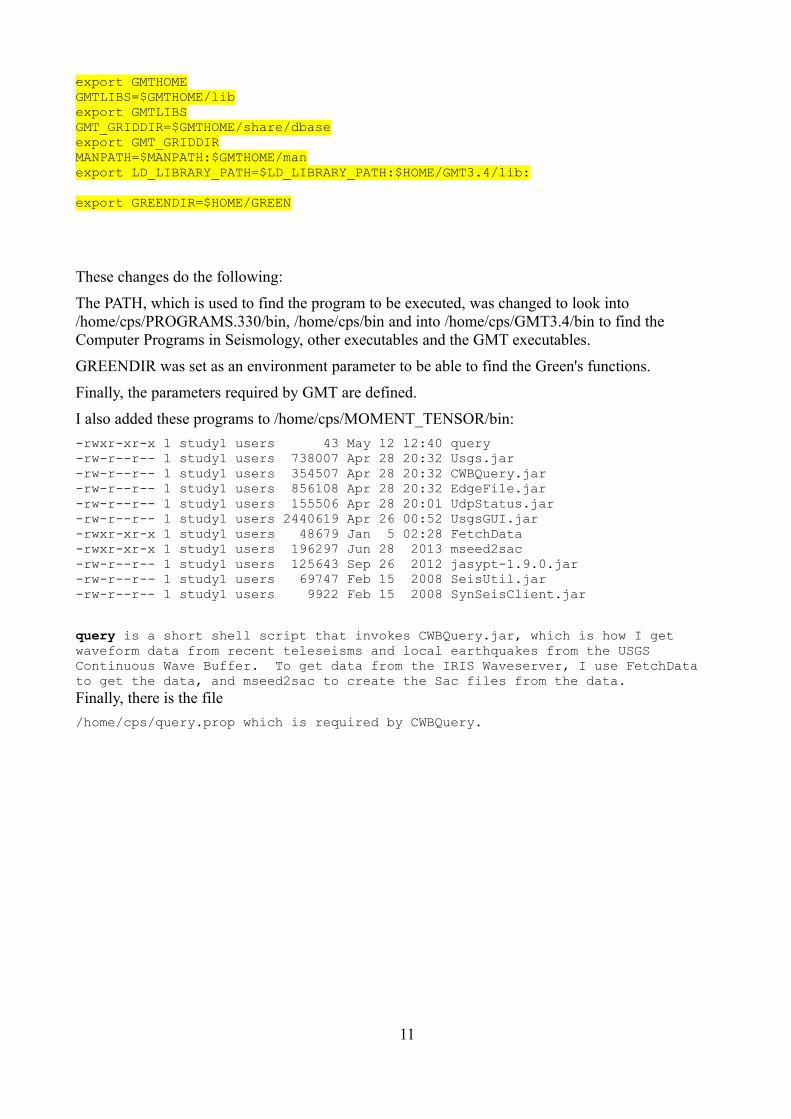
export GMTHOMEGMTLIBS=$GMTHOME/libexport GMTLIBSGMT_GRIDDIR=$GMTHOME/share/dbaseexport GMT_GRIDDIRMANPATH=$MANPATH:$GMTHOME/manexport LD_LIBRARY_PATH=$LD_LIBRARY_PATH:$HOME/GMT3.4/lib:

export GREENDIR=$HOME/GREEN

These changes do the following:

The PATH, which is used to find the program to be executed, was changed to look into /home/cps/PROGRAMS.330/bin, /home/cps/bin and into /home/cps/GMT3.4/bin to find the Computer Programs in Seismology, other executables and the GMT executables.

GREENDIR was set as an environment parameter to be able to find the Green's functions.

Finally, the parameters required by GMT are defined.

I also added these programs to /home/cps/MOMENT_TENSOR/bin:

-rwxr-xr-x 1 study1 users 43 May 12 12:40 query-rw-r--r-- 1 study1 users 738007 Apr 28 20:32 Usgs.jar-rw-r--r-- 1 study1 users 354507 Apr 28 20:32 CWBQuery.jar-rw-r--r-- 1 study1 users 856108 Apr 28 20:32 EdgeFile.jar-rw-r--r-- 1 study1 users 155506 Apr 28 20:01 UdpStatus.jar-rw-r--r-- 1 study1 users 2440619 Apr 26 00:52 UsgsGUI.jar-rwxr-xr-x 1 study1 users 48679 Jan 5 02:28 FetchData-rwxr-xr-x 1 study1 users 196297 Jun 28 2013 mseed2sac-rw-r--r-- 1 study1 users 125643 Sep 26 2012 jasypt-1.9.0.jar-rw-r--r-- 1 study1 users 69747 Feb 15 2008 SeisUtil.jar-rw-r--r-- 1 study1 users 9922 Feb 15 2008 SynSeisClient.jar

query is a short shell script that invokes CWBQuery.jar, which is how I get waveform data from recent teleseisms and local earthquakes from the USGS Continuous Wave Buffer. To get data from the IRIS Waveserver, I use FetchData to get the data, and mseed2sac to create the Sac files from the data.Finally, there is the file

/home/cps/query.prop which is required by CWBQuery.

11

4. Moment Tensor Inversion – ChileGo to the work area MECH.CL. In this directory you will see the following files if you use the ls command, e.g.,

rbh> ls0XXXREG DOIRIS DOSETUP DOWSSETUP PROTO.WSDO DOISETUP DOSOLUTION PROTO.CWB mech.shDOCWB DOQUERY DOWS PROTO.I

If we use the command ls -F a '/' will appear to indicate that the item is a directory, and an '*' to indicate that the item is an executable program or script

rbh> ls -F0XXXREG/ DOIRIS* DOSETUP* DOWSSETUP* PROTO.WS/DO* DOISETUP* DOSOLUTION* PROTO.CWB/ mech.sh*DOCWB* DOQUERY* DOWS* PROTO.I/

All items starting with 'DO' are processing scripts. The PROTO directories contain scripts for removing the instrument response, rotating the traces and performing quality control. The 0XXXREG directory contains the prototypes for the source inversion processing.

To see the directory structure, enter the command

rbh> du0 ./0XXXREG/DAT.REG/NOUSE0 ./0XXXREG/DAT.REG80 ./0XXXREG/GRD.REG48 ./0XXXREG/HTML.REG24 ./0XXXREG/MAP.REG8 ./0XXXREG/MT.OTHER24 ./0XXXREG/NEW2.REG48 ./0XXXREG/SYN.REG232 ./0XXXREG64 ./PROTO.CWB56 ./PROTO.I72 ./PROTO.WS528 .

This shows the subdirectories and gives the disk usage for each.

As an example, we will process the earthquake with the following source parameters given by the USGS:

M 5.5 - 85km WNW of Iquique, ChileTime 2014-05-17 09:11:06 UTCLocation 20.014°S 70.927°WDepth 9.2km

To start processing we must create a “GO” script in the proper format. This can be done using an editor or by the shell script mech.sh, which requires the program dialog to be in PROGRAMS.330/bin. In this example, we will use the mech.sh interface for data entry.

Step 1. Create the DO scriptrbh> mech.sh

12

This gives the menu

You can navigate by using the up/down arrow keys or by entering the letter on the keyboard. If you hit the 'Enter' key on the keyboard, then the highlighted item will take you to another menu where you can make entries, e.g.,

13

Continue the entries until you obtain the page

After going through everything, hitting ENTER on the “Quit” item, the result will be the creation of the script DO, which will also appear on ther terminal. Review the entries for correctness.

Note that negative values of latitude and longitude represent south and west, respectively.rbh> cat DO#!/bin/bash ###### valid regions# REG Region FELTID VELOCITY_MODEL# WSA Western S America sa WUS###### Command syntax:#DOCWB YEAR MO DY HR MN SC MSC LAT LON DEP MAG REG NEIC FELTID STATE/COUNTRY#####DOCWB "2014" "05" "17" "09" "11" "06" "000" " -20.0140" " -70.9270" " 9.2" " 5.50" "WSA" "NONE" "NONE" "Chile"

This may also be your first experience with a SHELL script. The first line tells the system that this is shell script. All other lines starting with the '#' symbol are comments. Only the last 'DOCWB' line will be executed. Note that I have taken the time to document this script.

Before executing the GO script, consider the entries for Region (REG) and SCRIPT in the menu. The Region here is designated WSA for Western South America. This indicates to the other scripts that the WUS velocity model is to be used for source inversion. If you wish to use another velocity model, those Green's functions must be computed and the scripts modified.

The other entry is SCRIPT. For this example of processing for Chile, you will be presented with thefollowing choices:

14

The choice CWB will place DOCWB in the DO script. This will get the waveforms from the USGSPublic Continuous Wave Buffer, which has about 4 weeks of live data from public networks as well as continuous data from the USGS IU network.

The choice, WS, places DOWS in the DO script. This uses the IRIS Waveserver to get the waveforms. At present, the CWB has more stations in Chile.

Finally, the choice IRIS, places DOIRIS in the DO script. You will have to obtain a SEED volume from IRIS, perhaps using Wilber III, or from www.webdc.eu/wendc3 using WebDC3. The WebDC3will give the public stations in Chile run by the Europeans. In each case, the processing script will show where to place the SEED volume and how to unpack it.

Step 2 – Execute the DO script

Start the processing with the command:

rbh> DOThis will create the event directory and subdirectories (note that the * and / are not part of the name,but rather indicate that the item is an executable or a directory):

rbh> ls -F0XXXREG/ DOIRIS* DOSOLUTION* PROTO.I/20140517091106/ DOISETUP* DOWS* PROTO.WS/DO* DOQUERY* DOWSSETUP* mech.sh*DOCWB* DOSETUP* PROTO.CWB/ out

The contents of the 20140517091106 directory are

rbh> ls -FR 20140517091106/ GRD.REG/ MAP.REG/ NEW2.REG/ VMODEL.usedDAT.REG/ HTML.REG/ MT.OTHER/ SYN.REG/./20140517091106:CWBDODEC* CWBDOEVT* CWBDOQC* CWBDOROT* Sac/CWBDODIST* CWBDOGCARC* CWBDOQCTEL* MFT/ evt.proto

./20140517091106/MFT:

15

./20140517091106/Sac:

./DAT.REG:NOUSE/

./DAT.REG/NOUSE:

./GRD.REG:DOCLEANUP* DOGRD* DOPLTSAC.old*DODELAY* DOPLTSAC* DOSTA*

./HTML.REG:DOHTML* QUALITY SHWP* html.tmp

./MAP.REG:DOCOORD* DOMAP* na.gmt*

./MT.OTHER:00README

./NEW2.REG:DOGRID* DOPLTRAD*

./SYN.REG:DOCLEANUP* DOMCH* DOPLTSAC* DOSTA* DOSYN*

Each directory accomplishes a different task:

20140517091106 - the location of the raw and deconvolved, rotated waveformsDAT.REG - this is where the waveforms for the source inversion are storedGRD.REG - this is the work area for the source inversionHTML.REG - this is where the final documentation is storedMAP.REG - this is used for the surface-wave spectral amplitude studiesMT.OTHER - this is used to document solutions by other groupsNEW2.REG - this is where the surface-wave spectral amplitude inversion is performedSYN.REG - this is where a forward synthetic is made to verify the surface-wave solution

For waveform inversion, the first four directories will be used.

This particular DO script will get waveform data from the USGS CWB, deconvolve the data to ground velocity in units of m/s, rotate to vertical, radial and transverse components, place theoretical P- and S-wave first arrival times into the Sac file headers using the WUS velocity model,and then select those waveforms at short distance for quality control.

The quality control presents the waveforms in the same manner that they will be used for the inversion, e.g., the time window and filtering are the same. Placing the cursors on a trace, and clicking any mouse button will cause a red '+' symbol to be plotted to indicate that this trace should be used for inversion. A trace will not be used if you do not click on the trace sub-window or if you enter 'r', for reject, from the keyboard. You can use the Sac commands 'x' and 'x' to reposition the trace (or the gsac '+' '-' 'spacebar'). The traces are presented in order of increasing distance. Use the 'n' key to go to the next set of traces. Continuing moving through the traces.

I look for the same P-wave polarity on the vertical and radial, little or no P-wave on the transverse, and Rayleigh wave particle motion on the vertical and radial at large distance. Recall that the fundamental Rayleigh-wave motion is retrograde elliptical. The display also shows the group velocity of the arrival by the vertical blue bars with the numbers indicating the velocity. This feature

16

may assist in identifying an signal in the presene of noise. The vertical red lines indicate the origin time and the WUS model P- and S-arrival time predictions for this distance.

As you move the cursor over the traces, a cross-hair will appear. To select a trace for processing, click any mouse button. A red '+' sign appears. If you decide to undo a selection, place the cursor over the same trace and hit the 'r' key.

17

When done with this set of three traces, go to the next page by hitting the 'n' key. The idea is to quickly select traces for inversion.

When you have examined the last trace, the selected waveforms are copied to the DAT.REG directory above and processing begins in GRD.REG.

The search output will then appear on the screen.

WVFGRD96 2.0 160 40 -90 5.18 0.4270WVFGRD96 4.0 345 80 -80 5.28 0.3372WVFGRD96 6.0 345 85 -80 5.28 0.4712WVFGRD96 8.0 165 90 85 5.35 0.5530WVFGRD96 10.0 165 80 85 5.36 0.6360WVFGRD96 12.0 165 70 85 5.39 0.7154WVFGRD96 14.0 350 30 100 5.42 0.7820WVFGRD96 16.0 160 60 85 5.43 0.8241WVFGRD96 18.0 160 60 85 5.44 0.8391WVFGRD96 20.0 160 60 85 5.45 0.8348WVFGRD96 22.0 160 60 85 5.46 0.8192WVFGRD96 24.0 160 60 85 5.47 0.7933WVFGRD96 26.0 160 65 80 5.47 0.7614WVFGRD96 28.0 160 65 80 5.48 0.7257

The column entries are the name of the inversion program used, here wvfgrd96, the source depth,

18

strike, dip and rake angles, Mw and the fit. The best solution has the largest value for the fit. I have highlighted the best fitting solution.

For comparison, other solutions for this event are

Type Magnitud

eDepth NP1 NP2 Author Catalog Contributor

Mww 5.6 17.5 km 163°, 72°, 90° 345°, 18°, 91° us us us

Mwr 5.4 17.0 km 161°, 61°, 89° 343°, 29°, 92° us us us

Mwb 5.5 12.0 km 171°, 63°, 98° 334°, 28°, 75° us us us

Mwc 5.6 18.9 km 165°, 67°, 90° 346°, 23°, 91° gcmt gcmt us

Mww uses the W phase, Mwr actually use the same WUS Green's functions but with a least-squares inversion for the deviatoric moment tensor rather than a grid search for the best shear dislocation. Mwb uses teleseismic P and S waves, while Mwc is the GCMT solution. The regional moment tensor Mw values, ours and Mwr, are slightly lower than the others primarily because the WUS velocity model has lower velocities in the crust.

Since this processing is for Chile, the default selection of depths is from 2 to 108 km in increments of 2 km. The GRD.REG/DOGRD script can be modified to select other depths.

After the processing is completed, the results are placed in the HTML.REG directory. If I direct my browser to the file, for example,

file::///home/cps/MOMENT_TENSOR/MECH.CL/20140517091106/HTML.REG/index.html ,

a web page will appear with detailed information about the solution, waveforms used and processing parameters. Some images from the web page are as follow (note that the URL was created on another machine):

19

This figure shows the goodness of fit as a function of source depth. The lower hemisphere focal mechanism plot for the best solution at each depth is also shown.

Next we examine the waveform fit. In this plot the columns give the component of the motion. On each trace the observed (red) and predicted (blue) are plotted together using the same scale. The peak filtered velocity is indicated at the top left of the trace comparison. On the right are shown the time shift in sec required to align the traces and the quality of fit (in percent) between the observed and predicted traces.

20

Near the bottom of the page, the time shifts are used to test the epicenter and origin time parameters that started the process. A large change may indicate the need to relocate the event and rerun the processing.

Finally the bottom of the page tabulates the velocity model used.

21

This documentation is meant to be complete, so that others using the same velocity model and processing parameters will obtain essentially the same results. The velocity model is given since thesource depth and moment magnitude depend on it.

Step 3 – Further processing

Remove bad traces

To remove some traces and then to rerun, there are two steps:

First, go to the DAT.REG directory and move the unwanted traces. I place them in the NOUSE subdirectory. For example, if I do now wish to use transverse component of PB11CXBHT because of the noise, I go to the directory 20140517091106/DAT.REG and execute the command

rbh> mv PB11*T NOUSE

Note that I do not remove the file. By placing it into the subdirectory, I preserve a list of traces that Idid not use. These may be useful to identify network problems at the station.

The definition of a bad trace is subjective, but must be done carefully to preserve the scientific method. I reject traces because of noise which may be due to site effects and instrumentation. We previously selected these traces on the basis of signal appearance and signal-to-noise levels. Because we have performed the inversion, we are now performing a QC on whether or not the traceagrees with source and wave propagation theory.

To rerun the processing, just

22

rbh> cd ../GRD.REGrbh> (DOGRD;DODELAY;DOPLTSAC;DOCLEANUP;cd ../HTML.REG;DOHTML)

The second line requires an explanation. The (…) indicates that the commands inside are to be run in a sub-shell. The advantage is that when we see the command prompt (rbh>) again, we will still be in the GRD.REG directory. The ';' separates individual commands. This line means rerun the grid search, use the time shifts to evaluate the epicentral coordinates, create the graphics, cleanup the directory, and then move to the HTMLREG directory to create the web page.

In the GRD.REG directory, you will find two Encapsulated PostScript files: cmp1.eps and wdelay.eps. The cmp1.eps shows the trace comparison. To make the web page, these eps files are converted to Portable Network Graphics (png) files using the ImageMagick convert program. I often view the cmp1.eps graphics with the commands

rbh> gv cmp1.eps &orrbh> evince cmp1.eps &

Modify processing

When working with small events, it is always a challenge to find a frequency band with good signal-to-noise or to focus on the signal and not the noise.

The script DOGRD calls DOSTA to prepare the data for the inversion. DOSTA reads each trace in DAT.REG, finds the Green's functions for the given depth at a distance nearest to the observed data,windows and filters the observed trace and the Green's functions identically, and finally resamples the observed data so that the time sample interval of each is the same,

The script DOSTA is well commented to indicate the meaning of each parameter. It is easy to change the frequency band and event to reject microseisms.

Use a different model

This requires more work, since the following files have to be changed:

HTML.REG/DOHTMLGRD.REG/DOSTA20140517091106/CWBDOROT (or IDOROT)

The processing must then be re-started at the lowest level, e.g., when using CWB,

cd 20140517091106CWBDOROTCWBDODISTCWBDOQCcd ../GRD.REGDOGRDDODELAYDOPLTSACDOCLEANUPcd ../HTML.REGDOHTML

Once you have performed inversions for a region, you will have a better idea of which velocity model to use.

23

Our experience is that the WUS model works well for Chile. We also use this in Europe and Alaska.

As more experience is acquired, a new set of Green's functions can be computed and used.

5. Moment Tensor Inversion – North AmericaThe processing scripts are in the directory MECH.NA. The files and directory structure are virtuallyidentical to those in MECH.CL. Because of an initial intent to regionalize US Networks, the scriptshave more options.

When running mech.sh, the Region and SCRIPT menu items are tailored for this processing.

The Region script is

24

The main thing to notice is that this guides the use of different velocity models for different areas. The choice of velocity model to be used was based on some experimentation.

The SCRIPT page is the same as for the Chile example above.

For this example we will use a SEED volume downloaded from IRIS, this the IRIS entry will be selected.

25

We will determine the source parameters an Mw=5.2 earthquake in the central United States that occurred on April 18, 2008. This earthquake occurred within a seismic network that Saint Louis University operates for the U. S. Geological Survey, and provided significant information on high frequency ground motion scaling [Herrmann, R. B, M. Withers and H. Benz (2008). The April 18, 2008 Illinois earthquake – an ANSS monitoring success, Seism. Res. Letters 79, 830-843].

The event information and name of the SEED volume is in the RAW directory:

Year Mo Dy HR Mn Sc Lat Lon H Mag State Seed Volume 2008/04/18 09:37:00 38.45 -87.89 11.6 5.2 Illinois 20080418093700.seed

Step 1 – Create the DO script

We again use mech.sh to create the DO script. The final menu page will appear as follows:

After pressing the 'Enter' key for 'Quit', you will see this on the terminal:

#!/bin/bash ###### valid regions# REG Region FELTID VELOCITY_MODEL# HI Hawaii hi [Not implemented June 23, 2007]# SAK Alaska ak WUS (to 69 km deep)# NAK Alaska ak CUS (in continent from Rockies -no deep)# CA California ca WUS# PNW Pacific Northwestrn pnw WUS# IMW Intermountain west imw WUS# CUS Central US cus CUS

26

# NE Northeastern US ne CUS# ECAN Eastern Canada ous CUS (in continent from Rockies)# WCAN Western Canada ous [Not implemented June 23, 2007]###### Command syntax:#DOCWB YEAR MO DY HR MN SC MSC LAT LON DEP MAG REG NEIC FELTID STATE/COUNTRY#####DOIRIS "2008" "04" "18" "09" "37" "00" "000" " 38.4500" " -87.8900" " 11.6" " 5.20" "CUS" "NONE" "NONE" "Illinois"********To enter the command DO to begin the moment tensor procedure************************************************************Step 2 – Create the event directories

Step 2 – Execute DO script

Start the processing with the command:

rbh> DO

This will return the following message:1. PLACE THE SEED_VOLUME FROM IRIS in /home/cps/MOMENT_TENSOR/MECH.NA/20080418093700/20080418093700 cp SEED_VOLUME /home/cps/MOMENT_TENSOR/MECH.NA/20080418093700/200804180937002. UNPACK the SEED_VOLUME FROM IRIS as follows cd /home/cps/MOMENT_TENSOR/MECH.NA/20080418093700/20080418093700 cd Sac rdseed -f ../SEED_VOLUME -R -d -o 1 [Note use the name of the downloaded file for SEED_VOLUME, e.g., 20090116.seed]3. Return to the top level directory where you started: cd /home/cps/MOMENT_TENSOR/MECH.NA4. enter the command: DOFINISH

Before we continue, examine what has changed:

rbh> ls00README DOELOC* DOSETUP* PROTO/0XXXREG/ DOFINISH* DOSOLUTION* PROTO.CWB/20080418093700/ DOIRIS* DOWS* PROTO.I/DO* DOISETUP* DOWS2K* PROTO.WS/DOCWB* DOQUERY* DOWSSETUP* mech.sh

You will now see the 'DO' script, an 'out' file that contains a detailed listing of what the script 'DO' actually did, and the event directory 20080418093700. We can look at what is in this event directory by using the 'ls -R' command to get a recursive listing:

rbh> ls -R 2008041809370020080418093700:20080418093700/ GRD.REG/ MAP.REG/ NEW2.REG/DAT.REG/ HTML.REG/ MT.OTHER/ SYN.REG/

20080418093700/20080418093700:evt.proto IDODIST* IDOGCARC* IDOQCTEL* MFT/IDODEC* IDOEVT* IDOQC* IDOROT* Sac/

20080418093700/20080418093700/MFT:

20080418093700/20080418093700/Sac:

20080418093700/DAT.REG:NOUSE/

20080418093700/DAT.REG/NOUSE:

20080418093700/GRD.REG:DOCLEANUP* DODELAY* DOGRD* DOPLTSAC* DOSTA*

27

20080418093700/HTML.REG:DOHTML* html.tmp QUALITY SHWP*

20080418093700/MAP.REG:DOCOORD* DOMAP* na.gmt*

20080418093700/MT.OTHER:00README

20080418093700/NEW2.REG:DOGRID* DOPLTRAD*

20080418093700/SYN.REG:DOCLEANUP* DOMCH* DOPLTSAC* DOSTA* DOSYN*

The directory is indicated by a line such as 20080418093799/HTML.REG:

Each directory accomplishes a different task:

20080418093700 - this is the location of the raw and deconvolved, rotated waveforms

DAT.REG - this is where the waveforms for the source inversion are stored

GRD.REG - this is the work area for the source inversion

HTML.REG - this is where the final documentation is stored

MAP.REG - this is used for the surface-wave spectral amplitude studies

MT.OTHER - this is used to document solutions by other groups

NEW2.REG - this is where the surface-wave spectral amplitude inversion is performed

SYN.REG - this is where a forward synthetic is made to verify the surface-wave solution

For sample data sets, the first four directories will be used.

Step 3 – Place data into the event processing directory and process

We now copy the data set to the work area, unpack the SEED volume into Sac files, and then start the final process.

First remember where we are:

rbh> pwd /home/cps/MOMENT_TENSOR/MECH.NA

We now follow the instructions to copy the SEED volume, which we have dwnloaded, to the work area.

rbh> cp 20080418093700.seed \

/home/cps/MOMENT_TENSOR/MECH.NA/20080418093700/20080418093700rbh> cd /home/cps/MOMENT_TENSOR/MECH.NA/20080418093700/20080418093700rbh> cd Sacrbh> rdseed -f ../*.seed -R -d -o 1

(The '\' indicates that the command continues to the next line).

The SEED volume is now unpacked and we return to the top level:

rbh> cd /home/cps/MOMENT_TENSOR/MECH.NA

and enter the last command

28

rbh> DOFINISH

You will see a lot of output as the instrument response is removed to convert the digital counts to ground velocity in m/s. The predicted P arrival times using the CUS continental model are placed inthe trace headers, the three-component traces are rotated to vertical (up positive), radial and transverse components, all traces at distances less than 700 km are selected, and an interactive quality control begins.

The quality control presents the waveforms in the same manner that they will be used for the inversion, e.g., the time window and filtering are the same. Placing the cursors on a trace, and clicking any mouse button will cause a red '+' symbol to be plotted to indicate that this trace should be used for inversion. A trace will not be used if you do not click or if you enter 'r', for reject, from the keyboard. You can use the Sac commands 'x' and 'x' to reposition the trace (or the gsac '+' '-' 'spacebar'). The traces are presented in increasing distance order. Use the 'n' key to go to the next setof traces.

I look for the same P-wave polarity on the vertical and radial, little or no P-wave on the transverse, and Rayleigh wave particle motion on the vertical and radial at large distance. Recall that the fundamental Rayleigh-wave motion is retrograde elliptical. The display indicates the group velocity of the arrival by the vertical blue bars with the numbers indicating the velocity. The verticalred lines indicate the origin time and the CUS model P- and S-arrival time predictions for this distance.

29

30

The station USIN is closest. SLM is far enough away that the Love and Rayleigh waves separate out and the Rayleigh wave particle motion on the Z and R traces is seen. The TZTN horizontals are not used since the T and R traces are identical in shape, an indication of problems with the original N and E traces.

31

When finished with the data set, either when you run out of traces to review or when you enter the 'q', the traces selected will be moved from the 20080418093700/20080418093700/FINAL.QC directory up one level to 20080418093799/DAT.REG and the processing will begin in the 20080418093700/GRD.REG directory.

32

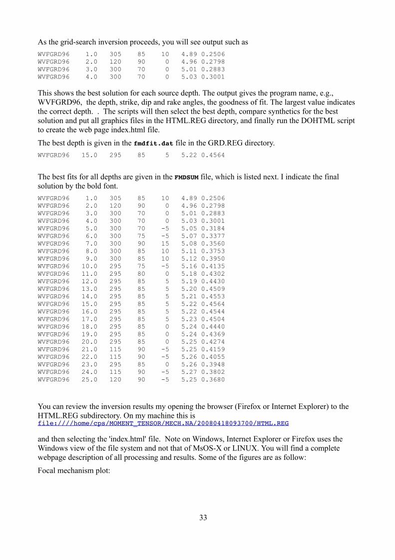
As the grid-search inversion proceeds, you will see output such as

WVFGRD96 1.0 305 85 10 4.89 0.2506WVFGRD96 2.0 120 90 0 4.96 0.2798WVFGRD96 3.0 300 70 0 5.01 0.2883WVFGRD96 4.0 300 70 0 5.03 0.3001

This shows the best solution for each source depth. The output gives the program name, e.g., WVFGRD96, the depth, strike, dip and rake angles, the goodness of fit. The largest value indicates the correct depth. . The scripts will then select the best depth, compare synthetics for the best solution and put all graphics files in the HTML.REG directory, and finally run the DOHTML script to create the web page index.html file.

The best depth is given in the fmdfit.dat file in the GRD.REG directory.

WVFGRD96 15.0 295 85 5 5.22 0.4564

The best fits for all depths are given in the FMDSUM file, which is listed next. I indicate the final solution by the bold font.

WVFGRD96 1.0 305 85 10 4.89 0.2506WVFGRD96 2.0 120 90 0 4.96 0.2798WVFGRD96 3.0 300 70 0 5.01 0.2883WVFGRD96 4.0 300 70 0 5.03 0.3001WVFGRD96 5.0 300 70 -5 5.05 0.3184WVFGRD96 6.0 300 75 -5 5.07 0.3377WVFGRD96 7.0 300 90 15 5.08 0.3560WVFGRD96 8.0 300 85 10 5.11 0.3753WVFGRD96 9.0 300 85 10 5.12 0.3950WVFGRD96 10.0 295 75 -5 5.16 0.4135WVFGRD96 11.0 295 80 0 5.18 0.4302WVFGRD96 12.0 295 85 5 5.19 0.4430WVFGRD96 13.0 295 85 5 5.20 0.4509WVFGRD96 14.0 295 85 5 5.21 0.4553WVFGRD96 15.0 295 85 5 5.22 0.4564WVFGRD96 16.0 295 85 5 5.22 0.4544WVFGRD96 17.0 295 85 5 5.23 0.4504WVFGRD96 18.0 295 85 0 5.24 0.4440WVFGRD96 19.0 295 85 0 5.24 0.4369WVFGRD96 20.0 295 85 0 5.25 0.4274WVFGRD96 21.0 115 90 -5 5.25 0.4159WVFGRD96 22.0 115 90 -5 5.26 0.4055WVFGRD96 23.0 295 85 0 5.26 0.3948WVFGRD96 24.0 115 90 -5 5.27 0.3802WVFGRD96 25.0 120 90 -5 5.25 0.3680

You can review the inversion results my opening the browser (Firefox or Internet Explorer) to the HTML.REG subdirectory. On my machine this isfile:////home/cps/MOMENT_TENSOR/MECH.NA/20080418093700/HTML.REG

and then selecting the 'index.html' file. Note on Windows, Internet Explorer or Firefox uses the Windows view of the file system and not that of MsOS-X or LINUX. You will find a complete webpage description of all processing and results. Some of the figures are as follow:

Focal mechanism plot:

33

Map showing event location and seismograph stations used:

Goodness of fit as a function of depth:

34

Comparison between observed (red) and predicted waveforms (blue):

35

Use of time shift to check location:

The seismogram comparison is useful. One can justify removing traces if it seems that the instrument is not working correctly, e.g., the USIN horizontals, or the UTMT instruments. Such decisions require some experience and an understanding of seismic wave propagation.

36

The solution for this earthquake is given at

http://www.eas.slu.edu/eqc/eqc_mt/MECH.NA/20080418093700/index.html

More things to do

Remove bad traces

To remove some traces and then to rerun, there are two steps:

First, go to the DAT.REG directory and move the unwanted traces. I place them in the NOUSE subdirectory

rbh> mv UTMT* NOUSE rbh> mv USINBHT NOUSE

Second go to the processing directory, and cleanup

rbh> cd ../GRD.REG rbh> DOCLEANUP

The DOCLEANUP script removes all files ending with .obs .pre Z R and T. If you wish to change the filtering bands, e.g., to change the time window, bandpass corner frequencies or apply the microseism filter, carefully modify the DOSTA script. Now restart everything and generate the revised documentation.

rbh> DOGRD; DOPLTSAC; cd ../HTML.REG; DOHTML

The ';' indicates the end of a command. This is one way to issue all of the commands at once, and then have everything run to completion.

Try a different model.

The mech.sh permits the use of the WUS model, which is not proper for the April 18, 2008 eastern U.S. earthquake. Rerun the inversion and compare the results. You will see that the fit is not as good.

37

6. Quality Control Using TeleseismsUsing a known moment tensor solution for a teleseism (great circle arc distance 30º – 95º), forward synthetics will be generated to compare to observed three component observations. To ensure a comparison of a large amplitude signal, we model the vertical component P, the transverse component SH and the radial component SV. The scripts to accomplish this are essentially those use for the determination of the moment tensor using long-period body waves.

For the purposes of this documentation, it is assumed that you are on the CYGWIN system, and thateverything was installed in the /home/cps/MOMENT_TENSOR directory.

Step 1

Go to the work area for quality control using teleseisms.

cd /home/cps/MOMENT_TENSOR/MECHQC.TEL

Examine the contents of the directory:

rbh> ls0XXXTELQC/ DOIRISTELQC* DO.save* mechqctel.sh* RAW/DOCWBTELQC* DOISETUPTEL* DOSETUPTELQC* PROTO.CWB/DOFINISHTELQC* DOQUERYTEL* DOSOLUTIONTELQC* PROTO.I/

As you can see, the naming is very similar to that used for the regional inversion, except that the scripts have been renamed to indicate that they are designed to be used for waveform comparison using teleseisms. The 0XXXTELQC directory has the prototypes for the processing and documentations.

Step 2 – Get the data

Normally one must get the waveform data. An easy way to accomplish this for significant earthquakes is to use the Wilbur III interface at IRIS

http://www.iris.edu/wilber3/find_event

or at Orfeus

http://www.orfeus-eu.org/cgi-bin/wilberII/wilberII_page1.pl

The IRIS Wilbur III interface starts by selecting the earthquake, followed by selecting the station networks, and finally by selecting the individual stations. A SEED volume is created which provides the station coordinates, the instrument orientations and responses as well as the digital data. The result is downloaded using ftp or wget. Always ask for a complete SEED volume and not the miniSEED.

Step 3 – Sample data sets

We will select a data set from inversion from the RAW directory,

rbh> ls RAW00README 20081129055917.seed 20090115174939.seed

and look at the contents of the 00README file:

rbh> cat RAW/00READMEYEAR MO DY HR MN SC LAT LON DEP MAG SEED_VOLUME MT_DEPTH STRIKE DIP RAKE MW2008/11/29 05:59:17 -18.69 -177.72 386 6.0 20081129055917.seed 396 30 42 17 6.02009/01/15 17:49:39 46.86 155.16 36 7.4 20090115174939.seed 44 10 45 80 7.4

38

This file provides the origin time and location of the earthquake as well as the body-wave moment tensor solution obtained by the GCMT.

Step 4 – Create the DO script

We will use the magnitude 7.4 Kurile event of 2009/01/15 as an example. We run the script mechqctel.sh to create the DO script. The last interactive screen is shown next.

And the script isDOIRISTELQC "2009" "01" "15" "17" "49" "39" "000" "46.8600" "155.1600" "36.0" "7.40" "AK135" "NONE" "NONE" "Kurile" "44.0" "10.0" "45.0" "80.0" "7.4"

Step 5 – Create the event directories

Start the processing with the command: rbh> DO

This will return the following message:

39

rbh> DO

1. PLACE THE SEED_VOLUME FROM IRIS in

/home/cps/MOMENT_TENSOR/MOMENT_TENSOR/MECHQC.TEL/20090115174939/20090115174939 2. UNPACK the SEED_VOLUME FROM IRIS as follows cd Sac rdseed -f ../SEED_VOLUME -R -d -o 1 [Note use the name of the downloaded file for SEED_VOLUME, e.g., 20090116.seed] 3. Return to the top level directory where you started: cd /home/cps/MOMENT_TENSOR/MOMENT_TENSOR/MECHQC.TEL4. enter the command: DOFINISHTELQCrbh> DO1. PLACE THE SEED_VOLUME FROM IRIS in /home/cps/MOMENT_TENSOR/MOMENT_TENSOR/MECHQC.TEL/20090115174939/200901151749392. UNPACK the SEED_VOLUME FROM IRIS as follows cd Sac rdseed -f ../SEED_VOLUME -R -d -o 1 [Note use the name of the downloaded file for SEED_VOLUME, e.g., 20090116.seed]3. Return to the top level directory where you started: cd /home/cps/MOMENT_TENSOR/MOMENT_TENSOR/MECHQC.TEL4. enter the command: DOFINISHTELQC

Step 6 – Place data into the event processing directory and process

We now copy the data set to the work area and unpack the SEED volume in the Sac subdirectory using the following steps:rbh> pushd .rbh> cp RAW/20090115174939.seed 20090115174939/20090115174939rbh> cd 20090115174939/20090115174939/Sacrbh> rdseed -f ../*.seed -R -d -o 1<< IRIS SEED Reader, Release 4.7.5 >> R = print response data (with addressing for evresp) d = read data from tape Taking input from ../20090115174939.seedOutput data format will be sac.binary.Warning... Azimuth and Dip out of Range on ANMO,BH1Defaulting to subchannel identifier (for multiplexed data only)Warning... Azimuth and Dip out of Range on ANMO,BH1Defaulting to subchannel identifier (for multiplexed data only)Writing IU.ANMO.00.BH1, 50528 samples (binary), starting 2009,015 17:58:39.0195 UT . . . . . . . . . . . . . . . . . . . IU XMAS 10 BHZ 2007,164,17:00:00 2999,000,00:00:00.0000 2.044849 -157.445320 1.0 -90.0 0.0 40 RESP.IU.XMAS.10.BHZrdseed completed.rbh> popd

You are now back at the top level. Complete the processing:

rbh> DOFINISHTELQC

The script will remove the instrument response, rotate the components, and select traces at distancesof 30º-95º.

There is no trace quality step since the purpose is to compare observed and predicted traces.

When the DOFINISHTELQC is completed, the results can be viewed by pointing the browser at the

file:///home/cps/MOMENT_TENSOR/MECHQC.TEL/20090115174939/HTML.TEL/index.html

file. The initial part of the display documents the processing done to make the synthetics, by defining the band-pass filters as well as the source parameters. Four figures are generated that show the station distribution and the comparison of the P-wave signal on the vertical component, the SH-wave signal on the transverse and the SV-wave signal on the radial component.

The station distribution is shown on the next figure:

40

The next figure shows the P-wave comparison:

41

42

For this figure, observed (red) and predicted seismograms (blue) are ordered by increasing epicentral distance. Each pair of traces is annotated with the wave type and a station identifier (station, network, and channel id's), epicentral distance in degrees, source-to-station azimuth in degrees. Each seismogram pair is plotted with the same scale and the peak amplitudes in meters are shown above to the left of each trace. Red circles flag seismograms with amplitude misfits of a factor of 2 or more.

The processing serves two purposes. First it can be used to check the performance of instruments. The SSPA station has a high long-period noise level, where the noise is 25 times larger than the prediction. One would then verify that the station was operating correctly. The other purpose is the ability to remove a trace from source inversion if the anomalous amplitude can be attributed to malfunction or, in some cases, improperly recorded instrument responses.

One can change the time windows in the DOPZSTA, DOSHSTA and DOSVSTA scripts in the SYN.TEL directory to compare more signal, including the mantle surface waves.

43

7. Moment Tensor Determination for TeleseismsFor the purposes of this documentation, it is assumed that you are on the CYGWIN system, and that

everything was installed in the /home/cps/MOMENT_TENSOR directory.

Step 1

Go to the work area for North American earthquakes

cd /home/cps/MOMENT_TENSOR/MECH.TEL

Examine the contents of the directory:

rbh> ls0XXXTEL/ DOIRISTEL* DO.save* mechtel.sh* RAW/DOCWBTEL* DOISETUPTEL* DOSETUPTEL* PROTO.CWB/DOFINISHTEL* DOQUERYTEL* DOSOLUTIONTEL* PROTO.I/

As you can see, the naming is very similar to that used for the regional inversion, except that the scripts have been renamed to indicate that they are designed to be used for inversion of long period teleseismic body waves. The 0XXXTEL directory has the prototypes for the processing and documentations.

Step 2 – Get the data

Normally one must get the waveform data. An easy way to accomplish this for significant earthquakes is to use the Wilbur III interface at IRIS

http://www.iris.edu/wilber3/find_event

or at Orfeus

http://www.orfeus-eu.org/cgi-bin/wilberII/wilberII_page1.pl

The IRIS Wilbur III interface starts by selecting the earthquake, followed by selecting the station networks, and finally by selecting the individual stations. A SEED volume is created which provides the station coordinates, the instrument orientations and responses as well as the digital data. The result is downloaded using ftp, ( or wget). Always request the complete SEED volume and not the miniSEED.

Step 3 – Sample data sets

We will select a data set from inversion from the RAW directory,rbh> ls RAW00README 20081129055917.seed 20090115174939.seed

and look at the contents of the 00README file:rbh> cat RAW/00READMEYEAR MO DY HR MN SC LAT LON DEP MAG SEED_VOLUME 2008/11/29 05:59:17 -18.69 -177.72 386 6.0 20081129055917.seed 2009/01/15 17:49:39 46.86 155.16 36 7.4 20090115174939.seed

This file provides the origin time and location of the earthquake as well as the body-wave moment tensor solution obtained by the USGS.

Step 4 – Create the DO script

We will use the magnitude 7.4 Kurile event of 2009/01/15 as an example. We run the script mechtel.sh to create the DO script. The last interactive screen is shown next.

44

The script is

DOIRISTEL "2009" "01" "15" "17" "49" "39" "000" "46.8600" "155.1600" "36.0" "7.40" "" "NONE" "NONE" "Kuriles"

Step 5 – Create the event directories

Start the processing with the command:

rbh> DO1. PLACE THE SEED_VOLUME FROM IRIS in /home/cps/MOMENT_TENSOR/MOMENT_TENSOR/MECH.TEL/20090115174939/20090115174939 2. UNPACK the SEED_VOLUME FROM IRIS as follows cd Sac rdseed -f ../SEED_VOLUME -R -d -o 1 [Note use the name of the downloaded file for SEED_VOLUME, e.g., 20090116.seed] 3. Return to the top level directory where you started: cd /home/cps/MOMENT_TENSOR/MOMENT_TENSOR/MECH.TEL4. enter the command: DOFINISHTELQCrbh> DO1. PLACE THE SEED_VOLUME FROM IRIS in /home/cps/MOMENT_TENSOR/MOMENT_TENSOR/MECH.TEL/20090115174939/200901151749392. UNPACK the SEED_VOLUME FROM IRIS as follows cd Sac rdseed -f ../SEED_VOLUME -R -d -o 1 [Note use the name of the downloaded file for SEED_VOLUME, e.g., 20090116.seed]3. Return to the top level directory where you started: cd /home/cps/MOMENT_TENSOR/MOMENT_TENSOR/MECH.TEL4. enter the command: DOFINISHTEL

Step 6 – Place data into the event processing directory and process

We now copy the data set to the work area, using the following steps:rbh> pushd .rbh> cp RAW/20090115174939.seed 20090115174939/20090115174939rbh> cd 20090115174939/20090115174939/Sacrbh> rdseed -f ../*.seed -R -d -o 1

45

<< IRIS SEED Reader, Release 4.7.5 >> R = print response data (with addressing for evresp) d = read data from tape Taking input from ../20090115174939.seedOutput data format will be sac.binary.Warning... Azimuth and Dip out of Range on ANMO,BH1Defaulting to subchannel identifier (for multiplexed data only)Warning... Azimuth and Dip out of Range on ANMO,BH1Defaulting to subchannel identifier (for multiplexed data only)Writing IU.ANMO.00.BH1, 50528 samples (binary), starting 2009,015 17:58:39.0195 UT . . . . . . . . . . . . . . . . . . . IU XMAS 10 BHZ 2007,164,17:00:00 2999,000,00:00:00.0000 2.044849 -157.445320 1.0 -90.0 0.0 40 RESP.IU.XMAS.10.BHZrdseed completed.rbh> popd

You are now at the top level. Complete the processing:rbh> DOFINISHTEL

The script will remove the instrument response, rotate the components, and select traces at distancesof 30º-95º. The Quality Control will present the traces filtered and windowed as for an M=6 earthquake.

The source inversion will take a long time because of the many traces and the exhaustive source at all depths between the surface and 700 km.

The best fitting solution is associated with the maximum value in the FMDSUM file in the GRD.TEL directory, and is WVFGRD96 39.0 10 40 85 7.23 0.5288

The solution given on the USGS Body-Wave Moment tensor page had a depth of 35 km, strike dip and rake angles of 24, 45 and 106 degrees, respectively and a moment magnitude of 7.3. The GlobalCMT Project solution gave 44.6 km, strike of 10, dip of 45 and a rake of 80 degrees with a moment magnitude of 7.4 which is very similar tot he USGS Centroid Moment Tensor solution.

The web page created in the HTML.TEL directory provides detail on the choice of filters used for theinversion. The inversion starts by assuming a moment magnitude 6 earthquake, and if the computedmoment is much larger, the inversion will be repeated at the same depth, but now assuming the larger moment magnitude. The inversion uses frequencies much less that the corner frequency of the earthquake to avoid the extra effort to define the source time function. The time window and source time function are modified as a function of the moment magnitude to ensure that the effect of the direct and depth phases are included.

46

The goodness of fit as a function of depth clearly selects the source depth as seed in the figure

generated:

The fit to the vertical component P-wave is good.

47

8. Modifications for other regional networksThe are two areas of modification: the regional velocity model and the raw network responses and data sets.

To generate a new set of Green's functions, you can follow the tutorial:

http://www.eas.slu.edu/eqc/eqc_cps/TUTORIAL/GREEN/index.html

To simplify the other changes that you will make, use a simple name for the model, e.g., ETUR for eastern Turkey. Follow the procedures in the tutorial but edit the script to compute only the distances that you actually need. Finally put a copy of the model, e.g., ETUR.mod into the upper level Models directory. If you do a

rbh> ls ${GREENDIR}

you will then see AK135.TEL/ CUS.REG/ Models/ WUS.REG/

Since this change applies to just Turkey, go to the MOMENT_TENSOR/MECH.TR directory and carefully change the DOSETUP and mech.sh files to add the option of using a new model. The result would be that one could select the ETUR model in the interactiive mech.sh and that this would be used for the processing and the documentation in the HTML.REG/index.html would indicate this fact. [You will observe that I believe in complete documentation so that another researcher can repeat the processing and obtain the same results.]

The other modification required for use with other networks is to convert the distributed data to Sac and to properly characterize the instrument response. Some networks use SEISAN, and a SEISAN → Sac conversion program is required. We must also be careful about the instrument response.

It may be simpler to create a pole-zero file of the instrument response. Since the pole-zero file just defines a filter, it knows nothing of physical units. You are permitted to use comments in a Sac pole-zero file by placing a '*' is the first column. The rdseed program distributed with Computer Programs in Seismology, and also the current rdseed from IRIS, can create pole-zero response filesfrom the SEED volume by using the command

rdseed -f seed_volume -p

which will provide a documented file

* ***** NETWORK (KNETWK): CN* STATION (KSTNM ): WHY* COMPONENT (KCMPNM): BHZ* LOCATION (KHOLE ):* START : 1997,308,22:04:00* END : No Ending Time* INPUT UNIT : METER* OUTPUT UNIT : COUNT* LATITUDE (DEG) : 60.65970* LONGITUDE (DEG) : -134.88060* ELEVATION (M) : 1292.00000* DEPTH (M) : 0.00000* DIP (DEG) : -90.00000* AZIMUTH (DEG) : 0.00000* INSTRUMENT COMMENT:* CHANNEL_FLAG : G* ****ZEROS 3POLES 4-0.0314 0.0000-0.2090 0.0000-222.1110 -222.1780-222.1110 222.1780

48

CONSTANT 4.937605e+14

Only the last 7 lines are used by Sac or gsac to remove the instrument response. The most importantinformation concerns the units. This is a filter that converts ground displacement in meters to counts.

If this file is called SAC_PZs_CN_WHY_BHZ, then the Sac/gsac command to convert the recorded digital counts to ground velocity in m/s istransfer from polezero subtype SAC_PZs_CN_WHY_BHZ to vel freqlimits 0.002 0.004 ${FHL} ${FHH}

Here the FHL and FHH are defined at 0.25/dt and 0.50/dt, respectively, where dt is the sample interval. The purpose of the

freqlimits 0.004 0.005 ${FHL} ${FHH} is to provide stability to the deconvolution.

In the case of the responses for the Turkish network, the response converts ground velocity to digital counts and the command used istransfer from polezero subtype pzfile TO NONE FREQLIMITS 0.002 0.004 ${FHL} ${FHH}

Here the NONE is used to indicate that we wish to use the response as given without further modification. Also recall that I wish to work with ground velocity in m/s units.

Be careful. Some networks choose to give the pole-zero respoonse with INPUT UNIT: NM for nanometers. In order to convert the output to units of m/s it is necessary to modify the script to perform the commands

div 1.0e+9

after the transfer command. This is done in MECH.NA/PROTO.CWB/CWBDOEVT since the USGS CWB gives the polezero response in terms of NM in and COUNTS out.

If there are any questions, please sent me Email.

49

Appendix

Installation of VirtualBox

Go to

https://www.virtualbox.org/wiki/Downloads

Download the virtual box binary for your OS and also the corresponding extension pack, e.g.,for Windows on June 1, 2014 I downloaded the following

VirtualBox-4.3.16-95972-Win.exeOracle_VM_VirtualBox_Extension_Pack-4.3.16-95972.vbox-extpack

Now open and run VirtualBox-4.3.16-95973-Win.exe. The following images will indicate the responses to set up the system. Note that for installation under MacOS-X and LINUX, the images are essentially the same.

Note that this is an older figure. Use 4.3.16

Select the recommended installation folders:

50

51

Installation of Lubuntu32 and Course software

Now start Virtual Box. You will see that I already have Mint12 installed on the test computer.

We will want to install Lubuntu32.

52

Put the flash drive into the USB port and copy Lubuntu32.vdi to the desktop or preferably to a folder in perhaps c:\users\rbh\.VirtualBox. The second option is suggested since you will always require this image and it will be in the way on the Desktop.

Click New in the VirtualBox Manager. The following menu appears.

After clicking Next, change the memory to 1Gb if you have more than this on you computer.

After selecting Next, select Use an existing virtual hard drive file, and select Lbuntu32.vdi from the Desktop or from your c:\users\rbh\.VirtualBox folder. Then enter Create.

53

Now on the new main page, you will see Lubuntu32 as an option. Click on this to highlight the entry. At this stage you can change the settings. For example, under Settings -> System -> Motherboard you may wish to enable PS/2 Mouse instead of USB Tablet.

Select Lubuntu32 and Start

54

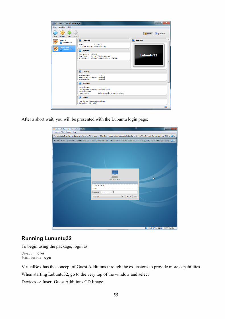
After a short wait, you will be presented with the Lubuntu login page:

Running Lununtu32

To begin using the package, login as

User: cpsPassword: cps

VirtualBox has the concept of Guest Additions through the extensions to provide more capabilities.

When starting Lubuntu32, go to the very top of the window and select

Devices -> Insert Guest Additions CD Image

55

Now stop Lubuntu32. If you look at Storage, you will see VboxGuestAdditions.iso

When you restart Lubuntu32, open the terminal window and enter df.cps: dfFilesystem 1K-blocks Used Available Use% Mounted on/dev/sda1 15093768 9688196 4638856 68% /udev 505496 8 505488 1% /devtmpfs 102560 736 101824 1% /runnone 5120 0 5120 0% /run/locknone 512784 0 512784 0% /run/shm/dev/sr0 63252 63252 0 100% /media/VBOXADDITIONS_4.3.12_93733

cps: cd /mediacps: cd VBOX*cps: sudo sh ./VboxLinuxAdditions.run (enter PROGRAMS.330 as password)

As the result of this operation, you will not have to use the special command for mouse capture.

Changing Keyboard from US

The Lubuntu was set up to use the US Keyboard. To be able to find the proper keys on your keyboard, you may must change the keyboard driver.

First click the button at the bottom left,

Then Preferences → Keyboard and Mouse

56

Then Select keyboard tab and click on “lxkeymap”

57

For this example select “Spain” on the left and “Spanish” on the right. The left columns is for the language and the right is for the keyboard.

Click “Apply”

You may test the selection by typing text in the box “Type here to test your keyboard” There shouldnow be a proper correspondence between what you see on the keys and the character that is recognized by the computer operating system.

58

and then Preferences → Keyboard and Mouse

then Keyboard → lxkeymap, then Spain Spanish → Apply

You can then test the keyboard in the small window “Type here to test your keyboard” to make surethat what you type is actually recognized by the computer.

VBox Additions

The additions adds some very nice features, such as better mouse control and access to files in the underlying computer system.

If you update the distributed Lubuntu32 system and update the kernel, you will have to do the following:

cd /media/VBOXADDITIONS_4.3.30_101610sudo ./VBoxLinuxAdditions.run (use cps as the password)

Then reboot.

You will see that the mouse integration works, and that you can access the files on your real computer if you follow the instructions below.

59

Accessing Host Filesystem

The host data files can be accessed either by using ssh or scp to log into the host system or by mounting the host file system under Lubuntu. We will consider these in turn. A third option is to transfer files to a remote server or dropbox under Lubuntu and then access the remote server or dropbox from the host machine, and vice versa.

One other reason for transferring files from the guest operating system to the host operating system is to be able to use the printers connected to the host.

Access using Shared Folders

Once the Extensions are added to the guest operating system, Lubuntu32 in this case, the main VirtualBox menu can be used to permit Lubuntu32 to access the host file system. The distribution has a mount point at /media/sf_rbh, where the sf indicates shared folder. The following will show how to be able to access the host file system for both MacOS-X and Windows.

First, start VirtualBox, but do not start the Lubuntu32. Highlight the Lubuntu32 and then

Settings → Shared Folders to get the following screen:

Select the “+” icon to add a shared folder. To give the next screen.

60

Now for Windows, set the Folder Path to C:\ and the folder name to rbh, which is the name used in the Lubuntu32 distribution. Also check the Auto-mount option. The screen should now look likethe following.

After pressing OK you will see the following.

61

Now start Lubuntu32 and open the Terminal Window. I ran the commands

df to learn that a share file system was mounted with the path under Lununtu32 of /media/sf_rbh. The ls command was used to demonstrate that the windows files could be accessed. The touch /media/sf_rbh/Users/rbh/hello was executed to demonstrate that I could create a file on the Windows side. [note to make the screen dump for get this figure, I executed the xwd command in the other terminal window at the bottom

62

On my MacBook Air, the Settings → Shared Folders looks like the following:

You will see that only difference is that the host file system name is different. On my LINUX machines, I would set the path to /home/rbh.

If you wish to have access to more that one folder on the host, do the following [for safety do a google search on the topic].

First in Settings ->Shared Folders, add a new folder. For this example, assume that I have a raid on my host LINUX system with the path /rrd0. So in the menu for adding a share drive, give the path as /rrd0 and give it a unique name, e.g., rbhd.

Now start Lubuntn32, and create a mount point, e.g., do something like

sudo mkdir /media/sf_rbhd

Now mount the drive,

sudo mount -t vboxsf rbhd /media/rbhd [Actually on my test, this auto-mounted when I restarted the Guest machine, so you may not have to do anything].

Finally to avoid using sudo to access the files on the host system, I modified the line in /etc/group

vboxsf:x:

to read

vboxsf:x:124:cps

because the default permittion on the shared folder is

63

drwxrwx--- 1 root vboxsf 3230 Sep 7 19:46 sf_rbh

Access using ssh/scp

The first thing is to identify the internet addresses used under Lubuntu. Open a terminal winow and enter the following commands:

cps:~$ netstat -rnKernel IP routing tableDestination Gateway Genmask Flags MSS Window irtt Iface0.0.0.0 10.0.2.2 0.0.0.0 UG 0 0 0 eth010.0.2.0 0.0.0.0 255.255.255.0 U 0 0 0 eth0cps:~$ ifconfig eth0 Link encap:Ethernet HWaddr 08:00:27:46:4e:66 inet addr:10.0.2.15 Bcast:10.0.2.255 Mask:255.255.255.0 inet6 addr: fe80::a00:27ff:fe46:4e66/64 Scope:Link UP BROADCAST RUNNING MULTICAST MTU:1500 Metric:1 RX packets:242 errors:0 dropped:0 overruns:0 frame:0 TX packets:249 errors:0 dropped:0 overruns:0 carrier:0 collisions:0 txqueuelen:1000 RX bytes:23429 (23.4 KB) TX bytes:21838 (21.8 KB)

lo Link encap:Local Loopback inet addr:127.0.0.1 Mask:255.0.0.0 inet6 addr: ::1/128 Scope:Host UP LOOPBACK RUNNING MTU:16436 Metric:1 RX packets:160 errors:0 dropped:0 overruns:0 frame:0 TX packets:160 errors:0 dropped:0 overruns:0 carrier:0 collisions:0 txqueuelen:0 RX bytes:13467 (13.4 KB) TX bytes:13467 (13.4 KB)

cps:~$

The important addresses here are th Gateway 10.0.2.2 and the local address 10.0.2.15 which are highlighted above. The address of the Lubuntu machine is 10.0.2.15. The address of the host computer, under which the VirtualBox runs, is 10.0.2.2.

It is now possible to use secure shell, ssh, to log into the host machine and to use secure copy, scp, to transfer tiles if the host machine permits remote logins.

MacOS-X

1. Click on System Preferences

2. Click on Security & Privacy

3. Click on Firewall

4. Ensure that Firewall is off so that incoming connections are allowed. To do this you must “Click the lock to make changes” and then enter the password on the Mac.

You will now be able to log into the host from the Lubuntu terminal window using the command:

ssh user@10.0.2.2

You can copy files to the host from lubuntu by using the command

scp file user@10.0.2.2:

64

or from the host to the Luuntu machine by using the command

scp user@10.0.2.2 .

Notes

If you make a mistake and hit the sequence ALT C (command C on MacOSX), the screen display will change to a different resolution. Just his ALT C again to return to the previous screen.

65