Embed Size (px)
Citation preview

Computer Science & Information Technology 43


Natarajan Meghanathan
Jan Zizka (Eds)
Computer Science & Information Technology
Third International Conference of Advanced Computer Science &
Information Technology (ACSIT 2015)
Zurich, Switzerland, June 13~14, 2015
AIRCC

Volume Editors
Natarajan Meghanathan,
Jackson State University, USA
E-mail: [email protected]
Jan Zizka,
Mendel University in Brno, Czech Republic
E-mail: [email protected]
ISSN: 2231 - 5403
ISBN: 978-1-921987-40-3
DOI : 10.5121/csit.2015.51201 - 10.5121/csit.2015.51207
This work is subject to copyright. All rights are reserved, whether whole or part of the material is
concerned, specifically the rights of translation, reprinting, re-use of illustrations, recitation,
broadcasting, reproduction on microfilms or in any other way, and storage in data banks.
Duplication of this publication or parts thereof is permitted only under the provisions of the
International Copyright Law and permission for use must always be obtained from Academy &
Industry Research Collaboration Center. Violations are liable to prosecution under the
International Copyright Law.
Typesetting: Camera-ready by author, data conversion by NnN Net Solutions Private Ltd.,
Chennai, India

Preface
The Third International Conference of Advanced Computer Science & Information Technology
(ACSIT-2015) was held in Zurich, Switzerland, during June 13~14, 2015. The Third International
Conference on Foundations of Computer Science & Technology (FCST-2015), The Third
International Conference of Information Technology, Control and Automation (ITCA-2015) and The
Seventh International Conference on Computer Networks & Communications (CoNeCo-2015) were
collocated with the ACSIT-2015. The conferences attracted many local and international delegates,
presenting a balanced mixture of intellect from the East and from the West.
The goal of this conference series is to bring together researchers and practitioners from academia and
industry to focus on understanding computer science and information technology and to establish new
collaborations in these areas. Authors are invited to contribute to the conference by submitting articles
that illustrate research results, projects, survey work and industrial experiences describing significant
advances in all areas of computer science and information technology.
The ACSIT-2015, FCST-2015, ITCA-2015, CoNeCo-2015 Committees rigorously invited
submissions for many months from researchers, scientists, engineers, students and practitioners related
to the relevant themes and tracks of the workshop. This effort guaranteed submissions from an
unparalleled number of internationally recognized top-level researchers. All the submissions
underwent a strenuous peer review process which comprised expert reviewers. These reviewers were
selected from a talented pool of Technical Committee members and external reviewers on the basis of
their expertise. The papers were then reviewed based on their contributions, technical content,
originality and clarity. The entire process, which includes the submission, review and acceptance
processes, was done electronically. All these efforts undertaken by the Organizing and Technical
Committees led to an exciting, rich and a high quality technical conference program, which featured
high-impact presentations for all attendees to enjoy, appreciate and expand their expertise in the latest
developments in computer network and communications research.
In closing, ACSIT-2015, FCST-2015, ITCA-2015, CoNeCo-2015 brought together researchers,
scientists, engineers, students and practitioners to exchange and share their experiences, new ideas and
research results in all aspects of the main workshop themes and tracks, and to discuss the practical
challenges encountered and the solutions adopted. The book is organized as a collection of papers
from the ACSIT-2015, FCST-2015, ITCA-2015, CoNeCo-2015
We would like to thank the General and Program Chairs, organization staff, the members of the
Technical Program Committees and external reviewers for their excellent and tireless work. We
sincerely wish that all attendees benefited scientifically from the conference and wish them every
success in their research. It is the humble wish of the conference organizers that the professional
dialogue among the researchers, scientists, engineers, students and educators continues beyond the
event and that the friendships and collaborations forged will linger and prosper for many years to
come.
Natarajan Meghanathan
Jan Zizka

Organization
General Chair
Natarajan Meghanathan Jackson State University, USA
Dhinaharan Nagamalai Wireilla Net Solutions PTY LTD, Australia
Program Committee Members
Ahmed Hafaifa University of Djelfa, Algeria
BenZidane Moh University of Constantine, Algeria
Christian Esposito ICAR-CNR, Italy
Chun-Yi Tsai National Taitung University,Taiwan
Daniel Mihalyi Technical University of Kosice, Slovakia
Debajit Sensarma University of Calcutta, India
Deema Alathel King Saud University,Saudi Arabia
Diego Reforgiato Italian National Research Council(CNR), Italy
Dmitry Namiot Lomonosov Moscow State University, Russia
Dong Hwan Lee Purdue University, USA
Dudin Alexander N Belarusian State University, Belarus
Ehsan Saradar Torshizi Urmia University, Iran
Elena Somova Plovdiv University, Bulgaria
Fatih Korkmaz Cankiri Karatekin University, Turkiye
Fatih Ozaydin Isik University, Turkey
Foudil Cherif Biskra University, Algeria
Francesco Riganti Fulginei Roma Tre University, Italy
Gennady Krivoulya University of Radioelectronics, Ukraine
Girish Tere Thakur College of Science and Commerce, India
Grienggrai Rajchakit Maejo University, Thailand.
Halla Noureddine Tlemcen University, Algeria
Hamza Zidoum Sultan Qaboos University, Oman
Hassan Saadat Islamic Azad University, Iran
Hoda farahani University of Mazandaran, Iran
Hossein Jadidoleslami Mut University, Iran
Huahao Shou Zhejiang University of Technology, China
Iram Siraj Aligarh Muslim University, India
Isa Maleki Islamic Azad University, Iran
Islam Atef Alexandria University, Egypt
Jaesoo Yoo Chungbuk National University, Korea
Jasmine Seng Edith Cowan University, Australia
Jose Enrique Armendariz-Inigo Public University of Navarre, Spain
Juhua Pu Beihang University, China
Julie M. David MES College, India
Juntao Fei Hohai University, China
Kuppusamy K Alagappa University, India
Le Anh Tuan Vietnam Maritime University, Vietnam

Lubomir Brancik Brno University of Technology, Czech Republic
Majlinda Fetaji South East European University, Macedonia
Manish Sharma D Y Patil College of Engineering, India
Manoj Jain Tata consultancy Services, India
Marcin Michalak Silesian University of Technology, Poland
Maurya S.K University of Nizwa, Oman
Meyyappan T Alagappa University, India
Mohamed Khamiss Suez Canal University, Egypt.
Mohamed Khayet University Complutense of Madrid,Spain
Mohammad Masdari Islamic Azad University, Iran
Mujiono Sadikin Universitas Mercu Buana, Indonesia
Munish Patil University of Pune, India
Muthukumar Murugesan Mphasis Limited (an HP Company), India
Neetesh Saxena State University of New York, South Korea
Nisheeth Joshi Banasthali University, India
Othman Chahbouni University of Hassan II Casablanca, Morocco
Owen Kufandirimbwa University of Zimbabwe, Zimbabwe
P.Thirusakthimurugan Pondicherry Engineering College, India
Paramartha Dutta Visvabharati University, West Bengal
Pierluigi Siano University of Salerno, It aly
Pourdarvish University of Mazandaran, Iran
Prasad Halgaonkar Mit College of Engineering, India
Quanxin Zhu Nanjing Normal University, China
Raed I Hamed University of Anbar Ramadi, Iraq.
Rafah M. Almuttairi University of Babylon, Iraq
Rahul Gupta Fractal Analytics, India
Rajiv Kapoor Delhi Technological University, India
Rajput BS Kumaun University Nainital, India
Ramkumar Prabhu Dhaanish Ahmed College of Engineering, India
Reza Ebrahimi Atani University of Guilan, Iran
Roopali Garg Panjab University, India
Saadat Pourmozafari Tehran Poly Technique, Iran
Saba Khalid Integral University, India
Sabu Mes M.E.S College, India
Santhi Balaji Bangalore University, India
Savita Wali Basaveshwar Engineering College, Bagalkot
Seyed Davood Sadatian Sadabad Ferdowsi University of Mashhad, Iran
Seyyed Amirreza Abedini Islamic Azad University, Iran
Shahid Siddiqui Integral University, India
Shahryar Salimi University of Kurdistan, Iran
Shashank Sharma Manipal University, India
Shengjie Liu Highway school of Chang'an University,China
Simon Fong University of Macau, Macau
Simona Caraiman Technical University of Iasi, Romania
Sinha G.R Shri Shankaracharya Technical Campus, India
Soheil Ganjefar Bu Ali Sina University, Iran
Soubhik Chakraborty Birla Institute of Technology, India
Suman Deb NIT Agartala, India
Sunanda Gupta Shri Mata Vaishno Devi University, India

T. Kishore Kumar NIT Warangal,India
Tchavdar Marinov Southern University, United States
Te Jeng Chang Chung Yu Institute of Technology, Taiwan
Thirusakthimurugan P Pondicherry Engineering College, India
Venkatesh Prasad Chirala Engineering College, India
Vijaya Kathiravan K.S.R. College of Technology, India
Vishal Shrivastava Arya Group of Colleges, India
Volkan Erol Netas Telecommunication Inc, Turkey
Vu Trieu Minh Tallinn University of Technology, Estonia
Wang Heng Institute for Infocomm Research, Singapore
Xingwu Liu Chinese Academy of Sciences, China
Yahya M. H. AL-Mayali University of Kufa, Iraq
Zoltan Mann Budapest University of Technology, Hungary
Technically Sponsored by
Networks & Communications Community (NCC)
Computer Science & Information Technology Community (CSITC)
Digital Signal & Image Processing Community (DSIPC)
Organized By
Academy & Industry Research Collaboration Center (AIRCC)

TABLE OF CONTENTS
The Third International Conference of Advanced Computer Science &
Information Technology (ACSIT 2015)
Efficient Failure Processing Architecture in Regular Expression
Processor ………………………………………………………………………….. 01 - 06
SangKyun Yun
The Third International Conference on Foundations of Computer
Science & Technology (FCST 2015)
Time-Optimal Heuristic Algorithms for Finding Closest-Pair of Points in 2D
and 3D………………………………………………………………..…………….. 07 - 13
Mashilamani Sambasivam
Gradual-Randomized Model of Powered Roof Supports Working Cycle …..... 15 - 24
Marcin Michalak
The Third International Conference of Information Technology,
Control and Automation (ITCA 2015)
Neural Networks with Technical Indicators Identify Best Timing to Invest
in the Selected Stocks …………………..…………………………..…………….. 25 - 33
Asif Ullah Khan and Bhupesh Gour
Microwave Imaging of Multiple Dielectric Objects by FDTD and APSO ...….. 35 - 42
Chung-Hsin Huang, Chien-Hung Chen, Jau-Je Wu and Dar-Sun Liu
Evaluating the Capability of New Distribution Centers Using Simulation
Techniques …………………………………………………………..…………….. 43 - 59
Kingkan Puansurin and Jinli Cao
The Seventh International Conference on Computer Networks &
Communications (CoNeCo 2015)
Energy Efficient Hierarchical Cluster-Based Routing for Wireless Sensor
Networks ………………………………....…………………………..…………….. 61- 69
Shideh Sadat Shirazi and Aboulfazl Torqi Haqiqat

Natarajan Meghanathan et al. (Eds) : ACSIT, FCST, ITCA, CoNeCo - 2015
pp. 01–06, 2014. © CS & IT-CSCP 2015 DOI : 10.5121/csit.2015.51201
EFFICIENT FAILURE PROCESSING
ARCHITECTURE IN REGULAR
EXPRESSION PROCESSOR
SangKyun Yun
Department of Computer and Telecom. Engineering,
Yonsei University, Wonju, Korea [email protected]
ABSTRACT
Regular expression matching is a computational intensive task, used in applications such as
intrusion detection and DNA sequence analysis. Many hardware-based regular expression
matching architectures are proposed for high performance matching. In particular, regular
expression matching processors such as ReCPU have been proposed to solve the problem that
full hardware solutions require re-synthesis of hardware whenever the patterns are updated.
However, ReCPU has inefficient failure processing due to data backtracking. In this paper, we
propose an efficient failure processing architecture for regular expression processor. The
proposed architecture uses the failure bit included in instruction format and provides efficient
failure processing by removing unnecessary data backtracking.
KEYWORDS
String matching, Regular expression, Application Specific Processor, Intrusion detection
1. INTRODUCTION
Text pattern matching is a computational intensive task, exploited in several applications such as
intrusion detection and DNA sequence analysis. A regular expression (RE) [1] is an expression
that represents a set of strings. In many applications, text patterns are represented by regular
expressions. Regular expression matching has become a bottleneck in software-based solutions of
many applications. To achieve high-speed regular expression matching, full hardware based
solutions have been proposed [2,3,4]. These solutions generate non-deterministic finite automata
(NFA) based HDL description for given regular expressions and implements them on FPGA.
However, these approaches require regeneration of the HDL description and re-synthesis of
FPGA implementation whenever the patterns are updated.
To avoid the problem of full hardware solution, a processor-based approach such as ReCPU
[5,6], SMPU [7], and REMP [8] has been proposed. This approach does not require re-synthesis
of the hardware and guarantees the flexibility. ReCPU is a special-purpose processor for regular
expression matching. In ReCPU, a regular expression is mapped into a sequence of instructions,
which are stored in the instruction memory. When an instruction fails to match, the instruction

2 Computer Science & Information Technology (CS & IT)
sequence is restarted from the next address of data where the first match occurred. If one or more
instructions are matching and then matching fails, data should be backtracked, which leads to
inefficient failure processing. SMPU is another regular expression processor and it does not
address the inefficient failure processing problem although it proposes the concept of dual exit
instructions for efficient pipelining. We should solve the inefficient failure processing problem
due to excessive data backtracking.
In this paper, we propose an efficient failure processing architecture for regular expression
processor. The proposed architecture provides efficient failure processing by removing
unnecessary data backtracking.
2. RELATED WORKS
In this section, we review previous regular expression processors and present their inefficient
failure processing problem. ReCPU [5] is a processor based regular expression matching
hardware. The regular expression operators that have been implemented in ReCPU are as
follows: � (concatenation), * (zero or more repetition), + (one or more repetition), | (alternative),
and parenthesis. In ReCPU, regular expression operators and characters are mapped into
instruction opcodes and operands, respectively. The instruction format of ReCPU has multi-
character operand as shown in Figure 1(a) for parallel comparison and ReCPU can perform more
than one character comparison per clock cycle. In addition, the multi-character operand in an
instruction is simultaneously compared with several consecutive input data starting by shifted
positions as shown in Figure 1(b). The operators like * and + correspond to loop style
instructions. To use the nested parentheses, a open parenthesis ‘(’ is treat as a function call and a
close parenthesis ‘)’ , which is usually combined with an operator such as ‘)*’, as a return.
Figure 1. ReCPU (a) instruction format (b) comparator clusters
SMPU and REMP are regular expression processors improving the weakness of ReCPU. SMPU
[7] proposes the concept of dual exit instructions for efficient pipelining and REMP [8] proposes
an instruction set architecture for efficient repetitive operations.
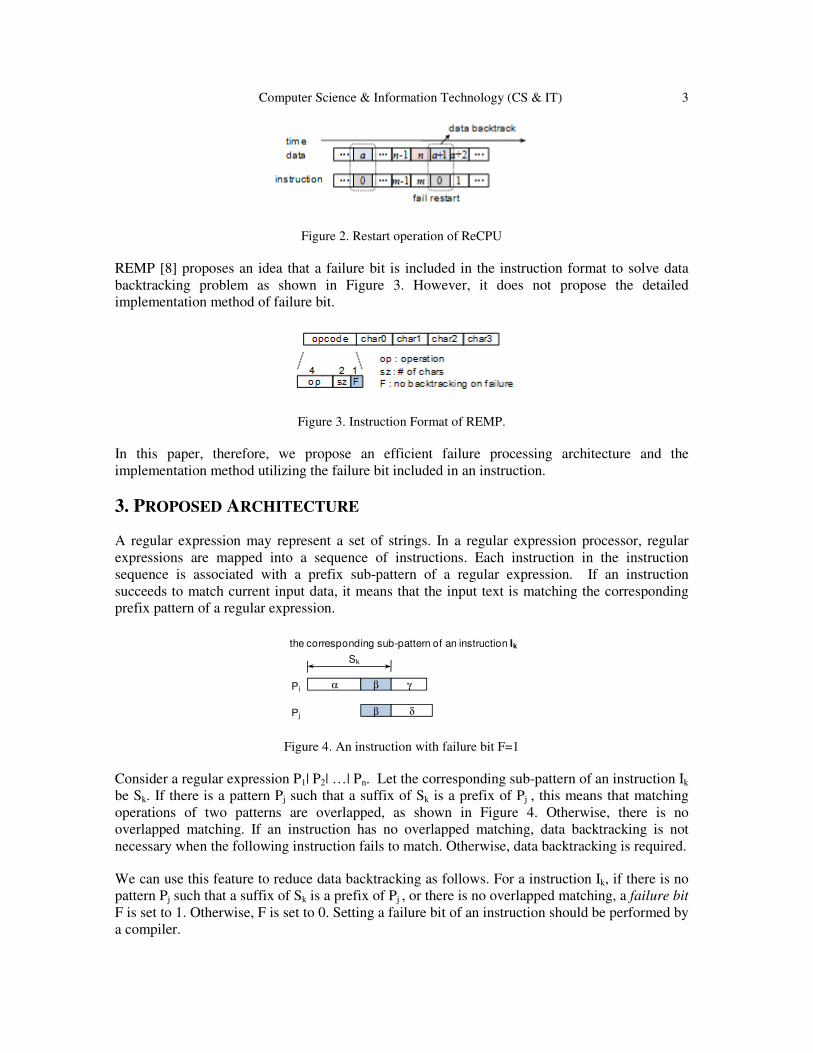
Whenever one or more instruction are matching the input text and then the matching fails,
ReCPU program is restarted from the next address of data where RE starts to match, as shown in
Figure 2. Since data backtracking degrades the pattern matching performance, it is desirable to
reduce unnecessary data backtracking.
Computer Science & Information Technology (CS & IT) 3
Figure 2. Restart operation of ReCPU
REMP [8] proposes an idea that a failure bit is included in the instruction format to solve data
backtracking problem as shown in Figure 3. However, it does not propose the detailed
implementation method of failure bit.
Figure 3. Instruction Format of REMP.
In this paper, therefore, we propose an efficient failure processing architecture and the
implementation method utilizing the failure bit included in an instruction.
3. PROPOSED ARCHITECTURE
A regular expression may represent a set of strings. In a regular expression processor, regular
expressions are mapped into a sequence of instructions. Each instruction in the instruction
sequence is associated with a prefix sub-pattern of a regular expression. If an instruction
succeeds to match current input data, it means that the input text is matching the corresponding
prefix pattern of a regular expression.
Figure 4. An instruction with failure bit F=1
Consider a regular expression P1| P2| …| Pn. Let the corresponding sub-pattern of an instruction Ik
be Sk. If there is a pattern Pj such that a suffix of Sk is a prefix of Pj , this means that matching
operations of two patterns are overlapped, as shown in Figure 4. Otherwise, there is no
overlapped matching. If an instruction has no overlapped matching, data backtracking is not
necessary when the following instruction fails to match. Otherwise, data backtracking is required.
We can use this feature to reduce data backtracking as follows. For a instruction Ik, if there is no
pattern Pj such that a suffix of Sk is a prefix of Pj , or there is no overlapped matching, a failure bit
F is set to 1. Otherwise, F is set to 0. Setting a failure bit of an instruction should be performed by
a compiler.
α γβPi
δβPj
the corresponding sub-pattern of an instruction Ik
Sk

4 Computer Science & Information Technology (CS & IT)
In the proposed regular expression processor, the next address of data where the first match
occurred is stored as a backtracked data address (bk_addr). Without the failure bit information,
when an instruction fails to match, data should be always backtracked to address bk_addr.
However, we can use failure bit information in determining whether backtracking is required and
adjusting the backtracked data address in order to reduce unnecessary data backtracking.
Figure 5. Restart operation of the proposed architecture
If an instruction succeeds to match, its failure bit F is stored as previous failure bit (PF). When an
instruction fails to match and the instruction sequence is restarted, the data backtracking is
determined according to PF value. If PF is 1, data backtracking is not required; If PF is 0, data
backtracking is required. Figure 5 shows the restart operation of the proposed architecture. Thus,
using failure bit information, we can remove unnecessary data backtracking.
If an instruction with F=1 succeeds to match, bk_addr is adjusted to the next data address since
data backtracking is not required at current location. Adjusting the backtracked data address
reduces the backtracking distance of data.
Example: Figure 6 shows a REMP [8] program for two patterns P1 and P2. It also shows the
corresponding sub-pattern of each instruction. Multiple patterns are combined into one REMP
program by using OR (for short patterns) or ORX (for long patterns) instructions. If ORX
succeeds to match, the instruction sequence goes to the next instruction. Otherwise, the
instruction sequence jumps to the instruction for an alternative pattern (in this example, CMP
efxy), whose location is specified by a relative address. STAR, PLUS, and OPT instructions
perform *, +, and ? operations for a short pattern, respectively. Figure 6 also shows failure bit
values of instructions. Only two instructions in address 1 and 3 have F=0.
patterns : P1 = abc(ef)*(st)+xyabz?a, P2 = efxyzw
program sub-pattern F
0 ORX abc, +7
1 STAR ef
2 PLUS st
3 CMP xyab
4 OPT z
5 CMP k
6 MATCH 1
7 CMP efxy
8 CMP zw
9 MATCH 2
abc
abc(ef)*
abc(ef)*(st)+
abc(ef)*(st)+xyab
abc(ef)*(st)+xyabz?
abc(ef)*(st)+xyabz?k
(match P1)
efxy
efxyzw
(match P2)
1
0
1
0
1
1
-
1
1
-
Figure 6. REMP program and corresponding subpatterns

Computer Science & Information Technology (CS & IT) 5
For an input string “gabcefstxyabzpabcef…”, the REMP program executes as shown in Figure 7.
When the instruction at address 5 fails to match and the instruction sequence is restarted, data is
not backtracked and the instruction sequence is restarted from the current data since PF is 1. The
start instruction of an instruction sequence compares four shifted data in parallel and non-start
instructions match one of four shifted data specified by previous instruction.
input string: gabc efst xyab zpab cef …
instr. sequence input text PF / match result
0 ORX abc, +7
1 STAR ef
1 STAR ef
2 PLUS st
2 PLUS st
3 CMP xyab
4 OPT z
5 CMP k
0 ORX abc, +7
…
gab/abc/bce/cef
ef
st
st
xy
xyab
z
p
zpa/pab/abc/bce
…
0 / success
1 / success
0 / fail – try alternative
0 / success
1 / fail – try alternative
1 / success
0 / success
1 / fail - restart, no backtrack
1 / success
…
Figure 7. Instruction Execution Sequence and PF snapshot
4. EVALUATION
Table 1 shows advantages of the proposed architecture in comparison to previous regular
expression processors such as ReCPU and SMPU. The proposed architecture using failure bit
information reduces data backtracking. However, in ReCPU and SMPU, a data backtracking is
always required whenever one or more instructions are matching and then matching fails.
Moreover, data backtracking requires additional clock cycles since double word data should be
fetched for instruction execution. The proposed architecture provides more efficient failure
processing performance than previous processors by removing unnecessary data backtracking.
Table 1. Comparison between proposed architecture and previous processors
previous processors (ReCPU …) proposed architecture
data backtracking always in necessary cases
backward jump address the next address of first match data adjust it forward if needed
5. CONCLUSIONS
Regular expression matching is a computational intensive task, exploited in several applications
such as intrusion detection and DNA sequence analysis. Regular expression matching processors
such as ReCPU have been proposed to solve the problem that full hardware solutions require re-
synthesis of hardware whenever the patterns are updated. However, ReCPU has inefficient failure
processing due to excessive data backtracking. In this paper, we proposed an efficient failure
processing architecture using the failure bit included in instruction format for regular expression
processor. The proposed architecture provides efficient failure processing by removing
unnecessary data backtracking and reducing data backtracking distance.

6 Computer Science & Information Technology (CS & IT)
ACKNOWLEDGEMENTS
This research was supported by Basic Science Research Program through the National Research
Foundation of Korea (NRF) funded by the Ministry of Education, Science and Technology
(2011-0025467).
REFERENCES
[1] J. Friedl, Mastering Regular Expressions, 3rd ed., O’Reilly Media, August 2006..
[2] R. Sidhu and V. Prasanna, “Fast regular expression matching using FPGAs,” in IEEE Symp. Field-
Programmable Custom Computing Machines (FCCM’01), 2001.
[3] C.-H. Lin, C.-T. Huang, C.-P. Jiang, and S.-C. Chang, “Optimization of regular expression pattern
matching circuits on FPGA,” in Proc conf. Design, automation and test in Europe (DATE ’06), 2006.
[4] J. C. Bispo, I. Sourdis, J. M. Cardoso, and S. Vassiliadis, “Regular expression matching for
reconfigurable packet inspection,” in IEEE Int. Conf Field Programmable Technology (FPT’06),
2006.
[5] M. Paolieri, I. Bonesana, M.Santambrogio, “ReCPU: a Parallel and Pipelined Architecture for
Regular Expression Matching,” in Proc. IFIP Int. Conf. VLSI-SoC, 2007.
[6] I. Bonesana, M. Paolieri, and M.Santambrogio, “An adaptable FPGA-based system for regular
expression matching.” In Proc. conf. Design, Automation and Test in Europe, (DATE'08), 2008.
[7] Q. Li, J. Li, J.Wang, B. Zhao, and Y. Qu, “A pipelined processor architecture for regular expression
string matching,” Microprocessors and Microsystems,” vol. 36, no. 6, pp. 520–526, Aug. 2012
[8] B. Ahn, K. Lee, and S.K. Yun, “Regular expression matching processor supporting efficient repetive
operations,” Journal of KIISE: Computing Practices and Letters, vol. 19, no. 11, pp. 553–558, Nov.
2013 (in Korean).
AUTHORS
SangKyun Yun received the BS degree in electronics engineering from Seoul National University, Korea
and the MS and Ph.D degrees in electrical engineering from KAIST, Korea. He is a professor in the
Department of Computer and Telecom. Engineering, Yonsei University, Wonju, Korea.

Natarajan Meghanathan et al. (Eds) : ACSIT, FCST, ITCA, CoNeCo - 2015
pp. 07–13, 2014. © CS & IT-CSCP 2015 DOI : 10.5121/csit.2015.51202
TIME-OPTIMAL HEURISTIC ALGORITHMS
FOR FINDING CLOSEST-PAIR OF POINTS
IN 2D AND 3D
Mashilamani Sambasivam
(formerly) Department of Computer Science, Texas A&M University, USA
ABSTRACT
Given a set of n points in 2D or 3D, the closest-pair problem is to find the pair of points which
are closest to each other. In this paper, we give a new O(n log n) time algorithm for both 2D
and 3D domains. In order to prove correctness of our heuristic empirically, we also provide
java implementations of the algorithms. We verified the correctness of this heuristic by verifying
the answer it produced with the answer provided by the brute force algorithm, through 600 trial
runs, with different number of points. We also give empirical results of time taken by running
our implementation with different number of points in both 2D and 3D.
KEYWORDS
Closest-pair, Algorithm, Heuristic, Time-Optimal, Computational Geometry, 2D, 3D
1. INTRODUCTION
The closest-pair solution has many applications in real-life. It forms a main step in many
problem-solving procedures. These include applications in air/land/water traffic-control systems.
A traffic control system can use the solution in order to avoid collisions between vehicles. The
algorithm has applications in detecting collisions after they happen. There are also applications in
self-navigating vehicles. The solution also has applications in bodies which must always keep
close to particular other bodies. The problem also has applications in imaging technologies,
pattern recognition, CAD, VLSI.
2. PREVIOUS WORK
The most popular algorithm in 2D appears in the book by Cormen et al[1] and is due to Preparata
and Shamos[2]. The algorithm divides the problem spatially and uses a divide-and conquer
method. Following this algorithm, many similar divide-and-conquer algorithms have been
devised for 3D by dividing the points spatially by a plane.[3][4][5] contain a good survey of
computational geometry algorithms. Our algorithm differs from previous algorithms in that it is
much simpler and therefore much easier to implement practically. The previous best algorithms
for 2D have a time bound of O(n log n) similar to our 2D algorithm. However, I am unable to

8 Computer Science & Information Technology (CS & IT)
establish the best time bound achieved by previous algorithms for 3D. I think the best time bound
achieved by previous algorithms for 3D is O(n*log2n).
3. OUR ALGORITHMS
We present the 2D and 3D algorithms separately for clarity.
3.1. Algorithm for 2D
Algorithm 2D-ClosestPair( )
Given: n – number of points, p[1..n] – points array
Data structures used by algorithm:
d1[1..n] , d2[1..n], d3[1..n], d4[1..n] - distance arrays
sum[1..n] – sum array
index[1..n] – index array
1. a. Find point p1 such that its x coordinate is lower or equal to any other point in the array
of points p.
b. Find point p2 such that its x coordinate is higher or equal to any other point in the
array of points p.
c. Find point p3 such that its y coordinate is lower or equal to any other point in the array
of points p.
d. Find point p4 such that its y coordinate is higher or equal to any other point in the
array of points p.
2. a. Find distance of each point in the p array from p1 and put its square in the d1 array.
For i=1..n, d1[i] = (distance between p1 and p[i])2
b. Find distance of each point in the p array from p2 and put its square in the d2 array.
For i=1..n, d2[i] = (distance between p2 and p[i])2
c. Find distance of each point in the p array from p3 and put its square in the d3 array.
For i=1..n, d3[i]=(distance between p3 and p[i])2
d. Find distance of each point in the p array from p4 and put its square in the d4 array.
For i=1..n, d4[i] = (distance between p4 and p[i])2

Computer Science & Information Technology (CS & IT) 9
3. Calculate the sum array using the following formula:
For i=1..n, sum[i] = 11* d1[i] + 101 * d2[i] + 1009* d3[i] + 10007 * d4[i]
4. Initialise the index array to contain the indexes.
For i=1..n, index[i] = i
5. Mergesort the sum array. While mergesorting, if you exchange any 2 indices i and j of
sum array, be sure to exchange the corresponding entries i and j of index array.
6. For i=1..(n-1), Compare each point p[index[i]] to the 10 next points (if they exist).
ie. p[index[i+1]], p[index[i+2]]..p[index[i+10]]
If the 2 points being compared is the closest pair found so far, then store the 2 points.
7. Output the closest pair of points found.
Figure 1. Closest Pair
Assume p1, p2, p3, p4, seen in the Figure 1 above, are the extreme points found in step 1 of our
algorithm. Then the basic idea of our algorithm is that the closest pair of points (the 2 points
inside the rectangle) should be almost equidistant from each of the 4 points (see Figure 1 above).
That is, a1 should be near A1 numerically, and a2 should be near A2 numerically, and a3 should
be near A3 numerically, and a4 should be near A4 numerically.
So what our algorithm does is that it calculates the distance of each point from the 4 extreme
points and puts its square in the corresponding d array. We wish to find (d1,d2,d3,d4) of a point x
such that it almost equals (d1,d2,d3,d4) of a point y. The closer the match of the d’s, the closer
the points are in the 2D plane.

10 Computer Science & Information Technology (CS & IT)
So what we do to find the closest match of (d1, d2, d3, d4) among all points in the d array, is that
we multiply each by a prime number and add them to get the sum array. The closer the (d1, d2,
d3, d4) of point x is to (d1,d2,d3,d4) of point y, the closer will be the sum numerically.
Multiplying by prime numbers gives us a unique signature of each point in the sum array. Note
that the prime numbers are all different from each other.
So then, we let the index array carry the index of the point corresponding to the sum array. We
then mergesort the sum array, taking care to exchange corresponding entries of index array when
we exchange 2 elements of the sum array.
Now, we have the sorted sum array, and the points they represent are in the index array. Now, all
we have to do is compare each point in the index array with 10 points that follow it. If the
distance between 2 points being compared is the closest pair we have so far, it get stored. The
closest pair of points is then output.
3.2. Algorithm for 3D
Algorithm 3D-ClosestPair( )
Given: n – number of points, p[1..n] – points array
Data structures used by algorithm:
d1[1..n] , d2[1..n], d3[1..n], d4[1..n], d5[1..n], d6[1..n] - distance arrays
sum[1..n] – sum array, index[1..n] – index array
1. a. Find point p1 such that its x coordinate is lower or equal to any other point in the array
of points p.
b. Find point p2 such that its x coordinate is higher or equal to any other point in the
array of points p.
c. Find point p3 such that its y coordinate is lower or equal to any other point in the array
of points p.
d. Find point p4 such that its y coordinate is higher or equal to any other point in the
array of points p.
e. Find point p5 such that its z coordinate is lower or equal to any other point in the array
of points p.
f. Find point p6 such that its z coordinate is higher or equal to any other point in the array
of points p.
2. a. Find distance of each point in p array from p1 and put its square in the d1 array.
For i=1..n, d1[i] = (distance between p[i] and p1)2

Computer Science & Information Technology (CS & IT) 11
b. Find distance of each point in p array from p2 and put its square in the d2 array
For i=1..n, d2[i] = (distance between p[i] and p2)2
c. Find distance of each point in p array from p3 and put its square in the d3 array.
For i=1..n, d3[i] = (distance between p[i] and p3)2
d. Find distance of each point in p array from p4 and put its square in the d4 array.
For i=1..n, d4[i] = (distance between p[i] and p4)2
e. Find distance of each point in p array from p5 and put its square in the d5 array.
For i=1..n, d5[i] = (distance between p[i] and p5)2
f. Find distance of each point in p array from p6 and put its square in the d6 array.
For i=1..n, d6[i] = (distance between p[i] and p6)2
3. Calculate the sum array using the following formula:
For i=1..n,
sum[i] = 11*d1[i] + 101* d2[i] + 547*d3[i] + 1009*d4[i] + 5501*d5[i] + 10007*d6[i]
4. Initialise the index array to contain the indexes.
For i=1..n, index[i] = i
5. Mergesort the sum array. While mergesorting, if you exchange any 2 indices i and j of
sum array, be sure to exchange the corresponding entries i and j of index array.
6. For i=1..(n-1), Compare each point p[index[i]] to the 100 next points (if they exist)
ie. p[index[i+1]], p[index[i+2]]..p[index[i+100]]
if the 2 points being compared is the closest pair found so far, then store the 2 points.
7. Output the closest pair of points found.
Assume p1, p2, p3, p4, p5, p6 are the extreme points found in step 1 of our 3D algorithm. Then
the basic idea of our algorithm is that the closest pair of points should be almost equidistant from
each of the 6 points.
So what our algorithm does is that it calculates the distance of each point from the 6 extreme
points and puts its square in the corresponding d array. We wish to find (d1,d2,d3,d4,d5,d6) of a
point x such that it almost equals (d1,d2,d3,d4,d5,d6) of a point y. The closer the match of the
d’s, the closer the points are in 3D.
So what we do to find the closest match of (d1, d2, d3, d4, d5, d6) among all points in the d array,
is that we multiply each by a prime number and add them to get the sum array. The closer the
(d1, d2, d3, d4, d5, d6) of point x is to (d1, d2, d3, d4, d5, d6) of point y, the closer will be the

12 Computer Science & Information Technology (CS & IT)
sum numerically. Multiplying by prime numbers gives us a unique signature of each point in the
sum array. Note that the prime numbers are all different from each other.
So then, we let the index array carry the index of the point corresponding to the sum array. We
then mergesort the sum array, taking care to exchange corresponding entries in the index array
when we exchange 2 elements of the sum array.
Now, we have the sorted sum array, and the points they represent are in the index array. Now, all
we have to do is compare each point in the index array with 100 points that follow it. If the
distance between 2 points being compared is the closest pair we have so far, it get stored.The
closest pair of points is then output.
3.3 Correctness of our Heuristic Algorithm
We implemented our algorithms in 2D and 3D in java. The programs can be downloaded from
the private url: https://drive.google.com/file/d/0B2MLVfnv5msBVlBnWEthcjRkM00/view?
usp=sharing. We ran 600 trial runs with number of points ranging from 1 hundred to 10 million.
We verified the answer we got with the answer got from the brute force algorithm of finding the
closest pair. Our program got it right 100% of time.
The correctness of our heuristic is also intuitive—that the closest-pair of points will be almost
equidistant from each of the extreme points found. Also, multiplying by a prime is intuitive in
that it gives us a unique signature of each point in the sum array.
3.4 Running Time of our algorithm
Each of the steps in our algorithm takes O(n) time, except the mergesort step5. Mergesort step
takes O(n log n) time. Note that the 6th step takes O(10n) for 2D algorithm and O(100n) for 3D
algorithm, which is essentially O(n) time. So the total time taken by our algorithm is O(n log n).
The following tables gives the running time of our algorithm with varying number of points. It
compares the running time against the running time of a brute force O(n2) algorithm. Each entry
in the table (except brute-force algorithm entries for 1 million and 10 million points) is the
average time of running the algorithm over 50 trial runs. The trials were run on a single-processor
with base frequency of 1.6 GHz.
Table 1. Running time of our 2D algorithm and brute-force algorithm
Number of Points Our 2D algorithm time Brute force algorithm time
1000 17 millisecs 47 millisecs
10000 70 millisecs 1200 millisecs
100000 330 millisecs 99 secs
1 million 1.7 secs > 12 hours
10 million 15.5 secs >> 12 hours

Computer Science & Information Technology (CS & IT) 13
Table 2. Running time of our 3D algorithm and brute-force algorithm
Number of Points Our 3D algorithm time Brute force algorithm time
1000 54 millisecs 49 millisecs 10000 165 millisecs 1700 millisecs 100000 731 millisecs 139 secs 1 million 5.2 secs > 12 hours 10 million 47 secs >> 12 hours
4. CONCLUSIONS
We found our heuristic algorithm gives the right answer 100% of time. Since the algorithm’s
correctness cannot be proved mathematically, it is still a heuristic. However, we have proved our
algorithm’s correctness empirically. Our algorithm is also time-optimal in that both the
algorithms for 2D and 3D run in O(n log n) time. We verified empirically that our algorithm is
time optimal.
Future work in finding closest pair of points can include finding the pair with multi-
cores/multiprocessors, which are becoming more common day to day.
ACKNOWLEDGEMENTS
The author would like to thank Perumal. S, Sambasivam. K and Shankari. S for their support.
REFERENCES [1] Thomas H. Cormen, Charles E. Leiserson, Ronald L. Rivest & Clifford Stein (2009) Introduction to
Algorithms, PHI Learning, Eastern Economy Edition.
[2] Franco P. Preparata & Michael Ian Shamos (1985) Computational Geometry: An Introduction,
Springer.
[3] Herbert Edelsbrunner (1987) Algorithms in Combinatorial Geometry, Vol. 10 of EATCS
Monographs on Theoretical Computer Science, Springer.
[4] Joseph O’Rourke (1998) Computational Geometry in C, Cambridge University Press.
[5] Mark de Berg, Otfried Cheong, Marc van Kreveld & Mark Overmars (2011) Computational
Geometry: Algorithms and Applications, Springer.
AUTHORS
Mashilamani. S holds a Masters degree in Computer Science from Texas A&M
University, College Station, USA and a Bachelors in Computer Science and Eng.
from Madras University.

14 Computer Science & Information Technology (CS & IT)
INTENTIONAL BLANK

Natarajan Meghanathan et al. (Eds) : ACSIT, FCST, ITCA, CoNeCo - 2015
pp. 15–24, 2014. © CS & IT-CSCP 2015 DOI : 10.5121/csit.2015.51203
GRADUAL-RANDOMIZED MODEL OF
POWERED ROOF SUPPORTS WORKING
CYCLE
Marcin Michalak
Institute of Informatics, Silesian University of Technology, Gliwice, Poland
ABSTRACT
Due to increasing efforts on saving natural environment – observed also as an increase of
renewable resource energy production – a traditional underground coal mining introduces new
technologies of machine diagnosis to assure this process to be more safe and generate less
pollution. Also the economic reasons influence development of monitoring systems. Among the
most important elements of underground coal mining are longwall systems, whose essential
parts are powered roof supports. Avoiding failures and limitation of power consumption should
result in more ecological underground coal mining. The paper presents the new model of
powered roof support single unit work. The better understanding of its operating and the
possibility to generate data describing a proper and improper operation will help to develop
monitoring and diagnosis systems.
KEYWORDS
Machine Modelling, Longwall Systems, Machine Diagnosis, Coal Mining, Underground
Mining
1. INTRODUCTION
Despite increasing significance of renewable resource energy production, coal based energy
production still remains a meaningful part of industry of many countries (just to mention Poland
and Germany [1][2]). Due to this fact problems of coal mining still have a global meaning.
Among many methods of coal mining the most common technology is longwall mining. In this
technology a coal deposit is drawn out in the place called a longwall. A typical longwall is
several hundred meters long and consists of longwall shearer which tears off the coal from the
rock, a conveyor which transports the output out of the wall and the powered roof support whose
main task is to protect the people and the equipment of the falling rocks from the roof. A simple
scheme of a longwall complex is presented on the Fig. 1.Almost all of longwall complex
components are points of interest of monitoring and diagnostic systems and scientific research
[3][4][5][6][7].

16 Computer Science & Information Technology (CS & IT)
A proper operation of a whole longwall complex, including the powered roof support, becomes
an essential issue from the both the safety considerations and economical aspects. The safety of
the operation depends on the various factors: natural, technical and human. It is expected from
the monitoring and diagnostic systems to detect and recognize a proper machine operation but
also – what is probably even more important – improper operation and some defects and failures.
It is usually very hard or even impossible to gather the data describing all possible situations, data
that will become a training set for a monitoring system. Therefore it is demanded to know the
characteristics of proper and improper device operations, characteristics of effects of failures and
include them in the model of machine. If the model of the machine work is ready, it is possible to
generate an artificial data and put it into the diagnostic system as patterns.
Fig. 1 Longwall complex scheme (http://www.changingcoast.org.uk/).
In this paper extension of the model of single powered roof support work is presented. The paper
is organized as follows: it starts from the brief description of a system of powered roof support –
its structure and typical work characteristic. Then a previous simple model of modelling a proper
unit working cycle is described – the decomposition of a working cycle and mathematical model
of each phase. Afterwards a modified version of the model is explained, assuring more stable and
reliable values after the second phase of the cycle and more authentic characteristic of a gradual
leg pressure increase. The paper ends with some results of modelling and final conclusions and
goals of further works.
2. POWERED ROOF SUPPORTS
Powered roof supports are essential element of the longwall complex as their main role is to prop
the rock over workers and machines (Fig. 2). This implies the need of a proper roof supports
operation and permanent observation of operating conditions and diagnostic state of separate
powered roof support units. For better understanding of these aspects in this section a brief
description of structure and typical working cycle of a single unit of powered roof support will be
presented.

Computer Science & Information Technology (CS & IT) 17
Fig. 2 The profile of a single unit in the longwall (www.mining.com).
2.1 Unit Structure
The unit consists of one or more hydraulic prop (legs), holding up the upper part of the unit (roof-
bar) and hydraulic shifting system, responsible for shifting the unit with the longwall advance
simultaneously. Each unit should prop the roof with the demanded strength to assure the safety of
mining. After each shearer passage the unit shifts and then props the newly bared rocks.
Fig. 3Single unit of powered roof support (www.joy.com).
2.1 Working cycle
Each unit of a powered roof support performs the same activities sequentially. Starting from the
moment of the shearer passage a typical sequence of events can be defined. After a shearer
passage there is a new roof unpropped. The hydraulic system decreases the pressure in the leg to
break the contact with the roof. Then a shifting is performed. Afterwards a rapid pressure
increase in the leg is performed to restore the contact with the roof. The pressing formation tries
to compress the unit – to decrease its height – but the hydraulic system avoids it by the pressure

18 Computer Science & Information Technology (CS & IT)
increase in legs. It is visible as the slow and gradual pressure increase. Shortly before the next
shearer passage a faster pressure increase can be observed as the effect of preceding units lack of
roof contact.6000 second long leg pressure series is presented on the Fig. 4
Fig. 4. Real time series of pressure in the unit leg.
The very short and fast pressure decrease can be observed between 635th and 648
th second. The
shifting is performed between 649th and 751
st second. The initial pressure increase can be
observed between the 752nd
and 772nd
second. The further slow pressure increase, caused by the
formation pressure, is observed between 773rd
and 4000th second. The last mentioned phase is
observed between the 4000th second and the 4400
th – the beginning of the next unit working
cycle.
3. RANDOMIZED MODEL OF A SINGLE UNIT WORK
The gradual-randomized model, presented in this paper, is the extension of the mathematical
(also randomized) model described in [8]. Its basics and the current extension will be presented in
the following subsections.
3.1 Working Cycle Decomposition
For the purpose of unit operation modelling a single working cycle was divided into the
following five phases, starting from the moment of a rapid leg pressure decrease:
- treading,
- spragging,
- overbuilding,
- pre-treading,
- pressure lowering.
3.2. Randomized Phase Duration
The previous model assumed a linear pressure change in the three first phases: very low during
treading and overbuilding and quite high in the spragging. The model of pressure lowering was
0 1000 2000 3000 4000 5000 60000
50
100
150
200
250
300
350
t [s]
P [
100 k
Pa]

Computer Science & Information Technology (CS & IT) 19
dual: rapid or gradual. For the purpose of pre-treading modelling one of four models was drawn.
These models are described in Table 1 and presented on Fig. 5.
Table 1. Four pre-treading models equations.
Model Equation
Linear � = �
Squared � = ��
Exponential � = exp ((� − 1))
Arched � = 1 − �1 − ��
Also the duration of each phase was drawn from the range, prepared for each phase separately.
The initial level of the pressure for the first modelled phase was also randomized, but starting
from the second phase, the initial pressure value implied from the final pressure in the preceding
one. Also the initial value of the pressure during the second treading implied from the final value
of a first pressure lowering.
3.3 Randomized Phase Dynamic
All parameters of phases – especially slopes for linear sections – were drawn from the specified
range but without taking into consideration the phase duration. It was clearly visible when the
pressure value at the end of the spragging was considered. It was expected to obtain comparative
values, due to the fact that usually propping the roof should start at specified level of the pressure.
Inexactness of this approach is visible on the Fig. 7.
4. GRADUAL-RANDOMIZED MODEL OF A SINGLE UNIT WORK
The presented model disadvantages led to its extension and modification. The modification
consist in assuring more stable dynamic in the spragging phase. The extension of the model
consist in particular discretization of a continuous pressure change characteristic into the interval
one.
Fig. 5. Possible pressure increase characteristics in the pre-treading phase.
0 0.1 0.2 0.3 0.4 0.5 0.6 0.7 0.8 0.9 10
0.1
0.2
0.3
0.4
0.5
0.6
0.7
0.8
0.9
1
y=x
y=x2
y=1-sqrt(1 - x2)
y=e6(x-1)
20 Computer Science & Information Technology (CS & IT)
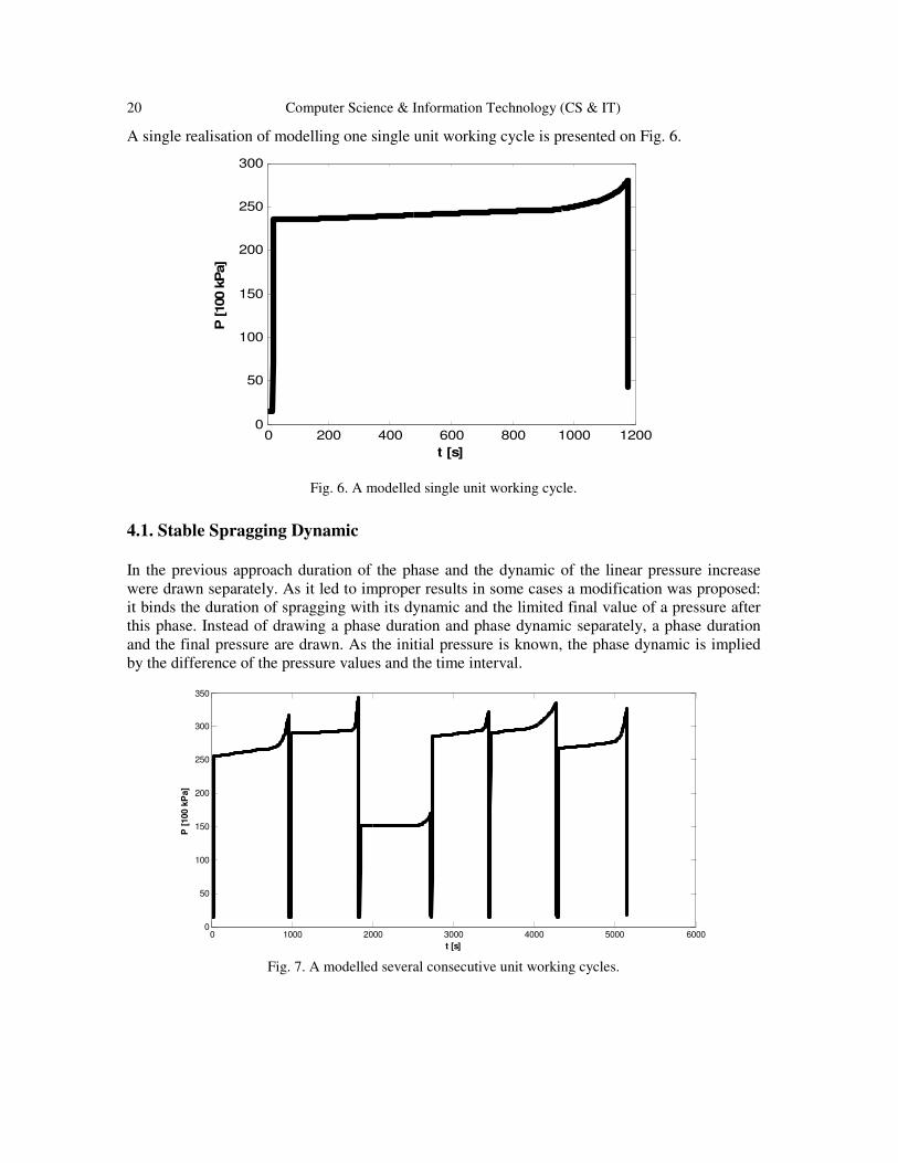
A single realisation of modelling one single unit working cycle is presented on Fig. 6.
Fig. 6. A modelled single unit working cycle.
4.1. Stable Spragging Dynamic
In the previous approach duration of the phase and the dynamic of the linear pressure increase
were drawn separately. As it led to improper results in some cases a modification was proposed:
it binds the duration of spragging with its dynamic and the limited final value of a pressure after
this phase. Instead of drawing a phase duration and phase dynamic separately, a phase duration
and the final pressure are drawn. As the initial pressure is known, the phase dynamic is implied
by the difference of the pressure values and the time interval.
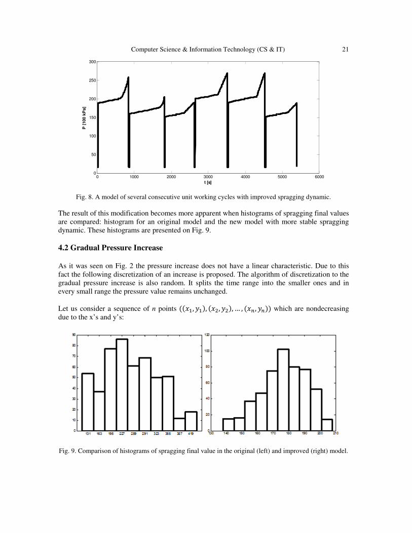
Fig. 7. A modelled several consecutive unit working cycles.
0 200 400 600 800 1000 12000
50
100
150
200
250
300
t [s]
P [100 k
Pa]
0 1000 2000 3000 4000 5000 60000
50
100
150
200
250
300
350
t [s]
P [
100 k
Pa]
Computer Science & Information Technology (CS & IT) 21
Fig. 8. A model of several consecutive unit working cycles with improved spragging dynamic.
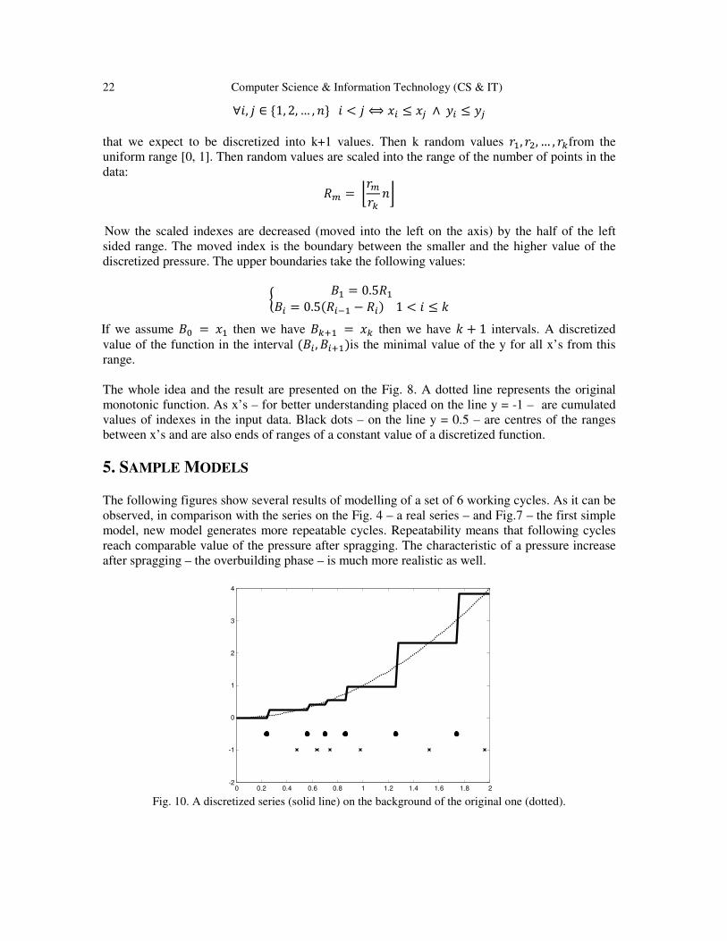
The result of this modification becomes more apparent when histograms of spragging final values
are compared: histogram for an original model and the new model with more stable spragging
dynamic. These histograms are presented on Fig. 9.
4.2 Gradual Pressure Increase
As it was seen on Fig. 2 the pressure increase does not have a linear characteristic. Due to this
fact the following discretization of an increase is proposed. The algorithm of discretization to the
gradual pressure increase is also random. It splits the time range into the smaller ones and in
every small range the pressure value remains unchanged.
Let us consider a sequence of n points ((��, ��), (��, ��), … , (��, ��)) which are nondecreasing
due to the x’s and y’s:
Fig. 9. Comparison of histograms of spragging final value in the original (left) and improved (right) model.
0 1000 2000 3000 4000 5000 60000
50
100
150
200
250
300
t [s]
P [
100 k
Pa]
22 Computer Science & Information Technology (CS & IT)
∀�, � ∈ {1, 2, … , �} � < � ⟺ �� ≤ �� ∧ �� ≤ ��
that we expect to be discretized into k+1 values. Then k random values !�, !�, … , !"from the
uniform range [0, 1]. Then random values are scaled into the range of the number of points in the
data:
#$ = %!$!"
�&
Now the scaled indexes are decreased (moved into the left on the axis) by the half of the left
sided range. The moved index is the boundary between the smaller and the higher value of the
discretized pressure. The upper boundaries take the following values:
' (� = 0.5#�(� = 0.5(#�,� − #�) 1 < � ≤ -.
If we assume (/ = �� then we have ("0� = �" then we have - + 1 intervals. A discretized
value of the function in the interval ((� , (�0�)is the minimal value of the y for all x’s from this
range.
The whole idea and the result are presented on the Fig. 8. A dotted line represents the original
monotonic function. As x’s – for better understanding placed on the line y = -1 – are cumulated
values of indexes in the input data. Black dots – on the line y = 0.5 – are centres of the ranges
between x’s and are also ends of ranges of a constant value of a discretized function.
5. SAMPLE MODELS
The following figures show several results of modelling of a set of 6 working cycles. As it can be
observed, in comparison with the series on the Fig. 4 – a real series – and Fig.7 – the first simple
model, new model generates more repeatable cycles. Repeatability means that following cycles
reach comparable value of the pressure after spragging. The characteristic of a pressure increase
after spragging – the overbuilding phase – is much more realistic as well.
Fig. 10. A discretized series (solid line) on the background of the original one (dotted).
0 0.2 0.4 0.6 0.8 1 1.2 1.4 1.6 1.8 2-2
-1
0
1
2
3
4

Computer Science & Information Technology (CS & IT) 23
Fig. 11. A discretized series (solid line) on the background of the original one (dotted).
6. CONCLUSIONS
Building a diagnostic models and software requires a lot of data from the monitored device. This
is particularly difficult to obtain the data, containing patterns of various ways of operating,
including also faults and human mistakes, from complicated complexes. The process of
delivering a reliable data generator simplifies and accelerates building up diagnostic models as it
allows analysis even very sophisticated deviation of the proper machine operation. In this paper
the improved model of building a model of a single powered roof support unit was presented.
This model reflects all typical phases of the correct work of the device, assures a stability of
steady value after spragging and gives more realistic characteristic of a gradual pressure increase.
In its current form the model does not include many aspects of real disturbances, just to mention
the most important ones as leakage of the hydraulic liquid, correlation between two (three) legs
of the same unit, influence of the other units work phases, shearer localisation. Further works will
focus on including mentioned elements in the model progressively.
0 1000 2000 3000 4000 5000 60000
50
100
150
200
250
300
t [s]
P [
100 k
Pa]
0 1000 2000 3000 4000 5000 60000
50
100
150
200
250
t [s]
P [
100 k
Pa]
0 1000 2000 3000 4000 5000 60000
50
100
150
200
250
300
t [s]
P [
100 k
Pa]

24 Computer Science & Information Technology (CS & IT)
ACKNOWLEDGEMENTS
This work was supported by the European Union from the European Social Fund (grant
agreement number: UDA-POKL.04.01.01-106/09).
REFERENCES
[1] Statystyka elektroenergetyki polskiej (in Polish), ARE annual report
[2] International Energy Agency Report,
http://www.iea.org/statistics/statisticssearch/report/?year=2012&country=GERMANY&product=Elec
tricityandHeat
[3] Bartelmus W.: Condition Monitoring of Open Cast Mining Machinery.Wroclaw University of
Technology Press, Wroclaw 2006.
[4] Gąsior S.: Diagnosis of Longwall Chain Conveyor. Mining Review, Vol. 57, No. 7-8, pp. 33–36,
2001.
[5] Kacprzak M., Kulinowski P, Wędrychowicz D.: ComputerizedInformation System Used for
Management of Mining Belt ConveyorsOperation., Eksploatacja i Niezawodnosc - Maintenance and
Reliability,Vol. 13, No. 2, pp. 81–93, 2011.
[6] Michalak M., Sikora M.: Analiza pracy silników przenośników ścianowych - propozycje raportów i
wizualizacji” (in Polish), Mechanizacja i Automatyzacja Górnictwa, Vol. 436, No. 5, pp. 17–26,
2007.
[7] Michalak M., Sikora M., Sobczyk J.: Analysis of the Longwall ConveyorChain Based on a Harmonic
Analysis”, Eksploatacja i Niezawodnosc- Maintenance and Reliability, Vol. 15, No. 4, pp. 332–336,
2013.
[8] Michalak M.: Modelling of Powered Roof Supports Work.International Journal of Computer,
Information Science and Engineering, 2015 (to appear)
AUTHOR
Marcin Michalak Marcin Michalak was born inPoland in 1981. He received his M.Sc.
Eng. Incomputer science from the Silesian University of Technology in 2005 and Ph.D.
degree in 2009 from the same university. His scientific interests are in machine learning,
data mining, rough sets and biclustering. He is an author and coauthor of over 60
scientific papers.

Natarajan Meghanathan et al. (Eds) : ACSIT, FCST, ITCA, CoNeCo - 2015 pp. 25–33, 2014. © CS & IT-CSCP 2015 DOI : 10.5121/csit.2015.51204
NEURAL NETWORKS WITH TECHNICAL
INDICATORS IDENTIFY BEST TIMING TO
INVEST IN THE SELECTED STOCKS
Dr. Asif Ullah Khan1 and Dr. Bhupesh Gour2
1Professor Dept. of Computer Sc. & Engineering, TIT , Bhopal [email protected]
2Professor Dept. of Computer Sc. & Engineering, TIT , Bhopal [email protected]
ABSTRACT
Selections of stocks that are suitable for investment are always a complex task. The main aim of
every investor is to identify a stock that has potential to go up so that the investor can maximize
possible returns on investment. After identification of stock the second important point of
decision making is the time to make entry in that particular stock so that investor can get
returns on investment in short period of time. There are many conventional techniques being
used and these include technical and fundamental analysis. The main issue with any approach is
the proper weighting of criteria to obtain a list of stocks that are suitable for investments. This
paper proposes an improved method for stock picking and finding entry point of investment that
stock using a hybrid method consist of self-organizing maps and selected technical indicators.
The stocks selected using our method has given 19.1% better returns in a period of one month in
comparison to SENSEX index.
KEYWORDS
Neural Network, Stocks Classification, Technical Analysis, Fundamental Analysis, Self-
Organizing Map (SOM).
1. INTRODUCTION
Selection of stocks that are suitable for investment is a challenging task. Technical Analysis [1] provides a framework for studying investor behaviour, and generally focuses on price and volume data. Technical Analysis using this approach has short-term investment horizons, and access to price and exchange data. Fundamental analysis involves analysis of a company’s performance and profitability to determine its share price. By studying the overall economic conditions, the company’s competition, and other factors, it is possible to determine expected returns and the intrinsic value of shares. This type of analysis assumes that a share’s current (and future) price depends on its intrinsic value and anticipated return on investment. As new information is released pertaining to the company’s status, the expected return on the company’s shares will change, which affects the stock price. So the advantages of fundamental analysis are its ability to predict changes before they show up on the charts. Growth prospects are related to the current economic environment. Stocks have been selected by us on the basis of fundamental

26 Computer Science & Information Technology (CS & IT)
analysis criteria. These criteria are evaluated for each stock and compared in order to obtain a list of stocks that are suitable for investment. Stocks are selected by applying one common criteria on the stocks listed on Bombay Stock Exchange, Mumbai (BSE). The purpose of this paper is to develop a method of classification of selected stocks in to fixed number of classes by Self Organizing map. Each of the class is having its own properties; stocks having properties closer to a particular class get assigned to it. After getting best class stocks we then select stock for investment using technical analysis.
2. STOCKS CLASSIFICATION Stocks are often classified based on the type of company it is, the company’s value, or in some cases the level of return that is expected from the company. Some companies grow faster than others, while some have reached what they perceive as their peak and don’t think they can handle more growth. In some cases, management just might be content with the level of business that they’ve achieved, thus stalling to make moves to gain further business. Before investing in a particular company, it is very important to get to know the company on a personal level and find out what the company’s goals and objectives are for the short and long term. In order to prosper in the world of stock investing, a person must have a clear understanding of what they are doing, or they shouldn’t be doing it at all. Stocks can be a very risky investment, depending on the level of knowledge held by the person(s) making the investment decisions. Below is a list of classifications which are generally known to us- Growth Stocks, Value Stocks, Large Cap Stocks, Mid Cap Stocks, and Small Cap Stocks. Stocks are usually classified according to their characteristics. Some are classified according to their growth potential in the long run and the others as per their current valuations. Similarly, stocks can also be classified according to their market capitalization. The classifications are not rigid and no rules are laid down anywhere for their classification. We classified stocks by taking in account the Shareholding Pattern, P/E Ratio, Dividend Yield, Price/Book Value Ratio, Return on Net worth (RONW), Annual growth in Sales, Annual growth in Reported Profit After Tax, Return on Capital Employed (ROCE) and Adjusted Profit After Tax Margin (APATM) with Self-Organizing Map.
3. STOCK MARKET INDEX
A stock market index is a method of measuring a stock market as a whole. Stock market indexes may be classed in many ways. A broad-base index represents the performance of a whole stock market — and by proxy, reflects investor sentiment on the state of the economy. The most regularly quoted market indexes are broad-base indexes comprised of the stocks of large companies listed on a nation's largest stock exchanges, such as the American Dow Jones Industrial Average and S&P 500 Index, the British FTSE 100, the French CAC 40, the German DAX, the Japanese Nikkei 225, the Indian Sensex and the Hong Kong Hang Seng Index. Movements of the index should represent the returns obtained by "typical" portfolios in the country. Ups and downs in the index reflect the changing expectations of the stock market about future dividends of country's corporate sector. When the index goes up, it is because the stock market thinks that the prospective dividends in the future will be better than previously thought. When prospects of dividends in the future become pessimistic, the index drops.

Computer Science & Information Technology (CS & IT) 27
3.1. COMPOSITION OF STOCK MARKET INDEX
The most important type of market index is the broad-market index, consisting of the large, liquid stocks of the country. In most countries, a single major index dominates benchmarking, index funds, index derivatives and research applications. In addition, more specialised indices often find interesting applications. In India, we have seen situations where a dedicated industry fund uses an industry index as a benchmark. In India, where clear categories of ownership groups exist, it becomes interesting to examine the performance of classes of companies sorted by ownership group. We compared BSE-30 SENSEX with the stock selected using SOM and GA-BPN. We choose BSE-30 SENSEX for comparison because SENSEX is regarded to be the pulse of the Indian stock market. As the oldest index in the country, it provides the time series data over a fairly long period of time (From 1979 onwards). Small wonder, the SENSEX has over the years become one of the most prominent brands in the country. SENSEX is calculated using the "Free-float Market Capitalization" methodology. As per this methodology, the level of index at any point of time reflects the free-float market value of 30 component stocks relative to a base period. The market capitalization of a company is determined by multiplying the price of its stock by the number of shares issued by the company. This market capitalization is further multiplied by the free-float factor to determine the free-float market capitalization. The base period of SENSEX is 1978-79 and the base value is 100 index points. This is often indicated by the notation 1978-79=100. The calculation of SENSEX involves dividing the Free-float market capitalization of 30 companies in the Index by a number called the Index Divisor. The Divisor is the only link to the original base period value of the SENSEX. It keeps the Index comparable over time and is the adjustment point for all Index adjustments arising out of corporate actions, replacement of scrips etc. During market hours, prices of the index scrips, at which latest trades are executed, are used by the trading system to calculate SENSEX every 15 seconds and disseminated in real time.
Table 1: List of companies of SENSEX
4. APPLICATION OF NEURAL NETWORKS IN STOCKS
4.1. Overview
The ability of neural networks to discover nonlinear relationships [3] in input data makes them ideal for modeling nonlinear dynamic systems such as the stock market. Neural networks, with
SENSEX
BAJAJ AUTO, BHARTI AIRTEL, BHEL, CIPLA, COAL INDIA, DRREDDY, GAIL, HDFC, HDFCBANK, HEROMOTORCO, HINDALCO, HUL, ICICIBANK, INFY, ITC, JINDALSTEEL, LNT, MARUTI, MNM, NTPC, ONGC, RIL, SBI, STERLITEIND, SUNPHARMA, TATAMOTORS, TATAPOWER, TATASTL, TCS, WIPRO

28 Computer Science & Information Technology (CS & IT)
their remarkable ability to derive meaning from complicated or imprecise data, can be used to extract patterns and detect trends that are too complex to be noticed by either humans or other computer techniques. A neural network method can enhance an investor's forecasting ability [4]. Neural networks are also gaining popularity in forecasting market variables [5]. A trained neural network can be thought of as an expert in the category of information it has been given to analyze. This expert can then be used to provide projections given new situations of interest and answer "what if" questions. Traditionally forecasting research and practice had been dominated by statistical methods but results were insufficient in prediction accuracy [6]. Monica et al’s work [7] supported the potential of NNs for forecasting and prediction. Asif Ullah Khan et al. [8] used the back propagation neural networks with different number of hidden layers to analyze the prediction of the buy/sell. Neural networks using back propagation algorithms having one hidden layer give more accurate results in comparison to two, three, four and five hidden layers.
4.2 Kohonen self-organizing map
Self-organizing maps (SOM) belong to a general class of neural network methods, which are nonlinear regression techniques that can be applied to find relationships between inputs and outputs or organize data so as to disclose so far unknown patterns or structures. It is an excellent tool in exploratory phase of data mining [9]. It is widely used in application to the analysis of financial information [10]. The results of the study indicate that self-organizing maps can be feasible tools for classification of large amounts of financial data [11]. The Self-Organizing Map, SOM, has established its position as a widely applied tool in data-analysis and visualization of high-dimensional data. Within other statistical methods the SOM has no close counterpart, and thus it provides a complementary view to the data. The SOM is, however, the most widely used method in this category, because it provides some notable advantages over the alternatives. These include, ease of use, especially for inexperienced users, and very intuitive display of the data projected on to a regular two-dimensional slab, as on a sheet of a paper. The main potential of the SOM is in exploratory data analysis, which differs from standard statistical data analysis in that there are no presumed set of hypotheses that are validated in the analysis. Instead, the hypotheses are generated from the data in the data-driven exploratory phase and validated in the confirmatory phase. There are some problems where the exploratory phase may be sufficient alone, such as visualization of data without more quantitative statistical inference upon it. In practical data analysis problems the most common task is to search for dependencies between variables. In such a problem, SOM can be used for getting insight to the data and for the initial search of potential dependencies. In general the findings need to be validated with more classical methods, in order to assess the confidence of the conclusions and to reject those that are not statistically significant. In this contribution we discuss the use of the SOM in searching for dependencies in the data. First we normalize the selected parameters and then we initialize the SOM network. We then train SOM to give the maximum likelihood estimate, so that we can associate a particular stock with a particular node in the classification layer. The self-organizing networks assume a topological structure among the cluster units [2]. There are m cluster units, arranged in a one or two dimensional array: the input signals are n-dimensional. Fig. 1 shows architecture of self-organizing network (SOM), which consists of input layer, and Kohonen or clustering layer.

Computer Science & Information Technology (CS & IT)
Figure.1:
The shadowed units in the Fig. 1 are processing units. SOM network may cluster the data into N number of classes. When a self-step. These vectors constitute the “environment” of the network. Each new input produces an adaptation of the parameters. If such modifications are correctly controlled, the network can build a kind of internal representation of the environment.
Fig. 2: A one
The n-dimensional weight vectors the clustering for each unit is to learn the space as shown in Fig. 2. When an input from such a region is fed into the network, the corresponding unit should compute the maximum excitation.misclassification errors [12]. Kohonen’s learning algorithm is used to guarantee that this effect is achieved. A Kohonen unit computes the Euclidian distance between an input vector w. The complete description of Kohonen learning algorithm can be found in [2] and [3].
5. TECHNICAL ANALYSIS
Technical analysis is a method of evaluating securities by analyzing the statistics generated by market activity, such as past prices and volume. Technical analysts do not attempt to measure a security's intrinsic value, but instead use charts and other tosuggest future activity. Just as there are many investment styles on the fundamental side, there are also many different types of technical traders. Some rely on chart patterns; others use technical indicators and oscillators, and most use some combination of the two. In any case, technical analysts' exclusive use of historical price and volume data is what separates them from their fundamental counterparts. Unlike fundamental analysts, technical analysts don't care whetherstock is undervalued - the only thing that matters is a security's past trading data and what information this data can provide about where the security might move in the future. The field of technical analysis is based on three assumptions:
1. The market discounts everything.2. Price moves in trends 3. History tends to repeat itself.
Computer Science & Information Technology (CS & IT)
Figure.1: Architecture of Kohonen self-organizing map
The shadowed units in the Fig. 1 are processing units. SOM network may cluster the data into N -organizing network is used, an input vector is presented at each
constitute the “environment” of the network. Each new input produces an adaptation of the parameters. If such modifications are correctly controlled, the network can build a kind of internal representation of the environment.
Fig. 2: A one-dimensional lattice of computing units.
dimensional weight vectors w1, w2, …,wm are used for the computation. The objective of the clustering for each unit is to learn the specialized pattern present on different regions of input
When an input from such a region is fed into the network, the corresponding unit should compute the maximum excitation. SOM may distinctly reduce
Kohonen’s learning algorithm is used to guarantee that this effect is . A Kohonen unit computes the Euclidian distance between an input x and its weight . The complete description of Kohonen learning algorithm can be found in [2] and [3].
NALYSIS
Technical analysis is a method of evaluating securities by analyzing the statistics generated by market activity, such as past prices and volume. Technical analysts do not attempt to measure a security's intrinsic value, but instead use charts and other tools to identify patterns that can suggest future activity. Just as there are many investment styles on the fundamental side, there are also many different types of technical traders. Some rely on chart patterns; others use technical
ors, and most use some combination of the two. In any case, technical analysts' exclusive use of historical price and volume data is what separates them from their fundamental counterparts. Unlike fundamental analysts, technical analysts don't care whether
the only thing that matters is a security's past trading data and what information this data can provide about where the security might move in the future. The field of technical analysis is based on three assumptions:
market discounts everything.
29
The shadowed units in the Fig. 1 are processing units. SOM network may cluster the data into N organizing network is used, an input vector is presented at each
constitute the “environment” of the network. Each new input produces an adaptation of the parameters. If such modifications are correctly controlled, the network can
are used for the computation. The objective of specialized pattern present on different regions of input
When an input from such a region is fed into the network, the SOM may distinctly reduce
Kohonen’s learning algorithm is used to guarantee that this effect is and its weight
. The complete description of Kohonen learning algorithm can be found in [2] and [3].
Technical analysis is a method of evaluating securities by analyzing the statistics generated by market activity, such as past prices and volume. Technical analysts do not attempt to measure a
patterns that can suggest future activity. Just as there are many investment styles on the fundamental side, there are also many different types of technical traders. Some rely on chart patterns; others use technical
ors, and most use some combination of the two. In any case, technical analysts' exclusive use of historical price and volume data is what separates them from their fundamental counterparts. Unlike fundamental analysts, technical analysts don't care whether a
the only thing that matters is a security's past trading data and what information this data can provide about where the security might move in the future. The field of

30 Computer Science & Information Technology (CS & IT)
Despite all the fancy and exotic tools it employs, technical analysis really just studies supply and demand in a market in an attempt to determine what direction, or trend, will continue in the future. In other words, technical analysis attempts to understand the emotions in the market by studying the market itself, as opposed to its components. Moving Average, MACD, ROC and RSI are mostly used technical indicators.
5.1 RSI
The name "Relative Strength Index" is slightly misleading as the RSI does not compare the relative strength of two securities, but rather the internal strength of a single security. A more appropriate name might be "Internal Strength Index”. The RSI usually tops above 70 and bottoms below 30. It usually forms these tops and bottoms before the underlying price chart.9-day RSI is used for calculation.
5.2. Williams %R
Williams %R is a momentum indicator that is the inverse of the Fast Stochastic Oscillator. Also referred to as %R, Williams %R reflects the level of the close relative to the highest high for the look-back period. In contrast, the Stochastic Oscillator reflects the level of the close relative to the lowest low. %R corrects for the inversion by multiplying the raw value by -100. As a result, the Fast Stochastic Oscillator and Williams %R produce the exact same lines, only the scaling is different. Williams %R oscillates from 0 to -100. Readings from 0 to -20 are considered overbought. Readings from -80 to -100 are considered oversold. Unsurprisingly, signals derived from the Stochastic Oscillator are also applicable to Williams %R.
5.3 Ultimate Oscillator
Ultimate Oscillator is a momentum oscillator designed to capture momentum across three different timeframes. The multiple timeframe objective seeks to avoid the pitfalls of other oscillators. Many momentum oscillators surge at the beginning of a strong advance and then form bearish divergence as the advance continues. This is because they are stuck with one time frame. The Ultimate Oscillator attempts to correct this fault by incorporating longer timeframes into the basic formula. Williams identified a buy signal based on a bullish divergence and a sell signal based on a bearish divergence.
5.4 MACD
It is based on 3 exponential moving averages, or EMA. These averages can be of any period, though the most common combination, and the one we have focused on, is the 12-26-9 days MACD. If the MACD is above the 9-days EMA buy signal is generated and If MACD is below the 9-days EMA sell signal is generated
5.5 Stochastic Oscillator
The Stochastic Oscillator is a momentum indicator that shows the location of the close relative to the high-low range over a set number of periods.The Stochastic Oscillator "doesn't follow price, it doesn't follow volume or anything like that. It follows the speed or the momentum of price. As a rule, the momentum changes direction before price." As such, bullish and bearish divergences

Computer Science & Information Technology (CS & IT)
in the Stochastic Oscillator can be used to foreshadow reversals. This was the first, and most important, signal that Lane identified. Lane also used this oscillator to identify bull and bear setups to anticipate a future reversal. Because the Stochastic Oscillator is range bfor identifying overbought and oversold levels.
5.6 On Balance Volume (OBV)
On Balance Volume (OBV) measures buying and selling pressure as a cumulative indicator that adds volume on up days and subtracts volume on down days. OBV wasGranville . It was one of the first indicators to measure positive and negative volume flow. Chartists can look for divergences between OBV and price to predict price movements or use OBV to confirm price trends.
6. EXPERIMENTAL RESULTS The system has been developed and tested on Windows XP operating system .We have used Visual Basic and Microsoft Access as front end and back end tool.from Indian Bombay Stock Exchange (BSE).We have selected technical indicators Williams %R, Ultimate Oscillator, With these inputs SOM divides them into different classeproblem where stocks of different companies are to be compared on some common parameters and arranges in the form of different classes. Out of these classes we compared stocks belonging to the best class with the above specified technical indicators.selected to keep the dimensionality of input vectors relatively small [16]. are primary quantitative factors for individual equities and from quantitativequalitative factor of the market sentiment can be derived. So we used close rate of stocks as our input in the technical indicators. Stocks classified using SOM and then selected by technical indicators is compared with BSEfound that our selected stock gives 19.1% more returns in comparison to BSEin fig. 3.
Table 2: Buy and Sell rates of Selected Stocks and Sensex
Computer Science & Information Technology (CS & IT)
illator can be used to foreshadow reversals. This was the first, and most important, signal that Lane identified. Lane also used this oscillator to identify bull and bear setups to anticipate a future reversal. Because the Stochastic Oscillator is range bound, is also useful for identifying overbought and oversold levels.
5.6 On Balance Volume (OBV)
On Balance Volume (OBV) measures buying and selling pressure as a cumulative indicator that adds volume on up days and subtracts volume on down days. OBV was developed by Joe Granville . It was one of the first indicators to measure positive and negative volume flow. Chartists can look for divergences between OBV and price to predict price movements or use
ESULTS
The system has been developed and tested on Windows XP operating system .We have used Visual Basic and Microsoft Access as front end and back end tool. Simulation data was sourced from Indian Bombay Stock Exchange (BSE).We have selected technical indicators
Ultimate Oscillator, MACD, Stochastic Oscillator, On Balance Volume (OBV). With these inputs SOM divides them into different classes. As the SOM are more relevant to the problem where stocks of different companies are to be compared on some common parameters and arranges in the form of different classes. Out of these classes we compared stocks belonging
e specified technical indicators. Input attributes should be carefully selected to keep the dimensionality of input vectors relatively small [16]. As we know close rates are primary quantitative factors for individual equities and from quantitative factors the key qualitative factor of the market sentiment can be derived. So we used close rate of stocks as our input in the technical indicators. Stocks classified using SOM and then selected by technical indicators is compared with BSE-30 index for the period 20/07/2009 to 20/08/2009. We have found that our selected stock gives 19.1% more returns in comparison to BSE-30 Index as shown
Table 2: Buy and Sell rates of Selected Stocks and Sensex
31
illator can be used to foreshadow reversals. This was the first, and most important, signal that Lane identified. Lane also used this oscillator to identify bull and bear set-
ound, is also useful
On Balance Volume (OBV) measures buying and selling pressure as a cumulative indicator that developed by Joe
Granville . It was one of the first indicators to measure positive and negative volume flow. Chartists can look for divergences between OBV and price to predict price movements or use
The system has been developed and tested on Windows XP operating system .We have used Simulation data was sourced
from Indian Bombay Stock Exchange (BSE).We have selected technical indicators RSI, , Stochastic Oscillator, On Balance Volume (OBV).
s. As the SOM are more relevant to the problem where stocks of different companies are to be compared on some common parameters and arranges in the form of different classes. Out of these classes we compared stocks belonging
Input attributes should be carefully As we know close rates
factors the key qualitative factor of the market sentiment can be derived. So we used close rate of stocks as our input in the technical indicators. Stocks classified using SOM and then selected by technical
e period 20/07/2009 to 20/08/2009. We have 30 Index as shown

32 Computer Science & Information Technology (CS & IT)
Table 3: Comparison of Selected Stocks and
Figure. 3: Comparison chart between stocks selected using SOM and technical indicators with BSE
7. CONCLUSION
This paper compares the performances of the stock selected by using hybrid model of SelfOrganizing Maps and technical model of SOM and technical indicators help the investor not only in selecting stocks but also in identifying the timing of purchasing the particular stock. The result shows that the performance of stocks belonging to the best class among the classes generated by selfthen stock selected using Technical Indicators gives better returns on investment. Stock selected using SOM and Technical Indicators gives 28.41% more returns in co
REFERENCES
[1] Mizuno, H., Kosaka, M., Yajima, H. and Komoda N., “Application of Neural Network to Technical
Analysis of Stock Market Prediction”, Studies in Informatic and Control, 1998, Vol.7, No.3, pp.111120.
[2] Haykin, Simon, “Neural Networks: A Comprehensive Foundation”, Macmillian College Publishing Company, New York, 1994.
[3] Phillip D. Wasserman, Van Nostrand, "Neural Computing: Theory and Practice", Van Nostrand Reinhold, New York, 1989.
[4] Youngohc yoon and George swales, “Predicting stock price performance: a neural network approach”, IEEE publishing, 1991.
[5] Shaikh A. Hamid, “Primer on using neural networks for forecasting market variables”, in proceedings of the conference at school of business,
0.0
5.0
10.0
15.0
20.0
25.0
30.0
35.0
40.0
Computer Science & Information Technology (CS & IT)
Table 3: Comparison of Selected Stocks and Sensex
Figure. 3: Comparison chart between stocks selected using SOM and technical indicators with BSE
Index.
This paper compares the performances of the stock selected by using hybrid model of SelfOrganizing Maps and technical indicators with BSE-30 Index. The stocks selected by Hybrid model of SOM and technical indicators help the investor not only in selecting stocks but also in identifying the timing of purchasing the particular stock. The result shows that the performance
stocks belonging to the best class among the classes generated by self-organizing maps and then stock selected using Technical Indicators gives better returns on investment. Stock selected using SOM and Technical Indicators gives 28.41% more returns in comparison to BSE
Mizuno, H., Kosaka, M., Yajima, H. and Komoda N., “Application of Neural Network to Technical Analysis of Stock Market Prediction”, Studies in Informatic and Control, 1998, Vol.7, No.3, pp.111
on, “Neural Networks: A Comprehensive Foundation”, Macmillian College Publishing Company, New York, 1994. Phillip D. Wasserman, Van Nostrand, "Neural Computing: Theory and Practice", Van Nostrand
yoon and George swales, “Predicting stock price performance: a neural network approach”, IEEE publishing, 1991. Shaikh A. Hamid, “Primer on using neural networks for forecasting market variables”, in proceedings of the conference at school of business, Southern New Hampshire university, 2004.
Comparison Chart between
Sensex and Selected Stocks
1 2 3 4
S TOCK S / S ENS EX
STOCK SENSEX
Figure. 3: Comparison chart between stocks selected using SOM and technical indicators with BSE-30
This paper compares the performances of the stock selected by using hybrid model of Self-30 Index. The stocks selected by Hybrid
model of SOM and technical indicators help the investor not only in selecting stocks but also in identifying the timing of purchasing the particular stock. The result shows that the performance
organizing maps and then stock selected using Technical Indicators gives better returns on investment. Stock selected
mparison to BSE-30 Index.
Mizuno, H., Kosaka, M., Yajima, H. and Komoda N., “Application of Neural Network to Technical Analysis of Stock Market Prediction”, Studies in Informatic and Control, 1998, Vol.7, No.3, pp.111-
on, “Neural Networks: A Comprehensive Foundation”, Macmillian College Publishing
Phillip D. Wasserman, Van Nostrand, "Neural Computing: Theory and Practice", Van Nostrand
yoon and George swales, “Predicting stock price performance: a neural network
Shaikh A. Hamid, “Primer on using neural networks for forecasting market variables”, in proceedings

Computer Science & Information Technology (CS & IT) 33
[6] Ramon Lawrence, “Using Neural Networks to Forecast Stock Market Prices”, Course Project, University of Manitoba Dec. 12, 1997.
[7] Monica Adya and Fred Collopy, “How Effective are Neural Networks at Forecasting and Prediction? A Review and Evaluation”, Journal of Forecasting, 1998.
[8] Asif Ullah Khan et al., “Stock Rate Prediction Using Back Propagation Algorithm: Analyzing the prediction accuracy with different number of hidden layers”, Glow gift, Bhopal, 2005.
[9] Juha Vesanto and Esa Alhoniemi, “Clustering of the Self-Organizing Map”, IEEE Transactions on Neural Networks, Vol. 11, No. 3, May 2000.
[10] Serrano, C., “Self Organizing Neural Networks for Financial Diagnosis", Decision Support Systems Elsevier Science, 1996, Vol 17, July, pp. 227-238.
[11] Tomas Eklund, “Assesing the feasibility of self organizing maps for data mining financial information”, ECIS, June 6–8, 2002, Gdansk, Poland.
[12] Egidijus Merkevicius, Gintautas Garsva, “Forecasting of credit classes with the self organizing maps”, Informacines Technologies (ISSN 1392 – 124X) Ir Valdymas, 2004, Nr.4(33).
[13] D. E. Goldberg, “Genetic Algorithms in Search, Optimization and Machine Learning.” New York: Addison-Wesley, 1989.
[14] K. Bergerson and D. Wunsch, “A commodity trading model based on a neural network- expert system hybrid”, IJCNN-91- Seattle International Joint Conference, Volume I, Issue 8-14 Jul 1991, Page(s): 289 – 293.
[15] Asif Ullah Khan et al., “ Comparisons of Stock Rates Prediction Accuracy using Different Technical Indicators with Backpropagation Neural Network and Genetic Algorithm Based Backpropagation Neural Network”, pp. 575-580, 978-0-7695-3267-7/08 $25.00 © 2008 IEEE DOI 10.1109/ICETET.2008.59.
[16] H. White, “Economic prediction using neural networks: The case of IBM daily stock returns”, in Neural Networks in Finance and Investing, chapter18, pages 315–328, 1993.

34 Computer Science & Information Technology (CS & IT)
INTENTIONAL BLANK

Natarajan Meghanathan et al. (Eds) : ACSIT, FCST, ITCA, CoNeCo - 2015
pp. 35–42, 2014. © CS & IT-CSCP 2015 DOI : 10.5121/csit.2015.51205
MICROWAVE IMAGING OF MULTIPLE
DIELECTRIC OBJECTS BY FDTD AND APSO
Chung-Hsin Huang, Chien-Hung Chen, Jau-Je Wu and Dar-Sun Liu
Department of Marine Engineering,
Taipei College of Maritime Technology, Taipei City, Taiwan, R.O.C. [email protected]
ABSTRACT
An imaging approach to clear detection of two-dimensional geometries is proposed in this
paper. The imaging reconstruction of multiple dielectric objects is retrieved by finite difference
time domain (FDTD) method and the asynchronous particle swarm optimization (APSO) to
determine the shape, location and permittivity of each dielectric object. The forward problem is
solved based on the subgrid FDTD method by using EM pulse to illuminate the dielectric object.
In order to reduce the number of the unknown parameters for the imaging problem, the shape
function of the object is interpolated in terms of the cubic spline. The inverse problem is
resolved by an optimization approach, and the global searching scheme APSO is then employed
to search the parameter space. Numerical results demonstrate that, even when the initial guess
is far away from the exact one, good reconstruction can be obtained.
KEYWORDS
FDTD, Multiple Dielectric Objects, Asynchronous Particle Swarm Optimization, Inverse
Problems
1. INTRODUCTION
Microwave imaging is a kind of inverse scattering technique to estimate unknown objects. The
scattered wave from an object carries information of electromagnetic properties of the scatterer,
such as geometry, size, location and permittivity. The original object properties can be
reconstructed by numerically time reversing the scattering process. Since there are many
applications such as geophysical prospecting, medical imaging, non-destructive evaluated, and
determination of underground tunnels, etc [1]-[3].
A variety of electromagnetic imaging techniques [4–6] have been proposed based on the finite-
difference time-domain (FDTD) method to calculate inverse scattering problems. The
nonlinearity of the problem is coped with by applying iterative optimization techniques [4]-[5].

36 Computer Science & Information Technology (CS & IT)
Traditional iterative inverse algorithms are founded on a functional minimization via some
gradient-type scheme. In general, during the search of the global minimum, they tend to get
trapped in local minima when the initial guess is far from the exact one. In contrast to traditional
deterministic methods, stochastic searching schemes, such as such as genetic algorithm[6],
particle swarm optimization[7], provides a more robust and efficient approach for solving inverse
scattering problems.
The particle swarm optimization (PSO) is a kind of evolutionary algorithm than has gained
popularity in electromagnetic problem recently. One of the PSO advantage is the fact the very
few parameters have to be adjusted to obtain the optimum results. In the recent, a new updating
strategy for the PSO to produce the results with better performance than the original PSO, which
named asynchronous particle swarm optimization (APSO)[8]. To the best of our knowledge,
there is still no investigation on using the APSO to reconstruct the electromagnetic imaging of
multiple dielectric objects under time domain. Thus, this paper presents a computational scheme
combining the FDTD and APSO to reconstruct the microwave imaging of a 2D multiple
dielectric objects r with arbitrary cross section in free space.
2. FORWARD PROBLEM
Consider a homogeneous dielectric cylinder located in free space as depicted in Fig. 1. The cross
section of the object is star like shape that can be representation in polar coordinates in the x-y
plane with respect to the center position. The permittivity and permeability of free space and
dielectric object are denoted by and , respectively. The dielectric object is illuminated by
Gaussian pulse line source located at the points denote by Tx and scattered waves are recorded at
those points denoted by Rx. The computational domain is discretized by the Yee’s cell. It should
be mentioned that the computational domain is surrounded by the optimized PML absorber [9] to
reduce the reflection from the air-PML interface.
Figure 1. Geometrical configuration of the problem.
The direct scattering problem is to calculate the scattered electricfields while the shape, location
and permittivity of the scatterer is given. The shape function )(θF of the scatter is approximated
by the trigonometric series in the direct scattering problem
Computer Science & Information Technology (CS & IT) 37
)sin()cos()(2/
1
2/
0
θθθ nCnBFN
n
n
N
n
n ∑∑==
+=
(1)
where Bn and Cn are real coefficients to expand the shape function. In order to closely describe
the shape of the cylinder for the forward scattering procedure, the sub gridding technique[10] is
implemented in the FDTD code. For the time domain scattering and/or inverse scattering
problem, the scatterers can be assigned with the fine region such that the fine structure can be
easily described. If higher resolution is needed, only the fine region needs to be rescaled using a
higher ratio for subgridding. This can avoid gridding the whole problem space using the finest
resolution such that the computational resources are utilized in a more efficient way, which is
quite important for the computational intensive inverse scattering problems.
3. INVERSE PROBLEM
For the inverse scattering problem, the shape, location and permittivity of the dielectric cylinder
are reconstructed through the given scattered electric fields obtained at the receivers. This
problem is formulated into an optimization approach, for which the global searching scheme
APSO is employed to minimize the following cost function (CF):
),,(
),,(),,(
exp
011
exp
011
tmnE
tmnEtmnECF
z
T
tt
M
m
N
n
cal
zz
T
tt
M
m
N
n
i
i
∆===
∆===
∑∑∑
−∑∑∑= (2)
where exp
zE and cal
zE are the experimental electric fields and calculated electric fields,
respectively. The Ni and M are the total number of the transmitters and receivers, respectively. T
is the total time step number of the recorded electric fields.
3.1. Asynchronous Particle Swarm Optimization (APSO)
Particle swarm global optimization is a class of derivative-free, population-based and self-
adaptive search optimization technique. Particles (potential solutions) are distributed throughout
the searching space and their positions and velocities are modified based on social behavior. The
social behavior in PSO is a population of particles moving towards the most promising region of
the search space. Clerc [11] proposed the constriction factor to adjust the velocity of the particle
for obtaining the better convergence; the algorithm was named as constriction factor method.
PSO starts with an initial population of potential solutions that is randomly generated and
composed of Np individuals (also called particles) which represents the permittivity, location and
the geometrical radiuses of the objects.
After the initialization step, each particle of population has assigned a randomized velocity and
position. Thus, each particle has a position and velocity vector, and moves through the problem
space. In each generation, the particle changes its velocity by its best experience, called pbestx ,
and that of the best particle in the swarm, calledgbestx .

38 Computer Science & Information Technology (CS & IT)
Assume there are Np particles in the swarm that is in a search space in D dimensions, the position
and velocity could be determine according to the following equations (constriction factor
method):
( ) ( )( )1 1 1
1 1 , 2 2 ,
k k k k
id id pbest id id gbest d idv v c x x c x xχ φ φ− − −= ⋅ + ⋅ ⋅ − + ⋅ ⋅ − (3)
k
id
k
id
k
id vxx += −1 (4)
where
φφφχ
42
2
2 −−−=
, 421 ≥+= ccφ .1c and
2c are learning coefficients, used to control the impact
of the local and global component in velocity equation (3). k
idv and k
idx are the velocity and
position of the i-th particle in the d-th dimension at k-th generation, 1ϕ and
2ϕ are both the
random number between 0 and 1.
The key distinction between APSO and a typical synchronous PSO is on the population updating
mechanism. In the synchronous PSO, the algorithm updates all the particles velocities and
positions using equations (3) and (4) at end of the generation, and then update the best positions,
pbestx and gbestx . Alternatively, the updating mechanism of APSO is that the new best position is
found after each particle position updates if the best position is better than the current best
position. The new best position will be used in following particles swarm immediately. The
swarm reacts more quickly to speed up the convergence because the updating occurs immediately
after objective function evaluation for each particle. The pseudo code of the APSO is listed as
Table 1. Table 1.pseudo code of the APSO.
pseudo code of the APSO.
1. randomly initialize the particles position and velocity;
2. while The stoppingcriterion(number of iterations) doesn’t meet do
3. Evaluate the fitness (calculate the cost function) of each particle.
4. fori= 1 to Np (number of particles) do
5. for D = 1 to maximum dimension do
6 if The Fitness(xi) > Fitness(pbesti)then
7. pbesti= xi.
8. end if
9. if Fitness(pbesti)> Fitness(gbest) tthen
10. gbest = pbesti
11. end if
12. update particle’s velocity and position usingequations 3to 4
13. end for
14. go to next iternation until meet stopping criterion.
15. end while
16. Return the position of gbest (the optimal filter mask).

Computer Science & Information Technology (CS & IT) 39
3.2. Cubic spline interpolation method
In order to reduce the unknowns required to describe a cylinder of arbitrary cross section, the
shape function of the cylinder is expressed in terms of a cubic spline. As shown in Figure 2, the
cubic spline consists of the polynomials of degree 3. )(θiP , Ni ,,2,1 Λ= .Through the interpolation
of the cubic spline, an arbitrary smooth cylinder can be easily described through the radius
parameters Nρρρ ,,, 21 Λ and the slope
Nρ′
)ρ,(θ 11
)ρ,(θ)ρ,(θ NN00 =
)ρ,(θ ii
)ρ,(θ 1i1i ++
)θ(PN
)ρ,(θ 1N1N −−( )θP 1i+
)θ(Pi
)Y,(X oo
Figure 2. A cylinder with arbitrary shape is described in terms of the cubic spline.
3.3. Numerical Results
As shown in Figure 1, the problem space is divided in 100100× grid cells with grid size yx ∆=∆
=5.95mm. The homogeneous dielectric cylinder is located in free space and illuminated by
transmitters at four different positions (Ni=4). The scattered E fields for each illumination are
collected by eight receivers (M=8) that are uniformly distributed along a circle. The transmitters
and receivers are collocated at a distance of 40 grids from the origin. The excitation waveform
)(tI z of the transmitter is the Gaussian pulse, given by:
w
wtt
zTt
TtAetI
>
≤
=∆−−
,
,
0)(
2)( βα
(11)
where 24=β , 1000=A , s.33731 pt =∆ , tTw ∆= β2 , and 2
4
1
∆=
tβα .
The time durationis set to 350 t∆ ( 350=K ). Note that in order to describe the shape of the
cylinder more accurately, the subgridding FDTD technique is employed both in the forward
scattering (1:9) and the inverse scattering (1:5) parts – but with different scaling ratios as
indicated in the parentheses. For the forward scattering, the E fields generated by the FDTD with
finer subgrids are used to mimic the experimental data in (2).let us consider the problem for two
separate dielectric cylinders o different relative permittivities. The first dielectric cylinder is
located at (-59.5mm, -35.7mm) of which the shape function is )cos(9.1175.29)( 211 θθ +=F mm

40 Computer Science & Information Technology (CS & IT)
and relative permittivity is 6.31, =rε . The shape function and relative permittivity of the second
dielectric cylinder are chosen as: )cos(95.575.29)( 422 θθ +=F mm and 56.22, =rε ,
respectively. The position of the other dielectric cylinder is (35.7mm, 35.7mm)). The
reconstructed images at different generations and the relative error of the final example are shown
in Fig.3and Fig 4, respectively.
Figure 3 shows that the reconstructed image of the second object is better than the image of the
first object. This is due to the fact that the intrinsic high scattering strength of the first object with
higher dielectric constant is strong than the scattering strength of the second one. Thus, the minor
relative errors of the reconstructed image of the strong scatterer have significant effect in
reconstructed quality of the weak scatterer consequentially. The achieved shape error (DF) and
relative permittivity error (DIPE) of the first object (strong scatterer) in the final generation are
1.4% and 0.4%, respectively. The error of the relative permittivity (DIPE) of the second object
(weak scatterer) is about 0.7% such that the shape error (DF) is raised to 4.2%. Although the
reconstructed quality of the weak scatterer is poorer than the quality of the strong scatterer, the
proposed method still yield acceptable reconstructed results.
Figure 3.The reconstructed cross section of the cylinder at different generations.
Figure 4.Shape function error and permittivity error at sequential generations.

Computer Science & Information Technology (CS & IT) 41
4. CONCLUSIONS
In this paper, we study the imaging reconstruction problem of multiple dielectric objects with
arbitrary cross section in time domain By combining the FDTD method and the APSO, good
reconstructed results are obtained. In order to describe the shape of the scatterer more effectively,
a cubic spline interpolation technique is utilized. The inverse problem is reformulated into an
optimization one, and then the global searching scheme APSO is employed to search the
parameter space. By using the APSO, the shape, location and permittivity of the object can be
successfully reconstructed. Numerical results have been carried out, even when the initial guess is
far from the exact one, the APSO can still yield a good solution for the properties of the objects.
ACKNOWLEDGEMENTS
This work was supported by Ministry of Science and Technology,Republic of China, under grant
number MOST 103-2221-E-229 -001.
REFERENCES
[1] F. Soldovieri, R. Solimene, A. Brancaccio, and R. Pierri, (2007)“Localization of the interfaces of a
slab hidden behind a wall,” IEEE Transactions on Geoscience and Remote Sensing, Vol. 45, No. 8,
pp. 2471–2482.
[2] Y. Wang and A. E. Fathy, (2012)“Advanced System Level Simulation Platform for
ThreeDimensional UWB Through-Wall Image” IEEE Transactions on Geoscience and Remote
Sensing, Vol. 50, pp. 1986-2000.
[3] S. C. Hagness, A. T. Taflove, and J. E. Bridges, (1998)“Two dimension FDTD Analysis of a Pulsed
Microwave Confocal System for Breast Cancer Detection: Fixed-Focus and Antenna Array Sensors”
IEEE Transactions on Biomedical Engineering, Vol.45.
[4] I. T. Rekanos, (2003)“Time-domain inverse scattering using lagrange multipliers: an iterative FDTD-
based optimization technique, ” Journal of Electromagnetic Waves and Applications, vol. 17, No. 2,
pp. 271-289,.
[5] T. Takenaka, H. Jia, and T. Tanaka, (2000)“Microwave imaging of electrical property distributions
by a forward-backward time-stepping method,” Journal of Electromagnetic Waves Application, vol.
14, pp. 1609–1625.
[6] C. H. Huang, C. C. Chiu, C. L. Li, and Y. H. Li, (2008)“Image Reconstruction of the Buried Metallic
Cylinder Using FDTD Method and SSGA,” Progress In Electromagnetics Research, PIER 85, 195-
210.
[7] M. Donelli and A. Massa, (2005) “Computational approach based on a particle swarm optimizer for
microwave imaging of two-dimensional dielectric scatterers,” IEEE Transactions on Microwave
Theory and Techniques, vol. 53, No. 5, pp. 1761 - 1776.
[8] A. Carlisle and G. Dozier, (2001)“An Off-The-Shelf PSO,” Proceedings of the 2001 Workshop on
Particle Swarm Optimization, pp.1-6.
[9] C. L. Li, C. W. Liu, and S. H. Chen, (2003) “Optimization of a PML Absorber’s Conductivity Profile
using FDTD,” Microwave and Optical Technology Letters, vol. 37, pp. 380-383.
[10] M. W. Chevalier, R. J. Luebbers and V. P. Cable, (1997) “FDTD local grid with materical traverse,”
IEEE Trans. Antennas and Propagation, Vol. 45, No. 3,.
[11] M. Clerc, (1999) “The swarm and the queen: towards a deterministic and adaptive particle swarm
optimization,” Proceedings of Congress on Evolutionary Computation, Washington, DC, pp 1951-
1957.
42 Computer Science & Information Technology (CS & IT)
AUTHORS
Chung-Hsin Huang was born in Tucheng, Taiwan, Republic of China, on February
1, 1980. He received M.S.E.E. and Ph.D degrees in electrical engineering from
Tamkang University, Taipei, Taiwan, in 2004 and 2009 respectively. He is currently
an Assistant Professor with the Department of Marine Engineering, Taipei College of
Maritime Technology. His current resear
problem, optimization methods, dielectric material characterization and wireless
communications.
Chien-Hung Chen was born in Kaohsiung, Taiwan Republic of China, On March 8,
1971. He received Ph.D degree in electrical engineering form Tamkang University
Taipei, Taiwan. He is currently an Assistant Professor with the Department of
Information Technology and Mobile Co
include indoor wireless communications.
Jau-Je Wu was born in Taiwan, Republic of China. He receives the
from Virginia Polytechnic Inst. and State Univ., Blacksburg
joined the faculty of the Department of Marine Engineering, Taipei College of
Maritime Technology, Taipei City, Taiwan, where he is now an Associate Professor.
His current research interests include numerical techniques in Structural Mechanics.
Dar-Sun Liu was born in Taiwan, Republic of China. He receives the Ph.D degrees
from National University, Taiwan. In 2012 he
Marine Engineering, Taipei College of Maritime Technology, Taipei City, Taiwan,
where he is now an Associate Professor. His current research interests include Micro
fluidic device and Modular design.
Computer Science & Information Technology (CS & IT)
was born in Tucheng, Taiwan, Republic of China, on February
1, 1980. He received M.S.E.E. and Ph.D degrees in electrical engineering from
Tamkang University, Taipei, Taiwan, in 2004 and 2009 respectively. He is currently
epartment of Marine Engineering, Taipei College of
Technology. His current research interests include inverse scattering
problem, optimization methods, dielectric material characterization and wireless
was born in Kaohsiung, Taiwan Republic of China, On March 8,
1971. He received Ph.D degree in electrical engineering form Tamkang University
Taipei, Taiwan. He is currently an Assistant Professor with the Department of
n Technology and Mobile Communication. His current research interests
include indoor wireless communications.
was born in Taiwan, Republic of China. He receives the Ph.D degrees
st. and State Univ., Blacksburg University. In 2012 he
e faculty of the Department of Marine Engineering, Taipei College of
Maritime Technology, Taipei City, Taiwan, where he is now an Associate Professor.
His current research interests include numerical techniques in Structural Mechanics.
orn in Taiwan, Republic of China. He receives the Ph.D degrees
from National University, Taiwan. In 2012 he joined the faculty of the Department of
Marine Engineering, Taipei College of Maritime Technology, Taipei City, Taiwan,
Professor. His current research interests include Micro
Natarajan Meghanathan et al. (Eds) : ACSIT, FCST, ITCA, CoNeCo - 2015
pp. 43–59, 2014. © CS & IT-CSCP 2015 DOI : 10.5121/csit.2015.51206
EVALUATING THE CAPABILITY OF NEW
DISTRIBUTION CENTERS USING
SIMULATION TECHNIQUES
Kingkan Puansurin and Jinli Cao
Department of Computer Science and Computer Engineering,
La Trobe University, Victoria, Australia [email protected] and [email protected]
ABSTRACT
One of the difficulties in a product distribution management system of new Distribution
Centers(DCs) is no historical data and no experience. In this paper, we develop a product
distribution model to estimate the capability of the product distribution system of the new DCs
associated a question on the increasing arrival product volumes. In order to develop the model,
the exponential distribution and triangular distribution techniques were used to vary on the
process of importing arrival product and the operating process in the system . The real life
application is used. Chiang Khong, Chiang Sean and Mae Sai DCs in Chiang Rai province,
Thailand were applied as the case study. The product distribution system of the new DCs was
systematically described by simulating the models. The bottleneck problem finally reflects on the
efficiency of the system by improving the capability of the system.
KEYWORDS
Product Distribution Analysis, Product Distribution Model, Modelling Product Distribution
Capability System for New Distribution Center
1. INTRODUCTION
An increasing demand of product distribution because of rapid economic growth of China is
obvious. The southern region of China (Yunnan province) is the majority of agricultural products
requires its products transporting to global market. However, its location is in an isolated area
surrounding by steep mountains for distributing its products to Chinese seaports. These reasons
initiate the North South Economic Corridor (NSEC) originating from the south of China to
Thailand via the north of Laos PDR or the north of Myanmar. The NSEC is considered as the
best transporting route being a part of the Free Trade Agreement (FTA) of Association of South
East Asian Nations (ASEAN) member countries under name of ASEAN-China FTAN or ACFTA
[3]. Three new DCs have been establishing in Chiang Rai province, Thailand at Chiang Khong
district, Chiang Sean district and Mae Sae district in order to facilitate product distribution
originating from Yunnan through the global market.

44 Computer Science & Information Technology (CS & IT)
Figure 1 shows the transporting routes from Yunnan pass the northern part of Thailand (Chiang
Rai province) to Thai seaport before distributing the products to the global market [6]. The blue
line is the waterway transportation that could convey the products from Yunnan to Chiang Rai at
Chiang Sean DC. Then these products would be loaded on the trucks at the DCs in order to
transport to Thai seaport by using the road network system of Chiang Rai. On the other hand, the
gray box on the right side in Figure 1 indeed shows two road transporting routes. The green route
is from Yunnan to Mae Sai DC in Chiang Rai province while the red route is from Yunnan to
Chiang Khong DC at Chiang Rai province. These road transportation routes would converge in
Chiang Rai province and direct the seaport of Thailand via the highway. Consequently, we
consider Chiang Khong, Chiang Sean, and Mae Sai DC as the case study in order to simulate the
product distribution management system.
Figure 1. Road and waterway transportation from Yunnan province, China passing three new DCs at
Chiang Rai province, Thailand to Thai Seaport
As reviewed literatures, simulation is to design a process model of a real system under the
expected conditions, and investigate the model in order to understand the system behaviour or to
evaluate various tactics for the system operation before implementing [12], [14]. In addition,
ARENA is a commercial software simulating the capability of the model and it is designed for
analysing the changing behaviours of the system. Moreover, this software is flexible for
simulating various systems such as supply chain, manufacturing, processing, logistics,
distribution and warehousing [7], [8]. It was also applied in many field research areas [1], [4], [5],
[9], [13].
The comprehensive review of simulation application convinces us to use ARENA to develop the
model describing the capability of the system. The scenarios will be proposed to define the
unknown amount of the increasing arrival products from the southern part of China. The

Computer Science & Information Technology (CS & IT) 45
proposed scenarios are expected to identify the possible problem occurring in the system of the
new DCs when increasing arrival products as well as improving the efficiency of the system.
Finally, we expect that the results of the model could generalise for other similar systems.
2. RESEARCH OBJECTIVES
The specific objectives of this paper are: (a) to develop a product distribution model for new DCs
in order to systematically describe the capability of the product distribution system, and (b) to
reflect the problem of the system in order to apply for improving the capability of the system
efficiently.
3. RESEARCH LIMITATIONS
The context of this paper considers only the product distribution system established at three new
DCs: Chiang Khong, Chiang Sean, and Mae Sai district in Chiang Rai province, Thailand. The
operating time of the models is only 12hours a day (06:00 to 18:00). As for period of imported
products considering in the study, the data collection was derived in 2012 from the Chiang
Khong and Mae Sai model, but Chiang Sean model used the data collection in 2008. The data
collection was monthly collected. The monthly maximum arrival product volume will be
considered because of the increasing product from Yunnan. Arrival product volumes were
assumed to contain in a container.
4. METHODOLOGY
This section will provide the fundamental concepts for developing the product distribution model
of the new DCs. The model development is based on the field observation and the data collection
in order to develop the model as actual as possible. The parameter setting and model are
described in order to define the possible problem and to reveal the results.
4.1 Field Observation and Data Collection
Due to the study area at three new DCs (Chiang Khong, Chiang Sean and Mae Sai DC in Chiang
Rai province, Thailand), the field observation and data collection were done and detailed below.
4.1.1 Field Observation
We surveyed the facilities of Chiang Khong, Chiang Sean, and Mae Sai DC. Figure 2 shows the
location of Chiang Khong DC using a connection bridge in order to distribute products to Lao
PDR. After the arrival products completed all processes at the DC, the finished products will
leave the DCs using trucks as shown in Figure 4. Mae Sai DC functions to faciliate the arrival
products as same as Chiang Khong DC, but the transporting products are from Myanmar. Figure
3 and 5 show the location of new Chiang Sean DC that functions to facilitate the arrival products
transporting by waterway transportation. Then these products will leave the DC by road
transportation.
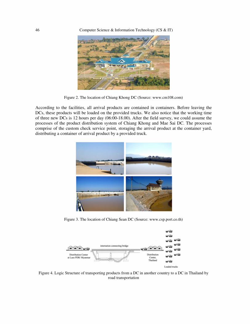
46 Computer Science & Information Technology (CS & IT)
Figure 2. The location of Chiang Khong DC (Source: www.cm108.com)
According to the facilities, all arrival products are contained in containers. Before leaving the
DCs, these products will be loaded on the provided trucks. We also notice that the working time
of three new DCs is 12 hours per day (06:00-18.00). After the field survey, we could assume the
processes of the product distribution system of Chiang Khong and Mae Sai DC. The processes
comprise of the custom check service point, storaging the arrival product at the container yard,
distributing a container of arrival product by a provided truck.
Figure 3. The location of Chiang Sean DC (Source: www.csp.port.co.th)
Figure 4. Logic Structure of transporting products from a DC in another country to a DC in Thailand by
road transportation

Computer Science & Information Technology (CS & IT) 47
Figure 5. Logic Structure of transporting products from a DC in another country to a DC in Thailand with
multiple transportation
The processes of Chiang Sean product distribution system composes of lifting contatiners of
arrival products, the custom check service point, distributing a container of arrival product by an
available truck.
This survey helps us to design the processess of three new DCs when we develop the product
distribution models of three new DCs.
4.1.2. Data Collection
We collected the data of arrival products from the southern region of China to Chiang Khong
custom house in year 2012, Chiang Sean custom house in year 2009, and Mae Sai custom house
in year 2012 as detailed in Table 1. The data collection of the importing product volume of
Chiang Khong and Mae Sai custom house was derived from their annually reports [2], [10] while
we derived the arrival products of Chiang Sean custom house from the Marine Department,
Thailand [11].
We use the collected data as the base of the arrival product volume. However, the derived data is
the historical data, but the arrival product volumes expect to increase unknowingly. Before the
new DCs will be able to implement, we need to study the capability of the system.
Table 1. Arrival products at Chiang Khong, Chiang Sean, and Mae Sai custom
Unit: Ton
Month Custom
Chiang Khong in
2012
Chiang Sean
in 2009
Mae Sai
in 2012
January 25,540 18,268 11,542
February 32,280 9,467 12,688
March 29,160 9,752 8,437
April 26,780 9,354 12,676
May 35,020 14,407 4,941
June 29,460 16,266 26,353
July 39,700 29,251 5,078
August 39,080 29,223 4,103
September 30,740 47,448 3,508
October 34,720 51,148 5,659
November 37,560 51,001 8,783
December 34,480 37,510 9,865
Total 394,520 323,095 113,633

48 Computer Science & Information Technology (CS & IT)
4.2. Model Construction
Based on the field observation and the data collection, two product distribution models were
developed. The first model was provided for distributing products by using road transportation,
and Chiang Khong, and Mae Sai DCs were applied as the case study (as in Figure 6). Chiang
Sean DC was the case study of the product distribution model using waterway transportation and
releasing products by road transportation (as in Figure 7). Figure 6 and 7 show the conceptual
modules functioning in the product distribution systems with a First-In First-Out (FIFO) queue.
An arrival product in the system is contained in a container on a truck. The container will be
processed sequentially and immediately if the system is available; otherwise it needs to wait.
The designed model could represent the processes in the system which undergoes with the data
requirement to characterize the system. The data requirements for each module in the model will
be described in the parameter setting section. Figure 6 explains the process flowchart of the
Chiang Khong and Mae Sai DC.
The first component named "Arrival" represents an arrival container that arrives into the system
by using the random exponential distribution to simulate the arriving time for a container entering
the system.
In the second component, if the "CustomCheck" process is ready to process, the list of invoice of
arrival container is needed to be lodged at the Customs service counter. The officer will verify the
invoice list and generate the import invoice; otherwise the invoice list will be asked to modify for
correction and lodged again. After that, the import invoice needs to be paid.
When completed from "CustomCheck", the payment will be declared with containers of products.
Then containers will be stored at the container yard in "LiftAtYard" module in order to wait for
available trucks in the next module.
In "LiftOnTruck" module, the payment and containers will be verified and prepared for available
trucks. Then containers will be loaded on the available trucks, and continued to leave the system
at "Distributing" module in order to transport a container through the road network.
Figure 7 illustrates the process flowchart of Chiang Sean DC where facilitates an arrival container
shipped by waterway transportation and it will be flown out off the DC by road transportation.
The "Arrival" module in Figure 7 represents a container importing into the system by using the
random exponential distribution as same as in Chiang Khong and Mae Sai models. If the system
is idle, a container will be lift up from a ship at "LiftUp" module; otherwise it will be hold in a
queue. The lift containers will be delivered by the provided facilities in the system. Then, the
containers of products need to be declared and moved to the next module after completed.
"CustomCheck" module is the next process that will check a container following the custom
regulation as same as in Chiang Khong and Mae Sai systems. After that, a container will be
loaded up to an available truck, but there are only 80% that a container could get an available
truck. Then, this truck will transport to the terminal through the road network system [1], [13].
These designed models properly describe and cover the functions of the product distribution
system for three new DCs.

Computer Science & Information Technology (CS & IT) 49
Figure 6. Process flowchart of the product distribution model at the new DC facilitating road transportation
Figure 7. Process flowchart of the product distribution model at the new DC facilitating waterway
transportation and releasing as road transportation
4.3. Parameter Settings
It is obvious that the volume of importing products from the south of China has dramatically
increased, but the unknown volumes of arrival products will be imported to three new DCs. In
order to find an appropriated parameter for the system, the various parameters require to examine
by the product distribution model. In this work, it is not possible to find the arrival product
volumes as well as the capability of the system with the field observation because the facilities of
the new DCs are constructing. Therefore, the random exponential distribution and random
triangular distribution techniques are used to measure the arrival product volumes and the
capability of the system, respectively.

50 Computer Science & Information Technology (CS & IT)
The random exponential distribution will be used in order to arrange the interval of arrival time
for arriving products as same as happening in the real system. The models need to avoided from
bias because arrival containers will not enter the system with the specified arriving time. In detail,
the following equations will be combined to set the parameters:
�: Ω → �
a random variable � is functioned above by Ω is the basic simple space; � is named as the state
space of � comprising of all possible values that � could attribute. � random number belongs to a
standard normal distribution with a standard deviation of one and a zero mean.
��� = 1 − ���� , � ≥ 0
Exponential distribution: an exponential random variable, �, attributes values in the positive half-
line � = �0, ∞�. The distribution is described by �����. The �~����� is by � is called the rate
parameter; noted that the corresponding parameter is the mean 1 �⁄ , in ARENA. Figure 8 shows
the probability density function of exponential distribution. The interval (mean) of arriving
product will be randomly entered into the system but closed to the interval of arriving product.
Figure 8 :Probability density function of exponential distribution
��� =� ! "
2� − $% − $& − $ , '� $ ≤ � ≤ &
2% − �% − $% − &
) '� & ≤ � ≤ %
0, �*ℎ�,-'.�/
Triangular distribution : a triangular random variable � attributes values in an interval � = �$, %�, with the "mode" value. The probability linearly goes up in the subinterval �$, &�, and linearly
goes down in the subinterval �&, %� as shown in Figure 9. The distribution is described by
0,'$$, %, &.
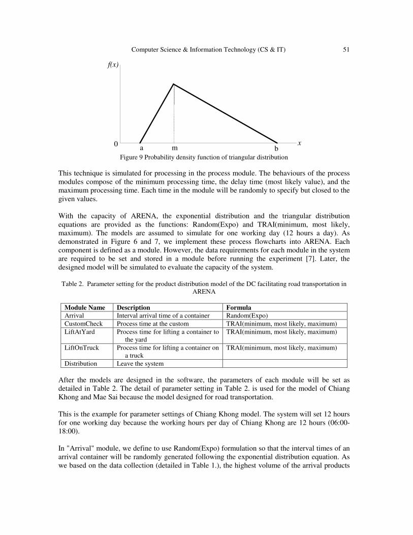
Computer Science & Information Technology (CS & IT) 51
Figure 9 Probability density function of triangular distribution
This technique is simulated for processing in the process module. The behaviours of the process
modules compose of the minimum processing time, the delay time (most likely value), and the
maximum processing time. Each time in the module will be randomly to specify but closed to the
given values.
With the capacity of ARENA, the exponential distribution and the triangular distribution
equations are provided as the functions: Random(Expo) and TRAI(minimum, most likely,
maximum). The models are assumed to simulate for one working day (12 hours a day). As
demonstrated in Figure 6 and 7, we implement these process flowcharts into ARENA. Each
component is defined as a module. However, the data requirements for each module in the system
are required to be set and stored in a module before running the experiment [7]. Later, the
designed model will be simulated to evaluate the capacity of the system.
Table 2. Parameter setting for the product distribution model of the DC facilitating road transportation in
ARENA
Module Name Description Formula
Arrival Interval arrival time of a container Random(Expo)
CustomCheck Process time at the custom TRAI(minimum, most likely, maximum)
LiftAtYard Process time for lifting a container to
the yard
TRAI(minimum, most likely, maximum)
LiftOnTruck Process time for lifting a container on
a truck
TRAI(minimum, most likely, maximum)
Distribution Leave the system
After the models are designed in the software, the parameters of each module will be set as
detailed in Table 2. The detail of parameter setting in Table 2. is used for the model of Chiang
Khong and Mae Sai because the model designed for road transportation.
This is the example for parameter settings of Chiang Khong model. The system will set 12 hours
for one working day because the working hours per day of Chiang Khong are 12 hours (06:00-
18:00).
In "Arrival" module, we define to use Random(Expo) formulation so that the interval times of an
arrival container will be randomly generated following the exponential distribution equation. As
we based on the data collection (detailed in Table 1.), the highest volume of the arrival products
a m b0 x
f(x)

52 Computer Science & Information Technology (CS & IT)
in 2012 at Chiang Khong custom house was 39,700 tons in July. We divide 39,700tons by 20 in
order to convert a weight of ton into a container because we assume to transport an arrival
product container by a truck (one container loading on one truck). There are 66 containers
importing into the model in 12hours. It means 66 containers will continue importing into the
model one by one to process in every 11minutes. Therefore, we set the value for Random(Expo)
formulation equals 11.
For "CustomCheck", "LiftAtYard", and "LiftOnTruck" modules, we set the action for these
modules as "Seize Delay Release". This action identifies the system would seize the resource of
the system for processing a module when processing an arrival container. The action will be
automatically set as delay action when the module is processing. The waiting containers will wait
in a queue to be processed. These containers will use FIFO rule when the module is idle to
process. "CustomCheck", "LiftAtYard", and "LiftOnTruck" modules will use TRAI(minimum,
most likely, maximum) as Triangular probability distribution formulation. This formulation
indicates the probability distribution of an arrival container spending time in a module.
Triangular probability composes of the minimum, most likely and maximum time values that are
required to be set in Triangular probability distribution formula. "CustomCheck" module will be
set TRAI(15,20,25) because the custom normally consumes 15 minutes to complete the work in a
module, 20 minutes for the time of delay in a process, and 25 minutes in the maximum duration
of a process. "LiftAtYard" and "LiftOnTruck" modules will be set TRAI(8,12,16) because the
work will be done in these modules using for 8 minutes. The time delay in these modules is 12
minutes while the maximum processing time is 16minutes.
Mae Sai product distribution model is similar to Chiang Khong model. Some values need to
adjust due to the arrival products at Mae Sai custom in 2012 and its facilities. The value of
Random(Expo) formulation at "Arrival" module equals 16 because the highest volume of the
arrival product at Mae Sai was 44 containers per day in June 2009. "CustomCheck" module will
be set the value for the function as same as the CustomCheck" module of Chiang Khong because
the custom check procedures have done similarly. "LiftAtYard" and "LiftOnTruck" modules will
be set TRAI(8,10,12) because Mae Sai DC can facilitate faster than Chiang Khong DC. Mae Sai
DC has smaller size than Chiang Khong DC but its arrival product volumes were less than
Chiang Khong.
On the other hand, the modules of Chiang Sean model compose of "Arrival", "LiftUp", and
"CustomCheck" components as shown in Table 3. In "Arrival" module, the value for
Random(Expo) sets to 8. The data collection of Chiang Sean custom house in 2009 will be
calculated as same as done in Chiang Khong and Mae Sai models. The value for TRAI(minimum,
most likely, maximum) in the "LiftUp" module sets to TRAI(15,20,25) because of the field
survey. For "CustomCheck" module, the value will be set as same as the "CustomCheck" module
of Chiang Khong and Mae Sai models. Since arrival containers ship by waterway transportation
and change to road transportation, these containers need to put in a decision module. In the real
system, a provided truck may not be available for distributing a container when it is completed.
In "Decide" module, we will set 80% for the probability of delivery by an available truck, and
20% for the probability of detention when there is no available truck [8]. However, the parameter
setting is an example for the model. The modellers are allowed to readjust and organise the model
as appropriated.

Computer Science & Information Technology (CS & IT) 53
Table 3. Parameter setting for the product distribution model at the new DC facilitating waterway
transportation and releasing as road transportation in ARENA
Module Name Description Formula
Arrival Interval arrival time of a container Random(Expo)
LiftUp Process time for lifting up a container
from a ship
TRAI(minimum, most likely, maximum)
CustomCheck Process time at the custom TRAI(minimum, most likely, maximum)
Decide Consideration for delivery or
detention
80% for delivering a container (True) 20%
for detaining a container (False)
Distribution Leave the system
4.4 Model Application
In our study, we formulated the model to explain the capacity of the system. As mentioned, the
arrival product volumes from the south of China has dramatically increased, but the arrival
product volumes that importing into three new DCs are unknown. We collected the data of the
arrival product volumes in Chiang Khong, Chiang Sean, Mae Sai custom house in 2012, 2009,
and 2012, respectively. We used these data as the base for modelling.
We propose a scenario for model application in order to estimate the arrival product volumes
importing to the new DCs systematically. We assume that arrival product volume would increase
from the base data to 25%, 50%, 75%, and 100%, respectively. This is because we expect that the
experiment can describe the capacity of the systems. We also expect that the capability of all
processes will be revealed. Therefore, we can offer the solutions or the alternatives for the system
in order to prevent the and the models can be generalise in similar systems.
5. COMPUTATIONAL RESULTS
After developing the models and setting the parameters, we will experiment the model
considering the proposed scenario. We expect to evaluate the capacity of the product distribution
system by increasing the unknown arrival products. Our scenario is to increase the unknown
arrival products from the base data to 25%, 50%, 75%, and 100%. As mentioned, the working
time of the system for one day is 12hours (06:00-18:00).
Table 4. shows the result of Chiang Khong model. The waiting number of trucks per 12working
hours in "CustomCheck", "LiftAtYard", and "LiftOnTruck" process is detailed. Table 4. also
reports the number out from the system, and total number of arrival truck.
The total number of arrival truck in the system relates to our criteria (25%, 50%, 75%, and 100%,
respectively). However, the number out from the system (truck/12hr) in all criteria slightly
increases. It is interesting that many arrival trucks are waiting for "CustomCheck" process when
comparing with "LiftAtYard" and "LiftOnTruck" process.
Under the same conditions of Chiang Khong model, Table 5. shows the result of Chiang Sean
model. It also reports the waiting number of trucks per 12working hours in "LiftUp" and
"CustomCheck" process. The transporting trucks from the system, and total number of arrival
truck are detailed. We notice that Chiang Sean model confront the same problem of Chiang

54 Computer Science & Information Technology (CS & IT)
Khong model. The first module ("LiftUp") has a long queue waiting for processing. The increase
of the waiting number in this module relates to the criteria of increasing arrival truck.
Table 4. Result from Chiang Khong model by increasing arrival trucks
Increasing
arrival
truck
Waiting number in a module (truck/12hr) Number out
from the
system
(truck/12h
r)
Total number
of arrival
truck
(truck/12hr)
CustomCheck LiftAtYard LiftOnTruck
Base data 7 7 1 52 67
+25% 12 11 2 54 79
+50% 28 12 3 56 99
+75% 30 14 2 56 102
+100% 53 12 1 57 123
Table 5. Result from Chiang Sean model by increasing arrival trucks
Increasing arrival
truck
Waiting number in a module
(truck/12hr)
Number out
from the
system
(truck/12hr)
Total number of
arrival truck
(truck/12hr) LiftUp CustomCheck
Base data 27 1 33 61
+25% 34 1 33 69
+50% 40 1 33 74
+75% 52 1 33 86
+100% 70 1 34 105
Table 6. reports the waiting number is each module of Mae Sai product distribution system, the
number of trucks out from the system, and the total number of arrival trucks in the system. With
the same conditions such as working hours per day, and criteria of increasing arrival products, the
number of trucks out from the system continuingly increases. The waiting number of truck in
each module is not significant.
Table 6. Result from Mae Sai model by increasing arrival trucks
Increasing
arrival
truck
Waiting number in a module (truck/12hr) Number out
from the
system
(truck/12h
r)
Total number
of arrival
truck
(truck/12hr)
CustomCheck LiftAtYard LiftOnTruck
Base data 3 1 1 38 43
+25% 5 1 1 59 66
+50% 6 2 1 61 70
+75% 8 2 1 61 72
+100% 15 2 1 66 84
In addition, the waiting number in each module of Chiang Sean is very high. The system and
Chiang Khong model also confront the same problem, but not serious as in Chiang Sean system.
Mae Sai system can manage the system well with few waiting numbers of truck in each module.

Computer Science & Information Technology (CS & IT) 55
Figure 10. Waiting truck in each module of Chiang Khong model
Figure 10. illustrates that Chiang Khong system faced with the bottleneck problem. The problem
shows with the number of waiting trucks per 12 hours in each module of the system. With the
criteria of increasing arrival trucks into the system from the base data to 25%, 50%, 75%, and
100%, the total number of trucks in the system relates to the proposed criteria. The waiting truck
number is particularly significant in the first module ("CustomCheck"). The waiting trucks in the
second module ("LiftAtYard") are small while there is very few in the third module
("LiftOnTruck"). The bottleneck problem is the issue on the first process because the volume of
arrival trucks, and the processing time were higher than others. However, the capability of the
system can maintain its system well because the ratio of trucks out from the system and waiting
trucks in modules are 2 to 1. The ratio slightly declines when increasing the arrival trucks
following the conditions. It is because the capability of the system becomes overloaded.
The results from the experiment indicate Chiang Sean system confronts the serious bottleneck
problem more than other systems because the arrival products imported to the system were higher
than others almost 30% as referred in the data collection. Figure 11. shows the number of trucks
waited for processing in each module in one working day (12hours). In two modules of Chiang
Sean system, there is a long queue in the first module named "LiftUp" module, but it is not
significant in the second module ("CustomCheck"). Indeed, the number of waiting truck for
processing increasingly related with the criteria of increasing arrival from the base data to 25%,
50%, 75%, and 100%. The total number of waiting truck in 12hours of Chiang Sean system is
almost 75 trucks per 12 hours at increasing arrival product for 100%. When comparing with the
finished trucks from the system, the ratio of the waiting trucks and the finished trucks in the
system is 3 to 1.
However, the waiting truck was very few in the second module because all modules of the system
was processed sequentially. All arrival trucks were required to complete the process at the first
module. All trucks waited for processing in a queue at the first module as well, so the second
module could have time to finish its process while the waiting truck for processing in module was
usually less than the first module. Therefore, the bottleneck problem is very serious for Chiang
0
25
50
75
100
125
Base Data 25 Percent 50 Percent 75 Percent 100 Percent
(truck/12hr)
Waiting truck in each module of Chiang Khong model
Truck Number Out
LiftOnTruck
LiftAtYard
CustomCheck
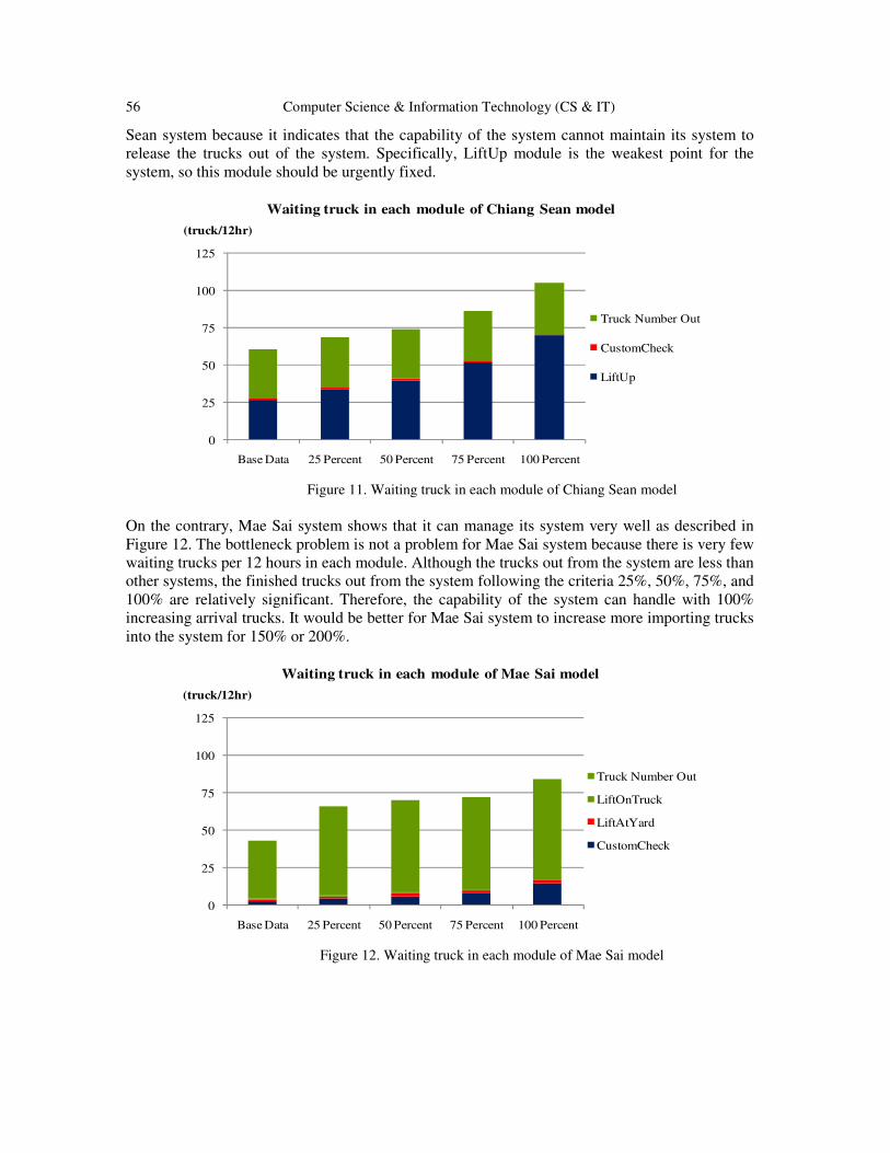
56 Computer Science & Information Technology (CS & IT)
Sean system because it indicates that the capability of the system cannot maintain its system to
release the trucks out of the system. Specifically, LiftUp module is the weakest point for the
system, so this module should be urgently fixed.
Figure 11. Waiting truck in each module of Chiang Sean model
On the contrary, Mae Sai system shows that it can manage its system very well as described in
Figure 12. The bottleneck problem is not a problem for Mae Sai system because there is very few
waiting trucks per 12 hours in each module. Although the trucks out from the system are less than
other systems, the finished trucks out from the system following the criteria 25%, 50%, 75%, and
100% are relatively significant. Therefore, the capability of the system can handle with 100%
increasing arrival trucks. It would be better for Mae Sai system to increase more importing trucks
into the system for 150% or 200%.
Figure 12. Waiting truck in each module of Mae Sai model
0
25
50
75
100
125
Base Data 25 Percent 50 Percent 75 Percent 100 Percent
(truck/12hr)
Waiting truck in each module of Chiang Sean model
Truck Number Out
CustomCheck
LiftUp
0
25
50
75
100
125
Base Data 25 Percent 50 Percent 75 Percent 100 Percent
(truck/12hr)
Waiting truck in each module of Mae Sai model
Truck Number Out
LiftOnTruck
LiftAtYard
CustomCheck

Computer Science & Information Technology (CS & IT) 57
6. CONCLUSION AND DISCUSSION
Regarding to the objectives of our research, we propose to develop a model of product
distribution system for new DCs in order to evaluate the capability of the system, and we expect
that the designed model can reflect the problem of the system that can efficiently use to improve
the capability of the system. The system of Chiang Khong, Chiang Sean, and Mae Sai DC were
the study area of this paper. These three DCs have been under constructing for facilitating the
increasing arrival products from the southern part of China. It becomes difficult because there is
no recorded data and no experience at these new DCs. Therefore, the increasing arrival products
that will be imported into these new DCs are unknown.
To model the product distribution system for these new DCs, we used the efficiency of ARENA
to develop the model relating to the field survey of facilities, and the data collection of the arrival
products from the past year. Chiang Khong and Mae Sai models had the same processes that
comprised of "Arrival", "LiftAtYard", "LiftOnTruck" modules. Chiang Sean model was designed
to import the arrival product from ship and distributed the completed products by truck. The
modules of Chiang Sean system composed of "LiftUp" and "CustomCheck" processes.
During the model development, the parameters in each process of the designed systems needed to
be set. The random exponential distribution and the random triangular distribution techniques
were used. The exponential distribution technique was used for importing the arrival product into
the system. This technique could simulate as same as the actual system. Each arrival product
containing in a container was randomly generated into the system in every specific time. Only
one container could be processed in a module and it would sequentially continue to the next
module when it was done. For another technique, it was used for the process module because the
triangular distribution functions for three circumstances that are the completed work, the delay
time waiting for processing, and the maximum time for processing.
Due to the unknown arrival product transporting to the new DCs, we proposed the scenario to
evaluate the capability of the models by increasing the arrival product from the base data to 25%,
50%, 75% and 100%. After the experiment, the result showed that the product distribution system
of Mae Sai DC operated well. Almost 100% of arrival trucks can finish and leave all processes
with very few waiting trucks in the system. The system of Chiang Khong and Chiang Sean
reflect the bottleneck problem especially its first process. The first process of these two models
has a long queue waiting for processing. We found that the capability of the first process of
Chiang Khong and Chiang Sean models could not handle with the condition of increasing arrival
trucks. Chiang Khong system deals with the bottleneck problem better than Chiang Sean system,
because Chiang Khong system can release the finished trucks out from its system more than 50%
of arrival trucks. Moreover, the queue of Chiang Khong model in the first process was less than
the queue of Chiang Sean model in the first process because the arrival product volumes of
Chiang Khong model were less than the arrival products of Chiang Sean model.
In conclusion, the designed models for the new DCs successfully developed. The results from the
experiment reflect the capability of the systems. We suggest that these three new DCs should
double the capability of each module because the bottleneck problem occurred in the system.
After doubling the capability of each module, we also recommend to increase the criteria of
increasing arrival product volume to 150% and 200%, so we can expand our view and we may

58 Computer Science & Information Technology (CS & IT)
handle the wider problem. Finally, we notice that ARENA is capable of problem identification
for the system, so the developed models can be generalised for similar systems.
ACKNOWLEDGEMENTS
The work described in this paper was sponsored by Rajamangala University of Technology
Lanna (RMUTL), Thailand.
REFERENCES [1] Cheng, Lifei. & Duran, Marco A., (2002) “World-Wide Crude Transportation Logisitics: A Decision
Support System Base on Simulation and Optimization”, In Proceedings Foundations of Computer
Aided Process Operations, pp187-201.
[2] Chiang Khong Customs House, (2012) Operational Annual Report 2008-2012, Chiang Rai, Thailand.
[3] Cordenillo, Raul L., (2005) The Economic Benefits to ASEAN of the ASEAN-China Free Trade
Area (ACFTA), http://www.asean.org.
[4] Das, Shantanu, & Levinson, David, (2004) “Queuing and Statistical Analysis of Freeway Bottleneck
Formation”, Journal of Transportation Engineering ASCE, pp787-795.
[5] Fahimnia, Behnam, Luong, Lee. & Marian, Romeo, (2008) “Optimization/simulation modelling of
the integrated production distribution plan: an innovative survey”, WSEAS Transactions on Business
and Economics, Vol.5, No.3, pp52-65.
[6] Kasikorn Research Center, Mega Projects of Transportation: Move forward even increasing cost,
http://www.kasikornresearch.com.
[7] Kelton, W.David, Sadowski, Randall P. & Sadowski, Deborah A., (1998) Simulation with Arena,
McGraw Hill, McGraw Hill Publishing.
[8] Kelton, W.David, Sadowski, Randall P. & Sturrock, David T., (2003) Simulation with Arena, (3eds),
McGraw Hill, McGraw Hill Publishing.
[9] Kleinschmidt, Tristan, Guo, Xufeng, Ma, Wenbo, Yarlagadda, Prasad K.D.V., (2011) “Including
Airport Duty-Free Shopping in Arrival Passenger Simulation and the Opportunities this Presents”, In
Proceedings of the 2011 Winter Simulation Conference.
[10] Mae Sai Customs House, (2012) Operational Annual Report 2008-2012, Chiang Rai, Thailand
[11] Marine Department of Thailand. http:// www.md.go.th/md/
[12] Shannon, Robert E., (1975) Systems Simulation: The Art and Science, Prentice-Hall, Englewood
Cliffs.
[13] Teri, Sergio. & Cavalieri, Sergio, (2004) “Simulation in the supply chain context: a survey”,
Computers in Industry Transactions on ScienceDirect, Vol.53, No.1 pp3-16.
[14] Vieira, Guilherme Ernani, (2004) “Ideas for Modelling and Simulation of Supply Chains with
ARENA”, In Proceedings of the 2004 Winter Simulation Conference, Vol. 2, pp1418-1427.
AUTHORS
Kingkan Puansurin is currently a PhD (Computer Science) student at La Trobe
University. Her research is mainly concerned with methods and techniques for
Multiple Criteria Decision Analysis and Modelling.

Computer Science & Information Technology (CS & IT) 59
Jinli Cao Dr Cao is a Senior Lecturer in Department of Computer Science and IT, La
Trobe University, Melbourne Australia. She has been active in areas of database
systems, Key words search in XML documents, Top-K query on probabilistic data
and Web Services. She ha s published over 80 research papers in refereed
international journals and conference proceedings such as IEEE Transactions on
Distributed and Parallel Processing, IEEE Transactions on Knowledge and Data
Engineering (TKDE) etc.

60 Computer Science & Information Technology (CS & IT)
INTENTIONAL BLANK

Natarajan Meghanathan et al. (Eds) : ACSIT, FCST, ITCA, CoNeCo - 2015
pp. 61–69, 2014. © CS & IT-CSCP 2015 DOI : 10.5121/csit.2015.51207
ENERGY EFFICIENT HIERARCHICAL
CLUSTER-BASED ROUTING FOR
WIRELESS SENSOR NETWORKS
Shideh Sadat Shirazi, Aboulfazl Torqi Haqiqat
Faculty of Computer and Information Technology Engineering,
Qazvin Branch, Islamic Azad University, Qazvin, Iran [email protected]
ABSTRACT
In this paper we propose an energy efficient routing algorithm based on hierarchical clustering
in wireless sensor networks (WSNs).This algorithm decreases the energy consumption of nodes
and helps to increase the lifetime of sensor networks. To achieve this goal, this research
network is divided into 4segments that lead to uniform energy consumption among sensor
nodes. We also propose a multi-step clustering method to send and receive data from nodes to
the base station. The simulation results show that our algorithm is better than existing
algorithms in terms of saving energy, balancing energy dissipation and prolonging network
lifetime.
KEYWORDS
Wireless sensor networks, energy efficient, data aggregation algorithms, clustering.
1. INTRODUCTION
In recent years, many ways of routing protocols based on clustering have been proposed. Cluster-
based data aggregation algorithms are the most popular ones because they have the advantages of
high flexibility and reliability. Recent advances in wireless communications and electronics have
led to the development of WSNs, which are composed of many small-size, low-cost, low-power
and multifunctional sensor nodes [1]. The process of aggregating the data from multiple nodes to
eliminate redundant transmission and provide fused data to the BS – the so-called data
aggregation – is considered as an effectual technique for WSNs to save energy [2]. The most
popular data aggregation algorithms are cluster-based data aggregation algorithms, in which the
nodes are grouped into clusters; each cluster consists of a cluster head (CH) and some members,
each of them transmitting data to its CH. Then, each CH aggregates the collected data and
transmits the fused data to the BS.

62 Computer Science & Information Technology (CS & IT)
Unbalanced energy dissipation is an inherent problem of cluster-based WSNs. Some nodes drain
their energy faster than others which results in an earlier failure of network. Some researchers
have studied this problem and proposed their algorithms, which have both advantages and
disadvantages. Our motivation is to propose a novel solution to this problem in the cluster-based
and homogeneous WSNs, in which the CHs transmit data to the BS by one-hop communication,
with an objective of balancing energy consumption by an energy efficient way and, thus,
prolonging network lifetime.
2. RELATED WORK
Some of these other algorithms which are related to our method will be discussed briefly. Most of
the routing algorithms are based on a LEACH clustering algorithm; the algorithm is implemented
to improve the routing. The LEACH algorithm was proposed in 2000 [3] of the random rotation
techniques to select the cluster head node in the network uses. LEACH performances, in turn, are
organized so that each turn consists of a setup phase and a maintenance phase. In the setup phase,
nodes organize themselves into clusters so that each cluster node will work as a cluster head
itself. Deciding to become a cluster head within each node is done locally. On average, the
percentage of the predetermined spatial location in each of the nodes serves as cluster head. The
length of phase transitions is selected for each cluster head node of the cluster to collect data and,
before sending it directly to the base station, the process of aggregating data is done. HEED [4]
periodically selects CHs and builds equal clusters according to a hybrid of the residual energy of
nodes and a secondary parameter. UCS [5] is the first proposed algorithm to resolve the problem
of unbalanced energy dissipation by forming unequal clusters. EECS [6] and EDUC [7] are
unequal cluster-based algorithms for WSNs in which the CHs transmit data to the BS by one-hop
communication. EECS is proposed for homogeneous WSNs, it elects some tentative CHs
randomly and utilizes a cluster head competition method to choose CHs from tentative CHs, after
that, each ordinary node selects CH basing on the distance from itself to CH and the distance
from CH to the BS to construct unequal clusters. EDUC is proposed for heterogeneous WSNs. In
[8] Mr.JanYue and colleagues have offered an EEBCDA algorithm. In this algorithm, the
network environment as well as the swim lane is divided in sections of the size of the swim lane –
size, length and width are equal. Each swim lane, also called grid, is divided into smaller parts.
Grid size is different in each swim lane. The greater the distance from the BS, the larger is the
grid size. The grid node with the highest energy is selected as the cluster head node. This type of
fencing can have a grid that contains a number of nodes with greater distance from the BS. As a
result, a greater number of nodes become cluster-heads. This results in balancing the energy
consumption of nodes and improving the network lifetime.
3. EXPRESSION OF PROPOSAL
The main issue of this paper is to introduce a routing method to enhance and improve the lifetime
of sensor nodes and, thus, increase the lifetime of sensor networks. The main steps are divided
into three stages. In the first stage, the network is divided into sections that can uniform energy
consumption among sensor nodes. A heterogeneous distribution of nodes for this purpose is
introduced. Secondly, a clustering algorithm for data aggregation is presented. And in the third
phase, a multi-step hierarchical tree for sending aggregated data from nodes to the base station is
presented.

Computer Science & Information Technology (CS & IT) 63
3.1. A Heterogeneous Distribution of Nodes
The initial energy of heterogeneous nodes is not equal. For this purpose, three types of nodes with
different initial energies are considered. The distance between the BS is divided into three areas:
The closest node to node with the lowest energy is placed in the middle part of the average energy
and the farthest node with the highest energy content of each. Since nodes consume far more
energy to send data to this node, energy consumption becomes more balanced and cause the
nodes to die almost simultaneously.
Figure 1.Network is divided into three zones
3.2. Network Model
To simplify the network model, we consider a WSN that N heterogeneous nodes are uniformly
dispersed within a square deployment area with border B. The left bottom vertex of deployment
area locates at (O_x, O_y) in Cartesian coordinate plane. In addition, we make a few assumptions:
1) the BS and all nodes are time synchronized and are stationary after deployment, the BS is
located at (BS_x, BS_y) which transmission power level according to the distance to the receiver;
3) the BS and all nodes are location-aware.
The first two assumptions are familiar in other algorithms. The third assumption is reasonable in
many applications of WSNs in which the sensed data only make sense with location information,
for other applications, the locations of BS and nodes can be easily obtained by utilizing
localization algorithms. The time synchronization algorithms and localization algorithms are not
discussed in our work.
3.3. Energy Consumption Model
We use the same energy consumption model used in EECS. The free space model is used if the
distance between the transmitter and receiver less than a threshold d0, otherwise, the multipath
model is used. The energy spent for transmitting an l-bit message over distance d is

64 Computer Science & Information Technology (CS & IT)
where Eelec is the energy dissipated per bit to run the transmitter or the receiver circuit, εfs or
εmp, is the energy dissipated per bit to run the transmit amplifier. To receive this message, the
expended energy is
The consumed energy of aggregating m messages with l-bit is
where EDA is the energy dissipated per bit to aggregate message signal.
3.4. Problem Statement
In the cluster-based WSNs in which the CHs transmit data to the BS by one-hop communication,
there are three reasons leading to unbalanced energy dissipation: 1) a CH often spends more
energy than a member;2) the amounts of received data of CHs are different; 3) the distances of
transmitted data of CHs indifferent regions are different. Both LEACH and equal cluster-based
algorithms are not able to balance the energy dissipation completely. Unequal cluster-based
algorithms are considered as better solutions, they form clusters with unequal size according to
the distance from each CH to BS, expect that the CH further away from the BS has less members
so that it is able to consume less energy to receive data and preserve more energy to transmit data.
But the existing unequal cluster-based algorithms are deficient.
First of all, they do not consider the distribution of CHs in CHs rotation scheme, the selected CHs
are randomly scattered in the network and the purpose of unequal clustering is affected. In
addition, many unequal cluster-based algorithms make some ordinary nodes choose further CHs
but not the closest CHs to form unequal clusters, so that these nodes have to spend excessive
energy to transmit data.
4. OUR PROPOSED METHOD
Our proposed clustering method is also divided into rounds and every round consists of a set-up
phase and a steady-state phase, especially, there is a network-division phase before the first
round. The network is divided into rectangular regions firstly, called swim lanes, then, each swim
lane is further partitioned into smaller rectangular regions, called grids. The node with maximal
residual energy of each grid and the shortest distance to the BS is selected as CH. The grids
further away from the BS are bigger and have more nodes to participate in CHs rotation. In Fig 2,
in which the dashed lines mark the division of swim lanes, the dotted-dashed lines denote the
division of grids.
4.1. Network-Division Phase
Without loss of generality, we assume that the BS is above the deployment area along Y-axis. At
first, the deployment area is divided into S rectangular swim lanes along X-axis. All swim lanes

Computer Science & Information Technology (CS & IT) 65
have equal width W, and the length of each swim lane is equal to the border of deployment area.
We use a sequence of integers from 1 to S as the IDs of swim lanes, and the ID of the leftmost
swim lane is 1.
Then, each swim lane is partitioned into several rectangular grids along Y-axis. Each grid of each
swim lane is assigned a level, we also use a sequence of integers starting from 1 as the levels of
grids in each swim lane, and the level of the bottommost grid is 1. Each grid has the same width
with swim lane. Both the number of grids and the length of each grid in a swim lane are related
with the distance from the swim lane to BS. Our proposed method adjusts the size of each grid by
setting its length. For different swim lanes, the further a swim lane is away from BS, the fewer
grids it has. For same swim lane, the grid further away from the BS has longer length. We define
an array A with S elements, in which the k-th element is the number of grids in swim lane k. Each
grid is assigned a tuple (i, j) as ID, which means that it is in swim lane i and has level j. In
addition, we define S arrays to denote the lengths of grids, the v-th array Hv is the lengths of grids
in swim lane v, and the w-th element hvw of Hv is the length of grid (v, w). The bounds of grid
(i, j) are
�� + �� − �� × < � ≤ �� + � × (4)
�� + ∑ ℎ�� < � ≤ �� + ∑ ℎ��������
�������� (5)
4.2. Analysis
Initially, the BS broadcasts a BS_MSG ((O_x, O_y), (BS_x, BS_y), B, W, S, A, H1, …,HS)
message to all nodes and each node calculates the ID of the grid. At each stage of the
implementation of the proposed method, a cluster head is selected for each grid. Between the
nodes of a grid, as the cluster head node which has the highest residual energy is chosen. In the
first round, all nodes is equal to the initial energy of all nodes close to the BS is selected as the
cluster head. In subsequent rounds, if multiple nodes have the same energy, one that is closer to
the BS as a cluster head is selected. In the first round by the cooperation of all nodes of a cluster
head, the grid is selected. Initially, each node contains a message NODE_MSG (k, (v, w), Er, (x,
y)) which is sent to other nodes on the grid. Where k: id nodes, (v, w): Number grid, Er: residual
energy and node (x, y): Location node. With this message, each node can get the information of
rest of the nodes in a grid and then the node which has the highest residual energy is selected as
the cluster head. After the first round, subsequent rounds of cluster head are selected by the
cluster heads of the previous stage. In this case, the cluster head selects all nodes to send their
data to the cluster head of the previous stage. The cluster heads steps before all nodes are sorted
based on the residual energy and the new cluster head based on remaining energy level picks. To
find information about all other nodes in the new cluster head, cluster head id message contains
the previously selected cluster head sends information to all nodes in the grid.

66 Computer Science & Information Technology (CS & IT)
Figure 3. Displaying the nodes in the desired range and cluster heads are selected in the grid
5. SIMULATION
To simulate the algorithm, we examine two different environments :an area with a range of 200 to
200 meters in which 400 nodes are randomly placed, and an area with a range of 100 to 100
meters in which 100 nodes are randomly placed. Points on the bottom left to the top will be
displayed as (O_x, O_y) and on the top right as (OW_x, OW_y). Consider the following
assumptions for the network:
1) BS and the rest of the nodes in a fixed position, and BS nodes located outside the enclosure.
2) Distances between nodes are considered symmetric.
3) BS and all other nodes are aware of each other's location.
The initial model is shown in Figure 3, the network nodes are randomly placed in the desired
range.
For network segmentation of 200 meters by 200 meters, the grid of the parameters is initialized as
follows:
◌S=4; W=50; A={3,4,4,3}; H1=H4={100, 70, 30}; H2=H3={80, 60, 40, 20}
Table 1. Parameters of simulation
value parameter
400 Number of nodes
(0, 0)-(200,200)m Deployment area
(100,200)m Location of BS
0.5 J Initial energy of
each node
50 nJ/bit Eelec
10 pJ/(bit·m2) εfs
0.0013 pJ/(bit·m4) εmp
87 m d0
5 nJ/(bit·signal) EDA
800 bit Message size
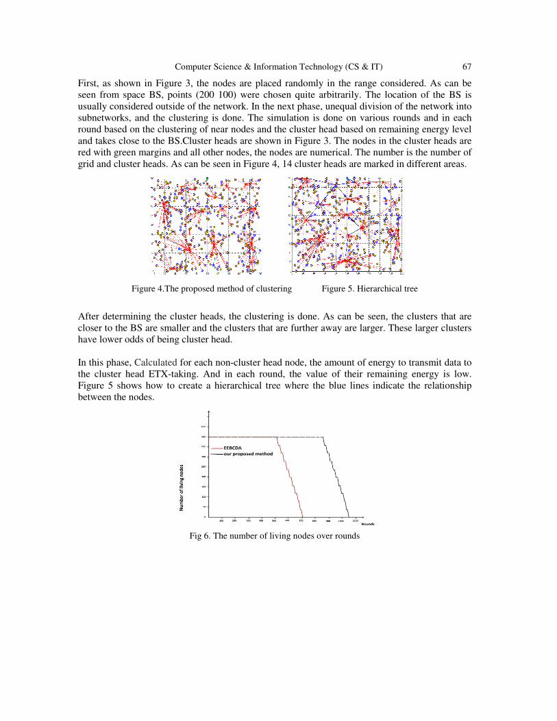
Computer Science & Information Technology (CS & IT) 67
First, as shown in Figure 3, the nodes are placed randomly in the range considered. As can be
seen from space BS, points (200 100) were chosen quite arbitrarily. The location of the BS is
usually considered outside of the network. In the next phase, unequal division of the network into
subnetworks, and the clustering is done. The simulation is done on various rounds and in each
round based on the clustering of near nodes and the cluster head based on remaining energy level
and takes close to the BS.Cluster heads are shown in Figure 3. The nodes in the cluster heads are
red with green margins and all other nodes, the nodes are numerical. The number is the number of
grid and cluster heads. As can be seen in Figure 4, 14 cluster heads are marked in different areas.
Figure 4.The proposed method of clustering Figure 5. Hierarchical tree
After determining the cluster heads, the clustering is done. As can be seen, the clusters that are
closer to the BS are smaller and the clusters that are further away are larger. These larger clusters
have lower odds of being cluster head.
In this phase, Calculated for each non-cluster head node, the amount of energy to transmit data to
the cluster head ETX-taking. And in each round, the value of their remaining energy is low.
Figure 5 shows how to create a hierarchical tree where the blue lines indicate the relationship
between the nodes.
Fig 6. The number of living nodes over rounds

68 Computer Science & Information Technology (CS & IT)
Fig 7.The total residual energy of network over rounds
First of all, we measure the lifetime of network. Fig 5 gives the number of living nodes over
rounds. As evident from the figure, our proposed method has a longer network lifetime than
EEBCDA. The first node of EEBCDA and our proposed method dies in the 591st round and
920th round, the last node dies in 698th round and 1058th round, respectively, our proposed
method improves the network lifetime over by EEBCDA 23.56% and 13.12%. Secondly, we
compare the energy dissipation of our proposed method and EEBCDA. We take statistics of the
total residual energy of network over rounds, as shown in Fig 5. It is explicit that our proposed
method has more residual energy than EEBCDA in every same round, which intuitively
illuminates that our proposed method is more energy efficient than EEBCDA. The ratio of time
interval between the time when the first node dies and the time when the last node dies to the full
time of network is able to indicate the balanced extent of energy dissipation, and the algorithm
with smaller ratio has a better performance in aspect of balancing energy dissipation. The result
of contrast shows that our proposed method is able to achieve more balanced energy dissipation
than EEBCDA.
The next criterion for comparison is the number of packets being transferred to the BS in the
simulation modeling process. Since the curve of the other available methods of data transfer
depending on the total number of different methods are shown in table 2.As can be seen from
these criteria, the proposed method is better.
Table 2.The number of packets transmitted
Name of method The number of
packetstransmitted
EEBCDA 12000
Our proposed method 18000
6. CONCLUSION
In this paper, we focus on the problem of unbalanced energy dissipation in cluster-based and
propose a novel cluster-based data aggregation protocol. The proposed method has been tried by
a heterogeneous distribution of node energy consumption of nodes and network partitioning
becomes more balanced and their lifetime is quite similar to that carried out this evaluation was
realized. By creating a hierarchical structure, we optimize and minimize the energy consumption

Computer Science & Information Technology (CS & IT) 69
of nodes. Finally, when the new approach is used in the MATLAB simulation of the proposed
method, we are able to obtain acceptable results.
REFERENCES
[1] Akyildiz IF, Su W, Sankarasubramaniam Y, Cayirci E. A survey on sensor networks. IEEE Commun
Mag, 2002, 40(8), p.102–114.
[2] Rajagopalan R, Varshney PK. Data-aggregation techniques in sensor networks: a survey. IEEE
Commun Surv & Tutor, 2006,8(4), p. 48–63.
[3] Heinzelman WB, Chandrakasan AP, Balakrishnan H. Energy-efficient communication protocol for
wireless microsensor networks. In Proc of IEEE Conf on System Sciences, 2000, p. 3005–3014.
[4] Younis O, Fahmy S. HEED: a hybrid, energy-efficient, distributed clustering approach for ad hoc
sensor networks. IEEE Trans on Mobile Computing, 2004, 3(4), p. 366–379.
[5] Soro S, Heinzelman WB. Prolonging the lifetime of wireless sensor networks via unequal clustering.
In Proc of IEEE Parallel and Distributed Processing Symposium, 2005, p. 1–8.
[6] Ye M, Li C, Chen G, Wu J. An energy efficient clustering scheme in wireless sensor networks. Ad
Hoc & Sensor Wireless Networks, 2006, 3, p. 99–119.
[7] Yu J, Qi Y, Wang G. An energy-driven unequal clustering protocol for heterogeneous wireless sensor
networks, J Control Theory Appl, 2011, 9(1), p. 133–139.
[8] Yue J, Zhang W, Xiao W, Tang D, Tang J. Energy Efficient and Balanced Cluster-Based Data
Aggregation Algorithm for Wireless Sensor Networks. International Workshop on Information and
Electronics Engineering (IWIEE), 2012,2,p.2009-2015.
AUTHORS
Shideh Sadat Shirazi
Shideh Sadat Shirazi was born on 20 September 1986 in Tehran, Iran. She has been
studying Computer Sciences at Islamic Azad University in Qazvin, Iran since 2011.
One of the focuses of her studies are wireless sensor networks, with a special interest
in energy efficiency. This paper represents an excerpt of her works in this field.
Aboulfazl Torqi Haqiqat
Abdoulfazl Torqi Haqiqat is Assistant Professor, Ph.D. in Computer Engineering at
Islamic Azad University in Qazvin, Iran. He is an expert in the fields of high speed
computer networks, wireless and mobile networks, i.e. MANET and sensor networks,
distributed systems and distributed operating systems, computational intelligence. His
interests also include neural networks, genetic algorithms, ant colonies, taboo searches,
robotics, modeling, simulation and performance evaluation of computer systems and
queuing theory.

AUTHOR INDEX
Aboulfazl Torqi Haqiqat 61
Asif Ullah Khan 25
Bhupesh Gour 25
Chien-Hung Chen 35
Chung-Hsin Huang 35
Dar-Sun Liu 35
Jau-Je Wu 35
Jinli Cao 43
Kingkan Puansurin 43
Marcin Michalak 15
Mashilamani Sambasivam 07
SangKyun Yun 01
Shideh Sadat Shirazi 61