1

Computer Vision- Binary Image Processing

By

Chaitanya Chandra, Jitesh Butala, Sanjay Patil

Department of Electrical EngineeringUniversity of Texas at Arlington

2

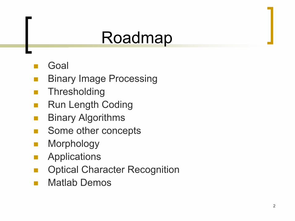
RoadmapGoalBinary Image ProcessingThresholdingRun Length CodingBinary AlgorithmsSome other conceptsMorphologyApplicationsOptical Character RecognitionMatlab Demos

3

Goal

To understand the basic concepts in Binary Image ProcessingTo demonstrate the use of Binary Image Processing

4

Binary Images

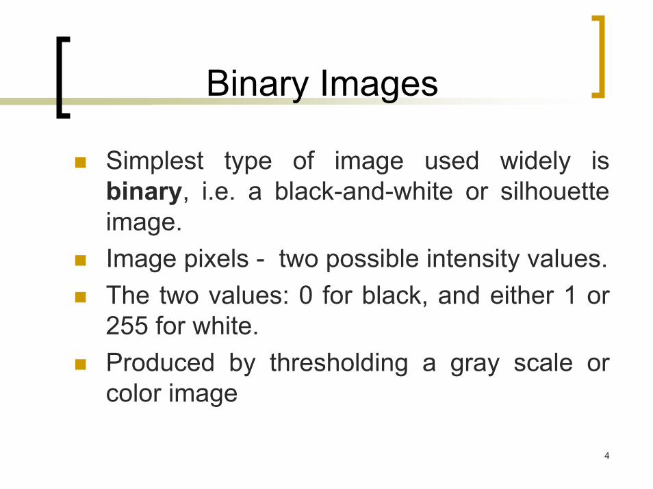
Simplest type of image used widely is binary, i.e. a black-and-white or silhouette image.Image pixels - two possible intensity values.The two values: 0 for black, and either 1 or 255 for white.Produced by thresholding a gray scale or color image

5

Binary Image Processing -Advantages

Easy to acquireLow memory requirementSimple processing

6

Binary Image Processing Disadvantages

Limited applicationCannot not extend to 3DSpecialized lighting is required for silhouettes

7

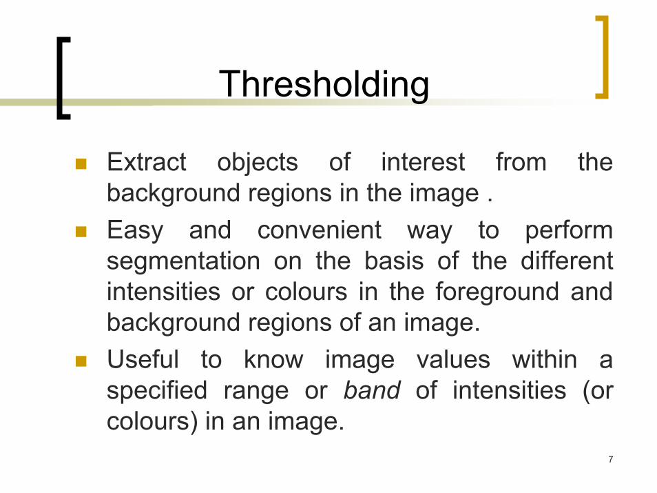
Thresholding

Extract objects of interest from the background regions in the image . Easy and convenient way to perform segmentation on the basis of the different intensities or colours in the foreground and background regions of an image. Useful to know image values within a specified range or band of intensities (or colours) in an image.

8

Types of thresholding

Fixed threshold.Histogram-derived thresholds. Isodata algorithm. Background-symmetry algorithm.Triangle algorithm and many more

9

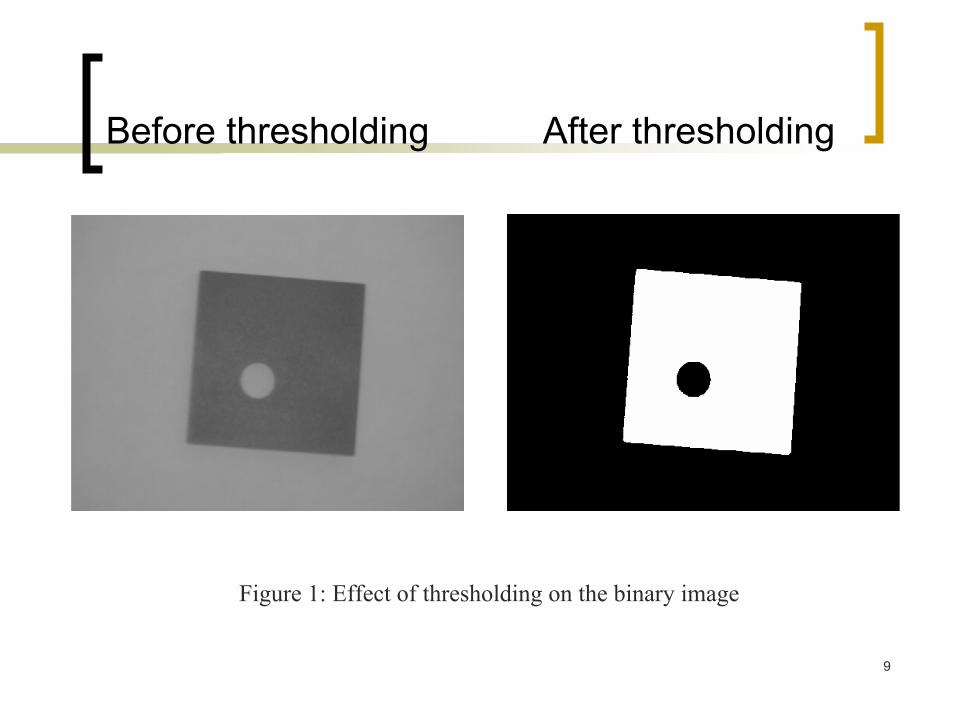
Before thresholding After thresholding

Figure 1: Effect of thresholding on the binary image

10

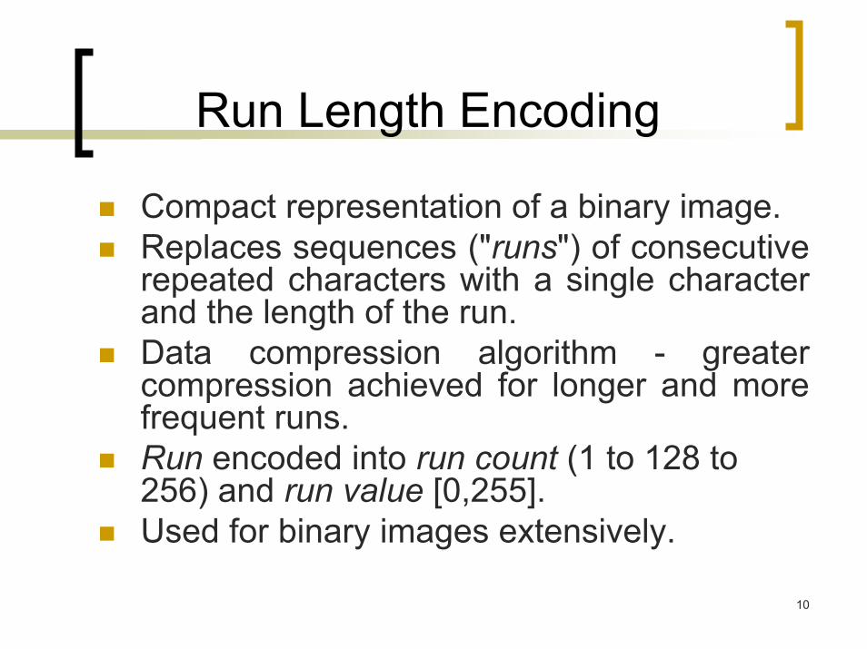
Run Length Encoding

Compact representation of a binary image.Replaces sequences ("runs") of consecutive repeated characters with a single character and the length of the run. Data compression algorithm - greater compression achieved for longer and more frequent runs. Run encoded into run count (1 to 128 to 256) and run value [0,255].Used for binary images extensively.

11

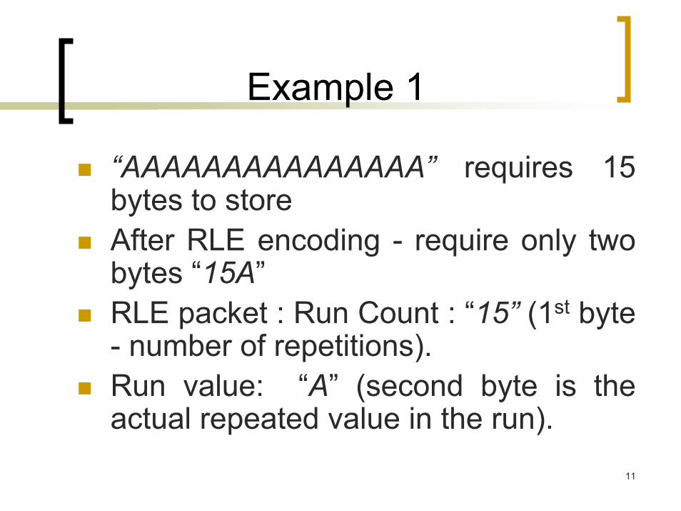
Example 1

“AAAAAAAAAAAAAAA” requires 15 bytes to storeAfter RLE encoding - require only two bytes “15A” RLE packet : Run Count : “15” (1st byte - number of repetitions). Run value: “A” (second byte is the actual repeated value in the run).

12

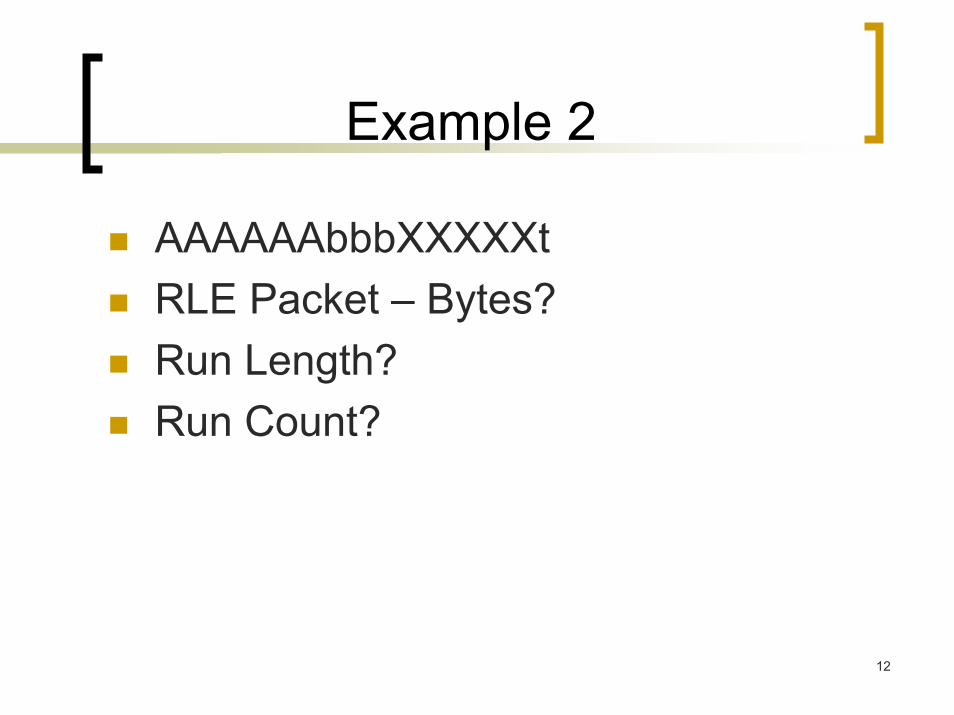
Example 2

AAAAAAbbbXXXXXtRLE Packet – Bytes?Run Length?Run Count?

13

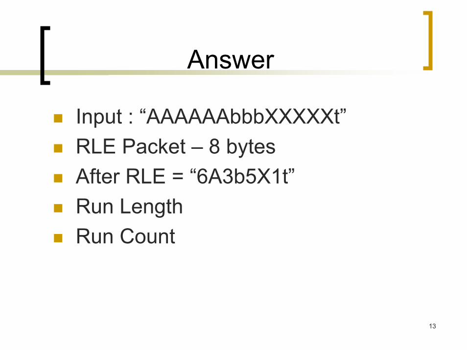
Answer

Input : “AAAAAAbbbXXXXXt” RLE Packet – 8 bytesAfter RLE = “6A3b5X1t”Run LengthRun Count

14

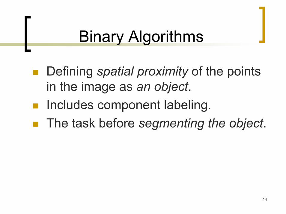
Binary Algorithms

Defining spatial proximity of the points in the image as an object.Includes component labeling.The task before segmenting the object.

15

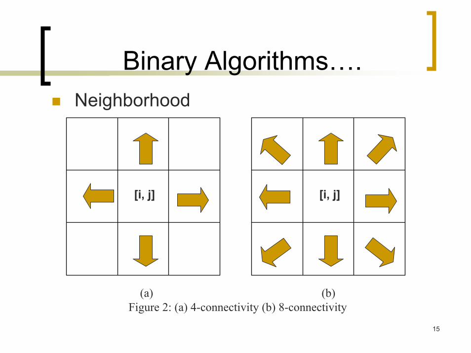
Binary Algorithms….Neighborhood

[i, j] [i, j]

(a) (b)Figure 2: (a) 4-connectivity (b) 8-connectivity

16

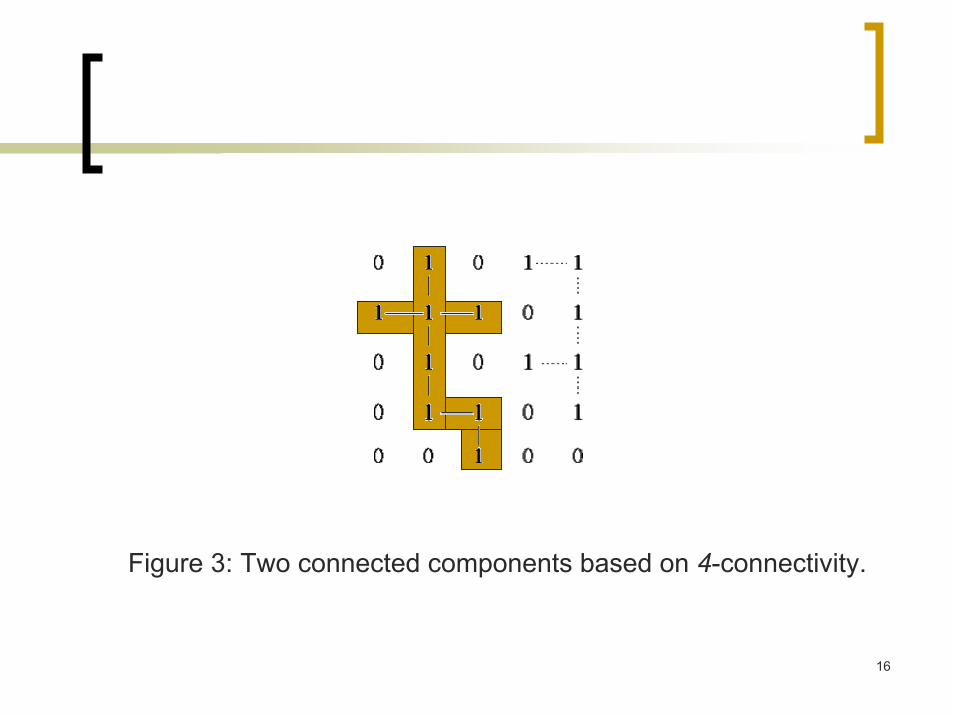
Figure 3: Two connected components based on 4-connectivity.

17

Component Labeling

To find the connected components, so as to identify the object.Requires the characteristics of the component

size, position, orientation, bounding rectangle.

Recursive and Sequential algorithms

18

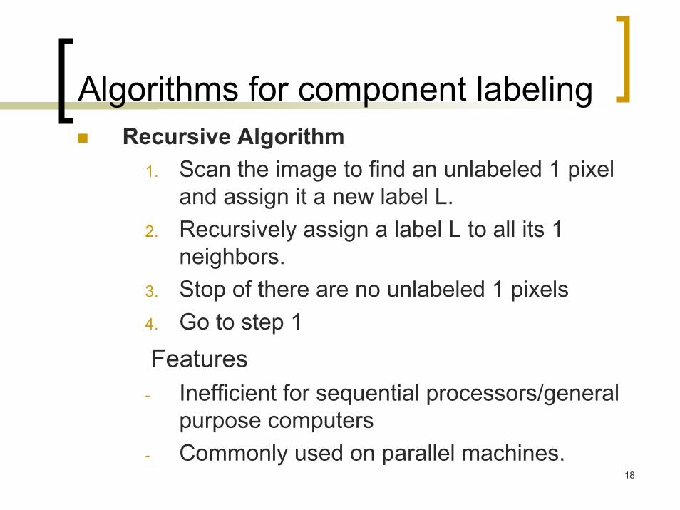
Algorithms for component labelingRecursive Algorithm

1. Scan the image to find an unlabeled 1 pixel and assign it a new label L.

2. Recursively assign a label L to all its 1 neighbors.

3. Stop of there are no unlabeled 1 pixels4. Go to step 1Features

- Inefficient for sequential processors/general purpose computers

- Commonly used on parallel machines.

19

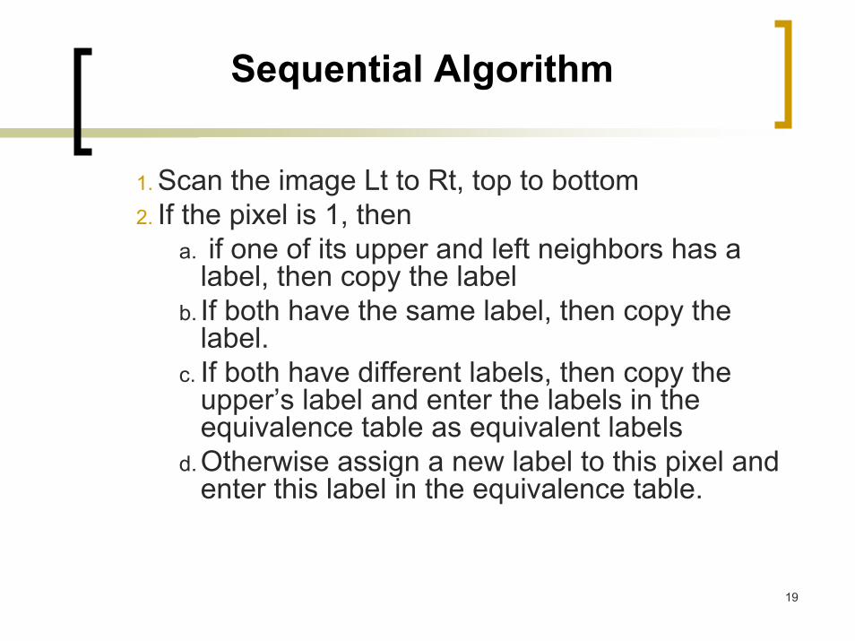
Sequential Algorithm

1. Scan the image Lt to Rt, top to bottom2. If the pixel is 1, then

a. if one of its upper and left neighbors has a label, then copy the label

b. If both have the same label, then copy the label.

c. If both have different labels, then copy the upper’s label and enter the labels in the equivalence table as equivalent labels

d. Otherwise assign a new label to this pixel and enter this label in the equivalence table.

20

Sequential Algorithm….

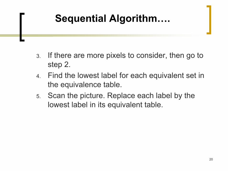
3. If there are more pixels to consider, then go to step 2.

4. Find the lowest label for each equivalent set in the equivalence table.

5. Scan the picture. Replace each label by the lowest label in its equivalent table.

21

Sequential Algorithm….

1. Will require more than one pass – iteration- over the image.

2. image file can be stored, memory space availability is not a issue

22

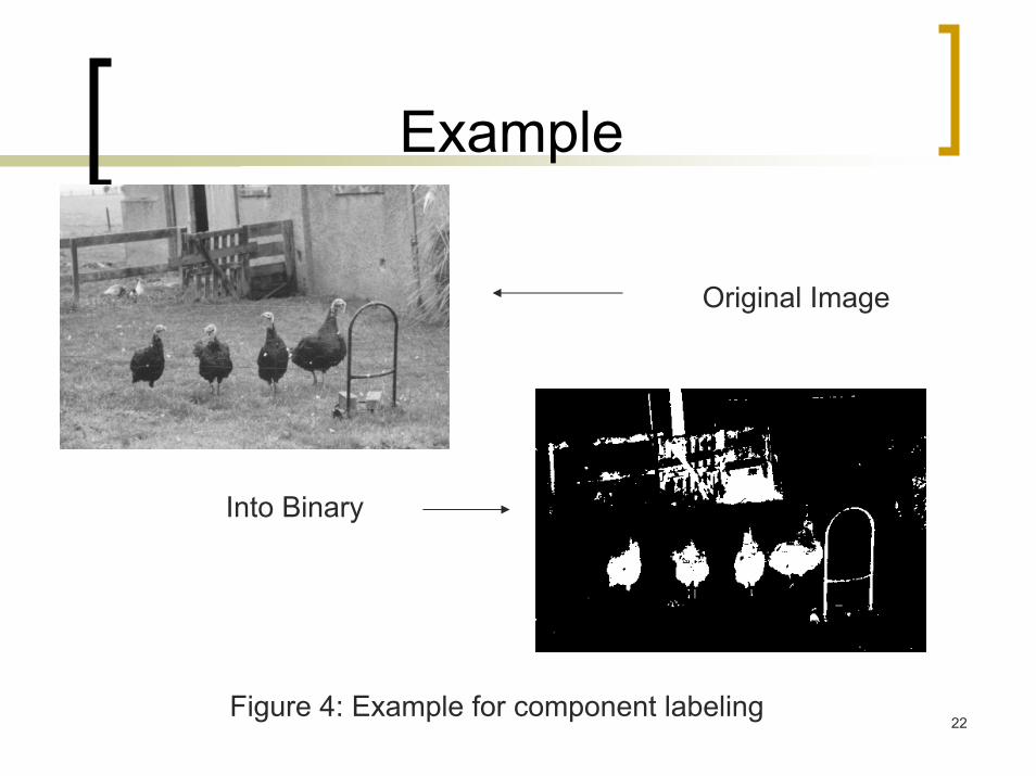
Example

Original Image

Into Binary

Figure 4: Example for component labeling

23

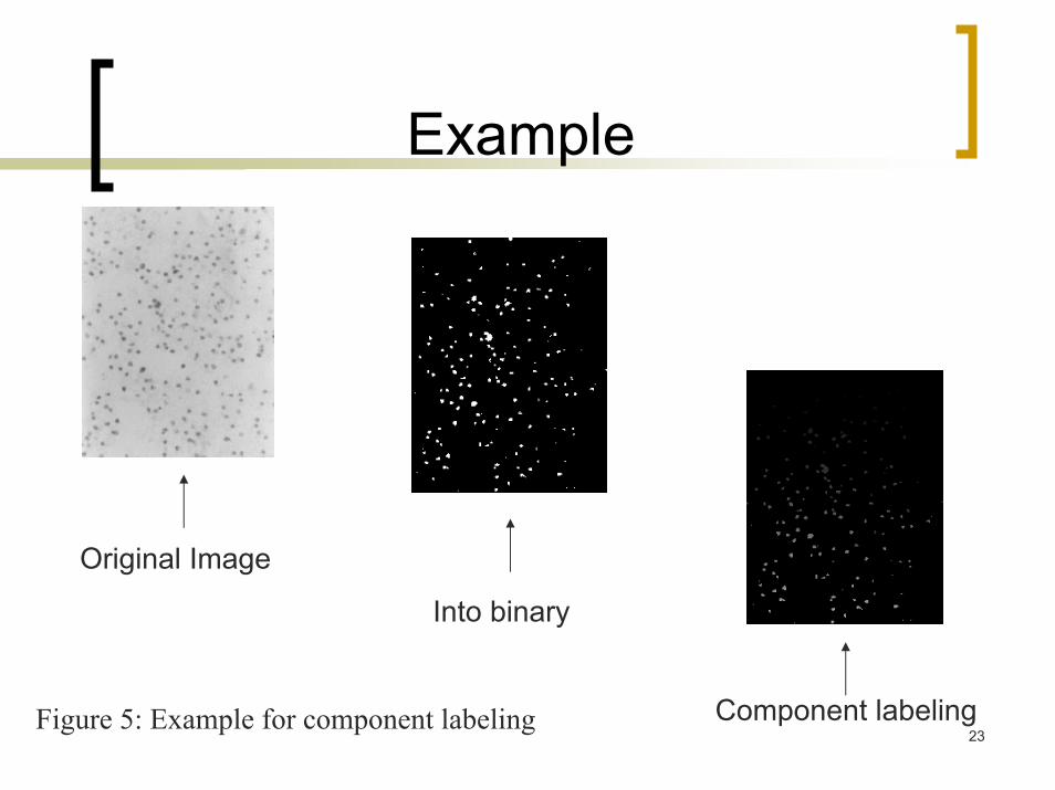
Example

Original Image

Into binary

Component labelingFigure 5: Example for component labeling

24

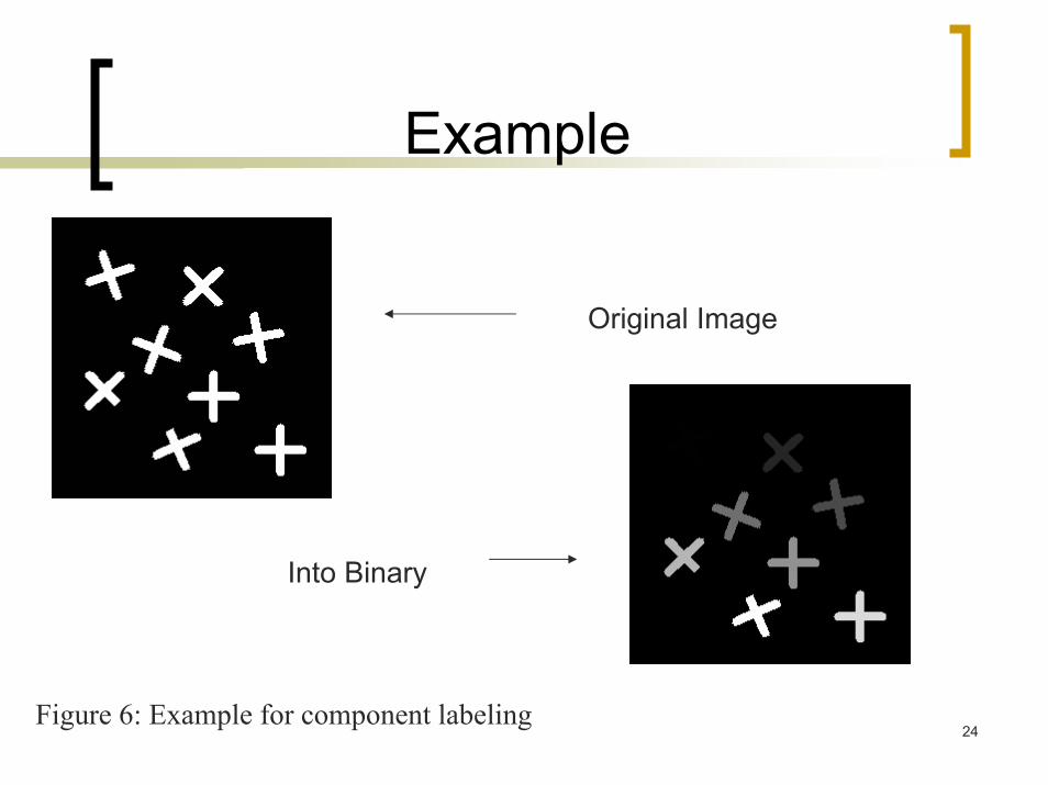
Example

Original Image

Into Binary

Figure 6: Example for component labeling

25

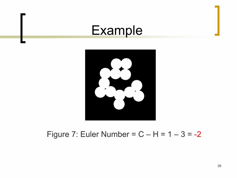
Euler Number

E (Euler No.) - used as a feature of an object.E = C – H ;

C = No of connected components (objects)H = No. of holes

Invariant to translation, rotation and scaling.

26

Example

Figure 7: Euler Number = C – H = 1 – 3 = -2

27

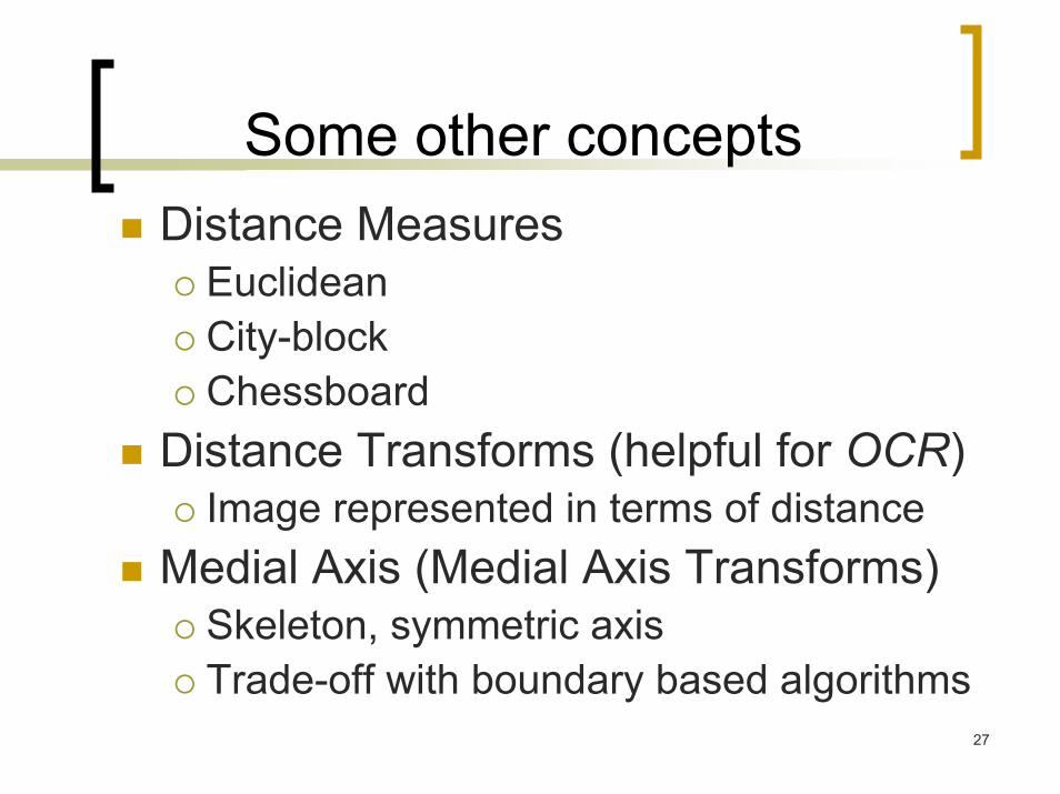
Some other conceptsDistance Measures

EuclideanCity-blockChessboard

Distance Transforms (helpful for OCR)Image represented in terms of distance

Medial Axis (Medial Axis Transforms)Skeleton, symmetric axis Trade-off with boundary based algorithms

28

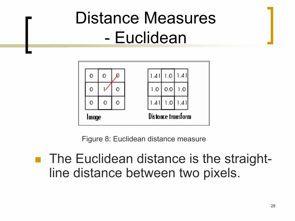
Distance Measures - Euclidean

Figure 8: Euclidean distance measure

The Euclidean distance is the straight-line distance between two pixels.

29

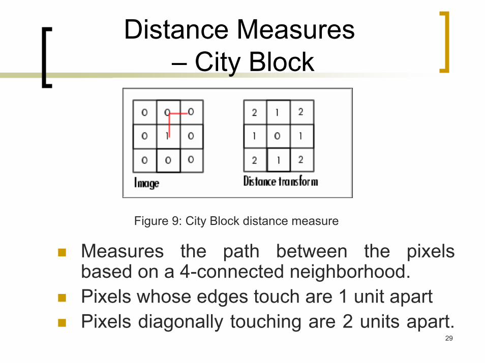
Distance Measures– City Block

Measures the path between the pixels based on a 4-connected neighborhood. Pixels whose edges touch are 1 unit apart Pixels diagonally touching are 2 units apart.

Figure 9: City Block distance measure

30

Distance Measures– Chess Board

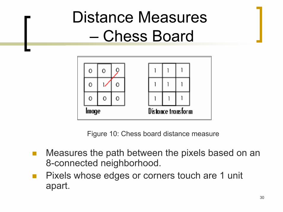
Figure 10: Chess board distance measure

Measures the path between the pixels based on an 8-connected neighborhood. Pixels whose edges or corners touch are 1 unit apart.

31

Distance Transforms

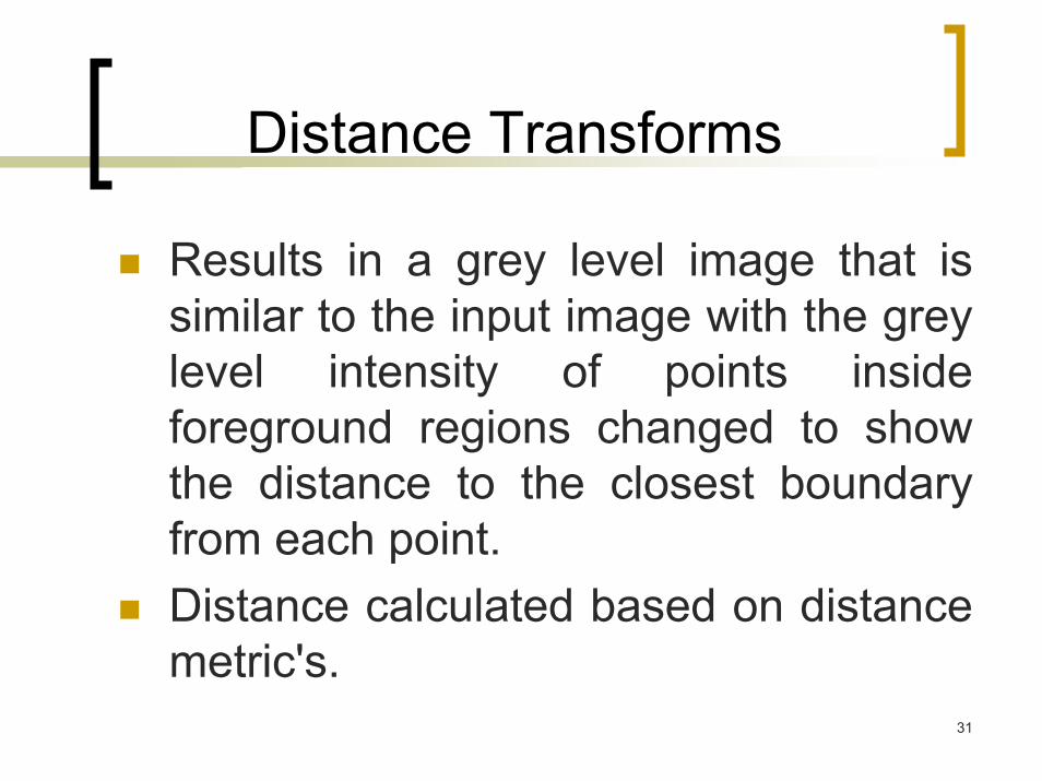
Results in a grey level image that is similar to the input image with the grey level intensity of points inside foreground regions changed to show the distance to the closest boundary from each point. Distance calculated based on distance metric's.

32

Medial Axis / Skeletonization

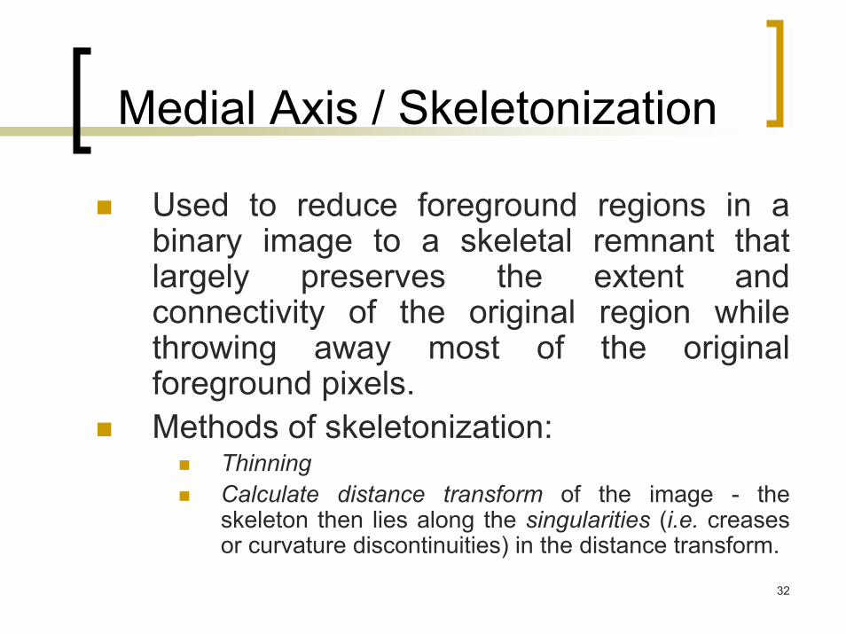
Used to reduce foreground regions in a binary image to a skeletal remnant that largely preserves the extent and connectivity of the original region while throwing away most of the original foreground pixels. Methods of skeletonization:

Thinning Calculate distance transform of the image - the skeleton then lies along the singularities (i.e. creases or curvature discontinuities) in the distance transform.

33

Example

Image Skeleton

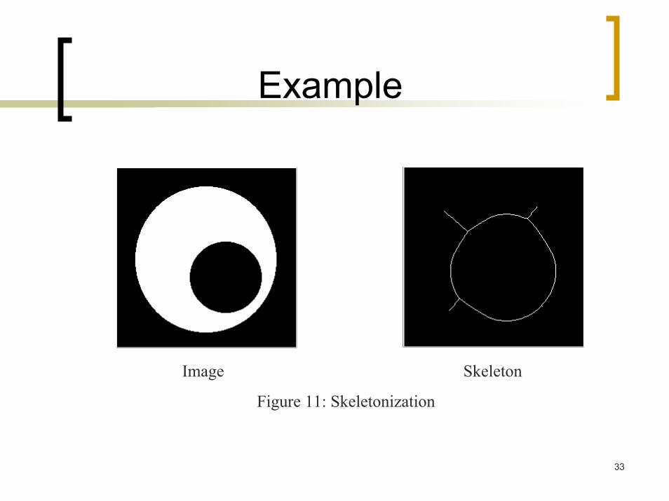
Figure 11: Skeletonization

34

Thinning

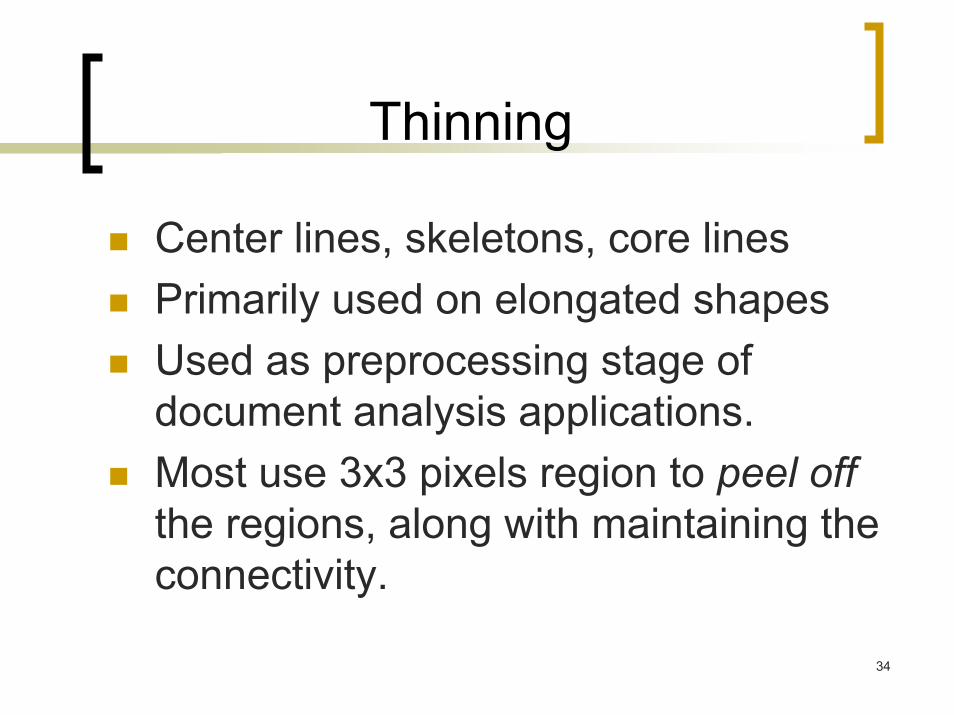
Center lines, skeletons, core linesPrimarily used on elongated shapesUsed as preprocessing stage of document analysis applications.Most use 3x3 pixels region to peel offthe regions, along with maintaining the connectivity.

35

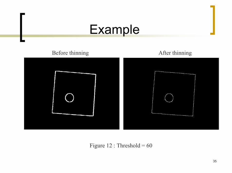
ExampleBefore thinning After thinning

Figure 12 : Threshold = 60

36

Expanding and Shrinking

Expanding followed by Shrinking can be used for filling undesirable holes.Shrinking followed Expanding by can be used for removing isolated noise pixels.Used to determine isolated components and clusters

37

Example

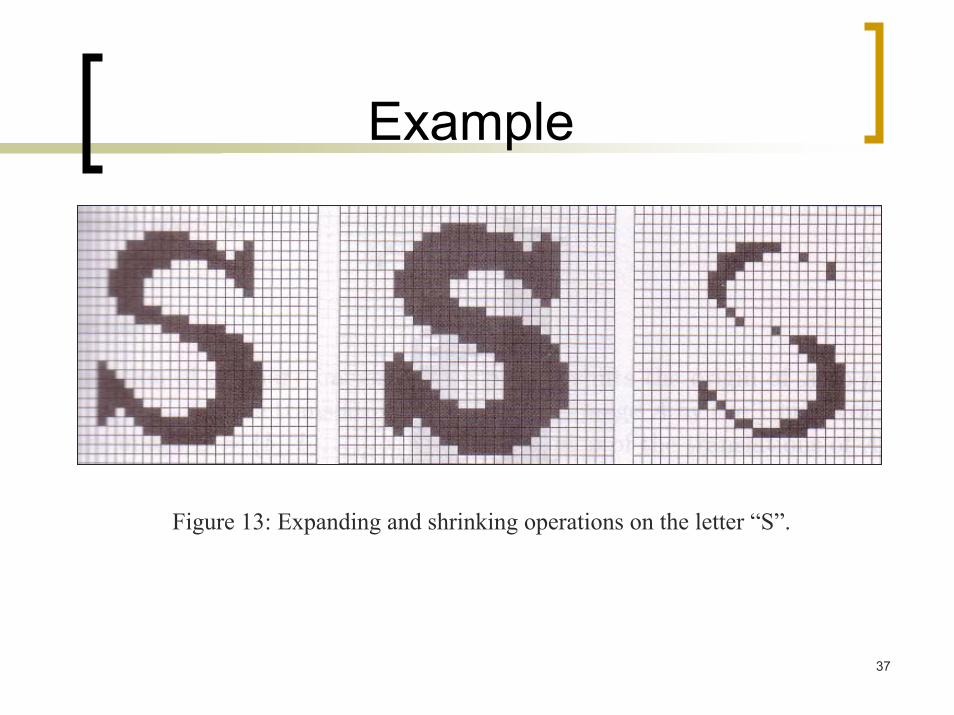
Figure 13: Expanding and shrinking operations on the letter “S”.

38

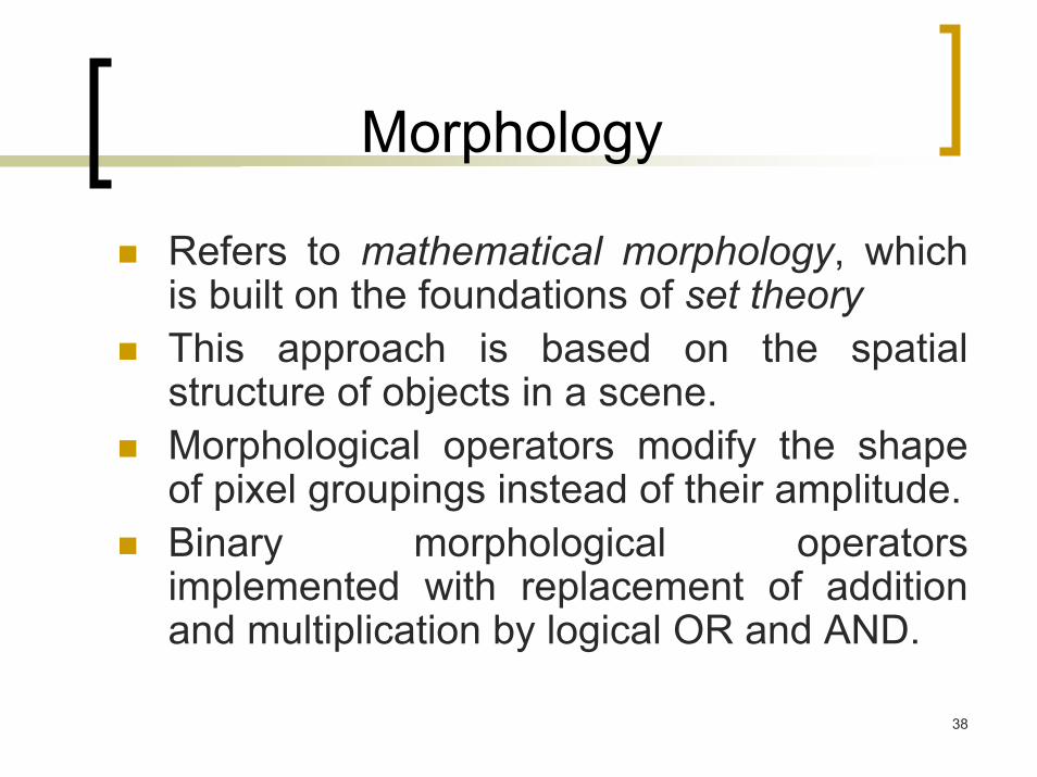
Morphology

Refers to mathematical morphology, which is built on the foundations of set theoryThis approach is based on the spatial structure of objects in a scene.Morphological operators modify the shape of pixel groupings instead of their amplitude.Binary morphological operators implemented with replacement of addition and multiplication by logical OR and AND.

39

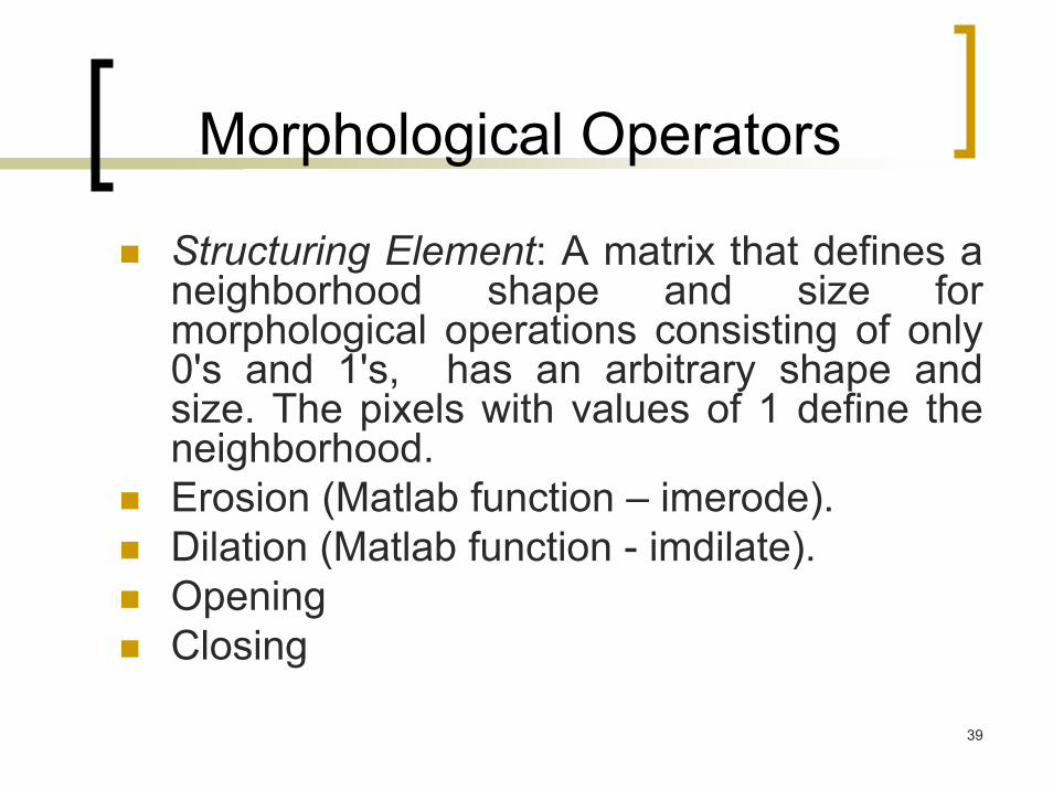
Morphological Operators

Structuring Element: A matrix that defines a neighborhood shape and size for morphological operations consisting of only 0's and 1's, has an arbitrary shape and size. The pixels with values of 1 define the neighborhood. Erosion (Matlab function – imerode).Dilation (Matlab function - imdilate).OpeningClosing

40

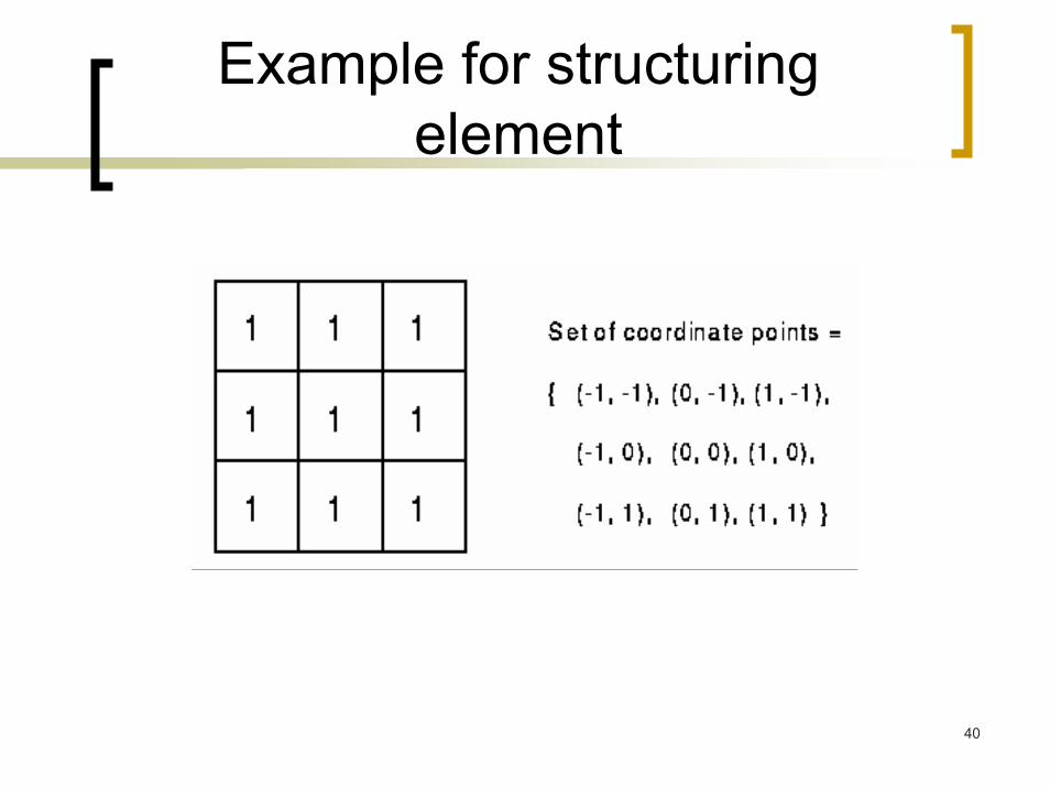
Example for structuring element

41

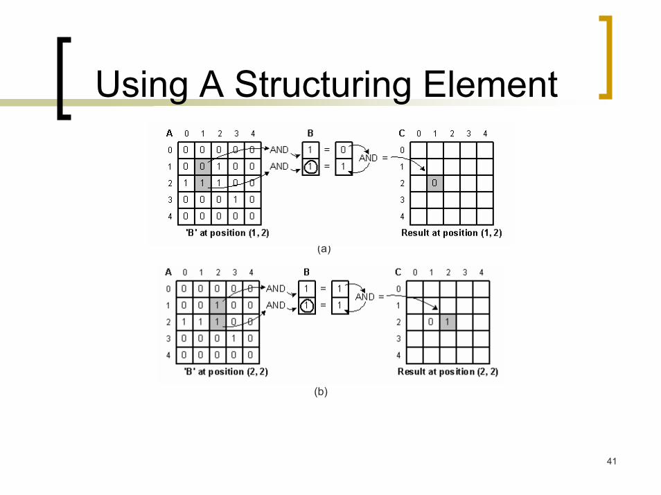
Using A Structuring Element

(a)

(b)

42

Erosion

The basic effect of the operator on a binary image is to erode away the boundaries of regions of foreground pixels (i.e. white pixels, typically). Shrink areas of foreground pixels in size and holes within those areas become larger.Input to erosion operator: Image and structuring element

43

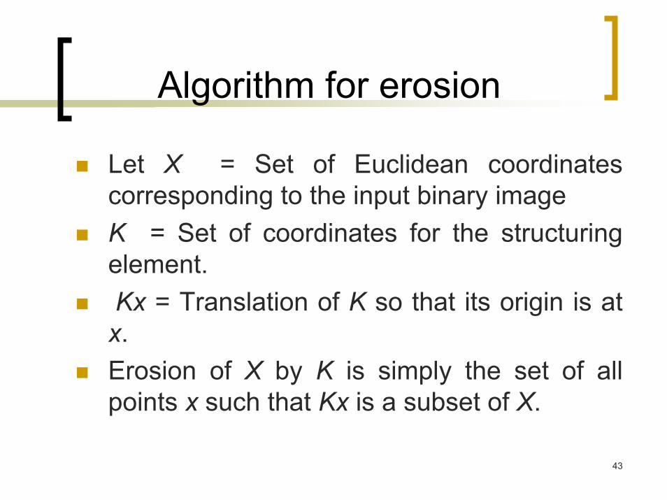
Algorithm for erosion

Let X = Set of Euclidean coordinates corresponding to the input binary imageK = Set of coordinates for the structuring element. Kx = Translation of K so that its origin is at

x. Erosion of X by K is simply the set of all points x such that Kx is a subset of X.

44

Erosion ….

In other words, For each foreground (input) pixel, superimpose the structuring element with the input image The input pixel is left as it is if it is the foreground pixel in the structuring element. If any of the corresponding pixels in the image are background however, the input pixel is also set to background value.

45

Effect of erosion

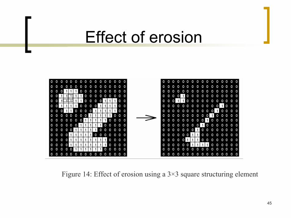
Figure 14: Effect of erosion using a 3×3 square structuring element

46

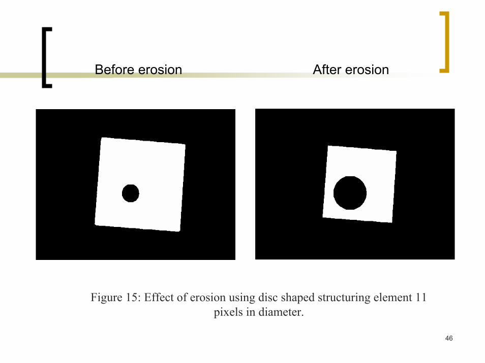
Before erosion After erosion

Figure 15: Effect of erosion using disc shaped structuring element 11 pixels in diameter.

47

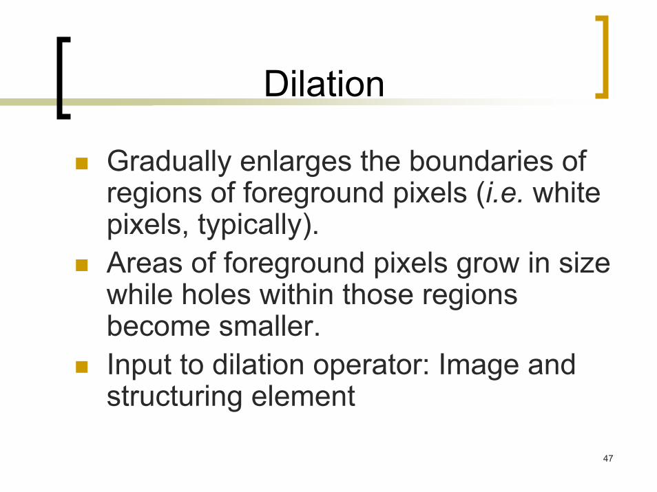
Dilation

Gradually enlarges the boundaries of regions of foreground pixels (i.e. white pixels, typically). Areas of foreground pixels grow in size while holes within those regions become smaller. Input to dilation operator: Image and structuring element

48

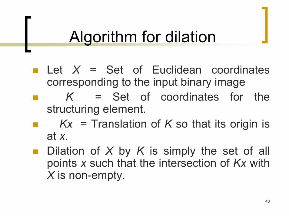
Algorithm for dilation

Let X = Set of Euclidean coordinates corresponding to the input binary image

K = Set of coordinates for the structuring element.

Kx = Translation of K so that its origin is at x. Dilation of X by K is simply the set of all points x such that the intersection of Kx with X is non-empty.

49

Dilation….

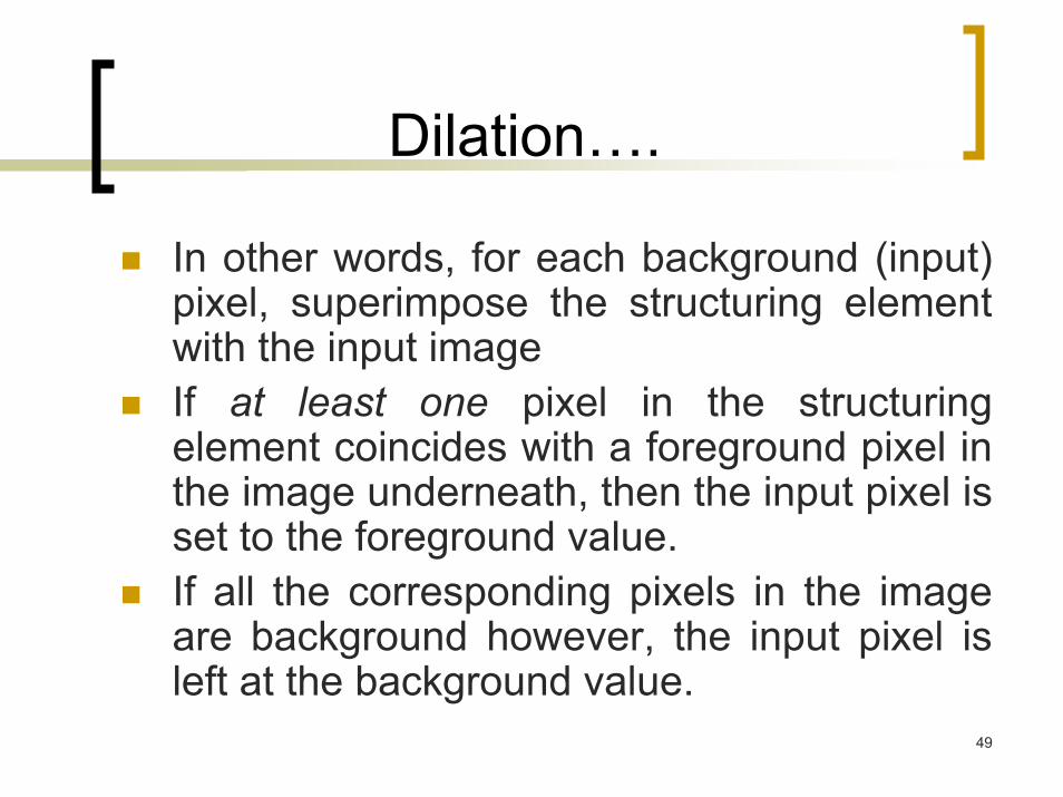
In other words, for each background (input) pixel, superimpose the structuring element with the input image If at least one pixel in the structuring element coincides with a foreground pixel in the image underneath, then the input pixel is set to the foreground value. If all the corresponding pixels in the image are background however, the input pixel is left at the background value.

50

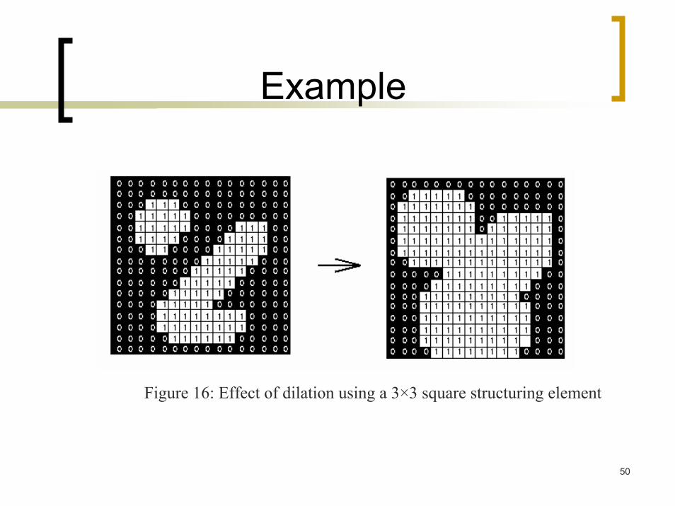
Example

Figure 16: Effect of dilation using a 3×3 square structuring element

51

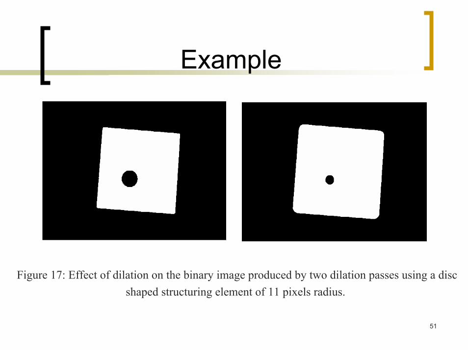
Example

Figure 17: Effect of dilation on the binary image produced by two dilation passes using a discshaped structuring element of 11 pixels radius.

52

Opening

Somewhat like erosion - it tends to remove some of the foreground (bright) pixels from the edges of object region. Less destructive than erosion in general. Structuring element. Used to preserve foreground regions that have a similar shape to the structuring element.Grey level opening consists simply of a greylevelerosion followed by a greylevel dilation. Def: An erosion followed by a dilation using the same structuring element for both operations. Inputs : Image for opening and structuring element

53

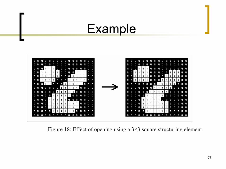
Example

Figure 18: Effect of opening using a 3×3 square structuring element

54

Before opening After opening

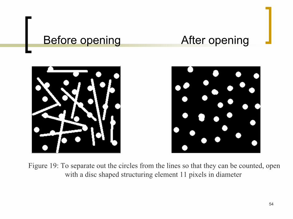
Figure 19: To separate out the circles from the lines so that they can be counted, openwith a disc shaped structuring element 11 pixels in diameter

55

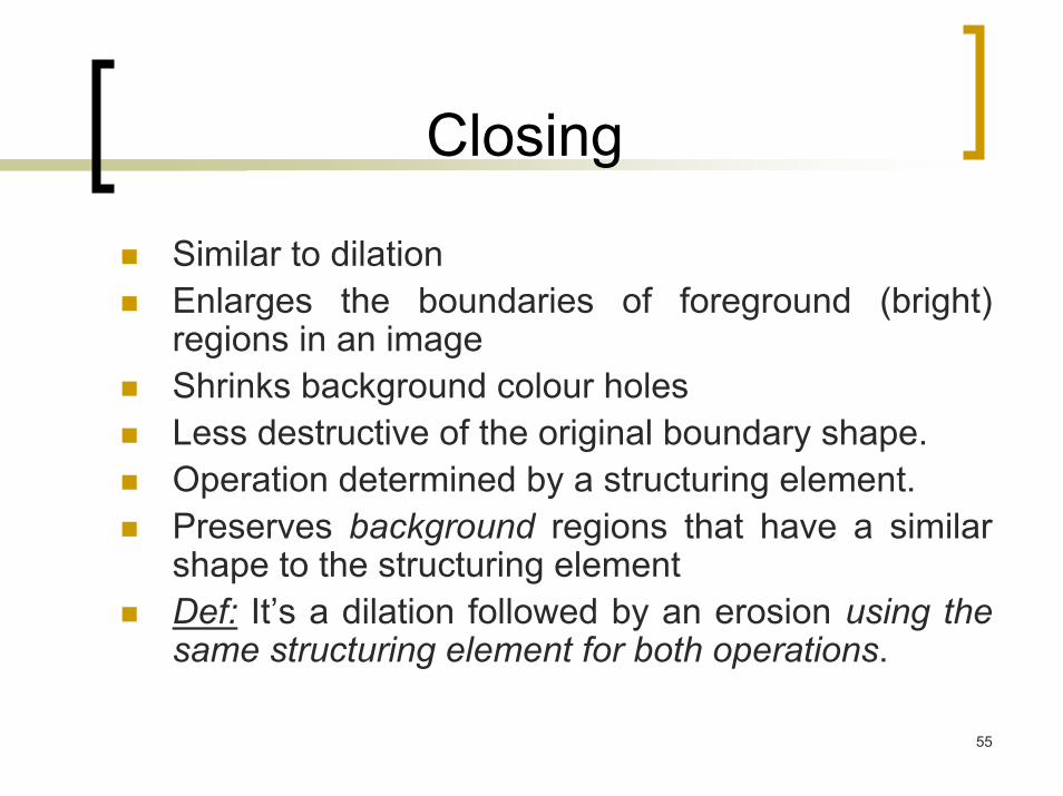
Closing

Similar to dilation Enlarges the boundaries of foreground (bright) regions in an image Shrinks background colour holes Less destructive of the original boundary shape. Operation determined by a structuring element. Preserves background regions that have a similar shape to the structuring elementDef: It’s a dilation followed by an erosion using the same structuring element for both operations.

56

Example

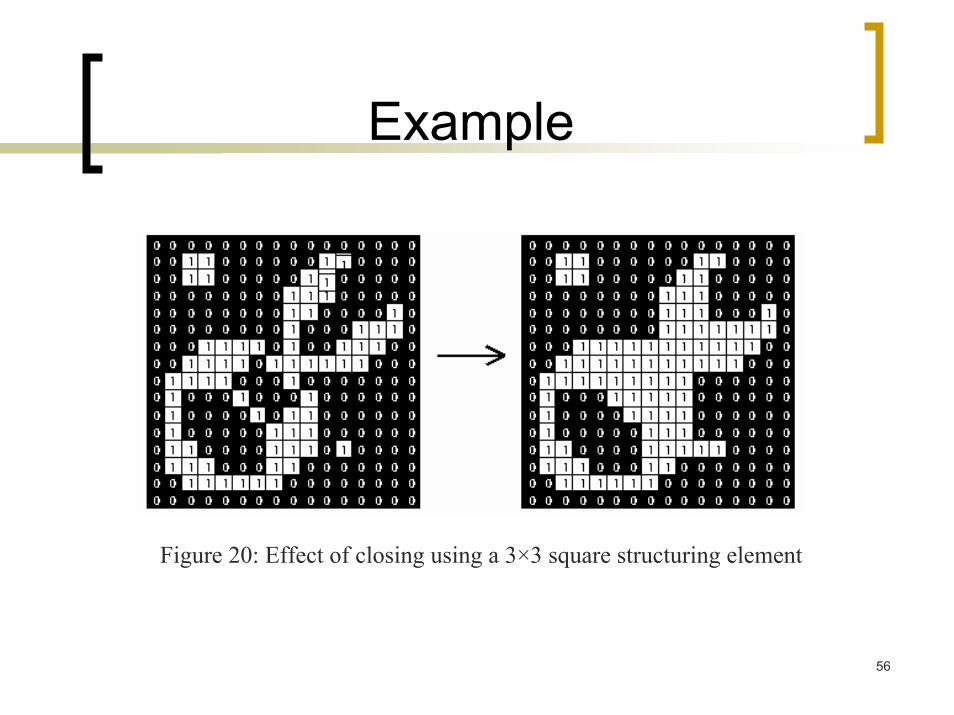
Figure 20: Effect of closing using a 3×3 square structuring element

57

Before closing After closing

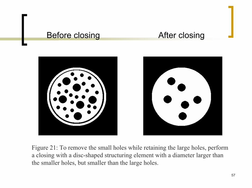
Figure 21: To remove the small holes while retaining the large holes, perform a closing with a disc-shaped structuring element with a diameter larger than the smaller holes, but smaller than the large holes.

58

Applications

Character recognition: Mail sorting, Label reading, Super-market product labeling, Bank check processing, text reading. Medical image processing: Tumor detection, measurement of size and shape of internal organs, chromosome analysis, blood cell count. Industrial automation: Parts identification on assembly lines, Defect and fault inspection. Robotics: Recognition and interpretation of objects in a scene, Motion control and execution through visual feedback. Cartography: Map making from photographs, Synthesis of weather maps.

59

Applications ….

Forensics: Finger-print, iris-print matching and analysis for automated security systems. Radar Imaging: Target detection and identification guidance of helicopters and aircraft in landing, guidance of remotely piloted vehicles, Missiles and satellite from visual clues. Remote Sensing: Multispectral image analysis, Weather prediction, Classification and marine environment from satellite images. Entertainment, arts and web applications: Image and video compression, Content-base image retrieval.

60

Optical Character Recognition

One of the basic applications of DIPUsed extensively as a basis for machine visionUsed to convert written or typed text into format recognizable by a computer

61

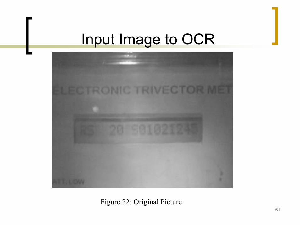
Input Image to OCR

Figure 22: Original Picture

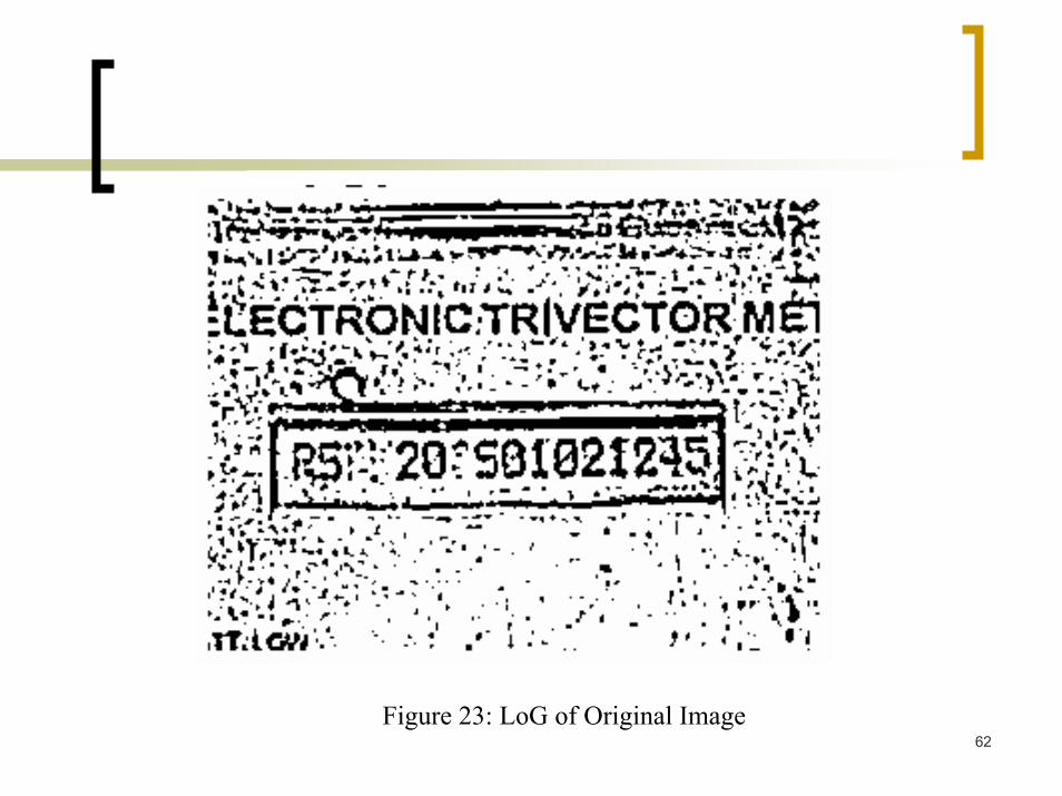
62Figure 23: LoG of Original Image

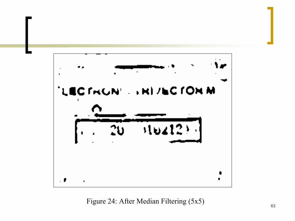
63Figure 24: After Median Filtering (5x5)

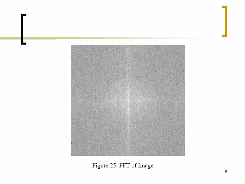
64Figure 25: FFT of Image

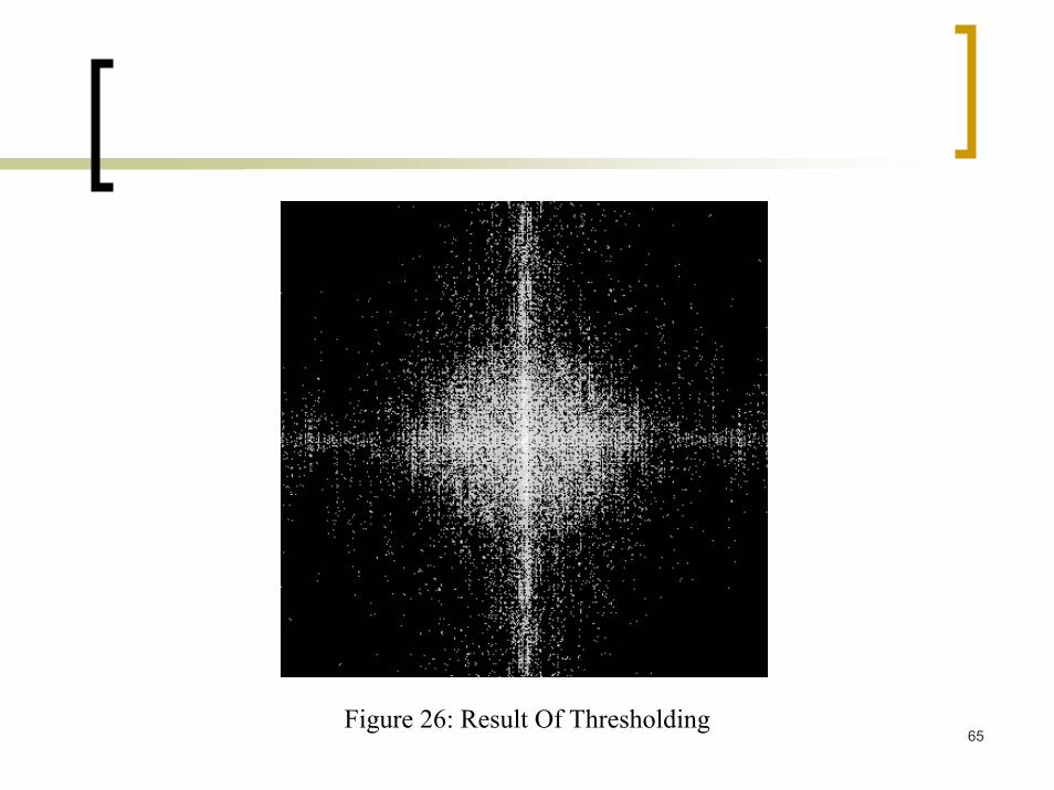
65Figure 26: Result Of Thresholding

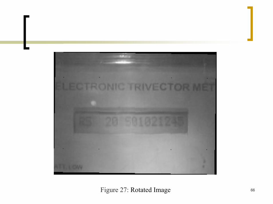
66Figure 27: Rotated Image

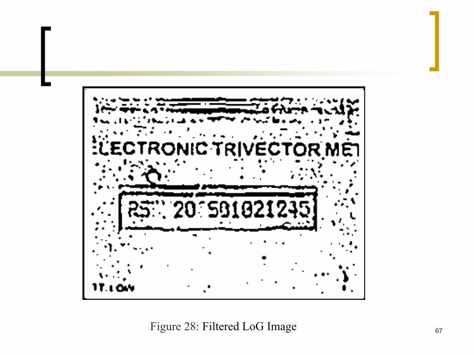
67Figure 28: Filtered LoG Image

68

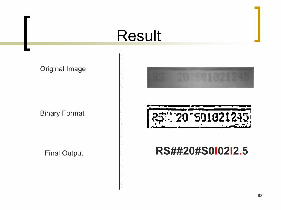
Result

Original Image

Binary Format

RS##20#S0I02I2.5Final Output

69

Matlab Demo