Embed Size (px)
Citation preview

Computer Vision : CISC 4/689
Note to self
David Jacob’s notes:ConvolutionCorrelationDerivativesSeparability

Computer Vision : CISC 4/689
Linear Filters
• General process:– Form new image whose pixels
are a weighted sum of original pixel values, using the same set of weights at each point.
• Properties– Output is a linear function of
the input
– Output is a shift-invariant function of the input (i.e. shift the input image two pixels to the left, the output is shifted two pixels to the left)
• Example: smoothing by averaging– form the average of pixels in a
neighbourhood
• Example: smoothing with a Gaussian– form a weighted average of
pixels in a neighbourhood
• Example: finding a derivative– form a weighted average of
pixels in a neighbourhood

Computer Vision : CISC 4/689
Convolution
• Represent these weights as an image, F
• F is usually called the kernel
• Operation is called convolution– it’s associative
• Result is:
Rij H i u, j vFuvu,v

Computer Vision : CISC 4/689
Convolution
• Formalization of idea of overlap (product) of two functions as one is shifted across the other
• The area under convolution is product of areas under the functions
• The convolution of two Gaussians is another Gaussian
courtesy of mathworld.wolfram.com

Computer Vision : CISC 4/689
Convolution Notes
• Note the assumption that both f
and g are continuous and defined everywhere
• Properties– Commutative
– Associative
Computer Vision : CISC 4/689
Discrete 2-D Convolution
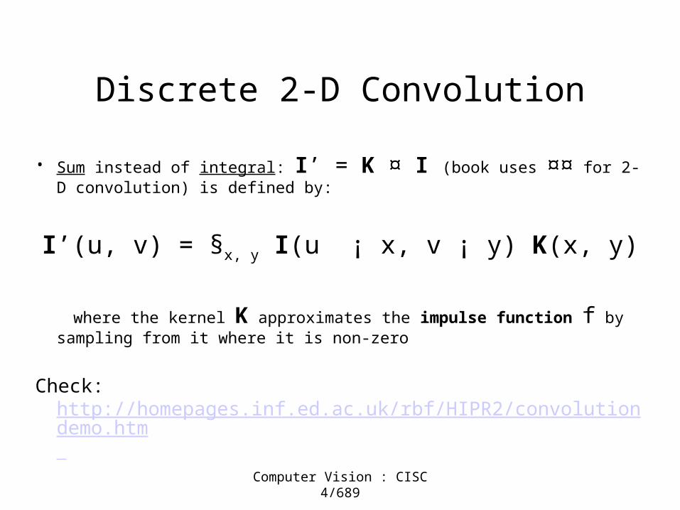
• Sum instead of integral: I’ = K ¤ I (book uses ¤¤ for 2-D convolution) is defined by:
I’(u, v) = §x, y I(u ¡ x, v ¡ y) K(x, y)
where the kernel K approximates the impulse function f by sampling from it where it is non-zero
Check: http://homepages.inf.ed.ac.uk/rbf/HIPR2/convolutiondemo.htm

Computer Vision : CISC 4/689
Example: Smoothing by Averaging

Computer Vision : CISC 4/689
Smoothing with a Gaussian
• Smoothing with an average actually doesn’t compare at all well with a defocussed lens– Most obvious difference is that
a single point of light viewed in a defocussed lens looks like a fuzzy blob; but the averaging process would give a little square.
• A Gaussian gives a good model of a fuzzy blob

Computer Vision : CISC 4/689
exp x2 y2
22
An Isotropic Gaussian
• The picture shows a smoothing kernel proportional to
(which is a reasonable model of a circularly symmetric fuzzy blob)

Computer Vision : CISC 4/689
Smoothing with a Gaussian

Computer Vision : CISC 4/689
Problem: Image Noise
from Forsyth & Ponce

Computer Vision : CISC 4/689
Solution: Smoothing (Low-Pass) Filters
• If object reflectance changes slowly and noise at each pixel is independent, then we want to replace each pixel with something like the average of neighbors
– Disadvantage: Sharp (high-frequency) features lost
7 x 7 averaging neighborhood
Original image

Computer Vision : CISC 4/689
Smoothing Filters: Details
• Filter types– Mean filter (box)– Median (nonlinear)– Gaussian
• Can specify linear operation by shifting kernel over image and taking product
111
111
111
3 x 3 box filter kernel

Computer Vision : CISC 4/689
Gaussian Kernel
• Idea: Weight contributions of neighboring pixels by nearness
• Smooth roll-off reduces “ringing” seen in box filter
0.003 0.013 0.022 0.013 0.0030.013 0.059 0.097 0.059 0.0130.022 0.097 0.159 0.097 0.0220.013 0.059 0.097 0.059 0.0130.003 0.013 0.022 0.013 0.003
5 x 5, = 1

Computer Vision : CISC 4/689
Gaussian Smoothing
• In theory, the Gaussian distribution is non-zero everywhere, which would require an infinitely large convolution mask, but in practice it is effectively zero more than about three standard deviations from the mean, and so we can truncate the mask at this point
• Discrete approximation to Gaussian function with sd = 1.4• (gets normalized so that sum is 1.0)
Source: http://www.cee.hw.ac.uk/hipr/html/gsmooth.html

Computer Vision : CISC 4/689
Gaussian Smoothing
• Once a suitable mask has been calculated, then the Gaussian smoothing can be performed using standard convolution methods. The convolution can in fact be performed fairly quickly since the equation for the 2-D isotropic Gaussian shown above is separable into x and y components. Thus the 2-D convolution can be performed by first convolving with a 1-D Gaussian in the x direction, and then convolving with another 1-D Gaussian in the y direction. (The Gaussian is in fact the only completely circularly symmetric operator which can be decomposed in such a way.) Below shows the 1-D x component mask that would be used to produce the full mask shown in previous slide. The y component is exactly the same but is oriented vertically.
A further way to compute a Gaussian smoothing with a large standard deviation is to convolve an image several times with a smaller Gaussian. While this is computationally complex, it can have applicability if the processing is carried out using a hardware pipeline.
Computer Vision : CISC 4/689
Gaussian Smoothing
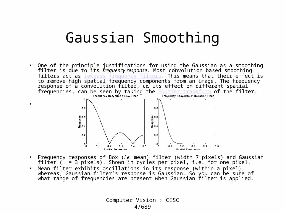
• One of the principle justifications for using the Gaussian as a smoothing filter is due to its frequency response. Most convolution based smoothing filters act as lowpass frequency filters. This means that their effect is to remove high spatial frequency components from an image. The frequency response of a convolution filter, i.e. its effect on different spatial frequencies, can be seen by taking the Fourier transform of the filter.
•
• Frequency responses of Box (i.e. mean) filter (width 7 pixels) and Gaussian filter ( = 3 pixels). Shown in cycles per pixel, i.e. for one pixel.
• Mean filter exhibits oscillations in its response (within a pixel), whereas, Gaussian filter’s response is Gaussian. So you can be sure of what range of frequencies are present when Gaussian filter is applied.

Computer Vision : CISC 4/689
Example: Gaussian Smoothing
= 1 = 3
7 x 7kernel
Original image Box filter

Computer Vision : CISC 4/689
Correlation
• Same as convolution, a dot product, thus it is largest when the pattern matches (vectors are parallel), this can be used to find texture patterns
• This yields a value that is +ve when the image region looks like the filter kernel, and small and –ve when it is opposite. Can be squared if pattern reversal doesn’t matter.
• Since value maybe large if image is bright, so divide by root sum of squares of image region and filter. (dot of unit vectors)
• Some ways to interpret what the kernel is doing– As a template being matched by correlation – As simply a set of weights on the corresponding image pixels

Computer Vision : CISC 4/689
Normalized correlation
• Think of filters of a dot product– now measure the angle
– i.e normalised correlation output is filter output, divided by root sum of squares of values over which filter lies
• Tricks:– ensure that filter has a zero
response to a constant region (helps reduce response to irrelevant background)
– subtract image average when computing the normalizing constant (i.e. subtract the image mean in the neighborhood)
– absolute value deals with contrast reversal
Computer Vision : CISC 4/689
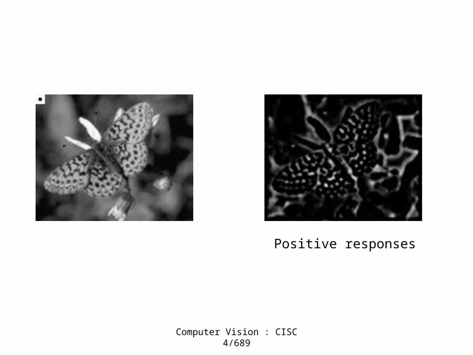
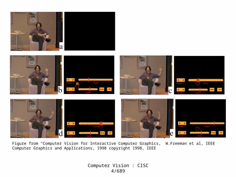
Positive responses

Computer Vision : CISC 4/689
Positive responses
Computer Vision : CISC 4/689
Figure from “Computer Vision for Interactive Computer Graphics,” W.Freeman et al, IEEE Computer Graphics and Applications, 1998 copyright 1998, IEEE
Computer Vision : CISC 4/689
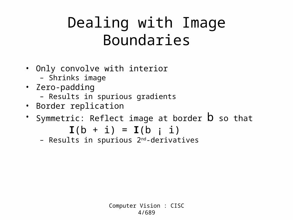
Dealing with Image Boundaries
• Only convolve with interior– Shrinks image
• Zero-padding– Results in spurious gradients
• Border replication• Symmetric: Reflect image at border b so that
I(b + i) = I(b ¡ i)– Results in spurious 2nd-derivatives

Computer Vision : CISC 4/689
Step 1
3
2
1
2
2
1
3
2
32
21
22
32 5
3
2
1
2
2
1
3
2
32
21
22
32
1-2-1
24-1
111
1-1-1
12-1
111
zero
-pad
ded

Computer Vision : CISC 4/689
Step 2
3
2
1
2
2
1
3
2
32
21
22
32 45
3
2
1
2
2
1
3
2
32
21
22
32
3-1-2
24-2
111
1-1-1
12-1
111

Computer Vision : CISC 4/689
Step 3
3
2
1
2
2
1
3
2
32
21
22
32 4 45
3
2
1
2
2
1
3
2
32
21
22
32
3-3-1
34-2
111
1-1-1
12-1
111

Computer Vision : CISC 4/689
Step 4
3
2
1
2
2
1
3
2
32
21
22
32 4 4 -25
3
2
1
2
2
1
3
2
32
21
22
32
1-3-3
16-2
111
1-1-1
12-1
111

Computer Vision : CISC 4/689
Step 5
3
2
1
2
2
1
3
2
32
21
22
32 4 4
9
-25
3
2
1
2
2
1
3
2
32
21
22
32
2-2-1
14-1
221
1-1-1
12-1
111

Computer Vision : CISC 4/689
Step 6
3
2
1
2
2
1
3
2
32
21
22
32
6
4 4
9
-25
3
2
1
2
2
1
3
2
32
21
22
32
1-2-2
32-2
222
1-1-1
12-1
111

Computer Vision : CISC 4/689
and so on…

Computer Vision : CISC 4/689
Final Result
2 2 2 3
2 1 3 3
2 2 1 2
1 3 2 2 12
7
6
4
8
6
14
4
59
59
511
-25
I’I
1-1-1
12-1
111
Why is I’ large in some places and small in others?

Computer Vision : CISC 4/689
Linear Shift Invariance
• Possible properties of f– Superposition: f(I1 + I2) = f(I1) + f(I2)– Scaling: f(®I) = ®f(I)– Shift invariance:
f(Shift(I, k)) = Shift (f(I), k)
A system with these properties is performing convolution

Computer Vision : CISC 4/689
Imaging Systems
• An imaging system describes a functional transformation f of an image due to…– Physics: A real-world phenomenon such as blurring from defocus or fish-eye
lens distortion– Filtering: A transformation we apply in order to
• Undo or mitigate the bad effects of a physical system (e.g., deblur, undistort, etc.)
• Emphasize or highlight particular image properties (e.g., color similarity, edges, etc.)
• Noise reduction!!
I I’f

Computer Vision : CISC 4/689
What’s Not a Convolution?
• Nonlinear systems– E.g., radial distortion of fish-eye lens is not LSI because geometric
transformation depends on pixel location
f
courtesy of M. Fiala

Computer Vision : CISC 4/689
Filtering in Matlab
• imfilter(I, K)filters image I with kernel K– Default filtering is correlation (no kernel rotation)– Can set options on border handling
• corr2, conv2 are the generic versions• Kernel creation
– Custom (create a matrix)– fspecial function

Computer Vision : CISC 4/689
Differentiation and convolution
• Recall
• Now this is linear and shift invariant, so must be the result of a convolution.
• We could approximate this as
(which is obviously a convolution; it’s not a very good way to do things, as we shall see)
fx
lim 0
f x , y
f x,y
fx
f xn1,y f xn , y
x

Computer Vision : CISC 4/689
Finite differences
Partial derivative in x-direction: gives vertical stripes.mid-gray = 0, dark gray = -ve, light gray = +veKernel = (1,0,-1)
Computer Vision : CISC 4/689
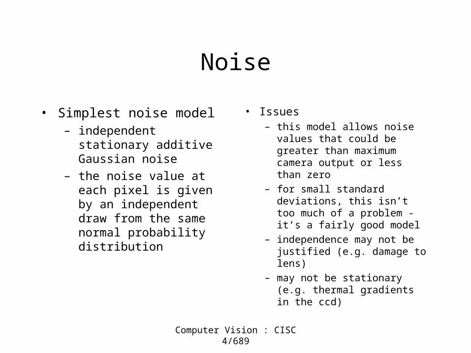
Noise
• Simplest noise model– independent stationary additive
Gaussian noise
– the noise value at each pixel is given by an independent draw from the same normal probability distribution
• Issues– this model allows noise values
that could be greater than maximum camera output or less than zero
– for small standard deviations, this isn’t too much of a problem - it’s a fairly good model
– independence may not be justified (e.g. damage to lens)
– may not be stationary (e.g. thermal gradients in the ccd)

Computer Vision : CISC 4/689
sigma=1

Computer Vision : CISC 4/689
sigma=16
Computer Vision : CISC 4/689
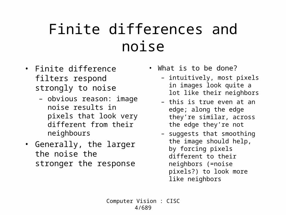
Finite differences and noise
• Finite difference filters respond strongly to noise– obvious reason: image noise
results in pixels that look very different from their neighbours
• Generally, the larger the noise the stronger the response
• What is to be done?– intuitively, most pixels in
images look quite a lot like their neighbors
– this is true even at an edge; along the edge they’re similar, across the edge they’re not
– suggests that smoothing the image should help, by forcing pixels different to their neighbors (=noise pixels?) to look more like neighbors

Computer Vision : CISC 4/689
Finite differences responding to noise
Increasing noise ->(this is zero mean additive Gaussian noise)

Computer Vision : CISC 4/689
Filter responses (of noise) are correlated
• Filtered noise is sometimes useful– looks like some natural textures, can be used to simulate fire, etc.

Computer Vision : CISC 4/689

Computer Vision : CISC 4/689

Computer Vision : CISC 4/689

Computer Vision : CISC 4/689
Smoothing reduces noise
• Generally expect pixels to “be like” their neighbours– surfaces turn slowly
– relatively few reflectance changes
• Generally expect noise processes to be independent from pixel to pixel
• Implies that smoothing suppresses noise, for appropriate noise models
• Scale– the parameter in the symmetric
Gaussian
– as this parameter goes up, more pixels are involved in the average
– and the image gets more blurred
– and noise is more effectively suppressed

Computer Vision : CISC 4/689
The effects of smoothing Each row shows smoothingwith Gaussians of differentwidth; each column showsdifferent realisations of an image of Gaussian noise.

Computer Vision : CISC 4/689
Gradients and edges
• Points of sharp change in an image are interesting:– change in reflectance
– change in object
– change in illumination
– noise
• Sometimes called edge points
• General strategy– determine image gradient
– now mark points where gradient magnitude is particularly large wrt neighbours (ideally, curves of such points).

Computer Vision : CISC 4/689
The Gradient and Edges
• Consider image intensities as a 2-D height function I(x, y). Then the image gradient is the vector field defined by:
• Definition of an edge– Line segment separating regions of contrasting intensity– Location: Where gradient magnitude is high – Direction: Orthogonal to the gradient

Computer Vision : CISC 4/689
Edge Causes
• Depth discontinuity
• Surface orientation discontinuity
• Reflectance discontinuity (i.e., change in surface material properties)
• Illumination discontinuity (e.g., shadow)

Computer Vision : CISC 4/689
Edges
• Edge normal: unit vector in the direction of maximum intensity change.
• Edge direction: unit vector perpendicular to the edge normal.
• Edge position: the image position at which the edge is located.
• Edge strength: related to the local image contrast along the normal.

Computer Vision : CISC 4/689
Edges
• Searching for Edges:– Filter: Smooth image
– Enhance: Apply numerical derivative approximation
– Detect: Threshold to find strong edges
– Localize/analyze: Reject spurious edges, include weak but justified edges

Computer Vision : CISC 4/689
Edge Detection• An edge point can be regarded as a
point in an image where a discontinuity (in gradient) occurs across some line. A discontinuity may be classified as one of five types
Gradient Discontinuity -- where the gradient of the pixel values changes across a line. This type of discontinuity can be classed as roof edges, ramp edges convex edges concave edges, by noting the sign of the component of the gradient perpendicular to the edge on either side of the edge. Ramp edges have the same signs in the gradient components on either side of the discontinuity, while roof edges have opposite signs in the gradient components.
A Jump or Step Discontinuity -- where pixel values themselves change suddenly across some line. A Bar Discontinuity -- where pixel values rapidly increase then decrease again (or vice versa) across some line.
Source: http://homepages.inf.ed.ac.uk/rbf/CVonline/LOCAL_COPIES/MARSHALL/node28.html
Computer Vision : CISC 4/689
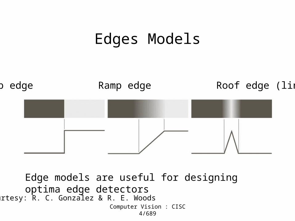
Edges Models
Step edge Ramp edge Roof edge (line)
Edge models are useful for designing optima edge detectors
Courtesy: R. C. Gonzalez & R. E. Woods

Computer Vision : CISC 4/689
Step and Ramp edge detection
• Two typical ways to find step and ramp edges. Look for:– Pixels with large (in absolute value) first order derivatives– Zero-crossings of second derivatives
Courtesy: R. C. Gonzalez & R. E. Woods
Computer Vision : CISC 4/689
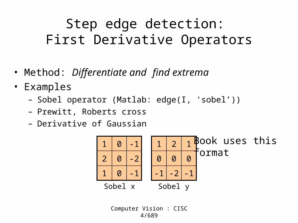
Step edge detection: First Derivative Operators
• Method: Differentiate and find extrema
• Examples– Sobel operator (Matlab: edge(I, ‘sobel’))
– Prewitt, Roberts cross
– Derivative of Gaussian
-1-2-1
000
121
-101
-202
-101
Sobel x Sobel y
Book uses thisformat

Computer Vision : CISC 4/689
Sobel Edge Filtering Example
1 0 -1
2 0 -2
1 0 -1
0 0 2 2
0 0 2 2
0 0 2 2
0 0 2 2
Rotate
10-1
20-2
10-1

Computer Vision : CISC 4/689
Step 1
0
0
1
2
2
1
2
2
22
20
20
22 0
0
0
0
0
2
2
2
2
20
20
20
20
00-1
00-2
10-1
10-1
20-2
10-1

Computer Vision : CISC 4/689
Step 2
0
0
1
2
2
2
3
2
22
20
20
22 60
0
0
0
0
2
2
2
2
20
20
20
20
200
400
10-1
10-1
20-2
10-1

Computer Vision : CISC 4/689
Step 3
0
0
1
2
2
2
3
2
30
20
20
30 6 60
0
0
0
0
2
2
2
2
20
20
20
20
200
400
10-1
10-1
20-2
10-1

Computer Vision : CISC 4/689
Step 4
0
0
0
0
2
2
3
2
30
20
20
30 6 6 -60
0
0
0
0
2
2
2
2
20
20
20
20
10-2
20-4
10-1
10-1
20-2
10-1
edgeeffectfrom zero-padding

Computer Vision : CISC 4/689
Sobel Edge Filtering Example: Result
6
8
8
6
6
8
8
6
-80
-60
-80
-60
(pad with zeroes again, replace the boundarywith zeros) and then we threshold…
Computer Vision : CISC 4/689
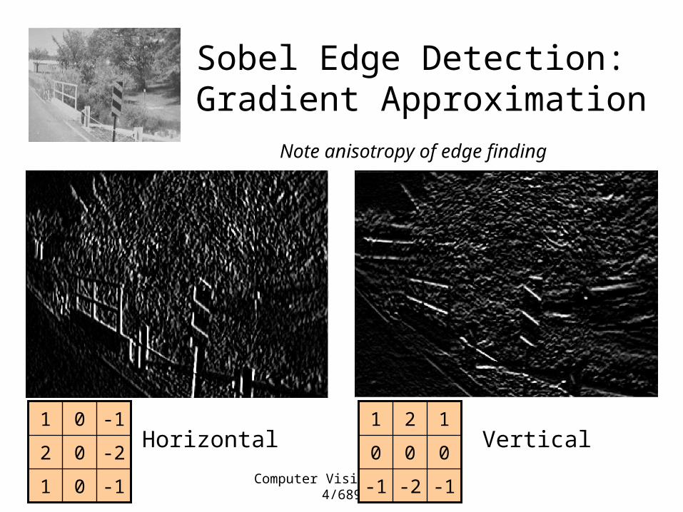
Sobel Edge Detection: Gradient Approximation
Horizontal Vertical
-1-2-1
000
121
-101
-202
-101
Note anisotropy of edge finding

Computer Vision : CISC 4/689
Sobel
• These can then be combined together to find the absolute magnitude of the gradient at each point and the orientation of that gradient. The gradient magnitude is given by:
• an approximate magnitude is computed using:
which is much faster to compute.
• The angle of orientation of the edge (relative to the pixel grid) giving rise to the spatial gradient is given by:
In this case, orientation 0 is taken to mean that the direction of maximum contrast from black to white runs from left to right on the image, and other angles are measured anti-clockwise from this.

Computer Vision : CISC 4/689
Courtesy: R. C. Gonzalez & R. E. Woods
Mag. Of 1st
Derivative andzero-crossing of2nd derivative

Computer Vision : CISC 4/689
Ramp edges
• 1st derivative is non-zero along the entire ramp
• 2nd derivative nonzero only at onset and end
• Most image edges are ramps rather than step edges
• 1st order derivatives produce thicker edges

Computer Vision : CISC 4/689
Step edge
• Second derivative produces a double edge response
• The sign of the second order derivative can be used to locate edges

Computer Vision : CISC 4/689
More..
• Noise: The 2nd derivative response is much stronger than the 1st derivative response
• Line (roof edge): 2nd derivative response is again stronger than the 1st derivative response
• Point detection: second order derivatives have a stronger response to isolated points
• What second order derivative operator can we use?

Computer Vision : CISC 4/689
Laplacian (derive..)
The implementationsare rotationallyinvariant only inincrements such as45 or 90 degrees.
Turn by 45 and add.
Weights from analytical eqns.

Computer Vision : CISC 4/689
Scale is important
So far, we donot have scaleFor Laplacian, i.e, extent forLaplacian.

Computer Vision : CISC 4/689
Derivative of Gaussian