Embed Size (px)
Citation preview
Computer Vision I -Algorithms and Applications:Basics of Image Processing
Carsten Rother
Computer Vision I: Basics of Image Processing
28/10/2013

Link to lectures
• Slides of Lectures and Exercises will be online:
http://www.inf.tu-Dresden/index.php?node_id=2091&ln=en
(on our webpage > teaching > Computer Vision)
28/10/2013Computer Vision I: Basics of Image Processing 2
Roadmap: Basics Digital Image Processing
• Images
• Point operators (ch. 3.1)
• Filtering: (ch. 3.2, ch 3.3, ch. 3.4) – main focus
• Linear filtering
• Non-linear filtering
• Fourier Transformation (ch. 3.4)
• Multi-scale image representation (ch. 3.5)
• Edges (ch. 4.2)
• Edge detection and linking
• Lines (ch. 4.3)
• Line detection and vanishing point detection
28/10/2013Computer Vision I: Basics of Image Processing 3
Roadmap: Basics Digital Image Processing
• Images
• Point operators (ch. 3.1)
• Filtering: (ch. 3.2, ch 3.3, ch. 3.4) – main focus
• Linear filtering
• Non-linear filtering
• Fourier Transformation (ch. 3.4)
• Multi-scale image representation (ch. 3.5)
• Edges (ch. 4.2)
• Edge detection and linking
• Lines (ch. 4.3)
• Line detection and vanishing point detection
28/10/2013Computer Vision I: Basics of Image Processing 4
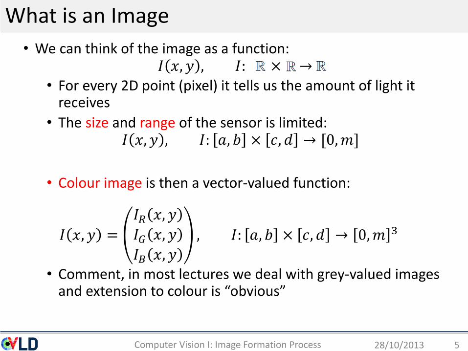
What is an Image
• We can think of the image as a function:𝐼 𝑥, 𝑦 , 𝐼: ∗ × ∗ →∗
• For every 2D point (pixel) it tells us the amount of light it receives
• The size and range of the sensor is limited:𝐼 𝑥, 𝑦 , 𝐼: 𝑎, 𝑏 × 𝑐, 𝑑 → [0,𝑚]
• Colour image is then a vector-valued function:
𝐼 𝑥, 𝑦 =
𝐼𝑅 𝑥, 𝑦
𝐼𝐺 𝑥, 𝑦
𝐼𝐵 𝑥, 𝑦
, 𝐼: 𝑎, 𝑏 × 𝑐, 𝑑 → 0,𝑚 3
• Comment, in most lectures we deal with grey-valued images and extension to colour is “obvious”
28/10/2013Computer Vision I: Image Formation Process 5
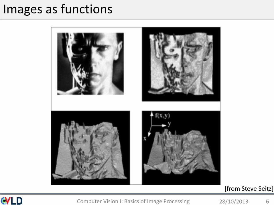
Images as functions
28/10/2013Computer Vision I: Basics of Image Processing 6
[from Steve Seitz]
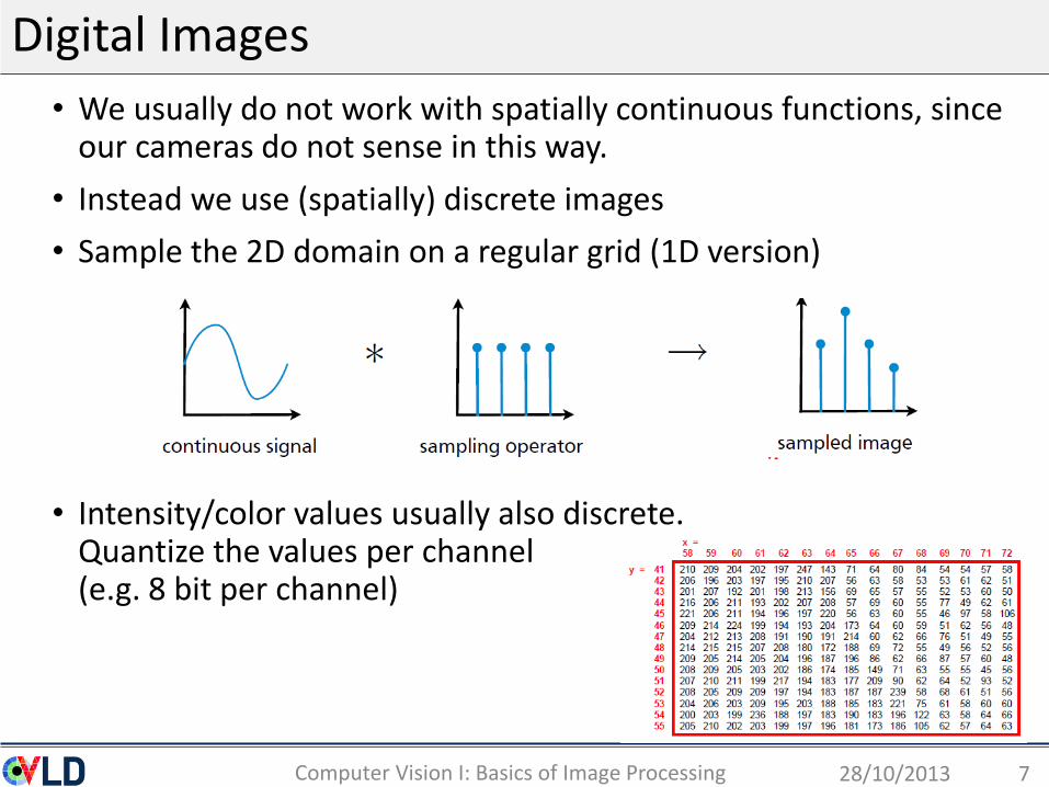
Digital Images
• We usually do not work with spatially continuous functions, since our cameras do not sense in this way.
• Instead we use (spatially) discrete images
• Sample the 2D domain on a regular grid (1D version)
• Intensity/color values usually also discrete. Quantize the values per channel (e.g. 8 bit per channel)
28/10/2013Computer Vision I: Basics of Image Processing 7
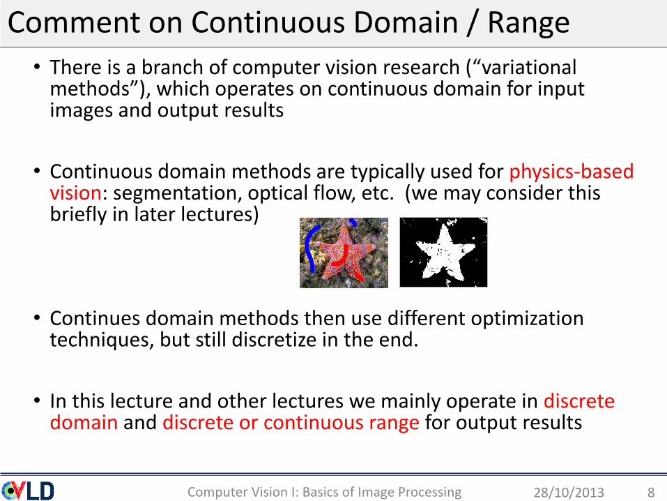
Comment on Continuous Domain / Range
28/10/2013Computer Vision I: Basics of Image Processing 8
• There is a branch of computer vision research (“variationalmethods”), which operates on continuous domain for input images and output results
• Continuous domain methods are typically used for physics-based vision: segmentation, optical flow, etc. (we may consider this briefly in later lectures)
• Continues domain methods then use different optimization techniques, but still discretize in the end.
• In this lecture and other lectures we mainly operate in discrete domain and discrete or continuous range for output results
Roadmap: Basics Digital Image Processing
• Images
• Point operators (ch. 3.1)
• Filtering: (ch. 3.2, ch 3.3, ch. 3.4) – main focus
• Linear filtering
• Non-linear filtering
• Fourier Transformation (ch. 3.4)
• Multi-scale image representation (ch. 3.5)
• Edges (ch. 4.2)
• Edge detection and linking
• Lines (ch. 4.3)
• Line detection and vanishing point detection
28/10/2013Computer Vision I: Basics of Image Processing 9
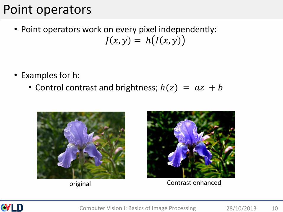
Point operators
• Point operators work on every pixel independently:𝐽 𝑥, 𝑦 = ℎ 𝐼 𝑥, 𝑦
• Examples for h:
• Control contrast and brightness; ℎ(𝑧) = 𝑎𝑧 + 𝑏
28/10/2013Computer Vision I: Basics of Image Processing 10
Contrast enhancedoriginal
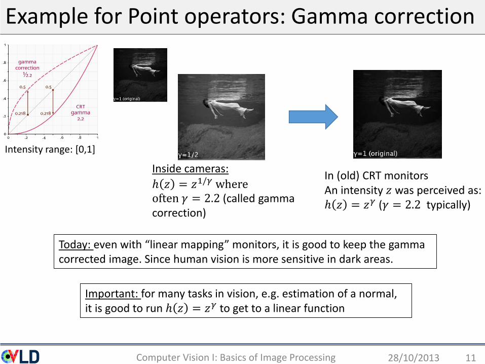
Example for Point operators: Gamma correction
28/10/2013Computer Vision I: Basics of Image Processing 11
Intensity range: [0,1]
In (old) CRT monitorsAn intensity 𝑧 was perceived as: ℎ 𝑧 = 𝑧𝛾 (𝛾 = 2.2 typically)
Inside cameras:
ℎ 𝑧 = 𝑧1/𝛾 where often 𝛾 = 2.2 (called gamma correction)
Important: for many tasks in vision, e.g. estimation of a normal, it is good to run ℎ 𝑧 = 𝑧𝛾 to get to a linear function
Today: even with “linear mapping” monitors, it is good to keep the gamma corrected image. Since human vision is more sensitive in dark areas.

Example for Point Operators: Alpha Matting
28/10/2013Computer Vision I: Basics of Image Processing 12
𝐶 𝑥, 𝑦 = 𝛼 𝑥, 𝑦 𝐹 𝑥, 𝑦 + 1 − 𝛼 𝑥, 𝑦 𝐵(𝑥, 𝑦)
Background 𝐵
Composite 𝐶Matte 𝛼
(amount of transparency)
Foreground 𝐹
Roadmap: Basics Digital Image Processing
• Images
• Point operators (ch. 3.1)
• Filtering: (ch. 3.2, ch 3.3, ch. 3.4) – main focus
• Linear filtering
• Non-linear filtering
• Fourier Transformation (ch. 3.4)
• Multi-scale image representation (ch. 3.5)
• Edges (ch. 4.2)
• Edge detection and linking
• Lines (ch 4.3)
• Line detection and vanishing point detection
28/10/2013Computer Vision I: Basics of Image Processing 13
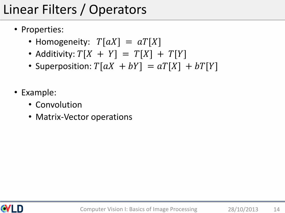
Linear Filters / Operators
• Properties:
• Homogeneity: 𝑇[𝑎𝑋] = 𝑎𝑇[𝑋]
• Additivity: 𝑇[𝑋 + 𝑌] = 𝑇[𝑋] + 𝑇[𝑌]
• Superposition: 𝑇[𝑎𝑋 + 𝑏𝑌] = 𝑎𝑇[𝑋] + 𝑏𝑇[𝑌]
• Example:
• Convolution
• Matrix-Vector operations
28/10/2013Computer Vision I: Basics of Image Processing 14
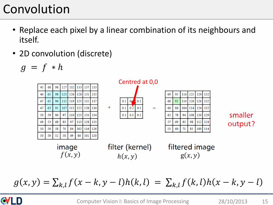
Convolution
• Replace each pixel by a linear combination of its neighbours and itself.
• 2D convolution (discrete)
𝑔 = 𝑓 ∗ ℎ
28/10/2013Computer Vision I: Basics of Image Processing 15
𝑔 𝑥, 𝑦 = 𝑘,𝑙 𝑓 𝑥 − 𝑘, 𝑦 − 𝑙 ℎ 𝑘, 𝑙 = 𝑘,𝑙 𝑓 𝑘, 𝑙 ℎ 𝑥 − 𝑘, 𝑦 − 𝑙
𝑓 𝑥, 𝑦 ℎ 𝑥, 𝑦 g 𝑥, 𝑦
Centred at 0,0
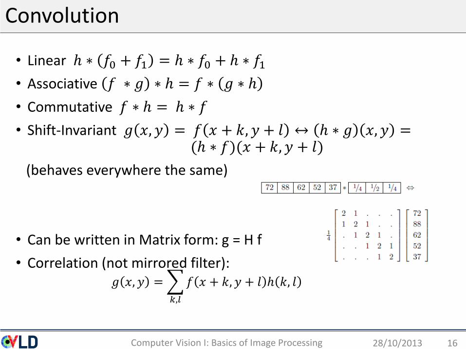
Convolution
28/10/2013Computer Vision I: Basics of Image Processing 16
• Linear ℎ ∗ 𝑓0 + 𝑓1 = ℎ ∗ 𝑓0 + ℎ ∗ 𝑓1
• Associative 𝑓 ∗ 𝑔 ∗ ℎ = 𝑓 ∗ 𝑔 ∗ ℎ
• Commutative 𝑓 ∗ ℎ = ℎ ∗ 𝑓
• Shift-Invariant 𝑔 𝑥, 𝑦 = 𝑓 𝑥 + 𝑘, 𝑦 + 𝑙 ↔ ℎ ∗ 𝑔 𝑥, 𝑦 =(ℎ ∗ 𝑓)(𝑥 + 𝑘, 𝑦 + 𝑙)
(behaves everywhere the same)
• Can be written in Matrix form: g = H f
• Correlation (not mirrored filter):𝑔 𝑥, 𝑦 =
𝑘,𝑙
𝑓 𝑥 + 𝑘, 𝑦 + 𝑙 ℎ 𝑘, 𝑙
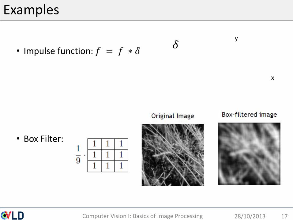
Examples
28/10/2013Computer Vision I: Basics of Image Processing 17
• Impulse function: 𝑓 = 𝑓 ∗ 𝛿
• Box Filter:
x
y𝛿
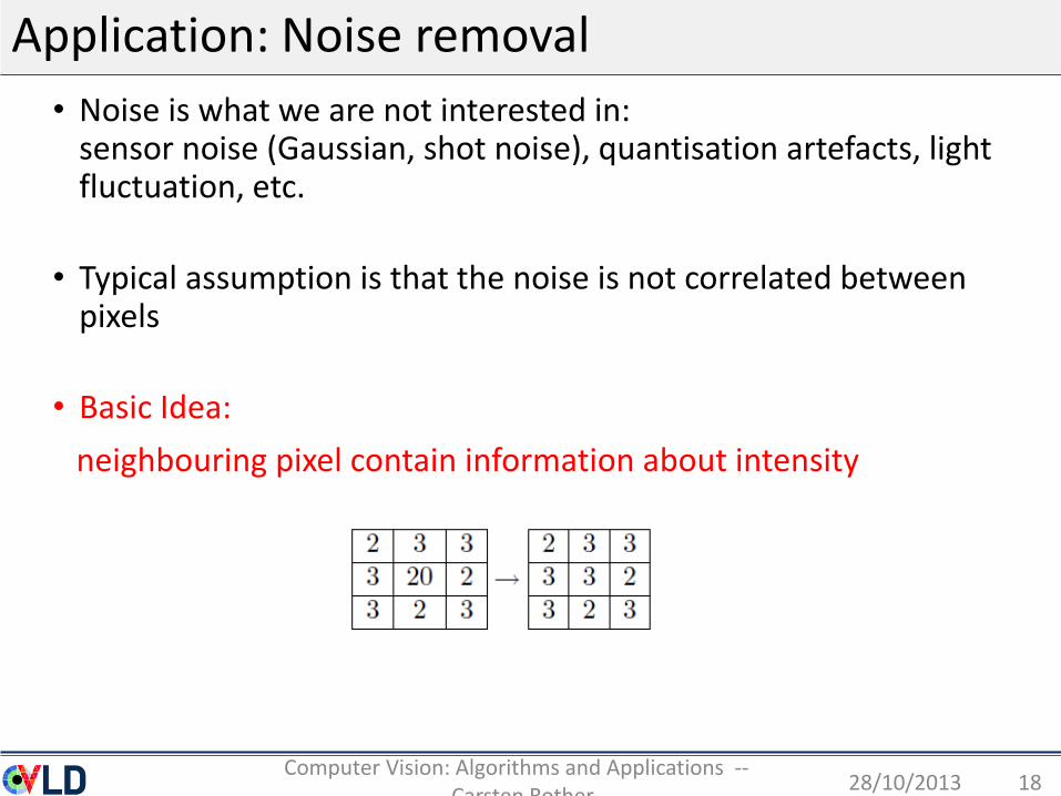
Application: Noise removal
• Noise is what we are not interested in:sensor noise (Gaussian, shot noise), quantisation artefacts, light fluctuation, etc.
• Typical assumption is that the noise is not correlated between pixels
• Basic Idea:
neighbouring pixel contain information about intensity
28/10/2013Computer Vision: Algorithms and Applications --
- Carsten Rother18
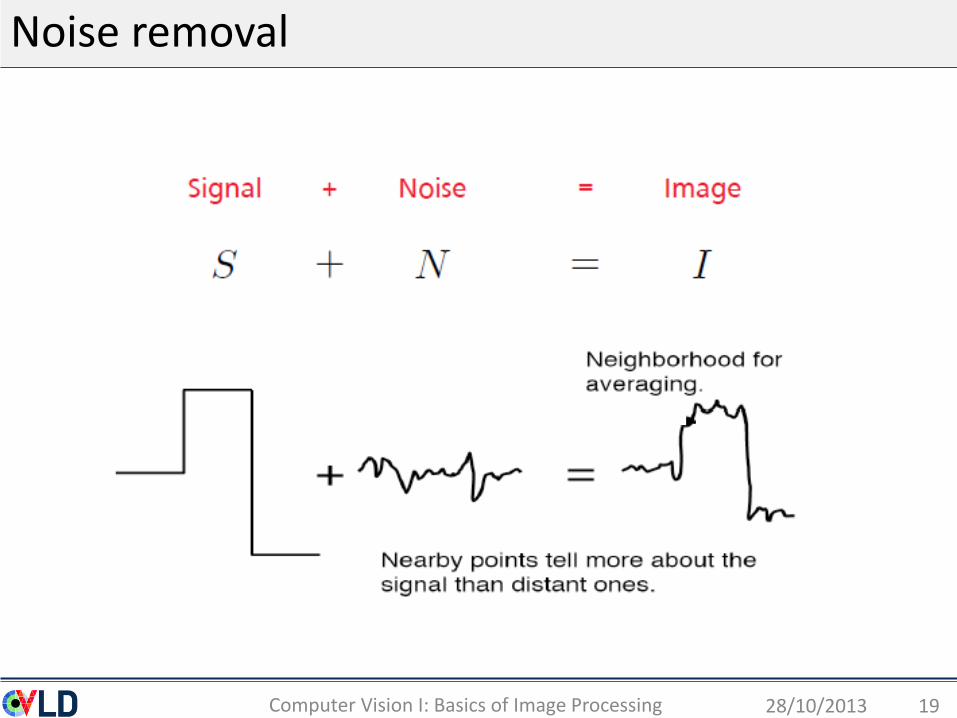
Noise removal
28/10/2013Computer Vision I: Basics of Image Processing 19
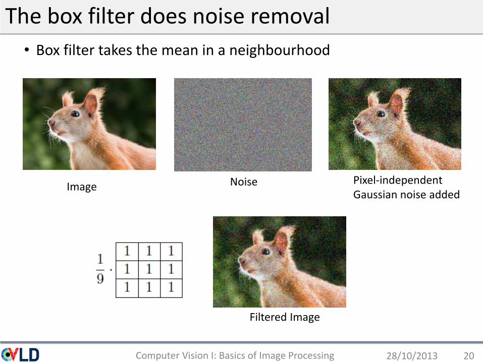
The box filter does noise removal
• Box filter takes the mean in a neighbourhood
28/10/2013Computer Vision I: Basics of Image Processing 20
Filtered Image
Image Pixel-independent Gaussian noise added
Noise
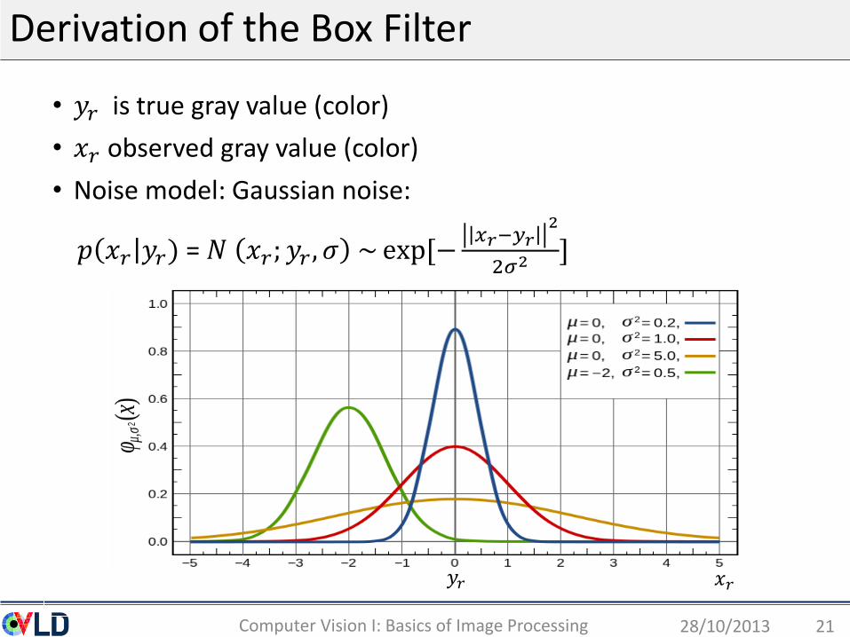
Derivation of the Box Filter
• 𝑦𝑟 is true gray value (color)
• 𝑥𝑟 observed gray value (color)
• Noise model: Gaussian noise:
𝑝 𝑥𝑟 𝑦𝑟) = 𝑁 𝑥𝑟; 𝑦𝑟 , 𝜎 ~ exp[−𝑥𝑟−𝑦𝑟
2
2𝜎2]
28/10/2013Computer Vision I: Basics of Image Processing 21
𝑦𝑟 𝑥𝑟

Derivation of Box Filter
28/10/2013Computer Vision I: Basics of Image Processing 22
Further assumption: independent noise
Find the most likely solution the true signal 𝑦Maximum-Likelihood principle (probability maximization):
𝑝(𝑥) is a constant (drop it out), assume (for now) uniform prior 𝑝(𝑦). So we get:
𝑝 𝑥 𝑦) ~ exp[−𝑥𝑟−𝑦𝑟
2
2𝜎2]
𝑟
𝑦∗ = 𝑎𝑟𝑔𝑚𝑎𝑥𝑦 𝑝 𝑦 𝑥) = 𝑎𝑟𝑔𝑚𝑎𝑥𝑦𝑝 𝑦 𝑝 𝑥 𝑦
𝑝(𝑥)
the solution is trivial: 𝑦𝑟 = 𝑥𝑟 for all 𝑟
additional assumptions about the signal 𝒚 are necessary !!!
𝑝 𝑦 𝑥) = 𝑝 𝑥 𝑦 ∼ exp[−𝑥𝑟 − 𝑦𝑟
2
2𝜎2]
𝑟
posterior
likelihoodprior
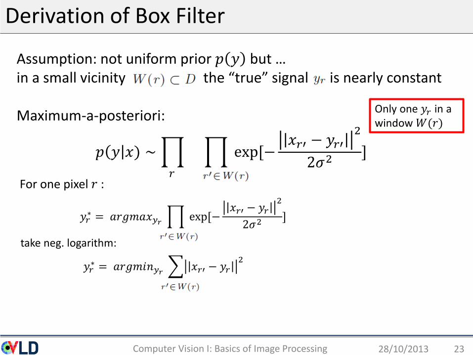
Derivation of Box Filter
28/10/2013Computer Vision I: Basics of Image Processing 23
Assumption: not uniform prior 𝑝 𝑦 but …in a small vicinity the “true” signal is nearly constant
Maximum-a-posteriori:
𝑝 𝑦 𝑥) ∼ exp[−𝑥𝑟′ − 𝑦𝑟′
2
2𝜎2]
𝑦𝑟∗ = 𝑎𝑟𝑔𝑚𝑎𝑥𝑦𝑟 exp[−
𝑥𝑟′ − 𝑦𝑟2
2𝜎2]
𝑦𝑟∗ = 𝑎𝑟𝑔𝑚𝑖𝑛𝑦𝑟 𝑥𝑟′ − 𝑦𝑟
2
Only one 𝑦𝑟 in a window 𝑊(𝑟)
𝑟For one pixel 𝑟 :
take neg. logarithm:

Derivation of Box Filter
28/10/2013Computer Vision I: Basics of Image Processing 24
𝑦𝑟∗ = 𝑎𝑟𝑔𝑚𝑖𝑛𝑦𝑟 𝑥𝑟′ − 𝑦𝑟
2
How to do the minimization:
Take derivative and set to 0:
(the average)𝑦𝑟∗
Box filter optimal under pixel-independent Gaussian Noise and constant signal in window
𝐹 𝑦𝑟 = 𝑥𝑟′ − 𝑦𝑟2

Gaussian (Smoothing) Filters
• Nearby pixels are weighted more than distant pixels
• Isotropic Gaussian (rotational symmetric)
28/10/2013Computer Vision I: Basics of Image Processing 25
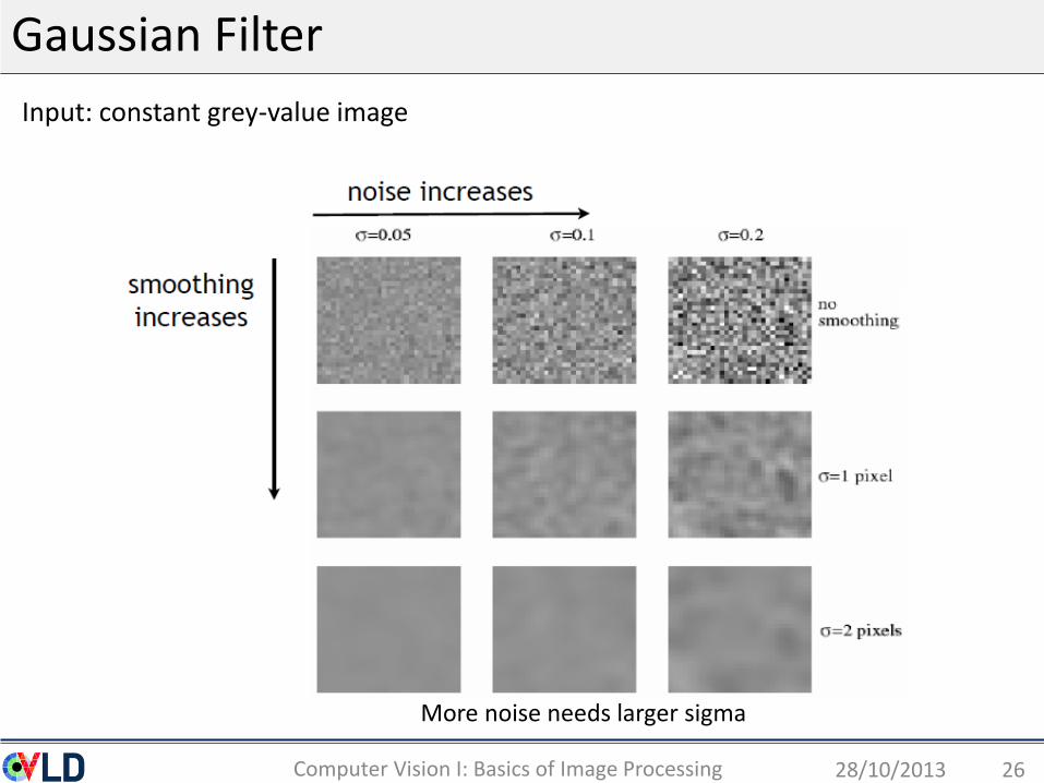
Gaussian Filter
28/10/2013Computer Vision I: Basics of Image Processing 26
Input: constant grey-value image
More noise needs larger sigma
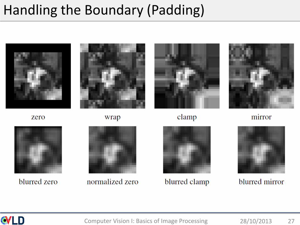
Handling the Boundary (Padding)
28/10/2013Computer Vision I: Basics of Image Processing 27
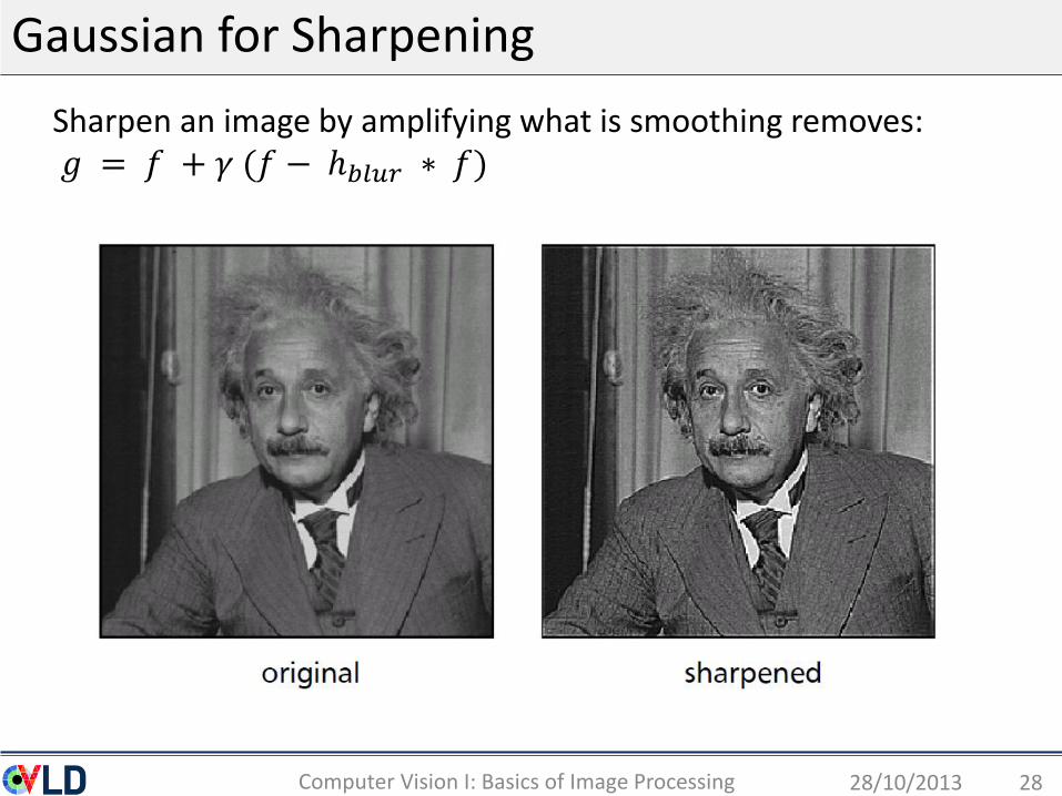
Gaussian for Sharpening
28/10/2013Computer Vision I: Basics of Image Processing 28
Sharpen an image by amplifying what is smoothing removes:𝑔 = 𝑓 + 𝛾 (𝑓 − ℎ𝑏𝑙𝑢𝑟 ∗ 𝑓)
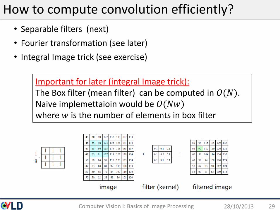
How to compute convolution efficiently?
• Separable filters (next)
• Fourier transformation (see later)
• Integral Image trick (see exercise)
28/10/2013Computer Vision I: Basics of Image Processing 29
Important for later (integral Image trick):The Box filter (mean filter) can be computed in 𝑂(𝑁). Naive implemettaioin would be 𝑂(𝑁𝑤)where 𝑤 is the number of elements in box filter
Separable filters
28/10/2013Computer Vision I: Basics of Image Processing 30
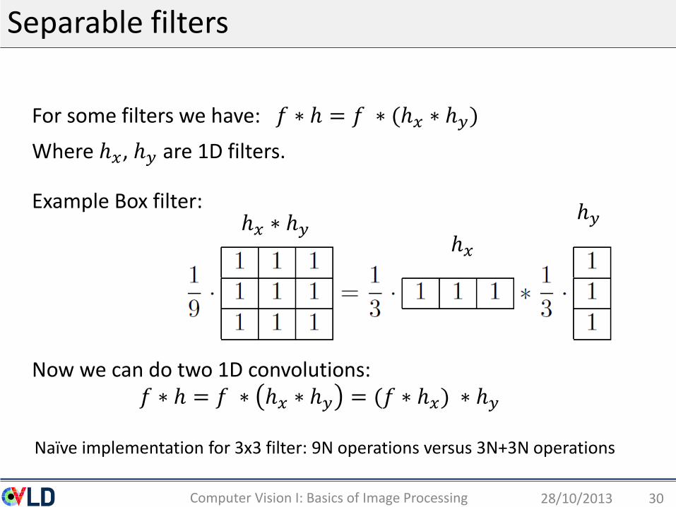
For some filters we have: 𝑓 ∗ ℎ = 𝑓 ∗ (ℎ𝑥 ∗ ℎ𝑦)
Where ℎ𝑥, ℎ𝑦 are 1D filters.
Example Box filter:
Now we can do two 1D convolutions: 𝑓 ∗ ℎ = 𝑓 ∗ ℎ𝑥 ∗ ℎ𝑦 = (𝑓 ∗ ℎ𝑥) ∗ ℎ𝑦
Naïve implementation for 3x3 filter: 9N operations versus 3N+3N operations
ℎ𝑥 ∗ ℎ𝑦ℎ𝑥
ℎ𝑦
Can any filter be made separable?
28/10/2013Computer Vision I: Basics of Image Processing 31
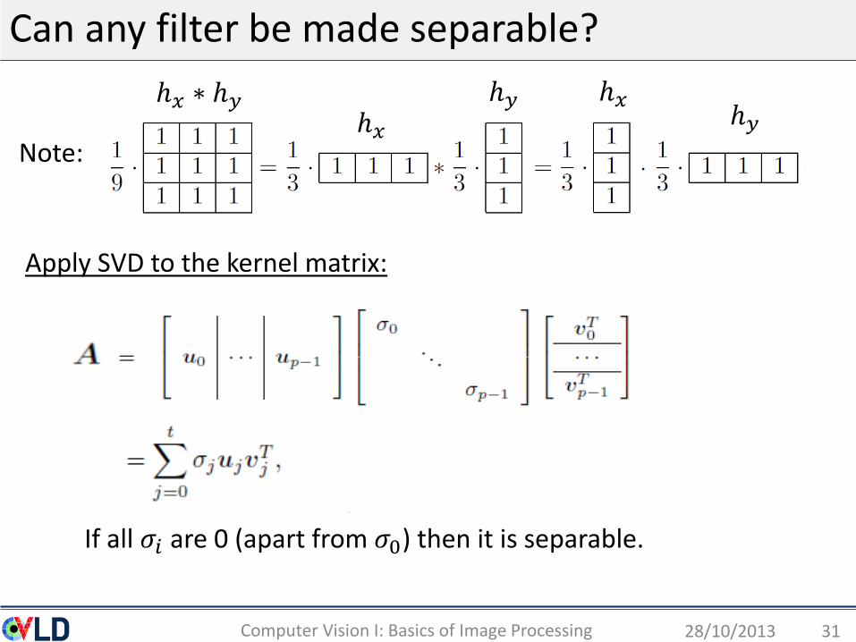
Apply SVD to the kernel matrix:
If all 𝜎𝑖 are 0 (apart from 𝜎0) then it is separable.
Note:
ℎ𝑥 ∗ ℎ𝑦ℎ𝑥
ℎ𝑥ℎ𝑦ℎ𝑦
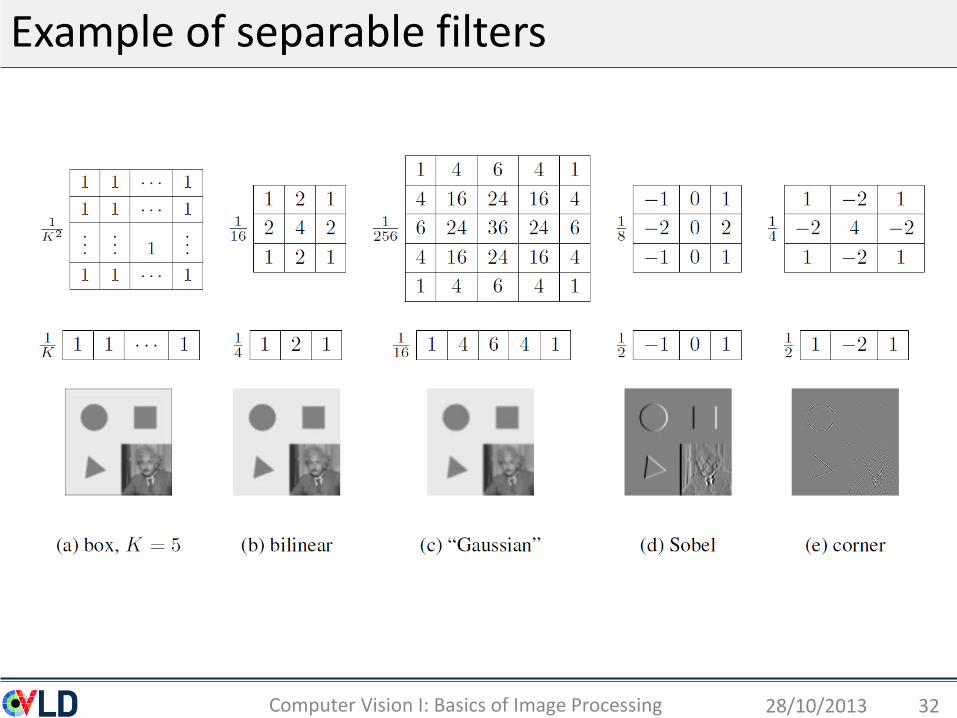
Example of separable filters
28/10/2013Computer Vision I: Basics of Image Processing 32

Roadmap: Basics Digital Image Processing
• Images
• Point operators (ch. 3.1)
• Filtering: (ch. 3.2, ch 3.3, ch. 3.4) – main focus
• Linear filtering
• Non-linear filtering
• Fourier Transformation (ch, 3.4)
• Multi-scale image representation (ch. 3.5)
• Edges (ch. 4.2)
• Edge detection and linking
• Lines (ch. 4.3)
• Line detection and vanishing point detection
28/10/2013Computer Vision I: Basics of Image Processing 33
Non-linear filters
• There are many different non-linear filters. We look at a selection:
• Median filter
• Bilateral filter (Guided Filter)
• Morphological operations
28/10/2013Computer Vision I: Basics of Image Processing 34
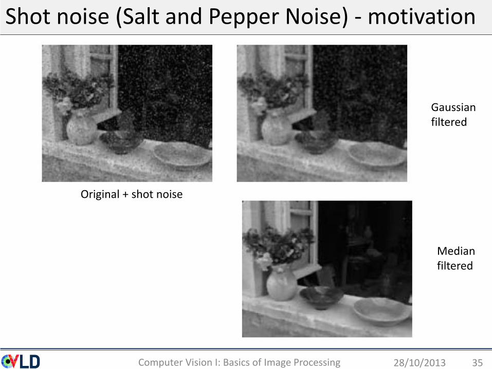
Shot noise (Salt and Pepper Noise) - motivation
28/10/2013Computer Vision I: Basics of Image Processing 35
Original + shot noise
Gaussian filtered
Medianfiltered
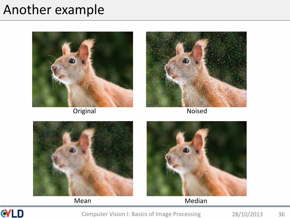
Another example
28/10/2013Computer Vision I: Basics of Image Processing 36
Original
Mean Median
Noised
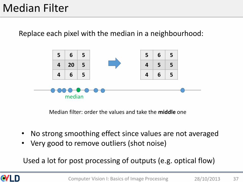
Median Filter
28/10/2013Computer Vision I: Basics of Image Processing 37
Replace each pixel with the median in a neighbourhood:
Used a lot for post processing of outputs (e.g. optical flow)
5 6 5
4 20 5
4 6 5
5 6 5
4 5 5
4 6 5
• No strong smoothing effect since values are not averaged• Very good to remove outliers (shot noise)
median
Median filter: order the values and take the middle one
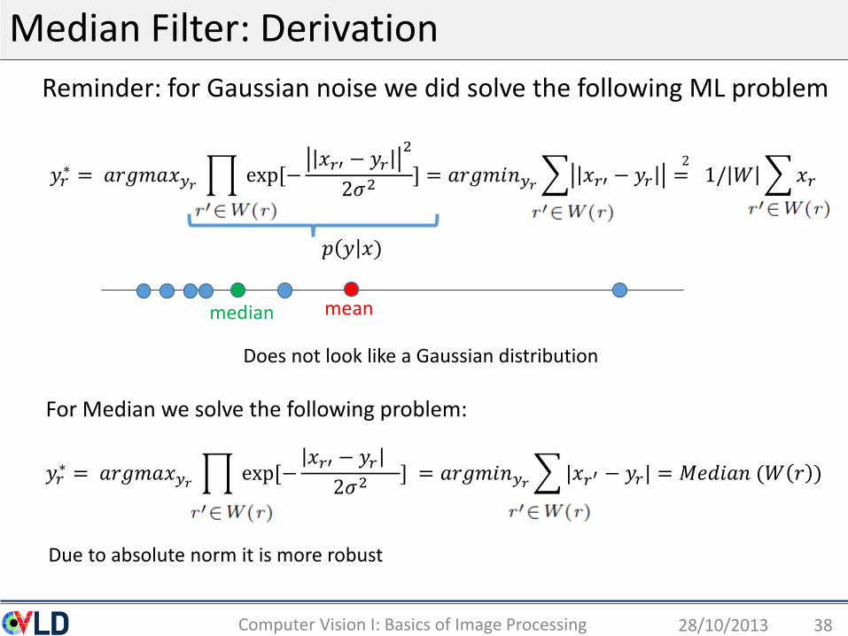
Median Filter: Derivation
Reminder: for Gaussian noise we did solve the following ML problem
28/10/2013Computer Vision I: Basics of Image Processing 38
𝑦𝑟∗ = 𝑎𝑟𝑔𝑚𝑎𝑥𝑦𝑟 exp[−
𝑥𝑟′ − 𝑦𝑟2
2𝜎2] = 𝑎𝑟𝑔𝑚𝑖𝑛𝑦𝑟 𝑥𝑟′ − 𝑦𝑟 = 1/ 𝑊 𝑥𝑟
Does not look like a Gaussian distribution
meanmedian
𝑦𝑟∗ = 𝑎𝑟𝑔𝑚𝑎𝑥𝑦𝑟 exp[−
𝑥𝑟′ − 𝑦𝑟2𝜎2
] = 𝑎𝑟𝑔𝑚𝑖𝑛𝑦𝑟 |𝑥𝑟′ − 𝑦𝑟| = 𝑀𝑒𝑑𝑖𝑎𝑛 (𝑊 𝑟 )
2
For Median we solve the following problem:
Due to absolute norm it is more robust
𝑝 𝑦 𝑥)
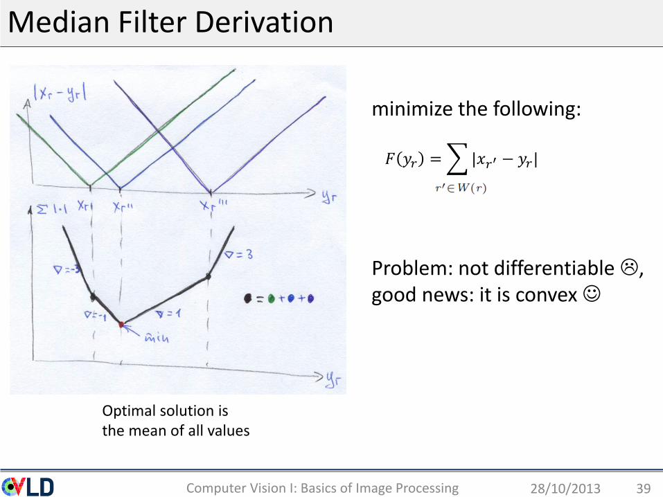
Median Filter Derivation
28/10/2013Computer Vision I: Basics of Image Processing 39
minimize the following: function:
Problem: not differentiable ,good news: it is convex
𝐹 𝑦𝑟 = |𝑥𝑟′ − 𝑦𝑟|
Optimal solution is the mean of all values

Motivation – Bilateral Filter
28/10/2013Computer Vision I: Basics of Image Processing 40
Original + Gaussian noise Gaussian filtered Bilateral filtered
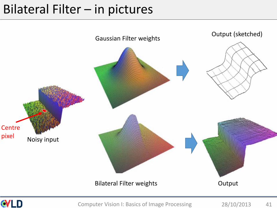
Bilateral Filter – in pictures
28/10/2013Computer Vision I: Basics of Image Processing 41
Bilateral Filter weights Output
Centre pixel
Gaussian Filter weights
Noisy input
Output (sketched)

Bilateral Filter – in equations
28/10/2013Computer Vision I: Basics of Image Processing 42
Filters looks at: a) distance of surrounding pixels (as Gaussian)b) Intensity of surrounding pixels
Problem: computation is slow 𝑂 𝑁𝑤 ; approximations can be done in 𝑂(𝑁)Comment: Guided filter (see later) is similar and can be computed exactly in 𝑂(𝑁)
See a tutorial on: http://people.csail.mit.edu/sparis/bf_course/
Similar to Gaussian filter Consider intensity
Linear combination
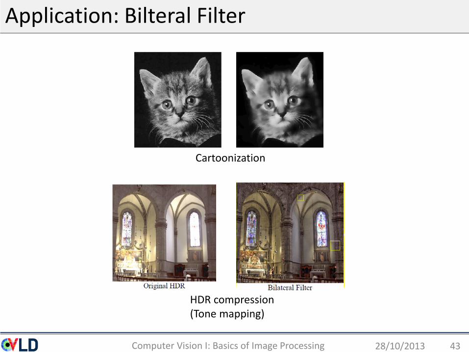
Application: Bilteral Filter
28/10/2013Computer Vision I: Basics of Image Processing 43
Cartoonization
HDR compression(Tone mapping)
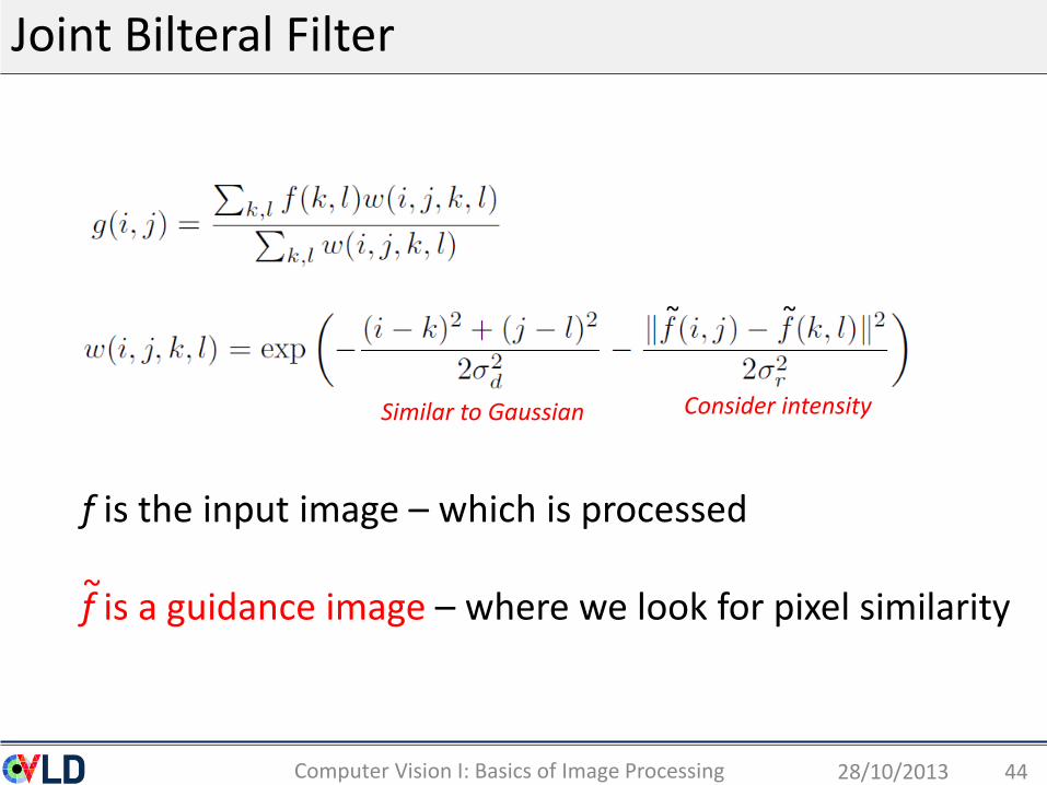
Joint Bilteral Filter
28/10/2013Computer Vision I: Basics of Image Processing 44
Similar to Gaussian Consider intensity
f is the input image – which is processed
f is a guidance image – where we look for pixel similarity
~ ~
~
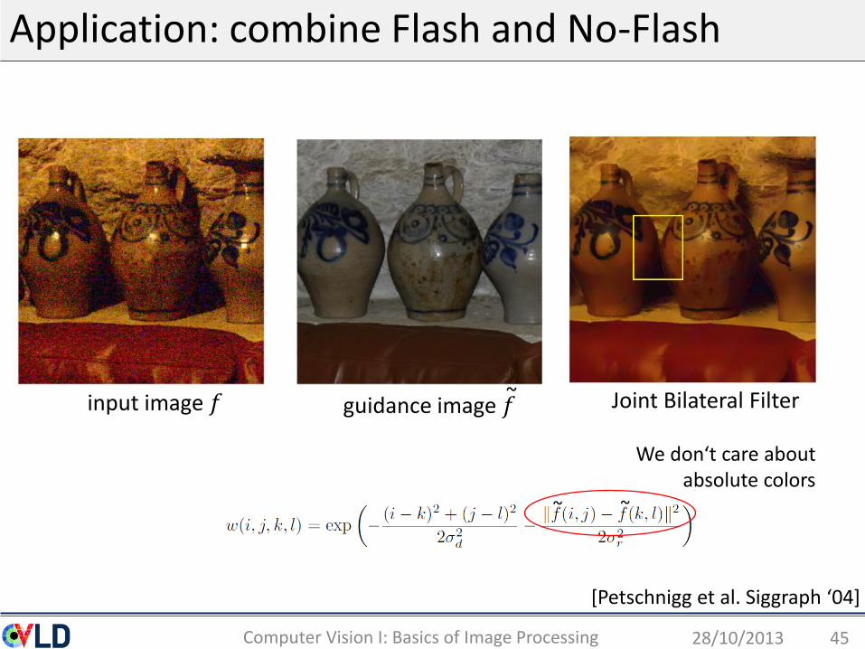
Application: combine Flash and No-Flash
28/10/2013Computer Vision I: Basics of Image Processing 45
[Petschnigg et al. Siggraph ‘04]
input image 𝑓 guidance image 𝑓
We don‘t care about absolute colors
~ Joint Bilateral Filter
~ ~
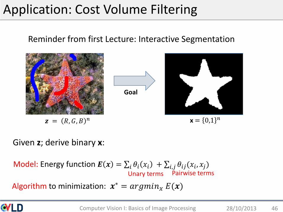
Application: Cost Volume Filtering
28/10/2013Computer Vision I: Basics of Image Processing 46
Goal
Given z; derive binary x:
Algorithm to minimization: 𝒙∗ = 𝑎𝑟𝑔𝑚𝑖𝑛𝑥 𝐸(𝒙)
𝒛 = 𝑅, 𝐺, 𝐵 𝑛 x= 0,1 𝑛
Reminder from first Lecture: Interactive Segmentation
Model: Energy function 𝑬 𝒙 = 𝑖 𝜃𝑖 𝑥𝑖 + 𝑖,𝑗 𝜃𝑖𝑗(𝑥𝑖 , 𝑥𝑗)Unary terms Pairwise terms

Reminder: Unary term
28/10/2013Computer Vision I: Introduction 47
Optimum with unary terms onlyDark means likely
backgroundDark means likely
foreground
𝜃𝑖(𝑥𝑖 = 0)𝜃𝑖(𝑥𝑖 = 1)
New query image 𝑧𝑖
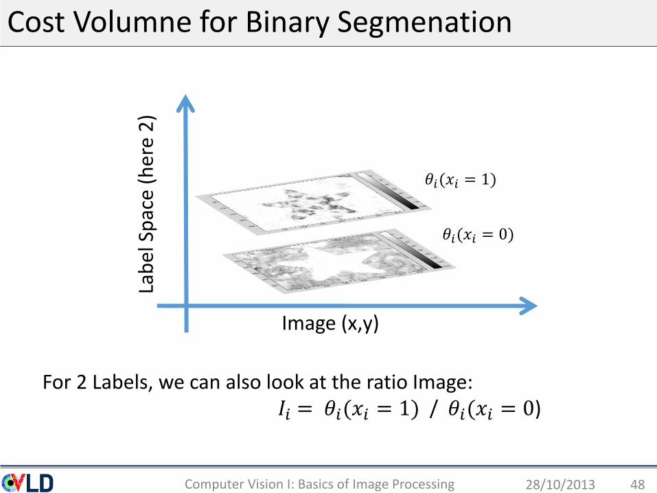
Cost Volumne for Binary Segmenation
28/10/2013Computer Vision I: Basics of Image Processing 48
𝜃𝑖(𝑥𝑖 = 0)
𝜃𝑖(𝑥𝑖 = 1)
Image (x,y)
Lab
el S
pac
e (h
ere
2)
For 2 Labels, we can also look at the ratio Image:𝐼𝑖 = 𝜃𝑖(𝑥𝑖 = 1) / 𝜃𝑖(𝑥𝑖 = 0)

Application: Cost Volumne Filtering
28/10/2013Computer Vision I: Basics of Image Processing 49
An alternative to energy minimization
Filtered cost volume
Energy minimization
Guidance Input Image 𝑓(user brush strokes)
Winner takes all Result
Ratio Cost-volume is the Input Image 𝑓
~
[C. Rhemann, A. Hosni, M. Bleyer, C. Rother, and M. Gelautz, Fast Cost-Volume Filtering for Visual Correspondence and Beyond, CVPR 11]
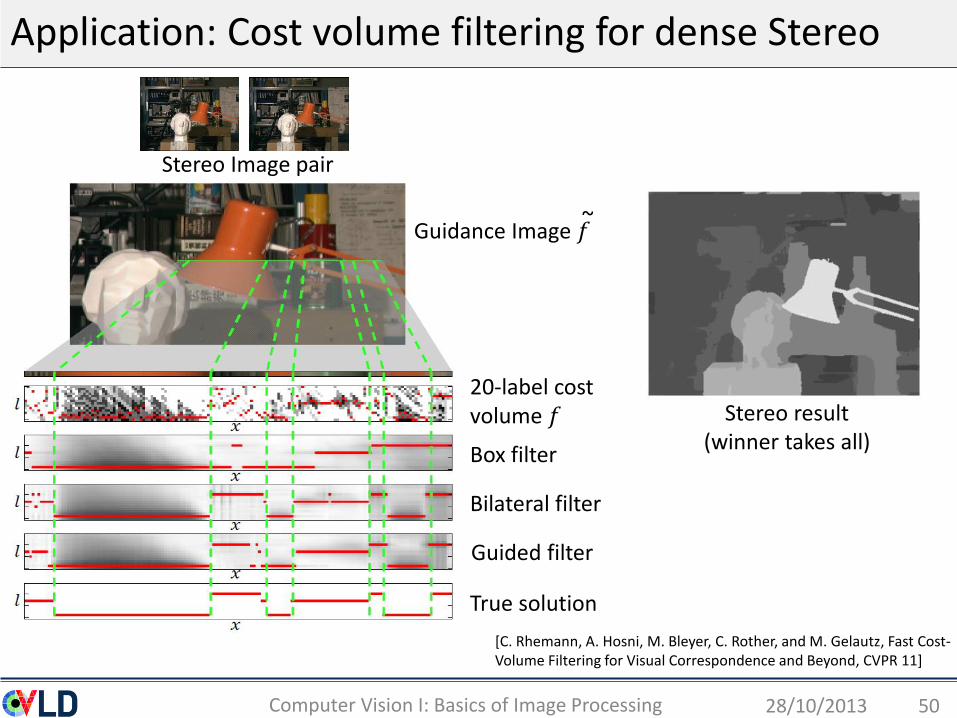
Application: Cost volume filtering for dense Stereo
28/10/2013Computer Vision I: Basics of Image Processing 50
Stereo result(winner takes all)
20-label cost volume 𝑓
Box filter
True solution
Bilateral filter
Guided filter
Guidance Image 𝑓
[C. Rhemann, A. Hosni, M. Bleyer, C. Rother, and M. Gelautz, Fast Cost-Volume Filtering for Visual Correspondence and Beyond, CVPR 11]
Stereo Image pair
~
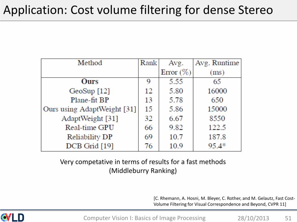
Application: Cost volume filtering for dense Stereo
28/10/2013Computer Vision I: Basics of Image Processing 51
Very competative in terms of results for a fast methods(Middleburry Ranking)
[C. Rhemann, A. Hosni, M. Bleyer, C. Rother, and M. Gelautz, Fast Cost-Volume Filtering for Visual Correspondence and Beyond, CVPR 11]
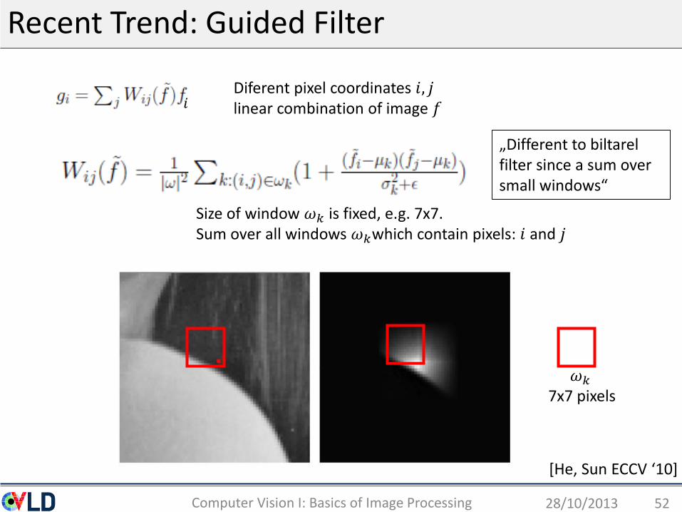
Recent Trend: Guided Filter
28/10/2013Computer Vision I: Basics of Image Processing 52
Diferent pixel coordinates 𝑖, 𝑗linear combination of image 𝑓
Size of window 𝜔𝑘 is fixed, e.g. 7x7.Sum over all windows 𝜔𝑘which contain pixels: 𝑖 and 𝑗
„Different to biltarel filter since a sum over small windows“
𝜔𝑘7x7 pixels
𝑖
[He, Sun ECCV ‘10]
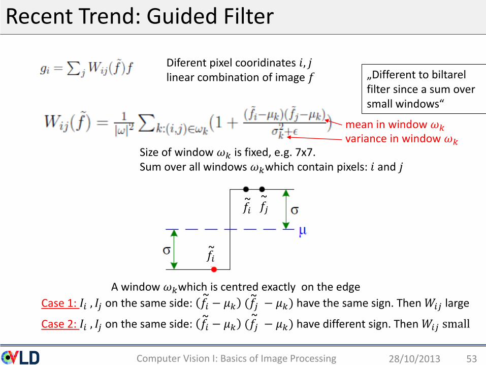
Recent Trend: Guided Filter
28/10/2013Computer Vision I: Basics of Image Processing 53
Diferent pixel cooridinates 𝑖, 𝑗linear combination of image 𝑓
A window 𝜔𝑘which is centred exactly on the edge
Size of window 𝜔𝑘 is fixed, e.g. 7x7.Sum over all windows 𝜔𝑘which contain pixels: 𝑖 and 𝑗
„Different to biltarel filter since a sum over small windows“
Case 1: 𝐼𝑖 , 𝐼𝑗 on the same side: 𝑓𝑖 − 𝜇𝑘 (𝑓𝑗 − 𝜇𝑘) have the same sign. Then 𝑊𝑖𝑗 large
Case 2: 𝐼𝑖 , 𝐼𝑗 on the same side: 𝑓𝑖 − 𝜇𝑘 (𝑓𝑗 − 𝜇𝑘) have different sign. Then 𝑊𝑖𝑗 small
variance in window 𝜔𝑘
mean in window 𝜔𝑘
𝑓𝑖~
𝑓𝑖~ 𝑓𝑗
~
~ ~
~~
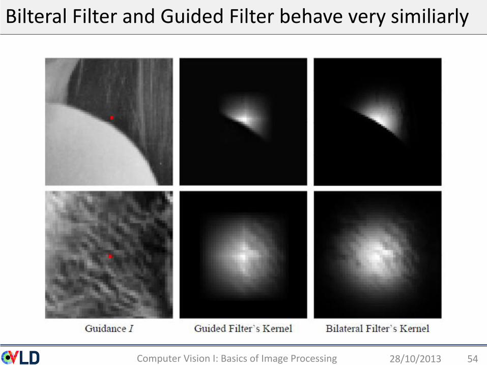
Bilteral Filter and Guided Filter behave very similiarly
28/10/2013Computer Vision I: Basics of Image Processing 54

Bilteral Filter and Guided Filter behave very similiarly
28/10/2013Computer Vision I: Basics of Image Processing 55
Guided Filter Bilteral Filter
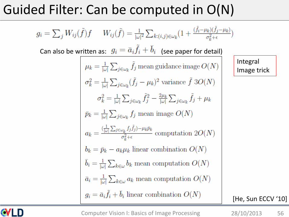
Guided Filter: Can be computed in O(N)
28/10/2013Computer Vision I: Basics of Image Processing 56
Can also be written as: (see paper for detail)
[He, Sun ECCV ‘10]
Integral Image trick
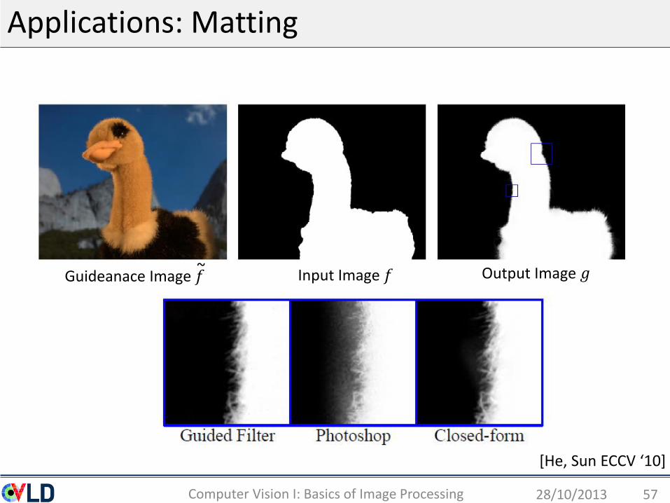
Applications: Matting
28/10/2013Computer Vision I: Basics of Image Processing 57
Guideanace Image 𝑓~ Input Image 𝑓 Output Image 𝑔
[He, Sun ECCV ‘10]
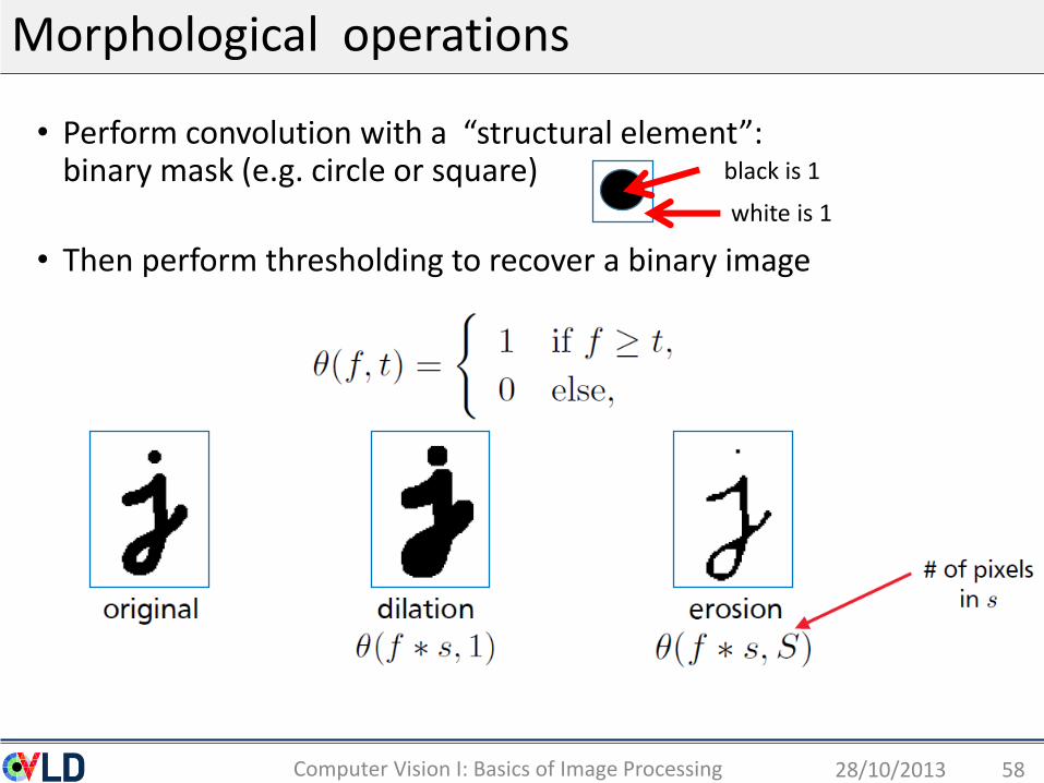
Morphological operations
28/10/2013Computer Vision I: Basics of Image Processing 58
• Perform convolution with a “structural element”: binary mask (e.g. circle or square)
• Then perform thresholding to recover a binary image
black is 1
white is 1

Opening and Closing Operations
28/10/2013Computer Vision I: Basics of Image Processing 59
• Opening operation: 𝑑𝑖𝑙𝑎𝑡𝑒 𝑒𝑟𝑜𝑑𝑒 𝑓, 𝑠 , 𝑠
• Closing opertiaon: 𝑒𝑟𝑜𝑑𝑒 𝑑𝑖𝑎𝑙𝑡𝑒 𝑓, 𝑠 , 𝑠
closingopeningInput image
erode and dilate are not commutative
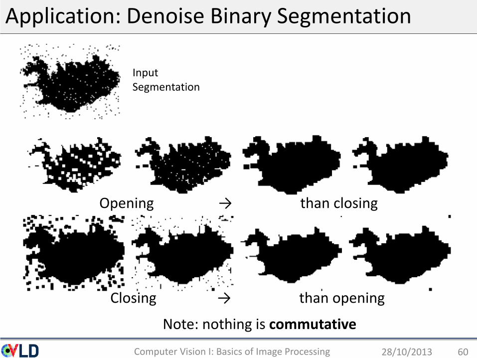
Application: Denoise Binary Segmentation
28/10/2013Computer Vision I: Basics of Image Processing 60
Note: nothing is commutative
Closing → than opening
Opening → than closing
Input Segmentation
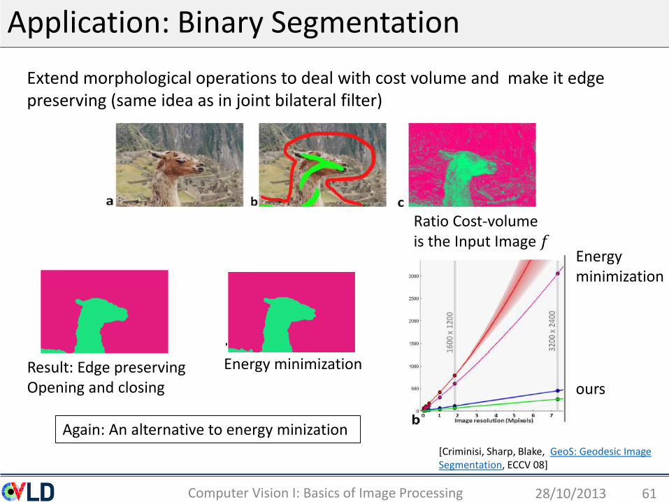
Application: Binary Segmentation
28/10/2013Computer Vision I: Basics of Image Processing 61
[Criminisi, Sharp, Blake, GeoS: Geodesic Image Segmentation, ECCV 08]
Result: Edge preservingOpening and closing
Extend morphological operations to deal with cost volume and make it edge preserving (same idea as in joint bilateral filter)
Again: An alternative to energy minization
Ratio Cost-volume is the Input Image 𝑓
Energy minimization
Energy minimization
ours

Related nonlinear operations on binary images
28/10/2013Computer Vision I: Basics of Image Processing 62
Distance transform
Binary Image
Skeleton
Binary Input Image Connected components

Roadmap: Basics Digital Image Processing
• Images
• Point operators (Ch. 3.1)
• Filtering: (ch. 3.2, ch 3.3, ch. 3.4) – main focus
• Linear filtering
• Non-linear filtering
• Fourier Transformation (ch. 3.4)
• Multi-scale image representation (ch. 3.5)
• Edges (Ch. 4.2)
• Edge detection and linking
• Lines (Ch 4.3)
• Line detection and vanishing point detection
28/10/2013Computer Vision I: Basics of Image Processing 63

Fourier Transformation … to analyse Filters
28/10/2013Computer Vision I: Basics of Image Processing 64
Complex valued, continuous sinusoid for different frequency 𝜔
𝑜 𝑥 = ℎ 𝑥 ∗ 𝑠 𝑥 = 𝐴 𝑒𝑗(𝑤𝑥+𝜙) =𝐴 [ cos(𝜔 𝑥 + 𝜙) + 𝑗 𝑠𝑖𝑛(𝜔 𝑥 + 𝜙) ]
Amplitude phase
Simply try all possible 𝜔 and record 𝐴, 𝜙 . The Fourier transformation of ℎ(𝑥) is then:𝐻 𝜔 = ℎ 𝑥 = 𝐴 𝑒𝑗𝜙 = 𝐴 (cos 𝜙 + 𝑗 sin 𝜙 )
Filter/Image
How does a sinusoid influences a given filter/Image ℎ(𝑥) ?
Output signal
The output is also a sinusoid
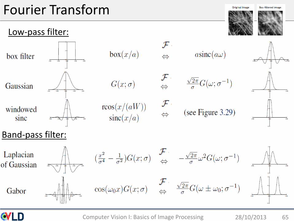
Fourier Transform
28/10/2013Computer Vision I: Basics of Image Processing 65
Low-pass filter:
Band-pass filter:
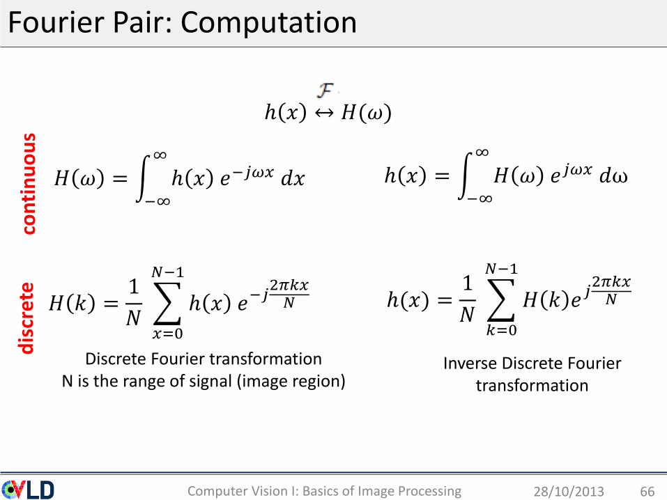
Fourier Pair: Computation
28/10/2013Computer Vision I: Basics of Image Processing 66
ℎ 𝑥 ↔ 𝐻(𝜔)
𝐻 𝜔 = −∞
∞
ℎ 𝑥 𝑒−𝑗𝜔𝑥 𝑑𝑥 ℎ 𝑥 = −∞
∞
𝐻 𝜔 𝑒𝑗𝜔𝑥 𝑑ω
𝐻 𝑘 =1
𝑁
𝑥=0
𝑁−1
ℎ 𝑥 𝑒−𝑗2𝜋𝑘𝑥𝑁
Discrete Fourier transformationN is the range of signal (image region)
ℎ(𝑥) =1
𝑁
𝑘=0
𝑁−1
𝐻 𝑘 𝑒𝑗2𝜋𝑘𝑥𝑁
con
tin
uo
us
dis
cret
e
Inverse Discrete Fourier transformation

Discrete Inverse Fourier Transform: Visualization
28/10/2013Computer Vision I: Basics of Image Processing 67
h(x) =1
𝑁
𝑘=0
𝑁−1
𝐻 𝑘 𝑒𝑗2𝜋𝑘𝑥𝑁
For this signal a reconstruction with sinus function only is sufficient
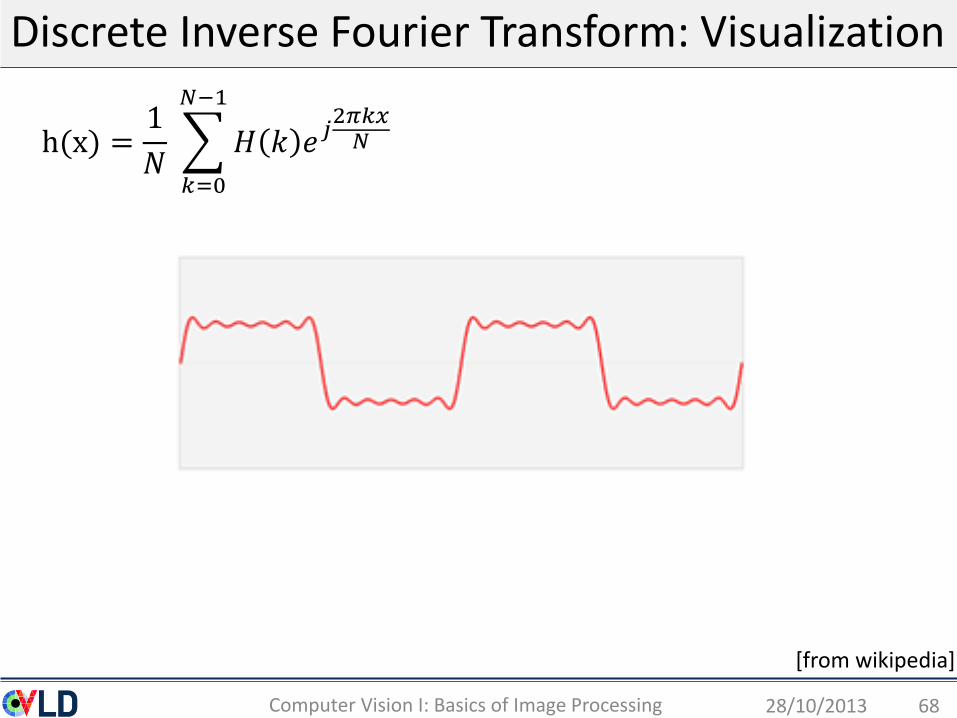
Discrete Inverse Fourier Transform: Visualization
28/10/2013Computer Vision I: Basics of Image Processing 68
h(x) =1
𝑁
𝑘=0
𝑁−1
𝐻 𝑘 𝑒𝑗2𝜋𝑘𝑥𝑁
[from wikipedia]
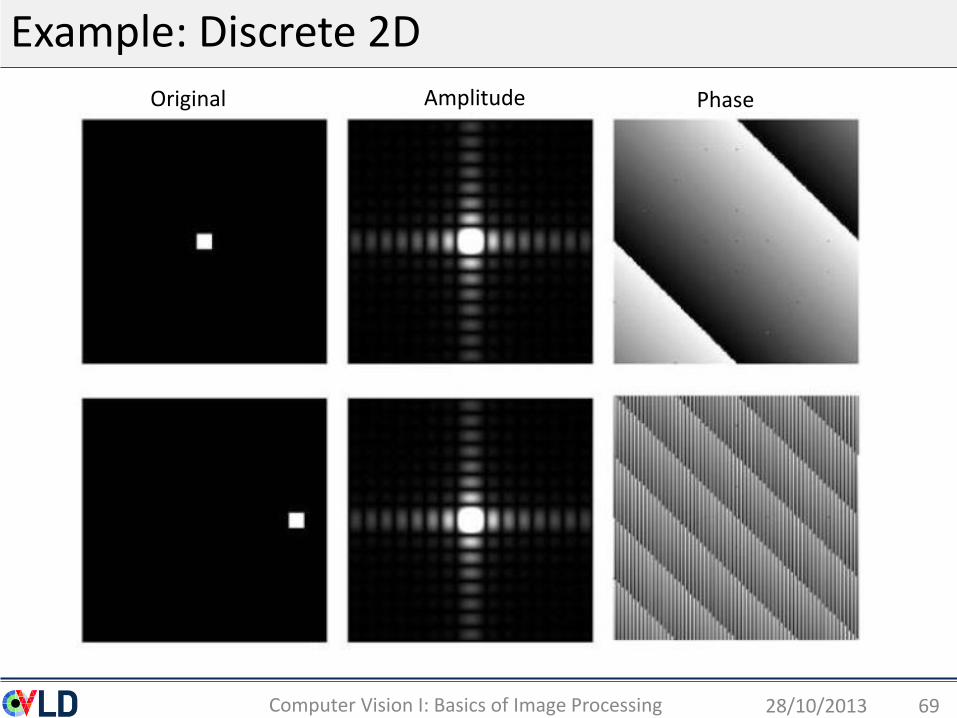
Example: Discrete 2D
28/10/2013Computer Vision I: Basics of Image Processing 69
Original Amplitude Phase

Example: Discrete 2D
28/10/2013Computer Vision I: Basics of Image Processing 70
Original Amplitude Phase
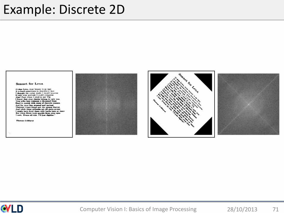
Example: Discrete 2D
28/10/2013Computer Vision I: Basics of Image Processing 71

Fast Fourier Transformation
28/10/2013Computer Vision I: Basics of Image Processing 72
• Important property: (𝑔 𝑥 ∗ ℎ 𝑥 ) = 𝐺(𝜔) 𝐻(𝜔)
• Fast computation:
𝑓 𝑥 , ℎ(𝑥)O(Nw)
convolution𝑓 𝑥 ∗ ℎ(𝑥)
𝐹 𝜔 ,𝐻(𝜔)
O(N logN)fourier transform
O(N) multiplication
O(N logN)inverse fourier transform
𝐹 𝜔 𝐻(𝜔)
O(N log N)
Roadmap: Basics Digital Image Processing
• Images
• Point operators (Ch. 3.1)
• Filtering: (ch. 3.2, ch 3.3, ch. 3.4) – main focus
• Linear filtering
• Non-linear filtering
• Fourier Transformation (ch. 3.4)
• Multi-scale image representation (ch. 3.5)
• Edges (Ch. 4.2)
• Edge detection and linking
• Lines (Ch 4.3)
• Line detection and vanishing point detection
28/10/2013Computer Vision I: Basics of Image Processing 73
Reading for next class
This lecture:
• Chapter 3 (in particular: 3.2, 3.3) - Basics of Digital Image Processing
Next lecture:
• Chapter 3.5: multi-scale representation
• Chapter 4.2 and 4.3 - Edge and Line detection
• Chapter 2 (in particular: 2.1, 2.2) – Image formation process
• And a bit of Hartley and Zisserman – chapter 2
28/10/2013Computer Vision I: Introduction 74