Embed Size (px)
Citation preview
Computer Vision I -Algorithms and Applications:
Discrete Labelling
Carsten Rother
Computer Vision I: Discrete Labelling03/02/2014

Roadmap this lecture (chapter B.4-5 in book)
• Define: Markov Random Fields
• Formulate applications as discrete labeling problems
• Discrete Optimization: • Pixels-based: Iterative Conditional Mode (ICM),
Simulated Annealing• Line-based: Dynamic Programming (DP)• Field-based: Graph Cut and Alpha-Expansion
03/02/2014 Computer Vision I: Discrete Labelling 2
Roadmap this lecture (chapter B.4-5 in book)
• Define: Markov Random Fields
• Formulate applications as discrete labeling problems
• Discrete Optimization: • Pixels-based: Iterative Conditional Mode (ICM),
Simulated Annealing• Line-based: Dynamic Programming (DP)• Field-based: Graph Cut and Alpha-Expansion
03/02/2014 Computer Vision I: Discrete Labelling 3
Machine Learning: Big Picture
03/02/2014 Computer Vision I: Discrete Labelling 4
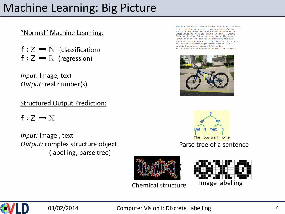
”Normal” Machine Learning:
f : Z N (classification) f : Z R (regression)
Input: Image, textOutput: real number(s)
f : Z X
Input: Image , textOutput: complex structure object
(labelling, parse tree) Parse tree of a sentence
Image labellingChemical structure
Structured Output Prediction:
Structured Output Prediction
03/02/2014 Computer Vision I: Discrete Labelling 5
Ad hoc definition (from [Nowozin et al. 2011])
Data that consists of several parts, and not only the parts themselves contain information, but also the way in which the parts belong together.
Graphical models to capture structured problems
03/02/2014 Computer Vision I: Discrete Labelling 6
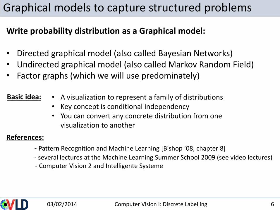
Write probability distribution as a Graphical model:
• Directed graphical model (also called Bayesian Networks)• Undirected graphical model (also called Markov Random Field)• Factor graphs (which we will use predominately)
• A visualization to represent a family of distributions• Key concept is conditional independency• You can convert any concrete distribution from one
visualization to another
Basic idea:
References:
- Pattern Recognition and Machine Learning [Bishop ‘08, chapter 8]
- several lectures at the Machine Learning Summer School 2009 (see video lectures)- Computer Vision 2 and Intelligente Systeme
Factor Graphs
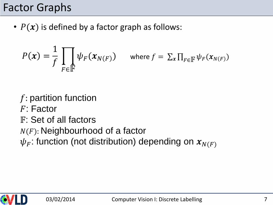
• 𝑃(𝒙) is defined by a factor graph as follows:
03/02/2014 Computer Vision I: Discrete Labelling 7
𝑓: partition function
𝐹: Factor
𝔽: Set of all factors
𝑁(𝐹):Neighbourhood of a factor
𝜓𝐹: function (not distribution) depending on 𝒙𝑁(𝐹)
𝑃 𝒙 =1
𝑓
𝐹∈𝔽
𝜓𝐹(𝒙𝑁 𝐹 ) where 𝑓 = 𝒙 𝐹∈𝔽𝜓𝐹(𝒙𝑁 𝐹 )
Factor Graphs - example
03/02/2014 Computer Vision I: Discrete Labelling 8
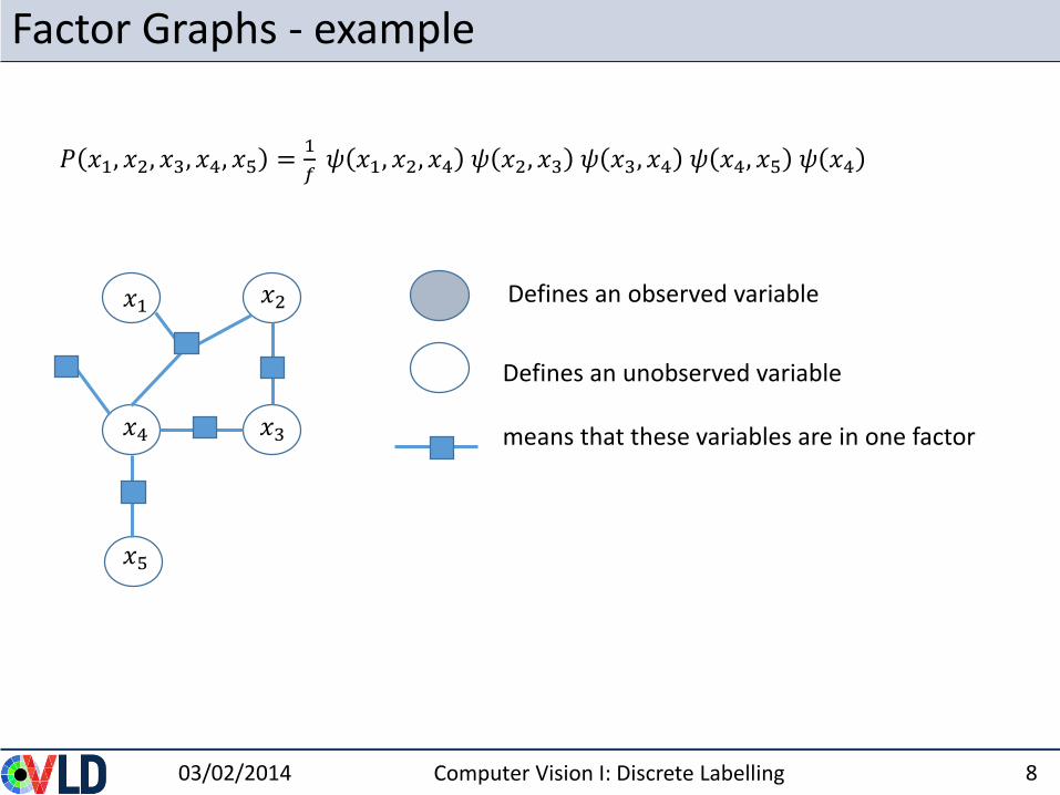
Defines an unobserved variable
means that these variables are in one factor
Defines an observed variable
𝑃 𝑥1, 𝑥2, 𝑥3, 𝑥4, 𝑥5 =1
𝑓𝜓 𝑥1, 𝑥2, 𝑥4 𝜓 𝑥2, 𝑥3 𝜓 𝑥3, 𝑥4 𝜓 𝑥4, 𝑥5 𝜓 𝑥4
𝑥1 𝑥2
𝑥3𝑥4
𝑥5
Introducing energies
03/02/2014 Computer Vision I: Discrete Labelling 9
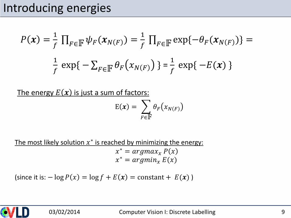
𝑃 𝒙 =1
𝑓 𝐹∈𝔽𝜓𝐹(𝒙𝑁 𝐹 ) =
1
𝑓 𝐹∈𝔽 exp{−𝜃𝐹(𝒙𝑁 𝐹 )} =
1
𝑓exp{ −
𝐹∈𝔽𝜃𝐹 𝑥𝑁 𝐹 } = 1
𝑓exp{ −𝐸(𝒙) }
The energy 𝐸 𝒙 is just a sum of factors:
E 𝒙 =
𝐹∈𝔽
𝜃𝐹 𝑥𝑁 𝐹
The most likely solution 𝑥∗ is reached by minimizing the energy:𝑥∗ = 𝑎𝑟𝑔𝑚𝑎𝑥𝑥 𝑃 𝑥𝑥∗ = 𝑎𝑟𝑔𝑚𝑖𝑛𝑥 𝐸(𝑥)
(since it is: − log𝑃 𝑥 = log 𝑓 + 𝐸 𝒙 = constant + 𝐸(𝒙) )
Gibbs Distribution
03/02/2014 Computer Vision I: Discrete Labelling 10
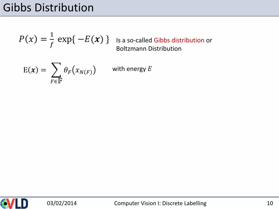
𝑃 𝑥 =1
𝑓exp{ −𝐸(𝒙) }
E 𝒙 =
𝐹∈𝔽
𝜃𝐹 𝑥𝑁 𝐹
Is a so-called Gibbs distribution or Boltzmann Distribution
with energy 𝐸
03/02/2014 Computer Vision I: Discrete Labelling 11
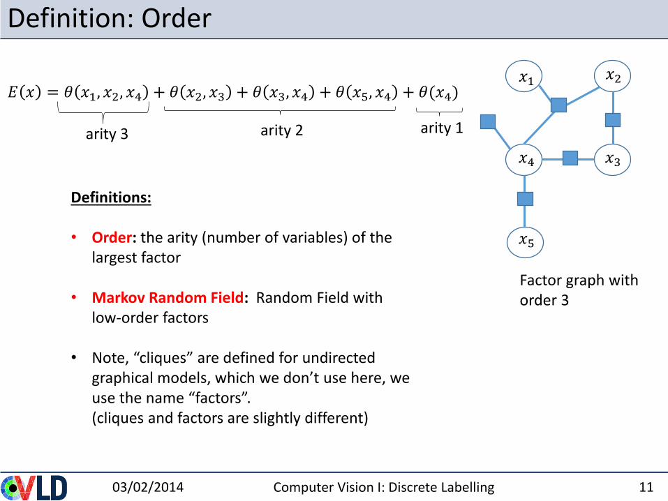
Definition: Order
arity 3 arity 2
Definitions:
• Order: the arity (number of variables) of the largest factor
• Markov Random Field: Random Field with low-order factors
• Note, “cliques” are defined for undirected graphical models, which we don’t use here, we use the name “factors”. (cliques and factors are slightly different)
𝑥1 𝑥2
𝑥3𝑥4
𝑥5
Factor graph with order 3
𝐸 𝑥 = 𝜃 𝑥1, 𝑥2, 𝑥4 + 𝜃 𝑥2, 𝑥3 + 𝜃 𝑥3, 𝑥4 + 𝜃 𝑥5, 𝑥4 + 𝜃(𝑥4)
arity 1
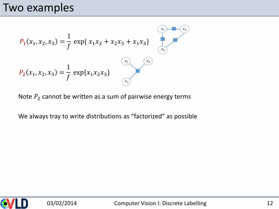
Two examples
03/02/2014 Computer Vision I: Discrete Labelling 12
𝑃1 𝑥1, 𝑥2, 𝑥3 =1
𝑓exp{ 𝑥1𝑥2 + 𝑥2𝑥3 + 𝑥1𝑥3}
𝑃2 𝑥1, 𝑥2, 𝑥3 =1
𝑓exp{𝑥1𝑥2𝑥3}
We always tray to write distributions as “factorized” as possible
Note 𝑃2 cannot be written as a sum of pairwise energy terms
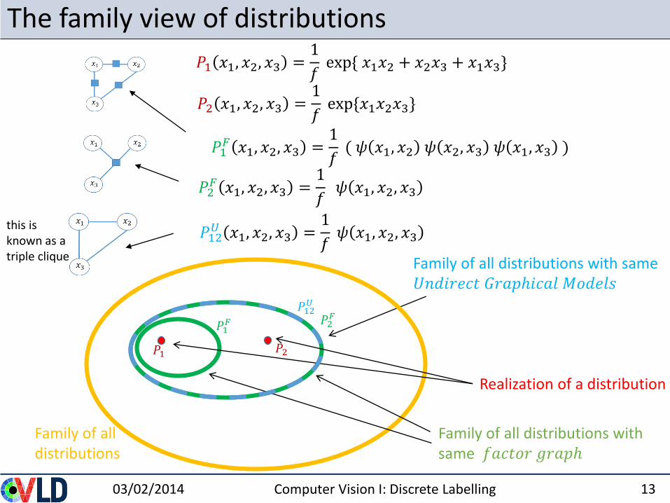
The family view of distributions
03/02/2014 Computer Vision I: Discrete Labelling 13
Family of all distributions
Family of all distributions with same 𝑈𝑛𝑑𝑖𝑟𝑒𝑐𝑡 𝐺𝑟𝑎𝑝ℎ𝑖𝑐𝑎𝑙 𝑀𝑜𝑑𝑒𝑙𝑠
Realization of a distribution
𝑃1 𝑥1, 𝑥2, 𝑥3 =1
𝑓exp{ 𝑥1𝑥2 + 𝑥2𝑥3 + 𝑥1𝑥3}
𝑃1𝐹 𝑥1, 𝑥2, 𝑥3 =
1
𝑓( 𝜓 𝑥1, 𝑥2 𝜓 𝑥2, 𝑥3 𝜓 𝑥1, 𝑥3 )
𝑃12𝑈 𝑥1, 𝑥2, 𝑥3 =
1
𝑓𝜓 𝑥1, 𝑥2, 𝑥3
𝑃2 𝑥1, 𝑥2, 𝑥3 =1
𝑓exp{𝑥1𝑥2𝑥3}
𝑃2𝐹 𝑥1, 𝑥2, 𝑥3 =
1
𝑓𝜓 𝑥1, 𝑥2, 𝑥3
Family of all distributions with same 𝑓𝑎𝑐𝑡𝑜𝑟 𝑔𝑟𝑎𝑝ℎ
this is known as a triple clique
𝑃1 𝑃2
𝑃1𝐹 𝑃2
𝐹𝑃12𝑈
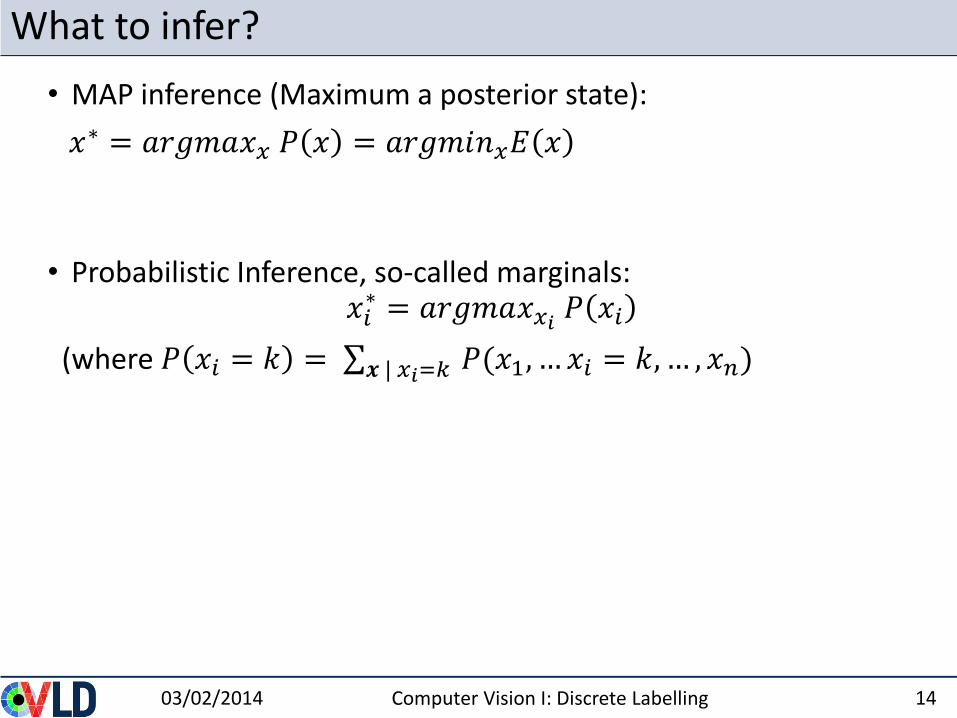
What to infer?
• MAP inference (Maximum a posterior state):
𝑥∗ = 𝑎𝑟𝑔𝑚𝑎𝑥𝑥 𝑃 𝑥 = 𝑎𝑟𝑔𝑚𝑖𝑛𝑥𝐸 𝑥
• Probabilistic Inference, so-called marginals:𝑥𝑖∗ = 𝑎𝑟𝑔𝑚𝑎𝑥𝑥𝑖 𝑃 𝑥𝑖
(where 𝑃 𝑥𝑖 = 𝑘 = 𝒙 | 𝑥𝑖=𝑘 𝑃(𝑥1, … 𝑥𝑖 = 𝑘,… , 𝑥𝑛)
03/02/2014 Computer Vision I: Discrete Labelling 14
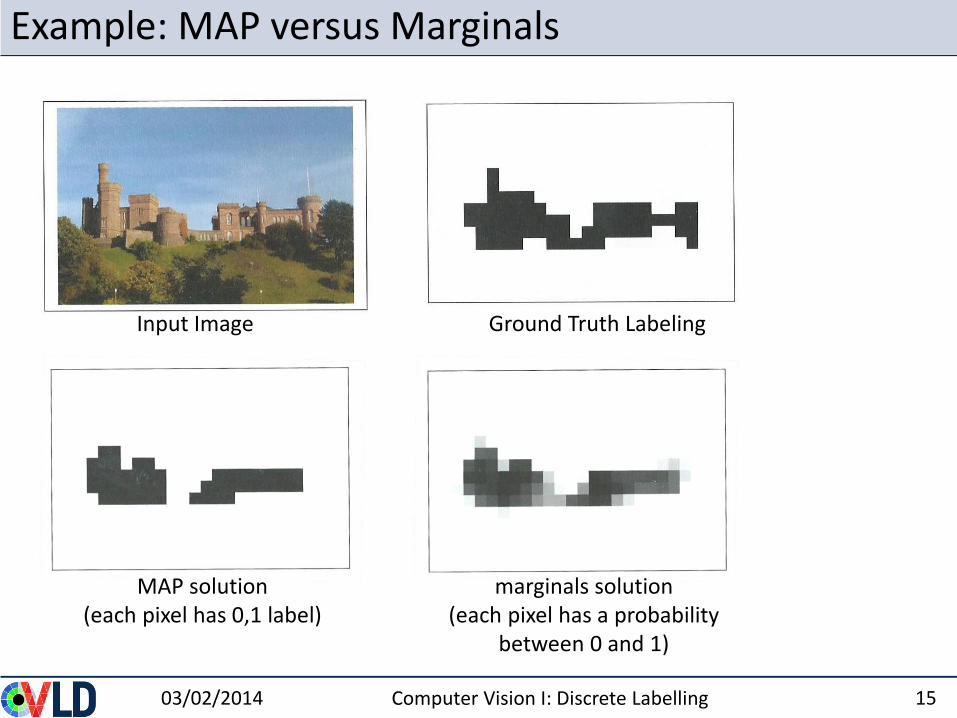
Example: MAP versus Marginals
03/02/2014 Computer Vision I: Discrete Labelling 15
Input Image Ground Truth Labeling
MAP solution (each pixel has 0,1 label)
marginals solution (each pixel has a probability
between 0 and 1)
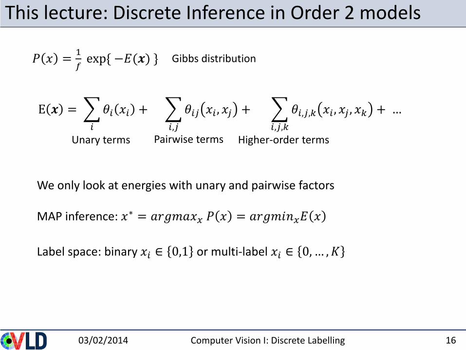
This lecture: Discrete Inference in Order 2 models
03/02/2014 Computer Vision I: Discrete Labelling 16
𝑃 𝑥 =1
𝑓exp{ −𝐸(𝒙) }
E 𝒙 =
𝑖
𝜃𝑖 𝑥𝑖 +
𝑖,𝑗
𝜃𝑖𝑗 𝑥𝑖 , 𝑥𝑗 +
𝑖,𝑗,𝑘
𝜃𝑖,𝑗,𝑘 𝑥𝑖 , 𝑥𝑗 , 𝑥𝑘 + …
Gibbs distribution
Unary terms Pairwise terms Higher-order terms
MAP inference: 𝑥∗ = 𝑎𝑟𝑔𝑚𝑎𝑥𝑥 𝑃 𝑥 = 𝑎𝑟𝑔𝑚𝑖𝑛𝑥𝐸 𝑥
Label space: binary 𝑥𝑖 ∈ 0,1 or multi-label 𝑥𝑖 ∈ 0,… , 𝐾
We only look at energies with unary and pairwise factors
Roadmap this lecture (chapter B.4-5 in book)
• Define: Markov Random Fields
• Formulate applications as discrete labeling problems
• Discrete Optimization: • Pixels-based: Iterative Conditional Mode (ICM),
Simulated Annealing• Line-based: Dynamic Programming (DP)• Field-based: Graph Cut and Alpha-Expansion
03/02/2014 Computer Vision I: Discrete Labelling 17
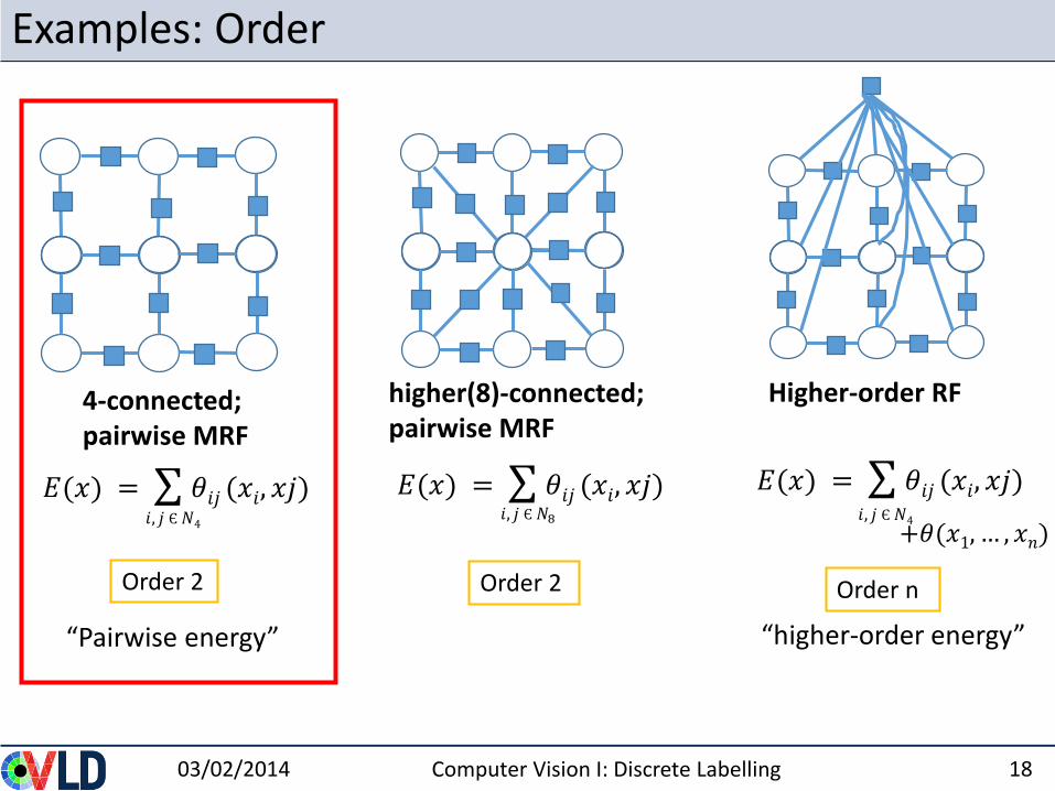
Examples: Order
03/02/2014 Computer Vision I: Discrete Labelling 18
4-connected; pairwise MRF
Higher-order RF
𝐸(𝑥) = 𝜃𝑖𝑗 (𝑥𝑖, 𝑥𝑗)𝑖, 𝑗 Є𝑁4
higher(8)-connected; pairwise MRF
Order 2 Order 2 Order n
𝐸(𝑥) = 𝜃𝑖𝑗 (𝑥𝑖, 𝑥𝑗)
“Pairwise energy” “higher-order energy”
𝐸(𝑥) = 𝜃𝑖𝑗 (𝑥𝑖, 𝑥𝑗)𝑖, 𝑗 Є𝑁8 𝑖, 𝑗 Є𝑁4
+𝜃(𝑥1, … , 𝑥𝑛)
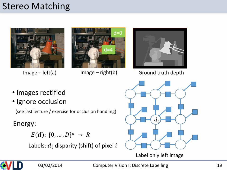
Stereo Matching
03/02/2014 Computer Vision I: Discrete Labelling 19
d=4
d=0
Ground truth depthImage – left(a) Image – right(b)
• Images rectified• Ignore occlusion
(see last lecture / exercise for occlusion handling)
𝐸(𝒅): {0, … , 𝐷}𝑛 → 𝑅
Energy:
Labels: 𝑑𝑖 disparity (shift) of pixel 𝑖
𝑑𝑖
Label only left image
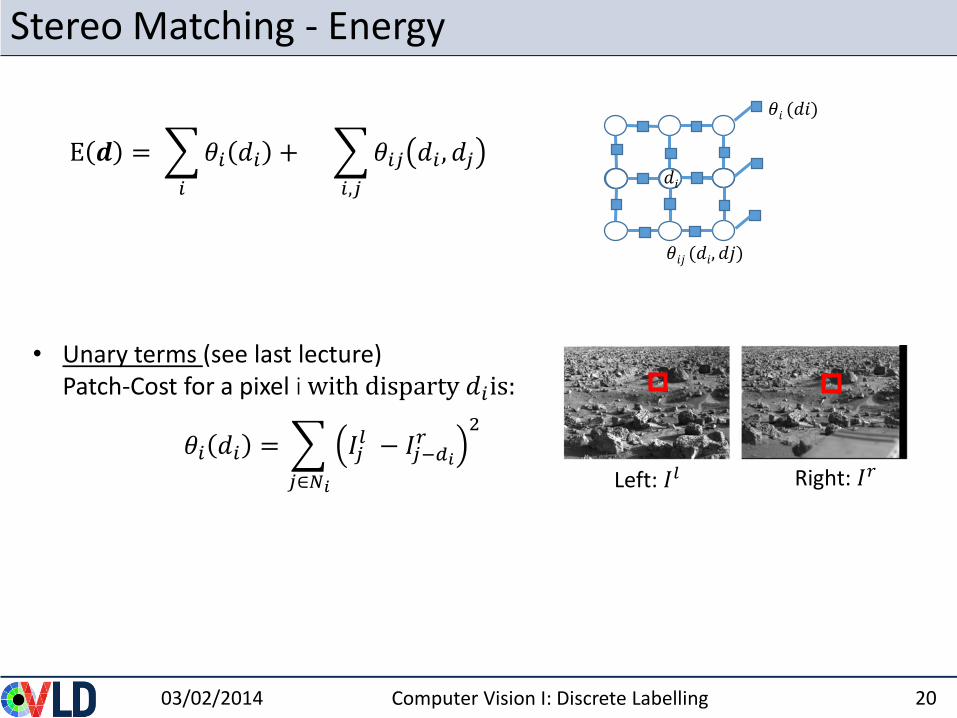
Stereo Matching - Energy
03/02/2014 Computer Vision I: Discrete Labelling 20
• Unary terms (see last lecture)Patch-Cost for a pixel i with disparty 𝑑𝑖is:
𝜃𝑖 𝑑𝑖 =
𝑗∈𝑁𝑖
𝐼𝑗𝑙 − 𝐼𝑗−𝑑𝑖𝑟2
Left: 𝐼𝑙
E 𝒅 =
𝑖
𝜃𝑖 𝑑𝑖 +
𝑖,𝑗
𝜃𝑖𝑗 𝑑𝑖 , 𝑑𝑗
Right: 𝐼𝑟
𝑑𝑖
𝜃𝑖 (𝑑𝑖)
𝜃𝑖𝑗 (𝑑𝑖, 𝑑𝑗)
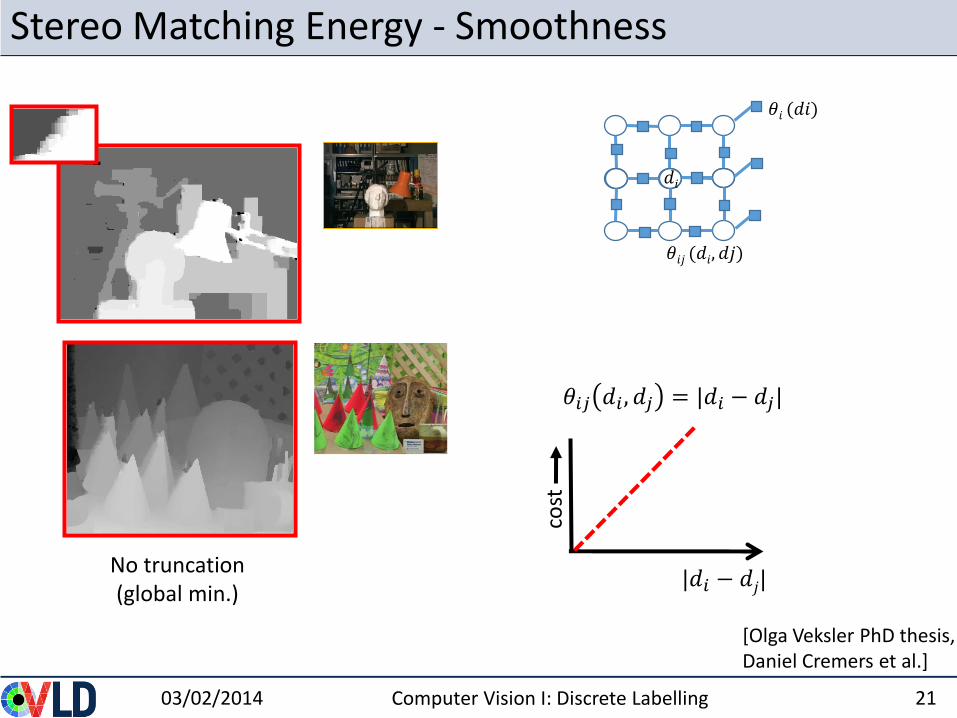
Stereo Matching Energy - Smoothness
03/02/2014 Computer Vision I: Discrete Labelling 21
[Olga Veksler PhD thesis, Daniel Cremers et al.]
|𝑑𝑖 − 𝑑𝑗|co
stNo truncation(global min.)
𝜃𝑖𝑗 𝑑𝑖 , 𝑑𝑗 = |𝑑𝑖 − 𝑑𝑗|
𝑑𝑖
𝜃𝑖 (𝑑𝑖)
𝜃𝑖𝑗 (𝑑𝑖, 𝑑𝑗)
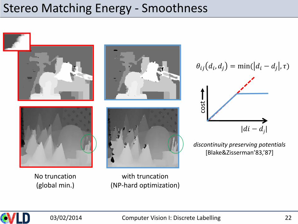
Stereo Matching Energy - Smoothness
03/02/2014 Computer Vision I: Discrete Labelling 22
discontinuity preserving potentials[Blake&Zisserman’83,’87]
cost
No truncation(global min.)
with truncation(NP-hard optimization)
|𝑑𝑖 − 𝑑𝑗|
𝜃𝑖𝑗 𝑑𝑖 , 𝑑𝑗 = min( 𝑑𝑖 − 𝑑𝑗 , 𝜏)
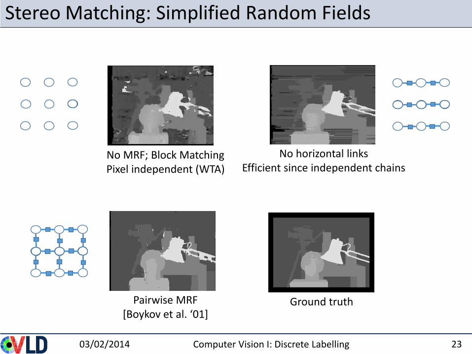
Stereo Matching: Simplified Random Fields
03/02/2014 Computer Vision I: Discrete Labelling 23
No MRF; Block MatchingPixel independent (WTA)
No horizontal links Efficient since independent chains
Ground truthPairwise MRF[Boykov et al. ‘01]
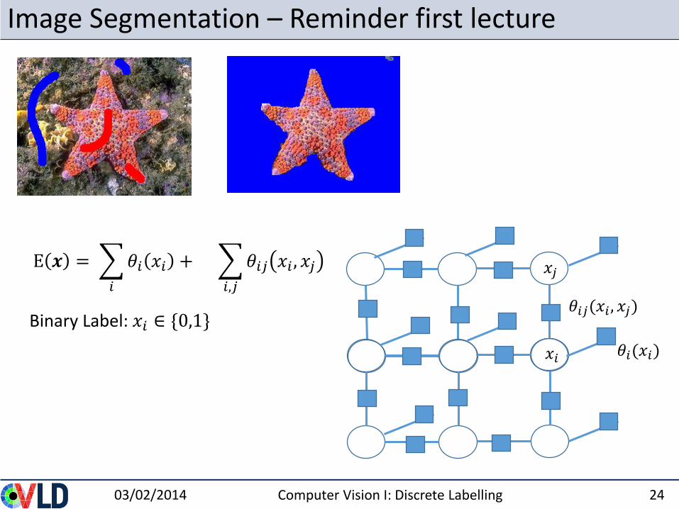
Image Segmentation – Reminder first lecture
03/02/2014 24
𝜃𝑖𝑗(𝑥𝑖 , 𝑥𝑗)
𝑥𝑗
𝜃𝑖(𝑥𝑖)𝑥𝑖
E 𝒙 =
𝑖
𝜃𝑖 𝑥𝑖 +
𝑖,𝑗
𝜃𝑖𝑗 𝑥𝑖 , 𝑥𝑗
Binary Label: 𝑥𝑖 ∈ {0,1}
Computer Vision I: Discrete Labelling
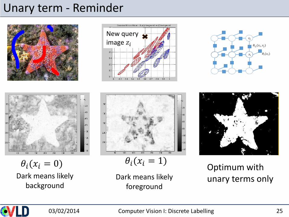
Unary term - Reminder
03/02/2014 25
Optimum with unary terms onlyDark means likely
backgroundDark means likely
foreground
𝜃𝑖(𝑥𝑖 = 0)𝜃𝑖(𝑥𝑖 = 1)
New query image 𝑧𝑖
Computer Vision I: Discrete Labelling
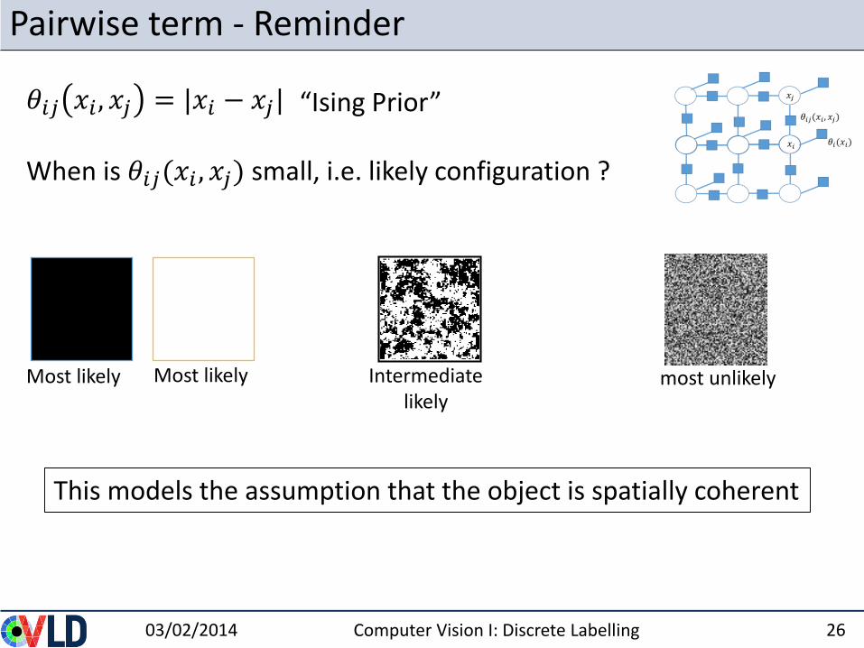
Pairwise term - Reminder
03/02/2014 26
Most likely Most likely Intermediate likely
“Ising Prior”
most unlikely
This models the assumption that the object is spatially coherent
𝜃𝑖𝑗 𝑥𝑖 , 𝑥𝑗 = |𝑥𝑖 − 𝑥𝑗|
When is 𝜃𝑖𝑗(𝑥𝑖 , 𝑥𝑗) small, i.e. likely configuration ?
Computer Vision I: Discrete Labelling
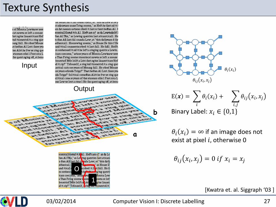
Texture Synthesis
03/02/2014 Computer Vision I: Discrete Labelling 27
Input
Output
[Kwatra et. al. Siggraph ‘03 ]
b
a
O
1
E 𝒙 =
𝑖
𝜃𝑖 𝑥𝑖 +
𝑖,𝑗
𝜃𝑖𝑗 𝑥𝑖 , 𝑥𝑗
Binary Label: 𝑥𝑖 ∈ {0,1}
𝜃𝑖𝑗 𝑥𝑖 , 𝑥𝑗
𝜃𝑖 𝑥𝑖
𝜃𝑖𝑗 𝑥𝑖 , 𝑥𝑗 = 0 𝑖𝑓 𝑥𝑖 = 𝑥𝑗
𝜃𝑖 𝑥𝑖 = ∞ if an image does not exist at pixel 𝑖, otherwise 0
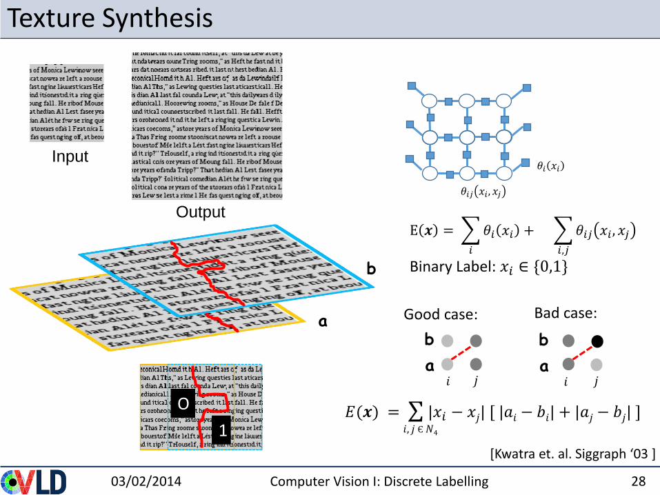
Texture Synthesis
03/02/2014 Computer Vision I: Discrete Labelling 28
Input
Output
[Kwatra et. al. Siggraph ‘03 ]
b
a
O
1
E 𝒙 =
𝑖
𝜃𝑖 𝑥𝑖 +
𝑖,𝑗
𝜃𝑖𝑗 𝑥𝑖 , 𝑥𝑗
Binary Label: 𝑥𝑖 ∈ {0,1}
𝜃𝑖𝑗 𝑥𝑖 , 𝑥𝑗
𝜃𝑖 𝑥𝑖
a
b
a
b
𝑖 𝑗 𝑖 𝑗
Good case: Bad case:
𝐸(𝒙) = |𝑥𝑖 − 𝑥𝑗| [ |𝑎𝑖 − 𝑏𝑖| + |𝑎𝑗 − 𝑏𝑗| ]𝑖, 𝑗 Є𝑁4
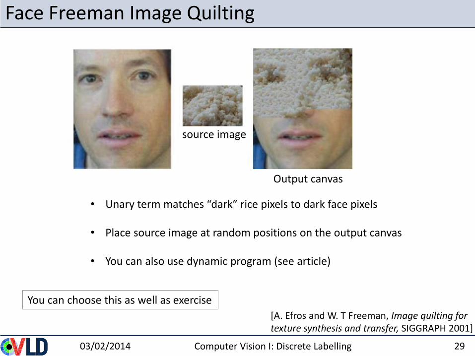
Face Freeman Image Quilting
03/02/2014 Computer Vision I: Discrete Labelling 29
You can choose this as well as exercise
[A. Efros and W. T Freeman, Image quilting for texture synthesis and transfer, SIGGRAPH 2001]
• Unary term matches “dark” rice pixels to dark face pixels
• Place source image at random positions on the output canvas
• You can also use dynamic program (see article)
source image
Output canvas
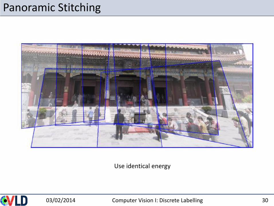
Panoramic Stitching
03/02/2014 Computer Vision I: Discrete Labelling 30
Use identical energy
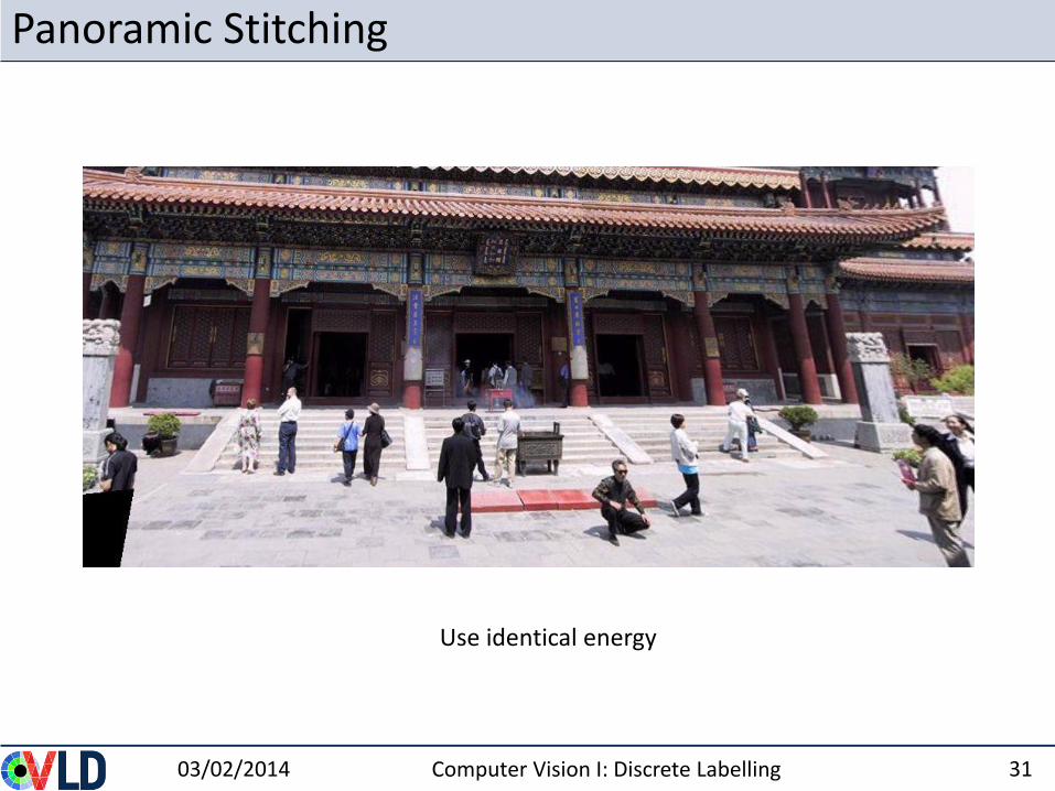
Panoramic Stitching
03/02/2014 Computer Vision I: Discrete Labelling 31
Use identical energy
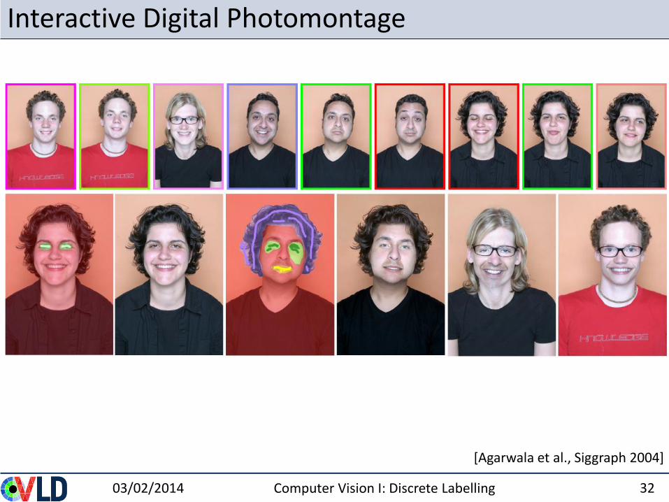
Interactive Digital Photomontage
03/02/2014 Computer Vision I: Discrete Labelling 32
[Agarwala et al., Siggraph 2004]
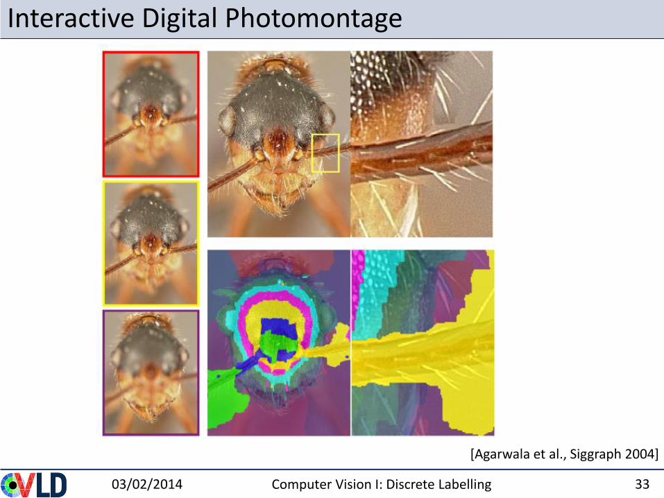
Interactive Digital Photomontage
03/02/2014 Computer Vision I: Discrete Labelling 33
[Agarwala et al., Siggraph 2004]
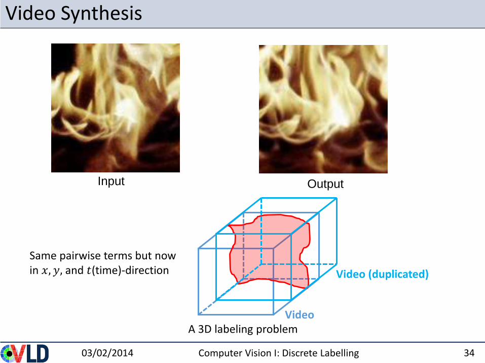
Video Synthesis
03/02/2014 Computer Vision I: Discrete Labelling 34
OutputInput
Video
Video (duplicated)
A 3D labeling problem
Same pairwise terms but now in 𝑥, 𝑦, and 𝑡(time)-direction
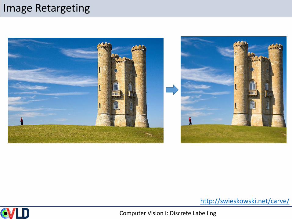
Image Retargeting
http://swieskowski.net/carve/
Computer Vision I: Discrete Labelling
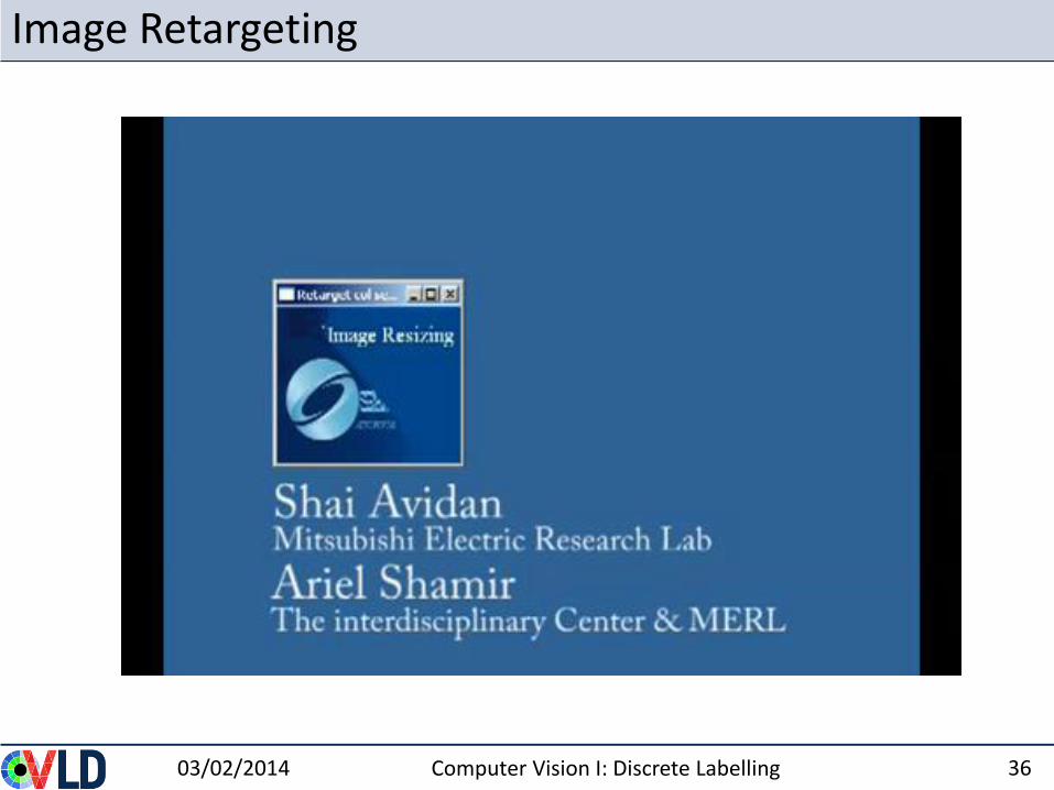
Image Retargeting
03/02/2014 Computer Vision I: Discrete Labelling 36
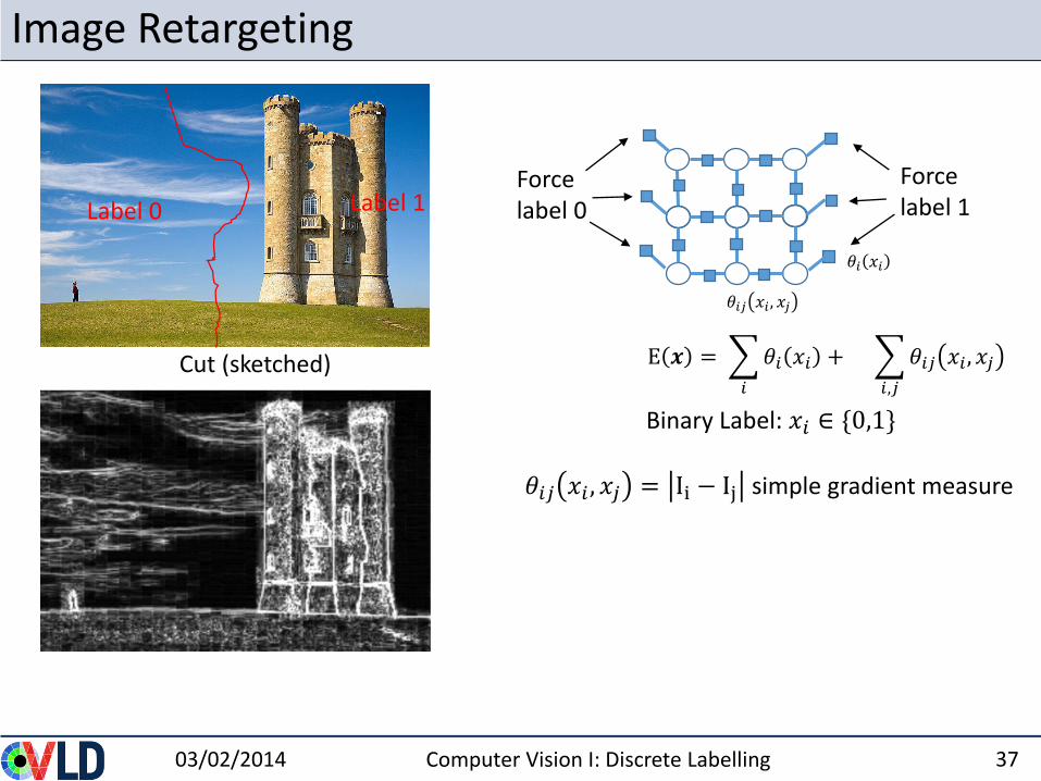
Image Retargeting
03/02/2014 Computer Vision I: Discrete Labelling 37
E 𝒙 =
𝑖
𝜃𝑖 𝑥𝑖 +
𝑖,𝑗
𝜃𝑖𝑗 𝑥𝑖 , 𝑥𝑗
Binary Label: 𝑥𝑖 ∈ {0,1}
𝜃𝑖𝑗 𝑥𝑖 , 𝑥𝑗
𝜃𝑖 𝑥𝑖
Force label 0
Force label 1
Cut (sketched)
Label 0 Label 1
𝜃𝑖𝑗 𝑥𝑖 , 𝑥𝑗 = Ii − Ij simple gradient measure
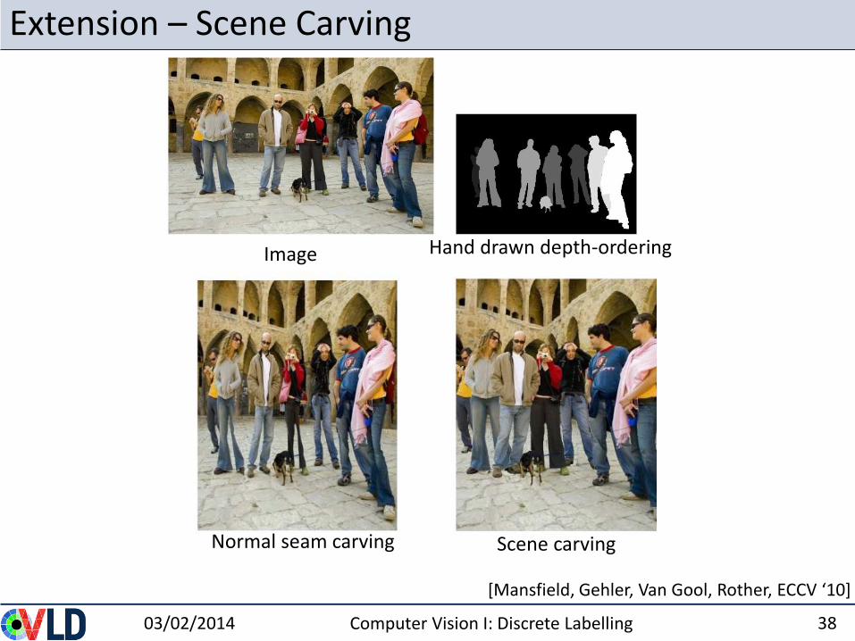
Extension – Scene Carving
03/02/2014 Computer Vision I: Discrete Labelling 38
[Mansfield, Gehler, Van Gool, Rother, ECCV ‘10]
Image Hand drawn depth-ordering
Normal seam carving Scene carving
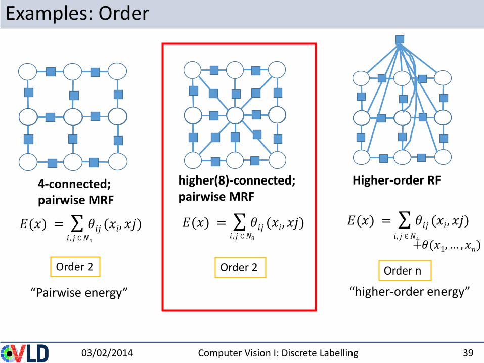
Examples: Order
03/02/2014 Computer Vision I: Discrete Labelling 39
4-connected; pairwise MRF
Higher-order RF
𝐸(𝑥) = 𝜃𝑖𝑗 (𝑥𝑖, 𝑥𝑗)𝑖, 𝑗 Є𝑁4
higher(8)-connected; pairwise MRF
Order 2 Order 2 Order n
𝐸(𝑥) = 𝜃𝑖𝑗 (𝑥𝑖, 𝑥𝑗)
“Pairwise energy” “higher-order energy”
𝐸(𝑥) = 𝜃𝑖𝑗 (𝑥𝑖, 𝑥𝑗)𝑖, 𝑗 Є𝑁8 𝑖, 𝑗 Є𝑁4
+𝜃(𝑥1, … , 𝑥𝑛)
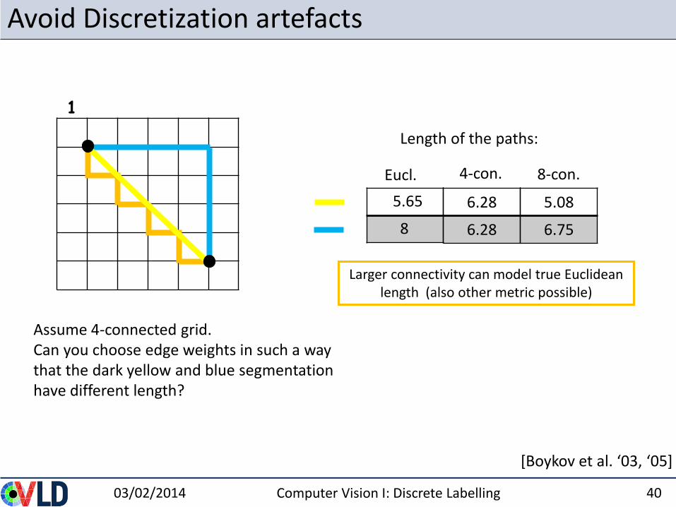
Avoid Discretization artefacts
03/02/2014 Computer Vision I: Discrete Labelling 40
[Boykov et al. ‘03, ‘05]
Larger connectivity can model true Euclidean length (also other metric possible)
Eucl.
Length of the paths:
4-con.
5.65
8
1
8-con.
6.28
6.28
5.08
6.75
Assume 4-connected grid.Can you choose edge weights in such a way that the dark yellow and blue segmentation have different length?
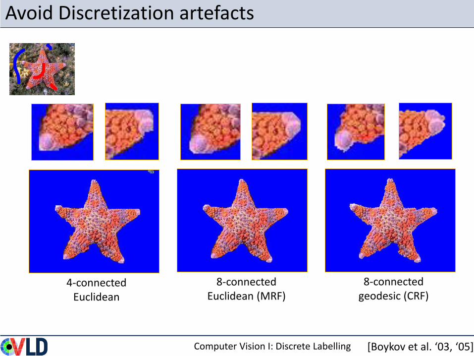
Avoid Discretization artefacts
[Boykov et al. ‘03, ‘05]
4-connected Euclidean
8-connected Euclidean (MRF)
8-connected geodesic (CRF)
Computer Vision I: Discrete Labelling
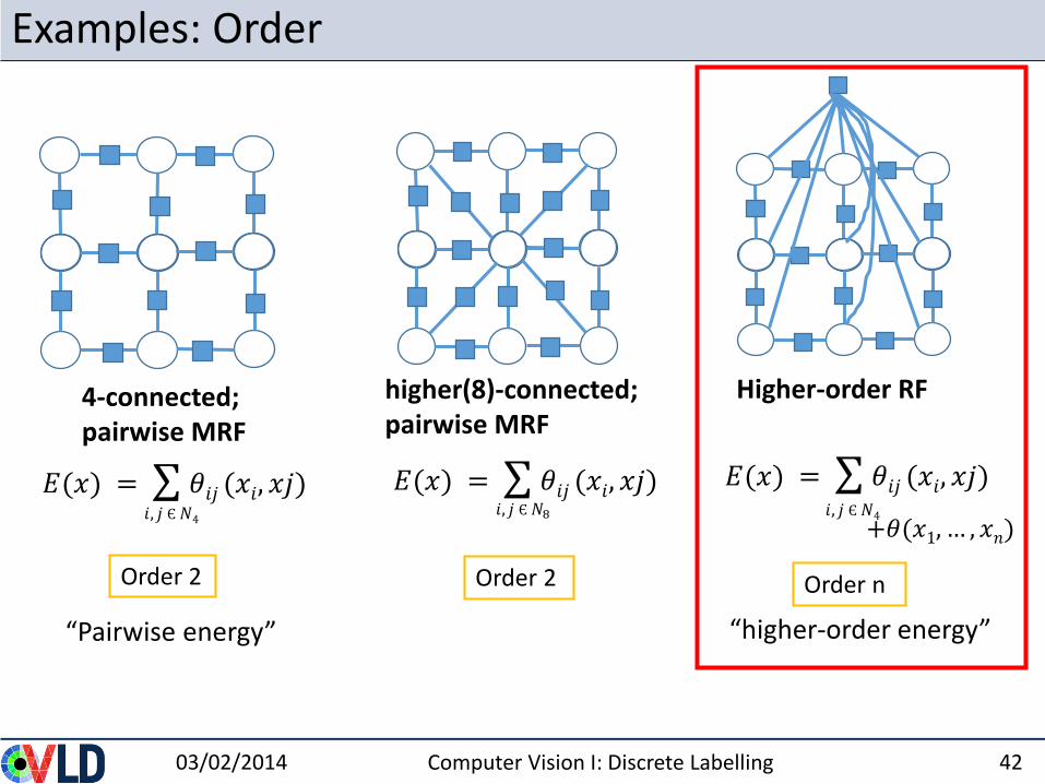
Examples: Order
03/02/2014 Computer Vision I: Discrete Labelling 42
4-connected; pairwise MRF
Higher-order RF
𝐸(𝑥) = 𝜃𝑖𝑗 (𝑥𝑖, 𝑥𝑗)𝑖, 𝑗 Є𝑁4
higher(8)-connected; pairwise MRF
Order 2 Order 2 Order n
𝐸(𝑥) = 𝜃𝑖𝑗 (𝑥𝑖, 𝑥𝑗)
“Pairwise energy” “higher-order energy”
𝐸(𝑥) = 𝜃𝑖𝑗 (𝑥𝑖, 𝑥𝑗)𝑖, 𝑗 Є𝑁8 𝑖, 𝑗 Є𝑁4
+𝜃(𝑥1, … , 𝑥𝑛)
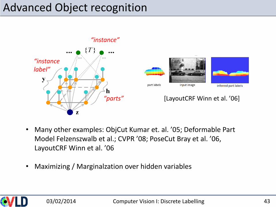
Advanced Object recognition
03/02/2014 Computer Vision I: Discrete Labelling 43
• Many other examples: ObjCut Kumar et. al. ’05; Deformable Part Model Felzenszwalb et al.; CVPR ’08; PoseCut Bray et al. ’06, LayoutCRF Winn et al. ’06
• Maximizing / Marginalzation over hidden variables
“parts”
“instancelabel”
“instance”
[LayoutCRF Winn et al. ’06]
Roadmap this lecture (chapter B.4-5 in book)
• Define: Markov Random Fields
• Formulate applications as discrete labeling problems
• Discrete Optimization: • Pixels-based: Iterative Conditional Mode (ICM),
Simulated Annealing• Line-based: Dynamic Programming (DP)• Field-based: Graph Cut and Alpha-Expansion
03/02/2014 Computer Vision I: Discrete Labelling 44
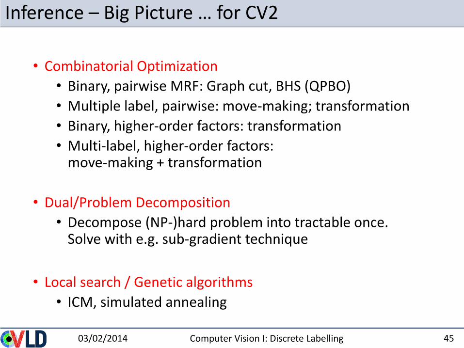
Inference – Big Picture … for CV2
03/02/2014 Computer Vision I: Discrete Labelling 45
• Combinatorial Optimization
• Binary, pairwise MRF: Graph cut, BHS (QPBO)
• Multiple label, pairwise: move-making; transformation
• Binary, higher-order factors: transformation
• Multi-label, higher-order factors: move-making + transformation
• Dual/Problem Decomposition
• Decompose (NP-)hard problem into tractable once.Solve with e.g. sub-gradient technique
• Local search / Genetic algorithms
• ICM, simulated annealing
03/02/2014 Computer Vision I: Discrete Labelling 46
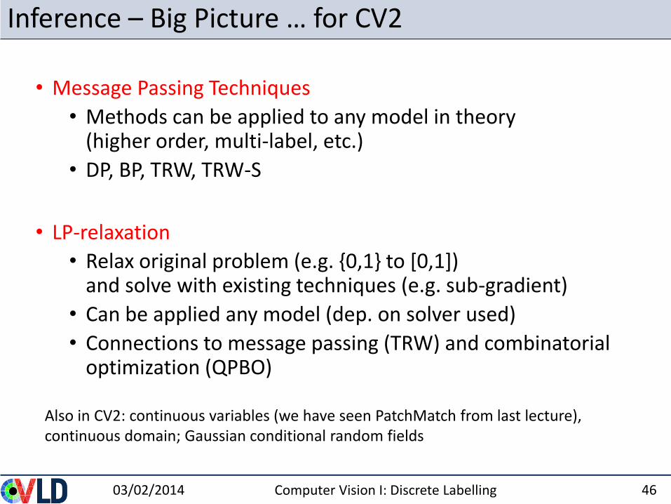
Inference – Big Picture … for CV2
• Message Passing Techniques
• Methods can be applied to any model in theory(higher order, multi-label, etc.)
• DP, BP, TRW, TRW-S
• LP-relaxation
• Relax original problem (e.g. {0,1} to [0,1]) and solve with existing techniques (e.g. sub-gradient)
• Can be applied any model (dep. on solver used)
• Connections to message passing (TRW) and combinatorial optimization (QPBO)
Also in CV2: continuous variables (we have seen PatchMatch from last lecture), continuous domain; Gaussian conditional random fields
Function Minimization: The Problems
03/02/2014 Computer Vision I: Discrete Labelling 47
• Which functions are exactly solvable?
• Approximate solutions of NP-hard problems
Function Minimization: The Problems
03/02/2014 Computer Vision I: Discrete Labelling 48
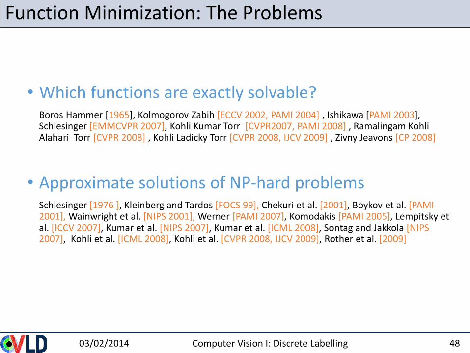
• Which functions are exactly solvable?Boros Hammer [1965], Kolmogorov Zabih [ECCV 2002, PAMI 2004] , Ishikawa [PAMI 2003], Schlesinger [EMMCVPR 2007], Kohli Kumar Torr [CVPR2007, PAMI 2008] , Ramalingam Kohli Alahari Torr [CVPR 2008] , Kohli Ladicky Torr [CVPR 2008, IJCV 2009] , Zivny Jeavons [CP 2008]
• Approximate solutions of NP-hard problemsSchlesinger [1976 ], Kleinberg and Tardos [FOCS 99], Chekuri et al. [2001], Boykov et al. [PAMI 2001], Wainwright et al. [NIPS 2001], Werner [PAMI 2007], Komodakis [PAMI 2005], Lempitsky et al. [ICCV 2007], Kumar et al. [NIPS 2007], Kumar et al. [ICML 2008], Sontag and Jakkola [NIPS 2007], Kohli et al. [ICML 2008], Kohli et al. [CVPR 2008, IJCV 2009], Rother et al. [2009]
ICM - Iterated conditional mode
03/02/2014 Computer Vision I: Discrete Labelling 49
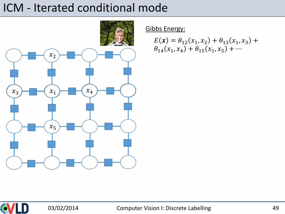
Gibbs Energy:
𝑥2
𝑥1𝑥3 𝑥4
𝑥5
𝐸 𝒙 = 𝜃12 𝑥1, 𝑥2 + 𝜃13 𝑥1, 𝑥3 +𝜃14 𝑥1, 𝑥4 + 𝜃15 𝑥1, 𝑥5 +⋯
ICM - Iterated conditional mode
03/02/2014 Computer Vision I: Discrete Labelling 50
𝑥2
𝑥1𝑥3 𝑥4
𝑥5
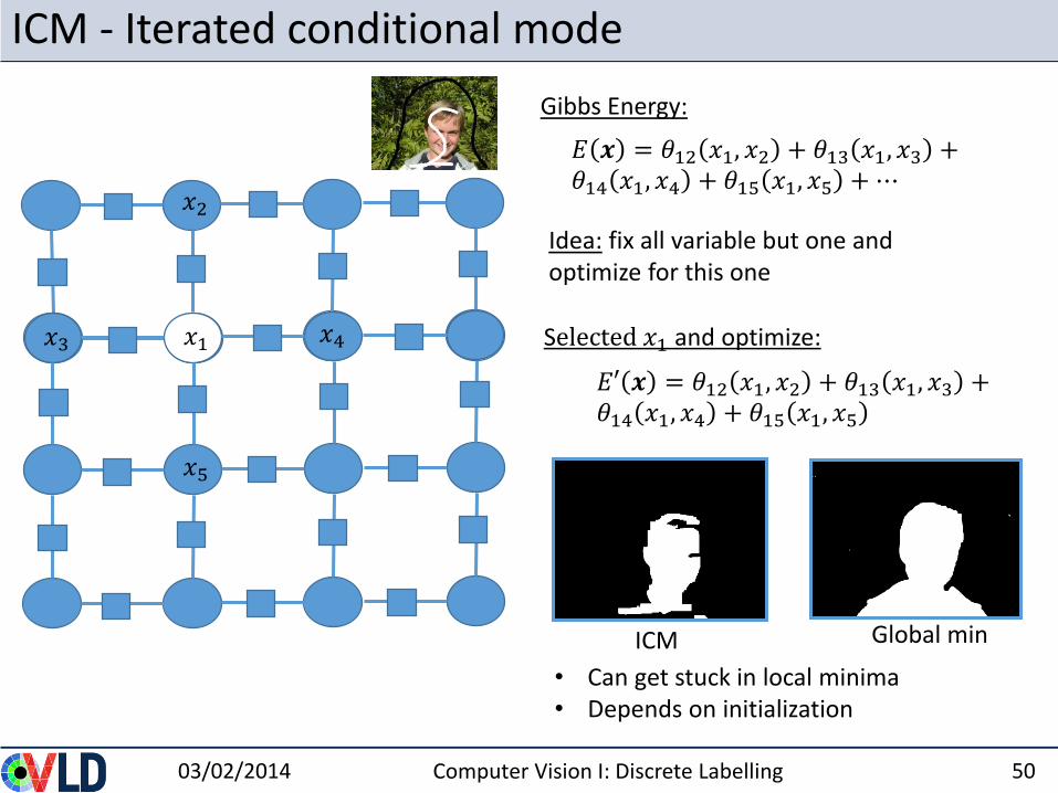
Idea: fix all variable but one and optimize for this one
Selected 𝑥1 and optimize:
Gibbs Energy:
• Can get stuck in local minima• Depends on initialization
ICM Global min
𝐸 𝒙 = 𝜃12 𝑥1, 𝑥2 + 𝜃13 𝑥1, 𝑥3 +𝜃14 𝑥1, 𝑥4 + 𝜃15 𝑥1, 𝑥5 +⋯
𝐸′ 𝒙 = 𝜃12 𝑥1, 𝑥2 + 𝜃13 𝑥1, 𝑥3 +𝜃14 𝑥1, 𝑥4 + 𝜃15 𝑥1, 𝑥5
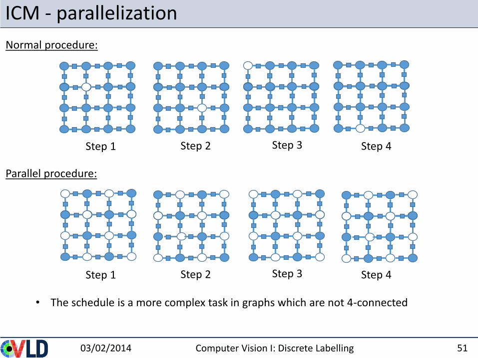
ICM - parallelization
03/02/2014 Computer Vision I: Discrete Labelling 51
• The schedule is a more complex task in graphs which are not 4-connected
Normal procedure:
Step 1 Step 2 Step 3 Step 4
Parallel procedure:
Step 1 Step 2 Step 3 Step 4
ICM - Iterated conditional mode
Extension / related techniques
03/02/2014 Computer Vision I: Discrete Labelling 52
• Simulated annealing (next)• Block ICM (see exercise)• Gibbs sampling• Lazy Flipper: MAP Inference in Higher-Order Graphical Models by Depth-limited
Exhaustive Search [Bjoern Andres, Joerg H. Kappes, Ullrich Koethe, Fred A. Hamprecht]
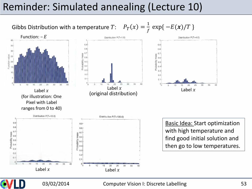
Reminder: Simulated annealing (Lecture 10)
03/02/2014 Computer Vision I: Discrete Labelling 53
Gibbs Distribution with a temperature 𝑇: 𝑃𝑇 𝑥 =1
𝑓exp{ −𝐸(𝒙)/𝑇 }
Basic Idea: Start optimization with high temperature and find good initial solution and then go to low temperatures.
Function: –𝐸
Label 𝑥(for illustration: One
Pixel with Label ranges from 0 to 40)
(original distribution)Label 𝑥 Label 𝑥
Label 𝑥 Label 𝑥
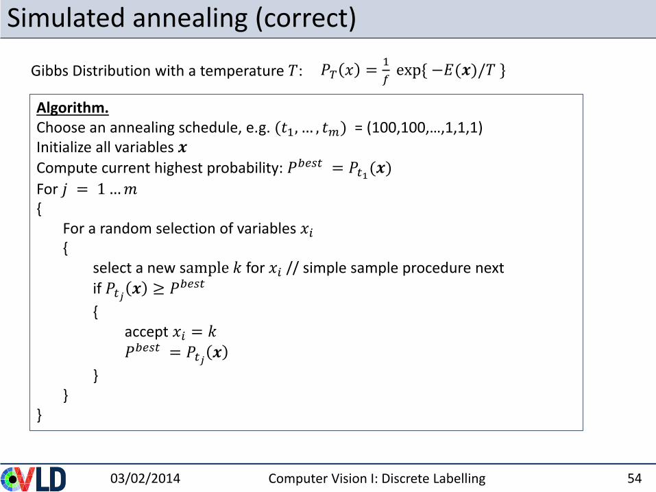
Simulated annealing (correct)
03/02/2014 Computer Vision I: Discrete Labelling 54
Algorithm.Choose an annealing schedule, e.g. (𝑡1, … , 𝑡𝑚) = (100,100,…,1,1,1)Initialize all variables 𝒙
Compute current highest probability: 𝑃𝑏𝑒𝑠𝑡 = 𝑃𝑡1(𝒙)
For 𝑗 = 1…𝑚{
For a random selection of variables 𝑥𝑖{
select a new sample 𝑘 for 𝑥𝑖 // simple sample procedure next
if 𝑃𝑡𝑗 𝒙 ≥ 𝑃𝑏𝑒𝑠𝑡
{accept 𝑥𝑖 = 𝑘
𝑃𝑏𝑒𝑠𝑡 = 𝑃𝑡𝑗 𝒙
}}
}
Gibbs Distribution with a temperature 𝑇: 𝑃𝑇 𝑥 =1
𝑓exp{ −𝐸(𝒙)/𝑇 }
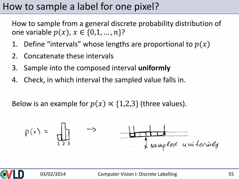
How to sample a label for one pixel?
03/02/2014 55
How to sample from a general discrete probability distribution of one variable 𝑝(𝑥), 𝑥 ∈ {0,1,… , 𝑛}?
1. Define “intervals” whose lengths are proportional to 𝑝(𝑥)
2. Concatenate these intervals
3. Sample into the composed interval uniformly
4. Check, in which interval the sampled value falls in.
Below is an example for 𝑝 𝑥 ∝ {1,2,3} (three values).
Computer Vision I: Discrete Labelling
1 2 3
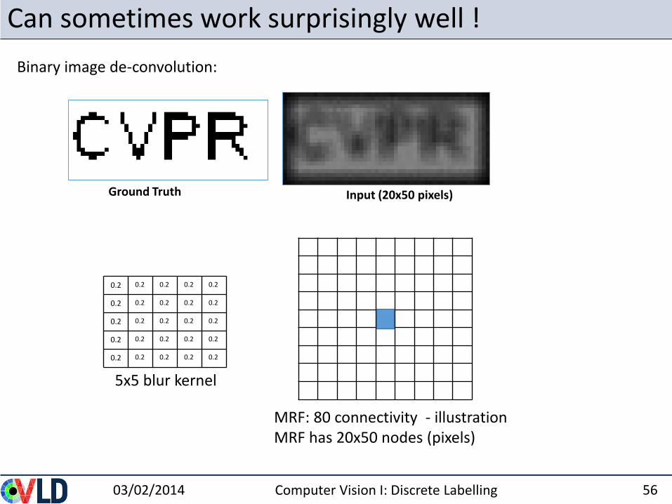
Can sometimes work surprisingly well !
03/02/2014 Computer Vision I: Discrete Labelling 56
Ground Truth Input (20x50 pixels)
0.2 0.2 0.2 0.2 0.2
0.2 0.2 0.2 0.2 0.2
0.2 0.2 0.2 0.2 0.2
0.2 0.2 0.2 0.2 0.2
0.2 0.2 0.2 0.2 0.2
MRF: 80 connectivity - illustrationMRF has 20x50 nodes (pixels)
5x5 blur kernel
Binary image de-convolution:
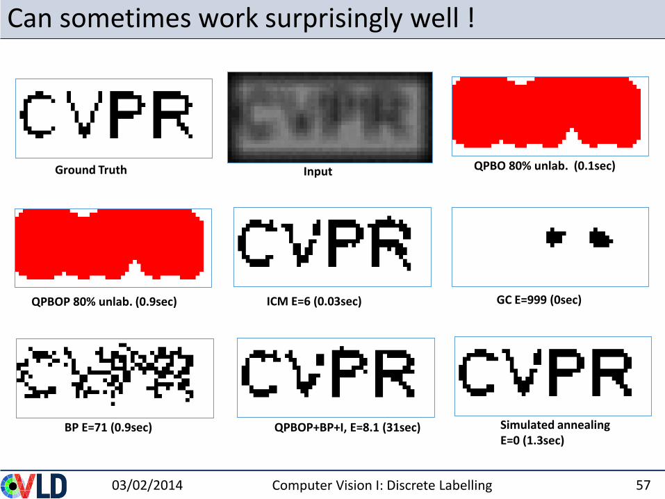
Can sometimes work surprisingly well !
03/02/2014 Computer Vision I: Discrete Labelling 57
Ground Truth QPBO 80% unlab. (0.1sec)Input
ICM E=6 (0.03sec)QPBOP 80% unlab. (0.9sec) GC E=999 (0sec)
BP E=71 (0.9sec) QPBOP+BP+I, E=8.1 (31sec) Simulated annealingE=0 (1.3sec)
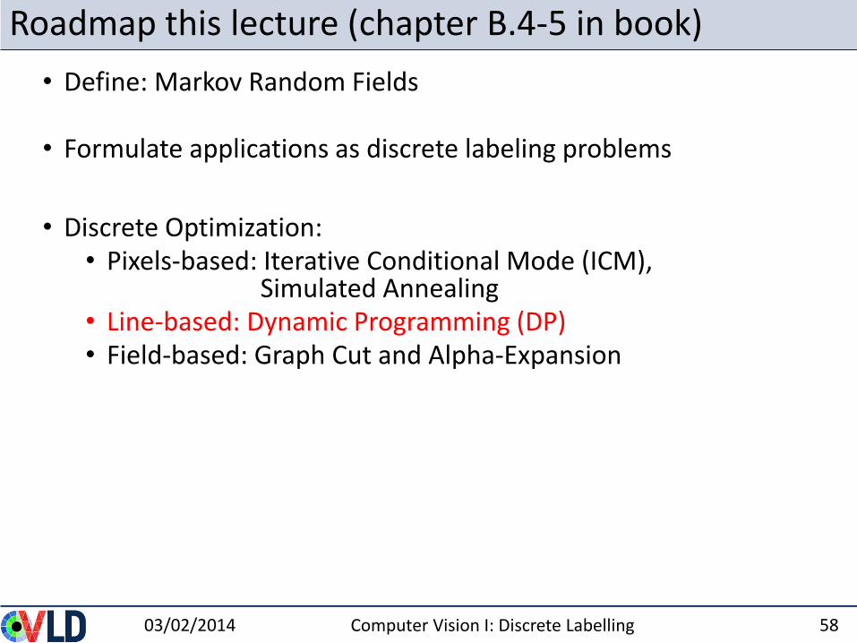
Roadmap this lecture (chapter B.4-5 in book)
• Define: Markov Random Fields
• Formulate applications as discrete labeling problems
• Discrete Optimization: • Pixels-based: Iterative Conditional Mode (ICM),
Simulated Annealing• Line-based: Dynamic Programming (DP)• Field-based: Graph Cut and Alpha-Expansion
03/02/2014 Computer Vision I: Discrete Labelling 58
What is dynamic programming?
dynamic programming is a method for solving complex problems by breaking them down into simpler subproblems. It will examine all possible ways to solve the problem and will find the optimal solution.
03/02/2014 Computer Vision I: Discrete Labelling 59
[From Wikipedia]
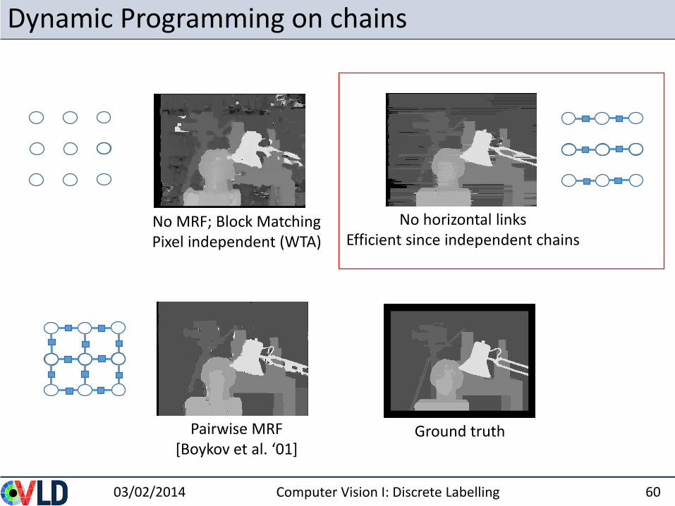
Dynamic Programming on chains
03/02/2014 Computer Vision I: Discrete Labelling 60
No MRF; Block MatchingPixel independent (WTA)
No horizontal links Efficient since independent chains
Ground truthPairwise MRF[Boykov et al. ‘01]
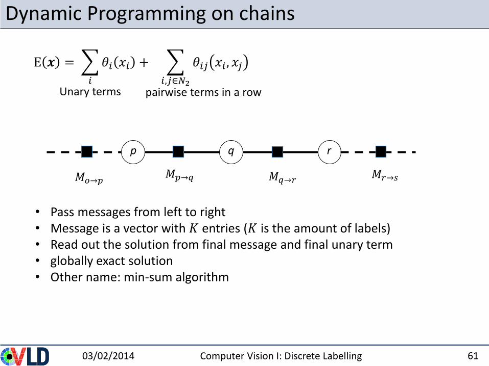
Dynamic Programming on chains
03/02/2014 Computer Vision I: Discrete Labelling 61
qp r
• Pass messages from left to right • Message is a vector with 𝐾 entries (𝐾 is the amount of labels)• Read out the solution from final message and final unary term• globally exact solution• Other name: min-sum algorithm
𝑀𝑞→𝑟
E 𝒙 =
𝑖
𝜃𝑖 𝑥𝑖 +
𝑖,𝑗∈𝑁2
𝜃𝑖𝑗 𝑥𝑖 , 𝑥𝑗
Unary terms pairwise terms in a row
𝑀𝑝→𝑞 𝑀𝑟→𝑠𝑀𝑜→𝑝
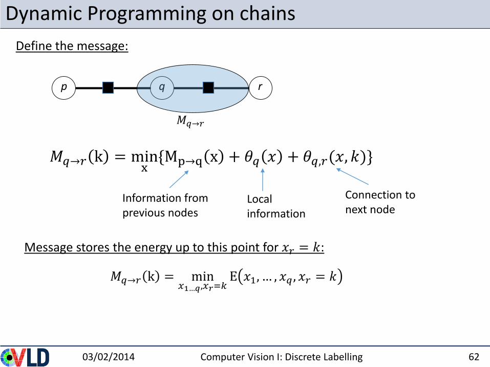
Dynamic Programming on chains
03/02/2014 Computer Vision I: Discrete Labelling 62
qp r
𝑀𝑞→𝑟
Define the message:
𝑀𝑞→𝑟 k = minx{Mp→q x + 𝜃𝑞 𝑥 + 𝜃𝑞,𝑟(𝑥, 𝑘)}
Information from previous nodes
Local information
Connection to next node
Message stores the energy up to this point for 𝑥𝑟 = 𝑘:
𝑀𝑞→𝑟 k = min𝑥1…𝑞,𝑥𝑟=𝑘
E 𝑥1, … , 𝑥𝑞 , 𝑥𝑟 = 𝑘
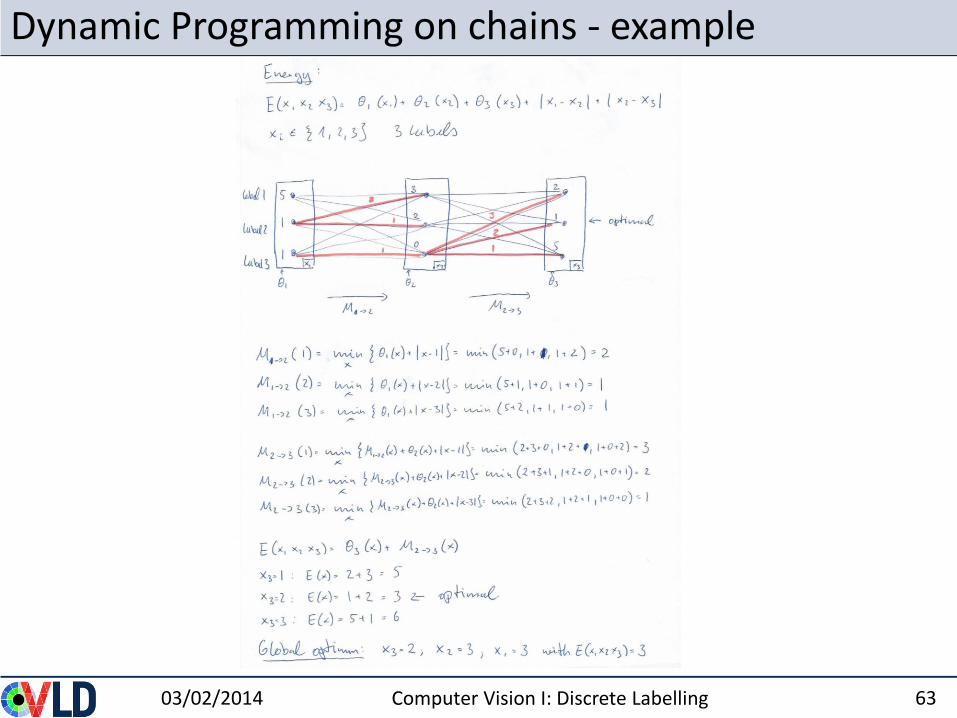
Dynamic Programming on chains - example
03/02/2014 Computer Vision I: Discrete Labelling 63
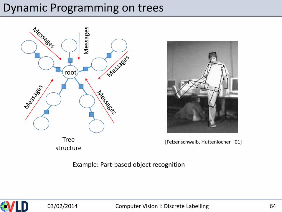
Dynamic Programming on trees
03/02/2014 Computer Vision I: Discrete Labelling 64
Treestructure
root
Example: Part-based object recognition
[Felzenschwalb, Huttenlocher ‘01]
Mes
sage
s
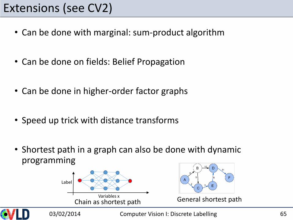
Extensions (see CV2)
• Can be done with marginal: sum-product algorithm
• Can be done on fields: Belief Propagation
• Can be done in higher-order factor graphs
• Speed up trick with distance transforms
• Shortest path in a graph can also be done with dynamic programming
03/02/2014 Computer Vision I: Discrete Labelling 65
Chain as shortest path General shortest path Variables x
Label
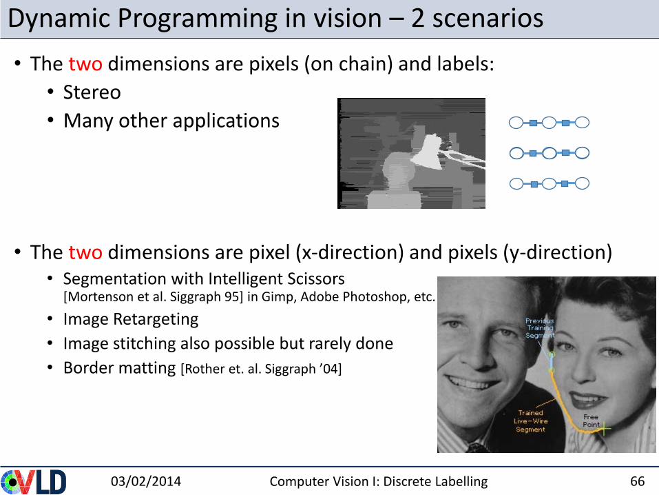
Dynamic Programming in vision – 2 scenarios
• The two dimensions are pixels (on chain) and labels:
• Stereo
• Many other applications
• The two dimensions are pixel (x-direction) and pixels (y-direction)• Segmentation with Intelligent Scissors
[Mortenson et al. Siggraph 95] in Gimp, Adobe Photoshop, etc.
• Image Retargeting
• Image stitching also possible but rarely done
• Border matting [Rother et. al. Siggraph ’04]
03/02/2014 Computer Vision I: Discrete Labelling 66
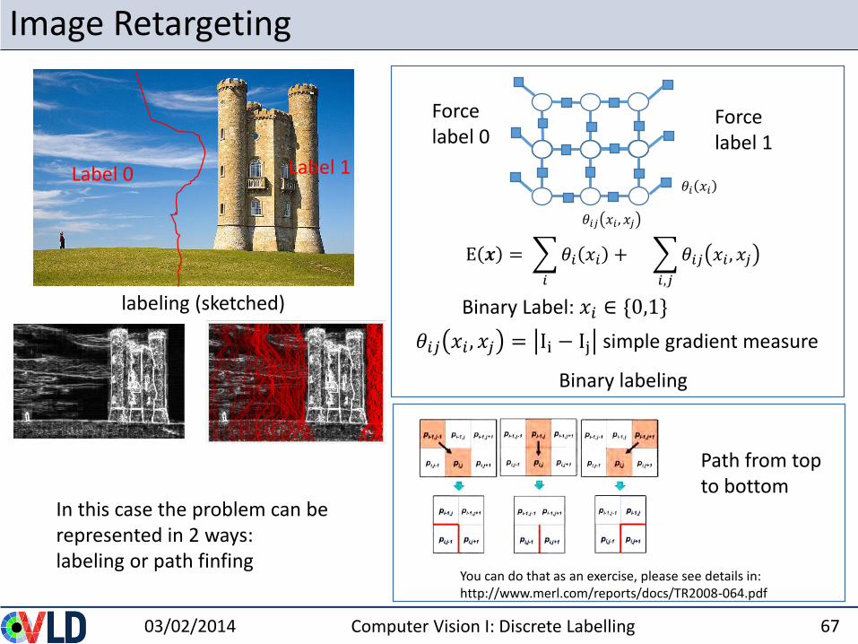
Image Retargeting
03/02/2014 Computer Vision I: Discrete Labelling 67
E 𝒙 =
𝑖
𝜃𝑖 𝑥𝑖 +
𝑖,𝑗
𝜃𝑖𝑗 𝑥𝑖 , 𝑥𝑗
Binary Label: 𝑥𝑖 ∈ {0,1}
𝜃𝑖𝑗 𝑥𝑖 , 𝑥𝑗
𝜃𝑖 𝑥𝑖
Force label 0
Force label 1
labeling (sketched)
Label 0 Label 1
𝜃𝑖𝑗 𝑥𝑖 , 𝑥𝑗 = Ii − Ij simple gradient measure
Path from top to bottom
Binary labeling
In this case the problem can be represented in 2 ways: labeling or path finfing
You can do that as an exercise, please see details in: http://www.merl.com/reports/docs/TR2008-064.pdf
Roadmap this lecture (chapter B.4-5 in book)
• Define: Markov Random Fields
• Formulate applications as discrete labeling problems
• Discrete Optimization: • Pixels-based: Iterative Conditional Mode (ICM),
Simulated Annealing• Line-based: Dynamic Programming (DP)• Field-based: Graph Cut and Alpha-Expansion
03/02/2014 Computer Vision I: Discrete Labelling 68
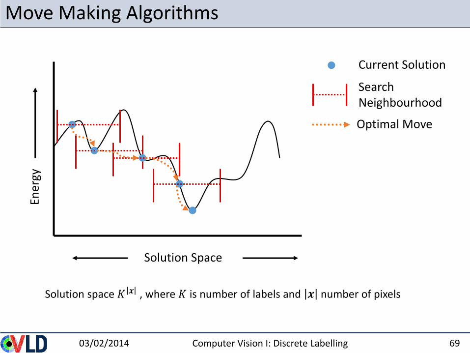
Move Making Algorithms
03/02/2014 Computer Vision I: Discrete Labelling 69
Search Neighbourhood
Current Solution
Optimal Move
Solution Space
Ener
gy
Solution space 𝐾 𝒙 , where 𝐾 is number of labels and 𝒙 number of pixels
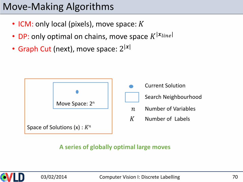
Move-Making Algorithms
• ICM: only local (pixels), move space: 𝐾
• DP: only optimal on chains, move space 𝐾|𝒙𝑙𝑖𝑛𝑒|
• Graph Cut (next), move space: 2|𝒙|
03/02/2014 Computer Vision I: Discrete Labelling 70
Space of Solutions (x) : 𝐾𝑛
Move Space: 2nSearch Neighbourhood
Current Solution
𝑛 Number of Variables
𝐾 Number of Labels
A series of globally optimal large moves
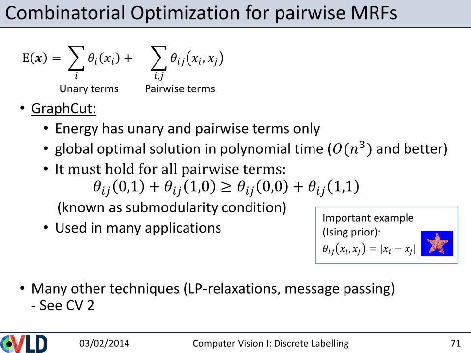
Combinatorial Optimization for pairwise MRFs
• GraphCut:
• Energy has unary and pairwise terms only
• global optimal solution in polynomial time (𝑂(𝑛3) and better)
• It must hold for all pairwise terms:𝜃𝑖𝑗 0,1 + 𝜃𝑖𝑗 1,0 ≥ 𝜃𝑖𝑗 0,0 + 𝜃𝑖𝑗 1,1
(known as submodularity condition)
• Used in many applications
• Many other techniques (LP-relaxations, message passing)- See CV 2
03/02/2014 Computer Vision I: Discrete Labelling 71
E 𝒙 =
𝑖
𝜃𝑖 𝑥𝑖 +
𝑖,𝑗
𝜃𝑖𝑗 𝑥𝑖 , 𝑥𝑗
Unary terms Pairwise terms
𝜃𝑖𝑗 𝑥𝑖 , 𝑥𝑗 = |𝑥𝑖 − 𝑥𝑗|
Important example (Ising prior):
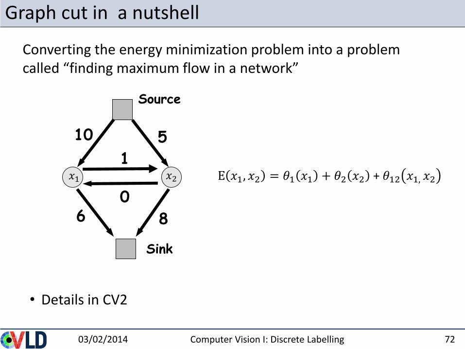
Graph cut in a nutshell
• Details in CV2
03/02/2014 Computer Vision I: Discrete Labelling 72
Converting the energy minimization problem into a problem called “finding maximum flow in a network”
10
1
Sink
Source
5
6 8
0
𝑥1 𝑥2 E 𝑥1, 𝑥2 = 𝜃1 𝑥1 + 𝜃2 𝑥2 + 𝜃12 𝑥1, 𝑥2
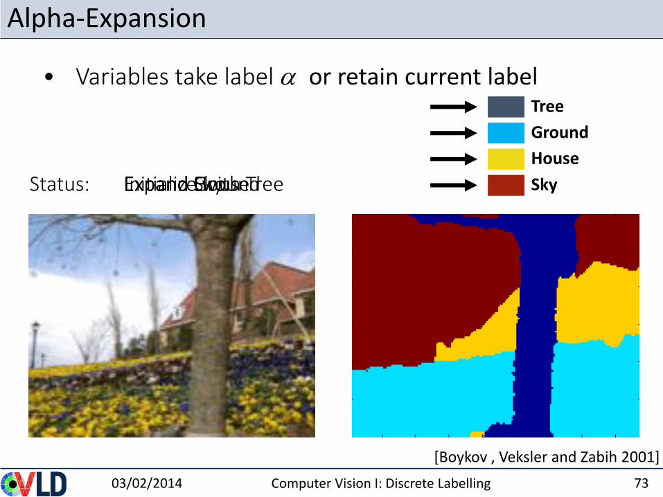
Alpha-Expansion
03/02/2014 Computer Vision I: Discrete Labelling 73
[Boykov , Veksler and Zabih 2001]
Sky
House
Tree
Ground
Initialize with TreeStatus: Expand GroundExpand HouseExpand Sky
• Variables take label a or retain current label
03/02/2014 Computer Vision I: Discrete Labelling 74
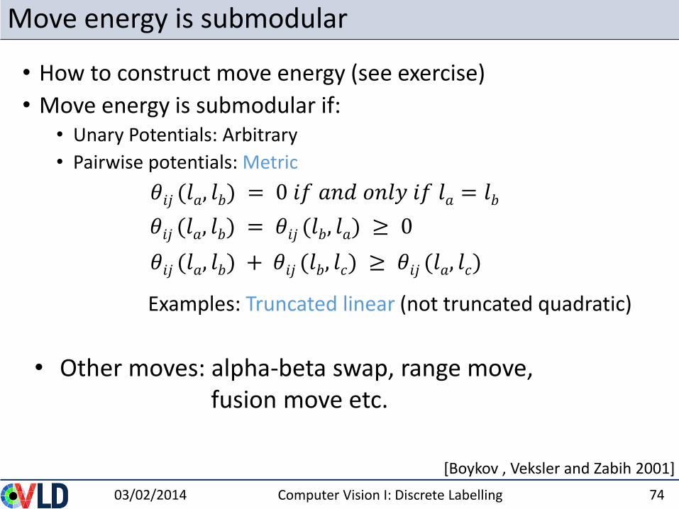
Move energy is submodular
• How to construct move energy (see exercise)
• Move energy is submodular if:• Unary Potentials: Arbitrary
• Pairwise potentials: Metric
[Boykov, Veksler, Zabih]
𝜃𝑖𝑗 (𝑙𝑎, 𝑙𝑏) = 0 𝑖𝑓 𝑎𝑛𝑑 𝑜𝑛𝑙𝑦 𝑖𝑓 𝑙𝑎 = 𝑙𝑏
Examples: Truncated linear (not truncated quadratic)
[Boykov , Veksler and Zabih 2001]
• Other moves: alpha-beta swap, range move, fusion move etc.
𝜃𝑖𝑗 (𝑙𝑎, 𝑙𝑏) + 𝜃𝑖𝑗 (𝑙𝑏, 𝑙𝑐) ≥ 𝜃𝑖𝑗 (𝑙𝑎, 𝑙𝑐)
𝜃𝑖𝑗 (𝑙𝑎, 𝑙𝑏) = 𝜃𝑖𝑗 (𝑙𝑏, 𝑙𝑎) ≥ 0
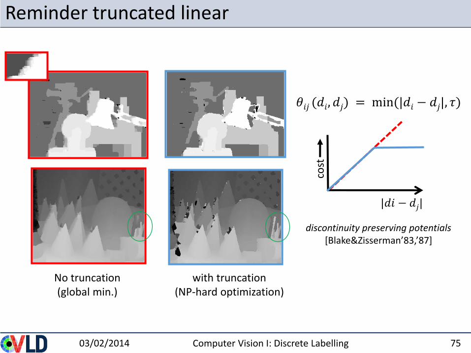
Reminder truncated linear
03/02/2014 Computer Vision I: Discrete Labelling 75
discontinuity preserving potentials[Blake&Zisserman’83,’87]
𝜃𝑖𝑗 (𝑑𝑖, 𝑑𝑗) = min(|𝑑𝑖 − 𝑑𝑗|, 𝜏)
cost
No truncation(global min.)
with truncation(NP-hard optimization)
|𝑑𝑖 − 𝑑𝑗|
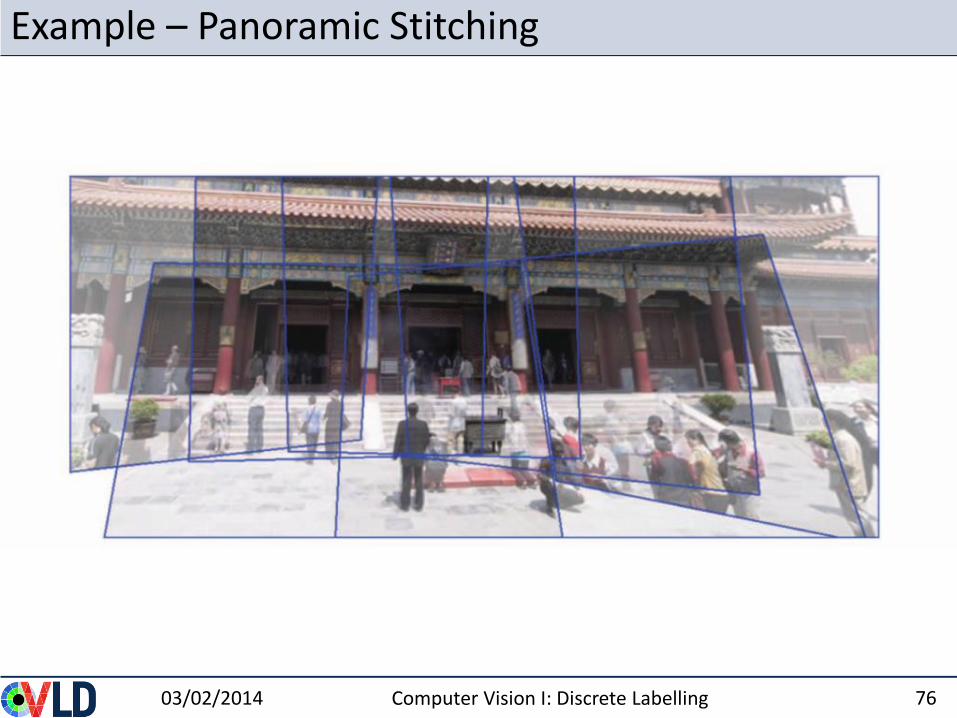
Example – Panoramic Stitching
03/02/2014 Computer Vision I: Discrete Labelling 76
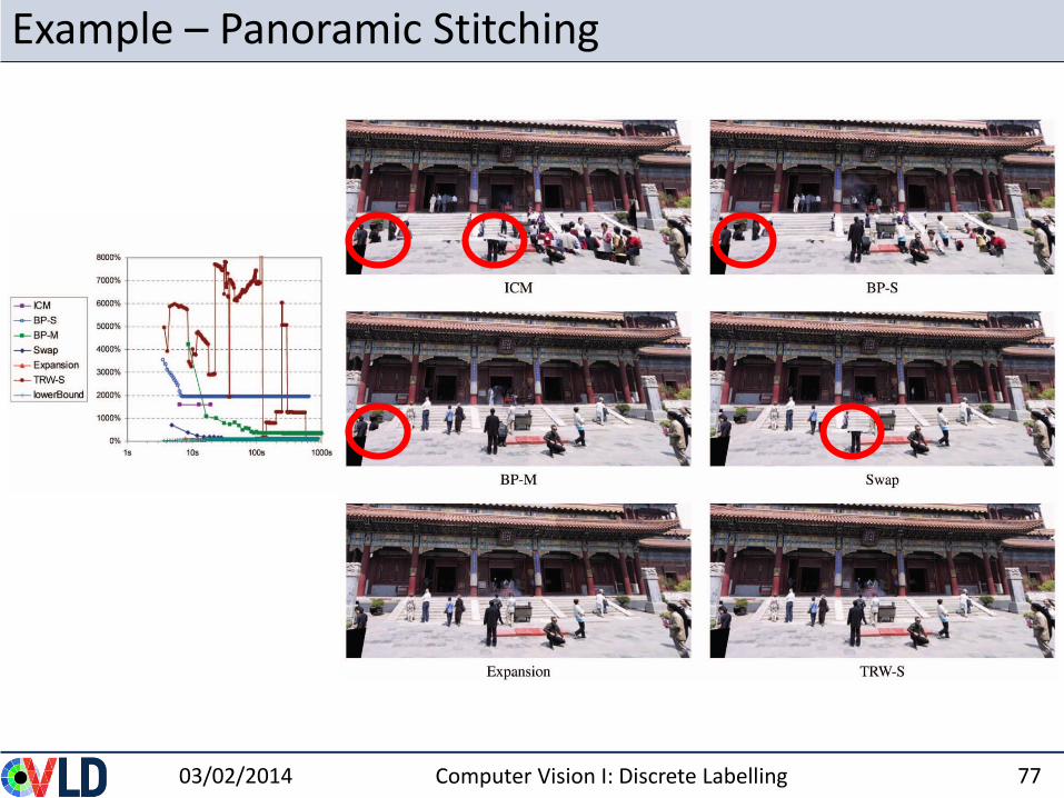
Example – Panoramic Stitching
03/02/2014 Computer Vision I: Discrete Labelling 77
Summary this lecture
• Define: Markov Random Fields
• Formulation applications as discrete Labeling problems
• Discrete Optimization: • Pixels-based: Iterative Conditional Mode (ICM),
Simulated Annealing• Line-based: Dynamic Programming (DP)• Field-based: Graph Cut and Alpha-Expansion
03/02/2014 Computer Vision I: Discrete Labelling 78


![Algorithms Lecture 1: Discrete Probability [Sp’20] · 2020-04-07 · Algorithms Lecture 1: Discrete Probability [Sp’20] Moregenerally,acountablesetofeventsfAi ji 2Igisfullyormutuallyindependentifand](https://img.pdfslide.net/doc/110x75/5f8ded7df702d4365b6a0d5e/algorithms-lecture-1-discrete-probability-spa20-2020-04-07-algorithms-lecture.jpg)


![Algorithms Lecture 1: Discrete Probability [Sp’17]jeffe.cs.illinois.edu/teaching/algorithms/notes/01-random.pdf · Algorithms Lecture 1: Discrete Probability [Sp’17] The first](https://img.pdfslide.net/doc/110x75/5f8dedcb8dd33f5a0f7c51b1/algorithms-lecture-1-discrete-probability-spa17jeffecs-algorithms-lecture.jpg)