Embed Size (px)
Citation preview
Computer Vision
Optical Flow
Some slides from K. H. Shafique [http://www.cs.ucf.edu/courses/cap6411/cap5415/] and T. Darrell
Bahadir K. Gunturk EE 7730 - Image Analysis II 2
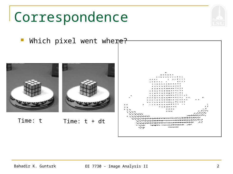
Correspondence
Which pixel went where?
Time: t Time: t + dt
Bahadir K. Gunturk EE 7730 - Image Analysis II 3
Motion Field vs. Optical Flow
Scene flow: 3D velocities of scene points. Motion field: 2D projection of scene flow. Optical flow: Approximation of motion field derived
from apparent motion of brightness patterns in image.
Bahadir K. Gunturk EE 7730 - Image Analysis II 4
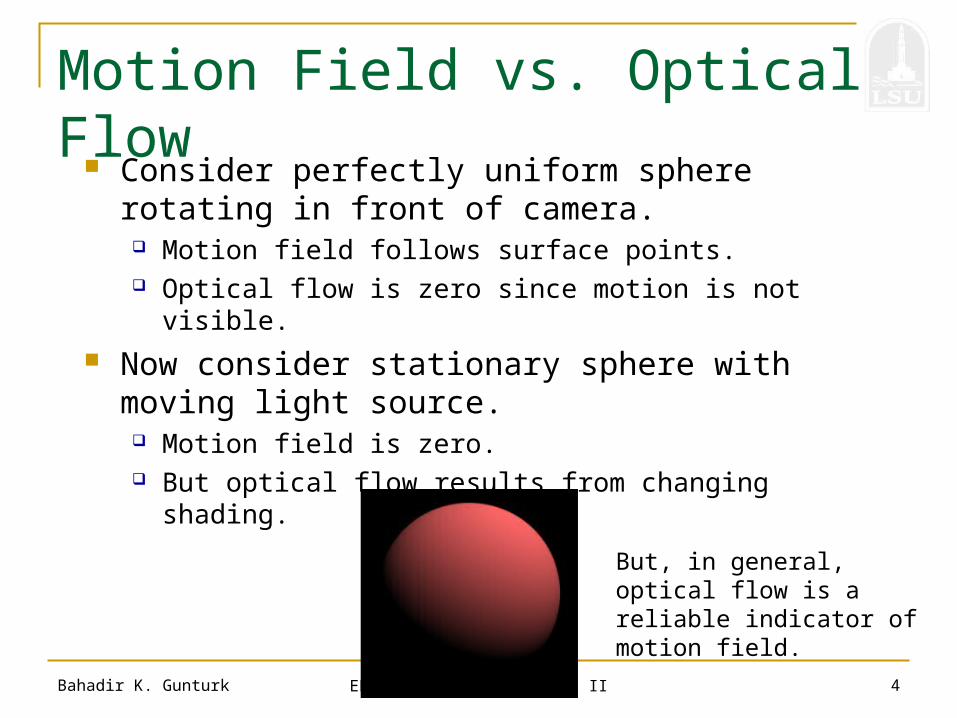
Motion Field vs. Optical Flow
Consider perfectly uniform sphere rotating in front of camera.
Motion field follows surface points. Optical flow is zero since motion is not visible.
Now consider stationary sphere with moving light source.
Motion field is zero. But optical flow results from changing shading.
But, in general, optical flow is a reliable indicator of motion field.

Bahadir K. Gunturk EE 7730 - Image Analysis II 5
Applications
Object tracking Video compression Structure from motion Segmentation Correct for camera jitter (stabilization) Combining overlapping images (panoramic image
construction) …
Bahadir K. Gunturk EE 7730 - Image Analysis II 6
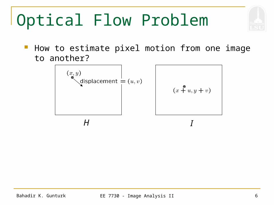
Optical Flow Problem
How to estimate pixel motion from one image to another?
H I
Bahadir K. Gunturk EE 7730 - Image Analysis II 7
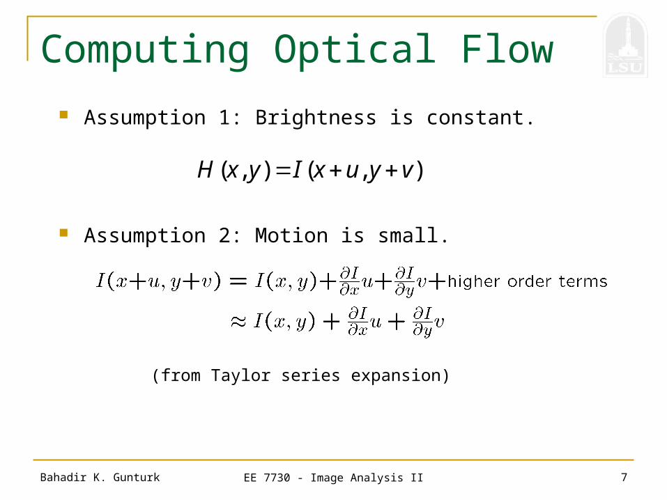
Computing Optical Flow
Assumption 1: Brightness is constant.
Assumption 2: Motion is small.
( , ) ( , )H x y I x u y v
(from Taylor series expansion)

Bahadir K. Gunturk EE 7730 - Image Analysis II 8
Computing Optical Flow
Combine
tI
0 t x yI I u I v
In the limit as u and v goes to zero, the equation becomes exact
(optical flow equation)

Bahadir K. Gunturk EE 7730 - Image Analysis II 9
Computing Optical Flow
At each pixel, we have one equation, two unknowns.
This means that only the flow component in the gradient direction can be determined.
0 t x yI I u I v (optical flow equation)
The motion is parallel to the edge, and it cannot be determined.
This is called the aperture problem.
Bahadir K. Gunturk EE 7730 - Image Analysis II 10
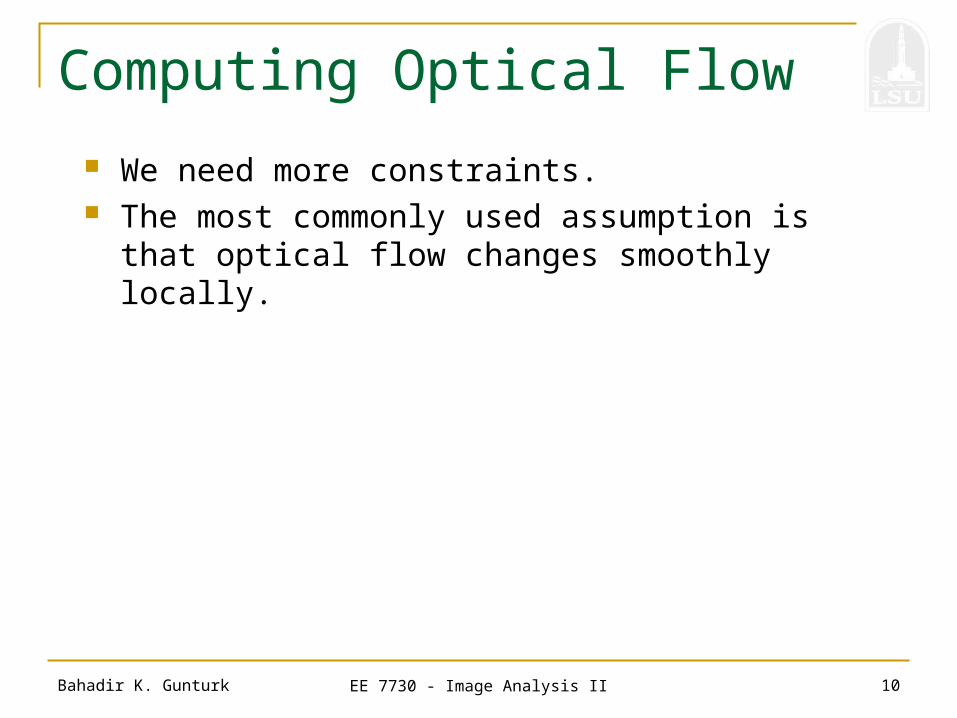
Computing Optical Flow
We need more constraints. The most commonly used assumption is that optical
flow changes smoothly locally.
Bahadir K. Gunturk EE 7730 - Image Analysis II 11
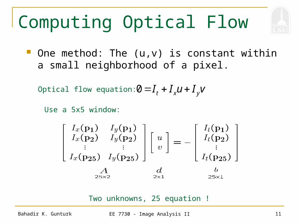
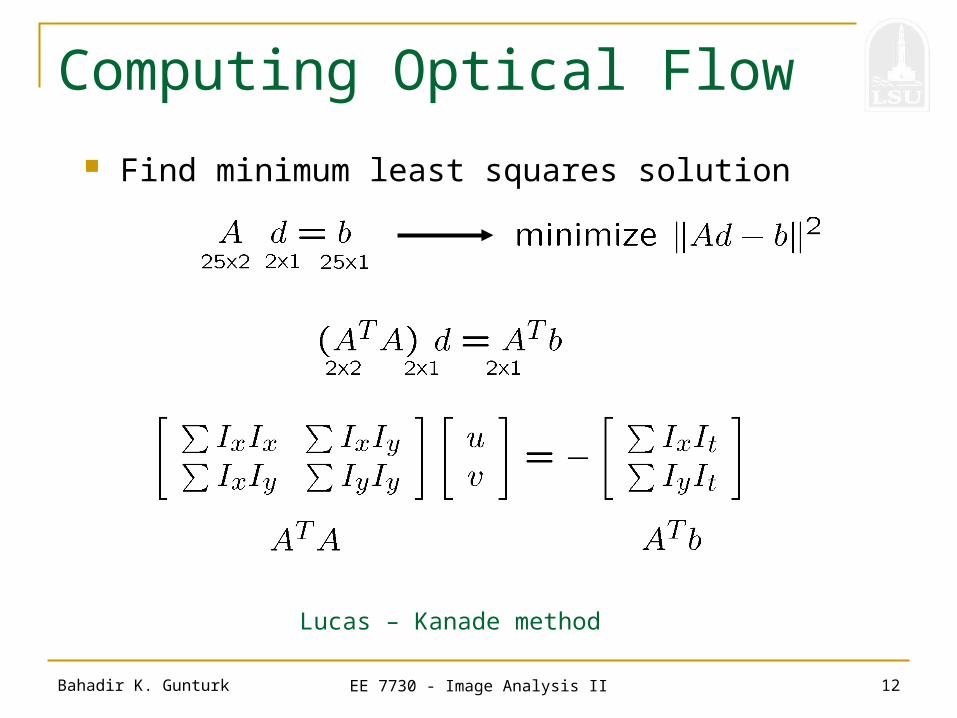
Computing Optical Flow
One method: The (u,v) is constant within a small neighborhood of a pixel.
0 t x yI I u I v Optical flow equation:
Use a 5x5 window:
Two unknowns, 25 equation !
Bahadir K. Gunturk EE 7730 - Image Analysis II 12
Computing Optical Flow
Find minimum least squares solution
Lucas – Kanade method
Bahadir K. Gunturk EE 7730 - Image Analysis II 13
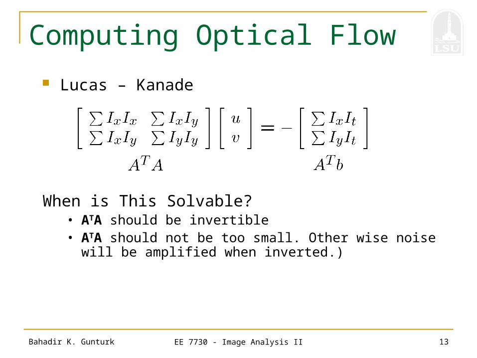
Computing Optical Flow
Lucas – Kanade
When is This Solvable?• ATA should be invertible • ATA should not be too small. Other wise noise will be
amplified when inverted.)

Bahadir K. Gunturk EE 7730 - Image Analysis II 14
Computing Optical Flow What are the potential causes of errors in this procedure?
Brightness constancy is not satisfied The motion is not small A point does not move like its neighbors
window size is too large
Bahadir K. Gunturk EE 7730 - Image Analysis II 15
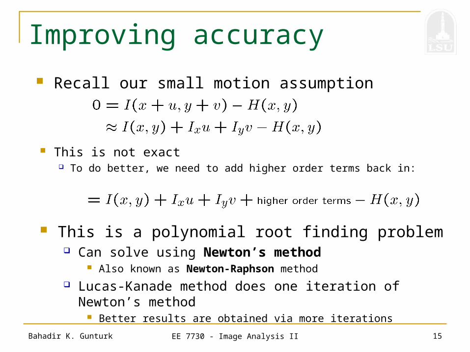
This is a polynomial root finding problem Can solve using Newton’s method
Also known as Newton-Raphson method
Lucas-Kanade method does one iteration of Newton’s method Better results are obtained via more iterations
Improving accuracy
Recall our small motion assumption
This is not exact To do better, we need to add higher order terms back in:
Bahadir K. Gunturk EE 7730 - Image Analysis II 16
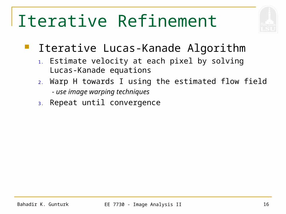
Iterative Refinement Iterative Lucas-Kanade Algorithm
1. Estimate velocity at each pixel by solving Lucas-Kanade equations
2. Warp H towards I using the estimated flow field- use image warping techniques
3. Repeat until convergence
Bahadir K. Gunturk EE 7730 - Image Analysis II 17
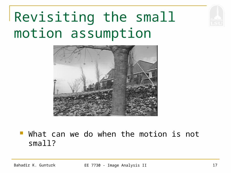
Revisiting the small motion assumption
What can we do when the motion is not small?
Bahadir K. Gunturk EE 7730 - Image Analysis II 18
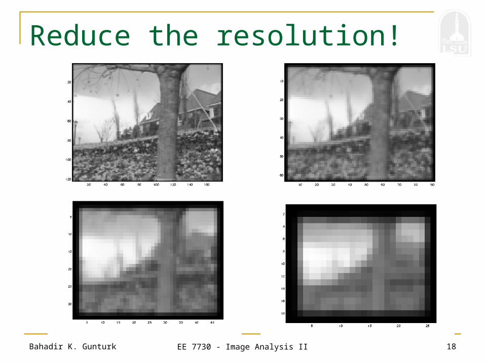
Reduce the resolution!
Bahadir K. Gunturk EE 7730 - Image Analysis II 19
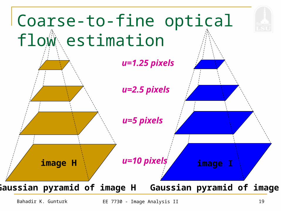
image Iimage H
Gaussian pyramid of image H Gaussian pyramid of image I
image Iimage H u=10 pixels
u=5 pixels
u=2.5 pixels
u=1.25 pixels
Coarse-to-fine optical flow estimation
Bahadir K. Gunturk EE 7730 - Image Analysis II 20
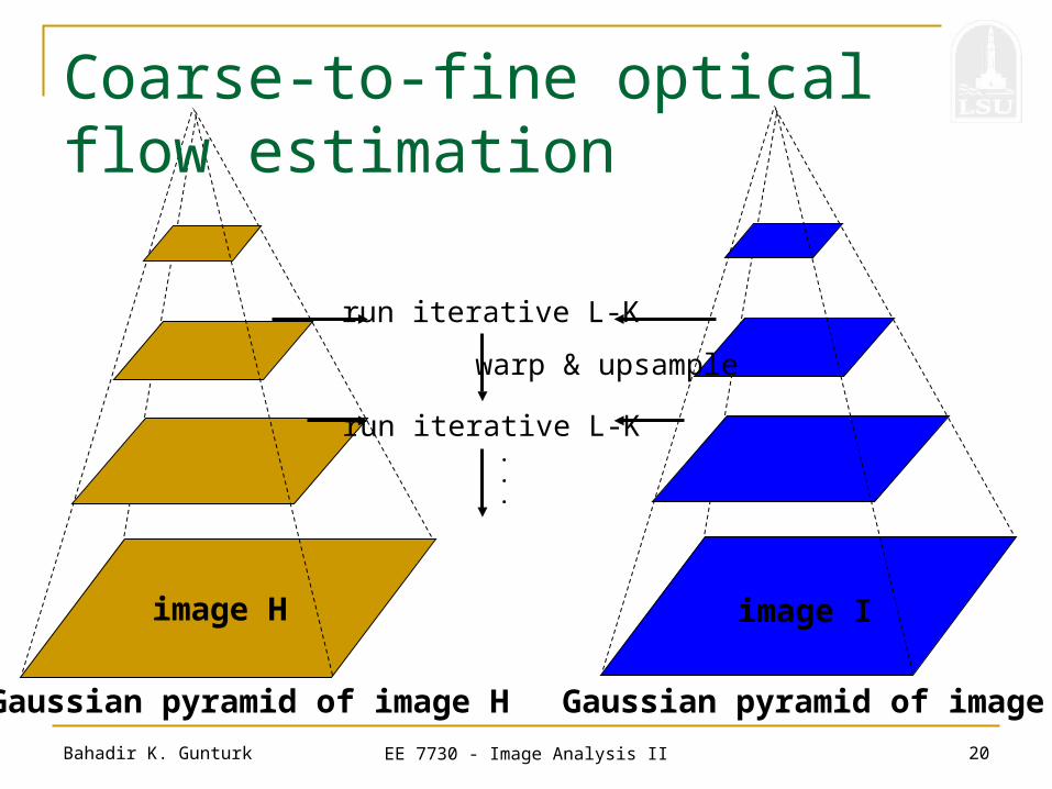
Gaussian pyramid of image H Gaussian pyramid of image I
image Iimage H
Coarse-to-fine optical flow estimation
run iterative L-K
run iterative L-K
warp & upsample
.
.
.
Bahadir K. Gunturk EE 7730 - Image Analysis II 21
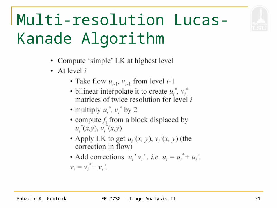
Multi-resolution Lucas-Kanade Algorithm
Bahadir K. Gunturk EE 7730 - Image Analysis II 22
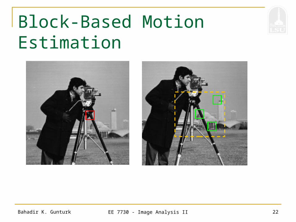
Block-Based Motion Estimation
Bahadir K. Gunturk EE 7730 - Image Analysis II 23
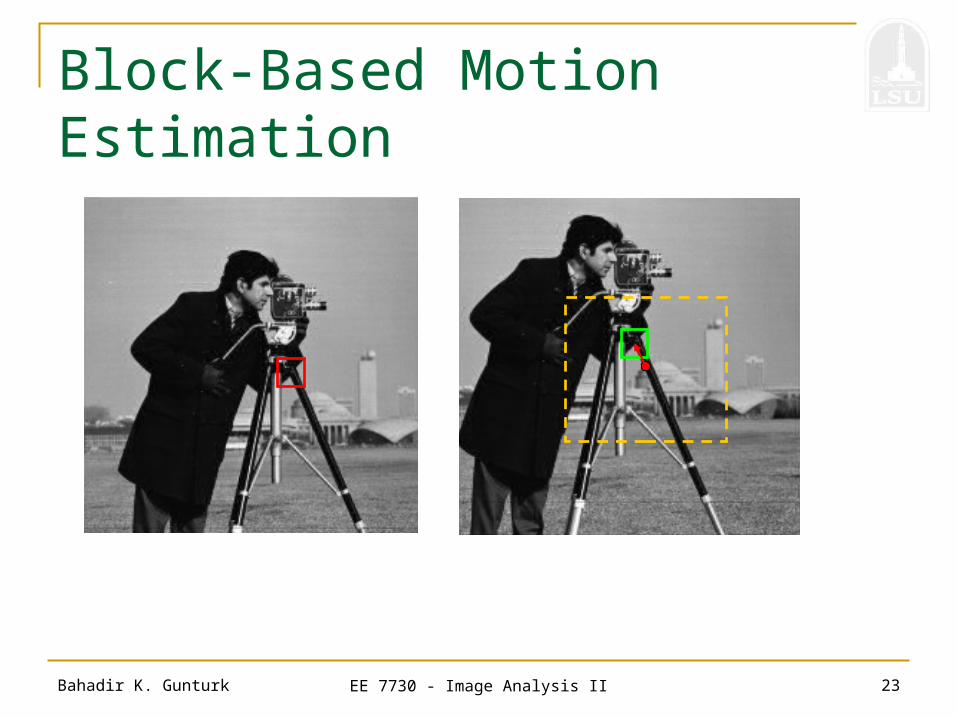
Block-Based Motion Estimation
Bahadir K. Gunturk EE 7730 - Image Analysis II 24
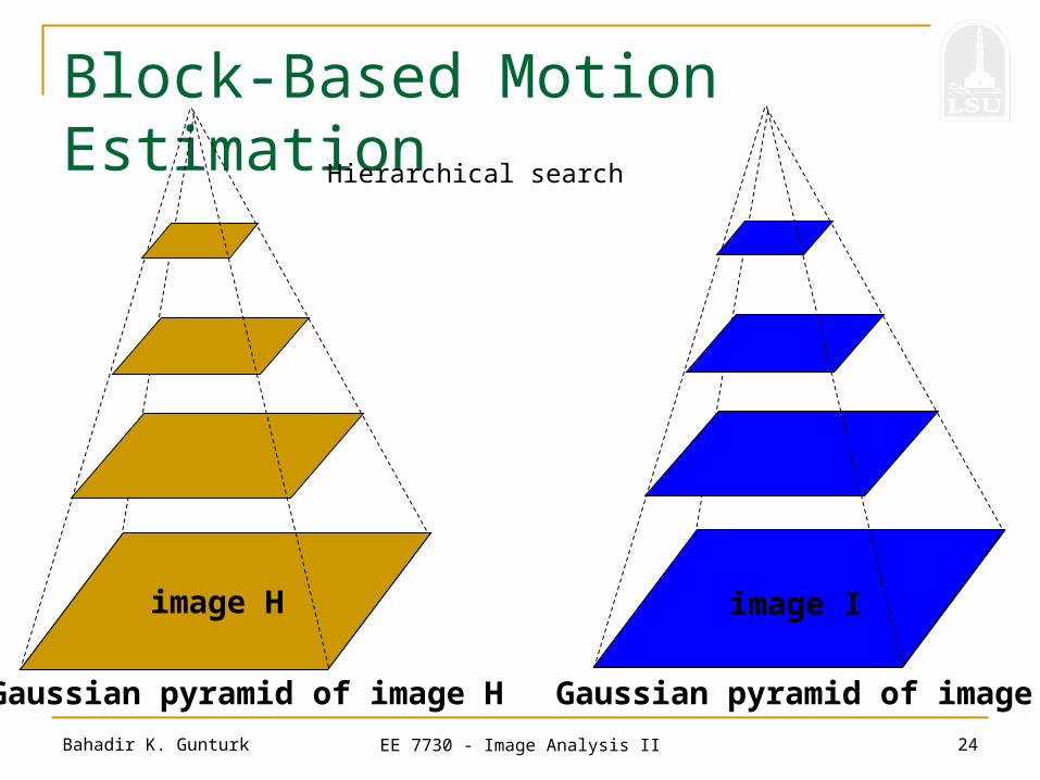
Block-Based Motion Estimation
image Iimage H
Gaussian pyramid of image H Gaussian pyramid of image I
image Iimage H
Hierarchical search
Bahadir K. Gunturk EE 7730 - Image Analysis II 25
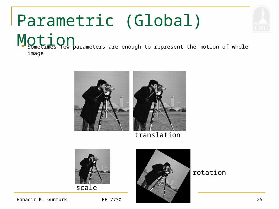
Parametric (Global) Motion Sometimes few parameters are enough to represent the motion of whole image
translation
scale
rotation

Bahadir K. Gunturk EE 7730 - Image Analysis II 26
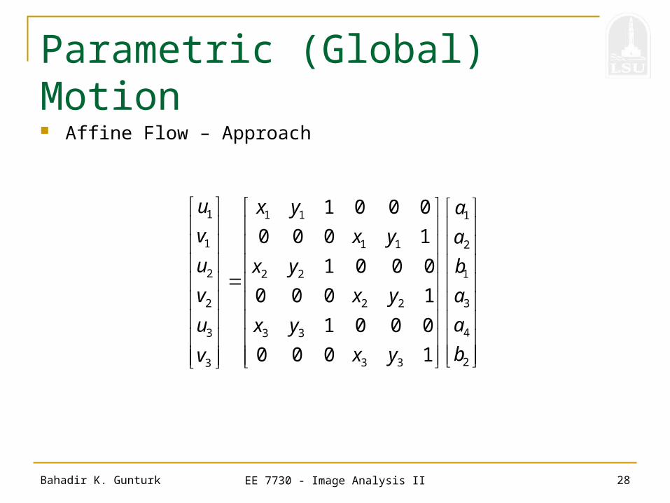
Parametric (Global) Motion
Affine Flow
1 2 1
3 4 2
( , )
( , )
u x y a x a y b
v x y a x a y b
u xA B
v y
2
1
43
21
b
b
y
x
aa
aa
yy
xx
v
u

Bahadir K. Gunturk EE 7730 - Image Analysis II 27
Parametric (Global) Motion
Affine Flow
1 2 1
3 4 2
( , )
( , )
u x y a x a y b
v x y a x a y b
2
4
3
1
2
1
1000
0001
b
a
a
b
a
a
yx
yx
v
u
2
1
43
21
b
b
y
x
aa
aa
yy
xx
v
u
Bahadir K. Gunturk EE 7730 - Image Analysis II 28
Parametric (Global) Motion
Affine Flow – Approach
1 1 1 1
1 1 1 2
2 2 2 1
2 2 2 3
43 3 3
23 33
1 0 0 0
0 0 0 1
1 0 0 0
0 0 0 1
1 0 0 0
0 0 0 1
u x y a
v x y a
u x y b
v x y a
au x y
bx yv
Bahadir K. Gunturk EE 7730 - Image Analysis II 29
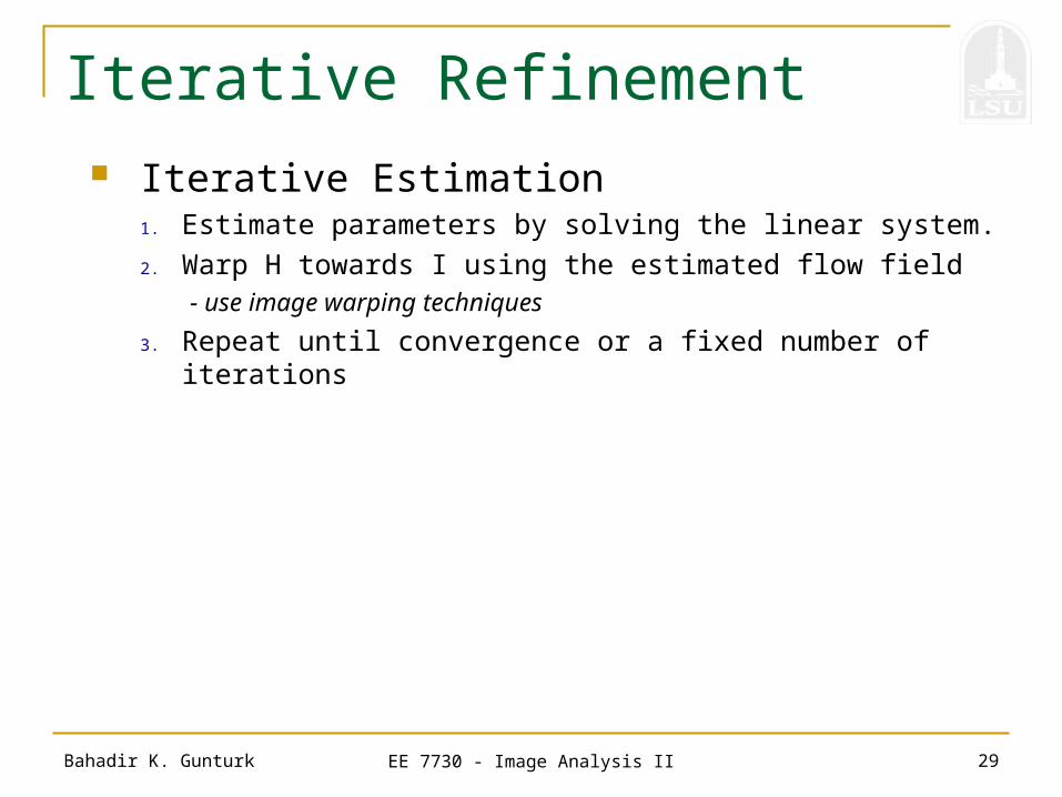
Iterative Refinement Iterative Estimation
1. Estimate parameters by solving the linear system.
2. Warp H towards I using the estimated flow field- use image warping techniques
3. Repeat until convergence or a fixed number of iterations
Bahadir K. Gunturk EE 7730 - Image Analysis II 30
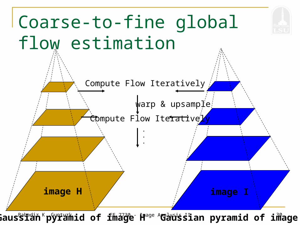
image Iimage J
Gaussian pyramid of image H Gaussian pyramid of image I
image Iimage H
Coarse-to-fine global flow estimation
Compute Flow Iteratively
Compute Flow Iteratively
warp & upsample
.
.
.
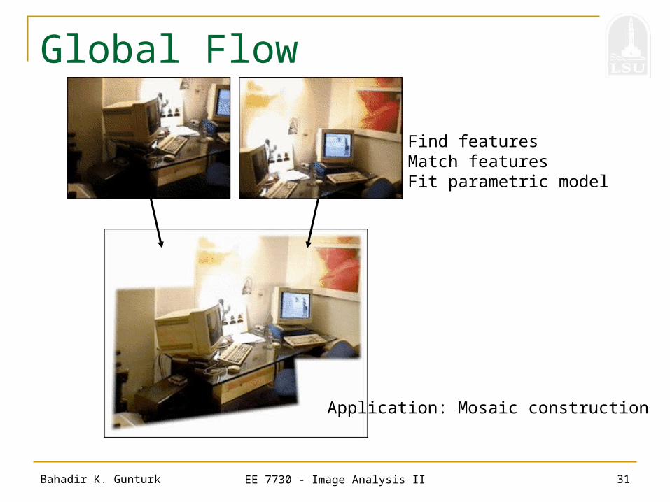
Bahadir K. Gunturk EE 7730 - Image Analysis II 31
Global Flow
Application: Mosaic construction
Find featuresMatch featuresFit parametric model
Bahadir K. Gunturk EE 7730 - Image Analysis II 32
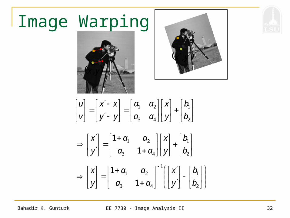
Image Warping
yx, yx ,
2
1
43
21
b
b
y
x
aa
aa
yy
xx
v
u
2
1
43
21
1
1
b
b
y
x
aa
aa
y
x
2
1
1
43
21
1
1
b
b
y
x
aa
aa
y
x

Bahadir K. Gunturk EE 7730 - Image Analysis II 33
Image Warping
yx,
yx ,
Interpolate to find the intensity at (x’,y’)
Pixel values are known in this image
Pixel values are to found in this image
Bahadir K. Gunturk EE 7730 - Image Analysis II 34
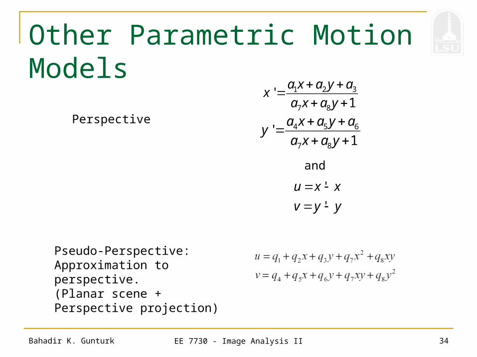
Other Parametric Motion Models
Perspective
Pseudo-Perspective: Approximation to perspective. (Planar scene + Perspective projection)
1 2 3
7 8
'1
a x a y ax
a x a y
4 5 6
7 8
'1
a x a y ay
a x a y
'
'
u x x
v y y
and