Computers and Fluids 181 (2019) 188–207

Contents lists available at ScienceDirect

Computers and Fluids

journal homepage: www.elsevier.com/locate/compfluid

Implementation of an implicit pressure–velocity coupling for the

Eulerian multi-fluid model

Gabriel G.S. Ferreira

a , Paulo L.C. Lage

a , ∗, Luiz Fernando L.R. Silva

b , Hrvoje Jasak

c , d

a Programa de Engenharia Química, COPPE, Universidade Federal do Rio de Janeiro, P.O. Box 68502, Rio de Janeiro, RJ 21941-972, Brazil b Escola de Química, Universidade Federal do Rio de Janeiro, Rio de Janeiro, RJ 21941-909, Brazil c Faculty of Mechanical Engineering and Naval Architecture, University of Zagreb, Ivana Lu ̌ci ́ca 5, Zagreb, Croatia d Wikki Ltd, 459 Southbank House, SE1 7SJ, London, United Kingdom

a r t i c l e i n f o

Article history:

Received 29 January 2018

Revised 19 November 2018

Accepted 15 January 2019

Available online 15 January 2019

Keywords:

Pressure–velocity implicit coupling

Eulerian multi-fluid model

Finite volume method

Momentum interpolation consistency

Multiphase flow

CFD

a b s t r a c t

An implicitly coupled pressure–velocity transient scheme for the solution of the Eulerian multi-fluid

model with any number of phases (MIC) was developed and implemented in OpenFOAM

®. The numerical

methodology is based on the phase-intensive momentum equations for the phase velocities and a pres-

sure equation using a deferred-correction approach of the Rhie–Chow interpolation. An extension of the

compact momentum interpolation method (CMI) to a system with any number of phases was developed.

The developed methodology was tested against a segregated multiphase solver (MS) and a steady-state

single phase solver, in cases considering up to four phases. The proposed method has proven to be more

robust and accurate than the segregated counterpart, being able to converge in cases with large drag

coefficients, providing time-step independent steady-state solutions.

© 2019 Elsevier Ltd. All rights reserved.

m

m

s

u

t

l

s

t

w

e

p

b

f

c

v

s

d

t

i

p

1. Introduction

A multiphase flow simulator that embraces all possible flow

regimes and number of phases would be of great use for research

and development in several industries. However, after more than

three decades since the development of the first two-phase CFD

models [32] , problem-specific modeling and solution strategies are

preferred both in segregated and in dispersed flows. The explana-

tions for the lack of generalization fall into two main categories.

The first is the physical complexity of the multiphase flows, which

commonly leads to scale filtering approximations during the de-

velopment of the models, leading to physical uncertainties and the

need of parameter fitting, reducing its range of applicability. The

second is the poor robustness of the solution algorithms, when

changes in the value of physical coefficients may lead to conver-

gence difficulties or even failure by divergence of the numerical

solution.

Regarding the physical model, one of the main strategies em-

ployed for the simulations of multiphase flows is the usage of an

Eulerian multi-fluid model [15] . As it is still unfeasible to accu-

rately solve all the scales of the multiphase flow in industrial ap-

plications, an averaging procedure is applied to the mass and mo-

∗ Corresponding author.

E-mail address: paulo@peq.coppe.ufrj.br (P.L.C. Lage).

p

[

a

https://doi.org/10.1016/j.compfluid.2019.01.018

0045-7930/© 2019 Elsevier Ltd. All rights reserved.

entum conservation equations and the resulting interfacial mo-

entum exchange terms are modeled through closure laws, in-

tead of directly calculated from the solution. Then, the physical

ncertainties arise mainly from the development and selection of

he appropriate closure models [15] for the inter-phase transfer

aws, stress tensor, turbulence, etc.

However, even for cases where the closure laws yield a rea-

onable physical description of the system, it may be possible

hat the numerical procedure is not robust enough, leading to

rong, or even non-physical results. For instance, there exist sev-

ral pressure-based algorithms to solve the pressure–velocity cou-

ling in incompressible single phase flows and each algorithm can

e potentially extended to a multiphase flow model [23] . As each

ormulation has its own advantages and drawbacks, it is very diffi-

ult to develop a single methodology that applies to all cases.

Most modern solution algorithms are based on a collocated

ariable arrangement, where both the pressure and velocity are

tored in the center of the computational mesh cells. However,

uring the finite volume discretization, it is necessary to compute

he volumetric fluxes at the cell faces, and the application of an

nappropriate numerical discretization scheme may lead to decou-

ling of the pressure and velocity fields, leading to non-physical

ressure oscillations. This problem was solved by Rhie and Chow

27] for steady single phase incompressible flows. They introduced

special interpolation scheme for the evaluation of the volumet-

G.G.S. Ferreira, P.L.C. Lage and L.F.L.R. Silva et al. / Computers and Fluids 181 (2019) 188–207 189

r

t

s

M

C

a

p

C

d

t

s

C

t

p

e

e

f

l

c

m

t

v

t

t

f

g

Nomenclature

( · ) f cell to face interpolation operator

A cross section area divided by particle volume (m

−1 )

A main diagonal submatrix of the linear system ob-

tained from discretization of part of the momentum

conservation equation (s −1 )

C drag coefficient

Co Courant number

d dispersed phase diameter (m)

D P pressure equation coefficient (kg −1 s m

3 )

E error

F B body force vector (m s −2 )

g gravitational acceleration (m s −2 )

H off-diagonal part of the linear system obtained from

discretization of part of the momentum conserva-

tion equation, ϒS − (ϒA − A ) u (m s −2 )

K generalized drag coefficient (kg m

−3 s −1 )

M interfacial momentum transfer term (kg m

−2 s −2 )

n number of control volumes in the mesh

N number of iterations

p pressure (kg m

−1 s −2 )

P number of phases

Q number of parallel processes

r phase fraction

Re Reynolds number

S speedup

S face area vector (m

2 )

t time (s)

u velocity component (m s −1 )

u velocity vector (m s −1 )

x position vector (m)

Greek letters

� variation

εt transient deviation

η parallelism efficiency

� ratio of numerical coefficients

λ tolerance

ν kinematic viscosity (m

2 s −1 )

ρ density (kg m

−3 )

τ viscous stress tensor per unit mass (m

2 s −2 )

ϒ numerical coefficients of the linear system obtained

from the discretization of part of the momentum

conservation equation (m s −2 )

φ volumetric flux at the cell faces (m

3 s −1 )

Subscripts

α relative to phase αβ relative to phase βχ relative to phase or variable χA indicates the coefficient matrix of a discretized lin-

ear system

c continuous phase

d dispersed phase

D relative to the drag term

f face value

F B relative to the body force term

inner inner iterations

m relative to the mixture

outer outer iterations

pU relative to the pressure–velocity inner loop

x x component

y y component

a

r relative quantity

S indicates the source vector of a discretized linear

system

T relative to the temporal term

Superscripts ∗ modified

ˆ pseudo (velocity or flux)

abs absolute

C correction

comp computational

k value at present ( k ) iteration

k − 1 value at previous ( k − 1 ) iteration

rel relative

t − 1 at the previous time instant

T transpose

tot total

Abbreviations

AAMG Agglomerative algebraic multigrid

BFS Backward-facing step

CFD Computational fluid dynamics

CMI Compact momentum interpolation

GAMG Generalized algebraic multigrid

HC Horizontal channel

IPSA Inter-Phase Slip Algorithm

MIC Multiphase implicitly coupled

MS Multiphase segregated

OpenFOAM Open source field operation and manipulation

PEA Partial Elimination Algorithm

pUC Pressure–velocity implicitly coupled

PISO Pressure-implicit with splitting of operator

SAMG Selective algebraic multigrid

SIMPLE Semi-implicit method for pressure-linked equa-

tions

ic face fluxes, applying a correction for the pressure gradient term

hat is commonly referred as Rhie–Chow interpolation.

Later, this interpolation method was extended and modified for

everal other applications. It was shown by Majumdar [21] and

iller and Schmidt [22] that the results obtained using the Rhie–

how interpolation are dependent on the value of the relax-

tion factors, and they both proposed different solutions for the

roblem. Choi [2] verified that the direct extension of the Rhie–

how interpolation to transient problems yielded time-step size

ependent solutions, proposing a modified momentum interpola-

ion method to remove this dependency. However, it was later

hown by Kawaguchi et al. [19] that the approach proposed by

hoi [2] was still dependent on the time-step size, being the first

o propose a momentum interpolation method that is both inde-

endent on the time-step size and relaxation factor values. How-

ver, before the analysis performed by Kawaguchi et al. [19] , Shen

t al. [30] reported an improved Rhie–Chow interpolation method

or unsteady flows that can be considered the first to provide so-

utions that are truly independent from the time-step size.

More recently, Cubero and Fueyo [4] developed the so-called

ompact momentum interpolation procedure, an alternative mo-

entum interpolation approach that yielded converged solutions

hat were also independent of the time-step and relaxation factor

alues. This methodology is based on a special interpolation prac-

ice for the numerical coefficients that arise from the discretiza-

ion of the temporal term, leading to a new correction formula

or the volumetric face fluxes that considers not only the pressure

radient, but also the contributions from the time discretization

nd relaxation schemes. The main advantages of the approach of

190 G.G.S. Ferreira, P.L.C. Lage and L.F.L.R. Silva et al. / Computers and Fluids 181 (2019) 188–207

l

t

p

s

2

2

a

a

a

m

w

v

fi

i

τ

D

w

t

M

w

a

t

o

i

d

M

w

i

p

s

K

w

p

p

v

A

T

o

C

w

R

w

Cubero and Fueyo [4] over the one presented by Kawaguchi et al.

[19] is the possibility to treat both linear and inertial relaxation

factors and the easy generalization of the temporal correction term

to higher-order time discretization schemes.

Another key aspect in the solution of the Navier–Stokes equa-

tions is the choice of an adequate solution algorithm for the sys-

tem composed by the momentum and continuity equations. For

years, the most popular algorithms were those based on the SIM-

PLE procedure [25] . These methods are commonly referred as seg-

regated algorithms, being based on the separate solution of the

momentum and pressure equations that are iterated until conver-

gence. However, as pointed out by Darwish et al. [8] , with the

increasing availability of computer memory and due to scalabil-

ity problems in the segregated methods, the implicitly coupled

methods have gained renewed interest. Darwish et al. [8] imple-

mented an implicitly coupled scheme for the solution of steady

single phase flows, showing that the CPU times of the coupled ap-

proach are substantially smaller than those of the segregated one,

with larger speedups for finer meshes.

When dealing with multiphase flows, care must be taken not

only with the pressure–velocity solution algorithm, but also with

the interfacial momentum coupling method. A common practice is

to consider also a Rhie–Chow-like correction for the drag and the

body force terms [23] . Cubero et al. [5] have extended their com-

pact momentum interpolation formulation for unsteady two-phase

flows by using a special interpolation practice for the drag coeffi-

cient, which included a drag correction for the face flux equations,

resulting in the compact momentum interpolation method (CMI).

They have shown that the absence of the drag correction led to

spurious relative velocities, that created non-physical oscillations

in the volumetric phase fraction fields. Their method was based on

the most popular solution algorithm for two-phase flows, the Inter-

Phase Slip Algorithm (IPSA), which is a generalization of the single-

phase SIMPLE method for unsteady two-phase flows [32] . How-

ever, the IPSA method has some drawbacks, as it converges very

slowly when the interfacial momentum transfer term is dominant.

This problem was solved by the development of the Partial Elimi-

nation Algorithm (PEA) [33] , which creates an explicit approxima-

tion for the phase velocity that can be substituted into the other

phase momentum equation to enhance the coupling between the

phases. However, the PEA method is not easily generalized to a

many phase system and it can only be applied to decouple one

phase pair at a time [24] . A remedy for this issue is to use an

implicitly coupled method to solve all the momentum equations

simultaneously, also coupling the inter-phase momentum transfer

terms implicitly. Darwish and Moukalled [6] have implemented a

steady two-phase implicitly coupled solver considering the simul-

taneous solution of the pressure and the phase velocities, obtaining

speedups between 1.3 and 4.6, in comparison to the segregated so-

lution approach. Usually, the smaller the particles, the stronger is

the coupling between the phases. Thus, several applications that

deals with small particles present critical interfacial momentum

coupling issues, such as gas-solid particle flows [35] and emulsion

flows [9] .

In this work we developed a solver for the solution of the un-

steady multi-fluid model with any number of phases. This was

achieved by combining a generalization of the CMI method [5] to

a many phase system with the implicitly coupled solution for the

pressure and all phase velocity fields. The CMI is used on the de-

velopment of a volumetric face flux equation that is used to de-

velop the multiphase pressure equation, that considers the pres-

sure, temporal, drag and body force corrections. The methodology

was implemented using the block-coupled matrix structure imple-

mented in foam-extend , a fork of the OpenFOAM

® software. The

developed code is tested and verified against a steady implicitly

coupled single phase and a multiphase segregated solver, being the

atter developed by extending the conventional segregated code,

woPhaseEulerFoam , that is available in foam-extend . The

arallel scalabilities of both the coupled and segregated multiphase

olvers were also evaluated.

. Eulerian multi-fluid model

.1. Multi-fluid equations

In this work we use the Eulerian multi-fluid model, which is

generic framework for the treatment of multiphase flows with

ny number of phases. For a system of P incompressible phases

nd neglecting mass transfer between phases, the phasic mass and

omentum conservation equations reduce to [13] :

∂(r αρα)

∂t + ∇ · ( r αραu α) = 0 , (1)

∂(r αραu α )

∂t + ∇ · ( r αραu αu α ) = −r α∇p − ∇ · ( r αρατα) + r αραg + M α

(2)

here r is the volumetric phase fraction, ρ is the density, u is the

elocity, p is pressure shared by all the phases and g is the gravity

eld. The stress tensor per unit mass τ for a laminar flow, assum-

ng a Newtonian functional form, is given as:

α = −να

[ 2 D α − 2

3

(∇ · u α) I ]

(3)

α =

1

2

[∇ u α + ( ∇ u α) t ], (4)

here ν is the kinematic viscosity. The interfacial momentum

ransfer terms are written in the following form:

α =

P ∑

β=1 β � = α

M α,β (5)

here M α, β is the momentum exchanged between phases αnd β , such that M α,β = −M β,α . Usually, these interfacial transfer

erms are decomposed in drag, lift and virtual mass forces, among

thers, but in this work we considered only the drag force, since

n the current analysis we were interested in cases where it is the

ominant term. Then, M α, β is written as:

α,β = r αr βK αβu r,αβ (6)

here K αβ is the generalized drag coefficient and u r,αβ = u β − u α

s the relative velocity between phases α and β . For cases where

hase inversion is possible, Weller [36] proposed the following

ymmetric model for the generalized drag coefficient:

αβ =

1

2

(r αρβA αC α,β + r αρβA βC β,α

)∣∣u r,αβ

∣∣ (7)

here C α, β is the drag coefficient considering phase α as the dis-

ersed phase and phase β the continuous phase, A α is the α-phase

article projected area normal to the relative velocity divided by its

olume. For a spherical particle with diameter d α , we have:

α =

3

2 d α(8)

he drag coefficient was calculated using a modified formulation

f the Schiller and Naumann [29] correlation:

α,β = max

[0 . 44 ,

24

Re α,β

(1 + 0 . 15 Re 0 . 687

α,β

)](9)

here the particle Reynolds number is defined by:

e α,β =

ραu r,αβd α

μβ(10)

here μ is the dynamic viscosity.

G.G.S. Ferreira, P.L.C. Lage and L.F.L.R. Silva et al. / Computers and Fluids 181 (2019) 188–207 191

3

t

e

3

f

S

a

w

τ

T

l

g

o

w

i

U

−

w

F

U

w

b

3

i

m

w ∑

e

a

e

⌊

w

r

p

e

s

3

f

3

w

T

r

(

t

c

t

ϒ

w

t

t

t

u

A

w

c

b

t

i

. Numerical formulation

In this section we describe the numerical formulation used in

his work, detailing the two different coupling algorithms consid-

red for the multiphase flow solution.

.1. Phase intensive formulation

In the current work we applied the phase-intensive formulation

or the momentum equations, the same used by Rusche [28] and

ilva and Lage [31] . It is obtained by dividing Eq. (2) by ρα and r αnd making some rearrangements:

∂u α

∂t + ∇ · ( u αu α) − u α( ∇ · u α) − ∇ ·

(να

∇r α

r αu α

)

+ u α∇ ·(

να∇r α

r α

)− ∇ · ( να∇u α)

+ ∇ · τ C α +

∇r α

r α· τ C

α =

M α

r αρα− 1

ρα∇p + g (11)

here the stress correction term, τ C α , is defined by

C α = −να

[ (∇u α) T − 2

3

(∇ · u α) I ] . (12)

hen, in order to stabilize the gravity source term in cases with

arge buoyant forces, we applied a modified formulation of the

ravity and pressure gradient term [28] . The formulation is based

n the definition of a modified pressure, given as:

p ∗ = p − ρm

(g · x ) (13)

here ρm

is the mixture average density, ρm

=

∑ P α=1 r αρα, and x

s the position vector with respect to an inertial reference frame.

sing Eq. (13) , we can find that [12,28] :

1

ρα∇p + g = − 1

ρα∇p ∗ + F ∗Bα, (14)

ith the modified body force F ∗Bα being written as:

∗Bα = − 1

ρα( g · x ) ∇ρm

+

(1 − ρm

ρα

)g (15)

sing Eq. (14) , Eq. (11) can be rewritten as:

∂u α

∂t + ∇ · ( u αu α) − u α( ∇ · u α) − ∇ ·

(να

∇r α

r α + δu α

)

+ u α∇ ·(

να∇r α

r α + δ

)− ∇ · ( να∇u α)

+ ∇ · τ C α +

∇r α

r α + δ· τ C

α =

M α

r αρα− ∇p ∗

ρα

− 1

ρα( g · x ) ∇ρm

+

(1 − ρm

ρα

)g (16)

here δ is a positive small parameter introduced to avoid division

y zero.

.2. Phase fraction equations

The phase fraction equation formulation is based on the one

ntroduced by Weller [36] . It was later generalized to a multiphase

ixture with any number of phases by Silva and Lage [31] to yield:

∂r α

∂t + ∇ · ( u r α) + ∇ ·

⎛

⎜ ⎝

P ∑

β=1 β � = α

r βr αu r,αβ

⎞

⎟ ⎠

= 0 (17)

here u is the mixture average velocity, defined by u = P α=1 r αu α . This formulation has the advantage of ensuring bound-

dness of r α , since the terms are written in a conservative form,

nd a better coupling between the phases is achieved by the pres-

nce of the relative velocities [28] .

Eq. (17) was discretized in the following form:

∂[ r α]

∂t

⌋+ � ∇ · ( u [ r α] ) � +

⎢ ⎢ ⎢ ⎢ ⎣

∇ ·

⎛

⎜ ⎝

P ∑

β=1 β � = α

u r,αβr β [ r α]

⎞

⎟ ⎠

⎥ ⎥ ⎥ ⎥ ⎦

= 0 (18)

here the terms written as � [ ψ] � are discretized implicitly with

espect to variable ψ . Eq. (18) was sequentially solved for each

hase after the solution of the pressure and velocity discretized

quations in both the segregated (MS) and implicitly coupled (MIC)

olvers.

.3. Segregated pressure-velocities coupling scheme

In this section we describe the numerical methodology applied

or the multiphase segregated (MS) solver.

.3.1. Multiphase momentum equations

The MS scheme used as a reference implementation in this

ork is mainly based on the implementation of Silva and Lage [31] .

he main differences arise from the consideration of the symmet-

ic drag formulation ( Eq. (7) ), the usage of the modified pressure

Eq. (13) ) and the absence of the lift and virtual mass momentum

ransfer terms. Despite these differences, we adopted a similar dis-

retization procedure and solution algorithm. The discretization of

he left-hand side of Eq. (16) gives [28] :

α :=

⌊∂[ u α]

∂t

⌋+ � ∇ · ( u α[ u α] ) � − � ( ∇ · u α) [ u α] �

−⌊∇ ·

(να

∇r α

r α + δ[ u α]

)⌋

− � ∇ · ( να∇[ u α] ) � +

⎢ ⎢ ⎢ ⎢ ⎣

∑ P β=1 β � = α

r βK αβ [ u α]

ρα

⎥ ⎥ ⎥ ⎥ ⎦

+

⌊∇ ·

(να

∇r α

r α + δ

)[ u α]

⌋+ ∇ · τ C

α +

∇r α

r α + δ· τ C

α (19)

here ϒα represents the numerical coefficients of the linear sys-

em obtained in the discretization. Considering that the linear sys-

em of equations are stored in ϒα in the form

(ϒα) A u α = (ϒα) S , (20)

he matrix coefficients of ( ϒα) A and the source term ( ϒα) S can besed to assemble the following approximation to Eq. (16) :

αu α − H α = −∇p ∗

ρα− ( g · x ) ∇ρm

ρα+

(1 − ρm

ρα

)g +

∑ P β=1 β � = α

r βK αβu β

ρα

(21)

here A α represents the diagonal coefficients of ( ϒα) A and H α is

alculated explicitly using the current-level of iteration value of u α

y H α = ( ϒα) S − ( ϒα) N u α, being ( ϒα) N the non-diagonal part of

he matrix ( ϒα) A , that is ( ϒα) N = (ϒα) A − A α . Then, using Eq. (21) we can write the following explicit approx-

mation for the phase velocities:

192 G.G.S. Ferreira, P.L.C. Lage and L.F.L.R. Silva et al. / Computers and Fluids 181 (2019) 188–207

w

a

t

�

w

D

A

a

t

u

w

t

o

v

g

3

o

3

C

a

d

e

[

w

A

A

C

e

C

w

u

a

�α α α

u α =

H α

A α− ∇p ∗

ραA α− (g · x ) ∇ρm

ραA α+

(1 − ρm

ρα

)g

A α+

∑ P β=1 β � = α

r βK αβu β

ραA α,

(22)

which is used to derive the face-flux equations, as will be detailed

in the next section.

3.3.2. Pressure equation and face flux update

The pressure equation is derived by enforcing the global conti-

nuity. The global continuity equation can be expressed as:

∇ ·(

P ∑

α=1

r αu α

)

= 0 (23)

Applying the finite-volume discretization to the divergence opera-

tor in Eq. (23) , it is rewritten as:

∇ ·(

P ∑

α=1

r αu α

)

=

∑

f

(

P ∑

α=1

r α f u α f · S f

)

= ∇ D ·(

P ∑

α=1

(r α) f φα

)

,

(24)

where φα = u α f · S f is the volumetric face flux, the subscript f in-

dicates that a variable is evaluated at a face of the control volume,

whereas () f represents the face value approximated by an inter-

polation scheme using the neighbor cell-centered values. The op-

erator ( ∇ D · ) represents the discretized divergent operator, being

defined for notational convenience.

The face fluxes are obtained using the Rhie and Chow [27] in-

terpolation, rather than by linear interpolation of the velocity pre-

dicted by Eq. (22) . This enhances the pressure–velocity coupling,

since the pressure gradient at the cell faces is calculated based

on a reduced stencil using the cell centered values of the pressure

at the neighbor control volumes, instead of interpolating the cell-

centered pressure gradient values. This reduced stencil formulation

for discretization of the gradient at the face centers is written here

as ∇ f . Then, the volumetric face fluxes are calculated assuming the

following equation:

φα =

ˆ φα + φ∗α + φddtCorr

α +

1

ρα( A α) f ∇ f p

∗ · S f (25)

ˆ φα =

(H α

A α

)f

(26)

φ∗α = − (g · x ) ∇ f ρm

ρα(A α) f · S f +

[(1 − ρm

ρα

)f

g

( A α) f

]· S f

+

P ∑

β=1 β � = α

(r β ) f (K αβ ) f

ρα( A α) f φβ (27)

The φddtCorr α term is a correction of the volumetric face fluxes as-

sociated to the interpolation errors in the explicit part of the dis-

cretization of the transient term, similar to the one developed by

Choi [2] but with an additional empirical factor. The form of the

temporal correction term depends on the time integration scheme

employed [4] , but for the first-order Euler implicit method it is

given as:

φddtCorr α =

γ

�t

1

( A α) f

[ φt−1

α −(u

t−1 α

)f · S f

] (28)

where the empirical factor γ is defined as:

γ = 1 − min

( | φt−1 −(u

t−1 α

)f · S f |

| φt−1 | + δ, 1

)

(29)

here the superscript t − 1 stands for the value of the variable at

previous timestep. Substitution of Eq. (25) into Eq. (24) provides

he following pressure equation:

∇ D ·(D P ∇ f [ p

∗] · S f )� = ∇ D ·

[

P ∑

α=1

r α

(ˆ φα + φ∗

α + φddtCorr α

)]

(30)

here

P =

P ∑

α=1

(r α) f ρα(A α) f

(31)

fter the solution of the pressure equation, the volumetric fluxes

re calculated with Eq. (25) using the updated pressure field, and

he cell centered velocities are explicitly updated as:

α =

H α

A α+

[φ∗

α +

1

ρα( A α) f ∇ f p

∗ · S f

]f→ c

(32)

here the subscript f → c denotes a vector field reconstruction at

he cell centers from face flux values. A solution algorithm based

n the PISO approach of Issa [16] was applied for the pressure–

elocity coupling. Further details of the solution algorithm are

iven in Section 4.5 .

.4. Implicit coupling scheme

In the following we describe the numerical methodology devel-

ped for the multiphase implicitly coupled (MIC) solver.

.4.1. Momentum equations

For the multiphase system with P phases, we had to extend the

MI developed by Cubero et al. [5] . First, we separate the temporal

nd drag coefficients from the A α and H α operators of the semi-

iscretized momentum equation ( Eq. (21) ), obtaining the following

quation:

A α + A T α + A Dα] u α − H α − H T α = −∇p ∗

ρα+ F ∗Bα +

P ∑

β=1 β � = α

A Dαβu β

(33)

here the total drag coefficients A D α and the other phases drag

D αβ are defined by:

Dα =

P ∑

β=1 β � = α

A Dαβ, A Dαβ =

r βK αβ

ρα(34)

onsidering a first-order Euler scheme with a fixed time step, the

xplicit temporal coefficient is given by H T α = A T αu

t−1 α . Following

ubero et al. [5] , we divide both sides of Eq. (33) by A α to obtain:

( 1 + �T α + �Dα) u α =

ˆ u α +

P ∑

β=1 β � = α

�Dαβu β + �T αu

t−1 α +

F ∗Bα

A α− ∇p ∗

ραA α

(35)

here the pseudo-velocities ˆ u α are defined by:

ˆ α =

H α

A α, (36)

nd the coefficient ratios, �, as:

T α =

A T α

A

, �Dα =

A Dα

A

, �Dαβ =

A Dαβ

A

(37)

G.G.S. Ferreira, P.L.C. Lage and L.F.L.R. Silva et al. / Computers and Fluids 181 (2019) 188–207 193

T

u

3

t

u

w

〈

m

r

E

〈

T

y

〈

w

a

n

i

t

n

m

�

T

c

w

fl

c

t

f

F

B

m

p

s

S

i

p

〈w

b

b

〈

〈

〈

〈

3

l

f

v

φ

T

∇

w

p

∇

w

D

4

4

r

Λ

w

r

hen, the following approximation for the velocities is obtained:

α =

1

1 + �T α + �Dα

⎡

⎢ ⎣ ̂

u α +

P ∑

β=1 β � = α

�Dαβu β + �T αu

t−1 α +

F ∗Bα

A α− ∇p ∗

ραA α

⎤

⎥ ⎦

(38)

.4.2. Momentum interpolation

Following Cubero and Fueyo [4] and Cubero et al. [5] , we define

he velocities at the cell faces u α, f by:

α, f = (u α) f + 〈 u α〉 (39)

here ( u α) f is the linearly interpolated velocity at the faces and

u α〉 is the velocity correction term. Depending on how the mo-

entum equation is written, different correction terms can be de-

ived. The derivation of a correction term is obtained by rewriting

q. (39) as:

u α〉 = u α, f − (u α) f , (40)

hen, Eq. (38) can be substituted into the above equation toield:

u α〉 =

ˆ u α, f

1 + �T α, f + �Dα, f

−(

ˆ u α

1 + �T α + �Dα

)f

+

∑ P β=1 β � = α

�Dαβ, f u β, f

1 + �T α, f + �Dα, f

−

⎛

⎜ ⎝

∑ P β=1 β � = α

�Dαβu β

1 + �T α + �Dα

⎞

⎟ ⎠

f

+

�T α, f u

t−1 α, f

1 + �T α, f + �Dα, f

−(

�T αu

t−1 α

1 + �T α + �Dα

)f

+

F ∗Bα, f (

1 + �T α, f + �Dα, f

)A α, f

−(

F ∗Bα

( 1 + �T α + �Dα ) A α

)f

−∇p ∗

f (1 + �T α, f + �Dα, f

)ραA α, f

+

( ∇p ∗

( 1 + �T α + �Dα ) ραA α

)f

(41)

hich is exact and could have been directly applied. However, we

pplied several approximations in the above equation. As there is

o better approximation for the face value of many of the variables

n Eq. (41) than the linear interpolation of the cell-centered values,

his was assumed for these terms. Hence, the cell face value of the

umerical coefficients �T α, f , �D α, f , �D αβ , f and A α, f are approxi-

ated as:

T α, f = (�T α) f ; �Dα, f = (�Dα) f ; �Dαβ, f = (�Dαβ ) f ;A α, f = (A α) f (42)

he values of the face velocities u α, f are not actually needed be-

ause, in the derivation of pressure equation, only its dot product

ith the face area vector, S f , which defines the volumetric face

ux, φα , is necessary. The face pressure and density gradients are

alculated from the cell-centered values of the volumes that share

he face. Then, ∇p ∗f

= ∇ f p ∗ and the modified body force at the

aces F ∗Bα, f

is calculated by:

∗Bα, f = − 1

ρα( g · x ) f ∇ f ρm

+

(1 − ρm

ρα

)f

g , (43)

esides that, in order to save computational time, it is very com-

on in CFD codes to consider that ( ∏

i ψ i ) f =

∏

i (ψ i ) f . This sim-

lification introduces second order errors that are of little con-

equence for discretization schemes up to second order accurate.

ince it simplifies code implementation and speeds up calculations,

t was used in most of the correction terms.

Applying the above simplifications, the correction for the

seudo-velocities, ˆ u α, vanishes and Eq. (41) simplifies to:

u α〉 = 〈 u α〉 D + 〈 u α〉 T + 〈 u α〉 F B + 〈 u α〉 ∇p ∗ (44)

here 〈 u α〉 D , 〈 u α〉 T , 〈 u α〉 F B and 〈 u α〉 ∇p ∗ are the drag, temporal,

ody force and pressure corrections, respectively, which are given

y:

u α〉 D =

∑ P β=1 β � = α

(�Dαβ ) f [u β, f − (u β ) f

]1 + (�T α) f + (�Dα) f

(45)

u α〉 T =

(�T α) f [u

t−1 α, f

− (u

t−1 α ) f

]1 + (�T α) f + (�Dα) f

(46)

u α〉 F B =

F ∗Bα, f

− (F ∗Bα) f [1 + (�T α) f + (�Dα) f

](A α) f

(47)

u α〉 ∇p ∗ =

(∇p ∗) f − ∇ f p ∗[

1 + (�T α) f + (�Dα) f ]ρα(A α) f

(48)

.4.3. Pressure equation

In order to derive an implicitly coupled scheme, we use the ve-

ocity correction deduced in Eq. (44) to evaluate the volumetric

ace fluxes in the global continuity equation ( Eq. (24) ). Then, the

olumetric face fluxes are written as:

α =

[(u α) f + 〈 u α〉 ] · S f (49)

he above relation is substituted in Eq. (24) to yield:

D ·(

P ∑

α=1

(r α) f [(u α) f + 〈 u α〉 ] · S f

)

= 0 (50)

hich, using Eqs. (44) –(48) , gives the following equation for the

ressure:

D ·[D P ∇ f p

∗ · S f ]

= ∇ D ·(

P ∑

α=1

(r α) f (u α) f · S f

)

+ ∇ D ·[D P (∇p ∗) f · S f

]

+ ∇ D ·

⎡

⎢ ⎣

P ∑

α=1

( r α) f

⎛

⎜ ⎝

∑ P β=1 β � = α

(�Dαβ ) f [φβ − (u β ) f · S f

]1 + (�T α) f + (�Dα) f

+

(�T α) f [φt−1

α − (u

t−1 α ) f · S f

]1 + (�T α) f + (�Dα) f

+

[F ∗

Bα, f − (F ∗Bα) f

]· S f [

1 + (�T α) f + (�Dα) f ](A α) f

) ]

(51)

here the pressure equation coefficient is given by:

P =

P ∑

α=1

(r α) f [1 + (�T α) f + (�Dα) f

]ρα(A α) f

. (52)

. Implementation of the implicit coupling

.1. Block coupled matrix structure

The finite volume discretization of a single transport equation

esults in a linear system of the following form:

A y = ΛB (53)

here ΛA is the coefficient matrix, y is a vector of unknowns rep-

esenting the cell center values for the field that is being solved

194 G.G.S. Ferreira, P.L.C. Lage and L.F.L.R. Silva et al. / Computers and Fluids 181 (2019) 188–207

w

t

g

e

i

e

c

b

f

t

t

t

t

4

[

i

i

t

l

t

w

d

o

e

i

a

w

�

�

�

I

p

t

for, and ΛB is a vector of sources. The coefficient matrix is a n × n

square matrix, while y and ΛB both have dimension equal to the

number of discretization volumes n :

ΛA =

⎡

⎢ ⎢ ⎣

a 1 , 1 a 1 , 2 · · · a 1 ,n a 2 , 1 a 2 , 2 · · · a 2 ,n

. . . . . .

. . . . . .

a n, 1 a n, 2 · · · a n,n

⎤

⎥ ⎥ ⎦

; y =

⎡

⎢ ⎢ ⎣

y 1 y 2 . . .

y n

⎤

⎥ ⎥ ⎦

;

ΛB =

⎡

⎢ ⎢ ⎣

b 1 b 2 . . .

b n ,

⎤

⎥ ⎥ ⎦

(54)

As the finite volume method formulations are usually based on lo-

cal approximations using a small stencil of cells, matrix ΛA is a

sparse matrix, that is, most a i, j coefficients are equal to zero.

However, in a multi-variable block-coupled solution, there are d

unknowns for each cell value. In this work, we performed the im-

plicitly coupled solution of the momentum and pressure equations

for a system composed of P phases. This means that our block cou-

pled matrix has (3 P + 1) × (3 P + 1) coefficients for each cell, given

by the three cartesian components of the phase velocities and the

pressure equation ( d = 3 P + 1 ).

For a two-phase flow, the variables are the phase velocity fields,

u a and u b and the modified pressure, p ∗. In the following, the ma-

trix coefficient arrangement is illustrated for the two-phase flow

case, where, for the i -index cell, we can write the sub-vector of

unknowns, y i , the sub-vector of source terms, ΛB,i , and the sub-

matrix of coefficients that relates this cell with the j neighbor cell,

ΛA,i, j , as:

y i =

[

u ai

u bi

p ∗

]

, ΛB,i =

[

b u a i

b u b i

b p ∗

i

]

, ΛA,i, j =

⎡

⎣

a u a , u a i, j

a u a , u b i, j

a u a ,p ∗

i, j

a u b , u a i, j

a u b , u b i, j

a u b ,p ∗

i, j

a p ∗, u a

i, j a

p ∗, u b i, j

a p ∗,p ∗

i, j

⎤

⎦

(55)

where

b u αi

=

[

b u αx

i

b u αy

i b u αz

i

]

, a u α, u βi, j

=

⎡

⎢ ⎢ ⎣

a u αx ,u βx

i, j a

u αx ,u βy

i, j a

u αx ,u βz

i, j

a u αy ,u βx

i, j a

u αy ,u βy

i, j a

u αy ,u βz

i, j

a u αz ,u βx

i, j a

u αz ,u βy

i, j a

u αz ,u βz

i, j

⎤

⎥ ⎥ ⎦

,

a u α,p ∗

i, j =

⎡

⎢ ⎢ ⎣

a u αx ,p ∗

i, j

a u αy ,p ∗

i, j

a u αz ,p ∗

i, j

⎤

⎥ ⎥ ⎦

, (a p

∗, u αi, j

)T =

⎡

⎢ ⎢ ⎣

a p ∗,u αx

i, j

a p ∗,u αy

i, j

a p ∗,u αz

i, j

⎤

⎥ ⎥ ⎦

(56)

and a η,ξi, j

is the coefficient submatrix that represents the influence

of the variable ξ at cell j in the variable η at cell i .

The foam-extend-4.0 version of OpenFOAM

®has several fa-

cilities for the implementation of block-coupled solvers, which

were used in this work to fill the block-coupled matrix with the

appropriate coefficients [1,3,17] . The numerical treatment applied

to each equation is described in the next section.

4.2. Implicit terms in the momentum equations

As shown in Section 3.1 , we employed the phase intensive for-

mulation of the momentum equation. The discretized version for a

phase α is given by: ⌊∂[ u α]

∂t

⌋+ � ∇ · ( u α[ u α] ) � − � u α( ∇ · [ u α] ) �

−⌊∇ ·

(να

∇r α

r α + δ[ u α]

)⌋− � ∇ · ( να∇[ u α] ) �

+

⌊∇ ·

(να

∇r α

r α + δ

)[ u α]

⌋+

⎢ ⎢ ⎢ ⎢ ⎣

P ∑

β=1 β � = α

r βK αβ

ρα[ u α]

⎥ ⎥ ⎥ ⎥ ⎦

−P ∑

β=1 β � = α

⌊r βK αβ

ρα[ u β ]

⌋+

⌊ 1

ρα∇[ p ∗]

⌋

= −∇ · τ C α +

∇r α

r α + δ· τ C

α + F ∗Bα (57)

here the terms inside brackets are treated implicitly, including

he drag terms from the other phases and the modified pressure

radient. The terms at the right hand side of Eq. (57) are treated

xplicitly. During matrix filling, for a given phase α, the operators

n [ u α] feed values in a u α, u αi, j

and b u αi

, while the pressure gradi-

nt term stores information into a u α,p ∗i, j

and, depending on the dis-

retization method applied to the pressure gradient, maybe into

u αi

. The drag term does not depend on neighbor cells and, there-

ore, feeds values only in the a u α, u βi,i

coefficients. All the explicit

erms are inserted into the source term b u αi

. For a multiphase sys-

em, the discretization of the phase momentum equations feeds

he first 3 P rows of the submatrices ΛA,i, j . The last row is fed by

he discretized pressure equation, which is described below.

.3. Implicit terms in the pressure equation

In this work we follow the same approach of Cubero and Fueyo4] and Darwish et al. [7] to develop a pressure equation for themplicit solution of the pressure–velocity coupling in incompress-ble flows, which consists of applying the velocity correction equa-ions to the global continuity equation in order to obtain a Poisson-ike equation for the pressure. A first step is the reorganization ofhe velocity divergence term and part of the drag term in Eq. (51) ,hose details are given in Appendix A . These terms are implicitly

iscretized. Then, the terms that depend on the volumetric fluxesr on the linear interpolation of the pressure gradient are treatedxplicitly considering the current iteration values of φ and p ∗. Tak-ng into account all these discretizations, Eq. (51) can be rewrittens:

−⌊∇ D ·

(D P ∇ f [ p

∗] · S f )⌋

+

P ∑

α=1

⎢ ⎢ ⎢ ⎢ ⎣

∇ D ·

⎧ ⎪ ⎨

⎪ ⎩

⎡

⎢ ⎣

(r α ) f −P ∑

β=1 β � = α

(r β ) f (�Dβα ) f

1 + (�T β ) f + (�Dβ ) f

⎤

⎥ ⎦

( [ u α] ) f · S f

⎫ ⎪ ⎬

⎪ ⎭

⎥ ⎥ ⎥ ⎥ ⎦

= −∇ D ·[D P (∇p ∗) f · S f

]+ �D + �T + �F B (58)

here

D = ∇ D ·

⎡

⎢ ⎣

P ∑

α=1

(r α) f

−∑ P β=1 β � = α

(�Dαβ ) f φβ

1 + (�T α) f + (�Dα) f

⎤

⎥ ⎦

(59)

T = ∇ D ·{

P ∑

α=1

(r α) f (�T α) f

[(u

t−1 α ) f · S f − φt−1

α

]1 + (�T α) f + (�Dα) f

}

(60)

F B = ∇ D ·{

P ∑

α=1

(r α) f

[(F ∗Bα) f − F ∗

Bα, f

]· S f [

1 + (�T α) f + (�Dα) f ]( A α) f

}

(61)

n Eq. (58) , the terms on the left hand side are discretized im-

licitly with respect to the pressure and phase velocities, respec-

ively, whereas those on the right hand side are treated explicitly.

G.G.S. Ferreira, P.L.C. Lage and L.F.L.R. Silva et al. / Computers and Fluids 181 (2019) 188–207 195

T

fi

v

f

t

E

i

t

4

w

φ

e

φ

w

v

v

e

t

b

4

M

c

o

i

i

E

E

w

t

u

i

E

T

M

Fig. 1. Test cases: (a) backward-facing step geometry and (b) horizontal channel.

I

f

a

t

5

5

t

s

t

5

c

s

a

g

t

u

b

b

(

he operator in [ p ∗] can be recognized as the Laplacian, and it de-

nes the coefficients a p ∗,p ∗i, j

and feeds information into b p ∗i

. The di-

ergence operator in [ u α] sets up the coefficients a p ∗, u αi, j

and also

eeds values in b p ∗i

. As usual, the explicit terms are inserted into

he source b p ∗i

. Note that Eq. (51) was multiplied by −1 to provide

q. (58) . This was performed to force all the numerical coefficients

n the main diagonal of the block-coupled matrix, ΛA,i, j , to have

he same sign, which is beneficial for the linear system solver.

.4. Face flux correction equation

After solution of the block-coupled system to a given tolerance,

e obtain the new values for u α and p ∗ fields, and the face fluxes

are updated by combining Eqs. (44) and (49) into the following

quation:

α = ( u α) f · S f +

∑ P β=1 β � = α

(�Dαβ ) f

[φk −1

β−(

u

k β

)f · S f

]1 + (�T α) f + (�Dα) f

+

(�T α) f [φt−1

α − (u

t−1 α ) f · S f

]1 + (�T α) f + (�Dα) f

+

[F ∗

Bα, f − (F ∗Bα) f

]· S f [

1 + (�T α) f + (�Dα) f ](A α) f

+

[(∇p ∗k −1 ) f − ∇ f p

∗k ]

· S f [1 + (�T α) f + (�Dα) f

]ρα(A α) f

(62)

here the k − 1 superscript refers to the variable value at the pre-

ious iteration level, being calculated using the same numerical

alues used in the assembly of the right hand side of the pressure

quation ( Eq. (58) ), while the k superscript refers to the values at

he current iteration level, which are obtained after solution of the

lock-coupled system.

.5. Solution algorithms and convergence criteria

In order to carry out a fair performance analysis of the MS and

IC solvers, they both employed the same error criteria for the

onvergence of the solution within a time step. The convergence

f the pressure–velocity coupling was evaluated through the max-

mum error of the pressure and velocity fields between successive

nner or outer iterations using a mixed tolerance criterion given by

mixed χ < 1 , where E mixed

χ is the mixed error that is defined by:

mixed χ = max

( | χ k − χ k −1 | λabs

χ + λrel χ | χ k |

)(63)

here λabs χ and λrel

χ are chosen values for the absolute and relative

olerances. The convergence of the phase fraction fields was eval-

ated using the absolute error between the iterations, E abs χ , which

s defined by:

abs χ = max

(| χ k − χ k −1 | ) (64)

hen, for each time step, the solution procedure applied for the

IC and MS solvers is the following:

1. Outer loop iterations: For a given maximum number of itera-

tions, N

max outer , or until E mixed

χ, outer < 1 for the modified pressure and

all components of the velocity fields and E abs r α

< λabs r α, outer , α =

1 , . . . , P .

(a) Pressure–velocity coupling iterations: For a given maximum

number of iterations, N

max pU, inner

, or until E mixed χ, inner

< 1 for the

modified pressure and all components of the velocity fields. • For the MIC solver:

(1) Update the drag coefficients, the momentum equation

operators A α and H α , the numerical coefficients de-

fined in Eq. (37) and the explicit correction terms in

Eqs. (59) –(61) .

(2) Assembly the block-coupled matrix for p ∗ − u α

with the coefficients from the discretization of

Eqs. (57) and (58) .

(3) Solve the block-coupled linear system for a given tol-

erance.

(4) Calculate the face fluxes using Eq. (62) .

• For the MS solver:

(1) Update the drag coefficients, the matrix operators A α

and H α and assemble the pressure equation.

(2) Update the pressure field solving the pressure equa-

tion ( Eq. (30) ).

(3) Use Eqs. (25) and (32) , to correct the volumetric

fluxes and the velocities, respectively.

(b) For a given maximum number of iterations, N

max r α, inner

, or un-

til E abs r α, inner

< λabs r α, inner

, α = 1 , . . . , P, solve the phase fraction

equations ( Eq. (18) ).

2. Advance timestep.

n order to evaluate the convergence performance of both solvers,

or each time step we stored the number of outer iterations N outer

nd the total number of pressure–velocity inner iterations used by

he algorithms, N

tot pU , inner

=

∑ N outer i =1

N pU , inner ,i .

. Simulation conditions

.1. Test cases

The MIC and MS methods were compared in two-dimensional

est cases considering two different geometries: a backward-facing

tep and a horizontal channel. The conditions considered in each

est case are detailed below.

.1.1. The backward-facing step

This simple geometry was chosen because it has a relatively

omplex flow pattern even in laminar flow conditions. The con-

idered geometry, shown in Fig. 1 (a), is the same tested by Silva

nd Lage [31] using L = 11 H, l = H, h = H/ 2 and H = 0 . 01 m . Two

roups of test cases, BFS1 and BFS2, were performed considering

his geometry.

The BFS1 test cases were used to compare the results obtained

sing the two coupling methods (MS and MIC) with those obtained

y the single phase steady-state implicitly coupled solver em-

edded in the foam-extend distribution, the pUCoupledFoampUC). These tests were performed in order to verify the temporal

196 G.G.S. Ferreira, P.L.C. Lage and L.F.L.R. Silva et al. / Computers and Fluids 181 (2019) 188–207

Table 1

Phase properties considered in the horizontal channel

cases.

Phases Properties

ρ [ kg m

−3 ] ν [m

2 / s ] d [m]

Continuous c 10 0 0 10 −5 10 −4

Dispersed A 20 0 0 10 −4 10 −4

B 50 10 −4 10 −4

C 20 0 0 10 −5 10 −4

D 20 0 0 10 −4 10 −5

Table 2

Inlet conditions for the different test cases in the horizontal channel geometry.

Case Dispersed phases Phase fractions u IN [m/s]

HC1 A r dA = 0 . 2

HC2 B r dB = 0 . 2

HC3 C r dC = 0 . 2

HC4 D r dD = 0 . 2 0.1

HC5 B, C, D r dB = 0 . 1 r dC = 0 . 05 r dD = 0 . 05

n

m

w

t

w

0

t

R

u

i

f

s

s

f

i

p

5

i

r

t

p

w

m

p

c

m

g

i

f

f

m

C

s

b

o

t

a

1

i

w

w

(

c

m

p

f

p

l

2

f

p

consistency of the momentum interpolation, as it is expected that

the steady-state solution of a consistent transient method should

be the same as the converged solution of a steady-state solver [4] .

For this case we considered a parabolic velocity profile at the in-

let with an average value of 0.5 m/s and a kinematic viscosity ν =10 −5 m

2 /s, resulting in a Reynolds number of 500, and the gravita-

tional force field was neglected. The multiphase solver was forced

to simulate a single phase flow case considering a two-phase sys-

tem with the same properties for both phases. The inlet phase frac-

tions were 0.2 and 0.8 for the two phases, both with a diameter

of 10 −3 m. A mesh convergence analysis was performed consid-

ering uniform cartesian meshes with 4200 (M1), 8820 (M2) and

16,800 (M3) cells, for which ( �x, �y ) are equal to (5 × 10 −4 m,

5 × 10 −4 m), (3 . 33 × 10 −4 m, 3 . 571 × 10 −4 m) and (2 . 5 × 10 −4 m,

2 . 5 × 10 −4 m), respectively.

The BFS2 test cases were carried out to verify the extension

of the numerical methodology to multiphase flows in both solvers

(MS and MIC). These test cases considered a two-phase flow with

a dispersed phase, a , and a continuous phase, b , with r a = 0 . 1 and

r b = 0 . 9 at the inlet. Different densities were considered for the

phases, with ρb = 900 kg/m

3 and ρa = 10 0 0 kg/m

3 . We also as-

sumed that r a = 0 at t = 0 for the whole domain, forcing density

gradients to exist in the beginning of the simulation. The results

of these two-phase simulations were compared to those from the

flow simulation of a three-phase system with two identical dis-

persed phases, a 1 and a 2, with half the original phase fraction

( r a 1 = r a 2 = 0 . 05 at the inlet). It should be noted that, in order to

make both cases comparable, we had to neglect the drag between

the dispersed phases a 1 and a 2. This analysis was carried out only

for the coarsest mesh M1 in order to enlarge the deviations be-

tween the two numerical methodologies. The temporal consistency

of the applied momentum interpolation methods was also inves-

tigated for this case by considering two different values for the

Courant number (0.2 and 0.4).

5.1.2. The horizontal channel

The flow in a horizontal channel of phases with different densi-

ties leads to inhomogeneities in the phase fraction fields, being an

interesting test case to compare the performance of the multiphase

flow solvers. We compared the performance of the MIC and MS

solvers considering continuous and dispersed phases with different

properties, which are shown in Table 1 . The continuous phase is

referred below simply as phase c. The dispersed phase used as ref-

erence was phase A and the other dispersed phases were selected

in order to verify the performance of the MIC and MS approaches

for different values of density (B), viscosity (C) and diameter (D) of

the dispersed phase.

The horizontal channel geometry consists of a rectangular two-

dimensional channel with a length L = 1 . 8 m and a height H =0 . 025 m and is shown in Fig. 1 (b). Gravity was aligned with

the y -axis pointing downwards with a magnitude of 9.8 m/s 2 . A

mesh convergence analysis was performed considering four n x × n y meshes, and the time steps were selected in order to keep the

maximum Co number in the mesh below 0.3: mesh 1 (M1) with

x = 250 and n y = 10 (total of 2500 volumes, with �t = 0 . 01 s),

esh 2 (M2) with n x = 500 and n y = 20 (total of 10,0 0 0 volumes,

ith �t = 0 . 005 s), mesh 3 (M3) with n x = 10 0 0 and n y = 40 (to-

al of 40,0 0 0 volumes, with �t = 0 . 0 025 s) and mesh 4 (M4)

ith n x = 20 0 0 and n y = 80 (total of 160,0 0 0 volumes, with �t = . 00125 s). A uniform velocity profile of 0.1 m/s was assumed at

he inlet, resulting in a hydrodynamic residence time of 18 s. The

eynolds number calculated based on the properties of the contin-

ous phase is 50. A total of five test cases were considered, whose

nlet conditions are summarized in Table 2 . The initial conditions

or each case were generated from a 30 s simulation without con-

idering the gravity force in order to develop the velocity and pres-

ure fields. These preliminary simulations were started using uni-

orm fields with values equal to the inlet conditions for the veloc-

ties and phase fractions and a zeroed value field for the modified

ressure.

.2. Numerical procedure

In all the cases, the numerical discretization schemes were sim-

lar. The first-order implicit Euler method was used for tempo-

al discretization. Laplacians, gradients and cell to face interpola-

ions were calculated considering a linear approximation. The im-

licitly discretized velocity divergence in the pressure equation

as also discretized considering a linear, second-order approxi-

ation. The upwind scheme was used for the momentum and

hase fraction advection. When using the MIC solver, the block-

oupled linear system was solved by clustering algebraic multigrid

ethods (AMG) [14,26] . Both the Block-Selective Algebraic Multi-

rid (SAMG) and aggregative (AAMG) methods were employed, be-

ng the former recently implemented by Uroi ́c and Jasak [34] in

oam-extend . The ILUC0 smoother described in [34] was applied

or both methods. For the MS solver, a generalized AMG (GAMG)

ethod with geometric pairing and a simplified diagonal-based

holesky (DIC) smoother was applied on the solution of the pres-

ure equation. The iterations of these linear solvers were controlled

y specifying absolute and relative tolerances for the residual norm

f the normalized linear system [18] . The relative tolerance is op-

ional and simply defines the minimum ratio between the final

nd initial values of this residual norm. A relative tolerance of

0 −2 and an absolute tolerance of 10 −9 were employed for the

mplicitly coupled solver, whereas an absolute tolerance of 10 −10

as used for the segregated solver. The phase fraction equations

ere solved using a preconditioned bi-conjugate gradient method

PBiCG [10] ) with a simplified diagonal-based incomplete LU pre-

onditioner [20] with an absolute tolerance of 10 −12 for the nor-

alized residual of the linear system.

A maximum of six external corrections ( N

max outer = 6 ) and fifty

ressure–velocity coupling corrections ( N

max pU, inner

= 50 ) were used

or both the MIC and MS methods. The convergence of the

ressure–velocity correction loop was controlled by setting abso-

ute tolerance values of λabs p ∗, inner

= 4 . 5 × 10 −2 Pa and λabs u α, inner

= × 10 −6 m/s, and a relative tolerance of λrel

p ∗, inner = λrel

u α, inner = 10 −5

or both variables. An absolute tolerance of λabs r α, inner

= 10 −5 was ap-

lied to the inner loops in the solution of the phase fraction fields.

G.G.S. Ferreira, P.L.C. Lage and L.F.L.R. Silva et al. / Computers and Fluids 181 (2019) 188–207 197

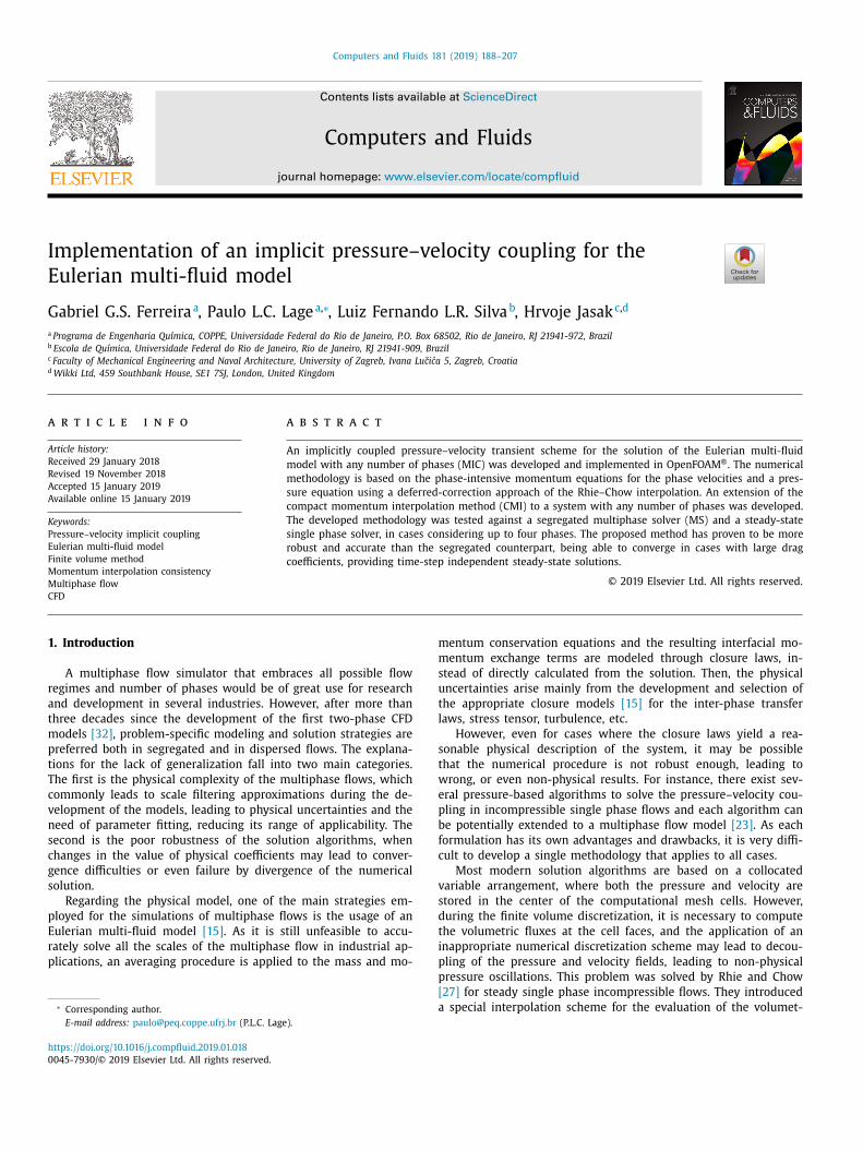
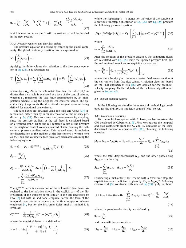
Fig. 2. Pressure (a) and velocity magnitude (b) fields for the flow over the

backward-facing step and the lines used for sampling. The results shown are for

the MIC solver with mesh M3, mimicking a single phase flow by considering two

identical phases.

F

f

a

λ

s

f

i

i

f

w

t

b

S

w

t

g

s

ε

w

6

6

t

w

fl

(

l

t

t

F

z

a

I

g

v

o

a

m

m

s

i

o

F

e

p

a

m

T

l

o

s

t

M

s

y

c

M

s

p

v

6

w

a

s

f

3

a

t

o

t

w

p

t

t

i

v

s

t

m

t

c

S

f

m

t

o

t

e

t

or the convergence of the outer loop the absolute tolerance values

or pressure and velocity were relaxed to λabs p ∗, outer = 4 . 5 × 10 −1 Pa

nd λabs u α, outer = 2 × 10 −5 m/s, respectively, a relative tolerance of

rel p ∗, outer = λrel

u α, outer = 10 −5 was used for both variables and an ab-

olute tolerance of λabs r α, outer = 10 −4 was employed for the phase

ractions.

The simulations were run in an Intel Xeon X5675 with 32 phys-

cal cores running at 3.07 GHz CPUs and the CentOS 6.6 operat-

ng system with the Open MPI package [11] version 1.6.5 installed

or the parallel runs. The parallelism efficiency, η, and the speedup

ith respect to the serial case, S , were calculated using the execu-

ion time, t comp , of the master processor for each case, being given

y:

=

t comp

serial

t comp

parallel

; η =

S

Q

(65)

here Q is the number of processes in the parallel run.

In order to detect the approach to a steady-state solution, a

ransient deviation εt χ was defined by comparing the fields of a

eneric variable χ at two time instants separated by 100 time

teps, that is:

tχ =

1

n

n ∑

i =1

√

( χi (t) − χi ( t − 100�t ) ) 2

(66)

here n is the number of control volumes.

. Results

.1. Flow over a backward-facing step

The steady-state results for the modified pressure and the con-

inuous phase velocity magnitude fields are shown in Fig. 2 , and

ere obtained with mesh M3 and MIC solver for the two-phase

ow of two identical phases, mimicking the single phase flow

BFS1 test cases). Fig. 2 also shows the vertical and horizontal lines,

ocated at x = 0 . 045 m from the inlet and at y = 0 . 0075 m from

he bottom wall, respectively, used for sampling and comparing

he results for the different meshes and numerical methodologies.

ig. 3 shows the steady-state values for the pressure at the hori-

ontal and vertical lines and the x and y -component of the velocity

t the vertical line for the BFS1 test cases using the three meshes.

t shows that the results obtained with the MIC solver have a very

ood agreement with those generated by the pUC solver, with a

isually exact superposition of the profiles. On the other hand, we

bserved that the MS algorithm show some deviations, which are

ttributed to the differences in the numerical formulation. As the

esh is refined, the difference between the methodologies also di-

inishes, suggesting that they should yield the same results on a

ufficiently fine mesh.

Fig. 4 show the dispersed phase fraction, pressure and veloc-

ty profiles along the vertical line for the BFS2 cases. The profiles

f the b -phase fraction at t = 0 . 1 s and t = 0 . 4 s are displayed in

ig. 4 (a) and (b), respectively. They show that, despite the differ-

nt results between the MS and MIC methodologies, both of them

rovide the same results when the two- and three-phase cases

re compared, showing that the generalization of the numerical

ethodology to any number of phases was performed correctly.

he steady-state profiles of pressure and y -component of the ve-

ocity are shown in Fig. 4 (c) and (d), respectively. It can also be

bserved that the results obtained with the a − b or a 1 − a 2 − b

ystems were the same in both formulations. The influence of the

ime-step size on the steady-state solution obtained by the MS and

IC solvers was also verified for the BFS2 cases. Fig. 5 (a) and (b)

how, respectively, the steady-state profiles of the pressure and the

-component of the velocity on the vertical line for the simulations

onsidering Courant number values of 0.2 and 0.4. As expected, the

S methodology failed in achieving time-step independent results

ince it does not apply a temporally consistent momentum inter-

olation technique. On the other hand, the MIC formulation pro-

ided the same results for the two employed Courant numbers.

.2. Flow in a horizontal channel

First, the parallel scalability of both MIC and MS approaches

ere evaluated. Table 3 displays the execution time, the speedup

nd the parallelism efficiency considering the serial and parallel

imulations divided in up to ten processors. This analysis was per-

ormed for case HC1 with M3 considering a transient simulation of

0 s. The comparison of the execution times spent with the AAMG

nd SAMG shows that the later is from 10 to 25 times faster than

he former. As discussed by Uroi ́c and Jasak [34] , the convergence

f the AAMG method stalls after few iterations. For this reason,

he number of iterations performed by the linear solver were al-

ays equal to the maximum allowed (10) without achieving the

rescribed tolerance, resulting in more pressure-velocities itera-

ions in the inner loop to achieve convergence. On the other hand,

he SAMG method is capable of reaching the prescribed tolerance

n few iterations, resulting in less iterations also in the pressure-

elocities coupling loop. The results for the MS solver are also

hown in Table 3 , revealing that the MS approach was from 5 to 10

imes faster than the MIC with SAMG. On the other hand, the MIC

ethod shows a better parallel scalability, as its efficiency is close

o 68% for the case with 10 parallel processes, while the MS effi-

iency was below 35%. This suggests that the MIC solver with the

AMG linear solver may eventually become faster than MS solver

or very large meshes.

In order to compare the results obtained with the MIC and MS

ethods, the HC test cases were run for a total of 500 s in order

o achieve a steady-state solution. Due to the better performance

f the SAMG linear solver when compared to the AAMG method,

he former was used in the simulations with the MIC solver to gen-

rate the results given in the following.

The vertical lines used for sampling the velocity and phase frac-

ion fields were located at x = 1 m and x = 1 . 65 m, respectively,

198 G.G.S. Ferreira, P.L.C. Lage and L.F.L.R. Silva et al. / Computers and Fluids 181 (2019) 188–207

Fig. 3. Verification of the multiphase methodologies against the single phase steady-state coupled solver for several meshes: (a) the pressure profile along the vertical line,

(b) the pressure profiles for the horizontal line, (c) the x - and (d) y -component velocity profiles along the vertical line.

Table 3

Comparison of the parallelism efficiency and computational times spent with the MIC using differ-

ent solution methods and comparison with the MS solver for several number of processes.

MIC MS

Q AAMG SAMG GAMG

t comp [s] S η t comp [s] S η t comp [s] S η

1 204,140 – – 13,431 – – 1434 – –

2 146,540 1.4 69.7% 7169 1.9 93.7% 855 1.7 83.9%

4 98,677 2.1 51.7% 3673 3.7 91.4% 554 2.6 64.7%

8 55,403 3.7 46.1% 2286 5.9 73.4% 442 3.2 40.6%

10 48,850 4.2 41.8% 1980 6.8 67.8% 424 3.4 33.9%

s

t

t

b

t

g

M

p

d

d

and the horizontal line used for sampling the modified pressure

was located at y = 0 . 0125 m, as displayed in Fig. 6 . The results ob-

tained in the case HC1 are shown in Fig. 7 . The velocity and pres-

sure profiles after 500 s of simulation are displayed in Fig. 7 (a) and

(b), respectively, and show that the results obtained with the MIC

and MS solvers are similar regardless of the mesh spacing for this

case. The dispersed phase fraction profile is shown in Fig. 7 (c). It is

also observed that the results obtained with the M3 mesh are very

similar to those using the M4 mesh. Hence, given the large compu-

tational cost of the simulations with M4, M3 was the finest mesh

used in the cases HC2, HC3, HC4 and HC5. As expected, Fig. 7 (c)

hows that the denser dispersed phase deposits at the bottom of

he channel. As the mesh refinement is increased, the phase frac-

ion gradients increase and the phase fraction at the vicinity of the

ottom wall reaches a unitary value, while the phase fraction near

he top wall approaches zero. Despite these steep phase fraction

radients, no convergence issues were observed for the MIC and

S approaches in the HC1 cases.

The maximum transient deviations in the velocity, modified

ressure and phase fraction fields obtained with the M3 mesh are

isplayed in Fig. 7 (d). In the first 100 s of simulation, the transient

eviations of both methods have the same order of magnitude.

G.G.S. Ferreira, P.L.C. Lage and L.F.L.R. Silva et al. / Computers and Fluids 181 (2019) 188–207 199

Fig. 4. Multiphase flow simulation considering different number of phases and numerical formulations (mesh M1): b -phase fraction at (a) t = 0 . 1 s and (b) t = 0 . 4 s and the

steady state profiles for (c) the pressure and (d) the y -component of the velocity along the vertical line.

T

v

b

s

v

r

m

t

t

t

m

m

(

e

s

t

t

o

t

s

i

M

f

o

t

r

w

n

p

b

a

a

l

n

s

i

s

s

a

c

c

(

t

M

hen, after 100 s, rapid declines are noticed in the transient de-

iations of the velocity and phase fraction in the MIC solver, which

ecome negligible after 200 s. This faster convergence to steady

tate may be credited to the better coupling between the phase

elocities in the MIC solver. The number of inner and outer cor-

ections performed by both solvers in each time step using the M3

esh is shown in Fig. 7 (e) and (f), respectively. During most of

he simulation time both methods performed only one outer itera-

ion per time step. Thus, these figures show only the beginning of

he simulation, where the number of iterations performed by both

ethods were different. Except for the first time step, where the

aximum allowed number of pressure–velocity coupling iterations

50) was employed, the MS method performed only one inner it-

ration per time step. On the other hand, the MIC solver executed

everal iterations in the first second of simulation. This explains

he lower computational cost of the MS solver when compared to

he MIC solver, as shown in Table 3 . Not only the cost per iteration

f the MS solver was lower, but also the number of inner itera-

ions required to achieve the convergence within the time step was

maller. However, this is a case were both methods yielded a phys-

cally sound solution. There are simulation conditions where the

S solver fails and the MIC method must be employed, as those

or the cases HC4 and HC5, which are analyzed below.

The test cases HC2 were designed to evaluate the performance

f the MIC and MS methods when exists a large density ratio be-

ween the dispersed and continuous phases ( ρc /ρdB = 20 ). The cor-

esponding results are shown in Fig. 8 . For this case, the MS solver

ith M2 diverged at t = 97 s and the steady state results could

ot be compared for this mesh. However, the velocity and pressure

rofiles shown in Fig. 8 (a) and (b) reveal a good mesh convergence

etween M2 and M3 using MIC. The results obtained with the MIC

nd MS solvers were similar for M1 and M3.

The dispersed phase fraction profiles for the HC2 simulations

re displayed in Fig. 8 (c). As expected, the phase fraction of the

ighter dispersed phase B is higher near the top of the chan-

el. As in the previous case, the phase fraction gradient becomes

teeper as the mesh is refined. Observing the transient deviations

n Fig. 8 (d) for the M3 mesh, it is noticed that both MIC and MS

olvers achieved state state solutions for which the pressure fields

till have some small fluctuations ( εt p∗ ∼ 10 −2 ). These fluctuations

re due to the large density gradients that emerge in this case. The

omparisons in the number of inner and outer loop iterations exe-

uted by both solvers for the M3 mesh are shown in Fig. 8 (e) and

f), respectively. They reveal that the convergence with the MIC for

his case is more costly than in the base case HC1. Both MIC and

S methods still perform only one iteration per time step for most

200 G.G.S. Ferreira, P.L.C. Lage and L.F.L.R. Silva et al. / Computers and Fluids 181 (2019) 188–207

Fig. 5. Verification of the time-step dependency of the multiphase methodologies:

profiles of (a) the pressure along the horizontal line and (b) the y -component of

the velocity along the vertical line for different Courant numbers using the MS and

MIC methodologies.

Fig. 6. Lines used for sampling the data in the horizontal case channel. The dis-

persed fraction field shown is for the HC2 case using the MIC solver.

f

t

o

e

a

t

d

s

T

a

t

w

o

f

w

t

a

c

w

v

a

M

c

o

a

a

M

p

t

s

o

p

t

u

w

t

s

i

s

T

s

i

(

d

T

p

w

s

t

p

f

a

o

d

w

o

t

s

F

n

s

s

t

of the simulated time, but MIC performs 3 inner iterations for al-

most 75 s of simulation, while MS performs more than one inner

iteration only in the first 0.06 s of simulation.

The test case HC3 evaluates the effect of a different value

for the dispersed phase viscosity in the performance of the two

solvers. The obtained results are shown in Fig. 9 . As in the previous

case, the velocity and pressure profiles have already achieved mesh

convergence for the M3 mesh, as shown in Fig. 9 (a) and (b). The

dispersed phase fraction profile, shown in Fig. 9 (c), is very similar

to that of case HC1, with the heavier dispersed phase C depositing

at the bottom wall, and the phase fraction gradients increasing as

the mesh is refined. However, the main difference in these two test

cases is the behavior of the transient deviations, shown in Fig. 9 (c)

or the M3 mesh. When the steady state solution was achieved,

he transient deviations using the MS solver are about five orders

f magnitude larger than those using the MIC solver. This can be

xplained by the fact that a lower dispersed phase viscosity cre-

tes larger relative velocities in the streamwise direction and, thus,

he continuous and dispersed phase velocity profiles have different

evelopment. The better coupling between the phases in the MIC

olver yields a smoother convergence to the steady state solution.

he number of inner and outer iterations are shown in Fig. 9 (e)

nd (f), respectively, for the M3 mesh. As in the previous cases,

he MS solver required more iterations in the first few time steps,

hile the MIC executed more inner iterations during the first 7 s

f simulation.

Fig. 10 shows the results for test case HC4, which was designed

or evaluating both solvers in the simulation of a dispersed phase

ith small particles (or drops). Fig. 10 (a) and (b) show, respec-

ively, the velocity and pressure profiles obtained from the MIC

nd MS methods. The results from the MIC method have mesh

onvergence but the results obtained from the MS method do not,

hich are very different for the three meshes. The MS method pro-

ides a velocity profile that tends to be flat instead of parabolic,

s expected. This happened due to numerical limitations of the

S solver when dealing with the large drag coefficients that oc-

ur for this case, as a result of the small value of the diameter

f the dispersed phase D. It must be pointed out that the toler-

nce criteria specified for controlling the inner and outer loop iter-

tions were fullfilled for all cases in all time steps. Therefore, the

S solver convergence has stalled. The dispersed phase fraction

rofile is shown in Fig. 10 (c), which shows that the phase frac-

ion gradients are less steep than the previous cases due to the

maller settling velocity caused by the decrease in the diameter

f the dispersed phase. As expected, the different velocity fields

rovided by the MS and MIC solvers led to different phase frac-

ion profiles. Fig. 10 (d) shows the transient deviations, which are

p to eight orders of magnitude larger for the MS method results

hen compared to those obtained by the MIC method. However,

he number of inner and outer iterations in both the MIC and MS

olvers, shown in Fig. 10 (e) and (f), respectively, are the same, that

s, only one iteration per time step, except at the beginning of the

imulations.

The results of the test case HC5 are shown in Figs. 11 and 12 .

hese tests were performed in order to evaluate the MIC and MS

olvers in a multiphase case with several dispersed phases includ-

ng large density differences and small particle sizes. Fig. 11 (a) and

b) show, respectively, the velocity and pressure profiles, which are

ifferent for the MIC and MS methods, similarly to the HC4 case.

his is related to the presence of the small-diameter dispersed

hase D and the numerical limitations of the MS solver to deal

ith large drag coefficients. However, for the HC5 case, the MS

olver results get closer to those obtained with the MIC solver as

he mesh is refined. This may be credited to the smaller fraction of

hase D in this test case when compared to HC4 case. The phase

raction profiles of the continuous and dispersed phases C, D and E

re shown in Fig. 11 (c)–(f), respectively. The results for both meth-

ds agree with what was qualitatively expected, with the lighter

ispersed phase B concentrating near the top wall of the channel

hereas the heavier dispersed phase C concentrated at the bottom

f the channel and the fraction of phase D followed the qualita-

ive pattern of the continuous phase fraction because of the small

ettling rate of its particles.

The transient deviations for the M3 mesh are shown in

ig. 12 (a). Their values for the MIC solver are seven orders of mag-

itude lower than those for the MS solver, indicating that, de-

pite the long simulation time, the latter did not converged to the

teady-state solution. The inner and outer iterations executed by

he MIC and MS solvers are shown in Fig. 12 (b) and (c), respec-

G.G.S. Ferreira, P.L.C. Lage and L.F.L.R. Silva et al. / Computers and Fluids 181 (2019) 188–207 201

Fig. 7. Results for the case HC1: (a) continuous phase velocity, (b) modified pressure, (c) dispersed phase fraction, (d) transient deviations, (e) total number of inner iterations

and (f) number of outer iterations within the timestep.

202 G.G.S. Ferreira, P.L.C. Lage and L.F.L.R. Silva et al. / Computers and Fluids 181 (2019) 188–207

Fig. 8. Results for the case HC2: (a) continuous phase velocity, (b) modified pressure, (c) dispersed phase fraction, (d) transient deviations, (e) total number of inner iterations

and (f) number of outer iterations within the timestep.

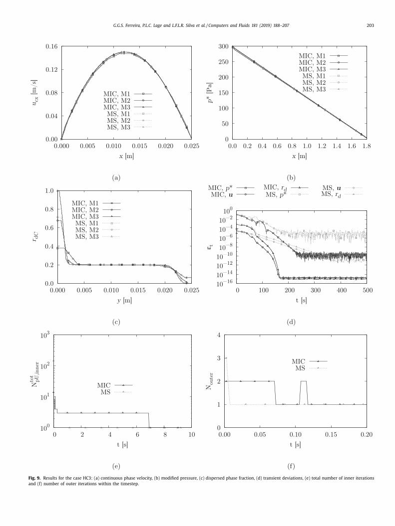
G.G.S. Ferreira, P.L.C. Lage and L.F.L.R. Silva et al. / Computers and Fluids 181 (2019) 188–207 203

Fig. 9. Results for the case HC3: (a) continuous phase velocity, (b) modified pressure, (c) dispersed phase fraction, (d) transient deviations, (e) total number of inner iterations

and (f) number of outer iterations within the timestep.

204 G.G.S. Ferreira, P.L.C. Lage and L.F.L.R. Silva et al. / Computers and Fluids 181 (2019) 188–207

Fig. 10. Results for the case HC4: (a) continuous phase velocity, (b) modified pressure, (c) dispersed phase fraction, (d) transient deviations, (e) total number of inner

iterations and (f) number of outer iterations within the timestep.

G.G.S. Ferreira, P.L.C. Lage and L.F.L.R. Silva et al. / Computers and Fluids 181 (2019) 188–207 205

Fig. 11. Results for the case HC5: (a) continuous phase velocity, (b) modified pressure, (c) continuous phase fraction and fraction of dispersed phases (d) B, (e) C and (f) D.

206 G.G.S. Ferreira, P.L.C. Lage and L.F.L.R. Silva et al. / Computers and Fluids 181 (2019) 188–207

Fig. 12. Results for the case HC5: (a) transient errors, (b) total number of inner

iterations and (c) number of outer iterations within the timestep for the case HC5

with M3.

t

w

e

0

t

N

i

h

t

T

s

7

s

p

f

O

i

s

p

i

e

t

t

o

t

s

f

s

a

n

s

u

h

m

s

f

s

t

c

w

M

d

v

i

v

r

A

4

P

g

g

t

G

C

–

E

ively. Both solvers performed only one outer iteration during the

hole simulation. The MIC solver executed from 1 to 4 inner it-

rations, with an average of 2.5 iterations, in the interval between

.0025 s and 68 s of the simulation, hence the number of itera-

ions plotted is the average of the total number of inner iterations,

tot

pU , inner , for this interval. After approximately 90 s, just one inner

teration was executed until the end of simulation. On the other

and, the MS solver performed several iterations only in the first

ime step, using only one iteration for the rest of the simulation.

herefore, the MS solver runned much faster, but yielded a wrong

olution.

. Summary and conclusions

The implementation and verification of an implicitly coupled

olver (MIC) for the multi-fluid model was performed. The com-

utational code was implemented in C++ using the libraries

rom foam-extend , a fork of the open-source CFD toolbox

penFOAM

®. The numerical methodology developed in this work

s based on the simultaneous solution of the momentum and pres-

ure equations, being extended for systems with any number of

hases.

We performed a thorough verification of the code, compar-

ng it with a steady-state single phase flow solver and with an

xtended multiphase version (MS) of the segregated solver for

he two-fluid Eulerian model implemented in foam-extend, the

woPhaseEulerFoam solver.

The Aggregative AMG and the Block-Selective AMG [34] meth-

ds were tested for the solution of the block-coupled matrix in

he MIC solver. The SAMG has proven to be more effective on the

olution of the problem, reaching the prescribed tolerance with

ew linear solver iterations. On the other hand, the AAMG solver

howed a poor convergence behavior, performing the maximum

llowed number of linear system iterations and requiring a large

umber of pressure–velocity coupling iterations to reach the de-

ired accuracy.

The parallel scalabilities of the MS and MIC solvers were eval-

ated for the solution of a two-phase flow in a two-dimensional

orizontal channel using 1–10 processors. For this case, the MS

ethod has shown to be from 4.6 to 9.3 times faster than the MIC

olver. However, its parallel efficiency was half of the one obtained

or the MIC solver for the 10-processor runs.

The analysis of the convergence to the steady-state solution in

everal test cases showed that the MIC method was more robust

hat the MS solver. Considering cases with similar convergence

riteria, the MIC method was able to reach steady-state solutions

ith smaller errors. The main advantage of the MIC solver over the

S solver is its capability of achieving convergence even when the

rag coefficient is large. For these cases, the segregated pressure–

elocity coupling used in the MS solver fails, providing flat veloc-

ty profiles and wrong pressure fields. These wrong solutions pro-

ided by the MS solver occur irrespective of the convergence crite-

ia used for controlling the inner and outer iteration loops.

cknowledgments

The authors thanks PETROBRAS contract 016/0 0 097-2 (SAP

60 0533021 , Jur 0 050.0102155.16.9 ); for the financial support.

aulo L.C. Lage acknowledges the financial support from CNPq ,

rants nos. 456905/2014-6 and 305265/2015-6 , and from FAPERJ ,

rant no. E-26/111.361/2010 . Luiz Fernando L.R. Silva acknowledges

he financial support from FAPERJ , grant no. E-26/110.150/2014 .

abriel G.S. Ferreira acknowledges the financial support from

NPq , grant no. 140292/2013-6 and from CAPES Finance code 001

Brazilian Federal Agency for Support and Evaluation of Graduate

ducation within the Ministry of Education of Brazil.

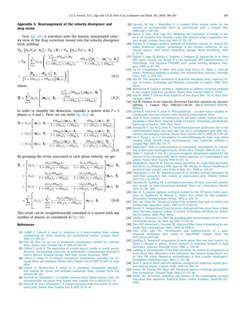
G.G.S. Ferreira, P.L.C. Lage and L.F.L.R. Silva et al. / Computers and Fluids 181 (2019) 188–207 207

A

d

i

t

∇

w

�

I

p

�

B

�

T

n

R

[

[

[

[

[

[

[

[

[

[

[

[

[

[

ppendix A. Rearrangement of the velocity divergence and

rag terms

First, Eq. (51) is rewritten with the linearly interpolated veloc-ty term of the drag correction moved into the velocity divergenceerm, yielding:

D ·[D P f ∇ f p

∗ · S f ]

= ∇ D · ( �) + ∇ D ·[D P f (∇p ∗) f · S f

]

+ ∇ D ·

⎡

⎢ ⎣

P ∑

α=1

( r α ) f

⎛

⎜ ⎝

∑ P β=1 β � = α

(�Dαβ ) f φβ

1 + (�T α) f + (�Dα ) f +

(�T α) f [φt−1

α − (u

t−1 α ) f · S f

]1 + (�T α) f + (�Dα ) f

+

[F ∗

Bα, f − (F ∗Bα ) f

]· S f [

1 + (�T α) f + (�Dα ) f ](A α ) f

) ] (A.1)

here

=

P ∑

α=1

(r α) f

⎡

⎢ ⎣

(u α) f · S f −

∑ P β=1 β � = α

(�Dαβ ) f (u β ) f · S f

1 + (�T α) f + (�Dα) f

⎤

⎥ ⎦

(A.2)

n order to simplify the deduction, consider a system with P = 3hases a, b and c . Then, we can write Eq. (A.2) as:

= (r a ) f

[(u a ) f · S f −

(�Dab ) f (u b ) f · S f

1 + (�Ta ) f + (�Da ) f − (�Dac ) f (u c ) f · S f

1 + (�Ta ) f + (�Da ) f

]

+ (r b ) f

[(u b ) f · S f −

(�Dba ) f (u a ) f · S f

1 + (�T b ) f + (�Db ) f − (�Dbc ) f (u c ) f · S f

1 + (�T b ) f + (�Db ) f

]

+ (r c ) f

[(u c ) f · S f −

(�Dca ) f (u a ) f · S f

1 + (�Tc ) f + (�Dc ) f − (�Dcb ) f (u b ) f · S f

1 + (�Tc ) f + (�Dc ) f

](A.3)

y grouping the terms associated to each phase velocity, we get:

=

[(r a ) f −

(r b ) f (�Dba ) f 1 + (�T b ) f + (�Db ) f

− ( r c ) f ( �Dca ) f 1 + (�Tc ) f + (�Dc ) f

](u a ) f · S f

+

[(r b ) f −

(r a ) f (�Dab ) f 1 + (�Ta ) f + (�Da ) f

− ( r c ) f ( �Dcb ) f 1 + (�Tc ) f + (�Dc ) f

](u b ) f · S f

+

[(r c ) f −

(r a ) f (�Dca ) f 1 + (�Ta ) f + (�Da ) f

− ( r b ) f ( �Dcb ) f 1 + (�T b ) f + (�Db ) f

](u c ) f · S f

=

P ∑

α=1

⎡

⎢ ⎣

(r α ) f −P ∑

β=1 β � = α

(r β ) f (�Dβα ) f

1 + (�T β ) f + (�Dβ ) f

⎤

⎥ ⎦

( u α ) f · S f (A.4)

his result can be straightforwardly extended to a system with any

umber of phases, as considered in Eq. (58) .

eferences

[1] Cardiff P , Tukovi ́c Z , Jasak H , Ivankovi ́c A . A block-coupled finite volumemethodology for linear elasticity and unstructured meshes. Comput Struct

2016;175:100–22 .

[2] Choi SK . Note on the use of momentum interpolation method for unsteadyflows. Numer Heat Transfer Part A 1999;36:545–50 .

[3] Clifford I , Jasak H . The application of a multi-physics toolkit to spatial reactordynamics. International conference on mathematics, computational methods &

reactor physics. Saratoga Springs, New York: Curran Associates; 2009 . [4] Cubero A , Fueyo N . A compact momentum interpolation procedure for un-

steady flows and relaxation. Numer Heat Transfer Part B 2007;52:507–29 . June

2014 [5] Cubero A , Sánchez-insa A , Fueyo N . A consistent momentum interpola-

tion method for steady and unsteady multiphase flows. Comput Chem Eng2014;62:96–107 .

[6] Darwish M , Moukalled F . A coupled pressure-based finite-volume solver forincompressible two-phase flow. Numer Heat Transfer Part B 2015;67:47–74 .

[7] Darwish M , Sraj I , Moukalled F . A coupled incompressible flow solver on struc-

tured grids. Numer Heat Transfer Part B 2007;52:37–41 .

[8] Darwish M , Sraj I , Moukalled F . A coupled finite volume solver for thesolution of incompressible flows on unstructured grids. J Comput Phys

2009;228(1):180–201 . [9] Favero JL , Silva LFLR , Lage PLC . Modeling and simulation of mixing in wa-

ter-in-oil emulsion flow through a valve-like element using a population bal-ance model. Comput Chem Eng 2015;75:155–70 .

[10] Fletcher R . Conjugate gradient methods for indefinite systems. In: Watson GA,editor. Numerical analysis: proceedings of the Dundee conference on nu-

merical analysis, 1975. Berlin, Heidelberg: Springer Berlin Heidelberg; 1976.

p. 73–89 . [11] Gabriel E , Fagg GE , Bosilca G , Angskun T , Dongarra JJ , Squyres JM , et al. Open

MPI: goals, concept, and design of a next generation MPI implementation. In:Proceedings, 11th European PVM/MPI users’ group meeting, Budapest, Hun-

gary; 2004. p. 97–104 . [12] Gu CY . Computation of flows with large body forces. In: Taylor C, Chin JH,

editors. Numerical methods in laminar and turbulent flow. Swansea: Pineridge

Press; 1991. p. 294–305 . [13] Hill DP . The computer simulation of dispersed two-phase flows. Imperial Col-

lege of Science, Technology and Medicine, University of London; 1998. Ph.D.thesis .

[14] Hutchinson B , Galpin P , Raithby G . Application of additive correction multigridto the coupled fluid flow equations. Numer Heat Transfer 1988;13:133147 .

[15] Ishii M , Hibiki T . Thermo-fluid dynamics of two-phase flow. 1st ed. Nova York:

Springer; 2006 . [16] Issa RI. Solution of the implicitly discretised fluid flow equations by operator-

splitting. J Comput Phys 1986;62(1):40–65. doi: 10.1016/0021-9991(86)90099-9 .

[17] Jareteg K , Vukcevik V , Jasak H . PUCoupledFoam - an open source coupled in-compressible pressure-velocity solver based on foam-extend; 2014 .

[18] Jasak H . Error analysis and estimation for the finite volume method with ap-

plications to fluid flows. Imperial College of Science, Technology and Medicine,University of London; 1996. Ph.D. thesis .

[19] Kawaguchi Y , Tao W-Q , Ozoe H . Checkerboard pressure predictions due to theunderrelaxation factor and time step size for a nonstaggered grid with mo-

mentum interpolation method. Numer Heat Transfer Part B 2002;41(1):85–94 .20] Lee J , Zhang J , Lu C-C . Incomplete LU preconditioning for large scale dense

complex linear systems from electromagnetic wave scattering problems. J

Comput Phys 2003;185:158–75 . [21] Majumdar S . Role of underrelaxation in momentum interpolation for calcula-

tion of flow with nonstaggered grids. Numer Heat Transfer 1988;14:125–32 . 22] Miller T , Schmidt F . Use of a pressure-weighted interpolation method for the

solution of the incompressible Navier-Stokes equations on a nonstaggered gridsystem. Numer Heat Transfer 1988;14:213–33 .

23] Moukalled F , Darwish M . Pressure based algorithms for single-fluid and multi-

fluid flows. In: Minkowycz WM, Sparrow EM, Murthy JY, editors. Handbook ofnumerical heat transfer. John Wiley & Sons, Inc.; 2009. p. 345–67 .

24] Passalacqua A , Fox RO . Implementation of an iterative solution procedure formulti-fluid gasparticle flow models on unstructured grids. Powder Technol

2011;213(1–3):174–87 . 25] Patankar SV , Spalding DB . A calculation procedure for heat, mass and momen-

tum transfer in three-dimensional parabolic flows. Int J Heat Mass Transfer1972;15:1787–806 .

26] Raw M . A coupled algebraic multigrid method for the 3D Navier-Stokes equa-

tions. In: Hackbusch W, Wittum G, editors. Fast solvers for flow problems.Wiesbaden: Vieweg+Teubner Verlag; 1995. p. 204–15 .

[27] Rhie CM , Chow WL . Numerical study of the turbulent flow past an airfoil withtrailing edge separation. AIAA J 1983;21(11):1525–32 .

28] Rusche H . Computational fluid dynamics of dispersed two-phase flows at highphase fractions. Imperial College of Science, Technology and Medicine, Univer-

sity of London; 2002. Ph.D. thesis .

29] Schiller L , Naumann AZ . Über die grundlegenden berechnungen bei der schw-erkraftaufbereitung. Ver Deut Ing 1933;77:318–20 .

30] Shen WZ , Michelsen J , Sorensen JN . Improved Rhie-Chow interpolation for un-steady flow computations. AIAA J 2001;39:2406–9 .

[31] Silva LFLR , Lage PLC . Development and implementation of a poly-dispersed multiphase flow model in OpenFOAM. Comput Chem Eng

2011;35(12):2653–66 .

32] Spalding D . Numerical computation of multi-phase flow and heat transfer. In:Taylor C, Morgan K, editors. Recent advances in numerical methods in fluid

mechanics. Swansea: Pineridge Press; 1980. p. 139–68 . 33] Spalding D . Developments of the IPSA procedure for numerical computation of

multi-phase flow phenomena with interphase slip, unequal temperatures, etc.In: Shih TM, editor. Numerical methodologies in heat transfer. Washington:

Hemisphere Publishing Corp.; 1983. p. 421–36 .

34] Uroi ́c T , Jasak H . Block-selective algebraic multigrid for implicitly coupled pres-sure-velocity system. Comput Fluids 2018;167:100–10 .

35] Venier CM , Damian SM , Nigro NM . Numerical aspects of Eulerian gas-particlesflow formulations. Comput Fluids 2016;133:151–69 .

36] Weller HG . Derivation, modelling and solution of the conditionally averagedtwo-phase flow equations. Technical report. United Kingdom: OpenCFD Ltd.;

2005 .