Embed Size (px)
Citation preview
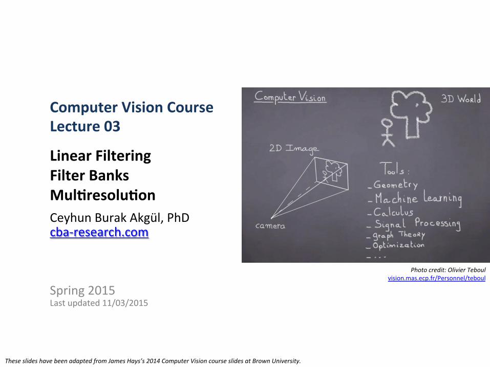
Linear Filtering Filter Banks Mul1resolu1on Ceyhun Burak Akgül, PhD cba-‐research.com Spring 2015 Last updated 11/03/2015
Computer Vision Course Lecture 03
Photo credit: Olivier Teboul vision.mas.ecp.fr/Personnel/teboul
These slides have been adapted from James Hays’s 2014 Computer Vision course slides at Brown University.
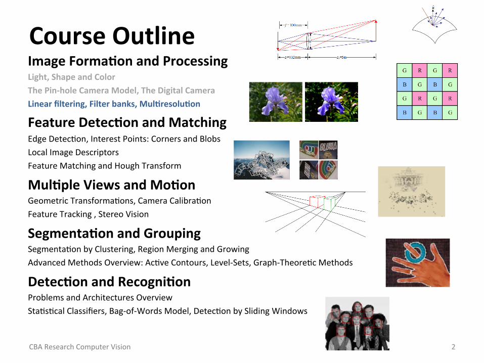
Course Outline Image Forma1on and Processing Light, Shape and Color The Pin-‐hole Camera Model, The Digital Camera Linear filtering, Filter banks, Mul1resolu1on
Feature Detec1on and Matching Edge DetecIon, Interest Points: Corners and Blobs Local Image Descriptors Feature Matching and Hough Transform
Mul1ple Views and Mo1on Geometric TransformaIons, Camera CalibraIon Feature Tracking , Stereo Vision
Segmenta1on and Grouping SegmentaIon by Clustering, Region Merging and Growing Advanced Methods Overview: AcIve Contours, Level-‐Sets, Graph-‐TheoreIc Methods
Detec1on and Recogni1on Problems and Architectures Overview StaIsIcal Classifiers, Bag-‐of-‐Words Model, DetecIon by Sliding Windows
2 CBA Research Computer Vision
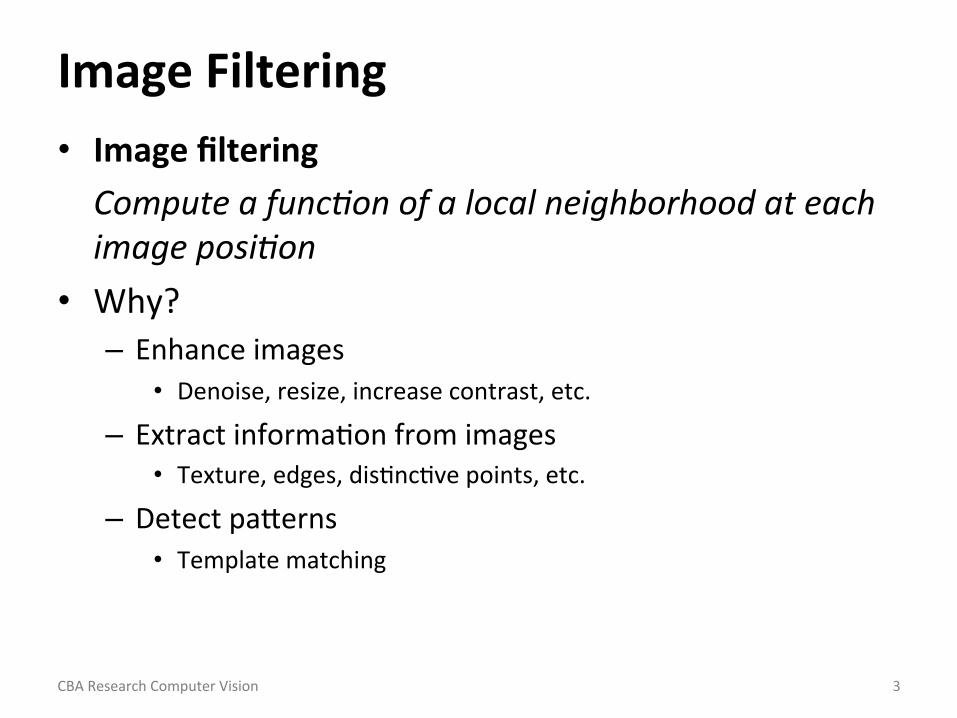
Image Filtering • Image filtering Compute a funcFon of a local neighborhood at each image posiFon
• Why? – Enhance images
• Denoise, resize, increase contrast, etc. – Extract informaIon from images
• Texture, edges, disIncIve points, etc. – Detect paZerns
• Template matching
CBA Research Computer Vision 3
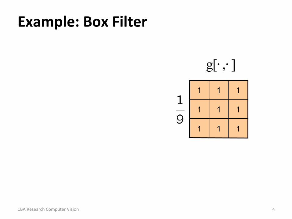
1 1 1
1 1 1
1 1 1
],[g ⋅⋅
Example: Box Filter
CBA Research Computer Vision 4
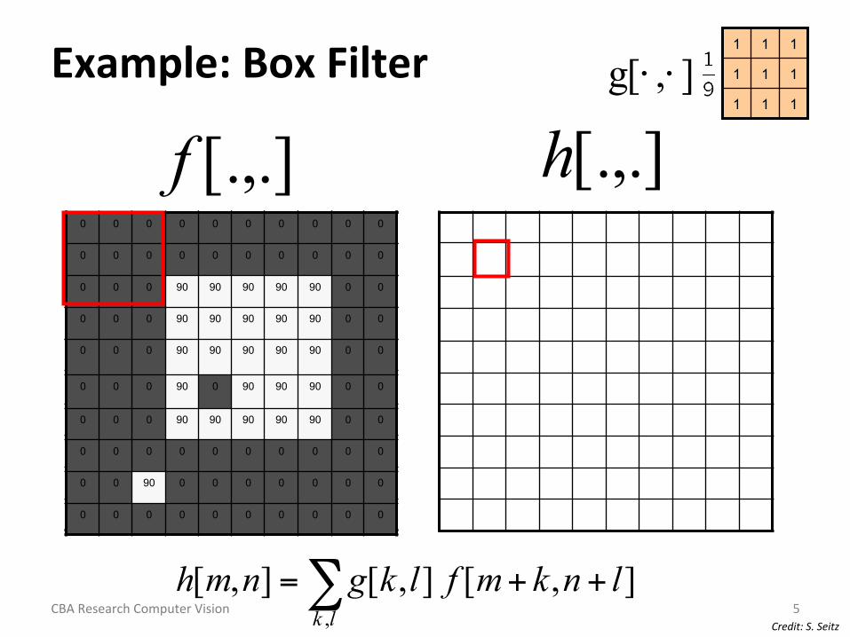
0 0 0 0 0 0 0 0 0 0
0 0 0 0 0 0 0 0 0 0
0 0 0 90 90 90 90 90 0 0
0 0 0 90 90 90 90 90 0 0
0 0 0 90 90 90 90 90 0 0
0 0 0 90 0 90 90 90 0 0
0 0 0 90 90 90 90 90 0 0
0 0 0 0 0 0 0 0 0 0
0 0 90 0 0 0 0 0 0 0
0 0 0 0 0 0 0 0 0 0
0
0 0 0 0 0 0 0 0 0 0
0 0 0 0 0 0 0 0 0 0
0 0 0 90 90 90 90 90 0 0
0 0 0 90 90 90 90 90 0 0
0 0 0 90 90 90 90 90 0 0
0 0 0 90 0 90 90 90 0 0
0 0 0 90 90 90 90 90 0 0
0 0 0 0 0 0 0 0 0 0
0 0 90 0 0 0 0 0 0 0
0 0 0 0 0 0 0 0 0 0
Credit: S. Seitz
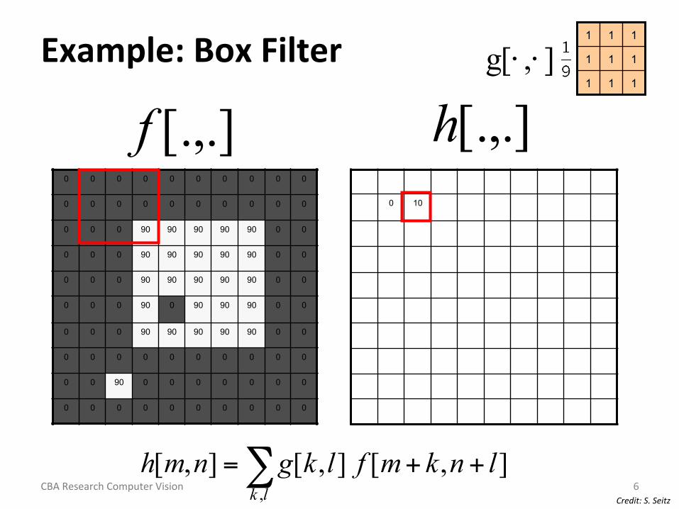
],[],[],[,
lnkmflkgnmhlk
++=∑
[.,.]h[.,.]f1 1 1
1 1 1
1 1 1
],[g ⋅⋅Example: Box Filter
CBA Research Computer Vision 5
0 0 0 0 0 0 0 0 0 0
0 0 0 0 0 0 0 0 0 0
0 0 0 90 90 90 90 90 0 0
0 0 0 90 90 90 90 90 0 0
0 0 0 90 90 90 90 90 0 0
0 0 0 90 0 90 90 90 0 0
0 0 0 90 90 90 90 90 0 0
0 0 0 0 0 0 0 0 0 0
0 0 90 0 0 0 0 0 0 0
0 0 0 0 0 0 0 0 0 0
0 10
0 0 0 0 0 0 0 0 0 0
0 0 0 0 0 0 0 0 0 0
0 0 0 90 90 90 90 90 0 0
0 0 0 90 90 90 90 90 0 0
0 0 0 90 90 90 90 90 0 0
0 0 0 90 0 90 90 90 0 0
0 0 0 90 90 90 90 90 0 0
0 0 0 0 0 0 0 0 0 0
0 0 90 0 0 0 0 0 0 0
0 0 0 0 0 0 0 0 0 0
[.,.]h[.,.]f1 1 1
1 1 1
1 1 1
],[g ⋅⋅
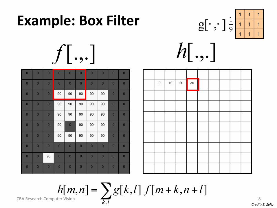
],[],[],[,
lnkmflkgnmhlk
++=∑
Example: Box Filter
Credit: S. Seitz CBA Research Computer Vision 6

0 0 0 0 0 0 0 0 0 0
0 0 0 0 0 0 0 0 0 0
0 0 0 90 90 90 90 90 0 0
0 0 0 90 90 90 90 90 0 0
0 0 0 90 90 90 90 90 0 0
0 0 0 90 0 90 90 90 0 0
0 0 0 90 90 90 90 90 0 0
0 0 0 0 0 0 0 0 0 0
0 0 90 0 0 0 0 0 0 0
0 0 0 0 0 0 0 0 0 0
0 10 20
0 0 0 0 0 0 0 0 0 0
0 0 0 0 0 0 0 0 0 0
0 0 0 90 90 90 90 90 0 0
0 0 0 90 90 90 90 90 0 0
0 0 0 90 90 90 90 90 0 0
0 0 0 90 0 90 90 90 0 0
0 0 0 90 90 90 90 90 0 0
0 0 0 0 0 0 0 0 0 0
0 0 90 0 0 0 0 0 0 0
0 0 0 0 0 0 0 0 0 0
[.,.]h[.,.]f1 1 1
1 1 1
1 1 1
],[g ⋅⋅
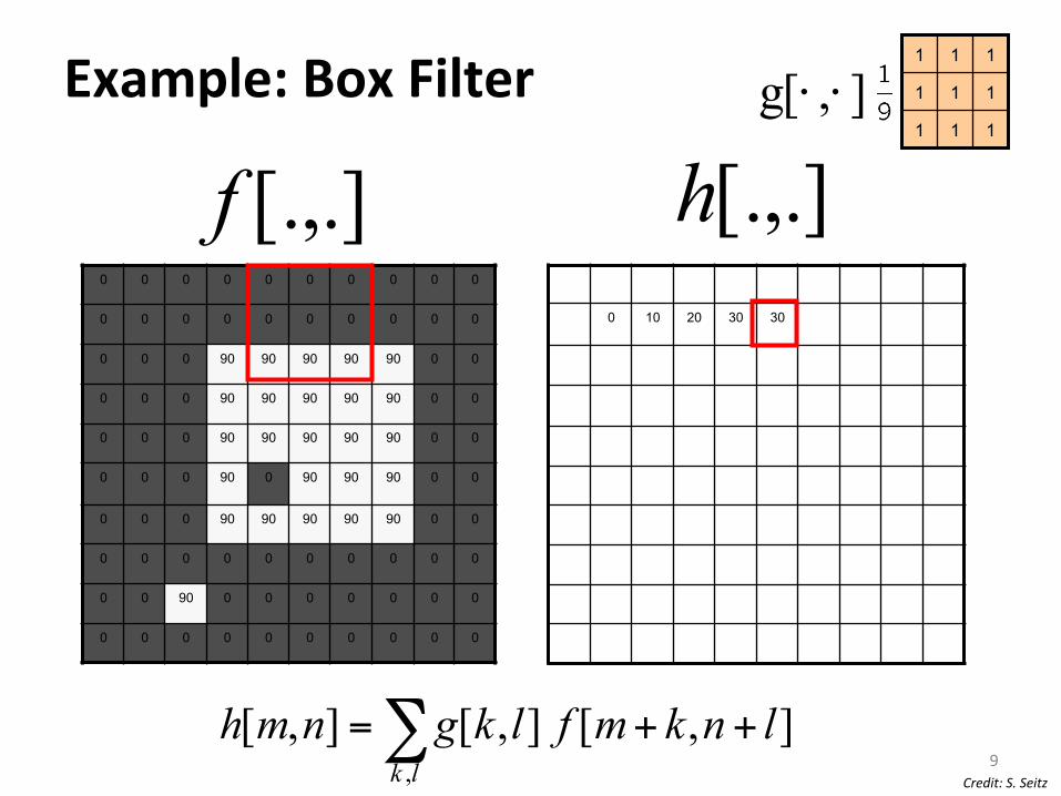
],[],[],[,
lnkmflkgnmhlk
++=∑
Example: Box Filter
Credit: S. Seitz CBA Research Computer Vision 7
0 0 0 0 0 0 0 0 0 0
0 0 0 0 0 0 0 0 0 0
0 0 0 90 90 90 90 90 0 0
0 0 0 90 90 90 90 90 0 0
0 0 0 90 90 90 90 90 0 0
0 0 0 90 0 90 90 90 0 0
0 0 0 90 90 90 90 90 0 0
0 0 0 0 0 0 0 0 0 0
0 0 90 0 0 0 0 0 0 0
0 0 0 0 0 0 0 0 0 0
0 10 20 30
0 0 0 0 0 0 0 0 0 0
0 0 0 0 0 0 0 0 0 0
0 0 0 90 90 90 90 90 0 0
0 0 0 90 90 90 90 90 0 0
0 0 0 90 90 90 90 90 0 0
0 0 0 90 0 90 90 90 0 0
0 0 0 90 90 90 90 90 0 0
0 0 0 0 0 0 0 0 0 0
0 0 90 0 0 0 0 0 0 0
0 0 0 0 0 0 0 0 0 0
[.,.]h[.,.]f1 1 1
1 1 1
1 1 1
],[g ⋅⋅
],[],[],[,
lnkmflkgnmhlk
++=∑Credit: S. Seitz
Example: Box Filter
CBA Research Computer Vision 8
0 10 20 30 30
0 0 0 0 0 0 0 0 0 0
0 0 0 0 0 0 0 0 0 0
0 0 0 90 90 90 90 90 0 0
0 0 0 90 90 90 90 90 0 0
0 0 0 90 90 90 90 90 0 0
0 0 0 90 0 90 90 90 0 0
0 0 0 90 90 90 90 90 0 0
0 0 0 0 0 0 0 0 0 0
0 0 90 0 0 0 0 0 0 0
0 0 0 0 0 0 0 0 0 0
[.,.]h[.,.]f1 1 1
1 1 1
1 1 1
],[g ⋅⋅
],[],[],[,
lnkmflkgnmhlk
++=∑
Example: Box Filter
Credit: S. Seitz 9
0 10 20 30 30
0 0 0 0 0 0 0 0 0 0
0 0 0 0 0 0 0 0 0 0
0 0 0 90 90 90 90 90 0 0
0 0 0 90 90 90 90 90 0 0
0 0 0 90 90 90 90 90 0 0
0 0 0 90 0 90 90 90 0 0
0 0 0 90 90 90 90 90 0 0
0 0 0 0 0 0 0 0 0 0
0 0 90 0 0 0 0 0 0 0
0 0 0 0 0 0 0 0 0 0
[.,.]h[.,.]f1 1 1
1 1 1
1 1 1
],[g ⋅⋅
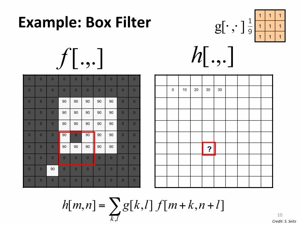
?
],[],[],[,
lnkmflkgnmhlk
++=∑
Example: Box Filter
Credit: S. Seitz 10
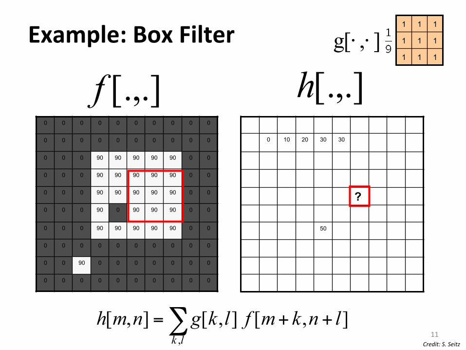
0 10 20 30 30
50
0 0 0 0 0 0 0 0 0 0
0 0 0 0 0 0 0 0 0 0
0 0 0 90 90 90 90 90 0 0
0 0 0 90 90 90 90 90 0 0
0 0 0 90 90 90 90 90 0 0
0 0 0 90 0 90 90 90 0 0
0 0 0 90 90 90 90 90 0 0
0 0 0 0 0 0 0 0 0 0
0 0 90 0 0 0 0 0 0 0
0 0 0 0 0 0 0 0 0 0
[.,.]h[.,.]f1 1 1
1 1 1
1 1 1
],[g ⋅⋅
?
],[],[],[,
lnkmflkgnmhlk
++=∑Credit: S. Seitz
Example: Box Filter
11
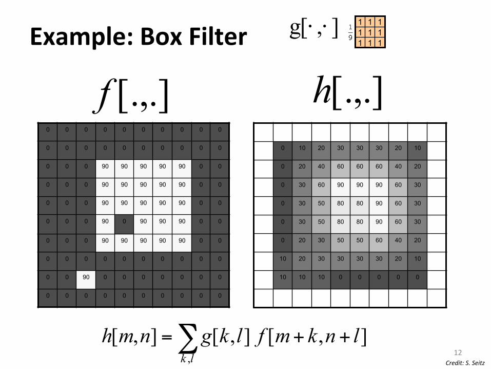
0 0 0 0 0 0 0 0 0 0
0 0 0 0 0 0 0 0 0 0
0 0 0 90 90 90 90 90 0 0
0 0 0 90 90 90 90 90 0 0
0 0 0 90 90 90 90 90 0 0
0 0 0 90 0 90 90 90 0 0
0 0 0 90 90 90 90 90 0 0
0 0 0 0 0 0 0 0 0 0
0 0 90 0 0 0 0 0 0 0
0 0 0 0 0 0 0 0 0 0
0 10 20 30 30 30 20 10
0 20 40 60 60 60 40 20
0 30 60 90 90 90 60 30
0 30 50 80 80 90 60 30
0 30 50 80 80 90 60 30
0 20 30 50 50 60 40 20
10 20 30 30 30 30 20 10
10 10 10 0 0 0 0 0
[.,.]h[.,.]f1 1 1 1 1 1 1 1 1 ],[g ⋅⋅
],[],[],[,
lnkmflkgnmhlk
++=∑
Example: Box Filter
Credit: S. Seitz 12
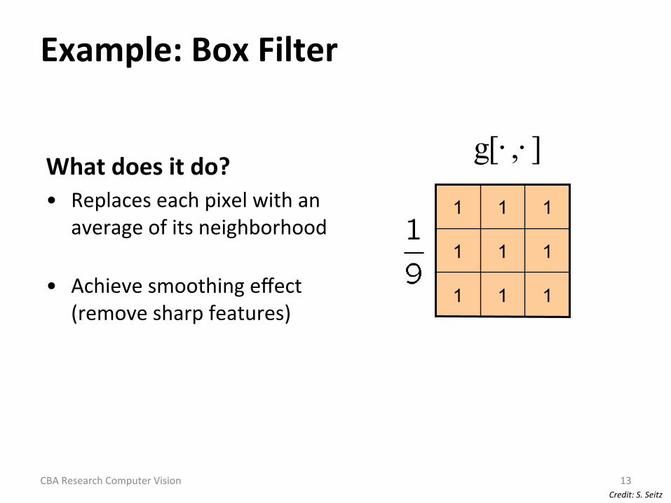
What does it do? • Replaces each pixel with an
average of its neighborhood
• Achieve smoothing effect (remove sharp features)
1 1 1
1 1 1
1 1 1
],[g ⋅⋅
Credit: S. Seitz
Example: Box Filter
CBA Research Computer Vision 13
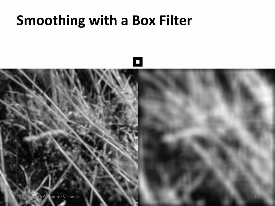
Smoothing with a Box Filter
14 CBA Research Computer Vision
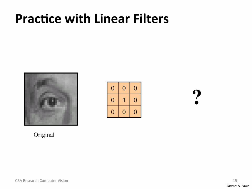
Prac1ce with Linear Filters
0 0 0
0 1 0
0 0 0
Original
?
Source: D. Lowe CBA Research Computer Vision 15
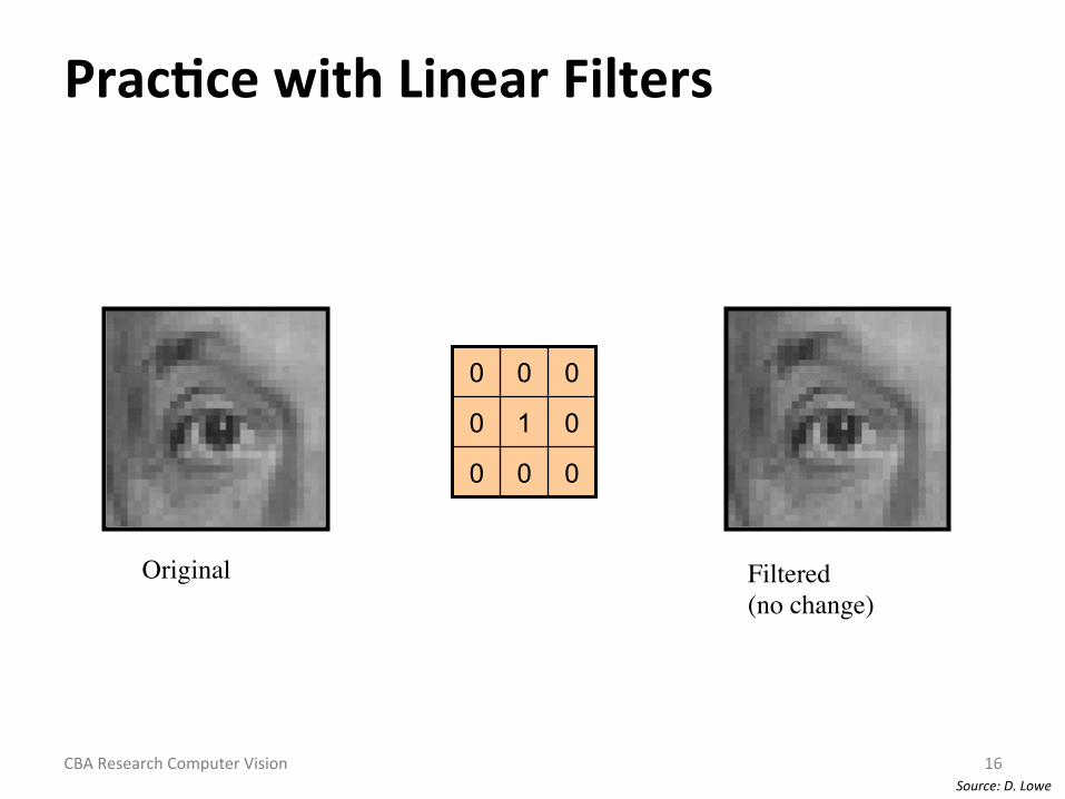
Prac1ce with Linear Filters
0 0 0
0 1 0
0 0 0
Original Filtered (no change)
Source: D. Lowe CBA Research Computer Vision 16

Prac1ce with Linear Filters
0 0 0
1 0 0
0 0 0
Original
?
Source: D. Lowe CBA Research Computer Vision 17
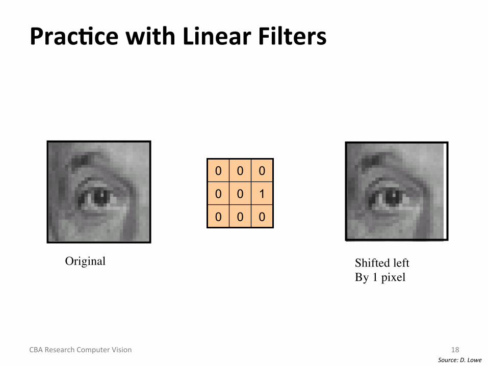
Prac1ce with Linear Filters
0 0 0
1 0 0
0 0 0
Original Shifted left By 1 pixel
Source: D. Lowe CBA Research Computer Vision 18
Prac1ce with Linear Filters
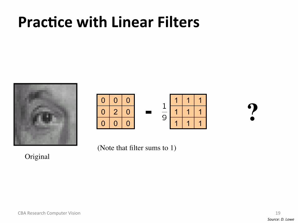
Original
1 1 1 1 1 1 1 1 1
0 0 0 0 2 0 0 0 0 - ?
(Note that filter sums to 1)
Source: D. Lowe CBA Research Computer Vision 19
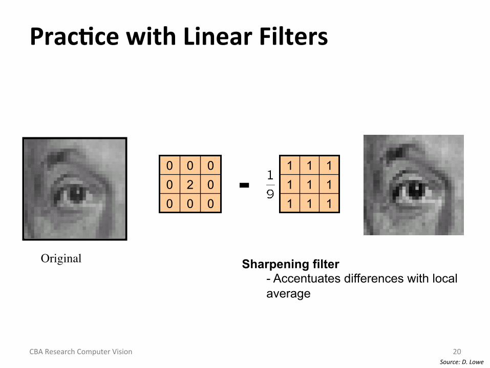
Prac1ce with Linear Filters
Original
1 1 1 1 1 1 1 1 1
0 0 0 0 2 0 0 0 0 -
Sharpening filter - Accentuates differences with local average
Source: D. Lowe CBA Research Computer Vision 20
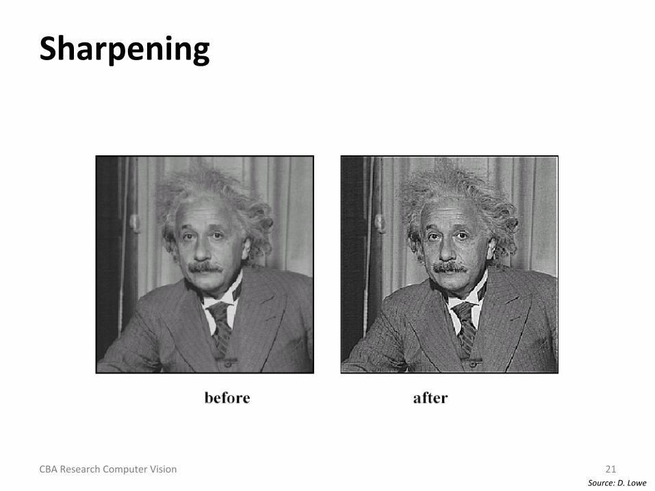
Sharpening
Source: D. Lowe CBA Research Computer Vision 21
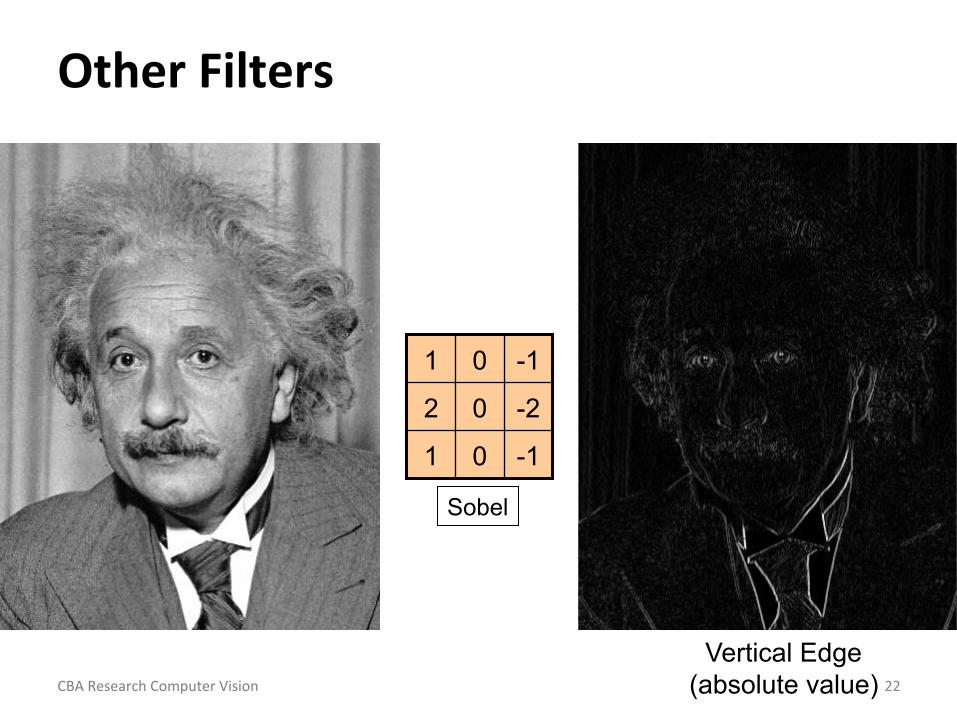
Other Filters
-1 0 1
-2 0 2
-1 0 1
Vertical Edge (absolute value)
Sobel
CBA Research Computer Vision 22
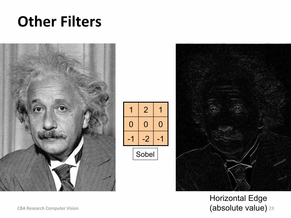
Other Filters
-1 -2 -1
0 0 0
1 2 1
Horizontal Edge (absolute value)
Sobel
CBA Research Computer Vision 23
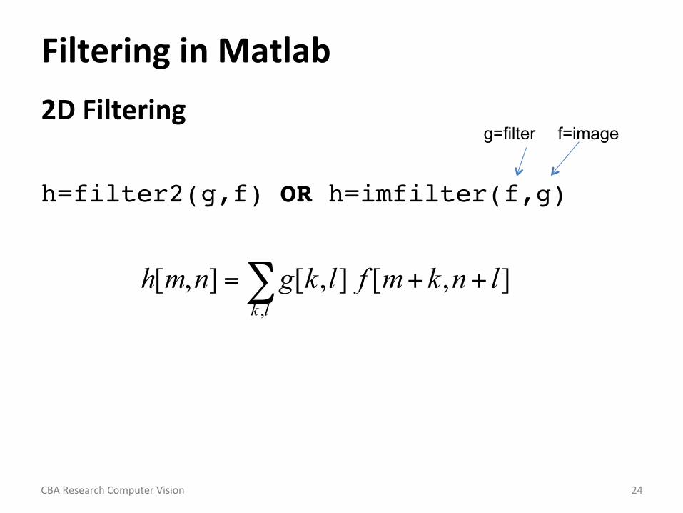
Filtering in Matlab 2D Filtering h=filter2(g,f) OR h=imfilter(f,g)!
f=image g=filter
],[],[],[,
lnkmflkgnmhlk
++=∑
CBA Research Computer Vision 24
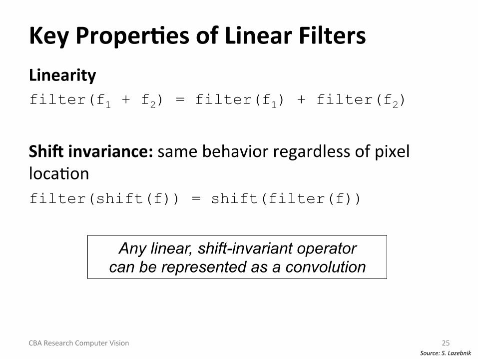
Key Proper1es of Linear Filters Linearity filter(f1 + f2) = filter(f1) + filter(f2) ShiR invariance: same behavior regardless of pixel locaIon filter(shift(f)) = shift(filter(f))
Source: S. Lazebnik
Any linear, shift-invariant operator can be represented as a convolution
CBA Research Computer Vision 25
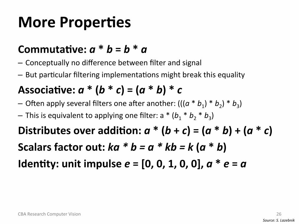
More Proper1es Commuta1ve: a * b = b * a – Conceptually no difference between filter and signal – But parIcular filtering implementaIons might break this equality
Associa1ve: a * (b * c) = (a * b) * c – Oeen apply several filters one aeer another: (((a * b1) * b2) * b3) – This is equivalent to applying one filter: a * (b1 * b2 * b3)
Distributes over addi1on: a * (b + c) = (a * b) + (a * c) Scalars factor out: ka * b = a * kb = k (a * b) Iden1ty: unit impulse e = [0, 0, 1, 0, 0], a * e = a
Source: S. Lazebnik CBA Research Computer Vision 26
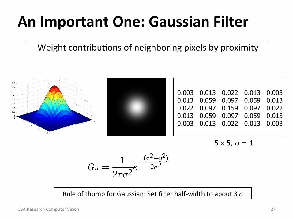
0.003 0.013 0.022 0.013 0.003 0.013 0.059 0.097 0.059 0.013 0.022 0.097 0.159 0.097 0.022 0.013 0.059 0.097 0.059 0.013 0.003 0.013 0.022 0.013 0.003
5 x 5, σ = 1
An Important One: Gaussian Filter Weight contribuIons of neighboring pixels by proximity
Rule of thumb for Gaussian: Set filter half-‐width to about 3 σ
CBA Research Computer Vision 27
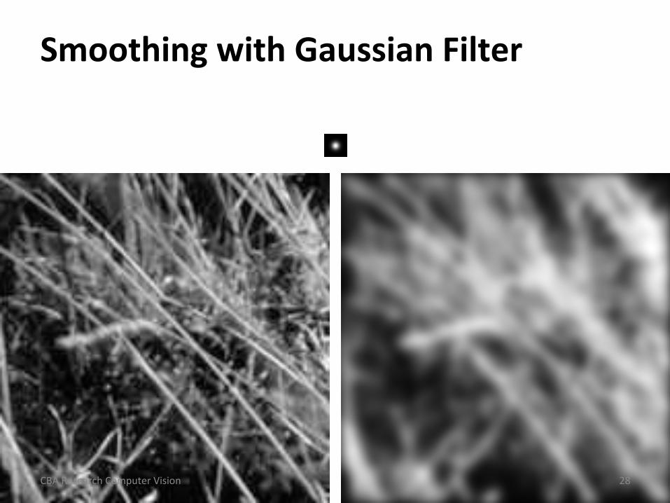
Smoothing with Gaussian Filter
28 CBA Research Computer Vision
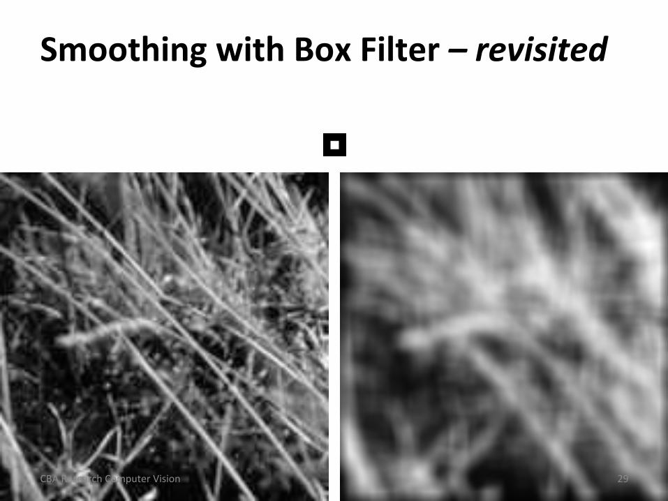
Smoothing with Box Filter – revisited
29 CBA Research Computer Vision
Gaussian Filters • Remove “high-‐frequency” components from the image (low-‐pass filter) – Images become more smooth
• ConvoluIon with self is another Gaussian – So can smooth with small-‐width kernel, repeat, and get same result as larger-‐width kernel would have
– Convolving two Imes with Gaussian kernel of width σ is same as convolving once with kernel of width σ√2
• Separable kernel – Factors into product of two 1D Gaussians
CBA Research Computer Vision 30
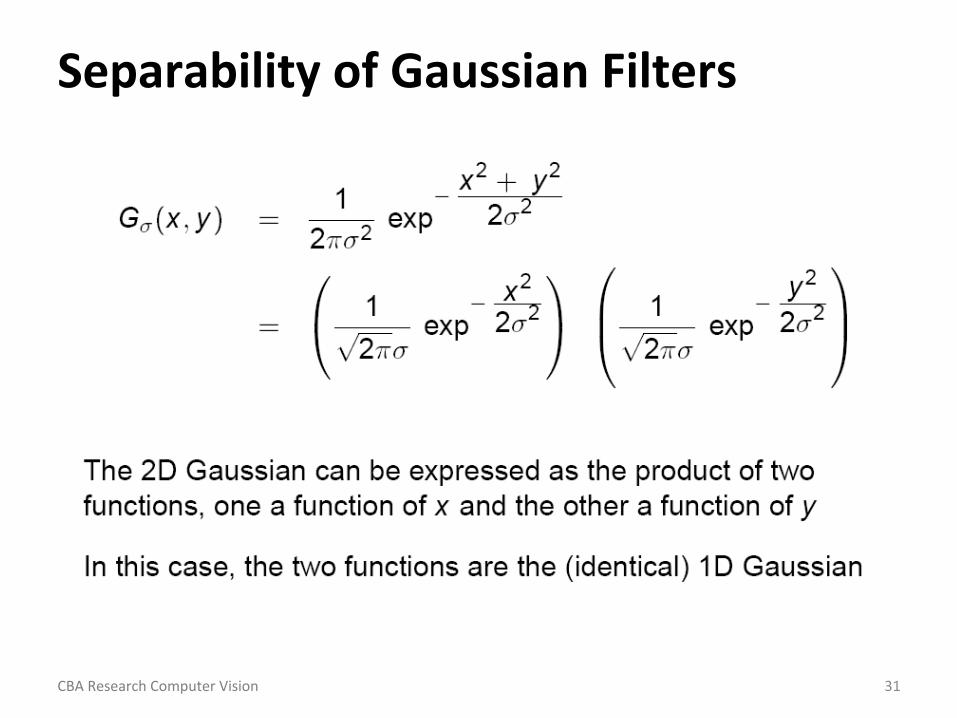
Separability of Gaussian Filters
CBA Research Computer Vision 31
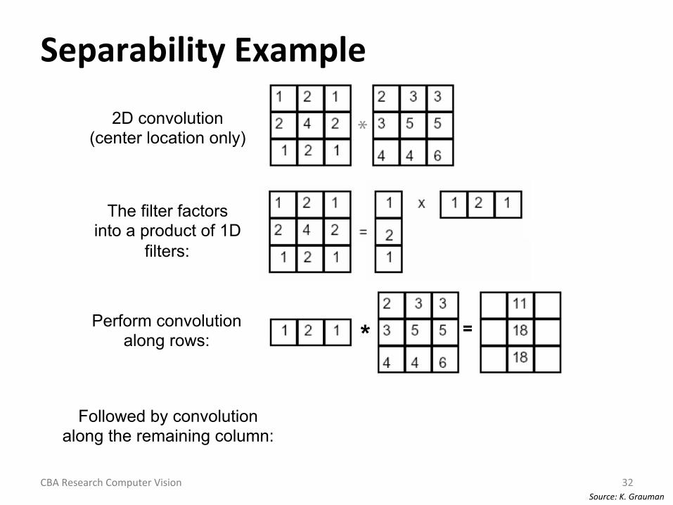
Separability Example
*
*
=
=
2D convolution (center location only)
Source: K. Grauman
The filter factors into a product of 1D
filters:
Perform convolution along rows:
Followed by convolution along the remaining column:
CBA Research Computer Vision 32
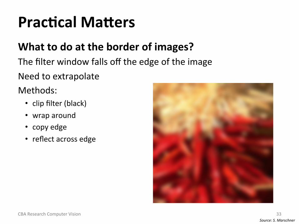
Prac1cal Ma]ers What to do at the border of images? The filter window falls off the edge of the image Need to extrapolate Methods:
• clip filter (black) • wrap around • copy edge • reflect across edge
Source: S. Marschner CBA Research Computer Vision 33
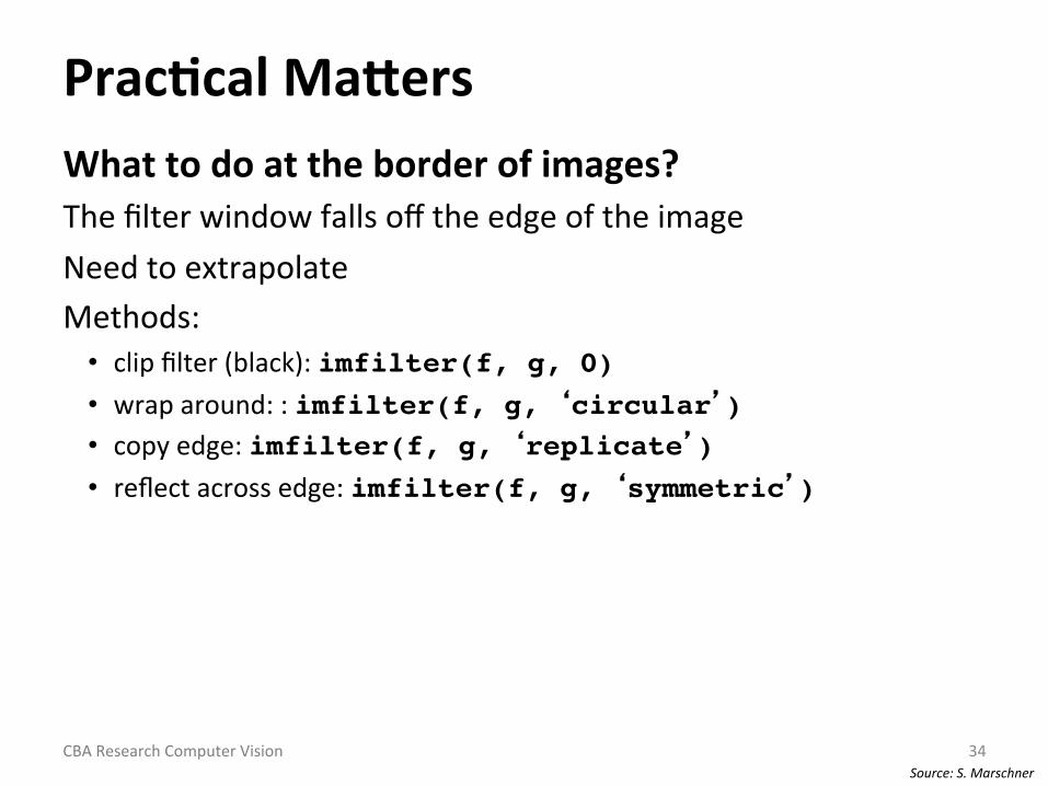
Prac1cal Ma]ers What to do at the border of images? The filter window falls off the edge of the image Need to extrapolate Methods:
• clip filter (black): imfilter(f, g, 0)!• wrap around: : imfilter(f, g, ‘circular’)!• copy edge: imfilter(f, g, ‘replicate’)!• reflect across edge: imfilter(f, g, ‘symmetric’)!
Source: S. Marschner CBA Research Computer Vision 34
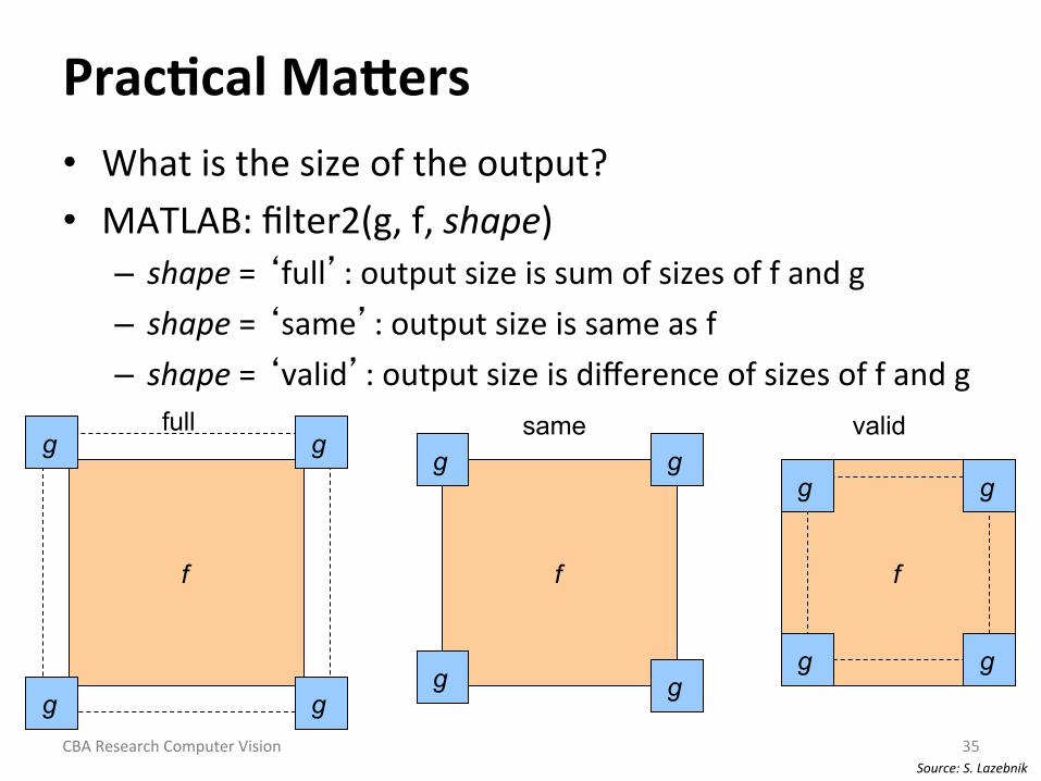
Prac1cal Ma]ers • What is the size of the output? • MATLAB: filter2(g, f, shape)
– shape = ‘full’: output size is sum of sizes of f and g – shape = ‘same’: output size is same as f – shape = ‘valid’: output size is difference of sizes of f and g
f
g g
g g
f
g g
g g
f
g g
g g
full same valid
Source: S. Lazebnik CBA Research Computer Vision 35
Median Filters
• A Median Filter operates over a window by selecIng the median intensity in the window.
• What advantage does a median filter have over a mean filter?
• Is a median filter a kind of convoluIon?
36 CBA Research Computer Vision
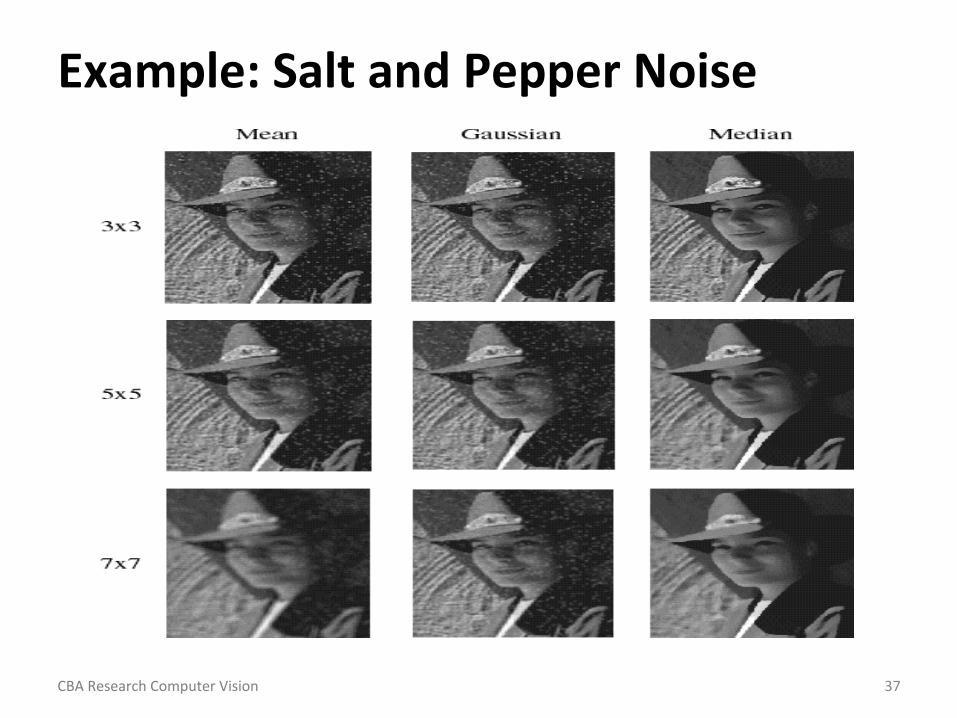
Example: Salt and Pepper Noise
CBA Research Computer Vision 37
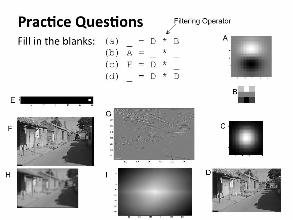
Prac1ce Ques1ons Fill in the blanks: (a) _ = D * B
(b) A = _ * _ (c) F = D * _ (d) _ = D * D
A
B
C
D
E
F
G
H I
Filtering Operator
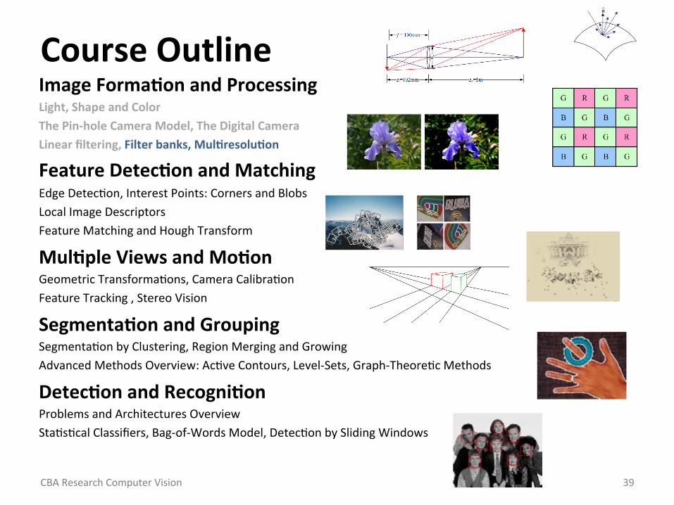
Course Outline Image Forma1on and Processing Light, Shape and Color The Pin-‐hole Camera Model, The Digital Camera Linear filtering, Filter banks, Mul1resolu1on
Feature Detec1on and Matching Edge DetecIon, Interest Points: Corners and Blobs Local Image Descriptors Feature Matching and Hough Transform
Mul1ple Views and Mo1on Geometric TransformaIons, Camera CalibraIon Feature Tracking , Stereo Vision
Segmenta1on and Grouping SegmentaIon by Clustering, Region Merging and Growing Advanced Methods Overview: AcIve Contours, Level-‐Sets, Graph-‐TheoreIc Methods
Detec1on and Recogni1on Problems and Architectures Overview StaIsIcal Classifiers, Bag-‐of-‐Words Model, DetecIon by Sliding Windows
39 CBA Research Computer Vision
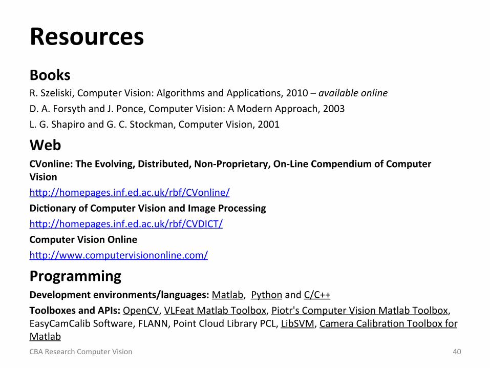
Resources Books R. Szeliski, Computer Vision: Algorithms and ApplicaIons, 2010 – available online D. A. Forsyth and J. Ponce, Computer Vision: A Modern Approach, 2003 L. G. Shapiro and G. C. Stockman, Computer Vision, 2001
Web CVonline: The Evolving, Distributed, Non-‐Proprietary, On-‐Line Compendium of Computer Vision hZp://homepages.inf.ed.ac.uk/rbf/CVonline/ Dic1onary of Computer Vision and Image Processing hZp://homepages.inf.ed.ac.uk/rbf/CVDICT/ Computer Vision Online hZp://www.computervisiononline.com/
Programming Development environments/languages: Matlab, Python and C/C++ Toolboxes and APIs: OpenCV, VLFeat Matlab Toolbox, Piotr's Computer Vision Matlab Toolbox, EasyCamCalib Soeware, FLANN, Point Cloud Library PCL, LibSVM, Camera CalibraIon Toolbox for Matlab CBA Research Computer Vision 40