Embed Size (px)
Citation preview

Computing Fundamentals 1 Introduction to CafeOBJ
Lecturer: Patrick BrowneLecture Room: K308
Lab Room: A308Based on work by: Nakamura Masaki, João Pascoal Faria, Prof. Heinrich Hußmann. See
notes on slides for details.
• High level programming languages (HLPG), like Java, are formal specifications. They specify what the machine should do. They must be converted into the actual language that the CPU can execute.
• However, HLPG are not good at expressing our understanding of a domain. They are too low level and contain too much detail. Using HLPG it is difficult to identify design errors, assumptions are not made explicit, they are implementation dependent. They focus on how system tasks are performed. They don’t allow us to reason about the system or describe what the system does.
• Domains of interest include the theory of sets, the theory of integers, the theory of bank accounts, the theory of a hospital record system. For this course we are primarily interested in specifying mathematical systems, such as set theory.
Why a specification language?
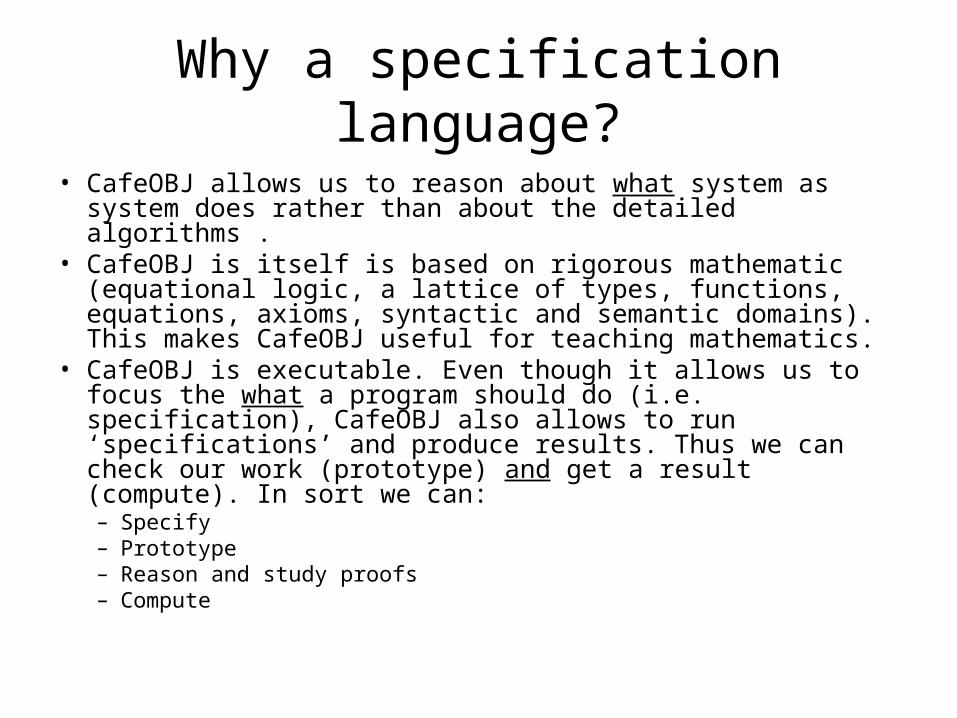
• CafeOBJ allows us to reason about what system as system does rather than about the detailed algorithms .
• CafeOBJ is itself is based on rigorous mathematic (equational logic, a lattice of types, functions, equations, axioms, syntactic and semantic domains). This makes CafeOBJ useful for teaching mathematics.
• CafeOBJ is executable. Even though it allows us to focus the what a program should do (i.e. specification), CafeOBJ also allows to run ‘specifications’ and produce results. Thus we can check our work (prototype) and get a result (compute). In sort we can:– Specify– Prototype – Reason and study proofs– Compute
Why a specification language?
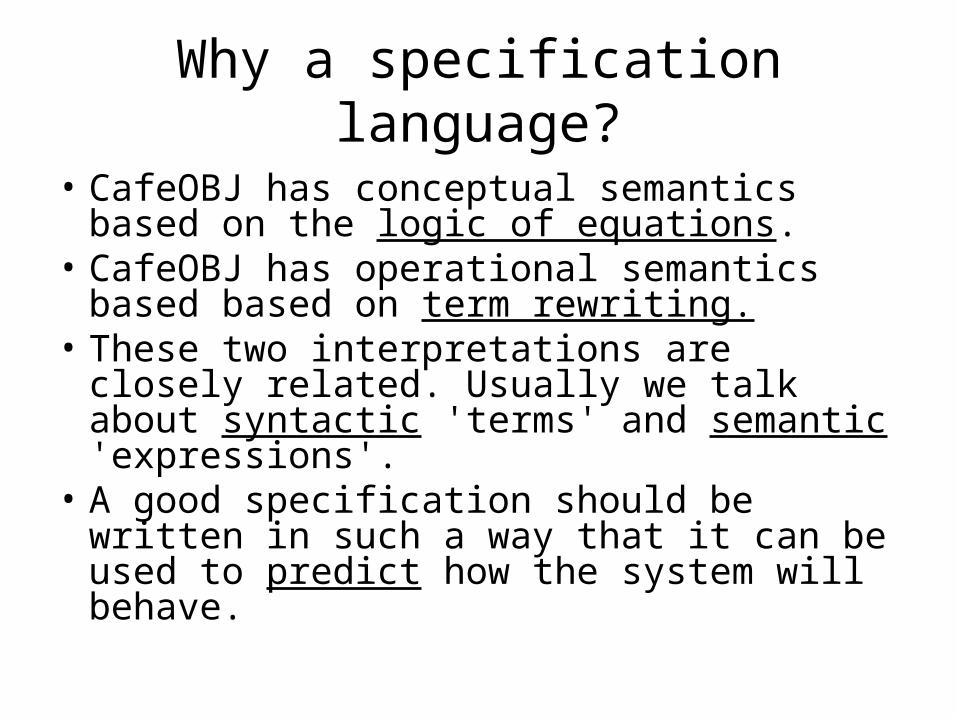
• CafeOBJ has conceptual semantics based on the logic of equations.
• CafeOBJ has operational semantics based based on term rewriting.
• These two interpretations are closely related. Usually we talk about syntactic 'terms' and semantic 'expressions'.
• A good specification should be written in such a way that it can be used to predict how the system will behave.
Why a specification language?
• The role of CafeOBJ on this course is to provide a functional and logic based language that can be used to represent the mathematical concepts such as logic, sets, and functions. The programming examples will be small.
Don’t Panic!
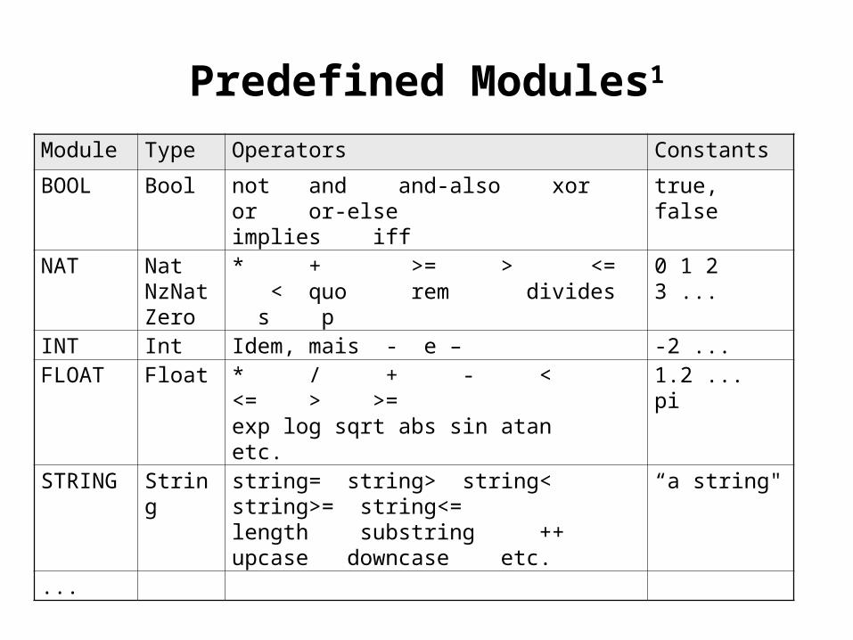
Predefined Modules1
Module Type Operators Constants
BOOL Bool not and and-also xor or or-else implies iff
true, false
NAT Nat NzNatZero
* + >= > <= < quo rem divides s p
0 1 2 3 ...
INT Int Idem, mais - e – -2 ... FLOAT Float * / + - < <= > >=
exp log sqrt abs sin atan etc.1.2 ...pi
STRING String string= string> string< string>= string<=length substring ++ upcase downcase etc.
“a string"
...
• You can download binary packages for Windows and Linux from http://www.ldl.jaist.ac.jp/cafeobj/
• The latest Window version is:• CafeOBJ 1.4.6p5, 2005.11.24 new • http://www.ldl.jaist.ac.jp/cafeobj/system.html
• Tutorial at:• www.jaist.ac.jp/~kokichi/class/i613-0510/pptPdfLectureNotes/How2useCafeOBJ.pdf
Downloading CafeOBJ
• CafeOBJ is a declarative language with firm mathematical and logical foundations. The mathematical semantics of CafeOBJ is based on state-of-the-art algebraic specification concepts and results, and is strongly based on category theory and the theory of institutions.
• Similar to our course text CafeOBJ uses Equational logic, which is the calculus of replacing terms by equal terms.
CafeOBJ
• Equational calculus derives (proves) a term equation from a conditional-equational axiom set. The deduction rules in this calculus are:
• Reflexivity: Any term is provably equal to itself (t = t).• Transitivity: If t1 is provably equal to t2 and t2 is
provably equal to t3, then t1 is provably equal to t3.• Symmetry: If t1 is provably equal to t2, then t2 is
provably equal to t1.• Congruence: If t1 is provably equal to t2, then any two
terms are provably equal which consist of some context built around t1 and t2.
CafeOBJ
• In general when writing algebraic specification one should include axioms that apply each observer or extension to each generator, except where an error might occur.
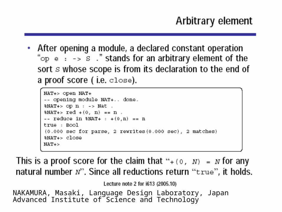
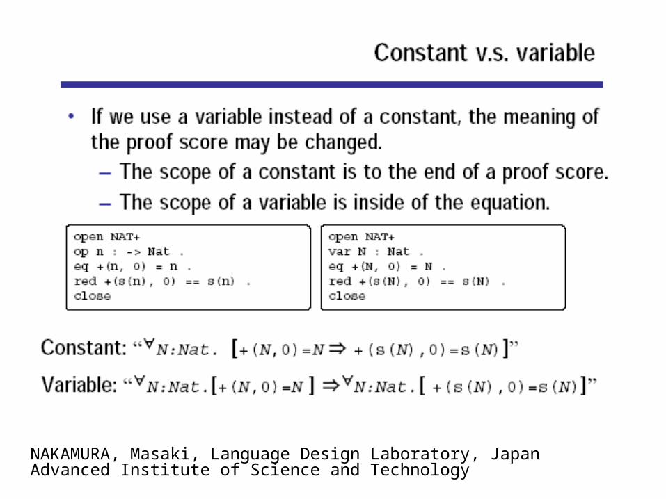
• The RHS should not be a single variable.• All variable in the RHS must appear in the LHS.• The scope of a constant is the module it is declared in
(or a proof score or interactive session).• The scope of a variable is only inside of the equation.
So, during evaluation a variable, say X, will have the same value in a given equation, but it may have different values in different equations in the same module.
• We would like to use equations to partition sets.
Writing equations in CafeOBJ

mod SORTS { [ s4 < s2 s3 < s1 , s5 < s1 , s6, t] op f1 : -> s1 op f2 : -> s2 op f3 : -> s3 op f4 : -> s4 op f5 : -> s5 op f6 : -> s6 op g : s2 -> t}
Types and subtypes1
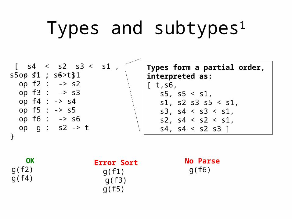
op f1 : -> s1 op f2 : -> s2 op f3 : -> s3 op f4 : -> s4 op f5 : -> s5 op f6 : -> s6 op g : s2 -> t}
[ s4 < s2 s3 < s1 , s5 < s1 , s6 t]
Types and subtypes1
OKg(f2) g(f4)
No Parseg(f6)
Error Sortg(f1) g(f3)g(f5)
Types form a partial order, interpreted as: [ t,s6, s5, s5 < s1, s1, s2 s3 s5 < s1, s3, s4 < s3 < s1, s2, s4 < s2 < s1, s4, s4 < s2 s3 ]
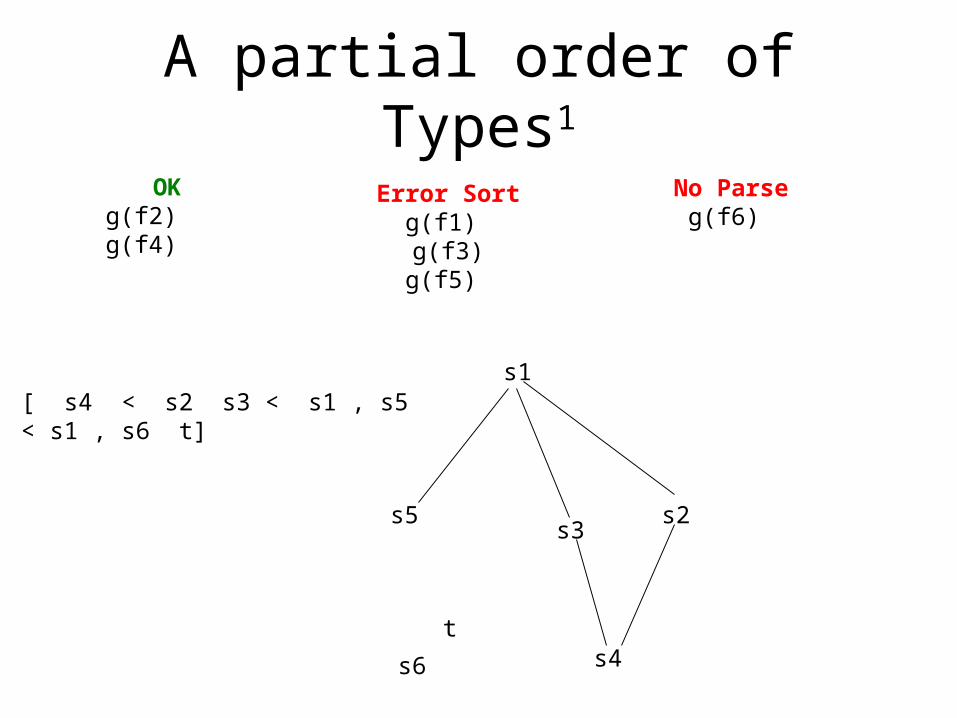
A partial order of Types1
s5
s1
s3
s4
s2
s6
t
OKg(f2) g(f4)
No Parseg(f6)
Error Sortg(f1) g(f3)g(f5)
[ s4 < s2 s3 < s1 , s5 < s1 , s6 t]
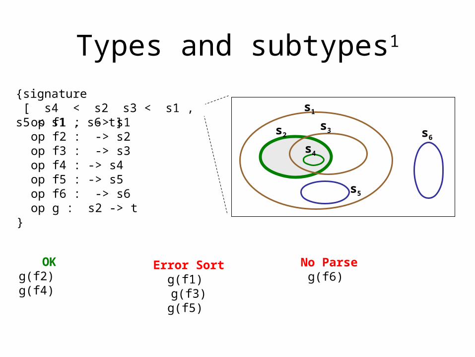
op f1 : -> s1 op f2 : -> s2 op f3 : -> s3 op f4 : -> s4 op f5 : -> s5 op f6 : -> s6 op g : s2 -> t}
s1
s2s3
s4
s5
s6
{signature [ s4 < s2 s3 < s1 , s5 < s1 , s6 t]
Types and subtypes1
OKg(f2) g(f4)
No Parseg(f6)
Error Sortg(f1) g(f3)g(f5)
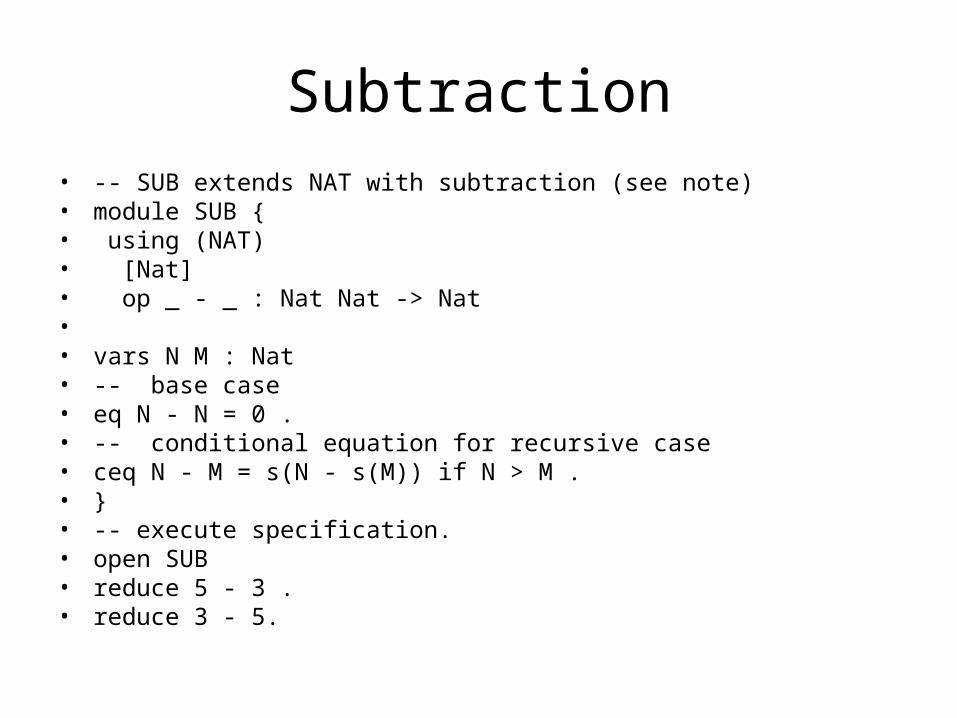
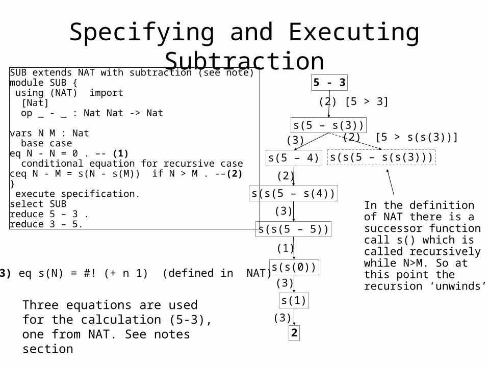
Subtraction• -- SUB extends NAT with subtraction (see note)• module SUB {• using (NAT) • [Nat]• op _ - _ : Nat Nat -> Nat • • vars N M : Nat• -- base case• eq N - N = 0 .• -- conditional equation for recursive case• ceq N - M = s(N - s(M)) if N > M . • }• -- execute specification.• open SUB• reduce 5 - 3 .• reduce 3 - 5.
Specifying and Executing Subtraction5 - 3
s(5 – s(3))(2) [5 > s(s(3))]
s(5 – 4)
(2) [5 > 3]
(3)
s(s(5 – s(s(3)))
s(s(5 – s(4))
(2)
s(s(5 – 5))
(3)
s(s(0))
(1)
s(1)
2
(3)
(3)
In the definition of NAT there is a successor function call s() which is called recursively while N>M. So at this point the recursion ‘unwinds’
SUB extends NAT with subtraction (see note)module SUB { using (NAT) import [Nat] op _ - _ : Nat Nat -> Nat vars N M : Nat base caseeq N - N = 0 . –- (1) conditional equation for recursive caseceq N - M = s(N - s(M)) if N > M . -–(2) } execute specification.select SUBreduce 5 – 3 .reduce 3 – 5.
(3) eq s(N) = #! (+ n 1) (defined in NAT)
Three equations are used for the calculation (5-3), one from NAT. See notes section
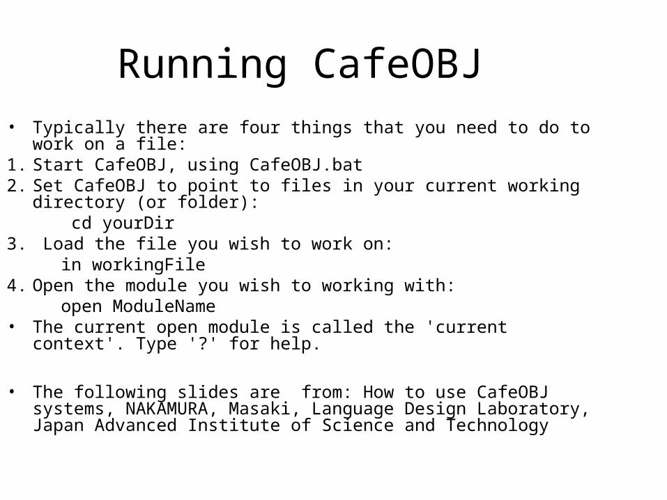
Running CafeOBJ• Typically there are four things that you need to do to work on a file:1. Start CafeOBJ, using CafeOBJ.bat2. Set CafeOBJ to point to files in your current working directory (or
folder): cd yourDir
3. Load the file you wish to work on:in workingFile
4. Open the module you wish to working with:open ModuleName
• The current open module is called the 'current context'. Type '?' for help.
• The following slides are from: How to use CafeOBJ systems, NAKAMURA, Masaki, Language Design Laboratory, Japan Advanced Institute of Science and Technology
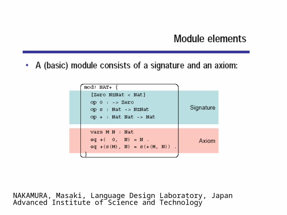
NAKAMURA, Masaki, Language Design Laboratory, Japan Advanced Institute of Science and Technology
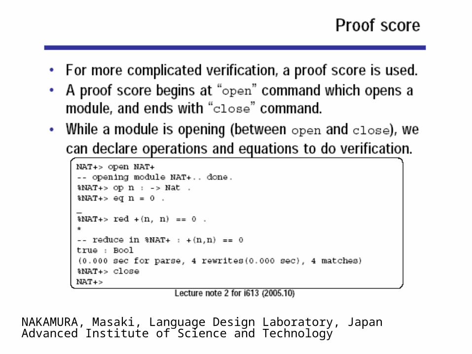
NAKAMURA, Masaki, Language Design Laboratory, Japan Advanced Institute of Science and Technology
NAKAMURA, Masaki, Language Design Laboratory, Japan Advanced Institute of Science and Technology
NAKAMURA, Masaki, Language Design Laboratory, Japan Advanced Institute of Science and Technology
NAKAMURA, Masaki, Language Design Laboratory, Japan Advanced Institute of Science and Technology
NAKAMURA, Masaki, Language Design Laboratory, Japan Advanced Institute of Science and Technology

NAKAMURA, Masaki, Language Design Laboratory, Japan Advanced Institute of Science and Technology
Automatic Theorem Proving
The CafeObj environment includes automatic theorem proving (ATP) software. ATP will try to show that some statement (often called a conjecture) is a logical consequence of a set of statements (often called axioms). The ATP in CafeOBJ is called PIGNOSE and is based on OTTER. Most of the logic problems on this course use PIGNOSE. For our purposes we set up the problems such as Portia, Superman, and Family using a convenient1 logical notation (->,<->, | & ~, ax, goal)

Automatic Theorem Proving
The basic steps in our examples are:
1)That we declare some predicates, with the keyword pred.
2)Then we define the axioms with a convenient1 logical notation (-> , <->, |, &, ~, ax)
3)Then we set the conjecture to be proved.
4)If PIGNOSE can prove the conjecture we can examine the proof. We may compare it to the manual proof.
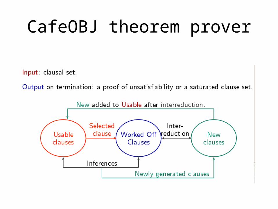
CafeOBJ theorem prover
The apply command.
• When you reduce an expression with the red command all of the equations (or rules) for all of the sub-terms are executed. Also, the equations or rules are performed in a strict left to right fashion (even though mathematical equations are symmetric). Sometimes we want to execute one equation at a time in either left to right or right to left manner.
The apply command.
• The apply command allows operate on equation in a very precise way, allowing actions, substitutions, ranges, and sub-term selection. We will apply (or bind) terms to LHS of equations.
• apply <action> [<substitution>]
<range> <selection>

The apply <action>
• The main action of interest on this course is called reduce (red) . To use red both the term and the module must first be selected.
• Each given term has a ‘top’ operator, e.g. in the term push(1,stack) the top operator is ‘push’ with ‘1’ and ‘stack’ as first level sub-terms.
• The precedence of a term is the precedence of its top operator. Brackets can be used to set the precedence to your requirements.
The apply [<substitution>]
• Substitution is optional ([]). • Consider the equation• (1) eq x * 0 = 0 • And its backwards version• (2) eq 0 = x * 0 • In (2) there is a variable on the RHS that is not in
the LHS, which means that it cannot be evaluated L->R. It is necessary to have a ‘binding’ for variables not on the LHS of (2) (i.e. x).
The apply [<substitution>]
• The syntax for this binding or substitution is:
• with <var>=<term> {,<var>=<term> ..}
• Example• apply .equation1 with x=a at term .
The apply sub-term
• Three ways of selecting sub-terms
• (arg1,sub2) occurrence
• [arg1,sub2 ] sequence
• {arg1,sub2 ,[]} subset
The apply sub-term
• Occurrence selection
• (arg1,sub2) selects the occurrence of argument where both sub-terms and argument position start at 1. For example, if the term is
• (a + (c * 2)
• then (2 1) selects c. • () selects the whole term.
The apply sub-term
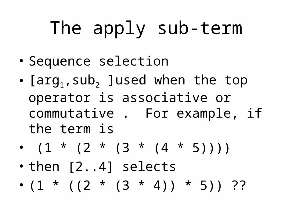
• Sequence selection
• [arg1,sub2 ]used when the top operator is associative or commutative . For example, if the term is
• (1 * (2 * (3 * (4 * 5))))
• then [2..4] selects• (1 * ((2 * (3 * 4)) * 5)) ??
The apply sub-term
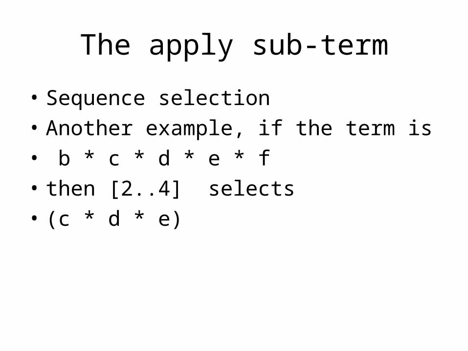
• Sequence selection
• Another example, if the term is
• b * c * d * e * f
• then [2..4] selects• (c * d * e)
The apply sub-term
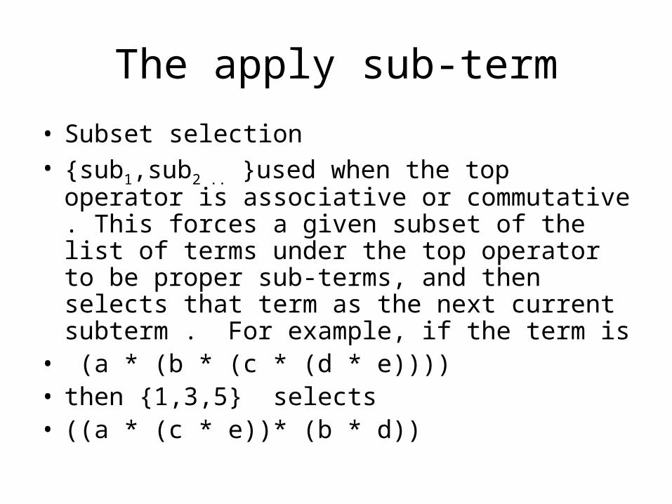
• Subset selection• {sub1,sub2 .. }used when the top operator is
associative or commutative . This forces a given subset of the list of terms under the top operator to be proper sub-terms, and then selects that term as the next current subterm . For example, if the term is
• (a * (b * (c * (d * e)))) • then {1,3,5} selects• ((a * (c * e))* (b * d))
The apply sub-term
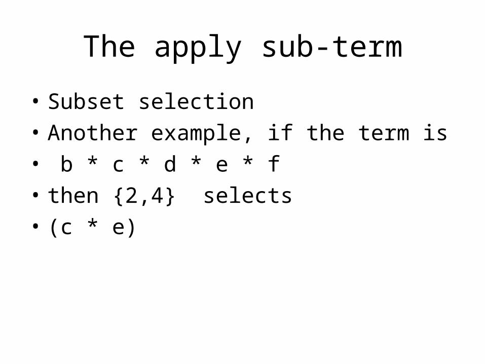
• Subset selection
• Another example, if the term is
• b * c * d * e * f
• then {2,4} selects• (c * e)
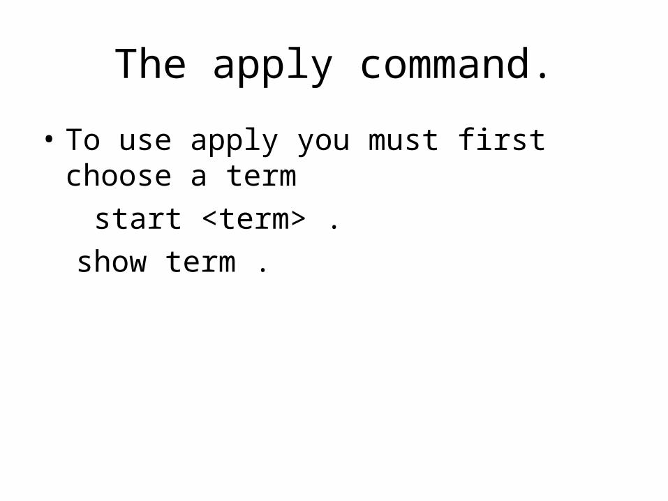
The apply command.
• To use apply you must first choose a term
start <term> .
show term .
Interactive proof: Right Inverse
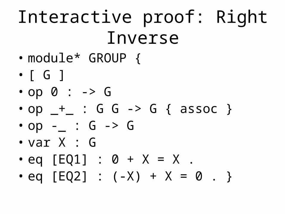
• module* GROUP {• [ G ] • op 0 : -> G • op _+_ : G G -> G { assoc } • op -_ : G -> G • var X : G • eq [EQ1] : 0 + X = X . • eq [EQ2] : (-X) + X = 0 . }
Interactive proof: Right Inverse
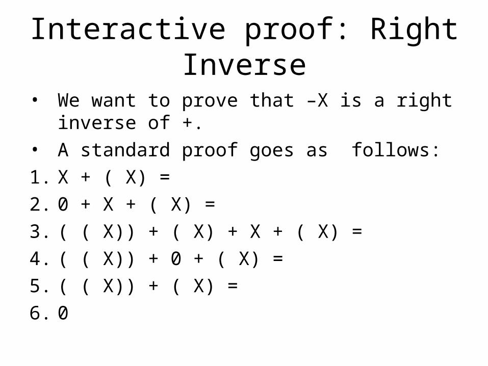
• We want to prove that –X is a right inverse of +.• A standard proof goes as follows:
1. X + ( X) =
2. 0 + X + ( X) =
3. ( ( X)) + ( X) + X + ( X) =
4. ( ( X)) + 0 + ( X) =
5. ( ( X)) + ( X) =
6. 0
Interactive proof: Right Inverse
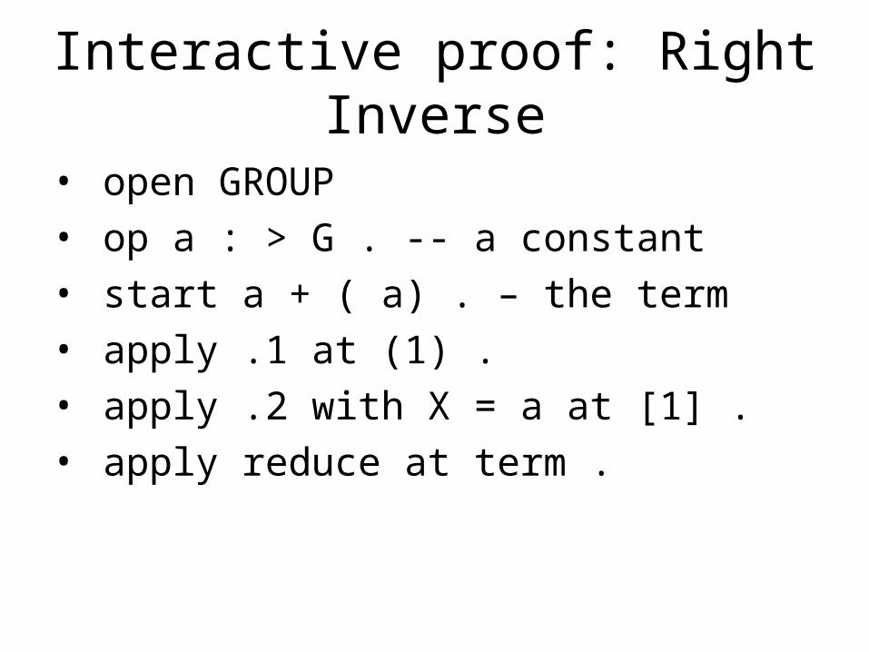
• open GROUP • op a : > G . -- a constant• start a + ( a) . – the term• apply .1 at (1) . • apply .2 with X = a at [1] . • apply reduce at term .
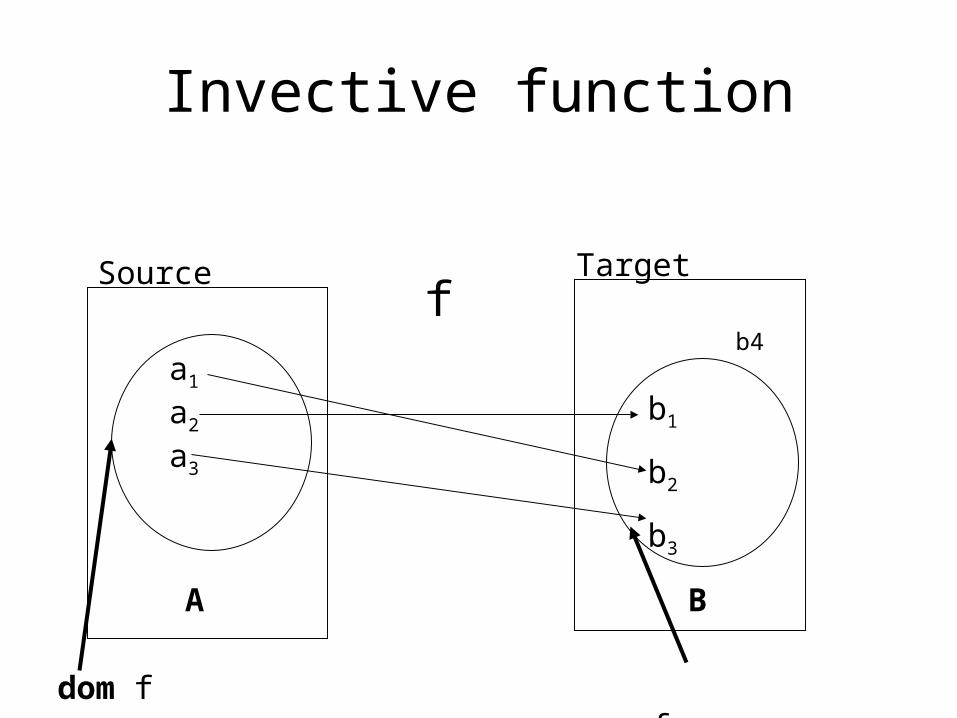
Invective function
a1
a2
a3
A
b1
b2
b3
f
dom f ran f
B
Source Target
b4

Interactive proof: Injective Function f
• A function f has at least one left inverse if it is an injection.
• A left inverse is a function g such that • g f a = a
or• g(f(a)) = a
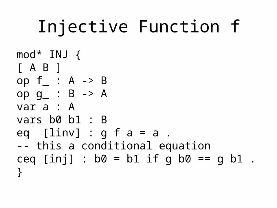
Injective Function f
mod* INJ {[ A B ]op f_ : A -> B op g_ : B -> Avar a : A vars b0 b1 : B eq [linv] : g f a = a .-- this a conditional equationceq [inj] : b0 = b1 if g b0 == g b1 .}
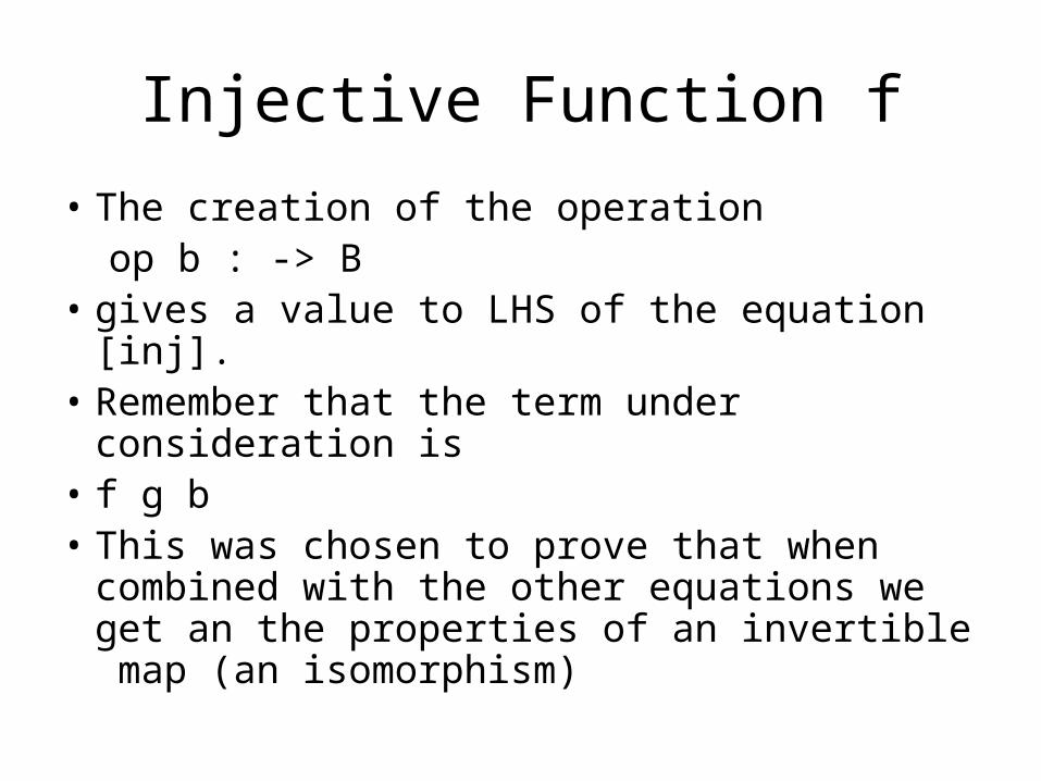
Injective Function f
• The creation of the operation op b : -> B • gives a value to LHS of the equation [inj].• Remember that the term under consideration is• f g b• This was chosen to prove that when combined
with the other equations we get an the properties of an invertible map (an isomorphism)

Injective Function f
• The creation of the operation
op b : -> B • gives a value to LHS of the equation [inj].• What happens in the proof is that, in order to apply
the rule [inj] to
f g b with B' = b, • we must first prove that the condition is true, which
in this case is that
g f g b == g b .
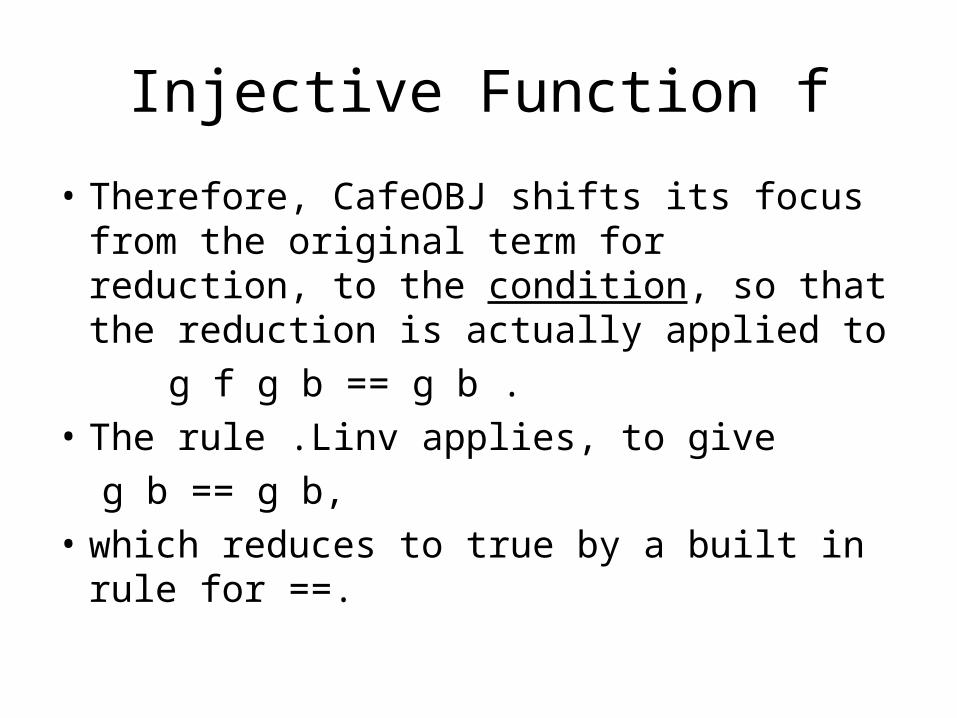
Injective Function f
• Therefore, CafeOBJ shifts its focus from the original term for reduction, to the condition, so that the reduction is actually applied to
g f g b == g b . • The rule .Linv applies, to give
g b == g b,
• which reduces to true by a built in rule for ==.
Injective Function f
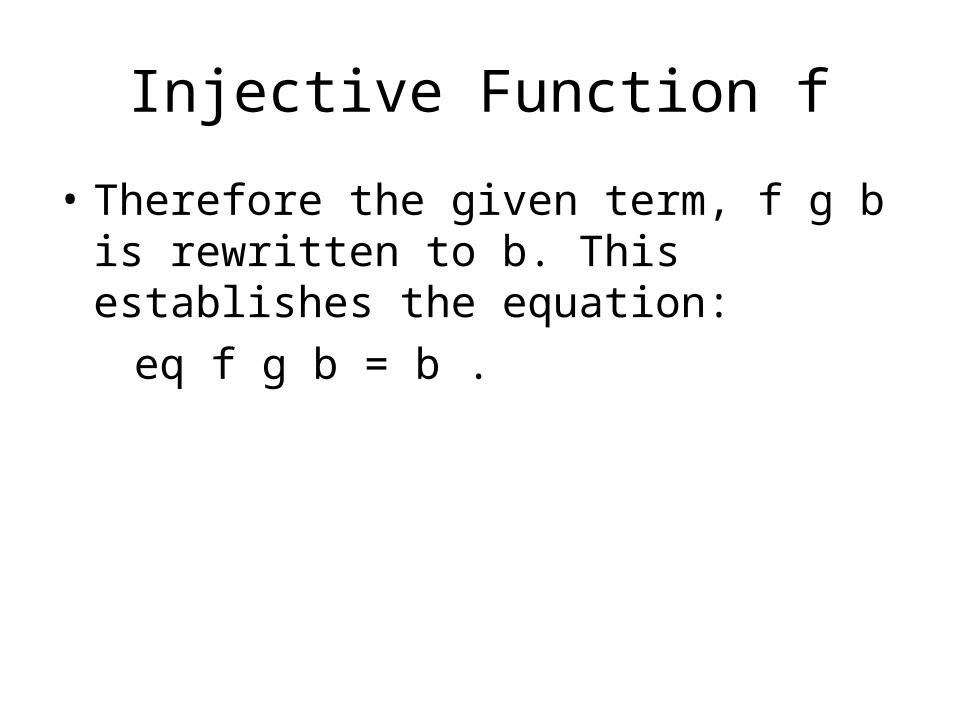
• Therefore the given term, f g b is rewritten to b. This establishes the equation:
eq f g b = b .
Injective Function f
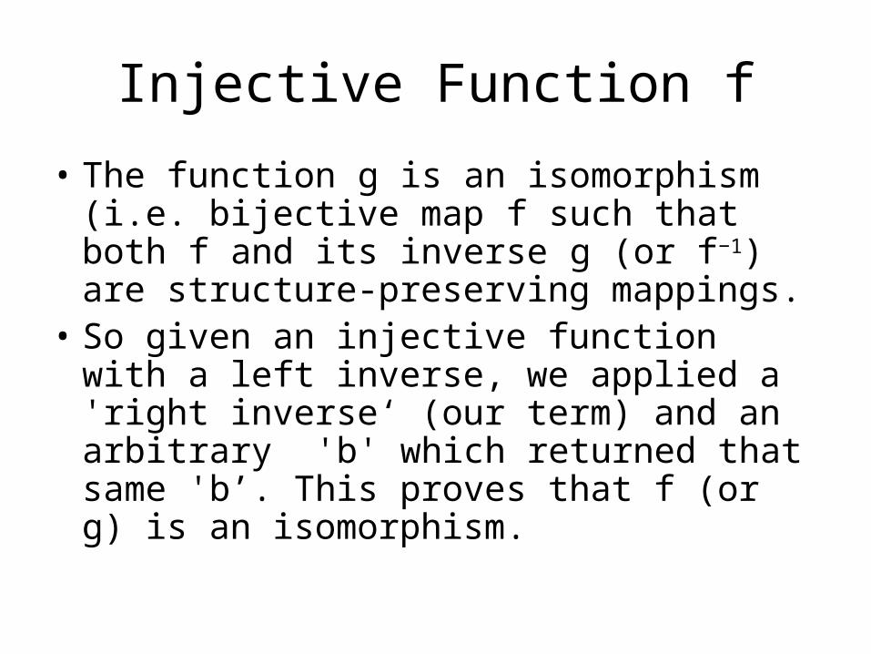
• The function g is an isomorphism (i.e. bijective map f such that both f and its inverse g (or f−1) are structure-preserving mappings.
• So given an injective function with a left inverse, we applied a 'right inverse‘ (our term) and an arbitrary 'b' which returned that same 'b’. This proves that f (or g) is an isomorphism.
Injective Function f
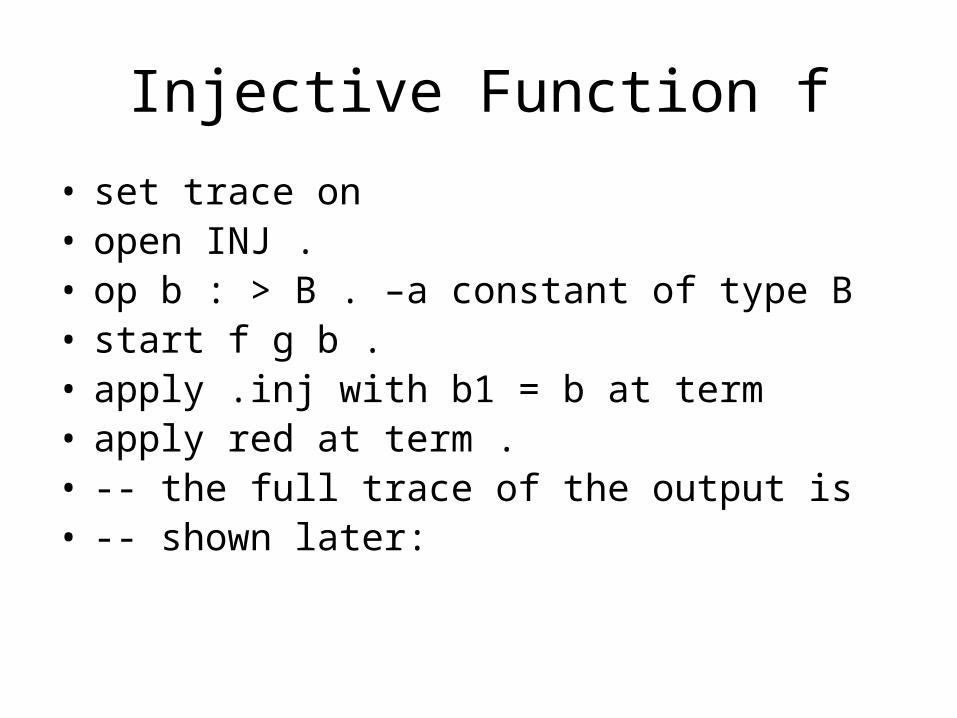
• set trace on• open INJ . • op b : > B . –a constant of type B• start f g b . • apply .inj with b1 = b at term • apply red at term .• -- the full trace of the output is• -- shown later:

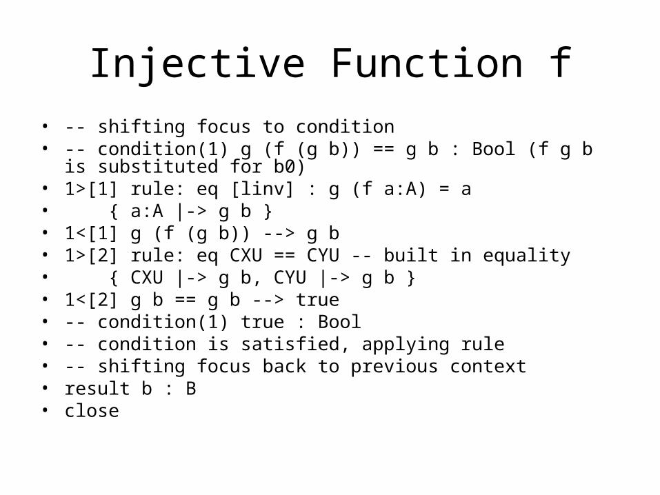
Injective Function f• -- shifting focus to condition• -- condition(1) g (f (g b)) == g b : Bool (f g b is substituted for b0)• 1>[1] rule: eq [linv] : g (f a:A) = a• { a:A |-> g b }• 1<[1] g (f (g b)) --> g b• 1>[2] rule: eq CXU == CYU -- built in equality• { CXU |-> g b, CYU |-> g b }• 1<[2] g b == g b --> true• -- condition(1) true : Bool• -- condition is satisfied, applying rule• -- shifting focus back to previous context• result b : B• close
Injective Function f• -- shifting focus to condition• -- condition(1) g (f (g b)) == g b : Bool (f g b is substituted for b0)• 1>[1] rule: eq [linv] : g (f a:A) = a• { a:A |-> g b }• 1<[1] g (f (g b)) --> g b• 1>[2] rule: eq CXU == CYU -- built in equality• { CXU |-> g b, CYU |-> g b }• 1<[2] g b == g b --> true• -- condition(1) true : Bool• -- condition is satisfied, applying rule• -- shifting focus back to previous context• result b : B• close

INJ Explained
1. eq [linv] : g f a = a .2. ceq [inj]: b0 = b1 if g b0 == g b1 .
3. open INJ . 4. op b : > B . 5. start f g b . 6. apply .inj with b1 = b at term7. apply red at term .Print out notes section slides 54-59, run
slide show 54-59. Try to relate notes to slide show.
INJ Explained
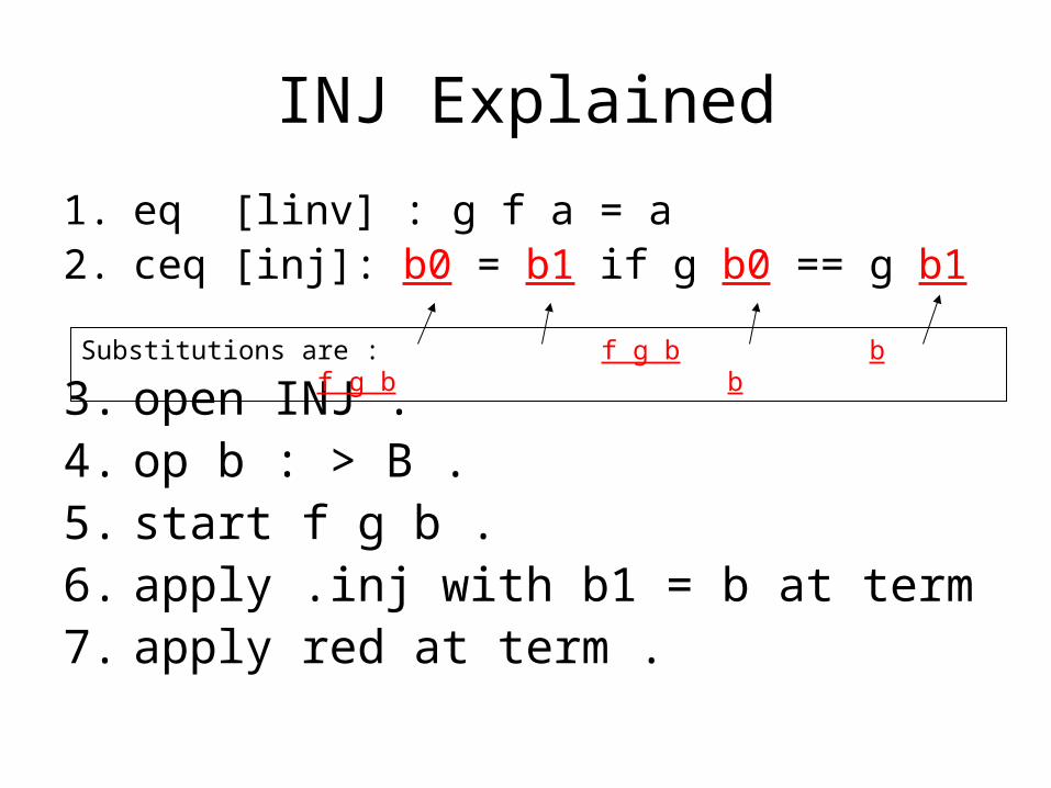
1. eq [linv] : g f a = a2. ceq [inj]: b0 = b1 if g b0 == g b1
3. open INJ . 4. op b : > B . 5. start f g b . 6. apply .inj with b1 = b at term7. apply red at term .
Substitutions are : f g b b f g b b
INJ Explained
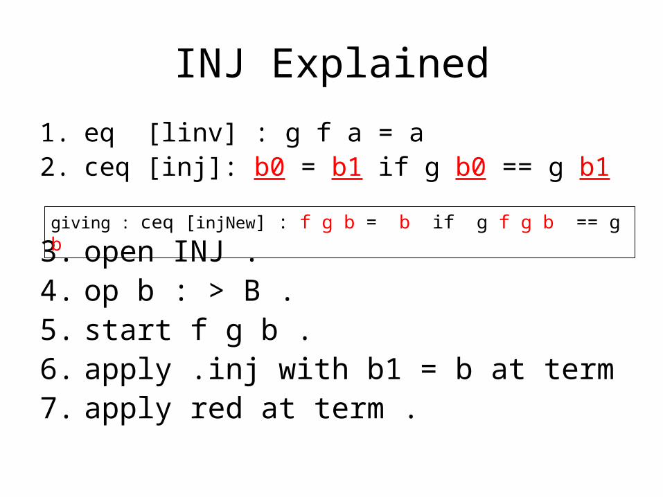
1. eq [linv] : g f a = a2. ceq [inj]: b0 = b1 if g b0 == g b1
3. open INJ . 4. op b : > B . 5. start f g b . 6. apply .inj with b1 = b at term7. apply red at term .
giving : ceq [injNew] : f g b = b if g f g b == g b
INJ Explained
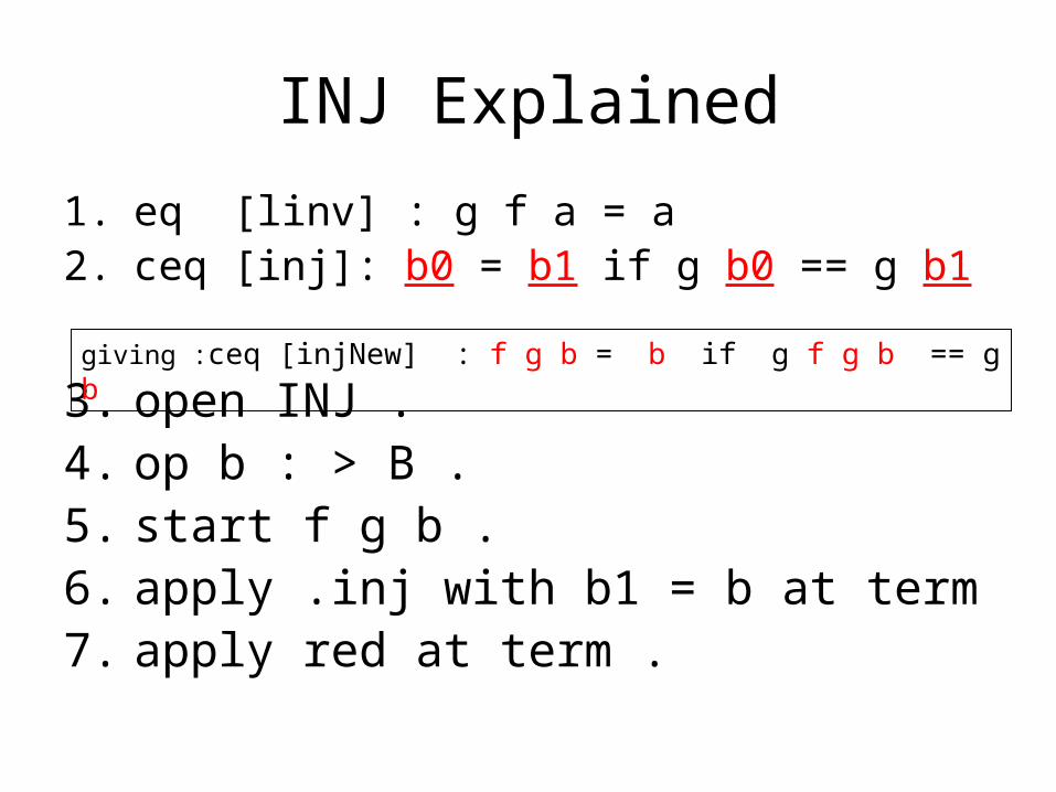
1. eq [linv] : g f a = a2. ceq [inj]: b0 = b1 if g b0 == g b1
3. open INJ . 4. op b : > B . 5. start f g b . 6. apply .inj with b1 = b at term7. apply red at term .
giving :ceq [injNew] : f g b = b if g f g b == g b
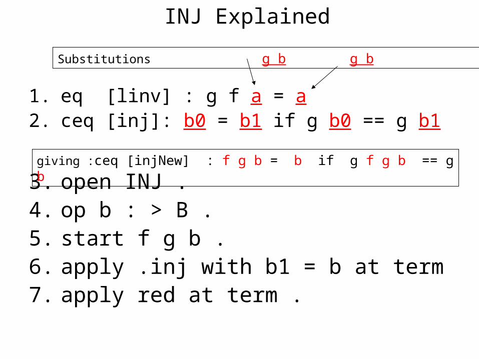
1. eq [linv] : g f a = a2. ceq [inj]: b0 = b1 if g b0 == g b1
3. open INJ . 4. op b : > B . 5. start f g b . 6. apply .inj with b1 = b at term7. apply red at term .
giving :ceq [injNew] : f g b = b if g f g b == g b
Substitutions g b g b
INJ Explained

1. eq [linv] : g f a = a2. ceq [inj]: b0 = b1 if g b0 == g b1
3. open INJ . 4. op b : > B . 5. start f g b . 6. apply .inj with b1 = b at term7. apply red at term .
giving :ceq [injNew] : f g b = b if g f g b == g b
Giving new equation eq [linvNew] : g f g b = g b
INJ Explained


![On the Multiple Sources and Privacy Preservation Issues ...static.tongtianta.site/paper_pdf/c6fb4336-a308-11e... · into defect prediction. Recently, Lee et al. [22] presented the](https://img.pdfslide.net/doc/110x75/5fd2996962664b794146bf67/on-the-multiple-sources-and-privacy-preservation-issues-into-defect-prediction.jpg)