Computing Internal Member Forces in a Bridge Truss Using

_____________________________________________________________________________________________________ *Corresponding author: E-mail: [email protected], [email protected];

Advances in Research 16(4): 1-21, 2018; Article no.AIR.43876 ISSN: 2348-0394, NLM ID: 101666096

Computing Internal Member Forces in a Bridge Truss Using Classical Iterative Numerical Methods

with Maple® & MATLAB®

Aliyu Bhar Kisabo1*, Bello Abdulazeez Opeyemi1 and Capt. Olayemi Balogun2

1Centre for Space Transport and Propulsion (CSTP), Epe, Lagos-State, Nigeria.

2Defence Space Agency (DSA) Abuja, Nigeria.

Authors’ contributions

This work was carried out in collaboration between all authors. All authors read and approved the final manuscript.

Article Information

DOI: 10.9734/AIR/2018/43876

Editor(s): (1) Dr. Sumit Gandhi, Department of Civil Engineering, Jaypee University of Engineering and Technology, Madhya Pradesh,

India. (2) Dr. Carlos Humberto Martins, Professor, Department of Civil Engineering, The State University of Sao Paulo, Brazil.

Reviewers: (1) Manish Mahajan, IKG- Punjab Technical University, India.

(2) Francesco Zirilli, Universita di Roma La Sapienza, Italy. (3) Oladele, Matthias Omotayo, The Federal Polytechnic, Ede, Nigeria.

Complete Peer review History: http://www.sciencedomain.org/review-history/26522

Received 22 June 2018 Accepted 06 September 2018

Published 05 October 2018

ABSTRACT

In this study, computation and analysis of internal member forces acting on a bridge truss were carried out. First, the forces were resolved at each joint and a system of equations was built to describe the truss as a Linear System of Algebraic Equations (LSAEs). The LSAEs developed here is of the order 8 x 8 and sparse. Aside from the truss system being a sparse matrix, it is neither positive definite nor a tridiagonal matrix. Hence, a weakly diagonally dominant matrix characterised by ρ (A) > 1. Secondly, 3 iterative numerical methods were applied to obtain a solution to the LSAEs. Third, with Maple®, Jacobi and Gauss-Seidel methods were used with relative ease to the LSAEs, and its solution converged after 30 and 18 iterations respectively. When Successive Over-relaxation (SOR) method was applied with ω = 1.25, a solution to the LSAEs failed to converge. In a novel approach, the error evolution was simulated against iteration number for ω = 0.1 - 0.99 in Maple

®. After analysing such results, ω = 0.93 was selected as the optimal value for the Relaxation

Technique and solution to the LSAEs converged after ten iterations. MATLAB® codes were then

written for the three iterative numerical methods to validate the results obtained in Maple®. The method proposed here proved to be very effective.

Original Research Article

Kisabo et al.; AIR, 16(4): 1-21, 2018; Article no.AIR.43876

2

Keywords: Truss; forces; classical iterative numerical methods; Sparse Matrix; Maple®; MATLAB®.

1. INTRODUCTION Computing internal member forces in trusses require good background knowledge of applied mechanics though; this pre-requisite is fundamental but is not enough. This means even if one is well grounded in such subject and cannot use STEM- based software like Maple

®

MATLAB®, Mathematica

®, Mathcad

® etc., to aid

such computations, it will be impossible to carry out. As such, the ability to be acquainted with STEM-based software for STEM computations and analysis cannot be overemphasise. STEM- based problems that are in the form of LSAEs could be easily solved with pen and paper (manual) if it is of a small order. But when the order increases, it can become a very irritating or an impossible task to be manually solved [1]. The need to be acquainted with computer- based numerical techniques is inevitable especially when it comes to real- life application problems. Errors in such computations could lead to enormous revenue losses, injuries and even loss in human lives, to mention a few. It is customary to explore solutions to STEM problems using more than one STEM- based software at the same time [2,3,4]. It is necessary to increase interest in STEM- based courses, thus, making teaching such subjects more intuitive. Also, solutions obtained from two or more different STEM- based software for the same problem serves as a means of validating simulation results. In this study, Maple® was used as the main STEM software for all the computation. Although Maple® is viewed as an analytical STEM- based software; it is also capable of numerical computations [5]. The study intends to show by example the ease and intuitive manner with which Maple

® handles classical iterative

numerical computation and analysis. This paper is divided into four sections. Section 2 highlights the need of determining the internal member forces on a bridge truss and development of the mathematical equations that describe the entire bridge truss. In section 3, iterative numerical algorithms of Jacobi’s method, Gauss-Seidel (GS) method and Successive Over-relaxation (SOR) methods were

described and applied to the solution of the bridge truss. Results were discussed, and section 4 concludes the study. 2. BRIDGE TRUSS AND INTERNAL

MEMBER FORCES Trusses are lightweight structures capable of carrying heavy loads. A truss is an advantageous structural configuration in which bars are connected at joints, and the overall configuration carries load through axial force in the bars. Generally, trusses are three-dimensional (3-D) although, they can be reduced to two-dimensional (2-D) form as depicted in Fig. 1. Uses of trusses include bridges, buildings, cranes, roofs etc. In bridge design, the individual members of the truss are connected with rotatable pin joints that permit forces to be transferred from one member of the truss to another [6,7]. Wherever trusses are present, the main objectives for an engineer are:

To determine the stability and determinacy of plane trusses;

To analyse and calculate the internal forces in truss members;

To calculate the deformation at any joints.

The present study is limited to the first two objectives outlined above.

2.1 Static Determinacy and Stability A structure that can be analysed using the equations of equilibrium is called statically determinate. Otherwise, such structures are termed statically indeterminate. Only statically determinate trusses can be analysed with the method of joints. A statically determinate truss with two reactions must satisfy [8], 2 3,j m (1)

Where, j is the number of joints and m is the number of members. Considering the bridge truss shown in Fig.1, the number of joints is four, and it has five members. To answer the question of whether the truss in Fig. 1 is statically determinate, the values of j = 4 and m = 5 in (1) were substituted. What we get after substituting the values of j and m is that both sides of (1) give us the number 8. Hence, the truss in Fig. 1 is statically determinate. This needs to be


3

established before one delves into writing equations of equilibrium for each joint to determine internal forces.

2.2 Calculate the Internal Forces in Truss Members

Computing internal forces in trusses are essential for engineers to determine the factor of safety (FOS) during their design. Generally, when FOS is used in the analysis of an existing structure, the factor of safety is defined as,

=

Failure LevelFactor of Safety

Actual Level (2)

In a truss, the actual force in a member is called the internal member force, and the force at which failure occurs is called the strength. Thus, equation (2) can be rewritten as,

=

StrengthFactor of Safety

Internal Member Force (3)

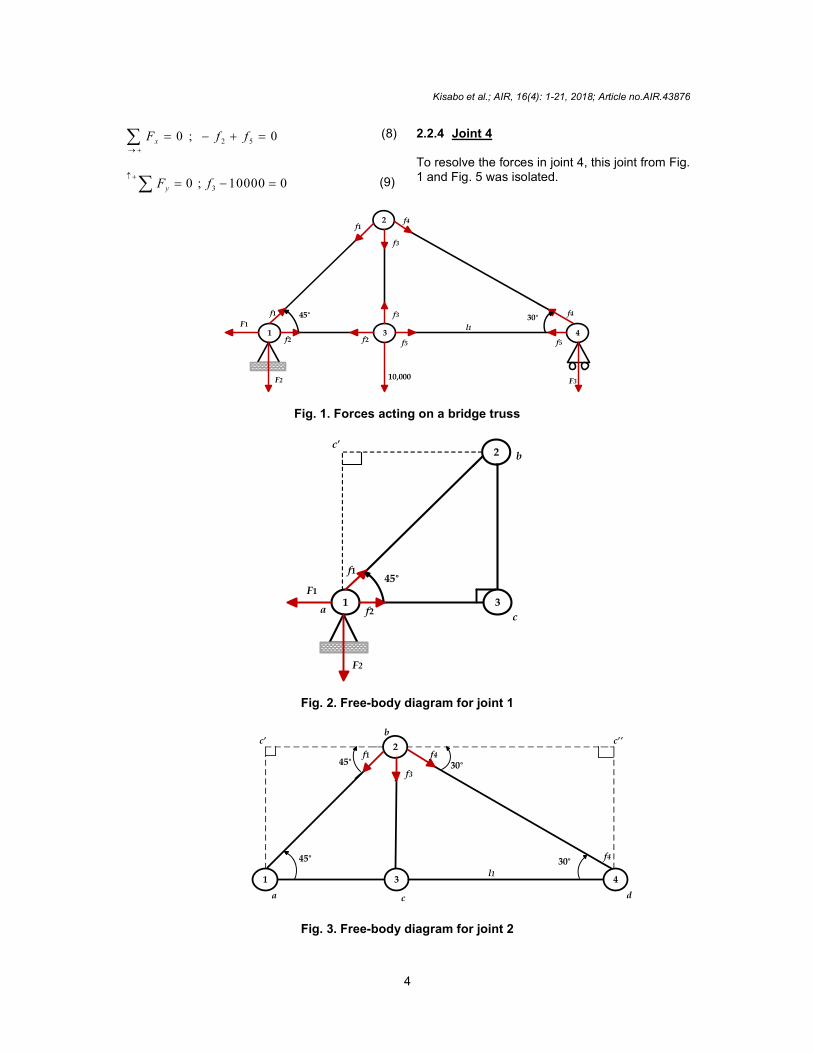
From (3), the engineer has to determine the internal member forces of any structure he/she is designing. For bridges, this is most important to ensure that the load exerted on the truss members at any time does not exceed the strength of the materials and joints. This type of analysis results in setting a limit to the load carrying capability of a bridge and also could be used as bases for computing lifespan (fatigue analysis) for the bridge. If the factor of safety is less than 1, then the member or structure is unsafe and will probably fail. If the factor of safety is 1 or slightly greater than 1, then the member or structure is nominally safe but has minimal margin for error—for variability in loads, unanticipated low member strengths, or inaccurate analysis results. Most structural design codes specify a factor of safety of 1.6 or larger (sometimes considerably larger) for structural members and connections [9,10]. To begin the computation of such forces, first, these forces must be resolved appropriately. Resolving forces in a member involves summing forces together. As vectors, direction and magnitude were taken into consideration. Hence, for this study, the vertical (y) upwards direction was taken as the positive vertical force direction. The horizontal (x) right-hand direction was taken as the positive horizontal force direction. In Fig. 1, the bridge truss was held stationary at the

lower left endpoint (joint 1) but was permitted to move horizontally at the lower right endpoint (joint 4), and had pin joints at 1, 2, 3 and 4. A load of 10KN was placed at joint 3, and the resulting internal member forces on the joints are shown in the Figure [11]. This section mathematically describes all the forces acting in the truss, and the study will begin by isolating each joint and the forces acting on them (free-body-diagram). 2.2.1 Joint 1 Re-producing the part of Fig.1 that deals with the forces in joint 1 gives us the image in Fig. 2. Resolving forces in the x-direction and considering Δ abc. The second term in (4), f1 is being resolved along the Δ side ac. Resolving forces in the y-direction and considering Δ abc

’ in

Fig 2 gives (5). Note, the second term in (5), f1 is being resolved along the ac

’ of Δ abc

’.

1 1 20 ; cos 45 0xF F f f

(4)

2 10 ; sin 45 0.yF F f

(5)

2.2.2 Joint 2 To compute the forces in this joint all other forces in other nodes were ignored and re produced Fig. 1 with only the forces at joint 2. This is depicted in Fig. 3. Considering Fig. 3, Resolving forces in the x-direction. YThe study, considered Δ abc

’, and

resolved f1 along the side bc’. Secondly, considering Δ bc’’d and resolving f4 along the side bc’’. These resolved forces are,

1 40 ; cos 45 cos 30 0xF f f

(6)

Resolving forces in the y-direction in Fig. 3. The study considered Δ abc, and resolved f1 along the side bc. Secondly, considering Δ bcd and resolving

f4 along the side bc. These gave the

second and third terms in (7).

3 1 40 ; cos 45 cos 60 0yF f f f

(7)

2.2.3 Joint 3 Isolating the forces in joint 3 from Fig. 1 gives Fig. 4. Forces in x-direction give (8) and resolving forces in y-direction gives (9).


4

2 50 ; 0xF f f

(8)

30 ; 10000 0yF f

(9)

2.2.4 Joint 4 To resolve the forces in joint 4, this joint from Fig. 1 and Fig. 5 was isolated.

2

1 3 4F1

f1

f2

F2

f2

f1

f3

f4

f3

f5 f5

F3

f4

10,000

l130°45°

Fig. 1. Forces acting on a bridge truss

2

1 3F1

f1

f2

F2

45°

ac

bc’

Fig. 2. Free-body diagram for joint 1


2

1 3 4

a

f1

f3

f4

d

f4

l130°45°

bc’ c’’

c

45° 30°


5

3f2

f3

f5

10,000


2

3 4f5

F3

f430°

30°

60°

d

c”b

c


Resolving forces in the x-direction, first, Δ bcd was considered, and resolving f4 along the side cd gave the second term in (10) as;

5 40 ; cos 30 0xF f f

(10)

Resolving forces in the y-direction. First, considering Δ bc

’’d, and resolving f4 along the

side c’d’ gave the second term in (11) as;

3 40 ; cos 60 0yF F f

(11)

2.3 Defining the system Equation

The proposed system variables were x = [F1 F2 F3 f1 f2 f3 f4 f5]

T, we can rewrite (4) to (11) as a Linear System of Algebraic Equations (LSAEs) as,

1 1 2

2 1

1 4

3 1 4

2 5

3

5 4

3 4

cos 45 0

sin 45 0

cos 45 cos 30 0

cos 45 cos 60 0

0

10, 000 0

cos 30 0

cos 60 0

F f f

F f

f f

f f f

f f

f

f f

F f

(12)

To complete the missing variables, equation (12) can be re-written as,

1 2 3 1 2 3 4 5

1 2 3 1 2 3 4 5

1 2 3 1 2 3 4 5

1 2 3 1 2 3 4 5

1 2 3 1 2 3

0 0 cos 45 0 0 0 0

0 0 sin 45 0 0 0 0 0

0 0 cos 45 0 0 cos 30 0 0

0 0 0 cos 45 0 cos 60 0 0

0 0 0 0 0

F F F f f f f f

F F F f f f f f

F F F f f f f f

F F F f f f f f

F F F f f f

4 5

1 2 3 1 2 3 4 5

1 2 3 1 2 3 4 5

1 2 3 1 2 3 4 5

0 0

0 0 0 0 0 0 0 10,000

0 0 0 0 0 0 cos 30 0

0 0 0 0 0 cos 60 0 0

f f

F F F f f f f f

F F F f f f f f

F F F f f f f f

(13)

The system of linear algebraic equations in (13) can be written in state-space form as,


6

1

2

3

1

2

3

4

4 5

1 0 0 cos 45 1 0 0 0 0

0 1 0 sin 45 0 0 0 0 0

0 0 1 cos 45 0 0 cos 30 0 0

0 0 0 cos 45 0 1 cos 60 0 0

0 0 0 0 1 0 0 1 0

0 0 0 0 0 1 0 0 10,000

0 0 0 0 0 0 cos 30 1 0

0 0 1 0 0 0 cos 60 0 0

F

F

F

f

f

f

f

f f

(14)

Notice that the last diagonal element in (14) is a zero. For some reasons which will be discussed later, equation (14) was re-arranged in such a way that (10) and (11) will have their position interchanged in (14). The result is (15), where all diagonal elements are non-zero. Hence, in State-Space have [12],

21 0 0 1 0 0 0

2

20 1 0 0 0 0 0 02

010 0 1 0 0 0 0

02

02 1, 0 0 0 0 1 0

02 2

0 0 0 0 1 0 0 1 10,000

0 0 0 0 0 1 0 0 0

02 30 0 0 0 0 0

2 2

30 0 0 0 0 0 1

2

A b

(15)

Now successfully resolved all internal forces in each member of the truss, ended up with a linear system of algebraic equations a given in (15). It is important to notice that (15) is an 8×8 matrix and has 47 zero entries and only 17 nonzero entries. In MATLAB, the sparsity of a matrix is the fraction of its elements that are zero. The MATLAB command nnz counts the number of nonzero elements in a matrix and defines the degree of sparsity by ascribing a number. A sparse matrix is a matrix whose sparsity is nearly equal to 1[13]. The following MATLAB code was used to determine whether the system as given in (15) is sparse:

Density = nnz(A)/prod(size(A)) Sparsity = 1 - density

The above code returned the value 0.7344, hence, (15) is a sparse matrix. Sparse matrix patterns that frequently occur are [14]; Tridiagonal; Band diagonal; Block diagonal matrices; Lower/Upper triangular and block lower/

upper triangular matrices

Conceptually, sparsity corresponds to systems which are loosely coupled. Large sparse matrices often appear in the STEM when solving partial differential equations. When storing and manipulating sparse matrices on a computer, it is beneficial and often necessary to use specialised algorithms, and data structures that take


7

advantage of the sparse structure of the matrix [15] Because (15) is a sparse matrix, the so- called direct strategies cannot be used to solve it. Most real-life application problems of LSAEs are sparse. Some industrial test data that are in this form can be downloaded from [16]. Two types of strategies which may be used to solve any LSAEs are either the direct methods or iteration methods. Example of direct strategies for solving LSAEs is Gaussian Elimination, LU factorisation, Crammer’s rule etc. In the absence of round-off error, such methods would yield the exact solution within a finite number of steps. The second strategy for solving LSAEs is called the numerical iterative methods. These methods are useful for problems involving special, huge matrices, for example, sparse matrices like (15). Problems posed in large sparse matrices are efficiently solved using the iterative methods because of its popularity in many areas of scientific computing. At the same time, parallel computing has infiltrated the same application areas, as inexpensive computer power has become much available [17].

Iterative numerical techniques are seldom used for solving LSAEs of small dimension since the time required for sufficient accuracy exceeds that is required for direct techniques such as Gaussian elimination. For large systems with a high percentage of zero entries, however, these techniques are efficient regarding both computer storage and computation.

3. ITERATIVE TECHNIQUES IN NUMERICAL ANALYSIS

There are two classes of iterative numerical methods. The stationary (or classical iterative methods) and the non-stationary methods [18]. The present study, is restricted ourselves with methods in the former class. Classical numerical iterative methods can be broadly grouped under Jacobi’s method, the Gauss-Seidel method, and the Relaxation technique popularly referred to as the Successive Over-Relaxation (SOR) method.

3.1 Jacobi’s Method

The Jacobi’s method dates back to the late eighteenth century. Two assumptions of the Jacobi’s method, are [19,20]; the linear system of algebraic equations

generally described as given in (16) must

also fit the state-space definition in (18), and (18) must have unique solutions.

11 1 12 2 1 1

21 1 22 2 2 2

1 1 2 2

n n

n n

n n nn n n

a x a x a x b

a x a x a x b

a x a x a x b

(16)

Where b1,…,bn and aij, such that 1 ,j n are

given elements of the system. In concise form, (16) can be written as,

1

1, ,n

ij j ij

a x b i n

(17)

Where aij, denotes the coefficient of the jth unknown xj in the ith equation, and the numbers aij, and bi, (hence xj) all are real. In matric form, (17) can be represented as

11 12 1 1 1

21 22 2 2 2

1 2

n

n

n n nn n n

a a a x b

a a a x bA x b

a a a x b

(18)

Note, A denotes the matrix with coefficients aij,, x the unknown column vector (state variables) and b the right- hand column vector. The second assumption for implementing the Jacobi’s method is,

The coefficient matrix A has no zeros on its main diagonal, namely, a11, a22, …, ann are non-zeros.

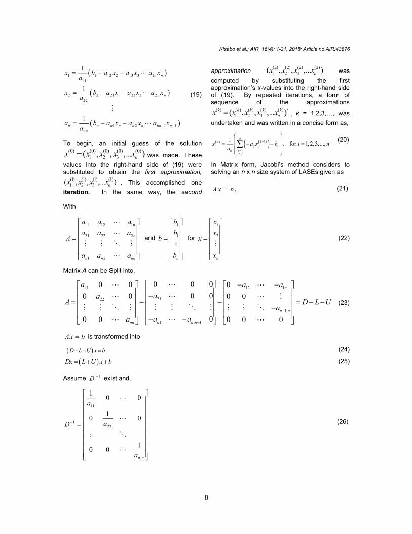
It is a method of solving a LSAEs in matrix form that has no zeros along its main diagonal. This was the reason, the last two rows in (14) were re-arranged to (15). Each diagonal element was solved for, and an approximate value plugged in. The process was then iterated until it converges. The Jacobi method was easily derived by examining each of the n equations in the linear system of equations Ax = b in isolation. Each equation was solved for one of the unknowns.

To apply the Jacobi’s method of solving any system of LSAEs given in the form (18), the first equation in (18) was used to obtain the value for x1, the second equation was used to solve for x2 and so on. Mathematically, the process is expressed as:


8

1 1 12 2 13 3 1

11

2 2 21 1 23 3 2

22

1 2 1 1

1

1

1

n n

n n

n n n n n n nn n

nn

x b a x a x a xa

x b a x a x a xa

x b a x a x a xa

(19)

To begin, an initial guess of the solution (0) (0) (0) (0) (0)

1 2 3( , , ,... )nx x x x x was made. These

values into the right-hand side of (19) were substituted to obtain the first approximation,

(1) (1) (1) (1)1 2 3( , , ,... )nx x x x . This accomplished one

iteration. In the same way, the second

approximation (2) (2) (2) (2)1 2 3( , , ,... )nx x x x was

computed by substituting the first approximation’s x-values into the right-hand side of (19). By repeated iterations, a form of sequence of the approximations

( ) ( ) ( ) ( ) ( )1 2 3( , , ,... )k k k k k t

nx x x x x , k = 1,2,3,…, was

undertaken and was written in a concise form as,

1( )

1

1, for 1, 2,3,...,

nkk

i ij j ijiii j

x a x b i na

(20)

In Matrix form, Jacobi’s method considers to solving an n x n size system of LASEs given as

,A x b (21)

With

11 12 1

21 22 2

1 2

n

n

n n nn

a a a

a a aA

a a a

and

1

1

n

b

bb

b

for

1

2

n

x

xx

x

(22)

Matrix A can be Split into,

11 12 1

2122

1,

1 , 1

0 0 00 0 0

0 00 0 0 0

00 0 0 0 0

n

n n

n n nnn

a a a

aaA D L U

a

a aa

(23)

Ax b is transformed into

D L U x b (24)

Dx L U x b (25)

Assume 1D exist and,

11

122

,

10 0

10 0

10 0

n n

a

aD

a

(26)


9

then,

1 1x D L U x D b (27)

The matrix form of Jacobi iterative method is

( ) 1 ( 1) 1k kx D L U x D b k = 1,2,3,…

(28)

The generalised matrix form of (27) can be expressed in a compact form using the following definitions:

1 ( ) ,T D L U (29)

1 ,C D b (30)

Hence, the Jacobi iteration method can also be written as

( ) ( -1)k kx Tx c k = 1,2,3,… (31)

In general, the iteration in (31) converges if the spectral radius (maximum eigenvalues of T), ρ (T) < 1 [21,22]. Also, if (15) is strictly diagonally dominant (SDD), then Jacobi’s method will converge to a solution from any initial guess. An n x n matrix A is SDD if the absolute value of each entry on the main diagonal is greater than the sum of the absolute values of the other entries in the same row. That is,

11 12 13 1

21 21 23 2

1 2 , 1

n

n

nn n n n n

a a a a

a a a a

a a a a

(32)

In concise form, (32) is written as

1

i n

ii ijjj i

a a

(33)

Aside (33), a matrix could be weakly diagonally dominant (WDD), meaning,

1

i n

ii ijjj i

a a

(34)

Often the term SDD is used instead of WDD [17]. Hence, this study investigated with (15), with the following:

Row 1: 2

1 12

Row 2: 2

12

Row 3: 1

12

Row 4: 2 1

12 2

Row 5: 1 1

Row 6: 1 0

Row 7: 3 2

2 2

Row 8: 3

12

With the result of Row 5, it can be inferred that (15) is a WDD. Much theory surrounds the convergence properties of strictly SDD matrices with iterative numerical methods [23,24,25,26], typical of which is, an n x n matrix is called convergent if

lim 0,k

ijxA

for each i = 1, 2, …., n and j = 1,

2,…,n (35)

If (35) holds then,

1,A (36)

Where, ρ is the spectral radius of the matrix A.

Surprisingly little or no work was available relating WDD and its convergence properties as it was applied to classical iterative numerical methods. With such type of matrices, the spectral radius test as given in (36) failed. The modulus of the maximum eigenvalues of a matrix is called spectral radius and is denoted by

max : A A : (37)

To compute (36) in Maple®, the following code

was invoked:

SpectralRadius(A): Evalf(%)


10

The result was,

1.065

With Maple®, one can quickly ascertain this fact with the following command;

MatrixConvergence(A)

It returned false

The results above for (36), buttress that of (34). From the spectral radius for LSAEs as given in (15), it is known to be a WDD. The question now is, how can one determine whether (15) will converge to a solution?

2

,A A A

(38)

Where,

max x ,A A the l∞ norm,

and

2 2x

max x ,A A the l2 norm

In Maple, to evaluate the norms outlined above the following was done; Norm (A, Euclidean); evalf(%); After it execution it returned, 1.96 With the commands (Norm, 2) and (Norm, infinity) in Maple

®, returned 2.71 in both cases.

Hence, (38) is true for this system of equation (1.065 < 1.96 < 2.71). On this, the study argues for a WDD, where (36) those not hold, then the WDD will converge if and only if (38) holds. Thus, it can safely be concluded that this system matrix as described by (15), designated as a WDD matrix will converge to a solution. Using Maple

® 2015 version running on a Laptop

with RAM 6.00GB, Intel(R) Core(TM) i5-2430M CPU @ 2.40GHz, with windows 7, the following commands were issued to initiate the solution process [27,28,29];

:with Student NumericalAnalysis

2 2 1 2 1: 8,8 1, 0, 0, ,1, 0, 0, 0 , 0, 1, 0, , 0, 0, 0, 0 , 0, 0, 1, 0, 0, 0, , 0 , 0, 0, 0, , 0, 1, , 0

2 2 2 2 2

2 3 3 0, 0, 0, 0, 0, 1, 0, 0,1 , 0, 0, 0, 0, 0,1, 0, 0 , 0, 0, 0, , 0, 0, , 0 , 0, 0, 0, 0, 0, 0, , 1

2 2 2

A

;

: 0, 0, 0, 0, 0,10000, 0, 0 ;b Vector

3, , 1.,1.,1.,1.,1.,1.,1.,1. , 10 ,

max 35, ,

IterativeApproximate A b initialapprox Vector tolerance

iteration stoppingcriterion relative method jacobi

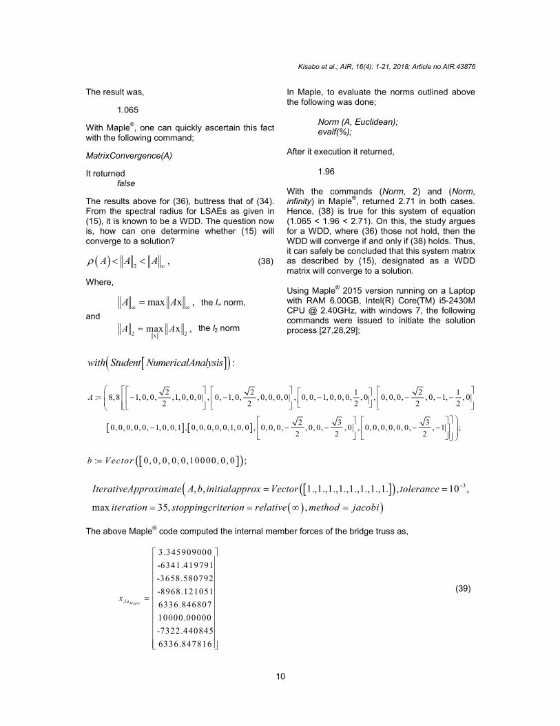
The above Maple® code computed the internal member forces of the bridge truss as,

3.345909000

-6341.419791

-3658.580792

-8968.121051

6336.846807

10000.00000

-7322.440845

6336.847816

MapleJax

(39)


11

To view the approximate solution with the error at each iteration as a column graph, we used the following Maple

® Code;

3, , 1.,1.,1.,1.,1.,1.,1.,1. , 10 ,

max 35, , , tan ;

IterativeApproximate A b initialapprox Vector tolerance

iteration stoppingcriterion relative method jacobi output plotdis ce

Observe that Jacobi’s method converged after 30 iterations as shown in Fig.6. From the fifth iteration, the trend in Fig. 6 is that of a decaying function. This is expected for errors to approach set tolerance value (usually less than zero).

Fig. 6. Evolution of the error with the number of iterations for Jacobi’s method In most situations where researchers work in independently, it is highly recommended to verify results using another STEM software. The study chose to implement the Jacobi’s method for solving (15) in MATLAB®. On the same Laptop that gave the above Maple® results running R2018a version of MATLAB

®, the following code gave the result in (40):

format long

A(1,1)=-1;

A(1,4)=(sqrt(2))/2;

A(1,5)=1;

A(2,2)=-1;

A(2,4)=(sqrt(2))/2;

A(3,3)=-1; A(3,7)=1/2;

A(4,4)=-(sqrt(2))/2;

A(4,6)=-1;

A(4,7)=-1/2;

A(5,5)=-1;

A(5,8)=1;

A(6,6)=1;

A(7,4)=-(sqrt(2))/2;

A(7,7)=(sqrt(3))/2;

A(8,7)=-(sqrt(3))/2;

A(8,8)=-1;

b=[0 0 0 0 0 10000 0 0]';

n=length(b); x=zeros(n,1);

x_0=[1 1 1 1 1 1 1 1]';

x=x_0;

nmaxit=31; % max iteration

tol=10^-2; % error tolerance

for t=1:nmaxit


12

for j=1:n

x(j)=(b(j)-A(j,[1:j-1, j+1:n])*x_0([1:j-1,j+1:n]))/A(j,j);

end

error=abs(x-x_0)

x_0=x;

if error<=tol

break

end

end

display(x)

3.34590843676

-6341.41979036144

-3658.58079229686

-8968.12104822703

6336.84680665998

10000.00000000000

-7322.44084601919

6336.84781585376

MATLABJax

(40)

Note, the difference between the Maple® and MATLAB® computed results using Jacobi’s method are very insignificant.

0.000000563240000

0.000000638559868

0.007130968599995

0.000002772969310x x

0.000000340020051

0

0.000001019189767

0.000000146240382

Maple MATLABJa Ja

(41)

To arrive at a result after 30 iterations seem sluggish. To compute the same result at faster pace literature proposes that the Gauss-Seidel algorithm will do a better job compared to Jacobi’s method and with a fewer number of iterations. 3.2 Gauss- Seidel (GS) The Gauss– Seidel algorithm is a variation of Jacobi’s algorithm that uses the updated value of each unknown variable as soon as that value is computed. Therefore, Gauss-Seidel algorithm

presents a feasible approach to solve many problems in engineering and science.

With the GS method, the new values ( 1)kix

were used as soon as they are known. For example, once ( 1 )

1kx was computed from the

first equation, its value was then used in the

second equation to obtain the new ( 1)2kx

and so

on. This could be depicted mathematically as,

first iteration:


13

( ,1) (0) (0) (0)1 1 12 2 13 3 1

11

( ,1) ( ,1) (0 ) (0)2 2 21 1 23 3 2

22

( ,1) ( ,1) ( ,1) (0)3 3 31 1 32 2 3

33

( ,1) ( ,1)1

1

1

1

1

newn n

new newn n

new new newn n

new newn n n n n

nn

x b a x a x a xa

x b a x a x a xa

x b a x a x a xa

x b a x aa

( ,1) ( ,1) (0)2 3 1 1

new newn n n nn nx a x a x

(42)

In a concise form, the GS method is presented as,

1

1

1 1

1, 1,2,... .

i nk k k

i ij j ij j ij j iii

x a x a x b i na

(43)

In matrix notation, the solution sorted can be casted as,

x d Cx (44)

Where,

1 11

2 22

n nn

b a

b ad

b a

(45)

and

12 11 13 11 1 11

21 22 23 22 2 22

31 33 32 33 3 33

1 2 3

0

0

0

0

n

n

n

n nn n nn n nn

a a a a a a

a a a a a a

C a a a a a a

a a a a a a

(46)

With the definitions of D, L and U given with the Jacobi method, the GS method is represented by

1x x b,

k kD L U

(47)

And

1 11

x x bk k

D L U D L

for each k =

1,2, … (48)

Letting

1

,gT D L U

(49)

And

1b,gc D L

(50)

Hence,

1x x .k k

g gT c

(51)

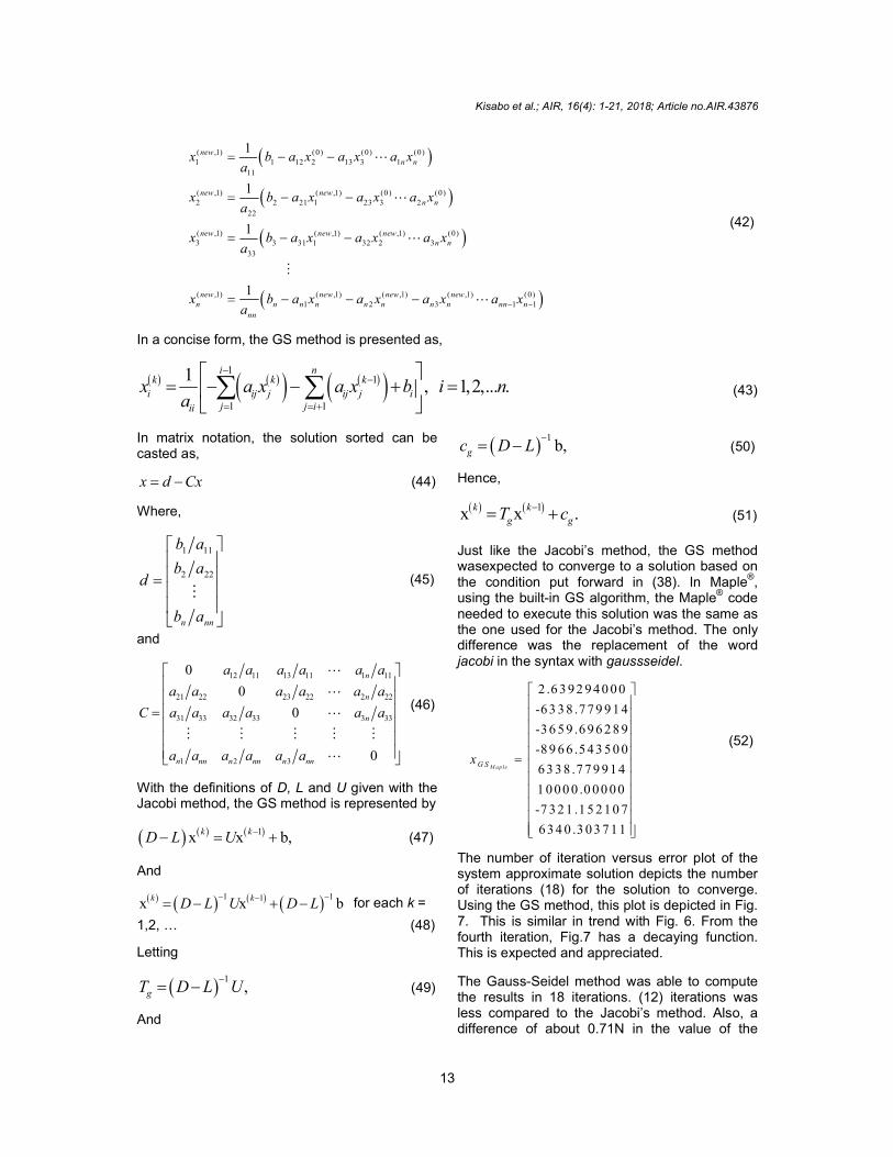
Just like the Jacobi’s method, the GS method wasexpected to converge to a solution based on the condition put forward in (38). In Maple

®,

using the built-in GS algorithm, the Maple® code needed to execute this solution was the same as the one used for the Jacobi’s method. The only difference was the replacement of the word jacobi in the syntax with gaussseidel.

2 .6 3 9 2 9 4 0 0 0

-6 3 3 8 .7 7 9 9 1 4

-3 6 5 9 .6 9 6 2 8 9

-8 9 6 6 .5 4 3 5 0 0

6 3 3 8 .7 7 9 9 1 4

1 0 0 0 0 .0 0 0 0 0

-7 3 2 1 .1 5 2 1 0 7

6 3 4 0 .3 0 3 7 1 1

MapleG Sx

(52)

The number of iteration versus error plot of the system approximate solution depicts the number of iterations (18) for the solution to converge. Using the GS method, this plot is depicted in Fig. 7. This is similar in trend with Fig. 6. From the fourth iteration, Fig.7 has a decaying function. This is expected and appreciated.

The Gauss-Seidel method was able to compute the results in 18 iterations. (12) iterations was less compared to the Jacobi’s method. Also, a difference of about 0.71N in the value of the


14

force F1 from both methods was noticed. This might look quite large because it can be approximated to 1N. On the other hand, the force F1 with magnitude 0.71N was just 0.0071% of the induced force f3 (10KN). In MATLAB

®, all the input parameters remained

the same as that of the Jacobi’s method (A matrix, b vector, and initial guess). For solving (15) with GS in MATLAB®, the number of maximum iterations (nmaxit) was only changed.

nmaxit=18; % SOR use 10 w=1; % SOR use 0.93; for t=1:nmaxit error=0; for i=1:n; s=0; xb=x(i); for j=1:n; if i~=j, s=s+A(i,j)*x(j); end end x(i)=w*(b(i)-s)/A(i,i)+(1-w)*x(i); error=error+abs(x(i)-xb); end if error/n<10^-2, break; end end

The above MATLAB® code gave the result in (53). Just like in the case with the Jacobi’s method, the difference between the Maple® and MATLAB

® computed results are all less than 1,

this is given in (54).

2.63929431481

-6338.77991338833

-3659.69628932854

-8966.54349719603.

6338.77991338833

10000.00000000000

-7321.15210820030

6340.30371067146

MATLABGSx

(53)

5

0.031480999984623

0.061166974774096

0.032853995435289

0.280397034657653x x 10 .

0.061166974774096

0

0.120030017569661

0.032853949960554

Maple MATLABSG SG

(54)

In literature, the Relaxation method suggests converging solution to a system like (15) faster than the GS method. The study intended to explore this fact here. This method is the third in the class of classical iterative method. 3.2 Successive Over-relaxation (SOR)

Method Relaxation method represents a slight modification of the Gauss-Seidel method that was designed to enhance convergence. After each new value is computed using (42), that value was modified by a weighted average of the results of the previous and the present iterations. Mathematically, it expressed as,

01 ,new ld newi i ix x x (55)

Where, ω is a weighting factor. If A is symmetric then,

2,A A (56)

With positive diagonal elements and for

0 2 , the SOR converges for any initial guess. Hence, elaborately the relaxation algorithm could be written as

Fig. 7. Number of iteration verse error in Gauss-Siedel Method

1

1 1

1 1

1 .i n

k k k k

i i ij j ij j ij j iii

x x a x a x ba

(57) If ω = 1, (57) reduces to (43). Hence, the Gauss-Seidel method is a special case of the relaxation method. For 0 < ω < 1, the procedures are called successive under-relaxation (SUR) methods, while choices of 1 < ω < 2 are called successive over-relaxation (SOR) methods. For the Relaxation method, no general answer could be


15

given to the question of how the appropriate value of ω is chosen. Literature informs of the choice of ω via the spectral radius of the system matrix as described by (58). If the system matrix is positive definite and tridiagonal, then

2

1g jT T (58)

Then, the optimal choice of ω for the SOR method is defined as

2

2

1 1 jT

(59)

To use (59) for the determination of the optimal choice of relaxation coefficient ω, the system matrix must be a tridiagonal matrix and positive definite (PD). And by definition, an n x n matrix is Positive Definite if it has the following properties:

A has an inverse; aii > 0 for each i = 1, 2, … n; max1 ≤ k,j ≤ n ≤ max1 ≤ i ≤ n |aii|; (aij)

2 < aiiaij for each i ≠ j

The above definition of PD requires the matrix to be symmetric (as given in (56), which does not hold for (15)), but not all authors make this requirement. For example, [30] requires only that xt Ax > 0 for each nonzero vector x. For the present system as given in (15), by mere inspection, the second property of PD does not hold. In Maple

®, the following command was

used to determine whether (15) is a PD matrix, IsMatrixShape(A, ‘positivedefinite’);

It returns false as an indication. Consistent with the definition, symmetry is required for a true result to be produced. The study now proceeds to determine whether this system as given in (15) is a tridiagonal matrix.

In linear algebra, a tridiagonal matrix is a band matrix that has nonzero elements only on the main diagonal (α), the first diagonal below (β) this, and the first diagonal above (γ) the main diagonal [31]. Generally, such matrix is square (n x n) and depicted as,

1 1

2 2 2

3 3

1

0 0

0 0

0 0n

n n

A

(60)

To determine whether the system as given in (15) is tridiagonal, the following command in Maple® was used,

IsMatrixShape(A, ‘strictlydiagonallydominant’);

The above code returns false. Hence, the system given by (15), is neither positive definite nor tridiagonal. This means (59) cannot be used to determine an optimal value for ω in this study. Thus, no choice but to go directly to Maple® and try to solve (15) using the SOR method and see the result.

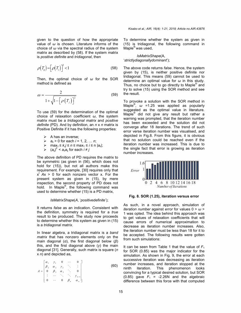
To provoke a solution with the SOR method in Maple®, ω =1.25 was applied as popularly suggested as the optimal value in literature. Maple® did not give any result but rather a warning was prompted, that the iteration number has been exceeded and the solution did not converge after 18 iterations. The trend of such error verse iteration number was visualised, and depicted in Fig.8. From this figure, it is obvious that no solution could be reached even if the iteration number was increased. This is due to the single fact that error is growing as iteration number increases.

Fig. 8. SOR (1.25), iteration versus error As such, in a novel approach, simulation of iteration number against error for values 0 > ω > 1 was opted. The idea behind this approach was to get values of relaxation coefficients that will cause errors of numerical approximation to decrease as iteration number increases. Also, the iteration number must be less than 18 for it to be accepted. The following results were gotten from such simulations:

It can be seen from Table 1 that the value of F1 for SOR (0.85) was the major indicator for the simulation. As shown in Fig. 9, the error at each successive iteration was decreasing as iteration number increases, and iteration stopped at the ninth iteration. This phenomenon looks convincing for a typical desired solution, but SOR (0.85) gave F1 = -2.26N and the algebraic difference between this force with that computed


16

by the GS method is 4.8985 N. This value of force also began to decrease from SOR (0.85). Notice that the result in (39) and (52) have four forces in tension (F1, f2, f3 and f5) and four in

compression (F2, F3, f1 and f4). This should be the same in the result sought with the SOR method. For SOR (0.84) to SOR(0.91), five forces are in compression and F1 is the culprit.

Table 1. Simulation results for SOR with ω = 0.84-0.99 in Maple

®

Method No. of iter.

S O Rx GS SORx x

SOR (ω = 0.84)

10 [-0.7568799675 -6339.745410 -3660.248047 -8965.7548047 6339.697981 9999.999890 -7320.508078 6339.744305 ]T

[3.3962 0.9655 0.55176 0.7887 0.91807 0.00011 0.64403 0.55941]T

SOR (ω = 0.85)

9 [-2.259211359 -6339.739104 -3660.232491 -8965.756926 6339.595385 9999.999616, -7320.508414 6339.740615 ]T

[4.8985 0.95919 0.5362 0.78657 0.81547 0.000384 0.64369 0.5631]T

SOR (ω = 0.86)

9 [-1.448685846 -6339.746631 -3660.242842 -8965.754113 6339.658256 9999.999793 -7320.507753 6339.743008]T

[4.088 0.96672 0.54655 0.78939 0.87834 0.000207 0.64435 0.5607]T

SOR (ω = 0.87)

9 [-0.8911709843-6339.746178 -3660.248206 -8965.753790 6339.697170 9999.999894 -7320.507443 6339.744174]T

[3.5305 0.96626 0.55192 0.78971 0.91726 0.000106 0.64466 0.55954]T

SOR (ω = 0.88)

9 [-0.5191194875 -6339.743031 -3660.249985 -8965.755568 6339.718916 9999.999848 -7320.508275 6339.745273]T

[3.1584 0.96312 0.5537 0.78793 0.939 0.000152 0.64383 0.55844]T

SOR (ω = 0.89)

9 [-0.3326921696 -6339.765987 -3660.258559 -8965.745868 6339.738200 9999.999876 -7320.504182 6339.743824]T

[2.972 0.98607 0.56227 0.79763 0.95829 0.000124 0.64793 0.55989]T

SOR (ω = 0.90)

9 [-0.4464763385 -6339.88603 -3660.303514 -8965.683594 6339.793636 9999.999990 -7320.471979 6339.726399]T

[3.0858 1.1061 0.60723 0.85991 1.0137 0.00001 0.68013 0.57731]T

SOR (ω = 0.91)

9 [-1.158045335 -6340.242016 -3660.448787 -8965.478803 6339.973317 9999.999996 -7320.354613 6339.655381]T

[3.7973 1.4621 0.7525 1.0647 1.1934 0.000004 0.79749 0.64833]T

SOR (ω = 0.92)

10 [0.9227326513 -6339.336863 -3660.081545 -8965.998649 6339.527694 10000.00 -7320.653514 6339.837940]T

[1.7166 0.55695 0.38526 0.54485 0.74778 0.0 0.49859 0.46577]T

SOR (ω = 0.93)

10 [2.440958649 -6338.701888 -3659.787956 -8966.413858 6339.121757 10000.00 -7320.924190 6340.024594]T

[0.19834 0.078026 0.091667 0.12964 0.34184 0.0 0.22792 0.27912]T

SOR (ω = 0.94)

11 [-2.153216175 -6340.640715 -3660.673515 -8965.161494 6340.335939 10000.00 -7320.114756 6339.469370]T

[4.7925 1.8608 0.091667 0.12964 1.556 0.0 1.0374 0. 83434]T

SOR (ω = 0.95)

12 [2.053732809 -6338.913998 -3659.846782 -8966.330671 6339.147896 10000.00 -7320.906786 6340.038723]T

[0.58556 0.13408 0.15049 0.21283 0.36798 0.0 0.24532 0.26499] T

SOR (ω = 0.96)

13 [-2.110024567 -6340.581081 -3660.679006 -8965.153728 6340.394730 10000.00 -7320.075563 6339.415822]T

[4.7493 1.8012 0.98272 1.3898 1.6148 0.0 1.0765 0.88789] T

SOR (ω = 0.97)

14 [2.325399179 -6338.845177 -3659.779166 -8966.426294 6338.994943 10000.00 -7321.008754 6340.141881]T

[0.31389 0.065263 0.082877 0.11721 0.21503 0.0 0.14335 0.16183] T

SOR (ω = 0.98)

15 [-2.738476941 -6340.785705 -3660.820281 -8964.953934 6340.671094 10000.00 -7319.891320 6339.242136]T

[5.3778 2.0058 1.124 1.5896 1.8912 0.0 1.2608 1.0616] T

SOR (ω = 0.99)

16 [3.434110452 -6338.466427 -3659.535846 -8966.770401 6338.536621 10000.00 -7321.314302 6340.424754]T

[0.79482 0.31349 0.16044 0.2269 0.24329 0.0 0.16219 0.12104] T


17

Fig. 9. SOR (0.85), iteration versus error Rejecting these results, the study went further to simulate for values of ω, beyond SOR (0.91). Questing for the value(s) of ω that will give F1 as a tension force, keeping other values of force as close as possible to those that the GS method gave in (52). SOR (0.92), gave four forces in compression and the remaining 4 were in tension. This result was similar to the GS method, and the trend of iteration number against error was similar to that depicted in Fig.

9. The only anomaly with SOR (0.92) is that the difference between its computed value of F1 with that of the GS method gives a force of 1.72N. Isolating some of the results that look very promising from Table 1 presented in Table 2 for closer examination.

From Fig. 10, it can be seen that SOR (0.93) is the global minimum of the fitted curve. Before ω = 0.85, the difference in F1 is high and beyond ω = 0.85, the difference in F1 is increasing. This trend depicted is actually what this study got when simulated for all values of ω. Though, those less than 0.84 were not documented in Table 1. In Fig. 11, outside the range ω = 0.85-0.93, iteration number increases even though result were converging to a solution. Note here that the solution sort for must converges at iteration much less than that of the GS method.

Table 2. Simulation range of interest

S/N SOR Method G S S O R

1 1F F

No. of Iter.

1 SOR(0.84) 3.3962 10 2 SOR(0.85) 4.8985 9 3 SOR(0.86) 4.088 9 4 SOR(0.87) 3.5305 9 5 SOR(0.88) 3.1584 9 6 SOR(0.89) 2.972 9 7 SOR(0.90) 3.0858 9 8 SOR(0.91) 3.7973 9 9 SOR(0.92) 1.7166 10 10 SOR(0.93) 0.19834 10

Fig. 10. Relaxation coefficient (0.85-0.93) against difference in F1

Fig. 11. Relaxation coefficient (0.85-0.93) against F1

|F1

(GS

)-F1

(SO

R)|

Itera

tion N

um

ber


18

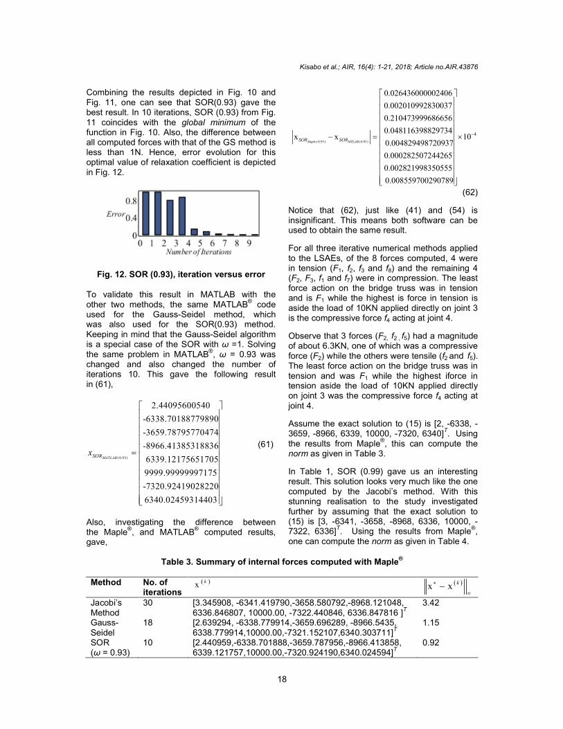
Combining the results depicted in Fig. 10 and Fig. 11, one can see that SOR(0.93) gave the best result. In 10 iterations, SOR (0.93) from Fig. 11 coincides with the global minimum of the function in Fig. 10. Also, the difference between all computed forces with that of the GS method is less than 1N. Hence, error evolution for this optimal value of relaxation coefficient is depicted in Fig. 12.

Fig. 12. SOR (0.93), iteration versus error To validate this result in MATLAB with the other two methods, the same MATLAB

® code

used for the Gauss-Seidel method, which was also used for the SOR(0.93) method. Keeping in mind that the Gauss-Seidel algorithm is a special case of the SOR with ω =1. Solving the same problem in MATLAB

®, ω = 0.93 was

changed and also changed the number of iterations 10. This gave the following result in (61),

( 0.93)

2.44095600540

-6338.70188779890

-3659.78795770474

-8966.41385318836

6339.12175651705

9999.99999997175

-7320.92419028220

6340.02459314403

MATLABSORx

(61)

Also, investigating the difference between the Maple

®, and MATLAB

® computed results,

gave,

(0.93) ( 0.93)

0.026436000002406

0.002010992830037

0.210473999686656

0.048116398829734x x 10

0.004829498720937

0.000282507244265

0.002821998350555

0.008559700290789

Maple MTLABSOR SOR

4

(62)

Notice that (62), just like (41) and (54) is insignificant. This means both software can be used to obtain the same result.

For all three iterative numerical methods applied to the LSAEs, of the 8 forces computed, 4 were in tension (F1, f2, f3 and f8) and the remaining 4 (F2, F3, f1 and f7) were in compression. The least force action on the bridge truss was in tension and is F1 while the highest is force in tension is aside the load of 10KN applied directly on joint 3 is the compressive force f4 acting at joint 4.

Observe that 3 forces (F2, f2 , f5) had a magnitude of about 6.3KN, one of which was a compressive force (F2) while the others were tensile (f2 and f5). The least force action on the bridge truss was in tension and was F1 while the highest iforce in tension aside the load of 10KN applied directly on joint 3 was the compressive force f4 acting at joint 4.

Assume the exact solution to (15) is [2, -6338, -3659, -8966, 6339, 10000, -7320, 6340]T. Using the results from Maple

®, this can compute the

norm as given in Table 3.

In Table 1, SOR (0.99) gave us an interesting result. This solution looks very much like the one computed by the Jacobi’s method. With this stunning realisation to the study investigated further by assuming that the exact solution to (15) is [3, -6341, -3658, -8968, 6336, 10000, -7322, 6336]T. Using the results from Maple®, one can compute the norm as given in Table 4.

Table 3. Summary of internal forces computed with Maple®

Method No. of

iterations

x k x x k

Jacobi’s Method

30 [3.345908, -6341.419790,-3658.580792,-8968.121048, 6336.846807, 10000.00, -7322.440846, 6336.847816 ]

T

3.42

Gauss-Seidel

18 [2.639294, -6338.779914,-3659.696289, -8966.5435, 6338.779914,10000.00,-7321.152107,6340.303711]

T

1.15

SOR (ω = 0.93)

10 [2.440959,-6338.701888,-3659.787956,-8966.413858, 6339.121757,10000.00,-7320.924190,6340.024594]T

0.92


19

Table 4. Please insert a table caption Method No. of

iterations

x k x x k

Gauss-Seidel

18 [2.639294, -6338.779914,-3659.696289, -8966.5435, 6338.779914,10000.00,-7321.152107,6340.303711]

T

4.3037

SOR (ω = 0.99)

16 [3.434110452 -6338.466427 -3659.535846 -8966.770401 6338.536621 10000.00 -7321.314302 6340.424754]

T

4.0246

Jacobi’s Method

30 [3.345908, -6341.419790,-3658.580792,-8968.121048, 6336.846807, 10000.00, -7322.440846, 6336.847816 ]

T

0.84782

SOR (0.99) is closer to the result obtained by Jacobi’s method as given in (41). This could be seen by the difference between the two as given in (63). Notice that (63) is similar to the result of SOR (0.96) in Table 1. Both evaluated differences have 5 forces greater than 1N.

(Ja) ( 0.99 )

0.088201

2.9534

0.95505

1.3507x x

1.6898

0

1.1265

3.5769

Maple MapleSOR SOR

(63)

Looking for other forms of similarity with (63), it was observed from Table 1 also, that SOR (0.98) has seven forces greater than 1N. And SOR (0.91) has 4 of it forces greater than 1N. As such, SOR (0.99) could be considered as a viable result and some special form of the Jacobi’s method. This assertion agrees with the literature [32,33]. There exists a special form of expressing the Jacobi’s method with a relaxation coefficient as given in (64). This is called Jacobi based Successive Relaxation method

1 1

1

.n

k k k

i i i ij jj iii

x x b a xa

(64)

With the realisation of (63), (64) and the computed forces with SOR (0.99), one can argue from a mathematical standpoint as to which result should be accepted, between Table 3 and Table 4. Such an argument is valid from a mathematical standpoint. But from an engineering perspective, it makes little or no difference. This is because, in both Tables, the largest induced force in the system is f1 with an absolute magnitude of 8.97KN. The design engineer will use this force to evaluates his FOS as given in (1). Hence, commence the design of

the truss members for the bridge, and its joints. To save computational cost, a scientist will always prefer to use the SOR method for such computation because of the obvious fact that it will require the least iteration number for the solution to converge. Hence, the result in Table 3 are our preferred solution to the bridge truss, because it closely conforms with theory in literature which states that the number of iterations needed for the GS method to converge to a solution is about half that of Jacobi’s method and for the Relaxation method is about half that of the GS method [34].

4. CONCLUSION Forces in a bridge truss member were resolved and built into a LSAEs. Classical iterative numerical methods namely; Jacobi’s method, Gauss-Seidel method and the Relaxation Technique, popularly called the SOR method were employed to obtain the solution to the LSAEs, using Maple® and MATLAB®. Due to the fact, the realised system of equations describing the bridge truss is sparse and weakly diagonally dominant, the study developed a simulation approach in Maple

® that could lead to

determining an optimal Relaxation coefficient. Here, LSAEs needed an under-relaxation coefficient to converge the solution faster than the Gauss-Seidel method. Also, the study was able to demonstrate the intuitive ability and capacity of Maple® to carry out classical iterative numerical computation with relative ease.

5. FUTURE WORK Non-classical iterative numerical methods need to be applied to the developed LSAEs describing the bridge truss in this study. These should at least include Conjugate Gradient method and Pre-Conditioned method. Results obtained should be compared with that of SOR (0.93) in this study. Also, an analytic formulation is needed for computing the optimal value of


20

relaxation coefficient for the SOR method for the weakly diagonally dominant matrix with ρ (A) ≥ 1. All MATLAB codes used for the three iterative numerical methods could be improved in such a way that the number of iterations is not fixed as presented in this study.

COMPETING INTERESTS Authors have declared that no competing interests exist.

REFERENCES

1. Aliyu Bhar Kisabo, et al 2018. Newton’s

method for solving non-linear system of algebraic equations (NLSAEs) with MATLAB/Simulink

® and MAPLE

®.

American Journal of Mathematical and Computer Modelling. 2017;2(4):117-131. DOI: 10.11648/j.ajmcm.20170204.14

2. Seongjai Kim. Numerical analysis using Maple

® and MATLAB

®. Department of

Mathematics and Statistics Mississippi State University Mississippi State, MS 39762 [email protected] (check online for published version); 2014.

3. Glyn James. Modern Engineering Mathematics. ISBN: 978-1-292-08082-6; 2015.

4. Inna Shingareva, Carlos Lizarraga-Celaya. Maple and Mathematica: A problem solving approach for mathematics. Second Edition, Springer New York; 2009. ISBN: 978-3-211-73264-9

5. Monagan MB, et al. Maple Introductory Programming Guide; 2009. ISBN: 978-1-897310-73-1

6. Alessio Pipinato. Innovative Bridge Design Handbook, Elsevier; 2015. ISBN: 9780128004876

7. Forces on Bridges with MATLAB. Available:http://mvhs.shodor.org/mvhsproj/bridges/bridge3.html

8. Krenk S, Høgsberg J. Statics and Mechanics of Structures. DOI: 10.1007/978-94-007-6113-1 2

9. Kulicki JM. Chapter 5: Highway bridge design specifications. Bridge Engineering Handbook, 2nd Edition: Fundamentals, Edited by Chen, W.F. and Duan, L., CRC Press, Boca Raton, FL.; 2014. ISBN: 9781439852217

10. The engineering tool box-resources, tools and basic information for engineering and design of technical applications.

Available:https://www.engineeringtoolbox.com/factors-safety-fos-d_1624.html (Accessed on 21 May 2018)

11. Richard L, Burden J. Douglas faires. Numerical Analysis. Ninth Edition Burden & Faires. Broke /Cole; 2011. ISBN: 13:978-0-538-73351-9

12. Sachin C. Patwardhan. Numerical analysis module 4 solving linear algebraic equations. Dept. of Chemical Engineering, Indian Institute of Technology, Bombay Powai, Mumbai, 400 076, Inda; 2014.

13. Jaan Kiusalaas. Numerical methods in engineering with MATLAB. Cambridge University press, New York; 2005. ISBN:13 978-0-511-12811-0

14. Sparse Matrix. Available:https://en.wikipedia.org/wiki/Sparse_matrix. Wikipedia (Accessed, March 11, 2018)

15. Michal Novak. Numerical Methods: Exercise Book. Department of Mathematics FEEC BUT; 2014. Available:http://www.umat.feec.vutbr.cz, [email protected]

16. Matrix Market. Available:http://math.nist.gov/MatrixMarket/data (Accessed on May, 28 2018)

17. Shawn Sickel. A comparison of some iterative methods in scientific computing. Department of Mathematics University of Wyoming; 2005.

18. Yousef Saad. Iterative methods for sparse linear systems. Society for Industrial and Applied Mathematics; 2003. ISBN: 13: 9780898715347

19. Kelley CT. Iterative Methods for Linear and Nonlinear Equations. North Carolina State University, Raleigh, North Carolina; 1995. eISBN: 978-1-61197-094-4

20. Steven C. Chapara. Applied numerical methods with MATLAB for engineers and scientist. Third Edition, Mc Graw Hill; 2012. ISBN: 978-0-07-340110-2

21. Nicholas Loehr. Advanced linear algebra. CRC Taylor & Francis Group; 2014. ISBN: 13:978-1-4665-5902-8

22. Zhi Ming Yangy. A simple method for estimating the bounds of spectral radius of nonnegative irreducible matrices. Applied Mathematics E-Notes. 2011;11:67-72. ISSN: 1607-2510 Available:http://www.math.nthu.edu.tw/_amen/


21

23. Thai Nhan. A brief introduction to iterative methods for solving linear systems with MATLAB. Ohlone College; 2016.

24. Zhanshan Yang, Bing Zheng, Xilan Liu. A new upper bound for ‖�−1‖ of a strictly �-diagonally dominant �-matrix. Hindawi Publishing Corporation. Advances in Numerical Analysis. Article ID 980615. 2013;6. Available:http://dx.doi.org/10.1155/2013/980615

25. Geir Dahl. A note on diagonally dominant matrices. Elsevier. Linear Algebra and its Applications. 2000;317:217–224. Available:www.elsevier.com/locate/laa

26. Farid O. Farid. On classes of matrices with variants of the diagonal dominance property. Advances in Linear Algebra & Matrix Theory; 2017. ISSN Online: 2165-3348 Available:http://www.scirp.org/journal/alamt

27. Cheng-yi Zhang, Zichen Xue, Shuanghua Luo. A convergence analysis of SOR iterative methods for linear systems with weak H-matrices. Open Math. 2016; 14:747–760. DOI: 10.1515/math-2016-0065

28. Monagan MB, et al. Maple 9 advanced programming guide. Maplesoft, a division of Waterloo Maple Inc., Canada; 2003. ISBN: 1-894511-44-1

29. Correa Silva EV. Numerical calculations using Maple: Why & how? Maple Tech Birkhauser Boston; 2008.

ISSN: 1061-5733

30. Mirko Navara, Ales Nemecek. Numerical analysis with Maple. Czech Technical University, Faculty of Electrical Engineering, Department of Cybernetics, Center for Machine Perception, Technicka 2, 166 27 Prague 6, Czech Republic; 2010.

31. Tridiagonal matrix.

Available:https://en.wikipedia.org/w/index.php?title=Tridiagonal_matrix&oldid=822910512

(Accessed, March 20 2018)

32. Gilbert Strang. Introduction to Linear Algebra. Fourth Edition; 2009.

ISBN: 978-0-9802327-1-4

33. Maxim A. Olshanskii, Eugene E. Tyrtyshnikov. Iterative methods for linear systems: Theory and Applications; 2014.

ISBN: 9781611973457

34. Essays UK. Comparison of rate of convergence of iterative methods philosophy essay; 2013.

Available:https://www.ukessays.com/essays/philosophy/comparison-of-rate-of-convergence-of-iterative-methods-philosophy-essay.php?vref=1

_________________________________________________________________________________ © 2018 Kisabo et al.; This is an Open Access article distributed under the terms of the Creative Commons Attribution License (http://creativecommons.org/licenses/by/4.0), which permits unrestricted use, distribution, and reproduction in any medium, provided the original work is properly cited.

Peer-review history: The peer review history for this paper can be accessed here:

http://www.sciencedomain.org/review-history/26522

Documents

Computing Internal Member Forces in a Bridge Truss Using