COMPUTING LONG-TERM DAYLIGHTING SIMULATIONS FROM …

2018 Building Performance Analysis Conference and

SimBuild co-organized by ASHRAE and IBPSA-USA

Chicago, IL

September 26-28, 2018

COMPUTING LONG-TERM DAYLIGHTING SIMULATIONS FROM HIGH DYNAMIC

RANGE IMAGERY USING DEEP NEURAL NETWORKS

Yue Liu1, Alex Colburn2, and Mehlika Inanici1 1University of Washington, Seattle, WA

2Zillow Group, Seattle, WA

ABSTRACT

Compared with illuminance-based metrics, luminance-

based metrics and evaluations provide better

understandings of occupant visual experience. However,

it is computationally expensive and time consuming to

incorporate luminance-based metrics into architectural

design practice because annual simulations require

generating a luminance map at each time step of the

entire year. This paper describes the development of a

novel prediction model to generate annual luminance

maps of indoor space from a subset of images by using

deep neural networks (DNNs). The results show that by

only rendering 5% of annual luminance maps, the

proposed DNNs model can predict the rest with

comparable accuracy that closely matches those high-

quality point-in-time renderings generated by Radiance

(RPICT) software. This model can be applied to

accelerate annual luminance-based simulations and lays

the groundwork for generating annual luminance maps

utilizing High Dynamic Range (HDR) captures of

existing environments.

INTRODUCTION

Architectural daylighting design is not only driven by

energy concerns but also motivated by a desire to

improve human comfort. The presence of daylight can

improve occupants’ health, awareness, and feelings of

well-being (Boyce 2014). However, uncontrollably

maximizing daylight penetration into buildings can lead

to undesirable luminous environments that can impair

vision or create visual discomfort.

Attitudes and research practices in architectural lighting

field are shifting towards luminance-based metrics and

evaluations. Compared with illuminance-based metrics,

luminance-based metrics provide more meaningful

information about occupant visual experience. For

example, the primary source of indoor visual discomfort

is discomfort glare caused by excessive light or contrast

in an occupant’s field of view. Therefore, glare can be

better understood through luminance distribution-based

metrics (Wienold and Christoffersen 2006, Jakubiec and

Reinhart 2012, Suk et al. 2013, Konis 2014, Van Den

Wymelenberg and Inanici 2015).

Practitioners and researchers need long-term daylighting

simulations to predict the effectiveness of their design

strategies and decisions. Although illuminance-based

annual simulations are accessible to lighting

professionals through a number of programs and metrics,

luminance-based annual simulations remain

computationally expensive. Long-term simulations are

computed through multi-phased daylight coefficient

methodologies, which have steep learning curves and

long simulation times. There is a need to improve the

availability and accessibility of long-term luminance-

based lighting simulations.

Accelerating annual daylight simulations is an active

area of research. Daylight coefficient (DC) approach has

been developed as a numerical methodology to perform

annual daylight predictions in a more efficient manner

(Tregenza and Waters 1983). The classic DC concept is

to divide the celestial hemisphere into discrete sky

segments and calculate the contribution of each segment

to the illuminance level at various sensor points. Further

developments of dynamic daylight simulation methods

(DDS) divide the light flux transfer process into multiple

phases to better model complex fenestration systems

(Laouadi et al. 2008, Ward et al. 2011).

More recent developments in lighting simulation

acceleration depend on advances in modern computing

technology. Two recent trends in lighting acceleration

research are: 1) Increasing rendering efficiency by

tracing multiple primary rays in parallel on a graphics

processing units (GPU) (Jones and Reinhart 2014).

Modern GPUs with highly parallel structure make them

more efficient than general purpose central processing

© 2018 ASHRAE (www.ashrae.org) and IBPSA-USA (www.ibpsa.us). For personal use only. Additional reproduction, distribution, or transmission in either print or digital form is not permitted without ASHRAE or IBPSA-USA's prior written permission.

119



Chicago, IL


units (CPUs) for parallel computing of large data blocks.

2) Predicting lighting performance using machine

learning based-algorithms.

This research follows the second trend and develops a

workflow to generate annual luminance maps of indoor

space from a subset of data using artificial neural

networks (ANNs). Machine learning, and specifically

ANN, has been used recently within the architectural

lighting field. ANNs have been investigated for

predicting indoor daylight illuminances (Kazanasmaz et

al. 2009, Zhou and Liu 2015, Navada et al. 2016, Ahmad

et al. 2017) and for developing and classifying sky

models (Li et al. 2010, Satilmis et al. 2016).

Although statistical methods have been utilized to

predict long-term luminance maps from limited number

of imagery (Inanici 2013), the predictions were more

successful for overcast skies and need further

improvements to better model the sun patches under

sunny skies. To the best of the authors’ knowledge, there

are no previous studies that utilize machine learning to

predict long-term luminance distributions. This study

provides a novel solution for long-term luminance

simulation accelerations. It is inspired by Ren et al.

(2015), which is based on learning the non-linear

mapping of pixel-scale luminance values from local and

contextual attributes of surface points. The accuracy,

applicability, and usefulness of the proposed DNNs

model is demonstrated, and its effectiveness is

exemplified through computer-generated images.

OBJECTIVES

The objective of this research is to demonstrate the

utilization of deep neural networks (DNNs) (a.k.a deep

ANNs) techniques to predict long-term luminance maps

from a small subset of data. The ultimate goal is to

generate annual luminance maps from High Dynamic

Range (HDR) photographs of existing environments,

which will enable quantitative analysis of daylit

environments without the time-consuming modeling

process. To reach this final goal, in this paper, simulated

images (instead of captures of existing buildings) are

utilized to facilitate the development of the algorithm

with adequate number of imageries under controlled

settings.

Specifically, the contributions of this paper are as

follows:

• A presentation of the first deep learning framework to

conduct architectural luminance predictions: The

proposed DNNs model accelerates annual luminance-

based simulations by generating annual luminance maps

extracted from a small set of rendered inputs. The

performance of the model is quantitatively investigated

to meet the scientific accuracy requirement for

applications in architectural lighting.

• An analysis of the sensitivity of prediction accuracy to

sample data size, which inform the optimum sample size

for data collection and generation: The study further

evaluates the impact of lower-precision predictions on

the design decision making processes by utilizing false

color images and visual discomfort indices.

• An exploration and analysis of the various processing

and design decisions of the proposed DNNs system.

• A demonstration of a workflow that accurately predicts

annual luminance maps from a small number of rendered

images.

METHODOLOGY

ANNs

Machine learning is an approach to analyze and model

complex systems. One popular and powerful Machine

learning technique is ANNs. ANNs were proposed in

1943 (McCulloch and Pitts 1943) and inspired by

biological neurons of animal brains and consist of

neuron-like connected computing units called nodes.

These nodes are organized into layers: input, output, and

the hidden layers (i.e. layers between input and output).

The connection between two nodes has a weight which

defines how much the previous node influences the next

node. The network gathers information and finds

relationships between inputs and outputs through a

learning (training) process. During the learning process,

information is transferred from layer to layer and learned

knowledge is stored in node weights. This enables neural

networks to solve complex problems, where numerical

solutions are difficult to obtain. A DNNs model is an

ANN model with multiple hidden layers between the

input and output layers. Like shallow ANNs, DNNs can

solve complicated nonlinear problems such as predicting

long-term luminance. In this study, DNNs are used to

approximate the non-linear relationship between the

image pixel luminance and daylighting conditions with

minimal inputs.

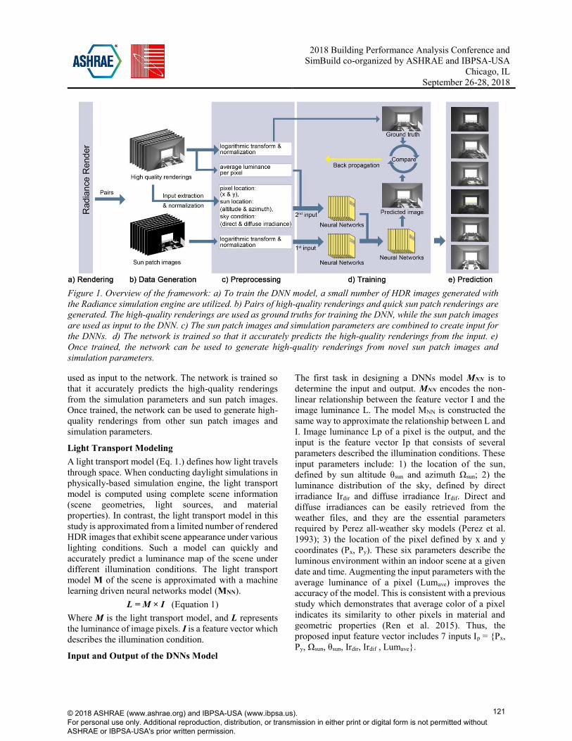
Fig. 1. gives an overview of the proposed methodology.

The workflow starts with the generation of sample data

(HDR renderings) using the Radiance simulation engine.

Radiance (Ward, 1994) is a physically-based simulation

engine that has been validated against illuminance

measurements in full-scale spaces (Mardaljevic 2000).

Each sample consists of the input parameters and a pair

of images: a high-quality rendering and a sun patch

image. The high-quality renderings are used as ground

truth for training the neural networks, while the low-

quality sun patch images and simulation parameters are


120



Chicago, IL


used as input to the network. The network is trained so

that it accurately predicts the high-quality renderings

from the simulation parameters and sun patch images.

Once trained, the network can be used to generate high-

quality renderings from other sun patch images and

simulation parameters.

Light Transport Modeling

A light transport model (Eq. 1.) defines how light travels

through space. When conducting daylight simulations in

physically-based simulation engine, the light transport

model is computed using complete scene information

(scene geometries, light sources, and material

properties). In contrast, the light transport model in this

study is approximated from a limited number of rendered

HDR images that exhibit scene appearance under various

lighting conditions. Such a model can quickly and

accurately predict a luminance map of the scene under

different illumination conditions. The light transport

model M of the scene is approximated with a machine

learning driven neural networks model (MNN).

L = M × I (Equation 1)

Where M is the light transport model, and L represents

the luminance of image pixels. I is a feature vector which

describes the illumination condition.

Input and Output of the DNNs Model

The first task in designing a DNNs model MNN is to

determine the input and output. MNN encodes the non-

linear relationship between the feature vector I and the

image luminance L. The model MNN is constructed the

same way to approximate the relationship between L and

I. Image luminance Lp of a pixel is the output, and the

input is the feature vector Ip that consists of several

parameters described the illumination conditions. These

input parameters include: 1) the location of the sun,

defined by sun altitude θsun and azimuth Ωsun; 2) the

luminance distribution of the sky, defined by direct

irradiance Irdir and diffuse irradiance Irdif. Direct and

diffuse irradiances can be easily retrieved from the

weather files, and they are the essential parameters

required by Perez all-weather sky models (Perez et al.

1993); 3) the location of the pixel defined by x and y

coordinates (Px, Py). These six parameters describe the

luminous environment within an indoor scene at a given

date and time. Augmenting the input parameters with the

average luminance of a pixel (Lumave) improves the

accuracy of the model. This is consistent with a previous

study which demonstrates that average color of a pixel

indicates its similarity to other pixels in material and

geometric properties (Ren et al. 2015). Thus, the

proposed input feature vector includes 7 inputs Ip = {Px,

Py, Ωsun, θsun, Irdir, Irdif , Lumave}.

Figure 1. Overview of the framework: a) To train the DNN model, a small number of HDR images generated with

the Radiance simulation engine are utilized. b) Pairs of high-quality renderings and quick sun patch renderings are

generated. The high-quality renderings are used as ground truths for training the DNN, while the sun patch images

are used as input to the DNN. c) The sun patch images and simulation parameters are combined to create input for

the DNNs. d) The network is trained so that it accurately predicts the high-quality renderings from the input. e)

Once trained, the network can be used to generate high-quality renderings from novel sun patch images and

simulation parameters.


121



Chicago, IL


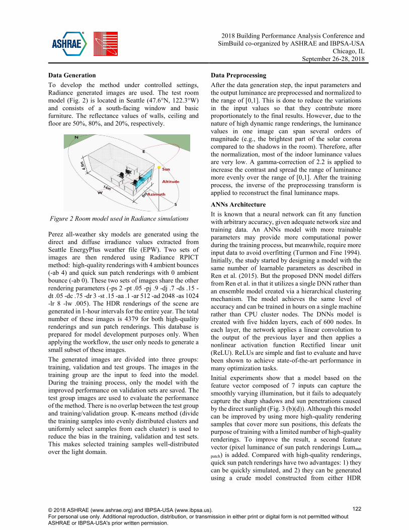
Data Generation

To develop the method under controlled settings,

Radiance generated images are used. The test room

model (Fig. 2) is located in Seattle (47.6°N, 122.3°W)

and consists of a south-facing window and basic

furniture. The reflectance values of walls, ceiling and

floor are 50%, 80%, and 20%, respectively.

Perez all-weather sky models are generated using the

direct and diffuse irradiance values extracted from

Seattle EnergyPlus weather file (EPW). Two sets of

images are then rendered using Radiance RPICT

method: high-quality renderings with 4 ambient bounces

(-ab 4) and quick sun patch renderings with 0 ambient

bounce (-ab 0). These two sets of images share the other

rendering parameters (-ps 2 -pt .05 -pj .9 -dj .7 -ds .15 -

dt .05 -dc .75 -dr 3 -st .15 -aa .1 -ar 512 -ad 2048 -as 1024

-lr 8 -lw .005). The HDR renderings of the scene are

generated in 1-hour intervals for the entire year. The total

number of these images is 4379 for both high-quality

renderings and sun patch renderings. This database is

prepared for model development purposes only. When

applying the workflow, the user only needs to generate a

small subset of these images.

The generated images are divided into three groups:

training, validation and test groups. The images in the

training group are the input to feed into the model.

During the training process, only the model with the

improved performance on validation sets are saved. The

test group images are used to evaluate the performance

of the method. There is no overlap between the test group

and training/validation group. K-means method (divide

the training samples into evenly distributed clusters and

uniformly select samples from each cluster) is used to

reduce the bias in the training, validation and test sets.

This makes selected training samples well-distributed

over the light domain.

Data Preprocessing

After the data generation step, the input parameters and

the output luminance are preprocessed and normalized to

the range of [0,1]. This is done to reduce the variations

in the input values so that they contribute more

proportionately to the final results. However, due to the

nature of high dynamic range renderings, the luminance

values in one image can span several orders of

magnitude (e.g., the brightest part of the solar corona

compared to the shadows in the room). Therefore, after

the normalization, most of the indoor luminance values

are very low. A gamma-correction of 2.2 is applied to

increase the contrast and spread the range of luminance

more evenly over the range of [0,1]. After the training

process, the inverse of the preprocessing transform is

applied to reconstruct the final luminance maps.

ANNs Architecture

It is known that a neural network can fit any function

with arbitrary accuracy, given adequate network size and

training data. An ANNs model with more trainable

parameters may provide more computational power

during the training process, but meanwhile, require more

input data to avoid overfitting (Turmon and Fine 1994).

Initially, the study started by designing a model with the

same number of learnable parameters as described in

Ren et al. (2015). But the proposed DNN model differs

from Ren et al. in that it utilizes a single DNN rather than

an ensemble model created via a hierarchical clustering

mechanism. The model achieves the same level of

accuracy and can be trained in hours on a single machine

rather than CPU cluster nodes. The DNNs model is

created with five hidden layers, each of 600 nodes. In

each layer, the network applies a linear convolution to

the output of the previous layer and then applies a

nonlinear activation function Rectified linear unit

(ReLU). ReLUs are simple and fast to evaluate and have

been shown to achieve state-of-the-art performance in

many optimization tasks.

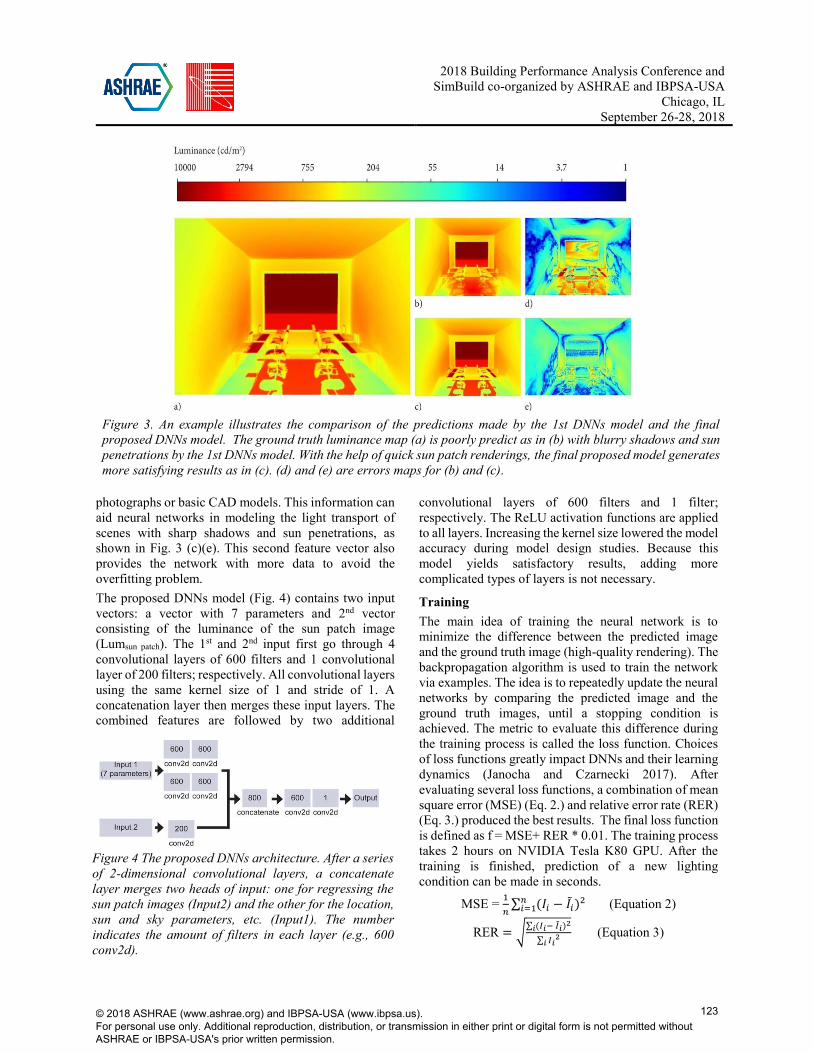
Initial experiments show that a model based on the

feature vector composed of 7 inputs can capture the

smoothly varying illumination, but it fails to adequately

capture the sharp shadows and sun penetrations caused

by the direct sunlight (Fig. 3 (b)(d)). Although this model

can be improved by using more high-quality rendering

samples that cover more sun positions, this defeats the

purpose of training with a limited number of high-quality

renderings. To improve the result, a second feature

vector (pixel luminance of sun patch renderings Lumsun

patch) is added. Compared with high-quality renderings,

quick sun patch renderings have two advantages: 1) they

can be quickly simulated, and 2) they can be generated

using a crude model constructed from either HDR

Figure 2 Room model used in Radiance simulations


122



Chicago, IL


photographs or basic CAD models. This information can

aid neural networks in modeling the light transport of

scenes with sharp shadows and sun penetrations, as

shown in Fig. 3 (c)(e). This second feature vector also

provides the network with more data to avoid the

overfitting problem.

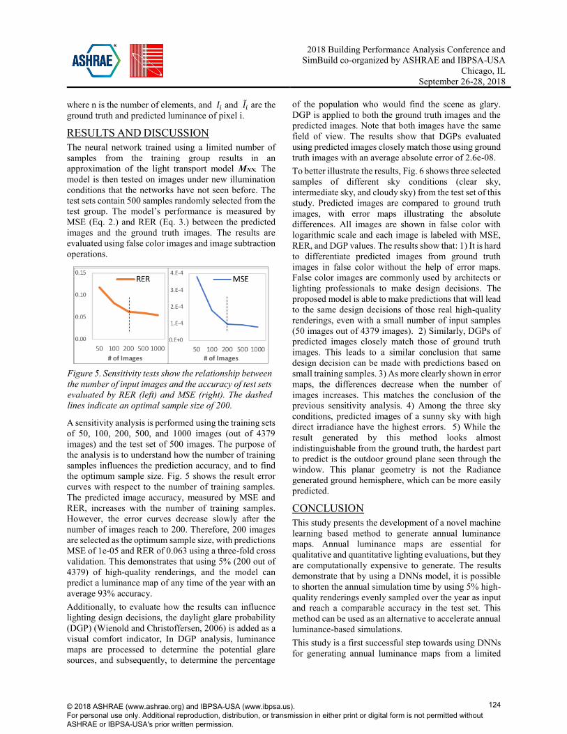
The proposed DNNs model (Fig. 4) contains two input

vectors: a vector with 7 parameters and 2nd vector

consisting of the luminance of the sun patch image

(Lumsun patch). The 1st and 2nd input first go through 4

convolutional layers of 600 filters and 1 convolutional

layer of 200 filters; respectively. All convolutional layers

using the same kernel size of 1 and stride of 1. A

concatenation layer then merges these input layers. The

combined features are followed by two additional

convolutional layers of 600 filters and 1 filter;

respectively. The ReLU activation functions are applied

to all layers. Increasing the kernel size lowered the model

accuracy during model design studies. Because this

model yields satisfactory results, adding more

complicated types of layers is not necessary.

Training

The main idea of training the neural network is to

minimize the difference between the predicted image

and the ground truth image (high-quality rendering). The

backpropagation algorithm is used to train the network

via examples. The idea is to repeatedly update the neural

networks by comparing the predicted image and the

ground truth images, until a stopping condition is

achieved. The metric to evaluate this difference during

the training process is called the loss function. Choices

of loss functions greatly impact DNNs and their learning

dynamics (Janocha and Czarnecki 2017). After

evaluating several loss functions, a combination of mean

square error (MSE) (Eq. 2.) and relative error rate (RER)

(Eq. 3.) produced the best results. The final loss function

is defined as f = MSE+ RER * 0.01. The training process

takes 2 hours on NVIDIA Tesla K80 GPU. After the

training is finished, prediction of a new lighting

condition can be made in seconds.

MSE = 1

𝑛∑ (𝐼𝑖 − 𝐼𝑖)2𝑛

𝑖=1 (Equation 2)

RER = √∑ (𝐼𝑖− 𝐼𝑖)2

𝑖

∑ 𝐼𝑖2

𝑖 (Equation 3)

Figure 3. An example illustrates the comparison of the predictions made by the 1st DNNs model and the final

proposed DNNs model. The ground truth luminance map (a) is poorly predict as in (b) with blurry shadows and sun

penetrations by the 1st DNNs model. With the help of quick sun patch renderings, the final proposed model generates

more satisfying results as in (c). (d) and (e) are errors maps for (b) and (c).

Figure 4 The proposed DNNs architecture. After a series

of 2-dimensional convolutional layers, a concatenate

layer merges two heads of input: one for regressing the

sun patch images (Input2) and the other for the location,

sun and sky parameters, etc. (Input1). The number

indicates the amount of filters in each layer (e.g., 600

conv2d).


123



Chicago, IL


where n is the number of elements, and 𝐼𝑖 and 𝐼𝑖 are the

ground truth and predicted luminance of pixel i.

RESULTS AND DISCUSSION

The neural network trained using a limited number of

samples from the training group results in an

approximation of the light transport model MNN. The

model is then tested on images under new illumination

conditions that the networks have not seen before. The

test sets contain 500 samples randomly selected from the

test group. The model’s performance is measured by

MSE (Eq. 2.) and RER (Eq. 3.) between the predicted

images and the ground truth images. The results are

evaluated using false color images and image subtraction

operations.

A sensitivity analysis is performed using the training sets

of 50, 100, 200, 500, and 1000 images (out of 4379

images) and the test set of 500 images. The purpose of

the analysis is to understand how the number of training

samples influences the prediction accuracy, and to find

the optimum sample size. Fig. 5 shows the result error

curves with respect to the number of training samples.

The predicted image accuracy, measured by MSE and

RER, increases with the number of training samples.

However, the error curves decrease slowly after the

number of images reach to 200. Therefore, 200 images

are selected as the optimum sample size, with predictions

MSE of 1e-05 and RER of 0.063 using a three-fold cross

validation. This demonstrates that using 5% (200 out of

4379) of high-quality renderings, and the model can

predict a luminance map of any time of the year with an

average 93% accuracy.

Additionally, to evaluate how the results can influence

lighting design decisions, the daylight glare probability

(DGP) (Wienold and Christoffersen, 2006) is added as a

visual comfort indicator, In DGP analysis, luminance

maps are processed to determine the potential glare

sources, and subsequently, to determine the percentage

of the population who would find the scene as glary.

DGP is applied to both the ground truth images and the

predicted images. Note that both images have the same

field of view. The results show that DGPs evaluated

using predicted images closely match those using ground

truth images with an average absolute error of 2.6e-08.

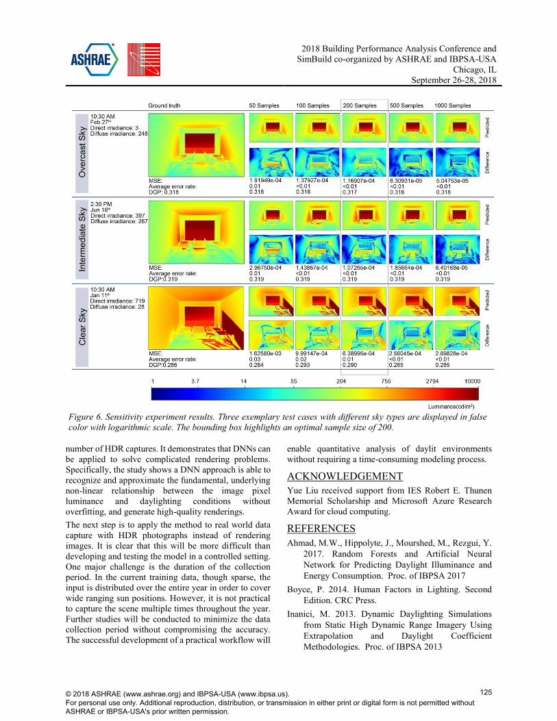
To better illustrate the results, Fig. 6 shows three selected

samples of different sky conditions (clear sky,

intermediate sky, and cloudy sky) from the test set of this

study. Predicted images are compared to ground truth

images, with error maps illustrating the absolute

differences. All images are shown in false color with

logarithmic scale and each image is labeled with MSE,

RER, and DGP values. The results show that: 1) It is hard

to differentiate predicted images from ground truth

images in false color without the help of error maps.

False color images are commonly used by architects or

lighting professionals to make design decisions. The

proposed model is able to make predictions that will lead

to the same design decisions of those real high-quality

renderings, even with a small number of input samples

(50 images out of 4379 images). 2) Similarly, DGPs of

predicted images closely match those of ground truth

images. This leads to a similar conclusion that same

design decision can be made with predictions based on

small training samples. 3) As more clearly shown in error

maps, the differences decrease when the number of

images increases. This matches the conclusion of the

previous sensitivity analysis. 4) Among the three sky

conditions, predicted images of a sunny sky with high

direct irradiance have the highest errors. 5) While the

result generated by this method looks almost

indistinguishable from the ground truth, the hardest part

to predict is the outdoor ground plane seen through the

window. This planar geometry is not the Radiance

generated ground hemisphere, which can be more easily

predicted.

CONCLUSION

This study presents the development of a novel machine

learning based method to generate annual luminance

maps. Annual luminance maps are essential for

qualitative and quantitative lighting evaluations, but they

are computationally expensive to generate. The results

demonstrate that by using a DNNs model, it is possible

to shorten the annual simulation time by using 5% high-

quality renderings evenly sampled over the year as input

and reach a comparable accuracy in the test set. This

method can be used as an alternative to accelerate annual

luminance-based simulations.

This study is a first successful step towards using DNNs

for generating annual luminance maps from a limited

Figure 5. Sensitivity tests show the relationship between

the number of input images and the accuracy of test sets

evaluated by RER (left) and MSE (right). The dashed

lines indicate an optimal sample size of 200.


124



Chicago, IL


number of HDR captures. It demonstrates that DNNs can

be applied to solve complicated rendering problems.

Specifically, the study shows a DNN approach is able to

recognize and approximate the fundamental, underlying

non-linear relationship between the image pixel

luminance and daylighting conditions without

overfitting, and generate high-quality renderings.

The next step is to apply the method to real world data

capture with HDR photographs instead of rendering

images. It is clear that this will be more difficult than

developing and testing the model in a controlled setting.

One major challenge is the duration of the collection

period. In the current training data, though sparse, the

input is distributed over the entire year in order to cover

wide ranging sun positions. However, it is not practical

to capture the scene multiple times throughout the year.

Further studies will be conducted to minimize the data

collection period without compromising the accuracy.

The successful development of a practical workflow will

enable quantitative analysis of daylit environments

without requiring a time-consuming modeling process.

ACKNOWLEDGEMENT

Yue Liu received support from IES Robert E. Thunen

Memorial Scholarship and Microsoft Azure Research

Award for cloud computing.

REFERENCES

Ahmad, M.W., Hippolyte, J., Mourshed, M., Rezgui, Y.

2017. Random Forests and Artificial Neural

Network for Predicting Daylight Illuminance and

Energy Consumption. Proc. of IBPSA 2017

Boyce, P. 2014. Human Factors in Lighting. Second

Edition. CRC Press.

Inanici, M. 2013. Dynamic Daylighting Simulations

from Static High Dynamic Range Imagery Using

Extrapolation and Daylight Coefficient

Methodologies. Proc. of IBPSA 2013

Figure 6. Sensitivity experiment results. Three exemplary test cases with different sky types are displayed in false

color with logarithmic scale. The bounding box highlights an optimal sample size of 200.


125



Chicago, IL


Jakubiec, J.A., Reinhart, C.F. 2012. The ‘Adaptive

Zone’ - A Concept for Assessing Discomfort Glare

throughout Daylit Spaces. Lighting Research and

Technology 44 (2): 149–70.

Janocha, K., Czarnecki, W.M. 2017. On Loss Functions

for Deep Neural Networks in Classification. CoRR

(2017), 1–10.

Jones, N., Reinhart, C. 2014. Irradiance Caching for

Global Illumination Calculation on Graphics

Hardware. Ashrae/Ibpsa-Usa, 111–20.

Kazanasmaz, T., Gunaydin, M., Binol, S. 2009.

Artificial Neural Networks to Predict Daylight

Illuminance in Office Buildings. Building and

Environment 44 (8): 1751–57

Konis, K. 2014. Predicting Visual Comfort in Side-Lit

Open-Plan Core Zones: Results of a Field Study

Pairing High Dynamic Range Images with

Subjective Responses. Energy and Buildings 77.:

67–79.

Laouadi, A., Reinhart, C.F., and Bourgeois, D. 2008.

Efficient Calculation of Daylight Coefficients for

Rooms with Dissimilar Complex Fenestration

Systems. Journal of Building Performance

Simulation 1: 3–15.

Li, D.H.W., Tang, H.L., Lee, E.W.M., Muneer, T. 2010.

Classification of CIE standard skies using

probabilistic neural network. International Journal

of Climatology 30: 305–315.

Mardaljevic J. 2000. Daylight simulation: validation, sky

models and daylight coefficients Ph.D. thesis De

Montfort University, Leicester, UK.

McCulloch, W.S. and Pitts, W. 1943. A Logical Calculus

of the Ideas Immanent in Nervous Activity. The

Bulletin of Mathematical Biophysics 5 (4): 115–33.

Navada, S.G., Adiga, C.S., and Kini, S.G. 2016.

Prediction of Daylight Availability for Visual

Comfort. International Journal of Applied

Engineering Research 11 (7): 4711–17.

Perez, R., Seals, R., and Michalsky, J. 1993. All-

Weather Model for Sky Luminance Distribution—

Preliminary Configuration and Validation. Solar

Energy 51: 423.

Satilmis, P., Bashford-Rogers, T., Chalmers, A.,

Debattista, K. 2016. A Machine Learning Driven

Sky Model. IEEE Computer Graphics and

Applications. 37 (1), 80-91.

Ren, P., Dong, Y., Lin, S., Tong, X., Guo, B. 2015.

Image Based Relighting Using Neural Networks.

ACM Transactions on Graphics 34 (4)

Suk, J.Y., Schiler, M., and Kensek, K. 2013.

Development of New Daylight Glare Analysis

Methodology Using Absolute Glare Factor and

Relative Glare Factor. Energy and Buildings

(64):113–22.

Tregenza, P.R. and Waters, I.M. 1983. Daylight

Coefficients. Lighting Research and Technology

15(2): 65–71.

Turmon, M.J. and Fine T.L. 1994. Sample Size

Requirements for Feedforward Neural Networks.

Proceedings of the 7th International Conference on

Neural Information Processing Systems 2 (1): 327–

34.

van den Wymelenberg, K. and Inanici, M. 2015.

Evaluating a New Suite of Luminance-Based

Design Metrics for Predicting Human Visual

Comfort in Offices with Daylight. Leukos 2724

(October): 1–26.

Ward, G., Mistrick, R., Lee, E.S., Mcneil, A., Jonsson,

J. 2011. Simulating the Daylight Performance of

Complex Fenestration Systems Using Bidirectional

Scattering Distribution Functions within Radiance

January. Leukos, Journal of the IESNA 7(4).

Ward, G., 1994. The RADIANCE Lighting Simulation

and Rendering System, Computer Graphics

(Proceedings of '94 SIGGRAPH conference) (July):

459-72

Wienold, J. and Christoffersen, J. 2006. Evaluation

methods and development of a new glare prediction

model for daylight environments with the use of

CCD cameras. Energy and Buildings, 38(7): 743-

757.

Zhou, S. and Liu. D. 2015. Prediction of Daylighting and

Energy Performance Using Artificial Neural

Network and Support Vector Machine. American

Journal of Civil Engineering and Architecture, Vol.

3: 1-8.


126

Documents

COMPUTING LONG-TERM DAYLIGHTING SIMULATIONS FROM …