Page 1

COMPUTING MECHANICAL PROPERTIES FROM ORIENTATION TENSORS FOR FIBER FILLED POLYMERS IN AXISYMMETRIC FLOW

AND PLANAR DEPOSITION FLOW

Blake P. Heller, Douglas E. Smith, David A. Jack Department of Mechanical Engineering, Baylor University, Waco, TX

Abstract Fused Filament Fabrication (FFF) is quickly becoming an industrially viable Additive

Manufacturing (AM) method that produces economical and intricate three-dimensional parts. The addition of discrete carbon fibers to the polymer feedstock has been shown to improve mechanical properties and the quality of the printed part. The improvement in mechanical properties is directly dependent on the fiber orientation state in the deposited polymer. To calculate the decoupled fiber orientation state, the flow field must be evaluated for the extrusion process. The flow fields of an axisymmetric nozzle and a two dimensional planar nozzle flow are modeled using Stokes’ flow of a Newtonian fluid. The models include the effects of extrudate swell at the die exit, including material redistribution when the extruded polymer contacts a moving surface. Fiber orientation tensors are calculated throughout the flow field using the Orthotropic Fitted Closure and the Folgar-Tucker isotropic rotary diffusion fiber interaction model. Fiber orientation tensors are used to evaluate mechanical properties using the orientation homogenization method of Jack and Smith. Fiber alignment is shown to increase in the convergence zone then decrease significantly in the extrudate swell. It is also shown that deposition onto a moving platform directly outside the die exit effects the velocity gradients within the melt flow and resulting fiber orientation. As a result, the mechanical properties of the extruded fiber filled composite are shown to be substantially effected by the abrupt changes in the flow field due to extrudate swell and melt deposition.

Introduction Fused Filament Fabrication (FFF) is currently transitioning from small scale rapid prototyping

to large scale Additive Manufacturing (AM) of industrially viable parts and tooling. One of the driving forces behind this transition is the addition of chopped carbon fiber to the polymer feedstock. The addition of chopped carbon fiber to ABS feedstock has recently been shown to increase the mechanical properties of the polymer and reduces the coefficient of thermal expansion of the composite [1]. The decrease in the composite CTE improves dimensional stability while decreasing the amount of warping and delamination’s [1]. The improvement in strength and toughness is directly dependent on the orientation of the chopped fibers suspended in the molten polymer, thus, there is a need for the accurate prediction of fiber orientation in the nozzle and immediately after the nozzle exit. An initial study by Nixon et al. [2] used Moldflow (Moldflow Corporation, Framingham, MA) to approximate the orientation of fibers suspended in a molten polymer that is being injected into a large open cavity. Heller et al. [3] studied the effects of extrudate swell and nozzle shape on fiber orientation using an axisymmetric model of an FFF nozzle. The effects of deposition flow on fiber orientation in the FFF process has yet to be properly addressed.

Page 2

The orientation of short fibers suspended in polymers is well established for polymer processes such as injection, compression, and extrusion molding. The evaluation of fiber orientation was first defined in Jeffery’s [4] work on a single ellipsoidal fiber undergoing pure shear flow. This work was then extended by the work of Folgar and Tucker [5] who introduced the use of the probability density function to represent the orientation of multiple fibers. Advani and Tucker [6] later popularized the computationally efficient orientation tensor approach. Software packages such as Moldex3D (Core Tech Systems Co., Ltd., Chupei City, Taiwan) and Moldflow (Moldflow Corporation, Framingham, MA) very accurately simulate these molding processes and predict fiber orientation using the Advani-Tucker [6] orientation tensor approach.

The swell of an extruded polymer has also been thoroughly studied in the past and is accurately defined for several fluid types. Georgiou et al. [7] and Reddy and Tanner [8] studied the swell behavior of Newtonian fluids and have shown a 13% swell from the original die diameter. Mitsoulis and Hatzikiriakos [9] as well as Kanvisi et al. [10] studied the swell behavior of viscoelastic fluids which tend to have greater swell percentages due to the elastic effects of the polymer melt.

In planar deposition flow the fiber filled polymer melt turns after leaving the nozzle while contacting and moving with the platform below. Particle filled turning flows have been studied as well. Akbarzadeh and Hrymak [11] modeled particle laden flows that travel through turns in closed channels. The flow fields studied by Akbarzadeh and Hrymak [11] only consider a contained particulate flow whereas in extrusion and deposition there exists a free surface.

This paper presents a computational approach to calculating the fiber orientation in an axisymmetric and planar deposition nozzle flow. The effects of nozzle convergence, extrudate swell, and deposition flow on the fiber orientation and the resulting mechanical properties are evaluated. The computationally efficient fiber orientation tensor approach from Advani and Tucker [6] is used with Folgar-Tucker [5] isotropic rotary diffusion for modeling fiber orientation. The Orthotropic Fitted Closure [12, 13] is employed to address the orientation tensor closure problem. Fiber orientation is calculated through an FFF nozzle with geometry similar to that of most commercially available desktop FFF printers, such as the Makerbot 2X (Makerbot Industries, LLC, Brooklyn, NY). In addition, fiber orientation-dependent mechanical properties are calculated at the nozzle exit, in the extrudate swell, and in the deposited material to quantify the effect of the extrudate swell and deposition flow. The Tandon and Weng [14] approach for calculating uniaxial compliance tensor components is used along with the orientation homogenization method by Jack and Smith [15] to predict the axial and radial moduli of the extruded composite.

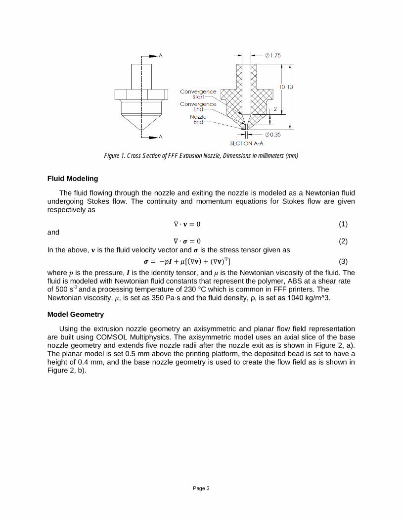
Methodology The polymer melt flow field is created using the geometry of a common FFF extrusion nozzle. The extrusion nozzle and its cross section are shown in Figure 1.

Page 3

Figure 1. Cross Section of FFF Extrusion Nozzle, Dimensions in millimeters (mm)

Fluid Modeling

The fluid flowing through the nozzle and exiting the nozzle is modeled as a Newtonian fluid undergoing Stokes flow. The continuity and momentum equations for Stokes flow are given respectively as

∇ ∙ 𝐯 = 0 (1) and

∇ ∙ 𝝈 = 0 (2) In the above, 𝐯 is the fluid velocity vector and 𝝈 is the stress tensor given as

𝝈 = −𝑝𝑰 + 𝜇[(∇𝐯) + (∇𝐯)T] (3) where 𝑝 is the pressure, 𝑰 is the identity tensor, and 𝜇 is the Newtonian viscosity of the fluid. The fluid is modeled with Newtonian fluid constants that represent the polymer, ABS at a shear rate of 500 s-1 and a processing temperature of 230 °C which is common in FFF printers. The Newtonian viscosity, 𝜇, is set as 350 Pa·s and the fluid density, ρ, is set as 1040 kg/m^3. Model Geometry

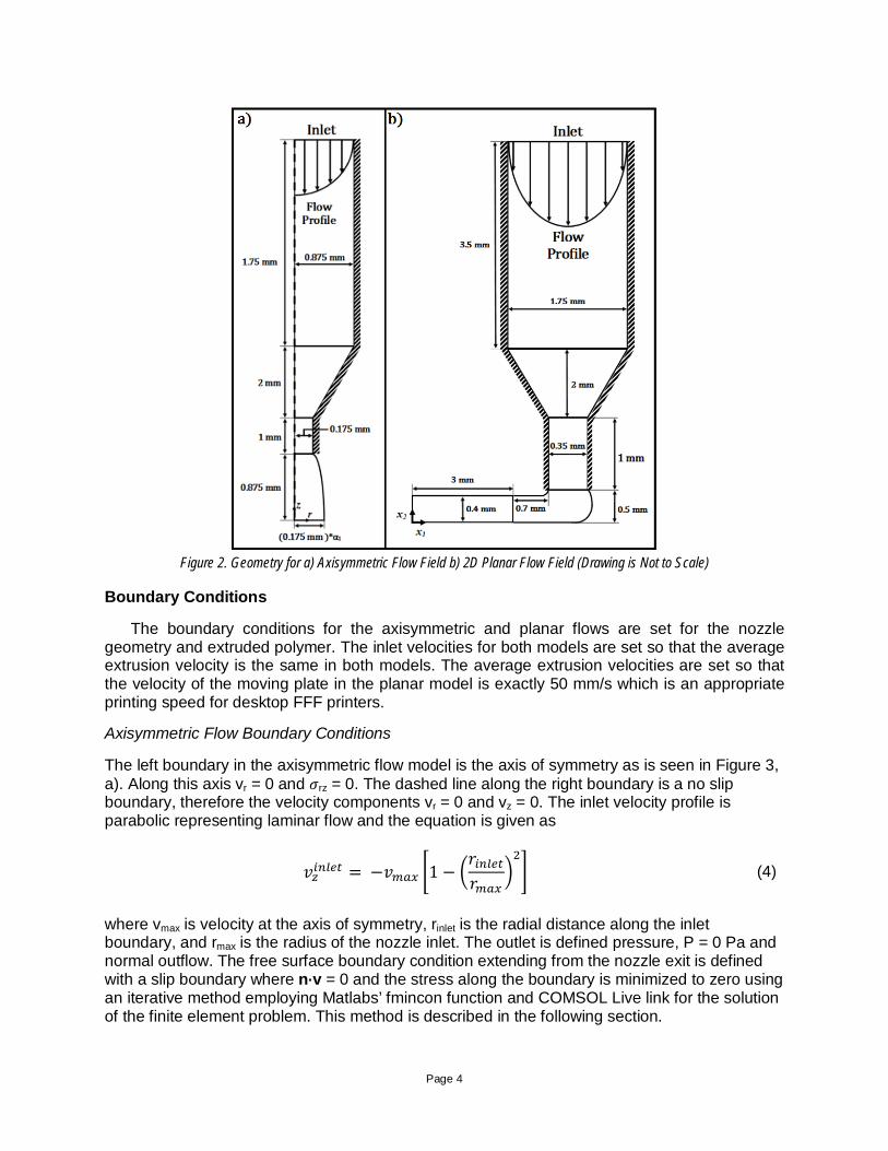
Using the extrusion nozzle geometry an axisymmetric and planar flow field representation are built using COMSOL Multiphysics. The axisymmetric model uses an axial slice of the base nozzle geometry and extends five nozzle radii after the nozzle exit as is shown in Figure 2, a). The planar model is set 0.5 mm above the printing platform, the deposited bead is set to have a height of 0.4 mm, and the base nozzle geometry is used to create the flow field as is shown in Figure 2, b).

Page 4

Figure 2. Geometry for a) Axisymmetric Flow Field b) 2D Planar Flow Field (Drawing is Not to Scale)

Boundary Conditions

The boundary conditions for the axisymmetric and planar flows are set for the nozzle geometry and extruded polymer. The inlet velocities for both models are set so that the average extrusion velocity is the same in both models. The average extrusion velocities are set so that the velocity of the moving plate in the planar model is exactly 50 mm/s which is an appropriate printing speed for desktop FFF printers.

Axisymmetric Flow Boundary Conditions

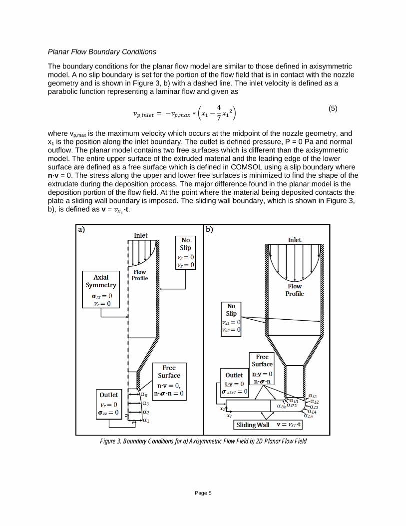
The left boundary in the axisymmetric flow model is the axis of symmetry as is seen in Figure 3, a). Along this axis vr = 0 and 𝜎rz = 0. The dashed line along the right boundary is a no slip boundary, therefore the velocity components vr = 0 and vz = 0. The inlet velocity profile is parabolic representing laminar flow and the equation is given as

𝑣𝑧𝑖𝑛𝑙𝑒𝑡 = −𝑣𝑚𝑎𝑥 �1 − �𝑟𝑖𝑛𝑙𝑒𝑡𝑟𝑚𝑎𝑥

�2� (4)

where vmax is velocity at the axis of symmetry, rinlet is the radial distance along the inlet boundary, and rmax is the radius of the nozzle inlet. The outlet is defined pressure, P = 0 Pa and normal outflow. The free surface boundary condition extending from the nozzle exit is defined with a slip boundary where n·v = 0 and the stress along the boundary is minimized to zero using an iterative method employing Matlabs’ fmincon function and COMSOL Live link for the solution of the finite element problem. This method is described in the following section.

Page 5

Planar Flow Boundary Conditions

The boundary conditions for the planar flow model are similar to those defined in axisymmetric model. A no slip boundary is set for the portion of the flow field that is in contact with the nozzle geometry and is shown in Figure 3, b) with a dashed line. The inlet velocity is defined as a parabolic function representing a laminar flow and given as

𝑣𝑝,𝑖𝑛𝑙𝑒𝑡 = −𝑣𝑝,𝑚𝑎𝑥 ∗ �𝑥1 −47𝑥12�

(5)

where vp,max is the maximum velocity which occurs at the midpoint of the nozzle geometry, and x1 is the position along the inlet boundary. The outlet is defined pressure, P = 0 Pa and normal outflow. The planar model contains two free surfaces which is different than the axisymmetric model. The entire upper surface of the extruded material and the leading edge of the lower surface are defined as a free surface which is defined in COMSOL using a slip boundary where n·v = 0. The stress along the upper and lower free surfaces is minimized to find the shape of the extrudate during the deposition process. The major difference found in the planar model is the deposition portion of the flow field. At the point where the material being deposited contacts the plate a sliding wall boundary is imposed. The sliding wall boundary, which is shown in Figure 3, b), is defined as v = 𝑣𝑥1·t.

Figure 3. Boundary Conditions for a) Axisymmetric Flow Field b) 2D Planar Flow Field

Page 6

Free Surface Stress Minimization

The stress along the free surface of the axisymmetric and planar flow models shown in Figure 3 a) and b) is done using LiveLink in COMSOL. This allows Matlab functions to be used in conjunction with COMSOL finite element solutions. Matlabs’ fmincon is used to minimize the stress along the free surfaces for the finite element model. The z locations in the axisymmetric model and likewise the x2 values in the planar model are set and the r and x1 values which are represented by the alpha values seen in Figure 3 a) and b) are moved to find the correct shape of the flow domain. The objective function that is minimized is defined as

𝑚𝑖𝑛𝛼 𝑓�𝛼� = � �𝜎𝑛�𝑆(𝛼)� + 𝜎𝑡�𝑆(𝛼)�� 𝑑𝐶 = 0

𝑆 (6)

where 𝜎𝑛 is the normal stress, 𝜎𝑡 is the tangential stress, and 𝑆(𝛼) is the surface defined by the design variables, alpha. When the minimization is completed the proper shape of the extruded material is found.

Fiber Orientation Evaluation

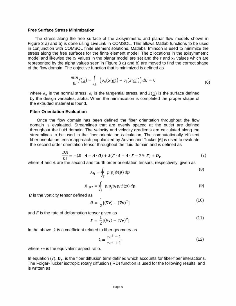
Once the flow domain has been defined the fiber orientation throughout the flow domain is evaluated. Streamlines that are evenly spaced at the outlet are defined throughout the fluid domain. The velocity and velocity gradients are calculated along the streamlines to be used in the fiber orientation calculation. The computationally efficient fiber orientation tensor approach popularized by Advani and Tucker [6] is used to evaluate the second order orientation tensor throughout the fluid domain and is defined as

𝐷𝑨𝐷𝑡

= −(𝜴 ∙ 𝑨 − 𝑨 ∙ 𝜴) + 𝜆(𝜞 ∙ 𝑨 + 𝑨 ∙ 𝜞 − 2𝔸:𝜞) + 𝑫𝒓 (7)

where 𝑨 and 𝔸 are the second and fourth order orientation tensors, respectively, given as

𝐴𝒊𝒋 = � 𝑝𝑖𝑝𝑗𝜓(𝒑)𝑆

𝑑𝒑 (8)

𝔸𝑖𝑗𝑘𝑙 = � 𝑝𝑖𝑝𝑗𝑝𝑘𝑝𝑙𝜓(𝒑)𝑆

𝑑𝒑 (9)

𝜴 is the vorticity tensor defined as

𝜴 = 12

[(∇𝐯) − (∇𝐯)T] (10)

and 𝜞 is the rate of deformation tensor given as

𝜞 = 12

[(∇𝐯) + (∇𝐯)T] (11)

In the above, 𝜆 is a coefficient related to fiber geometry as

λ = 𝑟𝑒2 − 1𝑟𝑒2 + 1

(12)

where 𝑟𝑒 is the equivalent aspect ratio. In equation (7), 𝑫𝒓, is the fiber diffusion term defined which accounts for fiber-fiber interactions. The Folgar-Tucker isotropic rotary diffusion (IRD) function is used for the following results, and is written as

Page 7

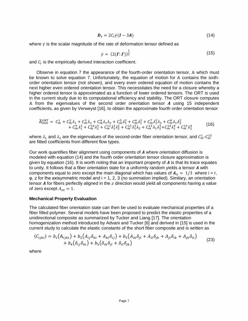
𝑫𝒓 = 2𝐶𝐼�̇�(𝑰 − 3𝑨) (14)

where �̇� is the scalar magnitude of the rate of deformation tensor defined as

�̇� = (2(𝜞:𝜞))12 (15)

and 𝐶𝐼 is the empirically derived interaction coefficient.

Observe in equation 7 the appearance of the fourth-order orientation tensor, 𝔸 which must be known to solve equation 7. Unfortunately, the equation of motion for 𝔸 contains the sixth-order orientation tensor (not shown), and every even ordered equation of motion contains the next higher even ordered orientation tensor. This necessitates the need for a closure whereby a higher ordered tensor is approximated as a function of lower ordered tensors. The ORT is used in the current study due to its computational efficiency and stability. The ORT closure computes 𝔸 from the eigenvalues of the second order orientation tensor 𝑨 using 15 independent coefficients, as given by Verweyst [16], to obtain the approximate fourth order orientation tensor

𝔸�𝑚𝑚𝑂𝑅𝑇 = 𝐶𝑚1 + 𝐶𝑚2 𝜆1 + 𝐶𝑚3 𝜆2 + 𝐶𝑚4 𝜆1𝜆2 + 𝐶𝑚5 𝜆12 + 𝐶𝑚6 𝜆12 + 𝐶𝑚7 𝜆12𝜆2 + 𝐶𝑚8 𝜆1𝜆22

+ 𝐶𝑚9 𝜆13 + 𝐶𝑚10𝜆23 + 𝐶𝑚11𝜆12𝜆22 + 𝐶𝑚12𝜆13𝜆2 + 𝐶𝑚13𝜆1𝜆23+𝐶𝑚14𝜆14 + 𝐶𝑚15𝜆24 (16)

where 𝜆1 and 𝜆2 are the eigenvalues of the second-order fiber orientation tensor, and 𝐶𝑚1 -𝐶𝑚15 are fitted coefficients from different flow types. Our work quantifies fiber alignment using components of 𝑨 where orientation diffusion is modeled with equation (14) and the fourth order orientation tensor closure approximation is given by equation (16). It is worth noting that an important property of 𝑨 is that its trace equates to unity. It follows that a fiber orientation state for a uniformly random yields a tensor 𝑨 with components equal to zero except the main diagonal which has values of 𝑨𝑖𝑖 = 1/3 where i = r, φ, z for the axisymmetric model and i = 1, 2, 3 (no summation implied). Similary, an orientation tensor 𝑨 for fibers perfectly aligned in the 𝑧 direction would yield all components having a value of zero except 𝐴𝑧𝑧 = 1. Mechanical Property Evaluation

The calculated fiber orientation state can then be used to evaluate mechanical properties of a fiber filled polymer. Several models have been proposed to predict the elastic properties of a unidirectional composite as summarized by Tucker and Liang [17]. The orientation homogenization method introduced by Advani and Tucker [6] and derived in [15] is used in the current study to calculate the elastic constants of the short fiber composite and is written as

⟨𝐶𝑖𝑗𝑘𝑙⟩ = 𝑏1�𝔸𝑖𝑗𝑘𝑙� + 𝑏2�𝐴𝑖𝑗𝛿𝑘𝑙 + 𝐴𝑘𝑙𝛿𝑖𝑗� + 𝑏3�𝐴𝑖𝑘𝛿𝑗𝑙 + 𝐴𝑖𝑙𝛿𝑗𝑘 + 𝐴𝑗𝑙𝛿𝑖𝑘 + 𝐴𝑗𝑘𝛿𝑖𝑙�+ 𝑏4�𝛿𝑖𝑗𝛿𝑘𝑙� + 𝑏5�𝛿𝑖𝑘𝛿𝑗𝑙 + 𝛿𝑖𝑙𝛿𝑗𝑘�

(23)

where

Page 8

𝑏1 = 𝐶11 + 𝐶22 − 2𝐶12 − 4𝐶66 𝑏4 = 𝐶23

𝑏2 = 𝐶12 + 𝐶22 𝑏5 =1

2(𝐶22 − 𝐶23) (24)

𝑏3 = 𝐶66 +1

2(𝐶23 + 𝐶22)

In the above, C11, C12, C22, C23, and C66 are the elasticity tensor coefficients of the associated unidirectional short fiber composite. In this study, these coefficients are calculated using the Tandon-Weng [14] approach.

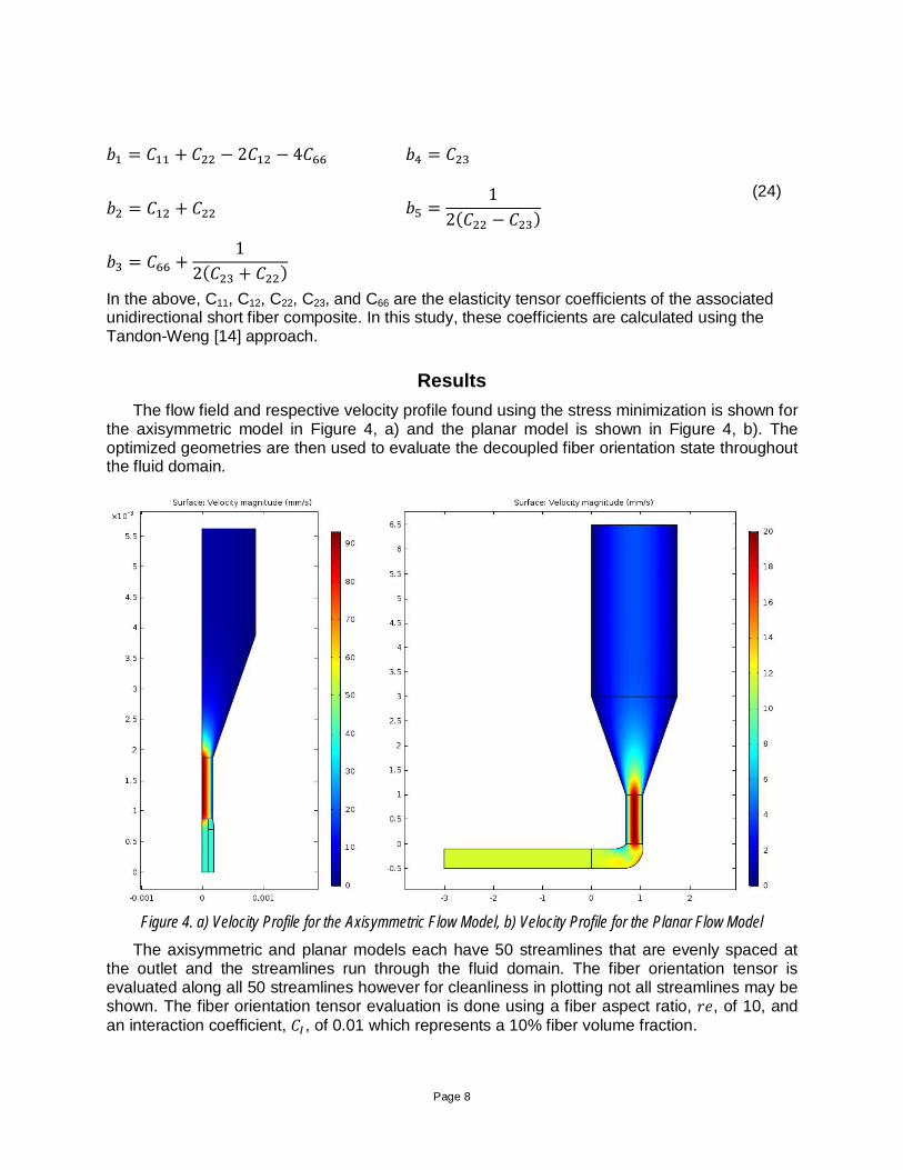
Results The flow field and respective velocity profile found using the stress minimization is shown for

the axisymmetric model in Figure 4, a) and the planar model is shown in Figure 4, b). The optimized geometries are then used to evaluate the decoupled fiber orientation state throughout the fluid domain.

Figure 4. a) Velocity Profile for the Axisymmetric Flow Model, b) Velocity Profile for the Planar Flow Model

The axisymmetric and planar models each have 50 streamlines that are evenly spaced at the outlet and the streamlines run through the fluid domain. The fiber orientation tensor is evaluated along all 50 streamlines however for cleanliness in plotting not all streamlines may be shown. The fiber orientation tensor evaluation is done using a fiber aspect ratio, 𝑟𝑒, of 10, and an interaction coefficient, 𝐶𝐼 , of 0.01 which represents a 10% fiber volume fraction.

Page 9

Axisymmetric Model

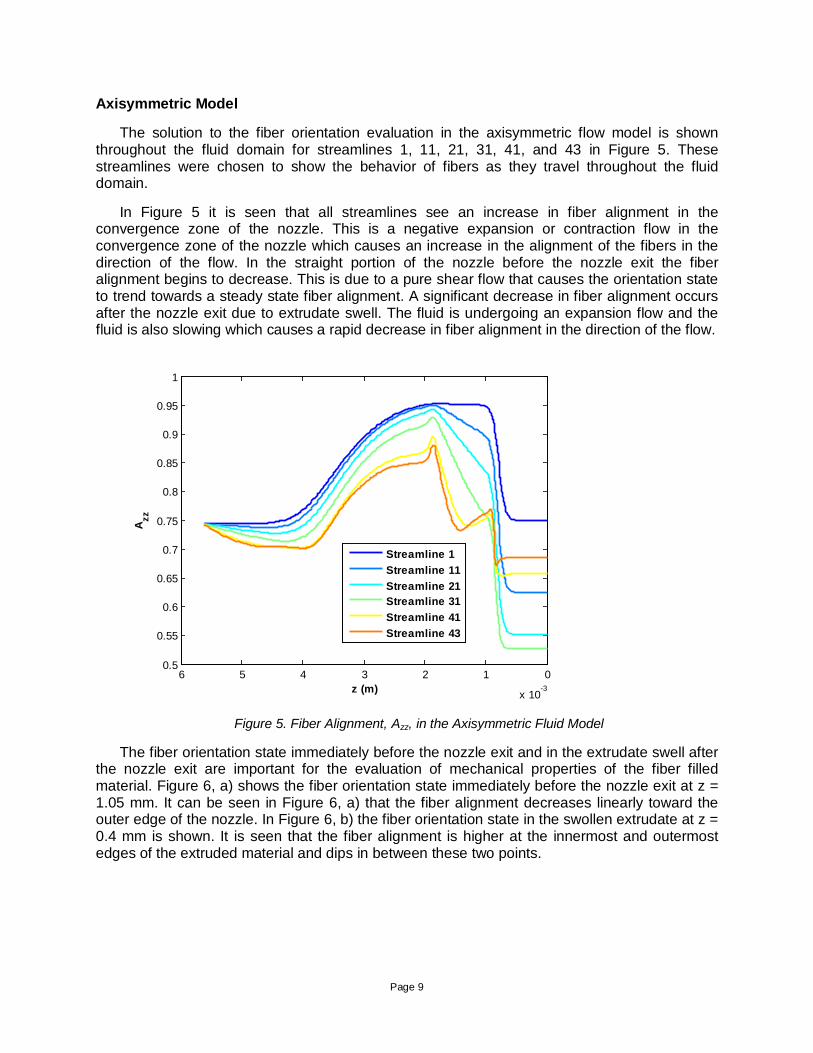
The solution to the fiber orientation evaluation in the axisymmetric flow model is shown throughout the fluid domain for streamlines 1, 11, 21, 31, 41, and 43 in Figure 5. These streamlines were chosen to show the behavior of fibers as they travel throughout the fluid domain.

In Figure 5 it is seen that all streamlines see an increase in fiber alignment in the convergence zone of the nozzle. This is a negative expansion or contraction flow in the convergence zone of the nozzle which causes an increase in the alignment of the fibers in the direction of the flow. In the straight portion of the nozzle before the nozzle exit the fiber alignment begins to decrease. This is due to a pure shear flow that causes the orientation state to trend towards a steady state fiber alignment. A significant decrease in fiber alignment occurs after the nozzle exit due to extrudate swell. The fluid is undergoing an expansion flow and the fluid is also slowing which causes a rapid decrease in fiber alignment in the direction of the flow.

Figure 5. Fiber Alignment, Azz, in the Axisymmetric Fluid Model

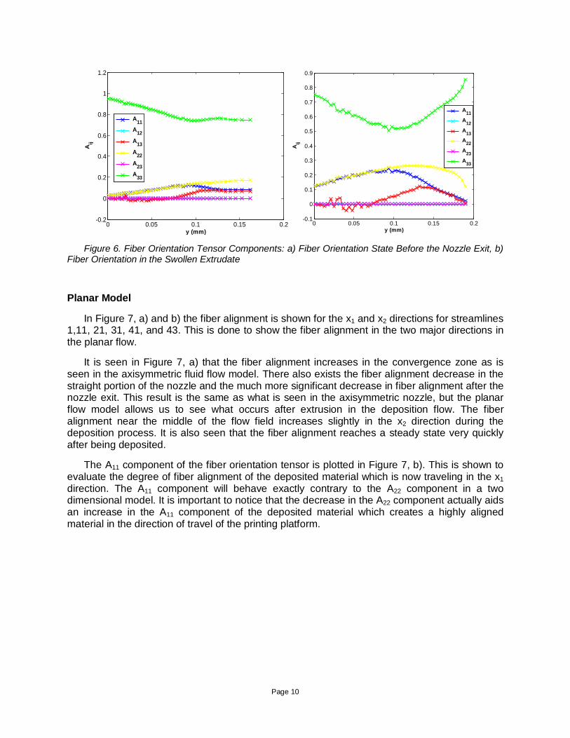
The fiber orientation state immediately before the nozzle exit and in the extrudate swell after the nozzle exit are important for the evaluation of mechanical properties of the fiber filled material. Figure 6, a) shows the fiber orientation state immediately before the nozzle exit at z = 1.05 mm. It can be seen in Figure 6, a) that the fiber alignment decreases linearly toward the outer edge of the nozzle. In Figure 6, b) the fiber orientation state in the swollen extrudate at z = 0.4 mm is shown. It is seen that the fiber alignment is higher at the innermost and outermost edges of the extruded material and dips in between these two points.

0123456

x 10-3

0.5

0.55

0.6

0.65

0.7

0.75

0.8

0.85

0.9

0.95

1

z (m)

Azz

Streamline 1Streamline 11Streamline 21Streamline 31Streamline 41Streamline 43

Page 10

Figure 6. Fiber Orientation Tensor Components: a) Fiber Orientation State Before the Nozzle Exit, b)

Fiber Orientation in the Swollen Extrudate

Planar Model

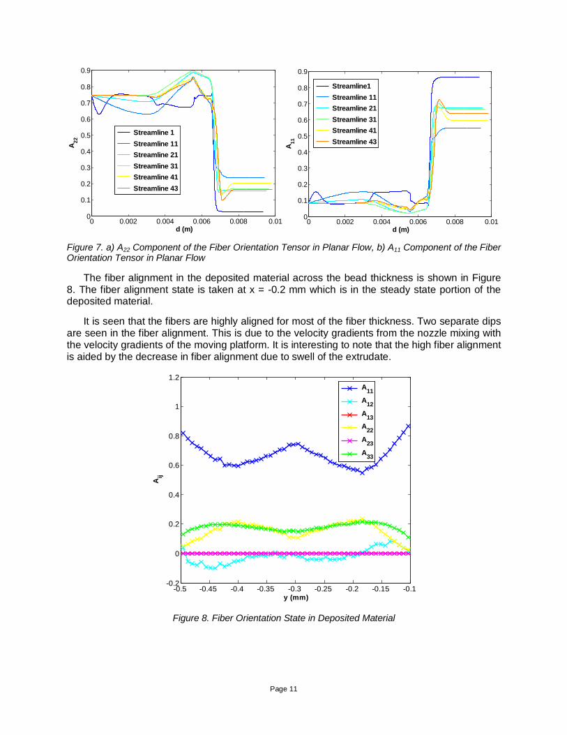
In Figure 7, a) and b) the fiber alignment is shown for the x1 and x2 directions for streamlines 1,11, 21, 31, 41, and 43. This is done to show the fiber alignment in the two major directions in the planar flow.

It is seen in Figure 7, a) that the fiber alignment increases in the convergence zone as is seen in the axisymmetric fluid flow model. There also exists the fiber alignment decrease in the straight portion of the nozzle and the much more significant decrease in fiber alignment after the nozzle exit. This result is the same as what is seen in the axisymmetric nozzle, but the planar flow model allows us to see what occurs after extrusion in the deposition flow. The fiber alignment near the middle of the flow field increases slightly in the x2 direction during the deposition process. It is also seen that the fiber alignment reaches a steady state very quickly after being deposited.

The A11 component of the fiber orientation tensor is plotted in Figure 7, b). This is shown to evaluate the degree of fiber alignment of the deposited material which is now traveling in the x1 direction. The A11 component will behave exactly contrary to the A22 component in a two dimensional model. It is important to notice that the decrease in the A22 component actually aids an increase in the A11 component of the deposited material which creates a highly aligned material in the direction of travel of the printing platform.

0 0.05 0.1 0.15 0.2-0.2

0

0.2

0.4

0.6

0.8

1

1.2

y (mm)

Aij

A11 A12 A13 A22 A23 A33

0 0.05 0.1 0.15 0.2-0.1

0

0.1

0.2

0.3

0.4

0.5

0.6

0.7

0.8

0.9

y (mm)

Aij

A11 A12 A13 A22 A23 A33

Page 11

Figure 7. a) A22 Component of the Fiber Orientation Tensor in Planar Flow, b) A11 Component of the Fiber Orientation Tensor in Planar Flow

The fiber alignment in the deposited material across the bead thickness is shown in Figure 8. The fiber alignment state is taken at x = -0.2 mm which is in the steady state portion of the deposited material.

It is seen that the fibers are highly aligned for most of the fiber thickness. Two separate dips are seen in the fiber alignment. This is due to the velocity gradients from the nozzle mixing with the velocity gradients of the moving platform. It is interesting to note that the high fiber alignment is aided by the decrease in fiber alignment due to swell of the extrudate.

Figure 8. Fiber Orientation State in Deposited Material

0 0.002 0.004 0.006 0.008 0.010

0.1

0.2

0.3

0.4

0.5

0.6

0.7

0.8

0.9

d (m)

A22

Streamline 1 Streamline 11 Streamline 21 Streamline 31 Streamline 41 Streamline 43

0 0.002 0.004 0.006 0.008 0.010

0.1

0.2

0.3

0.4

0.5

0.6

0.7

0.8

0.9

d (m)

A11

Streamline1 Streamline 11 Streamline 21 Streamline 31 Streamline 41 Streamline 43

-0.5 -0.45 -0.4 -0.35 -0.3 -0.25 -0.2 -0.15 -0.1-0.2

0

0.2

0.4

0.6

0.8

1

1.2

y (mm)

Aij

A11 A12 A13 A22 A23 A33

Page 12

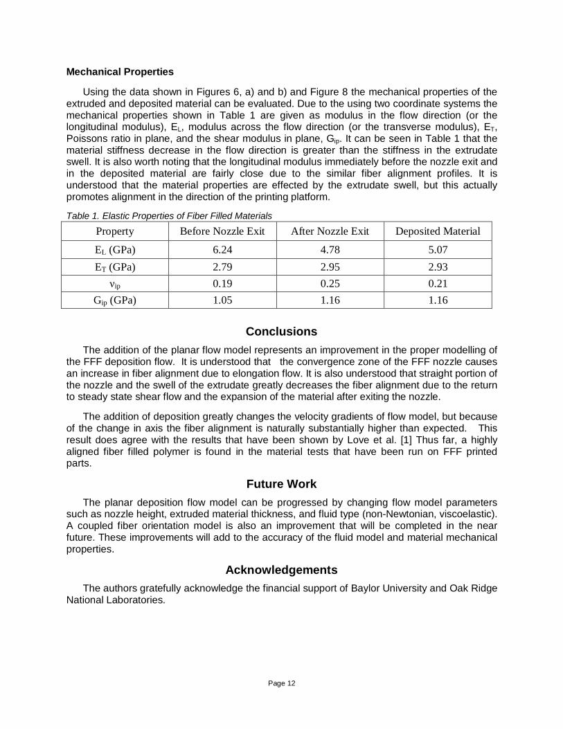
Mechanical Properties

Using the data shown in Figures 6, a) and b) and Figure 8 the mechanical properties of the extruded and deposited material can be evaluated. Due to the using two coordinate systems the mechanical properties shown in Table 1 are given as modulus in the flow direction (or the longitudinal modulus), EL, modulus across the flow direction (or the transverse modulus), ET, Poissons ratio in plane, and the shear modulus in plane, Gip. It can be seen in Table 1 that the material stiffness decrease in the flow direction is greater than the stiffness in the extrudate swell. It is also worth noting that the longitudinal modulus immediately before the nozzle exit and in the deposited material are fairly close due to the similar fiber alignment profiles. It is understood that the material properties are effected by the extrudate swell, but this actually promotes alignment in the direction of the printing platform.

Table 1. Elastic Properties of Fiber Filled Materials

Property Before Nozzle Exit After Nozzle Exit Deposited Material

EL (GPa) 6.24 4.78 5.07 ET (GPa) 2.79 2.95 2.93

νip 0.19 0.25 0.21 Gip (GPa) 1.05 1.16 1.16

Conclusions The addition of the planar flow model represents an improvement in the proper modelling of

the FFF deposition flow. It is understood that the convergence zone of the FFF nozzle causes an increase in fiber alignment due to elongation flow. It is also understood that straight portion of the nozzle and the swell of the extrudate greatly decreases the fiber alignment due to the return to steady state shear flow and the expansion of the material after exiting the nozzle.

The addition of deposition greatly changes the velocity gradients of flow model, but because of the change in axis the fiber alignment is naturally substantially higher than expected. This result does agree with the results that have been shown by Love et al. [1] Thus far, a highly aligned fiber filled polymer is found in the material tests that have been run on FFF printed parts.

Future Work The planar deposition flow model can be progressed by changing flow model parameters

such as nozzle height, extruded material thickness, and fluid type (non-Newtonian, viscoelastic). A coupled fiber orientation model is also an improvement that will be completed in the near future. These improvements will add to the accuracy of the fluid model and material mechanical properties.

Acknowledgements The authors gratefully acknowledge the financial support of Baylor University and Oak Ridge

National Laboratories.

Page 13

Bibliography 1. Love, L.J., V. Kunc, O. Rios, C.E. Duty, A.M. Elliot, B.K. Post, R.J. Smith, C.A. Blue, “The

Importance of Carbon Fiber to Polymer Additive Manufacturing”, Journal of Materials Research, Vol. 29, No. 17, pp. 1893-1898, 2014.

2. Nixon, J., B. Dryer, D. Chiu, I. Lempert, D.I. Bigio, “Three Parameter Analysis of Fiber Orientation in Fused Deposition Modeling Geometries,” pp. 985–995, 2014.

3. Heller, B.P., D.E., Smith, D.A., Jack, “Effects of Extrudate Swell and Nozzle Geometry on Fiber Orientation in Fused Filament Fabrication Nozzle Flow,” Journal of Additive Manufacturing, Accepted for Publication May 2016.

4. Jeffery, G.B., “The Motion of Ellipsoidal Particles Immersed in a Viscous Fluid,” Proceedings of The Royal Society of London A, Vol. 102 No. 715, pp. 161–179, 1923.

5. Folgar, F., C.L. Tucker III, “Orientatrion Behavior of Fibers in Concentrated Suspensions,” Journal of Reinforced Plastic Composites, Vol. 3, No. 2, pp. 98-119, 1984.

6. Advani, S.G., C.L. Tucker III, “The Use of Tensors to Describe and Predict Fiber Orientation in Short Fiber Composites,” Journal of Rheology, Vol. 31, pp. 751-784, 1987.

7. Georgiou, G.C., “The Compressible Newtonian Extrudate Swell Problem,” International Journal of Numerical Methods in Fluids, Vol. 20, pp. 255-261, 1995.

8. Reddy, K.R., R.I. Tanner, Finite Element Solution of Viscous Jet Flows with Surface Tension, Computers and Fluids, Vol. 6, No. 2, pp. 83-91, 1978.

9. Mitsoulis, E., S.G. Hatzikiriakos, “Annular Extrudate Swell of Fluoropolymer Melt,” International Journal of Polymer Processing, Vol. 27, No. 5, pp. 535-546, 2012.

10. Kanvisi, M., S. Motahari, B. Kaffashi, “Numerical Investigation and Experimental Observation of Extrudate Swell for Viscoelastic Polymer Melts,” International Journal of Polymer Processing, Vol. 29, No. 2, pp. 227-232, 2014.

11. Akbarzadeh, V., A.N., Hrymak, “Coupled CFD-DEM of Particle-Laden Flows in a Turning Flow with a Moving Wall,” Journal of Computers and Chemical Engineering, Vol. 86, pp. 184-191, 2016.

12. Cintra, J.S., C.L. Tucker III, “Orthotropic Closure Approximations for Flow-Induced Fiber Orientation,” Journal of Rheology, Vol. 39, No. 6, pp. 1095–1122, 1995.

13. Wetzel, E.D., C.L. Tucker III, “Area Tensors for Modeling Microstructure During Laminar Liquid-Liquid Mixing,” International Journal of Multiphase Flow, Vol. 25, pp. 35-61, 1999.

14. Tandon, G.P., G.J. Weng, “The Effect of Aspect Ratio of Inclusions on the Elastic Properties of Unidirectionally Aligned Composites,” Journal of Polymer Composites, Vol. 5, No. 4, pp. 327-333, 1984.

15. Jack, D.A., D.E. Smith, “The Effect of Fiber Orientation Closure Approximations on Mechanical Property Predictions,” Composites Part A, Vol. 38, No. 3, pp. 975-982, 2006.

16. VerWeyst, B.E., C.L., Tucker, “Fiber Suspensions in Complex Geometries: Flow-Orientation Coupling,” The Canadian Journal of Chemical Engineering, Vol. 80, pp. 1093–1106, 2002.

17. Tucker III, C.L., E. Liang, “Stiffness Predictions for Unidirectional Short-Fiber Composites: Review and Evaluation,” Composites Science Technology, Vol. 59, No. 5, pp. 655–671, 1999.