Computing Query Probability with IncidenceAlgebras

Technical Report UW-CSE-10-03-02University of Washington

Nilesh Dalvi, Karl Schnaitter and Dan Suciu

Revised: August 24, 2010

Abstract

We describe an algorithm that evaluates queries over probabilistic databasesusing Mobius’ inversion formula in incidence algebras. The queries we considerare unions of conjunctive queries (equivalently: existential, positive First Ordersentences), and the probabilistic databases are tuple-independent structures. Ouralgorithm runs in PTIME on a subset of queries called ”safe” queries, and is com-plete, in the sense that every unsafe query is hard for the class FP#P . The al-gorithm is very simple and easy to implement in practice, yet it is non-obvious.Mobius’ inversion formula, which is in essence inclusion-exclusion, plays a keyrole for completeness, by allowing the algorithm to compute the probability ofsome safe queries even when they have some subqueries that are unsafe. We alsoapply the same lattice-theoretic techniques to analyze an algorithm based on liftedconditioning, and prove that it is incomplete.

1 IntroductionIn this paper we show how to use incidence algebras to evaluate unions of conjunctivequeries over probabilistic databases. These queries correspond to the select-project-join-union fragment of the relational algebra, and they also correspond to existentialpositive formulas of First Order Logic. A probabilistic database, also referred to asa probabilistic structure, is a pair (A, P ) where A = (A, RA1 , . . ., RAk ) is first orderstructure over vocabularyR1, . . . , Rk, and P is a function that associates to each tuple tin A a number P (t) ∈ [0, 1]. A probabilistic structure defines a probability distributionon the set of substructures B of A by:

PA(B) =k∏i=1

(∏t∈RB

i

P (t)×∏

t∈RAi −RB

i

(1− P (t))) (1)

1

We describe a simple, yet quite non-obvious algorithm for computing the proba-bility of an existential, positive FO sentence Φ, PA(Φ)1, based on Mobius’ inversionformula in incidence algebras. The algorithm runs in polynomial time in the size ofA. The algorithm only applies to certain sentences, called safe sentences, and is soundand complete in the following way. It is sound, in that it computes correctly the proba-bility for each safe sentence, and it is complete in that, for every fixed unsafe sentenceΦ, the data complexity of computing Φ is FP#P -hard. This establishes a dichotomyfor the complexity of unions of conjunctive queries over probabilistic structures. Thealgorithm is more general than, and significantly simpler than a previous algorithm forconjunctive sentences [5].

The existence of FP#P -hard queries on probabilistic structures was observed byGradel et al. [8] in the context of query reliability. In the following years, several stud-ies [4, 6, 12, 11], sought to identify classes of tractable queries. These works providedconditions for tractability only for conjunctive queries without self-joins. The only ex-ception is [5], which considers conjunctive queries with self-joins. We extend thoseresults to a larger class of queries, and at the same time provide a very simple algo-rithm. Some other prior work is complimentary to ours, e.g., the results that considerthe effects of functional dependencies [12].

Our results have applications to probabilistic inference on positive Boolean expres-sions [7]. For every tuple t in a structure A, let Xt be a distinct Boolean variable.Every existential positive FO sentence Φ defines a positive DNF Boolean expressionover the variables Xt, sometimes called lineage expression, whose probability is thesame as PA(Φ). Our result can be used to classify the complexity of computing theprobability of Positive DNF formulas defined by a fixed sentence Φ. For example, thetwo sentences2

Φ1 = R(x), S(x, y) ∨ S(x, y), T (y) ∨R(x), T (y)Φ2 = R(x), S(x, y) ∨ S(x, y), T (y)

define two classes of positive Boolean DNF expressions (lineages):

F1 =_

a∈R,(a,b)∈S

XaYa,b ∨_

(a,b)∈S,b∈T

Ya,b, Zb ∨_

a∈R,b∈S

XaYb

F2 =_

a∈R,(a,b)∈S

XaYa,b ∨_

(a,b)∈S,b∈T

Ya,b, Zb

Our result implies that, for each such class of Boolean formulas, either all formulas inthat class can be evaluated in PTIME in the size of the formula, or the complexity forthat class is hard for FP#P ; e.g. F1 can be evaluated in PTIME using our algorithm,while F2 is hard.

The PTIME algorithm we present here relies in a critical way on an interestingconnection between existential positive FO sentences and incidence algebras [17]. Byusing the Mobius inversion formula in incidence algebras we resolve a major difficulty

1This is the marginal probability PA(Φ) =P

B:B|=Φ PA(B).2We omit quantifiers and drop the conjunct they are clear from the context, e.g. Φ2 = ∃x∃y(R(x) ∧

S(x, y) ∨ S(x, y) ∧ T (y)).

2

of the evaluation problem: a sentence that is in PTIME may have a subexpression that ishard. This is illustrated by Φ1 above, which is in PTIME, but has Φ2 as a subexpression,which is hard; to evaluate Φ1 one must avoid trying to evaluate Φ2. Our solution isto express P (Φ) using Mobius’ inversion formula: subexpressions of Φ that have aMobius value of zero do not contribute to P (Φ), and this allows us to compute P (Φ)without computing its hard subexpressions. The Mobius inversion formula correspondsto the inclusion/exclusion principle, which is ubiquitous in probabilistic inference: theconnection between the two in the context of probabilistic inference has already beenrecognized in [9]. However, to the best of our knowledge, ours is the first applicationthat exploits the full power of Mobius inversion to remove hard subexpressions from acomputation of probability.

Another distinguishing, and quite non-obvious aspect of our approach is that weapply our algorithm on the CNF, rather than the more commonly used DNF represen-tation of existential, positive FO sentences. This departure from the common repre-sentation of existential, positive FO is necessary in order to handle correctly existentialquantifiers.

We call sentences on which our algorithm works safe; those on which the algo-rithm fails we call unsafe. We prove a theorem stating that the evaluation problem ofa safe query is in PTIME, and of an unsafe query is hard for FP#P : this establishesboth the completeness of our algorithm and a dichotomy of all existential, positive FOsentences. The proof of the theorem is in two steps. First, we define a simple class ofsentences called forbidden sentences, where each atom has at most two variables, anda set of simple rewrite rules on existential, positive FO sentences; we prove that thesafe sentences can be characterized as those that cannot be rewritten into a forbiddensentence. Second, we prove that every forbidden sentence is hard for FP#P , using adirect, and rather difficult proof which we include in [3]. Together, these two resultsprove that every unsafe sentence is hard for FP#P , establishing the dichotomy. No-tice that our characterization of safe queries is reminiscent of minors in graph theory.There, a graph H is called a minor of a graph G if H can be obtained from G througha sequence of edge contractions. “Being a minor of” defines a partial order on graphs:Robertson and Seymour’s celebrated result states that any minor-closed family is char-acterized by a finite set of forbidden minors. Our characterization of safe queries isalso done in terms of forbidden minors, however the order relation is more complexand the set of forbidden minors is infinite.

In the last part of the paper, we make a strong claim: that using Mobius’ inver-sion formula is a necessary technique for completeness. Today’s approaches to gen-eral probabilistic inference for Boolean expressions rely on combining (using someadvanced heuristics) a few basic techniques: independence, disjointness, and condi-tioning. In conditioning, one chooses a Boolean variable X , then computes P (F ) =P (F | X)P (X)+P (F | ¬X)(1−P (X)). We extended these techniques to unions ofconjunctive queries, an approach that is generally known as lifted inference [13, 16, 15]and given a PTIME algorithm based on these three techniques. The algorithm performsconditioning on subformulas of Φ instead of Boolean variables. We prove that this al-gorithm is not complete, by showing a formula Φ (Fig. 2) that is computable in PTIME,but for which it is not possible to compute using lifted inference that combines condi-tioning, independence, and disjointness on subformulas. On the other hand, we note

3

that conditioning has certain practical advantages that are lost by Mobius’ inversion for-mula: by repeated conditioning on Boolean variables, one can construct a Free BinaryDecision Diagram [18], which has further applications beyond probabilistic inference.There seems to be no procedure to convert Mobius’ inversion formula into FBDDs; infact, we conjecture that the formula in Fig. 2 does not have an FBDD whose size ispolynomial in that of the input structure.

Finally, we mention that a different way to define classes of Boolean formulas hasbeen studied in the context of the constraint satisfaction problem (CSP). Creignou etal. [2, 1] showed that the counting version of the CSP problem has a dichotomy intoPTIME and FP#P -hard. These results are orthogonal to ours: they define the class offormulas by specifying the set of Boolean operators, such as and/or/not/majority/parityetc, and do not restrict the shape of the Boolean formula otherwise. As a consequence,the only class where counting is in PTIME is defined by affine operators: all classesof monotone formulas are hard. In contrast, in our classification there exist classes offormulas that are in PTIME, for example the class defined by Φ1 above.

2 Background and OverviewPrior Results A very simple PTIME algorithm for conjunctive queries without self-joins is discussed in [4, 6]. When the conjunctive query is connected, the algorithmchooses a variable that occurs in all atoms (called a root variable) and projects it out,computing recursively the probabilities of the sub-queries; if no root variable exists,then the query is FP#P -hard. When the conjunctive query is disconnected, then the al-gorithm computes the probabilities of the connected components, then multiples them.Thus, the algorithm alternates between two steps, called independent projection, andindependent join. For example, consider the conjunctive query3:

ϕ = R(x, y), S(x, z)

The algorithm computes its probability by performing the following steps:

P (ϕ) = 1−∏a∈A

(1− P (R(a, y), S(a, z)))

P (R(a, y), S(a, z)) = P (R(a, y)) · P (S(a, z))

P (R(a, y)) = 1−∏b∈A

(1− P (R(a, b)))

P (S(a, z)) = 1−∏c∈A

(1− P (S(a, c)))

The first line projects out the root variable x, where A is the active domain of theprobabilistic structure: it is based on fact that, in ϕ ≡ ∨

a∈A(R(a, y), S(a, z)), thesub-queries R(a, y), S(a, z) are independent for distinct values of the constant a. The

3All queries are Boolean and quantifiers are dropped; in complete notation, ϕ is∃x.∃y.∃z.R(x, y), S(x, z).

4

second line applies independent join; and the third and fourth lines apply independentproject again.

This simple algorithm, however, cannot be applied to a query with self-joins be-cause both the projection and the join step are incorrect. For a simple example, con-sider R(x, y), R(y, z). Here y is a root variable, but the queries R(x, a), R(a, z) andR(x, b), R(b, z) are dependent (both depend on R(a, b) and R(b, a)). Hence, it is notpossible to do an independent projection on y. In fact, this query is FP#P -hard.

Queries with self-joins were analyzed in [5] based on the notion of an inversion. Ina restricted form, an inversion consists of two atoms, over the same relational symbol,and two positions in those atoms, such that the first position contains a root variablein the first atom and a non-root variable in the second atom, and the second positioncontains a non-root / root pair of variables. In our example above, the atoms R(x, y)and R(y, z) and the positions 1 and 2 form an inversion: position 1 has variables xand y (non-root / root) and position 2 has variables y and z (root / non-root). Thepaper describes a first PTIME algorithm for queries without inversions, by expressingits probability in terms of several sums, each of which can be reduced to a polynomialsize expression. Then, the paper notices that some queries with inversion can also becomputed in polynomial time, and describes a second PTIME algorithm that uses onesum (called eraser) to cancel the effect of a another, exponentially sized sum. Thealgorithm succeeds if it can erase all exponentially sized sums (corresponding to sub-queries with inversions).

Our approach The algorithm that we describe in this paper is both more general(it applies to unions of conjunctive queries), and significantly simpler than either of thetwo algorithms in [5]. We illustrate it here on a conjunctive query with a self-join (Soccurs twice):

ϕ = R(x1), S(x1, y1), S(x2, y2), T (x2)

Our algorithm starts by applying the inclusion-exclusion formula:

P (R(x1), S(x1, y1), S(x2, y2), T (x2)) =P (R(x1), S(x1, y1)) + P (S(x2, y2), T (y2))−P (R(x1), S(x1, y1) ∨ S(x2, y2), T (x2))

This is the dual of the more popular inclusion-exclusion formula for disjunctions;we describe it formally in the framework of incidence algebras in Sec. 3. The first twoqueries are without self-joins and can be evaluated as before. To evaluate the query onthe last line, we simultaneously project out both variables x1, x2, writing the query as:

ψ =∨a∈A

(R(a), S(a, y1) ∨ S(a, y2), T (a))

The variables x1, x2 are chosen because they satisfy the following conditions: theyoccur in all atoms, and for the atoms with the same relation name (S in our case)they occur in the same position. We call such a set of variables separator variables(Sec. 4). As a consequence, sub-queriesR(a), S(a, y1)∨S(a, y2), T (a) corresponding

5

to distinct constants a are independent. We use this independence, then rewrite the sub-query into CNF and apply the inclusion/exclusion formula again:

P (ψ) = 1−Ya∈A

(1− P (R(a), S(a, y1) ∨ S(a, y2), T (a)))

R(a), S(a, y1) ∨ S(a, y2), T (a) ≡ (R(a) ∨ T (a)) ∧ S(a, y)

P ((R(a) ∨ T (a)) ∧ S(a, y))

= P (R(a) ∨ T (a)) + P (S(a, y))− P (R(a) ∨ T (a) ∨ S(a, y))

= P (R(a)) + P (T (a))− P (R(a)) · P (T (a))

−1 + (1− P (R(a)))(1− P (T (a)))Yb∈A

(1− P (S(a, b)))

In summary, the algorithm alternates between applying the inclusion/exclusion for-mula, and performing a simultaneous projection on separator variables: when no sep-arator variables exists, then the query is FP#P -hard. The two steps can be seen asgeneralizations of the independent join, and the independent projection for conjunctivequeries without self-joins.

Ranking Before running the algorithm, a rewriting of the query is necessary. Con-sider R(x, y), R(y, x): it has no separator variable because neither x nor y occurs inboth atoms on the same position. After a simple rewriting, however, the query canbe evaluated by our algorithm: partition the relation R(x, y) into three sets, accord-ing to x < y, x = y, x > y, call them R<, R=, R>, and rewrite the query asR<(x, y), R>(y, x) ∨ R=(z). Now x, z is a separator, because the three relationalsymbols are distinct. We call this rewriting ranking (Sec. 5). It needs to be done onlyonce, before running the algorithm, since all sub-queries of a ranked queries are ranked.A similar but more general rewriting called coverage was introduced in [5]: rankingcorresponds to the canonical coverage.

Incidence Algebras An immediate consequence of using the inclusion-exclusionformula is that sub-queries that happen to cancel out do not have to be evaluated. Thisturns out to be a fundamental property of the algorithm that allows it to be completesince, as we have explained, some queries are in PTIME but may have sub-queries thatare hard. This cancellation is described by the Mobius inversion formula, which groupsequal terms in the inclusion-exclusion expansion under coefficients called the Mobiusfunction. Using this notion, it is easy to state when a query is PTIME: this happensif and only if all its sub-queries that have a non-zero Mobius function are in PTIME.Thus, while the algorithm itself could be described without any reference to the Mobiusinversion formula, by simply using inclusion-exclusion, the Mobius function gives akey insight into what the algorithm does: it recurses only on sub-queries whose Mobiusfunction is non-zero. In fact, we prove the following result (Theorem 6.6): for everyfinite lattice, there exists a query whose sub-queries generate precisely that lattice, suchthat all sub-queries are in PTIME except that corresponding to the bottom of the lattice.Thus, the query is in PTIME iff the Mobius function of the lattice bottom is zero. Inother words, any formulation of the algorithm must identify, in some way, the elementswith a zero Mobius function in an arbitrary lattice: queries are as general as any lattice.For that reason we prefer to expose the Mobius function in the algorithm rather thanhide it under the inclusion/exclusion formula.

6

Lifted Inference At a deeper level, lattices and their associated Mobius functionhelp us understand the limitations of alternative query evaluation algorithms. In Sec. 7we study an evaluation algorithm based on lifted conditioning and disjointness. Weshow that conditioning is equivalent to replacing the lattice of sub-queries with a certainsub-lattice. By repeated conditioning one it is sometimes possible to simplify the latticesufficiently to remove all hard sub-queries whose Mobius function is zero. However,we given an example of a lattice with 9 elements (Fig 2) whose bottom element has theMobius function equal to zero, but where no conditioning can further restrict the lattice.Thus, the algorithm based on lifted conditioning makes no progress on this lattice, andcannot evaluate the corresponding query. By contrast, our algorithm based on Mobius’inversion formula will easily evaluate the query by skipping the bottom element (sinceits Mobius function is zero). Thus, our new algorithm based on Mobius’ inversionformula is more general than existing techniques based on lifted inference. Finally, wecomment on the implications for the completeness of the algorithm in [5].

In the rest of the paper we will refer to conjunctive queries and unions of con-junctive queries as conjunctive sentences, and existential positive FO sentences (or justpositive FO sentences) respectively.

3 Existential Positive FO and Incidence AlgebrasWe describe here the connection between positive FO and incidence algebras. We startwith basic notations.

3.1 Existential Positive FOFix a vocabulary R = {R1, R2, . . .}. A conjunctive sentence ϕ is a first-order logicalformula obtained from positive relational atoms using ∧ and ∃:

ϕ = ∃x.(r1 ∧ . . . ∧ rk) (2)

We allow the use of constants. V ar(ϕ) = x denotes the set of variables in ϕ, andAtoms(ϕ) = {r1, . . . , rk} the set of atoms. Consider the undirected graph where thenodes are Atoms(ϕ) and edges are pairs (ri, rj) s.t. ri, rj have a common variable. Acomponent of ϕ is a connected component in this graph. Each conjunctive sentence ϕcan be written as:

ϕ = γ1 ∧ . . . ∧ γpwhere each γi is a component; in particular, γi and γj do not share any common vari-ables, when i 6= j.

A disjunctive sentence is an expression of the form:

ϕ′ = γ′1 ∨ . . . ∨ γ′qwhere each γ′i is a single component.

7

An existential, positive sentence Φ is obtained from positive atoms using ∧, ∃ and∨; we will refer to it briefly as positive sentence. We write a positive sentence either inDNF or in CNF:

Φ = ϕ1 ∨ . . . ∨ ϕm (3)Φ = ϕ′1 ∧ . . . ∧ ϕ′M (4)

where ϕi are conjunctive sentences in DNF (3), and ϕ′i are disjunctive sentences inCNF (4). The DNF can be rewritten into the CNF by:

Φ =∨

i=1,m

∧j=1,pi

γij =∧f

∨i

γif(i)

where f ranges over functions with domain [m] s.t. ∀i ∈ [m], f(i) ∈ [pi]. Thisrewriting can increase the size of the sentence exponentially4. Finally, we will oftendrop ∃ and ∧ when clear from the context.

A classic result by Sagiv and Yannakakis [14] gives a necessary and sufficient con-dition for a logical implication of positive sentences written in DNF: if Φ =

∨i ϕi and

Φ′ =∨j ϕ′j , then:

Φ⇒ Φ′ iff ∀i.∃j.ϕi ⇒ ϕ′j (5)

No analogous property holds for CNF:R(x, a), S(a, z) logically impliesR(x, y), S(y, z)(where a is a constant), butR(x, a) 6⇒ R(x, y), S(y, z) and S(a, z) 6⇒ R(x, y), S(y, z).We show in Sec. 5 a rewriting technique that enforces such a property.

3.2 Incidence AlgebrasNext, we review the basic notions in incidence algebras following Stanley [17]. A finitelattice is a finite ordered set (L,≤) where every two elements u, v ∈ L have a leastupper bound u ∨ v and a greatest lower bound u ∧ v, usually called join and meet.Since it is finite, it has a minimum and a maximum element, denoted 0, 1. We denoteL = L − {1} (departing from [17], where L denotes L − {0, 1}). L is a meet-semi-lattice. The incidence algebra I(L) is the algebra5 of real (or complex) matrices t ofdimension |L|×|L|, where the only non-zero elements tuv (denoted t(u, v)) are for u ≤v; alternatively, a matrix can be seen as a linear function t : RL → RL. Two matricesare of key importance in incidence algebras: ζL ∈ I(L), defined as ζL(u, v) = 1 forallu ≤ v; and its inverse, the Mobius function µL : {(u, v) | u, v ∈ L, u ≤ v} → Z,defined by:

µL(u, u) = 1

µL(u, v) = −∑

w:u<w≤v

µL(w, v)

4Our algorithm runs in PTIME data complexity; we do not address the expression complexity in thispaper.

5An algebra is a vector space plus a multiplication operation [17].

8

We drop the subscript and write µ when L is clear from the context.The fact that µ is the inverse of ζ means the following thing. Let f : L → R be

a real function defined on the lattice. Define a new function g as g(v) =∑u≤v f(u).

Then f(v) =∑u≤v µ(u, v)g(u). This is called Mobius’ inversion formula, and is a

key piece of our algorithm. Note that it simply expresses the fact that g = ζ(f) impliesf = µ(g).

3.3 Their ConnectionA labeled lattice is a triple L = (L,≤, λ) where (L,≤) is a lattice and λ assigns toeach element in u ∈ L a positive FO sentence λ(u) s.t. λ(u) ≡ λ(v) iff u = v.

Definition 3.1 A D-lattice is a labeled lattice L where, forall u 6= 1, λ(u) is conjunc-tive, forall u, v, λ(u∧v) is logically equivalent to λ(u)∧λ(v), and λ(1) ≡ ∨u<1 λ(u).

A C-lattice is a labeled lattice L where, forall u 6= 1, λ(u) is disjunctive, forallu, v, λ(u ∧ v) is logically equivalent to λ(u) ∨ λ(v), and λ(1) =

∧u<1 λ(u).

In a D-lattice, u ≤ v iff λ(u)⇒ λ(v). This is because λ(u) = λ(u∧v) is logicallyequivalent to λ(u) ∧ λ(v). Similarly, in a C-lattice, u ≤ v iff λ(v) ⇒ λ(u). If L is aD- or C-lattice, we say L represents Φ = λ(1).

Proposition 3.2 (Inversion formula for positive FO) Fix a probabilistic structure (A, P )and a positive sentence Φ; denote PA as P . Let L be either a D-lattice or a C-latticerepresenting Φ. Then:

P (Φ) = P (λ(1)) = −∑v<1

µL(v, 1)P (λ(v)) (6)

Proof: The proof for the D-lattice is from [17]. Denote f(u) = P (λ(u)∧¬(∨v<u λ(v))).

Then:

P (λ(u)) =∑v≤u

f(v) ⇒ f(u) =∑v≤u

µ(v, u)P (λ(v))

The claim follows by setting u = 1 and noting f(1) = 0. For a C-lattice, writeλ′(u) = ¬λ(u). Then P (λ(1)) = 1−P (λ′(1)) = 1 +

∑v<1 µ(v, 1)P (λ′(v)) and the

claim follows from the fact that∑v∈L µ(v, 1) = 0. 2

The proposition generalizes the well known inclusion/exclusion formula (for D-lattices), and its less well known dual (for C-lattices):

P (a ∨ b ∨ c) = P (a) + P (b) + P (c)−P (a ∧ b)− P (a ∧ c)− P (b ∧ c) + P (a ∧ b ∧ c)

P (a ∧ b ∧ c) = P (a) + P (b) + P (c)−P (a ∨ b)− P (a ∨ c)− P (b ∨ c) + P (a ∨ b ∨ c)

We show how to construct a canonical D-lattice, LD(Φ) that represents a positivesentence Φ. Start from the DNF in Eq.(3), and for each subset s ⊆ [m] denote ϕs =

9

1

!1 !3 !2

!1,!3 !2,!3

0 = !1,!2,!3

1

!4 !5

0 = !4 ! !5

(a) (b)

1

!1 !2 !3

!1,!2 !1,!3 !2,!3

!4

0 = !1,!2,!3,!4

1

1

!1 !3 !2

!1,!3 !2,!3

0 = !1,!2,!3

1

!4 !5

0 = !4 ! !5

(a) (b)

1

!1 !2 !3

!1,!2 !1,!3 !2,!3

!4

0 = !1,!2,!3,!4

1

(a) (b)

Figure 1: The D-lattice (a) and the C-lattice (b) for Φ (Ex. 3.3).

∧i∈s ϕi. Let L be the set of these conjunctive sentences, up to logical equivalence,

and ordered by logical implication (hence, |L| ≤ 2m). Label each element u ∈ L,u 6= 1, with its corresponding ϕs (choose any, if there are multiple equivalent ones),and label 1 with

∨s6=∅ ϕs (≡ Φ). We denote the resulting D-lattice LD(Φ). Similarly,

LC(Φ) is the C-lattice that represents Φ, obtained from the CNF of Φ in Eq.(4), settingϕ′s =

∨i∈s ϕ

′i.

The first main technique of our algorithm is this. Given Φ, compute its C-lattice,then use Eq.(6) to compute P (Φ); we explain later why we use the C-lattice instead ofthe D-lattice. It remains to compute the probability of disjunctive sentences P (λ(u)):we show this in the next section. The power of this technique comes from the fact that,whenever µ(u, 1) = 0, then we do not need to compute the corresponding P (λ(u)).As we explain in Sec. 7 this is strictly more powerful than the current techniques usedin probabilistic inference, such as lifted conditioning.

Example 3.3 Consider the following positive sentence:

Φ = R(x1), S(x1, y1) ∨ S(x2, y2), T (y2) ∨R(x3), T (y3)= ϕ1 ∨ ϕ2 ∨ ϕ3

The Hasse diagram of the D-lattice LD(Φ) is shown in Fig. 1 (a). There are eight sub-sets s ⊆ [3], but only seven up to logical equivalence, because6 ϕ1, ϕ2 ≡ ϕ1, ϕ2, ϕ3.The values of the Mobius function are, from top to bottom: 1,−1,−1,−1, 1, 1, 0,hence the inversion formula is7:

P (Φ) = P (ϕ1) + P (ϕ2) + P (ϕ3)− P (ϕ1ϕ3)− P (ϕ2ϕ3)

The Hasse diagram of the C-lattice LC(Φ) is shown in Fig. 1 (b). To see this, first

6There exists a homomorphism ϕ1, ϕ2, ϕ3 → ϕ1, ϕ2 that maps R(x3) to R(x1) and T (y3) to T (y2).7One can arrive at the same expression by using inclusion-exclusion instead of Mobius’ inversion for-

mula, and noting that ϕ1, ϕ2 ≡ ϕ1, ϕ2ϕ3, hence these two terms cancel out in the inclusion-exclusionexpression.

10

express Φ in CNF:

Φ = (R(x1), S(x1, y1) ∨ S(x2, y2), T (y2) ∨R(x3)) ∧(R(x4), S(x4, y4) ∨ S(x5, y5), T (y5) ∨ T (y6))

= (R(x3) ∨ S(x2, y2), T (y2)) ∧ (R(x4), S(x4, y4) ∨ T (y6))= ϕ4 ∧ ϕ5

Note that 0 is labeled with ϕ4 ∨ ϕ5 ≡ R(x3) ∨ T (y6). The inversion formula here is:

P (Φ) = P (ϕ4) + P (ϕ5)− P (ϕ4 ∨ ϕ5)

where ϕ4 ∨ ϕ5 ≡ R(x3) ∨ T (y6).

3.4 MinimizationBy minimizing a conjunctive sentence ϕ we mean replacing it with an equivalent sen-tence ϕ0 that has the smallest number of atoms. A disjunctive sentence Φ =

∨γi is

minimized if every conjunctive sentence is minimized and there is no homomorphismϕi ⇒ ϕj for i 6= j. If such a homomorphism exists, then we call ϕj redundant: clearlywe can remove it from the expression Φ without affecting its semantics.

For the purpose of D-lattices, it doesn’t matter if we minimize the sentence or not: ifthe sentence is not minimized, then one can show that all lattice elements correspondingto redundant terms have the Mobius function equal to zero. More precisely, any twoD-lattices that represent the same sentence have the same set of elements with a non-zero Mobius function: we state this fact precisely in the remainder of this section. Asimilar fact does not hold in general for C-lattices, but it holds over ranked structures(Sec. 5.2).

An element u in a lattice covers v if u > v and there is no w s.t. u > w > v. Anatom8 is an element that covers 0; a co-atom is an element covered by 1. An elementu is called co-atomic if it is a meet of coatoms. Let L0 denote the set of co-atomicelements: L0 is a meet semilattice, and L0 = L0 ∪ {1} is a lattice. The proof isAppendix I.

Proposition 3.4 (1) If u ∈ L and µL(u, 1) 6= 0 then u is co-atomic. (2) Forall u ∈ L0,µL(u, 1) = µL0

(u, 1).

Let L and L′ be D-lattices representing the sentences Φ and Φ′. If Φ ≡ Φ′, then Land L′ have the same co-atoms, up to logical equivalence. Indeed, we can write Φ asthe disjunction of co-atom labels in L, and one co-atom cannot imply another. Thus,by applying Eq.(5) in both directions, we get a one-to-one correspondence between theco-atoms of L and L′, indicating logical equivalence. It follows from Prop. 3.4 that,when D-lattices represent equivalent formulas, the set of labels λ(u) where µ(u, 1) 6= 0are equivalent. Thus, an algorithm that inspects only these labels is independent of theparticular representation of a sentence.

8Not to be confused with a relational atom ri in (2).

11

A similar property fails on C-lattices, because Eq.(5) does not extend to CNF. Forexample, Φ = R(x, a), S(a, z) and Φ′ = R(x, a), S(a, z), R(x′, y′), S(y′, z′) are log-ically equivalent, but have different co-atoms. The co-atoms of Φ are R(x, a) andS(a, z) (the C-lattice is V -shaped, as in Fig. 1 (b)), and the co-atoms of Φ′ areR(x, a),(R(x′, y′), S(y′, z′)), and S(a, z) (the C-lattice is W -shaped, as in Fig. 1 (a)).

4 Independence and SeparatorsNext, we show how to compute the probability of a disjunctive sentence

∨i γi; this

is the second technique used in our algorithm, and consists of eliminating, simultane-ously, one existential variable from each γi, by exploiting independence.

Let ϕ be a conjunctive sentence. A valuation h is a substitution of its variableswith constants; h(ϕ), is a set of ground tuples. We call two conjunctive sentencesϕ1, ϕ2 tuple-independent if for all valuations h1, h2, we have h1(ϕ1) ∩ h2(ϕ2) = ∅.Two positive sentences Φ,Φ′ are tuple-independent if, after expressing them in DNF,Φ =

∨i ϕi, Φ′ =

∨j ϕ′j , all pairs ϕi, ϕ′j are independent.

Let Φ1, . . . ,Φm be positive sentences s.t. any two are tuple-independent. Then:

P (∨i

Φi) = 1−∏i

(1− P (Φi))

This is because the m lineage expressions for Φi depend on disjoint sets of Booleanvariables, and therefore they are independent probabilistic events. In other words,tuple-independence is a sufficient condition for independence in the probabilistic sense.Although it is only a sufficient condition, we will abbreviate tuple-independence withindependence in this section.

Let ϕ be a positive sentence, V = {x1, . . . , xm} ⊆ V ar(ϕ), and a a constant.Denote ϕ[a/V ] = ϕ[a/x1, . . . , a/xm] (all variables in V are substituted with a).

Definition 4.1 Let ϕ =∨i=1,m γi be a disjunctive sentence. A separator is a set of

variables V = {x1, . . . , xm}, xi ∈ V ar(γi), such that for all a 6= b, ϕ[a/V ], ϕ[b/V ]are independent.

Proposition 4.2 Let ϕ be a disjunctive sentence with a separator V , and (A, P ) aprobabilistic structure with active domain D. Then:

P (ϕ) = 1−∏a∈D

(1− P (ϕ[a/V ])) (7)

The claim follows from the fact that ϕ ≡ ∨a∈D ϕ[a/V ] on all structures whoseactive domain is included in D.

In summary, to compute the probability of a disjunctive sentence, we find a sepa-rator, then apply Eq.(7): each expression ϕ[a/V ] is a positive sentence, simpler thanthe original one (it has strictly fewer variables in each atom) and we apply again theinversion formula. This technique, by itself, is not complete: we need to “rank” therelations in order to make it complete, as we show in the next section. Before that, weillustrate with an example.

12

Example 4.3 Consider ϕ = R(x1), S(x1, y1) ∨ S(x2, y2), T (x2). Here {x1, x2} isa separator. To see this, note that for any constants a 6= b, the sentences ϕ[a] =R(a), S(a, y1) ∨ S(a, y2), T (a) and ϕ[b] = R(b), S(b, y1) ∨ S(b, y2), T (b) are inde-pendent, because the former only looks at tuples that start with a, while the latter onlylooks at tuples that start with b.

Consider ϕ = R(x1), S(x1, y1)∨S(x2, y2), T (y2). This sentence has no separator.For example, {x1, x2} is not a separator because both sentences ϕ[a] and ϕ[b] have theatom T (y2) in common: if two homomorphisms h1, h2 map y2 to some constant c, thenT (c) ∈ h1(ϕ[a]) ∩ h2(ϕ[b]), hence they are dependent. The set {x1, y2} is also nota separator, because ϕ[a] contains the atom S(a, y1), ϕ[b] contains the atom S(x2, b),and these two can be mapped to the common ground tuple S(a, b).

We end with a necessary condition for V to be a separator.

Definition 4.4 If γ is a component, a variable of γ is called a root variable if it occursin all atoms of γ.

Note that components do not necessarily have root variables, e.g.,R(x), S(x, y), T (y).We have:

Proposition 4.5 If V is a separator of∨i γi, then each separator variable xi ∈ V ar(γi)

is a root variable for γi.

The claim follows from the fact that, if r is any atom in ϕi that does not contain xi:then r is unchanged in γi[a] and in γi[b], hence they are not independent.

5 RankingIn this section, we define a simple restriction on all formulas and structures that sim-plifies our later analysis: we require that, in each relation, the attributes may be strictlyordered A1 < A2 < . . . We show how to alter any positive sentence and probabilis-tic structure to satisfy this constraint, without changing the sentence probability. Thisis a necessary preprocessing step for our algorithm to work, and a very convenienttechnique in the proofs.

5.1 Ranked StructuresThroughout this section, we use < to denote a total order on the active domain of aprobabilistic structure (such an order always exists). In our examples, we assume that< is the natural ordering on integers, but the order may be chosen arbitrarily in general.

Definition 5.1 A relation instanceR is ranked if every tupleR(a1, . . . , ak) is such thata1 < · · · < ak. A probabilistic structure is ranked if all its relations are ranked.

To motivate ranked structures, we observe that the techniques given in previoussections do not directly lead to a complete algorithm. We illustrate by reviewing theexample in Sec. 2: γ = R(x, y), R(y, x). This component is connected, so we cannot

13

use Mobius inversion to simplify it, and we also cannot apply Eq.(7) because there is noseparator: indeed, {x} is not a separator because R(a, y), R(y, a) and R(b, y), R(y, b)are not independent (they share the tuple R(a, b)), and by symmetry neither is {y}.However, consider a structure with a unary relation R12 and binary relations R1<2,R2<1 defined as:

R12 = πX1(σX1=X2(R)) R2<1 = πX2X1(σX2<X1(R))R1<2 = σX1<X2(R)

Here, we use Xi to refer to the i-th attribute of R. This is a ranked structure: inboth relations R1<2 and R2<1 the first attribute is less than the second. Moreover: γ ≡R12(z)∨R1<2(x, y), R2<1(x, y) and now {z, x} is a separator, becauseR1<2(a, y), R2<1(a, y)and R1<2(b, y), R2<1(b, y) are independent. Thus, Eq.(7) applies to the formula overthe ranked structure, and we can compute the probability of γ in polynomial time.

Definition 5.2 A positive sentence is in reduced form if each atom R(x1, . . . , xk) issuch that (a) each xi is a variable (i.e. not a constant), and (b) the variables x1, . . . , xkare distinct.

We now prove that the evaluation of any sentence can be reduced to an equivalentsentence over a ranked structure, and we further guarantee that the resulting sentenceis in reduced form.

Proposition 5.3 Let Φ0 be positive sentence. Then, there exists a sentence Φ in re-duced form such that for any structure A0, one can construct in polynomial time aranked structure A such that PA0(Φ0) = PA(Φ).

Proof: Let R(X1, . . . , Xk) be a relation symbol and let ρ be a maximal, consistentconjunction of order predicates involving attributes of R and the constants occurringin Φ0. Thus, for any pair of attributes names or constants y, z, ρ implies exactly one ofy < z, y = z, y > z. Before describing Φ, we show to construct the ranked structureA from an unranked one A0. We say Xj is unbound if ρ 6⇒ Xj = c for any constantc. The ranked structure will have one symbol Rρ for every symbol R in the unrankedstructure and every maximal consistent predicate ρ. The instance A is computed asRρ = πX(σρ(R)) where X contains one Xj in each class of unbound attributes thatare equivalent under ρ, listed in increasing order according to ρ. Clearly A can becomputed in PTIME from A0.

We show now how to rewrite any positive sentence Φ0 into an equivalent, reducedsentence Φ over ranked structures s.t. PA0(Φ0) = PA(Φ). We start with a conjunctivesentence ϕ = r1, . . . , rn and let Ri denote the relation symbol of ri. Consider amaximally consistent predicate ρi on the attributes of Ri, for each i = 1, n, and letρ ≡ ρ1, . . . , ρn be the conjunction. We say that ρ is consistent if there is a valuationh such that h(ϕ) |= ρ. Given a consistent ρ, divide the variables into equivalenceclasses of variables that ρ requires to be equal, and choose one representative variablefrom each class. Let rρi

i be the result of changing Ri(x1, . . . , xk) to Rρi

i (y1, . . . , ym),where y1, . . . , ym are chosen as follows. Consider the unbound attribute classes in Ri,in increasing order according to ρi. Choose yp to be the representative of a variable

14

that occurs in the position of an attribute in the p-th class of unbound attributes. Thisworks because the position of any unbound attribute X must have a variable: if thereis a constant a, then h(ri) |= X = a for all valuations h. But ρi ⇒ X 6= a so thiscontradicts the assumption that ρ is consistent. Using a similar argument, we can showthat each yi is distinct, so rρi

i is in reduced form. Furthermore, ϕ ≡ ∧ρ rρ11 , . . . , rρnn

where the disjunction ranges over all maximal ρi such that ρ is consistent. For a positivesentence Φ0, we apply the above procedure to each conjunctive sentence in the DNFof Φ0 to yield a sentence in reduced form on the ranked relations Rρ. 2

Example 5.4 Let ϕ = R(x, a), R(a, x). If we define the ranked relations R1 =πX2(σX1=a(R)), R2 = πX1(σX2=a(R)), and R12 = π∅(σX1=X2=a(R)), we haveϕ ≡ R1(x), R2(x) ∨R12().

Next, consider ϕ = R(x), S(x, x, y), S(u, v, v). Define

S123 = πX1(σX1=X2=X3(S))S23<1 = πX2X1(σX2=X3<X1((S))

and so on. We can rewrite ϕ as:

ϕ ≡ R(x), S123(x)

∨ R(x), S12<3(x, y), S1<23(u, v) ∨R(x), S12<3(x, y), S23<1(v, u)

∨ R(x), S3<12(y, x), S1<23(u, v) ∨R(x), S3<12(y, x), S23<1(v, u)

and note that these relations are ranked.

Thus, when computing PA(Φ), we may conveniently assume w.l.o.g. that A isranked and Φ is in reduced form. When we replace separator variables with a constantas in Eq.(7), we can easily restore the formula to reduced form. Given a disjunctivesentence ϕ in reduced form and a separator V , we remove a from ϕ[a/V ] as follows.For each relation R, suppose the separator variables occur at position Xi of R. Thenwe remove all rows from R where Xi 6= a, reduce the arity of R by removing columni, and remove xi = a from all atoms R(x1, . . . , xk) in ϕ[a/V ].

We end this section with two applications of ranking. The first shows a homomor-phism theorem for CNF sentences.

Proposition 5.5 Assume all structures to be ranked, and all sentences to be in reducedform.

• If ϕ,ϕ′ are conjunctive sentences, and ϕ is satisfiable over ranked structures9

then ϕ⇒ ϕ′ iff there exists a homomorphism h : ϕ′ → ϕ.

• Formula (5) holds for positive sentences in DNF.

• The dual of (5) holds for positive sentences in CNF:∧i ϕi ⇒

∧j ϕ′j iff ∀j.∃i.ϕi ⇒ ϕ′j

9Meaning: it is satisfied by at least one (ranked) structure.

15

Proof: • Let V = V ar(ϕ) and construct a graph on V such that (u, v) is an edgewhenever some atom of ϕ imposes the constraint u < v based on ranking. Thisgraph is acyclic because there exists a valuation h from ϕ to a ranked structure,which means h(u) < h(v) for all edges (u, v). Let x1, . . . , x|V | be a topologicalordering of V , i.e., such that i < j for all edges (xi, xj). Replace each xi withi in ϕ, and let A be the ranked structure consisting of all atoms in ϕ after thismapping. Clearly A |= ϕ, hence A |= ϕ′: the latter gives a valuation ϕ′ → A,which, composed with the mapping i 7→ xi, gives a homomorphism ϕ′ → ϕ.

• Standard argument, omitted.

• Assume for contradiction that there exists p, s.t. ∀i, it is not the case that ϕi ⇒ϕ′p. Let Ai be a structure s.t. Ai |= ϕi but Ai 6|= ϕp. The active domain of Ai isunconstrained by ϕi because the sentence is in reduced form, and hence containsno constants. Hence we may assume w.l.o.g. that for i1 6= i2, the structures Ai1

and Ai2 have disjoint active domains. Define A =⋃iAi. Then A |= ∨

ϕi,implying that A |= ∨

ϕ′j . In particular, A |= ϕ′p, hence there exists a valuationϕ′p → A. Since the active domains of each Ai are disjoint, its image must becontained in a single Ai, contradicting the fact that ϕi 6⇒ ϕ′p.

2

The first two items are known to fail for conjunctive sentences with order predi-cates: for example R(x, y), R(y, x) logically implies R(x, y), x ≤ y, but there is nohomomorphism from the latter to the former. They hold for ranked structures becausethere is a strict total order on the attributes of each relation. The last item implies thefollowing. If L and L′ are two C-lattices representing equivalent sentences, then theyhave the same co-atoms. In conjunction with Prop. 3.4, this implies that an algorithmthat ignores lattice elements where µ(u, 1) = 0 does not depend on the representationof the positive sentence. This completes our discussion at the end of Sec. 3.

The second result shows how to handle atoms without variables.

Proposition 5.6 Let γ0, γ1 be components in reduced form s.t. V ar(γ0) = ∅, V ar(γ1) 6=∅. Then γ0, γ1 are independent.

Proof: Note that γ0 contains a single atom R(); if it had two atoms then it is not acomponent. Since γ1 is connected, each atom must have at least one variable, hence itcannot have the same relation symbol R(). 2

Letϕ =∨γi be a disjunctive sentence, ϕ0 =

∨i:V ar(γi)=∅ γi andϕ1 =

∨i:V ar(γi) 6=∅ γi.

It follows that:

P (ϕ) = 1− (1− P (ϕ0))(1− P (ϕ1)) (8)

5.2 Finding a SeparatorAssuming structures to be ranked, we give here a necessary and sufficient condition fora disjunctive sentence in reduced form to have a separator, which we use both in thealgorithm and to prove hardness for FP#P . We need some definitions first.

16

Let ϕ = γ1 ∨ . . .∨ γm be a disjunctive sentence, in reduced form. Throughout thissection we assume that ϕ is minimized and that V ar(γi) ∩ V ar(γj) = ∅ for all i 6= j(if not, then rename the variables). Two atoms r ∈ Atoms(γi) and r′ ∈ Atoms(γj)are called unifiable if they have the same relational symbol. We may also say r, r′

unify. It is easy to see that γi and γj contain two unifiable atoms iff they are not tuple-independent. Two variables x, x′ are unifiable if there exist two unifiable atoms r, r′

such that x occurs in r at the same position that x′ occurs in r′. This relationship isreflexive and symmetric. We also say that x, x′ are recursively unifiable if either x, x′

are unifiable, or there exists a variable x′′ such that x, x′′ and x′, x′′ are recursivelyunifiable.

A variable x is maximal if it is only recursively unifiable with root variables. Henceall maximal variables are root variables. The following are canonical examples of sen-tences where each component has a root variable, but there are no maximal variables:

h0 = R(x0), S1(x0, y0), T (y0)h1 = R(x0), S1(x0, y0) ∨ S1(x1, y1), T (y1)h2 = R(x0), S1(x0, y0) ∨ S1(x1, y1), S2(x1, y1) ∨ S2(x2, y2), T (y2). . .hk = R(x0), S1(x0, y0) ∨ S1(x1, y1), S2(x1, y1) ∨

. . . ∨ Sk−1(xk−1, yk−1), Sk(xk−1, yk−1) ∨ (Sk(xk, yk), T (yk)

In each hk, k ≥ 1, the root variables are xi−1, yi for i = 1, k − 1, and there are nomaximal variables.

Maximality propagates during unification: if x is maximal and x, x′ unify, then x′

must be maximal because otherwise xwould recursively unify with a non-root variable.Let Wi be the set of maximal variables occurring in γi. If an atom in γi unifies

with an atom in γj , then |Wi| = |Wj | because the two atoms contain all maximalvariables in each component, and maximality propagates through unification. Sincethe structures are ranked, for every i there exists a total order on the maximal variablesin Wi: xi1 < xi2 < . . . The rank of a variable x ∈ Wi is the position where it occursin this order. The following result gives us a means to find a separator if it exists:

Proposition 5.7 A disjunctive sentence has a separator iff every component has a max-imal variable. In that case, the set comprising maximal variables with rank 1 forms aseparator.

Proof: Consider the disjunctive sentence ϕ =∨mi=1 γi and set of variables V =

{x1, . . . , xm} s.t. xi ∈ V ar(γi), i = 1,m. It is straightforward to show that V isa separator iff any pair of unifiable atoms have a member of V in the same position.Hence, if V is a separator, then each xi ∈ V can only (recursively) unify with anotherxj ∈ V . Since xj is a root variable (Prop. 4.5), each xi ∈ V ar(γi) is maximal, asdesired.

Now suppose every component has a maximal variable. Choose V such that xi isthe maximal variable in γi with rank 1. If two atoms r, r′ unify, then they have maximalvariables occurring in the same positions. In particular, the first maximal variable hasrank 1, and thus is in V . We conclude that V is a separator. 2

17

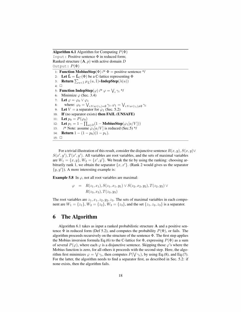
Algorithm 6.1 Algorithm for Computing P (Φ)Input: Positive sentence Φ in reduced form;Ranked structure (A, p) with active domain DOutput: P (Φ)

1: Function MobiusStep(Φ) /* Φ = positive sentence */2: Let L = LC(Φ) be a C-lattice representing Φ3: Return

∑u<1 µL(u, 1)∗IndepStep(λ(u))

4: 2

5: Function IndepStep(ϕ) /* ϕ =∨i γi */

6: Minimize ϕ (Sec. 3.4)7: Let ϕ = ϕ0 ∨ ϕ1

8: where: ϕ0 =∨i:V ar(γi)=∅ γi, ϕ1 =

∨i:V ar(γi)6=∅ γi

9: Let V = a separator for ϕ1 (Sec. 5.2)10: If (no separator exists) then FAIL (UNSAFE)11: Let p0 = P (ϕ0)12: Let p1 = 1−∏a∈D(1−MobiusStep(ϕ1[a/V ]))13: /* Note: assume ϕ1[a/V ] is reduced (Sec.5) */14: Return 1− (1− p0)(1− p1).15: 2

For a trivial illustration of this result, consider the disjunctive sentenceR(x, y), S(x, y)∨S(x′, y′), T (x′, y′). All variables are root variables, and the sets of maximal variablesare W1 = {x, y}, W2 = {x′, y′}. We break the tie by using the ranking: choosing ar-bitrarily rank 1, we obtain the separator {x, x′}. (Rank 2 would gives us the separator{y, y′}). A more interesting example is:

Example 5.8 In ϕ, not all root variables are maximal:

ϕ = R(z1, x1), S(z1, x1, y1) ∨ S(z2, x2, y2), T (z2, y2) ∨R(z3, x3), T (z3, y3)

The root variables are z1, x1, z2, y2, z3. The sets of maximal variables in each compo-nent are W1 = {z1}, W2 = {z2}, W3 = {z3}, and the set {z1, z2, z3} is a separator.

6 The AlgorithmAlgorithm 6.1 takes as input a ranked probabilistic structure A and a positive sen-

tence Φ in reduced form (Def 5.2), and computes the probability P (Φ), or fails. Thealgorithm proceeds recursively on the structure of the sentence Φ. The first step appliesthe Mobius inversion formula Eq.(6) to the C-lattice for Φ, expressing P (Φ) as a sumof several P (ϕ), where each ϕ is a disjunctive sentence. Skipping those ϕ’s where theMobius function is zero, for all others it proceeds with the second step. Here, the algo-rithm first minimizes ϕ =

∨γi, then computes P (

∨γi), by using Eq.(8), and Eq.(7).

For the latter, the algorithm needs to find a separator first, as described in Sec. 5.2: ifnone exists, then the algorithm fails.

18

The expression P (ϕ0) represents the base case of the algorithm: this is when therecursion stops, when all variables have been substituted with constants from the struc-ture A. Notice that ϕ0 is of the form

∨ri, where each ri is a ground atom. Its prob-

ability is 1 −∏i(1 − P (ri)), where P is the probability function of the probabilisticstructure (A, P ). We illustrate the algorithm with two examples.

Example 6.1 Let Φ = R(x1), S(x1, y1) ∨ S(x2, y2), T (y2) ∨ R(x3), T (y3). Thisexample is interesting because, as we will show, the subexpression R(x1), S(x1, y1)∨S(x2, y2), T (y2) is hard (it has no separator), but the entire sentence is in PTIME.The algorithm computes the C-lattice, shown in Fig. 1 (b), then expresses P (Φ) =P (ϕ4) + P (ϕ5) − P (ϕ6) where ϕ6 = R(x) ∨ T (y) (see Example 3.3 for notations).Next, the algorithm applies the independence step to each of ϕ4, ϕ5, ϕ6; we illustratehere for ϕ4 = R(x3) ∨ S(x2, y2), T (y2) only; the other expressions are similar. Here,{x3, y2} is a set of separator variables, hence:

P (ϕ4) = 1−∏a∈A

(1− P (R(a) ∨ S(x2, a), T (a)))

Next, we apply the algorithm recursively on R(a) ∨ S(x2, a), T (a). In CNF it be-comes10 (R(a)∨S(x2, a))(R(a)∨T (a)), and the algorithm returnsP (R(a)∨S(x2, a))+P (R(a)∨T (a))−P (R(a)∨S(x2, a)∨T (a)). Consider the last of the three expressions(the other two are similar): its probability is

1− (1− P (R(a) ∨ T (a)))∏b∈A

(1− P (S(b, a)))

Now we have finally reached the base case, where we compute the probabilities ofsentences without variables: P (R(a) ∨ T (a)) = 1 − (1 − P (R(a)))(1 − P (T (a))),and similarly for the others.

Example 6.2 Consider the sentence ϕ in Example 5.8. Since this is already CNF (itis a disjunctive sentence), the algorithm proceeds directly to the second step. Theseparator is V = {z1, z2, z3} (see Ex. 5.8), and therefore:

P (ϕ) = 1−∏a∈A

(1− P (ϕ[a/V ])

where ϕ[a/V ] is:

R(a, x1), S(a, x1, y1) ∨ S(a, x2, y2), T (a, y2) ∨R(a, x3), T (a, y3)

After reducing the sentence (i.e. removing the constant a), it becomes identical toExample 6.1.

In the rest of this section we show that the algorithm is complete, meaning that, ifit fails on a positive sentence Φ, then Φ is FP#P -hard.

10Strictly speaking, we would have had to rewrite the sentence into a reduce form first, by rewritingS(x2, a) into S2<a(x2), etc.

19

6.1 Safe SentencesThe sentences on which the algorithm terminates (and thus are in PTIME) admit char-acterization as a minor-closed family, for a partial order that we define below.

Let ϕ be a disjunctive sentence. A level is a non-empty set of variables11 W suchthat every atom in ϕ contains at most one variable in W and for any unifiable variablesx, x′, if x ∈ W then x′ ∈ W . In particular, a separator is a level W that has onevariable in common with each atom; in general, a level does not need to be a separator.For a variable x ∈W , let nx be the number of atoms that contain x; let n = maxx nx.Let A = {a1, . . . , ak} be a set of constants not occurring in ϕ s.t. k ≤ n. Denoteϕ[A/W ] the sentence obtained as follows: substitute each variable x ∈ W with someconstant ai ∈ A and take the union of all such substitutions:

ϕ[A/W ] =∨

θ:W→A

ϕ[θ]

Note that ϕ[A/W ] is not necessarily a disjunctive sentence, since some componentsγi may become disconnected in ϕ[A/W ]. Moreover, since our vocabulary is ranked,we assume that in ϕ[A/W ] have a new symbol Sa for every symbol S that contains anattribute on the level W , and every constant a ∈ A: thus, Sa(x1, x2, . . . , y1, y2, . . .)denotes S(x1, x2, . . . , a, y1, y2, . . .).

Definition 6.3 Define the following rewrite rule Φ→ Φ0 on positive sentences. Below,ϕ,ϕ0, ϕ1, denote disjunctive sentences:

ϕ → ϕ[A/W ] W is a level, A is a set of constantsϕ0 ∨ ϕ1 → ϕ1 if V ar(ϕ0) = ∅

Φ → ϕ ∃u ∈ LC(Φ).µ(u, 1) 6= 0, ϕ = λ(u)

The second and third rules are called simple rules. The first rule is also simple if W isa separator and |A| = 1.

The first rewrite rule allows us to substitute variables with constants; the secondto get rid of disjuncts without any variables; the last rule allows us to replace a CNFsentence Φ with one element of its C-lattice, provided its Mobius value is non-zero.The transitive closure ∗→ defines a partial order on positive sentences.

Definition 6.4 A positive sentence Φ is called unsafe if there exists a sequence of sim-ple rewritings Φ ∗→ ϕ s.t. ϕ is a disjunctive sentence without separators. Otherwise itis called safe.

Thus, the set of safe sentences can be defined as the downwards closed family (un-der the partial order defined by simple rewritings) that does not contain any disjunctivesentence without separators. The main result in this paper is:

Theorem 6.5 (Soundness and Completeness) Fix a positive sentence Φ.

11No connection to the maximal sets Wi in Sec. 5.2.

20

Soundness If Φ is safe then, for any probabilistic structure, Algorithm 6.1 terminatessuccessfully (i.e. doesn’t fail), computes correctly P (Φ), and runs in timeO(nk),where n is the size of the active domain of the structure, and k the largest arityof any symbol in the vocabulary.

Completeness If Φ is unsafe then it is hard for FP#P .

Soundness follows immediately, by induction: if the algorithms starts with Φ, thenfor any sentence Φ0 processed recursively, it is the case that Φ ∗→ Φ0, where all rewritesare simple. Thus, if the algorithm ever gets stuck, Φ is unsafe; conversely, if Φ is safe,then the algorithm will succeed in evaluating it on any probabilistic structure. Thecomplexity follows from the fact that each recursive step of the algorithm removes onevariable from every atom, and traverses the domain D once, at a cost O(n). Complete-ness is harder to prove, and we discuss it in Sec. 6.3.

For a simple illustration, consider the sentence:

ϕ = R(z1, x1), S(z1, x1, y1) ∨ S(z2, x2, y2), T (z2, y2)

To show that it is hard, we substitute the separator variables z1, z2 with a constanta, and obtain

ϕ → R(a, x1), S(a, x1, y1) ∨ S(a, x2, y2), T (a, y2)

Since the latter is a disjunctive sentence without a separator, it follows that ϕ is hard.

6.2 DiscussionAn Optimization The first step of the algorithm can be optimized, as follows. Ifthe DNF sentence Φ =

∧γi is such that the relational symbols appearing in γi are

distinct for different i, then the first step of the algorithm can be optimized to computeP (Φ) =

∏i P (γi) instead of using Mobius’ inversion formula. To see an example,

consider the sentence Φ = R(x), S(y), which can be computed as

P (Φ) = (1−∏a

(1− P (R(a))))(1−∏a

(1− P (S(a))))

Without this optimization, the algorithm would apply Mobius’ inversion formulafirst:

P (Φ) = P (R(x)) + P (S(y))− P (R(x) ∨ S(y))

= 1−Ya

(1− P (R(a))) + 1−Ya

(1− S(a))

− 1 +Ya

(1− P (R(a))− P (S(a)) + P (R(a)) · P (S(a)))

The two expressions are equal, but the former is easier to compute.A Justification We justify here two major choices we made in the algorithm: using

the C-lattice instead of the D-lattice, and relying on the inversion formula with theMobius function instead of some simpler method to eliminate unsafe subexpressions.

21

To see the need for the C-lattice, let’s examine a possible dual algorithm, whichapplies the Mobius step to the D-lattice. Such an algorithm fails on Ex. 5.8, becausehere the D-lattice is 2[3], and the Mobius function is +1 or −1 for every element of thelattice. The lattice contains R(z1, x1), S(z1, x1, y1), S(z2, x2, y2), T (z2, y2), which isunsafe12. Thus, the dual algorithm fails.

To see the need of the Mobius inversion, we prove that an existential, positive FOsentence can be “as hard as any lattice”.

Theorem 6.6 (Representation theorem) Let (L,≤) be any lattice. There exists a pos-itive sentence Φ such that: LD(Φ) = (L,≤, λ), λ(0) is unsafe, and for all u 6= 0, λ(u)is safe. The dual statement holds for the C-lattice.

Proof: Call an element r ∈ L join irreducible if whenever v1 ∨ v2 = r, then eitherv1 = r or v2 = r. (Every atom is join irreducible, but the converse is not true ingeneral.) Let R = {r0, r1, . . . , rk} be all join irreducible elements in L. For everyu ∈ L denote Ru = {r | r ∈ R, r ≤ u}, and note that Ru∧v = Ru ∪ Rv . Define thefollowing components13:

γ0 = R(x1), S1(x1, y1)γi = Si(xi+1, yi+1), Si+1(xi+1, yi+1) i = 1, k − 1γk = Sk(xk, yk), T (yk)

Consider the sentences Φ and Ψ below:

Φ =∨u<1

∧ri∈Ru

γi Ψ =∧u<1

∨ri∈Ru

γi

Then both LD(Φ) and LC(Ψ) satisfy the theorem. 2

The theorem says that the lattice associated to a sentence can be as complex asany lattice. There is no substitute for checking if the Mobius function of a sub-queryis zero: for any complex lattice L one can construct a sentence Φ that generates thatlattice and where the only unsafe sentence is at 0: then Φ is safe iff µL(0, 1) = 0.

6.3 Outline of the Completeness ProofIn this section we give an outline of the completeness proof and defer details to theAppendix. We have seen that Φ is unsafe iff there exists a rewriting Φ ∗→ ϕ whereϕ has no separators. Call a rewriting maximal if every instance of the third rule inDef. 6.3, Φ→ λ(u), is such that for all lattice elements v > u, λ(v) is safe: that is u isa maximal unsafe element in the CNF lattice. Clearly, if Φ is unsafe then there exists amaximal rewriting Φ ∗→ ϕ where ϕ has no separators. We prove the following:

12It rewrites to R(a, x1), S(a, x1, y1), S(a, x2, y2), T (a, y2) −→ R(a, x1), S(a, x1, y1) ∨S(a, x2, y2), T (a, y2).

13That is,Wγi = hk.

22

Lemma 6.7 If Φ ∗→ ϕ is a maximal rewriting, then there exists a PTIME algorithm forevaluating PA(ϕ) on probabilistic structure A, with a single access to an oracle forcomputing PB(Φ) on probabilistic structures B.

Thus, to prove that every unsafe sentence is hard, it suffices to prove that everysentence without separators is hard. To prove the latter, we will continue to apply thesame rewrite rules to further simplify the sentence, until we reach an unsafe sentencewhere each atom has at most two variables: we call it a forbidden sentence. Then, weprove that all forbidden sentences are hard.

However, there is a problem with this plan. We may get stuck during rewriting be-fore reaching a sentence with two variables per atom. This happens when a disjunctivesentence has no level, which prevents us from applying any rewrite rule. We illustratehere a simple sentence without a level:

ϕ = R(x, y), S(y, z) ∨R(x′, y′), S(x′, y′)

Each consecutive pair of variables in the sequence x, x′, y, y′, z is unifiable. This in-dicates that no level exists, because it would have to include all variables, while bydefinition a level may have at most one variable from each atom; hence, this sentencedoes not have any level. While this sentence already has only two variables per atom,it illustrates where we may get stuck in trying to apply a rewriting.

To circumvent this, we transform the sentence (with two variables or more) asfollows. Let V = V ar(ϕ). A leveling is a function l : V → [L], where L > 0, s.t.for all i ∈ [L], l−1(i) is a level. Conceptually, l partitions the variables into levels,and assigns an integer to each level. This, in turn, associates exactly one level to eachrelation attribute, since unifiable variables must be in the same level. We also call ϕ anL-leveled sentence, or simply leveled sentence. Clearly, a leveled sentence has a level:in fact it has L disjoint levels. We show that each sentence is equivalent to a leveledsentence, on some restricted structures.

Call a structure A L-leveled if there exists a function l : A → [L] s.t. if twoconstants a 6= b appear in the same tuple then l(a) 6= l(b), and if they appear in thesame column of a relation then l(a) = l(b). For example, consider a single binary re-lation R(A,B). An instance of R represents a graph. There are no 1-leveled instances,because for every tuple (a, b) we must have l(a) 6= l(b). A 2-leveled instance is abipartite graph. There are no 3-leveled structures, except if one level is empty. For asecond example, consider two relations R(A,B), S(A,B). (Recall that our structuresare ranked, hence for every tuple R(a, b) or S(a, b) we have a < b). An exampleof a 3-leveled structure is a 3-partite graph where the R-edges go from partition 1 topartition 2 and the S-edges go from partition 2 to partition 3.

Proposition 6.8 Let ϕ be a disjunctive sentence that has no separators. Then thereexists L > 0 and an L-leveled sentence ϕL s.t. that ϕL has no separator and theevaluation problem of ϕL over L-leveled structures can be reduced in PTIME to theevaluation problem of ϕ.

23

The proof is in Appendix II. We illustrate the main idea on the example above. Wechoose L = 4 and the leveled sentence ϕ becomes:

ϕL = R23(x2, y3), S34(y3, u4) ∨R12(x1, y2), S23(y2, z3) ∨R23(x′2, y

′3), S23(x′2, y

′3)

Here ϕL is leveled, and still does not have a separator. It is also easy to see that if aprobabilistic structure A is 4-leveled, then ϕ and ϕL are equivalent over that structure.Thus, it suffices to prove hardness of ϕL on 4-leveled structures: this implies hardnessof ϕ.

To summarize, our hardness proof is as follows. Start with a disjunctive sentencewithout separators, and apply the leveling construct once. Then continue to apply therewritings 6.3: it is easy to see that, whenever ϕ→ ϕ′ and ϕ is leveled, then ϕ′ is alsoleveled; in other words we only need to level once.

Definition 6.9 A forbidden sentence is a disjunctive sentence ϕ that has no separator,and is 2-leveled; in particular, every atom has at most two variables.

All sentences hk in Sec. 5.2 are forbidden sentences. Another example of a forbid-den sentence is:

Q = S1(x, y1), S2(x, y2) ∨ S1(x1, y), S2(x2, y)

On the other hand, R(x, y), S(y, z), T (x, z) is not a forbidden sentence because it has3 levels.

We prove the following in Appendix II.

Theorem 6.10 Suppose ϕ is leveled, and has no separator. Then there exists a rewrit-ing ϕ ∗→ ϕ′ s.t. ϕ′ is a forbidden sentence.

The level L may decrease after rewriting. In this theorem we must be allowed touse non-simple rewritings ϕ → ϕ[A/W ], where W is not a separator (of course) andA has more than one constant. We show in Appendix II examples were the theoremfails if one restricts A to have size 1.

Finally, the completeness of the algorithm follows from the following theorem,which is technically the hardest result of this work. The proof is in Appendix III.

Theorem 6.11 If ϕ is a forbidden sentence then it is hard for FP#P over 2-leveledstructures.

7 Lifted InferenceConditioning and disjointness are two important techniques in probabilistic inference.The first expresses the probability of some Boolean expression Φ as P (Φ) = P (Φ |X)∗P (X) + P (Φ | ¬X)∗(1 − P (X)) where X is a Boolean variable. Disjointnessallows us to write P (Φ∨Ψ) = P (Φ)+P (Ψ) when Φ and Ψ are exclusive probabilisticevents. Recently, a complementary set of techniques called lifted inference has been

24

shown to be very effective in probabilistic inference [13, 16, 15], by doing inferenceat the logic formula level instead of at the Boolean expression level. In the case ofconditioning, lifted conditioning uses a sentence rather than a variable to condition.

We give an algorithm that uses lifted conditioning and disjointness in place of theMobius step of Algorithm 6.1. When the algorithm succeeds, it runs in PTIME inthe size of the probabilistic structure. However, we also show that the algorithm isincomplete; in fact, we claim that no algorithm based on these two techniques only canbe complete.

Given Φ =∨ϕi, our goal is to computeP (Φ) in a sequence of conditioning/disjointness

steps, without Mobius’ inversion formula. The second step of Algorithm 6.1 (existen-tial quantification based on independence) remains the same and is not repeated here.For reasons discussed earlier, that step requires that we have a CNF representation ofthe sentence, Ψ =

∧ϕi, but both conditioning and disjointness operate on disjunc-

tions, so we apply De Morgan’s laws P (∧ϕi) = 1 − P (

∨¬ϕi). Thus, with someabuse of terminology we assume that our input is a D-lattice, although its elements arelabeled with negations of disjunctive sentences.

We illustrate first with an example.

Example 7.1 Consider the sentence in Example 6.1:

Φ = R(x1), S(x1, y1) ∨ S(x2, y2), T (y2) ∨R(x3), T (y3)= ϕ1 ∨ ϕ2 ∨ ϕ3

We illustrate here directly on the DNF lattice, without using the negation. (This worksin our simple example, but in general one must start from the CNF, then negate.) TheHasse diagram of the DNF lattice is shown in Fig. 1. First, let’s revisit Mobius’ inver-sion formula:

P (Φ) = P (ϕ1) + P (ϕ2) + P (ϕ3)− P (ϕ1ϕ3)− P (ϕ2ϕ3)

The only unsafe sentence in the lattice is the bottom element of the lattice, where ϕ1

and ϕ2 occur together, but that disappears from the sum because µ(0, 1) = 0. We showhow to compute Φ by conditioning on ϕ3. We denote ϕ = ¬ϕ for a formula ϕ:

P (Φ) = P (ϕ3) + P ((ϕ1 ∨ ϕ2) ∧ ϕ3)= P (ϕ3) + P ((ϕ1, ϕ3) ∨ (ϕ2, ϕ3))= P (ϕ3) + P (ϕ1, ϕ3) + P (ϕ2, ϕ3)= P (ϕ3) + (P (ϕ1)− P (ϕ1, ϕ3)) + (P (ϕ2)− P (ϕ2, ϕ3))

The first line is conditioning (ϕ3 is either true, or false), and the third line is basedon mutual exclusion: ϕ1 and ϕ2 become mutually exclusive when ϕ3 is false. Weexpand one more step, because our algorithm operates only on positive sentences: thisis the fourth line. This last expansion may be replaced with a different usage, e.g. theconstruction of a BDD, not addressed in this paper. All sentences in the last line aresafe, and the algorithm can proceed recursively.

25

For lifted conditioning to work, it is of key importance that we choose the correctsubformula to condition. Consider what would happen if we conditioned on ϕ1 instead:

P (Φ) = P (ϕ1) + P ((ϕ2 ∨ ϕ3) ∧ ϕ1)= P (ϕ1) + P (ϕ2 ∧ ϕ1) + P (ϕ3 ∧ ϕ1)

Now we are stuck, because the expression ϕ2 ∧ ϕ1 is hard.

Algorithm 7.1 computes the probability of a DNF formula using conditionals anddisjointness. The algorithm operates on a DNF lattice (the negation of a CNF sen-tence). The algorithm starts by minimizing the expression

∨i ϕi, which corresponds to

removing all elements that are not co-atomic from the DNF lattice L (Prop 3.4). Recallthat Φ =

∨u<1 λ(u).

Next, the algorithm chooses a particular sub-lattice E, called the cond-lattice,and conditions on the disjunction of all sentences in the lattice. We define E be-low: first we show how to use it. Denote u1, . . . , uk the minimal elements of {z |¬(∃x ∈ E.z ≤ x)}. For any subset S ⊆ L, denote ΦS =

∨u∈S,u<1 λ(u); in particu-

lar, ΦL = Φ.The conditioning and the disjointness rules give us:

P (ΦL) = P (ΦE) + P (ΦL−E ∧ (¬ΦE))

= P (ΦE) +∑i=1,k

(Φ[ui,1] ∧ (¬ΦE))

We have used here the fact that, for i 6= j, the sentences Φ[ui,1] and Φ[uj ,1] are disjointgiven ¬ΦE . Finally, we do this:

P (Φ[ui,1] ∧ (¬ΦE)) = P (Φ[ui,1])− P (Φ[ui,1]∧E)

where [ui, 1] ∧ E = {u ∧ v | u ≥ ui, v ∈ E − {1}}This completes the high level description of the algorithm. We show now how to

choose the cond-lattice, then show that the algorithm is incomplete.

7.1 Computing the Cond-LatticeFix a lattice (L,≤). The set of zero elements, Z, and the set of z-atoms ZA are definedas follows14:

Z = {z | µL(z, 1) = 0}ZA = {a | a covers some element z ∈ Z}

The algorithm reduces the problem of computing P (ΦL) for the entire lattice L tocomputing P (ΦK) for three kinds of sub-lattices K: E, [ui, 1] ∧ E, and [ui, 1]. The

14“Covers” is defined in Sec. 3.

26

goal is to choose E to avoid computing unsafe sentences. We assume the worse: thatevery zero element z ∈ Z is unsafe (if a non-zero element is unsafe then the sentence ishard). So our goal is: choose E s.t. for any sub-lattice K above, if z is a zero elementand z ∈ K, then µK(z, 1) = 0. That is, we can’t necessarily remove the zeros in oneconditioning step, but if we ensure that they continue to be zeroes, they will eventuallybe eliminated.

The join closure of S ⊆ L is cl(S) = {∨u∈s u | s ⊆ S}. Note that 0 ∈ cl(S). Thejoin closure is a join-semilattice and is made into a lattice by adding 1.

Definition 7.2 Let L be a lattice. The cond-lattice E ⊆ L is E = {1} ∪ cl(Z ∪ ZA).

Next, we show that, if some element z ∈ Z remains in one of the smaller lattices,then its Mobius function is the same as at was in L: since we assumed µL(z, 1) = 0,this implies that z continues to be a Zero in the smaller lattice.

We start with the lattices [ui, 1]: here the claim holds vacuously, because Z ∩[ui, 1] = ∅.

Next, consider the lattice E. We prove in Appendix I:

Proposition 7.3 For all z ∈ Z, µL(z, 1) = µE(z, 1).

Finally, consider the lattices [ui, 1] ∧ E. We prove in Appendix I:

Proposition 7.4 For all z ∈ Z, and all u ∈ L, µE(z, 1) = µ[u,1]∧E(z, 1).

Combined with Prop. 7.3, we obtain µL(z, 1) = µ[u,1]∧E(z, 1).

Example 7.5 Consider Example 7.1. The cond-lattice for Fig. 1 (a) is

E = cl({0, (ϕ1, ϕ3), (ϕ3, ϕ2)})= {0, (ϕ1, ϕ3), (ϕ3, ϕ2), ϕ3, 1}

Notice that this set is not co-atomic: in other words, when viewed as a sentence, itminimizes to ϕ3, and thus we have gotten rid of 0.

To get a better intuition on how conditioning works from a lattice-theoretic per-spective, consider the case when Z = {0}. In this case ZA is the set of atoms, andE is simply the set of all atomic elements; usually this is a strict subset of L, andconditioning partitions the lattice into E, [ui, 1] ∧ E, and [u1, 1]. When processing Erecursively, the algorithm retains only co-atomic elements. Thus, conditioning worksby repeatedly removing elements that are not atomic, then elements that are not co-atomic, until 0 is removed, in which case we have removed the unsafe sentence and wecan proceed arbitrarily.

27

1

!1 !3 !2

!1,!3 !2,!3

0 = !1,!2,!3

1

!4 !5

0 = !4 ! !5

1

!1 !2 !3

!1,!2 !1,!3 !2,!3

!4

0 = !1,!2,!3,!4

1

γ1 = R(x1), S1(x1, y1)γ2 = S1(x2, y2), S2(x2, y2)γ3 = S2(x3, y3), S3(x3, y3)γ4 = S3(x4, y4), T (y4)

ϕ1 = γ3, γ4

ϕ2 = γ2, γ4

ϕ3 = γ1, γ4

ϕ4 = γ1, γ2, γ3

Φ = ϕ1 ∨ ϕ2 ∨ ϕ3 ∨ ϕ4

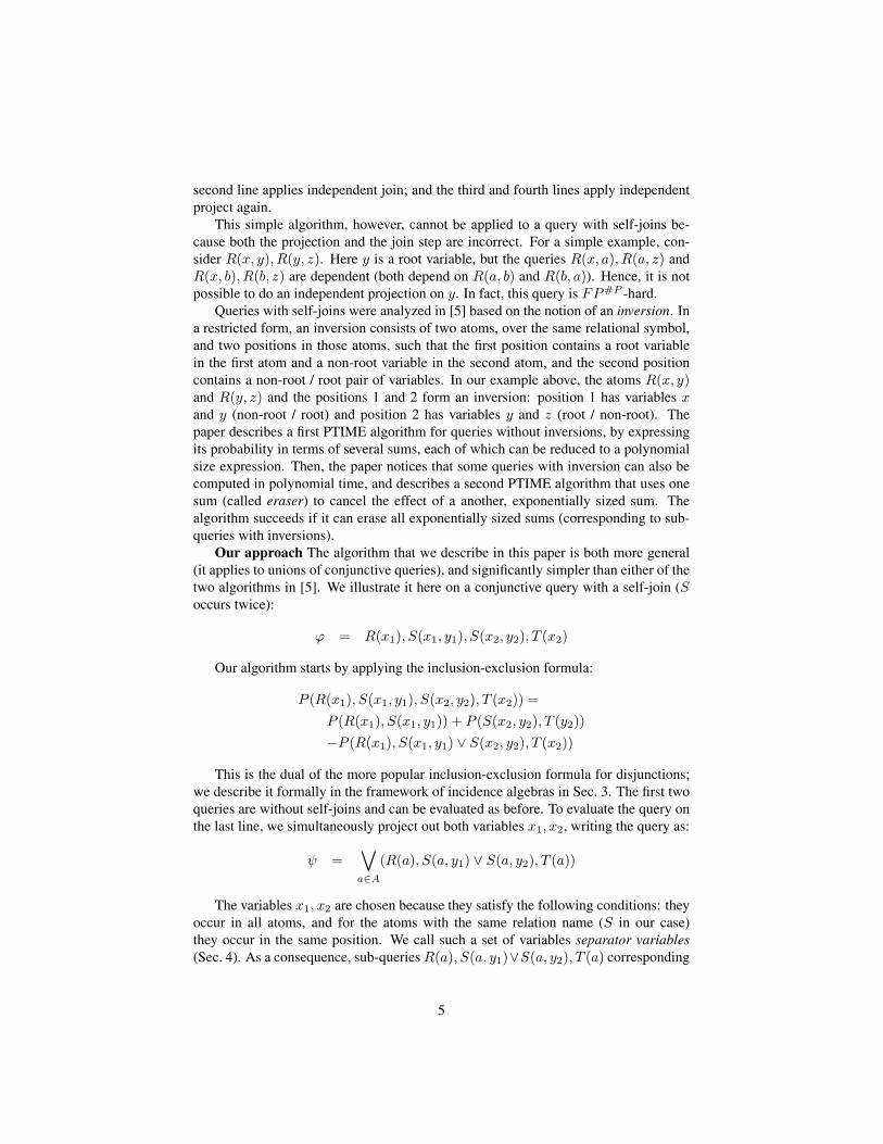
Figure 2: A lattice that is atomic, coatomic, and µ(0, 1) = 0. Its sentence Φ is givenby Th. 6.6 (compare to h3 in Sec. 5.2).

7.2 IncompletenessAssume 0 is an unsafe sentence, and all other sentences in the lattice are safe. Liftedconditioning proceeds by repeatedly replacing the lattice L with a smaller lattice E,obtained as follows: first retain only the atomic elements (= cl(Z ∪ ZA)), then retainonly the co-atomic elements (this is minimization of the resulting formula). Condition-ing on any formula other than E is a bad idea, because then we get stuck having toevaluate the unsafe formula at 0. Thus, lifted conditioning repeatedly trims the latticeto the atomic-, then to the co-atomic-elements, until, hopefully, 0 is removed. Proposi-tion 3.4 implies that, if 0 is eventually removed this way, then µ(0, 1) = 0. But doesthe converse hold ?

Fig.2 shows a lattice where this process fails. Here µ(0, 1) = 0; by Th. 6.6 thereexists a sentence Φ that generates this lattice, where 0 is unsafe and all other elementsare safe (Φ is shown in the Figure). Yet the lattice is both atomic and co-atomic. Hencecond-lattice is the entire lattice E = L. We cannot condition on any formula andstill have µ(0, 1) = 0 in the new lattice. In other words, no matter what formula wecondition on, we will eventually get stuck having to evaluate the sentence at 0. On theother hand, Mobius’ inversion formula easily computes the probability of this sentence,by exploiting directly the fact that µ(0, 1) = 0.

8 ConclusionsWe have proposed a simple, yet non-obvious algorithm for computing the probabil-ity of an existential, positive sentence over a probabilistic structure. For every safesentence, the algorithm runs in PTIME in the size of the input structure; every unsafesentence is hard. Our algorithm relies in a critical way on Mobius’ inversion formula,which allows it to avoid attempting to compute the probability of sub-sentences that arehard. We have also discussed the limitations of an alternative approach to computingprobabilities, based on conditioning and independence.

28

Algorithm 7.1 Compute PΦ) using lifted conditionalInput: Φ =

∨i=1,m ϕi, L = LDNF (Φ)

Output P (Φ)1: Function Cond(L)2: If L has a single co-atom Then proceed with IndepStep3: Remove from L all elements that are not co-atomic (Prop 3.4)4: Let Z = {u | u ∈ L, µL(u, 1) = 0}5: Let ZA = {u | u ∈ L, u covers some z ∈ Z}6: If Z = ∅ Then E := [u, 1] for arbitrary u7: Else E := cl(Z ∪ ZA)8: If E = L then FAIL (unable to proceed)9: Let u1, . . . , uk be the minimal elements of L− E

10: Return Cond(E) +∑i=1,k Cond(ui)−Cond([ui, 1] ∧ E)

Acknowledgments We thank Christoph Koch and Paul Beame for pointing us (in-dependently) to incidence algebras, and the anonymous reviewers for their comments.This work was partially supported by NSF IIS-0713576.

References[1] N. Creignou and M. Hermann. Complexity of generalized satisfiability counting

problems. Inf. Comput, 125(1):1–12, 1996.

[2] Nadia Creignou. A dichotomy theorem for maximum generalized satisfiabilityproblems. J. Comput. Syst. Sci., 51(3):511–522, 1995.

[3] N. Dalvi, K. Schnaitter, and D. Suciu. Computing query probability with inci-dence algebras. Tehnical Report UW-CSE-10-03-02, University of Washington,March 2010.

[4] N. Dalvi and D. Suciu. Efficient query evaluation on probabilistic databases. InVLDB, Toronto, Canada, 2004.

[5] N. Dalvi and D. Suciu. The dichotomy of conjunctive queries on probabilisticstructures. In PODS, pages 293–302, 2007.

[6] N. Dalvi and D. Suciu. Management of probabilistic data: Foundations and chal-lenges. In PODS, pages 1–12, Beijing, China, 2007. (invited talk).

[7] Adnan Darwiche. A differential approach to inference in bayesian networks.Journal of the ACM, 50(3):280–305, 2003.

[8] E. Gradel, Y. Gurevich, and C. Hirsch. The complexity of query reliability. InPODS, pages 227–234, 1998.

[9] Kevin H. Knuth. Lattice duality: The origin of probability and entropy. Neuro-computing, 67:245–274, 2005.

29

[10] C. Krattenthaler. Advanced determinant calculus. Seminaire Lotharingien Com-bin, 42 (The Andrews Festschrift):1–66, 1999. Article B42q.

[11] Dan Olteanu and Jiewen Huang. Secondary-storage confidence computation forconjunctive queries with inequalities. In SIGMOD, pages 389–402, 2009.

[12] Dan Olteanu, Jiewen Huang, and Christoph Koch. Sprout: Lazy vs. eager queryplans for tuple-independent probabilistic databases. In ICDE, pages 640–651,2009.

[13] D. Poole. First-order probabilistic inference. In IJCAI, 2003.

[14] Yehoushua Sagiv and Mihalis Yannakakis. Equivalences among relational expres-sions with the union and difference operators. Journal of the ACM, 27:633–655,1980.

[15] P. Sen, A.Deshpande, and L. Getoor. Bisimulation-based approximate lifted in-ference. In UAI, 2009.

[16] Parag Singla and Pedro Domingos. Lifted first-order belief propagation. In AAAI,pages 1094–1099, 2008.

[17] Richard P. Stanley. Enumerative Combinatorics. Cambridge University Press,1997.

[18] Ingo Wegener. BDDs–design, analysis, complexity, and applications. DiscreteApplied Mathematics, 138(1-2):229–251, 2004.

Part I

Lattice TheoryA BackgroundWe review here a few results from lattice theory that we need throughout the paper.

Proposition A.1 [17, pp.159, exercise 30] Let (L,≤) be a finite lattice. A mappingx → x on L is called a closure if forall x, y ∈ L: (a) x ≤ x, (b) if x ≤ y then x ≤ y,and (c) ¯x = x. A closed element is an element x s.t. x = x. Denote L the subset ofclosed elements. Then:

µL(x, y) =∑

z∈L:z=y

µL(x, z)

Corollary A.2 Let E ⊆ L be a subset that is closed under meet. If all coatoms are inE then forall u ∈ E, µE(u, 1) = µL(u, 1).

30

Proof: The mapping x→ x =∧y∈E:y≤x y is a closure. The proposition follows from

the fact that the only element z s.t. z = 1 is z = 1 (because all coatoms are closed). 2

Finally, we review the form of the Mobius function on a product space, whichwe need in Part III. Here we use the notation L = L ∪ {1} for the completion of asemilattice L.

Lemma A.3 Let (L,≤) be a meet-semilattice, and let L = L ∪ {1} be its completionto a lattice. Let (LX ,≤) be the product space of the meet-semilattice, and LX =LX ∪ {1} be its completion. Then, forall f ∈ LX , µ

LX (f, 1) = −∏a∈X µL(f(a), 1)

Proof: Recall that if K is any lattice, then µKX (f, g) =∏a∈X µK(f(a), g(a)). That

is, the Mobius function of the cartesian product is the product of the Mobius functions.The lattice LX , is not a cartesian product. In fact, it is a strict subset of the cartesianproduct (L)X . However, for every f, g ∈ LX , the subset [f, g] ⊆ LX is a lattice, andis the cartesian product of lattices, [f, g] =

∏a∈X [f(a), g(a)]. Let f ∈ LX . Using the

standard identity for the Mobius function we have:

µLX (f, 1) = −

∑g∈LX :f≤g<1

µLX (f, g)

If g ∈ LX and g < 1 then g ∈ LX , hence:

µLX (f, 1) = −

∑g∈LX :f≤g

µLX (f, g)

= −∑

g∈LX :f≤g

µ[f,g](f, g) = −∑

g∈LX :f≤g

(∏a∈X

µ[f(a),g(a)](f(a), g(a))

)= −

∏a∈X

∑u∈L:f(a)≤u

µL(f(a), u) = −∏a∈X

(−µL(f(a), 1))

= (−1)|X|+1∏a∈X

µL(f(a), 1)

2

B ProofsWe can prove now Prop. 3.4, Prop. 7.3, and Prop 7.4.

Proof: (of Proposition 3.4) (1) See [17]. (2) Apply Corollary A.2 to the set of co-atomic elements. 2

Proof: (Of Prop. 7.3) It is a standard fact in incidence algebras that µL(x, y) de-pends only on the sublattice [x, y]. Thus, µL(z, 1) = µ[z,1](z, 1) and µE(z, 1) =µE∩[z,1](z, 1). We need to prove µ[z,1](z, 1) = µE∩[z,1](z, 1), and for that we use thedual of Corollary A.2, in the lattice [z, 1]. By construction of E, the set E ∩ [z, 1] isclosed under joins, and contains all atoms of [z, 1], which proves the claim. 2

31

Proof: (Of Prop 7.4) The proof is identical to that of Prop. 7.3. First, notice thatE ⊆ [u, 1] ∧ E, because every element x ∈ E can be written as 1 ∧ x. DenoteL′ = [u, 1] ∧ E. Then E is a subset of L′ that is closed under joins, and contains allatoms of [z, 1]. Then, as in Prop. 7.3, we have µE∩[z,1](z, 1) = µ([u,1]∧E)∩[z,1](z, 1) 2

Part II

Rewriting to Forbidden QueriesC Rewriting Preserves Hardness

We prove here Lemma 6.7, which states that, if Φ ∗→ ϕ is a maximal rewriting, thenthe evaluation problem for ϕ can be reduced to that for Φ.

Proof: We consider each type of rewriting (1) ϕ → ϕ[C/W ] and ϕ[C/W ], whereW is a level and C is a set of constants. Suppose we are given an input structure Afor ϕ[C/W ]. Recall that this structure is over a different vocabulary, where each sym-bol S containing an element of the level W is replaced with |C| symbols Sa, foralla ∈ C. Given the structure A, we construct a new structure B for the vocabularyfor ϕ as follows: for every tuple Sa(b1, b2, . . . , c1, c2, . . .) in A we create a tupleSa(b1, b2, . . . , a, c1, c2, . . .) in B, with the same probability. All tuples belonging torelations that do not have any attributes in the level W we simply copy from the struc-ture A to B. Obviously, PA(ϕ[C/W ]) = PB(ϕ).

(2) Assume ϕ = ϕ0 ∨ ϕ1 and ϕ1 is unsafe. Let A be a structure. Remove from Aall ground tuples that occurs in ϕ0; this does not affect P (ϕ1), because the alphabet isranked, hence ϕ0 and ϕ1 are independent; call B the new structure. Then PA(ϕ1) =PB(ϕ).

(3) Assume Φ → ϕ, where ϕ = λ(u), for u ∈ LC s.t. µ(u, 1) 6= 0. Here we willchoose u s.t. it is a maximal element in the lattice with this property. In other words,forall v > u, λ(v) is safe. That is, we choose a particular rewriting from Φ into asentence without separator. Let A be an input structure. We construct a new structureB by adding some more tuples to A, as follows. Write ϕ =

∨γi. Let v ∈ L be such

that u 6< v, and denote ϕ′ = λ(v) =∨j γ′j . Since ϕ′ 6⇒ ϕ, there exists a component γ′j

s.t. for any i, γ′j 6⇒ γi. Let Av be a structure obtained from γ′j by substituting a freshconstant for each variable; that is, Av |= γ′j . Moreover, set the probabilities of all thesetuples to 1. We claim that PA(ϕ) = PA∪Av (ϕ). Suppose a component γi of ϕ is trueon some substructure of A ∪Av . Since γi is a component, it must be true in either asubstructure of A or in Av: to prove this we use that fact that the only constants sharedbetween A and Av are those in C (the constants in Φ), and none of the variables in γican be mapped to C (because the vocabulary is ranked w.r.t. C), hence, since γi is acomponent it is mapped either entirely to one or the other. But γi cannot be mappedto Av , because that would mean that there exists a homomorphism γi → γ′j , implyingγ′j ⇒ γi. Thus, we can add to A all structures Av for all v s.t. u 6< v, without affectingthe probability of ϕ. Denote B the resulting structure. We have: , P (ϕ) can be reduced

32

in PTIME to P (Φ), because PB(Φ) = PB(∧v∈L λ(v)) = PB(

∧v≥u λ(v)) because

for all v 6> u, λ(v) is true on the substructure Av , and all those tuples have probability1. Mobius’ inversion formula gives us gives us PB(Φ) = −∑v≥u µ(v, 1)PB(λ(v)).For v = u, we have µ(u, 1) 6= 0 and PB(λ(u)) = PA(λ(u)) = PA(ϕ). For v > uwe have that λ(v) is safe, and therefore we can compute PB(λ(v)) in PTIME usingAlgorithm 6.1. This gives us PA(ϕ). 2

D LevelingWe give now the Proof of Prop. 6.8.

We start with a more formal definition of a level. Let V denote all variables in thedisjunctive sentence ϕ = γ1 ∨ . . . ∨ γm (we assume that γi and γj have disjoint setsof variables, when i 6= j). Let A denote the set of all attributes in the vocabulary:that is A is a set of pairs a = (i, j), where i is the index of a relation symbol Ri andj = 1,arity(Ri). Define two functions:

f : V → A f(v) = {a | v appears on the position of the attribute a}g : A→ V g(a) = {v | a contains the variable v}

When extended to sets, f, g form a Galois connection. Recall that f and g define abijection between the closed subsets of V and the closed subsets of A. We call a levelany closed subset of V ; equivalently, a level is any closed subset of A. Thus, everysentence ϕ defines, through f, g above, a family of closed subsets of V and A whichwe call levels. One can check that ϕ is leveled if for any two distinct attributes a, b ofthe same relation symbol R, a 6= b. We also assume w.l.o.g. that l−1(k) 6= ∅, for allk ∈ [L].

Consider a disjunctive sentenceϕ =∨i=1,m γi without separators. Suppose V ar(γi)∩

V ar(γj) = ∅ for i 6= j, and let L = |V ar(ϕ)|m2. We will construct a new L-leveled

sentence varphiL over a new vocabulary, s.t. for any L-leveled structure A for ϕL canbe translated in PTIME to a structure B for ϕ s.t. pA(ϕL) = pB(ϕ), and, furthermore,ϕL has no separator.

We start by describing the new vocabulary, which we call the leveled vocabulary.For every relational symbol R of arity k and every k-tuple n = (n1, . . . , nk) of kdistinct numbers 1 ≤ n1 < n2 < . . . < nk ≤ L, define a new relational symbol Rn.The mapping from an L-leveled structure A over the new vocabulary to a structure Bover the vocabulary for ϕ is straightforward: take RB to be the union of all (Rn)A.This union is disjoint: that is, if n 6= m, then no two tuples inRn andRm can be equal,because the structure A is leveled, which implies that attributes at different levels donot share any common constants. Thus, we define the probability of a tuple in B to bethe same as that of the unique tuple in A that generated it.

Next, we define the leveled sentence ϕL. First, we level the variables. For everyvariable x ∈ V ar(ϕ) and every n = 1, . . . , L define a new variable xn: here n is thelevel of the new variable. A valid atom over the leveled vocabulary is an atom of theform a = Rn1n2...nk(xn1

1 , . . . , xnk

k ), i.e. where each variable has the same level as the

33

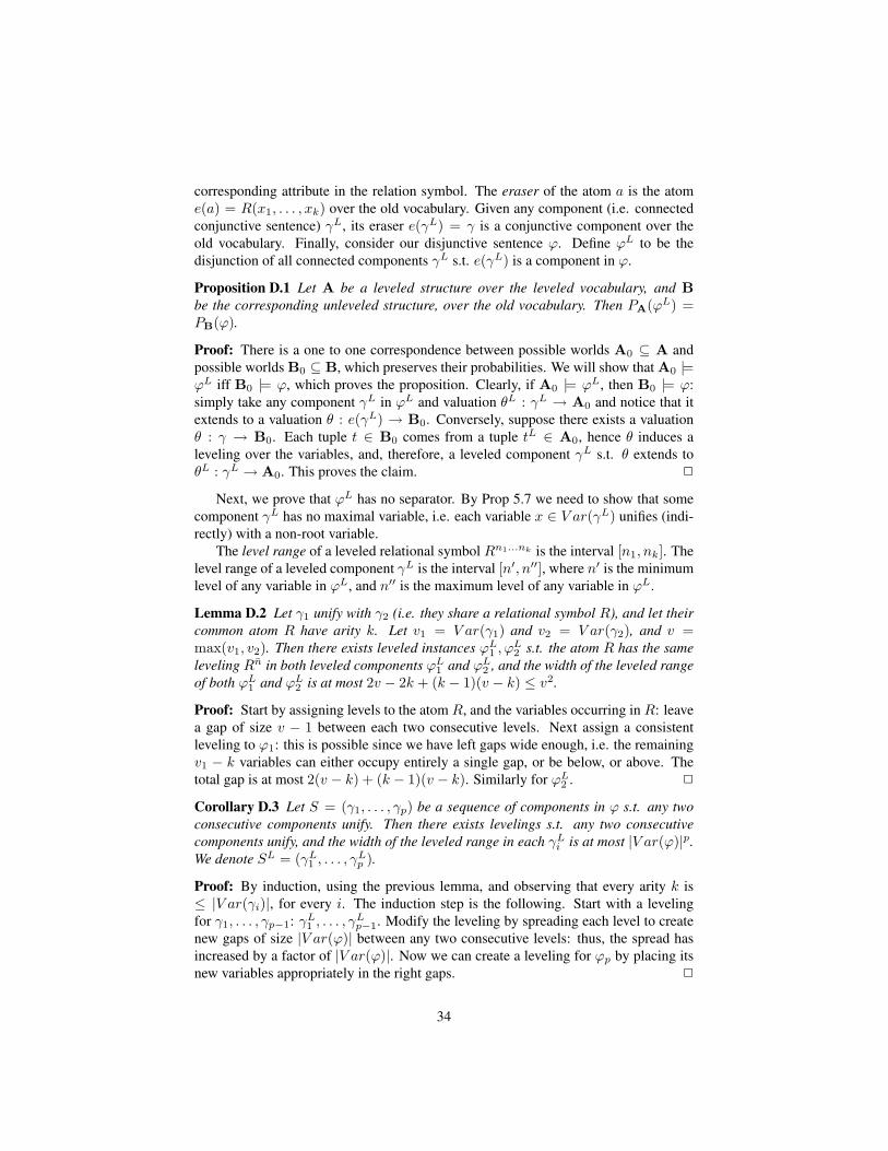
corresponding attribute in the relation symbol. The eraser of the atom a is the atome(a) = R(x1, . . . , xk) over the old vocabulary. Given any component (i.e. connectedconjunctive sentence) γL, its eraser e(γL) = γ is a conjunctive component over theold vocabulary. Finally, consider our disjunctive sentence ϕ. Define ϕL to be thedisjunction of all connected components γL s.t. e(γL) is a component in ϕ.

Proposition D.1 Let A be a leveled structure over the leveled vocabulary, and Bbe the corresponding unleveled structure, over the old vocabulary. Then PA(ϕL) =PB(ϕ).

Proof: There is a one to one correspondence between possible worlds A0 ⊆ A andpossible worlds B0 ⊆ B, which preserves their probabilities. We will show that A0 |=ϕL iff B0 |= ϕ, which proves the proposition. Clearly, if A0 |= ϕL, then B0 |= ϕ:simply take any component γL in ϕL and valuation θL : γL → A0 and notice that itextends to a valuation θ : e(γL) → B0. Conversely, suppose there exists a valuationθ : γ → B0. Each tuple t ∈ B0 comes from a tuple tL ∈ A0, hence θ induces aleveling over the variables, and, therefore, a leveled component γL s.t. θ extends toθL : γL → A0. This proves the claim. 2

Next, we prove that ϕL has no separator. By Prop 5.7 we need to show that somecomponent γL has no maximal variable, i.e. each variable x ∈ V ar(γL) unifies (indi-rectly) with a non-root variable.

The level range of a leveled relational symbol Rn1...nk is the interval [n1, nk]. Thelevel range of a leveled component γL is the interval [n′, n′′], where n′ is the minimumlevel of any variable in ϕL, and n′′ is the maximum level of any variable in ϕL.

Lemma D.2 Let γ1 unify with γ2 (i.e. they share a relational symbol R), and let theircommon atom R have arity k. Let v1 = V ar(γ1) and v2 = V ar(γ2), and v =max(v1, v2). Then there exists leveled instances ϕL1 , ϕ

L2 s.t. the atom R has the same

leveling Rn in both leveled components ϕL1 and ϕL2 , and the width of the leveled rangeof both ϕL1 and ϕL2 is at most 2v − 2k + (k − 1)(v − k) ≤ v2.

Proof: Start by assigning levels to the atom R, and the variables occurring in R: leavea gap of size v − 1 between each two consecutive levels. Next assign a consistentleveling to ϕ1: this is possible since we have left gaps wide enough, i.e. the remainingv1 − k variables can either occupy entirely a single gap, or be below, or above. Thetotal gap is at most 2(v − k) + (k − 1)(v − k). Similarly for ϕL2 . 2

Corollary D.3 Let S = (γ1, . . . , γp) be a sequence of components in ϕ s.t. any twoconsecutive components unify. Then there exists levelings s.t. any two consecutivecomponents unify, and the width of the leveled range in each γLi is at most |V ar(ϕ)|p.We denote SL = (γL1 , . . . , γ

Lp ).

Proof: By induction, using the previous lemma, and observing that every arity k is≤ |V ar(γi)|, for every i. The induction step is the following. Start with a levelingfor γ1, . . . , γp−1: γL1 , . . . , γ

Lp−1. Modify the leveling by spreading each level to create

new gaps of size |V ar(ϕ)| between any two consecutive levels: thus, the spread hasincreased by a factor of |V ar(ϕ)|. Now we can create a leveling for ϕp by placing itsnew variables appropriately in the right gaps. 2

34

Finally, we have:

Corollary D.4 Fix γ, and let S1, S2, . . . , St be t sequences of unifications. Thenthere exists a leveling of all components occurring in all sequences s.t. all sequencesSL1 , . . . , S

Lt are valid sequences of unifications in ϕL and the widths of their spreads

is at most |V ar(ϕ)pt, where p is the maximum length of any sequence Si.

The proof extends the one above.

Example D.5 Let:

ϕ = R(x, y), S(y, z) ∨R(x′, y′), S(x′, y′) = γ0 ∨ γ1

To level this sentence, we choose L = 4, and consider three leveling labels for both Rand S: 12, 23, and 34. The sentence becomes:

ϕL = R23(x2, y3), S34(y3, u4) ∨R12(x1, y2), S23(y2, z3) ∨R23(x′2, y

′3), S23(x′2, y

′3)

And inversion is (x2, y3), (x′2, y′3), (y2, z3).

E Rewriting to a Forbidden QueryWe give here the Proof of Theorem 6.10. Let ϕ be a leveled, disjunctive sentencewithout separators, and with at least three distinct levels. More precisely, if V is its setof variables, then there exists a leveling function l : V → [L] where L ≥ 3, and thereis no leveling function V → [2]. We will prove that ϕ rewrites to a simpler disjunctivesentence, still without separator.

E.1 DefinitionsDefinition E.1 The co-occurrence graph of ϕ =

∨i γi is the following undirected

graph. The nodes are all components γi and there exists an edge from a component γito γj if γi and γj share a common relational symbol.

The connected components of the co-occurrence graph partition ϕ into ϕ1∨ϕ2∨. . .s.t. ϕi and ϕj do not share any common predicate, for i 6= j. Obviously, ϕ has aseparator iff every ϕi has a separator. Since ϕ has no separator, assume w.l.o.g. thatϕ1 also has no separator. Then ϕ ∗→ ϕ1. To see this, simply rewrite all the other ϕj bysubstituting their variables with constants (i.e. repeated applications of the first rule inDef. 6.3), thus ϕ ∗→ ϕ0 ∨ ϕ1, where ϕ0 consists only of constant atoms. Then applythe second rewrite rule in Def. 6.3, ϕ0 ∨ ϕ1 → ϕ1. Therefore, to prove Theorem 6.10,it suffices to assume w.l.o.g. that the co-occurrence graph of ϕ is connected.

35

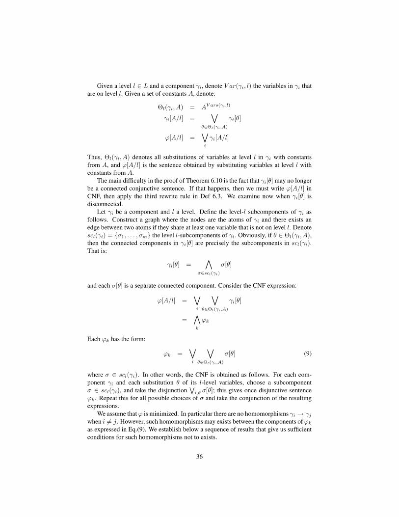
Given a level l ∈ L and a component γi, denote V ar(γi, l) the variables in γi thatare on level l. Given a set of constants A, denote:

Θl(γi, A) = AV ars(γi,l)

γi[A/l] =∨

θ∈Θl(γi,A)

γi[θ]

ϕ[A/l] =∨i

γi[A/l]

Thus, Θl(γi, A) denotes all substitutions of variables at level l in γi with constantsfrom A, and ϕ[A/l] is the sentence obtained by substituting variables at level l withconstants from A.

The main difficulty in the proof of Theorem 6.10 is the fact that γi[θ] may no longerbe a connected conjunctive sentence. If that happens, then we must write ϕ[A/l] inCNF, then apply the third rewrite rule in Def 6.3. We examine now when γi[θ] isdisconnected.

Let γi be a component and l a level. Define the level-l subcomponents of γi asfollows. Construct a graph where the nodes are the atoms of γi and there exists anedge between two atoms if they share at least one variable that is not on level l. Denotescl(γi) = {σ1, . . . , σm} the level l-subcomponents of γi. Obviously, if θ ∈ Θl(γi, A),then the connected components in γi[θ] are precisely the subcomponents in scl(γi).That is:

γi[θ] =∧

σ∈scl(γi)

σ[θ]

and each σ[θ] is a separate connected component. Consider the CNF expression:

ϕ[A/l] =∨i

∨θ∈Θl(γi,A)

γi[θ]

=∧k

ϕk

Each ϕk has the form:

ϕk =∨i

∨θ∈Θl(γi,A)

σ[θ] (9)

where σ ∈ scl(γi). In other words, the CNF is obtained as follows. For each com-ponent γi and each substitution θ of its l-level variables, choose a subcomponentσ ∈ scl(γi), and take the disjunction

∨i,θ σ[θ]; this gives once disjunctive sentence

ϕk. Repeat this for all possible choices of σ and take the conjunction of the resultingexpressions.

We assume thatϕ is minimized. In particular there are no homomorphisms γi → γjwhen i 6= j. However, such homomorphisms may exists between the components ofϕkas expressed in Eq.(9). We establish below a sequence of results that give us sufficientconditions for such homomorphisms not to exists.

36

Lemma E.2 Let γi and γj be two components, and l a level. Suppose that forall σk ∈scl(γi) there exists a homomorphism hk : σk → γj such that forall k1, k2 and all x ∈V ar(γi, l), hk1(x) = hk2(x); that is, for all subcomponents, their homomorphismsagree on the variables at level l. Then there exists a homomorphism γi → γj . Inparticular, if ϕ is minimized, then i = j.

Proof: The proof follows immediately from the definition of subcomponents. Anytwo subcomponents σk1 and σk2 share only variables at level l, and their homomor-phisms agree on these variables. Hence, we can extend the homomorphisms to a singlehomomorphism on the entire γi. 2

This immediately implies:

Corollary E.3 Letϕ be minimized, and let i 6= j. Then for any function h : V ar(γi, l)→V ar(γj) there exists a subcomponent σ ∈ scl(σi) s.t. there is no homomorphismσ → γj that agrees with h on the variables at level l.

Fix a component γi, a subcomponent σi ∈ scl(γi), and an injective substitutionθi : V ars(γi, l)→ A; such a substitution exists whenever |A| ≥ |V ars(γi, l)|. Let ϕkbe a disjunctive sentence given by Eq.(9); the conjunction of all the ϕk’s forms ϕ[A/l].

Definition E.4 We say that ϕk contains σi[θi], if after minimizing ϕk one of its com-ponents is (isomorphic to) σi[θi].

Recall that, if ϕk1 ⇒ ϕk2 then we need to remove ϕk1 from the CNF expressionϕ[A/l] =

∧k ϕk. However, if ϕk1 contains σi[θi], then so does ϕk2 , by the contain-

ment criteria of Sagiv and Yannakakis [14] (see Eq.(5)). Thus, to prove that σi[θi]appears in ϕ[A/l] it suffices to show that there exists some k s.t. ϕk contains it. We donot need to worry whether ϕk is redundant.

Recall that ϕk is uniquely determined by choosing, for each component γj andsubstitution θ ∈ Θj(γj , A), a subcomponent σ ∈ scl(γj): then ϕk is the disjunction∨j,θ σ[θ]. We say that σ ∈ scl(γj) is compatible with σi[θi] and θ if there exists a

homomorphism σ[θ]→ σi[θi]. Otherwise we call it incompatible.

Corollary E.5 If ϕ is minimized then forall σi ∈ scl(γi), θi ∈ Θl(γi, A) and θ ∈Θl(γj , A), if θi is injective then there exists a subcomponent σ ∈ scl(γj) s.t. σ[θ] isincompatible with σi[θi].

Proof: Since θi is injective it admits a left inverse g : A → V ar(γi, l): that is, g isa partial function s.t. g(θi(x)) = x forall x ∈ V ar(γi, l). Define h = g ◦ θ; thisis a function h : V ar(γj , l) → V ar(γi, l), which is possibly partial. If it is a totalfunction, then choose σ ∈ scl(γj) as given in Corollary E.3, i.e. such that there existsno homomorphism σ → γi that extends h: it follows that there is no homomorphismk : σ[θ]→ σi[θi] because if there were one then g ◦ k ◦ θ would give a homomorphismσ → σi that extends h, which is a contradiction. If h is not a total function, thenchoose σ ∈ scl(γj) arbitrary: there is no homomorphism σ[θ] → σi[θi] because σ[θ]uses constants in A that do not occur in σi[θi] (this is why h is not total). 2

37

Corollary E.6 Fix γi, σ ∈ scl(γi) and θi ∈ Θl(γi, A) s.t. θi is injective. Let ϕk bea disjunctive sentence in the CNF expression of ϕ[A/l] obtained as follows: for each(γj , θ) 6= (γi, θi), choose a component σ ∈ scl(γj) that is incompatible with σi[θi];for γi, θi, choose the subcomponent σi. Then ϕk contains σi[θi]. In particular, thereexists ϕk s.t. contains σi[θi].

The proof follows immediately from the previous corollary.

E.2 Root VariablesRecall that a root variable for γi is a variable that occurs in all atoms. Suppose γi hasno root variables: then γi is not a hierarchical sentence [4, 6]. It is possible to showthat directly that every non-hierarchical sentence is #P-hard, and thus remove themcompletely from the discussion: we have proven this in [5] for conjunctive querieswith self-joins, and also include a proof here in Theorem J.1. However, Theorem 6.10also holds for non-hierarchical queries, which is a result of independent interest fromtheir hardness property, and therefore we treat non-hierarchical queries together withthe rest. We give here the proof of Theorem 6.10 for the case when one component γihas no root variables; in particular, it is non-hierarchical.

Clearly, if γi has no root variables, then ϕ =∨i γi does not have a separator: this

follows from the fact that a separator must include a root variable from each compo-nent. Notice that γi has at least two variables x, y s.t. (a) there exists an atom thatcontains both x and y; in particular l(x) 6= l(y); (b) there exists an atom that containsx but not y, and (c) there exists an atom that contains y but not x. Let l be a levelthat is different from l(x) and l(y); choose A a set of constants s.t. |A| ≥ |V ar(γj , l)|forall γj , and consider the CNF expression (9) for ϕ[A/l]. Let σi ∈ scl(γi) be thesubcomponent that contains the variables x and y, and let θi ∈ Θl(γi, A) be any injec-tive substitution. By Corollary E.6 there exists a disjunctive sentence ϕk in the CNFexpression of ϕ[A/l] that contains σi[θi], even after minimization. Then, ϕk does nothave a separator: indeed, σi[θi] continues to have the two variables x, y, and they stillsatisfy conditions (a), (b), (c), hence none of them is a root variable. Thus, ϕk does nothave a separator. Then, the two step rewriting:

ϕ→ ϕ[A/l]→ ϕk

proves Theorem 6.10.Thus, from now on we will assume that every component γi in ϕ has at least one

root variable.

E.3 The ProofIf l is a level, then |scl(γi)| > 1 iff γi has exactly one root variable, and its level isl. This is because γi must have a root variable, and if it has at least one root variableon a level other than l, then that variable will keep all atoms of γi connected, hence|scl(γi)| = 1.

Denote:

38

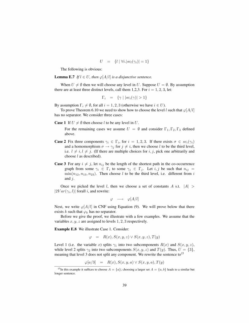
U = {l | ∀i.|scl(γi)| = 1}The following is obvious:

Lemma E.7 If l ∈ U , then ϕ[A/l] is a disjunctive sentence.

When U 6= ∅ then we will choose any level in U . Suppose U = ∅. By assumptionthere are at least three distinct levels, call them 1,2,3. For i = 1, 2, 3, let:

Γi = {γ | |sci(γ)| > 1}By assumption Γi 6= ∅, for all i = 1, 2, 3 (otherwise we have i ∈ U ).

To prove Theorem 6.10 we need to show how to choose the level l such that ϕ[A/l]has no separator. We consider three cases:

Case 1 If U 6= ∅ then choose l to be any level in U .

For the remaining cases we assume U = ∅ and consider Γ1,Γ2,Γ3 definedabove.

Case 2 Fix three components γi ∈ Γi, for i = 1, 2, 3. If there exists σ ∈ sci(γi)and a homomorphism σ → γj for j 6= i, then we choose l to be the third level,i.e. l 6= i, l 6= j. (If there are multiple choices for i, j, pick one arbitrarily andchoose l as described).

Case 3 For any i 6= j, let nij be the length of the shortest path in the co-occurrencegraph from some γi ∈ Γi to some γj ∈ Γj . Let i, j be such that nij =min(n12, n13, n23). Then choose l to be the third level, i.e. different from iand j.

Once we picked the level l, then we choose a set of constants A s.t. |A| >|2V ar(γi, l)| forall i, and rewrite:

ϕ −→ ϕ[A/l]

Next, we write ϕ[A/l] in CNF using Equation (9). We will prove below that thereexists k such that ϕk has no separator.

Before we give the proof, we illustrate with a few examples. We assume that thevariables x, y, z are assigned to levels 1, 2, 3 respectively.

Example E.8 We illustrate Case 1. Consider:

ϕ = R(x), S(x, y, z) ∨ S(x, y, z), T (y)

Level 1 (i.e. the variable x) splits γ1 into two subcomponents R(x) and S(x, y, z),while level 2 splits γ2 into two subcomponents S(x, y, z) and T (y). Thus, U = {3},meaning that level 3 does not split any component. We rewrite the sentence to15

ϕ[a/3] = R(x), S(x, y, a) ∨ S(x, y, a), T (y)15In this example it suffices to choose A = {a}; choosing a larger set A = {a, b} leads to a similar but

longer sentence.

39

The new disjunctive sentence is still without separator. Note that it would have been amistake to choose level 1 because in that case the sentence rewrites to:

ϕ[a/1] = R(a), S(a, x, y) ∨ S(a, y, z), T (y)= (R(a) ∨ S(a, y, z), T (y)) ∧ (S(a, x, y) ∨ S(a, y, z), T (y))

and both conjuncts have a separator (the sentence is actually safe). Thus, Case 1 isnecessary.

We show now why it is necessary to choose |A| > 1. Consider:

ϕ = R(x, z1)S(x, y1, z1)S(x, y2, z2)U(x, z2) ∨ S(x, y, z)T (y) ∨R(x, z)U(x, z)

We also have U = {3}, because variable x disconnects the first component, and vari-able y disconnects the second. So we pick level 3 to rewrite. However, if we use asingle constant a then the first component becomes redundant and the sentence mini-mizes:

ϕ[a/3] = R(x, a)S(x, y1, a)S(x, y2, a)U(x, a) ∨ S(x, y, a)T (y) ∨R(x, a)U(x, a)= S(x, y, a)T (y) ∨R(x, a)U(x, a)

Therefore ϕ[a/3] has a separator (it is actually safe). We need to choose two constants,A = {a, b}:

ϕ[{a, b}/3] = R(x, a)S(x, y1, a)S(x, y2, b)U(x, b) ∨R(x, b)S(x, y1, b)S(x, y2, a)U(x, a) ∨S(x, y, a)T (y) ∨ S(x, y, b)T (y) ∨R(x, a)U(x, a) ∨R(x, b)U(x, b)

One can check that ϕ[{a, b}/3] is minimized and has no separator.

Example E.9 Next we illustrate Case 2. Consider:

ϕ = R(x, y, z)S(x, y′, z′) ∨R(x, y, z)T (x′, y, z′) ∨ S(x, y, z), T (x′, y′, z)= γ1 ∨ γ2 ∨ γ3

Level 1 (variable x) splits the first component into two subcomponents: R(x, y, z)and S(x, y′, z′); similarly levels 2 and 3 split the second and third components. ThusU = ∅. Moreover, Case 2 applies here, because every subcomponent maps into everyother component. That is, we may choose any level l to do the rewriting. We illustratewith l = 3. Here we must choose at least two constants: A = {a, b} and rewrite to:

ϕ[{a, b}/3] = γ1[{a, b}/3] ∨ γ2[{a, b}/3] ∨ S(x, y, a)T (x′, y′, a) ∨ S(x, y, b)T (x′, y′, b)= (γ1[{a, b}/3] ∨ γ2[{a, b}/3] ∨ S(x, y, a) ∨ S(x, y, b)) ∧

(γ1[{a, b}/3] ∨ γ2[{a, b}/3] ∨ S(x, y, a) ∨ T (x′, y′, b)) ∧(γ1[{a, b}/3] ∨ γ2[{a, b}/3] ∨ T (x′, y′, a) ∨ S(x, y, b)) ∧(γ1[{a, b}/3] ∨ γ2[{a, b}/3] ∨ T (x′, y′, a) ∨ T (x′, y′, b))

40

The CNF expression is given in the last four rows, and has four conjuncts: each row isobtained by choosing, for each constant a, b, either the subcomponent S(x, y, z) or thesubcomponent T (x′, y′, z), for a total of four conjuncts. Consider the second conjunct:

ϕ2 = γ1[{a, b}/3] ∨ γ2[{a, b}/3] ∨ S(x, y, a) ∨ T (x, y, b)

Expanding the first two expressions results in 8 components. Some of these are redun-dant, because they contain either S(x, y, a) or T (x, y, b). However, the following twocomponents are not redundant:

ϕ2 = . . . R(x, y, a)S(x, y′, b) ∨R(x, y, a)T (x′, y, a) . . .

Hence ϕ2 has no separator, because neither level 1 nor level 2 is a separator (they arenot root levels in the two components above).

In the example above Case 2 applied, but we were allowed to pick any level wewanted. We illustrate now how Case 2 may restrict our choice. Consider:

ϕ = U(x, y′, z′)V (x, y′′, z′′) ∨R(x′, y, z′)S(x′′, y, z′′)U(x′′, y, z′′) ∨ V (x′, y′, z)S(x′, y′, z)T (x′′, y′′, z)= γ1 ∨ γ2 ∨ γ3

Here the variable x splits γ1 into two subcomponents: U(x, y′, z′) and V (x, y′′, z′′).There is homomrphism from the first subcomponent to γ2: by Case 2 we should notselect levels 1 or 2, but select level l = 3 to expand. There is also a homomorphismfrom the second component to γ3: by Case 2 we should select level l = 2 to expand.But we should not select level 1. In other words, Case 2 allows us to select levels 2 or3, but not level 1. To see why level 1 doesn’t work, consider expanding it with a set ofconstants A = {a, b, c, . . .}:

ϕ[A/1] =∨v∈A

U(v, y′, z′)V (v, y′′, z′′) ∨ γ2[A/1] ∨ γ3[A/1]

=∧k

ϕk

Hereϕk represent the disjuncts in the CNF expansion. Each suchϕk contains γ2[A/1]∨γ3[A/1] and, for each constant v ∈ A, it contains either U(v, y′, z′) or V (v, y′′, z′′)(thus, there are 2|A| disjunctive sentences ϕk). However, each ϕk has a separator. In-deed, consider two terms from the expansion of γ2[A/1]∨ γ3[A/1] that, together, haveno separator:

γi = . . . R(a, y, z′)S(b, y, z′′)U(b, y, z′′) ∨ V (b, y′, z)S(b, y′, z)T (x′′, y′′, z)

Note that we must use the same common constant, say b, in the two atoms S, to allowthem to be unifiable (otherwise the two components have a separator). But γi containseither U(b, y′, z′) or V (b, y′′, z′′), making either the first or the second componentabove redundant. This shows that we cannot expand on level 1. Instead, if we followCase 2, then we will expand on either level 2 or 3. Choosing l = 3 and a single constant

41

a we obtain:

ϕ[a/3] = U(x, y′, a)V (x, y′′, a) ∨R(x′, y, a)S(x′′, y, a)U(x′′, y, a) ∨ V (x′, y′, a)S(x′, y′, a)T (x′′, y′′, a)= (U(x, y′, a)V (x, y′′, a) ∨R(x′, y, a)S(x′′, y, a)U(x′′, y, a) ∨ V (x′, y′, a)S(x′, y′, a)) ∧

(U(x, y′, a)V (x, y′′, a) ∨R(x′, y, a)S(x′′, y, a)U(x′′, y, a) ∨ T (x′′, y′′, a))

Neither conjunct has a separator.

Suppose ϕ has no separator. Our theorem follows from the following three lemmas.

Lemma E.10 (Case 1) Suppose ϕ has no separator, U 6= ∅, and let l ∈ U . Let A be aset of constants s.t. |A| ≥ |V ar(γi, l)| for all i. Then ϕ[A/l] is a disjunctive sentenceand has no separator.

Proof: For any substitution θ ∈ Θl(γi, A), γi[θ] is connected. Thus, ϕ[A/l] is adisjunctive sentence. Some of the components γi[θ] may be redundant. However,by Corollary E.6, for any injective substitution θi : V ars(γi, l) → A, γi[θ] is notredundant.

We show now that ϕ[A/l] has no separator. Suppose it had a separator V ′. Con-struct a separator V for ϕ as follows. For each component γi, let θ be any injectivesubstitution θ : V ar(γi, l)→ A. Define the separator variable xi for γi to be the sameseparator variable for γi[θ] (the two sentences are isomorphic and “the same variable”means up to this isomorphism). Note that this definition is independent on our choiceof θ. Indeed, if θ′ is another injective substitution that agrees with θ on at least onevariable x (θ(x) = θ′(x)) then γi[θ] and γi[θ′] have two atoms that unify, hence theirseparator variables must unify, which means that they correspond to the same variablein γi. It is easy to check that the set {xi | i = 1, . . .} is indeed a separator for ϕ: ifγi and γj unify, then there exists substitutions θ, θ′ s.t. γi[θ] unifies with γj [θ′], andtherefore the separator variables must unify as well. 2

From now on we will assume that Case 1 does not apply. Let 1,2,3 be three arbitrarylevels, and Γ1,Γ2,Γ3 be as defined above. Fix γi ∈ Γi, for i = 1, 2, 3.

Lemma E.11 (Case 2) Suppose there exists σ1 ∈ sc1(γ1) and a homomorphism h :σ1 → γ2. Let A be a set of constants such that |A| ≥ |V ar(γ1, 3)| + |V ar(γ2, 3)|(the number of variables on the 3rd level in γ1 plus those in γ2). Consider the CNFexpression for ϕ[A/3] =

∧ϕk. Then there exists k s.t. ϕk has no separator.

Proof: Let θ2 ∈ Θ3(γ2, A) be any injective substitution, and denoteA2 ⊆ A the set ofconstants in Im(θ2). Define θ1 to be injective and s.t. forall x ∈ V ar(γ1, 3)∩V ar(σ1),θ1(x) = θ2(h(x)); that is, we use |V ar(γ1, 3)−V ar(σ1)| constants in addition to thosein Im(θ2): denote A1 the set consisting of these constants. We claim that there existssome ϕk in Eq.(9) that contains both components γ1[θ1] and γ2[θ2] (note that both areconnected). Note that this proves our claim: ϕk does not have a separator, because theonly root variable in γ1[θ1] is on level 1, and the only root variable in γ2[θ2] is on level2.

42

Suppose that there exists a homomorphism σ[θ] → γi[θi], for i = 1 or 2, whereσ ∈ sc3(γ). Then γ ∈ Γ3: otherwise σ = γ and we obtain a homomorphism γ → γi,contradicting the fact that the sentence ϕ was minimized. Thus, assume γ ∈ Γ3, andlet z denote the variable at level 3 in γ (z is the single root variable in γ). Recall that,when defining ϕk, we may choose any σ ∈ sc3(γ) for each γ, θ. We consider twocases. First, when θ(z) ∈ A2. Then we choose σ s.t. it is incompatible with γ2[θ2]:this is possible by Corollary E.5. It follows that there is no homomorphism σ[θ] →γ1[θ1] either, because the image of such a homomorphism must be in σ1[θ1] (since allconstants in A2 are here), and this would give us a homomorphism σ[θ] → γ2[θ2].Second, when θ(z) ∈ A1. Then we choose σ to be incompatible with γ1[θ1]. Clearlythere is no homomorphism σ[θ] → γ1[θ1]. In addition there is no homomorphismσ[θ] → γ2[θ2] either, because every atom in σ[θ] contains the constant θ(z), whichdoes not occur in γ2[θ2]. 2

Fix i 6= j, and γi ∈ Γi and γj ∈ Γj . Since we assumed that the co-occurrencegraph is connected, there is a path δ0 = γi, δ1, δ2, . . . , δn = γj s.t. any two consecutivecomponents δk−1, δk share a common relational symbol. Call n the length of the pathfrom γi to γj . Let nij be the length of the shortest path from any component in Γi toany component in Γj

Lemma E.12 (Case 3) Suppose n12 = min(n12, n13, n23). LetA be a set of constantssuch that |A| ≥ maxi(|V ar(γ, 3)|), for all components γ in ϕ. Then there exists adisjunctive sentence γk in the expansion (9) of ϕ[A/3] that has no separator.

Proof: Let δ0 = γ1, δ1, . . . , δn = γ2 be a shortest path from some component γ1 ∈ Γ1

to some component γ2 ∈ Γ2; thus, n12 = n. Note that δi 6∈ Γ3 for all i = 0, n:otherwise, we would have a shorter path from Γ1 to Γ3.

Define, inductively, the substitutions θi ∈ Θ(δi, A) as follows. Start by definingθ0 : V ar(δ0, 3)→ A to be any injective substitution. To define θk : V ar(δk, 3)→ A,consider the two atoms in δk−1 and δk that share a common relational symbol. Theymay share at most one variable at level 3: choose θk to be any injective substitutionthat agrees with θk−1 on the common variable at level 3. Note that δi[θi] is connected,for all i = 0, . . . , n, because none of the δi’s is in Γ3.

We will show now that there exists a disjunctive sentence γk that contains all com-ponents δi[θi]: this proves our claim, since γk cannot have a separator, because the onlyroot variable in δ0 is on level 1, and the only root variable in δn is on level 2. Thus, weneed to show that, for every component γ and every substitution θ ∈ Θ3(γ,A), thereexists σ ∈ sc3(γ) s.t. σ[θ] is incompatible with δi[θi] for all i = 0, . . . , n.

First, notice that the only way we can have a homomorphism σ[θ] → δi[θi] is ifγ ∈ Γ3: otherwise, |sc3(γ)| = 1, and σ = γ, and a homomorphism γ[θ] → δi[θi]implies a homomorphism γ → δ, which is a contradiction. So assume γ ∈ Γ3. Thenwe cannot have i = 0 or i = n, because then we would be in Case 2, and we haveassumed that the condition for Case 2 does not hold. Thus i ∈ {1, . . . , n − 1}. Weconsider two cases.

Case 1: there exists σ, θ such that there exists a homomorphism σ[θ] → δi[θi],for some i = 1, . . . , n − 1. This gives us the path δ0 = γ1, δ1, . . . , δi, γ in the co-occurrence graph from Γ1 to Γ3. Since we assumed our path from Γ1 to Γ2 is the

43

shortest one, we conclude i = n−1. Similarly, we obtain the path γ, δi+1, . . . , δn = γ2

from Γ3 to Γ2: we conclude that i = 1. Thus, n = 2, in other words the path from Γ1

to Γ2 is γ1, δ1, γ2. For any γ, θ, choose σ ∈ sc3(γ) such that σ[θ] is incompatible withδ1[θ1]: this is possible by Corollary E.5. Then the resulting ϕk contains the entire pathγ1[θ0], δ1[θ1], γ2[θ2].

Case 2: there is no homomorphism σ[θ] → δi[θi], for any i = 1, . . . , n − 1. Thenany ϕk contains all components δi[θi], for i = 0, . . . , n. 2

Part III

Forbidden Queries are HardWe give here the proof of the most difficult result in this paper: that all forbiddensentences are hard. We use in this chapter the term Boolean query or simply query torefer to a positive, existential FO sentence.

F Problem SettingLet Q be a disjunctive query:

Q = q1 ∨ q2 ∨ q3 ∨ . . .

where each qi is a connected, conjunctive query, called a component. The queryis 2-leveled: that means, there exists a function l : V ar(Q) → {1, 2} s.t. forallk ∈ {1, 2}, l−1(k) is a level, i.e. contains exactly one variable from each atom, and isclosed under unification.

Definition F.1 The co-occurrence graph ofQ is the following undirected graphG(Q).The nodes are all relation symbols, and there exists an edge from Si to Sj if Si and Sjco-occur in a component qk.

Denote l−1(1) = {x1, x2, . . .} and l−1(2) = {y1, y2, . . .}. Each atom may containat most one x-variable and one y-variable. We call a component qi a left component ifno variable y occurs in all atoms; we call it a right component if no variable x occursin all atoms. Any symbol that occurs in some left component is called a left symbol;any symbol occurring in some right component is a right symbol.

Definition F.2 A 2-leveled disjunctive query Q is called a forbidden query if thereexists a path in G(Q) from a left symbol to a right symbol.

Lemma F.3 A 2-leveled query Q is forbidden iff it has no separator.

Proof: Suppose that there exists a path from S to S′. We show that there is no sepa-rator. Suppose W is a separator. Let q be a left component that contains S: then W

44

must contain the x-variable in q. Similarly, if q′ is a right component containing S′,then W must contain the y-variable from q′. Consider path from S to S′ in the co-occurrence graph. Each edge between two symbols Si, Sj corresponds to a componentthat contains both symbols. Augment the beginning of the path with the edge S, S (cor-responding to q) and the end of the path with the edge S′, S′ (corresponding to q′). Theseparator contains either an x- or a y-variable from each query along the path. Since itstarts with an x-variable and ends with a y-variable, there exists two consecutive edgeswhere the separator chooses an x-variable from qi on the first edge, and a y-variablefrom qj on the other edge; but this violates the condition that the separator be closedunder unification.

Conversely, assume no such path exists. Then we partition the co-occurrence graphinto connected components. We show how to construct a separator, by including fromeach component either a x or a y variable, as follows. There are three kinds of con-nected components: (a) those that contain at least one left-component; then it cannotcontain a right component: here choose the x-variable. (b) those that contain at leastone right-component; here choose the y-variable. (c) those that contain only middlequeries; choose arbitrarily the x-variable. 2

In this document we prove:

Theorem F.4 For every forbidden queryQ, computingP (Q) on a probabilistic databaseis hard for FP#P .

G The Signature Counting ProblemLet Φ =

∨(x,y)∈E x ∧ y be a PP2DNF. The counting problem for PP2DNF, denoted

#PP2DNF, asks for the number of assignments that make the formula true. It is knownto be #P-complete [1].

Equivalently, Φ is a bipartite graph (X,Y,E), where E ⊆ X × Y . Let n1 = |X|,n2 = |Y |, n = |E|. We call interchangeably xy an edge, or a conjunct in Φ. Letm1,m2 = O(1) be two numbers, m1 ≥ 2,m2 ≥ 2: that is, these numbers are fixed,and independent of n1, n2, and are at least 2. We define the set of left labels and rightlabels as LL = [m1] and RR = [m2]. In all definitions below we assume that thebipartite graph Φ is fixed.

Definition G.1 A labeling is a pair of functions l = (l1, l2), where l1 : X → LL andl2 : Y → RR. There are nm1

1 × nm22 labelings.

Definition G.2 An edge signature σE , a node signature on the left σX and a nodesignature on the right σY are functions:

σE : LL×RR→ {0, 1, . . . , n}σX : LL→ {0, 1, . . . , n}σY : LL→ {0, 1, . . . , n}

Definition G.3 We define four types of signatures: the left end may be of type 1 or 2,and the right end may be of type 1 or 2.

45

• A signature of type 1-1 is σ = σE .

• A signature of type 1-2 is σ = (σE , σY ).

• A signature of type 2-1 is σ = (σX , σE).

• A signature of type 2-2 is σ = (σX , σE , σY ).

We write a signature as σ = ([σX , ]σE [, σY ]) to indicate that σX and σY areoptional. In the sequel, the type of all signatures is fixed by the query Q, and is oneof 1-1, 1-2, 2-1, 2-2. We will assume the type to be fixed, and denote Σm1,m2 bethe set of signatures of the fixed type, for the bipartite graph Φ. Note: |Σm1,m2 | ≤nm1m2+m1+m2 .

Definition G.4 Let l = (l1, l2) be a labeling. The signature of the labeling l is σl =([σXl , ]σ

El [, σYl ]), where:

σEl (τ1, τ2) = |{(x, y) ∈ E | l1(x) = τ1, l2(y) = τ2}| ∀(τ1, τ2) ∈ LL×RRσXl (τ1) = |{x ∈ X | l1(x) = τ1}| ∀τ1 ∈ LLσYl (τ2) = |{y ∈ Y | l2(y) = τ2}| ∀τ2 ∈ RR

Definition G.5 Let σ ∈ Σm1,m2(Φ) be a signature. The signature count of σ, denoted#σ, is the number of labelings that have signature σ:

#σ = |{l | σl = σ}|Let #Σm1,m2(Φ) = {#σ | σ ∈ Σm1,m2(Φ)} denote the set of all signature counts.There are |#Σm1,m2(Φ)| ≤ nm1m2+m1+m2 signature counts.

Definition G.6 Fix m1,m2 ≥ 2. The m1,m2-Signature-Counting (SC) problem is thefollowing: given a bipartite graph Φ, compute #Σm1,m2(Φ).

Example G.7 Let m1 = m2 = 2. Assume the type 1-1. Then the 2,2-countingproblem is the following. Given a bipartite graph Φ = (X,Y,E), for all tuples of 4numbers σ = σE = (n11, n12, n21, n22) where n11, n12, n21, n22 ≤ |E|, compute#σ the number of possible labelings of the X-nodes and the Y -nodes s.t. exactly n11

edges have their endpoints labeled 1 and 1, exactly n12 edges have their endpointslabeled 1 and 2, etc. Note that, if n11 + n12 + n21 + n22 6= n, then #σ = 0, becauseno such labelings is possible: we leave such inconsistent signatures in the problemdefinition, for convenience. Suppose now that the type is 2-2. Then forall 8 numbersσE = (n11, n12, n21, n22), σX = (n1, n2) and σY = (n′1, n

′2) we need to compute the

number of labelings s.t., the number of edges whose endpoints are labeled 1,1 is n11

etc; the number of nodes in X labeled 1 is n1 and the number of nodes in X labeled2 is n2; and the number of nodes in Y labeled 1 is n′1 and the number of nodes in Ylabeled 2 is n′2.

Let m1 ≤ m′1 and m2 ≤ m′2. Given an m1,m2 signature σ, we can view it asan m′1,m

′2-signature by setting σ(τ1, τ2) = 0 whenever τ1 > m1 or τ2 > m2. With

this convention, we have Σm1,m2(Φ) ⊆ Σm′1,m

′2(Φ) and similarly #Σm1,m2(Φ) ⊆

#Σm′1,m

′2(Φ).

46

Proposition G.8 SC is hard for FP#P .

Proof: By reduction from the PP2DNF problem. Assume that we have an oracle forsolving the m1,m2-SC problem, for m1,m2 ≥ 2. We can assume w.l.o.g. that the sig-natures are of type 1,1: if the signatures are of, say, type 2,2, then we convert signaturecounts #(σX , σE , σY ) into #σE by summing over all signatures σX and σY . Thus,we assume all signatures are of type 1,1. From Σm1,m2(Φ) we obtain Σ2,2(Φ) (sinceΣ2,2(Φ) ⊆ Σm1,m2(Φ)). Next, we use an oracle for the 2, 2-SC problem to solve the#PP2DNF problem: assuming the encoding 1 = false, 2 = true, we obtain thenumber of satisfying assignments to the Boolean expression Φ by summing #σ overall signatures σ where |{(x, y) ∈ E | l1(x) = 2, l2(y) = 2}| ≥ 1:

#PP2DNF =∑{#σ | σ ∈ Σ2,2(Φ), σ(2, 2) ≥ 1}

2

The proof Theorem F.4 is the following: we will show that, for every forbiddenquery Q, there exists two numbers m1,m2 ≥ 2 such that the m1,m2-SC problem canbe reduced to the evaluation problem P (Q) over probabilistic databases D.

H An ExampleWe illustrate the key elements of the proof, by proving hardness of the query:

H1 = R(x), S(x, y) ∨ S(x, y), T (y)

Recall that hardness of H0 = R(x), S(x, y), T (y) is very easy to prove, by directreduction from #PP2DNF: given Φ = (X,Y,E) construct a database having tuplesR(ai), T (bj), S(ai, bj) with probabilities 1/2, 1/2, 1, forall ai ∈ X , bj ∈ Y , and(ai, bj) ∈ E: the number of satisfying assignments for Φ is exactly the number ofworlds that make H0 true. Hence, the associated counting problem for H0 is #P-hard.

We do not know of a similarly simple construct for H1, or for any other forbiddenquery, and this forces us to use a more complex proof. We illustrate here the hardnessproof forH1. This query is of type 1-1, so all signatures below are of type 1-1. We willprove its hardness by providing a PTIME algorithm for the 2, 2-SC problem with accessto an oracle for computing P (H1): this shows that P (H1) is hard for FP#P . Note thatthe 2, 2-SC problem is more general that the #PP2DNF (but still complete for FP#P ).There are two parts to the hardness proof of H1, which we call the Algorithmic and theAlgebra. There is a third part, called the Combinatorics, for more complex queries.

H.1 Algorithmic PartFix Φ = (X,Y,E), X = {ai | i = 1, n1}, Y = {bj | j = 1, n2}, E ⊆ X × Y ,|E| = n. Construct a probabilistic database D as the union of blocks D(ai, bj), onefor each edge (ai, bj) ∈ E. Each blockD(ai, bj) is, in turn, of the union of four blocksDk(ai, bj), for k = 1, 2, 3, 4:

47

D =⋃

(ai,bj)∈E

D(ai, bj)

D(ai, bj) = D1(ai, bj) ∪D2(ai, bj) ∪D3(ai, bj) ∪D4(ai, bj)Dk(ai, bj) = {R(ai), S(ai, cijk), T (cijk), S(dijk, cijk), R(dijk), S(dijk, bj), T (bj)}

The only tuples shared between blocks are R(ai), T (bj): we set their probabilitiesto 1/2 and call them endpoints. Each block Dk(ai, bj) contains two endpoints and fiveadditional tuples. We fix the probabilities of four of them to some constant values (samevalues forall i, j, k), and for the fifth tuple we set its probability to be some variablexk ∈ (0, 1) (same forall i, j, different for k = 1, 2, 3, 4). For example, we may setP (S(dijk, cijk)) = xk, and for all other tuples we set their probabilities to 1/2, butthis choice needs to be made carefully, as we explain below. For now it suffices to saythat a single tuple in each block Dk(ai, bj) has a variable probability.

Let LL = RR = {1, 2}. Each possible world W ⊆ D defines lW = (lW1 , lW2 ) forΦ as follows:

lW1 (ai) ={

1 if R(ai) ∈W2 if R(ai) 6∈W lW2 (bj) =

{1 if T (bj) ∈W2 if T (bj) 6∈W

Fix a labeling l and consider the event “a possible world W ⊆ D has labeling l”,formally lW = l. Clearly P (lW = l) = 1/2n1+n2 . We want to compute the probabilitythat H1 is false conditioned on lW = l: P (¬H1|lW = l).

Fix an edge (ai, bj) and let τ1 = l(ai), τ2 = l(bj) be the labeling of its endpoints,τ = (τ1, τ2). Denote fτ (xk) the probability that the query H1 is false on the blockDk(ai, bj), conditioned on the label τ . That is, given that R(ai) and T (bj) are trueor false, as specified by τ1 and τ2, fτ (xk) denotes the probability that Hk is false onDk(ai, bj); for example, f12(xk) denotes the probability that H1 is false on a blockDk(ai, bj), assuming R(ai) is true and T (bj) is false. Note that fτ (xk) is the same forall i and j, so we do not include the indices i, j in the expression. Thus, fτ (xk) is alinear polynomial in xk:

fτ (xk) = Aτ +Bτxk

The two coefficients depend on the labeling τ . The probability that H1 is false onD(ai, bj) conditioned on the label τ is:

Fτ (x) = fτ (x1) · fτ (x2) · fτ (x3) · fτ (x4) (10)

This gives us:

48

P (¬H1|lW = l) =∏

(ai,bj)∈E

Fl1(ai),l2(bj)(x)

=∏

τ∈LL×RRFσl(τ)τ (x)

= Fn1111 (x) · Fn12

12 (x) · Fn2121 (x) · Fn22

22 (x)

where σl = (n11, n12, n21, n22), and each nτ represents the number of edges inE whose endpoints are labeled τ . For each σ ∈ Σ2,2(Φ) there are #σ labelings l s.t.σl = σ, and therefore we obtain (recall that P (lW = l) = 1/2n1+n2 ):

P (¬H1) =∑l

P (¬H1|lW = l)P (lW = l)

=1

2n1+n2

∑σ∈Σ2,2(Φ)

∏τ∈LL×RR

Fσ(τ)τ (x) ·#σ

We will use repeatedly an oracle for computing P (¬H1) in order to obtain thevalues #σ, forall σ ∈ Σ2,2(Φ), thus solving the 2,2-SC problem. Since |Σ2,2(Φ)| =(n+ 1)4, we have (n+ 1)4 unknowns16 #σ. Choose (n+ 1)4 different values for thefour variables x = (x1, x2, x3, x4), x = v1, v2, . . . , v(n+1)4 and invoke the P (H1)-oracle for each value. We obtain a linear system with (n+ 1)4 equations and (n+ 1)4

unknowns, whose matrix is:

M = (∏τ

Fσ(τ)τ (v))σ∈Σ,v∈V

= (Fn1111 (vi) · Fn12

12 (vi) · Fn2121 (vi) · Fn22

22 (vi)) n11, n12, n21, n22 ≤ ni = 0, . . . , (n+ 1)4

where V = {v1, v2, . . . , v(n+1)4}. If M is non-singular, then we can solve thesystem in polynomial time, and thus obtain the solution to the 2,2-SC problem, provinghardness for the computation problem for P (H1).

H.2 Algebra PartIt remains to show that M is non-singular. This follows from three facts, which wedescribe below, continuing to restrict the discussion to H1.

Fact H.1 Let F (x) = (F1(x), F2(x), F3(x), F4(x)), where x = (x1, x2, x3, x4) bea function R4 → R4, where each Fk is a multilinear polynomial. Suppose that the

16For every labeling l, its signature has the propertyPτ∈LL×RR #σl(τ) = n. If a signature does not

have this property, then #σ = 0, hence there are only O(n3) unknowns, but we prefer to treat all #σ’s asan unknowns, for a total of (n+ 1)4.

49

Jacobian x→ F is non-zero at some point x ∈ R4. Define the following matrix:

M =(F j11 (xi) · F j22 (xi) · F j33 (xi) · F j44 (xi)

)i = 1, (n+ 1)4

0 ≤ j1, j2, j3, j4 ≤ n(11)

That is, the columns are given by four independent exponents j1, j2, j3, j4 and the rowsare given by (n+1)4 values for the variables x. ThenM is nonsingular, and, moreover,one can find in PTIME (n+ 1)4 values V = {v1, . . . , v(n+1)4} such that the matrix Mat these values is non-singular.

We give the general statement and proof in Sec. I.1. The intuition is quite simple,however. When the values V are considered unknowns, then det(M) is a multivariatepolynomial in 4(n+ 1)4 variables, where each variable has degree ≤ 4(n+ 1)4. Thus,the idea in the proof is to show that one can find in PTIME values for the unknowns s.t.det(M) 6= 0. To give the intuition why this is possible, consider a simpler problem:given a polynomial f(x) in a single variable x, of degree N , find a value v s.t. f(v) 6=0. Clearly this can be done in time O(N), times the time needed to evaluate f . Indeed,by trying out at most N + 1 values for x, one can find a value v s.t. f(v) 6= 0. We willshow that this idea extends to a proof of the claim.

Next, we turn to the Jacobian of the function F (x).

Fact H.2 Let f1(x), f2(x), f3(x), f4(x) be four linear, non-constant polynomials inone variable x. Suppose their roots are distinct. For k = 1, . . . , 4 define:

Fk(x1, x2, x3, x4) = fk(x1) · fk(x2) · fk(x3) · fk(x4)

Then, for any four distinct values v = (v1, v2, v3, v4), the Jacobian of F (x) is non-zeroat v.

We give the general statement and proof in Sec. I.2.Next, we need to show that the polynomials f11, f12, f21, f22 have distinct roots.

Recall that two multivariate polynomials f, g are called equivalent if there exists anumber c 6= 0 s.t. f = c·g. If f(x), g(x) are two linear polynomials in a single variablex, then they are equivalent iff their roots are equal. A multivariate polynomial is calledirreducible if it cannot be expressed as a product of two non-constant polynomials:a classic result in algebra states that every multivariate polynomial can be uniquelydecomposed as a product of irreducible polynomials, up to equivalence. Recall that weobtained the polynomials f11(x), . . . , f22(x) by setting other variables to constants.We prove:

Fact H.3 Let p1, p2, p3, p4 be four multilinear polynomials. Suppose that they havesome irreducible factors p0

1, p02, p

03, p

04, such that p0

i is a factor of pi, with the follow-ing properties: the four factors are pairwise inequivalent, and they share a commonvariable x. Let y be all variables other than x in p1, . . . , p4. Then there exists val-ues v such that after substituting v for y in p1, . . . , p4 the resulting linear polynomialsf1(x), . . . , f4(x) are not constants, and have distinct roots.

50

We give the general statement and the proof in Sec. I.3.This brings us to the very core of the hardness proof: the connection between

queries without separator and irreducible polynomials. Recall that the blockDk(ai, bj)has five tuples: S(ai, cijk), T (cijk), S(dijk, cijk), R(dijk), S(dijk, bj). DenoteZ1, . . . , Z5

the events that the tuples are not present in a possible world W ⊆ Dk(ai, bj), andX,Y the events that R(ai) and T (bj) are not in W . Then, the event that H1 is false onDk(ai, bj) is given by the Boolean expression:

ϕ = (X ∨ Z1)(Z1 ∨ Z2)(Z2 ∨ Z3)(Z3 ∨ Z4)(Z4 ∨ Z5)(Z5 ∨ Y )

Let ϕτ1τ2 denote the event “the query is false given that R(ai) and T (bj) are labeledτ1 and τ2 respectively”:

ϕ11 = (Z1 ∨ Z2)(Z2 ∨ Z3)(Z3 ∨ Z4)(Z4 ∨ Z5)ϕ12 = (Z1 ∨ Z2)(Z2 ∨ Z3)(Z3 ∨ Z4)Z5

ϕ21 = Z1(Z2 ∨ Z3)(Z3 ∨ Z4)(Z4 ∨ Z5)ϕ22 = Z1(Z2 ∨ Z3)(Z3 ∨ Z4)Z5

Denote p11, p12, p21, p22 the multivariate polynomials in real variables z1, . . . , z5

giving the probabilities of ϕ11, ϕ12, ϕ21, ϕ22. We claim that these polynomials factor-ize as follows:

p11 = p011

p12 = p012 · z5

p21 = z1 · p021

p22 = z1 · p022 · z5

where p011, p

012, p

021, p

022 are inequivalent irreducible polynomials, having the variables

z2, z3, z4 in common. Indeed, start with p11 = p(ϕ11). Suppose it had two non-trivialfactors p11 = f ·g. Since p11 is multilinear, f and g do not share any common variables.In that case one could express ϕ11 as ϕ11 = ψ ∧ ν, where ψ and ν are Booleanexpressions that do not share any common variables. But this is not possible: theexpression ϕ11 connects all variables Z1, . . . , Z5 and cannot be written as the conjunctof two independent expressions. Thus, p11 is irreducible. On the other hand, p22 hasthree factors, z1, z5 and the multilinear polynomial in z2, z3, z4 giving the probabilityof (Z2 ∨ Z3)(Z3 ∨ Z4).

The four irreducible polynomials have three common variables z2, z3, z4. Chose xto be any one of them, say x = z3, and set the other variables to some constants toobtain for linear polynomials f11(x), . . . , f22(x) that have distinct roots.

It is interesting to notice that this does not work if the query Q is not forbidden.For example, consider the queryQ = R(x), S1(x, y)∨S2(x, y), T (y) can be separatedinto two independent parts, and the p-polynomials factorize as:

51

p11 = q1r1 p12 = q1r2 p21 = q2r1 p22 = q2r2

qi and rj cannot have any variables in common. If we choose a variable x thatoccurs in r1, r2 only, then after setting all other variables to constants the polynomialsbecome a · r1(x), a · r2(x), b · r1(x), b · r2(x) where a, b are constants: thus, thefirst and third polynomials are equivalent, and so are the second and fourth. We canactually prove a necessary and sufficient condition: Q is not a forbidden query iff acorresponding polynomial factorizes in a way that separates the left from the right.

H.3 Combinatorics PartFor queries Q more complex than H1 we need to pre-process them, both in order todevelop the algorithm, and in order to prove the algebraic properties.

I Part 1 of the Proof: Algebra

I.1 Solving for det(M) 6= 0

Here we formalize and generalize Fact H.1. This consists of two theorems. The first is:

Theorem I.1 Let x = (x1, . . . , xm) bem variables, and G(x) = (G1(x), . . . , Gn(x))be n multivariate polynomials in x. Consider n distinct copies of x, denoted xi, i =1, n, and let X = (xi)i=1,n be the set of m · n distinct variables. Define the matrix ofpolynomials:

M(G) = (Gj(xi))i,j=1,n (12)

We assume m = O(1). Then there exists an algorithm that runs in time nO(1) andeither determines that det(M) ≡ 0 (as a multivariate polynomial in X) or finds valuesV s.t. det(M(G)[V /X]) 6= 0.

The second theorem is:

Theorem I.2 Let F (x) = (F1(x), . . . , Fm(x)) be m multivariate polynomials, eachin m variables x. For each n > 0, define (n+ 1)m polynomials G(x) as follows:

G = (∏i=1,m

F jii (x))0≤j1,...,jm≤n (13)

Thus, for each m-tuple (j1, j2, . . . , jm) ∈ {0, . . . , n}m there is one polynomial inG. Suppose that the Jacobian of the function x → F (x) is not identically zero. Thendet(M(G)) 6≡ 0, where M(G) is the matrix defined in Eq.(12).

Together, these two theorems prove the following, which generalizes Fact H.1.Suppose we are given m polynomials F1(x), . . . , Fm(x) in m variables x with a non-zero Jacobian. Define a matrixM of dimensions (n+1)m×(n+1)m, where each row

52

is given by G in Eq.(13) and distinct rows differ only in the choice of the argumentsx. Thus, the matrix generalizes that given by Eq.(11). Then det(M) is not identicallyzero, and one can find in PTIME (n+ 1)m values V for x s.t. det(M)[V ] 6= 0.

In the remainder of this section we prove the two theorems. We start with a theoremthat we will also need later.

Theorem I.3 For a multivariate polynomial P in m variables, denote V(P ) the set ofpoints in the m-dimensional complex vector space where P is zero:

V(P ) = {v | v ∈ Cm, P (v) = 0}

This is called the variety of P . Suppose F is a multilinear polynomial s.t. V(F ) ⊆V(P ). Then there exists a polynomial G s.t. P = F ·G

Proof: Recall Hilbert’s Nullstellensatz: for any multivariate polynomialsF1, . . . , Fk, P ,if V(F1)∩ . . .V(Fk) ⊆ V(P ) then there exists n ≥ 1 and polynomials G1, . . . , Gk s.t.Pn = F1 ·G1 + . . .+ Fk ·Gk. (In other words, Pn belongs to the ideal generated byF1, . . . , Fk.) In our case, this implies that there exists G and n ≥ 1 s.t. Pn = F · G.Decompose F into irreducible factors: F = f1f2 · · · Since F is multilinear, no twofactors share any common variables. In particular, all factors are distinct, and, sinceeach factor divides P , it follows that P is divisible by F , proving our claim. 2

To prove Theorem I.1 we need the following two lemmas.

Lemma I.4 Let P (x1, . . . , xm) be a multivariate polynomial of degree n, with m =O(1) variables. Suppose we have an Oracle that, given values v1, . . . , vm, computesP (v1, . . . , vm) in time T . Then there exists an algorithm that runs in time O(nmT )and either determines that P ≡ 0 or returns a set of values v = (v1, . . . , vm) s.t.P (v) 6= 0.

Proof: By induction on m. Choose n + 1 distinct values for the last variable: xm =v0m, xm = v1

m, . . ., xm = vnm. For each value vim we substitute xm = vim inP . We obtain a new polynomial, Q = P [xm/vim], with m − 1 variables. Ap-ply induction hypothesis to this polynomial, to find a set of values v1, . . . , vm−1 s.t.Q[x1/v1, . . . , xm−1/vm−1] 6= 0. If we find such values, then augment them withvim and return (v1, . . . , vm−1, v

im). If we don’t find them, then we know that Q =

P [vim/xm] ≡ 0, in other words P is divisible by xm − vim, by Theorem I.3. If thelatter case holds for all n + 1 values for xm, then we know that the polynomial isidentically 0. 2

Recall that n multivariate polynomials G1, . . . , Gn are called linearly independentif, for any constants c1, . . . , cn, if c1G1 + . . .+ cnGn ≡ 0 then c1 = . . . = cn = 0.

Lemma I.5 The polynomials G1, . . . , GN are linearly dependent iff det(M(G)) ≡ 0(where M is given by Eq.(12)).

53

Proof: The “if” direction follows immediately from the fact that the columns in Mare linearly dependent. For the “only if” direction, we prove by induction on n that,if n polynomials G1, . . . , Gn are linearly independent, then det(M) 6≡ 0. Let M ′

be the (n − 1) × (n − 1) upper-left minor of M . Since G1, . . . , Gn−1 are also lin-early independent, det(M ′) 6≡ 0. Hence, there exists values V ′ = (v1, . . . , vn−1) s.t.det(M ′)[V ′] 6≡ 0. Consider now det(M)[V ′]: that is, we substitute x1, . . . , xn−1 withthe values V ′, and keep only the variables xN . Then det(M(V ′)) has in the last rowthe polynomialsG1(xn), . . . , Gn(xn), and has constants in all other rows. Its value is alinear combination of the polynomials in the last row: det(M) = c1 ·G1+. . .+cn ·Gn.The last coefficient, cn = det(M ′)[V ′], is non-zero, hence det(M) 6≡ 0, because thepolynomials are linearly independent. 2

We can now prove Theorem I.1.

Proof: (of Theorem I.1) We proceed by induction on n. Consider the upper left minorM ′ of dimensions (n − 1) × (n − 1). Run the algorithm on the matrix M ′, and thistakes (n − 1)O(1) steps. If we determine that det(M ′) ≡ 0, then this implies thatG1, . . . , Gn−1 are linearly dependent, and therefore so are G1, . . . , Gn, which impliesdet(M) = 0. Otherwise, we have computed a set of values V ′ = (v1, . . . , vn−1) thatmake the upper left minor M ′ non-singular. Then det(M) is a polynomial P (xn) inm = O(1) variables xn. We also have an oracle for computing P in time O(n3):given values v, substitute them in last row ofM , then compute det(M) using Gaussianelimination. Thus, we can apply Lemma I.4 to compute a set of values v for which thispolynomial is non-zero. Return the vector consisting of V ′ concatenated with v. 2

Next, we prove Theorem I.2. For this, we need to recall two notions. A Vander-monde matrix of dimensions n× n is:

V (y1, . . . , yn) =(yj−1i

)i,j=1,n

The Kronecker product of two matrices A = (aij), B = (bkl) of dimensionsn1×n1 and n2×n2 respecitvely, is the following matrix of dimensions n1n2×n1n2:

A⊗B = (aij · bkl)(i,k)∈[n1]×[n2];(j,l)∈[n1]×[n2]

Furthermore, if det(A) 6= 0 and det(B) 6= 0 then det(A⊗B) 6= 0.

Proof: (of Theorem I.2) Note that here the matrix M(G) has dimension (1 + n)m ×(1+n)m. Consider row i of the matrix: its entries are products of the form F j11 · · ·F jmmfor all possible values j1, . . . , jm ∈ {0, . . . , n}, and all over the same set of variablesxi.

Since the Jacobian of F (x) is non-zero, the image of F includes a closed, m-dimensional cube C. Therefore, for each dimension i = 1,m one can choose a setYi = {yi,0, yi,1, . . . , yi,n} of n + 1 numbers yi,0 < yi,1 < yi,2 < . . . < yi,n suchthat all (n + 1)m points can can be formed with these coordinates are in C, i.e. Y =

54

Y1 × . . . × Ym ⊆ C. In other words, for every y ∈ Y there exists values xi s.t.F (x) = y. By choosing these (n + 1)m values for xi in the definition of M(G) weobtain the following matrix:

M(G) =(yj11 · · · yjmm

)(y1,...,ym)∈Y ,(j1,...,jm)∈{0,...,n}m

= V (y1,0, y1,1, . . . , y1,n)⊗ · · · ⊗ V (ym,0, y1,1, . . . , ym,n)

Each Vandermonde matrix is non-singular, because the values yi,0, . . . , yi,n are dis-tinct, hence M is non-singular. 2

I.2 Non-zero JacobianHere we formalize and generalize Fact H.2.

Theorem I.6 Let pi(x) = aix+ bi, i = 1, n be n linear polynomials in one variable xs.t. ai 6= 0 forall i = 1, n, with distinct roots (that is, they are inequivalent polynomi-als). Define the following n multivariate polynomials, where x1, . . . , xn are n distinctvariables:

fi(x1, . . . , xn) = pi(x1) · pi(x2) · · · pi(xn)

Let J(x) = D(f)/D(x) be the Jacobian. Let v = (v1, . . . , vn) ∈ Rn be any n distinctvalues. Then det(J(v)) 6= 0.

Proof: We can assume w.l.o.g. that a1 = . . . = an = 1. Thus, the polynomials can bewritten as pi(x) = x + yi, where y1, . . . , yn are distinct values. Then the Jacobian J ,and its determinant are:

J =

∏k 6=j

(xk + yi)

ij

det(J) =∏i<j

(xi − xj)(yi − yj) (14)

Thus, det(J) is a polynomial in the variables x and y, which is non-zero wheneverboth the xj’s are distinct and the yi’s are distinct.

We prove now the identity (14). Denote det(J) = P (x, y); obviously P is amultivariate polynomial in the variables x, y. The degree of any variable xj is at mostn− 1; indeed, xj occurs in each column of J with degree 1, except in column j whereit does not occur at all. Next, express det(J) in terms of det(M) for the followingmatrix M :

M =(

1xj + yi

)ij

P (x, y) =∏ij

(xj + yi) · det(M)

55

(The determinant of M is called Cauchy’s double alternant [10].) We notice thatM is symmetric in x and y, which implies that the degree of every variable yi in Pis also at most n − 1. Next, consider what happens to det(M) if we set xi = xj :we obtain det(M) = 0, because two columns become equal. Hence, by Theorem I.3the polynomial P is divisible by (xi − xj), for all i < j. Similarly, it is divisibleby (yi − yj). It follows that P = c

∏i<j(xi − xj)(yi − yj). It remains to com-

pute the constant c. For that, we compute in det(J) the coefficient of the monomialm = c · x0

1x12 · · ·xn−1

n y01y

12 · · · yn−1

n . In the first row, none of the columns 2, 3, . . . , ncontributes tom, because they have the factor x1 +y1, thus all terms will contain eitherx1 or y1. Consider now the first column in the first row, (x2+y1)(x3+y1) · · · (xn+y1).When viewed as a polynomial in y1, only the free term x2x3 · · ·xn contributes tom (all others contain y1). Dividing m by x2x3 · · ·xn, we obtain a new monomialc·x0

2x13 · · ·xn−2

n y02y

13 · · · yn−2

n , which is obtained from the lower right minor of det(J);we can conclude inductively that c = 1. 2

I.3 Irreducible PolynomialsHere we formalize and generalize Fact. H.3. Recall that two multivariate polynomialsp and q are called equivalent if there exists a constant c 6= 0 such that p ≡ c · q.

Theorem I.7 Let p1(x), p2(x), . . . , pn(x) be n multi-linear polynomials in variablesx. Suppose that, for each i, pi has an irreducible factor p0

i s.t. p01, . . . , p

0n are inequiv-

alent, and all depend on a common variable x. Let y = x − {x} denote all the othervariables. Then there exists real values v, s.t. denoting fi = pi[v/y], the linear poly-nomials f1(x), . . . , fn(x) have the following properties: (a) each of them depends onx, (b) they are inequivalent (i.e. have distinct roots).

Proof: Write p0i (x) = ai∗x − bi where ai, bi are polynomials in the variables y.

We have ai 6≡ 0 because p0i depends on x. We prove that for any distinct i, k, the

polynomials aibk and akbi are not identical. Suppose otherwise, i.e. aibk ≡ akbi.Then we can factorize them like this:

ai = u · vbk = w · zak = u · zbi = v · w

Then p0i (x) = u · v · x + v · w = v · (u · x + w) and p0

k(x) = z · (u · x + w). Weknow that u 6≡ 0, because ai 6≡ 0 (and ak 6≡ 0). Since both p0

i and p0k are irreducible,

we must have both v and z constant polynomials. But then p0i and p0

k are equivalent,which is a contradiction. This proves the claim that aibk 6≡ akbi.

Consider the following polynomial:

F (y) = (∏i

ai)× (∏ik

(ai∗bk − ak∗bi))

56

Here F (y) is a multivariate polynomial in variables y that is not identically zero.Hence there are values y = v s.t. F [v/y] 6= 0. We check that these values satisfythe two conditions in the theorem. Indeed, we have ai[v/y] 6= 0, hence fi(x) =ai[v/y] · x− bi[v/y] depends on x, thus (a) is satisfied. To check (b) it suffices to notethat, forall i 6= k, ai[v/y]bk[v/y] 6= ai[v/y]bi[v/y]. 2

J Part 2 of the Proof: CombinatoricsThe reduction from a Signature Counting problem to a forbidden query that we sketchedin Sec. H does not work for all queries. Instead, in this section we describe severalways to simplify the query until it reaches a normal form, where the reduction from SCworks.

For example, consider the following variation of H1:

Q = R1(x), R2(x), S1(x, y) ∨ S1(x, y), S2(x, y) ∨ S2(x, y), T1(y), T2(y)

A naive way to attempt this reduction is to consider four left labels, correspondingto all possible truth assignments to the events R1(a), R2(a), and similarly four rightlabels. But this a reduction from the 4,4-SC problem fails, because we do not obtain16 distinct irreducible polynomials: the truth assignments (0, 1), (1, 0), and (1, 1) toR1(a), R2(a) lead to the same expressions, and same for T1(a), T2(a), and there areonly four in-equivalent polynomials instead of 16. Instead, we prove hardness for Qby making all tuples R2(a) and T2(a) deterministic: then Q becomes H1.

We assume throughout this section that the query Q is minimized. We transform aforbidden query into two ways: first we make it “long”, then we “normalize” it.

Let l denote the leveling function for Q =∨i qi. Denoting the variables in l−1(1)

with x, x1, x2, . . . and those in l−1(2) with y, y1, y2, . . .. Every atom has at most onex- and one y-variable. A variable is a root variable in qi if it occurs in all atoms of qi;qi is hierarchical if it has a root variable.

We start by showing that we can discard non-hierarchical queries, by giving a directproof that every non-hierarchical query is hard. The proof is similar to the proof givenin [5] for the fact that non-hierarchical conjunctive queries are hard; we included it herefor completeness.

Theorem J.1 If Q is minimzed and has a non-hierarchical component q, then comput-ing p(Q) on probabilistic databases is hard for #P .

Proof: By reduction from the PP2DNF problem. Let Φ = (X,Y,E) be a bipartitedgraph representing a PP2DNF instance

∨(a,b)∈E a ∧ b.

Since q is connected and non-hierarchical, there exists two variables x, y and threeatoms S1(x,−), S2(x, y), S3(−, y) s.t. S2 contains both x, y, S1 contains x and pos-sibly a second variable, and S3 contains y and possibly a second variable. For ev-ery other variable z in Q let cz be a fresh constant, unique for z. For every pair ofconstants a ∈ X and b ∈ Y denote D(a, b) the structure consisting of all tuples inq[a/x, b/y, . . . cz/z . . .]. Define D =

⋃(a,b)∈E D(a, b). Set the probabilities of all

57

unary tuples S1(a,−), S3(−) to 1/2, and the probabilities of all other tuples to 1. Weprove that pD(Q) is precisely the probability that Φ is true when each Boolean variableis set to true with probability 1/2.

Let W ⊆ D be a world. W corresponds uniquely to a truth assigment of theBoolean variables in Φ, namely a is true iff S1(a,−) ∈ W and similarly b is true iffS3(−, b) ∈ W . We prove that W |= Q iff the corresponding truth assignment makesΦ true. Indeed, let θ be a valuation from some component q1 in Q to W . Composethis valuation with the homomorphism W → q that maps a to x, b to y, and eachconstant cz to the variable z: we obtain a homomorphism q1 → q. Thus, q1 is q andthe homomorphism q1 → q is an isomorphism. Thus, the valuation θ must containboth tuples S1(a,−) and S3(−, b) where (a, b) ∈ E, and therefore it corresponds to anassigment making Φ true. The converse is straightforward: if the assignment θ makesΦ true then there exists (a, b) ∈ E s.t. both S1(a,−) and S3(−, b) are in W , hence themapping x 7→ a and y 7→ b is a valuation from q to W . 2

Thus, from now on we will assume w.l.o.g. that Q is hierarchical. Thus, eachcomponent has a root variable, which is either x, or y, or both, and we have:

Definition J.2 Let qi be a component in Q.

• qi is a left component if it has an x-root but no y-root variable.

• qi is a right component if it has a y-root but no x-root variable.

• qi is a center component if it has both an x-root and a y-root variable.

A center component has exactly two variables, x, y, both root variables.

Definition J.3 A relational symbol S (binary or unary) is called a left symbol if itoccurs in a left component; it is called a right symbol if it occurs in a right component.A symbol that is neither left nor right is called a center symbol.

Definition J.4 Let q be a component of Q. A subcomponent of q is a maximal subsetof atoms that contain exactly the same set of variables.

For example, consider the component q:

q = R(x), S1(x, y1), S2(x, y1), S1(x, y2), S3(x, y2)

it has three subcomponents s1, s2, s3:

s1 = R(x) s2 = S1(x, y1), S2(x, y1) s3 = S1(x, y2), S3(x, y2)

J.1 Long Forbidden QueriesDefinition J.5 The forbidden query Q is called long if no component contains both aleft and a right symbol.

58

Example J.6

H1 = R(x), S(x, y) ∨ S(x, y), T (y)H2 = R(x), S1(x, y) ∨ S1(x, y), S2(x, y) ∨ S2(x, y), T (y)H3 = R(x), S1(x, y) ∨ S1(x, y), S2(x, y) ∨ S2(x, y), S3(x, y) ∨ S3(x, y), T (y)

. . .

Every Hk for k ≥ 3 is long; H1, H2 are short.

Q = S1(x, y1), S2(x, y2) ∨ S1(x1, y), S2(x2, y)

Query Q a forbidden query because both S1, S2 are both left and right symbols; but Qis short.

Our reduction from the SC-Problem only works when Q is long. In this section weprove the following:

Proposition J.7 For every hierarchical forbidden query Q there exists a long forbid-den query Qm such that the evaluation problem of Qm on 2-leveled structures can bereduced to the evaluation problem of Q on 2-leveled structures.

Proof: Let Q be a (short) forbidden query. Let nx be the maximum number of xivariables, and ny the maximum number of yi variables in any component q. Fix anumber m ≥ 2: for the claim in the proposition it suffices to set m = 2, but wedescribe the proof for general m ≥ 2.

Given two constants d, c, construct the following 2-leveled structureG(d, c), whichwe call the template:

• The level 1 constants are: X = X1 ∪X2 ∪ . . .∪Xm where X1 = {d} and foralli = 2,m, |Xi| = nx.

• The level 2 constants are: Y = Y1 ∪ Y2 ∪ . . . ∪ Ym where forall j = 1,m − 1,|Yj | = ny , and Ym = {c}.

• For every left unary symbol R(x), the structure contains all tuples of the formR(u) for u ∈ X .

• For every right unary symbol T (y), the structure contains all tuples of the formT (v) for v ∈ Y .

• For every binary symbol S(x, y), the structure contains all tuples for the formS(u, v) where u ∈ Xi and v ∈ Yi, or u ∈ Xi+1 and v ∈ Yi.

One can think of the template G(d, c) as a bipartite graph, where both the leftnodes and the right nodes are partitioned into m sets. The subgraph restricted to Xi, Yiis complete; the subgraph restricted toXi+1, Yi is also complete; and there are no otheredges. We call d and c the distinguished nodes of the template.

59

We will define Qm over a new vocabulary, with the following property. For every2-leveled probabilistic database Dm over the vocabulary of Qm, there exits a 2-leveledprobabilistic database D over Q’s vocabulary such that pD(Q) = pDm(Qm).

We describe the new vocabulary for Qm together with the translation Dm 7→ D.Recall thatDm must be leveled: : letA = l−1(1) andB = l−1(2). ThenD consists ofthe union of structures G(a, b) forall a ∈ A, b ∈ B. More precisely, for every pair ofconstants a, b and every template node u ∈ X ∪ Y , D contains a distinct constant ua,b

except that we equate ca,b = a and da,b = b. Thus, two different substructures G(a, b)and G(a, b′) share the node a and nothing else; similarly G(a, b) and G(a′, b) shareb and nothing else. Now we describe the new vocabulary for Qm and the translationDm 7→ D:

• For every left unary symbol R(x) for Q, there is a unary symbol R(x) for Qm.Every tupleR(a) inDm is copied to a tupleR(a) inD. Moreover, for every non-distinguish node u ∈ X , there is a binary symbol Ru(x, y) in the vocabulary forQm. Every tuple Ru(a, b) in Dm is copied to a tuple R(ua,b) in D.

• Similarly for a right unary unary symbol T (y) for Q: there is a unary sym-bol T (y) for Qm and there are binary symbols T v(x, y), one for each non-distinguish node v ∈ Y .

• For every tuple S(u, v) in the template G(c, d) there exists a binary symbolSu,v(x, y) in the vocabulary for Qm. Every tuple Su,v(a, b) is copied to a tupleS(ua,b, va,b) in D. Here we apply the convention that, if u = d then ua,b = a,and if v = c then va,b = b.

We define now the translated query Qm. Let q be a component in Q, and let η :q → G(d, c) be any valuation from q to the template G(d, c). We define qη to be thefollowing component in Qm:

• Suppose q has a root variable x (thus, it is a left component or a center com-ponent) and η(x) = d (the distinguished node). In that case we copy each leftunary atom R(x) in q to qη (for all left unary symbols R), and for each binaryatom S(x, yi) in q we insert a binary atom Sd,η(yi)(x, yi) in qη .

• Suppose q has a root variable y and η(y) = c (the distinguished node). The weproceed similarly to the case above.

• Otherwise, qη will have exactly two variables x, y. For each left unary atomR(xi) in q we create a binary atom Rη(xi)(x, y); for each binary atom S(xi, yj)we create a binary atom Sη(xi),η(yj)(x, y); and for each right unary atom T (yj)we create a binary atom T η(yj)(x, y) in qη .

Finally, define Qm =⋃q,η q

η .Note that every component qη has either a root variable x, or a root variable y, or

both. Thus, Qm is hierarchical.We first prove that Qm is a long query. For that we notice that a left component

in Q consists of only the unary symbols R(x), and of binary symbols Suv , where

60

(u, v) ∈ X1 × Y1; thus, these are the only left symbols. Similarly the right symbolsare T , and all symbols Suv where (u, v) ∈ Xm × Ym. On the other hand, everycomponent contains symbols whose level differs by at most one. That is, if qη containsboth symbols Su1v1

1 and Su2v22 and (u1, vl) ∈ Xi1 × Yj1 , (u2, v2) ∈ Xi2 × Yj2 , then

i1 = i2 and |j1 − j2| ≤ 1, or |i1 − i2| ≤ 1 and j1 = j2|. It follows that, if m ≥ 2, thenno component qη may contain both a left symbol and a right symbol.

Next we prove that Qm is forbidden. This follows from the following four claims.Claim 1: if q is a left component in Q, S is a left symbol in q, and (c, u) ∈ X1×Y1

is an edge, then there exists η s.t. qη is a left component, contains the symbol Scu, andis non-redundant in Q. Indeed, let S(x, yi) be any atom in q containing S. Then anyinjective mapping η from the variables in q to the nodes of the template G(d, c) thatmaps yi to u satisfies the conditions. To see that this is a left component, notice that qeither has two distinct y-variables, or has a unary predicate R(x), and these propertiesare preserved in qη . To see that it is non-redundant, we notice that any homomorphismqη11 → qη can be extended to a homomorphism q1 → q, contradicting the fact that Qis minimal.

Claim 2: symmetrically, if q is a right component in Q, S is a right symbol in q,and (u, d) ∈ Xm × Ym is an edge, then there exists η s.t. qη is a right component,contains the symbol Sud, and is non-redundant in Q. The proof is similar to claim 1and omitted.

Claim 3: if q is a central component in Q, S a symbol in q, and (u, v) an edge inthe template, then there exists a non-redudant component qη that contains the symbolSuv . This follows immediately from the mapping η(x) = u, η(y) = v, and all atomsS(x, y) in q become Suv(x, y) (same u, v for all atoms).

Claim 4: if q is a left component in Q, then for any two consecutive edges (u, v) ∈Xi × Yi−1 and (u,w) ∈ Xi × Yi, and every two (not necessarily distinct) binarysymbols S1, S2 in q, the symbols Suv1 and Suw2 are connected in the co-occurrencegraph. The proof considers two cases. The first is when there exists two atoms withthe relation symbols S1, S2 that have distinct y-variables: S1(x, y1), S2(x, y2). Thenlet η be x 7→ u, y1 7→ v, y2 7→ w, and every other variable yi is mapped to an-other distinct constant in either Yi−1 or Yi. The resulting query qη has the formSuv1 (x, y), Suw2 (x, y) . . . Suzi

j , (x, y) . . .. We show that it is non-redudant. If there werea homomorphism qη11 → qη then superscripts of the relation name in qη11 must have thesame shape uv, uw, . . . uzi . . . Whenever we have a distinct node zi, there is a distinctvariable yi in q1. This allows us to construct a homomorphism q1 → q, contradictingthe fact that Q is minimal. The second case is when S1(x, y), S2(x, y) have the same yvariable. If there exists a unary predicate R(x) in q, then we consider two mappings η:the first maps x, y to u, v, and hence maps R(x), S1(x, y) to Ru(x, y), Suv1 (x, y); thesecond maps x, y to u,w and hence maps the atomsR(x), S2(x, y) toRu(x, y), Suw2 (x, y).Thus, Suv1 and Suw2 are connected in the co-occurrence graph. If there is no unary sym-bol, then there is another binary symbol using a different variable y: S3(x, y3). Here weconsider three mappings: x, y, y3 7→ u, v, w, resulting in the symbols Suv1 , Suv2 , Suw3 ,then x, y, y3 7→ u,w, v, resulting in the symbols Suw1 , Suw2 , Suv3 . To connect them, weconsider a third mapping η3: x, y, y3 7→ u, v, v, resulting in Suv1 (x, y), Suv2 (x, y), Suv3 (x, y).If qη3 is non-redundant, then we are done. Otherwise, there exists a homomorphismrη

′ → qη3 . Then rη′

forms the needed connection.

61

Claim 5: symmetrically, if q is a right component inQ, then for any two consecutiveedges (u, v) ∈ Xi×Yi and (w, v) ∈ Xi+1×Yi, and every two (not necessarily distinct)binary symbols S1, S2 in q, Suv1 and Swv2 are connected in the co-occurrence graph ofQm.

Combining claims 1-4 allows us to prove that there exists a path in the co-occurrencegraph of Qm from a left to a right symbol. Consider a path in Q from a left symbol S1

to a right symbol Sk. Start in Qm with a left component that contains the left symbolSdu1 , for any u ∈ Y1 (claim 1). Using claim 3, we argue that it is connected to Scuk ;using claim 5 we connect this to Swuk , where w ∈ X2; using claim 3 we connect it toSwu1 , then claim 1 to connect it to Swv1 , for v ∈ Y2, etc. Continuing this way we end atSuck where c ∈ Xm.

Finally, we prove that pD(Q) = pDm(Qm). For that, we claim the following. LetWm ⊆ Dm be a possible world, andW ⊆ D be its corresponding possible world inD.Then W |= q iff there exists η s.t. Wm |= qη: this implies that pD(Q) = pDm(Qm).It remains to prove the claim.

Suppose W |= q. Then there exists a valuation θ from V ar(q) to the active domainof W s.t. all atoms in q are mapped to tuples in W . We will define η by consideringthree cases, and prove that Wm |= qη .

Case 1 The image of θ does not contain any constants a ∈ A or b ∈ B. Then Im(θ)is contained in a single template G(a, b). Every variable xi is mapped to someconstant ua,b ∈ X and every yj is mapped to va,b ∈ Y . Define η(xi) = u andη(yj) = v. Consider a binary atom Suv(x, y) in qη . This means that there existsan atom S(xi, yj) in q s.t. u(xi) = u and u(yj) = v. This means that thereexists a tuple S(ua,b, va,b) in W : the corresponding tuple Suv(a, b) must be inWm. Similarly, consider a binary atom Ru(x, y) in qη . This means that thereexists an atom R(xi) in q s.t. η(xi) = u; hence there exists a tuple R(ua,b) inW ; therefore the corresponding tuple Ru(a, b) must exists in Wm. Similarly fora binary atom Tu(x, y).

Case 2 The image of θ contains some constant a. Then it cannot contain a constantb, and hence Im(θ) is included in D(a, b1) ∪D(a, b2) ∪ . . . In this case q mustbe a left or center component, hence it has a unique variable x, and θ(x) = aFor each variable yi, assume θ(yi) = va,bj . Define η(yi) = v. First, any unarypredicate R(x) in q is the same unary predicate in qη , and since R(a) ∈ W weknow that it is also in Wm. Now consider a binary predicate S(x, yi). This ismapped to S(a, va,b) ∈W . The corresponding atom in qη is Sdv(x, y); and thiscorresponds to the tuple Sdv(a, b) inWm, which we know must be present sinceit corresponds to S(a, vab) ∈W .

Case 3 The image of θ contains some constant b. This case is similar to the previousone and is omitted.

Conversely, suppose that Wm |= qη for some η, thus there exists a valuation θm

from qη to Wm. We prove that W |= q. Since qη is hierarchical, it has either aroot variable x or a root variable y. Assume the former. We define the valuation θas follows. For a binary symbol S(x, yi), consider the corresponding binary symbol

62

Suv(x, yi) in qm: this is mapped to Suv(a, bj) in Wm. We define θ to map S(x, yi) toS((η(x))a,bj , η(yi)a,bj ). For a unary symbol R(x), then we either map it to R(a) (ifη(x) = d) or to R((η(x))a,bj ) (if η(x) is a non-distinguished node). 2

The construction in the proof looks similar to the blocks Dk(ai, bj) that we illus-trated in Sec. H, but they are in fact quite different. For example, here we change thevocabulary, while in the construction in Sec. H we keep the same vocabulary. Thesetwo constructions are different, and are used at different places in the proof.

Example J.8 Consider H1, which is not a long query. Taking m = 2 (as in the proofof Prop.J.7) we transform it into a long query:

H1 = R(x), S(x, y) ∨ S(x, y), T (y)H2

1 = R(x), S11(x, y) ∨ S11(x, y), T 1(x, y) ∨R2(x, y), S21(x, y) ∨ S21(x, y), T 1(x, y) ∨R2(x, y), S22(x, y) ∨ S22(x, y), T (y)

The left symbols are R and S11; the right symbols are S22 and T . They do notco-occur, hence the query is long. The following is a path in the co-occurrence graph,proving that the query is forbidden:

S11, T 1, S21, R2, S22

Consider now:

Q = S1(x, y1), S2(x, y2) ∨ S1(x1, y), S2(x2, y)

Take m = 2 and define X1 = {1}, X2 = {2, 2′}. Similarly Y1 = {1, 1′}, Y2 ={2}. Then:

63

Q2 =∨

u,v∈Y1

S1u1 (x, y1)S1v

2 (x, y2)

∨∨u∈Y1

S1u1 (x, y)S1u

2 (x, y) /∗ redundant ∗/

∨∨

u∈X2,v∈Y1

S1v1 (x, y), Suv2 (x, y)

∨∨

u∈X2,v∈Y1

Suv1 (x, y), S1v2 (x, y)

∨∨

u∈X2,v∈Y1

Suv1 (x, y), Suv2 (x, y)

∨∨

u∈X2,v∈Y1

Suv1 (x, y), Su22 (x, y)

∨∨

u∈X2,v∈Y1

Su21 (x, y), Suv2 (x, y)

∨∨u∈X2

Su21 (x, y), Su2

2 (x, y) /∗ redundant ∗/

∨∨

u,v∈X2

Su21 (x1, y), Sv2

2 (x2, y)

The left symbols are S11k , S11′

k for k = 1, 2; the right symbols are S22k , S2′2

k , fork = 1, 2. They do not co-occur in any component, thus the query Q2 is long.

From now on we will assume wlog that the query is long, and will we prove hard-ness only for long queries.

As a final remark, we note that the construction in the proof of Prop. J.7 also worksfor some non-hierarchical queries. For example, consider H0: we can transform it intoa long query by taking m = 3:

H0 = R(x), S(x, y), T (y)H3

1 = R(x), S11(x, y), T 1(x, y)R2(x, y), S21(x, y), T 1(x, y)R2(x, y), S22(x, y), T 2(x, y)R3(x, y), S32(x, y), T 2(x, y)R3(x, y), S33(x, y), T (y)

However, if applied to arbitrary non-hierarchical queries Qm then it doesn’t work.An example is:

64

Q = S1(x1, y1), S2(x1, y2), S3(x2, y1), S4(x2, y2) ∨S1(x, y), S2(x, y) ∨ S1(x, y), S3(x, y) ∨ S1(x, y), S4(x, y) ∨S2(x, y), S3(x, y) ∨ S2(x, y), S4(x, y) ∨ S3(x, y), S4(x, y)

This is a forbidden query because the first component is non-hierarchical (hence allits symbols are both left and right). If we computeQm as in Prop. J.7, then the resultingquery is no longer forbidden. This is because whenever we equate either x1 = x2 ory1 = y2 in the first component, it becomes redundant.

J.2 Normalizing Forbidden QueriesWe further simplify the query by repeatedly applying three simple rewrite rules; wecall the resulting query normalized. In this section we establish several properties ofnormalized queries, which we later use to show that certain multivariate polynomialsare irreducible.

The three rewrite rules are the following. Given a conjunctive query q, denoteq[S = 0] to be q if it doesn’t contain the symbol S, and ∅ if it contains S. Denoteq[S = 1] to be the query obtained from q by removing all atoms that contain S, thenminimizing the resulting query. If Q is a disjunctive query, then we write Q[S = 0]and Q[S = 1] the query obtained by replacing each component q with q[S = 0] orq[S = 1] respectively, then minimizing the query.

Definition J.9 LetQ, Q′ be two 2-leveled queries, over two different vocabularies. Wesay that Q rewrites to Q′, in notation Q→ Q′, if Q′ can be obtained from Q by one ofthe following steps.

Empty rewriting Set a unary or binary symbol Si to 0 (empty), thus Q′ ≡ Q[Si = 0].The vocabulary of Q′ is that of Q less Si.

Deterministic rewriting Set a unary or binary symbol Si to 1 (deterministic), thusQ′ ≡ Q[Si = 1]. The vocabulary of Q′ is that of Q less Si.

Left unary rewriting Let c1, . . . , ck be fresh constants. For each subcomponent s(x, y)that contains only left symbols, replace it with s(x, y)∨ s(x, c1)∨ . . .∨ s(x, ck),then replace each Si(x, cj) with a new unary relation name Rij(x). After thisstep we need to convert Q′ to DNF, then minimize it. The vocabulary of Q′

consist of that of Q, plus all new unary symbols Rij .

Right unary rewriting Symmetrically.

The left unary rewriting differs from the first rewriting in Def. 6.3 in that it allowsthe subcomponent s(x, y) to exists. In fact, because of that, the rewriting always resultsin a query that is equivalent toQ: however, before we minimize the rewritten query, wewill apply an empty rewriting, and thus remove some of the subcomponents s(x, y).

65

Proposition J.10 If Q→ Q′ then the query evaluation problem for Q′ can be reducedto that for Q.

Proof: Let D′ be a probabilistic database instance for Q′. For an empty rewriting, addto D′ a new relation symbol Si which is empty (i.e. it has no tuples; equivalently, allits tuples have probability 0). For a deterministic rewriting, add a new relation symbolSi with all tuples Si(a, b) over the active domain of D′, and with probability 1. For aunary rewriting, replace each tuple Rij(a) with Si(a, cj). Call D the new probabilisticdatabase. In all three cases, the probability of Q over D is equal to the probability ofQ′ over D′. 2

Thus, if Q′ is hard, then Q is hard. For example, recall the query at the beginningof this section:

Q = R1(x), R2(x), S1(x, y) ∨ S1(x, y), S2(x, y) ∨ S2(x, y), T1(y), T2(y)

By rewritingQ[R2 = 1] we obtain a query that is isomorphic toH1, and, therefore,Q is hard.

Notice that there are infinitely long rewritings, because of the unary rewriting. Toavoid this, we introduce a simple restriction:

Definition J.11 We say that Q strictly rewrites to Q′, Q ⇒ Q′, if Q → Q′ using anempty or a deterministic rewriting, or if there exists Q′′ s.t. Q → Q′′ with a unaryrewriting, and Q′′ → Q′ using an empty rewriting on a binary symbol.

Consider the transitive closure ∗⇒; it is always terminating, because every rewrit-ing either results in strictly fewer binary symbols, or has the same number of binarysymbols and strictly fewer unary symbols.

Definition J.12 A forbidden query Q is in normal form if there is no forbidden queryQ′ such that Q⇒ Q′.

Obviously, every forbidden query rewrites to some (not necessarily unique) forbid-den query in normal form.

We describe now some key properties of normalized queries. Recall that a query Qis forbidden if the co-occurrence graph contains a path S0, S1, S2, . . . , Sn where S0 isa left symbol, Sn is a right symbol, and any pair of symbols Si−1, Si co-occur in somecomponent qi. Equivalently, consider the dual graph: the nodes are components qi, andtwo components are connected by an edge if they share a common symbol.

Definition J.13 A left-to-right path, or LR-path, from a left symbol S to a right symbolS′ is a path P = (q1, q2, . . . , qn) where q1 contains S and qn contains S′.

Obviously, Q is forbidden iff there exists a left-to-right path. We call an LR-pathstrict if no subpath is an LR-path:

Definition J.14 P = (q1, . . . , qn) is a strict LR path if q1 contains a left symbol, qncontains a right symbol, and for all i = 2, n− 1, qi contains only central symbols.

66

If the query Q is long, then n ≥ 2 because no left and right symbols co-occur.

Proposition J.15 If Q is a forbidden query then there exists a strict LR-path.

Proof: Any LR path of minimal length is a strict LR path. 2

Definition J.16 A component qi is called useful if there exists a strict LR path contain-ing q; otherwise it is called useless, or superfluous. A symbol S is called useful if itoccurs in some useful component; otherwise it is called useless, or superfluous.

Example J.17 Consider the following query in normal form:

K = S(x, y1), S1(x, y1), S(x, y2), S2(x, y2),∨ S1(x, y), S2(x, y), C(x, y)∨ C(x, y), S′1(x, y), S′2(x, y)∨ S′(x1, y), S′1(x1, y), S′(x2, y), S′2(x2, y) (15)

The left symbols are S, S1, S2; the right symbols are S′1, S′2, S′; symbol C is a center

symbol. Components 2 and 3 are useful; components 1 and 4 are superfluous. SymbolsS1, S2, C, S

′1, S′2 are useful; symbols S, S′ are superfluous.

Consider the following query in normal form:

K ′ = S(x, y1), S1(x, y1), S(x, y2), S2(x, y2),∨ S(x, y), S1(x, y), D(x, y)∨ S1(x, y), S2(x, y), C(x, y), D(x, y)∨ C(x, y), S′(x, y)∨ S′(x, y), T (y)

S, S1, S2 are left symbols; S′, T are right symbols; D,C are center symbols. Compo-nents 3,4 are useful; components 1,2,5 are superfluous; symbols S1, S2, C,D, S

′ areuseful; symbols S, T are superfluous.

All left components, and all right components are superfluous, and all unary sym-bols are superfluous; the examples above show that the converse fails.

Proposition J.18 Let Q be a normalized query and P = (q1, q2, . . . , qn) be any strictLR-path. Then every central symbol C occurs in P , i.e. there exists i s.t. qi containsC. In particular, every central symbol is useful.

For example, in K ′ above both central symbols C,D are useful.

Proof: LetC be a central symbol that does not occur in the path. The by settingC = 0we rewrite the query to Q[C = 0] which is still a forbidden query because it continuesto have the path P ; this contradicts the fact that Q is normalized. 2

67

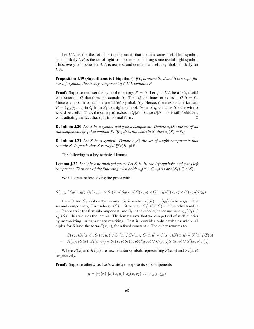
Let UL denote the set of left components that contain some useful left symbol,and similarly UR is the set of right components containing some useful right symbol.Thus, every component in UL is useless, and contains a useful symbol; similarly forUR.

Proposition J.19 (Superfluous is Ubiquitous) IfQ is normalized and S is a superflu-ous left symbol, then every component q ∈ UL contains S.

Proof: Suppose not: set the symbol to empty, S = 0. Let q ∈ UL be a left, usefulcomponent in Q that does not contain S. Then Q continues to exists in Q[S = 0].Since q ∈ UL, it contains a useful left symbol, S1. Hence, there exists a strict pathP = (q1, q2, . . .) in Q from S1 to a right symbol. None of qi contains S, otherwise Swould be useful. Thus, the same path exists inQ[S = 0], soQ[S = 0] is still forbidden,contradicting the fact that Q is in normal form. 2

Definition J.20 Let S be a symbol and q be a component. Denote sq(S) the set of allsubcomponents of q that contain S. (If q does not contain S, then sq(S) = ∅.)

Definition J.21 Let S be a symbol. Denote c(S) the set of useful components thatcontain S. In particular, S is useful iff c(S) 6= ∅.

The following is a key technical lemma.

Lemma J.22 LetQ be a normalized query. Let S, S1 be two left symbols, and q any leftcomponent. Then one of the following must hold: sq(S1) ⊆ sq(S) or c(S1) ⊆ c(S).

We illustrate before giving the proof with:

S(x, y1)S2(x, y1), S1(x, y2) ∨ S1(x, y)S2(x, y)C(x, y) ∨ C(x, y)S′(x, y) ∨ S′(x, y)T (y)

Here S and S1 violate the lemma. S1 is useful, c(S1) = {q2} (where q2 = thesecond component), S is useless, c(S) = ∅, hence c(S1) 6⊆ c(S). On the other hand inq1, S appears in the first subcomponent, and S1 in the second, hence we have sq1(S1) 6⊆sq1(S). This violates the lemma. The lemma says that we can get rid of such queriesby normalizing, using a unary rewriting. That is, consider only databases where alltuples for S have the form S(x, c), for a fixed constant c. The query rewrites to:

S(x, c)S2(x, c), S1(x, y2) ∨ S1(x, y)S2(x, y)C(x, y) ∨ C(x, y)S′(x, y) ∨ S′(x, y)T (y)≡ R(x), R2(x), S1(x, y2) ∨ S1(x, y)S2(x, y)C(x, y) ∨ C(x, y)S′(x, y) ∨ S′(x, y)T (y)

WhereR(x) andR2(x) are new relation symbols representing S(x, c) and S2(x, c)respectively.

Proof: Suppose otherwise. Let’s write q to expose its subcomponents:

q = [s0(x), ]s1(x, y1), s2(x, y2), . . . , sk(x, yk)

68

q may, or may not have unary symbols, hence s0(x) is optional. By assumption thereexists a component si in q that contains S1(x, yi) but does not contain S. (It is pos-sible that q does not contain S at all.) Also, since c(S1) 6⊆ c(S), there exists a strictLR-path P = (q1, q2, . . . , qn) s.t. q1 contains S1 but does not contain S. Performa left unary rewriting with m constants, followed by the empty rewriting S = 0.This means that, for each binary symbol S′(x, y) we create k fresh unary symbolsS′(x, c1), . . . , S′(x, ck), and rewrite the query by replacing each subcomponent s(x, y)with s(x, y) ∨ s(x, c1) ∨ . . . ∨ s(x, ck): then we rewrite the query in DNF, minimize,then substitute S(x, y) with empty, S = 0. Thus, Q⇒ Q′. Let’s examine the structureof the resulting query Q′:

• Each component r in Q that does not contain S is also in Q′. This is because,when we expand in DNF, one of the components contains exactly all the orig-inal subcomponents s(x, y) in r. (On the other hand if r contains S, then thesubcomponents that contain S no longer exists after rewriting; only their unaryrewritings s(x, ci) survive.) In particular, the strict LR-path P continues to existsin Q′, since it doesn’t contain S.

• From the component q, we obtain the following component q′ (among others):[s0], s′1, s

′2, . . . , s

′k, where s′i is si(x, y) if si does not contain S, and is si(x, ci)

if it contains S. In other words, we provide each subcomponent containing Swith a fresh constant, and leave other subcomponents untouched. Notice thatat least one subcomponent containing S1(x, y) remains (since by assumptionsq(S1) 6⊆ sq(S)), and therefore this is still a left component. It remains to checkthat it is not redundant. This follows from the fact that we have chosen enoughconstants c1, . . . , ck: if there exists a homomorphism h : r′ → q′, then, byrenaming the constants ci to variables yi we obtain a homomorphism h : r → q,contradicting the fact that Q was minimal.

Thus, the new query Q′ is still forbidden, because the same path P is still a strictLR-path, contradicting the fact that Q was normalized. 2

Since this is the most difficult lemma involving rewritings, we illustrate with a fewexamples. By a unary rewriting for S we mean a unary rewriting, followed by S = 0.

Example J.23 Consider:

Q = S(x, y1)S1(x, y2) ∨ S(x, y1)S2(x, y2) ∨ S1(x, y)S2(x, y)C(x, y) . . .

The left unary rewriting for S is:

Q → (S(x, y1) ∨ S(x, c))(S1(x, y2) ∨ S1(x, c))∨(S(x, y1) ∨ S(x, c))(S2(x, y2) ∨ S2(x, c))∨S1(x, y)S2(x, y)C(x, y) . . .

→ S(x, c), S1(x, y2) ∨ S(x, c), S1(x, c) ∨ S(x, c), S2(x, y2) ∨ S(x, c), S2(x, c) ∨ . . .= R(x), S1(x, y) ∨R(x), R1(x) ∨R(x), S2(x, y) ∨R(x), R2(x) ∨ . . .

69

In the first step we replaced every symbol Si(x, y) with Si(x, y) ∨ Si(x, c). Noticethat there is no C(x, c): by definition of the unary rewriting only the left symbols arerewritten. (Thus, the definition only makes sense if no symbol is both left and right.) Inthe second step we made S(x, y) = 0. The last line replaces every Si(x, c) with unarysymbols Ri(x).

The important thing to see here is that we have started with the left componentS(x, y1)S1(x, y2) and rewritten it into a left component R(x)S1(x, y), and eliminatedcompletely the binary symbol S(x, y). The query above further reduces, by settingR1 = 0.

Example J.24 This shows why we need more constants. Consider a query with twoleft components:

Q = S(x, y1)S1(x, y1), S(x, y2)S2(x, y2)S3(x, y2), S4(x, y3) ∨ /∗q∗/S(x, y1)S1(x, y1)S2(x, y1), S(x, y2), S3(x, y2) /∗q′∗/. . .

Suppose we do a unary rewriting for S. If we use a single constant c, then the firstcomponent q rewrites to:

Q′ = S(x, c)S1(x, c), S2(x, c), S3(x, c), S4(x, y3) ∨ /∗q∗/S(x, c)S1(x, c)S2(x, c), S(x, c), S3(x, c) /∗q′∗/

The problem is that now q is redudant: there exists a homomorphism from thesecond component. However, if we use two constants c1, c2 (since there are two occur-rences of S in q) then one of the rewritings of q is:

Q′ = S(x, c1)S1(x, c1), S(x, c2), S2(x, c2), S3(x, c2), S4(x, y3) ∨S(x, c1)S1(x, c1)S2(x, c1), S(x, c2), S3(x, c2) ∨ . . .

(each component must contain all four combinations c1c1, c1c2, c2c1, c2c2; only c1c2is shown). Each of the two components shown above is isomorphic to their image inQ,up to remaining of c1, c2 as y1, y2. Therefore no new homomorphisms are introduced,and both are non-redudnat.

Example J.25 This shows that the unary rewriting for q may wipe out some othersymbol S1:

q = S(x, y1)S1(x, y1), S2(x, y2)

After the unary rewriting for S, the component becomes:

q′ = S(x, c)S1(x, c), S2(x, y2)

70

That is, we lost S1(x, y). This may be important, if S1 is the only link to the right side.This is why in the lemma we only do a unary rewriting for S when we know that thereexists a useful symbol S1 s.t. sq(S1) 6⊆ sq(S). In this example sq(S1) = sq(S), andwe cannot apply the rewriting.

Intuitively, Lemma J.22 implies that, if S is supefluous (i.e. c(S) = ∅), then sq(S)must be very big. We make this precise.

Definition J.26 Call a binary left S symbol ubiquitous if, for every q ∈ UL and everybinary subcomponent s of q, s contains S. That is, sq(S) is the set of all binarysubcomponents of q. Similarly for right ubiquitous symbols.

For an illustration, consider the query K in Example J.17: the symbol S is ubiqui-tous because it occurs in both subcomponents of S(x, y1)S1(x, y1)S(x, y2)S2(x, y2).

Corollary J.27 If Q is in normal form, then all superfluous symbols are ubiquitous.

Proof: Let S be a superfluous symbol. For any useful symbol S1 we have c(S) = ∅and c(S1) 6= ∅, which implies c(S1) 6⊆ c(S). Thus, by Lemma J.22, for any leftcomponent q ∈ UL we have sq(S1) ⊆ sq(S). Let:

sq(∗) =⋃{sq(S1) | S1 is useful }

Thus, sq(∗) is the set of all subcomponents in q that contain some useful symbol.For every superfluous symbol S, sq(∗) ⊆ sq(S) because sq(S1) ⊆ sq(S) for anyuseful symbol S1. Supose S is a superfluous symbol that is not ubiquituous, i.e. thereexists a left component q ∈ UL s.t. sq(S) is not the set of all binary subcomponents;let si be a binary subcomponent s.t. si 6∈ sq(S). Then si 6∈ sq(∗), hence si consistsonly of binary, superfluous symbols S′. Since q ∈ UL it contains some useful symbolS1; let sj be a subcomponent that contains S1. In addition, sj contains all superfluoussymbols S′, because sq(S1) ⊆ sq(S′). This implies that there exists a homomorphismssi → sj , contradicting the fact that Q is minimized. 2

Corollary J.28 If Q is in normal form then every left component contains a usefulsymbol. In other words, every left component is in UL.

Proof: Otherwise some left component q contains only supefluous components. Letq1 be any component in UL. We prove that there exists a homomorphism q → q1,contradicting the fact that Q is minimal. Consider first any unary symbol R in q. SinceR is superfluous (all unary symbols are superfluous), it follows that R occurs in allcomponent in UL: thus, R is in q1. Consider a binary symbol S in q. Since S issuperfluous (by assumption), it is ubiquitous, hence it occurs in all binary componentsof q1. Therefore there exists a homomorphism q → q1. 2

The converse to Corollary J.27 fails in general. For example in:

H3 = R(x), S1(x, y) ∨ S1(x, y), S2(x, y) ∨ S2(x, y), S3(x, y) ∨ S3(x, y), T (y)

S1 is both ubiquitous and useful. However, the converse does hold under a restriction:

71

Corollary J.29 If Q is in normal form and has at least one non-ubiquitous binarysymbol, then all left ubiquitous symbols are superfluous.

Proof: Let S be a left ubiquitous symbol, and consider the rewriting S = 1. We provethat the resulting query Q[S = 1] is also forbidden. First, we show that every leftcomponent q remains non-redundant after the rewriting: this is because every homo-morphism h : r[S = 1] → q[S = 1] extends to a homomorphism h : r → q, becauseS appears in all binary subcomponents of q. Also, q[S = 1] continues to be a leftcomponent (i.e. doesn’t become a central component), because it has exactly the samenumber of subcomponents as q. Next, assuming S is useful, consider any strict LRpath P = (q1, q2, . . .) where q1 contains S. Let S1 be any non-ubiquitous binary sym-bol. (There exists at least, by the assumption of the corollary.) Since sq(S) 6⊆ sq(S1)for any left query q, we have c(S) ⊆ c(S1), hence S1 occurs in q1. Thus, the pathP is also a path from S1 to the right, so if we show that all components in P remainin Q[S = 1] then we have proven that Q[S = 1] is a forbidden query. Suppose thereexists a homomorphism h : r[S = 1] → qi[S = 1]. Clearly r must contain S. Thereare two cases. Case 1: i > 1 then qi contains only central or right symbols: thereforeall symbols in r[S = 1] must be center symbols (since S doesn’t co-occur with a rightsymbol). r cannot be a left component, because then r[S = 1] contains at least oneleft symbol, so r must be a central component. r is also a useful component, becausethe path r, qi, qi+1, . . . is a strict, LR path connecting the left symbol S to the right.Thus, r ∈ c(S), hence it also contains S1, which is a contradiction because qi does notcontain S1. Consider case 2, i = 1. Then q1 contains S, and we can extend the homo-morphism r[S = 1] → q1[S = 1] to a homomorphism r → q1. Thus, we have proventhatQ[S = 1] is also a forbidden query, contradicting the fact that it was normalized. 2

J.3 Classification of Forbidden QueriesIn addition to the properties of normal queries described so far, we give now a clas-sification of their endpoings. We show that their left end is of one of two types, andsimilarly their right end; thus, there are four types of forbidden queries.

Definition J.30 (Type 1) If Q has a left unary symbol R, then we say that its left endis of Type 1. Similarly for the right end.

Theorem J.31 Suppose Q is in normal form and has the left-end of type 1. Then thefollowing hold:

• Q has exactly one left unary symbol.

• Every left binary symbol is useful.

• Every left component has exactly two variables x, y.

Similarly for a right-end of Type 1.

The second item is stronger than Corollary J.28.

72

Definition J.32 (Type 2) If Q has no left unary symbols, then we say that its left endis of Type 2. Similarly for the right end.

Theorem J.33 Suppose Q is in normal form and has the left-end of type 2. Then thefollowing hold:

• There exists q such that q ∈ c(S1) for all left useful symbols S1.

• There exists at least one superfluous symbol S.

Similarly for the right.

Thus, there are for types of normalized forbidden queries: 1-1, 1-2, 2-1, or 2-2.In the rest of the section we prove the two theorems, through a sequence of lemmas.

Lemma J.34 If Q is in normal form and the left end is of Type 1, then it has exactlyone unary symbol R.

Proof: Let R1, R2, . . . , Rm be all left unary symbols, m ≥ 1 (because the query is ofType 1). Since all area superfluous, every component q ∈ UL contains all symbols Ri(Prop. J.19). Suppose m > 1. Then choose any symbol Rj and rewrite Q by makingRj deterministic: Rj = 1. No component becomes redundant, hence the new query isstill forbidden, contradicting the assumption that Q was normalized. 2

Next, we show that Q has no superfluous left binary symbols. For example:

R(x), S(x, y), S1(x, y) ∨ S1(x, y), C(x, y) ∨ . . .

contains the superfluous left symbol S: simply set S = 1 and we remove it. On theother hand, consider:

R(x), S(x, y), S1(x, y) ∨ S(x, y), S1(x, y), D(x, y) ∨ S1(x, y), D(x, y), C(x, y)∨C(x, y), S′1(x, y) ∨ S′1(x, y), T (y)

Here S is still superfluous, but we cannot set S = 1 because we make the S1DCcomponent redundant, disconnecting the left from the right. Instead, we set S1 = 1:now S becomes a useful symbol.

Lemma J.35 IfQ is in normal form and the left end is of Type 1, then every left symbolS is useful.

Proof: Let S1 be any useful left symbol, and consider a strict LR-path P from S1 to aright symbol, P = (q1, q2, . . .). Let S be a binary, left superfluous symbol; by Corol-lary J.27 it, is ubiquitous, i.e. occurs in all binary subcomponents of all components inUL.

Define R the set of all components r with the following properties: r contains Sand there exists a homomorphism h : r[S = 1] → q1 (the first component in P ). Weconsider two cases.

73

First, R = ∅. Then rewrite Q by setting S = 1. None of the components onthe path P becomes redundant in Q[S = 1]: indeed if there exists a homomorphismr[S = 1]→ qi then we must have i ≥ 2. Then r cannot be a left component, because itwould contain the symbol R(x). Hence r is a central component. Moreover, r[S = 1]consists only of central symbols, because it maps to qi and i ≥ 2: but in that case(r, qi, qi+1, . . .) is an LR path from S to a right symbol contradicting the assumptionthat S is superfluous. Thus, the path P continues to exists in Q[S = 1]. Let q ∈ ULbe a left component containing S1. Since S is ubiquitous, q[S = 1] is not redundantbecause any homomorphism q′[S = 1]→ q[S = 1] extends to q′ → q, and is still a leftcomponent (contains the left unary symbol R(x), and also S1(x, y)). Thus, Q[S = 1]still has the strict LR path P .

Second, suppose R 6= ∅. Rewrite Q by setting S1 = 1: we prove that in Q[S1 = 1]there exists a LR path from the left symbol S to a right symbol, contradicting the factthat Q is normalized. At least one component r[S1 = 1] for r ∈ R is not redundant.This is because any homomorphism r′[S1 = 1]→ r[S1 = 1] implies a homomorphismr′[S1 = 1, S = 1] → r[S1 = 1, S = 1] → q1[S1 = 1] (since, by definition, thereexists a homomorphism r[S = 1] → q1), which can be extended to a homomorphismr′[S = 1] → q1, meaning r′ ∈ R. Thus, any component in R that becomes redundantdoes so because of some other component also in R, and at least one r[S1 = 1] willremain non-redundant inQ[S1 = 1], for some r ∈ R. Obviously q1[S1 = 1] also existsin Q[S1 = 1], because q1 already contains S1 and cannot become redundant by settingit to 1. Thus, in Q[S1 = 1] we have a path from S to a right symbol.

It remains to prove S is a left symbol in Q[S1 = 1], and for that we will showthat at least one component q ∈ UL remains in Q[S1 = 1], i.e. it does not becomeredundant. Then, q[S1 = 1] still contains the symbol S (since it is ubiquitous), andalso contains the unary symbolR, and hence it is a left component. To prove the claim,denote UL(S1) the set of components in UL that contain the symbol S1. We will showthat, for every q ∈ UL(S1) if there exists a homomorphism r[S1 = 1] → q[S1 =1], then r ∈ UL(S1): this immediately implies that at least one q[S1 = 1] remainsnonredundant. Indeed, suppose r 6∈ UL(S1). Clearly r contains S1 (otherwise we geta homomorphism r → q), hence the only possibility is for r to be a central component.It cannot have any central symbols (since q doesn’t have central symbols), and it is asingle subcomponent: r = S1(x, y), S2(x, y), S3(x, y) . . . The homomorphism mustmap r[S1 = 1] to a single subcomponent of q, that contains S2, S3, . . . but does notcontain S1 (otherwise we have a homomorphism r → q). Fix i ≥ 2. We have sq(S1) 6⊆sq(Si) and sq(Si) 6⊆ sq(S1). By Lemma J.22 c(S1) = c(Si); furthermore, this holdsfor any i. In this case, however, every starting point q1 of a LR path from S1 to aright symbol is redundant: indeed, q1 ∈ c(S1) = c(S2) = . . ., hence q1 contains allsymbols S2, S3, . . ., hence there exists a homomrphism r → q1, contradicting that Qis minimal. 2

Lemma J.36 If Q is in normal form and the left end is of Type 1, then all left compo-nents have exactly two variables x, y.

Proof: Recall that all left components are in UL (Corollary J.28). Let q0 ∈ UL vio-late our condition. Thus q0 = R(x), s1(x, y1), . . . , sk(x, yk), with k ≥ 2. Consider

74

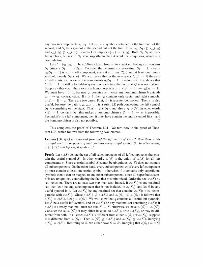
any two subcomponents s1, s2. Let S1 be a symbol contained in the first but not thesecond, and S2 be a symbol in the second but not the first. Thus, sq0(S1) 6⊆ sq0(S2)and sq0(S2) 6⊆ sq0(S1); Lemma J.22 implies c(S1) = c(S2). Both S1, S2 are use-ful symbols, because if S1 were superfluous then it would be ubiquitous, which is acontradiction.

Let P = (q1, q2, . . .) be aLR-strict path from S1 to a right symbol; q1 also containsS2 (since c(S1) = c(S2)). Consider the deterministic rewriting, S1 = 1: clearlyq0[S1 = 1] is still a left component, since it still has R(x) and at least one binarysymbol, namely S2(x, y). We will prove that in the new query Q[S1 = 1] the pathP still exists, i.e. none of the components qi[S1 = 1] is redundant: this shows thatQ[S1 = 1] is still a forbidden query, contradicting the fact that Q was normalized.Suppose otherwise: there exists a homomorphism h : r[S1 = 1] → qi[S1 = 1].We must have i > 1, because q1 contains S1, hence any homomorphism h extendsto r → q1, contradiction. If i > 1, then qi contains only center and right symbols,qi[S1 = 1] = qi. There are two cases. First, if r is a center component. Then r is alsouseful, because the path r, qi, qi+1, . . . is a strict LR path connecting the left symbolS1 to something on the right. Thus, r ∈ c(S1), and also r ∈ c(S2), in other wordsr[S1 = 1] contains S2: this makes a homomorphism r[S1 = 1] → qi impossible.Second, if r is a left component, then it must have contain the unary symbol R(x), andthe homomorphism is also not possible. 2

This completes the proof of Theorem J.31. We turn now to the proof of Theo-rem J.33, which follows from the following two lemmas.

Lemma J.37 If Q is in normal form and the left end is of Type 2, then there existsa useful central component q that contains every useful symbol S. In other words,q ∈ c(S) forall left useful symbols S.

Proof: Let s∗(S) denote the set of all subcomponents of all left components that con-tain the useful symbol S. In other words, s∗(S) is the union of sq(S) for all leftcomponents q. Since a useful symbol S cannot be ubiquitous, s∗(S) does not containall subcomponents. On the other hand, every subcomponent s (of every left componentq) must contain at least one useful symbol: otherwise, if it contains only superfluoussymbols then it can be mapped to any other subcomponent, since all superfluous sym-bols are ubiquitous, contradicting the fact that q is minimized. Order the sets s∗(S) byset inclusion. There are at least two maximal sets. Indeed, if s∗(S1) is any maximalset, then let s be any subcomponent that is not included in s∗(S1), and let S be anyuseful symbol in s. Let s∗(S2) be any maximal set that contains s∗(S): it is incom-parable with s∗(S1). Since s∗(S1) 6⊆ s∗(S2) and s∗(S2) 6⊆ s∗(S1) it follows thatc(S1) = c(S2). Let q ∈ c(S1). We will show that q contains all useful left symbols.Let S be a useful left symbol, and let s∗(S′) be any maximal set containing s∗(S): ifs∗(S) is already maximal, then we take S′ = S, otherwise we have s∗(S) ⊂ s∗(S′).Consider the set s∗(S′): it may either be equal to s∗(S1), or to s∗(S2), or may be dif-ferent from both. In all cases s∗(S′) is different from either s∗(S1) or s∗(S2): supposeit is different from s∗(S1). Then s∗(S′) 6⊆ s∗(S1) and s∗(S1) 6⊆ s∗(S′), implyingc(S1) = c(S′). Returning to S, we either have S = S′, implying that c(S1) = c(S)

75

hence q contains S, or s∗(S) ⊂ s∗(S1), implying c(S1) ⊆ c(S), and we also concludethat q contains S. 2

Lemma J.38 If Q is in normal form and the left end is of Type 2, then there exists atleast one superfluous symbol S.

Proof: Indeed, let q be the component given by the previous lemma, i.e. q ∈ c(S1)forall left useful symbols S1. In other words, q contains all left useful symbols S1. Letq0 be any left component with a useful symbol. If q0 contains no superfluous symbols,then there exists a homomorphism q0 → q, contradicting the fact that Q is minimal.This proves the third item. 2

K Part 3 of the Proof: AlgorithmLet Q be a forbidden query. We assume throughout this section that Q is minimized,long, and normalized. We describe in this section PTIME algorithm for the m1,m2-Signature-Counting problem with an oracle for computingP (Q) over tuple-independentdatabases. Here m1,m2 ≥ 2 and depende on the query Q.

K.1 The LabelsWe define two sets of labels LL and RR for the left end, and for the right end of Q.

Definition K.1 If the left end of Q is of Type 1, then LL = {τ1, τ2}, where τ1, τ2 arethe following queries:

τ1 = ¬R(x)τ2 = R(x)

Here R is the unique left unary symbol in Q.Similarly, if the right end of Q is of Type 1, then RR = {τ1, τ2} where:

τ1 = ¬T (x)τ2 = T (x)

Here T is the unique right unary symbol in Q.

Assume that the left end of Q is of type 2. Call a pre-label a disjunction of con-junctive queries of the form S1(x, y), S2(x, y), . . . , Sk(x, y), for k ≥ 1.

Definition K.2 Let Q have a left end of Type 2, and let UL = {q1, . . . , qk}. Let a bea constant. The base labels are the prelabels τ1, . . . , τm1 such that:

τ1[a/x] ∧ . . . ∧ τm1 [a/x] ≡ q1[a/x] ∨ . . . ∨ qk[a/x]

and the CNF expression above is not redundant. The set LL is defined as the closureunder ∨ of all base labels.

76

In particular, it follows that for any left component q ∈ UL and every left labelτ ∈ LL, q ⇒ τ .

Example K.3 We illustrate here by showing only the left components of Q. Considerfirst a query with one left component:

Q = S(x, y1)S1(x, y1), S(x, y2)S2(x, y2), S(x, y3)S3(x, y3) ∨ . . .The labels are:

τ1 = S(x, y), S1(x, y)τ2 = S(x, y), S2(x, y)τ3 = S(x, y), S3(x, y)

and their closure under disjunctions. Thus, LL has 7 elements.Consider a query with two left components:

Q = S(x, y1), S1(x, y1), S(x, y2), S2(x, y2) ∨S(x, y1), S1(x, y1), S(x, y3), S3(x, y3) ∨ . . .

The labels are:

τ1 = S(x, y), S1(x, y)τ2 = S(x, y), S2(x, y) ∨ S(x, y), S3(x, y)

and τ1 ∨ τ2. Thus, LL has 3 elements.

Thus, for every query Q we have two sets of labels LL and RR. Denote m1 =|LL|, m2 = |RR|. It should be clear that m1 ≥ 2 and m2 ≥ 2.

K.2 The Expansion FormulaFor a left label τ1 ∈ LL and constant a ∈ X , denote τ [a/x] the query obtained bysubstituting xwith the constant a. Its negation, ¬τ [a/x], is a formula that is universallyquantified in the variable y. Similarly we denote τ [b/y] when τ ∈ RR and b ∈ Y .

Lemma K.4 Let W be a world (i.e. a deterministic database) s.t. Q is false on W .Then, for every constant in its active domain, a ∈ Adom(W ) there exists a labelτ ∈ LL s.t. τ [a/x] is false on W . In notation:

W |= ¬Q ⇒ ∀a ∈ Adom(W )∃τ ∈ LL : W |= ¬τ [a/x]

Proof: If Q’s left end is of type 1, then the lemma is trivial: for every a ∈ W eitherR(a) is false or ¬R(a) is false. Suppose Q’s left end is of type 2. We proof bycontradiction. If the statement is false, then for each i = 1, . . . ,m1 there exists aconstant bi s.t. W |= τi[a/x, bi/y]. In other words:

W |=∧

i=1,m1

τi[a/x]

hence W |= ∨q∈UL q[a/x]. But this implies W |= Q, contradiction. 2

77

We write W (a, b) to denote a deterministic structure with two distinguished con-stants, s.t. W (a, b) does not share any constants other than a, b with other structures.When we don’t care naming b, then we write W (a, ∗); similarly W (∗, b).

If the left end of Q is of Type 1, then a label τ ∈ LL is either ¬R(x) or R(x).Define ετ ∈ {0, 1} as follows:

ε¬R(x) = 0εR(x) = 1

Recall that Q[R = 0] means the query Q obtained by setting R(x) ≡ false; andQ[R = 1] means the query Q obtained by setting R(x) ≡ true. Thus, (τ [a/x] ∨Q)[R = ¬ετ ] is equivalent to Q[R = ¬ετ ], because τ [a/b] is false after the sub-stitution R(a) = ¬ετ . On the other hand if the left end of Q is of Type 2, then(τ [a/x] ∨ Q)[R = ¬ετ ] simply denotes τ [a/x] ∨ Q, since in this case there is nosymbol R. Similarly for the right end.

For fixed a ∈ X, b ∈ Y , define the following queries:

Qa,bτ1,τ2 = (τ1[a/x] ∨Q ∨ τ2[b/y])[R = ¬ετ1 , T = ¬ετ2 ]Qaτ1,∗ = (τ1[a/x] ∨Q)[R = ¬ετ1 ]

Qb∗,τ2 = (Q ∨ τ2[b/y])[T = ¬ετ2 ]

Fix an instance of the m1,m2-SC problem: Φ = (X,Y,E), where X = {ai |i = 1, n1}, Y = {bj | j = 1, n2}, E ⊆ X × Y , |E| = n. The type of the signature tobe the same as the type of the left and right endings of the query (i.e. type 1,1 or 1,2 or2,1 or 2,2). (See Sec. G for the definitions.)

We associate to Φ a probabilistic database D that is the union of three types ofblocks:

• One block D(a, b) for each edge (a, b) ∈ E.

• If Q’s left end is of type 2, then one block D(a, ∗) for each node a ∈ X .

• If Q’s right end is of type 2, then one block D(∗, b) for each node b ∈ Y .

• If the left end is of type 1, then we set p(R(a)) = 1/2 forall a ∈ X ∪ {∗}• If the right end is of type 1, then we set p(T (b)) = 1/2 forall b ∈ Y ∪ {∗}.

Blocks do not share any constants, except the constants in X and Y . All blocksD(a, b) isomorphic; all blocks D(a, ∗) are isomorphic; all blocks D(∗, b) are isomor-phic. All probabilities other than those of the unary tuples are left unspecified: wewill set them later. However, we require the tuple probabilities to be preserved by theisomorphisms: that is, we only need to specify the probabilities for one block D(a, b),one block D(a, ∗), and one block D(∗, b); the probabilities in all other blocks will beequal.

78

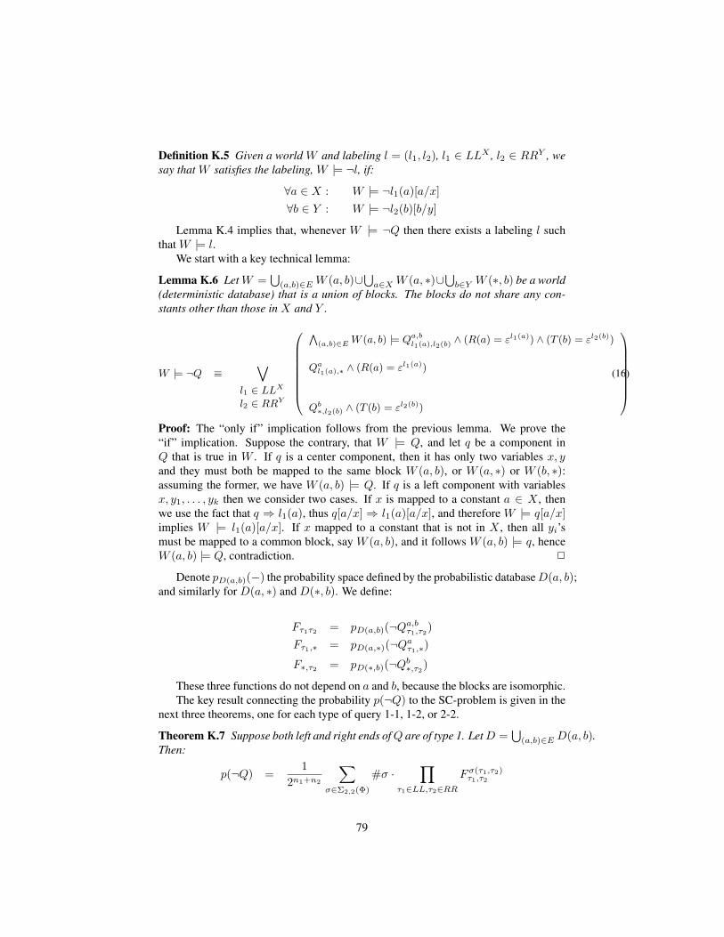
Definition K.5 Given a world W and labeling l = (l1, l2), l1 ∈ LLX , l2 ∈ RRY , wesay that W satisfies the labeling, W |= ¬l, if:

∀a ∈ X : W |= ¬l1(a)[a/x]∀b ∈ Y : W |= ¬l2(b)[b/y]

Lemma K.4 implies that, whenever W |= ¬Q then there exists a labeling l suchthat W |= l.

We start with a key technical lemma:

Lemma K.6 LetW =⋃

(a,b)∈EW (a, b)∪⋃a∈XW (a, ∗)∪⋃b∈Y W (∗, b) be a world(deterministic database) that is a union of blocks. The blocks do not share any con-stants other than those in X and Y .

W |= ¬Q ≡_

l1 ∈ LLXl2 ∈ RRY

0BBBBBBB@

V(a,b)∈EW (a, b) |= Qa,bl1(a),l2(b) ∧ (R(a) = εl1(a)) ∧ (T (b) = εl2(b))

Qal1(a),∗ ∧ (R(a) = εl1(a))

Qb∗,l2(b) ∧ (T (b) = εl2(b))

1CCCCCCCA(16)

Proof: The “only if” implication follows from the previous lemma. We prove the“if” implication. Suppose the contrary, that W |= Q, and let q be a component inQ that is true in W . If q is a center component, then it has only two variables x, yand they must both be mapped to the same block W (a, b), or W (a, ∗) or W (b, ∗):assuming the former, we have W (a, b) |= Q. If q is a left component with variablesx, y1, . . . , yk then we consider two cases. If x is mapped to a constant a ∈ X , thenwe use the fact that q ⇒ l1(a), thus q[a/x] ⇒ l1(a)[a/x], and therefore W |= q[a/x]implies W |= l1(a)[a/x]. If x mapped to a constant that is not in X , then all yi’smust be mapped to a common block, say W (a, b), and it follows W (a, b) |= q, henceW (a, b) |= Q, contradiction. 2

Denote pD(a,b)(−) the probability space defined by the probabilistic databaseD(a, b);and similarly for D(a, ∗) and D(∗, b). We define:

Fτ1τ2 = pD(a,b)(¬Qa,bτ1,τ2)Fτ1,∗ = pD(a,∗)(¬Qaτ1,∗)F∗,τ2 = pD(∗,b)(¬Qb∗,τ2)

These three functions do not depend on a and b, because the blocks are isomorphic.The key result connecting the probability p(¬Q) to the SC-problem is given in the

next three theorems, one for each type of query 1-1, 1-2, or 2-2.

Theorem K.7 Suppose both left and right ends ofQ are of type 1. LetD =⋃

(a,b)∈E D(a, b).Then:

p(¬Q) =1

2n1+n2

∑σ∈Σ2,2(Φ)

#σ ·∏

τ1∈LL,τ2∈RRFσ(τ1,τ2)τ1,τ2

79

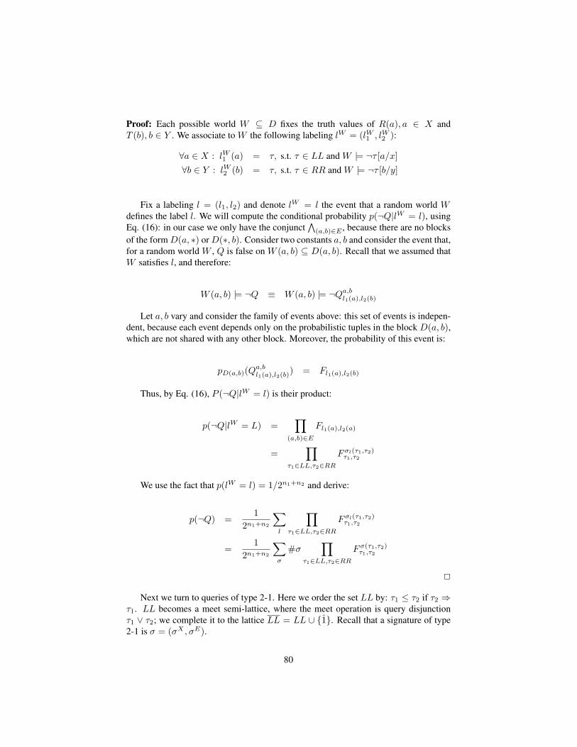
Proof: Each possible world W ⊆ D fixes the truth values of R(a), a ∈ X andT (b), b ∈ Y . We associate to W the following labeling lW = (lW1 , lW2 ):

∀a ∈ X : lW1 (a) = τ, s.t. τ ∈ LL and W |= ¬τ [a/x]∀b ∈ Y : lW2 (b) = τ, s.t. τ ∈ RR and W |= ¬τ [b/y]

Fix a labeling l = (l1, l2) and denote lW = l the event that a random world Wdefines the label l. We will compute the conditional probability p(¬Q|lW = l), usingEq. (16): in our case we only have the conjunct

∧(a,b)∈E , because there are no blocks

of the formD(a, ∗) orD(∗, b). Consider two constants a, b and consider the event that,for a random world W , Q is false on W (a, b) ⊆ D(a, b). Recall that we assumed thatW satisfies l, and therefore:

W (a, b) |= ¬Q ≡ W (a, b) |= ¬Qa,bl1(a),l2(b)

Let a, b vary and consider the family of events above: this set of events is indepen-dent, because each event depends only on the probabilistic tuples in the block D(a, b),which are not shared with any other block. Moreover, the probability of this event is:

pD(a,b)(Qa,bl1(a),l2(b)) = Fl1(a),l2(b)

Thus, by Eq. (16), P (¬Q|lW = l) is their product:

p(¬Q|lW = L) =∏

(a,b)∈E

Fl1(a),l2(a)

=∏

τ1∈LL,τ2∈RRFσl(τ1,τ2)τ1,τ2

We use the fact that p(lW = l) = 1/2n1+n2 and derive:

p(¬Q) =1

2n1+n2

∑l

∏τ1∈LL,τ2∈RR

Fσl(τ1,τ2)τ1,τ2

=1

2n1+n2

∑σ

#σ∏

τ1∈LL,τ2∈RRFσ(τ1,τ2)τ1,τ2

2

Next we turn to queries of type 2-1. Here we order the set LL by: τ1 ≤ τ2 if τ2 ⇒τ1. LL becomes a meet semi-lattice, where the meet operation is query disjunctionτ1 ∨ τ2; we complete it to the lattice LL = LL ∪ {1}. Recall that a signature of type2-1 is σ = (σX , σE).

80

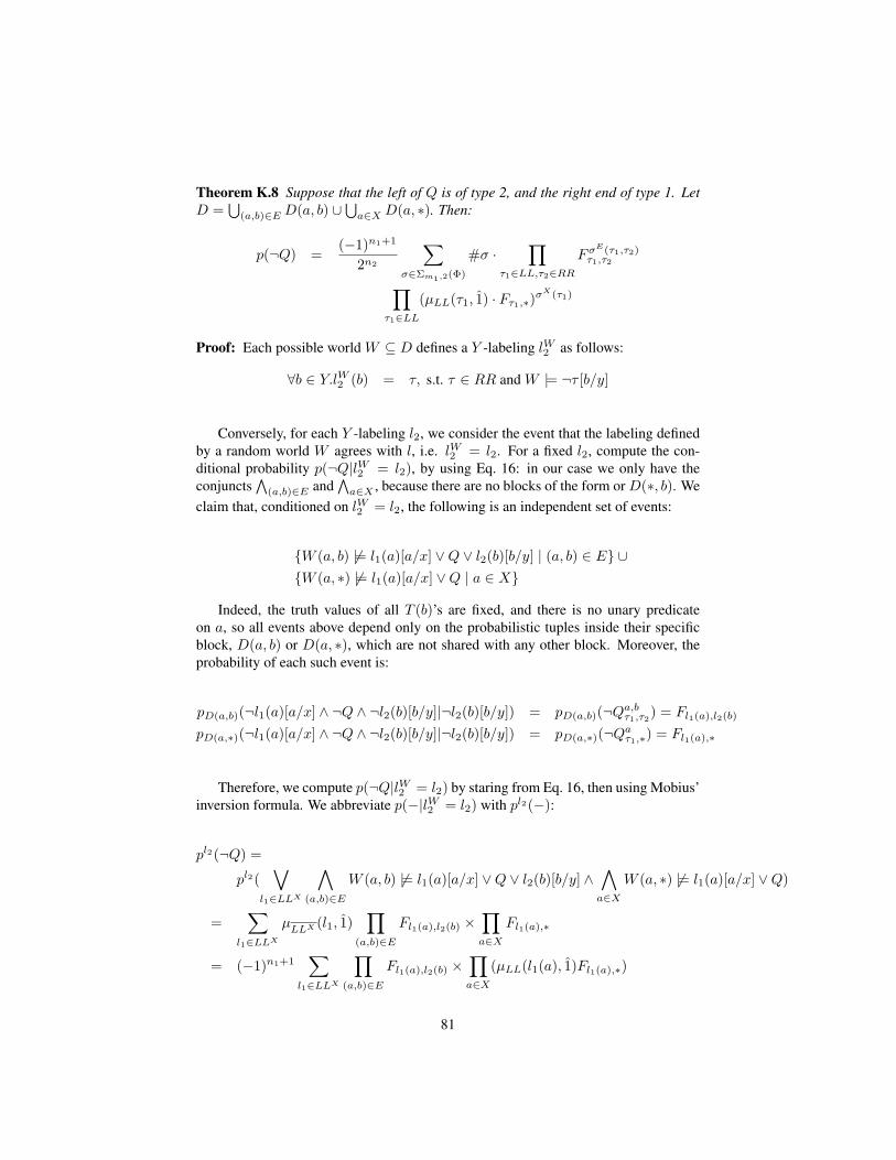
Theorem K.8 Suppose that the left of Q is of type 2, and the right end of type 1. LetD =

⋃(a,b)∈E D(a, b) ∪⋃a∈X D(a, ∗). Then:

p(¬Q) =(−1)n1+1

2n2

∑σ∈Σm1,2(Φ)

#σ ·∏

τ1∈LL,τ2∈RRFσ

E(τ1,τ2)τ1,τ2∏

τ1∈LL(µLL(τ1, 1) · Fτ1,∗)σ

X(τ1)

Proof: Each possible world W ⊆ D defines a Y -labeling lW2 as follows:

∀b ∈ Y.lW2 (b) = τ, s.t. τ ∈ RR and W |= ¬τ [b/y]

Conversely, for each Y -labeling l2, we consider the event that the labeling definedby a random world W agrees with l, i.e. lW2 = l2. For a fixed l2, compute the con-ditional probability p(¬Q|lW2 = l2), by using Eq. 16: in our case we only have theconjuncts

∧(a,b)∈E and

∧a∈X , because there are no blocks of the form or D(∗, b). We

claim that, conditioned on lW2 = l2, the following is an independent set of events:

{W (a, b) 6|= l1(a)[a/x] ∨Q ∨ l2(b)[b/y] | (a, b) ∈ E} ∪{W (a, ∗) 6|= l1(a)[a/x] ∨Q | a ∈ X}

Indeed, the truth values of all T (b)’s are fixed, and there is no unary predicateon a, so all events above depend only on the probabilistic tuples inside their specificblock, D(a, b) or D(a, ∗), which are not shared with any other block. Moreover, theprobability of each such event is:

pD(a,b)(¬l1(a)[a/x] ∧ ¬Q ∧ ¬l2(b)[b/y]|¬l2(b)[b/y]) = pD(a,b)(¬Qa,bτ1,τ2) = Fl1(a),l2(b)

pD(a,∗)(¬l1(a)[a/x] ∧ ¬Q ∧ ¬l2(b)[b/y]|¬l2(b)[b/y]) = pD(a,∗)(¬Qaτ1,∗) = Fl1(a),∗

Therefore, we compute p(¬Q|lW2 = l2) by staring from Eq. 16, then using Mobius’inversion formula. We abbreviate p(−|lW2 = l2) with pl2(−):

pl2(¬Q) =

pl2(∨

l1∈LLX

∧(a,b)∈E

W (a, b) 6|= l1(a)[a/x] ∨Q ∨ l2(b)[b/y] ∧∧a∈X

W (a, ∗) 6|= l1(a)[a/x] ∨Q)

=∑

l1∈LLX

µLLX (l1, 1)

∏(a,b)∈E

Fl1(a),l2(b) ×∏a∈X

Fl1(a),∗

= (−1)n1+1∑

l1∈LLX

∏(a,b)∈E

Fl1(a),l2(b) ×∏a∈X

(µLL(l1(a), 1)Fl1(a),∗)

81

In the last line above we used Lemma A.3, which states that the Mobius functionin the lattice LLX is the product of Mobius functions in the lattice LL. The claim ofthe theorem follows from the fact that p(lW2 = l2) = 1/2n1 . 2

Finally, when both left and right ends are of type 2 then we have:

Theorem K.9 Suppose both that both left and right ends of Q are of type 2. Let D =⋃(a,b)∈E D(a, b) ∪⋃a∈X D(a, ∗) ∪⋃b∈Y D(∗, b). Then:

p(¬Q) = (−1)n1+n2∑

σ∈Σm1,m2 (Φ)

#σ ·∏

τ1∈LL,τ2∈RRFσ

E(τ1,τ2)τ1,τ2∏

τ1∈LL(µLL(τ1, 1) · Fτ1,∗)σ

X(τ1) ·∏

τ2∈RR(µRR(τ2, 1) · F∗,τ1)σ

Y (τ1)

The proof is similar to the previous theorem and omitted.

K.3 Irreducible PolynomialsConsider a positive CNF formula ϕ =

∧i Ci, where each clause Ci = X1 ∨X2 ∨ . . .

is a disjunction of Boolean variables. We assume ϕ is non-redundant, i.e. no clause Ciis contained in any other clause Cj .

Definition K.10 The co-occurrence graph of ϕ is the following: the nodes are theBoolean variables, and there is an (undirected) edge from Xi to Xj if they co-occur ina clause.

Theorem K.11 Let f(x1, . . . , xn) be the multilinear polynomial corresponding to ϕ.Write it as a product of irreducible factors: f = g1g2 . . . gm: each variable xi occursin at most one irreducible (since f is multilinear). Then, forall i, j the variables xi, xjoccur in the same irreducible iff Xi, Xj are connected in the co-occurrence graph.

Proof: Assume Xi, Xj are disconnected in the co-occurrence graph. Hence ϕ =ϕ1 ∧ ϕ2 where ϕ1 contains Xi, ϕ2 contains Xj , and ϕ1, ϕ2 do not share any com-mon variables. Then f = f1f2, where xi occurs in f1 and x2 occurs in f2.

Assume xi, xj occur in different irreducible factors. Write f = f1f2, and let ϕ1, ϕ2

be the (minimal) CNF formulas corresponding to f1 and f2. Obviously ϕ ≡ ϕ1∧ϕ2. 2

The theorem also extends to non-monotone CNF, but in that case there is no notionof “reduced” formula, so stating the theorem requires more care. We don’t need non-monotone CNF.

Let D be a probabilistic database, defining a probability distribution on possibleworlds W ⊆ D.

Definition K.12 The colineage of a query Q =∨i qi over a database D is the follow-

ing CNF formula ϕQD.

82

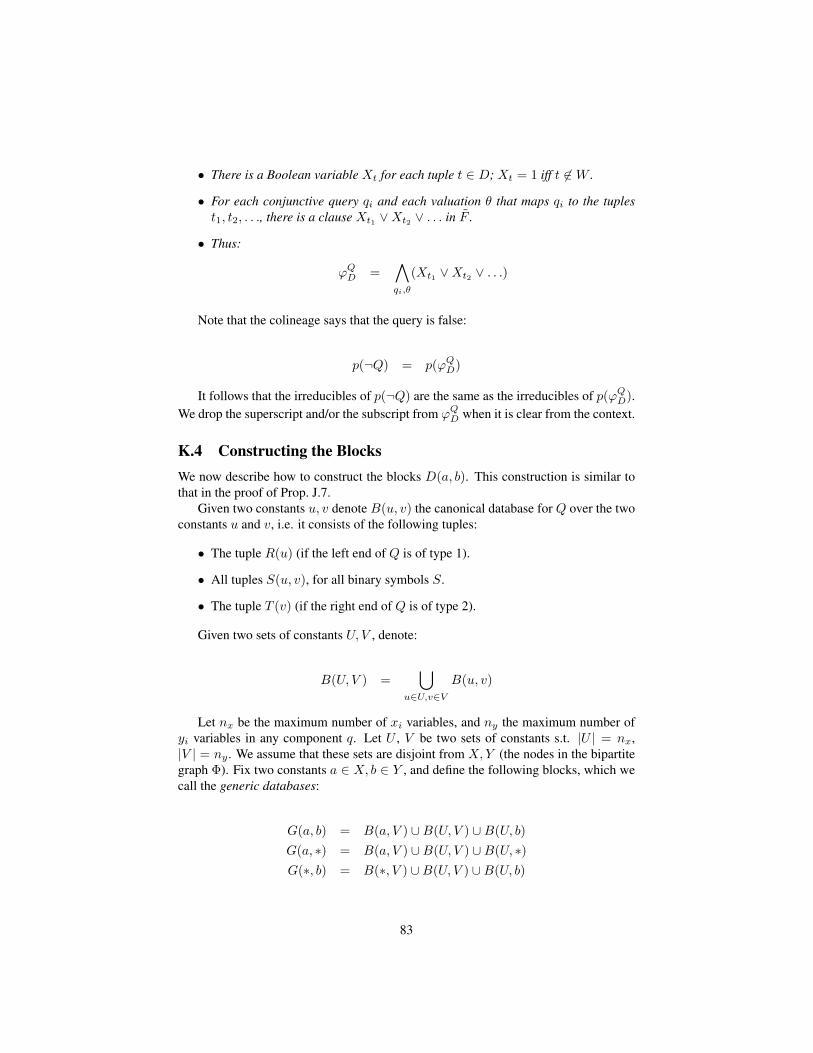
• There is a Boolean variable Xt for each tuple t ∈ D; Xt = 1 iff t 6∈W .

• For each conjunctive query qi and each valuation θ that maps qi to the tuplest1, t2, . . ., there is a clause Xt1 ∨Xt2 ∨ . . . in F .

• Thus:

ϕQD =∧qi,θ

(Xt1 ∨Xt2 ∨ . . .)

Note that the colineage says that the query is false:

p(¬Q) = p(ϕQD)

It follows that the irreducibles of p(¬Q) are the same as the irreducibles of p(ϕQD).We drop the superscript and/or the subscript from ϕQD when it is clear from the context.

K.4 Constructing the BlocksWe now describe how to construct the blocks D(a, b). This construction is similar tothat in the proof of Prop. J.7.

Given two constants u, v denote B(u, v) the canonical database for Q over the twoconstants u and v, i.e. it consists of the following tuples:

• The tuple R(u) (if the left end of Q is of type 1).

• All tuples S(u, v), for all binary symbols S.

• The tuple T (v) (if the right end of Q is of type 2).

Given two sets of constants U, V , denote:

B(U, V ) =⋃

u∈U,v∈VB(u, v)

Let nx be the maximum number of xi variables, and ny the maximum number ofyi variables in any component q. Let U , V be two sets of constants s.t. |U | = nx,|V | = ny . We assume that these sets are disjoint from X,Y (the nodes in the bipartitegraph Φ). Fix two constants a ∈ X, b ∈ Y , and define the following blocks, which wecall the generic databases:

G(a, b) = B(a, V ) ∪B(U, V ) ∪B(U, b)G(a, ∗) = B(a, V ) ∪B(U, V ) ∪B(U, ∗)G(∗, b) = B(∗, V ) ∪B(U, V ) ∪B(U, b)

83

For each tuple in G(a, b) denote x ∈ [0, 1] its probability. Let x denote the proba-bilities of all tuples in G(a, b); we view x as a set of unknowns. Similarly, y, z denotethe probabilities of all tuples in G(a, ∗), G(∗, b). Let:

fτ1,τ2(x) = pG(a,b)(Qa,bτ1,τ2)fτ1,∗(y) = pG(a,b)(Qaτ1,∗)

f∗,τ2(z) = pG(a,b)(Qb∗,τ2)

Let m = m1m2, and define:

• Forall k = 1,m: Dk(a, b) is an isomorphic copy of G(a, b) and xk are its prob-abilities.

• Forall k = 1,m1: Dk(a, ∗) is an isomorphic copy of G(a, ∗) and yk are itsprobabilities.

• Forall k = 1,m2: Dk(∗, b) is an isomorphic copy of G(∗, b) and zk are itsprobabilities.

Finally, define:

D(a, b) =⋃k

Dk(a, b)

D(a, ∗) =⋃k

Dk(a, ∗)

D(∗, b) =⋃k

Dk(∗, b)

Lemma K.13

Fτ1,τ2(x1, . . . , xm) =∏

k=1,m

fτ1,τ2(xk)

Fτ1,∗(y1, . . . , ym1) =∏

k=1,m1

fτ1,∗(yk)

F∗,τ2(z1, . . . , zm2) =∏

k=1,m2

f∗,τ2(zk)

Proof: Consider the following event: for a random world W ⊆ D(a, b), W |=¬Qa,bτ1,τ2 . This is the conjunction of the following independent events: W ∩Dk(a, b) |=Qa,bτ1,τ2 , since the queryQa,bτ1,τ2 only depends on binary tuples (any unary tuplesR(x), T (y)are set to either false or true in Qa,bτ1,τ2 ). Hence, these events are independent,which implies the claim in the lemma. 2

84

Definition K.14 Let q be a conjunctive query whose set of variables is X ∪ Y , and letU, V be two sets of constants. Denote

q[U, V ] =∨

θx:X→U,θy :Y→V

θ(q)

Thus, q[U, V ] is a ground query, where all atoms are grounded.

We will now study the irreducible factors in the multilinear polynomials fτ1,τ2 ,fτ1,∗, f∗,τ2 . Let:

Q = QL ∨QC ∨QR

where QL contains all left components, QC contains all center components, and QRcontains all right components. Consider the generic database G(a, b) = B(a, V ) ∪B(U, V ) ∪B(U, b).

Qτ1,τ2 = QL[a, V ] ∨QC[a, V ] ∨QR[a ∪ U, V ]∨QC[U, V ] ∨

QL[U, V ∪ b] ∨QC[U, b] ∨QR[U, b]

This is a grounded query, where all atoms are grounded atoms (i.e. have no vari-ables). We minimize this query: some of the grounded components are redundant andthus are eliminated during minimization. However:

• If q is a left component, then every grounding in q[a, V ] or in q[U, V ] that usesdistinct constants vi for distinct variables yi is non-redundant in Q.

• If q is center component, then every grounding in q[a, V ], a[U, V ], q[U, b] isnon-redundant in Q.

• If q is a right component, then every grounding in q[U, V ] or in q[U, b] that usesdistinct constants ui for distinct variables xi is non-redundant in Q.

In particular, this implies that the connection graph of Q has a path from left atomS(a, v) to any right atom S′(u, b).

For every τ1 ∈ LL, τ2 ∈ RR define:

Qτ1,τ2 = (τ1[a, V ] ∨ Q ∨ τ2[U, b])[R(a) = ετ1 , T (b) = ετ2 ]

Qτ1,∗ = (τ1[a, V ] ∨ Q)[R(a) = ετ1 ]

Q∗,τ2 = (Q ∨ τ2[U, b])[T (b) = ετ2 ]

It follows that:

85

fτ1,τ2(x) = pG(a,b)(Qτ1,τ2)

fτ1,∗(y) = pG(a,b)(Qτ1,∗)

f∗,τ2(z) = pG(a,b)(Q∗,τ2)

Recall that the variables of fτ1,τ2 correspond to tuples in D(a, b). Therefore, asubset of these variables correspond to tuples in QC[U, V ]. Similarly, a subset of thevariables of fτ1,∗ correspond to tuples of QC[U, V ], and similarly for f∗,τ2 .

Proposition K.15 Let x be any variable of fτ1,τ2 corresponding to a tuple inQC[U, V ].Denote f0

τ1,τ2 the irreducible factor containing x. Then these factors are inequivalentfor distinct labels τ1, τ2. More precisely: if f0

τ1,τ2 ≡ f0τ ′1,τ

′2

then τ1 = τ ′1 and τ2 = τ ′2.Let y be any variable of fτ1,∗ corresponding to a tuple in QC[U, V ] and f0

τ1,∗ isthe irreducible factor containing y. Then f0

τ1,∗ ≡ f0τ ′1,∗

implies τ1 = τ ′1.Let z be any variable of f∗,τ2 corresponding to a tuple in QC[U, V ] and f0

τ1,∗ isthe irreducible factor containing z. Then f0

∗,τ2 ≡ f0∗,τ ′

2implies τ2 = τ ′2.

Proof: We prove the first statement only, the other two are similar. Suppose the leftend of Q is of type 1. Then τ1[a, V ][R(a) = ετ1 ] ≡ false. Thus, τ1 affects onlyQL[a, V ][R(a) = ετ1 ], as follows. When τ1 = R(x), then it sets R(a) = 0 andthus removes QL completely. In this case the connection graph of Qτ1,τ2 remainsconnected on the left. Thus, f0

R(x),τ2contains all variables corresponding to all tuples

in Q[a, V ]∨QC[U, V ] (and possibly more). When τ1 = ¬R(x) then it sets R(a) = 1,and some of the center components QC[a, V ] may become redundant. Note that thegrounded queries in QC[U, V ] are not affected, i.e. f0

¬R(x),τ2contains all variables

corresponding to the tuples in QC[U, V ]. Moreover, QR(x),τ2 6≡ Q¬R(x),τ2 , becauseQ depends on R(a), and therefore fR(x),τ2 6≡ f¬R(x),τ2 .

Suppose now that the left end ofQ is of type 2. Then the assignments [R(a) = 0] or[R(a) = 1] are vacuous, and we will omit them. Here τ1[a, V ]∨QL[a, V ] ≡ τ1[a, V ].That is, all queries in QL[a, V ] are redundant; some queries in QC[a, V ] may also be-come redudant. However, recall that there exists a useless left symbol S and there existsa center component q ∈ QC that contains all useful symbols S1. Any instance q[a, v]is non-redudant, because every conjunctive query in τ1[a, V ] contains the useless sym-bol S, and therefore cannot map to q[a, v]. Thus, all symbols in QC[U, V ] remain con-nected to q[a, v], and therefore all symbols inQL[a, V ], QC[a, V ], QR[a, V ], QC[U, V ]are connected. Therefore, f0

τ1,τ2 contains all their corresponding variables. Further-more, for τ1 6≡ τ ′1 we have Qτ1,τ2 6≡ Qτ ′

1,τ2, and therefore f0

τ1,τ2 6≡ f0τ ′1,τ2

. 2

Consider the generic database G(a, b), and fix any tuple in QC[U, V ]: call it thedistinguished tuple, and let x be its variable. From Theorem I.7 we conclude thatthere are values v of all other tuple variables in G(a, b) s.t. after substituting thosevariables with v, the resulting linear polynomials fτ1,τ2(x) in the single variable x areinequivalent. We use the same values v for all non-distinguished tuples in all copiesDk(a, b) of the generic block G(a, b): that is the probabilities of all tuples in Dk(a, b)

86

are set according to v. The distinguished tuples will have distinct probabilities, setto some unknown value xk ∈ [0, 1], for k = 1,m. We repeat the same argument tochoose m1 distinguished tuples in D(a, ∗), and similarly for m2 distinguished tuplesin D(∗, b). It follows that:

Fτ1,τ2 = fτ1,τ2(x1) · · · fτ1,τ2(xm)Fτ1,∗ = fτ1,∗(y1) · · · fτ1,∗(ym1)F∗,τ2 = f∗,τ2(z1) · · · f∗,τ2(zm2)

K.5 Completing the ProofLet Q be a normalized, minimized forbidden query; it can be of type 1-1, or 2-1, or2-2 (the case 1-2 is similar to 2-1). We use an oracle for computing P (Q) to solvean instance Φ of the m1,m2-Signature Counting problem of the same type. First weconstruct a databaseD consisting of blocksD(a, b) (and possiblyD(a, ∗) andD(∗, b),depending on the type of Q). This database has m = m1m2 unknown probabilitiesx = (x1, . . . , xm), (and possibly m1 unknown probabilities y and m2 probabilities z).For that, we use Theorem I.1 to find nm values for the variables x (or nmnm1

1 valuesfor x, y, or nmnm1

1 nm22 values for x, y, z) such that the matrix M of the system of

equations given by the formula in Theorem K.7 (or Theorem K.8 or Theorem K.9) isnon-singular.

We must prove that such values exists, and for that we use Theorem I.2. In turn,this requires us to check that the following Jaboians are non-zero:

(x1, . . . , xm) → ((Fτ1,τ2)τ1∈LL,τ2∈RR)(x1, . . . , xm, y1, . . . , ym1) → ((Fτ1,τ2)τ1∈LL,τ2∈RR, (Fτ1,∗)τ1∈LL)

(x1, . . . , xm, y1, . . . , ym1 , z1, . . . , zm2) → ((Fτ1,τ2)τ1∈LL,τ2∈RR, (Fτ1,∗)τ1∈LL, (F∗,τ2)τ2∈RR)

The first follows immediately from Theorem I.6 and the fact that we have chosenthe distinguished tuple inG(a, b) for the variable x and the values of the other variablessuch that the conditions in Theorem I.7 are met. The same argument implies that themapping y → (Fτ1,∗)τ1∈LL has a non-zero Jacobian, hence the combined mappinggiven in line 2 above has a non-zero Jacobian. Same for the third line.

This completes the proof.

87