Computing VaR and AVaR In InfinitelyDivisible Distributions

Young Shin KimDepartment of Statistics, Econometrics and Mathematical Finance, School of Economics andBusiness Engineering, University of Karlsruhe and KITKollegium am Schloss, Bau II, 20.12, R210, Postfach 6980, D-76128, Karlsruhe, GermanyE-mail: aaron.kim@statistik.uni-karlsruhe.deSvetlozar T. RachevChair-Professor, Chair of Statistics, Econometrics and Mathematical Finance, School of Eco-nomics and Business Engineering, University of Karlsruhe and KIT, and Department of Statisticsand Applied Probability, University of California, Santa Barbara, and Chief-Scientist, FinAnalyt-ica INCKollegium am Schloss, Bau II, 20.12, R210, Postfach 6980, D-76128, Karlsruhe, GermanyE-mail: rachev@statistik.uni-karlsruhe.deMichele Leonardo BianchiDepartment of Mathematics, Statistics, Computer Science and Applications, University of Berg-amoVia dei Caniana 2, I-24127, Bergamo, ItalyE-mail:michele-leonardo.bianchi@unibg.itFrank J. FabozziProfessor in the Practice of Finance, Yale School of ManagementNew Haven, CT USAE-mail: frank.fabozzi@yale.edu

Acknowledgment: Rachev gratefully acknowledges research support by grants from the Di-vision of Mathematical, Life and Physical Sciences, College of Letters and Science, University ofCalifornia, Santa Barbara, the Deutschen Forschungsgemeinschaft and the Deutscher Akademis-cher Austausch Dienst. The authors are grateful to Hyung Keun Koo for his helpful comments andsuggestions.

1

Abstract

In this paper we derive closed-form solutions for the cumulative densityfunction and the average value-at-risk for five subclasses of the infinitelydivisible distributions: classical tempered stable distribution, Kim-Rachevdistribution, modified tempered stable distribution, normal tempered stabledistribution, and rapidly decreasing tempered stable distribution. We presentempirical evidence using the daily performance of the S&P 500 for the pe-riod January 2, 1997 through December 29, 2006.

Key words: tempered stable distribution, infinitely divisible distribu-tion, value-at-risk, conditional value-at-risk, average value-at-risk.

2000 AMS Mathematics Subject Classifications: 60E07, 91B28

JEL Classifications: G11 G21

1 IntroductionIn finance, numerous studies of return and price distributions of different asset

classes and national financial markets reject the notion that the distributions arenormal. The most popular alternative to the normal distribution is the class α-stable and tempered stable distributions. Although the α-stable distribution doesnot have finite moments, generally, tempered stable distributions have finite mo-ments for all orders and finite exponential moments. Moreover, tempered stabledistributions include non-Gaussian α-stable distributions as the limiting case. Forthis reason, tempered stable distributions have been preferred to the normal andused as extension of α-stable distributions for modeling the distribution of assetreturns.

There is ample empirical evidence that daily asset returns are skewed and lep-tokurtic. These well-documented findings reported for asset returns are not mereacademic conclusions that hold little interest for practitioners. Rather, they haveimportant implications for asset managers and risk managers. Not properly ac-counting for these stylized facts can result in models that result in inferior invest-ment performance by asset managers and disastrous financial consequences forfinancial institutions that rely upon them for risk management. More specifically,a thorough understanding of the tail loss distribution for a portfolio or trading

2

position is critical for the design of stress tests. The failure of stress tests in iden-tifying potential losses has been identified by several researchers as the cause ofthe failure of risk management systems to identify the losses suffered by the majordealers in the subprime mortgage market in 2007−2008. Although the risk man-agement systems of these financial entities were structured such that they werecompatible with what was thought to be the historical performance of subprimemortgage returns, they proved to be inadequate because of their failure to focuson the distribution in the tails. Better modeling of asset return distributions is anessential component of stress testing and should be considered in bank stress teststhat are currently being formulated by bank regulators.

It is important to mention that random variables with tempered heavy tails,which are still infinitely divisible distributed, retain many of the properties of ran-dom variables with the usual heavy tails such as α-stable random variable (seeGrabchak and Samorodnitsky, 2009, Klebanov et al., 2006, and Rachev and Mit-tnik, 2000).

In particular, risk calculations with tempered heavy tails will have much incommon with risk calculations with the usual heavy tails, although they are notidentical. In particular, the density functions of a tempered stable random variableand a α-stable are comparable in the center, even if the tail behavior is slightly dif-ferent. Furthermore, at level of processes, if the time scale increases, a temperedstable process converges to a Brownian motion, while if the time scale decreases itconverges to a α-stable one. This property seems to be common for financial assetreturn processes. For this reason, in the class of infinitely divisible distributionswe select distribution that belong to the tempered stable family.

The value-at-risk (VaR) measure has been adopted as a standard risk measurein the financial industry. Nevertheless, it has a number of well-known limitationsas a risk measure. For example it does not satisfy the subadditivity property, andhence VaR is not a coherent risk measure.1

The average value-at-risk (AVaR) is the average of VaRs larger than the VaRfor a given tail probability.2 AVaR is a superior alternative to VaR because it sat-isfies all axioms of coherient risk measures and it is consistent with preference re-lations of risk-averse investors (see Rachev et al., 2007).3 Moreover, AVaR is stilla coherent measure, while ETL is not. Consequently, in dealing with risk man-agement and portfolio optimization problems, it is important to compute AVaRaccurately for non-normal distributions. The closed-form solution for AVaR for

1The notion of a coherent risk measure was introduced by Artzner et al. (1999).2AVaR is also known as conditional value-at-risk (CVaR). See Pflug (2000) and Rockafellar

and Uryasev (2000, 2002)3AVaR and another popular risk measure, expected tail loss (ETL), coincide if the loss distri-

bution is continuous at the corresponding VaR level. However, if there is discontinuity, then AVaRand ETL differ

3

the α-stable distribution and on the skewed-t distribution have been presented byStoyanov et al. (2006) and Dokov et al. (2008), respectively. Explicit formulasfor VaR and AVaR are of great importance in operational risk assessment becauseof the need to calculate these risk measures at the extreme tail when the use ofMonte Carlo methods is impractical.

In this paper, we develop a closed-form solution for the calculation of the VaRand AVaR on some subclass of infinitely divisible distributions. We apply this for-mula to five classes of tempered stable distributions, which are a parametric sub-class of infinitely divisible distributions. The remainder of this paper is organizedas follows. The integral representation of the cumulative density function and theAVaR are presented in Section 2. Section 3 discusses the computational issues.Section 4 reviews the five classes of tempered stable distributions and applies theformula for VaR and AVaR to each class. The empirical results are reported inSection 5. Section 6 summarizes the principal conclusions of the paper.

2 VaR and AVaR on infinitely divisible distributionsIn this section, the random variable X represents the loss of a portfolio, and

FX(x) = P (X ≤ x), FX(x) = P (X ≥ x), fX(x) = ddx

FX(x), φX(u) = E[eiuX ]stand for the cumulative density function (cdf), the complementary cumulativedensity function (ccdf), the probability density function (pdf), and the character-istic function (ch.f) of X , respectively. For convenience, in this paper we denote(x)+ = max(x, 0), and <(z) and =(z) represent the real part and imaginary partof a complex number z, respectively.

We first investigate an integral representation of FX .

Proposition 1. Suppose a random variable X is infinitely divisible.(i) if there is ρ > 0 such that |φX(z)| < ∞ for all complex z with =(z) = ρ, then

FX(x) =exρ

π<

(∫ ∞

0

e−ixu φX(u + iρ)

ρ− uidu

), for x ∈ R. (1)

(ii) if there is ρ < 0 such that |φX(z)| < ∞ for all complex z with =(z) = ρ, then

FX(x) =exρ

π<

(∫ ∞

0

e−ixu φX(u + iρ)

ui− ρdu

), for x ∈ R. (2)

Proof. (i) By the definition of the cumulative density function, we have

FX(x) = P (X ≤ x) =

∫ x

−∞fX(t)dt.

4

The probability density function fX(t) can be obtained from the characteristicfunction φX by the complex inverse formula (see Doetsch, 1970); that

fX(t) =1

2π

∫ ∞+iρ

−∞+iρ

e−itzφX(z)dz,

and we have

FX(x) =

∫ x

−∞

1

2π

∫ ∞+iρ

−∞+iρ

e−itzφX(z)dzdt

=1

2π

∫ ∞+iρ

−∞+iρ

∫ x

−∞e−itzdt φX(z)dz.

Note that if ρ > 0, then

limt→−∞

∣∣e−it(a+iρ)∣∣ = lim

t→∞

∣∣eit(a+iρ)∣∣ = lim

t→∞e−ρt = 0, a ∈ R,

and hence ∫ x

−∞e−itzdt = − 1

iz

[e−itz

]x

−∞ = − 1

ize−ixz

where z ∈ C with =(z) = ρ. Thus, we have

FX(x) = − 1

2π

∫ ∞+iρ

−∞+iρ

1

ize−ixzφX(z)dz

= − 1

2π

∫ ∞

−∞

1

i(u + iρ)e−ix(u+iρ)φX(u + iρ)du

=exρ

2π

∫ ∞

−∞e−ixu φX(u + iρ)

ρ− iudu.

Let

gρ(u) =φX(u + iρ)

ρ− iu,

then we can show that gρ(−u) = gρ(u) with u ∈ R, and hence we have∫ ∞

−∞e−ixugρ(u)du = 2<

(∫ ∞

0

e−ixugρ(u)du

).

Therefore we obtain (1).(ii) By the definition of the complementary cumulative density function and

the complex inverse formula, we have

FX(x) =

∫ ∞

x

fX(t)dt

=1

2π

∫ ∞+iρ

−∞+iρ

∫ ∞

x

e−itzdt φX(z)dz.

5

Note that if ρ < 0, then

limt→∞

∣∣e−it(a+iρ)∣∣ = lim

t→∞eρt = 0, a ∈ R,

and hence ∫ ∞

x

e−itzdt = − 1

iz

[e−itz

]∞x

=1

ize−ixz

where z ∈ C with =(z) = ρ. Using similar arguments as in the proof of (i), wecan prove (ii).

The VaR of X at tail probability ε is defined as

VaRε(X) = inf{y ∈ R : P (X ≥ y) ≤ (1− ε)}= inf{y ∈ R : FX(y) ≥ ε}.

The AVaR at tail probability ε is defined as the average of the VaRs which arelarger than VaRε(X), that is

AVaRε(X) =1

1− ε

∫ 1

ε

VaRt(X)dt. (3)

If the cumulative density function FX(x) is continuous, then we have

VaRε(X) = F−1X (ε) = F−1

X (1− ε) (4)

and∫ 1

ε

VaRt(X)dt =

∫ 1

ε

F−1X (t)dt =

∫ ∞

F−1X (ε)

s dFX(s) = E[X1{X≥F−1

X (ε)}].

By (3), we obtain

AVaRε(X) =1

1− εE

[X1{X≥VaRε(X)}

]

=1

1− εE[VaRε(X)1{X≥VaRε(X) } + (X − VaRε(X))+]

= VaRε(X) +1

1− εE[(X − VaRε(X))+]. (5)

In order to obtain the closed-form solution of AVaRε(X) for the infinitely divisiblerandom variable X , we need the following lemma.

Lemma 1. Let K ∈ R. If X is infinitely divisible and there is ρ < 0 such that|φX(z)| < ∞ for all complex z with =(z) = ρ, then

E[(X −K)+] = −eKρ

π<

(∫ ∞

0

e−iuK φX(u + iρ)

(u + iρ)2du

). (6)

6

Proof. Since the characteristic function φX(z) of X is defined for all complex zwith =(z) = ρ, the probability density function fX(x) of X is equal to

fX(x) =1

2π

∫ ∞+iρ

−∞+iρ

e−ixzφX(z)dz

by the complex inversion formula. Thus we have,

E[(X −K)+] =

∫ ∞

K

(x−K)fX(x)dx

=

∫ ∞

K

(x−K)1

2π

∫ ∞+iρ

−∞+iρ

e−ixzφX(z)dzdx

=1

2π

∫ ∞+iρ

−∞+iρ

(∫ ∞

K

(x−K)e−ixzdx

)φX(z)dz.

Note that if ρ < 0, then

limx→∞

∣∣∣∣1 + ix(a + iρ)

(a + iρ)2e−ix(a+iρ) − iK

(a + iρ)e−ix(a+iρ)

∣∣∣∣ = 0,

for a ∈ R. We have∫ ∞

K

(x−K)e−ixzdx =

[1 + ixz

z2e−ixz − iK

ze−ixz

]∞

K

= −e−iKz

z2

where z ∈ C with =(z) = ρ. Therefore,

E[(X −K)+] = − 1

2π

∫ ∞+iρ

−∞+iρ

e−iKz

z2φX(z)dz.

By using u + iρ instead of z, we obtain

E[(X −K)+] = −eKρ

2π

∫ ∞

−∞e−iKu φX(u + iρ)

(u + iρ)2du.

Let

hρ(u) =φX(u + iρ)

(u + iρ)2,

then we can show that hρ(−u) = hρ(u) with u ∈ R, and hence∫ ∞

−∞e−iuKhρ(u)du = 2<

(∫ ∞

0

e−iuKhρ(u)du

),

which completes the proof.

7

By Lemma 1, we obtain the closed-form solution of AVaR for continuous andinfinitely divisible random variable as follows:

Proposition 2. Suppose X is infinitely divisible and FX(x) is continuous. If thereis ρ < 0 such that |φX(u)| < ∞ for all u with =(u) = ρ, then

AVaRε(X) (7)

= VaRε(X)− eVaRε(X)ρ

π(1− ε)<

(∫ ∞

0

e−iuVaRε(X)φX(u + iρ)

(u + iρ)2du

).

Proof. Equation (5) leads to equation (7) by substituting K = VaRε(X) intoequation (6).

In operational risk management, the loss is always positive, and its distribu-tion is right skewed and has a heavy right tail.4 For this reason, the log-normaland log-α-stable random variable have been often used to model operational loss.We will derive the closed-form solution of the AVaR for a more general class ofdistributions, including the log-normal distribution.

Consider a random variable Y such that log Y is infinitely divisible. Then therandom variable Y is referred to as the log infinitely divisible random variable.Since a normal random variable is infinitely divisible, the log-normal random vari-able is also log infinitely divisible. Using Proposition 1, we obtain the followingcorollary.

Corollary 1. Assume random variable Y is log infinitely divisible and φlog Y isthe characteristic function of log Y .(i) If there is ρ > 0 such that |φlog Y (z)| < ∞ for all complex z with =(z) = ρ,then

FY (y) =yρ

π<

(∫ ∞

0

y−iu φlog Y (u + iρ)

ρ− uidu

), y > 0. (8)

(ii) If there is ρ < 0 such that |φlog Y (z)| < ∞ for all complex z with =(z) = ρ,then

FY (y) =yρ

π<

(∫ ∞

0

y−iu φlog Y (u + iρ)

ui− ρdu

), y > 0. (9)

Proof. Since

FY (y) = P(Y ≤ y) = P(log Y ≤ log y) = Flog Y (log y), y > 0,

where Flog Y is the cumulative density function of log Y , we can prove (i) and (ii)by substituting x = log y into (i) and (ii) of Proposition 1, respectively.

4See Chernobai et al. (2007).

8

If the cumulative density function FY (y) of a log infinitely divisible randomvariable Y is continuous, then we have

VaRε(Y ) = F−1Y (ε) = F−1

Y (1− ε). (10)

In order to obtain a closed-form solution of AVaRε(Y ) for the log infinitely divis-ible random variable Y , we need the following lemma.

Lemma 2. Assume random variable Y is the log infinitely divisible and φlog Y isthe characteristic function of log Y . If there is ρ < −1 such that |φlog Y (z)| < ∞for all complex z with =(z) = ρ, then

E[(Y −K)+] = −K1+ρ

π<

(∫ ∞

0

K−iuφlog Y (u + iρ)

(u + iρ)(u + i(1 + ρ))du

), (11)

for K > 0.

Proof. Let X = log Y . Since the characteristic function φX(z) of X is definedfor all complex z with =(z) = ρ, the probability density function fX(x) of X isequal to

fX(x) =1

2π

∫ ∞+iρ

−∞+iρ

e−ixzφX(z)dz

by the complex inversion formula. Thus we have,

E[(Y −K)+] = E[(eX −K)+]

=

∫ ∞

log K

(ex −K)fX(x)dx

=

∫ ∞

log K

(ex −K)1

2π

∫ ∞+iρ

−∞+iρ

e−ixzφX(z)dzdx

=1

2π

∫ ∞+iρ

−∞+iρ

(∫ ∞

log K

(ex −K)e−ixzdx

)φX(z)dz.

Note that if ρ < −1, then

limx→∞

∣∣∣∣e(1−i(a+iρ))x

1− i(a + iρ)+

Ke−i(a+iρ)x

i(a + iρ)

∣∣∣∣ = 0,

for a ∈ R. We have∫ ∞

log K

(ex −K)e−ixzdx =

[e(1−iz)x

1− iz+

Ke−izx

iz

]∞

log K

= − K1−iz

z(i + z),

9

where z ∈ C with =(z) = ρ. Therefore,

E[(Y −K)+] = − 1

2π

∫ ∞+iρ

−∞+iρ

K1−iz

z(i + z)φX(z)dz.

By using u + iρ instead of z, we obtain

E[(Y −K)+] = −K

2π

∫ ∞

−∞

K−i(u+iρ)φX(u + iρ)

(u + iρ)(u + i(1 + ρ))du

= −K1+ρ

2π

∫ ∞

−∞

K−iuφX(u + iρ)

(u + iρ)(u + i(1 + ρ))du.

Let

hρ(u) =K−iuφX(u + iρ)

(u + iρ)(u + i(1 + ρ)),

then we can show that hρ(−u) = hρ(u) with u ∈ R, and hence∫ ∞

−∞hρ(u)du = 2<

(∫ ∞

0

hρ(u)du

),

which completes the proof.

Proposition 3. Let Y be a log infinitely divisible random variable, and FY andφlog Y be the cumulative density function of Y and the characteristic function oflog Y , respectively. If FY (x) is continuous for x > 0 and there is ρ < −1 suchthat |φlog Y (u)| < ∞ for all u with =(u) = ρ, then

AVaRε(Y ) (12)

= VaRε(Y )− (VaRε(Y ))1+ρ

π(1− ε)<

(∫ ∞

0

(VaRε(Y ))−iuφlog Y (u + iρ)

(u + iρ)(u + i(1 + ρ))du

).

Proof. Equation (5) leads to equation (12) by substituting K = VaRε(Y ) intoequation (11).

3 Computational issuesAccording to Proposition 1, the cumulative density function and the comple-

mentary cumulative density function of an infinitely divisible random variable Xare equal to

FX(x) =exρ

π<

(∫ ∞

0

e−ixug1(u)du

),

FX(x) =exρ

π<

(∫ ∞

0

e−ixug2(u)du

),

10

where

g1(u) =φX(u + iρ)

ρ− uiand g2(u) =

φX(u + iρ)

ui− ρ.

By Proposition 2, AVaR of X is also obtained by

AVaRε(X) = x− exρ

π(1− ε)<

(∫ ∞

0

e−iuxg3(u)du

),

where x = VaRε(X) and

g3(u) =φX(u + iρ)

(u + iρ)2.

By Proposition 3, AVaR of a log infinitely divisible random variable Y is alsoobtained by

AVaRε(Y ) = ex − ex(1−ρ)

π(1− ε)<

(∫ ∞

0

e−iuxg4(u)du

),

where x = log VaRε(Y ) and

g4(u) =φX(u + iρ)

(u + iρ)(u + i(1 + ρ)).

Therefore, we can obtain the cumulative density function, the complementary cu-mulative density function, and AVaR, if we can compute the integral

g(x) :=

∫ ∞

0

e−ixug(u)du.

If xj = 2πjN∆u

, j = 0, 1, 2, · · · , N − 1 for sufficiently large positive integer N andsufficiently small positive real value ∆u, then g(xj) can be approximated by

g(xj) ≈N−1∑n=0

e−ixj(n∆u)g(n∆u)∆u =N−1∑n=0

wnjgn,

where w = e−2πi/N and gn = g(n∆u)∆u. If x ∈ (xj, xj+1), then g(x) is obtainedby the interpolation between g(xj) and g(xj+1). The approximation

∑N−1n=0 wnjgn

is calculated efficiently using the fast Fourier transform (FFT) method. The FFTmethod is implemented by many numerical software packages.

The value Varε(X) = F−1X (1− ε) is a solution to the following equation:

FX(x) + ε− 1 = 0.

11

We can find the solution by various numerical methods such as the Newton-Raphson method. Using Newton-Raphson method, we iterate the following

xi+1 = xi +FX(xi) + ε− 1

F ′X(xi)

,

until the relative error between xj and xj+1 becomes sufficiently small. In thiscase, F ′

X(xi) = −fX(xi) is the pdf of X , and it can be obtained numerically.The Newton-Raphson method is also implemented by many numerical softwarepackages.

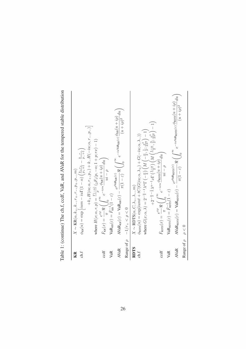
4 Tempered Stable DistributionsIn this section, we present five subclasses of infinitely divisible distributions

for modeling a portfolio loss distribution: classical tempered stable distribution,Kim-Rachev distribution, modified tempered stable distribution, normal temperedstable distribution, and rapidly decreasing tempered stable distribution. In the lit-erature, these distributions have been referred to as tempered stable distributions.In general, these distributions do not have closed-form solution for the probabilitydensity function. Instead, they are defined by their characteristic functions.

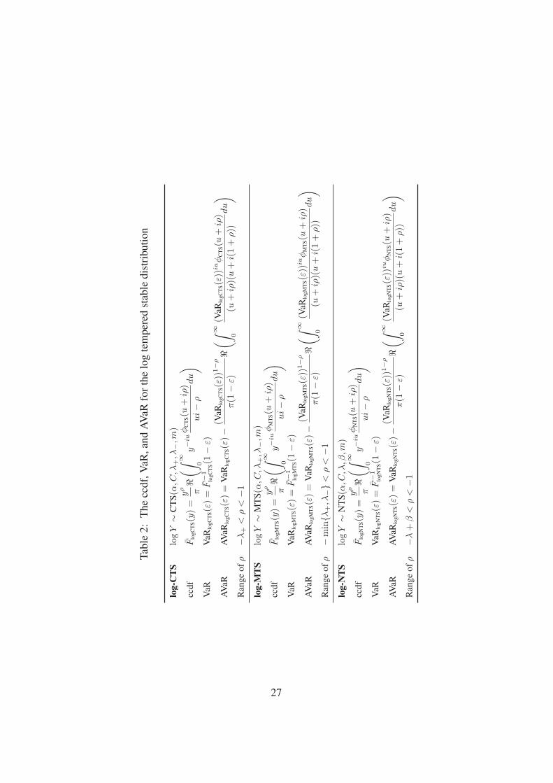
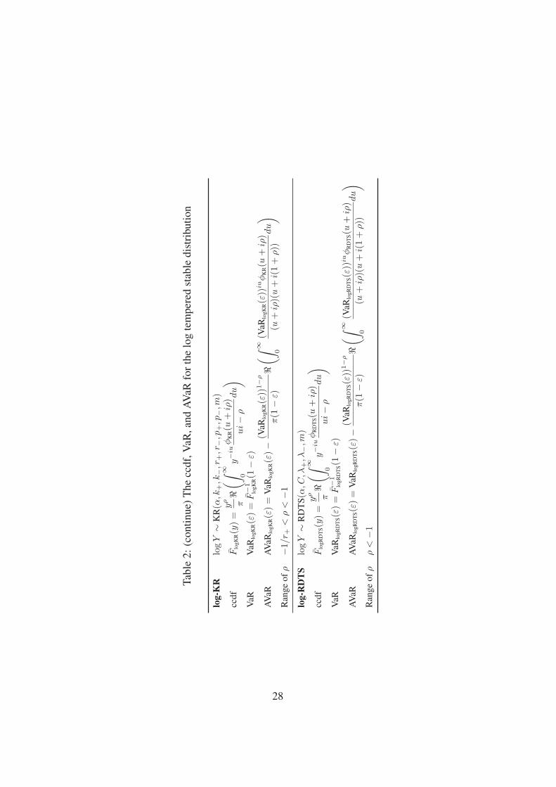
Below we will let a random variable X denote a tempered stable distributedrandom variable. Consider a random variable Y such that log Y is a temperedstable distribution. Then the random variable Y is referred to as the log temperedstable random variable.

4.1 Classical Tempered Stable DistributionLet α ∈ (0, 2), C, λ+, λ− > 0, and m ∈ R. X is said to follow the classical

tempered stable (CTS) distribution 5 if the characteristic function of X is given by

φCTS(u) := φX(u)

= exp(ium− iuCΓ(1− α)(λα−1+ − λα−1

− )

+ CΓ(−α)((λ+ − iu)α − λα+ + (λ− + iu)α − λα

−)),

and we denote X ∼ CTS(α, C, λ+, λ−,m). The mean of X is m, and cumulantscn(X) = dn

dun log φX(u)|u=0 of X are

cn(X) = CΓ(n− α)(λα−n+ + (−1)nλα−n

− ),

for n = 2, 3, · · · .5See Koponen (1995), Boyarchenko and Levendorskii (2000), and Carr et al. (2002).

12

By analytic continuation in complex analysis, the function φCTS(u) can be ex-tended analytically to the region {z ∈ C : =(z) ∈ (−λ+, λ−)}, that is |φCTS(z)| <∞ for all complex z with =(z) ∈ (−λ+, λ−). Therefore, there exists ρ < 0 suchthat |φCTS(z)| < ∞ for all complex z with =(z) = ρ. Hence, FX(x), VaRε(X),and AVaRε(X) are obtained by Proposition 1, equation (4), and Proposition 2 asfollows:

FCTS(x) := FX(x) =exρ

π<

(∫ ∞

0

e−ixu φCTS(u + iρ)

ui− ρdu

),

VaRCTS(ε) := VaRε(X) = F−1CTS (1− ε),

AVaRCTS(ε) := AVaRε(X)

= VaRCTS(ε)− eρVaRCTS(ε)

π(1− ε)<

(∫ ∞

0

e−iuVaRCTS(ε)φCTS(u + iρ)

(u + iρ)2du

),

for −λ+ < ρ < 0.If a random variable Y is a log infinitely divisible distribution such that

log Y ∼ CTS(α, C, λ+, λ−,m),

then Y is referred to as a log-CTS random variable. If λ+ > 1, then there existsρ < −1 such that |φCTS(z)| < ∞ for all complex z with =(z) = ρ. Hence,FY (x), VaRε(Y ), and AVaRε(Y ) are obtained by Corollary 1, equation (10), andProposition 3 as follows:

FlogCTS(y) := FY (y) =yρ

π<

(∫ ∞

0

y−iu φCTS(u + iρ)

ui− ρdu

), y > 0,

VaRlogCTS(ε) := VaRε(Y ) = F−1logCTS(1− ε),

for −λ+ < ρ < 0, and

AVaRlogCTS(ε) := AVaRε(Y )

= VaRlogCTS(ε)− (VaRlogCTS(ε))1−ρ

π(1− ε)<

(∫ ∞

0

(VaRlogCTS(ε))iuφCTS(u + iρ)

(u + iρ)(u + i(1 + ρ))du

),

for −λ+ < ρ < −1.

4.2 Kim-Rachev DistributionLet α ∈ (0, 2) \ {1}, , k+, k−, r+, r− > 0, p+, p− ∈ {p > −α | p 6= −1, p 6=

0}, and m ∈ R. X is said to follow the Kim-Rachev (KR) distribution6 if the

6See Kim et al. (2008a,b).

13

characteristic function of X is given by

φKR(u) := φX(u)

= exp(ium− iuΓ(1− α)

(k+r+

p+ + 1− k−r−

p− + 1

)

+ k+H(iu; α, r+, p+) + k−H(−iu; α, r−, p−))

where

H(x; α, r, p) =Γ(−α)

p(2F1(p,−α; 1 + p; rx)− 1)

where 2F1 is the hypergeometric function,7 and we denote X ∼ KR( α, k+, k−,r+, r−, p+, p−, m). The mean of X is m, and cumulants of X are

cn(X) = Γ(n− α)

(k+rn

+

p+ + n+ (−1)n k−rn

−p− + n

),

for n = 2, 3, · · · . If p+ and p− approach to the infinite, then KR distributionconverges to the CTS distribution.

The function φKR(u) can be extended analytically to the region {z ∈ C :=(z) ∈ (−r−1

+ , r−1− )}. Therefore, there exists ρ < 0 such that |φKR(z)| < ∞

for all complex z with =(z) = ρ. Hence, FX(x), VaRε(X), and AVaRε(X) areobtained by Proposition 1, equation (4), and Proposition 2 as follows:

FKR(x) := FX(x) =exρ

π<

(∫ ∞

0

e−ixu φKR(u + iρ)

ui− ρdu

),

VaRKR(ε) := VaRε(X) = F−1KR (1− ε),

AVaRKR(ε) := AVaRε(X)

= VaRKR(ε)− eρVaRKR(ε)

π(1− ε)<

(∫ ∞

0

e−iuVaRKR(ε)φKR(u + iρ)

(u + iρ)2du

),

for −r−1+ < ρ < 0.

If Y is a log infinitely divisible random variable such that

log Y ∼ KR(α, k+, k−, r+, r−, p+, p−,m)

then Y is referred to as a log-KR random variable. If 1/r+ > 1, then there existsρ < −1, such that |φKR(z)| < ∞ for all complex z with =(z) = ρ. Hence,

7See Andrews (1998).

14

FY (x), VaRε(Y ), and AVaRε(Y ) are obtained by Corollary 1, equation (10), andProposition 3 as follows:

FlogKR(y) := FY (y) =yρ

π<

(∫ ∞

0

y−iu φKR(u + iρ)

ui− ρdu

), y > 0,

VaRlogKR(ε) := VaRε(Y ) = F−1logKR(1− ε),

for −r−1+ < ρ < 0, and

AVaRlogKR(ε) := AVaRε(Y )

= VaRlogKR(ε)− (VaRlogKR(ε))1−ρ

π(1− ε)<

(∫ ∞

0

(VaRlogKR(ε))iuφKR(u + iρ)

(u + iρ)(u + i(1 + ρ))du

),

for −r−1+ < ρ < −1.

4.3 Modified Tempered Stable DistributionLet α ∈ (0, 2) \ {1}, C, λ+, λ− > 0, and m ∈ R. X is said to follow the

modified tempered stable (MTS) distribution8 if the characteristic function of X isgiven by

φMTS(u) := φX(u)

= exp(ium + C(GR(u; α,C, λ+) + GR(u; α, C, λ−))

+ iuC(GI(u; α, λ+)−GI(u; α, λ−))),

where for u ∈ R,

GR(x; α, λ) = 2−α+3

2√

πΓ(−α

2

) ((λ2 + x2)

α2 − λα

)

and

GI(x; α, λ) =2−α+1

2 Γ

(1− α

2

)λα−1

[2F1

(1,

1− α

2;3

2;−x2

λ2

)− 1

],

and we denote X ∼ MTS(α, C, λ+, λ−,m). The mean of X is m, and cumulantsof X are equal to

cn(X) = 2n−α+32 CΓ

(n + 1

2

)Γ

(n− α

2

)(λα−n

+ + (−1)nλα−n− ),

for n = 2, 3, · · · .8See Kim et al. (2008c).

15

The function φMTS(u) can be extended analytically to the region {z ∈ C :|=(z)| < min{λ+, λ−}}, that is |φMTS(z)| < ∞ for all complex z with |=(z)| <min{λ+, λ−}. Therefore, there exists ρ < 0 such that |φMTS(z)| < ∞ for allcomplex z with =(z) = ρ. Hence, FX(x), VaRε(X), and AVaRε(X) are obtainedby Proposition 1, equation (4), and Proposition 2 as follows:

FMTS(x) := FX(x) =exρ

π<

(∫ ∞

0

e−ixu φMTS(u + iρ)

ui− ρdu

),

VaRMTS(ε) := VaRε(X) = F−1MTS(1− ε),

AVaRMTS(ε) := AVaRε(X)

= VaRMTS(ε)− eρVaRMTS(ε)

π(1− ε)<

(∫ ∞

0

e−iuVaRMTS(ε)φMTS(u + iρ)

(u + iρ)2du

),

for −min{λ+, λ−} < ρ < 0.If Y is a log infinitely divisible random variable such that

log Y ∼ MTS(α,C, λ+, λ−,m),

then Y is referred to as a log-MTS random variable. If λ+ > 1 and λ− > 1, thenthere exists ρ < −1 such that |φMTS(z)| < ∞ for all complex z with =(z) = ρ.Hence, FY (x), VaRε(Y ), and AVaRε(Y ) are obtained by Corollary 1, equation(10), and Proposition 3 as follows:

FlogMTS(y) := FY (y) =yρ

π<

(∫ ∞

0

y−iu φMTS(u + iρ)

ui− ρdu

), y > 0,

VaRlogMTS(ε) := VaRε(Y ) = F−1logMTS(1− ε),

for −min{λ+, λ−} < ρ < 0, and

AVaRlogMTS(ε) := AVaRε(Y )

= VaRlogMTS(ε)− (VaRlogMTS(ε))1−ρ

π(1− ε)<

(∫ ∞

0

(VaRlogMTS(ε))iuφMTS(u + iρ)

(u + iρ)(u + i(1 + ρ))du

),

for −min{λ+, λ−} < ρ < −1.

16

4.4 Normal Tempered Stable DistributionLet α ∈ (0, 2), C, λ > 0, |β| < λ, and m ∈ R. X is said to follow the normal

tempered stable (NTS) distribution9 if the characteristic function of X is given by

φNTS(u) := φX(u)

= exp(ium + iu2−

α+12 C

√πΓ

(−α

2

)αβ(λ2 − β2)

α2−1

+ 2−α+1

2 C√

πΓ(−α

2

) ((λ2 − (β + iu)2)

α2 − (λ2 − β2)

α2

) ),

and we denote X ∼ NTS(α, C, λ, β, m). The mean of X is m. The generalexpressions for cumulants of X are omitted since they are rather complicated.Instead of the general form, we present three cumulants that

c2(X) = κα(λ2 − β2)α2−2(αβ2 − λ2 − β2),

c3(X) = −καβ(λ2 − β2)α2−3(α2β2 − 3αλ2 − 3αβ2 + 6λ2 + 2β2),

c4(X) = κα(α− 2)(λ2 − β2)α2−4

× (α2β4 − 6αλ2β2 − 4αβ4 + 3β4 + 18λ2β2 + 3λ4),

where κ = 2−α+1

2 C√

πΓ(−α

2

).

The function φNTS(u) can be extended analytically to the region {z ∈ C :=(z) ∈ (−λ + β, λ + β)}, that is |φNTS(z)| < ∞ for all complex z with =(z) ∈(−λ + β, λ + β). Therefore, there exists ρ < 0 such that |φNTS(z)| < ∞ for allcomplex z with =(z) = ρ. Hence, FX(x), VaRε(X), and AVaRε(X) are obtainedby Proposition 1, equation (4), and Proposition 2 as follows:

FNTS(x) := FX(x) =exρ

π<

(∫ ∞

0

e−ixu φNTS(u + iρ)

ui− ρdu

),

VaRNTS(ε) := VaRε(X) = F−1NTS (1− ε),

AVaRNTS(ε) := AVaRε(X)

= VaRNTS(ε)− eρVaRNTS(ε)

π(1− ε)<

(∫ ∞

0

e−iuVaRNTS(ε)φNTS(u + iρ)

(u + iρ)2du

),

for −λ + β < ρ < 0.If Y is a log infinitely divisible random variable such that

log Y ∼ NTS(α, C, λ, β, m),

then Y is referred to as a log-NTS random variable. If λ − β > 1, then thereexists ρ < −1, such that |φNTS(z)| < ∞ for all complex z with =(z) = ρ. Hence,

9See Barndorff-Nielsen and Levendorskii (2001) and Kim et al. (2008d).

17

FY (x), VaRε(Y ), and AVaRε(Y ) are obtained by Corollary 1, equation (10), andProposition 3 as follows:

FlogNTS(y) := FY (y) =yρ

π<

(∫ ∞

0

y−iu φNTS(u + iρ)

ui− ρdu

), y > 0,

VaRlogNTS(ε) := VaRε(Y ) = F−1logNTS(1− ε),

for −λ + β < ρ < 0, and

AVaRlogNTS(ε) := AVaRε(Y )

= VaRlogNTS(ε)− (VaRlogNTS(ε))1−ρ

π(1− ε)<

(∫ ∞

0

(VaRlogNTS(ε))iuφNTS(u + iρ)

(u + iρ)(u + i(1 + ρ))du

),

for −λ + β < ρ < −1.

4.5 Rapidly Decreasing Tempered Stable DistributionLet α ∈ (0, 2)\{1}, C, λ+, λ− > 0, and m ∈ R. X is said to follow the rapidly

decreasing tempered stable (RDTS) distribution10 if the characteristic function ofX is given by

φRDTS(u) = φX(u)

= exp (ium + C(G(iu; α, λ+) + G(−iu; α, λ−))) ,

where

G(x; α, λ) = 2−α2−1λαΓ

(−α

2

) (M

(−α

2,1

2;

x2

2λ2

)− 1

)

+ 2−α2− 1

2 λα−1xΓ

(1− α

2

)(M

(1− α

2,3

2;

x2

2λ2

)− 1

),

and M is the confluent hypergeometric function Andrews (1998), and we denoteX ∼ RDTS(α, C, λ+, λ−,m). The mean of X is m, and cumulants of X are

cn(X) = 2n−α−2

2 CΓ

(n− α

2

) (λα−n

+ + (−1)nλα−n−

),

for n = 2, 3, · · · .The function φRDTS(u) is expandable to an entire function on C. Hence,

AVaRε(X) is obtained by equation (7) if ρ < 0, that is |φRDTS(z)| < ∞ for all

10See Bianchi et al. (2008) and Kim et al. (2009).

18

complex z. Therefore, there exists ρ < 0 such that |φRDTS(z)| < ∞ for all com-plex z with =(z) = ρ. Hence, FX(x), VaRε(X), and AVaRε(X) are obtained byProposition 1, equation (4), and Proposition 2 as follows:

FRDTS(x) := FX(x) =exρ

π<

(∫ ∞

0

e−ixu φRDTS(u + iρ)

ui− ρdu

),

VaRRDTS(ε) := VaRε(X) = F−1RDTS(1− ε),

AVaRRDTS(ε) := AVaRε(X)

= VaRRDTS(ε)− eρVaRRDTS(ε)

π(1− ε)<

(∫ ∞

0

e−iuVaRRDTS(ε)φRDTS(u + iρ)

(u + iρ)2du

),

for ρ < 0.If Y is a log infinitely divisible random variable such that

log Y ∼ RDTS(α,C, λ+, λ−,m),

then Y is referred to as a log-RDTS random variable. Since |φRDTS(z)| < ∞ forall complex z, we have |φRDTS(z)| < ∞ for all complex z with =(z) = ρ < −1.Hence, FY (x), VaRε(Y ), and AVaRε(Y ) are obtained by Corollary 1, equation(10), and Proposition 3 as follows:

FlogRDTS(y) := FY (y) =yρ

π<

(∫ ∞

0

y−iu φRDTS(u + iρ)

ui− ρdu

), y > 0,

VaRlogRDTS(ε) := VaRε(Y ) = F−1logRDTS(1− ε),

for ρ < 0, and

AVaRlogRDTS(ε) := AVaRε(Y )

= VaRlogRDTS(ε)− (VaRlogRDTS(ε))1−ρ

π(1− ε)<

(∫ ∞

0

(VaRlogRDTS(ε))iuφRDTS(u + iρ)

(u + iρ)(u + i(1 + ρ))du

),

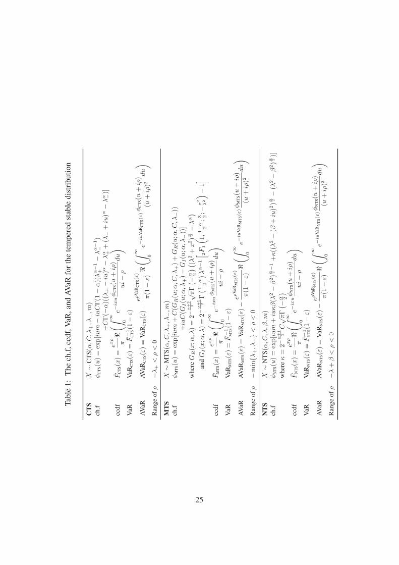
for ρ < −1.Characteristic functions, complementary cumulative density functions, VaRs,

and AVaRs of tempered stable and log tempered stable random variables are pre-sented in Table 1 and Table 2.

5 Empirical ExampleIn this section, we estimate parameters for the five tempered stable distribu-

tions and the normal distribution (N(µ, σ2)), and then calculate the AVaR for each

19

using those estimated parameters. We use daily closing prices of the S&P 500 in-dex from January 2, 1997 through December 29, 2006. Data were obtained fromYahoo! Finance. Daily losses are observed by taking the minus sign for daily log-returns of the S&P 500 index. The parameters are estimated using the maximumlikelihood estimation (MLE). In this empirical study, we do not focus the opera-tional risk. Hence, the closed-form solution of AVaR for log infinitely divisiblerandom variables will not be concerned in this section.

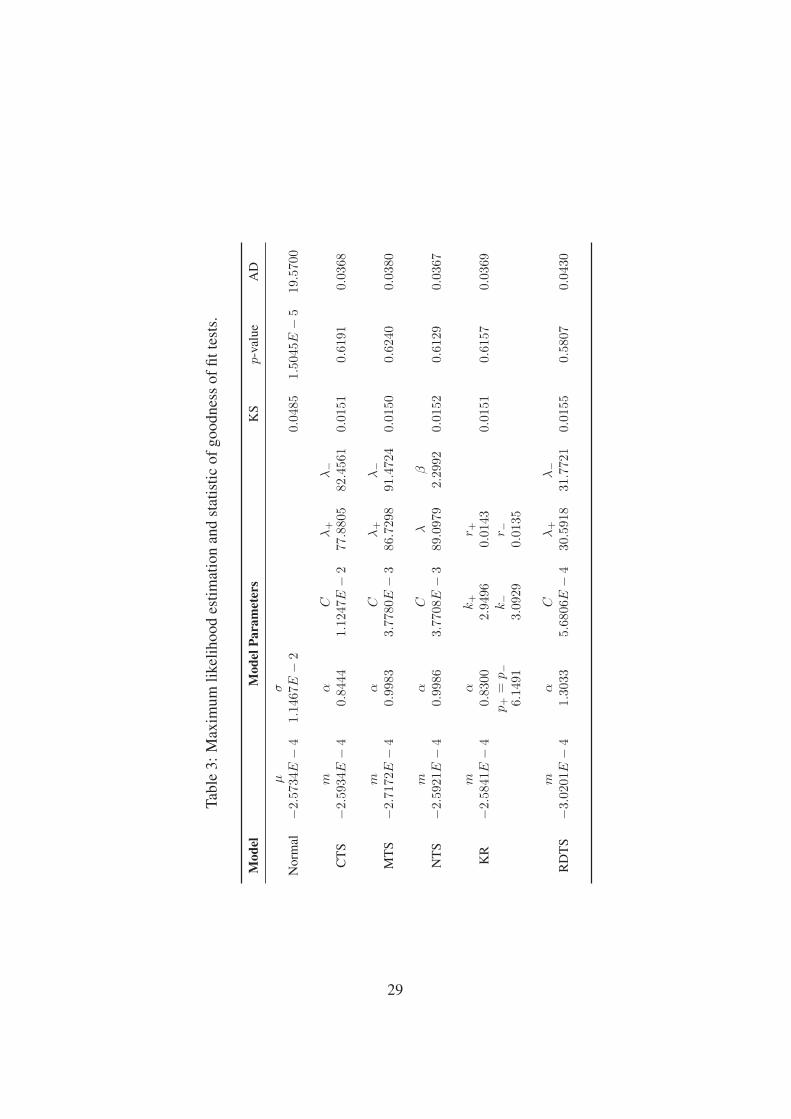
We report the estimated parameters in Table 3. For the assessment of thegoodness-of-fit, we utilize the Kolmogrov-Smirnov (KS) test. We also calculatethe Anderson-Darling (AD) statistic to better evaluate the tail fit.11 Table 3 givesthe KS and AD statistics, and the p-value of the KS statistic. The normal distribu-tion is rejected for our sample, but the other five tempered stable distributions arenot rejected based on the p-value of KS statistic. The AD statistic of the normal fitis dramatically larger than the other classes; that is, the normal distribution doesnot capture the tail property of the empirical distribution.

In Table 4, the variance, skewness, and excess kurtosis are provided. As canbe seen, the variance of the normal distribution is similar to the variance of theempirical distribution, but the normal distribution cannot describe the nonzeroskewness and nonzero excess kurtosis of the empirical distribution. The five tem-pered stable distributions have positive skewness values and positive excess kur-tosis values. From Table 4 it can be seen that the CTS and the RDTS distributionshave the closest excess kurtosis and the closest skewness to the empirical values,respectively. Therefore, the tempered stable distributions are more realistic distri-butions in describing the data than the normal distribution for the historical datainvestigated.

Comparing the performance of AVaRs, we use empirical AVaR provided inRachev et al. (2007) as a benchmark value. Denote (1) the observed portfolio (orasset) losses by x1, x2, · · · , xn at time instant t1, t2, · · · , tn and (2) the sortedsample by x(1) ≤ x(2) ≤ · · · ≤ x(n). The empirical AVaR of the loss at tail

11The KS statistic is defined as

KS = supxi

|F (xi)− F (xi)|,

and the AD statistic is defined as

AD = supxi

|F (xi)− F (xi)|√F (xi)(1− F (xi))

,

where F is the cumulative distribution function with estimated parameters and F is the empiricalcumulative distribution function for a given observation {xi}.

20

probability ε is estimated by

AVaRε =1

1− ε

1

n

n∑

dnεe+1

x(k) +

(dnεen

− ε

)x(dnεe)

,

where the notation dxe stands for the smallest integer larger than x. In addition,empirical VaR is defined by

VaRε = x(dnεe).

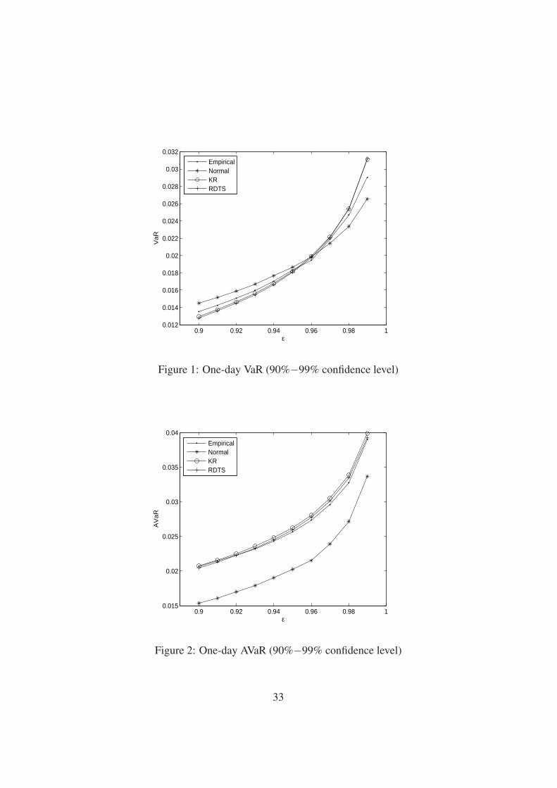
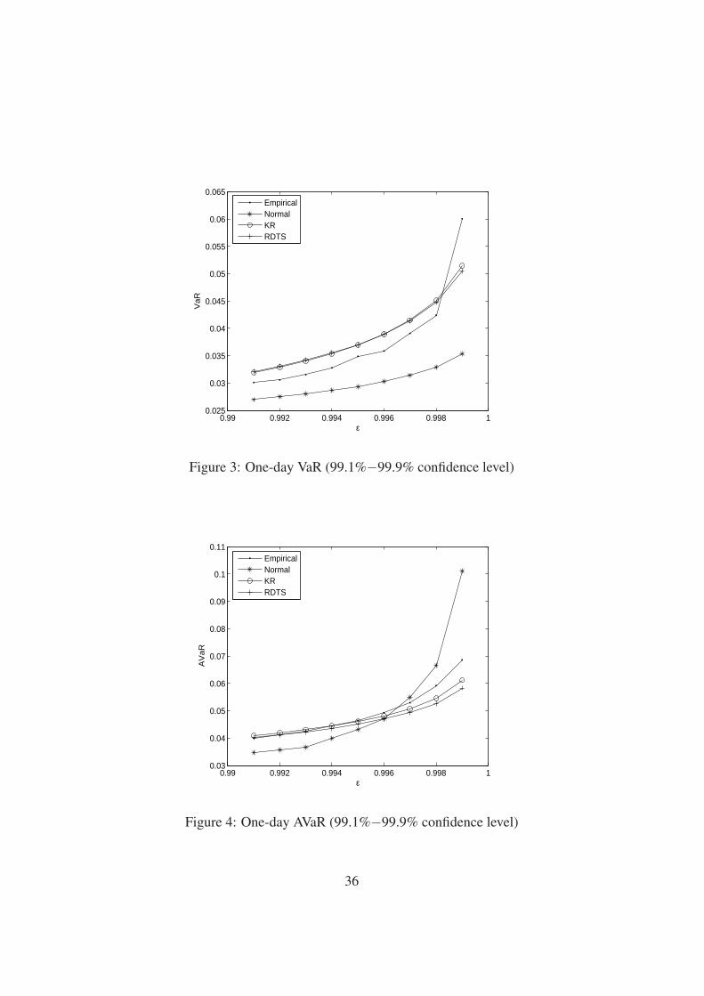
The VaR and the AVaR values for confidence levels {90%, 91%, · · · , 99%}are provided in Table 5 and Table 6, respectively, and the values are also plotted inFigure 1 and Figure 2, respectively. The VaR and the AVaR values for confidencelevels for extreme events, {99.1%, 99.%, · · · , 99.9%}, are provided in Table 9 andTable 10, respectively, and the values are also plotted in Figure 3 and Figure 4,respectively. Since the VaR and the AVaR values of the CTS, the MTS, the NTS,and the KR distributions are very similar, and the values of the RDTS distributionis more or less different from the KR case, we plot only the values of the KR andthe RDTS distributions in the figures.

According to Table 5 and Figure 1, the normal VaR is larger than the empiricalVaR, and the tempered stable VaRs are smaller, if the confidence level is less thanor equal to 95%. If the confidence level is larger than 96%, the tempered stableVaRs are larger than the empirical VaR, and the normal VaR is smaller. If one usesthe normal VaR with 99% confidence level for measuring the risk, the measuredrisk is less than the real risk in this empirical study. Moreover, according to Table 6and Figure 2, the AVaRs of the tempered stable distributions are relatively similarto the empirical AVaR compared to the normal distribution.

According to Table 9 and Figure 3, normal VaR values are always smaller thanempirical VaR values, and tempered stable VaR values are larger than empiricalVaR values if confidence levels are less than 99.9%. According to Table 10 andFigure 4, the AVaRs of the tempered stable distributions are relatively similarto the empirical AVaR compared to the normal distribution considering extremeevents.

Table 7 and Table 11 report relative errors between the empirical VaR and nor-mal and tempered stable VaR, and Table 8 and Table 12 between the empiricalAVaR and normal and tempered stable AVaR. The average of relative errors arealso presented in the bottom line of both tables. The average errors of the normalVaR and normal AVaR have the largest value in those tables. The average errorsof the KR VaR and the MTS VaR are the smallest in Table 7 and Table 11, respec-tively. The average errors of the RDTS AVaR and the KR AVaR are the smallestin Table 8 and Table 12, respectively.

21

6 ConclusionIn this paper, we derive closed-form solution of the AVaR for five subclasses of

the infinitely divisible distribution. If a loss distribution is infinitely divisible andthe characteristic function of the loss distribution is defined on the complex subset{z ∈ C : =(z) = ρ} for some ρ < 0, then we can obtain the closed-form solutionof the AVaR. If a loss distribution is log infinitely divisible and its characteristicfunction is defined on the complex subset {z ∈ C : =(z) = ρ} for some ρ < −1,then we can also obtain closed-form solutions of the cumulative density functionand the AVaR. In order to apply the closed-form solution we derived, we con-sidered five tempered stable distributions: classical tempered stable distribution,Kim-Rachev distribution, modified tempered stable distribution, normal temperedstable distribution, and rapidly decreasing tempered stable distribution. We esti-mated the parameters of those distributions for the S&P 500 index, and obtainedVaR and AVaR values using closed-form solutions with the estimated parameters.In our investigation, the tempered stable VaR and AVaR are more realistic than thenormal VaR and the normal AVaR.

ReferencesAndrews, L. D. (1998). Special Functions Of Mathematics For Engineers, 2nd

ed. Oxford University Press.

Barndorff-Nielsen, O. E. and Levendorskii, S. (2001). Feller processes of normalinverse gaussian type. Quantitative Finance, 1, 318 – 331.

Bianchi, M. L., Rachev, S. T., Kim, Y. S., and Fabozzi, F. J. (2008). Tem-pered infinitely divisible distributions and processes. Technical report, Chairof Econometrics, Statistics and Mathematical Finance School of Economicsand Business Engineering University of Karlsruhe (https://www.statistik.uni-karlsruhe.de/download/doc secure1/TID20080729.pdf).

Boyarchenko, S. I. and Levendorskii, S. Z. (2000). Option pricing for truncatedLevy processes. International Journal of Theoretical and Applied Finance, 3,549–552.

Carr, P., Geman, H., Madan, D., and Yor, M. (2002). The fine structure of assetreturns: An empirical investigation. Journal of Business, 75(2), 305–332.

22

Chernobai, A. S., Rachev, S. T., and Fabozzi, F. J. (2007). Operational risk: Aguide to Basel II capital requirements, models, and analysis. John Wiley &Sons.

Doetsch, G. (1970). Introduction to the Theory and Application of the LaplaceTransformation. Springer-Verlag.

Dokov, S., Stoyanov, S. V., and Rachev, S. T. (2008). Computing VaR and AVaRof skewed-t distribution. Journal of Applied Functional Analysis, 3(1), 189–208.

Grabchak, M. and Samorodnitsky, G. (2009). Do financial returns have finite orinfinite variance? A paradox and an explanation. Cornell University, Ithaca,NY.

Kim, Y. S., Rachev, S. T., Bianchi, M. L., and Fabozzi, F. J. (2008a). Financialmarket models with Levy processes and time-varying volatility. Journal ofBanking and Finance, 32, 1363–1378.

Kim, Y. S., Rachev, S. T., Bianchi, M. L., and Fabozzi, F. J. (2008b). A newtempered stable distribution and its application to finance. In G. Bol, S. T.Rachev, and R. Wuerth (Eds.), Risk Assessment: Decisions in Banking andFinance, Physika Verlag, Springer. 77–110.

Kim, Y. S., Rachev, S. T., Bianchi, M. L., and Fabozzi, F. J. (2009). Tempered sta-ble and tempered infinitely divisible GARCH models. Technical report, Chairof Econometrics, Statistics and Mathematical Finance School of Economicsand Business Engineering University of Karlsruhe (https://www.statistik.uni-karlsruhe.de/download/doc secure1/RDTS-GARCH-MathFin.pdf).

Kim, Y. S., Rachev, S. T., Chung, D. M., and Bianchi, M. L. (2008c). The modifiedtempered stable distribution, GARCH-models and option pricing. Probabilityand Mathematical Statistics. To appear.

Kim, Y. S., Rachev, S. T., Chung, D. M., and Bianchi, M. L. (2008d). A modifiedtempered stable distribution with volatility clustering. In J. O. Soares, J. P.Pina, and M. Catalao-Lopes (Eds.), New Developments in Financial Modelling,Cambridge Scholars Publishing. 344–365.

Klebanov, L., Kozubowski, T., and Rachev, S. T. (2006). Ill-Posed Problems inProbability and Stability of Random Sums. New York: Nova Science Publish-ers.

23

Koponen, I. (1995). Analytic approach to the problem of convergence of truncatedLevy flights towards the Gaussian stochastic process. Physical Review E, 52,1197–1199.

Pflug, G. (2000). Some remarks on the value-at-risk and the conditional value-at-risk. In S. Uryasev (Ed.), Probabilistic Constrained Optimization: Methodol-ogy and Applications, Kluwer Academic Publishers. 272–281.

Rachev, S. T. and Mittnik, S. (2000). Stable Paretian Models in Finance. JohnWiley & Sons.

Rachev, S. T., Stoyanov, S., and Fabozzi, F. J. (2007). Advanced Stochastic Mod-els, Risk Assessment, and Portfolio Optimization: The Ideal Risk, Uncertainty,and Performance Measures. New Jersey: John Wiley & Sons.

Rockafellar, R. T. and Uryasev, S. (2000). Optimization of conditional value-at-risk. Journal of Risk, 2(3), 21–41.

Rockafellar, R. T. and Uryasev, S. (2002). Oconditional value-at-risk for generalloss distributions. Journal of Banking and Finance, 26, 1443–1471.

Stoyanov, S., Samorodnitsky, G., Rachev, S. T., and Ortobelli, S. (2006). Com-puting the portfolio conditional value-at-risk in the α-stable case. Probabilityand Mathematical Statistics, 26(1), 1–22.

24

Tabl

e1:

The

ch.f,

ccdf

,VaR

,and

AVaR

fort

hete

mpe

red

stab

ledi

stri

butio

n

CT

SX∼

CT

S(α,C

,λ+,λ−

,m)

ch.f

φC

TS(u

)=

exp[

ium−

iuC

Γ(1−

α)(

λα−

1+

−λ

α−

1−

)+

CΓ(−

α)(

(λ+−

iu)α−

λα +

+(λ−

+iu

)α−

λα −

)]

ccdf

FC

TS(x

)=

exρ

π<

( ∫∞

0

e−ix

uφ

CT

S(u

+iρ

)ui−

ρdu

)

VaR

VaR

CT

S(ε

)=

F−

1C

TS(1−

ε)

AVaR

AVaR

CT

S(ε

)=

VaR

CT

S(ε

)−

eρV

aRC

TS(ε

)

π(1−

ε)<

( ∫∞

0

e−iu

VaR

CT

S(ε

)φ

CT

S(u

+iρ

)(u

+iρ

)2du

)

Ran

geof

ρ−λ

+<

ρ<

0

MT

SX∼

MT

S(α,C

,λ+,λ−

,m)

ch.f

φM

TS(u

)=

exp[

ium

+C

(GR(u

;α,C

,λ+)+

GR(u

;α,C

,λ−

))+

iuC

(GI(u

;α,λ

+)−

GI(u

;α,λ−

))]

whe

reG

R(x

;α,λ

)=

2−α+

32√ π

Γ( −

α 2

)((λ

2+

x2)α 2−

λα)

and

GI(x

;α,λ

)=

2−α+

12

Γ( 1−

α2

) λα−

1[ 2

F1

( 1,1−

α2

;3 2;−

x2

λ2

) −1]

ccdf

FM

TS(x

)=

exρ

π<

( ∫∞

0

e−ix

uφ

MT

S(u

+iρ

)ui−

ρdu

)

VaR

VaR

MT

S(ε

)=

F−

1M

TS(1−

ε)

AVaR

AVaR

MT

S(ε

)=

VaR

MT

S(ε

)−

eρV

aRM

TS(ε

)

π(1−

ε)<

( ∫∞

0

e−iu

VaR

MT

S(ε

)φ

MT

S(u

+iρ

)(u

+iρ

)2du

)

Ran

geof

ρ−

min{λ

+,λ−}<

ρ<

0

NT

SX∼

NT

S(α,C

,λ,β

,m)

ch.f

φN

TS(u

)=

exp[

ium

+iu

κβ(λ

2−

β2)α 2−

1+

κ((

λ2−

(β+

iu)2

)α 2−

(λ2−

β2)α 2

)]w

here

κ=

2−α+

12

C√ π

Γ( −

α 2

)

ccdf

FN

TS(x

)=

exρ

π<

( ∫∞

0

e−ix

uφ

NT

S(u

+iρ

)ui−

ρdu

)

VaR

VaR

NT

S(ε

)=

F−

1N

TS(1−

ε)

AVaR

AVaR

NT

S(ε

)=

VaR

NT

S(ε

)−

eρV

aRN

TS(ε

)

π(1−

ε)<

( ∫∞

0

e−iu

VaR

NT

S(ε

)φ

NT

S(u

+iρ

)(u

+iρ

)2du

)

Ran

geof

ρ−λ

+β

<ρ

<0

25

Tabl

e1:

(con

tinue

)The

ch.f,

ccdf

,VaR

,and

AVaR

fort

hete

mpe

red

stab

ledi

stri

butio

n

KR

X∼

KR

(α,k

+,k−

,r+,r−

,p+,p−

,m)

ch.f

φK

R(u

)=

exp

[ ium−

iuΓ(1−

α)( k

+r+

p+

+1−

k−

r−

p−

+1

)

+k+H

(iu;α

,r+,p

+)+

k−

H(−

iu;α

,r−

,p−

)]

whe

reH

(x;α

,r,p

)=

Γ(−

α)

p( 2

F1(p

,−α;1

+p;r

x)−

1)

ccdf

FK

R(x

)=

exρ

π<

( ∫∞

0

e−ix

uφ

KR(u

+iρ

)ui−

ρdu

)

VaR

VaR

KR(ε

)=

F−

1K

R(1−

ε)

AVaR

AVaR

KR(ε

)=

VaR

KR(ε

)−

eρV

aRK

R(ε

)

π(1−

ε)<

( ∫∞

0

e−iu

VaR

KR(ε

)φ

KR(u

+iρ

)(u

+iρ

)2du

)

Ran

geof

ρ−1

/r +

<ρ

<0

RD

TS

X∼

RD

TS(

α,C

,λ+,λ−

,m)

ch.f

φR

DT

S(u

)=

exp[

ium

t+

tC(G

(iu;α

,λ+)+

G(−

iu;α

,λ−

))w

here

G(x

;α,λ

)=

2−α 2−

1λ

αΓ

( −α 2

)(M

( −α 2,

1 2;

x2

2λ

2

) −1)

+2−

α 2−

1 2λ

α−

1xΓ

( 1−

α2

)(M

( 1−

α2

,3 2;

x2

2λ

2

) −1)

ccdf

FR

DT

S(x

)=

exρ

π<

( ∫∞

0

e−ix

uφ

RD

TS(u

+iρ

)ui−

ρdu

)

VaR

VaR

RD

TS(ε

)=

F−

1R

DT

S(1−

ε)

AVaR

AVaR

RD

TS(ε

)=

VaR

RD

TS(ε

)−

eρV

aRR

DT

S(ε

)

π(1−

ε)<

( ∫∞

0

e−iu

VaR

RD

TS(ε

)φ

RD

TS(u

+iρ

)(u

+iρ

)2du

)

Ran

geof

ρρ

<0

26

Tabl

e2:

The

ccdf

,VaR

,and

AVaR

fort

helo

gte

mpe

red

stab

ledi

stri

butio

n

log-

CT

Slo

gY∼

CT

S(α,C

,λ+,λ−

,m)

ccdf

Flo

gCT

S(y

)=

yρ π<

( ∫∞

0

y−

iuφ

CT

S(u

+iρ

)ui−

ρdu

)

VaR

VaR

logC

TS(ε

)=

F−

1lo

gCT

S(1−

ε)

AVaR

AVaR

logC

TS(ε

)=

VaR

logC

TS(ε

)−

(VaR

logC

TS(ε

))1−

ρ

π(1−

ε)<

( ∫∞

0

(VaR

logC

TS(ε

))iu

φC

TS(u

+iρ

)(u

+iρ

)(u

+i(

1+

ρ))

du

)

Ran

geof

ρ−λ

+<

ρ<−1

log-

MT

Slo

gY∼

MT

S(α,C

,λ+,λ−

,m)

ccdf

Flo

gMT

S(y

)=

yρ π<

( ∫∞

0

y−

iuφ

MT

S(u

+iρ

)ui−

ρdu

)

VaR

VaR

logM

TS(ε

)=

F−

1lo

gMT

S(1−

ε)

AVaR

AVaR

logM

TS(ε

)=

VaR

logM

TS(ε

)−

(VaR

logM

TS(ε

))1−

ρ

π(1−

ε)<

( ∫∞

0

(VaR

logM

TS(ε

))iu

φM

TS(u

+iρ

)(u

+iρ

)(u

+i(

1+

ρ))

du

)

Ran

geof

ρ−

min{λ

+,λ−}<

ρ<−1

log-

NT

Slo

gY∼

NT

S(α,C

,λ,β

,m)

ccdf

Flo

gNT

S(y

)=

yρ π<

( ∫∞

0

y−

iuφ

NT

S(u

+iρ

)ui−

ρdu

)

VaR

VaR

logN

TS(ε

)=

F−

1lo

gNT

S(1−

ε)

AVaR

AVaR

logN

TS(ε

)=

VaR

logN

TS(ε

)−

(VaR

logN

TS(ε

))1−

ρ

π(1−

ε)<

( ∫∞

0

(VaR

logN

TS(ε

))iu

φN

TS(u

+iρ

)(u

+iρ

)(u

+i(

1+

ρ))

du

)

Ran

geof

ρ−λ

+β

<ρ

<−1

27

Tabl

e2:

(con

tinue

)The

ccdf

,VaR

,and

AVaR

fort

helo

gte

mpe

red

stab

ledi

stri

butio

n

log-

KR

log

Y∼

KR

(α,k

+,k−

,r+,r−

,p+,p−

,m)

ccdf

Flo

gKR(y

)=

yρ π<

( ∫∞

0

y−

iuφ

KR(u

+iρ

)ui−

ρdu

)

VaR

VaR

logK

R(ε

)=

F−

1lo

gKR(1−

ε)

AVaR

AVaR

logK

R(ε

)=

VaR

logK

R(ε

)−

(VaR

logK

R(ε

))1−

ρ

π(1−

ε)<

( ∫∞

0

(VaR

logK

R(ε

))iu

φK

R(u

+iρ

)(u

+iρ

)(u

+i(

1+

ρ))

du

)

Ran

geof

ρ−1

/r+

<ρ

<−1

log-

RD

TS

log

Y∼

RD

TS(

α,C

,λ+,λ−

,m)

ccdf

Flo

gRD

TS(y

)=

yρ π<

( ∫∞

0

y−

iuφ

RD

TS(u

+iρ

)ui−

ρdu

)

VaR

VaR

logR

DT

S(ε

)=

F−

1lo

gRD

TS(1−

ε)

AVaR

AVaR

logR

DT

S(ε

)=

VaR

logR

DT

S(ε

)−

(VaR

logR

DT

S(ε

))1−

ρ

π(1−

ε)<

( ∫∞

0

(VaR

logR

DT

S(ε

))iu

φR

DT

S(u

+iρ

)(u

+iρ

)(u

+i(

1+

ρ))

du

)

Ran

geof

ρρ

<−1

28

Tabl

e3:

Max

imum

likel

ihoo

des

timat

ion

and

stat

istic

ofgo

odne

ssof

fitte

sts.

Mod

elM

odel

Para

met

ers

KS

p-v

alue

AD

µσ

Nor

mal

−2.5

734E

−4

1.14

67E−

20.

0485

1.50

45E−

519

.570

0

mα

Cλ

+λ−

CT

S−2

.593

4E−

40.

8444

1.12

47E−

277

.880

582

.456

10.

0151

0.61

910.

0368

mα

Cλ

+λ−

MT

S−2

.717

2E−

40.

9983

3.77

80E−

386

.729

891

.472

40.

0150

0.62

400.

0380

mα

Cλ

βN

TS

−2.5

921E

−4

0.99

863.

7708

E−

389

.097

92.

2992

0.01

520.

6129

0.03

67

mα

k+

r +K

R−2

.584

1E−

40.

8300

2.94

960.

0143

0.01

510.

6157

0.03

69p+

=p−

k−

r −6.

1491

3.09

290.

0135

mα

Cλ

+λ−

RD

TS

−3.0

201E

−4

1.30

335.

6806

E−

430

.591

831

.772

10.

0155

0.58

070.

0430

29

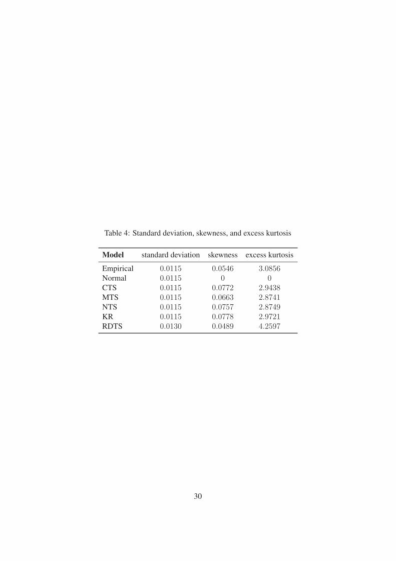
Table 4: Standard deviation, skewness, and excess kurtosis

Model standard deviation skewness excess kurtosis

Empirical 0.0115 0.0546 3.0856Normal 0.0115 0 0CTS 0.0115 0.0772 2.9438MTS 0.0115 0.0663 2.8741NTS 0.0115 0.0757 2.8749KR 0.0115 0.0778 2.9721RDTS 0.0130 0.0489 4.2597

30

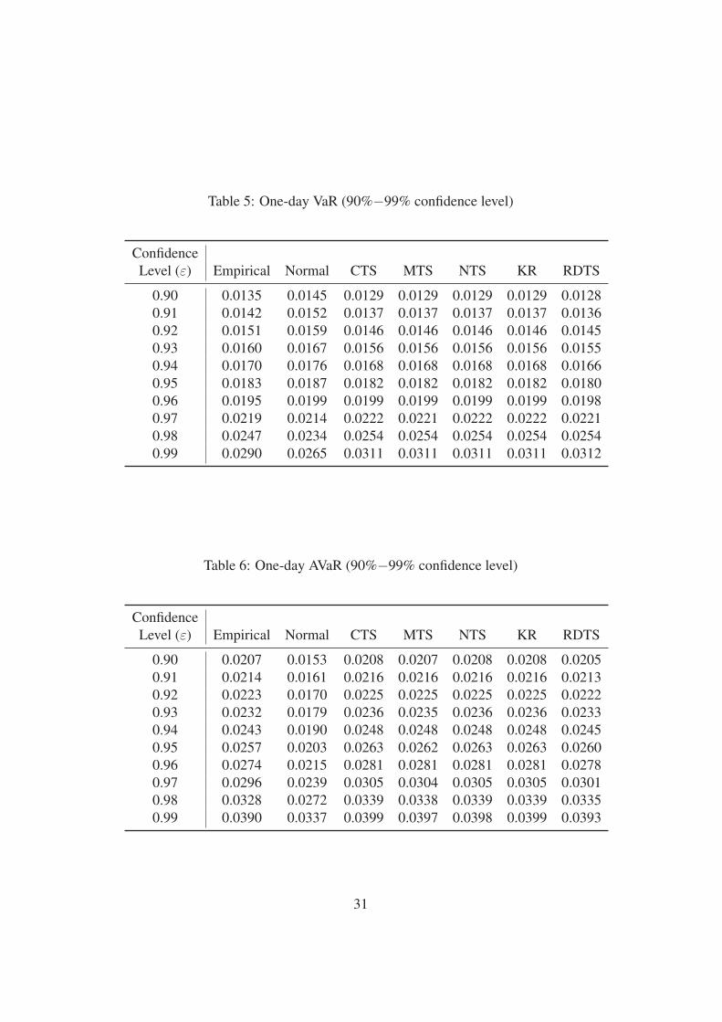
Table 5: One-day VaR (90%−99% confidence level)

ConfidenceLevel (ε) Empirical Normal CTS MTS NTS KR RDTS

0.90 0.0135 0.0145 0.0129 0.0129 0.0129 0.0129 0.01280.91 0.0142 0.0152 0.0137 0.0137 0.0137 0.0137 0.01360.92 0.0151 0.0159 0.0146 0.0146 0.0146 0.0146 0.01450.93 0.0160 0.0167 0.0156 0.0156 0.0156 0.0156 0.01550.94 0.0170 0.0176 0.0168 0.0168 0.0168 0.0168 0.01660.95 0.0183 0.0187 0.0182 0.0182 0.0182 0.0182 0.01800.96 0.0195 0.0199 0.0199 0.0199 0.0199 0.0199 0.01980.97 0.0219 0.0214 0.0222 0.0221 0.0222 0.0222 0.02210.98 0.0247 0.0234 0.0254 0.0254 0.0254 0.0254 0.02540.99 0.0290 0.0265 0.0311 0.0311 0.0311 0.0311 0.0312

Table 6: One-day AVaR (90%−99% confidence level)

ConfidenceLevel (ε) Empirical Normal CTS MTS NTS KR RDTS

0.90 0.0207 0.0153 0.0208 0.0207 0.0208 0.0208 0.02050.91 0.0214 0.0161 0.0216 0.0216 0.0216 0.0216 0.02130.92 0.0223 0.0170 0.0225 0.0225 0.0225 0.0225 0.02220.93 0.0232 0.0179 0.0236 0.0235 0.0236 0.0236 0.02330.94 0.0243 0.0190 0.0248 0.0248 0.0248 0.0248 0.02450.95 0.0257 0.0203 0.0263 0.0262 0.0263 0.0263 0.02600.96 0.0274 0.0215 0.0281 0.0281 0.0281 0.0281 0.02780.97 0.0296 0.0239 0.0305 0.0304 0.0305 0.0305 0.03010.98 0.0328 0.0272 0.0339 0.0338 0.0339 0.0339 0.03350.99 0.0390 0.0337 0.0399 0.0397 0.0398 0.0399 0.0393

31

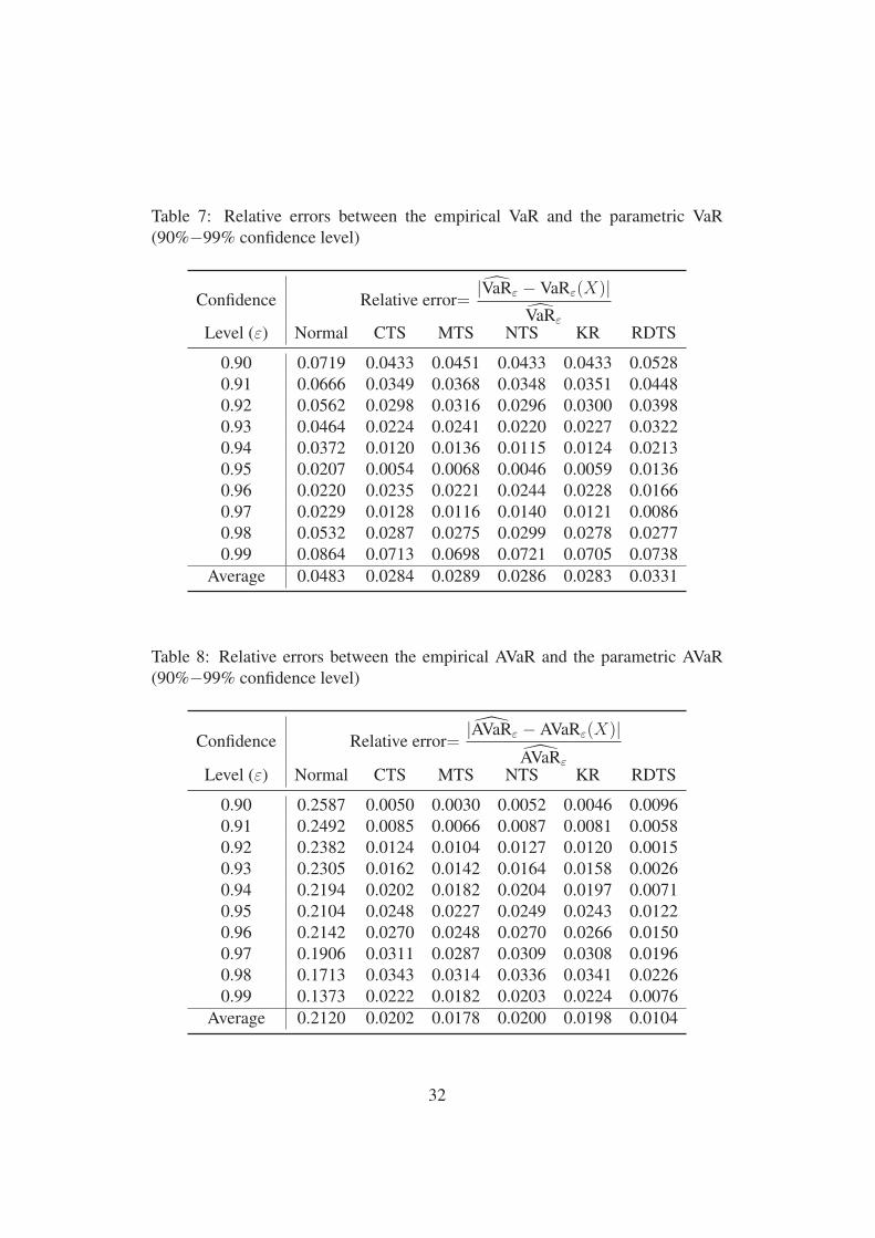
Table 7: Relative errors between the empirical VaR and the parametric VaR(90%−99% confidence level)

Confidence Relative error=|VaRε − VaRε(X)|

VaRε

Level (ε) Normal CTS MTS NTS KR RDTS

0.90 0.0719 0.0433 0.0451 0.0433 0.0433 0.05280.91 0.0666 0.0349 0.0368 0.0348 0.0351 0.04480.92 0.0562 0.0298 0.0316 0.0296 0.0300 0.03980.93 0.0464 0.0224 0.0241 0.0220 0.0227 0.03220.94 0.0372 0.0120 0.0136 0.0115 0.0124 0.02130.95 0.0207 0.0054 0.0068 0.0046 0.0059 0.01360.96 0.0220 0.0235 0.0221 0.0244 0.0228 0.01660.97 0.0229 0.0128 0.0116 0.0140 0.0121 0.00860.98 0.0532 0.0287 0.0275 0.0299 0.0278 0.02770.99 0.0864 0.0713 0.0698 0.0721 0.0705 0.0738

Average 0.0483 0.0284 0.0289 0.0286 0.0283 0.0331

Table 8: Relative errors between the empirical AVaR and the parametric AVaR(90%−99% confidence level)

Confidence Relative error=|AVaRε − AVaRε(X)|

AVaRε

Level (ε) Normal CTS MTS NTS KR RDTS

0.90 0.2587 0.0050 0.0030 0.0052 0.0046 0.00960.91 0.2492 0.0085 0.0066 0.0087 0.0081 0.00580.92 0.2382 0.0124 0.0104 0.0127 0.0120 0.00150.93 0.2305 0.0162 0.0142 0.0164 0.0158 0.00260.94 0.2194 0.0202 0.0182 0.0204 0.0197 0.00710.95 0.2104 0.0248 0.0227 0.0249 0.0243 0.01220.96 0.2142 0.0270 0.0248 0.0270 0.0266 0.01500.97 0.1906 0.0311 0.0287 0.0309 0.0308 0.01960.98 0.1713 0.0343 0.0314 0.0336 0.0341 0.02260.99 0.1373 0.0222 0.0182 0.0203 0.0224 0.0076

Average 0.2120 0.0202 0.0178 0.0200 0.0198 0.0104

32

0.9 0.92 0.94 0.96 0.98 10.012

0.014

0.016

0.018

0.02

0.022

0.024

0.026

0.028

0.03

0.032

ε

Va

R

EmpiricalNormalKRRDTS

Figure 1: One-day VaR (90%−99% confidence level)

0.9 0.92 0.94 0.96 0.98 10.015

0.02

0.025

0.03

0.035

0.04

ε

AV

aR

EmpiricalNormalKRRDTS

Figure 2: One-day AVaR (90%−99% confidence level)

33

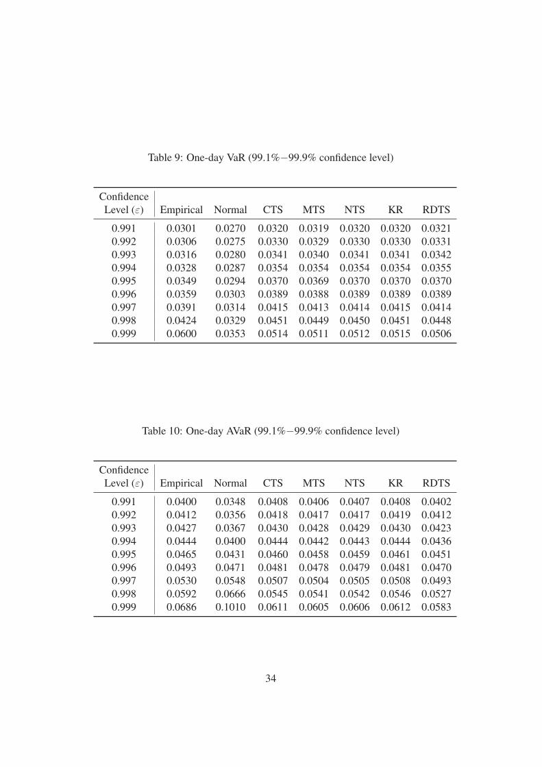
Table 9: One-day VaR (99.1%−99.9% confidence level)

ConfidenceLevel (ε) Empirical Normal CTS MTS NTS KR RDTS

0.991 0.0301 0.0270 0.0320 0.0319 0.0320 0.0320 0.03210.992 0.0306 0.0275 0.0330 0.0329 0.0330 0.0330 0.03310.993 0.0316 0.0280 0.0341 0.0340 0.0341 0.0341 0.03420.994 0.0328 0.0287 0.0354 0.0354 0.0354 0.0354 0.03550.995 0.0349 0.0294 0.0370 0.0369 0.0370 0.0370 0.03700.996 0.0359 0.0303 0.0389 0.0388 0.0389 0.0389 0.03890.997 0.0391 0.0314 0.0415 0.0413 0.0414 0.0415 0.04140.998 0.0424 0.0329 0.0451 0.0449 0.0450 0.0451 0.04480.999 0.0600 0.0353 0.0514 0.0511 0.0512 0.0515 0.0506

Table 10: One-day AVaR (99.1%−99.9% confidence level)

ConfidenceLevel (ε) Empirical Normal CTS MTS NTS KR RDTS

0.991 0.0400 0.0348 0.0408 0.0406 0.0407 0.0408 0.04020.992 0.0412 0.0356 0.0418 0.0417 0.0417 0.0419 0.04120.993 0.0427 0.0367 0.0430 0.0428 0.0429 0.0430 0.04230.994 0.0444 0.0400 0.0444 0.0442 0.0443 0.0444 0.04360.995 0.0465 0.0431 0.0460 0.0458 0.0459 0.0461 0.04510.996 0.0493 0.0471 0.0481 0.0478 0.0479 0.0481 0.04700.997 0.0530 0.0548 0.0507 0.0504 0.0505 0.0508 0.04930.998 0.0592 0.0666 0.0545 0.0541 0.0542 0.0546 0.05270.999 0.0686 0.1010 0.0611 0.0605 0.0606 0.0612 0.0583

34

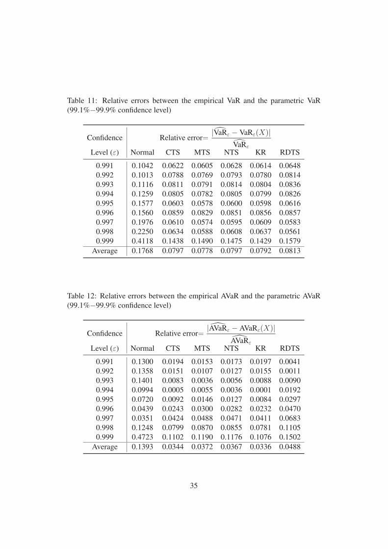
Table 11: Relative errors between the empirical VaR and the parametric VaR(99.1%−99.9% confidence level)

Confidence Relative error=|VaRε − VaRε(X)|

VaRε

Level (ε) Normal CTS MTS NTS KR RDTS

0.991 0.1042 0.0622 0.0605 0.0628 0.0614 0.06480.992 0.1013 0.0788 0.0769 0.0793 0.0780 0.08140.993 0.1116 0.0811 0.0791 0.0814 0.0804 0.08360.994 0.1259 0.0805 0.0782 0.0805 0.0799 0.08260.995 0.1577 0.0603 0.0578 0.0600 0.0598 0.06160.996 0.1560 0.0859 0.0829 0.0851 0.0856 0.08570.997 0.1976 0.0610 0.0574 0.0595 0.0609 0.05830.998 0.2250 0.0634 0.0588 0.0608 0.0637 0.05610.999 0.4118 0.1438 0.1490 0.1475 0.1429 0.1579

Average 0.1768 0.0797 0.0778 0.0797 0.0792 0.0813

Table 12: Relative errors between the empirical AVaR and the parametric AVaR(99.1%−99.9% confidence level)

Confidence Relative error=|AVaRε − AVaRε(X)|

AVaRε

Level (ε) Normal CTS MTS NTS KR RDTS

0.991 0.1300 0.0194 0.0153 0.0173 0.0197 0.00410.992 0.1358 0.0151 0.0107 0.0127 0.0155 0.00110.993 0.1401 0.0083 0.0036 0.0056 0.0088 0.00900.994 0.0994 0.0005 0.0055 0.0036 0.0001 0.01920.995 0.0720 0.0092 0.0146 0.0127 0.0084 0.02970.996 0.0439 0.0243 0.0300 0.0282 0.0232 0.04700.997 0.0351 0.0424 0.0488 0.0471 0.0411 0.06830.998 0.1248 0.0799 0.0870 0.0855 0.0781 0.11050.999 0.4723 0.1102 0.1190 0.1176 0.1076 0.1502

Average 0.1393 0.0344 0.0372 0.0367 0.0336 0.0488

35

0.99 0.992 0.994 0.996 0.998 10.025

0.03

0.035

0.04

0.045

0.05

0.055

0.06

0.065

ε

Va

R

EmpiricalNormalKRRDTS

Figure 3: One-day VaR (99.1%−99.9% confidence level)

0.99 0.992 0.994 0.996 0.998 10.03

0.04

0.05

0.06

0.07

0.08

0.09

0.1

0.11

ε

AV

aR

EmpiricalNormalKRRDTS

Figure 4: One-day AVaR (99.1%−99.9% confidence level)

36