Embed Size (px)
Citation preview
COMSAT TECHNICAL REVIEWVolume 6 Number 2 , Fall 1976
219 A MODEL FOR TDMA BURST ASSIGNMENT AND SCHEDULINGAdvisory Board Joseph V. CharykWilliam W. HagertyJohn V. Harrington
53
A. Sinha
ADAPTIVE POLARIZATION CONTROL FOR SATELLITE FREQUENCY
Editorial Beard
Sidney Metzger
Pier L. Bargellini, Chairman85
REUSE SYSTEMS D. DiFonzo , W. Trachtman AND A. Williams
A CONTIGUOUS BAND MULTIPLEXER M Chen F Assaf ANDRobert D. BriskmanS. J. CampanellaWilliam L. Cook
09
. , .
C. Mahle
NETWORK TOPOLOGIES TO ENHANCE THE RELIABILITY OF COM-Denis J. CurtinJorge D. FuenzalidaR. W. Kreutel
23
MUNICATIONS SATELLITES F. Assal, C. Mahle AND A. Berman
PCM/FDMA SATELLITE TELEPHONY WITH 4-DIMENSIONALLY-Akos G. ReveszRobert Strauss
39
CODED QUADRATURE AMPLITUDE MODULATION G. Welti
A STRATEGY FOR DELTA MODULATION IN SPEECH RECONSTRUC-Editorial Staff Stephen D. SmokeMANAGING EDITOR
Leonard F. Smith57
TION J. Su, H . Suyderhoud AND S. Campanella
PHASE AMBIGUITY RESOLUTION IN A 4-PHASE PSK MODULATIONMargaret B. Jacocks
TECHNICAL EDITORS
Edgar BolenPRODUCTION
79
SYSTEM WITH FORWARD-ERROR-CORRECTING CONVOLUTIONAL
CODES Y. Tsuji
A MODEL FOR MICROWAVE PROPAGATION ALONG AN EARTH-Michael K. Glasby
CIRCULATION
13
SATELLITE PATH D. Fang AND J. Jih
CTR NOTES:
COMSAT TECHNICAL REVIEW is published twice a year by
Communications Satellite Corporation (COMSAT). Subscrip-
tions, which include the two issues published within a calen-
dar year, are: one year, $7 U.S.; two years, $12; three years,$15; single copies, $5; article reprints, $1. Make checks pay-
able to COMSAT and address to Treasurer's Office, Communi-cations Satellite Corporation, 950 L'Enfant Plaza, S. W.,Washington, D.C. 20024, U.S.A.
TV COCHANNEL INTERFERENCE ON A PCM-PSK SCPC SYSTEM
D. Kurjan AND M. Wachs 413
PITCH AXIS ADAPTIVE COMPENSATION J. Hsing 425
435 TRANSLATIONS OF ABSTRACTS
FRENCH 435
SPANISH 441
Q COMMUNICATIONS SATELLITE CORPORATION 1976
Index : time-division multiplexing , mathematical models,scheduling, earth station , computer program
A model for TDMA burst assignmentand scheduling
A. K. SINHA
(Manuscript received March 25, 1976)
Abstract
This paper presents a simple mathematical formulation of the problem oftime-division multiple-access (TDMA) burst assignment and scheduling for ageneral communications satellite system including an arbitrary earth stationnetwork, beam coverage pattern, and transponder configuration. Relevant
concepts of beam overlap (over earth stations), burst overlap (in time), andearth station equipment requirements are introduced and precisely defined. In
addition, useful parameters for evaluating the efficiency of system utilizationare identified. Finally, a semianalytical algorithm is proposed for schedulingTDMA bursts so that earth segment equipment requirements are minimized andachievable scheduling efficiencies are optimized for a given traffic data base andsystem configuration. An example of a schedule obtained from a newly preparedcomputer program based on this approach is presented.
Introduction
In recent years the growing interest in the development and applicationof time-division multiple access (TDMA) for communications satellites ingeneral [1]-[6] and the INTELSAT system in particular [7]-[9] stems from its
This paper is based upon work performed at ComsAT Laboratories under thesponsorship of the International Telecommunications Satellite Organization(INTELSAT). Views expressed in this paper are not necessarily those of INTELSAT.
219 '
220 COMSAT TECHNICAL REVIEW VOLUME 6 NUMBER 2, FALL 1976
distinct advantages over frequency-division multiple access (FUMA). Be-cause in TDMA the entire bandwidth of the transponder is allocated to asingle link, the problems of intermodulation and the related requirementof power backoff caused by the nonlinear transponder response, which aremajor drawbacks of FDMA, are mitigated. Thus, the satellite power can beused more efficiently, thereby enhancing communications capacity. Fur-thermore, for a large and evolving communications network such as theINTELSAT system, the tedious task of determining frequency plans consis-tent with existing earth station equipment inventories at various stages ofgrowth is replaced by the relatively simpler problem of reprogrammingTDMA burst schedules. Inexpensive transponder hopping with or withoutfrequency hopping, depending on the frequency reuse scheme, is possible
for earth stations.In short, the TDMA mode of satellite communications offers the possi-
bility of considerably enhancing the overall system utilization efficiencyrelative to that obtained with FDMA. However, the exact degree to whichincreased efficiency can be realized in practice depends on the efficacy ofTDMA burst scheduling. In the case of a multitransponder satellite operatingin the TDMA mode, the burst scheduling must, of course, be coupled witha suitable assignment of bursts to transponders.
Adequate tools for analyzing the TDMA burst assignment and schedulingproblem must be developed for a realistic evaluation of new or proposedTDMA satellite systems, or for comparing alternative system configurationson the basis of performance, efficiency, and economic considerations. Theproblem is generally complex due to the number of system parameters andthe complexity of their interrelationships. In particular, apart from the twobasic "orthogonal" degrees of freedom, frequency and time, a new degreeof freedom is created by the use of satellite onboard directional antennaswhich provide isolation between earth stations based on orthogonalpolarization or spatial separation. This "spatial" degree of freedom allowsfor multiple reuse of the frequency spectrum. Extensive use of this degreeof freedom is envisioned in the future in the so-called satellite-switchedTDMA (ss/TDMA) or space-division multiple-access (SDMA) systems [10]-[13]. Thus, the basic degrees of freedom involved in a general TDMA satel-lite system-frequency, time, coding, polarization, and spatial isolation ofbeams-can generally be exploited to advantage in burst assignment and
scheduling.Although various aspects of the TDMA concepts and techniques have been
analyzed at length, rather limited attention has been paid to the scheduling
A MODEL FOR TDMA BURST ASSIGNMENT AND SCHEDULING 221
problem [14]. The necessity for a quantitative analysis of various algorithmsfor TDMA burst assignment and scheduling in a multitransponder multi-beam satellite with arbitrary beam coverage, connectivity, frequencyreuse, and transponder hopping as well as a set of pertinent system con-straints and options can hardly be overemphasized. Since the size and com-plexity of the problem generally prohibit a completely analytical solution,the development of a computer simulation model based on the basicmathematical model is necessary to provide the best possible tradeoffamong maximization of satellite capacity utilization, minimization ofearth station equipment cost, and flexibility for network expansion andtraffic growth.
The present paper deals with the formulation of a simple mathematicalmodel and analytical algorithms for the TDMA scheduling problem in a gen-eral satellite communications system. From the previous discussion, it canbe seen that TDMA scheduling clearly involves two important interrelatedprocedures: assignment of traffic to transponders and time ordering of theassigned traffic within the transponder frames. This paper proposes asimple algorithm based on sequential assignment of transponders andtime slots that provides a systematic combined treatment of these two pro-cedures. The algorithm is further generalized to accommodate specificsystem constraints as well as various schemes for determining hierarchyand priority.
For simplicity, the present discussion is confined to the case of a singlenon-ss/TDMA satellite of specified transponder design, including chan-nelization, connectivity, capacity, and beam coverage patterns. Generaliza-tions to the case of multisatellite systems, including SS/TDMA transponders,are fairly straightforward.
First, the basic elements of the model are considered to establish thenotation and to organize related observations. Symbolic representationsare introduced to concisely describe the earth and space segments of thesystem under study in terms of the traffic matrix and traffic growth, beamcoverage, transponder channelization and connectivity, and earth stationequipment inventory. The characteristic parameters of TDMA bursts areidentified, and certain basic or operational system constraints for burstassignment and scheduling, including burst format, burst overlap, burstlength, earth station equipment requirements, and other related factors,are formulated. Quantitative measures of system utilization efficiency areintroduced, followed by a simple semianalytical algorithm for burstassignment and scheduling. Finally, the computer implementation of the
222 COMSAT TECHNICAL REVIEW VOLUME 6 NUMBER 2 , FALL 1976
model is described and an example is presented. It is shown that satisfactory
results can be obtained by using the model.
Mathematical model description
The basic set of system components consists of the traffic data base,satellite beam coverages, satellite configuration, earth station equipmentinventory, and transponder utilization efficiency. A general mathematicaldescription of these quantities and the implications thereof is provided in
the following subsections.
Traffic data base
For X earth stations labeled S,, S,, ..., S, the traffic from station Si to
station S,(i 5,4j) is given by the element f;;(l < i < T, I < j < T) of the
X X T square traffic matrix P, which is generally a function of time, reflect-ing the growth of the traffic over a number of years. If it is assumed thatbursts are to be assigned subject to constraints imposed by the availabilityof a prespecified set of transponders and earth station equipment, there isobviously an upper limit on the traffic growth that can be accommodatedin the system. The traffic growth can be symbolically represented by
P=p(g,t) (1)
where g and t denote the growth rate and time, respectively. Beyond a cer-
tain stage of growth corresponding to time t,,
1(g, t,) = F (2)
no further growth may be accommodated by the system, and the matrix P
is defined as the saturation matrix.As mentioned previously, the schedules may be determined at any stage
of growth. Alternatively, if it is desirable to avoid rescheduling at everystage for a growing traffic base, it is best to start with a traffic matrix whichalready includes the projected growth. The necessary operations can thenbe performed to provide a schedule and to determine the equipment re-quirements at saturation. Conversely, if the equipment requirements aresubject to prespecified constraints, growth can be simulated in stages todetermine through scheduling the maximum traffic or saturation date con-sistent with the specified constraints. In any case, after the scheduling forthe saturation traffic matrix is completed, the traffic schedule for any stage
A MODEL FOR TDMA BURST ASSIGNMENT AND SCHEDULING 223
prior to saturation can be obtained simply by reducing all the traffic ele-ments proportionately. This leaves additional gaps in the time frame whichare gradually filled up as the traffic grows so that the original configurationis attained at saturation.
Satellite beam coverages
Assume that there are µ satellite antenna beams BI, Bz, ..., B„ covering
the stations according to a specified distribution
{S,} C {Bm}, II <1<X, I <m<is . (3)
The specified beam coverage pattern can be represented by the X X
matrix B with the following designation for the elements:
B1,,, =0, otherwise
A
(4)
Each beam B. is connected to one or more transponders for up- anddown-link transmission and can accordingly be associated with a charac-teristic frequency pair S2m/Sim, where U,, and U,, represent the characteristicfrequencies of transponders connected to B,, for up- and down-link trans-mission, respectively. In case of frequency reuse, two or more of the Q.(and Sim) values are identical. For frequency reuse with dual polarization,the respective frequency values will be denoted as where the super-scripts (+) and (-) represent the horizontal (or right circular) and vertical(left circular) polarizations, respectively. In particular, two beams withidentical geographical coverage and/or identical operating frequencies butorthogonal polarizations are physically independent and will be treated as
distinct beams.The geographical overlap pattern of the set of µ beams described above
can be completely derived from the matrix B, whose columns can be re-garded as beam vectors. The magnitudes of individual vectors are relatedto the total number of stations covered by the respective beams, and thescalar product P.. between two vectors represents the number of common
stations in the corresponding beams B. and B,,. Two beams B., and B. with
no common station (P,,,,, = 0) will be referred to as spatially disjoint;conversely, two beams with at least one common station will be referredto as spatially overlapping. The member of the set {B,,} covering all thestations obviously has the highest magnitude and spatial overlap with each
224 COMSAT TECHNICAL REVIEW VOLUME 6 NUMBER 2, FALL 1976
of the remaining members of the set; this beam is termed a global beam.Spatially overlapping beams must differ in terms of characteristic frequencypair, polarization, or transponder channelization for optimal utilization ofthe satellite capacity. In particular, in a global beam, access to all stationsis achieved at the expense of bandwidth reuse. In the other extreme case,if each beam in the set {Bm} covers only one station (, = X), then thisaccess limitation permits maximum bandwidth utilization throughfrequency reuse up to X times.
Satellite configuration
Assume that there are v transponders T1, T2, ., T, with a speci-fied distribution of up- and down-link connectivity over the µ beams
BI, B2, ..., B,,:
{Tk}E{Bm}, I<k<v, 1<m<y . (5)
The transponder beam connectivity may change systematically over theframe length, r, in the case of an SS/TDMA system; otherwise the connec-
tivity remains unaltered.Each transponder is characterized by a specified frequency bandwidth
and reference capacity over the frame length. For convenience, thisassociation can be described as follows. Assume that there are v discretefrequency divisions cr, c2, ..., c, having bandwidths of br, b2, ..., b, and
capacities of cl, c2, ., c„ respectively. Capacity Ck of transponder
Tk(k = 1, 2, ..., v) can be expressed by specifying the particular frequencydivisions with which the transponder is associated, or, equivalently, thecorresponding starting and ending division numbers, kl and k,,respectively.
If it is assumed for simplicity that the bandwidths of various divisionsare integral multiples of a fundamental unit bandwidth b0,
Ck = C,Ak (6)
where co is the capacity associated with b0, and
Ak=k2-k1+1 (7)
is the number of fundamental unit bandwidth divisions handled bytransponder Tk.
A MODEL FOR TDMA BURST ASSIGNMENT AND SCHEDULING 225
Earth station equipment inventory
Burst assignment and scheduling may be subject to constraints on theearth station equipment inventory or, conversely, equipment requirementsmay be determined as a result of the scheduling procedure. The earthsegment or equipment inventory can generally be represented by the set
{Q I,, I = 1, 2..... A; p = 1, 2, ...}, where QL is the amount of equipmentof type p at station Si. Before earth station equipment requirements areconsidered, it is useful to introduce the concept of burst overlap and to
discuss the basic system constraints.
BURST OVERLAP
The criteria for burst overlap in the time and frequency domains will beexamined first; the impact of such overlaps on the earth station equipment
inventory will be considered later.The application of any TDMA scheduling algorithm will result in a series
of bursts, each having a certain up-link carrier frequency (and a corre-sponding down-link frequency), a certain time duration in a given trans-ponder, and a certain starting time. Each burst originates at a certain sta-tion and terminates at certain other stations. Thus, if individual bursts are
sequentially labeled %ir, $2... ., Rmy, where No is the total number of bursts
within the satellite over the repeat length, r, then each $,(l < p < NO)is characterized by a carrier frequency, start and end times, transmittingand receiving stations, up- and down-link beams, and a transponder.
For all practical purposes, it is sufficient to consider only a dis-
crete set of carrier frequencies wl, w,, wz, distributed over the setof bandwidth divisions {c,,, 1 < n < v}, and hence over the set of trans-
ponders {T,, 1 < k < v}.The time variable may be treated as a continuous variable or a discrete
one.* Each option offers certain advantages and disadvantages. A con-tinuous treatment is more convenient for analytical purposes as well asfor minimizing inefficient utilization of the time space. A discrete treat-ment, on the other hand, is more suitable for bookkeeping purposes, suchas TDMA frame synchronization, and for modular utilization of the timespace. The discrete treatment, in which the full frame length (repeat
*A suitable time slot size maybe chosen on the basis of the conventional optionof assigning traffic in multiples of a quantum size, such as 6, 12, or 60 voicechannels.
226 COMSAT TECHNICAL REVIEW VOLUME 6 NUMBER 2, FALL 1976
length), r, is divided into a large number , N, of time slots t,, t2, ..., 4v ofequal duration
A MODEL FOR TDMA BURST ASSIGNMENT AND SCHEDULING 227
(10b)
S = ?N (8)
Similarly, two bursts (3„ and R, will be assumed to have a frequency overlapif they share the same carrier frequency (&,. =(o,), a beam overlap if theyhave beam overlaps in up- and/or down-link transmissions (B„ = B,
will be adopted here. If necessary, continuous treatment can be approxi-mated to any degree by simply taking the limits S -> 0, N such thatthe product SN - r, the constant repeat length.
As mentioned previously, the individual burst i , can be labeled accord-ing to the base carrier frequency, Co,; the beginning time slot, i,;the end time slot, I,,; the transmitting station, S,; the receiving station(s),S,,(S,-', S,,-', ...); the up-link beam, h,; the down-link beam, B,-; and thetransponder, 3',. Then, symbolically,
b, -> b,,; T,), I < p < Ne, t,' > I, (9)
where the entries on the right are members of the prescribed sets" andstation, beam , and transponder accessibility and connectivity are assumed.(That is, T, is assumed to have up -link connectivity with B, covering S,and down -link connectivity with b,, covering Sp ....)
Two bursts R, and R, will be assumed to have a time overlap if one ormore of the time slot indices within the inclusive intervals (1,,, i,,,) and(t„ t,,) are identical. This will occur whenever the following two inequalitieshold t:
i,<tu'
and
(10a)
*That is, .} E IS,, 1 < I < \}; {c3,} c (w„ 1 < r < L};{r„i,,} C {t^,1<q<N};{B„B,.} E (B.,1<m<µ};and {T,} E {T,,1<k<v}.
}Due to the finite length of each time slot, an overlap may also be said tooccur when (3u starts at the same time slot at which R, ends, or vice versa. Such atime overlap is described by changing either one of the two (but not both)inequalities in (10a) and (10b) into an equality.
and/or h., and a transponder overlap if they occupy the sametransponder (Tu = T,).
SYSTEM CONSTRAINTS
Some typical system constraints involved in a TDMA scheduling algorithmare as follows:
a. Burst isolation: No two bursts p„ and R, can have both a timeoverlap and a transponder overlap. Since this is a universal con-straint, compliance is best achieved by requiring that no two non-dis-joint beams B. and B„- be connected to transponders having the sameinput/output carrier frequency or, more generally, sharing the samebandwidth and polarization.
b. Burst format: Each burst must be accompanied by a preamblecontaining coded bits for demodulator synchronization, unique word,station identification, and engineering requirements [7]. Conse-quently, the total content, &, (in voice channels or bits), of a burstRu is actually composed of two distinct parts:
« _ (zu' - to 1) = IIu + P„ (11)
where Cu is the reference capacity of transponder T,,, h. is the con-tent of the preamble, and P„ is the traffic component. For simplicity,the preamble component will be assumed to be a constant, o„ (i.e.,U,, = u,, I < u < Np). Furthermore, it will be assumed that anyguard space required to prevent time overlap of consecutive burstswill be absorbed in the preamble component. At the start of eachTDMA frame, a synchronization burst is transmitted by the referencestation for network timing and synchronization [15] [19]. This willalso be treated as a special form of preamble.
c. Maximum burst length: In practice it is convenient to introduce
a parameter O,a, called the maximum burst length. The length of anyburst pu in the transponder frame must not exceed 8,;,:
228 COMSAT TECHNICAL REVIEW VOLUME 6 NUMBER 2, FALL 1976
0 < Ba = (iu- - t.a + 1) a < Bm . (12)
In units of voice channels (or bits), the maximum burst length, 0,,,,can be written as
(13)
The maximum burst length constraint is relevant to the minimizationof earth station equipment requirements , since the equipment of areceiving station must usually be engaged continuously from the burstpreamble until the data for a given station are received , even if theburst content during the intervening time is of no interest to thatstation.
d. Digital speech interpolation : If certain parts of the traffic can betransmitted using digital speech interpolation ( DSI) [20], the resultingTDMA/Dsl burst sizes are smaller than the original (TDMA withoutDM) burst sizes by a factor f(-1/2):
0(D) = 3'8,. (14)
where the superscript D denotes the burst length after DSI gain. Theactual DSI gain increases with the burst size so that in general i maybe a function of 0,,.
EARTH STATION EQUIPMENT
Excellent descriptions of TDMA earth station equipment are available inthe literature [7], [8]. For the present study, it is sufficient to divide thisequipment into two categories: the TDMA terminal (or simply terminal)and the hopping converter (or simply converter). The terminal refers to theassembly of hardware used for transmission/reception of TDMA burstsand includes such components as the multiplexer/demultiplexer, differ-ential encoder/decoder, modulator/demodulator, and preamble genera-tor/detector. Note that a single terminal can simultaneously perform thetransmit and receive functions. The converter refers to the hardwareassembly involved in IE-to-RE conversion and includes the splitter, up/down frequency converter, and local oscillator. For consistency, it will beassumed that one converter will be required for each discrete carrier fre-quency transmitted or received by a station, although the use of a singlehopping converter in conjunction with multiple local oscillators may per-
A MODEL FOR TDMA BURST ASSIGNMENT AND SCHEDULING 229
mit frequency hopping (via transponder hopping) in burst transmission orreception.
To analyze and evaluate scheduling algorithms , the number of terminalsand converters needed at various stations to implement schedules obtainedfrom a particular algorithm must usually be determined . For a scheduleobtained from a given algorithm subject to the specified constraints, letfii' denote the number of TDMA terminals required at station S, for timeslot t,. In addition , let {QV} denote the set of N numbers obtained for N
time slots tr , t 2 ,... , tN comprising the frame length, T. The required num-ber of TDMA terminals , Qn, at station Sz is then given by the maximumvalue in the specified set
Qr = max {Qi0,I
1 <q<N . (15)
Finally, if [QzI] denotes the set of TDMA terminals required at SI for vari-ous algorithms, the minimum number of terminals required within thelimits of the attempted algorithms (local optimum) is given by
QzI = min [QzI] = min [max {Q ii'}] (16)a a
where the suffix a indicates algorithmic variation.Similarly, the minimum number of converters, Q,2, at station St can be
obtained as follows. Let Q«' represent the number of bursts in time slot t„which have mutually distinct carrier frequencies and Sz as the transmittingor receiving station. Let {Qa21} denote the set resulting from consideringthese bursts for the set of all time slots it,, 1 < q < N}. Then,
Qzz =min [max {Q[z'}J . (17)
The preceding criterion of optimality, known as the mini-max criterion(see for example, Reference 21), can obviously be generalized for the wholenetwork by linear summation of Qq, (p = 1, 2). More generally, itis possible to attempt to minimize the objective functionfQ,
z, z
fQ = ± ± WAIL - Qll)1=1 P-1
(18)
where wp is a weighting factor related to the cost and/or tradeoff priority
230 COMSAT TECHNICAL REVIEW VOLUME 6 NUMBER 2, FALL 1976
of equipment of type p, and Q l, is the absolute minimum amount of p-typeequipment required at station S1. Qi,, can be determined on the basis ofany suitable criterion; for instance, Qir is given by the total traffic of stationS, divided by the reference capacity of a transponder (or the average ref-erence capacity for transponders of varying capacities). A search for aglobal optimum solution can be conducted to obtain the minimum valueof the objective function. In addition, the objective function can be furthergeneralized to incorporate the space segment (transponder utilization). It isuseful, however, to have independent measures of transponder utilization
efficiency as well.
Transponder utilization efficiency
Due to system constraints, it may not always be possible to utilize allof the satellite capacity available for TDMA bursts,
VT = L Ckk=I
where IT is referred to as the satellite reference capacity. If the capacityused by burst Q. is denoted as u8, the total capacity utilized by all bursts is
No
Vfl = E V. . (19)s=I
A portion of us is devoted to overhead , specifically preambles,and the remainder contains traffic data P ;j from station S; to station Si
0,j = 1, 2, ..., X). The overhead capacity is given by
V„ = v,N0 (20)
where u, is the capacity devoted to a unit preamble associated with each
burst. The difference
Vr = Vs - V^ (21)
is the so-called configured capacity. Since some of the slots may be onlypartially filled with traffic due to the discrete nature of the time slots, it isuseful to introduce the concept of assigned capacity, ur(< ur), represent-ing the actual amount of traffic assigned over the transponders . (If all
traffic is scheduled , ur = L.- E;_ r P,1.)
A MODEL FOR TDMA BURST ASSIGNMENT AND SCHEDULING 231
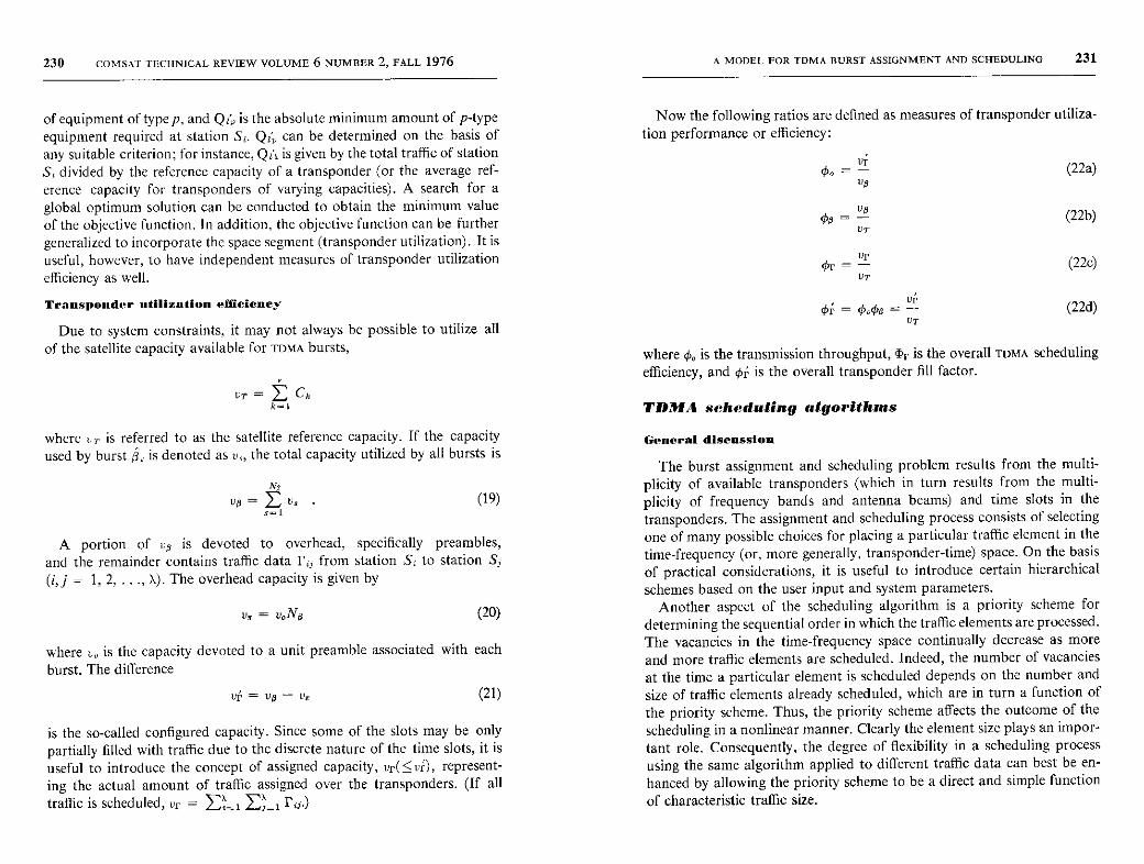
Now the following ratios are defined as measures of transponder utiliza-tion performance or efficiency:
Vr0a = (22a)
Vg
Vs(22b)
VT
VF01 (22c)VT
Up
Or= OoO9 =- (22d)VT
where 0, is the transmission throughput, Tr is the overall TDMA schedulingefficiency, and 0r is the overall transponder fill factor.
TDMA scheduling algorithms
General discussion
The burst assignment and scheduling problem results from the multi-plicity of available transponders (which in turn results from the multi-plicity of frequency bands and antenna beams) and time slots in thetransponders. The assignment and scheduling process consists of selectingone of many possible choices for placing a particular traffic element in thetime-frequency (or, more generally, transponder-time) space. On the basisof practical considerations, it is useful to introduce certain hierarchicalschemes based on the user input and system parameters.
Another aspect of the scheduling algorithm is a priority scheme fordetermining the sequential order in which the traffic elements are processed.The vacancies in the time-frequency space continually decrease as moreand more traffic elements are scheduled. Indeed, the number of vacanciesat the time a particular element is scheduled depends on the number andsize of traffic elements already scheduled, which are in turn a function ofthe priority scheme. Thus, the priority scheme affects the outcome of thescheduling in a nonlinear manner. Clearly the element size plays an impor-tant role. Consequently, the degree of flexibility in a scheduling processusing the same algorithm applied to different traffic data can best be en-hanced by allowing the priority scheme to be a direct and simple function
of characteristic traffic size.
232 COMSAT TECHNICAL REVIEW VOLUME 6 NUMBER 2, FALL 1976
With these factors in mind, the related algorithms can be discussed morespecifically. First, sequential assignment of transponder-time space will bedescribed based on the criterion that traffic elements are processed in asequential order. (The exact sequence is governed by a priority scheme.) Inaddition, a transponder is selected for a particular element by sequentialexamination of the transponder set. (The exact sequence is governed bythe beam and transponder hierarchical scheme, and the element is placedin the first available member of the sequence.) Finally, within a transpon-der, it is assumed that the time slots are utilized in a sequential ordercorresponding to their serial numbers, since, except for burst overlapcharacteristics, all time slots are intrinsically equivalent. The generaliza-tion of this algorithm to account for the burst overlap criteria as wellas other system constraints will be considered later in this paper.
Sequential assignment
For the present study, it is useful to treat the problem of TDMA schedul-ing as a multistage decision process. Therefore, without loss of generality,suppose that, at any stage of the process, a subset of traffic elements I"_ { I p i, j = 1, 2, ..., T'}, belonging to a subset of stations S' = {Si, Si,
, Sr,}, is to be assigned to appropriate regions of the transponder-timespace. It is assumed that I", which will be called a partial traffic matrix, is asubset* of the full traffic matrix r such that all relevant transmitting sta-tions are in beam region B. and all relevant receiving stations are in beam
region B,. Suppose that a subset of transponders T' = {T, k = 1, 2,
., v'} connects to B„ and B, for up- and down-link transmission, respec-tively, and that Ci is the reference capacity of Tk. Then the TDMA assign-ment and scheduling problem consists of distributing the members of thesubset of traffic elements I" over the time frames of the members of thesubset of transponders T' with appropriate time ordering. Several feasiblesolutions may exist, and the solution which optimizes the parameters ofsystem utilization efficiency is the optimum solution.
For convenience, the traffic assignment or distribution is described interms of the total transmit traffic, a,, for station Si belonging to subset S',
j = 1, 2, • ., V . (23)
If the traffic transmitted from station Si! and assigned to transponder T;,
*The prime denotes specified subsets of the respective original sets.
A MODEL FOR TDMA BURST ASSIGNMENT AND SCHEDULING 233
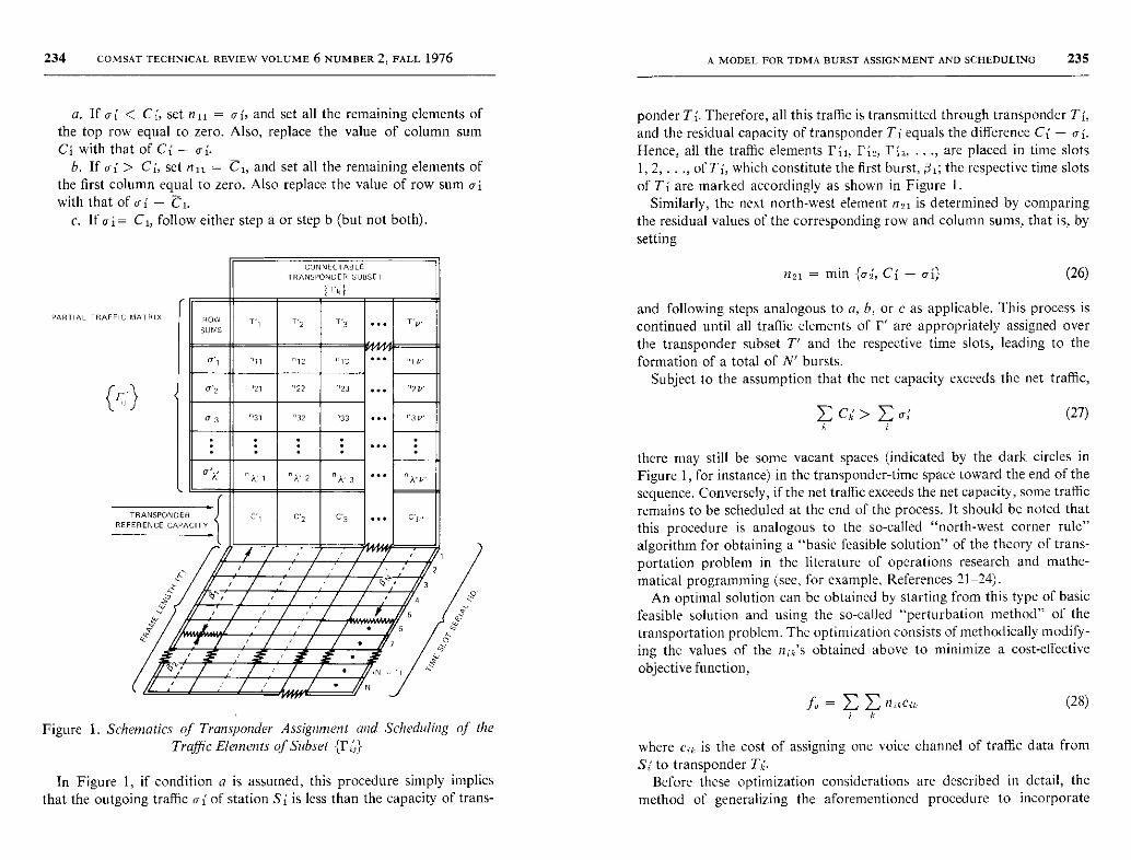
is nik (i = 1, 2, ..., T ; k = 1, 2, ..., 3), the burst assignment probleminvolves determining the values of nik, subject to the constraints
nik = Oi,k=1
(24a)
T•
nik < C,, k = 1, 2, ..., v' (24b)i= I
and
nik > 0 . (24c)
In addition, the time ordering of the nik's within the transponder framesmust be determined.
The problem is represented in tabular form in Figure 1. The partialtraffic matrix containing only the set of elements {P,;} is shown on the left,with the row sums a as indicated. The transponder labels Tk appear in thetop row on the right and the respective transponder capacity C% in thebottom row, with the requisite numbers nik between them. The time framefor each transponder is shown as an independent system coordinate on aslant scale at the bottom, with slots 1 through N marked serially along the
bottom right side.The assignment scheme can be explained by arbitrarily starting with the
transmitting station at the top, Si, and transponder Ti of the first columnand determining the corresponding "north-west" element nil. Then, forthe subsequent transmitting stations Si, S,, ..., the subsequent transpon-
ders Tj, T,, ..., as necessary, are considered sequentially. It should benoted that the time frames of each transponder should be filled as much aspossible before going to the next transponder. Since Ti cannot containmore traffic than its capacity, Ci,
nil = min {of, Cr} (25)
where C, = Ci if any link can be split in two or more parts. Otherwise, Clrepresents the sum in equation (23) excluding the traffic elements that cause
the sum to exceed Ci.Once the first north-west element nil has been determined, all other
elements in either the top row or the first column (but not both) can be
determined as follows:
234 COMSAT TECHNICAL REVIEW VOLUME 6 NUMBER 2, FALL 1976
a. If of < Cl, set n1T = ai, and set all the remaining elements ofthe top row equal to zero. Also, replace the value of column sumCi with that of Cl' - ai•
b. If ai > Cf, set n11 = C1, and set all the remaining elements ofthe first column equal to zero. Also replace the value of row sum o1with that of of - C1.
C. If ai= C1, follow either step a or step b (but not both).
TRANSPONDERREFERENCE CAPACITY
CONNECTABLE
TRANSPONDER SUBSET
1Tkl
T T3 T'3 . T'P.
^„ ^13 /113 . /ilY
1121 '22 n23 . ^9 V'
"31 '32 ^ 33 . "3 V
n^ 1 "^• 2 3 . n^. y.
C'1 C'2 C3 . Cy.
_7 7-7Q= 3
7
7 / 11 Z ^11
Figure 1. Schematics of Transponder Assignment and Scheduling of theTraffic Elements of Subset {pij}
In Figure 1, if condition a is assumed, this procedure simply impliesthat the outgoing traffic ai of station Sf is less than the capacity of trans-
A MODEL FOR TDMA BURST ASSIGNMENT AND SCHEDULING 235
ponder Tf . Therefore, all this traffic is transmitted through transponder Ti,and the residual capacity of transponder Ti equals the difference Cf - af.Hence, all the traffic elements I'i1, Pie, Pia, ..., are placed in time slots1, 2, ..., of Ti, which constitute the first burst, 01; the respective time slotsof Ti are marked accordingly as shown in Figure 1.
Similarly, the next north -west element n21 is determined by comparingthe residual values of the corresponding row and column sums, that is, bysetting
n21 = min {cl, Ci - ai} (26)
and following steps analogous to a, b, or c as applicable. This process iscontinued until all traffic elements of r' are appropriately assigned overthe transponder subset T' and the respective time slots, leading to the
formation of a total of N' bursts.Subject to the assumption that the net capacity exceeds the net traffic,
E C^> Ea;F 1
(27)
there may still be some vacant spaces (indicated by the dark circles inFigure 1, for instance) in the transponder -time space toward the end of the
sequence . Conversely , if the net traffic exceeds the net capacity, some trafficremains to be scheduled at the end of the process . It should be noted thatthis procedure is analogous to the so-called "north-west corner rule"algorithm for obtaining a "basic feasible solution" of the theory of trans-portation problem in the literature of operations research and mathe-matical programming (see, for example , References 21-24).
An optimal solution can be obtained by starting from this type of basicfeasible solution and using the so-called "perturbation method" of thetransportation problem. The optimization consists of methodically modify-ing the values of the nrk ' s obtained above to minimize a cost -effective
objective function,
J B - E E n ikCiF.1 k
(28)
where cik is the cost of assigning one voice channel of traffic data from
S{ to transponder Ti.Before these optimization considerations are described in detail, the
method of generalizing the aforementioned procedure to incorporate
236 COMSAT TECHNICAL REVIEW VOLUME 6 NUMBER 2, FALL 1976
various operational constraints will be described . First, the subset N_ {I'{;, i, j = 1, 2, ..., X'} is chosen according to any arbitrary priorityscheme, with or without regard to beam coverage . In general , there is nowa multiplicity of beam coverages for the transmitting and receiving stationsof the resulting partial traffic matrix . Hence, the entire transponder setT = {Tr, k = 1, 2, ..., v} (rather than a subset thereof ) must normallybe considered in connection with the assignment/scheduling of its trafficelements, and a systematic or hicrarchial search for appropriate trans-ponders must be conducted for each traffic element.
Other system constraints mentioned previously are also explicitly super-imposed on the preceding assignment scheme. For example, a preamblemust be provided to accompany each burst; the burst length must besubject to an upper limit, i.e., the maximum burst length ; TDMA/DSI com-pression must be provided ; and excessive burst overlap must be avoidedto minimize the equipment requirements of transmitting and receivingstations. The exact sequential order in which the transponders and thetime slots are used may be (and generally is) modified due to the presenceof these constraints . Hence, the scheduling mustbe performed dynamically.In other words , the scheduling decisions at any stage can be made only byexamining the result of all the relevant prior decisions ; these decisions willthen affect all subsequent decisions.
For instance, the total preamble or overhead requirement involved can-not be determined a priori, but will depend on how often a new burst mustbe started for the transmitting station to comply with the maximum burstlength constraint or the minimum burst overlap condition. The latter, inturn, will require that certain time slots in a given transponder be skippedin the scheduling of a given traffic element , leaving gaps in the transponderframe which may or may not be filled by another traffic element at a laterstage of the scheduling process. Similar to the total overhead , the totalnumber of vacancies or the amount of unutilized capacity resulting fromthe nonoverlap condition cannot be determined a priori; instead , it may bea sensitive function of the input data structure and the dynamic decisionprocedures involved.
Certain other special system considerations have also been incorporatedand will be mentioned subsequently . At this point it is sufficient to notethat the generalized north -west corner rule type of algorithm is con-veniently used in the framework of the mathematical model describedpreviously to obtain a basic feasible solution of the TDMA schedulingproblem. However, a completely analytical method for optimizing thesolution, such as the perturbation method of the theory of transportation
A MODEL FOR TDMA BURST ASSIGNMENT AND SCHEDULING 237
problem, is impractical due to the inherent size of the problem and thecomplexity introduced by the system constraints. This limitation is com-pounded by the fact that the cost factors c,k in equation (28) usually can-not be determined systematically or objectively. In view of these difficulties,a search for the optimum solution is made heuristically by using certaincontrol parameters governing the priority scheme and burst configuration.These parameters will be described in the following subsection, along withthe computer implementation of the preceding mathematical model andalgorithm.
Computer model
The following is a brief summary of the important steps and optionsimplemented in a computer program for TDMA scheduling recently de-veloped by the author. The scheduling is performed by first reordering therows and columns of the traffic matrix (without altering its symmetriccharacter) on the basis of beam coverage and traffic size so that narrowerbeams and stations with a larger total traffic requirement are given a higherhierarchical order. The rearranged traffic matrix (hereafter denoted as I')is sorted into four partial traffic matrices
I =rtu+F2 +r + r(4) (29a)
(29b)
In equation (29a), I'M includes, in part, those elements of F which are
large enough to equal or exceed the capacity of a transponder (minus the
necessary overhead). A part of such an element is extracted to form the
corresponding element of I'ID so that this element (plus the necessary
overhead) completely fills one or more transponders. The remaining ele-
ments of F'' are zero. Similarly, the nonzero elements of I'I'" are those ele-
ments of F - II') whose size exceeds the user-specified maximum burst
length, 8,,,. rI" consists of those elements of r - I'I1I - I1(2) which corre-
spond to stations with net 1-way traffic less than a user-specified lower
limit, 8,,,. Finally, the elements of I'I"' are simply the remaining elements
[i.e., I'I'I = r - 1'(') - I'I2' - I'(")]. Note that, except for the possible
splitting of links to form the nonzero elements of rI", each link specified
in I' appears in one and only one partial traffic matrix.
This classification of traffic data is useful for exercising flexible controlover the priority scheme for various traffic elements in the scheduling
238 COMSAT TECHNICAL REVIEW VOLUME 6 NUMBER 2, FALL 1976
process. The elements of r1') are assigned and scheduled first, followed bythose of r(,), f(3), and rt"), in that order. The elements of a particularpartial traffic matrix are scheduled according to their row numbers re-ferred to the rearranged matrix F. The elements of the same row arescheduled according to their column numbers (referred to r) or, optionally,according to their relative sizes, with the largest first. At this stage eachelement is considered to be indivisible and is scheduled integrally, therebyminimizing the number of up-chains. A particular element is assigned/scheduled by searching for the appropriate up- and down-link beams,transponders, and vacant time segments ( consisting of a sufficiently largenumber of contiguous empty time slots), in that order, subject to user-specified beam coverage, transponder connectivity, and hierarchy. After asuitable vacancy is found, the final assignment is made by checking forburst overlap and, if necessary, moving the burst (or a single link compo-nent thereof, called the sub-burst) to another suitable vacancy to avoidoverlap. A provision for necessary preambles is included throughout, as isa provision for evaluating various parameters of transponder utilizationefficiency and for determining the required earth station equipmentinventory.
This scheme tends to optimize the utilization of transponders, terminals(transmitters), and up-converters by minimizing overhead (preamble), sub-ject to the maximum burst length constraint. Furthermore, this schemeassigns higher priority to larger traffic elements and stations with largetraffic requirements, and at the same time tends to prevent excessive equip-ment requirements for stations with very small traffic requirements. Drasticvariations in the implicit priority scheme described above can be effectedsimply by varying the input values of the parameters 8,,, and Bm. Almostany arbitrary distribution of elements within rr", 170', and r(4) can beachieved by varying the 0and B„ values over a suitable range. In particu-lar, a very small value of B„ will cause all remaining nonzero elements to beexcluded from p('). The converse applies to the choice of 0,n for inclusionor exclusion of elements with respect to r(2). A very small value of 8,,, isnot recommended, however, since it will lead to excessive overhead re-quirements associated with the small value of the implied maximum burstlength.
Several options for choosing the overall priority in the scheduling processare provided in the program. For example, the elements can be sequen-tially packed in transponders without checking for burst overlaps or leav-ing gaps in the transponder frames, thereby optimizing the fill factor.Alternatively, as mentioned previously, the relevant transponder-time
A MODEL FOR TDMA BURST ASSIGNMENT AND SCHEDULING 239
space may be scanned before each traffic element is assigned to avoidexcessive burst overlaps, thereby minimizing equipment (terminal) re-quirements for transmitting or receiving stations. If excessive equipmentrequirements are unavoidable, it is possible either to accept the increasedrequirements and proceed with scheduling, or to omit the specific trafficelement subject to the specified minimum equipment constraint. Similarly,if no transponder-time space is available for a particular traffic element,scheduling may be continued with the remaining elements or terminatedaltogether so that a fresh trial with modified input values of the controlparameters can be made.
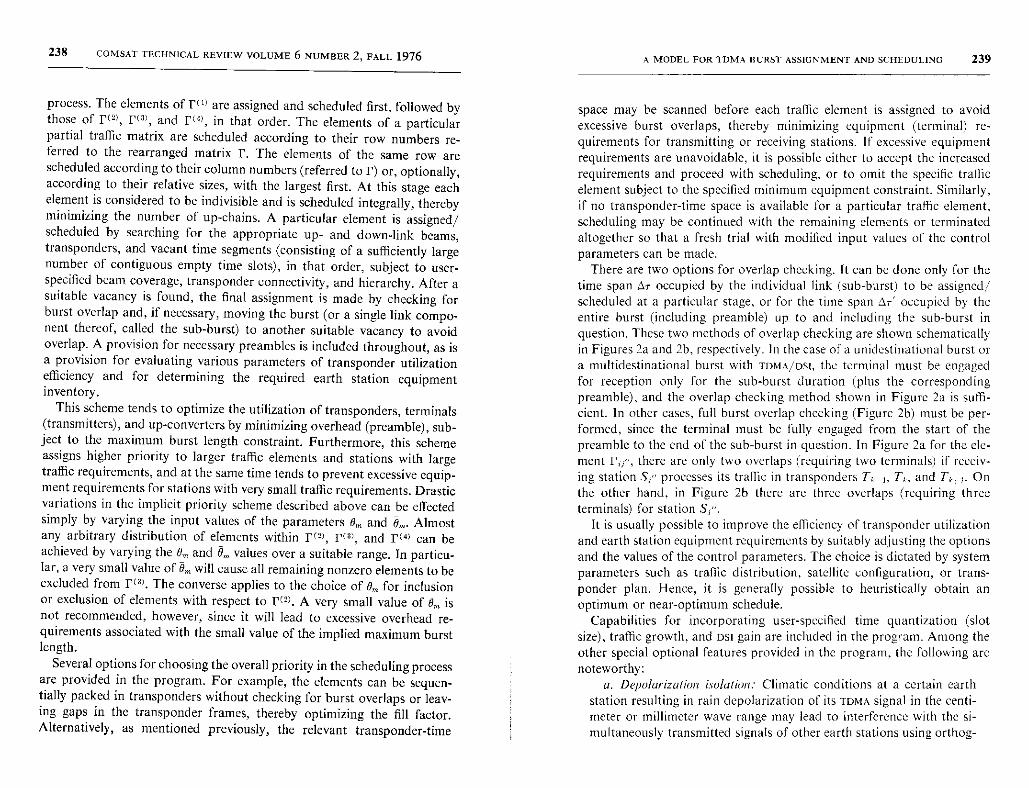
There are two options for overlap checking. It can be done only for thetime span AT occupied by the individual link (sub-burst) to be assigned/scheduled at a particular stage, or for the time span dr' occupied by theentire burst (including preamble) up to and including the sub-burst inquestion. These two methods of overlap checking are shown schematicallyin Figures 2a and 2b, respectively. In the case of a unidestinational burst ora multidestinational burst with TDMA/DSI, the terminal must be engagedfor reception only for the sub-burst duration (plus the correspondingpreamble), and the overlap checking method shown in Figure 2a is suffi-cient. In other cases, full burst overlap checking (Figure 2b) must be per-formed, since the terminal must be fully engaged from the start of thepreamble to the end of the sub-burst in question. In Figure 2a for the ele-ment 1';, there are only two overlaps (requiring two terminals) if receiv-ing station S,° processes its traffic in transponders T,,_,, Ta, and Tf.; . Onthe other hand, in Figure 2b there are three overlaps (requiring threeterminals) for station S;°.
It is usually possible to improve the efficiency of transponder utilizationand earth station equipment requirements by suitably adjusting the optionsand the values of the control parameters. The choice is dictated by systemparameters such as traffic distribution, satellite configuration, or trans-ponder plan. Hence, it is generally possible to heuristically obtain anoptimum or near-optimum schedule.
Capabilities for incorporating user-specified time quantization (slotsize), traffic growth, and DSI gain are included in the program. Among theother special optional features provided in the program, the following arenoteworthy:
a. Depolarization isolation. Climatic conditions at a certain earthstation resulting in rain depolarization of its TDMA signal in the centi-meter or millimeter wave range may lead to interference with the si-multaneously transmitted signals of other earth stations using orthog-
240 COMSAT TECHNICAL REVIEW VOLUME 6 NUMBER 2, FALL 1976
.c Qr ^h m
° .c
• • •
•0•
__1 I-- ___TI f-_I
• • •
• • •
o
1 U y
I-
d
J U
to
IO y
y~ v
c OQ Q
(r ^
A MODEL FOR TDMA BURST ASSIGNMENT AND SCHEDULING 241
onal polarization . To avoid such depolarization - induced interference.the signal of the station in question may be isolated in the frame sothat the signal of any other stations (or the signal of any member of acertain subset of other stations ) is not transmitted during its time slots.
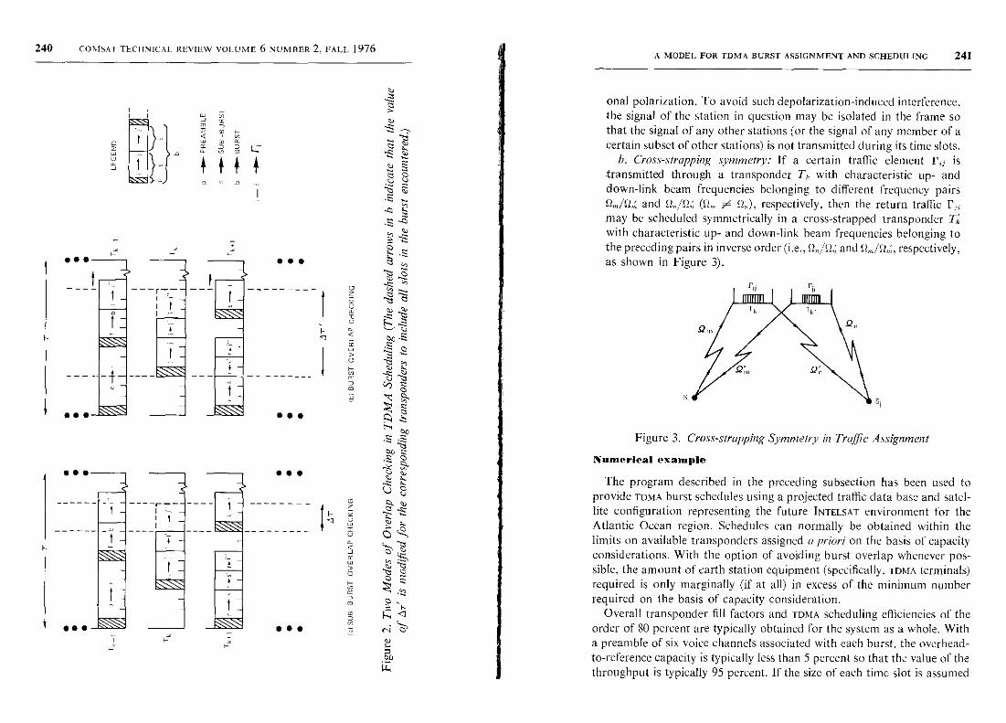
h. Cross-strapping symmetry : If a certain traffic element p0; istransmitted through a transponder T,, with characteristic up- anddown-link beam frequencies belonging to different frequency pairsS2m^12,;, and (12„ x S2„), respectively , then the return traffic p,;may be scheduled symmetrically in a cross-strapped transponder T^with characteristic up- and down - link beam frequencies belonging tothe preceding pairs in inverse order (i.e., Sln^Sl;, and S2m/S2,;,, respectively,as shown in Figure 3).
r
Tk Tk
I2 iT 4n
gn, Qn
S
Figure 3. Cross-strapping Symmetry in Traffic Assignment
Numerical example
The program described in the preceding subsection has been used toprovide TOMA burst schedules using a projected traffic data base and satel-lite configuration representing the future INTELSAT environment for theAtlantic Ocean region. Schedules can normally be obtained within thelimits on available transponders assigned a priori on the basis of capacityconsiderations. With the option of avoiding burst overlap whenever pos-sible, the amount of earth station equipment (specifically, TDMA terminals)required is only marginally (if at all) in excess of the minimum numberrequired on the basis of capacity consideration.
Overall transponder fill factors and TDMA scheduling efficiencies of theorder of 80 percent are typically obtained for the system as a whole. Witha preamble of six voice channels associated with each burst, the overhead-to-reference capacity is typically less than 5 percent so that the value of thethroughput is typically 95 percent. If the size of each time slot is assumed
242 COMSAT TECHNICAL REVIEW VOLUME 6 NUMBER 2, FALL 1976 A MODEL FOR TDMA BURST ASSIGNMENT AND SCHEDULING 243
to be equivalent to the capacity of six voice channels, the ratio of assignedto configured capacity is typically 96 percent; therefore, the capacitydegradation due to reasonable quantization of the time scale is only
marginal.Since a specific example involving a large traffic data base is not possible
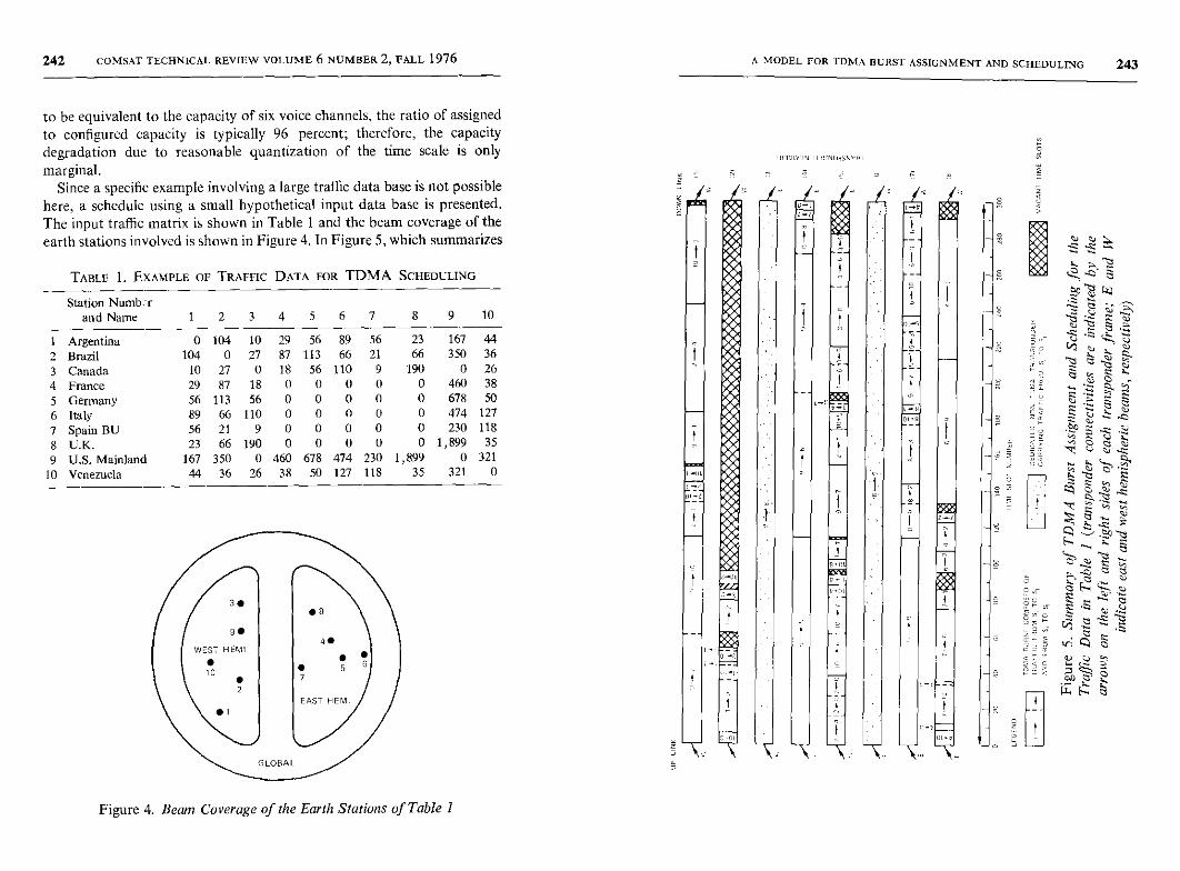
here, a schedule using a small hypothetical input data base is presented.The input traffic matrix is shown in Table 1 and the beam coverage of theearth stations involved is shown in Figure 4. In Figure 5, which summarizes
TABLE 1. EXAMPLE OF TRAFFIC DATA FOR TDMA SCHEDULING
Station Numberand Name 1 2 3 4 5 6 7 8 9 10
7 Argentina 0 104 10 29 56 89 56 23 167 44
2 Brazil 104 0 27 87 113 66 21 66 350 36
3 Canada 10 27 0 18 56 110 9 190 0 26
4 France 29 87 18 0 0 0 0 0 460 38
5 Germany 56 113 56 0 0 0 0 0 678 50
6 Italy 89 66 110 0 0 0 0 0 474 127
7 Spain BU 56 21 9 0 0 0 0 0 230 118
8 U.K. 23 66 190 0 0 0 0 0 1,899 35
9 U.S. Mainland 167 350 0 460 678 474 230 1,899 0 321
10 Venezuela 44 36 26 38 50 127 118 35 321 0
1 LHIlN , urNUnsmvai
[Jw
Figure 4. Beam Coverage of the Earth Stations of Table 1
^>T
244 COMSAT TECHNICAL REVIEW VOLUME 6 NUMBER 2, FALL 1976
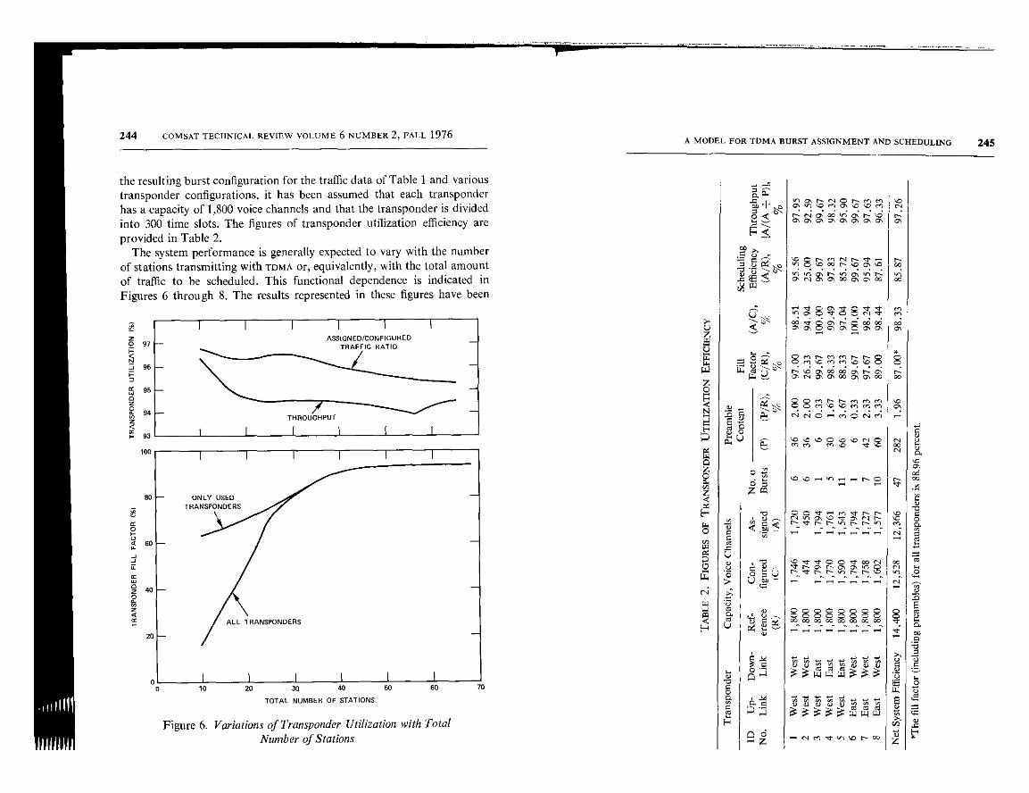
the resulting burst configuration for the traffic data of Table I and varioustransponder configurations, it has been assumed that each transponderhas a capacity of 1,800 voice channels and that the transponder is dividedinto 300 time slots. The figures of transponder utilization efficiency are
provided in Table 2.The system performance is generally expected to vary with the number
of stations transmitting with TDMA or, equivalently, with the total amountof traffic to be scheduled. This functional dependence is indicated inFigures 6 through 8. The results represented in these figures have been
® 0 10 20 30 40 50
TOTAL NUMBER OF STATIONS
60 70
Figure 6. Variations of Transponder Utilization with Total
Number of Stations
A MODEL FOR TDMA BURST ASSIGNMENT AND SCHEDULING
FQ
0 ' Ana, ^a,a cn
aN, rn a aa. a a rnrn
v̀ai CC wN Co^„onnrnN V,aitnNa, N a, a, 00 a, p, 00
C
a,
N
00
U- a\ O V a 8 N 4
ti
a\a, g o, a,g a, o, 0\
S m N m rn N N O
^rn ,a (+1 M ^D ,C O
b`w W N ^C a, 00 ro p, N a,a, N O, a, 00 a, p, W m
8SMNNeneneVJ ,C (n (n rn a,
A u N N O^ M C N •n
4 U pC C b O ,C C N Sn cn ^C aV
N
O Vz
N
N VU vW V
°!aCaaNN
C t V C C V 00 NV N a, N a, a, n O
O O O C O C O O00 W W ^ V2 V2 UJ 00
N
h
N
S
3 CQa
2 Crte. r-1
Qz
33www333
33333www
.- N I V 0/ ' N W
245
246 COMSAT TECHNICAL REVIEW VOLUME 6 NUMBER 2, FALL 1976
100
90
60
70
60
50
USED TRANSPONDERS ONLY(INCLUDING PREAMBLES)
IEXCLUOING PREAMBLES) X
az 241-
20
103 X 103
I I I I I I I4 5 6 7 6 9 1 X 10⁴
ASSIGNED TRAFFIC ( VOICE CHANNELS)
12
I I I II
10 18 25 3965
NUMBER OF STATIONS
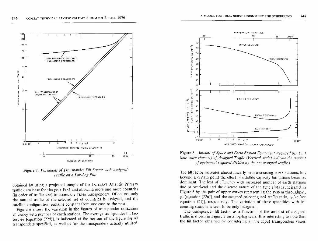
Figure 7. Variations of Transponder Fill Factor with Assigned
Traffic on a Log-Log Plot
obtained by using a projected sample of the INTELSAT Atlantic Primarytraffic data base for the year 1985 and allowing more and more countries(in order of traffic size) to access the TDMA transponders. Of course, onlythe mutual traffic of the selected set of countries is assigned, and thesatellite configuration remains constant from one case to the next.
Figure 6 shows the variation in the figures of transponder utilizationefficiency with number of earth stations. The average transponder fill fac-tor, q,1 [equation (22d)], is indicated at the bottom of the figure for alltransponders specified, as well as for the transponders actually utilized.
20
A MODEL FOR TDMA BURST ASSIGNMENT AND SCHEDULING 247
92
88
84
80
76
72
68
64
0NUMBER OF STATIONS
18 25 3965
60
36r
32
28 -
16
12-
8
4
TSPACE SEGMENT
TRANSPONDER
F-'7
EARTH SEGMENT
TDMA TERMINAL
CONVERTER
04X103 5 6 7 8 9 1X10⁴
ASSIGNED TRAFFIC (VOICE CHANNELS)
f2 3X10⁴
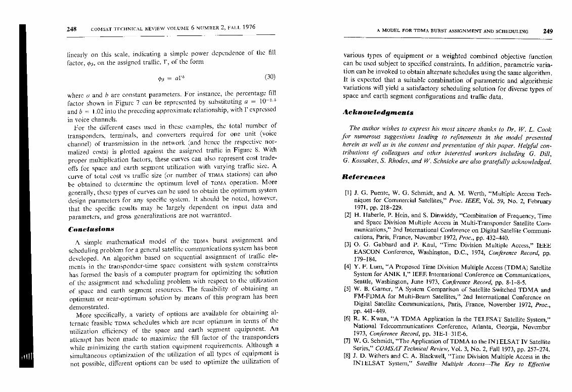
Figure 8. Amount of Space and Earth Station Equipment Required per Unit(one voice channel) of Assigned Traffic ( Vertical scales indicate the amount
of equipment required divided by the net assigned traffic.)
The fill factor increases almost linearly with increasing TDMA stations, butbeyond a certain point the effect of satellite capacity limitations becomesdominant. The loss of efficiency with increased number of earth stationsdue to overhead and the discrete nature of the time slots is indicated inFigure 6 by the pair of upper curves representing the system throughput,0. [equation (22a)], and the assigned-to-configured traffic ratio, uc/ur [seeequation (21)], respectively. The variation of these quantities with in-creasing stations is seen to be only marginal.
The transponder fill factor as a function of the amount of assignedtraffic is shown in Figure 7 on a log-log scale. It is interesting to note thatthe fill factor obtained by considering all the input transponders varies
248 COMSAT TECHNICAL REVIEW VOLUME 6 NUMBER 2 , FALL 1976
linearly on this scale, indicating a simple power dependence of the fill
factor, 0o , on the assigned traffic, F, of the form
oa = aI'a (30)
where a and b are constant parameters . For instance , the percentage fill
factor shown in Figure 7 can be represented by substituting a = 10-2.5
and b = 1.02 into the preceding approximate relationship , with F expressed
in voice channels.For the different cases used in these examples , the total number of
transponders , terminals, and converters required for one unit (voice
channel) of transmission in the network (and hence the respective nor-
malized costs) is plotted against the assigned traffic in Figure 8. Withproper multiplication factors, these curves can also represent cost trade-offs for space and earth segment utilization with varying traffic size. A
curve of total cost vs traffic size ( or number of TDMA stations) can also
be obtained to determine the optimum level of TDMA operation. Moregenerally, these types of curves can be used to obtain the optimum systemdesign parameters for any specific system. It should be noted, however,that the specific results may be largely dependent on input data and
parameters , and gross generalizations are not warranted.
Conclusions
A simple mathematical model of the TDMA burst assignment andscheduling problem for a general satellite communications system has beendeveloped. An algorithm based on sequential assignment of traffic ele-ments in the transponder-time space consistent with system constraintshas formed the basis of a computer program for optimizing the solutionof the assignment and scheduling problem with respect to the utilizationof space and earth segment resources. The feasibility of obtaining anoptimum or near-optimum solution by means of this program has been
demonstrated.More specifically, a variety of options are available for obtaining al-
ternate feasible TDMA schedules which are near optimum in terms of theutilization efficiency of the space and earth segment equipment. Anattempt has been made to maximize the fill factor of the transponderswhile minimizing the earth station equipment requirements. Although asimultaneous optimization of the utilization of all types of equipment isnot possible, different options can be used to optimize the utilization of
A MODEL FOR TDMA BURST ASSIGNMENT AND SCHEDULING 249
various types of equipment or a weighted combined objective functioncan be used subject to specified constraints. In addition, parametric varia-tion can be invoked to obtain alternate schedules using the same algorithm.It is expected that a suitable combination of parametric and algorithmicvariations will yield a satisfactory scheduling solution for diverse types ofspace and earth segment configurations and traffic data.
Acknowledgments
The author wishes to express his most sincere thanks to Dr. W. L. Cookfor numerous suggestions leading to refinements in the model presentedherein as well as in the content and presentation of this paper. Helpful con-tributions of colleagues and other interested workers including G. Dill,G. Kossakes, S. Rhodes, and W. Schnicke are also gratefully acknowledged.
References
[1] J. G. Puente, W. G. Schmidt, and A. M. Werth, "Multiple Access Tech-niques for Commercial Satellites," Proc. IEEE, Vol. 59, No. 2, February1971, pp. 218-229.
[2] H. Haberle, P. Hein, and S. Dinwiddy, "Combination of Frequency, Time
and Space Division Multiple Access in Multi-Transponder Satellite Com-munications," 2nd International Conference on Digital Satellite Communi-cations, Paris, France, November 1972, Proc., pp. 432-440.
[3] O. G. Gabbard and P. Kaul, "Time Division Multiple Access," IEEEEASCON Conference, Washington, D.C., 1974, Conference Record, pp.179-184.
[4] Y. F. Lum, "A Proposed Time Division Multiple Access (TDMA) SatelliteSystem for ANIK I," IEEE International Conference on Communications,Seattle, Washington, June 1973, Conference Record, pp. 8-1-8-5.
[5] W. B. Garner, "A System Comparison of Satellite Switched TDMA andFM-FDMA for Multi-Beam Satellites," 2nd International Conference on
Digital Satellite Communications, Paris, France, November 1972, Proc.,pp. 441-449.
[6] R. K. Kwan, "A TDMA Application in the TELESAT Satellite System,"National Telecommunications Conference, Atlanta, Georgia, November1973, Conference Record, pp. 3IE-1-31E-6.
[7] W. G. Schmidt, "The Application of TDMA to the INTELSAT IV SatelliteSeries," COMSAT Technical Review, Vol. 3, No. 2, Fall 1973, pp. 257-274.
[8] J. D. Withers and C. A. Blackwell, "Time Division Multiple Access in theINTELSAT System," Satellite Multiple Access-The Key to Effective
250 COMSAT TECHNICAL REVIEW VOLUME 6 NUMBER 2, TALL 1976 A MODEL FOR TDMA BURST ASSIGNMENT AND SCHEDULING 2$1
Utilization, IEEE International Convention, New York, N.Y., March 1973,
pp. 1-7.[9] S. Browne, "The INTELSAT Global Satellite Communications System,"
COMSAT Technical Review, Vol. 4, No. 2, Fall 1974, pp. 477-487.
[10] W. Schmidt, "An On-Board Switched Multiple Access System for Milli-meter-Wave Satellites," INTELSAT/IEE International Conference on
Digital Satellite Communications, London, England, November 1969,
Proc., pp. 399-407.[11] T. Muratani, "Satellite Switched Time-Domain Multiple Access," IEEE
EASCON Conference, Washington, D.C., 1974, Conference Record, pp.
189-196.[12] R. Cooperman and W. G. Schmidt, "Satellite-Switched SDMA and TDMA
System for Wide Band Multibeam Satellite," IEEE International Conference
on Communications, Seattle, Washington, June 1973, Conference Record,
pp. 12-7-12-12.[13] W. G. Schmidt, "Satellite Switched TDMA -Transponder Switched or
Beam-Switched," AIAA 5th Communications Satellite Systems Conference,
Los Angeles, California, April 1974, Paper No. 74-460.[14] R. A. J. Smith, "TDMA Multiple Transponder Operation by Means of
Frequency Hopping," 2nd International Conference on Digital Satellite
Communications, Paris, France, November 1972, Proc., pp. 425-431.
[15] N. Shimasaki and R. Rapuano, "Synchronization for a CommunicationsDistribution Center On-Board a Satellite," IEEE International Conference
on Communications, 1971, Conference Record, pp. 42-20- 42-55.
[16] C. Carter and S. S. Haykin, "Precision Synchronization to a SwitchingSatellite Using PSK Signals," IEEE International Conference on Com-
munications, Minneapolis, Minnesota, June 1974, Conference Record,
pp. 43D-1-43D-5.[17] H. Ganssmantel and B. Ekstrom, "TDMA Synchronization for Future
M ultitransponder Satellite Communications," IEEE International Con-ference on Communications, Minneapolis, Minnesota, June 1974, Con-
ference Record, pp. 43C-1-43C-5.[18] J. W. Schwartz, J. M. Acin, and J. Kaiser, "Modulation Techniques for
Multiple Access to a Hard-Limiting Satellite Repeater," Proc. IEEE, Vol.
54, No. 5, May 1966, pp. 763-777.[19] L. Lundquist, "Optimizing a TDMA Channel Including Synchronization,"
IEEE International Conference on Communications, Minneapolis, Minne-
sota, June 1974, Conference Record, pp. 43A-1-43A-4.
[20] S. J. Campanella and H. G. Suyderhoud, "Digital Speech Interpolation forTelephone Communications," IEEE EASCON Conference, Washington,
D.C., 1974, Conference Record, pp. 331-336.
[21] G. B. Dantzig, Linear Programming and Extensions, Princeton, New Jersey:
Princeton University Press, 1963.
[22] S. I. Gass, Linear Programming, New York: McGraw-Hill Book Co., 1964.
[23] M. Simonard, Linear Programming, New Jersey: Prentice-Hall, Inc., 1966.[24] G. S. G. Beveridge and R. S. Schechter, Optimization: Theory and Practice,
New York: McGraw-Hill Book Co., 1970.
Ashok K. Sinha received a B.Sc. (1963) and anM.Sc. (1965) in physics from Patna University,
India, and a Ph.D. in physics from the Universityof Maryland (1971). As a Research Associate forthe U. of Md. (1971-1973) and as a member ofthe technical staff of Computer Sciences Corpora-tion (1974), he was involved with several NASA-sponsored geophysical research and analysisprojects, including ionospheric, upper atmospheric,
and geomagnetic field modeling and ionosphericscintillations . He joined COMSAT Laboratories in 1974 as a member of thetechnical staff of the Transmission Systems Laboratory, where he is cur-rently involved with communications satellite system modeling and long-range planning methodology . He is a member of the American GeophysicalUnion and the International Association of Geomagnetism and Aeronomy.
®1
Index : adaptive control , polarization , orthogonality,frequency reuse
Adaptive polarization control forsatellite frequency reuse systems
D. F. DIFONZO, W. S. TRACHTMAN, AND A. E. WILLIAMS
(Manuscript received February 19, 1976)
Abstract
This paper describes networks for the adaptive restoration of polarizationorthogonality. These networks may be used to minimize the mutual interferenceof a dual-polarized satellite communications link operating in the presence of adepolarizing medium. For a properly designed system, the time-varying depolar-ization due to a variety of sources may necessitate adaptive network control. Asdescribed herein, the circuits to accomplish this objective are based on theassumption that the error voltages for adaptive control are derived from narrow-band pilot signals provided within the communications spectrum. In general,
four control parameters are required to achieve orthogonality correction, butwhen differential attenuation may be neglected, a suboptimal control systememploying two control parameters leads to a simple and attractive solution.
Introduction
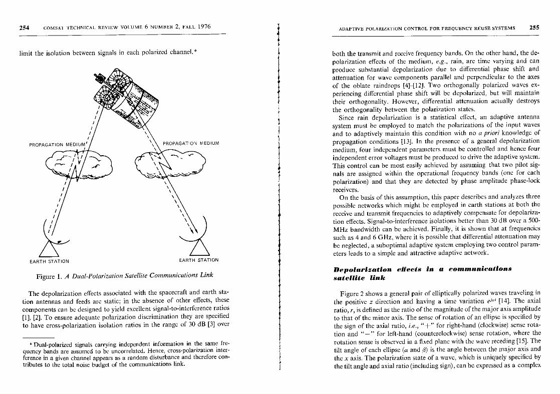
A typical dual-polarized satellite communications link is shown inFigure 1. In such a link the depolarizing effects of the earth station an-tennas, the satellite antennas, and the propagation medium all combine to
This paper is based upon work performed in COMSAT Laboratories under thesponsorship of the International Telecommunications Satellite Organization(INTELSAT). Views expressed in this paper are not necessarily those of INrELSAT.
253
254 COMSAT TECHNICAL REVIEW VOLUME 6 NUMBER 2, FALL 1976
limit the isolation between signals in each polarized channel.*
t
PROPAGATION MEDIUM' IA PROPAGATION MEDIUM
EARTH STATION EARTH STATION
Figure 1. A Dual-Polarization Satellite Communications Link
The depolarization effects associated with the spacecraft and earth sta-tion antennas and feeds are static; in the absence of other effects, thesecomponents can be designed to yield excellent signal-to-interference ratios[1], [2]. To ensure adequate polarization discrimination they are specifiedto have cross-polarization isolation ratios in the range of 30 dB [3] over
* Dual-polarized signals carrying independent information in the same fre-quency bands are assumed to be uncorrelated. Hence, cross-polarization inter-ference in a given channel appears as a random disturbance and therefore con-tributes to the total noise budget of the communications link.
ADAPTIVE POLARIZATION CONTROL FOR FREQUENCY REUSE SYSTEMS 255
both the transmit and receive frequency bands. On the other hand, the de-polarization effects of the medium, e.g., rain, are time varying and canproduce substantial depolarization due to differential phase shift andattenuation for wave components parallel and perpendicular to the axesof the oblate raindrops [4]-12]. Two orthogonally polarized waves ex-periencing differential phase shift will be depolarized, but will maintaintheir orthogonality. However, differential attenuation actually destroysthe orthogonality between the polarization states.
Since rain depolarization is a statistical effect, an adaptive antennasystem must be employed to match the polarizations of the input waves
and to adaptively maintain this condition with no a priori knowledge of
propagation conditions [13]. In the presence of a general depolarizationmedium, four independent parameters must be controlled and hence fourindependent error voltages must be produced to drive the adaptive system.This control can be most easily achieved by assuming that two pilot sig-nals are assigned within the operational frequency bands (one for eachpolarization) and that they are detected by phase amplitude phase-lock
receivers.On the basis of this assumption, this paper describes and analyzes three
possible networks which might be employed in earth stations at both thereceive and transmit frequencies to adaptively compensate for depolariza-tion effects. Signal-to-interference isolations better than 30 dB over a 500-MHz bandwidth can be achieved. Finally, it is shown that at frequenciessuch as 4 and 6 GHz, where it is possible that differential attenuation maybe neglected, a suboptimal adaptive system employing two control param-eters leads to a simple and attractive adaptive network.
Depolarization effects in a communicationssatellite link
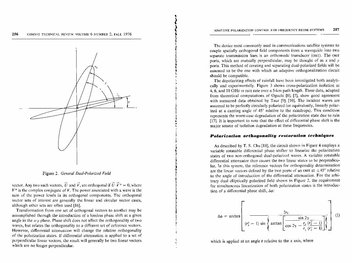
Figure 2 shows a general pair of elliptically polarized waves traveling inthe positive z direction and having a time variation era, [14]. The axialratio, r, is defined as the ratio of the magnitude of the major axis amplitudeto that of the minor axis. The sense of rotation of an ellipse is specified bythe sign of the axial ratio, i.e., "+" for right-hand (clockwise) sense rota-tion and "-" for left-hand (counterclockwise) sense rotation, where therotation sense is observed in a fixed plane with the wave receding [15]. Thetilt angle of each ellipse (a and p) is the angle between the major axis andthe x axis. The polarization state of a wave, which is uniquely specified bythe tilt angle and axial ratio (including sign), can be expressed as a complex
256 COMSAT TECHNICAL REVIEW VOLUME 6 NUMBER 2 , FALL 1976
Figure 2. General Dual-Polarized Field
vector. Any two such vectors, U and V, are orthogonal if U V* = 0, whereV* is the complex conjugate of V. The power associated with a wave is thesum of the power levels in its orthogonal components. The orthogonalvector sets of interest are generally the linear and circular vector cases,although other sets are often used [16].
Transformation from one set of orthogonal vectors to another may beaccomplished through the introduction of a lossless phase shift at a givenangle in the x-y plane. Phase shift does not affect the orthogonality of twowaves, but relates the orthogonality to a different set of reference vectors.However, differential attenuation will change the relative orthogonalityof the polarization states. If differential attenuation is applied to a set ofperpendicular linear vectors, the result will generally be two linear vectorswhich are no longer perpendicular.
r1.
ADAPTIVE POLARIZATION CONTROL FOR FREQUENCY REUSE SYSTEMS 257
The device most commonly used in communications satellite systems tocouple spatially orthogonal field components from a waveguide into twoseparate transmission lines is an orthomode transducer (OMT). The OMTports, which are mutually perpendicular, may be thought of as x and yports. This method of creating and separating dual-polarized fields will beassumed to be the one with which an adaptive orthogonalization circuitshould be compatible.
The depolarizing effects of rainfall have been investigated both analyti-cally and experimentally. Figure 3 shows cross-polarization isolation at4, 6, and 11 GHz vs rain rate over a 5-km path length. These data, adaptedfrom theoretical computations of Oguchi [6], [7], show good agreementwith measured data obtained by Taur [9], [10]. The incident waves areassumed to be perfectly circularly polarized (or equivalently, linearly polar-ized at a canting angle of 45° relative to the raindrops). This conditionrepresents the worst-case degradation of the polarization state due to rain[17]. It is important to note that the effect of differential phase shift is themajor source of isolation degradation at these frequencies.
Polarization orthogonality restoration techniques
As described by T. S. Chu [18], the circuit shown in Figure 4 employs avariable rotatable differential phase shifter to linearize the polarizationstates of two non-orthogonal dual-polarized waves. A variable rotatabledifferential attenuator then causes the two linear states to be perpendicu-lar. In this system, the reference vectors for orthogonality determinationare the linear vectors defined by the two ports of an OMT at ±45° relativeto the angle of introduction of the differential attenuation. For the arbi-trary dual elliptically polarized field shown in Figure 2, the requirementfor simultaneous linearization of both polarization states is the introduc-
tion of a differential phase shift, 0O:
00 = arctan2r6
(1)sin 2y 1(rb - 1) sin
{
arctan
Ccos 2y -'° (re l) J^
((( rb (r - 1) 1
which is applied at an angle 0 relative to the x axis, where
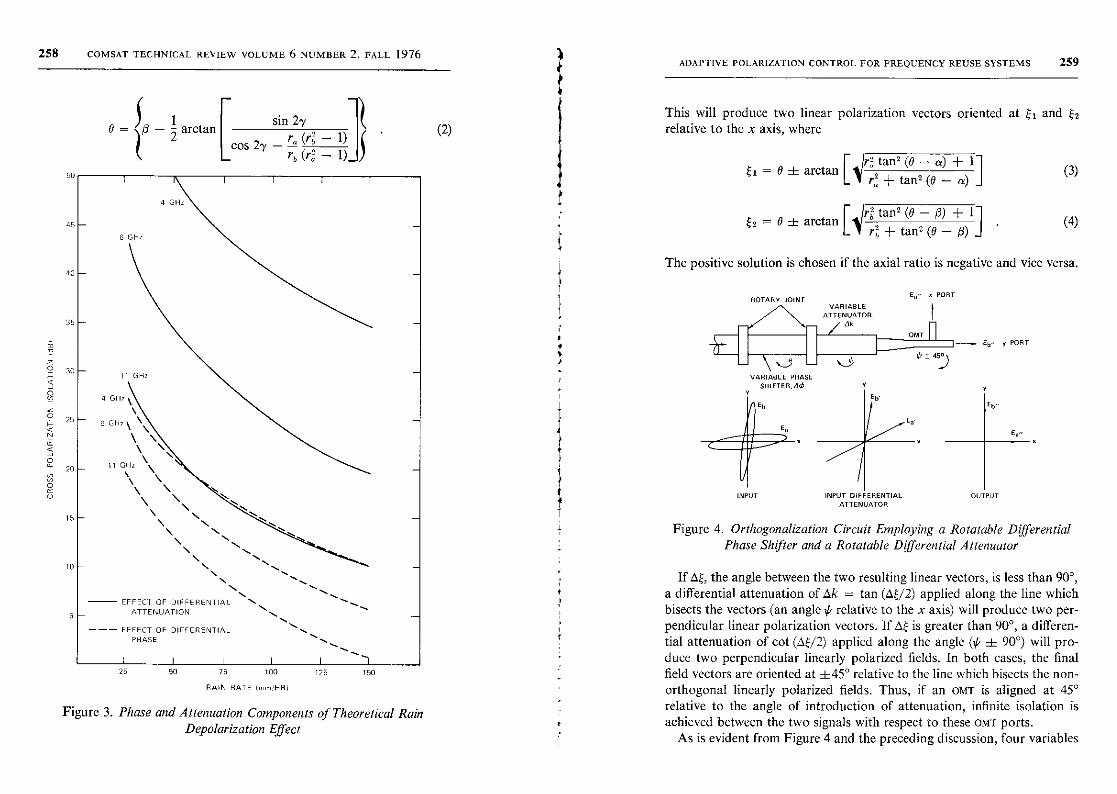
258 COMSAT TECHNICAL REVIEW VOLUME 6 NUMBER 2, FALL 1976ADAPTIVE POLARIZATION CONTROL FOR FREQUENCY REUSE SYSTEMS 259
18=6-2arctan-
cos 2y-rm
(r
ti- 1
)L rE (r2 - 1)50
45
40
35
15
10
5
i I
N\N
NN
NEFFECT OF DIFFERENTIAL N^
ATTENUATION N
--- EFFECT OF DIFFERENTIAL
PHASE
I I
25 50175 100
RAIN RATE (mm/HRI
I125
I
150
Figure 3. Phase and Attenuation Components of Theoretical RainDepolarization Effect
sin 2y(2)
This will produce two linear polarization vectors oriented at !;, andrelative to the x axis, where
r;; tang (B - a) 1+= B f arctan
^(3)
ra + tan2 (0 - a)
rztan2 (0 - p) + 1 1
Q2 = 0 zE arctan (4)r2 + tangy (B - p) J
The positive solution is chosen if the axial ratio is negative and vice versa.
ROTARY JOINTVARIABLE
ATTENUATOR,7rz\ r_1 Ak
VARIABLE PHASESHIFTER,AO
INPUT
Y
Ea R PORT
OMT- Ey y PORT
INPUT DIFFERENTIAL OUTPUT
ATTENUATOR
Figure 4. Orthogonalization Circuit Employing a Rotatable DifferentialPhase Shifter and a Rotatable DWerential Attenuator
If Ag, the angle between the two resulting linear vectors, is less than 90°,a differential attenuation of dk = tan (a4/2) applied along the line whichbisects the vectors (an angle ¢ relative to the x axis) will produce two per-pendicular linear polarization vectors. If A^ is greater than 90°, a differen-tial attenuation of cot (Di;/2) applied along the angle (fr f 90°) will pro-duce two perpendicular linearly polarized fields. In both cases, the finalfield vectors are oriented at ±45° relative to the line which bisects the non-orthogonal linearly polarized fields. Thus, if an OMT is aligned at 45°relative to the angle of introduction of attenuation, infinite isolation isachieved between the two signals with respect to these OMT ports.
As is evident from Figure 4 and the preceding discussion, four variables
260 COMSAT TECHNICAL REVIEW VOLUME 6 NUMBER 2, FALL 1976
are involved in matching the orthogonality of two arbitrary dual-polarizedsignals to a set of OMT ports. In this method, these four variables appear asAO, 0, Ak, and ¢. Two of these variables are associated with phase shift andtwo with attenuation. This process is one way of correcting for rain de-polarization which is caused by differential phase shift and differentialattenuation. The rain model, however, predicts that the differential phaseand attenuation are introduced into the original field at the same angle.Thus, the rain model has only three degrees of freedom, while the methoddescribed herein requires four to achieve orthogonalization. The essentialdifference is twofold. First, these two general ellipses are not necessarilybeing returned to the polarization states which they assumed before en-countering the rain. Second, the amount of attenuation introduced tocorrect for the depolarization is generally different from that which causedit. It can be shown that the value of Ak in this correction circuit is the mini-mum possible to effect orthogonalization [19] and is generally less than thevalue of attenuation introduced by the rain. Thus, this technique mini-mizes both Ak and the signal-to-noise degradation at the expense of anadditional degree of freedom.
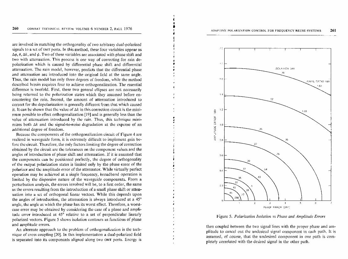
Because the components of the orthogonalization circuit of Figure 4 arerealized in waveguide form, it is extremely difficult to implement gain be-fore the circuit. Therefore, the only factors limiting the degree of correctionobtained by the circuit are the tolerances on the component values and theangles of introduction of phase shift and attenuation. If it is assumed thatthe components can be positioned perfectly, the degree of orthogonalityof the output polarization states is limited only by the phase error of thepolarizer and the amplitude error of the attenuator. While virtually perfectoperation may be achieved at a single frequency, broadband operation islimited by the dispersive nature of the waveguide components. From aperturbation analysis, the errors involved will be, to a first order, the sameas the errors resulting from the introduction of a small phase shift or atten-uation into a set of orthogonal linear vectors. While this depends uponthe angles of introduction, the attenuation is always introduced at a 45°angle, the angle at which the phase has its worst effect. Therefore, a worst-case error may be obtained by considering the case of a phase and ampli-tude error introduced at 45° relative to a set of perpendicular linearlypolarized vectors. Figure 5 shows isolation contours as functions of phaseand amplitude errors.
An alternate approach to the problem of orthogonalization is the tech-nique of cross coupling [20]. In this implementation a dual-polarized fieldis separated into its components aligned along two OMT ports. Energy is
S
ADAPTIVE POLARIZATION CONTROL FOR FREQUENCY REUSE SYSTEMS 261
LSOLAIION ORI
20
AXIAL RATIO Wtll
16
22
2
0
8
0.6
0.a
02
25
95
3 4
PHASE ERROR (OEO)
33
Figure 5. Polarization Isolation vs Phase and Amplitude Errors
then coupled between the two signal lines with the proper phase and am-plitude to cancel out the undesired signal component in each path. It isassumed, of course, that the undesired component in one path is com-pletely correlated with the desired signal in the other path.
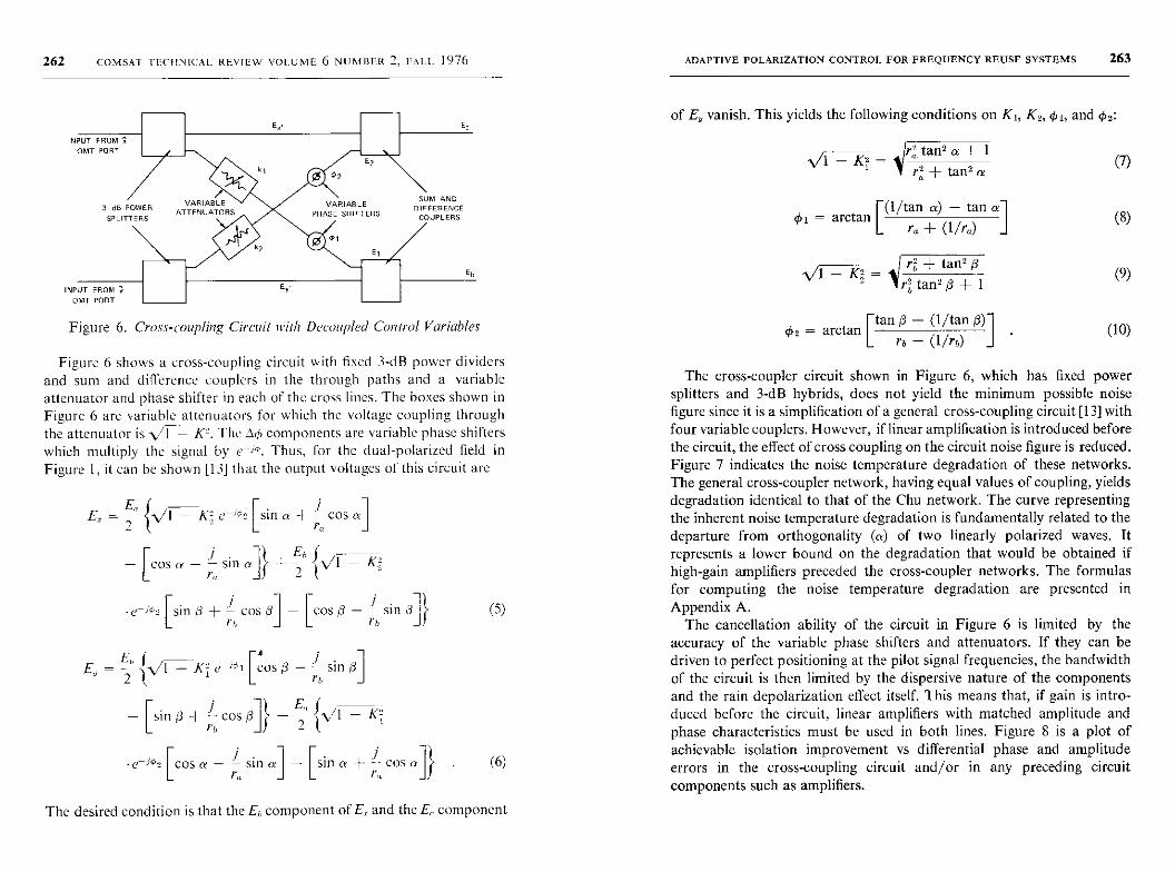
262 COMSAT TECHNICAL REVIEW VOLUME 6 NUMBER 2, FALL 1976 ADAPTIVE POLARIZATION CONTROL FOR FREQUENCY REUSE SYSTEMS 263
INPUT FROM I
OMT PORT
SPLITTERS
kZ }^
INPUT FROM
OMT PORT
SUM AND
DIFFERENCE
COUPLERS
Figure 6. Cross-coupling Circuit nith Decoupled Control Variables
Figure 6 shows a cross-coupling circuit with fixed 3-dB power dividersand sum and difference couplers in the through paths and a variableattenuator and phase shifter in each of the cross lines. The boxes shown inFigure 6 are variable attenuators for which the voltage coupling throughthe attenuator is -\/T- K''. The 4o components are variable phase shifterswhich multiply the signal by e ,'. Thus, for the dual-polarized field inFigure 1, it can be shown [13] that the output voltages of this circuit are
El = E.v/I - K-, e iS2 sin a + _ cos a
2
[cos a - 1 sin a] } + Eli
.e-;a, [sin i3 + coss) [cos - Ib sin (5)
2{-0 K; e'J-0, [Cos 0 - b sin
l
E°- C sin lj + 1' -cos O 11Jl + 2 Kl1'b
e-w° [COS a - L sin aj - [sin a + - i- cos a]} (6)
of E. vanish. This yields the following conditions on K,, K2, ¢I, and 02:
r;;. tan' a + 11 K =
ra+tan2a
th, = RTCtanC(1/tan a) - tan al
rR + (1/PR) JK^ = re + tangs
VI rptan' l3 +1
rho = aretanC
tang +(1/tan$)
rb- (1/4)
(7)
(8)
(9)
(10)
The cross-coupler circuit shown in Figure 6, which has fixed powersputters and 3-dB hybrids, does not yield the minimum possible noisefigure since it is a simplification of a general cross-coupling circuit [13] withfour variable couplers. However, if linear amplification is introduced beforethe circuit, the effect of cross coupling on the circuit noise figure is reduced.Figure 7 indicates the noise temperature degradation of these networks.The general cross-coupler network, having equal values of coupling, yieldsdegradation identical to that of the Chu network. The curve representingthe inherent noise temperature degradation is fundamentally related to thedeparture from orthogonality (a) of two linearly polarized waves. Itrepresents a lower bound on the degradation that would be obtained ifhigh-gain amplifiers preceded the cross-coupler networks. The formulasfor computing the noise temperature degradation are presented in
Appendix A.The cancellation ability of the circuit in Figure 6 is limited by the
accuracy of the variable phase shifters and attenuators. If they can bedriven to perfect positioning at the pilot signal frequencies, the bandwidthof the circuit is then limited by the dispersive nature of the componentsand the rain depolarization effect itself. This means that, if gain is intro-duced before the circuit, linear amplifiers with matched amplitude andphase characteristics must be used in both lines. Figure 8 is a plot ofachievable isolation improvement vs differential phase and amplitudeerrors in the cross-coupling circuit and/or in any preceding circuitcomponents such as amplifiers.
The desired condition is that the E component of Ey and the E, component
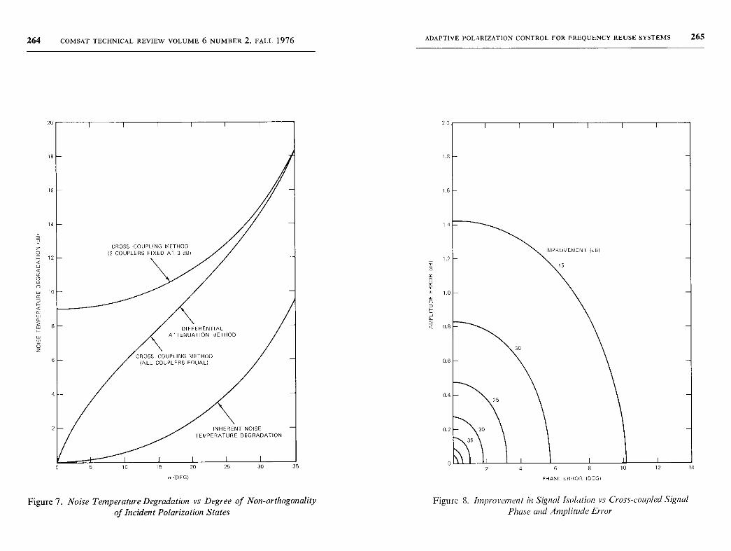
264 COMSAT TECHNICAL REVIEW VOLUME 6 NUMBER 2, FALL 1976
20
B
6
4
12
01-
8
6
DIFFERENTIAL
ATTENUATION METHOD
CROSS COUPLING METHOD(ALL COUPLERS EDUAL)
INHERENT NOISE
TEMPERATURE DEGRADATION
CROSS COUPLING METHOD12 COUPLERS FIXED AT 3 dB)
10 15 20 25 30
a (DEG)
35
Figure 7. Noise Temperature Degradation vs Degree of Non-orthogonalityof Incident Polarization States
ADAPTIVE POLARIZATION CONTROL FOR FREQUENCY REUSE SYSTEMS 265
PHASE ERROR IDEGI
Figure S. ImprovemenI in Signal Isolation vs Cross-coupled Signal
Phase and Amplitude Error
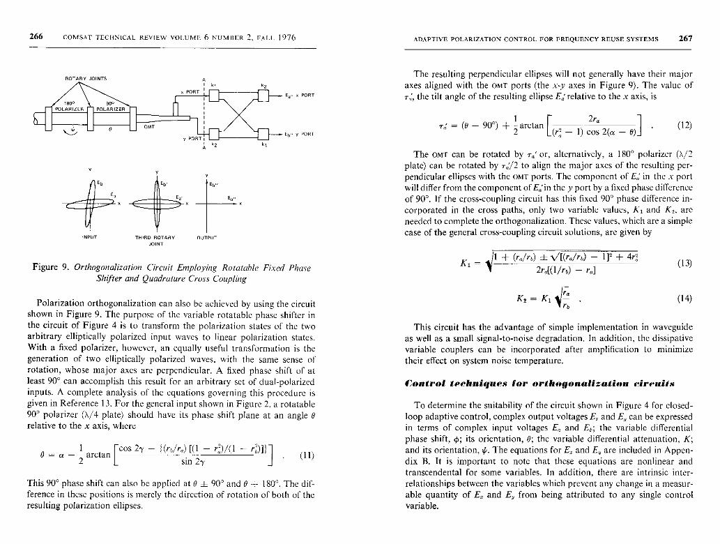
266 COMSAT TECHNICAL REVIEW VOLUME 6 NUMBER 2, FALL 1976
ROTARY JOINTS
180° x 90°POLARIZER POLARIZER
OMT
A
I k
A
INPUT THIRD ROTARY
JOINT
2
OUTPUT
s PORT
Eb y PORT
Figure 9. Orthogonalization Circuit Employing Rotatable Fixed PhaseShifter and Quadrature Cross Coupling
Polarization orthogonalization can also be achieved by using the circuitshown in Figure 9. The purpose of the variable rotatable phase shifter inthe circuit of Figure 4 is to transform the polarization states of the twoarbitrary elliptically polarized input waves to linear polarization states.With a fixed polarizer, however, an equally useful transformation is thegeneration of two elliptically polarized waves, with the same sense ofrotation, whose major axes are perpendicular. A fixed phase shift of atleast 90° can accomplish this result for an arbitrary set of dual-polarizedinputs. A complete analysis of the equations governing this procedure isgiven in Reference 13. For the general input shown in Figure 2, a rotatable90° polarizer (T/4 plate) should have its phase shift plane at an angle arelative to the x axis, where
I Ccos try - i(r6/r,) [(I - r')/(l - re)]I .0 = a - 2 arctan - sin 2 - (11)Y
This 90° phase shift can also be applied at B f 90° and B t 180°. The dif-ference in these positions is merely the direction of rotation of both of theresulting polarization ellipses.
k2
ADAPTIVE POLARIZATION CONTROL FOR FREQUENCY REUSE SYSTEMS 267
The resulting perpendicular ellipses will not generally have their majoraxes aligned with the OMT ports (the x-y axes in Figure 9). The value ofro, the tilt angle of the resulting ellipse Ea relative to the x axis, is
rd = (0 - 90°) + I arctan --2r0
2 (r - 1) cos 2(a - B)(12)
The OMT can be rotated by rA' or, alternatively, a 180° polarizer (X/2plate) can be rotated by T°/2 to align the major axes of the resulting per-pendicular ellipses with the OMT ports. The component of Ea in the x portwill differ from the component of E„in they port by a fixed phase differenceof 90°. If the cross-coupling circuit has this fixed 90° phase difference in-corporated in the cross paths, only two variable values, K, and Ks, areneeded to complete the orthogonalization. These values, which are a simplecase of the general cross-coupling circuit solutions, are given by
Kr^I + (r„/rb) f 1/[(r5/r6) - I]s + 4r;
2r0[(1/rb (13)-rR]
raKs= K1 Jr6
(14)
This circuit has the advantage of simple implementation in waveguideas well as a small signal-to-noise degradation. In addition, the dissipativevariable couplers can be incorporated after amplification to minimizetheir effect on system noise temperature.
Control techniques for orthogonalization circuits
To determine the suitability of the circuit shown in Figure 4 for closed-loop adaptive control, complex output voltages E, and E„ can be expressedin terms of complex input voltages E. and EL; the variable differentialphase shift, 0; its orientation, 0; the variable differential attenuation, K;and its orientation, k. The equations for E. and E, are included in Appen-dix B. It is important to note that these equations are nonlinear andtranscendental for some variables. In addition, there are intrinsic inter-relationships between the variables which prevent any change in a measur-able quantity of E. and E, from being attributed to any single controlvariable.
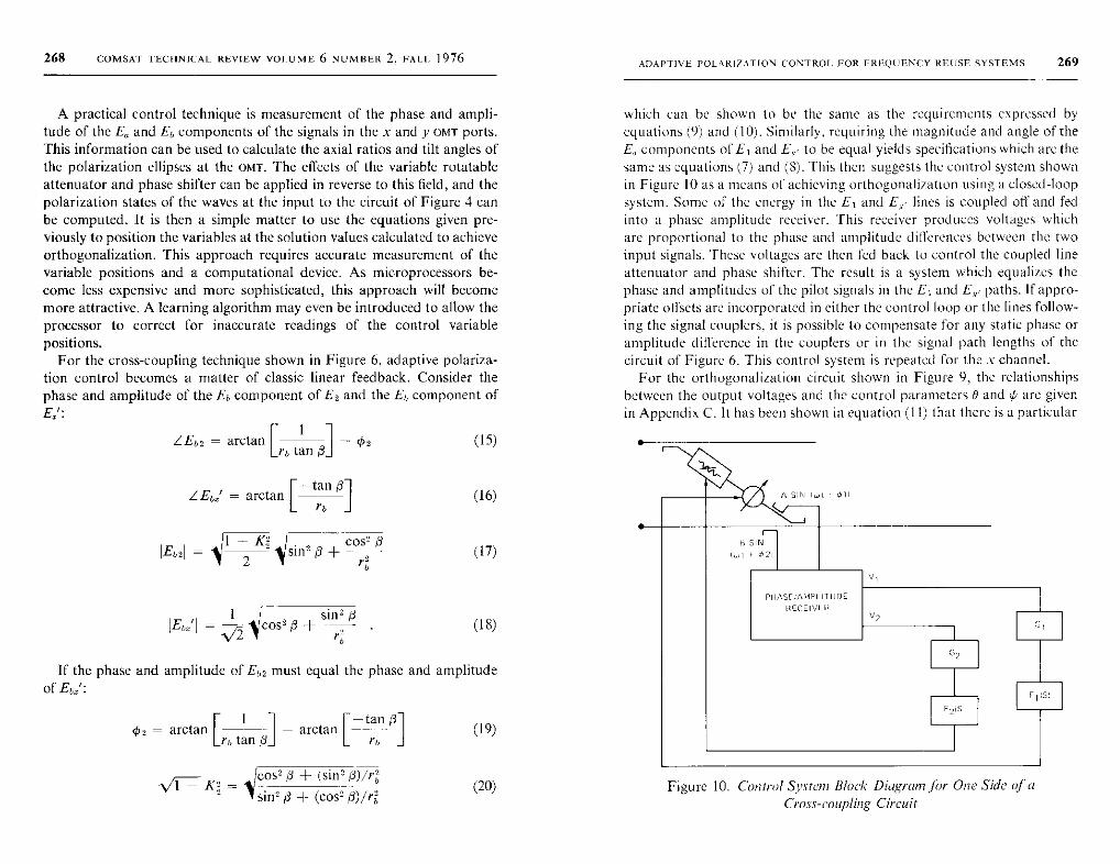
268 COMSAT TECHNICAL REVIEW VOLUME 6 NUMBER 2 . FALL 1976
A practical control technique is measurement of the phase and ampli-tude of the E. and Eb components of the signals in the x and y OMT ports.This information can be used to calculate the axial ratios and tilt angles ofthe polarization ellipses at the CIMT. The effects of the variable rotatableattenuator and phase shifter can be applied in reverse to this field, and thepolarization states of the waves at the input to the circuit of Figure 4 canbe computed. It is then a simple matter to use the equations given pre-viously to position the variables at the solution values calculated to achieveorthogonalization. This approach requires accurate measurement of thevariable positions and a computational device. As microprocessors be-come less expensive and more sophisticated, this approach will becomemore attractive. A learning algorithm may even be introduced to allow theprocessor to correct for inaccurate readings of the control variablepositions.
For the cross-coupling technique shown in Figure 6, adaptive polariza-tion control becomes a matter of classic linear feedback. Consider thephase and amplitude of the Eh component of E2 and the Eb component ofEms':
LEbs = arctan - 02rb tan 0
^Eb 2[
(15)
LEby' = arctan C-tan01
(16)Yb
1 - Kz I. COS-$
2 a rb(17)
JEbX' = ^cos2 P + sin' (18)
If the phase and amplitude of Ebz must equal the phase and amplitudeof Eb,':
02 = arctan Crb tan 01 arctan tan
0
cos'' p + (sin= R) /reK, =sin' 0 + (cos- /3)/r,'
(19)
(20)
ADAPTIVE POLARIZATION CONTROL FOR FREQUENCY REUSE SYSTEMS 269
which can he shown to be the same as the requirements expressed byequations (9) and (10). Similarly, requiring the magnitude and angle of theE, components of E, and E, to be equal yields specifications which arc thesame as equations (7) and (8). This then suggests the control system shownin Figure 10 as a means of achieving orthogonalization using a closed-loopsystem. Some of the energy in the E, and E„ lines is coupled off and fedinto a phase amplitude receiver. This receiver produces voltages whichare proportional to the phase and amplitude differences between the twoinput signals. These voltages are then fed back to control the coupled lineattenuator and phase shifter. The result is a system which equalizes thephase and amplitudes of the pilot signals in the EI and E„- paths. If appro-priate offsets are incorporated in either the control loop or the lines follow-ing the signal couplers, it is possible to compensate for any static phase oramplitude difference in the couplers or in the signal path lengths of thecircuit of Figure 6. This control system is repeated for the x channel.
For the orthogonalization circuit shown in Figure 9, the relationshipsbetween the output voltages and the control parameters B and lG are givenin Appendix C. It has been shown in equation (11) that there is a particular
Figure 10. Control System Block Diagram far One Side of a
Cross-coupling Circuit
270 COMSAT TECHNICAL REVIEW VOLUME 6 NUMBER 2, FALL 1976
solution for 0 and >G which will convert the general input field of Figure 1to one with spatially perpendicular elliptically polarized signals rotatingin the same sense. In terms of the voltages E. and E,, this means that the
E. component of E, leads (or lags) the E. component of E, by 90°. There-
fore, the important phase differences are
LEa = LE.. - LE.,
LEb = LEu - LEb,
which can be expressed as [13]
LEa = arctan
LEa = arctan
tan (0 + a - 24') (1 - ra) seen 0
(r„ tan 0 - 1) (r, + tan 0) tan2 (0 + a - 24')
+ (tan 0 - r,) (r, tan 0 + 1)
tan (0 + 0 - 24') ( 1 - rb) sec' 0
1(rb tan 0 - 1) (rb + tan 0) tan2 (0 + Q - 21G)
+ (tan 0 - rb) (rb tan 0 + 1)
(21)
(22)
(23)
(24)
While amplitude coupling may be controlled through a system similarto the amplitude control loop of the cross-coupling circuit described pre-viously, phase control for this circuit is more complicated. To decouplethe phase parameters from the amplitude coupling parameters, it seemsbest to measure the phase in the coupling arms rather than after the can-cellation signal has been mixed with the interfering signal. However, theredoes not appear to be any simple way to directly feed back the phase in-formation to drive the 90° and 180° polarizers without first processing it.
The desired steady-state condition for operation is LE, = LEb = 90°,
which also means that LE, - LEb = 0. Unfortunately, due to the inter-
dependence of 0 and 4', neither of these can be considered to be a sufficienterror voltage for closed-loop control. However, through computer simula-tion it appears that a technique of sequential adjustment of 0 and 4' tosimultaneously minimize the cross polarization in both channels willusually lead to a solution. Unfortunately, there are local minima in thecontrol surface and the minimum seeking algorithms must be chosen care-fully so that the circuit finds the true global minimum and not a local
minimum.
ADAPTIVE POLARIZATION CONTROL FOR FREQUENCY REUSE SYSTEMS 271
This circuit can also be adaptively controlled by using a minicomputer.A processor can be constructed to measure the phase and amplitude in-formation and compute the axial ratios and tilt angles of the polarizationellipses after the 90° and 180° polarizers. The reciprocity theorem canthen be used to find, by calculation, the initial incident polarization statesat the input to the correction circuit. Finally, the input polarization ellipseinformation can be applied to the equations given previously to calculatethe desired positions of 0 and 4'.
A suboptimal adaptive polarization restorationsystem
It has been noted that four parameters are generally required to providecomplete restoration of a dual-polarized frequency reuse system. If raindepolarization is assumed to be the only disturbance, then three parameterssuffice since the canting angles of both the phase shift and the differentialattenuation are identical. For a 4/6-GHz satellite communications link, afurther simplification may be made by neglecting the effect of differentialattenuation. From a system point of view, this can be justified by referringto Figure 3. For a 5-km average rain path length, 30-dB isolation isachieved at rain rates of 62 mm/hr * with differential phase correction only.This results in a suboptimal adaptive polarization restoration system whichrequires only two variable parameters and which can be most easily im-plemented by a cascaded set of independently rotatable 90° and 180°polarizers (see Figure 9 [to section A-A]). One method of providing adap-tive control with this circuit is shown in Figure 11.
Since the error voltage magnitudes and/or phases are not directly re-lated to the angular positions of the two polarizers, simple direct errorfeedback is not possible. Therefore, some form of error signal processing,together with an algorithm to direct the rotation of the polarizers, isrequired to minimize these error voltages.
In the particular adaptive control network shown in Figure 11, theoutput signals from the x port of the oMT will contain the interference fromchannel 2 and those from the y port of the OMT will contain the interfer-ence from channel 1. The interchannel interference is therefore minimizedif the error signals are simultaneously minimized. An algorithm which
* For example, a rain rate of 62 mm/hr is exceeded only 0.01 percent of thetime, i.e., 1 hr/yr in the Washington , D.C., area.
272 COMSAT TECHNICAL REVIEW VOLUME 6 NUMBER 2, FALL 1976
TO RECEIVER I
IFEED HORN
180° POLARIZES
R Ri
MOTOR OTOR 2
90° POLARIZEDTRANSITION
OMT TO RECEIVER 2
RECEIVER 1 RECEIVER 2
B
z_MOTOR
TRANSLATOR
MOTORTRANSLATOR ELECTRONIC
CONTROL ANDMICROPROCESSOR
Figure 11. Adaptive Correction Circuit
successively rotates the polarizers and minimizes the sum of the errorpower levels has been modeled on a computer. This procedure is shownin Figure 12 for dual circular polarization and differential phase and atten-
A
-0E
0 0.sX AXIS
Figure 12a. Circularly Polarized Signals
-10
ADAPTIVE POLARIZATION CONTROL FOR FREQUENCY REUSE SYSTEMS 273
1
E
I I I I-0.s o
X AXIS
I I I I
0.5 10
Figure 12b. Circularly Polarized Signals Subjected to a 125-mm/hr RainRate at a 450 Canting AngleI -p I I I
-1.0-10
X AXIS
Figure 12c. Resultant Signals Following Polarizer Correction Network
274 COMSAT TECHNICAL REVIEW VOLUME 6 NUMBER 2, FALL 1976 ADAPTIVE POLARIZATION CONTROL FOR FREQUENCY REUSE SYSTEMS 275
nation of 28.5° and 0.245 dB, respectively. (This corresponds to a theo-retical rain rate of 125 mm/hr at 4 GHz.) The ellipticity of the final vectorsis directly related to the differential attenuation of 0.245 dB, with a resul-tant isolation of 37 dB (see Figure 3). Error contours for the adaptivenetwork are shown in Figure 13.
-z-^-\1 ^-cam =
-100 -50
ANGLE OF 9D PLATE (DEG)
0
Figure 13. Error Contours Following Polarizer Correction Network
50
It is interesting to note that the physical arrangement of the 90° and 180°polarizers affects the speed of response of the adaptive circuit. In Figure 12,the 90° polarizer is adjacent to the 0MT. These properties are indicated inFigures 14a and 14b, which show the domain of solutions for the polarizerangles as a function of the differential phase shift and canting angle of therain. Because the range of polarizer angle solutions for the network ofFigure 12 is smaller for input waves that are nearly circularly polarized,the speed of response for this network can be superior.
The polarization control network was tested in the laboratory using the4-GHz 90° polarizer [21], rotary joints, and orthomode junction shown in
o2
275 COMSAT TECHNICAL REVIEW VOLUME 6 NUMBER 2 , FALL 1976ADAPTIVE POLARIZATION CONTROL FOR FREQUENCY REUSE SYSTEMS 277
Figure 15. Since the 90° polarizer had an axial ratio better than 0.15 dBand the OMT port-port isolation was greater than 50 dB over a 500-MHzbandwidth, polarization discrimination better than 37 dB was achieved atthe pilot signal frequency.
I
Figure 15. 4-GHz Waveguide Adaptive Circuit
Conclusions and Discussion
There are several network concepts which can be used to restore theorthogonality of dual-polarized fields on an adaptive basis, i.e., withouta priori knowledge of the depolarizing properties of the medium. Incor-porating pilot signals and suitable receivers for these signals makes itpossible to derive error voltages to control the adaptive circuits. Signal-to-interference ratios of at least 30 dB are practical with these techniques.
For the cross-coupling circuit, voltage-controlled attenuators and phaseshifters allow rapid response times (e.g., circuit bandwidths > 100 Hz).However, to realize minimum system noise figure degradation, these cir-cuits should follow a "matched" pair of low-noise amplifiers whose phaseand amplitude tracking must be tightly controlled.
The waveguide correction circuits can be connected to the feed system
278 COMSAT TECHNICAL REVIEW VOLUME 6 NUMBER 2, FALL. 1976
of an existing earth station antenna. Minimum degradation in the carrier-to-noise ratio is achieved since the differential phase shift is directly re-
moved by the first rotating polarizer . However, the large inertia of the
waveguide components indicates a small control bandwidth or a slowcircuit response time of the order of 0.5 second.
A particularly attractive correction circuit for use in the 4/6-GHz satel-
lite bands is the suboptimal realization described in the preceding section.Here, only differential phase shift is removed and only two control
parameters must be monitored.
Aclenowledgnrents
The authors are pleased to acknowledge helpful discussions with Mr. R. W.
Kreutel and Dr. A. E. Atia. Special thanks are due to Mr. R. W. Grunerfor supplying the excellent 4-GHz OMT and polarizers, and to Mr. J.
Bleiweiss, who designed the microprocessor.
References
[1] D. F. DiFonzo and R. W. Kreutel, "Communications Satellite Antennasfor Frequency Reuse," G-AP International Symposium, September 1971,
pp. 287-289.[2] Nippon Electric Company, Ltd., Tokyo, Japan, "Final Report for Wide-
band Mode Transducer/Polarizer Assembly," prepared for INTELSAT
under contract CSC-IS-473.[3] W. Sones and M. Grossman, "Polarization Isolation and Spurious Signal
Rejection Requirements for a Dual-Polarized Unattended Earth Terminal,"
COMSAT Technical Review, Vol. 5, No. 2, Fall 1975, pp. 367-386.
[4] J. A. Morrison and T. S. Chu, "Perturbation Calculations of Rain-InducedDifferential Attenuation and Differential Phase Shift at Microwave
Frequencies," Bell System Technical Journal, Vol. 52, No. 10, December
1973, pp. 1907-1913.[5] J. A. Morrison, M. J. Cross, and T. S. Chu, "Rain-induced Differential
Attenuation and Differential Phase Shift at Microwave Frequencies," Bell
System Technical Journal, Vol. 52, No. 4, April 1973, pp. 599-604.
[6] T. Oguchi, "Attenuation of Electromagnetic Waves Due to Rain with Dis-
torted Raindrops, Part I," Journal of the Radio Research Labs (Japan),
No. 33, September 1960, pp. 467-485.[7] T. Oguchi, "Attenuation of Electromagnetic Waves Due to Rain with Dis-
torted Raindrops, Part 1I," Journal of the Radio Research Labs (Japan),
No. 53, January 1965, pp. 19-44.[8] T. Oguchi, "Attenuation and Phase Rotation of Radio Waves Due to Rain:
Calculation at 19.3 and 34.8 GHz," Radio Science, Vol. 8, No. 1, January
1973, pp. 31-38.
ADAPTIVE POLARIZATION CONTROL FOR FREQUENCY REUSE SYSTEMS 279
[9] R. Taur, "Rain Depolarization: Theory and Experiment," COMSATTechnical Review, Vol. 4, No. 1, Spring 1974, pp. 187-190.
[10] R. Taur, "Rain Depolarization at 4, 6 and 11 GHz," 1974 URSI Meeting,Atlanta, Georgia, June 1974.
[11] M. Saunders, "Cross-Polarization at 18 and 30 GHz Due to Rain," IEEETransactions on Antennas and Propagation, AP-l9, No. 2, March 1971, pp.273-277.
[12] R. A. Semplak, "Simultaneous Measurements of Depolarization by RainUsing Linear and Circular Polarization at 18 GHz," Bell System TechnicalJournal, Vol. 53, No. 2, February 1974, pp. 400-404.
[13] W. S. Trachtman, "Adaptive Orthogonalization of Polarized Signals withApplications to Satellite Communications," M.S. Thesis, M.I.T., June1975.
[14] V. H. Rumsey et al., "Techniques for Handling Elliptically Polarized Waveswith Special Reference to Antennas," Proc. IRE, May 1951, pp. 553-556.
[15] International Radio Consultative Committee (C.C.I. R.), XIIth PlenaryAssembly, New Delhi, 1970, Vol. III, Report 321, Geneva: InternationalTelecommunications Union, 1970.
[16] J. S. Hollis et al., "Microwave Antenna Measurements," Scientific Atlanta,Inc., July 1970.
[17] P. A. Watson and M. Arabi, "Rainfall Cross-Polarization of Linearly andCircularly Polarized Waves at Microwave Frequencies," Electronic Letters,Vol. 8, No. 11, June 1972.
[18] T. S. Chu, "Restoring the Orthogonality of Two Polarizations in RadioCommunication Systems, I," Bell System Technical Journal, Vol. 50, No. 9,November 1971, pp. 3063-3069.
[19] T. S. Chu, "Restoring the Orthogonality of Two Polarizations in RadioCommunication Systems, 1I," Bell System Technical Journal, Vol. 52, No. 3,March 1973, pp. 319-327.
[20] D. F. DiFonzo, A. E. Williams, and W. S. Trachtman, "Adaptive Polariza-tion Control for Satellite Frequency Reuse Systems," IEEE/AP-S Sym-posium, June 1975, pp. 209-216.
[21] R. W. Groner and W. J. English, "A C.P. Reference Standard Antenna
System for Satellite or Earth Station Applications," International IEEE-AP-S Symposium, June 1975.
Appendix A. SOlse temperature consideratinns
For the Chu circuit of Figure 4, assume that the proper phase shift has beenapplied so that the input to the differential attenuator is a field with two non-orthogonal linearly polarized signals spatially separated by an angle '' andoriented from the x and .v ports by an angle a, where a = (90 - 45)/2. The anglea is a measure of the non-orthogonality of the signal states. It is now of interest
280 COMSAT TECHNICAI REVIEW VOLUME 6 NUMBER 2 , FALL 1976 ADAPTIVE POLARIZATION CONTROL FOR FREQUENCY REUSE SYSTEMS 281
to find the amount of noise temperature degradation caused by the operation ofthe orthogonahzation circuit as a function of a. Let the noise temperature of theantenna and propagation path be Ta. If it is assumed that the noise power incidenton the attenuator circuit has no preferred spatial orientation, the noise voltage
seen at the x and y OMT ports is given by
V„r„ _ 8 I +2 K2 T. (A-1)
where K is the value of the attenuator (resistive card).If it is assumed that the resistive card is a thermal noise generator producing a
noise signal oriented parallel to the direction of the attenuation, the contributionto the noise voltage of each of the x and y OMT ports due to the resistive card
will be
Fnre _ 2 K? Ta (A-2)
where T. is the effective noise temperature of the resistive card in Kelvin.
If T and T. are from totally uncorrclated noise sources , the noise power, P,,,
in either port will be
P. = (12 K2) T + ^l T. . (A-3)
On the other hand, if the signal voltage incident on the circuits is E„ then the
signal power, P, is given by
P; = E [K2 Cosa 2 + sine 2]
Therefore, the equivalent noise temperature of this circuit is
T.K2 Coss 2 + sin 2 2
which reduces to
(1 2K)T„+(1 22) T.
Ta T. sin 2aT„= - d-
-[cos 2a]" [cos 2a]
(A-4)
(A-5)
(A-6)
The noise temperature is clearly degraded by two separate effects. The Tcomponent, which is the antenna and propagation path noise, is degraded by thereduction in input signal strength. This can be assumed to be an inherent noisetemperature degradation attributable to the process of orthogonalization itselfeven if a noiseless attenuator (To = 0) is used in the circuit. The T. term is recog-nizable as the noise generated by the attenuator itself.
The inherent noise temperature degradation of Figure 7 is a plot of-20 log10 [cos 2a], while the differential attenuation curve is a plot of the noisetemperature degradation of equation (A-6) for T. = 40 K and T, = 290 K.Similarly, it can be shown that the cross-coupler circuit having equal couplingvalues exhibits a noise temperature degradation identical to that of Chu's cir-cuit. With fixed 3-dB couplers the noise temperature degradation is inherentlyworse for small a. If a matched set of high-gain parametric amplifiers precedes thecircuit, the noise temperature will approach the lower curve.
Appendix B. Control voltage equations forthe Chu correction network
Straightforward analysis of the network of Figure 4 leads to the followingexpressions for the output voltages in terms of the input parameters:
where
E E. { e tO[A cos 0 + B sin 0] [ C cos 0 + D sin 0]
}+ [B cos 0 - A sin 0] [D cos 0 - C sin 01
+1
E)e 1Acos0 +Bsin0][Esin0+Fcos6]
+ [B cos 0 - A sin 0] [E cos 0 - F sin 0] )
E„ -Ea{etm[G cos 0 + H sin 0] [C cos 0 + D sin 0]
+[Hcos0-Gsin0][Dcos0-Csin0])
+ -2{E e 'm[ G cos 0 + H sin 0] [F cos 0 + E sin 0]
+ [H cos 0 - G sin 6] [E cos 0 - F sin 0] }
A = K cos >G + sin l'B = K sin 'G - cos k
C = cos a - L sin ara
D = sin a + L cos ara
282 COMSAT TECHNICAL REVIEW VOLUME 6 NUMBER 2, FALL 1976 ADAPTIVE POLARIZATION CONTROL FOR FREQUENCY REUSE SYSTEMS 283
E = sin + J cosrb
F = cos (j - sinrb
G = K cos +y - sin >GH= K sin 4' + Cos4'
Appendix C. Control voltage equations for
the netu'oric of Figure 9
Expressing the output voltages for the network of Figure 9 in terms of the
input voltages and angular positions of the 180° and 90° polarizers yields
E = E°{(A Cos 24' + C sin 2tG)(j cost 0 - sin 2 0)
+ (A sin 24' - C cos 24')(sin 0 Cos 0)(1 +j)}
+ E,{(B cos 24' + D sin 24)(j cos° 0 - sin 2 0)
+ (B sin 24' - D cos 2,k)(sin 0 cos 0)(1 +1) {
E5 = Eb{(A sin 20 - C cos 24') (j sin 2 0 - cos° 0)
+ (A cos 24' + C sin 24')(sin 0 cos 0)(1 +j)}
+ Et(B sin 2,' - D Cos 24')(j sin 2 0 - cos° 0)
+ (B cos 24' + D sin 2C (sin 0 cos 0) (1 +i)J
where the angle 4, refers to the angular position of the 180° plate, the angle 0
refers to the angular position of the 90° plate, and
A = [Cos a - j sinara
B = Coos p - I sin g]rb
C = [sin a + 2 COS a]ra.
D= [sin 0+j Coss]rb
Daniel F. DiFonzo received a B.E.E. fromVillanova University in 1962 and an M.S. fromCalifornia State University in 1972. He ispresently Assistant Manager of the AntennasDepartment of the Microwave Laboratory atCOMSAT Laboratories. He is responsible fordirecting and carrying out research and devel-opment related to communications satellite andearth station antenna systems. Specifically, hehas performed extensive analytical and experi-
mental studies of techniques for the control of microwave antennapolarization properties and the design of multiple-beam spacecraft an-tennas. He is a member of IEEE, APS, and G-MTT.
Albert E. Williams was born in Albany,Australia. He received a BE, in electrical en-gineering from the University of WesternAustralia, Perth, in 1962, and a Ph.D. fromUniversity College, London, England, in 1966.From 1966 to 1968 he was a lecturer in theDepartment of Electrical Engineering, Univer-sity of Western Australia. Currently, he is atechnical staff member of the Antennas Depart-ment of the Microwave Laboratory at COMSATLaboratories, where he is working on antenna and filter theory appli-cable to future communications satellites. Dr. Williams was a jointrecipient of the Institute of Electrical Engineers (London) Sylvanus P.Thompson Premium award in 1966.
Warren S. Trachtman received both aB.S.E.E. and an M.S.E.E. from M.I.T. in1975. In July of 1975, he joined COMSATLaboratories, where he is presently a memberof the technical staff of the Antennas Depart-ment of the Microwave Laboratory . His majorprojects have involved adaptive interferencereduction techniques, antenna cross -polariza-tion measurements, and shaped-beam antennacoverage designs.
_ _ \1 I'.'
,tmay
Index: multiplexer, 1NTELSAT V, transponder,waveguide
11 contiguous band multiplexer
M. H. CHEN, F. ASSAL, AND C. MAHLE
(Manuscript received March 18, 1976)
Abstract
A 4-channel waveguide-manifold-type contiguous band multiplexer has beendesigned, fabricated, and tuned to meet the essential specifications of anINTELSAT v zone output multiplexer. This development allows a substantialweight savings in the satellite transponder in the case of complex antenna sys-
tems such as those contemplated for INTELSAT V. Current satellites use multi-plexers with guard bands of more than one full channel bandwidth and combinethe transmit power of the even and odd channels into two separate output ports,thereby requiring two transmit antennas. A contiguous band multiplexer reducesthe guard band to 10 percent of the channel bandwidth and combines all thechannels (even and odd) into a single output port, thereby requiring only onetransmit antenna. An insertion loss of less than 0.5 dB has been achieved inthe experimental model, the feasibility of the concept has clearly been estab-lished, and consequently one set of transmit antennas (hemispherical and zonal)can be eliminated in an INTELSAT v application.
Introduction
In communications satellites, the allocated 500-MHz communications
band is subdivided into contiguous frequency increments (channels) to
This paper is based upon work performed in COMSAT Laboratories Linder the
sponsorship of the International Telecommunications Satellite Organization
(INTELSAT). Views expressed in this paper are not necessarily those of INTELSAT.
7R It
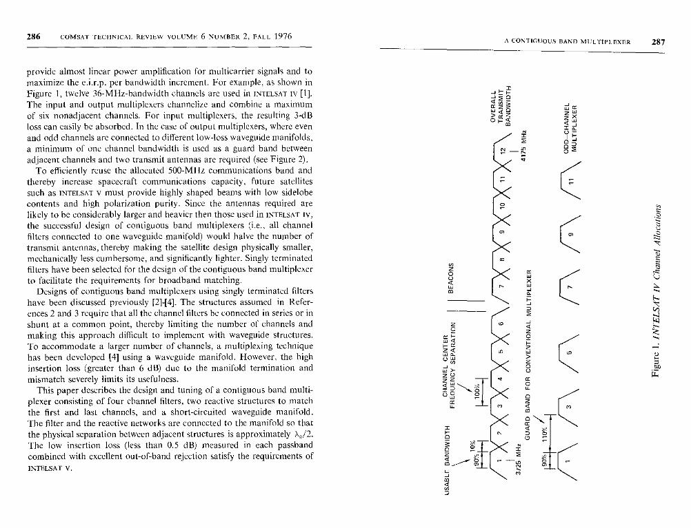
286 COMSAT LECFINICAI. REVIEW VOLUME 6 NUMBER 2, FALL 1976 A CONTIGUOUS BAND MULTIPLEXER 287
provide almost linear power amplification for multicarrier signals and tomaximize the e.i.r.p. per bandwidth increment. For example, as shown inFigure 1, twelve 36-MHz-bandwidth channels are used in INTELSAT Iv [1].The input and output multiplexers channelize and combine a maximumof six nonadjacent channels. For input multiplexers, the resulting 3-dBloss can easily be absorbed. In the case of output multiplexers, where evenand odd channels are connected to different low-loss waveguide manifolds,a minimum of one channel bandwidth is used as a guard band betweenadjacent channels and two transmit antennas are required (see Figure 2).
To efficiently reuse the allocated 500-MHz communications band andthereby increase spacecraft communications capacity, future satellitessuch as INTELSAT V must provide highly shaped beams with low sidelobecontents and high polarization purity. Since the antennas required arelikely to be considerably larger and heavier then those used in INTELSAT Iv,the successful design of contiguous band multiplexers (i.e., all channelfilters connected to one waveguide manifold) would halve the number oftransmit antennas, thereby making the satellite design physically smaller,mechanically less cumbersome, and significantly lighter. Singly terminatedfilters have been selected for the design of the contiguous band multiplexerto facilitate the requirements for broadband matching.
Designs of contiguous band multiplexers using singly terminated filtershave been discussed previously [2]-[4]. The structures assumed in Refer-ences 2 and 3 require that all the channel filters be connected in series or inshunt at a common point, thereby limiting the number of channels andmaking this approach difficult to implement with waveguide structures.To accommodate a larger number of channels, a multiplexing techniquehas been developed [4] using a wavcguide manifold. However, the highinsertion loss (greater than 6 dB) due to the manifold termination andmismatch severely limits its usefulness.
This paper describes the design and tuning of a contiguous band multi-
plexer consisting of four channel filters, two reactive structures to match
the first and last channels, and a short-circuited waveguide manifold.
The filter and the reactive networks are connected to the manifold so that
the physical separation between adjacent structures is approximately T„/2.
The low insertion loss (less than 0.5 dB) measured in each passband
combined with excellent out-of-band rejection satisfy the requirements of
INTELSAT V.
xJ ^ ( JQ N J
wao ww
ol-mz Xzw
2 a
S5
U F
o j
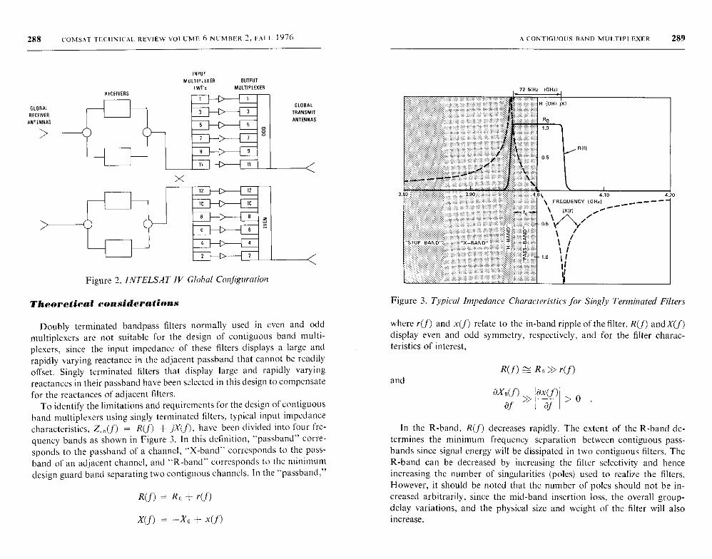
288 COMSAT TECHNICAL REVIEW VOLUME 6 NUMBER 2, PALL 1976
GLOBAL
RECEIVER
ANTENNAS
RECEIVERS
INPUT
MULTIPLEXER OUTPUT
TWE MULTIPLEXER
1
5
fl
X
11
12
10
a
6
I
12
10
8
6
Figure 2. INTELSAT IV Global Configuration
Theoretical considerations
GLOBAL
TRANSMIT
ANTENNAS
Doubly terminated bandpass filters normally used in even and oddmultiplexers are not suitable for the design of contiguous band multi-plexers. since the input impedance of these filters displays a large andrapidly varying reactance in the adjacent passband that cannot be readily
offset. Singly terminated filters that display large and rapidly varyingreactances in their passband have been selected in this design to compensatefor the reactances of adjacent filters.
To identify the limitations and requirements for the design of contiguousband multiplexers using singly terminated filters, typical input impedance
characteristics , Z;,,(f) - R(J) + jX(f), have been divided into four fre-
quency bands as shown in Figure 3. In this definition, "passband " corre-
sponds to the passband of a channel , " X-band" corresponds to the pass-
band of an adjacent channel, and "" R-band" corresponds to the minimumdesign guard band separating two contiguous channels. In the "passband,"
R(J) - RG + r(1)
X(f) - -X1 + x(f)
A CONTIGUOUS BAND MULTIPLEXER 289
Figure 3. Typical Impedance Characteristics for Singly Terminated Filters
where r(f) and x(J) relate to the in-band ripple of the filter . R(f) and X(f)display even and odd symmetry , respectively , and for the filter charac-teristics of interest,
andR(f)=RG»r(f)
axG(f) ax(f)
di ^In the R-band, R(f) decreases rapidly. The extent of the R-band de-
termines the minimum frequency separation between contiguous pass-bands since signal energy will be dissipated in two contiguous filters. TheR-band can be decreased by increasing the filter selectivity and henceincreasing the number of singularities (poles) used to realize the filters.However, it should be noted that the number of poles should not be in-creased arbitrarily, since the mid-band insertion loss, the overall group-delay variations, and the physical size and weight of the filter will alsoincrease.
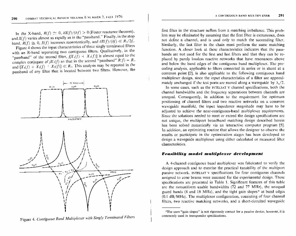
290 COMSAT TECHNICAL REVIEW VOLUME 6 NUMBER 2, FALL 1976
In the X-band, R(f) = 0, aX(f)/(8f) > 0 (Foster reactance theorem),
and X(f) varies almost as rapidly as in the "passband." Finally, in the stop
band, R(f) 0, X(f) increases monotonically, and aX(f)/(df) << R„/2f.
Figure 4 shows the input characteristics of three singly terminated filterswith an R-band separating two contiguous filters. Qualitatively, in the
"passband" of the second filter, i[X,(f) + X„(f)] is almost equal to the
complex conjugate of /X2(f) so that in the second "passband" R(f) = R0
and [X,(f) + X2(f) + X3(f)] << R2. This analysis may be repeated in the
passband of any filter that is located between two filters. However, the
FRE QUENCV
Figure 4. Contiguous Band Multiplexer with Singly Terminated Filters
A CONTIGUOUS BAND MULTIPLEXER 291
first filter in the structure suffers from a matching imbalance. This prob-lem may be eliminated by assuming that the first filter is extraneous, doesnot define a channel, and is used only to match the succeeding filter.Similarly, the last filter in the chain must perform the same matchingfunction. A closer look at these characteristics indicates that the pass-bands are not used for the first and last filters and that they can be re-placed by purely lossless reactive networks that have resonances aboveand below the band edges of the contiguous band multiplexer. The pre-ceding analysis, applicable to filters connected in series or in shunt at acommon point [2], is also applicable to the following contiguous bandmultiplexer design, since the input characteristics of a filter are approxi-mately unchanged if the test ports are moved along a waveguide by X„/2.
In some cases, such as the INTELSAT v channel specifications, both thechannel bandwidths and the frequency separations between channels areunequal. Consequently, in addition to the requirement for optimumpositioning of channel filters and two reactive networks on a commonwaveguide manifold, the input impedance magnitude may have to beadjusted to achieve the near-contiguous-band multiplexer requirements.Since the solutions needed to meet or exceed the design specifications arcnot unique, the multiport broadband matching design described hereinhas been solved numerically via an interactive computer program [5].In addition, an optimizing routine that allows the designer to observe theresults or participate in the optimization stages has been developed todesign a waveguide multiplexer using either calculated or measured filtercharacteristics.
Feasibility model multiplexer development
A 4-channel contiguous band multiplexer was fabricated to verify thedesign approach and to exercise the practical tunability of the multiportpassive network. INTELSAT V specifications for four contiguous channelsassigned to zone beams were assumed for the experimental design. Thesespecifications are presented in Table 1. Significant features of this tableare the nonuniform usable bandwidths (72 and 77 MHz), the unequalguard bands (8 and 18 MHz), and the tight gain slopes* at band edges(0.1 dB/MHz). The multiplexer configuration, consisting of four channelfilters, two reactive matching networks, and a short-circuited waveguide
*The term "gain slopes" is not rigorously correct for a passive device; however, it iscommonly used in transponder specifications.
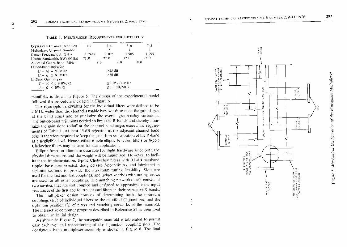
2292 COMSAT TECHNICAL REVIEW VOLUME 6 NUMBER 2, FALL 1976
TABLE I. MULTIPLEXER REQUIREMENTS FOR INTELSAT V
INTELSAT v Channel Definition
Multiplexer Channel NumberCenter Frequency, fi; (GHz)
Usable Bandwidth , BWk (MHz)
Allocated Guard Band (MHz)Out-of-Band Rejection
If - fkI = 50MHzIf- f)I > 60 MHz
In-Band Gain SlopesIf - f,I < 0.9 BWk/2^./- fAI < BWA-/2
1-2 3-41 2
3.7425 3.82577.0 72.0
8.0
5-6 7-83 4
3.905 3.99572.0 72.0
8.0 18.0
>25 dB>30 dB
<0.05 dB/MHz<0.1 dB/MHz
manifold, is shown in Figure 5. The design of the experimental model
followed the procedure indicated in Figure 6.The equiripple bandwidths for the individual filters were defined to be
2 MHz wider than the channel's usable bandwidth to meet the gain slopesat the band edges and to minimize the overall group-delay variations.The out-of-band rejections needed to limit the R-bands and thereby mini-mize the gain slope rolloff at the channel band edges exceed the require-ments of Table I. At least 15-dB rejection at the adjacent channel bandedge is therefore required to keep the gain slope contribution of the R-bandat a negligible level. Hence, either 6-pole elliptic function filters or 8-poleChebychev filters may be used for this application.
Elliptic function filters are desirable for flight hardware since both thephysical dimensions and the weight will be minimized. However, to facil-itate the implementation, 8-pole Chebychev filters with 0.l-dB passbandripples have been selected, designed (see Appendix A), and fabricated inseparate sections to provide the maximum tuning flexibility. Slots areused for the first and last couplings, and inductive irises with tuning screwsare used for all other couplings. The matching networks each consist oftwo cavities that are slot coupled and designed to approximate the inputreactances of the first and fourth channel filters in their respective X-bands.
The multiplexer design consists of determining both the optimum
couplings (RK) of individual filters to the manifold (T-junction), and theoptimum position (Ik) of filters and matching networks of the manifold.The interactive computer program described in Reference 5 has been used
to obtain an initial design.As shown in Figure 7, the waveguide manifold is fabricated to permit
easy exchange and repositioning of the T-junction coupling slots. Thecontiguous band multiplexer assembly is shown in Figure 8. The final
COMSAT IECHNICAI- REVIEW VOLUME 6 NUMBER 2, PALL 1976
o0
293
r-t^LL a
0
WN^
z asU
ofoV
Soz^ z- _F_^
woro MO^ wz
O zfRg }en
ws _Oeraw-P
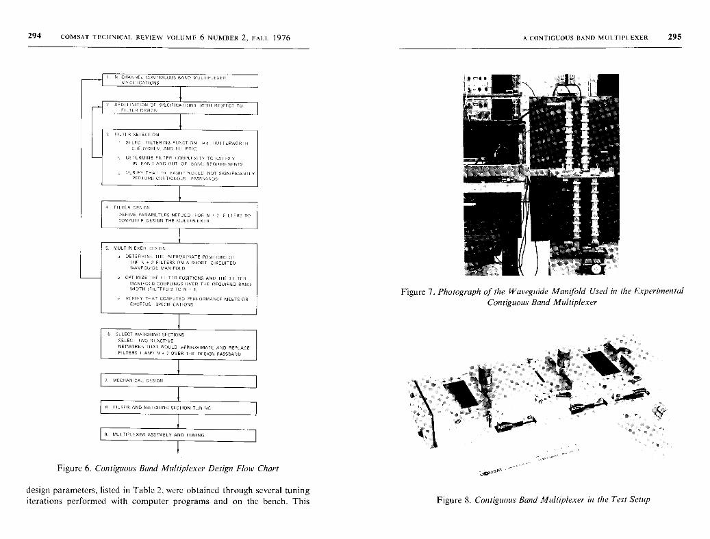
294 COMSAT TECHNICAL REVIEW VOLUME 6 NUMBER 2, FALL 1976
;HANNLL CONTIGUOUS BAND MULTIPLESSEC CIE ICATIO NS
FDEFINITION OF SPEGIFIAnoNS ISITH RESPECT TDFL]LR DESIGN
FILI1 I SEI ECI ION
SELECT FILTERING FUNCTION I I.. 1UITLRWORnI
CuFDYCIIEV. AND ELI IPTO
HE ILHMINE FIT IFR COMPLEXITY TO SATISFY
IN HAND AND OUT OF RANG REQUIREMENTS
I 3 LRIFY THAI -1 RANG WUULU NUT 51GNIFICANIL
PFRIUI111 CONTIGUOUS PASSRANOS
FILTER DESIGN
DERIVE PARAMETERS NEEDED FOR N 2 FILTFIR
,OMPDIFH DESIGN THE MULTI IRE EXER
5. VULTIPI EXER DESIGN
.I. DETERMI NL THE APPROXIMATE POSITIONS OF
lIF N , 7 FILTERS ON A SHORT CIRCUITED
L. OPTIMIZE IEEE I TITER POSITIONS ANN IIIE FILTER
MAN IFOI.0 COUPLINGS OVER THE REQUIRED BANEWIDTH IFILTFSS 2 TO N . 11
I,. VEHIFY THAT COMPUTED FEB FORMANCF MEETS OR
EXCFFUS SPECIFICATIONS
6. SELECT MATCHING SECTIONS
SELECT TWO REACTIVE
NETWORKS THAT WOULD APPHOXI MATE AND REPLACE
FILTERS I AND N ♦ 2 OVER THE DESIGN PASSRAND
7 MECHANICAL DESIGN
R. FILTER AND MAICHIND SECTION TUNING
9. MULTIPLEXER ASSEMBLY AND TUNING
Figure 6. Contiguous Band Multiplexer Design Flow Chart
design parameters, listed in Table 2, were obtained through several tuningiterations performed with computer programs and on the bench. This
A CONTIGUOUS BAND MULTIPLEXER 295
Figure 7. Photograph of the Waveguide Manifold Used in the ExperimentalContiguous Band Multiplexer
Figure 8. Contiguous Band Multiplexer in the Test Setup
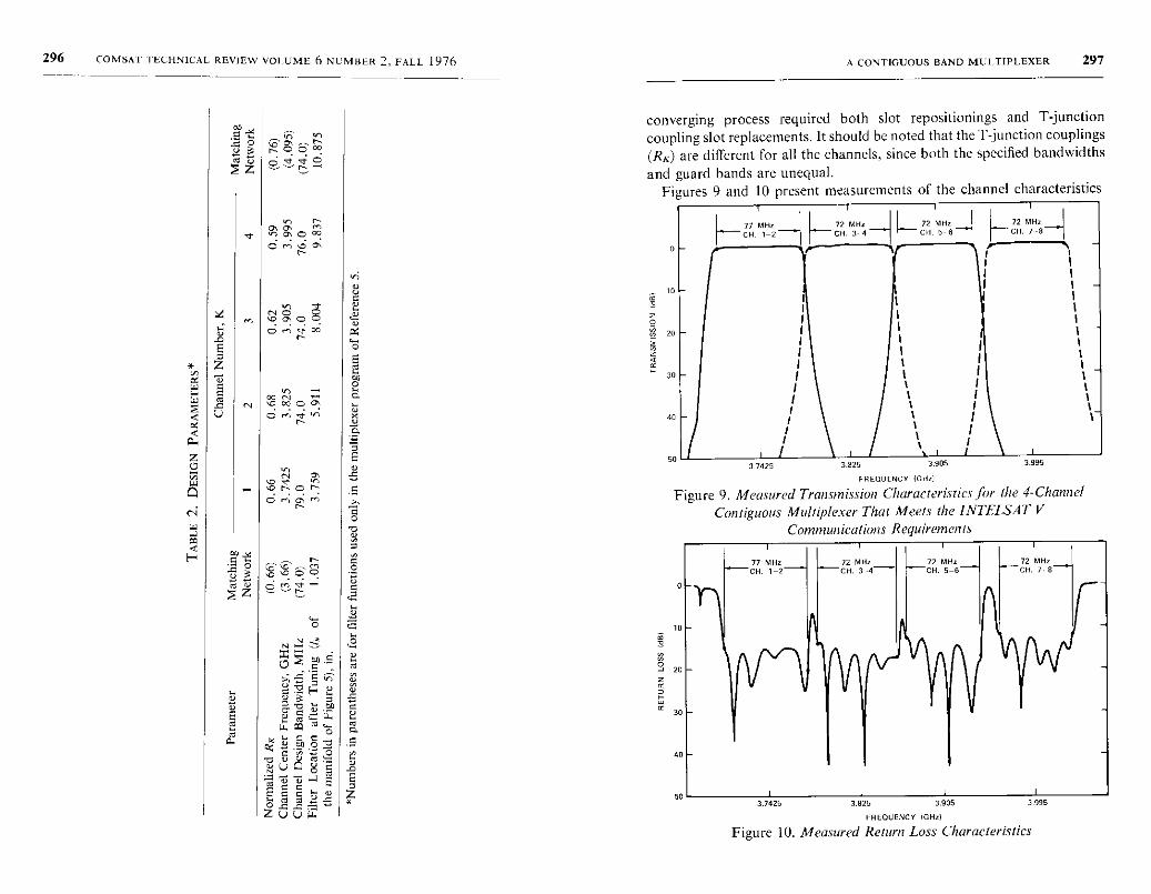
296 COMSAT TECHNICAL REVIEW VOLUME 6 NUMBER 2 , FALL 1976
mh 0'O O
CW y
0
z
N
297
converging process required both slot repositionings and T-junctioncoupling slot replacements. It should be noted that the T-junction couplings(R%) are different for all the channels, since both the specified bandwidths
and guard bands are unequal.Figures 9 and 10 present measurements of the channel characteristics
0N
40
50
MHz7
)
71H2^ I^ CH. 3H4 ^CH. 5Hfi CHCH.
c1
I II II
11
III
II II
I!3 7425 3025 3905 3 995
FREQUENCY (GHz)
M y3
N0
0 3 C)"z C
C)
0 K
0
c7^ ^.c C)9
°L C y N
C 9 0rcC
La 3 3v 3 .^ ^. pp C
Q; b o Am
vy a0 O d C
z ti v m.°U O m 9
^m v`a E Ez
p t t
UUU:
0
40
503.7425
A CONTIGUOUS BAND MULTIPLEXER
3.825 3 ,905
FREQUENCY GHz)
3 995
Figure 10. Measured Return Loss Characteristics
Figure 9. Measured Transmission Characteristics for the 4- Channel
Contiguous Multiplexer That Meets the INTELSAT V
Communications Requirements
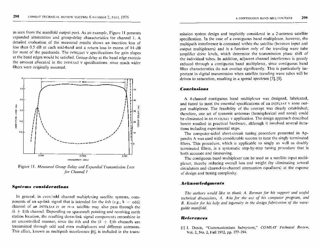
298 COMSAT TECHNICAL REVIEW VOLUME 6 NUMBER 2, FALL 1976
as seen from the manifold output port. As an example, Figure 11 presentsexpanded attenuation and group-delay characteristics for channel 1. Adetailed evaluation of the measured results shows an insertion loss ofless than 0.5 dB at each mid-band and a return loss in excess of 14 dBfor most of the passbands. The INTELSAT V specifications for gain slopesat the band edges would be satisfied. Group delay at the band edge exceedsthe amount allocated in the INTELSAT V specifications, since much widerfilters were originally assumed.
77 MHz
1.0
20
0
50
50
40
I I
30 r
1 I 3I 0
20
10
-ice
3.704 37425
FREQUENCY (GHZI
3.781
Figure 11. Measured Group Delay and Expanded Transmission Lossfor ChannelI
Systems considerations
In general , in even /odd channel multiplexing satellite systems, com-ponents of an up-link signal that is intended for the kth (e.g., k = odd)channel of an INTELSAT lv or Iv-A satellite may also pass through the(k + l)th channel . Depending on spacecraft pointing and receiving earthstation location, the resulting down -link signal components recombine inan uncontrolled manner, since the kth and the (k + l)th channels aretransmitted through odd and even multiplexers and different antennas.This effect, known as multipath interference [6], is included in the trans-
A CONTIGUOUS BAND MULTIPLEXER 299
mission system design and implicitly considered in a 2-antenna satellitespecification. In the case of a contiguous band multiplexer, however, themultipath interference is contained within the satellite (between input andoutput multiplexers) and is a function only of the traveling wave tubeamplifier drive levels, which determine the transmission phase shift ofthe individual tubes. In addition, adjacent channel interference is greatlyreduced through a contiguous band multiplexer, since contiguous bandfilter characteristics do not overlap significantly. This is particularly im-portant in digital transmission when satellite traveling wave tubes will bedriven to saturation, resulting in a spread spectrum [7], [8].
Conclusions
A 4-channel contiguous band multiplexer was designed, fabricated,and tuned to meet the essential specifications of an INTELSAT V zone out-put multiplexer. The feasibility of the concept was clearly established;therefore, one set of transmit antennas (hemispherical and zonal) couldbe eliminated in an INTELSAT v application. The design approach describedherein resulted in practical hardware, although it involved several itera-tions including experimental steps.
The computer-aided short-circuit tuning procedure presented in Ap-pendix A was used with considerable success to tune the singly terminatedfilters. This procedure, which is applicable to singly as well as doublyterminated filters, is a systematic step-by-step tuning procedure that is
both accurate and timesaving.The contiguous band multiplexer can be used as a satellite input multi-
plexer, thereby reducing overall loss and weight (by eliminating severalcirculators and channel-to-channel attenuation equalizers) at the expense
of design and tuning complexity.
Acknowledgments
The authors would like to thank A. Berman for his support and usefultechnical discussions, A. Aria for the use of his computer program, andR. Kessler for his help and ingenuity in the design fabrication of the wave-
guide manifold.
Rclerenees
[1] 1. Dostis, "Communications Subsystem," COMSAT Technical Review,
Vol. 2, No. 2, Fall 1972, pp. 277-294.
300 COMSAT TECHNICAL REVIEW VOLUME 6 NUMBER 2, FALL 1976
[2] E. G. Cristal and C. L. Matthaei, "A Technique for the Design of Multi-plexers Having Contiguous Channels," IEEE Transactions on MicrowaveTheory and Techniques, MTT-12, January 1964, pp. 88-93.
[3] G. L. Matthaei, L. Young, and E. M. T. Jones, Microwave Filters, Impedance-Matching Networks and Coupling Structures, New York: McGraw-HillBook Co., 1964.
[4] W. A. Edson and J. Wakabayashi, "Input Manifolds for Microwave Chan-nelizing Filters," IEEE Transactions on Microwave Theory and Techniques,MTT-18, May 1970, pp. 270-276.
[5] A. E. Atia, "Computer-Aided Design of Waveguide Multiplexers," IEEETransactions on Microwave Theory and Techniques, MTT-22, March 1974,pp. 322-336.
[6] A. L. Berman, C. Mahle, and M. R. Wachs, "Transmission Modeling,"COMSAT Technical Review, Vol. 2, No. 2, Fall 1972, p. 495.
[7] G. Robinson, 0. Shimbo, and R. Fang, "PSK Signal Power SpectrumSpread Produced by Memoryless Nonlinear TWTs," COMSAT TechnicalReview, Vol. 3, No. 2, Fall 1973, pp. 227-257.
[8] C. Devieux, "Analysis of PSK Signal Power Spectrum Spread with a MarkovChain Model," COMSAT Technical Review, Vol. 5, No. 2, Fall 1975, pp.225-252.
Appendix A. Filter design and tuning
To design an N-channel contiguous band multiplexer, the computer programof Reference 5 requires the normalized coupling coefficients of N + 2 filters,as indicated in Figure 6. These parameters may be derived once the filter func-
tion, center frequencies, and bandwidths are selected. The low-pass clementvalues may be derived for an m-pole singly terminated Chebychev filter accord-ing to standard procedures given in Reference 3.
Conventional filter tuning for a doubly terminated filter is based upon thefilter's return loss characteristics. Minimization of the reflection in the passband
with correct center frequency and bandwidth is (he usual criterion for filtertuning. However, since a singly terminated filter is not matched over the entirepassband due to the existence of passband reactance, the criterion of minimumreflection may not be used for filter tuning. Instead, a method based upon theshort-circuit impedance [Al] may be used. It consists of matching the computedand measured short-circuit impedance of the filter over a wide frequency rangeand thereby determining the correct tuning screw position. This impedancemeasurement technique has been used successfully for tuning all the experimen-tal 8-pole Chebychev filters. Figures A-1 and A-2 demonstrate the accuracy ofthe tuning procedure.
A CONTIGUOUS nAND MULTIPLEXER 301
Ileterenee
[Al] A. E. Atia and A. E. Williams, " Measurements of Intercavity Couplings,"
IEEE Transactions on Microwave Theory and Techniques , MTT-23, No. 6,
pp. 519-522.
-ik- COMPUTED
MEASURED
30
40
3 750 3.775 3800 3875 3.9003.850
FREQUENCY (GHz)
Figure A -1. Transmission Response for 3.825-GHz Filter
200
100
40
3.69
-------------
- MEASUREDX COMPUTED
) REFLECTION PHASE
--- MEASUREDRETURN LOSS
COMPUTED
>n t
I
3.825
p
3.825
FREQUENCY IGHz)
Figure A -2. Reflection Responses for 3.825-GHz Filter
____________
3.98
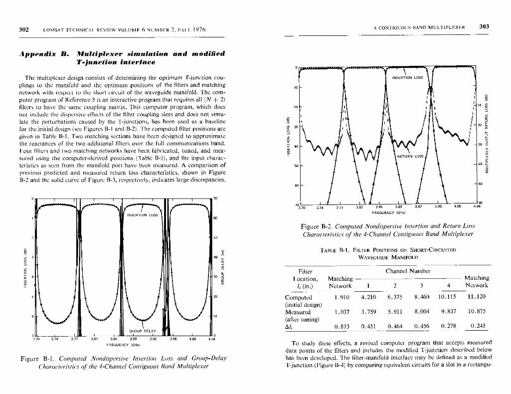
302 COMSAT TECHNICAL REVIEW VOLUME 6 NUMBER 2, FALL 1976
Appendix IS. Multiplexer simulation and modifiedT-junetion interface
The multiplexer design consists of determining the optimum T-junction cou-plings to the manifold and the optimum positions of the filters and matchingnetwork with respect to the short circuit of the waveguide manifold. The com-puter program of Reference 5 is an interactive program that requires all (N + 2)filters to have the same coupling matrix. This computer program, which doesnot include the dispersive effects of the filter coupling slots and does not simu-late the perturbations caused by the T-junctions , has been used as a baselinefor the initial design (see Figures B-I and B-2). The computed filter positions aregiven in Table B-1. Two matching sections have been designed to approximatethe reactances of the two additional filters over the full communications band.Four filters and two matching networks have been fabricated , tuned, and mea-sured using the computer-derived positions (Table B-1), and the input charac-teristics as seen from the manifold port have been measured . A comparison ofprevious predicted and measured return loss characteristics , shown in FigureB-2 and the solid curve of Figure B -3, respectively , indicates large discrepancies.
INSERTION LOSS
10
20
30
40
50
60
703,70 81
A CONTIGUOUS BAND MULTIPLEXER 303
FREQUENCY (GHZ)
85 3.89
50
6092 3.96 400 604
Figure B-2. Computed Nondispersive Insertion and Return LossCharacteristics of the 4-Channel Contiguous Band Multiplexer
TABLE B-1. FILTER POSITIONS ON SHORT-CIRCUITED
WAVEGUIDE MANIFOLD
GROUP DELAY
74 3 77 3.81 3 85 3.69 3.92
FREQUENCY IGHZI
Figure B-1. Computed Nondispersive Insertion Loss and Group-DelayCharacteristics of the 4-Channel Contiguous Band Multiplexer
Filter Channel Number
L i M t hi Matchingocat on, c ngaIF (in.) Network 1 2 3 4 Network
Computed 1.910 4.210 6.375 8.460 10.115 11.120
(initial design)
Measured 1.037 3.759 5.911 8.004 9.837 10.875
(after tuning)
Ali 0.873 0.451 0.464 0.456 0.278 0.245
To study these effects, a revised computer program that accepts measureddata points of the filters and includes the modified T-junction described belowhas been developed. The filter-manifold interface may be defined as a modifiedT-junction (Figure B-4) by comparing equivalent circuits for a slot in a rectangu-
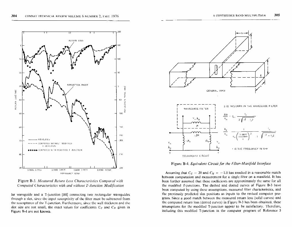
304 COMSAT TECHNICAL. REVIEW VOLUME 6 NUMBER 2, FALL 1976 A CONTIGUOUS BAND MULTIPI EXER 305
MEASURED
- - - - COMPUTED WITHOUT MODIFIEDT-JUNCTION
**$** COMPUTED WITH MODIFIED T JUNCTION
I I I I I 1 13.2055-3.7795 37880 3.8520 3.5580 3,9420 39580 4.0320
FREQUENCY IGHUI
Figure B-3. Measured Return Loss Characteristics Compared withComputed Characteristics with and without T-Junction Modification
lar waveguide and a T-junction [B1J connecting two rectangular waveguidesthrough a slot, since the input susceptivity of the filter must be subtracted fromthe susceptance of the T-junction. Furthermore, since the wall thickness and theslot size are not small, the exact values for coefficients Cc and C,3, given inFigure B-4 are not known.
T
I WAVEGUIDE FILTER
r - ---------- I
EQUIVALENT CIRCUIT
B IS INCLUDED IN THE WAVEGUIDE FILTER
AB
YU
iC
2 f2 - fC2
I/11.802] 2
\ 1ic2
f IS THE FREQUENCY IN GH,
T
Figure B-4. Equivalent Circuit for the Filter-Manifold Interface
Assuming that Cc = 20 and IL,, = -1.0 has resulted in a reasonable matchbetween computation and measurement for a single filter on a manifold. It hasbeen further assumed that these coefficients are approximately the same for allthe modified T-junctions. The dashed and dotted curves of Figure B-3 havebeen computed by using these assumptions, measured filter characteristics, andthe previously predicted slot positions as inputs to the revised computer pro-gram. Since a good match between the measured return loss (solid curves) andthe computed return loss (dotted curves) in Figure B-3 has been obtained, theseassumptions for the modified T-jtmction appear to be satisfactory. Therefore,including this modified T-junction in the computer program of Reference 5
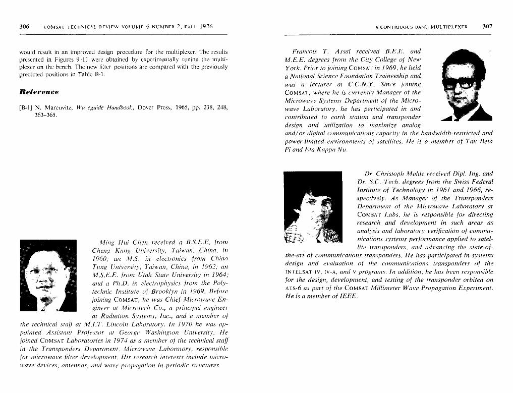
306 COMSAT TECHNICAL. REVIEW VOLUME 6 NUMBER 2, FALL 1976
would result in an improved design procedure for the multiplexer. The resultspresented in Figures 9-11 were obtained by experimentally tuning the multi-
plexer on the bench. The new filter positions are compared with the previouslypredicted positions in Table B-1.
iRelerenee
[B-1] N. Marcuvitz, Waveguide Handbook, Dover Press, 1965, pp. 238, 248,
363-365.
Ming Hui Chen received a B.S.E.E. from
Cheng Kung University, Taiwan, China, in
1960; an M.S. in electronics front Chino
Tung University, Taiwan, China, in 1962; an
M.S.E.E. front Utah State University in 1964;
and a Ph.D. in electrophysics from the Poly-
technic Institute of Brooklyn in 1969. Before
joining COMSAT, he was Chief Microwave En-
gineer at Microtech Co., a principal engineer
at Radiation Systems, Inc., and a member of
the technical staff at M.I.T. Lincoln Laboratory. In 1970 lie was ap-
pointed Assistant Professor at George Washington University. He
joined COMSAT Laboratories in 1974 as a member of the technical staff
in the Transponders Department, Microwave Laboratory, responsible
for microwave filter development. His research interests include micro-
wave devices, antennas, and wave propagation in periodic structures.
A CONTIGUOUS BAND MULTIPLEXER 307
and/or digital communications capacity in the bandwidth-restricted andpower-limited environments of satellites. He is a member of Tau BetaPi and Eta Kappa Nu.
Francois 'I. Assal received B.E.E. andM.E.E. degrees from the City College of New
York. Prior to joining COMSAT in 1969, he held
a National Science Foundation Traineeship and
was a lecturer at C.C.N.Y. Since joining
COMSAT, where he is currently Manager of theMicrowave Systems Department of the Micro-wave Laboratory, he has participated in andcontributed to earth station and transponderdesign and utilization to maximize analog
Dr. Christoph Malde received Dipl. Ing. andDr. S.C. Tech. degrees from the Swiss FederalInstitute of Technology in 1961 and 1966, re-spectively. As Manager of the TranspondersDepartment of the Microwave Laboratory atCOMSAT Labs, he is responsible for directingresearch and development in such areas asanalysis and laboratory verification of commu-nications systems performance applied to satel-lite transponders, and advancing the state-of-
the-art of communications transponders. He has participated in systemsdesign and evaluation of the communications transponders of theINTELSAT IV, IV-A, and v programs. In addition, he has been responsiblefor the design, development, and testing of the transponder orbited onATS-6 as part of the COMSAT Millimeter Wave Propagation Experiment.He is a member of IEEE.
Index: traveling wave tube amplifier, network topology,service life, reliability
Network topologies to enhance thereliability of communicationssatellites
F. ASSAL, C. MAHLE, AND A. BERMAN
(Manuscript received March 17, 1975)
Abstract
In the past, the reliability of failure-prone devices or subsystems was enhancedby providing 2-for-1 or 3-for-2 redundancy. The overall survival probability oflarge systems degrades as the number of failure-prone devices is increased. Hence,24 traveling wave tube amplifiers ('rwrAS) were included in the INTELSAT Ivsatellites to achieve a probability of 0.9 that 9 out of 12 channelized transmitters
would survive seven years in space.This paper presents a network topology that would significantly enhance the
end-of-life reliability of communications satellites by pooling together all failure-prone devices such as TWTAS. The resulting topology, identified by a double-ringstructure, requires a small number of 4-port 4-position switching elements or Rswitches to provide interconnect flexibility. Enhancement of the end-of-life(7-year) probability of survival from 0.69 to 0.91 is demonstrated for a double-ring redundancy configuration consisting of 12 TwTAS for eight active units. Itis also shown that the double-ring topology permits numerous input-to-outputaccesses to satisfy the requirements of particular designs. For example, the out-puts of two TWTAS can be combined to provide greater power for some paths.
This paper is based upon work performed at COMSAT Laboratories under the
sponsorship of the International Telecommunications Satellite Organization
(INTELSAT). Views expressed in this paper are not necessarily those of INTELSAT.
309
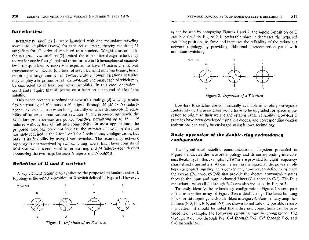
310 COMSAT TECHNICAL REVIEW VOLUME 6 NUMBER 2, FALL 1976
Introduction
INTELSAT Iv satellites [1] were launched with one redundant travelingwave tube amplifier (TWTA) for each active TWTA, thereby requiring 24amplifiers for 12 active ehannelized transponders. Weight constraints inthe INTELSAT Iv-A satellites [2] limited the transmitter design redundancyto two for one in four global and three for two in 16 hemispherical channel-ized transponders. INTELSAT v is expected to have 37 active channelizedtransponders connected to a total of seven transmit antenna beams, hencerequiring a large number of TwTAS. Future communications satellitesmay employ a large number of narrow-beam antennas, each of which maybe connected to at least one active amplifier. In this case, operationalconstraints require that all beams must function at the end of life of the
satellite.This paper presents a redundant network topology [3] which provides
flexible routing of N inputs to N outputs through M (M > N) failure-
prone devices such as TWTAS to significantly enhance the end-of-life relia-bility of future communications satellites. In the proposed approach, the
M failure-prone devices are pooled together, permitting up to M - N
failures without loss of full inter connectivity. In most applications, theproposed topology does not increase the number of switches that arenormally required in the 2-for-I or 3-for-2 redundancy configurations, butobtains its flexibility by using 4-port switches. The redundancy networktopology is characterized by two switching layers. Each layer consists of
M 4-port switches connected to form a ring, and M failure-prone devices
connecting the two rings between N inputs and N outputs.
Definition of R and T switches
A key element required to synthesize the proposed redundant networktopology is the 4-port 4-position or R switch defined in Figure 1. However,
POSITION 1 2 3 4
B e
A 4^ C A C A C
0 0 D
Figure 1. Definition of an R Switch
NETWORK TOPOLOGIES TO ENHANCE SATELLITE RELIABILITY 311
as can be seen by comparing Figures 1 and 2, the 4-pole 3-position or Tswitch defined in Figure 2 is preferable since it decreases the requiredswitching positions to three and increases the reliability of the redundantnetwork topology by providing additional interconnection paths withminimum switching.
POSITION 1 2
n
3
n B
A C A C A C
0 0 0
Figure 2. Definition of a T Switch
Low-loss R switches are commercially available in a rotary waveguideconfiguration. These switches would have to be upgraded for space appli-cation to minimize their weight and establish their reliability. Low-loss Tswitches have been developed using PIN diodes, and corresponding coaxialrealizations can easily be envisaged using known technology.
Basic operation of the double-ring redundancyconfiguration
The hypothetical satellite communications subsystem presented inFigure 3 indicates the network topology and its corresponding intercon-nect flexibility. In this example, 12 TWTAS are provided for eight frequency-channelized transmitters. As can be seen in the figure, all the power ampli-fiers are pooled together. It is convenient, however, to define as primarythe TWTAS (P-1 through P-8) that provide the shortest transmission pathsthrough the input and output channel filters (C-I through C-8). The fourredundant TwTAS (R-l through R-4) are also indicated in Figure 3.
To easily identify the redundancy configuration, Figure 4 shows partof the transmitter array of Figure 3 as a double ring. The basic buildingblock for this topology is also identified in Figure 4. Four primary amplifierfailures (P-3, P-4, P-6, and P-7) are shown to indicate one possible rerout-ing pattern. It should be noted that other interconnections can be pro-vided. For example, the following rerouting may be commanded: C-2through R-1, C-3 through P-2, C-4 through R-2, C-5 through P-5, andC-6 through R-3.
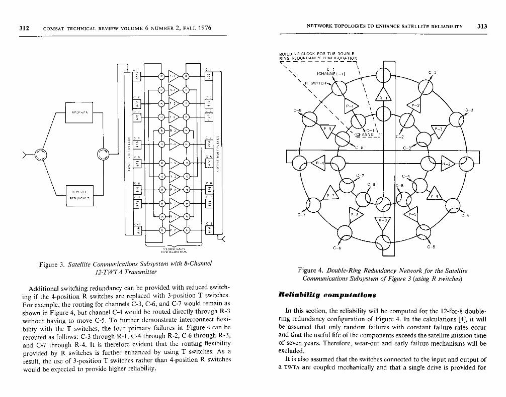
312 COMSAT TECHNICAL REVIEW VOLUME 6 NUMBER 2, FALL 1976 NETWORK TOPOLOGIES TO ENHANCE SATELLITE RELIABILITY 313
REDUND ANCYCONE GU RATION
Figure 3. Satellite Communications Subsystem with 8-Channel
12-TWTA Transmitter
Additional switching redundancy can be provided with reduced switch-ing if the 4-position R switches are replaced with 3-position T switches.For example, the routing for channels C-3, C-6, and C-7 would remain asshown in Figure 4, but channel C-4 would be routed directly through R-3without having to move C-5. To further demonstrate interconnect flexi-bility with the T switches, the four primary failures in Figure 4 can bererouted as follows: C-3 through R-1, C-4 through R-2, C-6 through R-3,and C-7 through R-4. It is therefore evident that the routing flexibilityprovided by R switches is further enhanced by using T switches. As aresult, the use of 3-position T switches rather than 4-position R switches
would be expected to provide higher reliability.
BUILDING BLOCK FOR THE DOUBLE-RING REDUNDANCY CONFIGURATION
C-6
C-2
Figure 4. Double-Ring Redundancy Network Jbr the SatelliteCommunications Subsystem of Figure 3 (using R switches)
Reliability computations
In this section, the reliability will be computed for the 12-for-8 double-ring redundancy configuration of Figure 4. In the calculations [4], it willbe assumed that only random failures with constant failure rates occurand that the useful life of the components exceeds the satellite mission timeof seven years. Therefore, wear-out and early failure mechanisms will beexcluded.
It is also assumed that the switches connected to the input and output ofa TWTA are coupled mechanically and that a single drive is provided for
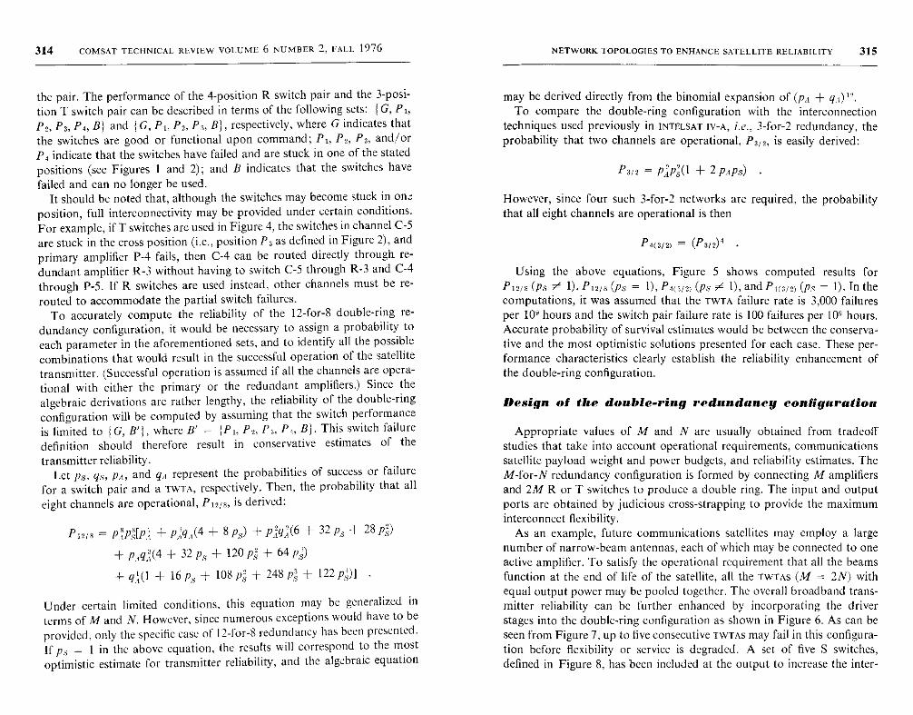
314 COMSAT TECHNICAL REVIEW VOLUME 6 NUMBER 2, FALL 1976
the pair. The performance of the 4-position R switch pair and the 3-posi-tion T switch pair can be described in terms of the following sets: { C, PI,
P2, P,, P°, B) and {G, P1, P", Pa, B}, respectively, where G indicates that
the switches are good or functional upon command; PI, Pg, Pa, and/orP4 indicate that the switches have failed and are stuck in one of the statedpositions (see Figures 1 and 2); and B indicates that the switches have
failed and can no longer be used.It should be noted that, although the switches may become stuck in on.
position, full interconnectivity may be provided under certain conditions.For example, if T switches are used in Figure 4, the switches in channel C-5are stuck in the cross position (i.e., position P" as defined in Figure 2), andprimary amplifier P-4 fails, then C-4 can be routed directly through re-dundant amplifier R-3 without having to switch C-5 through R-3 and C-4through P-5. If R switches are used instead, other channels must be re-
routed to accommodate the partial switch failures.To accurately compute the reliability of the 12-for-8 double-ring re-
dundancy configuration, it would be necessary to assign a probability toeach parameter in the aforementioned sets, and to identify all the possiblecombinations that would result in the successful operation of the satellitetransmitter. (Successful operation is assumed if all the channels are opera-tional with either the primary or the redundant amplifiers.) Since thealgebraic derivations are rather lengthy, the reliability of the double-ringconfiguration will be computed by assuming that the switch performance
is limited to {G, B'}, where B' _ {P1, P", Pa, Pa, B}. This switch failure
definition should therefore result in conservative estimates of the
transmitter reliability.
Let ps, qs, PA, and q,l represent the probabilities of success or failure
for a switch pair and a TWTA, respectively. Then, the probability that all
eight channels are operational, PI"/8, is derived:
F 1218 = P "p,"[1)" + Piq,l(4 + 8 pS) + p,'q'(6 + 32 ps + 28 ps)
+ Png'(4 + 32 ps + 120 ps + 64 PS)
+ q,1'(1 + 16 ps + 1081 + 248 ps + 122 p4)] .
Under certain limited conditions, this equation may be generalized in
terms of M and N. However, since numerous exceptions would have to be
provided, only the specific case of 12-for-8 redundancy has been presented.If ps = I in the above equation, the results will correspond to the mostoptimistic estimate for transmitter reliability, and the algebraic equation
NETWORK TOPOLOGIES TO ENHANCE SATELLITE RELIABILITY 315
may be derived directly from the binomial expansion of (p,, + q_I)1".To compare the double -ring configuration with the interconnection
techniques used previously in INTELSAT Iv-A, i.e., 3-for-2 redundancy, theprobability that two channels are operational , P3/", is easily derived:
P312 = P}P4( I + 2 PA PS)
However, since four such 3-for-2 networks are required, the probabilitythat all eight channels are operational is then
P°(3/2) = (F312)°
Using the above equations , Figure 5 shows computed results for
P12/8 (Ps 7' 1), P1218 (PS = 1), P.Oy/°I (ps V 1), and P4 ( 8/Q) (PS = 1). In the
computations , it was assumed that the TWTA failure rate is 3,000 failures
per 109 hours and the switch pair failure rate is 100 failures per 10" hours.
Accurate probability of survival estimates would be between the conserva-
tive and the most optimistic solutions presented for each case. These per-
formance characteristics clearly establish the reliability enhancement of
the double-ring configuration.
Design of the double-ring redundancy configuration
Appropriate values of M and N are usually obtained from tradeoffstudies that take into account operational requirements, communicationssatellite payload weight and power budgets, and reliability estimates. TheM-for-N redundancy configuration is formed by connecting M amplifiersand 2M R or T switches to produce a double ring. The input and outputports are obtained by judicious cross-strapping to provide the maximuminterconnect flexibility.
As an example, future communications satellites may employ a largenumber of narrow-beam antennas, each of which may be connected to oneactive amplifier. To satisfy the operational requirement that all the beamsfunction at the end of life of the satellite, all the TWTAS (M = 2N) withequal output power may be pooled together. The overall broadband trans-mitter reliability can be further enhanced by incorporating the driverstages into the double-ring configuration as shown in Figure 6. As can beseen from Figure 7, up to five consecutive TWTAS may fail in this configura-tion before flexibility or service is degraded. A set of five S switches,defined in Figure 8, has been included at the output to increase the inter-
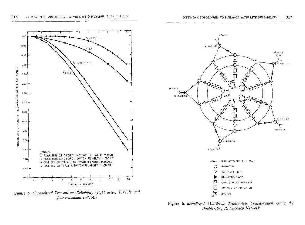
316 COMSAT TECHNICAL REVIEW VOLUME 6 NUMBER 2, FALL 1976
1.00
0.96
0.92
0.88
0 84
0 00
0.76
072
0.68
0.64
0 60
0.56
0.52
0.48
0.44
0 400
I T I
LEGEND.FOUR SETS OF 3FOR2; NO SWITCH FAILURE POSSIBLE
• FOUR SETS OF 3FOR2; SWITCH RELIABILITY - 100 FITo ONE SET OF 12FOR8 , NO SWITCH FAILURE POSSIBLEx ONE SET OF 12-FOR -B; SWITCH RELIABILITY = 100 FIT
2 4 5 6
YEARS IN SERVICE
7 8 9
I
10
Figure 5. Channelized Transmitter Reliability (eight active TWTAs and
four redundant TWTAs)
NETWORK TOPOLOGIES TO ENHANCE SATELLITE RELIABILITY 317
BEAM 2
---►- INDICATES SIGNAL FLOW
® R-SWITCH
D TWT AMPLIFIER
10.
GS
rL
p TRANSISTOR AMPLIFIER
DEFECTIVE TWTA
GAIN STEP ATTENUATOR
HYBRID
Figure 6. Broadband Multibeam Transmitter Configuration Using the
Double- Ring Redundancy Network
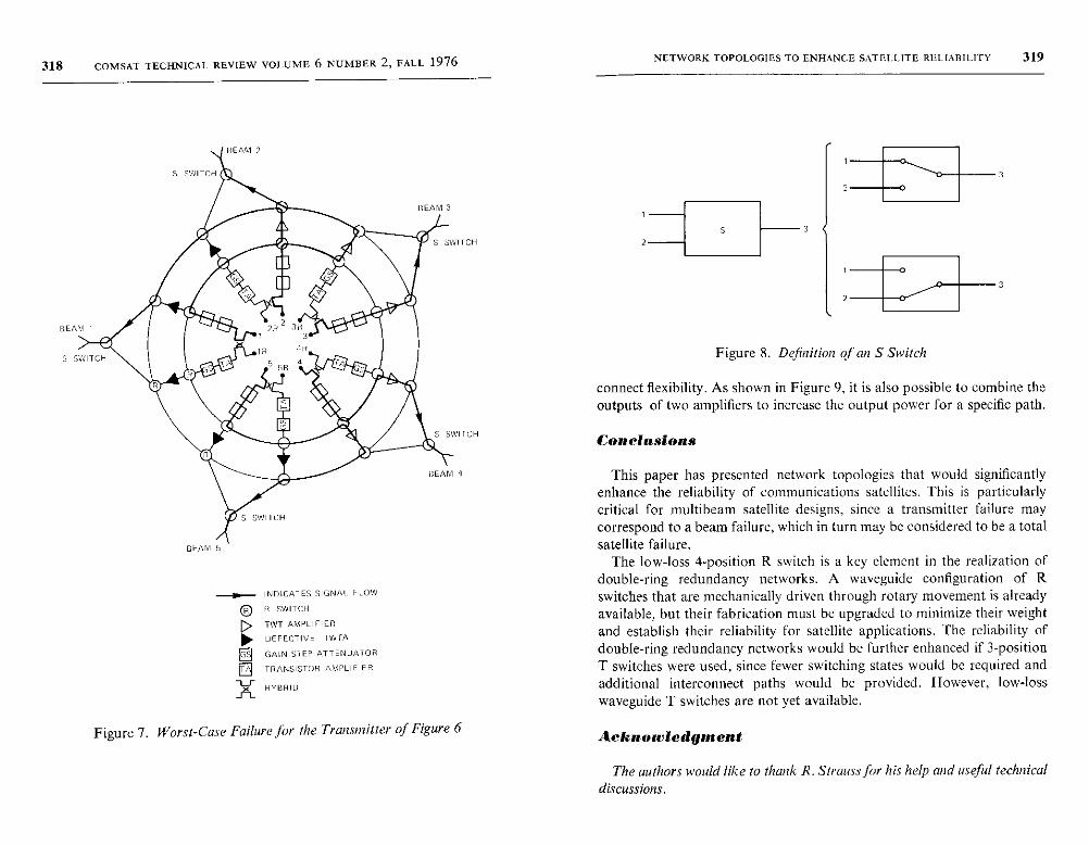
318 COMSAT TECHNICAL REVIEW VOLUME 6 NUMBER 2, FALL 1976
Gs
0
INDICATES SIGNAL FLOW
H SWITCH
TWT AMPLIFIER
DEFECTIVE TWOA
GAIN STEP ATTENUATOR
TRANSISTOR AMPLIFIER
Kr HYBRID
NETWORK TOPOLOGIES TO ENHANCE SATELLITE RELIABILITY 319
S
Figure S. Definition of an S Switch
connect flexibility. As shown in Figure 9, it is also possible to combine theoutputs of two amplifiers to increase the output power for a specific path.
Conclusions
This paper has presented network topologies that would significantlyenhance the reliability of communications satellites. This is particularlycritical for multibeam satellite designs, since a transmitter failure maycorrespond to a beam failure, which in turn may be considered to be a totalsatellite failure.
The low-loss 4-position R switch is a key element in the realization ofdouble-ring redundancy networks. A waveguide configuration of Rswitches that are mechanically driven through rotary movement is alreadyavailable, but their fabrication must be upgraded to minimize their weightand establish their reliability for satellite applications. The reliability ofdouble-ring redundancy networks would be further enhanced if 3-positionT switches were used, since fewer switching states would be required andadditional interconnect paths would be provided. However, low-losswaveguide T switches are not yet available.
Figure 7. Worst-Case Failure for the Transmitter of Figure 6 Aeknowledgment
The authors would like to thank R. Strauss for his help and useful technical
discussions.
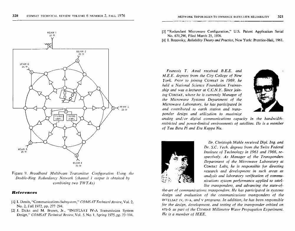
320 COMSAT TECHNICAL REVIEW VOLUME 6 NUMBER 2 , FALL 1976
BEAM 150 W
BEAM 425 W
BEAM 3
25 W
Figure 9. Broadband Multibeam Transmitter Configuration Using theDouble-Ring Redundancy Network (channel 1 output is obtained by
combining two TWTAs)
References
[1] 1. Dostis, "Communications Subsystem," COMSAT Technical Review, Vol. 2,No. 2, Fall 1972, pp. 277-294.
[2] J. Dicks and M. Brown, Jr., "INTELSAT IV-A Transmission SystemDesign." COMSAT Technical Review. Vol. 5, No. 1, Spring 1975, pp. 73-104.
NETWORK TOPOLOGIES TO ENHANCE SATELLITE RELIABILITY 321
[3] "Redundant Microwave Configuration," U.S. Patent Application SerialNo. 670,290, Filed March 25, 1976.
[4] 1. Bozovsky, Reliability Theory and Practice, New York: Prentice-Hall, 1961.
analog and/or digital communications capacity in the bandwidth-restricted and power-limited environments of satellites. He is a memberof Tau Beta Pi and Eta Kappa Nu.
Francois T. Assal received B.E.E. andM.E.E. degrees from the City College of NewYork. Prior to joining COMSAT in 1969, heheld a National Science Foundation Trainee-ship and was a lecturer at C.C.N. Y. Since join-ing COMSAT, where he is currently Manager ofthe Microwave Systems Department of theMicrowave Laboratory, he has participated inand contributed to earth station and trans-ponder design and utilization to maximize
Dr. Christoph Mahle received Dipl. Ing. andDr. S.C. Tech. degrees from the Swiss FederalInstitute of Technology in 1961 and 1966, re-
spectively. As Manager of the TranspondersDepartment of the Microwave Laboratory atCOMSAT Labs, he is responsible for directing
research and development in such areas asanalysis and laboratory verification of commu-nications system performance applied to satel-
lite transponders, and advancing the state-of-the-art of communications transponders. He has participated in systems
design and evaluation of the communications transponders of the
INTELSAT Iv, IV-A, and v programs. In addition, he has been responsible
for the design, development, and testing of the transponder orbited on
ATS-6 as part of the COMSAT Millimeter Wave Propagation Experiment.
He is a member of IEEE.

322 COMSAT TECHNICAL REVIEW VOLUME 6 NUMBER 2, FALL 1976
Arnold L. Berman received a B.S.E.E. from
M.I.T. in 1957. Prior to joining COMSAT in
1964, he performed communications system
analysis for meteorological and communica-
tions satellite systems at the Astro-Electronics
Division of RCA, Princeton, New Jersey. At
COMSAT he initially participated in the Interim
C.C.I.R. Conference (Monaco, 1965). He later
participated in the development of the
INTELSAT 11, 111, and Iv communications sys-
tems and the COMSAT ATS-F Propagation Experiment transponder.
He is presently Director of the Microwave Laboratory of COMSAT
Laboratories.
Index : coding, modulation, signal processing,transmission , satellite communications
PCM/FDMA satellite telephony with4-dimensionally-coded quadratureamplitude modulation
G. R. WELTI
(Manuscript received March 22, 1976)
Abstract
This paper shows that quadrature amplitude modulation (QAM) with 4-dimensional (4D) coding is more efficient in terms of power and bandwidthutilization than ordinary QAM. Combined with companded PCM, it permits astraightforward increase in FDMA transponder capacity. The shortest code, which
contains eight waveforms, provides performance similar to that of 4-phasePSK transmission with rate 3/4 forward error correction and soft decision de-
coding. For codes with 32 or more waveforms, the bandwidth can be reducedwith a minimal increase in power consumption. Power/bandwidth tradeoffs arecalculated for 4D-QAM with code lengths from 8 to 1,352. Satellite transpondercapacities are found to be 1.5 to 2 times higher with 4D-QAM than with FM.
Introduction
As the terrestrial telephone network progresses toward the use of digitalsystems, it is appropriate to investigate the transmission of PcM multiplex
This paper is based upon work performed in COMSAT Laboratories under thesponsorship of the International Telecommunications Satellite Organization(INTELSAT) and the Communications Satellite Corporation. Views expressed inthis paper are not necessarily those of INTELSAT or COMSAT.
323
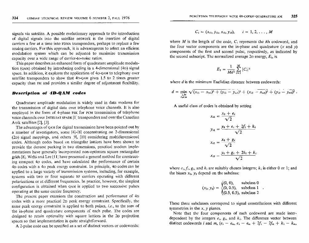
324 COMSAT TECHNICAL REVIEW VOLUME 6 NUMBER 2, FALL 1976
signals via satellite. A possible evolutionary approach to the introductionof digital signals into the satellite network is the insertion of digitalcarriers a few at a time into FDMA transponders, perhaps to replace a fewanalog carriers. For this approach, it is advantageous to select an efficientmodulation system which can be adjusted to maximize transmissioncapacity over a wide range of carrier-to-noise ratios.
This paper describes an enhanced form of quadrature amplitude modula-tion (QAM) obtained by introducing coding in a 4-dimensional (4D) signalspace. In addition, it explores the application of 4D-QAM to telephony oversatellite transponders to show that 4D-QAM gives 1.5 to 2 times greatercapacity than FM and provides a similar degree of adjustment flexibility.
Description of 4D-QAM codes
Quadrature amplitude modulation is widely used in data modems for
the transmission of digital data over telephone voice channels . It is also
employed in the form of 4-phase PSK for PcM transmission of telephone
voice channels over INTELSAT SPADE [ 1] transponders and over the Canadian
Anik satellites [2], [3].
The advantages of QAM for digital transmission have been pointed out bya number of investigators , some [4]-[8] concentrating on 2-dimensional(2D) signal mappings, and others [9], [10] considering multidimensional
codes. Although codes based on triangular lattices have been shown toprovide the densest packing in two dimensions , practical modem imple-mentations have generally incorporated non-optimum square rectangulargrids [8]. Welti and Lee [11] have presented a general method for construct-ing compact 4D codes, and have calculated the performance of certain4D codes with a 4D peak energy constraint . In principle , 4D codes can beapplied to a large variety of transmission systems, including , for example,systems with two or four separate RF carriers operating with differentpolarizations or at different frequencies. In practice , however, the simplestconfiguration is obtained when QAM is applied to two successive pulsesoperating at the same carrier frequency.
The present paper examines the construction and performance of 4Dcodes with a more practical 2D peak energy constraint . Specifically, thesame peak energy constraint is applied to both pulses , i.e., to the sum ofthe in-phase and quadrature components of each pulse . The codes aredesigned to retain optimality with square lattices in the 2D projectionspaces so that implementation is quite straightforward.
A 2-pulse code can be specified as a set of distinct vectors or codewords:
PCM/FDMA TELEPHONY WITH 4D-CODED QUADRATURE AM 325
C: = (xa, Yo, xi2, Yi2), i = 1, 2, .. , M
where M is the length of the code, Ci represents the ith codeword, andthe four vector components are the in-phase and quadrature (x and y)components of the first and second pulse, respectively, as indicated bythe second subscript. The normalized average 2D energy, E,, is
1 ME2=Md,i'Cil2
where d is the minimum Euclidian distance between codewords:
d = min 1/(xi1 - xmj)2 + (YiI - Yml)2 + (x12 - xm2)2 + (Yi2 - Ym2)2 .i, mis.
A useful class of codes is obtained by setting
xo + eixi1 =
Yil =
-\/2
yo +ei+2f+ki
V2
Yo + gi + 2hi + kiX,2
where ei, f, gi, and hi are suitablyand h are suitably chosen integers ; ki is either 0 or 1; andthe biases x,, yo depend on the subclass:
(0, 0), subclass 0
(x0, ya) = (0, 0.5), subclass 1(0.5, 0.5), subclass 2
These three subclasses correspond to signal constellations with differentsymmetries in the x, y planes.
Note that the four components of each codeword are made inter-dependent by the integers ei, gi, and ki. The difference vector betweendistinct codewords i and in, (ei - em, ei - em + 2f1 - 2f + ki - km,
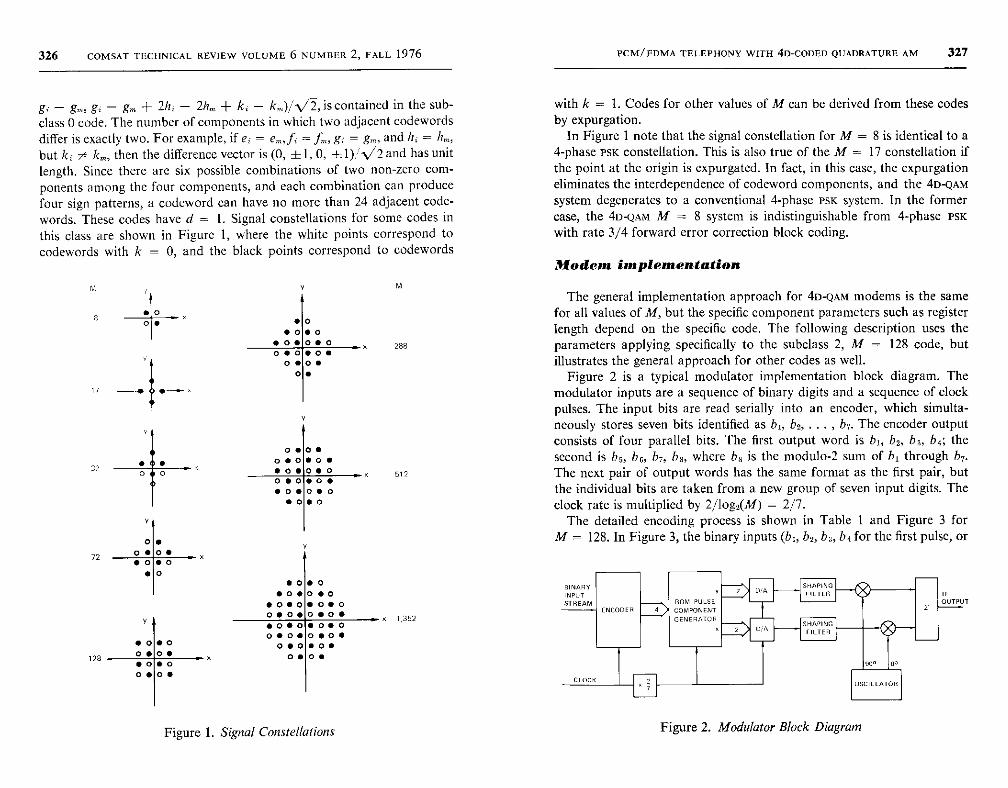
326 COMSAT TECHNICAL REVIEW VOLUME 6 NUMBER 2, FALL 1976
gi - g,,, g; - gm + 2h; - 2hm + k, - k,)/-,12, is contained in the sub-
class 0 code . The number of components in which two adjacent codewordsdiffer is exactly two. For example, if ei = em, fi = f,,,, gi = g,,,, and hi = hm,
but ki ^ km, then the difference vector is (0, f 1, 0, -E 1);' '/2 and has unitlength. Since there are six possible combinations of two non-zero com-ponents among the four components , and each combination can produce
four sign patterns , a codeword can have no more than 24 adjacent code-
words. These codes have d = 1. Signal constellations for some codes inthis class are shown in Figure 1, where the white points correspond to
codewords with k = 0, and the black points correspond to codewords
PCM/FDMA TELEPHONY WITH 4D-CODED QUADRATURE AM 327
with k = 1. Codes for other values of M can be derived from these codesby expurgation.
In Figure 1 note that the signal constellation for M = 8 is identical to a4-phase PSK constellation. This is also true of the M = 17 constellation ifthe point at the origin is expurgated. In fact, in this case, the expurgationeliminates the interdependence of codeword components, and the 4D-QAMsystem degenerates to a conventional 4-phase PSK system. In the formercase, the 4D-QAM M = 8 system is indistinguishable from 4-phase PSKwith rate 3/4 forward error correction block coding.
Modem implementation
32
72
128
0 0
Y1
0•
o
Y
M
0• o • 0
• 0 0 00 0 2880 0 0 • 0
0 O0 0
0 o•
0 • 0 •
• 0 0 000 519000• 0
0 0
00 •
0 • 0
•o
000 • o
• 0 000
000 O • O • O
0 0 0 0 0 • 01,352
• 0 0 0 • 00 0
O • 00 0 000•0 0 0 0 • OO
00 00soo
Figure 1. Signal Constellations
The general implementation approach for 4D-QAM modems is the samefor all values of M, but the specific component parameters such as registerlength depend on the specific code. The following description uses theparameters applying specifically to the subclass 2, M = 128 code, butillustrates the general approach for other codes as well.
Figure 2 is a typical modulator implementation block diagram. Themodulator inputs are a sequence of binary digits and a sequence of clockpulses. The input bits are read serially into an encoder, which simulta-neously stores seven bits identified as b,, b...... b7. The encoder output
consists of four parallel bits. The first output word is b5, b2, b3, b4; thesecond is b5, b6, b7, be, where b,3 is the modulo-2 sum of b, through b,.The next pair of output words has the same format as the first pair, butthe individual bits are taken from a new group of seven input digits. Theclock rate is multiplied by 2/log2(M) = 2/7.
The detailed encoding process is shown in Table 1 and Figure 3 forM = 128. In Figure 3, the binary inputs (b1, b,, b,, b4 for the first pulse, or
BINARY
PUT
STREAM
CLOC
ENCODERROM PULSE
COMPONENT
GENERATOR
SHAPING
FILTER
SHAPINGFILTER
SE' Bo
OSCILLATOR
Figure 2. Modulator Block Diagram
IF
OUTPUT
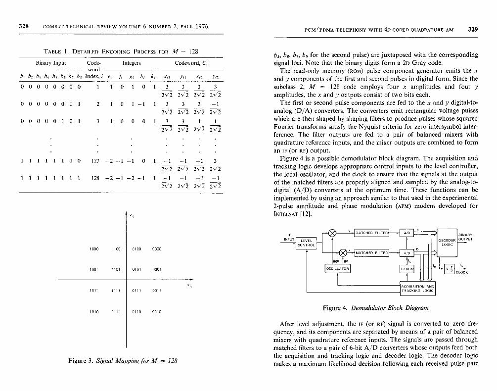
328 COMSAT TECHNICAL REVIEW VOLUME 6 NUMBER 2 , FALL 1976
TABLE 1. DETAILED ENCODING PROCESS FOR M = 128
Binary Input Code- Integers Codeword, C;dwor
h1 b, b, b, b; b, b, b,, Index, i e, f, gi hi ki x;, }'i1 xi, yi2
0 0 0 0 0 0 0 0 1 1 0 1 0 1 3 3 3 3
2/2 21/2 21/2 2/2
0 0 0 0 0 0 1 1 2 1 0 1 -1 1 3 3 3 -I
21/2 21/2 21/2 2V2
0 0 0 0 0 1 0 1 3 1 0 0 0 1 3 3 1 1
21/2 21/2 2V`2 21/2
1 1 1 1 1 1 0 0 127 -2 -1 -1 0 1 -1 -1 -1 3
2/2 2/2 2/2 2/2
1 1 1 1 1 1 1 1 128 -2 -1 - 2 -1 1 -1 -1 -1 -1
2/2 2/2 2x/2 2/2
1000 1100 0100 GOOD
1001 1101 0101 0001
1011 1111 0111 0011
1010 1110 0110 0010
Figure 3. Signal Mapping for M = 128
PCM/FDMA TELEPHONY WITH 4D-CODED QUADRATURE AM 329
bs, be, b,, be for the second pulse) are juxtaposed with the correspondingsignal loci. Note that the binary digits form a 2D Gray code.
The read-only memory (ROM) pulse component generator emits the xand y components of the first and second pulses in digital form. Since thesubclass 2, M = 128 code employs four x amplitudes and four yamplitudes, the x and y outputs consist of two bits each.
The first or second pulse components are fed to the x and y digital-to-analog (D/A) converters. The converters emit rectangular voltage pulseswhich are then shaped by shaping filters to produce pulses whose squaredFourier transforms satisfy the Nyquist criteria for zero intersymbol inter-ference. The filter outputs are fed to a pair of balanced mixers withquadrature reference inputs, and the mixer outputs are combined to forman IF (or RF) Output.
Figure 4 is a possible demodulator block diagram. The acquisition andtracking logic develops appropriate control inputs to the level controller,the local oscillator, and the clock to ensure that the signals at the outputof the matched filters are properly aligned and sampled by the analog-to-digital (A/D) converters at the optimum time. These functions can beimplemented by using an approach similar to that used in the experimental2-pulse amplitude and phase modulation (APM) modem developed forINTELSAT [12].
IFINPUT
OSCILLATOR
MATCHED FILTER
CLOD
ACQUISITION ANDTRACKING LOGIC
Figure 4. Demodulator Block Diagram
After level adjustment, the IF (or RF) signal is converted to zero fre-quency, and its components are separated by means of a pair of balancedmixers with quadrature reference inputs. The signals are passed throughmatched filters to a pair of 6-bit A/D converters whose outputs feed boththe acquisition and tracking logic and decoder logic. The decoder logicmakes a maximum likelihood decision following each received pulse pair
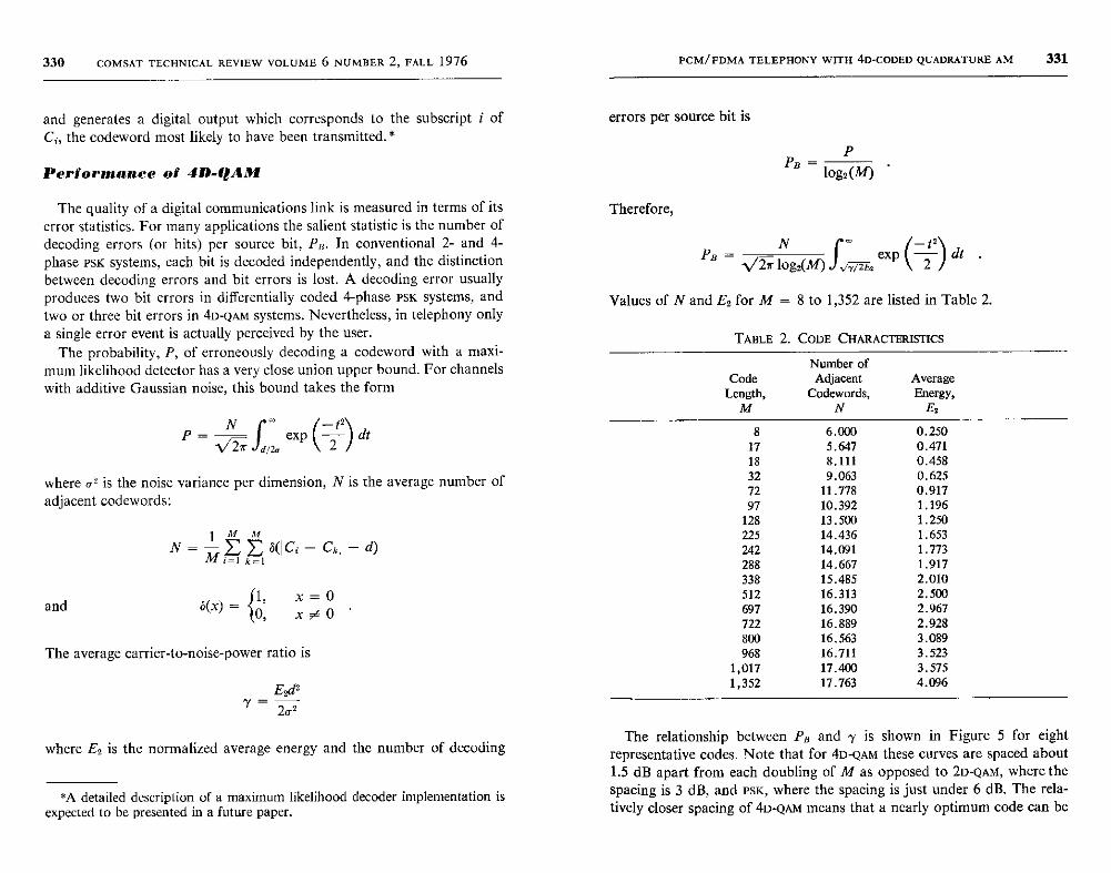
330 COMSAT TECHNICAL REVIEW VOLUME 6 NUMBER 2, FALL 1976 PCM/FDMA TELEPHONY WITH 4D-CODED QUADRATURE AM 331
and generates a digital output which corresponds to the subscript i of errors per source bit isC;, the codeword most likely to have been transmitted. *
P
Yerformanec of 4D-QAM PR 1092(M)
The quality of a digital communications link is measured in terms of itserror statistics. For many applications the salient statistic is the number ofdecoding errors (or hits) per source bit, PB. In conventional 2- and 4-phase PSK systems, each bit is decoded independently, and the distinctionbetween decoding errors and bit errors is lost. A decoding error usuallyproduces two bit errors in differentially coded 4-phase PSK systems, andtwo or three bit errors in 4D-QAM systems. Nevertheless, in telephony onlya single error event is actually perceived by the user.
The probability, P, of erroneously decoding a codeword with a maxi-mum likelihood detector has a very close union upper bound. For channels
with additive Gaussian noise, this bound takes the form
2P =
1/2aN exp 2 dt
f'12.
where o2 is the noise variance per dimension, N is the average number of
adjacent codewords:
and
1 M M
N EL o(C1- Ck^-d)Al i -I k=I
S(x) = 1, x = 00, x#0
The average carrier-to-noise-power ratio is
E2d2.y =2a2
where E, is the normalized average energy and the number of decoding
*A detailed description of a maximum likelihood decoder implementation isexpected to be presented in a future paper.
Therefore,
N /-1 2PB = m exp -
1/2n log2(M) , 2E, 2
Values of N and E2 for M = 8 to 1,352 are listed in Table 2.
TABLE 2. CODE CHARACTERISTICS
Number ofCode Adjacent Average
Length, Codewords , Energy,M N Ez
8 6.000 0.250
17 5.647 0.47118 8.111 0.45832 9.063 0.62572 11.778 0.917
97 10. 392 1.196128 13 . 500 1.250225 14.436 1.653242 14.091 1.773288 14 .667 1.917
338 15.485 2.010
512 16.313 2.500
697 16 . 390 2.967722 16.889 2.928800 16.563 3.089968 16.711 3.523
1,017 17.400 3.5751,352 17.763 4.096
The relationship between PB and y is shown in Figure 5 for eightrepresentative codes. Note that for 4D-QAM these curves are spaced about1.5 dB apart from each doubling of M as opposed to 2D-QAM, where thespacing is 3 dB, and PSK, where the spacing is just under 6 dB. The rela-tively closer spacing of 4D-QAM means that a nearly optimum code can be
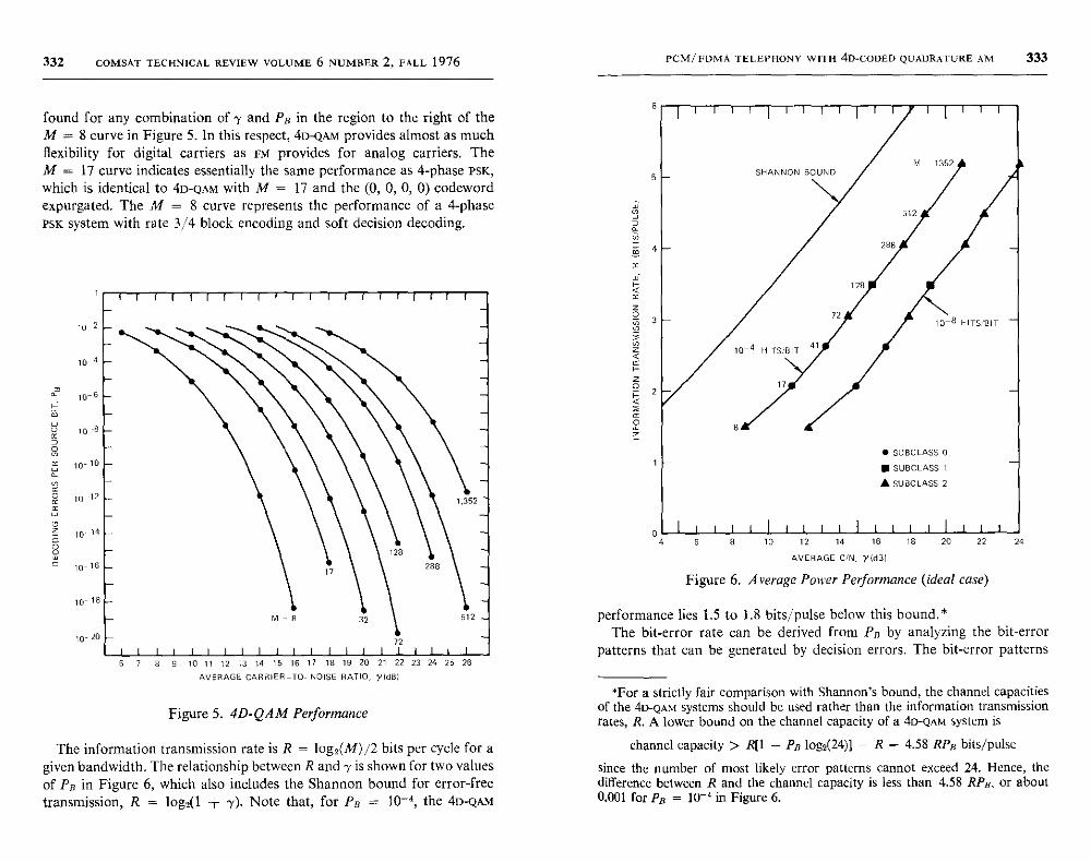
332 COMSAT TECHNICAL REVIEW VOLUME 6 NUMBER 2 , FALL 1976
found for any combination of y and PB in the region to the right of theM = 8 curve in Figure 5. In this respect, 4D-QAM provides almost as muchflexibility for digital carriers as FM provides for analog carriers. TheM = 17 curve indicates essentially the same performance as 4-phase PSK,which is identical to 4D-QAM with M = 17 and the (0, 0, 0, 0) codewordexpurgated. The M = 8 curve represents the performance of a 4-phasePSK system with rate 3/4 block encoding and soft decision decoding.
10-2
10- 4
10-6
10 _8
10-10
10
10
10
12
14
16
PCM/FDMA TELEPHONY WITH 4D-CODED QUADRATURE AM 333
5
4
3
2
• SUBCLASS 0
n SUBCLASS 1
A SUBCLASS 2
40
24
11 I 1 1 I I I I 11 1 1 1 I 1 1 16 8 10 12 14 16
AVERAGE C/N, y(dB)
18 20 22
Figure 6. Average Power Performance (ideal case)
10- 20
6 7 8 9 10 11 12 13 14 15 16 17 18 19 20 21 22 23 24 25 26
AVERAGE CARRIER-TO-NOISE RATIO, yWdBI
Figure 5. 4D-QAM Performance
The information transmission rate is R = log2 (M)/2 bits per cycle for agiven bandwidth . The relationship between R and -y is shown for two valuesof PR in Figure 6, which also includes the Shannon bound for error-freetransmission , R = log2(1 + y). Note that, for PB = 10-4, the 4D-QAM
performance lies 1.5 to 1.8 bits/pulse below this bound.*The bit-error rate can be derived from Pa by analyzing the bit-error
patterns that can be generated by decision errors. The bit-error patterns
*For a strictly fair comparison with Shannon 's bound, the channel capacitiesof the 4D-QAM systems should be used rather than the information transmissionrates, R. A lower bound on the channel capacity of a 4D-QAM system is
channel capacity > R[1 - PR log2(24)] = R - 4.58 RPR bits/pulse
since the number of most likely error patterns cannot exceed 24 . Hence, thedifference between R and the channel capacity is less than 4.58 RPB, or about0.001 for PR = 10-4 in Figure 6.
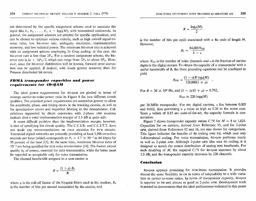
334 COMSAT TECHNICAL REVIEW VOLUME 6 NUMBER 2, FALL 1976
are determined by the specific assignment scheme used to associate theinput bits hl, b2, • • • , b,,, n = log2(M), with transmitted codewords. Ingeneral, the assignment schemes are selected for specific applications, andcan be chosen to optimize various criteria, such as high overall signal-to-noise ratio, low bit-error rate, ambiguity resolution, implementationeconomy, and low radiated power. The minimum bit-error rate is achievedwith an assignment scheme employing 2D Gray coding; in this case, thebit-error rate is less than 2Pn. For a random assignment scheme, the bit-error rate is (n + l )Pu/2, which can range from 2Pa to about SP13. How-ever, since the bit-error distribution will be known, forward error correc-tion can be applied, if desired, with much greater economy than forPoisson distributed bit errors.
FDMA transponder capacities and powerrequirements for 4D-QAM
The ideal power requirements for 4D-QAM are plotted in terms ofaverage carrier-to-noise-power ratio in Figure 6 for two different circuitqualities. The practical power requirements are somewhat greater to allowfor amplitude, phase, and timing errors in the tracking circuits, as well asfor quantization errors and imperfect filtering in the demodulator. Cal-culations supported by direct experience with 2-phase APM modemsindicate that a total implementation margin of 1.5 dB is quite safe.
A more difficult problem than the implementation margin, however,is that of specifying the circuit quality. The C.C.I.R. and C.C.I.T.T. havenot made any recommendations on error statistics for PCM circuits.Terrestrial digital networks are presently providing at least 3,596 error-freeseconds per hour (which corresponds to Pb = 1.7 X 10⁻⁸ at 64 kbps) for95 percent of the time [13]. At the same time, maximum bit-error rates of10-4 are being specified for PCM voice transmission [14]. The former circuitquality is, of course, essential for data transmission, while the latter mustbe regarded as acceptable only for voice transmission.
The channel bandwidth assigned to a QAM carrier is
(1+p)RbB R
where p is the roll-off factor of the Nyquist filters used in the modem, Rbis the number of bits per second transmitted by the carrier, and
PCM/FDMA TELEPHONY WITH 4D-CODED QUADRATURE AM 335
R _ log2(M)
2
is the number of bits per cycle associated with a 4D code of length M.
However,R 64,000NcHR, =
1-E
where NcJ is the number of voice channels and E is the fraction of servicedigits in the digital stream. To obtain the capacity of a transponder with auseful bandwidth of B, the three preceding equations can be combined toyield
(1 - e)B log2(M)Ncrr =
128,000(1 + p)
For B = 36 X 106 Hz, and (1 - E)/(1 + p) = 0.782,
NCH 220log2(M)
per 36-MHz transponder. For rru digital carriers, c lies between 0.005and 0.012, thus permitting a p value as high as 0.26 in the worst case.Since p values of 0.15 are state-of-the-art, the capacity formula is con-servative.
Figure 7 shows transponder capacity versus C/N for M = 8 to 1,024.Capacities for FM carriers, derived from Reference 15, and for 2-pulseAPM, derived from References 12 and 16, are also shown for comparison.This figure indicates the benefits of 4D coding over FM, which uses only1-dimensional coding. For voice transmission, 4D-QAM performs nearlyas well as 2-pulse APM. Although 2-pulse APM also uses 4D coding, it isdesigned to match the source distribution of analog FDM basebands. Foreach doubling of M, the required C/N for 4D-QAM increases by about1.5 dB, and the transponder capacity increases by 220 channels.
Conclusion
4D-QAM appears promising for PCM/FDMA transmission. It providesalmost the same flexibility as FM in terms of adaptability to a wide varia-tion in carrier-to-noise ratios. In terms of transponder capacity, 4D-QAMis superior to FM and almost as good as 2-pulse APM. Development workis needed to demonstrate that the ideal performance indicated in this paper
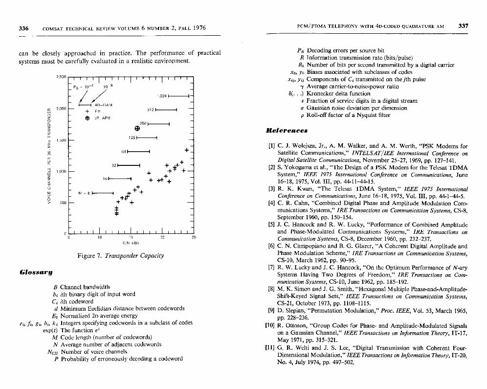
336 COMSAT TECHNICAL REVIEW VOLUME 6 NUMBER 2, FALL 1976 PCM/FDMA TELEPHONY WITH 4D-CODED Q UADRATURE AM 337
can be closely approached in practice. The performance of practicalsystems must be carefully evaluated in a realistic environment.
2,500
2000
1,500
1 ,000
500
PB 10-4 10 8
1 r4D-GAM
+ FM
® 2P APM
F- 32
1 ,024 -5121
Pa Decoding errors per source bitR Information transmission rate (bits/pulse)
Rb Number of bits per second transmitted by a digital carrierx0, yo Biases associated with subclasses of codes
xi;, yi; Components of C1 transmitted on the jth pulsey Average carrier-to-noise-power ratio
S(...) Kronecker delta functiont Fraction of service digits in a digital streama Gaussian noise deviation per dimensionp Roll-off factor of a Nyquist filter
2501 I
1281 I
641 1
161 I
+M=8`r +
i++_'+
+ +* t
+ +f +
I I I I I 1 I I I I 1 I I I 1 1
10
Glossary
15 20 25
Figure 7. Transponder Capacity
B Channel bandwidthb1 ith binary digit of input word
C4 ith codewordd Minimum Euclidian distance between codewords
E2 Normalized 2D average energy
ei, f, gi, hi, k; Integers specifying codewords in a subclass of codesexp(t) The function e'
M Code length (number of codewords)N Average number of adjacent codewords
NNII Number of voice channelsP Probability of erroneously decoding a codeword
References
[1] C. J. Wolejsza, Jr., A. M. Walker, and A. M. Werth, "PSK Modems forSatellite Communications," INTELSAT/IEE International Conference onDigital Satellite Communications, November 25-27, 1969, pp. 127-141.
[2] S. Yokogama et al., "The Design of a PSK Modem for the Telesat TDMASystem," IEEE 1975 International Conference on Communications, June16-18, 1975, Vol. III, pp. 44-11-44-15.
[3] R. K. Kwan, "The Telesat TDMA System," IEEE 1975 InternationalConference on Communications, June 16-18, 1975, Vol. III, pp. 44-1-44-5.
[4] C. R. Cahn, "Combined Digital Phase and Amplitude Modulation Com-munications Systems," IRE Transactions on Communication Systems, CS-8,September 1960, pp. 150-154.
[5] J. C. Hancock and R. W. Lucky, "Performance of Combined Amplitudeand Phase-Modulated Communications Systems," IRE Transactions onCommunication Systems, CS-8, December 1960, pp. 232-237.
[6] C. N. Campopiano and B. G. Glazer, "A Coherent Digital Amplitude andPhase Modulation Scheme," IRE Transactions on Communication Systems,CS-10, March 1962, pp. 90-95.
[7] It. W. Lucky and J. C. Hancock, "On the Optimum Performance of N-ary
Systems Having Two Degrees of Freedom," IRE Transactions on Com-munication Systems, CS-10, June 1962, pp. 185-192.
[8] M. K. Simon and J. G. Smith, "Hexagonal Multiple Phase-and-Amplitude-Shift-Keyed Signal Sets," IEEE Transactions on Communication Systems,CS-21, October 1973, pp. 1108-1115.
[9] D. Slepian, "Permutation Modulation," Proc. IEEE, Vol. 53, March 1965,pp. 228-236.
[10] R. Ottoson, "Group Codes for Phase- and Amplitude-Modulated Signalson a Gaussian Channel," IEEE Transactions on Information Theory, IT-17,May 1971, pp. 315-321.
[11] G. R. Welti and J. S. Lee, "Digital Transmission with Coherent Four-Dimensional Modulation," IEEE Transactions on Information Theory, IT-20,No. 4, July 1974, pp. 497-502.
338 COMSAT TECHNICAL REVIEW VOLUME 6 NUMBER 2 , FALL 1976
(12] T. Furuya, M. Sugiyama, et al., "Hybrid Modem for 120 Channels FDM
Telephony Signal Transmission," Third International Conference on Digital
Satellite Communications, November 1975, pp. 91-98.
[13] C. A. Buzzard, "Error Performance of Digital Data System ChannelsBetween Philadelphia and New York," National TelecommunicationsConference, December 2-4, 1974, NTC'74 Record, pp. 818-823.
[14] International Radio Consultative Committee (C.C.I.R.), "Fixed Service
Using Communication Satellites (Study Group 4),"XIIIth Plenary Assembly,
Geneva, 1974, Vol. IV, Geneva: International Telecommunications Union,
1975, p. 120.[15] J. L. Dicks and M. P. Brown, Jr., "Frequency Division Multiple Access
(FDMA) for Satellite Communication Systems," EASCON '74 Record,October 7-9, 1974, pp. 167-178.
[16] G. R. Welti, "Application of Hybrid Modulation to FDMA Telephony viaSatellite," COMSAT Technical Review, Vol. 3, No. 2, Fall 1973, pp. 419-430.
George R. Welti received B.S. and M.S. degreesin Mechanical Engineering in 1947 and 1948,
respectively, and an M.S. degree in Electrical
Engineering in 1955 from M.I.T. He was Director
of the Advanced Studies Laboratory from 1968 to
1973, and is presently a Senior Scientist at
COMSAT Laboratories. He was previously em-
ployed by Westinghouse Electric Corporation;DECO Electronics, Inc.; Raytheon Co.; M.I.T.;and Sperry Gyroscope Company. He holds a
number of patents in fire control, radar, and communications.
Index : adaptive communications, binary transmission,computerized simulation , delta modulation , quantization,speech processing , variable slope control , digital variableslope control
A strategy for delta modulationin speech reconstruction
J. C. Su, H. G. SUYDERHOUD AND S. J. CAMPANELLA
(Manuscript received April 23, 1976)
Abstract
An adaptive slope control strategy has been developed and incorporated into alinear delta modulation system operating at 32 kbps for the reconstruction ofhigh-quality speech signals. The linear delta modulation system consists of abistate comparator in the forward loop and a 2-pole, 1-zero linear low-passfilter in the feedback loop. The adaptive loop for slope control utilizes a variable
step size function Q(I), which, at each sampling instant, determines the stepsize based on the four most recent bits obtained by sampling the comparator.
The signal-to-distortion ratio has been used to objectively evaluate and com-pare the performance of the adaptive slope control strategy with that of conven-tional companded ecM. In addition, critical listener preference tests have beenconducted. The source speech used in these tests consists of five phoneticallybalanced test sentences spoken by two male and two female talkers.
The objective performance characteristics are presented for a speech inputlevel dynamic range of 0 to -50 dBmO. The effects of bit-error rates in the rangeof 10-3 to 10-1 have also been investigated. Finally, a graphic display of originaland reconstructed speech is presented.
Introduction
Digital transmission of speech is becoming increasingly important forboth terrestrial and satellite communications applications. The present
339
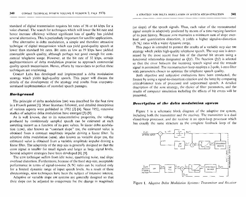
340 COMSAT TECHNICAL REVIEW VOLUME 6 NUMBER 2 , FALL 1976
standard of digital transmission requires bit rates of 56 or 64 kbps for avoice channel. The search for techniques which will lower the bit rate andhence increase efficiency without significant loss of quality has yieldedseveral alternatives. This is particularly important for satellite applications.
One alternative is delta modulation, a simple and therefore attractivetechnique of digital transmission which can yield good-quality speech atlower than standard bit rates. Bit rates as low as 19 kbps have yieldedreasonable speech quality, although perhaps not good enough for com-mercial telephone usage. However, at the bit rate of 32 kbps, certainimplementations of delta modulation promise to approach commercialquality speech transmission. Hence, efforts by researchers to perfect thesetechniques are continuing.
COMSAT Labs has developed and implemented a delta modulationstrategy which yields high-quality speech. This paper will discuss thedetails of the development of the strategy and results from computer-simulated implementation of recorded speech passages.
Background
The principle of delta modulation (DM) was described for the first timein a French patent [1]. More literature followed, and detailed descriptionsof various aspects were published in 1952 [2]-[4]. Since 1952, extensivestudies of adaptive delta modulation have emerged [5]-[9].
As is well known, due to its autocorrelative properties, the voltageproduced by continuously sampled speech can be estimated at eachsampling instant as a function of its past values. In linear delta modula-tion (LDM), also known as "constant slope" DM, the estimated value isobtained from a constant amplitude impulse driving a linear filter. Inadaptive delta modulation (ADM), also known as variable slope DM, theestimated value is obtained from a variable amplitude impulse driving alinear filter. The adaptivity of the step size is generally designed so that theerror signal is smaller for small signals and larger at large signal levels.Several adaptive strategies have been developed [8], [9].
The LDM technique suffers from idle noise, quantizing noise, and slopeoverload distortion. Furthermore, because of the fixed step size, acceptableperformance in terms of signal-to-noise (S/N) ratio can be realized onlyfor a limited dynamic range of input speech levels. As a result of theseshortcomings, ADM techniques have been the subject of intensive interest.
Adaptive or variable slope DM systems are generally designed so thattheir slope can be adjusted to compensate for the change in magnitude
A STRATEGY FOR DELTA MODULATION IN SPEECH RECONSTRUCTION 341
(or slope) of the speech signals. Thus, each value of the reconstructedsignal sample is adaptively predicted by means of a time-varying functionof its past history. Because ADM maintains a minimum sum of slope over-load and quantization distortion, it yields a higher signal-to-distortion(S/NQ) ratio with a wider dynamic range.
This paper is intended to present the results of a variable step size DMstrategy which yields high-quality telephone speech. The step size is deter-mined by the most recent four bits of the channel bit stream using afunctional relationship designated as Q(I). The function Q(1) is selectedso that the error between the incoming speech signal and the remadesignal is minimized. The reconstruction loop employs a 2-pole, I-zero filterwith parameters chosen to optimize the telephone speech quality.
Both objective and subjective evaluations have been conducted, theformer by using a signal-to-distortion criterion and the latter by comparingcritical-listener tests of processed and unprocessed speech. A detaileddescription of the ADM strategy, the choice of filter parameters, and theresults of computer simulation including the effects of bit errors will be
presented.
Description of the delta modulation system
Figure 1 is a schematic block diagram of the adaptive DM system,including both the transmitter and the receiver. The transmitter is a dualclosed-loop processor, and the receiver is an open-loop processor whichhas exactly the same structure as the complete feedback loop of the
XoT)SPEECH INPUT
,n
X(.1U 1(nTlLPF
SPEECH
OUTPUT
YT)
LDF
Fpl
LDF PInII X DIII a
TO
hIPT) /_ OIII InT
IInT STRATEGY.EVICE
STRATEGYDEVICE
Figure 1. Adaptive Delta Modulation Systems: Transmitter and Receiver
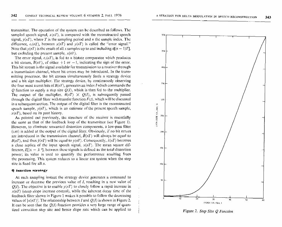
342 COMSAT TECHNICAL REVIEW VOLUME 6 NUMBER 2, FALL 1976 A STRATEGY FOR DELTA MODULATION IN SPEECH RECONSTRUCTION 343
transmitter. The operation of the system can be described as follows. Thesampled speech signal, x(nT), is compared with the reconstructed speechsignal, y(nT), where T is the sampling period and n the sample index. Thedifference, e,(nT), between x(nT) and y(nT) is called the "error signal."Note that y(T) is the result of all x samples up to and including x[(n - 1)T],but excluding the present sample, x(nT).
The error signal, e,(nT), is fed to a bistate comparator which producesa bit stream, B(nT), of either +1 or -1, indicating the sign of the error.This bit stream is the signal available for transmission to a receiver througha transmission channel, where bit errors may be introduced. In the trans-mitting processor, the bit stream simultaneously feeds a strategy deviceand a bit sign multiplier. The strategy device, by continuously observingthe four most recent bits of B(nT), generates an index Iwhich commands theQ function to supply a step size Q(I), which is then fed to the multiplier.The output of the multiplier, B(nT) X Q(I), is subsequently passedthrough the digital filter with transfer function F(z), which will be discussedin a subsequent section. The output of the digital filter is the reconstructed
speech sample, y(nT), which is an estimate of the present speech sample,
x(nT), based on its past history.As pointed out previously, the structure of the receiver is essentially 250
the same as that of the feedback loop of the transmitter (see Figure 1).However, to eliminate unwanted distortion components, a low-pass filter(LPF) is added at the output of the digital filter. Obviously, if no bit errors 200 Fare introduced in the transmission channel, B(nT) will always be equal to
B(nT), and thus y(nT) will be equal to y(nT). Consequently, x(nT) becomes
a close replica of the input speech signal, x(nT). The mean square dif-150 ~ference, E[Ix - .%2], between these signals is defined as the total distortion
power; its value is used to quantify the performance resulting fromthe processing. This system reduces to a linear DM system when the stepsize is fixed for all it. 100
Q funetiou strategy
At each sampling instant the strategy device generates a command toincrease or decrease the previous value of I, resulting in a new value ofQ(1). The objective is to enable y(nT) to closely follow a rapid increase inx(nT) (steep slope increase control), while the inherent decay time of thefeedback filter shown in Figure 1 makes it possible to follow the decreasing
values of lx(nT) i. The relationship between I and Q(I) is shown in Figure 2.
It can be seen that the Q(1) function provides a very large range of quan-tized correction step size and hence slope rate which can be applied to Figure 2. Step Size Q Function
5050 60
344 COMSAT TECHNICAL REVIEW VOLUME 6 NUMBER 2, FALL 1976
the feedback correction loop. As a result, distortion induced by the DMprocessing is significantly decreased. For input signals having a low rateof change, the quantizing step size should be small to minimize quantizingnoise. For such signals the strategy unit must generate low values of index I.
For functions having a high rate of change, the quantizing step sizemust be much greater and the strategy unit must accordingly generatehigh values of index I. The unit must also be able to change quickly fromlow to high index values to follow the abrupt changes in signal slope whichare characteristically encountered in speech. The periodic exponentiallydecaying sinusoid characteristic of larynx excited sounds and the burstand fricative consonants are typical examples of this type of speech func-tion. Changes from high to low index values need not be as rapid becauseof the exponential decay characteristic of the typical pitch impulse func-
tion. It can be seen that the Q(I) function has a nonlinear relationship
with I, which is the result of experimental trimming to produce the mini-mum mean square error for a set of speech samples comprising sentences
spoken by men and women.The rules for increasing the quantizing step size are based on the
occurrence of runs of the same bit value. Such runs indicate the occurrenceof slope overload, which can be overcome only by increasing the quantizingstep size. It will be seen that the logic is organized to provide increasinglyrapid step size augmentation to keep pace with abrupt increases in signalrate of change as the run length increases. The following rules apply
to the logic for increasing quantizing step size:
a. rule 1: If two consecutive bits have the same sign, the Q value is
increased by one step size (4I = 1);
b. rule 2: if three consecutive bits have the same sign, the Q value
is increased by two steps (DI = 2);
c. rule 3: if four consecutive bits have the same sign, the Q value
is increased by three steps (4I = 3);
d. rule 4: if more than four consecutive bits have the same sign,
the Q value is increased by two steps (AI = 2).
Because decreases in quantizing step size are required only to followthe exponential decay of the speech pitch period, they need not be as rapid.Hence, there is only one rule for decreasing the quantizing step size. Thisrule prevails when the bit stream is characterized by randomly alternatingbits, a condition which occurs when the quantization step size is equal to orgreater than that needed to fulfill the rate of change requirement. The rule
is stated as follows:
A STRATEGY FOR DELTA MODULATION IN SPEECH RECONSTRUCTION 345
rule 5: If the sign of the current bit is the opposite of the sign of itsimmediate predecessor, the Q value is decreased by one step (i.e.,AI = -1); this rule overrides all others.
These rules have been devised with the following general objectives:
a. Only one rule should apply to any situation.b. When steep slopes are initially encountered, three consecutive
bits with the same sign will occur and rule 2 will ensure a large increasein Q(1).
c. When very steep slopes occur, four consecutive bits with thesame sign will result and rule 3 will be invoked to ensure very largeQ(I) values.
d. Rule 4 will prevent Q(I) from becoming excessive during a shortinterval.
e. When the reconstructed signal exceeds the input signal, rule 5will moderately reduce the step size. It will also produce the minimumoutput when no signal is present.
The nonlinear relationship between I and Q(I) results in a rapidlyincreasing quantizing step size to cope with rapid increases in the signalrate of change. This significantly reduces slope overload by causing thequantizing step size to accurately follow the rms signal slope. Thus, theadaptive DM strategy is a form of nonuniform nonlinear processing similarto companding.
The Q function shown in Figure 2 has been developed with due consider-ation of the statistical properties of the speech signal. The maximum valueof Q(I) is approximately 2.50., where a, is the rms value of the maximumspeech signal. Other parameters such as maximum S/N,, sampling fre-quency, and input power level have also been taken into consideration.Furthermore, if a curve to the right of the particular Q function shown inFigure 2 had been chosen, it would have resulted in greater slope overloadnoise, but less granular noise. On the other hand, a curve to the left wouldhave resulted in more granular noise and less slope overload noise.
Digital feedback filter
It has been shown by deJager [3] that, for LDM systems, the reconstructedsignal can be improved by using a double integrator in the feedback loop.However, a pure double-pole filter used in conjunction with a hard limiter(bistate comparator) can cause oscillation and lack stability under certainconditions [10]. To avoid this instability, a zero must be introduced into
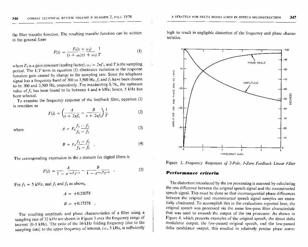
346 COMSAT TECHNICAL REVIEW VOLUME 6 NUMBER 2, FAIL 1976
the filter transfer function. The resulting transfer function can be written
in the general form
P(s)(s + w 1) (s + w2) T
(1)
where Fo is a gain constant (scaling factor), w, = 2Tfi, and T is the sampling
period. The 1/T term in equation (1) eliminates variation in the responsefunction gain caused by change in the sampling rate. Since the telephonesignal has a frequency band of 300 to 3,500 Hz, f1 and f, have been chosento be 300 and 3,500 Hz, respectively. For maximizing S/Ne, the optimumvalue off, has been found to lie between 4 and 6 kHz; hence, 5 kHz has
been selected.To examine the frequency response of the feedback filter, equation (1)
is rewritten as
F(s) =
where
Fo(s + w3) 1
( A B 1 (2)
\s + 2Tfi s + 2Tfi T
A = F•of3 - fl
fz - fl
B = Fo f3 frz
f2 -f1 .
The corresponding expression in the z domain for digital filters is
(3)
(4)
A B (5)F(z)
= 1 - e m Tr1 - 1- e d Ty-,
For f3 = 5 kHz, and fI and fs as above,
A = +0.55078
B = +0.17578
The resulting amplitude and phase characteristics of a filter using asampling rate of 32 kHz are shown in Figure 3 over the frequency range ofinterest (0-5 kHz). The ratio of the 16-kHz folding frequency (due to the
sampling rate) to the upper frequency of interest, i.e., 5 kHz, is sufficiently
A STRATEGY FOR DELTA MODULATION IN SPEECH RECONSTRUCTION 347
high to result in negligible distortion of the frequency and phase charac-teristics.
1 12 3 4
FREQUENCY(kHz)
Figure 3. Frequency Responses of 2-Pole, ]-Zero Feedback Linear Filter
Performance criteria
The distortion introduced by the DM processing is assessed by calculatingthe rms difference between the original speech signal and the reconstructedspeech signal. This must be done so that inconsequential phase differencesbetween the original and reconstructed speech signal samples are essen-tially eliminated. To accomplish this in the evaluations reported here, theoriginal speech was processed via the same low-pass filter characteristicthat was used to smooth the output of the DM processor. As shown inFigure 4, which presents examples of the original speech, the direct deltamodulator output, the low-passed original speech, and the low-passeddelta modulator output, this resulted in relatively precise phase corre-
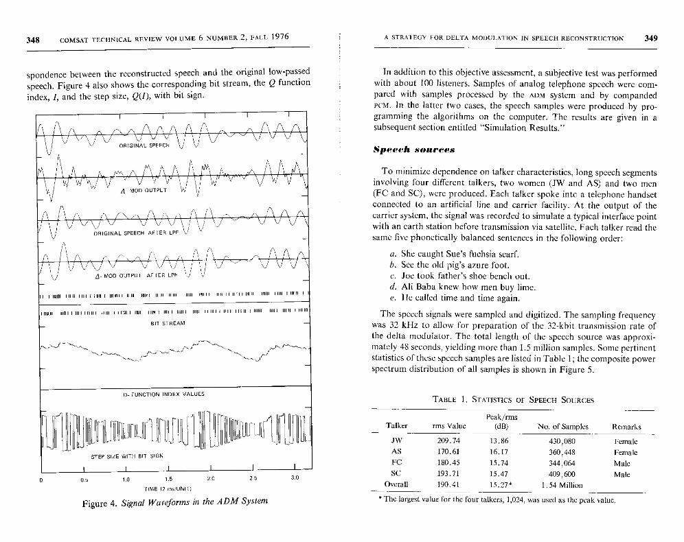
348 COMSAT TECHNICAL REVIEW VOLUME 6 NUMBER 2 , FALL 1976
spondence between the reconstructed speech and the original low-passedspeech. Figure 4 also shows the corresponding bit stream, the Q function
index, I, and the step size, Q(I), with bit sign.
ORIGINAL SPEECH
11d-Moo OUTPUT 0, V
11 A
J^1 vORIGINAL SPEECH AFTER LPF
^\ d- MOD OUTPUT AFTER LPF Ni
Inm nrn IIII Inn I moll 11 10 1111 11111 Inn illm Doll loll 11 Inu 11111 1901 Inn 111111 I
1111 1 1 1 1 0 1 1 1 1 1 1 ' ' 1 1 1 111) 111111 1 1-11 I'M 11m I IIn11 11111 I nlu I n nl 11111 1 nn11 11111 III U 119 m
BIT STREAM
Q-FUNCTION INDEX VALUES
000ffllli mniuiIS TEP SIZE WITH BIT SIGN
0 0.5 10
A STRATEGY FOR DELTA MODULATION IN SPEECH RECONSTRUCTION 349
In addition to this objective assessment, a subjective test was performedwith about 100 listeners. Samples of analog telephone speech were com-pared with samples processed by the ADM system and by compandedPcM. In the latter two cases, the speech samples were produced by pro-gramming the algorithms on the computer. The results are given in asubsequent section entitled "Simulation Results."
Speech sources
To minimize dependence on talker characteristics, long speech segmentsinvolving four different talkers, two women (JW and AS) and two men(FC and SC), were produced. Each talker spoke into a telephone handsetconnected to an artificial line and carrier facility. At the output of thecarrier system, the signal was recorded to simulate a typical interface pointwith an earth station before transmission via satellite. Each talker read thesame five phonetically balanced sentences in the following order:
a. She caught Sue's fuchsia scarf.h. See the old pig's azure foot.c. Joe took father's shoe bench out.d. Ali Baba knew how men buy lime.e. He called time and time again.
The speech signals were sampled and digitized. The sampling frequencywas 32 kHz to allow for preparation of the 32-kbit transmission rate ofthe delta modulator. The total length of the speech source was approxi-mately 48 seconds, yielding more than 1.5 million samples. Some pertinentstatistics of these speech samples are listed in Table 1; the composite powerspectrum distribution of all samples is shown in Figure 5.
TABLE 1. STATISTICS OF SPEECH SOURCES
Talker rms ValuePeak/rms
(dB) No. of Samples Remarks
JW 209.74 13.86 430,080 FemaleAS 170.61 16.17 360,448 FemaleFC 180.45 15.74 344,064 Male
Sc 193.71 15.47 409,600 Male
Overall 190.41 15.27* 1.54 Million
* The largest value for the four talkers, 1,024, was used as the peak value.Figure 4. Signal Waveforms in the ADM System
1.5
TIME 12 ms/UNITI
2.0 2.5 3.0
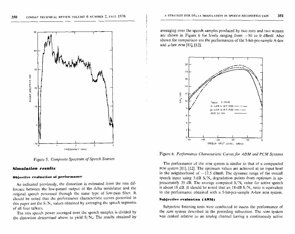
A STRATEGY FOR DELTA MODULATION IN SPEECH RECONSTRUCTION 351350 COMSAT TECHNICAL REVIEW VOLUME 6 NUMBER 2, FALL 1976 j
averaging over the speech samples produced by two men and two womenare shown in Figure 6 for levels ranging from -50 to 0 dBmO. Alsoshown for comparison are the performances of the 5-bit-per-sample A-lawand y-law PcM [11], [12].
TMAX ' 2 dBmO
A-LAW 5-BIT PCM ----
/I-LAW 5-BIT PCM ---
ADM 32 kbii
4
Figure 5. Composite Spectrum of Speech Sources
Simulation results
Objective evaluation of performance
As indicated previously, the distortion is estimated from the rms dif-ference between the low-passed output of the delta modulator and theoriginal speech processed through the same type of low-pass filter. Itshould be noted that the performance characteristic curves presented inthis paper are the S/N, values obtained by averaging the speech segments
of all four talkers.The rms speech power averaged over the speech samples is divided by
the distortion determined above to yield S/NC. The results obtained by
-50
I I I 1
-40 -30 -20 -10
SPEECH INPUT LEVEL (dBm0)0
Figure 6. Performance Characteristic Curves for ADM and PCM Systems
The performance of the ADM system is similar to that of a compandedPCM system [11], [12]. The optimum values are achieved at an input levelin the neighborhood of -12.5 dBmO. The dynamic range of the overallspeech input using 3-dB S/NC degradation points from optimum is ap-proximately 35 dB. The average computed S/N, value for active speechis about 18 dB. It should be noted that an 18-dB S/N,, ratio is equivalentto the performance obtained with a 5-bit-per-sample A-law PcM system.
Subjective evaluation (ADM)
Subjective listening tests were conducted to assess the performance ofthe ADM system described in the preceding subsection. The ADM systemwas ranked relative to an analog channel having a continuously active
352 COMSAT TECHNICAL REVIEW VOLUME 6 NUMBER 2, FALL 1976
speech-to-Gaussian-noise ratio of 38 dB and relative to 5- and 7-biterror-free A-law companded PCM. The results indicated that the ADMsystem was equivalent in performance to both the 5-bit PCM processedspeech and the 38-dB SAN analog speech, thus confirming a strong cor-relation between the objective evaluation and the subjective assessment.
Impact of bit errors
Bit-error rates in the range of 10-1 to 10-1 produced by a Gaussiannoise generator were introduced in the transmission channel. For eacherror rate, three different error patterns were simulated. Quality evaluationswere made by a jury of four communications engineers. The impact of anerror rate smaller than 10 3 was not perceptible through either a high-fidelity loudspeaker or a telephone set. As the bit-error rate increased to0.5 X 10-1, the effect became noticeable when the samples were playedback through a loudspeaker; amplitude modulation due to bit errors wasbeing heard. However, the quality of the speech was still good. Moreover,this modulation phenomenon was hardly perceptible for bit-error ratesup to 10-4 when a telephone handset was used. As the bit-error rateincreased to 0.5 X 10⁻¹, the quality of speech played back through both aloudspeaker and a telephone handset deteriorated, but the intelligibilitywas still good. For a bit-error rate greater than 10-1, the speech becamesomewhat amplitude modulated and noisy, and intelligibility was judged
as fair.
Conclusions
A new ADM strategy, incorporating a nonlinear step size Q function,has been presented for the reconstruction of high-quality speech. Anextensive computer simulation of ADM transmitted at a 32-kbps rate wasmade with the speech of two women and two men as input. Each talkerread the same phonetically balanced sentences. The total length of theinput source was approximately 48 seconds.
As an objective measure of the performance, the signal-to-distortionerror was computed for the ADM system over a 50-dB dynamic range ofsignal level. The ADM performance characteristic curve exhibited a behavior
similar to that of 5-bit companded PcM.A subjective rank order comparison test was also conducted with
approximately 100 listeners. The subjects indicated that the quality of theerror-free reconstructed speech was equivalent to that of 5-bit compandedPCM and to that of an analog channel having a continuously active speech-
signal-to-Gaussian-noise ratio of 38 dB.
A STRATEGY FOR DELTA MODULATION IN SPEECH RECONSTRUCTION 353
An investigation of the effect of bit-error rate in the range of 10-1 to10-1 indicated that no effect is perceptible until the bit-error rate increasesto 10-'. As the bit-error rate reaches a value of 0.5 X 10⁻¹, the speechquality starts to deteriorate in the form of volume modulation, althoughgood intelligibility is maintained. For a bit-error rate larger than 10',the speech becomes noisy and increasingly modulated in volume, but still
very intelligible.The ADM incorporating the new slope control logic demonstrates that
transmission at 32 kbps can provide good-quality telephone communi-cations and that good performance can he expected at bit-error rates as
high as 10-".
Acknowledgment
The authors would like to acknowledge Frank Corcoran for the carefulpreparation of the telephone speech source tapes and the playback simula-tion facility for subjective evaluations. Furthermore, the authors would liketo acknowledge Joseph Jankowski for designing the hardware implementa-
tion of the system.
References
[1] E. M. Deloraine . S. Van Micro, and B. Derjavitch . " Methode et Systcmc
de Transmission par Impulsions," French Patent 932140, August 1946.
[21 L. J. Libois, "Un Nouveau Procedc de Modulation Codee la Modulation
en Delta." L'Onde Electrique . Vol. 32, June 1952, pp . 26-31.
[3] F. dclager, "Delta Modulation , A Method of PCM Transmission Using
the I-Unit Code ," Phillips Research Report 7, 1952, pp. 442-466.
[4] C. C. Cutler, "Differential Quantization of Communications Signals,"
U.S. Patent 2605361, July 29, 1952.
[51 J. E. Abate , "Linear and Adaptive Delta Modulation," Proc. IEEE, Vol.
55, No. 3, March 1967, pp. 298-308.
[61 J. A. Greefkes and F. deJagcr, "Continuous Delta Modulation ," Phillips
Research Report, Vol. 32, No. 2, 1968 , pp. 233-246.
[71 J. A. Greefkes and K. Riemcus, "Code Modulation with Digitally Con-
trolled Companding for Speech Transmission ," Phillips Technical Report,
Vol. 31, No. 11-12, 1970, pp. 335-353.[8] J. A. Greefkes, "A Digitally Companded Delta Modulation Modern for
Speech Transmission ," International Conference on Communications,
June 1970, Proc ., pp. 7-33-7-48.
[9] N. S. Jayant, "Adaptive Delta Modulation with a One-hit Memory," Bell
System Technical Journal, Vol . 49, No. 3, March 1970, pp. 321-342.
354 COMSAT TECHNICAL REVIEW VOLUME 6 NUMBER 2 , FALL 1976
[10] J. E. Gibson, Nonlinear Automatic Control, New York: McGraw-Hill
Book Company, 1963, pp. 342-438.
[11] Members of the Technical Staff, Bell Laboratories, Inc., 7ranstnission
Systems for Communications, Fourth Edition, Winston-Salem: Western
Electric Company, 1970.[12] J. C. Su and S. J. Campanella, "Quantization Noise and Distortion Power
Spectra of PCM Systems," COMSAT Technical Review, Vol. 4, No. 2,
Fall 1974, pp. 393-410.
James C. Su received his B.S.E.E. from TaiwanUniversity and his Ph.D. in electrical engineering
from the University of Pennsylvania. From 1963to 1967, while at the Moore School of ElectricalEngineering, he worked on functional seriesrepresentation of time-varying nonlinear systemswith arbitrary input.
As a member of the technical staff at COMSAT
Laboratories since 1967, Dr. Si, has been engagedin digital signal processing techniques for speech
transmission. He has developed a system for regenerating the pointing data
of synchronous satellites and ct nonlinear phase-locked loop for fast acquisi-
tion of the signal.
A STRATEGY FOR DELTA MODULATION IN SPEECH RECONSTRUCTION 355
Processing Laboratory , he is responsible for signal processing research anddevelopment for satellite application using both digital and analog techniques.
Prior to joining COMSAT, Mr. Suyderhoud worked for 11 years at BellTelephone Laboratories on exchange area transmission engineering, tollcarriers, and picturephone . He is a member of the IEEE and the AmericanStatistical Association.
H. G. Suyderhoud was born in Borneo, Indo-nesia. He received the Ingenieur degree fromDelft Technological University in the Nether-lands in 1955, and the M.S. degree in appliedmathematical statistics from Rutgers, NewBrunswick, N.J., in 1966. Joining COMSATLaboratories in 1968, he worked extensively onresearch and development of echo cancellationtechniques. Presently Manager of the SignalProcessing Department of the Communications
S. J. Campanella received a B.S.E.E. from theCatholic University of America, an M.S.E.E.from the University of Maryland, and a Ph.D.in electrical engineering from the Catholic Uni-versity of America. Before joining COMSAT, hewas Manager of the Electronics Research Cen-ter at Melpar, Inc.
He is presently Director of the Communica-tions Processing Laboratory of COMSAT Labora-tories where he is responsible for the technical
orientation of the efforts pursued in the Signal Processing and Multi-plexing, Image Processing , Digital Control , and Modulation TechniquesDepartments.
Dr. Campanella is a member of AIAA, AAAS, IEEE, Sigma Xi, PhiEta Sigma, and the Acoustical Society of America. He is also a memberof the board of directors of EASCON.
Index: phase shift keying , error correction code, phasemodulation
Phase ambiguity resolution in a4 -phase PSK modulation systemwith forward-error-correctingconvolutional codes
Y. Tsuji
(Manuscript received March 19, 1976)
Abstract
When 4-phase PSK modulation and coherent detection are used, the phaseambiguity of a reference carrier at a receive side must be resolved. The phaseambiguity can be eliminated by using a differential coding technique or a syn-
chronization word. However, when forward-error-correcting (Pee) codes areused, the conventional differential coding method implemented inside an ateencoder and decoder pair (codec) has a drawback. That is, one erroneouslydetected phase will cause two consecutive false symbols (a burst error) even ifthe next phase is received correctly. In this case, the random error-correctingcapability of the error decoder must be doubled to maintain the same perfor-
mance. On the other hand, the use of a synchronization word will sometimesresult in the reduction of transmission efficiency.
This paper investigates two methods of resolving phase ambiguity by differ-ential coding which are compatible with the application of an FEC code. The
first uses differential coding inside an FEC codec in conjunction with an inter-
leaving technique. The second utilizes a syndrome pattern to resolve the pri-mary phase ambiguity followed by differential coding outside an FEC codecto resolve the remaining ambiguity.
This paper is based upon work performed at COMSAT Laboratories under thesponsorship of the International Telecommunications Satellite Organization(INTELSAT). Views expressed in this paper are not necessarily those of INTELSAT.
357
358 COMSAT TECHNICAL REVIEW VOLUME 6 NUMBER 2, FALL 1976
Introduction
Application of forward-error-correcting (EEC) codes to digital satellitecommunications systems such as single-channel-per-carrier (scPc) [1],digital television communications (DITEC) [2], time-division multiple-access (TDMA) [3], and frequency-division multiple-access/phase shiftkeyed/digital speech interpolation (FDMA/PSK/DSL) [4] systems has beenconsidered. A 4-phase P5K modulation system is usually adopted in thesedigital systems. When 4-phase PSK modulation and coherent detectionare used, the recovered carrier phase ambiguity must be resolved on thebasis of the received PSK signal. In addition, the phase rotation directionambiguity due to frequency conversion must be resolved. The recoveredcarrier phase ambiguity can be eliminated by differential coding, as inthe 4-phase PSK modem in the TDMA system [5]. Use of a synchronizationword, as in the 4-phase P5K modem in the SPADE system, makes it possibleto resolve both recovered carrier phase and phase rotation directionambiguity [6].
When FEc codes are used, resolution of phase ambiguity becomesmore involved. For example, with the conventional differential codingmethod implemented inside an FEC codec, one erroneously detected phasewill cause two consecutive false symbols (a burst error) even if the nextphase is received correctly [3], [7]. In this case, the random error-correctingcapability of an error decoder must be doubled to maintain the sameperformance. On the other hand, the use of a synchronization word willsometimes result in the reduction of transmission efficiency. One methodof overcoming this problem, which is peculiar to conventional differentialcoding, is to develop a new FEC code which corrects the pairwise errorpattern which is most likely to appear in a differentially encoded coherent4-phase PSK system [8].
This paper describes two alternative methods of resolving phase am-biguity which are compatible with the application of a conventional FECcode. The first uses differential coding inside an FEC codec, but it providesa means of breaking up the burst errors peculiar to conventional differ-ential coding. This method still utilizes differential coding inside an FECcodec, but burst errors after differential decoding are changed into randomerrors at the input of an FEc decoder.
The second method is phase ambiguity resolution by differential codingused outside an FEC codec. This method utilizes a syndrome pattern inthe error decoder followed by a differential decoder to resolve the phaseambiguity. Through observation of the syndrome pattern, the various
PHASE AMBIGUITY RESOLUTION IN A CODED PSK CHANNEL 359
kinds of phase ambiguities degenerate into some phase ambiguities whichcannot be distinguished by the syndrome pattern. To resolve these re-maining ambiguities, a differential decoder is used after error correction.Reference 7 shows the configuration for recovered carrier phase ambiguityusing a transparent coder.
This paper includes techniques for resolving both recovered carrierphase ambiguity and combined recovered carrier phase and phase rotationdirection ambiguity when either a transparent or a nontransparent FEccoder is used. These studies are based on the following assumptions:
a. a 4-phase P5K modulation system,b. systematic FEc convolutional codes (n, n - 1) with n even,c. a synchronizer using a trial and error method in the decoder.
Classification of phase ambiguity
Phase rotation direction ambiguity
It is assumed that a PSK signal of intermediate frequency f is up-con-verted by the transmit local frequency f - f to yield the PsK microwavefrequencyf, . At the receive side,f, is down-converted by the receiver localfrequency to obtain the PSK signal at f . In this case, two receive localfrequencies can be considered, as shown in Figure 1. That is, the receivelocal frequency may be selected so that it is higher than the receive micro-wave frequency by f, or it may be selected so that it is lower than the receivemicrowave frequency by f.
The resultant phase rotation direction will be reversed relative to theoriginal phase rotation direction depending on the receive local frequencywhich is selected. This phenomenon is called phase rotation directionambiguity. This ambiguity can usually be avoided by specifying the re-lationship between the transmit local frequency and the receive localfrequency. Hence, it will not occur in PCM/PSK/TDMA and FDMA/PSK/DSIsystems, for example. However, it is difficult to avoid in SPADE and scPcsystems.
The SPADE system has about 800 carriers in one 36-MHz satellite trans-ponder. These carriers, located over a 36-MHz bandwidth from 98 to134 MHz, are classified as lower band carriers (Lacs) and upper bandcarriers (uPes), as shown in Figure 2. When a certain channel uses oneof the LBCS, its return channel must use a UBC, which will result in a differ-ence of 18 MHz between the carriers. For example, if channel i of station 1is using F(i), then the return channel j of station 2 uses FQ), where F(X)
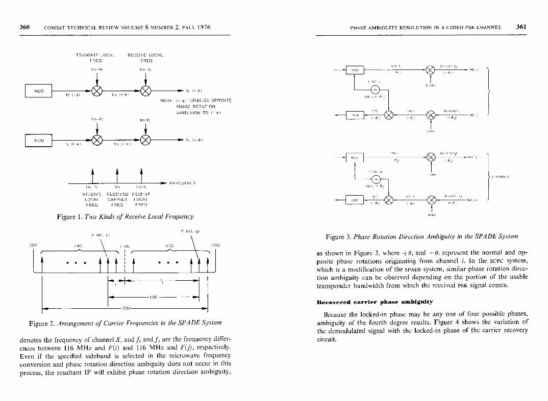
360 COMSAT TECHNICAL REVIEW VOLUME 6 NUMBER 2 , FALL 1976
TRANSMIT LOCAL RECEIVE LOCAL
FRED FRED
Im-IC Im-lc
MODIc (i9) `CY im (+91
(1-91
NOTE I- 0) DENOTES OPPOSITE
PHASE ROTATION
DIRECTION TO (I 9)
im-ic
MOD
tm*Ic
FREOUENCV
RECEIVE RECEIVED RECEIVE
LOCAL CARRIER LOCAL
FRED FREQ FRED
F NO I,
Figure 1. Two Kinds of Receive Local Frequency
F NO. (,I
98M LRC (160 UPC 134M
f ••• ffff •" fff
36M
(SM
Figure 2. Arrangement of Carrier Frequencies in the SPADE System
denotes the frequency of channel X, and f, and ff are the frequency differ-
ences between 116 MHz and F(i) and 116 MHz and F(j), respectively.
Even if the specified sideband is selected in the microwave frequencyconversion and phase rotation direction ambiguity does not occur in thisprocess, the resultant IF will exhibit phase rotation direction ambiguity,
PHASE AMBIGUITY RESOLUTION IN A CODED PSK CHANNEL 361
Figure 3. Phase Rotation Direction Ambiguity in the SPADE System
as shown in Figure 3, where +0, and -Of represent the normal and op-posite phase rotations originating from channel i. In the scee system,which is a modification of the SPADE system, similar phase rotation direc-tion ambiguity can be observed depending on the portion of the usabletransponder bandwidth from which the received PsK signal comes.
Recovered carrier phase ambiguity
Because the locked-in phase may be any one of four possible phases,ambiguity of the fourth degree results. Figure 4 shows the variation ofthe demodulated signal with the locked-in phase of the carrier recovery
circuit.
362 COMSAT TECHNICAL REVIEW VOLUME 6 NUMBER 2 , FALL 1976
ONloll. 1 .Inl
- P CH 1RANSMII
Um
011
D CH
P ON
q o1
TO
1001
IS,
UP)
oo'
Uo
PD
AMBIGUITY DUE TOP CH CARRIER PHASE
ROTATION DIRECTION
OU
1 X1111
PD-GPD
DD-P
loll
O
ID P
1 `lollPD
1001' 1 `1101 Ia01oU
PU P
DD-O
PC O
OD-P
PD D
OD P
PD
101
-\14,
10ot, I AIUII
PU P
OD D
B ESULTANF AMBIGUITY
DUE TO RECOVERED
CARRIER PHASE
AND PHASE ROTA ('ION
DIRECTION
PD 0'. THANSMITTEU 0 CHANNEI IS OBTAINED AT uE MODUI ATOR IIU FP11T PU
Figure 4. Recovered Carrier Phase and Phase Rotation Direction Ambiguity
Phase ambiguity resolution by differential codinginside an FEC codec
Recovered carrier phase ambiguity is resolved by differential codinginside an FEC codec in systems such as TDMA. The direction of phase rota-tion should be given to the differential decoder in transmission systems in
PHASE AMBIGUITY RESOLUTION IN A CODED PSK CHANNEL 363
which phase rotation direction ambiguity results from the frequency
conversion system, as in the scPc and SPADE systems.
PSK modulation with differential coding transmits information by usingthe amount of phase shift, and the information is received by comparingthe difference between two consecutive phases. Hence, in the differentialcoding scheme, one erroneously detected phase will cause two consecutivefalse symbols (a burst error) even if the next phase is received correctly.Some means of breaking up these burst errors is necessary to permit theerror decoder to work properly when phase ambiguity resolution bydifferential coding is used inside an FEC codec.
One advantage of this method is that it does not require synchroniza-tion time to eliminate the phase ambiguity for the error decoder. Thus,it can be used in either a burst mode signal or a continuous mode signal,although the bit-error rate equivalent to the decoder input is twice thatwithout differential coding. Methods of breaking up the consecutivedouble errors which are associated with differential coding are describedin the following subsections.
Columnwise writing and rowwise reading method
As shown in Figure 5, on the transmit side a train of input signals isapplied to the FEC convolutional encoder. The encoder output is writtencolumnwise in the buffer, and the signal stored in the buffer is read row-wise. These steps are reversed on the receive side. If the numbers of bufferrows and columns are selected to accommodate the constraint length ofthe convolutional codes, the burst error caused by differential codingwill be converted into a random error in the receive buffer output.
SERIAL INPUT FEC
ENCODER mWRITE
COLUMNWISE
BUFFERREAD
ROW WISE
Figure 5. Column wise Writing and Rowwise Reading Method
Symbol interleaving method
The symbol interleaving method is intended to eliminate the adverseeffect of differential coding by encoding even and odd symbols inde-pendently so that a burst error is changed to a random error, hence justi-fying the use of the random error-correcting convolutional codes. Figure 6
364 COMSAT TECHNICAL REVIEW VOLUME 6 NUMBER 2, FALL 1976
SERIAL INPUT-1CONV
Q
EECL NCODER
EECENCODER
A
BUFFERS
Figure 6. Method of Applying Symbol Interleaving
is a transmit side block diagram showing the application of this methodto 4-phase PSK modulation with differential coding. Figure 7 shows
SERIAE INPUT 1 1 2 1 3 1 4 1 5 1 6 1 10 11 12
P 1 11
2 4 6 8 10 12
5 1 P1 l 7 1 9 11 P3
Q 2 4 6 Pp 8 10 12 P4
A, 1 2 6 J 0 11 12
A2 4 P 2 I 10 I IP3 A4
Figure 7. Example of Bit Correspondence for a (4, 3) Code withSymbol Interleaving
individual bit correspondence when the (4, 3) code is used in 4-phasePSK modulation with differential coding.
As shown in Figure 7, the symbol interleaving method comprises three
steps:a. STEP 1: An input signal train is changed into parallel signals
P and Q.b. STEP 2: Parallel signals P and Q are separately applied to the
two FEC encoders.c. STEP 3: Encoder outputs P' and Q' are applied to the buffer
memories, and the bits corresponding to a symbol are alternatelyread out from two buffer memories as independent symbols.
PHASE AMBIGUITY RESOLUTION IN A CODED PSK CHANNEL 365
These steps are reversed at the receive side. This method does not degradethe capability of FEC codes with simplified hardware.
M-symbol differential coding method
Differential coding in phase modulation refers to the transmission ofthe difference between the present phase and the previous phase, whichcorresponds to the information to be transmitted. Hence, the receivingside can regenerate the received information from the phase shift betweentwo consecutive phases. In this technique, if the nth symbol on the trans-mission path is erroneous, then the (n + 1)th symbol is also erroneous.
For M-symbol differential coding in phase modulation, a naturalextension of conventional differential coding, the difference between thepresent phase and the Mth previous phase corresponds to the informationto be transmitted. Hence, the receiving side can recover the receivedinformation from the difference between one phase which has been re-ceived and that received M symbols previously. If the nth symbol on thetransmission path is erroneous, then the (n + M)th symbol will also beerroneous. If M is determined to be sufficiently longer than the constraintlength, a pairwise error in one constraint length can be avoided.
Phase ambiguity resolution by differential codingoutside an FEC codec
It should be noted that phase ambiguity resolution by differential codingoutside an FEC codec is to be used together with the synchronizer circuitof the EEC decoder shown in Figure 8. The synchronizer continually ob-
FROM CH4-PHASE
PSK CH QDEMOD-ULATOR
PHASE
AMBIGUITY
REMOVAL CIRCUIT
STATECOUNTER &
SYNCHRONIZER
P/PCONY k
SYNDROME
OELA
DELAv
SYNDROME REGISTER 1
THRESHOLD
CIRCUITS
DELAY
Figure 8. (4, 3) Convolutional Code Decoder with Phase Ambiguity ResolvingCircuit
366 COMSAT TECHNICAL REVIEW VOLUME 6 NUMBER 2, FALL 1976
serves the syndrome pattern and compares the number of corrections witha predetermined threshold value. Once the threshold is exceeded, thestate of the phase ambiguity resolving circuit is changed . If the new stateis not correct, another state is selected until the proper state for ambiguityresolution is found. Differential coding is used to resolve the particularphase ambiguity which the synchronizer of the decoder cannot resolvebecause of the nature of convolutional codes.
Since the differential coding is used outside an FEC codec, the error-correcting decoder does not encounter the double -error phenomenon andonly the bit-error rate of the error -correcting decoder output ( improvedbit-error rate) is doubled. Doubling the decoder output error rate resultsin a smaller Eb/No loss than doubling the input error rate because thecurve of error rate versus Eb/No is steeper for the output . Thus, in terms ofbit-error rate improvement characteristics , this method is superior to
phase ambiguity resolution by differential coding inside an FEC codec.The primary disadvantage of this method is that a relatively long time
is required to resolve the phase ambiguity. Therefore, it may not be suitablefor application to burst mode operation , as in a TDMA system . Since thismethod exploits the inherent characteristics of FEC convolutional codes,two kinds of subgenerators , g(j), which define (n,n - 1) FEC convolutional
codes, are assumed (se/e' Figure 9). A transparent subgenerator, g(j)
= [goQ), g1(j), . .., g,-1(j)], is defined as
N-I
Egi(j) =21- Ii =B
whereas a nontransparent subgenerator , g(j) = [go(j), g1(j), • -,gN-1(j)11is defined as
N-I
Eg.(j)=21i=B
where 1 = integerN = constraint length in blocks
j = 1, 2, . . ., n - 1 .
If g;(j) = 0 , there is no connection to the ith register from thejth informa-tion stream , while if g,(j) = 1, there is a connection to the ith registerfrom thejth information stream. Codes which are generated are designated
PHASE AMBIGUITY RESOLUTION IN A CODED PSK CHANNEL 367
INFORMATION BITS
m111 (1111
ONE BLOCK DELAY
DENOTES A CONNECTION IF g,F) i;
NO CONNECTION IF ST)-0
(AI (nn 1 ) CONVOLUTIONAL ENCODER
P CHANNEL
0 CHANNEL
C1(1)
(6) TRANSMIT FORMAT
C1(21
C1In12121
C113)
Cl(,, 2131
I m BLOCK
010,2)
o, mlC, 1,(11
LI+i (nit -II
] m EVEN
q( F, - 11
C101)
PARITY BIT
Figure 9. (n, n - 1) Convolutional Encoder and Transmit Format
as transparent or nontransparent depending on the generator which is
used.As described previously, two kinds of ambiguity states can be con-
sidered. One consists of recovered carrier phase ambiguity only, and theother consists of both covered carrier phase ambiguity and phase rotation
direction ambiguity.
Recovered carrier phase ambiguity
PCM/PSK/TDMA and FDMA/PSK/DSI satellite communications systems
are examples of systems which experience only recovered carrier phaseambiguity because the same sequence of frequency conversion can alwaysbe expected. In this case, there are four kinds of phase ambiguity:
Transmit Receive
P P P Q QQ Q Q P P

368 COMSAT TECHNICAL REVIEW VOLUME 6 NUMBER 2, FALL 1976
Therefore, Figure 10 can be assumed to be the carrier phase ambiguityresolution circuit. In this logic diagram, it may be assumed that the(P, Q) state may remain unresolved due to the nature of the decoder.since (Q, P), (Q, P) will be changed to (P, Q) or (P, Q) by the carrierphase ambiguity resolution circuit. It is also assumed that the decoderwill not work properly in the (Q, P) or (Q, P) state.
DEMODULATED SIGNAL
SWITCHBOX
CONTROL SIGNAL
FROM STATE COUNTER
OF THE SYNCHRONIZER
PARALLEL
PARALLEL
CONY
01111 TO ERROR
C1(21 DECODER
CI On
Figure 10. Logic Diagram of Phase Ambiguity Resolution Circuit forRecovered Carrier Phase Ambiguity
APPLICATION OF TRANSPARENT CODES
As shown in Figure 9, then transmitted digits of the Ith code block areexpressed as follows:
CI(j) = tn1(j), j = 1, 2, ..., it - I
PHASE AMBIGUITY RESOLUTION IN A CODED PSK CHANNEL 369
where m1(j) = n - I message digits of the lth block
(7 = 1,2,...,n - 1)
CI(n) = parity bit of the lth block.
When the receive ambiguity state is (P, Q), mi-0) becomes mij (j).
Therefore, estimated parity bit CI(n), which is generated in the decoderby the same algorithm used in the encoder, is expressed as follows:
N-I n-I
Z E m1-7i(j) gi(j)i=0 i-l
= CI(n)
„IL) SIP m1121FECA
N since E E g;(j) = 21+ 1 for j = 1,2..... n - 1 and n even.Since estimated parity bit Z'1(n) coincides with received parity bit
C1(n) in the case of (P, Q), the syndrome pattern will be all "0's" and thesynchronizer will assume that the phase ambiguity has been resolved.In this case, if there is no error in the transmission line, m i (the inverse ofthe transmitted message) will be obtained from the decoder output sothat the binary differential encoder and decoder shown in Figure 11 will
be necessary [7].
INFORMATION
m1(IIBI 'S DIFFERENTI L 1
(2)
I MOD -,ENCODER CONY ENCODER
- - - - - - - - - - - - - - - - - - - - - - - - - - - - - -M '1 0)
I r-' 1 II
DEM
F-► IO
FEC
DECODER
m 1121
n'IIn-1!CONY
DIFFERENTIAL
DECODERm111)
NOTE m'1(1) DENOTES DIFFERENTIALLY ENCODED m1111
AMBIGUITY: RECOVERED CARRIER PHASE ONLY
CODE: TRANSPARENT
A-I a-1
CI(n) _ E E tn1_ U) g,(j) (1)Figure 11. Phase Ambiguity Resolution by Differential Coding
1=0 }=1 Outside an FEC Codec (case 1)
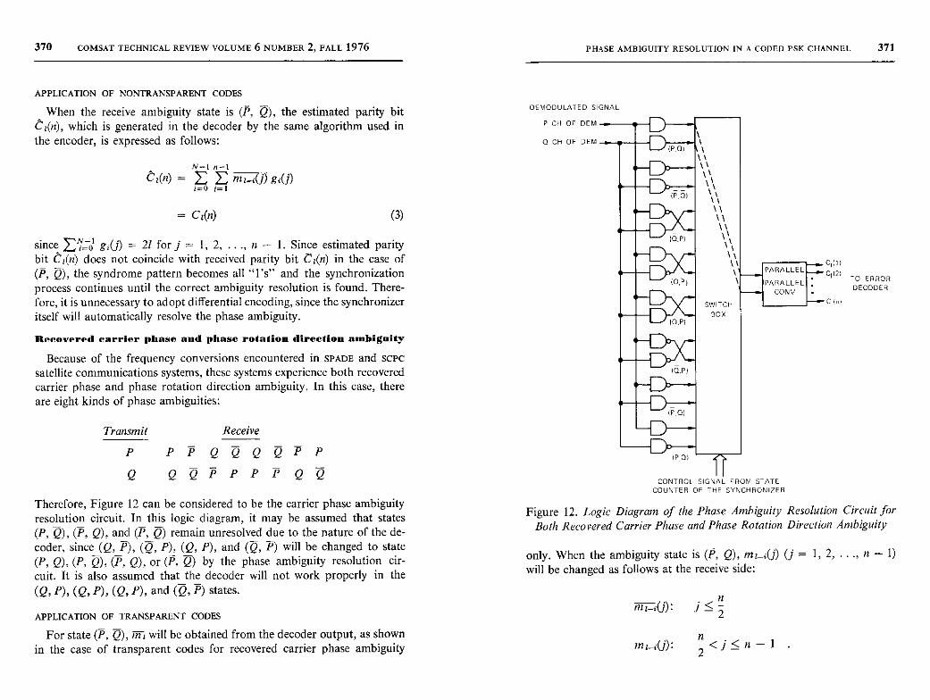
370 COMSAT TECHNICAL REVIEW VOLUME 6 NUMBER 2, FALL 1976
APPLICATION OF NONTRANSPARENT CODES
When the receive ambiguity state is (P, Q), the estimated parity bitCa(n), which is generated in the decoder by the same algorithm used inthe encoder, is expressed as follows:
N-I n-1
Ct(n) _ mz-.(7) g:(j)I=0 j= I
= CI(n) (3)
since EN o gi(j) = 21 for j = 1, 2, ..., n - 1. Since estimated paritybit CI(n) does not coincide with received parity bit CI(n) in the case of(P, Q), the syndrome pattern becomes all "l's" and the synchronizationprocess continues until the correct ambiguity resolution is found. There-fore, it is unnecessary to adopt differential encoding, since the synchronizeritself will automatically resolve the phase ambiguity.
Recovered carrier phase and phase rotation direction ambiguity
Because of the frequency conversions encountered in SPADE and ScPcsatellite communications systems, these systems experience both recoveredcarrier phase and phase rotation direction ambiguity. In this case, thereare eight kinds of phase ambiguities:
Transmit Receive
P P P Q Q Q Q P P
Q Q Q P P P P Q Q
Therefore, Figure 12 can be considered to be the carrier phase ambiguityresolution circuit. In this logic diagram, it may be assumed that states(P, Q), (P, Q), and (P, a) remain unresolved due to the nature of the de-
coder, since (Q, P), (Q, P), (Q, P), and (Q, P) will be changed to state
(P, Q), (P, Q), (P, Q), or (P, Q) by the phase ambiguity resolution cir-cuit.-It is also assumed that the decoder will not work properly in the
(Q, P), (Q, P), (Q, P), and (Q, P) states.
PHASE AMBIGUITY RESOLUTION IN A CODED PSK CHANNEL 371
DEMODULATED SIGNAL
P CH OF DEM
0 CH DF DEM
I
IO,PI
SWITCH
BOX
PARALLEL
PARALLELCONv
IP,OI
CONTROL SIGNAL FROM STATE
COUNTER OF THE SYNCHRONIZER
01)21
Cl(N
TO ERROR
DECODER
Figure 12. Logic Diagram of the Phase Ambiguity Resolution Circuit for
Both Recovered Carrier Phase and Phase Rotation Direction Ambiguity
only. When the ambiguity state is (P, Q), ml-i(j) (j = 1, 2, ..., n - 1)will be changed as follows at the receive side:
APPLICATION OF TRANSPARENT CODES
For state (P, Q), m I will be obtained from the decoder output, as shownin the case of transparent codes for recovered carrier phase ambiguity
mz--;(j):
m t-;(1)
nj < 2
n2 < j < n - 1
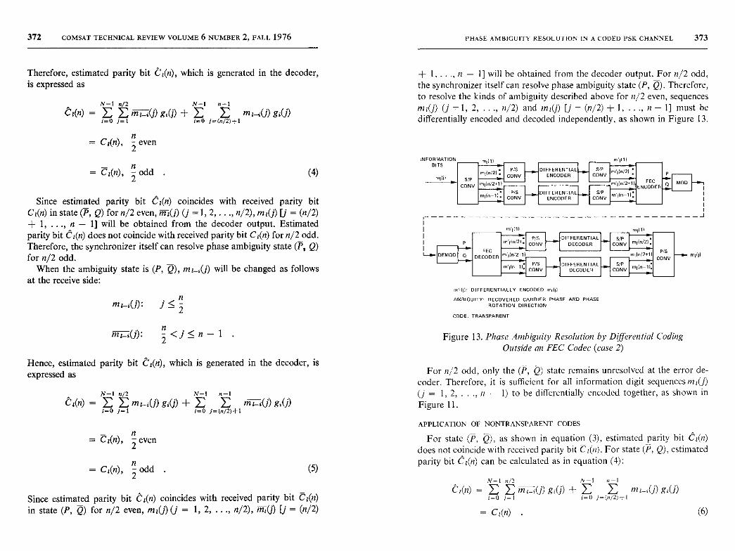
372 COMSAT TECHNICAL REVIEW VOLUME 6 NUMBER 2 , FALL 1976
Therefore, estimated parity bit CI(n), which is generated in the decoder,is expressed as
N-I n/2 N-I n-I
Ca(n) _ in j) gi(j) + E E m,-i(j) gi(j)i=0 j=1 i=0 j=(n/2)+I
n= C,(n), 2 even
PHASE AMBIGUITY RESOLUTION IN A CODED I'SK CHANNEL 373
+ 1, ..., n - 1] will be obtained from the decoder output. For n/2 odd,the synchronizer itself can resolve phase ambiguity state (P, Q). Therefore,to resolve the kinds of ambiguity described above for n/2 even, sequences
m1(j) (j =1, 2, ..., n/2) and ma(j) U- (n/2) + l , ..., n-1] must bedifferentially encoded and decoded independently, as shown in Figure 13.
INFORMATION m10)BITS
= C,(n), Z odd (4) m(/21•Inull S/P
CONY min/211)
Since estimated parity bit C,(n) coincides with received parity bitCl in state (P, Q) for n/2 even, i(j) (j =1, 2, ..., n/2), m,(j) [j = (n/2)+ 1, ..., It - 1] will be obtained from the decoder output . Estimatedparity bit Ca(n) does not coincide with received parity bit Ca(n) for n/2 odd.Therefore , the synchronizer itself can resolve phase ambiguity state (P, Q)for n/2 odd.
When the ambiguity state is (P, Q), to j) will be changed as followsat the receive side:
nm ;(j): j <_ 2
z<j<n-1
Hence, estimated parity bit C,(n), which is generated in the decoder, isexpressed as
N-I R/2 N -I n -I
CI(n) _ Z E ml -i(j) g:Q) + E E mi(j) g(j)i=B j-1 I=0 i= (n/2)+1
= Ca(n),
= Ci(n),
It2 even
2 odd (5)
Since estimated parity bit CI(n) coincides with received parity bit CI(n)in state (P, Q) for n/2 even, m,(j) (j = 1, 2, ..., n/2), m1(j) if = (n/2)
m1111
P/5 DIFFERENTIAL S/P mlln/21CONV ENCODER CONV P
CONV ENCODER GUY
mlln/N1) ENCODER 0 MOD
- - - - - - - - - - - - - - - - - - - - - - - - - - - - - - - - - -
^ m lrn mlm• P/5 DIFFERENTIAL
P°II°/21' CONY DECODER CONPV mll°/2•
DEMOO O DECOOEfl '^IrJ2+11 m16n12a1) P/SCONV
P/S DIFFERENTIAL 5/PTI/. 11• CONY DECODER CONY
m/fi1+ DIFFERENTIALLY ENCODED mllp
AMBIGUITY: RECOVERED CARRIER PHASE AND PHASEROTATION DIRECTION
CODE : TRANSPARENT
n-, I•
- ► mifll
Figure 13. Phase Ambiguity Resolution by Differential CodingOutside an FEC Codec ( case 2)
For n/2 odd, only the (P, Q) state remains unresolved at the error de-coder. Therefore, it is sufficient for all information digit sequences m,(j)j = 1, 2, ..., it - 1) to be differentially encoded together, as shown in
Figure 11.
APPLICATION OF NONTRANSPARENT CODES
For state (P, ), as shown in equation (3), estimated parity bit Ca(n)does not coincide with received parity bit C/n). For state (P, Q), estimatedparity bit C(n) can be calculated as in equation (4):
N-I n/2 N-1 l-I
C(n) _ m1_=(j) g/j) + E L mi_.(j) g/j)i=0 j=1 I-U j=(n/2)+1
= C(n) . (6)
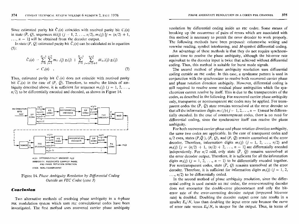
374 COMSAT TECHNICAL REVIEW VOLUME 6 NUMBER 2, FALL 1976
Since estimated parity bit Ca(n) coincides with received parity bit CI(n)in state (P, Q), sequences n21(j) (j = 1, 2, ..., n/2), m,(j) [j = (n/2) + 1,
., n - 1] will be obtained from the decoder output.In state (P, Q) estimated parity bit C1(n) can be calculated as in equation
(5):
N-I 4'2 N-I -I
Ca(n) m-,(j) g(j) + me-rU) g1Q)z=o j=1 a=U j=(n/2)+I
= Ca(n) . (7)
Thus, estimated parity bit C,(n) does not coincide with received paritybit C,(n) in the case of (P, ). Therefore , to resolve the kinds of am-biguity described above, it is sufficient for sequence mz(j) (j = 1, 2, ...,n/2) to be differentially encoded and decoded, as shown in Figure 14.
lln m'llnINFORMATION
BITS mlln/2PIS ^DIEFERE NTIAL' _I SIP
mlln121 Pm111) SIP
ONv NCODER CONYFEC D
CONY m,W2N11 ENCODERO MO
do-^1
minl
m"Iln/21 PISTOW
DEMODI 0 DECODER Imll°/2+1I
DIFFERENTIAL
DECODER
mlln-n
mlljlDIFFERENTIALLY ENCODED m11jI
AMBIGUITY : RECOVERED CARRIER PHASE
AND PHASE ROTATION DIRECTION
CODE: NON-TRANSPARENT
mdnSIPONV LrIln/21
PIS
CONY
Figure 14. Phase Ambiguity Resolution by Differential CodingOutside an FEC Codec (case 3)
Conclusion
Two alternative methods of resolving phase ambiguity in a 4-phasePSK modulation system which uses FEc convolutional codes have beeninvestigated. The first method uses recovered carrier phase ambiguity
PHASE AMBIGUITY RESOLUTION IN A CODED PSK CHANNEL 375
resolution by differential coding inside an FEC codec. Some means ofbreaking up the occurrence of pairs of errors which are associated withthis method is necessary to permit the error decoder to work properly.The following methods have been proposed : columnwise writing androwwise reading , symbol interleaving, and M-symbol differential coding.
An advantage of these methods is that they do not require synchroni-zation time to resolve the phase ambiguity , although the bit-error rateequivalent to the decoder input is twice that achieved without differentialcoding. Thus, this method is suitable for burst mode signals.
The second method of phase ambiguity resolution uses differentialcoding outside an FEC codec . In this case , a syndrome pattern is used inconjunction with the synchronizer to resolve both recovered carrier phaseand phase rotation direction ambiguity. However , differential coding isstill required to resolve some residual phase ambiguities which the syn-chronizer cannot resolve by itself. This is due to the transparencies of thecodes, as described in the following . For recovered carrier phase ambiguityonly, transparent or nontransparent FEC codes may be applied . For trans-parent codes the (P, Q) state remains unresolved at the error decoder sothat all the information digits ma (j) (j = 1, 2, ..., n - I) must be differen-tially encoded. In the case of nontransparent codes, there is no need fordifferential coding, since the synchronizer itself can resolve the phaseambiguity.
For both recovered carrier phase and phase rotation direction ambiguity,the same two codes are applicable . In the case of transparent codes andn/2 even, states (P, Q ), (P, Q), and (P, Q) remain unresolved at the errordecoder. Therefore , information digits ml(j) (j = 1, 2, ., n/2) and
mz(j) [j = (n/2) + 1, (n/2) + 2, ..., n - 1] are differentially encodedindependently . For n/2 odd , only state (P, Q) remains unresolved atthe error decoder output . Therefore, it is sufficient for all the informationdigits ml(j) (j = 1, 2, ..., n - 1) to be differentially encoded together.For nontransparent codes, state (P, Q) remains unresolved at the errordecoder . Therefore , it is sufficient for information digits mz(j) (j = 1, 2,
., n/2) to be differentially coded.In the second method of phase ambiguity resolution , since the differ-
ential coding is used outside an FEC codec , the error- correcting decoderdoes not encounter the double -error phenomenon and only the bit-error rate of the error-correcting decoder output (improved bit-errorrate) is doubled . Doubling the decoder output error rate results in asmaller E,/NP loss than doubling the input error rate because the curveof error rate versus Eb/ Nn is steeper for the output . Thus, in terms of
376 COMSAT TECHNICAL REVIEW VOLUME 6 NUMBER 2, FALL 1976
bit-error rate improvement characteristics, the second method is superiorto the first. The disadvantage of the second method is that a relativelylong time is required to resolve the phase ambiguity. Therefore, it may notbe suitable for application to burst mode operation, as in a TDMA orSPADE system.
Acknowledgments
The author wishes to thank Dr. S. J. Campanella and Dr. W. W. Wu
for their careful review and helpful comments.
References
[1] R. B. McClure, "Status and Progress of the INTELSAT SCPC System,"IEEE 1975 International Conference on Communications, San Francisco,
California, June 1975, Proc., pp. 12-6-12-11.[2] L. S. Golding, "DITEC-A Digital Television Communications System for
Satellite Links," Second International Conference on Digital Satellite Com-
munications, Paris, France, November 1972, Proc., pp. 384-397.
[3] 1. Matsushita, Y. Tsuji, and Y. Solana, "Applications of Error-CorrectingCodes to TDMA Satellite Communications," IEEE 1973 InternationalConference on Communications, Seattle, Washington, June 1973.
[4] R. C. Davis and R. J. F. Fang, "Channel Capacity Extension via FDMA/PSK/DSI," Third International Conference on Digital Satellite Com-
munications, Kyoto, Japan, November 1975, Proc., pp. 170-179.[5] D. J. Withers and A. K. Jefferis, "A Time Division Multiple Access System
for INTELSAT," AIAA 4th Communications Satellite Systems Conference,
Washington, D.C., April 1972, Paper no. 72-538.[6] E. R. Cacciamani, Jr. and C. J. Wolejsza, Jr., "Phase-Ambiguity Resolution
in a Four-Phase PSK Communications System," IEEE Transactions on
Communication Technology, COM-19, No. 6, Pt. 11, December 1971, pp.
1200-1210.[7] G. D. Forney, Jr. and E. K. Bower, "A High-Speed Sequential Decoder:
Prototype Design and Test," IEEE Transactions on Communication Tech-
nology, COM-19, No. 5, Pt. 11, October 1971, pp. 821-834.[8] P. L. Chen and R. A. Rutledge, "Error Correcting Codes for Satellite Com-
munications Channels," IBM Journal of Research and Development, Vol. 20,
No. 2, March 1976, pp. 168-175.
PHASE AMBIGUITY RESOLUTION IN A CODED PSK CHANNEL 377
Yoshikazu Tsuji received B.S. and M.S.
degrees in electrical engineering from Kyoto
University in 1965 and 1967, respectively. Im-mediately thereafter, he joined Fujitsu Ltd.,where he was engaged in the developmentof digital satellite communications systems. InMarch 1975 he joined COMSAT Laboratories asan INTELSAT nominee. Since that time, he hasbeen engaged in the development of SS-TDMAsatellite communications systems. He is amember of IECE of Japan.
Index: microwave transmission , propagation, rain,electromagnetic wave propagation
A model for microwave propagationalong an earth-satellite path
D. J. FANG AND J. JIH
(Manuscript received March 15, 1976)
Abstract
Recent studies of microwave transmission through a precipitation mediumhave contributed to clarify the mechanism of propagation and have also provideda framework for the interpretation of measurements at centimeter and milli-meter wavelengths. However, the problem of utilizing the results of theoreticalstudies to establish engineering models in order to make reliable predictions ofpropagation characteristics on a specific satellite-earth microwave link remains
to be resolved. The primary difficulties are related to the effect of elevationangles on propagation parameters, which is not known in detail; the preciseevaluation of the raindrop canting effect, for which equations are not available;and the scaling of the propagation parameters, for which proper procedures arenot established.
The present paper attempts to provide engineering solutions to these problems.A slant path model is developed for electromagnetic wave propagation at centi-meter and millimeter wavelengths through rain. Considerations which take intoaccount the random canting effect of raindrops are provided. The scaling pro-cedures for transferring propagation information from one polarization to
This paper is based upon work performed at COMSAT Laboratories under thesponsorship of the International Telecommunications Satellite Organization(INTELSAT). Views expressed in this paper are not necessarily those of INTELSAT.
379
380 COMSAT 'TECHNICAL REVIEW VOLUME 6 NUMBER 2, FAI1. 1976
another, one frequency to another, and one elevation angle to another are
demonstrated step by step.
Introduction
It is known that rain is a principal cause of signal attenuation and crosspolarization in a terrestrial or satellite transmission link at centimeterand millimeter wavelengths. It can be shown that most of the currenttheoretical studies on microwave propagation through rain follow three
steps:a. analysis of forward scattering for a plane electromagnetic wave
incident upon a single raindrop,b. calculation of the diffraction of the wave penetrating per-
pendicularly across a thin layer of precipitation,c. multiple-layer iterative integration to derive the wave field
which passes through a precipitation medium.Papers indicating the scientific and technical findings obtained from
all or part of these steps are numerous (see, for example, References 1-9).Some of these papers provide experimental data to substantiate the theo-retical findings. Thus, theoretical studies are not only important in theelucidation of the physics of electromagnetic waves through precipitation,but also for establishing valid frameworks within which experimenterscan apply and interpret the data collected from the various propagationexperiments. On the other hand, for an engineer involved in estimatingpropagation parameters for the design of a specific microwave link, theresults of existing theoretical studies are inadequate and/or inapplicable.
A review of the literature reveals many limitations in the theoreticalstudies. For instance, in step a, the numerical methods of matching theboundary conditions for a spheroidal raindrop are so tedious and expensivethat only a very limited number of computations of forward scatteringfields for selected frequencies, drop sizes, and drop temperatures havebeen performed [1], [3], [4], [9]. Also, in most computations, the propaga-tion direction is assumed to be perpendicular to the raindrops' axes ofsymmetry, which renders the results inapplicable to slant path propagation.For step b, the Laws and Parsons drop size distribution [1][4], [7] hasbeen used consistently for simplicity, although it is now known thatother distributions, such as the Marshall-Palmer [10] and Joss distributions[11], may be more realistic for heavy storms. In step c, the analysis isgenerally based on the electric field differentials from one layer to thenext [5], [6], [8], [12] without including dispersion effects. These short-
MICROWAVE PROPAGATION ALONG AN EARTH-SATELLITE PATH 381
comings, together with the meteorological uncertainties, such as thespatial rain rate distribution along a propagation path, provide inadequatebuilding blocks for engineering design applications.
On the basis of available theoretical results, this paper proposes aformat for compiling and editing the relevant data, and for makingengineering interferences to supplement relevant yet scanty data, asrequired for practical applications on a slant path satellite-earth link.The following section introduces a format which will permit detailed de-scription of the dependence of propagation parameters on elevation angles,a vital piece of information for slant path applications. The next sectionanalyzes the effect of raindrop canting. This effect is much more compli-cated in slant path propagation than in terrestrial links, simply because therelative angles between the axes of the canted raindrops and wave vectorsare not trivial. Precise formulas for the evaluation of the random cantingeffect on propagation parameters will also be presented.
Another difficulty which engineers must face when applying the theo-retical results involves the scaling of propagation parameters from onefrequency to another, one polarization to another, and one elevation angleto another. To demonstrate the procedure, a special example of slantpath transmission will be discussed.
A new formulation of field equations for microwavepropagation through a precipitation medium
The geometry for analyzing wave scattering through a rain cloud isshown in Figure 1. In a simplified example, the raindrops are presumed tofall vertically downward. The axis of symmetry of the spheroidal raindrops,denoted as Z, is aligned along the vertical axis. The x axis is chosen sothat the incident wave normal lies in the x-z plane, making an anglewith the z axis. The unit vector for wave propagation, v„ is given by
ik = -1, Cos'' - i1 sin ^' (1)
At the penetrating point, the incident wave field, E,,, is decomposed intohorizontally and vertically polarized components, E,l, and E,,,,, respectively,for separate scattering analysis. The standard wave factor exp[iwt- ik(ikv)] is omitted for simplicity. The sense of polarization is such thatthe unit vectors in and iv are specified as
(2a)
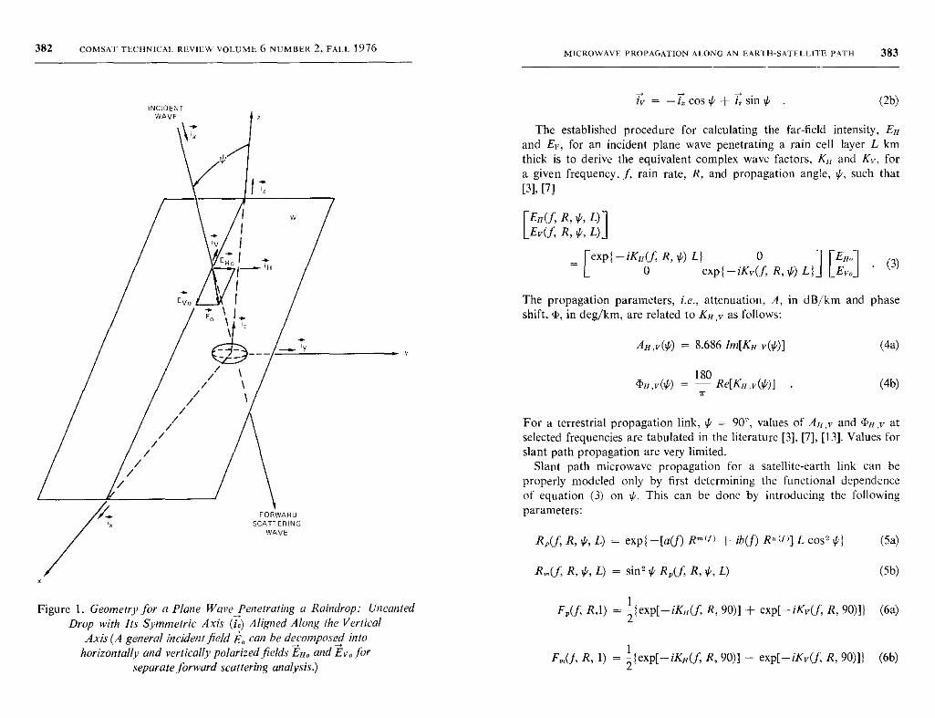
382 COMSAT TECHNICAL REVIEW VOLUME 6 NUMBER 2, FALL 1976 MICROWAVE PROPAGATION ALONG AN EARTH-SATELLITE PATH 383
iv = -iz cos 4, + is sin >G . (2b)
Figure 1. Geometry for a Plane Wave _Penetrating a Raindrop: (IncantedDrop with Its Symmetric Axis (ic) Aligned Along the Vertical
Axis (A general incident field E. can be decomposed intohorizontally and vertically polarized fields EHO and Evo for
separate forward scattering analysis.)
The established procedure for calculating the far-field intensity, EHand Ev, for an incident plane wave penetrating a rain cell layer L kmthick is to derive the equivalent complex wave factors, KH and KT, fora given frequency, f, rain rate, R, and propagation angle, 4', such that
[3], [7]
[EH(f, R, 0, L)1Ev(f, R, 4', L)
rexp { - iKn(f, R, V,) L } 0 EHa0 exp {-iKv(f R, P) L} Evo
. (3)
The propagation parameters, i.e., attenuation, A, in dB/km and phaseshift, 4, in deg/km, are related to KH,v as follows:
AH,v(4/) = 8.686Im [KHv(IG)]
4'n,v(>G) =180
Re[KH,v('G)]a
(4a)
(4b)
For a terrestrial propagation link, >G = 90°, values of A,, and 4)H,v atselected frequencies are tabulated in the literature [3], [7], [13]. Values forslant path propagation are very limited.
Slant path microwave propagation for a satellite-earth link can beproperly modeled only by first determining the functional dependenceof equation (3) on ,G. This can be done by introducing the followingparameters:
RP(f, R, 4', L) = exp{ -[a(f) Rm(tl + ib(f) R, (f)] L cost 4' (5a)
R.m(f, R, 4, L) = sin 2 tG RP(f, R, 4', L) (5b)
F,(f, R,1) = 2{exp[-iKn(f, R, 90)] + exp[-iKv(f, R, 90)]} (6a)
F,,,(J, R, 1) = 2{ exp[-iKH (f, R, 90)] - exp[-iKv (f, R, 90)]} (6b)
384 COMSAT TLCIINICAL REVIEW VOLUME 6 NUMBER 2 . FAIL 1976
Fn(,f; R, L) _ [F8 (f, R, 1)]L (7a)
Fm(f, R, L) = L [F8 (f, R, 1 )]L-1 F,,,(f R, 1) . (71b)
The formalization of parameters F, (f, R, L) and F(f R. L) is presentedin Appendix A. It su04ces herein to note that equation (6) gives the per-kilometer values (L = 1) of F„ and F,,, based on terrestrial propagationconditions (>' = 90) and that equation (7) can be used to evaluate 1-1, andF at any distance L once the per-kilometer values are known. Equation (3)can then be written as
Fu(f, R, L) = F„(l, R. L) R„(f R, L)1 0 En„
Fv(f, R,'G• L) 10 11CFvJ
+ F,(f; R, L) Rm(f, R, ^, L) C10] CEn01 . (8)
0 1 Evo
This formulation of field equations for microwave propagation througha precipitation medium, which is believed to be novel, provides a descrip-tion of the electric fields as functions of rain rate. frequency , propagationangle,and path length. Values of a(f), b(f),m(f), and n (f) in equation (5a)can be assessed on the basis of available theoretical data of Oguchi [3],[13] and Chu [7]. The results are plotted in Figure 2, which also givesspecific numerical magnitudes atf = 4, 6, 11, 30, and 34.8 GHz. Based onthe same data source, the complex quantities F,(, R, 1) and F,,,(f, R, 1)can be evaluated for specific rain rates and frequencies . The results areplotted in Figures 3a and 3b. Details of the formulation are given inAppendix A.
For practical applications with f, R, k, and L as variables, equation (8)is more straightforward than other forms of equations which operateindirectly through parameters An,v and fin , v. In actual calculations theinputs F„(f, R, 1) and F (f, R, 1) can be generated from reliable terres-trial experiments if they yield more realistic values than those given inFigures 3a and 3b. It is also of interest to note that , in earlierstudies [6], [7], [ 14] in which the t' dependence could be described onlythrough the differences of All - AT and `b1 - Tv, the differences weremodeled as proportional to sin' '. Equation ( 8) provides a much morerefined description of the V, dependence ; it indicates that the sin2 4' pro-portionality is good only to the first order for frequencies lower than20 GHz.
MICROWAVE PROPAGATION ALONG AN EARTH -SATELLITE PATH 385
20
10
J.0
1.0
0.5
4 G 8 II 15 20 25 30 34.8
FREQUFNCY IGH,I
50
2 x 10⁻²
10-2
J x 10-3
2 X 10⁻³
10 3
5 x 10 4
Figure 2. Values of a, b, in, and n of the Modeling Equation (5) (The derivationis given in Appendix A; marked values are for 4-, 6-, 11-,
30-, and 34.8-GHz frequencies, respectively.)
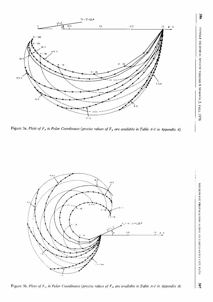
Fp - IFPILe
„c
Figure 3a. Plots of F,, in Polar Coordinates (precise values of F, are available in Table A -7 in Appendix A)
Figure 3b. Plots ofF,,, in Polar Coordinates (precise values ofFm are available in Table A-l in Appendix A)
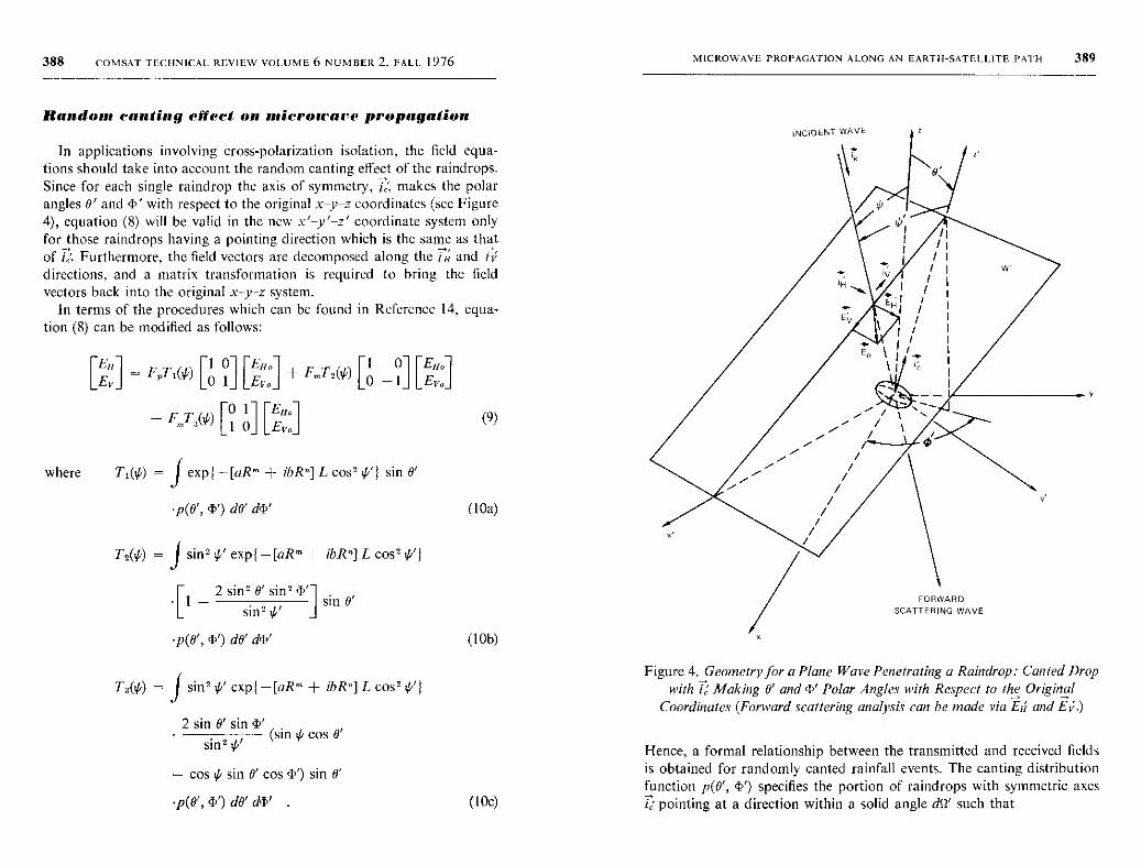
388 COMSAT TECHNICAL REVIEW VOLUME 6 NUMBER 2 , FALL 1976
Random canting effect on snierounre propagation
In applications involving cross-polarization isolation, the field equa-tions should take into account the random canting effect of the raindrops.Since for each single raindrop the axis of symmetry, I,, makes the polarangles 0' and 4' with respect to the original x y-z coordinates (see Figure4), equation (8) will be valid in the new x'-y'-z' coordinate system onlyfor those raindrops having a pointing direction which is the same as thatof f,. Furthermore, the field vectors are decomposed along the la and ivdirections, and a matrix transformation is required to bring the fieldvectors back into the original x-y-z system.
In terms of the procedures which can be found in Reference 14, equa-tion (8) can be modified as follows:
where
[En] [1 0 En 1 1 0 Eno
Ev = FPTi ( G) [0 1] [Evo] + PmTs(tt) [0 I [Ev
oF T3(k)
0 1[ 1 0 [EEnva
TI(¢) = J exp { -[aRm + ibR°] L cost ,y'} sin 0'
(9)
•p(0', V) dB' d4,' (10a)
T2(^) _ j sin 2 >b' exp { - [aRm + ibR ^] L cos2 ,G' J
Cl - 2 sin 2 0' sine h'l sinB'
sine' J
•p(O', T') do' dT' (10b)
Ta('P) = f sin 2 p' exp{ -[aRm + ibR,] L cost,/'}
2 sin 0' sin V
sin 2 i`'
(sin >G cos 0'
- cos >' sin 0' cos 'h') sin 0'
•p(a', c1') do' d'F' . (10c)
MICROWAVE PROPAGATION ALONG AN EARTH-SATELLITE PATH 389
Figure 4. Geometry for a Plane Wave Penetrating a Raindrop : Canted Dropwith T 'Making 0' and f' Polar Angles with Respect to the Original
Coordinates (Forward scattering analysis can be made via Ex and k, .)
Hence, a formal relationship between the transmitted and received fieldsis obtained for randomly canted rainfall events. The canting distributionfunction p(0', Y) specifies the portion of raindrops with symmetric axesi., pointing at a direction within a solid angle dR' such that
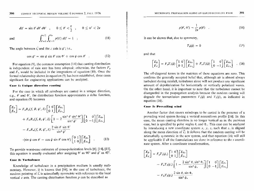
390 COMSAT I ECHNICAI. REVIEW VOLUME 6 NUMBER 2, PAIL 1976
and
dil'= sin0'do ' d4' , 0<B'<2 , 0<4,'<2r
f J J P(S2') dSl' = 1 (11)/1 2
e=u m=u
The angle between 1? and the z axis is d ; i.e.,
cos >G' = sin tG sin B' cos P' + cos ,G cos B' . (12)
For equation (9), the common assumption [14] that canting distributionis independent of rain rate has been adopted; otherwise, the factors FP
and Fm would be included in the integrations of equation (10). Once theformal relationship shown in equation (9) has been established, three casessignificant for engineering applications can be analyzed.
Case 1: IJnigne direction canting
For the case in which all raindrops are canted in a unique direction,e.g., B' and V, the distribution function approximates a delta function,
and equation (9) becomes
LJ = FvRP(, R, k% L)1 0
[0 1] LE„
Ev1 EvJ
sine B' sine V 1 0] EH.+F,RmUR,G,L) L1 2 sin2#f ] LO -1LEvJ
- F„nRm(f R, 0', L)2 sin 0' sin c
sine tG'
ao (13)[t 0] [EEv(sin t' cos 0' - cos sin 0' cos ^') 0 1
To provide worst-case estimates of cross-polarization levels [6], [14], [15],this equation is usually evaluated after assigning i as 90° and 1G' as 45°.
Case 2: Turbulence
Knowledge of turbulence in a precipitation medium is usually rudi-mentary. However, it is known that [16], in the case of turbulence, therandom pointing of la is azimuthally symmetric with reference to the localvertical z axis. The canting distribution function p can be described as
MICROWAVE PROP AGATION ALONG AN EARTH-SATELLITE PATH 391
PW,`h)=2 1 a
PW) .
It can be shown that, due to symmetry,
(14)
Ta(¢) = 0 (15)
and that
rElll = F,TI(#G)rl 0]
[Ell'] + F, ,(V,) [1 _0] [E-.] . (16)LEvJ 0 1 J E, 0 1 Eva
The off-diagonal terms in the matrices of these equations are zero. Thisconfirms the generally accepted belief that, although air is almost alwaysturbulent during rainfall, turbulence alone will not produce any significantamount of depolarization for horizontally or vertically polarized waves.On the other hand, it is important to note that the turbulence cannot bedisregarded in the propagation analysis because the random canting willdegrade the transmission parameters T,(,,) and T2(,/i), as indicated inequation (16).
Case 3: Prevailing wind
Another factor that causes raindrops to be canted is the presence of aprevailing wind system having a vertical nonuniform profile [16]. In thiscase, the mean canting direction is no longer vertical as in the previouscase, but is specified by polar angles 0, and T,. This case can be analyzedby introducing a new coordinate system x, y, Z, such that z, is alignedalong the mean direction of i,. It follows that the random canting will beazimuthally symmetric in the new system, and that equation (16) will stillbe applicable if all the formulations are done in reference to the s coordi-nate system. After a coordinate transformation,
Ev = FvTI(it) 0 1 EveLEN] [l 0] LEvi
2 sin2 0, sin2 4), 1 0 EN,+ F,,,T2(,^,) [1 - ____
sin]'/, - 10 -1 [Evo
2 sin 0., sin fi,- FmT2(&,)
sine Pe

392 COMSAT TECIINICAL REVIEW VOLUME 6 NUMBER 2. FA11 1976
- (sin cos , t , cos 4,,) C0 1] [Ermi (17)G (.. -cos sin 1 0 Evo
where cos >', = sin ^ sin 0, cos T. + cos d cos 0, . (18)
The presence of off-diagonal terms in equation (17) indicates that thecross polarization exists.
Simulation of the canting distribution function
The actual p(0', fi') function is dictated by meteorological factorsincluding turbulence , the prevailing wind system and its spatial gradient,individual raindrop vibrations , and drop size distributions . Only pre-liminary studies relating to p(0', T') are currently available [16], [17]. Toexamine the random canting effect on microwave transmission , it is oftennecessary to perform theoretical calculations based on an approximatelypostulated profile of p(0', fi') which is sufficiently versatile to simulate anyrealistic distribution of the canting.
The profile postulated here is
P(0','F') = u 2a 1 cos" 0
where u = 4 + loglo(gcos 2ffa)) (19b)
with a peak centered at 0' = 0 whose width is determined by an angleo, such that
f,1
C,
p(0', T') sin 0' do' dT' = 1 (20)=o to 2
i.e., 50 percent of the random pointing of it is within the solid anglecentered at 0' = 0 and bounded by 0' = us.
Values of T,, T2, and T3 can be evaluated from equation (10) by firstexpanding the exponentials in Taylor series terms. Since the absolutevalue of the exponential term is much less than unity, only the first threeterms up to the order of W2, where
MICROWAVE PROPAGATION ALONG AN EARTH-SATELLITE PATH 393
W = (uR" + ibR ^) L (21)
are needed in the expansion. In terms of equations (12) and (19), term-by-term integrations of T,, T2, and T3 are possible. After several passages,
T2(VI) = I u^u2+ (12-W)u+35-7W(u + 3) (u + 5) (u + 7) ttt
3+2W2 -u[(W+1)u2+(12+4W-3W2)11 + 35
T1(#) = I -(1+ucos241) +u + 3 2(u^ 3)(u+5)
•[3+6ucos' '-(3-u)uCOST
- 21W+ 2 W2] cos24, + u[W(l + )u2+ W
(5 - 6W) u-2W(7-5W)]Cos, 41 +[ -2u3 +3u2
4u] W2 cosy^I (22b)
(19a)
T3(t0) = 0 . (22c)
An important application of these equations relates a physical distribu-tion of random canting to the so-called "effective mean canting" usedextensively by wave propagationists. "Effective mean canting" meansthat, although the pointing of i for the raindrops is random, its effect onmicrowave propagation can always be evaluated by assuming that allthe raindrops point in a unique direction after properly adjusting theevaluated microwave field to take into account the randomness. Com-parison of equations (9) and (13) with specific inputs from equations (19)-(22) makes it possible to find the effective mean canting direction as well asthe magnitude required to adjust for modeling an arbitrarily canted rain-fall event as a unique direction event.
Slant path propagation studies
The relationships between the transmitted field and received field givenin equations (8), (9), (13), (16), and (17) can be reduced to the form
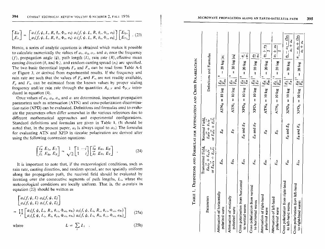
394 COMSAT TECHNICAL REVIEW VOLUME 6 NUMBER 2, FALL 1976
CE,r] - Fa,(f, L, R, 0,, 4.,, ae) a2 (f, 4', L, R, 0.-, T„ ae)1 F& 1 (23)Ev L a3(f, L, R, 0,, 4'„ ae) a+(.f, L, R, 0.,, `h„ ae) Evo
Hence, a series of analytic equations is obtained which makes it possibleto calculate numerically the values of a,, a2, a, and a, once the frequency(f), propagation angle (+f), path length (L), rain rate (R), effective mean
canting direction (0, and 4,.,), and random canting spread (ae) are specified.
The two basic theoretical inputs F„ and F,,, can be read from Table A-1or Figure 3, or derived from experimental results. If the frequency andrain rate are such that the values of F, and Fare not readily available,F, and F,, can be estimated from the known values by proper scalingfrequency and/or rain rate through the quantities Au,v and 411,,v intro-duced in equation (4).
Once values of a,, a2, a3, and at are determined, important propagationparameters such as attenuation (ATN) and cross-polarization discrimina-tion ratio (XPD) can be evaluated. Definitions and formulas used to evalu-ate the parameters often differ somewhat in the various references due todifferent mathematical approaches and experimental configurations.Standard definitions and formulas are given in Table 1. (It should benoted that, in the present paper, a2 is always equal to a3.) The formulasfor evaluating ATN and XPD in circular polarization are derived afterusing the following conversion equations:
C
1x EL' E,, 1 1 i ,x E„o Ea
la E,, ER^ 1/2 Ll i^ LI Evo Ev^(24)
It is important to note that, if the meteorological conditions, such asrain rate, canting direction, and random spread, are not spatially uniformalong the propagation path, the received field should be evaluated byiterating over the consecutive segments of path lengths, Li, where themeteorological conditions are locally uniform. That is, the a-matrix in
equation (23) should be written as
a,(f, 4,, L) a2(f, 4', L)^a3(f, tt, L) a1(.f, G, L)
,,
aei)= 11 al(f, 4+f
',
,
L. R;, 0,, Cra3(f,L,, Ri, O,i, aei)
where L =
a2(f, L;, Ri, 0,,, aei)1 (25a)a4(f Li, Ri, 0, j, ae,)
E Li .I
(25b)
MICROWAVE PROPAGATION ALONG AN EARTH-SATELLITE PATH 395
N
W$
WW
n
+
a
N
0
0
+ N
0N
4 m a 4
W4
Ct0
U
03)
1.T C 9
O 0 U.C)
i 01 ON
0 3 m
o m 3N O ^
Bm
O 9
_
B
d
0A N
0.0
c aO y
N
o gCO ^B N
C oa
'a> 'a$ o a
4 U U Q
a
0
+
a
00
II
N
+
a
+
0
0II
N -I
to
0II
0k
Cc
W
B
w
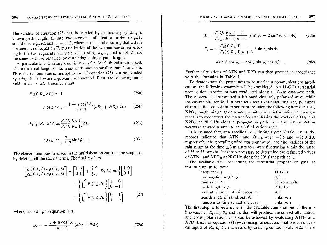
396 COMSAr TECHNICAL REVIEW VOLUME 6 NUMBER 2 , FALL 1976
The validity of equation (25) can be verified by deliberately splitting aknown path length, L, into two segments of identical meteorological
conditions, e.g., aL and (1 - o) L, where c < 1, and ensuring that within
the tolerance of equation (7) multiplication of the two matrices correspond-ing to the two segments will yield values of a1, a2, a1, and a1 which arethe same as those obtained by evaluating a single path length.
A particularly interesting case is that of a local thunderstorm cell,where the total length of the slant path may be smaller than I to 2 km.Then the tedious matrix multiplication of equation (25) can be avoidedby using the following approximation method. First, the following limits
hold as Li = OL; becomes small:
F,(f, R1, 4Li) ^ I
T 1(^s) ' 1- 1 + u cos^,y, (aR",
+ ibR^) OLiu+3
R„(f Ra 1) OLF„(f, Ri, oLJ^'
FP(3, Ri, 1)
UTs(4,s) ' a+3sine '. .
(26a)
(26b)
(26c)
(26d)
The element matrices involved in the multiplication can then be simplified
by deleting all the (ALi) 2 terms . The final result is
ra1(f G, L) az(f, ^, L)1 = [1 0] + (" D (L,) dL,}[1 0J(f G, L) a,(J,'p, L) 0 1 o 0 1
+ {f` E,(L,) dL;}[1-01+ { f L F,(Li) dL`}[O1 01
where, according to equation (17),
I + u cost #3(a&' + ibR^)
u+3
(27)
(28a)
MICROWAVE PROPAGATION ALONG AN EARTH-SATELLITE PATH 397
F„ (f, R j, 1) uE; - -- [sin' >G, - 2 sin 2 B„ sin 2 `h,] (28b)
FP(f,R„1)u+3
F, F^,(f, R_ 1) ii2 sin B, sin Ts
FP(3, R1, 1) a + 3
.(sin 'G cos 4,, - cos ' sin #8 cos „) . (28c)
Further calculations of ATN and XPD can then proceed in accordancewith the formulas in Table 1.
To demonstrate the procedures to be used in a communications appli-cation, the following example will be considered. An 11-GHz terrestrialpropagation experiment was conducted along a 10-km east-west path.The western site transmitted a left-hand circularly polarized wave, whilethe eastern site received in both left- and right-hand circularly polarizedchannels. Records of the experiment included the following items: ATN1„XPDL, rough rain gauge data, and prevailing wind information. The assign-ment is to reconstruct the records for establishing the levels of ATNH andXPD1 at 28 GHz along a propagation path from the eastern stationwestward toward a satellite at a 30° elevation angle.
It is assumed that, at a specific time t, during a precipitation event, therecords indicated that ATNL and XPDL, were -3.5 and -25.0 dB,respectively; the prevailing wind was southward; and the readings of therain gauge at the time 7E3 minutes to t, were fluctuating within the rangeof 35 to 75 mm/hr. It is then necessary to determine the estimated valuesof ATNH and XPDH at 28 GHz along the 30° slant path at to.
The available data concerning the terrestrial propagation path atinstant t" are as follows:
frequency, f. 11 GHzpropagation angle, ,G: 900rain rate, Rp: 35-75 mm/hrpath length, Lo: < 10 kmazimuthal angle of raindrops , P,: 90°zenith angle of raindrops, 08: unknownrandom canting spread angle, ae: unknown
The first step is to determine all the available combinations of the un-knowns, i.e., R,,, Le, 6 , and a o, that will produce the correct attenuationand cross polarization. This can be achieved by evaluating ATNL andXPDL, based on equations (17)-(22) using various combinations of numeri-cal inputs of R0, L0, 0 , and a, and by drawing contour plots of A, where
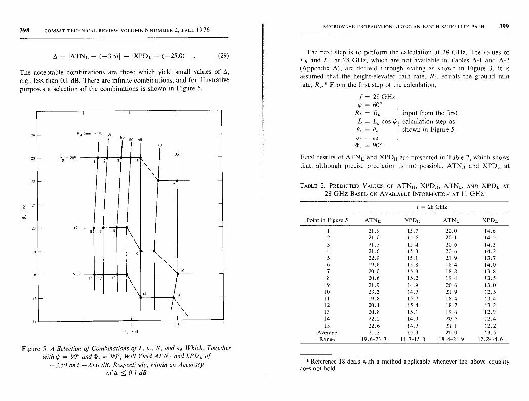
398 COMSAT TECHNICAL REVIEW VOLUME 6 NUMBER 2, FALL 1976
A = ATNL, - (- 3.5) 1 + XPDL. - (-25.0)1 . (29)
The acceptable combinations are those which yield small values of A,e.g., less than 0.1 dB. There are infinite combinations , and for illustrativepurposes a selection of the combinations is shown in Figure 5.
L, Roil
Figure 5. A Selection of Combinations of L, 0 ,., R, and ue Which , Together
with ' = 90° and l,, = 90°, Will Yield ATNL, and XPDL of
-3.50 and -25 .0 dB, Respectively , within an Accuracyof A < 0.1 dB
MICROWAVE PROPAGATION ALONG AN EARTH-SATELLITE PATH 399
The next step is to perform the calculation at 28 GHz. The values ofFIB and F,,, at 28 GHz, which are not available in Tables A-1 and A-2(Appendix A), are derived through scaling as shown in Figure 3. It isassumed that the height-elevated rain rate, R, equals the ground rainrate, R0.* From the first step of the calculation,
j= 28 GHz60°
RI, = Rv input from the firstL = Lo cos >L calculation step as6. _ ©.. I shown in Figure 5
oe
41„ =
Ro
90°
Final results of ATNII and XPDB are presented in Table 2, which showsthat, although precise prediction is not possible, ATN1 and XPD11 at
TABLE 2. PREDICTED VALUES OF ATN11, XPD1, ATNL, AND XPDL AT
28 GHz BASED ON AVAILABLE INFORMATION AT I I GHz
f = 28 GHz
Point in Figure 5 ATNn XPDn ATNL XPDL
1 21.9 15.7 20.0 14.62 21.0 15.6 20.1 14.53 21.5 15.4 20.6 14.34 21.6 15.3 20.6 14.25 22.9 15.1 21.9 13.76 19.6 15.8 18.4 14.07 20.0 15.3 18.8 13.88 20.6 15.2 19.4 13.59 21.9 14.9 20.6 13.010 23.3 14.7 21.9 12.511 19.8 15.7 18.4 13.412 20.1 15.4 18.7 13.213 20.8 15.1 19.4 12.914 22.2 14.9 20.6 12.415 22.6 14.7 21.1 12.2
Average 21.3 15.3 20.0 13.5Range 19.6-23.3 14.7-15.8 1&4-21.9 12.2-14.6
* Reference 18 deals with a method applicable whenever the above equalitydoes not hold.
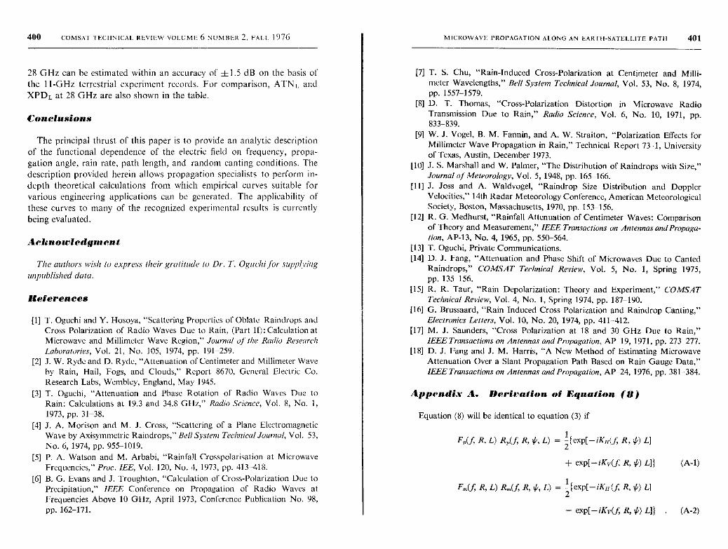
400 COMSAT TECHNICAL REVIEW VOLUME 6 NUMBER 2, FALL 1976
28 GHz can be estimated within an accuracy of f1.5 dB on the basis ofthe 11-GHz terrestrial experiment records. For comparison , ATNI, andXPDL at 28 GHz are also shown in the table.
Conclusions
The principal thrust of this paper is to provide an analytic descriptionof the functional dependence of the electric field on frequency, propa-gation angle, rain rate, path length, and random canting conditions. Thedescription provided herein allows propagation specialists to perform in-depth theoretical calculations from which empirical curves suitable forvarious engineering applications can be generated. The applicability ofthese curves to many of the recognized experimental results is currentlybeing evaluated.
Acknowledgment
The authors wish to express their gratitude to Dr. T. Oguchi for supplyingunpublished data.
References
[1] T. Oguchi and Y. Hosoya, "Scattering Properties of Oblate Raindrops andCross Polarization of Radio Waves Due to Rain, (Part 11): Calculation atMicrowave and Millimeter Wave Region," Journal of the Radio Research
Laboratories, Vol. 21, No. 105, 1974, pp. 191-259.[2] J. W. Ryde and D. Ryde, "Attenuation of Centimeter and Millimeter Wave
by Rain, Hail, Fogs, and Clouds," Report 8670, General Electric Co.
Research Labs, Wembley, England, May 1945.
[3] T. Oguchi, "Attenuation and Phase Rotation of Radio Waves Due to
Rain: Calculations at 19.3 and 34.8 GHz," Radio Science, Vol. 8, No. 1,
1973, pp. 31-38.
[4] J. A. Morison and M. J. Cross, "Scattering of a Plane Electromagnetic
Wave by Axisymmetric Raindrops," Bell System Technical Journal, Vol. 53,
No. 6, 1974, pp. 955-1019.
[5] P. A. Watson and M. Arbabi, "Rainfall Crosspolarisation at Microwave
Frequencies," Proc. LEE, Vol. 120, No. 4, 1973, pp. 413-418.
[6] B. G. Evans and J. Troughton, "Calculation of Cross-Polarization Due to
Precipitation," IEEE Conference on Propagation of Radio Waves atFrequencies Above 10 GHz, April 1973, Conference Publication No. 98,
pp. 162-171.
MICROWAVE PROPAGATION ALONG AN EARTH-SATELLITE PATH 401
[71 T. S. Chu, "Rain-Induced Cross-Polarization at Centimeter and Milli-meter Wavelengths," Bell System Technical Journal, Vol. 53, No. 8, 1974,pp. 1557-1579.
[8] D. T. Thomas, "Cross-Polarization Distortion in Microwave RadioTransmission Due to Rain," Radio Science, Vol. 6, No. 10, 1971, pp.833-839.
[9] W. J. Vogel, B. M. Fannin, and A. W. Straiten, "Polarization Effects forMillimeter Wave Propagation in Rain," Technical Report 73-1, Universityof Texas, Austin, December 1973.
[10] J. S. Marshall and W. Palmer, "The Distribution of Raindrops with Size,"Journal of Meteorology, Vol. 5, 1948, pp. 165-166.
[11] J. Joss and A. Waldvogel, "Raindrop Size Distribution and Doppler
Velocities," 14th Radar Meteorology Conference, American MeteorologicalSociety, Boston, Massachusetts, 1970, pp. 153-156.
[12] R. G. Medhurst, "Rainfall Attenuation of Centimeter Waves: Comparisonof Theory and Measurement," IEEE Transactions on Antennas and Propaga-tion, AP-13, No. 4, 1965, pp. 550-564.
[13] T. Oguchi, Private Communications.
[14] D. J. Fang, "Attenuation and Phase Shift of Microwaves Due to CantedRaindrops," COMSAT Technical Review, Vol. 5, No. 1, Spring 1975,pp. 135-156.
[15] R. R. Taut, "Rain Depolarization: Theory and Experiment," COMSATTechnical Review, Vol. 4, No. 1, Spring 1974, pp. 187-190.
[16] G. Brussaard, "Rain Induced Cross Polarization and Raindrop Canting,"Electronics Letters, Vol. 10, No. 20, 1974, pp. 411-412.
[17] M. J. Saunders, "Cross Polarization at 18 and 30 GHz Due to Rain,"IEEE Transactions on Antennas and Propagation, AP-19, 1971, pp. 273-277.
[18] D. J. Fang and J. M. Harris, "A New Method of Estimating MicrowaveAttenuation Over a Slant Propagation Path Based on Rain Gauge Data,"
IEEE Transactions on Antennas and Propagation, AP-24, 1976, pp. 381-384.
Appendix A. Derivation of Equation (8)
Equation (8) will be identical to equation (3) if
F,(f, R, L) R,(f, R, G, L) = 2{exp[-iKI(f, R, k) L]
+ exp[-iKv(f, R, P) L]} (A-1)
Fr(f, R, L) Rm(f, R, 1/i, L) = 2{exp[-iKe(f R, ik) L]
- exp[-iKv(f, R, ') L]} . (A-2)
402 COMSAT TECHNICAL. REVIEW VOLUME 6 NUMBER 2. FALL 1976
Based on these equations and equations (4a) and (4b), FFRF and F,,,R,,, arecalculated as shown in Tables A-1 through A-4 using theoretical data supplied
by Oguchi [Al], [A2] and Chu [A3].It can be seen the last columns in the tables that, for rain rates less than
50 mm/hr,
Fm(f R, 1) R",(f R, P, 1)
Fv(f, R, 1) RF(f, R, 4', 1)
Taylor series approximation then implies that
<< 1 . (A-3)
FF(f R, L) = RF(f R, ^P, L) [F,(f, R, 1) R2(f, R, 'G, 1)]L
Fm(f R, L)= Rm(f R, 4',
L) [FF(f, R, 1) RF(f,, R, 'G, 1)1"
• Fm(f R, 1) R,,,(f, R, d', 1)
These equations can be readily reduced to yield equation (7). Equation (7) isvalid even for rain rates greater than 50 mm/hr, for which inequality (A-3)is, in a few cases, no longer appropriate. This is because the effective path length,
L, for storms of R > 50 mm/hr is generally short, e.g., less than or very close to
unity [A4]-[A6].The values ofa(1), b( f),In(f),and n(f) shown in Figure 2 are generated by trial
and error. Their validity can best be shown by tabulating the ratio of either
FFRF or FmR generated by using equations (A-1) and (A-2) to that generated
by using equations (5) and (6); i.e.,
C(f, R, 4')
(1/2){exp[-iKlr (4')]+exp[-iKv (4l')]} exp{[aRm + ibR"]cos2 4'} (A-4)
(1 /2)1 exp[-iKa (90)] + exp[-iKv(90)]}
D(f, R, J')
(1/2) {exp[-iKzr(f)] - exp[-iKv(4')]} exp{[aRm + ibR"] Cos1>G}
(1/2){exp[-iKrr(90)] - exp[-iKv(90)]} sin'V/
in Tables A-5 and A-6 for ¢ = 700, 50°, and 30 ° based on the available data at
f = 4, 6, 11, 30, and 34.8 GHz. For practical purposes , both C and D are unity
in magnitude and zero in phase. Therefore , FF and F. at L = 1 km are indeed
independent of the propagation angle 4' as postulated in the paper , and FFRF
and F .mR", given by equations (5) and (6) are indeed consistent with those defined
by equations (A-1) and (A-2). Equation (7) implies further that FF and F,,, are
insensitive to 4' at longer path lengths.
MICROWAVE PROPAGATION ALONG AN EARTH-SATELLITE PATH 403
TABLE At VALUES OF FFRF AND FmR, AT 4' = 90° AND L = I km"
FFRF = A,L0p F.R. = AmLB°t R (Am/AF)
(GHz) (mm) AF eF A. x 100 em x 1004.0° 0.25 0.99998 -0.145 0.00646 -91.084 0.006464.0 1.25 0.99990 -0.569 0.03491 -91.629 0.034914.0 2.50 0.99981 -1.035 0.07304 -92.175 0.073064.0 5.00 0.99962 -1.895 0.15531 -93.147 0.155374.0 12.50 0.99901 -4.236 0.42121 -95.687 0.421634.0 25.00 0.99783 -7.897 0.90605 -99.637 0.908014.0 50.00 0.99499 -14.964 1.97267 -107.110 1.982604.0 100.00 0.98782 -28.620 4.27463 -121.371 4.327364.0 150.00 0.97862 -42.274 6.75161 -135.624 6.89912
4.0° 0.25 0.99997 -0.144 0.00576 -91.245 0.005764.0 1.25 0.99989 -0.562 0.03133 -91.744 0.031344.0 2.50 0.99979 -1.021 0.06563 -92.293 0.065644.0 12.50 0.99892 -4.178 0.37673 -95.787 0.377144.0 25.00 0.99763 -7.792 0.81100 -99.716 0.812934.0 50.00 0.99458 -14.714 1.76358 -107.070 1.773194.0 100.00 0.98688 -28.290 3.83960 -121.297 3.890654.0 150.00 0.97799 -41.652 5.98334 -135.020 6.11799
5.0 0.25 0.99996 -0.180 0.00724 -91.579 0.007255.0 1.25 0.99981 -0.706 0.03945 -92.342 0.039465.0 2.50 0.99962 -1.285 0.08291 -93.128 0.082955.0 12.50 0.99776 -5.299 0.48384 -98.117 0.484925.0 25.00 0.99463 -9.931 1.04237 -103.903 1.048015.0 50.00 0.98654 -18.867 2.26617 -114.300 2.297085.0 100.00 0.96448 -36.486 4.85359 -134.196 5.032325.0 150.00 0.93737 -53.903 7.42621 -151.561 7.92238
6.0 0.25 0.99994 -0.217 0.00864 -92.016 0.008646.0 1.25 0.99969 -0.853 0.04793 -93.087 0.047956.0 2.50 0.99935 -1.556 0.10128 -94.243 0.101346.0 12.50 0.99554 -6.463 0.59128 -101.457 0.593936.0 25.00 0.98870 -12.139 1.26822 -108.763 1.282726.0 50.00 0.97079 -23.118 2.70076 -121.885 2.782036.0 100.00 0.92386 -44.665 5.58868 -145.987 6.049256.0 150.00 0.87097 -65.928 8.28603 -168.854 9.51360
11.0" 0.25 0.99971 -0.409 0.01837 -94.745 0.0183811.0 1.25 0.99804 -1.638 0.10360 -98.901 0.1038111.0 2.50 0.99530 -3.003 0.21738 -102.286 0.2184111.0 5.00 0.98860 -5.524 0.45541 -107.175 0.4606611.0 12.50 0.96389 -12.373 1.19403 -117.541 1.2387511.0 25.00 0.91601 -22.739 2.40206 -130.582 2.6223011.0 50.00 0.81422 -41.876 4.54823 -152.442 5.5860311.0 100.00 0.62879 -76.128 7.39110 160.355 11.7545211.0 150.00 0.48101 -108.055 8.84560 136.984 18.38966

404 COMSAT TECHNICAL REVIEW VOLUME 6 NUMBER 2 , FALL 1976
TABLE A-l. VALUES OF F,R, AND FmRm AT 'G = 90° AND L = 1 kma
(Continued)
F,RP=A,,LBP F,,,R,=AmZOmI R (Am/AP)
(GHz) (mm) AP 6, A,,, X 100 0m X 100
11.01 0.25 0.99970 -0.406 0.01645 -94.895 0.0164611.0 1.25 0.99804 -1.612 0.09134 -99.020 0.0915211.0 2.50 0.99534 -2.954 0.19363 -102.234 0.1945311.0 12.50 0.96488 -12.153 1.07188 -117.079 1.1108911.0 25.00 0.91851 -22.366 2.16181 -130.000 2.3536111.0 50.00 0.82103 -41.113 4.11145 -151.401 5.0076511.0 100.00 0.63821 -75.306 6.79138 171.350 10.6413111.0 150.00 0.49380 -106.965 8.13634 138.369 16.47713
15.0' 0.25 0.99929 -0.560 0.02295 -97.971 0.0229715.0 1.25 0.99521 -2.214 0.12691 -104.093 0.1275215.0 2.50 0.98895 -4.026 0.26547 -108.391 0.2684415.0 12.50 0.92775 -15.970 1.41701 -127.326 1.5273615.0 25.00 0.84782 -28.777 2.75795 -143.706 3.2530015.0 50.00 0.70027 -51.722 4.87814 -170.737 6.9660715.0 100.00 0.47344 -92.789 7.07185 143.428 14.9372015.0 150.00 0.32042 -131.100 7.55109 102.172 23.56615
18.16 0.25 0.99882 -0.685 0.03139 -100.311 0.0314218.1 1.25 0.99211 -2.704 0.17311 -107.850 0.1744918.1 2.50 0.98222 -4.879 0.35940 -113.218 0.3659018.1 5.00 0.96100 -8.771 0.74062 - 120.563 0.7706718.1 12.50 0.89382 -18.830 1.85267 -135.630 2.0727418.1 25.00 0.78729 - 33.431 3.46476 -154.934 4.4008818.1 50.00 0.60476 -59.317 5.69326 173.801 9.4141518.1 100.00 0.35974 -104.617 7.15352 121.852 19.8850918.1 150.00 0.21336 - 146.474 6.57781 75.268 30.82904
19.31 0.25 0.99862 -0.724 0.03006 -101.412 0.0301119.3 1.25 0.99107 -2.829 0.16515 -109.430 0.1666419.3 2.50 0.98013 - 5.092 0.34476 - 114.994 0.3517519.3 12.50 0.88430 -19.555 1.76234 -138.935 1.9929219.3 25.00 0.77035 -34.667 3.25863 -159.281 4.2300819.3 50.00 0.57996 -61.203 5.19945 168.244 8.9651819.3 100.00 0.32830 -107.976 6.21271 114.330 18.9240019.3 150.00 0.18672 - 150.795 5.39867 66.444 28.91396
30.0h 0.25 0.99597 -1.131 0.05351 - 110.725 0.0537330.0 1.25 0.97622 -4.281 0.29025 -124.634 0.2973230.0 2.50 0.95017 -7.503 0.58618 -133.906 0.6169230.0 5.00 0.89889 - 13.035 1.13888 - 146.144 1.2669830.0 12.50 0.75812 - 26.380 2.50140 - 168.936 3.2994930.0 25.00 0.57469 -44.317 3.80753 165.360 6.6253430.0 50.00 0.33664 - 73.600 4.43103 127.708 13.1623530.0 100.00 0.12799 -121.100 3.18444 71.499 24.8799630.0 150.00 0.05212 -163.384 1.83971 24.612 35.29517
MICROWAVE PROPAGATION ALONG AN EARTH-SATELLITE PATH 405
TABLE A-1. VALUES OF FR,, AND FmRm AT t` = 90° AND L = 1 km"
(Continued)
F7,Rp = AP z 0, Fm.R, = Am z OmI R (Am/AP)
(GHz) (mm) AP 0, A X 100 B,,m x 100
34.8° 0.25 0.99449 -1.291 0.05714 -115.605 0.0574634.8 1.25 0.96852 -4.776 0.30277 -132.330 0.3126134.8 2.50 0.93520 -8.261 0.59817 -142.848 0.6396134.8 12.50 0.70617 -27.695 2.28977 179.510 3.2425334.8 25.00 0.50697 -45.329 3.20918 153.757 6.3300834.8 50.00 0.27447 -73.097 3.33174 117.729 12.1388834.8 100.00 0.09269 -118.005 2.06967 64.763 22.3280934.8 150.00 0.03454 -158.563 1.08545 20.864 31.42561
50.00 0.25 0.98766 -1.765 0.08238 -133.791 0.0834150.0 1.25 0.93719 -5.958 0.38321 -156.421 0.4088950.0 2.50 0.88041 -9.724 0.69928 -168.939 0.7942650.0 12.50 0.57446 -27.463 1.99070 154.122 3.4653350.0 25.00 0.36766 -41.719 2.34363 132.412 6.3745350.0 50.00 0.17105 -63.344 1.97056 104.039 11.5204350.0 100.00 0.04621 -101.845 0.95265 61.317 20.6148150.0 150.00 0.01388 -137.956 0.40228 23.459 28.97725
The values are equivalent to those of F,, and F„ plotted in Figure 3, sinceRP= R,,,= 1 at'G=90°.
Original inputs of Au.v and 1,1,,v are from Chu [A3].° Original inputs of AH,v and 4'11,v are from Oguchi [A2]. Oguchi's inputs at
19.3 and 34.8 GHz are also available in Reference Al.
TABLE. A-2. VALUES OF F,R, AND Fm/C, AT'k - 70° AND L = 1 km
F,,Rn=A,,z0P F,Rm= Amz0„°f R (A IA,)
(GHz) (mm) Ap 0P A,,, X 100 B„ X 100
4.0° 0.25 0.99998 -0.144 0.00506 -91.214 0.005064.0 1.25 0.99989 -0.564 0.02758 -91.752 0.027584.0 2.50 0.99979 -1.025 0.05725 -92.312 0.057264.0 12.50 0.99891 -4.202 0.33312 -95.803 0.333494.0 25.00 0.99763 -7.843 0.71605 -99.764 0.717754.0 50.00 0.99462 -14.819 1.54642 -107.192 1.554804.0 100.00 0.98709 -28.516 3.38269 -121.533 3.426924.0 150.00 0.97851 -41.995 5.28279 -135.361 5.39881
6.01 0.25 0.99994 -0.218 0.00768 -92.001 0.007686.0 1.25 0.99969 -0.856 0.04226 -93.093 0.042276.0 2.50 0.99935 -1.562 0.08992 -94.233 0.089986.0 12.50 0.99556 -6.498 0.52152 -101.491 0.523856.0 25.00 0.98878 -12.214 1.12067 -108.853 1.133386.0 50.00 0.97113 -23.280 2.37600 -122.096 2.446626.0 100.00 0.92498 -45.029 4.94299 -146.334 5.343916.0 150.00 0.87311 -66.513 7.33048 -169.425 8.39579
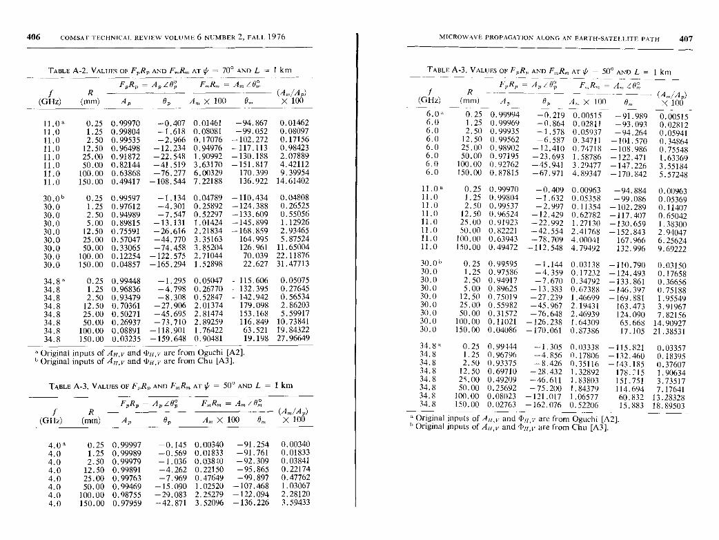
406 COMSAT TECHNICAL REVIEW VOLUME 6 NUMBER 2 , FAL1. 1976
TABLE A-2. VALUES OF FPR, AND FRm AT ,' = 700 AND L = 1 km
FPR, = A,LO, F,,,R,,, = AmLO°R (A IA,)
(GHz) (mm) A,, 0P A„ X 100 B„ X 100
11.0' 0.25 0.99970 -0.407 0.01461 -94.867 0.0146211.0 1.25 0.99804 -1.618 0.08081 -99.052 0.0809711.0 2.50 0.99535 -2.966 0.17076 -102.272 0.1715611.0 12.50 0.96498 -12.234 0.94976 -117.113 0.9842311.0 25.00 0.91872 -22.548 1.90992 -130.188 2.0788911.0 50.00 0.82144 -41.519 3.63170 -151.817 4.4211211.0 100.00 0.63868 -76.277 6.00329 170.399 9.3995411.0 150.00 0.49417 -108.544 7.22188 136.922 14.61402
30.06 0.25 0.99597 -1.134 0.04789 -110.434 0.0480830.0 1.25 0.97612 -4.301 0.25892 -124.388 0.2652530.0 2.50 0.94989 -7.547 0.52297 -133.609 0.5505630.0 5.00 0.89815 -13.131 1.01424 -145.899 1.1292630.0 12.50 0.75591 -26.616 2.21834 -168.859 2.9346530.0 25.00 0.57047 -44.770 3.35163 164.995 5.8752430.0 50.00 0.33065 -74.458 3.85204 126.961 11.6500430.0 100.00 0.12254 -122.575 2.71044 70.039 22.1187630.0 150.00 0.04857 -165.294 1.52898 22.627 31.47713
34.8a 0.25 0.99448 -1.295 0.05047 -115.606 0.0507534.8 1.25 0.96836 -4.798 0.26770 -132.395 0.2764534.8 2.50 0.93479 -8.308 0.52847 -142.942 0.5653434.8 12.50 0.70361 -27.906 2.01374 179.098 2.8620334.8 25.00 0.50271 -45.695 2.81474 153.168 5.5991734.8 50.00 0.26937 -73.710 2.89259 116.849 10.7384134.8 100.00 0.08891 -118.901 1.76422 63.521 19.8432234.8 150.00 0.03235 -159.648 0.90481 19.198 27.96649
Original inputs of AH,v and 44II,v are from Oguchi [A2].Original inputs of Arr,y and ^DH,v are from Chu [A3].
TABLE A-3. VALUES OF FPRP AND F,,,Rr AT t = 50° AND L = 1 km
00FPRP= A,,z0 F„R,„= A-zf R (A.m/Av)
(GHz) (mm) AP 0P A. X 100 ©,,, x 100
4.Oa 0.25 0.99997 -0.145 0.00340 -91.254 0.003404.0 1.25 0.99989 -0.569 0.01833 -91.761 0.018334.0 2.50 0.99979 -1.036 0.03810 -92.309 0.038414.0 12.50 0.99891 -4.262 0.22150 -95.865 0.221744.0 25.00 0.99763 -7.969 0.47649 -99.897 0.477624.0 50.00 0.99469 -15.090 1.02520 -107.468 1.030674.0 100.00 0.98755 -29.083 2.25279 -122.094 2.281204.0 150.00 0.97959 -42.871 3.52096 -136.226 3.59433
f
MICROWAVE PROPAGATION ALONG AN EARTH-SATELLITE PATH 407
TABLE A-3. VALUES OF FPRP AND F„R„ AT >(i = 50° AND L = 1 knt
f(GHz)
F,Rv = AP L6°v FR,,, = Am Z0,R -- - -- -
(mm) AP By AX 100 8,,,- (A„3AP)
X 100
6.0' 0.25 0.999946.0 1.25 0.999696.0 2.50 0.999356.0 12.50 0.995626.0 25.00 0.989026.0 50.00 0.971956.0 100.00 0.927626.0 150.00 0.87815
11.0° 0.25 0.9997011.0 1.25 0.9980411.0 2.50 0.9953711.0 12.50 0.9652411.0 25.00 0.9192311.0 50.00 0.8222111.0 100.00 0.6394311.0 150.00 0.49472
-0.219 0.00515 - 91.989 0.00515-0.864 0.02811 -93.093 0.02812-1.578 0.05937 - 94.264 0.05941-6.587 0.34711 -101.570 0.34864-12.410 0.74718 -108.986 0.75548-23.693 1.58786 -122.471 1.63369-45.941 3.29477 -147.226 3.55184-67.971 4.89347 -170.842 5.57248
- 0.409 0.00963 - 94.884 0.00963-1.632 0.05358 - 99.086 0.05369-2.997 0.11354 - 102.289 0.11407-12.429 0.62782 -117.407 0.65042- 22.992 1.27130 -130.659 1.38300-42.554 2.41768 - 152.843 2.94047- 78.709 4.00041 167.966 6.25624-112.548 4.79492 132.996 9.69222
30.06 0.25 0.99595 -1.144 0.03138 -110.790 0.0315030.0 1.25 0.97586 -4.359 0.17232 -124.493 0.1765830.0 2.50 0.94917 -7.670 0.34792 -133.861 0.3665630.0 5.00 0.89625 -13.383 0.67388 -146.397 0.7518830.0 12.50 0.75019 -27.239 1.46699 -169.881 1.9554930.0 25.00 0.55982 -45.967 2.19431 163.473 3.9196730.0 50.00 0.31572 -76.648 2.46939 124.090 7.8215630.0 100.00 0.11021 -126.238 1.64309 65.668 14.9092730.0 150.00 0.04086 -170.061 0.87386 17.105 21.38531
34.8° 0.25 0.99144 -1.305 0.03338 -115.821 0.0335734.8 1.25 0.96796 -4.856 0.17806 -132.460 0.1839534.8 2.50 0.93375 -8.426 0.35116 -143.185 0.3760734.8 12.50 0.69710 -28.432 1.32892 178.215 1.9063434.8 25.00 0.49209 -46.611 1.83803 151.751 3.7351734.8 50.00 0.25692 -75.200 1.84379 114.694 7.1764134.8 100.00 0.08023 -121.017 1.06577 60.832 13.2832834.8 150.00 0.02763 -162.076 0.52206 15.883 18.89503
° Original inputs of Au,,- and 4'11,v are from Oguchi [A2].6 Original inputs of Arr,v and 4,,v are from Chu [A3].
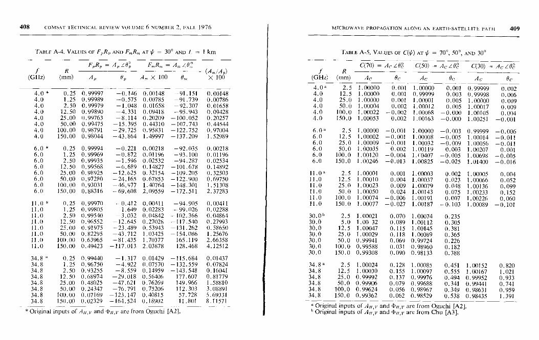
40 68 COMSAT IECIINICAI. REVIEW VOLUME NUMBER 2, FALL. 1976 MICROWAVE PROPAGATION ALONG AN EARTII-SATELLITE PATH 409
TABLE A-4. VALUES OF F,,,R2 AND FmRm AT ' = 30° AND L = I km TABLE A-5. VALUES OF C(o) AT ' = 70°, 50°, AND 30°
f RF,,R, = An /On FmR,,, = A. /0,°
(A /A ) f RC(70) = A,-LO8 C(50) = Ac/Oc' C(30) = Ac/0'
m F(GHz) (mm) AP 0p A„ X 100 0,1, X 100 (GHz) (mm) Ac 0c Ac 0c Ac Oc
4.0a 2.5 1.00000 0.001 1.00000 0.001 0.99999 0.0024.0 0.25 0.99997 -0.146 0.00148 -91.151 0.00148 4.0 12.5 1.00000 0.001 0.99999 0.003 0.99998 0.0064.0 1.25 0.99989 -0.575 0.00785 -91.739 0.00786 4.0 25.0 1.00000 0.001 1.00001 0.005 1.00000 0.0094.0 2.50 0.99979 -1.048 0.01658 - 92.307 0.01658 4.0 50.0 1.00004 0.002 1.00012 0.005 1.00017 0.0094.0 12.50 0.99890 -4.331 0.09418 -95.943 0.09428 4.0 100.0 1.00022 -0.002 1.00068 -0.000 1.00105 0.0044.0 25.00 0.99763 -8.114 (1.20209 - 100.052 0.20257 4.0 150.0 1.00053 0.002 1.00163 -0.000 1.00251 -0.0014.0 50.00 0.99475 -15.395 0.44310 - 107.743 0.445444.0 100.00 0.98791 -29.725 0.95831 - 122.752 0.97004 6.0° 2.5 1.00000 -0.001 1.00000 -0.003 0.99999 -0.0064.0 150.00 0.98044 -43.864 1.49997 - 137.209 1.52989 6.0 12.5 1.00002 -0.001 1.00008 -0.005 1.00014 -0.011
6.0 25.0 1.00009 -0.001 1.00032 -0.009 1.00056 -0 0116.0 * 0.25 0.99994 -0.221 0.00218 - 92.035 0.00218 6.0 50.0 1.00035 0.002 1.00119 0.003 1.00207
.0.001
6.0 1.25 0.99969 -0.872 0.01196 - 93.100 0.01196 6.0 100.0 1.00120 -0.004 1.(0407 -0.005 1.00698 -0.0056.0 2.50 0.99935 -1.596 0.02532 -94.287 0.02534 6.0 150.0 1.00246 -0.013 1.00825 -0.025 1.01400 -0.0166.0 12.50 0.99568 -6.689 0.14827 -101.678 0.148926.0 25.00 0.98925 -12.625 0.32154 - 109.205 0.32503 11.0" 2.5 1.00001 0.001 1.00003 0.002 1.00005 0.0046.0 50.00 0.97280 -24.165 0.67853 -122.900 0.69750 11.0 12.5 1.00010 0.004 1.00037 0.023 1.00066 0.0526.0 100.00 0.93031 -46.977 1.40764 - 148.301 1.51308 11.0 25.0 1.00023 0.009 1.00079 0.048 1.00136 0.0996.0 150.00 0.88316 -69.608 2.09559 -172.511 2.37283 11.0 50.0 1.00050 0.024 1.00143 0.075 1.00233 0.152
11.0 100.0 1.00074 -0,006 1.00191 0.007 1.00226 0.06011.0 0.25 0.99970 -0.412 0.00411 - 94.905 0.00411 11.0 150.0 1.00077 -0.027 1.00187 -0.103 1.00089 -0.10111.0 1.25 0.99805 -1.649 0.02283 -99.026 0.0228811.0 2.50 0.99540 -3.032 0.04842 -102.366 0.04864 30.0" 2.5 1.00021 0.070 1.00074 0.23511.0 12.50 0.96552 -12.645 0.27028 -117.540 0.27993 30.0 5.0 1.00 32 0.089 1.00112 0.30511.0 25.00 0.91975 -23.489 0.53943 -131.262 0.58650 30.0 12.5 1.00047 0.115 1.00145 0.38111.0 50.00 0.82295 -43.712 1.03425 -154.086 1.25676 30.0 25.0 1.00029 0.118 1.00089 0.36511.0 100.00 0.63965 -81.435 1.70377 165.119 2.66358 30.0 50.0 0.99941 0.069 0.99724 0.22611.0 150.00 0.49423 -117.013 2.03878 128.468 4.12512 30.0 100.0 0.99588 0.031 0.98960 0.182
30.0 150.0 0.99308 0.090 0.98133 0.38834.8 * 0.25 0.99440 -1.317 0.01429 -115.684 0.0143734.8 1.25 0.96750 -4.922 0.07570 -132.559 0.07824 34.8a 2.5 1.00024 0.128 1.00085 0.451 1.00152 0.82034.8 2.50 0.93255 - 8.559 0.14959 -143.548 0.16041 34.8 12.5 1.00030 0.155 1.00097 0.555 1.00167 1.02134.8 12.50 0.68974 -29.018 0.56406 177.607 0.81779 34.8 25.0 0.99992 0.137 0.99976 0.494 0.99952 0.93334.8 25.00 0.48025 -47.621 0.76269 149.966 1.58810 34.8 50.0 0.99906 0.079 0.99688 0.341 0.99441 0.74134.8 50.00 0.24347 -76.791 0.75206 112.303 3.08891 34.8 100.0 0.99624 0.056 0.98967 0.349 0.98631 0.95934.8 100.00 0.07169 -123.147 0.40815 57.728 5.69331 34.8 150.0 0.99362 0.062 0.98529 0.538 0.98435 1.39134.8 150.00 0.02329 -164.524 0.18902 11.801 8.11571
° Original inputs of Ax,y and 'ln,y are from Oguchi [A2].* Original inputs of Ally and Qiu,y are from Oguchi [A2]. I, Original inputs of Airy and c1 are from Chu [A3].
410 COMSAT TECHNICAL REVIEW VOLUME 6 NUMBER 2 , FALL 1976
TABLE A-6. VALUES OF D(4') AT 4' = 70°, 50°, AND 30°
D(70) = AD L 9D D (50) = AD z QD D(30) = AD L 9llf R
(GHz) (mm) AD 0D Aa 6D AD OD
4.0- 2.5 0.98790 -0.015 0.99706 0.000 1.01063 0.0144.0 12.5 1.00138 0.010 1.00191 0.010 0.99995 0.0034.0 25.0 0.99988 0.003 1.00121 0.001 0.99676 -0.0054.0 50.0 0.99303 -0.014 0.99062 -0.018 1.00500 0.0184.0 100.0 0.99771 -0.011 0.99983 -0.004 0.99835 -0.0164.0 150.0 0.99988 0.004 1.00279 0.012 1.00276 0.023
6.0- 2.5 1.00555 0.015 0.99895 -0.002 1.00000 -0.0096.0 12.5 0.99887 -0.000 1.00039 0.005 1.00306 -0.0056.0 25.0 1.00072 -0.016 1.00397 0.038 1.01414 0.0336.0 50.0 0.99630 -0.048 1.00189 -0.009 1.00495 0.0326.0 100.0 1.00163 0.013 1.00463 0.032 1.00749 -0.0066.0 150.0 1.00187 0.000 1.00638 0.031 1.01162 0.007
11.0a 2.5 0.99873 -0.025 0.99928 -0.009 1.00018 -0.04911.0 12.5 1.00346 0.051 0.99811 -0.029 1.00863 0.08211.0 25.0 1.00052 0.002 1.00212 0.015 0.99812 -0.04011.0 50.0 1.00033 0.013 1.00206 0.074 1.00621 0.06611.0 100.0 1.00106 0.015 1.00378 0.026 1.00349 -0.04111.0 150.0 1.00519 0.105 1.00426 0.108 1.00231 0.046
30.p° 2.5 1.01086 0.411 1.01326 0.44730.0 5.0 1.00970 0.430 1.01241 0.40030.0 12.5 1.00773 0.428 1.01142 0.29630.0 25.0 1.00456 0.205 1.00906 0.12930.0 50.0 1.00177 0.179 1.00984 -0.34430.0 100.0 1.00264 0.046 1.01055 -0.51130.0 150.0 1.00298 0.014 1.01323 -0.442
34.4 2.5 1.00121 0.081 1.00279 0.279 1.00467 0.41834.8 12.5 0.99988 -0.046 1.00284 -0.003 1.01051 0.44234.8 25.0 1.00163 -0.086 1.00529 -0.229 1.00304 -0.56634.8 50.0 1.00088 -0.189 1.00430 -0.592 1.01217 -0.99034.8 100.0 1.00265 -0.290 1.00331 -0.569 1.00597 -0.93334.8 150.0 1.00139 -0.518 1.00953 -0.931 1.01684 -1.710
a Original inputs of An,v and 44,,,v are from Oguchi [A2].s Original inputs of Au.v and 45n,v are from Chu [A3].
References
[Al] T. Oguchi, "Attenuation and Phase Rotation of Radio Waves Due to
Rain : Calculations at 19.3 and 34.8 GHz," Radio Science, Vol. 8, No. 1,
1973, pp. 31-38.[A2] T. Oguchi, Private Communications.
MICROWAVE PROPAGATION ALONG AN EARTH-SATELLITE PATH 411
[A3] T. S. Chu, "Rain-Induced Cross-Polarization at Centimeter and Milli-meter Wavelengths," Bell System Technical Journal, Vol. 53, No. 8, 1974,pp. 1557-1579.
[A4] L. J. Ippolito, "Summary and Evaluation of Results from the ATS Milli-meter Wave Experiment," Earth-Satellite Propagation Above 10 GHz,NASA Document X-751-72-208, May 1972.
[A5] H. W. Evans, "Attenuation on Earth-Space Paths at Frequencies up to30 GHz," International Conference on Communications, June 1971,Montreal, Canada, Proc., pp. 27-1 to 27-5.
[A6] International Radio Consultative Committee (C.C.I.R.), "PropagationData Required for Space Telecommunications Systems," U.K. Contribu-tion, Document S/154-E, October 1973.
Dickson J. Fang received his B.S.E.E. in 1962from Taiwan University, Taipei, China, and hisM.S.E.E. and Ph.D. from Stanford University in1964 and 1967. From 1967 to 1674 he was aradio physicist at Stanford Research Institute,and he authored 17 papers on wave propagation,radio auroras, and ionospheric irregularities.While on leave from Stanford (1969-1970) he wasa visiting professor at Taiwan University, wherehe published a graduate textbook on electro-
magnetic theory and five articles on the college education system. He joinedCOMSAT in 1974 and is currently responsible for research on propagationover 10-GHz frequencies.
Jiausen Jib received a B.S. in mechanical en-gineering from National Taiwan University in1956, an M.S. in aeronautical engineering fromthe University of Maryland in 1962, and a D.Sc.in mechanical engineering from George Washing-ton University in 1976. In January 1969 he joinedCOMSAT as a member of the technical staff. He ispresently Manager of the Engineering Applica-tions Department of the Computer Center. Heis a member of ACM.
CTR Notes
TV coehannel interference on a PCM -PSK SCPCsystem
D. KURJAN AND M. WACHS
(Manuscript received May 12, 1976)
Measurements have been made while investigating the effects of co-channel Tv frequency modulating an interfering carrier on a multicarriersingle-channel-per-carrier (sere) system with PCM-PSK modulation. Thisnote presents results which deal with a single voice channel.
Experimental setup
The sere system under consideration would consist of several hundred64-kbps 4-phase PSK channel slots in a single transponder. Since it wouldbe impractical to generate that many carriers, multicarrier operation wassimulated by using six 32-kbps 2-phase PSK carriers independently r5Kmodulated and clocked. The total power in these six carriers was adjustedso that the operating point of the traveling wave tube amplifier (TWTA)was at an input backoff of 10 dB. The sere carrier under test was located
This note is based upon work performed at COMSAT Laboratories under thesponsorship of the International Telecommunications Satellite Organization(INTELSAT). Views expressed in this note are not necessarily those of INTELSAT.
Mr. Kurjan is a member of the technical staff in the Systems Applicationsand Simulation Department of the Transmissions Systems Laboratory,COMSAT Laboratories.
Mr. Wachs is Manager, Systems Applications and Simulation Depart-ment, Transmission Systems Laboratory , COMSAT Laboratories.
413
414 COMSAT TECHNICAL REVIEW VOLUME 6 NUMBER 2, FALL 1976
at a frequency corresponding to a carrier-to-intermodulation (C/I) ratioof approximately 20 dB.
Figure 1 is a schematic of the experimental setup. An scrc carrier isgenerated and up-converted to 4 GHz along with the six PSK cotranspondercarriers. The up-converter is linear, providing a 2-carrier C/I greater than40 dB. After amplification by the TWT, the composite is down-convertedto 70 MHz. A common local oscillator is used for up- and down-conver-sion to eliminate translation oscillator instability. The TV interference andthermal noise are added at IF on the down-link. The TV interference iscentered on the desired scrc channel frequency and is represented as afrequency modulated carrier driven by a triangular dispersal wave witha peak-to-peak deviation of 1 MHz.
Test results
The performance of the scrc modem in a back-to-back configurationwithout added interference is shown in the bit-error rate (BER) vs carrier-to-noise (C/N) ratio curve of Figure 2. It can be seen that an error prob-ability (P,) of 10-" occurs at a C/N of 11.65 dB. The corresponding ratioof energy per bit to noise density (Eo/No) is computed as follows:
E5/No = (C/N) BT,,
where B = channel bandwidth = 38 kHz
T5 = information bit period =1
64 kbps
= 1.56 X 10⁻⁵ seconds.
Then,(E6/No)men, = 11.65 - 2.26 = 9.4 dB
while theoretical calculations yield
(Eb/N0),h = 8.4 dB
The performance of the scrc channel through the INTELSAT Iv satellitesimulator without external (i.e., TV) interference is shown in Figure 3.The BER vs C/N curve for a C/I of 30 dB is the same as that for the back-to-back case (Figure 2). For C/I ratios of 20 and 15 dB, a Pe of 10-s
TV COCHANNEL INTERFERENCE ON A PCM-PSK SCPC SYSTEM 415
u 0>LLF
I I w CF
^l^ Iw 0Va 1o
0S
I >
x^, m i a
>>o ^
}7^l
a 3I l ^
z v
Hu 4
aV
2
C
?ll
to
0
Y
416 COMSAT TECHNICAL REVIEW VOLUME 6 NUMBER 2, FALL 1976
requires C/N ratios of 12.45 and 16.6 dB, respectively. It should be notedthat C/I refers to the modulated carrier power relative to the intermodula-tion power measured after the demodulator input filter without addedthermal noise or interference.
10-2
10 3
10-3
I
10-5
.1
10 5
10-57 8 9 10 11 12 13
C/N IIBI
14 15
Figure 2. SCPC Modem Back-to-Back Performance
16 17
TV COCHANNEL INTERFERENCE ON A PCM-PSK SCPC SYSTEM 417
10 2
E
910 -6
10111 12
SIDERED SCPC CARRIER
6 COTRANSPONDER PSKCARRIERS THROUGH TWTAB0, 10 dB
a - C/I - 30 dB
b ......... CiI = 20 a8
C --- CiI = 15 dB
13 14 15 16 17 18 19
C/N (dB)
Figure 3. SCPC Performance Through a Transponder
The carrier -to-interference (C/INT) ratio is defined as the ratio of
modulated carrier power to the power of an unmodulated external inter-
418 COMSAT TECHNICAL REVIEW VOLUME 6 NUMBER 2, FALL 1976
Terence source at the demodulator input without added thermal noise (orintennodulation, in the case of transponder operation). The scpe per-formance in a back-to-back mode with a frequency dispersal (TV) inter-ference source added is shown in curves a-c of Figure 4. It can be seenthat a C/INT of 10 dB yields an increase in the required C/N of less than0.75 dB for a 10-4 bit-error probability. The average modulated (sweeping)interference power appearing after the demodulator input filter is 14.2dB less than the power of the unmodulated interference source, since theswept interference source is in the channel bandwidth 3.8 percent of thetime in these tests. Therefore, for a C/INT of 10 dB, the average powerratio of modulated carrier to modulated interference source at the channelfilter output is 24.2 dB.
Curve d in Figure 4 shows the result of an unmodulated interferencesource at 70 MHz with the same C/INT (24 dB). In this case, performanceis seen to be better than for the modulated interference source, eventhough the average power levels of the interference source at the channelfilter output are the same. This performance difference is a result oftransient effects in the demodulator caused by the spreading wavesweeping through the channel rather than being a stationary carrier withinthe band. Performance through the transponder with the spreading waveinterference source added is shown in Figure 5, which considers the caseof a 20-dB C/I for a range of interference levels. As can be seen from thefigure, the presence of the swept interference source results in a furtherperformance degradation of 0.5 dB for a C/INT of 15 dB, while a C/INTof 10 dB yields a 1.2-dB degradation for a F, of 10-4.
The effect of the modulating frequency (f,) of the interference sourceis shown in Figure 6. It can be seen that the average BER does not varysignificantly from 20 to 1,200 Hz. Even though the average BER is almostconstant, the actual number of errors per interference sweep will varydirectly with the time during which the interference source is in the channelbandwidth. No periodic effects were noticed in the quality of the channelover the entire range of sweep frequencies.
A "window" error rate, which corresponds to the error rate in the periodduring which the interference source sweeps through the channel band-width, can be computed from Figures 3 and 5 by eliminating the errorrate due to noise and intermodulation alone. The resulting window errorrate curves are shown in Figure 7. The fact that these error rates are notconstant indicates that the additional errors in this period are not inde-pendent of the thermal noise.
For a typical operating condition of C/N = 15 dB and C/I ti 20 dB,
TV COCHANNEL INTERFERENCE ON A PCM-PSK SCPC SYSTEM 419
10 3
I-C
0U 10-4
IT 5
10-6
I
I I I I I I I I I
9 10 12 13 14 15 16
I
j
CIN (dB)
Figure 4. SCPC Performance with Spreading Wave (back to back)
C/INT was varied to determine the point at which the synchronization
became unreliable . It was found that at C/INT = 9 dB occasional bursts
LINEAR CHANNELSPREADING WAVEFORMINTERFERER
50- IT, TRIANGULAR WAVE
1-MHz Pk -Pk DEV.
z _ C/INT m
b--- CANT = 15 dB
........ C/INT - 10 dB
d -.- C/INT - 24 dB - UNMODULATED
TONE INTERFERENCE SOURCE
420 COMSAT TECHNICAL REVIEW VOLUME 6 NUMBER 2, FALL 1976 TV COCHANNEL INTERFERENCE ON A PCM-PSK SCPC SYSTEM 421
10 2
DESIRED SCPC CARRIER 16 COTRANSPONDER
PSK CARRIERS THROUGH TWTA
BOi - 10 dB
50 Hz; 1 MHz Pk Pk DEV-
TRIANGULAR SPREADING WAVE
C,I 20 dB
12
IF 3
10 4
10-5
a - C IN T -00
b --- DINT - 20 dB
C ------ C/INT - 15 dB
d - - C /INT - 10 HE
e C/INT - 8 dB
f---C/INT=6dB
910-6
T---]
10 16 17
j
N
18
I I13 14 15
C/N (dBl
19
Figure 5. SCPC Performance Through a Transponder Plus SpreadingWare Interference
of approximately 100 errors occurred, corresponding to the loss of start-of-message synchronization.
10-50
I
DESIRED SCPC CARRIER 16 COTRANSPONDERPSK CARRIERS THROUGH TWTA
30, - 10 IS
CI 19dS
CANT 10 1IR
50 Ht ; 1-MHz Pk -Pk UEV.
TRIANGULAR SPREADING WAVE
I I I I I I I I I100 200 300 400 500 600 700 800 900 1000 1100 1200
FREQUENCY OF TRIANGULAR WAVE, IWI
Figure 6. Effect of interference Source Modulating Frequency
The sere channel performance through the simulator with both thespreading wave and Tv signal (black field plus sync pulse and color burst)is shown in curves a and b of Figure 8. There is no significant differencebetween the corresponding curves of Figures 5 and 8 to within measure-ment accuracy. In this case, a spreading wave alone yields slightly highererror rates. Curve c in Figure 8 shows that error rates are lower for colorbars than for a black field.
Conefusions
Based on the experimental results presented in this note, the followinggeneral conclusions can be drawn. In the PCM-PSK sere system, the errorrate increase caused by a wideband sweeping inference source whoseaverage power within a particular channel slot is at a certain level cannot
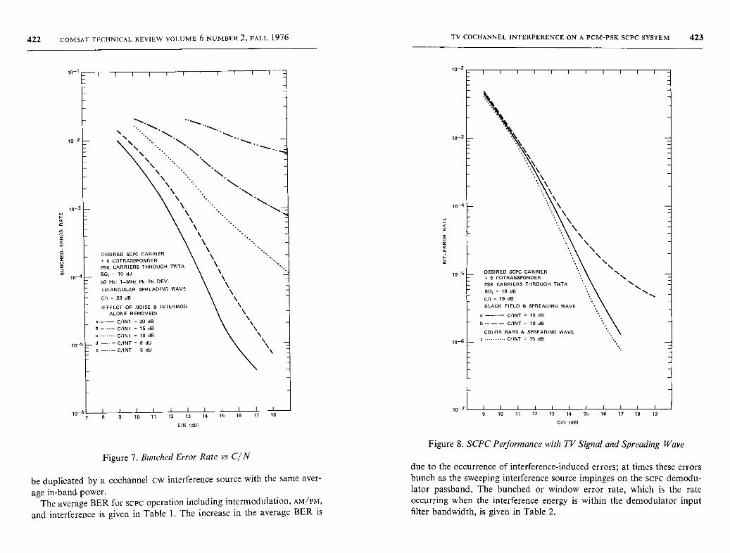
422 COMSAT TECHNICAL REVIEW VOLUME 6 NUMBER 2, FALL 1976 TV COCHANNEL INTERFERENCE ON A PCM-PSK SCPC SYSTEM 423
2D
10-1
10-2
10-3
0
10-4
10-5
DESIRED SCPC CARRIER
a 6 COTRANSPONDER
P5K CARRIERS THROUGH TWTA
BOi 10 dO
50 Hz; 1 -MHz Pk-Pk DEV.
TRIANGULAR SPREADING WAVE
vl 20 113
(EFFECT OF NOISE & INTERMOD
ALONE REMOVED)
- (/INT 20 dB
b --- C/INT 15 dB
_ d -- C/INT = 8 dB
Ce ---- C/INT - 6 dB
10-6 Ll
I 1 1
8 9 10 11 12 13 14 15 16 17 18
BIN (dB)
Figure 7. Bunched Error Rate vs C/N
be duplicated by a cochannel cw interference source with the same aver-
age in-band power.The average BER for scPC operation including intermodulation, AM/Pnt,
and interference is given in Table 1. The increase in the average BER is
10-2
10-a
10-5
10-6
1o-T
DESIRED SCPC CARRIER6 COTRANSPONDER
P5K CARRIERS THROUGH TWTA
BOL = 10 tl8
C/I 19 dB
BLACK FIELD & SPREADING WAVE
a - C/INT - 15 dB
b --- C/INT = 10 dB
COLOR BARS & SPREADING WAVE
e ---- C/INT = 15 dB
I
9 10 11 12 15 10 15 16 1T 10 19
C/N (de)
3
Figure 8. SCPC Performance with TV Signal and Spreading Wave
due to the occurrence of interference-induced errors; at times these errorsbunch as the sweeping interference source impinges on the scrc demodu-lator passband. The bunched or window error rate, which is the rateoccurring when the interference energy is within the demodulator inputfilter bandwidth, is given in Table 2.
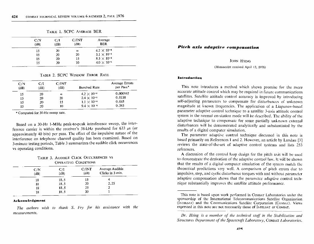
424 COMSAT TECHNICAL REVIEW VOLUME 6 NUMBER 2, FALL 1976
TABLE 1. SCPC AVERAGE BER
C/N C/I C/INT Average
(dB) (dB) (dB) BER
15 20 Go 4.2 X 10⁻⁶
15 20 20 5.1 X 10-615 20 15 8.5 X 10-615 20 10 4.0 X 10⁻⁶
TABLE 2. SCPC WINDOW ERROR RATE
C/N C/I C/INT Average Errors
(dB) (dB) (dB) Bunched Rate per Pass*
15 20 4.2 X 10⁻⁶ 0.000167
15 20 20 2.4 X 10⁻⁶ 0.0138
15 20 15 1.1 X 10⁻⁴ 0.045
15 20 10 9.4 X 10⁻⁴ 0.383
* Computed for 30-Hz sweep rate.
Based on a 30-Hz 1-MHz peak-to-peak interference sweep, the inter-ference carrier is within the receiver's 38-kHz passband for 633 As (orapproximately 40 bits) per pass. The effect of the impulsive nature of theinterference on telephone channel quality has been examined. Based on3-minute testing periods, Table 3 summarizes the audible click occurrences
vs operating conditions.
TABLE 3. AUDIBLE CLICK OCCURRENCES VS
OPERATING CONDITIONS
C/N C/I C/INT Average Audible
(dB) (dB) (dB) Clicks in 3 min.
18 18.5 15 4
18 18.5 20 2.25
18 18.5 25 2
18 18.5 30 1
Acknowledgment
The authors wish to thank S. Fry for his assistance with the
measurements.
Pitch axis adaptive compensation
JOHN HSING
(Manuscript received April 12, 1976)
Introduction
This note introduces a method which shows promise for the moreaccurate attitude control which may be required in future communicationssatellites. Satellite attitude control accuracy is improved by introducingself-adjusting parameters to compensate for disturbances of unknownmagnitude at known frequencies. The application of a Liapunov-basedparameter adaptive control technique to a satellite 3-axis attitude controlsystem in the normal on-station mode will be described. The ability of theadaptive technique to compensate for some partially unknown externaldisturbances will be demonstrated analytically and substantiated by theresults of a digital computer simulation.
The parameter adaptive control technique discussed in this note isbased primarily on References I and 2. However, an article by Landau [3]reviews the state-of-the-art of adaptive control systems and lists 253references.
A discussion of the control loop design for the pitch axis will be usedto demonstrate the derivation of the adaptive control law. It will be shownthat the results of a digital computer simulation of the system match thetheoretical predictions very well. A comparison of pitch errors due toimpulsive, step, and cyclic disturbance torques with and without parameteradaptive compensation shows that the parameter adaptive control tech-nique substantially improves the satellite attitude performance.
This note is based upon work performed in COMSAT Laboratories under the
sponsorship of the International Telecommunications Satellite Organization
(INTELSAT) and the Communications Satellite Corporation (COMSAT). Views
expressed in this note are not necessarily those of INTELSAT or COMSAT.
Dr. Hsing is a member of the technical staff in the Stabilization andStructures Department of the Spacecraft Laboratory, COMSAT Laboratories.
sic
426 COMSAT TECHNICAL REVIEW VOLUME 6 NUMBER 2, FALL 1976
System definition and pitch control law
Consider a 3-axis-stabilized satellite in a geostationary orbit with thereference coordinates and nominal angular momentum vector defined inFigure 1. With an earth sensor, this type of biased momentum wheel
Wa, ORBIT RATE
ROLL AXIS, x
WHEEL ANGULAR MOMENTUM
CTR NOTE: PITCH AXIS ADAPTIVE COMPENSATION 427
h„o = K1(r„B + 0) + k,(t) + k2(t) cos wt + k3(t) sin wt (3)
where K„ and r„ are the pitch autopilot gain and time constant, respectively,
and k,(t), k2(t), and k3(t) are the adaptive parameters which will self-adjust
so that the controlled pitch loop is asymptotically stable.Substituting equations (2) and (3) into equation (1) yields
1 + K„rv9 + KPB = SI (t) + s2(t) cos wt + Sa(t) Sin wt (4)
where S,(t) ° ao - kl (t) (5a)
s2(t) ° a, - k2(t) (5b)
33(t) d bl - k3(t) (5c)
are the parameter misalignments contributing to the driving torque of
the controlled pitch differential equation [equation (4) ].
The adaptive parameters ki(t) are adjusted on the basis of Liapunov's
direct method.
TO EARTH
PITCH AXIS, y
Figure 1. Reference Frame and Wheel Angular Momentum
offers pitch control torque through wheel speed modulation. Based on aclassical formulation [4] which assumes a rigid body with internal momen-tum, the linearized pitch attitude differential equation is
is + hec = Tau (1)
where Id is the pitch moment of inertia, B is the pitch angle, h., represents
the control torque, and Td„ represents disturbance torques with unknown
magnitudes at known frequencies. For ease of analysis it will be assumed
that
Td1 = no + a, cos wt + bl sin wt (2)
where ao, al, and b, are unknown constants and w is some known frequency.
The objective is to select the control function in equation (1) so thatthe pitch error due to these external disturbances asymptotically converges
to zero. A satisfactory control law is
Liapuuov 's direct method
Liapunov's direct method is a technique used to design an adaptivecontroller for adjusting feedback gains so that the controlled system isasymptotically stable. The most attractive feature of this method is thatthe stability of a system can be ascertained directly from the equationsdescribing the system without recourse to explicit form solutions.
Equation (4) can be rewritten in the vector matrix form
3
Y(t) = Ay(t) + b si(t) gi(t)
wherey(t) ° [0 ,
Of
0 1
A °Ky Kur„
/v I„
ib 0,
T
(6)
(7)
(8)
(9)
428 COMSAT TECHNICAL REVIEW VOLUME 6 NUMBER 2, FALL 1976
and g1(t) = 1, g2(t) = cos wt, and g;,(t) = sin wt. The control function inequation (6) is directly related to the adaptive parameters of equation (5).These parameters will be defined so that y = 0 is an asymptotically stableequilibrium point.
A potential Liapunov function of positive-definite quadratic form ischosen:
3 1V = yTPy + + 0ryTPhgi)2
where the superscript T represents the transpose of a vector, P is a sym-metric positive-definite matrix to be defined later, and a; and 0, are arbi-trary positive constants. Taking the time derivative of equation (10) andsubstituting equation (6) and its transpose for y and ill' yields
yT(PA + ATP) y + 2yTPb S,gi
+ 2 L J (6i + 0,yTPbgi) ['si + dt (aiy_TPbg,)] (11)
where the relationship yTPh = bTPy has been used.For a stable matrix A, there exists a unique positive-definite symmetric
matrix P which is the solution of
PA + ATP = -Q (12)
where Q is a given positive-definite symmetric matrix [5]. Thus, the firstterm in equation (11) will be negative-definite if A is selected properly.For V to be negative-definite, which is a design requirement, the secondand third terms in equation (11) should at least be negative-semidefinite.This will be true if the fii's in equation (11) are defined as
-a,yTPbi - Ri dt (YTPbi) (13)
fori=1,2,3.Substituting equations ( 12) and ( 13) into equation ( 11) gives
CTR NOTE: PITCH AXIS ADAPTIVE COMPENSATION 429
3V = -yTQy - 2 L Ri(VTPbgi)2 (14)
i= 1
which is negative-definite as expected. According to Liapunov's directmethod [5], the controlled pitch loop is asymptotically stable with respectto the partially unknown disturbance torques.
The adjustment mechanism for parameters ki(t) can be obtained by
substituting equation (5) into equation (13):(10)
aTPbg; + 0, dt (yTPbgi)ki(t) = iy (15)
for i = 1, 2, 3. If equation (15) is used to adjust the adaptive parameterswhich form the control function of the pitch loop, the attitude error willbe driven to zero due to Liapunov's design of the control law.
parameters defined in equation (15) as
ki(t) _ al- f(PO + pziB) dt +RI- (plzB + pszB) (16)
k,(t) = a2J (puG + p220) cos wt dt
02+ (PI29 + przaB) cos Wt (17)
u
Simulation results and comparison
It has been shown in the previous section that the control torque inequation (3) with the adaptive parameters defined in equation (15) guaran-tees that the controlled pitch loop is asymptotically stable. To providehigh damping and rapid response to the driving function in equation (4),
values of Ky and ry are nominally chosen to critically damp the system.
During the simulation, Ky = 0.7 N-m/rad and ry = 50 s were chosen,
implying a critically damped pitch loop. The positive-definite symmetricmatrix Q in equation (12) was selected as a unit matrix and the positiveconstants in equation (15) were arbitrarily selected as a, = 0, = 10 fori = 1, 2, 3. Equations (7), (9), and (12) can be used to rewrite the adaptive
k,,(t)IX3
= I (pi20 + p220) sin wt dtv
430 COMSAT TECHNICAL REVIEW VOLUME 6 NUMBER 2 , FALL 1976
Ra(PI20 + P220) sin wt
Y(18)
where P12 and P22 are the components of the matrix P. The correspondingpitch control loop is shown in Figure 2.
By
Ty
TJV
E 9 )IVs S
P22
ly IC
) a
SIN (WO
RCOS (W')
°2
fl2
SIN (wt)
0 s EnP3
Figure 2. Pitch Adaptive Control Loop
This control system has been simulated on a digital computer withIy = 440 kg-tn2. The pitch responses for impulsive, step, and cyclic(orbital rate) disturbance torques are plotted in Figure 3 and summarizedin Table 1. The angles have been normalized as 0/ jTdy I with units of
0.35
005
Figure 3. Pitch Response with Adaptive Compensation
deg/N-m, where I I. represents the maximum magnitude of a variable.These results substantiate the analysis discussed in previous sections.
TABLE 1. IMPROVEMENTS USING ADAPTIVE COMPENSATION
Without AdaptiveCompensation
With AdaptiveCompensation
Disturbance Time Time
Max. Error(deg/N-m)
Constant(s)
Max. Error(deg/N-m)
Constant(s)
Impulsive 0 . 6 80 0.07 20
Step 80 55 0.42 20
Cyclic 80 0.42 20
(orbital rate)
For ease of comparison, the normalized responses produced by a
pitch autopilot without handling unknown disturbances, i.e., k,(t) = 0
for i = I, 2, 3, are plotted in Figure 4, where the steady-state errors due tostep and cyclic disturbances are constant and cyclic, respectively. The com-parison shows that both transient and steady-state attitude performance
can be improved through adaptive compensation.
CTR NOTE: PITCH AXIS ADAPTIVE COMPENSATION 431
01 II( - NORMALIZED IMPULSE RESPONSE
02 It) NORMALIZED STEP RESPONSE
03 It) - NORMALIZED CYCLIC ( ORBITAL RATE ) RESPONSE
432 COMSAT 'TECHNICAL REVIEW VOLUME 6 NUMBER 2 , FALL 1976
NOTE MAIb EO IMP U LSE HESOCENSE
NO R N. A L ILL') S,ER 11t1111.11
NORMALIZrD CYGI IC IORBITAL RATE: RESPONSE
CTR NOTE: PITCH AXIS ADAPTIVE COMPENSATION 433
sation is added, Figure 3 shows that the maximum error has decreasedby more than two orders of magnitude, and that, after the transient de-cays, the error is even smaller. In Figure 3, 0, and B3 share the same curvedue to the low frequency of the solar pressure torque. It is also possibleto adaptively compensate for cyclic disturbances at other frequencies,
and the pitch error asymptotically converges to the null.
Conclusions
LD 10
n.II
-I
A parameter adaptive control system based on Liapunov's direct methodhas been applied to a pitch attitude control loop design in the normalon-station mode of a 3-axis-stabilized geostationary satellite. The abilityof the adaptive technique to compensate for some unknown disturbancetorques has been demonstrated for both transient and steady-state con-ditions. With the adaptive scheme, the pitch errors due to partially un-known disturbance torques will asymptotically converge to zero, whereaswithout adaptive compensation they will not. It can he concluded thattransient and steady-state attitude performance can he substantially
improved through adaptive compensation.
Acknowledgment
The author would like to thank Messrs. A. Ramos and P. R. Schrantz
for useful discussions and comments. Thanks are also due to Dr. G. D.Gordon for his careful review of the original manuscript and valuable
suggestions.
Figure 4. Pitch Response without Adaptive Compensation
Three cases were compared. In the first comparison an impulsive dis-turbance torque was used. Figure 4 shows the expected response of acritically damped control loop without adaptive compensation. Whenadaptive compensation is introduced, the rise to about 0.07 deg/N-m inthe first few seconds is about the same. However, the pitch error is cut offand exhibits oscillations with rapidly diminishing amplitude. The maxi-mum error is decreased by a factor of nine, and the time constant by afactor of four.
For the second comparison, the pitch response to a step disturbancewithout adaptive compensation is shown in Figure 4. Since the disturbancecontinues in time, a normalized error of 80 deg/N-m continues indefi-nitely. When adaptive compensation is added (see Figure 3), the maximumerror is reduced to 0.42 deg/N-m and damps out rapidly to zero. Thedecrease of more than two orders of magnitude in the maximum errorgenerated demonstrates the effectiveness of adaptive compensation.
The last comparison is for a cyclic solar pressure torque. Withoutadaptive compensation, Figure 4 shows the expected cyclic pitch error,with a normalized amplitude of 80 deg/N-m. When adaptive compen-
References
[1] P. C. Parks, "Liapunov Redesign of Model Reference Adaptive Control
Systems," IEEE Transactions on Automatic Control, AC-Il, 1966, pp. 262-
267.[2] J. W. Gilbart, R. V. Monopoli, and C. F. Price, "Improved Convergence
and Increased Flexibility in the Design of Model Reference Adaptive Con-trol Systems," Ninth Symposium on Adaptive Processes, the University of
Texas at Austin, December 7-9, 1970.[3] 1. D. Landau, "A Survey of Model Reference Adaptive Techniques-Theory
and Applications," Automatics, Vol. 10, Pergamon Press, 1974, pp. 353-379.
[4] M. G. Lyons, K. L. Lebsock, and E. D. Scott, "Double Gimbaled ReactionWheel Attitude Control System for High Altitude Communications Satel-lites," AIAA Guidance, Control and Flight Mechanics Conference, Hofstra
University, Hempstead, New York, August 16-18, 1971, AIAA Paper
71-949.[5] J. C. Hsu and A. J. Meyer, Modern Control Principles and Applications,
New York: McGraw-Hill Book Co., 1968.
Translations of Abstracts in this issue
Modele d'assignation et de program ►nation despaquets AMILT
A. K. SINHA
Sommaire
Cet article propose une expression mathematique simple du problemede ('assignation et de la programmation des paquets d'information dans on
systeme d'acees multiple par repartition dans le temps (AMRT) destine a unsysteme general de telecommunications par satellite dans lequel on choisitde facon arbitraire le reseau de stations terriennes, ainsi que Ic diagramme decouverture de l'antenne et la configuration du repcteur d'un satellite. On
presente les concepts applicables aux problemes de superposition de dif-ferents diagrammes de couverture, stir une m"eme station terrienne, et durecouvrement dans le temps de diffcrents paquets, ainsi que ceux dos aux
contraintes des Cquipements des stations terriennes. On met egalement enevidence certains parametres utiles a ('evaluation de 1'ef£icacite de ('utilisation
du systeme. Enfin, on propose tin algorithme semi-analytique permettant de
programmer les paquets AMRT de facon a reduire an minimum les equipe-ments requis aux stations terriennes et a optimiser 1'efficacite de la program-mation pour des donnees de trafic specifices et one configuration de systemedonnee. On presente tin exemple obtenu grace it on programme d'ordinateur
qui vient d'etre ClaborC suivant cette methode.
nestauration autonatique de L'orthogonalite depolarisation dans les systen►es de satellitesit reutilisation de frequency
D. F. DIFONZO, W. S. TRACHTMAN ET A. E. WILLIAMS
Sonmaire
Cet article decrit des reseaux retablissant automatiquement 1'orthogonalite depolarisation. Ces rescaux peuvcnt "etre utilises pour minimiser les brouillages
reciproques qui se produisent dans une liaison de telecommunication par
435