Embed Size (px)
Citation preview

VERSION 4.3
Reference Guide
Comsol Java API

C o n t a c t I n f o r m a t i o n
Visit www.comsol.com/contact for a searchable list of all COMSOL offices and local representatives. From this web page, search the contacts and find a local sales representative, go to other COMSOL websites, request information and pricing, submit technical support queries, subscribe to the monthly eNews email newsletter, and much more.
If you need to contact Technical Support, an online request form is located at www.comsol.com/support/contact.
Other useful links include:
• Technical Support www.comsol.com/support
• Software updates: www.comsol.com/support/updates
• Online community: www.comsol.com/community
• Events, conferences, and training: www.comsol.com/events
• Tutorials: www.comsol.com/products/tutorials
• Knowledge Base: www.comsol.com/support/knowledgebase
Part No. CM020007
C O M S O L J a v a A P I R e f e r e n c e G u i d e 1998–2012 COMSOL
Protected by U.S. Patents 7,519,518; 7,596,474; and 7,623,991. Patents pending.
This Documentation and the Programs described herein are furnished under the COMSOL Software License Agreement (www.comsol.com/sla) and may be used or copied only under the terms of the license agree-ment.
COMSOL, COMSOL Desktop, COMSOL Multiphysics, and LiveLink are registered trademarks or trade-marks of COMSOL AB. Other product or brand names are trademarks or registered trademarks of their respective holders.
Version: May 2012 COMSOL 4.3

C o n t e n t s
C h a p t e r 1 : I n t r o d u c t i o n
About the COMSOL Java API 10
Where Do I Find More Information? . . . . . . . . . . . . . . . 10
Getting Started 13
The Model Object . . . . . . . . . . . . . . . . . . . . . . 13
Compiling a Model Java-File . . . . . . . . . . . . . . . . . . . 14
The Model Java-File . . . . . . . . . . . . . . . . . . . . . . 14
Running a Model Class-file from the Desktop . . . . . . . . . . . . 15
Running a Model Class-file as a Batch Job from the Desktop . . . . . . 15
Running a Model Class-file with the COMSOL Batch Command . . . . . 15
Getting the COMSOL Installation Path from the Windows Registry . . . 16
Setting up Eclipse for Compiling and Running a Java File . . . . . . . . 16
C h a p t e r 2 : G e n e r a l C o m m a n d s
About General Commands 20
Extrusion Coupling Operators. . . . . . . . . . . . . . . . . . 57
Projection Coupling Operators . . . . . . . . . . . . . . . . . 62
Integration Coupling Operators . . . . . . . . . . . . . . . . . 64
Average Coupling Operators . . . . . . . . . . . . . . . . . . 65
Maximum/Minimum Coupling Operators . . . . . . . . . . . . . . 65
Least-Squares Objective Functions . . . . . . . . . . . . . . . 115
C h a p t e r 3 : G e o m e t r y
About Geometry Commands 164
Features for Creating Geometric Primitives . . . . . . . . . . . . 166
Features for Geometric Operations. . . . . . . . . . . . . . . 167
Features for Virtual Operations . . . . . . . . . . . . . . . . 169
C O N T E N T S | 3

4 | C O N T E N T S
Features for Mesh Control . . . . . . . . . . . . . . . . . . 169
Geometry Object Information Methods . . . . . . . . . . . . . 171
Working with a Geometry Sequence 173
Adding a Model (Geometry) . . . . . . . . . . . . . . . . . 173
Adding a Geometry Feature. . . . . . . . . . . . . . . . . . 174
Editing a Geometry Feature . . . . . . . . . . . . . . . . . . 174
Building Geometry Features. . . . . . . . . . . . . . . . . . 176
Feature Status . . . . . . . . . . . . . . . . . . . . . . . 177
Accessing Geometry Object Names . . . . . . . . . . . . . . 177
Deleting and Disabling Geometry Features . . . . . . . . . . . . 178
Deleting Geometry Objects. . . . . . . . . . . . . . . . . . 179
Geometry Settings 180
Length Unit . . . . . . . . . . . . . . . . . . . . . . . . 180
Angular Unit . . . . . . . . . . . . . . . . . . . . . . . 180
Scale Values When Changing Unit . . . . . . . . . . . . . . . 181
Geometry Representation in 3D . . . . . . . . . . . . . . . . 181
Default Relative Repair Tolerance . . . . . . . . . . . . . . . 182
Automatic Rebuild . . . . . . . . . . . . . . . . . . . . . 182
Work Planes 183
Virtual Operations 184
About Virtual Operations . . . . . . . . . . . . . . . . . . 184
Mesh Control Entities . . . . . . . . . . . . . . . . . . . . 184
Geometry Object Information 186
General Information . . . . . . . . . . . . . . . . . . . . 187
Geometric Entity Counters . . . . . . . . . . . . . . . . . . 187
Adjacency . . . . . . . . . . . . . . . . . . . . . . . . 188
Evaluation on an Edge . . . . . . . . . . . . . . . . . . . . 189
Evaluation on a Face . . . . . . . . . . . . . . . . . . . . 190
Geometry Representation Arrays . . . . . . . . . . . . . . . 191
Measurements 193
Measuring Geometric Entities in Objects . . . . . . . . . . . . . 193
Measuring Objects . . . . . . . . . . . . . . . . . . . . . 193

Inserting a Geometry Sequence from a File 195
Exporting Geometry to File 196
How to Export the Finalized Geometry . . . . . . . . . . . . . 196
Exporting to an STL File . . . . . . . . . . . . . . . . . . . 197
Exporting to a Parasolid File . . . . . . . . . . . . . . . . . 197
Compatibility in 3D . . . . . . . . . . . . . . . . . . . . . 197
Geometry Commands 198
C h a p t e r 4 : M e s h
About Mesh Commands 306
Operation Features . . . . . . . . . . . . . . . . . . . . . 307
Attribute Features . . . . . . . . . . . . . . . . . . . . . 307
Features for Imported Meshes . . . . . . . . . . . . . . . . . 308
Working with a Meshing Sequence 309
Adding a Meshing Sequence . . . . . . . . . . . . . . . . . . 310
Adding a Mesh Feature . . . . . . . . . . . . . . . . . . . 310
Editing a Mesh Feature. . . . . . . . . . . . . . . . . . . . 311
Building Mesh Features . . . . . . . . . . . . . . . . . . . 311
Feature Status . . . . . . . . . . . . . . . . . . . . . . . 312
Deleting Mesh Features . . . . . . . . . . . . . . . . . . . 312
Disabling Mesh Features . . . . . . . . . . . . . . . . . . . 312
Clearing Meshes . . . . . . . . . . . . . . . . . . . . . . 313
Units . . . . . . . . . . . . . . . . . . . . . . . . . . 313
Selections . . . . . . . . . . . . . . . . . . . . . . . . 313
Physics-Controlled Meshing 315
Information and Statistics 316
Statistics . . . . . . . . . . . . . . . . . . . . . . . . . 316
Number and Types of Elements . . . . . . . . . . . . . . . . 317
Quality of Elements . . . . . . . . . . . . . . . . . . . . . 318
Volume of Elements and Mesh . . . . . . . . . . . . . . . . . 318
C O N T E N T S | 5

6 | C O N T E N T S
Growth Rate in Mesh . . . . . . . . . . . . . . . . . . . . 319
Mesh Status . . . . . . . . . . . . . . . . . . . . . . . . 319
Getting and Setting Mesh Data 321
Accessing Mesh Data . . . . . . . . . . . . . . . . . . . . 321
Setting or Modifying Mesh Data . . . . . . . . . . . . . . . . 322
Block Versions . . . . . . . . . . . . . . . . . . . . . . . 326
Element Numbering Conventions . . . . . . . . . . . . . . . 326
Errors and Warnings 328
Continuing Operations . . . . . . . . . . . . . . . . . . . 328
Stopping Operations . . . . . . . . . . . . . . . . . . . . 328
The MeshError Feature . . . . . . . . . . . . . . . . . . . 329
The MeshWarning Feature . . . . . . . . . . . . . . . . . . 329
Retrieving Problem Information . . . . . . . . . . . . . . . . 329
Exporting Mesh to File 331
Mesh Commands 332
C h a p t e r 5 : S o l v e r
About Solver Commands 392
Features Producing and Manipulating Solutions . . . . . . . . . . 393
Features with Solver Settings . . . . . . . . . . . . . . . . . 394
Solution Object Information Methods . . . . . . . . . . . . . . 395
Solution Feature Information Methods. . . . . . . . . . . . . . 398
Solution Object Data 399
General Information . . . . . . . . . . . . . . . . . . . . 400
Solution Data . . . . . . . . . . . . . . . . . . . . . . . 402
Solution Creation . . . . . . . . . . . . . . . . . . . . . 405
General Matrix Information . . . . . . . . . . . . . . . . . . 406
Matrix Data . . . . . . . . . . . . . . . . . . . . . . . . 407

C h a p t e r 6 : R e s u l t s
About Results Commands 476
Commands Grouped by Function . . . . . . . . . . . . . . . 479
Use of Data Sets 482
Extracting Data 484
Retrieving Plot Data. . . . . . . . . . . . . . . . . . . . . 484
Retrieving Numerical Results . . . . . . . . . . . . . . . . . 485
Solution Selection 488
About Selecting Solutions . . . . . . . . . . . . . . . . . . 488
Selecting Solutions by Solution Number . . . . . . . . . . . . . 489
Selecting Solutions by Solution Level . . . . . . . . . . . . . . 489
Choosing Solution Selection Method . . . . . . . . . . . . . . 489
C h a p t e r 7 : G r a p h i c a l U s e r I n t e r f a c e
Getting Started 700
Example Graphical User Interface 701
Introduction . . . . . . . . . . . . . . . . . . . . . . . 701
Downloading Extra Material. . . . . . . . . . . . . . . . . . 702
Creating the Java Code for the Model . . . . . . . . . . . . . . 702
Construction of the Initial GUI with Graphics . . . . . . . . . . . 703
Handling of Progress Information. . . . . . . . . . . . . . . . 706
Setting Up Inputs From the GUI to the Model . . . . . . . . . . . 708
Displaying Results in the GUI . . . . . . . . . . . . . . . . . 710
Other Details . . . . . . . . . . . . . . . . . . . . . . . 712
GUI Classes 717
C O N T E N T S | 7

8 | C O N T E N T S

1
I n t r o d u c t i o n
This COMSOL Java API Reference Guide details features and techniques that help you control COMSOL Multiphysics using the application programming interface (API). The COMSOL Java API can be used from a standalone Java application as well as from the LiveLink™ for MATLAB® interface.
In this chapter:
• About the COMSOL Java API
• Getting Started
9

10 | C H A P T E R
Abou t t h e COMSOL J a v a AP I
You can use the COMSOL Java API to develop custom applications based on COMSOL. The COMSOL API is a Java-based interface, which means that a Java Development Kit (JDK) is required in order to compile your Java files into class files. You can download a JDK from www.oracle.com/technetwork/java/index.html. The comsol compile command helps you compile your Java files using the JDK.
You can run Java class files with COMSOL API-based applications in different ways:
• From the COMSOL Desktop. A model created using a class file appears automatically in the Desktop.
• From a batch sequence in a study.
• Using the comsol batch command.
The LiveLink for MATLAB operates using the COMSOL Java API and additional utility M-file functions. See the LiveLink™ for MATLAB ®User’s Guide for additional information.
Where Do I Find More Information?
A number of Internet resources provide more information about COMSOL Multiphysics, including licensing and technical information. The electronic documentation, Dynamic Help, and the Model Library are all accessed through the COMSOL Desktop.
See Typographical Conventions in the COMSOL Multiphysics User’s Guide.
Note
If you are reading the documentation as a PDF file on your computer, the blue links do not work to open a model or content referenced in a different guide. However, if you are using the online help in COMSOL Multiphysics, these links work to other modules, model examples, and documentation sets.
Important
1 : I N T R O D U C T I O N

T H E D O C U M E N T A T I O N
The COMSOL Multiphysics User’s Guide and COMSOL Multiphysics Reference Guide describe all interfaces and functionality included with the basic COMSOL Multiphysics license. These guides also have instructions about how to use COMSOL Multiphysics and how to access the documentation electronically through the COMSOL Multiphysics help desk.
To locate and search all the documentation, in COMSOL Multiphysics:
• Press F1 for Dynamic Help,
• Click the buttons on the toolbar, or
• Select Help>Documentation ( ) or Help>Dynamic Help ( ) from the main menu
and then either enter a search term or look under a specific module in the documentation tree.
T H E M O D E L L I B R A R Y
Each model comes with documentation that includes a theoretical background and step-by-step instructions to create the model. The models are available in COMSOL as MPH-files that you can open for further investigation. You can use the step-by-step instructions and the actual models as a template for your own modeling and applications.
SI units are used to describe the relevant properties, parameters, and dimensions in most examples, but other unit systems are available.
To open the Model Library, select View>Model Library ( ) from the main menu, and then search by model name or browse under a module folder name. Click to highlight any model of interest, and select Open Model and PDF to open both the model and the documentation explaining how to build the model. Alternatively, click the Dynamic
Help button ( ) or select Help>Documentation in COMSOL to search by name or browse by module.
The model libraries are updated on a regular basis by COMSOL in order to add new models and to improve existing models. Choose View>Model Library Update ( ) to update your model library to include the latest versions of the model examples.
If you have any feedback or suggestions for additional models for the library (including those developed by you), feel free to contact us at [email protected].
C O N T A C T I N G C O M S O L B Y E M A I L
For general product information, contact COMSOL at [email protected].
A B O U T T H E C O M S O L J A V A A P I | 11

12 | C H A P T E R
To receive technical support from COMSOL for the COMSOL products, please contact your local COMSOL representative or send your questions to [email protected]. An automatic notification and case number is sent to you by email.
C O M S O L WE B S I T E S
Main Corporate web site www.comsol.com
Worldwide contact information www.comsol.com/contact
Technical Support main page www.comsol.com/support
Support Knowledge Base www.comsol.com/support/knowledgebase
Product updates www.comsol.com/support/updates
COMSOL User Community www.comsol.com/community
1 : I N T R O D U C T I O N

Ge t t i n g S t a r t e d
In this section:
• The Model Object
• Compiling a Model Java-File
• The Model Java-File
• Running a Model Class-file from the Desktop
• Running a Model Class-file as a Batch Job from the Desktop
• Running a Model Class-file with the COMSOL Batch Command
• Getting the COMSOL Installation Path from the Windows Registry
• Setting up Eclipse for Compiling and Running a Java File
The Model Object
In the COMSOL Java API you access models through the model object, which contains all algorithms and data structures for a COMSOL model. The COMSOL Desktop also uses the model object to represent your model. This means that the model object and the COMSOL Desktop behavior are virtually identical.
You use methods to create, modify, and access your model. The model object provides a large number of methods, including methods for setting up and running sequences of operations to create geometry, meshes, and for solving your model. The methods are structured in a tree-like way, much similar to the nodes in the model tree in the Model Builder window on the COMSOL Desktop. The top-level methods just return references that support further methods. At a certain level the methods perform actions, such as adding data to the model object, performing computations, or returning data.
You must have a basic understanding of the Java programming language in order to fully appreciate how to work with the model object. However, most of the syntax for creating a model using the COMSOL Java API can be learned by first creating a model using the COMSOL Desktop and then saving the model as a Model Java-file.
G E T T I N G S T A R T E D | 13

14 | C H A P T E R
Compiling a Model Java-File
First make sure that COMSOL Multiphysics is installed. See the COMSOL Installation and Operations Guide for more information if required.
Before getting started, also download and install a Java Development Kit (JDK) from www.oracle.com/technetwork/java/index.html. You need the JDK to compile the Java file that COMSOL generates.
To test compiling a Model Java-file, load feeder_clamp.mph from the COMSOL Multiphysics Model Library into the COMSOL Desktop. To open the model, choose Model Library from the View menu. In the Model Library tree, expand COMSOL
Multiphysics and then Structural Mechanics. Select the feeder_clamp model, then click the Open button to open it. To get a Java file to compile, choose Save As Model Java-File from the File menu. It is suggested that you save the file as feeder_clamp.java in your home directory.
To compile feeder_clamp.java, type
<COMSOL path>\bin\win32\comsolcompile -jdkroot <JDK path> feeder_clamp.java
on Windows and
<COMSOL path>/bin/comsol compile -jdkroot <JDK path> \ feeder_clamp.java
on Linux and Mac, where <COMSOL path> is the COMSOL installation directory and <JDK path> is the installation directory for the JDK.
The Model Java-File
The Model Java-file has the following structure:
import com.comsol.model.*;import com.comsol.model.util.*;
public class feeder_clamp {
public static void main(String[] args) { run(); }
public static Model run() { Model model = ModelUtil.create("Model"); ... return model;
1 : I N T R O D U C T I O N

}}
Any model that you create in the COMSOL Desktop can be saved as a Model Java-file.
Running a Model Class-file from the Desktop
Select Open on the File menu. In the Open dialog box, under File name, select Model
Class File (*.class). Click Open. The file is run and appears as the model in the COMSOL Desktop user interface.
Running a Model Class-file as a Batch Job from the Desktop
Right-click Job Sequences in a study and add a study. In the added study, right-click and add External Class under Other. Then right-click on the batch sequence and select Compute.
Runs the main function of a compiled class with the system property cs.currentmodel set to the tag of the model calling the class. Thus you can retrieve the current model using the steps:
import java.io.*;
tag = System.getProperty("cs.currentmodel");model = ModelUtil.model(tag);
Running a Model Class-file with the COMSOL Batch Command
To run the file, enter
When you compile a Model Java-file into a class file and run it, COMSOL runs exactly those instructions that are included in the Model Java-file. When opening an MPH-file and saving it as a Java-file only those sequences that have been explicitly run will be run in the Java-file. For example, when importing an MPH-file from version 3.5a, a solver sequence is set up to solve the problem and a separate container to hold the 3.5a solution. But saving as a Model Java-file does not contain a runAll command for the version 4 solver sequence. To run a solver sequence, add a line similar to model.sol("sol1").runAll();(where sol1 is the tag for the solver to run) at the bottom of the Model Java-file, above the line that contains return model;.
Note
G E T T I N G S T A R T E D | 15

16 | C H A P T E R
<COMSOL path>\bin\win32\comsolbatch -inputfile feeder_clamp.class
on Windows, or enter
<COMSOL path>/bin/comsol batch -inputfile feeder_clamp.class
on Linux and Mac, where <COMSOL path> is the COMSOL installation directory.
Getting the COMSOL Installation Path from the Windows Registry
If you want to have an application finding a COMSOL installation automatically you can have your application can examine the registry key
HKEY_LOCAL_MACHINE\SOFTWARE\Wow6432Node\COMSOL\COMSOL43
on 64-bit computers and
HKEY_LOCAL_MACHINE\SOFTWARE\COMSOL\COMSOL43\
on 32-bit computers. The value name COMSOLROOT contains the installation path.
Setting up Eclipse for Compiling and Running a Java File
Instead of using COMSOL’s commands for compiling and running a Java file that uses the COMSOL Java API one can use an Integrated Development Environment for doing these tasks. Using Eclipse makes it easier to write the Java code because Eclipse has built-in support for code completion and syntax highlighting. Furthermore, the debugger that comes as a part of Eclipse can be used to run the code line by line to verify the function of the code and check for any programming errors. Eclipse is free and can be downloaded from www.eclipse.org. In order to set up Eclipse for running an exported Java file perform the following actions in Eclipse:
1 Create a new Java Project and click Next.
2 Go to the Libraries tab and click Add External JARs. Add all the JAR files placed in the plugins directory under the COMSOL installation directory (typically C:\Program Files\COMSOL\COMSOL43). This allows Eclipse to find the definitions of the classes used by the COMSOL Java API and to run the code in client/server mode. Click Finish.
3 Drag and drop your exported Java file the src folder of your Eclipse project.
4 Add this line to the beginning of the main method
ModelUtil.initStandalone(false);The argument should be false for programs that do not use graphics and true for applications that does.
1 : I N T R O D U C T I O N

5 The Java program can now be started in either Run or Debug mode from Eclipse. The Java program is now being run as a single process where the COMSOL libraries are being loaded as requested. This is the preferred way of running normal, small model files.
6 For large simulation where the application itself has to hold many megabytes in memory in addition to the memory requirement of COMSOL it may be beneficial to run in client/server mode. Open the Java file in the editor and go to the main method. Now you have to remove the line added in step 4 and add two new lines that control the connection to the COMSOL server from your own program. The main method needs to look like this:
public static void main(String[] args) { ModelUtil.connect("localhost", 2036); run(); ModelUtil.disconnect();}
When you have edited the main method you must save the file. Eclipse automatically compiles the file.
7 To run the code you must first start the COMSOL server. When the server has started note the port number that is written in the console. If this number does not match the number written in the call to ModelUtil.connect you have to edit this call and save the file again.
8 The Java program can now be started in either Run or Debug mode from Eclipse. Notice that the COMSOL server window responds by writing that a connection has been set up when your application starts.
G E T T I N G S T A R T E D | 17

18 | C H A P T E R
1 : I N T R O D U C T I O N
2
G e n e r a l C o m m a n d s
This chapter contains reference information about geneal commands for creating and modifying the main parts of the model object and for creating general-purpose functionality in a model, such as functions, variables, units, coordinate systems, and coupling operators. This chapter is About General Commands.
19

20 | C H A P T E R
Abou t Gen e r a l C ommand s
The following table contains the available general-purpose commands:
TABLE 2-1: GENERAL COMMANDS GROUPED BY FUNCTION
FUNCTION PURPOSE
getType() Access objects of the basic data types
set() Assign objects of the basic data types
setIndex() Assign objects at indices of the basic data types.
Selections Manipulate selections
ModelUtil Model object utility methods
model Multiphysics model object
model.attr() Model entity list methods.
model.attr(<tag>) Model entity methods
model.batch() Run several jobs in a sequence automatically
model.capeopen() Manipulate Cape-Open settings
model.coeff() Manipulate coefficient form contributions
model.constr() Manipulate constraints
model.coordSystem() Manipulate coordinate systems
model.cpl() Manipulate coupling operators
model.elem() Manipulate elements
model.solverEvent() Manipulate events
model.field() Manipulate fields
model.frame() Manipulate frames
model.func() Manipulate functions
model.geom() Manipulate geometry
model.intRule() Manipulate integration orders
model.init() Manipulate initial values
model.material() Manipulate materials
model.mesh() Manipulate meshes
model.modelNode() Manipulate model nodes
model.ode() Manipulate global equation
model.opt() Manipulate optimization
2 : G E N E R A L C O M M A N D S

model.pair() Manipulate pairs
model.param() Manipulate model parameters
model.physics() Manipulate physics interfaces
model.probe() Manipulate probes
model.result() Manipulate result objects
model.savePoint() Manipulate selections and hide feature used by result features
model.selection() Manipulate domain selections
model.shape() Manipulate shape functions
model.sol() Manipulate solutions
model.study() Manipulate studies
model.unitSystem() Manipulate units
model.variable() Manipulate variables
model.view() Manipulate views
model.weak() Add and manipulate weak form contributions
TABLE 2-1: GENERAL COMMANDS GROUPED BY FUNCTION
FUNCTION PURPOSE
A B O U T G E N E R A L C O M M A N D S | 21

getType()
22 | C H A P T E
getType()Purpose Access objects of the basic data types.
Syntax something.getString(<name>);something.getStringArray(<name>);something.getDblStringArray(<name>);something.getInt(<name>);something.getIntArray(<name>);something.getDouble(<name>);something.getDoubleArray(<name>);
Description Use these methods to read parameter/property values.
The names of the access methods indicate the data type returned.
something.getString(<name>)
returns the value as a string.
something.getStringArray(<name>)
returns the value as a string array.
something.getStringMatrix(<name>)
returns the value as a string matrix.
something.getInt(<name>)
returns the value as an integer.
something.getIntArray(<name>)
returns the value as an integer array.
something.getDouble(<name>)
returns the value as a double.
something.getDoubleArray(<name>)
returns the value as a double array.
something.getDoubleMatrix(<name>)
returns the value as a double matrix.
something.selection(<name>)
returns the value as a selection object, which can be edited. This is not simply an access function. It used to obtain a selection object both for editing and accessing data from.
R 2 : G E N E R A L C O M M A N D S

getType()
Notes All arrays that are returned contain copies of the data; writing to the array does not change the data in the model object. This observation applies to all access methods of the model object that return arrays of basic data types.
Throughout this manual, the access methods are collectively referred to as getType(<name>), where Type can be any of the basic data types listed above.
See Also set()
23

set()
24 | C H A P T E
set()Purpose Assign objects of the basic data types.
Syntax something.set(name,<value>);something.set(name,pos,<value>);something.set(name,pos1,pos2,<value>);
Description Use these methods to assign parameter/property values. All assignment methods return the parameter object, which means that assignment methods can be appended to each other.
The basic method for assignments is
something.set(name,<value>);
The name argument is a string with the name of the parameter/property. The <value> argument can be of different types as indicated in Table 2-2, where the two different syntaxes for assignment in the COMSOL Java API and the COMSOL MATLAB interface are listed.
To modify data in an array use the method
something.set(name,pos,<value>)
The value can be a string, a string array, an integer, or a double.
The methods changes the value in the given position.
For double string arrays the method
something.set(name,pos1,pos2,<value>)
can be used to change the value in position (pos1,pos2).
TABLE 2-2: JAVA AND MATLAB SYNTAXES FOR ASSIGNMENT METHODS.
TYPE JAVA SYNTAX MATLAB SYNTAX
string set("name","value") set('name','value')
string array set("name", new String[]{"val1","val2"})
set('name',{'val1','val2'})
double string array
set("name",new String[][]{{"1","2"}, {"3","4"}})
set('name',{'1','2';'3','4'})
integer set("name",17) set('name',17)
integer array set("name",new int[]{1,2}) set('name',[1 2])
double set("name",1.3) set('name',1.3)
double array set("name",new double[]{1.3,2.3}) set('name',[1.3 2.3])
double matrix set("name",new double[][]{{1.3,2.3}, {3.3,4.3}})
set('name', ... [1.3 2.3; 3.3 4.3])
R 2 : G E N E R A L C O M M A N D S

set()
For double string arrays the modifying method is also of use when assigning the value in MATLAB, if not all arrays have the same length. When using a cell matrix, all rows must have the same length. The method
something.set(name,pos,<value>)
can be used to get around that limitation. It inserts a string array in the position pos in the double array. The MATLAB code
something.set('name',1,{'1','2','3'}) something.set('name',2,{'4','5'})
is equivalent to the java code
something.set("name",new String[][]{{"1","2","3"},{"4","5"}})
For matrix-type properties, set(name,<string>) splits the string at spaces and commas.
See Also getType()
25

setIndex()
26 | C H A P T E
setIndex()Purpose Assign objects at indices of the basic data types.
Syntax something.setIndex(name,<value>,<index>);something.setIndex(name,<value>,<firstIndex>,<secondIndex>);
Description Use these methods to assign values to specific indices (0-based) in array or matrix properties. All assignment methods return the parameter object, which means that assignment methods can be appended to each other.
The name argument is a string with the name of the property. <value> is a string representation of the value to set. A double array element, for example, can still be set from a string representation of the double, typically used when the property value depends on a model parameter. For example:
something.setIndex(name,"param1",2)
This sets the second index of an array property name to be the value of a parameter param1. If the parameter later changes, this property changes accordingly.
See Also set()
R 2 : G E N E R A L C O M M A N D S

Selections
SelectionsPurpose Manipulate selections.
Syntax selection.global();selection.geom(<gtag>);selection.geom(<gtag>,dim);selection.geom(<gtag>,highdim,lowdim,typelist);selection.geom(dim);selection.allGeom();selection.all();selection.set(<domlist>);selection.add(<domlist>);selection.remove(<domlist>);selection.inherit(bool);selection.named(<stag>);
selection.isGlobal();selection.isGeom();selection.geom();selection.dimension();selection.entities(dim);selection.interiorEntities(dim);selection.isInheriting();selection.inputDimension();selection.inputEntities();selection.named();
Description This section describes the general syntax for selections. Many objects use selections, but most of them only support a subset of the assignment methods described here. The methods the selections in model.selection() support are listed in the section model.selection(). Other objects which use a selection supports the methods which are relevant for the type of feature they represent. For example, a physics boundary condition feature requires a boundary selection. Therefore is does not support selection.global() which makes the selection global or selection.allGeom() which makes the selection apply to the whole geometry at all levels. Using an unsupported assignment method results in an error.
There can also be a filtering of the entities assigned to a selection. Again, take a physics boundary condition as an example. Some boundary conditions only apply to the boundaries exterior to the domains where the physics interface is active, other boundary conditions only to boundaries interior to where the physics interface is active, and so on. Therefore selection.entities(dim) can sometimes return less entities than have been assigned using selection.set(<domlist>). On the other hand selection.inputEntities() always returns all entities used in the assignment selection.set(<domlist>).
27

Selections
28 | C H A P T E
Some selections only allow a single geometric entity, a single domain, a single boundary, edge, or point. Such selections are called single selections. Single selections cannot be defined by another selection and therefore do not support selection.named(<stag>).
selection.global() sets the selection to be the global selection.
selection.geom(<gtag>) sets the selection to be all domains in the geometry <gtag>.
selection.geom(<gtag>,dim) specifies that subsequent calls to all, set, add, and remove refer to domains at the dimension dim on the geometry <gtag>. If there is only one possible geometry, using selection.geom(dim) is equivalent. Also, if there is only one allowed dimension dim, then all, set and remove can be used directly as it is then unambiguous to which geometry and dimension their arguments apply to.
selection.geom(<gtag>,highdim,lowdim,<typelist>) specifies that subsequent calls to all, set, add, and remove refer to domains of dimension highdim on the geometry <gtag>. The domains that are obtained are those that are both of dimension lowdim and of any of the types listed in <typelist>. It is required that highdim > lowdim. The available types are:
• exterior: All domains of dimension lowdim that lie on the exterior of the domains at dimension highdim.
• interior: All domains of dimension lowdim that lie in the interior of the domains at dimension highdim.
• meshinterior: All mesh boundaries of dimension lowdim that lie in the interior of the domains at dimension highdim.
selection.allGeom() sets the selection to a whole geometry. Can be used instead of selection.geom(<gtag>) when the geometry tag is unambiguous.
selection.geom(dim) specifies that subsequent calls to all, set, add, and remove refer to domains at the dimension dim. Can be used instead of selection.geom(<gtag>,dim) when the geometry tag is unambiguous.
selection.all() sets the selection to use all geometric entities in the geometry at the dimension where the selection applies.
selection.set(<domlist>) sets the selection to use the geometric entities in <domlist>. Note that the list of domain numbers is always sorted in ascending order and duplicates are removed before storing the numbers in the selection object.
R 2 : G E N E R A L C O M M A N D S

Selections
selection.add(<domlist>) adds the geometric entities in <domlist> in the geometry to the set of geometric entities that the selection uses to obtain the selection.
selection.remove(<domlist>) removes the geometric entities in <domlist> in the geometry from the set of geometric entities that the selection uses.
selection.inherit(bool) indicates whether the selection should include all geometric entities that are specified by any of the other methods and all geometric entities at lower dimensions that are adjacent to the ones already specified.
selection.named(<stag>) specifies that the selection is defined by the selection model.selection(<stag>).
selection.isGlobal() returns true if the selection is global.
selection.isGeom() returns true if the selection is a whole geometry.
selection.geom() returns the geometry tag of the selection as a string. If the selection is global, null is returned.
selection.dimension() returns the dimensions on a geometry where the selection applies as an integer array.
selection.entities(dim) returns the geometric entities of the selection on the given geometry at the given dimension as an integer array.
selection.interiorEntities(dim) returns the interior mesh domains as an integer array.
selection.isInheriting() returns true if the selection is inherited to lower dimension levels.
selection.inputDimension() returns the dimension of the domains used as input to the selection.
selection.inputEntities() returns the entities used as input to the selection.
If the selection is defined by another selection, selection.named() returns the tag of that selection. Otherwise selection.named() returns an empty string.
Notes The methods global(), geom(<gtag>), geom(<gtag>,dim), geom(<gtag>,highdim,lowdim,typelist), and geom(dim), clear the data set by other methods.
29

Selections
30 | C H A P T E
Not all assignment methods are supported by all model entities. The list of supported methods also serves as a guide for the restriction to those named selections that can be used by that entity. All access methods are always supported.
See Also model.geom()
R 2 : G E N E R A L C O M M A N D S

ModelUtil
ModelUtilPurpose Model object utility methods.
Synopsis import com.comsol.model.*;import com.comsol.model.util.*;
ModelUtil.create(<tag>);ModelUtil.remove(<tag>);ModelUtil.clear();ModelUtil.tags();ModelUtil.model(<tag>);ModelUtil.load(<tag>,<filename>);ModelUtil.showProgress(bool);ModelUtil.showProgress(<filename>);ModelUtil.initStandalone(bool);ModelUtil.initStandalone(bool,<guiToolkit>);ModelUtil.getPreference(<prefsName>);ModelUtil.setPreference(<prefsName>, <value>);ModelUtil.listPreferences();ModelUtil.loadPreferences();ModelUtil.savePreferences();
ModelUtil.connect();ModelUtil.connect(<host>,<port>);ModelUtil.disconnect();
Description This section describes general methods that manipulate the environment for the model object. It also describes methods for the client/server machinery.
ModelUtil.create(<tag>) creates a model with tag <tag>. Returns a reference to the model. If there is already a model with this tag the previous model is removed.
ModelUtil.remove(<tag>) removes the model tagged <tag>.
ModelUtil.clear() removes all models.
ModelUtil.tags() obtains the current list of model tags.
ModelUtil.model(<tag>) returns a reference to the model tagged <tag>.
ModelUtil.load(<tag>,<filename>) loads a model from file and names it <tag>. Loading a file from a directory sets the model directory. The model directory is used for saving files if you do not provide an absolute path to the file.
ModelUtil.showProgress(bool) turns on or off showing of progress in a window or on a file when running lengthy tasks when connected to a server.
ModelUtil.showProgress(<filename>) turns on logging of progress to the file <filename>. If <filename> is null progress is logged to the standard output.
31

ModelUtil
32 | C H A P T E
ModelUtil.connect(<host>,<port>) connects to a COMSOL server. The arguments <host> and <port> provide host name and port number for the COMSOL server.
ModelUtil.initStandalone(bool) Initializes the environment for using the COMSOL API from a standalone Java application. You should not use this command from the LiveLink for MATLAB. Set the argument to true if support for plotting in a GUI using Java Swing widgets should be available.
ModelUtil.initStandalone(bool,<guiToolkit>) allows to specify that support for using a given Java GUI tookit should be availble. The optional <guiToolkit> parameter can have the values "swing" or "swt" telling that Swing widgets or widgets from the Standard Widget Toolkit (SWT) can be used.
ModelUtil.getPreference(<prefsName>) returns the value of a preference.
ModelUtil.setPreference(<prefsName>, <value>) sets the value of a preference.
ModelUtil.listPreferences() returns a string with a listing of the preferences names and their decsriptions.
ModelUtil.loadPreferences() loads the preferences from file. Use this is standalone java application which do not load the preferences at launch time.
ModelUtil.savePreferences() saves the preferences to file.
ModelUtil.connect() connects to a COMSOL server. The COMSOL command arguments -Dcs.host=<host> and -Dcs.port=<port> can provide host name and port number. In case those are not provided, and the both client and server access the same file system, the host and port can be automatically transferred.
ModelUtil.disconnect() disconnects from a COMSOL server.
See Also model
R 2 : G E N E R A L C O M M A N D S
model
modelPurpose Model object methods.
Syntax model.baseSystem();model.baseSystem(<system>)model.dateModified()model.fontFamily();model.fontFamily(<family>);model.fontSize();model.fontSize(<size>);model.hist().isComplete();model.hist().complete(bool);model.hist().enable();model.hist().disable();model.lastModifiedBy();model.modelPath();model.modelPath(<path>);model.resetHist()model.save(<filename>);model.save(<filename>,<type>);
Description model is a model object that you can create, for example, by using ModelUtil.create(<tag>).
model.baseSystem(<system>) sets the unit system for the entire model to the given system. The default is the SI-system, which has the tag SI. Other supported unit systems are bft (British engineering units), cgs, mpa, emu, esu, fps, ips, and psi.
model.dateModified() returns the modification date of the model.
model.fontFamily(<family>) sets the font family to be used in plots. The font default is always available. If using Windows, most system fonts can also be used.
model.fontSize(<size>) sets the font size to be used in plots.
model.hist().complete(bool) enables or disables history logging for methods where the arguments typically are very large objects.
model.hist().isComplete() returns true if history logging is enabled for methods where the arguments typically are very large objects.
model.hist().disable() Disables logging of top-level API calls to the history. Use this method sparingly; the normal state is that the history should be logged.
model.hist().enable() Removes the most recent disabling of top-level API calls to the history. Calling enable() can be viewed as removing an entry from a stack of disable records; logging will only occur if the stack is empty.
33

model
34 | C H A P T E
model.lastModifiedBy() returns the last user to modify the model.
model.modelPath(<path>) sets the model path. The model path is used for reading files required by the model if no path is provided to the file. <path> is a list of directories separated by semicolon. It attempts to find a file in the following locations:
1 The absolute path as given in the file name
2 The model directory, if provided
3 The directories defined by modelPath model, if any
4 The directories in the cs.path setting (ordered and semicolon separated)
5 The current directory
The model directory is used for saving and exporting files if you do not provide an absolute path to the file.
model.modelPath() returns the model path.
model.resetHist() rebuilds the model from scratch to generate a compacted Model Java or Model M-file history. If the model has errors, or has invalid property values, the method fails and the old history is kept.
model.save(<filename>) saves the model as a multiphysics model file in <filename>. The model directory is used if no path is provided.
model.save(<filename>,<type>) saves the multiphysics model in <filename>. If type is java, a Model Java-file is saved. If type is m and you have the MATLAB interface, this command saves a Model M-file.
See Also model.modelNode(), model.unitSystem()
R 2 : G E N E R A L C O M M A N D S

model.attr()
model.attr()Purpose Model entity list methods.
Synopsis model.attr().clear();model.attr().copy(<tag>, <copytag>);model.attr().copy(<tag>, <copytag>, <modeltag>);model.attr().copyTo(<tag>, <copytag>, <insertafter>);model.attr().duplicate(<tag>, <copytag>);model.attr().duplicateTo(<tag>, <copytag>, <insertafter>);model.attr().get(<tag>);model.attr().size();model.attr().tags();model.attr().remove(<tag>);model.attr().uniquetag(<tag>);
Description model.attr() is a model entity list. The symbol attr is a generic method name for accessing the model entity list.
model.attr().clear() removes all tagged model entities.
model.attr().copy(<tag>, <copytag>) creates a new model entity with the tag <tag>, which is a copy of the model entity with the tag <copytag>. The <copytag> should be combination of tags separated by slashes to uniquely identify the entity. For example, pg1/surf1/htgh1 identifies model.result("pg1").feature("surf1").feature("htgh1"). How to interpret the combined tag depends on the context. The difference between duplicate and copy is that copy can use a source anywhere in the model, whereas duplicate requires that the source is in the same list. Not all model entities support the copy operation. The difference between copy and copyTo is that copyTo copies the entity to a specific position in the list, whereas copy copies to a default position in the list. Not all model entities support the copyTo operation.
model.attr().copy(<tag>, <copytag>, <modeltag>) creates a copy and assigns it to the model <modeltag>.
model.attr().copyTo(<tag>, <copytag>, <insertafter>) creates a copy and inserts it in the list after the entity with tag <insertafter>. If <insertafter> is an empty string, the entity is inserted first in the list. Not all model entities support the copyTo operation.
model.attr().duplicate(<tag>, <copytag>) creates a new model entity with the tag <tag> which is a duplicate of the model entity with tag <copytag>. Not all model entities support the duplicate operation.
model.attr().duplicateTo(<tag>, <copytag>, <insertafter>) creates a new model entity and inserts it in the list after the entity with tag <insertafter>.
35

model.attr()
36 | C H A P T E
If <insertafter> is an empty string, the entity is inserted first in the list. Not all model entities support the duplicateTo operation.
model.attr().get(<tag>) returns the entity with tag <tag> from the entity list model.attr().
model.attr().remove(<tag>) removes the model entity with tag <tag>.
model.attr().size() returns the number of model entities.
model.attr().tags() returns a string array with the tags of all model entities.
model.attr().uniquetag(<tag>) returns a unique tag in the list context.
See also model
R 2 : G E N E R A L C O M M A N D S

model.attr(<tag>)
model.attr(<tag>)Purpose Model entity methods.
Synopsis model.attr(<tag>).active(bool);model.attr(<tag>).author();model.attr(<tag>).author(<author>);model.attr(<tag>).comments();model.attr(<tag>).comments(<comments>);model.attr(<tag>).dateCreated();model.attr(<tag>).isActive();model.attr(<tag>).name();model.attr(<tag>).name(<name>);model.attr(<tag>).resetAuthor(<author>);model.attr(<tag>).tag();model.attr(<tag>).tag(<newtag>);model.attr(<tag>).version();model.attr(<tag>).version(<version>);
Description model.attr(<tag>) is a model entity with tag <tag>. The symbol attr is generic method name for accessing a model entity with tag <tag>.
model.attr(<tag>).active(bool) makes the entity with tag <tag> active or inactive.
model.attr(<tag>).author() returns the author of the entity.
model.attr(<tag>).author(<author>) sets the author of the entity.
model.attr(<tag>).comments() returns the comments of the entity.
model.attr(<tag>).comments(<comments>) sets the comments of the entity.
model.attr(<tag>).dateCreated() returns the creation date of the entity.
model.attr(<tag>).isActive() returns true if the entity with tag <tag> is active.
model.attr(<tag>).name() returns the name of the entity.
model.attr(<tag>).name(<name>) sets the name of the model entity. The name is an arbitrary non-empty string.
model.attr(<tag>).resetAuthor(<author>) sets the author of the entity and all its children. In particular, when used on the model itself, the method sets the author on all model entities of the model.
model.attr(<tag>).tag() returns the tag of the entity.
model.attr(<tag>).tag(<newtag>) assigns the new tag <newtag> to the entity <tag>.
37

model.attr(<tag>)
38 | C H A P T E
model.attr(<tag>).version(<version>) sets the version of the entity. The version is a user defined string.
model.attr(<tag>).version() returns the version of the entity.
model.attr(<tag>).help() and model.attr(<tag>).help(string) return a string pointer to locally installed HTML documentation. string is the name of a method within the model object.
See also model
R 2 : G E N E R A L C O M M A N D S

model.batch()
model.batch()Purpose Run several jobs in a sequence automatically.
Syntax model.batch().create(<tag>,jobtype);model.batch().remove(<tag>);model.batch().size();model.batch().tags();
model.batch(<tag>).attach(<stag>);model.batch(<tag>).detach(<stag>);model.batch(<tag>).remove(<ttag>);model.batch(<tag>).run();model.batch(<tag>).set(jtype,<value>);model.batch(<tag>).study(<stag>);
model.batch(<tag>).feature().create(<ttag>,tasktype);model.batch(<tag>).feature(<ttag>).set(ttprop,<value>);
Description J O B S
model.batch().create(<tag>,jobtype); creates a job tagged <tag> of type jobtype, where jobtype is Parametric, Batch, or Cluster.
model.batch().remove(<tag>) removes a job.
model.batch().size() returns number of jobs.
model.batch().tags() returns the tags of the jobs.
model.batch(<tag>).attach(<stag>) attaches a job with tag <tag> to a study with tag <stag>, which includes assigning it to the study.
model.batch(<tag>).detach(<stag>) detaches a job from a study with tag <stag>.
model.batch(<tag>).remove(<ttag>) removes the task.
model.batch(<tag>).run() runs the job.
model.batch(<tag>).set(jprop,<jvalue>) sets the property jprop to the value <jvalue>.
model.batch(<tag>).study(<stag>) assigns a job to a study tag <stag>.
model.batch(<tag>).study() returns the study tag of job with tag <tag>.
39
model.batch()
40 | C H A P T E
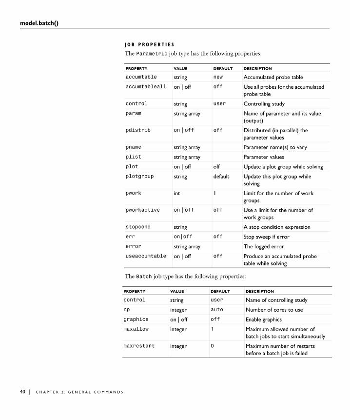
J O B P R O P E R T I E S
The Parametric job type has the following properties:
The Batch job type has the following properties:
PROPERTY VALUE DEFAULT DESCRIPTION
accumtable string new Accumulated probe table
accumtableall on | off off Use all probes for the accumulated probe table
control string user Controlling study
param string array Name of parameter and its value (output)
pdistrib on | off off Distributed (in parallel) the parameter values
pname string array Parameter name(s) to vary
plist string array Parameter values
plot on | off off Update a plot group while solving
plotgroup string default Update this plot group while solving
pwork int 1 Limit for the number of work groups
pworkactive on | off off Use a limit for the number of work groups
stopcond string A stop condition expression
err on|off off Stop sweep if error
error string array The logged error
useaccumtable on | off off Produce an accumulated probe table while solving
PROPERTY VALUE DEFAULT DESCRIPTION
control string user Name of controlling study
np integer auto Number of cores to use
graphics on | off off Enable graphics
maxallow integer 1 Maximum allowed number of batch jobs to start simultaneously
maxrestart integer 0 Maximum number of restarts before a batch job is failed
R 2 : G E N E R A L C O M M A N D S

model.batch()
maxalive integer 300 Maximum number of seconds before the batch job must say it is running
starttime now | 0 | 1 | 2 | 3 | 4 | 5 | 6 | 7 | 8 | 9 | 10 | 11 | 12 | 13 | 14 | 15 | 16 | 17 | 18 | 19 | 20 | 21 | 22 | 23
now The time when the batch job should start
batchdir string home directory
The directory to store files used by the batch job
client on | off off Run the batch job as client
port integer 2036 The host port number
host string localhost Name of host
batchfile string batchmodel.mph
Name of batch model file
clear on | off on Clear the previous model file
clearmesh on | off off Clear meshes before saving model
clearsolution on | off off Clear solutions before saving model
savefile on | off on Save model after run
specbatchdir on | off off Specify different directory for batch process than used by the current process
rundir string home directory
The directory used by the batch job when specbatchdir is on
speccomsoldir on | off off Specify different directory for the COMSOL installation than used by the current process
comsoldir string COMSOL installation directory
The COMSOL installation directory used by the batch job when speccomsoldir is on
synchsolutions
on | off off Synchronize solutions after batch job finishes
PROPERTY VALUE DEFAULT DESCRIPTION
41

model.batch()
42 | C H A P T E
The Cluster job type has the following properties:
synchaccumprobetable
on | off off Synchronize accumulated probe tables after batch job finishes
probesel all | none | manual
all The probes to compute
probes string array Probes to compute
useaccumtable on | off off Use the accumulated probe table
accumtable string new Name of table to use
accumtableall on | off on Use all probes
client on | off off Run as client
host string localhost Name of server
port integer Server port number
PROPERTY VALUE DEFAULT DESCRIPTION
clustertype general | whpc2008 | wccs2003 | sge | none
general The type of cluster job
control string user Name of controlling study
nn integer 1 Number of processes to start
sgenn integer 1 Number of slots in SGE
precmd string DOS/Linux command to execute prior to the batch job
postcmd string DOS/Linux command to execute after the batch job finished
mpd on | off off If an mpd is running on the computer or not
perhost integer 1 Number of processes / host
hostfile string Path to hostfile
mpirsh string Path to rsh or ssh
sgequeue string Name of SGE queue
exclusive on|off on Demand exclusive right to nodes on wccs2003 and whpc2008
schedule string localhost Name of the scheduler on wccs2003 and whpc2008
PROPERTY VALUE DEFAULT DESCRIPTION
R 2 : G E N E R A L C O M M A N D S

model.batch()
TA S K S
model.batch(<tag>).feature().create(<ttag>,tasktype); creates a task of type tasktype tagged <ttag>. Find options for tasktype in Table 2-3 below.
nodegran node | socket| core
node Node granularity on whpc2008
sgegran host | slot | manual
host Node granularity on SGE
reqnodes string array Requested nodes on wccs2003 and whpc2008
corespernode integer 0 Minimum number of cores per node on wccs2003 and whpc2008
memorypernode integer 0 Minimum amount of memory per node on wccs2003 and whpc2008
runtime DD:HH:MM | Infinite
Infinite Maximum time to run before stopping on wccs2003 and whpc2008
user string User name on wccs2003 and whpc2008
priority Highest | AboveNormal | Normal | BelowNormal | Lowest
Normal Priority of job on wccs2003 and whpc2008
sgepriority integer 0 Priority of job on SGE
batch string Tag of batch job to run
TABLE 2-3: BATCH TASK TYPE OPTIONS
TASK TYPE DESCRIPTION
Geomseq A geometry sequence to build
Meshseq A mesh sequence to build
Solutionseq A solver sequence to compute
Jobseq A job sequence to run
Postseq A post sequence to run
Numericalseq A numerical results seq to run
Exportseq An export sequence to run
Save Saves the state of the model at this point in the job sequence
PROPERTY VALUE DEFAULT DESCRIPTION
43

model.batch()
44 | C H A P T E
TA S K TY P E P R O P E R T I E S
model.batch(<tag>).feature(<ttag>).set(ttprop,<tpvalue>) sets the task type property ttprop to the value <tpvalue>.
Task type properties can have the values listed in Table 2-4.
T H E D A T A T A S K TY P E
The Data task type contains child nodes with process information of type Process; see Table 2-5.
Class Runs the main function of a compiled class with the system property cs.currentmodel set to the name of the model calling the class
Data Created by batch jobs to store external process information
TABLE 2-4: TASK TYPE PROPERTY VALUES
PROPERTY VALUE DEFAULT DESCRIPTION
clear on | off on Clear the currently stored data
filename string Name of file to store or open
openfile string array none Name of file that was saved
param string array Name of parameter and its value
files string array Name of files for each parameter
input string array Input to class file
seq string all Name of sequence to run
num string array Name of numerical result feature that generated value
paramvalue string array Computed numerical result
store on | off off Copy solution
psol string none Tag of solver sequence where solutions are stored
TABLE 2-5: DATA CHILD NODES
TASKTYPE DESCRIPTION
Process Contains information about running processes
TABLE 2-3: BATCH TASK TYPE OPTIONS
TASK TYPE DESCRIPTION
R 2 : G E N E R A L C O M M A N D S

model.batch()
model.batch(<tag>).feature(<ttag>).feature(<ptag>).set(ptype, <pvalue>) sets the property ptype to the value <pvalue>. ptype can have the values listed in Table 2-6
Example Create a parametric sweep over a geometry sequence that creates a batch job that runs a parametric sweep that runs a solver.
Model model = ModelUtil.create("Model");model.batch().create("sweep1","Parametric");model.batch("sweep1").set("pname","a");model.batch("sweep1").set("plist",new double[]{1,2});model.batch("sweep1").feature().create("sol","Solutionseq");model.batch("sweep1").feature("sol").set("seq","sol3");model.batch().create("batch1","Batch");model.batch("batch1").feature().create("task","Jobseq");model.batch("batch1").feature("task").set("seq","sweep1");model.batch().create("sweep2","Parametric");model.batch("sweep2").set("pname","b");model.batch("sweep2").set("plist",new double[]{1,2,3});model.batch("sweep2").feature().create("gtask","Geomseq");model.batch("sweep2").feature("gtask").set("seq","geom1");model.batch("sweep2").feature().create("task","Jobseq");model.batch("sweep2").feature("task").set("seq","batch1");model.batch("sweep2").run();
Determine the parameter names and values from a parametric sweep that has already been run.
model.batch(pname).feature(fname).getString('psol')
where pname is the name of the parametric sweep feature that ran and fname is the name of the solution feature that stored the solutions. Use
TABLE 2-6: PTYPE PROPERTY VALUES
PROPERTY VALUE DEFAULT DESCRIPTION
cmd string The command that started the external process
filename string Name of file where model is stored
operation update | progress | cancel | stop | clear | rerun
update Name of operation to perform on the process
status string Current status of the process
45

model.batch()
46 | C H A P T E
model.sol(sname).feature().tags()
to find out the tags of the stored solutions. Use
model.sol(sname).feature(fname).getString('sol')
to find the solver sequence for a parameter. Use
model.sol(sname).getParamNames()
and
model.sol(sname).getParamVals()
See Also model.sol(), model.study()
R 2 : G E N E R A L C O M M A N D S

model.capeopen()
model.capeopen()Purpose Manipulate Cape-Open settings.
Syntax model.capeopen().create(<tag>)model.capeopen().feature().create(<tag>)model.capeopen().feature(<tag>).set(prop,value)
Description model.capeopen().create(<tag>) creates a Cape-Open entity.
model.capeopen().feature().create(<cotag>) creates a Cape-Open feature.
model.capeopen().feature(<tag>).set(prop,<value>) sets property prop to value <value>.
See Also model.func()
47

model.coeff()
48 | C H A P T E
model.coeff()Purpose Manipulate coefficient form contributions.
Syntax model.coeff().create(<tag>,<fields>);model.coeff(<tag>).field(<fields>);model.coeff(<tag>).field(<pos>,<fields>);model.coeff(<tag>).intRule(<irlist>);model.coeff(<tag>).intRule(<pos>,<irule>);model.coeff(<tag>).feature().create(<ftag>);model.coeff(<tag>).feature(<ftag>).set(ctype,<cvalue>);model.coeff(<tag>).feature(<ftag>).selection().named(<seltag>);model.coeff(<tag>).feature(<ftag>).selection().set(...);
model.coeff(<tag>).field();model.coeff(<tag>).intRule();model.coeff(<tag>).feature(<ftag>).getType(ctype);model.coeff(<tag>).feature(<ftag>).selection().named();model.coeff(<tag>).feature(<ftag>).selection().getType();
Description model.coeff(<tag>) is coefficient form entity with tag <tag>.
model.coeff().create(<tag>,<fields>) creates a new coefficient form entity using the fields <fields>. The field tags refer to the fields defined by the model.field() entity. The shape entities referred to by the fields are internally also used to find the derivatives of the field variables if converting the coefficient features to weak form. By default, all coefficients are designed to be non-contributing to the equation under consideration. For example, model.coeff().create("foo",new String[]{"u","v"}).
model.coeff(<tag>).field(<fields>) sets the coefficient form field variables. <fields> is a string with a field tag or a vector of field tags, for example new String[]{"u","v"}. Reassigning the fields has the side effect that the size of the coefficients change if the number of field variables changes.
model.coeff(<tag>).field(<pos>,<fields>) edits the field at position <pos> in the field vector <fields>.
model.coeff(<tag>).intRule(<irlist>) assigns integration rules to the coefficient form entity. The list must have the same length as the number of field variables defined by the fields, or have length 1. In the latter case all equations use the same integration rule. The number of field variables is not necessarily the same as the number of strings specified in model.coeff(<tag>).field().
model.coeff(<tag>).intRule(<pos>,<irule>) edits the integration rule at position <pos> in the vector <irule>.
R 2 : G E N E R A L C O M M A N D S

model.coeff()
model.coeff(<tag>).feature(<ftag>) is a coefficient form feature with tag <ftag> in the coefficient form entity with tag <tag>.
model.coeff(<tag>).feature().create(<ftag>) creates a new coefficient form feature with tag <ftag>.
model.coeff(<tag>).feature(<ftag>).set(ctype,<cvalue>) sets the value of the coefficient of type ctype to <value>. All string data types that are listed in Table 2-2 are supported; which argument types are applicable depends on the coefficient. ctype is one of c, al, ga, be, a, f, da, ea, q, and g. These coefficients are available at all dimensions. In addition at level edim==sdim-1, the coefficients q and g are allowed, corresponding to a and f respectively. All coefficients have a default 0 contribution.
model.coeff(<tag>).feature(<ftag>).selection().named(<seltag>) or, alternatively model.coeff(<tag>).feature(<ftag>).selection().set(...) assigns the coefficient form contribution to geometric entities. For a complete list of methods available under selection(), see model.selection(). Only selections at a single geometry level is allowed in the selection.
model.coeff(<tag>).field() returns the fields as a string array.
model.coeff(<tag>).intRule() returns the integration rule tags as a string array.
model.coeff(<tag>).feature(<ftag>).getType(ctype) returns the coefficient value. See the section getType() for available methods.
model.coeff(<tag>).feature(<ftag>).selection().named() returns the selection tag as a string.
model.coeff(<tag>).feature(<ftag>).selection().getType() returns domain information. See model.selection() for available methods.
Example Define two uncoupled Poisson-like equations on the domain dtag.
model.coeff().create("c1",new String[]{"u","v"});model.coeff("c1").intRule(new String[]{"gp1","gp1"});CoeffFeature f1 = model.coeff("c1").feature().create("f1");f1.set("c",1,new String[]{"1","0.1","2"});f1.set("c",2,"3");f1.set("f",new String[]{"2","1"});f1.selection().geom("g1",2);f1.selection().set(new int[]{1});
See Also model.shape(), model.weak()
49

model.constr()
50 | C H A P T E
model.constr()Purpose Manipulate constraints.
Syntax model.constr().create(<tag>,<shtags>);model.constr(<tag>).shape(<shtags>);model.constr(<tag>).shape(<pos>,<shtags>);model.constr(<tag>).feature().create(<ftag>);model.constr(<tag>).feature(<ftag>).set(ctype,<value>);model.constr(<tag>).feature(<ftag>).selection().named(<seltag>);model.constr(<tag>).feature(<ftag>).selection().set(...);
model.constr(<tag>).shape();model.constr(<tag>).feature(<ftag>).getType(ctype);model.constr(<tag>).feature(<ftag>).selection().named();model.constr(<tag>).feature(<ftag>).selection().getType();
Description model.constr(<tag>) is a constraint entity with tag <tag>.
model.constr().create(<tag>,<shtags>) creates a constraint entity with tag <tag> using the shape functions <shtags>.
model.constr(<tag>).shape(<shtags>) points to the shape functions associated with the constraint object. Reassigning the shape functions can have the side effect of modifying the constraints since the number of constraints can change as the size of each constraint vector can change.
model.constr(<tag>).feature(<ftag>) is a feature in the constraint object <tag>.
model.constr(<tag>).feature().create(<ftag>) creates a constraint feature.
model.constr(<tag>).feature(<ftag>).set(ctype,<value>) sets the parameter ctype to <value>, where ctype is either constr or constrf, and <value> is a single constraint expression or a list of constraint expressions. The number of elements in the constraint expression depends on the shape function. A Lagrange shape function requires a single item, whereas a vector shape function requires one item for each space dimension. The supported set methods are the ones for double string arrays defined in Table 2-2.
model.constr(<tag>).feature(<ftag>).selection().named(<seltag>)
assigns the constraint to the selection <seltag>. Only selections at a single geometry level is allowed in the selection.
model.constr(<tag>).shape() returns the shape function tags as a string array.
R 2 : G E N E R A L C O M M A N D S

model.constr()
model.constr(<tag>).feature(<ftag>).getType(ctype) returns the constraint or constraint force value. For available methods, see getType().
model.constr(<tag>).feature(<ftag>).selection().named() returns the selection tag as a string.
model.constr(<tag>).feature(<ftag>).selection().getType() returns domain information. For available methods, see Selections.
Examples Set several constraint by using multiple constr entities:
Model model = ModelUtil.create("Model");model.constr().create("c1",new String[]{"shu","shv"});ConstrFeature f = model.constr("c1").feature().create("f1");f.set("constr",new String[]{"u-1","v"});f.selection().geom("geom1",1);f.selection().all();
Vector elements need a set of constraints:
Model model = ModelUtil.create("Model");model.constr().create("c2",new String[]{"shE"});ConstrFeature f = model.constr("c2").feature().create("f1");f.set("constr",new String[]{"Ex-1","Ey-0","Ez-0"});f.selection().geom("geom1",1);f.selection().all();
See Also model.shape()
51

model.coordSystem()
52 | C H A P T E
model.coordSystem()Purpose Manipulate coordinate systems.
Syntax model.coordSystem().create(<tag>,<gtag>,type);model.coordSystem(<tag>).set(property, <value>);model.coordSystem(<tag>).setIndex(property, <value>, row);model.coordSystem(<tag>).setIndex(property, <value>, row, col);
model.coordSystem(<tag>).coord()model.coordSystem(<tag>).isOrthonormal()model.coordSystem(<tag>).isLinear()
Description model.coordSystem().create(<tag>,<gtag>,type) creates a coordinate system with tag <tag> on geometry <gtag> of type type. There are currently five types of systems, mapped system (Mapping), base-vector system (VectorBase), rotated system (Rotated), boundary system (Boundary), and cylindrical system
(Cylindrical). The boundary system only applies to boundaries.
model.coordSystem(<tag>).set("orthonormal","on") specifies that this is a orthonormal system. This affects the internal calculation of systems, so some simplifications on expressions can be made. It is recommended to use this option when possible. Boundary systems, rotated systems, and cylindrical system are always orthonormal.
M A P P E D S Y S T E M
model.coordSystem().create(<tag1>,<gtag>,"Mapping") creates a mapped system. In a mapped system you specify the coordinate mapping given in some of the available frame coordinates (usually x, y, z).
model.coordSystem(<tag1>).setIndex("map", "x+1", 0) sets the mapping of the first coordinate system coordinate to be a function of the first frame coordinate, x.
TABLE 2-7: PROPERTIES FOR MAPPING SYSTEM
PROPERTY VALUE DEFAULT DESCRIPTION
coord String matrix [(x1,x2,x3)] Coordinate names
map String array (x,y,z) The map
orthonormal String (on | off) off If the system is orthonormal
frametype String (mesh | material | spatial)
spatial The frame type
R 2 : G E N E R A L C O M M A N D S

model.coordSystem()
model.coordSystem(<tag1>).setIndex("map", "y+1", 2) sets the mapping of the third coordinate system coordinate to be a function of the second frame coordinate y.
B A S E VE C T O R S Y S T E M
model.coordSystem().create(<tag2>,"VectorBase") creates a base-vector system. In a base-vector system you specify the base vectors given in components of a frame system. If the components are independent of frame coordinates this is a linear system and can be applied for any frame.
model.coordSystem(<tag2>).setIndex("base", "1", 0, 1) sets the first base vector’s second component to one. As an alternative, it is possible to specify the full base-vector matrix using the following syntax:
model.coordSystem(<tag2>).set("base",
new String[][]{{"0","1","0"},{"0","0","1"},{"1","0","0"}}) sets the base vector matrix so the first base vector is equal to the y-axis of the frame system, the second is the z-axis, and so on. In 2D, you only use a two rows and two columns from the full base vector matrix for the in plane base vectors. As an option, it is therefore possible to specify which of the coordinate system base vectors that corresponds to the out-of-plane axis in the frame system. Internally, this base vector always gets the components {"0","0","1"}. The third column is also set using these components. To make a general 3D system in 2D, you have to use the mapped system.
model.coordSystem(<tag2>).set("outofplane", "2") sets the third base vector to represent the out-of-plane vector (z-axis in 2D). The value is zero based. In 1D the out-of-plane index is set using the syntax “1,2” to set second and third base vectors to represent the out-of-plane vector.
TABLE 2-8: PROPERTIES FOR BASE VECTOR SYSTEM
PROPERTY VALUE DEFAULT DESCRIPTION
coord String matrix [(x1,x2,x3)] Coordinate names
base String matrix [(1,0,0)(0,1,0)(0,0,1)]
Base vectors
orthonormal String (on | off) off If the system is orthonormal or not
outofplane String “2” in 2D, “1,2” in 1D
Out of plane index
53

model.coordSystem()
54 | C H A P T E
R O T A T E D S Y S T E M
model.coordSystem().create(<tag3>,"Rotated") creates a rotated system. In 3D you specify the Z-X-Z Euler angles, which corresponds to sequential rotation first about the z-axis, then the x-axis, and finally the z-axis again. In 2D you can only rotate about the out-of-plane axis.
model.coordSystem(<tag3>).setIndex("angle","12[deg]",0) sets the first rotation about the z-axis to 12 degrees. The default unit for angles are radians.
B O U N D A R Y S Y S T E M
model.coordSystem().create(<tag4>,<gtag>,"Boundary") creates a new boundary system. There is always one boundary system added by default for each geometry.
TABLE 2-9: PROPERTIES FOR ROTATED SYSTEM
PROPERTY VALUE DEFAULT DESCRIPTION
coord String matrix [(x1,x2,x3)] Coordinate names
angle String array (0,0,0) Rotation angles
outofplane String “2” in 2D, “1,2” in 1D
Out of plane index
TABLE 2-10: PROPERTIES FOR BOUNDARY SYSTEM
PROPERTY VALUE DEFAULT DESCRIPTION
coord String matrix [(x1,x2,x3)] Coordinate names
frametype String (mesh | material | spatial)
spatial Frame type
reversenormal String (on | off) off Reverse normal direction
tangent String array Tangent direction
mastersystem String (manual | globalCartesian | <tag>)
globalCartesian Which system to create first tangential direction from
mastercoordsyscomp
String “2” in axisymmetry, “3” otherwise
Which axis to create first tangential direction from
R 2 : G E N E R A L C O M M A N D S

model.coordSystem()
model.coordSystem(<tag4>).set("reversenormal","on") flips the normal direction for this system, so it is opposite to the normal direction given by the geometry.
model.coordSystem(<tag4>).set("mastersystcomp","2") sets the first tangential direction from the second axis of the specified master system.
model.coordSystem(<tag4>).set("mastersystem","manual") specifies that no master system is used and that the tangential direction must be entered by the user.
model.coordSystem(<tag4>).setIndex("tangent","1") sets the first component of the first tangential direction.
C Y L I N D R I C A L S Y S T E M
model.coordSystem().create(<tag5>,<gtag>,"Cylindrical") creates a cylindrical system. You can specify the origin, axis direction and radial base vector.
model.coordSystem(<tag5>).set("origin", new String[]{"1",”0”,”0”}) sets the origin to (1,0,0).
TABLE 2-11: PROPERTIES FOR CYLINDRICAL SYSTEM
PROPERTY VALUE DEFAULT DESCRIPTION
coord String matrix [(r, phi, a)] Coordinate names
origin String array (0,0,0) Origin of system
axis String array (0,0,1) Axis direction
radialbasevector
String array (1,0,0) Radial base vector direction a j=0
55

model.cpl()
56 | C H A P T E
model.cpl()Purpose Manipulate coupling operators.
Syntax model.cpl().create(<tag>,type,<gtag>);model.cpl(<tag>).selection().named(<seltag>);model.cpl(<tag>).selection().set(...);model.cpl(<tag>).set(property,<value>);model.cpl(<tag>).set("opname",<opname>)model.cpl(<tag>).selection(property).named(<seltag>);model.cpl(<tag>).selection(property).set(...);model.cpl(<tag>).feature().create(<subtag>,subtype);model.cpl(<tag>).feature(<subtag>).set(property,<value>);model.cpl(<tag>).feature(<subtag>).selection().named(<seltag>);model.cpl(<tag>).feature(<subtag>).selection().set(...);model.cpl(<tag>).feature(<subtag>).selection(property). named(<seltag>);model.cpl(<tag>).feature(<subtag>).selection(property).set(...);
model.cpl(<tag>).selection().named();model.cpl(<tag>).selection().getType(...);model.cpl(<tag>).properties();model.cpl(<tag>).getType(property,<value>);model.cpl(<tag>).selection(property).named();model.cpl(<tag>).selection(property).getType(...);model.cpl(<tag>).feature(<subtag>).selection().named();model.cpl(<tag>).feature(<subtag>).selection().getType(...);model.cpl(<tag>).feature(<subtag>).properties();model.cpl(<tag>).feature(<subtag>).getType(property,<value>);
Description model.cpl().create(<tag>,type,<gtag>) creates a coupling operator entity of type type on the geometry <gtag>. The supported types are GeneralExtrusion, LinearExtrusion, BoundarySimilarity, IdentityMapping, GeneralProjection, LinearProjection, Integration, Average, Maximum, and Minimum.
model.cpl(<tag>).selection().named(<seltag>) or, alternatively, model.cpl(<tag>).selection().set(...) specifies source geometric entities for all types of coupling operators. For a complete list of methods available under selection(), see Selections.
model.cpl(<tag>).set(property,<value>) specifies properties relevant for the selected coupling operator type, see below.
model.cpl(<tag>).set("opname",<opname>) sets the operator name of the coupling operator. The default operator name is <tag>.
model.cpl(<tag>).selection(property).named(<seltag>) or, alternatively, model.cpl(<tag>).selection(property).set(...) specifies the entities in a
R 2 : G E N E R A L C O M M A N D S

model.cpl()
selection property for certain types of coupling operators. For a complete list of methods available under selection(property), see Selections.
model.cpl(<tag>).feature().create(<subtag>,subtype) creates a sub feature of type subtype. This can only be done when type is BoundarySimilarity.
model.cpl(<tag>).selection().named() returns the source selection of the coupling.
model.cpl(<tag>).selection().getType(...) queries the source selection.
model.cpl(<tag>).properties() returns the list of assigned properties as a string array.
model.cpl(<tag>).getType(property) returns the value of a specified property.
model.cpl(<tag>).selection(property).named() returns the tag of a selection property.
model.cpl(<tag>).selection(property).getType(...) queries a selection property.
Notation: srcedim = dimension of source selection, srcsdim = space dimension of source geometry.
Extrusion Coupling Operators
An extrusion coupling operator oper maps an expression e defined on (a part of) the source selection to an expression oper(e) that can be evaluated on (a part of) the destination geometry/geometries. For each point ps in the source selection, there can be zero, one or several corresponding points pd in the destination. The inverse mapping psm(pd) is always one-to-one. The value of oper(e) at the point pd is defined as the value of e at the point ps.
The inverse mapping m is specified as the composition of a destination map md and the inverse of a source map ms: psm(pd)ms
1(md(pd)). In other words, ms(ps)md(pd)—both the destination map and the source map into the same intermediate space. For all operator types except GeneralExtrusion, the intermediate space coincides with the source geometry. The source map is always one-to-one. By default, the source map is the identity.
57
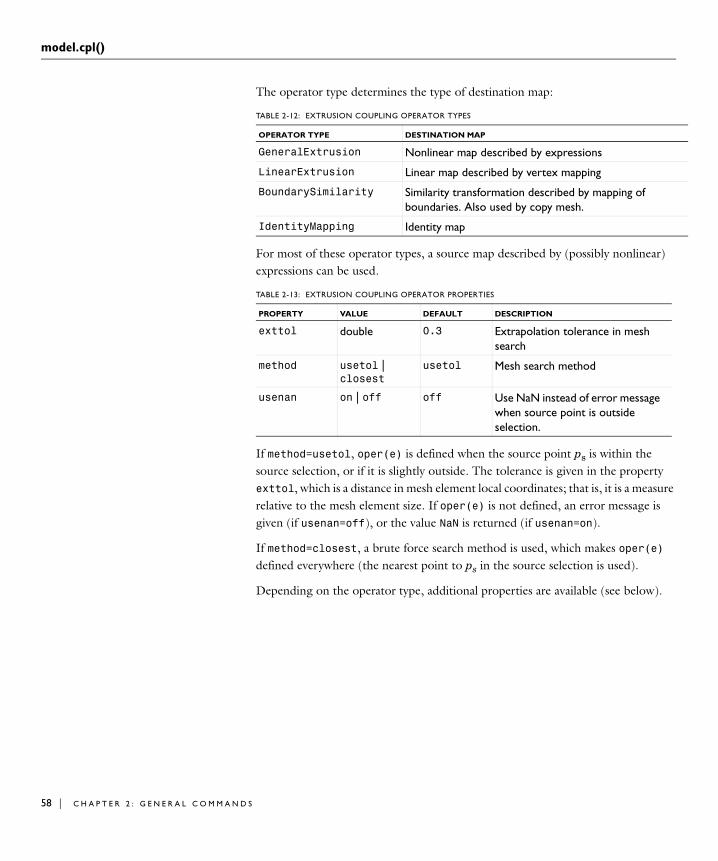
model.cpl()
58 | C H A P T E
The operator type determines the type of destination map:
For most of these operator types, a source map described by (possibly nonlinear) expressions can be used.
If method=usetol, oper(e) is defined when the source point ps is within the source selection, or if it is slightly outside. The tolerance is given in the property exttol, which is a distance in mesh element local coordinates; that is, it is a measure relative to the mesh element size. If oper(e) is not defined, an error message is given (if usenan=off), or the value NaN is returned (if usenan=on).
If method=closest, a brute force search method is used, which makes oper(e) defined everywhere (the nearest point to ps in the source selection is used).
Depending on the operator type, additional properties are available (see below).
TABLE 2-12: EXTRUSION COUPLING OPERATOR TYPES
OPERATOR TYPE DESTINATION MAP
GeneralExtrusion Nonlinear map described by expressions
LinearExtrusion Linear map described by vertex mapping
BoundarySimilarity Similarity transformation described by mapping of boundaries. Also used by copy mesh.
IdentityMapping Identity map
TABLE 2-13: EXTRUSION COUPLING OPERATOR PROPERTIES
PROPERTY VALUE DEFAULT DESCRIPTION
exttol double 0.3 Extrapolation tolerance in mesh search
method usetol | closest
usetol Mesh search method
usenan on | off off Use NaN instead of error message when source point is outside selection.
R 2 : G E N E R A L C O M M A N D S
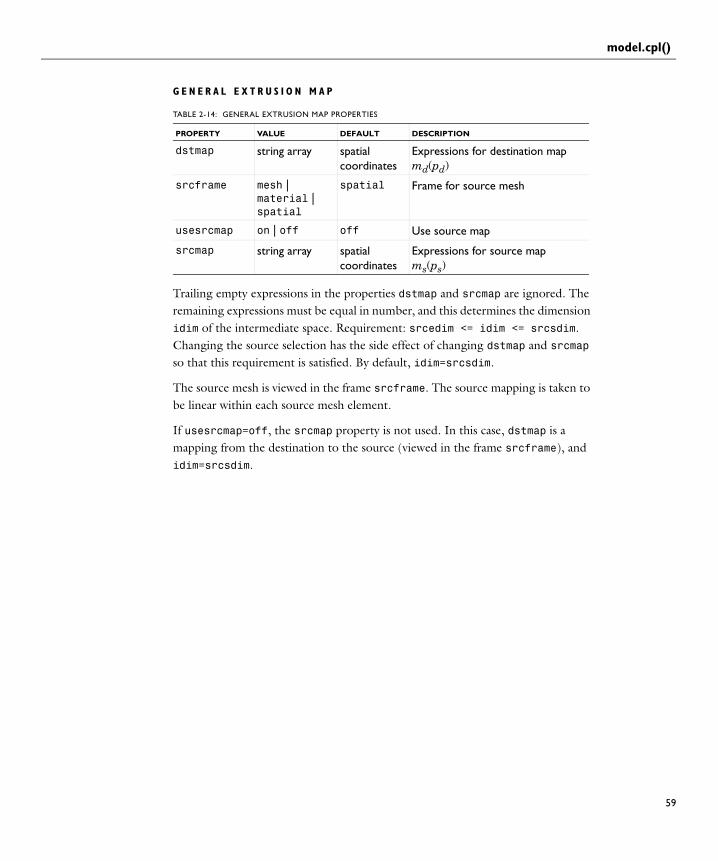
model.cpl()
G E N E R A L E X T R U S I O N M A P
Trailing empty expressions in the properties dstmap and srcmap are ignored. The remaining expressions must be equal in number, and this determines the dimension idim of the intermediate space. Requirement: srcedim <= idim <= srcsdim. Changing the source selection has the side effect of changing dstmap and srcmap so that this requirement is satisfied. By default, idim=srcsdim.
The source mesh is viewed in the frame srcframe. The source mapping is taken to be linear within each source mesh element.
If usesrcmap=off, the srcmap property is not used. In this case, dstmap is a mapping from the destination to the source (viewed in the frame srcframe), and idim=srcsdim.
TABLE 2-14: GENERAL EXTRUSION MAP PROPERTIES
PROPERTY VALUE DEFAULT DESCRIPTION
dstmap string array spatial coordinates
Expressions for destination map md(pd)
srcframe mesh | material | spatial
spatial Frame for source mesh
usesrcmap on | off off Use source map
srcmap string array spatial coordinates
Expressions for source map ms(ps)
59

model.cpl()
60 | C H A P T E
L I N E A R E X T R U S I O N M A P
The number of selections srcvertexN and dstvertexN is 4. These are used only for 1<=N<=dim+1, where dim is a number less than or equal to min(srcsdim,dstsdim). The remaining 4-dim selections should be empty.
The destination map is the following linear (affine) map from the destination geometry to the source geometry:
1 First, if dim<dstsdim, an orthogonal projection onto the affine space spanned by the destination vertices. The number of destination vertices is dim+1. Thus, dim=2 gives a plane, and dim=1 gives a line.
2 Then, a linear (affine) map mapping the destination vertices onto the source vertices.
B O U N D A R Y S I M I L A R I T Y ( 3 D )
The destination transformation is a similarity transformation that maps a destination face (destination) onto a set of source faces (the source selection). The mesh is always viewed in the mesh frame.
TABLE 2-15: LINEAR EXTRUSION MAP PROPERTIES
PROPERTY VALUE DEFAULT DESCRIPTION
srcvertexN Selection Source vertex number N
dstgeom String source geometry
Destination geometry
dstvertexN Selection Destination vertex number N
srcframe mesh | material | spatial
spatial Frame for evaluation of source vertex coordinates
dstframe mesh | material | spatial
spatial Frame for evaluation of destination vertex coordinates
usesrcmap on | off off Use source map
srcmap String[srcsdim] spatial coordinates
Expressions for source map ms(ps)
TABLE 2-16: BOUNDARY SIMILARITY PROPERTIES IN 3D
PROPERTY VALUE DEFAULT DESCRIPTION
destination Selection Destination face
usesrcmap on | off off Use source map
srcmap String[srcsdim] spatial coordinates
Expressions for source map ms(ps).
R 2 : G E N E R A L C O M M A N D S

model.cpl()
By default, the algorithm automatically chooses a transformation when symmetries make several transformations possible. To control this choice, one of the following subfeatures can be added.
EdgeMap SubfeatureYou specify that a certain destination edge should be mapped onto a certain source edge. Their relative direction is given by the property direction. The edges must be adjacent to the given faces.
OnePointMap SubfeatureYou specify that a certain destination vertex should be mapped onto a certain source vertex.
TwoPointMap SubfeatureYou specify that two destination vertices should be mapped onto two source vertices.
TABLE 2-17: SUBFEATURE TYPES
SUB FEATURE REMARKS
EdgeMap Specify how one source edge is mapped.
OnePointMap Specify how one source vertex is mapped.
TwoPointMap Specify how two source vertices are mapped.
TABLE 2-18: PROPERTIES FOR EDGEMAP SUBFEATURE
PROPERTY VALUE DEFAULT DESCRIPTION
srcedge Selection Source edge
dstedge Selection Destination edge
direction auto | same | opposite
auto Edge direction
TABLE 2-19: PROPERTIES FOR ONEPOINTMAP SUBFEATURE
PROPERTY VALUE DEFAULT DESCRIPTION
srcpoint1 Selection Vertex on source face
dstpoint1 Selection Vertex on destination face
TABLE 2-20: PROPERTIES FOR ONEPOINTMAP SUBFEATURE
PROPERTY VALUE DEFAULT DESCRIPTION
srcpoint1 Selection Vertex 1 on source face
srcpoint2 Selection Vertex 2 on source face
61

model.cpl()
62 | C H A P T E
B O U N D A R Y S I M I L A R I T Y ( 2 D )
The destination transformation is a similarity transformation that maps a destination edge (destination) onto a set of source edges (the source selection). Their relative direction is given by the property direction. The mesh is always viewed in the mesh frame.
I D E N T I T Y M A P
The destination transformation is an identity mapping between the given frames.
Projection Coupling Operators
A projection coupling operator oper maps an expression e defined on (a part of) the source selection to an expression oper(e) that can be evaluated on (a part of) the destination geometries. It does so by performing integration along curves in the source selection. These curves correspond to lines in an intermediate space, whose dimension is equal to srcedim. There is a source map ms mapping the source selection into the intermediate space, and a destination map md mapping the
dstpoint1 Selection Vertex 1 on destination face
dstpoint2 Selection Vertex 2 on destination face
TABLE 2-21: BOUNDARY SIMILARITY PROPERTIES IN 2D
PROPERTY VALUE DEFAULT DESCRIPTION
destination Selection Destination edge
direction auto | same | opposite
auto Edge direction
usesrcmap on | off off Use source map
srcmap String[srcsdim] spatial coordinates
Expressions for source map ms(ps)
TABLE 2-22: NORMAL EXTRUSION MAP PROPERTIES
PROPERTY VALUE DEFAULT DESCRIPTION
dstframe mesh | material | spatial
spatial Frame for evaluation of destination coordinates
srcframe mesh | material | spatial
spatial Frame for evaluation of source coordinates
TABLE 2-20: PROPERTIES FOR ONEPOINTMAP SUBFEATURE
PROPERTY VALUE DEFAULT DESCRIPTION
R 2 : G E N E R A L C O M M A N D S

model.cpl()
destination geometries into the subspace of intermediate space where the last coordinate is zero. The source map is always one-to-one. The value of oper(e) at a destination point pd is defined as follows:
1 In the intermediate space, consider the line that is parallel to the last coordinate axis, and goes through the point md(pd).
2 Map this line to a curve in the source selection using the inverse of the source map.
3 Integrate the expression e over this curve.
This implies that the value of oper(e) at the destination point pd is the integral of e along a curve through the source point ps = ms
1(md(pd)).
The operator type determines the type of the maps:
Additional properties are available depending on the operator type, see below.
G E N E R A L P R O J E C T I O N M A P
L I N E A R P R O J E C T I O N M A P
The mapping between destination and source is given by a linear map defined by vertices. Let v be the vector from the first source vertex to the last source vertex.
TABLE 2-23: PROJECTION COUPLING OPERATOR TYPES
OPERATOR TYPE MAP TYPES
GeneralProjection Nonlinear map described by expressions
LinearProjection Linear map described by vertex mapping
TABLE 2-24: PROJECTION COUPLING OPERATOR PROPERTIES
PROPERTY VALUE DEFAULT DESCRIPTION
intorder int 4 Order of integration formula
TABLE 2-25: GENERAL PROJECTION COUPLING OPERATOR PROPERTIES
PROPERTY VALUE DEFAULT DESCRIPTION
dstmap String[srcedim-1] spatial coordinates
Expressions for destination map md(pd)
srcframe mesh | material | spatial
spatial Frame for source mesh.
srcmap String[srcedim] spatial coordinates
Expressions for source map ms(ps)
63

model.cpl()
64 | C H A P T E
The value of oper(e) at a point pd is equal to the integral of e over the line through the point ps=ms
-1(md(pd)) with direction vector v.
The number of selections srcvertexN is 4. These are used only for 1<=N<=srcedim+1. The remaining selections should be empty. The number of source vertices is srcedim+1. The source map is a linear (affine) map that maps the source vertices onto the points 0, e1, e2,..., esrcedim in the intermediate space, where ei is the ith unit vector.
The number of selections dstvertexN is 4. These are used only for 1<=N<=srcedim. The remaining selections should be empty. The number of destination vertices is srcedim. The destination map is the following linear (affine) map from the destination geometry to the intermediate space:
1 First, if srcedim-1<dstsdim, an orthogonal projection onto the affine space spanned by the destination vertices. Thus, srcedim=3 gives a plane, and srcedim=2 gives a line.
2 Then, a linear (affine) map mapping the destination vertices onto the points 0, e1, e2,..., esrcedim-1 in the intermediate space, where ei is the ith unit vector.
Integration Coupling Operators
By default, an integration coupling operator oper integrates an expression e over the source selection. The resulting value oper(e) can be used anywhere. If
TABLE 2-26: LINEAR PROJECTION COUPLING OPERATOR PROPERTIES
PROPERTY VALUE DEFAULT DESCRIPTION
srcvertexN Selection Source vertex number N
dstgeom String source geometry
Destination geometry
dstvertexN Selection Destination vertex number N
srcframe mesh | material | spatial
spatial Frame for evaluation of source vertex coordinates
dstframe mesh | material | spatial
spatial Frame for evaluation of destination vertex coordinates
R 2 : G E N E R A L C O M M A N D S

model.cpl()
method=summation, the expression is instead summed over the nodes in the source selection.
Average Coupling Operators
An average coupling operator oper integrates an expression e over the source selection, and divides with the measure of the source selection. The resulting value oper(e) can be used anywhere.
Maximum/Minimum Coupling Operators
A maximum or minimum coupling operator oper finds the maximum/minimum of an expression e over the source selection. The resulting value oper(e) can be used anywhere. An optional second argument is evaluated at the point where the first argument has its maximum or minimum. Use x, y, or z, for example, to get the coordinate location of the maximum or minimum.
TABLE 2-27: INTEGRATION COUPLING OPERATOR PROPERTIES
PROPERTY VALUE DEFAULT DESCRIPTION
intorder String 4 Integration order
frame mesh | material | spatial
spatial Frame to integrate in (determines volume element)
method integration | summation
integration Method of computation
TABLE 2-28: AVERAGE COUPLING OPERATOR PROPERTIES
PROPERTY VALUE DEFAULT DESCRIPTION
intorder String 4 Integration order
frame mesh | material | spatial
spatial Frame to integrate in (determines volume element)
TABLE 2-29: MAXIMUM/MINIMUM COUPLING OPERATOR PROPERTIES
PROPERTY VALUE DEFAULT DESCRIPTION
intorder String 4 Integration rule
points node | integration | lagrange
node Type of point
65

model.cpl()
66 | C H A P T E
The maximum/minimum is approximated by evaluating the expression in the specified points.
intorder String 4 Integration order
lagrange String 2 Lagrange order
TABLE 2-29: MAXIMUM/MINIMUM COUPLING OPERATOR PROPERTIES
PROPERTY VALUE DEFAULT DESCRIPTION
R 2 : G E N E R A L C O M M A N D S

model.elem()
model.elem()Purpose Manipulate elements.
Syntax model.elem().create(<tag>,eltype);model.elem(<tag>).set(<ftag>,value);model.elem(<tag>).field().create(<ftag>,"record");model.elem(<tag>).field(<ftag>).set(<ftag>,value);model.elem(<tag>).field().create(<atag>,"array");model.elem(<tag>).field(<atag>).pos().create("string",value);model.elem(<tag>).field(<atag>).pos().create("array");model.elem(<tag>).field(<atag>).pos(pos).create("string",value);model.elem(<tag>).src().create(<fttag>);model.elem(<tag>).src(<fttag>).set(<ftag>,value);model.elem(<tag>).src(<fttag>).selection().named(<stag>);model.elem(<tag>).src(<fttag>).selection().set(...);model.elem(<tag>).src(<fttag>).field().create(<ftag>,"array");model.elem(<tag>).geomdim().create(<fttag>);
Description Externally generated element syntax contributions. These element syntax contributions are also be used by, for example, the far-field feature and the elpric element. The syntax is not specific to a certain type of element but works for all types of elements. As a result, the syntax can be rather lengthy in some cases.
model.elem().create(<tag>,eltype) creates a new element of type eltype, for example elinterp, elpric, elvar, elode, and so on.
model.elem(<tag>).set(<ftag>,value) sets the field tagged <ftag> to value. Examples of fields and values are, file and solution_interp.txt, global and 1, and so on.
model.elem(<tag>).field().create(<ftag>,"record") creates a new field tagged <ftag> of type record under the element tagged <tag>.
model.elem(<tag>).field(<ftag>).set(sname,value) sets the field tagged sname to value. The field is located under the record field tagged <ftag>.
model.elem(<tag>).field(<ftag>).field().create(<rtag>,"record") creates a new record field tagged <rtag> that is a field under the record field <ftag>.
model.elem(<tag>).field().create(<atag>,"array") creates a new array field tagged <atag>.
model.elem(<tag>).field(<atag>).pos().create("array") adds a new element of type array to the array tagged <atag>.
67

model.elem()
68 | C H A P T E
model...field(<atag>).pos(1).pos().create("string","1") adds a new array element of type string with value 1 to the first array element of the array stored in the field <atag>.
In the text below, all occurrences of src can be replaced with geomdim.
model.elem(<tag>).src().create(<fttag>) creates a src feature tagged <fttag> under the element. A feature must have a domain selection.
model.elem(<tag>).src(<fttag>).selection().dim(2).set(gname) assigns all domains of dimension 2 from geometry gname to the selection of feature <fttag>.
model.elem(<tag>).src(<fttag>).set(<ftag>,value) sets the field <ftag> to value under the feature <fttag>.
model.elem(<tag>).src(<fttag>).field().create(rname,"record") adds a new record field rname under the feature <fttag>.
Examples Specifies an interpolation element that takes its data from a file named solution_data.txt.
Model model = ModelUtil.create("Model");model.elem().create("fun1","elinterp");model.elem("fun1").set("name",new String[]{"sol"});model.elem("fun1").set("file","solution_data.txt");model.elem("fun1").set("fileindex",new String[]{"1"});model.elem("fun1").set("defvars",new String[]{"true"});model.elem("fun1").set("method",new String[]{"linear"});model.elem("fun1").set("extmethod",new String[]{"const"});
The example below creates two integration coupling operators.
model.elem().create("elem1","elcplscalar");model.elem("elem1").set("var",new String[]{"aa","bb"});model.elem("elem1").set("global",new String[]{"1","2"});model.elem("elem1").src().create("feat1");model.elem("elem1").src("feat1").selection().geom("g",2).set(new int[]{1});model.elem("elem1").src("feat1").set("expr",new String[][]{{"1"},{"2"}}model.elem("elem1").src("feat1").set("ipoints",new String[][]{{"2"},{"2"}}model.elem("elem1").src("feat1").set("frame",new String[][]{{"spatial"},{"spatial"}};
This complicated example creates a constr element with two constraints (usually done with constraint features).
R 2 : G E N E R A L C O M M A N D S
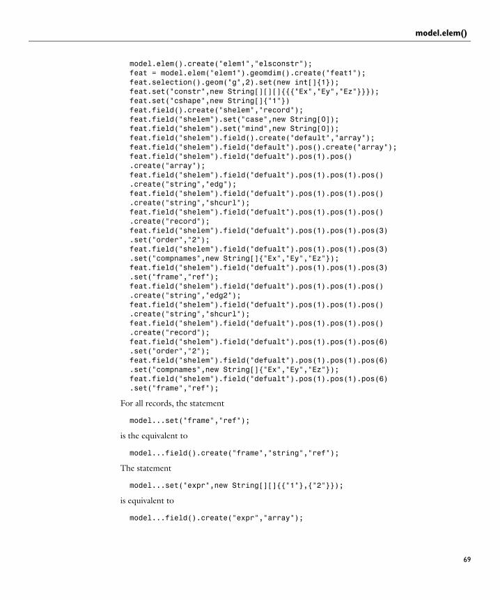
model.elem()
model.elem().create("elem1","elsconstr");feat = model.elem("elem1").geomdim().create("feat1");feat.selection().geom("g",2).set(new int[]{1});feat.set("constr",new String[][][]{{{"Ex","Ey","Ez"}}});feat.set("cshape",new String[]{"1"})feat.field().create("shelem","record");feat.field("shelem").set("case",new String[0]);feat.field("shelem").set("mind",new String[0]);feat.field("shelem").field().create("default","array");feat.field("shelem").field("default").pos().create("array");feat.field("shelem").field("defualt").pos(1).pos().create("array");feat.field("shelem").field("defualt").pos(1).pos(1).pos().create("string","edg");feat.field("shelem").field("defualt").pos(1).pos(1).pos().create("string","shcurl");feat.field("shelem").field("defualt").pos(1).pos(1).pos().create("record");feat.field("shelem").field("defualt").pos(1).pos(1).pos(3).set("order","2");feat.field("shelem").field("defualt").pos(1).pos(1).pos(3).set("compnames",new String[]{"Ex","Ey","Ez"});feat.field("shelem").field("defualt").pos(1).pos(1).pos(3).set("frame","ref");feat.field("shelem").field("defualt").pos(1).pos(1).pos().create("string","edg2");feat.field("shelem").field("defualt").pos(1).pos(1).pos().create("string","shcurl");feat.field("shelem").field("defualt").pos(1).pos(1).pos().create("record");feat.field("shelem").field("defualt").pos(1).pos(1).pos(6).set("order","2");feat.field("shelem").field("defualt").pos(1).pos(1).pos(6).set("compnames",new String[]{"Ex","Ey","Ez"});feat.field("shelem").field("defualt").pos(1).pos(1).pos(6).set("frame","ref");
For all records, the statement
model...set("frame","ref");
is the equivalent to
model...field().create("frame","string","ref");
The statement
model...set("expr",new String[][]{{"1"},{"2"}});
is equivalent to
model...field().create("expr","array");
69

model.elem()
70 | C H A P T E
model...field("expr").pos().create("array").model...field("expr").pos(1).create("string","1");model...field("expr").pos().create("array").model...field("expr").pos(2).create("string","1");
so the set method is often a much more convenient way to create simple fields.
R 2 : G E N E R A L C O M M A N D S

model.event()
model.solverEvent()Purpose Manipulate events.
Syntax model.solverEvent().create(<tag>,evtype);model.solverEvent(<tag>).start(expr);model.solverEvent(<tag>).start();model.solverEvent(<tag>).period(expr);model.solverEvent(<tag>).period();model.solverEvent(<tag>).condition(expr);model.solverEvent(<tag>).condition();model.solverEvent(<tag>).reinit();model.solverEvent(<tag>).reinit().create(<tag>);model.solverEvent(<tag>).reinit(<tag>).set(<var>,expr);
Description Create events and manipulate event settings. There are two types of events; Explicit and Implicit.
model.solverEvent().create(<tag>,evtype) creates a new event of type evtype, either Explicit and Implicit.
E X P L I C I T E V E N T S
Explicit events triggers on a predefined timing.
model.solverEvent(<tag>).start(expr) sets the start time for an explicit event.
model.solverEvent(<tag>).period(expr) sets the period for an explicit event. After the start time, the event then triggers after each period.
I M P L I C I T E V E N T S
Implicit events trigger when a condition goes from false to true.
model.solverEvent(<tag>).condition(expr) sets the condition for an implicit event.
R E - I N I T I A L I Z A T I O N
When an event is triggered, any degree of freedom may be re-initialized. This typically means that they get a new value. You specify these values with a re-initialization entity that has the same syntax as an init entity.
model.solverEvent(<tag>).reinit().create(<tag>) adds a new reinit feature to the event. In most cases you only need one, but you need more when you have re-initializtion conditions on several geometric entity levels, for example on a global selection and a domain selection.
71

model.event()
72 | C H A P T E
E V E N T S T A T E V A R I A B L E S
An event needs state variables in most cases. There are discrete states and indicator states. Discrete states are just ODE states that only change during re-initialization, and can only have a zero-valued equation (or no equation). The indicator states are needed for implicit events, and are ode states with non-zero equations.
model.ode().create(<tag>).type(<ode type>) creates a new ODE entity that contains event state variables if you set the ode type to discrete for discrete states and quadrature for indicator states.
model.ode(<tag>).state(<states>) adds a new discrete states to the ode feature.
model.ode(<tag>).ode(<state>,"sin(2*pi*t)") adds a new indicator state and its right-hand-side to the ODE entity. The left-hand side of the equation is the state variable, so the full equation for the indicator state becomes nojac(sin(2*pi*t))-<state>.
Examples Example of an idealized bouncing ball using implicit events.
Model model = ModelUtil.create("Model");model.study().create("std1");model.study("std1").feature().create("time1", "Transient");model.study("std1").feature("time1").set("tlist", "0 10");model.study("std1").feature("time1").set("rtol", 1e-6);// Non-discrete statesmodel.ode().create("ode1");model.ode("ode1").ode("y", "-2*y-ytt");model.init().create("ode1");model.init("ode1").selection().global();model.init("ode1").set("y", "1");// Discrete statesmodel.ode().create("ode2").type("quadrature");model.ode("ode2").ode("z1", "y");// Implicit eventmodel.solverEvent().create("impl1", "Implicit");model.solverEvent("impl1").condition("!(z1>=0)");model.solverEvent("impl1").reinit().create("reinit");model.solverEvent("impl1").reinit("reinit").selection().global();model.solverEvent("impl1").reinit("reinit").set("y", "y");// Bounce reverts velocitymodel.solverEvent("impl1").reinit("reinit").set("yt", "-yt");model.sol().create("sol1");model.sol("sol1").createAutoSequence("std1");// Special solver settings for events model.sol("sol1").feature("t1").set("tout", "tsteps");
R 2 : G E N E R A L C O M M A N D S

model.event()
model.sol("sol1").feature("t1").set("atolglobal", "1e-6");model.sol("sol1").feature("t1").set("initialstepbdfactive", "on");model.sol("sol1").feature("t1").set("initialstepbdf", "1e-6");model.sol("sol1").feature("t1").set("eventtol", "2e-6");model.sol("sol1").feature("t1").set("ewtrescale", "off");model.sol("sol1").runAll();
See Also model.ode(), model.init()
73

model.field()
74 | C H A P T E
model.field()Purpose Manipulate fields.
Syntax model.field().create(<tag>,<fname>);model.field(<tag>).field(<fname>);model.field(<tag>).shape(<shlist>);
model.field(<tag>).field();model.field(<tag>).shape();model.field(<tag>).geom();
Description model.field(<tag>) is a field entity with tag <tag>.
model.field().create(<tag>,<fname>) creates a field entity with tag <tag> with the field name <fname>.
model.field(<tag>).field(<fname>) sets the field name.
model.field(<tag>).shape(<shlist>) sets the shape functions defining the field variables. <shlist> is a list of shape entities. Each shape function defines one or more field variables. Together the shape functions specify which field variables there are in the field.
model.field(<tag>).field() returns the field name as a string.
model.field(<tag>).shape() returns the shape entity tags as a string array.
model.field(<tag>).geom() returns the geometry associated with the field.
See Also model.shape(), model.coeff()
R 2 : G E N E R A L C O M M A N D S

model.frame()
model.frame()Purpose Manipulate frames.
Syntax model.frame().create(<tag>,<gtag>);model.frame(<tag>).coord(<coordlist>);model.frame(<tag>).coord(<pos>,<coord>);model.frame(<tag>).meshFrame();model.frame(<tag>).materialFrame();model.frame(<tag>).geometryFrame();model.frame(<tag>).spatialFrame();model.frame(<tag>).sorder(order);model.frame(<tag>).sshape.create(<stag>,type);model.frame(<tag>).sshape(<stag>).type(type);model.frame(<tag>).sshape(<stag>).sorder(order);model.frame(<tag>).sshape(<stag>).coorddof(<dofs>);model.frame(<tag>).sshape(<stag>).coorddof(<pos>,<dof>);model.frame(<tag>).sshape(<stag>).refframe(<ftag>);model.frame(<tag>).sshape(<stag>).coordexpr(<exprs>);model.frame(<tag>).sshape(<stag>).coordexpr(<pos>,<expr>);model.frame(<tag>).sshape(<stag>).selection().named(<seltag>);model.frame(<tag>).sshape(<stag>).selection().set(...);
model.frame(<tag>).coord();model.frame(<tag>).identifier();model.frame(<tag>).varNameSuffix();model.frame(<tag>).geom();model.frame(<tag>).isMeshFrame();model.frame(<tag>).isGeometryFrame();model.frame(<tag>).isMaterialFrame();model.frame(<tag>).isSpatialFrame();model.frame(<tag>).sorder();model.frame(<tag>).sshape(<stag>).type();model.frame(<tag>).sshape(<stag>).sorder();model.frame(<tag>).sshape(<stag>).coorddof();model.frame(<tag>).sshape(<stag>).refframe();model.frame(<tag>).sshape(<stag>).coordexpr();model.frame(<tag>).sshape(<stag>).selection().named();model.frame(<tag>).sshape(<stag>).selection().getType();
Description model.frame().create(<tag>,<gtag>) creates a new frame and assigns it to geometry <gtag>.
model.frame(<tag>).coord(<coordlist>) defines <coordlist> as a list of independent variables. (Formerly sdim.)
model.frame(<tag>).coord(<pos>,<coord>) edits the coordinate at position <pos> in the coordinate list.
model.frame(<tag>).meshFrame() sets this frame to be the mesh frame. Each geometry requires exactly one mesh frame. The first one added becomes the mesh
75

model.frame()
76 | C H A P T E
frame. When assigning one frame to be the mesh frame, this flag is cleared in the previous frame being the mesh frame.
model.frame(<tag>).geometryFrame() sets this frame to be the geometry frame. Each geometry requires exactly one geometry frame. The first one added becomes the geometry frame. When assigning one frame to be the geometry frame, this flag is cleared in the previous frame being the geometry frame.
model.frame(<tag>).materialFrame() sets this frame to be the material frame. Each geometry requires exactly one material frame. The first one added becomes the material frame. When assigning one frame to be the material frame, this flag is cleared in the previous frame being the material frame.
model.frame(<tag>).spatialFrame() sets this frame to be the spatial frame. Each geometry requires exactly one spatial frame. The first one added becomes the spatial frame. When assigning one frame to be the spatial frame, this flag is cleared in the previous frame being the spatial frame.
model.frame(<tag>).sorder(order) sets the geometrical shape order. This value is used if the frame is the reference frame. The reference frame ignores all sshape features.
model.frame(<tag>).sshape().create(<stag>,type) creates a spatial shape feature of the given type. Possible types are fixed (default), moving_abs, moving_rel, and moving_expr.
model.frame(<tag>).sshape(<stag>).type(type) sets the type of the spatial shape feature.
model.frame(<tag>).sshape(<stag>).sorder(order) sets the spatial approximation order for <stag> to order.
model.frame(<tag>).sshape(<stag>).coorddof(<dofs>) sets the spatial coordinates for <stag> when the moving_rel type is used.
model.frame(<tag>).sshape(<stag>).coorddof(<pos>,<dof>) edits the coordinate name at position <pos> in the degree of freedom list.
model.frame(<tag>).sshape(<stag>).refframe(<ftag>) sets the reference frame for <stag> when the moving_rel type is used.
model.frame(<tag>).sshape(<stag>).coordexpr(<exprs>) sets the expressions for the mesh displacement for <stag>.
R 2 : G E N E R A L C O M M A N D S

model.frame()
model.frame(<tag>).sshape(<stag>).coordexpr(<pos>,<expr>) edits the expression at position <pos> in the expression list.
model.frame(<tag>).sshape(<stag>).selection().named(<seltag>) or, alternatively, model.frame(<tag>).sshape(<stag>).selection().set(...) sets the domains for <stag>. For a complete list of methods available under selection(), see model.selection(). All types of selections are supported except the global one and selections containing interior mesh boundaries.
model.frame(<tag>).coord() returns the coordinate names as a string array.
model.frame(<tag>).identifier() returns the frame’s identifier as a string.
model.frame(<tag>).varNameSuffix() returns the variable name suffix as a string.
model.frame(<tag>).geom() returns the geometry name as a string.
model.frame(<tag>).isMeshFrame() returns true if this frame is the mesh frame.
model.frame(<tag>).isGeometryFrame() returns true if this frame is the geometry frame.
model.frame(<tag>).isMaterialFrame() returns true if this frame is the material frame.
model.frame(<tag>).isSpatialFrame() returns true if this frame is the spatial frame.
model.frame(<tag>).sorder() returns the geometrical shape order.
model.frame(<tag>).sshape(<stag>).type() returns the type as a string.
model.frame(<tag>).sshape(<stag>).sorder() returns the spatial approximation order as an integer.
model.frame(<tag>).sshape(<stag>).coorddof() returns the spatial coordinates as a string array.
model.frame(<tag>).sshape(<stag>).refframe() returns the reference frame as a string.
model.frame(<tag>).sshape(<stag>).coordexpr() returns the spatial coordinate expressions as a string array.
77

model.frame()
78 | C H A P T E
model.frame(<tag>).sshape(<stag>).selection().named() returns the selection tag as a string.
model.frame(<tag>).sshape(<stag>).selection().getType() returns domain information. For available methods, see model.selection().
See Also model.shape()
R 2 : G E N E R A L C O M M A N D S

model.func()
model.func()Purpose Manipulate functions.
Syntax model.func().create(<tag>,<type>);model.func(<tag>).model(<mtag>)model.func(<tag>).set(property,<value>);model.func(<tag>).set("funcname",<funcname>)model.func(<tag>).importData()
model.func(<tag>).model()model.func(<tag>).getType(property);
Description model.func().create(<tag>,<type>) creates a new function object of type <type> with the tag <tag>.
model.func(<tag>).model(<mtag>) sets the model of the function.
model.func(<tag>).set(property,<value>) sets the value of a property of the function.
model.func(<tag>).set("funcname",<funcname>) sets the operator name of the function. The default function name is <tag>.
model.func(<tag>).model() returns the model.
model.func(<tag>).getType(property) retrieves a value of a property of the function.
model.func(<tag>).importData() imports the file that the function references into the model. This is possible for interpolation, elevation, and image function.
What properties are available depends on the type of function. The following function types are available:
Analytic Generate function using an analytic expression.
TABLE 2-30: ANALYTIC PROPERTIES
NAME VALUE DEFAULT DESCRIPTION
argders Nx2 String array
{} (argument, partial derivative) pairs if dermethod is manual
args String array {} The arguments to the function
complex boolean false True if the function can produce complex results for real inputs
79

model.func()
80 | C H A P T E
Interpolation Generate interpolation function.
dermethod automatic | manual
Automatic Automatic differentiation or manual control over the derivatives
expr String None The expression defining the function
funcname String The tag name. The name of the function
periodic boolean false True if the function should be extended to a periodic function
periodiclower String 0 The lower limit of the interval that is extended periodically
periodicupper String 1 The upper limit of the interval that is extended periodically
argunit String A comma separated list of required units for each argument
fununit String The unit of the function’s result
TABLE 2-31: INTERPOLATION PROPERTIES
NAME VALUE DEFAULT DESCRIPTION
defineinv on | off off If source is table: Whether to define the inverse function.
defvars boolean false If source is file and defvars is set, the space variables are used as default arguments to the function if no arguments are supplied in a call to it.
extrap const | interior | linear | value
const The extrapolation method
extrapvalue double 0 The extrapolation value if extrap is value
filename String The file that contains the data if source is file.
TABLE 2-30: ANALYTIC PROPERTIES
NAME VALUE DEFAULT DESCRIPTION
R 2 : G E N E R A L C O M M A N D S

model.func()
funcinvname String If source is table and defineinv is on: The name of the inverse function.
funcname String The tag name. The name of the function if source is table
funcs String matrix Used source is file; the first column contains function names and the second column contains the positions in the file where the corresponding function is defined
interp neighbor | linear | piecewisecubic | cubicspline
piecewisecubic The interpolation method
modelres String If sourcetype is model, specifies the model resource in model.file() that contains the interpolation data
nargs integer (1-3) 1 The number of function arguments if struct is spreadsheet.
source table | file table If sourcetype is user, specifies whether the data is entered in a table or read from a file
sourcetype model | user user Specifies if the data for the function is stored in the model or provided by the user
struct sectionwise | spreadsheet
spreadsheet The data format if source is file
table Nx2 String array
Empty Contains the point/value pairs if the source is table
argunit String A comma separated list of required units for each argument
fununit String The unit of the function’s result
TABLE 2-31: INTERPOLATION PROPERTIES
NAME VALUE DEFAULT DESCRIPTION
81

model.func()
82 | C H A P T E
Piecewise Generate piecewise interpolation function
Gaussian Pulse Generate Gaussian pulse function.
TABLE 2-32: PIECEWISE PROPERTIES
NAME VALUE DEFAULT DESCRIPTION
arg String x The argument to the function
extrap const | interior | none | periodic | value
const The extrapolation method
extrapvalue double 0 The extrapolation value if extrap is value
funcname String The tag name. The name of the function
pieces Nx3 String array
Empty (left, right, expression) for each interval
smooth none | cont | contd1 | contd2
none The type of smoothing
smoothzone double 0.1 The relative size of the smoothing zone if smoothing is enabled
argunit String A comma separated list of required units for each argument
fununit String The unit of the function’s result
TABLE 2-33: GAUSSIAN PULSE PROPERTIES
NAME VALUE DEFAULT DESCRIPTION
funcname String The tag name. The name of the function
location String 0 Where the pulse peaks.
sigma String 1 The standard deviation of the underlying normal distribution.
R 2 : G E N E R A L C O M M A N D S

model.func()
Ramp Generate ramp function.
Random Generate random function.
Rectangle Generate rectangle-shaped function.
TABLE 2-34: RAMP PROPERTIES
NAME VALUE DEFAULT DESCRIPTION
cutoffactive boolean false If true, then the ramp ends when it reaches the cutoff value
cutoff double 1 If cutoffactive is true, the level where the ramp ends
funcname String The tag name. The name of the function
location String 0 Where the ramp starts
slope String 1 The slope of the ramp
smoothcutoff boolean false Smooth the transition where the ramp ends at the cutoff?
smoothloc boolean false Smooth the transition where the ramp starts?
smoothzone double 0.1 The relative size of the smoothing zone if smoothing is enabled
TABLE 2-35: RANDOM PROPERTIES
NAME VALUE DEFAULT DESCRIPTION
funcname String The tag name.
The name of the function
mean String 0 The average value
nargs integer 1 The number of arguments
normalsigma String 1 The standard deviation if type is Normal
type uniform | normal
Uniform The distribution type
uniformrange String 1 The range if type is Uniform
TABLE 2-36: RECTANGLE PROPERTIES
NAME VALUE DEFAULT DESCRIPTION
funcname String The tag name. The name of the function
lower String -0.5 Where the high zone begins
83

model.func()
84 | C H A P T E
Step Generate step function.
Triangle Generate triangle-shaped function.
External Generate external function.
smooth boolean true Smooth the transitions?
smoothzone String 0.1 The size of the smoothing zone on both sides of the transitions
upper String 0.5 Where the high zone ends
TABLE 2-37: STEP PROPERTIES
NAME VALUE DEFAULT DESCRIPTION
from String 0 The value to the left of the location
funcname String The tag name. The name of the function
location String 0 Where the step is located
smooth boolean true Smooth the transition?
smoothzone String 0.1 The size of the smoothing zone on both sides of location
to String 1 The value to the right of the location
TABLE 2-38: TRIANGLE PROPERTIES
NAME VALUE DEFAULT DESCRIPTION
funcname String The tag name. The name of the function
lower String -0.5 Where the high zone begins
smooth boolean true Smooth the transitions?
smoothzone String 0.1 Size of smoothing zone on both sides of the transitions
upper String 0.5 Where the high zone ends
TABLE 2-39: EXTERNAL PROPERTIES
NAME VALUE DEFAULT DESCRIPTION
ders Nx3 String array (function name, argument, partial derivative) triplets
funcs String array The functions defined by the library.
TABLE 2-36: RECTANGLE PROPERTIES
NAME VALUE DEFAULT DESCRIPTION
R 2 : G E N E R A L C O M M A N D S

model.func()
An external function is a function defined in a shared library written by the user. The shared library must define the following three functions with C linkage:
• int init(const char *str) is called when the function is initialized with the string from the Initialization data field. It returns a nonzero value in case of success and zero in case of failure. This function might be called several times; it is always called before solving a model that uses the function.
• int eval(const char *func, int nArgs, const double **inReal, const double **inImag, int blockSize, double *outReal, double
*outImag) is called for elementwise evaluation of the function func called with nArgs arguments of length blockSize. The array inReal contains the real parts of the arguments; it has length nArgs, and each element has length blockSize.
If the arguments are all-real, then inImag is null, otherwise it contains the imaginary parts of the arguments. If the function evaluation is successful, 1 is returned if it resulted in an all-real array and 2 is returned if it resulted in a complex array. The function should return 0 in case of error. In case of a real result, the function values should be written to the array outReal. In case of a complex result, the real parts of the function should be written to outReal and the imaginary parts to outImag. The outReal and outImag arrays both have length blockSize. All matrices are allocated and deallocated by COMSOL.
• const char *getLastError() returns the last error that has occurred. A null or empty string is returned if no error has occurred. Calling init() or eval() must set the last error string to "" or null. All memory allocation of this string is handled by the shared library. There is no localization of the error messages.
If you are using Microsoft Visual Studio to compile your library, you can declare the functions as __declspec(dllexport) to export them from the DLL.
An example of a library that defines a function called extsinc that computes the sinc function (sin(x)/x):
#include <math.h>#include <stdlib.h>
init String The string that is sent to the library when the function feature is initialized.
path String The path to the shared library that defines the functions.
TABLE 2-39: EXTERNAL PROPERTIES
NAME VALUE DEFAULT DESCRIPTION
85

model.func()
86 | C H A P T E
#include <string.h>
static const char *error = NULL;
int init(const char *str) { return 1;}
const char * getLastError() { return error;}
int eval(const char *func, int nArgs, const double **inReal, const double **inImag, int blockSize, double *outReal, double *outImag) { int i, j;
if (strcmp("extsinc", func) == 0) { if (nArgs != 1) { error = “One argument expected”; return 0; } for (i = 0; i < blockSize; i++) { double x = inReal[0][i]; outReal[i] = (x == 0) ? 1 : sin(x) / x; } return 1; } else { error = "Unknown function"; return 0; }}
External MATLAB. Declare use of function in MATLAB. This requires the LiveLink for MATLAB.
TABLE 2-40: MATLAB PROPERTIES
NAME VALUE DEFAULT DESCRIPTION
ders Nx3 String array
(function name, argument, partial derivative) triplets
funcs String array The functions defined by MATLAB.
R 2 : G E N E R A L C O M M A N D S

model.func()
Wave Generate wave-shaped function.
Elevation: Generate Elevation function from a DEM file.
manpath String If pathtype is manual, this MATLAB path is used.
pathtype auto | manual auto If auto, COMSOL tries to determine the MATLAB path.
TABLE 2-41: WAVE PROPERTIES
NAME VALUE DEFAULT DESCRIPTION
amplitude String 1 The amplitude
freq String 1 The angular frequency
funcname String The tag name. The name of the function
phase String 0 The phase
smooth boolean true Smooth the transitions? (Only used for wave forms with discontinuous function values or derivatives.)
smoothzone String 0.1 The size of smoothing zone on both sides of the transitions
type sawtooth | sine | square | triangle
sine The type of wave form
TABLE 2-42: ELEVATION PROPERTIES
NAME VALUE DEFAULT DESCRIPTION
extrap const | interior | linear | value
const The extrapolation method
extrapvalue double 0 The extrapolation value if extrap is value
filename String The name of the DEM file.
funcname String The tag name. The name of the function
interp neighbor | linear
linear The interpolation method
TABLE 2-40: MATLAB PROPERTIES
NAME VALUE DEFAULT DESCRIPTION
87

model.func()
88 | C H A P T E
Image Generate Image function from a BMP, GIF, JPEG, or PNG file.
TABLE 2-43: IMAGE PROPERTIES
NAME VALUE DEFAULT DESCRIPTION
argunit string The unit of the function arguments.
clipmaxx double 1000 If clipping is manual: The maximum pixel x-coordinate that is kept.
clipminx double 0 If clipping is manual: The minimum pixel x-coordinate that is kept.
clipmaxy double 1000 If clipping is manual: The maximum pixel y-coordinate that is kept.
clipminy double 0 If clipping is manual: The minimum pixel y-coordinate that is kept.
clipping none | manual none The clipping method.
extrap const | interior | linear | value
const The extrapolation method
extrapvalue double 0 The extrapolation value if extrap is value
fununit string The unit of the function value.
filename String The name of the DEM file.
flipx boolean false If inplace is false: Whether to flip the image horizontally when mapping it to the xy-plane.
flipy boolean false If inplace is false: Whether to flip the image vertically when mapping it to the xy-plane.
funcname String The tag name. The name of the function
inplace boolean false If true, the image is mapped to the xy-plane without scaling; 1 length unit corresponds to 1 pixel.
interp neighbor | linear
linear The interpolation method
R 2 : G E N E R A L C O M M A N D S

model.func()
See Also model.material()
manualexpr String (r+g+b)/3 If scaling is manual: The scaling function expressed in terms of the red (r), green (g), and blue (b) pixel intensities.
scaling automatic | manual
automatic The method used for computing function values from pixel colors.
xmax double 1 If inplace is false: The maximum x-coordinate of the region to which the image is mapped.
xmin double 0 If inplace is false: The minimum x-coordinate of the region to which the image is mapped.
ymax double 1 If inplace is false: The maximum y-coordinate of the region to which the image is mapped.
ymin double 0 If inplace is false: The minimum y-coordinate of the region to which the image is mapped.
TABLE 2-43: IMAGE PROPERTIES
NAME VALUE DEFAULT DESCRIPTION
89

model.geom()
90 | C H A P T E
model.geom()Purpose Manipulate geometry.
R 2 : G E N E R A L C O M M A N D S

model.geom()
Syntax model.geom().create(<tag>,<sdim>);model.geom().create(<tag>,<meshtag>,<filename>);model.geom(<tag>).model(<mtag>);model.geom(<tag>).model();model.geom(<tag>).axisymmetric(boolean);model.geom(<tag>).isAxisymmetric();model.geom(<tag>).lengthUnit(<unit>);model.geom(<tag>).lengthUnit();model.geom(<tag>).angularUnit(<unit>);model.geom(<tag>).angularUnit();model.geom(<tag>).scaleUnitValue(boolean);model.geom(<tag>).scaleUnitValue();model.geom(<tag>).repairTol(<relTol>);model.geom(<tag>).repairTol();model.geom(<tag>).geomRep(geomrep);model.geom(<tag>).geomRep();model.geom().remove(<tag>);
model.geom(<tag>).feature().create(<ftag>,type);model.geom(<tag>).feature(<ftag>).set(property,<value>);model.geom(<tag>).feature(<ftag>).getType(property);model.geom(<tag>).feature(<ftag>).selection(property).selMethod;model.geom(<tag>).feature(<ftag>).geom().geomMethod;model.geom(<tag>).feature(<ftag>).active(boolean);model.geom(<tag>).feature(<ftag>).isActive();model.geom(<tag>).feature().move(<ftag>,<position>);model.geom(<tag>).feature().remove(<ftag>);
model.geom(<tag>).run(<ftag>);model.geom(<tag>).runPre(<ftag>);model.geom(<tag>).runCurrent();model.geom(<tag>).runAll();model.geom(<tag>).run();model.geom().run();
model.geom(<tag>).current();model.geom(<tag>).feature(<ftag>).status();model.geom(<tag>).feature(<ftag>).message();
model.geom(<tag>).objectNames();model.geom(<tag>).feature(<ftag>).objectNames();model.geom(<tag>).object(<objname>).geomInfoMethodmodel.geom(<tag>).geomInfoMethod
model.geom(<tag>).measure().selection().selMethod;model.geom(<tag>).measure().geomMeasurementMethod;model.geom(<tag>).measureFinal().selection().selMethod;model.geom(<tag>).measureFinal().geomMeasurementMethod;
model.geom(<tag>).export().selection().selMethod;;
91

model.geom()
92 | C H A P T E
model.geom(<tag>).export(<filename>);model.geom(<tag>).exportFinal(<filename>);
model.geom(<tag>).defeaturing(<tooltag>).defeaturingMethod;model.geom(<tag>).feature(<ftag>).find();model.geom(<tag>).feature(<ftag>).detail().selMethod;
Description C R E A T I N G A N D D E L E T I N G A G E O M E T R Y S E Q U E N C E
model.geom().create(<tag>,<sdim>) creates a geometry of space dimension <sdim> and assigns it the tag <tag>.
model.geom().create(<tag>,<meshtag>,<filename>) creates a geometry sequence tagged <tag> and a corresponding meshing sequence tagged <meshtag>. The parameter <filename> specifies a file that contains a geometry or a mesh, and an import feature is inserted into the geometry or mesh sequence.
model.geom(<tag>).feature().move(<ftag>,<position>) moves the feature <ftag> to the zero indexed position <position> in the sequence.
model.geom().remove(<tag>) deletes the geometry tagged <tag>.
G E N E R A L G E O M E T R Y S E T T I N G S
model.geom(<tag>).model(<mtag>) sets the model of the geometry <tag> to <mtag>.
String mtag = model.geom(<tag>).model() returns the model tag of the geometry.
model.geom(<tag>).axisymmetric(boolean) indicates if the geometry is axisymmetric. This is only applicable for 1D and 2D geometries.
model.geom(<tag>).isAxisymmetric() returns true if the geometry is axisymmetric and false otherwise.
model.geom(<tag>).lengthUnit(<unit>) sets the length unit.
String unit = model.geom(<tag>).lengthUnit() returns the length unit.
model.geom(<tag>).angularUnit(<unit>) sets the angular unit.
String unit = model.geom(<tag>).angularUnit() returns the angular unit.
model.geom(<tag>).scaleUnitValue(boolean) sets the geometry to scale property values when units are changed.
R 2 : G E N E R A L C O M M A N D S

model.geom()
model.geom(<tag>).scaleUnitValue() returns true if the geometry is set to scale property values when units are changed.
model.geom(<tag>).repairTol(<relTol>) sets the default relative repair tolerance to use when creating new features.
double relTol = model.geom(<tag>).repairTol() returns the default relative repair tolerance.
model.geom(<tag>).geomRep(geomrep) sets the geometry representation to use in a 3D geometry. The geomrep string can be bezier, meaning the COMSOL kernel, cadps, meaning the CAD Import Module kernel (Parasolid), or auto, meaning an automatic choice of kernel.
String geomrep = model.geom(<tag>).geomRep() returns the geometry representation.
C R E A T I N G , E D I T I N G , D I S A B L I N G , A N D D E L E T I N G F E A T U R E S
model.geom(<tag>).feature().create(<ftag>,type) adds a geometry feature <ftag> of type type to the geometry <tag>, after the current feature.
model.geom(<tag>).feature(<ftag>).set(property,<value>) sets a property in the geometry feature <ftag>. All data types listed in Table 2-2 are supported; the applicable data types differ between the properties. String expressions can use parameters from model.param().
model.geom(<tag>).feature(<ftag>).getType(property) returns the value of a property in the geometry feature <ftag>.
model.geom(<tag>).feature(<ftag>).selection(property).selMethod manipulates the geometry object selection property property. The available selection methods are described in Geometry Object Selection Methods.
model.geom(<tag>).feature(<ftag>).geom().geomMethod manipulates the 2D geometry sequence corresponding to the work plane feature <ftag>. The available methods are the same as for a 2D geometry model.geom(<gtag>).
model.geom(<tag>).feature(<ftag>).active(false) disables the feature <ftag>.
model.geom(<tag>).feature(<ftag>).active(true) enables the feature <ftag>.
93

model.geom()
94 | C H A P T E
model.geom(<tag>).feature(<ftag>).isActive() returns true if the feature <ftag> is enabled, and false otherwise.
model.geom(<tag>).feature().remove(<ftag>) removes the feature <ftag>.
B U I L D I N G F E A T U R E S
After each build operation, the current feature is set as the last of the active features that were built. The current state contains all objects that are generated by these features.
model.geom(<tag>).run(<ftag>) builds all features up to (and including) the feature <ftag>.
model.geom(<tag>).runPre(<ftag>) builds all features preceding the feature <ftag>.
model.geom(<tag>).runCurrent() builds all features up to (and including) the current feature.
model.geom(<tag>).runAll() builds all features preceding the Finalize feature.
model.geom(<tag>).run() builds all features, including the Finalize feature. The finalized geometry and all selections are also updated.
model.geom().run() builds the finalized geometry in all geometries.
G E T T I N G B U I L D S T A T U S
String fTag = model.geom(<tag>).current() returns the tag of the current feature. If the current state is before the first feature, the empty string "" is returned.
String status = model.geom(<tag>).feature(<ftag>).status() returns the status of the feature <ftag>. The status is built, warning, needs_rebuild, edited, or error.
String msg = model.geom(<tag>).feature(<ftag>).message() returns the warning/error message of the feature <ftag>.
G E T T I N G I N F O R M A T I O N A B O U T G E O M E T R Y O B J E C T S
String[] n = model.geom(<tag>).objectNames() returns the names of all objects that exist in the current state.
String[] n = model.geom(<tag>).feature(<ftag>).objectNames() returns the names of the output object generated by the feature <ftag>.
R 2 : G E N E R A L C O M M A N D S

model.geom()
model.geom(<tag>).object(<objname>).geomInfoMethod returns information about the object <objname>. The available methods are described in Geometry Object Information.
model.geom(<tag>).geomInfoMethod returns information about the finalized geometry of geometry <tag>.
G E O M E T R I C M E A S U R E M E N T S
Use model.geom(<tag>).measure().selection().selMethod to specify the domains, boundaries, or edges in geometry objects that you want to measure. You can also specify one vertex or two vertices to get the coordinates of the vertex or the distance between the two vertices, respectively. The available selection methods are described in Geometry Object Selection Methods.
model.geom(<tag>).measure().geomMeasurementMethod returns the volume, area, length, vertex coordinates, or distance between two vertices according to the selection. The available measurement methods are described in Geometry Object Information.
Use model.geom(<tag>).measureFinal().selection().selMethod to specify the domains, boundaries, or edges in the finalized geometry that you want to measure. You can also specify one vertex or two vertices to get the coordinates of the vertex or the distance between the two vertices, respectively. The available selection methods are described in model.selection().
model.geom(<tag>).measureFinal().geomMeasurementMethod returns the volume, area, length, vertex coordinates, or distance between two vertices according to the selection. The available measurement methods are described in Measurements.
E X P O R T I N G G E O M E T R Y O B J E C T S
model.geom(<tag>).export().selection().selMethod can be used to select a number of geometry objects to export to file. The available selection methods are described in Geometry Object Selection Methods.
model.geom(<tag>).export(<filename>) exports the selected objects to a file.
model.geom(<tag>).exportFinal(<filename>) exports the finalized geometry to a file.
95

model.geom()
96 | C H A P T E
C A D D E F E A T U R I N G
If you have a licence for the CAD Import Module, or a LiveLink product for CAD software, the following functionality is available. For details, see Defeaturing Tools in the CAD Import Module User’s Guide.
model.geom(<tag>).defeaturing(tooltag).defeaturingMethod uses a defeaturing tool to create a feature that deletes small details. Available tools are listed in the CAD Import Module User’s Guide.
model.geom(<tag>).feature(<ftag>).find() searches for small details, for a defeaturing feature <ftag>.
model.geom(<tag>).feature(<ftag>).detail().selMethod manipulates the selection of details to remove, for a defeaturing feature <ftag>.
G E O M E T R Y O B J E C T S E L E C T I O N M E T H O D S
For a geometry object selection sel, the following methods are available.
sel.init() sets the selection to be a selection of whole geometry objects. Subsequent calls to set, add, and remove select objects.
sel.init(dim) sets the selection property to be a selection of geometric entities of dimension dim. Subsequent calls to all, set, add, remove, and clear select entities.
The following three methods are applicable when the selection consists of whole objects. The argument <onames> can be an array of strings, or several string arguments.
sel.set(<onames>) sets the selection to be the objects <onames>.
sel.add(<onames>) adds the objects <onames> to the selection.
sel.remove(<onames>) removes the objects <onames> from the selection.
The following five methods are applicable when the selection consists of geometric entities. The argument <entities> can be an array of integers, or several integer arguments.
sel.all(<oname>) sets the selection to be all the entities of object <oname>. The selections on other objects are not affected.
sel.set(<oname>, <entities>) sets the selection on object <oname> to be <entities>. The selections on other objects are not affected.
R 2 : G E N E R A L C O M M A N D S

model.geom()
sel.add(<oname>, <entities>) adds the entities <entities> to the selection on object <oname>. The selections on other objects are not affected.
sel.remove(<oname>, <entities>) removes the entities <entities> from the selection on object <oname>. The selections on other objects are not affected.
sel.clear(<oname>) clears the selection on object <oname>. The selections on other objects are not affected.
To get information about the selection, use:
String[] onames = sel.object() returns the names of the selected objects.
int dim = sel.dimension() returns the dimension for the entities in the selection if the selection consists of geometric entities.
int[] ent = sel.entities(<oname>, dim) returns the entities in the selection on object <oname> if the selection consists of geometric entities.
Example Create a 2D geometry model as the union of a circle and rectangle
Model model = ModelUtil.create("Model");model.geom().create("geom1",2);model.geom("geom1").feature().create("r1","Rectangle");model.geom("geom1").feature("r1").set("size", new double[]{0.5,1});model.geom("geom1").feature("r1").set("pos", new double[]{-1,0});model.geom("geom1").feature().create("c1","Circle");model.geom("geom1").feature("c1").set("r",0.5);model.geom("geom1").feature("c1").set("pos", new double[]{0.5,0});model.geom("geom1").run();
Compatibility The following COMSOL 3.5a commands correspond to the above example:
r1 = rect2(0.5,1,'pos',[-1,0]);c1 = circ2(0.5,'pos',[0.5,0]);clear ss.objs = {r1,c1};s.name = {'R1','C1'};s.tags = {'r1','c1'};fem.draw = struct('s',s);fem.geom = geomcsg(fem);
See Also model.mesh()
97

model.group()
98 | C H A P T E
model.group()Purpose Define group identifiers.
Syntax model.group().create(<tag>,type);model.group(<tag>).identifier(<id>);
model.group(<tag>).type();model.group(<tag>).identifier();
Description model.group().create(<tag>,type) creates a new group of the specified type, which can be either LoadGroup or ConstraintGroup.
model.group(<tag>).identifier(<id>) sets the group identifier, which is used for defining a parameter called group.<id>.
model.group(<tag>).type() returns the group type as a string.
model.group(<tag>).identifier() returns the group identifier.
R 2 : G E N E R A L C O M M A N D S

model.init()
model.init()Purpose Manipulate initial values.
Syntax model.init().create(<tag>);model.init(<tag>).set(<fieldname>,<expr>);model.init(<tag>).remove(<fieldname>);model.init(<tag>).selection().named(<seltag>);model.init(<tag>).selection().set(...);
model.init(<tag>).varnames();model.init(<tag>).get(<fieldname>);model.init(<tag>).selection().named();model.init(<tag>).selection().getType();
Description model.init(<tag>).set(<fieldname>,<expr>) defines the expression <expr> as the initial value for the dependent variable (field variable) <fieldname>.
model.init(<tag>).remove(<fieldname>) removes the field variable <fieldname> from the init entity <tag>.
model.init(<tag>).selection().named(<seltag>) or, alternatively, model.init(<tag>).selection().set(...) sets the domains to the initial value entity. For a complete list of methods available under selection(), see Selections. Only selections at a single geometry level is allowed except for ODE states which require the global selection.
model.init(<tag>).varnames() returns the names of the variables for the init entity <tag> as a string array.
model.init(<tag>).get(<fieldname>) returns the initial value for the field variable <fieldname> as a string.
model.init(<tag>).selection().named() returns the selection name for the init entity <tag> as a string.
model.init(<tag>).selection().getType() returns domain information for the init entity <tag>; see Selections for available methods.
99

model.intRule()
100 | C H A P T
model.intRule()Purpose Manipulate integration rules.
Syntax model.intRule().create(<tag>,<ftag>);model.intRule(<tag>).frame(<ftag>);model.intRule(<tag>).feature().create(<ftag>);model.intRule(<tag>).feature(<ftag>).order(gporder);
model.intRule(<tag>).frame();
Description model.intRule().create(<tag>,<ftag>) creates an integration rule for the frame <ftag>.
model.intRule(<tag>).frame(<ftag>) sets the frame for the integration rule.
model.intRule(<tag>).feature().create(<ftag>) creates an integration rule feature.
model.intRule(<tag>).feature(<ftag>).order(gporder) specifies the integration order of the integration rule.
model.intRule(<tag>).frame() returns the frame as a string.
Examples Specify two integration rules, one with the integration order 2 and one with the integration order 4.
Model model = ModelUtil.create("Model");model.intRule().create("ir1","f");model.intRule("ir1").feature().create("ir1").order(2);model.intRule("ir1").feature().create("ir2").order(4);
See Also model.shape()
E R 2 : G E N E R A L C O M M A N D S

model.material()
model.material()Purpose Manipulate materials and material models.
Syntax model.material().create(<tag>);model.material(<tag>).info(<itag>);model.material(<tag>).info();model.material(<tag>).materialModel(<mtag>);model.material(<tag>).materialModel();model.material(<tag>).prefix(<prefix>);model.material(<tag>).prefix();model.material(<tag>).selection();model.material().move(<tag>,<position>);
MaterialModel mm = model.material(<tag>).materialModel(). create(<mtag>,<descr>);mm.addInput(<quantity>);mm.func();mm.func(<ftag>);mm.getString(<pname>);mm.getStringArray(<pname>);mm.hasParam(<pname>);mm.info(<itag>);mm.info();mm.input();mm.isOutput(<pname>);mm.params();mm.removeInput(<quantity>);mm.set(<pname>,<expr>);mm.size(<pname>);mm.suffix(<suffix>);mm.suffix();
mm.info().create(<itag>,<descr>);mm.info(<itag>).title(<title>);mm.info(<itag>).title();mm.info(<itag>).body(<body>);mm.info(<itag>).body();
Description A Material is a collection of material models, where each material model defines a set of material properties, material functions, and model inputs. A material property can either be a visible output property or a local parameter. The output property is visible for physics interfaces and local parameters are only visible inside the material model. If two material models define the same output property, the last material model determines the value of the output property. The material function is used by the material model to calculate a property or parameter value as a function of other variables, usually model inputs. The model input is a quantity that the material model recognizes as an input variable (temperature, for example). The actual
101

model.material()
102 | C H A P T
variable that represents the model input is not known until the model is solved, and it can also be different between physics interfaces.
There are two types of material models, user defined and specialized. When a material is created, there is always one default user-defined material model present. To this material model it is possible to add output properties from a predefined list of quantities. These quantities are recognized by all physics interfaces as material properties—for example, thermal conductivity, electric conductivity, and density. The full list is presented in the user interface for the default material model. The specialized material models are built in and usually define few output properties that only some physics interfaces can access. These output properties are not necessarily part of the allowed properties for the default material model. An example of such specialized model is the refractive index material model, which defines the real and imaginary part of the refractive index as output properties. These properties can only be accessed by the Electromagnetic Waves physics interface.
model.material().create(<tag>) creates a new material for the current geometry.
model.material(<tag>).info(<itag>) returns an information item for a material.
model.material(<tag>).input() returns the list of model inputs.
model.material(<tag>).materialModel(<mtag>) gets the material model named <mtag> for the material.
model.material(<tag>).identifier(<identifier>) changes the identifier of the material. The default is mat<num>.
model.material(<tag>).selection() returns the selection of the material. The selection determines which geometry the material belongs to.
model.material().move(<tag>,<position>) moves the material <tag> to the zero indexed position <position> in the list.
mm = model.material(<tag>).materialModel().create(<tag>,<descr>) creates a new material model and stores it in the variable mm.
mm.addInput(<quantity>) adds a new model input to the material model of the given quantity.
mm.func(<ftag>) returns the function object named <ftag>. For information about how to add and modify functions, see model.func().
E R 2 : G E N E R A L C O M M A N D S

model.material()
mm.getString(<pname>) Returns the string value of the given parameter. If it is a vector or matrix quantity, the first value is returned.
mm.getStringArray(<pname>) Returns the string array value of the given parameter. Matrix values are returned in a columnwise order.
mm.hasparam(<pname>) Returns true if the parameter is defined by the material model.
mm.info(<itag>) Returns the information object for the material model.
mm.isOutput(<pname>) Returns true if the given parameter is an output property. For user-defined material models the method returns true for all predefined material properties known to all physics interfaces. For the specialized material models, it can also return true for other properties.
mm.params() Returns a list of all parameters stored in the material model.
mm.removeInput(<quantity>) Removes the given quantity from the list of model inputs.
mm.set(<pname>,<expr>) sets the expression for the given property. The expression can use local names for the properties, parameters, and model inputs. For vector and matrix properties, the expression can be string arrays of varying size. Isotropic matrices only require one element or a string, diagonal matrices require three elements, and so forth. Vectors always require three elements.
mm.size(<pname>) Returns the size of the stored parameter, which usually is 1-by-1, 3-by-1 or 3-by-3, but other sizes are supported.
mm.identifier(<identifier>) sets the identifier for local model parameters. The default is mod<num> for new property groups.
mm.identifier() Returns the identifier that are prepended to all items declared by the material model. The prefix of the material is also used. The parameter values are not stored outside the material unless it is used by a physics interface. The reason is that such parameters cannot be evaluated if it uses a model input, which is unknown to the material but not the physics interface.
model.material(<tag>).materialModel() returns a list of all material models in the material.
model.material(<tag>).materialModel(<tag>).info().
create(<tag>,<descr>) creates a new information entity that can contain
103

model.material()
104 | C H A P T
detailed information about this material model. This could, for example, be used by the Material Library to define the Phase/Condition and Orientation/Condition fields.
mm.info(<itag>).title(<title>) Sets the title of the info object.
mm.info(<itag>).title() Returns the title.
mm.info(<itag>).body(<body>) Sets the body text of the information object.
mm.info(<itag>).body() Returns the body text.
Note The term material model used in this context is the same thing as property group in the graphical user interface.
See Also model.func(), model.physics()
E R 2 : G E N E R A L C O M M A N D S

model.mesh()
model.mesh()Purpose Manipulate meshes.
Syntax model.mesh().create(<tag>,<gtag>);model.mesh().remove(<tag>);model.mesh(<tag>).feature().create(<ftag>,operation);model.mesh(<tag>).feature(<ftag>).set(property,<value>);model.mesh(<tag>).feature(<ftag>).getType(property);model.mesh(<tag>).feature(<ftag>).selection().selMethodmodel.mesh(<tag>).feature(<ftag>).selection(property).selMethodmodel.mesh(<tag>).feature(<ftag>).feature().meshMethodmodel.mesh(<tag>).current(<ftag>);model.mesh(<tag>).feature(<ftag>).active(boolean);model.mesh(<tag>).feature(<ftag>).isActive();model.mesh(<tag>).feature().move(<ftag>,<position>);model.mesh(<tag>).feature().remove(<ftag>);model.mesh(<tag>).clear();
model.mesh(<tag>).run(<ftag>);model.mesh(<tag>).run();model.mesh().run();
model.mesh(<tag>).current();model.mesh(<tag>).feature(<ftag>).status();model.mesh(<tag>).feature(<ftag>).message();
model.mesh(<tag>).meshGetMethodmodel.mesh(<tag>).data().meshModificationMethodmodel.mesh(<tag>).stat().meshStatisticsMethod
model.mesh(<tag>).export(<filename>);
Description Creating and Deleting a Meshing Sequence
model.mesh().create(<tag>,<gtag>) creates a meshing sequence for the geometry <gtag> and assigns it the tag <tag>.
model.mesh().remove(<tag>) removes the meshing sequence <tag>.
C R E A T I N G , E D I T I N G , A N D D E L E T I N G F E A T U R E S
model.mesh(<tag>).feature().create(<ftag>,operation) adds a feature <ftag> of type operation to the meshing sequence <tag>, after the current feature.
model.mesh(<tag>).feature(<ftag>).set(property,<value>) sets the property property defined for the feature <ftag> to the value <value>. All data types listed in Table 2-2 are supported; the applicable data types differ between the properties. String expressions can use parameters from model.param().
105

model.mesh()
106 | C H A P T
model.mesh(<tag>).feature(<ftag>).getType(property) returns the value of a property in the feature <ftag>.
model.mesh(<tag>).feature(<ftag>).selection().selMethod manipulates the selection of the feature <ftag>. The available selection methods are described in Selection Methods.
model.mesh(<tag>).feature(<ftag>).selection(property).selMethod manipulates the selection of the property property. The available selection methods are described in Selection Methods.
model.mesh(<tag>).feature(<ftag>).feature().meshMethod manipulates the entity list for the feature <ftag>.
model.mesh(<tag>).current(<ftag>) sets the current feature to be <ftag>.
model.mesh(<tag>).feature(<ftag>).active(false) disables the feature <ftag>.
model.mesh(<tag>).feature(<ftag>).active(true) enables the feature <ftag>.
model.mesh(<tag>).feature(<ftag>).isActive() returns true if the feature <ftag> is enabled, and false otherwise.
model.mesh(<tag>).feature().move(<ftag>,<position>) moves the feature <ftag> to the zero indexed position <position> in the sequence.
model.mesh(<tag>).feature().remove(<ftag>) removes the feature <ftag>.
model.mesh(<tag>).clear() removes all features from the sequence and clears the mesh.
B U I L D I N G F E A T U R E S
After each build operation, the current feature is set as the last of features that were built. The mesh is updated to be the mesh generated by these features.
model.mesh(<tag>).run(<ftag>) builds all features up to (and including) the feature <ftag>.
model.mesh(<tag>).run() builds all features.
model.mesh().run() builds all meshing sequences.
E R 2 : G E N E R A L C O M M A N D S

model.mesh()
G E T T I N G B U I L D S T A T U S
String fTag = model.mesh(<tag>).current() returns the tag of the current feature. If the current state is before the first feature, the empty string "" is returned.
String status = model.mesh(<tag>).feature(<ftag>).status() returns the status of the feature <ftag>. The status is built, warning, needs_rebuild, edited, or error.
String msg = model.mesh(<tag>).feature(<ftag>).message() returns the warning/error message of the feature <ftag>.
G E T T I N G A N D S E T T I N G M E S H D A T A
model.mesh(<tag>).meshGetMethod gets mesh data from the mesh <tag>. The available methods are described in Accessing Mesh Data.
model.mesh(<tag>).data().meshModificationMethods are used to modify mesh data on a low level. You can access and modify individual elements. The available methods are described in Accessing Mesh Data.
model.mesh(<tag>).data().createMesh() transfers the manipulated data into to the mesh <tag>.
M E S H S T A T I S T I C S
model.mesh(<tag>).stat().selection().selMethod can be used to select a number of geometric entities for which statistics is wanted. The available selection methods are described in Selection Methods.
model.geom(<tag>).stat().meshStatisticsMethod returns mesh statistics about the selected geometric entities. The available methods are described in Information and Statistics.
E X P O R T I N G A M E S H T O F I L E
model.mesh(<tag>).export(<filename>) exports the mesh <tag> to an mphbin or mphtxt file.
S E L E C T I O N M E T H O D S
selection.allGeom() sets the selection to be the entire geometry (that is, all geometric entities).
selection.remaining() sets the selection to be the geometric entities that remains to be meshed when the feature is about to be built.
107

model.mesh()
108 | C H A P T
selection.geom(<dim>).all() sets all geometric entities in dimension <dim>.
selection.geom(<dim>).set(<entities>) sets the selection to be the geometric entities specified in the integer array <entities> in dimension <dim>.
selection.geom(<dim>).add(<entities>) adds the geometric entities specified in the integer array <entities> in dimension <dim> to the selection.
selection.geom(<dim>).remove(<entities>) removes the geometric entities specified in the integer array <entities> in dimension <dim> from the selection.
selection.geom(<dim>).clear() clears the selection.
To access the selections use:
int[] dims = selection.dimension() returns the geometric entity level in dims[0] for the entities in the selection. If dims is empty the selection defines the entire geometry.
selection.isRemaining() returns true if the selection specifies the remaining entities, otherwise false.
selection.dom(<dim>) returns the geometric entities in dimension <dim> for the selection.
Example Create a 2D geometry by the union of a circle and square. Build a triangle mesh with hmax = 0.1 in domains 1 and 3, and hmax = 0.01 in domain 2.
Model model = ModelUtil.create("Model");model.modelNode().create("mod1");model.geom().create("geom1", 2);model.mesh().create("mesh1", "geom1");
model.geom("geom1").feature().create("c1", "Circle");model.geom("geom1").feature().create("sq1", "Square");model.geom("geom1").feature().create("uni1", "Union");model.geom("geom1").feature("uni1").selection("input") .set(new String[]{"c1", "sq1"});
model.mesh("mesh1").feature().create("size1", "Size");model.mesh("mesh1").feature("size1").selection(). geom(2).set(new int[]{1, 3});model.mesh("mesh1").feature("size1").set("hmax", "0.1");model.mesh("mesh1").feature().create("size2", "Size");model.mesh("mesh1").feature("size2").selection(). geom(2).set(new int[]{2});model.mesh("mesh1").feature("size2").set("hmax", "0.025");model.mesh("mesh1").feature().create("ftri1", "FreeTri");model.mesh("mesh1").run();
E R 2 : G E N E R A L C O M M A N D S

model.mesh()
See Also model.geom()
109

model.modelNode()
110 | C H A P T
model.modelNode()Purpose Manipulate model nodes.
Syntax model.modelNode().create(<tag>);model.modelNode(<tag>).identifier(<scopename>);
model.modelNode(<tag>).identifier();model.modelNode(<tag>).scope();model.modelNode(<tag>).baseSystem();model.modelNode(<tag>).baseSystem(<system>);model.modelNode(<tag>).sorder();model.modelNode(<tag>).sorder(<stype>);
Description model.modelNode(<tag>) represents a model node in the model tree.
model.modelNode().create(<tag>) creates a modelNode with the given tag.
model.modelNode(<tag>).identifier(<scopename>) sets the scope name of the model node.
model.modelNode(<tag>).identifier() returns the scope name of the model node.
model.modelNode(<tag>).scope() returns the fully qualified scope name.
model.modelNode(<tag>).baseSystem(<system>) use the given base system as unit system for the model node. This overrides the global unit system specified for the entire model object. To use global system again, set the base system of the model node to null.
model.modelNode(<tag>).sorder() returns the geometry shape order used for the model node and it’s descendants.
model.modelNode(<tag>).sorder(<stype>) Sets the geometry shape order. Allowed values are automatic, linear, quadratic, cubic, quartic, and quintic, and the default is automatic. With automatic shape order the physics interfaces under the model node decide the most optimum shape order.
Note You assign a model node to a physics interface, a geometry and so forth by using the methods
model.geom(<tag>).model(<mtag>);model.physics(<tag>).model(<mtag>);
The methods
model.geom(<tag>).model();model.physics(<tag>).model();
E R 2 : G E N E R A L C O M M A N D S

model.modelNode()
return the tag of the current model node.
The last created model node is the default model node for any geometry or physics interface that you create. If no model node exists when you create a geometry or a physics interface, a default model node with tag mod1 is automatically created for you.
Examples model.modelNode().create("mod1");
model.geom().create("geom1", 3);model.geom("geom1").model("mod1");
model.func().create("an1", "Analytic");model.func("an1").model("mod1");
111

model.ode()
112 | C H A P T
model.ode()Purpose Manipulate global equations.
Syntax model.ode().create(<tag>);model.ode(<tag>).state(<statelist>);model.ode(<tag>).state(<pos>,<state>);model.ode(<tag>).ode(<state>,<equation>);model.ode(<tag>).descr(<state>,<descr>);model.ode(<tag>).weak(<wlist>);model.ode(<tag>).weak(<pos>,<wexpr>);model.ode(<tag>).discrete(<boolean>);
model.ode(<tag>).state();model.ode(<tag>).ode(<state>);model.ode(<tag>).descr(<state>);model.ode(<tag>).weak();model.ode(<tag>).discrete();
Description model.ode(<tag>) is an ODE entity with tag <tag>.
model.ode().create(<tag>) creates an ODE entity and assigns it the name <tag>.
model.ode(<tag>).state(<statelist>) sets the states of the ODE entity tagged <tag> according to the list <statelist>.
model.ode(<tag>).state(<pos>,<state>) edits the state at position <pos> in the state vector for the ODE entity <tag>.
model.ode(<tag>).ode(<state>,<equation>) sets the equation for the state <state>. If the state variable has not previously been added using model.ode(<tag>).state(<statelist>) then <state> is appended to the list of state variables.
model.ode(<tag>).descr(<state>,<descr>) adds a description for the state <state>.
model.ode(<tag>).weak(<wlist>) adds weak equations.
model.ode(<tag>).weak(<pos>,<wexpr>) edits the weak expression at position <pos> in the weak list.
model.ode(<tag>).state() returns the state variables as a string array.
model.ode(<tag>).ode(<state>) returns the ODE equation for the state variable <state> as a string.
E R 2 : G E N E R A L C O M M A N D S

model.ode()
model.ode(<tag>).descr(<state>) returns the description of the state variable <state> as a string.
model.ode(<tag>).weak() returns the weak equations as a string array.
model.ode(<tag>).discrete(true) specifies that the an ODE entity contains event states.
Examples Model model = ModelUtil.create("Model");model.ode().create("ode1");model.ode("ode1").ode("u","ut+1");model.ode("ode1").ode("v","vt-1");model.ode("ode1").weak(new String[]{"u_test*v"});
See Also model.init(), model.solverEvent()
113

model.opt()
114 | C H A P T
model.opt()Purpose Manipulate objective functions, variables, and constraints
Syntax model.opt().objective().create(<tag>,type)model.opt().objective(<tag>).set(property,<value>)model.opt().objective(<tag>).selection().set(...)
model.opt().constr().create(<tag>)model.opt().constr(<tag>).etc
model.opt().gconstr().create(<tag>)model.opt().gconstr(<tag>).constr(<constrExpr>)model.opt().gconstr(<tag>).lbound(<lboundExpr>)model.opt().gconstr(<tag>).ubound(<uboundExpr>)
Description The purpose of model.opt is to manage information relating to optimization and sensitivity analysis. Most of the fields under model.opt are read and interpreted directly by the optimization and sensitivity solvers. They never affect the result of other solvers.
model.opt().objective().create(<tag>,type) adds an objective function of the specified type. The supported types are Global and LeastSquares.
model.opt().objective(<tag>).set(property,<value>) sets an objective function property. Objective functions of type Global support the single property expr, which takes a globally defined expression as value. Allowed properties for objectives of type LeastSquares are described below.
model.opt().objective(<tag>).selection().named(<seltag>) or, alternatively, model.opt().objective(<tag>).selection().set(...) specifies a selection for the objective function. For a complete list of methods available under selection(), see model.selection(). Only objective functions of type LeastSquares require a selection. See further below.
model.opt().constr().create(<tag>) adds a pointwise (mesh-based) constraint on the control variables. The syntax is shared with model.constr() with the exception that the ctype parameter expects values constr, lbound, and ubound for constraint, lower bound, and upper bound, respectively.
model.opt().gconstr().create(<tag>) registers a global constraint with the optimization solvers. Such constraints consist of a globally available expression, which can depend both on optimization variables and on the forward PDE solution, together with likewise global expressions for lower and upper bound.
E R 2 : G E N E R A L C O M M A N D S
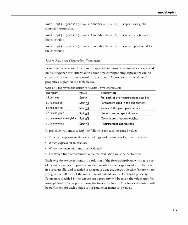
model.opt()
model.opt().gconstr(<tag>).constr(<constrExpr>) specifies a global constraint expression.
model.opt().gconstr(<tag>).lbound(<lboundExpr>) sets lower bound for the constraint.
model.opt().gconstr(<tag>).ubound(<lboundExpr>) sets upper bound for the constraint.
Least-Squares Objective Functions
Least-squares objective functions are specified in terms of measured values, stored on file, together with information about how corresponding expressions can be evaluated for the current control variable values. An overview of the allowed properties is given in the table below.
In principle, you must specify the following for each measured value:
• To which experiment the value belongs and parameters for that experiment
• Which expression to evaluate
• Where the expression must be evaluated
• For which time or parameter value the evaluation must be performed
Each experiment corresponds to a solution of the forward problem with a given set of parameter values. In practice, measurements for each experiment must be stored in a separate file, and specified as a separate LeastSquares objective feature where you give the full path of the measurement data file in the filename property. Parameters specified in the paramnames property will be given the values specified using paramexprs property during the forward solution. One forward solution will be performed for each unique set of parameter names and values.
TABLE 2-44: PROPERTIES FOR OBJECTIVE FUNCTION TYPE LEASTSQUARES
PROPERTY VALUE DESCRIPTION
filename String Full path of the measurement data file
paramnames String[] Parameters used in the experiment
paramexprs String[] Values of the given parameters
columntypes String[] List of column type indicators
columnexprsweights String[] Column contribution weights
columnexprs String[] Measurement expressions
115

model.opt()
116 | C H A P T
The required measurement data file format is row- and column-oriented. Entries on each row must be separated by commas or semicolons, while rows are separated by line feeds. Use the columtypes property to specify the content of each column, in the order that they appear in the data file, according to the following table:
Columns of type time are only allowed for transient problems. The measurements on the same row are assumed to be made at the specified time. Forward model values are interpolated to the given times. There must only be one column of type time, and it requires no further parameters.
Columns of type param contain parameter values for which the measurements on the same row have been made, and for which the forward problem must be solved. A data file may contain multiple parameter columns. Corresponding parameter names must be given in the columnnames property.
Columns of type coord contain global coordinates where the measurements on the same row have been made. The coordinate columns must be coupled to a coordinate variable by specifying the coordinate variable name in the columnnames property for the given column and the frame tag spatial, material or mesh in the columnexprs property. For example, in a 3D model, you will need three columns of type coord with columnnames entries x, y and z, respectively.
A value column contains measured data. For each value column, a corresponding expression to be evaluated must be specified in the columnexprs property. Entries in value columns will be interpreted as real numbers when possible. Anything else, including for example hash marks (#) and the literal strings nan, Nan, NaN and NAN is interpreted as an illegal value which will be excluded from the least squares objective function evaluation. A weight for the objective contribution from a column, multiplying the squared difference between the measured value and the expression, can be specified as a positive globally expression that can be evaluated using the columnexprsweights property. To exclude a measurement from a comma-separated file, you can also simply leave a value column empty.
TABLE 2-45: ALLOWED COLUMN TYPES
TYPE COLUMN CONTENTS
time Actual measurement times
param Actual parameter values
coord Actual measurement coordinates
value Measured values
none Ignored column
E R 2 : G E N E R A L C O M M A N D S

model.opt()
Columns of type none can be used to exclude columns from the data file.
Coordinates are interpreted as global in the context of the objective feature’s selection. This means that the value column expressions will be evaluated at the points within the selection that best match the given coordinates. If the interpolation fails for some point because its coordinates lie too far outside the selection, the corresponding value will be ignored.
117

model.pair()
118 | C H A P T
model.pair()Purpose Manipulate pairs.
Syntax model.pair().create(<tag>,type,<gtag>);model.pair(<tag>).type(type);model.pair(<tag>).type();model.pair(<tag>).pairName(<pname>);model.pair(<tag>).pairName();model.pair(<tag>).source().selMethod;model.pair(<tag>).source().named(<seltag>);model.pair(<tag>).source().named();model.pair(<tag>).destination().selMethod;model.pair(<tag>).destination().named(<seltag>);model.pair(<tag>).destination().named();model.pair(<tag>).swap();model.pair(<tag>).srcFrame(<frame>);model.pair(<tag>).srcFrame();model.pair(<tag>).dstFrame(<frame>);model.pair(<tag>).dstFrame();model.pair(<tag>).hasAutoSelection();model.pair(<tag>).manualSelection(manual);model.pair(<tag>).manualSelection();model.pair(<tag>).searchMethod(method);model.pair(<tag>).searchMethod();model.pair(<tag>).manualDist(manual);model.pair(<tag>).manualDist();model.pair(<tag>).searchDist(<dist>);model.pair(<tag>).searchDist();model.pair(<tag>).opName(src2dst);model.pair(<tag>).mphOpName(src2dst);model.pair(<tag>).gapName(src2dst);model.pair(<tag>).active(boolean);model.pair(<tag>).isActive();model.pair().remove(<tag>);
Description model.pair().create(<tag>,type,<gtag>) creates a boundary pair with tag <tag> in the geometry with tag <gtag>. The type type is either Contact or Identity. model.pair(<tag>).type() returns the pair type as a string. model.pair(<tag>).type(type) changes the pair type.
model.pair(<tag>).pairName(<pname>) sets the pair name, which is used as a suffix in operator names and variable names. By default, the pair name is the same as the tag. model.pair(<tag>).pairName() returns the pair name.
model.pair(<tag>).source().named(<seltag>) or, alternatively, model.pair(<tag>).source().set(...) specifies the source boundaries. model.pair(<tag>).source().named() returns the source selection tag as a
E R 2 : G E N E R A L C O M M A N D S

model.pair()
string. See model.selection() for additional methods that can be applied on model.pair(<tag>).source().
model.pair(<tag>).destination().named(<seltag>) or, alternatively, model.pair(<tag>).destination().set(...) specifies the destination boundaries. model.pair(<tag>).destination().named() returns the destination selection tag as a string. See model.selection() for additional methods that can be applied on model.pair(<tag>).destination().
model.pair(<tag>).swap() swaps the source and destination selections.
model.pair(<tag>).srcFrame(<frame>) and model.pair(<tag>).dstFrame(<frame>) sets the source and destination frames for the identity mapping. The argument <frame> can have the values spatial, material, or mesh. The default is spatial. These frames are only used for identity pairs. model.pair(<tag>).srcFrame() and model.pair(<tag>).dstFrame() returns the frame tags.
model.pair(<tag>).hasAutoSelection() returns true if the contact pair was created automatically, using the create pairs check box in the finalize geometry node.
model.pair(<tag>).manualSelection(manual) enables or disables manual control of the selections for a pair that was created automatically. model.pair(<tag>).manualSelection() returns true if manual control of selections is enabled, and false otherwise.
model.pair(<tag>).searchMethod(method) sets the search method for a contact pair. The argument method can be fast or direct. The default is fast. model.pair(<tag>).searchMethod() returns the search method
model.pair(<tag>).manualDist(manual) enables or disables manual control of the search distance for a contact pair. The argument manual is boolean. The default value false means that the search distance is automatically computed based on the size of the geometry. model.pair(<tag>).manualDist() returns true if manual control of search distance is enabled, and false otherwise.
model.pair(<tag>).searchDist(<dist>) sets the search distance for a contact pair, when manual control of the search distance is enabled. The argument <dist> is a string whose default unit is the geometry’s length unit. The default is 1e-2. model.pair(<tag>).searchDist() returns the search distance as a string.
119

model.pair()
120 | C H A P T
model.pair(<tag>).opName(src2dst) returns the name of the operator transferring an expression from source to destination (if src2dst=true) or from destination to source (if src2dst=false).
model.pair(<tag>).mphOpName(src2dst) returns the name of the multiphysics operator transferring an expression from source to destination (if src2dst=true) or from destination to source (if src2dst=false). When the test operator is applied on this operator, it does not give any contribution (reaction force) on the SME interface’s degrees of freedom due to the variable point mapping. These operators are available only for contact pairs.
model.pair(<tag>).gapName(src2dst) returns the name of the geometric gap variable seen from the destination (if src2dst=true) or seen from the source (if src2dst=false). These variables are available only for contact pairs.
model.pair(<tag>).active(boolean) enables or disables the pair.
boolean enabled = model.pair(<tag>).isActive() returns true if the pair is enabled, and false otherwise.
model.pair().remove(<tag>) deletes the pair.
Example Create a contact pair in the geometry geom1 with source boundaries 4 and 6 and destination boundaries 10 and 12.
Model model = ModelUtil.create("Model");model.geom().create("geom1", 3);model.geom("geom1").feature().create("blk1", "Block");model.geom("geom1").feature().create("blk2", "Block");model.geom("geom1").feature("blk2") .set("pos", new String[]{"0.5", "0.5", "1"});model.geom("geom1").feature("fin").name("Form Assembly");model.geom("geom1").feature("fin").set("action", "assembly");model.geom("geom1").feature("fin").set("imprint", true);model.geom("geom1").feature("fin").set("createpairs", false);model.geom("geom1").run();
model.pair().create("p1", "Contact", "geom1");model.pair("p1").source().set(new int[]{4, 6});model.pair("p1").destination().set(new int[]{10, 12});
E R 2 : G E N E R A L C O M M A N D S

model.param()
model.param()Purpose Manipulate model parameters.
Syntax model.param().set(<param>,<expr>);model.param().set(<param>,<expr>,<descr>);model.param().descr(<param>,<descr>);model.param().remove(<param>);
model.param().varnames();model.param().get(<param>);model.param().descr(<param>);
Description model.param() is a collection of model parameters.
model.param().set(<param>,<expr>) defines the parameter <param> as <expr>.
model.param().set(<param>,<expr>,<descr>) defines the parameter <param> as <expr> and assigns it the description <descr>.
model.param().descr(<param>,<descr>) sets the description for the parameter <param>.
model.param().remove(<param>) removes the parameter <param>.
model.param().varnames() returns the names of all parameters as a string array.
model.param().get(<param>) returns the parameter value as a string.
model.param().descr(<param>) returns the parameter description as a string.
Example Define the parameter c in terms of another parameter a and then remove c.
Model model = ModelUtil.create("Model");model.param().set("c","1+a");model.param().remove("c");
See Also model.variable()
121

model.physics()
122 | C H A P T
model.physics()Purpose Manipulate physics interfaces.
Syntax model.physics().create(<tag>,physint);model.physics().create(<tag>,physint,<geomtag>);model.physics().create(<tag>,physint,<geomtag>,<varnames>);model.physics(<tag>).model(<mtag>);model.physics(<tag>).field(fieldname).fieldname(<namelist>);model.physics(<tag>).field(fieldname).fieldname(<pos>,<name>);model.physics(<tag>).identifier(<scopename>);model.physics(<tag>).selection().named(<seltag>);model.physics(<tag>).selection().set(...);model.physics(<tag>).prop(propname).set(property,<value>);model.physics(<tag>).feature().create(<ftag>,feature);model.physics(<tag>).feature().create(<ftag>,feature,<dim>);model.physics(<tag>).feature(<ftag>).set(property,<value>);model.physics(<tag>).feature(<ftag>).selection().named(<seltag>;model.physics(<tag>).feature(<ftag>).selection().set(...);model.physics(<tag>).feature().move(<ftag>,<position>);
model.physics(<tag>).feature(<ftag>).feature();model.physics(<tag>).feature(<ftag>).feature(<ftag2>);model.physics(<tag>).feature(<ftag>).featureInfo();model.physics(<tag>).feature(<ftag>).featureInfo("info");feature = model.physics(<tag>).feature(<ftag>);feature.featureInfo("info").lock(variable,<value>);feature.featureInfo("info").getInfoTable(id);
model.physics(<tag>).model();model.physics(<tag>).field(fieldname).fieldname();model.physics(<tag>).identifier();model.physics(<tag>).scope();model.physics(<tag>).geom();model.physics(<tag>).selection().named():model.physics(<tag>).selection().getType();model.physics(<tag>).prop(propname).getType(<pname>);model.physics(<tag>).prop(propname).param();model.physics(<tag>).feature(<ftag>).getType(<pname>);model.physics(<tag>).feature(<ftag>).param();model.physics(<tag>).feature(<ftag>).selection().named();model.physics(<tag>).feature(<ftag>).selection().getType();
Description model.physics(<tag>) is a physics interface.
model.physics().create(<tag>,physint) or model.physics().create(<tag>,physint,<geomtag>) adds a physics interface to the model and initializes it with defaults. The physint argument specifies which physics interface to create. There can be several different values of physint which create the same internal physics interface class, but which set different defaults. The
E R 2 : G E N E R A L C O M M A N D S

model.physics()
constructor without the <geomtag> argument can only be used (and should be used) by 0D physics interfaces.
model.physics().create(<tag>,physint,<geomtag>,<varnames>) adds an physics interface with the field variable names <varnames>. Only physics interfaces supporting a varying number of field variables considers this argument. Providing the variable names in the create method rather than changes them afterwards using model.physics(<tag>).field(fieldname).fieldname(<namelist>) ensures that the default features are correct.
model.physics(<tag>).model(<mtag>) sets the model of a 0D physics interface. For interfaces with a geometry, the model is deduced from the geometry.
model.physics(<tag>).field(fieldname).fieldname(<namelist>) sets a name of a dependent variable. The entity fieldname (which could be, for example, temperature, x-velocity, electric field) specifies which dependent variable to set the name for. The available fields are provided by the physics interface. The argument <namelist> can be a list of names for physics interfaces supporting an arbitrary number of dependent variables. The physics interfaces provide default names for the dependent variables.
model.physics(<tag>).field(fieldname).fieldname(<pos>,<name>) changes the name at position <pos> in the list of field names.
model.physics(<tag>).identifier(<scopename>) sets the scope name of the physics interface. The create() method provides a default value for the identifier. It has to be unique within the model.
model.physics(<tag>).selection().named(<seltag>) or, alternatively, model.physics(<tag>).selection().set(...) specifies where the physics interface is active. For a complete list of methods available under selection(), see Selections. The selection must apply to the physics interface’s maximum geometry level. The create() method sets a default that the physics interface is active in all domains. 0D physics interfaces are always active globally and do not support these methods.
model.physics(<tag>).prop(propname).set(pname,<value>) sets the value of some property parameter. All string types listed in Table 2-2 are supported.
model.physics(<tag>).feature().create(<ftag>,feature) adds a new feature instance to the physics interface and initializes the feature with defaults. The available features are given by the physics interface.
123

model.physics()
124 | C H A P T
model.physics(<tag>).feature().create(<ftag>,feature,<dim>) adds a new feature instance to the physics interface and initializes the feature with defaults. The feature is assigned to the domain level <dim>. Use this constructor for features which can be applied to more than one domain level. The constructor without the <dim> argument assigns the feature to the highest domain level, which the feature supports.
model.physics(<tag>).feature(<ftag>).set(pname,<value>) sets a parameter value. All string types listed in the section Table 2-2 are supported.
model.physics(<tag>).feature(<ftag>).selection().named(<seltag>) or, alternatively, model.physics(<tag>).feature(<ftag>).selection().set(...) assigns the feature to the domains. For a complete list of methods available under selection(), see Selections. 0D features need no domain selection.
model.physics(<tag>).feature().move(<ftag>,<position>) moves the feature <ftag> to the zero indexed position <position> in the list. A feature cannot be moved before a default feature and the default features cannot be moved.
model.physics(<tag>).feature().create(<itag>,"init") creates an initial value feature, using the reserved feature ID init.
model.physics(<tag>).feature(<itag>).set(varname,<value>) specifies an initial value. The variable names are the field variables. For wave problems, the time derivatives of the field variables are also included in the list of variables.
model.physics(<tag>).model() returns the model of the interface.
model.physics(<tag>).field(fieldname).fieldname() returns the field names as a string array.
model.physics(<tag>).identifier() returns the scope name of the interface.
model.physics(<tag>).scope() returns the fully qualified scope name.
model.physics(<tag>).geom() returns the geometry tag as a string.
model.physics(<tag>).selection().named() returns the selection tag as a string.
model.physics(<tag>).selection().getType() returns domain information. See Selections for available methods.
E R 2 : G E N E R A L C O M M A N D S

model.physics()
model.physics(<tag>).prop(propname).getType(pname) returns the parameter value. See getType() for available methods.
model.physics(<tag>).prop(propname).param() returns the parameter names as a string array.
model.physics(<tag>).feature(<ftag>).getType(<pname>) returns the parameter value. See getType() for available methods.
model.physics(<tag>).feature(<ftag>).param() returns the parameter names as a string array.
model.physics(<tag>).feature(<ftag>).selection().named() returns the selection tag as a string array.
model.physics(<tag>).feature(<ftag>).feature() returns the list of feature attributes. This list supports the same methods as model.physics(<tag>).feature().
model.physics(<tag>).feature(<ftag>).feature(<ftag2>) returns the feature attribute <ftag2>. The feature attributes support the same methods as model.physics(<tag>).feature(<ftag>).
model.physics(<tag>).feature(<ftag>).featureInfo() returns a list of info objects.
model.physics(<tag>).feature(<ftag>).featureInfo("info") returns the info object that contains information about the variables, weak expressions, and constraints that a feature generates. The model.physics(<tag>) and model.coordSystem(<tag>) objects also have this list that you access with model.physics(<tag>).featureInfo("info"). These objects do not support the lock method, which only works for the object model.physics(<tag>).feature(<ftag>).
feature.featureInfo("info").lock(variable,<value>) locks the named variable to the given expression. The expression must be given as a string array.
feature.featureInfo("info").getInfoTable(id) returns a table that lists all information about a certain table id. The supported id:s are Expression, Shape, Weak, and Constraint.
Examples This example creates an Electrostatics physics interface. It sets boundaries 3 and 8 to the ground potential and assigns the electric potential of 1 V at boundary 4.
125

model.physics()
126 | C H A P T
When the physics interface is created a couple of default features are automatically added. One of them is the Charge Conservation feature, which has the tag ccn1. The relative permittivity is this feature is set to 1.
model.physics().create("es","Electrostatics","geom1");model.physics("es").feature().create("gnd1", "Ground", 2);model.physics("es").feature("gnd1").selection().set(new int[]{3, 8});model.physics("es").feature().create("pot1", "ElectricPotential", 2);model.physics("es").feature("pot1").selection().set(new int[]{4});model.physics("es").feature("pot1").set("V0", "1");model.physics("es").feature("ccn1").set("epsilonr_mat", "userdef");model.physics("es").feature("ccn1").set("epsilonr", "1");
Compatibility From version 4.3 the methods
model.physics(<tag>).feature(<ftag>).params();model.physics(<tag>).prop(propname).params();
are deprecated and replaced by the methods
model.physics(<tag>).feature(<ftag>).param();model.physics(<tag>).prop(propname).param();
See Also model.material(), model.study()
E R 2 : G E N E R A L C O M M A N D S

model.probe()
model.probe()Purpose Manipulate probe objects.
Syntax model.probe().create(<tag>, type);model.probe(<tag>).model(<mtag>);model.probe(<tag>).set(property,<value>);model.probe(<tag>).feature().create(<etag>, etype);model.probe(<tag>).feature(<etag>).set(eproperty,<evalue>);
Description model.probe().create(<tag>, type) creates a probe of type type with tag <tag>.
model.probe(<tag>).model(<mtag>) sets the model to <mtag>.
model.probe(<tag>).set(property,<value>) set property to <value>.
model.probe(<tag>).selection(...) set the selection for the probe. This is possible for the probes of the types Domain, Boundary and Edge.
model.probe(<tag>).feature().create(<etag>, etype) creates a point probe expression of type etype and tag <tag>.
model.probe(<tag>).feature(<etag>).set(eproperty,<evalue>) sets the property eproperty on the point probe expression <etag>.
Probes can be of the following types:.
Probe points can be of the following types:
TABLE 2-46: PROBE TYPES
TYPE DESCRIPTION
Boundary Probe that defines a value as an integral, maximum, minimum or average over boundaries.
Domain Probe that defines a value as an integral, maximum, minimum or average over domains.
Edge Probe that defines a value as an integral, maximum, minimum or average over edges (in 3D).
GlobalVariable Probe that defines a value using a global variable.
PointExpr Probe that defines a value by interpolation of an expression in a probe point. The probe point is defined by the parent, a DomainPoint or a BoundaryPoint.
TABLE 2-47: PROBE POINT TYPES
TYPE DESCRIPTION
BoundaryPoint Defines a probe coordinate on a boundary in 3D.
DomainPoint Defines a probe coordinate in a domain.
127

model.probe()
128 | C H A P T
Probes takes the following properties:
A probe point of the type DomainPoint takes the following properties:
TABLE 2-48: PROBE PROPERTIES
NAME VALUE DEFAULT DESCRIPTION
descr String Description of the probe. Used for model.result().
descractive on | off off Manual control of description.
expr String The expression defining the probe.
frame String spatial frame Frame used for defining the probe.
intorder Integer 4 Integration order (DomainProbe and BoundaryProbe).
method integration | summation
integration Method used (DomainProbe and BoundaryProbe).
probename String probe tag Probe variable name.
table String default Table to use for probe evaluation.
type average | maximum | minimum | integral
average Type of probe (DomainProbe and BoundaryProbe).
unit String unit of expr Unit for the probe. Used for model.result().
window String default The plot window to use for the probe.
TABLE 2-49: PROBE PROPERTIES
NAME VALUE DEFAULT DESCRIPTION
bndsnap1 on | off off Snap to nearest point (1D).
bndsnap2 on | off off Snap to nearest boundary point (2D).
bndsnap3 on | off off Snap to nearest boundary point (3D).
coords Matrix of doubles
Probe coordinates.
E R 2 : G E N E R A L C O M M A N D S

model.probe()
A probe point of BoundaryPoint types take the following properties:
depthpointnormal
Double 0 Depth along line defined by the pointnormal method.
depthpointdirection
Double 0 Depth along line defined by the pointdirection method.
depthtwopoints
Double 0 Depth along line defined by the twopoints method.
dimension 1 | 2 | 3 3 The spatial dimension in which the point resides.
first Double array The coordinates of the first point on the probe line.
method pointnormal | pointdirection | twopoints | none
pointnormal Line entry method.
second Double array The coordinates of the second point (for method=twopoints)
twopointscurrent
first | second first Point selector (for method=twopoints)
TABLE 2-50: PROBE PROPERTIES
NAME VALUE DEFAULT DESCRIPTION
coords Double array 0,0,0 Probe coordinates.
rawcoords Double array 0,0,0 Full precision probe coordinates.
snapcoords Double array 0,0,0 The boundary-snapped coordinates.
TABLE 2-49: PROBE PROPERTIES
NAME VALUE DEFAULT DESCRIPTION
129

model.result()
130 | C H A P T
model.result()Purpose Manipulate result objects.
Syntax model.result().create(<pgtag>,dim);model.result().create(<pgtag>,ftype);model.result().autoplot();model.result().autoplot(<value>);model.result(<pgtag>).set(property,<value>);model.result(<pgtag>).run();
model.result(<pgtag>).feature().create(<ftag>,ftype);model.result(<pgtag>).feature(<ftag>).getType();model.result(<pgtag>).feature(<ftag>).selection(...);model.result(<pgtag>).feature(<ftag>).set(property,<value>);model.result(<pgtag>).feature(<ftag>).run();
model.result(<pgtag>).feature(<ftag>) .create(<attrtag>, attrtype);
model.result(<pgtag>).feature(<ftag>) .feature(<attrtag>).set(property,<value>);
model.result().dataset().create(<dtag>,dtype);model.result().dataset(<dtag>).selection(...);model.result().dataset(<dtag>).set(property,<value>);
model.result().export().create(<etag>,<pgtag>,ctype);model.result().export(<etag>).set(property,<value>);model.result().export(<etag>).run();
model.result().numerical().create(<ntag>,ntype);model.result().numerical(<ntag>).selection(...);model.result().numerical(<ntag>).set(property,<value>);model.result().numerical(<ntag>).run();
model.result().table().create(<ftag>,ntype);model.result().table(<ftag>).setColumnHeaders(<headers>);model.result().table(<ftag>).setTableData(<realData>,<imagData>);model.result().table(<ftag>).getColumnHeaders();model.result().table(<ftag>).getReal();model.result().table(<ftag>).getImag();model.result().table(<ftag>).isComplex();model.result().table(<ftag>).clearTableData();model.result().table(<ftag>).save(<filename>);
E R 2 : G E N E R A L C O M M A N D S

model.result()
model.result().report().create(<rtag>);model.result().report(<rtag>).set(rprop,<value>);model.result().report(<rtag>).feature().create(<r2tag>,frtype);model.result().report(<rtag>).feature(<r2tag>)... .set(rprop,<value>);model.result().report(<rtag>).feature(<r2tag>)... .feature().create(<r3tag>,frtype);model.result().report(<rtag>).feature(<r2tag>)... .feature(<r3tag>)set(rprop,<value>);model.result().report(<rtag>).run();
Description model.result().create(<pgtag>,dim) creates a plot group with the tag <pgtag>, of dimension dim, where dim can be 1, 2, or 3.
model.result().create(<pgtag>,ftype) creates a plot group of type ftype.
model.result().autoplot() returns true if plot features are plotted automatically when selected. model.result().autoplot(true) and model.result().autoplot(false) enable and disable automatic plotting, respectively.
model.result(<pgtag>).feature().create(<ftag>,ftype) creates a plot feature of type ftype tagged <ftag> belonging to the plot group <pgtag>.
model.result(<pgtag>).feature(<ftag>).getType() returns the type of the feature <ftag>. This is the same string ftype that was used to create the feature.
model.result(<pgtag>).feature(<ftag>).create(<attrtag>, attrtype) creates an attribute feature with the tag <attrtag> of type attrtype, belonging to the feature <ftag>.
model.result(<pgtag>).run() plots the plot group.
model.result().dataset().create(<dtag>,dtype) creates a data set feature with the tag <dtag> and the type dtype.
model.result().export().create(<etag>,<pgtag>,etype) creates an export feature with the tag <etag>, belonging to plot group <pgtag> and of export feature type etype.
model.result().numerical().create(<ntag>, ntype) creates a numerical results feature with the tag <ntag> of the numerical feature type ntype.
model.result().numerical(<ntag>).run() evaluates the numerical feature.
131

model.result()
132 | C H A P T
model.result().table().create(<ftag>,ntype) creates a table feature with the tag <ftag>. The set and get methods used to manipulate tables are described in Table.
The data extraction methods used to retrieve plot or numerical data are described in Results.
model.result().report().create(<rtag>,"Report") creates a report with tag <rtag>.
report.feature().create(<tptag>,"TitlePage") adds a title page to the report report. Only one title-page feature can be added.
report.feature("<tptag>).set(prop,value) sets the title-page property prop to the value value.
report().feature().create(<toctag>,"TableOfContents") adds a table of contents to the report report. Only one table-of-contents feature can be added.
report.feature().create(<stag>,"Section") adds an additional section level to a report.
report.feature(<stag>).set(prop,value)
report.feature(<stag>).feature().create(<ftag>),feature)
report.feature(<stag>).feature(<ftag>).set(prop,value)
To add a report contents feature—that is, a feature corresponding to content in the report—to a report section feature section, type, section.feature().create(<frtag>,frtype,…). Depending on the report feature type frtype, the create operation includes zero, one or two tags that refer to the model feature to report about. The tags must refer to an existing feature of the correct type. The following report feature types are available:
REPORT FEATURES DESCRIPTION
Model Prints information about the model root, such as model file.
ModelNode Prints information about a model, its identifier.
Parameter Reports on the global model parameters.
Variables Reports on a variables feature.
Functions Reports on a function feature.
Probe Reports on a probe feature.
ModelCoupling Reports on a model-coupling feature.
E R 2 : G E N E R A L C O M M A N D S

model.result()
To point a report feature rFeature to another feature with tag <ftag> in the tree, use the method rFeature.set("noderef",<ftag>) method. A report contents feature must point to a feature of the type it is designed to report on; see the table above. Instead of a feature tag, set "noderef" to "none" to clear a reference.
model.result().report(<rtag>).feature(<stag>).feature(<frtag>) .set(frprop, <value>)
to set a property in a report feature.
Examples Create a solution data set and set it to point to the tagged solution sol1 from a solver sequence:
model.result().dataset().create("dset", "Solution");model.result().dataset("dset").set("solution", "Sol1");
Create 3D plot group containing a streamline plot and a plane with a contour plot on:
result().create("pg1",3);result("pg1").set("data","dset");result("pg1").feature().create("stream","Streamline");model.result("pg1").feature("stream").set("expr",
Selection Reports on a selection feature.
CoordinateSystem Reports on a coordinate system feature.
PML Reports on a PML feature.
InfiniteElements Reports on an infinite elements feature.
Pair Reports on a pair feature.
Geometry Reports on a geometry.
Material Reports on a material feature.
Physics Reports on a physics interface and its features.
Mesh Reports on a mesh.
Study Reports on a study.
Solver Reports on a solver.
DataSet Reports on a data-set feature.
DerivedValues Reports on a derived-values feature.
Table Includes a results table in the report.
PlotGroup Includes a plot group in the report.
Export Includes an export feature in the report.
REPORT FEATURES DESCRIPTION
133

model.result()
134 | C H A P T
new String[]{"2-x", "0", "z"});model.result("pg1").feature("stream"). selection().set(new int[]{2});
result().dataset().create("cutp1","CutPlane");
result("pg1").feature().create("cont1","Contour");result("pg1").feature("cont1").set("data","cutp1");result("pg1").run();
See Also
E R 2 : G E N E R A L C O M M A N D S

model.savePoint()
model.savePoint()Purpose Manipulate selections and hide features used by result features.
Syntax model.savePoint(<tag>).geom(<gtag>)model.savePoint(<tag>).geom(<gtag>).selection(<stag>)model.savePoint(<tag>).geom(<gtag>).view(<vtag>)
Description model.savePoint(<tag>) is a container of selections and hide features used by result features. When solving, a copy of the model is made—a save point model—which is used in results and analysis. The selections and hide features contained in model.savePoint(<tag>) refer to the geometry in this copy.
Editing the data in model.savePoint(<tag>) may only be done in the following circumstances.
• The geometry on which the analysis is done has been modified after solving. In this case the selections and hide feature may be edited but not created or removed.
• The geometry on which the analysis is done has been removed. In this case the selections and hide features may be both edited, created, and deleted.
In all other circumstances, edit the selections in model.selection(), and the hide features in model.view(). Changes there are synchronized with the data in model.savePoint().
model.savePoint(<tag>).geom(<gtag>) returns a container with selections and views with hide features for a geometry in the save point model.
model.savePoint(<tag>).geom(<gtag>).selection(<stag>) returns a selection.
model.savePoint(<tag>).geom(<gtag>).view(<vtag>) returns a view. Contrary to the views in model.view(), only the hide features in view.hideEntities() can be edited.
See also model.selection(), model.weak()
135

model.selection()
136 | C H A P T
model.selection()Purpose Manipulate tagged selections.
Syntax model.selection().create(<tag>);model.selection().create(<tag>,<type>);model.selection(<tag>).model(<mtag>);model.selection(<tag>).set(property,<value>);model.selection(<tag>).geom(<gtag>,dim);model.selection(<tag>).geom(<gtag>,highdim,lowdim,typelist);model.selection(<tag>).geom(dim);model.selection(<tag>).all();model.selection(<tag>).set(<domlist>);model.selection(<tag>).add(<domlist>);model.selection(<tag>).remove(<domlist>);model.selection(<tag>).inherit(bool);
model.selection(<tag>).model();model.selection(<tag>).isGeom();model.selection(<tag>).geom();model.selection(<tag>).dimension();model.selection(<tag>).entities(dim);model.selection(<tag>).interiorEntities(dim);model.selection(<tag>).isInheriting();model.selection(<tag>).inputDimension();model.selection(<tag>).inputEntities();
Description model.selection(<tag>) is a tagged domain selection.
model.selection().create(<tag>) creates a selection of type explicit.
model.selection().create(<tag>,<type>) creates a selection of type <type>.
model.selection(<tag>).model(<mtag>) sets the model of the selection. Only geometries in the model can be used in selections.
model.selection(<tag>).model() returns the model of the selection.
model.selection(<tag>).set(property,<value>) sets a property value for the selection. Which properties are available for the different selection types are listed on the following pages. All other assignment methods are only supported by the Explicit selection type.
All other methods are explained in the section Selections.
Other entities can use any of the selections in model.selection() when defining its selection. For example, create a selection sel1:
model.selection().create("sel1");model.selection("sel1").model("mod1");
E R 2 : G E N E R A L C O M M A N D S

model.selection()
Then, for example, a variable entities can use this selection:
model.variable().create("var1”);model.variable("var1").model("mod1");model.variable("var1").selection().named("sel1");
What properties are available depends on the type of selection. The following selection types are available:
Explicit Selection defined by an explicit set of entities.
Explicit selections do not have any properties.
Ball Selection of entities in a ball.
The posx, posy and posz properties define the center of the ball, and r defines the radius. These properties take their units from the corresponding geometry sequence.
When condition is intersects, all entities that intersect the ball are included in the selection. The rendering mesh is used for the calculation. The accuracy of the rendering mesh can be set in Options > Preferences > Graphics > Detail.
NAME VALUE DEFAULT DESCRIPTION
entitydim 0 | 1 | 2 | 3 sdim Dimension of entities to select
inputent all | selections
all Use all entities or entities defined by input property
input String[] {} Input selections
condition intersects | inside | somevertex | allvertices
intersects Condition for inclusion of an entity
posx double 0 Center of ball, first coordinate
posy double 0 Center of ball, second coordinate
posz double 0 Center of ball, third coordinate
r double 0 Radius
137

model.selection()
138 | C H A P T
When condition is inside, all entities that are completely inside the ball are included in the selection. The rendering mesh is used for the calculation.
When condition is somevertex, all entities that have at least one adjacent vertex inside the ball are included in the selection.
When condition is allvertices, all entities that have all adjacent vertices inside the ball are included in the selection.
When inputent is selections, the selection is restricted to the entities in the selections defined by the input property. When inputent is all, all entities in the geometry are considered.
Box Selection of entities in a box.
The xmax, xmin, ymax, ymin, zmax and zmin properties define the box. These properties take their units from the corresponding geometry sequence.
When condition is intersects, all entities that intersect the box are included in the selection. The rendering mesh is used for the calculation. The accuracy of the rendering mesh can be set in Options > Preferences > Graphics > Detail.
When condition is inside, all entities that are completely inside the box are included in the selection. The rendering mesh is used for the calculation.
NAME VALUE DEFAULT DESCRIPTION
entitydim 0 | 1 | 2 | 3 sdim Dimension of entities to select
inputent all | selections
all Use all entities or entities defined by input property
input String[] {} Input selections
condition intersects | inside | somevertex | allvertices
intersects Condition for inclusion of an entity
xmax double inf Maximum x-coordinate of box
xmin double -inf Minimum x-coordinate of box
ymax double inf Maximum y-coordinate of box
ymin double -inf Minimum y-coordinate of box
zmax double inf Maximum z-coordinate of box
zmin double -inf Minimum z-coordinate of box
E R 2 : G E N E R A L C O M M A N D S

model.selection()
When condition is somevertex, all entities that have at least one adjacent vertex inside the box are included in the selection.
When condition is allvertices, all entities that have all adjacent vertices inside the box are included in the selection.
When inputent is selections, the selection is restricted to the entities in the selections defined by the input property. When inputent is all, all entities in the geometry are considered.
Union Selection defined by the union of a set of selections.
Intersection Selection defined by the intersection of a set of selections.
Difference Selection defined by the difference between two sets of selections.
Complement Selection defined by the complement of a set of selections.
NAME VALUE DEFAULT DESCRIPTION
entitydim 0 | 1 | 2 | 3 sdim Dimension of entities to select
input String[] {} Selections to add
NAME VALUE DEFAULT DESCRIPTION
entitydim 0 | 1 | 2 | 3 sdim Dimension of entities to select
input String[] {} Selections to intersect
NAME VALUE DEFAULT DESCRIPTION
entitydim 0 | 1 | 2 | 3 sdim Dimension of entities to select
add String[] {} Selections to add
subtract String[] {} Selections to subtract
NAME VALUE DEFAULT DESCRIPTION
entitydim 0 | 1 | 2 | 3 sdim Dimension of entities to select
input String[] {} Selections to invert
139

model.selection()
140 | C H A P T
Adjacent Selection of entities adjacent to entities in another selection.
Examples Define the selection equ1 as the domain of a rectangle and the selection bnd1 as the boundary of the rectangle.
Model model = ModelUtil.create("Model");model.geom().create("geom1",2);model.geom("geom1").feature().create("f1","Rectangle");model.geom("geom1").runAll();model.selection().create("equ1").geom(2);model.selection("equ1").all();model.selection().create("bnd1").geom(1);model.selection("bnd1").all();
Create a selection for all interior mesh boundary boundaries and all internal boundaries of the union of a Circle and a Rectangle:
Model model = ModelUtil.create("Model");model.geom().create("geom1",2);model.geom("geom1").feature().create("r1","Rectangle");model.geom("geom1").feature().create("c1","Circle");model.geom("geom1").runAll();model.selection().create("ultra").geom("geom1",2,1, new String[]{"interior","meshinterior"});model.selection("ultra").all();
The above selection is typically used in very weak formulations to include all internal mesh boundaries and the internal boundaries in a single expression.
The (outer) boundaries for the model can be set with the selection
Model model = ModelUtil.create("Model");model.geom().create("geom1",2);model.geom("geom1").feature().create("r1","Rectangle");model.selection().create("outer").geom("geom1",2,1,new String[]{"exterior"});
NAME VALUE DEFAULT DESCRIPTION
entitydim 0 | 1 | 2 | 3 sdim Dimension of entities to select
input String[] {} Input selections
outputdim 0 | 1 | 2 | 3 sdim-1 Dimension of output entities
exterior on | off on Include exterior boundaries/edges
interior on | off off Include interior boundaries/edges.
E R 2 : G E N E R A L C O M M A N D S
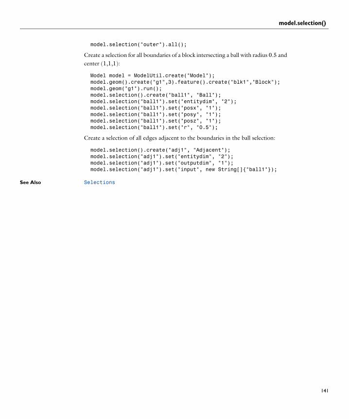
model.selection()
model.selection("outer").all();
Create a selection for all boundaries of a block intersecting a ball with radius 0.5 and center (1,1,1):
Model model = ModelUtil.create("Model");model.geom().create("g1",3).feature().create("blk1","Block");model.geom("g1").run();model.selection().create("ball1", "Ball");model.selection("ball1").set("entitydim", "2");model.selection("ball1").set("posx", "1");model.selection("ball1").set("posy", "1");model.selection("ball1").set("posz", "1");model.selection("ball1").set("r", "0.5");
Create a selection of all edges adjacent to the boundaries in the ball selection:
model.selection().create("adj1", "Adjacent");model.selection("adj1").set("entitydim", "2");model.selection("adj1").set("outputdim", "1");model.selection("adj1").set("input", new String[]{"ball1"});
See Also Selections
141

model.shape()
142 | C H A P T
model.shape()Purpose Manipulate shape functions.
Syntax model.shape().create(<tag>,<frame>);model.shape(<tag>).elementSet(<condition>);model.shape(<tag>).frame(<ftag>);model.shape(<tag>).feature().create(<ftag>,<func>);model.shape(<tag>).feature(<ftag>).shape(<func>);model.shape(<tag>).feature(<ftag>).set(property,<value>);model.shape(<tag>).selection().named(<seltag>);model.shape(<tag>).selection().set(...);model.shape(<tag>).slits().named(<seltag>);model.shape(<tag>).slits().set(...);model.shape(<tag>).upFlux(<varName>);model.shape(<tag>).downFlux(<varName>);model.shape(<tag>).domainFlux(<expressions>,<frame>);
model.shape(<tag>).elementSet();model.shape(<tag>).frame();model.shape(<tag>).feature(<ftag>).shape();model.shape(<tag>).feature(<ftag>).getType(property);model.shape(<tag>).feature(<ftag>).properties;model.shape(<tag>).fieldVariable();model.shape(<tag>).selection().named();model.shape(<tag>).selection().getType();model.shape(<tag>).slits().named();model.shape(<tag>).slits().getType();model.shape(<tag>).upFlux();model.shape(<tag>).downFlux();
Description model.shape(<tag>) is a shape entity.
model.shape().create(<tag>,<frame>) creates a shape entity with tag <tag> and assigns the frame <frame> to it.
model.shape(<tag>).frame(<ftag>) assigns frame <ftag> to the shape function. See model.frame() for a discussion on the default frame.
model.shape(<tag>).feature().create(<ftag>,<func>) creates a shape feature with the shape function func. func can be a shape function name, for example shlag, or a shape function with arguments, for example, shlag(2,u). The latter is interpreted as an assignment of some property values.
model.shape(<tag>).feature(<ftag>).shape(<func>) sets the shape function.
model.shape(<tag>).feature(<ftag>).set(property,<value>) sets a property for the shape function. Of the data types listed in Table 2-2, the ones
E R 2 : G E N E R A L C O M M A N D S

model.shape()
supported are those for integers, strings, and string arrays. Which ones are applicable differs for each property.
model.shape(<tag>).selection().named(<seltag>) or, alternatively, model.shape(<tag>).selection().set(...) assigns the shape function to the specified domains. For a complete list of methods available under selection(), see Selections.
model.shape(<tag>).upFlux(<varName>) and model.shape(<tag>).downFlux(<varName>) set the names of the up and down boundary flux variables. model.shape(<tag>).domainFlux(<expressions>,<frame>) sets expressions for the domain flux in a given frame. This is required to make the boundary flux variables produce accurate results. Only Lagrange shape functions support boundary flux variables.
model.shape(<tag>).frame() returns the frame tag as a string.
model.shape(<tag>).feature(<ftag>).shape() returns the shape function as a string.
model.shape(<tag>).feature(<ftag>).getType(property) returns a property value. For available data types, see getType().
model.shape(<tag>).feature(<ftag>).properties() returns the names of the properties as a string array.
model.shape(<tag>).fieldVariable() returns the field variables which the shape functions define.
model.shape(<tag>).selection().named() returns the selection tag as a string.
model.shape(<tag>).elementSet() returns the element set condition, empty string means no condition.
model.shape(<tag>).elementSet(<condition>) sets the element set condition to the given string.
model.shape(<tag>).selection().getType() returns domain information. For available methods, see model.selection().
model.shape(<tag>).slits() returns a selection used to generate a slit on the shape. Works exactly as selections.
143

model.shape()
144 | C H A P T
model.shape(<tag>).upFlux() and model.shape(<tag>).downFlux() return the names of the up and down flux variables (an empty string if the variable names have not been set.)
Examples Define the shape function shlag(2,"u").
model.shape().create("shu","f");model.shape("shu").feature().create("f1","shlag");model.shape("shu").feature("f1").set("order",2);model.shape("shu").feature("f1").set("basename","u");model.shape("shu").selection().named("equ1");
See Also model.coeff(), model.intRule(), model.weak()
E R 2 : G E N E R A L C O M M A N D S

model.sol()
model.sol()Purpose Manipulate solutions.
Syntax model.sol().create(<tag>)model.sol().create(<tag>,<studytag>)model.sol().create(<tag>,<studytag>,<varstag>)model.sol().remove(<tag>)
model.sol(<tag>).feature().create(<ftag>,<oper>)model.sol(<tag>).feature().remove(<ftag>)model.sol(<tag>).feature(<ftag>).set(property,<value>)model.sol(<tag>).clearSolution()model.sol(<tag>).copySolution(<ctag>)model.sol(<tag>).createAutoSequence(<stag>)model.sol(<tag>).createSolution()model.sol(<tag>).updateSolution()model.sol(<tag>).run(<ftag>)model.sol(<tag>).runFrom(<ftag>)model.sol(<tag>).runAll()model.sol(<tag>).run()model.sol(<tag>).continueCun()
Description model.sol().create(<tag>) adds a solution to the model.
model.sol().create(<tag>,<studytag>) adds a solution to the model. The constructor adds one feature of the type StudyStep to the solver sequence with the tag <studytag>. This StudyStep feature is connected to a study step (see model.study()).
model.sol().create(<tag>,<studytag>,<varstag>) adds a solution to the model. The constructor adds one feature of the type StudyStep with the tag <studytag> and one feature of the type Variables with the tag <varstag> to the solver sequence.
model.sol().remove(<tag>) removes a solution object from the model.
sol(<tag>).feature().create(<ftag>,<oper>) creates a solution operation feature.
model.sol(<tag>).feature().remove(<ftag>) removes the feature <ftag>.
model.sol(<tag>).feature(<ftag>).set(property,<value>) sets the property property for the feature <ftag>.
model.sol(<tag>).clearSolution() clears the solution data associated with the solution <tag>. The features are not changed.
145

model.sol()
146 | C H A P T
model.sol(<tag>).copySolution(<ctag>) copies the solution data associated with the solution <tag> to a new solution <ctag>. The features are not copied.
model.sol(<tag>).createAutoSequence(<stag>) creates a sequence of features automatically from the study <stag>. The sequence of study steps are used as input to the sequence generation algorithm but also the physics used in the study steps are used to automatically adopt the solver settings.
model.sol(<tag>).createSolution() creates a solution object from one or more set operations (setU(..), ...), see Solution Creation for details.
model.sol(<tag>).updateSolution() updates a solution object to make it consistent with the current model.
model.sol(<tag>).run(<ftag>) runs the features for a solution object up to and including the feature <ftag>.
model.sol(<tag>).runFrom(<ftag>) runs the features for a solution object from and including the feature <ftag>.
model.sol(<tag>).runAll() and model.sol(<tag>).run() run all the features for a solution object.
model.sol(<tag>).continueRun() continues to run a solver sequence.
Examples Assume that a study st1 represents one stationary study step with the tag stat1 for some equations.
model.sol().create("s","step1","vars1");model.sol("s").feature("step1").set("study","st1");model.sol("s").feature("step1").set("studystep","stat1");model.sol("s").feature().create("solver1","Stationary");
Assume that a second study step with frequency response is added to the study with tag freq1 and that we want to make a frequency sweep from 10 to 1000 using the parametric solver and the solution above as the linearization point (bias solution).
model.sol("s").feature().create("step2","StudyStep");model.sol("s").feature("step2").set("study","st1");model.sol("s").feature("step2").set("studystep","freq1");model.sol("s").feature().create("vars2","Variables");SolverFeature s2 = (SolverFeature) model.sol("s").feature().create("solver2","Stationary");s2.set("nonlin","linper"); (*)s2.set("linpmethod","sol");s2.set("linpsol", "s");s2.set("storelinpoint", "on");
E R 2 : G E N E R A L C O M M A N D S

model.sol()
s2.feature().create("par","Parametric");s2.feature("par").set("pname","freq");s2.feature("par").set("plist",new double[]{10,1000});s2.runAll();
At this point the solution s is associated to the study step freq1 (but it depends indirectly on the bias study step stat1 as well).
(*) Uses the new small signal study functionality, which makes it possible to access also the linearization point for postprocessing together with the small signal solution. Here it is assumed that the bias problem and the small signal problem can be setup independently for the two study steps.
See Also model.study()
147

model.study()
148 | C H A P T
model.study()Purpose Manage studies.
Syntax model.study().create(<tag>);model.study(<tag>).feature().create(<ftag>,type);model.study(<tag>).feature().move(<ftag>,position);
model.study(<tag>).run()model.study(<tag>).runNoGen()model.study(<tag>).createAutoSequences(type)model.study(<tag>).showAutoSequences(type)
step = model.study(<tag>).feature(<ftag>);
step.mesh(<geom>,<mesh>);step.activate(<physpath>,<bool>);step.discretization(<physpath>,<discr>);step.mglevel.create(<mglevel>);step.mglevel(<mglevel>).mesh(<geom>,<mesh>);step.mglevel(<mglevel>).discretization(<physpath>,<discr>);
step.type();step.activate(<physpath>);step.discretization(<physpath>);step.mesh(<geom>);step.mglevel(<mglevel>).mesh(<geom>);step.mglevel(<mglevel>).discretization(<physpath>);
Description The entity model.study stores a list of studies, each of which consists of a number of study steps. Each study step, in turn, defines a solver-ready problem. This means that a study step can be turned into an extended mesh, and a basic solver (Stationary, Time, Eigenvalue, Modal, AWE, Optimization) can be applied, resulting in a solution object.
The central property of a study step is its study type, which on one hand controls the equations generated by physics interfaces, and on the other hand triggers automatic selection of a suitable solver. Another important property of a study step is which mesh to use (for each geometry in the model). Other fundamental simulation parameters can also be found among the study step settings, like the time span for a Time Dependent study type and frequency range for a Frequency Domain type.
Under a study step, you can add multigrid levels. The parent node still defines the problem to be solved (for example, the study type and the mesh). Therefore, the added multigrid levels must necessarily be coarser than the parent study step.
E R 2 : G E N E R A L C O M M A N D S

model.study()
Most physics interface features and also some other parts of the model object (for example expression features) must support a step member, which (in analogy to the spatial selection) controls for which study steps the feature is active. In many ways, the study selection can be seen as a fourth, discrete, dimension.
model.study().create(<tag>) creates a new study sequence.
model.study(<tag>).run() computes study.
model.study(<tag>).runNoGen() runs the attached solver sequence without regenerating it.
model.study(<tag>).createAutoSequences(type) creates an attached solver sequence and/or job using default solver settings. The argument type is one of all, jobs, or sol, corresponding to creating both jobs and solver sequences or one of then.
model.study(<tag>).showAutoSequences(type) generates a new attached solver sequence and/or job using default solver settings. The previous item describes the type argument.
model.study(<tag>).feature().create(<ftag>,type) creates a new study step of the given type within the specified sequence. The set of allowed values should be limited to study types supported by at least one physics interface present in the model (Stationary, Time, Frequency, and Eigenvalue should always be allowed).
model.study(<tag>).feature().move(<ftag>,position) moves the feature <ftag> to the zero indexed position <position> in the list.
step = model.study(<tag>).feature(<ftag>) obtains a reference to a specified study step.
step.mesh(<geom>,<mesh>) specifies which mesh to use for geometry <geom> in the model.
step.activate(<physpath>,<bool>) activates or deactivates a physics interface or a physics feature. The string <physpath> is a path to a node in a physics interface. Currently only the tag of the physics interface tag itself is supported.
step.discretization(<physpath>,<discr>) assigns discretization for a physics interface. The string <physpath> is the path of a physics interface. The string <discr> is a tag of a discretization feature under a physics mode. The default <discr> the physics interface tag. It can be changed to the tag of a discretization node under a physics interface.
149

model.study()
150 | C H A P T
step.mglevel.create(<mglevel>) adds a (coarser) multigrid level to a study.
step.mglevel(<mglevel>).mesh(<geom>,<mesh>) specifies a mesh for the multigrid level. The set of allowed values must, in addition to the actual meshes, include an option “from parent”. This should be the default choice and indicates that the multigrid level uses the same mesh as the parent study.
step.mglevel(<mglevel>).discretization(<physpath>,<discr>) assigns discretization for a multigrid level. The string <physpath> is the path of a physics interface. The string <discr> is a tag of a discretization feature under a physics mode. The default <discr> the physics interface tag. It can be changed to the tag of a discretization node under a physics interface.
step.type() returns the study type.
step.mesh(<geom>) returns the mesh selected for the given geometry.
step.activate(<physpath>) returns activation status of a physics interface or a physics interface feature. Currently only the tag of the physics interface tag itself is supported.
step.mglevel(<mglevel>).mesh(<geom>) returns the mesh for the selected multigrid level and geometry.
step.mglevel(<mglevel>).discretization(<discpath>) returns activation status of a discretization feature.
Examples The following code sets up a study sequence to analyze the influence of structural deformation on a waveguide with a numerical port boundary condition. It consists of three steps: stationary structural mechanics followed by an eigenvalue study for the port and finally a wave propagation problem solved with manual multigrid levels (to get nested meshes).
Model model = ModelUtil.create("Model");model.geom().create("geom1", 3);model.geom("geom1").feature().create("blk1", "Block");model.geom().run();model.mesh().create("mesh1", "geom1");model.mesh().create("mesh2", "geom1");model.mesh().create("mesh3", "geom1");
model.physics().create("rfw1", "ElectromagneticWaves", "geom1");model.study().create("seq1");Study s1 = model.study("seq1");s1.feature().create("struct","Stationary");s1.feature("struct").mesh("geom1","mesh1");
E R 2 : G E N E R A L C O M M A N D S

model.study()
s1.feature().create("port","BoundaryModeAnalysis");s1.feature("port").set("PortName","port1");s1.feature("port").mesh("geom1","mesh2");s1.feature().create("wave","Frequency");s1.feature("wave").mesh("geom1","mesh2");s1.feature("wave").mglevel().create("mgl1");s1.feature("wave").mglevel().create("mgl2");s1.feature("wave").mglevel("mgl2").mesh("geom1","mesh3");model.physics("rfw1").feature(). create("mgl1","Discretization");model.physics("rfw1").feature("mgl1").set("order","1");
In this case, the only settings that must be applied in the study members of other features are the ones relating to multigrid levels. The physics interfaces’ equation form is by default set to automatic, which means that they respond suitably to the study type each time an xmesh is created.
See Also model.batch(), model.physics(), model.sol()
151

model.unitSystem()
152 | C H A P T
model.unitSystem()Purpose Manipulate unit systems.
Syntax UnitSystem us = model.unitSystem().create(<tag>);us.baseUnit().create(<tag>,<symbol>,<quantity>)us.derivedUnit().create(<tag>,<units>,<powers>);us.additionalUnit().create(<tag>,<dim>);model.unitSystem().builtInTags();
us.baseUnit(<tag>);us.derivedUnit(<tag>);us.additionalUnit(<tag>)us.derivedUnit(<tag>).aliases();us.baseUnit(<tag>).dimension();us.derivedUnit(<tag>).quantity();us.derivedUnit(<tag>).offset();us.derivedUnit(<tag>).scale();us.derivedUnit(<tag>).symbol();us.derivedUnit(<tag>).definition(<units>,<powers>);us.additionalUnit(<tag>).aliases(<aliases>);us.additionalUnit(<tag>).quantity(<quantity>);us.additionalUnit(<tag>).offset(<offset>);us.additionalUnit(<tag>).scale(<scale>);us.additionalUnit(<tag>).offset(<offset>);us.additionalUnit(<tag>).symbol(<symbol>);
Description model.unitSystem().create(<uname>) creates a unit system <uname>.
us.baseUnit().create(<tag>,<symbol>,<quantity>) creates a base unit for the quantity <quantity>, tagged <tag> with the symbol <symbol>. The quantity is any of the 7 base dimensions (length, mass, time, current, temperature, substance, and intensity).
us.derivedUnit().create(<tag>,<units>,<powers>) creates a new derived dimension tagged <tag> and derived from the units in <units> each to the power of the powers in <powers>.
us.derivedUnit(<tag>).definition(<units>,<powers>) sets the definition of a derived unit in powers of other units. The resulting dimension must agree with any previously specified dimension for this unit. Use the create method to define a dimension from the derived units.
us.additionalUnit().create(<tag>,<dim>) creates a new additional unit.
All methods below are valid for all units, no matter what unit list they belong to. Furthermore, only the set methods are described here, but there is also a corresponding get method.
E R 2 : G E N E R A L C O M M A N D S

model.unitSystem()
model.unitSystem().builtInTags() returns the tags of the built-in unit systems. The method model.unitSystem().tags() returns the tags of the user defined unit systems. Both sets of tags can be used to retrieve the unit system using model.unitSystem(<tag>).
us.additionalUnit(<tag>).aliases(<aliases>) sets alternate names for the unit that can be used in unit expressions.
us.additionalUnit(<tag>).quantity(<quantity>) assigns a physical quantity to the given unit.
us.additionalUnit(<tag>).scale(<scale>) sets the scale of the additional unit.
us.derivedUnit(<tag>).symbol(<symbol>) sets the symbol of the derived unit.
us.derivedUnit(<tag>).offset(<offset>) sets the offset of the derived unit.
Notes There is only one unit system per model object, but it is possible to use all units defined by the unit systems in the list. The SI-system is read only and always created by default.
Examples Model model = ModelUtil.create("Model");UnitSystem us = model.unitSystem().create("cgs2");model.baseSystem("cgs2");us.baseUnit().create("centimeter","cm","length");us.derivedUnit().create("meter_per_second", new int[]{1,0,-1,0,0,0,0,0});Unit du = us.derivedUnit("meter_per_second");du.definition(new String[]{"meter","second"}, new int[]{1,-1,0,0,0,0,0,0});Unit au = us.additionalUnit().create("celsius", new int[]{0,0,0,0,1,0,0,0});au.offset(273.15);
See Also model.physics()
153

model.variable()
154 | C H A P T
model.variable()Purpose Manipulate variables.
Syntax model.variable().create(<tag>);model.variable(<tag>).set(<var>,<expr>);model.variable(<tag>).set(<var>,<expr>,<descr>);model.variable(<tag>).descr(<var>,<descr>);model.variable(<tag>).remove(<var>);model.variable(<tag>).model(<mtag>);model.variable(<tag>).selection().named(<seltag>);model.variable(<tag>).selection().set(...);
model.variable(<tag>).varnames();model.variable(<tag>).get(<var>);model.variable(<tag>).descr(<var>);model.variable(<tag>).model();model.variable(<tag>).scope();model.variable(<tag>).selection().named();model.variable(<tag>).selection().getType();
Description model.variable(<tag>) is a tagged variable entity. It can contain several variables, but only one selection.
model.variable(<tag>).set(<var>,<expr>) defines the variable <var> by the expression <expr>.
model.variable(<tag>).set(<var>,<expr>,<descr>) defines a variable and gives it a description.
model.variable(<tag>).descr(<var>,<descr>) defines a description for the variable <var>.
model.variable(<tag>).model(<mtag>) sets the model.
model.variable(<tag>).selection().named(<seltag>) or, alternatively, model.variable(<tag>).selection().set(...) assigns the variable entity with tag <tag> to the specified domains. Before assigning a selection, the variable’s model must be set using model.variable(<tag>).model(<mtag>). Only the global selection and selections on a geometry in the model can be used. For a complete list of methods available under selection(), see Selections.
model.variable(<tag>).remove(<var>) removes a variable from the tagged variable entity.
model.variable(<tag>).varnames() returns the names of all expressions as a string array.
model.variable(<tag>).get(<var>) returns the variable value as a string.
E R 2 : G E N E R A L C O M M A N D S

model.variable()
model.variable(<tag>).descr(<var>) returns the variable description as a string.
model.variable(<tag>).model() returns the model.
model.variable(<tag>).scope() returns the fully qualified scope name.
model.variable(<tag>).selection().named() returns the selection tag as a string.
model.variable(<tag>).selection().getType() returns domain information. For available methods, see model.selection().
Examples Define the expression e as x+1 in Domains 1 and 2 and as x-1 in Domain 3.
Model model = ModelUtil.create("Model");model.modelNode().create("mod1");model.geom().create("geom1",3);model.geom("geom1").feature().create("blk1", "Block");model.geom("geom1").run();model.variable().create("e1").set("e","x+1");model.variable("e1").model("mod1");model.variable("e1").selection().geom("geom1",2);model.variable("e1").selection().set(new int[]{1,2});model.variable().create("e2").set("e","x-1");model.variable("e2").model("mod1");model.variable("e2").selection().geom("geom1",2);model.variable("e2").selection().set(3);
See Also model.selection()
155

model.view()
156 | C H A P T
model.view()Purpose Manipulate views.
Syntax model.view().create(<vtag>,<gtag>)model.view().create(<vtag>,<viewdim>)model.view().create(<vtag>,<gtag>,<workplane>)model.view(<vtag>).set(<pname>,<pvalue>)model.view(<vtag>).getType(<pname>)
model.view(<vtag>).axis().set(<pname>, <pvalue>)model.view(<vtag>).axis().getType(<pname>)model.view(<vtag>).camera().set(<pname>, <pvalue>)model.view(<vtag>).camera().getType(<pname>)model.view(<vtag>).light().create(<ltag>, <ltype>)model.view(<vtag>).light(<ltag>).set(<pname>, <pvalue>)model.view(<vtag>).light(<ltag>).getType(<pname>)model.view(<vtag>).hideObjects().create(<htag>)model.view(<vtag>).hideObjects(<htag>).set(<pname>, <pvalue>)model.view(<vtag>).hideObjects(<htag>).getType(<pname>)model.view(<vtag>).hideEntities().create(<htag>)model.view(<vtag>).hideEntities(<htag>).set(<pname>, <pvalue>)model.view(<vtag>).hideEntities(<htag>).getType(<pname>)
Description model.view() is a list of views that can be used when viewing geometry/mesh and plot groups. Each view has an axis and some properties on the top level. In 3D a view also has a camera and a list of lights. All views also have a list of hide features.
model.view().create(<vtag>,<gtag>) creates a view tied to the geometry with the given tag. The dimension of the view will be the same as the dimension for the geometry.
model.view().create(<vtag>,<viewdim>) creates a view with the given tag for the given dimension (1, 2 or 3). These views are not tied to any geometry and will show up under the Views node under Results.
model.view().create(<vtag>,<gtag>,<workplane>) creates a view tied to the work plane with the given tag in the geometry sequence with the given tag. The dimension of the view will be 2.
model.view(<vtag>).set(<pname>,<pvalue>) sets the given property to the given value.
E R 2 : G E N E R A L C O M M A N D S

model.view()
model.view(<vtag>).getType(<pname>) returns the property with the given name of type Type.
model.view(<vtag>).axis().set(<pname>, <pvalue>) sets the given axis property to the given value. Which axis properties that are available in the different dimensions are given in the table below.
model.view(<vtag>).axis().getType(<pname>) returns the axis property with the given name.
TABLE 2-51: VIEW PROPERTIES
NAME VALUE DIMENSIONS DESCRIPTION
default on | off 1, 2, 3 If this is the default view to use when viewing the geometry and mesh.
headlight on | off 3 If the light in the camera should be turned on.
locked on | off 1, 2, 3 If the settings should be updated from interactive changes or not.
scenelight on | off 3 If the background lights as specified by the added lights should be turned on.
wireframe on | off 3 If wireframe rendering should be used.
TABLE 2-52: AXIS PROPERTIES
NAME VALUE DIMENSIONS DESCRIPTION
auto on | off 1, 2, 3 Set if axis settings should be automatically stored and updated from interactive changes using mouse and toolbar buttons.
equal on | off 2, 3 Should the same scaling be used for all directions
extrax double array 2 An array with extra x grid lines
extray double array 2 An array with extra y grid lines
logx on | off 1 Should log scale be used for the x-axis
logy on | off 1 Should log scale be used for the y-axis
manualspacing on | off 2 Should manual spacing be used for x and y grid lines.
manuallimits on | off 1, 2, 3 Should manual axis limits be used. If not a zoom extents is performed each time something is plotted into the axis.
xmin double 1, 2, 3 The minimum x-coordinate
157

model.view()
158 | C H A P T
model.view(<vtag>).camera().set(<pname>, <pvalue>) sets the given camera property to the given value.
model.view(<vtag>).camera().getType(<pname>) returns the camera property with the given name.
model.view(<vtag>).light().create(<ltag>,<ltype>) creates a light with the given tag and type. <ltype> can be any of 'Direction', 'Point' and 'Spot'.
model.view(<vtag>).light(<ltag>).set(<pname>,<pvalue>) sets the given light property to the given value. Different properties are available for the different types of lights according to the table below.
xmax double 1, 2, 3 The maximum x-coordinate
xspacing double 2 Manual spacing for x grid lines
ymin double 2, 3 The minimum y-coordinate
ymax double 2, 3 The maximum y-coordinate
yspacing double 2 Manual spacing for y grid lines
zmin double 3 The minimum z-coordinate
zmax double 3 The maximum z-coordinate
TABLE 2-53: CAMERA PROPERTIES
NAME VALUE DESCRIPTION
auto on | off Set if camera settings should be automatically stored and updated from interactive changes using the mouse.
position double array The position of the camera
target double array The point the camera looks at
up double array The up direction
viewangle double The view angle of the camera
TABLE 2-52: AXIS PROPERTIES
NAME VALUE DIMENSIONS DESCRIPTION
E R 2 : G E N E R A L C O M M A N D S

model.view()
model.view(<vtag>).light(<ltag>).getType(<pname>) returns the light property with the given name.
model.view(<vtag>).hideObjects().create(<htag>) creates a hide feature of geometric objects.
model.view(<vtag>).hideEntities().create(<htag>) creates a hide feature of geometric entities.
The API for manipulating them are similar to the API for selections.
See Also model.result()
TABLE 2-54: LIGHT PROPERTIES
NAME VALUE LIGHT TYPES DESCRIPTION
color String or RGB-triplet
all The color of the light.
cameracoord on | off all If the light should be defined in the camera coordinate system or the world coordinate system.
direction double array DirectionSpot
The direction from which the light shines or is directed at.
position double array Point, Spot
The position from which the light shines.
spreadangle double Spot The spread angle for the light.
159
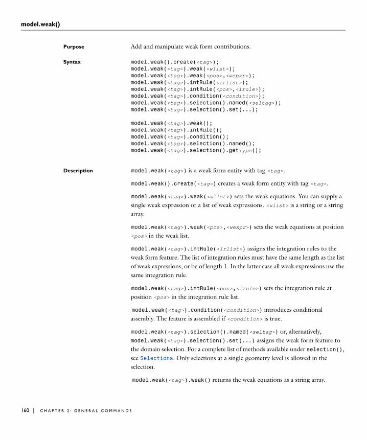
model.weak()
160 | C H A P T
model.weak()Purpose Add and manipulate weak form contributions.
Syntax model.weak().create(<tag>);model.weak(<tag>).weak(<wlist>);model.weak(<tag>).weak(<pos>,<wepxr>);model.weak(<tag>).intRule(<irlist>);model.weak(<tag>).intRule(<pos>,<irule>);model.weak(<tag>).condition(<condition>);model.weak(<tag>).selection().named(<seltag>);model.weak(<tag>).selection().set(...);
model.weak(<tag>).weak();model.weak(<tag>).intRule();model.weak(<tag>).condition();model.weak(<tag>).selection().named();model.weak(<tag>).selection().getType();
Description model.weak(<tag>) is a weak form entity with tag <tag>.
model.weak().create(<tag>) creates a weak form entity with tag <tag>.
model.weak(<tag>).weak(<wlist>) sets the weak equations. You can supply a single weak expression or a list of weak expressions. <wlist> is a string or a string array.
model.weak(<tag>).weak(<pos>,<wexpr>) sets the weak equations at position <pos> in the weak list.
model.weak(<tag>).intRule(<irlist>) assigns the integration rules to the weak form feature. The list of integration rules must have the same length as the list of weak expressions, or be of length 1. In the latter case all weak expressions use the same integration rule.
model.weak(<tag>).intRule(<pos>,<irule>) sets the integration rule at position <pos> in the integration rule list.
model.weak(<tag>).condition(<condition>) introduces conditional assembly. The feature is assembled if <condition> is true.
model.weak(<tag>).selection().named(<seltag>) or, alternatively, model.weak(<tag>).selection().set(...) assigns the weak form feature to the domain selection. For a complete list of methods available under selection(), see Selections. Only selections at a single geometry level is allowed in the selection.
model.weak(<tag>).weak() returns the weak equations as a string array.
E R 2 : G E N E R A L C O M M A N D S

model.weak()
model.weak(<tag>).intRule() returns the integration rule tags as a string array.
model.weak(<tag>).condition() returns the condition as a string.
model.weak(<tag>).selection().named() returns the selection tag as a string.
model.weak(<tag>).selection().getType() returns domain information. See Selections for available methods.
Examples Define the weak expressions u*u_test and v*v_test on the selection dom1, integration rule gp1 and frame ref.
model.weak().create("w1").selection().named("dom1");model.weak("w1").intRule("gp1");model.weak("w1").weak(new String[]{"u*u_test","v*v_test"});
See Also model.coeff(), model.shape()
161

model.weak()
162 | C H A P T
E R 2 : G E N E R A L C O M M A N D S
3
G e o m e t r y
This chapter includes reference information about the geometry commands and how to work with a geometry sequence and the geometry objects to create the model geometry.
In this chapter:
• About Geometry Commands
• Working with a Geometry Sequence
• Geometry Settings
• Work Planes
• Virtual Operations
• Geometry Object Information
• Measurements
• Inserting a Geometry Sequence from a File
• Exporting Geometry to File
• Geometry Commands
163

164 | C H A P T E
Abou t Geome t r y Command s
The following list includes the geometry commands that are documented in this chapter:
• Array
• BezierPolygon
• Block
• Chamfer
• Circle
• CollapseEdges
• Compose, Union, Intersection, Difference
• CompositeDomains
• CompositeEdges
• CompositeFaces
• Cone
• ConvertToSolid, ConvertToSurface, ConvertToCurve, ConvertToPoint
• Cylinder
• Delete
• ECone
• EditObject
• Ellipse
• Ellipsoid
• Extrude
• Fillet
• Finalize
• FromMesh
• Helix
• Hexahedron
• IgnoreEdges
• IgnoreFaces
R 3 : G E O M E T R Y

• IgnoreVertices
• Import DXF
• Import ECAD
• Import geometry sequence
• Import mphbin/mphtxt
• Import STL/VRML
• Interpolation Curve
• Interval
• MeshControlDomains
• MeshControlEdges
• MeshControlFaces
• MeshControlVertices
• MergeVertices
• Mirror
• Move, Copy
• ParametricCurve
• ParametricSurface
• Point
• Polygon
• Pyramid
• Rectangle
• Revolve
• Rotate
• Scale
• Selection
• Sphere
• Split
• Square
• Sweep
• Tangent
• Tetrahedron
A B O U T G E O M E T R Y C O M M A N D S | 165

166 | C H A P T E
• Torus
• WorkPlane
Features for Creating Geometric Primitives
Table 3-1 is an overview of the features for creating 3D geometric primitives:
• Features for Creating Geometric Primitives
• Features for Geometric Operations
• Features for Virtual Operations
• Features for Mesh Control
• Geometry Object Information Methods
See Also
TABLE 3-1: 3D GEOMETRIC PRIMITIVES
NAME DESCRIPTION
BezierPolygon Chain of connected line segments, quadratic or cubic curves
Block Right-angled parallelepiped (box)
Cone Right circular cone or cone frustum
Cylinder Right circular cylinder
ECone Oblique cone or cone frustum with elliptic base
Ellipsoid Ellipsoid
Helix Helix solid, surface, or curve
Hexahedron Hexahedron bounded by bilinear faces
ParametricCurve Curve defined by coordinate expressions
ParametricSurface Surface defined by coordinate expressions
Point One or several points
Polygon Chain of connected line segments
Pyramid Rectangular pyramid
Sphere Sphere or ball
Tetrahedron Tetrahedron
Torus Torus
R 3 : G E O M E T R Y

Table 3-2 is an overview of the features for creating 2D geometric primitives:
Table 3-3 is an overview of the features for creating 1D geometric primitives:
Features for Geometric Operations
The Import feature imports geometry objects from a file or from another geometry. The FromMesh feature constructs a geometry object from a (deformed) mesh.
Table 3-4 through Table 3-8 list the features that create new geometric objects from existing ones:
TABLE 3-2: 2D GEOMETRIC PRIMITIVES
NAME DESCRIPTION
BezierPolygon Chain of connected line segments, quadratic or cubic curves
Circle Circle or disc
Ellipse Ellipse
ParametricCurve Curve defined by coordinate expressions
Point One or several points
Polygon Chain of connected line segments
Rectangle Rectangle
Square Square
TABLE 3-3: 1D GEOMETRIC PRIMITIVES
NAME DESCRIPTION
Interval One interval, or a chain of connected intervals
Point One or several points
TABLE 3-4: WORK-PLANE RELATED FEATURES (ONLY 3D)
NAME DESCRIPTION
WorkPlane Create a work plane for drawing 2D objects that are embedded into 3D
Extrude Extrude planar objects into 3D
Revolve Revolve planar objects into 3D
Sweep Sweep a face along a spine curve to create a solid in 3D
A B O U T G E O M E T R Y C O M M A N D S | 167
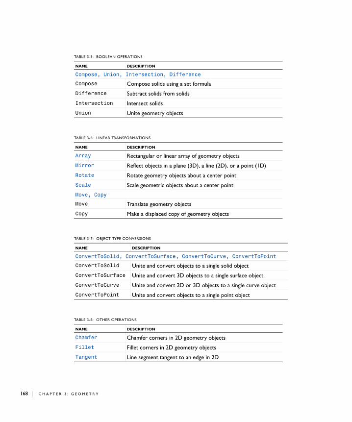
168 | C H A P T E
TABLE 3-5: BOOLEAN OPERATIONS
NAME DESCRIPTION
Compose, Union, Intersection, Difference
Compose Compose solids using a set formula
Difference Subtract solids from solids
Intersection Intersect solids
Union Unite geometry objects
TABLE 3-6: LINEAR TRANSFORMATIONS
NAME DESCRIPTION
Array Rectangular or linear array of geometry objects
Mirror Reflect objects in a plane (3D), a line (2D), or a point (1D)
Rotate Rotate geometry objects about a center point
Scale Scale geometric objects about a center point
Move, Copy
Move Translate geometry objects
Copy Make a displaced copy of geometry objects
TABLE 3-7: OBJECT TYPE CONVERSIONS
NAME DESCRIPTION
ConvertToSolid, ConvertToSurface, ConvertToCurve, ConvertToPoint
ConvertToSolid Unite and convert objects to a single solid object
ConvertToSurface Unite and convert 3D objects to a single surface object
ConvertToCurve Unite and convert 2D or 3D objects to a single curve object
ConvertToPoint Unite and convert objects to a single point object
TABLE 3-8: OTHER OPERATIONS
NAME DESCRIPTION
Chamfer Chamfer corners in 2D geometry objects
Fillet Fillet corners in 2D geometry objects
Tangent Line segment tangent to an edge in 2D
R 3 : G E O M E T R Y

Features for Virtual Operations
Table 3-9 lists the features that correspond to virtual operations:
Features for Mesh Control
Table 3-10 lists the features that correspond to mesh control operations:
Delete Delete entities (domains, boundaries, edges, or points) from objects, or delete entire geometry objects
Split Split geometry objects into their constituent entities
Finalize Finalize geometry by uniting all geometry objects to a single one
TABLE 3-9: VIRTUAL GEOMETRY RELATED FEATURES (ONLY 2D AND 3D)
NAME DESCRIPTION
IgnoreVertices Virtually remove isolated vertices or vertices adjacent to two edges only
IgnoreEdges Virtually remove isolated edges or edges adjacent to precisely two faces or between two domains
IgnoreFaces Virtually remove isolated faces or faces between two domains
CompositeEdges Form virtual composite edges from sets of connected edges by ignoring the vertices between the edges in each set
CompositeFaces Form virtual composite faces from sets of connected faces by ignoring the edges between the faces in each set
CompositeDomains Form virtual composite domains from sets of connected domains by ignoring the boundaries between the domains in each set
CollapseEdges Virtually collapse each edge into a vertex by merging its adjacent vertices
MergeVertices Virtually merge one adjacent vertex of an edge with the other adjacent vertex
TABLE 3-10: MESH CONTROL RELATED FEATURES (ONLY 2D AND 3D)
NAME DESCRIPTION
MeshControlVertices Use vertices for mesh control only
MeshControlEdges Use edges for mesh control only
TABLE 3-8: OTHER OPERATIONS
NAME DESCRIPTION
A B O U T G E O M E T R Y C O M M A N D S | 169

170 | C H A P T E
MeshControlFaces Use faces for mesh control only
MeshControlDomains Use domains for mesh control only
TABLE 3-10: MESH CONTROL RELATED FEATURES (ONLY 2D AND 3D)
NAME DESCRIPTION
R 3 : G E O M E T R Y

Geometry Object Information Methods
G E N E R A L I N F O R M A T I O N
G E O M E T R I C E N T I T Y C O U N T E R S
A D J A C E N C Y
TABLE 3-11: GENERAL GEOMETRY INFORMATION METHODS
METHOD DESCRIPTION
check Check object for errors
getBoundingBox Get bounding box around object
getSDim Get space dimension
getType Get object type (solid, surface, curve, point, mixed, empty)
hasCadRep Is represented using CAD Import Module kernel
TABLE 3-12: GEOMETRIC ENTITY COUNTERS
METHOD DESCRIPTION
getNEntities Get number of entities of different dimensions
getNVertices Get number of vertices
getNEdges Get number of edges
getNFaces Get number of faces
getNBoundaries Get number of boundaries
getNDomains Get number of domains
getNEntitiesMesh Get number of entities of different dimensions in the geometry used for meshing
TABLE 3-13: ADJACENCY BETWEEN GEOMETRIC ENTITIES
METHOD DESCRIPTION
getStartEnd Get start and end vertices of edges
getUpDown Get up and down domain indices
getVertexDomain Get domain index for isolated vertices
getSD Get domain index for isolated vertices
getAdj Get adjacency matrices
getAdjOrient Get adjacency orientation
getAdjSparse Get adjacency matrix in sparse format
A B O U T G E O M E T R Y C O M M A N D S | 171

172 | C H A P T E
E D G E E V A L U A T I O N
F A C E E V A L U A T I O N
G E O M E T R Y R E P R E S E N T A T I O N A R R A Y S
TABLE 3-14: EDGE EVALUATION METHODS
METHOD DESCRIPTION
edgeParamRange Get parameter range of edge
edgeX Evaluate coordinates
edgeDX Evaluate first derivative
edgeDDX Evaluate second derivative
edgeNormal Evaluate normal vector in 2D
edgeCurvature Evaluate curvature
edgeTorsion Evaluate torsion in 3D
TABLE 3-15: FACE EVALUATION METHODS
METHOD DESCRIPTION
faceParamRange Get parameter ranges of face
faceX Evaluate coordinates
faceDX Evaluate first derivatives
faceDDX Evaluate second derivatives
faceNormal Evaluate normal vector
faceFF1 Evaluate first fundamental form
faceFF2 Evaluate second fundamental form
faceGaussCurvature Evaluate Gauss curvature
faceMeanCurvature Evaluate mean curvature
TABLE 3-16: GET ARRAYS IN GEOMETRY REPRESENTATION
METHOD DESCRIPTION
getVertex Get vertex matrix
getEdges Get edge matrix
getFaces Get face matrix
getPVertex Get parameter vertices (embeddings of vertices in faces)
getPEdge Get parameter edges (embeddings of edges in faces)
getVertexCoord Get vertex coordinates
R 3 : G E O M E T R Y

Work i n g w i t h a Geome t r y S e qu en c e
This section describes how to construct geometries using Java methods. A geometry is defined by a geometry sequence consisting of geometry features. Each feature generates a set of output geometry objects when you build the feature. An operation feature takes previously generated geometry objects as input and usually deletes them. Each geometry sequence in 1D ends with a Finalize feature that forms a single output object by uniting all existing geometry objects. A geometry sequence in 2D or 3D also contains a Finalize feature, but in 2D and 3D it is possible to add features corresponding to virtual operations after the Finalize feature (see Virtual Operations for more information). The output object of the last feature of a sequence is referred to as the finalized geometry. The finalized geometry is used for meshing and physics modeling.
In this section:
• Adding a Model (Geometry)
• Adding a Geometry Feature
• Editing a Geometry Feature
• Building Geometry Features
• Feature Status
• Accessing Geometry Object Names
• Deleting and Disabling Geometry Features
• Deleting Geometry Objects
Adding a Model (Geometry)
To add a new geometry to the model object model, enter
model.geom().create(<tag>,sDim);
• Geometry Modeling Features in the COMSOL Multiphysics Reference Guide
• Geometry Modeling and CAD Tools in the COMSOL Multiphysics User’s Guide
See Also
W O R K I N G W I T H A G E O M E T R Y S E Q U E N C E | 173

174 | C H A P T E
where <tag> is the geometry’s tag (an identifier of your choice), and sDim is its space dimension (1, 2, or 3).
The geometry is added to the last created model node. If no model node exists in the model, a model node tagged mod1 is automatically created for you. A physics interface using the geometry must belong to the same model node as the geometry.
You can change the model of a geometry by entering
model.geom(<tag>).model(<mtag>);
where <mtag> is the tag of a model node.
Adding a Geometry Feature
To add a feature to a geometry tagged <tag>, enter
model.geom(<tag>).feature().create(<ftag>,ftype);
where <ftag> is the feature’s tag (an identifier of your choice), and ftype is the feature’s type. Feature types are capitalized and case-sensitive, for example Rectangle.
When you add a feature, it is inserted after the current feature. You can get the tag of the current feature type by entering
String ftag = model.geom(<tag>).current();
If ftag is the empty string, the current feature is the beginning of the geometry sequence, that is, the empty state before all features. When the feature has been added, it automatically becomes current, but it is not built automatically.
All properties in a new feature get a default value.
Editing a Geometry Feature
To change a property value in a feature, enter
model.geom(<tag>).feature(<ftag>).set(property,<value>);
where property is a property name and <value> is a property value.
model.modelNode()See Also
R 3 : G E O M E T R Y

All numeric properties can be given either as a numeric value or as a string expression that can contain parameters defined in model.param(). When building the feature, the string expressions are evaluated using the current values of the parameters.
To get the value of a property, enter one of the following, depending on the type of the property:
double d = model.geom(<tag>).feature(<ftag>).getDouble(property);String s = model.geom(<tag>).feature(<ftag>).getString(property);double[] da = model.geom(<tag>).feature(<ftag>).getDoubleArray(property);String[] sa = model.geom(<tag>).feature(<ftag>).getStringArray(property);double[][] dm = model.geom(<tag>).feature(<ftag>).getDoubleMatrix(property);String[][] sm = model.geom(<tag>).feature(<ftag>).getStringMatrix(property);
If you request a numerical value for a string property, it is evaluated using the current values of the parameters in model.param().
S E L E C T I O N S
There are primitive features and operation features. Operations features take existing geometry objects as input and create new geometry objects from them. The input objects are usually specified in the input selection:
model.geom(<tag>).feature(<ftag>).selection("input") set(inputObjects);
Behavior has changed since version 3.5a. String expression arguments are retained and not converted to numeric values.
Note
• getType()
• set()See Also
W O R K I N G W I T H A G E O M E T R Y S E Q U E N C E | 175

176 | C H A P T E
where inputObjects is a string array with object or feature names. If inputObjects contains a feature name, it refers to all objects generated by this feature.
Usually, the input objects of an operation feature is removed when building the feature. To change this behavior, a property keep is available for many operations features. If keep is set to on, the input objects are kept when building the feature.
Building Geometry Features
To generate the output objects of a feature, you must build the feature. Enter
model.geom(<tag>).run(<ftag>);
to build the feature <ftag> and all its preceding features (the features are built in the order from the first to the last). When the build has completed, the feature <ftag> becomes current.
To build all preceding features of the feature <ftag>, enter
model.geom(<tag>).runPre(<ftag>);
To build all features preceding the Finalize feature, enter
model.geom(<tag>).runAll();
To build all features, including the Finalize feature, enter
model.geom(<tag>).run();
E R R O R S
If an error occurs when building a feature, the build stops, and the feature before the failing feature becomes current. The failing feature gets a error feature appended, which contains the error message. To access the error message, enter
String msg = model.geom(<tag>).feature(<ftag>).message();
To access the error feature, its message and detailed message, enter
String msg = model.geom(<tag>).feature(<ftag>).problem("error"). getString("message");String det = model.geom(<tag>).feature(<ftag>).problem("error"). getString("details");
Geometry Object Selection MethodsSee Also
R 3 : G E O M E T R Y

WA R N I N G S
After a successful build, a feature can get warning features appended, which contain warning messages. To access the first warning message, enter
String msg = model.geom(<tag>).feature(<ftag>).message();
To access the warning features, their messages and detailed messages, enter
String msg = model.geom(<tag>).feature(<ftag>).problem(<wtag>). getString("message");String det = model.geom(<tag>).feature(<ftag>).problem(<wtag>). getString("details");
where <wtag> is warning1, warning2, and so on.
Feature Status
The status of a feature can be one of the following:
• Built or warning. This means that the none of the feature’s properties have changed since the feature was last built, and the features of the input objects are all built. If the status is warning, the feature contains warning messages.
• Edited. This means that some of the feature’s properties have changed since the feature was last built.
• Needs rebuild. This means that the feature generating some input object is not built.
• Error. This means that the feature contains an error message.
You can examine the status of a feature by entering
String status = model.geom(<tag>).feature(<ftag>).status();
Accessing Geometry Object Names
Each feature produces one or several output geometry objects. To get the names of these objects, enter
String[] oNames = model.geom(<tag>).feature(<ftag>).objectNames();
To get the names of all currently existing geometry objects (the geometry objects that were generated by the last build), enter
String[] oNames = model.geom(<tag>).objectNames();
To access one of these objects, you can enter
W O R K I N G W I T H A G E O M E T R Y S E Q U E N C E | 177

178 | C H A P T E
GeomObject go = model.geom(<tag>).object(<objname>);
where the string <objname> is an object name. If <objname> does not exist in the current state, you get an error message. You can get information about the geometry object go by using the geometry information methods, for example
int numberOfFaces = go.getNFaces();
To access the finalized geometry (the output of the last feature), use
model.geom(<tag>)
N A M I N G O F G E O M E T R Y O B J E C T S
The names of the output objects of a feature are formed by appending characters after the feature’s tag, in one of the following ways:
• ftag(index), for example split1(1), split1(2), split1(3) if the feature tagged split1 has three output objects. This method is used for most features.
• ftag(i1,i2,...), for example arr1(1,1), arr1(1,2), arr(2,1), arr1(2,2) for a 2-by-2 array feature tagged arr1. This method is only used for the Array feature.
• ftag.objectNameIn2D, for example wp1.r1, wp1.pt1(1), wp1.pt1(2) if the work plane feature wp1 contains the 2D objects r1, pt1(1), and pt1(2). This method is only used for the WorkPlane feature.
• ftag.objectName. This method can be used for the Import feature, and then objectName is taken from the CAD file.
Deleting and Disabling Geometry Features
To delete a feature, enter
model.geom(<tag>).feature().remove(<ftag>);
To disable a feature, enter
model.geom(<tag>).feature(<ftag>).active(false);
Geometry Object InformationSee Also
R 3 : G E O M E T R Y

The disabled feature does not affect the finalized geometry—its output is empty. To enable a disabled feature, enter
model.geom(<tag>).feature(<ftag>).active(true);
You can get the enabled/disabled status of a feature by entering
boolean isEnabled = model.geom(<tag>).feature(<ftag>).active();
Deleting Geometry Objects
You can use the following operation to delete objects from the geometry sequence.
model.geom(<tag>).delete(String[]);
In the input string array you specify the names of the objects to delete. The operation deletes objects that correspond to primitive geometry features by removing these features from the sequence. The operation then deletes the remaining objects by adding and building a Delete feature with the objects in its selection.
When using the delete operation the status of the current feature and all its preceding features must be built.
Note
W O R K I N G W I T H A G E O M E T R Y S E Q U E N C E | 179

180 | C H A P T E
Geome t r y S e t t i n g s
You can control the following general settings for a geometry:
• Length Unit
• Angular Unit
• Scale Values When Changing Unit
• Geometry Representation in 3D
• Default Relative Repair Tolerance
• Automatic Rebuild
Length Unit
The default length unit is meter. To change the length unit, enter
model.geom(<tag>).lengthUnit(newLengthUnit);
where newLengthUnit is a string like "mm", "in", or "ft".
To get the current length unit, enter
String currentUnit = model.geom(<tag>).lengthUnit();
The length unit is used in fields for lengths, and for visualization of the geometry. In fields you can override the unit, for example by entering 13[mm]. When solving the model, all lengths are converted to meters.
Angular Unit
The default angular unit is degrees. To change the angular unit, enter
model.geom(<tag>).angularUnit(newAngularUnit);
where newAngularUnit is deg or rad.
To get the current angular unit, enter
String currentUnit = model.geom(<tag>).angularUnit();
The angular is used in fields for angles. You can override the unit, for example by entering 0.3[rad]. Numeric inputs and outputs of trigonometric functions are always assumed to be in radians, though.
R 3 : G E O M E T R Y

Scale Values When Changing Unit
When you change the length unit or angular unit there are two possibilities to interpret pure numeric values in the geometry and meshing sequences. The first possibility is to reinterpret the numeric value in the new unit; a circle of radius 1.0 (meter) becomes a circle of radius 1.0 (millimeter), assuming the length unit changes from meter to millimeter.
The other possibility is to scale the numbers; a circle of radius 1.0 (meter) becomes a circle of radius 1000.0 (millimeter). To control the behavior, use
model.geom(<tag>).scaleUnitValue(newScaleValue);
where newScaleValue is true if you want values to be scaled, and false otherwise. The default value is false.
To get the currently used method, enter
boolean currentScaleValue = model.geom(<tag>).scaleUnitValue();
Geometry Representation in 3D
This setting controls which kernel (modeler) is used to represent and operate on the geometry objects, COMSOL Multiphysics’ own kernel or the CAD Import Module’s kernel (Parasolid). To change the geometry representation, enter
model.geom(<tag>).geomrep(newGeomRep);
where newGeomRep is comsol or cadps.
• If you choose comsol, all objects are represented using COMSOL’s kernel.
• If you choose cadps, all features that support this use the CAD Import Module’s kernel. For example, the Work Plane, Extrude, and Revolve features currently do not support this kernel. This alternative requires that you have license for the CAD Import Module.
The default geometry representation is controlled by the preference setting Geometry
> Default Geometry representation. To change or read this preference setting, enter
ModelUtil.setDefaultGeometryKernel(defaultGeomRep);ModelUtil.getDefaultGeometryKernel();
If the chosen geometry representation cannot be used (for example, because a feature requires the CAD Import Module’s kernel or because no CAD license is available), the behavior is controlled by the preference setting Geometry > Switch kernel automatically. To change or read this preference setting, enter
G E O M E T R Y S E T T I N G S | 181

182 | C H A P T E
ModelUtil.setAutoSwitchGeometryKernel(auto);ModelUtil.getAutoSwitchGeometryKernel();
If automatic switching is enabled, the geometry kernel will automatically be switched when needed. If automatic switching is disabled, an error message will be generated if the selected kernel cannot be used.
When you change the geometry representation setting, all features that support the CAD Import Module’s kernel get edited status. To rebuild the geometry using the new kernel, use the run or runAll methods.
Default Relative Repair Tolerance
The default relative repair tolerance is 1e-6 by default. You can change it by entering model.geom(<tag>).repairTol(<newDefaultRepairtol>);
To get the current default relative repair tolerance, enter
double reptol = model.geom(<tag>).repairTol();
The default relative repair tolerance is the default value that is used when you add a new feature that has a repairTol property, for example Boolean operations and conversions. Changing the default relative repair tolerance does not affect the tolerances in existing features. Adjust the relative repair tolerance if you experience problems with a Boolean operation. The absolute repair tolerance is the relative repair tolerance times the maximum coordinate of the input objects. Geometric entities that have a distance less than the absolute repair tolerance is merged.
Automatic Rebuild
This setting controls if the geometry sequence is automatically rebuilt when clicking on a node in the model tree outside the geometry sequence. You can change it by entering:
model.geom(<tag>).autoRebuild(<newAutoRebuild>);
where <newAutoRebuild> is either on or off.
The default geometry representation is controlled by the preference setting Geometry
> Automatic rebuild > Default in new geometries.
R 3 : G E O M E T R Y

Work P l a n e s
In 3D, you can create 3D objects by defining 2D objects in work planes and then extruding and revolving these into 3D objects.
To add a WorkPlane feature, use
model.geom(<tag>).feature().create(<ftag>,"WorkPlane");
You access a work planes 2D geometry sequence by the geom() method. To add a 2D feature to a work plane, use
model.geom(<tag>).feature(<ftag>).geom().feature(). create(<ftag1>,ftype);
where <ftag> refers to a WorkPlane feature and ftype refers to a 2D feature type.
A work plane’s geometry sequence inherits its settings from its 3D sequence.
When you build a work plane feature its corresponding 2D sequence builds automatically and the geometry objects defined by the 2D sequence embed into 3D geometry objects in the 3D sequence. You can then extrude or revolve these embedded point, curve, or surface objects into curve, surface, or solid objects, respectively, by Extrude or Revolve features, respectively.
A work plane’s geometry sequence does not contain a Finalize feature.
Note
For more information on the settings for a geometry sequence see Geometry Settings.
See Also
W O R K P L A N E S | 183

184 | C H A P T E
V i r t u a l Ope r a t i o n s
In this section:
• About Virtual Operations
• Mesh Control Entities
About Virtual Operations
In 2D and 3D it is possible to reduce the number of vertices, edges, faces, and domains of the geometry by using virtual operation features. To add the first virtual operation feature to a sequence you need to build the finalize feature by entering
model.geom(<tag>).run("fin");
You can then add the virtual operation feature by entering
model.geom(<tag>).feature().create(<ftag>,ftype);
where <ftag> is the feature’s tag (an identifier of your choice), and ftype is the feature’s type. To build the feature, enter
model.geom(<tag>).run(<ftag>);
To build all features, including the finalize feature and all virtual operation features, and to create the finalized geometry, enter
model.geom(<tag>).run();
The finalized geometry of a sequence that contains virtual operation features is referred to as a virtual geometry. If you form a composite edge, face, or domain by using either a CompositeEdges, CompositeFaces, or a CompositeDomains feature, respectively (or the analogues IgnoreVertices, IgnoreEdges, or IgnoreFaces features) the resulting edge, face, or domain is referred to as a virtual composite edge, virtual composite face, or virtual composite domain, respectively, or more generally, a virtual composite entity.
Mesh Control Entities
Sometimes it is desirable to use certain geometric entities only when constructing the mesh. For example, you can add a curve inside a domain to control mesh element size there. If you mark this curve as a mesh control entity, it is not included in the geometry
R 3 : G E O M E T R Y

used when defining the physics. An advantage is that the final mesh need not respect this curve exactly; it is used only to control element size.
You can use the keepformesh property of the Composite and Ignore features described above to define mesh control entities. Alternatively, you can use the MeshControlDomains, MeshControlVertices, MeshControlEdges, or MeshControlFaces features.
V I R T U A L O P E R A T I O N S | 185

186 | C H A P T E
Geome t r y Ob j e c t I n f o rma t i o n
You can get the geometry object named <objname> via
model.geom(<tag>).object(<objname>)
The geometry itself,
model.geom(<tag>)
works as an object, namely the final geometry resulting from the sequence. To get information about these objects, you can apply the methods described in this section.
The corresponding COMSOL 3.5a functionality is also indicated in the tables below. This functionality existed in three forms: as options to the function geominfo, as get methods on geometry objects, and as utility functions starting with flgeom.
In this section:
• General Information
• Geometric Entity Counters
• Adjacency
• Evaluation on an Edge
• Evaluation on a Face
• Geometry Representation Arrays
Accessing Geometry Object NamesSee Also
R 3 : G E O M E T R Y

General Information
• check() returns true if the object is valid, and false if it contains errors.
• exists() returns true if an object exists.
• getBoundingBox() returns a bounding box for the object in the order xmin, xmax, ymin, ymax, zmin, zmax.
• getSDim() returns the space dimension of the geometry.
• getType() returns the object type: solid, surface, curve, point, mixed, or empty.
• hasCadRep() returns true if the object is represented using the CAD Import Module’s geometry kernel (Parasolid).
Geometric Entity Counters
The following geometric entity counter methods are available:
• getNEntities returns a vector of length 2 in 1D, length 3 in 2D, and length 4 in 3D. The vectors contain the number of geometric entities for each entity dimension.
TABLE 3-17: GENERAL GEOMETRY INFORMATION METHODS
METHOD OUTPUT TYPE
check() boolean
exists() boolean
getBoundingBox() double[sdim*2]
getSDim() int
getType() String
hasCadRep() boolean
TABLE 3-18: GEOMETRIC ENTITY COUNTER METHODS
METHOD 1D 2D 3D OUTPUT TYPE 3.5A NAME
getNEntities() int[]
getNVertices() int nv, flgeomnv
getNEdges() int ne, flgeomnes
getNFaces() int nf
getNBoundaries() int nbs, flgeomnbs
getNDomains() int ns, flgeomnmr
getNEntitiesMesh() int[]
G E O M E T R Y O B J E C T I N F O R M A T I O N | 187

188 | C H A P T E
The methods getNVertices, getNEdges, getNFaces, getNBoundaries, and getNDomains return the number of entities of the specified type.
• getNEntitiesMesh returns a vector of length 2 in 1D, length 3 in 2D, and length 4 in 3D. The vectors contain the number of geometric entities for each entity dimension in the geometry used for meshing. If there are no mesh control entities in the geometry, the output is identical to that of getNEntities.
Adjacency
The following geometry adjacency information methods are available:
• getStartEnd returns the start and end vertices of all edges in the first and second row of the returned matrix.
• getUpDown returns the up and down domain number for all boundaries in the first and second row of the returned matrix.
• getVertexDomain returns the domain index for each vertex. For non-isolated vertices, the domain index is -1.
• getSD returns the domain index for each vertex. For non-isolated vertices, the domain index is NaN.
• a = getAdj(fromDim, toDim) returns a matrix where a[fromIdx]=getAdj(fromDim,toDim,fromIdx) contains the entities in dimension toDim that are adjacent to entity fromIdx in dimension fromDim.
• ao = getAdjOrient(fromDim, toDim) returns a matrix where ao[fromIdx]=getAdjOrient(fromDim,toDim,fromIdx) contains the
TABLE 3-19: GEOMETRY ADJACENCY INFORMATION METHODS
METHOD 1D 2D 3D OUTPUT TYPE 3.5A NAME
getStartEnd() int[2][] se,flgeomse
getUpDown() int[2][] ud,flgeomud
getVertexDomain() int[] sd,flgeomsd
getSD() double[] sd,flgeomsd
getAdj(int,int) int[][] adj, flgeomadj
getAdj(int,int,int) int[] adj, flgeomadj
getAdjOrient(int,int) int[][] adj, flgeomadj
getAdjOrient(int,int,int)
int[][] adj, flgeomadj
getAdjSparse(int,int) int[3][] adj, flgeomadj
R 3 : G E O M E T R Y

orientation flag for the entities in getAdj(fromDim,toDim,fromIdx). The orientation flag is 1 if the adjacent entities have the same orientation, and -1 if they have the opposite orientation, and 2 if the relative orientation cannot be determined (for instance, for an edge interior to a face).
• as = getAdjSparse(fromDim, toDim) returns the adjacency matrix from entities in dimension fromDim to entities in dimension toDim on a sparse format, that is, as[0] are the entity numbers in dimension fromDim, as[1] are the entity numbers in dimension toDim, and as[2] are the corresponding orientation flags.
Evaluation on an Edge
The following edge evaluation methods are available in 2D and 3D:
The first input argument of all methods is the edge number. The second input argument, when it exists, is an array of parameter values for which to perform evaluation on the edge. For all but the first method, the first index in the output corresponds to the different parameter values, and the second index corresponds to the spatial coordinates.
• edgeParamRange returns the parameter range for evaluation on the edge.
• edgeX evaluates the parameters to coordinate values.
• edgeDX evaluates the parameters to first order derivative values.
• edgeDDX evaluates the parameters to second order derivative values.
• edgeNormal evaluates the parameters to normal vector values.
• edgeCurvature evaluates the parameters to curvature values.
• edgeTorsion evaluates the parameters to torsion values.
TABLE 3-20: EDGE EVALUATION METHODS IN 2D AND 3D
METHOD 2D 3D OUTPUT TYPE 3.5A NAME
edgeParamRange(int) double[2] rng
edgeX(int, double[]) double[][D] xx
edgeDX(int, double[]) double[][D] dxx
edgeDDX(int, double[]) double[][D] ddx
edgeNormal(int, double[]) double[][D] nor
edgeCurvature(int, double[]) double[] crv
edgeTorsion(int, double[]) double[] crv
G E O M E T R Y O B J E C T I N F O R M A T I O N | 189

190 | C H A P T E
Evaluation on a Face
Use the following method for face evaluation in 3D. They do not work on virtual geometry objects.
The first input argument of all methods is the face number. The second input argument, when it exists, is a matrix of parameter points, for which to perform evaluation. For all but the first method, the first index in the output corresponds to the different parameter points.
• faceParamRange returns two parameter ranges for evaluation on the face.
• faceX evaluates the parameters to coordinate values.
• faceDX evaluates the parameters to first order derivative values.
• faceDDX evaluates the parameters to second order derivative values.
• faceNormal evaluates the parameters to normal vector values.
• faceFF1 evaluates the parameters to the first fundamental form values.
• faceFF2 evaluates the parameters to the second fundamental form values.
• faceGaussCurvature evaluates the parameters to Gauss curvature values.
• faceMeanCurvature evaluates the parameters to mean curvature values.
TABLE 3-21: FACE EVALUATION METHODS IN 3D
METHOD OUTPUT TYPE 3.5A NAME
faceParamRange(int) double[4] rng, flgeomfs
faceX(int, double[][2]) double[][3] xx
faceDX(int, double[][2]) double[][3][2] dx
faceDDX(int, double[][2]) double[][3][2][2] ddx
faceNormal(int, double[][2]) double[][3] nor
faceFF1(int, double[][2]) double[][2] ff1
faceFF2(int, double[][2]) double[][2] ff2
faceGaussCurvature(int, double[][2])
double[] crv
faceMeanCurvature(int, double[][2])
double[] crv
R 3 : G E O M E T R Y

Geometry Representation Arrays
Use the following methods to access the arrays in the internal representation of COMSOL geometry objects. They do not work on objects represented using the CAD Import Module’s kernel, assembly geometries, or virtual geometries.
• In 2D and 3D, getVertex returns (sdim+2)-by-nv matrix representing the vertices of the object. The first sdim rows are the coordinates of the vertices. Row sdim+1 contains the domain number if the vertex is isolated and is unspecified otherwise. The last row contains a relative local tolerance for the vertex. For nontolerant vertices the tolerance is NaN. This method does not work on virtual geometry objects.
• In 1D, getVertex returns a 3-by-nvtx matrix representing the vertices of the 1D object. Row 1 provides the coordinates of the vertices. Rows 2 and 3 provide the up and down domain numbers, respectively.
• getPVertex returns a 6-by-npv matrix containing embeddings of vertices in faces. Row 1 contains the vertex index (that is, column from getVertex), rows 2 and 3 contain (s, t) coordinates of the vertex on the face, row 4 contains a face index, and row 5 contains the manifold index into the manifolds. Row 6 contains a relative local tolerance for the vertex. This method does not work on virtual geometry objects.
TABLE 3-22: GET ARRAYS IN GEOMETRY REPRESENTATION
METHOD 1D 2D 3D OUTPUT TYPE 3.5A NAME
getVertex() double[][] vertex
getEdge() double[][] edge
getFace() double[][] face
getPVertex() double[][] pvertex
getPEdge() double[][] pedge
getVertexCoord() double[][] mp, flgeomvtx
voidsAreLabeled() boolean
In version 4.2a, a possibility to represent void regions with negative domain labels was introduced. This can affect the methods getVertex, getEdge, and getFace. If the method voidsAreLabeled() returns true, the geometry object uses such domain labels. If voidsAreLabeled() returns false, all void regions are represented with the domain label 0, like in version 4.2.
Note
G E O M E T R Y O B J E C T I N F O R M A T I O N | 191

192 | C H A P T E
• In 3D, getEdge returns a 7-by-ne matrix representing the edges of the 3D object. Rows 1 and 2 contain the start and end vertex indices of the edge (0 if they do not exist), respectively. Rows 3 and 4 give the parameter values of these vertices. Row 5 gives the index of a domain if the edge is not adjacent to a face, and is unspecified otherwise. Row 6 gives a sign and an index to the underlying manifold. The sign indicates the direction of the edge relative the curve. Finally, row 7 contains a relative local tolerance for the edge. This method does not work on virtual geometry objects.
• In 2D, getEdge returns a 8-by-ne matrix representing the edges of the 2D object. Rows 1 and 2 contain the start and end vertex indices of the edge, respectively (0 if they do not exist). Rows 3 and 4 give the parameter values of these vertices. Rows 5 and 6 contain the left and right domain number of the edge, respectively. Row 7 gives a sign and an index to the array of underlying curves. The sign indicates the direction of the edge relative the curve. Row 8 contains a relative local tolerance for the edge.
• getPEdge returns a 10-by-npe matrix representing the embeddings of the edges in faces. The first row gives the index of the edge in getEdge. Rows 2 and 3 contain the start and end vertex indices from getPVertex, respectively. Rows 4 and 5 give the parameter values of these vertices. Row 6 and 7 give the indices of the faces to the left and right of the edge, respectively. Row 8 gives a sign and index to the parameter curve (if any), and row 9 gives the index to the surface. Row 10 contains a relative local tolerance for the edge. This method does not work on virtual geometry objects.
• getFace returns a 4-by-nf matrix representing the faces of the 3D geometry. Rows 1 and 2 contain the up and down domain index of the face, respectively, and row 3 contains the manifold index of the face. Row 4 contains a relative local tolerance for the face. This method does not work on virtual geometry objects.
• getVertexCoord returns a matrix with the vertex coordinates. Its dimension is the space dimension times the number of vertices.
R 3 : G E O M E T R Y
Mea s u r emen t s
Geometric measurements is a tool to measure geometric entities and objects. You access it by entering
model.geom(<tag>).measure()
In this section:
• Measuring Geometric Entities in Objects
• Measuring Objects
Measuring Geometric Entities in Objects
To select entities you want to measure, enter
model.geom(<tag>).measure().selection().init(entDim);model.geom(<tag>).measure().selection().set(<objname>,entities);
where entDim is the dimension of the entities, <objname> is the object name, and entities is an integer array containing the entity numbers.
To get the volume/area/length of the selected entities, enter
double vol = model.geom(<tag>).measure().getVolume();
To get the area/length of the boundary of the selected entities, enter
double bndVol = model.geom(<tag>).measure().getBoundaryVolume();
If you have selected two vertices, you can get their distance by entering
double[] d = model.geom(<tag>).measure().getVtxDistance();
d[0] is the distance, and d[i] is the distance in the ith coordinate (i = 1, 2, 3).
If you have selected one vertex, you can get its coordinates by entering
double[] coord = model.geom(<tag>).measure().getVtxCoord();
Measuring Objects
To select objects you want to measure, enter
model.geom(<tag>).measure().selection().init();model.geom(<tag>).measure().selection().set(<objnames>);
where <objnames> is a string array containing the object names.
M E A S U R E M E N T S | 193

194 | C H A P T E
To get the total number of entities in the selected objects, enter
int[] entitiesPerDimension = model.geom(<tag>).measure().getNEntities();
R 3 : G E O M E T R Y

I n s e r t i n g a Geome t r y S e qu en c e f r om a F i l e
To insert a geometry sequence from an MPH-file, enter
model.geom(<tag>).insertFile(<filename>, <sequencename>);
where <filename> and <sequencename> are strings.
To insert a geometry sequence from a different model, enter
model.geom(<tag>).insertSequence(<modeltag>, <sequencename>);
where <modeltag> and <sequencename> are strings.
Example
The following sequence imports three different geometry sequences from two different files.
Model model = ModelUtil.create("Model");model.geom().create("g", 2);model.geom("g").insertFile("filename", "geom1");ModelUtil.load("Model2", "filename2");model.geom("g").insertSequence("Model2", "geom1/wp1");model.geom("g").insertSequence("Model2", "geom1/wp2");
I N S E R T I N G A G E O M E T R Y S E Q U E N C E F R O M A F I L E | 195

196 | C H A P T E
Expo r t i n g Geome t r y t o F i l e
In this section:
• How to Export the Finalized Geometry
• Exporting to an STL File
• Exporting to a Parasolid File
• Compatibility in 3D
How to Export the Finalized Geometry
To export the finalized geometry to a file, enter
model.geom(<tag>).exportFinal(<filename>);
where <filename> is a string.
To export selected geometry objects to a file, first select the objects to export using
model.geom(<tag>).export().selection().set(<objnames>);
where <objnames> is a string array of object names. Then export them by entering
model.geom(<tag>).export(<filename>);
The file can be any of the following formats:
TABLE 3-23: VALID FILE FORMATS
FILE FORMAT NOTE FILE EXTENSIONS
COMSOL Multiphysics Binary .mphbin
COMSOL Multiphysics Text .mphtxt
Parasolid Binary (3D) 1 .x_b
Parasolid Text (3D) 1 .x_t
STL Binary (3D) 2 .x_b
STL Text (3D) 2 .x_t
DXF (2D) .dxf1 This format requires a license for the COMSOL CAD Import Module.2 Use model.geom(<tag>).export().setSTLFormat(<format>) to specify the STL file format (“binary” or “text”)
R 3 : G E O M E T R Y

Exporting to an STL File
To export to an STL file, start with specifying a file format using
model.geom(<tag>).export().setSTLFormat(<format>);
where <format> is string with only two allowed values: binary and text
Use the following methods to select domains or boundaries to export:
model.geom(<tag>).export().selection().init(<edim>);model.geom(<tag>).export().selection().set(<objnames>, <entlst>);
Use the following methods to select objects to export:
model.geom(<tag>).export().selection().init();model.geom(<tag>).export().selection().set(<objnames>);
Finish the export by using the following line
model.geom(<tag>).export(<filename>);
Exporting to a Parasolid File
When exporting to Parasolid text or binary format, a unit conversion can optionally be performed during export. Use the following method to select the export length unit:
model.geom(<tag>).export().setLengthUnit(<unit>);
where <unit> is either fromgeom to disable unit conversion, or a COMSOL length unit, such as m for meters or in for inches.
Compatibility in 3D
If you want to open a COMSOL Multiphysics 3D geometry file in the 3.5a version of COMSOL, you need to set the compat property to 3.5a using
model.geom(<tag>).export().set("compat","3.5a");
E X P O R T I N G G E O M E T R Y T O F I L E | 197

198 | C H A P T E
Geome t r y Command s
• Array
• BezierPolygon
• Block
• Chamfer
• Circle
• CollapseEdges
• Compose, Union, Intersection, Difference
• CompositeDomains
• CompositeEdges
• CompositeFaces
• Cone
• ConvertToSolid, ConvertToSurface, ConvertToCurve, ConvertToPoint
• Cylinder
• Delete
• ECone
• EditObject
• Ellipse
• Ellipsoid
• Extrude
• Fillet
• Finalize
• FromMesh
• Helix
• Hexahedron
• IgnoreEdges
• IgnoreFaces
• IgnoreVertices
• Import DXF
R 3 : G E O M E T R Y

• Import ECAD
• Import geometry sequence
• Import mphbin/mphtxt
• Import STL/VRML
• Interpolation Curve
• Interval
• MergeVertices
• MeshControlEdges
• MeshControlFaces
• MeshControlVertices
• Mirror
• Move, Copy
• ParametricCurve
• ParametricSurface
• Point
• Polygon
• Pyramid
• Rectangle
• Revolve
• Rotate
• Scale
• Selection
• Sphere
• Split
• Square
• Sweep
• Tangent
• Tetrahedron
• Torus
• WorkPlane
G E O M E T R Y C O M M A N D S | 199

Array
200 | C H A P T
ArrayPurpose Create block shaped (3D), rectangular (2D, 3D) or linear array of geometry objects
Syntax model.geom(<tag>).feature().create(<ftag>,"Array");model.geom(<tag>).feature(<ftag>).selection(property);model.geom(<tag>).feature(<ftag>).set(property,<value>);model.geom(<tag>).feature(<ftag>).getType(property);
Description Use model.geom(<tag>).feature().create(<ftag>,"Array") to create an array of geometry objects.
Use model.geom(<tag>).feature(<ftag>).selection("input") to select the objects to array. The default selection is empty.
The following properties are available:
If size is a scalar, a linear (oblique) array with size copies of the input objects is constructed. The displacement between two consecutive copies is given by the vector displ. The names of the output objects are ftag(i), where ftag is the tag of the feature, and i is a 1-based index. If there are more than one input object, the output objects are named ftag(i,in), where in is a 1-based index corresponding to the input objects.
2D: If size is an array of length 2, a rectangular array with size[0]-by-size[1] copies of the input object is constructed. The x- and y-displacements are displ[0] and displ[1], respectively. The names of the output objects are ftag(i1,i2), where ftag is the name of the feature, and i1 and i2 are 1-based indices. If there are more than one input object, the output objects are named ftag(i1,i2,in), where in is a 1-based index corresponding to the input objects.
3D: If size is an array of length 3, a three-dimensional (block shaped) array with size[0]-by-size[1]-by-size[2] copies of the input object is constructed. The x-, y-, and z-displacements are displ[0], displ[1], and displ[2], respectively. The names of the output objects are ftag(i1,i2,i3), where ftag is the name of the feature, and i1, i2, and i3 are 1-based indices. If there are more than one input
TABLE 3-24: VALID PROPERTIES
NAME VALUE DEFAULT DESCRIPTION
input Selection Objects to array
displ double[sdim] 1 Displacements in axis directions
size int | int[sdim] 1 Array size
createselection on | off off Create selections
E R 3 : G E O M E T R Y

Array
object, the output objects are named ftag(i1,i2,i3,in), where in is a 1-based index corresponding to the input objects.
The input object is deleted and an identical object is constructed as a part of the array.
If createselection is set to on, predefined selections for all entities (all or some of domains, boundaries, edges and points) in the finalized geometry are created. To access the selections, use model.selection(<tag>_<ftag>_<lvl>), where <tag> is the geometry tag, <ftag> the feature tag and <lvl> is one of dom, bnd, edg, pnt. The createselection property is not available in work-plane geometries.
Compatibility In COMSOL version 3.5a it was possible to use geomarrayr to copy an object to an arbitrary set of positions. Now, use the Copy feature to do this.
model.geom(<tag>).feature().create(<ftag>,"arrayr") constructs an Array feature
Example The following sequence creates a block with four equally sized holes.
Model model = ModelUtil.create("Model1");model.geom().create("geom1",3);model.geom("geom1").feature().create("cyl1","Cylinder");model.geom("geom1").feature().create("arr1","Array");model.geom("geom1").feature("arr1"). selection("input").set("cyl1");model.geom("geom1").feature("arr1").set("displ", "4 4 0");model.geom("geom1").feature("arr1").set("size", "2 2 1");model.geom("geom1").feature().create("blk1","Block");model.geom("geom1").feature("blk1").set("size", "10 14 5");model.geom("geom1").feature("blk1").set("pos", "-3 -5 -4");model.geom("geom1").feature().create("dif1","Difference");model.geom("geom1").feature("dif1"). selection("input").set("blk1");model.geom("geom1").feature("dif1"). selection("input2").set("arr1");model.geom("geom1").runAll();
See Also Move, Copy
201

BezierPolygon
202 | C H A P T
BezierPolygonPurpose Create curve or solid polygon consisting of Bézier segments in 2D or 3D
Syntax model.geom(<tag>).feature().create(<ftag>,"BezierPolygon");model.geom(<tag>).feature(<ftag>).set(property,<value>);model.geom(<tag>).feature(<ftag>).getType(property);
Description Use model.geom(<tag>).feature().create(<ftag>,"BezierPolygon") to create a Bézier polygon or a line segment. The following properties are available
If type is open or closed, a curve consisting of line, quadratic, or cubic rational Bézier segments is constructed. If type is solid, the solid enclosed by such a closed polygon is constructed. If type is closed or solid, but the first and last control points are different, an extra linear segment is added to close the curve.
The degree of the nth segment is degree[n], and it must be 1 (linear), 2 (quadratic), or 3 (cubic). The nth segment has degree[n]+1 control points and weights. The weights are stored consecutively in the array w, which has length degree[0]+...+degree[N-1]+N, where N is the number of segments. The ith coordinates of the control points are stored consecutively in the array p[i]. Adjacent segments share the common control point, which means that p[i] has length degree[0]+...+degree[N-1]+1.
For a linear or cubic segment, the default weights are 1. For a quadratic segment, the default weights are 1, 1/ , 1.
If createselection is set to on, predefined selections for all entities (all or some of domains, boundaries, edges, and points) in the finalized geometry are created. To access the selections, use model.selection(<tag>_<ftag>_<lvl>), where <tag> is the geometry tag, <ftag> the feature tag and <lvl> is one of dom, bnd, edg, or pnt. The createselection property is not available in work-plane geometries.
Examples Construct a solid triangle b1, and an elliptic arc b2:
TABLE 3-25: VALID PROPERTY/VALUE PAIRS
PROPERTY VALUE DEFAULT DESCRIPTION
degree int[] | int 1 Degree of Bézier segments
p double[][] Control points
type solid | open | closed
solid (2D)open (3D)
Object type. solid is not available in 3D.
w double[] Weights
createselection on | off off Create selections
2
E R 3 : G E O M E T R Y

BezierPolygon
Model model = ModelUtil.create("Model1");model.geom().create("geom1",2);model.geom("geom1").feature().create("b1","BezierPolygon");model.geom("geom1").feature("b1").set("p", new double[][]{{0, 0, 2}, {1, 0 ,0}});
model.geom("geom1").feature().create("b2","BezierPolygon");model.geom("geom1").feature("b2").set("type","open");model.geom("geom1").feature("b2").set("degree",2);model.geom("geom1").feature("b2").set("p", new double[][]{{0, 0, 1}, {0, 1, 1}});model.geom("geom1").runAll();
See Also Polygon
203
Block
204 | C H A P T
BlockPurpose Create a right-angled solid or surface block in 3D
Syntax model.geom(<tag>).feature().create(<ftag>,"Block");model.geom(<tag>).feature(<ftag>).set(property,<value>);model.geom(<tag>).feature(<ftag>).getType(property);
Description Use model.geom(<tag>).feature().create(<ftag>,"Block") to create a block. The following properties are available:
If createselection is set to on, predefined selections for all entities (all or some of domains, boundaries, edges and points) in the finalized geometry are created. To access the selections, use model.selection(<tag>_<ftag>_<lvl>), where <tag>
TABLE 3-26: VALID PROPERTY/VALUE PAIRS
PROPERTY VALUE DEFAULT DESCRIPTION
axis double[] {0,0,1} Direction of the edge on the local z-axis. Vector has length 3 if axistype is cartesian, and length 2 if axistype is spherical.
axistype cartesian | spherical
cartesian Coordinate system used for axis. The value is synchronized with axis.
base corner | center
corner Positions the object either centered about pos or with one corner in pos.
layer double[] Thicknesses of layers
layertop on | off off Apply layers on top
layerbottom on | off on Apply layers on bottom
layerleft on | off off Apply layers to the left
layerright on | off off Apply layers to the right
layerfront on | off off Apply layers on front
layerback on | off off Apply layers on back
size double[] {1,1,1} Edge lengths.
pos double[] {0,0,0} Position of the object.
rot double 0 Rotational angle about axis.
type solid | surface
solid Object type.
createselection on | off off Create selections
E R 3 : G E O M E T R Y

Block
is the geometry tag, <ftag> the feature tag and <lvl> is one of dom, bnd, edg, pnt. The createselection property is not available in work-plane geometries.
Compatibility model.geom(<tag>).feature().create(<ftag>,"block2") constructs a solid block.
model.geom(<tag>).feature().create(<ftag>,"block3") constructs a surface block.
The following properties are also available:
The property const is no longer available.
Examples The following commands create a solid and surface block, where the position is defined in the two alternative ways.
Model model = ModelUtil.create("Model1");model.geom().create("geom1",3);model.geom("geom1").feature().create("b1","Block");model.geom("geom1").feature("b1").set("size","1 2.1 0.5");model.geom("geom1").feature("b1").set("base","center");model.geom("geom1").feature("b1").set("pos","1 0 1");model.geom("geom1").feature("b1").set("axis","1 0 0");model.geom("geom1").feature("b1").set("rot",30);double[] a = model.geom("geom1").feature("b1"). getDoubleArray("pos");model.geom("geom1").feature().create("b2","Block");model.geom("geom1").feature("b2").set("type","surface");model.geom("geom1").feature("b2").set("size","1 2.1 0.5");model.geom("geom1").feature("b2").set("pos",a);String b = model.geom("geom1").feature("b2"). getString("pos");
See Also Hexahedron
TABLE 3-27: VALID PROPERTY/VALUE PAIRS
PROPERTY VALUE DEFAULT DESCRIPTION
ax2 double[] {0,0} Alias for axis when axistype is spherical
ax3 double[] {0,0,1} Alias for axis when axistype is cartesian
lx, ly, lz double 1 Alias for size
x, y, z double 0 Alias for pos
205

Chamfer
206 | C H A P T
ChamferPurpose Create flattened corners in 2D objects
Syntax model.geom(<tag>).feature().create(<ftag>,"Chamfer");model.geom(<tag>).feature(<ftag>).selection(property);model.geom(<tag>).feature(<ftag>).set(property,<value>);model.geom(<tag>).feature(<ftag>).getType(property);
Description Use model.geom(<tag>).feature().create(<ftag>,"Chamfer") to chamfer corners in 2D.
Use model.geom(<tag>).feature(<ftag>).selection("point") to select the corners to chamfer. The default selection is empty.
If createselection is set to on, predefined selections for all entities (all or some of domains, boundaries, edges and points) in the finalized geometry are created. To access the selections, use model.selection(<tag>_<ftag>_<lvl>), where <tag> is the geometry tag, <ftag> the feature tag and <lvl> is one of dom, bnd, edg, pnt. The createselection property is not available in work-plane geometries.
Compatibility In version 3.5a, the default was to chamfer all vertices in the input objects. The 3.5a properties angles, dist1, dist2, edges, length, and out are no longer available.
Example Chamfer a rectangle.
Model model = ModelUtil.create("Model1");model.geom().create("geom1",2);model.geom("geom1").feature().create("r1","Rectangle");model.geom("geom1").feature().create("cha1","Chamfer");model.geom("geom1").feature("cha1").selection("point"). set("r1(1)",new int[]{1,2,3,4});model.geom("geom1").feature("cha1").set("dist",0.1);model.geom("geom1").run();
Diagnostics If a chamfer cannot be created according to the specified properties this vertex is ignored. When the chamfers generate intersections with other edges in the geometry, an error message is given.
See Also Fillet
PROPERTY VALUE DEFAULT DESCRIPTION
dist double 0 Distance from vertex to chamfer
point Selection Vertices to chamfer
createselection on | off off Create selections
E R 3 : G E O M E T R Y

Circle
CirclePurpose Create circle or disk in 2D
Syntax model.geom(<tag>).feature().create(<ftag>,"Circle");model.geom(<tag>).feature(<ftag>).set(property,<value>);model.geom(<tag>).feature(<ftag>).getType(property);
Description Use model.geom(<tag>).feature().create(<ftag>,"Circle") to create a disk in 2D. The following properties are available:
If createselection is set to on, predefined selections for all entities (all or some of domains, boundaries, edges and points) in the finalized geometry are created. To access the selections, use model.selection(<tag>_<ftag>_<lvl>), where <tag> is the geometry tag, <ftag> the feature tag and <lvl> is one of dom, bnd, edg, pnt. The createselection property is not available in work-plane geometries.
Compatibility model.geom(<tag>).feature().create(<ftag>,"circ2") creates a solid disk.
model.geom(<tag>).feature().create(<ftag>,"circ1") creates a circle curve.
The following properties are also available:
The property const is no longer available.
Example The sequence below creates a unit disk (solid circle object).
TABLE 3-28: VALID PROPERTY/VALUE PAIRS
PROPERTY VALUE DEFAULT DESCRIPTION
base corner | center center Positions the object either centered about pos or with the lower left corner of a surrounding box in pos
layer double[] Thicknesses of layers
pos double[] {0,0} Position of the object
r double 1 Radius
rot double 0 Rotational angle about pos
type solid | curve solid Object type
createselection on | off off Create selections
TABLE 3-29: VALID PROPERTY/VALUE PAIRS
PROPERTY VALUE DEFAULT DESCRIPTION
x, y double 0 Alias for pos
207

Circle
208 | C H A P T
Model model = ModelUtil.create("Model1");model.geom().create("geom1",2);model.geom("geom1").feature().create("c1","Circle");model.geom("geom1").feature("c1").set("pos",new double[]{2,3});String base = model.geom("geom1").feature("c1"). getString("base");
See Also Ellipse
E R 3 : G E O M E T R Y

CollapseEdges
CollapseEdgesPurpose Collapse edges
Syntax model.geom(<tag>).feature().create(<ftag>,"CollapseEdges");model.geom(<tag>).feature(<ftag>).selection(property);model.geom(<tag>).feature(<ftag>).set(property,<value>);model.geom(<tag>).feature(<ftag>).getType(property);
Description Use model.geom(<tag>).feature().create(<ftag>,"CollapseEdges") to collapse edges.
Use model.geom(<tag>).feature(<ftag>).selection("input") to select the edges to collapse. The default selection is empty.
The feature collapses an edge by removing it, merging its adjacent vertices to the vertex with lowest index, and re-connecting the adjacent edges to the merged vertex.
The output object is a virtual geometry.
The following properties are available:
See Also MergeVertices
TABLE 3-30: VALID PROPERTIES
NAME VALUE DEFAULT DESCRIPTION
input Selection Edges to collapse
209
Compose, Union, Intersection, Difference
210 | C H A P T
Compose, Union, Intersection, DifferencePurpose Compose objects using a boolean set formula.
Syntax model.geom(<tag>).feature().create(<ftag>,"Compose");model.geom(<tag>).feature().create(<ftag>,"Union");model.geom(<tag>).feature().create(<ftag>,"Intersection");model.geom(<tag>).feature().create(<ftag>,"Difference");model.geom(<tag>).feature(<ftag>).selection(property);model.geom(<tag>).feature(<ftag>).set(property,<value>);model.geom(<tag>).feature(<ftag>).getType(property);
Description Use model.geom(<tag>).feature().create(<ftag>,operationName) to combine geometric objects in different ways.
Use model.geom(<tag>).feature(<ftag>).selection(property) to select the objects to combine. The default selection is empty.
The following properties are available:
For the features Compose, Intersection, and Difference, the input objects must be solids. For the Union feature, the input objects can be of arbitrary type.
The following boolean operation is performed:
• For Compose, the input objects are combined using the set formula in the property formula. The operators +, *, and - correspond to the set operations union, intersection, and difference. The precedence of the operators + and -are the same. * has higher precedence.
• For Union, the objects in input are united.
TABLE 3-31: VALID PROPERTY/VALUE PAIRS
PROPERTY VALUE DEFAULT DESCRIPTION
formula String Set formula (only for Compose feature)
input Selection Objects to compose
input2 Selection Objects to subtract (only for Difference feature)
intbnd on | off on Keep interior boundaries.
keep on | off off Keep input objects
repairtol double 1e-6 Repair tolerance, relative to size of union of inputs
createselection on | off off Create selections
E R 3 : G E O M E T R Y

Compose, Union, Intersection, Difference
• For Intersection, the objects in input are intersected.
• For Difference, the objects in input2 are subtracted from the union of the objects in input.
If createselection is set to on, predefined selections for all entities (all or some of domains, boundaries, edges and points) in the finalized geometry are created. To access the selections, use model.selection(<tag>_<ftag>_<lvl>), where <tag> is the geometry tag, <ftag> the feature tag and <lvl> is one of dom, bnd, edg, pnt. The createselection property is not available in work-plane geometries.
Compatibility The following properties are also supported, see the Delete feature:
The property out is no longer available.
See Also ConvertToSolid, ConvertToSurface, ConvertToCurve, ConvertToPoint, Finalize
TABLE 3-32: VALID PROPERTY/VALUE PAIRS
PROPERTY VALUE DEFAULT DESCRIPTION
edge all | none none Delete isolated edges on a face (3D) Delete interior edges and edges not adjacent to a domain (2D, alias for indbnd)
face all | none none Delete interior faces (3D, alias for intbnd)
point all | none none Delete isolated vertices on a face (3D). Delete isolated vertices in a domain (2D)
211

CompositeDomains
212 | C H A P T
CompositeDomainsPurpose Form composite domains.
Syntax model.geom(<tag>).feature().create(<ftag>,"CompositeDomains");model.geom(<tag>).feature(<ftag>).selection(property);model.geom(<tag>).feature(<ftag>).set(property,<value>);model.geom(<tag>).feature(<ftag>).getType(property);
Description Use model.geom(<tag>).feature().create(<ftag>,"CompositeDomains") to form composite domains.
Use model.geom(<tag>).feature(<ftag>).selection("input") to select the domains to composite. The default selection is empty.
The feature forms a composite domain for each connected domain component of the selected domains by ignoring the boundaries between the domains. The output object is a virtual geometry.
The following properties are available:
Use ignoreadj to specify if the feature also removes the ignorable edges (3D only) and vertices on the boundary of each resulting composite domain.
Use keepformesh to keep the input domains while meshing, to help you in constructing the mesh.
Example Create a composite domain of domain 2 and 3.
Model model = ModelUtil.create("Model");model.geom().create("geom", 2);model.geom("geom").feature().create("r1", "Rectangle");model.geom("geom").feature().create("c1", "Circle");model.geom("geom").run("fin");model.geom("geom").feature().create("cmd1","CompositeDomains");model.geom("geom").feature("cmd1").selection("input"). set("fin", 2, 3);model.geom("geom").run();
See Also CompositeEdges, CompositeFaces, IgnoreEdges, IgnoreFaces
TABLE 3-33: VALID PROPERTIES
NAME VALUE DEFAULT DESCRIPTION
ignoreadj on | off on Ignore edges (3D only) and vertices on boundary
input Selection Edges to composite
keepformesh on | off off Keep input domains for mesh control
E R 3 : G E O M E T R Y
CompositeEdges
CompositeEdgesPurpose Form composite edges.
Syntax model.geom(<tag>).feature().create(<ftag>,"CompositeEdges");model.geom(<tag>).feature(<ftag>).selection(property);model.geom(<tag>).feature(<ftag>).set(property,<value>);model.geom(<tag>).feature(<ftag>).getType(property);
Description Use model.geom(<tag>).feature().create(<ftag>,"CompositeEdges") to form composite edges.
Use model.geom(<tag>).feature(<ftag>).selection("input") to select the edges to concatenate. The default selection is empty.
The feature forms a composite edge for each connected edge component (of manifold type) of the selected edges by ignoring the vertices between the edges. The output object is a virtual geometry.
The following properties are available:
Use keepformesh to keep the input edges while meshing, to help you in constructing the mesh.
Note that the operation will never form composite edges that are closed loops or periodic, that is, every resulting edge will have distinct start and end vertices.
Example Compose edges 2 and 4 of a circle into one edge.
Model model = ModelUtil.create("Model");model.geom().create("geom1", 2);model.geom("geom1").feature().create("c1", "Circle");model.geom("geom1").run("fin");model.geom("geom1").feature().create("cme1", "CompositeEdges");model.geom("geom1").feature("cme1").selection("input"). set("fin", 2, 4);model.geom("geom1").run();
See Also CompositeDomains, CompositeFaces, IgnoreVertices
TABLE 3-34: VALID PROPERTIES
NAME VALUE DEFAULT DESCRIPTION
input Selection Edges to composite
keepformesh on | off off Keep input edges for mesh control
213

CompositeFaces
214 | C H A P T
CompositeFacesPurpose Form composite faces
Syntax model.geom(<tag>).feature().create(<ftag>,"CompositeFaces");model.geom(<tag>).feature(<ftag>).selection(property);model.geom(<tag>).feature(<ftag>).set(property,<value>);model.geom(<tag>).feature(<ftag>).getType(property);
Description Use model.geom(<tag>).feature().create(<ftag>,"CompositeFaces") to form composite faces.
Use model.geom(<tag>).feature(<ftag>).selection("input") to select the faces to concatenate. The default selection is empty.
The feature forms a composite face for each connected face component (of manifold type) of the selected faces by ignoring the edges between the faces. The output object is a virtual geometry.
The following properties are available:
Use ignorevtx to specify if the feature also removes the ignorable vertices on the boundary of each resulting composite face.
Use keepformesh to keep the input faces while meshing, to help you in constructing the mesh.
Example A COMSOL standard cone has six faces. Using the following composite face operation, the result is a cone with three faces: top, bottom and side.
Model model = ModelUtil.create("Model");model.geom().create("geom1", 3);model.geom("geom1").feature().create("cone1", "Cone");model.geom("geom1").run("fin");model.geom("geom1").feature().create("cmf1", "CompositeFaces");model.geom("geom1").feature("cmf1").selection("input"). set("fin", 1, 2, 5, 6);model.geom("geom1").run();
See Also CompositeDomains, CompositeEdges, IgnoreEdges
TABLE 3-35: VALID PROPERTIES
NAME VALUE DEFAULT DESCRIPTION
input Selection Faces to composite
ignorevtx on | off on Ignore vertices on boundary
keepformesh on | off off Keep input faces for mesh control
E R 3 : G E O M E T R Y

Cone
ConePurpose Create a solid or surface circular right cone or frustum in 3D
Syntax model.geom(<tag>).feature().create(<ftag>,"Cone");model.geom(<tag>).feature(<ftag>).set(property,<value>);model.geom(<tag>).feature(<ftag>).getType(property);
Description Use model.geom(<tag>).feature().create(<ftag>,"Cone") to create a cone. The following properties are available:
TABLE 3-36: VALID PROPERTY/VALUE PAIRS
PROPERTY VALUE DEFAULT DESCRIPTION
ang double arctan(1/2) Semi-angle, that is, the angle between the axis and a generator of the conical surface
axis double[] {0,0,1} Direction of the axis. Vector has length 3 if axistype is cartesian, and length 2 if axistype is spherical.
axistype cartesian | spherical
cartesian Coordinate system used for axis. The value is synchronized with axis.
h double 1 Height
layer double[] Thicknesses of layers
layertop on | off off Apply layers on top
layerbottom on | off off Apply layers on bottom
layerside on | off on Apply layers on side
pos double[] {0,0,0} Center of the bottom circle
r double 1 Radius of bottom circle
rot double 0 Rotational angle about axis
rtop double 0.5 Radius of top circle
specifytop angle | radius
angle If axistype is angle, the radius of the top circle is given by the ang property. If axistype is radius, the radius of the top circle is given by the rtop property.
type solid | surface
solid Object type
createselection on | off off Create selections
215

Cone
216 | C H A P T
If createselection is set to on, predefined selections for all entities (all or some of domains, boundaries, edges and points) in the finalized geometry are created. To access the selections, use model.selection(<tag>_<ftag>_<lvl>), where <tag> is the geometry tag, <ftag> the feature tag and <lvl> is one of dom, bnd, edg, pnt. The createselection property is not available in work-plane geometries.
Compatibility model.geom(<tag>).feature().create(<ftag>,"cone3") creates a solid cone.
model.geom(<tag>).feature().create(<ftag>,"cone2") creates a surface cone.
The following properties are also available:
The property const is no longer available.
Examples Create a cone with an apex.
double r = 2;double h = 3;Model model = ModelUtil.create("Model1");model.geom().create("geom1",3);model.geom("geom1").angularUnit("rad");model.geom("geom1").feature().create("c1","Cone");model.geom("geom1").feature("c1").set("r",r);model.geom("geom1").feature("c1").set("h",h);model.geom("geom1").feature("c1").set("ang", Math.atan(r/h));double ang = model.geom("geom1").feature("c1").getDouble("ang");
Created a truncated and rotated cone.
model.geom("geom1").feature().create("c2","Cone");model.geom("geom1").feature("c2").set("pos", "1 -2 4");model.geom("geom1").feature("c2").set("axis", "1 -1 0.3");model.geom("geom1").feature("c2").set("rot",Math.PI/3);
model.geom("geom1").runAll();
TABLE 3-37: VALID PROPERTY/VALUE PAIRS
PROPERTY VALUE DEFAULT DESCRIPTION
ax2 double[] {0,0} Alias for axis when axistype is spherical
ax3 double[] {0,0,1} Alias for axis when axistype is cartesian
x, y, z double 0 Alias for pos
E R 3 : G E O M E T R Y

Cone
See Also Cylinder, ECone
217

ConvertToSolid, ConvertToSurface, ConvertToCurve, ConvertToPoint
218 | C H A P T
ConvertToSolid, ConvertToSurface, ConvertToCurve, ConvertToPointPurpose Unite and convert objects to a solid, surface, curve, or point object.
Syntax model.geom(<tag>).feature().create(<ftag>,"ConvertToSolid");model.geom(<tag>).feature().create(<ftag>,"ConvertToSurface");model.geom(<tag>).feature().create(<ftag>,"ConvertToCurve");model.geom(<tag>).feature().create(<ftag>,"ConvertToPoint");model.geom(<tag>).feature(<ftag>).selection(property);model.geom(<tag>).feature(<ftag>).set(property,<value>);model.geom(<tag>).feature(<ftag>).getType(property);
Description Use model.geom(<tag>).feature().create(<ftag>,convertOperation) to reduce or extend the topological dimension of objects.
Use model.geom(<tag>).feature(<ftag>).selection("input") to select the objects to convert. The default selection is empty.
The following properties are available:
The input objects are united, and the resulting object is converted to the requested type.
If createselection is set to on, predefined selections for all entities (all or some of domains, boundaries, edges and points) in the finalized geometry are created. To access the selections, use model.selection(<tag>_<ftag>_<lvl>), where <tag> is the geometry tag, <ftag> the feature tag and <lvl> is one of dom, bnd, edg, pnt. The createselection property is not available in work-plane geometries.
Compatibility The object type Surface was called Face in version 3.5a.
See Also Compose, Union, Intersection, Difference
TABLE 3-38: VALID PROPERTY/VALUE PAIRS
PROPERTY VALUE DEFAULT DESCRIPTION
input Selection Objects to convert
keep on | off off Keep input objects
repairtol double 1e-6 Repair tolerance, relative to size of union of inputs
createselection on | off off Create selections
E R 3 : G E O M E T R Y

Cylinder
CylinderPurpose Create a solid or surface right circular cylinder in 3D
Syntax model.geom(<tag>).feature().create(<ftag>,"Cylinder");model.geom(<tag>).feature(<ftag>).set(property,<value>);model.geom(<tag>).feature(<ftag>).getType(property);
Description Use model.geom(<tag>).feature().create(<ftag>,"Cylinder") to create a cylinder. The following properties are available:
If createselection is set to on, predefined selections for all entities (all or some of domains, boundaries, edges and points) in the finalized geometry are created. To access the selections, use model.selection(<tag>_<ftag>_<lvl>), where <tag> is the geometry tag, <ftag> the feature tag and <lvl> is one of dom, bnd, edg, pnt. The createselection property is not available in work-plane geometries.
Compatibility model.geom(<tag>).feature().create(<ftag>,"cylinder3") creates a solid cylinder.
model.geom(<tag>).feature().create(<ftag>,"cylinder2") creates a surface cylinder.
TABLE 3-39: VALID PROPERTY/VALUE PAIRS
PROPERTY VALUE DEFAULT DESCRIPTION
axis double[] {0,0,1} Direction of the axis. Vector has length 3 if axistype is cartesian, and length 2 if axistype is spherical.
axistype cartesian| spherical
cartesian Coordinate system used for axis. The value is synchronized with axis.
layer double[] Thicknesses of layers
layertop on | off off Apply layers on top
layerbottom on | off off Apply layers on bottom
layerside on | off on Apply layers on side
h double 1 Height
pos double[] {0,0,0} Center of the bottom circle
r double 1 Radius of bottom circle
rot double 0 Rotational angle about axis
type solid | surface
solid Object type
createselection on | off off Create selections
219

Cylinder
220 | C H A P T
The following properties are also available:
The property const is no longer available.
Examples The following commands generate a surface cylinder and a solid cylinder.
Model model = ModelUtil.create("Model1");model.geom().create("geom1",3);model.geom("geom1").angularUnit("rad");model.geom("geom1").feature().create("c2","Cylinder");model.geom("geom1").feature("c2").set("type","surface");model.geom("geom1").feature("c2").set("r",0.5);model.geom("geom1").feature("c2").set("h",4);model.geom("geom1").feature("c2").set("pos","1 1 0");model.geom("geom1").feature("c2").set("axis","pi/2 0");model.geom("geom1").feature().create("c3","Cylinder");model.geom("geom1").feature("c3").set("r",20);model.geom("geom1").feature("c3").set("h",40);model.geom("geom1").feature("c3").set("pos","0 0 -100");model.geom("geom1").feature("c3").set("axis","1 1 1");model.geom("geom1").run();
See Also Cone, ECone
TABLE 3-40: VALID PROPERTY/VALUE PAIRS
PROPERTY VALUE DEFAULT DESCRIPTION
ax2 double[] {0,0} Alias for axis when axistype is spherical
ax3 double[] {0,0,1} Alias for axis when axistype is cartesian
x, y, z double 0 Alias for pos
E R 3 : G E O M E T R Y

Delete
DeletePurpose Delete vertices, edges, faces, domains, or objects
Syntax model.geom(<tag>).feature().create(<ftag>,"Delete");model.geom(<tag>).feature(<ftag>).selection(property);model.geom(<tag>).feature(<ftag>).set(property,<value>);model.geom(<tag>).feature(<ftag>).getType(property);
Description Use model.geom(<tag>).feature().create(<ftag>,"Delete") to delete geometric entities.
Use model.geom(<tag>).feature(<ftag>).selection("input") to select the entities to delete. The default selection is empty.
Deleting a domain, face, or edge automatically deletes all lower-dimensional adjacent entities, except those needed to bound surviving entities.
In 2D and 3D, vertices that are adjacent to an edge can not be deleted.
In 3D, an edge can be deleted if it has no adjacent faces, or if it is interior to a face.
If createselection is set to on, predefined selections for all entities (all or some of domains, boundaries, edges and points) in the finalized geometry are created. To access the selections, use model.selection(<tag>_<ftag>_<lvl>), where <tag> is the geometry tag, <ftag> the feature tag and <lvl> is one of dom, bnd, edg, pnt. The createselection property is not available in work-plane geometries.
Compatibility In version 4.3, the algorithm was changed slightly. The main difference is that the old algorithm preserved the object type for solid, surface, and curve objects. To get the old behavior, set compat to 4.2a.
model.geom(<tag>).feature().create(<ftag>,"del") creates a Delete feature.
In 3D, the default value for edge and point was all in version 3.5a. Now the default is empty (corresponds to none in 3.5a). The value all for subdomain, face, edge, point is no longer available. The property out is no longer available.
TABLE 3-41: VALID PROPERTY/VALUE PAIRS
PROPERTY VALUE DEFAULT DESCRIPTION
input Selection Vertices, edges, faces, domains, or objects to delete
compat 4.2a | 4.3 4.3 Algorithm version
createselection on | off off Create selections
221

Delete
222 | C H A P T
Example Delete face 5 from a surface block:
Model model = ModelUtil.create("Model1");model.geom().create("geom1",3);model.geom("geom1").feature().create("blk1","Block");model.geom("geom1").feature("blk1").set("type", "surface");model.geom("geom1").run("blk1");model.geom("geom1").feature().create("del1","Delete");model.geom("geom1").feature("del1").selection("input"). set("blk1",5);model.geom("geom1").runAll();
See Also Compose, Union, Intersection, Difference
E R 3 : G E O M E T R Y

ECone
EConePurpose Create solid or surface eccentric oblique cone or frustum in 3D
Syntax model.geom(<tag>).feature().create(<ftag>,"ECone");model.geom(<tag>).feature(<ftag>).set(property,<value>);model.geom(<tag>).feature(<ftag>).getType(property);
Description Use model.geom(<tag>).feature().create(<ftag>,"ECone") to create an eccentric oblique cone. The following properties are available:
If createselection is set to on, predefined selections for all entities (all or some of domains, boundaries, edges and points) in the finalized geometry are created. To access the selections, use model.selection(<tag>_<ftag>_<lvl>), where <tag> is the geometry tag, <ftag> the feature tag and <lvl> is one of dom, bnd, edg, pnt. The createselection property is not available in work-plane geometries.
TABLE 3-42: VALID PROPERTY/VALUE PAIRS
PROPERTY VALUE DEFAULT DESCRIPTION
axis double[] {0,0,1} Direction of the normal to the bottom ellipse. Vector has length 3 if axistype is cartesian, and length 2 if axistype is spherical.
axistype cartesian | spherical
cartesian Coordinate system used for axis. The value is synchronized with axis.
displ double[2] {0,0} Displacement of top ellipse relative to bottom ellipse, in local coordinate system
h double 1 Height
pos double[3] {0,0,0} Center of the bottom ellipse
r double 1 Radius of bottom ellipse
rat double 0.5 Ratio between perimeter for top ellipse and bottom ellipse
rot double 0 Rotational angle about axis.
semiaxes double[2] {1,1} Semi-axes of bottom ellipse
type solid | surface
solid Object type
createselection
on | off off Create selections
223

ECone
224 | C H A P T
Compatibility model.geom(<tag>).feature().create(<ftag>,"econe3") creates a solid eccentric cone.
model.geom(<tag>).feature().create(<ftag>,"econe2") creates a surface eccentric cone.
The following properties are also available:
The property const is no longer available.
Examples Create a truncated eccentric cone with the base face in the xy-plane.
Model model = ModelUtil.create("Model1");model.geom().create("geom1",3);model.geom("geom1").feature().create("e1","ECone");model.geom("geom1").feature("e1").set("semiaxes","10 40");model.geom("geom1").feature("e1").set("h",20);
Create an eccentric cone with an apex, that is, a singular patch, on top.
model.geom("geom1").feature().create("e2","ECone");model.geom("geom1").feature("e2").set("semiaxes","1 2");model.geom("geom1").feature("e2").set("h",4);model.geom("geom1").feature("e2").set("rat",0);model.geom("geom1").feature("e2").set("displ","1 1");model.geom("geom1").feature("e2").set("pos","100 100 100");model.geom("geom1").feature("e2").set("axis","0 1 4");model.geom("geom1").feature("e2").set("rot",45);model.geom("geom1").runAll();
See Also Cone, Cylinder
TABLE 3-43: VALID PROPERTY/VALUE PAIRS
PROPERTY VALUE DEFAULT DESCRIPTION
a, b double 1 Alias for semiaxes
ax2 double[] {0,0} Alias for axis when axistype is spherical
ax3 double[] {0,0,1} Alias for axis when axistype is cartesian
x, y, z double 0 Alias for pos
E R 3 : G E O M E T R Y

EditObject
EditObjectPurpose Create an Edit object feature in 2D
Syntax model.geom(<tag>).feature().create(<ftag>,"EditObject");model.geom(<tag>).feature(<ftag>).set(property,<value>);model.geom(<tag>).feature(<ftag>).getType(property);model.geom(<tag>).feature(<ftag>).vertexNew();model.geom(<tag>).feature(<ftag>).vertexDelete(<vertex>);model.geom(<tag>).feature(<ftag>).vertexSnap(<vertex>);model.geom(<tag>).feature(<ftag>).startVertexDisconnect(<edge>);model.geom(<tag>).feature(<ftag>).endVertexDisconnect(<edge>);model.geom(<tag>).feature(<ftag>).edgeNew();model.geom(<tag>).feature(<ftag>).edgeDelete(<edge>);
Description Use model.geom(<tag>).feature().create(<ftag>,"EditObject") to create an edit object feature.
Use model.geom(<tag>).feature(<ftag>).vertexNew() to add a new vertex to the object.
Use model.geom(<tag>).feature(<ftag>).vertexDelete(<vertex>) to delete <vertex> from the object.
Use model.geom(<tag>).feature(<ftag>).vertexSnap(<vertex>) to delete <vertex> from the object, and move any adjacent edges to the closest remaining vertex.
Use model.geom(<tag>).feature(<ftag>).startVertexDisconnect(<edge>) to create a new vertex and use this vertex as the start vertex for <edge>.
Use model.geom(<tag>).feature(<ftag>).endVertexDisconnect(<edge>) to create a new vertex and use this vertex as the end vertex for <edge>.
Use model.geom(<tag>).feature(<ftag>).edgeNew() to add a new edge to the object.
Use model.geom(<tag>).feature(<ftag>).edgeDelete(<edge>) to delete <edge> from the object.
The following properties are available:
TABLE 3-44: VALID PROPERTY/VALUE PAIRS
PROPERTY VALUE DEFAULT DESCRIPTION
input Selection Geometry object to edit
vertex integer|"" Vertex to edit
225

EditObject
226 | C H A P T
If createselection is set to on, predefined selections for all entities (all or some of domains, boundaries, edges and points) in the finalized geometry are created. To access the selections, use model.selection(<tag>_<ftag>_<lvl>), where <tag> is the geometry tag, <ftag> the feature tag and <lvl> is one of dom, bnd, edg, pnt. The createselection property is not available in work-plane geometries.
Example The sequence below edits a circle, setting the degree of one edge to one to create a straight edge.
Model model = ModelUtil.create("Model");model.geom().create("geom1", 2);model.geom("geom1").feature().create("c1", "Circle");model.geom("geom1").run("c1");model.geom("geom1").feature().create("edo1", "EditObject"); model.geom("geom1").feature("edo1").selection("input").set(new String[]{"c1"});model.geom("geom1").feature("edo1").set("edge", "1");model.geom("geom1").feature("edo1").set("degree", "1");model.geom("geom1").run("edo1");
See Also BezierPolygon
xvertex double 0 x-coordinate of vertex being edited
yvertex double 0 y-coordinate of vertex being edited
edge integer | "" Edge to edit
x double[] x-coordinates of control points of edge being edited
y double[] y-coordinates of control points of edge being edited
weights double[] Weights of control points of edge being edited
knots double[] Knots of NURBS curve for edge being edited
degree 1 | 2 | 3 Degree of edge being edited
start integer | "" Start vertex of edge being edited
end integer | ""
End vertex of edge being edited
createselection on | off off Create selections
TABLE 3-44: VALID PROPERTY/VALUE PAIRS
PROPERTY VALUE DEFAULT DESCRIPTION
E R 3 : G E O M E T R Y

Ellipse
EllipsePurpose Create a solid or curved ellipse in 2D
Syntax model.geom(<tag>).feature().create(<ftag>,"Ellipse");model.geom(<tag>).feature(<ftag>).set(property,<value>);model.geom(<tag>).feature(<ftag>).getType(property);
Description Use model.geom(<tag>).feature().create(<ftag>,"Ellipse") to create an ellipse. The following properties are available:
If createselection is set to on, predefined selections for all entities (all or some of domains, boundaries, edges and points) in the finalized geometry are created. To access the selections, use model.selection(<tag>_<ftag>_<lvl>), where <tag> is the geometry tag, <ftag> the feature tag and <lvl> is one of dom, bnd, edg, pnt. The createselection property is not available in work-plane geometries.
Compatibility model.geom(<tag>).feature().create(<ftag>,"ellip2") is a solid ellipse.
model.geom(<tag>).feature().create(<ftag>,"ellip1") is an ellipse curve.
The following properties are also available:
The property const is no longer available.
Example The sequence below creates a solid ellipse.
TABLE 3-45: VALID PROPERTY/VALUE PAIRS
PROPERTY VALUE DEFAULT DESCRIPTION
base corner | center
center Positions the object either centered about pos or with the lower left corner of surrounding box in pos
layer double[] Thicknesses of layers
pos double[] {0,0} Position of the object
rot double 0 Rotational angle about pos
semiaxes double[] {1,1} Semi-axes
type solid | curve
solid Object type
createselection on | off off Create selections
TABLE 3-46: VALID PROPERTY/VALUE PAIRS
PROPERTY VALUE DEFAULT DESCRIPTION
a, b double 1 Alias for semiaxes
x, y double 0 Alias for pos
227
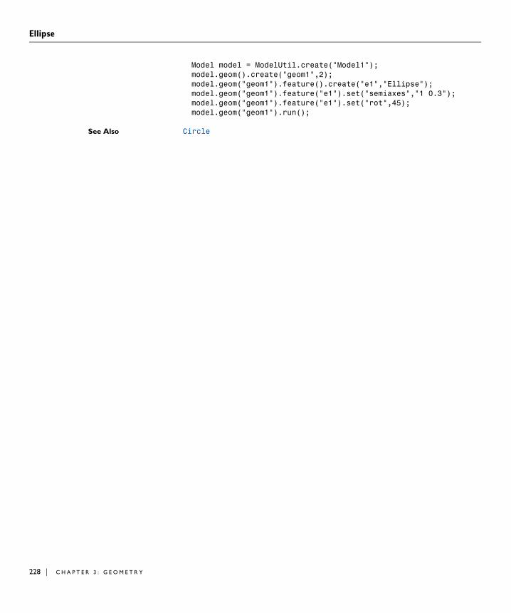
Ellipse
228 | C H A P T
Model model = ModelUtil.create("Model1");model.geom().create("geom1",2);model.geom("geom1").feature().create("e1","Ellipse");model.geom("geom1").feature("e1").set("semiaxes","1 0.3");model.geom("geom1").feature("e1").set("rot",45);model.geom("geom1").run();
See Also Circle
E R 3 : G E O M E T R Y

Ellipsoid
EllipsoidPurpose Create a solid or surface ellipsoid in 3D.
Syntax model.geom(<tag>).feature().create(<ftag>,"Ellipsoid");model.geom(<tag>).feature(<ftag>).set(property,<value>);model.geom(<tag>).feature(<ftag>).getType(property);
Description Use model.geom(<tag>).feature().create(<ftag>,"Ellipsoid") to create an ellipsoid. The following properties are available:
If createselection is set to on, predefined selections for all entities (all or some of domains, boundaries, edges and points) in the finalized geometry are created. To access the selections, use model.selection(<tag>_<ftag>_<lvl>), where <tag> is the geometry tag, <ftag> the feature tag and <lvl> is one of dom, bnd, edg, pnt. The createselection property is not available in work-plane geometries.
Compatibility model.geom(<tag>).feature().create(<ftag>,"ellipsoid3") creates a solid ellipsoid.
model.geom(<tag>).feature().create(<ftag>,"ellipsoid2") creates a surface ellipsoid.
TABLE 3-47: VALID PROPERTY/VALUE PAIRS
PROPERTY VALUE DEFAULT DESCRIPTION
axis double[] {0,0,1} Direction of the local z-axis. Vector has length 3 if axistype is cartesian, and length 2 if axistype is spherical.
axistype cartesian | spherical
cartesian Coordinate system used for axis. The value is synchronized with axis.
layer double[] Thicknesses of layers
pos double[] {0,0,0} Center
rot double 0 Rotational angle about axis
semiaxes double[3] {1,1,1} Semi-axes
type solid | surface
solid Object type
createselection on | off off Create selections
229

Ellipsoid
230 | C H A P T
The following properties are also available:
The property const is no longer available.
Examples The following commands create a surface and solid ellipsoid, where the position and semi-axes are defined in the two alternative ways.
Model model = ModelUtil.create("Model1");model.geom().create("geom1",3);model.geom("geom1").feature().create("e2","Ellipsoid");model.geom("geom1").feature("e2").set("type","surface");model.geom("geom1").feature("e2").set("pos","0 1 0");
model.geom("geom1").feature().create("e3","Ellipsoid");model.geom("geom1").feature("e3").set("semiaxes","12 10 8");
model.geom().run();
See Also Sphere
TABLE 3-48: VALID PROPERTY/VALUE PAIRS
PROPERTY VALUE DEFAULT DESCRIPTION
a, b, c double 1 Alias for semiaxes
ax2 double[] {0,0} Alias for axis when axistype is spherical
ax3 double[] {0,0,1} Alias for axis when axistype is cartesian
x, y, z double 0 Alias for pos
E R 3 : G E O M E T R Y

Extrude
ExtrudePurpose Extrude planar objects into 3D
Syntax model.geom(<tag>).feature().create(<ftag>,"Extrude");model.geom(<tag>).feature(<ftag>).selection(property);model.geom(<tag>).feature(<ftag>).set(property,<value>);model.geom(<tag>).feature(<ftag>).getType(property);
Description Use model.geom(<tag>).feature().create(<ftag>,"Extrude") to extrude objects from a work plane or planar faces from the 3D geometry.
Use model.geom(<tag>).feature(<ftag>).selection("input") to select the work plane objects to extrude. The default selection is all available objects from the last preceding work plane.
Use model.geom(<tag>).feature(<ftag>).selection("inputface") to select the faces to extrude. Faces are extruded when the workplane property is none, otherwise work plane objects are extruded.
The following properties are available:
TABLE 3-49: VALID PROPERTY/VALUE PAIRS
PROPERTY VALUES DEFAULT DESCRIPTION
crossfaces on | off on Keep cross-sectional faces
displ double[nd][2] {{0,0}} Displacement (parallel to work plane) of extrusion top (of each layer) in local coordinate system
distance double | double[nd] 1 Extrusion distance(s), that is, local z-coordinate for the top (of each layer)
extrudefrom workplane | faces
Extrude work plane objects or faces from 3D objects
input Selection all objects Objects to extrude
intputface Selection Faces to extrude
polres double 50 Polygon resolution of edges
reverse on | off off Reverse the extrude direction
scale double[nd][2] {{1,1}} Scale of extrusion top (of each layer)
twist double | double[nd] 0 Twist angle (of each layer)
unite on | off on Unite extruded objects with input objects
231

Extrude
232 | C H A P T
Each planar input is extruded in nd layers defined by a local coordinate system. By default, nd=1. The property distance is the extrusion distance (of each layer) in the z-axis direction of the local system. The properties displ, scale, and twist define the translation displacements, scale factors and rotation of the top (of each layer) with respect to the bottom of the extruded object. The last array dimension in the properties displ, scale, and twist can be omitted if the same value is desired for all layers.
When extruding work plane objects, the local system is defined as the local system of the work plane. When extruding faces, the local system is defined by the face with the smallest face number in the object that comes first in the geometry sequence. The local z-axis is parallel to the face normal and located at the center of the face. The local x-axis is defined by the tangent direction corresponding to the first parameter in the surface representation for the face.
When unite is set to on, the input objects are united with the corresponding extruded objects, after which the input objects are removed. When extruding from work plane object, this has the same effect as deleting the input objects. When unite is set to off, the extruded objects remain separate from the input objects and the input objects are kept.
If createselection is set to on, predefined selections for all entities (all or some of domains, boundaries, edges and points) in the finalized geometry are created. To access the selections, use model.selection(<tag>_<ftag>_<lvl>), where <tag> is the geometry tag, <ftag> the feature tag and <lvl> is one of dom, bnd, edg, pnt. The createselection property is not available in work-plane geometries.
Compatibility The cubic interpolated extrusion is no longer supported.
The following property is also supported:
workplane String Work plane to extrude
createselection on | off off Create selections
TABLE 3-49: VALID PROPERTY/VALUE PAIRS
PROPERTY VALUES DEFAULT DESCRIPTION
TABLE 3-50: VALID PROPERTY/VALUE PAIRS
PROPERTY VALUES DEFAULT DESCRIPTION
face all | none all Cross-sectional faces to delete, alias for crossfaces
keep on | off off Alias for unite property with opposite value
E R 3 : G E O M E T R Y

Extrude
Example Creation of a cylinder of height 1.3.
Model model = ModelUtil.create("Model1");model.geom().create("geom1",3);model.geom("geom1").feature().create("wp1","WorkPlane"); model.geom("geom1").feature("wp1").geom(). feature().create("c1","Circle");model.geom("geom1").run("wp1");model.geom("geom1").feature().create("e1","Extrude");model.geom("geom1").feature("e1").set("distance",1.3);model.geom("geom1").run();
See Also Revolve, WorkPlane
233

Fillet
234 | C H A P T
FilletPurpose Create circular rounded corners in 2D geometry objects
Syntax model.geom(<tag>).feature().create(<ftag>,"Fillet");model.geom(<tag>).feature(<ftag>).selection(property);model.geom(<tag>).feature(<ftag>).set(property,<value>);model.geom(<tag>).feature(<ftag>).getType(property);
Description Use model.geom(<tag>).feature().create(<ftag>,"Fillet") to round corners in 2D.
Use model.geom(<tag>).feature(<ftag>).selection("point") to select which corners to round. The default selection is empty.
If createselection is set to on, predefined selections for all entities (all or some of domains, boundaries, edges and points) in the finalized geometry are created. To access the selections, use model.selection(<tag>_<ftag>_<lvl>), where <tag> is the geometry tag, <ftag> the feature tag and <lvl> is one of dom, bnd, edg, pnt. The createselection property is not available in work-plane geometries.
Compatibility In version 3.5a, the default was to fillet all vertices in the input objects.
The properties edges, out, and radii are no longer available.
Examples Fillet a rectangle object:
Model model = ModelUtil.create("Model1");model.geom().create("geom1",2);model.geom("geom1").feature().create("r1","Rectangle");model.geom("geom1").feature().create("fil1","Fillet");model.geom("geom1").feature("fil1").selection("point"). set("r1(1)",new int[]{1,2,3,4});model.geom("geom1").feature("fil1").set("radius",0.1);model.geom("geom1").run();
Diagnostics If Fillet does not succeed in creating a rounded corner according to the specified radius, the vertex is skipped. When a fillet intersects another edge, the function generates an error message.
See Also Chamfer
TABLE 3-51: VALID PROPERTY/VALUE PAIRS
PROPERTY VALUE DEFAULT DESCRIPTION
point Selection Vertices to fillet
radius double 0 Radius of fillet
createselection on | off off Create selections
E R 3 : G E O M E T R Y

Finalize
FinalizePurpose Create finalized geometry.
Syntax model.geom(<tag>).feature(<ftag>).set(property,<value>);model.geom(<tag>).feature(<ftag>).getType(property);
Description The finalize features combines all available geometry objects in the sequence to form a single geometry object. In 3D, you can modify this object by using virtual operations. The output of the last geometry feature is the finalized geometry used when meshing and when setting up physics. If the property action is set to union, and multiple geometry objects are present in the geometry sequence, the objects are combined into a single object with multiple domains corresponding to the input objects and eventual overlaps between these.
Set the property action to assembly to keep multiple objects in the finalized geometry. Use this option when modeling physics that needs separate geometry objects, for example when modeling mechanical contact.
See Also Compose, Union, Intersection, Difference
TABLE 3-52: VALID PROPERTIES
NAME VALUE DEFAULT DESCRIPTION
action union | assembly union Handling of multiple objects
createpairs on | off on Create pairs (used if action=assembly)
imprint on | off off Create imprints (used if action=assembly)
repairtol double 1e-6 Repair tolerance, relative to size of union of inputs
pairtype identity | contact identity Type of pairs to create
235

FromMesh
236 | C H A P T
FromMeshPurpose Create geometry (deformed configuration) from a (deformed) mesh.
Syntax model.geom(<tag>).feature(<ftag>).set(property,<value>);model.geom(<tag>).feature(<ftag>).getType(property);model.geom(<tag>).feature(<ftag>).importData();
Description To create a geometry sequence from a deformed mesh, use the createDeformedConfig method on a solution dataset, see Solution. Such a geometry sequence contains a FromMesh feature. This feature has the following properties
model.geom(<tag>).feature(<ftag>).importData() updates the geometry based on the current value of the solution in the feature’s corresponding solver sequence.
TABLE 3-53: VALID PROPERTIES
NAME VALUE DEFAULT DESCRIPTION
solnum non-negative integer Last solution The index of the solution to use.
E R 3 : G E O M E T R Y

Helix
HelixPurpose Create a solid, surface or curve helix in 3D
Syntax model.geom(<tag>).feature().create(<ftag>,"Helix");model.geom(<tag>).feature(<ftag>).set(property,<value>);model.geom(<tag>).feature(<ftag>).getType(property);
Description Use model.geom(<tag>).feature().create(<ftag>,"Helix") to create a helix. The following properties are available:
If createselection is set to on, predefined selections for all entities (all or some of domains, boundaries, edges and points) in the finalized geometry are created. To
TABLE 3-54: VALID PROPERTY/VALUE PAIRS
PROPERTY VALUE DEFAULT DESCRIPTION
axialpitch double 0.3 Axial pitch
axis double[] {0,0,1} Direction of the helix axis. Vector has length 3 if axistype is cartesian, and length 2 if axistype is spherical.
axistype cartesian | spherical
cartesian Coordinate system used for axis. The value is synchronized with axis.
chirality right | left right Chirality
endcaps paraaxis | perpaxis | perpspine
paraaxis Direction of end caps
grep bezier | spline
spline Geometry representation
pos double[] {0,0,0} Position of the object
radialpitch double 0 Radial pitch
rmaj double 1 Major radius
rmin double 0.1 Minor radius
rot double 0 Rotational angle about axis
rtol double 1e-4 Relative tolerance
turns double 3 Number of turns
type solid | surface
solid Object type
twistcomp on | off on Twist compensation
createselection on | off off Create selections
237

Helix
238 | C H A P T
access the selections, use model.selection(<tag>_<ftag>_<lvl>), where <tag> is the geometry tag, <ftag> the feature tag and <lvl> is one of dom, bnd, edg, pnt. The createselection property is not available in work-plane geometries.
Examples The following sequence generates a surface helix and a solid helix.
Model model = ModelUtil.create("Model1");model.geom().create("geom1",3);model.geom("geom1").feature().create("h1","Helix");model.geom("geom1").feature("h1").set("type","surface");model.geom("geom1").feature("h1").set("rmaj",2);model.geom("geom1").feature("h1").set("rmin",0.3);model.geom("geom1").feature("h1").set("axialpitch",1);
model.geom("geom1").feature().create("h2","Helix");model.geom("geom1").feature("h2").set("rmaj",10);model.geom("geom1").feature("h2").set("rmin",2);model.geom("geom1").feature("h2").set("axialpitch",1);model.geom("geom1").feature("h2").set("pos","0,0,-100");model.geom("geom1").feature("h2").set("axis","1,1,1");model.geom("geom1").feature("h2").set("rot",60);model.geom("geom1").run();
See Also Torus, Sweep
E R 3 : G E O M E T R Y

Hexahedron
HexahedronPurpose Create solid or surface hexahedron bounded by bilinear faces
Syntax model.geom(<tag>).feature().create(<ftag>,"Hexahedron");model.geom(<tag>).feature(<ftag>).set(property,<value>);model.geom(<tag>).feature(<ftag>).getType(property);
Description Use model.geom(<tag>).feature().create(<ftag>,"Hexahedron") to create a general hexahedron. The following properties are available:
For a hexahedron approximately aligned to the coordinate planes, the points in p are ordered as follows. The first four points and the last four points projected down to the (x, y)-plane defines two negatively oriented quadrangles. The corresponding plane for the second quadrangle must lie above the plane of the first quadrant in the z direction. Generally oriented hexahedra have the points of p ordered in a similar way, except for a rigid transformation of the defining point set.
If createselection is set to on, predefined selections for all entities (all or some of domains, boundaries, edges and points) in the finalized geometry are created. To access the selections, use model.selection(<tag>_<ftag>_<lvl>), where <tag> is the geometry tag, <ftag> the feature tag and <lvl> is one of dom, bnd, edg, pnt. The createselection property is not available in work-plane geometries.
Example The following command generates a solid hexahedron object.
Model model = ModelUtil.create("Model1");model.geom().create("geom1",3);model.geom("geom1").feature().create("h1","Hexahedron");model.geom("geom1").feature("h1").set("p",new double[][] {{0,0.0,1,1.0,0,0,1.0,1}, {0,0.8,1,0.0,0,1,1.2,0}, {0,0.1,0,0.2,1,1,2.0,1}});model.geom("geom1").run();
See Also Block, Pyramid, Tetrahedron
TABLE 3-55: VALID PROPERTY/VALUE PAIR
PROPERTY NAME PROPERTY VALUE
DEFAULT DESCRIPTION
p double[3][8] {{0,0,1,1,0,0,1,1},
{0,1,1,0,0,1,1,0},
{0,0,0,0,1,1,1,1}}
Corner coordinates
type solid | surface
solid Object type
createselection on | off off Create selections
239

IgnoreEdges
240 | C H A P T
IgnoreEdgesPurpose Ignore edges
Syntax model.geom(<tag>).feature().create(<ftag>,"IgnoreEdges");model.geom(<tag>).feature(<ftag>).selection(property);model.geom(<tag>).feature(<ftag>).set(property,<value>);model.geom(<tag>).feature(<ftag>).getType(property);
Description Use model.geom(<tag>).feature().create(<ftag>,"IgnoreEdges") to ignore edges.
Use model.geom(<tag>).feature(<ftag>).selection("input") to select the edges to ignore. The default selection is empty.
The feature removes the selected edges that are isolated, that are adjacent to precisely two faces, or that are between two domains. If an edge is adjacent to two faces in 3D, the operations forms a composite face, if an edge is between two domains in 2D, the operation forms composite domain. The output object is a virtual geometry.
The following properties are available:
Use ignorevtx to specify if the feature also removes the ignorable vertices on the boundary of each resulting composite face.
Use keepformesh to keep the ignored edges while meshing, to help you in constructing the mesh.
Example Create a sphere and ignore all edges and, implicitly, all vertices.
Model model = ModelUtil.create("Model");model.geom().create("geom1", 3);model.geom("geom1").feature().create("sph1", "Sphere");model.geom("geom1").feature().create("ige1", "IgnoreEdges");model.geom("geom1").feature("ige1").selection("input"). set("fin(1)", 1,2,3,4,5,6,7,8,9,10,11,12);model.geom("geom1").run("ige1");
See Also CompositeFaces, IgnoreFaces, IgnoreVertices, MeshControlEdges
TABLE 3-56: VALID PROPERTIES
NAME VALUE DEFAULT DESCRIPTION
input Selection Edges to ignore
ignorevtx on | off on Ignore vertices on boundary
keepformesh on | off off Keep edges for mesh control
E R 3 : G E O M E T R Y

IgnoreFaces
IgnoreFacesPurpose Ignore faces
Syntax model.geom(<tag>).feature().create(<ftag>,"IgnoreFaces");model.geom(<tag>).feature(<ftag>).selection(property);model.geom(<tag>).feature(<ftag>).set(property,<value>);model.geom(<tag>).feature(<ftag>).getType(property);
Description Use model.geom(<tag>).feature().create(<ftag>,"IgnoreFaces") to ignore faces in 3D.
Use model.geom(<tag>).feature(<ftag>).selection("input") to select the faces to ignore. The default selection is empty.
The feature removes the selected faces that are isolated or that are between two domains. In the latter case, the operation forms a composite domain. The output object is a virtual geometry.
The following properties are available:
Use ignoreadj to specify if the feature also removes the ignorable edges and vertices on the boundary of each resulting composite domain.
Use keepformesh to keep the ignored faces while meshing, to help you in constructing the mesh.
Example Ignore faces to form one composite domain. The operation will also create composite faces and composite edges.
Model model = ModelUtil.create("Model");model.geom().create("geom1", 3);model.geom("geom1").feature().create("blk1", "Block");model.geom("geom1").feature().create("cyl1", "Cylinder");model.geom("geom1").run("fin");model.geom("geom1").feature().create("igf1", "IgnoreFaces");model.geom("geom1").feature("igf1").selection("input"). set("fin", 6, 7, 10);model.geom("geom1").run("igf1");
See Also CompositeDomains, IgnoreEdges, IgnoreVertices, MeshControlFaces
TABLE 3-57: VALID PROPERTIES
NAME VALUE DEFAULT DESCRIPTION
input Selection Faces to ignore
ignoreadj on | off on Ignore edges and vertices on boundary
keepformesh on | off off Keep faces for mesh control
241

IgnoreVertices
242 | C H A P T
IgnoreVerticesPurpose Ignore vertices
Syntax model.geom(<tag>).feature().create(<ftag>,"IgnoreVertices");model.geom(<tag>).feature(<ftag>).selection(property);model.geom(<tag>).feature(<ftag>).set(property,<value>);model.geom(<tag>).feature(<ftag>).getType(property);
Description Use model.geom(<tag>).feature().create(<ftag>,"IgnoreVertices") to ignore vertices.
Use model.geom(<tag>).feature(<ftag>).selection("input") to select the vertices to ignore. The default selection is empty.
The feature removes the selected vertices that are isolated or that are adjacent to precisely two edges. If a vertex is adjacent to two edges, the operation forms a composite edge. The output object is a virtual geometry.
The following properties are available:
Use keepformesh to keep the ignored vertices while meshing, to help you in constructing the mesh.
Example Create an ellipse and ignore vertices 1 and 3, which gives you two remaining edges in the final geometry.
Model model = ModelUtil.create("Model");model.geom().create("geom1", 2);model.mesh().create("mesh1", "geom1");model.geom("geom1").feature().create("e1", "Ellipse");model.geom("geom1").run("fin");model.geom("geom1").feature().create("igv1", "IgnoreVertices");model.geom("geom1").feature("igv1").selection("input"). set("fin", 1, 3);model.geom("geom1").run();
See Also CompositeEdges, IgnoreEdges, IgnoreFaces, MeshControlVertices
TABLE 3-58: VALID PROPERTIES
NAME VALUE DEFAULT DESCRIPTION
input Selection Vertices to ignore
keepformesh on | off off Keep vertices for mesh control
E R 3 : G E O M E T R Y

Import DXF
Import DXFPurpose Import geometry objects from a DXF file to 2D
Syntax model.geom(<tag>).feature().create(<ftag>,"Import");model.geom(<tag>).feature(<ftag>).set(property,<value>);model.geom(<tag>).feature(<ftag>).getType(property);model.geom(<tag>).feature(<ftag>).getLayers();model.geom(<tag>).feature(<ftag>).importData();
Description Use model.geom(<tag>).feature().create(<ftag>,"Import") to create a geometry import feature. When the property filename is set to a file recognized as a DXF CAD drawing, the property type is set to dxf and the following properties are available:
The file specified by filename can be of any of the following formats:
The imported objects are represented using COMSOL’s geometry modeler.
The property layers controls which DXF layers are imported. The value is an array of strings containing the names of the layers that are to be imported. The layers found in the file defined by the property filename can be retrieved by the command
model.geom(<tag>).feature(<ftag>).getLayers()
The method
TABLE 3-59: VALID PROPERTY/VALUE PAIRS
PROPERTY VALUE DEFAULT DESCRIPTION
convert solid | curve | off
solid Unite all objects in each layer, and convert it to a solid or curve object
filename String File name
layers String[] all layers Layers to import
repairgeom on | off on Repair geometry
repairtol double 1e-5 Repair tolerance, relative to size of union of imported objects
type dxf Type of import
createselection on | off off Create selections
TABLE 3-60: SUPPORTED FILE FORMATS
FILE FORMAT FILE EXTENSIONS
DXF .dxf
243

Import DXF
244 | C H A P T
model.geom(<tag>).feature(<ftag>).importData()
imports the file again.
If createselection is set to on, predefined selections for all entities (all or some of domains, boundaries, edges and points) in the finalized geometry are created. To access the selections, use model.selection(<tag>_<ftag>_<lvl>), where <tag> is the geometry tag, <ftag> the feature tag and <lvl> is one of dom, bnd, edg, pnt. If more than one object is imported, additional selections are created for each imported object. To access the selections, use model.selection(<tag>_<otag>_<lvl>), where <otag> is a tag derived from the name of the imported object. For standard object names of the form <ftag>(<n>), where <n> is an object number, the corresponding <otag> is <ftag>_<n>. For non-standard object names derived from CAD files, <otag> is derived by replacing space and dot characters with underscore characters, and removing other characters that are not numbers or upper- or lowercase English characters (a-z). Additionally, if required to make <otag> unique, _<m> is appended, where <m> is an integer. The createselection property is not available in work-plane geometries.
Compatibility The following property is also supported:
PROPERTY VALUE DEFAULT DESCRIPTION
coercion solid | face | curve | off
solid Alias for convert. The value face is equivalent to solid.
E R 3 : G E O M E T R Y

Import ECAD
Import ECADPurpose Import geometry objects from an ECAD file in 2D and 3D
Syntax model.geom(<tag>).feature().create(<ftag>,"Import");model.geom(<tag>).feature(<ftag>).set(property,<value>);model.geom(<tag>).feature(<ftag>).getType(property);model.geom(<tag>).feature(<ftag>).getLayers();model.geom(<tag>).feature(<ftag>).importData();
Description Use model.geom(<tag>).feature().create(<ftag>,"Import") to create a geometry import feature.
Note: ECAD import requires a license for any of the following modules: AC/DC Module, MEMS Module, or RF Module.
When the property filename is set to a file recognized as an ECAD file, the property type is set to ecad or odb and the following properties are available:
The file specified by filename can be of any of the following formats:
TABLE 3-61: VALID PROPERTY/VALUE PAIRS
PROPERTY VALUE DEFAULT DESCRIPTION
filename String File name
elevation String[] Z-position of layers
height String[] Height of layers
importlayer String[] Layers to import
manualelevation on | off off Manual control of elevations
repairgeom on | off on Repair imported objects
repairtol double 1e-5 Repair tolerance, relative to size of union of imported objects
type ecad | odb Type of import
createselection on | off off Create selections
TABLE 3-62: SUPPORTED FILE FORMATS
FILE FORMAT FILE EXTENSIONS
GDS .gds
NETEX-G .asc
ODB++(X) .xml
245

Import ECAD
246 | C H A P T
The imported objects are represented using COMSOL’s geometry modeler.
The property type determines which properties are available. To import a GDS or NETEX-G file, type must be ecad. To import an ODB++ file, type must be odb. The property type is automatically initialized from the property filename, according to the table above.
The property importlayer determines which layers to import. It is a string array of the same length as the number of layers, holding the strings on or off. The property is initialized with a valid default when setting the property filename. To inspect available layers, use the method
model.geom(<tag>).feature(<ftag>).getLayers();
The property height determines the height of all layers. It is a string array of the same length as the number of layers, holding string representations of the layer height, for example 1[mm]. The property is initialized with a valid default when setting the property filename.
The property manualelevation controls how imported layers are positioned in the Z direction. When manualelevation is off, the imported layers are stacked on top of each other with no gaps, so the Z positions are computed from the height property. When manualelevation is on and grouping is set to layer or none, the imported layers are positioned in the Z direction as specified by the elevation property.
The property elevation determines the Z-position of all layers. It is a string array of the same length as the number of layers, holding string representations of the layer elevation. The property is initialized with a valid default when setting the property filename.
Additional properties available when type is ecad or odb.
TABLE 3-63: VALID PROPERTY/VALUE PAIRS FOR ECAD IMPORT
PROPERTY NAME PROPERTY VALUE
DEFAULT DESCRIPTION
grouping all | layer | none
all The grouping of the imported layers, where all returns one single object, and layers gives you one object per layer. In 2D, all is the same as layer.
importtype full3d | shell
full3d Determine if metal layers are imported as solid or faces in 3D
intbnd on | off on Keep interior boundaries of nets
E R 3 : G E O M E T R Y

Import ECAD
Properties that are only available when type is ecad.
When findarcs is auto or manual, line segments are combined to form arcs. If findarcs is manual, the properties arcdistancetol, arcradiustol, arcminangle, arcmaxangle, and findlines can be used to tune the arc recognition algorithm, otherwise the algorithm tries to determine optimal parameters.
If createselection is set to on, predefined selections for all entities (all or some of domains, boundaries, edges and points) in the finalized geometry are created. To access the selections, use model.selection(<tag>_<ftag>_<lvl>), where
TABLE 3-64: VALID PROPERTY/VALUE PAIRS FOR GDS AND NETEX-G
PROPERTY NAME PROPERTY VALUE
DEFAULT DESCRIPTION
arcdistancetol double 0.3 Tolerance for segment length deviation
arcmaxangle double 36 Maximum angle for segments
arcminangle double 3.6 Minimum angle for segments to part of an arc
arcradiustol double 0.4 Tolerance for arc curvature
bondtype edge | block | cylinder
edge Specify how bond wires are modeled for NETEX-G files
bottommargin doubler 0 Distance to the bottom edge of the dielectric region
cell String top net Name of top net or cell to import
dielectric on | off on Import dielectric regions
findarcs auto | manual | off
auto Control arc recognition
findlines on | off on Turn on straight line recognition. Only available when findarcs is manual
leftmargin double 0 See bottommargin
rightmargin double 0 See bottommargin
topmargin double 0 See bottommargin
TABLE 3-65: VALID PROPERTY/VALUE PAIRS FOR ODB++
PROPERTY NAME PROPERTY VALUE
DEFAULT DESCRIPTION
ignoretext on | off on Ignore objects marked as text in ODB++ files
247

Import ECAD
248 | C H A P T
<tag> is the geometry tag, <ftag> the feature tag and <lvl> is one of dom, bnd, edg, pnt. If more than one layer is imported, additional selections are created for each imported layer. To access the selections, use model.selection(<tag>_<ftag>_<otag>_dom), where <otag> is a tag derived from the name of the imported layer. <otag> is derived by replacing space and dot characters with underscore characters, and removing other characters that are not numbers or upper- or lowercase English characters (a-z). Additionally, if required to make <otag> unique, _<m> is appended, where <m> is an integer. The createselection property is not available in work-plane geometries.
E R 3 : G E O M E T R Y

Import geometry sequence
Import geometry sequencePurpose Import geometry objects from another geometry sequence
Syntax model.geom(<tag>).feature().create(<ftag>,"Import");model.geom(<tag>).feature(<ftag>).set(property,<value>);model.geom(<tag>).feature(<ftag>).getType(property);model.geom(<tag>).feature(<ftag>).importData();
Description Use model.geom(<tag>).feature().create(<ftag>,"Import") to create a geometry import feature. Set the property sequence to the tag of another geometry sequence in the model.
When building, the import feature takes all the existing objects in the specified sequence and imports them into the feature’s sequence.
The method
model.geom(<tag>).feature(<ftag>).importData()
imports the sequence again. The imported objects are represented using COMSOL’s geometry modeler, or the CAD Import Module’s geometry modeler (Parasolid).
If createselection is set to on, predefined selections for all entities (all or some of domains, boundaries, edges and points) in the finalized geometry are created. To access the selections, use model.selection(<tag>_<ftag>_<lvl>), where <tag> is the geometry tag, <ftag> the feature tag and <lvl> is one of dom, bnd, edg, pnt. If more than one object is imported, additional selections are created for each imported object. To access the selections, use model.selection(<tag>_<otag>_<lvl>), where <otag> is a tag derived from the name of the imported object. For standard object names of the form <ftag>(<n>), where <n> is an object number, the corresponding <otag> is <ftag>_<n>. For non-standard object names derived from CAD files, <otag> is derived by replacing space and dot characters with underscore characters, and removing other characters that are not numbers or upper- or lowercase English characters (a-z). Additionally, if required to make <otag> unique, _<m> is appended, where <m> is an integer. The createselection property is not available in work-plane geometries.
PROPERTY VALUE DEFAULT DESCRIPTION
sequence String Tag of other geometry sequence
type sequence Type of import
createselection on | off off Create selections
249

Import mphbin/mphtxt
250 | C H A P T
Import mphbin/mphtxtPurpose Import geometry objects from a file using COMSOL’s geometry formats
Syntax model.geom(<tag>).feature().create(<ftag>,"Import");model.geom(<tag>).feature(<ftag>).set(property,<value>);model.geom(<tag>).feature(<ftag>).getType(property);model.geom(<tag>).feature(<ftag>).importData();
Description Use model.geom(<tag>).feature().create(<ftag>,"Import") to create a geometry import feature. When the property filename is set to a file recognized as an mphbin or mphtxt file, the property type is set to native and the following properties are available:
The file specified by filename can be of any of the following formats:
The imported objects are represented using COMSOL’s geometry modeler, or the CAD Import Module’s geometry modeler (Parasolid).
The method
model.geom(<tag>).feature(<ftag>).importData()
imports the file again.
If createselection is set to on, predefined selections for all entities (all or some of domains, boundaries, edges and points) in the finalized geometry are created. To access the selections, use model.selection(<tag>_<ftag>_<lvl>), where <tag> is the geometry tag, <ftag> the feature tag and <lvl> is one of dom, bnd, edg, pnt. If more than one object is imported, additional selections are created for each imported object. To access the selections, use model.selection(<tag>_<otag>_<lvl>), where <otag> is a tag derived from the name of the imported object. For standard object names of the form <ftag>(<n>), where <n> is an object number, the corresponding <otag> is <ftag>_<n>. For non-standard object names derived from CAD files, <otag> is
TABLE 3-66: VALID PROPERTY/VALUE PAIRS
PROPERTY VALUE DEFAULT DESCRIPTION
filename String File name
type native Type of import
createselection on | off off Create selections
TABLE 3-67: SUPPORTED FILE FORMATS
FILE FORMAT FILE EXTENSIONS
COMSOL Multiphysics Binary .mphbin
COMSOL Multiphysics Text .mphtxt
E R 3 : G E O M E T R Y

Import mphbin/mphtxt
derived by replacing space and dot characters with underscore characters, and removing other characters that are not numbers or upper- or lowercase English characters (a-z). Additionally, if required to make <otag> unique, _<m> is appended, where <m> is an integer. The createselection property is not available in work-plane geometries.
251

Import STL/VRML
252 | C H A P T
Import STL/VRMLPurpose Import geometry objects from a STL or VRML file containing a surface mesh
Syntax model.geom(<tag>).feature().create(<ftag>,"Import");model.geom(<tag>).feature(<ftag>).set(property,<value>);model.geom(<tag>).feature(<ftag>).getType(property);model.geom(<tag>).feature(<ftag>).importData();
Description Use model.geom(<tag>).feature().create(<ftag>,"Import") to create a geometry import feature. When the property filename is set to a file recognized as an STL or VRML file, the property type is set to stlvrml and the following properties are available:
TABLE 3-68: VALID PROPERTY/VALUE PAIRS
PROPERTY VALUE DEFAULT DESCRIPTION
curvedface auto | manual
auto Control parameters for partitioning of curved faces.
extrangle double 0.6 degrees Maximum angle between boundary element normal and extrusion plane that causes the element to be a part the extruded face if possible
faceangle double 110 degrees Maximum angle between any two boundary elements in the same face
facecleanup double 0.01 Avoid creating small faces. Faces with an area less than facecleanup * the mean face area, are merged with adjacent faces
facecurv double 10 degrees Maximum relative curvature deviation between any two boundary elements in the same face
facepartition auto | manual
auto Manual or automatic face partitioning
filename String File name
minareacurv double 1 Minimum relative area of face to be considered as a face with constant curvature
E R 3 : G E O M E T R Y

Import STL/VRML
The file specified by filename can be of any of the following formats:
The imported objects are represented using COMSOL’s geometry modeler.
The method
model.geom(<tag>).feature(<ftag>).importData()
imports the file again.
If createselection is set to on, predefined selections for all entities (all or some of domains, boundaries, edges and points) in the finalized geometry are created. To access the selections, use model.selection(<tag>_<ftag>_<lvl>), where <tag> is the geometry tag, <ftag> the feature tag and <lvl> is one of dom, bnd, edg, pnt. If more than one object is imported, additional selections are created for
minareaextr double 0.05 Minimum relative area of face to be considered extruded
minareaplane double 0.005 Minimum relative area of face to be considered planar
neighangle double 20 degrees Maximum angle between a boundary element and a neighbor that causes the elements to be part of the same boundary domain if possible
planar on | off on Detect planar faces
planarangle double 0.6 degrees Maximum angle between boundary element normal and a neighbor that causes the element to be a part the planar face if possible
report on | off on Display a progress window
type stlvrml Type of import
createselection on | off off Create selections
TABLE 3-69: SUPPORTED FILE FORMATS
FILE FORMAT FILE EXTENSIONS
STL .stl
VRML .wrl, .vrml
TABLE 3-68: VALID PROPERTY/VALUE PAIRS
PROPERTY VALUE DEFAULT DESCRIPTION
253

Import STL/VRML
254 | C H A P T
each imported object. To access the selections, use model.selection(<tag>_<otag>_<lvl>), where <otag> is a tag derived from the name of the imported object. For standard object names of the form <ftag>(<n>), where <n> is an object number, the corresponding <otag> is <ftag>_<n>. For non-standard object names derived from CAD files, <otag> is derived by replacing space and dot characters with underscore characters, and removing other characters that are not numbers or upper- or lowercase English characters (a-z). Additionally, if required to make <otag> unique, _<m> is appended, where <m> is an integer. The createselection property is not available in work-plane geometries.
E R 3 : G E O M E T R Y

Interpolation Curve
Interpolation CurvePurpose Create a curve interpolating or approximating a sequence of points in 2D or 3D
Syntax model.geom(<tag>).feature().create(<ftag>,"InterpolationCurve");model.geom(<tag>).feature(<ftag>).importToTable();model.geom(<tag>).feature(<ftag>).importData();
Description To create an interpolation curve use model.geom(<tag>).feature().create(<ftag>,"InterpolationCurve") The following properties are available:
Use model.geom(<tag>).feature(<ftag>).importToTable() to read data from the file defined by the filename property and store the data in the table property. The source property is also changed to table.
If source is file, the interpolation curve is not automatically rebuilt when the data in the file changes. Use model.geom(<tag>).feature(<ftag>).importData() to rebuild the interpolation curve after such a change.
If createselection is set to on, predefined selections for all entities (all or some of domains, boundaries, edges and points) in the finalized geometry are created. To access the selections, use model.selection(<tag>_<ftag>_<lvl>), where <tag> is the geometry tag, <ftag> the feature tag and <lvl> is one of dom, bnd, edg, pnt. The createselection property is not available in work-plane geometries.
Example The commands below create a curve interpolating four points.
Model model = ModelUtil.create("Model");model.geom().create("geom1", 2);model.geom("geom1").feature().create("ic1",
TABLE 3-70: VALID PROPERTY/VALUE PAIRS
PROPERTY VALUE DEFAULT DESCRIPTION
filename String If source is file, the file that contains the data
source table | file
table Specifies whether data is entered in table or read from file.
table double[][] Data points, size N*sdim.
rtol double 0 Maximum relative error. 0 implies interpolation.
type open | closed | solid
open Type of curve
createselection on | off off Create selections
255

Interpolation Curve
256 | C H A P T
"InterpolationCurve");model.geom("geom1").feature("ic1").set("table", new double[][]{{0,0}, {1,0}, {1,1}, {0,1}});model.geom("geom1").run();
See Also BezierPolygon
E R 3 : G E O M E T R Y

Interval
IntervalPurpose Create one or several connected intervals in 1D
Syntax model.geom(<tag>).feature().create(<ftag>,"Interval");model.geom(<tag>).feature(<ftag>).set(property,<value>);model.geom(<tag>).feature(<ftag>).getType(property);
Description Use model.geom(<tag>).feature().create(<ftag>,"Interval") to create one or more intervals. The following properties are available:
To specify one interval, set the properties p1 and p2. Then, intervals is automatically set to one.
To specify a sequence of connected intervals, set the property p. Then, intervals is automatically set to many.
If createselection is set to on, predefined selections for all entities (all or some of domains, boundaries, edges and points) in the finalized geometry are created. To access the selections, use model.selection(<tag>_<ftag>_<lvl>), where <tag> is the geometry tag, <ftag> the feature tag and <lvl> is one of dom, bnd, edg, pnt. The createselection property is not available in work-plane geometries.
Compatibility model.geom(<tag>).feature().create(<ftag>,"solid1") creates an interval.
Example The commands below create a solid consisting of two intervals.
Model model = ModelUtil.create("Model1");model.geom().create("geom1",1);model.geom("geom1").feature().create("i1","Interval");model.geom("geom1").feature("i1").set("p","0 1 3");model.geom("geom1").runAll();
See Also BezierPolygon
TABLE 3-71: VALID PROPERTY/VALUE PAIRS
PROPERTY VALUE DEFAULT DESCRIPTION
intervals one | many one Use properties p1 and p2, or p
p double[] {0,1} Vertex coordinates
p1 double 0 Left endpoint
p2 double 1 Right endpoint
createselection on | off off Create selections
257

MergeVertices
258 | C H A P T
MergeVerticesPurpose Merge two vertices
Syntax model.geom(<tag>).feature().create(<ftag>,"MergeVertices");model.geom(<tag>).feature(<ftag>).selection(property);model.geom(<tag>).feature(<ftag>).set(property,<value>);model.geom(<tag>).feature(<ftag>).getType(property);
Description Use model.geom(<tag>).feature().create(<ftag>,"MergeVertices") to merge two vertices.
Use model.geom(<tag>).feature(<ftag>).selection("keepvtx") to select the vertex to keep. The default selection is empty.
Use model.geom(<tag>).feature(<ftag>).selection("removevtx") to select the vertex to remove. The default selection is empty.
The feature merges the two vertices by collapsing the edge between the vertices and re-connecting the edges adjacent to the removed vertex to the resulting merged vertex.
The output object is a virtual geometry.
The following properties are available:
See Also CollapseEdges
TABLE 3-72: VALID PROPERTIES
NAME VALUE DEFAULT DESCRIPTION
keepvtx Selection Vertex to keep
removevtx Selection Vertex to remove
E R 3 : G E O M E T R Y

MeshControlDomains
MeshControlDomainsPurpose Define mesh control domains
Syntax model.geom(<tag>).feature().create(<ftag>,"MeshControlDomains");model.geom(<tag>).feature(<ftag>).selection(property);model.geom(<tag>).feature(<ftag>).set(property,<value>);model.geom(<tag>).feature(<ftag>).getType(property);
Description Use model.geom(<tag>).feature(). create(<ftag>,"MeshControlDomains") to define mesh control domains.
Use model.geom(<tag>).feature(<ftag>).selection("input") to select the domains to include. The default selection is empty.
The feature creates a composite domain by removing all faces (in 3D) or edges (in 2D) between the selected domains and adjacent domains. The removed entities are kept for mesh control.
The following property is available:
See Also MeshControlFaces, MeshControlEdges
TABLE 3-73: VALID PROPERTIES
NAME VALUE DEFAULT DESCRIPTION
input Selection Edges to ignore
259

MeshControlEdges
260 | C H A P T
MeshControlEdgesPurpose Define mesh control edges
Syntax model.geom(<tag>).feature().create(<ftag>,"MeshControlEdges");model.geom(<tag>).feature(<ftag>).selection(property);model.geom(<tag>).feature(<ftag>).set(property,<value>);model.geom(<tag>).feature(<ftag>).getType(property);
Description Use model.geom(<tag>).feature().create(<ftag>,"MeshControlEdges") to define mesh control edges.
Use model.geom(<tag>).feature(<ftag>).selection("input") to select the edges to include. The default selection is empty.
The feature removes the selected edges that are isolated, that are adjacent to precisely two faces (in 3D), or that are between two domains (in 2D). The edges are kept for mesh control.
The following properties are available:
Use includevtx to specify if the feature also removes the ignorable start and end vertices of the edge.
See Also IgnoreEdges, MeshControlDomains, MeshControlFaces, MeshControlVertices
TABLE 3-74: VALID PROPERTIES
NAME VALUE DEFAULT DESCRIPTION
input Selection Edges to ignore
includevtx on | off on Include start and end vertices
E R 3 : G E O M E T R Y

MeshControlFaces
MeshControlFacesPurpose Define mesh control faces
Syntax model.geom(<tag>).feature().create(<ftag>,"MeshControlFaces");model.geom(<tag>).feature(<ftag>).selection(property);model.geom(<tag>).feature(<ftag>).set(property,<value>);model.geom(<tag>).feature(<ftag>).getType(property);
Description Use model.geom(<tag>).feature().create(<ftag>,"MeshControlFaces") to define mesh control faces in 3D.
Use model.geom(<tag>).feature(<ftag>).selection("input") to select the faces to include. The default selection is empty.
The feature removes the selected faces that are isolated or that are between two domains. The faces are kept for mesh control.
The following properties are available:
Use includeadj to specify if the feature also includes the ignorable edges and vertices on the boundary of each resulting composite domain.
See Also IgnoreFaces, MeshControlDomains, MeshControlEdges, MeshControlVertices
TABLE 3-75: VALID PROPERTIES
NAME VALUE DEFAULT DESCRIPTION
input Selection Faces to include
includeadj on | off on Include edges and vertices on boundary
261

MeshControlVertices
262 | C H A P T
MeshControlVerticesPurpose Define mesh control vertices
Syntax model.geom(<tag>).feature().create(<ftag>,"MeshControlVertices");model.geom(<tag>).feature(<ftag>).selection(property);model.geom(<tag>).feature(<ftag>).set(property,<value>);model.geom(<tag>).feature(<ftag>).getType(property);
Description Use model.geom(<tag>).feature(). create(<ftag>,"MeshControlVertices") to define mesh control vertices.
Use model.geom(<tag>).feature(<ftag>).selection("input") to select the vertices to include. The default selection is empty.
The feature removes the selected vertices that are isolated or that are adjacent to precisely two edges. The vertices are kept for mesh control.
The following properties are available:
See Also IgnoreVertices, MeshControlFaces, MeshControlEdges
TABLE 3-76: VALID PROPERTIES
NAME VALUE DEFAULT DESCRIPTION
input Selection Vertices to include
E R 3 : G E O M E T R Y

Mirror
MirrorPurpose Reflect objects in a plane (3D), a line (2D), or a point (1D)
Syntax model.geom(<tag>).feature().create(<ftag>,"Mirror");model.geom(<tag>).feature(<ftag>).selection(property);model.geom(<tag>).feature(<ftag>).set(property,<value>);model.geom(<tag>).feature(<ftag>).getType(property);
Description Use model.geom(<tag>).feature().create(<ftag>,"Mirror") to mirror geometry objects.
Use model.geom(<tag>).feature(<ftag>).selection("input") to select the objects to mirror. The default selection is empty.
The following properties are available:
In 3D, the input objects are reflected in the plane through pos with normal vector axis. In 2D, the input objects are reflected in the line through pos with normal vector axis. In 1D, the input objects are reflected in the point pos.
If createselection is set to on, predefined selections for all entities (all or some of domains, boundaries, edges and points) in the finalized geometry are created. To access the selections, use model.selection(<tag>_<ftag>_<lvl>), where <tag> is the geometry tag, <ftag> the feature tag and <lvl> is one of dom, bnd, edg, pnt. The createselection property is not available in work-plane geometries.
Compatibility The property out is no longer available.
Examples In 2D:
Model model = ModelUtil.create("Model1");model.geom().create("geom1",2);model.geom("geom1").feature().create("r1","Rectangle");model.geom("geom1").feature().create("m1","Mirror");
TABLE 3-77: VALID PROPERTY/VALUE PAIRS
PROPERTY VALUE DEFAULT DESCRIPTION
input Selection Objects to reflect
keep on | off off Keep input objects
pos double[] 0 A point to be fixed during reflection
axis double[] {0 0 1} (3D){1 0} (2D){1} (1D)
Vector in the direction to reflect
createselection on | off off Create selections
263

Mirror
264 | C H A P T
model.geom("geom1").feature("m1").selection("input").set("r1");model.geom("geom1").feature("m1").set("pos","2 2");model.geom("geom1").feature("m1").set("axis","1 1");model.geom("geom1").run();
In 3D:
Model model = ModelUtil.create("Model1");model.geom().create("geom1",3);model.geom("geom1").feature().create("blk1","Block");model.geom("geom1").feature().create("m1","Mirror");model.geom("geom1").feature("m1"). selection("input").set("blk1");model.geom("geom1").feature("m1").set("pos","2 2 2");model.geom("geom1").feature("m1").set("axis","1 1 1");model.geom("geom1").run();
See Also Move, Copy, Rotate, Scale
E R 3 : G E O M E T R Y

Move, Copy
Move, CopyPurpose Move or copy geometry object(s) by translation
Syntax model.geom(<tag>).feature().create(<ftag>,"Move");model.geom(<tag>).feature().create(<ftag>,"Copy");model.geom(<tag>).feature(<ftag>).selection(property);model.geom(<tag>).feature(<ftag>).set(property,<value>);model.geom(<tag>).feature(<ftag>).getType(property);
Description Use model.geom(<tag>).feature().create(<ftag>,"Move") to move geometry objects.
Use model.geom(<tag>).feature().create(<ftag>,"Copy") to move a copy of geometry objects.
Use model.geom(<tag>).feature(<ftag>).selection("input") to select the objects to move or copy. The default selection is empty.
The following properties are available:
If displ is a one-dimensional array, a single copy of each input object is created using the translation vector displ. If displ is a two-dimensional array, several copies can be created, where the nth copy has translation displ[i][n] in the ith coordinate.
If createselection is set to on, predefined selections for all entities (all or some of domains, boundaries, edges and points) in the finalized geometry are created. To access the selections, use model.selection(<tag>_<ftag>_<lvl>), where <tag> is the geometry tag, <ftag> the feature tag and <lvl> is one of dom, bnd, edg, pnt. The createselection property is not available in work-plane geometries.
Example The sequence below moves a circle from the origin to (2,3).
Model model = ModelUtil.create("Model1");model.geom().create("geom1",2);model.geom("geom1").feature().create("c1","Circle");
TABLE 3-78: VALID PROPERTIES
NAME VALUE DEFAULT DESCRIPTION
input Selection Objects to move or copy
keep on | off off (Move)on (Copy)
Keep input objects
displ double[] | double[][] 0 Displacement vector(s)
createselection on | off off Create selections
265

Move, Copy
266 | C H A P T
model.geom("geom1").feature().create("m1","Move");model.geom("geom1").feature("m1").selection("input").set("c1");model.geom("geom1").feature("m1"). set("displ", new double[][]{{2},{3}});model.geom("geom1").run();
See Also Array, Mirror, Rotate, Scale
E R 3 : G E O M E T R Y

ParametricCurve
ParametricCurvePurpose Create a parametric curve defined by coordinate expressions in 2D or 3D
Syntax model.geom(<tag>).feature().create(<ftag>,"ParametricCurve");model.geom(<tag>).feature(<ftag>).set(property,<value>);model.geom(<tag>).feature(<ftag>).getType(property);model.geom(<tag>).feature(<ftag>).importData();
Description Use model.geom(<tag>).feature().create(<ftag>,"ParametericCurve") to create a parametric curve. Self-intersecting curves are not supported, except the case of a closed curve (that is, when the start and end points coincide). The following properties are available:
The expressions in coord can contain functions defined in the model. If the definition of such a function is changed, the parametric curve is not automatically rebuilt. Use model.geom(<tag>).feature(<ftag>).importData() to rebuild the parametric curve after such a change.
If createselection is set to on, predefined selections for all entities (all or some of domains, boundaries, edges and points) in the finalized geometry are created. To access the selections, use model.selection(<tag>_<ftag>_<lvl>), where <tag>
TABLE 3-79: VALID PROPERTY/VALUE PAIRS
PROPERTY VALUE DEFAULT DESCRIPTION
axis double[] {0,0,1} Direction of the z-axis of the local coordinate system. Vector has length 3 if axistype is cartesian, and length 2 if axistype is spherical.
axistype cartesian | spherical
cartesian Coordinate system used for axis. The value is synchronized with axis.
coord String[2] | String[3]
empty Coordinates of parametric curve as function of parameter
maxknots int 1000 Maximum number of knots
parname String s Parameter name
parmax double 1 Maximum parameter value
parmin double 0 Minimum parameter value
pos double[] {0,0,0} Position of the object
rot double 0 Rotational angle about axis
rtol double 1e-6 Relative tolerance
createselection on | off off Create selections
267

ParametricCurve
268 | C H A P T
is the geometry tag, <ftag> the feature tag and <lvl> is one of dom, bnd, edg, pnt. The createselection property is not available in work-plane geometries.
Examples The following commands create a parametric curve in 3D with the shape of a helix.
Model model = ModelUtil.create("Model1");model.geom().create("geom1",3);model.geom("geom1").feature().create("pc1","ParametricCurve");model.geom("geom1").feature("pc1").set("parmax","2*pi");model.geom("geom1").feature("pc1").set("coord", new String[]{"cos(s)","sin(s)","s*0.2"});model.geom("geom1").run();
See Also BezierPolygon, ParametricSurface
E R 3 : G E O M E T R Y

ParametricSurface
ParametricSurfacePurpose Create a parametric surface defined by coordinate expressions in 3D
Syntax model.geom(<tag>).feature().create(<ftag>,"ParametricSurface");model.geom(<tag>).feature(<ftag>).set(property,<value>);model.geom(<tag>).feature(<ftag>).getType(property);model.geom(<tag>).feature(<ftag>).importData();
Description Use model.geom(<tag>).feature().create(<ftag>,"ParametericSurface") to create a parametric surface. Self-intersecting surfaces are not supported. The following properties are available:
TABLE 3-80: VALID PROPERTY/VALUE PAIRS
PROPERTY VALUE DEFAULT DESCRIPTION
axis double[] {0,0,1} Direction of the z-axis of the local coordinate system. Vector has length 3 if axistype is cartesian, and length 2 if axistype is spherical.
axistype cartesian | spherical
cartesian Coordinate system used for axis. The value is synchronized with axis.
coord String[3] empty Coordinates of parametric surface as function of parameters
maxknots int 10 Maximum number of knots in each parameter coordinate
parname1 String s1 First parameter name
parname2 String s2 Second parameter name
parmax1 double 1 Maximum value of first parameter
parmax2 double 1 Maximum value of second parameter
parmin1 double 0 Minimum value of first parameter
parmin2 double 0 Minimum value of second parameter
pos double[] {0,0,0} Position of the object
rot double 0 Rotational angle about axis
rtol double 1e-6 Relative tolerance
createselection on | off off Create selections
269

ParametricSurface
270 | C H A P T
The expressions in coord can contain functions defined in the model. If the definition of such a function is changed, the parametric surface is not automatically rebuilt. Use model.geom(<tag>).feature(<ftag>).importData() to rebuild the parametric surface after such a change.
If createselection is set to on, predefined selections for all entities (all or some of domains, boundaries, edges and points) in the finalized geometry are created. To access the selections, use model.selection(<tag>_<ftag>_<lvl>), where <tag> is the geometry tag, <ftag> the feature tag and <lvl> is one of dom, bnd, edg, pnt. The createselection property is not available in work-plane geometries.
Examples The following commands create a parametric surface in 3D with the shape of a twisted rectangle.
Model model = ModelUtil.create("Model1");model.geom().create("geom1",3);model.geom("geom1").feature().create("ps1","ParametricSurface");model.geom("geom1").feature("ps1").set("parmin1","-1");model.geom("geom1").feature("ps1").set("parmax2","pi");model.geom("geom1").feature("ps1").set("coord", new String[]{"s1*cos(s2)","s1*sin(s2)","s2"});model.geom("geom1").run();
See Also ParametricCurve
E R 3 : G E O M E T R Y

Point
PointPurpose Create point object.
Syntax model.geom(<tag>).feature().create(<ftag>,"Point");model.geom(<tag>).feature(<ftag>).set(property,<value>);model.geom(<tag>).feature(<ftag>).getType(property);
Description Use model.geom(<tag>).feature().create(<ftag>,"Point") to create one or more points. The following property is available:
If p is a one-dimensional array, a single point with these coordinates is constructed. If p is a two-dimensional array, a point object containing several points is constructed, where the nth point has ith coordinate p[i][n].
If createselection is set to on, predefined selections for all entities (all or some of domains, boundaries, edges and points) in the finalized geometry are created. To access the selections, use model.selection(<tag>_<ftag>_<lvl>), where <tag> is the geometry tag, <ftag> the feature tag and <lvl> is one of dom, bnd, edg, pnt. The createselection property is not available in work-plane geometries.
Compatibility The following aliases work in 1D, 2D, and 3D, respectively:
model.geom(<tag>).feature().create(<ftag>,"point1");model.geom(<tag>).feature().create(<ftag>,"point2");model.geom(<tag>).feature().create(<ftag>,"point3");
Example The following commands generate a point at (1,2).
Model model = ModelUtil.create("Model1");model.geom().create("geom1",2);model.geom("geom1").feature().create("p1","Point");model.geom("geom1").feature("p1"). set("p",new double[][]{{1},{2}});
model.geom("geom1").run();
TABLE 3-81: VALID PROPERTY/VALUE PAIR
PROPERTY NAME PROPERTY VALUE DEFAULT DESCRIPTION
p double[] | double[][]
0 Coordinates
createselection on | off off Create selections
271
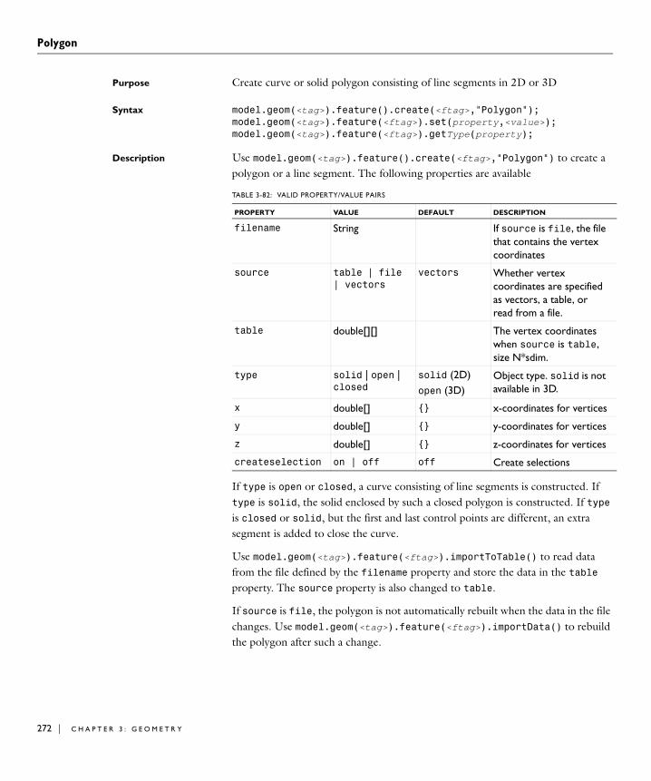
Polygon
272 | C H A P T
PolygonPurpose Create curve or solid polygon consisting of line segments in 2D or 3D
Syntax model.geom(<tag>).feature().create(<ftag>,"Polygon");model.geom(<tag>).feature(<ftag>).set(property,<value>);model.geom(<tag>).feature(<ftag>).getType(property);
Description Use model.geom(<tag>).feature().create(<ftag>,"Polygon") to create a polygon or a line segment. The following properties are available
If type is open or closed, a curve consisting of line segments is constructed. If type is solid, the solid enclosed by such a closed polygon is constructed. If type is closed or solid, but the first and last control points are different, an extra segment is added to close the curve.
Use model.geom(<tag>).feature(<ftag>).importToTable() to read data from the file defined by the filename property and store the data in the table property. The source property is also changed to table.
If source is file, the polygon is not automatically rebuilt when the data in the file changes. Use model.geom(<tag>).feature(<ftag>).importData() to rebuild the polygon after such a change.
TABLE 3-82: VALID PROPERTY/VALUE PAIRS
PROPERTY VALUE DEFAULT DESCRIPTION
filename String If source is file, the file that contains the vertex coordinates
source table | file | vectors
vectors Whether vertex coordinates are specified as vectors, a table, or read from a file.
table double[][] The vertex coordinates when source is table, size N*sdim.
type solid | open | closed
solid (2D)open (3D)
Object type. solid is not available in 3D.
x double[] {} x-coordinates for vertices
y double[] {} y-coordinates for vertices
z double[] {} z-coordinates for vertices
createselection on | off off Create selections
E R 3 : G E O M E T R Y

Polygon
If createselection is set to on, predefined selections for all entities (all or some of domains, boundaries, edges and points) in the finalized geometry are created. To access the selections, use model.selection(<tag>_<ftag>_<lvl>), where <tag> is the geometry tag, <ftag> the feature tag and <lvl> is one of dom, bnd, edg, pnt. The createselection property is not available in work-plane geometries.
Compatibility model.geom(<tag>).feature().create(<ftag>,"line1") constructs an open polygon.
model.geom(<tag>).feature().create(<ftag>,"poly1") constructs a closed polygon.
model.geom(<tag>).feature().create(<ftag>,"line2") or model.geom(<tag>).feature().create(<ftag>,"poly2") constructs a solid polygon.
Examples Construct a solid triangle pol1:
Model model = ModelUtil.create("Model1");model.geom().create("geom1",2);model.geom("geom1").feature().create("pol1","Polygon");model.geom("geom1").feature("pol1").set("x","0,0,2") .set("y","1,0,0");model.geom("geom1").runAll();
See Also BezierPolygon
273

Pyramid
274 | C H A P T
PyramidPurpose Create solid or surface rectangular pyramid or frustum in 3D
Syntax model.geom(<tag>).feature().create(<ftag>,"Pyramid");model.geom(<tag>).feature(<ftag>).set(property,<value>);model.geom(<tag>).feature(<ftag>).getType(property);
Description Use model.geom(<tag>).feature().create(<ftag>,"Pyramid") to create a pyramid. The following properties are available:
If createselection is set to on, predefined selections for all entities (all or some of domains, boundaries, edges and points) in the finalized geometry are created. To access the selections, use model.selection(<tag>_<ftag>_<lvl>), where <tag> is the geometry tag, <ftag> the feature tag and <lvl> is one of dom, bnd, edg, pnt. The createselection property is not available in work-plane geometries.
Compatibility model.geom(<tag>).feature().create(<ftag>,"pyramid3") creates a solid pyramid.
TABLE 3-83: VALID PROPERTY/VALUE PAIRS
PROPERTY VALUE DEFAULT DESCRIPTION
a, b double 1 Side lengths for bottom rectangle
axis double[] {0,0,1} Direction of the axis orthogonal to the bottom rectangle. Vector has length 3 if axistype is cartesian, and length 2 if axistype is spherical.
axistype cartesian | spherical
cartesian Coordinate system used for axis. The value is synchronized with axis.
h double 1 Height
pos double[] {0,0,0} Center of the bottom rectangle
rat double 0.5 Ratio of perimeter of top rectangle and bottom rectangle
rot double 0 Rotational angle about axis
type solid | surface
solid Object type
createselection on | off off Create selections
E R 3 : G E O M E T R Y

Pyramid
model.geom(<tag>).feature().create(<ftag>,"pyramid2") creates a surface pyramid.
The following properties are also available:
The property const is no longer available.
Examples Create a pyramid frustum with the base face in the xy-plane.
Model model = ModelUtil.create("Model1");model.geom().create("geom1",3);model.geom("geom1").feature().create("e1","Pyramid");model.geom("geom1").feature("e1").set("a",10).set("b",40);model.geom("geom1").feature("e1").set("h",20);
Create a pyramid with an apex.
model.geom("geom1").feature().create("e2","Pyramid");model.geom("geom1").feature("e2").set("a",1).set("b",2);model.geom("geom1").feature("e2").set("h",4);model.geom("geom1").feature("e2").set("rat",0);model.geom("geom1").feature("e2").set("pos","100 100 100");model.geom("geom1").feature("e2").set("axis","0 1 4");model.geom("geom1").feature("e2").set("rot",45);model.geom("geom1").run();
See Also Cone, ECone
TABLE 3-84: VALID PROPERTY/VALUE PAIRS
PROPERTY VALUE DEFAULT DESCRIPTION
ax2 double[] {0,0} Alias for axis when axistype is spherical
ax3 double[] {0,0,1} Alias for axis when axistype is cartesian
x, y, z double 0 Alias for pos
275

Rectangle
276 | C H A P T
RectanglePurpose Create solid or curve rectangle in 2D
Syntax model.geom(<tag>).feature().create(<ftag>,"Rectangle");model.geom(<tag>).feature(<ftag>).set(property,<value>);model.geom(<tag>).feature(<ftag>).getType(property);
Description Use model.geom(<tag>).feature().create(<ftag>,"Rectangle") to create a rectangle. The following properties are available:
If createselection is set to on, predefined selections for all entities (all or some of domains, boundaries, edges and points) in the finalized geometry are created. To access the selections, use model.selection(<tag>_<ftag>_<lvl>), where <tag> is the geometry tag, <ftag> the feature tag and <lvl> is one of dom, bnd, edg, pnt. The createselection property is not available in work-plane geometries.
Compatibility model.geom(<tag>).feature().create(<ftag>,"rect2") creates a solid rectangle.
model.geom(<tag>).feature().create(<ftag>,"rect1") creates a curve rectangle.
TABLE 3-85: VALID PROPERTY/VALUE PAIRS
PROPERTY VALUE DEFAULT DESCRIPTION
base corner | center
corner Positions the object either centered about pos or with the lower left corner in pos
layer double[] Thicknesses of layers
layerleft on | off off Apply layers to the left
layerright on | off off Apply layers to the right
layertop on | off off Apply layers on top
layerbottom on | off on Apply layers on bottom
pos double[] {0,0} Position of the object
rot double 0 Rotational angle about pos
size double[] {1,1} Side lengths
type solid | curve
solid Object type
createselection on | off off Create selections
E R 3 : G E O M E T R Y

Rectangle
The following properties are also available:
The property const is no longer available.
TABLE 3-86: VALID PROPERTY/VALUE PAIRS
PROPERTY VALUE DEFAULT DESCRIPTION
lx, ly double 1 Alias for size
x, y double 0 Alias for pos
277

Revolve
278 | C H A P T
RevolvePurpose Revolve planar objects into 3D
Syntax model.geom(<tag>).feature().create(<ftag>,"Revolve");model.geom(<tag>).feature(<ftag>).selection(property);model.geom(<tag>).feature(<ftag>).set(property,<value>);model.geom(<tag>).feature(<ftag>).getType(property);
Description Use model.geom(<tag>).feature().create(<ftag>,"Revolve") to revolve objects from a work plane.
Use model.geom(<tag>).feature(<ftag>).selection("input") to select the work plane objects to revolve. The default selection is all available objects from the last preceding work plane.
Use model.geom(<tag>).feature(<ftag>).selection("inputface") to select the faces to revolve. Faces are revolved when the workplane property is none, otherwise work plane objects are revolved.
The following properties are available:
TABLE 3-87: VALID PROPERTY/VALUE PAIRS
PROPERTY VALUES DEFAULT DESCRIPTION
angle1 double 0 Start revolution angle
angle2 double 0 End revolution angle
angtype specang | full specang Type of specification
axis double[2] {0,1} Direction of axis of revolution (in local coordinate system)
axis3 double[3] {0,1,0} Direction of axis of revolution (in 3D coordinate system)
axistype 2d | 3d 2d Type of revolution axis
input Selection all objects Objects to revolve
intputface Selection Faces to revolve
origfaces off | on on Keep original faces
polres double 50 Polygon resolution of edges
pos double[2] {0,0} A point on the axis of revolution (in work plane’s coordinate system)
pos3 double[3] {0,0,0} A point on the axis of revolution (in 3D coordinate system)
E R 3 : G E O M E T R Y

Revolve
Each 2D object in input or planar face in inputface is revolved about the revolution axis. The range of angles is given by the properties angle1 and angle2. If axistype is 2d, the revolution axis is defined in a local coordinate system. The revolution axis goes through pos with direction axis. If axistype is 3d, the revolution axis is defined in the 3D coordinate system. The revolution axis goes through pos3 with direction axis3.
When revolving work plane objects, the local system is defined as the local system of the work plane. When revolving faces, the local system is defined by the face with the smallest face number in the object that comes first in the geometry sequence. The local z-axis is parallel to the face normal and located at the center of the face. The local x-axis is defined by the tangent direction corresponding to the first parameter in the surface representation for the face.
When unite is set to on, the input objects are united with the corresponding revolved objects, after which the input objects are removed. When revolving from work plane object, this has the same effect as deleting the input objects. When unite is set to off, the revolved objects remain separate from the input objects and the input objects are kept.
If createselection is set to on, predefined selections for all entities (all or some of domains, boundaries, edges and points) in the finalized geometry are created. To access the selections, use model.selection(<tag>_<ftag>_<lvl>), where <tag> is the geometry tag, <ftag> the feature tag and <lvl> is one of dom, bnd, edg, pnt. The createselection property is not available in work-plane geometries.
revolvefrom workplane | faces
Revolve work plane objects or faces from 3D objects
unite on | off on Unite revolved objects with input objects
workplane String Work plane to revolve or none to revolve faces
createselection on | off off Create selections
TABLE 3-87: VALID PROPERTY/VALUE PAIRS
PROPERTY VALUES DEFAULT DESCRIPTION
279

Revolve
280 | C H A P T
Compatibility Additional properties:
Example Create torus about the y-axis:
Model model = ModelUtil.create("Model1");model.geom().create("geom1",3);model.geom("geom1").feature().create("wp1","WorkPlane"); model.geom("geom1").feature("wp1").geom(). feature().create("c1", "Circle");model.geom("geom1").feature("wp1").geom(). feature("c1").set("pos", "2 0");model.geom("geom1").run("wp1");model.geom("geom1").feature().create("r1","Revolve");model.geom("geom1").run();
See Also Extrude, WorkPlane
TABLE 3-88: VALID PROPERTY/VALUE PAIRS
PROPERTY VALUES DEFAULT DESCRIPTION
angles double | double[2] 2*pi Alias for angle1 and angle2
keep on | off off Alias for unite property with opposite value
revaxis double[2][2] {{0,0},
{ 0,1}}
Alias for pos (first column) and axis (second column)
E R 3 : G E O M E T R Y

Rotate
RotatePurpose Rotate objects about a point in 2D or an axis in 3D.
Syntax model.geom(<tag>).feature().create(<ftag>,"Rotate");model.geom(<tag>).feature(<ftag>).selection(property);model.geom(<tag>).feature(<ftag>).set(property,<value>);model.geom(<tag>).feature(<ftag>).getType(property);
Description Use model.geom(<tag>).feature().create(<ftag>,"Rotate") to rotate geometry objects.
Use model.geom(<tag>).feature(<ftag>).selection("input") to select the objects to rotate. The default selection is empty.
The following properties are available:
If createselection is set to on, predefined selections for all entities (all or some of domains, boundaries, edges and points) in the finalized geometry are created. To access the selections, use model.selection(<tag>_<ftag>_<lvl>), where <tag> is the geometry tag, <ftag> the feature tag and <lvl> is one of dom, bnd, edg, pnt. The createselection property is not available in work-plane geometries.
Compatibility The possibility to set and get a rotation matrix has been removed.
The property out is no longer available.
Example The command below rotates an ellipse by 10 degrees about (2,3).
Model model = ModelUtil.create("Model1");model.geom().create("geom1",2);
TABLE 3-89: VALID PROPERTIES
NAME VALUE DEFAULT DESCRIPTION
axis double[] {0,0,1} Rotation axis in 3D. Vector has length 3 if axistype is cartesian, and length 2 if axistype is spherical.
axistype cartesian | spherical
cartesian Coordinate system used for axis. The value is synchronized with axis.
input Selection Objects to rotate
keep on | off off Keep input objects
pos double[] Center of rotation
rot double 0 Rotation angle
createselection on | off off Create selections
281

Rotate
282 | C H A P T
model.geom("geom1").feature().create("e1","Ellipse");model.geom("geom1").feature("e1").set("semiaxes","1 3");model.geom("geom1").feature().create("r1","Rotate"); model.geom("geom1").feature("r1").selection("input").set("e1");model.geom("geom1").feature("r1").set("rot",10);model.geom("geom1").feature("r1").set("pos", "2 3");model.geom("geom1").run();
See Also Mirror, Move, Copy, Scale
E R 3 : G E O M E T R Y

Scale
ScalePurpose Scale objects around a point.
Syntax model.geom(<tag>).feature().create(<ftag>,"Scale");model.geom(<tag>).feature(<ftag>).selection(property);model.geom(<tag>).feature(<ftag>).set(property,<value>);model.geom(<tag>).feature(<ftag>).getType(property);
Description Use model.geom(<tag>).feature().create(<ftag>,"Scale") to scale geometry objects.
Use model.geom(<tag>).feature(<ftag>).selection("input") to select the objects scale. The default selection is empty.
The following properties are available:
If factor is an array, the inputs are scaled by the factor[i] in the ith coordinate. If createselection is set to on, predefined selections for all entities (all or some of domains, boundaries, edges and points) in the finalized geometry are created. To access the selections, use model.selection(<tag>_<ftag>_<lvl>), where <tag> is the geometry tag, <ftag> the feature tag and <lvl> is one of dom, bnd, edg, pnt. The createselection property is not available in work-plane geometries.
Example The sequence below scales the unit circle by (1,2) about (2,3).
Model model = ModelUtil.create("Model1");model.geom().create("geom1",2);model.geom("geom1").feature().create("c1","Circle");model.geom("geom1").feature().create("s1","Scale"); model.geom("geom1").feature("s1").selection("input").set("c1");model.geom("geom1").feature("s1").set("factor", "1,2");model.geom("geom1").feature("s1").set("pos",new double[]{2,3});model.geom("geom1").run();
Compatibility The property out is no longer available.
See Also Mirror, Move, Copy, Rotate
TABLE 3-90: VALID PROPERTIES
NAME VALUE DEFAULT DESCRIPTION
factor double | double[] 1 Scale factor(s)
input Selection Objects to scale
keep on | off off Keep input objects
pos double[] 0 Center of scaling
createselection on | off off Create selections
283

Selection
284 | C H A P T
SelectionPurpose Create selections for objects in the geometry sequence.
Syntax model.geom(<tag>).feature().create(<ftag>,"Selection");model.geom(<tag>).feature(<ftag>).selection(property);
Description Use model.geom(<tag>).feature().create(<ftag>,"Selection") to create selections for geometric entities in the geometry sequence.
Use model.geom(<tag>).feature(<ftag>).selection("selection") to select the entities to create selections for. The default selection is empty.
Use model.selection(<tag>_<ftag>) to access the corresponding selections in the finalized geometry.
Example The sequence below creates a block and a cylinder and creates a selection on the block domain.
Model model = ModelUtil.create("Model");model.geom().create("geom1", 3);model.geom("geom1").feature().create("blk1", "Block");model.geom("geom1").run("blk1");model.geom("geom1").feature().create("sel1", "Selection"); model.geom("geom1").feature("sel1").selection("selection") .set("blk1", new int[]{1});model.geom("geom1").feature().create("cyl1", "Cylinder");model.geom("geom1").run();int[] domains = model.selection("geom1_sel1").entities(3);// domains == {2,3}
E R 3 : G E O M E T R Y

Sphere
SpherePurpose Create a solid ball or surface sphere in 3D.
Syntax model.geom(<tag>).feature().create(<ftag>,"Sphere");model.geom(<tag>).feature(<ftag>).set(property,<value>);model.geom(<tag>).feature(<ftag>).getType(property);
Description Use model.geom(<tag>).feature().create(<ftag>,"Sphere") to create a sphere. The following properties are available:
If createselection is set to on, predefined selections for all entities (all or some of domains, boundaries, edges, and points) in the finalized geometry are created. To access the selections, use model.selection(<tag>_<ftag>_<lvl>), where <tag> is the geometry tag, <ftag> the feature tag and <lvl> is one of dom, bnd, edg, and pnt. The createselection property is not available in work-plane geometries.
Compatibility model.geom(<tag>).feature().create(<ftag>,"sphere3") creates a solid sphere.
model.geom(<tag>).feature().create(<ftag>,"sphere2") creates a surface sphere.
TABLE 3-91: VALID PROPERTY/VALUE PAIRS
PROPERTY VALUE DEFAULT DESCRIPTION
axis double[] {0,0,1} Direction of the local z-axis. Vector has length 3 if axistype is cartesian, and length 2 if axistype is spherical.
axistype cartesian | spherical
cartesian Coordinate system used for axis. The value is synchronized with axis.
layer double[] Thicknesses of layers
pos double[] {0,0,0} Center
r double 1 Radius
rot double 0 Rotational angle about axis
type solid | surface
solid Object type
createselection on | off off Create selections
285

Sphere
286 | C H A P T
The following properties are also available:
The property const is no longer available.
Examples The following commands create a surface and solid sphere, where the position and radius are defined differently.
Model model = ModelUtil.create("Model1");model.geom().create("geom1",3);model.geom("geom1").feature().create("s2","Sphere");model.geom("geom1").feature("s2").set("type","surface");model.geom("geom1").feature("s2").set("pos","0 1 0");model.geom("geom1").feature().create("s3","Sphere");model.geom("geom1").feature("s3").set("r",4); model.geom("geom1").run();
See Also Ellipsoid
TABLE 3-92: VALID PROPERTY/VALUE PAIRS
PROPERTY VALUE DEFAULT DESCRIPTION
ax2 double[] {0,0} Alias for axis when axistype is spherical
ax3 double[] {0,0,1} Alias for axis when axistype is cartesian
x, y, z double 0 Alias for pos
E R 3 : G E O M E T R Y

Split
SplitPurpose Split (explode) objects into their domains, faces, edges, or vertices.
Syntax model.geom(<tag>).feature().create(<ftag>,"Split");model.geom(<tag>).feature(<ftag>).selection(property);model.geom(<tag>).feature(<ftag>).set(property,<value>);model.geom(<tag>).feature(<ftag>).getType(property);
Description Use model.geom(<tag>).feature().create(<ftag>,"Split") to split geometry objects.
Use model.geom(<tag>).feature(<ftag>).selection("input") to select the objects to split. The default selection is empty.
A solid object is split into solids corresponding to its domains.
A surface object is split into surface objects corresponding to its faces.
A curve object is split into curve objects corresponding to its edges.
A point object is split into point objects corresponding to its vertices.
A general (mixed) object is split into solids (corresponding to the domains), surface objects (corresponding to faces not adjacent to a domain), curve objects (corresponding to edges not adjacent to a face or domain), and point objects (corresponding to vertices not adjacent to an edge, face, or domain).
If createselection is set to on, predefined selections for all entities (all or some of domains, boundaries, edges, and points) in the finalized geometry are created. To access the selections, use model.selection(<tag>_<ftag>_<lvl>), where <tag> is the geometry tag, <ftag> the feature tag and <lvl> is one of dom, bnd, edg, and pnt. The createselection property is not available in work-plane geometries.
Example Split union of a solid circle and a solid rectangle.
Model model = ModelUtil.create("Model1");model.geom().create("geom1",2);model.geom("geom1").feature().create("r1","Rectangle");model.geom("geom1").feature().create("c1","Circle");model.geom("geom1").feature().create("u1","Union");model.geom("geom1").feature("u1").selection("input").
TABLE 3-93: VALID PROPERTY/VALUE PAIRS
PROPERTY VALUE DEFAULT DESCRIPTION
input Selection Objects to split
keep on | off off Keep input objects
createselection on | off off Create selections
287

Split
288 | C H A P T
set(new String[]{"r1","c1"});model.geom("geom1").feature().create("spl1","Split");model.geom("geom1").feature("spl1").selection("input"). set("u1");model.geom("geom1").run();
See Also Compose, Union, Intersection, Difference, Delete
E R 3 : G E O M E T R Y

Square
SquarePurpose Create solid or curve square in 2D
Syntax model.geom(<tag>).feature().create(<ftag>,"Square");model.geom(<tag>).feature(<ftag>).set(property,<value>);model.geom(<tag>).feature(<ftag>).getType(property);
Description Use model.geom(<tag>).feature().create(<ftag>,"Square") to create a square. The following properties are available:
If createselection is set to on, predefined selections for all entities (all or some of domains, boundaries, edges and points) in the finalized geometry are created. To access the selections, use model.selection(<tag>_<ftag>_<lvl>), where <tag> is the geometry tag, <ftag> the feature tag and <lvl> is one of dom, bnd, edg, pnt. The createselection property is not available in work-plane geometries.
Compatibility model.geom(<tag>).feature().create(<ftag>,"square2") creates a solid square.
model.geom(<tag>).feature().create(<ftag>,"square1") creates a curve square.
TABLE 3-94: VALID PROPERTY/VALUE PAIRS
PROPERTY VALUE DEFAULT DESCRIPTION
base corner | center
corner Positions the object either centered about pos or with the lower left corner in pos
layer double[] Thicknesses of layers
layerleft on | off off Apply layers to the left
layerright on | off off Apply layers to the right
layertop on | off off Apply layers on top
layerbottom on | off on Apply layers on bottom
pos double[] {0,0} Position of the object
rot double 0 Rotational angle about pos
size double 1 Side length
type solid | curve solid Object type
createselection on | off off Create selections
289

Square
290 | C H A P T
The following properties are also available:
The property const is no longer available.
Example The sequence below creates a unit solid square.
Model model = ModelUtil.create("Model1");model.geom().create("geom1",2);model.geom("geom1").feature().create("sq1","Square");model.geom("geom1").run();
See Also Rectangle
TABLE 3-95: VALID PROPERTY/VALUE PAIRS
PROPERTY VALUE DEFAULT DESCRIPTION
l double 1 Alias for size
x, y double 0 Alias for pos
E R 3 : G E O M E T R Y

Sweep
SweepPurpose Sweep a face along a spine curve into a solid in 3D
Syntax model.geom(<tag>).feature().create(<ftag>,"Sweep");model.geom(<tag>).feature(<ftag>).selection(property);model.geom(<tag>).feature(<ftag>).set(property,<value>);model.geom(<tag>).feature(<ftag>).getType(property);
Description Use model.geom(<tag>).feature().create(<ftag>,"Sweep") to sweep a face along a spine curve.
Use model.geom(<tag>).feature(<ftag>).selection("face") to select the face to sweep.
Use model.geom(<tag>).feature(<ftag>).selection("edge") to select the edges to sweep along.
Use model.geom(<tag>).feature(<ftag>).selection("diredge") to select the edge whose direction defines the positive sweep direction. If this selection is empty, it is automatically set when the edge selection is set. The diredge selection can be empty if the edge selection contains a single edge.
The following properties are available:
TABLE 3-96: VALID PROPERTY/VALUE PAIRS
PROPERTY VALUES DEFAULT DESCRIPTION
adjustlen double 0 Spine adjustment parameter length. Used when align is set to adjustspine.
align noadjust | adjustspine | moveface
noadjust Type of alignment between face and spine curve
diredge Selection Direction-defining edge
edge Selection Edges that form spine curve
face Selection Face to sweep
grep bezier | spline spline Geometry representation
includefinal on | off off Include all used input objects in finalize operation
keep on | off on Keep input objects
maxknots int 1000 Maximum number of knots
parname String s Parameter name
reversedir on | off off Reverse sweep direction
rtol double 1e-4 Relative tolerance
291

Sweep
292 | C H A P T
The expressions in scale and twist can contain functions defined in the model. If the definition of such a function is changed, the swept object is not automatically rebuilt. Use model.geom(<tag>).feature(<ftag>).importData() to rebuild the swept object after such a change.
If includefinal is off, input objects are automatically removed in the finalize operation, if they are completely used by this feature. Objects used in face are considered completely used if they contain a single face. Objects used in edge are considered completely used if they contain no faces and all their edges are included in edge. If an object is considered completely used by one property but not completely used by another property, the object will not be removed in the finalize operation. If includefinal is on, input objects are not removed in the finalize operation.
If createselection is set to on, predefined selections for all entities (all or some of domains, boundaries, edges, and points) in the finalized geometry are created. To access the selections, use model.selection(<tag>_<ftag>_<lvl>), where <tag> is the geometry tag, <ftag> the feature tag and <lvl> is one of dom, bnd, edg, or pnt. The createselection property is not available in work-plane geometries.
Compatibility In COMSOL 4.2a and earlier versions, the positive sweep direction was defined as the curve direction instead of the edge direction.
Example Create a half torus about the y-axis:
Model model = ModelUtil.create("Model1");model.geom().create("geom1",3);model.geom("geom1").feature().create("wp1","WorkPlane");model.geom("geom1").feature("wp1").geom(). feature().create("c1","Circle");model.geom("geom1").feature().create("pc1","ParametricCurve");model.geom("geom1").feature().create("swe1","Sweep");model.geom("geom1").feature("pc1").set("parmax","pi");model.geom("geom1").feature("pc1"). set("coord",new String[]{"(cos(s)-1)*3","0","sin(s)*3"});model.geom("geom1").feature("swe1").selection("face").
scale String 1 Scale factor for cross section
twist String 0 Twist angle for cross section
twistcomp on | off on Twist compensation
createselection on | off off Create selections
TABLE 3-96: VALID PROPERTY/VALUE PAIRS
PROPERTY VALUES DEFAULT DESCRIPTION
E R 3 : G E O M E T R Y

Sweep
set("wp1.c1", new int[]{1});model.geom("geom1").feature("swe1").selection("edge"). set("pc1(1)",new int[]{1});model.geom("geom1").run();
See Also Extrude, Helix, Revolve, WorkPlane
293

Tangent
294 | C H A P T
TangentPurpose Create a tangent line segment to one or two 2D edges.
Syntax model.geom(<tag>).feature().create(<ftag>,"Tangent");model.geom(<tag>).feature(<ftag>).selection(property);model.geom(<tag>).feature(<ftag>).set(property,<value>);model.geom(<tag>).feature(<ftag>).getType(property);
Description Use model.geom(<tag>).feature().create(<ftag>,"Tangent") to create a line segment tangent to two edges or tangent to one edge with a fixed end point. The following properties are available:
If type is edge a common tangent line to two edges are constructed. Then, the following additional properties are available:
If type is point a tangent line through a given point is constructed. Then, the following additional property is available:
TABLE 3-97: VALID PROPERTY/VALUE PAIRS
PROPERTY VALUE DEFAULT DESCRIPTION
edge Selection Edge in an geometry object to find tangent to
start double 0.5 Start guess for parameter value of point of tangency
type edge | point | coord
edge Type of tangent
createselection on | off off Create selections
TABLE 3-98: VALID PROPERTY/VALUE PAIRS
PROPERTY VALUE DEFAULT DESCRIPTION
edge2 Selection Second edge in some geometry object to find tangent to
start2 double 0.5 Start guess for parameter value of point of tangency
TABLE 3-99: VALID PROPERTY/VALUE PAIRS
PROPERTY VALUE DEFAULT DESCRIPTION
point Selection Point in some geometry object
E R 3 : G E O M E T R Y

Tangent
If type is coord a tangent line through a point with given coordinates are constructed. Then, the following additional property is available:
If a tangent cannot be found, a tangent to some adjacent edge is constructed, if possible.
If createselection is set to on, predefined selections for all entities (all or some of domains, boundaries, edges and points) in the finalized geometry are created. To access the selections, use model.selection(<tag>_<ftag>_<lvl>), where <tag> is the geometry tag, <ftag> the feature tag and <lvl> is one of dom, bnd, edg, pnt. The createselection property is not available in work-plane geometries.
Compatibility model.geom(gname).feature().create(fname,"tangent") creates a Tangent feature.
The following properties are no longer supported:
Examples The following sequence generates a tangent from the unit circle to the point (2, 0).
Model model = ModelUtil.create("Model1");model.geom().create("geom1",2);model.geom("geom1").feature().create("c1","Circle");model.geom("geom1").run("c1");model.geom("geom1").feature().create("tan1","Tangent");
TABLE 3-100: VALID PROPERTY/VALUE PAIRS
PROPERTY VALUE DEFAULT DESCRIPTION
coord double[] {0,0} Coordinates
TABLE 3-101: OBSOLETE PROPERTY/VALUE PAIRS
PROPERTY NAME PROPERTY VALUE
DEFAULT DESCRIPTION
edim1 0 | 1 geometry dependent
Starting point element dimension: 0 for vertex, 1 for edge
edim2 0 | 1 geometry dependent
Ending point element dimension: 0 for vertex, 1 for edge
dom1 integer 1 Starting point entity number
dom2 integer 1 Ending point entity number
out cell array of strings
{} Additional output data
start1 double 0.5 Starting point parameter value on specified edge
295

Tangent
296 | C H A P T
model.geom("geom1").feature("tan1").set("type","coord");model.geom("geom1").feature("tan1").selection("edge"). set("c1",3);model.geom("geom1").feature("tan1").set("coord","2 0");model.geom("geom1").run();
The following sequence generates a common tangent between two circles.
Model model = ModelUtil.create("Model1");model.geom().create("geom1",2);model.geom("geom1").feature().create("c1","Circle");model.geom("geom1").feature().create("c2","Circle");model.geom("geom1").feature("c2").set("pos", "2 2");model.geom("geom1").run("c2");model.geom("geom1").feature().create("tan1","Tangent");model.geom("geom1").feature("tan1").selection("edge"). set("c1",4);model.geom("geom1").feature("tan1").selection("edge2"). set("c2",4);model.geom("geom1").run();
See Also BezierPolygon
E R 3 : G E O M E T R Y

Tetrahedron
TetrahedronPurpose Create solid or surface tetrahedron in 3D.
Syntax model.geom(<tag>).feature().create(<ftag>,"Tetrahedron");model.geom(<tag>).feature(<ftag>).set(property,<value>);model.geom(<tag>).feature(<ftag>).getType(property);
Description Use model.geom(<tag>).feature().create(<ftag>,"Tetrahedron") to create a tetrahedron. The following properties are available:
If createselection is set to on, predefined selections for all entities (all or some of domains, boundaries, edges and points) in the finalized geometry are created. To access the selections, use model.selection(<tag>_<ftag>_<lvl>), where <tag> is the geometry tag, <ftag> the feature tag and <lvl> is one of dom, bnd, edg, pnt. The createselection property is not available in work-plane geometries.
Compatibility model.geom(<tag>).feature().create(<ftag>,"tetrahedron3") creates a solid tetrahedron.
model.geom(<tag>).feature().create(<ftag>,"tetrahedron2") creates a surface tetrahedron.
Example The following command generate a solid tetrahedron object.
Model model = ModelUtil.create("Model1");model.geom().create("geom1",3);model.geom("geom1").feature().create("t1","Tetrahedron");model.geom("geom1").feature("t1").set("p", new double[][]{{0,0,1,0},{0,0.8,1,0},{0,0.1,0,0.2}});
model.geom("geom1").run();
See Also Hexahedron, Pyramid
TABLE 3-102: VALID PROPERTY/VALUE PAIR
PROPERTY NAME PROPERTY VALUE DEFAULT DESCRIPTION
p double[3][4] {{0,0,1,0}, {0,1,0,0}, {0,0,0,1}}
Corner coordinates
type solid | surface solid Object type
createselection on | off off Create selections
297

Torus
298 | C H A P T
TorusPurpose Create a solid or surface torus in 3D
Syntax model.geom(<tag>).feature().create(<ftag>,"Torus");model.geom(<tag>).feature(<ftag>).set(property,<value>);model.geom(<tag>).feature(<ftag>).getType(property);
Description Use model.geom(<tag>).feature().create(<ftag>,"Torus") to create a torus. The following properties are available:
If createselection is set to on, predefined selections for all entities (all or some of domains, boundaries, edges and points) in the finalized geometry are created. To access the selections, use model.selection(<tag>_<ftag>_<lvl>), where <tag> is the geometry tag, <ftag> the feature tag and <lvl> is one of dom, bnd, edg, pnt. The createselection property is not available in work-plane geometries.
Compatibility model.geom(<tag>).feature().create(<ftag>,"torus3") creates a solid torus.
model.geom(<tag>).feature().create(<ftag>,"torus2") creates a surface torus.
TABLE 3-103: VALID PROPERTY/VALUE PAIRS
PROPERTY VALUE DEFAULT DESCRIPTION
angle double 360 Revolution angle
axis double[] {0,0,1} Direction of the revolution axis. Vector has length 3 if axistype is cartesian, and length 2 if axistype is spherical.
axistype cartesian | spherical
cartesian Coordinate system used for axis. The value is synchronized with axis.
intfaces on | off off Create cross section faces inside the torus.
pos double[] {0,0,0} Center coordinates
rmaj double 1 Directrix radius
rmin double 0.5 Generatrix radius
rot double 0 Rotational angle about axis
type solid | surface
solid Object type
createselection on | off off Create selections
E R 3 : G E O M E T R Y

Torus
The following properties are also available:
The property const is no longer available.
Examples The following sequence generates a surface torus and a solid torus.
Model model = ModelUtil.create("Model1");model.geom().create("geom1",3);model.geom("geom1").feature().create("t2","Torus");model.geom("geom1").feature("t2").set("type","surface");model.geom("geom1").feature("t2").set("rmaj",2);model.geom("geom1").feature("t2").set("rmin",1);
model.geom("geom1").feature().create("t3","Torus");model.geom("geom1").feature("t3").set("rmaj",10);model.geom("geom1").feature("t3").set("rmin",2);model.geom("geom1").feature("t3").set("pos","0,0,-100");model.geom("geom1").feature("t3").set("axis","1,1,1");model.geom("geom1").feature("t3").set("rot",60);model.geom("geom1").run();
See Also Cylinder
TABLE 3-104: VALID PROPERTY/VALUE PAIRS
PROPERTY VALUE DEFAULT DESCRIPTION
ax2 double[] {0,0} Alias for axis when axistype is spherical.
ax3 double[] {0,0,1} Alias for axis when axistype is cartesian.
x, y, z double 0 Alias for pos.
299

WorkPlane
300 | C H A P T
WorkPlanePurpose Create a work plane in 3D for drawing 2D objects that can be extruded or revolved.
Syntax model.geom(<tag>).feature().create(<ftag>,"WorkPlane");model.geom(<tag>).feature(<ftag>).set(property,<value>);model.geom(<tag>).feature(<ftag>).getType(property);model.geom(<tag>).feature(<ftag>).geom().geomSequenceMethodmodel.geom(<tag>).feature(<ftag>).geom().feature();
Description A work plane embeds 2D objects in 3D. The sections below describe how to define the location of the work plane, and how to create 2D objects in it.
D E F I N I N G T H E L O C A T I O N O F T H E WO R K P L A N E
A work plane has a local coordinate system that is orthonormal and positively oriented (right-handed). The work plane coincides with the xy-plane in the local coordinate system. The following properties control how the work plane is defined.
If createselection is set to on, predefined selections for all entities (all or some of domains, boundaries, edges and points) in the finalized geometry are created. To access the selections, use model.selection(<tag>_<ftag>_<lvl>), where <tag> is the geometry tag, <ftag> the feature tag and <lvl> is one of dom, bnd, edg, pnt.
Depending on planetype, additional properties are available.
QuickThis creates a work plane parallel to one of the coordinate planes.
TABLE 3-105: VALID PROPERTY/VALUE PAIRS
PROPERTY VALUE DEFAULT DESCRIPTION
planetype quick | faceparallel | edgeangle | vertices | general
quick Type of data defining the work plane
createselection on | off off Create selections
TABLE 3-106: VALID PROPERTY/VALUE PAIRS
PROPERTY VALUE DEFAULT DESCRIPTION
quickplane xy | yz | zx | yx | zy | xz
xy Coordinate plane
quickx double 0 x-coordinate for work plane (used when plane is yz or zy).
E R 3 : G E O M E T R Y

WorkPlane
Face ParallelThis creates a work plane that is parallel to a planar face in a geometry object. Use the origin property to specify if the origin of the local coordinate system is set in the center of the face (origin=center) or as the projection onto the face of the minimum parameter coordinates of the face’s parameter space bounding box (origin=boxcorner). The local x-axis is in the direction of the face’s first parameter. The local z-axis is in the direction of the surface normal or its opposite.
Edge AngleThis creates a work plane through a straight edge of a geometry object. The work plane makes a given angle with the tangent plane of a face in the same geometry object. The face must be adjacent to the edge, and its tangent plane must be the same at all points on the edge. The origin of the local coordinate system coincides with the start vertex (if reverse is off) or end vertex (if reverse is on) of the edge. The direction of the local x-axis coincides with the direction of the edge (if reverse is off) or its opposite (if reverse is on). If the property angle is zero, the direction
quicky double 0 y-coordinate for work plane (used when plane is xz or zx).
quickz double 0 z-coordinate for work plane (used when plane is xy or yx).
TABLE 3-107: VALID PROPERTY/VALUE PAIRS
PROPERTY VALUE DEFAULT DESCRIPTION
face Selection Planar face
offset double 0 Signed offset in the direction of the local z-axis
origin facecenter | boxcorner
facecenter Origin of local coordinate system
reverse on | off off Reverse direction of local z-axis
TABLE 3-106: VALID PROPERTY/VALUE PAIRS
PROPERTY VALUE DEFAULT DESCRIPTION
301

WorkPlane
302 | C H A P T
of the local y-axis points into the face. In general, the local coordinate system is rotated by angle about the local x-axis.
VerticesThis creates a work plane parallel to a plane through three vertices v1, v2, v3. When offset=0, the origin of the local coordinate system coincides with the first vertex v1. The x-axis of the local coordinate system is in the direction v2-v1. The direction of the local z-axis is given by (v2-v1)x(v3-v1) or its opposite (if reverse is on).
GeneralThis creates a work plane through three points p1, p2, p3. The origin of the local coordinate system coincides with the first point p1. The x-axis of the local coordinate system is in the direction p2-p1. The direction of the local z-axis is given by (p2-p1)x(p3-p1).
TABLE 3-108: VALID PROPERTY/VALUE PAIRS
PROPERTY VALUE DEFAULT DESCRIPTION
angle double 0 Angle between face and work plane
edge Selection Straight edge
adjface Selection Face adjacent to edge in the same object
reverse on | off off Reverse direction of local x-axis
TABLE 3-109: VALID PROPERTY/VALUE PAIRS
PROPERTY VALUE DEFAULT DESCRIPTION
offset double 0 Signed offset in the direction of the local z-axis
reverse on | off off Reverse direction of local z-axis
vertex1 Selection First vertex
vertex2 Selection Second vertex
vertex3 Selection Third vertex
TABLE 3-110: VALID PROPERTY/VALUE PAIRS
PROPERTY VALUE DEFAULT DESCRIPTION
genpoints double[3][3] {{0,0,0},
{1,0,0},
{0,1,0}}
Points
E R 3 : G E O M E T R Y

WorkPlane
genpoints[n][i] is the ith coordinate of the nth point.
C R E A T I N G 2 D O B J E C T S I N T H E WO R K P L A N E
The work plane owns a geometry sequence that contains the features that define the 2D objects you draw in the work plane. You access this geometry sequence by
model.geom(<tag>).feature(<ftag>).geom()
where <ftag> is the name of the work plane feature. You can add geometry features in this 2D sequence as usual.
Example Create a work plane with a rectangle. When the work plane is built, the rectangle is embedded in the space of the 3D sequence
Model model = ModelUtil.create("Model1");model.geom().create("geom1",3);model.geom("geom1").feature().create("wp1","WorkPlane");model.geom("geom1").feature("wp1").set("quickplane","yz");model.geom("geom1").feature("wp1").geom(). feature().create("r1","Rectangle");model.geom("geom1").feature("wp1").geom(). feature("r1").set("pos", "1 1");model.geom("geom1").runAll();
See Also Extrude, Revolve
303

304 | C H A P T E
R 3 : G E O M E T R Y
4
M e s h
Details include reference information about the mesh commands and utility methods.
In this chapter:
• About Mesh Commands
• Working with a Meshing Sequence
• Physics-Controlled Meshing
• Information and Statistics
• Getting and Setting Mesh Data
• Errors and Warnings
• Exporting Mesh to File
• Mesh Commands
305

306 | C H A P T E
Abou t Me s h Command s
The following list includes the mesh commands that are documented in this chapter:
• BndLayer
• BndLayerProp
• Convert
• CopyEdge
• CopyFace
• Delete
• Distribution
• Edge
• EdgeGroup
• EdgeMap
• FreeQuad
• FreeTet
• FreeTri
• Import
• Map
• OnePointMap
• Point
• Reference
• Refine
• Scale
• Size
• Sweep
• TwoPointMap
• Operation Features
• Attribute FeaturesSee Also
R 4 : M E S H
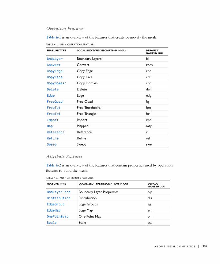
Operation Features
Table 4-1 is an overview of the features that create or modify the mesh.
Attribute Features
Table 4-2 is an overview of the features that contain properties used by operation features to build the mesh.
TABLE 4-1: MESH OPERATION FEATURES
FEATURE TYPE LOCALIZED TYPE DESCRIPTION IN GUI DEFAULT NAME IN GUI
BndLayer Boundary Layers bl
Convert Convert conv
CopyEdge Copy Edge cpe
CopyFace Copy Face cpf
CopyDomain Copy Domain cpd
Delete Delete del
Edge Edge edg
FreeQuad Free Quad fq
FreeTet Free Tetrahedral ftet
FreeTri Free Triangle ftri
Import Import imp
Map Mapped map
Reference Reference rf
Refine Refine ref
Sweep Swept swe
TABLE 4-2: MESH ATTRIBUTE FEATURES
FEATURE TYPE LOCALIZED TYPE DESCRIPTION IN GUI DEFAULT NAME IN GUI
BndLayerProp Boundary Layer Properties blp
Distribution Distribution dis
EdgeGroup Edge Groups eg
EdgeMap Edge Map em
OnePointMap One-Point Map pm
Scale Scale sca
A B O U T M E S H C O M M A N D S | 307

308 | C H A P T E
Features for Imported Meshes
Table 4-3 is an overview of the features that deals with imported meshes.
Size Size size
TwoPointMap Two-Point Map ppm
TABLE 4-3: FEATURES FOR IMPORTED MESHES
FEATURE TYPE LOCALIZED TYPE DESCRIPTION IN GUI DEFAULT NAME IN GUI
Ball Ball ball
Box Box box
CreateVertex Create Vertex vtx
DeleteEntities Delete Entities dele
Import Import imp
JoinEntities Join Entities join
TABLE 4-2: MESH ATTRIBUTE FEATURES
FEATURE TYPE LOCALIZED TYPE DESCRIPTION IN GUI DEFAULT NAME IN GUI
R 4 : M E S H

Work i n g w i t h a Me s h i n g S e qu en c e
This section describes how to build meshes using Java methods. A mesh is defined by a meshing sequence consisting of mesh features. A meshing feature is either an attribute feature or an operation feature. Each operation feature modifies the mesh when you build the feature using properties defined by attribute features.
An attribute feature is defined on a geometric entity selection and has a set of properties. Running an attribute feature does not change the mesh, but affects the subsequent operation features in the sequence. For example, the FreeTet operation feature, that creates a tetrahedral mesh, uses properties from the Distribution, Scale, and Size attribute features, that define the size and distribution of the mesh elements. You can add an attribute feature directly to the meshing sequence, this is referred to as a global attribute feature, or add it to an operation feature, this is referred to as a local attribute feature. Properties defined in local attribute features of an operation feature overrides corresponding properties defined in preceding global feature properties (on the same selection).
An operation features makes operations on the mesh as defined by the meshing sequence. Some operation features, like FreeTet and Sweep generate new mesh. Other operation features, like Refine and Convert modify existing mesh.
In this section:
• Adding a Meshing Sequence
• Adding a Mesh Feature
• Editing a Mesh Feature
• Building Mesh Features
• Feature Status
• Deleting Mesh Features
• Disabling Mesh Features
• Clearing Meshes
W O R K I N G W I T H A M E S H I N G S E Q U E N C E | 309

310 | C H A P T E
• Units
• Selections
Adding a Meshing Sequence
To add a new meshing sequence to a model object model, enter
model.mesh().create(<mtag>,<gtag>);
where mTag is the mesh’s tag (an identifier of your choice) and gTag is the tag of the associated geometry. If you want to import a mesh, you must specify an empty geometry sequence; the geometry is then defined by the mesh.
Adding a Mesh Feature
To add a feature to a mesh with tag <tag>, enter
model.mesh(<tag>).feature().create(<ftag>,ftype);
where <ftag> is the feature’s tag (an identifier of your choice), and ftype is the feature’s type. Feature types are capitalized and case-sensitive, for example FreeTet.
When you add a feature, it is inserted after the current feature. You can get the tag of the current feature type by entering
String ftag = model.mesh(<tag>).current();
If ftag is the empty string, the current feature is the beginning of the meshing sequence, that is, the empty state before all features. Adding a meshing feature, it automatically becomes current, but it is not built automatically.
For some operation features it is possible to add attribute features. To add an attribute feature to an operation feature, enter
model.mesh(<tag>).feature(<ftag>).feature(). create(<ftag1>,ftype);
where <ftag1> is the attribute feature’s tag (an identifier of your choice), and ftype is the attribute feature’s type.
• Meshing Features in the COMSOL Multiphysics Reference Guide
• Meshing in the COMSOL Multiphysics User’s GuideSee Also
R 4 : M E S H

All properties in a new feature get a default value.
Editing a Mesh Feature
To change a property value in a feature, enter
model.mesh(<tag>).feature(<ftag>).set(property,<value>);
where property is a property name and <value> is a property value.
All numeric properties can be given either as a numeric value or as a string expression that can contain parameters defined in model.param(). When building the feature, the string expressions are evaluated using the current values of the parameters.
To get the value of a property, enter one of the following, depending on the property type:
double d = model.mesh(<tag>).feature(<ftag>).getDouble(property);String s = model.mesh(<tag>).feature(<ftag>).getString(property);double[] da = model.mesh(<mtag>).feature(<ftag>).getDoubleArray(property);String[] sa = model.mesh(<tag>).feature(<ftag>).getStringArray(property);
If you request a numerical value for a string property, it is evaluated using the current values of the parameters in model.param().
Building Mesh Features
To modify the mesh, you must build an operation feature. Enter
model.mesh(<tag>).run(<ftag>);
to build the feature <ftag> and all its preceding features (the features are built in the order from the first to the last). When the build has completed, the feature <ftag> becomes the current feature.
To build all features, enter
model.mesh(<tag>).run();
Behavior has changed since COMSOL version 3.5a. String expression arguments are retained and not converted to numeric values.
Note
W O R K I N G W I T H A M E S H I N G S E Q U E N C E | 311

312 | C H A P T E
Feature Status
The status of a feature can be one of the following:
• Built. This means that the none of the feature’s properties have changed since the feature was last built, and the features of the input objects are all built. The feature may contain warning messages.
• Edited. This means that some of the feature’s properties have changed since the feature was last built.
• Needs rebuild. This means that any of the preceding features is edited.
• Error. This means that the feature contains an error message.
• Warning. This means that the feature contains a warning message.
You can examine the status of a feature by entering
boolean built = model.mesh(<tag>).feature(<ftag>).isBuilt();boolean edited = model.mesh(<tag>).feature(<ftag>).isEdited();boolean hasError = model.mesh(<tag>).feature(<ftag>).hasError();boolean hasWarning = model.mesh(<tag>).feature(<ftag>).hasWarning();boolean needsRebuild = !(built || edited || hasError || hasWarning);
Deleting Mesh Features
To delete a feature, enter
model.mesh(<tag>).feature().remove(<ftag>);
Disabling Mesh Features
To disable a feature, enter
model.mesh(<tag>).feature(<ftag>).active(false);
To enable a disabled feature, enter
model.mesh(<tag>).feature(<ftag>).active(true);
You can get the enabled/disabled status of a feature by entering
boolean isEnabled = model.mesh(<tag>).feature(<ftag>).active();
R 4 : M E S H

Clearing Meshes
To clear the mesh of a sequence, enter
model.mesh(<tag>).clearMesh();
To clear the mesh and remove all features in a sequence, enter
model.mesh(<tag>).feature().clear();
To clear all meshes for all geometries in a model, enter
model.mesh().clearMeshes();
Units
The meshing sequence uses the same base unit system as the geometry sequence. The string versions of setters and getters support units and unit conversion using the standard machinery.
Selections
Most mesh features have selections, to specify where they operate. To access a feature’s selection, use the syntax
model.mesh(<tag>).feature(<ftag>).selection();
To specify the entire geometry, write
model.mesh(<tag>).feature(<ftag>).selection().allgeom();
To specify all geometric entities in dimension <dim>, write
model.mesh(<tag>).feature(<ftag>).selection().geom(<dim>).all();
To specify the geometric entities that remains to be meshed when the feature is about to be built, use
model.mesh(<tag>).feature(<ftag>).selection().remaining();
It is not possible to retrieve the geometric entities of this selection, unless the feature is built.
If entities is an integer array of geometric entities in dimension dim, use the following syntax to select these entities
model.mesh(<tag>).feature(<ftag>).selection(). geom(dim).set(entities);
For example, to selection domain 1 and 2 in a 3D geometry, write
W O R K I N G W I T H A M E S H I N G S E Q U E N C E | 313

314 | C H A P T E
model.mesh(<tag>).feature(<ftag>).selection(). geom(3).set(new int[]{1,2});
To add the geometric entities specified in the integer array <entities> in dimension <dim> to the selection, write
model.mesh(<tag>).feature(<ftag>).selection(). geom(<dim>).add(<entities>);
To remove the geometric entities specified in the integer array <entities> in dimension <dim> from the selection, write
model.mesh(<tag>).feature(<ftag>).selection(). geom(<dim>).remove(<entities>);
To clear the selection in dimension <dim>, write
model.mesh(<tag>).feature(<ftag>).selection(). geom(<dim>).clear();
Some features have more than one selection, for example sweep, where it is possible to specify source and destination faces. Use the following syntax to access these selections.
model.mesh(<tag>).feature(<ftag>).selection(<property>);
Thus, to specify boundary 5 as source face on the sweep feature swe1, write
model.mesh(<tag>).feature(<ftag>).selection("sourceface"). geom(2).set(5);
R 4 : M E S H

Phy s i c s - C on t r o l l e d Me s h i n g
A physics-controlled meshing sequence examines the physics to automatically determine size attributes and sequence operations needed to create a mesh adapted to the problem. The physics-controlled sequence is based on heuristics and knowledge built-in by application experts. It is not adapted by numerical error estimates—that type of adaptation is provided by mesh adaptation in the solver sequence.
When a mesh is built or a problem solved, the physics-controlled sequence is updated to match the currently active physics. If the sequence is in any other state than physics-controlled, it is not updated or modified before it is built.
By default, a meshing sequence is in the physics-controlled state. If you manually add a feature to the sequence or edit a feature, the sequence automatically switches to the user-controlled state. It is also possible to explicitly switch to user-controlled state by entering
model.mesh(<tag>).automatic(false);
To switch back to physics-controlled mesh, enter
model.mesh(<tag>).automatic(true);
The current sequence is then modified or overwritten next time the sequence is built or the problem is solved.
Use model.mesh(<tag>).isAutomatic() to determine in which state the sequence is.
You can adjust the overall size of a physics-induced mesh by using the method
model.mesh(<tag>).autoMeshSize(<size>);
The value 5 of <size> corresponds to the default size, the values 4, 3, 2, and 1, gives you (increasingly) finer mesh, whereas the values 6, 7, 8, and 9 gives you a coarser mesh. The method model.mesh(<tag>).autoMeshSize() returns the current size adjustment.
When a physics-controlled sequence is built, a sequence of ordinary meshing features is created. This sequence can be customized by editing these features. However, do not assume the existence of a certain feature in a java program designed to run with future versions of COMSOL Multiphysics. The actual contents of the sequence might change.
Caution
P H Y S I C S - C O N T R O L L E D M E S H I N G | 315

316 | C H A P T E
I n f o rma t i o n and S t a t i s t i c s
In this section:
• Statistics
• Number and Types of Elements
• Quality of Elements
• Volume of Elements and Mesh
• Mesh Status
Statistics
Use the stat() method on the meshing sequence to determine the number of elements of different types and the quality of elements. Use the info() method to obtain topological information, the number of geometric entities and so forth. When importing mesh, use infoCurrent() to obtain topological information about the current (last built) mesh feature, and info() to obtain this information about the finalized mesh. See Geometry Object Information Methods for a list of available methods.
The stat() method returns an object with a collection of methods that can be queried for statistical information about the current mesh. There is also a selection,
model.mesh(<tag>).stat().selection()
which is used to select geometric entities for which the statistics is calculated. The default selection is the entire geometry. The methods described below also exist directly on the meshing sequence. These methods always return statistics for the entire geometry.
Statistics can be requested per element type. The type is given as a string, denoted type, and the possible types is given in the following table.
TABLE 4-4:
STRING ELEMENT ELEMENT DIMENSION
vtx Vertex element 0
edg Edge element 1
tri Triangular element 2
quad Quadrilateral element 2
R 4 : M E S H

The parameter string all gives statistics for all elements with the same dimension as the maximal dimension of the current selection. For example, if the entire geometry is selected in 2D, the parameter all provides combined statistics for triangular and quadrilateral elements.
Number and Types of Elements
To determine the number of elements of a certain type, use
int model.mesh(<tag>).stat().getNumElem(type);
To get the number of elements of all types, use
int model.mesh(<tag>).stat().getNumElem();
To determine the element types, use
String[] model.mesh(<tag>).stat().getTypes();
If the current selection is not the entire geometry, only elements and types in the current selection is returned. You can also use the methods
int model.mesh(<tag>).getNumElem(type);int model.mesh(<tag>).getNumElem();String[] model.mesh(<tag>).getTypes();
to obtain information about the entire geometry.
tet Tetrahedral element 3
pyr Pyramid element 3
prism Prism element 3
hex Hexahedral element 3
all All elements of maximal dimension in the selection
TABLE 4-4:
STRING ELEMENT ELEMENT DIMENSION
• Geometry Object Information
• SelectionsSee Also
I N F O R M A T I O N A N D S T A T I S T I C S | 317

318 | C H A P T E
Quality of Elements
The quality of an element is a double between 0 and 1, where 0.0 represents a degenerated element and 1.0 represents a completely symmetric element.
To retrieve the minimal quality, use
double model.mesh(<tag>).stat().getMinQuality(type);double model.mesh(<tag>).stat().getMinQuality();
To retrieve the mean quality, use
double model.mesh(<tag>).stat().getMeanQuality(type);double model.mesh(<tag>).stat().getMeanQuality();
To calculate a distribution of qualities, use the getQualityDistr method.
int[] model.mesh(<tag>).stat().getQualityDistr(type, <size>);int[] model.mesh(<tag>).stat().getQualityDistr(<size>);
The size parameter is a positive integer determining how detailed the distribution is, and equals the size of the output array. The distribution can by used to plot a histogram of the element quality. For example, if size equals 10, the first entry in the returned array is the number of elements with quality less than 0.1 and the last entry is the number of elements with quality better than 0.9.
The following methods are available directly on the sequence, and provide statistics for the entire geometry.
double model.mesh(<tag>).getMinQuality(type);double model.mesh(<tag>).getMinQuality();double model.mesh(<tag>).getMeanQuality(type);double model.mesh(<tag>).getMeanQuality();int[] model.mesh(<tag>).getQualityDistr(type, <size>);int[] model.mesh(<tag>).getQualityDistr(<size>);
Volume of Elements and Mesh
To determine minimum element volume, area, or length of a certain type, use the method getMinVolume.
double model.mesh(<tag>).stat().getMinVolume(type);double model.mesh(<tag>).stat().getMinVolume();
To determine maximum element volume, area, or length of a certain type, use the method getMaxVolume.
double model.mesh(<tag>).stat().getMaxVolume(type);double model.mesh(<tag>).stat().getMaxVolume();
R 4 : M E S H

To determine the volume, area, or length of the mesh, use the method getVolume.
double model.mesh(<tag>).stat().getVolume(type);double model.mesh(<tag>).stat().getVolume();
The following methods are available directly on the sequence, and provide volume information about the entire geometry.
double model.mesh(<tag>).getMinVolume(type);double model.mesh(<tag>).getMinVolume();double model.mesh(<tag>).getMaxVolume(type);double model.mesh(<tag>).getMaxVolume();double model.mesh(<tag>).getVolume(type);double model.mesh(<tag>).getVolume();
Growth Rate in Mesh
The growth rate value is a local measure greater than or equal to 1 indicating the maximum element size growth rate between two neighboring elements.
To retrieve the maximal growth rate value for a selection, use
double model.mesh(<tag>).stat().getMaxGrowthRate();
To retrieve the average growth rate for a selection, use
double model.mesh(<tag>).stat().getMeanGrowthRate();
The following methods are available directly on the sequence, and provide statistics for the entire geometry.
double model.mesh(<tag>).getMaxGrowthRate();double model.mesh(<tag>).getMeanGrowthRate();
Mesh Status
You can check if the entire selected geometry has a mesh by calling the isComplete method.
boolean model.mesh(<tag>).stat().isComplete();
To check if the entire geometry is meshed, use
boolean model.mesh(<tag>).isComplete();
You can also check if the selected geometry has an empty mesh by calling the isEmpty method.
boolean model.mesh(<tag>).stat().isEmpty();
I N F O R M A T I O N A N D S T A T I S T I C S | 319

320 | C H A P T E
To check if the entire geometry has an empty mesh, use
boolean model.mesh(<tag>).isEmpty();
R 4 : M E S H

Ge t t i n g and S e t t i n g Me s h Da t a
The data in the mesh object can be accessed and manipulated via getters and setters. You can get vertex coordinates, elements, and for each element the number of its geometric entity. The element matrix consist of indexes into the vertex list. The entity list contains the entity number of each element. There is one element matrix and one entity number list for each type.
In this section:
• Accessing Mesh Data
• Setting or Modifying Mesh Data
• Block Versions
• Element Numbering Conventions
Accessing Mesh Data
To get the number of mesh vertices, use
int model.mesh(<tag>).getNumVertex();
To get the coordinates of the mesh vertices, use
double[][] model.mesh(<tag>).getVertex();
which gives you a matrix where each column corresponds to a mesh vertex.
To get the element types in the mesh, use
String[] model.mesh(<tag>).getTypes();
The possible types are given by the following table. See Element Numbering Conventions for an explanation of each type.
STRING ELEMENT DIMENSION NUMBER OF NODES
vtx Vertex element 0 1
edg Edge element 1 2
tri Triangular element 2 3
quad Quadrilateral element 2 4
tet Tetrahedral element 3 4
pyr Pyramid element 3 5
G E T T I N G A N D S E T T I N G M E S H D A T A | 321

322 | C H A P T E
To get the number of elements of a specific type, use
int model.mesh(<tag>).getNumElem(type);
To get the elements for a specific type, use
int[][] model.mesh(<tag>).getElem(type);
which gives you a matrix where each column contains the mesh vertex indices of an element’s corners.
To get the geometric entity number for the elements of a specific type, use
int[] model.mesh(<tag>).getElemEntity(type);
Setting or Modifying Mesh Data
You can manipulate the mesh object of a meshing sequence via the data() method. Using this method you access a temporary object (MeshData) storing mesh data. When you use the data() method the first time the MeshData object is empty. You can fill it with mesh data either by using various set methods or by transferring mesh data from the mesh of the meshing sequence. Call the method data().createMesh to construct a complete mesh from the MeshData object and store it in the meshing sequence. If the geometry is not empty, the new mesh is checked to ensure that it matches the geometry. Thus, to create an arbitrary mesh, you need to create an empty geometry sequence and a corresponding empty meshing sequence and construct the mesh on the empty meshing sequence.
To set the mesh vertices, use
model.mesh(<tag>).data().setVertex(double[][]);
where each column of the input matrix contains the coordinates of a mesh vertex.
To set the elements of a specific type, use
prism Prism element 3 6
hex Hexahedral element 3 8
STRING ELEMENT DIMENSION NUMBER OF NODES
Information and StatisticsSee Also
R 4 : M E S H

model.mesh(<tag>).data().setElem(type, int[][]);
where each column of input element matrix contains the mesh vertex indices of an element’s corners.
If you want to specify the geometric entity number for the elements of a specific type, use
model.mesh(<tag>).data().setElemEntity(type, int[]);
The MeshData object has the same access methods as the meshing sequence.
int model.mesh(<tag>.data().getNumVertex();double[][] model.mesh(<tag>).data().getVertex();String[] model.mesh(<tag>).data().getTypes();int model.mesh(<tag>).data().getNumElem(type);int[][] model.mesh(<tag>).data().getElem(type);int[] model.mesh(<tag>).data().getElemEntity(type);
It is also possible to fill the MeshData object with mesh data from the mesh of a meshing sequence. To transfer the mesh from the current meshing sequence into the MeshData object, use
model.mesh(<tag>).data().transferMesh();
To transfer the mesh from another meshing sequence, specified by mtag, into the MeshData object, use
model.mesh(<tag>).data().transferMesh(mtag);
To clear the MeshData object, use
model.mesh(<tag>).data().clearData();
To create a complete mesh from the MeshData object and store it in the sequence, use
model.mesh(<tag>).data().createMesh();
This method uses several properties when creating a complete mesh from the specified mesh data. To set a property, use
model.mesh(<tag>).data().set(property, <value>);
To get a property, use
Accessing Mesh DataSee Also
G E T T I N G A N D S E T T I N G M E S H D A T A | 323

324 | C H A P T E
model.mesh(<tag>).data().getType(property);
The following properties are available.
TABLE 4-5: VALID PROPERTY/VALUE PAIRS
PROPERTY VALUE DEFAULT 2D 3D DESCRIPTION
extrangle double 0.6 degrees
Maximum angle between boundary element normal and extrusion plane that causes the element to be a part the extruded face if possible
faceangle double 360 degrees
Maximum angle between any two boundary elements in the same face
facecleanup double 0.01 Avoid creating small faces. Faces with an area less than Facecleanup * the mean face area, are merged with adjacent faces
facecurv double 10 degrees
Maximum relative angle deviation between any two boundary elements in the same face
faceparam on/off on Parameterize faces
minareacurv double 1 Minimum relative area of face to be considered as a face with constant curvature
minareaextr double 0.05 Minimum relative area of face to be considered extruded
minareaeplane double 0.005 Minimum relative area of face to be considered planar
R 4 : M E S H

E X A M P L E S O F S E T T I N G O R M O D I F Y I N G M E S H D A T A
The following examples create a triangular mesh on a square, extracts the vertices and the triangles. Then the vertices are transformed and inserted into a new meshing sequence.
Model model = ModelUtil.create("Model");
model.geom().create("geom1", 2);model.mesh().create("mesh1", "geom1");
// Create a rectangle and a meshmodel.geom("geom1").feature().create("r1", "Rectangle");model.mesh("mesh1").feature().create("ftri1", "FreeTri");model.mesh("mesh1").run();
double[][] vtx = model.mesh("mesh1").getVertex();int[][] tri = model.mesh("mesh1").getElem("tri");
// Transform x coordinatesfor (int k=0; k<vtx[0].length; k++) vtx[0][k] *= 0.5;
// Create a new geometry and meshmodel.geom().create("geom2", 2);model.mesh().create("mesh2", "geom2");
// Insert vertices and triangles and create meshmodel.mesh("mesh2").data().setElem("tri", tri);model.mesh("mesh2").data().setVertex(vtx);model.mesh("mesh2").data().createMesh();
neighangle double 20 degrees
Maximum angle between a boundary element and a neighbor that causes the elements to be part of the same boundary domain if possible
planarangle double 0.6 degrees
Maximum angle between boundary element normal and a neighbor that causes the element to be a part the planar face if possible
TABLE 4-5: VALID PROPERTY/VALUE PAIRS
PROPERTY VALUE DEFAULT 2D 3D DESCRIPTION
G E T T I N G A N D S E T T I N G M E S H D A T A | 325

326 | C H A P T E
Block Versions
Since the amount of available Java memory might be limited, there are block versions of the mesh setters and getters, which sets or gets a subset of the data. The getters take a position argument, which specifies the first item to get, and a number argument, which specifies the number of items to get. The setters takes only the position argument; the number of items is determined by the size of the provided data. When working with the setters, remember that it is more efficient to set the data at the last position first, since sufficient space in then allocated directly and no copying and reallocation is needed.
double[][] model.mesh(<tag>).getVertex(int position, int number);int[][] model.mesh(<tag>).getElem(type, int position, int number);int[] model.mesh(<tag>).getGeomEntity(type, int position,
int number);
model.mesh(<tag>).data().setVertex(double[][], int position);model.mesh(<tag>).data().setElem(type, int[][], int position);model.mesh(<tag>).data().setGeomEntity(type, int[],
int position);
double[][] model.mesh(<tag>).data().getVertex(int position, int number);
int[][] model.mesh(<tag>).data().getElem(type, int position, int number);
int[] model.mesh(<tag>).data().getGeomEntity(type, int position, int number);
Element Numbering Conventions
The (local) numbering of the corners of an element is defined according to the following.
Edge element (edg):
2
1
R 4 : M E S H

Triangular element (tri): Quadrilateral element (quad):
Tetrahedral element (tet): Pyramid element (pyr):
Prism element (prism): Hexahedral element (hex):
2
3
12
4
1
3
2
3
4
1
42
1
5
3
3
56
1
4
2
67
8
42
1
5
3
G E T T I N G A N D S E T T I N G M E S H D A T A | 327

328 | C H A P T E
E r r o r s and Wa rn i n g s
COMSOL Multiphysics treats problems encountered when building a meshing feature in two different ways depending on if it is possible to avoid the problem and continue the operation or if the operation must be stopped.
In this section:
• Continuing Operations
• Stopping Operations
• The MeshError Feature
• The MeshWarning Feature
• Retrieving Problem Information
Continuing Operations
When you build FreeTri, FreeQuad, or FreeTet features all problems related to meshing of faces and domains are avoided by leaving the corresponding faces and domains unmeshed. The operation continues meshing the remaining entities and stores information on the encountered problems in the feature. A feature that encountered this type of problems during the build gets a warning status. If you build several features in a sequence the build is not stopped by a feature that gets a warning status.
The information on the encountered problems for a feature with warning status is contained in MeshError and MeshWarning features stored in the feature. There is one MeshError feature for each geometric entity that failed to be meshed and one MeshWarning feature for each dimension where there exists an entity that could not be meshed due to failures meshing any of its boundary entities.
You can control whether a free meshing feature should avoid encountered problems and continue to mesh or if it should stop at the first encountered problem by the continue property.
Stopping Operations
When you build other operation features than the FreeTri, FreeQuad, or FreeTet features the operations stops if a problem is encountered. This means that no changes
R 4 : M E S H

are made to the mesh. The feature gets an error status and if it is part of a sequence build the build stops and the preceding feature becomes the current feature. Information on the error is contained in a MeshError feature stored in the feature.
The MeshError Feature
A MeshError feature contains an error message and can be equipped with a selection defining the failed entity, or a coordinate value specifying a position related to the error. It can also be equipped with details about the error. A MeshError feature can have a children feature of MeshError type that contains low-level error information. This means that an error can be represented by a stack of MeshError features that reflects the stack trace of the error.
The MeshWarning Feature
One MeshWarning feature is generated for each dimension where there are entities that cannot be meshed due to previous errors. For example, if there are edges that fail to be meshed for a FreeTet feature operating on the entire geometry there is one MeshWarning feature for the adjacent faces and one MeshWarning feature for the adjacent domains.
The MeshWarning feature contains a selection defining the entities that could not be meshed and a message describing the cause for this.
Retrieving Problem Information
Build a geometry.
Model mdl = com.comsol.model.util.ModelUtil.create("Model1");mdl.geom().create("g",3);mdl.geom("g").feature().create("cyl1","Cylinder").set("h",3.0);mdl.geom("g").feature().create("cyl2","Cylinder").set("h",3.0).set("r",0.95);mdl.geom("g").feature().create("co1","Difference");mdl.geom("g").feature("co1").selection("input").set("cyl1");mdl.geom("g").feature("co1").selection("input2").set("cyl2");
Build a mesh.
MeshSequence ms = mdl.mesh().create("m", "g");ms.feature("size").set("hauto", 9);ms.feature().create("ftri1","FreeTri");ms.feature("ftri1").selection().geom(2).set(1, 2, 7, 10);
E R R O R S A N D W A R N I N G S | 329

330 | C H A P T E
ms.feature().create("ftet1","FreeTet");ms.feature("ftet1").feature().create("ms1","Size");ms.run();
Check if the mesh was built with problems.
boolean problem = ms.hasProblems();
Get the names of the features with problems. In this case the feature ftet1.
String[] problemNames = ms.feature().problemNames();
Get error information.
String[] errorNames = ms.feature(problemNames[0]).problem().errorNames();for (String errorName : errorNames) { int errorDepth = ms.feature(problemNames[0]). problem(errorName).depth(); for (int i=0; i<errorDepth; ++i) { MeshFeature errorFeature = ms.feature(problemNames[0]). problem(errorName).get(i); String errorMessage = errorFeature.getString("message"); MeshSelection sel = null; if (errorFeature.hasSelection()) sel = errorFeature.selection(); }}
Get warning information.
String[] warningNames = ms.feature(problemNames[0]).problem().warningNames();MeshFeature warningFeature = ms.feature(problemNames[0]).problem(warningNames[0]);String warningMessage = warningFeature.getString("message");MeshSelection sel = warningFeature.selection();
R 4 : M E S H

Expo r t i n g Me s h t o F i l e
To export a mesh to a file, enter
model.mesh(<tag>).export(<filename>);
where <filename> is a string. The file can be any of the following formats.
TABLE 4-6: VALID FILE FORMATS
FILE FORMAT NOTE FILE EXTENSIONS
COMSOL Multiphysics Binary .mphbin
COMSOL Multiphysics Text .mphtxt
STL Binary (3D) 1 .stl
STL Text (3D) 1 .stl1 Use model.mesh(<tag>).export().setSTLFormat(<format>) to specify the STL file format (“binary” or “text”)
E X P O R T I N G M E S H T O F I L E | 331

332 | C H A P T E
Me sh Command s
The following list includes the available commands for creating and modifying meshes:
• Ball
• BndLayer
• BndLayerProp
• Box
• Convert
• CopyEdge
• CopyFace
• CopyDomain
• CreateVertex
• Delete
• DeleteEntities
• Distribution
• Edge
• EdgeGroup
• EdgeMap
• FreeQuad
• FreeTet
• FreeTri
• Import
• JoinEntities
• Map
• OnePointMap
• Point
• Reference
• Refine
• Scale
• Size
R 4 : M E S H

• Sweep
• TwoPointMap
M E S H C O M M A N D S | 333

Ball
334 | C H A P T
BallPurpose Split geometric entities of an imported mesh by a ball.
Syntax model.mesh(<tag>).feature().create(<ftag>,"Ball");model.mesh(<tag>).feature(<ftag>).selection();model.mesh(<tag>).feature(<ftag>).set(property,<value>);model.mesh(<tag>).feature(<ftag>).getType(property);model.mesh(<tag>).feature(<ftag>).feature(). create(<ftag1>,"Ball");
Description Use model.mesh(<tag>).feature().create(<ftag>,"Ball") to split geometric entities of an imported 2D or 3D mesh by an element set defined by a ball.
Use model.mesh(<tag>).feature(<ftag>).selection() to specify geometric entities to split. If you do not specify the selection, the feature operates on the entire geometry.
The following properties are available:
See Also Import, Box
TABLE 4-7: AVAILABLE PROPERTIES
PROPERTY VALUE DEFAULT DESCRIPTION
posx double 0 Center, first coordinate
posy double 0 Center, second coordinate
posz double 0 Center, third coordinate
r double 1 Radius
condition allvertices | somevertex
allvertices Condition for inclusion of an element
E R 4 : M E S H

BndLayer
BndLayerPurpose Create boundary layer mesh.
Syntax model.mesh(<tag>).feature().create(<ftag>,"BndLayer");model.mesh(<tag>).feature(<ftag>).selection();model.mesh(<tag>).feature(<ftag>).set(property,<value>);model.mesh(<tag>).feature(<ftag>).getType(property);model.mesh(<tag>).feature(<ftag>).feature(). create(<ftag1>,"BndLayerProp");
Description Use model.mesh(<tag>).feature().create(<ftag>,"BndLayer") to create a boundary layer mesh in 2D or 3D.
Use model.mesh(<tag>).feature(<ftag>).selection() to specify the domain selection. If you do not specify the selection, the feature operates on all domains.
Use model.mesh(<tag>).feature(<ftag>).feature().create(<ftag1>,"BndLa
yerProp") to add a BndLayerProp attribute feature defining the locations and properties of the boundary layers.
The feature reads properties from the BndLayerProp attribute feature.
The following properties are available:
TABLE 4-8: AVAILABLE PROPERTIES
PROPERTY VALUE DEFAULT DESCRIPTION
sharpcorners none | split | trim
split Specifies the handling of sharp corners in 2D and sharp edges in 3D.
splitangle double 240 [deg] Minimum angle between boundary layer boundaries to introduce a boundary layer split.
splitdivangle double 100 [deg] Maximum angle per split
trimmaxangle double 20 [deg] Maximum angle between boundary layer boundaries for boundary layer trimming.
trimminangle double 240 [deg] Minimum angle between boundary layer boundaries for boundary layer trimming.
layerdec integer 2 Maximum difference in number of boundary layers between neighboring points on boundary layer boundaries.
335

BndLayer
336 | C H A P T
Compatibility The following properties from the corresponding COMSOL 3.5a command, meshbndlayer, have been removed:
Examples Insert boundary layers to an existing mesh containing both quadrilateral elements and triangular elements.
Model model = ModelUtil.create("Model");model.geom().create("geom1", 2);model.mesh().create("mesh1", "geom1");
model.geom("geom1").feature().create("sq1", "Square");model.geom("geom1").feature().create("sq2", "Square");model.geom("geom1").feature("sq2").setIndex("pos", "1", 0);model.geom("geom1").feature().create("c1", "Circle");model.geom("geom1").feature("c1").set("r", "0.2");model.geom("geom1").feature("c1").setIndex("pos", "1.5", 0);model.geom("geom1").feature("c1").setIndex("pos", "0.5", 1);model.geom("geom1").feature().create("co1", "Compose");model.geom("geom1").feature("co1").selection("input"). init().set(new String[]{"c1", "sq1", "sq2"});model.geom("geom1").feature("co1"). set("formula", "sq1+sq2-c1");model.geom("geom1").run();
model.mesh("mesh1").feature().create("map1", "Map");
smoothtransition on | off on Specifies if the operation smoothes the transition to interior mesh.
smoothmaxiter integer 8 in 2D, 4 in 3D
Specifies the number of smoothing iterations.
smoothmaxdepth integer 16 in 2D, 6 in 3D
Specifies the maximum element smoothing depth.
TABLE 4-8: AVAILABLE PROPERTIES
PROPERTY VALUE DEFAULT DESCRIPTION
TABLE 4-9: REMOVED PROPERTIES
PROPERTY REASON
blbnd Defined by the selection of BndLayerProp
hauto Input mesh provided by meshing sequence
mcase Defined by meshing sequence
meshstart Input mesh provided by meshing sequence
out Output mesh provided by meshing sequence
subdomain Defined by the selection
E R 4 : M E S H

BndLayer
model.mesh("mesh1").feature("map1").selection(). geom("geom1", 2);model.mesh("mesh1").feature("map1").selection(). set(new int[]{1});model.mesh("mesh1").feature().create("ftri1", "FreeTri");model.mesh("mesh1").feature().create("bl1", "BndLayer");model.mesh("mesh1").feature("bl1").feature(). create("blp", "BndLayerProp");model.mesh("mesh1").feature("bl1").feature("blp").selection(). set(new int[]{2, 3, 5, 6, 8, 9, 10, 11});model.mesh("mesh1").run();
Create a boundary layer mesh consisting of prism elements along the boundary layer boundaries and tetrahedral elements in the interior.
Model model = ModelUtil.create("Model");model.geom().create("geom1", 3);model.mesh().create("mesh1", "geom1");
model.geom("geom1").feature().create("blk1", "Block");model.geom("geom1").feature("blk1").setIndex("size", "10", 0);model.geom("geom1").feature("blk1").setIndex("size", "5", 1);model.geom("geom1").feature("blk1").setIndex("size", "5", 2);model.geom("geom1").feature().create("sph1", "Sphere");model.geom("geom1").feature("sph1").setIndex("pos", "3", 0);model.geom("geom1").feature("sph1").setIndex("pos", "2.5", 1);model.geom("geom1").feature("sph1").setIndex("pos", "2.5", 2);model.geom("geom1").feature().create("dif1", "Difference");model.geom("geom1").feature("dif1").selection("input"). init().set(new String[]{"blk1"});model.geom("geom1").feature("dif1").selection("input2"). init().set(new String[]{"sph1"});model.geom("geom1").run();
model.mesh("mesh1").feature().create("ftet1", "FreeTet");model.mesh("mesh1").feature().create("bl1", "BndLayer");model.mesh("mesh1").feature("bl1").feature(). create("blp", "BndLayerProp");model.mesh("mesh1").feature("bl1").feature("blp").selection(). set(new int[]{2, 3, 4, 5, 6, 7, 8, 9, 10, 11, 12, 13});model.mesh("mesh1").run();
See Also BndLayerProp, Map, Sweep
337

BndLayerProp
338 | C H A P T
BndLayerPropPurpose Boundary layer meshing properties.
Syntax model.mesh(<tag>).feature(<ftag>).feature(). create(<ftag1>,"BndLayerProp");model.mesh(<tag>).feature(<ftag>).feature(<ftag1>).selection();model.mesh(<tag>).feature(<ftag>).feature(<ftag1>). set(property,<value>);model.mesh(<tag>).feature(<ftag>).feature(<ftag1>). getType(property);
Description Use model.mesh(<tag>).feature(<ftag>).feature().create(<ftag1>,"BndLa
yerProp") to define boundary layer properties for the BndLayer feature <ftag>.
Use model.mesh(<tag>).feature(<ftag>).feature(<ftag1>).selection() to specify the boundary selection. If you do not specify the selection, it is empty.
The following properties are available:
Use the properties blhmin, blstretch, and blnlayers to specify the distribution of the boundary layers. blhmin specifies the thickness of the initial boundary layer, blstretch a stretching factor, and blnlayers the number of boundary layers. This means that the thickness of the mth boundary layer (m=1 to blnlayers) is blstretchm1blhmin. The number of boundary layers and the thickness of the boundary layers might be automatically reduced in thin regions.
It is also possible to specify the thickness of the initial layer by using the blhminfact property. Then, the thickness of the first layer is 1/20 of the local domain element height. Use the blhminfact property to specify a scaling factor that multiplies this default size.
TABLE 4-10: AVAILABLE PROPERTIES
PROPERTY VALUE DEFAULT DESCRIPTION
blhminfact String | double 1 Factor used to adjust the default thickness
blhmin String | double Manual initial boundary layer thickness
blnlayers String | integer 8 Number of boundary layers
blstretch String | double 1.2 Boundary layer stretching factor
inittype blhminfact | blhmin
blhminfact Selects whether blhmin or blhminfact is used.
E R 4 : M E S H

BndLayerProp
The property inittype determines which of blhminfact or blhmin that is used. You do not need to set it explicitly, since the feature automatically changes it when you set one of blhmin or blhminfact.
The values of blhmin, blhminfact, and blstretch are positive real scalars, or strings that evaluate to positive real scalars, given the evaluation context provided by the property const.
The value of blnlayers is a positive integer scalar, or a string that evaluates to a positive integer, given the evaluation context provided by the property const.
See Also BndLayer, Scale, Size
339

Box
340 | C H A P T
BoxPurpose Split geometric entities of an imported mesh by a box.
Syntax model.mesh(<tag>).feature().create(<ftag>,"Box");model.mesh(<tag>).feature(<ftag>).selection();model.mesh(<tag>).feature(<ftag>).set(property,<value>);model.mesh(<tag>).feature(<ftag>).getType(property);model.mesh(<tag>).feature(<ftag>).feature(). create(<ftag1>,"Box");
Description Use model.mesh(<tag>).feature().create(<ftag>,"Box") to split geometric entities of an imported 2D or 3D mesh by an element set defined by a box.
Use model.mesh(<tag>).feature(<ftag>).selection() to specify geometric entities to split. If you do not specify the selection, the feature operates on the entire geometry.
The following properties are available:
See Also Import, Ball
TABLE 4-11: AVAILABLE PROPERTIES
PROPERTY VALUE DEFAULT DESCRIPTION
xmin double -inf Minimum x-coordinate of box
xmax double inf Maximum x-coordinate of box
ymin double -inf Minimum y-coordinate of box
ymax double inf Maximum y-coordinate of box
zmin double -inf Minimum z-coordinate of box
zmax double inf Maximum z-coordinate of box
condition allvertices | somevertex
allvertices Condition for inclusion of an element
E R 4 : M E S H

Convert
ConvertPurpose Convert to simplex mesh.
Syntax model.mesh(<tag>).feature().create(<ftag>,"Convert");model.mesh(<tag>).feature(<ftag>).selection();model.mesh(<tag>).feature(<ftag>).set(property,<value>);model.mesh(<tag>).feature(<ftag>).getType(property);
Description Use model.mesh(<tag>).feature().create(<ftag>,"Convert") to convert non-simplex elements in a mesh to simplex elements, that is, triangles and tetrahedra.
Use model.mesh(<tag>).feature(<ftag>).selection() to specify the domain or face selection. If you do not specify the selection the feature converts all quadrilateral, pyramidal, prismatic, and hexahedral elements in the mesh.
The following properties are available:
Use the property splitmethod to specify how to split quadrilateral and hexahedral elements into triangular and tetrahedral elements, respectively. Use the diagonal option to split each quadrilateral element into two triangular elements and each hexahedral element into five tetrahedral element. Use the center option to split each quadrilateral element into four triangular elements and each hexahedral element into 28 tetrahedral elements. The conversion also affects quadrilateral elements on the boundaries of the specified domains in 3D, which are converted into two triangular elements (when the option diagonal is used) or four triangular elements (when the option center is used).
Compatibility The following properties from the corresponding COMSOL 3.5a command, meshconvert, have been removed:
Examples Create a mapped quad mesh on a unit rectangle and convert each quadrilateral element into four triangular elements:
TABLE 4-12: AVAILABLE PROPERTIES
PROPERTY VALUE DEFAULT DESCRIPTION
splitmethod diagonal | center
diagonal Split method for quadrilateral and hexahedral elements
TABLE 4-13: REMOVED PROPERTIES
PROPERTY REASON
face Defined by the selection
out Output mesh provided by meshing sequence
domain Defined by the selection
341

Convert
342 | C H A P T
Model model = ModelUtil.create("Model");model.geom().create("geom1", 2);model.mesh().create("mesh1", "geom1");
model.geom("geom1").feature().create("r1", "Rectangle");model.geom("geom1").run();
model.mesh("mesh1").feature().create("map1", "Map");model.mesh("mesh1").feature().create("conv1", "Convert");model.mesh("mesh1").run();
Create a prism mesh and convert each prism into three tetrahedral elements.
Model model = ModelUtil.create("Model");model.geom().create("geom1", 3);model.mesh().create("mesh1", "geom1");
model.geom("geom1").feature().create("blk1", "Block");model.geom("geom1").run();
model.mesh("mesh1").feature().create("ftri1", "FreeTri");model.mesh("mesh1").feature("ftri1").selection(). set(new int[]{1});model.mesh("mesh1").feature().create("swe1", "Sweep");model.mesh("mesh1").feature().create("conv1", "Convert");model.mesh("mesh1").run();
See Also BndLayer, Map, Refine, Sweep
E R 4 : M E S H

CopyEdge
CopyEdgePurpose Copy edge mesh.
Syntax model.mesh(<tag>).feature().create(<ftag>,"CopyEdge");model.mesh(<tag>).feature(<ftag>).selection(property);model.mesh(<tag>).feature(<ftag>).set(property,<value>);model.mesh(<tag>).feature(<ftag>).getType(property);
Description Use model.mesh(<tag>).feature().create(<ftag>,"CopyEdge") to copy mesh between edges in a 2D or 3D geometry.
The following properties are available:
Use the properties source and destination to specify the source and destination edges. The copymethod property determines if many-to-one or many-to-many copying is used. The direction property controls the orientation of the copied mesh, and is relative the direction of the source edge with smallest number and the direction of the destination edge.
Copying a mesh is only possible if the destination edge is not adjacent to a meshed domain. The copy feature overwrites any existing mesh on the destination edge.
TABLE 4-14: AVAILABLE PROPERTIES
PROPERTY VALUE DEFAULT DESCRIPTION
direction auto | same | opposite
auto Direction of the copied mesh
copymethod auto | singlecopy | arraycopy
auto Type of copy operation
source Selection Empty Source edges
destination Selection Empty Destination edges
smoothcontrol on | off on Specifies if the operation smooths the mesh across removed control entities.
smoothmaxiter integer 8 in 2D, 4 in 3D
Specifies the number of smoothing iterations.
smoothmaxdepth integer 8 in 2D, 4 in 3D
Specifies the maximum element smoothing depth.
343

CopyEdge
344 | C H A P T
Compatibility The following properties from the corresponding COMSOL 3.5a command, meshcopy, have been removed:
Example Mesh Edge 1 and copy the mesh to Edges 2, 3, and 4.
Model model = ModelUtil.create("Model");model.geom().create("geom1", 2);model.mesh().create("mesh1", "geom1");
model.geom("geom1").feature().create("sq1", "Square");model.geom("geom1").run();
model.mesh("mesh1").feature().create("edg1", "Edge");model.mesh("mesh1").feature("edg1").selection(). set(new int[]{1});model.mesh("mesh1").feature().create("cpe1", "CopyEdge");model.mesh("mesh1").feature("cpe1"). selection("source").set(new int[]{1});model.mesh("mesh1").feature("cpe1"). selection("destination").set(new int[]{2, 3, 4});model.mesh("mesh1").run();
See Also CopyFace, CopyDomain
TABLE 4-15: REMOVED PROPERTIES
PROPERTY REASON
mcase Defined by the meshing sequence
E R 4 : M E S H

CopyFace
CopyFacePurpose Copy face mesh.
Syntax model.mesh(<tag>).feature().create(<ftag>,"CopyFace");model.mesh(<tag>).feature(<ftag>).selection(property);model.mesh(<tag>).feature(<ftag>).feature(). create(<ftag1>,ftype);
Description Use model.mesh(<tag>).feature().create(<ftag>,"CopyFace") to copy mesh between faces in a 3D geometry.
If you want to specify the orientation of the source mesh on the destination, use model.mesh(<tag>).feature(<ftag>).feature().create(<ftag1>,ftype) to add an EdgeMap, a OnePointMap, or a TwoPointMap attribute feature.
The following properties are available:
Use the properties source and destination to specify the source and destination boundaries. The copymethod property determines if many-to-one or many-to-many copying is used.
Compatibility The following properties from the corresponding COMSOL 3.5a command, meshcopy, have been removed:
TABLE 4-16: AVAILABLE PROPERTIES
PROPERTY VALUE DEFAULT DESCRIPTION
copymethod auto | singlecopy | arraycopy
auto Type of copy operation
source Selection Empty Source boundaries
destination Selection Empty Destination boundary
smoothcontrol on | off on Specifies if the operation smooths the mesh across removed control entities.
smoothmaxiter integer 8 in 2D, 4 in 3D
Specifies the number of smoothing iterations.
smoothmaxdepth integer 8 in 2D, 4 in 3D
Specifies the maximum element smoothing depth.
TABLE 4-17: REMOVED PROPERTIES
PROPERTY REASON
direction Defined by the attribute feature EdgeMap
mcase Defined by the meshing sequence
345

CopyFace
346 | C H A P T
Example Mesh Face 1 of a block and copy the mesh to the opposite Face 6.
Model model = ModelUtil.create("Model");model.geom().create("geom1", 3);model.mesh().create("mesh1", "geom1");
model.geom("geom1").feature().create("blk1", "Block");model.geom("geom1").run();
model.mesh("mesh1").feature().create("ftri1", "FreeTri");model.mesh("mesh1").feature("ftri1").selection(). set(new int[]{1});model.mesh("mesh1").feature().create("cpf1", "CopyFace");model.mesh("mesh1").feature("cpf1"). selection("source").set(new int[]{1});model.mesh("mesh1").feature("cpf1"). selection("destination").set(new int[]{6});model.mesh("mesh1").run();
See Also CopyEdge, CopyDomain, EdgeMap, OnePointMap, TwoPointMap
sourceedg Defined by the attribute feature EdgeMap
targetedg Defined by the attribute feature EdgeMap
TABLE 4-17: REMOVED PROPERTIES
PROPERTY REASON
E R 4 : M E S H

CopyDomain
CopyDomainPurpose Copy Domain mesh.
Syntax model.mesh(<tag>).feature().create(<ftag>,"CopyDomain");model.mesh(<tag>).feature(<ftag>).selection(property);model.mesh(<tag>).feature(<ftag>).feature(). create(<ftag1>,ftype);
Description Use model.mesh(<tag>).feature().create(<ftag>,"CopyDomain") to copy mesh between domains in a a 2D or 3D geometry.
If you want to specify the orientation of the source mesh on the destination, use model.mesh(<tag>).feature(<ftag>).feature().create(<ftag1>,ftype) to add an EdgeMap, a OnePointMap, or a TwoPointMap attribute feature.
The following properties are available:
Use the properties source and destination to specify the source and destination boundaries. The copymethod property determines if many-to-one or many-to-many copying is used.
Example Mesh block 1 and copy the mesh to the block 2.
Model model = ModelUtil.create("Model");model.geom().create("geom1", 3);model.mesh().create("mesh1", "geom1");
model.geom("geom1").feature().create("blk1", "Block");model.geom("geom1").feature().create("blk2", "Block");model.geom("geom1").feature("blk2").setIndex("pos", "2", 0);model.geom("geom1").run();
TABLE 4-18: AVAILABLE PROPERTIES
PROPERTY VALUE DEFAULT DESCRIPTION
copymethod auto | singlecopy | arraycopy
auto Type of copy operation
source Selection Empty Source domains
destination Selection Empty Destination domains
smoothcontrol on | off on Specifies if the operation smooths the mesh across removed control entities.
smoothmaxiter integer 8 in 2D, 4 in 3D
Specifies the number of smoothing iterations.
smoothmaxdepth integer 8 in 2D, 4 in 3D
Specifies the maximum element smoothing depth.
347

CopyDomain
348 | C H A P T
model.mesh("mesh1").feature().create("ftet1", "FreeTet");model.mesh("mesh1").feature("ftet1").selection(). set(new int[]{1});model.mesh("mesh1").feature().create("cpd1", "CopyDomain");model.mesh("mesh1").feature("cpd1"). selection("source").set(new int[]{1});model.mesh("mesh1").feature("cpd1"). selection("destination").set(new int[]{2});model.mesh("mesh1").run();
See Also CopyEdge, CopyFace, EdgeMap, OnePointMap, TwoPointMap
E R 4 : M E S H

CreateVertex
CreateVertexPurpose Create an additional vertex in an imported mesh.
Syntax model.mesh(<tag>).feature().create(<ftag>,"CreateVertex");model.mesh(<tag>).feature(<ftag>).set(property,<value>);model.mesh(<tag>).feature(<ftag>).getType(property);model.mesh(<tag>).feature(<ftag>).feature(). create(<ftag1>,"CreateVertex");
Description Use model.mesh(<tag>).feature().create(<ftag>,"CreateVertex") to create an additional vertex in the mesh point closest to a specified position.
The following properties are available:
See Also Import
TABLE 4-19: AVAILABLE PROPERTIES
PROPERTY VALUE DEFAULT DESCRIPTION
x double 0 x-coordinate
y double 0 y-coordinate
z double 0 z-coordinate
349

Delete
350 | C H A P T
DeletePurpose Delete elements from mesh.
Syntax model.mesh(<tag>).feature().create(<ftag>,"Delete");model.mesh(<tag>).feature(<ftag>).selection();model.mesh(<tag>).feature(<ftag>).set(property,<value>);model.mesh(<tag>).feature(<ftag>).getType(property);
Description Use model.mesh(<tag>).feature().create(<ftag>,"Delete") to delete elements from the mesh.
Use model.mesh(<tag>).feature(<ftag>).selection() to specify the geometric entity selection. Allowed selections are meshed geometric entities of any dimension and the entire geometry, which can be partially meshed.
The following properties are available:
Deleting elements corresponding to a specific domain, all elements on adjacent domains of higher dimension are deleted as well.
Compatibility The following properties from the corresponding COMSOL 3.5a command, meshdel, have been removed:
Examples Create a mesh of a 2D geometry with 3 domains. First, delete the elements belonging to Domain 3 only. Then delete the elements belonging to Domain 1 and all adjacent domains of lower dimensions that can be deleted. At last, delete the edge elements belonging to Edge 1. The elements belonging to the adjacent domain (Domain 2) are deleted as well.
Model model = ModelUtil.create("Model");model.modelNode().create("mod1");
TABLE 4-20: AVAILABLE PROPERTIES
PROPERTY VALUE DEFAULT DESCRIPTION
deladj on | off on Specifies if elements belonging to adjacent domains of lower dimensions are deleted as well
TABLE 4-21: REMOVED PROPERTIES
PROPERTY REASON
out Output mesh provided by meshing sequence
edge Defined by the selection
face Defined by the selection
point Defined by the selection
domain Defined by the selection
E R 4 : M E S H

Delete
model.geom().create("geom1", 2);model.mesh().create("mesh1", "geom1");
model.geom("geom1").feature().create("R1", "Rectangle");model.geom("geom1").feature().create("C1", "Circle");model.geom("geom1").run();
model.mesh("mesh1").feature().create("ftri1", "FreeTri");
model.mesh("mesh1").feature().create("del1","Delete");model.mesh("mesh1").feature("del1").selection().geom(2).set(3);model.mesh("mesh1").feature("del1").set("deladj","off");
model.mesh("mesh1").feature().create("del2","Delete");model.mesh("mesh1").feature("del2").selection().geom(2).set(1);model.mesh("mesh1").feature("del2").set("deladj","on");
model.mesh("mesh1").feature().create("del3","Delete");model.mesh("mesh1").feature("del3").selection().geom(1).set(1);
model.mesh("mesh1").run();
See Also FreeTet, Map, Sweep
351

DeleteEntities
352 | C H A P T
DeleteEntitiesPurpose Delete geometric entities from an imported mesh.
Syntax model.mesh(<tag>).feature().create(<ftag>,"DeleteEntities");model.mesh(<tag>).feature(<ftag>).selection();model.mesh(<tag>).feature(<ftag>).set(property,<value>);model.mesh(<tag>).feature(<ftag>).getType(property);model.mesh(<tag>).feature(<ftag>).feature(). create(<ftag1>,"DeleteEntities");
Description Use model.mesh(<tag>).feature().create(<ftag>,"DeleteEntities") to delete geometric entities from an imported 2D or 3D mesh.
Use model.mesh(<tag>).feature(<ftag>).selection() to specify geometric entities to delete.
The following properties are available:
See Also Import, JoinEntities
TABLE 4-22: AVAILABLE PROPERTIES
PROPERTY VALUE DEFAULT DESCRIPTION
deleteadj boolean true Specifies if the operation removes lower dimensional adjacent entities
E R 4 : M E S H

Distribution
DistributionPurpose Mesh element distribution properties.
Syntax model.mesh(<tag>).feature().create(<ftag>,"Distribution");model.mesh(<tag>).feature(<ftag>).selection();model.mesh(<tag>).feature(<ftag>).set(property,<value>);model.mesh(<tag>).feature(<ftag>).getType(property);model.mesh(<tag>).feature(<ftag>).feature(). create(<ftag1>,"Distribution");model.mesh(<tag>).feature(<ftag>).feature(<ftag1>).selection();model.mesh(<tag>).feature(<ftag>).feature(<ftag1>). set(property,<value>);model.mesh(<tag>).feature(<ftag>).feature(<ftag1>). getType(property);
Description Use model.mesh(<tag>).feature().create(<ftag>,"Distribution") to specify element distribution properties in the sequence. Use model.mesh(<tag>).feature(<ftag>).feature().create(<ftag1>,"Distr
ibution") to specify element distribution properties for the feature <ftag> that can be any of the types Edge, FreeQuad, FreeTri, FreeTet, Map, or Sweep.
Use model.mesh(<tag>).feature(<ftag>).selection() or model.mesh(<tag>).feature(<ftag>).feature(<ftag1>).selection() to specify the edge or domain selection.
You can specify a mesh element distribution in three different ways; by specifying the number of elements only, by specifying the number of elements together with properties determining the distribution of the elements, or by specifying the element distribution explicitly. The property type determines which of the three alternatives you want to use. However, you need not set type manually since it is automatically updated when you set a property from one of the three groups below.
The following group of properties are available:
Use the property numelem to specify the number of elements, but let the algorithm determine a suitable distribution, taking geometry and surrounding mesh into account.
TABLE 4-23: AVAILABLE PROPERTIES WHEN TYPE IS NUMBER
PROPERTY VALUE DEFAULT DESCRIPTION
numelem integer Number of elements
TABLE 4-24: AVAILABLE PROPERTIES WHEN TYPE IS EXPLICIT
PROPERTY VALUE DEFAULT DESCRIPTION
explicit double[] Explicitly defined element distribution
353

Distribution
354 | C H A P T
Use the explicit property to specify an explicit element distribution. The value of this property is an array with increasing values starting at 0.
When the type is predefined, the distribution as calculated from the parameters given above.
This Distribution feature can be assigned to edges in 2D and 3D, domains in 3D or the entire geometry. The FreeTet, FreeTri, FreeQuad, Edge, and Map features use this property on when defined on edges, the Sweep feature uses this property defined on domains.
See Also Scale, Size
TABLE 4-25: AVAILABLE PROPERTIES WHEN TYPE IS PREDEFINED
PROPERTY VALUE DEFAULT DESCRIPTION
elemcount integer Number of elements
elemratio double 1 Specifies the ratio in size between the last element and first element along the edge.
method arithmetic | geometric
arithmetic Specifies if the element distribution is an arithmetic or a geometric sequence.
reverse on | off off Specifies if the distribution is defined in the opposite edge direction for the edge in the selection with lowest index.
symmetric on | off off Specifies if the distribution is made symmetric.
E R 4 : M E S H

Edge
EdgePurpose Create edge mesh.
Syntax model.mesh(<tag>).feature().create(<ftag>,"Edge");model.mesh(<tag>).feature(<ftag>).selection();model.mesh(<tag>).feature(<ftag>).set(property,<value>);model.mesh(<tag>).feature(<ftag>).getType(property);model.mesh(<tag>).feature(<ftag>).feature(). create(<ftag1>,ftype);
Description Use model.mesh(<tag>).feature().create(<ftag>,"Edge") to create an edge mesh.
Use model.mesh(<tag>).feature(<ftag>).selection() to specify the edge selection. If you do not specify any selection, the feature creates a mesh on the remaining entities in 1D. In 3D and 2D, the default selection is empty.
Use model.mesh(<tag>).feature(<ftag>).feature().create(<ftag1>,ftype) to add Size or Distribution attribute features.
The following properties are available:
See Also Distribution, Point, Size
TABLE 4-26: AVAILABLE PROPERTIES
PROPERTY VALUE DEFAULT DESCRIPTION
smoothcontrol on | off on Specifies if the operation smooths the mesh across removed control entities.
smoothmaxiter integer 8 in 2D, 4 in 3D
Specifies the number of smoothing iterations.
smoothmaxdepth integer 8 in 2D, 4 in 3D
Specifies the maximum element smoothing depth.
355

EdgeGroup
356 | C H A P T
EdgeGroupPurpose Define edge groups for mapped meshes.
Syntax model.mesh(<tag>).feature(<ftag>).feature(). create(<ftag1>,"EdgeGroup");model.mesh(<tag>).feature(<ftag>).feature(<ftag1>).selection();model.mesh(<tag>).feature(<ftag>).feature(<ftag1>). selection(property);
Description Use model.mesh(<tag>).feature(<ftag>).feature().create(<ftag1>,"EdgeG
roup") to define edge groups for the Map feature <ftag>.
Use model.mesh(<tag>).feature(<ftag>).feature(<ftag1>).selection() to specify the domain.
The following properties are available:
The value of each property is an edge selection that combines edges to defines a logical side of the corresponding domain (in 2D) or boundary (in 3D). No specific ordering of the edges is required.
See Also Distribution, Map, Size
TABLE 4-27: AVAILABLE PROPERTIES
PROPERTY VALUE DEFAULT DESCRIPTION
edge1 Selection First group of edges
edge2 Selection Second group of edge
edge3 Selection Third group of edge
edge4 Selection Fourth group of edge
E R 4 : M E S H
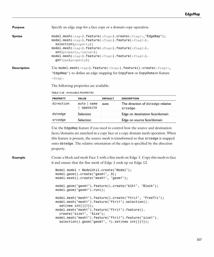
EdgeMap
EdgeMapPurpose Specify an edge map for a face copy or a domain copy operation.
Syntax model.mesh(<tag>).feature(<ftag>).create(<ftag1>,"EdgeMap");model.mesh(<tag>).feature(<ftag>).feature(<ftag1>). selection(property);model.mesh(<tag>).feature(<ftag>).feature(<ftag1>). set(property,<value>);model.mesh(<tag>).feature(<ftag>).feature(<ftag1>). getType(property);
Description Use model.mesh(<tag>).feature(<ftag>).feature().create(<ftag1>,"EdgeMap") to define an edge mapping for CopyFace or CopyDomain feature <ftag>.
The following properties are available:
Use the EdgeMap feature if you need to control how the source and destination faces/domains are matched in a copy face or a copy domain mesh operation. When this feature is present, the source mesh is transformed so that srcedge is mapped onto dstedge. The relative orientation of the edges is specified by the direction property.
Example Create a block and mesh Face 1 with a fine mesh on Edge 1. Copy this mesh to face 6 and ensure that the fine mesh of Edge 1 ends up on Edge 12.
Model model = ModelUtil.create("Model");model.geom().create("geom1", 3);model.mesh().create("mesh1", "geom1");
model.geom("geom1").feature().create("blk1", "Block");model.geom("geom1").run();
model.mesh("mesh1").feature().create("ftri1", "FreeTri");model.mesh("mesh1").feature("ftri1").selection(). set(new int[]{1});model.mesh("mesh1").feature("ftri1").feature(). create("size1", "Size");model.mesh("mesh1").feature("ftri1").feature("size1"). selection().geom("geom1", 1).set(new int[]{1});
TABLE 4-28: AVAILABLE PROPERTIES
PROPERTY VALUE DEFAULT DESCRIPTION
direction auto | same | opposite
auto The direction of dstedge relative srcedge.
dstedge Selection Edge on destination face/domain
srcedge Selection Edge on source face/domain
357
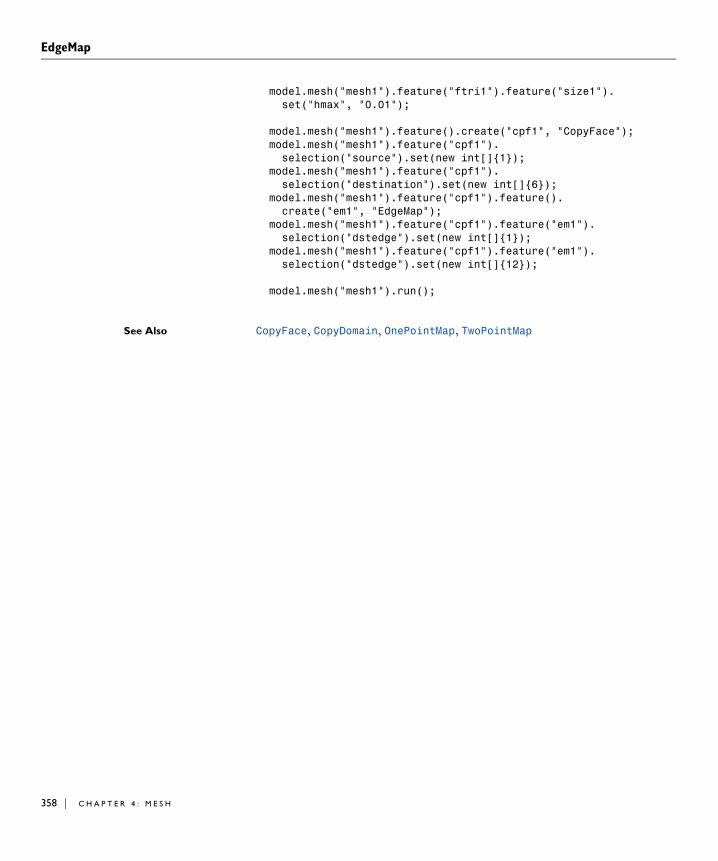
EdgeMap
358 | C H A P T
model.mesh("mesh1").feature("ftri1").feature("size1"). set("hmax", "0.01");
model.mesh("mesh1").feature().create("cpf1", "CopyFace");model.mesh("mesh1").feature("cpf1"). selection("source").set(new int[]{1});model.mesh("mesh1").feature("cpf1"). selection("destination").set(new int[]{6});model.mesh("mesh1").feature("cpf1").feature(). create("em1", "EdgeMap");model.mesh("mesh1").feature("cpf1").feature("em1"). selection("dstedge").set(new int[]{1});model.mesh("mesh1").feature("cpf1").feature("em1"). selection("dstedge").set(new int[]{12});
model.mesh("mesh1").run();
See Also CopyFace, CopyDomain, OnePointMap, TwoPointMap
E R 4 : M E S H

FreeQuad
FreeQuadPurpose Create unstructured quadrilateral mesh.
Syntax model.mesh(<tag>).feature().create(<ftag>,"FreeQuad");model.mesh(<tag>).feature(<ftag>).selection();model.mesh(<tag>).feature(<ftag>).set(property,<value>);model.mesh(<tag>).feature(<ftag>).getType(property);model.mesh(<tag>).feature(<ftag>).feature(). create(<ftag1>,ftype);
Description Use model.mesh(<tag>).feature().create(<ftag>,"FreeQuad") to create an unstructured quadrilateral mesh.
Use model.mesh(<tag>).feature(<ftag>).selection() to specify the domain (boundary in 3D) selection. If you do not specify any selection the feature creates a mesh on the remaining geometric entities in 2D. In 3D, the default selection is empty.
Use model.mesh(<tag>).feature(<ftag>).feature().create(<ftag1>,ftype) to add Size or Distribution attribute features.
The following properties are available:
See the FreeTet feature for more information on the properties.
This feature uses the same attribute feature as the FreeTet feature.
TABLE 4-29: AVAILABLE PROPERTIES
PROPERTY VALUE DEFAULT DESCRIPTION
continue on | off on When enabled, the mesher does not stop if there is an error
xscale double 1 Scale geometry in x direction before meshing
yscale double 1 Scale geometry in y direction before meshing
zscale double 1 Scale geometry in z direction before meshing
smoothcontrol on | off on Specifies if the operation smooths the mesh across removed control entities.
smoothmaxiter integer 8 in 2D, 4 in 3D
Specifies the number of smoothing iterations.
smoothmaxdepth integer 8 in 2D, 4 in 3D
Specifies the maximum element smoothing depth.
359

FreeQuad
360 | C H A P T
Compatibility See FreeTet.
See Also Distribution, FreeTri, Size
E R 4 : M E S H
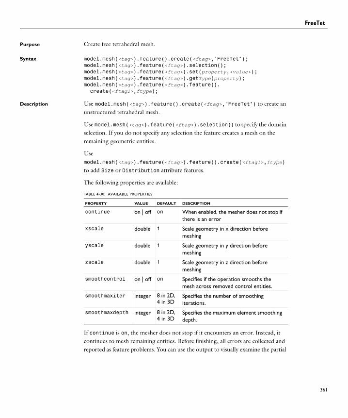
FreeTet
FreeTetPurpose Create free tetrahedral mesh.
Syntax model.mesh(<tag>).feature().create(<ftag>,"FreeTet");model.mesh(<tag>).feature(<ftag>).selection();model.mesh(<tag>).feature(<ftag>).set(property,<value>);model.mesh(<tag>).feature(<ftag>).getType(property);model.mesh(<tag>).feature(<ftag>).feature(). create(<ftag1>,ftype);
Description Use model.mesh(<tag>).feature().create(<ftag>,"FreeTet") to create an unstructured tetrahedral mesh.
Use model.mesh(<tag>).feature(<ftag>).selection() to specify the domain selection. If you do not specify any selection the feature creates a mesh on the remaining geometric entities.
Use model.mesh(<tag>).feature(<ftag>).feature().create(<ftag1>,ftype) to add Size or Distribution attribute features.
The following properties are available:
If continue is on, the mesher does not stop if it encounters an error. Instead, it continues to mesh remaining entities. Before finishing, all errors are collected and reported as feature problems. You can use the output to visually examine the partial
TABLE 4-30: AVAILABLE PROPERTIES
PROPERTY VALUE DEFAULT DESCRIPTION
continue on | off on When enabled, the mesher does not stop if there is an error
xscale double 1 Scale geometry in x direction before meshing
yscale double 1 Scale geometry in y direction before meshing
zscale double 1 Scale geometry in z direction before meshing
smoothcontrol on | off on Specifies if the operation smooths the mesh across removed control entities.
smoothmaxiter integer 8 in 2D, 4 in 3D
Specifies the number of smoothing iterations.
smoothmaxdepth integer 8 in 2D, 4 in 3D
Specifies the maximum element smoothing depth.
361

FreeTet
362 | C H A P T
mesh; this can help you understand what the problems are and how they can be fixed.
The properties xscale, yscale, and zscale specify scalar factors in each axis direction that the geometry is scaled by before meshing. The resulting mesh is then scaled back to fit the original geometry. The values of other properties correspond to the scaled geometry. By default, no scaling is done.
The following attribute features are used:
Compatibility The following properties from the corresponding COMSOL 3.5a command, meshinit, have been removed:
TABLE 4-31: ATTRIBUTE FEATURES USED
FEATURE REMARKS
Distribution Used when defined on edges
Scale Scales Size and Distribution
Size All properties are used
TABLE 4-32: REMOVED PROPERTIES
PROPERTY REASON
edge Defined by the selection
edgelem Defined by the attribute feature Distribution
face Defined by the selection
hauto Defined by attribute feature Size
hcurveedg Defined by the selection for hcurve in Size
hcurvefac Defined by the selection for hcurve in Size
hcutoffedg Defined by the selection for hmin in Size
hcutofffac Defined by the selection for hmin in Size
hgradvtx Defined by the selection for hgrad in Size
hgradedg Defined by the selection for hgrad in Size
hgradfac Defined by the selection for hgrad in Size
hgradsub Defined by the selection for hgrad in Size
hmaxvtx Defined by the selection for hmax in Size
hmaxedg Defined by the selection for hmax in Size
hmaxfac Defined by the selection for hmax in Size
hmaxfact Defined by the selection for hmax in Size
hmaxsub Defined by the selection for hmax in Size
E R 4 : M E S H

FreeTet
See Also Distribution, FreeTri, Size
hnumedg Defined by the selection for hnum in Distribution
hnumsub Defined by the selection for hnum in Distribution
hpntedg No longer supported
hpnt No longer supported
hpntfac No longer supported
jiggle No longer supported. Mesh quality improvements is always done.
mcase Defined by meshing sequence
meshstart Input mesh provided by meshing sequence
minit No longer supported
mlevel Defined by the selection
point Defined by the selection
out Output mesh provided by meshing sequence
subdomain Defined by the selection
TABLE 4-32: REMOVED PROPERTIES
PROPERTY REASON
363

FreeTri
364 | C H A P T
FreeTriPurpose Create unstructured triangular mesh.
Syntax model.mesh(<tag>).feature().create(<ftag>,"FreeTri");model.mesh(<tag>).feature(<ftag>).selection();model.mesh(<tag>).feature(<ftag>).set(property,<value>);model.mesh(<tag>).feature(<ftag>).getType(property);model.mesh(<tag>).feature(<ftag>).feature(). create(<ftag1>,ftype);
Description Use model.mesh(<tag>).feature().create(<ftag>,"FreeTri") to create an unstructured triangular mesh.
Use model.mesh(<tag>).feature(<ftag>).selection() to specify the domain (boundary in 3D) selection. If you do not specify any selection the feature creates a mesh on the remaining geometric entities in 2D. In 3D, the default selection is empty.
Use model.mesh(<tag>).feature(<ftag>).feature().create(<ftag1>,ftype) to add Size or Distribution attribute features.
The following properties are available:
TABLE 4-33: AVAILABLE PROPERTIES
PROPERTY VALUE DEFAULT DESCRIPTION
continue on | off on When enabled, the mesher does not stop if there is an error
method auto | af | del
auto Triangulation method
xscale double 1 Scale geometry in x direction before meshing
yscale double 1 Scale geometry in y direction before meshing
zscale double 1 Scale geometry in z direction before meshing
smoothcontrol on | off on Specifies if the operation smooths the mesh across removed control entities.
smoothmaxiter integer 8 in 2D, 4 in 3D
Specifies the number of smoothing iterations.
smoothmaxdepth integer 8 in 2D, 4 in 3D
Specifies the maximum element smoothing depth.
E R 4 : M E S H

FreeTri
Use the property method to specify the method used to triangulate domains in 2D and faces in 3D. A Delaunay based method is used if the property is set to del and an advancing front method is used if the property is set to af. If method is set to auto, the program tries to choose the best method for each geometric entity.
Compatibility See FreeTet.
See Also Distribution, FreeTet, FreeQuad, Size
365

Import
366 | C H A P T
ImportPurpose Import mesh from file or other meshing sequence.
Syntax model.mesh(<tag>).feature().create(<ftag>,"Import");model.mesh(<tag>).feature(<ftag>).set(property,<value>);model.mesh(<tag>).feature(<ftag>).getType(property);model.mesh(<tag>).feature(<ftag>).importData();
Description Use model.mesh(<tag>).feature().create(<ftag>,"Import") to import a mesh into a sequence without a corresponding geometry. It is only possible to use this feature when the geometry sequence is empty. If the sequence already contains a mesh, the imported mesh is added to the existing mesh.
Use model.mesh(<tag>).feature(<ftag>).importData() to import the file again.
The following mesh formats are supported:
The following properties are available:
FORMAT FILE EXTENSION
COMSOL Multiphysics text file .mphtxt
COMSOL Multiphysics binary file .mphbin
NASTRAN file .nas | .bdf | .dat
PROPERTY VALUES DEFAULT
DESCRIPTION
elemsplit on | off off Specifies if mesh elements of different element forms get different domain labels when importing a NASTRAN file.
facepartition auto | manual auto Manual or automatic face partitioning in 3D
filename String File name
linearelem on | off off Specifies if extended node points in the NASTRAN file are ignored.
materialsplit on | off on Specifies if material data in the NASTRAN file is used to determine the domain partitioning of the domain elements.
data all | mesh all Specifies the data to import from the NASTRAN file.
E R 4 : M E S H

Import
The properties elemsplit, linearelem, materialsplit, and data are only used for import of NASTRAN files.
elemsplit specifies if mesh elements of different element forms—that is, tetrahedral, pyramid, prism, or hexahedral—get different domain labels. The default value is off.
linearelem determines if extended node points are ignored. If the value is on all imported elements are linear. Otherwise, the order of the imported elements is determined from the order of the elements in the file. The default value is on.
materialsplit determines if material data in the file is used (if available) to determine the domain partitioning of the domain elements. If the value is off all domain elements in the imported mesh belongs to the same domain if possible. The default value is on.
If facepartition is set to manual in 3D, the following properties are available. If any of these properties are set explicitly, facepartition is automatically switched to manual
sequence String Meshing sequence name
source file | sequence | native | nastran | stlvrml
file Source for the import
TABLE 4-34: VALID PROPERTY/VALUE PAIRS
PROPERTY VALUE DEFAULT DESCRIPTION
curvedface auto | manual auto Control parameters for partitioning of curved faces.
extrangle double 0.6 degrees Maximum angle between boundary element normal and extrusion plane that causes the element to be a part the extruded face if possible
faceangle double 360 degrees Maximum angle between any two boundary elements in the same face
PROPERTY VALUES DEFAULT
DESCRIPTION
367

Import
368 | C H A P T
The table below specifies the supported NASTRAN bulk data entries.
facecleanup double 0.01 Avoid creating small faces. Faces with an area less than Facecleanup * the mean face area, are merged with adjacent faces
facecurv double 10 degrees Maximum relative angle deviation between any two boundary elements in the same face
minareacurv double 1 Minimum relative area of face to be considered as a face with constant curvature
minareaextr double 0.05 Minimum relative area of face to be considered extruded
minareaeplane double 0.005 Minimum relative area of face to be considered planar
neighangle double 20 degrees Maximum angle between a boundary element and a neighbor that causes the elements to be part of the same boundary domain if possible
planar on | off on Detect planar faces
planarangle double 0.6 degrees Maximum angle between boundary element normal and a neighbor that causes the element to be a part the planar face if possible
BULK DATA ENTRY
CBAR CORD2C CQUAD4 GRID
CHEXA CORD2R CQUAD8 MAT1
CORD1C CORD2S CTETRA MAT10
CORD1R CPENTA CTRIA3 PSHELL
CORD1S CPYRAM CTRIA6 PSOLID
TABLE 4-34: VALID PROPERTY/VALUE PAIRS
PROPERTY VALUE DEFAULT DESCRIPTION
E R 4 : M E S H

Import
The NASTRAN bulk data format uses reduced second-order elements; that is, the center node on quadrilateral mesh faces (quadNode) and the center node of hexahedral elements (hexNode) are missing. Importing a NASTRAN mesh with second-order elements, COMSOL Multiphysics interpolates the coordinates of these missing node points from the surrounding node points using the following formulas: quadNode = 0.5*quadEdgeNodes-0.25*quadCornerNodes, where quadEdgeNodes is the sum of the coordinates of the surrounding 4 edge nodes and quadCornerNodes is the sum of the coordinates of the surrounding 4 corner nodes, and hexNode = 0.25*hexEdgeNodes-0.25*hexCornerNodes, where hexEdgeNodes is the sum of the coordinates of the surrounding 12 edge nodes and hexCornerNodes is the sum of the coordinates of the surrounding 8 corner nodes.
Cautionary The Import feature does not handle NASTRAN files in free field format where the data fields are separated by blanks.
Compatibility The following properties from the corresponding COMSOL 3.5a command, meshimport, have been removed:
See Also Ball, Box, CreateVertex, DeleteEntities, JoinEntities
TABLE 4-35: REMOVED PROPERTIES
PROPERTY REASON
mcase Defined by meshing sequence
out Output mesh provided by meshing sequence
369

JoinEntities
370 | C H A P T
JoinEntitiesPurpose Join geometric entities of an imported mesh.
Syntax model.mesh(<tag>).feature().create(<ftag>,"JoinEntities");model.mesh(<tag>).feature(<ftag>).selection();model.mesh(<tag>).feature(<ftag>).set(property,<value>);model.mesh(<tag>).feature(<ftag>).getType(property);model.mesh(<tag>).feature(<ftag>).feature(). create(<ftag1>,"JoinEntities");
Description Use model.mesh(<tag>).feature().create(<ftag>,"JoinEntities") to join adjacent geometric entities of an imported 2D or 3D mesh.
Use model.mesh(<tag>).feature(<ftag>).selection() to specify geometric entities to join.
The following properties are available:
See Also Import, DeleteEntities
TABLE 4-36: AVAILABLE PROPERTIES
PROPERTY VALUE DEFAULT DESCRIPTION
joinadj boolean true Specifies if the operation joins lower dimensional adjacent entities
E R 4 : M E S H

Map
MapPurpose Create structured quadrilateral mesh.
Syntax model.mesh(<tag>).feature().create(<ftag>,"Map");model.mesh(<tag>).feature(<ftag>).selection();model.mesh(<tag>).feature(<ftag>).set(property,<value>);model.mesh(<tag>).feature(<ftag>).getType(property);model.mesh(<tag>).feature(<ftag>).feature(). create(<ftag1>,ftype);
Description Use model.mesh(<tag>).feature().create(<ftag>,"Map") to create a structured quadrilateral mesh.
Use model.mesh(<tag>).feature(<ftag>).selection() to specify the domain (boundary in 3D) selection. If you do not specify any selection the feature creates a mesh on the remaining domains in 2D. In 3D, the default selection is empty.
Use model.mesh(<tag>).feature(<ftag>).feature().create(<ftag1>,ftype) to add a Size, Distribution, or EdgeGroup attribute feature.
The following properties are available:
The following attribute features are used:
TABLE 4-37: AVAILABLE PROPERTIES
PROPERTY VALUE DEFAULT DESCRIPTION
adjustedgdistr on | off off When enabled, the mapped mesher adjusts evenly distributed edge mesh.
interpmethod auto | transfinite2D | transfinite3D
auto Interpolation method
smoothcontrol on | off on Specifies if the operation smooths the mesh across removed control entities.
smoothmaxiter integer 8 in 2D, 4 in 3D
Specifies the number of smoothing iterations.
smoothmaxdepth integer 8 in 2D, 4 in 3D
Specifies the maximum element smoothing depth.
TABLE 4-38: ATTRIBUTE FEATURES USED
FEATURE REMARKS
EdgeGroup Defined on the domain/face to be meshed
Distribution Used when defined on edges
371

Map
372 | C H A P T
Compatibility The following properties from the corresponding COMSOL 3.5a command, meshmap, have been removed:
See Also Distribution, FreeTri
Scale Scales Size and Distribution
Size Defined on domain/face. Uses only hauto and hmax.
TABLE 4-38: ATTRIBUTE FEATURES USED
FEATURE REMARKS
TABLE 4-39: REMOVED PROPERTIES
PROPERTY REASON
edgelem Defined by the Distribution
face Defined by the selection
mcase Defined by the meshing sequence
meshstart Input mesh provided by meshing sequence
out Output mesh provided by meshing sequence
domain Defined by the selection
E R 4 : M E S H

OnePointMap
OnePointMapPurpose Specify a one point map for a face copy or a domain copy operation.
Syntax model.mesh(<tag>).feature(<ftag>).create(<ftag1>,"OnePointMap");model.mesh(<tag>).feature(<ftag>).feature(<ftag1>). selection(property);
Description Use model.mesh(<tag>).feature(<ftag>).feature().create(<ftag1>,"OnePointMap") to define a one-point map for CopyFace or CopyDomain feature <ftag>.
The following properties are available:
Use the OnePointMap feature if you need to control how the source and destination faces/domains are matched in a copy face or a copy domain mesh operation. When this feature is present, the source mesh is transformed so that srcpoint1 is mapped to dstpoint1.
Example Create a block and mesh face 4 with a fine mesh near Point 8. Copy this mesh onto Face 3 and ensure that the fine mesh near Point 8 ends up near Point 3.
Model model = ModelUtil.create("Model");model.geom().create("geom1", 3);model.mesh().create("mesh1", "geom1");
model.geom("geom1").feature().create("blk1", "Block");model.geom("geom1").run();
model.mesh("mesh1").feature().create("ftri1", "FreeTri");model.mesh("mesh1").feature("ftri1").selection(). set(new int[]{4});model.mesh("mesh1").feature("ftri1").feature(). create("size1", "Size");model.mesh("mesh1").feature("ftri1").feature("size1"). selection().geom("geom1", 0).set(new int[]{8});model.mesh("mesh1").feature("ftri1").feature("size1"). set("hmax", "0.01");model.mesh("mesh1").feature().create("cpf1", "CopyFace");model.mesh("mesh1").feature("cpf1").selection("source"). geom("geom1", 2).set(new int[]{4});model.mesh("mesh1").feature("cpf1").selection("destination"). geom("geom1", 2).set(new int[]{3});model.mesh("mesh1").feature("cpf1").feature().
TABLE 4-40: AVAILABLE PROPERTIES
PROPERTY VALUE DEFAULT DESCRIPTION
srcpoint1 Selection Point on source face/domain
dstpoint1 Selection Point on destination face/domain
373

OnePointMap
374 | C H A P T
create("pm1", "OnePointMap");model.mesh("mesh1").feature("cpf1").feature("pm1"). selection("srcpoint1").set(new int[]{8});model.mesh("mesh1").feature("cpf1").feature("pm1"). selection("dstpoint1").set(new int[]{3});model.mesh("mesh1").run();
See Also CopyFace, CopyDomain, EdgeMap, TwoPointMap
E R 4 : M E S H
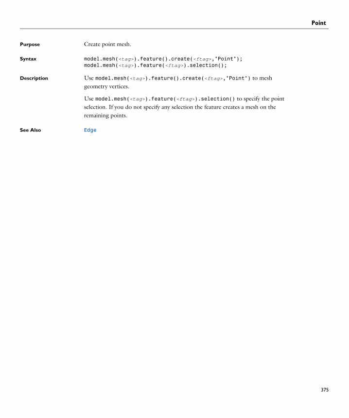
Point
PointPurpose Create point mesh.
Syntax model.mesh(<tag>).feature().create(<ftag>,"Point");model.mesh(<tag>).feature(<ftag>).selection();
Description Use model.mesh(<tag>).feature().create(<ftag>,"Point") to mesh geometry vertices.
Use model.mesh(<tag>).feature(<ftag>).selection() to specify the point selection. If you do not specify any selection the feature creates a mesh on the remaining points.
See Also Edge
375
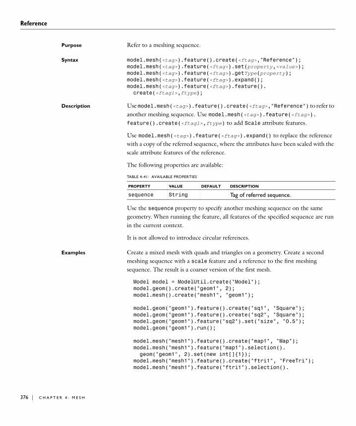
Reference
376 | C H A P T
ReferencePurpose Refer to a meshing sequence.
Syntax model.mesh(<tag>).feature().create(<ftag>,"Reference");model.mesh(<tag>).feature(<ftag>).set(property,<value>);model.mesh(<tag>).feature(<ftag>).getType(property);model.mesh(<tag>).feature(<ftag>).expand();model.mesh(<tag>).feature(<ftag>).feature(). create(<ftag1>,ftype);
Description Use model.mesh(<tag>).feature().create(<ftag>,"Reference") to refer to another meshing sequence. Use model.mesh(<tag>).feature(<ftag>).feature().create(<ftag1>,ftype) to add Scale attribute features.
Use model.mesh(<tag>).feature(<ftag>).expand() to replace the reference with a copy of the referred sequence, where the attributes have been scaled with the scale attribute features of the reference.
The following properties are available:
Use the sequence property to specify another meshing sequence on the same geometry. When running the feature, all features of the specified sequence are run in the current context.
It is not allowed to introduce circular references.
Examples Create a mixed mesh with quads and triangles on a geometry. Create a second meshing sequence with a scale feature and a reference to the first meshing sequence. The result is a coarser version of the first mesh.
Model model = ModelUtil.create("Model");model.geom().create("geom1", 2);model.mesh().create("mesh1", "geom1");
model.geom("geom1").feature().create("sq1", "Square");model.geom("geom1").feature().create("sq2", "Square");model.geom("geom1").feature("sq2").set("size", "0.5");model.geom("geom1").run();
model.mesh("mesh1").feature().create("map1", "Map");model.mesh("mesh1").feature("map1").selection(). geom("geom1", 2).set(new int[]{1});model.mesh("mesh1").feature().create("ftri1", "FreeTri");model.mesh("mesh1").feature("ftri1").selection().
TABLE 4-41: AVAILABLE PROPERTIES
PROPERTY VALUE DEFAULT DESCRIPTION
sequence String Tag of referred sequence.
E R 4 : M E S H

Reference
geom("geom1", 2).set(new int[]{2});model.mesh("mesh1").run();
model.mesh().create("mesh2", "geom1");model.mesh("mesh2").feature().create("sca1", "Scale");model.mesh("mesh2").feature("sca1").set("scale", "2");model.mesh("mesh2").feature().create("rf1", "Reference");model.mesh("mesh2").feature("rf1").set("sequence", "mesh1");model.mesh("mesh2").run();
See Also Scale
377

Refine
378 | C H A P T
RefinePurpose Refine mesh.
Syntax model.mesh(<tag>).feature().create(<ftag>,"Refine");model.mesh(<tag>).feature(<ftag>).selection();model.mesh(<tag>).feature(<ftag>).set(property,<value>);model.mesh(<tag>).feature(<ftag>).getType(property);
Description Use model.mesh(<tag>).feature().create(<ftag>,"Refine") to refine the mesh.
Use model.mesh(<tag>).feature(<ftag>).selection() to specify the domain selection or the entire geometry. If you do not specify any selection the feature refines all triangular and tetrahedral elements in the mesh.
The following properties are available:
Use the boxcoord property to refine elements inside a bounding box. To define the bounding box, set the properties xmin, xmax, ymin, ymax, zmax, and zmin on the feature, where (xmin,ymin,zmin) defines the lower-left corner and (xmax,ymax,zmax) defines the upper-right corner of the bounding box. The elements that have all its corner points in the bounding box are refined once. boxcoord is automatically set to on if one of the coordinates are set.
The default refinement method in 2D is regular refinement, where all of the specified triangles are divided into four triangles of the same shape. Longest edge refinement, where the longest edge of each specified triangle is bisected, can be selected by giving longest as rmethod. Using regular as rmethod results in regular refinement. Some triangles outside of the specified set may also be refined, in order to preserve the triangulation and its quality.
In 3D, the default refinement method is longest. The regular refinement method is only implemented for uniform refinements (that is, when all elements are refined).
PROPERTY VALUE DEFAULT DESCRIPTION
boxcoord on | off off Use coordinates of a bounding box to determine the elements to refine
rmethod longest | regular
see below
Refinement method
element int[] all List of elements to refine
numrefine int or int[] 1 Number of refinements
xmax, xmin, ymax, ymin, zmax, zmin
double Coordinates of bounding box
E R 4 : M E S H

Refine
In 1D, regular refinement, where each element is divided into two elements of the same shape, is always used.
By default, all elements are refined once. By using the element property, you can specify which elements are refined and the numrefine property specifies how many times the elements is refined. If numrefine is an integer, all refined elements are refined numrefine times. If numrefine is a vector, it must have the same length as the element vector, and gives the number of refinements for each element.
Compatibility The following properties from the corresponding COMSOL 3.5a command, meshrefine, have been removed:
Examples Mesh two squares with free mesh. Refine the mesh on sq2 once and refine the elements inside a box in sq1 twice.
Model model = ModelUtil.create("Model");model.geom().create("geom1", 2);model.mesh().create("mesh1", "geom1");
model.geom("geom1").feature().create("sq1", "Square");model.geom("geom1").feature().create("sq2", "Square");model.geom("geom1").feature("sq2").setIndex("pos", "1", 0);model.geom("geom1").run();
model.mesh("mesh1").feature().create("ftri1", "FreeTri");model.mesh("mesh1").feature().create("ref1", "Refine");model.mesh("mesh1").feature("ref1").selection(). geom("geom1", 2).set(new int[]{2});model.mesh("mesh1").feature().create("ref2", "Refine");model.mesh("mesh1").feature("ref2").set("xmin", "0.2");model.mesh("mesh1").feature("ref2").set("xmax", "0.8");model.mesh("mesh1").feature("ref2").set("ymin", "0.2");model.mesh("mesh1").feature("ref2").set("ymax", "0.6");model.mesh("mesh1").run();
See Also Convert
TABLE 4-42: REMOVED PROPERTIES
PROPERTY REASON
mcase Defined by meshing sequence
out Output mesh provided by meshing sequence
domain Defined by the selection
tri, tet Replaced by element and numrefine
379

Scale
380 | C H A P T
ScalePurpose Scale size properties.
Syntax model.mesh(<tag>).feature().create(<ftag>,"Scale");model.mesh(<tag>).feature(<ftag>).selection();model.mesh(<tag>).feature(<ftag>).set(property,<value>);model.mesh(<tag>).feature(<ftag>).getType(property);model.mesh(<tag>).feature(<ftag>).feature(). create(<ftag1>,"Scale");model.mesh(<tag>).feature(<ftag>).feature(<ftag1>).selection();model.mesh(<tag>).feature(<ftag>).feature(<ftag1>). set(property,<value>);model.mesh(<tag>).feature(<ftag>).feature(<ftag1>). getType(property);
Description Use model.mesh(<tag>).feature().create(<ftag>,"Scale") to scale size properties defined in the sequence and use model.mesh(<tag>).feature(<ftag>).feature().create(<ftag1>,"Scale
") to scale size properties defined in the sequence referred to by the Reference feature <ftag>.
Use model.mesh(<tag>).feature(<ftag>).selection() or model.mesh(<tag>).feature(<ftag>).feature(<ftag1>).selection() to specify the geometric entity selection or the entire geometry (which is default).
The following properties are available:
Scale is a positive number. The feature scales mesh size properties, distribution properties and boundary layer properties affecting mesh elements generated by features following the scale feature. The scale feature also affects size properties defined by Size, Distribution, and BndLayerProp features occurring later in the sequence.
A scale less than 1 gives smaller (more) elements; a scale greater than 1 gives larger (fewer) elements. The scale feature has no effect on mesh generated earlier in the sequence.
If two or more scale features exist on the same selection, the resulting scale on that selection is the product of the given scales.
TABLE 4-43: FEATURE PROPERTIES DEFINED
PROPERTY VALUE DEFAULT DESCRIPTION
scale double 1 Scale factor
E R 4 : M E S H
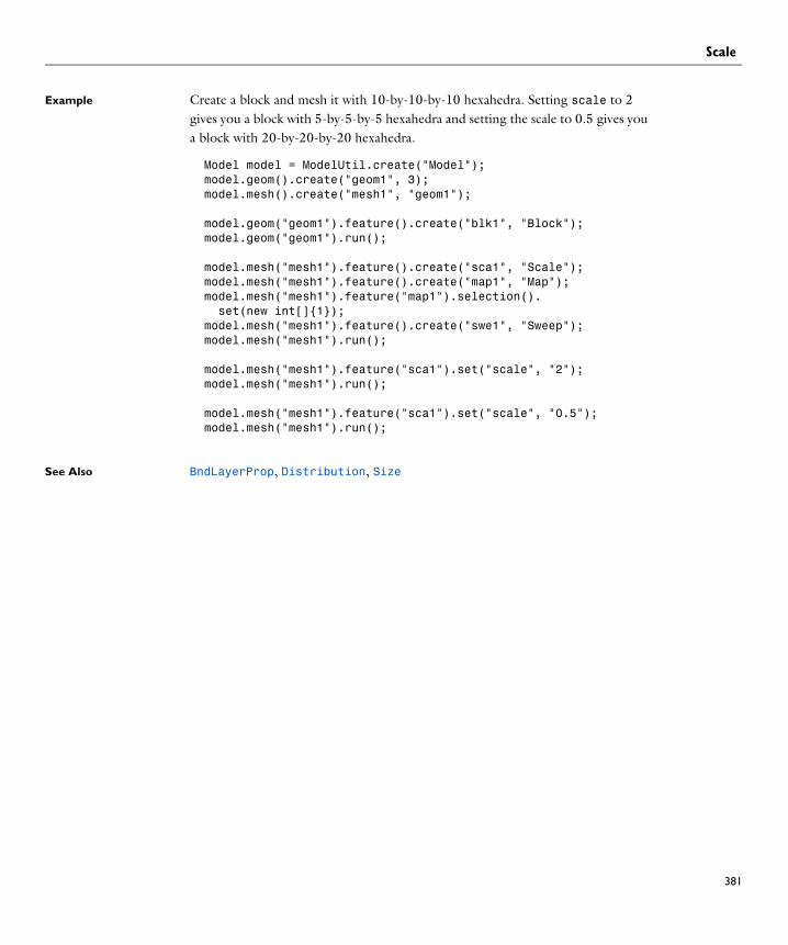
Scale
Example Create a block and mesh it with 10-by-10-by-10 hexahedra. Setting scale to 2 gives you a block with 5-by-5-by-5 hexahedra and setting the scale to 0.5 gives you a block with 20-by-20-by-20 hexahedra.
Model model = ModelUtil.create("Model");model.geom().create("geom1", 3);model.mesh().create("mesh1", "geom1");
model.geom("geom1").feature().create("blk1", "Block");model.geom("geom1").run();
model.mesh("mesh1").feature().create("sca1", "Scale");model.mesh("mesh1").feature().create("map1", "Map");model.mesh("mesh1").feature("map1").selection(). set(new int[]{1});model.mesh("mesh1").feature().create("swe1", "Sweep");model.mesh("mesh1").run();
model.mesh("mesh1").feature("sca1").set("scale", "2");model.mesh("mesh1").run();
model.mesh("mesh1").feature("sca1").set("scale", "0.5");model.mesh("mesh1").run();
See Also BndLayerProp, Distribution, Size
381

Size
382 | C H A P T
SizePurpose Mesh size properties.
Syntax model.mesh(<tag>).feature().create(<ftag>,"Size");model.mesh(<tag>).feature(<ftag>).selection();model.mesh(<tag>).feature(<ftag>).set(property,<value>);model.mesh(<tag>).feature(<ftag>).getType(property);model.mesh(<tag>).feature(<ftag>).feature(). create(<ftag1>,"Size");model.mesh(<tag>).feature(<ftag>).feature(<ftag1>).selection();model.mesh(<tag>).feature(<ftag>).feature(<ftag1>). set(property,<value>);model.mesh(<tag>).feature(<ftag>).feature(<ftag1>). getType(property);
Description Use model.mesh(<tag>).feature().create(<ftag>,"Size") to specify element size properties in the sequence. Use model.mesh(<tag>).feature(<ftag>).feature().create(<ftag1>,"Size") to specify element size properties for the feature <ftag> that can be any of the types Edge, FreeQuad, FreeTri, FreeTet, Map, or Sweep.
Use model.mesh(<tag>).feature(<ftag>).selection() or model.mesh(<tag>).feature(<ftag>).feature(<ftag1>).selection() to specify the geometric entity selection. If you do not specify any selection the size feature is defined on all geometric entities. The selection is not available for the default size feature, tagged size.
The following properties are available:
TABLE 4-44: FEATURE PROPERTIES DEFINED
PROPERTY VALUE DEFAULT DESCRIPTION
custom on | off off Setting custom to on deactivates all mesh parameters.
hauto double 5 Automatic settings for all mesh parameters.
hcurve double 0.3 | 0.6 Curvature mesh size
hcurveactive on | off on Specifies if hcurve is used
hgrad double 1.3 | 1.5 Element growth rate
hgradactive on | off on Specifies if hgrad is used
hmax double geometry dependent
Maximum element size
hmaxactive on | off on Specifies if hmax is used
E R 4 : M E S H

Size
Note: The properties with names ending in active are not available for the default size feature.
The property table is either cfd, default, or plasma and specifies the physics for which the element size is calibrated.
Hauto is a positive scalar. This value is used to set several mesh parameters in order to get a mesh of desired size. Smaller values of hauto generate finer meshes with more elements.The integers between 1 and 9 has a special interpretation; they correspond to the mesh settings Normal, Fine, Coarse and so forth in COMSOL Multiphysics. The value 5 correspond to Normal. When you set the property hauto, all other properties are set to their default value, according to the following tables (for table set to default).
hmin double geometry dependent
Minimum element size
hminactive on | off on Specifies if hmin is used
hnarrow double 0.5 Resolution of narrow regions
hnarrowactive on | off on Specifies if hnarrow is used
table cfd | default | plasma
default Specifies for which physics the element size is calibrated
TABLE 4-45: MESH PARAMETERS SET BY THE PROPERTY HAUTO IN 2D (FOR DEFAULT TABLE)
HAUTO HMAXFACT HCURVE HGRAD HMINFACT HNARROW
1 0.01 0.2 1.1 2e-5 1
2 0.02 0.25 1.2 7.5e-5 1
3 0.037 0.25 1.25 1.25e-4 1
4 0.053 0.3 1.3 3e-4 1
5 0.067 0.3 1.3 3e-4 1
6 0.1 0.4 1.4 0.002 1
7 0.13 0.6 1.5 0.006 1
8 0.2 0.8 1.8 0.016 1
9 0.33 1 2 0.05 0.9
TABLE 4-44: FEATURE PROPERTIES DEFINED
PROPERTY VALUE DEFAULT DESCRIPTION
383

Size
384 | C H A P T
The property hcurve is a real value that relates the mesh size to the curvature of the geometry boundaries. The gaussian radius of curvature is multiplied by the hcurve factor to obtain the mesh size along the boundary. The specified hcurve is only used if hcurveactive is on, otherwise hcurve is taken from a preceding size feature in the sequence. In the default size feature, tagged size, hcurve is always active and there is no hcurveactive property.
The property hgrad tells how fast the element size—measured as the length of the longest edge of the element—can grow from a region with small elements to a region with larger elements. If two elements lie one unit length apart, the difference in element size can be at most hgrad. The specified hgrad is only used if hgradactive is on, otherwise hgrad is taken from a preceding size feature in the sequence. In the default size feature, hgrad is always active and there is no hcurvegrad property.
The hmax parameter controls the size of the elements in the mesh. The algorithm aims at creating a mesh where no element size exceeds hmax. The default hmax value is hmaxfact * maxdist, where maxdist is the longest axis parallel distance in the geometry. The specified hmax is only used if hmaxactive is on, otherwise hmax is taken from a preceding size feature in the sequence. In the default size feature, hmax is always active and there is no hmaxactive property.
You can use hmin to control the minimum size of the elements. The main purpose of this parameter is to prevent the generation of many small elements near small curved parts of the geometry. The default hmin value is hminfact * maxdist, where maxdist is the longest axis parallel distance in the geometry. The specified hmin is only used if hminactive is on, otherwise hmin is taken from a preceding size feature
mesh parameters set by the property hauto in 3d (for default table)
HAUTO HMAXFACT HCURVE HGRAD HMINFACT HNARROW
1 0.02 0.2 1.3 2e-4 1
2 0.035 0.3 1.35 0.0015 0.85
3 0.055 0.4 1.4 0.004 0.7
4 0.08 0.5 1.45 0.01 0.6
5 0.1 0.6 1.5 0.018 0.5
6 0.15 0.7 1.6 0.028 0.4
7 0.19 0.8 1.7 0.04 0.3
8 0.3 0.9 1.85 0.054 0.2
9 0.5 1 2 0.07 0.1
E R 4 : M E S H
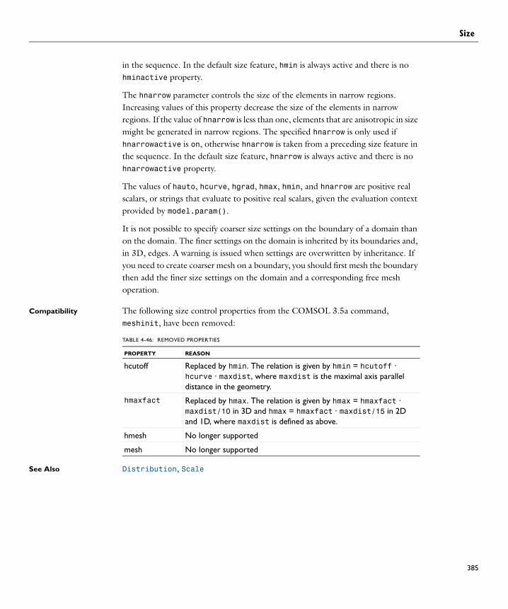
Size
in the sequence. In the default size feature, hmin is always active and there is no hminactive property.
The hnarrow parameter controls the size of the elements in narrow regions. Increasing values of this property decrease the size of the elements in narrow regions. If the value of hnarrow is less than one, elements that are anisotropic in size might be generated in narrow regions. The specified hnarrow is only used if hnarrowactive is on, otherwise hnarrow is taken from a preceding size feature in the sequence. In the default size feature, hnarrow is always active and there is no hnarrowactive property.
The values of hauto, hcurve, hgrad, hmax, hmin, and hnarrow are positive real scalars, or strings that evaluate to positive real scalars, given the evaluation context provided by model.param().
It is not possible to specify coarser size settings on the boundary of a domain than on the domain. The finer settings on the domain is inherited by its boundaries and, in 3D, edges. A warning is issued when settings are overwritten by inheritance. If you need to create coarser mesh on a boundary, you should first mesh the boundary then add the finer size settings on the domain and a corresponding free mesh operation.
Compatibility The following size control properties from the COMSOL 3.5a command, meshinit, have been removed:
See Also Distribution, Scale
TABLE 4-46: REMOVED PROPERTIES
PROPERTY REASON
hcutoff Replaced by hmin. The relation is given by hmin = hcutoff · hcurve · maxdist, where maxdist is the maximal axis parallel distance in the geometry.
hmaxfact Replaced by hmax. The relation is given by hmax = hmaxfact · maxdist/10 in 3D and hmax = hmaxfact · maxdist/15 in 2D and 1D, where maxdist is defined as above.
hmesh No longer supported
mesh No longer supported
385

Sweep
386 | C H A P T
SweepPurpose Create swept mesh.
Syntax model.mesh(<tag>).feature().create(<ftag>,"Sweep");model.mesh(<tag>).feature(<ftag>).selection();model.mesh(<tag>).feature(<ftag>).selection(property);model.mesh(<tag>).feature(<ftag>).set(property,<value>);model.mesh(<tag>).feature(<ftag>).getType(property);model.mesh(<tag>).feature(<ftag>).feature(). create(<ftag1>,ftype);
Description Use model.mesh(<tag>).feature().create(<ftag>,"Sweep") to create a swept mesh in 3D.
Use model.mesh(<tag>).feature(<ftag>).selection() to specify the domain selection. If you do not specify any selection the feature creates a mesh on the remaining domains.
Use model.mesh(<tag>).feature(<ftag>).feature().create(<ftag1>,ftype) to add a Size or Distribution attribute feature.
Use model.mesh(<tag>).feature(<ftag>).selection() to specify the 3D domain selection. If you do not specify any selection the feature creates a mesh on the remaining domains.
The following properties are available:
Use the property sourceface and targetface to specify the source faces and the destination faces of the sweep, respectively. For domains in the feature selection
TABLE 4-47: AVAILABLE PROPERTIES
PROPERTY VALUE DEFAULT DESCRIPTION
facemethod tri | quad quad Face meshing method
sourceface Selection Source faces selection
sweeppath String auto Sweep path
targetface Selection Destination face selection
targetmesh String auto Destination mesh method
smoothcontrol on | off on Specifies if the operation smooths the mesh across removed control entities.
smoothmaxiter integer 8 in 2D, 4 in 3D
Specifies the number of smoothing iterations.
smoothmaxdepth integer 8 in 2D, 4 in 3D
Specifies the maximum element smoothing depth.
E R 4 : M E S H

Sweep
where none of the surrounding faces are specified as either a source or a destination face, the software automatically tries to determine these faces.
Use the property sweeppath if you want to specify the shape of the sweep path. The string is either auto, straight, circular, or general. straight means that all interior mesh points are located on straight lines between the corresponding source and destination points. circular means that all interior mesh points are located on circular arcs between the corresponding source and destination points. general means that the positions of the interior mesh points are determined by a general interpolation procedure. auto, which is default, means that the sweeping algorithm automatically tries to determine if the sweep path is straight or circular. If this is the case sweeppath is set to straight or circular, respectively. Otherwise, sweeppath is set to general.
Any source face that is not meshed, is meshed automatically. The property facemethod controls which face meshing method is used. If facemethod is quad, you get quadrilateral face mesh and therefore hexahedral domain mesh. If facemehtod is tri, you get triangular face mesh and prism elements in the domain.
Use the property targetmesh if you want to specify the method to be used for transferring the source mesh to the destination face. The string is either auto, morph, or rigid. morph means that the destination mesh is created from the source mesh by a morphing technique, and rigid means that the destination mesh is created by a rigid transformation of the source mesh. The value auto, which is default, means that the sweeping algorithm automatically tries to determine a suitable method for creating the destination mesh.
The following attribute features are used:
If a Distribution feature is defined on a domain, it is used to determine the distribution of element layer in the sweep direction. Otherwise, if hauto or hmax is specified, equidistant element layers are generated.
TABLE 4-48: ATTRIBUTE FEATURES USED
FEATURE REMARKS
Distribution Used when defined on domains
Scale Scales Size and Distribution
Size Defined on domain.
387

Sweep
388 | C H A P T
Compatibility The following properties from the corresponding COMSOL 3.5a command, meshsweep, have been removed:
See Also Distribution, FreeQuad, FreeTri, Map
TABLE 4-49: REMOVED PROPERTIES
PROPERTY REASON
elsweeplayers Defined by the property elemdistr in Distribution
meshstart Input mesh provided by meshing sequence
out Output mesh provided by meshing sequence
domain Defined by the selection
E R 4 : M E S H

TwoPointMap
TwoPointMapPurpose Specify a two point map for a face copy or a domain copy operation.
Syntax model.mesh(<tag>).feature(<ftag>).create(<ftag1>,"TwoPointMap")model.mesh(<tag>).feature(<ftag>).feature(<ftag1>).selection(prop
erty)
Description Use model.mesh(<tag>).feature(<ftag>).feature().create(<ftag1>,"TwoPointMap") to define a two-point map for the CopyFace or CopyDomain feature <ftag>.
The following properties are available:
Use the TwoPointMap feature if you need to control how the source and destination faces/domains are matched in a copy face or a copy domain mesh operation. When this feature is present, the source mesh is transformed so that srcpoint1 is mapped to dstpoint1 and srcpoint2 is mapped to dstpoint2.
Example Create a block and mesh face 2. Copy this mesh onto the opposite Face 5 and ensure that Point 6 is mapped to Point 4 and Point 5 is mapped to Point 8.
Model model = ModelUtil.create("Model");model.geom().create("geom1", 3);model.mesh().create("mesh1", "geom1");
model.geom("geom1").feature().create("blk1", "Block");model.geom("geom1").run();
model.mesh("mesh1").feature().create("ftri1", "FreeTri");model.mesh("mesh1").feature("ftri1").selection(). set(new int[]{2});model.mesh("mesh1").feature("ftri1").feature(). create("size1", "Size");model.mesh("mesh1").feature("ftri1").feature("size1"). selection().geom("geom1", 1).set(new int[]{9});model.mesh("mesh1").feature("ftri1").feature("size1"). set("hmax", "0.01");model.mesh("mesh1").feature().create("cpf1", "CopyFace");model.mesh("mesh1").feature("cpf1"). selection("source").geom("geom1", 2).set(new int[]{2});
TABLE 4-50: AVAILABLE PROPERTIES
PROPERTY VALUE DEFAULT DESCRIPTION
srcpoint1 Selection First point on source face/domain
srcpoint2 Selection Second point on source face/domain
dstpoint1 Selection First point on destination face/domain
dstpoint2 Selection Second point on destination face/domain
389

TwoPointMap
390 | C H A P T
model.mesh("mesh1").feature("cpf1"). selection("destination").geom("geom1", 2).set(new int[]{5});model.mesh("mesh1").feature("cpf1").feature(). create("ppm1", "TwoPointMap");model.mesh("mesh1").feature("cpf1").feature("ppm1"). selection("srcpoint1").set(new int[]{6});model.mesh("mesh1").feature("cpf1").feature("ppm1"). selection("dstpoint1").set(new int[]{4});model.mesh("mesh1").feature("cpf1").feature("ppm1"). selection("srcpoint2").set(new int[]{5});model.mesh("mesh1").feature("cpf1").feature("ppm1"). selection("dstpoint2").set(new int[]{8});model.mesh("mesh1").run();
See Also CopyFace, CopyDomain, EdgeMap, OnePointMap
E R 4 : M E S H

5
S o l v e r
This chapter contains reference information about the solver command and utility commands for producing and handling solutions.
In this chapter:
• About Solver Commands
• Solution Object Data
391

392 | C H A P T E
Abou t S o l v e r C ommand s
The following list includes the solver commands that are documented in this chapter:
• Adaption
• Advanced
• Assemble
• AutoRemesh
• AWE
• Eigenvalue
• FullyCoupled
• Linear
• Modal
• Optimization
• Parametric
• PlotWhileSolving
• PreviousSolution
• Segregated
• SegregatedStep
• Sensitivity
• StateSpace
• Stationary
• StopCondition
• StoreSolution
• StudyStep
• Time
• TimeDiscrete
• TimeExplicit
R 5 : S O L V E R

• Variables
• XmeshInfo
Features Producing and Manipulating Solutions
Table 5-1 is an overview of the available features for producing and manipulating solution objects.
• Features Producing and Manipulating Solutions
• Features with Solver Settings
• Solution Object Information Methods
• Solution Feature Information Methods
In the COMSOL Multiphysics Reference Guide:
• Solver Features
• Advanced Solver Topics
In the COMSOL Multiphysics User’s Guide:
• Solvers and Study Types
See Also
TABLE 5-1: SOLUTION OBJECT FEATURES
FEATURE PURPOSE
Assemble Assembles and stores the matrices generated during assembly
AWE Solve parametric problem with asymptotic waveform evaluation
Eigenvalue Solve eigenvalue problem
Modal Solve time-dependent or parametric problem with modal analysis
Optimization Solve optimization problem
StateSpace Assembles and stores matrices that describe a model as a dynamic system
Stationary Solve stationary problem
StudyStep Specifies which PDE problem to compile
Time Solve time-dependent problem with implicit time-stepping
TimeDiscrete Solve time-dependent problem with user’s own time-stepping
A B O U T S O L V E R C O M M A N D S | 393

394 | C H A P T E
Features with Solver Settings
Table 5-2 is an overview of the available features for solver settings.
TimeExplicit Solve time-dependent problem with explicit time-stepping
Variables Handle variables solved for (initial values, scaling) and not solved for (prescribed values)
TABLE 5-2: SOLVER SETTING FEATURES
FEATURE SETTINGS HANDLED
Adaption Solve with adaptive mesh refinement
Advanced Advanced general settings
AutoRemesh Automatically remesh deformed geometries
ControlField Control fields (a set of control variables)
ControlState Set of global control variables
Direct Direct linear system solvers
Field Fields (a set of dependent variables)
FullyCoupled Fully coupled nonlinear solution approach
IncompleteLU Incomplete factorization preconditioners
Iterative Iterative linear system solvers
Jacobi Jacobi linear system preconditioners
KrylovPreconditioner Krylov linear system preconditioners
Multigrid Multigrid linear system preconditioners
Parametric Parameter stepping
PreviousSolution Previous solution solvers
Segregated Segregated nonlinear solution approach
SegregatedStep Segregated steps
Sensitivity Sensitivity analysis
SOR SOR linear system preconditioners
SORGauge SOR Gauge linear system preconditioners
SORLine SOR Line linear system preconditioners
SORVector SOR Vector linear system preconditioners
State Sets of global dependent variables
TABLE 5-1: SOLUTION OBJECT FEATURES
FEATURE PURPOSE
R 5 : S O L V E R

Solution Object Information Methods
The following tables are an overview of the solution object information methods.
StopCondition Stop conditions
Vanka Vanka linear system preconditioners
TABLE 5-2: SOLVER SETTING FEATURES
FEATURE SETTINGS HANDLED
A B O U T S O L V E R C O M M A N D S | 395

396 | C H A P T E
G E N E R A L I N F O R M A T I O N
S O L U T I O N D A T A
S O L U T I O N C R E A T I O N
TABLE 5-3: GENERAL SOLUTION INFORMATION METHODS
METHOD DESCRIPTION
getType Get object type ()
getSize Get number of dynamic solutions and length of solution vector
getSizeMulti Get number of local solution objects and total number of solutions
getMesh Get mesh name associated with solution and geometry
getNU Get number of solutions of a certain solution data type
getPNames Get parameter names
getParamName Get parameter names for parametric sweep
getParamVals Get parameter values for parametric sweep
TABLE 5-4: SOLUTION DATA ACCESS METHODS
METHOD DESCRIPTION
getU Get real part of solution vector
getUDot Get real part of the first time-derivative solution vector
getUImag Get imaginary part of solution vector
getUDotImag Get imaginary part of first time-derivative solution vector
getPVals Get the real part of the parameter values
getPValsImag Get the imaginary part of the parameter values
getUBlock A blocked version of the getU method
getUDotBlock A blocked version of the getUDot method
getUImagBlock A blocked version of the getUImag method
getUDotImagBlock A blocked version of the getUDotImag method
TABLE 5-5: SOLUTION CREATION METHODS
METHOD DESCRIPTION
setU Set real part of solution vector
setUDot Set real part of the first time-derivative solution vector
setUImag Set imaginary part of solution vector
R 5 : S O L V E R

setUDotImag Set imaginary part of first time-derivative solution vector
setPVals Set the real part of the parameter values
setPValsImag Set the imaginary part of the parameter values
setUBlock A blocked version of the setU method
setUDotBlock A blocked version of the setUDot method
setUImagBlock A blocked version of the setUImag method
setUDotImagBlock A blocked version of the setUDotImag method
TABLE 5-5: SOLUTION CREATION METHODS
METHOD DESCRIPTION
A B O U T S O L V E R C O M M A N D S | 397

398 | C H A P T E
Solution Feature Information Methods
G E N E R A L I N F O R M A T I O N
M A T R I X D A T A
TABLE 5-6: GENERAL MATRIX INFORMATION METHODS
METHOD DESCRIPTION
isReal Check if matrix is real
getM Get number of rows
getN Get number of columns
getNnz Get number of nonzeros in sparse matrix
TABLE 5-7: MATRIX ACCESS METHODS
METHOD DESCRIPTION
getSparseMatrixVal Get matrix values
getSparseMatrixValImag Get the imaginary matrix values
getSparseMatrixCol Get column numbers of matrix values
getSparseMatrixRow Get row numbers of matrix values
getVector Get the vector associated with the matrix type
getVectorImag Get the imaginary part of the vector associated with the matrix type
getSparseMatrixValBlock A blocked version of getSparseMatrixVal
getSparseMatrixValImagBlock
A blocked version of getSparseMatrixValImag
getSparseMatrixColBlock A blocked version of getSparseMatrixCol
getSparseMatrixRowBlock A blocked version of getSparseMatrixRow
getVectorBlock A blocked version of getVector
getVectorImagBlock A blocked version of getVectorImag
R 5 : S O L V E R

S o l u t i o n Ob j e c t Da t a
The solver sequence works as a solution object itself. The solution object data produced by running the sequence (partially or in whole) can be obtained by a number of access methods on the sequence. See Table 5-3 and Table 5-5 for an overview.
In this section:
• General Information
• Solution Data
• Solution Creation
• General Matrix Information
• Matrix Data
S O L U T I O N O B J E C T D A T A | 399

400 | C H A P T E
General Information
• model.sol(<tag>).isRealU() returns true if the solution is real.
• model.sol(<tag>).isRealU(<solnum>) returns true if solution <solnum> is real.
• model.sol(<tag>).isRealU(<solnum>,<uType>) returns true if the solution <solnum> of type <uType> is real.
• model.sol(<tag>).isRealU(<solnum>,<uType>,<uNum>) returns true if the solution <solnum> of type <uType> and solution index <uNum> is real.
• model.sol(<tag>).isRealUDot() returns true if the first time-derivative is real.
• model.sol(<tag>).isRealUDot(<solnum>) returns true if first time-derivative <solnum> is real.
• model.sol(<tag>).isRealPVals() returns true if the parameter values are real.
• model.sol(<tag>).isRealU() returns true if the solution vector is real.
TABLE 5-8: GENERAL SOLUTION OBJECT INFORMATION METHODS
METHOD OUTPUT TYPE
isRealU() Boolean
isRealU(int) Boolean
isRealU(int,string) Boolean
isRealU(int,string,int) Boolean
isRealUDot() Boolean
isRealUDot(int) Boolean
isRealPVals() Boolean
getType() String
getSize() int[2]
getSize(int) int[2]
getSizeMulti() int[2]
getMesh(string) String
getMesh(string,int) String
getNU(String) int
getPNames() String[]
getPVals() double[]
getParamNames() String[]
getParamVals() double[]
R 5 : S O L V E R

• model.sol(<tag>).getType() returns a string for the solution type which can be any of the strings; Stationary, Parametric, Time and Eigenvalue.
• model.sol(<tag>).getSize() returns an array of sizes for the solution data. The number of degrees of freedoms is stored in the first position and the number of solutions (solnums) in the second.
• model.sol(<tag>).getSize(<iMulti>) returns an array of sizes for the solution number <iMulti> of the multi solution. The number of degrees of freedoms is stored in the first position and the number of solutions (solnums) in the second.
• model.sol(<tag>).getSizeMulti() returns an array of sizes for the multi solution. The number of local solution objects is stored in the first position and the total number of solutions (solnums) in the second.
• model.sol(<tag>).getMesh(<geom>) returns the mesh name associated with the solution and the geometry <geom>.
• model.sol(<tag>).getMesh(<geom>,<iMulti>) returns the mesh name associated with the solution number <iMulti> of the multi solution and the geometry <geom>.
• model.sol(<tag>).getNU(<uType>) returns the number of solutions stored of the type <uType>. Here <uType> is the solution type as a string; Sol (main solution), Reacf (reaction force), Adj (adjoint solution), Fsens (functional sensitivity) and Sens (forward sensitivity).
• model.sol(<tag>).getPNames() returns the parameter names from continuation solver as an array of strings.
• model.sol(<tag>).getParamNames() returns the parameter names from parametric sweep as an array of strings.
• model.sol(<tag>).getParamVals() returns the parameter values from parametric sweep as an array of double.
S O L U T I O N O B J E C T D A T A | 401

402 | C H A P T E
Solution Data
• model.sol(<tag>).getU(<solnum>,<uType>,<uNum>) returns the real part of the solution vector for solution number <solnum>, the solution type <uType> and the 1-based solution index <uNum>. Here, 1 <= <uNum> <= N, where N = model.sol(<tag>).getNU(<uType>).
• model.sol(<tag>).getU(<solnum>,<uType>) returns the real part of the solution vector for the solution number <solnum> and the solution data type <uType>. The solution index <uNum>=1.
• model.sol(<tag>).getU(<solnum>) returns the real part of the solution vector for solution number <solnum>. The solution data type <uType> =Sol and the solution index <uNum>=1.
• model.sol(<tag>).getU() returns the real part of the solution vector. For a Time-dependent and Parametric type, the last solution number is used, and for a Eigenvalue type the first solution number. The solution data type <uType> =Sol and the solution index <uNum>=1.
• model.sol(<tag>).getUDot() returns the real part of the first time-derivative solution vector for a Time-dependent type and if the time-derivatives have been stored. The last solution number is used. For other types and if the time-derivatives have not been stored, an error message is given.
• model.sol(<tag>).getUDot(<solnum>) returns the real part of the first time-derivative solution vector for the solution number <solnum>.
• model.sol(<tag>).getPVals() returns for a solution of Parametric type the real part of all the parameter values stored. For multiple parameters all the parameter tuples are concatenated. For a solution of Time type, this is the times for which
TABLE 5-9: SOLUTION DATA ACCESS METHODS, REAL PART
METHOD OUTPUT TYPE
getU(int,string,int) double[]
getU(int,string) double[]
getU(int) double[]
getU() double[]
getUDot() double[]
getUDot(int) double[]
getPVals() double[]
getPVals(int) double[]
R 5 : S O L V E R

solution data is stored. For a solution of Eigenvalue type, this is the real part of the eigenvalues stored. For a Time-dependent and Parametric type, the last solution number is used, and for a Eigenvalue type the first solution number.
• model.sol(<tag>).getPVals(<solnum>) returns for a solution of Parametric type the real part of the parameter tuples stored for solution number <solnum>. For a solution of Time type, this is the time for solution number <solnum>. For a solution of Eigenvalue type, this is the real part of the eigenvalue stored at solution number <solnum>.
TABLE 5-10: SOLUTION DATA ACCESS METHODS, IMAGINARY PART
METHOD OUTPUT TYPE
getUImag() double[]
getUImag(int) double[]
getUImag(int,string) double[]
getUImag(int,string,int) double[]
getUDotImag() double[]
getUDotImag(int) double[]
getPValsImag() double[]
getPValsImag(int) double[]
S O L U T I O N O B J E C T D A T A | 403

404 | C H A P T E
• model.sol(<tag>).getUImag() returns the imaginary part of the solution vector. The same <solnum>, <uType> and <uNum> is used as for the method getU(). And similarly for the other Imag methods.
• model.sol(<tag>).getUBlock(<startpos>,<endpos>) returns a subset of the vector returned by getU(), the sub-array from position <startpos> to the position <endpos>. And similarly for the other Block methods.
TABLE 5-11: SOLUTION DATA ACCESS METHODS, BLOCKED VERSIONS
METHOD OUTPUT TYPE
getUBlock(int,int) double[]
getUBlock(int,int,int) double[]
getUBlock(int,string,int,int) double[]
getUBlock(int,string,int,int,int)
double[]
getUDotBlock(int,int) double[]
getUDotBlock(int,int,int) double[]
getUImagBlock(int,int) double[]
getUImagBlock(int,int,int) double[]
getUImagBlock(int,string,int,int)
double[]
getUImagBlock(int,string,int,int,int)
double[]
getUDotImagBlock(int,int) double[]
getUDotImagBlock(int,int,int) double[]
R 5 : S O L V E R

Solution Creation
• model.sol(<tag>).setU(<vals>) sets the real part of the solution vector to <vals>
• model.sol(<tag>).setU(<solnum>,<vals>)sets the real part of solution vector <solnum>, to <vals>.
• model.sol(<tag>).setPNames(<pnames>) sets parameter names of the solution vectors to <pnames>.
• model.sol(<tag>).setPVals(<vals>)sets the parameter values to <vals>.
• model.sol(<tag>).setPVals(<solnum>,<vals>)sets the parameter values <solnum> to <vals>.
• model.sol(<tag>).createSolution() creates solutions based on the input from the vectors previously set. The solution is created at this stage. Afterwards the user input is cleared. If a created solution is used before this function is run the result is unpredictable.
TABLE 5-12: SOLUTION CREATION METHODS, REAL PART
METHOD OUTPUT TYPE
setU(double[])
setU(int,double[])
setPNames(String[])
setPVals(double[])
setPVals(int,double[])
createSolution()
TABLE 5-13: SOLUTION CREATION METHODS, IMAGINARY PART
METHOD OUTPUT TYPE
setUImag(double[])
setUImag(int,double[])
setPValsImag(double[])
setPValsImag(int,double[])
S O L U T I O N O B J E C T D A T A | 405

406 | C H A P T E
• model.sol(<tag>).setUImag(<solnum>,<vals>) sets the imaginary part of solution vector <solnum> to <vals> (and similarly for the other Imag methods).
• model.sol(<tag>).setUBlock(<solnum>,<vals>,<start>) sets the real part of solution vector <solnum>, the sub-array from position <start> to position <start>+<vals>.length-1 to <vals> (and similarly for the other Imag methods).
General Matrix Information
• model.sol(<tag>).feature(<ftag>).isReal(<mname>) returns true if the matrix <mname> is real.
• model.sol(<tag>).feature(<ftag>).getM(<mname>) returns number of rows in the matrix <mname>.
• model.sol(<tag>).feature(<ftag>).getN(<mname>) returns number of columns in the matrix <mname>.
• model.sol(<tag>).feature(<ftag>).getNnz(<mname>) returns number of nonzero entries in the matrix <mname>.
TABLE 5-14: SOLUTION CREATION METHODS, REAL PART
METHOD OUTPUT TYPE
setUBlock(double[],int)
setUBlock(int,double[],int)
setUBImaglock(double[],int)
setUImagBlock(int,double[],int)
setUDotBlock(double[],int)
setUDotBlock(int,double[],int)
setUImagBlock(double[],int)
setUImagBlock(int,double[],int)
TABLE 5-15: GENERAL MATRIX OBJECT INFORMATION METHODS
METHOD OUTPUT TYPE
isReal(String) Boolean
getM(String) int
getN(String) int
getNnz(String) int
R 5 : S O L V E R

Matrix Data
• model.sol(<tag>).feature(<ftag>).getSparseMatrixVal(<mname>)
returns the real part of the sparse matrix values of matrix <mname> stored in feature <ftag>. Here, <mname>, is one of “K”, “D”, “E”, “N”, “NF”, “NP”, “Kc”, “Dc”, “Ec”, “Null”, “Nullf”, “Mc”, “MA”, “MB”, “C”.
• model.sol(<tag>).feature(<ftag>).getSparseMatrixCol(<mname>)
returns the column numbers of the sparse matrix values of matrix <mname> stored in feature <ftag>. Here, <mname>, is one of “K”, “D”, “E”, “N”, “NF”, “NP”, “Kc”, “Dc”, “Ec”, “Null”, “Nullf”, “Mc”, “MA”, “MB”, “C”.
• model.sol(<tag>).feature(<ftag>).getSparseMatrixRow(<mname>)
returns the row numbers of the sparse matrix values of matrix <mname> stored in feature <ftag>. Here, <mname>, is one of “K”, “D”, “E”, “N”, “NF”, “NP”, “Kc”, “Dc”, “Ec”, “Null”, “Nullf”, “Mc”, “MA”, “MB”, “C”.
• model.sol(<tag>).feature(<ftag>).getVector(<mname>) returns the real part of the vector <mname> stored in feature <ftag>. Here, <mname>, is one of “L”, “M”, “MP”, “MLB”, “MUB”, “ud”, “uscale”, “x0”.
• model.sol(<tag>).feature(<ftag>).getSparseMatrixValImag(<mname>)
returns the imaginary part of the sparse matrix values of matrix <mname> stored in feature <ftag>. Here, <mname>, is one of “K”, “D”, “E”, “N”, “NF”, “NP”, “Kc”, “Dc”, “Ec”, “Null”, “Nullf”, “Mc”, “MA”, “MB”, “C”.
TABLE 5-16: MATRIX DATA ACCESS METHODS, REAL PART
METHOD OUTPUT TYPE
getSparseMatrixVal(String) double[]
getSparseMatrixCol(String) int[]
getSparseMatrixRow(String) int[]
getVector(String) double[]
TABLE 5-17: MATRIX DATA ACCESS METHODS, IMAGINARY PART
METHOD OUTPUT TYPE
getSparseMatrixValImag(String) double[]
getVectorImag(String) double[]
S O L U T I O N O B J E C T D A T A | 407

408 | C H A P T E
• model.sol(<tag>).feature(<ftag>).getVectorImag(<mname>) returns the imaginary part of the vector <mname> stored in feature <ftag>. Here, <mname>, is one of “L”, “M”, “MP”, “MLB”, “MUB”, “ud”, “uscale”, “x0”.
• model.sol(<tag>).feature(<ftag>).getSparseMatrixValBlock(<mname>,
<startpos>,<endpos>) returns a subset of the real part of the sparse matrix values returned by getSparseMatrixVal(<mname>), the sub-array from the position <startpos> to the position <endpos>. And similarly for the other Block methods.
• model.sol(<tag>).feature(<ftag>).getVectorBlock(<mname>,<vals>)
returns a subset of the real part of the vector values returned by getVector(<mname>), the sub-vector from the position <startpos> to the position <endpos>. Here, <mname>, is one of “L”, “M”.
TABLE 5-18: MATRIX DATA ACCESS METHODS, BLOCKED VERSIONS
METHOD OUTPUT TYPE
getSparseMatrixValBlock(String,int,int) double[]
getSparseMatrixColBlock(String,int,int) int[]
getSparseMatrixRowBlock(String,int,int) int[]
getVectorBlock(String,int,int) double[]
getSparseMatrixValImagBlock(String,int,int) double[]
getVectorImagBlock(String,int,int) double[]
R 5 : S O L V E R

Adaption
AdaptionPurpose Handle adaptive mesh refinement parameters.
Syntax model.sol(sname).feature(solv).feature().create(fname,'Adaption')model.sol(sname).feature(solv).feature().
create(fname,'TimeAdaption')model.sol(sname).feature(solv).feature(fname).set(pname,value)
Description Handles settings for adaptive mesh refinement. There are two sorts of adaption features, of the type Adaption, which can be added to solvers of Eigenvalue or Stationary type and of the type TimeAdaption which can be added to a solver of Time-dependent type.
The Adaption feature runs an overall adaption iteration a number of steps, and in each iteration a new mesh is generated and solved for. The last mesh generated and the solution on this mesh is added to the model.
The TimeAdaption feature splits the overall time range into subintervals and in each interval an adapted mesh is generated and used. The meshes for these intervals as well as the solutions are added to the model. The solutions are stored in one container node (model.sol()) to facilitate the result processing.
The feature Adaption accepts the following property/value pairs
TABLE 5-19: VALID ADAPTION PROPERTY/VALUE PAIRS
PROPERTY VALUE DEFAULT DESCRIPTION
adjppr auto | on | off auto Use recovery for adjoint solution error estimate
eefun l2 | func l2 Error estimation function
eefunc string Error estimate functional name (eefun=func)
eigselect vector of positive scalars 1 Weights for eigenmodes
elementspar positive scalar Controls refinement if elselect=elements
elselect globalmin | worst | elements
Method for selecting elements to refine.
geomnum string Name of geometry sequence
globalminpar positive scalar Controls refinement if elselect=globalmin
l2scale vector of positive scalars 1 Scale factors for the L2 error norm
l2staborder vector of positive integers 2 Orders in the stability estimate for the L2 error estimate
maxt positive scalar Inf Maximum number of mesh elements
409

Adaption
410 | C H A P T
The feature TimeAdaption accepts the following property/value pairs
ngen scalar integer 5 (1D)2 (2D)1 (3D)
Maximum number of refinements
plot on | off off Plot while solving
plotgroup string default Plot group to use for plot while solving
resorder auto | scalar | vector auto Order of decrease of equation residuals
resorderactive
rmethod regular | longest | meshinit
longest Refinement method
worstpar positive scalar Controls refinement if elselect=worst
TABLE 5-19: VALID ADAPTION PROPERTY/VALUE PAIRS
PROPERTY VALUE DEFAULT DESCRIPTION
TABLE 5-20: VALID TIMEADAPTION PROPERTY/VALUE PAIRS
PROPERTY VALUE DEFAULT DESCRIPTION
consistentrestart
on | off off Consistent initialization after restart
convertmesh on | off on Convert to simplex mesh
eefuntime user user Error indicator function
eefunctime string Error indicator name (eefuntime=user)
elfrac positive scalar 0.2 Fraction of maximum refinement if tauto=automatic
elselect globalmin | worst | elements
Method for selecting elements to refine.
elselectauto globalmin Method for selecting elements to refine if tauto=automatic.
gf positive scalar 2 Interval growth factor
globalminpar positive scalar Controls refinement if elselect=globalmin
globalminparauto
positive scalar Controls refinement if elselectauto=globalmin
initialsteprestart
positive scalar 0.001 Initial time step size after restart
initialsteprestartactive
minti positive scalar 0.01 Minimal length of adaption time intervals
ngenlocal scalar integer 2 Maximum number of element refinements
rf positive scalar 0.5 Interval reduction factor
E R 5 : S O L V E R

Adaption
The Adaption algorithm solves a sequence of PDE problems using a sequence of refined meshes. The first mesh is obtained from the mesh sequence. The following generations of meshes are obtained by solving the PDE problem, computing a mesh element error indicator based on the error estimate function, selecting a set of elements based on the element pick function, and then finally refining these elements. The solution to the PDE problem is then recomputed. The loop continues until the maximum number of element generations has been reached or until the maximum number of elements is obtained.
The adaptive solver works in one geometry at a time. You specify the name of the geometry sequence in the property geomnum. The solver only supports simplex meshes.
Error EstimationThen, the residuals in the equations are computed for all mesh elements. The error estimation function is given by the property eefun. For solver type stationary there are two functions available: l2 and func. The function l2 computes the error indicator using the L2 norm, and the function func computes the error indicator using a functional. For the solver type eigenvalue only the l2 function is available.
If the error estimate function functional is used, you must provide a functional variable name using the property eefunc. This variable must have global scope. The algorithm computes the adjoint solution related to the functional and estimates the error in this solution. This error estimate is used for the selection of elements to refine. Two methods are supported to estimate the error in the adjoint solution: a recovery technique and a gradient-based method. By selecting adjppr=on you can enforce using the recovery technique, and with adjppr=off the adaptive solver uses the gradient method. When using the auto option, the algorithm automatically
rmethod regular | longest longest Refinement method
samplepts scalar | numeric vector range(0,0.1,1)
Where to check the error in next subinterval
tauto manual | automatic manual Time interval control
tfrac positive scalar 0.1 Length of adaption time intervals
tfracauto positive scalar 0.1 Length of initial adaption time interval if tauto=automatic
timeadapgeom string Name of geometry sequence
worstpar positive scalar Controls refinement if elselect=worst
TABLE 5-20: VALID TIMEADAPTION PROPERTY/VALUE PAIRS
PROPERTY VALUE DEFAULT DESCRIPTION
411

Adaption
412 | C H A P T
detects if the model uses only Lagrange basis function. If so, the recovery technique is used. Otherwise, the algorithm chooses the gradient-based method. In the Solver Log you can inspect which method is selected. See The Adaptive Solver Algorithm in the COMSOL Multiphysics Reference Guide for more information.
The error estimator gives local error indicators fijhjiVolj, where i is the equation number, j is the mesh element number, h is the mesh element size, and Vol is the mesh element volume. f(i, j) is the scaled absolute value of the ith equation residual on the jth mesh element. The mesh element error indicator is the sum of these local error indicators over the equation index i. The global error indicator is the root of the sum of the mesh element error indicators over the mesh element index j.
If the eigenvalue solver is used, you can specify the weighting of the error indicators for the different eigenfunctions using the property Eigselect. The nth component of the Eigselect vector is the weight for the error indicator of the nth eigenfunction.
Mesh RefinementThen, a refinement of the mesh is generated based on the local error indicators. The aim is to refine the mesh most where the errors are largest. The mesh refinements ratios are determined by the property elselect, and depending on the value of elselect on one of the parameters globalminpar, worstpar, and elementspar. If elselect=globalmin, the solver tries to minimize the total error for a prescribed mesh size, namely globalminpar times the current number of mesh elements. Each element can be refined several times. Otherwise, each element is refined at most once. If elselect=worst, the solver refines the elements with an error greater than a fraction worstpar of the worst error, whereas if elselect=elements the solver refines a given fraction of the elements, given in the property elementspar.
The property resorder is a scalar or vector that gives the order of decrease of the equation residuals as the mesh size h tends to 0. If it is a vector, the residual of the nth equation is O(hResorder(n)). If resorder equals auto, the software determines the order of decrease in equation residuals on the basis of the shape function orders in the model. Roughly speaking, the order is one less than the shape function order for the corresponding equation.
Once the mesh refinement ratios have been determined, the mesh is refined using the method given in the property rmethod, and the algorithm starts a new iteration. The refinement method is either longest, regular, or meshinit. Details on the first two refinement methods can be found in the entry on meshrefine. Meshinit
E R 5 : S O L V E R

Adaption
means that a new mesh is generated through a call to meshinit using the Hmesh property to control the element sizes.
Convergence ControlNo more than ngen successive refinements are attempted. Refinement is also stopped when the number of elements in the mesh exceeds maxt.
T I M E A D A P T I O N
The TimeAdaption algorithm solves a sequence of PDE problems on a sequence of adapted meshes. The first mesh, the base mesh, is obtained from the mesh sequence. The new adapted mesh is obtained by evaluating the mesh element error indicator, selecting a set of elements based on the element pick function, and then finally refining these elements. The solution to the PDE problem on the previous mesh is then mapped to the new mesh and time integration continues until the next mesh adaption takes place. The time of mesh adaption can be determined manually or automatically.
The time adaptive solver works in one geometry at a time. You specify the name of the geometry sequence in the property timeadapgeom. The solver only supports simplex meshes, and if the base mesh is not simplex it can be converted by using the property convertmesh.
The length of the time interval using a fixed adapted spatial mesh can be controlled manually or automatically by the property tauto. If the time integrator runs into problems the computation is restarted at the beginning of the previous time interval. The length of the new interval will be reduced to a fraction of the current interval length. This fraction is specified by the property rf. In the tauto=manual case the time interval length is given by property tfrac; if tauto=automatic the property tfracauto controls the initial interval length. For both cases the shortest possible interval length is given by the property minti.
If the property tauto is set to automatic the TimeAdaption algorithm tries to determine the length of the time interval according to the requested fraction of maximum refinement. The fraction is given by the value of the property elfrac. A value of zero means no refinement of the base mesh and a value of one means refinement everywhere with maximum element refinements (set through property ngenlocal). The algorithm strives to assume the given value of elfrac by controlling the size of the time interval. The shortening and lengthening of the interval is determined by the interval reduction and growth factors. These are the properties rf and gf respectively.
413

Adaption
414 | C H A P T
The error indicator is specified using the property eefunctime. A solution on the coarse base mesh is computed in the next time interval and the error indicator is evaluated at the points given by property samplepts. In this way a new adapted mesh appropriate for the next time interval can be generated and the computation on this new mesh is then started. The sample points must be specified as a number between 0 and 1 because they are interpreted as being relative to the time interval under consideration. Entering a scalar value of 0.5 means that the error indicator is evaluated at the midpoint of the interval.
After each mesh adaptation the time integration is restarted and you can control the time stepping by the Time type analogous properties consistentrestart and initialsteprestart.
E R 5 : S O L V E R

Advanced
AdvancedPurpose Handle advanced general solver parameters.
Syntax model.sol(sname).feature(solv).feature().create(fname,'Advanced')model.sol(sname).feature(solv).feature(fname).set(pname,value)
Description Advanced feature.
The Advanced section in the COMSOL Multiphysics Reference Guide, describes the functionality corresponding to the properties blocksize, complexfun, nullfun, and rowscale.
You can use the property symmetric to tell the solver that the model is symmetric/hermitian or you can use the automatic feature to find out (see Which Problems are Symmetric? in the COMSOL Multiphysics Reference Guide).
You can set convinfo=detailed to print more detailed information about the solver process in the log window. For example information about individual linear iterations or the scales per field computed by the automatic scaling algorithm. When convinfo=off only minimal information about the solution process is printed.
By default, COMSOL Multiphysics gives an error message if the solver encounters an undefined mathematical operation when solving the model, for instance 0/0 or log(0). If you instead want the solver to proceed, put the property matherr=off. Then 0/0=NaN (not a number) and log(0)=-Inf.
TABLE 5-21: VALID GENERAL PROPERTY/VALUE PAIRS
PROPERTY VALUES DEFAULT DESCRIPTION
autorescale §on | off on Automatic rescaling of linear equations (for the Stationary solver)
blocksize positive integer | auto auto Assembly block size
complexfun on | off off Use complex-valued functions with real input
convinfo on | detailed | off on Print info to log
D, E, K, L, M, N
on | off Manual control of reassembly
keep on | off Manual control of reassembly
matherr on | off on Error for undefined operations
nullfun flnullorth | flspnull | auto auto Null-space function
rowscale on | off on Equilibrate rows
symmetric symmetric | hermitian | nonsymmetric | auto
auto Symmetric matrices
415
Advanced
416 | C H A P T
The properties keep and D, E, K, L, M, and N allow manual control of reassembly. If keep=on, each of the other properties controls reassembly of a specific matrix or vector. Setting the property value to on, means that the quantity is constant, and therefore can be assembled once and then kept. The letters have the following meaning: E=constant mass, D=constant damping, K=constant Jacobian, L=constant load, M=constant constraint, N=constant constraint Jacobian.
The autorescale property control if the automatically computed scales should be recomputed. This property only affects stationary nonlinear problems and fields that are using the automatic scaling method and for the constant damping technique. The initially computed scales are based on the initial assembled matrix. When autorescale=on the scales are recomputed in each nonlinear iteration based on the current solution.
E R 5 : S O L V E R

Assemble
AssemblePurpose Assembles and stores the matrices generated during assembly.
Syntax model.sol(sname).feature().create(fname,'Assemble')model.sol(sname).feature(fname).set(pname,value)model.sol(sname).feature(fname).getSparseMatrixVal(mname)model.sol(sname).feature(fname).getSparseMatrixValImag(mname)model.sol(sname).feature(fname).getSparseMatrixRow(mname)model.sol(sname).feature(fname).getSparseMatrixCol(mname)model.sol(sname).feature(fname).getVector(vname)model.sol(sname).feature(fname).getVectorImag(vname)model.sol(sname).feature(fname).getSparseMatrixValBlock(mname,
start,stop)model.sol(sname).feature(fname).getSparseMatrixValImagBlock
(mname,start,stop)model.sol(sname).feature(fname).getSparseMatrixRowBlock(mname,
start,stop)model.sol(sname).feature(fname).getSparseMatrixColBlock(mname,
start,stop)model.sol(sname).feature(fname).getVectorBlock(vname,start,stop)model.sol(sname).feature(fname).getVectorImagBlock(vname,start,
stop)model.sol(sname).feature(fname).isReal(mname)model.sol(sname).feature(fname).getM(mname)model.sol(sname).feature(fname).getN(mname)
Description Assemble feature.
TABLE 5-22: VALID GENERAL PROPERTY/VALUE PAIRS
PROPERTY VALUES DEFAULT DESCRIPTION
K on | off off Assemble the stiffness matrix
L on | off off Assemble the load vector
M on | off off Assemble the constraint vector
N on | off off Assemble the constraint Jacobian
D on | off off Assemble the damping matrix
E on | off off Assemble the mass matrix
NF on | off off Assemble the constraint force Jacobian
NP on | off off Assemble the optimization constraint Jacobian
MP on | off off Assemble the optimization constraint vector
MLB on | off off Assemble the lower bound constraint vector
417

Assemble
418 | C H A P T
The assemble feature assembles the matrices specified as output matrices and stores them in the feature. The output is stored in the feature. You can access the result using the matrix and vector access methods. The linearization point is the solution stored in the sequence when the assemble feature is called. The linearization point is stored in the sequence after the run. For information about the eliminated system, see Elimination Constraint Handling in the COMSOL Multiphysics Reference Guide.
MUB on | off off Assemble the upper bound constraint vector
Kc on | off off Assemble the eliminated stiffness matrix
Lc on | off off Assemble the eliminated load vector
Dc on | off off Assemble the eliminated damping matrix
Ec on | off off Assemble the eliminated mass matrix
Null on | off off Assemble the constraint null-space basis
Nullf on | off off Assemble the constraint force null-space basis
ud on | off off Assemble the particular solution ud
uscale on | off off Assemble the scale vector
TABLE 5-22: VALID GENERAL PROPERTY/VALUE PAIRS
PROPERTY VALUES DEFAULT DESCRIPTION
E R 5 : S O L V E R

AutoRemesh
AutoRemeshPurpose Iteratively and automatically create deformed geometries and remesh these geometries. In each step, map the solution and restart the simulation.
Syntax model.sol(sname).feature(tname).create(fname,'AutoRemesh')model.sol(sname).feature(tname).feature(fname).set(pname,pvalue)
Description Operation feature. The following property/values are accepted:
The automatic remeshing solver works in one geometry at a time. You specify the name of the geometry sequence in the property autoremeshgeom. Automatic remeshing is available for Time-Dependent studies and is intended for usage with the Moving Mesh and Deformed Geometry interfaces.
The property stopexpr is the expression governing the mesh quality. If it becomes smaller than stopval the solver stops, remeshes and maps the solution at previously stored solution time. The simulation is then automatically restarted on the new mesh.
After each remeshing the time integration is restarted and you can control the time stepping by the Time type analogous properties consistentremesh and initialstepremesh.
If the time integrator runs into problems the computation is restarted at the beginning of the previous time interval using stricter time stepping controls.
TABLE 5-23: VALID PROPERTY/VALUE PAIRS
PROPERTY VALUE DEFAULT DESCRIPTION
autoremeshgeom string Name of geometry sequence
consistentremesh
on | off off Consistent initialization after remesh
initialstepremesh
positive scalar 0.001 Initial time step size after remesh
initialstepremeshactive
on | off off Use initialstepremesh
stopexpr string Mesh quality expression
stopval string 0.2 Minimal mesh quality
419

AWE
420 | C H A P T
AWEPurpose Solve a parametric PDE problem with asymptotic waveform evaluation (AWE).
Syntax model.sol(sname).feature().create(fname,'AWE')model.sol(sname).feature(fname).set(pname,pvalue)
Description Operation feature. The following property/values are accepted:
The AWE solver computes expansions of an underlying problem around certain parameter values. In the first step the largest and smallest values of plist are used as expansion points. Using these expansions, the values of one or more functions at intermediate parameter values are computed. If the two expansions give similar
TABLE 5-24: VALID AWE PROPERTY/VALUE PAIRS
PROPERTY VALUE DEFAULT DESCRIPTION
acceptshort on | off on If on, the solver accepts short intervals unconditionally
atol scalar 0.001 Absolute tolerance for parameter sweep
aweassemble all | one all Either assemble all the needed matrices at once, or one at a time
awefunc string | vector of strings
Expression(s) used in the search algorithm
expeval scalar | numeric vector
range(0.1,0.1,0.9)
Where to check the error in each subinterval
expsize scalar 3 Number of terms in expansion
exptype pade | taylor pade Use Padé or Taylor expansions to approximate the unknown
minint scalar 0 The shortest allowed subinterval length
minintactive on | off off If off, rtol times the parameter span is used. If on, minint is used
plist scalar | numeric vector
Parameter list
plot on | off off Plot while solving
plotgroup string default Plot group to use for plot while solving
pname vector of strings Parameter names
pout plist | psteps plist Output either the parameters in plist or the solution at the expansion points
probesel all | manual all Probe selector
probes vector of strings Probes to use when probesel=manual
rtol scalar 0.01 Relative tolerance for parameter sweep
E R 5 : S O L V E R

AWE
enough functional values at these internal points, the interval is accepted and no subdivisions of that particular interval are deemed necessary.
The property awefunc is used to specify the functionals of interest and the property expeval determines at which internal points these functionals are to be evaluated. The values for expeval are given relative the interval. That is, a value of 0.5 means that the functionals are evaluated at the midpoint of each interval. When the functional-values from the two expansions are compared, a check is performed to see if they fulfill the specified tolerances atol and rtol. If neither of the tolerances are fulfilled, the interval is bisected and the process is repeated for each subinterval. Before a bisection is performed a check is made to make sure that the new intervals are not shorter than the shortest allowed. By default the shortest allowed interval is given by the relative tolerance times the length of the interval defined by plist (when minintactive is set to off). If minintactive has been set to on the value of minint is the shortest interval allowed. If minint has been specified, the value of minintactive is on by default. The property acceptshort determines how to handle too short intervals. If acceptshort is set to off and a short interval is detected, the solver is interrupted with an error/warning. If acceptshort is set to on and a short interval is detected, the solver accepts the interval even if the tolerances have not been fulfilled.
In AWE several matrices are needed to compute each expansion. There are two options when it comes to assembling these matrices: With aweassemble set to all everything is assembled in a single call to the Xmesh. With aweassenble set to one, the matrices are assembled one at a time. The first option is faster but requires more memory.
421

Eigenvalue
422 | C H A P T
EigenvaluePurpose Solve PDE eigenvalue problem
Syntax model.sol(sname).feature().create(fname,'Eigenvalue')model.sol(sname).feature(fname).set(pname,value)
model.sol(sname).feature(fname).feature() .create(fname2,LinearType)
model.sol(sname).feature(fname).feature() .create(fname2,'Advanced')
Here LinearType is any of the allowed linear solver feature types.
Description Operation feature.
For both linear and nonlinear PDE problems, the eigenvalue problem is that of the linearization about a solution U0. If the eigenvalue appears nonlinearly, COMSOL Multiphysics reduces the problem to a quadratic approximation around a value 0 specified by the property eigref. The discretized form of the problem reads
where K, D, E, N, and NF are evaluated for UU0 and 0. is the Lagrange multiplier vector, is the eigenvalue. The eigenvalue name can be given by the property eigname. The linearization point U0 can be given with the property U. The shift, described below, is compensated according to the linearization point for the eigenvalue. Therefore, changing the linearization point has no effect at all for linear or quadratic eigenvalue problems.
The feature eigenvalue accepts the following property/value pairs:
TABLE 5-25: VALID EIGENVALUE PROPERTY/VALUE PAIRS
PROPERTY VALUES DEFAULT DESCRIPTION
control string user Name of controlling study
eigfunscale
eigname string lambda Name of eigenvalue variable
eigref string 0 Linearization point for the eigenvalue
krylovdim positive integer Dimension of Krylov space
KU 0– DU– 0– 2EU+ NF–=
NU M=
E R 5 : S O L V E R

Eigenvalue
Specify where to look for the desired eigenvalues with the property shift. Enter a real or complex scalar; the default value is 0, meaning that the solver tries to find eigenvalues close to 0.
For more information about the eigenvalue solver, see Eigenvalue Solver in the COMSOL Multiphysics Reference Guide.
If Solfile is on, the solution is stored on a temporary file. The temporary file is stored in the temporary directory created at startup. You can decide the temporary directory with the -tmpdir switch; see the section Options in the COMSOL Installation and Operations Guide for further details. A part of the solution is stored in memory in a few blocks (usually 1–5 blocks reside in memory). The
linpmethod init | solution init Method used for linearization point
linpsol zero | solution object
zero Linearization point solution
linpsoluse current | solution store
current
maxeigit positive integer
neigs positive integer 6 Number of eigenvalues sought
rtol scalar 1e-4 Relative tolerance
shift scalar 0 Eigenvalue search location
solfile off | on off Store solution on file
solfileblock positive scalar 16 Max size of solution block (MB)
solnum auto | all | positive integer
auto
transform
transformdescr
transformval
transinfo
TABLE 5-25: VALID EIGENVALUE PROPERTY/VALUE PAIRS
PROPERTY VALUES DEFAULT DESCRIPTION
423

Eigenvalue
424 | C H A P T
maximum block size (in megabytes) can be controlled with the property Solfileblock.
TABLE 5-26: REMOVED FEMEIG PROPERTIES
PROPERTY REASON
In Matrix import not supported
Out Solution object should be exported
E R 5 : S O L V E R

FullyCoupled
FullyCoupledPurpose Handle the fully coupled nonlinear solution approach.
Syntax model.sol(sname).feature(solv).feature().create(fname,'FullyCoupled')model.sol(sname).feature(solv).feature(fname).set(pname,value)model.sol(sname).feature(fname).feature(sname).set(pname,value)
Description This feature can be used as an attribute to the Time and Stationary features. The nonlinear solver is an affine invariant form of the damped Newton method.
TABLE 5-27: VALID FULLY COUPLED PROPERTY/VALUE PAIRS
PROPERTY VALUE DEFAULT DESCRIPTION
damp positive real 1 Damping factor for the damped Newton method
ddoginitdamp non-negative scalar 1 Initial damping factor for dtech set to ddog
dtech const | auto | hnlin|ddog
auto | const (Time) Damping technique
initstep non-negative scalar 1 Initial damping factor for dtech set to auto
initsteph non-negative scalar 1e-4 Initial damping factor for dtech set of hnlin
jtech minimal | once | onevery
onevery | minimal (Time)
Jacobian update technique for dtech set to const
maxiter positive integer 25 | 4 (Time) Maximum number of Newton iterations
minstep positive scalar 1 Minimum damping factor for dtech set to auto
minsteph positive scalar 1e-4 Minimum damping factor for dtech set to hnlin
niter positive integer 1 Fixed number of iterations
ntermauto tol | itertol tol Termination techniques for dtech set to auto/hnlin
ntermconst iter | tol | itertol tol Termination techniques for dtech set to const
ntolfact positive scalar 1 Tolerance factor
ratelimit positive scalar 0.9 (dtech set to const)
Limit on nonlinear convergence rate
plot on | off off Plot while solving
plotgroup string default Plot group to use for plot while solving
probesel all | manual all Probe selector
425

FullyCoupled
426 | C H A P T
The property dtech controls which damping factor to use in the damped Newton iterations.
For dtech set to auto, the solver determines an appropriate damping factor automatically. For this method the initial and minimally allowed damping factors are controlled by the properties initstep and minstep respectively.The termination technique is controlled by the property ntermauto.
For dtech set to hnlin, the solver determines an appropriate damping factor automatically but treat the problem as being highly nonlinear. This option can be tried if there is no convergence with dtech set to auto. For this method the initial and minimally allowed damping factors are controlled by the properties initsteph and minsteph respectively. Moreover, certain internal control structures are adapted. Especially, the error control is biased from a more absolute norm towards a relative norm. So this parameter is also useful if a solution with components of highly varying orders of magnitudes are present. In the context of parameter stepping, you can also try this option if the step sizes in the parameter seem to be too small.
When dtech=const, the constant damping factor specified in the property damp is used. For this method the termination technique is controlled by the property ntermconst. Furthermore, the property jtech can be used to control how often the Jacobian is updated. With jtech=minimal, the Jacobian is updated as seldom as possible (only once for a stationary problem and at most once per time step for a time-dependent problem). For time-dependent problems, the choice jtech=once makes the solver update the Jacobian once per time step. With jtech=onevery, the Jacobian is updated on every Newton iteration. The default is onevery for stationary problems and minimal for time-dependent problems.
When dtech is set to ddog (stationary problems), the double dogleg solver is used. The initial damping factor is controlled by the property ddoginitdamp and the property resscale controls the residual scaling. The option resscale=scalefieldwise scales the equations based on the field-wise sizes of
probes vector of strings Probes to use when probesel=manual
resscale scalefieldwise | scaleuniform
scalefieldwise Residual scaling technique for dtech set to ddog
rstep positive scalar 10 Restrictions for step-size update
useratelimit on | off off | on (Time) Use limit on nonlinear convergence rate
TABLE 5-27: VALID FULLY COUPLED PROPERTY/VALUE PAIRS
PROPERTY VALUE DEFAULT DESCRIPTION
E R 5 : S O L V E R

FullyCoupled
the initial residual. When the option resscale=scaleuniform is selected the algorithm terminates on the relative residual based on the initial residual.
The tolerance ntol gives the criterion for convergence for a stationary problem; see The Nonlinear Solver Algorithm in the COMSOL Multiphysics Reference Guide.
The property ntolfact controls how accurately the nonlinear system of equations is solved. The value given in ntolfact is multiplied with the main solver tolerance and used in the convergence criteria. Also, the solution process is interrupted (and the Jacobian updated or the time step reduced) if the convergence is too slow. This can be disabled by setting useratelimit=off. When useratelimit=on, what is to be considered as too slow convergence can be controlled through the property ratelimit. The solution process is interrupted if the estimated linear convergence rate (of all steps, when the segregated solver is used) becomes larger than the value given in ratelimit.
427

Linear
428 | C H A P T
LinearPurpose Handle linear system solvers with three different attribute features: Direct, Iterative, and Multigrid.
Syntax sol.feature(fname).create(lname,'Direct')sol.feature(fname).feature(lname).set(pname,value)
sol.feature(fname).create(lname,'Iterative')sol.feature(fname).feature(lname).set(pname,value)sol.feature(fname).feature(lname).create(pcname,PType);sol.feature(fname).feature(lname).feature(pcname). set(pname,value)
sol.feature(fname).create(lname,'Multigrid')sol.feature(fname).feature(lname).feature('presmooth'). create(prename,SType)sol.feature(fname).feature(lname).feature('postsmooth'). create(postname,SType)sol.feature(fname).feature(lname).feature('csolver'). create(cname,CType)sol.feature(fname).feature(lname).feature('presmooth'). feature(prename).set(pname,value)sol.feature(fname).feature(lname).feature('postsmooth'). feature(postname).set(pname,value)sol.feature(fname).feature(lname).feature('csolver'). feature(cname).set(pname,value)
PType is any of the allowed preconditioner feature types. These types are SOR, SOR Gauge, SOR Vector, Vanka, SOR Line, Incomplete LU, Krylov preconditioners. SType is any of the allowed smoother types. These are the same as the PType. CType is any of the allowed coarse grid solver types; Direct, Incomplete LU, Krylov Preconditioners.
Description Three attribute features for linear system solvers.
Examples:
1 GMRES with ILU as preconditioner:
solver = sol.feature(fname).create(‘iter1’,’Iterative’)solver.set(‘solver’,’gmres’)solver.create(‘ilu’,’IncompleteLU’)
E R 5 : S O L V E R

Linear
2 Change preconditioner to GMG/SORVector/SPOOLES:
solver.create(‘gmg’,’Multigrid’)solver(‘gmg’).set(‘solver’,’gmg’)solver(‘gmg’).feature(‘presmooth’).create(’p1’,’SorVec’)solver(‘gmg’).feature(‘postsmooth’).create(’p1’,’SorVec’)csolver = solver(‘gmg’).feature(‘csolver’).create(‘c1’,’Direct’)csolver.set(‘solver’,’spooles’)csolver.set(‘errorchkd’,’on’)
3 Use Conjugate Gradients instead of GMRES:
solver.set(‘solver’,’cg’)
D I R E C T P R O P E R T I E S
TABLE 5-28: VALID DIRECT PROPERTY/VALUE PAIRS (FOR ALL SOLVER)
PROPERTY VALUES DEFAULT DESCRIPTION
errorchk on | off | auto auto Check error estimate
linolver mumps | pardiso | spooles
mumps Method to use
rhob scalar > 1 4001 (coarse solver)
Factor in linear error estimate
TABLE 5-29: OPTIONAL DIRECT PROPERTY/VALUE PAIRS
PROPERTY VALUES DEFAULT DESCRIPTION
droptol scalar between 0 and 1
0.01 when used as pre- conditioner or smoother,0 when used as solver
Drop tolerance (SPOOLES, MUMPS)
mumpsreorder auto | amd | amf | qamd | nd
auto Preordering algorithm (MUMPS)
mumpsrreorder on | off on Row preordering (MUMPS)
ooc on | off off Use out-of-core (PARDISO, MUMPS)
429

Linear
430 | C H A P T
oocmemory positive real 512.0 Out-of-core memory (PARDISO, MUMPS)
pivotenable on | off on Use pivoting (MUMPS)
pivotperturb scalar between 0 and 1
1e-8 Pivot perturbation threshold (PARDISO, MUMPS)
pivotrefines non-negative integer
0 Number of forced iterative refinements (PARDISO, MUMPS)
pivotstrategy on | off on Use 2-by-2 Bunch-Kaufmann pivoting (PARDISO)
preorder mmd | nd | ms | bestof
nd Preordering algorithm (SPOOLES)
pardmtsolve on | off off Multithreaded forward and backward solve (PARDISO)
pardreorder mmd | nd | ndmt nd Preordering algorithm (PARDSIO)
pardrreorder on | off on Row preordering algorithm (PARDISO)
pardschedule auto | one | two auto Scheduling method (PARDISO)
thresh scalar between 0 and 1
0.1 Pivot threshold (MUMPS, SPOOLES)
TABLE 5-29: OPTIONAL DIRECT PROPERTY/VALUE PAIRS
PROPERTY VALUES DEFAULT DESCRIPTION
E R 5 : S O L V E R

Linear
I T E R A T I V E P R O P E R T I E S
TABLE 5-30: VALID ITERATIVE PROPERTY/VALUE PAIRS (FOR ALL SOLVERS)
PROPERTY VALUES DEFAULT DESCRIPTION
maxlinit positive integer 10000500 (coarse solver)
Maximum number of linear iterations (when used with a tolerance)
rhob scalar > 1 4001 (coarse solver)
Factor in linear error estimate
linsolver ilu | gmres | fgmres | bicgstab | sor | sorline | sorvec | sorgauge | vanka
gmres, ilu (precond)
Method to use
errorchk on | off | auto auto Validate error estimate
TABLE 5-31: OPTIONAL ITEARATIVE PROPERTY/VALUE PAIRS
PROPERTY VALUES DEFAULT DESCRIPTION
iluiter non-negative integer
1 Fixed number of iterations (when used as preconditioner, smoother, or coarse solver) (ILU)
iter non-negative integer
2 Fixed number of iterations (when used as preconditioner, smoother, or coarse solver) (all except ILU)
itrestart positive integer 50 Number of iterations before restart (gmres, fgmres)
prefuntype left | right left Left or right preconditioning (gmres, cg, bicgstab)
relax scalar between 0 and 2
1 Relaxation factor (Jacobi, SOR-based algorithms, ILU, and Vanka)
seconditer nonnegative integer
1 Number of secondary iterations (SOR vector and SOR gauge algorithms), number of SSOR updates (vanka)
431

Linear
432 | C H A P T
The property divcleantol is used in the inequality TTbdivcleantol · b to ensure that the numerical divergence after divergence cleaning is small enough; see The SSOR Gauge, SOR Gauge, and SORU Gauge Algorithms in the COMSOL Multiphysics Reference Guide.
sorblocked on | off on Blocked SOR method
sorvecdof vector of strings Vector element variables (SOR vector and SOR gauge algorithms)
symmetric on | off off Use symmetric form; ssor instead of sor, and so forth. (SOR, SORVector, SORGauge, SORLine)
transpose on | off off Use transposed form; soru instead of sor and so forth. (SOR, SORVector, SORGauge, SORLine)
vankablocked on | off on Blocked Vanka method
vankarelax scalar between 0 and 2
0.8 Relaxation factor for Vanka update
vankarestart positive integer 100 GMRES restart value (vanka)
vankasolv gmres | direct gmres Local block solver (vanka)
vankatol positive scalar 0.02 GMRES tolerance (vanka)
vankavars vector of strings {} Lagrange multiplier variables (vanka)
TABLE 5-31: OPTIONAL ITEARATIVE PROPERTY/VALUE PAIRS
PROPERTY VALUES DEFAULT DESCRIPTION
E R 5 : S O L V E R

Linear
M U L T I G R I D P R O P E R T I E S
TABLE 5-32: VALID MULTIGRID PROPERTIES
PROPERTY VALUES DEFAULT DESCRIPTION
gmglevels positive integer 1 Maximum number of geometric multigrid levels
iter integer 2 Fixed number of iterations (when used as preconditioner, smoother, or coarse solver)
linsolver gmg | amg gmg Method to use
maxlinit positive integer 10000, 500 (coarse solver)
Maximum number of linear iterations (when used with a tolerance)
mgcycle v | w | f v Cycle type
mglevels postitve integer 5 Maximum number of algebraic multigrid levels
rhob scalar > 1 4001 (coarse solver)
Factor in linear error estimate
TABLE 5-33: OPTIONAL MULTIGRID PROPERTITES
PROPERTY VALUES DEFAULT DESCRIPTION
amgauto integer from 1 to 10 3 Quality of multigrid hierarchy (amg)
geomuse vector of strings Geometries for geometric multigrid hierarchy
massem on | off on Assemble on multigrid levels (gmg)
maxcoarsedof positive integer 5000 Maximum number of DOFs at coarsest level (amg)
mcaseassem vector of strings Multigrid levels where assemble should be performed (gmg, mcasegen=manual)
mcasegen manual | all | any | coarse | coarseorder | refine | refineany | refineall
any Hierarchy generation method (gmg)
433

Linear
434 | C H A P T
For the geometric multigrid solver/preconditioners, the multigrid hierarchy is controlled in the following way (see also Geometric Multigrid in the COMSOL Multiphysics Reference Guide):
• If mcasegen=all, any, or coarse, coarseorder, then the multigrid hierarchy is automatically constructed starting from the mesh and discretization set by the study. The number of multigrid levels generated is given in the property gmglevels. The method all and any first tries to lower the discretization order for the shape functions used, and secondly coarsens the mesh. The method all lowers the order (by one) if all used shape functions can be lowered. The method any lowers the order (by one) if at least one shape function can be lowered. The method coarse does not lower the order, it only coarsens the mesh. The method coarseorder both lowers the order (for any shape functions that can be lowered by one) and coarsen the mesh, at the same time.
• If mcasegen=refine, refineany, or refineall then the multigrid hierarchy is automatically constructed by a combination of refining the mesh given by the study and changing the discretization. The number of multigrid levels generated is given in the property gmglevels. The refinement method can be specified using the property rmethod. The originally selected mesh for the study will in the case of refining the mesh be used in a multigridlevel and the finest multigrid level generated will be used for the study (solved for). The generated multigrid levels will be kept in the model and the mcasegen property will be changed into manual. The method refine will only refine the mesh and not change the shape function order. The method refineany and refineall will first try to lower the order, and secondly refine the mesh. The method refineany will construct a multigrid level by lower the order (by one) if at least on shape function can be
mcaseuse vector of strings Multigrid levels which should be used (gmg, mcasegen=manual)
mkeep on | off off Keep generated mesh cases (gmg)
rmethod regular | longest regular Mesh refinement method (gmg)
scale vector of positive numbers
2 Mesh scale factor (gmg)
TABLE 5-33: OPTIONAL MULTIGRID PROPERTITES
PROPERTY VALUES DEFAULT DESCRIPTION
E R 5 : S O L V E R

Linear
lowered. The method refineall will generate multigrid levels by lowering the order (by one) if all used shape function can be lowered.
• If mcasegen=manual, then the existing multigrid levels (children to the current study) can be used. The subset to use is selected by giving their tags to the mcaseuse property.
The construction of coarse level matrices is controlled by the property massem and mcaseassem. The first property controls if the matrices should be assembled for the automatically generated levels. If set to off prolongation and restriction matrices are used to project the matrices from the top level in the hierarchy. The second property controls which multigrid levels that should use the assemble technique in the mcasegen=manual case.
When an iterative solver is used as preconditioner, smoother, or coarse solver you can choose whether to solve using a tolerance or to perform a fixed number of iterations. When used as a coarse solver the default is to solve using a tolerance. When used as a preconditioner or smoother the default is to perform a fixed number of iterations. If both properties itol and iter (or iluiter for ILU) are given, the program solves using a tolerance.
435

Modal
436 | C H A P T
ModalPurpose Solve parametric or time dependent PDE problem with the eigenmodal method.
Syntax model.sol(sname).feature().create(fname,’Modal’)model.sol(sname).feature(fname).set(pname,pvalue)
Description Operation feature. The following property/values are accepted:
For frequency response analysis non-constant Neumann boundary conditions and constant Dirichlet boundary conditions are supported. The only allowed type of parameter dependent Dirichlet boundary condition are those that can be written as a constant vector times a scalar function. The scalar function is specified via the
TABLE 5-34: VALID MODAL PROPERTY/VALUE PAIRS
PROPERTY VALUE DEFAULT DESCRIPTION
analysistype frequency | transient
frequency Solve for frequency response or transient response
control string user Name of controlling study
dampratio scalar | numeric vector
0 Damping ratios for participating modes
eigsol solution object
Pre-computed eigenpairs (or other vectors) to be used in the modal analysis
loadfact string | vector of strings
empty Scalar function(s) for time and/or parameter dependent boundary conditions
modes integer vector
all Participating modes
plist scalar | numeric vector
Frequency list. Only applicable when analysistype has been set to frequency
pname vector of strings
Parameter names
pout plist | fraction | spread
plist Use plist as it stands or modify in relation to the participating modes
rtol scalar 0.01 Relative tolerance. Only applicable when analysistype has been set to transient
tlist scalar | numeric vector
Time list. Only applicable when analysistype has been set to transient
E R 5 : S O L V E R

Modal
property loadfact. For transient response analysis only constant Dirichlet boundary conditions are supported. Neumann conditions that can be written as a constant vector times a scalar function (which is specified via the property loadfact) are supported for transient response.
The property modes is index 0 based.
If pout is set to fraction the output frequencies are the ones in plist multiplied by the absolute value of the largest eigenvalue in eigsol (or some other fraction of the largest participating eigenvalue of eigsol). The purpose of this property is to be able to automatically compute the frequency response for reasonable frequencies. If pout is set to spread then plist is interpreted as an interval around each participating eigenvalue. For example, if plist is set to range(0.9,0.04,1.1) then each participating eigenvalue is multiplied by this list and the resulting lists are concatenated into the plist that is used.
Removed Properties
TABLE 5-35: REMOVED PROPERTIES FOR THE MODAL SOLVER SEQUENCE FEATURE
PROPERTY REASON
Callblevel Given by the solver sequence attribute feature
437

Optimization
438 | C H A P T
OptimizationPurpose Handle optimization solver parameters.
Syntax model.sol(sname).feature().create(fname,'Optimization')model.sol(sname).feature(fname).set(pname,value)model.sol(sname).feature(fname).feature()
.create(aname,SolverAttribute)
Description Operation feature. When this feature is used, a PDE-constrained optimization problem is solved. The computed solution object contains the PDE solution evaluated for the optimal set of design variables. When the gradient-evaluation method is analytic, it also returns the adjoint solution.
The two optimization-solvers SNOPT and Levenberg-Marquardt are available in COMSOL. Levenberg-Marquardt can only be used to solve problems with objective functions of a least-squares type. SNOPT can be used to solve any type of optimization problem. Another difference is that SNOPT supports constraints. Any constraints present are disregarded by Levenberg-Marquardt.
Choosing solver is done with the following property
When the optimization solver is set to SNOPT (snopt), the following property/value pairs are accepted:
TABLE 5-36: PROPERTY/VALUE PAIR TO SELECT OPTIMIZATION SOLVER
PROPERTY VALUE DEFAULT DESCRIPTION
optsolver snopt | lm snopt Optimization solver
TABLE 5-37: VALID PROPERTY/VALUE PAIRS FOR OPTSOLVER SNOPT
PROPERTY VALUE DEFAULT DESCRIPTION
feastol real scalar 1e-6 Linear constraint tolerance
funcprec real scalar 3.8e-11 Function precision
gradientsnopt analytic | numeric
analytic Gradient/Jacobian evaluation method
hessupd integer 10 Hessian updates
majfeastol real scalar 1e-6 Nonlinear constraint tolerance
manualhessupd on | off off Whether to use property hessupd
manualstepcond on | off off Whether to use manual step condition
nsolvemax positive integer
10000 Maximum number of objective evaluations
E R 5 : S O L V E R

Optimization
The property gradientsnopt is used to control if the gradient should be computed analytically (by solving the adjoint problem) or numerically. If the number of design variables is large, numerical computation of the gradient can be very time consuming. Analytic gradient is only supported when the underlying PDE-problem is stationary.
If manualstepcond is set to on, the expression in the property stepcond is evaluated when new values for the design variables have been computed. If the expression becomes negative, the new values are discarded and the optimization solver reduces the step length in the current line search.
When the optimization solver is set to Levenberg-Marquardt (lm), the following property/value pairs are accepted:
objcontrib all | manual all Whether to use all objective contributions present or specify manually.
optobj string Objective function that is minimized when objcontrib=manual
opttol real scalar 1e-6 Tolerance
plot on | off off Whether to plot while solving
plotgroup string default Name of plot group for plot while solving
probes vector of strings
Probes to use if probesel=manual
probesel all | manual all All probes or manual selection
qpsolver cholesky | cg | qn
cholesky QP subproblem algorithm
stepcond string empty Manual step condition
TABLE 5-38: VALID PROPERTY/VALUE PAIRS FOR OPTSOLVER LM
PROPERTY VALUE DEFAULT DESCRIPTION
gradientlm numeric numeric Gradient/Jacobian evaluation method
gradorder first | second
first Approximation order of the gradient
lmfact real scalar 1e-3 Initial Levenberg-Marquardt factor
TABLE 5-37: VALID PROPERTY/VALUE PAIRS FOR OPTSOLVER SNOPT
PROPERTY VALUE DEFAULT DESCRIPTION
439

Optimization
440 | C H A P T
For a description of the optimization properties, see Optimization Solver Properties in the COMSOL Optimization Module User’s Guide.
nsolvemax positive integer
10000 Maximum number of objective evaluations
opttol real scalar 1e-6 Tolerance
plot on | off off Whether to plot while solving
plotgroup string default Name of plot group for plot while solving
probes vector of strings
Probes to use if probesel=manual
probesel all | manual all All probes or manual selection
TABLE 5-39: REMOVED FEMOPTIM PROPERTIES
PROPERTY REASON
Callblevel Handled by attribute features
Solprop Handled by stationary or time
Solcomp Handled by variables
Report Handled by variables
Out Solution should be exported
TABLE 5-38: VALID PROPERTY/VALUE PAIRS FOR OPTSOLVER LM
PROPERTY VALUE DEFAULT DESCRIPTION
E R 5 : S O L V E R

Parametric
ParametricPurpose Handle parameters for parameter stepping for stationary problems.
Syntax model.sol(sname).feature().create(fname,'Stationary')model.sol(sname).feature(fname).feature()
.create(parname,'Parametric')model.sol(sname).feature(fname).feature(parname)
.set(pname,pvalue)
Description Attribute feature.
TABLE 5-40: PARAMETRIC PROPERTIES
PROPERTY VALUE DEFAULT DESCRIPTION
control string user Name of controlling study
paramtuning on | off off Setting this property to on enables the use of the properties pinitstep, pmaxstep, and pminstep
pdistrib on | off off If the solver should distribute the parameter sweep
pinitstep positive real Initial step size for parameter. See paramtuning
plist real array List of parameter values. Obsolete, use plistarr instead.
plistarr real matrix Lists of parameter values. One row of values for each parameter name.
pmaxstep positive real Maximum step size for parameter. See paramtuning
pminstep positive real Minimum step size for parameter. See paramtuning
pname vector of strings Parameter names
porder constant | linear linear Predictor order for parameter stepping
pout plist | psteps plist Output either the parameters in plist or the solution at the expansion points
plot on | off off Plot while solving
plotgroup string default Plot group to use for plot while solving
probesel all | manual all All probes or manual selection
probes array of strings Probes to use when probesel=manual
pwork integer 1 Maximum number of distributed groups
441

Parametric
442 | C H A P T
rstep real scalar > 1 10 Restriction for step size update
sweeptype sparse | filled sparse Method for doing the parameter variation. For sweeptype=sparse, the parameter tuples defined by the columns in plistarr will be solved for. This method requires equal length for the rows. For sweeptype=filled, all parameter combinations given by plistarr will be solved for.
TABLE 5-40: PARAMETRIC PROPERTIES
E R 5 : S O L V E R

PlotWhileSolving
PlotWhileSolvingPurpose Makes it possible, through a callback, to display plots during the solution process.
Syntax model.sol(sname).feature().create(fname,'PlotWhileSolving')model.sol(sname).feature(fname).set(pname,pvalue)
Description Attribute feature.
TABLE 5-41: VALID PLOT WHILE SOLVING PROPERTY/VALUE PAIRS
PROPERTY VALUE DEFAULT DESCRIPTION
Postfeature string Name of postprocessing feature to update at each callback
Callbfreq tout | tsteps tout Callback frequency
Callblevel nonlin | refine | time | param | optim
nonlin Solver level for the callback
443

PreviousSolution
444 | C H A P T
PreviousSolutionPurpose Previous parametric solution parameters
Syntax model.sol(sname).feature().create(fname,'Stationary')model.sol(sname).feature(fname).feature()
.create(parname,'Parametric')model.sol(sname).feature(fname).feature(parname).feature()
.create(psname,'PreviousSolution')model.sol(sname).feature(fname).feature(parname).feature(psname)
.set(pname,pvalue)
Description Attribute feature. After the solver has converged for a parameter step, the previous components are solved for in a separate solver step. These components are held fixed (not solved for) during the normal solver procedure.
E R 5 : S O L V E R

Segregated
SegregatedPurpose Handle the segregated solution approach.
Syntax model.sol(sname).feature(solv).feature().create(fname,'Segregated')
model.sol(sname).feature(solv).feature(fname).set(pname,value)model.sol(sname).feature(solv).feature(fname)
.feature(fname2).set(pname,value)
Description This feature can be used as an attribute for the Time and Stationary features. The approach taken is nonlinear Uzawa iterations in which user defined groups of variables are solved for separately (a segregated step) while other variables are held fixed. The segregated steps for the segregated solver is handled by sub-attributes of the sort SegregatedStep.
The Segregated attribute supports the following properties;
Termination of the segregated solver is controlled by the property segterm. The default setting is tol, in which case the segregated iterations are terminated when, for each group, the estimated error is below the corresponding tolerance set by the main tolerance for the parent solver multiplied with the nonlinear tolerance factor
TABLE 5-42: VALID SEGREGATED PROPERTY/VALUE PAIRS
PROPERTY VALUE DEFAULT DESCRIPTION
maxsegiter positive integer 100, 25 (Time) Maximum number of segregated iterations
ntolfact positive scalar 1 Tolerance factor
plot on | off off Plot while solving
plotgroup string default Plot group to use for plot while solving
probesel all | manual all All probes or manual selection
probes array of strings Probes to use when probesel=manual
ratelimit positive scalar 1 Limit on nonlinear convergence rate
segiter positive integer 1 Fixed number of segregated iterations
segterm iter | tol | itertol tol Segregated solver termination technique
useratelimit on | off off, on (time) Use limit on nonlinear convergence rate
445

Segregated
446 | C H A P T
ntolfact. However, a maximum number of allowed segregated iterations is chosen through the property maxsegiter; if the maximum is reached, the iterations are terminated and an error message is displayed. Termination after a fixed number of segregated iterations is achieved by instead choosing iter. The number of segregated iterations is controlled by the property segiter. The third available option for segterm is itertol, which is a combination of the other two options; the segregated iterations are terminated when one of the two convergence criteria of tol and iter is met. The property maxsegiter is only supported when tol is used for termination. For both the settings iter and itertol, the number of iterations is controlled by the property segiter.
The nonlinear solver uses an adaptive tolerance for termination of iterative linear system solvers. This adaptive tolerance is based on the maximum of ntol and itol. During the nonlinear iterations, it can, however, be larger or smaller than this number. The segregated solver uses the same tolerance as the linear solver when constant damping is used. However, when automatically adjusted damping is used, the adaptive tolerance of the nonlinear solver is used. The parametric solver uses the same tolerance as the corresponding stationary solver.
E R 5 : S O L V E R

SegregatedStep
SegregatedStepPurpose Handle a segregated solution step.
Syntax model.sol(sname).feature().create(fname,'SegregatedStep')model.sol(sname).feature(fname).set(pname,value)model.sol(sname).feature(fname).feature(sname).set(pname,value)
Description This feature controls one segregated solution step.
The fields/states to include in the step is defined through the property segvar. The property segvarspec controls which components of the fields/states in segvar to include in the step. By default segvarspec is all, in which case all components in
TABLE 5-43: VALID SEGREGATED STEP PROPERTY/VALUE PAIRS
PROPERTY VALUE DEFAULT DESCRIPTION
maxsubiter integer 20 Maximum number of substep iterations
segcomp vector of strings Field/State components in step if segvarspec=manual
segvar vector of strings Fields/States in step
segvarspec all | manual all Include all components or specify which manually
subdamp real 1.0 Substep damping factor
subdtech const | auto | hnlin | ddog
const Substep damping technique
subddoginitdamp
non-negative scalar 1 Initial damping factor for subdtech set to ddog
subinitstep real 1 Substep initial damping factor for subdtech=auto
subinitsteph real 1e-4 Substep initial damping factor for subdtech=hnlin
subiter integer 1 Substep iterations
subjtech minimal | once | onfirst | onevery
see below Substep Jacobian update technique for subdtech=const
subminstep real 1e-4 Substep minimum damping factor for subdtech=auto
subminsteph real 1e-8 Substep minimum damping factor for subdtech=hnlin
subntolfact real 10 Substep tolerance factor
subresscale scalefieldwise | scaleuniform
scalefieldwise
JResidual scaling technique for subdtech set to ddog
subrstep real 10 Substep restrictions for step-size update
subtermconst iter | tol | itertol iter Substep termination technique for subdtech=const
subtermauto tol | itertol itertol Substep termination technique for subdtech=auto/hnlin
447

SegregatedStep
448 | C H A P T
the fields/states of segvar are included. By setting segvarspec to manual, a subset of the fields/states of segvar can be included in the step. The components to include in the step are then defined through the property segcomp.
Analogously, the property subterm controls how each substep is terminated through the properties maxsubiter, subiter, and subntol/subntolfact for a stationary or time-dependent problem.
The damping technique used in each substep is controlled by the property subdtech. The default setting is const, which means that damped Newton iterations with a fixed damping factor is used. The damping factor is set in the property subdamp. The other available damping technique is autodamp in which case the damping factor is automatically adjusted. For substeps which uses autodamp, four other properties are supported: subhnlin, subinitstep, subminstep, and subrstep. For each substep, these properties set the properties hnlin, initstep, minstep, and rstep supported by the nonlinear solver, see FullyCoupled.
In substeps with subdtech=const, how often the Jacobian is updated is controlled by the property subjtech. The values minimal, once, and onevery give the same Jacobian update techniques as they do when applied to the coupled solver through the property jtech; see FullyCoupled. The value onfirst makes the solver update the Jacobian of the substep on the first subiteration each time the substep is solved for. Default value is onevery for stationary problems and minimal for time-dependent problems.
When subdtech is set to ddog (stationary problems), the double dogleg solver is used. The initial damping factor is controlled by the property subddoginitdamp and the property subresscale controls the residual scaling. The option resscale=scalefieldwise scales the equations based on the field-wise sizes of the initial residual. When the option subresscale=scaleuniform is selected the algorithm terminates on the relative residual based on the initial residual.
E R 5 : S O L V E R

Sensitivity
SensitivityPurpose Handle sensitivity solver parameters.
Syntax model.sol(sname).feature(solv).feature().create(fname,’Sensitivity’)
model.sol(sname).feature(solv).feature(fname).set(pname,value)
Description Attribute feature. This feature can be used to make analytic forward or backward sensitivity analysis. This analysis is done after the main problem has converged. The solution approach (coupled or segregated, Jacobians, and so on) for the main problem is reused.
TABLE 5-44: VALID SENSITIVITY PROPERTY/VALUE PAIRS
PROPERTY VALUE DEFAULT DESCRIPTION
sensfunc string Sensitivity functional variable name
sensmethod none | adjoint | forward
none Sensitivity analysis
449

StateSpace
450 | C H A P T
StateSpacePurpose Assembles and stores matrices that describe a model as a dynamic system.
Syntax model.sol(sname).feature().create(fname,'StateSpace')model.sol(sname).feature(fname).set(pname,value)model.sol(sname).feature(fname).getSparseMatrixVal(mname)model.sol(sname).feature(fname).getSparseMatrixValImag(mname)model.sol(sname).feature(fname).getSparseMatrixRow(mname)model.sol(sname).feature(fname).getSparseMatrixCol(mname)model.sol(sname).feature(fname).getVector(vname)model.sol(sname).feature(fname).getVectorImag(vname)model.sol(sname).feature(fname).getSparseMatrixValBlock(mname,
start,stop)model.sol(sname).feature(fname).getSparseMatrixValImagBlock
(mname,start,stop)model.sol(sname).feature(fname).getSparseMatrixRowBlock(mname,
start,stop)model.sol(sname).feature(fname).getSparseMatrixColBlock(mname,
start,stop)model.sol(sname).feature(fname).getVectorBlock(vname,start,stop)model.sol(sname).feature(fname).getVectorImagBlock(vname,start,
stop)model.sol(sname).feature(fname).isReal(mname)model.sol(sname).feature(fname).getM(mname)model.sol(sname).feature(fname).getN(mname)
Description State-space feature.
TABLE 5-45: VALID GENERAL PROPERTY/VALUE PAIRS
PROPERTY VALUES DEFAULT DESCRIPTION
input string array The input parameters that affect the model
output string array The output expressions
static on | off on Static linearized model
Mc on | off off Assemble the Mc matrix
MA on | off off Assemble the McA matrix
MB on | off off Assemble the McB matrix
C on | off off Assemble the C matrix
D on | off off Assemble the D matrix
Null on | off off Assemble the Null matrix
E R 5 : S O L V E R

StateSpace
The state-space feature assembles matrices that describe a model as a dynamic system when Static is off
In the case when Static is on a static linearized model of the system is described by
Let Null be the PDE constraint null-space matrix and ud a particular solution fulfilling the constraints. The solution vector U for the PDE problem can then be written
where u0 is the linearization point, which is the solution stored in the sequence once the state-space export feature is run. The input linearization point is stored in the sequence after the state-space feature is run.
The input parameters input should contain all parameters that are of interest as input to the model. The output expressions output should contain a list of all expressions that are to be evaluated as output from the model.
ud on | off off Assemble the ud vector
x0 on | off off Assemble the initial data
TABLE 5-45: VALID GENERAL PROPERTY/VALUE PAIRS
PROPERTY VALUES DEFAULT DESCRIPTION
Mcx· McAx= McBu+
y Cx Du+=
y D C McA 1– McB– u=
U Nullx ud u0+ +=
451

Stationary
452 | C H A P T
StationaryPurpose Solve stationary PDE problem with or without parameters, adaption, sensitivity, or optimization.
Syntax model.sol(sname).feature().create(fname,'Stationary')model.sol(sname).feature(fname).set(pname,value)
Description Operation feature.
The following (intrinsic) properties are available.
This solver uses a nonlinear solver if nonlin is on, and it uses the linear solver if nonlin is on or linper. If nonlin is set to auto an analysis is performed to automatically detect if the problem can be solved with a linear solver approach. For a description of the nonlinear solver see the entry under coupling.
The automatic nonlinear/linear detection works in the following way. The linear solver is called if the residual Jacobian matrix (the stiffness matrix, K) and the constraint Jacobian matrix (the constraint matrix, N) are both found not solution dependent and if these matrices are detected as complete. In all other situations the nonlinear solver is used. The analysis is performed by a symbolic analysis of the expressions contributing to these matrices. Complete here means that in the residual
TABLE 5-46: STATIONARY PROPERTIES
PROPERTY VALUE DEFAULT DESCRIPTION
control string user Name of controlling study
nonlin auto | on | off| linper
auto Use the nonlinear solver
linpmethod init | sol init Method used for linearization point
linpsol zero | solution object zero Linearization point solution
linpsoluse current | solution store
current
reacf on | off on Compute reaction forces
solnum auto | all | positive integer
auto Which solnums from another solution to use as linearization point
stol positive real 1e-3 Relative tolerance
storelinpoint on | off off Whether to store the linearization point
E R 5 : S O L V E R

Stationary
and constraint vectors, only expressions were found for which COMSOL Multiphysics computes the correct Jacobian contribution.
Therefore, if you want to solve a linearized (nonlinear) problem, you must set nonlin to off or linper. The off option uses the linearization point for both the residual computation and for the Jacobian and the solution to the liner problem is added to the linearization point. This corresponds to one step in the Newton method. For linper, the linearization point is used for the Jacobian, the zero solution is used for the assembly of the residual and the solution to the linear problem is returned as the solution. Furthermore, the residual assembled for linper is computed using loads marked with the linper operator.
There are variables for which COMSOL Multiphysics is conservative and therefore flags these, and their Jacobian contribution, as solution dependent even though they not always are. For these situations, the nonlinear solver is used even though the linear solver could be used. This should only result in some extra computational effort, and should not influence the result. The opposite situation however, where the linear solver is used for a nonlinear problem is more dangerous. So, select nonlin to off with great care.
The property reacf controls the computation and storage of constraint reaction forces. The value reacf=on (default) means that the solver stores the FEM residual vector L in the solution object fem.sol. Because L = NF for a converged solution, the residual is the same as the constraint force. Only the components of L that correspond to nonzero rows of NF are stored. The value reacf=off gives no computation or storage of the reaction force and saves some memory.
The linear solver uses the property itol for termination of iterative linear system solvers and for error checking for direct solvers (if enabled).
453

StopCondition
454 | C H A P T
StopConditionPurpose Handle stop conditions for time-dependent and parametric solver processes.
Syntax model.sol(sname).feature().create(fname,'Stationary')model.sol(sname).feature(fname).feature()
.create(pname,Parametric)model.sol(sname).feature(fname).feature(pname).feature()
.create(ocname, StopCondition)model.sol(sname).feature(fname).feature(pname).feature(ocname)
.set(pname,pvalue)
Description Attribute feature. Use the property Stopcond feature to make sure the solver stops when a specified condition is fulfilled. When you provide a scalar expression, then the expression is evaluated after each time or parameter step. The stepping is stopped if the real part of the expression is evaluated to something negative. The corresponding solution, for which the expression is negative is not returned. When you provide an integer the solver stops when the corresponding implicit event is triggered.
TABLE 5-47: VALID STOPCONDITION PROPERTY/VALUE PAIRS
PROPERTY VALUE DEFAULT DESCRIPTION
stopcondition String Stop condition expression
E R 5 : S O L V E R

StoreSolution
StoreSolutionPurpose A place holder for a solver sequence that is used to store a computed solution.
Syntax model.sol(sname).feature().create(fname,'StoreSolution')model.sol(sname).feature(fname).getString('sol')
Description The store solution feature stores a reference to a computed solution. Use the sol property to find out the name of the referenced solution.
In the case of a parametric sweep you can use the StoreSolution features to find the solutions created during the sweep. You first find out the solver sequence that holds the stored solutions
model.batch(pname).feature(fname).getString('psol')
where pname is the name of the parametric sweep feature that ran and fname is the name of the solution feature that stored the solutions. Use
model.sol(sname).feature().tags()
to find out the tags of the stored solutions. Use
model.sol(sname).feature(fname).getString('sol')
to find the solver sequence for a parameter. Use
model.sol(sname).getParamNames()
and
model.sol(sname).getParamVals()
to find the parameter values that created the solution object.
TABLE 5-48: VALID STORESOLUTION PROPERTY/VALUE PAIRS
PROPERTY VALUE DEFAULT DESCRIPTION
sol String A solver sequence Name of solver sequence that stores the solution
455

StudyStep
456 | C H A P T
StudyStepPurpose Specify which PDE problem to use for subsequent solver operations.
Syntax model.sol(sname).feature().create(fname,'StudyStep')model.sol(sname).feature(fname).set(pname,pvalue)
Description Utility feature. This feature determines which PDE problem to use for subsequent solver operations. It contains a reference to a study and a reference to a study step within that study. When run the corresponding low-level PDE representation is compiled.
TABLE 5-49: VALID CONFIGURATION PROPERTY/VALUE PAIRS
PROPERTY VALUE DEFAULT DESCRIPTION
study String Name of study to use
studystep String Name of study step to use
splitcomplex on | off off Represent complex variables by separate degrees of freedom for real and imaginary parts
E R 5 : S O L V E R

Time
TimePurpose Solve a time-dependent PDE problem.
Syntax model.sol(sname).feature().create(fname,'Time')model.sol(sname).feature(fname).set(pname,value)
Description Operation feature.
The time interval and possible intermediate time values are given in the property Tlist. The output times are controlled by the property Tout.
The feature Time accepts the following property/values:
TABLE 5-50: VALID PROPERTY/VALUE PAIRS
PROPERTY VALUES DEFAULT DESCRIPTION
atol string empty Absolute tolerance per field. See below
atolmethod string empty How to interpret the atolfields value. See below
atolglobal positive scalar 1e-3 Global absolute tolerance
atolglobalmethod scaled | unscaled scaled How to interpret the atolglobal value
atoludot string empty Absolute tolerance for time derivatives per field. Only applicable if atoludotactive is on. See below
atoludotactive string empty Used to activate manual specification of absolute tolerance for time derivatives. See below
complex on | off off Complex numbers
consistent off | on | bweuler bweuler Consistent initialization of DAE systems
control string user Name of controlling study
estrat include | exclude include Error estimation strategy
ewtrescale on | off on Update scaled absolute tolerance for BDF
incrdelay positive integer 15 Number of time steps to delay a time step increase
incrdelayactive on | off off Use delay in time step increase
initialstepbdf positive scalar 1e-3 Initial time step for BDF
initialstepgenalpha
positive scalar 1e-3 Initial time step for generalized alpha
masssingular yes | maybe maybe Singular mass matrix
maxorder integer between 1 and 5 5 Maximum BDF order
maxstepbdf positive scalar 1e-1 Maximum time step BDF
457

Time
458 | C H A P T
By default, you can control the process of solving the linear or nonlinear system of equations in each time step manually. For a coupled problem, this is done through the properties Damp, Dtech, Hnlin, Initstep, Jtech, Maxiter, Minstep, and Rstep listed under femnlin. For a segregated problem, the properties listed under femstatic that are related to the segregated solver are available. When Timemethod is set to bdf it is possible to use the internal nonlinear solver of the time integrator. This can be achieved by setting Nlsolver to automatic.
maxstepgenalpha positive scalar 1e-1 Maximum time step generalized alpha
minorder 1 | 2 1 Minimum BDF order
nlsolver automatic | manual manual Nonlinear solver settings
plot on | off off Plot while solving
plotfreq tsteps | tout tout Times to update plot
plotgroup string Name of plot group for plot while solving
probefreq tsteps | tout tsteps Times to update probe
probes vector of strings Probed to use if probesel=manual
probesel all | manual all All probes or manual selection
predictor linear | constant linear Predictor
reacf on | off on Compute reaction forces
rhoinf numeric 0.75 Amplification factor for high frequencies
rtol numeric 0.01 Relative tolerance
solfile on | off off Store solution on file
solfileblock positive scalar 16 Max size of solution block (MB)
storeudot on | off on Store time derivatives
timemethod bdf | genalpha | init bdf Time-stepping method
timestepgenalpha numeric scalar | numeric vector | string with expression
0.01 Time step when manual time stepping
tlist numeric vector Time list
tout tlist | tsteps tlist Output times
tstepsbdf free | intermediate | strict
free Time-stepping mode when Timemethod is set to bdf
tstepsgenalpha free | intermediate | strict | manual
free Time-stepping mode when Timemethod is set to genalpha
TABLE 5-50: VALID PROPERTY/VALUE PAIRS
PROPERTY VALUES DEFAULT DESCRIPTION
E R 5 : S O L V E R

Time
The properties atol, atolmethod, atolglobal, atolglobalmethod, atoludot, and atoludotactive require some additional explanation. The default value of the absolute tolerance for all fields is given by the property atolglobal. The modifier atolglobalmethod specifies whether the given value of atolglobal should be applied to scaled or unscaled variables. For variables where the automatic scaling does a good job, or where a manual scaling has been used, specifying the absolute tolerance in scaled variables is much easier. If either a different absolute value or scaling method than dictated by atolglobal and atolglobalmethod is wanted for one or several variables you can use the properties atol and atolmethod. Enter atol as a space separated string with alternating field names and tolerances (for example, “u 1e-3 v 1e-6”). Enter atolmethod as a space-separated string with alternating field names and one of the strings global, scaled, or unscaled (for example, “u unscaled v scaled”). By default atolmethod is equal to global for all fields. The lists atol and atolmethod do not have to contain all fields. The ones not present get absolute tolerances as specified by atolglobal and atolglobalmethod. When solving wave-type equations with timemethod set to bdf the time-derivatives of all fields are also treated as unknowns and therefore absolute tolerances have to be specified also for these components. By default these tolerances are chosen automatically. In some situations it might be necessary to specify them manually with the properties atoludot and atoludotactive. To turn on manual specification for, say, the two fields u and v set the property atoludotactive to the string "u on v on". If atoludot is not specified these two time-derivatives get the default absolute tolerance 1e-3. To specify other absolute tolerances set atoludot to, for instance, the string "u 1e-4 v 1e-7". The absolute tolerance method for all time-derivatives is the same as the method specified for the field itself.
The maximum allowed relative error in each time step (the local error) is specified using rtol. However, for small components of the solution vector U, the algorithm tries only to reduce the absolute local error in U below the given absolute tolerance.
There is no guarantee that the error tolerances are met strictly, that is, for hard problems they can be exceeded.
For the tolerance parameter in the convergence criterion for linear systems, the maximum of the numbers rtol and itol is used.
Use complex=on if complex numbers occur in the solution process.
The property Consistent controls the consistent initialization of a differential algebraic equation (DAE) system. The value Consistent=off means that the
459
Time
460 | C H A P T
initial values are consistent (this is seldom the case, because the initial value of the time derivative is 0). Otherwise, the solver tries to modify the initial values so that they become consistent. The value consistent=on can be used (when timemethod=bdf and nlsolver=automatic) for index1 DAEs. Then the solver fixes the values of the differential DOFs, and solve for the initial values of the algebraic DOFs and the time derivative of the differential DOFs. The value Consistent=bweuler can be used for both index-1 and index-2 DAEs. Then the solver perturbs the initial values of all DOFs by taking a backward Euler step.
For a DAE system, if Estrat=exclude, then the algebraic DOFs are excluded from the error norm of the time discretization error.
You can suggest a size of the initial time step using the property initialstepbdf when timemethod is set to bdf and the property initialstepgenalpha when timemethod is set to genalpha. You also have to set one of the properties initialstepbdfactive or initialstepgenalphaactive to on for the specified initial step to be active.
By default, the solver determines whether the system is differential-algebraic by looking after zero rows or columns in the mass matrix. If you have a DAE where the mass matrix has no zero rows or columns, put masssingular=yes.
The property maxorder gives the maximum degree of the interpolating polynomial in the BDF method (when timemethod=bdf).
The properties maxstepbdf (for timemethod=bdf) and maxstepgenalpha (for timemethod=genalpha) put an upper limit on the time step size (this property is not allowed when tstepsgenalpha=manual). You also have to set one of the properties maxstepbdfactive or maxstepgenalphaactive to on for the specified maximal step to be active.
The property timemethod is used to select which time-stepping method to use. With timemethod=bdf, the solver IDA (which uses variable order backward differentiation formula) is used. With timemethod=genalpha, the method generalized- is used. With generalized-, the numerical damping can be controlled by giving a value, , by which the amplitude of the highest possible frequency is multiplied each time step (hence, a small value corresponds to large damping while a value close to 1 corresponds to little damping). This is done through the property rhoinf. Also, the initial guess for the solution at the next time step (needed by the nonlinear solver) can be controlled through the property predictor when generalized- is used. With predictor=linear, linear extrapolation using the current solution and time-derivative is used. With
0 1
E R 5 : S O L V E R

Time
predictor=constant, the current solution is used as initial guess. When timemethod is set to init the solver computes consistent initial values (for the start time, as defined by the property tlist) for the system and then stop. Time derivatives of algebraic variables and indicator functions might still be uninitialized after this operation. Such uninitialized quantities are represented by NaN (not a number) in the solution object.
The property reacf controls the computation and storage of the constraint reaction force. The value reacf=on (default) means that the solver stores the FEM residual vector L in the solution object. Because L = NF for a converged solution, the residual is the same as the constraint force. Only the components of L that correspond to nonzero rows of NF are stored. For each time for which the solution is requested an extra residual vector assembly is performed. The value reacf=off gives no computation or storage of the reaction force and can therefore save some computational time.
The property tlist must be a strictly monotone vector of real numbers. Commonly, the vector consists of a start time and a stop time. If more than two numbers are given, the intermediate times can be used as output times, or to control the size of the time steps (see below). If just a single number is given, it represents the stop time, and the start time is 0.
The property tout determines the times that occur in the output. If tout=tsteps, then the output contains the time steps actually taken by the solver. If tout=tlist, then the output contains interpolated solutions for the times in the tlist property. The default is tout=tlist.
The properties tstepsbdf (applicable when timemethod=bdf) and tstepsgenalpha (applicable when timemethod=genalpha) control the selection of time steps. If either of these two properties is set to free, then the solver selects the time steps according to its own logic, disregarding the intermediate times in the tlist vector. If either of the properties is set to strict, then time steps taken by the solver contain the times in tlist. If either of the properties is set to intermediate, then there is at least one time step in each interval of the tlist vector. If tstepsgenalpha has been set to manual, the solver follows the time step specified in the property timestepgenalpha. If timestepgenalpha is a scalar value, this time step is taken in the entire simulation. When timestepgenalpha is a (strictly monotone) numeric vector, the solver computes the solution at the times in the vector. The start time and stop time is still obtained from tlist; the vector given in timestepgenalpha is truncated and/or expanded using the first and/or
461

Time
462 | C H A P T
last time step in the vector so that the start time and stop time agrees with the values in tlist. Finally, an expression using variables with global scope and which results in a scalar can be used as timestepgenalpha.
For problems of wave-type, the logic by which the solver selects the time step can sometimes result in a time step which oscillates in an inefficient manner. When timemethod=genalpha (the solver typically used for problems of wave-type), such oscillations in the time step can be avoided through the properties incrdelay and incrdelayactive. When incrdelayactive=on, a counter keeps track of the number of consecutive time steps for which a time step increase has been warranted. When this counter exceeds the number given in the property incrdelay, the time step is increased and the counter is set to zero.
For more information about the time-dependent solver; see Time-Dependent Solver in the COMSOL Multiphysics Reference Guide.
Caution In structural mechanics models, the displacements are often quite small, and it is critical that the absolute tolerance is chosen to be smaller than the actual displacements.
Removed Properties
TABLE 5-51: REMOVED FEMTIME PROPERTIES
PROPERTY REASON
Callblevel Callback
Callback Callback
Callbfreq Callback
Ntolfact Handled by Coupled
Out The solution is exported in the solver sequence
Keep Handled by Advanced
Ratelimit Handled by Coupled
Useratelimit Handled by Coupled
E R 5 : S O L V E R

TimeDiscrete
TimeDiscretePurpose Solve a time-discretized PDE problem.
Syntax model.sol(sname).feature().create(fname,”TimeDiscrete”)model.sol(sname).feature(fname).set(pname,value)
Description Operation feature.
The time interval and possible intermediate time values are given in the property tlist. The output times are controlled by the property tout.
The feature TimeDiscrete accepts the following property/values:
TABLE 5-52: VALID PROPERTY/VALUE PAIRS
PROPERTY VALUES DEFAULT DESCRIPTION
atol string empty Absolute tolerance per field. See below
atolmethod string empty How to interpret the atolfields value. See below
atolglobal positive scalar 1e-3 Global absolute tolerance
atolglobalmethod scaled | unscaled scaled How to interpret the atolglobal value
control string user Name of controlling study
plot on | off off Plot while solving
plotfreq tsteps | tout tout Times to update plot
plotgroup string Name of plot group for plot while solving
prevlevels positive integer 2 Number of previous time levels to store.
probefreq tsteps | tout tsteps Times to update probe
probes vector of strings Probed to use if probesel=manual
probesel all | manual all All probes or manual selection
rtol numeric 0.01 Relative tolerance
solfile on | off off Store solution on file
solfileblock positive scalar 16 Max size of solution block (MB)
463

TimeDiscrete
464 | C H A P T
The TimeDiscrete solver is used for solving time-dependent PDEs that have already been discretized in time using, for example, the prev operator or the bdf operator. Such discretization requires the solution at previous time steps. Different discretizations require different number of previous time steps. For example, the first order accurate bdf method requires the solution at the previous time step, while the second-order accurate bdf-method requires the solution at the two preceding time steps. How many previous time steps should be accessible to the solver is controlled through the property prevlevels.
You can control the process of solving the linear or nonlinear system of equations in each time step manually. For a coupled problem, this is done through the properties Damp, Dtech, Hnlin, Initstep, Jtech, Maxiter, Minstep, and Rstep listed under femnlin. For a segregated problem, the properties listed under femstatic that are related to the segregated solver are available.
Because only manual time stepping is available, there is no estimation of the error made in a time step. However, the tolerances, specified through the properties rtol, atol, atolmethod, atolglobal, and atolglobalmethod are still important as tolerances when solving the nonlinear system of equations in each time step. For a description of these properties, see Time. They should in general be set to the desired accuracy in the final solution.
The property tlist must be a strictly monotone vector of real numbers. Commonly, the vector consists of a start time and a stop time. If more than two numbers are given, the intermediate times can be used as output times, or to control the size of the time-steps (see below). If just a single number is given, it represents the stop time, and the start time is 0.
The property tout determines the times that occur in the output. If tout=tsteps, then the output contains the time steps actually taken by the solver. If tout=tlist, then the output contains interpolated solutions for the times in the tlist property. The default is tout=tlist.
timestepdiscrete numeric scalar | numeric vector | string with expression
0.01 Time step when manual time stepping
tlist numeric vector Time list
tout tlist | tsteps tlist Output times
TABLE 5-52: VALID PROPERTY/VALUE PAIRS
PROPERTY VALUES DEFAULT DESCRIPTION
E R 5 : S O L V E R

TimeDiscrete
The size of the time step is controlled through the property timestepdiscrete. If timestepdiscrete is a scalar value, this time step is taken in the entire simulation. When timestepdiscrete is a (strictly monotone) numeric vector, the solver computes the solution at the times in the vector. The start time and stop time is still obtained from tlist; the vector given in timestepdiscrete is truncated and/or expanded using the first and/or last time step in the vector so that the start time and stop time agrees with the values in tlist. Finally, an expression using variables with global scope and which results in a scalar can be used as timestepdiscrete.
For more information about the time discrete solver; see Time Discrete Solver in the COMSOL Multiphysics Reference Guide.
465

TimeExplicit
466 | C H A P T
TimeExplicit
Purpose Solve time-dependent problem with explicit time stepping.
Syntax model.sol(sname).feature().create(fname,'TimeExplicit')model.sol(sname).feature(fname).set(pname,pvalue)
Description Operation feature. The TimeExplicit solver is used for solving time-dependent PDEs using the classic Runge-Kutta explicit time-stepping scheme.
The order of the Runge-Kutta method can be set by the erkorder property. The size of the time step is controlled through the property rktimestep and can be given as a single scalar value, a (strictly monotone) numeric vector, or an expression using variables with global scope, which results in a scalar.
TABLE 5-53: VALID TIMEEXPLICIT PROPERTY/VALUE PAIRS
PROPERTY VALUES DEFAULT DESCRIPTION
control string user Name of controlling study
erkorder integer between 1 and 4
4 Runge-Kutta order
linsolver Linear solver
plot on | off off Plot while solving
plotfreq tsteps | tout tout Times to update plot
plotgroup string Name of plot group for plot while solving
probefreq tsteps | tout tsteps Times to update probe
probes vector of strings Probed to use if probesel=manual
probesel all | manual all All probes or manual selection
rktimestep positive scalar 1e-3 Time step
solfile on | off on Store solution out-of-core
storeudot on | off on Store time-derivatives
tlist vector of strings Specified time list
tout tsteps | tlist tlist Times to store in solution
E R 5 : S O L V E R

TimeParametric
TimeParametricPurpose Handle parameters for parameter stepping for a time-dependent problem.
Syntax model.sol(sname).feature().create(fname,'Time')model.sol(sname).feature(fname).feature()
.create(parname,'TimeParametric')model.sol(sname).feature(fname).feature(parname)
.set(pname,pvalue)
Description Attribute feature.
TABLE 5-54: PARAMETRIC PROPERTIES
PROPERTY VALUE DEFAULT DESCRIPTION
control string user Name of controlling study
pdistrib on | off off If the solver should distribute the parameter sweep
plist real array List of parameter values. Obsolete, use plistarr instead.
plistarr real matrix Lists of parameter values. One row of values for each parameter name.
pname vector of strings Parameter names
pwork integer 1 Maximum number of distributed groups
sweeptype sparse | filled sparse Method for doing the parameter variation. For sweeptype=sparse, the parameter tuples defined by the columns in plistarr will be solved for. This method requires equal length for the rows. For sweeptype=filled, all parameter combinations given by plistarr will be solved for.
467

Variables
468 | C H A P T
VariablesPurpose Handles initial data and scaling for variables solved, as well as how variables not solved for are computed. The methods are applied for the dependent variables present as Field or State subattributes. These attributes are automatically created and updated by this feature. So, if the Analysis (for the solver sequence) is altered or if a different Analysis is used in the sequence, then the Field attributes are changed accordingly.
Syntax model.sol(sname).feature().create(fname,'Variables')model.sol(sname).feature(fname).set(pname,pval)model.sol(sname).feature(fname).feature(varname).set(pname,pval)
Description Operation feature. Computes the initial values for the variables that are solved for and how the variables not solved for are computed. The variables handled are the ones present as Field or State attributes. The feature also handles scaling and which variables to store in output.
Attribute feature.
TABLE 5-55: VALID VARIABLE PROPERTY/VALUE PAIRS
PROPERTY VALUES DEFAULT DESCRIPTION
control string user Name of controlling study
initmethod init | sol init Method used for initial value computation
initsol zero | solution object zero Initial value solution object
initsoluse current | solution store
current
notsol zero | solution object zero Solution object for variables not solved for
notsolmethod init | sol init Method used for variables not solved for
notsolnum auto | all | positive integer
auto Which solnums from other solution to use for variables not solved for.
notsoluse current | solution store
current
scalemethod auto | init | none | manual
auto Method used for scaling of variables
E R 5 : S O L V E R

Variables
The properties initmethod, initsol, and initsoluse determine the initial value for the solution components you solve for.
The properties notsolmethod, notsol, notsoluse, and notsolnum determine the value of solution components you do not solve.
Which variables to solve for, and which variables to store in the solution is controlled by the properties solvefor and out in the Field or State attributes.
The properties scalemethod and scaleval determine a scaling of the degrees of freedom that is applied in order to get a more well-conditioned system. The possible values of scalemethod are:
scaleval scalar 1 Global scaling value
storesol init | u
TABLE 5-56: VALID VARIABLE SUB-ATTRIBUTE FIELD/STATE PROPERTY/VALUE PAIRS
PROPERTY VALUES DEFAULT DESCRIPTION
comp vector of strings Field/State components
out on | off on Store Field/State in output
scalemethod auto | init | none | manual | parent
parent Method used for scaling of variables
scaleval scalar 1 Scaling value
solvefor on | off on Solve for this Field/State
TABLE 5-57: VALUES FOR THE PROPERTY SCALEMETHOD
VALUE MEANING
auto The scaling is automatically determined
init The scaling is determined from the initial value. Use this if the sizes of the components of the initial value give a good estimate of the order of magnitude of the solution
none No scaling is applied
manual The scaling is user controlled by setting the property scaleval
parent Scaling method is inherited from the parent Variables feature (only for subattributes).
TABLE 5-55: VALID VARIABLE PROPERTY/VALUE PAIRS
PROPERTY VALUES DEFAULT DESCRIPTION
469

XmeshInfo
470 | C H A P T
XmeshInfoPurpose Get extended mesh information.
Syntax SolverFeature step = model.sol(seqTag).feature(studyStepTag);XmeshInfo xmi = step.xmeshInfo();XmeshInfo xmi = step.xmeshInfo(meshCase);SolverFeature var = model.sol(seqTag).feature(variablesTag);XmeshInfo xmi = var.xmeshInfo();XmeshInfo xmi = var.xmeshInfo(meshCase);XmeshInfo xmi = model.sol(seqTag).xmeshInfo();XmeshInfo xmi = model.sol(seqTag).xmeshInfo(meshCase);
String[] mcases = xmi.meshCases();
int nDofs = xmi.nDofs();String[] fieldNames = xmi.fieldNames();int[] fieldNDofs = xmi.fieldNDofs();String[] geomTags = xmi.geoms();String[] meshTypes = xmi.meshTypes();String[] meshTypes = xmi.meshTypes(geomTag);
XmeshInfoDofs dofs = xmi.dofs();int[] dofs.geomNums()int[] dofs.nodes()double[][] dofs.coords()String[] dofs.dofNames()int[] dofs.nameInds()
XmeshInfoNodes nodes = xmi.nodes();XmeshInfoNodes nodes = xmi.nodes(geomTag);double[][] nodes.coords()String[] nodes.dofNames()int[][] nodes.dofs()
XmeshInfoElements elems = xmi.elements(meshType);XmeshInfoElements elems = xmi.elements(meshType,geomTag);double[][] elems.localCoords()int[][] elems.nodes()String[] elems.localDofNames()double[][] elems.localDofCoords()int[][] elems.dofs()
model.sol(seqTag).feature(studyStepTag).clearXmesh();model.sol(seqTag).feature(variablesTag).clearXmesh();
Description The Xmesh information methods provide information about the numbering of elements, nodes, and degrees of freedom (DOFs) in the extended mesh and in the matrices returned by Assemble and the solvers.
E R 5 : S O L V E R

XmeshInfo
SolverFeature step = model.sol(seqTag).feature(studyStepTag);XmeshInfo xmi = step.xmeshInfo();
returns information about all degrees of freedom in the given study step, for the main mesh case.
XmeshInfo xmi = step.xmeshInfo(meshCase);
returns information about the given mesh case. The string meshCase can be main, adaptionresidual, or a multigrid level tag.
SolverFeature var = model.sol(seqTag).feature(variablesTag);XmeshInfo xmi = var.xmeshInfo();XmeshInfo xmi = var.xmeshInfo(meshCase);
returns information about the degrees of freedom solved for in the given variables feature. That is, the numbering of the degrees of freedom span over the DOFs solved for.
XmeshInfo xmi = model.sol(seqTag).xmeshInfo();XmeshInfo xmi = model.sol(seqTag).xmeshInfo(meshCase);
is equivalent to calling xmeshInfo on the last study step feature in the sequence.
model.sol(seqTag).feature(studyStepTag).clearXmesh();model.sol(seqTag).feature(variablesTag).clearXmes();
clears out the Xmesh object created by the call to xmeshInfo. After the required information has been obtained from the XmeshInfo object, this function should be called to release memory. When xmeshInfo is called on a solver sequence, an already existing Xmesh object is used, so there is no need to call clearXmesh.
G E N E R A L I N F O R M A T I O N
String[] mcases = xmi.meshCases() returns a string vector containing tags of all mesh cases.
int nDofs = xmi.nDofs() returns the total number of DOFs.
String[] fieldNames = xmi.fieldNames() returns the field names, or the field names solved for.
int[] fieldNDofs = xmi.fieldNDofs() returns the number of DOFs for each field.
String[] geomTags = xmi.geoms() returns the tags of all geometries that exist in the xmesh.
String[] meshTypes = xmi.meshTypes() returns all mesh types.
471

XmeshInfo
472 | C H A P T
String[] meshTypes = xmi.meshTypes(geomTag) returns all mesh types in geometry geomTag (a string). Possible mesh types are vtx, edg, tri, quad, tet, hex, prism, and pyr.
I N F O R M A T I O N A B O U T E A C H D O F
XmeshInfoDofs dofs = xmi.dofs() returns information about each DOF.
The class XmeshInfoDofs has the following methods:
I N F O R M A T I O N A B O U T E A C H N O D E PO I N T
XmeshInfoNodes nodes = xmesh.nodes() returns information about nodes. This method throws an error if there is more than one geometry.
XmeshInfoNodes nodes = xmesh.nodes(geomTag) returns information about nodes in geometry geomTag (a string).
The class XmeshInfoNodes has the following methods:
TABLE 5-58: XMESHINFODOFS METHODS
FIELD CONTENTS
int[] geomNums() 1-based geometry numbers for all DOFs
int[] nodes() 0-based node numbers for all DOFs. Note: Was 1-based in 3.5a.
double[][] coords() Global coordinates for all DOFs in the model length unit. The kth column of this matrix contains the coordinates of DOF number k.
double[][] gCoords() Same as coords() except that coordinates are given in the geometry length unit. If there is more than one geometry, the coordinates of each DOF are given in the length unit of the geometry of that DOF.
String[] dofNames() DOF names
int[] nameInds() 0-based indices into dofNames() for all DOFs. Note: Was 1-based in 3.5a.
TABLE 5-59: XMESHINFONODES CLASS METHODS
FIELD CONTENTS
double[][] coords() Global coordinates for all nodes. The nth column of the matrix coords contains the coordinates of node point number n
double[][] gCoords() Same as coords() except that coordinates are given in the geometry length unit.
E R 5 : S O L V E R
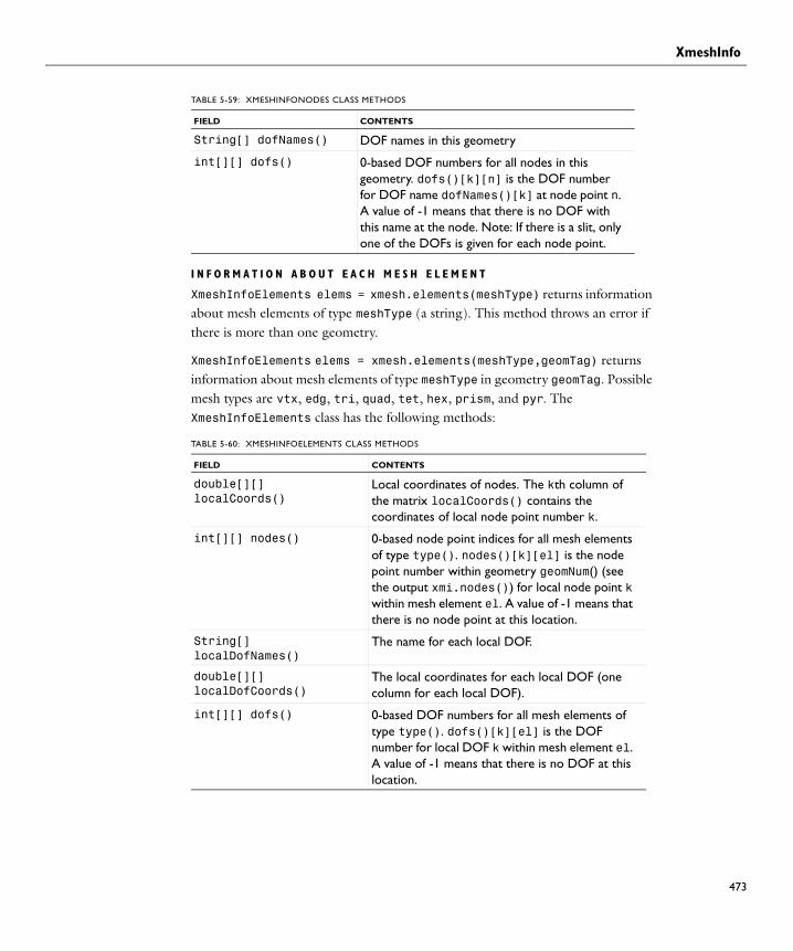
XmeshInfo
I N F O R M A T I O N A B O U T E A C H M E S H E L E M E N T
XmeshInfoElements elems = xmesh.elements(meshType) returns information about mesh elements of type meshType (a string). This method throws an error if there is more than one geometry.
XmeshInfoElements elems = xmesh.elements(meshType,geomTag) returns information about mesh elements of type meshType in geometry geomTag. Possible mesh types are vtx, edg, tri, quad, tet, hex, prism, and pyr. The XmeshInfoElements class has the following methods:
String[] dofNames() DOF names in this geometry
int[][] dofs() 0-based DOF numbers for all nodes in this geometry. dofs()[k][n] is the DOF number for DOF name dofNames()[k] at node point n. A value of -1 means that there is no DOF with this name at the node. Note: If there is a slit, only one of the DOFs is given for each node point.
TABLE 5-60: XMESHINFOELEMENTS CLASS METHODS
FIELD CONTENTS
double[][] localCoords()
Local coordinates of nodes. The kth column of the matrix localCoords() contains the coordinates of local node point number k.
int[][] nodes() 0-based node point indices for all mesh elements of type type(). nodes()[k][el] is the node point number within geometry geomNum() (see the output xmi.nodes()) for local node point k within mesh element el. A value of -1 means that there is no node point at this location.
String[] localDofNames()
The name for each local DOF.
double[][] localDofCoords()
The local coordinates for each local DOF (one column for each local DOF).
int[][] dofs() 0-based DOF numbers for all mesh elements of type type(). dofs()[k][el] is the DOF number for local DOF k within mesh element el. A value of -1 means that there is no DOF at this location.
TABLE 5-59: XMESHINFONODES CLASS METHODS
FIELD CONTENTS
473

XmeshInfo
474 | C H A P T
E R 5 : S O L V E R
6
R e s u l t s
Detailed COMSOL Java API reference information is included for the result features and utility methods.
In this chapter:
• About Results Commands
• Use of Data Sets
• Extracting Data
• Solution Selection
475

476 | C H A P T E
Abou t R e s u l t s C ommand s
The following list includes the available commands for results evaluation and visualization:
• Animation
• ArrowVolume, ArrowSurface, ArrowLine
• AvVolume, AvSurface, AvLine
• Average, Integral, Maximum, Minimum
• Color
• Contour
• Contour (data set)
• CoordSysLine, CoordSysSurface, CoordSysVolume
• CutLine2D, CutLine3D
• CutPlane
• CutPoint1D, CutPoint2D, CutPoint3D
• Data
• Deform
• Edge2D, Edge3D
• Eval
• EvalGlobal
• EvalGlobalMatrix
• EvalPoint
• FarField
• Filter
• Function1D, Function2D, Function3D
• Global (numerical)
• Global (plot)
• Height
• Histogram
• HistogramHeight
R 6 : R E S U L T S

• Image1D, Image2D, Image3D
• Interp
• IntVolume, IntSurface, IntLine
• Isosurface
• Isosurface (data set)
• Join
• Line
• LineGraph
• MaxMinVolume, MaxMinSurface, MaxMinLine
• MaxVolume, MaxSurface, MaxLine, MinVolume, MinSurface, MinLine
• Mesh
• Mesh (data set)
• Mesh (export)
• Mirror2D, Mirror3D
• Multislice
• Nyquist
• Parametric
• ParCurve2D, ParCurve3D
• ParSurface
• Particle
• Particle (evaluation)
• ParticleMass
• Player
• Plot
• PlotGroup1D, PlotGroup2D, PlotGroup3D
• PointGraph
• PolarGroup
• PrincipalSurface, PrincipalVolume
• Revolve1D, Revolve2D
• ScatterVolume, ScatterSurface
• Sector2D, Sector3D
A B O U T R E S U L T S C O M M A N D S | 477

478 | C H A P T E
• Slice
• Solution
• Streamline
• Surface
• Surface (data set)
• Table
• Table (plot)
• TableHeight
• TableSurface
• Volume
R 6 : R E S U L T S

Commands Grouped by Function
A T T R I B U T E S
D A T A S E T S
FUNCTION PURPOSE
Color Color expression
Deform Deformation
Filter Filter
Height Height
HistogramHeight Height for histogram plots
TableHeight Height for table plots
FUNCTION PURPOSE
Average, Integral, Maximum, Minimum Evaluation data sets
Contour (data set) Contour data set
CutLine2D, CutLine3D Cut line data sets
CutPlane Cut plane data set
CutPoint1D, CutPoint2D, CutPoint3D Cut point data sets
Edge2D, Edge3D Edge data sets.
Function1D, Function2D, Function3D Function data set
Isosurface (data set) Isosurface data set
Join Join data set
Mesh (data set) Mesh data set
Mirror2D, Mirror3D Mirror data set
Parametric Extends another data set by using a parameter as dimension
ParCurve2D, ParCurve3D Parameterized curve data set
ParSurface Parameterized face data set
Revolve1D, Revolve2D Revolution data set
Sector2D, Sector3D Sector symmetry data set
Solution Solution data set
Surface (data set) Surface data set
A B O U T R E S U L T S C O M M A N D S | 479

480 | C H A P T E
E X P O R T F E A T U R E S
N U M E R I C A L R E S U L T S
P L O T S
FUNCTION PURPOSE
Animation Animation export
Data Data export from data sets
Mesh (export) Mesh export from data sets
Image1D, Image2D, Image3D Image export
Player Animation player
Plot Plot export
FUNCTION PURPOSE
AvVolume, AvSurface, AvLine Average
Eval Generic evaluation
EvalGlobal Global evaluation
EvalGlobalMatrix Global matrix evaluation
EvalPoint Evaluation in points
Global (numerical) Generic evaluation
Interp Interpolation
IntVolume, IntSurface, IntLine Integration
MaxVolume, MaxSurface, MaxLine, MinVolume, MinSurface, MinLine
Maximum and minimum
Particle (evaluation) Evaluation on particle trajectories
FUNCTION PURPOSE
ArrowVolume, ArrowSurface, ArrowLine Arrow plots
Contour Contour plot
CoordSysLine, CoordSysSurface, CoordSysVolume Coordinate system plot
FarField Far-field plot
Global (plot) Global plot
Histogram Histogram plot
R 6 : R E S U L T S

TA B L E S
Isosurface Isosurface plot
Line Line plot
LineGraph Line graph plot
MaxMinVolume, MaxMinSurface, MaxMinLine Max/min marker plots
Mesh Mesh plot
Multislice Multislice plot
Nyquist Nyquist plot.
Particle Massless particle tracing plot
ParticleMass Particle tracing plot with mass
PointGraph Point graph plot
PrincipalSurface, PrincipalVolume Principal stress/strain plots
ScatterVolume, ScatterSurface Scatter plot
Slice Slice plot
Streamline Streamline plot
Surface Surface plot
Table (plot) Table plot
TableSurface Table surface plot
Volume Volume plot
FUNCTION PURPOSE
FUNCTION PURPOSE
Table Table containing real and imaginary data.
• Results Analysis and Plots in the COMSOL Multiphysics Reference Guide
• Results Evaluation and Visualization in the COMSOL Multiphysics User’s Guide
See Also
A B O U T R E S U L T S C O M M A N D S | 481

482 | C H A P T E
U s e o f Da t a S e t s
Table 6-1 shows applicability of data set output as data sets input. Rows correspond to data set output and columns to data set input. Check marks appear if the row data set output is accepted by the column data set. Evaluation indicates Average, Integral, Maximum, and Minimum data sets
TABLE 6-1: DATA SET INPUT VERSUS OUTPUT
DATA SETS
output versus input
CO
NT
OU
R
CU
TL
INE
2D
CU
TL
INE
3D
CU
TP
LA
NE
CU
TPO
INT
1D
CU
TPO
INT
2D
CU
TPO
INT
3D
EV
AL
UA
TIO
N
ISO
SU
RF
AC
E
JOIN
ME
SH
PA
RC
UR
VE
2D
PA
RC
UR
VE
3D
PA
RF
AC
E
RE
VO
LV
E1D
RE
VO
LV
E2D
SO
LU
TIO
N
Contour
CutLine2D
CutLine3D
CutPlane
CutPoint1D
CutPoint2D
CutPoint3D
Edge2D
Edge3D
Evaluation
Isosurface
Join
Mesh
ParCurve2D
ParCurve3D
ParFace
Revolve1D
Revolve2D
Sector2D
Sector3D
Solution
Surface
R 6 : R E S U L T S

Table 6-2 shows applicability of data set output as input to plot features. Rows correspond to data set output and columns to plot features. Checks appear if the data set output is accepted by the plot feature.
TABLE 6-2: DATA SET OUTPUT AS INPUT TO PLOT FEATURES
DATA SET OUTPUT
versus
AR
RO
W
CO
NT
OU
R
FAR
FIE
LD
GL
OB
AL
ISO
SU
RF
AC
E
LIN
E
LIN
EG
RA
PH
ME
SH
MU
LT
ISL
ICE
PA
RT
ICL
ET
RA
CIN
G
POIN
TG
RA
PH
SC
AT
TE
R
SL
ICE
ST
RE
AM
LIN
E
SU
RF
AC
E
VO
LU
ME
Contour
CutLine2D
CutLine3D
CutPlane
CutPoint1D
CutPoint2D
CutPoint3D
Edge2D
Edge3D
Evaluation
Isosurface
Join
Mesh
ParCurve2D
ParCurve3D v
ParSurface
Revolve1D
Revolve2D
Sector2D
Sector3D
Solution
Surface
U S E O F D A T A S E T S | 483

484 | C H A P T E
Ex t r a c t i n g Da t a
This section describes how to retrieve results or plot data directly through the Java API.
• Retrieving Plot Data
• Retrieving Numerical Results
Retrieving Plot Data
Each plot is made up of one or more groups or parts. Most plots contain only one group, such as Surface or Line plots, whereas for example Slice plots contain one group per slice. Retrieve the number of groups with the method
plot.getGroups(<renderIndex>)
where plot is any plot feature.
Retrieving the groups requires that you specify a render index for which you want the number of groups. Each plot is made up of one or more internal, or rendering, plot types. For example, particle tracing can contain both lines and spheres, which are separate rendering types. Most plot have only a single rendering type, in which case you can safely use 0 as the render index.
Extract the data contained in any plot feature using the following methods:
p = plot.getVertices(<renderIndex>, <groupIndex>) returns a float matrix containing one row for each dimension and one column for each vertex.
t = getElements(<renderIndex>, <groupIndex>) returns the indices to columns in p of a simplex mesh, each column in t representing a simplex.
d = getData(<renderIndex>, <groupIndex>, <dataType>) returns a float array containing the data for each point in p. The type of data to retrieve is given by the String <dataType>:"Color", "Height", and so forth.
To retrieve the available data types, use:
types = getDataTypes(<renderIndex>)
which returns a string array with the data types currently present in the plot.
R 6 : R E S U L T S

E X A M P L E
int renderDataGroups = plot.getRenderGroups();
for (int ri = 0; ri < renderDataGroups; ri++) {
String[] dataTypes = plot.getDataTypes(ri); int plotDataGroups = plot.getGroups(ri); for (int gi = 0; gi < plotDataGroups; gi++) { p = plot.getVertices(ri,gi); t = plot.getElements(ri,gi); //d = plot.getData(ri, gi, "Color"); d = plot.getData(ri, gi, dataTypes[0]); }}
Retrieving Numerical Results
It is possible to retrieve numerical results from any numerical feature, but there are a number of features especially designed for the Java API that are not present in the COMSOL Multiphysics GUI. These functions support multiple expressions, as well as some additional advanced properties, and a more convenient way to extract interpolated data. These two groups have slightly different access methods.
A P I - O N L Y N U M E R I C A L F E A T U R E S
result = model.result().numerical(<ftag>).getData() returns the real part of the result, recomputing the feature if necessary. result is a three-dimensional double matrix ordered result[expression][solnum][coordinates].
model.result().numerical(<ftag>).getData(<expressionIndex>) returns the real part of the result for one expression, equivalent to result[expressionIndex].
result = model.result().numerical(<ftag>).getImagData() returns the imaginary part of the result, recomputing the feature if necessary. result is a three-dimensional double matrix ordered result[expression][solnum][coordinates].
TABLE 6-3: API-ONLY NUMERICAL FEATURE
FUNCTION PURPOSE
Eval Generic evaluation
Global (numerical) Generic evaluation
Interp Interpolation
E X T R A C T I N G D A T A | 485

486 | C H A P T E
model.result().numerical(<ftag>).getImagData(<expressionIndex>) returns the imaginary part of the result for one expression, equivalent to result[expressionIndex].
model.result().numerical(<ftag>).isComplex() returns true if the result is complex. For models with outer solutions, isComplex() returns true if the result for the current value of outersolnum is complex.
model.result().numerical(<ftag>).isComplex(<outersolnum>) returns true if the result is complex for the given outer solution.
model.result().numerical(<ftag>).getNData() returns the number of data vectors in the result.
model.result().numerical(<ftag>).getCoordinates() returns the coordinates of the evaluation or interpolation.
model.result().numerical(<ftag>).getElements() returns indices to columns in p of a simplex mesh.
model.result().numerical(<ftag>).getVertexElements() returns indices to mesh elements for each point.
More details can be found in the documentation for each feature type.
S T A N D A R D N U M E R I C A L F E A T U R E S
model.result().numerical(<ftag>).getReal() returns the real result, recomputing the feature if necessary. Data is ordered such that one row contains data for all solution numbers. This is identical to (<columnwise>) when <columnwise> is false. If <columnwise> is true, the ordering is the opposite: each column contains the values for all solution numbers.
model.result().numerical(<ftag>).getImag(<allocate>, <columnwise>) returns the imaginary part of complex result, recomputing the feature if necessary. If
TABLE 6-4: STANDARD NUMERICAL FEATURES, ALSO PRESENT IN THE COMSOL MULTIPHYSICS GUI
FUNCTION PURPOSE
EvalGlobal Global evaluation
EvalPoint Evaluation in points
IntVolume, IntSurface, IntLine
Integration
R 6 : R E S U L T S

<allocate> is true, a zero-valued matrix is allocated even when the result is real. getImag() uses <allocate> true and <columnwise> false.
model.result().numerical(<ftag>).isComplex() returns true if the result is complex. For models with outer solutions, isComplex() returns true if the result is complex for any of the currently set outersolnum.
model.result().numerical(<ftag>).isComplex(<outersolnum>) returns true if the result is complex for the given outer solution.
More details can be found in the documentation for each feature type.
487

488 | C H A P T E
S o l u t i o n S e l e c t i o n
In this section:
• About Selecting Solutions
• Selecting Solutions by Solution Number
• Selecting Solutions by Solution Level
• Choosing Solution Selection Method
About Selecting Solutions
During the solution of, for example, time-dependent models or parametric sweep models, more than one solution is generated, and in order to do relevant postprocessing the correct set of solutions needs to be selected among them. How many solutions the result features can display vary, the main difference being between single-select and multi-select features. Single solution selection is available when only one solution at a time can be visualized, for example in 2D and 3D plots. In numerical features and 1D plots multi-select is used to be able to display plots relating to more than one parameter value at a time.
There are two ways to select solutions:
• by solution number
• by solution level
COMSOL keeps them synchronized as far as possible.
Selecting solutions by solution number is a method that is tightly linked to the solution representation used by the solvers. The solution level method is structurally similar to the set up of the studies. Setting any one property belonging to either method triggers a synchronisation in which all properties of that method are mapped to those of the other method. Mapping to the solution number method will always work, since that case is the more general. If, on the other hand, mapping to the solution level method fails, its properties are set to their default settings.
The solrepresentation property is set to "solnum" automatically if the solution number method is the only one able to represent the selection made. On solving it is set to "solutioninfo" if the solution level method can be used to represent the
R 6 : R E S U L T S

previous selection. The solutionrepresentation property also decides which method is visible in the GUI.
Selecting Solutions by Solution Number
In the solution number method, the solutions are selected as a collection of inner and outer solutions. Inner solutions are generated by the solvers in one step. Outer solutions are generated by parametric sweeps wrapping the inner solutions. If there are more than one inner or outer parameter, they will be represented and selected as tuples, that is, combinations of values of the different parameters. Depending on the setup of the studies the parameters can be either filled (all combinations) or sparse (a selection of combinations). In the single-selection case the properties used are solnum, t and outersolnum. In the multi-selection case the valid properties are innerinput, solnum, solnumindices, t, outerinput, outersolnum, and outerindices.
Selecting Solutions by Solution Level
In contrast, the solution level method handles all filled parameters, that is, parameters defined individually in the studies, in one level each, up to a maximum of three levels. If more levels than that exist in the study the outermost levels are combined in the third level. Parameters that together form sparse tuples in the studies are always presented on the same level. In the single-selection case the properties used are looplevel and interp. In the multi-selection case the valid properties are looplevelinput, looplevel, looplevelindices, and interp.
Choosing Solution Selection Method
Whether selection is made using the solution level method or the solution number method, the ways of selecting solutions are the same. In the single-selection case, solutions are selected by parameter index or, if the solution is time dependent, by value. In the multiselection case there are a number of selection input options all, first, last, by index from existing values, by manual indices, or, in time-dependent cases, by time.
Which method to use is not self-evident. The solution level method is perhaps the more intuitive of the two because it attempts to treat each individual level separately. The solution number method, however, is more general, and can pin-point which tuples to use with more precision. The recommendation is to use the solution level
S O L U T I O N S E L E C T I O N | 489

490 | C H A P T E
method wherever possible, and resort to the solution number method only if its special characteristics are needed.
R 6 : R E S U L T S

Animation
AnimationSynopsis Animate plots.
Syntax model.result().export().create(<ftag>,"Animation");model.result().export(<ftag>).set(property, <value>);model.result().export(<ftag>).run();
Description model.result().export().create(<ftag>,"Animation") creates an animation feature with the name <ftag>.
result().export(<ftag>).set("plotgroup", <ptag>) changes the source of the animation to the plot group named <ptag>.
The following properties are available:
TABLE 6-5: VALID PROPERTY/VALUE PAIRS
PROPERTY VALUE DEFAULT DESCRIPTION
antialias on | off on Enable/disable antialiasing.
avifilename string The name of the AVI file produced if movietype is avi.
aviqual double in [0,1]
0.75 The quality of the AVI file if movietype is avi; higher is better.
axes on | off on If options is on; enable/disable display of the coordinate axes. Used for 1D and 2D animations.
axisorientation on | off on If options is on; enable/disable display of the axis orientation indicator. Used for 3D animations.
background current | color
color The background color.
bmpfilename string The name of the output file if imagetype is bmp.
customcolor double array {1, 1, 1} If background is color; the red, green, and blue components of the background color.
cycletype fullharm | halfharm | linear
fullharm The transformation of the solution that is performed if sweeptype is dde.
flashfilename string The name of the Flash file produced if movietype is flash.
flashinterp on | off on Enable/disable interpolation between frames in the generated Flash file if movietype is flash.
flashopen on | off off Enable/disable opening of the generated Flash file in a browser if movietype is flash.
fontsize integer 9 The font size.
491

Animation
492 | C H A P T
fps positive integer
10 The number of frames per second.
giffilename string The name of the GIF file produced if movietype is gif.
gifopen on | off off Enable/disable opening of the generated GIF file in a browser if movietype is gif.
grid on | off on If options is on; enable/disable display of the coordinate grid. Used for 3D animations.
height integer 480 The height in pixels of the frames of the animation.
imagefilename string The base name of generated images if type is movieseq; the generated images have names of the form base1.ext, base2.ext, ...
legend on | off on If options is on; enable/disable display of the legend.
logo on | off on If options is on; enable/disable display of the logotype.
movietype gif | flash | avi
gif The movie format to use if type is movie.
options on | off off Enable/disable optional components of the image.
outerinnertype first | last | all
last When solnumtype is outer, outerinnertype controls whether to plot all, the first or the last inner solution. Applicable only for parametric sweep models.
outersolnumarray non-negative integer array
1 The index of the outer solutions to use. Applicable only for parametric sweep models when solnumtype is outer.
outersolnumsingle
non-negative integer
1 The index of the outer solutions to use. Applicable only for parametric sweep models when solnumtype is inner.
parameter string The model parameter that varies if sweeptype is parameter.
pframes positive integer
11 The number of frames if sweeptype is parameter.
plotgroup string The name of the plot group to animate.
pstart double 0 The start parameter if sweeptype is parameter.
TABLE 6-5: VALID PROPERTY/VALUE PAIRS
PROPERTY VALUE DEFAULT DESCRIPTION
E R 6 : R E S U L T S

Animation
Example Create a 2D animation of a surface and contour plot:
model.result().export().create("c2","pg1","Animation");model.result().export(“c2”).set(“plotgroup”, “pg1”);
Create animation:
model.result().export("c2").run();
See Also Image1D, Image2D, Image3D
pstop double 1 The stop parameter if sweeptype is parameter.
resolution integer 96 The frame resolution in dots per inch.
reverse on | off off Enable/disable reversal in time of the animation.
solnumtype inner | outer
inner Whether to sweep over inner or outer solutions in a parametric sweep model.
solnum integer array
all The solutions to animate if sweeptype is solutions
staticframes positive integer
11 The number of frames if sweeptype is dde.
sweeptype solutions | parameter | dde
solutions The parameter that varies during animation.
timeinterp on | off off Enable/disable sweep over interpolated times if sweeptype is solutions.
tint double array The interpolated times to animate if timeinterp is on.
title on | off on If options is on; enable/disable display of the title.
type imageseq | movie
movie The kind of output that is produced.
width integer 640 The width in pixels of the frames of the animation.
TABLE 6-5: VALID PROPERTY/VALUE PAIRS
PROPERTY VALUE DEFAULT DESCRIPTION
493

ArrowVolume, ArrowSurface, ArrowLine
494 | C H A P T
ArrowVolume, ArrowSurface, ArrowLineSynopsis Arrow plots.
Syntax model.result(<pgtag>).feature().create(<ftag>,"ArrowVolume");model.result(<pgtag>).feature().create(<ftag>,"ArrowSurface");model.result(<pgtag>).feature().create(<ftag>,"ArrowLine");model.result(<pgtag>).feature(<ftag>).set(property, <value>);model.result(<pgtag>).feature(<ftag>).run();
Description model.result(<pgtag>).feature().create(<ftag>,"Arrow...") creates an arrow plot feature named <ftag>.
Arrow plots are available in 2D and 3D. ArrowLine plots arrows on lines in 2D or 3D such as geometry boundaries in 2D or cut plane edges in 3D. ArrowSurface plots arrows on surfaces in 2D or 3D. ArrowVolume plots arrows in a 3D volume.
The following properties are available:
TABLE 6-6: VALID PROPERTY/VALUE PAIRS
PROPERTY VALUE DEFAULT DESCRIPTION
arrowcount positive integer 200 If placement is uniform: The approximate number of arrows. Available for ArrowEdge in 2D and 3D and for ArrowSurface in 3D.
arrowlength normalized | proportional | logarithmic
proportional The arrow scaling: Proportional uses the actual arrow length, normalized a unit length, and logarithmic a length proportional to the logarithm of the arrow length.
arrowtype arrow | cone arrow The type of arrow to draw.
arrowxmethod number | coord
number Indicates whether the x-coordinates of the arrows should be specified by number of points to distribute evenly across the data or by coordinates. Available for ArrowSurface in 2D and ArrowVolume in 3D.
arrowymethod number | coord
number Indicates whether the y-coordinates of the arrows should be specified by number of points to distribute evenly across the data or by coordinates. Available for ArrowSurface in 2D and ArrowVolume in 3D.
arrowzmethod number | coord
number Indicates whether the z-coordinates of the arrows should be specified by number of points to distribute evenly across the data or by coordinates. Available for ArrowVolume in 3D.
E R 6 : R E S U L T S

ArrowVolume, ArrowSurface, ArrowLine
color custom | black | blue | cyan | green | magenta | red | white | yellow
red The color to use.
const String array of property/value pairs
Empty Parameters to use in the expressions.
customcolor RGB-triplet {1,0,0} or last used color.
The uniform color to use. Active when color is set to custom.
data none | parent | data set name
parent The data set this feature refers to.
descr string Model-dependent
The description of the expressions in expr. Is used in the automatic title.
descriptionintitle
on | off on Whether the title contribution should contain the description when titletype is custom.
differential on | off on Whether the expression should be linearized at the linearization point. Applicable only if evalmethod is harmonic
evalmethod linpoint | harmonic | lintotal | lintotalavg | lintotalrms | lintotalpeak
harmonic Applicable only for solutions with a stored linearization point. Controls if the linearization point, the perturbation, or a combination should be used when evaluating the expression.
expr string array of length 2 in 2D and 3 in 3D
Mode-dependent The components to plot.
inheritarrowscale
boolean true If inheritplot is not none: Determines if arrow scale is inherited.
inheritcolor boolean true If inheritplot is not none: Determines if the color is inherited.
inheritplot none | plot name
none The plot that arrow scale, color, and deformation scale is inherited from.
TABLE 6-6: VALID PROPERTY/VALUE PAIRS
PROPERTY VALUE DEFAULT DESCRIPTION
495

ArrowVolume, ArrowSurface, ArrowLine
496 | C H A P T
interp double array Time corresponding to last selected solnum for transient levels.
The time to use, for transient levels. Available when data is not parent and the underlying data is transient.
logrange double > 1 100 If arrowlength is logarithmic: The ratio between the maximum arrow length and the arrow length below which no arrow is drawn.
looplevel array of non-negative integers and strings
Last solution for transient or parametric solution for each level. Otherwise first solution for each level.
The index of the solution to use, per level, or interp, but only for transient solutions. Available when data is not parent and the underlying data has multiple solutions.
outersolnum non-negative integer
1 The index of the outer solutions to use. Applicable only for parametric sweep models.
placement| elements | uniform | uniformanis
uniform If uniform, then the arrows are distributed uniformly. If uniformanisotropic, then the arrows are distributed uniformly with weights taken from the weight property. If elements, then arrows are drawn in each element. Available for ArrowEdge in 2D and 3D and for ArrowSurface in 3D.
prefixintitle
string Empty Added prefix to contribution to title.
scale positive double 1 If scaleactive is true: The length scale factor.
scaleactive boolean false Whether to use manual scaling.
solnum non-negative integer
Last solution for transient or parametric solution. Otherwise first solution.
The index of the solution to use. Available when data is not parent and the underlying data has multiple solutions.
solrepresentation
solnum | solutioninfo
solutioninfo Indicates which method of selecting solutions is active.
suffixintitle
string Empty Added suffix to contribution to title.
TABLE 6-6: VALID PROPERTY/VALUE PAIRS
PROPERTY VALUE DEFAULT DESCRIPTION
E R 6 : R E S U L T S

ArrowVolume, ArrowSurface, ArrowLine
Attributes Color, Deform, Filter
See Also Line, ScatterVolume, ScatterSurface, Surface, Volume
t double Time corresponding to last selected solnum.
The time to use, for transient problems. Available when data is not parent and the underlying data is transient.
timeinterp on | off off on if t is used to determine time steps, off if solnum is used.
title string The auto-title. The title to use when titletype is manual.
titletype auto | custom | manual | none
auto auto if the title contribution should be computed automatically, possibly using the group’s customization. custom if the title contribution should be computed automatically, but customized. manual if the manual title contribution should be used (the title property). none if no title contribution should be used.
typeintitle on | off on Whether the title contribution should contain the type when titletype is custom.
weight double array 1 If placement is uniformani: The weights given to the different axis directions.
xnumber non-negative integer
15 (3D), 7 (2D) Number of points in the x-direction. Active when arrowxmethod is set to number. Available for ArrowSurface in 2D and ArrowVolume in 3D.
xcoord double array Empty Absolute coordinates in the x-direction, active when arrowxmethod is set to coord. Available for ArrowSurface in 2D and ArrowVolume in 3D.
ynumber integer 15 (3D), 7 (2D) Number of points in the y-direction. Active when arrowymethod is set to number. Available for ArrowSurface in 2D and ArrowVolume in 3D.
ycoord double array Empty Absolute coordinates in the z-direction, active when arrowymethod is set to coord. Available for ArrowSurface in 2D and ArrowVolume in 3D.
znumber integer 15 (3D), 7 (2D) Number of points in the z-direction. Active when arrowzmethod is set to number. Available for ArrowVolume in 3D.
zcoord double array Empty Absolute coordinates in the z-direction, active when arrowzmethod is set to coord. Available for ArrowVolume in 3D.
TABLE 6-6: VALID PROPERTY/VALUE PAIRS
PROPERTY VALUE DEFAULT DESCRIPTION
497

AvVolume, AvSurface, AvLine
498 | C H A P T
AvVolume, AvSurface, AvLineSynopsis Averaging.
Syntax model.result().numerical().create(<ftag>,"AvVolume");model.result().numerical().create(<ftag>,"AvSurface");model.result().numerical().create(<ftag>,"AvLine");model.result().numerical(<ftag>).selection(...);model.result().numerical(<ftag>).set(property, <value>);model.result().numerical(<ftag>).getReal();model.result().numerical(<ftag>).getReal(<columnwise>);model.result().numerical(<ftag>).getReal(<outersolnum>);model.result().numerical(<ftag>).getReal(<columnwise>,
<outersolnum>);model.result().numerical(<ftag>).getImag();model.result().numerical(<ftag>).getImag(<allocate>,
<columnwise>);model.result().numerical(<ftag>).getImag(<outersolnum>);model.result().numerical(<ftag>).getImag(<allocate>, <columnwise>,
<outersolnum>);model.result().numerical(<ftag>).isComplex();model.result().numerical(<ftag>).isComplex(<outersolnum>);model.result().numerical(<ftag>).setResult();model.result().numerical(<ftag>).appendResult();
Description model.result().numerical().create(<ftag>,"AvVolume") creates a volume average feature with the name <ftag>.
model.result().numerical().create(<ftag>,"AvSurface") creates a surface average feature with the name <ftag>.
model.result().numerical().create(<ftag>,"AvLine") creates a line average feature with the name <ftag>.
model.result().numerical(<ftag>).getReal() returns the real result, recomputing the feature if necessary. Data is ordered such that one row contains data for all solution numbers. This is identical to (columnwise) when columnwise is false. If columnwise is true, the ordering is the opposite: each column contains the values for all solution numbers.
model.result().numerical(<ftag>).getImag(allocate, columnwise) returns the imaginary part of complex result, recomputing the feature if necessary. If allocate is true, a zero-valued matrix is allocated even when the result is real. getImag() uses allocate true and columnwise false.
model.result().numerical(<ftag>).isComplex() returns true if the result is complex.
E R 6 : R E S U L T S

AvVolume, AvSurface, AvLine
<outersolnum> is applicable only for parametric sweep solutions and is the index of each outer parametric solution.
model.result().numerical(<ftag>).setResult() and model.result().numerical(<ftag>).appendResult() evaluates the feature and set or append the result in the table indicated by the table property.
The following properties are available:
TABLE 6-7: VALID PROPERTY/VALUE PAIRS
NAME VALUE DEFAULT DESCRIPTION
data none | data set name
First compatible data set
The data set this feature refers to.
dataseries average | integral | maximum | minimum | none | rms | stddev | variance
none The operation that is applied to the data series formed by the evaluation.
const String array of property/value pairs
Empty Parameters to use in the expressions.
descr string Model-dependent The description of the expression in expr. Is used in the automatic title.
differential on | off on Whether the expression should be linearized at the linearization point. Applicable only if evalmethod is harmonic
evalmethod linpoint | harmonic | lintotal | lintotalavg | lintotalrms | lintotalpeak
harmonic Applicable only for solutions with a stored linearization point. Controls if the linearization point, the perturbation, or a combination should be used when evaluating the expression.
expr string Model-dependent The expression to plot.
innerinput all | first | last | manual | manualindices | interp
all How to input the solution to use. manual indicates that solnum is used. manualindices indicates that solnumindices is used. interp indicates that t is used.
499

AvVolume, AvSurface, AvLine
500 | C H A P T
interp double row matrix
Empty on all levels.
The times to use, for transient levels. Available when data is not parent and the underlying data is transient.
intorder positive integer
4 The integration order.
intorderactive on | off off Whether to use manually specified integration order.
intsurface on | off off Compute surface integral. Available for line integration features of axisymmetric models.
intvolume on | off off Compute volume integral. Available for surface integration features of axisymmetric models.
looplevel integer row matrix
All solutions on all levels
The solutions to use, per level.
looplevelindices
integer row matrix
Empty An alternate way to specify the solutions to use, allowing you to enter, for example, range(1,1,20). Applicable when looplevelinput is manualindices on a level.
looplevelinput String array with all | first | last | manual | manualindices | interp on each level
all on all levels How to input the solution to use, per level. manual on a level indicates that looplevel is used on that level. manualindices on a level indicates that looplevelindices is used on that level. interp on a level indicates that interp is used on that level.
maximumobj abs | real real The value being maximized if dataseries is maximum.
method auto | integration | summation
auto The integration method.
minimumobj abs | real real The value being minimized if dataseries is minimum.
outerinput all | first | last | manual | manualindices
all How to input the outer solutions to use. Applicable only for parametric sweep models. manual indicates that outersolnum is used. manualindices indicates that outersolnumindices is used.
outersolnum non-negative integer array
1 The index of the outer solutions to use. Applicable only for parametric sweep models. Since the various outer solutions can have different number of solnum, the solnum property is not used.
TABLE 6-7: VALID PROPERTY/VALUE PAIRS
NAME VALUE DEFAULT DESCRIPTION
E R 6 : R E S U L T S

AvVolume, AvSurface, AvLine
See Also IntVolume, IntSurface, IntLine
outersolnumindices
string or integer array
Empty An alternate way to specify the outer solutions to use, allowing you to enter, for example, range(1,1,20). Applicable when outerinput is manualindices.
solnum non-negative integer array
All solutions The solutions to use.
solnumindices string or integer array
Empty An alternate way to specify the solutions to use, allowing you to enter, for example, range(1,1,20). Applicable when innerinput is manualindices.
solrepresentation
solnum | solutioninfo
solutioninfo Indicates which method of selecting solutions is active.
t double array Empty The times to use. Available when the underlying solution is transient.
table new | table name
new The table to use when calling setResult() or appendResult(). new indicates that a new table is created.
tablecols inner | outer | data | level1
data Whether to use inner or outer solutions as columns in the table when calling setResult() or appendResult(). Applicable only for parametric sweep models. The level values (level1, level2, and so on) are the levels in the parametric sweep.
timeinterp on | off off on if t is used to determine time steps, off if solnum is used.
unit string Model-dependent The unit to use for the expression in expr. If the old unit is not valid when the expression changes, the unit property is reset to default.
TABLE 6-7: VALID PROPERTY/VALUE PAIRS
NAME VALUE DEFAULT DESCRIPTION
501

Average, Integral, Maximum, Minimum
502 | C H A P T
Average, Integral, Maximum, MinimumPurpose Evaluation data sets.
Syntax model.result().dataset().create(<dtag>,"Average");model.result().dataset().create(<dtag>,"Integral");model.result().dataset().create(<dtag>,"Maximum");model.result().dataset().create(<dtag>,"Minimum");model.result().dataset(<dtag>).set(property, <value>);model.result().dataset(<dtag>).selection(...);
Description model.result().dataset().create(<dtag>,"Average") creates a data set named <dtag> that computes the average of another data set.
model.result().dataset().create(<dtag>,"Integral") creates a data set named <dtag> that computes the average of another data set.
model.result().dataset().create(<dtag>,"Maximum") creates a data set named <dtag> that computes the maximum of another data set.
model.result().dataset().create(<dtag>,"Minimum") creates a data set named <dtag> that computes the minimum of another data set.
The following properties are available:
TABLE 6-8: COMMON PROPERTY/VALUE PAIRS
PROPERTY VALUE DEFAULT DESCRIPTION
name String None The name of this feature
data None | data set name
First compatible data set
The data set this feature refers to.
level fromdataset | volume | surface | edge | point
fromdataset The element dimension; if fromdataset, then the highest dimension supported by the data set is used.
descr string Model-dependent.
The description of the expression in expr. Is used in the automatic title.
differential on | off on Whether the expression should be linearized at the linearization point. Applicable only if evalmethod is harmonic
E R 6 : R E S U L T S

Average, Integral, Maximum, Minimum
The following properties are available:
evalmethod linpoint | harmonic | lintotal | lintotalavg | lintotalrms | lintotalpeak
harmonic Applicable only for solutions with a stored linearization point. Controls if the linearization point, the perturbation, or a combination should be used when evaluating the expression.
expr string Model-dependent.
The expression to plot.
TABLE 6-8: COMMON PROPERTY/VALUE PAIRS
PROPERTY VALUE DEFAULT DESCRIPTION
TABLE 6-9: ADDITIONAL PROPERTY/VALUE PAIRS FOR AVERAGE AND INTEGRAL
PROPERTY VALUE DEFAULT DESCRIPTION
intmethod auto | integration | summation
auto The integration method.
intorderactive on | off off Whether to use manually specified integration order.
intorder Positive integer
4 The manually set integration order.
503

Color
504 | C H A P T
ColorPurpose Color expression attribute.
Syntax model.result(<pgtag>).feature(<ftag>).feature().create(<atag>,"Color");
model.result(<pgtag>).feature(<ftag>).feature(<atag>).set(property, <value>);
Description model.result(<pgtag>).feature(<ftag>).feature().create(<atag>,
"Color") creates a color expression attribute named <atag> belonging to the plot feature <ftag>.
Use color expressions to add a coloring to the shapes defined by a plot. Color expressions can be added to surface plots, line plots, volume plots, arrow plots, contour plots, isosurface plots, particle tracing plots, and streamline plots.
The following properties are available:
TABLE 6-10: VALID PROPERTY/VALUE PAIRS
PROPERTY VALUE DEFAULT DESCRIPTION
color custom | black | blue | cyan | green | magenta | red | white | yellow
red The uniform color to use. Active when coloring is uniform.
coloring colortable | uniform
colortable How to color the parent plot.
colorlegend on | off on Whether to show color legend, when coloring is set to colortable.
colortable colortable name
Rainbow The color table to use when colormethod is set to colortable.
colortablerev on | off off Whether to reverse to color table when colormethod is set to colortable.
colortablesym on | off off Whether to symmetrize the color range around 0 when colormethod is set to colortable.
customcolor RGB-triplet {1,0,0} or last used color.
The uniform color to use. Active when color is set to custom.
descr string Model-dependent.
The description of the expression in expr. Is used in the automatic title.
descriptionintitle
on | off on Whether the title contribution should contain the description when titletype is custom.
E R 6 : R E S U L T S

Color
differential on | off on Whether the expression should be linearized at the linearization point. Applicable only if evalmethod is harmonic
evalmethod linpoint | harmonic | lintotal | lintotalavg | lintotalrms | lintotalpeak
harmonic Applicable only for solutions with a stored linearization point. Controls if the linearization point, the perturbation, or a combination should be used when evaluating the expression.
expr string Model-dependent.
The expression to plot.
expressionintitle
on | off off Whether the title contribution should contain the expression when titletype is custom.
prefixintitle string Empty Added prefix to contribution to title.
rangecoloractive on | off off Whether to use the manual color range specified in rangecolormin and rangecolormax. The color range specifies the minimum and maxim value in the plotted colors. Default is the minimum and maximum data values.
rangecolormax double Plot-dependent The maximum color range value. Active when rangecoloractive is on.
rangecolormin double Plot-dependent The minimum color range value. Active when rangecoloractive is on.
rangedatactive on | off off Whether to use the manual data range specified in rangedatamin and rangedatamax. Values outside the data range are not plotted.
rangedatamax double Plot-dependent The maximum data value. Active when rangedataactive is on.
rangedatamin double Plot-dependent The minimum data value. Active when rangedataactive is on.
suffixintitle string Empty Added suffix to contribution to title.
title string The auto-title. The title to use when titletype is manual.
titletype auto | custom | manual | none
auto auto if the title contribution should be computed automatically, possibly using the group’s customization. custom if the title contribution should be computed automatically, but customized. manual if the manual title contribution should be used (the title property). none if no title contribution should be used.
TABLE 6-10: VALID PROPERTY/VALUE PAIRS
PROPERTY VALUE DEFAULT DESCRIPTION
505

Color
506 | C H A P T
See Also Deform, Height, ArrowVolume, ArrowSurface, ArrowLine, Contour, Isosurface, Particle, ParticleMass, Streamline
typeintitle on | off on Whether the title contribution should contain the type when titletype is custom.
unit string Model-dependent
The unit to use for the expression in expr. If the old unit is not valid when the expression changes, the unit property is reset to default.
unitintitle on | off on Whether the title contribution should contain the unit when titletype is custom.
TABLE 6-10: VALID PROPERTY/VALUE PAIRS
PROPERTY VALUE DEFAULT DESCRIPTION
E R 6 : R E S U L T S

Contour
ContourSynopsis Contour plot.
Syntax model.result(<pgtag>).feature().create(<ftag>,"Contour");model.result(<pgtag>).feature(<ftag>).set(property, <value>);model.result(<pgtag>).feature(<ftag>).run();
Description model.result(<pgtag>).feature().create(<ftag>,"Contour") creates a contour plot feature named <ftag> belonging to the plot group <pgtag>. Contour plots are available in 2D and 3D plot groups. Contour lines are colored by their level. Add a color expression attribute to color them by an arbitrary expression.
The following properties are available:
TABLE 6-11: VALID PROPERTY/VALUE PAIRS
PROPERTY VALUE DEFAULT DESCRIPTION
color custom | black | blue | cyan | green | magenta | red | white | yellow
red The uniform color to use. Active when coloring is uniform.
coloring colortable | uniform
colortable How to color the contours.
colorlegend on | off on Whether to show color legend, when coloring is set to colortable.
colortable colortable name
Rainbow The color table to use when colormethod is set to colortable.
colortablerev on | off off Whether to reverse to color table when colormethod is set to colortable.
colortablesym on | off off Whether to symmetrize the color range around 0 when colormethod is set to colortable.
const String array of property/value pairs
Empty Parameters to use in the expressions.
contourlabels on | off off Whether to display labels next to the contour lines. Only applicable if contourtype is lines.
contourtype lines | filled
lines Whether to display lines for each level or a surface with bands of color.
customcolor RGB-triplet {1,0,0} or last used color.
The uniform color to use. Active when color is set to custom.
507

Contour
508 | C H A P T
customlabelcolor RGB-triplet {1,0,0} or last used color.
If contourlabels is on and labelcolor is custom: The label color to use.
data none | parent | data set name
parent The data set this feature refers to.
descr string Model-dependent.
The description of the expression in expr. Is used in the automatic title.
descriptionintitle
on | off on Whether the title contribution should contain the description when titletype is custom.
differential on | off on Whether the expression should be linearized at the linearization point. Applicable only if evalmethod is harmonic
evalmethod linpoint | harmonic | lintotal | lintotalavg | lintotalrms | lintotalpeak
harmonic Applicable only for solutions with a stored linearization point. Controls if the linearization point, the perturbation, or a combination should be used when evaluating the expression.
expr string Model-dependent.
The expression to plot.
expressionintitle
on | off off Whether the title contribution should contain the expression when titletype is custom.
inheritcolor boolean true If inheritplot is not none: Determines if the color is inherited.
inheritdeformscale
boolean true If inheritplot is not none: Determines if the deformation scale is inherited.
inheritplot none | plot name
none The plot that color and deformation scale is inherited from.
interp double array Time corresponding to last selected solnum for transient levels.
The time to use, for transient levels. Available when data is not parent and the underlying data is transient.
levelmethod number | levels
number How to specify contour levels.
TABLE 6-11: VALID PROPERTY/VALUE PAIRS
PROPERTY VALUE DEFAULT DESCRIPTION
E R 6 : R E S U L T S

Contour
labelcolor custom | black | blue | cyan | green | magenta | red | white | yellow
red If contourlabels is on: The label color to use.
labelprec positive integer If contourlabels is on: The number of significant digits in the labels.
levels double array The specific levels to plot. Active when levelmethod equals levels.
looplevel array of non-negative integers and strings
Last solution for transient or parametric solution for each level. Otherwise first solution for each level.
The index of the solution to use, per level, or interp, but only for transient solutions. Available when data is not parent and the underlying data has multiple solutions.
number positive integer
20 Total number of contour levels. Active when levelmethod equals number.
outersolnum non-negative integer
1 The index of the outer solutions to use. Applicable only for parametric sweep models.
prefixintitle string Empty Added prefix to contribution to title.
rangecoloractive on | off off Whether to use the manual color range specified in rangecolormin and rangecolormax. The color range specifies the minimum and maxim value in the plotted colors. Default is the minimum and maximum data values.
rangecolormax double Plot-dependent The maximum color range value. Active when rangecoloractive is on.
rangecolormin double Plot-dependent The minimum color range value. Active when rangecoloractive is on.
rangedatactive on | off off Whether to use the manual data range specified in rangedatamin and rangedatamax. Values outside the data range are not plotted.
rangedatamax double Plot-dependent The maximum data value. Active when rangedataactive is on.
TABLE 6-11: VALID PROPERTY/VALUE PAIRS
PROPERTY VALUE DEFAULT DESCRIPTION
509

Contour
510 | C H A P T
rangedatamin double Plot-dependent The minimum data value. Active when rangedataactive is on.
recover off | pprint | ppr
off The derivative recovery method.
refine non-negative integer
1 The element refinement to use, if resolution is set to manual. Bear in mind that this is the refinement used for the base data set, so the number of elements in the model can increase radically if the plot uses, for example, a revolve data set.
resolution norefine | coarse | normal | fine | finer | extrafine | custom
normal Controls the plot’s resolution. A finer setting results in a higher resolution by modifying the internally computed default refinement. Use custom to enter your own refinement in the refine property.
smooth none | internal | everywhere
internal Smoothing settings.
solnum Non-negative integer
Last solution for transient or parametric solution. Otherwise first solution.
The index of the solution to use. Available when data is not parent and the underlying data has multiple solutions.
solrepresentation
solnum | solutioninfo
solutioninfo
Indicates which method of selecting solutions is active.
suffixintitle string Empty Added suffix to contribution to title.
t double Time corresponding to last selected solnum.
The time to use, for transient problems. Available when data is not parent and the underlying data is transient.
timeinterp on | off off on if t is used to determine time steps, off if solnum is used.
title string The auto-title. The title to use when titletype is manual.
TABLE 6-11: VALID PROPERTY/VALUE PAIRS
PROPERTY VALUE DEFAULT DESCRIPTION
E R 6 : R E S U L T S

Contour
Attributes Color, Deform, Filter
See Also Contour (data set), Surface
titletype auto | custom | manual | none
auto auto if the title contribution should be computed automatically, possibly using the group’s customization. custom if the title contribution should be computed automatically, but customized. manual if the manual title contribution should be used (the title property). none if no title contribution should be used.
typeintitle on | off on Whether the title contribution should contain the type when titletype is custom.
unit string Model-dependent
The unit to use for the expression in expr. If the old unit is not valid when the expression changes, the unit property is reset to default.
unitintitle on | off on Whether the title contribution should contain the unit when titletype is custom.
wireframe on | off off Whether to plot filled elements or only their edges.
TABLE 6-11: VALID PROPERTY/VALUE PAIRS
PROPERTY VALUE DEFAULT DESCRIPTION
511

Contour (data set)
512 | C H A P T
Contour (data set)Synopsis Contour data set.
Syntax model.result().dataset().create(<dtag>,"Contour");model.result().dataset(<dtag>).set(property, <value>);
Description model.result().dataset().create(<dtag>,"Contour") creates a contour data set feature named <dtag>.
Contour lines are in general not parametrizable, and this limits the set of plots and transformations that can applied to them.
The following properties are available:
See Also Contour
TABLE 6-12: VALID PROPERTY/VALUE PAIRS
NAME VALUE DEFAULT DESCRIPTION
data none | data set name
First compatible data set
The data set this feature refers to.
descr string Description of expr.
differential on | off on Whether the expression should be linearized at the linearization point. Applicable only if evalmethod is harmonic
evalmethod linpoint | harmonic | lintotal | lintotalavg | lintotalrms | lintotalpeak
harmonic Applicable only for solutions with a stored linearization point. Controls if the linearization point, the perturbation, or a combination should be used when evaluating the expression.
expr string u Expression to find constant level for.
level double 0 Level that defines the data set. Active when levelmethod is level.
levelmethod number | levels
number How to specify contour levels.
number positive integer
20 Total number of contour levels. Active when levelmethod is number.
unit string Unit of expr. If the old unit is not valid when the expression changes, the unit property is reset to default.
E R 6 : R E S U L T S

CoordSysLine, CoordSysSurface, CoordSysVolume
CoordSysLine, CoordSysSurface, CoordSysVolumeSynopsis Coordinate system plot.
Syntax model.result(<pgtag>).feature().create(<ftag>,"CoordSysVolume");model.result(<pgtag>).feature().create(<ftag>,"CoordSysSurface");model.result(<pgtag>).feature().create(<ftag>,"CoordSysLine");
model.result(<pgtag>).feature(<ftag>).set(property, <value>);model.result(<pgtag>).feature(<ftag>).run();
Description model.result(<pgtag>).feature().create(<ftag>,"CoordSysVolume") creates a coordinate system plot named <ftag> belonging to the plot group <pgtag>.
The following properties are available:
TABLE 6-13: VALID PROPERTY/VALUE PAIRS
PROPERTY VALUE DEFAULT DESCRIPTION
arrowcount positive integer 200 If placement is uniform: The approximate number of points to display coordinate systems in. Available for CoordSysLine in 2D and 3D and for CoordSysSurface 3D.
arrowlength normalized | proportional | logarithmic
proportional The arrow scaling: Proportional uses the actual arrow length, normalized a unit length, and logarithmic a length proportional to the logarithm of the arrow length.
arrowtype arrow | cone arrow The type of arrow to draw.
arrowxmethod number | coord
number Indicates whether the x-coordinates of the arrows should be specified by number of points to distribute evenly across the data or by coordinates. Available for CoordSysSurface in 2D and CoordSysVolume in 3D.
arrowymethod number | coord
number Indicates whether the y-coordinates of the arrows should be specified by number of points to distribute evenly across the data or by coordinates. Available for CoordSysSurface in 2D and CoordSysVolume in 3D.
arrowzmethod number | coord
number Indicates whether the z-coordinates of the arrows should be specified by number of points to distribute evenly across the data or by coordinates. Available for CoordSysVolume in 3D.
data none | parent | data set name
parent The data set this feature refers to.
513

CoordSysLine, CoordSysSurface, CoordSysVolume
514 | C H A P T
descr string If mode is matrix: The description of the matrix expression to plot. Available for CoordSysSurface in 2D and CoordSysVolume in 3D.
differential on | off on Whether the expression should be linearized at the linearization point. Applicable only if evalmethod is harmonic
evalmethod linpoint | harmonic | lintotal | lintotalavg | lintotalrms | lintotalpeak
harmonic Applicable only for solutions with a stored linearization point. Controls if the linearization point, the perturbation, or a combination should be used when evaluating the expression.
expr string If mode is matrix: The matrix expression to plot. Available for CoordSysSurface in 2D and CoordSysVolume in 3D.
inheritarrowscale
boolean true If inheritplot is not none: Determines if arrow scale is inherited.
inherit color
boolean true If inheritplot is not none: Determines if the color is inherited.
inheritplot none | plot name
none The plot that arrow scale, color, and deformation scale is inherited from.
interp double array Time corresponding to last selected solnum for transient levels.
The time to use, for transient levels. Available when data is not parent and the underlying data is transient.
logrange double > 1 100 If arrowlength is logarithmic: The ratio between the maximum arrow length and the arrow length below which no arrow is drawn.
looplevel array of non-negative integers and strings
Last solution for transient or parametric solution for each level. Otherwise first solution for each level.
The index of the solution to use, per level, or interp, but only for transient solutions. Available when data is not parent and the underlying data has multiple solutions.
mode system | matrix system Chooses whether what’s plotted is taken from a coordinate system or a matrix variable. Available for CoordSysSurface in 2D and CoordSysVolume in 3D.
TABLE 6-13: VALID PROPERTY/VALUE PAIRS
PROPERTY VALUE DEFAULT DESCRIPTION
E R 6 : R E S U L T S
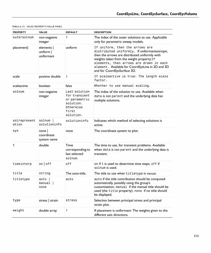
CoordSysLine, CoordSysSurface, CoordSysVolume
outersolnum non-negative integer
1 The index of the outer solutions to use. Applicable only for parametric sweep models.
placement| elements | uniform | uniformani
uniform If uniform, then the arrows are distributed uniformly. If uniformanisotropic, then the arrows are distributed uniformly with weights taken from the weight property.If elements, then arrows are drawn in each element. Available for CoordSysLine in 2D and 3D and for CoordSysSurface 3D.
scale positive double 1 If scaleactive is true: The length scale factor.
scaleactive boolean false Whether to use manual scaling.
solnum non-negative integer
Last solution for transient or parametric solution. Otherwise first solution.
The index of the solution to use. Available when data is not parent and the underlying data has multiple solutions.
solrepresentation
solnum | solutioninfo
solutioninfo Indicates which method of selecting solutions is active.
sys none | coordinate system name
none The coordinate system to plot.
t double Time corresponding to last selected solnum.
The time to use, for transient problems. Available when data is not parent and the underlying data is transient.
timeinterp on | off off on if t is used to determine time steps, off if solnum is used.
title string The auto-title. The title to use when titletype is manual.
titletype auto | manual | none
auto auto if the title contribution should be computed automatically, possibly using the group’s customization. manual if the manual title should be used (the title property). none if no title should be displayed.
type stress | strain stress Selection between principal stress and principal strain plot.
weight double array 1 If placement is uniformani: The weights given to the different axis directions.
TABLE 6-13: VALID PROPERTY/VALUE PAIRS
PROPERTY VALUE DEFAULT DESCRIPTION
515

CoordSysLine, CoordSysSurface, CoordSysVolume
516 | C H A P T
xnumber non-negative integer
15 (3D), 7 (2D) Number of points in the x-direction. Active when arrowxmethod is set to number. Available for CoordSysSurface in 2D and CoordSysVolume in 3D.
xcoord double array Empty Absolute coordinates in the x-direction, active when arrowxmethod is set to coord. Available for CoordSysSurface in 2D and CoordSysVolume in 3D.
ynumber integer 15 (3D), 7 (2D) Number of points in the y-direction. Active when arrowymethod is set to number. Available for CoordSysSurface in 2D and CoordSysVolume in 3D.
ycoord double array Empty Absolute coordinates in the z-direction, active when arrowymethod is set to coord. Available for CoordSysSurface in 2D and CoordSysVolume in 3D.
znumber integer 15 (3D), 7 (2D) Number of points in the z-direction. Active when arrowzmethod is set to number. Available for CoordSysVolume in 3D.
zcoord double array Empty Absolute coordinates in the z-direction, active when arrowzmethod is set to coord. Available for CoordSysVolume in 3D.
TABLE 6-13: VALID PROPERTY/VALUE PAIRS
PROPERTY VALUE DEFAULT DESCRIPTION
E R 6 : R E S U L T S

CutLine2D, CutLine3D
CutLine2D, CutLine3DSynopsis Cut line data set
Syntax model.result().dataset().create(<dtag>,"CutLine2D");model.result().dataset().create(<dtag>,"CutLine3D");model.result().dataset(<dtag>).set(property, <value>);
Description model.result().dataset().create(<dtag>,"CutLine2D") creates a 2D cut line data set feature named <dtag>.
model.result().dataset().create(<dtag>,"CutLine3D") creates a 3D cut line data set feature named <dtag>.
The following properties are available:
See Also LineGraph
TABLE 6-14: VALID PROPERTY/VALUE PAIRS
PROPERTY VALUE DEFAULT DESCRIPTION
bndsnap boolean false If true, each point is snapped to the closest boundary.
bounded on | off on Active when method equals twopoint, this property specifies if the line should be bounded by the two points or extend infinitely.
data none | data set name
First compatible data set
The data set this feature refers to.
genparaactive
on | off off Decides if parallel lines should be drawn.
genparadist double array {} Active when genparaactive is on, this property contains the distances from the extra parallel lines to the base line.
genpoints double matrix {{0, 0, 0}, {1,0,0}}
Active when method equals twopoint, this property contains the coordinates of the two points in the two rows of the matrix.
method twopoint | pointdir
twopoint Decides if the line should be specified by two points or through one point and a direction.
pddir double array Zero vector
Active when method equals pointdir, this property contains the direction.
pdpoint double array Zero vector
Active when method equals pointdir, this property contains the coordinates of the point.
spacevars String array of length 1
Created from the feature tag.
The name of the variable that evaluates to the line’s parameterization.
517
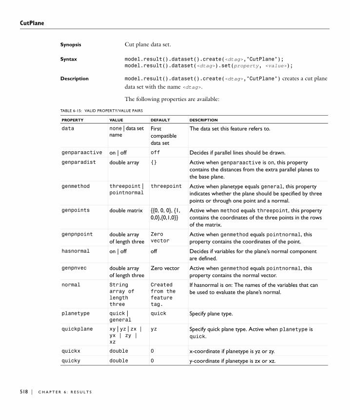
CutPlane
518 | C H A P T
CutPlaneSynopsis Cut plane data set.
Syntax model.result().dataset().create(<dtag>,"CutPlane");model.result().dataset(<dtag>).set(property, <value>);
Description model.result().dataset().create(<dtag>,"CutPlane") creates a cut plane data set with the name <dtag>.
The following properties are available:
TABLE 6-15: VALID PROPERTY/VALUE PAIRS
PROPERTY VALUE DEFAULT DESCRIPTION
data none | data set name
First compatible data set
The data set this feature refers to.
genparaactive on | off off Decides if parallel lines should be drawn.
genparadist double array {} Active when genparaactive is on, this property contains the distances from the extra parallel planes to the base plane.
genmethod threepoint | pointnormal
threepoint Active when planetype equals general, this property indicates whether the plane should be specified by three points or through one point and a normal.
genpoints double matrix {{0, 0, 0}, {1,0,0},{0,1,0}}
Active when method equals threepoint, this property contains the coordinates of the three points in the rows of the matrix.
genpnpoint double array of length three
Zero vector
Active when genmethod equals pointnormal, this property contains the coordinates of the point.
hasnormal on | off off Decides if variables for the plane’s normal component are defined.
genpnvec double array of length three
Zero vector Active when genmethod equals pointnormal, this property contains the normal vector.
normal String array of length three
Created from the feature tag.
If hasnormal is on: The names of the variables that can be used to evaluate the plane’s normal.
planetype quick | general
quick Specify plane type.
quickplane xy | yz | zx | yx | zy | xz
yz Specify quick plane type. Active when planetype is quick.
quickx double 0 x-coordinate if planetype is yz or zy.
quicky double 0 y-coordinate if planetype is zx or xz.
E R 6 : R E S U L T S

CutPlane
Examples This example creates a cut plane and plots a surface plot and a contour plot on it.
Create a solution data set and set it to point to the named solution Sol1 from a solver sequence:
model.result().dataset().create("dset1", "Solution");model.result().dataset("dset1").set("solution", "sol1");
Create 3D plot group:
result().create("pg1",3);result().dataset().create("cutp1","CutPlane");result().dataset("cutp1").set("data", "dset1");
result("pg1").feature().create("surf1","Surface");result("pg1").feature("surf1").set("data","cutp1");
result("pg1").feature().create("cont1","Contour");result("pg1").feature("cont1").set("data","cutp1");
See Also Surface
quickz double 0 z-coordinate if planetype is xy or yx.
spacevars String array of length 2
Created from the feature tag.
The names of the variables that evaluate to the plane’s parameterization.
TABLE 6-15: VALID PROPERTY/VALUE PAIRS
PROPERTY VALUE DEFAULT DESCRIPTION
519

CutPoint1D, CutPoint2D, CutPoint3D
520 | C H A P T
CutPoint1D, CutPoint2D, CutPoint3DSynopsis Cut point data set.
Syntax model.result().dataset().create(<dtag>,"CutPoint1D");model.result().dataset().create(<dtag>,"CutPoint2D");model.result().dataset().create(<dtag>,"CutPoint3D");model.result().dataset(<dtag>).set(property, <value>);
Description model.result().dataset().create(<dtag>,"CutPoint1D") creates a 1D cut point data set with the name <dtag>.
model.result().dataset().create(<dtag>,"CutPoint2D") creates a 2D cut point data set with the name <dtag>.
model.result().dataset().create(<dtag>,"CutPoint3D") creates a 3D cut point data set with the name <dtag>.
A cut point is the 0D analog of cut lines and cut planes. A difference compared to cut lines and cut planes is that a cut point feature can contain an arbitrary number of points. Cut points can exist in 1D, 2D, and 3D.
The following properties are available:
TABLE 6-16:
NAME VALUE DEFAULT DESCRIPTION
bndsnap boolean false If true, each point is snapped to the closest boundary.
data none | data set name
First compatible data set
The data set this feature refers to.
gridx double array If method is grid: The grid x-coordinates.
filename string If method is file: The file that contains the point coordinates in a spreadsheet format.
gridy double array If method is grid: The grid y-coordinates. (Only for CutPoint2D and CutPoint3D)
gridz double array If method is grid: The grid z-coordinates. (Only for CutPoint3D)
method coords | file | grid | regulargrid
coords The method used for defining the points.
pointx double array [] If method is coords: The point x-coordinates.
pointy double array [] If method is coords: The point y-coordinates. (Only for CutPoint2D and CutPoint3D)
E R 6 : R E S U L T S

CutPoint1D, CutPoint2D, CutPoint3D
See Also PointGraph
pointz double array [] If method is coords: The point z-coordinates. (Only for CutPoint3D)
regulargridx integer 10 If method is regulargrid: The number of grid points in the x-direction.
regulargridy integer 10 If method is regulargrid: The number of grid points in the y-direction. (Only for CutPoint2D and CutPoint3D)
regulargridz integer 10 If method is regulargrid: The number of grid points in the z-direction. (Only for CutPoint3D)
TABLE 6-16:
NAME VALUE DEFAULT DESCRIPTION
521

Data
522 | C H A P T
DataSynopsis Data export.
Syntax model.result().export().create(<ftag>,"Data");model.result().export().create(<ftag>,<dtag>,"Data");model.result().export(<ftag>).set(property, <value>);model.result().export(<ftag>).run();
Description model.result().export().create(<ftag>,"Data") creates a data export feature with the name <ftag>.
model.result().export().create(<ftag>,<dtag>,"Data") creates a data export feature with the name <ftag> for the data set <dtag>.
The following properties are available:
TABLE 6-17: VALID PROPERTY/VALUE PAIRS
PROPERTY VALUE DEFAULT DESCRIPTION
coordfilename
string If location is file: The file that contains coordinates to evaluate in.
const String array of property/value pairs
Empty Parameters to use in the expressions.
data string The name of the data set to export.
descr string array Descriptions of the expressions in expr.
differential on | off on Whether the expression should be linearized at the linearization point. Applicable only if evalmethod is harmonic
evalmethod linpoint | harmonic | lintotal | lintotalavg | lintotalrms | lintotalpeak
harmonic Applicable only for solutions with a stored linearization point. Controls if the linearization point, the perturbation, or a combination should be used when evaluating the expression.
expr string array The expressions to evaluate and export.
filename string The output file.
fullprec on | off on If on, floating-point numbers are written in full precision, otherwise they are written with six significant digits.
gporder poitive integer
1 If pattern is gauss: The Gauss point order.
gridstruct grid | spreadsheet
spreadsheet If location is grid or regulargrid: The format of the exported data.
E R 6 : R E S U L T S

Data
gridx1 double array If location is grid and the data set is 1D: x-coordinates to evaluate in.
gridx2 double array If location is grid and the data set is 2D: x-coordinates to evaluate in.
gridy2 double array If location is grid and the data set is 2D: y-coordinates to evaluate in.
gridx3 double array If location is grid and the data set is 3D: x-coordinates to evaluate in.
gridy3 double array If location is grid and the data set is 3D: y-coordinates to evaluate in.
gridz3 double array If location is grid and the data set is 3D: z-coordinates to evaluate in.
header on | off off Enable/disable a data header in the output file.
lagorder integer 1 The Lagrange point order to use if resolution is custom
level fromdataset | volume | surface | line | point
fromdataset The geometry level to evaluate on.
location fromdataset | file | grid | regulargrid
fromdataset The points evaluated in.
outersolnum non-negative integer
1 The index of the outer solutions to use. Applicable only for parametric sweep models.
pattern gauss | lagrange
lagrange If the data set is a solution: Specifies if evaluation takes place in Lagrange points or in Gauss points.
regulargridx1
positive integer
10 If location is regulargrid and the data set is 1D: The number of grid points along the x-axis.
regulargridx2
positive integer
10 If location is regulargrid and the data set is 2D: The number of grid points along the x-axis.
regulargridy2
positive integer
10 If location is regulargrid and the data set is 2D:The number of grid points along the y-axis.
regulargridx3
positive integer
10 If location is regulargrid and the data set is 3D: The number of grid points along the x-axis.
regulargridy3
positive integer
10 If location is regulargrid and the data set is 3D: The number of grid points along the y-axis.
TABLE 6-17: VALID PROPERTY/VALUE PAIRS
PROPERTY VALUE DEFAULT DESCRIPTION
523
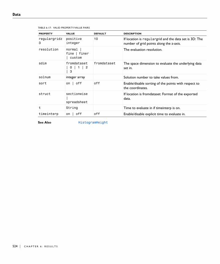
Data
524 | C H A P T
See Also HistogramHeight
regulargridz3
positive integer
10 If location is regulargrid and the data set is 3D: The number of grid points along the z-axis.
resolution normal | fine | finer | custom
The evaluation resolution.
sdim fromdataset | 0 | 1 | 2 | 3
fromdataset The space dimension to evaluate the underlying data set in.
solnum integer array Solution number to take values from.
sort on | off off Enable/disable sorting of the points with respect to the coordinates.
struct sectionwise | spreadsheet
If location is fromdataset: Format of the exported data.
t String Time to evaluate in if timeinterp is on.
timeinterp on | off off Enable/disable explicit time to evaluate in.
TABLE 6-17: VALID PROPERTY/VALUE PAIRS
PROPERTY VALUE DEFAULT DESCRIPTION
E R 6 : R E S U L T S

Deform
DeformSynopsis Deformation attribute.
Syntax model.result(<pgtag>).feature(<ftag>).feature().create(<atag>,"Deform");
model.result(<pgtag>).feature(<ftag>).feature(<atag>).set(property, <value>);
Description model.result(<pgtag>).feature(<ftag>).feature().create(<atag>,
"Deform") creates a deformation attribute feature with the name <atag>, belonging to the feature <ftag>.
Deformation attributes deform the coordinates of a plot feature according to an expression. The deformation attribute can be added to arrow plots, contour plots, isosurface plots, particle plots, slice plots, streamline plots, surface plots, volume plots, and mesh plots.
The following properties are available:
TABLE 6-18: VALID PROPERTY/VALUE PAIRS
PROPERTY VALUE DEFAULT DESCRIPTION
descr string Model-dependent The description of the expression in expr. Is used in the automatic title.
descriptionintitle
on | off on Whether the title contribution should contain the description when titletype is custom.
differential
on | off on Whether the expression should be linearized at the linearization point. Applicable only if evalmethod is harmonic
evalmethod linpoint | harmonic | lintotal | lintotalavg | lintotalrms | lintotalpeak
harmonic Applicable only for solutions with a stored linearization point. Controls if the linearization point, the perturbation, or a combination should be used when evaluating the expression.
expr string Model-dependent The expression to plot.
prefixintitle
string Empty Added prefix to contribution to title.
scale positive double
Model-dependent The scale factor for the deformation.
scaleactive on | off off Whether to use the automatically computed scale, or the scale in the scale property.
525

Deform
526 | C H A P T
See Also Color, Height, ArrowVolume, ArrowSurface, ArrowLine, Contour, Contour, Isosurface, Line, Mesh, Particle, ParticleMass, ScatterVolume, ScatterSurface, Slice, Streamline, Surface, Volume.
suffixintitle
string Empty Added suffix to contribution to title.
title string The auto-title. The title to use when titletype is manual.
titletype auto | custom | manual | none
auto auto if the title contribution should be computed automatically, possibly using the group’s customization. custom if the title contribution should be computed automatically, but customized. manual if the manual title contribution should be used (the title property). none if no title contribution should be used.
typeintitle on | off on Whether the title contribution should contain the type when titletype is custom.
unit string Model-dependent The unit to use for the expression in expr. If the old unit is not valid when the expression changes, the unit property is reset to default.
TABLE 6-18: VALID PROPERTY/VALUE PAIRS
PROPERTY VALUE DEFAULT DESCRIPTION
E R 6 : R E S U L T S

Edge2D, Edge3D
Edge2D, Edge3DSynopsis Edge data set.
Syntax model.result().dataset().create(<dtag>,"Edge2D");model.result().dataset().create(<dtag>,"Edge3D");
model.result().dataset(<dtag>).set(property, <value>);
Description model.result().dataset().create(<dtag>,"Edge2D") creates a 2D edge data set with the name <dtag>.
The edge data set makes it possible to evaluate edge of a model in 1D or the model’s dimension.
The following properties are available:
TABLE 6-19: VALID PROPERTY/VALUE PAIRS
PROPERTY VALUE DEFAULT DESCRIPTION
data none | data set name First compatible data set
The solution data set this feature refers to.
527

Eval
528 | C H A P T
EvalSynopsis Evaluate expressions in domains.
Syntax model.result().numerical().create(<ftag>,"Eval");model.result().numerical(<ftag>).selection(...);model.result().numerical(<ftag>).set(property, <value>);model.result().numerical(<ftag>).getData();model.result().numerical(<ftag>).getData(<expressionIndex>);model.result().numerical(<ftag>).getImagData();model.result().numerical(<ftag>).getImagData(<expressionIndex>);model.result().numerical(<ftag>).isComplex();model.result().numerical(<ftag>).isComplex(<outersolnum>);model.result().numerical(<ftag>).getNData();model.result().numerical(<ftag>).getCoordinates();model.result().numerical(<ftag>).getElements();model.result().numerical(<ftag>).getVertexElements();model.result().numerical(<ftag>).run();
Description model.result().numerical().create(<ftag>,"Eval") creates an evaluation feature with the name <ftag>.
Eval is a feature made specifically for users of the COMSOL Java API and does not appear in the COMSOL Multiphysics GUI. Interp combines cut points and evaluation features, as well as allowing evaluation of arbitrary data sets. It supports multiple expressions and some additional advanced properties not available when using cut points and EvalPoint features.
result = model.result().numerical(<ftag>).getData() returns the real part of the result, recomputing the feature if necessary. result is a three-dimensional double matrix ordered result[expression][solnum][coordinates].
model.result().numerical(<ftag>).getData(<expressionIndex>) returns the real part of the result for one expression, equivalent to result[expressionIndex].
result = model.result().numerical(<ftag>).getImagData() returns the imaginary part of the result, recomputing the feature if necessary. result is a three-dimensional double matrix ordered result[expression][solnum][coordinates].
model.result().numerical(<ftag>).getImagData(<expressionIndex>) returns the imaginary result for one expression, equivalent to result[expressionIndex].
E R 6 : R E S U L T S

Eval
model.result().numerical(<ftag>).isComplex() returns true if the result is complex.
<outersolnum> is applicable only for parametric sweep solutions and is the index of each outer parametric solution.
model.result().numerical(<ftag>).getNData() returns the number of data vectors in the result.
model.result().numerical(<ftag>).getCoordinates() returns node point coordinates.
model.result().numerical(<ftag>).getElements() returns indices to columns in p of a simplex mesh.
model.result().numerical(<ftag>).getVertexElements() returns indices to mesh elements for each point.
The following properties are available:
TABLE 6-20: VALID PROPERTY/VALUE PAIRS
NAME VALUE DEFAULT DESCRIPTION
const String array of property/value pairs
Empty Parameters to use in the expressions.
data none | data set name
First compatible data set
The data set this feature refers to.
differential on | off on Whether the expression should be linearized at the linearization point. Applicable only if evalmethod is harmonic
evalmethod linpoint | harmonic | lintotal | lintotalavg | lintotalrms | lintotalpeak
harmonic Applicable only for solutions with a stored linearization point. Controls if the linearization point, the perturbation, or a combination should be used when evaluating the expression.
expr string array Model-dependent
The expressions to evaluate.
complexfun on | off on Use complex-valued functions with real input
gporder poitive integer
1 If pattern is gauss: The Gauss point order.
matherr on | off off Error for undefined operation or variable
529

Eval
530 | C H A P T
See Also Interp, Global (numerical), EvalPoint, EvalGlobal
outersolnum non-negative integer
1 The index of the outer solutions to use. Applicable only for parametric sweep models.
refine auto | integer
auto Refinement of elements for evaluation points
recover off | pprint | ppr
off The derivative recovery method.
pattern gauss | lagrange
lagrange Specifies if evaluation takes place in Lagrange points or in Gauss points.
phase double 0 Evaluate solution at this angle, given in degrees.
smooth none | internal | everywhere
internal Smoothing settings.
solnum non-negative integer array
All solutions
The solutions to use.
t double array Empty The times to use. Available when the underlying solution is transient.
phase double 0 Evaluate solution at this angle, given in degrees.
unit String Model-dependent
The unit to use for the expression in expr. If the old unit is not valid when the expression changes, the unit property is reset to default.
TABLE 6-20: VALID PROPERTY/VALUE PAIRS
NAME VALUE DEFAULT DESCRIPTION
E R 6 : R E S U L T S

EvalGlobal
EvalGlobalSynopsis Evaluate quantities.
Syntax model.result().numerical().create(<ftag>,"EvalGlobal");model.result().numerical(<ftag>).set(property, <value>);model.result().numerical(<ftag>).getReal();model.result().numerical(<ftag>).getReal(<columnwise>);model.result().numerical(<ftag>).getReal(<outersolnum>);model.result().numerical(<ftag>).getReal(<columnwise>,
<outersolnum>);model.result().numerical(<ftag>).getImag();model.result().numerical(<ftag>).getImag(<allocate>,
<columnwise>);model.result().numerical(<ftag>).getImag(<outersolnum>);model.result().numerical(<ftag>).getImag(<allocate>, <columnwise>,
<outersolnum>);model.result().numerical(<ftag>).isComplex();model.result().numerical(<ftag>).isComplex(<outersolnum>);model.result().numerical(<ftag>).setResult();model.result().numerical(<ftag>).appendResult();
Description model.result().numerical().create(<ftag>,"EvalGlobal") creates an evaluation feature with the name <ftag>.
model.result().numerical(<ftag>).getReal() returns the real result, recomputing the feature if necessary. Data is ordered such that one row contains data for all solution numbers. This is identical to (<columnwise>) when columnwise is false. If columnwise is true, the ordering is the opposite: each column contains the values for all solution numbers.
model.result().numerical(<ftag>).getImag(<allocate>, <columnwise>) returns the imaginary part of complex result, recomputing the feature if necessary. If allocate is true, a zero-valued matrix is allocated even when the result is real. getImag() uses <allocate> true and <columnwise> false.
model.result().numerical(<ftag>).isComplex() returns true if the result is complex.
<outersolnum> is applicable only for parametric sweep solutions and is the index of each outer parametric solution.
model.result().numerical(<ftag>).setResult() and model.result().numerical(<ftag>).appendResult() evaluates the feature and set or append the result in the table indicated by the table property.
531

EvalGlobal
532 | C H A P T
The following properties are available:
TABLE 6-21: VALID PROPERTY/VALUE PAIRS
NAME VALUE DEFAULT DESCRIPTION
const String array of property/value pairs
Empty Parameters to use in the expressions.
data none | data set name
First compatible data set
The data set this feature refers to.
dataseries average | integral | maximum | minimum | none | rms | stddev | variance
none The operation that is applied to the data series formed by the evaluation.
descr string Model-dependent The description of the expression in expr. Is used in the automatic title.
differential on | off on Whether the expression should be linearized at the linearization point. Applicable only if evalmethod is harmonic
evalmethod linpoint | harmonic | lintotal | lintotalavg | lintotalrms | lintotalpeak
harmonic Applicable only for solutions with a stored linearization point. Controls if the linearization point, the perturbation, or a combination should be used when evaluating the expression.
expr string Model-dependent The expression to plot.
innerinput all | first | last | manual | manualindices | interp
all How to input the solution to use. manual indicates that solnum is used. manualindices indicates that solnumindices is used. interp indicates that t is used.
interp double row matrix
Empty on all levels.
The times to use, for transient levels. Available when data is not parent and the underlying data is transient.
looplevel integer row matrix
All solutions on all levels
The solutions to use, per level.
looplevelindices
integer row matrix
Empty An alternate way to specify the solutions to use, allowing you to enter, for example, range(1,1,20). Applicable when looplevelinput is manualindices on a level.
E R 6 : R E S U L T S

EvalGlobal
looplevelinput String array with all | first | last | manual | manualindices | interp on each level
all on all levels How to input the solution to use, per level. manual on a level indicates that looplevel is used on that level. manualindices on a level indicates that looplevelindices is used on that level. interp on a level indicates that interp is used on that level.
maximumobj abs | real real The value being maximized if dataseries is maximum.
minimumobj abs | real real The value being minimized if dataseries is minimum.
outerinput all | first | last | manual | manualindices
all How to input the outer solutions to use. Applicable only for parametric sweep models. manual indicates that outersolnum is used. manualindices indicates that outersolnumindices is used.
outersolnum non-negative integer array
1 The index of the outer solutions to use. Applicable only for parametric sweep models. Since the various outer solutions can have different number of solnum, the solnum property is not used.
outersolnumindices
string or integer array
Empty An alternate way to specify the outer solutions to use, allowing you to enter, for example, range(1,1,20). Applicable when outerinput is manualindices.
solnum non-negative integer array
All solutions The solutions to use.
solnumindices string or integer array
Empty An alternate way to specify the solutions to use, allowing you to enter, for example, range(1,1,20). Applicable when innerinput is manualindices.
solrepresentation
solnum | solutioninfo
solutioninfo Indicates which method of selecting solutions is active.
t double array Empty The times to use. Available when the underlying solution is transient.
table new | table name
new The table to use when calling setResult() or appendResult(). new indicates that a new table is created.
TABLE 6-21: VALID PROPERTY/VALUE PAIRS
NAME VALUE DEFAULT DESCRIPTION
533

EvalGlobal
534 | C H A P T
See Also EvalGlobalMatrix, Eval, EvalPoint
tablecols inner | outer | data | level1
data Whether to use inner or outer solutions as columns in the table when calling setResult() or appendResult(). Applicable only for parametric sweep models. The level values (level1, level2, and so on) are the levels in the parametric sweep.
unit string Model-dependent The unit to use for the expression in expr. If the old unit is not valid when the expression changes, the unit property is reset to default.
TABLE 6-21: VALID PROPERTY/VALUE PAIRS
NAME VALUE DEFAULT DESCRIPTION
E R 6 : R E S U L T S

EvalGlobalMatrix
EvalGlobalMatrixSynopsis Evaluate quantities
Syntax model.result().numerical().create(<ftag>,"EvalGlobalMatrix");model.result().numerical(<ftag>).set(property, <value>);model.result().numerical(<ftag>).getReal();model.result().numerical(<ftag>).getReal(<columnwise>);model.result().numerical(<ftag>).getReal(<outersolnum>);model.result().numerical(<ftag>).getReal(<columnwise>,
<outersolnum>);model.result().numerical(<ftag>).getImag();model.result().numerical(<ftag>).getImag(<allocate>,
<columnwise>);model.result().numerical(<ftag>).getImag(<outersolnum>);model.result().numerical(<ftag>).getImag(<allocate>, <columnwise>,
<outersolnum>);model.result().numerical(<ftag>).isComplex();model.result().numerical(<ftag>).isComplex(<outersolnum>);model.result().numerical(<ftag>).setResult();model.result().numerical(<ftag>).appendResult();
Description model.result().numerical().create(<ftag>,"EvalGlobalMatrix") creates an evaluation feature with the name <ftag>.
model.result().numerical(<ftag>).getReal() returns the real result, recomputing the feature if necessary. Data is ordered such that one row contains data for all solution numbers. This is identical to (<columnwise>) when columnwise is false. If columnwise is true, the ordering is the opposite: each column contains the values for all solution numbers.
model.result().numerical(<ftag>).getImag(<allocate>, <columnwise>) returns the imaginary part of complex result, recomputing the feature if necessary. If allocate is true, a zero-valued matrix is allocated even when the result is real. getImag() uses <allocate> true and <columnwise> false.
model.result().numerical(<ftag>).isComplex() returns true if the result is complex.
<outersolnum> is applicable only for parametric sweep solutions and is the index of each outer parametric solution.
model.result().numerical(<ftag>).setResult() and model.result().numerical(<ftag>).appendResult() evaluates the feature and set or append the result in the table indicated by the table property.
535

EvalGlobalMatrix
536 | C H A P T
The following properties are available:
TABLE 6-22: VALID PROPERTY/VALUE PAIRS
NAME VALUE DEFAULT DESCRIPTION
const String array of property/value pairs
Empty Parameters to use in the expressions.
data none | data set name
First compatible data set
The data set this feature refers to.
dataseries average | none | sum
none The operation that is applied to the data series formed by the evaluation over inner solutions.
descr string Model-dependent The description of the expression in expr. Is used in the automatic title.
differential on | off on Whether the expression should be linearized at the linearization point. Applicable only if evalmethod is harmonic
evalmethod linpoint | harmonic | lintotal | lintotalavg | lintotalrms | lintotalpeak
harmonic Applicable only for solutions with a stored linearization point. Controls if the linearization point, the perturbation, or a combination should be used when evaluating the expression.
expr string Model-dependent The matrix variable to plot.
ignorenan on | off on When on, NaN is ignored when taking the average in the inner or outer data series. If all entries are NaN for a given component, however, you get NaN as output.
innerinput all | first | last | manual | manualindices | interp
all How to input the solution to use. manual indicates that solnum is used. manualindices indicates that solnumindices is used. interp indicates that t is used.
interp double row matrix
Empty on all levels.
The times to use, for transient levels. Available when data is not parent and the underlying data is transient.
looplevel integer row matrix
All solutions on all levels
The solutions to use, per level.
looplevelindices
integer row matrix
Empty An alternate way to specify the solutions to use, allowing you to enter, for example, range(1,1,20). Applicable when looplevelinput is manualindices on a level.
E R 6 : R E S U L T S
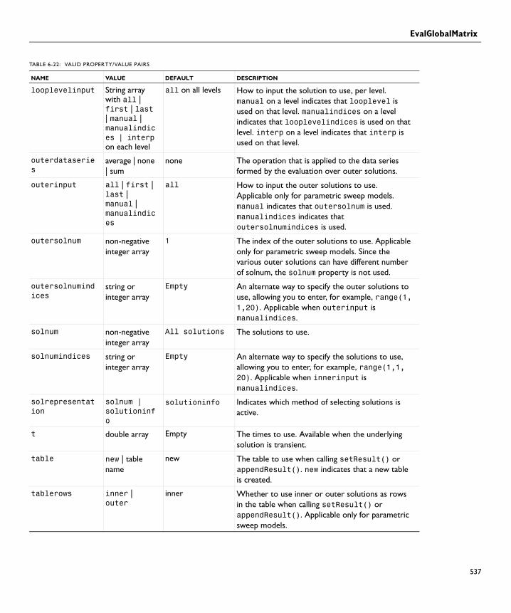
EvalGlobalMatrix
looplevelinput String array with all | first | last | manual | manualindices | interp on each level
all on all levels How to input the solution to use, per level. manual on a level indicates that looplevel is used on that level. manualindices on a level indicates that looplevelindices is used on that level. interp on a level indicates that interp is used on that level.
outerdataseries
average | none | sum
none The operation that is applied to the data series formed by the evaluation over outer solutions.
outerinput all | first | last | manual | manualindices
all How to input the outer solutions to use. Applicable only for parametric sweep models. manual indicates that outersolnum is used. manualindices indicates that outersolnumindices is used.
outersolnum non-negative integer array
1 The index of the outer solutions to use. Applicable only for parametric sweep models. Since the various outer solutions can have different number of solnum, the solnum property is not used.
outersolnumindices
string or integer array
Empty An alternate way to specify the outer solutions to use, allowing you to enter, for example, range(1,1,20). Applicable when outerinput is manualindices.
solnum non-negative integer array
All solutions The solutions to use.
solnumindices string or integer array
Empty An alternate way to specify the solutions to use, allowing you to enter, for example, range(1,1,20). Applicable when innerinput is manualindices.
solrepresentation
solnum | solutioninfo
solutioninfo Indicates which method of selecting solutions is active.
t double array Empty The times to use. Available when the underlying solution is transient.
table new | table name
new The table to use when calling setResult() or appendResult(). new indicates that a new table is created.
tablerows inner | outer
inner Whether to use inner or outer solutions as rows in the table when calling setResult() or appendResult(). Applicable only for parametric sweep models.
TABLE 6-22: VALID PROPERTY/VALUE PAIRS
NAME VALUE DEFAULT DESCRIPTION
537

EvalGlobalMatrix
538 | C H A P T
See Also EvalGlobal, Eval, EvalPoint
trans none | inverse | sy | sz | ys | yz | zs | zy
none The transformation to apply to the matrix.
unit string Model-dependent The unit to use for the expression in expr. If the old unit is not valid when the expression changes, the unit property is reset to default.
y0 double array Taken from the physics interfaces.
If trans is sy or ys: The characteristic admittance.
z0 double array Taken from the physics interfaces.
If trans is sz or zs: The characteristic impedance.
TABLE 6-22: VALID PROPERTY/VALUE PAIRS
NAME VALUE DEFAULT DESCRIPTION
E R 6 : R E S U L T S

EvalPoint
EvalPointSynopsis Evaluate quantities in points.
Syntax model.result().numerical().create(<ftag>,"EvalPoint");model.result().numerical(<ftag>).selection(...);model.result().numerical(<ftag>).set(property, <value>);model.result().numerical(<ftag>).getReal();model.result().numerical(<ftag>).getReal(<columnwise>);model.result().numerical(<ftag>).getReal(<outersolnum>);model.result().numerical(<ftag>).getReal(<columnwise>,
<outersolnum>);model.result().numerical(<ftag>).getImag();model.result().numerical(<ftag>).getImag(<allocate>,
<columnwise>);model.result().numerical(<ftag>).getImag(<outersolnum>);model.result().numerical(<ftag>).getImag(<allocate>, <columnwise>,
<outersolnum>);model.result().numerical(<ftag>).isComplex();model.result().numerical(<ftag>).isComplex(<outersolnum>);model.result().numerical(<ftag>).setResult();model.result().numerical(<ftag>).appendResult();
Description model.result().numerical().create(<ftag>,"EvalPoint") creates a point evaluation feature with the name <ftag>. Point evaluations can be performed both on points in a geometry or on cut points.
model.result().numerical(<ftag>).getReal() returns the real result, recomputing the feature if necessary. Data is ordered such that there is one row per point, with one row containing data for all solution numbers. This is identical to (<columnwise>) when <columnwise> is false. If <columnwise> is true, the ordering is the opposite: each column contains the values for all solution numbers.
model.result().numerical(<ftag>).getImag(<allocate>, <columnwise>) returns the imaginary part of complex result, recomputing the feature if necessary. If <allocate> is true, a zero-valued matrix is allocated even when the result is real. getImag() uses <allocate> true and <columnwise> false.
model.result().numerical(<ftag>).isComplex() returns true if the result is complex.
<outersolnum> is applicable only for parametric sweep solutions and is the index of each outer parametric solution.
model.result().numerical(<ftag>).setResult() and model.result().numerical(<ftag>).appendResult() evaluates the feature and set or append the result in the table indicated by the table property.
539

EvalPoint
540 | C H A P T
The following properties are available:
TABLE 6-23: VALID PROPERTY/VALUE PAIRS
NAME VALUE DEFAULT DESCRIPTION
const String array of property/value pairs
Empty Parameters to use in the expressions.
data none | data set name
First compatible data set
The data set this feature refers to.
dataseries average | integral | maximum | minimum | none | rms | stddev | variance
none The operation that is applied to the data series formed by the evaluation.
descr string Model-dependent The description of the expression in expr. Is used in the automatic title.
differential on | off on Whether the expression should be linearized at the linearization point. Applicable only if evalmethod is harmonic
evalmethod linpoint | harmonic | lintotal | lintotalavg | lintotalrms | lintotalpeak
harmonic Applicable only for solutions with a stored linearization point. Controls if the linearization point, the perturbation, or a combination should be used when evaluating the expression.
expr string Model-dependent The expression to plot.
innerinput all | first | last | manual | manualindices | interp
all How to input the solution to use. manual indicates that solnum is used. manualindices indicates that solnumindices is used. interp indicates that t is used.
interp double row matrix
Empty on all levels.
The times to use, for transient levels. Available when data is not parent and the underlying data is transient.
looplevel integer row matrix
All solutions on all levels
The solutions to use, per level.
looplevelindices
integer row matrix
Empty An alternate way to specify the solutions to use, allowing you to enter, for example, range(1,1,20). Applicable when looplevelinput is manualindices on a level.
E R 6 : R E S U L T S

EvalPoint
looplevelinput String array with all | first | last | manual | manualindices | interp on each level
all on all levels How to input the solution to use, per level. manual on a level indicates that looplevel is used on that level. manualindices on a level indicates that looplevelindices is used on that level. interp on a level indicates that interp is used on that level.
maximumobj abs | real real The value being maximized if dataseries is maximum.
minimumobj abs | real real The value being minimized if dataseries is minimum.
outerinput all | first | last | manual | manualindices
all How to input the outer solutions to use. Applicable only for parametric sweep models. manual indicates that outersolnum is used. manualindices indicates that outersolnumindices is used.
outersolnum non-negative integer array
1 The index of the outer solutions to use. Applicable only for parametric sweep models. Since the various outer solutions can have different number of solnum, the solnum property is not used.
outersolnumindices
string or integer array
Empty An alternate way to specify the outer solutions to use, allowing you to enter, for example, range(1,1,20). Applicable when outerinput is manualindices.
solnum non-negative integer array
All solutions The solutions to use.
solnumindices string or integer array
Empty An alternate way to specify the solutions to use, allowing you to enter, for example, range(1,1,20). Applicable when innerinput is manualindices.
solrepresentation
solnum | solutioninfo
solutioninfo Indicates which method of selecting solutions is active.
t double array Empty The times to use. Available when the underlying solution is transient.
table new | table name
new The table to use when calling setResult() or appendResult(). new indicates that a new table is created.
TABLE 6-23: VALID PROPERTY/VALUE PAIRS
NAME VALUE DEFAULT DESCRIPTION
541

EvalPoint
542 | C H A P T
See Also EvalGlobal
tablecols inner | outer | data | level1
data Whether to use inner or outer solutions as columns in the table when calling setResult() or appendResult(). Applicable only for parametric sweep models. The level values (level1, level2, and so on) are the levels in the parametric sweep.
unit string Model-dependent The unit to use for the expression in expr. If the old unit is not valid when the expression changes, the unit property is reset to default.
TABLE 6-23: VALID PROPERTY/VALUE PAIRS
NAME VALUE DEFAULT DESCRIPTION
E R 6 : R E S U L T S

FarField
FarFieldSynopsis Far-field plot.
Syntax model.result(<pgtag>).feature().create(<ftag>,"FarField");model.result(<pgtag>).feature(<ftag>).set(property, <value>);model.result(<pgtag>).feature(<ftag>).run();
Description model.result(<pgtag>).feature().create(<ftag>,"FarField") creates a plot feature named <ftag> belonging to the plot group <pgtag>.
Far-field plots are used to visualize radiation patterns in the far field for antennas, for example. They can be added to all types of plot groups.
The following properties are available:
TABLE 6-24: VALID PROPERTY/VALUE PAIRS
NAME VALUE DEFAULT DESCRIPTION
anglerestr manual | none
none Whether there is a restriction on the angle range that is evaluated.
autodescr on | off Model dependent
Whether the automatic legends should include the expression descriptions. Available in 1D.
autoexpr on | off Model dependent
Whether the automatic legends should include the expressions. Available in 1D.
autolegends on | off on Whether to use the automatically computed legends or the legends defined in the legends property. The automatic legends display the description and expression for each line. Available in 1D.
center double array of length 3
{0, 0, 0} If circle is manual: The center of the circle to evaluate on. Available in 2D and 3D.
center2 double array of length 2
{0, 0} If circle is manual and the data set is 2D: The center of the circle to evaluate on. Available in 1D.
center3 double array of length 3
{0, 0, 0} If circle is manual and the data set is 3D: The center of the circle to evaluate on. Available in 1D.
circle manual | unit
unit The circle to evaluate. Available in 1D.
colorexpr string Model-dependent. The color of the far-field surface. Available in 3D.
const String array of property/value pairs
Empty Parameters to use in the expressions.
543

FarField
544 | C H A P T
customgridcolor RGB-triplet {0,0,1} f grid is fine, normal, or coarse and gridcolor is custom: The grid’s color. Available in 3D.
customlinecolor RGB-triplet {0,0,1} or last used edgecolor.
The color to use for the lines. Active when linecolor is set to custom. Available in 1D.
data none | parent | data set name
parent The data set this feature refers to.
descr string array Model-dependent. The description of the expressions in expr. Is used in the automatic legends.
descriptionintitle
on | off on Whether the title contribution should contain the description when titletype is custom.
differential on | off on Whether the expression should be linearized at the linearization point. Applicable only if evalmethod is harmonic
directivity on | off off Whether to compute the maximum directivity and the direction where it is attained. Available in 2D and 3D.
evalmethod linpoint | harmonic | lintotal | lintotalavg | lintotalrms | lintotalpeak
harmonic Applicable only for solutions with a stored linearization point. Controls if the linearization point, the perturbation, or a combination should be used when evaluating the expression.
expr string array Model-dependent. The expressions to plot.
expressionintitle
on | off off Whether the title contribution should contain the expression when titletype is custom.
grid fine | normal | coarse | none
none The type of grid to display on the far-field surface. Available in 3D.
gridcolor custom | black | blue | cyan | green | magenta | red | white | yellow
black If grid is fine, normal, or coarse: The grid’s color. Available in 3D.
TABLE 6-24: VALID PROPERTY/VALUE PAIRS
NAME VALUE DEFAULT DESCRIPTION
E R 6 : R E S U L T S

FarField
inheritcolor boolean true If inheritplot is not none: Determines if the color is inherited. Available in 2D and 3D.
innerinput all | first | last | manual | manualindices | interp
all How to input the solution to use. manual indicates that solnum is used. manualindices indicates that solnumindices is used. interp indicates that t is used.
interp double row matrix
Empty on all levels.
The times to use, for transient levels. Available when data is not parent and the underlying data is transient.
legend on | off off Whether to show legends. Available in 1D.
legendmethod automatic | manual
automatic Whether to use the automatic legends or the legends supplied in the legends property. Available in 1D.
legends string array The last computed automatic legends.
Manual legends active when legendmethod is set to manual. Available in 1D.
linecolor custom | cycle | black | blue | cyan | green | magenta | red | white | yellow
cycle How to color the lines in the graph. Cycle indicates that the colors is different for each line. Available in 1D.
linewidth double 0.5 The line width. Available in 1D.
linemarker none | cycle | asterisk | circle | diamond | plus | point | square | star | triangle
none The line markers, if any. Cycle indicates that the marker is different for each line. Available in 1D.
linestyle none | cycle | solid | dotted | dashed | dashdot
solid The line style, if any. Cycle indicates that the line style is different for each line. Available in 1D.
TABLE 6-24: VALID PROPERTY/VALUE PAIRS
NAME VALUE DEFAULT DESCRIPTION
545

FarField
546 | C H A P T
looplevel integer row matrix
All solutions on all levels
The solutions to use, per level.
looplevelindices
integer row matrix
Empty An alternate way to specify the solutions to use, allowing you to enter, for example, range(1,1,20). Applicable when looplevelinput is manualindices on a level.
looplevelinput String array with all | first | last | manual | manualindices | interp on each level
all on all levels How to input the solution to use, per level. manual on a level indicates that looplevel is used on that level. manualindices on a level indicates that looplevelindices is used on that level. interp on a level indicates that interp is used on that level.
markerpos interp | datapoints
interp Controls whether the positions of the markers are in the data points of the plot, or interpolated depending on the number (set in markers). Markers are visible when linemarker is set. Available in 1D.
markers integer 8 The number of markers to show. Markers are visible when linemarker is set. Available in 1D.
normal double array of length 3
{0, 0, 1} If circle is manual and the data set is 3D: The normal of the circle to evaluate on. Available in 1D.
outerinput all | first | last | manual | manualindices
all How to input the outer solutions to use. Applicable only for parametric sweep models. manual indicates that outersolnum is used. manualindices indicates that outersolnumindices is used.
outersolnum non-negative integer array
1 The index of the outer solutions to use. Applicable only for parametric sweep models. Since the various outer solutions can have different number of solnum, the solnum property is not used.
outersolnumindices
string or integer array
Empty An alternate way to specify the outer solutions to use, allowing you to enter, for example, range(1,1,20). Applicable when outerinput is manualindices.
phidisc integer >= 2
50 The angular discretization in the phi direction. Available in 1D.
TABLE 6-24: VALID PROPERTY/VALUE PAIRS
NAME VALUE DEFAULT DESCRIPTION
E R 6 : R E S U L T S

FarField
phimin double 0 If anglerestr is manual: The minimum phi angle in degrees.
phirange double 360 If anglerestr is manual: The phi angle’s range in degrees.
prefixintitle string Empty Added prefix to contribution to title.
radius double 1 If circle is manual: The radius of the circle to evaluate on.
solnum non-negative integer array
All solutions The solutions to plot. Available when data is not parent and the underlying data has multiple solutions.
solnumindices string or integer array
Empty An alternate way to specify the solutions to use, allowing you to enter, for example, range(1,1,20). Applicable when innerinput is manualindices.
solrepresentation
solnum | solutioninfo
solutioninfo Indicates which method of selecting solutions is active.
sphere manual | unit
unit The sphere to evaluate on. Available in 2D and 3D.
suffixintitle string Empty Added suffix to contribution to title.
t double array Empty The times to plot. Available when data is not parent and the underlying solution is transient.
thetadisc integer >= 2
10 The angular discretization in the theta direction. Available in 2D and 3D.
thetamin double 0 If anglerestr is manual: The minimum theta angle in degrees. Available in 2D and 3D.
thetarange double 360 If anglerestr is manual: The phi angle’s range in degrees. Available in 2D and 3D.
titletype auto | custom | manual | none
auto auto if the title contribution should be computed automatically, possibly using the group’s customization. custom if the title contribution should be computed automatically, but customized. manual if the manual title contribution should be used (the title property). none if no title contribution should be used.
typeintitle on | off on Whether the title contribution should contain the type when titletype is custom.
TABLE 6-24: VALID PROPERTY/VALUE PAIRS
NAME VALUE DEFAULT DESCRIPTION
547

FarField
548 | C H A P T
Attributes None
unit string Model-dependent The unit to use for the expression in expr. If the old unit is not valid when the expression changes, the unit property is reset to default.
unitintitle on | off on Whether the title contribution should contain the unit when titletype is custom.
TABLE 6-24: VALID PROPERTY/VALUE PAIRS
NAME VALUE DEFAULT DESCRIPTION
E R 6 : R E S U L T S

Filter
FilterSynopsis Element filter attribute.
Syntax model.result(<pgtag>).feature(<ftag>).feature().create(<atag>,"Filter");
model.result(<pgtag>).feature(<ftag>).feature(<atag>).set(property, <value>);
Description model.result(<pgtag>).feature(<ftag>).feature().create(<atag>,
"Filter") creates an element filter attribute named <atag> belonging to the plot feature <ftag>.
Use filters to limit plots to elements satisfying a condition.
Filters can be added to arrow plots, contour plots, isosurface plots, line plots, mesh plots, slice plots, surface plots, and volume plots.
The following properties are available:
TABLE 6-25: VALID PROPERTY/VALUE PAIRS
PROPERTY VALUE DEFAULT DESCRIPTION
expr string 1 The logical expression that must be satisfied for an element to be included in the plot.
nodespec all | any | xor all The set of nodes in an element that have to satisfy the logical expression for it to be included in the plot.
549

Function1D, Function2D, Function3D
550 | C H A P T
Function1D, Function2D, Function3DSynopsis Data set that can evaluate functions.
Syntax model.result().dataset().create(<dtag>,"Function1D");model.result().dataset().create(<dtag>,"Function2D");model.result().dataset().create(<dtag>,"Function3D");model.result().dataset(<dtag>).set(property, <value>);
Description model.result().dataset().create(<dtag>,"Function1D") creates a 1D function data set feature named <dtag>.
This data set provides support for evaluation of functions on a domain. All functions in the same function list as the selected function can also be evaluated. The domain is an interval for Function1D, a rectangle for Function2D, and a block for Function3D. The domain need not have the same dimension as the number of arguments to the function.
The following properties are available:
TABLE 6-26: VALID PROPERTY/VALUE PAIRS
NAME VALUE DEFAULT DESCRIPTION
function none | function name
none The function this feature refers to.
parmin1 double 0 Lower bound for the first dimension of the domain.
parmax1 double 1 Upper bound for the first dimension of the domain.
parmin2 double 0 Lower bound for the second dimension of the domain. (For Function2D and Function3D.)
parmax2 double 1 Upper bound for the second dimension of the domain. (For Function2D and Function3D.)
parmin3 double 0 Lower bound for the third dimension of the domain. (For Function3D.)
parmax3 double 1 Upper bound for the third dimension of the domain. (For Function3D.)
resolution integer >= 2 1000 for 1D, 100 for 2D, and 30 for 3D
The number of points into which each dimension is discretized.
E R 6 : R E S U L T S
Global (numerical)
Global (numerical)Synopsis Evaluate quantities.
Syntax model.result().numerical().create(<ftag>,"Global");model.result().numerical(<ftag>).set(property, <value>);model.result().numerical(<ftag>).getData();model.result().numerical(<ftag>).getData(<expressionIndex>);model.result().numerical(<ftag>).getImagData();model.result().numerical(<ftag>).getImagData(<expressionIndex>);model.result().numerical(<ftag>).isComplex();model.result().numerical(<ftag>).isComplex(<outersolnum>);model.result().numerical(<ftag>).getNData();model.result().numerical(<ftag>).run();
Description model.result().numerical().create(<ftag>,"Global) creates an evaluation feature with the name <ftag>.
Global is a feature made specifically for users of the COMSOL Java API and does not appear in the COMSOL Multiphysics GUI. Global features support multiple expressions as well as some additional advanced properties not available in EvalGlobal.
result = model.result().numerical(<ftag>).getData() returns the real part of the result, recomputing the feature if necessary. result is a three-dimensional double matrix ordered result[expression][solnum][value].
model.result().numerical(<ftag>).getData(<expressionIndex>) returns the real part of the result for one expression, equivalent to result[expressionIndex].
result = model.result().numerical(<ftag>).getImagData() returns the imaginary part of the result, recomputing the feature if necessary. result is a three-dimensional double matrix ordered result[expression][solnum][value].
model.result().numerical(<ftag>).getImagData(<expressionIndex>) returns the imaginary part of the result for one expression, equivalent to result[expressionIndex].
model.result().numerical(<ftag>).isComplex() returns true if the result is complex.
<outersolnum> is applicable only for parametric sweep solutions and is the index of each outer parametric solution.
model.result().numerical(<ftag>).getNData() returns the number of data vectors in the result.
551

Global (numerical)
552 | C H A P T
The following properties are available:
See Also Eval, Interp, EvalPoint, EvalGlobal
TABLE 6-27: VALID PROPERTY/VALUE PAIRS
NAME VALUE DEFAULT DESCRIPTION
const String array of property/value pairs
Empty Parameters to use in the expressions.
data none | data set name
First compatible data set
The data set this feature refers to.
differential on | off on Whether the expression should be linearized at the linearization point. Applicable only if evalmethod is harmonic
evalmethod linpoint | harmonic | lintotal | lintotalavg | lintotalrms | lintotalpeak
harmonic Applicable only for solutions with a stored linearization point. Controls if the linearization point, the perturbation, or a combination should be used when evaluating the expression.
expr string array Model-dependent The expression to evaluate.
complexfun on | off on Use complex-valued functions with real input
matherr on | off off Error for undefined operation or variable
outersolnum non-negative integer
1 The index of the outer solutions to use. Applicable only for parametric sweep models.
phase double 0 Evaluate solution at this angle, given in degrees.
solnum non-negative integer array
All solutions The solutions to use.
t double array Empty The times to use. Available when the underlying solution is transient.
unit String Model-dependent The unit to use for the expression in expr. If the old unit is not valid when the expression changes, the unit property is reset to default.
E R 6 : R E S U L T S

Global (plot)
Global (plot)Synopsis Global plot for 1D plot groups.
Syntax model.result(<pgtag>).feature().create(<ftag>,"Global");model.result(<pgtag>).feature(<ftag>).set(property, <value>);model.result(<pgtag>).feature(<ftag>).run();
Description model.result(<pgtag>).feature().create(<ftag>,"Global") creates a plot feature named <ftag> belonging to the plot group <pgtag>.
Global plot is used to visualize defined variables, such as solutions to ODEs or coupling operators with a destination. Global plots can be added to 1D plot groups.
The following properties are available:
TABLE 6-28: VALID PROPERTY/VALUE PAIRS
NAME VALUE DEFAULT DESCRIPTION
autodescr on | off Model dependent
Whether the automatic legends should include the expression descriptions.
autoexpr on | off Model dependent
Whether the automatic legends should include the expressions.
autolegends on | off on Whether to use the automatically computed legends or the legends defined in the legends property. The automatic legends display the description and expression for each line.
const String array of property/value pairs
Empty Parameters to use in the expressions.
customlinecolor RGB-triplet {0,0,1} or last used edgecolor.
The color to use for the lines. Active when linecolor is set to custom.
data none | parent | data set name
parent The data set this feature refers to.
descr string array Model-dependent. The description of the expressions in expr. Is used in the automatic legends.
descriptionintitle
on | off on Whether the title contribution should contain the description when titletype is custom.
differential on | off on Whether the expression should be linearized at the linearization point. Applicable only if evalmethod is harmonic
553

Global (plot)
554 | C H A P T
evalmethod linpoint | harmonic | lintotal | lintotalavg | lintotalrms | lintotalpeak
harmonic Applicable only for solutions with a stored linearization point. Controls if the linearization point, the perturbation, or a combination should be used when evaluating the expression.
expr string array Model-dependent. The expressions to plot.
expressionintitle on | off off Whether the title contribution should contain the expression when titletype is custom.
freqmax integer If xaxisdata is spectrum and freqrangeactive is true: The upper frequency bound.
freqmin integer If xaxisdata is spectrum and freqrangeactive is true: The lower frequency bound.
freqrangeactive on | off false If xaxisdata is spectrum: Controls whether a manual frequency range is used.
innerinput all | first | last | manual | manualindices | interp
all How to input the solution to use. manual indicates that solnum is used. manualindices indicates that solnumindices is used. interp indicates that t is used.
interp double row matrix
Empty on all levels.
The times to use, for transient levels. Available when data is not parent and the underlying data is transient.
legend on | off off Whether to show legends.
legendmethod automatic | manual
automatic Whether to use the automatic legends or the legends supplied in the legends property.
legends string array The last computed automatic legends.
Manual legends active when legendmethod is set to manual.
linecolor custom | cycle | black | blue | cyan | green | magenta | red | white | yellow
cycle How to color the lines in the graph. Cycle indicates that the colors is different for each line.
linewidth double 0.5 The line width.
TABLE 6-28: VALID PROPERTY/VALUE PAIRS
NAME VALUE DEFAULT DESCRIPTION
E R 6 : R E S U L T S

Global (plot)
linemarker none | cycle | asterisk | circle | diamond | plus | point | square | star | triangle
none The line markers, if any. Cycle indicates that the marker is different for each line.
linestyle none | cycle | solid | dotted | dashed | dashdot
solid The line style, if any. Cycle indicates that the line style is different for each line.
looplevel integer row matrix
All solutions on all levels
The solutions to use, per level.
looplevelindices integer row matrix
Empty An alternate way to specify the solutions to use, allowing you to enter, for example, range(1,1,20). Applicable when looplevelinput is manualindices on a level.
looplevelinput String array with all | first | last | manual | manualindices | interp on each level
all on all levels How to input the solution to use, per level. manual on a level indicates that looplevel is used on that level. manualindices on a level indicates that looplevelindices is used on that level. interp on a level indicates that interp is used on that level.
markerpos interp | datapoints
interp Controls whether the positions of the markers are in the data points of the plot, or interpolated depending on the number (set in markers). Markers are visible when linemarker is set.
markers integer 8 The number of markers to show. Markers are visible when linemarker is set.
nfreqs integer 1 If xaxisdata is spectrum and nfreqsactive is true: The number of frequencies to plot.
nfreqsactive boolean false If xaxisdata is spectrum: Controls whether the number of frequencies is set manually.
outerinput all | first | last | manual | manualindices
all How to input the outer solutions to use. Applicable only for parametric sweep models. manual indicates that outersolnum is used. manualindices indicates that outersolnumindices is used.
TABLE 6-28: VALID PROPERTY/VALUE PAIRS
NAME VALUE DEFAULT DESCRIPTION
555

Global (plot)
556 | C H A P T
outersolnum non-negative integer array
1 The index of the outer solutions to use. Applicable only for parametric sweep models. Since the various outer solutions can have different number of solnum, the solnum property is not used.
outersolnumindices
string or integer array
Empty An alternate way to specify the outer solutions to use, allowing you to enter, for example, range(1,1,20). Applicable when outerinput is manualindices.
prefixintitle string Empty Added prefix to contribution to title.
scale boolean false If xaxisdata is spectrum: The frequency spectrum is transformed so that it has the same scale as the original data.
solnum non-negative integer array
All solutions The solutions to plot. Available when data is not parent and the underlying data has multiple solutions.
solnumindices string or integer array
Empty An alternate way to specify the solutions to use, allowing you to enter, for example, range(1,1,20). Applicable when innerinput is manualindices.
solrepresentation solnum | solutioninfo
solutioninfo Indicates which method of selecting solutions is active.
suffixintitle string Empty Added suffix to contribution to title.
t double array Empty The times to plot. Available when data is not parent and the underlying solution is transient.
title string The auto-title. The title to use when titletype is manual.
titletype auto | custom | manual | none
auto auto if the title contribution should be computed automatically, possibly using the group’s customization. custom if the title contribution should be computed automatically, but customized. manual if the manual title contribution should be used (the title property). none if no title contribution should be used.
typeintitle on | off on Whether the title contribution should contain the type when titletype is custom.
unit string Model-dependent The unit to use for the expression in expr. If the old unit is not valid when the expression changes, the unit property is reset to default.
TABLE 6-28: VALID PROPERTY/VALUE PAIRS
NAME VALUE DEFAULT DESCRIPTION
E R 6 : R E S U L T S

Global (plot)
Attributes None
See Also LineGraph
unitintitle on | off on Whether the title contribution should contain the unit when titletype is custom.
xdata expr | solution | spectrum | phase
solution x-axis data. expr uses the expression in xdataexpr. solution uses the available solutions in the underlying data set, such as time steps. phase uses a phase range, and rearranged phase plots.
xdataexpr string Model-dependent Expression for x-axis data.
xdatadescr string Model-dependent Description of expression in xdataexpr.
xdataphaserange double array range(0, 0.5, 2)
The phases for which the expressions should be evaluated when xdata is phase.
xdataphaseunit string rad The unit in which xdataphaserange is described.
xdatasolnumtype
all | inner | outer | valid level
outer Whether the expression should be evaluated for every inner or every outer solution, or for a specific level (level1, level2, and so on). Applicable only for models containing multiple levels.
xdataunit string Model-dependent The unit to use for the expression in xdataexpr. If the old unit is not valid when the expression changes, the unit property is reset to default.
TABLE 6-28: VALID PROPERTY/VALUE PAIRS
NAME VALUE DEFAULT DESCRIPTION
557

Height
558 | C H A P T
HeightSynopsis Height attribute for 2D line and surface plots.
Syntax model.result(<pgtag>).feature(<ftag>).feature().create(<atag>,"Height");
model.result(<pgtag>).feature(<ftag>).feature(<atag>).set(property, <value>);
Description model.result(<pgtag>).feature(<ftag>).feature().create(<atag>,
"Height") creates a Height attribute feature with the name <atag>, belonging to the feature <ftag>.
Height attributes are available for 2D line and surface plots. Adding a height attribute changes the rendered view to 3D. The plot group, however, still remains a 2D plot group. Any other plots in the group that do not have heights attribute is rendered at z=0.
The following properties are available:
TABLE 6-29: VALID PROPERTY/VALUE PAIRS
PROPERTY VALUE DEFAULT DESCRIPTION
descr string Model-dependent The description of the expression in expr. Is used in the automatic title.
descriptionintitle
on | off on Whether the title contribution should contain the description when titletype is custom.
differential on | off on Whether the expression should be linearized at the linearization point. Applicable only if evalmethod is harmonic
evalmethod linpoint | harmonic | lintotal | lintotalavg | lintotalrms | lintotalpeak
harmonic Applicable only for solutions with a stored linearization point. Controls if the linearization point, the perturbation, or a combination should be used when evaluating the expression.
expr string Model-dependent The expression to plot.
expressionintitle
on | off off Whether the title contribution should contain the expression when titletype is custom.
heightdata parent | expr
parent parent uses the expression and description in the plot the height feature has been added to. expr uses the expr and descr properties.
offset double 0 The offset along the z-axis where to place the height plot.
E R 6 : R E S U L T S

Height
See Also Color, Deform
prefixintitle
string Empty Added prefix to contribution to title.
scale positive double
1 If scaleactive is true: The scale factor for the height.
scaleactive boolean false Whether to use manual scaling.
suffixintitle
string Empty Added suffix to contribution to title.
title string The auto-title. The title to use when titletype is manual.
titletype auto | custom | manual | none
auto auto if the title contribution should be computed automatically, possibly using the group’s customization. custom if the title contribution should be computed automatically, but customized. manual if the manual title contribution should be used (the title property). none if no title contribution should be used.
typeintitle on | off on Whether the title contribution should contain the type when titletype is custom.
unit string Model-dependent The unit to use for the expression in expr. If the old unit is not valid when the expression changes, the unit property is reset to default.
unitintitle on | off on Whether the title contribution should contain the unit when titletype is custom.
TABLE 6-29: VALID PROPERTY/VALUE PAIRS
PROPERTY VALUE DEFAULT DESCRIPTION
559

Histogram
560 | C H A P T
HistogramSynopsis Histogram plot for 1D and 2D plot groups.
Syntax model.result(<pgtag>).feature().create(<ftag>,"Histogram");model.result(<pgtag>).feature(<ftag>).set(property, <value>);model.result(<pgtag>).feature(<ftag>).run();
Description model.result(<pgtag>).feature().create(<ftag>,"Histogram") creates a histogram plot feature named <ftag> belonging to the plot group <pgtag>.
Histogram are used to visualize the distribution of the range of an expression. The result is a plot with the expression’s range on the x-axis and element length, area, or volume on the y-axis. Histogram plots can be added to 1D plot groups.
The following properties are available:
TABLE 6-30: VALID PROPERTY/VALUE PAIRS
NAME VALUE DEFAULT DESCRIPTION
const String array of property/value pairs
Empty Parameters to use in the expressions.
cumulative boolean false Whether a cumulative histogram is plot.
customlinecolor
RGB-triplet {0,0,1} or last used edgecolor.
The color to use for the lines. Active when linecolor is set to custom.
data none | parent | data set name
parent The data set this feature refers to.
descr string Model-dependent. The description of the expression in expr. Is used in the automatic title.
descriptionintitle
on | off on Whether the title contribution should contain the description when titletype is custom.
differential on | off on Whether the expression should be linearized at the linearization point. Applicable only if evalmethod is harmonic
evalmethod linpoint | harmonic | lintotal | lintotalavg | lintotalrms | lintotalpeak
harmonic Applicable only for solutions with a stored linearization point. Controls if the linearization point, the perturbation, or a combination should be used when evaluating the expression.
expr string Model-dependent. The expression to plot.
expressionintitle
on | off off Whether the title contribution should contain the expression when titletype is custom.
E R 6 : R E S U L T S

Histogram
innerinput all | first | last | manual | manualindices | interp
all How to input the solution to use. manual indicates that solnum is used. manualindices indicates that solnumindices is used. interp indicates that t is used.
interp double row matrix
Empty on all levels.
The times to use, for transient levels. Available when data is not parent and the underlying data is transient.
level fromdataset | volume | surface | line | point
fromdataset The geometry level to evaluate on.
limits double array
0 1 The bin limits if method is limits.
linecolor custom | cycle | black | blue | cyan | green | magenta | red | white | yellow
cycle How to color the lines in the graph. Cycle indicates that the colors is different for each line.
linewidth double 0.5 The line width.
linemarker none | cycle | asterisk | circle | diamond | plus | point | square | star | triangle
none The line markers, if any. Cycle indicates that the marker is different for each line.
linestyle none | cycle | solid | dotted | dashed | dashdot
solid The line style, if any. Cycle indicates that the line style is different for each line.
looplevel integer row matrix
All solutions on all levels
The solutions to use, per level.
TABLE 6-30: VALID PROPERTY/VALUE PAIRS
NAME VALUE DEFAULT DESCRIPTION
561

Histogram
562 | C H A P T
looplevelindices
integer row matrix
Empty An alternate way to specify the solutions to use, allowing you to enter, for example, range(1,1,20). Applicable when looplevelinput is manualindices on a level.
looplevelinput String array with all | first | last | manual | manualindices | interp on each level
all on all levels How to input the solution to use, per level. manual on a level indicates that looplevel is used on that level. manualindices on a level indicates that looplevelindices is used on that level. interp on a level indicates that interp is used on that level.
markerpos interp | datapoints
interp Controls whether the positions of the markers are in the data points of the plot, or interpolated depending on the number (set in markers). Markers are visible when linemarker is set.
markers integer 8 The number of markers to show. Markers are visible when linemarker is set.
method limit | number
number The method used to specify the bins in which the expression’s range is split
normalization integral | none | peak
none The normalization of the values plot on the y-axis.
number non-negative integer
10 The number of bins if method is number.
outerinput all | first | last | manual | manualindices
all How to input the outer solutions to use. Applicable only for parametric sweep models. manual indicates that outersolnum is used. manualindices indicates that outersolnumindices is used.
outersolnum non-negative integer array
1 The index of the outer solutions to use. Applicable only for parametric sweep models. Since the various outer solutions can have different number of solnum, the solnum property is not used.
outersolnumindices
string or integer array
Empty An alternate way to specify the outer solutions to use, allowing you to enter, for example, range(1,1,20). Applicable when outerinput is manualindices.
prefixintitle string Empty Added prefix to contribution to title.
TABLE 6-30: VALID PROPERTY/VALUE PAIRS
NAME VALUE DEFAULT DESCRIPTION
E R 6 : R E S U L T S

Histogram
refine non-negative integer
1 The element refinement to use, if resolution is set to manual. Bear in mind that this is the refinement used for the base data set, so the number of elements in the model can increase radically if the plot uses, for example, a revolve data set.
resolution norefine | coarse | normal | fine | finer | extrafine | custom
normal Controls the plot’s resolution. A finer setting results in a higher resolution by modifying the internally computed default refinement. Use custom to enter your own refinement in the refine property.
sdim fromdataset | 0 | 1 | 2 | 3
fromdataset The space dimension to evaluate the underlying data set in.
solnum integer array All solutions The solutions to plot. Available when data is not parent and the underlying data has multiple solutions.
solnumindices string or integer array
Empty An alternate way to specify the solutions to use, allowing you to enter, for example, range(1,1,20). Applicable when innerinput is manualindices.
solrepresentation
solnum | solutioninfo
solutioninfo Indicates which method of selecting solutions is active.
suffixintitle string Empty Added suffix to contribution to title.
t double array Empty The times to plot. Available when data is not parent and the underlying solution is transient.
title string The auto-title. The title to use when titletype is manual.
titletype auto | custom | manual | none
auto auto if the title contribution should be computed automatically, possibly using the group’s customization. custom if the title contribution should be computed automatically, but customized. manual if the manual title contribution should be used (the title property). none if no title contribution should be used.
typeintitle on | off on Whether the title contribution should contain the type when titletype is custom.
TABLE 6-30: VALID PROPERTY/VALUE PAIRS
NAME VALUE DEFAULT DESCRIPTION
563

Histogram
564 | C H A P T
unit string Model-dependent The unit to use for the expression in expr. If the old unit is not valid when the expression changes, the unit property is reset to default.
unitintitle on | off on Whether the title contribution should contain the unit when titletype is custom.
TABLE 6-30: VALID PROPERTY/VALUE PAIRS
NAME VALUE DEFAULT DESCRIPTION
E R 6 : R E S U L T S

HistogramHeight
HistogramHeightSynopsis Height attribute for 2D histogram plots.
Syntax model.result(<pgtag>).feature(<ftag>).feature().create(<atag>,"HistogramHeight");
model.result(<pgtag>).feature(<ftag>).feature(<atag>).set(property, <value>);
Description model.result(<pgtag>).feature(<ftag>).feature().create(<atag>,
"HistogramHeight") creates a HistogramHeight attribute feature with the name <atag>, belonging to the feature <ftag>.
Adding a height attribute to a 2D histogram plot changes the rendered view to 3D. The plot group, however, still remains a 2D plot group. Any other plots in the group that do not have heights attribute is rendered at z=0.
The following properties are available:
See Also Height, Histogram
TABLE 6-31: VALID PROPERTY/VALUE PAIRS
PROPERTY VALUE DEFAULT DESCRIPTION
descriptionintitle
on | off on Whether the title contribution should contain the description when titletype is custom.
offset double 0 The offset along the z-axis where to place the height plot.
prefixintitle
string Empty Added prefix to contribution to title.
scale positive double
1 If scaleactive is true: The scale factor for the height.
scaleactive boolean false Whether to use manual scaling.
suffixintitle
string Empty Added suffix to contribution to title.
title string The auto-title. The title to use when titletype is manual.
titletype auto | custom | manual | none
auto auto if the title contribution should be computed automatically, possibly using the group’s customization. custom if the title contribution should be computed automatically, but customized. manual if the manual title contribution should be used (the title property). none if no title contribution should be used.
typeintitle on | off on Whether the title contribution should contain the type when titletype is custom.
565

Image1D, Image2D, Image3D
566 | C H A P T
Image1D, Image2D, Image3DSynopsis Export an image
Syntax model.result().export().create(<ftag>,"Image1D");model.result().export().create(<ftag>,"Image2D");model.result().export().create(<ftag>,"Image3D");model.result().export().create(<ftag>,<pgtag>,"Image1D");model.result().export().create(<ftag>,<pgtag>,"Image2D");model.result().export().create(<ftag>,<pgtag>,"Image3D");model.result().export(<ftag>).set(property, <value>);model.result().export(<ftag>).run();
Description model.result().export().create(<ftag>,"Image1D") creates a 1D image feature with the name <ftag>.
model.result().export().create(<ftag>,<pgtag>,"Image1D") creates a 1D image feature with the name <ftag> for the plot group <pgtag>.
result().export(<ftag>).set("plotgroup", <ptag>) changes the source of the image to the plot group named <ptag>.
Image features can be used both to export images and to have ready-made views of plot groups.
The following properties are available: The default values listed before any image has been exported successfully. After that, the settings from the last successful image export are used as default values the next time an image export feature is created.
TABLE 6-32: VALID PROPERTY/VALUE PAIRS
NAME VALUE DEFAULT DESCRIPTION
antialias on | off on Enable/disable antialiasing.
axes on | off on If options is on; enable/disable display of the coordinate axes. Used for 1D and 2D plots.
axisorientation on | off on If options is on; enable/disable display of the axis orientation indicator. Used for 3D plots.
background current | color
color The background color.
bmpfilename string The name of the output file if imagetype is bmp.
customcolor double array
{1, 1, 1} If background is color; the red, green, and blue components of the background color.
epsfilename string The name of the output file if imagetype is eps.
fontsize integer 9 The font size.
grid on | off on If options is on; enable/disable display of the coordinate grid. Used for 3D plots.
E R 6 : R E S U L T S

Image1D, Image2D, Image3D
Changing plot group after creation does not reset plot group-dependent default settings (title, colorlegend)
See Also Animation
height double 600 The height of the image.
imagetype png | eps | jpeg | bmp
png The type of image to export; eps can only be used for 1D plots.
jpegfilename string The name of the output file if imagetype is jpeg.
legend on | off on If options is on; enable/disable display of the legend.
lockratio boolean false If true, then the aspect ratio of the image is preserved when the width or the height is changed.
logo on | off on If options is on; enable/disable display of the logotype.
options on | off off Enable/disable optional components of the image.
pngfilename string The name of the output file if imagetype is png.
resolution integer 96 The frame resolution in dots per inch.
plotgroup string The plot group to export.
title on | off on If options is on; enable/disable display of the title.
unit px | mm | in
mm The unit for the dimensions of the image.
width double 800 The width of the image.
TABLE 6-32: VALID PROPERTY/VALUE PAIRS
NAME VALUE DEFAULT DESCRIPTION
567

Interp
568 | C H A P T
InterpSynopsis Evaluate expressions in arbitrary points or data sets.
Syntax model.result().numerical().create(<ftag>,"Interp");model.result().numerical(<ftag>).set(property, <value>);model.result().numerical(<ftag>).getCoordinates();model.result().numerical(<ftag>).getData();model.result().numerical(<ftag>).getData(<expressionIndex>);model.result().numerical(<ftag>).getImagData();model.result().numerical(<ftag>).getImagData(<expressionIndex>);model.result().numerical(<ftag>).isComplex();model.result().numerical(<ftag>).isComplex(<outersolnum>);model.result().numerical(<ftag>).getElements();model.result().numerical(<ftag>).getNData();model.result().numerical(<ftag>).run();model.result().numerical(<ftag>).setInterpolationCoordinates(<val
ue>);
Description model.result().numerical().create(<ftag>,"Interp") creates an interpolation feature with the name <ftag>.
Interp is a feature made specifically for users of the COMSOL Java API and does not appear in the COMSOL Multiphysics GUI. Interp combines cut points and evaluation features, as well as allowing evaluation of arbitrary data sets. It supports multiple expressions and some additional advanced properties not available when using cut points and EvalPoint features.
result = model.result().numerical(<ftag>).getData() returns the real part of the result, recomputing the feature if necessary. result is a three-dimensional double matrix ordered result[expression][solnum][coordinates].
model.result().numerical(<ftag>).getData(<expressionIndex>) returns the real part of the result for one expression, equivalent to result[expressionIndex].
result = model.result().numerical(<ftag>).getImagData() returns the imaginary part of the result, recomputing the feature if necessary. result is a three-dimensional double matrix ordered result[expression][solnum][coordinates].
model.result().numerical(<ftag>).getImagData(<expressionIndex>) returns the imaginary part of the result for one expression, equivalent to result[expressionIndex].
E R 6 : R E S U L T S
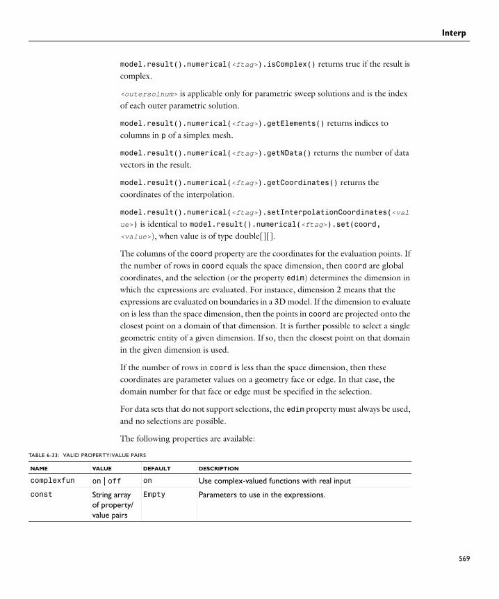
Interp
model.result().numerical(<ftag>).isComplex() returns true if the result is complex.
<outersolnum> is applicable only for parametric sweep solutions and is the index of each outer parametric solution.
model.result().numerical(<ftag>).getElements() returns indices to columns in p of a simplex mesh.
model.result().numerical(<ftag>).getNData() returns the number of data vectors in the result.
model.result().numerical(<ftag>).getCoordinates() returns the coordinates of the interpolation.
model.result().numerical(<ftag>).setInterpolationCoordinates(<val
ue>) is identical to model.result().numerical(<ftag>).set(coord, <value>), when value is of type double[][].
The columns of the coord property are the coordinates for the evaluation points. If the number of rows in coord equals the space dimension, then coord are global coordinates, and the selection (or the property edim) determines the dimension in which the expressions are evaluated. For instance, dimension 2 means that the expressions are evaluated on boundaries in a 3D model. If the dimension to evaluate on is less than the space dimension, then the points in coord are projected onto the closest point on a domain of that dimension. It is further possible to select a single geometric entity of a given dimension. If so, then the closest point on that domain in the given dimension is used.
If the number of rows in coord is less than the space dimension, then these coordinates are parameter values on a geometry face or edge. In that case, the domain number for that face or edge must be specified in the selection.
For data sets that do not support selections, the edim property must always be used, and no selections are possible.
The following properties are available:
TABLE 6-33: VALID PROPERTY/VALUE PAIRS
NAME VALUE DEFAULT DESCRIPTION
complexfun on | off on Use complex-valued functions with real input
const String array of property/value pairs
Empty Parameters to use in the expressions.
569

Interp
570 | C H A P T
coord double matrix
Empty The coordinates to evaluate in. Data sets that define an interpolation in themselves, such as cut planes, revolve etc., can be evaluated directly in the coordinates that define their shapes, without specifying coord.
coorderr on | off on If on, evaluating for a set of points that all fall outside the geometry results in an error being reported.
data none | data set name
First compatible data set
The data set this feature refers to.
differential on | off on Whether the expression should be linearized at the linearization point. Applicable only if evalmethod is harmonic
edim auto | 0 | 1 | 2 | 3
auto Element dimension. This is used for arbitrary data sets. Solution data sets use selections as usual to specify where to perform the evaluation, and ignore the value of the edim property.
evalmethod linpoint | harmonic | lintotal | lintotalavg | lintotalrms | lintotalpeak
harmonic Applicable only for solutions with a stored linearization point. Controls if the linearization point, the perturbation, or a combination should be used when evaluating the expression.
expr string array Model-dependent
The expressions to evaluate.
ext double between 0 and 1
0.1 Extrapolation distance: How much outside the mesh that the interpolation searches. The scale is in terms of the local element size.
matherr on | off off Error for undefined operation or variable
outersolnum non-negative integer
1 The index of the outer solutions to use. Applicable only for parametric sweep models.
phase double 0 Evaluate solution at this angle, given in degrees.
recover off | pprint | ppr
off The derivative recovery method.
solnum non-negative integer array
All solutions
The solutions to use.
TABLE 6-33: VALID PROPERTY/VALUE PAIRS
NAME VALUE DEFAULT DESCRIPTION
E R 6 : R E S U L T S

Interp
See Also Eval, Global (numerical), EvalPoint, EvalGlobal
t double array Empty The times to use. Available when the underlying solution is transient.
unit String Model-dependent
The unit to use for the expression in expr. If the old unit is not valid when the expression changes, the unit property is reset to default.
TABLE 6-33: VALID PROPERTY/VALUE PAIRS
NAME VALUE DEFAULT DESCRIPTION
571

IntVolume, IntSurface, IntLine
572 | C H A P T
IntVolume, IntSurface, IntLineSynopsis Integration numerical results.
Syntax model.result().numerical().create(<ftag>,"IntVolume");model.result().numerical().create(<ftag>,"IntSurface");model.result().numerical().create(<ftag>,"IntLine");model.result().numerical(<ftag>).selection(...);model.result().numerical(<ftag>).set(property, <value>);model.result().numerical(<ftag>).getReal();model.result().numerical(<ftag>).getReal(<columnwise>);model.result().numerical(<ftag>).getReal(<outersolnum>);model.result().numerical(<ftag>).getReal(<columnwise>,
<outersolnum>);model.result().numerical(<ftag>).getImag();model.result().numerical(<ftag>).getImag(<allocate>,
<columnwise>);model.result().numerical(<ftag>).getImag(<outersolnum>);model.result().numerical(<ftag>).getImag(<allocate>, <columnwise>,
<outersolnum>);model.result().numerical(<ftag>).isComplex();model.result().numerical(<ftag>).isComplex(<outersolnum>);model.result().numerical(<ftag>).setResult();model.result().numerical(<ftag>).appendResult();
Description model.result().numerical().create(<ftag>,"IntVolume") creates a volume integral feature with the name <ftag>.
model.result().numerical().create(<ftag>,"IntSurface") creates a surface integral feature with the name <ftag>.
model.result().numerical().create(<ftag>,"IntLine") creates a line integral feature with the name <ftag>.
model.result().numerical(<ftag>).getReal() returns the real result, recomputing the feature if necessary. Data is ordered such that one row contains data for all solution numbers. This is identical to (columnwise) when columnwise is false. If columnwise is true, the ordering is the opposite: each column contains the values for all solution numbers.
model.result().numerical(<ftag>).getImag(allocate, columnwise) returns the imaginary part of complex result, recomputing the feature if necessary. If allocate is true, a zero-valued matrix is allocated even when the result is real. getImag() uses allocate true and columnwise false.
model.result().numerical(<ftag>).isComplex() returns true if the result is complex.
E R 6 : R E S U L T S

IntVolume, IntSurface, IntLine
<outersolnum> is applicable only for parametric sweep solutions and is the index of each outer parametric solution.
model.result().numerical(<ftag>).setResult() and model.result().numerical(<ftag>).appendResult() evaluates the feature and set or append the result in the table indicated by the table property.
The following properties are available:
TABLE 6-34: VALID PROPERTY/VALUE PAIRS
NAME VALUE DEFAULT DESCRIPTION
const String array of property/value pairs
Empty Parameters to use in the expressions.
data none | data set name
First compatible data set
The data set this feature refers to.
dataseries average | integral | maximum | minimum | none | rms | stddev | variance
none The operation that is applied to the data series formed by the evaluation.
descr string Model-dependent The description of the expression in expr. Is used in the automatic title.
differential on | off on Whether the expression should be linearized at the linearization point. Applicable only if evalmethod is harmonic
evalmethod linpoint | harmonic | lintotal | lintotalavg | lintotalrms | lintotalpeak
harmonic Applicable only for solutions with a stored linearization point. Controls if the linearization point, the perturbation, or a combination should be used when evaluating the expression.
expr string Model-dependent The expression to plot.
innerinput all | first | last | manual | manualindices | interp
all How to input the solution to use. manual indicates that solnum is used. manualindices indicates that solnumindices is used. interp indicates that t is used.
573

IntVolume, IntSurface, IntLine
574 | C H A P T
interp double row matrix
Empty on all levels.
The times to use, for transient levels. Available when data is not parent and the underlying data is transient.
intorder positive integer
4 The integration order.
intorderactive on | off off Whether to use manually specified integration order.
intsurface on | off off Compute surface integral. Available for line integration features of axisymmetric models.
intvolume on | off off Compute volume integral. Available for surface integration features of axisymmetric models.
looplevel integer row matrix
All solutions on all levels
The solutions to use, per level.
looplevelindices
integer row matrix
Empty An alternate way to specify the solutions to use, allowing you to enter, for example, range(1,1,20). Applicable when looplevelinput is manualindices on a level.
looplevelinput String array with all | first | last | manual | manualindices | interp on each level
all on all levels How to input the solution to use, per level. manual on a level indicates that looplevel is used on that level. manualindices on a level indicates that looplevelindices is used on that level. interp on a level indicates that interp is used on that level.
maximumobj abs | real real The value being maximized if dataseries is maximum.
method auto | integration | summation
auto The integration method.
minimumobj abs | real real The value being minimized if dataseries is minimum.
outerinput all | first | last | manual | manualindices
all How to input the outer solutions to use. Applicable only for parametric sweep models. manual indicates that outersolnum is used. manualindices indicates that outersolnumindices is used.
TABLE 6-34: VALID PROPERTY/VALUE PAIRS
NAME VALUE DEFAULT DESCRIPTION
E R 6 : R E S U L T S

IntVolume, IntSurface, IntLine
See Also EvalGlobal, EvalPoint, Global (numerical)
outersolnum non-negative integer array
1 The index of the outer solutions to use. Applicable only for parametric sweep models. Since the various outer solutions can have different number of solnum, the solnum property is not used.
outersolnumindices
string or integer array
Empty An alternate way to specify the outer solutions to use, allowing you to enter, for example, range(1,1,20). Applicable when outerinput is manualindices.
solnum non-negative integer array
All solutions The solutions to use.
solnumindices string or integer array
Empty An alternate way to specify the solutions to use, allowing you to enter, for example, range(1,1,20). Applicable when innerinput is manualindices.
solrepresentation
solnum | solutioninfo
solutioninfo Indicates which method of selecting solutions is active.
t double array Empty The times to use. Available when the underlying solution is transient.
table new | table name
new The table to use when calling setResult() or appendResult(). new indicates that a new table is created.
tablecols inner | outer | data | level1
data Whether to use inner or outer solutions as columns in the table when calling setResult() or appendResult(). Applicable only for parametric sweep models. The level values (level1, level2, and so on) are the levels in the parametric sweep.
timeinterp on | off off on if t is used to determine time steps, off if solnum is used.
unit string Model-dependent The unit to use for the expression in expr. If the old unit is not valid when the expression changes, the unit property is reset to default.
TABLE 6-34: VALID PROPERTY/VALUE PAIRS
NAME VALUE DEFAULT DESCRIPTION
575

Isosurface
576 | C H A P T
IsosurfaceSynopsis Isosurface plot.
Syntax model.result(<pgtag>).feature().create(<ftag>,"Isosurface");model.result(<pgtag>).feature(<ftag>).set(property, <value>);model.result(<pgtag>).feature(<ftag>).run();
Description model.result(<pgtag>).feature().create(<ftag>,"Isosurface") creates an isosurface plot feature named <ftag> belonging to the plot group <pgtag>.
The following properties are available:
TABLE 6-35: VALID PROPERTY/VALUE PAIRS
PROPERTY VALUE DEFAULT DESCRIPTION
color custom | black | blue | cyan | green | magenta | red | white | yellow
red The uniform color to use. Active when coloring is uniform.
coloring colortable | uniform
colortable How to color this isosurface.
colorlegend on | off on Whether to show color legend, when coloring is set to colortable.
colortable colortable name
Rainbow The color table to use when colormethod is set to colortable.
colortablerev
on | off off Whether to reverse to color table when colormethod is set to colortable.
colortablesym
on | off off Whether to symmetrize the color range around 0 when colormethod is set to colortable.
const String array of property/value pairs
Empty Parameters to use in the expressions.
customcolor RGB-triplet {1,0,0} or last used color.
The uniform color to use. Active when color is set to custom.
data none | parent | data set name
parent The data set this feature refers to.
descr string Model-dependent
The description of the expression in expr. Is used in the automatic title.
E R 6 : R E S U L T S

Isosurface
descriptionintitle
on | off on Whether the title contribution should contain the description when titletype is custom.
differential on | off on Whether the expression should be linearized at the linearization point. Applicable only if evalmethod is harmonic
evalmethod linpoint | harmonic | lintotal | lintotalavg | lintotalrms | lintotalpeak
harmonic Applicable only for solutions with a stored linearization point. Controls if the linearization point, the perturbation, or a combination should be used when evaluating the expression.
expr string Model-dependent
The expression to plot.
expressionintitle
on | off off Whether the title contribution should contain the expression when titletype is custom.
inheritcolor boolean true If inheritplot is not none: Determines if the color is inherited.
inheritdeformscale
boolean true If inheritplot is not none: Determines if the deformation scale is inherited.
inheritplot none | plot name
none The plot that color and deformation scale is inherited from.
interactive on | off off If true, the isosurfaces can be moved interactively after the plot has been made.
interp double array Time corresponding to last selected solnum for transient levels.
The time to use, for transient levels. Available when data is not parent and the underlying data is transient.
levelmethod number | levels
number How to enter isosurface levels.
levels double array The levels to plot. Active when levelmethod equals levels.
TABLE 6-35: VALID PROPERTY/VALUE PAIRS
PROPERTY VALUE DEFAULT DESCRIPTION
577

Isosurface
578 | C H A P T
looplevel array of non-negative integers and strings
Last solution for transient or parametric solution for each level. Otherwise first solution for each level.
The index of the solution to use, per level, or interp, but only for transient solutions. Available when data is not parent and the underlying data has multiple solutions.
number positive integer
5 Total number of iso levels. Active when levelmethod equals number.
outersolnum non-negative integer
1 The index of the outer solutions to use. Applicable only for parametric sweep models.
prefixintitle
string Empty Added prefix to contribution to title.
recover off | pprint | ppr
off The derivative recovery method.
refine non-negative integer
1 The element refinement to use, if resolution is set to manual. Bear in mind that this is the refinement used for the base data set, so the number of elements in the model can increase radically if the plot uses, for example, a revolve data set.
resolution norefine | coarse | normal | fine | finer | extrafine | custom
normal Controls the plot’s resolution. A finer setting results in a higher resolution by modifying the internally computed default refinement. Use custom to enter your own refinement in the refine property.
smooth none | internal | everywhere
internal Smoothing settings.
shift double 0 If interactive is on: The shift that is applied to the level values.
TABLE 6-35: VALID PROPERTY/VALUE PAIRS
PROPERTY VALUE DEFAULT DESCRIPTION
E R 6 : R E S U L T S

Isosurface
Attributes Color, Deform, Filter
See Also Isosurface (data set), Slice, Volume
solnum non-negative integer
Last solution for transient or parametric solution. Otherwise first solution.
The index of the solution to use. Available when data is not parent and the underlying data has multiple solutions.
solrepresentation
solnum | solutioninfo
solutioninfo
Indicates which method of selecting solutions is active.
suffixintitle
string Empty Added suffix to contribution to title.
t double Time corresponding to last selected solnum.
The time to use, for transient problems. Available when data is not parent and the underlying data is transient.
timeinterp on | off off on if t is used to determine time steps, off if solnum is used.
title string The auto-title. The title to use when titletype is manual.
titletype auto | custom | manual | none
auto auto if the title contribution should be computed automatically, possibly using the group’s customization. custom if the title contribution should be computed automatically, but customized. manual if the manual title contribution should be used (the title property). none if no title contribution should be used.
typeintitle on | off on Whether the title contribution should contain the type when titletype is custom.
unit string Model-dependent
The unit to use for the expression in expr. If the old unit is not valid when the expression changes, the unit property is reset to default.
unitintitle on | off on Whether the title contribution should contain the unit when titletype is custom.
useder boolean true Only for isosurface plots: If true, space derivatives of the iso expression are used to produce smoother plots.
TABLE 6-35: VALID PROPERTY/VALUE PAIRS
PROPERTY VALUE DEFAULT DESCRIPTION
579

Isosurface (data set)
580 | C H A P T
Isosurface (data set)Synopsis Isosurface data set.
Syntax model.result().dataset().create(<dtag>,"Isosurface");model.result().dataset(<dtag>).set(property, <value>);
Description model.result().dataset().create(<dtag>,"Isosurface") creates an isosurface data set feature named <dtag>.
The following properties are available:
See Also Isosurface
TABLE 6-36: VALID PROPERTY/VALUE PAIRS
NAME VALUE DEFAULT DESCRIPTION
data none | data set name
First compatible data set
The data set this feature refers to.
descr string Description of expr.
differential on | off on Whether the expression should be linearized at the linearization point. Applicable only if evalmethod is harmonic
evalmethod linpoint | harmonic | lintotal | lintotalavg | lintotalrms | lintotalpeak
harmonic Applicable only for solutions with a stored linearization point. Controls if the linearization point, the perturbation, or a combination should be used when evaluating the expression.
expr string u Expression to find constant level for.
level double array {0} Levels that defines the data set if levelmethod is levels.
levelmethod number | levels
number How to specify levels.
number positive integer
5 Total number of contour levels. Active when levelmethod is number.
unit string Unit of expr. If the old unit is not valid when the expression changes, the unit property is reset to default.
E R 6 : R E S U L T S

Join
JoinSynopsis Join data set.
Syntax model.result().dataset().create(<dtag>,"Join");model.result().dataset(<dtag>).set(property, <value>);
Description model.result().dataset().create(<dtag>,"Join") creates a join data set feature named <dtag>.
The following properties are available:
TABLE 6-37: VALID PROPERTY/VALUE PAIRS
NAME VALUE DEFAULT DESCRIPTION
data none | data set name
None The first source data set.
data2 none | data set name
None The second source data set.
expr string data1-data2 When method is general: The way the evaluations in the first and second data sets is combined. data1 and data2 can be used as symbols for the values from the two data sets, respectively.
method difference | explicit | general | product | quotient | sum
difference How to combine the results from evaluating in the two source data sets.
solutions all | one all Whether to expose one or all solutions from the first data set.
solutions2 all | one all Whether to expose one or all solutions from the second data set.
581

Line
582 | C H A P T
LineSynopsis Line plot.
Syntax model.result(<pgtag>).feature().create(<ftag>,"Line");model.result(<pgtag>).feature(<ftag>).set(property, <value>);model.result(<pgtag>).feature(<ftag>).run();
Description model.result(<pgtag>).feature().create(<ftag>,"Line") creates a line plot feature named <ftag> belonging to the plot group <pgtag>.
Line plots display a quantity on lines, curves and edges in 2D or 3D.
The following properties are available:
TABLE 6-38: VALID PROPERTY/VALUE PAIRS
PROPERTY VALUE DEFAULT DESCRIPTION
color custom | black | blue | cyan | green | magenta | red | white | yellow
red The uniform color to use. Active when coloring is uniform.
coloring colortable | uniform
colortable How to color this line plot.
colorlegend on | off on Whether to show color legend, when coloring is set to colortable.
colortable colortable name
Rainbow The color table to use when colormethod is set to colortable.
colortablerev on | off off Whether to reverse to color table when colormethod is set to colortable.
colortablesym on | off off Whether to symmetrize the color range around 0 when colormethod is set to colortable.
const String array of property/value pairs
Empty Parameters to use in the expressions.
customcolor RGB-triplet {1,0,0} or last used color.
The uniform color to use. Active when color is set to custom.
data none | parent | data set name
parent The data set this feature refers to.
descr string Model-dependent.
The description of the expression in expr. Is used in the automatic title.
E R 6 : R E S U L T S

Line
descriptionintitle
on | off on Whether the title contribution should contain the description when titletype is custom.
differential on | off on Whether the expression should be linearized at the linearization point. Applicable only if evalmethod is harmonic
evalmethod linpoint | harmonic | lintotal | lintotalavg | lintotalrms | lintotalpeak
harmonic Applicable only for solutions with a stored linearization point. Controls if the linearization point, the perturbation, or a combination should be used when evaluating the expression.
expr string Model-dependent.
The expression to plot.
expressionintitle
on | off off Whether the title contribution should contain the expression when titletype is custom.
inheritcolor boolean true If inheritplot is not none: Determines if the color is inherited.
inheritdeformscale
boolean true If inheritplot is not none: Determines if the deformation scale is inherited.
inheritplot none | plot name
none The plot that color, color range, tube scale, and deformation scale is inherited from.
inheritrange boolean true If inheritplot is not none: Determines if the color and data ranges are inherited.
inherittubescale
boolean true If inheritplot is not none and linetype is tube: Determines if the tube scale is inherited.
interp double array Time corresponding to last selected solnum for transient levels.
The time to use, for transient levels. Available when data is not parent and the underlying data is transient.
linetype line | tube line Plot lines or tubes.
TABLE 6-38: VALID PROPERTY/VALUE PAIRS
PROPERTY VALUE DEFAULT DESCRIPTION
583

Line
584 | C H A P T
looplevel array of non-negative integers and strings
Last solution for transient or parametric solution for each level. Otherwise first solution for each level.
The index of the solution to use, per level, or interp, but only for transient solutions. Available when data is not parent and the underlying data has multiple solutions.
outersolnum non-negative integer
1 The index of the outer solutions to use. Applicable only for parametric sweep models.
prefixintitle string Empty Added prefix to contribution to title.
radiusexpr string 1 The tube radius. Active when linetype is tubes.
rangecoloractive
on | off off Whether to use the manual color range specified in rangecolormin and rangecolormax. The color range specifies the minimum and maxim value in the plotted colors. Default is the minimum and maximum data values.
rangecolormax double Plot-dependent The maximum color range value. Active when rangecoloractive is on.
rangecolormin double Plot-dependent The minimum color range value. Active when rangecoloractive is on.
rangedatactive on | off off Whether to use the manual data range specified in rangedatamin and rangedatamax. Values outside the data range is not plotted.
rangedatamax double Plot-dependent The maximum data value. Active when rangedataactive is on.
rangedatamin double Plot-dependent The minimum data value. Active when rangedataactive is on.
recover off | pprint | ppr
off The derivative recovery method.
refine non-negative integer
1 The element refinement to use, if resolution is set to manual. Bear in mind that this is the refinement used for the base data set, so the number of elements in the model can increase radically if the plot uses, for example, a revolve data set.
TABLE 6-38: VALID PROPERTY/VALUE PAIRS
PROPERTY VALUE DEFAULT DESCRIPTION
E R 6 : R E S U L T S

Line
resolution norefine | coarse | normal | fine | finer | extrafine | custom
normal Controls the plot’s resolution. A finer setting results in a higher resolution by modifying the internally computed default refinement. Use custom to enter your own refinement in the refine property.
smooth none | internal | everywhere
internal Smoothing settings.
solnum non-negative integer
Last solution for transient or parametric solution. Otherwise first solution.
The index of the solution to use. Available when data is not parent and the underlying data has multiple solutions.
solrepresentation
solnum | solutioninfo
solutioninfo
Indicates which method of selecting solutions is active.
suffixintitle string Empty Added suffix to contribution to title.
t double Time corresponding to last selected solnum.
The time to use, for transient problems. Available when data is not parent and the underlying data is transient.
timeinterp on | off off on if t is used to determine time steps, off if solnum is used.
title string The auto-title The title to use when titletype is manual.
titletype auto | custom | manual | none
auto auto if the title contribution should be computed automatically, possibly using the group’s customization. custom if the title contribution should be computed automatically, but customized. manual if the manual title contribution should be used (the title property). none if no title contribution should be used.
tuberadiusscale double 1 The scale factor applied to the tube radii if tuberadiusscaleactive is true.
tuberadiusscaleactive
boolean false If true, tuberadiusscale is used, otherwise the scale factor is computed automatically
typeintitle on | off on Whether the title contribution should contain the type when titletype is custom.
TABLE 6-38: VALID PROPERTY/VALUE PAIRS
PROPERTY VALUE DEFAULT DESCRIPTION
585

Line
586 | C H A P T
Attributes Deform, Filter, Height
Examples Line plot on 2D solution:
model.result().dataset().create("dset1", "Solution");model.result().dataset("dset1").set("solution", "sol1");
result().create("pg1",2);result("pg1").set("data","dset1");result("pg1").feature().create("line1","Line");
result("pg1").feature("lngr1").set("expr", "3*u");
Line plot on cut plane in 3D:
result().dataset().create("cp1", "CutPlane");result().dataset("cp1").set("data", "dset2");
result().create("pg2",3);result("pg2").feature().create("line2","Line");result("pg2").feature("line2").set("data", "cp1");result("pg2").feature("line2").set("expr", "2*u");result("pg2").feature("line2").set("colortable", "Thermal");
result("pg2").run();
See Also LineGraph
unit string Model-dependent
The unit to use for the expression in expr. If the old unit is not valid when the expression changes, the unit property is reset to default.
unitintitle on | off on Whether the title contribution should contain the unit when titletype is custom.
wireframe on | off off Whether to plot filled elements or only their edges.
TABLE 6-38: VALID PROPERTY/VALUE PAIRS
PROPERTY VALUE DEFAULT DESCRIPTION
E R 6 : R E S U L T S

LineGraph
LineGraphSynopsis Line graph plot.
Syntax model.result(<pgtag>).feature().create(<ftag>,"LineGraph");model.result(<pgtag>).feature(<ftag>).selection(...);model.result(<pgtag>).feature(<ftag>).set(property, <value>);model.result(<pgtag>).feature(<ftag>).run();
Description model.result(<pgtag>).feature().create(<ftag>,"LineGraph") creates a line graph plot feature named <ftag> belonging to the plot group <pgtag>.
Line graph plot is used to visualize quantities on lines, either cut lines or boundaries (2D) and edges (3D) in a geometry. Line graph plots can be added to 1D plot groups.
The following properties are available:
TABLE 6-39: VALID PROPERTY/VALUE PAIRS
NAME VALUE DEFAULT DESCRIPTION
autlegends on | off on Whether to use the automatically generated legends or the legends defined in the legends property.
const String array of property/value pairs
Empty Parameters to use in the expressions.
customlinecolor
RGB-triplet {0,0,1} or last used edgecolor.
The color to use for the lines. Active when linecolor is set to custom.
data none | parent | data set name
parent The data set this feature refers to.
descr string Model-dependent The description of the expression in expr. Is used in the automatic title.
descriptionintitle
on | off on Whether the title contribution should contain the description when titletype is custom.
differential on | off on Whether the expression should be linearized at the linearization point. Applicable only if evalmethod is harmonic
evalmethod linpoint | harmonic | lintotal | lintotalavg | lintotalrms | lintotalpeak
harmonic Applicable only for solutions with a stored linearization point. Controls if the linearization point, the perturbation, or a combination should be used when evaluating the expression.
expr string Model-dependent The expression to plot.
587

LineGraph
588 | C H A P T
expressionintitle
on | off off Whether the title contribution should contain the expression when titletype is custom.
innerinput all | first | last | manual | manualindices | interp
all How to input the solution to use. manual indicates that solnum is used. manualindices indicates that solnumindices is used. interp indicates that t is used.
interp double row matrix
Empty on all levels.
The times to use, for transient levels. Available when data is not parent and the underlying data is transient.
legend on | off off Whether to show legends.
legendmethod automatic | manual
automatic Whether to use the automatic legends or the legends supplied in the legends property.
legends string array The last computed automatic legends
Manual legends active when legendmethod is set to manual.
linecolor custom | cycle | black | blue | cyan | green | magenta | red | white | yellow
cycle How to color the lines in the graph. Cycle indicates that the colors is different for each line.
linewidth double 0.5 The line width.
linemarker none | cycle | asterisk | circle | diamond | plus | point | square | star | triangle
none The line markers, if any. Cycle indicates that the marker is different for each line.
looplevel integer row matrix
All solutions on all levels
The solutions to use, per level.
looplevelindices
integer row matrix
Empty An alternate way to specify the solutions to use, allowing you to enter, for example, range(1,1,20). Applicable when looplevelinput is manualindices on a level.
TABLE 6-39: VALID PROPERTY/VALUE PAIRS
NAME VALUE DEFAULT DESCRIPTION
E R 6 : R E S U L T S

LineGraph
looplevelinput String array with all | first | last | manual | manualindices | interp on each level
all on all levels How to input the solution to use, per level. manual on a level indicates that looplevel is used on that level. manualindices on a level indicates that looplevelindices is used on that level. interp on a level indicates that interp is used on that level.
markerpos interp | datapoints
interp Controls whether the positions of the markers are in the data points of the plot, or interpolated depending on the number (set in markers). Markers are visible when linemarker is set.
markers integer 8 The number of markers to show. Markers are visible when linemarker is set.
linestyle none | cycle | solid | dotted | dashed | dashdot
solid The line style, if any. Cycle indicates that the line style is different for each line.
outerinput all | first | last | manual | manualindices
all How to input the outer solutions to use. Applicable only for parametric sweep models. manual indicates that outersolnum is used. manualindices indicates that outersolnumindices is used.
outersolnum non-negative integer array
1 The index of the outer solutions to use. Applicable only for parametric sweep models. Since the various outer solutions can have different number of solnum, the solnum property is not used.
outersolnumindices
string or integer array
Empty An alternate way to specify the outer solutions to use, allowing you to enter, for example, range(1,1,20). Applicable when outerinput is manualindices.
prefixintitle string Empty Added prefix to contribution to title.
refine non-negative integer
1 The element refinement to use, if resolution is set to manual. Bear in mind that this is the refinement used for the base data set, so the number of elements in the model can increase radically if the plot uses, for example, a revolve data set.
TABLE 6-39: VALID PROPERTY/VALUE PAIRS
NAME VALUE DEFAULT DESCRIPTION
589

LineGraph
590 | C H A P T
resolution norefine | coarse | normal | fine | finer | extrafine | custom
normal Controls the plot’s resolution. A finer setting results in a higher resolution by modifying the internally computed default refinement. Use custom to enter your own refinement in the refine property.
solnum integer array All solutions The solutions to plot. Available when data is not parent and the underlying data has multiple solutions.
solnumindices string or integer array
Empty An alternate way to specify the solutions to use, allowing you to enter, for example, range(1,1,20). Applicable when innerinput is manualindices.
solrepresentation
solnum | solutioninfo
solutioninfo Indicates which method of selecting solutions is active.
suffixintitle string Empty Added suffix to contribution to title.
t double array Empty The times to plot. Available when data is not parent and the underlying solution is transient.
title string The auto-title The title to use when titletype is manual.
titletype auto | custom | manual | none
auto auto if the title contribution should be computed automatically, possibly using the group’s customization. custom if the title contribution should be computed automatically, but customized. manual if the manual title contribution should be used (the title property). none if no title contribution should be used.
typeintitle on | off on Whether the title contribution should contain the type when titletype is custom.
unit string Model-dependent The unit to use for the expression in expr. If the old unit is not valid when the expression changes, the unit property is reset to default.
unitintitle on | off on Whether the title contribution should contain the unit when titletype is custom.
xdata expr | solution
solution x-axis data. expr uses the expression in xdataexpr. solution uses the available solutions in the underlying data set such as time steps.
xdataexpr string Model-dependent Expression for x-axis data.
TABLE 6-39: VALID PROPERTY/VALUE PAIRS
NAME VALUE DEFAULT DESCRIPTION
E R 6 : R E S U L T S

LineGraph
Attributes None
See Also Line
xdatadescr string Model-dependent Description of expression in xdataexpr.
xdataunit string Model-dependent The unit to use for the expression in xdataexpr. If the old unit is not valid when the expression changes, the unit property is reset to default.
TABLE 6-39: VALID PROPERTY/VALUE PAIRS
NAME VALUE DEFAULT DESCRIPTION
591

MaxMinVolume, MaxMinSurface, MaxMinLine
592 | C H A P T
MaxMinVolume, MaxMinSurface, MaxMinLineSynopsis Max/min marker plots.
Syntax model.result(<pgtag>).feature().create(<ftag>,"MaxMinVolume");model.result(<pgtag>).feature().create(<ftag>,"MaxMinSurface");model.result(<pgtag>).feature().create(<ftag>,"MaxMinLine");model.result(<pgtag>).feature(<ftag>).set(property, <value>);model.result(<pgtag>).feature(<ftag>).run();
Description model.result(<pgtag>).feature().create(<ftag>,"MaxMinVolume") creates a max/min marker plot feature named <ftag> belonging to the plot group <pgtag>.
This plot type displays the maximum and minimum of an expression and the points there they are attained.
The following properties are available:
TABLE 6-40: VALID PROPERTY/VALUE PAIRS
NAME VALUE DEFAULT DESCRIPTION
color custom | black | blue | cyan | green | magenta | red | white | yellow
black The color with which markers will be plotted.
const String array of property/value pairs
Empty Parameters to use in the expressions.
customcolor RGB-triplet {1,0,0} or last used color
The color to use when color is set to custom.
data none | parent | data set name
parent The data set this feature refers to.
descriptionintitle
on | off on Whether the title contribution should contain the description when titletype is custom.
display minmax | min | max
minmax The selection determines which markers are shown.
differential on | off on Whether the expression should be linearized at the linearization point. Applicable only if evalmethod is harmonic
E R 6 : R E S U L T S

MaxMinVolume, MaxMinSurface, MaxMinLine
Attributes Deform
evalmethod linpoint | harmonic | lintotal | lintotalavg | lintotalrms | lintotalpeak
harmonic Applicable only for solutions with a stored linearization point. Controls if the linearization point, the perturbation, or a combination should be used when evaluating the expression.
expr string The expression to compute the maximum and minimum for.
expressionintitle
on | off off Whether the title contribution should contain the expression when titletype is custom.
inheritcolor boolean true If inheritplot is not none: Determines if the color is inherited.
inheritdeformscale
boolean true If inheritplot is not none: Determines if the deformation scale is inherited.
inheritplot none | plot name
none The plot that deformation scale is inherited from.
precision integer > 0 6 The number of decimals displayed in the labels in the GUI.
prefixintitle string Empty Added prefix to contribution to title.
refine integer > 0 2 The number of refinements of each mesh element when computing the maximum and minimum.
recover off | pprint | ppr
off The derivative recovery method.
suffixintitle string Empty Added suffix to contribution to title.
title string The auto-title The title to use when titletype is manual.
titletype auto | custom | manual | none
auto auto if the title contribution should be computed automatically, possibly using the group’s customization. custom if the title contribution should be computed automatically, but customized. manual if the manual title contribution should be used (the title property). none if no title contribution should be used.
typeintitle on | off on Whether the title contribution should contain the type when titletype is custom.
unitintitle on | off on Whether the title contribution should contain the unit when titletype is custom.
TABLE 6-40: VALID PROPERTY/VALUE PAIRS
NAME VALUE DEFAULT DESCRIPTION
593

MaxVolume, MaxSurface, MaxLine, MinVolume, MinSurface, MinLine
594 | C H A P T
MaxVolume, MaxSurface, MaxLine, MinVolume, MinSurface, MinLineSynopsis Finding external values.
Syntax model.result().numerical().create(<ftag>,"MaxVolume");model.result().numerical().create(<ftag>,"MinVolume");model.result().numerical().create(<ftag>,"MaxSurface");model.result().numerical().create(<ftag>,"MinSurface");model.result().numerical().create(<ftag>,"MaxLine");model.result().numerical().create(<ftag>,"MinLine");model.result().numerical(<ftag>).selection(...);model.result().numerical(<ftag>).set(property, <value>);model.result().numerical(<ftag>).getReal();model.result().numerical(<ftag>).getReal(<columnwise>);model.result().numerical(<ftag>).getReal(<outersolnum>);model.result().numerical(<ftag>).getReal(<columnwise>,
<outersolnum>);model.result().numerical(<ftag>).getImag();model.result().numerical(<ftag>).getImag(<allocate>,
<columnwise>);model.result().numerical(<ftag>).getImag(<outersolnum>);model.result().numerical(<ftag>).getImag(<allocate>, <columnwise>,
<outersolnum>);model.result().numerical(<ftag>).isComplex();model.result().numerical(<ftag>).isComplex(<outersolnum>);model.result().numerical(<ftag>).setResult();model.result().numerical(<ftag>).appendResult();
Description model.result().numerical().create(<ftag>,"MaxVolume") creates a volume maximum feature with the name <ftag>, and similarly for "MinVolume".
model.result().numerical().create(<ftag>,"MaxSurface") creates a surface maximum feature with the name <ftag>, and similarly for "MinSurface".
model.result().numerical().create(<ftag>,"MaxLine") creates a line maximum feature with the name <ftag>, and similarly for "MinLine".
model.result().numerical(<ftag>).getReal() returns the real result, recomputing the feature if necessary. Data is ordered such that one row contains data for all solution numbers. This is identical to (columnwise) when columnwise is false. If columnwise is true, the ordering is the opposite: each column contains the values for all solution numbers.
model.result().numerical(<ftag>).getImag(allocate, columnwise) returns the imaginary part of complex result, recomputing the feature if necessary. If allocate is true, a zero-valued matrix is allocated even when the result is real. getImag() uses allocate true and columnwise false.
E R 6 : R E S U L T S

MaxVolume, MaxSurface, MaxLine, MinVolume, MinSurface, MinLine
model.result().numerical(<ftag>).isComplex() returns true if the result is complex.
<outersolnum> is applicable only for parametric sweep solutions and is the index of each outer parametric solution.
model.result().numerical(<ftag>).setResult() and model.result().numerical(<ftag>).appendResult() evaluates the feature and set or append the result in the table indicated by the table property.
The following properties are available:
TABLE 6-41: VALID PROPERTY/VALUE PAIRS
NAME VALUE DEFAULT DESCRIPTION
const String array of property/value pairs
Empty Parameters to use in the expressions.
data none | data set name
First compatible data set
The data set this feature refers to.
dataseries average | integral | maximum | minimum | none | rms | stddev | variance
none The operation that is applied to the data series formed by the evaluation.
descr string Model-dependent The description of the expression in expr. Is used in the automatic title.
differential on | off on Whether the expression should be linearized at the linearization point. Applicable only if evalmethod is harmonic
evalmethod linpoint | harmonic | lintotal | lintotalavg | lintotalrms | lintotalpeak
harmonic Applicable only for solutions with a stored linearization point. Controls if the linearization point, the perturbation, or a combination should be used when evaluating the expression.
expr string Model-dependent The expression to plot.
innerinput all | first | last | manual | manualindices | interp
all How to input the solution to use. manual indicates that solnum is used. manualindices indicates that solnumindices is used. interp indicates that t is used.
595

MaxVolume, MaxSurface, MaxLine, MinVolume, MinSurface, MinLine
596 | C H A P T
interp double row matrix
Empty on all levels.
The times to use, for transient levels. Available when data is not parent and the underlying data is transient.
looplevel integer row matrix
All solutions on all levels
The solutions to use, per level.
looplevelindices
integer row matrix
Empty An alternate way to specify the solutions to use, allowing you to enter, for example, range(1,1,20). Applicable when looplevelinput is manualindices on a level.
looplevelinput String array with all | first | last | manual | manualindices | interp on each level
all on all levels How to input the solution to use, per level. manual on a level indicates that looplevel is used on that level. manualindices on a level indicates that looplevelindices is used on that level. interp on a level indicates that interp is used on that level.
obj abs | real real The function of each real or complex number that is maximized/minimized.
outerinput all | first | last | manual | manualindices
all How to input the outer solutions to use. Applicable only for parametric sweep models. manual indicates that outersolnum is used. manualindices indicates that outersolnumindices is used.
outersolnum non-negative integer array
1 The index of the outer solutions to use. Applicable only for parametric sweep models. Since the various outer solutions can have different number of solnum, the solnum property is not used.
outersolnumindices
string or integer array
Empty An alternate way to specify the outer solutions to use, allowing you to enter, for example, range(1,1,20). Applicable when outerinput is manualindices.
solnum non-negative integer array
All solutions The solutions to use.
solnumindices string or integer array
Empty An alternate way to specify the solutions to use, allowing you to enter, for example, range(1,1,20). Applicable when innerinput is manualindices.
TABLE 6-41: VALID PROPERTY/VALUE PAIRS
NAME VALUE DEFAULT DESCRIPTION
E R 6 : R E S U L T S

MaxVolume, MaxSurface, MaxLine, MinVolume, MinSurface, MinLine
See Also IntVolume, IntSurface, IntLine
solrepresentation
solnum | solutioninfo
solutioninfo Indicates which method of selecting solutions is active.
t double array Empty The times to use. Available when the underlying solution is transient.
table new | table name
new The table to use when calling setResult() or appendResult(). new indicates that a new table is created.
tablecols inner | outer | data | level1
data Whether to use inner or outer solutions as columns in the table when calling setResult() or appendResult(). Applicable only for parametric sweep models. The level values (level1, level2, and so on) are the levels in the parametric sweep.
timeinterp on | off off on if t is used to determine time steps, off if solnum is used.
unit string Model-dependent The unit to use for the expression in expr. If the old unit is not valid when the expression changes, the unit property is reset to default.
TABLE 6-41: VALID PROPERTY/VALUE PAIRS
NAME VALUE DEFAULT DESCRIPTION
597

Mesh
598 | C H A P T
MeshSynopsis Mesh plot.
Syntax model.result(<pgtag>).feature().create(<ftag>,"Mesh");model.result(<pgtag>).feature(<ftag>).set(property, <value>);model.result(<pgtag>).feature(<ftag>).run();
Description model.result(<pgtag>).feature().create(<ftag>,"Mesh") creates a mesh plot feature named <ftag> belonging to the plot group <pgtag>.
This plot type provides visualization of 2D and 3D meshes.
The following properties are available:
TABLE 6-42: VALID PROPERTY/VALUE PAIRS
NAME VALUE DEFAULT DESCRIPTION
colortable colortable name
Rainbow The element color table to use when elemcolor is set to quality.
data none | parent | data set name
parent The data set this feature refers to.
elemcolor quality | color
quality How to color the elements.
elemfilter random | quality | qualityrev | size | expression | logicalexpression
random If filteractive is on: The expression to use for filtering when only a subset of the elements are shown.
elemscale double in [0,1] 1 The factor with which the elements are scaled before display.
elemtype2 all | tri | quad
all 2D mesh element types to plot.
elemtype3 all | tet | prism | hex
all 3D mesh element types to plot.
filteractive on | off off Whether to use element filtering.
filterexpr string x The expression to use for filtering when elemfilter is set to expression.
logfilterexpr String '1' The logical expression to use for filtering when elemfilter is set to 'logicalexpression'.
E R 6 : R E S U L T S

Mesh
Attributes Filter
See Also Mesh (data set)
meshdomain all | point | edge | surface | volume (if 3D)
all Mesh domain level(s) to plot.
tetkeep Double in [0, 1]
1 The fraction of the elements to display.
title string The auto-title The title to use when titletype is manual.
titletype auto | manual | none
auto auto if the title contribution should be computed automatically, possibly using the group’s customization. manual if the manual title should be used (the title property). none if no title should be displayed.
wireframecolor none | color black How to color the wireframe mesh, 'none' means that it is not displayed at all.
TABLE 6-42: VALID PROPERTY/VALUE PAIRS
NAME VALUE DEFAULT DESCRIPTION
599

Mesh (data set)
600 | C H A P T
Mesh (data set)Synopsis Mesh data set.
Syntax model.result().dataset().create(<dtag>,"Mesh");model.result().dataset(<dtag>).set(property, <value>);
Description model.result().dataset().create(<dtag>,"Mesh") creates a mesh data set feature named <dtag>.
This data set provides support for evaluation of spatial coordinates and mesh variables on a mesh.
The following properties are available:
See Also Mesh
TABLE 6-43: VALID PROPERTY/VALUE PAIRS
NAME VALUE DEFAULT DESCRIPTION
mesh string Empty The mesh that this data set refers to.
E R 6 : R E S U L T S

Mesh (export)
Mesh (export)Synopsis Mesh export.
Syntax model.result().export().create(<ftag>,"Mesh");model.result().export().create(<ftag>,<dtag>,"Mesh");model.result().export(<ftag>).set(property, <value>);model.result().export(<ftag>).run();
Description model.result().export().create(<ftag>,"Mesh") creates a mesh export feature with the name <ftag>.
model.result().export().create(<ftag>,<dtag>,"Mesh") creates a mesh export feature with the name <ftag> for the data set <dtag>.
The following properties are available:
See Also Data
TABLE 6-44: VALID PROPERTY/VALUE PAIRS
PROPERTY VALUE DEFAULT DESCRIPTION
data string The name of the data set to export.
filename string The output file.
outersolnum non-negative integer
1 The index of the outer solutions to use. Applicable only for parametric sweep models.
solnum integer array Solution number to take values from.
stlformat binary | text binary STL file format.
t string Time to evaluate in if timeinterp is on.
timeinterp on | off off Enable/disable explicit time to evaluate in.
601

Mirror2D,Mirror3D
602 | C H A P T
Mirror2D, Mirror3DSynopsis Mirror data set.
Syntax model.result().dataset().create(<dtag>,"Mirror2D");model.result().dataset().create(<dtag>,"Mirror3D");model.result().dataset(<dtag>).set(property, <value>);
Description model.result().dataset().create(<dtag>,"Mirror2D") creates a 2D mirror data set feature named <dtag>.
model.result().dataset().create(<dtag>,"Mirror3D") creates a 3D mirror data set feature named <dtag>.
This data set takes data from another data set and adds a mirror copy with respect to an axis or plane of reflection (for 2D and 3D respectively).
The following properties are available for Mirror 2D and Mirror 3D:
The following properties are available for Mirror 3D:
TABLE 6-45: VALID PROPERTY/VALUE PAIRS
NAME VALUE DEFAULT DESCRIPTION
data none | data set name
First compatible data set
The data set this feature refers to.
genpoints double matrix {{0, 0, 0}, {1,0,0}} Active when method equals twopoint, this property contains the coordinates of the two points in the two rows of the matrix.
hasvar boolean false If true, an axis indicator variable is defined.
method twopoint | pointdir
twopoint Decides if the line should be specified by two points or through one point and a direction.
pddir double array {0,1} Active when method equals pointdir, this property contains the direction.
pdpoint double array {0,0} Active when method equals pointdir, this property contains the coordinates of the point.
sidevar string If hasvar is true: The name of the positive side variable, which is 1 on the side where the original data resides and 0 on the other side.
E R 6 : R E S U L T S

Mirror2D,Mirror3D
TABLE 6-46: VALID PROPERTY/VALUE PAIRS
NAME VALUE DEFAULT DESCRIPTION
data none | data set name
First compatible data set
The data set this feature refers to.
genmethod threepoint | pointnormal
threepoint Active when planetype equals general, this property indicates whether the plane should be specified by three points or through one point and a normal.
genpoints double matrix {{0, 0, 0}, {1,0,0},{0,1,0}}
Active when method equals threepoint, this property contains the coordinates of the three points in the rows of the matrix.
genpnpoint
double array of length three
Zero vector Active when genmethod equals pointnormal, this property contains the coordinates of the point.
genpnvec double array of length three
Zero vector Active when genmethod equals pointnormal, this property contains the normal vector.
hasvar boolean false If true, an axis indicator variable is defined.
planetype quick | general yz Specify plane type.)
quickplane
xy | yz | zx yz Specify quick plane type. Active when planetype is quick.
quickx double 0 x-coordinate if planetype is yz
quicky double 0 y-coordinate if planetype is zx
quickz double 0 z-coordinate if planetype is xy
sidevar string If hasvar is true: The name of the positive side variable, which is 1 on the side where the original data resides and 0 on the other side.
603

Multislice
604 | C H A P T
MultisliceSynopsis Slice plot in multiple directions at once.
Syntax model.result(<pgtag>).feature().create(<ftag>,"Multislice");model.result(<pgtag>).feature(<ftag>).set(property, <value>);model.result(<pgtag>).feature(<ftag>).run();
Description model.result(<pgtag>).feature().create(<ftag>,"Multislice") creates a slice feature in multiple directions named <ftag> belonging to the plot group <pgtag>.
The following properties are available:
TABLE 6-47: VALID PROPERTY/VALUE PAIRS
NAME VALUE DEFAULT DESCRIPTION
color custom | black | blue | cyan | green | magenta | red | white | yellow
red The uniform color to use. Active when coloring is uniform.
coloring colortable | uniform
colortable How to color the slices.
colorlegend on | off on Whether to show color legend, when coloring is set to colortable.
colortable colortable name
Rainbow The color table to use when colormethod is set to colortable.
colortablerev on | off off Whether to reverse to color table when colormethod is set to colortable.
colortablesym on | off off Whether to symmetrize the color range around 0 when colormethod is set to colortable.
const String array of property/value pairs
Empty Parameters to use in the expressions.
customcolor RGB-triplet {1,0,0} or last used color.
The uniform color to use. Active when color is set to custom.
data none | parent | data set name
parent The data set this feature refers to.
descr string Model-dependent. The description of the expression in expr. Is used in the automatic title.
descriptionintitle
on | off on Whether the title contribution should contain the description when titletype is custom.
E R 6 : R E S U L T S

Multislice
differential on | off on Whether the expression should be linearized at the linearization point. Applicable only if evalmethod is harmonic
evalmethod linpoint | harmonic | lintotal | lintotalavg | lintotalrms | lintotalpeak
harmonic Applicable only for solutions with a stored linearization point. Controls if the linearization point, the perturbation, or a combination should be used when evaluating the expression.
expr string Model-dependent. The expression to plot.
expressionintitle
on | off off Whether the title contribution should contain the expression when titletype is custom.
inheritcolor boolean true If inheritplot is not none: Determines if the color is inherited.
inheritdeformscale
boolean true If inheritplot is not none: Determines if the deformation scale is inherited.
inheritplot none | plot name
none The plot that color, color range, and deformation scale is inherited from.
inheritrange boolean true If inheritplot is not none: Determines if the color and data ranges are inherited.
interp double array Time corresponding to last selected solnum for transient levels.
The time to use, for transient levels. Available when data is not parent and the underlying data is transient.
looplevel array of non-negative integers and strings
Last solution for transient or parametric solution for each level. Otherwise first solution for each level.
The index of the solution to use, per level, or interp, but only for transient solutions. Available when data is not parent and the underlying data has multiple solutions.
multiplanexmethod
number | coord
number Indicates whether the x-coordinates of the x-planes should be specified by number of planes to distribute evenly across the data or by coordinates.
multiplaneymethod
number | coord
number Indicates whether the y-coordinates of the y-planes should be specified by number of planes to distribute evenly across the data or by coordinates.
TABLE 6-47: VALID PROPERTY/VALUE PAIRS
NAME VALUE DEFAULT DESCRIPTION
605

Multislice
606 | C H A P T
multiplanezmethod
number | coord
number Indicates whether the z-coordinates of the z-planes should be specified by number of planes to distribute evenly across the data or by coordinates.
outersolnum non-negative integer
1 The index of the outer solutions to use. Applicable only for parametric sweep models.
prefixintitle string Empty Added prefix to contribution to title.
rangecoloractive
on | off off Whether to use the manual color range specified in rangecolormin and rangecolormax. The color range specifies the minimum and maxim value in the plotted colors. Default is the minimum and maximum data values.
rangecolormax double Plot-dependent The maximum color range value. Active when rangecoloractive is on.
rangecolormin double Plot-dependent The minimum color range value. Active when rangecoloractive is on.
rangedatactive on | off off Whether to use the manual data range specified in rangedatamin and rangedatamax. Values outside the data range is not plotted.
rangedatamax double Plot-dependent The maximum data value. Active when rangedataactive is on.
rangedatamin double Plot-dependent The minimum data value. Active when rangedataactive is on.
recover off | pprint | ppr
off The derivative recovery method.
refine non-negative integer
1 The element refinement to use, if resolution is set to manual. Bear in mind that this is the refinement used for the base data set, so the number of elements in the model can increase radically if the plot uses, for example, a revolve data set.
resolution norefine | coarse | normal | fine | finer | extrafine | custom
normal Controls the plot’s resolution. A finer setting results in a higher resolution by modifying the internally computed default refinement. Use custom to enter your own refinement in the refine property.
smooth none | internal | everywhere
internal Smoothing settings.
TABLE 6-47: VALID PROPERTY/VALUE PAIRS
NAME VALUE DEFAULT DESCRIPTION
E R 6 : R E S U L T S

Multislice
suffixintitle string Empty Added suffix to contribution to title.
solnum non-negative integer
Last solution for transient or parametric solution. Otherwise first solution.
The index of the solution to use. Available when data is not parent and the underlying data has multiple solutions.
solrepresentation
solnum | solutioninfo
solutioninfo Indicates which method of selecting solutions is active.
t double Time corresponding to last selected solnum.
The time to use, for transient problems. Available when data is not parent and the underlying data is transient.
timeinterp on | off off on if t is used to determine time steps, off if solnum is used.
title string The auto-title. The title to use when titletype is manual.
titletype auto | custom | manual | none
auto auto if the title contribution should be computed automatically, possibly using the group’s customization. custom if the title contribution should be computed automatically, but customized. manual if the manual title contribution should be used (the title property). none if no title contribution should be used.
typeintitle on | off on Whether the title contribution should contain the type when titletype is custom.
unit string Model-dependent The unit to use for the expression in expr. If the old unit is not valid when the expression changes, the unit property is reset to default.
unitintitle on | off on Whether the title contribution should contain the unit when titletype is custom.
xnumber non-negative integer
1 Number of planes in the x-direction. Active when multiplanexmethod is set to number.
xcoord double array Empty Absolute coordinates in the x-direction, active when multiplanexmethod is set to coord.
ynumber integer 1 Number of planes in the y-direction. Active when multiplaneymethod is set to number.
ycoord double array Empty Absolute coordinates in the z-direction, active when multiplaneymethod is set to coord.
TABLE 6-47: VALID PROPERTY/VALUE PAIRS
NAME VALUE DEFAULT DESCRIPTION
607

Multislice
608 | C H A P T
Attributes Deform, Filter
See Also Slice, Volume
znumber integer 1 Number of planes in the z-direction. Active when multiplanezmethod is set to number.
zcoord double array Empty Absolute coordinates in the z-direction, active when multiplanezmethod is set to coord.
TABLE 6-47: VALID PROPERTY/VALUE PAIRS
NAME VALUE DEFAULT DESCRIPTION
E R 6 : R E S U L T S

Nyquist
NyquistSynopsis Nyquist plot.
Syntax model.result(<pgtag>).feature().create(<ftag>,"Nyquist");model.result(<pgtag>).feature(<ftag>).set(property, <value>);model.result(<pgtag>).feature(<ftag>).run();
Description model.result(<pgtag>).feature().create(<ftag>,"Nyquist") creates a Nyquist plot feature named <ftag> belonging to the plot group <pgtag>.
Nyquist plots are used to visualize complex variables. Nyquist plots can be added to 1D plot groups.
The following properties are available:
TABLE 6-48: VALID PROPERTY/VALUE PAIRS
NAME VALUE DEFAULT DESCRIPTION
autodescr on | off Model dependent
Whether the automatic legends should include the expression descriptions.
autoexpr on | off Model dependent
Whether the automatic legends should include the expressions.
autolegends on | off on Whether to use the automatically computed legends or the legends defined in the legends property. The automatic legends display the description and expression for each line.
const String array of property/value pairs
Empty Parameters to use in the expressions.
customlinecolor RGB-triplet {0,0,1} or last used edgecolor.
The color to use for the lines. Active when linecolor is set to custom.
data none | parent | data set name
parent The data set this feature refers to.
descr string array Model-dependent. The description of the expressions in expr. Is used in the automatic legends.
descriptionintitle
on | off on Whether the title contribution should contain the description when titletype is custom.
differential on | off on Whether the expression should be linearized at the linearization point. Applicable only if evalmethod is harmonic
609

Nyquist
610 | C H A P T
evalmethod linpoint | harmonic | lintotal | lintotalavg | lintotalrms | lintotalpeak
harmonic Applicable only for solutions with a stored linearization point. Controls if the linearization point, the perturbation, or a combination should be used when evaluating the expression.
expr string array Model-dependent. The expressions to plot.
expressionintitle
on | off off Whether the title contribution should contain the expression when titletype is custom.
legend on | off off Whether to show legends.
legendmethod automatic | manual
automatic Whether to use the automatic legends or the legends supplied in the legends property.
legends string array The last computed automatic legends.
Manual legends active when legendmethod is set to manual.
linecolor custom | cycle | black | blue | cyan | green | magenta | red | white | yellow
cycle How to color the lines in the graph. Cycle indicates that the colors is different for each line.
linewidth double 0.5 The line width.
linemarker none | cycle | asterisk | circle | diamond | plus | point | square | star | triangle
none The line markers, if any. Cycle indicates that the marker is different for each line.
linestyle none | cycle | solid | dotted | dashed | dashdot
solid The line style, if any. Cycle indicates that the line style is different for each line.
TABLE 6-48: VALID PROPERTY/VALUE PAIRS
NAME VALUE DEFAULT DESCRIPTION
E R 6 : R E S U L T S

Nyquist
markerpos interp | datapoints
interp Controls whether the positions of the markers are in the data points of the plot, or interpolated depending on the number (set in markers). Markers are visible when linemarker is set.
markers integer 8 The number of markers to show. Markers are visible when linemarker is set.
outersolnum non-negative integer array
1 The index of the outer solutions to use. Applicable only for parametric sweep models. Since the various outer solutions can have different number of solnum, the solnum property is not used.
outersolnumindices
string or integer array
Empty An alternate way to specify the outer solutions to use, allowing you to enter, for example, range(1,1,20). Applicable when outerinput is manualindices.
prefixintitle string Empty Added prefix to contribution to title.
solnum non-negative integer array
All solutions The solutions to plot. Available when data is not parent and the underlying data has multiple solutions.
solnumindices string or integer array
Empty An alternate way to specify the solutions to use, allowing you to enter, for example, range(1,1,20). Applicable when innerinput is manualindices.
suffixintitle string Empty Added suffix to contribution to title.
t double array Empty The times to plot. Available when data is not parent and the underlying solution is transient.
title string The auto-title. The title to use when titletype is manual.
titletype auto | custom | manual | none
auto auto if the title contribution should be computed automatically, possibly using the group’s customization. custom if the title contribution should be computed automatically, but customized. manual if the manual title contribution should be used (the title property). none if no title contribution should be used.
typeintitle on | off on Whether the title contribution should contain the type when titletype is custom.
TABLE 6-48: VALID PROPERTY/VALUE PAIRS
NAME VALUE DEFAULT DESCRIPTION
611

Nyquist
612 | C H A P T
unit string array Model-dependent The unit to use for the expression in expr. If the old unit is not valid when the expression changes, the unit property is reset to default.
unitcircle boolean false Whether to plot the unit circle along with the axis.
unitintitle on | off on Whether the title contribution should contain the unit when titletype is custom.
TABLE 6-48: VALID PROPERTY/VALUE PAIRS
NAME VALUE DEFAULT DESCRIPTION
E R 6 : R E S U L T S

Parametric
ParametricSynopsis Extends another data set by using a parameter as dimension.
Syntax model.result().dataset().create(<dtag>,"Parametric");odel.result().dataset(<dtag>).set(property, <value>);
Description model.result().dataset().create(<dtag>,"Parametric") creates a parametric data set feature named <dtag>. This data set extends another data set by using a parameter, such as time, as a dimension.
The following properties are available:
TABLE 6-49: VALID PROPERTY/VALUE PAIRS FOR THE PARAMETRIC DATA SET
NAME VALUE DEFAULT DESCRIPTION
data none | data set name
First compatible data set
The data set this feature refers to.
innerinput all | first | last | manual | manualindices | interp
all How to input the solution to use. manual indicates that solnum is used. manualindices indicates that solnumindices is used. interp indicates that t is used.
levelscale double 1 The scaling factor applied to the levels if levelscaleactive is true.
levelscaleactive
boolean false If true, levelscale is used to scale the levels, otherwise the scale factor is computed automatically.
solnum Integer array All solutions The solutions to use for extrapolation.
t double array Empty The times to use as intermediate layers in the extrusion.
613

ParCurve2D, ParCurve3D
614 | C H A P T
ParCurve2D, ParCurve3DSynopsis Parameterized curve data set.
Syntax model.result().dataset().create(<dtag>,"ParCurve2D");model.result().dataset().create(<dtag>,"ParCurve3D");model.result().dataset(<dtag>).set(property, <value>);
Description model.result().dataset().create(<dtag>,"ParCurve2D") creates a 2D parameterized curve data set feature named <dtag>.
model.result().dataset().create(<dtag>,"ParCurve3D") creates a 3D parameterized curve data set feature named <dtag>.
Evaluation is made along an arbitrary parameterized curve in 2D or 3D.
The following properties are available:
See Also ParSurface
TABLE 6-50: VALID PROPERTY/VALUE PAIRS
NAME VALUE DEFAULT DESCRIPTION
name string none The name of this feature.
data none | data set name
First compatible data set
The data set this feature refers to.
par1 string t The curve parameter.
parmin1 double 0 The minimum value for par.
parmax1 double 1 The maximum value for par.
exprx string 0 The expression for x(par).
expry string 0 The expression for y(par).
exprz string 0 The expression for z(par).
res integer 1000 Resolution (the number of discretization points along the curve).
E R 6 : R E S U L T S

ParSurface
ParSurfaceSynopsis The parametric surface data set.
Syntax model.result().dataset().create(<dtag>,"ParSurface");model.result().dataset(<dtag>).set(property, <value>);
Description model.result().dataset().create(<dtag>,"ParSurface") creates a parameterized surface data set feature named <dtag>.
Evaluation is made along an arbitrary parameterized surface in 3D.
The following properties are available:
See Also ParCurve2D, ParCurve3D
TABLE 6-51: VALID PROPERTY/VALUE PAIRS
NAME VALUE DEFAULT DESCRIPTION
data none | data set name
First compatible data set
The data set this feature refers to.
exprx string 0 The expression for x(par1, par2).
expry string 0 The expression for y(par1, par2).
exprz string 0 The expression for z(par1, par2).
par1 string s The first surface parameter.
par2 string t The second surface parameter.
parmin1 double 0 The minimum value for par1.
parmax1 double 1 The maximum value for par1.
parmin2 double 0 The minimum value for par2.
parmax2 double 1 The maximum value for par2.
res integer 200 Resolution (the number of discretization points for each parameter).
615

Particle
616 | C H A P T
ParticleSynopsis Massless particle tracing plot.
Syntax model.result(<pgtag>).feature().create(<ftag>,"Particle");model.result(<pgtag>).feature(<ftag>).set(property, <value>);model.result(<pgtag>).feature(<ftag>).run();
Description model.result(<pgtag>).feature().create(<ftag>,"Particle") creates a massless particle tracing plot feature named <ftag> belonging to the plot group <pgtag>.
With massless particle tracing, you can visualize path lines, that is, trajectories of particles released in a flow field, which can be time-dependent or static. For time-dependent flows you can also use a snapshot in time of the flow field as a static field. The motion of the particles does not affect the flow field. Particle tracing is available in 2D and 3D plot groups.
The following properties are available:
TABLE 6-52: VALID PROPERTY/VALUE PAIRS
PROPERTY VALUE DEFAULT DESCRIPTION
atol manual | automatic
automatic Whether to specify a manual absolute tolerance for the position. automatic indicates that the absolute tolerance for the position is the mean of the lengths of the bounding box of the geometry multiplied by the relative tolerance.
atolpos positive double
0.001 Absolute tolerance for the position. Active when atol is set to manual.
bndcoord double array 0 Vector of values from 0 to 1 to describe the start points. Active when bndmethod is set to coord. Available in 2D only.
bndmethod number | coord
number Active when posmethod is set to bnd. Available in 2D only.
bndnumber positive integer
10 The number of equidistant start points along the selected boundaries. Available in 2D only.
bndselection Reference to a named selection on boundaries
First available named selection
The boundaries to start from. Available in 2D only.
comettailexpr string array Active when pointtype is set to comettail. Determines the direction in which the comet tail points.
E R 6 : R E S U L T S

Particle
const String array of property/value pairs
Empty Parameters to use in the expressions.
customlinecolor RGB-triplet {1,0,0} or last used color.
The uniform color to use for lines. Active when linecolor is set to custom.
custompointcolor RGB-triplet {1,0,0} or last used color.
The uniform color to use for points. Active when pointcolor is set to custom.
data none | parent | data set name
parent The data set this feature refers to.
descr string Model-dependent
The description of the expressions in expr. Is used in the automatic title.
descriptionintitle
on | off on Whether the title contribution should contain the description when titletype is custom.
dropfreq positive double
1 Particles are released at these intervals when dropmethod is set to freq.
dropmethod once | freq | times
once Method to use when releasing particles.
droptimes double array 1 The specific times when to release particles. Used when dropmethod is set to times.
edgetol positive double
0.001 The absolute tolerance controlling how close to the geometry boundary the path lines are cut when they exit the geometry. A lower value cuts the line closer to the geometry boundary.
expr String array of length 2 in 2D and 3 in 3D
Model-dependent
Expressions for the components to plot.
hmax double 0.1 The maximum time step. Active when stepsize is set to manual.
hstart double 0.1 The initial time step. Active when stepsize is set to manual.
inheritdeformscale
boolean true If inheritplot is not none: Determines if the deformation scale is inherited.
inheritplot none | plot name
none The plot that sphere scale, tube scale, and deformation scale is inherited from.
TABLE 6-52: VALID PROPERTY/VALUE PAIRS
PROPERTY VALUE DEFAULT DESCRIPTION
617

Particle
618 | C H A P T
inheritspherescale
boolean true If inheritplot is not none: Determines if the sphere scale is inherited.
inherittubescale boolean true If inheritplot is not none and linetype is tube: Determines if the tube scale is inherited.
interp double array Time corresponding to last selected solnum for transient levels.
The time to use, for transient levels. Available when data is not parent and the underlying data is transient.
linecolor custom | black | blue | cyan | green | magenta | red | white | yellow
black (2D), red (3D)
The uniform color to use for lines.
linetype none | line | tube
line Plot particle traces as lines or tubes, or not at all.
looplevel array of non-negative integers and strings
Last solution for transient or parametric solution for each level. Otherwise first solution for each level.
The index of the solution to use, per level, or interp, but only for transient solutions. Available when data is not parent and the underlying data has multiple solutions.
maxsteps positive integer
1000 The maximum number of steps to use in the particle simulation. Active when maxstepsactive is set to on.
maxstepsactive on | off off Whether to manually specify the maximum number of steps used in particle simulation. off indicates that the limit varies in this way: for static flow fields, the algorithm uses the value 1000; for time-dependent flows, there is no upper limit of the number of steps, and the particle simulation goes on until it reaches the end time.
TABLE 6-52: VALID PROPERTY/VALUE PAIRS
PROPERTY VALUE DEFAULT DESCRIPTION
E R 6 : R E S U L T S

Particle
outersolnum non-negative integer
1 The index of the outer solutions to use. Applicable only for parametric sweep models.
pointcolor custom | black | blue | cyan | green | magenta | red | white | yellow
red The uniform color to use for points.
pointdom disappear | stick
stick stick plots the points on the boundary at the exit point, and disappear does not render these points at all.
pointlineanim on | off off When animating particle tracing plots with points, this property indicates whether the points at the current time should appear on top of the lines.
pointautoscale on | off on If enabled, the point radii are scaled so that the maximum radius is 0.01 of the plot scale.
pointradiusexpr string 1 The point radius expression.
pointtype none | point | comettail
none Selects between plotting the path lines’ endpoints as points, comet tails, or not at all.
posmethod start | bnd start The type of particle tracing positioning. Choose specific start points or a boundary to start from. Available in 2D only.
prefixintitle string Empty Added prefix to contribution to title.
radiusexpr string 1 The tube radius.
resolution coarser | coarse | normal | fine | finer | extrafine
Affects the number of output points by adding points between each time step taken in the ODE solver, using a 4th-order interpolation, to produce a smoother output.
rtol positive double
0.001 The relative error tolerance that the ODE solver uses.
TABLE 6-52: VALID PROPERTY/VALUE PAIRS
PROPERTY VALUE DEFAULT DESCRIPTION
619

Particle
620 | C H A P T
solnum non-negative integer
Last solution for transient or parametric solution. Otherwise first solution.
The index of the solution to use. Available when data is not parent and the underlying data has multiple solutions.
solrepresentation
solnum | solutioninfo
solutioninfo
Indicates which method of selecting solutions is active.
static on | off off Only affects time-dependent problems. When set to on, this property freezes the time and considers this a static flow field.
statictend double 1 The maximum time at which to end the particle-tracing simulation for static flow fields. Active when statictendactive is set to on.
statictendactive on | off off Whether to specify the end time for static flow fields automatically. (For time-dependent flows, the automatic end time is the last time that the time-dependent solver returns.) When set to off, there is no upper limit of the time. In this case, the particle simulation goes on until all particles exit the geometry or the simulation reaches the maximum number of steps.
stepsize automatic | manual
automatic Whether to specify initial (hstart) and maximum (hmax) time step manually.
suffixintitle string Empty Added suffix to contribution to title.
t double Time corresponding to last selected solnum.
The time to use, for transient problems. Available when data is not parent and the underlying data is transient.
tailscale positive double
1 Active when pointtype is set to comettail and tailscaleactive is on. Specifies the manual scale factor with which the comet tail expression is multiplied.
TABLE 6-52: VALID PROPERTY/VALUE PAIRS
PROPERTY VALUE DEFAULT DESCRIPTION
E R 6 : R E S U L T S

Particle
Attributes Color (applies to lines), Deform
See Also ParticleMass, Streamline
tailscaleactive on | off off Active when pointtype is set to comettail. Specifies whether manual tail scaling is enabled.
timeinterp on | off off on if t is used to determine time steps, off if solnum is used.
title string The auto-title.
The title to use when titletype is manual.
titletype auto | custom | manual | none
auto auto if the title contribution should be computed automatically, possibly using the group’s customization. custom if the title contribution should be computed automatically, but customized. manual if the manual title contribution should be used (the title property). none if no title contribution should be used.
tstart double 0 Manual start time. Active when tstartactive is set to on.
tstartactive on | off off on indicates a manual start time (set in the tstart property). Off indicates that the start time becomes either the first time value that the time-dependent solver returns or 0 for stationary flows. Available when dropmethod is set to once or freq.
tubeautoscale on | off on If enabled, the tube radii are scaled so that the maximum tube radius is 0.02 of the plot scale.
tvar string partt The name of the variable for time. Normally there is no need to change the default name. You can use this names in expressions as well as for the color when coloring the path lines according to an expression.
typeintitle on | off on Whether the title contribution should contain the type when titletype is custom.
xcoord double array Empty Absolute coordinates in the x-direction, active when posmethod is set to start.
ycoord double array Empty Absolute coordinates in the y-direction, active when postmethod is set to start.
zcoord double array Empty Absolute coordinates in the z-direction, active when posmethod is set to coord. Available in 3D only.
TABLE 6-52: VALID PROPERTY/VALUE PAIRS
PROPERTY VALUE DEFAULT DESCRIPTION
621

Particle (evaluation)
622 | C H A P T
Particle (evaluation)Synopsis Evaluate quantities on particle trajectories.
Syntax model.result().numerical().create(<ftag>,"Particle");odel.result().numerical(<ftag>).set(property, <value>);model.result().numerical(<ftag>).getReal();model.result().numerical(<ftag>).getReal(<columnwise>);model.result().numerical(<ftag>).getReal(<outersolnum>);model.result().numerical(<ftag>).getReal(<columnwise>,
<outersolnum>);model.result().numerical(<ftag>).getImag();model.result().numerical(<ftag>).getImag(<allocate>,
<columnwise>);model.result().numerical(<ftag>).getImag(<outersolnum>);model.result().numerical(<ftag>).getImag(<allocate>, <columnwise>,
<outersolnum>);model.result().numerical(<ftag>).isComplex();model.result().numerical(<ftag>).isComplex(<outersolnum>);model.result().numerical(<ftag>).setResult();model.result().numerical(<ftag>).appendResult();
Description model.result().numerical().create(<ftag>,"Particle") creates a particle evaluation feature with the name <ftag>. Particle evaluation can be performed on trajectories accessed through a particle data set.
model.result().numerical(<ftag>).getReal() returns the real result, recomputing the feature if necessary. Data is ordered such that there is one row per point, with one row containing data for all solution numbers. This is identical to (<columnwise>) when <columnwise> is false. If <columnwise> is true, the ordering is the opposite: each column contains the values for all solution numbers.
model.result().numerical(<ftag>).getImag(<allocate>, <columnwise>) returns the imaginary part of complex result, recomputing the feature if necessary. If <allocate> is true, a zero-valued matrix is allocated even when the result is real. getImag() uses <allocate> true and <columnwise> false.
model.result().numerical(<ftag>).isComplex() returns true if the result is complex.
<outersolnum> is applicable only for parametric sweep solutions and is the index of each outer parametric solution.
model.result().numerical(<ftag>).setResult() and model.result().numerical(<ftag>).appendResult() evaluates the feature and set or append the result in the table indicated by the table property.
The following properties are available:
E R 6 : R E S U L T S

Particle (evaluation)
TABLE 6-53: VALID PROPERTY/VALUE PAIRS
NAME VALUE DEFAULT DESCRIPTION
data none | data set name
First particle compatible data set
The particle data set this feature refers to.
descr string Model-dependent The description of the expression in expr. Is used in the automatic title.
evaluate all | fraction | number
al What particles to evaluate.
expr string Model-dependent The expression to plot.
fraction double 1 If evaluate is fraction: The fraction of particles to evaluate.
innerinput all | first | last | manual | manualindices | interp
all How to input the solution to use. manual indicates that solnum is used. manualindices indicates that solnumindices is used. interp indicates that t is used.
interp double row matrix
Empty on all levels.
The times to use, for transient levels. Available when data is not parent and the underlying data is transient.
looplevel integer row matrix
All solutions on all levels
The solutions to use, per level.
looplevelindices
integer row matrix
Empty An alternate way to specify the solutions to use, allowing you to enter, for example, range(1,1,20). Applicable when looplevelinput is manualindices on a level.
looplevelinput String array with all | first | last | manual | manualindices | interp on each level
all on all levels How to input the solution to use, per level. manual on a level indicates that looplevel is used on that level. manualindices on a level indicates that looplevelindices is used on that level. interp on a level indicates that interp is used on that level.
number double 100 If evaluate is number: The number of particles to evaluate.
outerinput all | first | last | manual | manualindices
all How to input the outer solutions to use. Applicable only for parametric sweep models. manual indicates that outersolnum is used. manualindices indicates that outersolnumindices is used.
623

Particle (evaluation)
624 | C H A P T
outersolnum non-negative integer array
1 The index of the outer solutions to use. Applicable only for parametric sweep models. Since the various outer solutions can have different number of solnum, the solnum property is not used.
outersolnumindices
string or integer array
Empty An alternate way to specify the outer solutions to use, allowing you to enter, for example, range(1,1,20). Applicable when outerinput is manualindices.
solnum non-negative integer array
All solutions The solutions to use.
solnumindices string or integer array
Empty An alternate way to specify the solutions to use, allowing you to enter, for example, range(1,1,20). Applicable when innerinput is manualindices.
solrepresentation
solnum | solutioninfo
solutioninfo Indicates which method of selecting solutions is active.
t double array Empty The times to use. Available when the underlying solution is transient.
table new | table name
new The table to use when calling setResult() or appendResult(). new indicates that a new table is created.
tablecols inner | outer | data | level1
data Whether to use inner or outer solutions as columns in the table when calling setResult() or appendResult(). Applicable only for parametric sweep models. The level values (level1, level2, and so on) are the levels in the parametric sweep.
unit string Model-dependent The unit to use for the expression in expr. If the old unit is not valid when the expression changes, the unit property is reset to default.
TABLE 6-53: VALID PROPERTY/VALUE PAIRS
NAME VALUE DEFAULT DESCRIPTION
E R 6 : R E S U L T S

ParticleMass
ParticleMassSynopsis Particle tracing plot with mass.
Syntax model.result(<pgtag>).feature().create(<ftag>,"ParticleMass");model.result(<pgtag>).feature(<ftag>).set(property, <value>);model.result(<pgtag>).feature(<ftag>).run();
Description model.result(<pgtag>).feature().create(<ftag>,"ParticleMass") creates a particle tracing plot feature named <ftag> belonging to the plot group <pgtag>.
With particle tracing, you can visualize path lines, that is, trajectories of particles released in a flow field, which can be time-dependent or static. For time-dependent flows you can also use a snapshot in time of the flow field as a static field. The motion of the particles does not affect the flow field. Particle tracing is available in 2D and 3D plot groups.
The following properties are available:
TABLE 6-54: VALID PROPERTY/VALUE PAIRS
PROPERTY VALUE DEFAULT DESCRIPTION
atol manual | automatic
automatic Whether to specify a manual absolute tolerance for the position and velocity. automatic indicates that the absolute tolerance for the position is the mean of the lengths of the bounding box of the geometry multiplied by the relative tolerance.
atolpos positive double
0.001 Absolute tolerance for the position. Active when atol is set to manual.
atolvel positive double
0.001 Absolute tolerance for the velocity. Active when atol is set to manual.
bndcoord double array 0 Vector of values from 0 to 1 to describe the start points. Active when bndmethod is set to coord. Available in 2D only.
bndmethod number | coord
number Active when posmethod is set to bnd. Available in 2D only.
bndnumber positive integer
10 The number of equidistant start points along the selected boundaries. Available in 2D only.
bndselection Reference to a named selection on boundaries
First available named selection
The boundaries to start from. Available in 2D only.
625

ParticleMass
626 | C H A P T
comettailexpr string array Active when pointtype is set to comettail. Determines the direction in which the comet tail points.
const String array of property/value pairs
Empty Parameters to use in the expressions.
customlinecolor RGB-triplet {1,0,0} or last used color.
The uniform color to use for lines. Active when linecolor is set to custom.
custompointcolor RGB-triplet {1,0,0} or last used color.
The uniform color to use for points. Active when pointcolor is set to custom.
data none | parent | data set name
parent The data set this feature refers to.
descr string Model-dependent
Description of forces to plot.
dropfreq positive double
1 Particles are released at these intervals when dropmethod is set to freq.
dropmethod once | freq | times
once Method to use when releasing particles.
droptimes double array 1 The specific times when to release particles. Used when dropmethod is set to times.
edgetol positive double
0.001 The absolute tolerance controlling how close to the geometry boundary the path lines are cut when they exit the geometry. A lower value cuts the line closer to the geometry boundary.
fx string Mode-dependent
x-component for the force expression.
fy string Mode-dependent
y-component for the force expression.
fz string Model-dependent
z-component for the force expression. In 2D, this property is only used if the underlying geometry is axisymmetric.
hmax double 0.1 The maximum time step. Active when stepsize is set to manual.
hstart double 0.1 The initial time step. Active when stepsize is set to manual.
TABLE 6-54: VALID PROPERTY/VALUE PAIRS
PROPERTY VALUE DEFAULT DESCRIPTION
E R 6 : R E S U L T S

ParticleMass
inheritdeformscale
boolean true If inheritplot is not none: Determines if the deformation scale is inherited.
inheritplot none | plot name
none The plot that sphere scale, tube scale, and deformation scale is inherited from.
inheritspherescale
boolean true If inheritplot is not none: Determines if the sphere scale is inherited.
inherittubescale boolean true If inheritplot is not none and linetype is tube: Determines if the tube scale is inherited.
interp double array Time corresponding to last selected solnum for transient levels.
The time to use, for transient levels. Available when data is not parent and the underlying data is transient.
linecolor custom | black | blue | cyan | green | magenta | red | white | yellow
black (2D), red (3D)
The uniform color to use for lines.
linetype none | line | tube
line Plot particle tracing lines as lines or tubes, or not at all.
looplevel array of non-negative integers and strings
Last solution for transient or parametric solution for each level. Otherwise first solution for each level.
The index of the solution to use, per level, or interp, but only for transient solutions. Available when data is not parent and the underlying data has multiple solutions.
mass string 1 The particle mass.
maxsteps positive integer
1000 The maximum number of steps to use in the particle simulation. Active when maxstepsactive is set to on.
TABLE 6-54: VALID PROPERTY/VALUE PAIRS
PROPERTY VALUE DEFAULT DESCRIPTION
627

ParticleMass
628 | C H A P T
maxstepsactive on | off off Whether to manually specify the maximum number of steps used in particle simulation. off indicates that the limit varies in this way: for static flow fields, the algorithm uses the value 1000; for time-dependent flows, there is no upper limit of the number of steps, and the particle simulation goes on until it reaches the end time.
outersolnum non-negative integer
1 The index of the outer solutions to use. Applicable only for parametric sweep models.
pointcolor custom | black | blue | cyan | green | magenta | red | white | yellow
red The uniform color to use for points.
pointdom disappear | stick
stick stick plots the points on the boundary at the exit point, and disappear does not render these points at all.
pointlineanim on | off off When animating particle tracing plots with points, this property indicates whether the points at the current time should appear on top of the lines.
pointtype none | point | comettail
none Selects between plotting the path lines’ endpoints as points, comet tails, or not at all.
posmethod start | bnd (in 2D)
start The type of particle tracing positioning. Choose specific start points or a boundary to start from. Available in 2D only.
radiusexpr string 1 The tube radius.
pointautoscale on | off on If enabled, the point radii are scaled so that the maximum radius is 0.01 of the plot scale.
pointradiusexpr string 1 The point radius expression.
resolution coarser | coarse | normal | fine | finer | extrafine
Affects the number of output points by adding points between each time step taken in the ODE solver, using a 4th-order interpolation, to produce a smoother output
rtol positive double
0.001 The relative error tolerance that the ODE solver uses.
TABLE 6-54: VALID PROPERTY/VALUE PAIRS
PROPERTY VALUE DEFAULT DESCRIPTION
E R 6 : R E S U L T S

ParticleMass
solnum non-negative integer
Last solution for transient or parametric solution. Otherwise first solution.
The index of the solution to use. Available when data is not parent and the underlying data has multiple solutions.
solrepresentation
solnum | solutioninfo
solutioninfo
Indicates which method of selecting solutions is active.
static on | off off Only affects time-dependent problems. When set to on, this property freezes the time and considers this a static flow field.
statictend double 1 The maximum time at which to end the particle-tracing simulation for static flow fields. Active when statictendactive is set to on.
statictendactive on | off off Whether to specify the end time for static flow fields automatically. (For time-dependent flows, the automatic end time is the last time that the time-dependent solver returns.) When set to off, there is no upper limit of the time. In this case, the particle simulation goes on until all particles exit the geometry or the simulation reaches the maximum number of steps.
stepsize automatic | manual
automatic Whether to specify initial (hstart) and maximum (hmax) time step manually.
t double Time corresponding to last selected solnum.
The time to use, for transient problems. Available when data is not parent and the underlying data is transient.
tailscale positive double
1 Active when pointtype is set to comettail and tailscaleactive is on. Specifies the manual scale factor with which the comet tail expression is multiplied.
tailscaleactive on | off off Active when pointtype is set to comettail. Specifies whether manual tail scaling is enabled.
TABLE 6-54: VALID PROPERTY/VALUE PAIRS
PROPERTY VALUE DEFAULT DESCRIPTION
629

ParticleMass
630 | C H A P T
timeinterp on | off off on if t is used to determine time steps, off if solnum is used.
title string The auto-title.
The title to use when titletype is manual.
titletype auto | manual | none
auto auto if the title contribution should be computed automatically, possibly using the group’s customization. manual if the manual title should be used (the title property). none if no title should be displayed.
tstart double 0 Manual start time. Active when tstartactive is set to on.
tubeautoscale on | off on If enabled, the tube radii are scaled so that the maximum tube radius is 0.02 of the plot scale.
tstartactive on | off off On indicates a manual start time (set in the tstart property). Off indicates that the start time becomes either the first time value that the time-dependent solver returns or 0 for stationary flows. Available when dropmethod is set to once or freq.
tvar string partt The name of the variable for time. Normally there is no need to change the default name. You can use this names in expressions as well as for the color when coloring the path lines according to an expression.
velvarx string partu The name of the variable for the x-component of the velocity.
velvary string partv The name of the variable for the y-component of the velocity.
velvarz string partw The name of the variable for the z-component of the velocity. In 2D, this property is only used if the underlying geometry is axisymmetric.
velstartx string 0 x-component for initial velocity.
velstarty string 0 y-component for initial velocity.
velstartz string 0 z-component for initial velocity. In 2D, this property is only used if the underlying geometry is axisymmetric.
xcoord double array Empty Absolute coordinates in the x-direction, active when posmethod is set to start.
TABLE 6-54: VALID PROPERTY/VALUE PAIRS
PROPERTY VALUE DEFAULT DESCRIPTION
E R 6 : R E S U L T S

ParticleMass
Attributes Color (applies to lines), Deform
See Also Particle, Streamline
ycoord double array Empty Absolute coordinates in the y-direction, active when postmethod is set to start.
zcoord double array Empty Absolute coordinates in the z-direction, active when posmethod is set to coord. Available in 3D only.
TABLE 6-54: VALID PROPERTY/VALUE PAIRS
PROPERTY VALUE DEFAULT DESCRIPTION
631

Player
632 | C H A P T
PlayerSynopsis Animation in a player in the COMSOL Multiphysics main window.
Syntax model.result().export().create(<ftag>,"Player");model.result().export().create(<ftag>,<pgtag>,<plottag>,
"Player");model.result().export(<ftag>).set(property, <value>);model.result().export(<ftag>).run();
Description model.result().export().create(<ftag>,"Player") creates a player feature with the name <ftag>.
The following properties are available:
TABLE 6-55: VALID PROPERTY/VALUE PAIRS
PROPERTY VALUE DEFAULT DESCRIPTION
const String array of property/value pairs
Empty Parameters to use in the expressions.
cycletype fullharm | halfharm | linear
fullharm The transformation of the solution that is performed if sweeptype is dde.
maxframes integer >= 2 25 The number of frames.
framesel all | number number When sweeptype is solutions, framesel controls whether to look through all solutions or a specified number of frames.
frametime positive double
0.1 The time in seconds that each frame is displayed when playing.
outerinnertype
first | last | all
last When solnumtype is outer, outerinnertype controls whether to plot all, the first or the last inner solution. Applicable only for parametric sweep models.
outersolnumarray
non-negative integer array
1 The index of the outer solutions to use. Applicable only for parametric sweep models when solnumtype is outer.
outersolnumsingle
non-negative integer
1 The index of the outer solutions to use. Applicable only for parametric sweep models when solnumtype is inner.
parameter string The model parameter that varies if sweeptype is parameter.
pframes positive integer
11 The number of frames if sweeptype is parameter.
plotgroup string The name of the plot group to animate.
E R 6 : R E S U L T S

Player
pstart double 0 The start parameter if sweeptype is parameter.
pstop double 1 The stop parameter if sweeptype is parameter.
repeat boolean false Whether to repeat from the beginning when the end is reached when playing.
showframe positive integer
1 The shown frame.
solnum integer array
all The solutions to animate if sweeptype is solutions
solnumtype inner | outer
inner Whether to sweep over inner or outer solutions in a parametric sweep model.
staticframes positive integer
11 The number of frames if sweeptype is dde.
sweeptype solutions | parameter | dde
solutions The parameter that varies during animation.
timeinterp on | off off Enable/disable sweep over interpolated times if sweeptype is solutions.
tint double array The interpolated times to animate if timeinterp is on.
TABLE 6-55: VALID PROPERTY/VALUE PAIRS
PROPERTY VALUE DEFAULT DESCRIPTION
633

Plot
634 | C H A P T
PlotSynopsis Plot export.
Syntax model.result().export().create(<ftag>,"Plot");model.result().export().create(<ftag>,<pgtag>,<plottag>, "Plot");model.result().export(<ftag>).set(property, <value>);model.result().export(<ftag>).run();
Description model.result().export().create(<ftag>,"Plot") creates a plot export feature with the name <ftag>.
model.result().export().create(<ftag>,<pgtag>,<plottag>, "Plot") creates a plot export feature with the name <ftag> for the plot <plottag> in the plot group <pgtag>.
The following properties are available:
See Also HistogramHeight
TABLE 6-56: VALID PROPERTY/VALUE PAIRS
PROPERTY VALUE DEFAULT DESCRIPTION
plotgroup string The name of the plot group containing the plot to export.
plot string The name of the plot (in plotgroup) to export.
compact boolean false Only applicable for streamline and particle tracing plots. If true, the exported data contains one line per streamline or particle rather than one line per point on a streamline or particle trajectory.
filename string The output file.
fullprec on | off on If on, floating-point numbers are written in full precision, otherwise they are written with six significant digits.
header on | off off Enable/disable a data header in the output file.
repeat on | off off Enable/disable repeated playing of the animation.
sort on | off off Enable/disable sorting of the points with respect to the coordinates.
struct sectionwise | spreadsheet
Format of the exported data.
E R 6 : R E S U L T S

PlotGroup1D, PlotGroup2D, PlotGroup3D
PlotGroup1D, PlotGroup2D, PlotGroup3DSynopsis Plot group.
Syntax model.result().create(<pgtag>, dim);model.result(<pgtag>).set(property, <value>);model.result(<pgtag>).run();
Description model.result().create(<pgtag>,dim) creates a plot group named <pgtag> of view dimension dim. A plot group is a group of plots that are shown together in a graphics window.
1D plot groups contain graph plots.
The following properties are available for 1D plot groups:
TABLE 6-57: VALID PROPERTY/VALUE PAIRS FOR 1D PLOT GROUPS
NAME VALUE DEFAULT DESCRIPTION
data none | data set name
First compatible data set
The data set this feature refers to. This is the default data set for all plots in the group.
datasetintitle on | off off Whether the title should contain the data set when titletype is custom.
descriptionintitle
on | off on Whether the title contribution of plots in this group should contain the description when titletype is custom.
expressionintitle
on | off off Whether the title contribution of plots in this group should contain the expression when titletype is custom.
innerinput all | first | last | manual | manualindices | interp
all How to input the solution to use. manual indicates that solnum is used. manualindices indicates that solnumindices is used. interp indicates that t is used.
interp double row matrix
Empty on all levels.
The times to use, for transient levels. Available when data is not none and the underlying data is transient.
legendpos upperright | lowerright | upperleft | lowerleft
upperright The position of the legends for all plots in this group.
looplevel integer row matrix
All solutions on all levels
The solutions to use, per level.
635

PlotGroup1D, PlotGroup2D, PlotGroup3D
636 | C H A P T
looplevelindices
integer row matrix
Empty An alternate way to specify the solutions to use, allowing you to enter, for example, range(1,1,20). Applicable when looplevelinput is manualindices on a level.
looplevelinput String array with all | first | last | manual | manualindices | interp on each level
all on all levels How to input the solution to use, per level. manual on a level indicates that looplevel is used on that level. manualindices on a level indicates that looplevelindices is used on that level. interp on a level indicates that interp is used on that level.
manualgrid on | off off Whether to use the automatic grid spacing or the grid settings specified in xspacing and yspacing.
outerinput all | first | last | manual | manualindices
all How to input the outer solutions to use. Applicable only for parametric sweep models. manual indicates that outersolnum is used. manualindices indicates that outersolnumindices is used.
outersolnum non-negative integer array
1 The index of the outer solutions to use. Applicable only for parametric sweep models. Since the various outer solutions can have different number of solnum, the solnum property is not used.
outersolnumindices
string or integer array
Empty An alternate way to specify the outer solutions to use, allowing you to enter, for example, range(1,1,20). Applicable when outerinput is manualindices.
phaseintitle on | off off Whether the title should contain the phase when titletype is custom.
prefixintitle string Empty Added prefix to group contribution to title.
preserveaspect on | off off Whether the x- and y-axis should have equal scale.
solnum Integer array All solutions The solutions to plot. Available when the underlying data has multiple solutions.
solnumindices string or integer array
Empty An alternate way to specify the solutions to use, allowing you to enter, for example, range(1,1,20). Applicable when innerinput is manualindices.
TABLE 6-57: VALID PROPERTY/VALUE PAIRS FOR 1D PLOT GROUPS
NAME VALUE DEFAULT DESCRIPTION
E R 6 : R E S U L T S

PlotGroup1D, PlotGroup2D, PlotGroup3D
solutionintitle
on | off on Whether the title should contain the solution when titletype is custom.
solrepresentation
solnum | solutioninfo
solutioninfo Indicates which method of selecting solutions is active.
suffixintitle string Empty Added suffix to group contribution to title.
t double array Empty The times to plot. Available when the underlying solution is transient.
title string The auto-title. The title to use when titletype is manual.
titletype auto | custom | manual | none
auto auto if the title should be computed automatically. custom if the title should be computed automatically, but customized. manual if the manual title should be used (the title property). none if no title should be displayed.
typeintitle on | off on Whether the title contribution of plots in this group should contain the type when titletype is custom.
unitintitle on | off on Whether the title contribution of plots in this group should contain the unit when titletype is custom.
xextra double array Empty Extra grid points to include along the x-axis.
xlabel string Empty The label on the x-axis.
xlabelactive on | off off on if a manual x-axis label should be used, off if it should be computed automatically.
xlog on | off off Whether to use a logarithmic scale along the x-axis.
xmax double Computed automatically
The maximum value of the x-axis.
xmin double Computed automatically
The minimum value of the x-axis.
xspacing double Computed automatically
The grid spacing on the x-axis. Used if manualgrid is set to on.
yextra double array Empty Extra grid points to include along the y-axis.
ylabel string Empty The label on the y-axis.
ylabelactive on | off off on if a manual y-axis label should be used, off if it should be computed automatically.
TABLE 6-57: VALID PROPERTY/VALUE PAIRS FOR 1D PLOT GROUPS
NAME VALUE DEFAULT DESCRIPTION
637

PlotGroup1D, PlotGroup2D, PlotGroup3D
638 | C H A P T
The following properties are available for 2D and 3D plot groups:
ylog on | off off Whether to use a logarithmic scale along the y-axis.
ymax double Computed automatically
The maximum value of the x-axis.
ymin double Computed automatically
The minimum value of the y-axis.
yspacing double Computed automatically
The grid spacing on the y-axis. Used of manualgrid is set to on.
window graphics | new | windowX, where X is an integer
graphics The window where the plot group is displayed. When plotting on a graphics server, graphics is equivalent to new.
windowtitle string Computed automatically
The title to use for the window where the plot group is displayed. It is not possible to change the title of the graphics window.
windowtitleactive
on | off off Set windowtitleactive to on to enter a manual window title in windowtitle.
TABLE 6-57: VALID PROPERTY/VALUE PAIRS FOR 1D PLOT GROUPS
NAME VALUE DEFAULT DESCRIPTION
TABLE 6-58: VALID PROPERTY/VALUE PAIRS FOR 2D AND 3DPLOT GROUPS
NAME VALUE DEFAULT DESCRIPTION
customedgecolor
RGB-triplet {1,1,1} or last used edgecolor.
The color to use when plotting data set edges. Active when edgecolor is set to custom.
data none | data set name
parent The data set this feature refers to. This is the default data set for all plots in the group.
datasetintitle on | off off Whether the title should contain the data set when titletype is custom.
edgecolor custom | black | blue | cyan | green | magenta | red | white | yellow
black The color to use when plotting data set edges.
edges on | off on Whether to plot data set edges.
E R 6 : R E S U L T S

PlotGroup1D, PlotGroup2D, PlotGroup3D
expressionintitle
on | off off Whether the title contribution of plots in this group should contain the expression when titletype is custom.
frametype mesh | material | spatial
spatial The frame used when data set edges are plotted.
interp double array Time corresponding to last selected solnum for transient levels.
The time to use, for transient levels. Available when data is not none and the underlying data is transient.
legendpos alternating | bottom | left | leftdouble | right | rightdouble
right The position of the legends for all plots in this group.
looplevel array of non-negative integers and strings
Last solution for transient or parametric solution for each level. Otherwise first solution for each level.
The index of the solution to use, per level, or interp, but only for transient solutions. Available when data is not none and the underlying data has multiple solutions.
outersolnum non-negative integer
1 The index of the outer solutions to use. Applicable only for parametric sweep models.
phaseintitle on | off off Whether the title should contain the phase when titletype is custom.
prefixintitle string Empty Added prefix to group contribution to title.
showhiddenobjects
on | off off Whether objects hidden in geometry sequence should be visible in plots.
solnum non-negative integer
Last solution for transient or parametric solution. Otherwise first solution.
The index of the solution to use. Available when the underlying data has multiple solutions.
solrepresentation
solnum | solutioninfo
solutioninfo Indicates which method of selecting solutions is active.
TABLE 6-58: VALID PROPERTY/VALUE PAIRS FOR 2D AND 3DPLOT GROUPS
NAME VALUE DEFAULT DESCRIPTION
639

PlotGroup1D, PlotGroup2D, PlotGroup3D
640 | C H A P T
solutionintitle
on | off on Whether the title should contain the solution when titletype is custom.
suffixintitle string Empty Added suffix to group contribution to title.
t double Time corresponding to last selected solnum.
The time to use, for transient problems. If it is not available in any solnum, the time is interpolated in the solution.
timeinterp on | off off on if t is used to determine time steps, off if solnum is used.
title string The auto-title. The title to use when titletype is manual.
titletype auto | custom | manual | none
auto auto if the title should be computed automatically. custom if the title should be computed automatically, but customized. manual if the manual title should be used (the title property). none if no title should be displayed.
typeintitle on | off on Whether the title contribution of plots in this group should contain the type when titletype is custom.
unitintitle on | off on Whether the title contribution of plots in this group should contain the unit when titletype is custom.
view auto | view name
auto The view settings to use when displaying this plot group. auto indicates that the view is selected automatically, or be created if there is none. Typically geometry-based data sets such as solution or mesh data sets use the current geometry view.
Surface plots with height attributes do not use the view setting.
window graphics | new | windowX, where X is an integer
graphics The window where the plot group is displayed. When plotting on a graphics server, graphics is equivalent to new.
windowtitle string Computed automatically
The title to use for the window where the plot group is displayed. It is not possible to change the title of the graphics window.
windowtitleactive
on | off off Set windowtitleactive to on to enter a manual window title in windowtitle.
TABLE 6-58: VALID PROPERTY/VALUE PAIRS FOR 2D AND 3DPLOT GROUPS
NAME VALUE DEFAULT DESCRIPTION
E R 6 : R E S U L T S

PlotGroup1D, PlotGroup2D, PlotGroup3D
See Also PolarGroup, Solution
xlabel string Empty The label on the x-axis. Available for 2D plot groups.
xlabelactive on | off off on if a manual x-axis label should be used, off if it should be computed automatically. Available for 2D plot groups.
ylabel string Empty The label on the y-axis. Available for 2D plot groups.
ylabelactive on | off off on if a manual y-axis label should be used, off if it should be computed automatically. Available for 2D plot groups.
TABLE 6-58: VALID PROPERTY/VALUE PAIRS FOR 2D AND 3DPLOT GROUPS
NAME VALUE DEFAULT DESCRIPTION
641

PointGraph
642 | C H A P T
PointGraphSynopsis Graph point plot.
Syntax model.result(<pgtag>).feature().create(<ftag>,"PointGraph");model.result(<pgtag>).feature(<ftag>).selection(...);model.result(<pgtag>).feature(<ftag>).set(property, <value>);model.result(<pgtag>).feature(<ftag>).run();
Description model.result(<pgtag>).feature().create(<ftag>,"PointGraph") creates a graph point plot feature named <ftag> belonging to the plot group <pgtag>.
Point plot is used to visualize quantities on points, either cut points or points in a geometry. Point plots can be added to 1D plot groups.
The following properties are available:
TABLE 6-59: VALID PROPERTY/VALUE PAIRS
NAME VALUE DEFAULT DESCRIPTION
autolegends on | off on Whether to use the automatically computed legends or the legends defined in the legends property. The automatic legends display the point numbers of the plotted points for geometry-based point plots. For cut point plots, the legend displays the point coordinates.
const String array of property/value pairs
Empty Parameters to use in the expressions.
customlinecolor
RGB-triplet {0,0,1} or last used edgecolor
The color to use for the lines. Active when linecolor is set to custom.
data none | parent | data set name
parent The data set this feature refers to.
descr string Model-dependent. The description of the expression in expr. Is used in the automatic title.
descriptionintitle
on | off on Whether the title contribution should contain the description when titletype is custom.
differential on | off on Whether the expression should be linearized at the linearization point. Applicable only if evalmethod is harmonic
E R 6 : R E S U L T S

PointGraph
evalmethod linpoint | harmonic | lintotal | lintotalavg | lintotalrms | lintotalpeak
harmonic Applicable only for solutions with a stored linearization point. Controls if the linearization point, the perturbation, or a combination should be used when evaluating the expression.
expr string Model-dependent. The expression to plot.
expressionintitle
on | off off Whether the title contribution should contain the expression when titletype is custom.
freqmax integer If xaxisdata is spectrum and freqrangeactive is true: The upper frequency bound.
freqmin integer If xaxisdata is spectrum and freqrangeactive is true: The lower frequency bound.
freqrangeactive
on | off false If xaxisdata is spectrum: Controls whether a manual frequency range is used.
innerinput all | first | last | manual | manualindices | interp
all How to input the solution to use. manual indicates that solnum is used. manualindices indicates that solnumindices is used. interp indicates that t is used.
interp double row matrix
Empty on all levels.
The times to use, for transient levels. Available when data is not parent and the underlying data is transient.
legend on | off off Whether to show legends.
legendmethod automatic | manual
automatic Whether to use the automatic legends or the legends supplied in the legends property.
legends String array The last computed automatic legends.
Manual legends active when legendmethod is set to manual.
linecolor custom | cycle | black | blue | cyan | green | magenta | red | white | yellow
cycle How to color the lines in the graph. Cycle indicates that the colors is different for each line.
linewidth double 0.5 The line width.
TABLE 6-59: VALID PROPERTY/VALUE PAIRS
NAME VALUE DEFAULT DESCRIPTION
643

PointGraph
644 | C H A P T
linemarker none | cycle | asterisk | circle | diamond | plus | point | square | star | triangle
none The line markers, if any. Cycle indicates that the marker is different for each line.
linestyle none | cycle | solid | dotted | dashed | dashdot
solid The line style, if any. Cycle indicates that the line style is different for each line.
looplevel integer row matrix
All solutions on all levels
The solutions to use, per level.
looplevelindices
integer row matrix
Empty An alternate way to specify the solutions to use, allowing you to enter, for example, range(1,1,20). Applicable when looplevelinput is manualindices on a level.
looplevelinput String array with all | first | last | manual | manualindices | interp on each level
all on all levels How to input the solution to use, per level. manual on a level indicates that looplevel is used on that level. manualindices on a level indicates that looplevelindices is used on that level. interp on a level indicates that interp is used on that level.
markerpos interp | datapoints
interp Controls whether the positions of the markers are in the data points of the plot, or interpolated depending on the number (set in markers). Markers are visible when linemarker is set.
markers integer 8 The number of markers to show. Markers are visible when linemarker is set.
nfreqs integer 1 If xaxisdata is spectrum and nfreqsactive is true: The number of frequencies to plot.
nfreqsactive boolean false If xaxisdata is spectrum: Controls whether the number of frequencies is set manually.
outerinput all | first | last | manual | manualindices
all How to input the outer solutions to use. Applicable only for parametric sweep models. manual indicates that outersolnum is used. manualindices indicates that outersolnumindices is used.
TABLE 6-59: VALID PROPERTY/VALUE PAIRS
NAME VALUE DEFAULT DESCRIPTION
E R 6 : R E S U L T S

PointGraph
outersolnum non-negative integer array
1 The index of the outer solutions to use. Applicable only for parametric sweep models. Since the various outer solutions can have different number of solnum, the solnum property is not used.
outersolnumindices
string or integer array
Empty An alternate way to specify the outer solutions to use, allowing you to enter, for example, range(1,1,20). Applicable when outerinput is manualindices.
prefixintitle string Empty Added prefix to contribution to title.
scale boolean false If xdata is spectrum: The frequency spectrum is transformed so that it has the same scale as the original data.
solnum integer array All solutions The solutions to plot. Available when data is not parent and the underlying data has multiple solutions.
solnumindices string or integer array
Empty An alternate way to specify the solutions to use, allowing you to enter, for example, range(1,1,20). Applicable when innerinput is manualindices.
solrepresentation
solnum | solutioninfo
solutioninfo Indicates which method of selecting solutions is active.
suffixintitle string Empty Added suffix to contribution to title.
t double array Empty The times to plot. Available when data is not parent and the underlying solution is transient.
title string The auto-title. The title to use when titletype is manual.
titletype auto | custom | manual | none
auto auto if the title contribution should be computed automatically, possibly using the group’s customization. custom if the title contribution should be computed automatically, but customized. manual if the manual title contribution should be used (the title property). none if no title contribution should be used.
typeintitle on | off on Whether the title contribution should contain the type when titletype is custom.
TABLE 6-59: VALID PROPERTY/VALUE PAIRS
NAME VALUE DEFAULT DESCRIPTION
645

PointGraph
646 | C H A P T
Attributes None
See Also LineGraph
unit string Model-dependent The unit to use for the expression in expr. If the old unit is not valid when the expression changes, the unit property is reset to default.
unitintitle on | off on Whether the title contribution should contain the unit when titletype is custom.
xdata expr | solution | spectrum | phase
solution x-axis data. expr uses the expression in xdataexpr. solution uses the available solutions in the underlying data set, for example, time steps. phase uses a phase range, and rearranged phase plots.
xdataexpr string Model-dependent Expression for x-axis data.
xdatadescr string Model-dependent Description of expression in xdataexpr.
xdataphaserange
double array range(0, 0.5, 2)
The phases for which the expression should be evaluated when xdata is phase.
xdataphaseunit string rad The unit in which xdataphaserange is described.
xdatasolnumtype
all | inner | outer | valid level
outer Whether the expression should be evaluated for every inner or every outer solution, or for a specific level (level1, level2, and so on). Applicable only for models containing multiple levels.
xdataunit string Model-dependent The unit to use for the expression in xdataexpr. If the old unit is not valid when the expression changes, the unit property is reset to default.
TABLE 6-59: VALID PROPERTY/VALUE PAIRS
NAME VALUE DEFAULT DESCRIPTION
E R 6 : R E S U L T S

PolarGroup
PolarGroupSynopsis Polar plot group.
Syntax model.result().create(<pgtag>, "PolarGroup");model.result(<pgtag>).set(property, <value>);model.result(<pgtag>).run();
Description model.result().create(<pgtag>,"PolarGroup") creates a polar plot group named <pgtag>. A polar plot group displays the containing graph plots in a polar coordinate system.
The following properties are available for polar plot groups:
TABLE 6-60: VALID PROPERTY/VALUE PAIRS FOR 1D PLOT GROUPS
NAME VALUE DEFAULT DESCRIPTION
data none | data set name
First compatible data set
The data set this feature refers to. This is the default data set for all plots in the group.
datasetintitle on | off off Whether the title should contain the data set when titletype is custom.
expressionintitle
on | off off Whether the title contribution of plots in this group should contain the expression when titletype is custom.
innerinput all | first | last | manual | manualindices | interp
all How to input the solution to use. manual indicates that solnum is used. manualindices indicates that solnumindices is used. interp indicates that t is used.
interp double row matrix
Empty on all levels.
The times to use, for transient levels. Available when data is not none and the underlying data is transient.
legendpos upperright | lowerright | upperleft | lowerleft
upperright The position of the legends for all plots in this group.
looplevel integer row matrix
All solutions on all levels
The solutions to use, per level.
looplevelindices
integer row matrix
Empty An alternate way to specify the solutions to use, allowing you to enter, for example, range(1,1,20). Applicable when looplevelinput is manualindices on a level.
647

PolarGroup
648 | C H A P T
looplevelinput String array with all | first | last | manual | manualindices | interp on each level
all on all levels How to input the solution to use, per level. manual on a level indicates that looplevel is used on that level. manualindices on a level indicates that looplevelindices is used on that level. interp on a level indicates that interp is used on that level.
manualgrid on | off off Whether to use the automatic grid spacing or the grid settings specified in rspacing and tspacing.
outerinput all | first | last | manual | manualindices
all How to input the outer solutions to use. Applicable only for parametric sweep models. manual indicates that outersolnum is used. manualindices indicates that outersolnumindices is used.
outersolnum non-negative integer array
1 The index of the outer solutions to use. Applicable only for parametric sweep models. Since the various outer solutions can have different number of solnum, the solnum property is not used.
outersolnumindices
string or integer array
Empty An alternate way to specify the outer solutions to use, allowing you to enter, for example, range(1,1,20). Applicable when outerinput is manualindices.
phaseintitle on | off off Whether the title should contain the phase when titletype is custom.
prefixintitle string Empty Added prefix to group contribution to title.
rextra double array Empty Extra grid points to include along the r-axis.
rmax double Computed automatically
The maximum value of the r-axis.
rmin double Computed automatically
The minimum value of the r-axis.
rspacing double Computed automatically
The grid spacing on the r-axis. Used if manualgrid is set to on.
solnum Integer array All solutions The solutions to plot. Available when the underlying data has multiple solutions.
solnumindices string or integer array
Empty An alternate way to specify the solutions to use, allowing you to enter, for example, range(1,1,20). Applicable when innerinput is manualindices.
TABLE 6-60: VALID PROPERTY/VALUE PAIRS FOR 1D PLOT GROUPS
NAME VALUE DEFAULT DESCRIPTION
E R 6 : R E S U L T S

PolarGroup
See Also PlotGroup1D, PlotGroup2D, PlotGroup3D
solutionintitle
on | off on Whether the title should contain the solution when titletype is custom.
solrepresentation
solnum | solutioninfo
solutioninfo Indicates which method of selecting solutions is active.
suffixintitle string Empty Added suffix to group contribution to title.
t double array Empty The times to plot. Available when the underlying solution is transient.
textra double array Empty Extra grid points to include along the -axis, in degrees.
title string The auto-title. The title to use when titletype is manual.
titletype auto | custom | manual | none
auto auto if the title should be computed automatically. custom if the title should be computed automatically, but customized. manual if the manual title should be used (the title property). none if no title should be displayed.
tspacing double Computed automatically
The grid spacing on the -axis. Used of manualgrid is set to on.
typeintitle on | off on Whether the title contribution of plots in this group should contain the type when titletype is custom.
unitintitle on | off on Whether the title contribution of plots in this group should contain the unit when titletype is custom.
window graphics | new | windowX, where X is an integer
graphics The window where the plot group is displayed. When plotting on a graphics server, graphics is equivalent to new.
windowtitle string Computed automatically
The title to use for the window where the plot group is displayed. It is not possible to change the title of the graphics window.
windowtitleactive
on | off off Set windowtitleactive to on to enter a manual window title in windowtitle.
TABLE 6-60: VALID PROPERTY/VALUE PAIRS FOR 1D PLOT GROUPS
NAME VALUE DEFAULT DESCRIPTION
649

PrincipalSurface, PrincipalVolume
650 | C H A P T
PrincipalSurface, PrincipalVolumeSynopsis Make principal stress/strain plot.
Syntax model.result(<pgtag>).feature().create(<ftag>,"PrincipalVolume");model.result(<pgtag>).feature().create(<ftag>,
"PrincipalSurface");model.result(<pgtag>).feature(<ftag>).set(property, <value>);model.result(<pgtag>).feature(<ftag>).run();
Description model.result(<pgtag>).feature().create(<ftag>,"PrincipalVolume") create a volume principal stress/strain plot named <ftag> belonging to the plot group <pgtag>.
The following properties are available:
TABLE 6-61: VALID PROPERTY/VALUE PAIRS
PROPERTY VALUE DEFAULT DESCRIPTION
arrowcount positive integer 200 The number of arrows. Available for PrincipalSurface in 3D.
arrowlength normalized | proportional | logarithmic
proportional The arrow scaling: Proportional uses the actual arrow length, normalized a unit length, and logarithmic a length proportional to the logarithm of the arrow length.
arrowtype arrow | cone arrow The type of arrow to draw.
arrowxmethod number | coord
number Indicates whether the x-coordinates of the arrows should be specified by number of points to distribute evenly across the data or by coordinates. Available for PrincipalSurface in 2D and PrincipalVolume in 3D.
arrowymethod number | coord
number Indicates whether the y-coordinates of the arrows should be specified by number of points to distribute evenly across the data or by coordinates. Available for PrincipalSurface in 2D and PrincipalVolume in 3D.
arrowzmethod number | coord
number Indicates whether the z-coordinates of the arrows should be specified by number of points to distribute evenly across the data or by coordinates. Available for PrincipalVolume in 3D.
color custom | black | blue | cyan | green | magenta | red | white | yellow
red The color to use.
E R 6 : R E S U L T S

PrincipalSurface, PrincipalVolume
const String array of property/value pairs
Empty Parameters to use in the expressions.
customcolor RGB-triplet {1,0,0} or last used color.
The uniform color to use. Active when color is set to custom.
data none | parent | data set name
parent The data set this feature refers to.
inheritarrowscale
boolean true If inheritplot is not none: Determines if arrow scale is inherited.
inherit color
boolean true If inheritplot is not none: Determines if the color is inherited.
inheritplot none | plot name
none The plot that arrow scale, color, and deformation scale is inherited from.
interp double array Time corresponding to last selected solnum for transient levels.
The time to use, for transient levels. Available when data is not parent and the underlying data is transient.
logrange double > 1 100 If arrowlength is logarithmic: The ratio between the maximum arrow length and the arrow length below which no arrow is drawn.
looplevel array of non-negative integers and strings
Last solution for transient or parametric solution for each level. Otherwise first solution for each level.
The index of the solution to use, per level, or interp, but only for transient solutions. Available when data is not parent and the underlying data has multiple solutions.
outersolnum non-negative integer
1 The index of the outer solutions to use. Applicable only for parametric sweep models.
placement| elements | uniform | uniformani
uniform If uniform, then the arrows are distributed uniformly. If uniformanisotropic, then the arrows are distributed uniformly with weights taken from the weight property.If elements, then arrows are drawn in each element. Available for PrincipalSurface in 3D.
princdirstrainexpr
3-by-3 string matrix
Physics-dependent
If type is strain: The expressions for the principal directions.
TABLE 6-61: VALID PROPERTY/VALUE PAIRS
PROPERTY VALUE DEFAULT DESCRIPTION
651
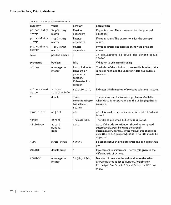
PrincipalSurface, PrincipalVolume
652 | C H A P T
princdirstressexpr
3-by-3 string matrix
Physics-dependent
If type is stress: The expressions for the principal directions.
princvalstrainexpr
1-by-3 string matrix
Physics-dependent
If type is strain: The expressions for the principal values.
princvalstressexpr
1-by-3 string matrix
Physics-dependent
If type is stress: The expressions for the principal values.
scale positive double 1 If scaleactive is true: The length scale factor.
scaleactive boolean false Whether to use manual scaling.
solnum non-negative integer
Last solution for transient or parametric solution. Otherwise first solution
The index of the solution to use. Available when data is not parent and the underlying data has multiple solutions.
solrepresentation
solnum | solutioninfo
solutioninfo Indicates which method of selecting solutions is active.
t double Time corresponding to last selected solnum
The time to use, for transient problems. Available when data is not parent and the underlying data is transient.
timeinterp on | off off on if t is used to determine time steps, off if solnum is used.
title string The auto-title. The title to use when titletype is manual.
titletype auto | manual | none
auto auto if the title contribution should be computed automatically, possibly using the group’s customization. manual if the manual title should be used (the title property). none if no title should be displayed.
type stress | strain stress Selection between principal stress and principal strain plot.
weight double array 1 If placement is uniformani: The weights given to the different axis directions.
xnumber non-negative integer
15 (3D), 7 (2D) Number of points in the x-direction. Active when arrowxmethod is set to number. Available for PrincipalSurface in 2D and PrincipalVolume in 3D.
TABLE 6-61: VALID PROPERTY/VALUE PAIRS
PROPERTY VALUE DEFAULT DESCRIPTION
E R 6 : R E S U L T S

PrincipalSurface, PrincipalVolume
xcoord double array Empty Absolute coordinates in the x-direction, active when arrowxmethod is set to coord. Available for PrincipalSurface in 2D and PrincipalVolume in 3D.
ynumber integer 15 (3D), 7 (2D) Number of points in the y-direction. Active when arrowymethod is set to number. Available for PrincipalSurface in 2D and PrincipalVolume in 3D.
ycoord double array Empty Absolute coordinates in the z-direction, active when arrowymethod is set to coord. Available for PrincipalSurface in 2D and PrincipalVolume in 3D.
znumber integer 15 (3D), 7 (2D) Number of points in the z-direction. Active when arrowzmethod is set to number. Available for PrincipalVolume in 3D.
zcoord double array Empty Absolute coordinates in the z-direction, active when arrowzmethod is set to coord. Available for PrincipalVolume in 3D.
TABLE 6-61: VALID PROPERTY/VALUE PAIRS
PROPERTY VALUE DEFAULT DESCRIPTION
653

Revolve1D, Revolve2D
654 | C H A P T
Revolve1D, Revolve2DSynopsis Revolve data set.
Syntax model.result().dataset().create(<dtag>,"Revolve1D");model.result().dataset().create(<dtag>,"Revolve2D");model.result().dataset(<dtag>).set(property, <value>);
Description model.result().dataset().create(<dtag>,"Revolve1D") creates a 1D revolved data set feature named <dtag>.
model.result().dataset().create(<dtag>,"Revolve2D") creates a 2D revolved data set feature named <dtag>.
The revolved data set needs to supply variables that cannot be expressed in terms of the coordinates of the underlying data set: The spatial coordinates and the rotation angle. Therefore the xmesh interpolation/evaluation has to be extended with support for supplying the values of these variables in a given set of points. The names of the spatial coordinates need not be exposed to the user, but the revolution angle should be available as revphi.
The source data sets for the revolutions can be any 1D and 2D data sets although the feature is primarily intended for axisymmetric coordinate systems.
The following properties are available for Revolve1D:
TABLE 6-62: VALID PROPERTY/VALUE PAIRS
NAME VALUE DEFAULT DESCRIPTION
anglevar String Derived from feature name
The name of the angle variable in the revolved coordinate system.
data none | data set name
First compatible data set
The data set this feature refers to.
hasspacevars boolean false If true, spacevars and anglevars are made available for evaluation.
planemap xy | xz xz The 3D plane that the 2D xy plane is mapped to.
point double 0 The point that is the axis of revolution.
revangle double 360 The revolution angle (degrees)
revlayers integer >= 3 50 The number of revolution layers.
spacevars String array Derived from feature name
The names of the space variables in the revolved coordinate system.
startangle double 0 The angle where the revolved sector begins (degrees).
E R 6 : R E S U L T S

Revolve1D, Revolve2D
The following properties are available for Revolve2D:
See Also Solution
TABLE 6-63: VALID PROPERTY/VALUE PAIRS
NAME VALUE DEFAULT DESCRIPTION
data none | data set name
First compatible data set
The data set this feature refers to.
method twopoint | pointdir
twopoint Decides if the line should be specified by two points or through one point and a direction.
genpoints double matrix {{0, 0, 0}, {1,0,0}} Active when method equals twopoint, this property contains the coordinates of the two points in the two rows of the matrix.
layermethod coarse | custom | fine | normal
normal The method used for choosing how many layers to use.
pdpoint double array {0,0} Active when method equals pointdir, this property contains the coordinates of the point.
pddir double array {0,1} Active when method equals pointdir, this property contains the direction.
revlayers integer >= 3 50 The number of revolution layers if layermethod is custom.
655

ScatterVolume, ScatterSurface
656 | C H A P T
ScatterVolume, ScatterSurfaceSynopsis Scatter plot.
Syntax model.result(<pgtag>).feature().create(<ftag>,"ScatterVolume");model.result(<pgtag>).feature().create(<ftag>,"ScatterSurface");model.result(<pgtag>).feature(<ftag>).set(property, <value>);model.result(<pgtag>).feature(<ftag>).run();
Description model.result(<pgtag>).feature().create(<ftag>,"Scatter...") creates a scatter plot feature named <ftag> belonging to the plot group <pgtag>.
Scatter plots are available in 2D and 3D.
The following properties are available:
TABLE 6-64: VALID PROPERTY/VALUE PAIRS
PROPERTY VALUE DEFAULT DESCRIPTION
arrowxmethod number | coord
number Indicates whether the x-coordinates of the spheres should be specified by number of points to distribute evenly across the data or by coordinates.
arrowymethod number | coord
number Indicates whether the y-coordinates of the spheres should be specified by number of points to distribute evenly across the data or by coordinates.
arrowzmethod number | coord
number Indicates whether the z-coordinates of the spheres should be specified by number of points to distribute evenly across the data or by coordinates. Available for ScatterVolume.
color custom | black | blue | cyan | green | magenta | red | white | yellow
red The color to use.
colorexpr string The expression for the colors of the spheres.
colordescr string A description of colorexpr.
const String array of property/value pairs
Empty Parameters to use in the expressions.
customcolor RGB-triplet {1,0,0} or last used color.
The uniform color to use. Active when color is set to custom.
data none | parent | data set name
parent The data set this feature refers to.
descr string Model-dependent
The description of the expressions in expr. Is used in the automatic title.
E R 6 : R E S U L T S

ScatterVolume, ScatterSurface
descriptionintitle
on | off on Whether the title contribution should contain the description when titletype is custom.
differential on | off on Whether the expression should be linearized at the linearization point. Applicable only if evalmethod is harmonic
evalmethod linpoint | harmonic | lintotal | lintotalavg | lintotalrms | lintotalpeak
harmonic Applicable only for solutions with a stored linearization point. Controls if the linearization point, the perturbation, or a combination should be used when evaluating the expression.
expr String array of length 2 in 2D and 3 in 3D
Mode-dependent The components to plot.
inheritcolor boolean true If inheritplot is not none: Determines if the color is inherited.
inheritplot none | plot name
none The plot that color and sphere scale is inherited from.
inheritspherescale
boolean true If inheritplot is not none: Determines if the sphere scale is inherited.
interp double array Time corresponding to last selected solnum for transient levels.
The time to use, for transient levels. Available when data is not parent and the underlying data is transient.
looplevel array of non-negative integers and strings
Last solution for transient or parametric solution for each level. Otherwise first solution for each level.
The index of the solution to use, per level, or interp, but only for transient solutions. Available when data is not parent and the underlying data has multiple solutions.
outersolnum non-negative integer
1 The index of the outer solutions to use. Applicable only for parametric sweep models.
prefixintitle
string Empty Added prefix to contribution to title.
radiusexpr string The expression for the radii of the spheres.
radiusdescr string A description of radiusexpr.
TABLE 6-64: VALID PROPERTY/VALUE PAIRS
PROPERTY VALUE DEFAULT DESCRIPTION
657

ScatterVolume, ScatterSurface
658 | C H A P T
solnum non-negative integer
Last solution for transient or parametric solution. Otherwise first solution.
The index of the solution to use. Available when data is not parent and the underlying data has multiple solutions.
solrepresentation
solnum | solutioninfo
solutioninfo Indicates which method of selecting solutions is active.
sphereradiusscale
double 1 The scale factor applied to the sphere radii if sphereradiusscaleactive is true.
sphereradiusscaleactive
boolean false If true, sphereradiusscale is used, otherwise the scale factor is computed automatically
suffixintitle
string Empty Added suffix to contribution to title.
t double Time corresponding to last selected solnum.
The time to use, for transient problems. Available when data is not parent and the underlying data is transient.
timeinterp on | off off on if t is used to determine time steps, off if solnum is used.
title string The auto-title. The title to use when titletype is manual.
titletype auto | custom | manual | none
auto auto if the title contribution should be computed automatically, possibly using the group’s customization. custom if the title contribution should be computed automatically, but customized. manual if the manual title contribution should be used (the title property). none if no title contribution should be used.
typeintitle on | off on Whether the title contribution should contain the type when titletype is custom.
xnumber non-negative integer
15 (3D), 7 (2D) Number of points in the x-direction. Active when arrowxmethod is set to number.
xcoord double array Empty Absolute coordinates in the x-direction, active when arrowxmethod is set to coord.
ynumber integer 15 (3D), 7 (2D) Number of points in the y-direction. Active when arrowymethod is set to number.
ycoord double array Empty Absolute coordinates in the z-direction, active when arrowymethod is set to coord.
TABLE 6-64: VALID PROPERTY/VALUE PAIRS
PROPERTY VALUE DEFAULT DESCRIPTION
E R 6 : R E S U L T S

ScatterVolume, ScatterSurface
Attributes None
See Also Surface, Volume
znumber integer 15 (3D), 7 (2D) Number of points in the z-direction. Active when arrowzmethod is set to number. Available for ScatterVolume.
zcoord double array Empty Absolute coordinates in the z-direction, active when arrowzmethod is set to coord. Available for ScatterVolume.
TABLE 6-64: VALID PROPERTY/VALUE PAIRS
PROPERTY VALUE DEFAULT DESCRIPTION
659

Sector2D, Sector3D
660 | C H A P T
Sector2D, Sector3DSynopsis Sector symmetry data set.
Syntax model.result().dataset().create(<dtag>,"Sector2D");model.result().dataset().create(<dtag>,"Sector3D");model.result().dataset(<dtag>).set(property, <value>);
Description model.result().dataset().create(<dtag>,"Sector2D") creates a 2D sector symmetry data set feature named <dtag>.
model.result().dataset().create(<dtag>,"Sector3D") creates a 3D sector symmetry feature named <dtag>.
This data set takes data from another data sets and expands it using sector symmetry around an axis.
The following properties are available for Sector 2D and Sector 3D:
TABLE 6-65: VALID PROPERTY/VALUE PAIRS
NAME VALUE DEFAULT DESCRIPTION
data none | data set name
First compatible data set
The data set this feature refers to.
genpoints double matrix {{0, 0, 0}, {1,0,0}} When method is twopoint: The coordinates of two points on the symmetry axis.Available for Sector3D.
hasspacevars
boolean false If true, spacevars are made available for evaluation.
hasvar boolean false If true, an axis indicator variable is defined.
method twopoint | pointdir
twopoint Decides if the line should be specified by two points or through one point and a direction. Available for Sector3D
mode integer 0 If sectors is odd or trans is rot: The azimuthal mode number use to transform the solution’s phase between sectors.
pddir double array {0,1} When method is pointdir: The direction in which the symmetry axis points. Available for Sector3D.
pdpoint double array {0,0} When method is pointdir: The coordinates of a point on the symmetry axis. Available for Sector3D.
point double array of length 2
{0, 0} The coordinates of the symmetry axis. Available for Sector2D.
reflaxis double array of length 2 in 2D and length 3 in3D
{1, 0} in 2D, {1, 0, 0} in 3D
If trans is rotrefl: The direction in which the reflection axis/plane (for 2D and 3D respectively) points.
sectors integer >= 2 2 The number of sectors.
E R 6 : R E S U L T S

Sector2D, Sector3D
spacevars string array of length 2 in 2D and length 3 in 3D
created from feature’s tag
Names of variables that when evaluate to the space coordinates in the coordinate system after sector symmetry expansion.
trans rot | rotrefl rot If sectors is even: Controls whether the transformation performed between consecutive sectors is rotation or rotation and reflection.
TABLE 6-65: VALID PROPERTY/VALUE PAIRS
NAME VALUE DEFAULT DESCRIPTION
661
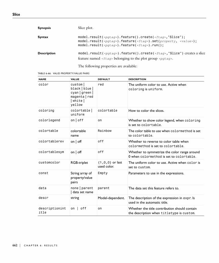
Slice
662 | C H A P T
SliceSynopsis Slice plot.
Syntax model.result(<pgtag>).feature().create(<ftag>,"Slice");model.result(<pgtag>).feature(<ftag>).set(property, <value>);model.result(<pgtag>).feature(<ftag>).run();
Description model.result(<pgtag>).feature().create(<ftag>,"Slice") creates a slice feature named <ftag> belonging to the plot group <pgtag>.
The following properties are available:
TABLE 6-66: VALID PROPERTY/VALUE PAIRS
NAME VALUE DEFAULT DESCRIPTION
color custom | black | blue | cyan | green | magenta | red | white | yellow
red The uniform color to use. Active when coloring is uniform.
coloring colortable | uniform
colortable How to color the slices.
colorlegend on | off on Whether to show color legend, when coloring is set to colortable.
colortable colortable name
Rainbow The color table to use when colormethod is set to colortable.
colortablerev on | off off Whether to reverse to color table when colormethod is set to colortable.
colortablesym on | off off Whether to symmetrize the color range around 0 when colormethod is set to colortable.
customcolor RGB-triplet {1,0,0} or last used color.
The uniform color to use. Active when color is set to custom.
const String array of property/value pairs
Empty Parameters to use in the expressions.
data none | parent | data set name
parent The data set this feature refers to.
descr string Model-dependent. The description of the expression in expr. Is used in the automatic title.
descriptionintitle
on | off on Whether the title contribution should contain the description when titletype is custom.
E R 6 : R E S U L T S

Slice
differential on | off on Whether the expression should be linearized at the linearization point. Applicable only if evalmethod is harmonic
evalmethod linpoint | harmonic | lintotal | lintotalavg | lintotalrms | lintotalpeak
harmonic Applicable only for solutions with a stored linearization point. Controls if the linearization point, the perturbation, or a combination should be used when evaluating the expression.
expr string Model-dependent. The expression to plot.
expressionintitle
on | off off Whether the title contribution should contain the expression when titletype is custom.
gendistance double array Empty Vector of distances from base plane, indicating position of additional parallel planes. Active when genparaactive equals on and genpara equals number.
genmethod threepoint | pointnormal
threepoint Active when planetype equals general, this property indicates whether the plane should be specified by three points or through one point and a normal.
gennumber positive integer 4 Number of additional parallel planes. Active when genparaactive equals on and genpara equals number.
genpara gennumber | gendistances
number Active when planetype equals general, and genparaactive equals on, this property indicates whether the additional parallel planes should be specify by a number, or by a vector of relative distances.
genparaactive on | off off Active when planetype equals general, this property indicates whether there should be additional parallel planes created.
genpnpoint double array of length three
{0,0,0} Active when genmethod equals pointnormal, this property contains the coordinates of the point.
genpnvec double array of length three
{0,0,0} Active when genmethod equals pointnormal, this property contains the normal vector.
genpoints double matrix of size 3x3
{{0,0,0}, {1,0,0}, {0,1,0}}
Active when genmethod equals threepoint, this property contains the coordinates of the three points, with one row per point.
TABLE 6-66: VALID PROPERTY/VALUE PAIRS
NAME VALUE DEFAULT DESCRIPTION
663

Slice
664 | C H A P T
inheritcolor boolean true If inheritplot is not none: Determines if the color is inherited.
inheritdeformscale
boolean true If inheritplot is not none: Determines if the deformation scale is inherited.
inheritplot none | plot name
none The plot that color, color range, and deformation scale is inherited from.
inheritrange boolean true If inheritplot is not none: Determines if the color and data ranges are inherited.
interactive on | off off If true, the isosurfaces can be moved interactively after the plot has been made.
interp double array Time corresponding to last selected solnum for transient levels.
The time to use, for transient levels. Available when data is not parent and the underlying data is transient.
looplevel array of non-negative integers and strings
Last solution for transient or parametric solution for each level. Otherwise first solution for each level.
The index of the solution to use, per level, or interp, but only for transient solutions. Available when data is not parent and the underlying data has multiple solutions.
outersolnum non-negative integer
1 The index of the outer solutions to use. Applicable only for parametric sweep models.
planetype quick | general
yz Specify plane type.
prefixintitle string Empty Added prefix to contribution to title.
quickplane xy | yz | zx yz Specify quick plane type. Active when planetype is quick.
quickx double array 0 Absolute x-coordinates for planes, active when quickxmethod is set to coord.
quickxmethod number | coord
number Active when planetype equals quick and quickplane equals yz, this property indicates whether the planes should be specified by one or more absolute coordinates along the x-axis, or a number indicating the number of planes to distribute evenly.
TABLE 6-66: VALID PROPERTY/VALUE PAIRS
NAME VALUE DEFAULT DESCRIPTION
E R 6 : R E S U L T S

Slice
quickxnumber positive integer 5 The number of planes when quickxmethod is set to number.
quicky double array 0 Absolute y-coordinates for planes, active when quickymethod is set to coord.
quickymethod number | coord
number Active when planetype equals quick and quickplane equals zx, this property indicates whether the planes should be specified by one or more absolute coordinates along the y-axis, or a number indicating the number of planes to distribute evenly.
quickynumber positive integer 5 The number of planes when quickymethod is set to number.
quickz double array 0 Absolute z-coordinates for planes, active when quickzmethod is set to coord.
quickzmethod number | coord
number Active when planetype equals quick and quickplane equals xy, this property indicates whether the planes should be specified by one or more absolute coordinates along the z-axis, or a number indicating the number of planes to distribute evenly.
quickznumber positive integer 5 The number of planes when quickzmethod is set to number.
rangecoloractive
on | off off Whether to use the manual color range specified in rangecolormin and rangecolormax. The color range specifies the minimum and maxim value in the plotted colors. Default is the minimum and maximum data values.
rangecolormax double Plot-dependent The maximum color range value. Active when rangecoloractive is on.
rangecolormin double Plot-dependent The minimum color range value. Active when rangecoloractive is on.
rangedatactive on | off off Whether to use the manual data range specified in rangedatamin and rangedatamax. Values outside the data range is not plotted.
rangedatamax double Plot-dependent The maximum data value. Active when rangedataactive is on.
rangedatamin double Plot-dependent The minimum data value. Active when rangedataactive is on.
TABLE 6-66: VALID PROPERTY/VALUE PAIRS
NAME VALUE DEFAULT DESCRIPTION
665

Slice
666 | C H A P T
recover off | pprint | ppr
off The derivative recovery method.
refine non-negative integer
1 The element refinement to use, if resolution is set to manual. Bear in mind that this is the refinement used for the base data set, so the number of elements in the model can increase radically if the plot uses, for example, a revolve data set.
resolution norefine | coarse | normal | fine | finer | extrafine | custom
normal Controls the plot’s resolution. A finer setting results in a higher resolution by modifying the internally computed default refinement. Use custom to enter your own refinement in the refine property.
shift double 0 If interactive is on: The shift that is applied to the level values.
smooth none | internal | everywhere
internal Smoothing settings.
solnum non-negative integer
Last solution for transient or parametric solution. Otherwise first solution.
The index of the solution to use. Available when data is not parent and the underlying data has multiple solutions.
solrepresentation
solnum | solutioninfo
solutioninfo Indicates which method of selecting solutions is active.
suffixintitle string Empty Added suffix to contribution to title.
t double Time corresponding to last selected solnum.
The time to use, for transient problems. Available when data is not parent and the underlying data is transient.
timeinterp on | off off on if t is used to determine time steps, off if solnum is used.
title string The auto-title. The title to use when titletype is manual.
TABLE 6-66: VALID PROPERTY/VALUE PAIRS
NAME VALUE DEFAULT DESCRIPTION
E R 6 : R E S U L T S

Slice
Note Only one direction of slices is possible in one plot. Use different slice plots together to accomplish several slices in different directions.
Attributes Deform, Filter
See Also Volume
titletype auto | custom | manual | none
auto auto if the title contribution should be computed automatically, possibly using the group’s customization. custom if the title contribution should be computed automatically, but customized. manual if the manual title contribution should be used (the title property). none if no title contribution should be used.
typeintitle on | off on Whether the title contribution should contain the type when titletype is custom.
unit string Model-dependent The unit to use for the expression in expr. If the old unit is not valid when the expression changes, the unit property is reset to default.
unitintitle on | off on Whether the title contribution should contain the unit when titletype is custom.
TABLE 6-66: VALID PROPERTY/VALUE PAIRS
NAME VALUE DEFAULT DESCRIPTION
667

Solution
668 | C H A P T
SolutionPurpose Solution data set.
Syntax model.result().dataset().create(<dtag>,"Solution");model.result().dataset(<dtag>).set(property, <value>);model.result().dataset(<dtag>).selection(...);model.result().dataset(<dtag>).createDeformedConfig(<gtag>, <mtag>);
Description model.result().dataset().create(<dtag>,"Solution") creates a solution data set.
Solution data sets refer to a solution in a solver sequence. All result features that perform evaluations on a solution refer to these data sets, rather than directly to the solution itself. The solution data sets specify which geometry and frame to use for evaluation and whether to evaluate only on a specific selection, among other things. It is possible to have multiple data set solutions referring to the same solution.
The following properties are available:
model.result().dataset(<dtag>).createDeformedConfig(<gtag>,<mtag>) creates a new geometry sequence (deformed configuration) tagged <gtag> together with a mesh sequence tagged <mtag> to use for remeshing of a deformed mesh. The created geometry sequence only contains a FromMesh feature.
Examples Create a solution data set and set it to point to the second geometry in the solver sequence sol1:
model.result().dataset().create("dset1", "Solution");model.result().dataset("dset1").set("solution", "sol1");model.result().dataset("dset1").set("geom", "geom2");
See Also PlotGroup1D, PlotGroup2D, PlotGroup3D
TABLE 6-67: VALID PROPERTY/VALUE PAIRS
NAME VALUE DEFAULT DESCRIPTION
frametype mesh | material | spatial
material or spatial
The frame type that this data set uses for evaluation of spatial coordinates.
geom string First available geometry, if any.
The geometry this data set refers to. Only applicable for solutions that refer to a geometry.
phase double 0 Evaluate solution at this angle, given in degrees.
scalefactor double 1 Multiply solution by this scaling factor.
solution string First compatible solution
The solution this data set refers to.
E R 6 : R E S U L T S

Streamline
StreamlineSynopsis Streamline plot.
Syntax model.result(<pgtag>).feature().create(<ftag>,"Streamline");model.result(<pgtag>).feature(<ftag>).set(property, <value>);model.result(<pgtag>).feature(<ftag>).run();
Description model.result(<pgtag>).feature().create(<ftag>,"Streamline") creates a streamline plot feature named <ftag> belonging to the plot group <pgtag>.
Streamlines visualize a vector quantity on domains. A streamline is a curve everywhere tangent to an instantaneous vector field. Streamlines are available in 2D and 3D plot groups.
The following properties are available:
TABLE 6-68: VALID PROPERTY/VALUE PAIRS
NAME VALUE DEFAULT DESCRIPTION
back on | off on Allow backward time integration. Only available for time-dependent data sets.
color custom | black | blue | cyan | green | magenta | red | white | yellow
black (2D), red (3D)
The uniform color to use.
const String array of property/value pairs
Empty Parameters to use in the expressions.
customcolor RGB-triplet {1,0,0} or last used color.
The uniform color to use. Active when color is set to custom.
data none | parent | data set name
parent The data set this feature refers to.
descr string Model-dependent The description of the expression in expr. Is used in the automatic title.
descriptionintitle
on | off on Whether the title contribution should contain the description when titletype is custom.
differential on | off on Whether the expression should be linearized at the linearization point. Applicable only if evalmethod is harmonic
669

Streamline
670 | C H A P T
evalmethod linpoint | harmonic | lintotal | lintotalavg | lintotalrms | lintotalpeak
harmonic Applicable only for solutions with a stored linearization point. Controls if the linearization point, the perturbation, or a combination should be used when evaluating the expression.
expr string array of length 2 in 2D and 3 in 3D
Model-dependent The components to plot.
inheritcolor boolean true If inheritplot is not none: Determines if the color is inherited.
inheritdeformscale
boolean true If inheritplot is not none: Determines if the deformation scale is inherited.
inheritplot none | plot name
none The plot that color, tube scale, and deformation scale is inherited from.
inherittubescale
boolean true If inheritplot is not none and linetype is tube or ribbon: Determines if the tube or ribbon scale is inherited.
interp double array Time corresponding to last selected solnum for transient levels.
The time to use, for transient levels. Available when data is not parent and the underlying data is transient.
inttol positive double
0.001 (2D), 0.01 (3D)
Integration tolerance.
linetype line | tube | ribbon
line Plot streamlines as lines, tubes, or ribbons.
looplevel array of non-negative integers and strings
Last solution for transient or parametric solution for each level. Otherwise first solution for each level.
The index of the solution to use, per level, or interp, but only for transient solutions. Available when data is not parent and the underlying data has multiple solutions.
looptol positive double
0.01 Loop tolerance.
madv manual | automatic
automatic Whether to specify advanced parameters when positioning method is magnitude.
TABLE 6-68: VALID PROPERTY/VALUE PAIRS
NAME VALUE DEFAULT DESCRIPTION
E R 6 : R E S U L T S

Streamline
maxsteps positive integer
5000 The maximum number of integration steps.
maxtime positive double
Inf Maximum integration time.
mdensity non-negative integer
20 The density of the streamlines. Active when posmethod is set to magnitude. Only available in 2D.
mdist double array of length two containing positive doubles
{0.05, 0.15} Minimum and maximum distance relative to the size of the geometry. Active when posmethod is set to magnitude. Only available in 3D.
minitref positive integer
1 Boundary element refinement. Active when madv is set to manual.
msatfactor non-negative double
1.3 Starting distance factor. Active when madv is set to manual. Only available in 3D.
mseed double array of length 2 or 3, depending on space dimension.
{0,0} (2D), {0,0,0} (3D)
The first start point. Active when mseedactive is set to on.
mseedactive on | off off Whether to manually specify first start point. Active when madv is set to manual.
normal on | off off on when vector field should be normalized.
number integer 20 Approximate number of streamlines. Active when startmethod is set to number.
outersolnum non-negative integer
1 The index of the outer solutions to use. Applicable only for parametric sweep models.
posmethod magnitude | start | uniform | selection
selection The type of streamline positioning. Either start point controlled, uniform density, magnitude controlled, or starting from selected lines (2D) or surfaces (3D).
prefixintitle string Empty Added prefix to contribution to title.
radiusexpr string 1 The tube radius.
TABLE 6-68: VALID PROPERTY/VALUE PAIRS
NAME VALUE DEFAULT DESCRIPTION
671

Streamline
672 | C H A P T
refine non-negative integer
1 The element refinement to use, if resolution is set to manual. Bear in mind that this is the refinement used for the base data set, so the number of elements in the model can increase radically if the plot uses, for example, a revolve data set.
resolution norefine | coarse | normal | fine | finer | extrafine | custom
normal Controls the plot’s resolution. A finer setting results in a higher resolution by modifying the internally computed default refinement. Use custom to enter your own refinement in the refine property.
selnumber non-negative integer
20 If posmethod is selection: The approximate number of streamlines placed on the selected edges (2D) or surfaces (3D).
solnum non-negative integer
Last solution for transient or parametric solution. Otherwise first solution.
The index of the solution to use. Available when data is not parent and the underlying data has multiple solutions.
solrepresentation
solnum | solutioninfo
solutioninfo Indicates which method of selecting solutions is active.
startdata none | cut line or cut plane name
none Active when posmethod is start: The line or plane where the start points are distributed evenly.
startmethod number | coord
number Active when posmethod is start. Indicates whether the start points should be specified by number of points to distribute evenly or by coordinates.
stattol positive double
0.01 Stationary point stop tolerance.
suffixintitle string Empty Added suffix to contribution to title.
t double Time corresponding to last selected solnum.
The time to use, for transient problems. Available when data is not parent and the underlying data is transient.
timeinterp on | off off on if t is used to determine time steps, off if solnum is used.
TABLE 6-68: VALID PROPERTY/VALUE PAIRS
NAME VALUE DEFAULT DESCRIPTION
E R 6 : R E S U L T S

Streamline
title string The auto-title. The title to use when titletype is manual.
titletype auto | custom | manual | none
auto auto if the title contribution should be computed automatically, possibly using the group’s customization. custom if the title contribution should be computed automatically, but customized. manual if the manual title contribution should be used (the title property). none if no title contribution should be used.
tuberadiusscale
double 1 The scale factor applied to the tube radii if tuberadiusscaleactive is true.
tuberadiusscaleactive
boolean false If true, tuberadiusscale is used, otherwise the scale factor is computed automatically
typeintitle on | off on Whether the title contribution should contain the type when titletype is custom.
uadv manual | automatic
automatic Whether to specify advanced parameters when positioning method is uniform.
udist positive double
0.15 (3D), 0.05 (2D)
Separating distance relative to the size of the geometry. Active when posmethod is set to uniform.
udistend non-negative double
0.5 Terminating distance factor. Active when uadv is set to manual.
uignoredist non-negative double
0.5 Fraction of streamline length to ignore. Active when uadv is set to manual.
uinitref positive integer
1 Boundary element refinement. Active when uadv is set to manual.
unit String Model-dependent The unit to use for the expression in expr. If the old unit is not valid when the expression changes, the unit property is reset to default.
usatfactor non-negative double
1.3 Starting distance factor. Active when uadv is set to manual.
useed double array of length 2 or 3, depending on space dimension.
{0,0} (2D) or {0,0,0} (3D)
The first start point. Active when useedactive is set to on.
useedactive on | off off Whether to manually specify first start point. Active when uadv is set to manual.
widthexpr string 1 The ribbon width.
TABLE 6-68: VALID PROPERTY/VALUE PAIRS
NAME VALUE DEFAULT DESCRIPTION
673

Streamline
674 | C H A P T
Attributes Color, Deform, Filter
See Also Particle, ParticleMass
widthscale double 1 The scale factor applied to the ribbon widths if widthscaleactive is true.
widthscaleactive
boolean false If true, widthscale is used, otherwise the scale factor is computed automatically
xcoord double array Empty Absolute coordinates in the x-direction, active when startmethod is set to coord.
ycoord double array Empty Absolute coordinates in the y-direction, active when startmethod is set to coord.
zcoord double array Empty Absolute coordinates in the z-direction, active when startmethod is set to coord. Available in 3D only.
TABLE 6-68: VALID PROPERTY/VALUE PAIRS
NAME VALUE DEFAULT DESCRIPTION
E R 6 : R E S U L T S
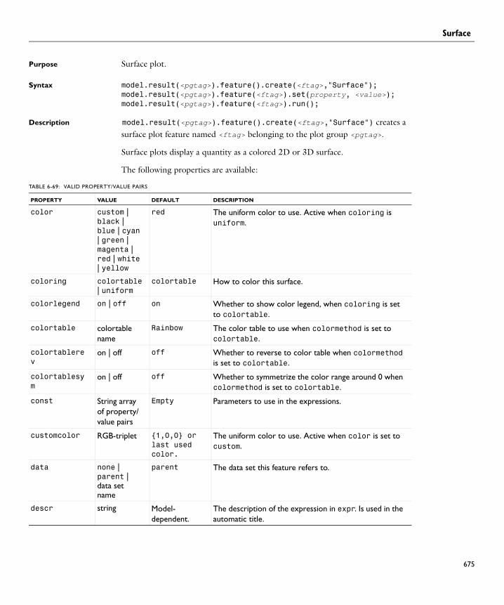
Surface
SurfacePurpose Surface plot.
Syntax model.result(<pgtag>).feature().create(<ftag>,"Surface");model.result(<pgtag>).feature(<ftag>).set(property, <value>);model.result(<pgtag>).feature(<ftag>).run();
Description model.result(<pgtag>).feature().create(<ftag>,"Surface") creates a surface plot feature named <ftag> belonging to the plot group <pgtag>.
Surface plots display a quantity as a colored 2D or 3D surface.
The following properties are available:
TABLE 6-69: VALID PROPERTY/VALUE PAIRS
PROPERTY VALUE DEFAULT DESCRIPTION
color custom | black | blue | cyan | green | magenta | red | white | yellow
red The uniform color to use. Active when coloring is uniform.
coloring colortable | uniform
colortable How to color this surface.
colorlegend on | off on Whether to show color legend, when coloring is set to colortable.
colortable colortable name
Rainbow The color table to use when colormethod is set to colortable.
colortablerev
on | off off Whether to reverse to color table when colormethod is set to colortable.
colortablesym
on | off off Whether to symmetrize the color range around 0 when colormethod is set to colortable.
const String array of property/value pairs
Empty Parameters to use in the expressions.
customcolor RGB-triplet {1,0,0} or last used color.
The uniform color to use. Active when color is set to custom.
data none | parent | data set name
parent The data set this feature refers to.
descr string Model-dependent.
The description of the expression in expr. Is used in the automatic title.
675

Surface
676 | C H A P T
descriptionintitle
on | off on Whether the title contribution should contain the description when titletype is custom.
differential on | off on Whether the expression should be linearized at the linearization point. Applicable only if evalmethod is harmonic
evalmethod linpoint | harmonic | lintotal | lintotalavg | lintotalrms | lintotalpeak
harmonic Applicable only for solutions with a stored linearization point. Controls if the linearization point, the perturbation, or a combination should be used when evaluating the expression.
expr string Model-dependent.
The expression to plot.
expressionintitle
on | off off Whether the title contribution should contain the expression when titletype is custom.
inheritcolor boolean true If inheritplot is not none: Determines if the color is inherited.
inheritdeformscale
boolean true If inheritplot is not none: Determines if the deformation scale is inherited.
inheritheightscale
boolean true If inheritplot is not none: Determines if height scale is inherited.
inheritplot none | plot name
none The plot that color, color range, and deformation scale is inherited from.
inheritrange boolean true If inheritplot is not none: Determines if the color and data ranges are inherited.
interp double array Time corresponding to last selected solnum for transient levels.
The time to use, for transient levels. Available when data is not parent and the underlying data is transient.
looplevel array of non-negative integers and strings
Last solution for transient or parametric solution for each level. Otherwise first solution for each level.
The index of the solution to use, per level, or interp, but only for transient solutions. Available when data is not parent and the underlying data has multiple solutions.
TABLE 6-69: VALID PROPERTY/VALUE PAIRS
PROPERTY VALUE DEFAULT DESCRIPTION
E R 6 : R E S U L T S

Surface
outersolnum non-negative integer
1 The index of the outer solutions to use. Applicable only for parametric sweep models.
prefixintitle
string Empty Added prefix to contribution to title.
rangecoloractive
on | off off Whether to use the manual color range specified in rangecolormin and rangecolormax. The color range specifies the minimum and maxim value in the plotted colors. Default is the minimum and maximum data values.
rangecolormax
double Plot-dependent The maximum color range value. Active when rangecoloractive is on.
rangecolormin
double Plot-dependent The minimum color range value. Active when rangecoloractive is on.
rangedatactive
on | off off Whether to use the manual data range specified in rangedatamin and rangedatamax. Values outside the data range is not plotted.
rangedatamax double Plot-dependent The maximum data value. Active when rangedataactive is on.
rangedatamin double Plot-dependent The minimum data value. Active when rangedataactive is on.
recover off | pprint | ppr
off The derivative recovery method.
refine non-negative integer
1 The element refinement to use, if resolution is set to manual. Bear in mind that this is the refinement used for the base data set, so the number of elements in the model can increase radically if the plot uses, for example, a revolve data set.
resolution norefine | coarse | normal | fine | finer | extrafine | custom
normal Controls the plot’s resolution. A finer setting results in a higher resolution by modifying the internally computed default refinement. Use custom to enter your own refinement in the refine property.
smooth none | internal | everywhere
internal Smoothing settings.
TABLE 6-69: VALID PROPERTY/VALUE PAIRS
PROPERTY VALUE DEFAULT DESCRIPTION
677

Surface
678 | C H A P T
Attributes Deform, Filter, Height
Examples Surface plot on 2D solution:
model.result().dataset().create("dset1", "Solution");
solnum non-negative integer
Last solution for transient or parametric solution. Otherwise first solution.
The index of the solution to use. Available when data is not parent and the underlying data has multiple solutions.
solrepresentation
solnum | solutioninfo
solutioninfo
Indicates which method of selecting solutions is active.
suffixintitle
string Empty Added suffix to contribution to title.
t double Time corresponding to last selected solnum.
The time to use, for transient problems. Available when data is not parent and the underlying data is transient.
timeinterp on | off off on if t is used to determine time steps, off if solnum is used.
title string The auto-title. The title to use when titletype is manual.
titletype auto | custom | manual | none
auto auto if the title contribution should be computed automatically, possibly using the group’s customization. custom if the title contribution should be computed automatically, but customized. manual if the manual title contribution should be used (the title property). none if no title contribution should be used.
typeintitle on | off on Whether the title contribution should contain the type when titletype is custom.
unit string Model-dependent
The unit to use for the expression in expr. If the old unit is not valid when the expression changes, the unit property is reset to default.
unitintitle on | off on Whether the title contribution should contain the unit when titletype is custom.
wireframe on | off off Whether to plot filled elements or only their edges.
TABLE 6-69: VALID PROPERTY/VALUE PAIRS
PROPERTY VALUE DEFAULT DESCRIPTION
E R 6 : R E S U L T S
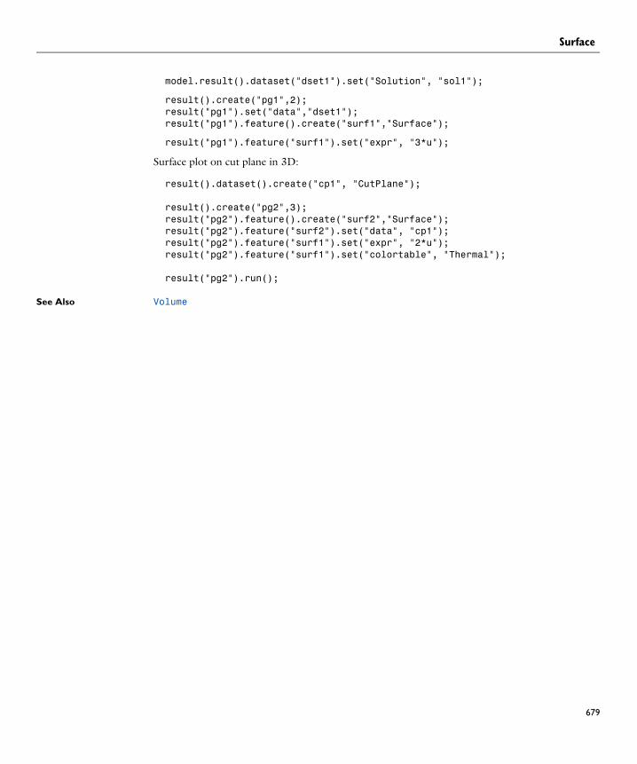
Surface
model.result().dataset("dset1").set("Solution", "sol1");
result().create("pg1",2);result("pg1").set("data","dset1");result("pg1").feature().create("surf1","Surface");
result("pg1").feature("surf1").set("expr", "3*u");
Surface plot on cut plane in 3D:
result().dataset().create("cp1", "CutPlane");
result().create("pg2",3);result("pg2").feature().create("surf2","Surface");result("pg2").feature("surf2").set("data", "cp1");result("pg2").feature("surf1").set("expr", "2*u");result("pg2").feature("surf1").set("colortable", "Thermal");
result("pg2").run();
See Also Volume
679

Surface (data set)
680 | C H A P T
Surface (data set)Synopsis Surface data set.
Syntax model.result().dataset().create(<dtag>,"Surface");model.result().dataset(<dtag>).set(property, <value>);
Description model.result().dataset().create(<dtag>,"Surface") creates a surface data set with the name <dtag>.
The surface data set makes it possible to evaluate surfaces of a 3D model in 2D or 3D. For evaluation in 2D, different parameterizations of the 2D projection are available.
The following properties are available:
TABLE 6-70: VALID PROPERTY/VALUE PAIRS
PROPERTY VALUE DEFAULT DESCRIPTION
data none | data set name
First compatible data set
The solution data set this feature refers to.
param face | xy | yz | zx | yx | zy | xz | expr
face The projection used when evaluating in 2D.
exprx String When param is expr: The x-axis expression when evaluating in 2D.
expry String When param is expr: The y-axis expression when evaluating in 2D.
E R 6 : R E S U L T S

Table
TablePurpose Feature containing a table of data.
Syntax model.result().table().create(<ftag>,"Table");model.result().table(<ftag>).setColumnHeaders(<headers>);model.result().table(<ftag>).setTableData(<realData>);model.result().table(<ftag>).setTableData(<realData>, <imagData>);model.result().table(<ftag>).addColumns(<headers>, <realData>);model.result().table(<ftag>).addColumns(<headers>, <realData>,
<imagData>);model.result().table(<ftag>).addRow(<realData>);model.result().table(<ftag>).addRow(<realData>,<imagData>);model.result().table(<ftag>).removeRow(<index>);model.result().table(<ftag>).getColumnHeaders();model.result().table(<ftag>).getReal();model.result().table(<ftag>).getImag();model.result().table(<ftag>).Row(<index>);model.result().table(<ftag>).getImagRow(<index>);model.result().table(<ftag>).getTableData(<fullPrecision>);model.result().table(<ftag>).getTableRow(<index>,
<fullPrecision>);model.result().table(<ftag>).getNRows();model.result().table(<ftag>).isComplex();model.result().table(<ftag>).clearTableData();model.result().table(<ftag>).set(property, <value>);model.result().table(<ftag>).save(<filename>);model.result().table(<ftag>).save(<filename>, <fullPrecision>);
Description model.result().table().create(<ftag>,"Table") creates a table feature named <ftag>. Tables support two data formats, all or filled. Filled data is typically produced from parametric sweeps and makes it possible to retrieve data for a pair of parameters on a matrix format. Filled tables can be used to make response surface plots. (See TableSurface.)
model.result().table(<ftag>).setColumnHeaders(<headers>) sets the table’s column headers from the string array <headers>.
model.result().table(<ftag>).setTableData(<realData>) sets the table content from a double matrix containing real data. Any previous real or imaginary data is removed.
model.result().table(<ftag>).setTableData(<realData>, <imagData>) sets both real and imaginary data from the double matrices <realData> and <imagData>, which must be of the same size. <imagData> can be null to indicate that there is no imaginary data.
681

Table
682 | C H A P T
model.result().table(<ftag>).getColumnHeaders() retrieves the column headers.
model.result().table(<ftag>).addColumns(<headers>, <realData>) adds one or more columns and associated real data to the table.
model.result().table(<ftag>).addColumns(<headers>, <realData>,
<imagData>) adds one or more columns and associated real data and imaginary data to the table.
model.result().table(<ftag>).addRow(<realData>) adds one row of real data to the table.
model.result().table(<ftag>).addRow(<realData>,<imagData>) adds one row of real and imaginary data to the table.
model.result().table(<ftag>).removeRow(<index>) removes the row with a given index from the table. If the row index is out of bounds, nothing happens.
model.result().table(<ftag>).getColumnHeaders() returns the column headers in the table.
model.result().table(<ftag>).getReal() returns the real part of the table content.
model.result().table(<ftag>).getImag() returns the imaginary part of the table content. Note: this method allocates imaginary data if there was none. Check for imaginary content with the isComplex method before calling this method if you want to avoid this.
model.result().table(<ftag>).getRealRow(<index>) returns the real data in one row.
model.result().table(<ftag>).getImagRow(<index>) returns the imaginary data in one row.
model.result().table(<ftag>).getFilledReal() returns the real part of the table content on a filled format, when available.
model.result().table(<ftag>).getFilledImag() returns the imaginary part of the table content on a filled format, when available.
model.result().table(<ftag>).getTableData(<fullPrecision>) returns the table data as a string matrix, with limited or full precision as specified by the boolean <fullPrecision>.
E R 6 : R E S U L T S

Table
model.result().table(<ftag>).getTableRow(<index>, <fullPrecision>) returns the table data for one row as a string array, with limited or full precision.
model.result().table(<ftag>).getNRows() returns the number of rows in the table.
model.result().table(<ftag>).isComplex() returns true if the table contains imaginary data. This method checks whether imaginary data has been allocated, not if it is different from 0.
model.result().table(<ftag>).clearTableData() removes all table data and column headers.
model.result().table(<ftag>).save(<filename>) saves the table <ftag> content to the text file <filename> in full precision.
The following properties are available:
TABLE 6-71: VALID PROPERTY/VALUE PAIRS
NAME VALUE DEFAULT DESCRIPTION
cols Parameters in table | none
none For tables with filled data, cols controls which parameter is used on the columns. May not be the same parameter as in rows.
datacol Positive integer
1 For tables with filled data, datacol controls which data column should be used to populate the filled table.
descr none | data | manual
data For tables with filled data, descr controls which description to use for the columns, in addition to the parameter values. none will give no description, manual uses the description in descrmanual an data uses the description in the table data.
descrmanual String Empty Manual column header for tables with filled data, used when descr is set to manual.
filename String Empty The name of the file on which the table is stored, used when storetable is set to inmodelandonfile or onfile.
filterstringdata
on | off off For tables with filled data, filterstringdata controls whether to filter the input column using showrowstep.
format all | filled all Controls whether you retrieve all or filled table data when calling the getTableData method.
683

Table
684 | C H A P T
See Also Table (plot), TableSurface
param Positive integer
1 For tables with filled data containing more than two parameters, param is the index indicating which values to use for fixing additional parameters. Additional parameters are ordered from left to right in the original table data.
rows Parameters in table | none
none For tables with filled data, rows controls which parameter is used on the rows.
showrowstep Positive integer
1 When retrieving filled data using the getTableData method, showrowstep controls whether to leave all but every showrowstep input cells empty, for example, every third cell in the first column. This refers to the input column only. Only applied when filterstringdata is on.
storetable inmodel | inmodelandonfile | onfile
inmodel Controls whether table will be stored in model(inmodel) or on file(onfile), or both(inmodelandonfile).
tablebuffersize Positive integer
Taken from buffer size preference. The default of which is 10000.
The size of the in memory buffer size table is stored, used when storetable is set to inmodel or inmodelandonfile. In the second case only the last tablebuffersize rows are kept in the model; the rest is read from file when necessary.
TABLE 6-71: VALID PROPERTY/VALUE PAIRS
NAME VALUE DEFAULT DESCRIPTION
E R 6 : R E S U L T S

Table (plot)
Table (plot)Purpose Plot data from a table in a graph plot.
Syntax model.result(<pgtag>).feature().create(<ftag>,"Table");model.result(<pgtag>).feature(<ftag>).set(property, <value>);model.result(<pgtag>).feature(<ftag>).run();
Description model.result(<pgtag>).feature().create(<ftag>,"Table") creates a graph table plot feature named <ftag>.
Table plots can be added to 1D and polar plot groups and displays data from a table.
The following properties are available:
TABLE 6-72: VALID PROPERTY/VALUE PAIRS
NAME VALUE DEFAULT DESCRIPTION
autolegends on | off on Whether to use the automatically generated legends or the legends defined in the legends property.
customlinecolor RGB-triplet {0,0,1} or last used edgecolor.
The color to use for the lines. Active when linecolor is set to custom.
freqmax integer If transform is spectrum and freqrangeactive is true: The upper frequency bound.
freqmin integer If transform is spectrum and freqrangeactive is true: The lower frequency bound.
freqrangeactive on | off false If transform is spectrum: Controls whether a manual frequency range is used.
imagplot on | off off If transform is none: When on, the imaginary part of the data in the table is plotted.
legend on | off off Whether to show legends.
legendmethod automatic | manual
automatic Whether to use the automatic legends or the legends supplied in the legends property.
legends string array The last computed automatic legends.
Manual legends active when legendmethod is set to manual.
linecolor custom | cycle | black | blue | cyan | green | magenta | red | white | yellow
cycle How to color the lines in the graph. Cycle indicates that the colors is different for each line.
685

Table (plot)
686 | C H A P T
linewidth double 0.5 The line width.
linemarker none | cycle | asterisk | circle | diamond | plus | point | square | star | triangle
none The line markers, if any. Cycle indicates that the marker is different for each line.
linestyle none | cycle | solid | dotted | dashed | dashdot
solid The line style, if any. Cycle indicates that the line style is different for each line.
markerpos interp | datapoints
interp Controls whether the positions of the markers are in the data points of the plot, or interpolated depending on the number (set in markers). Markers are visible when linemarker is set.
markers integer 8 The number of markers to show. Markers are visible when linemarker is set.
nfreqs integer 1 If transform is spectrum and nfreqsactive is true: The number of frequencies to plot.
nfreqsactive boolean false If transform is spectrum: Controls whether the number of frequencies is set manually.
plotcolumninput all | manual all The columns to plot. all indicates all columns excluding those used in xaxisdata, manual indicates the columns specified in plotcolumns.
plotcolumns positive integer array
Empty The columns to plot when plotcolumninput is manual.
scale boolean false If transform ffis spectrum: The frequency spectrum is transformed so that it has the same scale as the original data.
table none | table feature name
First available table
The table feature this plot refers to.
TABLE 6-72: VALID PROPERTY/VALUE PAIRS
NAME VALUE DEFAULT DESCRIPTION
E R 6 : R E S U L T S
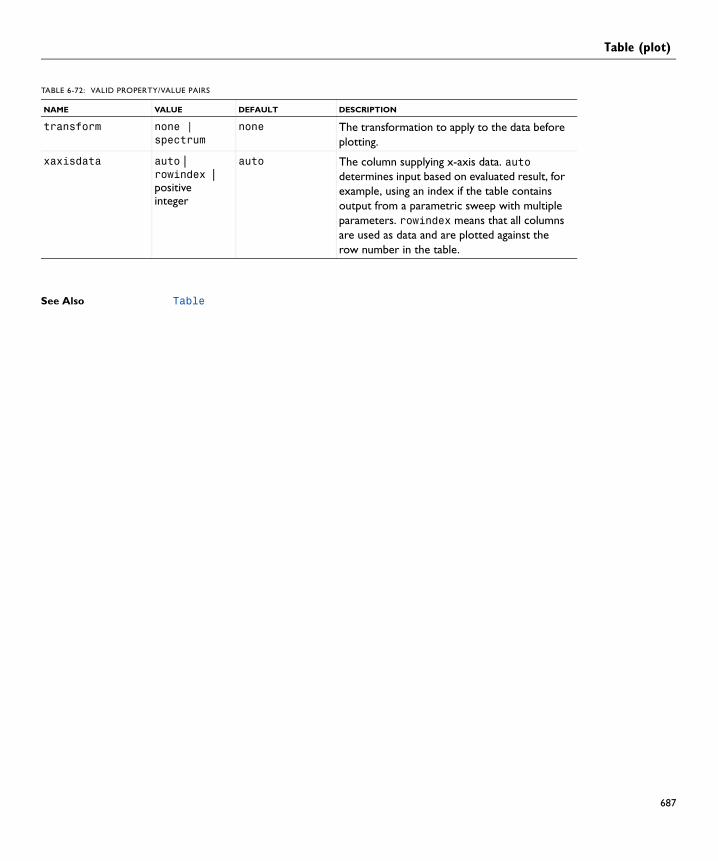
Table (plot)
See Also Table
transform none | spectrum
none The transformation to apply to the data before plotting.
xaxisdata auto | rowindex | positive integer
auto The column supplying x-axis data. auto determines input based on evaluated result, for example, using an index if the table contains output from a parametric sweep with multiple parameters. rowindex means that all columns are used as data and are plotted against the row number in the table.
TABLE 6-72: VALID PROPERTY/VALUE PAIRS
NAME VALUE DEFAULT DESCRIPTION
687

TableHeight
688 | C H A P T
TableHeightSynopsis Height attribute for 2D table plots.
Syntax model.result(<pgtag>).feature(<ftag>).feature().create(<atag>,"TableHeight");
model.result(<pgtag>).feature(<ftag>).feature(<atag>).set(property, <value>);
Description model.result(<pgtag>).feature(<ftag>).feature().create(<atag>,
"TableHeight") creates a TableHeight attribute feature with the name <atag>, belonging to the feature <ftag>.
Table height attributes are available for2D table surface plots. Adding a height attribute changes the rendered view to 3D. The plot group, however, still remains a 2D plot group. Any other plots in the group that do not have heights attribute is rendered at z=0.
The following properties are available:
See Also TableSurface, Table
TABLE 6-73: VALID PROPERTY/VALUE PAIRS
PROPERTY VALUE DEFAULT DESCRIPTION
datacol Positive integer
1 For tables with filled data, datacol controls which data column should be used to populate the filled table. Used when heightdata is data.
heightdata parent | data
parent parent uses the data from the surface plot the height feature has been added to. data uses the data specified by the height attribute’s properties.
offset double 0 The offset along the z-axis where to place the height plot.
scale positive double
1 If scaleactive is true: The scale factor for the height.
scaleactive boolean false Whether to use manual scaling.
title string The auto-title. The title to use when titletype is manual.
titletype auto | manual | none
auto auto if the title contribution should be computed automatically, possibly using the group’s customization. manual if the manual title contribution should be used (the title property). none if no title contribution should be used.
E R 6 : R E S U L T S

TableSurface
TableSurfacePurpose Plot data from a table in a surface plot.
Syntax model.result(<pgtag>).feature().create(<ftag>,"TableSurface");model.result(<pgtag>).feature(<ftag>).set(property, <value>);model.result(<pgtag>).feature(<ftag>).run();
Description model.result(<pgtag>).feature().create(<ftag>,"Table") creates a table surface plot feature named <ftag>.
Table surface plots can only be used with tables containing filled data, produced from a parametric sweep. They can be added to 2D plot groups.
The following properties are available:
TABLE 6-74: VALID PROPERTY/VALUE PAIRS
NAME VALUE DEFAULT DESCRIPTION
color custom | black | blue | cyan | green | magenta | red | white | yellow
red The uniform color to use. Active when coloring is uniform.
coloring colortable | uniform
colortable How to color this surface.
colorlegend on | off on Whether to show color legend, when coloring is set to colortable.
colortable colortable name
Rainbow The color table to use when colormethod is set to colortable.
colortablerev on | off off Whether to reverse to color table when colormethod is set to colortable.
colortablesym on | off off Whether to symmetrize the color range around 0 when colormethod is set to colortable.
customcolor RGB-triplet {1,0,0} or last used color.
The uniform color to use. Active when color is set to custom.
datacol Positive integer
1 For tables with filled data, datacol controls which data column should be used to populate the filled table.
689

TableSurface
690 | C H A P T
descr none | data | manual
data For tables with filled data, descr controls which description to use for the columns, in addition to the parameter values. none will give no description, manual uses the description in descrmanual an data uses the description in the table data.
descrmanual String Empty Manual column header for tables with filled data, used when descr is set to manual.
filterstringdata
on | off off For tables with filled data, filterstringdata controls whether to filter the input column using showrowstep.
format all | filled all Controls whether you retrieve all or filled table data when calling the getTableData method.
imagplot on | off off If transform is none: When on, the imaginary part of the data in the table is plotted.
inheritcolor boolean true If inheritplot is not none: Determines if the color is inherited.
inheritheightscale
boolean true If inheritplot is not none: Determines if height scale is inherited.
inheritplot none | plot name
none The plot that color, color range, and height scale is inherited from.
inheritrange boolean true If inheritplot is not none: Determines if the color and data ranges are inherited.
param Positive integer
1 For tables with filled data containing more than two parameters, param is the index indicating which values to use for fixing additional parameters. Additional parameters are ordered from left to right in the original table data.
plotdata table | manual
table For tables with filled data containing more than two parameters, plotdata controls whether to use manual settings in the plot (table row, column, and so forth), or the filled settings in the table feature. In the latter case, the table’s properties are automatically synchronized with the plot’s properties.
TABLE 6-74: VALID PROPERTY/VALUE PAIRS
NAME VALUE DEFAULT DESCRIPTION
E R 6 : R E S U L T S

TableSurface
rangecoloractive
on | off off Whether to use the manual color range specified in rangecolormin and rangecolormax. The color range specifies the minimum and maxim value in the plotted colors. Default is the minimum and maximum data values.
rangecolormax double Plot-dependent The maximum color range value. Active when rangecoloractive is on.
rangecolormin double Plot-dependent The minimum color range value. Active when rangecoloractive is on.
rangedatactive on | off off Whether to use the manual data range specified in rangedatamin and rangedatamax. Values outside the data range is not plotted.
rangedatamax double Plot-dependent The maximum data value. Active when rangedataactive is on.
rangedatamin double Plot-dependent The minimum data value. Active when rangedataactive is on.
showrowstep Positive integer
1 When retrieving filled data using the getTableData method, showrowstep controls whether to leave all but every showrowstep input cells empty, for example, every third cell in the first column. This refers to the input column only. Only applied when filterstringdata is on.
smooth none | internal | everywhere
internal Smoothing settings.
table none | table feature name
First available table
The table feature this plot refers to.
title string The auto-title. The title to use when titletype is manual.
titletype auto | manual | none
auto auto if the title contribution should be computed automatically, possibly using the group’s customization. manual if the manual title contribution should be used (the title property). none if no title contribution should be used.
xaxisdata Parameters in table | none
none For tables with filled data, xaxisdata controls which parameter is used on the x-axis.
TABLE 6-74: VALID PROPERTY/VALUE PAIRS
NAME VALUE DEFAULT DESCRIPTION
691

TableSurface
692 | C H A P T
See Also Table, Table (plot)
yaxisdata Parameters in table | none
none For tables with filled data, yaxisdata controls which parameter is used on the y-axis. May not be the same parameter as in xaxisdata.
wireframe on | off off Whether to plot filled elements or only their edges.
TABLE 6-74: VALID PROPERTY/VALUE PAIRS
NAME VALUE DEFAULT DESCRIPTION
E R 6 : R E S U L T S

Volume
VolumePurpose Volume plot.
Syntax model.result(<pgtag>).feature().create(<ftag>,"Volume");model.result(<pgtag>).feature(<ftag>).set(property, <value>);model.result(<pgtag>).feature(<ftag>).run();
Description model.result(<pgtag>).feature().create(<ftag>,"Volume") creates a volume plot feature named <ftag> belonging to the plot group <pgtag>.
A volume plot shows an expression evaluated in all elements of a 3D volume.
The following properties are available:
TABLE 6-75: VALID PROPERTY/VALUE PAIRS
NAME VALUE DEFAULT DESCRIPTION
color custom | black | blue | cyan | green | magenta | red | white | yellow
red The uniform color to use. Active when coloring is uniform.
coloring colortable | uniform
colortable How to color this surface.
colorlegend on | off on Whether to show color legend, when coloring is set to colortable.
colortable colortable name Rainbow The color table to use when colormethod is set to colortable.
colortablerev
on | off off Whether to reverse to color table when colormethod is set to colortable.
colortablesym
on | off off Whether to symmetrize the color range around 0 when colormethod is set to colortable.
const String array of property/value pairs
Empty Parameters to use in the expressions.
customcolor RGB-triplet {1,0,0} or last used color.
The uniform color to use. Active when color is set to custom.
data none | parent | data set name
parent The data set this feature refers to.
descr string Model-dependent. The description of the expression in expr. Is used in the automatic title.
descriptionintitle
on | off on Whether the title contribution should contain the description when titletype is custom.
693

Volume
694 | C H A P T
elemfilter random | expression
random If filteractive is on: The expression to use for filtering when only a subset of the elements are shown.
elemscale double in [0,1] 1 The scale factor with which each element is scaled.
differential on | off on Whether the expression should be linearized at the linearization point. Applicable only if evalmethod is harmonic
evalmethod linpoint | harmonic | lintotal | lintotalavg | lintotalrms | lintotalpeak
harmonic Applicable only for solutions with a stored linearization point. Controls if the linearization point, the perturbation, or a combination should be used when evaluating the expression.
expr string Model-dependent. The expression to plot.
expressionintitle
on | off off Whether the title contribution should contain the expression when titletype is custom.
filteractive on | off off Whether to use element filtering.
filterexpr string x The expression to use for filtering when elemfilter is set to expression.
inheritcolor boolean true If inheritplot is not none: Determines if the color is inherited.
inheritdeformscale
boolean true If inheritplot is not none: Determines if the deformation scale is inherited.
inheritplot none | plot name none The plot that color, color range, and deformation scale is inherited from.
inheritrange boolean true If inheritplot is not none: Determines if the color and data ranges are inherited.
interp double array Time corresponding to last selected solnum for transient levels.
The time to use, for transient levels. Available when data is not parent and the underlying data is transient.
TABLE 6-75: VALID PROPERTY/VALUE PAIRS
NAME VALUE DEFAULT DESCRIPTION
E R 6 : R E S U L T S

Volume
looplevel array of non-negative integers and strings
Last solution for transient or parametric solution for each level. Otherwise first solution for each level.
The index of the solution to use, per level, or interp, but only for transient solutions. Available when data is not parent and the underlying data has multiple solutions.
outersolnum non-negative integer
1 The index of the outer solutions to use. Applicable only for parametric sweep models.
prefixintitle
string Empty Added prefix to contribution to title.
rangecoloractive
on | off off Whether to use the manual color range specified in rangecolormin and rangecolormax. The color range specifies the minimum and maxim value in the plotted colors. Default is the minimum and maximum data values.
rangecolormax
double Plot-dependent The maximum color range value. Active when rangecoloractive is on.
rangecolormin
double Plot-dependent The minimum color range value. Active when rangecoloractive is on.
rangedatactive
on | off off Whether to use the manual data range specified in rangedatamin and rangedatamax. Values outside the data range is not plotted.
rangedatamax double Plot-dependent The maximum data value. Active when rangedataactive is on.
rangedatamin double Plot-dependent The minimum data value. Active when rangedataactive is on.
recover off | pprint | ppr
off The derivative recovery method.
refine non-negative integer
1 The element refinement to use, if resolution is set to manual. Bear in mind that this is the refinement used for the base data set, so the number of elements in the model can increase radically if the plot uses, for example, a revolve data set.
TABLE 6-75: VALID PROPERTY/VALUE PAIRS
NAME VALUE DEFAULT DESCRIPTION
695

Volume
696 | C H A P T
resolution norefine | coarse | normal | fine | finer | extrafine | custom
normal Controls the plot’s resolution. A finer setting results in a higher resolution by modifying the internally computed default refinement. Use custom to enter your own refinement in the refine property.
tetkeep double in [0, 1]
1 The fraction of the elements to display.
smooth none | internal | everywhere
internal Smoothing settings
solnum non-negative integer
Last solution for transient or parametric solution. Otherwise first solution.
The index of the solution to use. Available when data is not parent and the underlying data has multiple solutions.
solrepresentation
solnum | solutioninfo
solutioninfo Indicates which method of selecting solutions is active.
suffixintitle
string Empty Added suffix to contribution to title.
t double Time corresponding to last selected solnum.
The time to use, for transient problems. Available when data is not parent and the underlying data is transient.
timeinterp on | off off on if t is used to determine time steps, off if solnum is used.
title string The auto-title. The title to use when titletype is manual.
titletype auto | custom | manual | none
auto auto if the title contribution should be computed automatically, possibly using the group’s customization. custom if the title contribution should be computed automatically, but customized. manual if the manual title contribution should be used (the title property). none if no title contribution should be used.
typeintitle on | off on Whether the title contribution should contain the type when titletype is custom.
unit string Model-dependent The unit to use for the expression in expr. If the old unit is not valid when the expression changes, the unit property is reset to default.
TABLE 6-75: VALID PROPERTY/VALUE PAIRS
NAME VALUE DEFAULT DESCRIPTION
E R 6 : R E S U L T S

Volume
unitintitle on | off on Whether the title contribution should contain the unit when titletype is custom.
wireframe on | off off Whether to plot filled elements or only their lines
TABLE 6-75: VALID PROPERTY/VALUE PAIRS
NAME VALUE DEFAULT DESCRIPTION
697

698 | C H A P T E
R 6 : R E S U L T S
7
G r a p h i c a l U s e r I n t e r f a c e
In this chapter you find reference information about functionality that is useful if you want to create your own Graphical User Interface (GUI) that calls the COMSOL Java API.
Using the functionality described in this guide, you can create custom GUIs that utilize COMSOL’s modeling and analysis capabilities and create 1D, 2D, and 3D plots directly in your applications.
In this chapter:
• Getting Started
• Example Graphical User Interface
• GUI Classes
699

700 | C H A P T E
Ge t t i n g S t a r t e d
The COMSOL API is based on Java. You must have access to a Java compiler to create and compile programs that can utilize the functionality provided by the COMSOL API.
You can either use an old-fashioned compiler or you can use a integrated development environment.
You can get a compiler from www.oracle.com. Go to this website and download a Java JDK that suits you. The version for Java SE is suitable for most uses. The Oracle website also have plenty of background information on the Java language. Especially the Java Tutorial can be recommended for users that have little or no prior experience in using the Java language.
It is highly recommended that you use an integrated development environment (IDE) for writing and compiling the Java programs. An IDE helps when writing the source code because it provides the user with code completion, syntax highlighting, and access to help text (JavaDoc). An IDE usually also provides an integrated debugger that makes it possible to run the program line by line in order to easier find any bugs in the programs while running.
One such IDE is Eclipse. Eclipse is free and can be downloaded from www.eclipse.org. Together with Eclipse, also download the Eclipse IDE for Java Development.
The following sections assume that you have basic knowledge of the Java language and knows how to, for example, compile a Java program.
R 7 : G R A P H I C A L U S E R I N T E R F A C E

Examp l e G r aph i c a l U s e r I n t e r f a c e
In this section:
• Introduction
• Downloading Extra Material
• Creating the Java Code for the Model
• Construction of the Initial GUI with Graphics
• Handling of Progress Information
• Setting Up Inputs From the GUI to the Model
• Displaying Results in the GUI
• Other Details
Introduction
In the following sections a GUI is built based on a model of a cross section of a beam. Beam models are used within the field of structural mechanics, but the application area is not important to the given example. The example model itself solves a simple Poisson type of equation (heat transfer) to calculate the area and moment of inertia for the beam. These calculated values can then later be used as input parameters in a real beam model. A reference for the used modeling method can be found in Foundations of Solid Mechanics by Y.C. Fung.
The example includes:
• Save a Model Java-file from an existing COMSOL model
• Integrate the Java file into a GUI built in Java
• How to handle graphics in your own application
• How to handle progress information and, for example, stopping a solver
• How to hook up inputs in the GUI to the simulation
• How to show output from the simulation in the GUI
• Additional details such as adding a menu and icon to the application window
The example is based on the model stored in the BeamModel.mph file. The windows includes a lot of detail. The goal of creating a user-defined GUI is to be able to reduce the amount of clutter on the screen by only allowing suitable settings to be viewed and
E X A M P L E G R A P H I C A L U S E R I N T E R F A C E | 701

702 | C H A P T E
changed. This allows users who are not experienced in modeling to benefit from models created by others.
The final user interface looks like this
In this window only the absolutely necessary settings are provided on the left side. These settings are used to change the dimensions of the geometry. After the model has been solved the results are shown in the right side and can be copied to another application or report for further use.
Downloading Extra Material
Layout managers are used in Java applications to create appealing GUIs that support automatic resizing. This demo uses the MIG Layout Manager. It is a free Java layout manager that removes a lot of the pain of using layout managers in Java.
The MIG Layout manager is free and can be downloaded from www.miglayout.com.
Creating the Java Code for the Model
In the demo folder under the COMSOL installation directory there are some files that can be used for creating the demonstration example. The example models for this demonstration is placed in the demo\api\beammodel directory. There is a model file called BeamModel.mph. This file contains the model to use for the GUI. Open COMSOL and open the model.
R 7 : G R A P H I C A L U S E R I N T E R F A C E

You spend some time familiarizing yourself with the model. Note especially that the model has a set of parameters under Global Definitions that are used to update the dimensions of the geometry, and that there is a set of variables defined under Model>Defintions>Variables that are used to define the outputs from the simulations.
Although any parameter or setting in the model can be changed using the COMSOL Java API it is recommended that input and output data are well defined as shown in this model. Such definitions make it easier to follow the data flow in the model.
You can export a Model Java-file from the COMSOL Desktop. Before exporting it is worth while to reset the model history. This makes sure that the exported Java-file only contains the absolutely necessary steps that are needed to reproduce the model. Use File>Reset History to reset the model. Then export the Model Java-file using File>Save
As Model Java-File and name the file BeamModel.java.
Construction of the Initial GUI with Graphics
Perform the following steps to set up Eclipse for handling your exported Java-file and create a GUI:
1 Start Eclipse.
2 Create a new Java Project. Enter BeamModelDemo as the project name and click Next.
3 Go to the Libraries tab and click Add External JARs. Add all the JAR files placed in the plugins directory under the COMSOL installation directory (typically C:\Program Files\COMSOL\COMSOL43\plugins). This allows Eclipse to find the definitions of the classes used by the COMSOL Java API and to run the code. In addition add the external Jar file miglayout-3.7.4-swing.jar (the numbers may be different for the file you downloaded). Click Finish.
4 Drag and drop your exported Java file to the src folder of your Eclipse project. Choose Copy files when Eclipse asks you and click OK.
5 Open the copied Java-file by double-clicking it and navigate to the Main method. Remove the three lines of the Main method. A main method in this file is not required.
6 Navigate to the run method. The run method contains all settings necessary to set up the model and solve it. It even contains the definition of the Plot that is displayed in the application.
7 Remove this line that says model.sol("sol1").runAll(); The model does not require solving when setting it up.
E X A M P L E G R A P H I C A L U S E R I N T E R F A C E | 703

704 | C H A P T E
8 In order to be able to extract numerical results from the model add some Global nodes to the model. The Global nodes are only available in the COMSOL Java API and thus cannot be added using the COMSOL Desktop. Add the following lines to the bottom of the run() method; just above the return statement.
model.result().numerical().create("glA", "Global");model.result().numerical("glA").set("expr", "A");model.result().numerical().create("glIy", "Global");model.result().numerical("glIy").set("expr", "Iy");model.result().numerical().create("glIz", "Global");model.result().numerical("glIz").set("expr", "Iz");model.result().numerical().create("glJ", "Global");model.result().numerical("glJ").set("expr", "J");
The file BeamModel.java now contains all the necessary settings to set up a model. This file is not changed again.
Add the main() method of the program that opens the graphics window (frame) and shows the model.
1 Select New Java Class. Name the new class BeamModelDemo. Select that this class should have a public static void main(String[] args) method. Click Finish.
2 Add a Model field to the BeamModelDemo class by adding these lines to the top of the class
private JFrame frame;private Model model;
Eclipse might complain that JFrame and Model are unknown at this time, and you have to add import statements in order to resolve the names. For the Model variable it is the com.comsol.model package that you should import. Eclipse is helpful and can provide such import statements automatically if you point to the offending new class name and press Ctrl+1. Throughout this demonstration example, add new classes for which such import statements have to be added.
3 Navigate to the main method and edit it such that it contains these lines
public static void main(String[] args) { BeamModelDemo demo = new BeamModelDemo(); demo.init(); demo.start();}
4 Create an init method in BeamModelDemo. It should only contain a single line and the method should look like this:
public void init() { ModelUtil.initStandalone(true);
R 7 : G R A P H I C A L U S E R I N T E R F A C E

5 Create the start method. It is the main method to set up a model and the GUI used to display it. This method is updated frequently when setting up this demonstration model.
public void start() { frame = new JFrame("Beam GUI - based on COMSOL Multiphysics"); frame.setDefaultCloseOperation(JFrame.EXIT_ON_CLOSE); frame.setSize(1000, 730); JPanel mainPanel = new JPanel(); frame.getContentPane().add(mainPanel); mainPanel.setLayout(new BorderLayout()); SwingGraphicsPanel graphicsPanel = new SwingGraphicsPanel("window1", "Window1"); mainPanel.add(graphicsPanel, BorderLayout.CENTER); frame.setVisible(true);
model = BeamModel.run(); model.sol("sol1").runAll(); model.result("pg1").set("window", "window1"); model.result("pg1").run();
6 Right click on the BeamModelDemo.java file in the Package Explorer and select Run
as>Run configuration. Select the Environment tab. Click the New button. Use the Name PATH (on Windows), LD_LIBRARY_PATH (on Linux) or DYLD_LIBRARY_PATH (on Mac) and enter the following text in Value: <comsolinstalldir>/lib/<platformname> where <comsolinstalladir> is the directory where COMSOL Multiphysics is installed and <platformname> is one of win32/win64/glnx86/glnxa64/maci32/maci64 depending on your platform. Click Apply.
E X A M P L E G R A P H I C A L U S E R I N T E R F A C E | 705

706 | C H A P T E
7 Click Run. The application window opens and a COMSOL graphics panel displays. After several seconds the model is solved and the 2D graphics with the result are presented.
The application window is missing some information and some ways to control the simulation.
Handling of Progress Information
It is possible to create a monitor for the progress of the solver. This monitor can also be used to cancel long running simulations if desired.
The progress information is made available using two different classes. SwingProgressPanel is used to display the progress in the GUI, and SwingDemoProgressContext is used to handle the communication between COMSOL Multiphysics and the areas the application that needs information about progress.
SwingDemoProgressContext extends SwingProgressContext, which is described in the reference section at the end of this chapter.
Both classes are added by copying two files instead of writing them from scratch.
1 Use the mouse to drag and drop these files to the src folder shown in the Package
Explorer in Eclipse: SwingDemoProgressContext.java and SwingProgressPanel.java.
R 7 : G R A P H I C A L U S E R I N T E R F A C E

2 Open the BeamModelDemo.java file and navigate to the start method.
3 Add these lines before the call to frame.visible
SwingProgressPanel progressPanel = new SwingProgressPanel();mainPanel.add(progressPanel, BorderLayout.PAGE_END);progressPanel.updateProgressLog("Starting\n");ProgressWorker.setContext( new SwingDemoProgressContext(progressPanel));
4 These lines are added to the progress panel to the bottom of the main window and the context is set up between COMSOL and the user application.
5 In order to show any progress in the GUI the solver must not run in the main thread. This means that a separate thread for the solver is created. Create the following solve method by removing the corresponding lines from the start method:
private void solve() { ProgressWorker.run(new Runnable() { public void run() { model.sol("sol1").runAll(); model.result("pg1"). set("window", "window1"); model.result("pg1").run(); } });
6 Remember to add a call to the solve method at the end of the start method.
7 Run the application by right-clicking BeamModelDemo.java in the Package Explorer and select Run as>Java Application.
E X A M P L E G R A P H I C A L U S E R I N T E R F A C E | 707

708 | C H A P T E
8 The application window opens and shows progress information while starting and solving.
Setting Up Inputs From the GUI to the Model
In order to add some more dynamics to the application, add a method of inputting parameters to the model and create a Solve button.
The input data is provided by fields in the right side of the window.
Add these fields to the top of the class definition of the BeamModelDemo class:
JTextField editH;JTextField editb;JTextField edittf;JTextField editr;JTextField edittw;
A method leftPanel is created that sets up the various components.
private JPanel leftPanel() { MigLayout layout = new MigLayout("wrap 2"); JPanel panel = new JPanel(layout);
JLabel label = new JLabel("H:"); panel.add(label); editH = new JTextField(16); editH.setText("160"); panel.add(editH); label = new JLabel("b:");
R 7 : G R A P H I C A L U S E R I N T E R F A C E

panel.add(label); editb = new JTextField(16); editb.setText("145"); panel.add(editb);
label = new JLabel("tf:"); panel.add(label); edittf = new JTextField(16); edittf.setText("22"); panel.add(edittf);
label = new JLabel("tw:"); panel.add(label); edittw = new JTextField(16); edittw.setText("13"); panel.add(edittw);
label = new JLabel("r:"); panel.add(label); editr = new JTextField(16); editr.setText("12"); panel.add(editr, "wrap 10px");
JButton solveButton = new JButton("Solve"); panel.add(solveButton, "span, wrap 10px");
solveButton.addActionListener(new ActionListener() { public void actionPerformed(ActionEvent e) { solve(); } });
return panel;
Add a call to leftPanel in the start method just before the definition of the graphicsPanel variable. Also comment out the call to the solve method at the end of the start method. Solving is handled manually by clicking the Solve button.
JPanel panel = leftPanel();mainPanel.add(panel, BorderLayout.LINE_START);
E X A M P L E G R A P H I C A L U S E R I N T E R F A C E | 709

710 | C H A P T E
Run the application by, for example, pressing Ctrl+F11
It is now possible to re-solve the model by pressing the Solve button, but the fields still needs to be hooked into the model.
1 Navigate to the solve method in the BeamModelDemo.java file. Add the following lines to the top of the method:
model.param().set("H", editH.getText()+"[mm]");model.param().set("b", editb.getText()+"[mm]");model.param().set("tw", edittw.getText()+"[mm]");model.param().set("tf", edittf.getText()+"[mm]");model.param().set("r", editr.getText()+"[mm]");
2 Save the file and start the application again.
3 Try to change the H parameter to, for example, 200 and press the Solve button.
4 The new model geometry and new simulation results display.
Displaying Results in the GUI
The aim of the GUI is to provide the user with calculations of areas and moments of inertia based on the model. These results are added in a panel to the right of the graphics panel.
R 7 : G R A P H I C A L U S E R I N T E R F A C E

1 Add these fields to the top of the BeamModelDemo class file:
JTextField editA;JTextField editIy;JTextField editIz;JTextField editJ;
2 Add a method rightPanel at the end of the BeamModelDeom.java that contains the output. Choose JTextFields to display the result. It is possible to copy text from these fields for use in other applications.
private JPanel rightPanel() { MigLayout layout = new MigLayout("wrap 2"); JPanel panel = new JPanel(layout);
JLabel label = new JLabel("A:"); panel.add(label); editA = new JTextField(16); panel.add(editA);
label = new JLabel("Iy:"); panel.add(label); editIy = new JTextField(16); panel.add(editIy); label = new JLabel("Iz:"); panel.add(label); editIz = new JTextField(16); panel.add(editIz); label = new JLabel("J:"); panel.add(label); editJ = new JTextField(16); panel.add(editJ, "wrap 10px");
return panel;
3 A small utility method is required in order to extract numerical data from the Global nodes. Add this method after the rightPanel method.
private String getScalar(NumericalFeature num) { double[][] array = num.getData(0); double A = array[0][0]; return Double.toString(A);
4 Add a few lines to extract the numerical results from the model after is being solved and show the numbers in the main window. Add the following lines to the solve method just after the call to the run method
editA.setText(getScalar(model.result().numerical("glA")));editIy.setText(getScalar(model.result().numerical("glIy")));editIz.setText(getScalar(model.result().numerical("glIz")));editJ.setText(getScalar(model.result().numerical("glJ")));
E X A M P L E G R A P H I C A L U S E R I N T E R F A C E | 711

712 | C H A P T E
5 Add code for producing the rightPanel to the start method just below the addition of the graphicsPanel.
panel = rightPanel();mainPanel.add(panel, BorderLayout.LINE_END);
6 Run the application again.
Other Details
The application by now is able to accept input from the user, simulate a model, and display results graphically as well as numerical results.
In order to finalize the model, add some additional features to the application. At the end, there is a short description of things that remains to be done.
A D D I N G A M E N U
A menu is usually added.
1 Add implements ActionListener to the definition of the BeamModelDemo class such that the first line of the class definition reads
public class BeamModelDemo implements ActionListener {
2 Add a method that handles the event when the user performs actions with the menus. Here an action is added that can be used to exit the application and an about box is added that utilizes one of the JOptionPane dialog boxes.
public void actionPerformed(ActionEvent e) {
R 7 : G R A P H I C A L U S E R I N T E R F A C E

String ac = e.getActionCommand(); if (ac.equals("exit")) { System.exit(0); } else if (ac.equals("about")) { JOptionPane.showMessageDialog(frame, "Beam GUI Example\n"+ "Simple DEMO example\n"+ "Copyright 2011", "About", JOptionPane.DEFAULT_OPTION); }
3 Add a method that defines the menu and menu items. The code adds a File and a Help menu where the exit and about actions are placed as menu items.
private JMenuBar menu() { JMenuBar menubar = new JMenuBar();
JMenu menu = new JMenu("File"); menubar.add(menu);
JMenuItem item = new JMenuItem("Exit"); item.setActionCommand("exit"); item.addActionListener(this); menu.add(item);
menu = new JMenu("Help"); menubar.add(menu);
item = new JMenuItem("About"); item.setActionCommand("about"); item.addActionListener(this); menu.add(item);
return menubar;}
4 Add a call to menu in the start method just before the call to setVisible
JMenuBar menubar = menu();frame.setJMenuBar(menubar);
E X A M P L E G R A P H I C A L U S E R I N T E R F A C E | 713

714 | C H A P T E
5 Start the application
A D D I N G A N I C O N A N D A N I M A G E
An application that has to be used by other people should have appealing appearance and graphics and a suitable icon. For this application add the COMSOL logo to the window. Choose any icon you want to use for your own application.
1 Add a setIcon method to the BeamModelDemo class
private void setIcon(String filename) { BufferedImage img; img = null; try { img = ImageIO.read(new File(filename)); } catch (IOException e) { return; } frame.setIconImage(img);}
2 Add this line to the top of the start method (right after the call to setSize)
setIcon("comsolicon.png");
3 Place the icon file comsolicon.png in your workspace directory for this project. Right-click BeamModelDemo.java in the Package Explorer and choose Properties in order to determine the location of this directory.
R 7 : G R A P H I C A L U S E R I N T E R F A C E

4 It is convenient to have an image that describes the parameters used in the panel on the left side of the window. Start by adding the ImageComponent.java file to the project by dragging it to the src folder in the Package Explorer.
5 Add these lines to the leftPanel method just before the call the return panel;
ImageComponent img = new ImageComponent("beam_dim_small.png");panel.add(img, "span");
6 Place the beam_dim_small.png file in the workspace directory for this project.
7 Start the application
L O O K A N D F E E L
The appearance of a Java Swing application by default does not look like other applications that are written specifically for the platform you are running on. You can improve the appearance by setting the Look and Feel for the Java application:
1 Add a lookandfeel method to the BeamModelDemo class
private void lookandfeel() { try { UIManager.setLookAndFeel( UIManager.getSystemLookAndFeelClassName()); } catch (Exception e) {
E X A M P L E G R A P H I C A L U S E R I N T E R F A C E | 715

716 | C H A P T E
}}
2 Add a call to lookandfeel at the very top of the start method
lookandfeel();
3 Run the application. The application demonstration example is now complete.
F I N I S H I N G N O T E S
The demonstration example is not an application that is ready to be sent to customers. For further development of the application, consider adding the following functionality:
• Error handling such that the application becomes insensitive to user’s incorrect input and such that proper error messages are displayed in the event of an error or malfunction.
• For long running jobs, show an hour glass mouse pointer in order to show the user that a time consuming task has started.
• The model object keeps the history that is recorded every time the model object is changed such that a Model Java-file later can be saved that includes all actions on the object. If that is not required the history generation can be switched off, which saves memory.
• It is possible to have more than one model in an application. For example, it is possible to add a 3D beam model that utilizes the values calculated by the demonstration application.
• The graphics window can show 1D, 2D, and 3D graphics, so any results obtained in COMSOL can be shown in your own applications.
• Code can be added that remembers the choices made in the program. For example, to remember the location of the main window and the values entered in the fields.
• On-line help is missing.
• Calculated values could be copied to the clipboard or saved as a text file for easy sharing of the values.
R 7 : G R A P H I C A L U S E R I N T E R F A C E

GU I C l a s s e s
The following classes are available for working with graphical user interfaces:
• ProgressContext
• ProgressWorker
• SWTGraphicsPanel
• SwingGraphicsPanel
G U I C L A S S E S | 717

ProgressContext
718 | C H A P T
ProgressContextPurpose Receive progress and log information from lengthy tasks and cancel them.
Syntax progressUpdated(double progress);progressDescriptionUpdated(String description);progressLogUpdated(String message);started();finished(Throwable t);cancel();isCanceled();
Description ProgressContext is the base class that you can extend to create a class that handles progress and log information. There are 5 different methods that you can override to receive calls when various events happen. The calls to these methods display on the background thread that the task is running on. The default implementation in ProgressContext for these methods does nothing.
If you are creating a GUI in SWT the class SWTProgressContext is also available to extend from. It receives the method calls for the methods overridden on the SWT event dispatching thread. This is convenient since calls to update SWT widgets must be made from that thread.
progressUpdated(progress) is the method to override if you want to receive information when the current progress is updated. progress is a value between 0 and 1.
progressDescriptionUpdated(description) is called when the description for what progress task that is currently running is changed.
progressLogUpdated(message) is called when a new line is added to the log of messages. This is mostly used for log information from the solvers.
started() is called when the progress task is about to start.
finished(t) is called when the progress task is finished. If an exception occurred while the progress task was running it is non-null. You can use the isCanceled method to check if the progress task was canceled.
cancel() is the method to call if you want to request cancelation of the currently running progress task. You typically call it from a listener for a cancel button in your GUI.
isCanceled() returns true if the cancel method has been called.
E R 7 : G R A P H I C A L U S E R I N T E R F A C E

ProgressWorker
ProgressWorkerPurpose Run lengthy tasks on a separate thread and report progress and log information.
Syntax ProgressWorker.setContext(ProgressContext context);ProgressWorker.run(Runnable run);ProgressWorker.run(Runnable run, ProgressContext context);
Description ProgressWorker.setContext(context) sets that the ProgressContext context should receive progress information when the run method in ProgressWorker is called.
ProgressWorker.run(runnable) calls the run method on runnable on a separate thread and reports progress back to the registered ProgressContext.
ProgressWorker.run(runnable, context) calls the run method on runnable on a separate thread and reports progress back to the ProgressContext context.
719

SWTGraphicsPanel
720 | C H A P T
SWTGraphicsPanelPurpose Create an SWT Composite (panel) that can be used to plot COMSOL graphics into a custom GUI.
Syntax SWTGraphicsPanel(Composite parent, String tag, String description);
Description SWTGraphicsPanel(parent, tag, description) creates an SWT Composite that can be used in a GUI created using the Standard Widget Toolkit (SWT). parent is the SWT composite that is the parent of the panel in the GUI. tag is a unique tag used to identify the panel. The "window" property of a plot group in the model object should be set to this tag to plot into the panel.
E R 7 : G R A P H I C A L U S E R I N T E R F A C E
SwingGraphicsPanel
SwingGraphicsPanelPurpose Create an Swing JPanel that can be used to plot COMSOL graphics into a custom GUI.
Syntax SwingGraphicsPanel(String tag, String description);
Description SWTGraphicsPanel(tag, description) creates an Swing JPanel that can be used in a GUI created using Swing. tag is a unique tag used to identify the panel. The "window" property of a plot group in the model object should be set to this tag to plot into the panel.
This panel support 1D, 2D and 3D graphics.
721

722 | C H A P T E
R 7 : G R A P H I C A L U S E R I N T E R F A C E
I n d e x
1D
asymmetric geometry 92
coupling operators 56
cut point data set 520
cut point data sets 520
function data sets 550
geometric entity counter methods 187
geometric primitives 167
global plots 553, 560
images, exporting 566
intervals 257
line graphs 587
mesh refinements 410
nvtx matrix 191
plot groups 635, 638
point graphs 642
points, reflecting 263
revolved data sets 654
table plots 685
2D
asymmetric geometry 92
Bézier polygons 202
boundary similarity 62
chamfers 206
circles 207
coupling operators 56
cut point data set 520
cut point data sets 520
DXF files, importing 243
ECAD files, importing 245–247
ellipses 227
fillets 234
function data sets 550
geometric entity counter methods 187
getVertex 191
height attribute 558
images, exporting 566
lines, reflecting 263
objects, rotating 281
parameterized curve data sets 614
parametric curves 267
plot groups 635
Polygons 272
rectangles 276
rectangular arrays 200
revolved data sets 654
squares 289
tangents 294
work planes 300
3D
Bézier polygons 202
block shaped arrays 200
blocks 204
boundary similarity 60
coupling operators 56
cut point data set 520
cut point data sets 520
cylinders 219
ECAD files, importing 245–247
ellipsoids 229
extruding planar objects 231
function data sets 550
geometric entity counter methods 187
getVertex 191
helix 237
images, exporting 566
objects, rotating 281
parameterized curve data sets 614
parametric curves 267
parametric data sets 615
parametric surfaces 269
planar objects, revolving 278
I N D E X | 723

724 | I N D E X
planes, reflecting 263
plot groups 635
Polygons 272
pyramids 274
rectangular arrays 200
spheres 285
sweeps 291
tetrahedrons 297
torus 298
work planes 300
A absolute repair tolerance 182
access methods 22
Adaption (meshes) 409
adding
geometry 173
height attributes to 2D plots 558
meshing sequences 310
adjacency information, geometry 188
Advanced (solvers) 415
analytic functions 79
angular units 92, 180
Animation (plots) 491
Array 200
arrays, geometry 191
ArrowLine (plots) 494
ArrowSurface (plots) 494
ArrowVolume (plots) 494
Assemble (solvers) 417
asymptotic waveform evaluation (AWE)
420
Atolglobalmethod (solvers) 459
attribute feature, meshes 309
automatic rescaling of linear equations
415
Average (data sets) 502
average coupling operators 56, 65
AvVolume, AvSurface, AvLine 498
AWE (solvers) 420
axisymmetric geometries 92
B Ball (meshes) 334
ball, meshes 334, 340, 349, 352, 370
base-vector coordinate system 52
Batch (job type) 40
batch jobs
running Model Class-files 15
BezierPolygon 202
Block 204
block shaped arrays 200
block size, assembly 415
block versions, meshes 326
BndLayer (meshes) 335
BndLayerProp (meshes) 338
boolean operations 210
boundary coordinate systems 52, 54
boundary layers, meshes 335
boundary probes 127
boundary similarity coupling operators
56
Box (meshes) 340
build status, meshes 107, 312
building
geometry 94, 176
meshes 106, 309, 311
Bunch-Kaufmann pivoting 430
C C linkage 85
C matrix 450
CAD Import Module
3D kernels 181
arrays 191
cadps 93
defeaturing 96
geometry, exporting 196
geometry, importing 250
hasCadRep 171
cadps 93
callback 443

Chamfer 206
changing units 180
Circle 207
class files 10
Cluster (job type) 42
coarse grid solver types 428
coefficient form contributions 48
Color 504
compiling Model Java-files 14
Compose (geometry) 210
COMSOL Desktop 13
COMSOL server 32
Cone 215
Constraint group 98
constraint Jacobian 417
constraint vector 417
constraints 50
contact pairs 118
continuing operations, meshes 328
Contour 507
Convert (meshes) 341
converting objects 218
coordinate names 77
coordinate systems 52
coordinates, mesh vertices 321
CoordSysLine (plots) 513
CoordSysSurface (plots) 513
CoordSysVolume (plots) 513
Copy (geometry) 265
CopyDomain 347
CopyEdge 343
CopyFace 345
coupling operators 56
CreateVertex (meshes) 349
curves, creating 202, 272
CutLine2D (data sets) 517
CutLine3D (data sets) 517
CutPlane (data sets) 518
CutPoint (data sets) 520
Cylinder 219
cylindrical coordinate systems 52, 55
D D matrix 450
DAE 459
damped Newton method 425
damping matrix 417
damping ratios 436
Data (plots, exporting) 522
data job type 44
data sets, creating 131
data types 26
data, mesh 322
defeaturing, in CAD 96
Deform (plots) 525
Delete (geometry) 221
Delete (meshes) 350
DeleteEntities (meshes) 352
deleting
geometry 178–179
geometry sequences 92
mesh sequences 105
meshes 312
dependent variables 99
destination map 57, 62
Difference (geometry) 210
differential algebraic equation 459
Direct (solvers) 428
direct properties 429
Dirichlet boundary conditions 436
disabling
geometry 178
mesh features 312
Distribution (meshes) 353
documentation, finding 11
domain mesh, copying 347
domains, deleting 221
drop tolerance 429
I N D E X | 725

726 | I N D E X
DXF, CAD drawing 243
E ECAD 245–247
eccentric oblique cones, creating 223
Eclipse 700
setting up for compiling Java files 16
ECone 223
Edge (data sets) 527
Edge (meshes) 355
edge elements, meshes 326
edge evaluation, geometry 189
edge map 61
edge meshes, copying 343
edgeangle, plane type 300
EdgeGroup 356
EdgeMap 357
edges, deleting 221
edited status, meshes 312
editing
geometry 174
meshes 311
eigenmodal method 436
eigenpairs 436
Eigenvalue 422
Eigenvalue (solvers) 409
elements 67, 71
elements, deleting from meshes 350
Ellipse 227
Ellipsoid 229
emailing COMSOL 11
error estimation function 411
error features 176
error status, meshes 312, 329
Euler step 460
Eval (Java API only) 528
EvalGlobal 531
EvalPoint 539
expand (meshes) 376
explicit element distribution 354
explicit time stepping 466
exploding objects 287
exporting
geometry 95, 196
meshes 107, 331
external functions 84
extrapolation tolerance 58
Extrude 231
extruding, work planes 183
extrusion coupling operator 57
F face evaluation, geometry 190
face mesh, copying 345
faceparallel, plane type 300
faces, deleting 221
far-field feature 67
feature status 177
field attributes 74
Fillet 234
Filter (plot attribute) 549
Finalize (geometry) 235
finalized geometry 173
flattened corners, creating 206
fonts 33
force null-space basis 418
frames 75
FreeQuad (meshes) 359
FreeTet (meshes) 361
FreeTri (meshes) 364
FromMesh 236
frustums, creating 223, 274
FullyCoupled (solvers) 425
Function (data sets) 550
functional, as error estimator 411
G gaussian pulse functions 82
general extrusion coupling operator 56,
59
general matrix information 406
general projection coupling operator 56,

63
general, plane type 300
geometric entities 28, 56, 187
geometrical shape order 76–77
geometry
arrays 191
exporting 196
manipulating 90
name 77
object names 177
object selection 96
objects, moving and copying 265
representation 181
selection 28
geometry objects
importing 250
geometry sequences
constructing 173
deleting 92
importing 249
getType 22
global
attribute features 309
equations 112
selections 28
variable probes 127
Global (plot) 553, 560
Global numerical) 551
gradient/Jacobian evaluation method
438–439
growth rate
mesh 319
H Height 558, 565, 688
Helix 237
hexahedral elements, numbering 327
Hexahedron 239
highly nonlinear 426
host name 32
I identity mapping coupling operator 56
identity mapping coupling operators 62
identity pairs 118
Image (exporting) 566
Import (geometry) 243
Import (meshes) 366
importing
ECAD files 245
geometry objects 250
geometry sequences 249
meshes 310
mphbin 250
STL or VRML files 252–253
imprints, creating 235
initial values 99
installation path 16
Integral (data sets) 502
integrated development environment
700
integration coupling operator 56, 64
integration rules 48, 100
intermediate space 57, 62
Internet resources 10
Interp (data sets) 568
interpolation functions 80
Intersection (geometry) 210
Interval (geometry) 257
IntLine (results feature) 498, 572, 594
IntSurface (results feature) 498, 572,
594
IntVolume (results feature) 498, 572,
594
Isosurface (data sets) 580
Isosurface (plots) 576
Iterative (solvers) 428
iterative properties 431
J Jacobian update technique 425–426, 447
Java
I N D E X | 727

728 | I N D E X
development kit (JDK) 10, 14
evaluate expressions 528
memory, meshing limitations 326
syntax 24
syntax for data types 24
Java IDE 700
JDK 10
job 39
job type 39
JoinEntities (meshes) 370
K kernels 181
knowledge base, COMSOL 12
Krylov space 422
L length units 92, 180
Line (plots) 582
Linear (solvers) 428
linear extrusion coupling operator 56
linear extrusion map properties 60
linear projection coupling operator 56,
64
linearization point method 423
LineGraph 587
Load group 98
load vector 417
local attribute feature 309
lower bound constraint vector 417
M Map (meshes) 371
mapped coordinate systems 52
mass matrix 417
material frames 76
material models 101
materials 101
MATLAB
file names 34
functions, general 86
LiveLink for 10
objects, assigning 25
syntax 24
syntax for data types 24
matrix assembly 417
matrix data 407
matrix properties 26
Maximum (data sets) 502
maximum and minimum coupling opera-
tor 56, 65
MaxMinLine (plots) 592
MaxMinSurface (plots) 592
MaxMinVolume (plots) 592
Mc, McA, McB matrices 450
measuring
geometric entities 193
geometry 95
objects 193
mesh
growth rate 319
Mesh (datasets) 600
Mesh (exporting) 601
Mesh (plots) 598
Mesh control entity 184
MeshError 329
meshes
frames 75
importing 366
manipulating 105
refining 378, 409, 412
sequences 105
setting data 107
MeshWarning 329
MIG Layout Manager 702
Minimum (data sets) 502
Mirror (data sets) 602
Mirror (geometry) 263
Modal (solvers) 436
model
.batch 39

.coeff 48
.constr 50
.coordSystem 52
.cpl 56
.elem 67, 71
.field 74
.frame 75
.func 79
.geom 90
.group 98
.init 99
.intRule 100
.material 101
.mesh 105
.modelNode 110
.ode 112
.opt 114
.pair 118
.param 121
.physics 122
.probe 127
.result 130
.selection 136
.shape 142
.sol 145
.study 148
.unitSystem 152
.variable 154
.view 156
.weak 160
Model Builder 13
Model Class-files
running as batch jobs 15
running from Desktop 15
model entity 35, 37
Model Java-files
compiling 14
structure of 14
Model Library 11
model object 13
model parameters 121
model tree 110
models, adding geometry 173
ModelUtil.connect 31
Move (geometry) 265
mphbin 250
MPH-files 11
mphtxt 250
Multigrid (solvers) 428
multigrid levels 148
multigrid properties 433
MUMPS SPOOLES 430
N naming, geometry objects 178
NASTRAN bulk data format 369
needs rebuild status, meshes 312
Neumann boundary conditions 436
Newton iterations 425
nodes 110
nonlinear solver 425
null matrix 450
null-space basis 418
null-space function 415
number conventions, meshes 326
number of elements, meshes 317
O objective functions 114
objects, deleting 179, 221
one point map 61
OnePointMap (meshes) 373
operation features, geometry 173
operation features, meshes 309
Optimization 438
optimization 114
optimization constraint 417
orthonormal system 52
out-of-core solvers 429
I N D E X | 729

730 | I N D E X
P pairs, creating 118
Parametric (data sets) 613
Parametric (job type) 40
Parametric (solvers) 441
ParametricCurve (geometry) 267
Parasolid kernel 187
ParCurve (data sets) 614
PARDISO 430
ParSurface (data sets) 615
Particle (plots) 616
ParticleMass (plots) 625
PDE problems 422
physics interfaces, manipulating 122
physics-controlled meshing 315
piecewise functions 82
pivot perturbation threshold 430
planar objects 231
Player (plots) 632
Plot (exporting) 634
plot groups, creating 131
PlotGroup 635
plots, color attribute 504
PlotWhileSolving (solvers) 443
Point (geometry) 271
Point (meshes) 375
PointGraph 642
polar coordinate systems 647
PolarGroup 647
Polygon 272
port number 32
preconditioner feature types 428
preordering algorithm 430
PreviousSolution (solvers) 444
PrincipalSurface (plots) 650
PrincipalVolume (plots) 650
prism elements, numbering 327
probes 127
processes 44
projection coupling operator 62
properties, boundary layers 338
Pyramid 274
pyramid elements, numbering 327
Q quadrilateral elements, numbering 327
quadrilateral mesh, creating 359, 371
quality of elements, meshes 316, 318
quick, plane type 300
R ramp functions 83
random functions 83
reaction forces, computation and stor-
age of 453, 461
Rectangle (geometry) 276
rectangle functions 83
rectangular arrays 200
Reference (meshes) 376
Refine (meshes) 378
reflecting objects 263
registry key 16
relative repair tolerance 93, 182
relative tolerance 423
relaxation factor 431
results 130
Revolve (data sets) 654
Revolve (geometry) 278
revolving, work planes 183
Rotate (geometry) 281
rotated coordinate systems 52, 54
Runge-Kutta explicit time stepping 466
S save point model 135
Scale (geometry) 283
Scale (meshes) 380
scale vector 418
scaling values 181
ScatterSurface (plots) 656
ScatterVolume (plots) 656
Segregated (solvers) 445

SegregatedStep (solvers) 447
Selection (geometry) 284
selection name 78
Selections 27
selections
editing 175
frames and 77
manipulating 136
meshes and 313
sensitivity 114
Sensitivity (solvers) 449
sequences of operations 13
sequences, meshing 315
servers, connecting 31
set (assign parameters) 24
setIndex(data types) 26
shape functions 50, 142
simplex meshes, converting 341
Size (meshes) 382
Slice (plots) 662
solid polygons, creating 202, 272
Solution (data sets) 668
solutions
creating 405
manipulating 145
object data 399
solver sequences 399
source map 57, 62
spatial coordinates 77
spatial frames 76
spatial shapes 76
Sphere 285
Split (geometry) 287
splitmethod (meshes) 341
Square 289
StateSpace 450
static linearized model 450
Stationary (solvers) 409, 452
statistics, meshes 107, 316
status, meshes 312, 319
step functions 84
stiffness matrix 417
STL 252
StopCondition (solvers) 454
stopping operations, meshes 328
storing, mesh data 322
Streamline (plots) 669
study types 148
StudyStep (solvers) 145, 456
summary of commands 476
Surface (data sets) 680
Surface (plots) 675
Sweep (geometry) 291
Sweep (meshes) 386
symmetric matrices 415
T Table (data) 681
Table (plots) 685, 689
Tangent (geometry) 294
task 43
task type 43
task type property 44
technical support, COMSOL 12
tetrahedral elements, numbering 327
tetrahedral mesh, creating 361
Tetrahedron (geometry) 297
Time (solvers) 457
time dependencies 461, 464
TimeDiscrete (solvers) 463
TimeParametric (solvers) 467
Torus 298
transferring, mesh data 323
transposed form 432
triangle functions 84
triangular elements, numbering 327
triangular meshes, unstructured 364
two point map 61
I N D E X | 731

732 | I N D E X
TwoPointMap (meshes) 389
U Union (geometry) 210
unit systems 33, 152
upper bound constraint vector 418
user community, COMSOL 12
Uzawa iterations 445
V Vanka method 432
variable name suffix 77
variables 154
Variables (solvers) 468
vertices, deleting 221
vertices, plane type 300
views 156
virtual composite edge, face, domain, and
entity 184
virtual operations 173, 184
void regions, representing 191
Volume (plots) 693
volume of elements, meshes 318
VRML 252
W warning status, meshes 312, 328
warnings, build operations 177
wave functions 87–88
weak expressions 112
web sites, COMSOL 12
work planes 183, 300
WorkPlane (geometry) 300
X XmeshInfo (solvers) 470
xport feature 131