Embed Size (px)
Citation preview

Confidence Bounds & Intervals for Parameters Relating
to the Binomial, Negative Binomial, Poisson
and Hypergeometric Distributions
With Applications to Rare Events
Fritz Scholz1
November 17, 2019
1 Introduction and Overview
We present here by direct argument the classical Clopper-Pearson (1934) “exact” confidence boundsand corresponding intervals for the parameter p of the binomial distribution. The same argumentscan be applied to derive confidence bounds and intervals for the negative binomial parameter p, forthe Poisson parameter λ, for the ratio of two Poisson parameters, ρ = λ1/λ2, and for the parameterD of the hypergeometric distribution.
The 1-sided bounds presented here are exact in the sense that their minimum probability ofcovering the respective unknown parameter is equal to the specified target confidence level γ = 1−α,0 < γ < 1 or 0 < α < 1. If θL and θU denote the respective lower and upper confidence bounds forthe parameter θ of interest, this amounts to the following coverage properties
infθPθ(θL ≤ θ) = γ and inf
θPθ(θU ≥ θ) = γ .
Such infima of coverage probabilities are also referred to as confidence coefficients of the respec-tive bounds. For some parameters the coverage probability of these bounds is equal to or arbitrarilyclose to the desired confidence level while for the remaining parameters the coverage probability isgreater than γ. In that sense these one-sided bounds are conservative in their coverage.
By combining such one-sided bounds for θ, each with confidence coefficient 1−α/2 or with maximummiss probability α/2, we can use [θL, θU ] as confidence interval for θ with confidence coefficient≥ 1− α = γ.
This derives from the fact that typically we have P (θL ≤ θU) = 1 when the confidence coefficientsof the individual bounds are 1− α/2 ≥ 1/2, namely
1Please report any errors or typos to me at [email protected]
1

Pθ(θL ≤ θ ≤ θU) = 1−[Pθ(θL > θ ∪ θ > θU)
]= 1−
[Pθ(θL > θ) + Pθ(θU < θ)
]≥ 1− [α/2 + α/2] = 1− α .
Taking the infimum over all θ on both sides adds a further level of conservatism by yielding con-fidence intervals with minimum coverage probability or confidence coefficient ≥ γ = 1 − α. Thisminimum probability of interval coverage is typically > γ since the parameters where the respectiveone-sided bounds achieve their maximum miss probability of α/2 are usually not the same. This isillustrated in the context of the binomial distribution in Figures 4 and 5.
For confidence bounds in the hypergeometric situation the minimum achievable confidence level forone-sided bounds may be higher than the desired specified confidence level. However there are someconfidence levels where the minimum achievable confidence level or confidence coefficient coincideswith the specified confidence level. This issue is due to the discrete nature of the parameter D.Corresponding illustrations are given in Figures 22 and 23.
For the binomial situation Agresti and Coull (1998) have recently discussed advantages of alternatemethods, where the actual coverage oscillates more or less around the target value γ, and not aboveit. The advantage of such intervals is that they are somewhat shorter than the Clopper-Pearsonintervals. A recent similar discussion for the Poisson parameter can be found in Barker (2002).Given that we often deal with confidence bounds concerning rare events (accidents or undesirabledefects) we prefer the conservative approach of Clopper and Pearson. Any conservative propertiesshould be viewed as an additional bonus or precaution.
It is shown how such “exact” bounds for binomial, negative binomial, and Poisson parameters canbe computed quite easily using either the functions BETAINV and GAMMAINV in the Excel spreadsheet or using the functions qbeta and qgamma in the statistical packages R (R is available as FreeSoftware under the terms of the Free Software Foundation’s GNU General Public License for variousoperating systems (Unix, Linux, Windows, MacOS X) at http://cran.r-project.org/) or S-Plus(commercial http://www.insightful.com/). However, the GAMMAINV function in the Excel spreadsheet is not always stable in older versions of Excel. Thus care needs to be exercised.
As far as confidence bounds for the parameter D of the hypergeometric distribution are concernedExcel does not offer a convenient tool. However, it does have hypergeometric probability functionHYPGEOMDIST but no cumulative counterpart. Some sufficiently capable person can presumablycome up with a macro for Excel that produces such confidence bounds for D based on the recipegiven here.
However, all confidence bounds developed here can be computed in R using straightforward com-mands or functions that are supplied as part of an R work space on the web athttp://faculty.washington.edu/fscholz/Stat498B2008.html.
2
We first give the argument for confidence bounds for the binomial parameter p. The developmentof lower and upper bounds are completely parallel and it suffices to get a complete grasp of onlyone such derivation. Even though it becomes repetitive we give the complete arguments again forall other distributions.
This is followed by the corresponding argument for the negative binomial parameter p and thePoisson parameter λ. For very small p it is pointed out how to use the very effective Poissonapproximation to get bounds on p. Finally we give the classical method for constructing confidencebounds on the ratio ρ = λ1/λ2 based on two independent Poisson counts X and Y from Poissondistributions with parameters λ1 and λ2, respectively. This latter method nicely ties in with ourearlier binomial confidence bounds and is quite useful in assessing relative accident or incident rates.
The last section deals with the topic of inverse probability solving for the binomial and Poissondistributions and shows how to accomplish this in Excel.
We point out that the confidence bounds for a binomial success probability involve two probabilitieswithin the same confidence statement. The one probability concerns the target of interest, thesuccess probability p, while the other is invoked as the confidence level γ, which gives us someprobability assurance that the computed confidence bounds or intervals correctly cover the unknownp. In using such intervals we always allow for the ”rare” possibility that the target may be missedand we will not know whether that is the case or not. Of course, one can always increase theconfidence level γ.
A conceptual difficulty arises when trying to control risks in the case of very small values of p. Bystating an upper confidence bound on p we also take the additional risk (1− γ) of having missed p.How should one choose γ to balance out the two risks? The one risk (p) concerns future operationsunder the same set of conditions, and the other risk concerns the uncertainty in the collected datathat were used in computing the upper bound.
There is not much we can do about p itself. It is a given, although unknown. Concerning confidencebounds we can raise γ to make the risk of missing the target, namely 1 − γ, as small as we like.If the upper bound becomes too conservative we can always suggest to take larger sample sizes n.In either case there are costs involved and ultimately it becomes an issue of balancing cost andone of practicality. As far as we know, this interplay of risks and their reconciliation has not beenaddressed in the research literature.
For a unique reference on confidence intervals we refer to the text by Hahn and Meeker (1991).Their scope of applications is obviously much wider than what is attempted here. In particular, itcovers parameters for continuous distributions as well.
3

2 Binomial Distribution: Upper and Lower Bounds for p
Suppose X is a binomial random variable, i.e., X counts successes in n independent Bernoulli trialswith success probability p (0 ≤ p ≤ 1) in each trial. Then we have
Pp(X ≤ k) =k∑i=0
(n
i
)pi(1− p)n−i
and Pp(X ≥ k) = 1 − Pp(X ≤ k − 1). It is intuitive that Pp(X ≤ k) is strictly decreasing in p fork = 0, 1, . . . , n− 1 and by complement Pp(X ≥ k) is strictly increasing in p for k = 1, 2, . . . , n.
Using the identities i(ni
)= n
(n−1i−1
)and (n−i)
(ni
)= n
(n−1i
)a formal proof can be obtained by taking
the derivative of Pp(X ≥ k) with respect to p and canceling all but one term in the difference ofsums resulting from the differentiation, i.e., one gets
∂Pp(X ≥ k)
∂p=
n∑i=k
(n
i
)ipi−1(1− p)n−i −
n−1∑i=k
(n
i
)(n− i)pi(1− p)n−i−1
= n
[n∑i=k
(n− 1
i− 1
)pi−1(1− p)n−i −
n−1∑i=k
(n− 1
i
)pi(1− p)n−i−1
]= k
(n
k
)pk−1(1− p)n−k > 0 .
For k > 0 this immediately results in the following relationship between the binomial right tailsummation and the Beta distribution function (also called incomplete Beta function), namely
Pp(X ≥ k) =n∑i=k
(n
i
)pi(1− p)n−i = Ip(k, n− k + 1) , (1)
where
Iy(a, b) =Γ(a+ b)
Γ(a)Γ(b)
∫ y
0ta−1(1− t)b−1 dt = P (Y ≤ y)
denotes the cdf of a beta random variable Y with parameters a > 0 and b > 0. Note that by theFundamental Theorem of Calculus the derivative of
Ip(k, n− k + 1) =Γ(n+ 1)
Γ(k)Γ(n− k + 1)
∫ p
0tk−1(1− t)n−k dt = k
(n
k
)∫ p
0tk−1(1− t)n−k dt
with respect to p is
k
(n
k
)pk−1(1− p)n−k
which agrees with the previous derivative of Pp(X ≥ k) with respect to p. This proves the aboveidentity (1) since for both sides of that identity the starting value at p = 0 is 0.
By complement we get for k < n the following dual identity for the left tail binomial summation:
Pp(X ≤ k) = 1− Pp(X ≥ k + 1) = 1− Ip(k + 1, n− k) . (2)
4

2.1 General Monotonicity Property
Suppose the function ψ(x) defined on the integers x = 0, 1, . . . , n is monotone increasing (decreasing)and not constant, then the expectation Ep(ψ(X)) is strictly monotone increasing (decreasing) in p.
Proof: Using the identities x(nx
)= n
(n−1x−1
)and (n− x)
(nx
)= n
(n−1x
)and changing the summation
index to y = x− 1 in one of the sums, it follows by differentiation as above
∂Ep(ψ(X))
∂p=
∂
∂p
n∑x=0
(n
x
)px(1− p)n−xψ(x)
=n∑x=1
(n
x
)xpx−1(1− p)n−xψ(x)−
n−1∑x=0
(n
x
)(n− x)px(1− p)n−x−1ψ(x)
= nn∑x=1
(n− 1
x− 1
)px−1(1− p)n−xψ(x)− n
n−1∑x=0
(n− 1
x
)px(1− p)n−x−1ψ(x)
= nn−1∑y=0
(n− 1
y
)py(1− p)n−1−yψ(y + 1)− n
n−1∑x=0
(n− 1
x
)px(1− p)n−x−1ψ(x)
= nn−1∑y=0
(n− 1
y
)py(1− p)n−1−y[ψ(y + 1)− ψ(y)] > 0 q.e.d.
Of course, the previous monotonicity property of Pp(X ≤ k) ( Pp(X ≥ k)) follows from this resultby taking ψ(x) = 1 for x ≤ k and ψ(x) = 0 for x > k (ψ(x) = 0 for x < k and ψ(x) = 1 for x ≥ k),however by going through the direct argument we also obtained the useful identities (1) and (2).
2.2 Upper Bounds for p
Consider testing the hypothesis H(p0) : p = p0 against the alternative A(p0) : p < p0. Small valuesof X can be viewed as evidence against the hypothesis H(p0). Thus we reject H(p0) at targetsignificance level α when X ≤ k(p0, α), where k(p0, α) is chosen as the largest integer k for whichPp0(X ≤ k) ≤ α. Thus we have Pp0(X ≤ k(p0, α)) ≤ α and Pp0(X ≤ k(p0, α) + 1) > α. WhenX > k(p0, α) we accept H(p0).
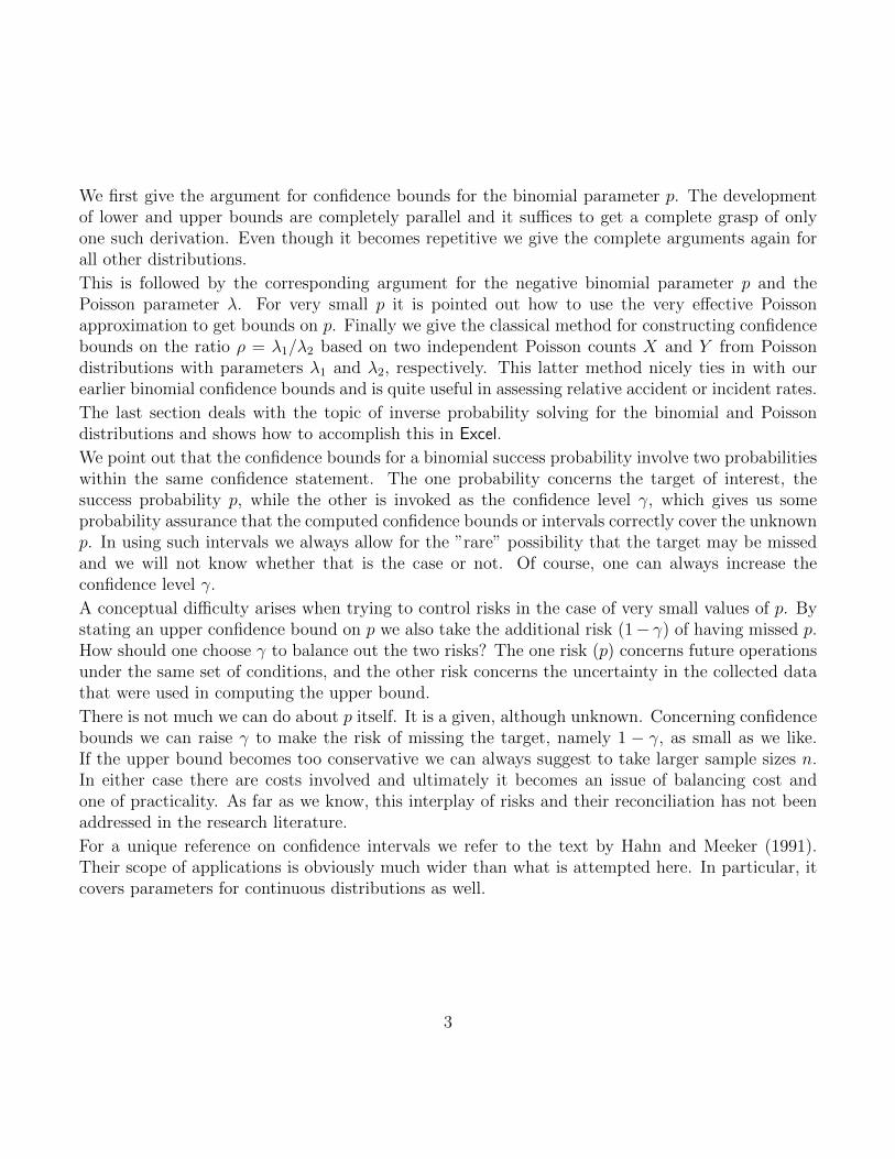
When testing hypotheses it is often more informative to report the p-value corresponding to anobserved value x of X. This p-value simply is the probability of seeing a result as extreme ormore extreme pointing away from the hypothesis in the direction of the entertained alternative,when in fact the hypothesis is true. In our testing situation this p-value corresponding to x isp(x, p0) = Pp0(X ≤ x). It is evident that the decision of rejecting or accepting H(p0) can be basedsimply on this p-value, namely reject H(p0) whenever p(x, p0) ≤ α and accept H(p0) wheneverp(x, p0) > α, see the illustration in Figure 1.
5
● ● ● ● ●●
●
●
●
●
●
●●
●
●
●
●
●
●
●●
● ● ● ● ● ● ● ● ● ● ● ● ● ● ● ● ● ● ● ●
0 10 20 30 40
0.00
0.04
0.08
0.12
x
Pp 0
(X=
x)
● ● ● ● ●●
●
●
●
●
●
●●
●
●
●
●
●
●
●●
● ● ● ● ● ● ● ● ● ● ● ● ● ● ● ● ● ● ● ●
Figure 1: Binomial Distribution.
● ● ● ● ● ●●
●
●
●
●
●
●
●
●
●
●
●● ● ● ● ● ● ● ● ● ● ● ● ● ● ● ● ● ● ● ● ● ● ●
0 10 20 30 40
0.0
0.2
0.4
0.6
0.8
1.0
x
p(x,
p0)
= P
p 0(X
≤x)
α = 0.05
k(p 0
, α)=
6la
rges
t x fo
r w
hich
to r
ejec
t
n = 40 , p0 = 0.3
α = 0.05
reject H(p0) since p(x, p0) ≤ 0.05accept H(p0) since p(x, p0) > 0.05
6

It is possible to establish a basic duality between testing hypotheses and confidence sets by definingsuch confidence sets as all values p0 for which the observed value x of X results in an acceptanceof the hypothesis Hp0 . Denote this confidence set as C(x). We can also view the collection of suchconfidence sets (defined for each x = 0, 1, . . . , n) as a random set C(X) before having realized anyobserved value x for X. The following coverage probability property then holds for C(X):
Pp0 (p0 ∈ C(X)) = 1− Pp0 (p0 /∈ C(X)) = 1− Pp0 (X ≤ k(p0, α)) ≥ 1− α for all p0 , (3)
i.e., this random confidence set has coverage probability ≥ γ = 1− α no matter what the value p0is. Thus we do not need to know p0 and we can consider C(X) as a 100γ% confidence set for theunknown parameter p0.
We point out that the inequality ≥ 1−α in (3) becomes an equality for some values of p0, becausethere are values p0 for which we have Pp0(X ≤ k(p0, α)) = α. This follows since for any integerk < n the probability Pp0(X ≤ k) decreases continuously from 1 to 0 as p0 increases from 0 to 1.Thus the confidence coefficient γ (the minimum coverage probability) of the confidence set C(X)is indeed 1− α = γ.
It remains to calculate the confidence set C(x) explicitly for all possible values x that could berealized, i.e., for x = 0, 1, . . . , n. According to the above definition of C(x) it can be expressed asfollows
C(x) = {p0 : p(x, p0) = Pp0(X ≤ x) > α} .Since Pp0(X ≤ x) is strictly decreasing in p0 for x = 0, 1, . . . , n − 1 we see that the confidence setC(x) for such x values consists of the interval [0, pU(γ, x, n)), where pU(γ, x, n) = pU(1− α, x, n) isthe value p that solves
Pp(X ≤ x) =x∑i=0
(n
i
)pi(1− p)n−i = α = 1− γ . (4)
Since Pp(X ≤ k) is continuous and strictly decreasing from 1 to 0 as p increases from 0 to 1,there is a unique value p satisfying equation (4). For x = n equation (4) has no solution sincePp(X ≤ n) = 1 for all p. However, according to the above definition of C(x) we get C(n) = [0, 1].We define pU(γ, n, n) = 1 in this special case.
Thus we can treat pU(γ,X, n) as a 100γ% upper confidence bound for p. Rather than findingpU(γ, x, n) for x < n by solving (4) for p we use the identity (2) involving the Beta distribution
Pp(X ≤ x) = 1− Ip(x+ 1, n− x) = 1− γ or Ip(x+ 1, n− x) = γ .
We see that the solution p is the γ-quantile of the Beta distribution with parameters x + 1 andn − x. This value p can be obtained from Excel by invoking BETAINV(γ, x + 1, n − x) and in R orS-Plus by the command qbeta(γ,x+ 1,n− x).
7

As a check example use the case k = 12 and n = 1600 with γ = .95, then one gets pU(.95, 12, 1600) =qbeta(.95, 12 + 1, 1600− 12) = .01212334 as 95% upper bound for p.
Using (4) it is a simple exercise to show that the sequence of upper bounds is strictly increasingin x, i.e., 0 < pU(γ, 0, n) < pU(γ, 1, n) < . . . < pU(γ, n − 1, n) < pU(γ, n, n) = 1. One immediateconsequence of this is that Pp(p < pU(γ,X, n)) ≥ Pp(p < pU(γ, 0, n)) = 1 for all p < pU(γ, 0, n).Figure 2 shows the set of all n + 1 upper bounds for γ = .95 and n = 100 superimposed on thecorresponding estimates p(x) = x/n.
0.0 0.2 0.4 0.6 0.8 1.0
0.0
0.2
0.4
0.6
0.8
1.0
x/n
p U(x
)
●●
●●
●●
●●
●●
●●
●●
●●
●●
●●
●●
●●
●●
●●
●●
●●
●●
●●
●●
●●
●●
●●
●●●●●●●●●●●●●●●●●●●●●●●●●●●●●●●●●●●●●●●●●●●●●●●●●●●●●●●●●γ = 0.95 , n = 100
0.02951 = smallest possible upper bound
●
estimatesupper bounds
Figure 2: Binomial Upper Bounds in Relation to the Corresponding Estimates.
8

2.2.1 The Confidence Coefficient γ
The confidence coefficient of the upper bound is defined as
γ = infp{Pp (p ∈ C(X))} = inf
p{Pp (p < pU(γ,X, n))} .
The confidence coefficient is γ = γ = 1−α since Pp (p ∈ C(X)) = γ for some p, or Pp (p /∈ C(X)) =Pp(X ≤ k(p, α)) = 1− γ = α for some p.
Proof: Recall that for x = 0, 1, . . . , n− 1 the value p = pU(γ, x, n) solved
Pp(X ≤ x) = α
Thus for pi = pU(γ, i, n), i = 0, 1, . . . , n− 1, with k(pi, α) = i we have
Ppi(X ≤ k(pi, α)) = Ppi(X ≤ i) = α , (5)
i.e., the infimum above is indeed attained at p = p0, p1, . . . , pn−1.
2.2.2 Special Cases
For x = 0 and x = n− 1 the upper bounds defined by (4) can be expressed explicitly as
pU(γ, 0, n) = 1− (1− γ)1/n and pU(γ, n− 1, n) = γ1/n .
Obviously, the bound for x = 0 is of more practical interest than the bound in the case of x = n−1.
For γ = .95 and approximating log(.05) = −2.995732 by −3 the upper bound for x = 0 becomes
pU(.95, 0, n) = 1− (.05)1/n = 1− exp
[log(.05)
n
]≈ 1− exp(−3/n) ≈ 3
n,
which is sometimes referred to as the Rule of Three, because of its mnemonic simplicity, see vanBelle (2002). Here the last approximation is valid only for large n, say n ≥ 100.
One common application of this Rule of Three is to establish the appropriate sample size n whenit is desired to establish with 95% confidence that p is bounded above by 3/n. For this to work onehas to be quite sure to see 0 “successes” (bad or undesirable outcomes) in n trials. For example, ifone wants to establish .001 = 3/n as 95% upper bound for p one should conduct n = 3/.001 = 3000trials and hope for the best, namely 0 events.
9

2.2.3 Side Comment on Treatment of X = 0
When one observes X = 0 successes in n trials, especially when n is large, one is still not inclinedto estimate the success probability p by p(0) = 0/n = 0, since that is a very strong statement.When p = 0 then we will never see a success in however many trials. Since p = 0 is such a strongstatement, but one still thinks that p is likely to be very small if X = 0 in a large number n oftrials, one common practice to get out of this dilemma is to “conservatively” pretend that the firstsuccess is just around the corner, i.e., happens on the next trial. With that one would estimate pby p = 1/(n + 1) which is small but not zero. There are other (and statistically better) rationalesfor justifying p = 1/(n + 1) as an estimate of p but we won’t enter into that here, since they haveno bearing on the issue of confidence that some construe out of the above “conservative” step.
As an estimate of the true value of p the use of p is not entirely unreasonable but somewhatconservative. It is however quite different from our 95% upper confidence bound of 3/n, namely byroughly a factor of 3. One could ask: what is the actual confidence associated with p?
We can assess this by solving 1− (1− γ)1/n = 1/(n+ 1) for γ, which leads to
γ = 1−(
n
n+ 1
)n= 1−
(1− 1
n+ 1
)n≈ 1− exp
(− n
n+ 1
)≈ 1− exp(−1) = .6321 .
This means that we can treat p = 1/(n + 1) only as a 63.21% upper confidence bound for p. Thisis substantially lower than the 95% which led to the factor 3 in 3/n as upper bound.
2.2.4 Closed Intervals or Open Intervals?
So far we have given the confidence sets in terms of the right open intervals [0, pU(γ, x, n)) with theproperty that
Pp(p < pU(γ,X, n)) ≥ γ and infp{Pp(p < pU(γ,X, n))} = γ ,
where the value γ is achieved at p = pU(γ, x, n) for x = 0, 1, . . . , n− 1.
The question arises quite naturally: why not take instead the right closed interval [0, pU(γ, x, n)],again with property
Pp(p ≤ pU(γ,X, n)) ≥ γ and infp{Pp(p ≤ pU(γ,X, n))} = γ .
The difference is that the infimum is not achieved at any p.
Whether we use the closed interval or not, the definition of pU(γ, x, n) stays the same. Any valuep0 equal to it or greater would lead to rejection of H(p0) when tested against A(p0) : p < p0. Byclosing the interval we add a single p to it, namely p = pU(γ, x, n), that is not acceptable.
10

2.2.5 Coverage Probability Continuity Properties
Let pi = p(γ, i, n) for i = 0, 1, . . . , n. Recall 0 < p0 < p1 < . . . < pn = 1.
For p ∈ [pi−1, pi) the set A = {j : p < p(γ, j, n)} = [i, n] does not change.
=⇒ Pp(X ∈ A) = Pp(X ≥ i) increases continuously in p over [pi−1, pi) .
When p = pi the set A loses the value j = i and Pp(p < p(γ,X, n)) drops by Ppi(X = i) toPpi(X ≥ i + 1) = 1 − Ppi(X ≤ i) = 1 − α = γ see (5), and so on. This behavior is illustrated inFigure 3.
0.0 0.2 0.4 0.6 0.8 1.0
0.95
0.96
0.97
0.98
0.99
1.00
p
Pro
babi
lity
of C
over
age
for
pU
nominal confidence level = 0.95sample size n = 10
Figure 3: Coverage Probability Behavior of Upper Bound
11

For p ∈ (pi−1, pi] the set B = {j : p ≤ p(γ, j, n)} = [i, n] does not change.
=⇒ Pp(X ∈ B) = Pp(X ≥ i) increases continuously in p over (pi−1, pi] .
As p ↘ pi−1 we have Pp(X ≥ i) ↘ Ppi−1(X ≥ i) = 1 − Ppi−1
(X ≤ i − 1) = 1 − α = γ see (5), butat p = pi−1 we have a jump since
Ppi−1(pi−1 ≤ p(γ,X, n)) = Ppi−1
(X ≥ i− 1) > Ppi−1(X ≥ i) ,
i.e., γ is never attained.
2.3 Lower Bounds for p
Large values of X can be viewed as evidence against the hypothesis H(p0) : p = p0 when testing itagainst the alternative A(p0) : p > p0. Again one can carry out the test in terms of the observedp-value p(x, p0) = Pp0(X ≥ x) by rejecting H(p0) at level α whenever p(x, p0) ≤ α and accepting itotherwise. Invoking again the duality between testing and confidence sets we get as confidence set
C(x) = {p0 : p(x, p0) = Pp0(X ≥ x) > α} .
Since Pp0(X ≥ x) is strictly increasing and continuous in p0 we see that for x = 1, 2, . . . , n thisconfidence set C(x) coincides with the interval (pL(γ, x, n), 1], where pL(γ, x, n) is that value of pthat solves
Pp(X ≥ x) =n∑i=x
(n
i
)pi(1− p)n−i = α = 1− γ . (6)
Invoking the identity (1) this value p can be obtained by solving
Ip(x, n− x+ 1) = α = 1− γ
for p, i.e., it is the α-quantile of a Beta distribution with parameters x and n − x + 1. For x = 0we have Pp0(X ≥ 0) = 1 > α and we cannot use (6), but the original definition of C(x) leads toC(0) = [0, 1] and we define pL(γ, 0, n) = 0 in that case.
In Excel we can obtain pL(γ, x, n) for x > 0 by invoking BETAINV(1 − γ, x, n − x + 1) and from Ror S-Plus by the command qbeta(1− γ,x,n− x+ 1).
As a check example take x = 4 and n = 500 with γ = .95, then one gets pL(.95, 4, 500) = .002737as 95% lower bound for p.
Using (6) it is a simple exercise to show that the sequence of lower bounds is strictly increasing inx, i.e., 0 = pL(γ, 0, n) < pL(γ, 1, n) < . . . < pL(γ, n − 1, n) < pL(γ, n, n) < 1. Again it follows thatPp(pL(γ,X, n) < p) ≥ Pp(pL(γ, n, n) < p) = 1 for p > pL(γ, n, n).
As in the case of the upper bound one may prefer to use the closed confidence set [pL(γ, x, n), 1],with the corresponding commentary. In particular, the lower endpoint p0 = pL(γ, x, n) does notrepresent an acceptable hypothesis value, while all other interval points are acceptable values.
12

2.3.1 Special Cases
For x = 1 and x = n the lower bounds defined by (6) can be expressed explicitly as
pL(γ, 1, n) = 1− γ1/n and pL(γ, n, n) = (1− γ)1/n
For obvious reasons the explicit lower bound in the case of x = n is of more practical interest thanthe lower bound for x = 1.
For γ = .95 and x = n the lower bound becomes
pL(.95, n, n) = (1− .95)1/n ≈ exp(−3/n) ≈ 1− 3
n,
a dual instance of the Rule of Three. Here the last approximation is only valid for large n. Thisduality should not surprise since switching the role of successes and failures with concomitant switchof p and 1− p turns upper bounds for p into lower bounds for p and vice versa.
2.3.2 Side Comment on Treatment of X = n
When observing X = n successes in n trials, especially when n is large, one is still not inclined toestimate p by p = n/n = 1, because of the consequences of such a strong statement. Because ofthe just mentioned duality when switching successes with failures we will not repeat the paralleldiscussion of Section 2.2.3.
2.4 Confidence Intervals for p
As outlined in the Introduction, such lower and upper confidence bounds, each with respectiveconfidence coefficient 1 − α/2, can be used simultaneously as a 100(1 − α)% confidence interval(pL(1−α/2, X, n), pU(1−α/2, X, n)), provided we show Pp(pL(1−α/2, X, n) < pU(1−α/2, X, n)) = 1for any p.
We demonstrate this by assuming that we have pU(1 − α/2, x, n) ≤ pL(1 − α/2, x, n) for some xand thus pU(1 − α/2, x, n) ≤ p0 ≤ pL(1 − α/2, x, n) for some p0 and some x. This means thatthe p-values from the respective hypothesis tests linked to the one-sided bounds would cause us toreject the hypothesis H(p0) in each case, i.e.,
Pp0(X ≤ x) ≤ α/2 and Pp0(X ≥ x) ≤ α/2
and by adding those two inequalities we get
1 + Pp0(X = x) ≤ α < 1 , i.e., a contradiction.
13

Using pL(1− α/2, x, n) < pU(1− α/2, x, n) for any p and any x = 0, 1, . . . , n we have
Pp(pL(1− α/2, X, n) < p < pU(1− α/2, X, n))
= 1− Pp(p ≤ pL(1− α/2, X, n) ∪ pU(1− α/2, X, n) ≤ p)
= 1− [Pp(p ≤ pL(1− α/2, X, n)) + Pp(pU(1− α/2, X, n) ≤ p)]
≥ 1− [α/2 + α/2] = 1− α .
2.5 Coverage
We examine here briefly the issue of coverage, namely, what is the actual probability for the upperor lower bounds or intervals to be above or below p or to contain p, respectively, for the variousvalues of p. Figures 4 and 5 show the results in the example case of n = 100 and nominal confidencelevel γ = .95 computed over a very fine grid of p values.
These plots were produced in R by calculating in the case of the lower bound coverage probability
P (pL(γ,X, n) ≤ p) = (1− p)n +n∑x=1
I{qbeta(1−γ,x,n−x+1)≤p}
(n
x
)px(1− p)n−x ,
where IA = 1 whenever A is true and IA = 0 otherwise. For the upper bound one computes thecoverage probabilities via
P (pU(γ,X, n) ≥ p) =n−1∑x=0
I{qbeta(γ,x+1,n−x)≥p}
(n
x
)px(1− p)n−x + pn ,
while for the confidence interval one calculates the coverage probability as
P (pL((1 + γ)/2, X, n) ≤ p ∩ pU((1 + γ)/2, X, n) ≥ p)
=n−1∑x=1
I{qbeta((1−γ)/2,x,n−x+1)≤p ∩ qbeta((1+γ)/2,x+1,n−x)≥p}
(n
x
)px(1− p)n−x
+(1− p)nI{qbeta((1+γ)/2,1,n)≥p} + pnI{qbeta((1−γ)/2,n,1)≤p}
Note that in the above calculations the closed form of the one-sided bounds or confidence intervalswas used. Close examination of the plots shows that the minimum coverage probability seems togo as low as the target γ = .95 for the one-sided bounds. The value .95 appears to be (almost)achieved at every dip, except for p near 0 or 1. The dips correspond to all possible confidencebound values. As discussed previously, for the closed one-sided bounds the coverage probabilityshould get arbitrarily close to .95 at all of these dips. The fact that .95 does not appear to befully approximated for p near 0 or 1 is due to the grid over which these coverage probabilities wereevaluated.
14

0.0 0.2 0.4 0.6 0.8 1.0
0.95
0.96
0.97
0.98
0.99
1.00
p
Pro
babi
lity
of C
over
age
for
pU
nominal confidence level = 0.95sample size n = 100
0.0 0.2 0.4 0.6 0.8 1.0
0.95
0.96
0.97
0.98
0.99
1.00
p
Pro
babi
lity
of C
over
age
for
pL
nominal confidence level = 0.95sample size n = 100
Figure 4: Binomial Coverage Probabilities for Upper and Lower Confidence Bounds
15

For the confidence interval the coverage probability appears to reach not quite as far down as .95,see Figure 5. To illustrate this more clearly we also show the corresponding plot for n = 11 in thebottom part of Figure 5. This conservative coverage is due to the fact that the supremum of asum is typically smaller than the sum of the suprema over the respective summands, because thepoint where one summand comes close to its supremum does not necessarily coincide with the pointwhere the other summand comes close to its supremum, i.e.,
infpPp(pL(1− α/2, X, n) ≤ p ≤ pU(1− α/2, X, n))
= 1− suppPp(p < pL(1− α/2, X, n) ∪ pU(1− α/2, X, n) < p)
= 1− supp{Pp(p < pL(1− α/2, X, n)) + Pp(pU(1− α/2, X, n) < p)}
≥ 1−{
suppPp(p < pL(1− α/2, X, n)) + sup
pPp(pU(1− α/2, X, n) < p)
}= 1− {α/2 + α/2} = 1− α .
Here the inequality ≥, for reasons explained above, typically takes the strict form >.
Furthermore, for p close to 0 or 1 the coverage probability rises effectively to 1 − α/2 = .975.This is a consequence of the previously noted coverage with probability 1, for upper bounds forp < pU(1− α/2, 0, n) and for lower bounds for p > pL(1− α/2, n, n), so that
Pp(pL(1− α/2, X, n) ≤ p ≤ pU(1− α/2, X, n))
= 1− Pp(pL(1− α/2, X, n) > p)− Pp(pU(1− α/2, X, n) < p)
= 1− Pp(pL(1− α/2, X, n) > p) ≥ 1− α/2 for p < pU(1− α/2, 0, n)
= 1− Pp(pU(1− α/2, X, n) < p) ≥ 1− α/2 for p > pL(1− α/2, n, n)
It would appear that for small p there is little sense in working with confidence intervals, allocatinghalf of the miss probability (α/2) to the lower bound and raising the confidence level of the righthandinterval endpoint to 1−α/2. This leads to a conservative assessment of the smallness of p. If smallp are of main concern (typical for risk situations) one should focus on upper bounds for p, i.e., usepU(1− α,X, n) instead of the higher righthand endpoint pU(1− α/2, X, n) of the interval.
16

0.0 0.2 0.4 0.6 0.8 1.0
0.95
0.96
0.97
0.98
0.99
1.00
p
Pro
babi
lity
of C
over
age
for
[ pL ,
pU ]
nominal confidence level = 0.95sample size n = 100
0.0 0.2 0.4 0.6 0.8 1.0
0.95
0.96
0.97
0.98
0.99
1.00
p
Pro
babi
lity
of C
over
age
for
[ pL ,
pU ]
nominal confidence level = 0.95sample size n = 11
Figure 5: Binomial Confidence Interval Coverage Probabilities
17

To get some sense of what might be given away in using the latter rather than the former we canask: How large a sample size m is needed to equate pU(1−α/2, 0,m) = pU(1−α, 0, n) when in factwe see 0 events in either case. This leads to the following equation
1− (α/2)1/m = 1− α1/n or m = nlog(α)− log(2)
log(α).
For α = .05 this becomes m = 1.2314 n, i.e., a 23% increase in sample size over n with the additionalstipulation that we also see no event during the additional trials.
A corresponding argument can be made for using the lower bound in place of an interval whenp near 1 is of primary concern. This arises typically in reliability contexts where the chance ofsuccessful operation is desired to be high.
2.6 Simulated Upper Bounds
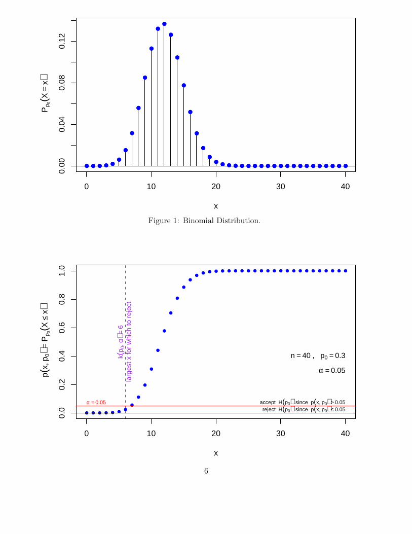
To get a better understanding of the nature of confidence bounds we simulated 1000 instances ofX from a binomial distribution Bin(n, p) for n = 100 and several different values of p. Figures 6-9show the resulting upper confidence bounds in relation to the respective true values of p.
The n+ 1 possible upper bounds are solely determined by the value n (recall qbeta(γ, x + 1, n− x)for x = 0, 1, . . . , n− 1 and pU(γ, n, n) = 1) and as the true p changes the distribution of X changes.As p increases we tend to see more high values of X. Note that Figure 6 shows no upper boundsbelow the target p, while Figure 7 shows 3.8% of the upper bounds barely below the target p. Wewould have expected 5% of the bounds below p with γ = .95, but due to the randomness of theparticular set of 1000 generated X values this should not surprise us.
As we raise the value of p in Figures 8 and 9, but still staying below the next possible upper boundvalue, we see that the percentage of upper bounds below p decreases. That is precisely due to thefact that we see fewer cases with X = 0 as p increases.
While in Figures 6-9 we were operating with values of p that we controlled, in the real life practicalsituation we do not know p and it is not clear whether we were lucky enough (≥ 95% of the time)to have gotten an upper bound above the unknown p or whether we were unlucky (≤ 5% of thetime). As Myles Hollander once put it: “Statistics means never having to say you’re certain.”
2.7 Elementary Classical Bounds Based on Normal Approximation
We point out here that the often and popularly given upper confidence bound for p, based on theestimate p = X/n and its estimated approximate normal distribution, is
p+ zγ
√p(1− p)
n, with zγ being the standard normal γ-quantile.
18
●
●●
●
●●
●
●
●
●
●
●
●●
●
●
●
●
●
●
●
●
●
●
●
●
●
●●
●●●
●
●
●
●
●
●
●
●
●
●
●
●●
●
●
●
●
●
●
●
●
●
●●
●
●●
●●
●
●●
●
●
●
●
●
●
●
●
●
●
●
●
●
●●
●●●
●●
●●
●
●
●
●●
●
●
●●
●
●
●
●●
●
●●
●
●
●
●
●
●●
●●
●
●
●
●●
●
●
●
●
●
●
●
●
●
●
●
●
●
●
●●
●
●●
●
●
●
●
●
●
●
●●
●
●
●
●●
●
●
●
●
●
●
●
●
●
●
●
●
●
●
●
●
●
●
●
●
●●
●
●
●
●
●
●
●
●
●
●
●
●
●●●●●●
●
●
●
●
●
●
●
●
●
●●●●
●●
●
●
●
●
●
●
●●
●
●●
●
●
●
●
●
●●
●
●●●
●
●
●
●●
●
●
●
●
●
●
●
●
●
●
●
●
●
●
●
●
●
●
●
●
●●
●
●
●●
●●●●●●
●
●
●
●
●●
●
●●●
●●
●
●●
●
●
●
●
●
●●
●
●
●
●●
●
●●
●
●
●
●
●
●
●
●●
●
●
●
●
●
●
●
●
●
●
●
●
●
●●
●
●
●
●
●
●●
●
●●●
●
●
●
●
●
●
●
●
●●
●
●
●
●
●
●
●●
●
●
●
●
●
●
●
●●
●
●●
●●
●
●
●
●
●
●
●
●
●
●
●
●
●
●
●
●
●
●●
●
●
●
●
●
●
●
●
●
●
●
●
●
●
●
●
●
●
●
●
●
●
●●
●
●●
●
●●
●●
●
●
●
●
●
●
●
●
●
●●●
●
●
●
●
●
●●●
●
●
●●
●
●●
●
●
●●
●
●●
●
●
●
●
●
●
●
●
●
●
●
●
●
●
●
●
●
●
●
●●
●
●
●
●
●
●
●
●
●
●
●
●
●
●●●
●
●●
●●
●●
●
●
●●
●
●
●
●
●
●
●
●
●
●●
●
●
●
●●●
●
●
●
●●●
●●
●
●●
●
●
●
●
●
●
●●
●
●
●
●
●●
●
●
●
●
●
●●●●
●●
●
●
●
●
●
●
●
●
●●
●
●
●
●●
●
●●
●
●
●
●●●
●
●●
●
●
●
●
●
●
●●●
●
●
●
●
●
●
●
●
●
●
●
●
●
●
●●
●●
●
●
●
●
●●●
●
●
●
●
●
●
●
●
●●
●
●
●
●
●
●
●
●
●
●
●●
●
●
●
●
●●●
●
●
●●
●
●
●●
●
●
●
●
●●
●
●
●
●
●
●
●
●
●●●
●
●
●●
●
●
●●
●
●
●
●
●
●
●●
●
●
●
●
●
●
●
●
●
●
●
●●●
●
●
●
●
●
●
●
●
●
●
●
●
●
●
●
●
●●●●
●
●
●
●
●
●
●
●
●
●
●
●●
●
●
●
●
●
●
●●
●
●
●
●
●
●
●
●
●
●
●
●
●
●
●
●●
●
●●
●●
●●
●
●
●
●
●
●
●
●
●●
●
●
●●
●
●
●
●
●●
●
●●
●
●
●
●●●
●
●
●
●
●
●
●●
●
●●
●
●
●
●
●●
●
●
●
●
●
●
●●
●●
●
●
●
●
●●
●
●
●
●
●
●
●●
●
●
●●
●
●
●
●
●
●
●
●
●
●
●
●
●
●
●●●
●
●
●
●
●
●
●●
●
●
●
●
●
●
●
●
●●
●
●
●
●
●
●
●
●
●●●
●
●
●
●●
●
●
●
●
●
●
●
●
●●
●
●
●
●
●
●●
●
●
●
●
●
●
●●
●
●
●
●
●
●
●
●
●
●
●
●
●
●
●
●
●
●
●●
●
●
●
●
●
●
●
●
●●
●
●
●
●
●
●
●
●
●
●
●
●
●●●
●
●
●
●
●
●
●●●
●
●●
●
●●
●●
●
●
●
●●
●
●●
●
●
●
●●
●●
●
●
●
●
●
●
●
●
●
●
●
●
●
●
●
●
0 200 400 600 800 1000
0.00
0.05
0.10
0.15
1000 simulated binomial x values
p U(x
)
γ = 0.95sample size n = 100
0 % of upper bounds pU(x) ≤ p = 0.029
smallest possible upper bound = 0.02951
Figure 6: 1000 Simulated Binomial Upper Bounds for p = .029.
●
●●●●●
●
●●
●
●●
●
●
●
●
●
●●
●
●
●
●
●
●
●
●
●●
●
●
●
●
●
●
●
●
●
●
●
●
●
●
●
●
●●
●
●
●
●
●
●
●●
●
●●●
●●
●
●
●
●
●●
●●
●●
●
●●
●●
●
●
●
●
●●
●
●
●●
●
●
●
●
●
●
●
●●●
●
●
●
●●
●●
●
●
●●
●●
●
●
●
●
●●
●
●
●
●
●
●●
●●●
●
●
●
●
●
●
●
●
●
●
●
●
●
●
●
●
●
●●
●
●
●
●
●●
●
●
●●
●
●●
●
●
●●
●
●
●
●●
●
●
●
●
●
●
●
●
●
●
●
●
●
●
●
●
●
●
●
●●
●
●
●●
●
●
●
●
●●
●
●
●
●
●
●
●
●
●
●●●●
●
●
●●●
●
●
●
●
●
●
●
●●
●
●
●●●
●
●
●●
●
●
●
●
●
●
●
●
●
●
●●
●
●
●●
●●
●
●
●●
●
●
●●
●
●●
●
●
●
●
●
●
●
●
●
●
●
●
●
●
●
●
●
●
●●
●
●
●
●●
●●
●
●
●
●
●
●●
●
●
●
●
●
●
●
●
●
●
●
●
●
●
●
●
●
●
●
●
●
●
●
●
●
●●
●
●
●
●
●
●
●
●
●
●
●
●●
●
●
●
●
●
●
●
●
●
●
●
●
●
●●●
●
●
●
●●●
●
●
●
●●●
●
●
●●
●
●
●
●
●
●
●
●
●
●
●
●
●
●
●
●
●
●
●
●●
●
●
●
●
●●
●
●
●
●
●
●
●
●
●●
●
●
●●
●
●
●
●
●
●
●
●
●●
●
●
●●●●
●
●
●
●
●
●
●●●
●
●
●●
●
●
●
●
●
●
●
●
●
●●
●
●●
●
●
●
●
●
●●
●
●
●
●
●
●●
●
●
●
●●
●
●
●
●
●
●●
●
●
●
●
●
●
●●
●
●
●
●
●
●
●
●
●
●
●
●
●
●●●
●●
●
●
●
●
●
●
●
●
●
●
●●
●
●
●
●●
●
●
●
●
●●
●
●
●
●
●
●
●
●
●
●
●●●
●●
●
●
●
●
●●
●●
●
●
●
●
●●
●
●
●
●
●●●
●
●
●
●
●
●
●
●
●●
●
●
●
●
●
●
●●
●
●
●●
●
●●
●●
●
●
●
●
●
●
●
●
●
●
●●
●
●
●●●
●
●
●●
●
●
●
●●
●
●
●
●
●
●
●●
●
●
●
●
●
●
●
●
●
●
●
●●
●
●
●
●
●
●●
●
●
●
●
●
●
●
●
●
●
●
●
●
●
●
●
●
●
●
●
●
●●
●
●
●
●
●
●
●
●
●
●
●
●
●
●
●
●●
●
●
●
●●●
●
●
●
●
●
●
●
●●
●
●
●
●
●
●
●●●
●●
●
●●
●
●
●●
●
●
●
●●
●
●
●
●
●
●
●
●
●
●●
●
●
●
●
●
●
●●●
●
●
●
●
●
●
●
●
●
●●
●
●
●
●●●
●
●
●
●
●
●
●●●
●
●
●
●
●●
●
●
●
●
●
●
●
●
●
●
●
●
●
●
●
●
●
●
●
●●
●
●●
●
●
●
●
●
●
●●
●
●
●
●
●
●
●
●●●
●
●
●
●
●
●
●
●●
●
●
●
●●
●
●
●
●
●
●
●
●
●
●
●
●
●
●
●
●
●
●
●
●
●
●●
●
●●●
●
●
●
●
●
●
●●
●
●●
●
●
●
●
●
●
●●
●●
●
●
●●●
●
●
●
●
●
●
●
●
●
●
●●●
●
●●
●
●
●
●
●
●
●
●
●
●
●
●●
●
●
●
●
●
●
●
●
●
●
●
●
●
●
●
●
●●
●
●
●
●
●
●
●●
●
●●
●
●●
●
●
●
●
●
●●
●
●
●●●
●
●
●
●
●
●
●
●
●
●
●
●●
●
●
●
●
●
●
●
●●
●
●
●●
●
●
●
●
●
●●
●
●
●
●
●
●
●
●
●●
●
0 200 400 600 800 1000
0.00
0.05
0.10
0.15
0.20
1000 simulated binomial x values
p U(x
)
γ = 0.95sample size n = 100
3.8 % of upper bounds pU(x) ≤ p = 0.03smallest possible upper bound = 0.02951
Figure 7: 1000 Simulated Binomial Upper Bounds for p = .030.
19

●
●
●
●
●●
●
●
●
●
●
●
●
●
●
●
●
●
●
●
●
●
●
●
●
●
●
●
●
●●
●
●
●
●
●●
●●
●
●
●●
●
●
●
●●
●
●
●
●
●
●
●
●●●
●
●
●
●
●
●
●
●
●
●
●
●●
●
●
●
●
●
●
●
●●
●
●
●
●
●●
●
●
●
●
●
●
●
●●
●
●
●
●
●
●
●
●
●
●
●
●
●●
●
●
●
●
●
●
●
●
●
●●
●
●●
●
●
●
●
●
●
●
●
●
●
●
●
●
●
●
●
●
●
●
●
●
●●
●
●
●
●
●
●
●
●
●
●
●
●
●
●
●
●●
●
●
●
●
●
●
●●
●
●●
●
●
●
●
●
●
●
●
●
●
●
●
●
●
●
●
●
●
●
●
●
●●●●
●
●
●
●
●
●
●
●
●
●
●
●●●
●
●
●
●
●
●
●
●
●
●
●
●
●
●
●
●
●●
●
●
●
●
●●
●●
●
●●
●●
●●
●
●
●
●
●●
●
●
●
●
●●
●
●●
●
●
●
●
●
●●
●●
●
●
●●
●
●
●
●
●
●●
●
●
●
●
●
●
●
●
●
●●●●
●
●
●
●●
●●●
●
●
●●
●
●
●
●
●
●
●
●
●
●
●
●●
●
●
●●
●
●
●
●
●
●
●
●
●
●
●
●
●
●
●
●
●
●
●
●
●●●
●
●
●
●
●
●
●
●●
●
●●●
●
●
●
●
●●
●●
●
●
●
●
●
●
●
●
●
●
●●
●
●
●●
●
●
●
●●
●
●
●
●
●
●
●
●
●
●
●
●
●
●
●
●●
●
●
●
●●
●
●
●●
●
●
●
●
●●
●
●
●●
●●
●
●
●
●
●
●
●
●●
●
●
●
●●
●
●
●
●●
●
●
●
●
●
●
●
●
●
●
●
●
●
●
●
●
●
●
●
●
●
●
●
●●●
●
●
●
●●
●
●
●
●
●
●
●
●●
●
●
●
●
●
●
●
●●
●
●
●
●
●
●
●
●
●●●●●
●●
●
●
●
●●
●●
●
●
●
●
●
●
●
●
●
●
●
●
●
●
●
●
●
●
●
●
●
●
●
●
●
●
●
●●
●
●
●
●
●●
●
●
●
●●●●●
●
●
●●
●
●
●
●
●
●
●
●
●
●
●
●●
●
●
●
●
●●
●
●
●
●
●
●
●
●
●
●
●
●
●●
●
●●●
●
●
●
●
●
●●
●
●
●
●
●
●
●
●●
●
●
●
●
●
●●
●
●
●
●
●
●
●
●●●
●
●
●
●
●
●●
●
●●
●
●
●
●
●
●
●
●
●
●
●
●
●
●
●
●
●
●
●●
●
●●
●
●
●
●
●●
●
●
●
●
●
●
●
●
●
●
●
●
●
●●
●
●
●●
●
●●
●
●●●
●
●
●●
●●
●
●
●
●
●
●●
●
●
●
●
●
●
●
●
●
●
●
●
●
●
●
●
●
●
●
●
●
●●
●
●
●
●
●●
●
●
●
●
●
●
●●
●
●
●
●
●
●
●
●
●
●
●
●
●
●
●
●●
●
●
●
●
●
●
●●
●
●
●
●
●●
●●
●
●
●
●
●
●
●
●
●
●●●
●
●●●●●
●
●
●
●
●
●
●
●●●
●
●
●
●
●
●
●
●
●
●
●
●
●
●
●
●
●●
●
●
●
●
●
●
●
●●
●
●
●
●
●●
●●
●
●
●
●
●
●
●
●
●
●
●
●
●
●
●
●
●
●
●
●
●
●
●
●
●
●
●
●
●
●
●
●
●
●
●
●
●
●
●
●
●●
●
●●
●
●●
●
●
●
●
●●
●
●
●●●●
●
●
●
●
●
●
●
●
●
●
●
●
●
●
●
●
●
●
●
●
●●
●
●
●
●
●
●●●
●
●
●
●
●
●
●●●
●
●
●●●
●
●
●
●
●●●
●
●
●
●
●●●
●
●
●●
●
●●
●
●●
●
●
●
●
●
●
●
●
●
●
●
●
●●
●
●
●●●
●
●
●
●●
●
●●
●
0 200 400 600 800 1000
0.00
0.05
0.10
0.15
1000 simulated binomial x values
p U(x
)
γ = 0.95sample size n = 100
1.7 % of upper bounds pU(x) ≤ p = 0.04smallest possible upper bound = 0.02951
Figure 8: 1000 Simulated Binomial Upper Bounds for p = .040.
●
●
●
●●
●
●
●
●
●●
●
●
●
●
●
●
●
●
●
●
●
●
●
●
●
●
●
●
●
●●
●
●
●
●
●
●
●
●●
●●
●
●
●
●
●●
●
●
●
●
●●
●
●
●
●●
●
●
●●
●
●●●
●
●
●
●●●
●●●●
●
●
●
●●
●
●
●●
●
●●
●
●●●
●
●●
●
●
●
●
●
●
●
●
●●
●
●
●
●
●
●
●
●
●
●●
●
●
●
●
●
●
●
●
●
●
●
●
●
●●●
●
●
●
●
●●
●
●
●
●
●
●
●
●●●
●
●
●
●
●●●
●
●
●
●
●
●
●
●
●
●
●
●
●
●
●
●
●●
●
●
●
●
●
●
●●
●●
●
●
●
●
●
●
●●
●
●
●
●
●
●●●
●
●
●
●●
●
●
●
●
●
●
●●
●●●
●
●
●
●●
●●●
●
●
●
●
●●
●●
●
●
●
●
●
●
●
●
●
●
●
●
●
●
●
●
●
●●
●
●
●
●
●
●
●
●
●
●
●
●●
●●
●
●
●
●
●
●●
●
●
●
●
●
●
●
●
●
●
●
●●
●
●
●●
●
●
●
●
●
●
●
●
●
●●
●
●
●
●
●
●
●●
●
●●
●
●
●
●
●
●
●
●
●
●
●
●
●
●
●
●
●●
●●
●
●
●●
●
●
●●
●
●
●
●
●
●
●
●●●
●
●
●
●
●
●
●
●
●
●
●
●
●
●
●
●
●
●
●
●
●
●
●
●
●
●
●
●
●
●
●
●
●
●
●
●
●
●
●
●
●
●
●
●
●
●●
●●●
●
●
●
●
●
●
●
●●
●
●
●
●
●
●
●
●●
●
●
●
●
●
●
●
●
●●
●
●
●
●●
●
●
●
●
●
●
●
●●
●
●
●
●
●
●
●
●
●
●●
●●
●●
●●
●●
●
●
●
●
●
●
●
●
●
●
●
●
●
●
●●
●
●
●●
●●
●●
●
●
●
●●
●●●●
●
●●
●
●
●
●
●
●
●
●
●
●
●
●
●
●
●
●
●
●
●
●
●
●
●
●●
●●●
●
●●
●
●
●
●●
●
●
●
●
●
●
●
●●
●●
●
●
●
●
●●
●
●
●●●
●
●
●
●
●●●
●
●
●
●
●
●
●
●
●
●●
●
●
●
●●
●
●
●
●
●
●
●
●
●
●
●
●
●
●
●
●
●
●
●
●●●
●
●
●
●
●
●
●
●
●
●●
●
●
●
●
●
●●
●
●
●●
●
●
●●
●
●
●
●●
●●
●
●
●
●●
●
●
●
●
●
●
●
●
●
●
●
●
●
●
●
●
●
●
●
●●●
●
●●
●
●
●
●
●
●
●
●
●
●
●
●
●
●●
●
●
●
●●●
●
●
●
●
●
●
●
●
●
●
●
●●
●
●
●
●
●●
●
●
●
●
●
●
●●
●
●
●
●
●
●
●
●●●
●
●
●
●
●●
●
●
●
●
●●
●
●
●
●●
●
●
●
●●
●●
●
●
●
●
●●
●
●
●●●
●
●
●
●
●
●
●
●
●
●
●
●
●
●
●
●
●
●●
●
●
●
●
●
●
●
●●
●
●
●
●
●
●
●
●
●
●
●
●
●
●
●
●
●
●
●
●
●
●
●
●
●
●
●
●●
●
●●●
●
●●
●
●
●
●●
●●
●
●
●
●●●
●
●
●
●
●
●
●
●
●
●
●
●
●
●
●●
●
●
●
●
●
●
●
●
●
●
●
●
●●●
●
●
●
●●
●
●
●
●
●
●
●
●
●
●
●
●
●
●
●●●
●
●
●●
●
●
●
●
●
●
●●
●
●
●
●
●
●
●
●
●
●●
●
●
●
●
●●
●
●
●
●●
●
●
●
●●
●
●
●
●
●
●
●
●●
●
●●
●
●
●●
●
●
●
●
●●
●
●
●
●●
●
●
●●
●
●
●
●
●
●
●
●
●
●
●
●
●
●
●●
●
●
●●
●
●
●
●
●
●●●
●
●
●
●
●●
●
●
●
●
●
●
●
●●
0 200 400 600 800 1000
0.00
0.05
0.10
0.15
0.20
1000 simulated binomial x values
p U(x
)
γ = 0.95sample size n = 1000.9 % of upper bounds pU(x) ≤ p = 0.043smallest possible upper bound = 0.02951
Figure 9: 1000 Simulated Binomial Upper Bounds for p = .043.
20

This upper bound has minimum coverage zero over all p ∈ (0, 1) and not the intended confidencelevel γ. This can be seen from the fact that for p > 0 very close to zero the chance that p = 0 getscloser and closer to one. But p = 0 implies that the above upper bound is zero as well and canthus no longer be ≥ p(> 0), with probability closer and closer to one. Hence the minimum coverageprobability is zero.
The reason for this failure of such a popularly cited procedure is that it is based on the approximate
normality of (p− p)/√p(1− p)/n. This approximation becomes problematic when p ≈ 0 or p ≈ 1,
in which case a larger and larger sample size n is required to make this approximation reasonable.However, even such a large n will not cover all contingencies w.r.t. p ∈ (0, 1). As p ↘ 0 or p ↗ 1this would lead to the requirement that n → ∞, which is hardly practical. A similar case can bemade in the case of lower bounds and intervals.
Figure 10 shows the coverage probability behavior of these elementary upper bounds. It makesquite clear that these upper bounds are reasonable only in the vicinity of p = .5.
0.0 0.2 0.4 0.6 0.8 1.0
0.80
0.85
0.90
0.95
1.00
p
Pro
babi
lity
of C
over
age
for
pU
nominal confidence level = 0.95sample size n = 100
Figure 10: Coverage Probabilities for Binomial Elementary Upper Confidence Bounds
21

2.8 Score Confidence Bounds
Agresti and Coull (1998) make a case for using score confidence intervals based on inverting scoretests. In the case of upper confidence bounds this simply amounts to solving equation (4) for p byapproximating the left hand side of (4) using the normal distribution, i.e., solve
α = Pp(X ≤ x) ≈ Φ
x− np√np(1− p)
,
where Φ is the standard normal cdf. This approximation is done without using a continuity correc-tion, which would amount to replacing x by x+ .5. The result is a rather unwieldy expression thatdoes not hold much mnemonic appeal, namely
pU(γ, x, n) =z2/(2n) + p
1 + z2/n+
z
1 + z2/n
√z2
4n2+p(1− p)
n,
where z is the γ-quantile of the standard normal distribution and p = x/n is the classical estimateof p. The corresponding lower bounds use instead the (1 − γ)-quantile or equivalently change thesign in front of the square root in the above upper bound expression. For intervals lower and upperbounds are combined with respective (1 + γ)/2 confidence levels.
Figure 11 shows the coverage behavior of the score upper bounds. The case made by Agresti andCoull in favor of these score bounds is that their average coverage probability is closer to the targetnominal. However, the minimum coverage probability can be quite a bit lower, although it occursfor p near 1, which is of not much concern in applications. When comparing the zigzag behavior inthis plot with that in Figure 4 it is difficult to see much of a difference in the range of amplitudes.It would appear that lowering the confidence level of the Clopper-Pearson bounds appropriatelywould bring the average coverage to the same level. In my opinion the criterion of average coverageis not appealing when trying to bound risks. It has too much the flavor of a statistician with hishead in the oven and his feet in an ice bucket, but feeling fine on average.
Out of curiosity we also computed the coverage probabilities for score upper bounds when usingin their derivation a continuity correction in the normal approximation. Such upper bounds arebasically the same as given previously, except that p is replaced by p = (x + .5)/n throughout.Figure 12 shows the result. While these bounds appear more conservative than the bounds withoutsuch a correction, they still do not guarantee the desired confidence level.
In all fairness to Agresti and Coull we point out that they made their case in the context of intervalsand not for one-sided bounds. Figure 13 shows the coverage probabilities for such intervals (withoutusing a continuity correction). While the average coverage behavior is as advocated, the coverageprobability deteriorates significantly near 0 or 1.
22

0.0 0.2 0.4 0.6 0.8 1.0
0.80
0.85
0.90
0.95
1.00
p
Pro
babi
lity
of C
over
age
for
p~U
nominal confidence level = 0.95
sample size n = 100
Figure 11: Coverage Probabilities for Score Upper Confidence Bounds
0.0 0.2 0.4 0.6 0.8 1.0
0.80
0.85
0.90
0.95
1.00
p
Pro
babi
lity
of C
over
age
for
p~U
nominal confidence level = 0.95
sample size n = 100
Figure 12: Coverage Probabilities for Score Upper Confidence Boundsusing continuity correction
23

0.0 0.2 0.4 0.6 0.8 1.0
0.80
0.85
0.90
0.95
1.00
p
Pro
babi
lity
of C
over
age
for
[ pL ,
pU ]
nominal confidence level = 0.95
sample size n = 100
Figure 13: Coverage Probabilities for Score Confidence Intervals
2.9 Corrosion Inspection
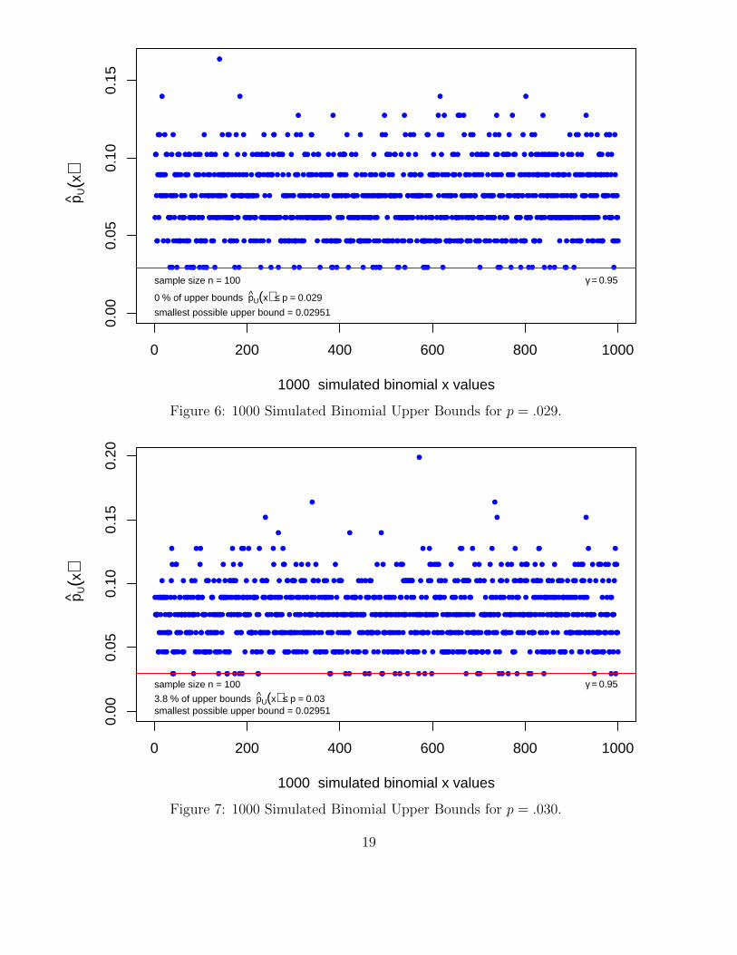
Airplanes are inspected for corrosion at a 10 year inspection interval. Based on the outcome of nsuch inspections the customer wants 95% lower confidence bounds on the probability of an airplanepassing its corrosion inspection without any findings. So far all n inspected aircraft made it throughcorrosion inspection without any findings. The customer did not tell me how many aircraft hadbeen inspected, he only told me that 2.5% of the fleet had been inspected. How do we deal withthis?
We can view each airplane’s corrosion experience over a 10 year exposure window as a Bernoullitrial with probability p of surviving 10 years without corrosion. Thus the number X of aircraftwithout any corrosion found at their respective inspections is a binomial random variable withparameters n and success probability p. Based on X = n the 95% lower confidence bound for pis pL(.95, n, n) = (1 − .95)1/n. Without knowing n we can only plot pL(.95, n, n) against n, as inFigure 14, and the customer can take it from there.
24
I suspect that this request arose because a particular airline, after finding no corrosion in n inspec-tions, is wondering about necessity of the onerous task of stripping the interior of an airplane forthe corrosion inspection. Maybe it is felt that this is a costly waste of resources or that the time toinspection should be increased so that cost is spread out over more service life. On the other hand,if corrosion is detected early it is a lot easier to fix than when it has progressed beyond extensiveor impossible repair.
For the sake of argument, if this airline has 200 aircraft of which 2.5% (or n = 5) had their 10 yearcheck, all corrosion free, then the 95% lower bound on p is about .55. This is not very reassuring.Jumping to any strong conclusions based on 5 successes in 5 trials has no basis. Most people don’thave a good grounding in matters of probability and that is why such requests arise again andagain.
0 50 100 150 200
0.6
0.7
0.8
0.9
1.0
number n of planes inspected, all without corrosion findings95 %
low
er c
onfid
ence
bou
nd o
n p=
P(n
o co
rros
ion
in 1
0 ye
ars)
Figure 14: Plot of pL(.95, n, n) against n.
25

2.10 Space Shuttle Application: Stud Hang-Up Issue
The two Solid Rocket Boosters (SRB) of the Space Shuttle are held down on the launch platformby 4 hold-down studs each, see Figure 152. These studs are about 3.5′′ in diameter and each isheld in place by a frangible nut, that explodes at takeoff to let the stud fall through cleanly, thusreleasing the Shuttle for takeoff. Due to various issues (explosion timing, etc) it sometimes happensthat these studs do not fall away cleanly but hang up instead. See
http://www.eng.uab.edu/ME/ETLab/HSC04/abstracts/HSC147.pdf
and http://www.nasa.gov/offices/nesc/home/Feature 1.html
for some of the issues and consequence involved. It is possible that such a 3.5′′ stud just getssnapped by the tremendous takeoff force.
Figure 15: Solid Rocket Booster Hold-Down Stud
2taken from a NASA Presentation titled SRB HOLDDOWN POST STUD HANG-UP LOADS, Feb 6, 2004.
26

Out of the 114 lift-offs there were 21 with a one hang-up out of the eight studs and there were twolift-offs with two stud hang-ups. No lift-off experienced more than two stud hang-ups.
One can estimate the probability p of a stud hang-up by p = (21× 1 + 2× 2)/(114× 8) = 25/912 =0.02741. Based on this estimate and assuming that the events of hang-ups from stud to stud occurindependently and with constant probability p one can estimate the probability pi of i hang-upsamong the 8 studs by the binomial probability formula
pi =
(8
i
)pi(1− p)8−i .
From this one gets p0 = 0.8006, p1 = 0.1805, p2 = 0.0178, and p3+ = 0.0010, where p3+ is theestimate for 3 or more stud hang-ups. Based on this one would have expected Ei = pi × 114lift-offs with i stud hang-ups. These expected numbers are E0 = 91.27, E1 = 20.58, E2 = 2.03and E3+ = 0.12 which compare reasonably well with the observed counts of O0 = 91, O1 = 21,O2 = 2, and O3+ = 0. Thus we do not have any indications that contradict the above assumptionof independence and constant probability p of a stud hang-up.
The Clopper-Pearson 95% upper confidence bound on p is
pu(.95, 25, 912) = qbeta(.95, 25 + 1, 912− 25) = 0.03807645 .
If X denotes the number of stud hang-ups during a single liftoff, we may be interested in an upperbound on the probability of seeing more than 3 hang-ups. Since Pp(X ≥ 4) = f4(p) is monotoneincreasing in p we can use
f4(pu(.95, 25, 912)) = 1− pbinom(3, 8, 0.03807645) = 0.00013
as 95% upper bound for this risk f4(p).
Because of that small risk it was decided to run simulation models of such liftoffs: 800 simulationsinvolving no hang-up, 800 simulations involving one hang-up, 800 simulations involving two hang-ups and 800 simulations involving three hang-ups. In those simulations many launch variables(stresses, deviations in angles, etc.) are monitored. If such a launch variable Y has a critical valuey0 it is desirable to get an upper confidence bound for Fp(y0) = Pp(Y > y0). By conditioning onX = k we have the following expression for Fp(y0)
Fp(y0) = P (Y > y0|X = 0)Pp(X = 0) + P (Y > y0|X = 1)Pp(X = 1)
+ P (Y > y0|X = 2)Pp(X = 2) + P (Y > y0|X = 3)Pp(X = 3)
+ P (Y > y0|X ≥ 4)Pp(X ≥ 4)
27

=3∑
x=0
P (Y > y0|X = x)Pp(X = x) + P (Y > y0|X ≥ 4)Pp(X ≥ 4)
≤3∑
x=0
P (Y > y0|X = x)Pp(X = x) + Pp(X ≥ 4) = Gp(y0) .
For many (but not for all) of the response variables one can plausibly assume that P (Y > y0|X = x)increases with x. Based on the monotonicity result in Section 2.1 we can get an upper confidencebound for Gp(y0) (and thus conservatively also for Fp(y0)) by replacing p by the appropriate upperbound pU(.95, 25, 912) in the expression for Gp(y0). To do so would require knowledge of theexceedance probabilities P (Y > y0|X = x) for x = 0, 1, 2, 3. These would come from the four setsof simulations that were run. Of course such simulations can only estimate P (Y > y0|X = x) withtheir accompanying uncertainties, but that is an issue we won’t address here.
In the Space Shuttle program it seems that, at least in certain areas of the program, the risk ismanaged to a 3σ limit. Since 3σ has different risk connotations for different distributions, sucha 3σ risk specification usually means that the normal distribution is meant, since it is the mostprevalent distribution in engineering applications. For a standard normal random variable Z wehave P (|Z| > 3) = .0027. When faced with other than normal variability or uncertainty phenomenaone should target this risk of .0023 (or .00135 when one-sided) for consistency. Thus we would liketo show that P (Y > y0) is less than .00135 with 95% confidence.
As an illustration we show in Figure 16 for a particular indicator variable the empirical cdfs ofthe 800 simulations, as they were obtained under 0, 1, 2, 3 hang-ups. These empirical cumulativedistribution functions are defined as F800(x) = proportion of simulated indicator values ≤ x. Thesefunctions jump in increments of 1/800 = .00125. For a threshold y0 = 55 we show in the bottom plot(magnified version of the right tail of the top plot) of Figure 16 the fractions of values exceedingy0. These fractions, i.e., 0, .00875, .03375, and .08375, and the upper bound pU(.95, 25, 912) =.03807645 = pU for p are then used to calculate the following 95% upper confidence bound forGp(55) ≥ P (Y > 55) as outlined previously
0×(
8
0
)p0U(1− pU)8 + .00875×
(8
1
)pU(1− pU)7 + .03375×
(8
2
)p2U(1− pU)6
+.08375×(
8
j
)p3U(1− pU)5 +
8∑j=4
(8
j
)pjU(1− pU)8−j = 0.003459802
This is larger than the one-sided .00135 risk associated with the 3σ requirement. We note that thelast summation term in the expression above is f4(pu(.95, 25, 912)) = .00013. It contributes lessthan 4% to the final result. Thus the upper bound use of Gp(55) for P (Y > 55) does not representa significant sacrifice.
28

x
−50 0 50 100
0.0
0.2
0.4
0.6
0.8
1.0
F(x
)=pr
opor
tion
of s
ampl
e X
i≤x
● ● ● ●●●●●●●●●●●●●●●●●●●●●●●●●●●●●●●●●●●●●●●●●●●●●●●●●●●●●●●●●●●●●●●●●●●●●●●●●●●●●●●●●●●●●●●●●●●●●●●●●●●●●●●●●●●●●●●●●●●●●●●●●●●●●●●●●●●●●●●●●●●●●●●●●●●●●●●●●●●●●●●●●●●●●●●●●●●●●●●●●●●●●●●●●●●●●●●●●●●●●●●●●●●●●●●●●●●●●●●●●●●●●●●●●●●●●●●●●●●●●●●●●●●●●●●●●●●●●●●●●●●●●●●●●●●●●●●●●●●●●●●●●●●●●●●●●●●●●●●●●●●●●●●●●●●●●●●●●●●●●●●●●●●●●●●●●●●●●●●●●●●●●●●●●●●●●●●●●●●●●●●●●●●●●●●●●●●●●●●●●●●●●●●●●●●●●●●●●●●●●●●●●●●●●●●●●●●●●●●●●●●●●●●●●●●●●●●●●●●●●●●●●●●●●●●●●●●●●●●●●●●●●●●●●●●●●●●●●●●●●●●●●●●●●●●●●●●●●●●●●●●●●●●●●●●●●●●●●●●●●●●●●●●●●●●●●●●●●●●●●●●●●●●●●●●●●●●●●●●●●●●●●●●●●●●●●●●●●●●●●●●●●●●●●●●●●●●●●●●●●●●●●●●●●●●●●●●●●●●●●●●●●●●●●●●●●●●●●●●●●●●●●●●●●●●●●●●●●●●●●●●●●●●●●●●●●●●●●●●●●●●●●●●●●●●●●●●●●●●●●●●●●●●●●●●●●●●●●●●●●●●●●●●●●●●●●●●●●●●●●●●●●●●●●●●●●●●●●●●●●●●●●●●●●●●●●●●●●●●●●●●●●●●●●●●●●●● ●● ●●● ●
−50 0 50 100
0.0
0.2
0.4
0.6
0.8
1.0
F(x
)=pr
opor
tion
of s
ampl
e X
i≤x
● ●●● ● ●●● ●●●●●●●●●●●●●●●●●●●●●●●●●●●●●●●●●●●●●●●●●●●●●●●●●●●●●●●●●●●●●●●●●●●●●●●●●●●●●●●●●●●●●●●●●●●●●●●●●●●●●●●●●●●●●●●●●●●●●●●●●●●●●●●●●●●●●●●●●●●●●●●●●●●●●●●●●●●●●●●●●●●●●●●●●●●●●●●●●●●●●●●●●●●●●●●●●●●●●●●●●●●●●●●●●●●●●●●●●●●●●●●●●●●●●●●●●●●●●●●●●●●●●●●●●●●●●●●●●●●●●●●●●●●●●●●●●●●●●●●●●●●●●●●●●●●●●●●●●●●●●●●●●●●●●●●●●●●●●●●●●●●●●●●●●●●●●●●●●●●●●●●●●●●●●●●●●●●●●●●●●●●●●●●●●●●●●●●●●●●●●●●●●●●●●●●●●●●●●●●●●●●●●●●●●●●●●●●●●●●●●●●●●●●●●●●●●●●●●●●●●●●●●●●●●●●●●●●●●●●●●●●●●●●●●●●●●●●●●●●●●●●●●●●●●●●●●●●●●●●●●●●●●●●●●●●●●●●●●●●●●●●●●●●●●●●●●●●●●●●●●●●●●●●●●●●●●●●●●●●●●●●●●●●●●●●●●●●●●●●●●●●●●●●●●●●●●●●●●●●●●●●●●●●●●●●●●●●●●●●●●●●●●●●●●●●●●●●●●●●●●●●●●●●●●●●●●●●●●●●●●●●●●●●●●●●●●●●●●●●●●●●●●●●●●●●●●●●●●●●●●●●●●●●●●●●●●●●●●●●●●●●●●●●●●●●●●●●●●●●●●●●●●●●●●●●●●●●●●● ●●●●●● ●●●●●●● ●●●● ●● ●●●●●●● ● ●●●●● ● ●
0 hang−ups1 hang−up2 hang−ups3 hang−ups
−50 0 50 100
0.0
0.2
0.4
0.6
0.8
1.0
F(x
)=pr
opor
tion
of s
ampl
e X
i≤x
●● ●●● ● ● ●●●●● ●●●●●●●●●●●●●●●●●●●●●●●●●●●●●●●●●●●●●●●●●●●●●●●●●●●●●●●●●●●●●●●●●●●●●●●●●●●●●●●●●●●●●●●●●●●●●●●●●●●●●●●●●●●●●●●●●●●●●●●●●●●●●●●●●●●●●●●●●●●●●●●●●●●●●●●●●●●●●●●●●●●●●●●●●●●●●●●●●●●●●●●●●●●●●●●●●●●●●●●●●●●●●●●●●●●●●●●●●●●●●●●●●●●●●●●●●●●●●●●●●●●●●●●●●●●●●●●●●●●●●●●●●●●●●●●●●●●●●●●●●●●●●●●●●●●●●●●●●●●●●●●●●●●●●●●●●●●●●●●●●●●●●●●●●●●●●●●●●●●●●●●●●●●●●●●●●●●●●●●●●●●●●●●●●●●●●●●●●●●●●●●●●●●●●●●●●●●●●●●●●●●●●●●●●●●●●●●●●●●●●●●●●●●●●●●●●●●●●●●●●●●●●●●●●●●●●●●●●●●●●●●●●●●●●●●●●●●●●●●●●●●●●●●●●●●●●●●●●●●●●●●●●●●●●●●●●●●●●●●●●●●●●●●●●●●●●●●●●●●●●●●●●●●●●●●●●●●●●●●●●●●●●●●●●●●●●●●●●●●●●●●●●●●●●●●●●●●●●●●●●●●●●●●●●●●●●●●●●●●●●●●●●●●●●●●●●●●●●●●●●●●●●●●●●●●●●●●●●●●●●●●●●●●●●●●●●●●●●●●●●●●●●●●●●●●●●●●●●●●●●●●●●●●●●●●●●●●●●●●●●●●●●●●●●●●●●●●●●●●●●●●●●●●●●●●●●●●●● ●●●●●●● ●●●●● ●●●●● ● ●●● ●●● ●● ●● ● ● ●
0 hang−ups1 hang−up2 hang−ups3 hang−ups
−50 0 50 100
0.0
0.2
0.4
0.6
0.8
1.0
F(x
)=pr
opor
tion
of s
ampl
e X
i≤x
● ● ●● ●● ●●●●●●●●●●●●●●●●●●●●●●●●●●●●●●●●●●●●●●●●●●●●●●●●●●●●●●●●●●●●●●●●●●●●●●●●●●●●●●●●●●●●●●●●●●●●●●●●●●●●●●●●●●●●●●●●●●●●●●●●●●●●●●●●●●●●●●●●●●●●●●●●●●●●●●●●●●●●●●●●●●●●●●●●●●●●●●●●●●●●●●●●●●●●●●●●●●●●●●●●●●●●●●●●●●●●●●●●●●●●●●●●●●●●●●●●●●●●●●●●●●●●●●●●●●●●●●●●●●●●●●●●●●●●●●●●●●●●●●●●●●●●●●●●●●●●●●●●●●●●●●●●●●●●●●●●●●●●●●●●●●●●●●●●●●●●●●●●●●●●●●●●●●●●●●●●●●●●●●●●●●●●●●●●●●●●●●●●●●●●●●●●●●●●●●●●●●●●●●●●●●●●●●●●●●●●●●●●●●●●●●●●●●●●●●●●●●●●●●●●●●●●●●●●●●●●●●●●●●●●●●●●●●●●●●●●●●●●●●●●●●●●●●●●●●●●●●●●●●●●●●●●●●●●●●●●●●●●●●●●●●●●●●●●●●●●●●●●●●●●●●●●●●●●●●●●●●●●●●●●●●●●●●●●●●●●●●●●●●●●●●●●●●●●●●●●●●●●●●●●●●●●●●●●●●●●●●●●●●●●●●●●●●●●●●●●●●●●●●●●●●●●●●●●●●●●●●●●●●●●●●●●●●●●●●●●●●●●●●●●●●●●●●●●●●●●●●●●●●●●●●●●●●●●●●●●●●●●●●●●●●●●●●● ●●●●●●●●●●●●●●●●●●●●●●●●●●●●●●●● ●●●●●●●●●●●●●●●●●●● ●● ● ●● ●●●●●●● ●● ● ●
0 hang−ups1 hang−up2 hang−ups3 hang−ups
x
60 70 80 90 100 110
0.92
0.94
0.96
0.98
1.00
F(x
)=pr
opor
tion
of s
ampl
e X
i≤x
60 70 80 90 100 110
0.92
0.94
0.96
0.98
1.00
F(x
)=pr
opor
tion
of s
ampl
e X
i≤x
60 70 80 90 100 110
0.92
0.94
0.96
0.98
1.00
F(x
)=pr
opor
tion
of s
ampl
e X
i≤x
60 70 80 90 100 110
0.92
0.94
0.96
0.98
1.00
F(x
)=pr
opor
tion
of s
ampl
e X
i≤x
0 hang−ups1 hang−up2 hang−ups3 hang−ups
proportion above 5500.008750.033750.08375
Figure 16: Simulation Results for a Specific Indicator VariableBottom Plot Shows Magnified Right Tail of Top Plot
29

We point out that the estimate of Gp(55) (using p = 25/912 instead of pU) only yields
0×(
8
0
)p0(1− p)8 + .00875×
(8
1
)p(1− p)7 + .03375×
(8
2
)p2(1− p)6
+.08375×(
8
j
)p3(1− p)5 +
8∑j=4
(8
j
)pj(1− p)8−j = 0.002300867 .
Thus it is not the 95% confidence bound that is at issue here. However, while the data are somewhatreal (transformed from real data) the threshold is entirely fictitious. It was chosen to point out whatmight happen in such (rare) situations. When the risk upper bound does not fall below the allowed3σ value of .00135 there usually is an action item to revisit the requirements for the chosen threshold.Often these are chosen conservatively and an engineering review of the involved stresses or angulardeviations may justify a relaxation of these thresholds.
We point out that the risks in the Space Shuttle program are of a different order of magnitudethan those tolerated in commercial aviation. In the latter arena one often is confronted by therequirement of demonstrating a risk of 10−9 or less, i.e., expect at most one bad event in 109
departures. This appears to be based on the assumption that the number of flight critical systemsis about 100 or less. If each such system is designed to the 10−9 requirement then the chance of atleast one of these systems failing is at most 100× 10−9 = 10−7, which is still well below the currentrate of hull losses and most of these are not due to any aircraft design deficiencies. See page 17 of
http : //www.boeing.com/news/techissues/pdf/statsum.pdf
which attributes 17% of hull losses during the period 1996-2005 to the Airplane as the primarycause.
Establishing a 10−9 risk directly from system exposure data is difficult if not impossible, and cer-tainly impracticable during the design phase. One usually builds up the exponent of such risks bymultiplying verifiable risks of higher order and using redundancy in the design, like having at leasttwo engines on a plane.
This difference in risk levels in the Space Program as compared to commercial aviation is based onmany factors. Major drivers among these are the frequency with which the risk is taken and theconsequences (loss of lives and financial losses) of a catastrophic event.
30

3 Negative Binomial Distribution: Upper and Lower Bounds for p
A negative binomial random variable N counts the number of required independent trials, withsuccess probability p (0 ≤ p ≤ 1) in each trial, in order to obtain a predetermined number k ofsuccesses. Then we have
Pp(N = n) =
(n− 1
k − 1
)pk(1− p)n−k, n = k, k + 1, . . .
based on the consideration that to realize N = n we must have k − 1 successes in the first n − 1trials and a success in the nth trial. From a different angle we have
Pp(N ≥ n) =k−1∑i=0
(n− 1
i
)pi(1− p)n−1−i ,
which is the probability of at most k − 1 successes in the first n− 1 trials.
On intuitive grounds it should get easier to satisfy the quota of k successes earlier as p increases.Thus we expect Pp(N ≥ n) to decrease as p increases. As in the binomial situation it is easy toshow that
∂Pp(N ≥ n)
∂p= −(n− 1)
(n− 2
k − 1
)pk−1(1− p)n−k−1 =
∂[1− Ip(k, n− k)]
∂p< 0 , (7)
i.e., for n > k the probability Pp(N ≥ n) decreases strictly from 1 to 0 as p increases from 0 to 1,while for n = k we have Pp(N ≥ k) = 1 for all p. For n > k the identity (7) yields
Pp(N ≥ n) = 1− Ip(k, n− k) . (8)
The negative binomial distribution is a useful vehicle in assessing success probabilities in Bernoullitrials when only a limited number of successes can be tolerated. For example, it could be that a“success” consists of a costly event, say destruction of the experimental unit, and only so manysuch units are available for running the trials. Shapiro and Gross (1981) cite the drilling for oil asan example, where success consists of finding a productive well and it is desired to drill as little aspossible in a given area.
Another application is in random testing of software when working against a deadline. Such randomtesting can either involve random selection of inputs according to some usage profile from a welldefined input space or it could consist of a session with a random person using the program (aspreadsheet or word processing program) in a given task. Each time a software run or sessionresults in faulty behavior it requires finding and fixing the responsible bug. Such fixes take timeand only so many (k) can be tolerated within a given time window.
31

3.1 Upper Bounds for p
Consider testing H(p0) : p = p0 against the alternative A(p0) : p < p0. Since it will take longer tofill the quota of k successes when p is small, large observed values N = n can be viewed as evidenceagainst the hypothesis. Thus we reject H(p0) at target significance level α when N ≥ n(p0, α),where n(p0, α) is chosen as the smallest integer n for which Pp0(N ≥ n) ≤ α. Thus we havePp0(N ≥ n(p0, α)) ≤ α and Pp0(N ≥ n(p0, α)− 1) > α.
As in the binomial situation we exploit the duality between confidence sets C(n) and tests ofhypotheses. Here n denotes the observed value of N . Again we express C(n) in terms of p-valuesp(n, p0) = Pp0(N ≥ n), namely as the set of all acceptable hypotheses H(p0) or all p0 for which thep-value p(n, p0) > α leads to acceptance of H(p0):
C(n) = {p0 : p(n, p0) = Pp0(N ≥ n) > α} .
When viewing the collection of confidence sets C(n), n = k, k + 1, . . . as a random set C(N), wehave again the following coverage probability property:
Pp0 (p0 ∈ C(N)) = 1− Pp0 (p0 /∈ C(N)) = 1− Pp0 (N ≥ n(p0, α)) ≥ 1− α for all p0 , (9)
i.e., this random confidence set has coverage probability ≥ γ = 1− α no matter what the value p0is. Thus we may consider C(N) as a 100γ% confidence set for the unknown parameter p0.
We point out that the inequality (9) becomes an equality for some values of p0, because there arevalues p0 for which Pp0(N ≥ n(p0, α)) = α. This follows since for any integer n > k the probabilityPp0(N ≥ n) decreases continuously from 1 to 0 as p0 increases from 0 to 1, i.e., takes on the valueα for some p0. This can be accomplished for any value n > k. Thus the confidence coefficient(minimum coverage probability) of the confidence set C(N) is indeed γ = 1− α = γ.
It remains to calculate the confidence set C(n) explicitly for all possible values n = k, k + 1, . . ..Since for n > k the p-value Pp0(N ≥ n) is continuous and strictly decreasing in p0, it follows thatthe confidence set C(n) is of the form [0, pU(γ, n, k)), where pU(γ, n, k) = pU(1 − α, n, k) is theunique value p that solves
Pp(N ≥ n) =k−1∑i=0
(n− 1
i
)pi(1− p)n−1−i = α = 1− γ . (10)
For n = k equation (10) has no solution since Pp(N ≥ k) = 1 for all p. According to the definitionof C(n) it follows directly that C(k) = [0, 1]. In that special case define pU(γ, k, k) = 1.
Thus we can treat pU(γ,N, k) as 100γ% upper confidence bound for p. In the case N = n > k,it is convenient to use the Beta distribution identity (8) in place of the binomial summation whensolving (10) for p, i.e., p is the γ-quantile of the Beta distribution with parameters k and n − k.
32

Thus pU(γ, n, k) can be obtained from Excel by invoking BETAINV(γ, k, n− k) and in R or S-Plus bythe command qbeta(γ,k,n− k).
As a check example take k = 25 and n = 1200 with γ = .95, then pU(.95, 1200, 25) = .028036 is the95% upper confidence bound for p.
Using (10) it is a simple exercise to show that
1 = pU(γ, k, k) > pU(γ, k + 1, k) > pU(γ, k + 2, k) > . . . > pU(γ, n, k) > . . .↘ 0 as n→∞.
As argued previously, it is precisely at the points p = pU(γ, n, k), n > k, that the coverage probabilityis exactly equal to γ.
For the case k = 1 the upper bounds defined by (10) can be expressed explicitly as
pU(γ, n, 1) = 1− (1− γ)1/(n−1) .
The case k = 1 becomes useful if n is large, i.e., it takes a long time to get the first success. Forγ = .95 the upper confidence bound in this latter case then becomes
pU(.95, n, 1) = 1− (.05)1/(n−1) = 1− exp
[log(.05)
n− 1
]≈ 1− exp
[− 3
n− 1
]≈ 3
n− 1,
which can be viewed as another instance of the Rule of Three. The last invoked approximation isonly valid for large n. The n− 1 in the denominator can be viewed as the number of failures (theonly random aspect here) that must precede the one success, that is assumed to happen a priori.
The case n = k+ 1 also entails an explicit form for the upper bound, namely pU(γ, k+ 1, k) = γ1/k.However, this case is of less practical interest.
3.2 Lower Bounds for p
When testing the hypothesis H(p0) : p = p0 against the alternative A(p0) : p > p0, small values ofN will serve as evidence against the hypothesis, since under A(p0) the quota of k successes is goingto be filled quicker than under H(p0). After observing N = n one can carry out the test at nominallevel α by rejecting H(p0) whenever the p-value p(n, p0) = Pp0(N ≤ n) ≤ α. Invoking again theduality between tests and confidence sets we get as γ = 1− α level confidence set
C(n) = {p0 : Pp0(N ≤ n) > α} with Pp0(p0 ∈ C(N)) ≥ 1− α ∀p0 ,
where equality is achieved for some values of p0. Since Pp0(N ≤ n) is continuous and strictlyincreasing in p0 we see that C(n) coincides with the interval (pL(γ, n, k), 1] where pL(γ, n, k) is theunique value of p that solves
Pp(N ≤ n) = 1− Pp(N ≥ n+ 1) = 1−k−1∑i=0
(n
i
)pi(1− p)n−i = α = 1− γ . (11)
33

Thus we can treat pL(γ, n, k) as a 100γ% lower confidence bound for p. Using again the identity(8) it can be obtained in Excel by invoking BETAINV(1 − γ, k, n − k + 1) and from R or S-Plus bythe command qbeta(1− γ,k,n− k+ 1). Note that this lower bound matches the binomial one forfor fixed n, while this is not true for the upper bounds.
As a check example take k = 5 and n = 30 with γ = .95, then pL(.95, 5, 30) = .068056 is the 95%lower confidence bound for p.
For k = 1 these lower bounds take the explicit form pL(γ, 1, n) = 1− γ1/n for n = 1, 2, . . ., but theyare not of much practical use, since they result in values close to 0. For k = n the lower bound alsohas an explicit expression, i.e., pL(γ, n, n) = (1− γ)1/n. For γ = .95 this becomes
pL(.95, n, n) = (1− .95)1/n ≈ exp(−3/n) ≈ 1− 3
n,
another instance of the Rule of Three. Here the last approximation is only valid for large n = k.Of course, using a large k only makes sense when p ≈ 1, i.e., successes are accumulated quickly sothat in the situation discussed we wind up with k successes in the first n = k trials. This is akinto seeing a lot of failures before seeing the first success, when reversing the role of successes andfailures, thus reducing this to the situation k = 1 discussed near the end of Section 3.1.
3.3 Confidence Intervals
The lower and upper bounds for p, i.e., pL(1 − α/2, n, k) and pU(1 − α/2, n, k), can be combinedinto a confidence interval (pL(1 − α/2, n, k), pU(1 − α/2, n, k)) at nominal level γ = 1 − α. Thedetails are too close to those of Section 2.4 and are not repeated here.
3.4 Bounding N
The negative binomial random variable N is unbounded. This could easily lead to a very largeN when p is very small. When the interest is focussed on bounding p from above one may wantto put an integer limit n? on N so that the possibility of a very small p does not degenerate intosquandering valuable resources, namely time and experimental units involved in the Bernoulli trials.Having many trials without achieving the full quota should still lead to very effective upper boundsfor p. Not much will change when deriving confidence bounds for p based on N = min(N, n?),where the choice of n? should obviously satisfy n? > k to be of any interest.
3.4.1 Upper Bounds for p
Clearly N is limited to the integers from k to n?. We also note that for n = k, . . . , n?
Pp(N ≥ n) = Pp(min(N, n?) ≥ n) = Pp({N ≥ n} ∩ {n? ≥ n}) = Pp(N ≥ n) , (12)
34

which for n > k is again a continuous and strictly decreasing function in p, and decreases from 1to 0 as p increases from 0 to 1, while for n = k we have Pp(N ≥ k) = 1 for all p. As before, largevalues of N (although bounded by n?) should cause us to reject H(p0) : p = p0 in favor of thealternative A(p0) : p < p0. In view of the equation (12) it should not surprise to find for p (as inthe unbounded case) the same upper confidence bounds, namely for the degenerate case n = k weget pU(γ, k, k) = 1 and for n = k + 1, . . . , n? we have
pU(γ, n, k) = qbeta(γ, k, n− k) = BETAINV(γ, k, n− k) .
There are only a finite number of such bounds and they satisfy
1 = pU(γ, k, k) > pU(γ, k + 1, k) > pU(γ, k + 2, k) > . . . > pU(γ, n?, k) > 0 .
Thus pU(γ, n?, k) is the smallest possible upper bound for p when using the bounded N . That isthe price one has to pay for bounding N and it makes intuitive sense. Without bounding N thebounds can get arbitrarily small.
How would one use this in practice? Chose k, e.g. k = 1, and then n? such that pU(γ, n?, k) issomewhat smaller than what is judged sufficiently small for p, i.e., pU(γ, n?, k) is sufficiently smallfor the application at hand. Obtaining smaller upper bounds, by raising the upper limit n?, wouldbe overkill.
3.4.2 Lower Bounds for p
Note that for k ≤ n < n?
Pp(N ≤ n) = Pp(min(N, n?) ≤ n) = Pp({N ≤ n} ∪ {n? ≤ n}) = Pp(N ≤ n) (13)
is again continuous and strictly increasing in p and increases from 0 to 1 as p increases from 0 to1. For n = n? we have Pp(N ≤ n?) = 1 for all p. Small values of N should induce us to rejectthe hypothesis H(p0) : p = p0 when testing it against the alternative A(p0) : p > p0. As in theunbounded case we obtain as lower bound
pL(γ, n, k) = qbeta(1− γ, k, n− k + 1) = BETAINV(1− γ, k, n− k + 1)
for k ≤ n < n?, while for n = n? we get pL(γ, n?, k) = 0 with the understanding that it results inthe closed lower bound interval [0, 1] since Pp(N ≤ n?) = 1 for all p and thus the duality basedconfidence set in that case is
C(n?) ={p : Pp(N ≤ n?) > α
}= [0, 1] .
35

3.4.3 Confidence Intervals for p
As in the unbounded case these one-sided bounds can be combined into confidence intervals, i.e.,(pL(1− α/2, n, k), pU(1− α/2, n, k)) can be considered as a 100γ% (γ = 1− α) confidence intervalfor p. Further details are again omitted.
3.5 The Probability of a Typo or Other Error
Recently I read the book The Calculus Wars, Newton and Leibniz, and the Greatest MathematicalClash of All Time by J.S. Bardi (2006). Although the book was definitely worth reading, I startedto get annoyed by typos and other mistakes so that I decided to mark them, starting with the useof “German” in place of “Germany” on page 59. I recall other such errors on prior pages but I wasnot going to reread those pages to mark them as well. Since page 59 was my decision point to startmarking these errors I will not count that error on page 59. I give here the pages on which I markedthe errors that I marked after that (I may well have overlooked some): 69, 81, 82, 92, 104, 107,113, 114, 121 (121), 123 (123), 130 (130), 135, 139, 144, 145, 147, 154, 182 (182) (182), 198, 204,205, 207, 213, 222, 229, 250, 251, 253, 253, 255 (255), 256. Pages with several errors are recordedin parentheses for each additional error. The last page was 257.
If we treat each page as a Bernoulli trial with “success” probability p of containing an error (ignoringall the parenthetical additional counts) we wish to give a 95% confidence interval for p. We can dothis based on the first 20 error pages found, starting with the first error on page 69 and the 20th onpage 204. Thus we observed N = 204− 59 = 145 and we get as .95% confidence interval
(pL(.975, 145, 20), pU(.975, 145, 20))
= (qbeta(.025, 20, 145− 20 + 1), qbeta(.975, 20, 145− 20)) = (0.0863, 0.1984) .
If we had limited ourselves to the next n? = 100 pages or 20 errors, whichever comes first, we wouldhave N = 100 = n? and our 95% confidence interval becomes
(pL(.975, 100, 20), pU(.975, 100, 20))
= (0, qbeta(.975, 20, 100− 20)) = (0, 0.2834) .
Had we counted the number of errors in the first 100 pages, pp. 60-159 we could treat this count(X = 17) as a binomial random variable with n = 100 and “success” probability p. The 95%confidence interval in that case is
(pL(.975, 17, 100), pU(.975, 17, 100))
= (qbeta(.025, 17, 100− 17 + 1), qbeta(.975, 17 + 1, 100− 17)) = (0.1023, 0.2582) .
36

4 Some Afterthoughts
The above analysis resulting in the interval (0, 0.2834) when reaching the upper limit of 100 pagesleaves an uneasy feeling with regard to the lower bound of 0. Somehow we did not take advantageof the X = 17 count reached when we stopped at n? = 100, i.e., a whole lot of informationwas discarded by focussing on just N when N = n? occurs. This could have happened withX = 0, 1, 2, . . . , 20. One should also use the number of successes accumulated when N = n? isreached. On intuitive grounds a smaller count of successes at the stopping state N = n? shouldspeak more strongly for a small p. The same concern about ignored information should be raisedwith respect to upper bounds.
In performing such a truncated negative binomial experiment we should track two data quantities,namely N = min(N, n?) and XN , where the latter counts the number of successes obtained by thetime we stop observing. For N = n = k, . . . , n? − 1 we have XN = k. For N = n? we could havehave stopped with XN = k, k−1, . . . , 0 successes. In terms of evidence for a small p these situationscan intuitively be ordered via
Y = N + k −XN
with small Y indicating a high value of p and a large Y indicating a small value of p. WhenN = k, k + 1, . . . , n? − 1 then Y takes on the values y = k, k + 1, . . . , n? − 1 (since then XN = k)and Y takes on the values y = n?, n? + 1, . . . , n? + k as N = n? and XN = Xn? = k, k − 1, . . . , 1, 0.
When testing the hypothesis H(p0) : p = p0 against A(p0) : p > p0 we should reject when Y is toosmall. By the duality principle we get the following γ = (1− α)-level confidence set
C(y) = {p0 : Pp0(Y ≤ y) > α} .
Note that
Pp(Y ≤ y) =
Pp(N ≤ y) for y = k, . . . , n?
Pp(Xn? ≥ n? + k − y) for y = n?, n? + 1, . . . , n? + k
is strictly increasing in p for y < n? +k while Pp(Y ≤ n? +k) = 1 for all p. Note that the two formsfor Pp(Y ≤ n?) agree, the first being the probability of reaching the quota of k at or before n? andthe second being the probability of seeing at least k successes in the first n? trials.
For y < n? + k the γ-level confidence set C(y) takes the form (pL(γ, y, k), 1] where p = pL(γ, y, k)solves Pp(Y ≤ y) = α. Thus
pL(γ, y, k) =
qbeta(1− γ, k, y− k + 1) for y = k, . . . , n?
qbeta(1− γ, n? + k− y, y− k + 1) for y = n?, n? + 1, . . . , n? + k
and as in previous situations take pL(γ, n? + k, k) = 0 since C(n? + k) = [0, 1].
37

To get the corresponding upper confidence bound consider testing the hypothesis H(p0) : p = p0against A(p0) : p < p0. We should reject H(p0) in favor of A(p0) when Y is too large. By theduality principle we then get the following γ = (1− α)-level confidence set
C(y) = {p0 : Pp0(Y ≥ y) > α} .
By complement we have that Pp(Y ≥ y) = 1 − Pp(Y ≤ y − 1) is strictly decreasing in p for y > kand in that case we have C(y) = [0, pU(γ, y, k)), where p = pU(γ, y, k) solves Pp(Y ≥ y) = α. Thus
pU(γ, y, k) =
qbeta(γ, k, y− k) for y = k + 1, . . . , n?
qbeta(γ, n? + k− y + 1, y− k) for y = n?, n? + 1, . . . , n? + k
For y = k we take pU(γ, k, k) = 1 since in that case we have C(k) = [0, 1].
As before, such one-sided bounds pL(1− α/2, y, k) and pU(1− α/2, y, k) can be combined to forma (1 − α)-level confidence interval for p, with confidence coefficient γ typically greater than thenominal level γ = 1− α.
Revisiting the previous example, where we limited ourselves to n? = 100 inspected pages with justX = 17 pages found with errors, we have as observed value Y = y = 100 + 20 − 17 = 103 and wenow get as 95% confidence interval for p
(pL(.975, 103, 20), pU(.975, 103, 20)
= (qbeta(.025, 100 + 20− 103, 103− 20 + 1), qbeta(.975, 100 + 20− 103 + 1, 103− 20))
= (0.1022649, 0.2581754)
This is certainly much improved over the interval (0, 0.2834) based on N and ignoring the informa-tion provided by XN = 17.
We note that the above confidence interval based on Y is exactly as it was in the last treatment ofthe example with a fixed number on n? = 100 trials and observing 17 successes. However, here wehad the possibility that the experiment could have stopped sooner if we had reached our quota ofk = 20 prior to the set limit n? = 100 inspected pages.
38

5 Poisson Distribution: Upper and Lower Bounds for λ
Suppose X is a Poisson random variable with mean λ (λ > 0), i.e.,
Pλ(X ≤ k) =k∑i=0
exp(−λ)λi
i!.
We also write X ∼ Poisson(λ) to indicate that X has this distribution. On intuitive grounds alarger mean λ should entail a decrease in Pλ(X ≤ k). Formally this is confirmed by taking thederivative of this probability with respect to λ and canceling all terms but one:
∂Pλ(X ≤ k)
∂λ= −
k∑i=0
exp(−λ)λi
i!+
k∑i=0
exp(−λ)iλi−1
i!
= −k∑i=0
exp(−λ)λi
i!+
k−1∑i=0
exp(−λ)λi
i!= −exp(−λ)λk
k!< 0
By the Fundamental Theorem of Calculus we have
∂Pλ(X ≤ k)
∂λ= −exp(−λ)λk
k!=
∂
∂λ
∫ ∞λ
exp(−x)xk+1−1
Γ(k + 1)dx
and thus obtain the following useful identity
Pλ(X ≤ k) =k∑i=0
exp(−λ)λi
i!=∫ ∞λ
exp(−x)xk+1−1
Γ(k + 1)dx , (14)
since both the left and right side converge to 1 as λ → 0. Here the righthand side of (14) is theright tail probability P (V ≥ λ) of a Gamma random variable V with scale 1 and shape parameterk + 1.
The Poisson distribution is useful for random variables X that count incidents (accidents) overintervals of time [0, T ], or occurrences of defects or damage over surface areas A or volumes V(inclusions). Given the number x of such a count, the locations in time or surface or space of thex incidents can be viewed as having been distributed according to a uniform distribution.
In such a context (when counting incidents over a time interval [0, T ], or occurrences over an areaA or volume V ) one usually expresses the mean λ also as λ = T ×λ1, or λ = A×λ1, or λ = V ×λ1,where λ1 would represent the mean of a count over a time interval of unit length, or over an area orvolume of measure 1. This is useful when trying to project counts to time intervals of length differentfrom T , or when comparing such counts coming from different time intervals, with correspondingadjustments when dealing with areas or volumes.
39

The Poisson distribution can also be viewed as a good approximation to a binomial distributionwith small p. The approximating Poisson distribution would have parameter λ = np. In fact,assuming npn = λ the limiting behavior of the binomial probabilities(
n
x
)pxn(1− pn)n−x =
(npn)x(1− pn)n
x!× (1− pn)−xn(n− 1) · · · (n− x+ 1)
nx−→ exp(−λ)λx
x!
as n→∞, is very instrumental in motivating the Poisson distribution.
However, even though the above argument involves a limiting operation (n → ∞) the actualapproximation quality is governed by how small p is and not by the magnitude of n. In fact, thereare much more general approximation results available.
Let I1, . . . , In be independent Bernoulli random variables with P (Ii = 1) = 1 − P (Ii = 0) = pi,i = 1, . . . , n, i.e., they are not necessarily identically distributed. The distribution ofW = I1+. . .+Inis called the Poisson-Binomial distribution and its computation is quite challenging when the pi arenot the same.
For small pi the distribution of W is very well approximated by the Poisson distribution with meanλ =
∑ni=1 pi = np. Thus, if X ∼ Poisson(λ), we can approximate P (W ∈ A) by P (X ∈ A) for any
set A. The total variation norm
dTV(W,X) = supA|P (W ∈ A)− P (X ∈ A)| = 1
2
∞∑j=0
|P (W = j)− P (X = j)|
is used to measure the quality of this approximation. Barbour, Holst, and Janson (1992) give thefollowing bound on this total variation norm
dTV(W,X) ≤ 1− exp(−λ)
λ
n∑i=1
p2i ≤ min(1, λ−1)n∑i=1
p2i ≤ max(p1, . . . , pn) (15)
which through the last inequality links up with our previous statement concerning the approximationquality in the binomial case.
Figures 17 and 18 illustrate the approximation quality in the case of the binomial distribution(p1 = . . . = pn = p). Note that n does not play much of a role, while the size of p does. Also shownare the actual total variation norms in each case and the first upper bound given in (15). Notethat the upper bounds for dTV are very close to p when λ > 1 and quite conservative (inflated byroughly a factor of 4) compared to the actually achieved dTV. For the first plot in Figure 17 wehave λ = .5 and the bound on dTV is different from p and is not quite as conservative compared tothe actually achieved value of dTV.
40

0 1 2 3 4
0.0
0.1
0.2
0.3
0.4
0.5
0.6
x
prob
abili
ty d
ensi
ty X BinomialY Poisson
n = 10 , p= 0.05λ = 0.5
dTV = supA
P(X ∈ A) − P(Y ∈ A)
dTV = 0.0119dTV bound = 0.0197
0 5 10 15
0.00
0.05
0.10
0.15
x
prob
abili
ty d
ensi
ty X BinomialY Poisson
n = 100 , p= 0.05λ = 5
dTV = supA
P(X ∈ A) − P(Y ∈ A)
dTV = 0.0126dTV bound = 0.0497
Figure 17: Poisson Approximation to Binomial(n, p): p = .05, n = 10, 100
41

0 20 40 60 80
0.00
0.01
0.02
0.03
0.04
0.05
0.06
x
prob
abili
ty d
ensi
ty X BinomialY Poisson
n = 1000 , p= 0.05λ = 50
dTV = supA
P(X ∈ A) − P(Y ∈ A)
dTV = 0.0124dTV bound = 0.05
0 5 10 15
0.00
0.05
0.10
0.15
x
prob
abili
ty d
ensi
ty X BinomialY Poisson
n = 1000 , p= 0.005λ = 5
dTV = supA
P(X ∈ A) − P(Y ∈ A)
dTV = 0.00123dTV bound = 0.00497
Figure 18: Poisson Approximation to Binomial(n, p): p = .05, .005, n = 1000
42

0 1 2 3 4 5
0.0
0.1
0.2
0.3
0.4
0.5
0.6
x
prob
abili
ty d
ensi
ty W Poisson−BinomialY Poisson
p = 0.01, 0.01, 0.01, 0.02, 0.02, 0.03, 0.03, 0.03, 0.03, 0.04, 0.04, 0.04, 0.05, 0.05, 0.06, 0.07
λ = 0.54
dTV = supA
P(W ∈ A) − P(Y ∈ A)
dTV = 0.0102dTV bound = 0.0178
Figure 19: Poisson Approximation to Poisson-Binomial
In R a program to recursively compute the Poisson-Binomial probabilities P (W = k) is quite short:
poisbin = function (k,p)
{
#=================================================================
# this function computes the probability of k success in n trials
# with success probabilities given in the n-vector p.
#=================================================================
if(length(p)==0 | length(k)==0) return("invalid length of k or p")
if(min(p*(1-p))<0) return("invalid p")
if(k-round(k,0)>0) return(0)
if(length(p)==1){
if(k==0|k==1) {p^k*(1-p)^(1-k)}else{0}
}else{
p[1]*poisbin(k-1,p[-1])+(1-p[1])*poisbin(k,p[-1])
}
}
However, note that there are about 2n recursions, where n denotes the length of the vector p. Thusthe time and memory requirements grow beyond practical limits very fast. Figure 19 shows the re-sults for n = 16 with the following probabilities: .01, .01, .01, .02, .02, .03, .03, .03, .04, .04, .05, .05, .07.
43

5.1 Upper Bounds for λ
Consider testing the hypothesis H(λ0) : λ = λ0 against the alternatives A(λ0) : λ < λ0.
Small values x of X can be viewed as evidence against the hypothesis H(λ0) and we would rejectthis hypothesis at significance level α when the p-value p(x, λ0) = Pλ0(X ≤ x) ≤ α. Again weexploit the basic duality between testing hypotheses and confidence sets by defining the confidenceset C(x) as the set of all acceptable hypothesis values λ0, i.e.,
C(x) = {λ0 : p(x, λ0) = Pλ0(X ≤ x) > α} .
Treating this family of confidence sets C(x), x = 0, 1, 2, . . . equivalently as a random set C(X) wehave again the following coverage probability property
Pλ0(λ0 ∈ C(X)) = 1− Pλ0(λ0 /∈ C(X)) ≥ 1− α = γ
for any λ0 > 0. Equality is achieved for some values of λ0. Since Pλ(X ≤ x) is continuous inλ and strictly decreasing from 1 to 0 it follows that C(x) takes the following more explicit form[0, λU(γ, x)) where λU(γ, x) is the unique value of λ that solves
Pλ(X ≤ x) =x∑i=0
exp(−λ)λi
i!= α = 1− γ . (16)
Thus we can treat λU(γ,X) as a 100γ% upper confidence bound for λ.
Rather than solving equation(16) for λ we exploit the identity (14) and get this upper bound as the1− α = γ quantile of the Gamma distribution with scale 1 and shape parameter x+ 1, also knownas the incomplete Gamma function with parameter x+ 1.
In Excel λU(γ, x) may be obtained by invoking GAMMAINV(γ, x + 1, 1) and in R or S-Plus by thecommand qgamma(γ,x+ 1).
As a check example use the case x = 2 with γ = .95. Then λU(.95, 2) = 6.295794 is obtained as95% upper bound for λ.
For the special case x = 0 there is an explicit formula for the upper bound, namely λU(γ, 0) =− log(1− γ). For γ = .95 this amounts to λU(.95, 0) = 2.995732 ≈ 3, another instance of the Ruleof Three.
5.2 Lower Bounds for λ
Here we consider testing H(λ0) : λ = λ0 against the alternatives A(λ0) : λ > λ0. Large valuesof X would serve as evidence against the hypothesis H(λ0). Upon observing X = x we would
44

reject H(λ0) whenever the p-value p(x, λ0) = Pλ0(X ≥ x) ≤ α. For any observable x we define theconfidence set C(x) as consisting of all λ0 corresponding to acceptable hypotheses H(λ0), i.e.,
C(x) = {λ0 : p(x, λ0) = Pλ0(X ≥ x) > α} .
This collection of confidence sets C(x), x = 0, 1, 2, . . . when viewed equivalently as a random setC(X) has the desired coverage probability
Pλ0(λ0 ∈ C(X)) = 1− Pλ0(λ0 /∈ C(X)) ≥ 1− α = γ
for any λ0 > 0. The inequality ≥ becomes an equality for some λ0. Thus the confidence coefficientγ of C(X) is γ.
Since Pλ0(X ≥ 0) = 1 for all λ0 we see that C(0) = (0,∞). For x > 0 the probability Pλ(X ≥ x)is continuous in λ and strictly increasing from 0 to 1. It follows that C(x) then takes the followingform (λL(γ, x),∞) where λL(γ, x) is the unique value of λ which solves
Pλ(X ≥ x) =∞∑i=x
exp(−λ)λi
i!= 1− γ . (17)
For consistency we define λL(γ, 0) = 0 to agree with the above form of C(0).
Thus we can treat λL(γ,X) as a 100γ% lower confidence bound for λ. In the case x > 0, rather thansolving equation (17) for λ, we use again the identity (14) and find that it is the (1− γ)-quantile ofthe Gamma distribution with scale parameter 1 and shape parameter x.
In Excel it is obtained by invoking GAMMAINV(1 − γ, x, 1) and in R or S-Plus by the commandqgamma(1− γ,x). For x = 1 one can give the formula for the lower bound explicitly as λL(γ, 1) =− log(γ), since
Pλ(X ≥ 1) = 1− Pλ(X = 0) = 1− exp(−λ) = 1− γ ⇒ exp(−λ) = γ ⇒ λ = − log(γ) .
As a check example use the case k = 30 with γ = .95. Then one gets λL(.95, 30) = 21.59399 as 95%lower bound for λ.
5.3 Confidence intervals
In order to combine lower and upper bounds for use as a γ = 1 − α level confidence interval(λL(1− α/2, x), λU(1− α/2, x)) for λ we need to show that λL(1− α/2, x) < λU(1− α/2, x) for allx = 0, 1, 2, . . . for 0 < α < 1.
Suppose to the contrary that λL(1 − α/2, x) ≥ λU(1 − α/2, x) for some x. Then there exists a λ0with λL(1 − α/2, x) ≥ λ0 ≥ λU(1 − α/2, x). For that λ0 this x would make us reject H(λ0) whentesting against A(λ0) : λ > λ0 or when testing it against A(λ0) : λ < λ0. Thus we must have
Pλ0(X ≥ x) ≤ α/2 and Pλ0(X ≤ x) ≤ α/2
45

and adding these two inequalities we get
1 > α/2 + α/2 ≥ Pλ0(X ≥ x) + Pλ0(X ≤ x) = 1 + Pλ0(X = x) > 1
which leaves us with a contradiction. Hence our assumption can’t be true.
Using λL(1− α/2, x) < λU(1− α/2, x) for all x = 0, 1, 2, . . . for 0 < α < 1 we have
Pλ(λL(1− α/2, x) < λ < λU(1− α/2, x))
= 1− [Pλ(λ ≤ λL(1− α/2, x) ∪ λU(1− α/2, x) ≤ λ)]
= 1− [Pλ(λ ≤ λL(1− α/2, x)) + Pλ(λU(1− α/2, x) ≤ λ)]
≥ 1− [α/2 + α/2] = 1− α .
5.4 Poisson Approximation to Binomial
As shown previously, for very small p the binomial distribution of X can be well approximated bythe Poisson distribution with mean λ = np. Thus confidence bounds for p = λ/n can be based onthose obtained via the Poisson distribution, namely by using λU(γ, k)/n and λL(γ, k)/n.
A typical application would concern the number X of well defined, rare incidents (crashes or partfailures) in n flight cycles in a fleet of airplanes. Here p would denote the probability of such anincident during a particular flight cycle. Typically p is very small and n, as accumulated over thewhole fleet, is very large.
5.5 Aircraft Accidents
Accident data on commercial jet aircraft are updated yearly at
http : //www.boeing.com/news/techissues/pdf/statsum.pdf
and provide ample opportunities for applying the confidence bound methods developed so far. Thesereports do not show such bounds. Figure 20 shows a page on hull loss accidents from the 2001 reportwhile Figure 21 shows a version with confidence bounds. Note how the confidence margins tightenas the number of accidents and the number of flights per aircraft model increase.
46

Accident Rates by Airplane TypeHull Loss Accidents - Worldwide Commercial Jet Fleet - 1959 Through 2001
HUIlIOSSE S
,
II ,I,//Not flying**
83-;,";.....•.-.
~. '-..~, .•.' ...•..'C', ~~n .• , ••••• , •. _ .•- ........... '•.••..•• ;>" .• , ~:.' •. ~~~:.f~,'''; ".~"n,I I:III :I
707/720 121 .._ v,,';,,:r.:.;.'v ::'d •• ~"#, ..'fI... ". ---~ ,.""""'--.",....•"c.ii<o:~ - .,- '"-,-~~.".»-.". . -
18.85IIIIIII!DC-8 73"'. ,.• ,,,,'Il-'i'::'!.''''~~'_.;'' ~,'J..... -' (~ ......'"5.87 I
I
72778 . '~'r~1.06 I IIII. II I I.
I
I737-1/-2 68<It"!l?:"" ,;, ~'f';.G1.29 II
I.I
I.I
II
IIDC-9 77 'Jm1't _",'I'I~1.26I
II
I
BAC 1-1122 ,1•.•.I1::t~"'~ . ~.,;-n 2.60 III
II
IIII II.I
F 2832 .,m.:U~'.',-, '. 3.6~ I
III
747-Early23 1.97I
, I
I
I-" II
III
IDC-1 021.; ~J.' 2.41
II
IIIII
IIIIA300-Early 9~.:.f' • ,,.,"'.,,"" 1 .59 I II
I
II II
II
II
I
II
L-10114 ••..0.75 III
III I
II II
Concorde1~. ':;',~'I'-JY""
,,~~.g.I'"ti<,·:.;t. """i., ..
MD-80/-9012
~ 0.43 I iI
II
II I
~0.32I
"1
II
I767 3 I
II I
iI II I
757 4~0.35I
IIIIII
!IIIIIBAe 146 3 '"0.64 I
II
III
A310 6 ;,-0(;,,'~{.t>.,.,~' ,.83I
I
II IIA300-600 4~..•~~~ .j 1.40 I
737-3/-4/-5
14~0:36 I II
IA320/319/321 9-"''''-. 0.72
II IHOO 4I'W\ ',' "~"':; 0.71
II
II I
I
747-4003i.." _'. '~1i!'!i:·'·i.1.04
I ! III
I II I I
I
MD-11 5"'.:;.s.":~;~.;);-~';..ty,~,;::~:;.r'·',::; ., .•••,~~~;'~~"':;"'f_ ••.~_.; ~",'--' .. ,~.~,,,,-.,,-...•. ,.~". ,4.59 III
I
I IRJ-70/-85/-100 2";'.i~t.:~ ",.•• }I:•. ,.,.,.1.41I
IIi !I
A34000.0' I
I IIi
I
II
A33000.0'
III I III
III
777 00.0 I III
II II
737NG 00.0 I I
I
I
IIi III
I
IIIII; II717 00.0 IIIIIII I I
Total Hull Losses681 1.72
14.56
12.02*
o 2 4 6 8Hull Loss Accident Rate Per Million Departures
** The Comet, CV-8801-990, Caravelle, Mercure, Trident & VC-10 are no longer in commercial service, and are combined in the "Not Flying" bar.
* These types have accumulated fewer than 1 million departures.
142001 STATISTICAL SUMMARY, JUNE 2002
10
Figure 20: Hull Loss Accident Rates
from Statistical Summary of Commercial Jet Airplane AccidentsWorldwide Operations 1959-2001
47

Hull Loss Accidents −− Worldwide Commercial Jet Fleet 1959−2001
accident rates/million departures & 95% upper confidence bounds
25349
144643
12149
2123322277687873121
● estimated rate95% upper confidence bound
RJ−70/−85/−100MD−11
B747−400F−100
A320/319/321B737−3/−4/−5
A300−600A310B757B767
MD−80/90Concorde
L−1011A300−Early
DC−10B747−Early
F−28BAC 1−11
DC−9B737−1/−2
B727DC−8
B707/B720
●
●
●
●
●
●
●
●
●
●
●
●
●
●
●
●
●
●
●
●
●
●
●
0.5
1.0
2.0
5.0
10.0
20.0
50.0
HullLosses
Figure 21: Hull Loss Accident Rates
With 95% Upper Confidence Bounds and on a log10-Scale.
48

In making such margin comparisons be mindful of the log10 scale. We calculated these 95% levelconfidence bounds based on the Poisson distribution and based on a binomial model as follows.From the given number x of hull losses and rate ρ (= number of losses per 1 million departures,as given in Figure 20) we backed out a reasonable number n of departures during which the losseswere observed for each aircraft model, namely:
ρ
1000000=x
n=⇒ n =
x× 1000000
ρwith rounding to the nearest integer.
For example, in the case of the Concorde we have x = 1, ρ = 12.02, hence n = 1000000/12.02 =83194.68 ≈ 83195. Denoting the probability of a hull loss per departure by p and using a Poissonapproximation model with λ = np we get as 95% upper bound for λ the value
λ(.95, 1) = qgamma(.95, 1 + 1) = 4.743865
which converts to an upper bound
pU(.95, 1, n) =λ(.95, 1)
n=λ(.95, 1)× ρ
1000000=
57.02125
1000000
for p or to an upper bound for the rate per million departures of
ρU(.95, 1, n) = 1000000× pU(.95, 1, n) = λ(.95, 1)× ρ = 57.02125 .
If we use a binomial based approach directly we get
pU(.95, 1, n) = qbeta(.95, 1 + 1, n− 1) = 5.701975e− 05 =57.01975
1000000
or a rate of ρU(.95, 1, n) = 57.01975 per million departures, which agrees with the previous valuequite well. In fact, all such computations for binomial based 95% upper bounds and correspondingPoisson based upper bounds agree to two decimal places and thus it suffices to show just one upperbound column in Table 1.
49

Table 1: Hull Loss Rates per Million Departures& 95% Upper Confidence Bounds
Aircraft Model Hull Losses ρ ρ(.95)
B707/B720 121 8.85 10.29DC-8 73 5.87 7.13B727 78 1.06 1.28
B737-1/-2 68 1.29 1.58DC-9 77 1.26 1.52
BAC 1-11 22 2.60 3.71F-28 32 3.64 4.89
B747-Early 23 1.97 2.79DC-10 21 2.41 3.47
A300-Early 9 1.59 2.77L-1011 4 0.75 1.72
Concorde 1 12.02 57.02MD-80/90 12 0.43 0.70
B767 3 0.32 0.83B757 4 0.35 0.80A310 6 1.83 3.61
A300-600 4 1.40 3.20B737-3/-4/-5 14 0.36 0.56
A320/319/321 9 0.72 1.26F-100 4 0.71 1.62
B747-400 3 1.04 2.69MD-11 5 4.59 9.65
RJ-70/-85/-100 2 1.41 4.44
50

6 Hypergeometric Distribution: Upper and Lower Bounds for D
When sampling n items without replacement from a finite population of N items containing Ddefective and N−D non-defective items we observe the number X of defective items in the sample.Rather than focusing on defective items they may be special items of interest.
A simple counting argument gives the probability function p(x) of the integer valued random variableX as
p(x) = PD(X = x) =
(Dx
)(N−Dn−x
)(Nn
) for max(n−N +D, 0) = Dm ≤ x ≤ DM = min(D,n)
with p(x) = 0 otherwise. Its cumulative distribution function is
FD(x) = PD(X ≤ x) =x∑
i=Dm
p(i) for Dm ≤ x ≤ DM
while FD(x) = 0 for x < Dm and FD(x) = 1 for x ≥ DM . On intuitive grounds it can be expectedthat FD(y) decreases or that PD(X ≥ x) increases as D increases.
This is seen rigorously as follows. Think of an urn containing D red balls, 1 pink ball, and theremaining N −D − 1 balls are white. Let X denote the number of red balls in the grab when thepink ball is viewed as white and let Y denote the number of red balls in the grab when the pinkball is viewed as red. There are
(Nn
)possible grabs or samples of size n from this urn. We divide
these different grabs into those (set A) that contain the pink ball and those (set B) that do not.We want to show PD(X ≥ x) < PD(Y ≥ x) = PD+1(X ≥ x) provided Dm + 1 ≤ x ≤ DM .
For all grabs ω ∈ B we have X(ω) = Y (ω). For all grabs ω ∈ A we have Y (ω) = X(ω) + 1.
For Dm + 1 ≤ x ≤ DM =⇒ PD ({X(ω) = x− 1} ∩ A) > 0
since for a grab ω ∈ {X(ω) = x} ∩ A we have not yet reached the minimum number of red balls,thus we can replace a red ball in ω with a white one from {ω}c, giving us the positive probability.
=⇒ PD ({X(ω) ≥ x} ∩ A) < PD ({X(ω) ≥ x− 1} ∩ A)
=⇒ PD(X ≥ x) = PD({ω : X(ω) ≥ x} ∩ A) + PD({ω : X(ω) ≥ x} ∩B)
= P ({ω : X(ω) ≥ x} ∩ A) + P ({ω : Y (ω) ≥ x} ∩B)
< PD({ω : X(ω) ≥ x− 1} ∩ A) + PD({ω : Y (ω) ≥ x} ∩B)
= PD({ω : Y (ω) ≥ x} ∩ A) + PD({ω : Y (ω) ≥ x} ∩B)
= PD(Y ≥ x) = PD+1(X ≥ x)
51

This argument aligns with the intuition and is more transparent than the usual abstract argumentsthat build on the monotone likelihood ratio (MLR) property underlying all of the strict monotonicitystatements in this document. For this broader and more general treatment look at Lehmannand Romano (2005), Lemma 3.4.2 (p. 70). That Lemma only shows monotonicity but not strictmonotonicity. Strict monotonicity is a byproduct of Theorem 3.4.1 (p. 65) in the same reference.However, that theorem is based on a fair amount of precursor machinery.
6.1 Upper Bounds for D
Following closely the derivation of the upper bound for p in the binomial case we view a small valueof X as evidence against the hypothesis H(D0) : D = D0 when testing it against the alternativeA(D0) : D < D0. Thus we reject H(D0) when the p-value p(x,D0) = PD0(X ≤ x) ≤ α = 1− γ. Wedefine again the corresponding confidence set as all acceptable hypotheses H(D0) at level α, i.e.,
C(x) = {D0 : p(x,D0) = PD0(X ≤ x) > α} .
Viewing the collection of all such confidence sets C(x), x = 0, 1, . . . , n as a random set C(X) wehave the following coverage probability
PD0(D0 ∈ C(X)) = 1− PD0(D0 /∈ C(X)) ≥ 1− α = γ .
Because of the discrete nature of the parameter D the minimum coverage probability is usually notequal to the target value of γ for any D0.
For x < n this p-value PD0(X ≤ x) is strictly decreasing in D0, decreasing from 1 to 0. It follows thatthere is a unique largestD0 for which p(x,D0) = PD0(X ≤ x) > α. We denote this value as DU(γ, x).For x = n we have p(n,D0) = PD0(X ≤ n) = 1 > α for all D0, thus C(n) = [0, N ] and we defineDU(γ, n) = N in that case. The confidence sets thus take the following form C(x) = [0, DU(γ, x)].Note the closed form of the interval here.
Since we automatically have x ≤ D, i.e., the number of defective items in the population must beat least as large as what was seen in the sample, we modify the above upper bound confidence setsinto intervals of the following type [x, DU(γ, x)]. This does not affect the confidence statement ofthe modified set, since the lower bound x on D is for sure. Such intervals can be computed byinvoking the function hypergeo.conf provided at
http : //faculty.washington.edu/fscholz/Stat498B2008.html
52

As a check example take N = 2500, n = 50, x = 11 and γ = .95 and obtain
> hypergeo.conf(11,50,2500,.95,type="upper",cc.flag=T)
$bounds
lower upper
11 841
$confidence
nominal minimum
0.9500000 0.9500011
i.e., DU = DU(γ, x) = 841 as 95% upper confidence bound for D. However, we also get theautomatic lower bound x = 11. Note that hypergeo.conf also computes the confidence coefficient(minimum coverage probability) when the logic flag cc.flag=T is set. Here it is 0.9500011, veryclose to the nominal level of .95.
This upper bound DU yields in turn a 95% upper bound of DU/N = 0.3364 for the populationproportion p = D/N of defective items. As a contrast, the upper bound for p based on the binomialdistribution (effectively assuming N =∞ or sampling with replacement) computes to pU = 0.3378,which is not much different. This is understandable because n = 50 is relatively small compared toN = 2500, so that sampling without replacement is close to sampling with replacement.
6.2 Lower Bounds for D
The lower bound for D is obtained in dual fashion. When testing H(D0) : D = D0 against thealternative A(D0) : D > D0 high values of X can be viewed as evidence against the hypothesisH(D0). Upon observing X = x we reject H(D0) at level α whenever the p-value p(x,D0) =PD0(X ≥ x) ≤ α. The corresponding confidence set is
C(x) = {D0 : p(x,D0) = PD0(X ≥ x) > α}
which again has coverage probability ≥ 1 − α = γ for all D0, possibly > γ for all D0, because ofthe discrete nature of the parameter D0.
For x > 0 the p-value PD0(X ≥ x) is strictly increasing in D0, from 0 to 1, as long as that probabilityis less than 1, it follows that there is a smallest value of D0 for which PD0(X ≥ x) > α. Denote itby DL(γ, x). For x = 0 we have PD0(X ≥ 0) = 1 for all D0, and in that case we define DL(γ, 0) = 0.Thus C(x) takes the following form [DL(γ, x), N ], which again has a closed form.
Thus we can consider DL = DL(γ,X) as a 100γ% lower confidence bound for D. We can improveon the upper bound statement N by replacing it by N − (n− x), since we saw n− x non-defective
53

items in the sample. This limits the number D in the population by N − (n − x) from above forsure, without impacting the confidence level of the lower bound.
As a check example take N = 2500, n = 50, x = 11, and γ = .95 and obtain
> hypergeo.conf(11,50,2500,.95,type="lower",cc.flag=T)
$bounds
lower upper
324 2461
$confidence
nominal minimum
0.9500000 0.9500011
i.e., DL = DL(γ, 11) = 324 as 95% lower confidence bound for D. The automatic upper bound onD is 2500 − (50 − 11) = 2461. Again the confidence coefficient γ was requested and is given as0.9500011.
This lower bound converts to a 95% lower confidence bound of 324/2500 = .1296 for p = D/N . Thecorresponding binomial based lower confidence bound (effectively assumingN =∞ or sampling withreplacement) computes to pL = 0.1286, which is not much different. This is again understandablebecause n = 50 is relatively small compared to N = 2500, so that sampling without replacement isclose to sampling with replacement.
6.3 Confidence Intervals for D
If DL(1−α/2, x) ≤ DU(1−α/2, x) for any x and α < 1 we may use [DL(1−α/2, X), DU(1−α/2, X)]as a confidence interval with coverage probability ≥ γ, since
PD(DL(1− α/2, X) ≤ D ≤ DU(1− α/2, X))
= 1− PD(D < DL(1− α/2, X) ∪ DU(1− α/2, X) < D)
= 1− [PD(D < DL(1− α/2, X)) + PD(DU(1− α/2, X) < D)]
≥ 1− [α/2 + α/2] = γ .
Thus it remains to show that the condition DL(1− α/2, x) ≤ DU(1− α/2, x) holds quite generally.The argument presented below is different from the corresponding arguments given previously. Thereason is that a negation of the above condition statement does not imply that there is a D such
54

DU(1−α/2, x) < D < DL(1−α/2, x), which precludes us from using the same angle of attack hereas was used previously.
Note that D0 = DU(1 − α/2, x) is by definition the largest D such that PD(X ≤ x) > α/2 andD1 = DL(1− α/2, x) is the smallest D such that PD(X ≥ x) > α/2 or such that PD(X ≤ x− 1) <1− α/2. Thus we have
α
2≥ PD0+1(X ≤ x) ≥ PD0(X ≤ x− 1) < 1− α
2,
where the last < holds because we can’t have α/2 ≥ 1−α/2, the first ≥ follows from the definitionof D0, and the middle ≥ holds generally as will be argued below. The inequality PD0(X ≤ x− 1) <1− α/2 implies that D1 ≤ D0, using the alternate definition of D1.
We now argue thatPD−1(X ≤ x− 1) ≤ PD(X ≤ x)
holds quite generally for all x and D. To show this we use again the urn model with D − 1 redballs, one pink ball, and N − D white balls. The set A consists of all those grabs of n balls thatcontain the pink ball and B consists of all grabs of n balls that don’t contain the pink ball. Therandom variable X counts the number of red balls in the grab, interpreting pink as white, while Ycounts the number of red balls in the grab, interpreting pink as red. We have X(ω) = Y (ω) for allgrabs ω in B and X(ω) + 1 = Y (ω) for all ω ∈ A. Then
PD−1(X ≤ x− 1) = P (X ≤ x− 1 ∩ A) + P (X ≤ x− 1 ∩B)
= P (Y ≤ x ∩ A) + P (Y ≤ x− 1 ∩B)
≤ P (Y ≤ x ∩ A) + P (Y ≤ x ∩B)
= P (Y ≤ x) = PD(X ≤ x) q.e.d.
One consequence of this inequality is that the upper bounds DU(γ, x) are strictly increasing in x.To see this, recall that DU(γ, x) is the largest D for which PD(X ≤ x) > α = 1 − γ. Using theabove inequality we see that
PD+1(X ≤ x+ 1) ≥ PD(X ≤ x) > α =⇒ DU(γ, x+ 1) ≥ DU(γ, x) + 1 > DU(γ, x) .
A corresponding property holds for DL(γ, x), i.e., it is also strictly increasing with x.
6.4 Coverage Probabilities
As in the binomial case we computed coverage probabilities as a function of D for an examplesituation, namely for n = 40, N = 400, and γ = .95. The results are shown in Figures 22 and 23.
55

0 100 200 300 400
0.95
0.96
0.97
0.98
0.99
1.00
D
Pro
babi
lity
of C
over
age
for
DU
nominal confidence level = 0.95population size N = 400
sample size n = 40
0 100 200 300 400
0.95
0.96
0.97
0.98
0.99
1.00
D
Pro
babi
lity
of C
over
age
for
DL
nominal confidence level = 0.95population size N = 400
sample size n = 40
Figure 22: Hypergeometric Confidence Bounds Coverage Probabilities
56
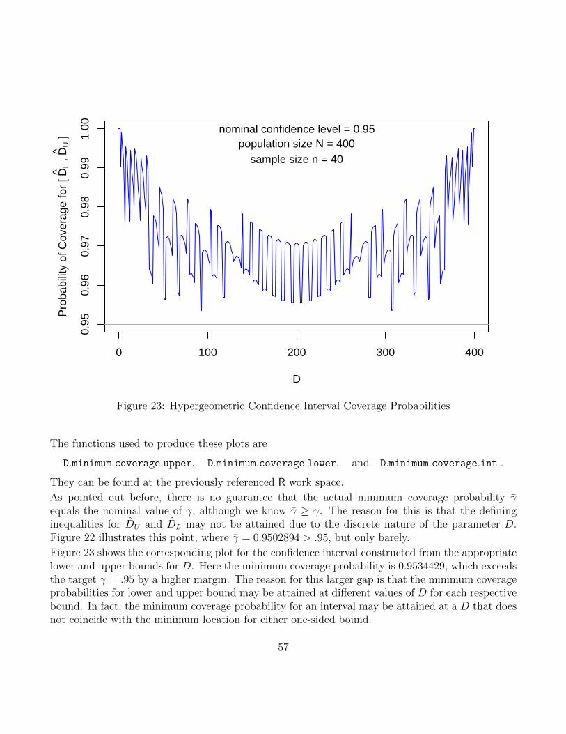
0 100 200 300 400
0.95
0.96
0.97
0.98
0.99
1.00
D
Pro
babi
lity
of C
over
age
for
[ DL ,
DU ]
nominal confidence level = 0.95population size N = 400
sample size n = 40
Figure 23: Hypergeometric Confidence Interval Coverage Probabilities
The functions used to produce these plots are
D.minimum.coverage.upper, D.minimum.coverage.lower, and D.minimum.coverage.int .
They can be found at the previously referenced R work space.
As pointed out before, there is no guarantee that the actual minimum coverage probability γequals the nominal value of γ, although we know γ ≥ γ. The reason for this is that the defininginequalities for DU and DL may not be attained due to the discrete nature of the parameter D.Figure 22 illustrates this point, where γ = 0.9502894 > .95, but only barely.
Figure 23 shows the corresponding plot for the confidence interval constructed from the appropriatelower and upper bounds for D. Here the minimum coverage probability is 0.9534429, which exceedsthe target γ = .95 by a higher margin. The reason for this larger gap is that the minimum coverageprobabilities for lower and upper bound may be attained at different values of D for each respectivebound. In fact, the minimum coverage probability for an interval may be attained at a D that doesnot coincide with the minimum location for either one-sided bound.
57

In the case of one-sided bounds it can be shown that there is a distinct set of γ values for whichthe minimum coverage probability γ equals γ. We will show this here for upper bounds.
For each set of integers D? and x? with
0 < PD?+1(X ≤ x?) = α(D?, x?) = α? < 1
we define γ(D?, x?) = γ? = 1 − α?. For such γ? it follows that the corresponding upper bound atx? equals D?, i.e.,
DU(γ?, x?) = D? since PD?+1(X ≤ x?) = α? and PD?(X ≤ x?) > α? ,
where the last > comes from the strict monotonicity property of PD(X ≤ x) with respect to D.Since DU(γ?, X) is strictly increasing in X and since DU(γ?, x?) = D? we have
PD?+1
(D? + 1 > DU(γ?, X)
)= PD?+1
(D? ≥ DU(γ?, X)
)= PD?+1 (X ≤ x?) = α?
and hencePD?+1
(D? + 1 ≤ DU(γ?, X)
)= γ(D?, x?) =⇒ γ(D?, x?) = γ? .
Figure 24 shows γ in relation to γ for upper (and lower) bounds over a γ range of [.97, .98] evaluatedover 1000 equally spaced points using the function hypergeo.conf.plot. The discrepancy betweenγ and γ appears to be small. Thus the discrete nature of the parameter D does not appear to havea strong effect on the difference γ − γ, at least not for the case n = 40, N = 400 examined here.
For intervals Figure 25, again produced by hypergeo.conf.plot, shows the corresponding rela-tionship between γ and γ over the interval [.94, .96]. It is again a step function but with coarsersteps. This may seem surprising at first but the explanation comes from the fact that the minimumcoverage probabilities for the one-sided bounds do not necessarily occur at the same D. Thus thewider zigzag behavior in the coverage probabilities for the one-sided bounds comes into play.
This suggests the possibility of manipulating the nominal γ until γ takes on the desired value, e.g.,choose γ somewhat less than .95 in order to attain γ = .95 or at least to come closer to it. This mayinvolve some trial and error. However, it may ultimately lead to making some form of compromise.
58

0.970 0.972 0.974 0.976 0.978 0.980
0.97
00.
972
0.97
40.
976
0.97
80.
980
nominal γ
min
imum
cov
erag
e γ
Figure 24: Confidence Coefficient γ as a Function of γ for Upper/Lower Bounds, n = 40, N = 400
0.940 0.945 0.950 0.955 0.960
0.94
00.
945
0.95
00.
955
0.96
0
nominal γ
min
imum
cov
erag
e γ
Figure 25: Confidence Coefficient γ as a Function of γ for Confidence Intervals, n = 40, N = 400
59

6.5 Hypergeometric Confidence Bounds with a Birthday Problem Twist
The classical birthday problem is often presented in elementary probability courses. The chancethat n random persons have birthdays on different days in the year can be given as follows
P (D) =(365)n365n
=365(365− 1) · · · (365− n+ 1)
365n
and thus the probability of at least one match is
P (M) = 1− (365)n365n
≥ .5 for n ≥ 23.
This is based on a non leap year and equal likelihoods of all birthdays for all n persons.
Once one of my students asked the following (somewhat modified) question: What is the chancethat all birthdays in a group of n persons are at least one day apart? This problem can be tackledby the following counting trick. First we find the number of ways of arranging a = 365−n N ’s andn B’s such that no two B’s are next to each other. This can be counted by setting up the a N ’snext to each other and regard each gap between two N ’s as a place where I can place a B, but atmost one such B per gap. There are (a− 1) + 1 = a such gaps, counting the gaps at the end as one
joined wrap around gap. Thus there are(an
)ways to place the n B’s into the a gaps. Each such
placement gives us a different collection of n birthdays in a year, which are separated by at leastone non-birthday. Now we have to count in how many ways these particular n birthdays could getassigned to the n persons involved. This can be done in n! ways. Thus the probability of the eventA, of getting n birthdays at least one day apart, is
P (A) =n!
365n
(365− n
n
)=
(365− n)n365n
=⇒ P (Ac) = 1− (365− n)n365n
.
Hence P (Ac) = .5013 for n = 13 and P (Ac) = .895 for n = 23. As pointed out to me by TatianaMaravina, the above formula for P (A) is incorrect. You may want to figure out why, aside fromgiving a counter example for n = 2, which gives P (A) = 365× 362/3652 = 362/365.
The correct formula is
P (A) =
(365− n− 1
n− 1
)(n− 1)!365
365n=
(365− 2n+ 1)(365− 2n+ 2) · · · (365− 2n+ n− 1)
365n−1
This can be argued as follows. There are 365 ways to choose the birthday for person 1. There are365− n non-birthdays. Their position is determined by by choosing the remaining n− 1 birthdaysto each fill one of the remaining 365 − n − 1 gaps between the non-birthdays. Finally, there are(n− 1)! ways to assigns these birthdays to the remaining (n− 1) persons. n = 14 gives the smallestn for which this P (A) ≥ .5, in fact we get P (A) = .5375. Figure 26 gives a visual comparison ofthese probabilities. The wrong and correct P (Ac) don’t differ by much.
60
●●
●●
●
●
●
●
●
●
●
●
●
●
●
●●
●●
●●
●● ● ● ● ● ● ● ● ● ● ● ● ● ● ● ● ● ● ● ● ● ● ● ● ● ● ●
10 20 30 40 50
0.0
0.2
0.4
0.6
0.8
1.0
number of persons n
prob
abili
ty
●●
●●
●
●
●
●
●
●
●
●
●
●
●
●●
●●
●●
●● ● ● ● ● ● ● ● ● ● ● ● ● ● ● ● ● ● ● ● ● ● ● ● ● ● ●
●●
●
●
●
●
●
●
●
●
●
●
●
●
●
●
●
●
●
●●
●●
●●
● ● ● ● ● ● ● ● ● ● ● ● ● ● ● ● ● ● ● ● ● ● ● ●
●
●
P(at least one matching B−day)P(at least one matching or adjacent B−day) (wrong)P(at least one matching or adjacent B−day) (correct)
Figure 26: Birthday Problem Probabilities
6.5.1 Problem Description and Assumptions
At some point after dealing with the extension of the birthday problem the following problem arosein connection with the Inertial Upper Stage of the Military Space Program.
http : //www.fas.org/spp/military/program/launch/ius.htm
We are dealing with a population of N = 200 parts (rocket motors) of which n = 12 are to be testedin some form. It is expected that all tested items will be non-defective. Based on this, what kindof upper confidence bounds DU can we place on the number D of defective parts in the population.
Furthermore, if k = 16 parts are selected at random from the population of N and are installedas a ship-set, what kind of lower bound p1 can be placed on the probability that this ship-set willcontain at most one defective?
After addressing this problem it was pointed out that the 16 parts will be arranged in a circularpattern and all that matters is that no two defective parts be placed next to each other. Whatlower confidence bound p2 can be placed on the probability that no two defective parts be placednext to each other in any randomly chosen ship-set of 16?
This does not quite match the birthday problem since we cannot have two defective parts in thesame position. However, it was sufficiently close to base the probability calculations on a similarcounting trick.
61

6.5.2 Assumptions and Analysis
To make any statistical inference we have to make certain assumptions. We will assume that then = 12 parts are selected randomly from the population. The same is assumed for the ship-set,where we assume that the n = 12 sampled ones were returned to the population before creating theship-set by random selection. Furthermore, the k = 16 parts are arranged in random order in thecircular pattern.
Let D denote the total number of defective parts in the population of N parts and X the numberof defective items in the tested sample of n = 12. In our case we expect to see X = 0. Based onsuch an expected result what kind of upper confidence bounds DU(γ, 0) can we place on D?
Recall that DU(γ, 0) = D if and only if PD(X = 0) > α = 1 − γ and PD+1(X = 0) ≤ α. Bychoosing the γ values judiciously as γD = 1− PD+1(X = 0), i.e., as high as possible for each valueof D = D(γ, 0), we can associate the highest possible confidence level with each such D. Note thatany γ > γD would result in PD+1(X ≤ 0) > 1− γ and thus in DU(γ, 0) ≥ D+ 1. We also point outthat this choice of γD ensures that γ = γD, as was shown previously.
This was carried out and the results are displayed in Table 2. There the first column gives theupper confidence bounds on D and columns 2-7 give the respective confidence levels for samplesizes n = 12, 20, 30, 40, 50, 60. Column 8 gives the lower bound p1 on the probability that we seeat most one defective in a shipset of size k = 16, with associated confidence levels as shown to theleft for the respective strengths of evidence n = 12, 20, . . . , 60 with zero defectives. The last columngives the lower bound p2 on the probability that we see no two defectives next to each other inthe circular arrangement of the k = 16 parts, again with confidence levels as shown to the left forrespective n with zero defectives.
The lower bounds p1 were arrived at in straightforward manner as follows. Let Y denote the randomnumber of defectives in the shipset sample of k = 16. Then the probability of seeing at most 1defective in that sample is
Q(D) = PD(Y ≤ 1) = PD(Y = 0) + PD(Y = 1) =
(D0
)(N−Dk−0
)(Nk
) +
(D1
)(N−Dk−1
)(Nk
) .
Since this probability decreases with increasing D we can take p1 = Q(DU(γ, 0)) as lower bound onQ(D) with same confidence level as was associated with DU(γ, 0).
To motivate the lower bound p2 we need to derive a formula for the probability that no two defectiveparts will be placed next to each other in a circular arrangement of k = 16 parts. This probabilitycan be expressed as follows
Q?(D) = PD(Y = 0) + PD(Y = 1) + PD(Y = 2)P (A2)
+ PD(Y = 3)P (A3) + . . .+ PD(Y = 8)P (A8) , (18)
62

Table 2: Confidence Bounds Based on Zero Defective Parts in a Sample of n
upper bound confidence levels γD lower bound
DU (γD, 0) = D n = 12 n = 20 n = 30 n = 40 n = 50 n = 60 p1 p2
1 0.117 0.190 0.278 0.361 0.438 0.511 1.000 1.0002 0.170 0.272 0.388 0.490 0.580 0.659 0.994 0.9993 0.221 0.346 0.481 0.594 0.687 0.763 0.983 0.9984 0.268 0.413 0.560 0.676 0.767 0.836 0.967 0.9955 0.313 0.473 0.628 0.743 0.827 0.886 0.948 0.9926 0.356 0.527 0.685 0.796 0.871 0.921 0.925 0.9887 0.396 0.576 0.734 0.838 0.905 0.946 0.900 0.9848 0.434 0.620 0.776 0.872 0.929 0.963 0.873 0.9789 0.469 0.660 0.811 0.899 0.948 0.974 0.845 0.97210 0.503 0.696 0.841 0.920 0.962 0.983 0.815 0.96611 0.534 0.728 0.866 0.937 0.972 0.988 0.784 0.95812 0.564 0.757 0.888 0.950 0.979 0.992 0.753 0.95013 0.592 0.783 0.906 0.961 0.985 0.994 0.721 0.94214 0.618 0.806 0.921 0.969 0.989 0.996 0.690 0.93215 0.643 0.827 0.934 0.976 0.992 0.997 0.658 0.92316 0.666 0.846 0.944 0.981 0.994 0.998 0.627 0.91317 0.688 0.863 0.954 0.985 0.996 0.999 0.596 0.90218 0.709 0.878 0.961 0.989 0.997 0.999 0.566 0.89019 0.728 0.891 0.968 0.991 0.998 0.999 0.536 0.87920 0.746 0.904 0.973 0.993 0.998 1.000 0.508 0.86721 0.763 0.914 0.978 0.995 0.999 1.000 0.480 0.85422 0.779 0.924 0.981 0.996 0.999 1.000 0.453 0.84123 0.794 0.933 0.985 0.997 0.999 1.000 0.427 0.82824 0.808 0.940 0.987 0.998 1.000 1.000 0.401 0.81425 0.821 0.947 0.989 0.998 1.000 1.000 0.377 0.80026 0.834 0.953 0.991 0.999 1.000 1.000 0.354 0.78627 0.845 0.959 0.993 0.999 1.000 1.000 0.332 0.77228 0.856 0.963 0.994 0.999 1.000 1.000 0.311 0.75729 0.866 0.968 0.995 0.999 1.000 1.000 0.291 0.74230 0.876 0.971 0.996 0.999 1.000 1.000 0.272 0.72731 0.884 0.975 0.997 1.000 1.000 1.000 0.254 0.71232 0.893 0.978 0.997 1.000 1.000 1.000 0.237 0.69633 0.900 0.980 0.998 1.000 1.000 1.000 0.220 0.68134 0.908 0.983 0.998 1.000 1.000 1.000 0.205 0.66535 0.914 0.985 0.998 1.000 1.000 1.000 0.190 0.64936 0.921 0.987 0.999 1.000 1.000 1.000 0.177 0.63437 0.926 0.988 0.999 1.000 1.000 1.000 0.164 0.61838 0.932 0.990 0.999 1.000 1.000 1.000 0.152 0.60239 0.937 0.991 0.999 1.000 1.000 1.000 0.141 0.58740 0.942 0.992 0.999 1.000 1.000 1.000 0.130 0.57141 0.946 0.993 1.000 1.000 1.000 1.000 0.120 0.55542 0.950 0.994 1.000 1.000 1.000 1.000 0.111 0.540
63

where Ay is the event that no two defective parts will be placed next to each other when y defectiveparts and k − y non-defective parts are arranged randomly in a circular pattern. We have
PD(Y = y) =
(Dy
)(N−Dk−y
)(Nk
) and P (Ay) =
(k−yy
)(k−1y
) .The latter is arrived at as follows. Label the y defective parts F1, . . . , Fy and the m = k − y non-defective parts by G1, . . . , Gm. There are k! ways of arranging these k parts in a circular pattern,all equally likely. Now we count how many of these patterns have no two F ’s next to each otherand take the ratio of this over k! as our probability P (Ay). We start by realizing that G1 can be inany of the k places. Next we can arrange the remaining m− 1 G’s in (m− 1)! ways to form somecircular sequence order of G’s with keeping only G1 in its chosen place. The other G’s are movablebut stay in the circular order chosen. Next we place the y F ’s between the G’s so that only oneF goes into any one gap between G’s. There are m gaps and
(my
)ways of designating the gaps to
receive just one F each and there are y! ways of arranging the order in which the y F ’s are placedin the designated gaps. All this amounts to the following total count of filling the k spots in thecircular pattern so that no two F ’s are next to each other, namely
k(m− 1)!
(m
y
)y! = k(k − y − 1)!
(k − yy
)y! =⇒ P (Ay) =
k(k − y − 1)!(k−yy
)y!
k!=
(k−yy
)(k−1y
) .Note that the formula gives the correct and appropriate value 1 in the two cases of y = 0 and y = 1and P (Ay) = 0 for y > k − y. When y > k − y there is no way of placing y defective items in sucha way that only one defective item falls between any two non-defective items, since there are onlyk − y gaps available.
Thus Q?(D) in (18) can be written as the expected value Q?(D) = ED(ψ(Y )) where ψ(y) = P (Ay).
Since Q?(D) is again decreasing with increasing D (see the Appendix) we can use p2 = Q?(DU(γ, 0))as lower bound for Q?(D) with same confidence as was applied to DU(γ, 0).
How do we interpret the results in Table 2? For the originally proposed sample size n = 12 fortesting we can be 80.8% confident that D ≤ 24 and that the probability of having less than twodefective items in the ship-set of k = 16 is at least .401, not a very happy state of affairs. Thisis based on the assumption that we see indeed no defective items in the sample of n = 12. Afterqualifying that the more than one defective parts only matter when at least two are adjacent, wecan be 80.8% confident that the probability of seeing no such adjacency is at least .814, which maystill not be satisfactory.
That was the reason for showing the columns for higher sample sizes, still expecting no defectiveitems among the n sampled items. Clearly this should provide us with a stronger feeling (confidence)
64

and higher probability of avoiding the adjacency issue. For example, when choosing n = 40 we canbe 95% confident that the probability of no adjacent defective parts is at least .95.
The function that computes p1 and p2 and the accompanying γ is p1p2.hat and is contained inthe previously referenced R work space. Note that the tabulated confidence levels in Table 2 areonly given to 3 decimals and thus should only serve as a rough guide. In fact, we get p1 = QD andp2 = QD.star by calling p1p2.hat with γ = .95
> p1p2.hat(0,40,.950,200,16)
$D.U
upper
12
$D.UX
upper
12
$QD
[1] 0.7528636
$QD.star
[1] 0.9502322
$gam.bar
minimum
0.9503716
When changing γ to a value that comes closer to γ = 0.9503716 we get
> p1p2.hat(0,40,.9503716,200,16)
. . . everything else staying the same
$gam.bar
minimum
0.9503716
=⇒ the highest possible confidence level γ = γ for that value of DU(0, γ) = D.U = 12.
Of course, if the observed result in the sample of size n is not zero but x > 0, one would substituteDU(γ, x) for DU(γ, 0) with DU(γ, 0) < DU(γ, x) and the resulting lower bounds p1 and p2 woulddecrease while the confidence levels stay at the indicated γ.
65

In fact, if x > 0 we would not return the defective items into the population of size N . That waywe would reduce N by x and D by x as well, i.e., N → N ′ = N −x and D → D′ = D−x. We thenshould use D′U(X, γ) = DU(X, γ)−x = D.UX as the upper confidence bound for D′ when calculatingp1 and p2.
As an example, assume that we see X = 1 when testing n = 40 items. Table 2 suggests to takeγ = .95 in order to get p2 = .95 when X = 0, but we previously saw that a better choice for γ isγ = 0.9503716, which gives us γ = γ. Calling p1p2.hat with x = 1 and that value of γ yields
> p1p2.hat(1,40,.9503716,200,16)
$D.U
upper
20
$D.UX
upper
19
$QD
[1] 0.5335137
$QD.star
[1] 0.8776381
$gam.bar
minimum
0.9503716
While the confidence level remains unaffacted there is a decrease in the respective lower confidencebounds p1 = QD and p2 = QD.star. That is the penalty for not achieving X = 0 as predicted.
As a note of warning, one should not try to trade off some of the confidence level (lowering it) toincrease the lower bounds p1 or p2. This would negate the theoretical underpinnings of confidencebounds. The confidence level should not become random (a function of X). This is not an emptywarning, since I have experienced this kind of ingenuity from engineers3.
3According to Webster’s, engineer and ingenuity have the same Latin origin ingenium.
66

7 Comparing Two Poisson Means
Suppose X and Y are independent Poisson random variables with respective means λ and µ. We areinterested in confidence bounds for ρ = λ/µ. If these Poisson distributions represent approximationsof binomials for small “success” probabilities π1 and π2, i.e., λ = n1π1 and µ = n2π2, then confidencebounds for the ratio ρ = λ/µ = (n1π1)/(n2π2) are equivalent to confidence bounds for π1/π2, sincen1 and n2 are typically known.
The classical method for getting confidence bounds for ρ is to view Y in the context of what wasobserved for X + Y , i.e., consider the conditional distribution of Y given T = X + Y = t, which is
P (Y = k|X + Y = t) =P (Y = k,X + Y = t)
P (X + Y = t)=P (Y = k,X = t− k)
P (X + Y = t)
=P (Y = k)P (X = t− k)
P (X + Y = t)=
[exp(−µ)µk]/k!× [exp(−λ)λt−k]/(t− k)!
exp(−[µ+ λ])[µ+ λ]t/t!
=
(t
k
)pi(1− p)t−i ,
where p = µ/(λ + µ) = 1/(1 + ρ). Here we used the fact that X + Y has a Poisson distributionwith mean µ+ λ. This is seen as follows
P (X + Y = t) =t∑i=0
P (X = i)× P (Y = t− i) =t∑i=0
exp(−λ)λi
i!× exp(−µ)µt−i
(t− i)!
=exp(−[λ+ µ])(λ+ µ)t
t!
t∑i=0
(t
i
)(λ
λ+ µ
)i (µ
λ+ µ
)t−i=
exp(−[λ+ µ])(λ+ µ)t
t!
Hence the conditional distribution of Y given X +Y = t is a binomial distribution with t trials andsuccess probability p = 1/(1 + ρ), which is a monotone function of ρ.
Given the previous treatment in Section 2 we can get 100γ% binomial upper confidence boundspU(γ, k, t) for p. By inverting the monotone relationship p = 1/(1 + ρ), i.e., ρ = 1/p − 1, we getfrom this a 100γ% lower confidence bound for ρ in
ρL(γ, k, t) =1
pU(γ, k, t)− 1 =
1
qbeta(γ, k + 1, t− k)− 1 .
Similarly one gets 100γ% upper confidence bounds for ρ in
ρU(γ, k, t) =1
pL(γ, k, t)− 1 =
1
qbeta(1− γ, k, t− k + 1)− 1
67

and 100γ% confidence intervals for ρ in
(ρL([1 + γ]/2, k, t), ρU([1 + γ]/2, k, t)) =
(1
pU([1 + γ]/2, k, t)− 1,
1
pL([1 + γ]/2, k, t)− 1
)
=
(1
qbeta([1 + γ]/2, k + 1, t− k)− 1,
1
qbeta([1− γ]/2, k, t− k + 1)− 1
)
In the context of the above Poisson approximations to binomial distributions one gets a 100γ%lower confidence bound for κ = π1/π2 in
κL(γ, k, t) =n2
n1
× ρL(γ, k, t) =n2
n1
×(
1
pU(γ, k, t)− 1
)
=n2
n1
×(
1
qbeta(γ, k + 1, t− k)− 1
).
Similarly one gets 100γ% upper confidence bounds for κ = π1/π2 in
κU(γ, k, t) =n2
n1
× ρU(γ, k, t) =n2
n1
×(
1
pL(γ, k, t)− 1
)
=n2
n1
×(
1
qbeta(1− γ, k, t− k + 1)− 1
).
and 100γ% confidence intervals for κ = π1/π2 in
(κL([1 + γ]/2, k, t), κU([1 + γ]/2, k, t))
=n2
n1
× (ρL([1 + γ]/2, k, t), ρU([1 + γ]/2, k, t))
=n2
n1
×(
1
pU([1 + γ]/2, k, t)− 1,
1
pL([1 + γ]/2, k, t)− 1
)
=n2
n1
×(
1
qbeta([1 + γ]/2, k + 1, t− k)− 1,
1
qbeta([1− γ]/2, k, t− k + 1)− 1
)
As an example consider some (fictitious) accident data. Among Modern Wide Body Airplanes wehad 0 accidents (substantial damage, hull loss, or hull loss with fatalities) during 11.128×10⁶ flights.Among Modern Narrow Body Airplanes we had 5 such accidents during 55.6× 10⁶ flights. Thus wehave Y = k = 5 and T = X + Y = t = 0 + 5 and n1 = 11.128× 10⁶ and n2 = 55.6× 10⁶. We find
pU(.95, 5, 5) = 1
68

and thus
κL(.95, 5, 5) =n2
n1
×(
1
1− 1
)= 0
andpL(.95, 5, 5) = qbeta(.05, 5, 5− 5 + 1) = (1− .95)1/5 = 0.5492803
resulting in
κU(.95, 5, 5) =n2
n1
×(
1
0.5492803− 1
)= 4.099871
Thus we can view 4.099871 as a 95% upper confidence bound for π1/π2, the ratio of rates for thetwo groups. Since this bound is above 1, one cannot rule out that the rates in the two groupsmay be the same. This is not surprising since the group with 5 accidents had about five times theexposure of the other group. Thus for a fifth of the exposures one might have expected to see onesuch accident in the second group. That is not all that different from zero in the realm of countingrare events.
7.1 Comparing Hull Loss Rates across Airplane Models
Based on the data in Figure 20 one may ask the question: How significant was the crash of the Con-corde when comparing it to experiences of other airplanes? We made two comparisons, comparingit with the MD11 and the B767.
In the comparison with the MD11 we had X = 5 hull losses and a rate of 4.59 per million departures,while the Concorde had Y = 1 such loss and a rate of 12.02 per million departures. This translatedinto n1 = 1089325 and n2 = 83195 departures for the MD11 and Concorde, respectively. Thisgives us (.04273, 18.06) as a 95% confidence interval for κ = π1/π2 which contains π1/π2 = 1as a possible value. Thus one cannot conclude that the MD11 and the Concorde had sufficientlydifferent experiences. However, the confidence intervals could be quite conservative in their coverageprobabilities based on the fact that only X + Y = 6 accidents were involved in this comparison.Since we are mostly interested in the question π1/π2 < 1 we should focus more on the upper boundfor π1/π2. The 95% upper confidence bound for π1/π2 is 8.896, which still exceeds 1 by a fair margin.However, here we know that the minimum coverage probability is .95, although its coverage behavioris coarsely fluctuating. Since the upper bound for π1/π2 is based on the lower bound pL(γ, Y, 6) forp = 1/(1+ρ) = 1/(1+n1π1/(n2π2)) we show in Figure 27 the coverage behavior of this lower boundand indicate by vertical lines positions for various values of π1/π2. Depending on the unknown valueof π1/π2 our coverage probability could be quite close to the desired level .95 or very much higher.
69

0.0 0.2 0.4 0.6 0.8 1.0
0.95
0.96
0.97
0.98
0.99
1.00
p
Pro
babi
lity
of C
over
age
for
pL
nominal confidence level = 0.95sample size n = 6
0.30.50.81.2
π1 π2
Figure 27: Coverage Behavior of Binomial Lower Bound for n = 6
In comparing the Concorde with the B767 we have X = 3 hull losses for the latter and a rate of.32 per million departures. This translates into n1 = 9375000 departures for the B767. Here our95% upper bound for π1/π2 is .6876, which is clearly below 1 and thus indicates a difference inexperience between the B767 and the Concorde, in favor of the B767.
70

The Concorde ceased service in 2003. On November 5, 2003, the Concorde now on display at theMuseum of Flight made its final landing at Boeing Field in Seattle. The photo below was takenwhile inspecting taxi ways at JFK.
Figure 28: Concorde Takeoff at JFK, June 18, 2003
71
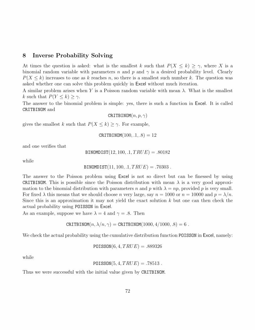
8 Inverse Probability Solving
At times the question is asked: what is the smallest k such that P (X ≤ k) ≥ γ, where X is abinomial random variable with parameters n and p and γ is a desired probability level. ClearlyP (X ≤ k) increases to one as k reaches n, so there is a smallest such number k. The question wasasked whether one can solve this problem quickly in Excel without much iteration.
A similar problem arises when Y is a Poisson random variable with mean λ. What is the smallestk such that P (Y ≤ k) ≥ γ.
The answer to the binomial problem is simple: yes, there is such a function in Excel. It is calledCRITBINOM and
CRITBINOM(n, p, γ)
gives the smallest k such that P (X ≤ k) ≥ γ. For example,
CRITBINOM(100, .1, .8) = 12
and one verifies thatBINOMDIST(12, 100, .1, TRUE) = .80182
whileBINOMDIST(11, 100, .1, TRUE) = .70303 .
The answer to the Poisson problem using Excel is not so direct but can be finessed by usingCRITBINOM. This is possible since the Poisson distribution with mean λ is a very good approxi-mation to the binomial distribution with parameters n and p with λ = np, provided p is very small.For fixed λ this means that we should choose n very large, say n = 1000 or n = 10000 and p = λ/n.Since this is an approximation it may not yield the exact solution k but one can then check theactual probability using POISSON in Excel.
As an example, suppose we have λ = 4 and γ = .8. Then
CRITBINOM(n, λ/n, γ) = CRITBINOM(1000, 4/1000, .8) = 6 .
We check the actual probability using the cumulative distribution function POISSON in Excel, namely:
POISSON(6, 4, TRUE) = .889326
whilePOISSON(5, 4, TRUE) = .78513 .
Thus we were successful with the initial value given by CRITBINOM.
72

References
1. Agresti, A. and Coull, B.A. (1998). “Approximate is better than “exact” for interval estima-tion of binomial proportions.” The American Statistician 52, 119-126.
2. Barbour, A.D., Holst, L., and Janson, S. (1992), Poisson Approximation, Clarendon Press,Oxford.
3. Bardi, J.S. (2006), The Calculus Wars, Newton and Leibniz, and the Greatest MathematicalClash of All Time, Thunder’s Mouth Press, New York.
4. Barker, Lawrence (2002). “A comparison of nine confidence intervals for a Poisson parameterwhen the expected number of events is ≤ 5,” The American Statistician, 56, 2, 85-89.
5. Clopper, C.J. and Pearson, E.S. (1934). “The use of confidence or fiducial limits illustratedin the case of the binomial.” Biometrika 26, 404-413.
6. Hahn, G.J. and Meeker, W.Q. (1991), Statistical Intervals, A Guide for Practitioners, JohnWiley & Sons, New York.
7. Lehmann, E.L. and Romano, J.P. (2005), Testing Statistical Hypotheses, Third Edition, JohnWiley & Sons, New York.
8. Shapiro, S.S. and Gross, A.J. (1981), Statistical Modeling Techniques, Marcel Dekker , Inc.,New York.
9. van Belle, G. (2002) Statistical Rules of Thumb, John Wiley & Sons, New York.
73

Appendix: Monotonicity of Q?(D)
As a first step one shows that ψ(y) = P (Ay) decreases as y increases from y = 1 to y = k/2(assuming that k is even). This is seen by
P (Ay+1)
P (Ay)=
(k − 2y)(k − 2y − 1)
(k − y)(k − y − 1)< 1 ⇐⇒ −2k + 3y + 1 < 0
which is true for y = 1, . . . , k/2.
The second step consists in showing that Q?(D + 1) = ED+1(ψ(Y )) ≤ ED(ψ(Y )) = Q?(D).
The proof is an adaptation of the argument given in Lehmann and Romano (2005), p.85.
First note that
pD+1(y) = PD+1(Y = y) =
(D+1y
)(N−D−1k−y
)(Nk
) <
(Dy
)(N−Dk−y
)(Nk
) = PD(Y = y) = pD(y) ⇔ y <k(D + 1)
N + 1.
Let A = {y : PD+1(Y = y) < PD(Y = y)} and B = {y : PD+1(Y = y) > PD(Y = y)}
and note that the previous equivalence implies that A lies to the left of B with k(D+ 1)/(N + 1) inbetween. Because of the decreasing nature of ψ(y) it follows that a = infA ψ(y) ≥ supB ψ(y) = b.Hence
ED+1[ψ(Y )]− ED[ψ(Y )] =∑y∈A
ψ(y) (pD+1(y)− pD(y)) +∑y∈B
ψ(y) (pD+1(y)− pD(y))
≤ a∑y∈A
(pD+1(y)− pD(y)) + b∑y∈B
(pD+1(y)− pD(y))
= (b− a)∑y∈B
(pD+1(y)− pD(y)) ≤ 0
since0 =
∑y
(pD+1(y)− pD(y)) =∑y∈A
(pD+1(y)− pD(y)) +∑y∈B
(pD+1(y)− pD(y))
and thus ∑y∈A
(pD+1(y)− pD(y)) = −∑y∈B
(pD+1(y)− pD(y)) .
74


![Java Algorithms for Computer Performance Analysis...A Java implementation of Asymptotic Bounds, Balanced Job Bounds and Geometric Bounds (as proposed in [6]), providing bounds on throughput,](https://img.pdfslide.net/doc/110x75/606dab6f274a5313cb504f0b/java-algorithms-for-computer-performance-analysis-a-java-implementation-of-asymptotic.jpg)