Concentration of personal and household crimes in … · Concentration of personal and household crimes in ... eg. a bike theft followed by a ... share characteristics associated

Concentration of personal and household crimes inEngland and Wales

Andromachi Tseloni1, Ioannis Ntzoufras2, Anna Nicolaou3 and Ken Pease4

1Division of Criminology, Public Health and Policy Studies, Nottingham Trent University, Burton street, Notting-

ham NG1 4BU, UK. E-mail: [email protected]. Corresponding author.2Dept. of Statistics, Athens Economic University, Patission 76, 10434 Athens, Greece. E-mail: [email protected]. of Business Administration, University of Macedonia, Egantia 156, 54006 Thessaloniki, Greece. E-mail:

[email protected] Professor, Midlands Centre for Criminology and Criminal Justice, University of Loughborough. 19

Withypool Drive,Stockport SK2 6DT. E-mail: [email protected].

Concentration of personal and household crimes in England and Wales 1

Abstract Crime is disproportionally concentrated in few areas. Though long-established, there

remains uncertainty about the reasons for variation in the concentration of similar crime (repeats)

or different crime (multiples). Wholly neglected have been composite crimes when more than

one crime types coincide as parts of a single event. The research reported here disentangles area

crime concentration into repeats, multiple and composite crimes. The results are based on esti-

mated bivariate zero-inflated Poisson regression models with covariance structure which explicitly

account for crime rarity and crime concentration. The implications of the results for criminological

theorizing and as a possible basis for more equitable police funding are discussed.

Keywords: Bivariate zero-inflated Poisson; Crime concentration; Personal crime; Property crime.


1 Introduction

The Pareto principle holds that in any population which contributes to a common effect, a relative

few of the contributors account for the bulk of the effect. It posits the existence of the ’vital few

and the trivial many’ (see Juran 1951). Crime is no exception. A minority of areas contributes

disproportionately to the national crime rates while most of the country has very low crime (Nicholas

et al. 2007, pages 115-7; Trickett et al. 1992). For instance, 38 percent of the 2006/07 recorded

robberies occurred in local authorities serving 8 percent of the population (Nicholas et al. 2007,

page 114). This long-established uneven distribution of crimes both across locales and individual

households has proved to be of enduring interest (see Forrester et al. 1988; 1990; Osborn et al.

1992; Farrell and Pease 1993; Chenery et al. 1996; Ellingworth et al. 1997; Osborn and Tseloni

1998; Hope et al. 2001; (Bowers et al. 2004; Tseloni 2006; Hope 2007).

Understanding crime concentration is necessary for the optimal deployment of police and other

resources. This is particularly important at the time of writing, when global recession threatens

public sector expenditure in general, and police funding in particular. Targeting places and people

at greatest risk is a cost-efficient strategy in most public services, expending effort where it is

most needed and facilitating the detection of the prolific offenders who specialize in repeating their

crimes against the same target (Farrell and Pease 2001; Pease 1998). The reduction of repeat

crimes against the same targets accounts for much of crime drop in England and Wales over the

past fifteen years (Thorpe 2007). Whether this is a consequence of increasing awareness of the

concentration issue is a moot point.

Ones first impulse in devising a deployment strategy for policing would be to ask police officers

with local knowledge to anticipate where crime will next occur. The research suggests that they are

surprisingly poor in doing so, and that their confidence in prediction is unrelated to their accuracy

(see for example McLoughlin et al. 2007). Optimal deployment therefore has to depend on a

modeling approach.

Previous statistical modelling of crime concentration include the compound Poisson model for


property crime counts (Osborn and Tseloni 1998; Tseloni 2006), the ’hurdle’ model of the odds

of ’single victim versus non-victim’ and ’repeat victim versus single’ (Osborn et al. 1996) and the

bivariate Probit model for joint property and personal crime risks (Hope et al. 2001). This body

of research uses the British Crime Survey (BCS) in conjunction with Census information to tap

into area level variation. The BCS, unlike police recorded crime, offers a wealth of individual and

contextual information (apart from land use) which may help to identify the attributes of high

crime areas and their residents. In this respect, prediction is based on area and residents’ profiling

as the post -1992 BCS geography is concealed from the public use file in the interests of interviewee

confidentiality. The various forms of crime concentration and the aims of the present work are

discussed in the following two sections (2 and 3). Section 4 provides an overview of the data (see

also Hales et al. 2000). Description of area personal and household crime events follows. The

sixth and seventh sections present the sets of explanatory variables and the statistical model with

explicit application to criminological theory, respectively. Section eight gives the empirical results

and discusses their theoretical implications. An overview and comparisons between observed and

fitted crime distributions across area deciles concludes the paper. The Appendix offers preliminary

statistical tests of the data.

2 Components of Crime Concentration

The foregoing made clear that addressing crime concentration is central in resource deployment,

and has been a driver of recent crime reduction. Designing and implementing informed crime

reduction policies can be aided by teasing out the elements which, taken together, comprise chronic

victimisation of the same people. Multiple crimes refer to the recurrence of distinct victimisation

events, each of a different type, against the same target, eg. a bike theft followed by a burglary.

Repeats denote repetition of crime incidents of the same type, for instance three separate incidents

of violence. Although early victimisation research employed the terms interchangeably (see, for

instance Hindelang et al. 1978; Reiss 1980) it is now common practice, not least in the Home Office

(the Ministry concerned with crime in England and Wales and its prevention) to present and analyse


them separately (Nicholas et al. 2007). Series, whereby victims report a number of incidents of the

same nature and believed by the victim to be probably the work of the same perpetrator(s) (Hough

and Mayhew 1983), form a component of repeats but are considered separately here because of the

particular counting problems which they pose. They are important in their contribution to total

crime counts (see for example Planty and Strom 2007) but will not be discussed further here.

In this study a fourth type of crime concentration which is not dealt with in crime survey

analysis is introduced and tested. This is provisionally labelled composite crime. Composite crimes

are multi-crime events, wherein more than one offence is committed during the same incident. For

instance, a burglary of an occupied property may well involve threat and assault if the burglar

comes face-to-face with the residents. This is a single criminal event in which burglary, threat

and assault, all took place against the same target, at the same time and almost certainly by the

same offender. Similarly, a common technique in car theft involves hooking the keys from inside

a home with a hook, thus committing burglary too. Composite crimes can be seen as a special

case of multiple crimes, just as series crimes can be seen as a special case of repeats. Offence

code classification rules are in place in the BCS to record each event as the most serious offence

that occurred during a single reported incident (Hales et al. 2000, p. 26 and Appendix G). But

the fact remains that the conventional recording of such incidents under a specific crime category

masks other offences that occurred in the same incident. The less serious components of composite

crimes are thus entirely invisible in statistics of crime. Thus, composite crimes are unobservable

in (survey) crime statistics unless a detailed analysis of victims narratives was undertaken. Their

extent can be more economically estimated via statistical modelling rather than examining victim

answers to the surveys open ended questions about ’What happened’, ’Why it happened’ etc.

3 Rationale and Aims

Research on crime concentration is useful for two related reasons. First, circumscribing crime

targets by place and time makes it possible to target resources efficiently. Second, clarifying how

concentration is patterned amongst crime types helps to understand what are the necessary elements


for a crime to be committed, and hence where leverage can be applied in its prevention. The current

study expands previous research on area crime concentration via examining whether this is of a

single offence type (repeats), a number of crime types which occurred sequentially (multiples) or

during the same event (composite crimes). To this end it employs crime measures and a large set

of theoretically informed predictors which are drawn from the BCS and the UK Census.

Two substantive research hypotheses are tested here: The first assumes that a specific crime type

is associated with a distinct area profile. Coincidence of more than one crime type in an area may

thereby be due to similarity of area profiles. This is termed the observed heterogeneity hypothesis

in that each offence type is associated with a particular set of area characteristics. Insofar as areas

share characteristics associated with different crime types they experience multiple crimes. Thus

different crime categories occur in the same areas simply because these share characteristics which

faciliate each crime type. Observed heterogeneity may thus result in multiple or repeat events due

to the coincidence or diversity of target attributes associated with different crime types. The second

hypothesis proposes that various offences are manifestations of a single underlying variable, reflected

in composite crime. It suggests that different crime categories are intrinsically connected in that

some situations and circumstances are favourable elements of the composite crime in combination.

The two aggregate crime categories, personal and household crime, are examined for a most

conservative test of the above hypotheses via respective area crime counts. The area is the lowest

common unit of analysis for personal and property crimes and their rates are positively correlated

across areas. Crime is relatively rare in most of England and Wales and BCS area crime counts

have a disproportionate number of zero values (see the next two sections and the final section). To

accommodate both attributes of crime (that it is rare but concentrated), we employ the zero-inflated

Poisson model which accounts for the excess of no crime areas (zero crimes) and the repetition of

crime events. Personal and property crime counts are jointly examined via the bivariate extension

of the zero-inflated Poisson model (Wang et al. 2003) which additionally allows for the endogeneity

of each crime category and tests for any intrinsic association between the two counts, i.e. composite


crime. Although composite crimes in this study refer to households as possible victims of property

offences which coincided with personal crimes against their members in the same incident, the unit

of analysis is the area.

Put simply, crime is concentrated in areas with measurable characteristics, such as population

density. Some area characteristics are expected to be strong correlates of either personal or property

crimes thereby predicting repeat victimisation; others may be associated with both therefore pre-

dicting multiple crimes; others may be associated with unaccounted and unconsidered multi-crime

events. Each type of crime concentration requires distinct prevention policies.

The most obvious original contribution to criminological knowledge is proposing and testing

for composite crimes with their implications for crime prevention. As far as we are aware, this

is the first attempt to model jointly a type of coincidence of action which arguably reflects crime

concentration better (and certainly complements) past efforts of single dependent variable analysis

(Tseloni 2006). The empirical model is informed by recent developments of victimisation theory

as it accounts for the endogeneity of different crime types (Hope et al. 2001) as well as crime

concentration (Pease 1998; Farrell and Pease 1993) and rarity (Hope 2007). Finally a routine in

R to calculate the standard errors of estimated model parameters is proposed (available from the

authors).

4 Data

The empirical distributions of property and personal crimes and relevant individual and household

characteristics for this study have been taken from the 2000 BCS (Hales et al. 2000). The 2000

BCS was conducted by a consortium of the National Centre for Social Research and the Social

Survey Division of the Office for National Statistics, on behalf of the Home Office. The BCS has

been administered biannually since 1982 and since 2001 on a rotating annual basis. It employs a

multistage stratified sample, in principle representative of the adult (16 years or older) population

of England and Wales living in private accommodation. The sampling frame is the Postcode


Address File. One adult (aged 16 or over) from each selected household is randomly chosen by the

interviewer, using selection tables.

The responses of a total of 17,189 respondents (sample size lower than for the full BCS sample

for reasons given in the next section) have been aggregated across 905 sampling points. The

sampling point which represents quarter postcode sectors is the study’s unit of analysis. Each

sampling point yielded an average of 17.4 interviews with a minimum of 4 and a maximum of 29.

The empirical models reported later explicitly account for the varying number of respondents per

sample point via the offset (see equation 7.3). In the 2000 BCS respondents were invited to report

any victimisation experienced since January 1999. The reference period is thus the 1999 calendar

year. Most interviews took place between January and March 2000 (73% and 69.3% of the core

and total sample, respectively) and the fieldwork was essentially completed by June 2000 (with the

last 0.8% conducted in July 2000) (Hales et al. 2000; Kershaw et al. 2000, p. 113). The survey

additionally gathers information on attitudes towards crime, policing, fear of crime etc.

The area characteristics were selected from the 1991 Census Small Area Statistics after stan-

dardization and addition of a 5% error variance by the BCS fieldwork contractor to ensure confi-

dentiality. The 8 year gap between survey and Census data is inevitable as this is the only recent

BCS sweep linked to Census and the linkage was done by the BCS fieldwork contractor at a time

when the 2001 Census results were not available. It does not however affect this analysis as most

factors come from the BCS (see the section after next) and the effects of the few Census variables

may be interpreted as the effects of historic attributes on crime rates.

5 Property and Personal Crimes

Crime rates calculated from the BCS Victim Forms are truncated at 5 events where a series of

related victimisation events are reported (see section 1), following standard Home Office practice

(see, Kershaw et al. 2000, p. 111) to avoid very atypical households, with very large numbers of


series victimisations, distorting overall averages (see the second section)1.

The two aggregates, for personal and household crimes respectively, are examined here. The

former comprises common assaults, wounding, robberies, thefts from person and other thefts from

person (Hales et al. 2000). Sex offences have been excluded due to small numbers although the

BCS tries to avoid systematic underreporting via the use of self-completion modules (Hales et al.

2000). Household crimes include vandalism, burglary (including attempts), theft from dwelling,

theft of motor vehicle, theft from motor vehicle and bicycle theft (Hales et al. 2000). The empirical

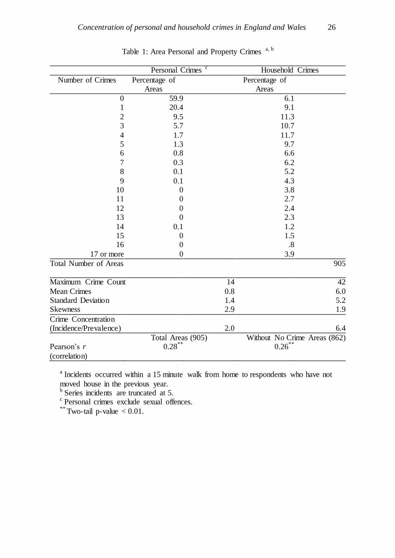
distribution of individual and household crimes per (quarter) post code sector is given as Table 1.

The usual BCS household and adult weight have not been applied since we are interested in area

aggregates and model selection rather than level or trend estimates. The vast majority of areas

(59.9%) suffered zero personal crimes and 90% suffered two or fewer such incidents. Household

crimes are more prevalent than personal crimes, being presents at 93.9% of the sampling points.

Their distribution however is heavily skewed, with few areas experiencing an extreme number of

events.

”Table 1 about here”

The concentration, namely the number of incidents per crime-reporting area or the ratio of the

national average number of crimes (incidence) over the proportion of areas where victims reside

(prevalence), of personal and household crimes numbers 2 and 6.4 events, respectively. To what

extent do personal and property crimes occur in the same areas? The two crime types have low but

statistically significant correlation of about 0.3 (see last line of Table 1). The observed proportion

of areas with no crimes by any type (4.8%) is likely to be overestimated due to the sampling points

with few respondents. This issue is revisited in the concluding sections of the paper.

We are interested in crimes relating to the current dwelling; this is to ensure that the area

characteristics used as predictors relate to the place where the crime(s) took place. To this end

only crimes which occurred within a 15 minute walk distance from victim’s home are included. For

1There are many purposes for which the writers would regard this as indefensible. Chronically victimized house-

holds do exist, and to exclude them by convention simply hides a real problem.


similar reasons respondents who moved during the 2000 BCS reference period (the 1999 calendar

year) are excluded from the analysis. The decision to move may be related to property crime

victimisation. In England and Wales, particularly, moving is related to higher property crime

before and after the move especially for non-home owners (Ellingworth and Pease 1998). The

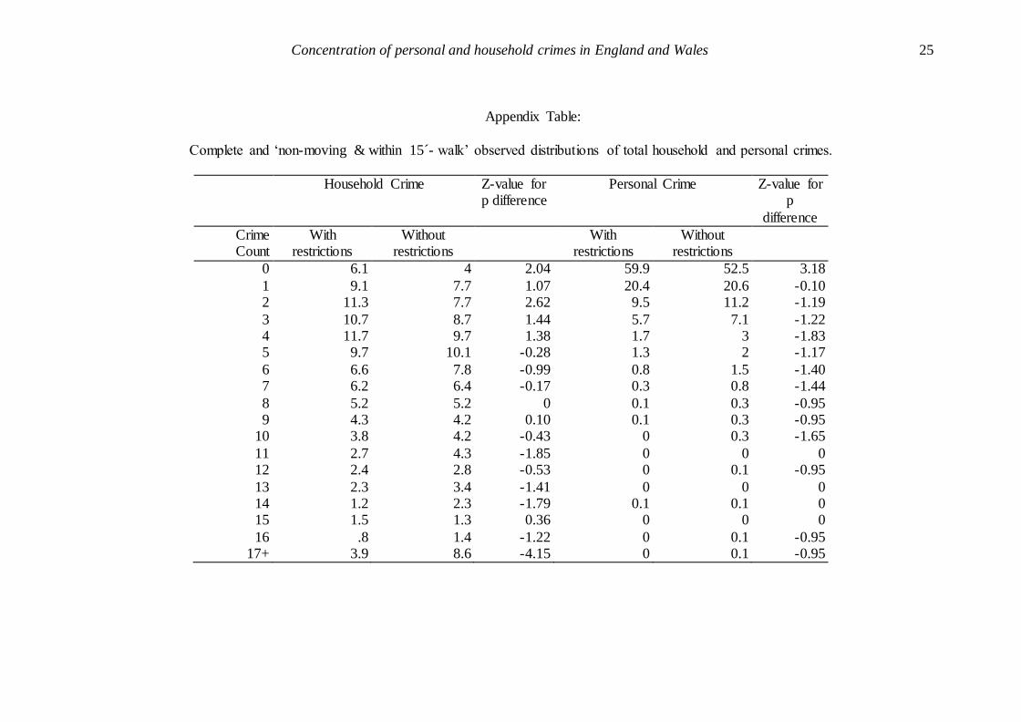
empirical distributions of personal and household area crime rates are fairly similar between the

full sample and the sample employed (’non-movers and within 15 minute walk’). Appendix A Table

presents the relevant comparisons and tests probability differences for each count. The rates are

only (significantly) different for zero crimes as restrictions inflate zero events and for 2 and 17 or

more household crimes. Therefore the restrictions do not introduce serious sampling bias to area

personal and property crimes. Most crime happens near the victim’s residence and extreme repeat

household victimisation is linked to moving house which replicates previous UK evidence.

6 Victimisation Theory, Sample and Area Characteristics

This study draws on the meso strain of routine activity theory and social disorganization theory

which operates at the macro level. Proponents of the former theory argue that the demographic

and socio-economic characteristics of individuals and their households, as well as their everyday

routine activities, together determine their exposure to crime (Cohen and Felson, 1979; Felson,

1998). Routine activities influence individuals’ chances of getting into contact with motivated

offenders in the absence of effective guardians.

Constructs pertinent to routine activity theory have been taken from the 2000 BCS. The set

of individual characteristics which may affect personal victimisation include demographic charac-

teristics (such as sex, age, ethnicity and children in the household), socio-economic characteristics

(namely educational attainment, social class, marital status, lone parents, length of residence,

tenure, income and car ownership), and routine activities or lifestyle indicators. Lifestyle includes

drinking habits, frequency of going to clubs, or pubs, or being out in a weekday. Most of the

aforementioned socio-economic variables are also relevant for property crimes. In particular, prop-

erty crimes are modelled over the same demographic and socio-economic characteristics as personal


crimes except educational level and marital status while the number of adults in the household and

accommodation type is used. Age in this case should refer to the ’head of household’ rather than

the respondent. Preliminary analysis showed a high correlation (0.907) between age of respondent

and that of the ’head of household’, thus the latter is omitted for parsimony. Routine activities

for households may be indicated by protection measures, frequency of house empty over a typical

week and participation in neighbourhood watch schemes.

All individual variables were originally categorical or binary except age and number of children

in the household. They have been aggregated within postcode sector as the percentage of each

(n-1) respective qualitative attribute. The mean age and number of children within each postcode

sector have been taken. All sample characteristics entered the regression models as standardized

values. Therefore a unit increase implies one standard deviation rise over the national average.

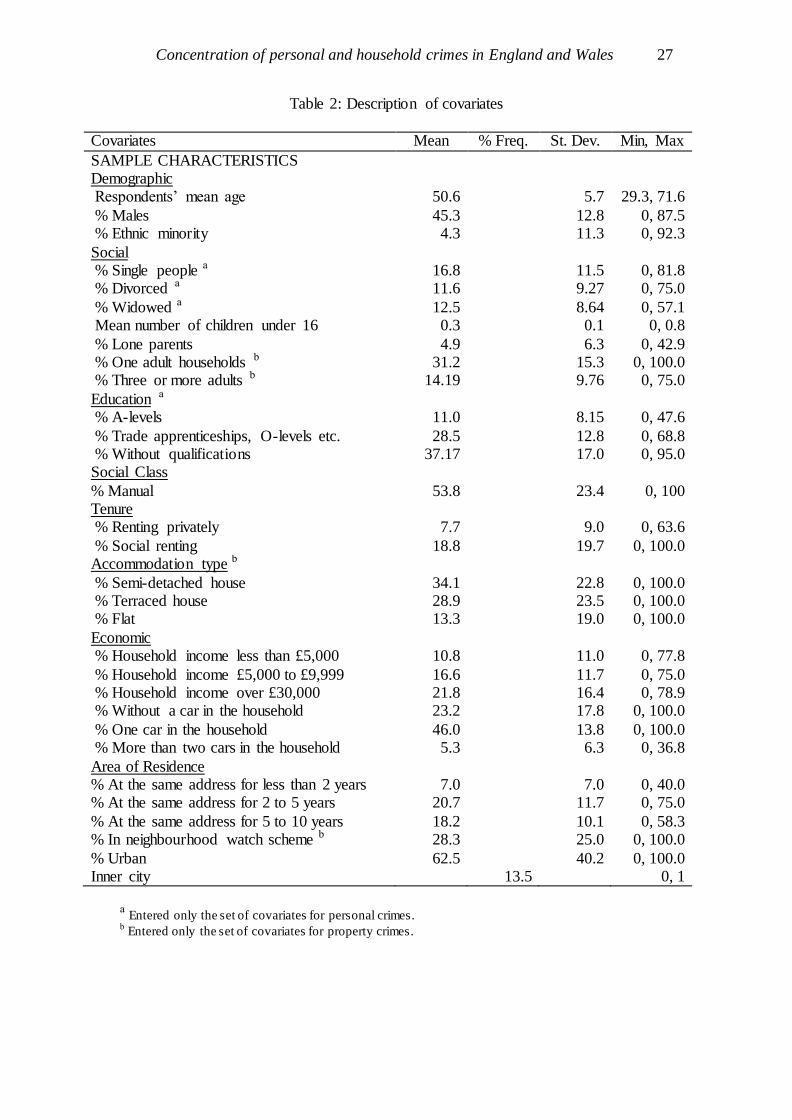
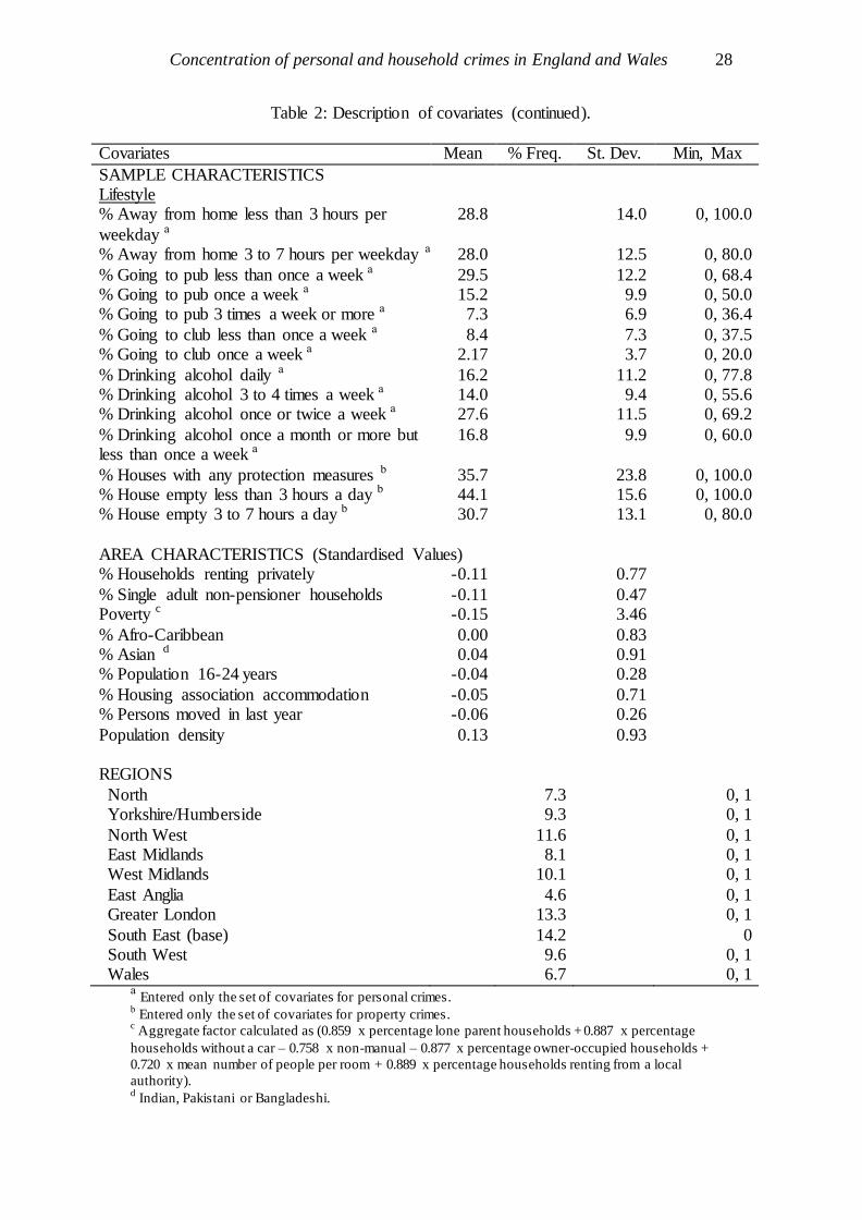
Table 2 presents the explanatory variables of this study with an indication whether the variable

under question is relevant for only one crime type.


Social disorganization theory (Shaw and McKay 1942; Sampson and Groves 1989) asserts that

crime is determined primarily by community attributes. They contend that the ability of a com-

munity to supervise teenage peer groups, develop local friendship networks and stimulate residents’

participation in local organizations depends on community characteristics. Social disorganization

and resulting crime and delinquency rates depend on the neighbourhood’s socio-economic status,

residential mobility, ethnic heterogeneity, family disruption and urbanization. Such community

attributes comprise the macro-level dimensions of victimisation models. As mentioned these con-

structs have been taken from the 1991 Census and they arguably inform on historic area profiles

due to the 8 years gap with the 2000 BCS.

To avoid the problem of multicollinearity which might have appeared due to the inclusion of

correlated variables, an overall poverty factor is included. It was constructed by aggregating the

percentage of lone parent households, households without car, the mean number of persons per


room, the percentage of households renting from Local Authority, households with non-manual

’head of household’, and owner occupied households (Kershaw and Tseloni 2005). The percentage

of households in housing association accommodation also indicates low economic status, but ex-

hibits a low correlation with the Poverty factor. Other area characteristics may affect residents’

victimisation according to the social disorganization theory and previous empirical evidence (Trick-

ett et al. 1995). Private renting rates and resident movement rates can be seen as measures of

neighbourhood stability. Racial diversity is indicated by the percentage of Black and Asian (namely

Indian, Pakistani, Sri Lankan or Bangladeshi) in an area. Population density is the obvious measure

of urbanisation while the percentage of single adult non-pensioner households indicates lack of in-

formal social control in a community. The population profile of a neighbourhood, more specifically

the supply of potential offenders, has a proxy in the percentage of the population aged 16-24. Apart

from the Census variables we include a BCS-defined nominal variable, region, to capture omitted

effects operating at a higher level of aggregation. Regionally, England and Wales is divided into

Wales and the nine Government Office Regions of England. The South East is used as the base

category in the later empirical models. Two more BCS-defined variables are inner city which is

indicated via a dummy variable and the standardized percentage of urban households. All macro

indicators originally entered the regressions of property and personal crimes.

7 Statistical Model

The Poisson distribution is commonly used to model crime counts. It is evident from Table 1 that in

the majority of areas no personal crime was reported. The presence of more zeros than expected for

the Poisson can be accommodated through a compound probability model for events, namely, the

zero-inflated Poisson (ZIP) distribution. The zeros are assumed to arise in two ways corresponding

to distinct underlying states or conditions of each area. The first state that an area has no crime

occurs with probability p and produces only zeros, while the other state where crime exists, occurs

with probability 1 − p and leads to a standard Poisson count. The bivariate zero-inflated Poisson

(BZIP) regression is an extension of the univariate ZIP for the joint analysis of positively correlated


counts with excess zeros. Li et al. (1999), Wang et al. (2003), Karlis and Ntzoufras (2005) and

Lee et al. (2005) give formal descriptions of the model and its estimation process. In what follows,

we shall discuss the generic structure of a BZIP model in the light of our substantive research

questions.

Let Y1, Y2 denote the observed personal and household crime events of an area. We assume that

the two dimensional response vector (Y1, Y2) follows the BZIP distribution

(Y1, Y2) =

(0, 0) with probability p

BP (λ1, λ2, λ3) with probability 1-p

, (7.1)

which is the mixture of a bivariate Poisson distribution BP (λ1, λ2, λ3) with a degenerate component

of point mass at (0, 0). The zero-inflation parameter p may be interpreted as the proportion of

areas with zero crime. The bivariate Poisson density

fBP(y1, y2; λ1, λ2, λ3) =

min(y1,y2)∑

j=0

λy1−j1 λ

y2−j2 λ

j3

(y1 − j)!(y2 − j)!j!exp(−λ)

where λ = λ1 + λ2 + λ3 is derived by the reduction Y1 = V1 + V3 and Y2 = V2 + V3 of independent

Poisson random variables V1, V2, V3 with respective means λ1, λ2 and λ3. These latent or unobserv-

able counts may be interpreted as follows. V1 and V2 represent events that are strictly personal

victimisations and crimes against the household, respectively. The third set of incidents, V3, are

composite crimes which involve both offences in the same event but perhaps only the most severe

was recorded according to standard practice. They should therefore be included in both observed

counts.

The marginal distributions of the BZIP are univariate zero inflated Poisson distributions

Yk =

0 with probability p

Poisson(λk + λ3) with probability 1-p

k = 1, 2.

The parameter λ3 acts additively on the marginal means. It can be verified that

Cov(Y1, Y2) = (1− p)[

λ3 + p(λ1 + λ3)(λ2 + λ3)]

.


For the value λ3 = 0 the BZIP distribution reduces to the double zero inflated Poisson (hereafter

double ZIP). The latter assumes that there are no distinct events V3 and the two broad crime types

are linked only due to common areas’ profile.

For independently distributed observations (y1i, y2i), i = 1, . . . , n as in (7.1) the observed data

log-likelihood function is given by

` =

n∑

i=1

[

δi log(

p + (1 − p)e−λi

)

+ (1 − δi)[

log(1 − p) + log fBP(y1i, y2i; λ1i, λ2i, λ3i)]

]

, (7.2)

where δi = 1(y1i = 0, y2i = 0) is a indicator function. Using canonical links, we assume that the

Poisson means λk = (λk1, . . . , λkn)′ k = 1, 2, 3 depend on covariates via

log(λk) = ηk = log(N ) + Xkβk k = 1, 2, 3 (7.3)

where X1, X2, X3 are design matrices incorporating the covariates and β1, β2, β3 are the associated

vectors of regression coefficients. In the 2000 BCS i = 1, 2, . . . , n, n = 905 is the number of

quarter postcode sectors and the offsets N = (N1, . . . , Nn)′ are their corresponding sampling sizes.

Partly different covariates entered initially the empirical BZIP model of household and personal

area crimes for each crime type (see previous section). Region, inner city, all census variables and a

subset of sampling characteristics (urban, tenure, lone parent, accommodation type, manual social

class, income and children) entered originally the composite crime rate, V3.

A double zero inflated Poisson model was also fitted for the pair of correlated responses, namely

the personal and household crimes. Formally this is identical to the set of equations (7.3) for k = 1, 2

but not 3. As mentioned above, the double ZIP model assumes that the overlap between the two

broad categories of victimisation types is only due to areas’ similar characteristics thereby testing

the observed heterogeneity hypothesis. If the double ZIP fits the data better than the BZIP model

multiple events would not entail composite crimes but would be attributable to common crime

correlates between personal and property crimes.

Maximum likelihood estimates of the model parameters can be obtained employing the EM

algorithm. For completeness the steps of the algorithm are briefly sketched. Latent indicator


variables Zi, for i = 1, . . . , n, take the values 1 or 0 according to whether the event (Y1i, Y2i) comes

from the degenerate zero or the bivariate Poisson component respectively. For Zi = 0, an additional

latent variable V3i emerges from the derivation of the bivariate Poisson distribution representing

the common part between the observed counts Y1i and Y2i. The complete data in EM terminology

consists of (Y1i, Y2i, V3i, Zi). The complete data likelihood arises from

n∏

i=1

P (Y1i = y1i, Y2i = y2i|Zi = zi)P (Zi = zi) =

n∏

i=1

pzi [(1 − p)fBP(y1i, y2i; λ1i, λ2i, λ3i)]1−zi .

If φ = log(p/(1−p)) and θ denotes the entire vector of parameters, the complete data log-likelihood

is expressed as lc(θ) = lc(φ) + lc(β1) + lc(β2) + lc(β3), where

lc(φ) =

n∑

i=1

{

zi log(p) + (1− zi) log(1 − p)}

lc(βk) =n

∑

i=1

{

(1 − zi)(

− λki + (yki − v3i) log(λki) − log[(yki − v3i)!])

}

, for k = 1, 2

lc(β3) =

n∑

i=1

(1− zi){

− λ3i + v3i log(λ3i) − log(v3i!)}

.

Should the missing data (v3i, zi), i = 1, . . . , n, were known the problem of maximizing the com-

plete data log-likelihood is equivalent to maximizing each of the components separately via logistic

regression for the first component and weighted Poisson regression for the remaining three. The EM

algorithm at each iteration t alternates between two calculations, the E-step and the M-step. Using

the current values of the parameters at t iteration of the algorithm, θ(t) =(

φ(t), β(t)1 , β

(t)2 , β

(t)3

)

, the

E-step requires the calculation of the expectation of the complete data log-likelihood, conditional

on the current value of the parameters Q(θ, θ(t)) = E(

lc(θ)∣

∣θ(t))

. Noting that the unobserved

variables V3i and Zi, i = 1, . . . , n are independent and the complete data log-likelihood is a linear

function of them, Q(θ, θ(t)) may be calculated replacing them with

z(t+1)i = E

(

Zi

∣

∣θ(t))

and v(t+1)3i = E

(

V3i

∣

∣θ(t))

;

the exact expressions of the conditional expectations are given respectively by formulae (7) and

(8) in Karlis and Ntzoufras, (2005). At the M-step θ(t+1) is chosen to be the value of θ which

maximizes Q(θ, θ(t)) with respect to its first argument. The estimated BZIP and double ZIP


models of household and personal crimes are obtained using the ”bivpois” package for R software

(Venables et al. 2007; Karlis and Ntzoufras 2005). The asymptotic standard errors of the regression

coefficients were obtained from the inverse of the observed information matrix. The R code for their

calculation is available from the authors. The final models have been selected via minimising the

Bayesian Information Criterion (BIC) (Davidian and Giltinan 1995; Greene 1997). The Akaike

Information Criterion (AIC) has not been used because it ’generally favor[s] inclusion of more

terms in the model’ (Davidian and Giltiman 1995, p. 207).

8 Results

8.1 Selected models and theory implications

Two models, i.e. sets of three marginal Poisson regressions, are presented in Tables 3 and 4: Model

A includes individual effects of covariates. Model B is identical to Model A except for allowing

combinantion crimes to be associated with inner city and its interaction with population density

rather than population density individually (Model A). A number of variables have been omitted

from the final models. These include the proportions of single people, one and three or more adult

households, one car households, educational attainment, less than 2 years and over 5 years length

of residence, households in neighbourhood watch schemes and all lifestyle measures except high

pub-going frequency and break-in protection. The Census characteristics which were dropped from

the models are the percentage of population 16-24 years old, households with ”head of household”

of Asian origin, single adult non-pensioner households, those in housing association accommodation

and persons moved in the year prior to the 1991 Census.

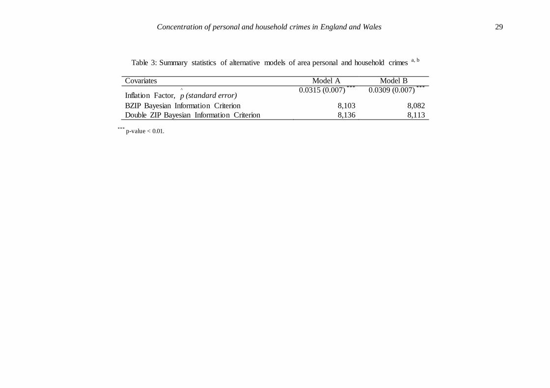
The estimated inflation factors, p̂, and the values of BIC for each BZIP, i.e. Model A and B,

and its respective double ZIP (see previous section) are displayed in Table 3. The respective BZIP

specification which includes the common latent count, V3, fits the data better than the double ZIP

for each Model. This statistical result implies that for a very small number of events personal

and property crimes occurred concurrently. The two aggregate crimes are not simply endogenous,

i.e. associated with (partly) similar area characteristics, to a (small) degree they are identical


events. The raw BCS data masks this (unless the narratives of the crime incidents are examined

via qualitative data analysis). According to the principal offence rule each reported crime incident

is recorded as the the most serious offence that occurred during the incident (see also last paragraph

of Section 2).

Therefore neither hypothesis set out earlier in this paper is rejected here. Area heterogeneity

is delineated in the marginal ZIP regressions for λ̂1 and λ̂2 while composite crime also exists as

outlined by λ̂3. The BZIP specification contrasts multiple events which are due to the overlap of

area characteristics associated with each crime type and composite crimes. A comparison of the

two BZIP specifications shows that Model B has a better fit. It is therefore discussed in the next

sections.


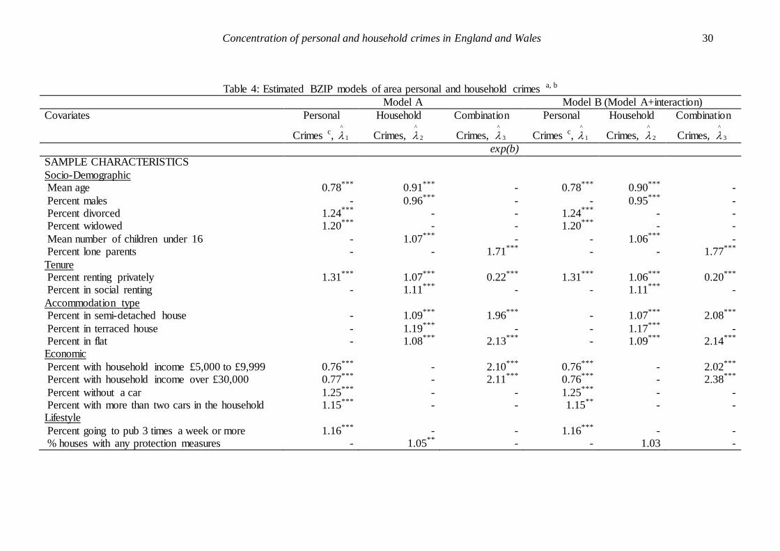
The estimated mean number of events λ̂k, k = 1, 2, 3, for the three marginal distributions of

personal, household and composite crimes associated with each covariate for Models A and B are

given in Table 4. The empirical estimates of the model parameters, β̂k, of the set of equations

(7.3) along with their standard errors are available upon request. The estimated mean number of

clearly personal and property crimes in a non-inner city area of South East England with nationally

average demographic and socio-economic attributes is 0.7 (calculated as the product of λ̂1 and the

nationally average sampling size of quarter postcode sectors, i.e., 0.04×17.43) and 5.93 (calculated

as 0.34× 17.43), respectively. The expected counts slightly underestimate the respective observed

values of 0.8 and 6.0 personal and property crimes (see Table 1). The estimated mean number of

composite crime counts is 0.035 (calculated as 0.002×17.43). Taking composite crimes into account

the estimated mean personal crimes are only marginally underestimated perhaps due to sensitivity

to inner city and regional differences while the estimated and observed property crime counts are

essentially identical.


The empirical models evidence that some characteristics are related to personal crimes (see λ̂1,


second or fifth column of Table 4), some to property crimes (see λ̂2, third or sixth column of Table

4) and some to multi-crime events (see λ̂3, fourth or seventh column of Table 4).

8.2 Multiple crimes

Age, private renting, 2 to 5 years length of residence, inner city and population density are indi-

vidually associated with each crime type. Insofar that these associations are in the same direction

for both crime types the above characteristics identify multiple crime areas. These are similar

observed heterogeneity factors whereby areas face multiple, i.e. personal and household, crimes

due to coincidence of characteristics which are associated with each aggregate crime type. Areas

with low mean population age and relatively stable residence (2 to 5 years) but high population

density and private renting (an indicator of transience) are expected to suffer high personal and

high property crime rates. In particular, an increase of mean population age by one standard de-

viation is associated with 22% and 9% respective drops of personal and property crimes. A similar

increase of the percentage of households with 2 to 5 years of residence relates to 18% and 9% less

personal and property crimes, respectively. By contrast, a standard deviation rise of population

density or private renting is associated with more personal (by 23% and 31%, respectively) and

property crimes (by 6% and 28%, respectively).

This set however excludes another common significant factor, inner city location. This is related

to higher household (by 40%) but lower personal (by 56%) crimes compared to other area types,

therefore it is unlikely to promote multiple crimes, rather repeat household offences. We will return

to how inner city relates to crime in the discussion of composite crimes.

8.3 Repeats

A number of covariates are correlated with either personal or household crimes thereby predicting

repeats and the area’s crime specialization. In particular, a standard deviation rise of an area’s

percentage of divorced or widowed residents, poverty, households without a car or with three or

more cars or residents’ going to the pub 3 times per week are associated with higher personal


crimes by 24%, 20%, 8%, 25%, 15% and 16%, respectively. A similar increase of the percentage of

households with low or high income is however related with a 24% drop of personal crimes. The

negative effect of high income on area’s personal crime is expected as affluent households reside in

relatively safe areas. The non-intuitive similar effect of £5, 000−£9, 000 household income however

may be justified by low income elderly pensioner households which have very low victimisation risk

(Kershaw et al. 2001).

An increase of the percentage of Afro-Caribbean population or males (by one standard devia-

tion) is associated with 6% and 5% less property crimes, respectively. A standard deviation rise of

the percentages of historic private renting (taken from the 1991 Census), flats, semi-detached and

terraced houses, urban, social renting (council housing) households or children in the area is related

to more household crimes by 8%, 9%, 7%, 17%, 11%, 11% and 6%, respectively. All the above

results except one agree with previous evidence from BCS-based and other empirical literature (for

an overview see Tseloni et al. 2002). The evidence however that property crime is adversely related

to high proportion of male population should be regarded with caution and requires additional

investigation.

8.4 Composite Crimes

As already mentioned, albeit to a small extent, i.e., 0.035 over and above the mean personal

and household crime of a South East non-inner city area with nationally average characteristics,

personal and household crimes happen concurrently during multi-crime events. Composite crimes,

λ̂3, are associated with high proportions of lone parents, semi-detached houses, flats, low (under

£9, 999) or high (over £30, 000) income households and inner cities with relatively low population

density. They are expected to rise by 77%, 108%, 114%, 102% and 138% following respective

increases of the above factors by one standard deviation. A similar increase of the percentage of

households renting privately is however related to an 80% drop of composite crime. This result is

arguably counter-intuitive but it may be explained by urban development in recent years. High

levels of private renting are a feature of inner cities which, unlike strictly commercial city centres,


are vibrant places 24/7. The fact that people are out and about at all times facilitates informal

guardianship. Centrally located rented accommodation is higher priced than suburban one and thus

attracts people with certain economic and social characteristics, i.e. single professionals. This result

reinforces the above-mentioned negative association between population density in inner cities and

crime. Indeed, while inner cities are expected to have 193% more composite crimes than non-inner

city areas, a standard deviation increase of population density within inner cities would drop them

by 57%. In effect there is no more composite crime in inner cities with population density just over

one and a quarter, 1.27 (calculated as −{1.08/(−0.85)}), standard deviations above the national

average than in other areas. All estimated composite crime parameters are highly significant.

8.5 Regions and Excess zeros

Region is not a predictor of composite crimes. Some regions have significantly different mean

levels of property or personal crimes. For instance, South West and the North have significantly

lower personal and property crimes compared to the South East other things being equal. East

Anglia fares well on personal crimes while Yorkshire-Humberside have significantly lower personal

but higher property crimes than the base region. Since the socio-economic composition of the

English regions and Wales differs these results are only an indication of regional crime problems

and targeted regional crime prevention should also consider the region’s population profile.

The estimated likelihood of zero personal and household victimisations is 0.03 for a non-inner

city area of South East with nationally average characteristics and number of selected households

within sampling points (17.4). It has been calculated by applying the estimated intercept values

of Table 4 and the estimated inflation factor, p̂, from Table 3 into equation (7.1). As anticipated

(see section five) this is lower that the observed probability of zero personal and household crimes

(0.048). The difference is due to regional and inner city deviations as well as the model’s adjustment

for zero crime areas due to the small number of respondents.


9 Overview

This study tested two hypotheses for understanding the concurrence of personal and property

crimes in residential areas: observed heterogeneity and composite crime. The former proposes that

different crimes overlap due to common identifiable area characteristics which are associated with

each crime type. The composite crimes hypothesis suggests that different crime types are mani-

festations of mutli-crime events which are latent due to offence recording practices. The empirical

evidence drawn here from the 2000 British Crime Survey via the bivariate zero-inflated Poisson

statistical model (with covariance structure) showed that both hypotheses cannot be rejected.

Personal and property crimes occur in the same areas because these areas share the following

characteristics: high population density, high private renting, low mean population age and low

proportion of households with 2-5 years length of residence. Such areas have multiple crimes. By

contrast, the inner city is related to higher household but lower personal crimes compared to other

places. Some area characteristics which have been outlined in the previous section are associated

with either personal or property crimes. To a small extent (by comparison to identifiable crimes)

composite crimes exist, especially in areas with high proportions of lone parent households, semi-

detached houses or flats, low (£5, 000−£9, 000) or high (above £30, 000) income households, inner

cities with low population density and low private renting. The above can be used to identify areas

with similar socio-economic and demographic profile for assessing the performance of comparable

Crime and Disorder Reduction Partnerships (regional divisions of England and Wales (UK) with

respect to crime and crime prevention) and deploying crime prevention efforts where they are most

needed. The relationship of private renting to crime however needs further investigation as it offers

contrasting evidence for composite and multiple crimes.

The current statistical formulation reflects recent criminological knowledge that crimes recur,

victims suffer more than one crime types but most people are non-victims (Pease 1998; Hope 2007)

and offers an elegant approach for estimating the standard errors of the BZIP parameters. Having

said that, it is hard to imagine areas (rather than households) with absolutely zero crimes in a


year. The observed distributions of crime counts, especially the extreme values of zero and very

high repeats, in the earlier Table 1 to some extent reflect sampling variability. The following section

employs the models predictions to correct for this.

10 Area Crime Concentration

In this last part the empirical model is used to predict crime rates across areas in order to identify

high and low crime areas and their difference. As mentioned the specific location of the areas in

England and Wales is concealed (see the first and fourth sections) but the empirical model can be

simulated across the country (inputting the values of the area characteristics which are included in

the model across the entirety of quarter postcode sectors) in order to identify risk areas. Due to

large error margins the precise ranking of areas with respect to crime rates would be unreliable but

ranking them into quartiles can predict high crime areas reasonably well (Lynn and Elliot 2000).

In this section the distributions of observed (from the raw data) and predicted (from the model)

crime rates are ranked by area deciles which are also sufficiently broad.

Trickett et al. (1992) employed the distribution of crime counts across area deciles to demon-

strate the inequality and, therefore, non-randomness of area crime concentration. Area crime spe-

cialization may be demonstrated via intersecting slopes of personal and property crimes across area

deciles while the composite crime hypothesis may be supported via strictly parallel personal and

property crime distributions over area deciles. Figure 1 displays observed and predicted property

and personal mean crime counts across area deciles of observed household crimes. The worst 10%

of observed property crime areas have on average 17.6 and 1.3 more property and personal crimes,

respectively, than the safest 10%. Predicted rates are however strikingly less contrasted between

low and high observed property crime areas. Indeed both crime types roughly double between the

safest and highest risk areas. This result reflects the adjustment for the size variability of sampling

points but it is somewhat misleading as it uses observed rates and groups together areas of very

different expected crime rates.


”Figure 1 about here”

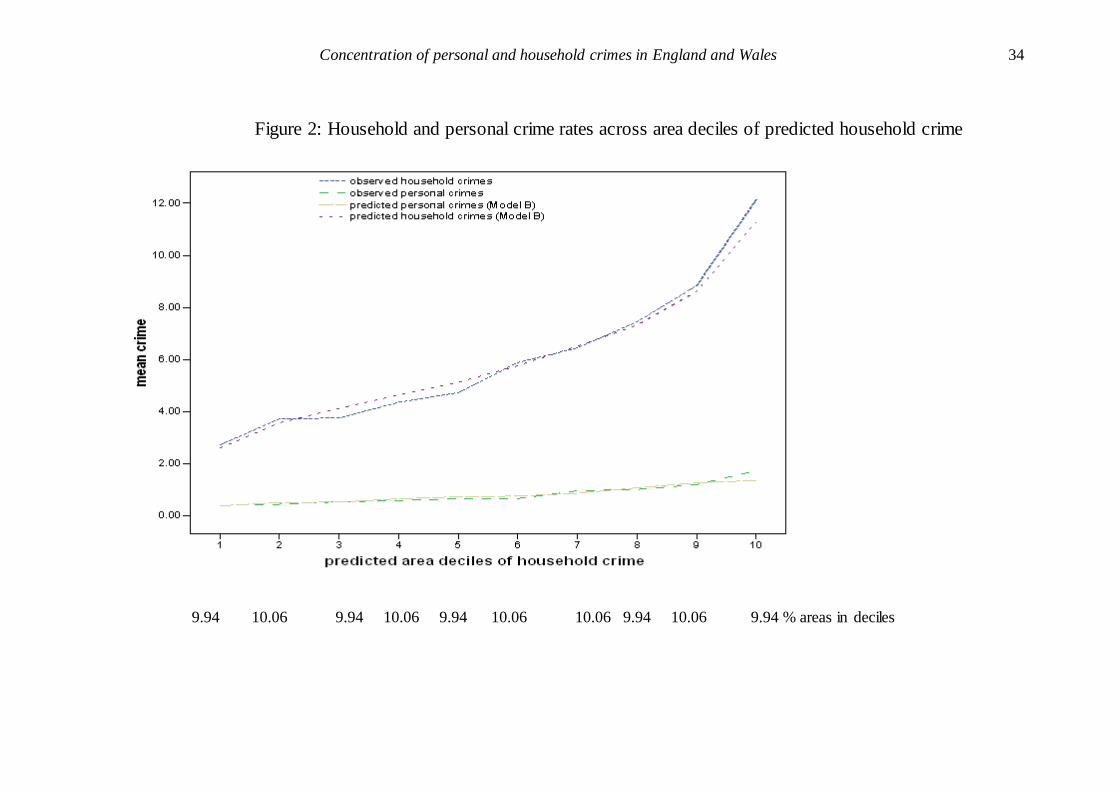
Figure 2 also presents observed and predicted property and personal crime rates but this time

across area deciles with respect to predicted property crime. Predicted crimes follow closely the

respective observed counts with the exception of the highest crime area decile wherein the latter

overestimate the predictions. The 10% of areas with the highest predicted property crime are

expected to have 4.4 and 3.6 more such and personal crimes, respectively, than the safest 10%.

Similar graphs across area deciles with respect to personal crime are available from the authors.

”Figure 2 about here”

The study has been the first attempt to incorporate all distributional characteristics of jointly

examined crime counts and further refinements are in order. For instance, covariance structure may

be added to models with different marginal probabilities for zero events across crime types, such

as the (zero-inflated) negative binomial (Wang 2003), and compare the two bivariate count models

via a bivariate extension of a recently developed score test (Xiang et al. 2007). The examination

of correlated specific crime counts against individuals or households clustered within areas which

would aid tailored crime prevention responses to individual needs can be achieved via hierarchical

extensions of such multivariate models for overdispersed counts.

To what use can the modeling be put? The resourcing of police force areas involves something

close to a Catch 22 situation. The obvious basis of sourcing would be crime counts in an area.

However, to use such a measure would risk local police inflating recorded crime counts to attract

additional funding. The current basis of funding in England and Wales involves a painstaking but

approximate regression approach (see Pease 2008). The modeling approach taken here may, with

appropriate testing, represent an advance. Further, each of the significant covariates challenges

criminological theorizing, perhaps especially those in relation to composite crime. This is the

wrong place and outlet to develop such theorizing, but the challenge should be taken up, by the

writers no less than by others.


References

Bowers, K.J., Johnson, S.D. and Pease, K. (2004) Prospective hot-spotting: The future of crime mapping?British Journal of Criminology, 44, 641-658.

Chenery, S., Ellingworth, D., Tseloni, A. and Pease, K. (1996) Crimes which repeat: Undigested evidencefrom the British Crime Survey 1992. International Journal of Risk, Security and Crime Prevention,1, 207-216.

Cohen, L. E. and Felson, M. (1979) Social change and crime rates and trends: A routine activity approach.American Sociological Review, 44, 588-608.

Davidian, M. and Giltinan, D.M. (1995) Nonlinear models for Repeated Measurement Data. Monographson Statistics and Applied Probability 62. London: Chapman and Hall.

Ellingworth, D., Hope, T., Osborn, D. R., Trickett, A. and Pease, K. (1997) Prior victimisation and crimerisk.International Journal of Risk, Security and Crime Prevention, 2, 201-214.

Ellingworth, D. and Pease, K. (1998) Movers and breakers: household property crime against those movinghome. International Journal of Risk, Security and Crime Prevention, 3, 35-42.

Farrell, G. and K. Pease.(1993) Once bitten, twice bitten: Repeat victimisation and its implications forcrime prevention, Crime Prevention Unit Paper 46. London: Home Office.

Farrell, G. and Pease, K. (2001) (eds.) Repeat Victimization. Monsey, NY: Criminal Justice Press.

Farrell, G., Tseloni, A. and Pease, K. (2005) Repeat Victimization in the ICVS and NCVS. Crime Preven-tion and Community Safety: An International Journal, 7, 7-18.

Felson, M. (1998) Crime and Everyday Life, 2nd edn. Thousand Oaks, CA: Pine Forge Press.

Forrester, D., Chatterton, M. and Pease, K. (1988) The Kirkholt Burglary Prevention Project, Rochdale,Crime Prevention Unit Paper 13. London: Home Office.

Forrester, D., Frenz, S., O’Connell, M. and Pease, K. (1990) The Kirkholt Burglary Prevention Project:Phase II, Crime Prevention Unit Paper 23. London: Home Office.

Greene WH (1997) Econometric Analysis. Upper Saddle River, NJ: Prentice Hall.

Hales, J., Henderson, L., Collins, D. and Becher, H. (2000) 2000 British Crime Survey (England and Wales):Technical Report. London: National Centre for Social Research.

Hindelang, M., Gottfredson, M.R. and Garofalo, J. (1978) Victims of Personal Crime: An EmpiricalFoundation for a Theory of Personal Victimisation. Cambridge: Ballinger.

Hope, T. (2007). The social epidemiology of crime victims. In Handbook on Victims and Victimology (ed.S. Walklate). Uffculme, Devon: Willan.

Hope, T., Bryan, J., Trickett, A. and Osborn, D.R. (2001) The phenomena of multiple victimisation. BritishJournal of Criminology, 41, 595-617.

Hough, M. and Mayhew, P. (1983) The British Crime Survey: First Report. Home Office Research Studyno. 76. London: Her Majesty’s Stationary Office.

Juran J.M. (1951) Quality Control Handbook. New York: McGraw-Hill.

Karlis, D. and Ntzoufras, I. (2005) Bivariate Poisson and diagonal inflated bivariate Poisson regressionmodels in R. Journal of Statistical Software 14 http://www.jstatsoft.org

Kennedy, L. W. and Forde, D.R. (1990) Routine activities and crime: An analysis of victimisation inCanada. Criminology, 28, 137-152.

Kershaw, C. and Tseloni, A. (2005) Predicting crime rates, fear and disorder based on area information:Evidence from the 2000 British Crime Survey. International Review of Victimology, 12, 295-313.

Kershaw, C., Budd, T., Kinshott, G., Mattinson, J., Mayhew, P. and Myhill, A. (2000) The 2000 BritishCrime Survey England and Wales. Statistical Bulletin 18/00. London: Home Office.

Kershaw, C., Chivite-Matthews, N., Thomas, C. and Aust, R. (2001) The 2001 British Crime Survey FinalResults, England and Wales. Home Office Statistical Bulletin 18/01. London: Home Office.


Lee, A.H., Wang, K., Yau, K.K.W., Carrivick, P.J.W. and Stevenson, M.R. (2005) Modelling bivariatecount series with excess zeros. Mathematical Biosciences, 196, 226-237.

Li, C., Lu, J., Park, J.P., Kim, K., Brinkley, P. A .and Peterson, J.P. (1999) Multivariate zero-inflatedPoisson models and their applications. Technometrics, 41, 29-38.

Lynn, P. and Elliot, D. (2000) The British Crime Survey: A Review of Methodology. National Centre forSocial Research, Paper 1974, March.

McLoughlin L.M., Johnson S.D., Bowers K.J., Birks D.J. and Pease K. (2007) Police perceptions of thelong and short-term spatial distribution of residential burglary. International Journal of Police Scienceand Management, 9, 99-111.

Nicholas, S., Kershaw, C. and Walker, A (Eds.) (2007) Crime in England and Wales 2006/07. Home OfficeStatistical Bulletin 11/07.

Osborn, D.R. and Tseloni, A,(1998) The distribution of household property crimes. Journal of QuantitativeCriminology, 14, 307-330.

Osborn, D.R., Trickett, A. and Elder, R. (1992) Area Characteristics and Regional Variates as Determinantsof Area Property Crime Levels. Journal of Quantitative Criminology, 8, 265-285.

Osborn, D. R., Ellingworth, D., Hope, T. and Trickett, A. (1996) Are repeatedly victimised householdsdifferent? Journal of Quantitative Criminology, 12, 223-245.

Pease, K, (1998) Repeat Victimisation: Taking Stock. Crime Detection and Prevention Series Paper No.90. London: Home Office.

Pease K. (2008) The Home Office and the Police: The Case of the Police Funding Formula. In Handbookof Intelligent Policing (eds. A. McVean and C. Harfield). Chichester: Wiley.

Planty, M. and Strom, K.J. (2007) Understanding the role of repeat victims in the production of annualvictimization rates Journal of Quantitative Criminology, 23, 179-200.

Reiss, A.J. (1980) Victim proneness in repeat victimization by type of crime. In Indicators of Crime andCriminal Justice Quantitative Studies(eds. S. Fienberg and A.J. Reiss), pp. 41-53. Washington:Department of Justice.

Sampson, R.J. and Groves, B.W. (1989) Community Structure and Crime: Testing Social DisorganizationTheory. American Journal of Sociology, 94, 774-802.

Shaw, C.R. and McKay, M.D. (1942) Juvenile Delinquency and Urban Areas. Chicago: Chicago UniversityPress.

Thorpe (2007) Multiple and repeat victimisation. In Jansson, K., Budd, S., Lovbakke, J., Moley, S. andThorpe, K. Attirudes, Perceptions and Risks of Crime: Supplementary Volume 1 to Crime in Englandand Wales 2006/07, Home Office Statistical Bulletin 19/07. London: Home Office. Pp. 81-98.

Trickett, A., Osborn, D., Seymour, J. (1992) What is different about high crime areas? British Journal ofCriminology, 32, 81-90.

Trickett A., Osborn, D.R. and Ellingworth, D. (1995) Property crime victimisation: The roles of individualand area influences. International Review of Victimology, 3, 273-295.

Tseloni, A. (2006). Multilevel modelling of the number of property crimes: Household and area effects. J.R. Statist. Soc. A, 169, 205-233.

Tseloni, A. Osborn, D.R., Trickett, A. and Pease, K. (2002) Modelling property crime using the BritishCrime Survey: What have we learned? British Journal of Criminology, 42, 89-108.

Venables, W.N., Smith, D.M. and the R Development Core Team (2007) An Introduction to R: Noteson R: A Progamming Environment for Data Analysis and Graphics, Version 2.5.1 (2007-06-27), RDevelopment Core Team, http://www.r-project.org/

Wang, P. (2003) A bivariate zero-inflated negative binomial regression model for count data with excesszeros. Economics Letters, 78, 373-378.

Wang, K., Lee, A.H., Yau, K.K.W. and Carrivick, P.J.W. (2003) A bivariate zero-inflated Poisson regressionmodel to analyse occupational injuries. Accident analysis & Prevention, 35, 625-629.

Xiang, L., Lee, A.H., Yau, K.K.W. and McLachlan, G.J. (2007) A score test for overdispersion in zero-inflated poisson mixed regression model. Statistics in Medicine, 26, 1608-1622.


Appendix Table:

Complete and ‘non-moving & within 15´- walk’ observed distributions of total household and personal crimes.

Household Crime Z-value for p difference

Personal Crime Z-value for p

difference

Crime Count

With restrictions

Without restrictions

With restrictions

Without restrictions

0 6.1 4 2.04 59.9 52.5 3.18

1 9.1 7.7 1.07 20.4 20.6 -0.10 2 11.3 7.7 2.62 9.5 11.2 -1.19

3 10.7 8.7 1.44 5.7 7.1 -1.22 4 11.7 9.7 1.38 1.7 3 -1.83 5 9.7 10.1 -0.28 1.3 2 -1.17

6 6.6 7.8 -0.99 0.8 1.5 -1.40 7 6.2 6.4 -0.17 0.3 0.8 -1.44

8 5.2 5.2 0 0.1 0.3 -0.95 9 4.3 4.2 0.10 0.1 0.3 -0.95

10 3.8 4.2 -0.43 0 0.3 -1.65

11 2.7 4.3 -1.85 0 0 0 12 2.4 2.8 -0.53 0 0.1 -0.95

13 2.3 3.4 -1.41 0 0 0 14 1.2 2.3 -1.79 0.1 0.1 0 15 1.5 1.3 0.36 0 0 0

16 .8 1.4 -1.22 0 0.1 -0.95 17+ 3.9 8.6 -4.15 0 0.1 -0.95


Table 1: Area Personal and Property Crimes a, b

Personal Crimes c Household Crimes

Number of Crimes Percentage of Areas

Percentage of Areas

0 59.9 6.1 1 20.4 9.1

2 9.5 11.3 3 5.7 10.7

4 1.7 11.7 5 1.3 9.7 6 0.8 6.6

7 0.3 6.2 8 0.1 5.2

9 0.1 4.3 10 0 3.8 11 0 2.7

12 0 2.4 13 0 2.3

14 0.1 1.2 15 0 1.5 16 0 .8

17 or more 0 3.9

Total Number of Areas 905

Maximum Crime Count 14 42

Mean Crimes 0.8 6.0 Standard Deviation 1.4 5.2 Skewness 2.9 1.9

Crime Concentration (Incidence/Prevalence)

2.0

6.4

Total Areas (905) Without No Crime Areas (862) Pearson’s r

(correlation)

0.28** 0.26**

a Incidents occurred within a 15 minute walk from home to respondents who have not

moved house in the previous year. b Series incidents are truncated at 5. c Personal crimes exclude sexual offences. ** Two-tail p-value < 0.01.


Table 2: Description of covariates

Covariates Mean % Freq. St. Dev. Min, Max

SAMPLE CHARACTERISTICS Demographic Respondents’ mean age 50.6 5.7 29.3, 71.6

% Males 45.3 12.8 0, 87.5 % Ethnic minority 4.3 11.3 0, 92.3

Social % Single people a 16.8 11.5 0, 81.8 % Divorced a 11.6 9.27 0, 75.0

% Widowed a 12.5 8.64 0, 57.1 Mean number of children under 16 0.3 0.1 0, 0.8

% Lone parents 4.9 6.3 0, 42.9 % One adult households b 31.2 15.3 0, 100.0 % Three or more adults b 14.19 9.76 0, 75.0

Education a % A-levels 11.0 8.15 0, 47.6

% Trade apprenticeships, O-levels etc. 28.5 12.8 0, 68.8 % Without qualifications 37.17 17.0 0, 95.0 Social Class

% Manual 53.8 23.4 0, 100 Tenure % Renting privately 7.7 9.0 0, 63.6

% Social renting 18.8 19.7 0, 100.0 Accommodation type b

% Semi-detached house 34.1 22.8 0, 100.0 % Terraced house 28.9 23.5 0, 100.0 % Flat 13.3 19.0 0, 100.0

Economic % Household income less than £5,000 10.8 11.0 0, 77.8

% Household income £5,000 to £9,999 16.6 11.7 0, 75.0 % Household income over £30,000 21.8 16.4 0, 78.9 % Without a car in the household 23.2 17.8 0, 100.0

% One car in the household 46.0 13.8 0, 100.0 % More than two cars in the household 5.3 6.3 0, 36.8

Area of Residence % At the same address for less than 2 years 7.0 7.0 0, 40.0 % At the same address for 2 to 5 years 20.7 11.7 0, 75.0

% At the same address for 5 to 10 years 18.2 10.1 0, 58.3 % In neighbourhood watch scheme b 28.3 25.0 0, 100.0

% Urban 62.5 40.2 0, 100.0 Inner city 13.5 0, 1

a Entered only the set of covariates for personal crimes. b Entered only the set of covariates for property crimes.


Table 2: Description of covariates (continued).

Covariates Mean % Freq. St. Dev. Min, Max

SAMPLE CHARACTERISTICS Lifestyle % Away from home less than 3 hours per

weekday a

28.8 14.0 0, 100.0

% Away from home 3 to 7 hours per weekday a 28.0 12.5 0, 80.0

% Going to pub less than once a week a 29.5 12.2 0, 68.4 % Going to pub once a week a 15.2 9.9 0, 50.0 % Going to pub 3 times a week or more a 7.3 6.9 0, 36.4

% Going to club less than once a week a 8.4 7.3 0, 37.5 % Going to club once a week a 2.17 3.7 0, 20.0

% Drinking alcohol daily a 16.2 11.2 0, 77.8 % Drinking alcohol 3 to 4 times a week a 14.0 9.4 0, 55.6 % Drinking alcohol once or twice a week a 27.6 11.5 0, 69.2

% Drinking alcohol once a month or more but less than once a week a

16.8 9.9 0, 60.0

% Houses with any protection measures b 35.7 23.8 0, 100.0 % House empty less than 3 hours a day b 44.1 15.6 0, 100.0 % House empty 3 to 7 hours a day b 30.7 13.1 0, 80.0

AREA CHARACTERISTICS (Standardised Values) % Households renting privately -0.11 0.77

% Single adult non-pensioner households -0.11 0.47 Poverty c -0.15 3.46

% Afro-Caribbean 0.00 0.83 % Asian d 0.04 0.91 % Population 16-24 years -0.04 0.28

% Housing association accommodation -0.05 0.71 % Persons moved in last year -0.06 0.26

Population density 0.13 0.93 REGIONS

North 7.3 0, 1 Yorkshire/Humberside 9.3 0, 1

North West 11.6 0, 1 East Midlands 8.1 0, 1 West Midlands 10.1 0, 1

East Anglia 4.6 0, 1 Greater London 13.3 0, 1

South East (base) 14.2 0 South West 9.6 0, 1 Wales 6.7 0, 1

a Entered only the set of covariates for personal crimes. b Entered only the set of covariates for property crimes.

c Aggregate factor calculated as (0.859 x percentage lone parent households + 0.887 x percentage

households without a car – 0.758 x non-manual – 0.877 x percentage owner-occupied households +

0.720 x mean number of people per room + 0.889 x percentage households renting from a local

authority). d Indian, Pakistani or Bangladeshi.


Table 3: Summary statistics of alternative models of area personal and household crimes a, b

Covariates Model A Model B

Inflation Factor, ^

p (standard error) 0.0315 (0.007) *** 0.0309 (0.007) ***

BZIP Bayesian Information Criterion 8,103 8,082

Double ZIP Bayesian Information Criterion 8,136 8,113

*** p-value < 0.01.

Concentration of personal and household crimes in England and Wales

30

Table 4: Estimated BZIP models of area personal and household crimes a, b

Model A Model B (Model A+interaction)

Covariates Personal

Crimes c, 1

^

Household

Crimes, 2

^

Combination

Crimes, 3

^

Personal

Crimes c, 1

^

Household

Crimes, 2

^

Combination

Crimes, 3

^

exp(b)

SAMPLE CHARACTERISTICS

Socio-Demographic Mean age 0.78*** 0.91*** - 0.78*** 0.90*** -

Percent males - 0.96*** - - 0.95*** - Percent divorced 1.24*** - - 1.24*** - - Percent widowed 1.20*** - - 1.20*** - -

Mean number of children under 16 - 1.07*** - - 1.06*** - Percent lone parents - - 1.71*** - - 1.77***

Tenure Percent renting privately 1.31*** 1.07*** 0.22*** 1.31*** 1.06*** 0.20*** Percent in social renting - 1.11*** - - 1.11*** -

Accommodation type Percent in semi-detached house - 1.09*** 1.96*** - 1.07*** 2.08***

Percent in terraced house - 1.19*** - - 1.17*** - Percent in flat - 1.08*** 2.13*** - 1.09*** 2.14*** Economic

Percent with household income £5,000 to £9,999 0.76*** - 2.10*** 0.76*** - 2.02*** Percent with household income over £30,000 0.77*** - 2.11*** 0.76*** - 2.38***

Percent without a car 1.25*** - - 1.25*** - - Percent with more than two cars in the household 1.15*** - - 1.15** - - Lifestyle

Percent going to pub 3 times a week or more 1.16*** - - 1.16*** - - % houses with any protection measures - 1.05** - - 1.03 -


31

Table 4: Estimated BZIP models of area personal and household crimes a, b (continued)

Model A Model B (Model A+interaction)

Covariates Personal

Crimes c, 1

^

Household

Crimes, 2

^

Combination

Crimes, 3

^

Personal

Crimes c, 1

^

Household

Crimes, 2

^

Combination

Crimes, 3

^

exp(b)

SAMPLE CHARACTERISTICS

Area of Residence Percent at the same address for 2 to 5

years

0.82*** 0.92*** - 0.82*** 0.91*** -

Inner city dummy 0.49*** 1.30*** - 0.44*** 1.40*** 2.93*** Percent urban residents - 1.12*** - - 1.11*** -

AREA CHARACTERISTICS % Afro-Caribbean - 0.93*** - - 0.94** -

Percent households renting privately - 1.09*** - - 1.08*** - Population density 1.23*** 1.18*** 0.67** 1.23*** 1.28*** - Poverty d 1.08** - - 1.08*** - -

Population density in inner city - 0.82*** 0.43*** REGION (base: South East)

South West 0.95 1.09 - 0.94 1.09 - Greater London 0.71* 0.65*** - 0.73* 0.65*** - East Anglia 0.63* 0.99 - 0.64* 0.98 -

East Midlands 0.82 1.01 - 0.82 1.02 - West Midlands 0.89 0.92 - 0.87 0.92 -

Yorkshire –Humberside 0.64** 1.10 - 0.64** 1.11* - North West 0.90 1.02 - 0.91 1.04 - North 0.68** 0.78*** - 0.67** 0.78*** -

Wales 0.89 0.93 - 0.88 0.94 - Intercept 0.042*** 0.337*** 0.002*** 0.043*** 0.339*** 0.002*** a Incidents occurred within a 15´ walk from home to respondents who have not moved house in th e previous year.


32

b Series incidents are truncated at 5 events.

c Personal crimes exclude sexual offences.

d Aggregate factor calculated as (0.859 x percentage lone parent households + 0.887 x percentage households without a car – 0.758 x non-manual – 0.877 x percentage

owner-occupied households + 0.720 x mean number of people per room + 0.889 x percentage households renting from a local authority). # Indian, Pakistani or Bangladeshi.

Two-tailed tests: *

0.05 < p-value< 0.10.

** 0.01 < p-value< 0.05.

*** p-value < 0.01.


33

Figure 1: Household and personal crime rates across area deciles of observed household crime

6.1 11.3 11.7 12.8 8.8 % areas in deciles 9.1 10.7 9.7 9.5 10.3


34

Figure 2: Household and personal crime rates across area deciles of predicted household crime

9.94 10.06 9.94 10.06 9.94 10.06 10.06 9.94 10.06 9.94 % areas in deciles

Documents

Concentration of personal and household crimes in … · Concentration of personal and household crimes in ... eg. a bike theft followed by a ... share characteristics associated