Preprint PP/MAT/SEM/0102-005, Glasgow Caledonian University, 2001

Concept of Normalised Equivalent StressFunctionals for Cyclic Fatigue

S.E. Mikhailov, I.V.Namestnikova

Dept. of Mathematics, Glasgow Caledonian Univ.,Cowcaddens Road, Glasgow, G4 0BA, UK

(s.mikhailov@gcal.ac.uk, i.namestnikova@gcal.ac.uk)

Abstract

Generalised fatigue durability diagrams and their properties are considered fora material under multi-axial loading given by a (non-regularly) oscillating functionof time. Material strength and durability under such loading is described in termsof durability and normalised equivalent stress. Relations between these functionalsare analysed. Phenomenological strength conditions are presented in terms of thenormalised equivalent stress. It is shown that the damage based fatigue durabilityanalysis is reduced to a particular case of such strength conditions. Examples of thereduction are presented for some known durability models. Some complex strengthconditions applicable to the durability description at fatigue, creep, dynamic loadingand their combination are presented. The normalised equivalent stress functionalinterpolation along classical periodic S–N diagrams is introduced.

Keywords: Durability; Strength conditions; Endurance limit; Cyclic loading

Nomenclature

τ, t = the natural continuous time;

σ(τ) = a uniaxial or multiaxial loading process in time;

σij(τ) = a multiaxial loading process in time;

m, n, j = a (quasi–)cycle number, discrete time;

σct(m) = {σij(τ); τm−1 ≤ τ ≤ τm} = a (quasi–)cycle with time parametrisation;

σcs(m) = a (quasi–) cycle as an oriented loop in the stress space without time parametri-sation;

σc(m) = σct(m) or σcs(m)

{σc(m)}m=1,2,... = {σ(m)}m=1,2,... = {σc} = {σ} = a (quasi–)cyclic loading process;

σmax(j) = maximum stress in j-th cycle;

σmin(j) = minimum stress in j-th cycle;

σa(j) = [σmax(j)− σmin(j)]/2 = stress amplitude in j-th cycle;

σm(j) = [σmax(j) + σmin(j)]/2 = mean stress in j-th cycle;

R = σm−σa

σm+σa= cycle asymmetry ratio;

1

S.E.Mikhailov, I.N.Namestnikova

σmaxa = maximum stress amplitude in a loading process;

σ0ij = constant stress tensor;

AR; bR; AR = material parameters in the Wohler S–N diagram;

σi = 1√2

√(σ1 − σ2)2 + (σ2 − σ3)2 + (σ3 − σ1)2, von Mises intensity of a stress tensor σkj

possessing principal stresses σ1 > σ2 > σ3;

σi,a = von Mises intensity of a stress amplitude tensor in multiaxial loading process;

σi,m = von Mises intensity of a mean stress tensor in multiaxial loading process;

σr = strength under monotone uniaxial loading;

σ∗R(n) = stress amplitude to reach rupture on n-th cycle under uniaxial periodic loadingwith asymmetry factor R;

σeq = equivalent stress amplitude e.g. von Mises or Tresca;

n∗{σ} = cyclic durability under a process {σ(m)}m=1,2..;

t∗(σ) = durability under a process {σ(τ)};n∗R(σa) = number of cycles up to rupture under periodic loading with stress amplitude

σa and cyclic asymmetry factor R;

λ = a non-negative number;

λN({σ}; n) = (a value of) the cyclic safety factor functional;

ΛN({σ}; n) = (a value of) the cyclic normalized equivalent stress functional, NESF;

σ∗−1∞ = fatigue limit amplitude under uniaxial reversing (R = 0) tension-compressionloading;

σ∗0∞ = fatigue limit (amplitude) under repeated (with zero minimum stress) tension load-ing;

σH,m = mean cyclic hydrostatic pressure;

σH,max = maximum cyclic hydrostatic pressure;

Sij = stress deviator;

P = period in a periodic process;

α, β = material constants in critical surface criteria;

σηη,a(~η, τ) = normal stress amplitude on a plane with a normal ~η;

τa(~η, τ) = shear stress amplitude acting in on a plane with a normal ~η;

σηξ,a = shear stress acting in a direction ~ξ on a plane with a normal ~η;

|σ| = a matrix norm of a tensor σij, e.g. |σ| =√∑3

i,j=1 σ2ij;

|||σc(m)||| = a norm of a tensor function σc(m) on the m−th cycle, e.g. |||σc(m)||| =supσ∈σc(m) |σ|;

σc(m) = σc(m)/|||σc(m)||| = normalised shape of a tensor function σc(m) on the m−thcycle;

|~S| = Euclidian norm of a vector (the vector length).

2

S.E.Mikhailov, I.N.Namestnikova

1 Introduction

In the traditional approach to cyclic strength of a material, the fatigue durability isevaluated from the inequality

ω({σ}, n) < 1 (1)

where the damage measure ω({σ}, n) is a functional of the loading history {σ(m)}m=1,2,...

and m,n are the cycle numbers. When the number of cycles is sufficiently large suchthat inequality (1) is violated (transfers into the equality), a material rupture occurs. Aparticular form of ω({σ}, n) for a non-periodic cycling (i.e. with varying cycles σ(m)) isusually related to a particular damage accumulation law. For example,

ω({σ}, n) =n∑

m=1

1

n∗p[σ(m)](2)

for a material obeying the Palmgren-Miner hypothesis of linear damage accumulation,where n∗p(σ) is the number of cycles to rupture in the periodic process, given by anappropriate S–N Wohler diagram with all the cycles equal to σ(m, y). By this way, adurability under non-periodic cyclic process is related to experimental data for corre-sponding periodic cyclic processes. However the linear accumulation rule does not workfor some cyclic processes and many attempts to improve it lead to some abstract damagemeasures that one can not obtain (or verify) from direct durability experiments. Evenmore methodical problems appear when the process under consideration is presented byrandom (with unclosed cycles) oscillations where the known procedures for a reduction ofsuch processes to cyclic ones (e.g. the rain flow method) give not accurate prediction ornot applicable at all (say, for out-of-phase random multiaxial oscillations).

To overcome those difficulties with processes sufficiently general in time, appearing notonly for oscillating but also for dynamic and creep loading, and to create a more robustand experimentally verifiable tool for durability analysis, some theoretical backgrounds ofa functional approach to durability description under a loading program (process) σij(τ),which is a (tensor) function of time τ , were considered by Mikhailov (1999, 2000). How-ever, the time dependence is not essential for the durability description of the materials,whose rupture depends only on the loading sequence but not on time itself or on the load-ing process rate (for considered loading conditions). The pure fatigue rupture (withoutcreep and ageing) is an example of such behavior. Although such processes may still beconsidered with respect to time as a natural parameter and the approach described byMikhailov (1999, 2000) holds true, some other parameterizations seem to be more relevantfor fatigue.

The (quasi–) cycle number m can be considered then as the so-called discrete time(see e.g. Bolotin 1989) and the main issues developed by Mikhailov (1999, 2000) forthe natural continuous time will be adopted here for the discrete time. We arrive af-ter this at the notions of durability (number of cycles to rupture) n∗{σ}, generalisedWohler S–N diagram λ 7→ n∗{λσ}, functional safety factor λN({σ}, n) and normalisedequivalent stress functional ΛN({σ}, n) defined on a loading process {σ(m)}m=1,2,.... Thisleads to a fatigue strength and durability phenomenological description in terms of thesemechanically meaningful and experimentally identifiable functionals without necessaryinvolvement of a geometrical, stiffness-related or abstract damage measure. On the other

3

S.E.Mikhailov, I.N.Namestnikova

hand, this approach allows rather simple deviation from a standard linear Palmgren-Minerdamage accumulation rule to describe better the experimental observations.

Fatigue under stress fields independent of the space coordinates is mainly analysed inthis paper with obvious reasoning about application to moderately inhomogeneous stressfields . Extension to highly inhomogeneous stress field incorporating a non-local approachby Mikhailov (1995) will be considered elsewhere (Mikhailov & Namestnikova 2002).

2 Cyclic and quasi-cyclic processes and their parametri-

sations

We will call a multiaxial process σij(τ), τ ≥ 0 cyclic if it can be represented as a temporalsequence of connected loops (cycles) σct(m) = {σij(τ); τm−1 ≤ τ ≤ τm} closed in thestress space, σij(τm) = σij(τm−1), where m = 1, 2, ... is the loop number. Here thenotation σct(m) includes information on the loop position [τm−1, τm] in time, the loopparametrisation with respect to time and consequently the loop shape in the stress space.If τm− τm−1 = P = const for m = m1, ...m2 and σij(τ + P ) = σij(τ), τm1−1 ≤ τ, τ + P ≤τm2 , we call the process {σct(m)}m=1,2,... periodic on τ ∈ [τm1−1, τm2 ] with the period P .

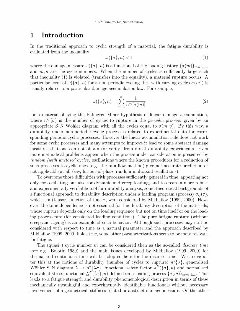
If a uniaxial process σ(τ) is randomly (not cyclically) oscillating, like in Fig. 1, wecan denote the local minima or local maxima or middle points between them as τm andcall the parts of the process σ(τ) on the segments [τm−1, τm] quasi–cycles σct(m). If

σ

ττn -1 τn

σc(n)

Figure 1: A parametrisation of a randomly oscillating process

σij(τ) is a multiaxial in-phase (proportional) process, i.e., σij(τ) = σ0ijf(τ), where σ0

ij is aconstant tensor and f(τ) is a scalar function, we can associate the quasi–cycle boundariesτm with the local minima or local maxima or local middle points of the function f(τ).If σij(τ) is a general multiaxial process, we can distribute points τm by a more or lessreasonable way, such that τ0 = 0, τm > τm−1, and call the parts of the process σij(τ) onthe time segments [τm−1, τm] quasi–cycles σct(m). After such a parameterization we canconsider any process as quasi–cyclic. Note that since a (quasi–) cycle σct(m) includes allthe information about the process σij(τ) behavior on the segment τm−1 ≤ τ ≤ τn, the

4

S.E.Mikhailov, I.N.Namestnikova

temporal sequence {σct(m)}m=1,2,... is equivalent to the original form σij(τ), 0 ≤ τ , of theprocess presentation.

However, the particular values of the instants τm as well as the natural time parametri-sation σij(τ) of a loop σct(m) is not essential for pure fatigue, for which only an orderof the loops, their shapes and orientations in the stress space is essential. To deal withsuch less informative presentation of loading processes, we will consider also the sequence{σcs(m)}m=1,2,... of connected oriented (quasi–) loops σcs(m) in the stress space, for which aparticular time parametrisation is not prescribed. If the loops coincide in the stress space,σcs(m) = σcs, for m = m1, ...m2, we will say the loading is periodic in the block of (quasi–)cycles [m1, m2]. Evidently, {σcs(m)}m=1,2,... is uniquely defined by {σct(m)}m=1,2,... but in-verse is not true. For example, two different temporal cyclic processes:

{σct(1)(m)}m=1,2,... = {sin(τ); 2π(m− 1) ≤ τ ≤ 2πm}m=1,2,...

{σct(2)(m)}m=1,2,... = {sin(τ 2);√

2π(m− 1) ≤ τ ≤√

2πm}m=1,2,...

define one and the same stress space loop sequences {σcs(1)(m)}m=1,2,... = {σcs(2)(m)}m=1,2,...,where each loop lies on the segment −1 ≤ σ ≤ 1 in the one-dimensional stress space.

Let {σ} be a uniaxial cyclic regular process, i.e. σ(τ) is defined in each instant τ of thecycle and has not more than one internal local infimum and one internal local supremumon each cycle. Let us denote by σmax(m) and σmin(m) the global supremum and infimumof σ(τ) during a cycle m including its start and end points, by R(m) = σmin(m)/σmax(m)the cycle asymmetry ratio, by σa(m) = (σmax(m)−σmin(m))/2 the stress cycle amplitudeand by σm(m) = (σmax(m) + σmin(m))/2 the stress cycle mean value. Then the sequence{σcs(m)}m=1,2,... is equivalently presented by the sequences {σmax(m), σmin(m)}m=1,2,...,{σa(m), R(m)}m=1,2,..., {σa(m), σm(m)}m=1,2,... or {σm(m), R(m)}m=1,2,....

Let σij(τ) be a multiaxial in-phase (proportional) cyclic regular process, i.e., σij(τ) =σ0

ijf(τ), where σ0ij is a constant tensor and f(τ) is a scalar function defined in each

instant τ of the cycle, which has not more than one internal local infimum and oneinternal local supremum on each cycle. Let us denote by fmax(m) and fmin(m) the globalsupremum and infimum of f(τ) during the cycle including its start and end points, byR(m) = fmin(m)/fmax(m) the cycle asymmetry ratio, and by

σij,max(m) = σ0ijfmax(m), σij,min(m) = σ0

ijfmin(m),

σij,a(m) = σ0ij(fmax(m)− fmin(m))/2, σij,m(m) = σ0

ij(fmax(m) + fmin(m))/2 (3)

the stress cycle maximum, minimum, amplitude and mean value tensors, respectively.Then similar to the previous paragraph, the sequence {σcs(m)}m=1,2,... is equivalently pre-sented by the sequences {σij,max(m), σij,min(m)}m=1,2,..., {σij,a(m), R(m)}m=1,2,...,{σij,a(m), σij,m(m)}m=1,2,... or {σij,m(m), R(m)}m=1,2,....

We will write {σc(m)}m=1,2,... when considering the both presentations {σct(m)}m=1,2,...

and {σcs(m)}m=1,2,... at the same time. We will further omit sometimes the superscript cand write σt(m), σs(m) or σ(m) for a (quasi–) cycle if this lead to no confusion. Sometimeswe denote a process {σc(m)}m=1,2,... as {σc} or {σ}.

5

S.E.Mikhailov, I.N.Namestnikova

3 (Quasi–) Cyclic Durability and Generalised S–N

Diagram

Let a material undergo a multiaxial quasi–cyclic loading process {σ(m)}m=1,2,.... We willdiscuss here rupture without specifying the rupture type and only assume that (i) one canunambiguously detect at the end of any (quasi–) cycle whether the material is rupturedor not, and (ii) if the material is ruptured during a (quasi–) cycle n1, it will be rupturedalso at any n2 > n2 (no repairing mechanism). The (quasi–) cycle number n∗{σ}, duringwhich a rupture for the material appears under a loading process {σ} is called (quasi–)cyclic durability or (quasi–) cyclic life time. For different loading processes σ1

ij(m), σ2ij(m),

m = 1, 2, ..., the durability has generally different values n∗{σ1}, n∗{σ2}.

3.1 Classical S–N diagram under periodic loading

Let {σ} be a uniaxial periodic regular process, i.e. a regular cyclic process, where allthe cycles σc(m) are independent of m. Under such a loading, it is usual to determineexperimentally the Wohler S–N diagram in the axes σa 7→ n∗R(σa), where n∗R(σa) = n∗{σ}is the number of cycles up to rupture.

An example of a simple S–N diagram given by a power law (a straight line in thedouble logarithmic coordinates) is usually written as

n∗{σ} = n∗R(σa) =[σ∗R1

σa

]−bR

. (4)

where σ∗R1 and bR are positive material parameters considered as depending generally onthe asymmetry ratio R but not on the amplitude σa.

Taking into account that n∗{σ} can take only integer values, this should be rewrittenmore precisely as

n∗{σ} = n∗R(σa) = Int+

([σ∗R1

σa

]−bR)

(5)

where Int+(x) is the minimal integer greater or equal to real x. However, both forms (4)and (5) for the durability n∗{σ} lead to equivalent results when it is used in the strengthcondition like n < n∗{σ} for an integer cycle number n, and we will not distinguish theforms sometimes.

If we introduce a notation |||σc||| = max(|σmax|, |σmin|), then the above relation can berewritten also in the form

n∗{σ} = Int+

[σ∗R1

|||σc|||

]−bR (6)

where σ∗R1 = σ∗R1max =

{2σ∗R1(1−R ), |R| ≤ 12σ∗R1(1−R−1), |R| > 1

}and b = bR.

Let now {σ} be an arbitrary periodic multi-axial cyclic loading process, i.e. the shapeof the periodicity loop σc is arbitrary. For multiaxial cases, let |σ| denote a matrix norm

of tensor σij, for example, |σ| =√∑3

i,j=1 σ2ij. Let |||σc(m)||| denote a norm of the tensor

function σc, for example, |||σc(m)||| = supσ∈σc(m) |σ|. Then power dependence (6) canbe used also for general periodic processes if we suppose that σ∗R1 = σ∗R1(σ

c/|||σc|||) and

6

S.E.Mikhailov, I.N.Namestnikova

b = b(σc/|||σc|||) are positive material parameters depending generally on the cycle σc shapein the stress space but not on the cycle norm |||σc|||.

3.2 Generalised S–N diagram under arbitrary loading

To present a generalised S–N diagram for an arbitrary multi-axial quasi–cyclic process{σc(m)}m=1,..., let us consider a family of proportional processes {λσc(n)}n=1,..., obtainedfrom the original process {σc} after its multiplication by a non-negative constant numberλ. Then the durability n∗{λσ} becomes an integer-valued (piece-wise constant) function

σ

τ

λ1σ

n*{λ2 σ}n*{σ}n*{λ1 σ}

λ2σ

σ

Figure 2: Proportional loading processes and durabilities, 0 < λ2 < 1 < λ1.

of the parameter λ (see on Fig. 2 an example for a quasi–cyclic uniaxial process, wherethe quasi–cycle boundaries are associated with the local minima of σ).

The generalised S–N diagram for a process {σc} is the dependence of the durabilityn∗{λσc} on parameter λ ≥ 0.

The concept propounded in the paper concerns mainly materials, which strength de-pends on the oscillating loading history but should work also in the particular case ofmaterials independent of history and for rather simple loading processes split into quasi–cycles. We will widely use the latter for illustrations.

Let us consider, for example, a material independent of history (that is, its strengthis determined only by the instants stress value) and obeying the strength condition |σ| <σr under uniaxial loading, where σr is a material constant. Suppose the material isperiodically loaded by a uniaxial process {σc}, where some minimal and maximal valuesσmin and σmax are reached during the cycle σc. Then the S–N diagram is given by theconstant sequence λm = σr/|||σc|||, m = 1, 2, ..., where |||σc||| = max(|σmax|, |σmin|) that is,

n∗{λσ} =

{∞, λ < σr/|||σc|||1, λ ≥ σr/|||σc|||

}.

Suppose the same material is loaded by a uniaxial loading process {σc} such that someminimum σmin(m) and maximum σmax(m) are reached during the cycle σc(m) and their

7

S.E.Mikhailov, I.N.Namestnikova

values grow linearly with the cycle number, hence |||σc(m)||| = max(|σmax(m)|, |σmin(m)|) =am, where a is a constant. Then the S–N diagram is given by a discrete hyperbolan∗{λσ} = Int+[σr/(aλ)].

Let us consider general properties of the generalised Wohler S–N diagram n∗{λσ} fora material under an arbitrary process {σc}. The function λ 7→ n∗{λσ} is defined on thehalf axis λ ∈ [0,∞) and is non-negative and integer-valued. When λ varies, differentsituations can arise. On Fig. 3a, we plot schematically an S–N diagram n∗{λσ} (step-like graphs) over corresponding durability diagram t∗{λσ} (smooth curves, see Mikhailov2000, Fig. 3a) for the same process. The diagram t∗{λσ} can be always obtained for a{σct} presentation of the process. Although we consider n∗{λσ} as a function of λ, thechoice of the axes directions on the plot is traditional for the fatigue analysis. The curvesa, b, c at large λ and curves d, e, f at small λ present different possible cases of thediagram behaviour, that is, one of the curves a, b or c continues by one of the curves d, eor f for a particular material under a particular loading {σ}.

To be consistent, we keep below the item numbering by Mikhailov (2000).(A-B): The rupture can occur at t = t∗(λ0σ) = 0 for a finite but sufficiently large λ0,

curve a on Fig. 3a, or t∗(λσij) can be non-zero at any finite λ but tends to zero as λtends to infinity, curve b on the Fig. 3a, i.e. λ0 = ∞. Since the rupture/strength stateof the material is checked only at the (quasi–) cycle ends, when using the discrete timedescription, the rupture is attributed to the first (quasi–) cycle in the both cases, that is,n∗{σ} = 1 when λ is sufficiently close to λ0 for the curve a, or sufficiently large for thecurve b.

(C): There exist loadings for some materials (or material models), that do not causerupture however large these loadings are. An example is the uniform three-axes con-traction cycling. Suppose a loading process σij(τ) is represented by such a loading on abeginning time interval 0 ≤ τ ≤ t+ followed by a loading able to cause rupture at sometime. Then there is no rupture on 0 ≤ τ ≤ t+ for any non-negative λ, curve c on the Fig.3a, and we can put λ = λ0 = ∞ on this segment. For the discrete parametrisation, therupture for some λ can appear not earlier than during a (quasi–) cycle n+ for which t+ iseither start or internal point, i.e., τn+−1 ≤ t+ < τn+ .

Let us consider the fatigue durability behaviour at large n∗, that is, at small λ.Let λ = 0. The durability n∗{0}, when no loading is applied, is either finite or infinite.(0): The first case means that rupture at t = t∗(0) < ∞, that attributed to a (quasi–)

cycle n∗{0} including that point is caused not by a mechanical load {σ(m)}m=1,2,... but foranother reason, for example, by a previous loading history at t < 0. Other possible reasonsfor such behaviour can be radiation, corrosion or other chemical reactions, dissolution etc.,which we can refer to as natural or artificial ageing leading to the complete degradation ofthe material at the time t∗(0) ((quasi–) cycle n∗{0}). We call the material self-degradingif t∗(0) < ∞.

Generally, ageing does not necessarily lead to complete degradation but means that ashift of a loading process in time does not cause the same shift in durability for an ageingmaterial (see Mikhailov 2000). Note that pure fatigue processes can not be ageing or, byother words, pure fatigue models will be not sufficient for materials with strength ageing.

(D): Curve d on Fig. 3a presents the case when the durability t∗(λσ) tends to a finitevalue t∗0(σ) ≤ t∗(0) and n∗{λσ} tends to a finite value n∗0{σ} ≤ n∗{0} as λ tends to 0.For example, this can be the case for a singular stress σij(τ) infinitely growing during the

8

S.E.Mikhailov, I.N.Namestnikova

t∗(0)t∗0t+n+

0n∗0 n∗(0)

a

b c

d e

f

t

λ

λ0

n1

λth{σ}

(a)

t∗(0)t∗0t+n+

0n∗0 n∗(0)

a

bc

d e

f

t

λ({σ};n)

λ0

n1

λth{σ}

(b)

ab

c

d

e

f

tt∗(0)t∗0t+

Λth{σ}

Λ({σ};n)

Λ 0

n+ n∗0n∗(0) n

(c)

Figure 3: (a) S–N diagram for a process {σ}. (b) Safety factor vs. n and t for the process.(c) Normalised equivalent stress vs. n and t for the process.

9

S.E.Mikhailov, I.N.Namestnikova

quasi–cycle n∗0{σ} as τ tends to t∗0 ∈ (τn∗0−1, τn∗0 ], e.g., for σij(τ) = σ0ij/(t

∗0 − τ).

(E): n∗{λσ} → n∗0{σ} = ∞ as λ → 0 and there exists no non-zero threshold, that is,the durability n∗{λσ} monotonously grows up to infinity with diminishing λ but is alwaysfinite at λ > 0, curve e on Fig. 3a.

(F): n∗{λσij} → n∗0{σ} = ∞ as λ → 0 and there exists a threshold value λth(σ) > 0such that n∗{λσ} = ∞ for all λ such as 0 ≤ λ ≤ λth{σ} and n∗{λσ} < ∞ for allλ > λth{σ}, curve f on Fig. 3a.

(G): n∗{λσ} has no definite limit n∗0(σ), this means it is not monotonous as λ → 0.This can happen for materials and processes that are not monotonously damaging (seebelow and Mikhailov 2000).

Cases E and F seem to be most usual in the fatigue durability analysis.Analysing the S–N diagram for intermediate λ, we should remark that the dependence

n∗{λσ} on λ can be either monotonously non-increasing or not.If n∗{λ1σ} ≥ n∗{λ2σ} for any numbers λ2 > λ1 ≥ 0, the (quasi–) cyclic process

will be called monotonously damaging (MD). A material is monotonously damaging if allprocesses are monotonously damaging for it (see Mikhailov 2000).

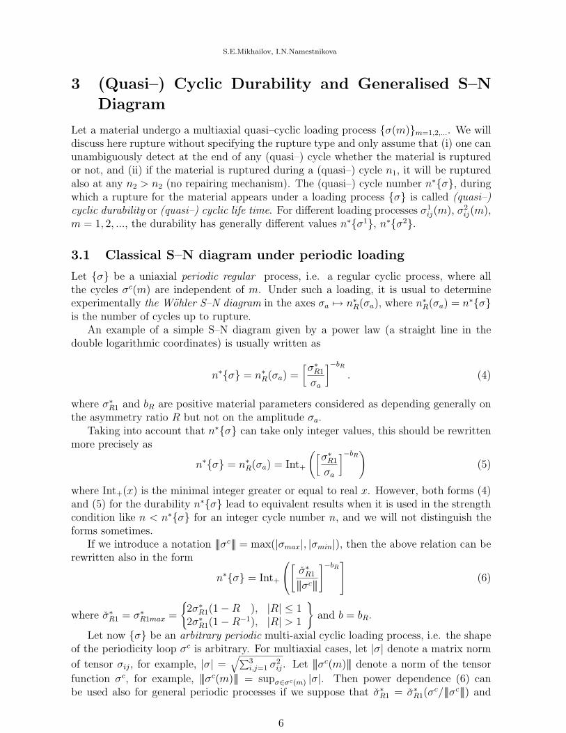
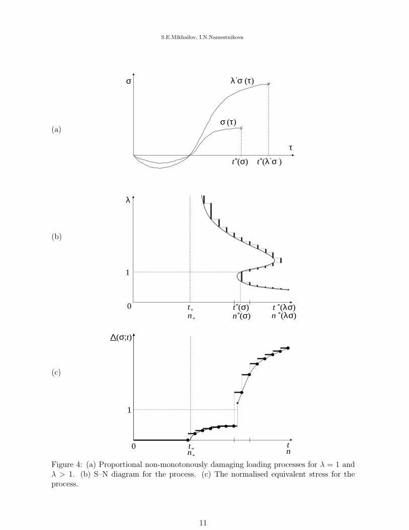
Note that there exist materials that are not monotonously damaging. For example,strength and durability of solidifying or cemented materials can be essentially increased,if the contracting (cyclic) loading is increased during the solidification or cementationphase, see Fig. 4.

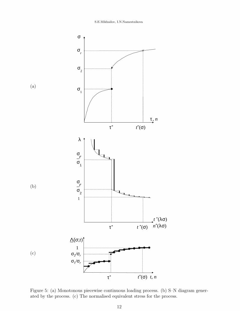
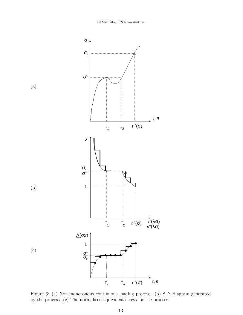
Further, in addition to the finite jumps along λ axis caused by the discrete numberingof the (quasi–) cycles, the S–N diagrams can have finite jumps along the n∗{λσ} axis aswell. Fig. 5, 6, and 7 give some examples of the loading processes with such features fora material independent of time and history, in which rupture appears at σ = σr.

3.3 Quasi– cyclic strength stability in proportional load pertur-bations

Quasi–cyclic strength is said to be stable with respect to proportional load perturbations(λ−stable) during a (quasi–) cycle n < ∞ under a (quasi–) cyclic process {σ(m)}m=1,2,...

if there is no rupture during and before the (quasi–) cycle n under {σ} and under slightlyhigher and lower loadings. More precisely, there exists ε > 0 such that there is no ruptureat and before the (quasi–) e n under the process {λσ} for any λ ∈ (1− ε, 1 + ε).

This implies that if the strength in a material is λ−unstable on a (quasi–) cycle n1, itcan not become λ−stable on any (quasi–) cycle n2 > n1.

We will denote by n∗∗{σ} the critical (quasi–) cycle number, that is such that (quasi–)cyclic strength is λ−stable at all (quasi–) cycles n < n∗∗{σ} but either rupture or strengthλ−instability exists on the (quasi–) cycle n = n∗∗{σ}.

It is evident, that the critical (quasi–) cycle number n∗∗{σ} is not greater than thedurability n∗{σ}. If n∗∗{σ} < n∗{σ}, then strength is λ−unstable on (quasi–) cyclesn ∈ [n∗∗{σ}, n∗{σ} − 1]. This means, the S–N diagram has at λ = 1 a horizontal jumpfrom n∗∗{σ} to n∗{σ} (see Fig. 7b at σ∧ = σr).

For n = ∞, the above reasoning can be modified by the following way.Endurance is said to be stable with respect to proportional load perturbations (λ−stable)

under a (quasi–) cyclic process {σ(m)}m=1,2,..., if there is no rupture under {σ} and underslightly higher and lower loadings at any (quasi–) cycle. More precisely, there exists ε > 0

10

S.E.Mikhailov, I.N.Namestnikova

σ

τ

λ’σ (τ)

σ (τ)

t*(λ’σ ) t*(σ)

(a)

t *(λσ)

λ

1

t*(σ)t+ n *(λσ) n*(σ)n+

0

(b)

t

1

Λ(σ;t)

t+ n+ n

0

(c)

Figure 4: (a) Proportional non-monotonously damaging loading processes for λ = 1 andλ > 1. (b) S–N diagram for the process. (c) The normalised equivalent stress for theprocess.

11

S.E.Mikhailov, I.N.Namestnikova

t*(σ)

σr

σ2

σ1

τ*

σ

τ, n

(a)

σ_rσ

1

σ_rσ

2

t *(σ)

λ

τ*

1

t *(λσ)n*(λσ)

(b)

t*(σ) τ* t, n

σ1/σr

σ2/σr

1

Λ(σ;t)

(c)

Figure 5: (a) Monotonous piecewise continuous loading process. (b) S–N diagram gener-ated by the process. (c) The normalised equivalent stress for the process.

12

S.E.Mikhailov, I.N.Namestnikova

t *(σ)

σ

σr

σ^

τ1

τ, n

τ2

(a)

t*(λσ)

λ

τ2

τ1

1

t *(σ)

σr

σ^

n*(λσ)

(b)

t *(σ)

Λ(σ;t)

τ1

t, nτ2

σ^

1

σr

(c)

Figure 6: (a) Non-monotonous continuous loading process. (b) S–N diagram generatedby the process. (c) The normalised equivalent stress for the process.

13

S.E.Mikhailov, I.N.Namestnikova

t *(σ)

σ

σr

σ^

τ1

ττ

2

, n

(a)

t*(λσ)

λ

τ2

τ1

1

t *(σ)

σr

σ^

n*(λσ)

(b)

t *(σ)

Λ(σ;t)

τ1

t, nτ2

σ^

1

σr

(c)

Figure 7: (a) Non-monotonous right-continuous loading process. (b) S–N diagram gener-ated by the process. (c) The normalised equivalent stress for the process.

14

S.E.Mikhailov, I.N.Namestnikova

such that there is no rupture at all (quasi–) cycles n < ∞ under the process {λσ} for anyλ ∈ (1− ε, 1 + ε).

4 Quasi–cyclic safety factor and normalised equiva-

lent stress

For a given process {σ(m)}m=1,2,..., we can determine (experimentally) a unique finite or in-finite durability n∗{λσ} for any number λ ≥ 0. Consider the inverse task: for any (quasi–)cycle number n ≥ 0, to determine a number λ∗({σ}; n) such that n∗{λ∗({σ}; n)σ} = n.This is equivalent to interpreting the S–N diagram λ 7→ n∗{λσ} as the dependencen 7→ λ∗({σ}; n). Examples of the diagrams on Fig. 3a, 4b, 5b, 6b, 7b show this isnot uniquely possible and for some cases is not possible at all since the dependence isnot defined for some (quasi–) cycles n. To overcome the difficulty, we introduce a notionof (quasi–) cyclic safety factor functional and (quasi–) cyclic normalised equivalent stressfunctional (NESF).

Definition 1 Let {σ(m)}m=1,2,... be a quasi–cyclic process. The (quasi–) cyclic safetyfactor λN({σ}; n) is supremum of λ ≥ 0 such that n∗{λ′′σ} > n for any λ′′ ∈ [0, λ]; ifthere is no such λ, we take λ({σ}; n) = 0.

The (quasi–) cyclic normalized equivalent stress ΛN({σ}; n) is defined as 1/λN({σ}; n)if λN({σ}; n) 6= 0 and ΛN({σ}; n) := ∞ otherwise.

The mappings ({σ}; n) 7→ λN({σ}; n) and ({σ}; n) 7→ ΛN({σ}; n) defined on a set ofprocesses {σ} and (quasi–) cycle numbers n are called the (quasi–) cyclic safety factorfunctional λN and the (quasi–) cyclic normalized equivalent stress functional Λ, respec-tively.

For monotonously damaging processes the definition can be simplified as follows.

Definition 1MD The (quasi–) cyclic safety factor λ({σ}; n) for a quasi–cyclic MD pro-cess {σ(m)}m=1,2,... is supremum of λ ≥ 0 such that n∗{λσ} > n; if there is no such λ,we take λN({σ}; n) = 0. The (quasi–) cyclic normalized equivalent stress ΛN({σ}; n) isdefined as 1/λN({σ}; n) if λN({σ}; n) 6= 0 and ΛN({σ}; n) := ∞ otherwise.

We call both λN and ΛN also the (quasi–) cyclic strength functionals. They are materialcharacteristics reflecting the influence of the endured (quasi–) cyclic loading process onthe material strength. Using these definitions, the functionals values can be obtainedfrom experiments for any process {σ} and any (quasi–) cycle n.

Particularly, if the durability functional n∗{λσ} is known for all λ ≥ 0, the value ofthe normalized equivalent stress ΛN({σ}; n) for any n is a supremum of solutions to thescalar equation

n∗{σ/Λ} = n

for each (quasi–) cycle n and loading process {σ} for which solutions do exist; otherwiseΛN({σ}; n) can be determined directly from Definition 1. Note that values of ΛN({σ}; n)are uniquely defined in the both cases.

But what information about ΛN can one extract from durability measurement n∗{σ}under only one process {σ}? From Definition 1, one can get for an MD material (see

15

S.E.Mikhailov, I.N.Namestnikova

Appendix A) only the inequality

ΛN({σ}; n∗{σ} − 1) ≤ 1 ≤ ΛN({σ}; n∗{σ}) (7)

This uncertainty is quite natural and is connected with the fact that the loadings slightlyhigher and slightly lower than {σ} can cause rupture during the same (quasi–) cyclen∗{σ}. In fact, it is a payment for identifying rupture only at the (quasi–) cycle endpoints but not at the (quasi–) cycle internal points.

Remark 1 One can observe from Definition 1 that one can replace the durability n∗{λσ}by the critical (quasi–) cycle number n∗∗{λσ} in the definition to arrive at exactly the samefunctionals, λ∗∗({σ}; n) = λ({σ}; n), Λ∗∗({σ}; n) = Λ({σ}; n) (see proof in Appendix B).

The (quasi–) cyclic safety factor λN({σ}; n) and (quasi–) cyclic normalized equiva-lent stress ΛN({σ}; n) are counterparts of the time-dependent safety factor λT (σ; t) andnormalized equivalent stress ΛT (σ; t) (Mikhailov 1999, 2000) and of the non-local safetyfactor functional λ(σ; x) and non-local normalized equivalent stress (load factor) func-tional Λ(σ; y) defined by Mikhailov (1995-I).

For brevity, we will drop the superscript N further in the paper if this will not leadto a confusion.

To justify the title normalized equivalent stress for Λ, we consider a regular periodicmultiaxial in-phase process {σ} where σij(τ) varies on each cycle from 0 to a tensor σaij

and back to 0. Let, for example, the material cyclic strength under such loading be associ-

ated with the von Mises equivalent stress σeq(σ) =√

[(σ1 − σ2)2 + (σ2 − σ3)2 + (σ3 − σ1)2]/2,

that is the strength condition has the form σeq(σa) < σ∗0(n), where the function σ∗0(n) isa material characteristic (classical S–N diagram under the uniaxial periodic cycling withR = 0) and σ1, σ2, σ3 are the principal stresses. Then Λ({σ}; n) is defined from theequation σeq(σa/Λ) = σ∗0(n), that is

Λ({σ}; n) = σeq(σa)/σ∗0(n). (8)

Formula (8) holds true not only for the von Mises equivalent stress but also for theTresca and other equivalent stress representations σeq(σa) that are functions positivelyhomogeneous of the order +1.

One can see from the above definitions (proof is similar to Mikhailov, 2000) that thesafety factor is a non-increasing and the normalised equivalent stress is a non-decreasingfunction of the (quasi–) cycle number, that is,

λ({σ}; n2) ≤ λ({σ}; n1), Λ({σ}; n2) ≥ Λ({σ}; n1) if n2 > n1. (9)

It follows from the definitions (see Mikhailov 2000, Appendix C) that for any n, thesafety factor functional and the normalised equivalent stress functional are non-negativepositively-homogeneous functionals of the orders -1 and +1 respectively, that is

λ({kσ}; n) =1

kλ({σ}; n) ≥ 0, Λ({kσ}; n) = kΛ({σ}; n) ≥ 0, for any k > 0. (10)

For infinite n we get the following corresponding definitions of the (quasi–) cyclicendurance safety factor and normalised equivalent stress.

16

S.E.Mikhailov, I.N.Namestnikova

Definition 2 The (quasi–) cyclic endurance (threshold) safety factor λNth{σ} is supremum

of λ ≥ 0 such that there is no body rupture under the process {λ′′σ} for any λ′′ ∈ [0, λ]for all n < ∞; if there is no such λ, we take λN

th{σ} = 0.The (quasi–) cyclic endurance (threshold) normalised equivalent stress is defined as

ΛNth{σ} = 1/λN

th{σ} if λNth{σ} 6= 0 and ΛN

th{σ} := ∞ otherwise.The mappings σ 7→ λN

th({σ}), σ 7→ ΛNth{σ} defined on a set of processes {σ} are called

the (quasi–) cyclic endurance (threshold) safety factor functional λNth and the endurance

(threshold) normalised equivalent stress functional ΛNth respectively.

Owing to monotonicity (9), we can define the endurance functionals also as

λth{σ} = λ({σ};∞) := limn→∞λ({σ}; n) = inf

n<∞λ({σ}; n), (11)

Λth{σ} = Λ({σ},∞) := limn→∞Λ({σ}; n) = sup

n<∞Λ({σ}; n). (12)

We can point out the cases, described in the previous section, for which λth{σ} = 0:case (0) when material is self-degrading, i.e. n∗{σ} < ∞; case (D), i.e. n∗({λσ}) →n∗0{σ} 6= ∞ as λ → 0; case (E); case (G) since the absence of a limit of the functionn∗({λσ}) as λ → 0 implies that there exists n < ∞ such that λ({σ}; n) = 0.

Evidently, the endurance safety factor and the endurance normalised equivalent stressmake sense as material characteristics only for non-self-degrading materials. As followsfrom the self-degradation definition above, a material is self-degrading, if and only if thereexists a (quasi–) cycle n∗{0} such that Λ({0}; n) = 0 for n < n∗{0} and Λ({0}; n) = ∞for n ≥ n∗{0}. This statement gives an equivalent definition of self-degradation in termsof the safety factor λ behaviour.

The safety factor λ({σ}; n) as function of n at a given process {σ} can also be con-sidered as a generalised S–N diagram n 7→ λ({σ}; n). As a function of discrete integerargument n, it takes only discrete values and hence is presented not by a curve but bya discrete set of points on the (n, λ) plane. At each n, the point is placed on the bot-tom of the vertical segment (lowest if it is not unique), corresponding to the n, on theλ 7→ n∗{λσ} diagram, see Fig. 4b. The points are also placed for integer n from thejump segment [n∗{(λ+0)σ}, n∗{(λ−0)σ}] for some λ where no values of the λ 7→ n∗{λσ}diagram do exist, see Fig. 6b, 7b. As shown above in this section, the n 7→ λ({σ}; n)diagram is monotonously non-increasing in n. The collection of such diagrams for allpossible processes in fact defines the functional λN .

One can also associate with each n−th (quasi–) cycle not a point n but a segment[n − 1, n] on the n−axis. Then, remaining in the discrete time description related withthe strength/rupture status detection only at the (quasi–) cycle end point, one shouldextend the status to the whole (quasi–) cycle except its start points being also end pointof the previous (quasi–) cycles. Using such approach, one can extend the point-wise S–N diagram n 7→ λ({σ}; n) to the piece-wise constant left-continuous function coincidingwith the monotonous parts of the corresponding diagram λ 7→ n∗{λσ} at the (quasi–)cycle ends and remaining constant at other points of the (quasi–) cycles. It cuts off thenon-monotonous (multi-valued) parts of the diagram λ∗({σ}; n) (connecting by the aboveway to the branch with the lowest λ∗ and making a corresponding finite jump in λ({σ}; n)in the branch beginning, see Fig. 4). It continues also the diagram onto the jump segment[n∗{(λ + 0)σ}, n∗{(λ− 0)σ}] where λ∗({σ}; n) does not exist, see Fig. 7b.

17

S.E.Mikhailov, I.N.Namestnikova

From the generalised S–N diagram n 7→ λ({σ}; n) for a given process {σ}, presentede.g. on Fig. 3b, we can obtain the corresponding diagram n 7→ Λ({σ}; n) = 1/λ({σ}; n)for the normalised equivalent stress Λ({σ}; n), Fig. 3c. Different curves correspond todifferent possible cases of its behaviour described in points (A)-(F) of Section 3. Generally,n 7→ Λ({σ}; n) is a non-decreasing function of the (quasi–) cycle number n (see above).Some examples are given on Fig. 4c, 5c, 6c, 7c.

The diagram can be used in two ways. First, it gives a number Λ({σ}; n) such thatthere is no rupture up to (quasi–) cycle n for any process {σ/Λ′} with Λ′ > Λ({σ}; n).For example, if the diagram includes curve f (see Fig. 3), then the process {σ/Λ′} withΛ′ > Λth{σ} causes no rupture for any n. Another way is to use the diagram together withthe stable strength condition (14) below for given {σ} and n. For example, if the diagramincludes the curve f , then the process {σ} causes no rupture for any n if Λth{σ} < 1.

Consider existence and uniqueness of the NESF Λ. Suppose the material (quasi–)cyclic strength under a process {σ} on a (quasi–) cycle n is described by a strengthcondition

F ({σ}; n) < 1 (13)

where F is a non-linear functional non-decreasing in n, known from experimental dataapproximation or from a (quasi–) cyclic durability theory on the processes {λσ} for allλ ≥ 0 for the considered n. Then the NESF Λ is uniquely determined from (13) byDefinition 1 for the process {σ} and the (quasi–) cycle n, although analytical expressingΛ in terms of F is not always possible.

However, if F ({σ}; n) is a non-negative positively homogeneous of order +1 functionalof {σ}, then simply Λ({σ}; n) = F ({σ}; n) (proof is similar to Mikhailov 2000). Thisrelation will be used in Section 6 to obtain the NESF from known strength conditions ofsome (quasi–) cyclic durability theories.

5 (Quasi–) cyclic strength and endurance conditions

Let {σ} be a process and n be a (quasi–) cycle number. From Definition 1 for the strengthfunctionals, we have the following conclusions:(i) The inequality

Λ({σ}; n) < 1 (14)

implies λ−stable strength under the process {σ} on or before the (quasi–) cycle n.(ii) The equality

Λ({σ}; n) = 1 (15)

implies either rupture or λ−unstable strength under the process {σ} on or before the(quasi–) cycle n.(iii) The inequality

Λ({σ}; n) > 1 (16)

implies rupture under the process {σ} on or before the (quasi–) cycle n if {σ} is an MDprocess.

Inversely, if strength is λ−stable for an MD process {σ} at and before a (quasi–)cycle n then (14) is satisfied (see proof by Mikhailov, 2000). Consequently, we have thefollowing

18

S.E.Mikhailov, I.N.Namestnikova

Statement 1 Inequality (14) gives a sufficient (and necessary, if {σ} is an MD process)condition of λ−stable (quasi–) cyclic strength on and before a (quasi–) cycle n under aprocess {σ}.

By the same way, we have from Definition 2 the following conclusions for the endurancefunctionals:

(i) The inequalityΛth{σ} < 1 (17)

implies λ−stable endurance for the process {σ}.(ii) The equality

Λth{σ} = 1 (18)

implies either rupture on a (quasi–) cycle n < ∞ that is, n∗{σ} < ∞, or λ−unstableendurance, that is, there is no rupture under the process {σ} on any (quasi–) cycle butfor any λ > 1 there exists λ′′ ∈ (1, λ] such that n∗{λ′′σ} < ∞.

(iii) The inequalityΛth{σ} > 1 (19)

implies rupture on a (quasi–) cycle n < ∞, that is, n∗{σ} < ∞ if {σ} is an MD process.Similarly to Statement 1, we have the following

Statement 2 Inequality (17) gives a sufficient (and necessary if {σ} is an MD process)condition of λ−stable (quasi–) cyclic endurance under a process {σ}.Conditions (14)-(19) together with the homogeneity of ΛN , ΛN

th also show that the func-tionals do really play the role of normalised equivalent stresses.

It follows from the Λ definition that if the durability n∗{λσ} is known for a process{σ} for all λ ≥ 0, then the normalised equivalent stress Λ({σ}; n) can be obtained for {σ}for any n = 1, 2, .... Consider now if it is possible to obtain values of the (quasi–) cyclicdurability functional n∗{λσ} for a process {σ} for any λ ≥ 0 if the values of the NESFΛ({σ}; n) are known for the process {σ} for any n = 1, 2, ....

It is evident that this is not possible if {σ} is not an MD process, since the informationabout the non-monotonous behaviour of n∗{λσ} as function of λ is lost in Λ({σ}; n).However, as one can prove similar to Mikhailov 2000, the following inequality holds forany process,

Λ({σ}; n∗{λσ}) ≥ 1/λ for all λ > 0. (20)

The discussion above shows that in addition to the non-sensitivity to non-monotonousbehaviour of the S–N diagram, the NESF Λ({σ}; n) does not also distinguish rupture fromnot λ−stable strength. For this reason it is the critical (quasi–) cycle n∗∗{σ} ≤ n∗{σ},who can be obtained from NESF Λ({σ}; n), but generally not the durability n∗{σ}. Thefollowing statement is proved in Appendix C.

Statement 3 Let {σ} be an MD process. Let n∗∗− {σ} be supremum of n such that

Λ({σ}; n) < 1. (21)

Then the critical (quasi–) cycle is n∗∗{σ} = n∗∗− {σ} + 1 if n∗∗− {σ} < ∞, otherwise the(quasi–) cyclic endurance is λ−stable under the process {σ}.

19

S.E.Mikhailov, I.N.Namestnikova

Taking into account that Λ({σ}; n) is monotonously non-decreasing in n and that ifn∗∗− {σ} = n∗∗{σ} − 1 is finite, it does satisfy inequality (21) but n∗∗{σ} does not, wehave the following corollary from Statement 3.

Corollary 1 A (quasi–) cycle n∗∗ is critical for an MD process {σ}, i.e. n∗∗ = n∗∗{σ},if and only if it satisfies the inequality

Λ({σ}; n∗∗ − 1) < 1 ≤ Λ({σ}; n∗∗). (22)

If such n∗∗ does not exist, the (quasi–) cyclic endurance is λ−stable under the process{σ}.

Thus, inequality (22) is a criterion of rupture or strength instability on a (quasi–)cycle n∗∗ under a (quasi–) cyclic MD process.

Applying Statement 3 to a process {λσ} and using the positive homogeneity of Λ({σ}; n),we get some generalisation of the Statement:

Corollary 2 Let {σ} be an MD process. Let n∗∗− {λσ} be supremum of n such that

Λ({σ}; n) < 1/λ. (23)

Then for any λ > 0, the critical (quasi–) cycle is n∗∗{λσ} = n∗∗− {λσ}+1 if n∗∗− {λσ} < ∞,otherwise the (quasi–) cyclic endurance is λ−stable under the process {λσ}.

Remark 2 As noted in Remark 1, one can replace the durability n∗{λσ} by the critical(quasi–) cycle number n∗∗{λσ} in Definition 1 to arrive at exactly the same functional,Λ∗∗N = ΛN . Thus, if the critical (quasi–) cycle number n∗∗{λσ} is known for a process{σ} at all λ ≥ 0, then values of the NESF Λ({σ}; n) are uniquely determined for theprocess {σ} at any n. Conversely, if values of the NESF Λ({σ}; n) are known for an MDprocess {σ} at all n, then numbers of the critical (quasi–) cycles n∗∗{λσ} are uniquelydetermined for the process {σ} at any λ ≥ 0 and particularly at λ = 1.

Note that namely the critical (quasi–) cycle number n∗∗{σ} is necessary for practicaldesign since, for the cases when n∗∗{σ} 6= n∗{σ}, the material strength is λ−unstable forn ∈ [n∗∗{σ}, n∗{σ}) and the material can be ruptured by an arbitrarily small increase ofloading {σ}.

5.1 General remarks

The (quasi–) cyclic NESF ΛN as well as durability n∗ and critical (quasi–) cycle n∗∗

functionals are supposed to be material characteristics in the sense that they may havedifferent values on the same processes {σ} for different materials but must give the samevalues on the same processes for the same material independent particularly of the shapeof the body consisting of the material.

The durability n∗{σ} does not depend on a particular time parametrisation of (quasi–)cycles σc(m) for materials with pure fatigue responses. Thus the pure fatigue NESF ΛN

must also be time-independent and non-sensitive to the loop time parametrisation butmay be sensitive to the loop shape and direction in the stress space as well as to the

20

S.E.Mikhailov, I.N.Namestnikova

(quasi–) cycle order in the sequence {σc(m)}m = 1, 2, .... This means the functional ΛN

should be defined on sequences {σcs} for pure fatigue.On the other hand, there are materials that manifest a rupture dependence on time

(e.g. under creep or dynamic loading) along with (quasi–) cyclic fatigue effects. For suchmaterials, the time sensitivity should be reflected also in the functional ΛN that will bethan defined on sequences {σct} to take into account the time-history-fatigue interaction.

All the written above in Sections 3-5 can be referred to each of the both loading processrepresentations {σc(m)}m=1,2,....

As material characteristics, the functionals n∗∗ and ΛN for a particular material canbe (approximately) identified from experimental data on durability n∗{σ}. Evidentlyonly a finite number of the durability tests n∗{σ} for different processes {σ} can be doneand identification of n∗{σ} or ΛN({σ}; n) for other processes and (quasi–) cycle numbersshould be done along those test results using an interpolation/approximation procedure.

In spite of the fact that it is just the durability n∗{σ}, which values are obtaineddirectly from experiments for some test processes {σ}, it is usually more straightforwardto approximate along those date first the NESF ΛN rather than n∗. This is because,although the both functionals are nonlinear, the functional ΛN({σ}; n) is homogeneousand can be considered as bounded with respect to {σ} in appropriate function spaces.

For the (quasi–) cyclic NESFs, any one durability test for a process {σ} will allocate,according to uncertainty inequality (7), the value 1 between the values of NESF for theneighbouring (quasi–) cycles, ΛN({σ}; n∗{σ}) and ΛN({σ}; n∗{σ})− 1. Typical numbersof (quasi–) cycles under fatigue loading vary between 103 and 107, and consequently onecan suppose rather small changes of ΛN({σ}; n) between the (quasi–) cycles and attributeΛN({σ}; n∗{σ}) ≈ 1. Then, taking into account the functional homogeneity, we obtainthe NESF for the one-dimensional linear set, ΛN({kσ}; n∗{σ}) = k ∀k ≥ 0.

In what is written above in the paper, we analysed strength and durability under a(quasi–) cyclic loading process {σc} where the stress field σ = σij(τ) is independent ofthe space coordinates. If the stress field depends not only on time (or (quasi–) cyclenumber) but also on the space coordinates x = (x1, x2, x3), i.e. σ = σij(x, τ), it is usuallysupposed that rupture is local, that is, rupture at a point y depends only on the stress(quasi–cyclic) history at the point y, that is on σij(y, τ) (or on {σc(y,m)}m=1,2,... for a(quasi–) cyclic process) and does not depend on the stress history at other points of thebody. This means, one can use the durability n∗ and the NESF ΛN , obtained from testsunder homogeneous in space loading processes, to predict rupture under inhomogeneousin space loadings. Particularly, the counterpart of condition (14) for prediction of stable(quasi–) cyclic strength in a point y during a (quasi–) cycle n will then have form

Λ({σ(y)}; n) < 1.

This approach works well for moderately inhomogeneous stress fields but fails, when astress field vary rather sharp, e.g. near a crack tip or other stress concentrator. Somenon-local approaches able to deal with such stress fields for time and history independentmaterials were considered by Mikhailov (1995–I&II). Their extension to history depen-dent materials under (quasi–) cyclic loadings is developed by Mikhailov & Namestnikova(2002).

21

S.E.Mikhailov, I.N.Namestnikova

6 Examples of (quasi–) cyclic normalised equivalent

stress

functionals for uniaxial loading

6.1 Uniaxial periodic loading processes for material indepen-dent of history

Let us consider a material independent of history (that is, its strength is determined onlyby the instants stress value) and obeying the strength condition

|σ| < σr

where σr is a material constant (the material strength under monotone uniaxial tension).Using the example in section 3.2, we have from the definition of NESF,

ΛN({σ}, n) = max1≤m≤n

|||σc(m)|||σr

,

where as above |||σc(m)||| = max(|σmax(m)|, |σmin(m)|).

6.2 Uniaxial regular periodic loading processes

The fatigue strength conditions at an n-th cycle of a uniaxial regular periodic loadingprocess {σ} can be written in the following form

σa < σ∗R(n), (24)

or inversely,n < n∗R(σa)

Here σa is a cycle amplitude and n∗R(σa) is the classical S-N diagram, depending on theasymmetry ratio R. Sometimes the maximum stress value σmax is used instead of thestress amplitude σa in a cycle if σmax > 0. Then the strength condition at the n-th cyclecan be rewritten as

σmax < σ∗R,max(n), (25)

where σ∗R,max(n) is the S–N diagram for σmax. Inversely,

n < n∗R,max(σmax)

Note that at R = −1 the stress amplitude coincides with the maximum stress value in acycle. According to the Definition 1 of the NESF, we have for arbitrary stress asymmetryratio R

ΛN({σ}; n) =σa

σ∗R(n)(26)

or, respectively,

ΛN({σ}; n) =σmax

σ∗R,max(n)(27)

22

S.E.Mikhailov, I.N.Namestnikova

Let the Wohler S–N diagram σ∗R(n) be approximated by a power law

σ∗R(n) = σ∗R1n−1/bR , (28)

where σ∗R1 and bR are positive material parameters generally dependent on R. Then theNESF is

ΛN({σ}; n) =σa

σ∗R1

n1/bR

Let the Wohler diagram σ∗R(n) for arbitrary R be approximated in terms of the Wohlerdiagram for symmetric cycling, σ∗−1(n), as

σ∗R(n) = σ∗−1(n)

[1 +

1 + R

1−R

σ∗−1(n)

σr

]−1

(29)

then we arrive at the strength condition at an n-th cycle, associated with the Haighdiagram

σa

σ∗−1(n)+

σm

σr

< 1 (30)

where σm = σmax+σmin

2is mean stress in the cycle. Note that the Haigh diagram can be

considered as the fatigue strength diagram at a fixed number of cycles n (constant-lifetimediagram) and also as the endurance diagram (then n = ∞).

The NESF corresponding to (29), (30) is

ΛN({σ}; n) =σa

σ∗−1(n)+

σm

σr

6.3 Uniaxial non-periodic regular cyclic loading processes

The approaches analysed below in this section were originally developed for block-periodicloadings. The block-periodicity usually means a large number of periodic cycles in asmall number of blocks. For this reason, the number of transitions between the blocksis also small and can be neglected in the durability analysis. However, all the block-periodic theories considered below can be equally applied also to arbitrary uniaxial loadingwith closed cycles, that is, periodicity in blocks is not necessary and there can be manytransitions between the blocks if the transitions are closed cycles.

6.3.1 Palmgren-Miner linear damage accumulation rule

For a uniaxial block-periodic loading process {σc(m)}, the cyclic strength condition ac-cording Palmgren(1924,1945)-Miner(1945) linear damage accumulation rule can be writ-ten as the inequality

n∑

j=1

1

n∗R(j)(σa(j))< 1. (31)

The value of n∗R(j)(σa(j)) is found from an appropriate classical S–N curve σa 7→ n∗R(σa) forthe same material under corresponding periodic cycling. For a process {λσc(m)}, whereλ ≥ 0, we have thus the strength condition

n∑

j=1

1

n∗R(j)(λσa(j))< 1. (32)

23

S.E.Mikhailov, I.N.Namestnikova

Definition 1 together with the strength condition (32) allow to obtain the NESF forany particular S–N diagram n∗R(σa) although not always explicitly. If any periodic loadingis monotonously damaging for the considered material, that is, n∗R(σa) is a non-increasingfunction of σa (what is usually the case for structural materials), then the left hand side of(32) is non-decreasing in λ and consequently any block-periodic loading is monotonouslydamaging for the material obeying the linear damage accumulation rule. In this case onecan apply a simplified Definition 1MD and obtain that ΛN({σ}; n) = 1/λN({σ}; n), whereλN({σ}; n) is the supremum of numbers λ ≥ 0 satisfying inequality (32).

Although as follows from the cyclic durability definition, n∗R(σa) is a piece-wise con-stant integer-valued function of σa, some continuous or piece-wise continuous interpolationof n∗R(σa) is usually used for simplicity in damage accumulation rules like (31) and we willoften follow this tradition below. This leads to an error less then one cycle for n∗R(σa),which is negligible in comparison with the durabilities 103 − 107 typical for fatigue.

If n∗R(σa) is a continuous monotonously decreasing function of σa, then the left handside of (32) is continuous and monotonously increasing in λ, and instead of taking supre-mum according to Definition 1MD, one can determine the NESF as ΛN({σ}; n) = 1/λ,where λ is a solution of the equation

n∑

j=1

1

n∗R(j)(λσa(j))= 1. (33)

In the case when n∗R(σa) is a piece-wise continuous monotonously decreasing function ofσa, one can also try to find the NESF in form ΛN({σ}; n) = 1/λ, where λ is a solution ofequation (33) if the solution does exist, or use more general Definition 1MD otherwise.

Suppose, particularly, that n∗R(σa) is given by the power law inverse to (28), that is,

n∗R(σa) =(σ∗R1

σa

)bR(34)

where σ∗R1, bR > 0. The so–defined n∗R(σa) is a continuous monotonously decreasingfunction of σa. Then ΛN({σ}; n) = 1/λ, where λ is a solution of the equation

n∑

j=1

λσa(j)

σ∗R(j)1

bR(j)

= 1 (35)

If bR = b does not depend on R, or R(j) = R does not depend on the cycle number j,then the equation can be solved explicitly and the NESF is

ΛN({σ}; n) =

n∑

j=1

σa(j)

σ∗R(j)1

b

1/b

(36)

in the first case and

ΛN({σ}; n) =1

σ∗R1

n∑

j=1

σbRa (j)

1/bR

(37)

in the second case.Note, perhaps the most significant shortcoming of the Palmgren-Miner hypothesis is

that it does not account for sequence effects; that is, that damage caused by a stress cycleis independent of where it occurs in the load history.

24

S.E.Mikhailov, I.N.Namestnikova

6.3.2 Marin damage accumulation rule

Marin (1962) proposed the damage accumulation rule for a block-periodic process with thestress asymmetry ratio R = −1. Using Marin’s hypothesis the fatigue strength conditioncan be written in form

1

n∗−1(σmaxa (n))

n∑

j=1

[σa(j)

σmaxa (n)

]d

< 1 (38)

Here σa(j) is the stress amplitude in the j-th cycle, σmaxa (n) = max

j=1,...nσa(j) is the maximum

stress amplitude in the process {σ(j)}nj=1, and n∗−1(σa) is the number of cycles up to

rupture in a periodic process with the stress amplitude σa and the asymmetry ratioR = −1, d is a material constant.

As above, under assumption (34) we can rewrite (38) in the following form

[σmax

a (n)

σ∗−1,1

]b−1 n∑

j=1

[σa(j)

σmaxa (n)

]d

< 1 (39)

We should note that strength condition (39) can be used only for d ≤ b−1. Otherwise,if we consider for example, a cyclic process with a constant amplitude σa, then, accordingto (39), the addition to the process of only one cycle with the amplitude 2σa increases thenumber of cycles to rupture by almost 2d−b−1 times, what does not seem to be natural.

From (39), the durability n∗(λσ) under the process {λσ(j)}j=1,2... is determined fromthe equation [

λσmaxa (n∗)σ∗−1,1

]b−1 n∗∑

j=1

[σa(j)

σmaxa (n∗)

]d

= 1

Finally we find

λ =σ∗−1,1

σmaxa (n∗)

(n∗∑

j=1

[σa(j)

σmaxa (n∗)

]d)−1/b−1

and have the following representation for the NESF,

ΛN({σ}; n) =σmax

a (n)

σ∗−1,1

(n∑

j=1

[σa(j)

σmaxa (n)

]d)1/b−1

=(σmax

a (n))1− d

b−1

σ∗−1,1

[n∑

j=1

[σa(j)]d

]1/b−1

(40)

for d ≤ b−1.Note, that the same expression (38) for the durability was obtained by Corten &

Dolan (1956) under other assumptions than by Marin. Consequently, the functional ΛN

for the Corten & Dolan fatigue model is also determined by (40) if the Wohler diagramis used in form (34). When n∗−1(σa) is given by (34) and d = b−1, the both damageaccumulation rules are reduced to strength condition (31) for the Palmgren-Miner lineardamage accumulation rule.

6.3.3 Pavlov non-linear accumulation rule

A non-linear strength condition, taking into account instantaneous rupture, was proposedby Pavlov (1988)

n∑

j=1

f [σmax(j), R(j)] +σmax(n)

σr

< 1 (41)

25

S.E.Mikhailov, I.N.Namestnikova

Where σmax(j) is the maximum stress in the j-th cycle. Under block-periodic loading, thefunction f [σmax(j), R(j)] was taken in the form

f [σmax(j), R(j)] =

(1− σmax(j)

σr

)1

n∗R(j)max[σmax(j)](42)

Substituting (42) into (41) we have

n∑

j=1

(1− σmax(j)

σr

)1

n∗R(j)max[σmax(j)]+

σmax(n)

σr

< 1 (43)

Assuming the Wohler diagram in form

n∗R,max(σmax) =(σ∗R1,max

σmax

)bR, (44)

where bR, σ∗R1 are material characteristics generally depending on R, we obtain after somealgebraic manipulations the following equation for ΛN ,

ΛbRσmax(n)

σr

+ Λn∑

j=1

(σmax(j)

σ∗R1,max

)bR − ΛbR+1 =n∑

j=1

(σmax(j)

σ∗R1,max

)bR σmax(j)

σr

, (45)

which can be solved numerically. Here bR = bR(j), σ∗R1 = σ∗R(j)1.Note that the strength condition (43) can be rewritten in the following form

1

σr − σmax(n)

n∑

j=1

σr − σmax(j)

n∗R(j),max[σmax(j)]< 1

This last inequality was generalized by Pavlov (1988) to the non-linear damage accumu-lation strength condition

l[σmax(n); R(n)]n∑

j=1

1

l[σmax(j); R(j)]n∗[σmax(j), R(j)]< 1. (46)

Here l[σmax(j); R(j)] is a parameter depending not only on the maximum stress in a cyclebut also on the cycle asymmetry ratio.

Assuming the Wohler diagram in form (44), the durability n∗(λσ) under the process{λσ(j)}j=1,2... is determined from the equation

l[λσmax(n∗); R(n∗))]

n∗∑

j=1

1

l[λσmax(j); R(j)]

λσmax(j)

σ∗R(j)1,max

bR(j)

= 1 (47)

Then, from (47), the NESF ΛN({σ}; n) is a solution of the equation

l[Λ−1σmax(n∗); R(n∗)]

n∑

j=1

Λ−bR(j)

l[Λ−1σmax(j); R(j)]

σmax(j)

σ∗R(j)1

bR(j)

= 1 (48)

which can be solved numerically. Note that if l(σmax; R) = const then (46) degeneratesinto (31) and (48) into (37).

26

S.E.Mikhailov, I.N.Namestnikova

6.3.4 Serensen-Kogaev model

To get a better agreement to the test data under a non-regular in time loading {σa(j)}j=1,2,...

with the stress asymmetry ratio R = −1, it was proposed by Serensen et al (1975) and Ko-gaev et al (1985) (see also in English Lagoda (2001)) to use an improved Palmgren-Minerhypothesis, for which we can write the strength condition in the form

n∑

j=1

σa(j)>σ∗−1∞

1

n∗−1(σa(j))< ap({σ}; n) (49)

The value ap({σ}; n) is defined as

ap({σ}; n) = max

[σ(n)− 0.5σ∗−1∞

σmaxa (n)− 0.5σ∗−1∞

, 0.1

](50)

Here

σ(n) =1

n

n∑

j=1

σa(j)>0.5σ∗−1∞

σa(j) (51)

Here n is a number of cycles out of n with the stress amplitudes σa(j) > 0.5σ∗−1∞, j =1, ..., n; σ∗−1∞ = σ∗−1(∞) is the fatigue limit for the symmetric loading (R = −1).

Note that as follows from (51), 0.5σ∗−1∞ ≤ σ ≤ σmaxa (n) if not all σa(j) < 0.5σ∗−1∞.

Then owing to (50), 0.1 ≤ ap ≤ 1. Hence the strength criterion (49) can describe only andecrease but not an increase of the durability in comparison with the prediction of theclassical Palmgren-Miner linear damage accumulation hypothesis (31).

The Wohler curve n∗−1(σa) is presented by two straight line parts in the double loga-rithmic coordinates. One of them, σa = σ∗−1∞ for the large number of cycles, is parallelto the abscissa axis. The non-constant part of the Wohler diagram is presented by thepower law (34). Then the coordinates for the point of the lines intersection are (n∗G, σ∗−1∞),where n∗G = (σ∗−1,1/σ

∗−1∞)b−1 . Substituting (34) into (49), we have

1

[σ∗−1,1]b−1

n∑

j=1

σa(j)>σ∗−1∞

[σa(j)]b−1 < ap({σ}; n)

Then the durability n∗(λσ) for the process {λσ} is determined from the equation

1

[σ∗−1,1]b−1

n∗∑

j=1

λσa(j)>σ∗−1∞

[λσa(j)

]b−1

= ap({λσ}; n∗) (52)

The NESF can be determined as ΛN({σ}; n) = 1/λ, where λ is a solution of equation (52)if the solution does exist, or from Definition 1MD otherwise.

27

S.E.Mikhailov, I.N.Namestnikova

If the fatigue limit σ∗−1∞ is equal to zero, strength condition (49) reduces to thefollowing inequality,

n∑

j=1

1

n∗−1(σa(j))< ap({σ}; n) = max

1

nσmaxa (n)

n∑

j=1

σa(j), 0.1

(53)

Using (34), we obtain the NESF for the case in the form

ΛN({σ}; n) =1

σ∗−1,1

1

ap({σ}; n)

n∑

j=1

[σa(j)]b−1

1/b−1

(54)

6.4 Remarks on applications to random uniaxial loadingprocesses

Under a random loading {σc(m)}m=1,2,..., the quasi-cycles σc(m) are not closed and con-sequently direct applying a linear or non-linear summation rule to reduce a durabilitydescription to a material characteristic determined under corresponding periodic pro-cesses is impossible. Usual in this case is an intermediate step: to define an auxiliaryreduced process, or better to say, a finite set of closed cycles {σc(m; n)}n

m=1 deemed tobe equivalent to a finite subsequence {σc(m)}n

m=1 of the original process, using one of thecycle counting methods (for example the rainflow method), see e.g. Dowling N.E. (1972),Downing S.D. & Socie D.F. (1982), Collins (1993), Rychlik (1987), the British Standards-5400 (1980). For a given process {σc(m)}m=1,2,..., both the reduced cycles σc(m; n) andtheir number n in the set depend on n. After this step, normally the linear summationrule is applied.

The cycle counting methods have several features important for our analysis:(i) The sequence effect is lost in the reduced cycle set {σc(m; n)}n

m=1.(ii) If {σc(m; n)}n

m=1 is a reduced set to a subsequence {σc(m)}nm=1, then {λσc(m; n)}n

m=1

is a reduced set to the subsequence {λσc(m)}nm=1 for any λ ≥ 0.

(iii) Suppose {σc(m)}n1m=1 and {σc(m)}n2

m=1 are two finite subsequences of an original se-quences {σc(m)}m=1,2,... and n2 > n1, then {σc(m)}n1

m=1 constitutes a part of {σc(m)}n2m=1.

For the reduced sets, n2 > n1 but the reduced set {σc( ˜m; n1)}n1m=1 does not generally

belong to the reduced set {σc( ˜m; n2)}n2m=1.

Using a cycle counting method and a summation rule, one can estimate durabilityunder a process {σc(m)}m=1,2,... by the durabilities under the reduced sets {σc(m; n)}n

m=1.Then one can estimate the NESF Λ({σc}; n) by the NESF under the reduced load set,

Λ({σc}; n) = Λ({σc(m; n)}n(n)m=1; n(n)).

As follows from item (ii) above, the NEFS Λ({σc}; n) obtained in this way satisfy thehomogeneity property (10) with respect to {σc}. However, the monotone non-decreasingwith respect to n, see (9), is not evident as follows from item (iii) above, and a detailedanalysis of particular cycle counting method is necessary to investigate this.

28

S.E.Mikhailov, I.N.Namestnikova

7 Examples of cyclic normalised equivalent stress

functionals for multiaxial loading

The fatigue strength criteria for multiaxial case can be classified roughly into three maincategories: criteria based on equivalent stress concept (approaches based on the stressinvariants), critical surface criteria and strain energy criteria. The approach based on anequivalent stress σeq, which is applicable to a cyclic loading with synchronous (propor-tional, coaxial, in-phase) cycling for all stress components, is described e. g. by Pavlov(1988), Lebedev (1990). The equivalent stress is defined as a function of the stress am-plitudes and the mean stresses in a cycle and then is substituted into the correspondingdurability expressions known for symmetric uniaxial periodic loading. In this way, thedurability analysis under asymmetric multiaxial cyclic loading is reduced to one S-N dia-gram under symmetric uniaxial cyclic loading.

The so-called critical surface criteria for in-phase loading, based on the von Misesequivalent stress and taking into account an influence of the hydrostatic stress on thefatigue endurance were proposed by Crossland (1956) and Sines (1959). The both criteriahave similar analytical formulas. The difference is that Sines used the mean on cyclehydrostatic stress σH,m while Crossland used in his criterion the maximal on cycle hydro-static stress σH,max. Another criterion, based on the Tresca maximum shear stress wasproposed by Dang Van (1973). Modifying the Sines criterion, Kakuno (1979) proposed totake into account an effect of the hydrostatic pressure amplitude. Endurance limits (orS–N diagrams) under several types of periodic loading are necessary to obtain the criteriaparameters (or their dependence on the cycle number). All these criteria were extendedfor the case of existing residual stress by Flavenot & Skalli (1989). Papadopoulos et al(1997) made an attempt to extend the critical surface approaches to non-proportionalperiodic processes.

7.1 Multiaxial loading processes for materials independent ofhistory

Let us consider a material independent of history (that is, its strength is determined onlyby the instants stress value) and obeying the strength condition

σeq(σ) < σr

where σeq(σ) is the von Mises, Tresca or other equivalent stress (positively homogeneousfunction of order +1), σr is a material constant (the material strength under monotoneuniaxial tension). Then we have from the definition of NESF,

ΛN({σ}, n) = max1≤m≤n

maxσ∈σc(m)

σeq(σ)

σr

= max1≤m≤n

|||σc(m)|||σ∗(σc(m))

. (55)

Here |||σc(m)||| denotes a norm of a tensor function σc(m) describing the stress tensorbehaviour on the m−th cycle, for example, |||σc(m)||| = supσ∈σc(m) |σ|, where the supremumis taken along the m−th cycle and |σ| denotes a matrix norm of a tensor σij, for example,

|σ| =√∑3

i,j=1 σ2ij;

σ∗(σc(m)) = minσ∈σc(m)

[σr/σeq(σ)], σc(m) = σc(m)/|||σc(m)|||. (56)

29

S.E.Mikhailov, I.N.Namestnikova

7.2 Multiaxial regular proportional periodic loading

7.2.1 Equivalent stress concept for regular periodic loading

Let σeq(σc) be an equivalent stress expressed in terms of stress amplitude tensor σij,a

and asymmetric ratio R or of maximum stresses tensor σij,max and R, in a multiaxialproportional cycle σc. The main assumption is that the number of cycles up to rupturen∗{σc} under multiaxial cyclic loading {σc

ik} with an equivalent stress σeq(σc) can be

found from fatigue curves n∗−1(σa) for uniaxial symmetric cyclic loading with the stressamplitude σa = σeq(σ

c) and the asymmetry ratio R = −1,

n∗{σc} = n∗−1(σeq(σc)) (57)

The function σeq is chosen such that σeq(σc) = σa for any uniaxial process σc with an

amplitude σa and the asymmetry ratio R = −1.For example, if the uniaxial durability is described by (34), then for a multiaxial

periodic loading we obtain from (57),

n∗(σc) := n∗−1(σeq(σc)) =

(σ∗−1,1

σeq(σ)

)b−1

, (58)

where σ∗−1,1 and b−1 are positive material constants.There are many possibilities to introduce the value σeq(σ). let us consider two expres-

sions presented by Pavlov (1988). First one is

σeq1(σc) =

σi,a

1− σi,m

σr

, (59)

where σr is the material strength under monotone uniaxial loading and σi,a, σi,m are theintensities (the von Mises equivalent stress) of stress amplitude and mean stress tensorsintroduced in (3), respectively. In terms of the tensor principal values σk,a, σk,m, k =1, 2, 3,

σi,a =1√2

[(σ1,a − σ2,a)

2 + (σ2,a − σ3,a)2 + (σ3,a − σ1,a)

2]1/2

,

σi,m =1√2

[(σ1,m − σ2,m)2 + (σ2,m − σ3,m)2 + (σ3,m − σ1,m)2

]1/2.

Expression (59) can be considered as a generalization of Haigh diagram for the multiaxialcase.

The second example is

σeq2(σc) =

ξa

1− ξm

σr

, (60)

ξa = ζσi,a + (1− ζ)σ1,a, ξm = ζσi,m + (1− ζ)σ1,m, ζ =1√

3− 1

(σ∗−1∞τ ∗−1∞

− 1

)

Here σ∗−1∞ := σ∗−1(∞) and τ ∗−1∞ := τ ∗−1(∞) are respectively the fatigue limits under peri-odic symmetric uniaxial and pure shearing cycling; σ1,a is the amplitude of the maximumprincipal stress, σ1,m is the mean value of the maximum principal stress. The values ηa

and ηm are the modified stress amplitude and the modified mean stress respectively.

30

S.E.Mikhailov, I.N.Namestnikova

Another expression for σeq under asymmetric cycling was given by Lebedev (1990)

σeq3(σc) = σi,a

[ (1− 2

3

σi,m

σr

)2

− 1

9

(σi,m

σr

)2]−1/2

(61)

For brittle materials under symmetric cycling R = −1 the maximal normal stressamplitude, that is, maximal principal stress amplitude σ1,a can be used as an equivalentstress (e.g. Lebedev, 1990),

σeq4(σc) = σ1,a (62)

Under the multiaxial regular periodic loading, the fatigue strength conditions for (59),(60), (61) and (62) at the n-cycles can be written in the following form respectively

σi,a

1− σi,m

σr

< σ∗−1(n), (63)

ξa

1− ξm

σr

< σ∗−1(n), (64)

σi,a

[ (1− 2

3

σi,m

σr

)2

− 1

9

(σi,m

σr

)2]−1/2

< σ∗−1(n). (65)

σ1,a < σ∗−1(n), (66)

Hence, according to the definition of the NESF, we have for (63), (64), (65) and (66),respectively,

ΛN({σ}; n) =σi,a

σ∗−1(n)+

σi,m

σr

ΛN({σ}; n) =ξa

σ∗−1(n)+

ξm

σr

ΛN({σ}; n) =2

3

σi,m

σr

+

√√√√(

σi,a

σ∗−1(n)

)2

+1

9

(σi,m

σr

)2

ΛN({σ}; n) =σ1,a

σ∗−1(n)

7.2.2 Invariant based critical surface approaches for regular periodic loading

Popular fatigue endurance conditions under in-phase multiaxial periodic loading, basedon the von Mises equivalent stress and taking into account an influence of the hydrostaticstress were proposed by Sines (1959),

σi,a + ασH,m < β, (67)

and Crossland (1956),σi,a + ασH,max < β. (68)

Here σH,m = σjj,m/3 is the mean and σH,max = −σjj,max/3 is the maximum on cyclehydrostatic stresses. The material parameters α and β can be found, for example, fromtension-compression tests with R = 0 and R = −1. Then we have,

α = 3

(σ∗−1∞σ∗0∞

− 1

), β = σ∗−1∞ (69)

31

S.E.Mikhailov, I.N.Namestnikova

for the Sines criterion and

α = 3

(σ∗−1∞ − σ∗0∞2σ∗0∞ − σ∗−1∞

), β =

σ∗−1∞σ∗0∞2σ∗0∞ − σ∗−1∞

(70)

for the Crossland criterion. The value σ∗0∞ = σ0(∞) denotes the fatigue limit at thereversed (with zero minimum stress, i.e. at R = 0) tension test. Note that the use of themaximum on cycle hydrostatic stress σH,max in the Crossland endurance condition allowsto describe, in particular, a difference between torsional and tensile or bending symmetric(R = −1) fatigue tests.

Another fatigue endurance condition, based on the Tresca equivalent stress i.e. on themaximum shear stress and also taking into account the hydrostatic stress, was proposedby Dang Van (1973), Dang Van et al (1989),

τa + ασH,max < β. (71)

Here τa is the shear stress amplitude acting on the plane of maximum shear. The unknownconstants α and β can be also determined from the tension tests with R = −1 and R = 0,

α =3

2

(σ∗−1∞ − σ∗0∞2σ∗0∞ − σ∗−1∞

), β =

σ∗−1∞σ∗0∞2(2σ∗0∞ − σ∗−1∞)

(72)

Note that for the Crossland and the Dang Van endurance conditions to be applicableto compression fatigue tests (with σH,max ≤ 0), the constant β in (68) and (71) shouldbe positive. Then relations (70), (72) imply 2σ∗0∞ = σ∗0∞,max > σ∗−1∞,max = σ∗−1∞, that is,the endurance limit under uniaxial tension-compression is higher under the cycling withzero minimum stress than with the negative one, in terms of the maximal stress. Thisdemand seems to be rather natural for structural materials.

Kakuno & Kawada (1979) proposed to take into account an effect of both the am-plitude and the mean value of hydrostatic stress, modifying the Sines criterion in thefollowing way

σi,a + α1σH,a + α2σH,m < β (73)

The material constants are defined from three simple tests, for example fully reversedtorsion test, fully reversed tension-compression test and repeating (zero minimum stress)tension test,

α1 = 3√

3τ ∗−1∞σ∗−1∞

− 3, α2 = 3√

3τ ∗−1∞

(1

σ∗0∞− 1

σ∗−1∞

), β =

√3τ ∗−1∞. (74)

Here τ ∗−1∞ is the fatigue limit in fully reversed torsion, σ∗−1∞ is the fatigue limit in fullyreversed tension-compression. The value σ∗0∞ denotes here the fatigue limit at repeated(zero minimum stress) tension. Note that the parameters σ∗−1∞, σ∗0∞ can be also referredto the bending tests.

Flavenot & Skalli (1989) extended all these criteria for the case of existing residualstress. The total hydrostatic stress was assumed to be the sum of the mean stress inducedby the external load and of the residual stresses.

Inequalities (67), (68), (71) and (73) can be used not only as the fatigue endurance (i.e.at n = ∞) conditions but also as the fatigue strength conditions at an arbitrary number

32

S.E.Mikhailov, I.N.Namestnikova

of cycles n if one replaces the constants α, β, α1 and α2 by corresponding functions. Tofind the functions α(n), β(n), α1(n) and α2(n), one could use e.g. corresponding relations(69), (70), (72), where σ∗−1∞, σ∗0∞ and τ ∗−1∞ should be replaced by σ∗−1(n), σ∗0(n) andτ ∗−1(n) respectively.

Using the fatigue strength conditions (67), (68), (71) and (73) we find the NESFs:

ΛN({σ}; n) =1

β(n)(σi,a + α(n)σH,m) (75)

for the Sines criterion;

ΛN({σ}; n) =1

β(n)(σi,a + α(n)σH,max) (76)

for the Crossland criterion;

ΛN({σ}; n) =1

β(n)(τa + α(n)σH,max) (77)

for the Dang Van criterion and

ΛN({σ}; n) =1

β(n)(σi,a + α1(n)σH,a + α2(n)σH,m) (78)

for the modified Sines (Kakuno & Kawada) criterion.In particular cases, when the parameters α(n), β(n), α1(n) and α2(n) are expressed

in terms of σ∗−1(n), σ∗0(n) and τ ∗−1(n), we can rewrite the NESF in terms of the uniaxialS–N diagrams under tension-compression and torsion periodic loadings:

ΛN({σ}; n) =σi,a(n)

σ∗−1(n)+ 3

(1

σ∗0(n)− 1

σ∗−1(n)

)σH,m(n) (79)

for the Sines criterion;

ΛN({σ}; n) =

(2

σ∗−1(n)− 1

σ∗0(n)

)σi,a(n) + 3

(1

σ∗0(n)− 1

σ∗−1(n)

)σH,max(n) (80)

for the Crossland criterion;

ΛN({σ}; n) = 2

(2

σ∗−1(n)− 1

σ∗0(n)

)τa(n) + 3

(1

σ∗0(n)− 1

σ∗−1(n)

)σH,max(n) (81)

for the Dang Van criterion and

ΛN({σ}; n) =1√

3τ ∗−1(n)σi,a(n) +

[3

σ∗−1(n)−

√3

τ ∗−1(n)

]σH,a(n)

+ 3

[1

σ∗0(n)− 1

σ∗−1(n)

]σH,m(n) (82)

for the modified Sines criterion.

33

S.E.Mikhailov, I.N.Namestnikova

7.2.3 Critical surface approaches for critical planes under regular periodicloading

The criteria based on the stress invariants (stress intensity amplitude and hydrostaticstress) are not able to determine a fracture (critical) plane. Including in a criterion somenon-invariant values (e.g. normal or shear stresses acting on a considered plane) allowesto predict not only a fracture point but also a fracture plane. One of such criteria can beobtained by a modification of the Matake criterion.

Matake criterion. Let ~η denote a normal vector to a material plane. Matake (1977)assumed that the critical plane ~η∗ is a plane on which the shear stress amplitude reachesits maximum and one can write the endurance condition in the form

τa(~η) + ασηη,max < β, (83)

for ~η = ~η∗, where α and β are some material constants; σηη,max is the maximum along thecycle of the normal stress σηη acting on the plane ~η. Using the definition of the endurancefunctional ΛN

th({σ}) = ΛN({σ},∞) we obtain from (83)

ΛNth({σ}) =

1

β[τa(~η

∗) + αση∗η∗,max] (84)

In particular, the constants can be identified from fully reversed torsion test and fullyreversed tension-compression test

α =2τ ∗−1∞σ∗−1∞

− 1, β = τ ∗−1∞ (85)

Then the endurance functional ΛNth is

ΛNth({σ}) =

τa(~η∗)

τ ∗−1∞+

[2

σ∗−1∞− 1

τ ∗−1∞

]ση∗η∗,max (86)

Inequality (83) can be used not only as the fatigue endurance condition (i.e. at n = ∞)but also as the fatigue strength condition at an arbitrary number of cycles n if one replacesthe constants α and β by corresponding functions α(n) and β(n), α1(n). Then we findthe NESF for the Matake criterion

ΛN({σ}; n) =1

β(n)[τa(~η

∗) + α(n)ση∗η∗,max] (87)

Modified Matake criterion. If we consider the left hand side of (83) not for themaximal shear stress plane but for an arbitrary plane ~η, we can realise that the maximumof this expression with respect to ~η will be not necessarily on the maximal shear stressplane. Thus it seems to be natural to modify the Matake criterion in the following way.Let

τa(~η) + ασηη,max(~η) < β, (88)

be the endurance condition for a plane ~η. The the endurance condition for a materialpoint, that is for all planes passing through the point, is

max~η

[τa(~η) + ασηη,max(~η)] < β, (89)

34

S.E.Mikhailov, I.N.Namestnikova

We assume now critical plane ~η∗ is that, where the maximum in the left hand side of (89)is achieved, that is,

τa(~η∗) + αση∗η∗,max = max

~η[τa(~η) + ασηη,max]. (90)

If the S–N diagrams τ ∗−1(n), σ∗−1(n) or at least their limits τ ∗−1∞ = τ ∗−1(∞), σ∗−1∞ =σ∗−1(∞) are available, we can interpret (89) as a Coulomb-Mohr strength condition andafter some trigonometric manipulations obtain a counterpart of (85) for the modifiedMatake criterion

α(n) =

2τ ∗−1(n)

σ∗−1(n)− 1

√√√√4τ ∗−1(n)

σ∗−1(n)−

(2τ ∗−1(n)

σ∗−1(n)

)2, β(n) =

τ ∗−1(n)√√√√4τ ∗−1(n)

σ∗−1(n)−

(2τ ∗−1(n)

σ∗−1(n)

)2(91)

The normalised equivalent endurance functional for the modified Matake criterion is

ΛNth({σ}) = max

~ηΛN

th({σ}; ~η) = max~η

{1

β[τa(~η) + ασηη,max)]

}(92)

and the NESF for a finite n is

ΛN({σ}; n) = max~η

ΛN({σ}; ~η; n) = max~η

{1

β(n)[τa(~η) + α(n)σηη,max)]

}(93)

McDiarmid criterion. If one chooses the parameters α and β in (83) as

α =τ ∗−1∞2σr

, β = τ ∗−1∞,

one arrives at a criterion proposed by McDiarmid (1991, 1994)

τa(~η) +τ ∗−1∞2σr

σηη < τ ∗−1∞ (94)

where ~η = ~η∗ is the critical plane supposed to be the maximum shear stress amplitudeplane. Then for the endurance functional Λth we obtain

Λth({σ}) =τa(~η

∗)τ ∗−1∞

+ση∗η∗(~η

∗)2σr

. (95)

The NESF for the McDiarmid criterion is

ΛN({σ}; n) =τa(~η

∗)τ ∗−1(n)

+ση∗η∗(~η

∗)2σr

(96)

One can also consider a modified version of criterion (94) interpreting it as an endurancecondition of a plane ~η. The critical plane is taken to be that subjected to the greatestvalue of the left hand side of (94) (McDiarmid, 1994). Then the normalised equivalentendurance functional becomes

ΛNth({σ}) = max

~ηΛN

th({σ}; ~η) = max~η

{τa(~η)

τ ∗−1∞+

σηη(~η)

2σr

}(97)

and the NESF for a finite n becomes

ΛN({σ}; n) = max~η

ΛN({σ}; ~η; n) = max~η

{τa(~η)

τ ∗−1(n)+

σηη(~η)

2σr

}(98)

35

S.E.Mikhailov, I.N.Namestnikova

A more general form of a critical surface-type fatigue life criterion was proposed byPapadopoulos (1998) for a plane, where the shear stress amplitude reaches its maximumvalue (considered by the author as a critical plane),

F (τa, |τm|, σηη,a, σηη,m, n) ≤ 1 (99)

Here τm is the mean shear stress acting on the plane of maximum shear, σηη,a is the normalstress amplitude acting on the plane of the maximum shear stress and σηη,m is the meanvalue of the normal stress. From (99) the durability n∗(λσ) under a process {λσ}, λ ≥ 0,is determined from the equation

F (λτa, λ|τm|, λσηη,a, λσηη,m, n) ≤ 1 (100)

If the left hand side of (100) is a function non-decreasing in n and positive homogenousof order +1 with respect to λ, then, as pointed out at the end of Section 4, we have thefollowing representation for the NESF,

ΛN({σ}; n) = F [τa, |τm|, σηη,a, σηη,m, n].

Note that as for the Matake criterion, it seems to be more justified to apply condition(99) to any plane and consider as critical the plane where F reaches maximum; such aplane may generally not be the maximum shear stress amplitude plane.

7.3 Palmgren-Miner hypothesis for multiaxial regular propor-tional cyclic loading

As for the uniaxial case, the damage accumulation theories considered in this section areequally applicable to multiaxial proportional loadings with a large number of periodiccycles in a small number of blocks and to arbitrary proportional loadings with closedcycles, that is, periodicity in blocks is not necessary and there can be many transitionsbetween the blocks if the transitions are closed cycles.

The strength condition for the Palmgren-Miner linear damage accumulation rule (31)can be easily generalised to a multiaxial cyclic loading,

n∑

j=1

1

n∗p(σc(j))< 1 (101)

Here σc(j) is the stress trajectory on the j−th cycle; n∗p(σc(j)) = n∗{σc}|σc=σc(j) is anappropriate S–N Wohler diagram, that is, the number of cycles up to rupture under amultiaxial periodic loading {σc

ik(m)}m=1,2,..., where σcik(m) = σc

ik(j).The other uniaxial damage accumulation from Section 6.3 can be generalised to the

multiaxial closed-cyclic loading by in a similar way.

7.3.1 Equivalent stress concept for regular proportional cyclic loading

Using the equivalent stress concept given for periodic loading by (57), one can expressthe multiaxial S–N diagram n∗p(σc(m)) in terms of the uniaxial one. Then the strengthcondition (101) can be written in the form

n∑

j=1

1

n∗−1(σeq(σc(j)))< 1. (102)

36

S.E.Mikhailov, I.N.Namestnikova

Using the equivalent stress σeq1(σ) given by (59) and the S–N diagram in form (58),we have the equations for finding the durability n∗({λσ)} for a process {λσik} for anyλ ≥ 0 from linear damage accumulation rule (102),

n∑

j=1

λσi,a(j)

σ∗−1,1

(1− λσi,m(j)

σr

)

b−1

= 1. (103)

The functional safety factor λN is the solution of the equations (103) and the NESF isΛN = 1/λN . Equation (103) can be analytically solved e.g. if σi,m(j) = σi,m = const.,

ΛN({σ}; n) =σi,m

σr

+1

σ∗−1,1

[n∑

j=1

σb−1

i,a (j)

]1/b−1

. (104)

Repeating the same manipulations for the equivalent stress σeq2(σ) given by (60) andtaking the S–N diagram in form (58), we obtain an equation similar to (103) for deter-mining λ and Λ, which can be analytically solved for the case of constant mean stressesσik,m(j) = σik,m = const

ΛN({σ}; n) =ξm

σr

+1

σ∗−1,1

[n∑

j=1

ξb−1a (j)

]1/b−1

. (105)

If we consider the equivalent stress σeq3(j) given by (61) and the S–N diagram in form(58), then the corresponding equation, obtained from (102) for the determination of theNESF ΛN = 1/λ (31), can be also analytically solved if σi,m(j) = σi,m = const

ΛN({σ}; n) =2

3

σi,m

σr

+

√√√√√ 1

(σ∗−1,1)2

[n∑

j=1

σb−1

i,a (j)

]2/b−1

+1

9

(σi,m

σr

)2

(106)

We can also use damage accumulation rule (102) and the equivalent stress σeq4(j)given by (62). If we take the S–N diagram in form (58), then we find,

ΛN({σ}; n) =1

σ∗−1,1

[n∑

j=1

σb−1

1,a (j)

]1/b−1

. (107)

7.3.2 Critical surface approaches for regular proportional cyclic loading

The critical surface approach can be also applied to find the multiaxial S–N n∗{σc} dia-gram under a periodic loading for (101). To do this, one should have the functions α(n),β(n), α1(n) and α2(n) and solve with respect to n an equation, obtained after replacementthe inequality by the equality sign in (67), (68), (71) or (73). Equivalently, one can solvethe equation ΛN({σ}; n) = 1 with respect to n, where ΛN({σ}; n) is given by (76)–(78)or, the same, by (79)–(82).

Let us use presentations (79)–(82) and suppose the S–N diagrams for σ∗−1(n), σ∗0(n)and if necessary for τ ∗−1(n) can be approximated by a power law with the same parameterb,

σ∗−1(n) = σ∗−1,1n−1/b, σ∗0(n) = σ∗0,1n

−1/b, τ ∗−1(n) = τ ∗−1,1n−1/b, (108)

37

S.E.Mikhailov, I.N.Namestnikova

where σ∗−1,1, σ∗0,1, τ ∗−1,1 and b are material parameters. Then the find the S–N diagramsunder a multiaxial periodic loading,

n∗({σ}) =

[σi,a

σ∗−1,1

+ 3

(1

σ∗0,1

− 1

σ∗−1,1

)σH,m

]−b

(109)

for the Sines criterion,

n∗({σ}) =

[(2

σ∗−1,1

− 1

σ∗0,1

)σi,a + 3

(1

σ∗0,1

− 1

σ∗−1,1

)σH,max

]−b

(110)

for the Crossland criterion,

n∗({σ}) =

[2

(2

σ∗−1,1

− 1

σ∗0,1

)τa + 3

(1

σ∗0,1

− 1

σ∗−1,1

)σH,max

]−b

(111)

for the Dang Van criterion and

n∗({σ}) =

[1√

3τ ∗−1,1

σi,a +

(3

σ∗−1,1

−√

3

τ ∗−1,1

)σH,a + 3

(1

σ∗0,1

− 1

σ∗−1,1

)σH,m

]−b

(112)

for the modified Sines criterion.After substituting (109) into the damage accumulation laws (31) or (43) (see also (49)

or (54)) we have the expressions for finding the durability n∗(λσ) for the process λσij.For example, using (31) and solving the corresponding equation with respect to λ, we findthe NESF ΛN = 1/λ

ΛN({σ}; n) =

[n∑

j=1

[σi,a(j)

σ∗−1,1

+ 3

(1

σ∗0,1(j)− 1

σ∗−1,1

)σH,m(j)

]b]1/b

(113)

Repeating the same manipulations for the Crossland criterion we obtain

ΛN({σ}; n) =

[n∑

j=1

[(2

σ∗−1,1

− 1

σ∗0,1

)σi,a(j) + 3

(1

σ∗0,1

− 1

σ∗−1,1

)σH,max(j)

]b]1/b

(114)

For the Dang Van criterion we have

ΛN({σ}; n) =

[n∑

j=1

[2

(2

σ∗−1,1

− 1

σ∗0,1

)τa(j) + 3

(1

σ∗0,1

− 1

σ∗−1,1

)σH,max(j)

]b]1/b

(115)

Finally, the NESF for the modified Sines criterion is

ΛN({σ}; n) =

[n∑

j=1

[1√

3τ ∗−1,1

σi,a(j) +

(3

σ∗−1,1

−√

3

τ ∗−1,1

)σH,a(j)

+ 3

(1

σ∗0,1

− 1

σ∗−1,1

)σH,m(j)

]b]1/b

(116)

38

S.E.Mikhailov, I.N.Namestnikova

7.4 Critical surface approaches for multiaxial non-proportionalperiodic process

General multiaxial periodic processes consist of the loops in the stress space that do notnecessarily lie on a line. Consequently, the notions of the amplitude and the mean stressbecome ambiguous and the approaches used in the case of proportional cycling need somegeneralisations.

To extend the critical surface approaches on the case of non-proportional periodicprocess, some generalised definitions of the mean value and amplitude of the hydrostaticstress σH and shear stress for multiaxial non-proportional periodic process were consideredby Papadopoulos et al (1997) and Papadopoulos (1998). The maximum, the minimum,the mean and the amplitude of the hydrostatic stress per cycle with a period P wasdefined as

σH,max = maxt∈[0,P ]

[σH(t)], σH,min = mint∈[0,P ]

[σH(t)]

σH,m =σH,max + σH,min

2, σH,a =

σH,max − σH,min

2(117)

Let us consider a material plane (with a normal vector) ~η. Let ~σ(~η, t) be the stressvector (traction) on the plane ~η and σηη(~η, t) be the normal stress tensor component onthe plane ~η. Then the maximum, the minimum, the mean and the amplitude of σηη(~η, t)per cycle can be defined as

σηη,max = maxt∈[0,P ]

[σηη(t)], σηη,min = mint∈[0,P ]

[σηη(t)]

σηη,m =σηη,max + σηη,min

2, σηη,a =

σηη,max − σηη,min

2(118)

During a cycle, the tip of the shear stress vector ~τ(~η, t) = ~σ(~η, t)− σηη(~η, t)~η on a plane ~ηis moving along a closed curve Ψ on the plane. To define the mean value of shear stressτm(~η, t) and the shear stress amplitude τa(~η, t) the minimum circumscribed circle to thecurve Ψ is constructed. The circle radius is taken as the shear stress amplitude on theplane ~η,

τa(~η) := min~τ ′

[maxt∈[0,P ]

|~τ(~η, t)− ~τ ′|]. (119)

The length of the vector, which points to the centre of this circle, is taken as mean shearstress τm(~η) on the plane ~η, that is, τm(~η) := |~τm(~η)|, where ~τm(~η) is such that

maxt∈[0,P ]

|~τ(~η, t)− ~τm(~η)| = τa(~η). (120)

The stress deviator Skj(t) = σkj(t)− 13σll(t)δkj can be mapped onto a vector ~S(t) in a five-

dimensional Euclidian space. The length of the vector ~S is equal to the stress intensity σi

multiplied by√

2/3. During a periodic loading the tip of the vector ~S(t) describes a closed

curve Φ. To obtain the unique value of σi,a, Papadopoulos et al (1997) and Papadopoulos(1998) constructed the unique minimum five-dimensional hypersphere circumscribed to

the curve Φ. The radius of this sphere is taken as√

2/3 σi,a, that is,

σi,a =√

3/2 minS′

[maxt∈[0,P ]

|~S(t)− ~S′|]. (121)

39

S.E.Mikhailov, I.N.Namestnikova

The length of the vector ~Sm which points to the centre of this hypersphere is taken as√2/3 σi,m, that is, σi,m =

√3/2 |~Sm|, where ~Sm is such that

maxt∈[0,P ]

|~S(t)− ~Sm| =√

2/3 σi,a.

After the above generalisations for the cycle parameters, the Sines criterion, the Cross-land criterion, the Kakuno-Kawada criterion, the Matake criterion and its modification,and the McDiarmid criterion and its modification can be extended for non-proportionalperiodic loading if one uses in (67), (68), (73), (83) and (94) the values given by (121) forσi,a, by (117) for σH,max, σH,m and σH,a and by (118) for σηη,max. The same generalisedcycle parameters should be used then in the corresponding NESF expressions (113), (114),(116), (87), (93), (96) and (98).

Consider some generalisation of the Dang Van criterion (71). Let ~τ(t) be the shear

stress vector in a plane ~η. Let us consider its projection σηξ(t) = ~τ(~η, t)~ξ on a direction ~ξin this plane and introduce the shear stress amplitude

σηξ,a =maxt∈[0,P ] σηξ(t)−mint∈[0,P ] σηξ(t)

2.

Following Papadopoulos et al (1997), the generalised Dang Van criterion can be writtenin the form √

〈τ 2a 〉+ ασH,max < β (122)

Here 〈τ 2a 〉 is the average value of the shear stress amplitude projection square,

〈τ 2a 〉 =

5

8π2

∫ 2π

0

∫ π

0

∫ 2π

0σ2

ηξ,adχξ sin(ϑη)dϑηdφη. (123)

The angles ϑη and φη spherical coordinates of the vector ~η, and χξ is a polar angle of the

vector ~ξ in the plane ~η.In particular, the constants can be identified from fully reversed torsion test and fully

reversed tension-compression test

α = 3τ ∗−1∞σ∗−1∞

−√

3, β = τ ∗−1∞ (124)

Then the NESF for the generalised Dang Van criterion a non-proportional periodic process{σ} will have the form

ΛN({σ}; n) =1

β(n)

(√〈τ 2

a 〉+ α(n)σH,max

). (125)

It can be shown that 〈τ 2a 〉 is equal to the square of the stress intensity amplitude

multiplied by a constant number, for a proportional periodic process. Hence this criterionis reduced to the Crossland criterion in that case.

Another modification of the Dang Van endurance criterion (71) applicable to non-proportional periodic loading was presented by Ballard P. et al (1995),

maxt∈[0,P ]

[τ(t) + ασH(t)

]< β, (126)

40

S.E.Mikhailov, I.N.Namestnikova

where τ is the maximum (along all planes) shear stress. Then according to the definition,the endurance functional Λth is

Λth{σ} =1

βmaxt∈[0,P ]

[τ(t) + ασH

](127)

The corresponding NESF for an arbitrary n can be written as

Λ({σ}; n) =1

β(n)maxt∈[0,P ]

[τ(t) + α(n)σH

](128)

7.5 Palmgren-Miner hypothesis for multiaxial non-proportionalcyclic loading

The Palmgren-Miner linear damage accumulation rule for this case will have the sameform (101), where n∗p(σc(m)) = n∗{σc}|σc=σc(m) is is an appropriate S–N Wohler diagramfor a multiaxial periodic non-proportional loading {σc

ij(k)}k=1,2,..., where σcij(k) = σc

ij(m).Suppose the Wohler diagram n∗p(σc

ij) is given by the power law (a straight line in thedouble logarithmic coordinates):

n∗p(σc) =

[ |||σc|||σ∗./1(σ

c)

]−b(σc)

. (129)

Here σc = σc/|||σc||| is the normalised shape of the cycle playing for the non-proportionalcycling the same role as the asymmetry ratio R in regular uniaxial processes; σ∗./1(σ

c) andb(σc) should be taken as positive material characteristics in the power S–N diagram forthe corresponding multiaxial periodic process, depending generally on the cycle σc shapein the stress space but not on the cycle norm |||σc|||.

Then we can determine NESF Λ({σ}; n) = 1λ, where λ is a solution to the equation

n∗∑

m=1

[λ|||σc(m)|||

σ∗./1(σc(m))

]b(σc(m))

= 1. (130)

We consider below two cases when it is possible to solve the equation analytically.

7.5.1 Self-similar multi-axial cyclic process

Suppose σij(t) is a self-similar multi-axial cyclic process σcij(m) = k(m)σc

ij(1), k(m) =|||σc(m)|||/|||σc(1)||| ≥ 0. Then the cycle shape σc(m) is independent on m and consequentlyb(σc(m)) = b = const and σ∗./1(σ

c(m)) = σ∗./1 = const, and we have from (130),

λ = σ∗./1

[n∗∑

m=1

|||σc(m)|||b]−1/b

. (131)

The right hand side of (131) is a monotonously non-increasing function of n∗. From thedefinition of Λ, we then have,

ΛN({σ}; n) =1

σ∗./1

[n∑

m=1

|||σc(m)|||b]1/b

. (132)

41

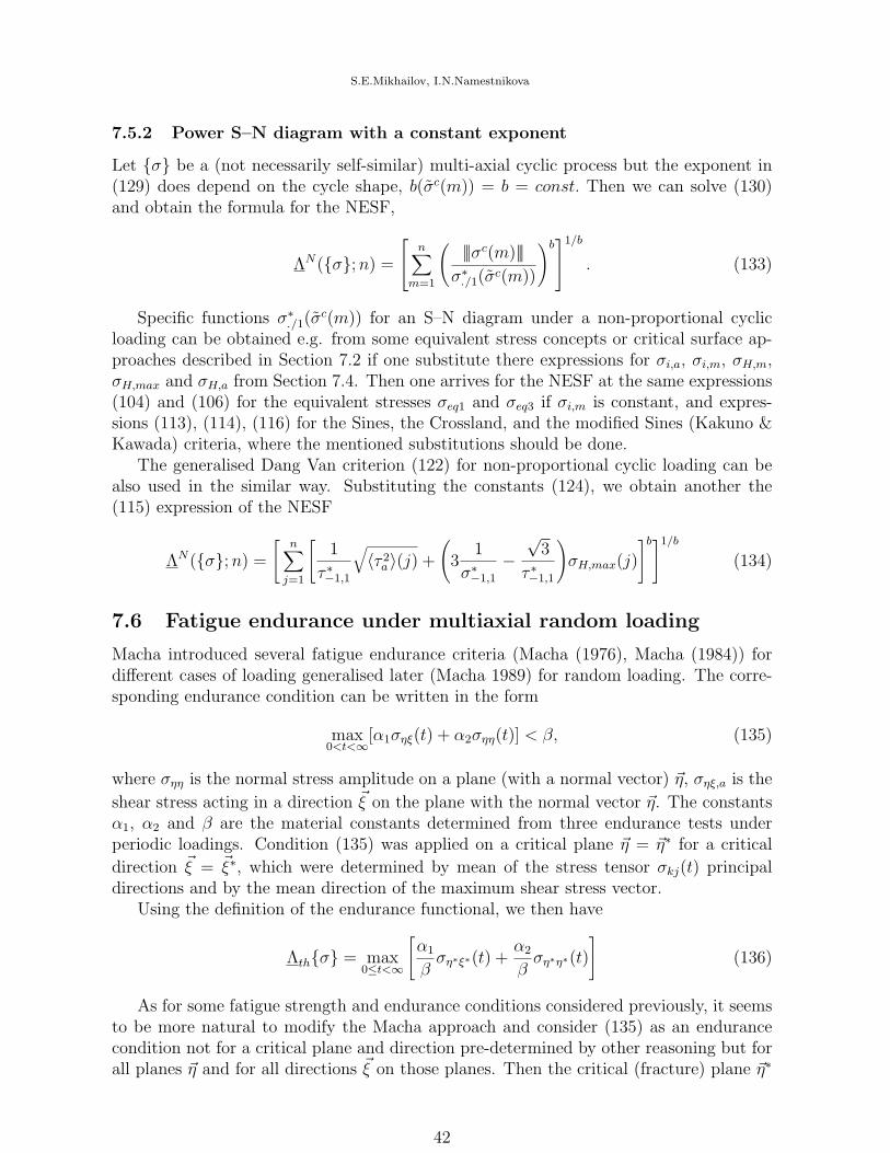
S.E.Mikhailov, I.N.Namestnikova

7.5.2 Power S–N diagram with a constant exponent

Let {σ} be a (not necessarily self-similar) multi-axial cyclic process but the exponent in(129) does depend on the cycle shape, b(σc(m)) = b = const. Then we can solve (130)and obtain the formula for the NESF,

ΛN({σ}; n) =

n∑

m=1

( |||σc(m)|||σ∗./1(σ

c(m))

)b

1/b

. (133)

Specific functions σ∗./1(σc(m)) for an S–N diagram under a non-proportional cyclic

loading can be obtained e.g. from some equivalent stress concepts or critical surface ap-proaches described in Section 7.2 if one substitute there expressions for σi,a, σi,m, σH,m,σH,max and σH,a from Section 7.4. Then one arrives for the NESF at the same expressions(104) and (106) for the equivalent stresses σeq1 and σeq3 if σi,m is constant, and expres-sions (113), (114), (116) for the Sines, the Crossland, and the modified Sines (Kakuno &Kawada) criteria, where the mentioned substitutions should be done.

The generalised Dang Van criterion (122) for non-proportional cyclic loading can bealso used in the similar way. Substituting the constants (124), we obtain another the(115) expression of the NESF

ΛN({σ}; n) =

[n∑

j=1

[1

τ ∗−1,1

√〈τ 2

a 〉(j) +

(3

1

σ∗−1,1

−√

3

τ ∗−1,1

)σH,max(j)

]b]1/b

(134)

7.6 Fatigue endurance under multiaxial random loading

Macha introduced several fatigue endurance criteria (Macha (1976), Macha (1984)) fordifferent cases of loading generalised later (Macha 1989) for random loading. The corre-sponding endurance condition can be written in the form

max0<t<∞

[α1σηξ(t) + α2σηη(t)] < β, (135)

where σηη is the normal stress amplitude on a plane (with a normal vector) ~η, σηξ,a is the

shear stress acting in a direction ~ξ on the plane with the normal vector ~η. The constantsα1, α2 and β are the material constants determined from three endurance tests underperiodic loadings. Condition (135) was applied on a critical plane ~η = ~η∗ for a critical

direction ~ξ = ~ξ∗, which were determined by mean of the stress tensor σkj(t) principaldirections and by the mean direction of the maximum shear stress vector.

Using the definition of the endurance functional, we then have

Λth{σ} = max0≤t<∞

[α1

βση∗ξ∗(t) +

α2

βση∗η∗(t)

](136)

As for some fatigue strength and endurance conditions considered previously, it seemsto be more natural to modify the Macha approach and consider (135) as an endurancecondition not for a critical plane and direction pre-determined by other reasoning but forall planes ~η and for all directions ~ξ on those planes. Then the critical (fracture) plane ~η∗

42

S.E.Mikhailov, I.N.Namestnikova

and the direction ~ξ∗ can be defined are those where the left hand side of (135) reachesmaximum. Thus we arrive at the strength condition

max0<t<∞

[α1ση∗ξ∗(t) + α2ση∗η∗(t)] = max~η

max(~ξ~η)=0

max0<t<∞

[α1σηξ(t) + α2σηη(t)] < β (137)

The corresponding endurance functional then becomes

Λth{σ} = max~η

max(~ξ~η)=0

max0≤t<∞

[α1

βσηξ(t) +

α2

βσηη(t)

](138)

In the case of bending and torsion, the empirical Gough-Pollard ”ellipse quadrant”criterion (Gough-Pollard, 1951) was also generalized on the case of a random loading inthe following way by Macha (Macha (1976), Macha (1984))

max0≤t<∞

[ (σηη(t)

σ∗−1∞

)2

+

(τ(t)

τ ∗−1∞

)2 ]= 1 (139)

The endurance functional Λth(~η) in this case (139) is

Λth(~η) = max0≤t<∞

√√√√[ (

σηη(t)

σ∗−1∞

)2

+

(τ(t)

τ ∗−1∞

)2 ](140)

Note, the NESF Λ(t) for some t < ∞ is obtained from (136), (138), (140) if themaximum in t is considered on the interval 0 ≤ t ≤ t.

8 Complex NESF for combined fatigue, creep and

instant loading

The NESF ΛN is a material characteristic which is not necessary connected with a ge-ometrical, stiffness-related or abstract damage measure and can be identified from somecyclic durability tests under homogeneous stress process fields. As was shown in the pre-vious sections, any cyclic strength condition written in terms of a damage measure canbe expressed in terms of a corresponding NESF (although not always analytically). Letus show some simple ways constructing NESFs to include e.g. instant overloading, creepor dynamic effects. Most of the damage accumulation rules mentioned above (exceptthe Pavlov rule) did not take into account sequence effects, that is damage caused by astress cycle is independent of where it occurs in the load history. We will see that thisshortcoming can be overcome in a simple way choosing a proper structure of NESFs.

Suppose one has a NESF ΛN({σ}; n) obtained e.g. from a damage measure approach,which do not take into account an influence of instantaneous overloads of material, espe-cially a finite strength σr under instantaneous loading. Particularly, NESFs (36), (37),(40), (113)–(116) based on the power-type S–N diagrams give such examples. If onewould like to avoid this shortcoming, one can introduce a new NESF and arrive at a localstrength condition e.g. in the form

ΛIN({σ}; n(t)) = sup0≤t′≤t

{σeq(σ(t′))

σr

+ ΛN({σ}; n(t′))

}< 1. (141)

43

S.E.Mikhailov, I.N.Namestnikova

Here σeq(σ) is e.g. von Mises, Tresca or other instantaneous equivalent stress; ΛN isnormalised equivalent stress functional defined, for example, from (132) or (113)-(116);σr is a material strength under uniaxial monotone tensile loading; the cycle number n(t)is a function of time t.

If one would like to take into account an influence of both the instantaneous overloadsof material and creep durability, one can add a term ΛT (σ; t′) connected with a durabilityunder creep (see Mikhailov 2000), and arrive at another one complex NESF and localstrength condition,

ΛITN({σ}; n(t)) = sup0≤t′≤t

{σeq(σ(t′))

σr

+ ΛT (σ; t′) + ΛN({σ}; n(t′))

}< 1 (142)

For example, if we take ΛN({σ}; n) in form (133) and associate ΛT (σ; t′) with theRobinson rule of time-dependent damage accumulation and power time-durability dia-gram (see Mikhailov 2000),

ΛT (σ; t′) =

[∫ t′

0

|σ(t′′|bT

AT (σ(t′′))dt′′

]1/bT

, (143)

the NESF (142) will take form

ΛITN({σ}; n(t)) = sup0≤t′≤t

{σeq(σ(t′))

σr

+

[∫ t′

0

|σ(t′′)|bT

AT (σ(t′′))dt′′

]1/bT

+

n(t′)∑

m=1

( |||σc(m)|||σ∗./1(σ

c(m))

)bN

1/bN }. (144)

where bT , bN are material parameters AT (σ(t′′)), is a material functions of the normalisedstress tensor σij(t

′′) = σij(t′′)/|σ(t′′)| at the instant t′′, σ∗./1(σ

c(m)) is a material functionsof the normalised shape of the stress cycle.

If there exist also dynamic effects on the material strength, one can replace the instantstrength term by a corresponding dynamic NESF ΛD(σ(t′) (see e.g. Mikhailov 2000) andarrive e.g. at the complex NESF and strength condition,

ΛDTN({σ}; n(t)) = sup0≤t′≤t

{ΛD(σ; t′) + ΛT (σ; t′) + ΛN({σ}; n(t′))

}< 1 (145)

For example, we can take ΛN({σ}; n) in form (133), ΛT (σ; t′) in form (143), andΛD(σ; t′) associated with the Morozov, Petrov and Utkin criterion (see Morozov andPetrov, 2000) generalised on the multiaxial case (see Mikhailov 2000), in the form

ΛD(σ; t′) =1

σr

σeq (σ(t′; tr)) , σkj(t′; tr) =

1

tr

∫ t′

t′−trσkj(t

′′)dt′′, (146)

where σr is, as before, a longitudinal material strength and σeq(σ) is e.g. von Mises,Tresca or other instantaneous equivalent stress and tr is a material constant. Then the

44

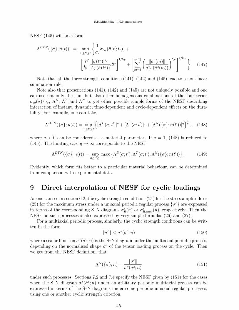
S.E.Mikhailov, I.N.Namestnikova

NESF (145) will take form

ΛDTN({σ}; n(t)) = sup0≤t′≤t

{1

σr

σeq (σ(t′; tr)) +

[∫ t′

0

|σ(t′′)|bT

AT (σ(t′′))dt′′

]1/bT

+

n(t′)∑

m=1

( |||σc(m)|||σ∗./1(σ

c(m))

)bN

1/bN }. (147)

Note that all the three strength conditions (141), (142) and (145) lead to a non-linearsummation rule.

Note also that presentations (141), (142) and (145) are not uniquely possible and onecan use not only the sum but also other homogeneous combinations of the four termsσeq(σ)/σr, ΛD, ΛT and ΛN to get other possible simple forms of the NESF describinginteraction of instant, dynamic, time-dependent and cycle-dependent effects on the dura-bility. For example, one can take,

ΛDTN({σ}; n(t)) = sup0≤t′≤t

{[ΛD(σ; t′)]q + [ΛT (σ; t′)]q + [ΛN({σ}; n(t′))]q

} 1q , (148)

where q > 0 can be considered as a material parameter. If q = 1, (148) is reduced to(145). The limiting case q →∞ corresponds to the NESF

ΛDTN({σ}; n(t)) = sup0≤t′≤t

max{ΛD(σ; t′), ΛT (σ; t′), ΛN({σ}; n(t′))

}. (149)

Evidently, which form fits better to a particular material behaviour, can be determinedfrom comparison with experimental data.

9 Direct interpolation of NESF for cyclic loadings

As one can see in section 6.2, the cyclic strength conditions (24) for the stress amplitude or(25) for the maximum stress under a uniaxial periodic regular process {σc} are expressedin terms of the corresponding S–N diagrams σ∗R(n) or σ∗R,max(n), respectively. Then theNESF on such processes is also expressed by very simple formulas (26) and (27).

For a multiaxial periodic process, similarly, the cyclic strength conditions can be writ-ten in the form

|||σc||| < σ∗(σc; n) (150)

where a scalar function σ∗(σc; n) is the S–N diagram under the multiaxial periodic process,depending on the normalised shape σc of the tensor loading process on the cycle. Thenwe get from the NESF definition, that

ΛN({σ}; n) =|||σc|||

σ∗(σc; n)(151)

under such processes. Sections 7.2 and 7.4 specify the NESF given by (151) for the caseswhen the S–N diagram σ∗(σc; n) under an arbitrary periodic multiaxial process can beexpressed in terms of the S–N diagrams under some periodic uniaxial regular processes,using one or another cyclic strength criterion.

45

S.E.Mikhailov, I.N.Namestnikova

For non-periodic process, it is usual to apply some damage accumulation theories toreduce a strength and durability analysis to some S–N diagrams under periodic processes.We discussed in sections 6.3 and 7.3 some of existing approaches. For any of them one canobtain a corresponding NESF, e.g., numerically but analytical formulas are not alwaysavailable and we given examples only for power S–N diagrams.

However, the damage accumulation theories, being quite suitable for the analysis interms of the damage (abstract or partial life time), is in fact not necessary for the NESFconcept. Instead, we will try to interpolate an NESF directly along the S–N diagramsfor periodic processes. Together with some additional properties implied either by theNESF definition or by some properties of the S–N diagrams for periodic processes, theinterpolating NESF is to meet the following conditions

(i) ΛN({σ}; n) must satisfy interpolation condition (151) on periodic processes {σ};(ii) ΛN({σ}; n) must be homogeneous in {σ};(iii) ΛN({σ}; n) must be non-decreasing in n;

(iv) the interpolation formula should be applicable to history independent materials, forwhich σ∗(σc; n) is given by (56).

9.1 Direct interpolation of NESF for uniaxial regular cyclic load-ing

9.1.1 Direct interpolation of NESF by a linear rule

We will try to write down a ”linear” accumulation rule not in the partial life times butin the normalised stress partial increments and start from the uniaxial case.

Let {σc} be first a uniaxial regular cyclic process with R = −1. If the process isperiodic, then we have from (26),

ΛN({σ}; n) =σa

σ∗−1(n)=

σa(1)

σ∗−1(n)(152)

for the NESF value at an n−th cycle. If the cycle amplitude increases after the first cycleand the process becomes periodic from the second cycle, we can take into account theamplitude increment as follows,

ΛN({σ}; n) =σa(1)

σ∗−1(n)+

σa(2)− σa(1)

σ∗−1(n− 1). (153)

If the cycle amplitude may increase on each cycle, we can continue the formula as

ΛN({σ}; n) =n∑

m=1

σa(m)− σa(m− 1)

σ∗−1(n−m + 1)

=σa(n)

σ∗−1(1)+

n−1∑

m=1

σa(m)

[1

σ∗−1(n−m + 1)− 1

σ∗−1(n−m)

], (154)

where the condition σa(0) = 0 was taken into account in the first part of (154).

46

S.E.Mikhailov, I.N.Namestnikova

To extend the NESF representation to an arbitrary change of the cycle amplitude fromcycle to cycle and comply with condition (iii) above, we write

ΛN({σ}; n) = max1≤n′≤n

n′∑

m=1

σa(m)− σa(m− 1)

σ∗−1(n′ −m + 1)

= max1≤n′≤n

σa(n′)

σ∗−1(1)+

n′−1∑

m=1

σa(m)

[1

σ∗−1(n′ −m + 1)

− 1

σ∗−1(n′ −m)

] (155)

for an arbitrary uniaxial regular cyclic process with R = −1.To consider uniaxial regular cyclic process with variable asymmetry ratio R(m), we

use the second part of representation (155) in the modified form,

ΛN({σ}; n) = max1≤n′≤n

σa(n′)

σ∗R(n′)(1)+

n′−1∑

m=1

σa(m)

1

σ∗R(m)(n′ −m + 1)

− 1

σ∗R(m)(n′ −m)

(156)

Let us check now the above conditions (i)-(iv) for NESF (156). For a periodic process,σa(m) = σa(1) and after some manipulations we have that ΛN({σ}; n) is reduced to (152),that is interpolation condition (i) is satisfied. Homogeneity condition (ii) and monotonicitycondition (iii) are obviously satisfied too.

Let us check condition (iv). Under definition, σ∗R(m)(m′) does not depend on m′ for a

history independent material and is an amplitude such that maxσ∈σc(m) σeq(σ) = σr. Thenσ∗R(m)(m

′) = σr/maxσ∈σc(m) σeq(σ). Consequently, NESF (156) for such material becomes

ΛN({σ}; n) = max1≤n′≤n

σa(n′)

σ∗R(n′)(1)= max

1≤n′≤nmax

σ∈σc(n′)

σr

σeq(σ)

what coincides with (56). Thus condition (iv) is satisfied.As an example, let us consider a particular case, when the S–N diagram σ∗R(n) is given

by power function (29). Then NESF (156) becomes

ΛN({σ}; n) = max1≤n′≤n

σa(n′)

σ∗R(n′),1+

n′−1∑

m=1

σa(m)

σR(m),1

[(n′ −m + 1)1/bR(m) − (n′ −m)1/bR(m)

] (157)

As one can see, unlike to the Palmgren-Miner rule described in Section 6.3.1, this approachgives an analytical presentation of NESF for an arbitrary process and a general dependencebR, however it is does not generally reduces to (36) or (37) for a constant bR or constantR.

9.1.2 Direct interpolation of NESF by a nonlinear rule

The linear interpolation of NESFs is not unique option. Let us consider a nonlinear in-terpolation in the following form,

ΛN({σ}; n) =

max1≤n′≤n

σa(n

′)σ∗R(n′)(1)

b

+n′−1∑

m=1

σa(m)

σ∗R(m)(n′ −m + 1)

b

− σa(m)

σ∗R(m)(n′ −m)

b

1b

(158)

47

S.E.Mikhailov, I.N.Namestnikova

Here b > 0 is considered as a material constant and the NESF (158) degenerates into(156) if b = 1. In the same way as for the linear rule, one can check the conditions (i)–(iv)are satisfied.

Let us consider the particular case, when the S–N diagram σ∗R(n) is given by powerfunction (29). Then NESF (158) becomes

ΛN({σ}; n) =

max1≤n′≤n

σa(n

′)σ∗R(n′),1

b

+n′−1∑

m=1

(σa(m)

σR(m),1

)b [(n′ −m + 1)b/bR(m) − (n′ −m)b/bR(m)

]

1b

(159)

One can see, that if bR(m) = b then (159) coincides with representation (36) obtainedfrom the Palmgren-Miner rule for the case of constant bR(m).

9.2 Direct interpolation of NESF for multiaxial cyclic loading

A multiaxial counterpart of uniaxial NESF (156) can be obtained if one takes into accountthat the cycle amplitude σa can be replaced by the cycle shape norm |||σc|||, the role ofthe asymmetry ratio R is plaid by the normalised cycle shape σc and the uniaxial S–Ndiagram σ∗R(n) for the amplitude σa should be replaced by the multiaxial S–N diagramσ∗(σc; n) for the norm |||σc|||. Then the normalised stress linear accumulation rule givesthe NESF

ΛN({σ}; n) = max1≤n′≤n

{ |||σc(n′)|||σ∗(σc(n′); 1)

+

n′−1∑

m=1

|||σc(m)|||[

1

σ∗(σc(m); n′ −m + 1)− 1

σ∗(σc(m); n′ −m)

] (160)

For a normalised stress nonlinear (power) accumulation rule, we similarly have a mul-tiaxial counterpart of (158),

ΛN({σ}; n) = max1≤n′≤n

( |||σc(n′)|||σ∗(σc(n′); 1)

)b

+

n′−1∑

m=1

( |||σc(m)|||σ∗(σc(m); n′ −m + 1)

)b

−( |||σc(m)|||

σ∗(σc(m); n′ −m)

)b

1b

(161)

Here b is considered as a material constant and the NESF (161) degenerates into (160) ifb = 1.

If the periodic S–N diagram σ∗(σc; n), used in (160) and (161), is not available for aparticular cycle shape σc, it can be expressed in terms of the uniaxial S–N diagrams forthe same material, using the approaches described in Sections 7.2 and 7.4.

Similar to the uniaxial case, one can check conditions (i)-(iv) are satisfied for NESFs(160) and (161).

As we have seen, NESF (161) interpolate the periodic S–N diagrams for any b > 0,including the NESF linear counterparts appearing for b = 1. However, if experiments on

48

S.E.Mikhailov, I.N.Namestnikova

non-periodic cyclic processes show some deviations of the formula predictions, one canpercept the NESF (161) as a first approximations to a NESF specific for a consideredmaterial and use an interpolation procedure to refine the approximation. Particularly theapproaches presented by Mikhailov (1997, 1998) can be adopted to this case.

10 Conclusion

The notions of generalised S–N diagram and normalised equivalent stress functional in-troduced by Mikhailov (2000) for arbitrary loading processes were adopted in this paperto oscillating loading by consideration some quasi-cyclic (discrete) parameterization morerelevant for cyclic fatigue.

The NESF concept reduces different durability and strength fatigue models to a uniqueform what facilitates their comparison. Numerous examples of the reduction are presentedin the paper for some known fatigue durability and strength models. Some complex NESFsdescribing interaction of instant , creep, fatigue and dynamic loading were introduced.

The NESF is a mechanically meaningful material characteristic, which can be approx-imated from a finite number of durability tests for different loading processes without anyother information such as micro-cracks or stiffness change. The NESFs interpolating theclassical S–N diagrams for periodic processes were presented in the paper. Methods for arefined NESF identification (interpolation) from a finite number of experimental data isto be developed further. Adaptation of the identification approaches by Mikhailov (1997,1998) to NESFs looks promising.

Fatigue under stress fields independent of the space coordinates was mainly analysedin this paper with obvious reasoning about application to moderately inhomogeneousstress fields . Extension to highly inhomogeneous stress field incorporating a non-localapproach by Mikhailov (1995) will be considered elsewhere (Mikhailov & Namestnikova2002).

ACKNOWLEDGEMENT

This work was completed under the research grant GR/M24592 ”Non-local approachto high cyclic fatigue: Theoretical basis” of the Engineering and Physical Sciences Re-search Council, UK.

Appendix

A Proof of inequality (7) for MD material

From Definition 1MD,

λN({σ}; n∗{σ}) = sup{λ : n∗{λσ} > n∗{σ}} =

sup{λ : λ ≤ 1, n∗{λσ} > n∗{σ}} ≤ 1

since n∗{λσ} ≤ n∗{σ} for all λ > 1 for MD materials. Similarly,

λN({σ}; n∗{σ} − 1) = sup{λ : n∗{λσ} > n∗{σ} − 1} =

sup{λ : λ ≥ 1, n∗{λσ} > n∗{σ} − 1} ≥ 1

49

S.E.Mikhailov, I.N.Namestnikova

since n∗{σ} > n∗{σ} − 1 and consequently n∗{λσ} > n∗{σ} − 1 for all λ ≤ 1 for MDmaterials.

B Proof of Remark 1

We define λ∗∗({σ}; n) := sup{λ : n∗∗{λ′′σ} > n ∀ λ′′ ∈ [0, λ]}. Since n∗∗{λ′′σ} ≤n∗{λ′′σ} then λ∗∗({σ}; n) ≤ λ({σ}; n).

Suppose λ∗∗({σ}; n) < λ({σ}; n). Then for any λ0, λ00 such that λ∗∗({σ}; n) < λ0 <λ00 < λ({σ}; n), we have,

n∗∗{λ0σ} ≤ n < n∗{λ0σ}, n∗∗{λ00σ} ≤ n < n∗{λ00σ} (162)

Consequently, strength is λ−unstable on the (quasi–) cycle n under the process {λ0σ},that is, for any ε > 0 there exists λ00 ∈ (λ0− ε, λ0 + ε) such that n∗{λ00σ} ≤ n. Choosingε ≤ min[λ({σ}; n) − λ0, λ0 − λ∗∗({σ}; n)], we have, λ∗∗({σ}; n) < λ00 < λ({σ}; n), andarrive at a contradiction with the last inequality in (162). Thus λ∗∗({σ}; n) = λ({σ}; n).

C Proof of Statement 3

Let us complete here the definition of n∗∗{σ} by∞ if the endurance under {σ} is λ−stable.Let n∗∗− {σ} < ∞, then supremum can be replaced by maximum in the definition ofn∗∗− {σ}. Suppose first n∗∗− {σ} + 1 < n∗∗{σ} ≤ ∞. For any n > n∗∗− {σ} and particularlyfor n = n∗∗− {σ} + 1, condition (21) is violated, that is λ({σ}; n) ≤ 1. Consequently,n∗{λ′σ} ≤ n∗∗− {σ} + 1 < n∗∗{σ} for any λ′ > 1 due to the definition of λ(σ; t) forMD processes. However the last inequality contradicts to the definition of the critical(quasi–) cycle n∗∗{σ} since the strength appears to be λ−unstable on the (quasi–) cyclen∗∗− {σ} + 1 < n∗∗{σ} under the process {σ}. Consequently n∗∗− {σ} + 1 can not be lessthan n∗∗{σ}. If n∗∗− {σ} = ∞ then evidently n∗∗− {σ}+ 1 also can not be less than n∗∗{σ}.

Suppose now first n∗∗{σ} < n∗∗− {σ} + 1 < ∞. Then we obtain from the definition ofn∗∗− {σ} that condition (21) holds for any n ≤ n∗∗− {σ} and particularly for n = n∗∗{σ}.Suppose then n∗∗{σ} < n∗∗− {σ}+1 = ∞. This means condition (21) holds for any n < ∞and particularly for n = n∗∗{σ}. That is, in the both cases there exists λ′ > 1 such thatn∗{λ′′σ} > n∗∗{σ} for all λ′′ ∈ [0, λ′]. This implies λ−stable strength on the (quasi–)cycle n∗∗(σ) under the MD process {σ}, which contradicts to the definition of the critical(quasi–) cycle n∗∗{σ}. The contradiction proves that n∗∗{σ} can not be less than thefinite or infinite n∗∗− {σ}+ 1.

Hence n∗∗− {σ} + 1 = n∗∗{σ} in all cases. For n∗∗− {σ} = ∞ this means n∗∗{σ} = ∞,that is, endurance is λ−stable under the process {σ}.

References

Ballard P., Dang Van K., Deperrois and Papadopoulos I.V. (1995) High-cycle fatigueand a finite element analysis, Fatigue and Fracture of Engineering Materials andStructures, 18(3), p. 397-411.

Bolotin, V.V., (1989). Prediction of service life for machines and structures, ASME Press,New York.

50

S.E.Mikhailov, I.N.Namestnikova

British Standards 5400, (1980).Steel concrete and composite bridges, Part 10 : Code ofpractice for fatigue.

Collins J.A., (1993). Failure of materials in mechanical design, A Wiley-Interscince pub-lication, New Yourk, 654 p.

Corten H.T., Dolan T.J., (1956). Cumulative fatigue damage, Proceedings of Interna-tional Conference on Fatigue of Metals, ASME and IME, p. 235.

Crossland B., (1956). Effect of large hydrostatic pressures on the torsional fatiguestrength of an alloy steel, Proc. Int. Conf. on Fatigue of Metals, I. Mech. E., London,p. 138-149.

Dang Van K., (1973). Sur la resistance a la fatigue des metaux, Sciences TechniquesArmement, 47 p.

Dang Van K.F, Griveau B. and Message O., (1989). On a new multiaxial fatigue crite-rion; theory and application, Biaxial and multiaxial fatigue, 2nd International con-ference on Biaxial/multiaxial fatigue. Papers. Edit. Brown M.W., Miller K.J., Me-chanical Engineering Publications Ltd, London, p. 479-496.

Dowling N.E., (1972). Fatigue failure prediction for complicated stress-strain histories,Journal of Materials, 7(1), p. 71-87.

Downing S.D. and Socie D.F., (1982). Simple rainflow counting algorithms, InternationalJournal of Fatigue, 4(1), p. 31-40.

Ellyin F., (1989). Cyclic strain energy as a criterion for multiaxial fatigue failure, Biax-ial and multiaxial fatigue, Edit. Brown M.W., Miller K.J., Mechanical EngineeringPublications Ltd, London, p. 571-583.

Flavenot J.F., Skalli N., (1989). A comparison of multiaxial fatigue criteria incorporatingresidual stress effects,Biaxial and multiaxial fatigue, Edit. Brown M.W., Miller K.J.,Mechanical Engineering Publications Ltd, London, p. 437-457.

Gough H.J., Pollard H.V., Clenshaw W.J., (1951). Some experiments on the resistanceof metals to fatigue under combined stresses ARC R and M, 2522, p. 141.

Kakuno H. and Kawada Y., (1979). Fatigue and Fracture of Engineering Materials andStructures, 2, p. 229.

Kogaev V.P., Makhutov N.A., Gusenkov A.P., (1985). Strength and durability analysis ofmachine components and structures, Mashinostroenie: Moscow, 1985, 224 p. (in Rus-sian).

Lagoda T., Macha E., Bedkowski W., (1999). A critical plane approach based on en-ergy concepts: application to biaxial random tension-compression high-cyclic fatigueregime, International Journal of Fatigue, 21, p.431-443.

Lagoda T., (2001). Energy models for fatigue life estimation under uniaxial random load-ing. Part I: The model elaboration, International Journal of Fatigue, 23, p.467-480.

Lebedev A.A., (1990). The reference book on strength analysis of structural components,Tehnica: Kiev, Edit. Lebedev A.A., 237 p. (in Russian).

Macha E., , (1976). Simulation of fatigue process in materials subjected to random com-plex state of stress, Simulation of Systems, North Holland Publishing Company, Edit.by Dekker, L., 1976, p. 1033-1041.

51

S.E.Mikhailov, I.N.Namestnikova

Macha E. , (1984). Fatigue failure criteria for materials under random triaxial state ofstress, Advances in Fracture Research, Proc. of the 6th Int. Conf. on Fracture (ICF6),Pergamon Press, Oxford, Eidt. by Valluri S.R. et.al., 3, p. 1895-1902.

Macha E., (1989). Generalisation of fatigue criteria for multiaxial sinusoidal loadings inthe range of random loadings, Biaxial and multiaxial fatigue, Edit. Brown M.W.,Miller K.J., Mechanical Engineering Publications Ltd, London, 1989, p. 425-436.

Macha E., Sonsino C.M., (1999). Energy criteria of multiaxial fatigue failure, Fatigue andFracture of Engineering Materials and Structures, Blackwell Science Ltd, Oxford, 22,p. 1053-1070.

Marin J., (1962). Mechanical behaviour of engineering materials, Englewood Cliffs, N.J.:Prentice-Hall.

Matake T., (1977). An explanation on fatigue limit under combined stress, Bull JSME,20, p. 257-263.

McDiarmid D.L., (1991). A general criterion for high-cycle multiaxial fatigue failure,Fatigue and Fracture of Engineering Materials and Structures, 14, p. 429-453.

McDiarmid D.L., (1994). A shear stress based critical-plane criterion of multiaxial fa-tigue failure for disign and life prediction, Fatigue and Fracture of Engineering Ma-terials and Structures, 17, p. 1475-1484.

Mikhailov, S.E., (1995-I). A functional approach to non–local strength conditions andfracture criteria – I. Body and point fracture. Engng Fracture Mech. 52, p. 731-743.

Mikhailov, S.E., (1995-II). A functional approach to non–local strength conditions andfracture criteria – II. Discrete fracture. Engng Fracture Mech. 52, p. 745-754.

Mikhailov, S.E. (1997) About interpolation of the non-local strength functionals by ex-perimental data. In: 15th IMACS World Congress on Scientific Computations, Mod-elling and Applied Mathematics: Berlin. (Proceedings) /ed. by A.Sydow, Berlin: Wis-senschaft und Technik Verl., Vol. 3, 515-520.

Mikhailov, S.E. (1998) A functional approach to non-local strength conditions at multi-axial loading. In: Damage and Fracture Mechanics: Computer aided assessment andcontrol, (Ed.: C.A.Brebbia & A.Carpentery), Southampton-Boston: ComputationalMechanics Publ., 429-438.

Mikhailov, S.E., (1999). A functional approach to durability description: Basic func-tionals. In: Ellyin, F., Provan, J. W. (Ed.), Progress in Mechanical Behaviour ofMaterials, ICM8, III: Advance Materials and Modelling of Mechanical Behaviour.Flemming Printing Ltd., Victoria BC, p. 1210-1215.

Mikhailov, S.E., (2000). Theoretical backgrounds of durability analysis by normalisedequivalent stress functionals, Preprint PP/MAT/SEM/00-122, Glasgow CaledonianUniversity, p. 1-19, (Mathematics and Mechanics of Solids, to appear).

Mikhailov, S.E., Namestnikova I.V. (2002). Non-local Approach to Cyclic Fatigue,Preprint PP/MAT/SEM/0102-006, Glasgow Caledonian University.

Miner M.A., (1945). Cumulative damage in fatigue, Journal of Applied Mechanics, 12,p. A159-A164.

52

S.E.Mikhailov, I.N.Namestnikova

Morozov, N., Petrov, Y., (2000). Dynamics of Fracture. Springer, Berlin-Heidelberg.

Palmgren A., (1924). Die lebensdauer von Kugellagern VdI-Z, 68 p. 339-341.

Palmgren A., (1945). Ball and roller bearing engineering, Translated by F.Palmgren andB.Ruley, SKF Industries, Inc., Philadelphia, p. 82-83.

Papadopoulos I.V., Davoli P., Gorla C., Filippini M. and Bernasconi A., (1997). A com-parative study of multiaxial high-cycle fatigue criteria for metals, International Jour-nal of Fatigue, 19(3), p. 219-235.

Papadopoulos I.V., (1998). Critical plane approaches in high-cycle fatigue: on the defini-tion of the amplitude and mean value of the shear stress acting on the critical plane,Fatigue and Fracture of Engineering Materials and Structures, 21, p. 269-285.

Pavlov P.A., (1988). The basis of engineering fatigue and damage analysis of machinecomponents, Mashinostroenie: Moscow, 1988, 252 p. (in Russian).

Rychlik I., (1987). A new definition of the rain-flow cycle counting method, InternationalJournal of Fatigue, 9, p. 119-121.

Schott G. (1997). Werkstoffermudung-Ermudungsfestigkeit, Stuttgart: Dt. Verl. furGrundstoffindustrie.

Serensen S.V., Kogaev V.P., Shneiderovich R.M., (1975). Failure assessment andstrength analysis of machine components, Mashinostroenie: Moscow, 488 p. (inRussian).

Sines G., (1959). Behaviour of metals under complex static and alternating stresses, MetalFatigue, Edit. G.Sines and J.L.Waisman, McGraw Hill, New York, p. 145-169.

Sobczyk K., Spencer B.F., (1992). Random fatigue. From data to theory, Academic PressLtd, London, 266 p.

53