Embed Size (px)
Citation preview

Concepts of Condensed Matter Physics
July 13, 2015
Contents
1 Introduction - an Overview 5
2 Spin Models 5
2.1 Model Building . . . . . . . . . . . . . . . . . . . . . . . . . . . . . . . . . . . . . . . . . . . . . . . . . . . . 5
2.1.1 First Quantization . . . . . . . . . . . . . . . . . . . . . . . . . . . . . . . . . . . . . . . . . . . . . . 5
2.1.2 Second Quantization . . . . . . . . . . . . . . . . . . . . . . . . . . . . . . . . . . . . . . . . . . . . . 5
2.1.3 Effective interactions: Direct (Hartree) Exchange (Fock) and Cooper (Pairing) channels . . . . . . . 7
2.1.4 Definition of Heisenberg’s Model . . . . . . . . . . . . . . . . . . . . . . . . . . . . . . . . . . . . . . 8
2.2 Mean Field Solution of the Heisenberg Model – Spontaneous Symmetry Breaking . . . . . . . . . . . . . . . 8
2.2.1 General Mean Field approximation . . . . . . . . . . . . . . . . . . . . . . . . . . . . . . . . . . . . . 8
2.2.2 Mean Field solution of the Heisenberg model . . . . . . . . . . . . . . . . . . . . . . . . . . . . . . . 9
2.3 Goldstone Modes (Magnons) . . . . . . . . . . . . . . . . . . . . . . . . . . . . . . . . . . . . . . . . . . . . 10
2.3.1 Holstein-Primakoff . . . . . . . . . . . . . . . . . . . . . . . . . . . . . . . . . . . . . . . . . . . . . . 11
2.3.2 Absence of LRO (Long Range Order) in 1D and 2D systems with broken continuous symmetries -Mermin-Wagner Theorem . . . . . . . . . . . . . . . . . . . . . . . . . . . . . . . . . . . . . . . . . . 12
2.3.3 Average magnetization . . . . . . . . . . . . . . . . . . . . . . . . . . . . . . . . . . . . . . . . . . . . 12
3 The Mermin-Wagner theorem (Tutorial) 13
4 Path integral formulation and the Hubbard-Stratonovich transformation (Tutorial) 17
4.1 Introduction . . . . . . . . . . . . . . . . . . . . . . . . . . . . . . . . . . . . . . . . . . . . . . . . . . . . . . 17
4.2 Coherent state path integrals . . . . . . . . . . . . . . . . . . . . . . . . . . . . . . . . . . . . . . . . . . . . 17
4.2.1 Bosonic coherent states . . . . . . . . . . . . . . . . . . . . . . . . . . . . . . . . . . . . . . . . . . . 17
4.2.2 Fermionic coherent states . . . . . . . . . . . . . . . . . . . . . . . . . . . . . . . . . . . . . . . . . . 18
4.2.3 Derivation of the path integral . . . . . . . . . . . . . . . . . . . . . . . . . . . . . . . . . . . . . . . 18
4.3 The Hubbard-Stratonovich transformation . . . . . . . . . . . . . . . . . . . . . . . . . . . . . . . . . . . . . 20
1

5 Superfluid (Based on Ref. [1]) 22
5.1 Symmetry (Global Gauge symmetry) . . . . . . . . . . . . . . . . . . . . . . . . . . . . . . . . . . . . . . . . 22
5.2 The Bose-Einstein condensation . . . . . . . . . . . . . . . . . . . . . . . . . . . . . . . . . . . . . . . . . . . 22
5.3 Weakly Interacting Bose Gas . . . . . . . . . . . . . . . . . . . . . . . . . . . . . . . . . . . . . . . . . . . . 25
5.3.1 Mean Field Solution . . . . . . . . . . . . . . . . . . . . . . . . . . . . . . . . . . . . . . . . . . . . . 25
5.3.2 Goldstone Modes . . . . . . . . . . . . . . . . . . . . . . . . . . . . . . . . . . . . . . . . . . . . . . . 25
5.4 Superfluidity . . . . . . . . . . . . . . . . . . . . . . . . . . . . . . . . . . . . . . . . . . . . . . . . . . . . . 27
5.5 Landau’s Argument . . . . . . . . . . . . . . . . . . . . . . . . . . . . . . . . . . . . . . . . . . . . . . . . . 28
5.6 Various Consequences . . . . . . . . . . . . . . . . . . . . . . . . . . . . . . . . . . . . . . . . . . . . . . . . 28
5.6.1 Quantization of Circulation . . . . . . . . . . . . . . . . . . . . . . . . . . . . . . . . . . . . . . . . . 28
5.6.2 Irrotational flow . . . . . . . . . . . . . . . . . . . . . . . . . . . . . . . . . . . . . . . . . . . . . . . 29
5.6.3 Vortices . . . . . . . . . . . . . . . . . . . . . . . . . . . . . . . . . . . . . . . . . . . . . . . . . . . . 29
6 Superconductivity 30
6.1 Basic Model and Mean field solution . . . . . . . . . . . . . . . . . . . . . . . . . . . . . . . . . . . . . . . . 30
6.2 The Anderson -Higgs Mechanism . . . . . . . . . . . . . . . . . . . . . . . . . . . . . . . . . . . . . . . . . . 30
6.2.1 Local gauge symmetry . . . . . . . . . . . . . . . . . . . . . . . . . . . . . . . . . . . . . . . . . . . . 30
6.3 London Equations (Phenomenology of Superconductivity) . . . . . . . . . . . . . . . . . . . . . . . . . . . . 32
6.4 Vortices in Superconductor . . . . . . . . . . . . . . . . . . . . . . . . . . . . . . . . . . . . . . . . . . . . . 33
6.4.1 The magnetic field penetration depth . . . . . . . . . . . . . . . . . . . . . . . . . . . . . . . . . . . 33
6.4.2 The Coherence Length . . . . . . . . . . . . . . . . . . . . . . . . . . . . . . . . . . . . . . . . . . . . 34
6.4.3 Two types of superconductors . . . . . . . . . . . . . . . . . . . . . . . . . . . . . . . . . . . . . . . . 35
6.4.4 Vortexes in Type II superconductor . . . . . . . . . . . . . . . . . . . . . . . . . . . . . . . . . . . . 37
7 Tutorial 4- The BCS theory of superconductivity (Tutorial) 39
7.1 Preliminaries . . . . . . . . . . . . . . . . . . . . . . . . . . . . . . . . . . . . . . . . . . . . . . . . . . . . . 39
7.2 BCS theory . . . . . . . . . . . . . . . . . . . . . . . . . . . . . . . . . . . . . . . . . . . . . . . . . . . . . . 40
7.3 Deriving the Ginzburg-Landau theory . . . . . . . . . . . . . . . . . . . . . . . . . . . . . . . . . . . . . . . 43
8 The 2D XY Model: The Berezinskii-Kosterlitz-Thouless transition 46
8.1 Vortices in the XY model . . . . . . . . . . . . . . . . . . . . . . . . . . . . . . . . . . . . . . . . . . . . . . 47
8.2 Kosterlitz-Thouless Argument . . . . . . . . . . . . . . . . . . . . . . . . . . . . . . . . . . . . . . . . . . . . 49
8.3 Describing vortices as a Coulomb gas . . . . . . . . . . . . . . . . . . . . . . . . . . . . . . . . . . . . . . . . 49
8.3.1 RG Approach . . . . . . . . . . . . . . . . . . . . . . . . . . . . . . . . . . . . . . . . . . . . . . . . . 50
8.3.2 The order of the KTB phase transition . . . . . . . . . . . . . . . . . . . . . . . . . . . . . . . . . . . 55
8.4 Coulomb gas and the Sine-Gordon mapping (Momentum RG) . . . . . . . . . . . . . . . . . . . . . . . . . . 56
8.4.1 Mapping between Coulomb Gas and the Sine Gordon model . . . . . . . . . . . . . . . . . . . . . . . 56
8.4.2 (Momentum shell) Renormalization group of the sine Gordon Model . . . . . . . . . . . . . . . . . . 57
8.4.2.1 First order term . . . . . . . . . . . . . . . . . . . . . . . . . . . . . . . . . . . . . . . . . . 57
8.4.2.1.1 Integrating out the fast variables – thinning the degrees of freedom . . . . . . . . 57
2

8.4.2.1.2 Rescaling . . . . . . . . . . . . . . . . . . . . . . . . . . . . . . . . . . . . . . . . . 58
8.4.2.1.3 Field rescaling . . . . . . . . . . . . . . . . . . . . . . . . . . . . . . . . . . . . . . 58
8.4.2.2 Second order term . . . . . . . . . . . . . . . . . . . . . . . . . . . . . . . . . . . . . . . . . 59
8.4.2.2.1 Integrating out the fast variables . . . . . . . . . . . . . . . . . . . . . . . . . . . 59
8.4.2.2.2 Rescaling . . . . . . . . . . . . . . . . . . . . . . . . . . . . . . . . . . . . . . . . . 60
8.4.2.2.3 Field Rescaling . . . . . . . . . . . . . . . . . . . . . . . . . . . . . . . . . . . . . . 60
9 Introduction to Graphene (Tutorial) 62
9.1 Tight binding models . . . . . . . . . . . . . . . . . . . . . . . . . . . . . . . . . . . . . . . . . . . . . . . . 62
9.2 Graphene . . . . . . . . . . . . . . . . . . . . . . . . . . . . . . . . . . . . . . . . . . . . . . . . . . . . . . . 62
9.3 Emergent Dirac physics . . . . . . . . . . . . . . . . . . . . . . . . . . . . . . . . . . . . . . . . . . . . . . . 64
10 The Quantum Hall Effect – This chapter is still under construction 67
10.1 Classical Hall Effect . . . . . . . . . . . . . . . . . . . . . . . . . . . . . . . . . . . . . . . . . . . . . . . . . 67
10.2 Quantum Hall effect . . . . . . . . . . . . . . . . . . . . . . . . . . . . . . . . . . . . . . . . . . . . . . . . . 69
10.2.1 Experimental observations . . . . . . . . . . . . . . . . . . . . . . . . . . . . . . . . . . . . . . . . . . 69
10.3 Basic explanation of the quantization effect . . . . . . . . . . . . . . . . . . . . . . . . . . . . . . . . . . . . 70
10.4 Additional conclusions, based on the existence of a gap in the system . . . . . . . . . . . . . . . . . . . . . . 72
10.4.1 Edge states . . . . . . . . . . . . . . . . . . . . . . . . . . . . . . . . . . . . . . . . . . . . . . . . . . 72
10.4.2 Fractional charges (Laughlin) . . . . . . . . . . . . . . . . . . . . . . . . . . . . . . . . . . . . . . . 73
10.4.3 Quantization of Hall conductance in the integer case . . . . . . . . . . . . . . . . . . . . . . . . . . . 73
10.4.4 Quantization of the Hall conductance and Chern numbers using Linear response . . . . . . . . . . . 74
11 Graphene – Quantum Hall effect without constant magnetic field 78
11.1 Graphene . . . . . . . . . . . . . . . . . . . . . . . . . . . . . . . . . . . . . . . . . . . . . . . . . . . . . . . 78
11.2 Tight-binding approximation for Graphene . . . . . . . . . . . . . . . . . . . . . . . . . . . . . . . . . . . . 78
11.3 Band structure - Dirac dispersion in quasi momentum . . . . . . . . . . . . . . . . . . . . . . . . . . . . . . 79
11.4 The Haldane model . . . . . . . . . . . . . . . . . . . . . . . . . . . . . . . . . . . . . . . . . . . . . . . . . . 79
11.5 Chern number in Haldane’s model and Obstruction of Stokes’ theorem . . . . . . . . . . . . . . . . . . . . . 81
11.5.1 Obstruction of Stokes’ theorem . . . . . . . . . . . . . . . . . . . . . . . . . . . . . . . . . . . . . . . 81
11.5.2 Chern number in Haldane’s model . . . . . . . . . . . . . . . . . . . . . . . . . . . . . . . . . . . . . 83
11.5.3 Chern number near a Dirac point . . . . . . . . . . . . . . . . . . . . . . . . . . . . . . . . . . . . . . 83
11.5.4 Explicit solution of edge mode in a massive Dirac spectrum . . . . . . . . . . . . . . . . . . . . . . . 84
11.6 Topological insulators and Spin-orbit coupling, Kane and Mele Model (2005)) . . . . . . . . . . . . . . . . . 86
@ Lecture notes taken by Dar Gilboa of the course taught by Prof. Yuval Oreg
3

References
[1] Alexander Altland and Ben Simons. Condensed Matetr Field Theory. Cambridge, University Press, second edition,2010. (document), 5
[2] Neil.W. Ashcroft and N. David Mermin. Solid State Physics. CBS publishing Asia Ltd., Philadelphia, 1987. 6.2.1
[3] Assa Auerbach. Interacting Electrons and Quantum Magnetism. Springer-Verlag, 1994. 2
[4] P. G. De-Gennes. Superconductivity of Metals and Alloys. Benjamin, New-York, 1966. 6.4.4
[5] M. O. Goerbig. Quantum Hall Effects. ArXiv e-prints, September 2009. 10
[6] Alexander O. Gogolin, Alexander A. Nersesyan, and Alexei M. Tsvelik. Bosonization and Strongly Correlated Systems.CAMBRIDGE UNIVERSITY PRESS, 1998. 8.4.2
[7] N. Nagaosa and S. Heusler. Quantum Field Theory in Condensed Matter Physics. Theoretical and MathematicalPhysics. Springer, 2010. 6.4.1
4
1 Introduction - an Overview
2 Spin Models
04/09/13 References: Chapters 1 and 2 in Ref. [3].
2.1 Model Building
2.1.1 First Quantization
We consider Bloch wave-functions which are the single electron solutions of the Hamiltonian
H0φks =
[−~2
2m∇2 + V ion(x)
]φks(x) = εkφks(x),
from which we can define a many electron Hamiltonian:
H0 =
Ne∑i=1
H0(∇i, xi).
The Hamiltonian H0 has eigenfunctions and eigenvalues
ΨFockK (x1,s1 , x2,s2 ...xNe,sNe ) = det
ij[φkisi(xi)] , EK =
Ne∑i=1
εki ,
where the εk are bounded by the Fermi energy EF .
The Hamiltonian H0 describes non-interacting electrons. We add an interaction term and consider
H = H0 +1
2
∑i,j
V el−el(xi, xj),
which we can write
H =
Ne∑i=1
(H0 + V eff [xi, ρ]
)+
1
2
∑ij
V (xi, xj),
where V eff is obtained by in a mean field sense by “freezing” one xi and summing over all other xj in V el−el and
V (xi, xj) = V el−el(xi, xj)−(V eff(xi) + V eff(xj)
)/Ne.
Taking the residual interactions V (xi, xj) instead of the of V el−el(xi, xj) represents screening. If we neglect V we obtainan effective non-interacting theory of Fermions. However, the theory has, compared to H0, new effective parameters thatmay be determined, for example, in a self-consistent way. We also assume dynamics which is slower than the plasmafrequency. The single electron approximation has been very successful in predicting various properties of many materials.However, to describe phenomena such as magnetism and superconductivity, one has to go beyond that and consider theresidual interactions.
2.1.2 Second Quantization
We would like now to present the Many body Hamiltonian using the second quantization formalism. For that we definea creation operator ψ†s(~r). When acting on the vacuum state (a state with zero particles that we denote |0〉) gives
〈~y, σ| ψ†s(~x) |0〉 = δsσδ(~x− ~y).
5

(Anti)Commutation relations of ψWe can choose a basis of the Hilbert space φα and write
ψ†s(~x) =∑α
φ∗αs(~x)c†αs (1)
ψ†s(~x), ψσ(~y)
=∑αβ
φ∗αs(~x)φβσ(~y)c†αs, cβσ
=∑αβ
φ∗αs(~x)φβσ(~y)δsσδαβ
=∑α
φ∗αs(~x)φασ(~y)δsσ =︸︷︷︸φcomplete
δsσδ(~x− ~y). (2)
The Hamiltonian is now
H0 =∑s
ˆd3xψ†s(~x)
[−~2
2m∇2 + V ion(~x) + V eff(~x)
]ψs(~x)
ˆV =1
2
ˆd3xd3yV (~x, ~y) [ρ(~x)ρ(~y)− δ(~x− ~y)ρ(~x)] (3)
where the second term is because we have no self-interaction. Since
ρ(~x) =∑s
ψ†s(~x)ψs(~x)
ρ(~x)ρ(~y) =∑s,σ
ψ†s(~x)ψs(~x)ψ†σ(~y)ψσ(~y) = −∑s,σ
ψ†s(~x)ψ†σ(~y)ψs(~x)ψσ(~y) +∑s
ψ†s(~x)ψσ(~y)δ(~x− ~y)δsσ
=∑s,σ
ψ†s(~x)ψ†σ(~y)ψσ(~y)ψs(~x) + ρ(~x)δ(~x− ~y)
setting this in Eq. (2) the second term cancels, giving us
ˆV =1
2
∑sσ
ˆd3xd3yV (~x, ~y)ψ†s(~x)ψ†σ(~y)ψσ(~y)ψs(~x). (4)
The ability to neglect V determines whether we can use a Fermi liquid theory with effective parameters or we get moredramatic interaction effects. For a rough estimate of weather V is large or small we note that in materials with an outerelectron in the s level the electron wave-functions obey 〈r〉 ∼ a where a is the lattice constant and 〈r〉 is the averagedistance of the electron from the nucleolus. For outer electrons in the d,f levels however, 〈r〉 a.
The typical kinetic energy of electrons is
EF =k2F
2m, kF ∼
1
a⇒ EF = vF kF ∼
vFa
while the interaction is (with κ being the dielectric constant)
U =e2
〈r〉κ.
giving a ratio
rs =U
EF=
e2
κvF
a
〈r〉
Hence, in most cases, V will be more important in d, f materials (we know that in many metals e2
κvF∼ 1 ).
6
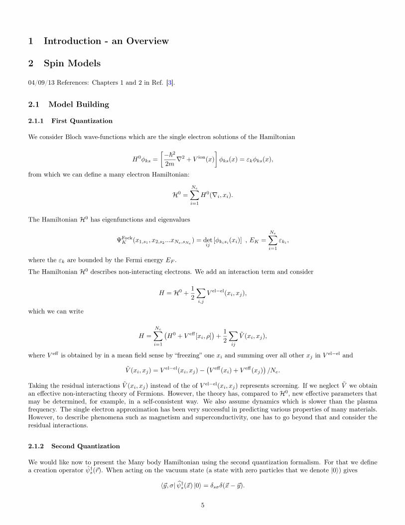
2.1.3 Effective interactions: Direct (Hartree) Exchange (Fock) and Cooper (Pairing) channels
Inserting Eq. (1) [ψ†s(~x) =∑αc†sαφ
∗α(~x)] in the interaction term ˆV of Eq. (4) and assuming that the wave-function φα
doesn’t depend on the spin - no SO coupling for instance. We have
ˆV =∑
σs,αβγδ
Mαβδγ c
†ασc†βscγscδσ
where
Mαβδγ =
1
2
ˆd3xd3yφ∗α(~x)φ∗β(~y)φγ(~y)φδ(~x); Mαβ
δγ =
13M
αβδγ if α = β = γ = δ
Mαβδγ otherwise
Assuming now that we can neglect interaction terms that do not contain at least two identical indexes1 we can split ˆVinto three channels
ˆV =∑αγsσ
Mαγαγ c†ασcασc
†γscγs +Mαγ
γα c†ασcαsc
†γscγσ +Mαα
γγ c†ασc†αscγσcγs,
(Notice the factor 1/3 in the diagonal term it is introduced to avoid double counting.) Using the following relation of thePauli matrices
~σσσ′ · ~σsσ = 2δσσδσ′s − δσσ′δsσand the definitions
nα =∑σ
c†ασcασ, ~sα =1
2
∑σs
c†ασ~σσscαs, t†α = c†α↑c
†α↓
we get
ˆV =∑αγ
(Mαγαγ −Mαγ
γα /2)nαnγ︸ ︷︷ ︸
Hartree (Direct)
− 2Mαγγα ~sα · ~sγ︸ ︷︷ ︸
Fock (Exchange)
+ Mααγγ t†αt†γ︸ ︷︷ ︸
Cooper (Pairing)
The three terms may be represented by diagrams, where the circles denote the paired indexes.
Figure 1: The direct (Hartree), exchange (Fock) and pairing (Cooper) channels.
In cases where the off diagonal Cooper terms are neglected the Hamiltonian reduces to1This will be a good approximation, for example, when the interaction is short-range and the wave function φ are fairly localized but demand
justification in other cases.
7

ˆV =∑
Uii′nini′ − 2Jii′~si · ~si′
Uii′ = δii′Uii + (1− δii′)(Uii′ −Jii′
2)
and Ui,i′ = M ii′
ii′ , Ji,i′ = M ii′
i′i .
2.1.4 Definition of Heisenberg’s Model
The Heisenberg model neglects the pairing and direct terms and assumes that the dominant contribution is from thesecond term, that mean
H = −2∑ij
Jij~si · ~sj
we will further assume
Jij =
J0 nearest neighbours0 otherwise
and J0 > 0 for a ferromagnetic interaction, J0 < 0 for an anti-ferromagnetic interaction.
In the ferromagnetic case (J0 > 0) spins will prefer to be aligned. That happens when the overlap between the i and jorbitals is large. Then (similar to the case of Hund’s rule) electron will tend to align their spin due to the Pauli principle.However if we have opposite spins sitting in neighboring atoms then it can be energetically preferable for one to tunnel,which is only possible if the spins are reversed, hence in this situation J0 < 0.
2.2 Mean Field Solution of the Heisenberg Model – Spontaneous Symmetry Breaking
Before discussing the mean field solution of the Heisenberg Model let us discuss the general mean field approach in general.
2.2.1 General Mean Field approximation
The general approach is to take a Hamiltonian of the form
H = A+B +AB
and simplify the interaction term by replacing the operator A by A → 〈A〉 + ∆A, where 〈A〉 is the mean value, and∆A contains the fluctuations around it. Within the mean-field approximation we will assume that ∆A is small. Forconsistency we need to check in the resulting solution that we have
∆A 〈A〉 ,
otherwise the mean field solution is incorrect.
After a similar substitution for B
H = A+B +A(B −∆B) + (A−∆A)B + ∆A∆B − (A−∆A) (B −∆B)
= A+B +A 〈B〉+ 〈A〉B + ∆A∆B − 〈A〉 〈B〉 .
Assuming the fluctuations are small we define the mean field Hamiltonian
HMF = A+B +A 〈B〉+ 〈A〉B − 〈A〉 〈B〉 .
8

2.2.2 Mean Field solution of the Heisenberg model
Coming back to the Heisenberg case we have
HMF = −2∑ij
Jij 〈si〉 sj − 2∑ij
Jijsi 〈sj〉+ 2∑ij
Jij 〈si〉 〈sj〉
since we can rotate all the spins together without changing the Hamiltonian, we will have 〈si〉 = 0 in the absence of anysymmetry breaking (i.e., if the ground state respects the symmetry for rotations). We look for a situation where spon-taneous symmetry breaking does occur, i.e., the system develops a spontaneous magnetization. In the case of symmetrybreaking we look for a state where 〈si〉 = 〈sz〉 ez. We define the magnetization
m = 2∑ij
Jij 〈sz〉 ez = 2nJ0 〈sz〉 ez
where n is the number of neighbors. Then if the total number of spins is N,
HMF = −2∑i
~m · ~si + |~m|N 〈sz〉
We write the partition function
ZMF = Tr(e−βHMF
)=(eβm + e−βm
)NeβmN〈sz〉 =
((eβm + e−βm
)eβm
2/2nJ0
)NWe want to minimize the free energy with respect to m to find the equilibrium value:
∂F
∂m= − 1
β
∂ lnZ
∂m= N
eβm − e−βm
eβm + e−βm+N
m
nJ0= 0
defining a = mnJ0
, b = nJ0β we obtain
a = tanh (ab) .
If we consider a as an order parameter which is zero in the disordered phase (since it is proportional to m), we can assumethat it is small and expand:
a ∼= ba− 1
3(ba)
3
we can look at different cases:
Figure 2: for b < 1 the to lines do not cross so there is no solution while for b > 1 there is a solution. The valueb = 1 = nJ0/Tc defines the phase transition temperature Tc.
9

from which we can see that we get a non-zero solution only if b > 1. The value of b which separates the two regimes definea critical temperature:
b = 1⇒ kTc = nJ0.
For small a we can solve giving
a =1
b
√3(b− 1)
b⇒ m = nJ0
√3Tc − TTc
taking T → 0⇒ b→∞ we get a→ 1 which means m→ nJ0 giving the following phase diagram
Figure 3: The magnetization as a function of the temperature
2.3 Goldstone Modes (Magnons)
The fact that when continuous symmetry is broken a soft (“gapless”) Goldstone mode arises is a general phenomenon.To be explicit, we will work on the Heisenberg model and consider the 1D case although similar results hold for higherdimensions.
We would like to find the low energy excitation of the problem. The ground state is |G〉 = |↑↑ ... ↑〉, i.e., the state whereall the spin point up.
H |G〉 = −2J∑ij
~si · ~sj |G〉 = −2J0
∑〈ij〉
szi szj |G〉 − J0
∑〈ij〉
s+i s−j + s−i s
+j |G〉 = −2J0Ns
2 |G〉 = EG |G〉 .
Notice that the term S+i destroy the state as the spin is already in its maximal value and in the last equation the pre-factor
is correct only in one dimension as each spin interacts with its left and right spin but we have to avoid double counting.
In looking for the energy of the excited states it is reasonable to assume that the first excited steaks will be build of linearcoherent combination of a single spin flip.
Denoting the single spin states:|i〉 = | ↑↑ ... ↑ ↓︸︷︷︸ith position
↑↑〉 and projecting on these single spin states is done by writing
H =∑ij
|i〉 〈i|H |j〉 〈j| .
The diagonal terms take the form 〈i|H |i〉 = EG + 2JS2 as two bonds are flipped (we assume that the spins are not atthe edge of the sample). However, because of the nearest neighbor coupling terms, the above states are not eigenstatesof the Hamiltonian. Due to the definition of the Heisenberg model, off diagonal matrix elements do not vanish only fornearest neighbor and given by〈i|H |i+ 1〉 = JS2 combing these we get the Hamiltonian (for the 1D case)
H =(EG + 2JS2
)∑i
|i〉 〈i| − JS2∑i
(|i+ 1〉 〈i|+ |i〉 〈i+ 1|) ,
10

which can be solved by a fourier transform: |q〉 =∑j
eiqaj |j〉, with a being the lattice constant. In general, such translation
invariant quadratic Hamiltonians can be diagonalized by going to Fourier space. We diagonalize the Hamiltonian and getthe spectrum :
Eq = EG + 2JS2 [1− cos(qa)] .
Taking q → 0 the excited state energies are
Eq − EG → Ja2q2.
These are the soft modes known as the Goldstone modes - their energy goes to 0 as the wave number goes to 0.
Generally the Goldstone modes are linear in q and not quadratic in q as in the ferromagnetic case. In the ferromagneticcase, our order parameter ~M ∝ ~Stot =
∑α ~sα commutes with the Hamiltonian:∑
αβγ
[SiαS
iβ , S
kγ
]=∑αβγ
Siα[Siβ , S
kγ
]+[Siα, S
kγ
]Siβ =
∑αβγ
iεikj
(SiαS
jγδβγ + SiαS
jβδαγ
)= ~Stot × ~Stot = 0.
Indeed writing the equation of motion in real space, assuming we have a quadratic dispersion, we get
m = D∇2m.
An integration gives a conserved total magnetization
M = D
˛∇m = 0,
which would not have happened if we had a linear dispersion.
(Remark: the situation is similar to the diffusion equation of particles that is quadratic in q implying that the total numberof particle is conserved.)
In the above we have demonstrated the very important concept of Goldstone bosons. These are gapless modes (or fields)that occur in quantum and classical field theories whenever a continuous symmetry is spontaneously broken.
2.3.1 Holstein-Primakoff
Before we talked about a system of spin 12 . Now we turn to talk about very large spins, for which (as we will see below)
quantum fluctuations become less important.
We seek a semi-classical approximation for the Heisenberg model. Considering ∆x∆p = 〈[x, p]〉 ∼ ~, the spin fluctuationsobey
∆si∆sj = 〈[si, sj ]〉 = |εijk 〈sk〉| ≤ s
∆sis
∆sjs≤ 1
s→s→∞
0
hence quantum fluctuations become negligible when we increase the spin size. Adding a lower index to denote lattice site,
[skm, sln] = iεkljs
jnδmn
and defining s±m = sxm ± isym we have
[s+m, s
−n ] = 2δmns
zm, [s
zm, s
±n ] = ±δnms±m
11

All this has been exact. Defining
s−m = a†m
√2s− a†mam, s+
m =
√2s− a†mamam, szm = s− a†mam
where am are bosonic ladder operators, we can check that the new operators obey the same commutation relations. TheHP approximation is taking the limit s→∞ (where s is the spin in each lattice) giving
s−m ≈√
2sa†m, s+m ≈
√2sam
in 1D with periodic BC we have
H = −2J∑m
(szms
zm+1 +
1
2
(s+ms−m+1 + s−ms
+m+1
))
→s→∞
−2JNs2 − 2Js∑m
(−2a†mam + a†mam+1 + h.c.
)Using periodic BC sm+N = sm ⇒ a†m+N = am and moving to Fourier space with am = 1√
N
∑e−ikmak giving
~ωk = 4Js (1− cosk) →k→0
2Jsk2
giving the same dispersion relation we found before.
Using the mean field analysis, we were able to demonstrate, neglecting fluctuations, that the Heisenberg model has aferromagnetic (ordered) phase which may occur at low temperatures. Once we understood that there is a ferromagneticphase, we turned to study the relevant degrees of freedom describing low energy excitations in this phase. In our case, thesewere the gapless spin waves (and in more general cases, these are called Goldstone modes). For the ferromagnetic phaseto be stable, the fluctuations generated by the Goldstone modes must not destroy the order. As we will see below, thisself consistency requirement is not fulfilled in low dimensions, leading to the absence of spontaneous symmetry breakingin 1D and 2D systems with continuous symmetries.
2.3.2 Absence of LRO (Long Range Order) in 1D and 2D systems with broken continuous symmetries -Mermin-Wagner Theorem
2.3.3 Average magnetization
We turn to study the deviations of the magnetization from it’s maximal value. Within the Holstein-Primakoff approach,this takes the form
∆m
2Jns=
1
N〈sztot〉 − s = − 1
N
∑k
nk
where nk are the average number operators, nk = 1e−ωk/T−1
, where we have used the fact that nk counts the number ofexcitations with a given k, which are decoupled bosons of energy ωk.
To perform the summation we introduce an IR cutoff k0 ∼ 1L for system size L and assuming ~ωk < T < Js we expand
the exponent and set the expression for ωk that we found
∆m = −k
k0
dkkd−1
(2π)d
T
2Jsk2− 1
N
∑k>k
nk
12

There is a clear dependence on dimensionality, in one and two dimensions the first term diverges with system size:
∆m ∝
− T
2Js1k0
1D
−Ts log(kk0
)2D
.
The divergences contradict the original assumption that fluctuations around the ordered state are small, and signal thatthe ordered phase is unstable.
This demonstrates the very general result, called the Mermin-Wagner theorem: continuous symmetries cannot be sponta-neously broken in systems with sufficiently short-range interactions in dimensions d ≤ 2 (see tutorial for more details).
On the other hand, in 3D we use 1e−ωk/T−1
=
∞∑n=1
e−nωk/T to write
∆m = −k
k0
dkk2
(2π)3
∞∑n=1
exp
(−2nk2Js
T
)≈ −1
8
(T
2Jsπ
)3/2 ∞∑n=1
1
n3/2= −1
8
(T
2Jsπ
)3/2
ζ(3
2).
This shows that in 3D the ferromagnetic state is stable. This remains true for higher dimensions. It is in fact a generalprinciple that as the dimension is increased, fluctuations become less important.
3 The Mermin-Wagner theorem (Tutorial)
This tutorial focuses on the famous Mermin-Wagner theorem. Basically, what the Mermin-Wagner theorem says is that2D systems with a continuous symmetry cannot be ordered, i.e., cannot spontaneously break that symmetry. It is a veryuniversal result that applies, for example, to magnets, solids, superfluids, and any other system characterized by a brokencontinuous symmetry. It illustrates the fact that as we go to lower dimensions, fluctuations become more important, andbelow D = 2, they destroy any potential ordering.
We start by focusing on a simple model: the classical xy model. In this model we have a square lattice with a planarspin on each site. The Hamiltonian takes the form
H = −J∑〈i,j〉
si · sj = −J∑〈i,j〉
cos(φi − φj).
The system is rotationally invariant (i.e., symmetric under φi → φi + c). However, the energy is minimal if all the spinspoint at the same direction, so the ground state spontaneously breaks the symmetry.
One would naively expect a ferromagnetic phase, with a broken rotational symmetry, to survive the introduction offinite temperatures (at least for low enough temperatures). This expectation is motivated by the naive intuition thatthe physics at zero temperature should not be different from the physics at a nearby infinitesimal temperature. At highenough temperatures, of course, there must be a transition to a disordered phase. In 3D, this is indeed the case - there isa finite temperature βJ , where β is a dimensionless number of order 1, below which the spins point at the same directionon average (even though they may be fluctuating locally).
How do we characterize order in this system? We can define a correlation function c(r− r′) =⟨ei(φ(r)−φ(r′))
⟩. At
zero temperature, where all the spins point at the same direction this function is 1. In an ordered system, at non-zerotemperatures the φs are homogenous on average and the correlation should remain non-zero even at large distances. Thismeans we have long range order. On the other hand, if the system is disordered, distant spins become uncorrelated andwe expect this function to go to 0 after some finite correlation length.
To see if our 2D system is ordered, we first assume it is and approximate the Hamiltonian based on this assumption.Then, we use the approximated Hamiltonian to calculate the correlation function. If the system is indeed ordered, self-consistency requires that the correlations stay non-zero. We will see that in 2D this is not the case, as the Mermin Wagnertheorem dictates.
In the first step, we say that if the system is ordered, the fluctuations between adjacent spins are small, so we canapproximate H ≈ E0 + J
2
∑〈i,j〉(φi − φj)2. Now we have a quadratic Hamiltonian, so we can actually calculate the above
13

correlation function. Before doing that, we make another simplification by noting that if the system is ordered, at lowenough temperatures the correlation length will be much larger than the lattice spacing (which is 1 in our units). In thiscase, we cannot “see” the lattice, so we can go to the continuum limit (small k expansion). In doing so, we rewrite thelattice theory as a field theory with the Hamiltonian
H ≈ J
2
ˆd2x(∇φ(r))2.
Note that this step is actually unnecessary, as we already had a quadratic Hamiltonian, but it will simplify later compu-tations.
First, let us decouple the Hamiltonian. As usual, this is done by going to Fourier space, and defining
φ(r) =1
2π
ˆd2keik·rφ(k).
Plugging this into the Hamiltonian, we get
H = − J
2 (2π)2
ˆd2r
ˆd2k
ˆd2k′eik·reik
′·rφ(k)φ(k′)k · k′.
By performing the integration over r, we get a delta-function of the form δ(k + k′), so we have
H =J
2
ˆd2kφ(k)φ(−k)k2 =
=1
2
ˆd2kε(k) |φ(k)|2 ,
with ε(k) = Jk2. Note that we have used the fact that the original field φ(r) is real, so φ(−k) = (φ(k))∗. In fact, theterms for k and −k are identical, so we can actually write this as an integral over half the plane:
H =
ˆk>
d2k |φ(k)|2 ε(k).
Since we now have many decoupled degrees of freedom, we can immediately write
〈φ(k)φ(k′)〉 =
´Dφφ(k)φ(k′)e−βH´
Dφe−βH=δ(k + k′)
βε(k).
Now recall that we want to calculate the correlation function c(r− r′) =⟨ei(φ(r)−φ(r′))
⟩. Since we have a Gaussian
Hamiltonian, we can immediately writec(r− r′) = e−1/2〈(φ(r)−φ(r′))2〉.
To calculate the expectation value⟨(φ(r)− φ(r′))2
⟩, we write it in terms of the decoupled Fourier components
⟨(φ(r)− φ(r′))2
⟩=
ˆd2k′d2k
(2π)2
(eik·r − eik·r
′)(
eik′·r − eik
′·r′)〈φ(k)φ(k′)〉 =
=1
(2π)2
ˆd2k′d2k
(eik·r − eik·r
′)(
eik′·r − eik
′·r′) δ(k + k′)
βε(k)=
1
(2π)2
ˆd2k
(eik·r − eik·r
′)(
e−ik·r − e−ik·r′) 1
βε(k)=
1
2βπ2
ˆd2k
(1− cos (δr · k))
ε(k).
Notice that in the large δr limit, we can separate the integral into two regions, k > δr−1, k ? δr−1, giving a qualitativelydifferent contribution. In the first case we have
ˆ 1/δr
d2k(1− cos (δr · k))
ε(k)≤ˆ 1/δr
d2k2
ε(k)→ 0,
14

so it will not be the leading order at large δr. In the second case, k ? δr−1, the cosine is strongly oscillating, and willagain not provide leading terms, so we neglect it. We end up with the integral
1
βJπ
ˆ1/δr
dk1
k.
Note that this integral has a logarithmic divergence at high momenta. This divergence is of course an artifact of theeffective continuum model, and in the original model the lattice spacing sets a high-momentum cutoff (that is, k isrestricted to the Brillouin zone). We put the cutoff back by hand, and get⟨
(φ(r)− φ(r′))2⟩
=1
βJπlog (αδr) ,
where α ∝ a−1 is the cutoff. Finally, putting this back in c, we get
c(r− r′) ∝ (αδr)−η(T )
,
where η = T2πJ .
This shows that the correlation between distant spins goes to zero and the system is not ordered at any non-zero tem-perature. In particular, the physics at zero-temperature is very different from the physics at an infinitesimal temperatureabove it. However, the way the correlation function goes to zero is different from the behavior of disordered systems.The power law correlations show a decay without a length-scale. The correlation length is actually infinite, similar to asecond order phase transition. The difference is that here we are not at an isolated point in parameter space, but find thisbehavior for a region of parameters. We call such a phase a quasi-long-range-ordered phase.
One may think that this result is specific to the classical xy model, but it is actually quite universal. Any classical systemin 2D with a continuous symmetry will have a massless field by the Goldstone theorem. The fluctuations created bythese Goldstone modes destroy the order in a similar fashion to what we have seen above - even if the correspondingHamiltonians are much more complicated. This has been proven in very general scenarios over the years.
For example, we can study the stability of 2D classical solids: let’s look at the case of a square lattice, and assigna displacement vector to each lattice point ui. Approximating the deviations of the potential from equilibrium to beharmonic, we write the energy in the form
K
2
∑〈i,j〉
(ui − uj)2.
Note the similarity of this to the form we wrote for the xy model. We can therefore immediately say that this Hamiltonianwill result in the fluctuation of the form ⟨
(ui − uj)2⟩∝ T log |i− j| .
This means that the relative displacement vector between two distant sites is wildly fluctuating, and the original crystalstructure is unstable.
The Mermin-Wagner theorem is not special to 2D classical problems. It actually applies to various quantum problems aswell. We have seen in the previous tutorial from the path integral formulation that the partition function of a quantummany body system takes the form
Z =
ˆD[ψ, ψ]e−
´ β0dτddx(ψ∂τψ+H[ψ,ψ]−µN [ψ,ψ]).
Thinking about the Lagrangian density as an effective classical Hamiltonian density, and about the τ (time) direction asanother spatial direction, we see that this partition function describes a classical d+ 1 dimensional system which is finitein one direction (the time direction), and infinite in the d other directions. At zero-temperature, the system is infinite inthe τ direction as well, so the quantum many-body problem is mapped into an infinite classical D = d + 1 dimensionalsystem. This mapping is called the quantum-classical mapping.
This way, a zero-temperature quantum problem in 1D is mapped into a 2D classical problem, where the Mermin Wagnertheorem applies. This means that 1D quantum problems with a continuous symmetry cannot be ordered. A 2D quantumproblem at zero-temperature is mapped onto a 3D classical problem, where order can occur. However, at finite temper-atures, the system is a “thick” 2D classical system, where the Mermin-Wagner theorem should apply (if we look at largeenough distances).
15

One last note: we have shown that the low temperature phase of the 2D xy model is quasi-long-range-ordered. It isinteresting to ask whether at high temperatures a phase transition occurs between the quasi-long-range-ordered to adisordered phase. We usually associate a phase transition with a process of symmetry breaking, but here neither of thephases breaks any symmetry, so one naively expects not to find a transition. As it turns out, there is a transition, andit is called the Berezinskii-Kosterlitz-Thouless transition. Historically, it was the first example of a topological phasetransition. You will study this transition extensively later in this course.
16

4 Path integral formulation and the Hubbard-Stratonovich transformation(Tutorial)
References: Altland & Simons Chapter 4 & 6.
4.1 Introduction
In this tutorial we have two objectives: (i) Imaginary time coherent state path integral formalism - to prove the identity(8). The motivation will be to show that quantum averages of many-body systems in thermal equilibrium can be computedusing functional integrals over field configurations. (ii) The Hubbard-Stratonovich transformation - To provide a rigorousformalism in which the phenomenological Ginzburg-Landau (GL) theory can be related to an underlying microscopictheory theory.
4.2 Coherent state path integrals
When we study single-body problems, the particle can be described by its position operator q. To get the path integralwe then work in an eigen basis of this operator and calculate the propagator 〈q′t′|q,t〉, for example, which turns out tobe related to integration over the paths q(t).
In field theory we have a field, i.e., a “position” operator at each point in space φ(x). We anticipate that the path integralwill be related to an integration over the field configurations φ(x, t). To make sense of this, it is clear that we first needto work in a basis that diagonalizes the field operators. The states that do this are called coherent states.
To be more specific, a coherent state is an eigenstate of an annihilation operator a
|ψ〉 = eζψa†|0〉
where ζ = 1 (ζ = −1) for Bosons (Fermions), such that a |ψ〉 = ψ |ψ〉. Remember that our field operators are annihilationoperators labeled by the spatial coordinates, so these are clearly the type of states we need in order to construct the pathintegral.
If we have many annihilation operators labeled by some index i (which in our case will be the spatial coordinate), we writea simultaneous eigenstate as
|ψ〉 = eζψia†i |0〉 ,
such that ai |ψ〉 = ψi |ψ〉.There are some crucial differences between the states corresponding to boson fields and those corresponding to fermionfields. Below we list the important properties of the two cases.
4.2.1 Bosonic coherent states
In the simpler case a describes a bosonic degree of freedom and ψ is simply a c-number. We will make use of three basicidentities: first the overlap between two coherent states
〈ψ1|ψ2〉 = eψ1ψ2 . (5)
The second is the resolution of identity which follows directly from (5)
1 =
ˆdψdψe−ψψ|ψ〉 〈ψ| (6)
Here we use the notation that ψ is a vector with a discrete set of components ψi corresponding to the underlying Fockspace. When studying a field theory in the continuum limit, this will be ψ(x). In the general case the above notationsmean ψψ ≡
∑i ψiψi and dψdψ ≡
∏idψidψiπ . Finally, the third identity is the Gaussian integral of the complex variables
ψ and ψ ˆdψdψe−ψAψ =
1
|A|where A is a matrix with a positive definite Hermitian part.
17

4.2.2 Fermionic coherent states
If the operator a describes a fermionic field things become a bit more complicated. To see this, let us assume againthat |ψ〉 is an eigen state such that ai |ψ〉 = ψi |ψ〉. The only way to make this consistent with the anti-commutationrelations between different a’s is to demand that different ψ′s anti-commute as well. We therefore need special numbersthat anti-commute. These are known as Grassmann numbers, and they satisfy:
ψiψj = −ψjψi.
The operation of integration and differentiation with these numbers are defined as followsˆdψ = 0;
ˆdψψ = 1
and ∂ψψ = 1.
The overlap between two coherent states and the resolution of identity remain in the form of (5) and (6). The Gaussianintegral on the other hand is significantly different
ˆdψdψe−ψAψ = |A| (7)
where A can be any matrix.
4.2.3 Derivation of the path integral
In what follows we will prove the central identity
Z = Tre−β(H−µN) =
ˆD[ψ, ψ]e−
´ β0dτ(ψ∂τψ+H[ψ,ψ]−µN [ψ,ψ]). (8)
where H and N are the Hamiltonian and particle number respectively and ψ, ψ are c-numbers (Grassmann numbers) inthe case that the particles have Bosonic (Fermionic) mutual statistics, assigned to each point of space and “time” τ . Theboundary conditions of this path integral is ψ(0) = ζψ(β) and ψ(0) = ζψ(β).
As mentioned above, our motivation will be computing expectation values of quantum many-body systems in thermalequilibrium. For example, if we have an operator A[a, a†], its expectation value will be
〈A〉 =1
Z
ˆD[ψ, ψ]A[ψ, ψ]e−
´ β0dτ(ψ∂τψ+H[ψ,ψ]−µN [ψ,ψ]).
Let start with the definition of the trace
Z = Tre−β(H−µN) =∑n
〈n|e−β(H−µN)|n〉 (9)
Notice that each term in this sum is the probability amplitude of finding the the system at the same Fock state it startedin, i.e. |n〉, after a time t = i~β, which, as you know, can be written as a Feynman path integral. In the first step we willwant to get rid of the summation over n. To do so we insert the resolution of identity (6) into equation (9)
Z =
ˆdψdψe−ψψ
∑n
〈n|ψ〉〈ψ|e−β(H−µN)|n〉
We can sum over n using the resolution of identity 1 =∑n |n〉〈n| but we first need to commute 〈n|ψ〉 with 〈ψ|e−β(H−µN)|n〉.
In the case of bosonic particles this is just a number and it commutes with anything. In the case of fermions Grassmannnumbers are involved and we need to be more careful. If we expand the matrix elements in terms of the Grassmannvariables, we find an additional sign:
Z =
ˆdψdψe−ψψ〈ζψ|e−β(H−µN)|ψ〉 (10)
18

Now let us continue to the second step: we divide the imaginary-time evolution operator into M small steps
e−β(H−µN) =(e−δ(H−µN)
)Mwhere δ = β/M . In the third step we insert M resolutions of identity in the expectation value in equation (10)
〈ζψ|[e−δ(H−µN)]M |ψ〉 =
ˆ M∏m=1
dψmdψme−∑m ψmψm× (11)
〈ζψ|ψM 〉〈ψM |e−δ(H−µN)|ψM−1〉 · · · 〈ψ2|e−δ(H−µN)|ψ1〉〈ψ1|e−δ(H−µN)|ψ〉
Expanding in small δ, we have
〈ψm+1|e−δ(H−µN)|ψm〉 ≈ 〈ψm+1|1− δ(H − µN
)|ψm〉
= 〈ψm+1|ψm〉(1− δ
(H[ψm+1, ψm]− µN [ψm+1, ψm]
))≈ eψ
m+1ψm−δ(H[ψm+1,ψm]−µN [ψm+1,ψm]),
where we have defined H[ψm+1, ψm] = 〈ψm+1|H|ψm〉〈ψm+1|ψm〉 .
Now if we insert this expression in (10) we get
Z =
ˆ M∏m=0
dψmdψme−δ∑Mm=0
[(ψm−ψm+1
δ
)ψm+H[ψm+1,ψm]−µN [ψm+1,ψm]
]
with ψ0 = ζψM+1 = ψ. Finally, in the fourth step we take M →∞ and obtain
Z =
ˆD[ψ, ψ]e−
´ β0dτ(ψ∂τψ+H[ψ,ψ]−µN [ψ,ψ])
where
D[ψ, ψ] ≡ limM→∞
M∏m=0
dψmdψm
The integration is to be carried over fields satisfying ψ(β) = ζψ(0). It is very important to note that by neglecting thetime derivative term we resume to the classical integration over configurations of the fields ψ and ψ. Indeed the timederivative term takes into account the effects of the non-trivial (anti-) commutation between ai and a
†i which have now
been transferred to fields ψi and ψi which always have trivial (anti-) commutation relations.
To be more specific, we usually discuss an interacting Hamiltonian of the form
S =
ˆ β
0
dτ
∑ij
ψi [(∂τ − µ) δij + hij ]ψj +∑ijkl
Vijklψi(τ)ψj(τ)ψk(τ)ψl(τ)
To compute path integrals we usually transform to the Fourier basis where the derivative operators are diagonal. Thisprocedure applies also for the imaginary time
ψ(τ) =1√β
∑ν
ψ(ν)e−iντ
in which case the action takes the form
S =∑n,ij
ψin [(−iνn − µ) δij + hij ]ψjn+
+1
β
∑ijkl,ni
Vijklψin1ψjn2
ψkn3ψln4
δn1+n2,n3+n4.
19

To obey the boundary conditions ψ(0) = ζψ(β) we choose the following frequencies in the wave functions e−iντ
νn =
2nπβ Bosons
(2n+1)πβ Fermion
These imaginary-time frequencies are known as Matsubara frequencies. Summing over them is a whole story to itself. Youwill see an example in the exercise. I want to note that in the limit of zero temperature (β → ∞) the sum becomes asimple integral 1
β
∑νn→´∞−∞
dν2π .
4.3 The Hubbard-Stratonovich transformation
In this tutorial we will learn a general method to relate a Ginzburg-Landau theory to the underlying microscopic theory.For example let us consider the GL theory of a ferromagnet
FGL =
ˆd3x
[−αm∇2m + am2 + βm4
].
Here, if a < 0 a transition to a ferromagnetic state may occur.
To see how to relate this theory to an underlying microscopic theory let us consider an interacting model of fermions
Z =
ˆD[ψ, ψ]e−S
S =
ˆ β
0
dτd3x
∑s=↑↓
ψs
(∂τ −
∇2
2m− µ
)ψs + gψ↑ψ↓ψ↓ψ↑
(12)
Notice that the local interactions may be reorganized in the following manner
ψ↑(x)ψ↓(x)ψ↓(x)ψ↑(x) = −s(x) · s(x)
where s(x) = 12 ψsσss′ψs′ and thus the action is equivalently given by
S =
ˆ β
0
dτd3x
∑s=↑↓
ψs
(∂τ −
∇2
2m− µ
)ψs − gs · s
= (13)
Now we will employ the Hubbard-Stratonovich transformation which relies on the following identityˆD[m] exp
[−ˆ β
0
dτd3x(m2 − 2m · s
)](14)
=
ˆD[m] exp
[−ˆ β
0
dτd3x (m− s)2
]︸ ︷︷ ︸
N
exp
[ˆ β
0
dτd3xs2
](15)
= N exp
[ˆ β
0
dτd3xs2
], (16)
where N does not depend on the field s. Thus, equation (12) may be equivalently written as follows
Z =1
N
ˆD[ψ, ψ,m]e−SHS (17)
where
SHS =
ˆ β
0
dτd3x
∑s=↑↓
ψs
(∂τ −
∇2
2m− µ
)ψs − 2gm · s + gm2
20

Notice that the action above resembles a mean-field decoupling of the interaction term. To see this substitute s = M+ δsin the interaction term, where M is the mean-field, and neglect terms of order O(δs2)
s · s = (M + δs)(M + δs) ≈ 2M · s−M2
However, there is a crucial difference: M is a mean-field with a single value whereas the field m fluctuates and we integrateover all possible paths of this field. Actually, equation (17) is exact, we made no approximations in deriving it. As youwill see in the exercise the saddle point approximation of this theory gives the self-consistent mean-field approximationobtained from a variational method. This observation suggests that the field m, introduced by some formal manipulations,may be interpreted as a local magnetization field.
Finally, let us discuss how we can use the HS theory (17) to obtain an effective theory for the magnetization field m.The standard way is to integrate over the Fermions. Since the m-field interacts with the fermions, their integration willgenerate terms containing the m field. First let us rewrite the theory as follows
SHS =
ˆ β
0
dτd3x
∑s=↑↓
ψs
(∂τ −
∇2
2m− µ
)δss′︸ ︷︷ ︸
G−1
− gm·σss′︸ ︷︷ ︸X
ψs′ + gm2
Formally, the fermionic part of the path integral has the quadratic form
ˆdψdψ e−ψAψ,
where A = G−1 −X[m]. Thus using (7) we can perform the integral over the fermions which gives
Z =1
N
ˆD[m]|A| e−gm
2
=1
N
ˆD[m] e−gm
2+log|A| =1
N
ˆD[m] e−gm
2+Tr logA
The trace of the logarithm can be expanded perturbatively in small X in the following manner:
Tr logA = Tr log(G−1 −X
)= Tr logG−1 + Tr log (1−GX) =
Tr logG−1 + Tr[−GX +
1
2GXGX + ...
]Now since X is linear in m each order gives the corresponding order in the Ginzburg-Landau theory. The first ordervanishes, as can be anticipated on symmetry grounds. The second order term, if expanded in momentum basis, gives thequadratic term
1
2Tr [GXGX] =
g2
βΩ
∑q,ω
Π (q, ω)mq(ω)m−q(−ω),
whereΠ =
1
βΩ
∑kν
1
−iν + k2
2m − µ· 1
−i(ν + ω) + (k+q)2
2m − µ,
and we have used the fact that G is diagonal in spin space and that the Pauli matrices are traceless. We can expand thisin small q and get the parameters of the Ginzburg-Landau theory:
a = g −Π(0, 0),
and
α =1
2
(∂2Π(q, 0)
∂q2
)∣∣∣∣q=0
.
Of course β will be derived from a higher order term with four powers of X.
21

5 Superfluid (Based on Ref. [1])
5.1 Symmetry (Global Gauge symmetry)
We consider a model described by
H =
ˆdra†(r)
(p2
2m− µ
)a(r) +
u
2
(a†(r)a(r)
)2and we write the partition function as an auxiliary field path integral:
Z = Tr(e−βH
)=
ˆDψDψ−S(ψ,ψ)
where S(ψ, ψ) =β
0
dτ´d3r
[ψ(r, τ)
(∂τ − 1
2m∇2 − µ
)ψ(r, τ) + u
2
(ψ(r, τ)ψ(r, τ)
)2]. Recall that in deriving the path inte-
gral, the ψ-fields were defined as the eigenvalues of the corresponding coherent states:
ψ |ψ〉 = a |ψ〉 , |ψ〉 = e−∑ψa† |0〉 .
We have a global U(1) symmetry ψ → e−iϕψ.
From Noether’s theorem we have a conserved current
Jµ =δS
δ(∂µψ
) ∂ψ∂ϕ
+δS
δ (∂µψ)
∂ψ
∂ϕ,
giving (using the relation ∂ψ/∂φ = iψ)
Ji = − 1
2mi
(ψ∇iψ − ψ∇iψ
).
The conserved charge is an integral over
J0 =δS
δ ˙ψiψ = ψψ = ρ.
Noether theorem itself gives the continuity equation ∂µjµ = ρ− ~∇ · ~J = 0, meaning the number of particles is conserved.Thus, the above U(1) symmetry is associated with charge conservation.
5.2 The Bose-Einstein condensation
We consider first the case u = 0 so that H → H0 =´dra†(r)
(−∇
2
2m − µ)a(r) .
Matsubara frequenciesTo represent the free partition function it is useful to use the imaginary (Matsubara) frequency using the relation:
ψ(τ, r) =1√β
∑n
e−iωnτψn(r), ψn(r) =1√β
ˆdτeiωnτψ(r, τ)
with
ψ(τ, r) =1√β
∑n
eiωnτ ψn(r), ψn(r) =1√β
ˆdτeiωnτ ψ(r, τ)
ωn = 2πnT for bosons , ωn = 2π
(n+
1
2
)T for fermions
ensuring periodic and anti-periodic boundary conditions in τ for boson and fermion respectfully.
22

Using the Matsubara presentation for ψ(r, τ) and the relation´ β
0e−iωnτdτ = βδωn,0 we have
β
0
dτψ(r, τ)∂τψ(r, τ) =∑ωn=2πτn
ψn(r)(−iωn)ψn(r). If we further diagonalize the Hamiltonian and develop the field in terms of the eigenfunctionφk,i.e.,
ψn(r) =∑k φkψkn we can write the partition functionZ in terms of the Fourier field ψkn
Z =
ˆDψDψ exp
[−S(ψ, ψ)
]=
ˆ ∏nk
ψknψkn exp
(−β∑kn
ψkn (−iωn + ξk)ψkn
)=∏k
∏n
1
β(−iωn + ξk)
with ξk = k2
2m − µ = εk − µ. Stability of these integrals demands µ ≤ 0. Using the thermodynamic relation for N(µ) wefind
N(µ) = −T ∂
∂µlogZ = −T ∂
∂µ
∑n,k
log
(−iωn + ξk
T
)= T
∑n,k
1
iωn − εk + µ. (18)
Knowing that this is a non-interacting problem, we expect N to be∑k
1eβ(εk−µ)−1
, and indeed we can see that this function
has poles at β(εk − µ) = 2πni, similar to 18 (since ωn = 2πnT ). Hence the two functions have the same poles, hintingthat they represent the same function. Contour integration with a few beautiful tricks (see for example Altland Simonspage 170) shows that indeed:
T∑n
1
iωn − εk + µ=
1
eβ(εk−µ) − 1≡ nB(ξk).
For a fixed external number of particles N the equation
N ≡ N [µ(T )]
is an equation for the chemical potential as a function of the temperature T . In three dimensions we can write thisequation as
N(µ) =∑k
nB(ξk) = Ω1
Ω
∑k
nB(ξk) = Ω1
(2π)3
ˆd3knB(ξk) = Ω
1
2π2
ˆdkk2nB(ξk) =
ΩLi 32
(eβµ)
2√
2π3/2(βm)3/2
with Ω being the system volume. Importantly to satisfy the equation N(µ) = N we must increase µ as we lower thetemperature until at µ = 0 we have
N(0) = Ωc1
λ3T
withλT =
1√mT
known as the particle thermal length and a numerical factor c =ζ( 3
2 )(2π)3/2 = 0.165869. If we go below the temperature for
which N(0) = Ωc 1λ3T
= N , we can not longer satisfy the equation N ≡ N [µ(T )]. This means that a macroscopic numberof particle N0 must occupy the ground state. We call such a phase a Bose-Einstein condensate. Notice that it occurs atthe temperature for which the average distance between the particles 1/n1/3 = (Ω/N)1/3 ≈ 0.54λT is of the order of thethermal length. This gives
Tc =(cn)2/3
m= 0.3
n2/3
m.
This gives a prediction: Tc increases for lighter particles and denser materials!
Below Tc we can write the action in terms of the field ψ0 corresponding to the ground state. We identify the number ofparticles in the ground state as
N0 = ψ0ψ0,
23

(a) (b)
Figure 4: (a)The chemical potential µas a function of the temperature T . (b) The number of bosons in the ground state.
and write the action
S = ψ0βµψ0 +∑k 6=0
ψkn (−iωn + εk − µ)ψkn.
Notice that the imaginary time derivative ∂τ → −iωndoes not appear in the first term, this is already an approximation.In the formulation of the path integral the derivative in imaginary time appeared due to the commutation relation of theoperators, neglecting them meaning that we omit quantum effects. In our case it is justified to perform this semiclassicalapproximation for the operator a0since a
†0a0 ≈ N 1while the commutation relations are
[a†0, a0
]= 1.
So that in the first term we take into consideartion only the thermal fluctuations (zero Matsubara frequency). In thesecond term, on the other hand, quantum fluctuations are included (We note that the Ginsburg-Landau theory infactneglects the quantum fluctuations).
Using the action S we can write the particle number as
N = −∂µF = ψ0ψ0 + T∑nk
1
iωn − εk= ψ0ψ0 +
Ω
(2π)3
ˆd3k
1
eβk2/2m − 1
= ψ0ψ0 +
(mT
2π
)3/2
ζ
(3
2
)= N0 +N
(T
Tc
)3/2
.
In 3D this gives us
N0
N=
(Tc−T
Tc
)3/2
We found a propagator
G(k, iωn) =⟨ψ(k, ω)ψ(k, ω)
⟩=
1
−iωn + εk
from which we can find the spectrum by analytic continuation, where we get poles at energy eigenvalues:
Gr(k, ω) = G(k, iωn → ω + iδ) =1
ω − εk + iδ
Im (Gr) = πδ(ω − εk)
24

Figure 5: (a)The action S for µ < 0 at the minimum |ψ0|2 = 0. (b) The action S for µ > 0. (c) The number of boson inthe condensate N0 = |ψ0|2.
5.3 Weakly Interacting Bose Gas
We now study the effects of weak interactions of the above non-interacting picture.
5.3.1 Mean Field Solution
We look at the action of the wave function ψ0 which describes the classical part of the wave function of the BEC.
TS(ψ0, ψ0) = −µψ0ψ0 +g
2Ld(ψ0ψ0
)2.
Notice that we take into consideration only the classical part of ψ (we assume that it does not depend on τ). Recall thatthis is justified because N0 = ψ0ψ0 1 and the commutation relation of the correspond operators is
[a†, a
]= 1.
The corresponding partition function is Z =´dψ0dψ0e
−TS(ψ0ψ0). For T µ we evaluate Z via the saddle pointapproximation, giving us the equations of motion:
δS
δψ0= 0⇒ ψ0
(−µ+
g
Ld(ψ0ψ0
))= 0,
with
|ψ0| =
õLd
g.
Notice that the total number of particle in the condensate ψ0ψ0 is proportional to the volume Ld as it should be. Dueto the interaction term g we no longer have a condition on the sign of µ, and the transition occurs at µ = 0. In theinteracting case, we find that the number of the particles in the condensate is proportional to µ.
5.3.2 Goldstone Modes
Notice that in the ground state |ψ0|2 6= 0. This forces ψ0 to have a well defined phase, thus spontaneously breaking theU(1) symmetry of the problem. As we saw for magnetic systems, since we have a continuous symmetry, we expect to findgapless excitations due to the Goldstone theorem.
We will find now the Goldstone modes of the system, to do so we define the average condensate density
ρ0 =ψ0ψ0
Ld
25

Allowing for spatial and temporal fluctuations, the field ψ0 is given by:
ψ =√ρ0 + ρ(r, t)eiφ(r,t).
The amplitude of the fluctuations is given by ρ(r, t) and the phase of the condensate is φ(r, t).
Substituting in the action, we find:
S =
ˆdτddrψ
[(∂τ −
∇2
2m
)ψ +
1
2g |ψ|2
(|ψ|2 − 2ρ0
)]this is equivalent to the action discussed above with ρ0g = µ, where we have added terms which depends on derivativeswith respect to time and space to account for the fluctuations. Assuming now that ρ(r, t) ρ0 and expanding the actionwe have
S ≈β
0
dτddr
[iρ0φ+ iρφ+
ρ0
2m(φ′)
2+
ρ′2
8mρ0+u
2ρ2
]+O(ρ3, (∇φ)
3)
In analogy to the Lagrangian of a single particle L = pq−H, where p and q are conjugate variables satisfying [p, q] = i, theunderlined terms in S helps us identify φ and ρ as conjugate variables. We therefore expect, in the operator (canonical)formulation, to get
[φ, ρ] = δ(x− x′).
We want to integrate over the ρ part to obtain an effective action for φ, the Goldstone mode.
For one variable we have
S =
ˆdτ
(ip∂τq −
p2
2m− V (q)
)integrating over p gives
ˆdτm (∂τq)
2
2− V (q).
In our case we first go to Fourier space and then perform the functional integral over ρ, giving us
S =
β
0
dτddk
(2π)d
[iρ0φ0 +
ρ0
2mk2φkφ−k +
1
2g (1 + k2ξ2)φkφ−k
]
ξ = 4mgρ0.
For kξ 1 we can easily transform back to real space, and we get the effective action
S =
β
0
dτddr
[iρ0∂τφ+
1
2u(∂τφ)
2+
ρ0
2m(∇φ)
2
](valid for r ξ).
This is a continuum XY model. The name XY originates from the fact that the order parameter ψ is a complex functionthat can be represented by a real and imaginary part i.e. a planar vector that "lives" in an XY plane.
Examining the action, it seems identical to the quadratic action we always had, with one important difference:φ is now acompact angle: φ+ 2π = φ. An implication of that is that to fully describe the theory, we need to consider vortices: 2Dsolutions in which the phase completes an integer number of windings as we wind around some point in space (see Fig.11) . An example of such a solution is φ(x, y) = n arctan
(y−y0
x−x0
). Such a solution is interesting because of it’s topological
26

stability: a vortex configuration cannot be locally deformed into a uniform configuration. In more general terms, theseare examples of topological defects. We will elaborate on vortices later.
A common definition is the superfluid density:
ρs =ρ0
m
which determines the energetic cost of deforming the condensate phase in space, and a compressibility
κ =1
g
which determines the cost of phase changes in time. Transforming to q, ω space we get
S =1
2
∑q,ω
(κω2
q + ρsq2)φqωφ−q−ω,
indicating that the dispersion is
ωq = cq ⇒ c =√ρs/κ =
√ρ0g
m.
Reminder: we assume |r| ξ, meaning we have performed coarse graining.
5.4 Superfluidity
To discuss superfluidity let us add an external chemical potential µext to the system. Working in the canonical formulation,we write the Hamiltonian as
H =1
2
ˆdx
[ρs (∇φ)
2+
1
κρ2 − µexρ
].
Recall, now ρ and φ should be understood as operators satisfying
[φ(x), ρ(x′)] = δ(x− x′).
The current operator is
J =1
2mi
(ψ∇ψ − ψ∇ψ
)=ρ(r, t)
m∇φ ≈ ρ0
m∇φ = ρs∇φ.
The Hamilton equations are
∂ρ
∂t= −∂H
∂φ= −ρs∇2φ = −∇ · J
which is the expected continuity equation. The more interesting equation is
∂φ
∂t=∂H
∂ρ= µex − uρ ≡ µ(r, t).
This is one of the Josephson relations - the time derivative of the phase depends linearly on an external potential.
To see how this system exhibits superfluidity let assume that φ = qx then we have
J =ρ0
m∇φ = q
ρ0
mx
and the phase vector in x space looks like this:
The surprising thing is that such a current is stable, since we have Goldstone modes (low energy excitations) in the systemwe could have expected that such a current would excite them.
27

x
Figure 6: Phase evolution in the presence of current
5.5 Landau’s Argument
A fluid moving uniformly in the lab frame without internal excitations has an energy E0 = 12mv
2. In viscous fluids, dueto friction with the wall, the fluid will lose its kinetic energy. Such a dissipative process takes place through the creationof excitations in the fluid. In case we have excitations they will move with the system.
We start by considering the system in its ground state, and moving to the center of mass frame, where there is no kineticenergy. If excitations are introduced, the entire energy of the system is their energy ε(p) = c · p. We now use the Galileantransformation to go back to the lab frame, where the walls are at rest. We get the energy
E1 =1
2mv2 + ~p · ~v + ε(p)
(the ~p · ~v term is from moving the excitations, just from moving something with momentum p with a velocity v)
To have dissipation, it must be energetically favorable to create excitations. Therefore, if we want to have dissipation asa result of excitations, we must have E1 − E0 < 0 ⇒ ~p · ~v + ε(p) = ~p · ~v + ~c · ~p < 0 which requires |v| > c. This meansthat for low speeds this doesn’t hold and there is no dissipation. The fact that we have a linear dispersion relation meansthat there is a range of velocities for which the system is non-dissipative. Usually we have a quadratic dispersion relationwhich means we can always excite the system.
5.6 Various Consequences
5.6.1 Quantization of Circulation
Considering
J =ρ0
m∇φ
we integrate over a closed path
˛∇φ = φ(L)− φ(0) = φ(2π)− φ(0)
and since φ is compact (ψ = ρeiφ) we require
28

˛∇φ = 2πn
⇒ˆv · dl =
ˆJ
ρ0· dl =
~m
2πn =hn
m
where we reintroduced ~. We have a quantization of superfluid velocity.
5.6.2 Irrotational flow
Due to the relation J = ρs∇φ, the flow is irrotational:
∇× J = ρs∇×∇φ = 0 (19)
5.6.3 Vortices
A vortex solution is a singular φ configuration, which violates Eq. 19. We take
φ = nθ, n ∈ Z.
where θ = arctan(xy ) is the polar angle in real space. The fact that n is an integer guarantees that after a full rotation inreal space the field ψ ∝ eiφ is single valued.
The current is given by:
J = ρs∇φ = ρsn
rθ.
It is easy to show, using Stoke’s theorem, that ~∇× ~∇φ = 2πnδ(r).
This seems to diverge for small r but we have a cutoff r > ξ. The velocity is:
v =~m
n
rθ.
The proportionality of the velocity field to 1/r is very different from a rigid rotation where
v = ωrθ,∇× v = ωz
29

04/30/13
6 Superconductivity
6.1 Basic Model and Mean field solution
Exercise number 4.
6.2 The Anderson -Higgs Mechanism
6.2.1 Local gauge symmetry
The essential difference from the case of the superfluid is that the particles are charged so we must add coupling to theelectromagnetic field. We now consider the consequences of coupling a Goldstone mode to a gauge field. As we will see,this will give rise to the various known experimental consequences of superconductors. In the tutorial we will get thiseffective field theory from the microscopic BCS theory.
The coupling to the electromagnetic field is done by the “minimal coupling”
S =
ˆ1
2m
∣∣∣∣(∇− ie
~A
)ψ
∣∣∣∣2 .This changes the symmetry from a global U(1) to a local gauge invariance under U(1)
ψ → ψeiφ(x), A→ A−∇φ(x)
and in the polar representation, taking e = ~ = c = 1, (and completely ignoring the fluctuations in √ρ), we get
=
ˆρ0
2m(∇φ−A)
2.
On the other hand, taking the lowest orders in the density fluctuations, and following steps similar to the ones we performedfor the neutral superfluid, we get after integrating out the massive fluctuations of the amplitude ρ (restoring the universalfactors e, c, ~)
S =1
2
ˆdτ
ˆd3r
(∂τφ)2
u+ρ0
m
(∇φ− e
c~A)2
.
30

When Quantum fluctuations can be ignored?To study the Anderson Mechanism we will ignore quantum fluctuations – when is that justified? The full GL action is
S[φ,A] =1
2
ˆdτd3r
1
u(∂τφ− eA0)
2+ (∇A0)
2+ρ0
m(∇φ−A) + (∇×A)
2
Looking at the terms which contain A0 in fourier space, we have
1
uω2φ2 +
2
ueωφ︸ ︷︷ ︸a
A0 +
(e2
u+ q2
)︸ ︷︷ ︸
b
A20
integrating over A0 gives 1
uω2 −
(1ueω
)2(e2
u + q2)︸ ︷︷ ︸
a2/4b
φ2 =ω2q2
e2
u + q2
Assuming no magnetic field and minimizing the free energy of the full action we have
ω2q2
e2
u + q2=ρ0
mq2
which for small q gives
ω2 =ρ0
m
e2
u=
4πe3n
m= ω2
p
This is the plasma frequency. It is related to the dielectric constant of a material by the following development (see p. 18of Ref. [2])
dρ
dt= eE,
dj
dt= −e
2nE
m; iωj = −en
mE ≡ σ(ω)E with σ(ω) =
ie2n
mω
using Maxwell’s equations we find:
−∇2E = ∇×∇× E = iω
c∇×H = i
ω
c
(4π
cj − iω
cE
)=ω2
c2
(1 +
4πiσ
ω
)E ≡ ω2
c2ε(ω)E (20)
and by definition
ε(ω) =
(1−
ω2p
ω2
)When ε is real and negative ω < ωp the solution of Eq. (20) decay in space, i.e. electric field can not propagate in thematerial, for ω > ωp radiation can propagate in the metal and it become transparent.The q2 term came from a 3D Fourier transform of a Coulomb interaction V (q). When the material is confined 2D (andthe electric field lines can propagate in 3D) v(q) ∝ q, giving ω ∼ √q. In 1D metal of width a when V (q) ∝ log qa givenω ∼ q and quantum fluctuations can not be ignored.
Taking the classical approximation (no τ dependence) and adding a Maxwell term for the action of the magnetic field
S[A, φ] =β
2
ˆd3r
ρ0
m
(∇φ− e
c~A)2
+ (∇×A)2
=β
2
ˆd3r
ρ0
m
(∇φ− e
c~A)2
+β
2
ˆd3r |B|2 .
In momentum space
S[A, φ] =β
2
∑q
ρ0
m
(i~qφ~q − ~A~q
)(−i~qφ−~q − ~A−~q
)+(~q × ~A~q
)(−~q × ~A−~q
)
31

=β
2
∑q
ρ0
m
[q2φ~qφ−~q − 2i~q · ~A−~qφ~q + ~A~q · ~A−~q
]+(~q × ~A~q
)(−~q × ~A−~q
)
We break up ~A into a longitudinal and transverse part: ~A~q = ~A~q −~q(~q · ~A~q
)q2︸ ︷︷ ︸
A⊥
+~q(~q · ~A~q
)q2︸ ︷︷ ︸A‖
.
Notice that only the transverse part will contribute to the magnetic field, since ~B~q = ~q×A⊥q (since ~q× ~q = 0). Performing
a gaussian integral on the φ degrees of freedom(´
e−x2+yx ∼ ey2
)we have
S[A] =β
2
∑q
ρ0
m
~A~q · ~A−~q −(~q · A
) (~q · ~A
)q2
+(q ×Aq
) (−q ×A−q
).
=β
2
∑q
(ρ0
m+ q2
)A⊥q A
⊥−q.
The equation of motion is
(ρ0
m−∇2
)A⊥ = 0. (21)
The mechanism that we encounter here can be summarized as follows:
1. A symmetry breaking that we find through a mean field solution.
2. The appearance of Goldstone soft modes φ in the superconducting case.
3. Coupling between the Goldstone mode and the gauge filed A.
4. Upon integrating the Goldstone mode, the gauge field acquires a mass.
This is known as the Anderson Higgs mechanism.
6.3 London Equations (Phenomenology of Superconductivity)
Taking a curl of Eq.(21) we get
(ρ0
m−∇2
)B = 0. (22)
This is the first London equation. It shows that the field decays inside the superconductor with a length scale
λ =
√m
ρ0=
√mc2
4πnse2,
where ns represents the density of particles in the superconducting phase.
Since
∇×∇×A =4π
cj
if we choose the London gauge~q · ~A~q = 0
32

Figure 7: The Meissner effect: due to the Anderson-Higgs mechanism. An external field outside the superconductorinduced diamagnetic supercurrent inside the superconductor – these current generates a counter field that diminishes theexternal field.
we get
q × q ×A⊥ = q2A⊥
∇2A =4π
cj
j =mc
nse2A. (23)
Eq. (23) is known as the second London equation. It presents a perfect diamagnetism (notice that it is not gaugeinvariant).
Physically the Meisenner effect results from currents that, due the the Biot-Savart law, create magnetic fields that cancelthe external one, see figure .
6.4 Vortices in Superconductor
6.4.1 The magnetic field penetration depth
To study the behavior of magnetic field in superconducting region we will start from the Ginzburg-Landau theory. TheGinzburg Landau theory can be obtained by introducing a Habburd-Stratanovich field ∆that decouples the interactionterm gψ4 → ∆ψ↓ψ↑ + ∆ψ↑ψ↓ − |∆|
2
g the action is then quadratic in ψ so we can integrate out the ψ field and expand theaction, assuming that ∆ is small. We finally get (See [7] for details):
Fs =
ˆfsd
3x
fs = fn + α |Ψ|2 +β
2|Ψ|4 +
1
2m
∣∣∣∣(~i∇− e∗
cA
)Ψ
∣∣∣∣2 +B2
8π
were we switch to the notation ∆→ Ψ. A microscopic theory gives
α = α′T − TcTc
, α′ =12π2mT 2
c
ζ(3)P 2F
, β =α′
ne, e∗ = 2e, m∗ = 2m
33

where ne is the electron density. fn describes the free energy of electrons which aren’t in the superconducting phase. Bis the magnetic field. For α < 0 we have a minimum at
fs − fn =−α2
2β+B2
8π
We expect that the field will eventually be too strong to be repelled by the superconductor, and the critical magnetic fieldis found from the above equation
H2c
8π=α2
2β=nemT
2c
P 2F
= mPFT2c
mPF is the density of states at EF .
This results should not be surprising as in the nornal state we have electrons near the Fermi level, while in the su-perconduting state a gap of size ∆ is formed the energy of the electrons that are “repelled” from the Fermi surface is∑i,εi<∆ εi ∼ ν∆2 . (See exercise)
We can identify a magnetic length by comparing terms in F
B2
8π=
(∇×A)2
8π∝ 1
λ2
A2
8π∼ e∗2
c21
2m∗∣∣ψ2∣∣A2
λ2eff =
m∗c2
4π |ψ|2 e∗2
|Ψ∞|2 = −αβ
= n∗s =ne2
=m∗c2
4πe∗2=
m∗c2
8πe2λ2eff
.
Notice that the units in the last equation are right as ~/mc has units of length and ~c/e2 is dimensionless so that |Ψ∞|2has units of 1/volume as it should. Finally we can identify
α(T ) =2e2
mc2H2c (T )λ2
eff(T ).
These relations are useful asHc and λare experimentally measurable quantities, so we can find α even without a microscopictheory.
05/07/13
6.4.2 The Coherence Length
We discussed the following free energy for the superconductor
fs = fn + α |Ψ|2 +β
2|Ψ|4 +
1
2m∗
∣∣∣∣(~i∇− e∗
cA
)Ψ
∣∣∣∣2 +B2
8π
and found the magnetic length
λ2eff =
m∗c2
4π |ψ|2 e∗2
We can also define another length scale - the coherence length. Minimizing the free energy, we get the equation
δf
δψ∗= 0⇒ αψ + βψ∗ψ2 − 1
2m∗ψ′′ = 0.
34

which has the homogeneous solution
|ψ∞|2 = −αβ.
Dividing the equation by ψ∞, we get
ψ
ψ∞−(−βα
)ψ∗
ψ∞ψ2 − 1
2m∗α
ψ′′
ψ∞= 0.
Assuming ψ is real and defining f = ψψ∞
we have
f − f3 +~2
2m∗ |α|f ′′ = 0.
The coefficient of the last term has units of 1/area, which allows us to define a coherence length:
ξ2(T ) =~2
2m∗ |α|∝ TcTc − T
.
At zero temperature
ξ2(T = 0) ∝ 1
mα∝︸︷︷︸
microscopic expression for α
p2f
m2T 2c
=v2f
T 2c
⇒ ξ =vfTc
For dirty systems with diffusion we derive a length scale from the diffusion equation which contains the mean free pathdue to diffusion:
D
ξ2d
= Tc ⇒ ξd =
√D
Tc=
√vpl
Tc=√ξl
We can look at small deviations from ψ∞ by defining f = g + 1 and linearizing the equation
(1 + g)− (1 + g)3
+ ξ2g′′ = 0
ξ2g′′ = 2g
g ∼ e±√
2x/ξ.
6.4.3 Two types of superconductors
The relation between the two length scales defines two types of superconductors.
In type I materials, λ ξ we expel the magnetic field which costs energy, but are not yet in the superconducting phasewhich is beneficial energetically, hence such a boundary costs energy
Fb > 0
In type II materials, λ ξ
In this case we obtain the reduced energy of entering the superconducting phase without having to spend much energy onexpelling the field. We then have
Fb < 0
35

Figure 8: The surface energy is positive when λ < ξ we "pay" (the free energy is positive) for repealing magnetic field andstill do not gain energy from the superconductor. For λ > ξ we have superconductor and still do not repel the magneticfield hence "gain" from both, the surface energy is negative.
and it becomes energetically favorable to increase the boundary as much as possible, which is done by generating vortices.
The phase diagram for type II looks like this (see Fig 9)
We recall that each vortex carries at least Φ0 of flux. Hence if the flux through the entire model is less than Φ0 there canbe no vortexes and we have a perfect Meissner effect. The next phase allows creation of vortexes. Eventually the vortexesare so common that they coalesce, leaving the superconducting phase only on the boundary.
36

Figure 9: Hc1 the critical filed when the first vortex penetrates. Hc2 when the vortices core overlap and Hc3 when theresidue superconductivity on the surface disappears
6.4.4 Vortexes in Type II superconductor
Looking at a type II superconductor near Hc1 where we have a single vortex. The energy is
F =
ˆd3r
1
8π
[h2 + λ2 (∇× h)
2]
the last term is the kinetic energy which was derived using j = ensv = ∇× h 4πc and λ =
√mc2
4πns
Ekin =1
2mv2ns =
1
2
m
nse2j2 = λ2 (∇× h)
2
Taking a variation we derive the equation of motion:
h+ λ2∇×∇× h = 0
We want to solve for a single vortex hence we add a term to ensure the integration over the surface gives the correct flux.
h+ λ2∇×∇× h = Φ0δ(r)
integrating over the surface of the model
ˆdsh+ λ2
ˆds∇×∇× h =
ˆdsh+ λ2
˛c
dl∇× h = Φ0
For r λ , the field is effectively uniform along the integration contour and the second term drops givingˆdsh = Φ0
37

while if ξ < r < λ the first term is negligible
λ2
˛c
dl∇× h = 2πrλ2∇× h = Φ0
dh
dr=
Φ0
2πλ2
1
r
h =Φ0
2πλ2
(log
(λ
r
)+ const
)while for r λ we have h ∼ e−r/λ.
We can also solve exactly by a Fourier transform:
h+ λ2h′′ = Φ0δ(r)
(1 + λ2k2
)hk = Φ0
h(r) =Φ0
(2π)2
ˆeikrcosθkdkdθ
1 + λ2k2=
Φ0
2π
ˆkdk
1 + λ2k2J0(kr) =
Φ0
2πλ2K0(r/λ)
The free energy of a vortex of a model of height L is given by
Fvor =
ˆdV
h2 + λ2 (∇× h)2
8π=
Φ0
8π
Φ0
2πλ2log
(λ
ξ
)L
The critical field for creating separated N vortex is thus given by
0 = Fvor −ˆBHc1
4π= N
(Fvor −
Φ0Hc1
4π
)where the second term is the multiplication of the internal B field by the external one (see Ref. [4] (pages 33 50 and 66)).
Hc1 =Φ0
4πλ2log
(λ
ξ
)We ignored the energetic cost of destroying the superconducting phase in this calculation. The energy we gained per unitvolume of superconductor is
α2
β=H2c
8π∝ mpFT 2
c
(Hc is defined for type 1 superconductors)
and this the energy loss due to the creation of the core of the vortex is
Ecore = CνT 2c ξ
2L
where ν is the density of states, and C is some parameter which contains the details of the shape of the core.
38

7 Tutorial 4- The BCS theory of superconductivity (Tutorial)
In the lectures you saw a phenomenological analysis of superconductors. In particular, you saw that given some empiricalresults, many additional predictions can be made using the Ginzburg-Landau formalism. Historically, this approach hasbeen very successful.
However, the theory is still incomplete without a microscopic explanation. In this tutorial we will fill this gap by reviewingthe famous BCS theory, established by Bardeen, Cooper, and Schrieffer about 50 years after the initial discovery ofsuperconductivity. Then, we will connect the microscopic picture to the phenomenological one by deriving the Ginzburg-Landau theory.
7.1 Preliminaries
The BCS theory is based on two important insights:
1. Cooper’s realization that attractive interactions between electrons in the vicinity of the Fermi-energy favor theformation of bound states made of two electrons, called cooper pairs.
2. The result that interaction between two electrons, mediated by phonons, can be attractive.
Once one realizes these things, the next step is to assume that the ground state of a many body system with attractiveinteractions can be described in terms of a condensate of such weakly interacting pairs. The pairs satisfy Bose statistics,giving rise to a physics similar to that of a superfluid, yet different due to the fact that the bosons are now charged. Wewill see that this picture is capable of explaining superconductivity.
First let us elaborate on the above two crucial points:
To see that pairs of electrons can form bound states, we examine the following toy model. We imagine a filled Fermi sea.On top of that, we add two electrons which have an attractive interaction only with each other (note that they do feel theFermi sea via the Pauli-principle). We would like to find the corresponding two-Fermion eigenstate. We assume that thetotal momentum is zero and that the spin-part of the wavefunction is antisymmetric. Then, we write the wavefunction as
ψ(r1,r2) =∑k
(gke
ik(r1−r2))
(|↑↓〉 − |↓↑〉) . (24)
The Schrodinger equation takes the form
[H0(r1) +H0(r2) + V (r1 − r2)]ψ(r1,r2) = Eψ(r1,r2), (25)
Plugging Eq. 24 in, we get∑k
gk [H0(r1) +H0(r2) + V (r1 − r2)] eik(r1−r2) = E∑k
gkeik(r1−r2).
In a translation invariant system we get∑k
gk [2εk + V (r1 − r2)] eik(r1−r2) = E∑k
gkeik(r1−r2).
Multiplying by e−iq(r1−r2) and integrating over space, we get
2εqgqΩ +∑k
ˆV (r1 − r2)ei(k−q)(r1−r2)gk = EgqΩ,
which can be written in the form ∑k
Vk,qgk = (E − 2εq) gq, (26)
withVk,q =
1
Ω
ˆV (r)ei(k−q)r.
39

Obviously the energies depend on the form of the interaction V , but the phenomena we want to see should be universalfor Fermions with attractive interactions, so we pick the simplest form we can think of:
Vk,q =
−V If EF < εk < EF + ∆E and the same for εq0 Otherwise
. (27)
Plugging this in Eq. 26, we have−V
∑k
gk = (E − 2εq) gq,
where the sum over k is restricted by the requirements given by Eq. 27. Dividing by E − 2εq and summing of over q(with the same restrictions), we get
−∑q
V
E − 2εq= 1.
Transforming this into an integration over energy:
−ˆ EF+∆E
EF
dεV n(ε)
E − 2ε= 1.
We Integrate over a thin shell, so we assume the DOS is constant over this region, and we write
−V n(EF )
ˆ EF+∆E
EF
dε1
E − 2ε= 1.
This leads to the equationV n(EF )
2log
(E − 2 (EF + ∆E)
E − 2EF
)= 1,
whose solution is given byE = 2EF − 2∆Ee
− 2V n(EF ) .
So we get a state with a lower energy than that of two non-interacting electrons added exactly at the Fermi-surface.In addition, by studying the corresponding wavefunction, one can show that this is indeed a bound state. This resultdemonstrates a general principle: if there is an attractive interaction (which can be arbitrarily small) between the electrons,there is an instability towards the formation of pairs. One can then assume that the ground state of a many-body systemwith attractive interactions is composed of many weakly interacting pairs.
We now turn to study the possible origin of such attractive interactions. As it turns out, these can originate from anelectron-electron interaction, mediated by phonons. We will only discuss a very qualitative picture here, but this can bemade more rigorous. The idea is that an electron can pass at some time near an ion and attract it. The electron passesafter a short time ∼ E−1
F , and now there is a large concentration of positive charges around the electron’s original position.Using the fact that the ion can return to equilibrium only after a time ∼ ω−1
D , which is much larger than E−1F , we find that
long after the original electron has passed, there is still a concentration of positive charges. This attracts other electrons.The net effect is an attractive interaction between the two electrons (which in reality is mediated by the phonons).
7.2 BCS theory
Having the above physics in mind, we postulate that as the system becomes superconducting, there is an instabilitytoward condensation of pairs. To investigate the physics that arises from that, we assume that the ground state ofa system with attractive interactions |Ωs〉 is characterized by a macroscopic number of pairs. This means that ∆ =gΩ
∑k 〈Ωs|ψ−k,↓ψk↑ |Ωs〉, and its complex conjugate ∆ = g
Ω
∑k 〈Ωs| c
†k↑c†−k,↓ |Ωs〉 is non-zero. We regard these quantities
as the order parameters of our system.
Using the above assumption, we use the usual mean field formulation to transform the interacting Hamiltonian into aquadratic one, neglecting some quantum fluctuations.
We start from a system of fermions with attractive interactions
H =∑k,σ
nk,σ(εk − µ)− g
Ω
∑k,k′,q
ψ†k+q↑ψ†−k↓ψ−k′+q↓ψk′↑.
40

Under our mean-field assumption,∑
k′ ψ−k′+q↓ψk′↑, is governed by small q’s, and we write∑k′
ψ−k′+q↓ψk′↑ =Ω∆
g+∑k′
ψ−k′+q↓ψk′↑ −Ω∆
g︸ ︷︷ ︸Small
,
and in the same way ∑k
ψ†k+q↑ψ†−k↓ =
Ω∆
g+∑k
ψ†k+q↑ψ†−k↓ −
Ω∆
g︸ ︷︷ ︸Small
.
Plugging this in the Hamiltonian and keeping only the first order terms in the small deviations, we get
H =∑k,σ
nk,σ(εk − µ) +Ω
g|∆|2 −∆
∑k
ψ†k↑ψ†−k↓ − ∆
∑k
ψ−k↓ψk↑.
This is sometimes called the Bogoliubov de-Gennes (BDG) Hamiltonian. We have transformed our interacting Hamiltonianinto a quadratic mean-field Hamiltonian that captures the correct ordering in our system. Note, however, that this formis dramatically different than the type of Mean field Hamiltonians we usually write as it doesn’t conserve the number ofparticles. The number of particles is indeed not conserved, but the parity of that number (i.e., the number of particlesmod 2) remains a good quantum number.
We would like to diagonalize the BDG Hamiltonian. To do so, we define the spinor Ψk =(ψk↑ ψ†−k↓
)T, in terms of
which we can writeH =
Ω
g|∆|2 +
∑k
(εk − µ) +∑k
Ψ†khBDGΨk,
withhBDG =
(εk − µ −∆−∆ − (εk − µ)
).
To see that this is true, let us plug the definition of Ψk in:
H =Ω
g|∆|2 +
∑k
(εk − µ) +∑k
Ψ†khBDGΨk =,
=Ω
g|∆|2 +
∑k
(εk − µ) +∑k
[(εk − µ)
(ψ†k↑ψk↑ − ψ−k↓ψ†−k↓
)−(
∆ψ†k↑ψ†−k↓ + ∆ψ−k↓ψk↑
)]=
=∑k,σ
nk,σ(εk − µ) +Ω
g|∆|2 −∆
∑k
ψ†k↑ψ†−k↓ − ∆
∑k
ψ−k↓ψk↑.
Because the matrix hBDG is Hermitian, we can always perform a unitary transformation and diagonalize it, such that(assuming ∆ is real)
UhBDGU−1 =
(λk 00 −λk
)χk =
(ck,1ck,2
)= U
(ψk↑ψ†−k↓
).
The unitary transformation can be parametrized by
U =
(cos θk sin θksin θk − cos θk
),
where tan(2θk) = − ∆εk−µ , and the eigenvalues are λk =
√∆2 + (εk − µ)2. In terms of these, the Hamiltonian takes the
diagonal form
H =Ω
g|∆|2 +
∑k
(εk − µ) +∑k
(λkc†k,1ck,1 − λkc
†k,2ck,2
). (28)
41

(a) (b)
Figure 10
Taking εk = k2
2m , we get the dispersion shown in Fig. 10a.
It is now simple to identify the ground state: it is the state in which all the negative energy states are occupied and thepositive energy states are empty, that is
|Ωs〉 =∏k
c†k,2ck,1 |0〉 ∝∏k
(cos θk − sin θkψ
†k↑ψ
†−k↓
)|0〉 ,
where |0〉 is the vacuum of our Fock space. And the ground state energy is
H =Ω
g|∆|2 +
∑k
(εk − µ− λk) .
To get excited states we can either destroy a ck2 particle, or create a ck1 - both with an energy cost of λk. The crucialpoint is that there is a gap ∆ to excitations. This gap is essential for superconductivity.
Recall that ∆ was defined as the expectation value ∆ = gΩ
∑k 〈Ωs|ψ−k,↓ψk↑ |Ωs〉. We are now in a position to write a
self-consistent equation for it. All we need to do is to write the ψ′s in terms of the c’s, and find 〈Ωs|ψ−k,↓ψk↑ |Ωs〉 =− 1
2 sin (2θk) = ∆2λk
. So we get the self consistent equation
∆ =g
2Ω
∑k
∆
λk.
Transforming this into an integral, and recalling that the attractive interaction occurs only at a thin shell of order ωDaround the Fermi-energy, we write
1 =g
2
ˆ ωD
−ωDdξ
n(ξ)√∆2 + ξ2
≈ gn
2
ˆ ωD
−ωD
dξ√∆2 + ξ2
= gn · sinh−1(ωD
∆
).
Solving this for ∆, and assuming the interaction is small, we get
∆ ≈ 2ωDe− 1gn .
It is instructive to find the critical temperature from this formalism. To do this we need to write the self-consistencyequation at finite temperatures. We can use the machinery we already have and write ∆ as a sum of Matsubara frequencies
42

using the coherent state path integral formulation. However, since we understand the excitations of the problem 28, wecan immediately write ⟨
c†k1ck1
⟩= nF (λk),
⟨c†k2ck2
⟩= 1− nF (λk).
Plugging this into the definition of ∆, we write the self consistent equation
∆ =g
Ω
∑k
〈ψ−k,↓ψk↑〉 =g∆
2Ω
∑k
1− 2nF (λk)
λk=g∆
2Ω
∑k
tanh(βλk
2
)λk
.
Therefore
1 =g
2Ω
∑k
tanh(βλk
2
)λk
.
Again, transforming this into an integral, we have
1 = gn
ˆ ωD
0
dξ
tanh
(β√
∆2+ξ2
2
)√
∆2 + ξ2.
That’s the well-known BCS gap equation. A comparison between the solution and experimental data is shown in Fig 10b.
We can now find the critical temperature by demanding ∆ = 0, which gives us the equation
1 = gn
ˆ ωD
0
dξtanh
(βξ2
)ξ
.
Finding β from this equation, we finally get the critical temperature
Tc = constant× ωDe−1gn .
To summarize this part, we now have a microscopic theory that explains the condensation of pairs and the emerging gapto excitations. However, this picture doesn’t actually allow us to find the electromagnetic response of the system. Tocapture this part, we need to include an additional degree of freedom in our picture: the Goldstone mode associated withchanging the phase of ∆. Such a treatment necessarily goes beyond the above mean field treatment, which treats ∆ as aconstant. This will be done next.
7.3 Deriving the Ginzburg-Landau theory
To make contact with the phenomenological analysis, and include the phase mode in the analysis, we turn to derive theGinzburg-Landau functional from the microscopics using the Hubbard-Stratonovich transformation. This is very similarin spirit to what we already saw when we discussed magnetism.
The partition function of the system is given by
Z =
ˆD[ψ, ψ]e−
´ β0dτ´dx[ψσ(∂τ+ieφ+ 1
2m (−i∇−eA)2−µ)ψσ−gψ↑ψ↓ψ↓ψ↑],
where we have introduced coupling to the electromagnetic field in the form of the minimal coupling (∂τ → ∂τ +ieφ,−i∇ →−i∇− eA).
To get the Ginzburg-Landau theory, we decouple the interacting term using
e´ β0dτ´dxgψ↑ψ↓ψ↓ψ↑ =
ˆD[∆ ¯,∆]e
−´ β0dτ´dx
[|∆|2g −(∆ψ↓ψ↑+∆ψ↑ψ↓)
].
The resulting action is identical to the mean-field action we had in the previous section if we treat ∆ as a constant field,giving ∆ the interpretation of the superconducting order parameter we had before. However, now it’s a dynamical field,and in particular, it has a phase which can fluctuate.
43

Defining the Nambu-spinor as
Ψ =
(ψ↑ψ↓
), Ψ =
(ψ↑ ψ↓
),
the full action takes the form
Z =
ˆD[ψ, ψ]D[∆, ∆]e
−´ β0dτ´dx
[|∆|2g −ΨG−1Ψ
],
with
G−1 =
( [G(p)
]−1∆
∆[G(h)
]−1
),
and the differential operators [G(p)
]−1
= −∂τ − ieφ−1
2m(−i∇− eA)
2+ µ[
G(h)]−1
= −∂τ + ieφ+1
2m(i∇− eA)
2 − µ.
We want an effective action for the order parameter ∆, so we would like to integrate out the Grassmann fields. This issimple, and the result is
Z =
ˆD[∆, ∆]e
−´ β0dτ´dx
[|∆|2g
]+log detG−1
.
If we want to recover the mean field results we can derive the equations of motion out of the effective action, neglectingquantum fluctuations in ∆, and get exactly the same gap equation we got in our mean field analysis above.
But we want to go beyond that, and consider the effect of fluctuations. We will assume that ∆ is small, which is trueclose to the transition, and expand log detG−1 = tr log G−1 to lowest orders.
To do so, we write G−1 = G−10 + ∆ = G−1
0
(1 + G0∆
), with G−1
0 = G−1(∆ = 0), and ∆ =
0 ∆∆ 0
, such that
tr log G−1 = tr log G−10 + tr log
(1 + G0∆
)= tr log G−1
0 −∞∑n=0
1
2ntr(G0∆
)2n
.
We will not calculate the traces here, but those who are interested in such details are referred to Altland & Simons,chapter 6. The results are:
SGL = β
ˆdx[r
2|∆|2 +
c
2|(∂ − 2ieA) ∆|2 + u |∆|4
]r = n
T − TcTC
,
if temporal fluctuations are neglected (making it a semi-classical Ginzburg-Landau theory). This brings us back to thephenomenological theory you saw in class.
Lets see how the unique experimental properties of superconductors arise from that. Below Tc, r < 0, so the potentialr2 |∆|
2+ u |∆|4 has a minimum at |∆|2 =
√−r4u = ∆2
0. However, the phase (i.e., the Goldstone mode) is not determinedby the potential, so we write ∆ = e2iθ∆0. Putting this back in the Ginzburg-Landau action and dropping the constantterms, we have
SGL = 2c∆20β
ˆdx (∂θ − eA)
2.
We want to find the electromagnetic response of the system. We treat the electromagnetic field as a dynamical field, sowe should also add its kinetic term SMaxwell = β
2
´dx(∇×A)2 (assuming φ = 0, and the field is static). The total action
isS[A, θ]
β=
ˆdx
[2c∆2
0 (∂θ − eA)2
+1
2(∇×A)2
].
44
In order to get an effective action for the A we integrate over the Goldstone mode. You already saw that explicitly in class,so I will not repeat this here, but the result is that after integrating out the θ-field, the electromagnetic field acquires amass
S[A]
β=
ˆdx
1
2
[ρ0
mA2 + ∂iA∂iA
](here we used the notations used in class). Deriving the equations of motion, we get ρ0
mA = ∇2A. Taking the curl of thatequation, we get the London equation ρ0
mB = ∇2B, which was discussed in class. In particular, it was already shown thatit results in the decay of the magnetic field as we go into the bulk of the superconductor.
The second effect we want to see is the zero DC resistivity. To do that, we find the current
j(r) =δ
δA(r)
ˆdx
ρ0
2mA2 =
ρ0
mA.
Taking the time-derivative, and working in a gauge where φ = 0, so E = −i∂τA, such that
−i∂τ j =ρ0
mE.
This equation says that if we have a constant DC current there is no electric field. A system with a finite DC current andzero electric field has, by definition, zero resistivity.
45

8 The 2D XY Model: The Berezinskii-Kosterlitz-Thouless transition
We turn to study the XY model. This model has a global U(1) symmetry, and its order parameter is therefore a planarvector S = (Sx, Sy), or equivalently a complex scalar
ψ = Sx − iSy.
A superfluid described by a complex order parameter, which has a phase and an amplitude is one example but there aremany other examples, e.g, spins confined to be in a plane, having only x and y components. Below we think of a classicalstatistical mechanics theory (or a quantum theory at relatively high temperatures). However, the results apply directlyto quantum systems by the quantum-classical mapping.
We define
ψ = ψ0eiφ(r),
and the corresponding classical Hamiltonian, favoring alignment of different points, is
H =1
2
ˆκ0 (∇φ)
2d2r. (29)
It can be seen that the U(1) symmetry of the problem is respected.
We already saw that 2D systems with a continuous symmetry do not have long range order. However, as we will seebelow, the system is not entirely disordered, as the correlation function decays without a characteristic length scale.
The correlation function is
〈ψ∗(r)ψ(0)〉 =⟨ψ0e
iφ(r)ψ0e−iφ(r)
⟩= |ψ0|2 e−
12 〈(φ(r)−φ(0))2〉 (30)
with ⟨(φ(r)− φ(0))
2⟩
=T
κ0
ˆd2k
(2π)2
∣∣∣ei~k·~r − 1∣∣∣2 ⟨φ2
k
⟩.
The last equation follows from the Fourier substitution:
φ(~r) =1
(2π)2
ˆei~k·~rd2kφ~k
and the relation:1
(2π)2
ˆd2rei(
~k−~k′)·~r = δ2(~k − ~k′)
Using the free Hamiltonian in Eq. (29) we find:
H = κ1
(2π)4
ˆd2r
ˆd2k
ˆd2k′∇(ei
~k·~rφ~k)∇(ei~k′·~rφ~k′) = κ
1
(2π)2
ˆd2kk2φ~kφ−~k
from this we can easily find the correlation function:⟨φ~kφ~k′
⟩= δ(~k − ~k′)κ 1
k2.
Using the relation
F (|~r|) =∣∣∣eik·r − 1
∣∣∣2 = (cos(kr)− 1)2
+ sin2(kr) = 1− 2 cos(kr) + cos2(kr) + sin2(kr) = 2− 2 cos(kr)
we notice that for ~k ·~r 1 the function F (|~r|) is zero. For kr 1, the cos terms is strongly oscillating so that the integralover it is not expected to be the leading order and we can ignore it. We can therefore approximate Eq. (30) by:
46

⟨(φ(r)− φ(0))
2⟩
=2
(2π)2
T
κ0
1/aˆ
1/r
2πk
k2dk =
T
πκ0log( ra
).
Here a is a short range (ultra violet) cutoff. Hence we have
〈ψ∗(r)ψ(0)〉 = |ψ0|2(
1
r
)η, η =
T
2πκ0.
The fact that the correlation vanishes at large distances shows that the system is not long range ordered. If the correlationsdecay as a power law, the system is said to be quasi-long-range ordered.
8.1 Vortices in the XY model
Figure 11: vortex and anti vortex in the spin configuration ψ = ψ0eiφ = Sx− iSy denoted by arrows in the spin direction
and in the velocity ∇φ dented by bold lines
For ψ 6= 0, we define a velocity field
∇φ(r) = v(r)
From the fact that eiφ is single valued, we have a condition for an integral around any point:
47

˛v(r)dr = 2πn.
If the contour does not enclose a vortex, n is zero. In general, the integer n counts the number of windings the phase φdoes, or equivalently, the number of vortices inside the contour:
n =1
2π
˛v(r)dr.
If the contour encloses a number of vortices, we get the generalized relation
˛v · dr =
∑i
2πNi ≡ 2πNc, (31)
where Ni represents the charges of the various vortices, and Nc is the total topological charge.
We can define a local vortex charge density
N(r) =∑i
Niδ(r −Ri). (32)
Using this definition, and Eq. 31, we get
Nc =
ˆdsN(r) =
1
2π
˛v(r)dr =
1
2π
ˆ∇× vds,
using Stoke’s theorem. We get the local relation
N(r) =1
2π∇× v,
which gives the following continuity equation
∂N
∂t=
∂
∂t
∑i
Niδ(r −Ri) =∑i
Ni∂Ri∂t
∂
∂Riδ(r −Ri) = −
∑i
Ni∂Ri∂t
∂
∂rδ(r −Ri)
= − ∂
∂r
(∑i
Ni∂Ri∂t
δ(r −Ri)
)≡ − ∂
∂rJv.
A configuration with a single vortex at (x0, y0) can be written in the form
φ(x, y) = n arctan
(y − y0
x− x0
),
where n is the topological charge. Using this expression, we find that the energy of a single vortex of charge 1 in a circularsystem of radius R is
E = Ecore +
R
ξ
2πrdrκ0(∇φ)
2
2= Ecore + πκ0
R
ξ
dr
r= Ecore + πκ0 log
(R
ξ
).
This expression diverges unless we add another vortex with an opposite charge at a distance x0 ξ, which results in
E2 = 2πκ0 log
(x0
ξ
)+ const,
where const ≈ 2Ecore.
48

8.2 Kosterlitz-Thouless Argument
We now wish to show that despite the diverging energy of a single vortex, it can become stable due to entropic effects. Aswe will see below, the positional entropy provides a diverging contribution to the free energy, which competes with theenergy found above.
The probability of creating a single vortex (at some fixed position) is
p1 ∼ e−H1/T = exp
(−πκ0
Tlog
R
ξ+EcT
)= e−Ec/T
(R
ξ
)−πκ0/T
.
We have (R/ξ)2 possible locations to place the core, giving us the probability
P =
(R
ξ
)2
e−Ec/T(R
ξ
)−πκ0/T
= e−Ec/T(R
ξ
)2−πκ0/T
.
Thus if
2− πκ0
T> 0⇒ T >
πκ0
2≡ TKT ,
it becomes preferable to create vortices. Below TKT isolated vortices are unstable. We saw that at low temperatures (inwhich case vortices were ignored)
〈ψ∗(r)ψ(0)〉 = |ψ0|2(
1
r
)η, η =
T
2πκ0,
hence if T < TKT ⇒ η < 1/4, and exactly at TKT we get η = 1/4.
The argument we gave here is equivalent to the competition described above between the energy and the entropy of asingle vortex. The free energy of the vortex is:
F = E − TS = πκ0 log
(R
ξ
)− 2T log
(R
ξ
).
If the temperature is low enough, the energy “wins”, and F is positive =⇒ vortices are not created. If the temperatureis above TKT the entropy term wins, F becomes negative, and vortices proliferate. We expect a phase transition atTKT = πκ0. Below TKT we will have vortices bound in pairs, and above Tc we will have free vortices – a plasma ofvortexes.
8.3 Describing vortices as a Coulomb gas
We will show now how this vortex plasma is mapped onto a 2D Coulomb gas, with logarithmic interactions. In the absenceof a magnetic field the total vorticity is zero hence the topological charges obey
∑Ni = 0.
We take the velocity field defined above and divide it into a rotational and irrotational part
~V = ~V0 + ~V1, ∇× ~V1 = 0, ∇ · ~V0 = 0
N(r) =∇× V
2π⇒ ∇× ~V0 = 2πN(r)
From which we have
49

ˆ~V1 · ~V0d
2r =
ˆ(∇ · φ) · ~V0d
2r =
ˆ∇ ·(φ ~V0
)d2r =
˛φ~V 0⊥dl = 0.
Defining
H = Hvortex +HSW
Hvortex =κ0
2
ˆ|V0|2 d2r + core energies
HSW =κ0
2
ˆ|V1|2 d2r
And defining an analog of the electric field of the form
~E = −2πκ0z × ~V0
we obtain
∇ · ~V0 = 0⇒ ∇× ~E = 0
~V0⊥ = 0⇒ ~E‖ = 0
∇× ~V0 = 2πN(r)⇒ ∇ · ~E =4πN(r)
ε0, ε0 =
1
πκ0
Hvortex =1
8πε0
ˆ|E|2 d2r + core =
1
2ε0
∑ij
NiNjG(~Ri, ~Rj) +∑
N2i Ec
where the last equality is from previous lectures (or by analogy to the electrostatic problem). The effective interaction issimilar to the 2D Coulomb interaction
G( ~Ri, ~Rj) = −2 log
(~Ri − ~Rjξ
).
8.3.1 RG Approach
We expect that when we apply coarse graining, the dielectric constant of the medium will change due to screening byintermediate vortex pairs which act as effective dipoles between any given vortex pair. We can define a new dielectricconstant
εR = ε0 + 4πχ
εR =
finite T < TC
∞ T > TC
here TC is the temperature that signals the onset of vortex proliferation (Note that vortices still exist at lower temperaturesdue to fluctuations despite the fact that they are not energetically favorable).
50
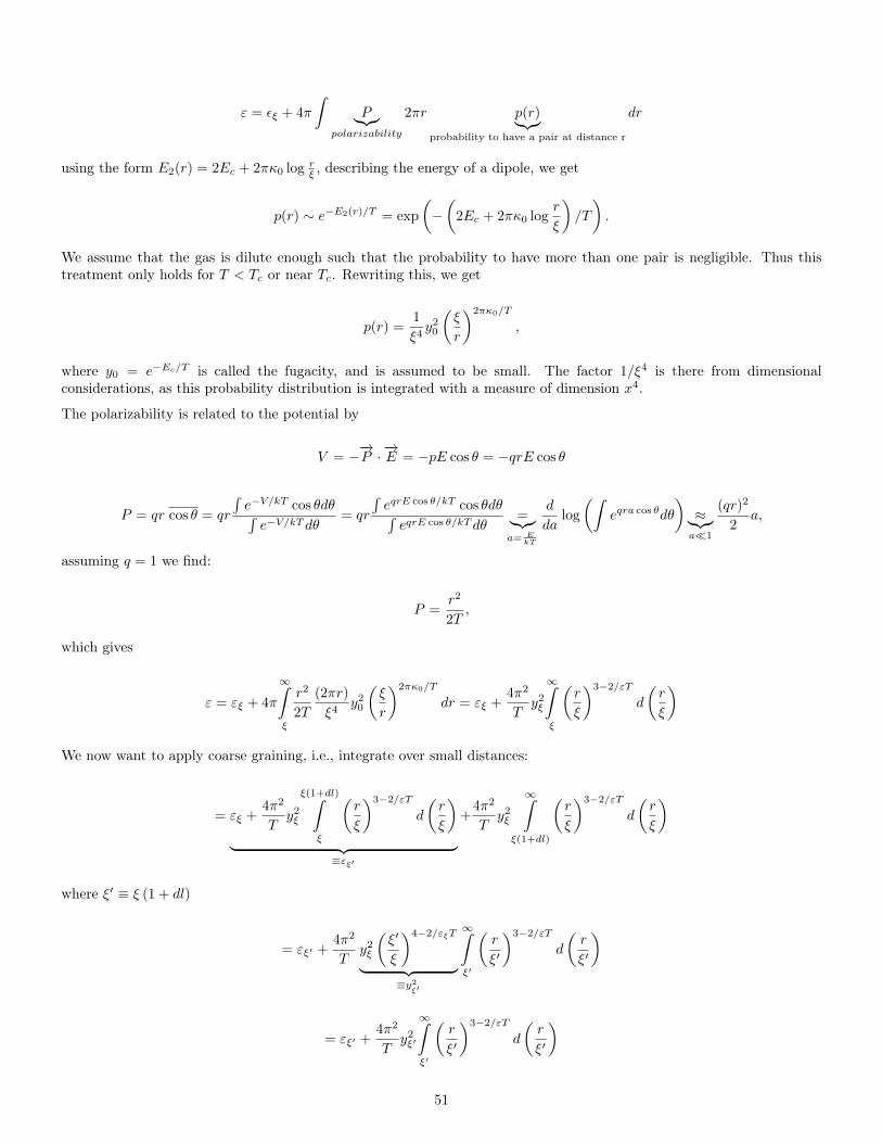
ε = εξ + 4π
ˆP︸︷︷︸
polarizability
2πr p(r)︸︷︷︸probability to have a pair at distance r
dr
using the form E2(r) = 2Ec + 2πκ0 log rξ , describing the energy of a dipole, we get
p(r) ∼ e−E2(r)/T = exp
(−(
2Ec + 2πκ0 logr
ξ
)/T
).
We assume that the gas is dilute enough such that the probability to have more than one pair is negligible. Thus thistreatment only holds for T < Tc or near Tc. Rewriting this, we get
p(r) =1
ξ4y2
0
(ξ
r
)2πκ0/T
,
where y0 = e−Ec/T is called the fugacity, and is assumed to be small. The factor 1/ξ4 is there from dimensionalconsiderations, as this probability distribution is integrated with a measure of dimension x4.
The polarizability is related to the potential by
V = −−→P ·−→E = −pE cos θ = −qrE cos θ
P = qr cos θ = qr
´e−V/kT cos θdθ´e−V/kT dθ
= qr
´eqrE cos θ/kT cos θdθ´eqrE cos θ/kT dθ
=︸︷︷︸a= E
kT
d
dalog
(ˆeqra cos θdθ
)≈︸︷︷︸a1
(qr)2
2a,
assuming q = 1 we find:
P =r2
2T,
which gives
ε = εξ + 4π
∞
ξ
r2
2T
(2πr)
ξ4y2
0
(ξ
r
)2πκ0/T
dr = εξ +4π2
Ty2ξ
∞
ξ
(r
ξ
)3−2/εT
d
(r
ξ
)
We now want to apply coarse graining, i.e., integrate over small distances:
= εξ +4π2
Ty2ξ
ξ(1+dl)ˆ
ξ
(r
ξ
)3−2/εT
d
(r
ξ
)︸ ︷︷ ︸
≡εξ′
+4π2
Ty2ξ
∞
ξ(1+dl)
(r
ξ
)3−2/εT
d
(r
ξ
)
where ξ′ ≡ ξ (1 + dl)
= εξ′ +4π2
Ty2ξ
(ξ′
ξ
)4−2/εξT
︸ ︷︷ ︸≡y2
ξ′
∞
ξ′
(r
ξ′
)3−2/εT
d
(r
ξ′
)
= εξ′ +4π2
Ty2ξ′
∞
ξ′
(r
ξ′
)3−2/εT
d
(r
ξ′
)
51

from the equation defining εξ′ ,
εξ′ = εξ + y2ξ
4π2
Tdl,
and the fact that dl is small, we get
dε
dl=
4π2
Ty2.
By definition
ξ′ ≡ ξ (1 + dl)⇒ dξ
ξ= dl⇒ ξ(l) = ξ0e
l.
The coarse-grained fugacity takes the form
y2ξ′ = y2
ξ + y2ξ
(2− 2
εT
)dl
dy2
dl= y2
(4− 2
εT
)Defining
κ =1
εTπ
dy
dl= (2− κπ) y +O(y3)
dκ−1
dl= 4πy2 +O(y4)
and for κπ < 2 y increases while for κπ > 2 it decreases.
x =2
κπ− 1
dκ−1 =π
2dx
π
2dx = 4π3y2
κ ≈ 2
π(1− x)
π
2dx = 4
dy
dl= 2xy,
dx
dl= 8π2y2
d2x
dl= (4πy)
2,d (4πy)
dl= 2x (4πy)
52

with x = 2x and y = 4πy we have
dx
dl= y2,
dy
dl= xy (33)
These are the KT RG flow equations.
We can define a constant of the motion by multiplying the first equation by x, the second by y and subtracting
d(x2 − y2
)dl
= 0 =⇒ x2 − y2 = const.
We remove the tildes from now on. Along the line x = −y
dy
dl= −y2
−dyy2
= dl⇒ 1
yξ− 1
y0= l = log
(ξ
ξ0
)
yξ =y0
1 + y0l≈ 1
l
y = −x = − 1
log(ξξ0
)at T = TC we have x = 0 ⇒ κ = κR
Tc= 2
π , εR = 12TC
where εR is the dielectric constant at TC .
The probability to find a pair at a distance r from one another at TC is
P (r) =y2
r4=
1
r4log2 (r/ξ0)
We now look at other regions of the phase diagram.
53

For T < TC , near y = 0
x2 − y2 = (T − TC) b2
we can assume a linear dependence because x2 − y2 changes sign when we change the relative sizes of T and TC
x = b√TC − T
κRTC
=2
π+ b√TC − T
This derivation breaks down in the area of positive x where y grows. This is because it was based on the assumption thatthe fugacity is small and the pair density is low.
For T > TC
y2 = x2 + b2 (T − TC)
dx
dl= x2 + b2 (T − TC)
ξ
ξ0
dl =
1
x0
dx
x2 + b2 (T − TC)
where we take x = 1 because at scales of order 1, our RG treatment breaks down
l =1
b√T − TC
tan−1
(x
b√T − TC
)∣∣∣∣1x0
≈ 1
b√T − TC
.
From this we can extract a length. We identify this temperature dependent length scale as the screening length
ξ+ = rsc = ξ0e1/b√T−TC
If we want to discover how many vortices we have, we can calculate the effective screening radius of a certain vortexconcentration and compare to the one we found. According to Debye
54
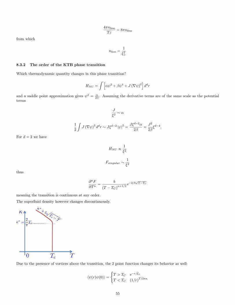
4πnfree
Tε= 8πnfree
from which
nfree =1
ξ2+
8.3.2 The order of the KTB phase transition
Which thermodynamic quantity changes in this phase transition?
HNU =
ˆ [αψ2 + βψ4 + J (∇ψ)
2]ddr
and a saddle point approximation gives ψ2 = α2β . Assuming the derivative terms are of the same scale as the potential
terms
J
ξ2∼ α
1
2
ˆJ (∇ψ)
2ddr ∼ Jξd−2 |ψ|2 =
Jξd−2α
2β=J2
2βξd−4.
For d = 2 we have
HNU ∝1
ξ2
Fsingular ∼1
ξ2
thus
∂nF
∂Tn=
b
(T − TC)n+1/2
e−2/b√T−TC
meaning the transition is continuous at any order.
The superfluid density however changes discontinuously.
Due to the presence of vortices above the transition, the 2 point function changes its behavior as well:
〈ψ(r)ψ(0)〉 =
T > TC e−r/ξ+
T < TC (1/r)T/2πκ
55
8.4 Coulomb gas and the Sine-Gordon mapping (Momentum RG)
8.4.1 Mapping between Coulomb Gas and the Sine Gordon model
SV =1
T
1
2ε0
∑ij
NiNjG(∣∣∣~Ri − ~Rj
∣∣∣ /ξ)+∑
N2i Ec
G(x) = −2 log (x)
z =∑
Ni=0,±1
exp (−SV )
where we drop vortices with charge larger than 1. Using the general formula for a Gaussian integral
ˆdx1...dxn
(2π)n/2
exp
(−1
2xiAijxj + xiJi
)= (detA)
−1/2exp
(1
2JiA
−1ij Jj
)
exp
(− 1
2ε0NiNjVij
)= det
(V −1
2ε
)1/21
(2π)1/2
ˆdϕ1..dϕnexp
(−1
2ϕiV
−1ij ϕj + iϕiNi
)and adding the core energy term
z = N
ˆDϕ(x)exp
−1
2
∑i 6=j
ϕ(xi)V−1 (xi − yi)ϕ(yi)2ε0T
Πi
∑Ni=0,±1,...
exp(iϕiNi +N2
i Ec/T)
≈ NˆDϕ(x)exp
−1
2
∑i 6=j
ϕ(xi)V−1 (xi − yi)ϕ(yi)2ε0T
Πi
(1 + 2 (cosϕi) exp (−Ec/T ))
≈ NˆDϕ(x)exp
−1
2
∑i 6=j
ϕ(xi)V−1 (xi − yi)ϕ(yi)2ε0T
exp(−y∑
2 (cosϕi))
V (q) = 1q2 ⇒ V −1(q) = q2 ⇒ V (x) = δ(x)∇2
= N
ˆDϕ(x)exp
(−1
2
ˆ(∇ϕ(x))
2d2x2ε0T +
2y
a2
ˆd2xcosϕ(x)
)changing variables to
√2ε0Tϕ, β = 1√
2ε0T,M = 2y0 = 2e−Ec/T
= N
ˆDϕ(x)exp
−1
2
ˆ(∇ϕ)2d2x︸ ︷︷ ︸
S0
+M
ˆd2x cos(βϕ)︸ ︷︷ ︸S1
56

8.4.2 (Momentum shell) Renormalization group of the sine Gordon Model
[Here we follow with some additional details chapter 10 of Ref. [6]]
We split a high momentum shell from the system (b > 1)
ϕΛ(x) =1√V
∑K<Λ
b
eikxϕK
︸ ︷︷ ︸ϕS(x)
+∑
Λb <K<Λ
eikxϕK
︸ ︷︷ ︸ϕF (x)
and since S0 is diagonal in momentum space,
zΛ =
ˆDϕSDϕF e−S0[ϕS ]−S0[ϕF ]−S1[ϕF+ϕS ]
=
ˆDϕF e−S0[ϕF ]
ˆDϕSe−S0[ϕS ]
´DϕF e−S0[ϕF ]−S1[ϕF+ϕS ]´
DϕF e−S0[ϕF ]
= zF
ˆDϕSe−S0[ϕS ]
⟨e−S1[ϕF+ϕS ]
⟩F
giving an effective action for the slow degrees of freedom:
Seff(ϕS) = S0 (ϕS)− log⟨e−S1[ϕF+ϕS ]
⟩F.
The basic idea here is to average over the fast degree of freedom a ϕf and obtain an effective action in terms of the slowvariables ϕs. The parameters of the action S are renormalized and the RG procedure is established.
We assume the core energy is small, hence M is small. Thus using the cumulant expansion log⟨1− S1 + 1
2S21
⟩= 〈S1〉 −
12
⟨S2
1
⟩+ 1
2 〈S1〉2 ,we get
Seff(ϕS) = S0 (ϕS)− 〈S1 (ϕF + ϕS)〉+1
2
⟨S2
1 (ϕF + ϕS)⟩− 1
2〈S1 (ϕF + ϕS)〉2
8.4.2.1 First order term
8.4.2.1.1 Integrating out the fast variables – thinning the degrees of freedom The first order term is
〈S1 (ϕF + ϕS)〉 =M
a2
ˆd2x 〈cos (β (ϕS + ϕF ))〉F
=1
2
M
a2
ˆd2x
∑σ=±1
eiβσϕS⟨eiβσϕF
⟩F
⟨eiβσϕF
⟩F
= e−12β
2〈ϕ2F 〉 ≡ e− 1
2β2G(0) ≡ A(0)
G(0) = 〈ϕF (0)ϕF (0)〉 =1
(2π)2
Λ
Λ−dΛ=Λ/b
d2k1
k2=
1
2π
ˆdk
k=
1
2πdlogΛ ≡ 1
2πdl
57

A(0) = e−12β
2〈ϕ2F 〉 = 1− β2
4πdl
Thus to first order
Seff(ϕS) =1
2
ˆ(∇ϕS)
2d2x+M
(1− β2
4πdl
)ˆd2x
a2cos (βϕS)
8.4.2.1.2 Rescaling We apply
x′ = x/b⇒ q′ = bq
where b = 11−dl
which doesn’t change S0
Seff(ϕS) =1
2
ˆ(∇ϕS)
2d2x′ +M
1 +
2− β2
4π︸︷︷︸dim
dl
ˆ d2x′
a2cos (βϕS)
M ′ = M (1 + (2− dim) dl)
M ′ −M =dM
dl= (2− dim)M
M(L) = M0
(L
a
)2−dim
M0 represents the fugacity. We can see that for dim < 2 the coefficient M grows and our approximation breaks. Thisallows us to obtain a scale which is an effective screening length, since beyond it there are many vortices and our treatmentbreaks down.
1 = M0
(ξ+a
)2−dim⇒ ξ+ =
(1M0
)1/(2−dim)
a.
It is useful to remember that an operator with a large dimension is irrelevant in the renormalization group sense
8.4.2.1.3 Field rescaling We neglected the fact that ϕS also depends on x when we changed variables to x′. We canshow that to first order this is trivial
ϕ(x) = ζϕS (x′)
ϕq = ζϕq′
we choose ζ = 1 to keep S0 invariant. This means
ϕq =
ˆd2xeiqxϕS(x) = b2
ˆd2x′ϕS(x′)eiq
′x′ = b2ϕq
giving
ζ = b2
58

8.4.2.2 Second order term
8.4.2.2.1 Integrating out the fast variables We now consider the O(M2) terms in the cumulant expansion ofSeff(ϕS):
2O(M2) =⟨S2
1 (ϕF + ϕS)⟩− 〈S1 (ϕF + ϕS)〉2
= M2
ˆd2xad
2xb⟨cos (β (ϕaF + ϕaS)) cos
(β(ϕbF + ϕbS
))⟩− 〈cos (β (ϕaF + ϕaS))〉
⟨cos(β(ϕbF + ϕbS
))⟩
=M2
4
ˆd2xad
2xb∑
σa,σb=±1
(⟨eiσaβϕ
aF eiσbβϕ
bF
⟩−⟨eiσaβϕ
aF
⟩⟨eiσbβϕ
bF
⟩)eiσaβϕ
aSeiσbβϕ
bS .
The sum over σa, σb = ± gives four terms. The one with σa = σb = 1 (whose integrand we denote by Y1) is given by
M2
4
ˆd2xad
2xb
(⟨eiβϕ
aF eiβϕ
bF
⟩−⟨eiβϕ
aF
⟩⟨eiβϕ
bF
⟩)eiβϕ
aSeiβϕ
bS ≡ M2
4
ˆd2xad
2xbY1eiβϕaSeiβϕ
bS .
Since the free part of the action is quadratic we have⟨e±iβϕ
aF
⟩= 1±〈iβϕaF 〉−
β2
2
⟨ϕa2F
⟩+ · · · = 1− β2
2
⟨ϕa2F
⟩= e−
β2
2 〈ϕa2F 〉.
(An alternative way to prove this identity is to complete to a square and perform the Gaussian integration.) Using thisidentity we find:
Y1 = e− β
2
2
⟨(ϕaF+ϕbF )
2⟩− e−
β2
2 〈ϕa2F 〉e−
β2
2 〈ϕb2F 〉 = e−β2〈ϕa2
F 〉(e−β
2〈ϕaFϕbF 〉 − 1)
≡ e−β2G(0)
(e−β
2G(xa−xb) − 1)≡ A2 (0)
(A2 (xa − xb)− 1
).
Averaging over the free field action S0 give the following expression for the function G:
G(xa − xb) =
Λ
Λ/b
eip(xa−xb)
(2π)2p2
d2p.
A similar term Y2 = Y1 when taking σa = σb = −1 and two other terms where the sign in the first exponent is flipped,giving
O(M2) =M2
4
ˆd2xad
2xb
[A2 (0)
(A2 (xa − xb)− 1
)cos(β(ϕaS + ϕbS
))+A2 (0)
(1
A2 (xa − xb)− 1
)cos(β(ϕaS − ϕbS
))].
For x bΛ the oscillations in G(x) ∝
Λ
Λ/b
eipx
p2 dp lead to G(x) ≈ 0⇒ A2(x) ≈ 1, and thus A2(x) 6= 1 only for small x < b/Λ.
Hence xa is very close to xb. Setting xa = xb the first term contains cos (2βϕaS) which is a vortex of charge 2 made by twooverlapping charge 1 vortices - even though we didn’t include such vortices in our partition function. In such situationswe say that the RG procedure generated a new term. For parameters near the KTB transition (large
The second will act like a derivative.
Defining z = xa+xb2 , ξ = xa − xb, around xa = xb
O(M2) =M2
2
ˆd2zd2ξ
[A2 (0)
(A2 (ξ)− 1
)cos (2βϕS (z)) +A2 (0)
(1
A2 (ξ)− 1
)cos (ξβ∂zϕS (z))
].
59

and since ξ is very small we can use the approximation cos (ξβ∂zϕS (z)) ≈ 1− 12 (ξβ∂zϕS (z))
2 to find:
O(M2) =M2
2
ˆd2z
[a1 cos (2βϕS (z)) + a3 −
a2β2
2(∇ϕS)
2
],
wherea1 =
ˆd2ξA2 (0)
(A2 (ξ)− 1
), a2 = ξ2
ˆd2ξA2 (0)
(1
A2 (ξ)− 1
), a3 =
ˆd2ξA2 (0)
(1
A2 (ξ)− 1
).
In addition
G(ξ) =1
(2π)2
Λ
Λ/b
eipξcosθ
p2pdpdθ =
1
2πJ0 (ξΛ)
dΛ
Λ
where J0 is a Bessel function. It features oscillations which are due to the fact that we used a sharp cutoff. Expandingthe exponent in A,
a2 ≈ β2 1
2π
ˆd2ξJ0 (ξΛ)
dΛ
Λ︸︷︷︸dl
≡ β2dlC
where C is a number. Carefully examining the last integral we see that it does not converge, it can be shown (we do notshow it here) that when the sharp cutoff is replaced by a soft one, the expression for C converges. This gives
O(M2) =1
2M2β4 (2C) dl (∇ϕS)
2.
Gathering terms of order M as well we write:
Seff =1
2
ˆd2x
[(1 +M2β42Cdl
)(∇ϕS)
2+M
(1− β2
4πdl
)cos (βϕS) + a1M
2 cos (2βϕS) + a3
]where the term ∝ a2 is irrelevant in the RG sense, and the term a3 is a normalization constant. The normalizationconstant is not important as it will drop off in all the Gaussian averaging procedures.
8.4.2.2.2 Rescaling Rescaling the space x as in sub paragraph 8.4.2.1.2 we obtain the equation:
M ′ = M
1−
2︸︷︷︸from rescaling of x
−β2
4π
dl
8.4.2.2.3 Field Rescaling Unlike the first order case the field rescaling here is not trivial. Defining
ϕnew =√
1 +M2β42CdlϕS ≈(1 +M2β4Cdl
)ϕS
β′ = β(1−M2β4Adl
)So that eventually
Seff == N ′ˆDϕ(x)exp
−1
2
ˆ(∇ϕ)2d2x︸ ︷︷ ︸
S0
+M ′ˆd2x cos(β′ϕ)︸ ︷︷ ︸S1
60

To complete the RG equation near the KTB transition we define β2
4π = 2 + x, y =√
2M and get the RG equations as inthe real space approach in Eq. (33)
dy
dl= −xy, dx
dl= −y2. (34)
The sign changed compared to the former renormalization is because now we go to smaller momenta vs. longer lengths.
61
9 Introduction to Graphene (Tutorial)
This chapter should be taught at the beginning of the course.
9.1 Tight binding models
We would like to analyze the general problem of non-interacting electrons in a periodic potential that results from a latticeof ions. We note that the tight binding method is more general than what is presented here. If you would like to learnmore, the book by Ashcroft and Mermin has a very good chapter on this subject.
In first quantization, we write the corresponding Schrodinger equation as(− ~2
2m∇2 + Vion(~r)
)ψ(~r) = Eψ(~r), (35)
with Vion(~r) =∑
R Vi(~r − ~R). Here, Vi(~r) is the contribution to the potential from a single ion located in the origin, andthe set of vectors ~R are the lattice vectors.
We start by approaching the problem from the limit where the ions are extremely far apart. In this limit, the single-particleeigenstates will be those that correspond to the problem of an electron affected by a single ion:(
− ~2
2m∇2 + Vi(~r)
)φn(~r) = Enφn(~r). (36)
The solutions are bound to the corresponding ion, hence the name tight binding.
Once the spatial extent of the single ion wavefunctions becomes comparable to the lattice spacing, this stops being true,and coupling between different sites must be taken into account. However, within the tight binding formalism, we writethe corrections to the above ideal picture in terms of the localized wavefunctions φn.
The coupling between φn(~r) and φn(~r − ~R) , which correspond to different ions introduces matrix elements of the form⟨φn(~r − ~R) |H|φn(~r)
⟩≡ −tn(~R). (37)
Working in second quantization, we define an operator c†n(~R) that creates an electron in the state φn(~r − ~R). In terms ofthese, we write the Hamiltonian in the quadratic form
H = −∑
n,R,R′
tn(~R− ~R′)c†n(~R)cn(~R′). (38)
9.2 Graphene
Graphene is a material made of a single atomic layer. This two dimensional system is made of Carbon atoms, arrangedin a honeycomb lattice, as depicted in figure 12a.
Remember that a honeycomb lattice is actually an hexagonal lattice with a basis of two ions in each unit cell. If a is thedistance between nearest neighbors, the primitive lattice vectors can be chosen to be
~a1 =a
2
(3,√
3),~a2 =
a
2
(3,−√
3),
and the reciprocal-lattice vectors are spanned by
~b1 =2π
3a
(1,√
3),~b2 =
2π
3a
(1,−√
3).
The first Brillouin zone is shown in figure 12b.
In this tutorial we want to calculate the spectrum of non-interacting electrons in this material. We restrict ourselves hereto the case of nearest-neighbor tunneling terms only. In the homework, you will extend this to slightly more complicated
62

(a) (b)
Figure 12
situations, and you will see that the important features of the spectrum remain the same as long as very large deviationsare not included.
We directly work in second quantization, and define the annihilation operators of an electron at the lowest orbital centeredaround atoms A and B:
A(~R), B(~R).
These operators satisfy the anti-commutation relationsA(~R), A†(~R′)
=B(~R), B†(~R′)
= δ~R,~R′ ,
A(~R), A(~R′)
=B(~R), B(~R′)
=A(~R), B(~R′)
=A(~R), B†(~R′)
= 0.
Notice that the nearest neighbor of an ion of type A is always an ion of type B (and vice versa). We therefore write thetight binding Hamiltonian as
H = −t∑〈~R,~R′〉
A†(~R)B(~R′) + h.c. = −t∑~R,δ
A†(~R)B(~R+δ) + h.c.
The vectors ~δ, connecting the A atoms to their nearest neighbors are given by
~δ1 =a
2
(1,√
3), ~δ2 =
a
2
(1,−√
3), ~δ3 = a (−1, 0) .
We want to diagonalize the Hamiltonian. Since we have a translation invariant system, it is a good idea to go to Fourierspace and write
A(~R) =1√N
∑~k∈BZ1
A(~k)ei~k·~R, B(~R) =
1√N
∑~k∈BZ1
B(~k)ei~k·~R.
Like the operators in real space, the non-vanishing anti-commutation relations areA(~k), A†(~k′)
=B(~k), B†(~k′)
= δ~k,~k′ ,
and the rest are zero. Plugging this into the Hamiltonian, we now have
H = −t∑~R,δ
A†(~R)B(~R+δ) + h.c. = − t
N
∑~R,δ
∑~k,~q
ei~q·δei~R·(~q−~k)A†(~k)B(~q) + h.c. =
= −t∑δ
∑~k,~q
ei~q·δA†(~k)B(~q)
1
N
∑~R
ei~R·(~q−~k)
+ h.c.
63

Using the fact that 1N
∑~R e
i ~R·(~q−~k) = δ~q,~k, we get
H = −t∑~k,~δ
ei~k·δA†(~k)B(~k) + h.c.
If we define ψ(~k) =(A(~k), B(~k)
)T,we can rewrite this as
H =∑~k
ψ†(~k)h(~k)ψ(~k),
where the matrix h, called the Bloch Hamiltonian, takes the form
h =
(0 f(~k)
f∗(~k) 0
),
with f(~k) = −t∑δ e
i~k·δ = −t(e−ikxa + 2eikxa/2 cos
(kya√
32
)).
Since h is an Hermitian matrix, it is guaranteed that we can diagonalize it using some unitary matrix U , such that
UhU† =
(ε+ 00 ε−
).
Defining Uψ = (c+, c−)T , we can write
H =∑~k
ε+(~k)c†+(~k)c+(~k) + ε−(~k)c†−(~k)c−(~k),
with the non-vanishing anti-commutation relationsc†+(~k), c+(~k′)
=c†−(~k), c−(~k′)
= δ~k,~k′ .
Notice that we have two bands, one for each element of the unit cell, and the corresponding energy spectra are given byε±(~k).
We understand that in order to get the spectrum, we need to diagonalize the Bloch Hamiltonian h.
The corresponding eigenvalues are given by
ε± = ±∣∣∣f(~k)
∣∣∣ = ±t√
3 + 2 cos(√
3kya)
+ 4 cos(√
3kya/2)
cos (3kxa/2).
The spectrum is shown in Fig. 13a.
9.3 Emergent Dirac physics
Notice that the two bands touch at some points in the first Brillouin zone. Since Graphene has one accessible electron peratom, we get by taking spin into account that the lower band is exactly filled. This means that if we would like to discusssmall excitations above the ground state, the excitations that will contribute are those near the crossing points.
To write the low energy theory, we would therefore like to identify these points. We get them from the condition f(~k) = 0.The two real equations that result from this requirement are
cos (kxa) + 2 cos (kxa/2) cos
(kya√
3
2
)= 0 (39)
− sin (kxa) + 2 sin (kxa/2) cos
(kya√
3
2
)= 0. (40)
64

(a) (b)
Figure 13
We can manipulate equation 40 such that it takes the form
sin (kxa/2)
(− cos
(kxa
2
)+ cos
(kya√
3
2
))= 0.
So we have two options: either sin (kxa/2) = 0 (which means that cos (kxa/2) = ±1), or cos(kxa
2
)= cos
(kya√
32
).
The first option gives us the points(
0,± 4π3√
3a
)plus any reciprocal lattice vector. The second option gives us ± 2π
3a
(1, 1√
3
),
and ± 2π3a
(1,− 1√
3
)(again, up to reciprocal lattice vectors).
Actually, all the points listed above sit in the corners of the first Brillouin zone. A simple inspection shows that the aboveset of k-space vectors is not independent: the set of vectors
(0, 4π
3√
3a
), 2π
3a
(1,− 1√
3
), 2π
3a
(−1,− 1√
3
)can be connected by
a reciprocal lattice vector. This is correct for the set(
0,− 4π3√
3a
), 2π
3a
(−1, 1√
3
), 2π
3a
(1, 1√
3
)as well. To see this, we write(
0,4π
3√
3a
)+~b2 =
2π
3a
(1,− 1√
3
)(41)
(0,
4π
3√
3a
)−~b1 =
2π
3a
(−1,− 1√
3
). (42)
The other equivalence relations result from taking linear combinations of the above equations. We choose one representativevector from each set. These are conventionally called K and K ′:
~K =2π
3a
(1,
1√3
), ~K ′ =
2π
3a
(1,− 1√
3
).
Remember that the energy bands cross at these points, and the gap closes. Because of that, there are two branches of lowenergy excitations - one of excitations with a given momentum close to K and another close to K ′.
Therefore, if we would like to focus on the low energy physics, we expand the Hamiltonian around each of these points.Expanding around K ′, for example, we get
f( ~K ′ + ~q) ≈ −3ta
2e−
2πi3 (qy + iqx) .
65

This means that the Hamiltonian can be approximated as
h(K ′ + q) = −3ta
2
(0 e−
2πi3 (qy + iqx)
e2πi3 (qy − iqx) 0
).
Upon changing the phases of A and B, which physically means changing the phases of the basis wavefunctions φn, thismatrix can be brought to the form
h( ~K ′ + ~q) = ~vF ~q · ~σ, (43)
where σ is the vector of Pauli-matrices. This is just the 2D massless Dirac Hamiltonian, which describes free relativisticelectrons, where the speed of light has been replaced by vF = 3ta
2~ .
Remember that the Dirac Hamiltonian takes the form HDirac = c∑i αipi +βmc2, where the matrices α and β satisfy the
relationsβ2 = 1
αi, β = 0
αi, αj = 2δij .
The effective Hamiltonian in equation 43 takes exactly this form in 2D, if we identify αi = σi, and m = 0.
The eigenvalues and eigenfunctions of this equation are
E = ±~vF |~q| , ψ± =1√2
( eiθq/2 ,±e−iθq/2 )T .
Here, θq is the angle of the planar vector ~q with respect to the x-axis.
Note that the phase of the wavefunction changes by π as q winds around the origin, and completes a full winding as wewind twice around the origin. The phase after a full cycle does not depend on the trajectory. We can view this phase asa vortex, and the corresponding winding number as an integer which characterizes this Dirac cone. This is an example ofa topological property, as it is insensitive to small deviations.
You will see in the homework how this topological property, together with the symmetries of the problem, makes it difficultto get rid of the Dirac cones. This means that the effective Dirac theory in our system is not an artifact of our nearestneighbor approximation, and can actually be expected to be observed in experiments. Indeed, the Dirac spectrum hasbeen successfully measured (see Fig. 13b).
Note that a similar derivation would give us, h( ~K + ~q) = h∗( ~K ′ + ~q), and we get the same spectrum around K.
If we want to describe the full low energy theory, we have two independent Dirac modes, one around K and anotheraround K ′. It’s therefore useful to work in a basis Ψ =
(A ~K+~q, B ~K+~q, A ~K′+~q, B ~K′+~q
), in terms of which the full low
energy Hamiltonian takes the form
h = vF
((~q · σ)
∗0
0 ~q · σ
).
We have found emergent Dirac physics. The physical picture we have at large length scales (that is, small q’s) is completelydifferent from the physics at the microscopic level. We started from a problem of non-relativistic electrons, and got thatthe low energy physics of the problem corresponds to that of relativistic fermions.
This is very exciting because now can use this fact to directly measure relativistic effects, and even some which havenever tested in any particle physics experiment. As an example of such a property, the Klein paradox, where a relativisticelectron, obeying the Dirac equation, is fully transmitted after hitting a very strong potential barrier, has been measuredin Graphene.
66

10 The Quantum Hall Effect – This chapter is still under construction
A nice review of the quantum Hall Effect is given in [5] it includes discussions of Graphene as well.
10.1 Classical Hall Effect
Figure 14: The Hall effect in classical system, current is driven in the x direction and in the presence of magnetic fieldthe Lorentz force pushes electrons to the boundaries of the sample. This process continues until the electric field due tothe electrons accumulated at the boundaries cancels the Lorentz force
The classic Hall experiment is depicted in Fig. 14. In response to the electric Field Ex current Jx is flowing in the wire.In addition due to the magnetic field B in the z direction a Lorentz force deflect the electrons. The deflected electronsare accumulated in the sample boundary and build up an electric field Ey that cancels the Lorentz force. Working in theconvention e = − |e| we find:
e
c~v × ~B = −eEy.
Defining j in terms of the carrier density n as j = env we find:
Benv
c× z = −enEy ⇒ ~E = − B
enc~J × z,
which gives
EyJx≡ RB =
−Benc
.
Hence, measuring the Hall voltage allows measuring the carrier density n and the sign of their charge. Notice that in theabsence of impurities the current flows in a direction that is perpendicular to both the the electric and the magnetic field~J ∝ ~E × ~B.
If we add impurities, quantify their strength by the mean free collision time τ between them the EOM become:
m~v = e ~E +e
c~v × ~B − m~v
τ⇒ ~J =
ne2
m~E +
e
cm~J × ~B − ~J/τ.
We solve the equation in the frequency space, with (i) ~J = iω ~J and (ii) the matrix relation between ~J and ~E
~E =
(ExEy
)= ρ ~J =
(ρxx ρxyρyx ρyy
)(JxJy
)we find:
ρ =
(mne2τ (1 + iωτ) B
nec
− Bnec
mne2τ (1 + iωτ)
).
67

Figure 15: the Hall conductance σxy as a function of magnetic
Using the matrix relation demand careful examination of the boundary conditions, for example assuming that we applyelectric field ~E = Ex in the presence of magnetic filed, ~B = Bz because current is not flowing in the y direction we willobtain Ey = ρxyJx.
We can rearrange ρ in the form:
ρ =1
σ0
(1 + iωτ ωcτ−ωcτ 1 + iωτ
),
where σ0 = ne2τm , ωc = eB
mc . Inversion of the resistivity matrix to the conductivity we have:
σ (ω = 0) =σ0(
1 + (ωcτ)2) ( 1 ωcτ
−ωcτ 1
)−→ωcτ1
(σ0
(ωcτ)2 −necBnecB
σ0
(ωcτ)2
). (44)
We note that for large ωcτ (large B) both the resistivity (ρxx and ρyy) and conductivity (σxx and σyy) on the diagonalare negligible (with ω = 0) with respect to the Hall terms.
This "wired"situation that both resistance and conductance are small is special to the motion of electrons in strongmagnetic field. To understand qualitatively the origin of this behavior we note that the terms on the diagonal can bewritten as:
e2n
m
[τ
1
(ωcτ)2
]
giving
τeff =1
ω2cτ
From dimensional considerations we can define a diffusion constant. [D] = [lv] = v2τ = l2/τ with l typical step lengthin a random motion and τ the typical time between steps. And hence (since the electrons move typically in the Fermivelocity) we have
68

D = v2F τeff =
(vFωc)2
τ=R2c
τ.
In strong magnetic field the typical step is Rc the cyclotron radius and the typical time between "hoping between circles" isτ . We note the surprising fact that increasing the impurities and hence decreasing τ will actually increase the conductivity.This can be explained by the fact that without impurities the electrons will simply perform circular orbits. The scatteringfrom the impurities will cause them to move in the direction of the external field.
10.2 Quantum Hall effect
The (Integer) Quantum Hall effect was discovered in 1980 by Klaus von Klitzing who measured the Hall resistancein a two-dimensional electron gas, realized with a silicon metal-oxide-semiconductor field-effect transistor. The Hallconductance was quantized of e2/hν with ν being an integer. Later, in 1982 Dan C. Tsui, Horst L. Stormer, and ArtC. Gossard observed conductance quantization at a fractional values ν = 1/3 more fraction were measured later onν = 2/5, 3/7, 2/3, 3/5, 1/5, 2/9, 3/13, 5/2, 12/5 . . . . The fractional values are observed originally and in most experimentslater on heterostructure of Aluminium Gallium Arsenide/ Gallium Arsenide. In the boundary between the two materialsa clean two dimensional electron gas is formed. Recently quantum and fractional Hall effect where also observed inGraphene.2
Two Nobel prizes were awarded for the discoveries and the explanation of the Integer and fractional quantum Hall effect.The purpose of this chapter is to highlight the experimental finding and to show how we use topological arguments toexplain the novel state of matter that give integer values for the Hall conductance.
The discussion here tries to exemplify the dialogue between theory and experiment. Experimental results give hints andclues for the state of the system then clever arguments lead to additional conclusions about the nature of the system,those are drawn even without having a microscopic theory.
10.2.1 Experimental observations
Fig. 16 depicts typical experimental observation of the quantum Hall effect, the main effects are:
1. Quantized values of the Hall resistance
The Hall resistance show plateaus at
ρxy =h
e2ν, ν ∈ N
With a stronger field there are also plateaus at fractional values
ν =1
3,
2
5,
3
4, ...
2. Effect of disorder It was found experimentally that for cleaner samples we have more plateaus however thatplateaus are narrower.
3. Vanishing longitudinal resistance RxxAs we can see in the Fig. 16 at small magnetic field there are small oscillations in the resistance these are knownas the Shubnikov-deHaas oscillations, similar oscillations in the magnetization are deHaas van Alphen oscillations).At stronger magnetic field when plateaus are developed in the Hall resistance Rxy the longitudinal resistance Rxxis close to zero. Notice that due to the strong magnetic field, not surprisingly, the longitudinal conductance is alsovery small. The temperature dependance of the resistance is not shown in Fig. 16, but it was found that it increasesexponentially with the temperature, i.e., σ ∼ e−T0/T .
2Notice that in a square 2D sample of thickness d and linear dimension Lx = Ly = L the resistance Rxx = ρ LxdLy
= ρd.
69

Figure 16: Here we plot the Hall resistance Rxy and the resistance Rxx In the classical Hall effect Rxx is constant andRxy depends linearly on the Magnetic field. As we see the experimental result are quite different, Rxx fluctuates with themagnetic field and is zero at filling integer and fractional filling factor.
10.3 Basic explanation of the quantization effect
The Hamiltonian describing electrons moving in three dimensions in the presence of magnetic field is given in Landau’sgauge by:
H =−~2
2m
∂2
∂y2+
1
2m(~kx − eBy)
2+ eExx+ U(x, y) +
k2z
2m− µ. (45)
In finite width samples (in the z direction) electrons can not move in the z direction hence kz = πnz/Lz is quantized. Wewill assume henceforth that only the first sub-band with nz = 1 is occupied and absorb the energy k2
z/2m in the definitionof µ . The potential U(x, y) describes the effect of disorder – scattering of the electrons due to impurities. In principle,we should include also interaction effects between the electrons. Microscopically, these interactions are responsible for theformation of the fractional states.
The motion of the electrons in a strong electric field lead to the formation of Landau’s levels. Taking periodic boundaryconditions in the x direction, (having a Corbino geometry) we obtain a set of of Landau levels as follows. First choose aconvenient gauge ψ(x, y) = eikxφ(y) the Schrodinger equation become:
Hψ(x, y) = eikxx[
1
2m(~kx − eyB)
2+
1
2m∂2y − µ
]φ(y) (46)
with the periodic boundary condition in the x direction we have kx = 2πL nx with nx an integer. Defining now:
ynx =2π~Be
nx =l2BLx
nx; Bl2B ≡h
e= Φ0
we obtain
70
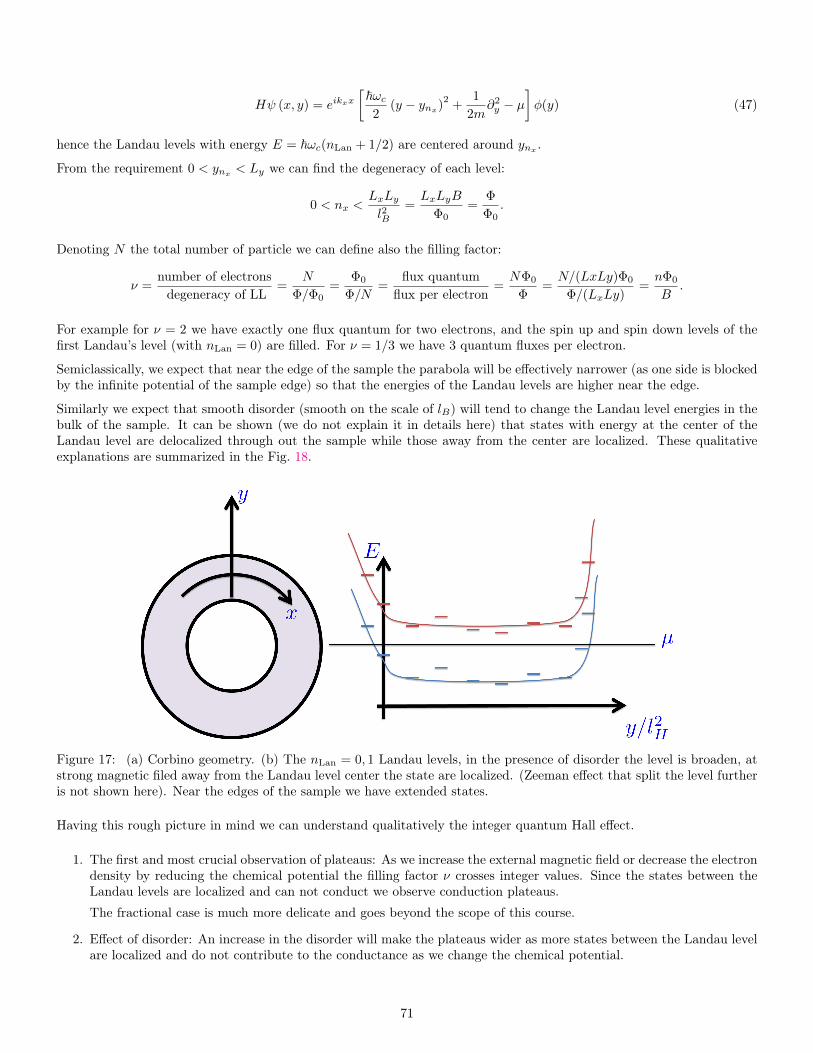
Hψ (x, y) = eikxx[~ωc2
(y − ynx)2
+1
2m∂2y − µ
]φ(y) (47)
hence the Landau levels with energy E = ~ωc(nLan + 1/2) are centered around ynx .
From the requirement 0 < ynx < Ly we can find the degeneracy of each level:
0 < nx <LxLyl2B
=LxLyB
Φ0=
Φ
Φ0.
Denoting N the total number of particle we can define also the filling factor:
ν =number of electronsdegeneracy of LL
=N
Φ/Φ0=
Φ0
Φ/N=
flux quantumflux per electron
=NΦ0
Φ=N/(LxLy)Φ0
Φ/(LxLy)=nΦ0
B.
For example for ν = 2 we have exactly one flux quantum for two electrons, and the spin up and spin down levels of thefirst Landau’s level (with nLan = 0) are filled. For ν = 1/3 we have 3 quantum fluxes per electron.
Semiclassically, we expect that near the edge of the sample the parabola will be effectively narrower (as one side is blockedby the infinite potential of the sample edge) so that the energies of the Landau levels are higher near the edge.
Similarly we expect that smooth disorder (smooth on the scale of lB) will tend to change the Landau level energies in thebulk of the sample. It can be shown (we do not explain it in details here) that states with energy at the center of theLandau level are delocalized through out the sample while those away from the center are localized. These qualitativeexplanations are summarized in the Fig. 18.
Figure 17: (a) Corbino geometry. (b) The nLan = 0, 1 Landau levels, in the presence of disorder the level is broaden, atstrong magnetic filed away from the Landau level center the state are localized. (Zeeman effect that split the level furtheris not shown here). Near the edges of the sample we have extended states.
Having this rough picture in mind we can understand qualitatively the integer quantum Hall effect.
1. The first and most crucial observation of plateaus: As we increase the external magnetic field or decrease the electrondensity by reducing the chemical potential the filling factor ν crosses integer values. Since the states between theLandau levels are localized and can not conduct we observe conduction plateaus.
The fractional case is much more delicate and goes beyond the scope of this course.
2. Effect of disorder: An increase in the disorder will make the plateaus wider as more states between the Landau levelare localized and do not contribute to the conductance as we change the chemical potential.
71

Interestingly from the third experimental observation, i.e., the exponential temperature dependance of the resistances wecan conclude that there us a gap in the system. This will lead us later on the a set of conclusions.
1. In the classical limit we saw that due to the matrix structure of the resistance both the conductance and the resistanceare small compared to the off diagonal terms. 3
Experimentally it is observed that bothρxxh/e2
∼ e−T0/T
and we expect that also the conductance will have similar exponential dependance on the temperature.As we know the dissipative conductance is related to the rate W of absorbing external electro-magnetic field W ∼~J ~E ∼ σE2. To calculate this rate we can use the standard Fermi golden rule:
W ∼∑
initial states
e−εi/t
z
∑final states
~ω |〈f |H ′|i〉|2 (δ (εf − εi − ω) + δ (εf − εi + ω)) ,
with H ′ presenting the interaction of the electrons in our sample with the external EM field. εi the energy of theinitial state and εf the energy of the final states. Since we are interested in the limit of ω = 0 we have to requireεf ∼ εi. If there is a gap in the system then the factor ∝ e−εi/T will yield an exponential dependance in thetemperature.
10.4 Additional conclusions, based on the existence of a gap in the system
10.4.1 Edge states
Figure 18: (a) Semiclassically: in the bulk electrons move in circles and near the edge in skipping orbits. (b) When wehave a gap we find σxx = 0, then on the boundary separating σxy 6= 0 and σxy = 0 we must have an edge state.
Due to the exponential dependance on the temperature we expect that at zero temperature σxx ≈ 0 so that the electronsmove perpendicularly both to the electric field and to the magnetic field. We saw that
σxy =νe2
h, σxx = 0
and since the current is perpendicular to both the magnetic and electric field, if we look at an edge parallel to the electricfield we have a current towards the edge. As we reach the edge, since charge can not be accumulated on the edge, wemust have a current parallel to the edge.
This can be explained semiclassically in terms of skipping orbits performed by electrons near the edge. As we alreadyso the motion of the electrons is perpendicular to both E and B the edge its self exert an electric field on the electronsperpendicular to the edge so that electron will move along the edge.
3Notice that in thin sample the resistance is Rxx = ρxxLx/(Lyd) so that for a square sample with Lx = Ly the resistance R is equal tothe resistivity ρ/d. Similarly the conductance G is equal to the conductivity σ times the thickness d. We therefore usually do not distinguishbetween conductivity and conductance (per square) or resistivity and resistance per square when discussing 2D systems.
72

10.4.2 Fractional charges (Laughlin)
Figure 19: A change of the flux by φ0 does not change the spectrum but push charges from edge to edge.
Noting σxy = ν e2
h we will show now (following an argument by Laughlin) that there are fractional charges in the system.To do so we will use to important concepts:
1. The adiabatic principle: Assume that the system has a gap Eg for excitations above the (non degenerate) groundstate |Ψ (R(t))〉. When we change the parameters R(t) controlling the system at a slow rate Γ such that Eg ~Γthen the system will follow the ground state |Ψ (R(t))〉 (and will not be excited to a different state).
2. Gauge invariance: Byers and Yang (1961): showed using gauge invariance, that spectra of rings threaded by fluxare periodic in the flux with period of the flux quantum φ0 = h/e. The Byers and Yang theorem is valid also in thepresence of disorder and electron electron interaction.
Assuming we have a solenoid passing through the core of the system and we slowly (compared to the gap in the system)increase the flux. This generates an electric field in the x direction. (See Fig. 19) As there is a constant magnetic filedperpendicular to the sample a Hall current will flow perpendicular to ~B and ~E, which will cause electrons to flow outwardtowards the edge.
From gauge invariance, after changing the flux by a flux quantum φ0 we must return to the original spectrum. Hence thetotal charge the transferred between the edges is:
∆Q =
ˆIydt =
ˆJ2πrdt = σxy
ˆ2πrEdt = σxy
ˆ∂Φ
∂tdt = σxy∆Φ
Using δΦ = φ0 = h/e we obtain: ∆Q = ν e2
hhe = νe
i.e. a fractional charge was transferred from edge to edge.
10.4.3 Quantization of Hall conductance in the integer case
In the presence of the flux the boundary condition on kx after Eq. (46) are modified so that eikxL = ei2πΦ(t)/φ0 whichgives:
kx(t) =2π
L
(n+
Φ(t)
φ0
).
Pictorially, the parabolas of the Landau levels are adiabatically moving in the y direction until for Φ(t) = φ each parabolasubstitution the position of its neighbor. For the ν = 1 case each state was filled exactly by 1 electron so that in thisprocess 1 electron was transected from edge to edge. So that we have:
73

Figure 20: A change of the flux adiabatically move the Landau states. At φ0 each state is replacing its neighbor position.
e = ∆Q =
ˆIydt =
ˆJ2πrdt = σxy
ˆ2πrEdt = σxy
ˆ∂Φ
∂tdt = σxy∆Φ
hence for a change of one flux quantum
σxy =e
Φ0=e2
h
10.4.4 Quantization of the Hall conductance and Chern numbers using Linear response
In this subsection we are following an argument by Thouless that lead to quantization of the Hall conductance. Thisargument is very similar to Laughlin arguments mentioned above and also related to works by Berry (The Berry phase)and Avron. It is based on a formalism that is called "The Linear Response" formalism.
the y direction, see Fig. 23
In the presence of electric field the Hamiltonian of Eq. (45) is modified by adding a term
δH = eEx
where E is the applied electric field in the x direction. For E = 0 we must have
Jy =⟨
Ψ0|Jy|Ψ0
⟩= 0.
Here |Ψ0〉 is the many body ground state. We now assume that E is small and calculate the change in the current usingperturbation theory.
The first order perturbation theory (in the operator E x) for the ground state gives
δ |Ψ0〉 =∑m6=0
x0m
E0 − Em|m〉 .
Writing it in a slightly different and compact form, that will simplify the notation later we have:
δ |Ψ0〉 = eE PE − H
x |Ψ0〉
= eE∑m
PE − H
|m〉 〈m| x |Ψ0〉 =∑m6=0
eEE0 − Em
xm0
where P is a projection operator that projects out the ground state and E = E0.
Similarly we have for the bra part of the ground state:
δ 〈Ψ0| = eE 〈Ψ0| xP
E − H.
74

Figure 21: This figure is taken from Thouless []
Combining the expressions we find:
〈Ψ| Jy |Ψ〉 = (〈Ψ0|+ δ 〈Ψ0|) Jy (|Ψ0〉+ δ |Ψ0〉)
= eE(⟨
Ψ0|JyP
E − Hx|Ψ0
⟩+
⟨Ψ0|x
PE − H
Jy|Ψ0
⟩). (48)
In addition we have the relation
Jx = e∂x
∂t=ei
~
[H, x
]⇒
−i~eJx |Ψ0〉 =
[H, x
]|Ψ0〉 = (H − E) x |Ψ0〉 ⇒
x |Ψ0〉 =i~e
PE − H
Jx |Ψ0〉 . (49)
Substituting Eq. (49) (and a similar expression for the bra term.) in Eq. (48) we obtain
Jy = −i~E
⟨Ψ0
∣∣∣∣∣∣∣JyP(
E − H)2 Jx − Jx
P(E − H
)2 Jy
∣∣∣∣∣∣∣Ψ0
⟩(50)
75

We can continue and express the current operators in a different form. Closing the two leads in each direction to form aloop which allows to pass a flux through it, using the relation
J =δH
δA, (51)
and defining Φv as the flux through the loop in the plane perpendicular to y and ΦJ as the flux in the loop in the planeperpendicular to x (see Fig. 23) we have
Jx =∂H
∂Φv, Jy =
∂H
∂ΦJ.
Substituting in Eq. (50) we have:
σH (Φv,ΦJ) = i~
⟨Ψ0
∣∣∣∣∣∣∣∂H
∂ΦJ
P(E − H
)2
∂H
∂Φv− ∂H
∂Φv
P(E − H
)2
∂H
∂ΦJ
∣∣∣∣∣∣∣Ψ0
⟩.
We can further simplified the expression by noting that writing
H = H0 +∂H
∂ΦvδΦv
we haveδ |Ψ〉 = δΦv
PE −H
∂H
∂Φv|Ψ0〉
giving ∣∣∣∣ ∂H∂Φv
⟩=
PE −H
∂H
∂Φv|ψ0〉
and henceσH = i~
(⟨∂ψ0
∂Φv
∣∣∣∣∣∣∣∣ ∂ψ0
∂ΦJ
⟩−⟨∂ψ0
∂ΦJ
∣∣∣∣∣∣∣∣ ∂ψ0
∂Φv
⟩).
Since the result cannot depend on the flux we used to perturb the system and create an electric field (as long as there isa gap in the spectrum), we can integrate over it and find:
σH = i~( eh
)2h/cˆ
0
dΦJ
h/cˆ
0
dΦv
(⟨∂ψ0
∂Φv
∣∣∣∣∣∣∣∣ ∂ψ0
∂ΦJ
⟩−⟨∂ψ0
∂ΦJ
∣∣∣∣∣∣∣∣ ∂ψ0
∂Φv
⟩)≡ i~
( eh
)2h/cˆ
0
dΦJ
h/cˆ
0
dΦvB.
Due to the periodicity in φ0 = h/e (due to the gauge invariance) both in ΦV and ΦJ the space of the fluxes forms a torus.
We can define a Berry curvature B and Berry connection A which obey
∇×A = B
~A =1
2
(⟨∂Ψ0
∂ΦJ
∣∣∣∣∣∣∣∣Ψ0
⟩−⟨ψ0
∣∣∣∣∣∣∣∣∂Ψ0
∂ΦJ
⟩,
⟨∂ψ0
∂Φv
∣∣∣∣∣∣∣∣ψ0
⟩−⟨ψ0
∣∣∣∣∣∣∣∣ ∂ψ0
∂Φv
⟩).
Notice that ~A is in fact given by the gradient of the argument of the wave function indeed, if we write |Ψ0,ΦJ ,ΦV 〉 =Ψ0,ΦJ ,ΦV (xi = rΦJ ,ΦV xieiηΦJ ,ΦV
xi, with the set xi being the set of the location of all the particles we have(suppressing the arguments in the middle terms):
i Im (〈∂Ψ0| |∂ΦΨ0〉) =1
2i
ˆ ∏i
dxi Im(r′eiηre−iη + iη′r2eiηe−iη + cc
)= i
ˆ ∏i
dxi∂η
∂Φ= i
∂ 〈η〉∂Φ
≡ i ∂η∂Φ
76

hence
~A =
(∂η
∂ΦJ,∂η
∂Φv
).
We now have to perform the integral. We use Stokes’ theorem to convert the integrals to ones over A.
ˆBdv =
ˆ∇×Adv =
˛Ads
Since the integral is on a torus we have to be a bit careful.
Figure 22: The integration contour for the calculation of the Chern number
We first integrate on loops of ΦV at different values of ΦJ . This integral will give the flux through that slice.
˛A (ΦJ + δΦJ) dΦv −
˛A (ΦJ) dΦv = η (ΦJ + δΦJ)− η (ΦJ) =
∂η
∂ΦJδΦJ .
And now it remain to integrate on the loop of ΦJ :
˛∂η
∂ΦJdΦJ = η (2π)− η (0) = 2πn
The last equal sign is correct because η is a phase on a loop and mast return to its value mod 2π after the rotation sothat the wave function is unique.
Substituting in the expression for the conductance we find finally
σH =e2
hn
with n defined as the Chern number, which we have shown is an integer.
77

Figure 23: Haldane’s Hamiltonian of Graphene with next nearest neighbor interactions finite flux in the shaded trianglesand opposite flux in the complementary triangles
11 Graphene – Quantum Hall effect without constant magnetic field
In this chapter we will show that a non zero Chern number leading to σxy 6= 0 and to the presence of edge modes canbe obtained in a lattice. The basic idea is to take a magnetic field which is alternating within the unit cell such that onaverage it is zero and the system still posses translational invariance. In such a case the Chern number can be formulatedas an integral over Berry curvature in the first Brillouin zone. As an example we will consider a Graphene sheet, whichhas hexagonal lattice structure.
11.1 Graphene
Graphene
11.2 Tight-binding approximation for Graphene
Carbon has four valence electrons, two of which fill the 2s orbital and two in the 2p. The two p electrons form the covalentbands that glue the carbon atoms to each other. Each atom in the hexagonal structure (Fig.23) shares 3 bonds withit’s nearest neighbors such that over all there is one electron per atom which does not participate in the bonding (it isanti-bonding). The repulsion of the existing bonding electrons pushes these free electrons away form the in-plane bondsinto the pz orbital state (pointing out of the plane).
Let us now turn to the lattice structure. The Bravais lattice is triangular with a basis containing a single additional site.One possible choice is to define the triangular Bravais lattice points on the blue sites named A in Fig.23 and then the Bsites are the basis connected by one of the three lattice vectors to the Bravais lattice. The three lattice vectors are givenby
δ1 =a
2
(√3,−1
), δ2 =
a
2
(−√
3,−1), δ3 = a (0, 1) .
The nearest neighbor tight binding approximation is obtained by computing the energy shift of the pz states withindegenerate perturbation theory
t = 〈pz;Rj |δH|pz;Rj + δa〉 (52)
where δH are terms in the Hamiltonian that hybridize neighboring sites.4 The resulting tight-binding Hamiltonian is thengiven by
H = −t∑<ij>
c†i cj (53)
where the <> brackets denote summation over nearest neighbors.4In the absence of any symmetry breaking term the only contribution to the hopping element t comes from the off-diagonal (not on site)
elements of the electron-ion Coulomb interaction t ≈´d3r φ∗pz (r)
e2
|r−δa|φpz (r − δa).
78

11.3 Band structure - Dirac dispersion in quasi momentum
The solution of the Hamiltonian (53) is obtained by dividing the lattice operators cR into to types belonging to the twosublattice sites A and B, and then transforming to momentum space
(c†jA, c
†j,B
)= 1√
N
∑k e−ik·Rj
(c†kA, c
†k,B
). The
resulting Hamiltonian is given by
H =∑k
(c†kA c†kB)
(0 −t
∑3a=1 e
−ik·δa
−t∑3a=1 e
ik·δa 0
)(ckAckB
)= −t
∑k
c†k d(k) · σ ck (54)
where d(k) = (2 cos√
3kxa2 cos
kya2 + cos kya,−2 cos
√3kxa2 sin
kya2 + sin kya) is a momentum dependent "magnetic field"
for the pseudo spinor c†k = (c†kA, c†skB) and s is the vector of Pauli matrices acting in the same basis. Note that the
Hamiltonian additionally two-fold degenerate due to real spin.
The dispersion which is simply the magnitude of the d-vector ε±(k) = ±|d(k)|, is plotted in Fig.23.
The most striking feature of this dispersion is the existence of two Dirac cones in each Brillouin zone, which are locatedat the two K-points
K =2π
3a
(1√3, 1
),K ′ =
4π
3√
3a(1, 0)
Expanding the Hamiltonian around these two points yields the two Dirac cones
d(k ∼ K) · σ ≈ v[
1
2(δkx +
√3δky)σx +
1
2(√
3δkx − δky)σy]
(55)
d(k ∼ K ′) · σ ≈ v [δkxσx − δkyσy] (56)
where δk is the vector relative to K or K ′ and v = 3ta/2 is the velocity. Therefore, at low energy we can throw away thenon-linear parts of the band structure and keep only two degenerate Dirac cones belonging to two valleys K and K ′.
Note that the sub-lattice degree of freedom can be treated as a pseudo-spin which winds around each Dirac cone likea vortex according to the momentum dependent "magnetic field" d(k). In the K valley the pseudo-spin structure isof an anti-vortex whereas the K one is a vortex. The vortex is a topological defect which is protected against smoothperturbations to the momentum distribution. This allows us to classify the type of perturbations that can "gap out" theDirac cones (exercise).
11.4 The Haldane model
Following Haldane, PRL 61, 2015 (1988) we define a hopping Hamiltonian which includes next nearest neighbors interac-tion:
H = t1∑〈ij〉
c†i cj + t2∑〈〈ij〉〉
e−iνijφc†i cj +M∑i
εic†i ci (57)
with εi = the on site energy . In Graphene all εi are identical, since they are all carbon atoms, but in other examples,like that of Boron Nitride where the A and B atoms are different the situation is modified. The gist of Haldane idea isto study situations with an alternating magnetic field whose average is zero. For example a situation for which trianglesaround the B atoms circling positive flux and the complementary triangles negative flux.
Formally, we can include the alternating magnetic field by adding phases to the second nearest neighbors hopping matrixelements. For example we can choose νij in Eq. (57) to be:
νij = sign (δi × δj)
where δi, δj are the vectors between sites i and j and the site between them. This ensures that a loop of 3 sites whichcontains a site gives a positive sign for ν while one that doesn’t gives a negative sign. Any other choice of phases consistentwith that condition is possible.
In Fourier space, choosing εA = 1, εB = −1 for the two sublattices we have:
79

H =∑
c†kh(k)ckwith h(k) = ε(k)I + di(k) · σi (58)
ε(k) = 2t2 cosφ∑i
cos(k · δi
)
d1 = t1∑i
cos (k · δi) , d2 = t1∑i
sin (k · δi) , d3 = M − 2t2 sinφ
(∑i
sin(k · δi
))
where δ1 = δ2 − δ3, δ2 = δ3 − δ1, δ3 = δ1 − δ2 are the vectors connecting the next nearest neighbors.
Few symmetry properties of the Hamiltonian are noticeable. To study them let us first analyze the consequences thattime-reversal has for Bloch Hamiltonians.
Time reversal symmetryFor spinless particles, T leaves the on-site creation operators unchanged, (unlike the case for spinful particles). We have:
TcjT−1 = cj
where we can add any orbital indices to the creation operators as long as the index is not spin.Using these rules we then have in the Fourier space:
TcjT−1 =
1√N
∑k
e−ikRjTckT−1 =
1√N
∑k
e−ikRjTckT−1
In the above, the Fourier exponent was complex conjugated because of the action of the T operator on complex c numbersis to complex conjugate them. Hence the action of the time-reversal operator on the annihilation operator of an electronat momentum k just flips the sign of the momentum. In order to fulfill the condition TcjT−1 = cj we must have
TckT−1 = c−k
this forms the rules for time reversal transformation of spin less particles in the momentum space.We are now ready to explore the condition for time reversal of a Bloch Hamiltonian h(k). By definition in clean systemswe have:
H =∑ij
c†jhi−jci =∑k
c†kh(k)ck
The time reversal operation will be then:
THT−1 =∑k
c†−kTh(k)T−1c−k =∑k
c†−kh ∗ (k)c−k,
we therefore conclude that THT−1 will be identical to H, i.e. will be time reversal invariant when h ∗ (k) = h(−k).Coming back to Haldane’s Hamiltonian in Eq, (58) we note that for the special case of φ = 0, π time reversal symmetryis preserved.Indeed at this point we have
ε(k)∗ = ε(k) = ε(−k)
di(k)∗ = di(k) = di(−k).
hence time reversal symmetry is preserved at these values of the flux.In addition h(k) unchanged also under the inversion symmetry I
I : σxh(−k)σx = h(k)
In the discussion of the conductivity using the fluxes we use Eq. (59) for the definition of current when the momentum kis a good quantum number the current can also be defined as:
J =e
~δH
δk, (59)
80
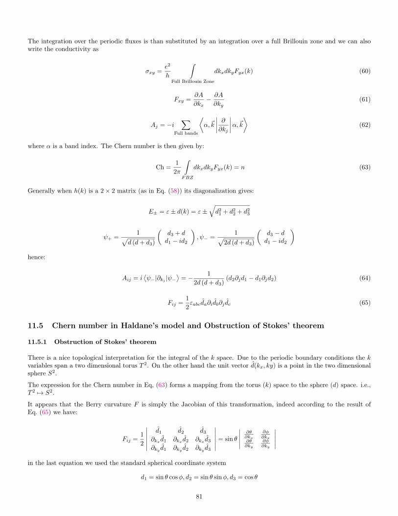
The integration over the periodic fluxes is than substituted by an integration over a full Brillouin zone and we can alsowrite the conductivity as
σxy =e2
h
ˆ
Full Brillouin Zone
dkxdkyFyx(k) (60)
Fxy =∂A
∂kx− ∂A
∂ky(61)
Aj = −i∑
Full bands
⟨α,~k
∣∣∣∣ ∂∂kj∣∣∣∣α,~k⟩ (62)
where α is a band index. The Chern number is then given by:
Ch =1
2π
ˆ
FBZ
dkxdkyFyx(k) = n (63)
Generally when h(k) is a 2× 2 matrix (as in Eq. (58)) its diagonalization gives:
E± = ε± d(k) = ε±√d2
1 + d22 + d2
3
ψ+ =1√
d (d+ d3)
(d3 + dd1 − id2
), ψ− =
1√2d (d+ d3)
(d3 − dd1 − id2
)hence:
Aij = i⟨ψ−|∂kj |ψ−
⟩= − 1
2d (d+ d3)(d2∂jd1 − d1∂jd2) (64)
Fij =1
2εabcda∂idb∂j dc (65)
11.5 Chern number in Haldane’s model and Obstruction of Stokes’ theorem
11.5.1 Obstruction of Stokes’ theorem
There is a nice topological interpretation for the integral of the k space. Due to the periodic boundary conditions the kvariables span a two dimensional torus T 2. On the other hand the unit vector d(kx, ky) is a point in the two dimensionalsphere S2.
The expression for the Chern number in Eq, (63) forms a mapping from the torus (k) space to the sphere (d) space. i.e.,T 2 7→ S2.
It appears that the Berry curvature F is simply the Jacobian of this transformation, indeed according to the result ofEq. (65) we have:
Fij =1
2
∣∣∣∣∣∣d1 d2 d3
∂kx d1 ∂kx d2 ∂kx d3
∂ky d1 ∂ky d2 ∂ky d3
∣∣∣∣∣∣ = sin θ
∣∣∣∣∣ ∂θ∂kx
∂φ∂kx
∂θ∂ky
∂φ∂ky
∣∣∣∣∣in the last equation we used the standard spherical coordinate system
d1 = sin θ cosφ, d2 = sin θ sinφ, d3 = cos θ
81

The expression for the Chern number is now:
Ch =1
4π
ˆ∂
sin θdθdφ,
but we have to determine the boundaries ∂ of integration.
To do so we neglect the ε which will not change the eigen vectors then the Hamiltonian is:
h(~k) = ε(~kk) + σ · d(~k)→(
cos θ sin θe−iφ
sin θeiφ − cos θ
)and the lower energy solution is:
ψI =1√
2d (d+ d3)
(d3 − dd1 − id2
)→(−e−iφ sin θ
2
cos θ2
)which isn’t defined at θ = 0. On the other hand we can multiply by a phase and have
ψII =
(− sin θ
2
eiφ cos θ2
)which isn’t defined at θ = π. Hence we can use each ψ only in the half sphere where it is well defined. We can then useStokes’ theorem to obtain that the integral over the sphere can be converted to two integrals over the respective Berryconnections of the two half spheres on the equator, giving:
1
4π
ˆcos θdφ =
1
4π
ˆ(AI −AII) dl
where Aj = i 〈ψj |∇|ψj〉 is the Berry connection for the region where ψj is defined.
We can easily calculate AI and AII on the equator and and find
AI =i
2
(eiφ, 1
)∂φ
(−eiφ
1
)= 1
and similarly
AII = −1
giving
Ch =1
4π
ˆ2dφ = 1
The conclusion of these procedure, known as the obstruction of stokes theorem, is the following: if the vector d of thesolution reaches both the north and the south poles of S2 the Chern number is 1. If on the other hand d span only thenorth hemisphere then we can do the whole integration with one of the wave function shrink the loop of integration to apoint and the Chern number is zero.
82

11.5.2 Chern number in Haldane’s model
Coming back to Haldane’s model in Eq. (58) we find the following results
for φ = 0, d3(k) = M = const so clearly as we change k we will not get into the south pole and the Chern number is zero.
A more careful analysis of the dependance of ~d(k) on k (we will discuss that in the next section) shows that it is sufficientto discuss the behavior of d3 near the special points K and K ′. At these points:
d3(K) = M − 3√
3t2 sinφ, d3(K ′) = M + 3√
3t2 sinφ
and we can use these values to see whether d reaches the south pole, which means we have non-zero Chern number. Thisgives the phase diagram
Figure 24: The Chern number for Haldane model
11.5.3 Chern number near a Dirac point
Developing the Hamiltonian around K,K ′ for the Haldane model in Eq. (58) we have:
H(k) = −3t2 cos (φ) +3
2t1 (kxσx + kyσy) +
(M ∓ 3
√3t2 sinφ
)σz
+9
4t2 cos (φ)
(k2x + k2
y
)+
9
4
√3 sinφt2
(k2x + k2
y
)σz (66)
where the ∓ is for K,K ′ respectively.
The linear part (divided by 3/2t2 with the relation ((M ∓ 3
√3t2 sinφ
)/(3/2t2) = m±) gives(
m± kx − ikykx + iky −m±
)= kxσ1 + kyσ2 +m±σ3
83

the Berry curvature near the massive Dirac point is given by
Fxy =m
2 (k2 +m2)3/2
So that we can easily calculate the Chern number:
Ch =1
2π
ˆm
2 (k2 +m2)3/2
2πkdk =m3
(m2)3/2
∞
0
dy
(1 + y)3/2
=sign (m)
2
The Chern number depends on the sign of m, and in the phase diagram the lines in fig 24represent the values of M andφ where m is 0 and changes sign across them.
Notice that the Chern number that we got from the the analysis of the massive Dirac point is half integer. We provehowever that it has to be a n integer. That occurs because we did not treat properly the other parts of the spectrum.The contribution of the other parts of the spectrum that must convert the Chern number to be an integer is called "thecontribution of spectator fermions". The change of the mass, however, at the Dirac points give correctly the change ofthe Chern number. it jumps by one when the mass change its sign.
In order to determine the contribution of the spectator fermions (that in principle could be positive or negative) weexamine the system in simple cases. In the so cold atomic limit when M →∞ we expect that system will not conduct atall, as there is a large gap and the electrons are localized on the atomic level. Thus for large M we expect that Ch = 0.The changes in the value of m gives the phase diagram of Fig. 24.
11.5.4 Explicit solution of edge mode in a massive Dirac spectrum
We show that a massive Dirac spectrum may have a Chern number that is not zero. From our studies of the Hall effectwe expect that when the Chern number is not zero the system will have edge modes. Unlike the Hall effect the simpleinterpretation in terms of skipping orbits on the edges does not exist here.
In this subsection we will construct an explicit solution of the edge modes: In order to do so we assume that we have asemi infinite system for positive x and write H as:
H = Hx +Hy,
examine Eq. (66) we find
Hx =(C −Dk2
x
)+(m−Bk2
x
)σz +Akxσx
Hy = −Dk2y −Bk2
yσz +Akyσy.
We want to solve this Hamiltonian on the edge of the model. We notice that the Dirac cone have a symmetry underrotations around the x axis which allows us to set initially
ky = 0, Hy = 0
to assume that there is a solution at E = 0 and then treat Hy perturbatively. Then the Hamiltonian is:
(C +D∂2
x +m+B∂2x iA∂x
−iA∂x C +D∂2x −m−B∂2
x
)ψ0 = Eψ0.
We use an ansatz
ψ0 = aeλx
84

with a being a two component vector. This yields
(m+Bλ2
)σza = −iσxaAλ,
multiplying by iσx we find
(m+Bλ2
)σya = aAλ.
The eigenvalues of σy are
a± =1√2
(eiπ/4
∓e−iπ/4), σya± = ±a±.
Setting these in the equation we find
(m+Bλ2
)a± = ±Aλa±.
We have 2 quadratic equations with 4 solutions. 2 of them are
λ1,2 =1
2B
(A±
√A2 − 4MB
)(for the other two take A→ −A) thus the eigenvectors are
ψ0 =(aeλ1x + beλ2x
)a+ +
(ce−λ1x + de−λ2x
)a−
We impose a boundary condition ψ(0) = 0 ⇒ b = −a, d = −c. The normalizability condition of the wave function willprevent ψ from exploding at infinity.
If Re (λ1) > 0 and Re (λ2) < 0 or vice versa the normalization can’t be achieved without setting all coefficients to 0, hencein this situation there is no solution.
However, if Re (λ1) < 0 andsign(Re(λ1)) = sign(Re(λ2)),
which is satisfied if
√A2 − 4MB < |A|
Then we have two options:A/B < 0⇒ Re(λ1, λ2) < 0
A/B > 0⇒ Re(λ1, λ2) > 0
Giving solutions
ψ0 = a(eλ1x − eλ2x
)a+, A/B < 0, Re(λ1, λ2) < 0
, c(e−λ1x − e−λ2x
)a−, A/B > 0, Re(λ1, λ2) > 0
We found that we have a 1D edge state with a linear dispersion relation if we perturb around it in the y direction.
∆E = 〈ψ0|Hy|ψ0〉 → Aky
85

11.6 Topological insulators and Spin-orbit coupling, Kane and Mele Model (2005))
Given some magnetic field induced by movement in an electric field
−→B = −
−→vc×−→E
We add a spin-orbit interaction (?sign)
Hso = −1
2gµB−→σ ·−→B ⇒ ~e
2m2c2−→σ · −→p ×
−→E
1
2
where the 12 factor comes from an exact development of this term from the Dirac equation. In the case of the atom with
a radial field with term will be proportional to σ · L.
In matter SO coupling can be a significant effect due to the strong fields in the locality of ions, as opposed to freelypropagating fermions. We can write
Hso =1
2m
e
c−→p ·
(~
4mc−→σ ×
−→E
)+e
c
(~
4mc−→σ ×
−→E
)· −→p
and identify−→A so ≡ ~
4mc−→σ ×
−→E .
The AB flux from a field passing through a ring of radius R is
Aθ =Φ
2πR
If we want an electric field which decays in the same manner we can generate it with a charged wire. This will affectdifferent spin states in the opposite direction.
Where can such electric field arise? It is natural to assume that there will be an abundance of positive charge around theions giving an effective negative charge between them
(drawing of graphene with charge distribution)
This effect can be introduced by adding the following term to the Hamiltonian
iλR∑ij
c†i
(~s · (~di × ~dj)
)cj
With ~di(j) are in-plane vectors connecting the next nearest neighbor i, j through a common neighbor. Each band producestwo edge modes for the two spin states. These are protected from scattering off each other from time reversal symmetry(there is no magnetic field in the problem). However, such states from different bands can scatter off each other whichusually destroys the conductance which can be produced by them.
86