Concepts of Probabilities and Statistics

Chapter 2

Concepts of Probability and Statistics

2.1 Introduction

The analysis of communication systems involves the study of the effects of noise on

the ability to transmit information faithfully from one point to the other using either

wires or wireless systems (in free space), including microwave signals (Lindsey and

Simon 1973; Schwartz 1980; Schwartz et al. 1996; Middleton 1996). Thus, it

is important to understand the properties of noise, which requires the study of

random variables and random processes. Additionally, the presence of fading and

shadowing in the channel (mainly the wireless ones which are more susceptible

to uncertainty) demands an understanding of the properties of random variables,

distribution, density functions, and so on (Helstrom 1968; Rohatgi and Saleh 2001;

Papoulis and Pillai 2002).

In this chapter, we will review, among others, the concepts of random variables,

the properties of the distribution and density functions, and moments. We will also

look at characterizing two or more random variables together so that we can exploit

their properties when we examine techniques such as the diversity combining

algorithms employed to mitigate fading and shadowing seen in wireless systems

(Brennan 1959; Suzuki 1977; Hansen and Meno 1977; Shepherd 1977; Jakes 1994;

Sklar 1997a, b; Vatalaro 1995; Winters 1998). In very broad terms, fading and

shadowing represent the random fluctuations of signal power observed in wireless

channels. Their properties are characterized in terms of their statistical nature,

mainly through the density functions (Saleh and Valenzuela 1987; Vatalaro 1995;

Yacoub 2000, 2007a, b; Cotton and Scanlon 2007; Nadarajah and Kotz 2007;

da Costa and Yacoub 2008; Karadimas and Kotsopoulos 2008, 2010; Shankar

2010; Papazafeiropoulos and Kotsopoulos 2011) and we will review all the perti-

nent statistical aspects to facilitate a better understanding of signal degradation and

mitigation techniques to improve the signal quality.

P.M. Shankar, Fading and Shadowing in Wireless Systems,DOI 10.1007/978-1-4614-0367-8_2, # Springer Science+Business Media, LLC 2012

7

2.2 Random Variables, Probability Density Functions,

and Cumulative Distribution Functions

A random variable is defined as a function that maps a set of outcomes in an

experiment to a set of values (Rohatgi and Saleh 2001; Papoulis and Pillai 2002).

For example, if one tosses a coin resulting in “heads” or “tails,” a random variable

can be created to map “heads” and “tails” into a set of numbers which will be

discrete. Similarly, temperature measurements taken to provide a continuous set of

outcomes can be mapped into a continuous random variable. Since the outcomes

(coin toss, roll of a die, temperature measurements, signal strength measurements

etc.) are random, we can characterize the random variable which maps these

outcomes to a set of numbers in terms of it taking a specific value or taking values

less than or greater than a specified value, and so forth. If we define X as the random

variable, {X � x} is an event. Note that x is a real number ranging from�1 to +1.

The probability associated with this event is the distribution function, more com-

monly identified as the cumulative distribution function (CDF) of the random

variable. The CDF, FX(x), is

FXðxÞ ¼ ProbfX � xg : (2.1)

The probability density function (pdf) is defined as the derivative of the CDF as

fXðxÞ ¼ d½FXðxÞ�dx

: (2.2)

From the definition of the CDF in (2.1), it becomes obvious that CDF is a

measure of the probability and, therefore, the CDF has the following properties:

FXð�1Þ ¼ 0;

FXð1Þ ¼ 1;

0 � FXðxÞ � 1;

FXðx1Þ � FXðx2Þ; x1 � x2: (2.3)

Based on (2.2) and (2.3), the probability density function has the following

properties:

0 � fXðxÞ;ð1

�1fXðxÞ dx ¼ 1;

FXðxÞ ¼ðx

�1fXðaÞ da;

Probfx1 � X � x2g ¼ FXðx2Þ � FXðx1Þ ¼ðx2

x1

fXðaÞ da: (2.4)

8 2 Concepts of Probability and Statistics

A few comments regarding discrete random variables and the associated CDFs

and pdfs are in order. For the discrete case, the random variable X takes discrete

values (1, 2, 3,. . ., n). The CDF can be expressed as (Helstrom 1991; Rohatgi and

Saleh 2001; Papoulis and Pillai 2002)

FXðxÞ ¼Xn

m¼1

ProbfX ¼ mgUðx� mÞ: (2.5)

In (2.5), U(.) is the unit step function. The pdf of the discrete random variable

becomes

fXðxÞ ¼Xn

m¼1

ProbfX ¼ mgdðx� mÞ: (2.6)

In (2.6), d(.) is the delta function (Abramowitz and Segun 1972).

It can be easily seen that for a continuous random variable there is no statistical

difference between the probabilities of outcomes where the random variable takes a

value less than (<) or less than or equal to (�) a specified outcome because the

probability that a continuous random variable takes a specified value is zero.

However, for the case of a discrete random variable, the probabilities of the two

cases would be different. We will now examine a few properties of the random

variables and density functions.

The moments of a random variable are defined as

mk ¼ hXki ¼ EðXkÞ ¼ð1

�1xkf ðxÞ dx: (2.7)

The first moment (k ¼ 1) is the mean or the expected value of the random

variable and <�> as well as E(.) represents the statistical average. The variance

(var) of the random variable is related to the second moment (k ¼ 2) and it is

defined as

varðxÞ ¼ s2 ¼ hX2i � hXi2: (2.8)

The quantity s is the standard deviation. Variance is a measure of the degree of

uncertainty and

s2 � 0: (2.9)

The equality in (2.9) means that the degree of uncertainty or randomness is

absent; we have a variable that is deterministic. Existence of higher values of

variance suggests higher level of randomness. For the case of a discrete random

variable, the moments are expressed as

hXki ¼Xn

m¼1

mkProbfX ¼ mg: (2.10)

2.2 Random Variables, Probability Density Functions. . . 9

The survival function S(x) of a random variable is defined as the probability that

{X > x}. Thus,

SðxÞ ¼ð1

x

fXðaÞ da ¼ 1� FXðxÞ: (2.11)

The coefficient of skewness is defined as (Evans et al. 2000; Papoulis and Pillai

2002)

�3 ¼m3s3

: (2.12)

The coefficient of kurtosis is defined as

�4 ¼m4s4

: (2.13)

The entropy or information content of a random variable is defined as

I ¼ �ð1

�1f ðxÞlog2½ f ðxÞ�dx: (2.14)

The mode of a pdf f(x) is defined as the value x where the pdf has the maximum.

It is possible that a pdf can have multiple modes. Some of the density functions will

not have any modes. The median xm of a random variable is defined as the point

where

ðxm

�1f ðxÞdx ¼

ð1

xm

f ðxÞdx: (2.15)

2.3 Characteristic Functions, Moment Generating Functions

and Laplace Transforms

The characteristic function (CHF) of a random variable is a very valuable tool

because of its use in the performance analysis of wireless communication systems

(Nuttall 1969, 1970; Tellambura and Annamalai 1999; Papoulis and Pillai 2002;

Tellambura et al. 2003; Goldsmith 2005; Withers and Nadarajah 2008). This will be

demonstrated later in this chapter when we discuss the properties of the CHFs. The

CHF, c(x), of a random variable having a pdf f(x) is given by

cXðoÞ ¼ hexpð joXÞi ¼ð1

�1f ðxÞ expð joxÞdx: (2.16)

Equation (2.16) shows that CHF is defined as the statistical average of exp ( jox).Furthermore, it is also the Fourier transform of the pdf of the random variable.


Rewriting (2.16) by replacing ( jo) by s, we get the moment generating function

(MGF) of the random variable as (Alouini and Simon 2000; Papoulis and Pillai 2002)

fXðsÞ ¼ hexpðsxÞi ¼ð1

�1f ðxÞ expðsxÞ dx: (2.17)

Defining (2.16) slightly differently, we can obtain the expression for the Laplace

transform of pdf as (Beaulieu 1990; Tellambura and Annamalai 1999, 2000;

Papoulis and Pillai 2002)

LXðsÞ ¼ð1

�1f ðxÞ expð�sxÞ dx: (2.18)

Consequently, we have the relationship between the bilateral Laplace transform

and the MGF of a random variable:

LXðsÞ ¼ fXð�sÞ: (2.19)

Going back to (2.16), we can define the inverse Fourier transform of the CHF to

obtain the pdf as

fXðxÞ ¼ 1

2p

ð1

�1cðoÞ expð�joxÞdo: (2.20)

By virtue of the property (2.20), CHF will uniquely determine the probability

density function. We will explore the use of CHFs in diversity analysis later in this

chapter and we will use the Laplace transform, CHF, and MGF to estimate the error

rates and outage probabilities to be seen in later chapters (Tellambura and

Annamalai 1999).

2.4 Some Commonly Used Probability Density Functions

We will now look at several random variables which are commonly encountered in

wireless communication systems analysis. We will examine their properties in

terms of the pdfs, CDFs and CHFs. Within the context of wireless communications,

we will explore the relationships among some of these random variables.

2.4.1 Beta Distribution

The beta distribution is not commonly seen in wireless communications. However,

it arises in wireless system when we are studying issues related to signal-to-

interference ratio (Jakes 1994; Winters 1984, 1987). The beta random variable is

2.4 Some Commonly Used Probability Density Functions 11

generated when the ratio of certain random variables is considered (Papoulis and

Pillai 2002). The beta density function is

f ðxÞ ¼xa�1ð1� xÞb�1

bða; bÞ ; 0< x< 1;

0 elsewhere:

8><

>:(2.21)

In (2.21), b(a,b) is the beta function given in integral form as

bða; bÞ ¼ð1

0

xa�1ð1� xÞb�1dx: (2.22)

Equation (2.22) can also be written in terms of gamma functions (Abramowitz

and Segun 1972):

bða; bÞ ¼ GðaÞGðbÞGðaþ bÞ ; (2.23)

where G(.) is the gamma function. The CDF of the beta random variable is

FðxÞ ¼

0; x � 0;ðx

0

ya�1ð1� yÞb�1

bða; bÞ dy; 0< x< 1;

1; x � 1:

8>>><

>>>:(2.24)

The moments of the beta random variable are

hXki ¼ Gðk þ aÞGðk þ bÞGðk þ aþ bÞGðkÞ : (2.25)

The mean and variance of the beta variable are

hXi ¼ a

aþ b; (2.26)

varðXÞ ¼ ab

ðaþ bþ 1Þðaþ bÞ2 : (2.27)

The beta density function is shown in Fig. 2.1 for three sets of values of (a,b).It can be seen that for the case of a ¼ b ¼ 1, the beta density becomes the

uniform density function as seen later in this chapter. Note that X is a beta variate

with parameters a and b; then Y ¼ 1�X is also a beta variate with parameters band a.


The beta density function allows significant flexibility over the standard uniform

distribution in the range {0, 1} as one can see from Fig. 2.1. As mentioned in the

beginning if X1 and X2 are two gamma variables with parameters (a, A) and (b, A)respectively, the ratio X1=ðX1 þ X2Þ will be a beta variate with parameters (a,b).This aspect will be shown later in this chapter when we examine the density

function of linear and nonlinear combination of two or more random variables.

2.4.2 Binomial Distribution

The binomial distribution is sometimes used in wireless systems when estimating

the strength of the interfering signals at the receiver, with the number of interferers

contributing to the interfering signal being modeled using a binomial random

variable (Abu-Dayya and Beaulieu 1994; Shankar 2005). For example, if there

are n interfering channels, it is possible that all of them might not be contributing to

the interference. The number of actual interferers contributing to the interfering

signal can be statistically described using the binomial distribution. This distribu-

tion is characterized in terms of two parameters, with the parameter n representing

the number of Bernoulli trials and the parameter p representing the successes from

the n trials. (A Bernoulli trial is an experiment with only two possible outcomes that

have probabilities p and q such that (p + q) ¼ 1). While n is an integer, the quantity

0 0.1 0.2 0.3 0.4 0.5 0.6 0.7 0.8 0.9 10

0.5

1

1.5

2

2.5

3

3.5

4

x

beta

den

sity

func

tion

a = 1 b =1a = 2 b = 3a = 8 b = 2

Fig. 2.1 The density function of the beta random variable


p is bounded as 0 < p < 1. The binomial probability is given by (Papoulis and

Pillai 2002)

ProbfX ¼ kg ¼ nk

� �pkð1� pÞn�k; k ¼ 0; 1; . . . : (2.28)

In (2.28),

nk

� �¼ Cn

k ¼n!

ðn� kÞ!k! : (2.29)

The mean of the variable is given by ðnpÞ and the variance is given by ðnpqÞwhere q ¼ ð1� pÞ. The binomial probabilities are shown in Fig. 2.2.

The binomial variate can be approximated by a Poisson variate (discussed later

in this section) if p < < 1 and n < 10. Later we will describe how the binomial

distribution approaches the normal distribution, when npq > 5 and 0.1 < p < 0.9.

The transition toward the normal behavior is seen in Fig. 2.2.

We alluded to Bernoulli trials which had only two outcomes. We can extend

such experiments to have more than two outcomes resulting in the generalized

Bernoulli trials. Instead of two outcomes, let us consider the case of r outcomes

(mutually exclusive) such that the total probability

p1 þ p2 þ � � � þ pr ¼ 1: (2.30)

0 1 2 3 4 5 6 7 8 9 100

0.1

0.2

0.3

0.4

x

Pro

babi

lity

0 1 2 3 4 5 6 7 8 9 100

0.1

0.2

0.3

0.4

x

Pro

babi

lity

0 1 2 3 4 5 6 7 8 9 100

0.1

0.2

0.3

0.4

x

Pro

babi

lity

0 1 2 3 4 5 6 7 8 9 100

0.1

0.2

0.3

0.4

x

Pro

babi

lity

n = 10p = 0.1

n = 10p = 0.2

n = 10p = 0.3

n = 10p = 0.5

Fig. 2.2 Binomial probabilities


Now, we repeat the experiment n times. Our interest is in finding out the

probability that outcome #1 occurs k1 times, #2 occurs k2 times, and so on.

In other words, we are interested in the Prob{#1 occurs k1 times, #2 occurs k2times,.., #r occurs kr times}. Noting that the number of ways in which these events

can occur is n!=ðk1!k2! . . . kr!Þ, the required probability becomes

pðk1; k2; . . . ; krÞ ¼ n!

k1!k2! . . . kr!pk11 p

k22 . . . pkrr ;

Xr

j¼1

kr ¼ n: (2.31)

We will use some of these results when we examine the order statistics later in

this chapter.

2.4.3 Cauchy Distribution

The Cauchy distribution arises in wireless systems when we examine the pdfs of

random variables which result from the ratio of two Gaussian random variables

(Papoulis and Pillai 2002). What is unique in terms of its properties is that its

moments do not exist. The Cauchy pdf is expressed as

f ðxÞ ¼ 1

pb½1þ ððx� aÞ=bÞ2� ; �1< x<1: (2.32)

The associated CDF is

FXðxÞ ¼ 1

2þ 1

ptan�1 x� a

b

� �: (2.33)

The CHF is

cðoÞ ¼ expð jao� jojbÞ: (2.34)

As mentioned, its moments do not exist and its mode and median are (each)

equal to a. Note that Cauchy distribution might appear similar to the normal

(Gaussian) distribution. While both the Cauchy and Gaussian distributions are

unimodal (only a single mode exists) and are symmetric (Gaussian around the

mean and Cauchy around a), the Cauchy distribution has much heavier tails than

the Gaussian pdf. The Cauchy pdf is shown in Fig. 2.3 for the case of a ¼ 0.

The heavier tails are seen as b goes up


2.4.4 Chi-Squared Distribution

This distribution arises in statistics (and in wireless systems) when we examine the

pdf of the sum of the squares of several Gaussian random variables. It is also used in

hypothesis testing such as the w2 goodness of fit test (Papoulis and Pillai 2002).

The chi square (or chi squared) random variable has a pdf given by

f ðxÞ ¼ xðn�2Þ=2 expð�ðx=2ÞÞ2n=2Gðn=2Þ ; 0< x<1: (2.35)

The shape parameter n is designated as the degrees of freedom associated with

the distribution. This density function is also related to the Erlang distribution used

in the analysis of modeling of the grade of service (GOS) in wireless systems and

the gamma distribution used to model fading and shadowing seen in wireless

systems. The gamma and Erlang densities are described later in this section. The

distribution is often identified as w2(n). The density function also becomes the

exponential pdf in the limiting case (n ¼ 2).

There is no simple analytical expression for the CDF, but, it can be expressed in

terms of incomplete gamma function as

FXðxÞ ¼ 1�G

n

2;x

2

� �

Gn

2

� � ¼g

n

2;x

2

� �

Gn

2

� � ; (2.36)

0.05

0.1

0.2

0.35

-10 10

f(x)

β = 2

β = 3

β = 1

α = 0

0 5-5

Fig. 2.3 Cauchy pdf is shown


where

Gða; bÞ ¼ð1

b

xa�1 expð�xÞ dx; gða; bÞ ¼ðb

0

xa�1expð�xÞ dx: (2.37)

G(.,.) is the (upper) incomplete gamma function, g(.,.) the (lower) incomplete

gamma function and G(.) is the gamma function (Abramowitz and Segun 1972;

Gradshteyn and Ryzhik 2007). Note that the pdf in (2.35) is a form of gamma pdf of

parameters (n/2) and 2 (as we will see later). The CHF is given by

cðoÞ ¼ ð1� 2joÞ�ðn=2Þ: (2.38)

The mean of the random variable is n and the variance is 2n. The mode is (n�2),

n > 2 and the median is (n�2/3). The density function is plotted in Fig. 2.4. It can

be seen that as the degrees of freedom (n) increases, the symmetry of the pdf

increases and it will approach the Gaussian pdf.

There is a related distribution called the non-central chi squared distribution

which is described later in this chapter.

An associated distribution is the chi distribution. The chi variable is the positivesquare root of a chi squared variable. The chi pdf is given by

f ðxÞ ¼ xn�1 expð�ðx2=2ÞÞ2ðn=2Þ�1Gðn=2Þ ; 0 � x � 1: (2.39)

0 5 10 15 20 25 30 35 40 45 500

0.02

0.04

0.06

0.08

0.1

0.12

0.14

0.16

0.18

0.2

n = 4

n = 8

n = 20

f(x)

x

Fig. 2.4 The Chi squared pdf. The density function becomes more symmetric as the degree of

freedom n goes up


The cumulative distribution becomes

FXðxÞ ¼ 1�G

n

2;x2

2

� �

Gn

2

� � ¼g

n

2;x2

2

� �

Gn

2

� � : (2.40)

When n ¼ 2, the chi pdf becomes the Rayleigh pdf, described later in this section.

2.4.5 Erlang Distribution

When we examine the density of a sum of exponential random variables, we get the

so-called Erlang pdf. The Erlang pdf is given by

f ðxÞ ¼ ðx=bÞc�1expð�ðx=bÞÞ

bðc� 1Þ! ; 0 � x � 1: (2.41)

Note that the shape parameter c is an integer. Equation (2.41) becomes the

gamma pdf if c is a non-integer. The CHF is given by

cðoÞ ¼ ð1� jboÞ�c: (2.42)

The mean of the random variable is (bc) and the variance is (b2c). The mode is

b(c�1), c � 1. The CDF can be expressed as

FXðxÞ ¼ 1� exp � x

b

� �� Xc�1

k¼0

ðx=bÞkk!

!: (2.43)

Note that the Erlang density function and chi-squared pdf in (2.35) have similar

functional form with c ¼ n=2 and b ¼ 2.

2.4.6 Exponential Distribution

The exponential distribution (also known as the negative exponential distribution)

arises in communication theory in the modeling of the time interval between events

when the number of events in any time interval has a Poisson distribution. It also

arises in the modeling of the signal-to-noise ratio (SNR) in wireless systems

(Nakagami 1960; Saleh and Valenzuela 1987; Simon and Alouini 2005). Further-

more, the exponential pdf is a special case of the Erlang pdf when c ¼ 1 and a

special case of chi-squared pdf when n ¼ 2. The exponential pdf is given by


f ðxÞ ¼ 1

bexp � x

b

� �; 0< x<1: (2.44)

The associated CDF is given by

FðxÞ ¼ 1� exp � x

b

� �: (2.45)

The CHF is given by

cðoÞ ¼ 1

1� job: (2.46)

The exponential has no mode. The mean is b and the variance is b2 and, thus, theexponential pdf is uniquely characterized in terms of the fact that the ratio of its

mean to its standard deviation is unity. The exponential pdf is shown in Fig. 2.5 for

three values of b.The exponential CDF is a measure of the outage probability (probability that the

signal power goes below a threshold) is shown in Fig. 2.6.

0 0.5 1 1.5 2 2.5 3 3.5 4 4.5 50

0.1

0.2

0.3

0.4

0.5

0.6

0.7

0.8

0.9

1

x

Pro

babi

lity

dens

ity fu

nctio

n

β = 1

β = 2

β = 3

Fig. 2.5 The exponential densities are plotted for three values of the mean


2.4.7 F (Fisher-Snedecor) Distribution

The SNR in fading is often modeled using gamma distributions (Simon and Alouini

2005; Shankar 2004). The ratio of two such variables is of interest when examining

the effects of interfering signals in wireless communications (Winters 1984). The Fdistribution arises when we examine the density function of the ratio of two chi-

squared random variables of even degrees of freedom or two Erlang variables or

two gamma variables of integer orders (Lee and Holland 1979; Nadarajah 2005;

Nadarajah and Gupta 2005; Nadarajah and Kotz 2006a, b). The F density can be

written as

f ðxÞ ¼ G ðmþ nÞ=2ð Þmm=2nn=2

G m=2ð ÞG n=2ð Þxm=2�1

ðnþ mxÞ ðmþnÞ=2½ � UðxÞ: (2.47)

In (2.47), m and n are integers. The mean is given by

hXi ¼ n

n� 2; n> 2: (2.48)

The variance is

varðxÞ ¼ 2n2ðnþ m� 2Þ

mðn� 4Þðn� 2Þ2 ; n> 4: (2.49)

0 2 4 6 8 10 12 14 16 18 200

0.1

0.2

0.3

0.4

0.5

0.6

0.7

0.8

0.9

1

x

Cum

ulat

ive

dist

ribut

ion

func

tion

β = 2

β = 4

β = 8

Fig. 2.6 (CDFs) of the exponential random variables are shown


The density function is identified as F(m,n), with (m,n) degrees of freedom. The

F distribution is shown in Fig. 2.7. The density function is sometimes referred to as

Fisher’s variance ratio distribution.

2.4.8 Gamma Distribution

The gamma distribution is used extensively in wireless communications to model

the power in fading channels (Nakagami 1960; Abdi and Kaveh 1999; Atapattu

et al. 2010). As mentioned earlier, the gamma pdf is a special case of the Erlang

distribution in (2.41). The pdf is given by

f ðxÞ ¼ ðx=bÞc�1expð�ðx=bÞÞbGðcÞ ; 0< x<1: (2.50)

Comparing (2.41) and (2.50), we see that for the gamma pdf c can be any

positive number while for the Erlang pdf, c must be an integer. The CDF can be

expressed in terms of the incomplete gamma function as

FXðxÞ ¼ gðc; ðx=bÞÞGðcÞ ¼ 1� Gðc; ðx=bÞÞ

GðcÞ : (2.51)

0 0.5 1 1.5 2 2.5 3 3.5 4 4.5 50

0.1

0.2

0.3

0.4

0.5

0.6

0.7

x

Pro

babi

lity

dens

ity fu

nctio

n F

(m,n

)

F(4,5)F(6,8)

Fig. 2.7 The F distribution is plotted for two sets of values


The moments are given by

EðXkÞ ¼ bkGðcþ kÞGðcÞ : (2.52)

The moments are identical to that of the Erlang distribution. The exponential

distribution is a special case of the gamma pdf with c ¼ 1. The received SNR or

power is modeled using the gamma pdf. The CHF of the gamma distribution is

cðoÞ ¼ ð1� jboÞ�c: (2.53)

The gamma pdf in (2.50) becomes the chi-squared pdf in (2.35) when n ¼ 2cand b ¼ 2. The relationship of the gamma pdf to other distributions is given in

Table 2.1.

The gamma pdf is plotted in Fig. 2.8 for three values of c, all having identical

mean of unity. One can see that as the order of the gamma pdf increases, the peaks

of the densities move farther to the right. This aspect will be seen later in Chap. 5

when we examine the impact of diversity in fading channels . The corresponding

CDFs are shown in Fig. 2.9.

2.4.9 Generalized Gamma Distribution

Instead of the two parameter distribution in (2.50), the three parameter gamma

distribution known as the generalized gamma distribution can be expressed as

(Stacy 1962; Stacy and Mihram 1965; Lienhard and Meyer 1967; Griffiths and

McGeehan 1982; Coulson et al. 1998a, b; Gupta and Kundu 1999; Bithas et al.

2006)

f ðxÞ ¼ lxlc�1

blcGðcÞ exp � x

b

� �l" #

; 0< x<1: (2.54)

Table 2.1 Relationship of gamma pdf to other distributions

c b Name of the distribution Probability density function

1 – Exponential 1

bexp � x

b

� �

Integer – Erlang ðx=bÞc�1expð�ðx=bÞÞ

bðc� 1Þ!c ¼ 2n 2 Chi-squared xðn�2Þ=2 expð�ðx=2ÞÞ

2n=2Gðn=2Þ


0 0.2 0.4 0.6 0.8 1 1.2 1.4 1.6 1.8 2

10-4

10-3

10-2

10-1

100

x

Cum

ulat

ive

dist

ribut

ion

func

tion

c = 2c = 3c = 4.5

< x > =1

Fig. 2.9 The CDFs of the gamma random variables for three values of the order. All have the

identical means (unity)

0 0.5 1 1.5 2 2.5 3 3.5 4 4.5 50

0.1

0.2

0.3

0.4

0.5

0.6

0.7

0.8

0.9

1

x

Pro

babi

lity

dens

ity fu

nctio

n

c = 2c = 3c = 4.5

< x > = 1

Fig. 2.8 The density functions of the gamma random variables for three values of the order.

All have the identical means (unity)


There is no simple expression for the CHF of the generalized gamma density

function. The generalized gamma random variable can be obtained from a gamma

random variable by scaling the random variable by (1/l). This distribution is also

known as the Stacy distribution (Stacy 1962), which is expressed in a slightly

different form as

f ðxÞ ¼ p

ad

� �xd�1

exp � x

a

� �p� �

Gd

p

� � ; x � 0; a> 0; p> 0; d> 0: (2.55)

Note that the generalized gamma pdf can also be expressed in yet another

form as

f ðxÞ ¼ lxlc�1

bcGðcÞ exp � xl

b

� �; 0< x<1: (2.56)

The GG pdf in (2.56) is plotted in Fig. 2.10 for the case of b ¼ 1. It can be seen

that as l increases the density function moves to the right, indicating that the density

function will approach Gaussian as is possible with the case of Erlang pdf. The

same effect will be present when c increases as well.The generalized gamma (GG) distribution can be used to model power (or

SNR) as well as the magnitude (or envelope) values in wireless communications

(Coulson et al. 1998a, b). This can be accomplished by varying c and l. Also, theGG distribution can morph into other distributions in limiting cases (Griffiths and

0 1 2 3 4 5 6 7 8 9 100

0.2

0.4

0.6

0.8

1

1.2

1.4

1.6

1.8

c = 1.5; λ = 0.5

c = 1.5; λ = 2

β = 1

c = 2.5; λ = 3

f(x)

x

Fig. 2.10 The generalized gamma pdf in (2.56)


McGeehan 1982). The CDF can once again be represented in terms of the incom-

plete gamma functions in (2.37) and (2.52). Using the representation in (2.56), the

expression for the CDF becomes

FXðxÞ ¼ 1� Gðc; ðxl=bÞÞGðcÞ : (2.57)

If we express the generalized gamma pdf in (2.54) as

f ðxÞ ¼ Axn exp � xm

bm

� �; 0 � x � 1; (2.58)

where b is a scaling factor and A is a normalization factor such that

ð1

0

f ðxÞ dx ¼ 1; (2.59)

we can relate the pdf in (2.58) to several density functions as described in Table 2.2

(Griffiths and McGeehan 1982).

There are also other forms of gamma and generalized gamma distribution.

Even though they are not generally used in wireless communications, we will still

Table 2.2 The generalized gamma distribution and its special cases. In all the expressions in the

last column, A is a normalization factor

m n b Name of the distribution Probability density function

1 – – Gamma Axn exp � x

b

� �

1 >0 (integer) – Erlang Axn exp � x

b

� �

1 >1 (integer) 2 Chi-squared Axn exp � x

b

� �

2 – – NakagamiAxn exp � x2

b2

� �

– – – StacyAxn exp � xm

bm

� �

– n ¼ m � 1 – WeibullAxm�1 exp � xm

bm

� �

1 0 – Exponential A exp � x

b

� �

2 0 – One sided GaussianA exp � x2

b2

� �

0 – Generalized exponentialA exp � xm

bm

� �

2 1 – RayleighAx exp � x2

b2

� �

– 1 – Generalized RayleighAx exp � xm

bm

� �


provide them so as to complete the information on the class of gamma densities.

One such gamma pdf is (Evans et al. 2000)

f ðxÞ ¼ ðx� gÞc�1expð�ðx� gÞ=bÞbcGðcÞ ; x> g> 0; c> 0; b> 0: (2.60)

Note that when g ¼ 0, (2.60) becomes the standard two parameter gamma

density defined in (2.50), another form of generalized gamma density function

has four parameters and it is of the form

f ðxÞ ¼ lðx� gÞlc�1

blcGðcÞ exp � x� gb

� �l" #

; x> g> 0; l> 0; c> 0; b> 0: (2.61)

Note that (2.61) becomes the generalized gamma distribution (Stacy’s pdf) in

(2.54) when g ¼ 0.

While the gamma pdf and the generalized gamma densities mentioned so far are

defined for positive values (single-sided), there also exists a double-sided

generalized gamma density function which has been used to model noise in certain

cases (Shin et al. 2005). The two-sided generalized gamma pdf is

f ðxÞ ¼ ljxjcl�1

2bcGðcÞ exp � jxjlb

!; �1< x<1: (2.62)

The two-sided generalized gamma pdf is flexible enough that it can become

Gaussian, Laplace, generalized gamma or gamma.

2.4.10 Inverse Gaussian (Wald) Distribution

This pdf is sometimes used to model shadowing in wireless systems because of the

closeness of its shape to the lognormal density function (Karmeshu and Agrawal

2007; Laourine et al. 2009). The pdf is expressed as

f ðxÞ ¼ l2px3

� �1=2

exp � lðx� mÞ22m2x

" #; 0< x<1: (2.63)

Note that both l and m are positive numbers. There is no simple analytical

expression for the CDF. The CHF is given by

cðoÞ ¼ explm

1� 1� 2jm2ol

� �1=2" #( )

: (2.64)


The mean is given by m and the variance is given by m3/l. The density function isshown in Fig. 2.11 for a few values of the parameters.

2.4.11 Laplace Distribution

This distribution is generally not used in wireless communication systems even

though research exists into its use in communication systems (Sijing and Beaulieu

2010). It is related to the exponential distribution in that it extends the range of the

variable down to �1. The pdf is expressed as

f ðxÞ ¼ 1

2bexp � jx� aj

b

� �; �1< x<1: (2.65)

The associated CDF is given by

FðxÞ ¼1

2exp � a� x

b

� �; x< a;

1� 1

2exp � x� a

b

� �; x � a:

8>>><

>>>:(2.66)

0 0.5 1 1.5 2 2.5 3 3.5 4 4.5 50

0.2

0.4

0.6

0.8

1

1.2

1.4

x

Pro

babi

lity

dens

ity fu

nctio

n

λ = 0.6

λ = 0.1

λ = 3.5μ = 1

Fig. 2.11 Inverse Gaussian distribution


The CHF is given by

cðoÞ ¼ expðjoaÞ1þ b2o2

: (2.67)

The mean, mode, and median are all equal to a, and the variance is equal to 2b2.The Laplace density function is shown in Fig. 2.12.

2.4.12 Lognormal Distribution

The lognormal pdf arises when central limit theorem for products of random variables

is applied (Papoulis and Pillai 2002). It is used to model long-term fading or

shadowing seen in wireless systems (Hudson 1996; Tjhung and Chai 1999; Coulson

et al. 1998a, b; Patzold 2002; Kostic 2005; Stuber 2000; Cotton and Scanlon 2007).

In certain cases, it finds applications inmodeling short-term fading aswell (Cotton and

Scanlon 2007). The pdf of the lognormal random variable is given by

f ðxÞ ¼ 1ffiffiffiffiffiffiffiffiffiffiffiffi2ps2x

p exp �ðlogeðxÞ � mÞ22s2

" #; 0< x<1: (2.68)

-5 -4 -3 -2 -1 0 1 2 3 4 50

0.05

0.1

0.15

0.2

0.25

0.3

0.35

0.4

0.45

0.5

x

Pro

babi

lity

dens

ity fu

nctio

n

beta = 1beta = 2beta = 3

α = 0

Fig. 2.12 The Laplace density functions


The CDF and CHF are not readily available in analytical form. The mean and

variance can be expressed as

EðXÞ ¼ exp mþ 1

2s2

� �; (2.69)

varðXÞ ¼ ½expðs2 � 1Þ� expð2mþ s2Þ: (2.70)

Equation (2.68) can also be expressed in a slightly different form using the

logarithm with the base 10 as

f ðxÞ ¼ ½10=logeð10Þ�ffiffiffiffiffiffiffiffiffiffiffiffiffiffi2ps2x2

p exp �ð10log10ðxÞ � mÞ22s2

" #; 0< x<1: (2.71)

In (2.71), m and s are in decibel units. Note that if the lognormal variable is

converted to decibel units, the pdf of the variable in dB will be Gaussian. This

density function (in terms of decibel units) is discussed in detail in Chap. 4.

Figure 2.13 shows the plots of the lognormal pdf in (2.68).

0 0.5 1 1.5 2 2.5 30

0.5

1

1.5

2

2.5

3

x

Pro

babi

lity

dens

ity fu

nctio

n

σ = 1

σ = 2

σ = 3μ = 0

Fig. 2.13 Lognormal density function in (2.68) is shown


2.4.13 Nakagami Distribution

Even though there are several forms of the Nakagami distribution, the most com-

monly known one is the “Nakagami-m distribution” with a pdf given by (Nakagami

1960; Simon and Alouini 2005)

f ðxÞ ¼ 2m

O

� �m x2m�1

GðmÞ exp �mx2

O

� �UðxÞ; m � 1

2: (2.72)

In (2.72),m is the Nakagami parameter, limited to values greater than or equal to ½.

The moments of the Nakagami distribution can be expressed as

hXki ¼ Gðmþ ðk=2ÞÞGðmÞ

Om

� �1=2

: (2.73)

The mean is

EðXÞ ¼G mþ 1

2

� �

G mð Þ

ffiffiffiffiOm

r: (2.74)

The variance is

varðXÞ ¼ O 1� 1

m

Gðmþ ð1=2ÞÞGðmÞ

� �2" #

: (2.75)

Note that the Nakagami pdf becomes the Rayleigh density function when m is

equal to unity. The square of the Nakagami random variable will have a gamma

pdf. Under certain limiting conditions, the Nakagami density function can approxi-

mate the lognormal distribution (Nakagami 1960; Coulson et al. 1998a, b). The

Nakagami pdf is plotted in Fig. 2.14.

The CDF associated with the Nakagami-m pdf can be expressed in terms of

incomplete gamma functions. The Nakagami-m CDF is

FXðxÞ ¼ 1� Gðm; ðm=OÞx2ÞGðmÞ : (2.76)

There is no simple analytical expression for the CHF. The Nakagami pdf is used

to model the magnitude or envelope of the signals in communication systems. The

density function of the square of the Nakagami random variable,

Y ¼ X2 (2.77)


with X having the Nakagami pdf in (2.72) is

fYðyÞ ¼ m

O

� �m ym�1

GðmÞ exp �m

Oy

� �; y � 0; m � 1

2: (2.78)

It can be seen that there is no difference between the pdf of the power (square of

the magnitude) expressed in (2.78) and the gamma pdf in (2.50) except that the

order of the gamma pdf m must be larger than ½ for it be associated with the

Nakagami pdf for the magnitude.

The CDF associated with the Nakagami-m distribution of power is

FYðyÞ ¼ 1� Gðm; ðm=OÞyÞGðmÞ : (2.79)

In (2.79),

G m;m

Oy

� �¼ð1

ðm=OÞyxm�1 expð�xÞ dx (2.80)

is the incomplete gamma function (Gradshteyn and Ryzhik 2007). The other forms

of the Nakagami distribution such as the Nakagami-Hoyt and Nakagami-Rice will

0 0.5 1 1.5 2 2.5 3 3.5 4 4.5 50

0.5

1

1.5

x

Pro

babi

lity

dens

ity fu

nctio

n

m = 0.75m = 1.5 m = 3

Ω = 1

Fig. 2.14 The Nakagami density


be discussed in Chap. 4 where specific statistical models for fading will be

presented (Okui 1981; Korn and Foneska 2001; Subadar and Sahu 2009).

It is also possible to define a generalized form of the Nakagami-m pdf called

the generalized Nakagami density function. This density function is obtained by the

exponential scaling of the Nakagami variable X as (Coulson et al. 1998a, b; Shankar

2002a, b)

Y ¼ Xð1=lÞ; l> 0: (2.81)

The density function of Y is the generalized density function given as

f ðyÞ ¼ 2lmmy2ml�1

GðmÞOm exp �m

Oy2l

� �UðyÞ: (2.82)

The generalized Nakagami pdf in (2.82) becomes the Rayleigh density function

in (2.94) when m and l are each equal to unity. It can be easily observed that the

generalized gamma random variable is obtained by squaring the generalized

Nakagami random variable.

2.4.14 Non-Central Chi-Squared Distribution

While we looked at chi-squared distribution which arises from the sum of the

squares of zero mean identical random variables, the non-central chi-squared

distribution arises when the Gaussian variables have non-zero means. The density

function can be expressed in several forms as (Evans et al. 2000; Papoulis and

Pillai 2002; Wolfram 2011)

f ðxÞ ¼ffiffiffil

p

2ðlxÞr=4exp � xþ l

2

� �xðr�1Þ=2Iðr=2Þ�1

ffiffiffiffiffilx

p� �; r> 0; (2.83)

f ðxÞ ¼ 1

2ðr=2Þexp � xþ l

2

� �xðr�1Þ=2X

1

k¼0

ðlxÞk22kk!Gðk þ ðr=2ÞÞ; r> 0; (2.84)

f ðxÞ ¼ 2�ðr=2Þ exp � xþ l2

� �xðr=2Þ�1

0F1 ½ �; r

2

h i;lx4

� �; r> 0: (2.85)

When l is zero, the non-central chi-squared distribution becomes the chi squared

distribution. In (2.83), I(.) is the modified Bessel function of the first kind and in

(2.85) F(.) is the hypergeometric function (Gradshteyn and Ryzhik 2007). The

mean and variance of the pdf in (2.83) are


hXi ¼ lþ r; (2.86)

varðxÞ ¼ 2ð2lþ rÞ: (2.87)

This distribution in its limiting form becomes the Rician distribution (Rice 1974;

Papoulis and Pillai 2002), which is discussed later. This density function also

occurs in clustering-based modeling of short-term fading in wireless systems. The

CDF can be expressed in terms of Marcum Q functions (Helstrom 1968; Nuttall

1975; Helstrom 1992, 1998; Chiani 1999; Simon 2002; Gaur and Annamalai 2003;

Simon and Alouini 2003).

The non-central chi-squared distribution is plotted in Fig. 2.15 for a few values

of r and l.

2.4.15 Normal (Gaussian) Distribution

The normal pdf is expressed as

f ðxÞ ¼ 1ffiffiffiffiffiffiffiffiffiffi2ps2

p exp �ðx� mÞ22s2

" #; �1< x<1: (2.88)

0 1 2 3 4 5 6 7 8 9 100

0.02

0.04

0.06

0.08

0.1

0.12

0.14

0.16

0.18

0.2

x

Pro

babi

lity

dens

ity fu

nctio

n

r = 4, λ = 0

r = 4, λ = 1

r = 4, λ = 2

Fig. 2.15 Non-central chi-squared density function


The CDF can be expressed in terms of error functions or Q functions (Haykin

2001; Proakis 2001; Sklar 2001; Papoulis and Pillai 2002; Simon and Alouini

2005). The CDF is

FðxÞ ¼ 1� Qx� ms

� �: (2.89)

In (2.89), the Q function is given by

QðaÞ ¼ð1

a

1ffiffiffiffiffiffi2p

p exp �w2

2

� �dw: (2.90)

The shaded area in Fig. 2.16 represents the value of the Q(.). The function and

its properties are discussed in detail in Chap. 3.

The CHF of the normal random variable is

cðoÞ ¼ exp jmo� 1

2s2o2

� �: (2.91)

The mean is m and the standard deviation is s. The mode and median are also equal

to m. Note that the normal pdf is used in the modeling of white noise (zero mean) in

communication systems. The pdf of the sum of the squares of two independent

identically distributed (zero mean) normal random variables leads to an exponen-

tially distributed random variable with a pdf in (2.44). The sum of the squares of

x

f(x)

0 α

Area = Q(α)

Fig. 2.16 The CDF of the Gaussian variable


several Gaussian random variables (zero mean) also leads to a chi-squared

distribution.

The normal distribution in (2.88) is identified in literature as N(m,s).

2.4.16 Poisson Distribution

The Poisson distribution is of the discrete type and is commonly used in communi-

cations to model the frequency of telephone calls being made (Stuber 2000;

Papoulis and Pillai 2002; Molisch 2005; Gallager 2008). Since the random variable

is of the discrete type, we need the probability that the number of outcomes equals a

specific non-negative integer. This can be expressed as

ProbfX ¼ kg ¼ Lk

k!expð�LÞ; k ¼ 0; 1; 2; . . . : (2.92)

In (2.92),L is the average of the Poisson variable. It is also equal to the variance.

When L increases, the density function approaches the normal or Gaussian pdf

(Papoulis and Pillai 2002). This is illustrated in Fig. 2.17.

0 5 10 150

0.1

0.2

0.3

0.4

x

Pro

babi

lity

0 5 10 15 200

0.05

0.1

0.15

0.2

x

Pro

babi

lity

0 5 10 15 200

0.05

0.1

0.15

0.2

x

Pro

babi

lity

0 5 10 15 200

0.05

0.1

0.15

0.2

x

Pro

babi

lity

Λ = 2 Λ = 4

Λ = 10Λ = 8

Fig. 2.17 Poisson probabilities


2.4.17 Rayleigh Distribution

The short-term fading observed in wireless channels is modeled by treating the

magnitude of the signal as having the Rayleigh pdf (Jakes 1994; Schwartz et al.

1996; Sklar 1997a, b; Steele and Hanzo 1999; Patzold 2002; Rappaport 2002;

Shankar 2002a, b). The density function results from the square root of the sum

of two independent and identically distributed zero mean Gaussian random

variables. In other words, if X1 and X2 are independent and identically distributed

zero mean Gaussian variables, the Rayleigh variable X will be

X ¼ffiffiffiffiffiffiffiffiffiffiffiffiffiffiffiffiX21 þ X2

2

q: (2.93)

The Rayleigh pdf can be expressed as

f ðxÞ ¼ x

bexp � x2

2b

� �; 0< x<1: (2.94)

The CDF can be expressed as

FðxÞ ¼ 1� exp � x2

2b

� �: (2.95)

There is no simple expression for the CHF. The mean and variance can be

expressed as

EðXÞ ¼ffiffiffiffiffiffibp2

r; (2.96)

varðXÞ ¼ 2� p2

� �b: (2.97)

Note that the Rayleigh random variable and exponential random variable are

related, with the square of a Rayleigh random variable having an exponential

distribution. The Rayleigh density function is also the special case of the Nakagami

pdf in (2.72) when the Nakagami parameter m ¼ 1. The Rayleigh pdf is shown in

Fig. 2.18. It must be noted that the Rayleigh pdf is characterized by the fact that the

ratio of its mean to its standard deviation is fixed at 1.91 and has no dependence on

the parameter b. Thus, regardless of the fact that the peak of the density function

moves to the right as b increases, such a shift would have no impact on the level of

fading in Rayleigh fading channels (as we will see in Chap. 4).

There is also another density function closely related to the Rayleigh pdf. This is

the so called Generalized Rayleigh distribution with a density function (Blumenson

and Miller 1963; Kundu and Raqab 2005; V.Gh. Voda 2009) of


f ðxÞ ¼ 2abx expð�bx2Þ½1� expð�bx2Þ�a�1; 0< x<1: (2.98)

Note that (2.98) becomes the conventional Rayleigh density function when

a ¼ 1. Another form of generalized Rayleigh is identified by the pdf

f ðxÞ ¼ m

b2Gð2=mÞ x exp � xm

bm

� �: (2.99)

Equation (2.99) is a special case of the generalized Gamma distribution in (2.54).

It becomes the simple Rayleigh density when m ¼ 2. There is no analytical

expression for the CDF associated with the density function in (2.99). The density

function in (2.99) is shown in Fig. 2.19.

There is another form of generalized Rayleigh distribution (Blumenson and

Miller 1963; Kundu and Raqab 2005; V.Gh. Voda 2009) as follows:

f ðxÞ ¼ 2akþ1

Gðk þ 1Þ x2kþ1 expð�ax2Þ; x � 0; a> 0; k � 0: (2.100)

Equation (2.100) becomes the Rayleigh density function when k ¼ 0. Once

again, there is no simple analytical expression for the CDF associated with the

pdf in (2.100). It must also be noted that the generalized Rayleigh distribution in

(2.100) is a more general form of the chi distribution in (2.39). Other aspects of the

Rayleigh density function are discussed in Chap. 4.

0 2 4 6 8 10 12 14 16 18 200

0.05

0.1

0.15

0.2

0.25

0.3

0.35

x

Pro

babi

lity

dens

ity fu

nctio

n

β = 2

β = 4

β = 8

Fig. 2.18 Plot of Rayleigh pdf for three values of b


2.4.18 Rectangular or Uniform Distribution

Uniform distribution is widely used in communication systems to model the statis-

tics of phase (Stuber 2000; Papoulis and Pillai 2002; Shankar 2002a, b; Vaughn and

Anderson 2003). If there are two independent normal random variables (X and Y)with zero means and identical variances, the pdf of the random variable

Z ¼ tan�Y

X

� �(2.101)

will have a uniform distribution. The density function f(z) can be expressed as

f ðzÞ ¼ 1

b� a; a< z< b: (2.102)

The CDF is given by

FðzÞ ¼ z� ab� a

: (2.103)

0 0.5 1 1.5 2 2.5 3 3.5 4 4.5 50

0.1

0.2

0.3

0.4

0.5

0.6

0.7

x

Pro

babi

lity

dens

ity fu

nctio

n

m=1m=2m=3b = 2

Fig. 2.19 The plot of the generalized Rayleigh pdf in (2.99) for three values of m and b ¼ 2. The

case of m ¼ 2 corresponds to the Rayleigh pdf in (2.94)


The CHF is given by

cðoÞ ¼ ½expðjboÞ � expðjaoÞ�joðb� aÞ : (2.104)

The mean and variance are given by

EðZÞ ¼ aþ b2

; (2.105)

varðZÞ ¼ ðb� aÞ212

: (2.106)

In multipath fading, the phase is uniformly distributed in the range [0,2p]. Thephase statistics can be displayed in two different ways. One is the conventional way

of sketching the pdf as shown in Fig. 2.20. The other one is using polar plots, in

which case uniformly distributed phase will appear as a circle. This is illustrated in

Fig. 2.21 which was obtained by taking the histogram of several random numbers

with the uniform pdf in the range [0,2p]. The histogram is seen as a circle.

The latter representation using the polar plot is convenient in understanding and

interpreting the fading seen in Rician fading channels, as we will see in Chap. 4.

2.4.19 Student’s t Distribution

The student t distribution in its shape looks very similar to the Gaussian and Cauchy

distributions, and in the limiting cases it approaches either the Gaussian or the

Cauchy distribution. Even though this density function is not directly used in

wireless communications it can arise when we examine the ratio of a normal

random variable to a normalized chi variable. This will be shown later in this

chapter when we explore the random variables generated by mixing two or more

random variables. This density function is also extensively used for testing to

validate the statistical fits to densities.

θ

f(θ)

12π

2π

0

Fig. 2.20 Rectangular or

uniform pdf


A random variable z has a Student t distribution with n degrees of freedom if the

pdf of Z is

fZðzÞ ¼ Gððnþ 1Þ=2Þffiffiffiffiffiffinp

pGðn=2Þ

1ffiffiffiffiffiffiffiffiffiffiffiffiffiffiffiffiffiffiffiffiffiffiffiffiffiffiffiffiffiffiffið1þ ðz2=nÞÞnþ1

q ; �1< x<1: (2.107)

When n ¼ 1, the Student t pdf in (2.107) becomes the Cauchy pdf in (2.32). The

Student t density is often identified as t(n).As n becomes large, the density function in (2.107) approaches a Gaussian pdf

since

1þ z2

n

� ��ððnþ1Þ=2Þ! exp � z2

2

� �as n ! 1: (2.108)

A simple expression for the CDF is not readily available. The moments of the

Student t distribution become

hZki ¼

0; k odd,

1:3:5:::ðk � 1Þnk=2ðn� 2Þðn� 4Þ . . . ðn� kÞ ; k even,

k; k even; n> k:

8>>><

>>>:(2.109)

30

210

60

240

90

270

120

300

150

330

180 0

Fig. 2.21 Polar representation of the uniform random variable [0, 2p]


Thus, this random variable has a mean of zero and variance of n=ðn� 2Þ; n> 2.

The student t distribution is shown in Fig. 2.22 for three values of n. The heavier

“tails” of the pdf are clearly seen at the lower values of n, indicating that the Studentt distribution belongs to a class of density functions with “heavy tails” or heavy

tailed distributions (Bryson 1974).

The transition to the Gaussian distribution is demonstrated in Fig. 2.23 where

the CDFs of the Student t variable and the normal variable with identical variance

are plotted. As n goes from 4 to 10, the CDFs almost match, indicating that

with increasing values of n, the Student t distribution approaches the Gaussian

distribution.

2.4.20 Weibull Distribution

In wireless communication systems, the Weibull pdf is also used to model the SNR

in short-term fading (Shepherd 1977; Cheng et al. 2004; Sahu and Chaturvedi 2005;

Alouini and Simon 2006; Ismail and Matalgah 2006). The Weibull density function

can be expressed as

f ðxÞ ¼ �x��1

b�exp � x

b

� �� ; 0< x<1: (2.110)

-6 -4 -2 0 2 4 60

0.05

0.1

0.15

0.2

0.25

0.3

0.35

0.4

x

Pro

babi

lity

dens

ity fu

nctio

n (S

tude

nt t)

n = 1n = 4n = 10

Fig. 2.22 Student t distribution


The Weibull pdf can also be written in a much simpler form as

f ðxÞ ¼ axa�1 expð�xaÞ; x � 0; a> 0: (2.111)

The pdf in (2.111) is shown in Fig. 2.24. The CDF associated with the pdf in

(2.110) is given by

FðxÞ ¼ 1� exp � x

b

� �� : (2.112)

There is no simple analytical expression for the CHF. The mean and variance

can be expressed as

EðXÞ ¼ bG 1þ 1

�

� �; (2.113)

varðXÞ ¼ b2 G 1þ 2

�

� �� G2 1þ 1

�

� �� : (2.114)

Note that the Weibull and generalized gamma (GG) random variables are

related. If we put c ¼ 1 and � ¼ l in (2.56), the GG variable becomes a Weibull

random variable.

-3 -2 -1 0 1 2 30

0.1

0.2

0.3

0.4

0.5

0.6

0.7

0.8

0.9

1

x

Cum

ulat

ive

dist

ribut

ion

func

tion

t(4)N(0,sqrt(2))t(10)N(0,sqrt(10/8))

Fig. 2.23 The cumulative distributions functions of the Student t distribution and the

corresponding Gaussian CDF with identical variances are shown


2.5 Joint, Marginal and Conditional Densities

If X1,. . ., Xk are a set of random variables, the joint CDF is defined as (Rohatgi and

Saleh 2001; Papoulis and Pillai 2002)

Fðx1; . . . ; xkÞ ¼ PðX1 � x1; . . . ;Xk � xkÞ: (2.115)

The joint pdf is obtained by differentiating (2.115) with respect to x1,. . ., xk,.We have

f ðx1; . . . ; xkÞ ¼ @k

@x1 . . . @xk½Fðx1; . . . ; xkÞ�: (2.116)

Marginal densities can be obtained from the joint density. The marginal density

of x1 is given as

f ðx1Þ ¼ð1

x2¼�1

ð1

x3¼�1. . .

ð1

xk¼�1f ðx1; . . . ; xkÞ dx2 dx3 . . . dxk: (2.117)

0 1 2 3 4 5 6 7 80

0.5

1

1.5

2

2.5

3

3.5

4

4.5

5

x

pdf

α = 0.5

α = 2

α = 4

Fig. 2.24 The Weibull densities

2.5 Joint, Marginal and Conditional Densities 43

Similarly,

f ðx1; x2Þ ¼ð1

x3¼�1

ð1

x4¼�1. . .

ð1

xk¼�1f ðx1; . . . ; xkÞ dx3 . . . dxk: (2.118)

If the random variables are independent, we have

f ðx1; . . . ; xkÞ ¼ f ðx1Þf ðx2Þ . . . f ðxkÞ; (2.119)

Fðx1; . . . ; xkÞ ¼ Fðx1ÞFðx2Þ . . .FðxkÞ: (2.120)

We can also define conditional densities. If we have a joint pdf of two random

variables f(x,y), the conditional density function of Y, conditioned on X ¼ x is

defined as

f ðyjX ¼ xÞ ¼ f ðyjxÞ ¼ f ðx; yÞf ðxÞ : (2.121)

It is obvious from (2.121), that if X and Y are independent, the conditional

density of Y is unaffected by the presence of X. It is given by f(y) itself. The

conditioning expressed in (2.121) can also be extended to multiple random

variables. On the other hand, if X and Y are dependent, the marginal density

function of Y can be obtained as

f ðyÞ ¼ð1

�1f ðyjxÞf ðxÞ dx ¼

ð1

�1f ðx; yÞ dx: (2.122)

Equation (2.122) can be interpreted as the Bayes Theorem for continuous

random variables (Papoulis and Pillai 2002). Extending eqn. (2.121) to multiple

random variables, we can express

f ðxn; . . . ; xkþ1jxk; . . . ; x1Þ ¼ f ðx1; x2; . . . ; xk; . . . ; xnÞf ðx1; . . . ; xkÞ : (2.123)

2.6 Expectation, Covariance, Correlation, Independence,

and Orthogonality

The expected value of a function of random variables, g(x1,. . ., xk) is defined as

(Papoulis and Pillai 2002)

E½gðx1; . . . ; xkÞ� ¼ hgðx1; . . . ; xkÞi

¼ð1

�1. . .

ð1

�1gðx1; . . . ; xkÞf ðx1; . . . ; xkÞ dx1 . . . dxk: (2.124)


Let us now look at the case of two random variables, X and Y. The joint expectedvalue of the product of the two random variables,

EðXYÞ ¼ð1

�1

ð1

�1xyf ðx; yÞ dx dy: (2.125)

The covariance Cxy of two random variables is defined as

Cxy ¼ E½ðX � �xÞðY � �yÞ�: (2.126)

In (2.126),

�x ¼ð ð

xf ðx; yÞ dx dy (2.127)

and

�y ¼ð ð

yf ðx; yÞ dx dy: (2.128)

Expanding (2.126), we have

Cxy ¼ EðXYÞ � �x�y: (2.129)

Note that if X and Y are independent random variables, using (2.119), we have

Cxy ¼ 0: (2.130)

The correlation coefficient of two random variables, rxy is defined as

rxy ¼Cxy

sxsy: (2.131)

It can be shown that

jrxyj � 1: (2.132)

Two random variables X and Y are said to be uncorrelated if

rxy ¼ 0 or Cxy ¼ 0 or EðXYÞ ¼ EðXÞEðYÞ: (2.133)

It can be easily seen that if the two random variables are independent, they will

be uncorrelated. The converse is true only for Gaussian random variables. Two

random variables are called orthogonal if

EðXYÞ ¼ 0: (2.134)

2.6 Expectation, Covariance, Correlation, Independence, and Orthogonality 45

2.7 Central Limit Theorem

If we have n independent random variables Xi, i ¼ 1,2,. . .,n, the pdf f(y) of theirsum Y

Y ¼Xn

i¼1

Xi (2.135)

approaches a normal distribution,

fYðyÞ ’ 1ffiffiffiffiffiffiffiffiffiffi2ps2

p exp �ðx� �Þ22s2

" #: (2.136)

In (2.136), � and s are the mean and standard deviation of Y. If the random variables

are identical, a lower value of n would be adequate for the pdf to become almost

Gaussian while a higher value of n will be required if the random variables are not

identical. In fact, for the case of independent identically distributed random

variables with marginal pdfs that are smooth, a value of n of 5 or 6 would be

enough to make the pdf of the sum approach the Gaussian distribution. Note that

one of the requirements for the CLT to hold true is that none of the random

variables can have variances of infinity. This would means that CLT is not applica-

ble if the random variables have Cauchy densities. It can also be concluded that the

chi-squared pdf in (2.35) will also approximate the Gaussian pdf when the number

of degrees of freedom n is large.

Instead of the sum of n independent random variables, we can consider the

product of n independent random variables, i.e.,

Z ¼Yn

i¼1

Xi: (2.137)

Then the pdf of Z is approximately lognormal.

fZðzÞ ’ 1ffiffiffiffiffiffiffiffiffiffiffiffi2pzs2

p exp � 1

2s2ðln y� �Þ2

� �: (2.138)

In (2.138),

� ¼Xn

i¼1

EðlnXiÞ; (2.139)

s2 ¼Xn

i¼1

varðlnXiÞ: (2.140)


Note that in the equations above, var is the variance and ln is the natural

logarithm. The central limit theorem for products can be restated by defining Y as

Y ¼ ln Z ¼Xn

i¼1

lnðXiÞ: (2.141)

Now, if we use the CLT for the sum, the pdf of Y will be Gaussian. One of the

justifications for the lognormal pdf for modeling the shadowing component in

wireless channels arises from the fact that the shadowing process resulting in the

lognormal pdf is a consequence of multiple scattering/reflections and consequent

applicability of the central limit theorem for products. This aspect will be covered

in Chap. 4 when we discuss the various models for describing, fading and

shadowing. It will be possible to determine the lower limit on the value of n such

that the central limit theorem for the products would hold.

2.8 Transformation of Random Variables

Although we examined the properties of random variables, often in wireless

communications, the signals pass through filters. We are interested in obtaining

the statistical properties of the outputs of the filters. The input to the filters may be

single variable or multiple variables. For example, in systems operating in the

diversity mode, the output might be the sum of the inputs or the strongest of

the inputs (Brennan 1959). The output might also be a scaled version of the input.

The output of interest might be the ratio of two random variables such as in the case

of the detection of desired signals in the presence of cochannel interference.

We will now look at techniques to obtain the density functions of the outputs,

knowing the density functions of the input random variables.

2.8.1 Derivation of the pdf and CDF of Y ¼ g(X)

As mentioned above, in wireless communications it is necessary to determine the

statistics of the signal when it has passed through filters, linear and nonlinear. For

example, if a signal passes through a square law device or an inverse law device, we

need to find out the density function of the output from the density function of the

input random variable. As a general case, we are interested in obtaining the pdf of Ywhich is the output of a filter as shown in Fig. 2.25.

If we consider the transformation that is monotonic, i.e., dy=dx is either positiveor negative, it is easy to determine the pdf of Y knowing the pdf of X. An example of

monotonic transformation is shown in Fig. 2.26. Starting with the definition of the

2.8 Transformation of Random Variables 47

random variable and CDF, the probability that the variable Y lies between y and

y + Dy is

Pfy< Y< yþ Dyg ¼ Pfx<X< xþ Dxg: (2.142)

Equation (2.142) is possible because of the monotonic nature of the transforma-

tion. Once again, using the definition of the CDF we can rewrite (2.142) as

fYðyÞDy ¼ fXðxÞDx: (2.143)

By letting Dx and, hence, Dy ! 0, (2.143) becomes

fYðyÞ ¼ fXðxÞjdy=dxj

x¼g�1ðyÞ

: (2.144)

The absolute sign in (2.144) merely reflects inclusion of both the monotonically

increasing and decreasing nature of Y and shows that the pdf is always positive. The

CDF can be found either from (2.144) or directly from the definition of the CDF as

FYðyÞ ¼ PfY< yg ¼ PfgðxÞ< yg ¼ FX½gðxÞ�: (2.145)

We can now consider the case of a non-monotonic transformation shown in

Fig. 2.27.

X Y= g(X)

g(.) Fig. 2.25 Input–output

relationship

x

y

g(x)

Δx

Δy

Fig. 2.26 Monotonic

transformation of the random

variable


If the transformation from X to Y is not monotonic as shown in Fig. 2.7, then,

(2.144) can be modified to

fYðyÞ ¼ fXðxÞjdy=dxj

x1¼g�1ðyÞ

þ fXðxÞjdy=dxj

x2¼g�1ðyÞ

þ . . .fXðxÞjdy=dxj

xn¼g�1ðyÞ

: (2.146)

In (2.146), x1, x2,. . ., xn are the n roots of the non-monotonic transformation

between X and Y.It is also possible that there may be instances where non-monotonic transforma-

tion might have infinite roots. Consider the case where X is a Gaussian random

variable with a zero mean and standard deviation of s. For example, let us consider

the case of a half wave rectifier, i.e.,

Y ¼ X; X � 0;0; X< 0:

(2.147)

This is shown in Fig. 2.28.

From (2.147), we have

FYðyÞ ¼1

2; y ¼ 0;

FXðyÞ; y> 0:

8<

: (2.148)

The pdf is obtained by differentiating keeping in mind that Y ¼ 0 is an event

with a probability of 0.5, resulting in

fYðyÞ ¼ 1

2dðyÞ þ fXðyÞUðyÞ: (2.149)

x

y

g(x)

Δx1 Δx3 Δx4Δx2

Δy

Fig. 2.27 Non-monotonic

transformation. Multiple

solutions are seen


2.8.2 Probability Density Function of Z ¼ X + Y

Let us find out the density function of the sum of two random variables

Z ¼ X þ Y: (2.150)

Using the fundamental definition of the probability, we have

FZðzÞ ¼ PfZ< zg ¼ PfX þ Y< zg ¼ðð

xþy< z

f ðx; yÞ dx dy: (2.151)

The region defined by (2.151) is shown in Fig. 2.29.

Rewriting (2.151),

FZðzÞ ¼ð1

y¼�1

ðz�y

x¼�1f ðx; yÞ dx dy: (2.152)

The pdf f(z) is obtained by differentiating (2.152) with respect to z. Using the

Leibnitz rule (Gradshteyn and Ryzhik 2007), we get

fZðzÞ ¼ð1

�1f ðz� y; yÞ dy: (2.153)

If X and Y are independent, (2.153) becomes

fZðzÞ ¼ð1

�1fXðz� yÞfYðyÞ dy: (2.154)

0 x

y

g(x)

0

Fig. 2.28 Many-to-one

transformation. For all

negative values of X, there isonly a single solution (Y ¼ 0)


Equation (2.154) shows that the pdf of the sum of two independent random

variables is the convolution of the marginal density functions. If X and Y exist only

for positive values, (2.154) becomes

fZðzÞ ¼ðz

0

fXðz� yÞfYðyÞ dy: (2.155)

2.8.3 Joint pdf of Functions of Two or More Random Variables

We will now look at ways of obtaining the joint pdf of two variables which are

functions of two random variables. For example, if U and V are two random

variables given expressed as

U ¼ gðX; YÞ;V ¼ hðX; YÞ: (2.156)

We are interested in obtaining f(u,v) given the joint pdf of X and Y, namely f(x,y).Extending the concept used in the derivation of (2.144) and (2.146), the joint pdf of

U and V can be expressed as

fU;Vðu; vÞ ¼ fX;Yðx; yÞjJðx; yÞj

x¼½u;v��1;y¼½u;v��1

: (2.157)

In (2.157), J(x,y) is the Jacobian given by

Jðx; yÞ ¼@u

@x

@u

@y

@v

@x

@v

@y

: (2.158)

00 x

y

x y z+ ≤

Fig. 2.29 The region defined

by x + y < z


If one is interested in the pdf of U or V, it can easily be obtained as

fUðuÞ ¼ðf ðu; vÞdv: (2.159)

We can also use (1.16) to obtain the pdf of the sum of two random variables.

Defining

Z ¼ X þ YV ¼ Y

�: (2.160)

The Jacobian will be

Jðx; yÞ ¼ 1: (2.161)

We have

f ðz; vÞ ¼ fx;yðz� v; vÞ: (2.162)

Using (2.159), we have

fZðzÞ ¼ð1

�1fz;vðz� v; vÞ dv: (2.163)

Equation (2.163) is identical to (2.153) obtained earlier directly. We will now

find the density function of the sum of two-scaled random variables such as

W ¼ aX þ bY: (2.164)

In (2.164), a and b are real-valued scalars. Defining an auxiliary variable

V ¼ Y; (2.165)

we have the Jacobian of the transformation as

Jðx; yÞ ¼ a: (2.166)

Using (2.157), we have the joint pdf

f ðw; vÞ ¼ fX;Yðx; yÞjJðx; yÞj

y¼v; x¼w�by

a

¼ 1

jaj fX;Yw� by

a; y

� �: (2.167)


The density function of the random variable in (2.164) now becomes

f ðwÞ ¼ 1

jajð1

�1fX;Y

w� by

a; y

� �dy: (2.168)

We will look at a few more cases of interest in wireless systems. For example,

one of the diversity combining algorithm uses the strongest signal from several

branches. Let us determine the density function of

Z ¼ MaxfX; Yg: (2.169)

The CDF of Z becomes

FZðzÞ ¼ PfMaxðX; YÞ< zg ¼ PfX< z; Y< zg ¼ FX;Yðz; zÞ: (2.170)

The CDF is the volume contained in the shaded area in Fig. 2.30.

If X and Y are independent, (2.170) becomes

FZðzÞ ¼ FXðzÞFYðzÞ: (2.171)

The pdf of the maximum of two independent random variables is obtained by

differentiating (2.171) w.r.t. z as

fZðzÞ ¼ fXðzÞFYðzÞ þ fYðzÞFXðzÞ: (2.172)

Furthermore, if X and Y are identical, (2.172) becomes

fZðzÞ ¼ 2fXðzÞFXðzÞ ¼ 2fYðzÞFYðzÞ: (2.173)

We can easily find out the density function of the minimum of two random

variables. Let us define W as

y

xX z,Y z

(z,z)

≤ ≤

Fig. 2.30 The region of

interest to obtain the pdf of

the maximum of two random

variables


W ¼ MinfX;Yg ¼ Y; X> Y;X; X � Y:

(2.174)

The CDF of W will be

FWðwÞ ¼ PfMinðX; YÞ<wg ¼ PfY<w;X> Yg þ PfX<w;X � Yg: (2.175)

The volume contained in the shaded area in Fig. 2.31 corresponds to this CDF.

Assuming X and Y to be independent, (2.175) can result in

FWðwÞ ¼ 1� PfW>wg ¼ 1� PfX>w; Y>wg¼ 1� PfX>wgPfY>wg: (2.176)

Equation (2.176) simplifies to

FWðwÞ ¼ FXðwÞ þ FYðwÞ � FXðwÞFYðwÞ: (2.177)

We get the pdf by differentiating (2.177) w.r.t w, and we have

f ðwÞ ¼ fXðwÞ þ fYðwÞ � fXðwÞFYðwÞ � fYðwÞFXðwÞ: (2.178)

Another random parameter of interest is the product of two random variables.

If U is the product of the two random variables

U ¼ XY: (2.179)

The density function of U might be obtained in a couple of different ways. First,

let us define a dummy variable V as X,

V ¼ Y: (2.180)

x

y

(w,w)

Fig. 2.31 The region of

interest to obtain the CDF of

the minimum of two variables


Thus, the joint pdf of U and V can be written using (2.157) as

f ðu; vÞ ¼ fX;Yððu=vÞ; vÞjvj : (2.181)

The density function of the product of two random variables is obtained as

fUðuÞ ¼ð1

�1

1

jvj fX;Yu

v; v

� �dv: (2.182)

Assuming that both X and Y are independent and exist only for positive values,

(2.182) becomes

fUðuÞ ¼ð1

0

1

yfX;Y

u

y; y

� �dy: (2.183)

One can also obtain the pdf of U from the fundamental definition of the CDF as

well. The CDF of U can be expressed as

FUðuÞ ¼ PfXY< ug ¼ P X<u

y

�¼ð1

0

ðu=y

0

f ðx; yÞ dx dy: (2.184)

The region with horizontal lines in Fig. 2.32 shows the region of interest for the

calculation of the probability volume in (2.184).

The pdf is obtained by differentiating (2.184) w.r.t u and using the Leibniz’s

rule. Therefore, we have

x

y

0

XY=U

Fig. 2.32 The probability

(volume) contained in the

shaded region corresponds to

the CDF


fUðuÞ ¼ð1

0

1

yfX;Y

u

y; y

� �dy: (2.185)

Working similarly, if

Z ¼ X

Y: (2.186)

The pdf of the ratio of two random variables (X,Y > 0) becomes,

fZðzÞ ¼ð1

0

yfX;Yðzy; yÞ dy: (2.187)

It is also possible to obtain the CDF first. This was done for the case of the

product of random variables in (2.184). Differentiating the CDF is given by the

shaded region (x > 0, y > 0) in Fig. 2.33, we can also find the density function of

W ¼ X2 þ Y2: (2.188)

Using the fundamental definition of CDF, we can write the CDF of the variable

W as

FWðwÞ ¼ ProbfX2 þ Y2 <wg : (2.189)

Since X2 þ Y2 � w represents a circle of radiusffiffiffiffiw

p, the CDF becomes

FWðwÞ ¼ð ffiffizp

y¼� ffiffiz

p

ð ffiffiffiffiffiffiffiz�y2

p

�ffiffiffiffiffiffiffiz�y2

p f ðx; yÞ dx dy: (2.190)

0x

y

X=YZ

0

Fig. 2.33 The probability

(volume) in the shaded region

corresponds to the CDF

X ¼ YZ


The pdf is obtained by differentiating the CDF in (2.190) resulting in

f ðwÞ ¼ð ffiffiffiwp

� ffiffiffiw

p1

2ffiffiffiffiffiffiffiffiffiffiffiffiffiffiw� y2

p fx;yffiffiffiffiffiffiffiffiffiffiffiffiffiffiw� y2

p; y

� �þ fx;y �

ffiffiffiffiffiffiffiffiffiffiffiffiffiffiw� y2

p; y

� �h idy: (2.191)

2.8.4 Use of CHF to Obtain pdf of Sum of Random Variables

One of the main uses of the CHF or the MGF is in diversity combining

(Beaulieu 1990; Tellambura and Annamalai 2003; Annamalai et al. 2005).

If the output of a diversity combining algorithm is given by the sum of several

outputs such as

Y ¼ X1 þ X2 þ � � � þ XM; (2.192)

and if we assume that the random variables X1,. . ., XM are independent, the pdf Ywill be obtained by theM-fold convolution of the pdfs of those random variables. If

the CHFs of X’s are available, the CHF of Y can instead be expressed as

cYðoÞ ¼ hexpðjoX1 þ joX2 þ � � � þ joXMÞi: (2.193)

Using the Fourier transform properties, we have

cYðoÞ ¼YM

k¼1

cXkðoÞ: (2.194)

If the random variables X’s are identical, (2.194) becomes

cYðoÞ ¼ ½cXðoÞ�M: (2.195)

The pdf of Y can now be obtained using the inverse Fourier transform property as

fYðyÞ ¼ 1

2p

ð1

�1½cXðoÞ�M expð�joyÞ do: (2.196)

Note that (2.196) is a single integral which replaces the M-fold convolution

required if one were to use the marginal pdfs directly.


2.8.5 Some Transformations of Interest in WirelessCommunications

We will now look at a few examples of transformations of random variables such as

the sum or difference of two random variables, the sum of the squares of random

variables, and the products and ratios of random variables.

Example #1 Let X and Y be two independent identically distributed random

variables each with zero mean. The joint pdf is

f ðx; yÞ ¼ f ðxÞf ðyÞ ¼ 1

2ps2exp � x2 þ y2

2s2

� �: (2.197)

We will find the joint pdf of

R ¼ffiffiffiffiffiffiffiffiffiffiffiffiffiffiffiffiX2 þ Y2

p; (2.198)

Y ¼ tan�1 Y

X

� �: (2.199)

Note that R is the envelope (or magnitude) and Y is the phase. The Jacobian

J(x,y) defined in (2.158) for the set of these two variables

Jðx; yÞ ¼@r

@x

@r

@y

@y@x

@y@y

¼

xffiffiffiffiffiffiffiffiffiffiffiffiffiffix2 þ y2

p yffiffiffiffiffiffiffiffiffiffiffiffiffiffix2 þ y2

p

�y

x2 þ y2x

x2 þ y2

¼ 1

r: (2.200)

The joint pdf now becomes

f ðr; yÞ ¼ f ðx; yÞjJðx; yÞj ¼

r

2ps2exp � r2

2s2

� �; 0 � r � 1; 0 � y � 2p: (2.201)

The marginal density function of R is

f ðrÞ ¼ðp

�pf ðr; yÞ dy ¼ r

s2exp � r2

2s2

� �; 0 � r � 1: (2.202)

The marginal density function of the phase is

f ðyÞ ¼ð1

0

f ðr; yÞ dr ¼ 1

2p; 0 � y � 2p: (2.203)


Note that R and Y are independent with R having a Rayleigh distribution and Yhaving a uniform distribution. Often, the range of the phase is also expressed as

�p < y < p. A discussion on the phase statistics appears in connection with the

next example.

Example #2 Another related case of interest arises when one of the Gaussian

random variables in Example #1 has a non-zero mean. Let

f ðx; yÞ ¼ 1

2ps2exp �ðx� AÞ2

2s2

" #exp � y2

2s2

� �: (2.204)

Our interest is still the joint and marginal pdfs of R andY in (2.198) and (2.199).

The Jacobian for the transformation will be unaffected by the existence of the mean

A of the random variable X. Thus, the joint pdf becomes

f ðr; yÞ ¼ r

2ps2exp � r2 þ A2

2s2

� �exp

rA cosðyÞs2

� �;

0 � r � 1; 0 � y � 2p:

(2.205)

The pdf of the magnitude R is

f ðrÞ ¼ r

s2exp � r2 þ A2

2s2

� �ð2p

0

1

2pexp

rA cosðyÞs2

� �dy: (2.206)

Noting the relationship between the integral in (2.206) and the modified Bessel

function of the first kind I0(.) (Abramowitz and Segun 1972; Gradshteyn and

Ryzhik 2007)

I0ðwÞ ¼ 1

2p

ð2p

0

exp½w cosðyÞ� dy: (2.207)

We can write (2.206) as

f ðrÞ ¼ r

s2exp � r2 þ A2

2s2

� �I0

rA

s2

� �; 0 � r � 1: (2.208)

Equation (2.208) is known as the Rician distribution of the magnitude or

envelope. This pdf arises in wireless systems when a direct path exists between

the transmitter and receiver in addition to the multiple diffuse paths (Nakagami

1960; Rice 1974; Polydorou et al. 1999). When A ! 0, the Rician pdf in (2.208)

becomes the Rayleigh pdf in (2.202). Another interesting observation on the Rician

pdf is its characteristics when A becomes large. If


A

s2� 1 (2.209)

we can use the approximation (Abramowitz and Segun 1972)

I0ðxÞ ¼ expðxÞffiffiffiffiffiffiffiffi2px

p : (2.210)

The Rician pdf now becomes (strong direct path and weak multipath component),

f ðrÞ ¼ 1ffiffiffiffiffiffiffiffiffiffi2ps2

p r

A

� �1=2exp � 1

2s2ðr � AÞ2

� �: (2.211)

Equation (2.211) has an approximate Gaussian shape but for the factor offfiffiffiffiffiffiffiffir=A

p.

This situation also arises in electrical communication systems when we examine the

sum of a strong sine wave signal and a weak narrow band additive Gaussian noise.

We can now look at the density function of the power Z,

Z ¼ R2: (2.212)

The pdf can be obtained using the properties of the transformation of variables as

f ðzÞ ¼ f ðrÞjdz=drj : (2.213)

Defining the Rician factor K0 as

K0 ¼ A2

2s2(2.214)

and

ZR ¼ 2s2 þ A2 (2.215)

(2.213) becomes

f ðzÞ ¼ ð1þ K0ÞZR

exp �K0 � ð1þ K0Þ z

ZR

� �I0 2

ffiffiffiffiffiffiffiffiffiffiffiffiffiffiffiffiffiffiffiffiffiffiffiffiffiffiffiffiK0ð1þ K0Þ z

ZR

r� �; 0 � z � 1:

(2.216)

Equation (2.216) is the Rician distribution of the power or SNR. Another point to

note is that the density function of the phaseYwill not be uniform (Goodman 1985;

Papoulis and Pillai 2002). By observing the joint pdf of the envelope and phase

in (2.205), we can also note that the variables R and Y are not independent.


The density functions of the phase and the changes in the densities as the Rician

factor changes can be observed in Fig. 2.34.

Example #3 Let X and Y be independent identically distributed exponential random

variables. The joint density function becomes

f ðx; yÞ ¼ 1

a2exp � xþ y

a

� �;UðxÞUðyÞ: (2.217)

We can find the pdf of

Z ¼ X þ Y: (2.218)

Using (2.155), the pdf of Z becomes

f ðzÞ ¼ðz

0

1

a2exp � x

a

� �exp � z� x

a

� �h idx ¼ z

a2exp � z

a

� �UðzÞ: (2.219)

Note that the pdf of Z in (2.219) is the Erlang distribution in (2.41) for the case of

c ¼ 2. If we now write

W ¼Xn

k¼1

Xk (2.220)

30

210

60

240

90

270

120

300

150

330

180 0

30

210

60

240

90

270

120

300

150

330

180 0

30

210

60

240

90

270

120

300

150

330

180 0

30

210

60

240

90

270

120

300

150

330

180 0

σ = 1

A = 10A = 5

A = 0 A = 2

Fig. 2.34 The histogram of the phase associated with the Rician pdf


where each of the random variable on the right hand side is exponentially distri-

buted with the parameter a, proceeding similarly we can get the pdf of W to be

f ðwÞ ¼ 1

aNwN�1

GðNÞ exp �w

a

� �UðwÞ: (2.221)

Equation (2.221) is the Erlang pdf in (2.41).

Example #4 Wewill repeat Example #2 when the two random variables are gamma

distributed with a joint pdf

f ðx; yÞ ¼ ðx=bÞc�1expð�ðx=bÞÞbGðcÞ

ðy=bÞc�1expð�ðy=bÞÞbGðcÞ ;

0 < x <1; 0< y<1:

(2.222)

Let

R ¼ X þ Y: (2.223)

Using (2.155), the pdf of R becomes

f ðrÞ ¼ðr

0

ðx=bÞc�1expð�ðx=bÞÞbGðcÞ

ððr � xÞ=bÞc�1expð�ðr � xÞ=bÞ

bGðcÞ dx: (2.224)

Using the table of integrals (Gradshteyn and Ryzhik 2007), the pdf of the sum of

the two gamma random variable becomes

f ðrÞ ¼ r2c�1

b2cGð2cÞ exp � r

b

� �; 0 � r � 1: (2.225)

In arriving at (2.225), we have made use of the following identity of doubling

formula for gamma functions (Gradshteyn and Ryzhik 2007; Wolfram 2011)

Gð2cÞ ¼ 22c�1

ffiffiffip

p GðcÞG cþ 1

2

� �: (2.226)

A comparison of (2.225) and (2.50) suggests that R is also a gamma random

variable with order 2c and mean of 2bc. In other words, R is a gamma random

variable of parameters 2c and b.

Example #5 Let us continue with the case of two independent and identically

distributed exponential random variables with a joint pdf in (2.217). We will now

find out the pdf of the product of the two variables,


U ¼ XY: (2.227)

Using the approach given in (2.182), we have

fUðuÞ ¼ð1

0

1

xfX;Y

u

x; x

� �dx ¼

ð1

0

1

a2xexp � u

ax

� �exp � x

a

� �dx: (2.228)

Using tables of integrals (Gradshteyn and Ryzhik 2007), eqn. (2.228) becomes

f ðuÞ ¼ 2

a2K0

2

a

ffiffiffiu

p� �; 0 � u<1: (2.229)

In (2.229), K0() is the modified Bessel function of the second kind of order zero

(Gradshteyn and Ryzhik 2007). Note that the pdf in (2.229) arises when we examine

the SNR in shadowed fading channels or cascaded channels (Shankar 2004; Bithas

et al. 2006; Andersen 2002; Nadarajah and Gupta 2005; Salo et al. 2006; Nadarajah

and Kotz 2006a, b).

If we define a new random variable as

W ¼ffiffiffiffiU

p; (2.230)

we can identify the pdf ofW as the double Rayleigh pdf (Salo et al. 2006). Using the

property of the monotonic transformation of random variables in (2.144), we can

write

f ðwÞ ¼ f ðuÞjdu=dwj ¼ 2

ffiffiffiu

p� 2a2

K0

2

a

ffiffiffiu

p� �¼ 4w

a2K0

2

aw

� �; 0 � w � 1: (2.231)

Example #6 We will repeat Example #5 for the case of two gamma random

variables, independent and identically distributed with a joint pdf in (2.222).

Using (2.182) the pdf of the product becomes

f ðuÞ ¼ð1

0

1

x

ðx=bÞc�1expð�ðx=bÞÞbGðcÞ

ðu=bxÞc�1expð�ðu=bxÞÞbGðcÞ dx: (2.232)

Using the table of integrals (Gradshteyn and Ryzhik 2007), we have

f ðuÞ ¼ 2

b2cG2ðcÞ uc�1K0

2

bffiffiffiu

p� �; 0 � u<1: (2.233)

Note that (2.233) becomes (2.229) when c ¼ 1.


If we limit the value of c > 1/2, and the pdf of W in (2.230) is compared with

the pdf of U in (2.233) the latter is identified as the double Nakagami pdf

(Wongtrairat and Supnithi 2009; Shankar and Gentile 2010). In general, (2.233)

is also known as the double gamma pdf and we will study its properties in Chap. 4

when we examine cascaded fading channels.

Using the procedure adopted in connection with (2.231), we get

ðwÞ ¼ f ðuÞjdu=dwj ¼ 2

ffiffiffiu

p� 2

b2cG2ðcÞ uc�1K0

2

bffiffiffiu

p� �¼ 4w2c�1

b2cG2ðcÞ� K0

2

bw

� �; 0 � w � 1:

(2.234)

Equation (2.234) is the pdf associated with the product of two Nakagami

variables.

Example #7 Another interesting case in wireless systems is variable created from

the product of two nonidentical gamma random variables. Let X and Y be two

gamma distributed variables with pdfs

f ðxÞ ¼ ðx=aÞc�1expð�ðx=aÞÞaGðcÞ ; (2.235)

f ðyÞ ¼ ðy=bÞm�1expð�ðy=bÞÞ

bGðmÞ : (2.236)

Let

S ¼ XY: (2.237)

Once again, pdf of S can be written using (2.183) as

f ðsÞ ¼ð1

0

1

x

ðx=aÞc�1expð�ðx=aÞÞaGðcÞ

ðs=bxÞm�1expð�ðs=bxÞÞ

bGðmÞ dx: (2.238)

Using the table of integrals (Gradshteyn and Ryzhik 2007), the pdf of S becomes

f ðsÞ ¼ 2ffiffiffiffiffiffiab

p� mþcGðmÞGðcÞ

sððmþcÞ=2Þ�1Km�c 2

ffiffiffiffiffiffis

ab

r� �; 0 � s � 1: (2.239)

The pdf in (2.239) is the gamma–gamma pdf or the generalized K distribution

(Lewinsky 1983; McDaniel 1990; Abdi and Kaveh 1998; Anastassopoulos et al.

1999; Shankar 2004). Note that if a ¼ b ¼ b and m ¼ c, (2.239) becomes (2.233).

Furthermore, if c ¼ 1, (2.233) is the so called K distribution or the K pdf (Jakeman

and Tough 1987; Abdi and Kaveh 1998; Iskander et al. 1999).


Example #8 We will now extend the Example #7 to two generalized gamma

random variables. Let

f ðxÞ ¼ lxlm�1 exp½�ðx=aÞl�almGðmÞ ; 0 � x � 1; (2.240)

f ðyÞ ¼ lyln�1 exp½�ðy=bÞl�blmGðnÞ ; 0 � y � 1: (2.241)

The pdf of S ¼ XY can be obtained using the integral in (2.183) as

f ðsÞ ¼ 2ls½ðl=2ÞðmþnÞ��1

ðabÞðl=2ÞðmþnÞGðmÞGðnÞKm�n 2

s

ab

� �ðl=2Þ" #; 0 � s � 1: (2.242)

Expressing

w ¼ ab; (2.243)

(2.242) becomes a four parameter pdf given as

f ðsÞ ¼ 2ls½ðl=2ÞðmþnÞ��1

ðwÞðl=2ÞðmþnÞGðmÞGðnÞKm�n 2

s

w

� �ðl=2Þ" #; 0 � s � 1: (2.244)

The pdf in (2.242) is known as the generalized Bessel K distribution (GBK)

which becomes the GK distribution in (2.239) when l ¼ 1 and becomes the K pdf

when l ¼ 1 and n ¼ 1 (Iskander and Zoubir 1996; Anastassopoulos et al. 1999;

Frery et al. 2002). Note that the GBK pdf is a five parameter distribution as in

(2.242) with shape parameters m, n, and l and scaling factors a and b or a four

parameter distribution in (2.244) with shape parameters m, n, and l and scaling

factor w. Several density functions can be obtained from the GBK pdf by varying

some of these shape parameters and following the details in Table 2.3.

Table 2.3 The relationship of GBK distribution to other pdfs

GBK pdf

f ðx;m; n; w; lÞ ¼ 2lx½ðl=2ÞðmþnÞ��1

ðwÞðl=2ÞðmþnÞGðmÞGðnÞKm�n 2

x

w

� �ðl=2Þ" #Probability density functions (special

case)

f ðx; 1;1; w; 1Þ Exponential

f ðx; 1;1; w; 2Þ Rayleigh

f ðx;m; n; w; 1Þ GK distribution

f ðx;m; 1; w; 1Þ K distribution

f ðx;m;1; w; 1Þ Gamma distribution

f ðx;m;1; w; lÞ Generalized gamma distribution

f x; 12;1; w; 2

� Half Gaussian


Example #9 Let us look at another case of interest in wireless communications

where the new random variable is the sum of several gamma random variables

(Moschopoulos 1985; Kotz and Adams 1964; Provost 1989; Alouini et al. 2002;

Karagiannidis et al. 2006). Let

Z ¼XN

k¼1

Xk: (2.245)

In (2.245), there are N independent and identically distributed random variables

X’s, each with a pdf of the form in (2.50). We will use the relationship between

density functions and CHFs to obtain the pdf in this case. Since the pdf of Zwill be a

convolution of the pdfs of N identical density functions, the CHF of Z can be written

as the product of N identical CHFs, each of them of the form given in (2.53). The

CHF of Z is

cZðoÞ ¼ ½cXðoÞ�N ¼ ð1� jboÞ�cN: (2.246)

The pdf of Z is now obtained from the Fourier relationship between CHF and pdf.

fZðzÞ ¼ 1

2p

ð1

�1

1

ð1� jboÞcN expð�jozÞ do: (2.247)

Using the Fourier integral tables (Gradshteyn and Ryzhik 2007), eqn. (2.247)

becomes

f ðzÞ ¼ zcN�1

bcNGðcNÞ exp � z

b

� �; z � 0: (2.248)

From (2.248), it is seen that the sum of N identically distributed gamma random

variables with parameters c and b is another gamma random variable with

parameters cN and b.

Example #10 Shadowing in wireless systems is modeled using the lognormal pdf.

In diversity systems, it might be necessary to obtain the density function of the sum

of several lognormal random variables, each having a pdf of the form in (2.71). If

Z ¼XN

k¼1

Xk (2.249)

7a simple analytical expression for the density function of Z is not readily available.

Several researchers have proposed approximate forms for the density function

(Beaulieu et al. 1995; Slimane 2001; Beaulieu and Xie 2004; Filho et al. 2005;


Lam and Le-Ngoc 2006; Lam and Tho 2007; Liu et al. 2008). One such approximation

results in the pdf of N independent identically distributed lognormal variables is

expressed as a shifted gamma pdf (Lam and Le-Ngoc 2006)

f ðzÞ ¼½10log10ðzÞ � d�a�1

½10=logeð10Þ�baGðaÞzexp � 10log10ðzÞ � d

b

� �; z> 10d=10

0; z � 10d=10

8>><

>>:: (2.250)

The three parameters, namely a, b, d (all in decibel units), can be obtained by

matching the first three moments of the variable in (2.249) and the moments of the

pdf in (2.250).

Example #11 We will explore another interesting case in wireless communications

involving the product of several random variables (Karagiannidis et al. 2007;

Shankar 2010). Let Z be the product of N random variables which forms a set of

independent random variables with the same density functions but with different

parameters.

Z ¼YN

k¼1

Xk (2.251)

Let the density of Xk be given by a gamma pdf as

f ðxkÞ ¼ xmk�1k

bmk

k GðmkÞ exp � xkbk

� �; k ¼ 1; 2; . . . ;N: (2.252)

Using MGFs and Laplace transforms, the density function of Z can be obtained

as (Kabe 1958; Stuart 1962; Podolski 1972; Mathai and Saxena 1973; Carter and

Springer 1977; Abu-Salih 1983; Nadarajah and Kotz 2006a, b; Karagiannidis et al.

2007; Mathai and Haubold 2008):

f ðzÞ ¼ 1

zQN

k¼1 GðmkÞGN;0

0;N

zQN

k¼1 GðbkÞ

�

m1;m2; . . . ;mN

!UðzÞ: (2.253)

In (2.253), G () is the Meijer’s G function. The CDF can be obtained using the

differential and integral properties of the Meijer’s G function as (Springer and

Thompson 1966, 1970; Mathai and Saxena 1973; Mathai 1993; Adamchik 1995):

FðzÞ ¼ 1QN

k¼1 GðmkÞGN;1

1;Nþ1

zQN

k¼1 GðbkÞ

1

m1;m2; . . . ;mN; 0

!UðzÞ: (2.254)

If X’s are identical and mk ¼ m ¼ 1 and bk ¼ b, we have the pdf of the productsof exponential random variables,


f ðzÞ ¼ 1

zGN;0

0;N

z

bN

�

1; 1; . . . ; 1|fflfflfflfflfflffl{zfflfflfflfflfflffl}N�terms

0

@

1

AUðzÞ: (2.255)

Using the relationship between the Meijer’s G function and modified Bessel

functions (Mathai and Saxena 1973; Wolfram 2011)

G1;00;1

z

b

�m

� �¼ z

b

� �mexp � z

b

� �(2.256)

(2.253) becomes the gamma pdf for N ¼ 1 and

G2;00;2

z

b2

�m; n

� �¼ 2

z

b2

� �ð1=2ÞðmþnÞKm�n

2

b

ffiffiz

p� �(2.257)

(2.253) becomes the GK pdf which is obtained for the pdf of the product of two

gamma random variables (Shankar 2005; Laourine et al. 2008).

It is also interesting to find out the pdf of the cascaded channels when lognormal

fading conditions exist in the channel. In this case, we take

f ðxkÞ ¼ ½10=logeð10Þ�ffiffiffiffiffiffiffiffiffiffiffiffiffiffi2ps2kx

2k

p exp �ð10log10ðxkÞ � mkÞ22s2k

" #; 0< x<1; k ¼ 1; 2; . . . ;N:

(2.258)

The cascaded output in (2.251) can be expressed in decibel form as

W ¼ 10log10ðZÞ ¼XN

k¼1

10log10ðXkÞ: (2.259)

Since X’s are lognormal and each term in the summation in (2.259) is therefore a

Gaussian random variable, the density function of the random variable W will be

Gaussian,

f ðwÞ ¼ 1ffiffiffiffiffiffiffiffiffiffiffiffiffiffiffiffiffiffiffi2pPN

k s2k

q exp �w�PN

k¼1 mk� �2

2PN

k s2k

264

375: (2.260)

Converting back, the density function of Z will be lognormal given by

f ðzÞ ¼ ½10=logeð10Þ�ffiffiffiffiffiffiffiffiffiffiffiffiffiffiffiffiffiffiffiffiffiffiffiffiffiffiffiffiffiffiffiffi2p

PNk¼1 s

2k

� �z2

r exp �10log10ðzÞ �

PNk¼1 mk

� �2

2PN

k¼1 s2k

264

375; 0 < z < 1:

(2.261)


Example #12 There is also interest in wireless communications to determine the

density function of the ratio of two random variables. For example, the received

signal generally has to be compared against an interference term which is also

random (Winters 1984; Cardieri and Rappaport 2001; Shah et al. 2000). Thus, if Xrepresents the signal (power) and Y represents the interference (power), we are

interested in finding out the pdf of

Z ¼ X

Y: (2.262)

In practical applications, we would want Z to be a few dB so that the signal

power will be stronger than the interference. Since we can assume that the signal

and interference are independent, the pdf of Z can be written from (2.187). If both Xand Y are gamma distributed (originating from Nakagami-m distributed envelope

values), we have

f ðxÞ ¼ m

a

� �m xm�1

GðmÞ exp �mx

a

� �; 0< x<1; (2.263)

f ðyÞ ¼ n

b

� �n xn�1

GðnÞ exp �ny

b

� �; 0< y<1: (2.264)

The density function of Z is written using (2.187) as

f ðzÞ ¼ð1

0

ym

a

� �m ðyzÞm�1

GðmÞ exp �myz

a

� � n

b

� �n yn�1

GðnÞ exp �ny

b

� �dy: (2.265)

Equation (2.265) can be solved easily. We have the pdf for the ratio of two

gamma distributed powers as

f ðzÞ ¼ Gðmþ nÞGðmÞGðnÞ ðanÞ

nðbmÞm zm�1

ðmzbþ naÞmþn ; 0 < z < 1: (2.266)

For the special case ofm ¼ n (corresponds to exponential distribution of power),we have the pdf of the ratio of the powers as

f ðzÞ ¼ ab

ðaþ bzÞ2 ; 0 < z < 1: (2.267)

Another interesting case in wireless communications arises when both the signal

power and the interfering component power have lognormal distributions (Sowerby

and Williamson 1987; Ligeti 2000). In this case, the density function of the ratio

can be determined in a straight forward fashion. From (2.71) we have


f ðxÞ ¼ ½10=logeð10Þ�ffiffiffiffiffiffiffiffiffiffiffiffiffiffi2ps2xx2

p exp �ð10log10ðxÞ � mxÞ22s2x

" #; 0 < x<1; (2.268)

f ðxÞ ¼ ½10=logeð10Þ�ffiffiffiffiffiffiffiffiffiffiffiffiffiffi2ps2yy2

q exp �ð10log10ðyÞ � myÞ22s2y

" #; 0< y<1: (2.269)

Taking the logrithm and converting into decibel units, (2.262) becomes

10log10ðZÞ ¼ 10log10ðXÞ � 10log10ðYÞ: (2.270)

Since X and Y are lognormal random variables, the variables on the right-hand

side of (2.270) will be Gaussian. Thus, the density function of

W ¼ 10log10ðZÞ (2.271)

will be Gaussian with a mean equal to the difference of the means of the two

variables on the right-hand side of (2.270) and variance equal to the sum of the

variances of the two variables on the right-hand side of (2.270). The pdf of W can

now be expressed as

f ðwÞ ¼ 1ffiffiffiffiffiffiffiffiffiffiffiffiffiffiffiffiffiffiffiffiffiffiffiffi2pðs2x þ s2yÞ

q exp � ½w� ðmx � myÞ�22ðs2x þ s2yÞ

( ): (2.272)

Converting back fromW to Zwe can see that the density function of the ratio will

also be lognormal. It can be expressed as

f ðzÞ ¼ ½10=logeð10Þ�ffiffiffiffiffiffiffiffiffiffiffiffiffiffi2ps2z2

p exp �ð10log10ðzÞ � mÞ22s2

" #; 0< z<1 (2.273)

with

m ¼ mx � my;

s2 ¼ s2x þ s2y : (2.274)

Example #13 In wireless communications we must also address the situation that

occurs when the receiver gets both the signal of interest (desired signal) and

unwanted cochannels in addition to the noise (Winters 1984; Shah et al. 2000;

Yacoub 2000; Aalo and Zhang 1999). The SNR at the receiver can be expressed as

Z ¼ SiN þ Sc

: (2.275)


In (2.275), Si is the signal power and Sc is the cochannel power. Both are random,

N is the noise power. Rewriting (2.275), we have

Z ¼ X

1þ Y: (2.276)

In (2.276), X is the SNR of the desired signal and Y is the SNR of the cochannel.

Defining an auxiliary variable W as

W ¼ Y: (2.277)

The Jacobian for the transformation involving Z and W becomes

Jðx; yÞ ¼1

1þ y0

� x

ð1þ yÞ2 1

¼ 1

1þ y¼ 1

1þ w: (2.278)

The joint pdf of W and Y now becomes

f ðw; zÞ ¼ j1þ wjfX;Yðzð1þ wÞ;wÞ: (2.279)

The pdf of Z now becomes

f ðzÞ ¼ð1

�1j1þ wjfX;Yðzð1þ wÞ;wÞ dw: (2.280)

Since X and Y represent random variables which only take nonzero values,

(2.280) can be rewritten as

f ðzÞ ¼ð1

0

ð1þ wÞfX;Yðzð1þ wÞ;wÞ dw: (2.281)

Example #14 Instead of the SNR defined in (2.276), we might see cases where the

random variable might be of the form

U ¼ X

X þ Y: (2.282)

Note that the random variable U can be rewritten as

U ¼ ðX=YÞX=Y þ 1

¼ V

1þ V: (2.283)


Let us examine a specific case of interest in wireless systems where both X and Yare gamma distributed, as in (2.235) and (2.236) with the special case of a ¼ b.The CDF of the variable in (2.283) can be expressed as

FUðuÞ ¼ ProbV

1þ V� u

� �¼ Prob V � u

1� u

h i: (2.284)

Rewriting, we have

FUðuÞ ¼ FVu

1� u

� �: (2.285)

The density function becomes

fUðuÞ ¼ 1

ð1� uÞ2 fVu

1� u

� �: (2.286)

Using (2.266) for the density of the ratio of two gamma variables, we have

f ðuÞ ¼ Gðmþ nÞGðmÞGðnÞ u

m�1ð1� uÞn�1; 0< u< 1: (2.287)

Note that (2.287) is the beta pdf described earlier.

Example #15 We will now establish the relationship among the Gaussian, Chi-

squared and Student t distributions. Let

Z ¼ XffiffiffiffiffiffiffiffiY=n

p : (2.288)

In (2.288), X is a Gaussian variable having a zero mean and unit standard

deviation identified as N(0,1) and Y is the chi squared variable identified by w2(n).Using the concept of an auxiliary or “dummy” variable, let us define

W ¼ Y: (2.289)

The Jacobian of the transformation becomes

Jðx; yÞ ¼ffiffiffiffin

w

r: (2.290)


The joint density function of Z and W now becomes

fZ;W ðz;wÞ ¼ffiffiffiffiw

n

rf ðx; yÞ

¼ffiffiffiffiw

n

r1ffiffiffiffiffiffi2p

p exp � w

2nz2

� � wðn=2Þ�1

2ðn=2ÞGðn=2Þ exp �w

2

� �: (2.291)

The density function of Z is obtained as

fZðzÞ ¼ð1

0

f ðz;wÞ dw: (2.292)

The limits of integration reflect the fact that w2(n) density function in (2.35)

exists only in the range 0 to 1. Carrying out the integration, we have

f ðzÞ ¼ Gððnþ 1Þ=2Þffiffiffiffiffiffinp

pGðn=2Þ

1ffiffiffiffiffiffiffiffiffiffiffiffiffiffiffiffiffiffiffiffiffiffiffiffiffiffiffiffiffiffiffið1þ ðz2=nÞÞnþ1

q ; �1 < x < 1: (2.293)

Note that (2.293) is identical to the Student t-distribution seen in (2.107).

2.9 Some Bivariate Correlated Distributions of Interest

in Wireless Communications

Wewill now look at a few joint distributions that are used in the analysis of wireless

communication systems. While the joint pdf is the product of marginal pdfs, when

the variables are independent (this property was used in some or most of the

examples given above), their functional forms are unique when correlation exists

between the two variables.

2.9.1 Bivariate Normal pdf

f ðx; yÞ ¼ A exp � 1

2ð1� r2Þðx� �1Þ2

s21� 2rðx� �1Þðy� �2Þ

s1s2þ ðx� �2Þ2

s22

" #( )

(2.294)

2.9 Some Bivariate Correlated Distributions. . . 73

In (2.294),

A ¼ 1

2ps1s2ffiffiffiffiffiffiffiffiffiffiffiffiffi1� r2

p ; jrj � 1 (2.295)

X and Y are Gaussian with means of �1 and �2 and standard deviations of s1 ands2 respectively, and r is the correlation coefficient defined earlier in (2.131). Note

that when r is zero, (2.294) becomes the product of the marginal density functions

42

0

-2-4 -4

-20

24

xy

Join

t pdf

ρ = 0.8

0.5

0.4

0.3

0.2

0.1

0

Fig. 2.36 Joint pdf of two Gaussian variables (r ¼ 0.8)

0.2

0.15

0.1

0.05

04

2

0

-2-4 -4

-20

24

xy

Join

t pdf

ρ = 0

Fig. 2.35 Joint pdf of two Gaussian variables (r ¼ 0)


of X and Y. Note that for the bivariate Gaussian, uncorrelatedness also implies

independence. The joint Gaussian pdf is plotted in Figs. 2.35–2.37 for two zero

mean variables each with unit variance for three values of the correlation coefficient

(r ¼ 0, 0.8 and �0.9). One can see that the joint pdf which is symmetric for the

independent case (r ¼ 0) takes on a ridge-like shape as the correlation increases

(Papoulis and Pillai 2002).

2.9.2 Bivariate Nakagami pdf

The bivariate Nakagami pdf can be written as (Nakagami 1960; Tan and Beaulieu

1997; Karagiannidis et al. 2003a, b)

f ðx; yÞ ¼ B exp � m

ð1� rÞx2

Oxþ y2

Oy

� �� Im�1

2mxyffiffiffir

pð1� rÞ ffiffiffiffiffiffiffiffiffiffiffi

OxOy

p" #

(2.296)

with

B ¼ 4mmþ1ðxyÞmGðmÞOxOyð1� rÞ ffiffiffiffiffiffiffiffiffiffiffiffiffiffi

rOxOy

p� m�1: (2.297)

In (2.296),

Ox ¼ EðX2Þ; Oy ¼ EðY2Þ: (2.298)

42

0

-2

-4 -4-2

02

4

xy

Join

t pdf

ρ = -0.9

1

0.8

0.6

0.4

0.2

0

Fig. 2.37 Joint pdf of two Gaussian variables (r ¼ �0.9)


The parameter r is the power correlation coefficient given by

r ¼ covðX2;Y2ÞffiffiffiffiffiffiffiffiffiffiffiffiffiffiffiffiffiffiffiffiffiffiffiffiffiffiffiffiffiffivarðX2ÞvarðY2Þp : (2.299)

In (2.299), cov(,) is the covariance defined in (2.126) and var is the variance.

Note that m is the Nakagami parameter which has been considered to be identical

for the two variables, X and Y. Im � 1() is the modified Bessel function of the first

kind of order (m � 1).

The bivariate Rayleigh pdf is obtained from (2.299) by putting m ¼ 1. We have

f ðx; yÞ ¼ 4xy

ð1� rÞOxOyexp � 1

ð1� rÞx2

Oxþ y2

Oy

� �� I0

2xyffiffiffir

pð1� rÞ ffiffiffiffiffiffiffiffiffiffiffi

OxOy

p" #

: (2.300)

2.9.3 Bivariate Gamma pdf

There are several forms of the bivariate gamma pdf. One of these representations is

(Kotz and Adams 1964; Mathai and Moschopoulos 1991; Tan and Beaulieu 1997;

Yue et al. 2001; Holm and Alouini 2004; Nadarajah and Gupta 2006; Nadarajah and

Kotz 2006a, b)

f ðx; yÞ ¼ ðxy=rÞ m�12

�

amþ1GðmÞð1� rÞ exp � xþ y

að1� rÞ� �

Im�1

2ffiffiffiffiffiffiffirxy

pað1� rÞ� �

: (2.301)

Note that r is the correlation coefficient of X and Y (of identical order m and

parameter a), and the density function in (2.301) is identified as the Kibble’s

bivariate gamma distribution. It must be noted that a pdf similar to (2.301) can

also be obtained from (2.296) by converting to power values and replacingΩ/m by a.The plots of the bivariate correlated gamma density functions are shown in

Figs. 2.38–2.40 for three values of the correlation (m ¼ 1).

Another form of a bivariate gamma distribution is known as McKay’s bivariate

gamma distribution (Nadarajah and Gupta 2006) and the density function is given by

f ðx; yÞ ¼ apþqxp�1

GðpÞGðqÞ ðy� xÞq�1expð�ayÞ;

y> x> 0; a> 0; p> 0; q> 0:

(2.302)

An examination of the density function in (2.302) clearly shows that the two

random variables X and Y are not independent.

A different form of bivariate gamma pdf is known as the Arnold and Strauss’s

bivariate gamma distribution. It has the joint pdf expressed as (Nadarajah 2005)


f ðx; yÞ ¼Kxa�1yb�1 exp½�ðaxþ byþ cxyÞ�;x> 0; y> 0; a> 0; b> 0; c> 0; a> 0; b> 0:

(2.303)

The parameter K is the normalization factor and it can be seen that the two

random variables X and Y are not independent.

2.9.4 Bivariate Generalized Gamma pdf

The bivariate generalized gamma pdf can be obtained from the bivariate gamma pdf

using the transformation of variables (Aalo and Piboongungon 2005). We have

01

23

45

01

23

450

0.05

0.1

0.15

0.2

xy

Pro

babi

lity

dens

ity f

unct

ion

Ω = 1ρ = 0.3

Fig. 2.39 Bivariate gamma pdf (r ¼ .3 and a ¼ Ω ¼ 1)

01

23

45

01

23

450

0.1

0.2

0.3

0.4

0.5

xy

Pro

babi

lity

dens

ity fu

nctio

nΩ = 1ρ = .01



f ðz;wÞ ¼ l2mmþ1ðzwÞððlðmþ1ÞÞ=2Þ�1rðð1�mÞ=2Þ

ðOzOwÞðð1þmÞ=2Þ ð1� rÞGðmÞ

� exp � m

ð1� rÞzl

Ozþ wl

Ow

� �� Im�1

2m

1� r

ffiffiffiffiffiffiffiffiffiffiffiffiffiffirðzwÞlOzOw

s24

35: (2.304)

In (2.304),

Oz ¼ EðZlÞ; Ow ¼ EðWlÞ (2.305)

and r is the correlation coefficient between Z2 and W2. Note that by putting m ¼ 1

in (2.305), we can obtain an expression for the bivariate Weibull pdf.

2.9.5 Bivariate Weibull pdf

The bivariate Weibull pdf can be obtained from the bivariate generalized gamma

pdf in (2.304) by putting m ¼ 1 as

f ðz;wÞ ¼ l2ðzwÞl�1

ðOzOwÞð1� rÞ exp � 1

ð1� rÞzl

Ozþ wl

Ow

� �� Im�1

2

1� r

ffiffiffiffiffiffiffiffiffiffiffiffiffiffirðzwÞlOzOw

s2

4

3

5

(2.306)

with

Oz ¼ EðZlÞ; Ow ¼ EðWlÞ: (2.307)

01

23

45

01

23

450

0.05

0.1

0.15

0.2

xy

Pro

babi

lity

dens

ity f

unct

ion

Ω = 1ρ = 0.7



2.9.6 Bivariate Rician Distribution

The bivariate Rician distribution of the SNR values Z and W can be expressed as

(Zogas and Karagiannidis 2005; Bithas et al. 2007; Panajotovic et al. 2009)

f ðz;wÞ ¼ ð1þ K0Þ22pZ2

Rð1� r2Þ exp � 2K0

1þ r� ð1þ K0Þðzþ wÞ

2ZRð1� r2Þ� �

R: (2.308)

In (2.308),

R¼ð2p

0

exp2rð1þK0Þ

ffiffiffiffiffiffizw

pcosðyÞ

ð1� r2ÞZR

� �I0

ffiffiffiffiffiffiffiffiffiffiffiffiffiffiffiffiffiffiffiffiffiffiffiffiffiffiffiffiffiffiffiffiffiffiffiffiffiffiffiffiffiffiffiffiffiffiffiffiffiffiffiffiffiffiffiffiffiffiffiffiffiffiffiffiffiffiffiffi4K0ð1þK0Þ zþwþ 2

ffiffiffiffiffiffizw

pcosðyÞð Þ

ZRð1þ rÞ2s" #

dy:

(2.309)

The parameter r is correlation coefficient between the two envelope values

A1 and A2 corresponding to the SNR values of Z and W respectively as

Z ¼ A21; W ¼ A2

2: (2.310)

The two variables (Z and W) are considered to be identical with equal average

SNR values equal to ZR. The Rician factor is given by K0 and was defined in

(2.214).

2.10 Order Statistics

Another important and interesting statistical entity of interest in wireless systems is

the order statistics (Rohatgi and Saleh 2001; Papoulis and Pillai 2002). For exam-

ple, in selection combining (SC) algorithm, we are interested in finding the largest

of a set of outputs and in generalized selection combining (GSC), we are interested

in picking the M largest of a total of L outputs (Alouini and Simon 1999; Ma and

Chai 2000; Alouini and Simon 2006; Annamalai et al. 2006). Both of these

outcomes can be analyzed in terms of the order statistics. Let X1, X2,. . ., XL

correspond to the a set of L random variables. We will assume that the random

variables are independent and identical. Our interest is in finding out the joint pdf of

the largest M variables, i.e., in finding the joint pdf of

fX1;X2; . . . ;XMg;X1 >X2 >X3 > � � � >XM; M � L: (2.311)

Even though the random variables are the same, to make matters simple and

eliminate confusion because the outputs and inputs of the selection process will

2.10 Order Statistics 79

contain X’s, the output set will be identified as {Y1,Y2,. . .,YM}. The joint CDF of

{Y1,Y2,. . .,YM}can be written as

Fðy1;y2; . . . ;yMÞ ¼XL

i¼1

FXiðy1Þ

XL

j¼1;j 6¼i

FXjðy2Þ . . .

YL

n¼1;n 6¼i;j;...

FXnðyMÞ; y1 > y2 > y3 > � � � > yM :

(2.312)

Since the random variables have been considered to be identical, (2.312)

becomes

Fðy1;y2; . . . ;yMÞ ¼ LFðy1Þ L� 1ð ÞF y2ð Þ . . . ðL�MÞFðyM�1Þ½FðyMÞ�L�Mþ1:

(2.313)

Equation (2.313) can be explained as follows. There are L different ways of

choosing the largest. Thus, this probability will be LF(y1). There are (L � 1) ways

of picking the second largest, and the probability of doing so will be (L � 1)F( y2)and so on. There are (L–M) ways of picking the next to the last in that order, and the

probability of doing so will be

(L � M)F(yM � 1). Since the rest of the variables (L � M + 1) will be either

equal to or smaller than yM, the probability of this event will be the last term

in (2.313). The joint pdf can be obtained by differentiating (2.313) with respect to

y1,y2,. . .,yM, and we have

f ðy1;y2; . . . ;yMÞ ¼ Lf ðy1ÞðL� 1Þf ðy2Þ . . . ðL�M þ 1Þf ðymÞ½FðymÞ�L�M: (2.314)

Equation (2.314) can be easily expressed as

f ðy1;y2; . . . ;yMÞ ¼ GðMþ 1Þ L

M

� �½FðymÞ�L�M

YM

k¼1

f ðykÞ; y1> y2> y3> � � � > yM:

(2.315)

In (2.315),

LM

� �¼ L!

M!ðL�MÞ! : (2.316)

If we are choosing the largest output,M ¼ 1, and we have the expression for the

pdf of the maximum of L independent and identically distributed variables as

f ðy1Þ ¼ L½Fðy1Þ�L�1f ðy1Þ: (2.317)

If one puts L ¼ 2 in (2.317), we have the pdf of the largest of the two random

variables, obtained earlier in (2.173).


We can now obtain the pdf of the kth largest variable. Let Yk be the kth largest

variable. If fM(y) is the pdf of the variable Yk, we can write

fkðyÞ dy ¼ Probfy � Yk � yþ dyg: (2.318)

The event fy � Yk � yþ dyg occurs iff exactly (k � 1) variables less than y, onein the interval fy; yþ dyg, and (L�k) variables greater than y. If we identify these

events as I and II and III respectively,

I ¼ ðx � yÞ; II ¼ ðy � x � yþ dyÞ; III ¼ ðx> yþ dyÞ: (2.319)

The probabilities of these events are

ProbðIÞ ¼ FXðyÞ; ProbðIÞ ¼ fXðyÞ dy; ProbðIIIÞ ¼ 1� FXðyÞ: (2.320)

Note that event I occurs (k � 1) times, event II occurs once, and event III occursL�k times. Using the concept of generalized Bernoulli trial and (2.31), (2.318)

becomes

fkðyÞ dy ¼ L!

ðk � 1Þ!1!ðL� kÞ! ½FXðyÞ�k�1fXðyÞ dy½1� FXðyÞ�L�k: (2.321)


fkðyÞ ¼ L!

ðk � 1Þ!ðL� kÞ! ½FXðyÞ�k�1½1� FXðyÞ�L�kfXðyÞ: (2.322)

When k equals L, we get the pdf of the largest variable (maximum), and (2.322)

becomes (2.317). If k ¼ 1, we get the pdf of the smallest of the random variable

(minimum) as described below.

We can also obtain the density function of the minimum of L random variables.

Let us define

Z ¼ minfx1; x2; . . . ; xLg: (2.323)

Noting the probability that at least one of the variables is less than Z, we can

express the CDF as

FZðzÞ ¼ 1� Probfx1 > z; x2 > z; . . . ; xL > zg ¼ 1� ½1� FXðzÞ�L: (2.324)

In (2.324), FX(.) and fX(.) are the marginal CDF and pdf of the X’s which are

treated to be identical and independent. Differentiating the CDF, we have the

density function of the minimum of a set of random variables as

fZðzÞ ¼ L½1� FXðzÞ�L�1fXðzÞ: (2.325)


Note that (2.322) can also be used to obtain the pdf of the minimum of the

random variables by setting k ¼ 1 and (2.322) reduces to (2.325).

Before we look at the specific cases of interest in wireless communications, let

us look at the special case of the exponential pdf. If X’s are independent and

identically distributed with exponential pdf,

f ðxiÞ ¼ 1

aexp � xi

a

� �; i ¼ 1; 2; . . . ; L (2.326)

the density function of the minimum of the set can be written using (2.325) as

f ðzÞ ¼ L

aexp � L

az

� �: (2.327)

In other words, the minimum of a set of independent and identically distributed

exponential random variables is another exponentially distributed random variable

with a mean of ða=LÞ, i.e., with a reduced mean.

2.10.1 A Few Special Cases of Order Statistics in WirelessCommunications

We will now look at a few special cases of interest in wireless systems, specifically,

the cases of bivariate Nakagami (or gamma) and bivariate lognormal distributions.

We will start with the bivariate Nakagami distribution. The bivariate Nakagami pdf

given in (2.296) is

f ða1; a2Þ ¼ 4mmþ1ða1a2ÞmGðmÞP01P02ð1� rÞ ffiffiffiffiffiffiffiffiffiffiffiffiffiffiffiffi

P01P02rpð Þm�1

� exp � m

ð1� rÞa21P01

þ a22P02

� �� Im�1 2m

a1a2ffiffiffir

pð1� rÞ ffiffiffiffiffiffiffiffiffiffiffiffiffiffi

P01P02

p� �

:

(2.328)

In (2.328), m is the Nakagami parameter considered to be identical for the two

variables, a1 and a2. The other parameters are

P01 ¼ ha21i; P02 ¼ ha22i; r ¼ covða21; a22Þvarða21Þvarða22Þ

: (2.329)

In (2.329), cov is the covariance and var is the variance. Note that by putting

m ¼ 1 in (2.328), we get the bivariate Rayleigh pdf


f ða1; a2Þ ¼ 4ða1a2ÞP01P02ð1� rÞ exp � 1

ð1� rÞa21P01

þ a22P02

� �� I0 2

a1a2ffiffiffir

pð1� rÞ ffiffiffiffiffiffiffiffiffiffiffiffiffiffi

P01P02

p� �

:

(2.330)

One of the interesting uses of the bivariate correlated pdf is in diversity combin-

ing. We will obtain the pdf of the selection diversity combiner in which the output

of the diversity algorithm is the stronger of the two input signals. We will also

simplify the analysis by assuming that the signals have identical powers, i.e.,

P01 ¼ P02 ¼ P0. Since the comparison is made on the basis of power or SNR, we

will rewrite (2.328) in terms of the powers

X ¼ a21; Y ¼ a22 (2.331)

as

f ðx; yÞ ¼ mmþ1ðxyÞððm�1Þ=2Þrðð1�mÞ=2Þ

GðmÞPmþ10 ð1� rÞ ffiffiffi

rp� m�1

exp � mðxþ yÞP0ð1� rÞ

� �Im�1 2m

ffiffiffiffiffiffiffixyr

pP0ð1� rÞ

� �:

(2.332)

Note that (2.332) is identical to the Kibble’s bivariate gamma pdf given in

(2.301) with an appropriately scaled average power. If we define

Z ¼ maxðX; YÞ: (2.333)

The pdf of the selection combining can be expressed as

f ðzÞ ¼ d

dz½ProbðX < z; Y< zÞ�: (2.334)

The expression for the pdf becomes

f ðzÞ ¼ 2mm

GðmÞP0

z

P0

� �m�1

exp �mz

P0

� �1� Qm

ffiffiffiffiffiffiffiffiffiffiffiffiffiffiffiffiffiffiffiffiffiffiffiffi2mr1� r

z

P0

� �s

;

ffiffiffiffiffiffiffiffiffiffiffiffiffiffiffiffiffiffiffiffiffiffiffiffi2m

1� rz

P0

� �s !" #:

(2.335)

In (2.335), Qm(,) is the generalized Marcum Q function given by (Simon 2002)

Qmða; bÞ ¼ 1

am�1

ð1

bwm exp �w2 þ a2

2

� �Im�1ðawÞ dw: (2.336)

We will also obtain the pdf of the maximum of two correlated lognormal random

variables. As we will discuss in Chap. 3, lognormal density function is often used to


model shadowing. It has been shown that short-term fading in some of the indoor

wireless channels can be modeled using the lognormal density functions. Conse-

quently, one can find the use of bivariate lognormal densities in the analysis of

diversity algorithms (Ligeti 2000; Alouini and Simon 2003; Piboongungon and

Aalo 2004).

Using the relationship between normal pdf and lognormal pdf, it is possible to

write the expression for the joint pdf of two correlated lognormal random variables

X and Y. The pdf is given by

f ðx;yÞ

¼ D

xyexp

(� 1

2ð1�r2Þ10log10ðxÞ�mx

sx

� �2

þ 10log10ðyÞ�mysy

� �2

�2rgðx;yÞ" #)

:

(2.337)

In (2.337),

D ¼ A20

2psxsyffiffiffiffiffiffiffiffiffiffiffiffiffi1� r2

p ; (2.338)

gðx; yÞ ¼ 10log10ðxÞ � mxsx

� �10log10ðyÞ � my

sy

� �: (2.339)

Note that m’s are the means and s’s the standard deviations of the corres-

ponding Gaussian random variables in decibel units. A0 was defined earlier and it

is given by

A0 ¼ 10

logeð10Þ: (2.340)

As in the case of the Nakagami random variables, r is the correlation coefficient

(power). If Z represents the maximum of the two random variables, the pdf of the

maximum can be written either as in (2.334) or as

f ðzÞ ¼ðz

0

fX;Yðz; yÞ dyþðz

0

fX;Yðx; zÞ dx: (2.341)

In (2.341), f(x,y) is the joint pdf of the dual lognormal variables expressed in

(2.337). The integrations in (2.341) can be performed by transforming the variables

to Gaussian forms by defining

a ¼ 10log10ðxÞ � mxsx

; (2.342)


b ¼ 10log10ðyÞ � mysy

; (2.343)

zdB ¼ 10log10ðzÞ: (2.344)

We get

f ðzÞ ¼ exp � 1

2

zdB � mxsx

� �2" #

g1 þ exp � 1

2

zdB � mysy

� �2" #

g2: (2.345)

In (2.345), g1 and g2 are given by

g1 ¼ Q �ðzdB � myÞ=sy � rððzdB � mxÞ=sxÞffiffiffiffiffiffiffiffiffiffiffiffiffi1� r2

p" #

; (2.346)

g2 ¼ Q �ðzdB � mxÞ=sx � rððzdB � myÞ=syÞffiffiffiffiffiffiffiffiffiffiffiffiffi1� r2

p" #

: (2.347)

In (2.346) and (2.347),

QðlÞ ¼ð1

l

1ffiffiffiffiffiffi2p

p exp �f2

2

� �df: (2.348)

The CDF of the maximum of two lognormal random variables can now be

expressed as

FðzÞ ¼ 1� Qa� mxsx

� �� Q

b� mysy

� �þ Q

a� mxsx

;b� mysy

; r� �

: (2.349)

In (2.349), the last function is given by (Simon and Alouini 2005)

Qðu; v; rÞ ¼ 1

2pffiffiffiffiffiffiffiffiffiffiffiffiffi1� r2

pð1

u

ð1

v

exp � x2 þ y2 � 2rxy2ð1� r2Þ

� �dx dy: (2.350)

2.11 Decision Theory and Error Rates

Digital communication mainly involves the transmission of signals with discrete

values (0’s and 1’s or any other set of M values M > 1) and reception of those

signals (Van Trees 1968; Helstrom 1968; Middleton 1996). The channel adds noise.

2.11 Decision Theory and Error Rates 85

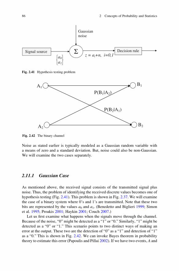
Noise as stated earlier is typically modeled as a Gaussian random variable with

a means of zero and a standard deviation. But, noise could also be non-Gaussian.

We will examine the two cases separately.

2.11.1 Gaussian Case

As mentioned above, the received signal consists of the transmitted signal plus

noise. Thus, the problem of identifying the received discrete values becomes one of

hypothesis testing (Fig. 2.41). This problem is shown in Fig. 2.37. We will examine

the case of a binary system where 0’s and 1’s are transmitted. Note that these two

bits are represented by the values a0 and a1. (Benedetto and Biglieri 1999; Simon

et al. 1995; Proakis 2001; Haykin 2001; Couch 2007.)

Let us first examine what happens when the signals move through the channel.

Because of the noise, “0” might be detected as a “1” or “0.” Similarly, “1” might be

detected as a “0” or “1.” This scenario points to two distinct ways of making an

error at the output. These two are the detection of “0” as a “1” and detection of “1”

as a “0.” This is shown in Fig. 2.42. We can invoke Bayes theorem in probability

theory to estimate this error (Papoulis and Pillai 2002). If we have two events, A and

Signal source

a0

a1

Σ

Gaussian noise

z = ai+n, i=0,1 Decision rule

Fig. 2.41 Hypothesis testing problem

A2

A1

B2

B1

P(B2|A1)

P(B1|A2)

Fig. 2.42 The binary channel


B, each with probabilities of P(A) and P(B), respectively, the conditional probabil-ity can be expressed in terms of Bayes theorem as

PðAjBÞ ¼ PðBjAÞPðAÞPðBÞ : (2.351)

Extending this notion to multiple events A ¼ {A1,A2,. . .,AM} and B ¼ {B1,

B2,. . .,BM}, the Bayes rule becomes

PðAijBjÞ ¼ PðBjjAiÞPðAiÞPðBjÞ

�i ¼ 1; 2; . . . ;Mj ¼ 1; 2; . . . ;M

; (2.352)

where

PðBjÞ ¼XM

i¼1

PðBjjAiÞPðAiÞ: (2.353)

In our description, A’s represent the input and B’s represent the received signals.We also identify P(Ai) as the a priori probability, P(Bj|Ai) as the conditional

probability and P(Ai|Bj) as the a posteriori probability. Equation (2.353) shows

that each output will have contributions from the complete input set. We can now

introduce the notion of errors by looking at a binary case (M ¼ 2). In the case of

binary signal transmission, we have two inputs {A1, A2} and two corresponding

outputs {B1,B2}. Since there is noise in the channel, B1 could be read as A2 and B2

could be read as A1. Thus, we have two ways in which error can occur. If the error is

represented by e, the probability of error can be written using the Bayes rule as

pðeÞ ¼ PðB2jA1ÞPðA1Þ þ PðB1jA2ÞPðA2Þ: (2.354)

We will now expand this notion to the transmission of digital signals through a

channel corrupted by noise. The received signal can be written as

z ¼ ai þ n; i ¼ 1; 2: (2.355)

Since the noise is Gaussian, we can represent the density function of noise as

(Shanmugam 1979; Schwartz 1980; Schwartz et al. 1996; Sklar 2001)

f ðnÞ ¼ 1ffiffiffiffiffiffiffiffiffiffi2ps2

p exp � n2

2s2

� �: (2.356)

Note that even though a’s only takes discrete values, z will be continuous as thenoise is not discrete. The density function of the received signal can be represented

as conditional density functions,


f ðzja1Þ ¼ 1ffiffiffiffiffiffiffiffiffiffi2ps2

p exp �ðz� a1Þ22s2

" #; (2.357)

f ðzja2Þ ¼ 1ffiffiffiffiffiffiffiffiffiffi2ps2

p exp �ðz� a2Þ22s2

" #: (2.358)

We will now identify the two hypotheses we have as H0 and H1, the former

corresponding to the transmission “0” (signal strength a0) and the latter corres-

ponding to the transmission of “1” (signal strength a1). We will rewrite (2.357) and

(2.358) as

f ðzja0Þ f ðzjH0Þ; (2.359)

f ðzja1Þ f ðzjH1Þ: (2.360)

These two density functions are plotted in Fig. 2.43.

Using simple logic, it would seem that we can decide on whether the received

signal belongs to hypothesis H0 or H1 as (Van Trees 1968)

f ðH1jzÞ>

<H0

H1

f ðH0jzÞ: (2.361)

Using the Bayes rule in (2.351)

f ðzjH1ÞPðH1Þ>

<H0

H1

f ðzjH0ÞPðH0Þ (2.362)

f(z|H0) f(z|H1)

za1 a2

Threshold

PMPF

Fig. 2.43 Concept of hypothesis testing


or

f ðzjH1Þf ðzjH0Þ� � >

<H0

H1

PðH0ÞPðH1Þ� �

: (2.363)

The left-hand side of (2.363) is known as the likelihood ratio; the entire equation

is identified as the likelihood ratio test. If both hypotheses are equally likely, the

right-hand side of (2.363) will be unity and take logarithms. We arrive at the log

likelihood ratio:

logef ðzjH1Þf ðzjH0Þ� � >

<H0

H1

0: (2.364)

Substituting (2.357) and (2.358), we have the threshold for the decision as

z ¼ zthr ¼ ða1 þ a2Þ2

(2.365)

Thus, (2.365) demonstrates that the threshold for making decision on whetherH1

is accepted for H0 is accepted is the midpoint of the two amplitude values. The

errors can occur in two ways. First, even when a “0” was transmitted, because of

noise, it can be read/detected as a “1.” This is called the probability of false alarm

(PF) and is given by the probability indicated by the shaded area in Fig. 2.12.

PF ¼ð1

zthr

f ðzjH0Þ dz: (2.366)

Second, when “1” was sent, it can be read/detected as “0.” This is called the

probability of miss (PM) and it is given by the shaded area corresponding to the

probability

PM ¼ðzthr

�1f ðzjH1Þ dz: (2.367)

The average probability of error is given by

pðeÞ ¼ pðejH1ÞPðH1Þ þ pðejH0ÞPðH0Þ (2.368)

or

pðeÞ ¼ PFPðH1Þ þ PMPðH0Þ: (2.369)


If both hypotheses are equally likely (0’s and 1’s being transmitted with equal

probability), the average probability of error will be

pe ¼ PF or PM: (2.370)

It can be seen that the average probability of error can be expressed in terms of

the CDF of the Gaussian random variable as well as the complimentary error

functions (Sklar 2001).

2.11.2 Non-Gaussian Case

While the detection of signals in additive white Gaussian noise is generally

encountered in communications, there are also instances when the receiver makes

decisions based on the envelope of the signal. Examples of these include envelope

detection of amplitude shift keying and frequency shift keying. It also includes

distinguishing the signals at the wireless receiver from the signal of interest and the

interference, both of which could be Rayleigh distributed when short-term fading is

present. As discussed earlier the statistics of the envelope might also be Rician

distribution. There is a need to minimize the error rate by determining the optimum

value of the threshold.

We would like to examine three separate cases, the first where both hypotheses

lead to Rayleigh densities, the second where one of the hypothesis leads to Rayleigh

while the other hypothesis results in Rician, and the third where both hypothesis

result in Rician densities. Let the two density functions be

f ðzjH0Þ ¼ z

s20exp � z2

2s20

� �; z> 0; (2.371)

f ðzjH1Þ ¼ z

s21exp � z2

2s21

� �; z> 0 (2.372)

with

s1 > s0: (2.373)

From (2.364) the log likelihood ratio test leads to a threshold of

zthr ¼ s0s1

ffiffiffiffiffiffiffiffiffiffiffiffiffiffiffiffiffiffiffiffiffiffiffiffilogeðs1=s0Þ2ðs21 � s20Þ

s

: (2.374)

The decision region and the two regions for the computation of error are shown

in Fig. 2.44.


The values of s0 and s1 for the Fig. 2.44 are 2 and 5, respectively, and the

threshold is at 4.177.

Next we consider the case where the density function of the envelope under the

hypothesis H0 is Rayleigh distributed, as previously given in (2.371), while the pdf

of the envelope is Rician distributed for the second hypothesis, namely H1. The pdf

for the envelope under the hypothesis H1 is as in (2.208)

f ðzjH1Þ ¼ z

s20exp � z2 þ A2

2s20

� �I0

zA

s20

� �; z> 0: (2.375)

Note that both the density functions in (2.371) and (2.375) come from Gaussian

random variables of identical standard deviation s0 and A is>0. A direct solution of

(2.364) is going to be difficult because of the existence of the Bessel function in

(2.375). We will use an indirect approach for solving the threshold. Let us assume

that � is the threshold. The probability of false alarm PF will be given by (Van Trees

1968; Cooper and McGillem 1986)

PF ¼ð1

�

f ðzjH0Þ dz ¼ exp � �2

2s20

� �: (2.376)

The probability of miss PM will be

PM ¼ð�

0

f ðzjH1Þ dz ¼ð�

0

z

s20exp � z2 þ A2

2s20

� �I0

zA

s20

� �dz: (2.377)

0 2 4 6 8 10 12 14 16 18 200

0.05

0.1

0.15

0.2

0.25

0.3

0.35

z

pdf

f(z|H0)

f(z|H1)

PF

PM

zthr

Fig. 2.44 Hypothesis testing (non-Gaussian case)


Since there is no analytical solution to (2.377), we will examine what happens if

we assume that the direct component A � s0. Invoking the approximation to the

modified Bessel function of the first kind mentioned in (2.210), and rewriting

(2.304) as

PM ¼ 1�ð1

�

z

s20exp � z2 þ A2

2s20

� �I0

zA

s20

� �dz (2.378)

we get

PM ¼ 1�ð1

�

ffiffiffiffiffiffiffiffiz=A

pffiffiffiffiffiffiffiffiffiffi2ps20

p exp �ðz� AÞ22s20

" #dz: (2.379)

The integrand in (2.379) is sharply peaked at z ¼ A, and the slowly varying

factorffiffiffiffiffiffiffiffiz=A

pmay be replaced with its value at the peak, i.e., unity, leading to a

simpler expression for the probability of miss as

PM ¼ 1�ð1

�

1ffiffiffiffiffiffiffiffiffiffi2ps20

p exp �ðz� AÞ22s20

" #dz: (2.380)

Using the Q function defined in (2.90), the probability of miss becomes

PM ¼ 1� Q� � A

s0

� �: (2.381)

The total error will be

pðeÞ ¼ 1

2½PF þ PM�: (2.382)

Taking the derivative of (2.382) and setting it equal to zero, we have

d½PF þ PM�d�

¼ 0: (2.383)

Using the derivative of the Q function as

d½QðxÞ�dx

¼ � 1ffiffiffiffiffiffi2p

p exp � x2

2

� �(2.384)

(2.384) becomes

� �

s20exp � �2

2s20

� �þ 1ffiffiffiffiffiffiffiffiffiffi

2ps20p exp �ð� � AÞ2

2s20

" #¼ 0: (2.385)


Once again, a solution to (2.385) is not straightforward. Instead, we import the

concept from the Gaussian pdfs in (2.365). At high values of the SNR, as seen in

(2.380), the envelope follows a Gaussian under the hypothesis H1. We can argue

that the threshold should be the midway point between the peaks of the two

density functions. This is shown in Fig. 2.45. This would mean that the optimum

threshold is

zthr ¼ 1

2½s0 þ A�: (2.386)

Note that in (2.386), A is the mode of the pdf of the envelope under hypothesis

H1 and s0 the mode of the pdf under the hypothesis H0. Since A � s0, the optimum

threshold is

zthr A

2: (2.387)

We can now look at the last case where the envelopes follow Rician pdf under

both hypotheses, with direct components of A0 and A1 respectively. Using the

Gaussian approximation to Rician, the optimum threshold will be

zthr ¼ 1

2½A1 þ A0�: (2.388)

0 5 10 150

0.1

0.2

0.3

0.4

0.5

0.6

0.7

z

pdf

f(z|H0): Rayleigh

f(z|H1): Rician

zthr = 2.98σ0 = 1; A = 5

zthr

PF

Fig. 2.45 Hypothesis testing (Rayleigh vs. Rician)


2.12 Upper Bounds on the Tail Probability

In wireless communications, it is often necessary to evaluate the probability that the

SNR exceeds a certain value or that SNR fails to reach a certain threshold value. In

Sect. 2.13, we saw two measures of error probabilities, a probability of false alarm,

i.e., the area under the upper tail of the pdf curve beyond a certain value, and a

probability of miss, i.e., the area under the lower tail below a certain value. Often, it

might not be possible to evaluate such areas. It might be necessary to get an

estimate of the upper bounds of such probabilities which correspond to areas

under the tails of the pdf curves. We will look at two bounds, one based on the

Chebyshev inequality and the other one called the Chernoff bound (Schwartz et al.

1996; Haykin 2001). The former one is a loose bound while the latter is much

tighter.

2.12.1 Chebyshev Inequality

Let f(x) be the pdf of a random variable X with a mean of m and standard deviation

of s. If d is any positive number, the Chebyshev inequality is given by (Papoulis and

Pillai 2002)

PðjX � mj � dÞ � s2

d2: (2.389)

In (2.389), P(.) is the probability. Equation (2.389) can be established from the

definition of variance as

s2 ¼ð1

�1ðx� mÞ2f ðxÞ dx: (2.390)

Changing the lower limit in (2.390), we have

s2 �ð1

jx�mj�dðx� mÞ2f ðxÞ dx ¼ d2

ð1

jx�mj�df ðxÞ dx: (2.391)


s2 � d2PðjX � mj � dÞ (2.392)

which is the Chebyshev inequality in (2.389). The Chebyshev inequality can also be

obtained in a slightly different way that would provide more insight into its

meaning. If we assume that the random variable has a mean of zero (i.e., define a

new random variable Y ¼ X�m), we can define a new function


gðYÞ ¼ 1; jYj � d;0; jYj � d:

(2.393)

The left-hand side of the Chebyshev inequality in (2.389) is related to the mean

of the new variable in (2.393)

hgðYÞi ¼ PðjYj � dÞ ¼ PðjX � mj � dÞ: (2.394)

The concept of this approach to Chebyshev inequality is shown in

Fig. 2.46. From the figure, it is seen that the g(Y) is bounded (upper) by the

quadratic (Y/d)2,

gðYÞ � Y

d

� �2

: (2.395)

Note that Y is a zero mean random variable and hence

hY2i ¼ hðX � mÞ2i ¼ s2: (2.396)

Thus,

hgðYÞi � Y2

d2

� �¼ hY2i

d2¼ s2

d2: (2.397)

Since (2.394) is the tail probability, (2.397) provides the Chebyshev inequality

in (2.389).

0

1

0-δ δY

g(Y)

Upperbound(Y/δ)2

Fig. 2.46 Concept of Chebyshev inequality

2.12 Upper Bounds on the Tail Probability 95

2.12.2 Chernoff Bound

In some of the cases we are interested in the area only under one tail. For most of the

wireless communications, SNR takes positive values only. We are often interested

in the probability that the SNR exceeds a certain value, i.e., the area under the tail

from d to 1. Since only a single tail is involved, we could use an exponential

function instead of the quadratic function in the Chebyshev inequality (Proakis

2001; Haykin 2001). Let g(Y) be such that

gðYÞ � exp½vðY � dÞ� (2.398)

with

gðYÞ ¼ 1; Y � d;0; Y< d:

(2.399)

In (2.398), the parameter v needs to be found and optimized. The exponential

upper bound is shown in Fig. 2.47.

The expected value of g(Y) is

hgðYÞi ¼ PðY � dÞ � hexp½vðY � dÞ�i: (2.400)

Note that v must be positive. Its value can be obtained by minimizing the

expected value of the exponential term in (2.400). A minimum occurs when

0

1

Yδ

Upperboundev(Y-δ)

g(Y)

Fig. 2.47 Concept of the Chernoff bound


d

dvhexp½vðY � dÞ�i ¼ 0: (2.401)

Changing the order of integration and differentiation in (2.401), we have

expð�vdÞ½hY expðvYÞi � dhexpðvYÞi� ¼ 0: (2.402)

The tightest bound is obtained from

hY expðvYÞi � dhexpðvYÞi ¼ 0: (2.403)

If v is the solution to (2.403), the upper bound on the one sided tail probability

from (2.400) is

PðY � dÞ � expð�vdÞhexpðvdÞi: (2.404)

As it can be observed, the Chernoff bound is tighter than the tail probability

obtained from the Chebyshev inequality because of the minimization in (2.401).

2.13 Stochastic Processes

We have so far examined the randomness of observed quantities, such as the signal

amplitude or power and noise amplitude or power at a certain fixed time instant.

While the signal and noise are spread over a long period of time, the random

variable we studied constituted only a sample taken from the time domain function

associated with the signal or noise (Taub and Schilling 1986; Gagliardi 1988;

Papoulis and Pillai 2002). In other words, we need to characterize the temporal

statistical behavior of the signals. This is accomplished through the concept of

random processes. Consider a simple experiment. Take, for example, the measure-

ment of a current or voltage through a resistor. Let us now set up several such

experiments, all of them with identical characteristics. In each of these experiments,

we measure the signal over a certain time period and we expect to see several time

functions as illustrated in Fig. 2.48.

The voltages are plotted along the X-axis for each experiment while the temporal

information is plotted along the Y-axis. For a fixed time (t1), if we take the samples

along the time line, we get different sample values which are random. In other

words, if each of the temporal functions are represented by X, we can express it as afunction of two variables, namely the “ensembles” x and “time” t. All such time

functions together constitute the random process which describes the noise voltage.

In other words, X(x,t) represents the random process and for a fixed time instant

tk, X(x,tk) represents a random variable, simply represented by X(tk). If the sample

value is fixed, i.e., for a fixed value of x, say xn, we have a pure time function as

X(xn,t). In other words, by fixing the time, we create a random variable from a

2.13 Stochastic Processes 97

process, and the random process becomes a pure time function when we fix the

ensemble value. Thus, the random process provides both temporal and ensemble

information on the noise or any other noise phenomenon. For example, we can

create a random process by making the phase of a cosine wave random as

XðtÞ ¼ cosð2pf0tþYÞ: (2.405)

In (2.405),Y is a random variable. Since the random process contains both time

and ensemble information, we can obtain two different types averages, autocorre-

lation values, and so on. Let us first define the density functions. For any value of t,X(t) is a random variable, and hence, the first-order CDF is expressed as

Fðx; tÞ ¼ P½xðtÞ< x�: (2.406)

The first order density function f(x,t) is obtained by differentiating (2.406)

w.r.t x as

f ðx; tÞ ¼ @Fðx; tÞ@x

: (2.407)

First, if we have time at two instants, t1 and t2, we can similarly obtain the second

density function

f ðx1; x2; t1; t2Þ ¼ @2Fðx1; x2; t1; t2Þ@x1@x2

: (2.408)

Time

# 1 # 2 # 3

t2

t1

t3

#

Fig. 2.48 Concept of a random process


Similarly we can create higher-order density functions. Once we have the first-

order density function, we have the so called first-order statistics and we get the nthorder statistics of the random process by defining the density function for ensembles

taken at the n unique time instants, t1, t2,. . .,tn.We define the ensemble average or statistical average �(t) as

�ðtÞ ¼ hXðtÞi ¼ðxf ðx; tÞ dx: (2.409)

The autocorrelation of X(t) is the joint moment of X(t1)X(t2) defined as

Rðt1; t2Þ ¼ð ð

x1x2 f x1; x2; t1; t2ð Þ dx1dx2: (2.410)

We can define the autocovariance as

Cðt1; t2Þ ¼ Rðt1; t2Þ � �ðt1Þ�ðt2Þ: (2.411)

Equation (2.411) provides the variance of the random process when t1 � t2 ¼ 0.

The average values defined so far have been based on the use of density functions.

Since the random process is a function of time as well, we can also define the

averages in the time domain. Let

s ¼ðb

a

XðtÞ dt (2.412)

and

s2 ¼ðb

a

ðb

a

Xðt1ÞXðt2Þ dt1dt2: (2.413)

The averages in (2.412) and (2.413) are random variables. To remove the random-

ness and to get the true mean, we need to take a further expectation (statistical) of the

quantities.

�ðsÞ ¼ hsi ¼ðb

a

hXðtÞi dt ¼ðb

a

�ðtÞ dt; (2.414)

hs2i ¼ðb

a

ðb

a

hXðt1ÞXðt2Þi dt1dt2 ¼ðb

a

ðb

a

Rðt1; t2Þ dt1dt2: (2.415)

In communications, it is easy to perform temporal averaging by observing the

signal in the time domain as in (2.412) or (2.413). If the temporal averages and

statistical averages are equal, it would be necessary for the integrals in (2.414) and


(2.415) to be equal. Such properties are associated with stationary processes.

A stochastic process X(t) is called strict sense stationary (SSS) if its statistical

properties are invariant to a shift in the origin. Thus, a process is first-order

stationary if

f ðx; tÞ ¼ f ðx; tþ cÞ ¼ f ðxÞ; c> 0: (2.416)

This would mean that the temporal average and statistical average are identical.

A process is second order stationary if the joint pdf depends only on the time

difference and not on the actual values of t1 and t2 as

f ðx1; x2; t1; t2Þ ¼ f ðx1; x2; tÞ; (2.417)

t ¼ t1 � t2: (2.418)

A process is called wide stationary sense (WSS) if

hXðtÞi ¼ �; (2.419)

hXðt1ÞXðt2Þi ¼ RðtÞ: (2.420)

Since t is midway point between t and t + t, we can write

RðtÞ ¼ X t� t2

� �X� tþ t

2

� �D E: (2.421)

In (2.421), we have treated the process as complex in the most general sense.

Note that a complex process

XðtÞ ¼ XrðtÞ þ jXiðtÞ (2.422)

is specified in terms of the joint statistics of the real processes Xr(t) and Xi(t).A process is called ergodic if the temporal averages are equal to the ensemble

averages. For a random process to be ergodic, it must be SSS. Using this concept of

ergodicity, we can see that a wide sense of stationary process is ergodic in the mean

and ergodic in the autocorrelation. These two properties are sufficient for most of

the analysis of communication systems.

The power spectral density (PSD) S( f ) of a wide sense stationary process X(t) isthe Fourier transform of its autocorrelation, R(t). As defined in (2.421) the process

may be real or complex. We have

Sð f Þ ¼ð1

�1RðtÞ expð�j2pf0tÞ dt: (2.423)


Note that S( f ) is real since R(�t) ¼ R*(t). From the Fourier inversion property,

RðtÞ ¼ð1

�1Sð f Þ expðj2pf0tÞ df : (2.424)

Furthermore, if X(t) is real and R(t) is real and even, then

Sðf Þ ¼ð1

�1RðtÞ cosðj2pf0tÞ dt ¼ 2

ð1

0

RðtÞ cosðj2pf0tÞ dt; (2.425)

RðtÞ ¼ 2

ð1

0

Sðf Þ cosðj2pf0tÞ df : (2.426)

As discussed earlier, the noise in communication systems is modeled as a

random process. The primary characteristic of the noise in communication systems,

referred to as thermal noise, is that it is zero mean Gaussian and that it is white

(Taub and Schilling 1986). This means that the thermal noise at any given time

instant has a Gaussian distribution with zero mean. The whiteness refers to the fact

that its spectral density is constant (shown in Fig. 2.49).

The spectral density Gn( f ) of the noise n(t) has a constant value of ðN0=2Þ overall the frequencies. This means that its autocorrelation is a delta function as shown

RðtÞ ¼ N0

2dðtÞ: (2.427)

Equation (2.427) suggests that any two samples of the noise taken at any

separation (however small this separation may be) will be uncorrelated. When the

noise passes through a low pass filter of bandwidth B, the noise energy will be

ððN0=2Þ2BÞ or N0B.

f 0

Gn(f)

N0 2

Rn(τ)

N0 2

τ0

Fig. 2.49 Spectral density and the autocorrelation of noise


2.14 Summary

In this chapter, we examined some theoretical aspects of probability density

functions and distributions encountered in the study of fading and shadowing in

wireless channels. We started with the basic definition of probability, then

discussed density functions and properties relating to the analysis of fading and

shadowing. We also examined the transformations of random variables in conjunc-

tion with relationships of different types of random variables. This is important in

the study of diversity and modeling of specific statistical behavior of the wireless

channels. The density functions of some of the functions of two or more random

variables were derived. We examined order statistics, placing emphasis on the

density functions of interest in diversity analysis. Concepts of stochastic processes

and their properties were outlined. Similarly, the characteristics of noise were

delineated within the context of signal detection. In addition, this study included

an exploration of ways of expressing some of the densities in more compact forms

using the hypergeometric functions and Meijer’s G function.

References

Aalo, V. A. and T. Piboongungon (2005). On the multivariate generalized gamma distribution with

exponential correlation. Global Telecommunications Conference, 2005. GLOBECOM ‘05.

IEEE: 3–5.

Aalo, V. and J. Zhang (1999). “On the effect of cochannel interference on average error rates in

Nakagami-fading channels.” Communications Letters, IEEE 3(5): 136–138.

Abdi, A. and M. Kaveh (1998). “K distribution: an appropriate substitute for Rayleigh-lognormal

distribution in fading-shadowing wireless channels.” Electronics Letters 34(9): 851–852.Abdi, A. and M. Kaveh (1999). On the utility of gamma PDF in modeling shadow fading (slow

fading). Vehicular Technology Conference, 1999 IEEE 49th: 2308–2312.

Abramowitz, M., Segun, I. A., eds. (1972). Handbook of Mathematical Functions with Formulas,Graphs, and Mathematical Tables, New York: Dover Publications.

Abu-Dayya, A. A. and N. C. Beaulieu (1994). “Outage probabilities in the presence of correlated

lognormal interferers.” Vehicular Technology, IEEE Transactions on 43(1): 164–173.

Abu-Salih, M. (1983). “Distributions of the product and the quotient of power-function random

variables.” Arab J. Math 4: 1–2.

Adamchik, V. (1995). “The evaluation of integrals of Bessel functions via G-function identities.”

Journal of Computational and Applied Mathematics 64(3): 283–290.Alouini, M., et al. (2002). “Sum of gamma variates and performance of wireless communication

systems over Nakagami-fading channels.” Vehicular Technology, IEEE Transactions on 50(6):1471–1480.

Alouini, M. S. and M. K. Simon (1999). “Performance of coherent receivers with hybrid SC/MRC

over Nakagami-m fading channels.” Vehicular Technology, IEEE Transactions on 48(4):

1155–1164.

Alouini, M. S. and M. K. Simon (2000). “An MGF-based performance analysis of generalized

selection combining over Rayleigh fading channels.” Communications, IEEE Transactions on48(3): 401–415.

Alouini, M. and M. Simon (2003). “Dual diversity over correlated log-normal fading channels.”

Communications, IEEE Transactions on 50(12): 1946–1959.


Alouini, M. S. and M. K. Simon (2006). “Performance of generalized selection combining over

Weibull fading channels.” Wireless Communications & Mobile Computing 6(8): 1077–1084.

Anastassopoulos, V. et al. (1999). “High resolution radar clutter statistics,” Aerospace andElectronics Systems, IEEE Transactions on, 35(1): 43–60.

Andersen, J. B. (2002). Statistical distributions in mobile communications using multiple scatter-

ing. presented at the 27th URSI General Assembly, Maastricht, Netherlands.

Annamalai, A. et al. (2006). “Analysis of generalized selection diversity systems in wireless

channels.” Vehicular Technology, IEEE Transactions on 55(6): 1765–1775.

Annamalai, A. et al. (2005). “A general method for calculating error probabilities over fading

channels.” Communications, IEEE Transactions on 53(5): 841–852.

Atapattu, S. et al. (2010). Representation of Composite Fading and Shadowing Distributions byUsing Mixtures of Gamma Distributions. Wireless Communications and Networking Confer-

ence (WCNC), 2010 IEEE. 1:5.

Beaulieu, N. C. (1990). “An infinite series for the computation of the complementary probability

distribution function of a sum of independent random variables and its application to the sum of

Rayleigh random variables.” Communications, IEEE Transactions on 38(9): 1463–1474.

Beaulieu, N. et al. (1995). “Estimating the distribution of a sum of independent lognormal random

variables.” Communications, IEEE Transactions on 43(12): 2869.

Beaulieu, N. and Q. Xie (2004). “An optimal lognormal approximation to lognormal sum

distributions.” Vehicular Technology, IEEE Transactions on 53(2): 479–489.

Benedetto, S. and E. Biglieri (1999). Principles of digital transmission: with WirelessApplications. New York, Kluwer Academic/Plenum Press.

Bithas, P. et al. (2006). “On the performance analysis of digital communications over generalized-

K fading channels.” Communications Letters, IEEE 10(5): 353–355.

Bithas, P. S. et al. (2007). “Dual diversity over correlated Rician fading channels,” J. Comm &Networks. 9(1) 1–8.

L. E. Blumenson and K. S. Miller (1963). “Properties of Generalized Rayleigh Distributions,” TheAnnals of Mathematical Statistics 34(3) 903–910.

Brennan, D. G. (1959). “Linear diversity combining techniques”, Proc. IRE 47(6): 1075–1102.

Bryson, B. C. (1974). “Heavy tailed distributions: Properties and tests,” Technometrics 16(1) 61–68.Cardieri, P. and T. Rappaport (2001). “Statistical analysis of co-channel interference in wireless

communications systems.” Wireless Communications and Mobile Computing 1(1): 111–121.

Carter, B. and M. Springer (1977). “The distribution of products, quotients and powers of

independent H-function variates.” SIAM Journal on Applied Mathematics 33(4): 542–558.Cheng, J. et al. (2004). “Performance of digital linear modulations on Weibull slow-fading

channels.” Communications, IEEE Transactions on 52(8): 1265–1268.

Chiani, M. (1999). “Integral representation and bounds for Marcum Q-function.” ElectronicsLetters 35(6): 445–446.

Cooper, G. R. and McGillem, C. D. (1986). Modern communications and Spread Spectrum. NewYork. McGraw-Hill.

Cotton, S. L. and W. G. Scanlon (2007). “Higher Order Statistics for Lognormal Small-Scale Fading

in Mobile Radio Channels.” Antennas and Wireless Propagation Letters, IEEE 6: 540–543.

Couch, L. W. (2007). Digital and analog communication systems. Upper Saddle River, N.J.,

Pearson/Prentice Hall.

Coulson, A. J. et al. (1998a). “Improved fading distribution for mobile radio,” Communications,IEE Proceedings 145(3) 197–202.

Coulson, A. J., et al. (1998b). “A Statistical Basis for Lognormal Shadowing Effects in Multipath

Fading Channels,” Communications, IEEE Trans. on 46(4) 494–502.

da Costa, B. D. and M. D. Yacoub (2008). “Moment generating functions of generalized fading

distributions and applications.” Communications Letters, IEEE 12(2): 112–114.

Evans, M., N. A. J. Hastings, et al. (2000). Statistical distributions. New York, John Wiley.

Filho, J. C. S. S. et al. (2005). “Simple accurate lognormal approximation to lognormal sums.”

Electronics Letters 41(18): 1016–1017.Frery, A. et al. (2002). “A model for extremely heterogeneous clutter.” Geoscience and Remote

Sensing, IEEE Transactions on 35(3): 648–659.

References 103

Gagliardi, R. M. (1988). Introduction to Communications Engineering New York, John Wiley.

Gallager, R. G. (2008). Principles of digital communication. Cambridge; New York, Cambridge

University Press.

Gaur, S. and Annamalai A. (2003). “Some Integrals Involving theQm affiffiffix

p; b

ffiffiffix

pð Þwith Applicationto Error Probability Analysis of Diversity Receivers,” Vehicular Technology, IEEETransactions on 52(6) 1568–1575.

Goldsmith, A. (2005). Wireless Communications. New York, Cambridge University Press.

Goodman, J. W. (1985). Statistical Optics. New York. Wiley.

Gradshteyn, I. S., I. M. Ryzhik (2007). Table of integrals, series and products. Oxford, Academic.

Griffiths, J. and McGeehan, J. P. (1982). “Inter relationship between some statistical distributions

used in radio-wave propagation”, Comm, Radar and Sig. Proc, IEE Proceedings on 129(6)

411–417.

Gupta, R. D. and Kundu, D. (1999). “Generalized exponential distributions,” Austral. & NewZealand J. Statistics 41(2), 173–188.

Hansen, F. and F. I. Meno (1977). “Mobile fading; Rayleigh and lognormal superimposed.”

Vehicular Technology, IEEE Transactions on 26(4): 332–335.

Haykin, S. S. (2001). Digital communications. New York, Wiley.

Helstrom, C. W. (1968). Statistical theory of signal detection. Oxford, New York, Pergamon Press.

Helstrom, C. W. (1991). Probability and stochastic processes for engineers. New York,

Macmillan.

Helstrom, C. W. (1992). “Computing the generalized Marcum Q function.” Information Theory,IEEE Transactions on 38(4): 1422–1428.

Helstrom, C. W. (1998). “Approximate inversion of Marcum’s Q-function.” Aerospace andElectronic Systems, IEEE Transactions on 34(1): 317–319.

Holm, H. and M. S. Alouini (2004). “Sum and difference of two squared correlated Nakagami

variates in connection with the McKay distribution.” Communications, IEEE Transactions on52(8): 1367–1376.

Hudson, J. E. (1996). A lognormal fading model and cellular radio performance. Global

Telecommunications Conference, 1996. GLOBECOM ‘96. ‘Communications: The Key to

Global Prosperity. 2: 1187–1191.

Iskander, R. D. and Zoubir, A. M. (1996). “On Coherent Modeling of Non-Gaussian Radar

Clutter,” Proc. 8th IEEE Signal Processing Workshop on statistical Signal and Array

Processing: 226–229.

Iskander, D. R. et al. (1999). “A method for estimating the parameters of the K distribution,”

Signal Processing, IEEE Transactions on 47: 1147–1151.

Ismail, M. H. and M. M. Matalgah (2006). “On the use of Pade approximation for performance

evaluation of maximal ratio combining diversity over Weibull fading channels.” EurasipJournal on Wireless Communications and Networking 6: 62–6.

Jakeman, E. and R. Tough (1987). “Generalized K distribution: a statistical model for weak

scattering.” Journal of the Optical Society of America A 4(9): 1764–1772.

Jakes, W. C. (1994). Microwave mobile communications. Piscataway, NJ, IEEE Press.

Kabe, D. G. (1958). “Some Applications of Meijer-G Functions to Distribution Problems in

Statistics,” Biometrika, 45(3/4): 578–580.Karadimas, P. and S. A. Kotsopoulos (2008). “A Generalized Modified Suzuki Model with

Sectored and Inhomogeneous Diffuse Scattering Component.” Wireless PersonalCommunications 47(4): 449–469.

Karadimas, P. and S. A. Kotsopoulos (2010). “A Modified Loo Model with Partially Blocked and

Three Dimensional Multipath Scattering: Analysis, Simulation and Validation.” WirelessPersonal Communications 53(4): 503–528.

Karagiannidis, G., N. Sagias, et al. (2006). “Closed-form statistics for the sum of squared

Nakagami-m variates and its applications.” Communications, IEEE Transactions on 54(8):

1353–1359.

Karagiannidis, G. K. et al. (2003a). “Performance analysis of triple selection diversity over

exponentially correlated Nakagami- m fading channels,” Communications, IEEE Transactionson 51(8):1245–1248.


Karagiannidis, G. K. et al. (2003b). “On the multivariate Nakagami-m distribution with exponen-

tial correlation,” Communications, IEEE Transactions on 51(8):1240–1244.

Karagiannidis, G. K. et al. (2007). “N*Nakagami: A novel statistical model for cascaded fading

channels,” Communications, IEEE Transactions on 55(8) 1453–145.

Karmeshu, J. and R. Agrawal (2007). “On efficacy of Rayleigh-inverse Gaussian distribution over

K-distribution for wireless fading channels.” Wireless Communications & Mobile Computing7(1): 1–7.

Korn, I. and Foneska, J. P. (2001). “M-CPM with MRC Diversity in Rician-, Hoyt-, and

Nakagami-Fading Channels,” Vehicular Technology, IEEE Transactions on 50(4) 1182–118.

Kostic, I. M. (2005). “Analytical approach to performance analysis for channel subject to

shadowing and fading.” Communications, IEE Proceedings- 152(6): 821–827.Kotz, S. and J. Adams (1964). “Distribution of sum of identically distributed exponentially

correlated gamma-variables.” The Annals of Mathematical Statistics: 277–283.Kundu, K. and Raqab, M. Z. (2005). “Generalized Rayleigh distribution: different methods of

estimations,” Computational Statistics & Data Analysis (49) 187–200.Lam, C. L. J. and T. Le-Ngoc (2006). “Estimation of typical sum of lognormal random variables

using log shifted gamma approximation.” Communications Letters, IEEE 10(4): 234–23.

Lam, C. L. J. and L.-N. Tho (2007). “Log-Shifted Gamma Approximation to Lognormal Sum

Distributions.” Vehicular Technology, IEEE Transactions on 56(4): 2121–2129.

Laourine, A. et al. (2008). “On the capacity of generalized-K fading channels.” WirelessCommunications, IEEE Transactions on 7(7): 2441–2445.

Laourine, A., et al. (2009). “On the Performance Analysis of Composite Multipath/Shadowing

Channels Using the G-Distribution,” Communications, IEEE Transactions on 57(4): 1162–1170.Lee, R. and B. Holland (1979). “Distribution of a ratio of correlated gamma random variables.”

SIAM Journal on Applied Mathematics 36(2): 304–320.D. J. Lewinsky (1983). “Nonstationary probabilistic target and cluttering scattering models,”

Aerospace Electronics and Systems, IEEE Transactions on 31: 490–49.

Ligeti, A. (2000). “Outage probability in the presence of correlated lognormal useful and

interfering components.” Communications Letters, IEEE 4(1): 15–17.

Lienhard, J. H. and Meyer, P. L. (1967). “A physical basis for the generalized gamma distribu-

tion,” Quarterly of Appl. Math. 25(3) 330–334.Lindsey, W. C. and Simon M. K. (1973). Telecommunication Systems Engineering. Englewood

Cliffs, N.J., Prentice-Hall.

Liu, Z. et al. (2008). “Approximating lognormal sum distributions with power lognormal

distributions.” Vehicular Technology, IEEE Transactions on 57(4): 2611–2617.

Ma, Y. and C. C. Chai (2000). “Unified error probability analysis for generalized selection

combining in Nakagami fading channels.” Selected Areas in Communications, IEEE Journalon 18(11): 2198–2210.

Mathai, A. and P. Moschopoulos (1991). “On a multivariate gamma.” Journal of MultivariateAnalysis 39(1): 135–153.

Mathai, A. M. (1993). A Handbook of Generalized Special Functions for Statistical and PhysicalSciences. Oxford University Press.

Mathai, A. M. and H. J. Haubold (2008). Special functions for applied scientists. New York,

Springer Science+Business Media.

Mathai, A. M. and R. K. Saxena (1973). Generalized hypergeometric functions with applicationsin statistics and physical sciences. Berlin, New York, Springer.

McDaniel, S. T. (1990). “Seafloor reverberation fluctuations”, J. Acoust. Soc. Amer. 88(3):

1530–1535.

Middleton, D. (1996). An Introduction to Statistical Communications Theory. Piscataway, N. J,IEEE Press.

Molisch, A. F. (2005). Wireless communications. Chichester, U. K. John Wiley & Sons.

Moschopoulos, P. (1985). “The distribution of the sum of independent gamma random variables.”

Annals of the Institute of Statistical Mathematics 37(1): 541–544.Nadarajah, S. (2005). “Products, and ratios for a bivariate gamma distribution.” Applied Mathe-

matics and Computation 171(1): 581–595.

References 105

Nadarajah, S. and A. Gupta (2005). “On the product and ratio of Bessel random variables.”

International Journal of Mathematics and Mathematical Sciences 2005(18): 2977–2989.Nadarajah, S. and A. Gupta (2006a). “Some bivariate gamma distributions.” Applied Mathematics

Letters 19(8): 767–774.Nadarajah, S. and S. Kotz (2006b). “Bivariate gamma distributions, sums and ratios.” Bulletin of

the Brazilian Mathematical Society 37(2): 241–274.Nadarajah, S. and S. Kotz (2006). “On the product and ratio of gamma and Weibull random

variables.” Econometric Theory 22(02): 338–344.Nadarajah, S. and S. Kotz (2007). “A class of generalized models for shadowed fading channels.”

Wireless Personal Communications 43(4): 1113–1120.Nakagami, M. (1960). The m-distribution—A general formula of intensity distribution of rapid

fading, in Statistical Methods in Radio Wave Propagation, W. C. Hoffman, Ed. Elmsford, NY:

Pergamon.

Nuttall, A. (1975). “Some integrals involving the Q_M function (Corresp.).” Information Theory,IEEE Transactions on 21(1): 95–96.

Nuttall, A. H. (1970). “Alternate forms for numerical evaluation of cumulative probability

distributions directly from characteristic functions.” Proceedings of the IEEE 58(11):

1872–1873.

Nuttall, A. H. (1969). “Numerical evaluation of cumulative probability distribution functions

directly from characteristic functions.” Proceedings of the IEEE 57(11): 2071–2072.

Okui, S. (1981). “Probability Distributions for Ratios of Fading Signal Envelopes and Their

Generalization,” Electronics and Communications in Japan 64-B(3), 72–80.

Panajotovic, A. S. et al. (2009). “Effect of Microdiversity and Macrodiversity on Average Bit

Error Probability in Shadowed Fading Channels in the Presence of Interference.” ETRI Journal31(5): 500–505.

Papazafeiropoulos, A. K. and S. A. Kotsopoulos (2011). “The a-l-m and a-m-m small scale general

fading distributions: A unified approach,” Wireless Personal Communications 57: 735–751.Papoulis, A. and S. U. Pillai (2002). Probability, random variables, and stochastic processes.

Boston, McGraw-Hill.

Patzold, M. (2002). Mobile Fading Channels. Chichester, U. K., John Wiley & Sons, Inc.

Piboongungon, T. and V. A. Aalo (2004). “Outage probability of L-branch selection combining in

correlated lognormal fading channels.” Electronics Letters 40(14): 886–888.Podolski, H. (1972). “The distribution of a product of n independent random variables with

generalized gamma distribution.” Demonstratio Math 4(2): 119–123.

Polydorou, D. S. et al. (1999). “Statistical characterization of fading in LOS wireless channels with

a finite number of dominant paths. Application in millimeter frequencies.” InternationalJournal of Infrared and Millimeter Waves 20(3): 461–472.

Proakis, J. G. (2001). Digital communications. Boston, McGraw-Hill.

Provost, S. (1989). “On sums of independent gamma random variables.” STATISTICS. 20(4):583–591.

Rappaport, T. S. (2002). Wireless communications: principles and practice. Upper Saddle River,N.J., Prentice Hall PTR.

Rice, S. (1974). “Probability Distributions for Noise Plus Several Sine Waves–The Problem of

Computation.” Communications, IEEE Transactions on 22(6): 851–853.

Rohatgi, V. K. and A. K. M. E. Saleh (2001). An introduction to probability and statistics. NewYork, Wiley.

Saleh, A. & Valenzuela R. A. (1987) “A statistical model for indoor multipath propagation”

Selected Areas in Communications, IEEE Journal on 5: 128–137.

Sahu, P. R. & Chaturvedi, A. K. (2005), “Performance analysis of predetection EGC receiver in

Weibull fading channel,” Electr. Lett. 41(2) 85–86.Salo, J. et al. (2006). “The distribution of the product of independent Rayleigh random variables.”

Antennas and Propagation, IEEE Transactions on 54(2): 639–643.

Schwartz, M. (1980). Information transmission, modulation, and noise: a unified approach tocommunication systems. New York, McGraw-Hill.

Schwartz, M. et al. (1996). Communication Systems and Techniques. Piscataway, NJ., IEEE Press.


Shah, A. et al. (2000). “Exact bit-error probability for optimum combining with a Rayleigh fading

Gaussian cochannel interferer.” Communications, IEEE Transactions on 48(6): 908–912.

Shankar, P. (2002a). Introduction to wireless systems, Wiley New York.

Shankar, P. (2002b). “Ultrasonic tissue characterization using a generalized Nakagami model.”

Ultrasonics, Ferroelectrics and Frequency Control, IEEE Transactions on 48(6): 1716–1720.

Shankar, P. M. (2004). “Error rates in generalized shadowed fading channels.” Wireless PersonalCommunications 28(3): 233–238.

Shankar, P. M. (2005). “Outage probabilities in shadowed fading channels using a compound

statistical model.” Communications, IEE Proceedings on 152(6): 828–832.

Shankar, P. M. and Gentile, C. (2010). Statistical Analysis of Short Term Fading and Shadowing in

Ultra-Wideband Systems. Communications (ICC), 2010 IEEE International Conference on.

Shankar, P. M. (2010). “Statistical Models for Fading and Shadowed Fading Channels in Wireless

Systems: A Pedagogical Perspective,” Wireless Personal Communications. DOI: 10.1007/s11277-010-9938-2

Shanmugam, K. S. (1979). Digital and analog communication systems. New York, Wiley.

Shepherd, N. H. (1977). “Radio wave loss deviation and shadow loss at 900 MHZ,” VehicularTechnology, IEEE Transactions on 26(4) 309–313.

Shin, J. et al. (2005). “Statistical modeling of speech signals based on generalized gamma

distribution.” Signal Processing Letters, IEEE 12(3): 258–261.

Sijing, J. and N. C. Beaulieu (2010). BER of antipodal signaling in Laplace noise., 2010 25th

Biennial Symposium on Communications (QBSC).

Simon, M. (2002). “The Nuttall Q function-its relation to the Marcum Q function and its applica-

tion in digital communication performance evaluation.” Communications, IEEE Transactionson 50(11): 1712–1715.

Simon, M. et al. (1995). Digital communication techniques: signal design and detection, PrenticeHall PTR.

Simon, M. K. and M. S. Alouini (2003). “Some new results for integrals involving the generalized

Marcum Q function and their application to performance evaluation over fading channels.”

Wireless Communications, IEEE Transactions on 2(4): 611–615.

Simon, M. K. and M.-S. Alouini (2005). Digital communication over fading channels. Hoboken,N.J., Wiley-Interscience.

Sklar, B. (1997a). “Rayleigh fading channels in mobile digital communication systems. I. Char-

acterization.” Communications Magazine, IEEE 35(7): 90–100.

Sklar, B. (1997b). “Rayleigh fading channels in mobile digital communication systems. II.

Mitigation.” Communications Magazine, IEEE 35(7): 102–109.

Sklar, B. (2001). Digital communications: fundamentals and applications. Upper Saddle River,

N.J., Prentice-Hall PTR.

Slimane, B. (2001). “Bounds on the distribution of a sum of independent lognormal random

variables.” Communications, IEEE Transactions on 49(6): 975–978.

Sowerby, K. W. and A. G. Williamson (1987). “Outage probability calculations for a mobile radio

system having two log-normal interferers.” Electronics Letters 23(25): 1345–1346.Springer, M. and W. Thompson (1966). “The distribution of products of independent random

variables.” SIAM Journal on Applied Mathematics 14(3): 511–526.Springer, M. and W. Thompson (1970). “The distribution of products of beta, gamma and

Gaussian random variables.” SIAM Journal on Applied Mathematics 18(4): 721–737.Stacy, E. (1962). “A generalization of the gamma distribution.” The Annals of Mathematical

Statistics 33(3): 1187–1192.Stacy, E. and G. Mihram (1965). “Parameter estimation for a generalized gamma distribution.”

Technometrics 7(3): 349–358.Steele, R. and L. Hanzo (1999). Mobile radio communications: second and third generation

cellular and WATM systems. Chichester, England; New York, John Wiley & Sons, Inc.

Stuart, A. (1962). “Gamma-distributed products of independent random variables.” Biometrika49(3–4): 564.

Stuber, G. L. (2000). Principles of mobile communication. New York, Kluwer Academic.

References 107

Subadar, R. & Sahu, P. R. (2009). “Performance Analysis of Dual MRC Receiver in Correlated

Hoyt Fading Channels,” Communications Letters, IEEE 13(6) 405–407.

Suzuki, H. (1977). “A statistical model for urban radio propagation”, Communications, IEEETransactions on 25: 673–680.

Tan, C. C. & Beaulieu, N. C. (1997). “Infinite Series Representations of the Bivariate Rayleigh and

Nakagami- Distributions,” Communications, IEEE Transactions on 45(10), 1159–1161.

Taub, H. & D. L. Schilling (1986). Principles of communication systems. New York, McGraw-

Hill.

Tellambura, C. and A. Annamalai (1999). “An unified numerical approach for computing the

outage probability for mobile radio systems.” Communications Letters, IEEE 3(4): 97–99.

Tellambura, C. and A. Annamalai (2000). “Efficient computation of erfc(x) for large arguments.”


Tellambura, C. and A. Annamalai (2003). Unified performance bounds for generalized selectiondiversity combining in fading channels. Wireless Communications and Networking (WCNC),

2003 IEEE.

Tellambura, C. et al. (2003). “Closed form and infinite series solutions for the MGF of a dual-

diversity selection combiner output in bivariate Nakagami fading.” Communications, IEEETransactions on 51(4): 539–542.

Tjhung, T. T. and C. C. Chai (1999). “Fade statistics in Nakagami-lognormal channels.”


Vaughn, R. A., J. B. Anderson, (2003). Channels, propagation and Antennas for MobileCommunications. Herts, U. K., IEE.

Van Trees, H. L. (1968) Detection, estimation, and modulation theory. Part I. New York: John

Wiley and Sons.

V.Gh. Voda, B. (2009). “A method constructing density functions: the case for a Generalized

Rayleigh variable,” Applications of Mathematics 54(5) 417–43.Vatalaro, F. (1995). “Generalised Rice-lognormal channel model for wireless communications.”

Electronics Letters 31(22): 1899–1900.Winters, J. (1987). “Optimum Combining for Indoor Radio Systems with Multiple Users.”


Winters, J. H. (1984). “Optimum combining in digital mobile radio with cochannel interference.”

Vehicular Technology, IEEE Transactions on 33(3): 144–155.

Winters, J. H. (1998). “The diversity gain of transmit diversity in wireless systems with Rayleigh

fading.” Vehicular Technology, IEEE Transactions on 47(1): 119–123.

Withers, C. and S. Nadarajah (2008). “MGFs for Rayleigh Random Variables.”Wireless PersonalCommunications 46(4): 463–468.

Wolfram (2011) http://functions.wolfram.com/, Wolfram Research, Inc.

Wongtrairat, W. and P. Supnithi (2009). “Performance of Digital Modulation in Double

Nakagami-m Fading Channels with MRC Diversity.” Communications, IEICE Transactionson E92b(2): 559–566.

Yacoub, M. D. (2000). “Fading distributions and co-channel interference in wireless systems.”

Antennas and Propagation Magazine, IEEE 42(1): 150–160.

Yacoub, M. D. (2007a). “The a-m Distribution: A Physical Fading Model for the Stacy Distribu-

tion.” Vehicular Technology, IEEE Transactions on 56(1): 27–34.

Yacoub, M. D. (2007b). “The m-m distribution and the Z-m distribution.” Antennas and Propaga-tion Magazine, IEEE 49(1): 68–81.

Yue, S. et al. (2001). “A review of bivariate gamma distributions for hydrological applications,”

J. Hydrology 246: 1–18.Zogas, D. and Karagiannidis, G. K. (2005). “Infinite-Series Representations Associated With the

Bivariate Rician Distribution and Their Applications,” Communications, IEEE Transactionson 53(11): 1790–179.


http://functions.wolfram.com/

http://www.springer.com/978-1-4614-0366-1

Documents

Concepts of Probabilities and Statistics