–i–

FEB 19, 2001

TESLA-2001-17

CONCEPTUAL DESIGN

FOR THE FINAL FOCUS QUADRUPOLE MAGNETS

FOR TESLA

A. Devred, C. Gourdin, F. Kircher, J.P. Lottin and J.M. Rifflet

(arnaud.devred@cea.fr)

Commissariat à l'Energie Atomique de Saclay (CEA/Saclay)

DSM/DAPNIA/STCM

F–91191 GIF-SUR-YVETTE CEDEX

FRANCE

ABSTRACT

We present a preliminary design of the superconducting final focusing quadrupole

magnets for TESLA and all their associated cryogenics.

–ii–

1 INTRODUCTION 1

2 ELECTROMAGNETIC DESIGN 2

3 MECHANICAL DESIGN 5

3.1 Overview 5

3.2 Numerical Model 6

3.3 Results 10

3.4 Conclusions 13

4 CABLE SPECIFICATION 13

5 CRYOGENICS 15

5.1 Overview 15

5.2 Cryostat 15

5.3 Refrigeration 16

5.4 Heat loads 17

REFERENCES 19

–1–

1 INTRODUCTION

The Tera Electron volts Superconducting Linear Accelerator (TESLA) is an

electron/positron linear collider, with an energy of 250 GeV per beam, under consideration at

the Deutsches Elektronen Synchrotron (DESY) [1]. Two superconducting magnet systems

are required in the TESLA interaction region where the beams cross with a zero angle: (1) a

set of four final focusing quadrupole magnets (two on each side of the collision point) and (2)

a large solenoid embedded in the detector array (surrounding the collision point). To benefit

from the experience and the development work carried out for the Large Hadron Collider

(LHC), presently under construction at the European Laboratory for Particle Physics

(commonly referred to as CERN) [2], the design of the two magnet systems is based on

existing LHC designs: the final focusing quadrupole magnets are modeled after the LHC arc

quadrupole magnets [3], and the solenoid is modeled after the Compact Muon enoid (CMS)

that will be implement in one of LHC experiments [4].

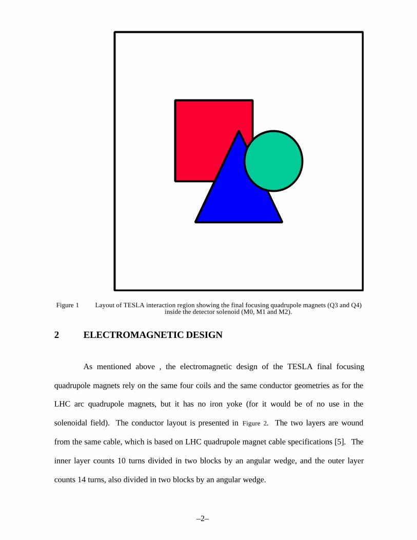
There is at least one major difference between TESLA and LHC: for beam optics

reasons, the TESLA final focusing quadrupole magnets must be localized very close to the

interaction point. As illustrated in Figure 1, they end up inside the solenoid and must operate

in its background field. Given the field requirements (4 T for the solenoid and 250 T/m

within an aperture of 56 mm for the quadrupole magnets), we are at the limit of NbTi cable

performances and it is more appropriate to consider Nb3Sn cables.

The present note describes a preliminary conceptual design of the final focusing

quadrupole magnets for TESLA, which is based on the LHC arc quadrupole magnet design,

but relies on Nb3Sn cables. The main goals are: to set a cable critical current specification,

and to dimension the coil support structure and cryostat.

–2–

Figure 1 Layout of TESLA interaction region showing the final focusing quadrupole magnets (Q3 and Q4)inside the detector solenoid (M0, M1 and M2).

2 ELECTROMAGNETIC DESIGN

As mentioned above , the electromagnetic design of the TESLA final focusing

quadrupole magnets rely on the same four coils and the same conductor geometries as for the

LHC arc quadrupole magnets, but it has no iron yoke (for it would be of no use in the

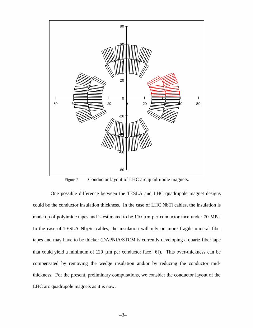
solenoidal field). The conductor layout is presented in Figure 2. The two layers are wound

from the same cable, which is based on LHC quadrupole magnet cable specifications [5]. The

inner layer counts 10 turns divided in two blocks by an angular wedge, and the outer layer

counts 14 turns, also divided in two blocks by an angular wedge.

–3–

-80

-60

-40

-20

0

20

40

60

80

-80 -60 -40 -20 0 20 40 60 80

Figure 2 Conductor layout of LHC arc quadrupole magnets.

One possible difference between the TESLA and LHC quadrupole magnet designs

could be the conductor insulation thickness. In the case of LHC NbTi cables, the insulation is

made up of polyimide tapes and is estimated to be 110 µm per conductor face under 70 MPa.

In the case of TESLA Nb3Sn cables, the insulation will rely on more fragile mineral fiber

tapes and may have to be thicker (DAPNIA/STCM is currently developing a quartz fiber tape

that could yield a minimum of 120 µm per conductor face [6]). This over-thickness can be

compensated by removing the wedge insulation and/or by reducing the conductor mid-

thickness. For the present, preliminary computations, we consider the conductor layout of the

LHC arc quadrupole magnets as it is now.

–4–

In this design, the quadrupole field gradient, g, can be estimated as a function of

supplied current, I, using

g = 17.7747 10-3 I (1)

From Eq. (1), it follows that the current, Iop, corresponding to an operating field

gradient of 250 T/m is

Iop ≈ 14,065 A (2)

In order to operate the quadrupole magnets with a margin of 20% along the load line,

the cable critical current, cableCI , must satisfy

A 17,581 0.8

opcableC ≈≥

II (3)

Furthermore, the peak magnetic flux density on the magnet coil when the quadrupole

magnet stands alone, Bp, can be estimated from

Bp ≈ 0.5436 10-3 I (4)

and it follows that the peak magnetic flux density, Bp,C, corresponding to the lower limit of

cableCI is simply

Bp,C ≈ 9.56 T (5)

When the quadrupole magnet is positioned inside the detector magnet, it seems

reasonable to assume that (at least in the quadrupole magnet straight section) the two

magnetic flux densities add up quadratically, as the two fields are roughtly orthogonal.

–5–

Hence, the superconducting cable must be specified to carry the current cableCI under a

magnetic flux density, Bspec, derived from

T 10,36 4 56.9 22spec ≈+≈B (6)

3 MECHANICAL DESIGN

3.1 OVERVIEW

The magnet coils will be produced according to the “wind, react & impregnate”

technique. Prior to winding, the un-reacted Nb3Sn cable will be wrapped with a mineral fiber

tape. Upon winding completion, the whole coil will be subjected to the heat treatment

required for Nb3Sn compound formation (typically: 660 ºC for 240 hours). After heat

treatment, the coil will be vacuum-impregnated with epoxy resin. It is worth mentioning that

an alternative insulation scheme is being investigated by DAPNIA/STCM, that may eliminate

the need for a vacuum-impregnation, but the design and the computations reported here

correspond to the standard (mineral fiber tape + epoxy resin) scheme.

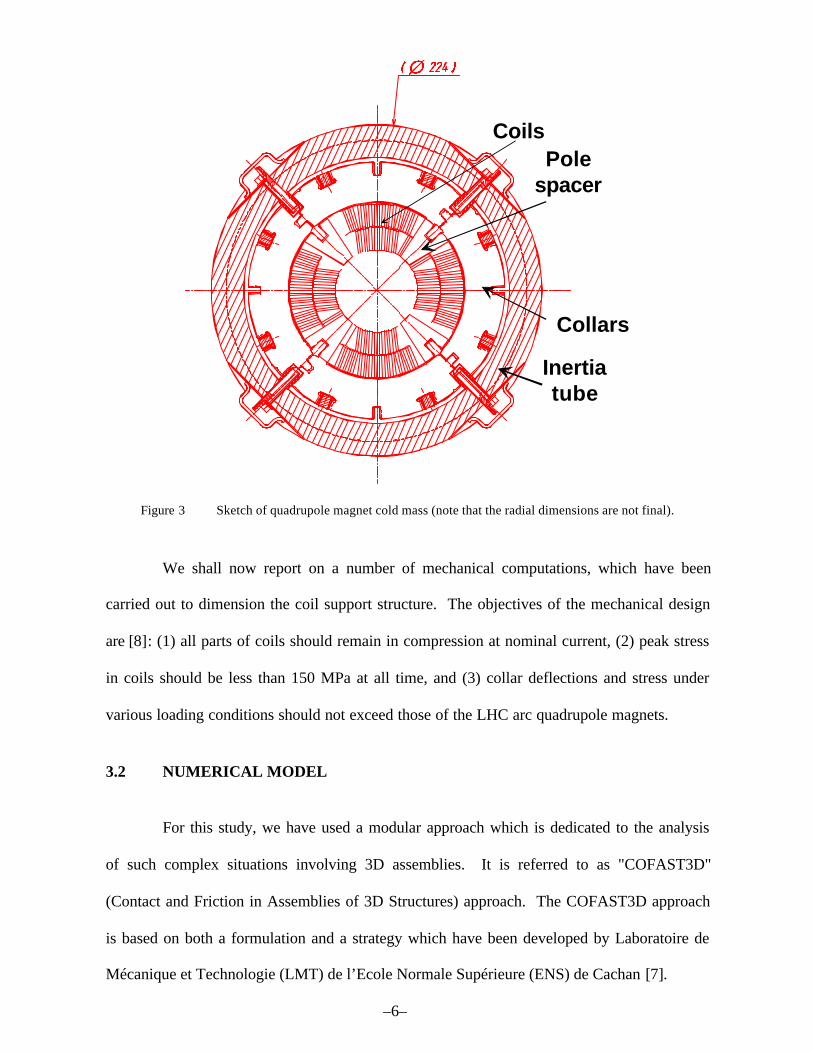
As in LHC arc quadrupole magnets, the coils will be restrained by laminated, 2-mm-

thick, austenitic steel collars locked around them by tapered keys. However, unlike in LHC

arc quadrupole magnets, there will be no iron yoke and the collared-coil assembly will be

centered directly within a precisely-machined, steel inertia tube delimiting the region of liquid

helium circulation. A sketch of the quadrupole magnet cold mass is shown in Figure 3 (note

that the radial dimensions are not final).

–6–

Coils

Collars

Inertia tube

Pole spacer

Figure 3 Sketch of quadrupole magnet cold mass (note that the radial dimensions are not final).

We shall now report on a number of mechanical computations, which have been

carried out to dimension the coil support structure. The objectives of the mechanical design

are [8]: (1) all parts of coils should remain in compression at nominal current, (2) peak stress

in coils should be less than 150 MPa at all time, and (3) collar deflections and stress under

various loading conditions should not exceed those of the LHC arc quadrupole magnets.

3.2 NUMERICAL MODEL

For this study, we have used a modular approach which is dedicated to the analysis

of such complex situations involving 3D assemblies. It is referred to as "COFAST3D"

(Contact and Friction in Assemblies of 3D Structures) approach. The COFAST3D approach

is based on both a formulation and a strategy which have been developed by Laboratoire de

Mécanique et Technologie (LMT) de l’Ecole Normale Supérieure (ENS) de Cachan [7].

–7–

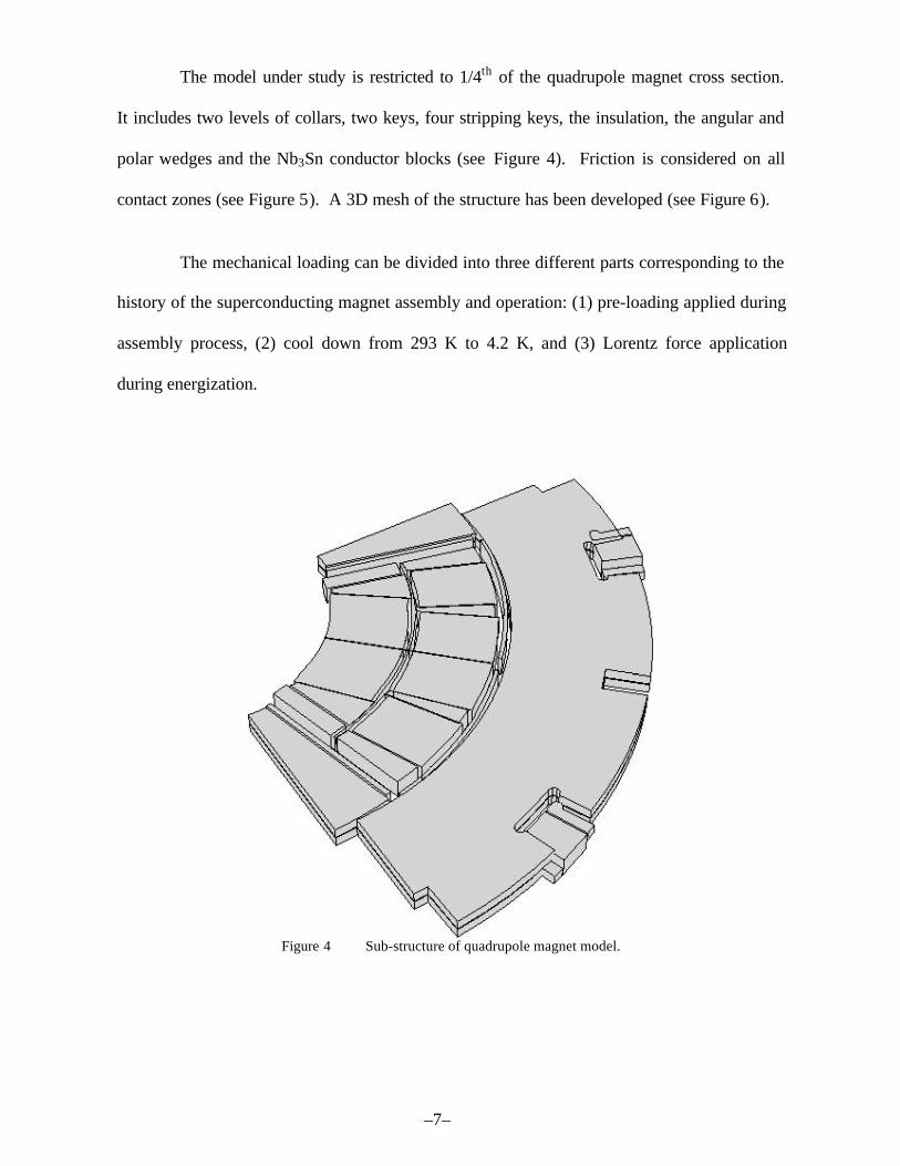
The model under study is restricted to 1/4th of the quadrupole magnet cross section.

It includes two levels of collars, two keys, four stripping keys, the insulation, the angular and

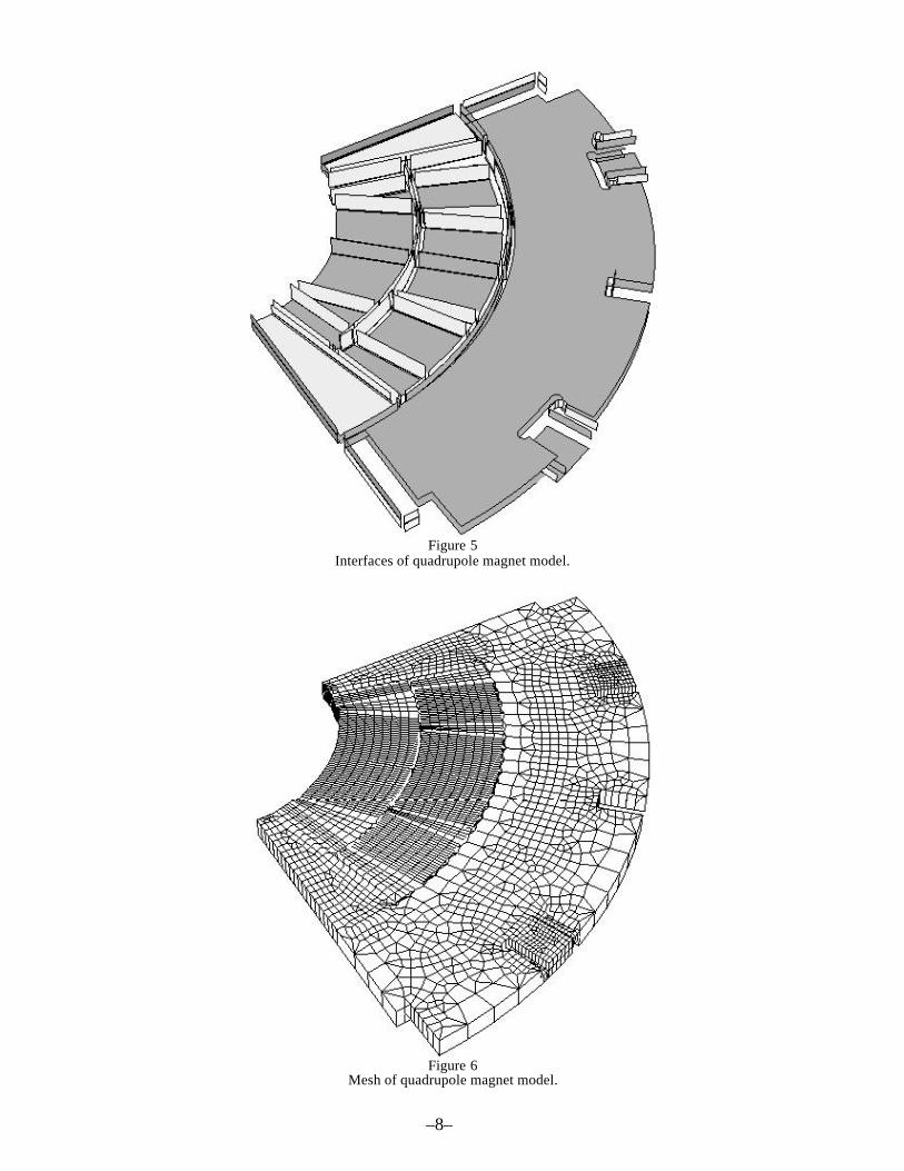
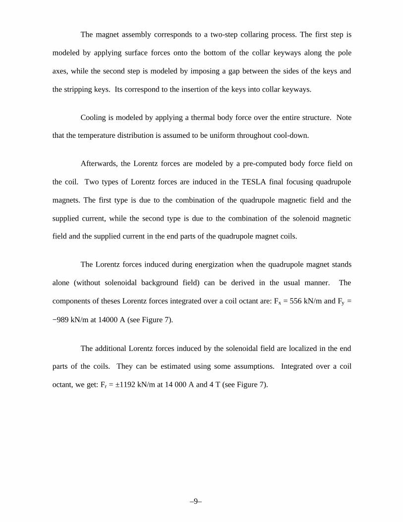
polar wedges and the Nb3Sn conductor blocks (see Figure 4). Friction is considered on all

contact zones (see Figure 5). A 3D mesh of the structure has been developed (see Figure 6).

The mechanical loading can be divided into three different parts corresponding to the

history of the superconducting magnet assembly and operation: (1) pre-loading applied during

assembly process, (2) cool down from 293 K to 4.2 K, and (3) Lorentz force application

during energization.

Figure 4 Sub-structure of quadrupole magnet model.

–8–

Figure 5Interfaces of quadrupole magnet model.

Figure 6Mesh of quadrupole magnet model.

–9–

The magnet assembly corresponds to a two-step collaring process. The first step is

modeled by applying surface forces onto the bottom of the collar keyways along the pole

axes, while the second step is modeled by imposing a gap between the sides of the keys and

the stripping keys. Its correspond to the insertion of the keys into collar keyways.

Cooling is modeled by applying a thermal body force over the entire structure. Note

that the temperature distribution is assumed to be uniform throughout cool-down.

Afterwards, the Lorentz forces are modeled by a pre-computed body force field on

the coil. Two types of Lorentz forces are induced in the TESLA final focusing quadrupole

magnets. The first type is due to the combination of the quadrupole magnetic field and the

supplied current, while the second type is due to the combination of the solenoid magnetic

field and the supplied current in the end parts of the quadrupole magnet coils.

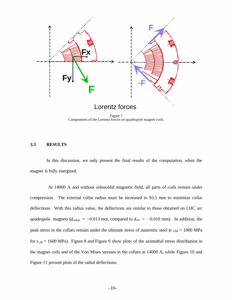
The Lorentz forces induced during energization when the quadrupole magnet stands

alone (without solenoidal background field) can be derived in the usual manner. The

components of theses Lorentz forces integrated over a coil octant are: Fx = 556 kN/m and Fy =

−989 kN/m at 14000 A (see Figure 7).

The additional Lorentz forces induced by the solenoidal field are localized in the end

parts of the coils. They can be estimated using some assumptions. Integrated over a coil

octant, we get: Fr = ±1192 kN/m at 14 000 A and 4 T (see Figure 7).

–10–

Fy

Fx

F

-FF

Lorentz forcesFigure 7

Components of the Lorentz forces on quadrupole magnet coils.

3.3 RESULTS

In this discussion, we only present the final results of the computation, when the

magnet is fully energized.

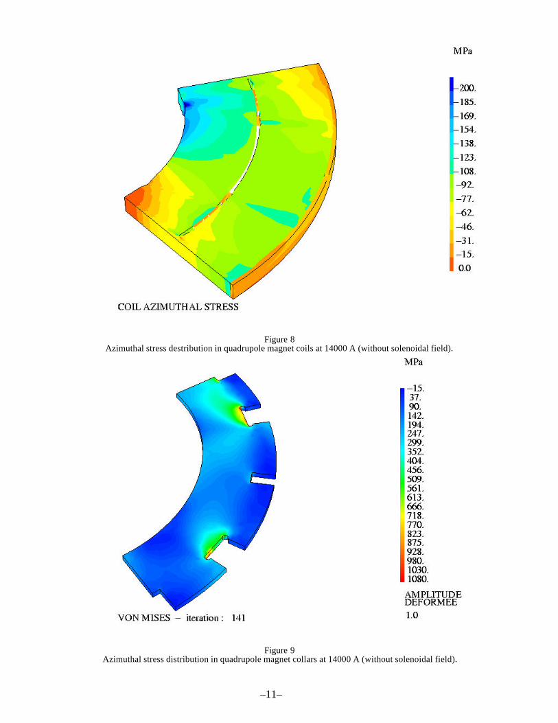
At 14000 A and without solenoidal magnetic field, all parts of coils remain under

compression. The external collar radius must be increased to 93.5 mm to minimize collar

deflections. With this radius value, the deflections are similar to those obtained on LHC arc

quadrupole magnets (dradial = −0.013 mm, compared to dréf = −0.010 mm). In addition, the

peak stress in the collars remain under the ultimate stress of austenitic steel (σVM = 1000 MPa

for σult = 1600 MPa). Figure 8 and Figure 9 show plots of the azimuthal stress distribution in

the magnet coils and of the Von Mises stresses in the collars at 14000 A, while Figure 10 and

Figure 11 present plots of the radial deflections.

–11–

Figure 8Azimuthal stress destribution in quadrupole magnet coils at 14000 A (without solenoidal field).

Figure 9Azimuthal stress distribution in quadrupole magnet collars at 14000 A (without solenoidal field).

–12–

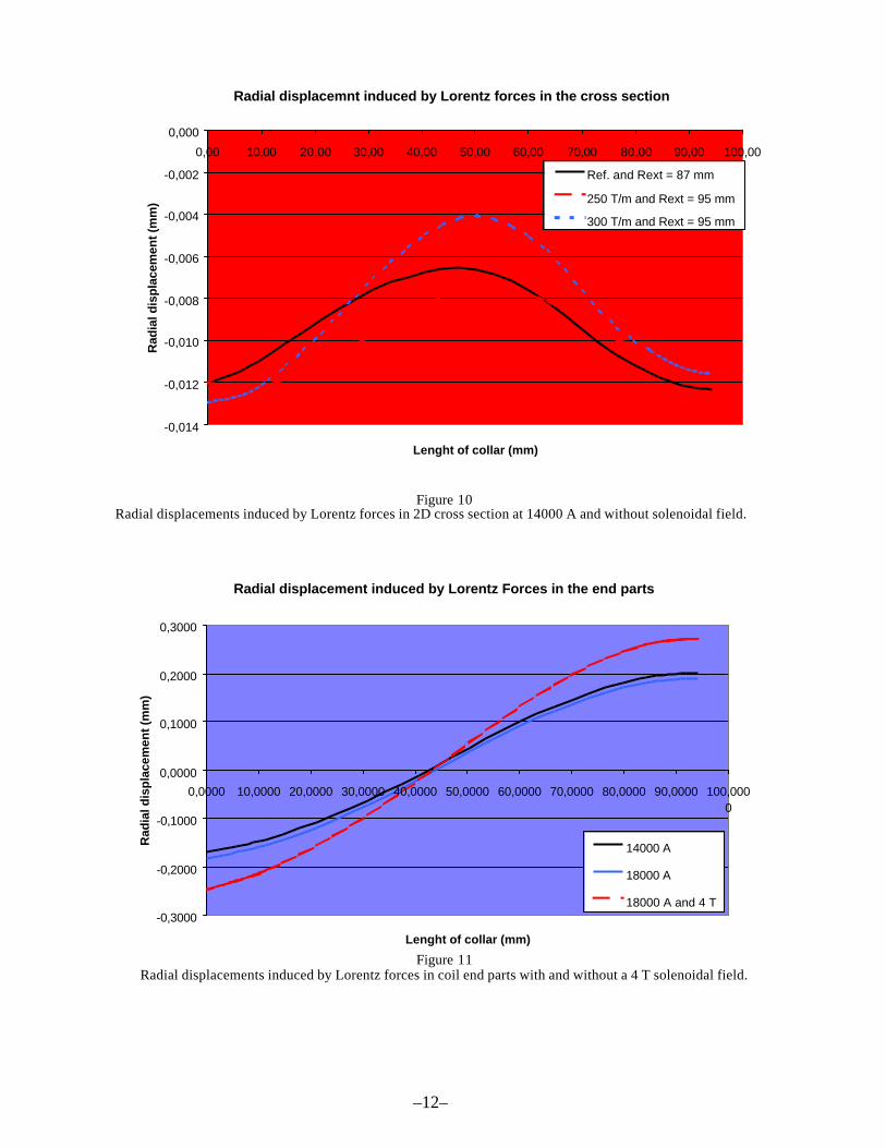
Figure 10Radial displacements induced by Lorentz forces in 2D cross section at 14000 A and without solenoidal field.

Radial displacement induced by Lorentz Forces in the end parts

-0,3000

-0,2000

-0,1000

0,0000

0,1000

0,2000

0,3000

0,0000 10,0000 20,0000 30,0000 40,0000 50,0000 60,0000 70,0000 80,0000 90,0000 100,0000

Lenght of collar (mm)

Rad

ial d

isp

lace

men

t (m

m)

14000 A

18000 A

18000 A and 4 T

Figure 11Radial displacements induced by Lorentz forces in coil end parts with and without a 4 T solenoidal field.

Radial displacemnt induced by Lorentz forces in the cross section

-0,014

-0,012

-0,010

-0,008

-0,006

-0,004

-0,002

0,000

0,00 10,00 20,00 30,00 40,00 50,00 60,00 70,00 80,00 90,00 100,00

Lenght of collar (mm)

Rad

ial d

ispl

acem

ent (

mm

)

Ref. and Rext = 87 mm

250 T/m and Rext = 95 mm

300 T/m and Rext = 95 mm

–13–

At 14000 A and with a 4 T solenoidal magnetic field, all parts of coils still remain

under compression, but the radial deflections become very large (dradial = ±0.2 mm). Hence,

an additional mechanical support will be needed to prevent any damage or to restrain coil end

deflections. The peak stress in the collars remain under the ultimate stress(σVM = 1250 MPa

for σult = 1600 MPa).

3.4 CONCLUSIONS

All parts of coils remain in compression at nominal current and with background

magnetic field.

The finite element computations validate the main features of the mechanical design,

providing that the collar radius is greater than 95 mm and that reinforcements are

implemented on the inner and outer radius of the coil ends. With this new value of collar

outer radius, it follows that the external radius of the inertia tube must be greater than 110 mm

(use of CODAP formula).

It should be stressed again that this study is very prelimenary and that more

computations will be needed to finalize the design.

4 CABLE SPECIFICATION

The cable specifications are inspired from those of the LHC quadrupole magnet

cable [5]. The cable has 36 strands, a 15.12-mm width, a 1.48-mm mid-thickness, and a 0.9°

keystone angle. The transposition pitch length is 100 mm, and the strand diameter is 0.825

mm. As explained above, the critical current is required to be greater than 17,581 A at

10.36 T.

–14–

Taking into account a 10% cabling degradation, the virgin strand critical current,

strandCI , must satisfy

A 543 36 x 0.9

17,581 strand

C ≈≥I at 10.36 T (7)

If we assume further a copper-to-non-copper ratio of 1.4 to 1, the above current

intensity specification translates into a critical current density specification in the non-copper,

JC,non-Cu, given by

2Cu-nonC, A/mm 2436 ≥J at 10.36 T (8)

Using the usual parametrization of the Nb3Sn critical surface [9], we derive

2Cu-nonC, A/mm 1800 ≥J at 12 T (9)

Such value is far above the specification for high performance ITER strands

(700 A/mm2 at 12 T and 4.2 K) [10], but has been achieved recently (and even exceeded) on

R&D wires produced by various manufacturers around the world (IGC and Oxford in the

USA, SMI in the Netherlands, and possibly MECo in Japan) [11]. Furthermore,

DAPNIA/STCM and Alstom/MSA are preparing a 4-year collaboration agreement to develop

a high performance Nb3Sn wire with a goal of 2000 A/mm2 at 12 T and 4.2 K. Hence, it

seems reasonable to assume that within the time frame of the TESLA project, Nb3Sn wires

meeting the critical current requirement of Eq. (7) will be readily available on the market.

One point of debate is the magnet operating temperature. The promising results on

R&D wires mentioned above were obtained at 4.2 K and the Alstom/MSA goal is also at

4.2 K. However, since 1.8-K cryogenics will be available at TESLA, a conservative approach

–15–

for the present time is to take advantage of it and to build more margin in the magnet design.

Thus, the operating temperature is set to 1.8 K.

5 CRYOGENICS

5.1 OVERVIEW

The cryogenics of the TESLA quadrupole magnets deals with the cryostat that

supports the cold masses of the magnet doublets on each side of the collision point (see Figure

1) and the refrigeration system connected to it.

5.2 CRYOSTAT

A cross sectional view of the cryostat is shown in Figure 12. It is made up of: (1) a

stainless steel vacuum vessel with an outer diameter of 355 mm and a overall length of 4200

mm, (2) an aluminum shield cooled with helium gas at 40-50 K, (3) the quadrupole magnet

cold masses Q3 and Q4 in their inertia tube with an electrical bus, (4) a set of supporting tie

rods and (5) the required tubing for cooling the cold masses. The cold masses and the shields

will be super-isolated, respectively, with 10 and 30 layers of double aluminized mylar sheets.

Salient dimensions of the various components are summarized in Table 1.

Table 1 Salient dimensions of various items.

Item Overall length Outer Diameter

Cryostat 4200 355

Cold mass Q3 1700 250

Cold mass Q4 1000 250

–16–

Figure 12 Cross sectional view of quadrupole magnet cryostat.

5.3 REFRIGERATION

The quadrupole magnet coils are in a pressurized bath of helium II at 1.8 K, which is

cooled by an internal saturated Helium II loop. The two cold masses are equipped with two

copper tubes Ø16x1 connected in parallel (mass flow rate of 0.42 g/s for a heat load of 10 W).

The thermal resistance of each tube is roughly 55 W/m, taking into account the Kapitza

resistance on tube wall, and thus for a heat load of 3 W/m a ∆T< 0.03 K.

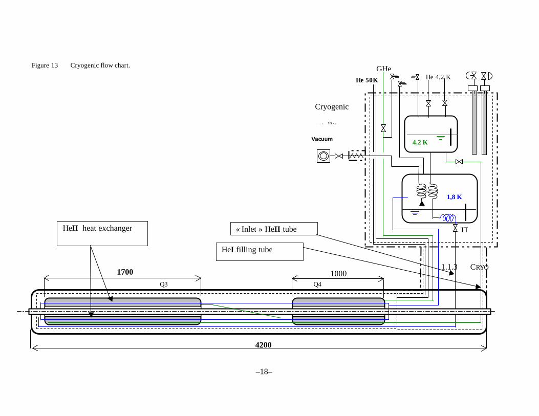
As illustrated in Figure 13, a cryogenic satellite is connected to the cryostat through a

cryogenic transfer line with pipes feeding it with fluids: helium gas at 50-70 K, liquid

helium I, liquid helium II and a busbar supplying the electrical current.

Ø48

HeI filling tubeHeII

heat exchanger

Schield heat exchanger tubes (Ø16x1)

Electrical bus

« Inlet » He II tube (Ø16x1)

Ø355

10

Ø250

–17–

The main components of the satellite, except its vacuum vessel and super-isolated

shield are:

(1) two 15 kA current leads that have control flow valves,

(2) a 1.8 K saturated helium II storage vessel connected to an outside pump with an

on-line electrical heater (1 kW). A liquid/vapor heat exchanger followed by a

liquid/liquid heat exchanger cools the liquid helium I before the Joule-Thomson

(JT) valve. The liquid helium II level is controlled by the JT valve and

temperature of the saturated helium II bath is controlled by the pumping system

(Psat = 1640 Pa for Tsat=1.8 K). The inlet tube of the saturated helium II loop is

cooling also the electrical bus.

(3) A 4,2 K saturated liquid vessel stores helium I and supplies the internal helium II

cooling loop or is used to fill up the cold mass vessels.

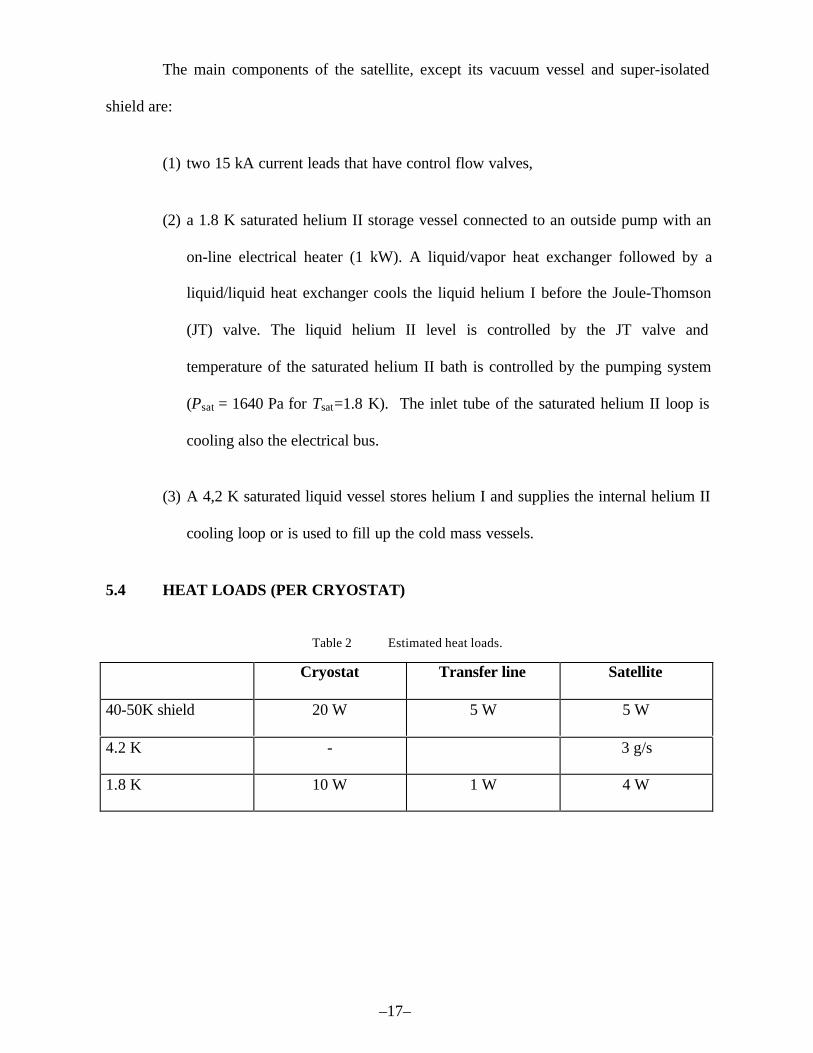
5.4 HEAT LOADS (PER CRYOSTAT)

Table 2 Estimated heat loads.

Cryostat Transfer line Satellite

40-50K shield 20 W 5 W 5 W

4.2 K - 3 g/s

1.8 K 10 W 1 W 4 W

–18–

Figure 13 Cryogenic flow chart.

Q3 Q4

4,2 K

1,8 K

HeII heat exchanger

(Ø16x1) HeI filling tube

Cryogenic

satellite

Vacuum

pump

1.1.2 CRYOSTAT

1.1.3 CRYO

He 4,2 KGHe

He 50K

1700 1000

« Inlet » HeII tube

4200

JT

–19–

REFERENCES

[1] R. Brinkmann, “Status of the design for the TESLA linear collider,” Proc. of 1995Particle Accelerator Conference (PAC 1995), IEEE Catalogue 95CH35843, pp. 674–676, 1996.

[2] P. Lefèvre and T. Petterson (eds.), The Large Hadron Collider: Conceptual Design,CERN/AC/95–05(LHC), Geneva: CERN, 20 October 1995.

[3] M. Peyrot, J.M. Rifflet, F. Simon, P. Vedrine, and T. Tortschanoff, “Construction ofthe new prototype of main quadrupole cold masses for the arc short straight sections ofLHC,” IEEE Trans. Appl. Supercond., Vol. 10 No. 1, pp. 170–173, 2000.

[4] F. Kircher, B. Levesy, Y. Pabot, D. Campi, B. Curé, A. Hervé, I.L. Horvath,P. Fabbricatore, and R. Musenich, “Status report on the CMS superconductingsolenoid for LHC,” IEEE Trans. Appl. Supercond., Vol. 9 No. 2, pp. 837–840, 1999.

[5] “Technical specification of the dipole outer layer and quadrupole superconductingcable for the LHC,” Internal Note LHC–MMS/97–153, CERN, Geneva, Switzerland,July 1997.

[6] A. Devred, M. Durante, C. Gourdin, F.P. Juster, M. Peyrot, J.M. Rey, J.M. Rifflet,F. Streiff, P. Védrine, “Development of a Nb3Sn quadrupole magnet model,”Presented at Applied Superconductivity Conference 2000, Virginia Beach, VA, USA,17-22 September 2000.

[7] L. Champaney, “Une nouvelle approche modulaire pour l’analyse d’assemblage destructures tri-dimensionnelles,” Thèse de l’ENS de Cachan, June 1996.

[8] C. Gourdin, A. Devred, M. Durante, M. Peyrot, J.M. Rifflet, P. Védrine, “Mechanicaldesign of a Nb3Sn quadrupole magnet,” Presented at EPAC2000, Vienna, Austria,June 2000.

[9] L.T. Summers, M.W. Guinan, J.R. Miller and P.A. Hahn, “A model for the predictionof Nb3Sn critical current as a function of field, temperature, strain and radiationdamage,” IEEE Trans. Magn., Vol. 27 No. 2, pp. 2041–2044, 1991.

[10] P. Bruzzone, H.H.J. ten Kate, C.R. Walters and M. Spadoni, “Testing of industrialNb3Sn strands for high field fusion magnets,” IEEE Trans. Magn., Vol. 30 No. 4,pp. 1986–1989, 1994.

[11] E. Barzi, P.J. Limon, R. Yamada and A.V. Zlobin, “Study of Nb3Sn strands forFermilab’s high field dipole models,” Presented at Applied SuperconductivityConference 2000, Virginia Beach, VA, USA, 17-22 September 2000.