Embed Size (px)
Citation preview
CONCRETE BRIDGE DECK BEHAVIOR UNDER
THERMAL LOADS
by
Jeffrey Keith Johnson
A thesis submitted in partial fulfillment of the requirements for the degree
of
Master of Science
in
Civil Engineering
MONTANA STATE UNIVERSITY Bozeman, Montana
July 2005

© COPYRIGHT
by
Jeffrey Keith Johnson
2005
All Rights Reserved
ii
APPROVAL
of a thesis submitted by
Jeffrey Keith Johnson
This thesis has been read by each member of the thesis committee and has been found to be satisfactory regarding content, English usage, format, citations, bibliographic style, and consistency, and is ready for submission to the College of Graduate Studies.
Dr. Jerry Stephens
Approved for the Department of Civil Engineering
Dr. Brett Gunnink
Approved for the College of Graduate Studies
Dr. Bruce McLeod
iii
STATEMENT OF PERMISSION TO USE
In presenting this thesis in partial fulfillment of the requirements for a master’s
degree at Montana State University – Bozeman, I agree that the library shall make it
available to borrowers under rules of the Library.
If I have indicated my intention to copyright this thesis by including a copyright
notice page, copying is allowable only for scholarly purposes, consistent with “fair use”
as prescribed in the U.S. Copyright Law. Requests for permission for extended quotation
from or reproduction of this thesis (paper) in whole or in parts may be granted only by
the copyright holder.
Jeffrey Keith Johnson
July 17, 2005

iv
ACKNOWLEDGEMENTS
I want to thank the people who have encouraged and inspired my pursuit of education
and to share with them the following definition as it illustrates those impressions they
have left for me to admire:
philomath \FIL-uh-math\, noun:
A lover of learning; a scholar.
v
TABLE OF CONTENTS
1. INTRODUCTION .........................................................................................................1
BACKGROUND.................................................................................................................1 OBJECTIVE AND SCOPE ...................................................................................................2
2. LITERATURE REVIEW ..............................................................................................5
BRIDGE DESIGN FOR THERMAL EVENTS .........................................................................5 Response Analysis ...................................................................................................9
THERMAL BEHAVIOR OF CONCRETE .............................................................................11 Coefficient of Thermal Expansion.........................................................................12
FROST ACTION..............................................................................................................19
3. CTE INVESTIGATION ..............................................................................................22
CTE METHODOLOGY....................................................................................................22 Specimens ..............................................................................................................23 Instrumentation ......................................................................................................24 Procedure ...............................................................................................................30
CTE FINDINGS..............................................................................................................33 True Strain .............................................................................................................33 CTE........................................................................................................................36 CTE Results for 1018 Steel....................................................................................37 CTE Results for Concrete ......................................................................................39 CTE Conclusions ...................................................................................................49
4. BRIDGE INVESTIGATION.......................................................................................52
DESCRIPTION OF THE BRIDGES......................................................................................52 Bridge Deck Construction......................................................................................56 Steel Reinforcement...............................................................................................59 Prestressed Girders.................................................................................................59 Long Term Strain Monitoring................................................................................60 Data Analysis .........................................................................................................63
BRIDGE FINDINGS .........................................................................................................68 Thermal Strain and CTE ........................................................................................68 Composite Behavior...............................................................................................73 Structural Behavior under Temperature Changes..................................................73 Bridge Deck Deformations ....................................................................................83 Longitudinal Thermal Behavior.............................................................................95 Temperature Loading.............................................................................................98
vi
TABLE OF CONTENTS – CONTIUNED
5. CONCLUSIONS AND RECOMMENDATIONS ....................................................100
CTE INVESTIGATION ..................................................................................................100 BRIDGE INVESTIGATION..............................................................................................101 RECOMMENDATIONS...................................................................................................103
BIBLIOGRAPHY............................................................................................................104
vii
LIST OF TABLES
Table Page
1. Bridge Characteristics..............................................................................................3
2. Uniform Temperature Ranges (from AASHTO 2000)............................................7
3. Gradient Temperatures (AASHTO 2000)................................................................8
4. Thermal Coefficients of Concrete (from NCHRP Report 276 1985) ....................13
5. Typical CTEs for Common Portland Cement Concrete Components (from Turner Fairbanks Research Center 2005) ..............................................................14
6. CTE Testing Regime..............................................................................................32
7. Average Slump and Air Content from Bridge Deck Concrete ..............................57
8. Average Compressive Strengths of Deck Concrete...............................................58
9. Average Modulus of Elasticity of Deck Concrete .................................................58
10. Average 28-day Prestressed Girder Concrete Compressive Strengths ..................60
viii
LIST OF FIGURES
Figure Page 1. Saco Bridge Gradient Temperature Distribution (for positive gradient
temperature) .............................................................................................................8
2. Concrete Structure (adapted from Mehta 1986) ....................................................12
3. Simplified Feldman-Sereda Model for the Structure of Cement Gel: A - interparticle Bonds: x – interlayer water: B – tobermorite sheets: o – physically adsorbed water (from Feldman and Sereda 1968)...............................17
4. The State of the Cement Gel Structure as Water Molecules (x) are Removed and Added to the Paste Structure (from Fieldman and Sereda 1968) ......................................................................................................................18
5. Specimen Dimensions and Layout.........................................................................25
6. Typical Concrete Strain Gage Installation.............................................................26
7. Circuitry used for the Strain Measurements ..........................................................28
8. Specimens placed in environmental chamber........................................................30
9. Specimen Layout within the Environmental Chamber and Labeling Nomenclature.........................................................................................................31
10. Measured Gage Strain with Time (Cycles 1 through 4) ........................................33
11. Measured Gage Strain with Time (Cycle 1) ..........................................................34
12. Measured Gage Strain with Time (Close Up)........................................................34
13. Gage Strain (Thermal Gage Effects Included).......................................................35
14. True Concrete Strain during Heating Cycle 4 (Thermal Gage Effects Subtracted Out) ......................................................................................................36
15. 1018 Steel Cooling All Cycles...............................................................................38
16. 1018 Steel Heating All Cycles...............................................................................38
17. Standard Concrete CTE Cooling - All Gages - Last Cycle ...................................40
18. Standard Concrete CTE Cooling – Gage CON 1-A - All Cycles ..........................41
ix
LIST OF FIGURES - CONTINUED
Figure Page
19. Traditional Concrete CTE Heating - All Gages - Last Cycle ................................43
20. Traditional Concrete CTE Heating – Gage CON 1-A - All Cycles.......................44
21. High Performance Concrete CTE Cooling - All Gages - Last Cycle ....................45
22. High Performance Concrete CTE Cooling – Gage HPC 1-A - All Cycles ...........46
23. High Performance Concrete CTE Heating - All Gages - Last Cycle ....................47
24. High Performance Concrete CTE Heating – Gage HPC 1-A - All Cycles............48
25. Coefficients of Thermal Expansion for the Last Cooling Cycle............................49
26. Coefficients of Thermal Expansion for the Last Heating Cycle............................51
27. Completed Bridge Deck.........................................................................................53
28. Elevation View of Typical Saco Bridge ................................................................53
29. Cross Sectional View.............................................................................................54
30. Plan View of Bridge Decks....................................................................................54
31. Typical Bridge Deck Cross-Sections and Steel Amounts......................................55
32. Steel Reinforcement Layout in the Saco Bridge Decks.........................................55
33. Placing the Deck Concrete.....................................................................................57
34. Dimensioned Cross-Section of Saco Bridge Girders.............................................59
35. Vibrating Wire Locations ......................................................................................60
36. Vibrating Wire Strain Gage (VCE-4200) ..............................................................61
37. Vibrating Wire Installation ....................................................................................62
38. Typical Shrinkage Strain for Saco Bridges............................................................67
39. Conventional Deck CTE Values at Location TV-D-3-B.......................................69
40. Empirical Deck CTE Values at Location TV-D-3-B.............................................70
x
LIST OF FIGURES - CONTINUED
Figure Page
41. High Performance Deck CTE Values at Location TV-D-3-B...............................70
42. High Performance Deck CTE Values at Location TV-D-5-B...............................71
43. Conventional Deck CTE Values at Location LV-F-3-T (Which is Known to be Cracked) ........................................................................................................72
44. Composite Action Diagram ...................................................................................75
45. Composite Action for a Uniform Temperature Change ........................................76
46. Composite Action for a Gradient Temperature Change ........................................78
47. Conventional Deck Composite CTE Values at Location TV D 3 B......................81
48. Empirical Deck Composite CTE Values at Location TV D 3 B ...........................81
49. High Performance Deck Composite CTE Values at Location TV D 5 B..............82
50. Internal Strain Angle..............................................................................................84
51. Conventional Deck Behavior at Location TV D 3 (Total Response) ....................86
52. Empirical Deck Behavior at Location TV D 3 (Total Response) ..........................87
53. High Performance Deck Behavior at Location TV D 3 (Total Response) ............87
54. Conventional Deck Behavior at Location TV D 5 (Total Response) ....................88
55. Expected Physical Bridge Deck Deformations (for a Negative Temperature Gradient)...........................................................................................91
56. Expected Physical Bridge Deck Deformations (for a Positive Temperature Gradient) ................................................................................................................91
57. Conventional Deck Behavior at Location TV-D-3 (Stress Related Response)...............................................................................................................94
58. Conventional Deck Behavior at Location TV-D-5 (Stress Related Response)...............................................................................................................94
59. Conventional Deck Behavior at Location LV-A-3 (Total Response) ...................96
xi
LIST OF FIGURES - CONTINUED
Figure Page
60. Conventional Deck Behavior at Location LV-B-3 (Total Response)....................96
61. Conventional Deck Behavior at Location LV-D-3 (Total Response) ...................97
62. Conventional Deck Behavior at Location LV-F-3 (Total Response) ....................97
63. Conventional Deck Temperature Measurements at Location TV-D-3..................99
xii
ABSTRACT
A major area of concern with concrete bridge decks is durability. The service life of bridge decks designed by traditional procedures is often shorter than desired. Typically, the decks crack under environmental loads, which lead to corrosion of the reinforcing steel and general deterioration of the concrete.
In this investigation, the response of three different bridge decks was studied in the field under environmental loads. The decks, located within a mile of each other on the same road, differ in their steel reinforcement and the type of concrete used; otherwise, they are identical. Therefore, they offer an opportunity to observe how these factors affect their behavior under environmental loads.
This investigation was divided into two tasks. In the first task, the basic response of the bridge deck concrete under changes in temperature was examined in the laboratory using specimens cast with the decks. The second task correlated the laboratory findings with measured responses in the bridges and examined the global thermal response of the decks.
The laboratory investigation showed that concrete has a distinct nonlinear strain response to temperature changes. This response is related to the concrete’s nanostructure, which affects the behavior of water within the paste during the heating and cooling process. The deck concretes’ coefficient of thermal expansion was generally found to range from 6 to 14 µε/°C as the temperature changed from -35°C to 40°C, and distinct differences were seen in the relationship between the strain and temperature for high performance versus standard concrete.
The bridge investigation showed that locally the thermal response of the bridges was similar to that measured in the laboratory. Globally, the transverse bridge response to changes in temperature was as expected (expansion and contraction with increasing and decreasing temperatures, respectively). Importantly, there were no significant differences in behavior between the three bridges. In reviewing the strain response to thermal events, it was discovered that anomalies in this response may be indicators of physical damage within the deck.
Because of the Saco bridges relatively young age (two years), continued investigation will be necessary as they mature and environmental degradation more readily presents itself.
1
CHAPTER 1
INTRODUCTION
Background
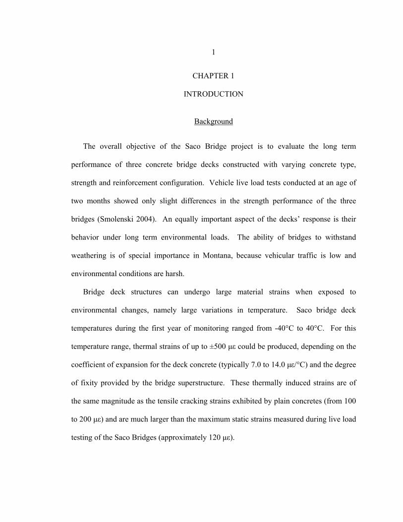
The overall objective of the Saco Bridge project is to evaluate the long term
performance of three concrete bridge decks constructed with varying concrete type,
strength and reinforcement configuration. Vehicle live load tests conducted at an age of
two months showed only slight differences in the strength performance of the three
bridges (Smolenski 2004). An equally important aspect of the decks’ response is their
behavior under long term environmental loads. The ability of bridges to withstand
weathering is of special importance in Montana, because vehicular traffic is low and
environmental conditions are harsh.
Bridge deck structures can undergo large material strains when exposed to
environmental changes, namely large variations in temperature. Saco bridge deck
temperatures during the first year of monitoring ranged from -40°C to 40°C. For this
temperature range, thermal strains of up to ±500 µε could be produced, depending on the
coefficient of expansion for the deck concrete (typically 7.0 to 14.0 µε/°C) and the degree
of fixity provided by the bridge superstructure. These thermally induced strains are of
the same magnitude as the tensile cracking strains exhibited by plain concretes (from 100
to 200 µε) and are much larger than the maximum static strains measured during live load
testing of the Saco Bridges (approximately 120 µε).
2
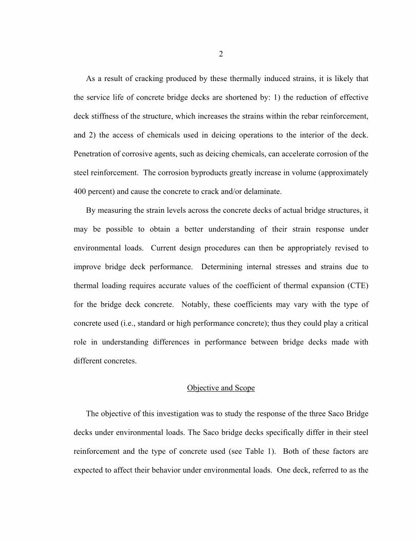
As a result of cracking produced by these thermally induced strains, it is likely that
the service life of concrete bridge decks are shortened by: 1) the reduction of effective
deck stiffness of the structure, which increases the strains within the rebar reinforcement,
and 2) the access of chemicals used in deicing operations to the interior of the deck.
Penetration of corrosive agents, such as deicing chemicals, can accelerate corrosion of the
steel reinforcement. The corrosion byproducts greatly increase in volume (approximately
400 percent) and cause the concrete to crack and/or delaminate.
By measuring the strain levels across the concrete decks of actual bridge structures, it
may be possible to obtain a better understanding of their strain response under
environmental loads. Current design procedures can then be appropriately revised to
improve bridge deck performance. Determining internal stresses and strains due to
thermal loading requires accurate values of the coefficient of thermal expansion (CTE)
for the bridge deck concrete. Notably, these coefficients may vary with the type of
concrete used (i.e., standard or high performance concrete); thus they could play a critical
role in understanding differences in performance between bridge decks made with
different concretes.
Objective and Scope
The objective of this investigation was to study the response of the three Saco Bridge
decks under environmental loads. The Saco bridge decks specifically differ in their steel
reinforcement and the type of concrete used (see Table 1). Both of these factors are
expected to affect their behavior under environmental loads. One deck, referred to as the
3
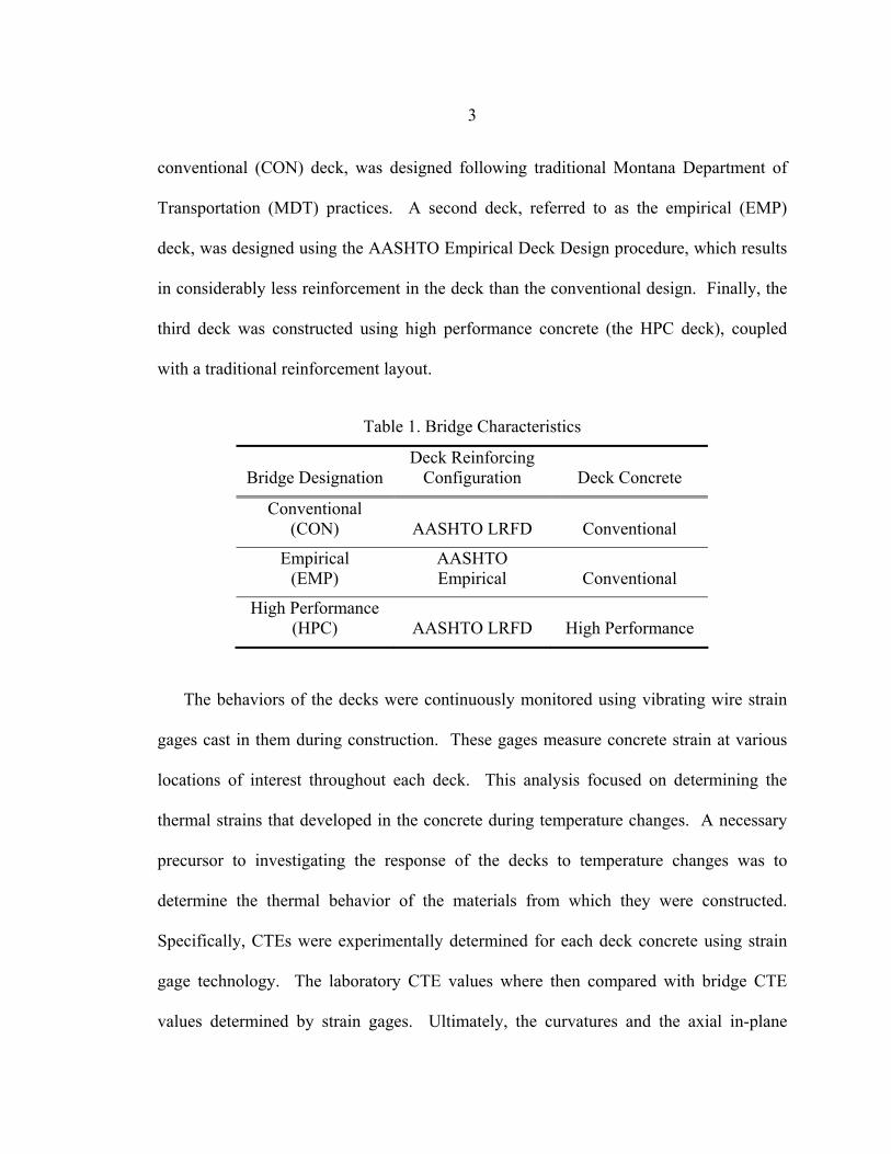
conventional (CON) deck, was designed following traditional Montana Department of
Transportation (MDT) practices. A second deck, referred to as the empirical (EMP)
deck, was designed using the AASHTO Empirical Deck Design procedure, which results
in considerably less reinforcement in the deck than the conventional design. Finally, the
third deck was constructed using high performance concrete (the HPC deck), coupled
with a traditional reinforcement layout.
Table 1. Bridge Characteristics
Bridge Designation Deck Reinforcing
Configuration Deck Concrete
Conventional (CON) AASHTO LRFD Conventional
Empirical (EMP)
AASHTO Empirical Conventional
High Performance (HPC) AASHTO LRFD High Performance
The behaviors of the decks were continuously monitored using vibrating wire strain
gages cast in them during construction. These gages measure concrete strain at various
locations of interest throughout each deck. This analysis focused on determining the
thermal strains that developed in the concrete during temperature changes. A necessary
precursor to investigating the response of the decks to temperature changes was to
determine the thermal behavior of the materials from which they were constructed.
Specifically, CTEs were experimentally determined for each deck concrete using strain
gage technology. The laboratory CTE values where then compared with bridge CTE
values determined by strain gages. Ultimately, the curvatures and the axial in-plane

4
strains were calculated for each deck using the data from the vibrating strain gages.
These aspects of the response were compared with and the expected temperature related
deformations.
5
CHAPTER 2
LITERATURE REVIEW
The first comprehensive investigation into the thermal effects on bridge decks in the
United States was National Cooperative Highway Research Program (NCHRP) Report
276, Thermal Effects in Concrete Bridge Superstructures, issued in 1985. An abridged
version of this report was then published by the American Association of State Highway
and Transportation Officials (AASHTO) as a recommended guide specification (rather
than as a modification to the AASHTO design specifications). The current AASHTO
LRFD Bridge Design Specifications now incorporate the recommendations of NCHRP
Report 276 (with slight modifications).
Bridge Design for Thermal Events
The temperature behavior of bridges is typically viewed as two superimposed effects.
The first effect is from a uniform change in temperature that occurs over the entire
superstructure. This temperature event causes an overall length change for an
unrestrained structure. If the structure is restrained, a uniform temperature change will
produce internal stresses in the structure. The second event is a temperature gradient that
occurs when the bridge superstructure heats unevenly (such as when the sun substantially
heats the deck surface or a freezing rain falls on a warm day). The gradient temperature
is only applied in the vertical direction, and no consideration is given to uneven heating
longitudinally or transversely to the bridge deck.
6
The setting (installation) temperature, as defined by AASHTO, for the bridge or any
of its components is determined by averaging the actual air temperature over the 24-hour
period immediately before the setting event. The setting temperature is the reference
temperature relative to the direction and magnitude of subsequent thermal behavior under
temperature changes. The setting temperature is of specific interest when installing
expansion bearings and deck joints. In addition to setting temperature, the range of
temperatures the deck will cycle through is of interest in design.
AASHTO divides the country into two regions for determining uniform temperature
ranges that bridges will experience based on the number of expected freezing days
(temperatures less than 0°C). Moderate climates are defined as having fewer than 14
freezing days per year; conversely, cold climates have 14 days or more freezing days.
This method is merely a general indication of the length of time a bridge deck could be
expected to be at a colder temperature but not necessarily the actual temperature
experienced. As expected, Table 2 indicates that cold climatic regions are to be designed
for colder temperatures. The temperature range considered in design also depends on the
bridge material. Metal bridges have quicker response to changes in temperature, where
the thermal mass of the concrete bridges acts as a temperature regulator, reducing its
ability to reach peak temperatures. Wood bridges have a further reduced temperature
range because of their superior performance to temperature changes (critical strains for
wood are much higher than those of concrete and steel and do not result in brittle
failures).
7
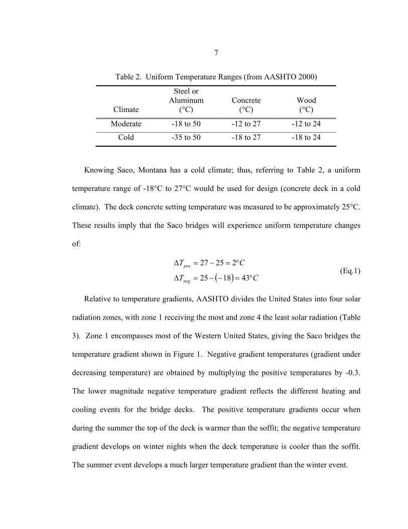
Table 2. Uniform Temperature Ranges (from AASHTO 2000)
Climate
Steel or Aluminum
(°C) Concrete
(°C) Wood (°C)
Moderate -18 to 50 -12 to 27 -12 to 24
Cold -35 to 50 -18 to 27 -18 to 24
Knowing Saco, Montana has a cold climate; thus, referring to Table 2, a uniform
temperature range of -18°C to 27°C would be used for design (concrete deck in a cold
climate). The deck concrete setting temperature was measured to be approximately 25°C.
These results imply that the Saco bridges will experience uniform temperature changes
of:
( ) CT
CT
neg
pos
°=−−=∆
°=−=∆
431825
22527 (Eq.1)
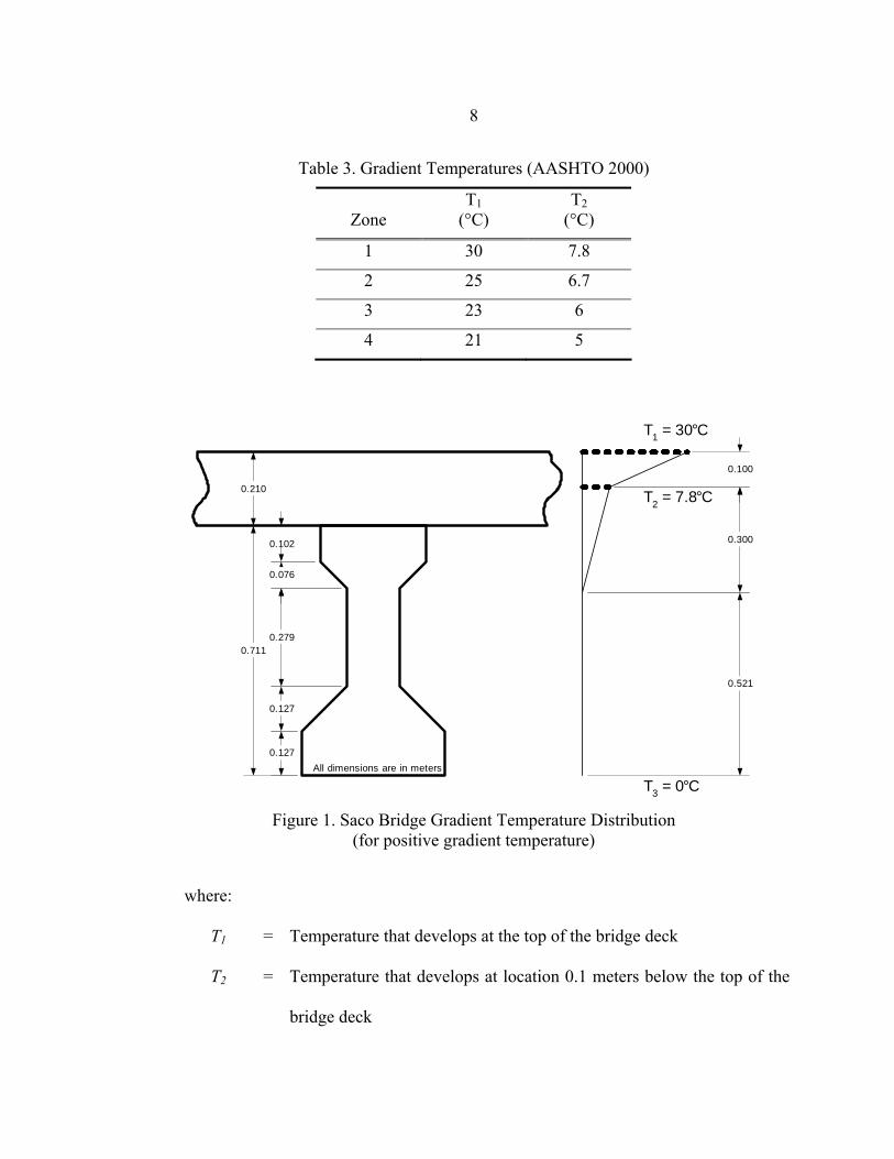
Relative to temperature gradients, AASHTO divides the United States into four solar
radiation zones, with zone 1 receiving the most and zone 4 the least solar radiation (Table
3). Zone 1 encompasses most of the Western United States, giving the Saco bridges the
temperature gradient shown in Figure 1. Negative gradient temperatures (gradient under
decreasing temperature) are obtained by multiplying the positive temperatures by -0.3.
The lower magnitude negative temperature gradient reflects the different heating and
cooling events for the bridge decks. The positive temperature gradients occur when
during the summer the top of the deck is warmer than the soffit; the negative temperature
gradient develops on winter nights when the deck temperature is cooler than the soffit.
The summer event develops a much larger temperature gradient than the winter event.
8
Table 3. Gradient Temperatures (AASHTO 2000)
Zone T1
(°C)
T2 (°C)
1 30 7.8
2 25 6.7
3 23 6
4 21 5
0.711
0.127
0.102
0.076
0.127
0.279
All dimensions are in meters
0.210
0.100
0.300
0.521
T1 = 30°C
T2 = 7.8°C
T3 = 0°C Figure 1. Saco Bridge Gradient Temperature Distribution
(for positive gradient temperature)
where:
T1 = Temperature that develops at the top of the bridge deck
T2 = Temperature that develops at location 0.1 meters below the top of the
bridge deck
9
T3 = Temperature that develops in the bottom of the superstructure
Response Analysis
Several methods of analysis exist to determine the effect of temperature changes on
structures. For simplification, the following assumptions are made when performing the
thermal analysis of bridge structures following the bridge deck specifications (AASHTO
1989):
1. The material is homogeneous and exhibits isotropic behavior.
2. Material properties are independent of temperature.
3. The material has linear stress-strain and temperature-strain relations. Thus,
thermal stresses can be considered independently of stresses or strains
imposed by other loading conditions, and the principle of superposition holds.
4. The Navier-Bernoulli hypothesis that initially plane sections remain plane
after bending is valid.
5. The temperature varies only with depth, but is constant at all points of equal
depth (except those points over an enclosed cell).
6. Longitudinal and transverse thermal responses of the bridge superstructure
can be considered independently and the results superimposed; i.e., the
longitudinal and transverse thermal stress fields are assumed to be uncoupled.
AASHTO LRFD Bridge Design Specifications (Section 4.6.6) provides the following
method for examining the force effects due to temperature deformations. The structure’s
response is divided into three effects: 1) axial expansion, 2) flexural deformation, and 3)
self equilibrating stresses.
10
Axial expansion is caused by the uniform component of the temperature gradient.
The uniform component of the temperature gradient is calculated as the average
temperature across the cross section:
∫ ∫= dwdzTA
T GC
UG1 (Eq.2)
where:
TUG = Temperature average across the cross-section
AC = Transformed cross-section area
TG = Temperature gradient
w = Width of element in cross-section
z = Vertical distance from centroid of cross-section
The uniform axial strain is:
[ ]UUGu TT +⋅= αε (Eq.3)
where:
α = Coefficient of thermal expansion
TU = Uniform specified temperature
Flexural deformation is a result of plane sections remaining plane under a linear
temperature gradient. This curvature is determined as:
∫ ∫= zdwdzTI G
T
ακ (Eq.4)
where:
κ = Curvature
IT = Transformed inertia of cross-section
11
Structures that are externally unrestrained develop no external forces. In a fully
restrained structure, however, axial forces develop as:
uCC AEN ε= (Eq.5)
where:
EC = Modulus of elasticity of the concrete
Moment forces from the flexural deformation also develop as:
κCC IEM = (Eq.6)
The internal “self-equilibrating” stresses are determined by first allowing the free
expansion of the material fibers for the temperature load; from this analysis the axial
force developed for the uniform temperature case, and the moment developed for the
gradient temperature case are subtracted. The resulting stress distribution is termed the
continuity stresses, which are required to keep plane sections plane.
[ ]zTTE GUGCE ⋅−⋅−⋅= καασ (Eq.7)
Thermal Behavior of Concrete
The behavior of concrete during temperature changes is complex and has been shown
to vary significantly between concrete mixtures. Concrete material models (including
those that address thermal behaviors) are incomplete and subjective because concrete
continues to change physically and chemically with, among other things, time,
temperature, and stress. Furthermore, observed behaviors are related to the physical and
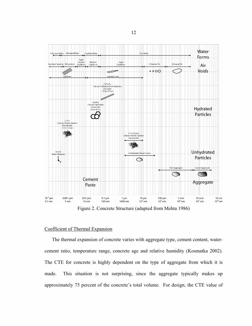
chemical structure of the concrete on a nanometer scale. The various constitutes of
concrete that influence its behavior and their scale are illustrated in Figure 2.
12
Figure 2. Concrete Structure (adapted from Mehta 1986)
Coefficient of Thermal Expansion
The thermal expansion of concrete varies with aggregate type, cement content, water-
cement ratio, temperature range, concrete age and relative humidity (Kosmatka 2002).
The CTE for concrete is highly dependent on the type of aggregate from which it is
made. This situation is not surprising, since the aggregate typically makes up
approximately 75 percent of the concrete’s total volume. For design, the CTE value of
13
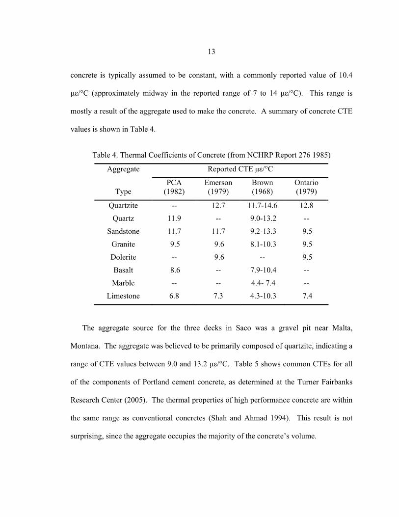
concrete is typically assumed to be constant, with a commonly reported value of 10.4
µε/°C (approximately midway in the reported range of 7 to 14 µε/°C). This range is
mostly a result of the aggregate used to make the concrete. A summary of concrete CTE
values is shown in Table 4.
Table 4. Thermal Coefficients of Concrete (from NCHRP Report 276 1985)
Aggregate Reported CTE µε/°C
Type PCA
(1982) Emerson (1979)
Brown (1968)
Ontario (1979)
Quartzite -- 12.7 11.7-14.6 12.8
Quartz 11.9 -- 9.0-13.2 --
Sandstone 11.7 11.7 9.2-13.3 9.5
Granite 9.5 9.6 8.1-10.3 9.5
Dolerite -- 9.6 -- 9.5
Basalt 8.6 -- 7.9-10.4 --
Marble -- -- 4.4- 7.4 --
Limestone 6.8 7.3 4.3-10.3 7.4
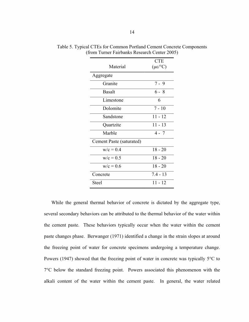
The aggregate source for the three decks in Saco was a gravel pit near Malta,
Montana. The aggregate was believed to be primarily composed of quartzite, indicating a
range of CTE values between 9.0 and 13.2 µε/°C. Table 5 shows common CTEs for all
of the components of Portland cement concrete, as determined at the Turner Fairbanks
Research Center (2005). The thermal properties of high performance concrete are within
the same range as conventional concretes (Shah and Ahmad 1994). This result is not
surprising, since the aggregate occupies the majority of the concrete’s volume.
14
Table 5. Typical CTEs for Common Portland Cement Concrete Components (from Turner Fairbanks Research Center 2005)
Material CTE
(µε/°C)
Aggregate
Granite 7 - 9
Basalt 6 - 8
Limestone 6
Dolomite 7 - 10
Sandstone 11 - 12
Quartzite 11 - 13
Marble 4 - 7
Cement Paste (saturated)
w/c = 0.4 18 - 20
w/c = 0.5 18 - 20
w/c = 0.6 18 - 20
Concrete 7.4 - 13
Steel 11 - 12
While the general thermal behavior of concrete is dictated by the aggregate type,
several secondary behaviors can be attributed to the thermal behavior of the water within
the cement paste. These behaviors typically occur when the water within the cement
paste changes phase. Berwanger (1971) identified a change in the strain slopes at around
the freezing point of water for concrete specimens undergoing a temperature change.
Powers (1947) showed that the freezing point of water in concrete was typically 5°C to
7°C below the standard freezing point. Powers associated this phenomenon with the
alkali content of the water within the cement paste. In general, the water related
15
temperature behaviors are deeply affected by the nanostructure of the cement paste.
Cement paste is composed of three primary constituents: 1) the cement gel, which
consists of the hardened hydration products, 2) unhydrated cement particles and 3) pores
of varying shape and size filled with water or air (excluding the gel pores, and interlayer
spaces). Cement gel has the following components (Kumar Mehta 1986):
• Tobermite: Calcium silicate hydrate [C-S-H] ~50-60% Volume
• Portlandite: Calcium hydroxide [Ca(OH)2] ~20-30% Volume
• Ettringite: Calcium sulfoaluminate hydrates [C6A Ŝ3H32] ~15-20% Volume
Where the following standard cement chemistry conventions have been employed:
C = CaO
S = SiO2
A = Al2O3
F = Fe2O3
Ŝ = SO3
H = H2O
There are two generally acknowledged models for the cement gel, namely, the
Powers-Brunauer model (Powers 1947) and the Feldman-Sereda model (Feldman 1968).
Both models rely on the theory of adsorption for determining the specific area of the
cement gel. Adsorption is a method of determining the surface area of a material by the
volume of a gas that is adsorbed by the material’s surface at a constant temperature and
pressure. As the pressure is increased, the gas penetrates into smaller voids. A
relationship can be developed between surface area and void size at a given pressure.

16
The Powers-Brunauer model used water vapor for adsorption while the Feldman-Sereda
model used nitrogen gas. Following the water vapor approach, the cement gel’s specific
surface was estimated to be 200 m2/g to 500 m2/g, which was from three to five times
larger than that estimated using nitrogen gas (50 m2/g). The Powers-Brunauer model
explains this difference by noting that the water molecule has a smaller diameter (0.325
nm) than the nitrogen molecule (0.405 nm) (Popovics 1998). The Feldman-Sereda model
contends that the difference is due to the interaction of the water vapor with the interlayer
water formed within the C-S-H formations. Because direct observation of the cement gel
structure is not possible (scanning electron microscopes only have a resolution in the
micrometer range while the gel structure is defined at the nanometer range), the true
structure must be inferred by empirical experiments. Popovics (1998) suggests that the
Feldman-Sereda model best explains the current observations.
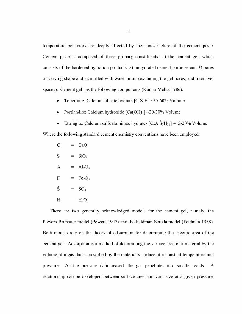
The Feldman-Sereda model (see Figure 3) leads to the existence of water in the
following states: 1) capillary water, 2) adsorbed water, 3) interlayer water, and 4)
chemically combined water (Kumar Mehta 1986). As will be discussed in Chapter 3, the
behavior of the water within each physical state and its movement between states may
help explain dimensional changes in the cement paste associated with changes in its
temperature.
17
Figure 3. Simplified Feldman-Sereda Model for the Structure of Cement Gel:
A - interparticle Bonds: x – interlayer water: B – tobermorite sheets: o – physically adsorbed water
(from Feldman and Sereda 1968)
Capillary water is the water present in voids greater than 5 nm in size. A portion of
the capillary water is given the distinction of free water, which is the water in the large
capillaries and other larger voids (> 50nm in size). It is called free water because its
removal from the hydrated cement paste does not cause a dimensional change.
Conversely, when water is removed from small and medium capillaries, shrinkage of the
hydrated cement paste may result.
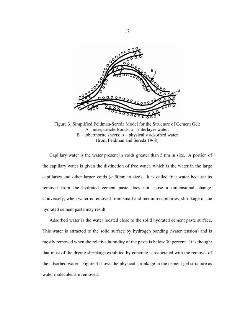
Adsorbed water is the water located close to the solid hydrated cement paste surface.
This water is attracted to the solid surface by hydrogen bonding (water tension) and is
mostly removed when the relative humidity of the paste is below 30 percent. It is thought
that most of the drying shrinkage exhibited by concrete is associated with the removal of
the adsorbed water. Figure 4 shows the physical shrinkage in the cement gel structure as
water molecules are removed.
18
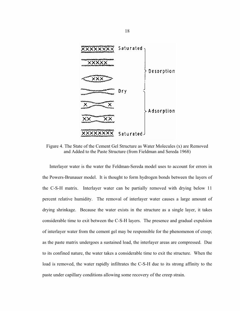
Figure 4. The State of the Cement Gel Structure as Water Molecules (x) are Removed
and Added to the Paste Structure (from Fieldman and Sereda 1968)
Interlayer water is the water the Feldman-Sereda model uses to account for errors in
the Powers-Brunauer model. It is thought to form hydrogen bonds between the layers of
the C-S-H matrix. Interlayer water can be partially removed with drying below 11
percent relative humidity. The removal of interlayer water causes a large amount of
drying shrinkage. Because the water exists in the structure as a single layer, it takes
considerable time to exit between the C-S-H layers. The presence and gradual expulsion
of interlayer water from the cement gel may be responsible for the phenomenon of creep;
as the paste matrix undergoes a sustained load, the interlayer areas are compressed. Due
to its confined nature, the water takes a considerable time to exit the structure. When the
load is removed, the water rapidly infiltrates the C-S-H due to its strong affinity to the
paste under capillary conditions allowing some recovery of the creep strain.
19
Chemically combined water strongly bonds within the hydrated paste and forms part
of the structure. This water is not lost on drying and reforms with the hydrates at high
temperatures (i.e., nonevaporable water).
Frost Action
Water in the cement paste affects the overall behavior and performance of a concrete
on macroscopic level, and is associated with concrete’s response to freezing and thawing
cycles. Freeze-thaw damage is directly associated with the phase change of the water in
the cement paste. There are three mechanisms that contribute to freeze-thaw damage: 1)
hydraulic pressure, 2) osmotic pressure, and 3) capillary effect (Kumar Mehta 1986).
The first mechanism, hydraulic pressure, is thought to typically develop in the
capillaries and other larger voids. When water freezes, it expands approximately 10
percent. If the water content of the void is above the critical saturation level (91.7
percent water), the expansion will cause the void to enlarge and/or cause some of the
water to exit the void. The pressure associated with this phenomenon is called the
hydraulic pressure, and it is proportional to the distance the water must travel to an
‘escape boundary’. This boundary is typically provided by air entrained into the
concrete. The required amount of air entrainment is determined by limiting the provided
‘escape boundary’ distance to a maximum value of 0.2 mm (as suggested by the
American Concrete Institute 2005).
Another phenomena that is believed to occur as the larger voids start to freeze, is that
the salts (alkalis, chlorides, and calcium hydroxide) naturally occurring in the hydrated
20
cement paste migrate into the adjacent water. The alkali concentration in the nearby
water greatly increases as a result, which lowers its freezing point. Osmotic pressures
develop from the differences in alkali concentrations, and adjacent water tries to flow
towards the high concentration. This pressure may become high enough to rupture the
cement paste near the surface, causing scaling.
The final mechanism that is believed to develop in the paste under freeze-thaw action
results from the thermodynamic imbalance between the frozen water in the larger voids
and the unfrozen water located in the gel pores. The interlayer and adsorbed water
remains unfrozen at super cooled temperatures (perhaps as cold as -78°C in the smallest
voids), due to its bonding with the C-S-H matrix, which greatly reduces its ability to
rearrange into ice. As the temperature decreases, the forces drawing the unfrozen water
towards the ice formation increase, causing a transmittal of water into more ice. Damage
is done when the concrete’s permeability is too low to allow the water transition needed
to meet external demand. When the forces become large enough, the cement gel can
rupture.
Air entrainment has historically shown to be the best remedy for concrete’s
susceptibility to freeze-thaw. The entrained air (typically assumed to be unsaturated)
reduces pressures within the matrix by allowing expansion of ice within the voids and by
providing an escape boundary for water towards the lower energy state. Its effectiveness
has been inferred from the differences observed in the temperature deformations of
normal concrete and air entrained concrete. Normal concrete, when cooled, typically
undergoes an expansion due to the formation of ice within the voids. Air entrained
21
concrete when cooled typically contracts at a different rate, a result of the combination of
the expansion of ice formations and the shrinkage of the C-S-H due to the removal of
water.
High performance concretes have characteristically lower permeabilities and
porosities compared to standard concretes. The strength gains in high performance
concretes are specifically attributed to the reduction in pore numbers and size. High
performance concretes typically have less available water for freeze-thaw than
conventional concrete, due to their relatively lower initial water to cement ratios. In
addition, their lower permeability reduces the ability for water to infiltrate into the
concrete from the external environment. Low permeability, however, also reduces the
ability of the water to move through the cement paste under the mechanisms stated
above. This situation could make high performance concretes more susceptible to
damage from rapid freezing and thawing (Zia et al. 2005). The two characteristics work
to offset each other. Research has suggested that non-air-entrained high performance
concrete has good frost resistance (Shah and Ahmad 1994) (Zia et al. 2005).
Hammer and Sellvold (1990) proposed much of the damage in concretes caused by
freeze-thaw could be attributed to thermal incompatibility of its components, instead of
the formation of ice, based on calorimeter data that suggested little ice formed at
temperatures above -20°C.
22
CHAPTER 3
CTE INVESTIGATION
This investigation was divided into two tasks. The first task consisted of determining
the specific CTEs of the concretes used in the three bridge decks at the Saco site. The
second task consisted of analyzing data collected from the bridges in Saco on their
response to environmental loads. Naturally, the results of the first task are critical to the
second task. Evaluation of the concrete used in the Saco bridges requires knowledge of
the laboratory measured CTEs (task one) and their unique features, as they relate to the
concrete microstructure (described in the previous sections).
CTE Methodology
A technique for determining CTE’s published by the MicroMeasurements Group
(Raleigh, North Carolina) was used to determine accurate CTE values for the bridge deck
concrete. This technique utilizes foil strain gage technology, which has the distinct
advantage of being easy to implement in a laboratory equipped to perform stress analysis.
A strain gage is installed on a reference material for which the CTE is well known. An
identical gage is then installed on the material of interest. The temperatures of the
specimens are changed in a controlled environment to induce thermal strain. Subtracting
the reference output from the sample output and dividing by the change in temperature
gives the difference in CTEs between the two materials:
( )
TRGOTSGOT
RS ∆
−=− )/(/)/(/ εε
αα (Eq.8)
23
where:
αR = CTE of the reference material
αS = CTE of the sample material
εT/O(G/R) = Strain measured on the reference material (including thermal gage
sensitivities)
εT/O(G/S) = Strain measured on the sample material (including thermal gage
sensitivities)
∆T = Temperature change the materials undergo
In this investigation, concrete specimens from each bridge were instrumented with
strain gages and placed in an environmental chamber. The specimens were cycled
through several temperature regimes, while strain and temperature were measured. This
data was subsequently used in the equation above to evaluate CTEs as a function of
temperature and cycle history.
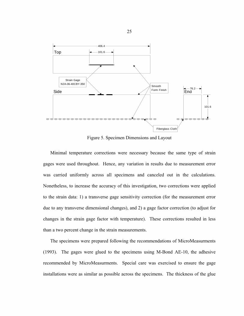
Specimens
Three concrete specimens from each bridge were used in this investigation. The
samples measured 406.4 x 101.5 x 76.2 mm. The samples were cast during deck
construction from concrete taken from different truckloads used at or close to the areas of
the bridge decks that were heavily instrumented.
The specimens used for this investigation were stored at the bridge site for the first
year and then move to a laboratory on the Montana State University campus for several
months. The laboratory is known to have a relative humidity of approximately 15 to 25
24
percent year round. The average humidity of the bridge deck structures during the past
two years was approximately 60 percent.
The reference material chosen for this experiment was titanium silicate, a specially
formulated glass developed for high precision optics. It was specifically chosen for this
purpose because of its extremely low CTE (0.03 µε/°C) and the consistency of its CTE
between different samples. A sample measuring 25.4 x 152.4 x 6.4 mm was obtained
from MicroMeasurments.
To further evaluate the accuracy of the instrumentation and testing methodology, a
precision ground bar (±0.0254 mm) of low carbon 1018 steel was also included in this
investigation. This material was chosen because it was used to determine the thermal
output curve provided by MicroMeasurments for the strain gage temperature corrections.
An annealed sample measuring50.8 x 609.6 x 3.2 mm with a Rockwell hardness of B61-
B62 was obtained through McMaster-Carr (Los Angeles, California). Similar to titanium
silicate, the CTE of 1018 steel is relatively constant, with a reported value of 12.1 µε/°C.
Instrumentation
The strain gages (type N2A-06-40CBY-350) used for this investigation were
purchased from MicroMeasurments (see Figure 5). These gages were chosen because of
their accuracy and ability to lay flat during installation. They were also used because
concrete’s non-homogeneous nature requires long gages to “average” the response.
According to the manufacturer, the thermal response of these gages was matched to
approximately 12.1 µε/°C, and therefore the thermal output was expected to be relatively
small over the temperature range of interest for the concrete and reference specimens.
25
SmoothForm Finish
Strain GageN2A-06-40CBY-350
Top
Side End
Fiberglass Cloth
406.4
76.2
101.6
101.6
Figure 5. Specimen Dimensions and Layout
Minimal temperature corrections were necessary because the same type of strain
gages were used throughout. Hence, any variation in results due to measurement error
was carried uniformly across all specimens and canceled out in the calculations.
Nonetheless, to increase the accuracy of this investigation, two corrections were applied
to the strain data: 1) a transverse gage sensitivity correction (for the measurement error
due to any transverse dimensional changes), and 2) a gage factor correction (to adjust for
changes in the strain gage factor with temperature). These corrections resulted in less
than a two percent change in the strain measurements.
The specimens were prepared following the recommendations of MicroMeasurments
(1993). The gages were glued to the specimens using M-Bond AE-10, the adhesive
recommended by MicroMeasurments. Special care was exercised to ensure the gage
installations were as similar as possible across the specimens. The thickness of the glue
26
between the gages and specimens was kept small, because of the effect this thickness can
have on measurement results. The room temperature at the time of installation was
documented, and the adhesive was not cured using elevated temperatures. This
procedure was followed to ensure a more repetitive installation quality and to reduce
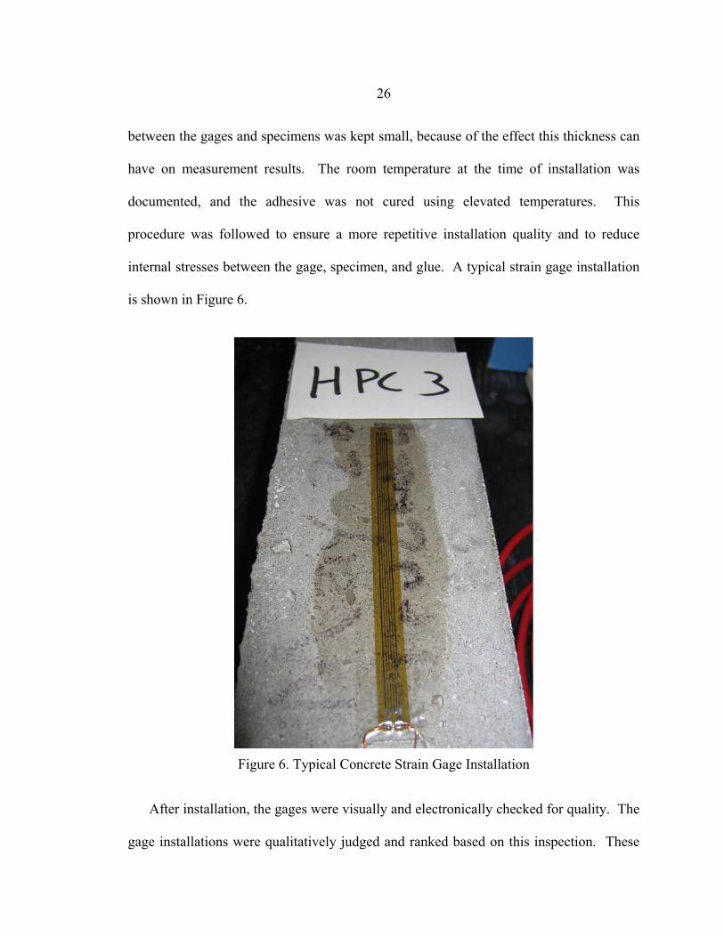
internal stresses between the gage, specimen, and glue. A typical strain gage installation
is shown in Figure 6.
Figure 6. Typical Concrete Strain Gage Installation
After installation, the gages were visually and electronically checked for quality. The
gage installations were qualitatively judged and ranked based on this inspection. These
27
rankings were then used to decide if any disparate results from a specific specimen
should simply be discarded due to a suspect gage installation. The gages were
thoroughly coated with silicon adhesive to protect them from moisture. Two strain gages
were installed on one of the specimens from each bridge to evaluate the repeatability and
accuracy of the gages.
Type T thermocouples purchased from Omega (Stamford, Connecticut) were used to
measure the temperature of each specimen. The T type thermocouples were chosen
because of their temperature range (–250°C to 350°C) and accuracy (the greater of 1.0°C
or 0.75 percent of the measurement). The thermocouples were fastened to the specimens
directly adjacent to the strain gages using silicon adhesive. An Omega thermocouple-to-
analog converter (Model SMCJ-T) was used to determine the junction temperature at the
multiplexer for the thermocouples used on the specimens.
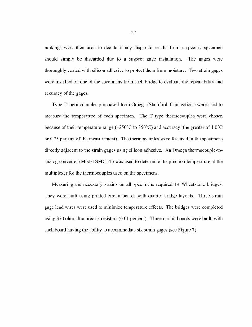
Measuring the necessary strains on all specimens required 14 Wheatstone bridges.
They were built using printed circuit boards with quarter bridge layouts. Three strain
gage lead wires were used to minimize temperature effects. The bridges were completed
using 350 ohm ultra precise resistors (0.01 percent). Three circuit boards were built, with
each board having the ability to accommodate six strain gages (see Figure 7).
28
Figure 7. Circuitry used for the Strain Measurements
The thermally induced strain (εT/O) in Equation 9 was determined using Wheatstone
bridges. It can be shown for a Wheatstone bridge in the quarter bridge configuration with
three lead wires that the strain output is related to the measured voltages as:
( ) ( )[ ]
( )( ) ⎭⎬⎫
⎩⎨⎧
−+−++−
=sizosoziio
ziozoisiziozoisoOT EEEEEEF
EEEEEEEEEEK
22
1/ε (Eq.9)
where:
K1 = Result of the specified nominal resistor values used within the
Wheatstone bridge circuitry and for this investigation was equal to -
(12/17477).
29
Ei = Measured input voltage from the strain gage during testing.
Eo = Measured output voltage from the strain gage during testing.
Esi = Measured input voltage from the strain gage during the shunt
calibration process. This term is used to determine the additional
resistance imparted to the system from the lead wires and connections.
Eso = Measured output voltage from the strain gage during the shunt
calibration process. This term is used to determine the additional
resistance imparted to the system from the lead wires and connections.
Ezi = Measured input voltage from the strain gage in the unstrained state.
This term accounts for changes in gage resistance during the
installation process and is meant to keep the Wheatstone bridge
balanced mathematically.
Ezo = Measured output voltage from the strain gage in the unstrained state.
This term accounts for changes in gage resistance during the
installation process and is meant to keep the Wheatstone bridge
balanced mathematically.
F = Strain gage factor, provided by manufacturer
Measurements were recorded using a Campbell Scientific CR10 data logger. The
capacity of this logger was expanded with a Campbell Scientific MX416 multiplexer.
The multiplexer was used to measure the temperature and strain for each specimen. The
multiplexer was located outside the environmental chamber because of its sensitivity to
temperature and humidity.
30
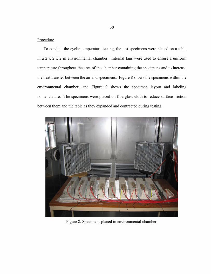
Procedure
To conduct the cyclic temperature testing, the test specimens were placed on a table
in a 2 x 2 x 2 m environmental chamber. Internal fans were used to ensure a uniform
temperature throughout the area of the chamber containing the specimens and to increase
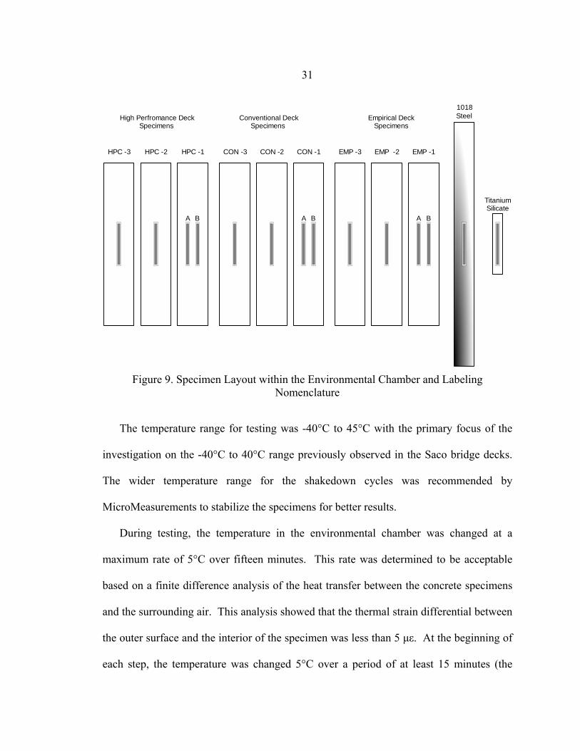
the heat transfer between the air and specimens. Figure 8 shows the specimens within the
environmental chamber, and Figure 9 shows the specimen layout and labeling
nomenclature. The specimens were placed on fiberglass cloth to reduce surface friction
between them and the table as they expanded and contracted during testing.
Figure 8. Specimens placed in environmental chamber.
31
HPC -3 HPC -2 HPC -1
A B
CON -3 CON -2 CON -1
A B
EMP -3 EMP -2 EMP -1
A B
TitaniumSilicate
1018SteelHigh Perfromance Deck
SpecimensConventional Deck
SpecimensEmpirical Deck
Specimens
Figure 9. Specimen Layout within the Environmental Chamber and Labeling
Nomenclature
The temperature range for testing was -40°C to 45°C with the primary focus of the
investigation on the -40°C to 40°C range previously observed in the Saco bridge decks.
The wider temperature range for the shakedown cycles was recommended by
MicroMeasurements to stabilize the specimens for better results.
During testing, the temperature in the environmental chamber was changed at a
maximum rate of 5°C over fifteen minutes. This rate was determined to be acceptable
based on a finite difference analysis of the heat transfer between the concrete specimens
and the surrounding air. This analysis showed that the thermal strain differential between
the outer surface and the interior of the specimen was less than 5 µε. At the beginning of
each step, the temperature was changed 5°C over a period of at least 15 minutes (the
32
ramp duration). It subsequently was held constant for at least 180 min. (the soak
duration), to allow the specimens to fully acclimate to the surrounding air temperature.
Six cycles from 20°C to the coldest temperature (-45°C or -40°C) to the hottest
temperature (50°C or 45°C) and back to 20°C (with 34 steps/cycle) were run extending
over one month (see Table 6). The first two cycles were used to stabilize the testing
system and evaluate the methodology used, while the last four were used to investigate
the repeatability of the experiment and obtain CTE values.
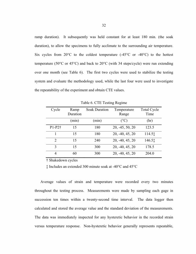
Table 6. CTE Testing Regime
Cycle Ramp Duration
Soak Duration Temperature Range
Total Cycle Time
(min) (min) (°C) (hr)
P1-P2† 15 180 20, -45, 50, 20 123.5
1 15 180 20, -40, 45, 20 114.5‡
2 15 240 20, -40, 45, 20 146.5‡
3 15 300 20, -40, 45, 20 178.5
4 60 300 20, -40, 45, 20 204.0
† Shakedown cycles
‡ Includes an extended 300 minute soak at -40°C and 45°C
Average values of strain and temperature were recorded every two minutes
throughout the testing process. Measurements were made by sampling each gage in
succession ten times within a twenty-second time interval. The data logger then
calculated and stored the average value and the standard deviation of the measurements.
The data was immediately inspected for any hysteretic behavior in the recorded strain
versus temperature response. Non-hysteretic behavior generally represents repeatable,
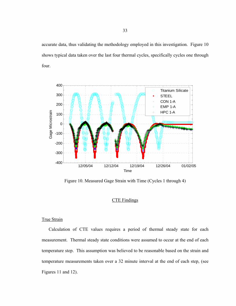
33
accurate data, thus validating the methodology employed in this investigation. Figure 10
shows typical data taken over the last four thermal cycles, specifically cycles one through
four.
12/05/04 12/12/04 12/19/04 12/26/04 01/02/05-400
-300
-200
-100
0
100
200
300
400
Time
Gag
e M
icro
stra
in
Titanium SilicateSTEELCON 1-AEMP 1-AHPC 1-A
Figure 10. Measured Gage Strain with Time (Cycles 1 through 4)
CTE Findings
True Strain
Calculation of CTE values requires a period of thermal steady state for each
measurement. Thermal steady state conditions were assumed to occur at the end of each
temperature step. This assumption was believed to be reasonable based on the strain and
temperature measurements taken over a 32 minute interval at the end of each step, (see
Figures 11 and 12).
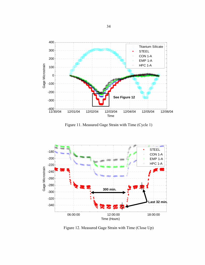
34
11/30/04 12/01/04 12/02/04 12/03/04 12/04/04 12/05/04 12/06/04-400
-300
-200
-100
0
100
200
300
400
Time
Gag
e M
icro
stra
inTitanium SilicateSTEELCON 1-AEMP 1-AHPC 1-A
See Figure 12
11/30/04 12/01/04 12/02/04 12/03/04 12/04/04 12/05/04 12/06/04-400
-300
-200
-100
0
100
200
300
400
Time
Gag
e M
icro
stra
inTitanium SilicateSTEELCON 1-AEMP 1-AHPC 1-A
See Figure 12
Figure 11. Measured Gage Strain with Time (Cycle 1)
06:00:00 12:00:00 18:00:00
-340
-320
-300
-280
-260
-240
-220
-200
-180
Time (Hours)
Gag
e M
icro
stra
in
STEELCON 1-AEMP 1-AHPC 1-A
300 min.
Last 32 min.
06:00:00 12:00:00 18:00:00
-340
-320
-300
-280
-260
-240
-220
-200
-180
Time (Hours)
Gag
e M
icro
stra
in
STEELCON 1-AEMP 1-AHPC 1-A
300 min.
Last 32 min.
Figure 12. Measured Gage Strain with Time (Close Up)
35
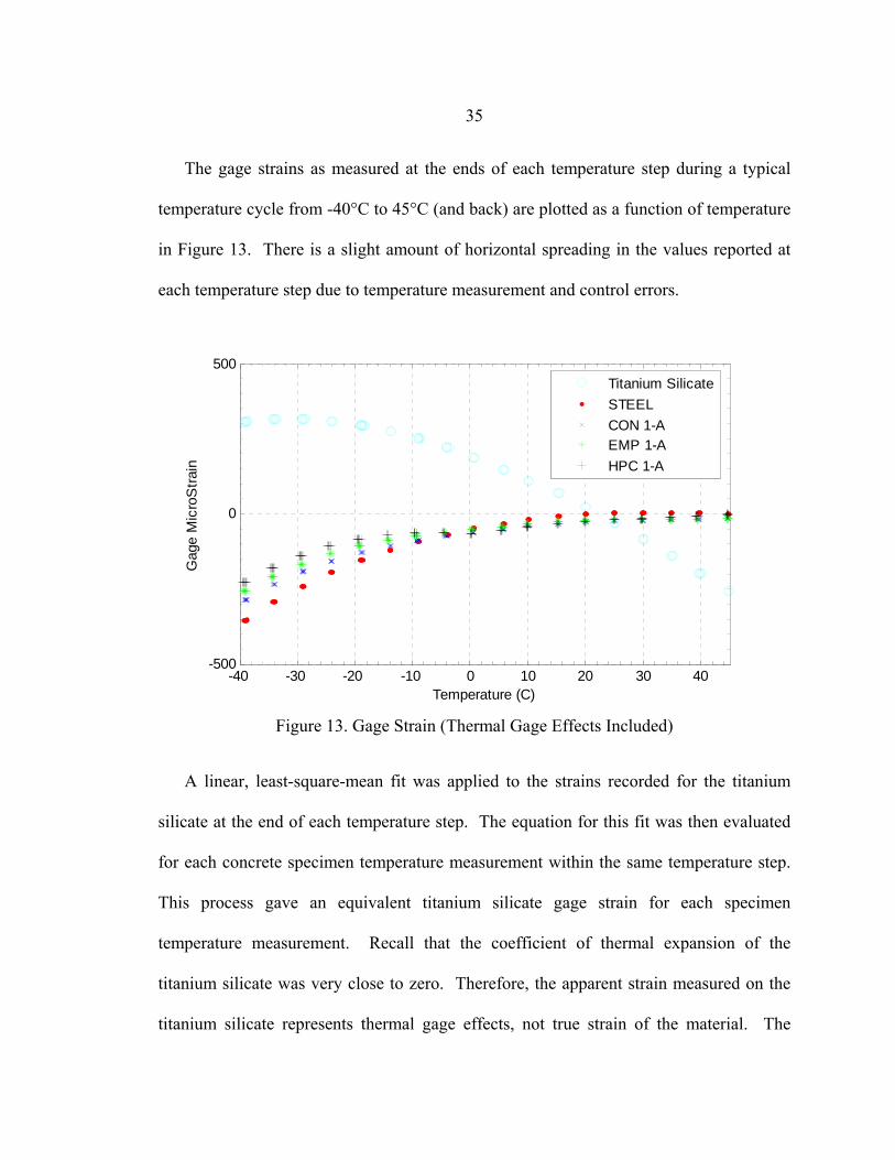
The gage strains as measured at the ends of each temperature step during a typical
temperature cycle from -40°C to 45°C (and back) are plotted as a function of temperature
in Figure 13. There is a slight amount of horizontal spreading in the values reported at
each temperature step due to temperature measurement and control errors.
-40 -30 -20 -10 0 10 20 30 40-500
0
500
Temperature (C)
Gag
e M
icro
Stra
in
Titanium SilicateSTEELCON 1-AEMP 1-AHPC 1-A
Figure 13. Gage Strain (Thermal Gage Effects Included)
A linear, least-square-mean fit was applied to the strains recorded for the titanium
silicate at the end of each temperature step. The equation for this fit was then evaluated
for each concrete specimen temperature measurement within the same temperature step.
This process gave an equivalent titanium silicate gage strain for each specimen
temperature measurement. Recall that the coefficient of thermal expansion of the
titanium silicate was very close to zero. Therefore, the apparent strain measured on the
titanium silicate represents thermal gage effects, not true strain of the material. The
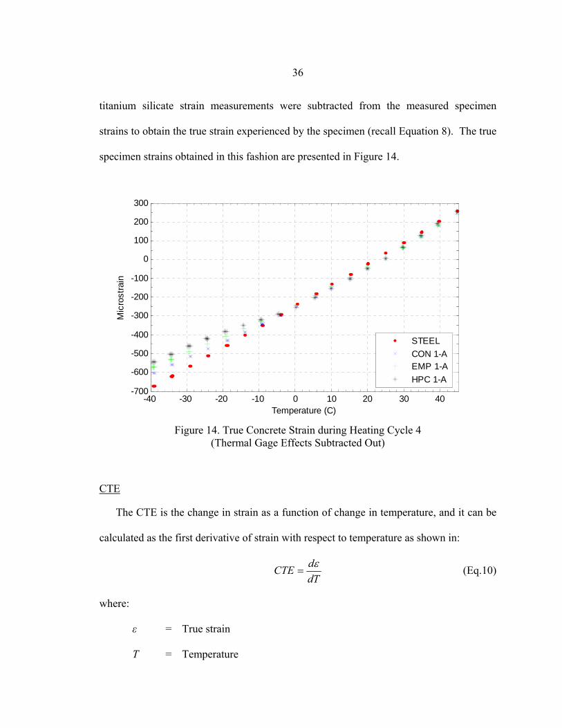
36
titanium silicate strain measurements were subtracted from the measured specimen
strains to obtain the true strain experienced by the specimen (recall Equation 8). The true
specimen strains obtained in this fashion are presented in Figure 14.
-40 -30 -20 -10 0 10 20 30 40-700
-600
-500
-400
-300
-200
-100
0
100
200
300
Temperature (C)
Mic
rost
rain
STEELCON 1-AEMP 1-AHPC 1-A
Figure 14. True Concrete Strain during Heating Cycle 4
(Thermal Gage Effects Subtracted Out)
CTE
The CTE is the change in strain as a function of change in temperature, and it can be
calculated as the first derivative of strain with respect to temperature as shown in:
dTdCTE ε
= (Eq.10)
where:
ε = True strain
T = Temperature
37
A piecewise linear, least-square-mean fit was first performed through a windowed subset
of the strain data with respect to temperature for each heating and cooling cycle. The
derivative of the fit was then numerically evaluated at the central temperature of the
moving window. Good results were obtained when the window extended over three
temperature steps (48 data points) because of the temperature measurement errors within
each step.
CTE Results for 1018 Steel
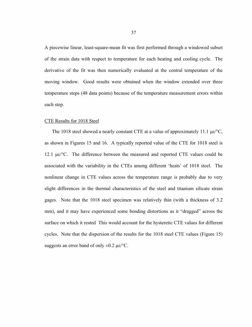
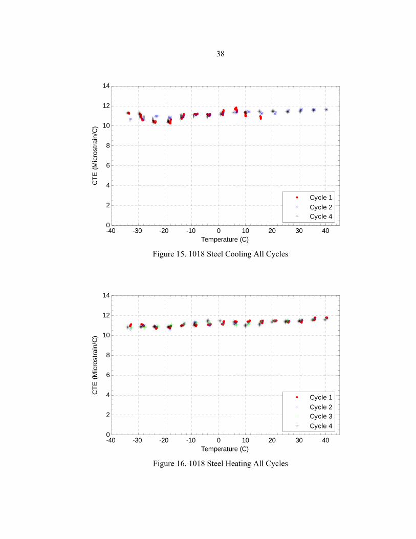
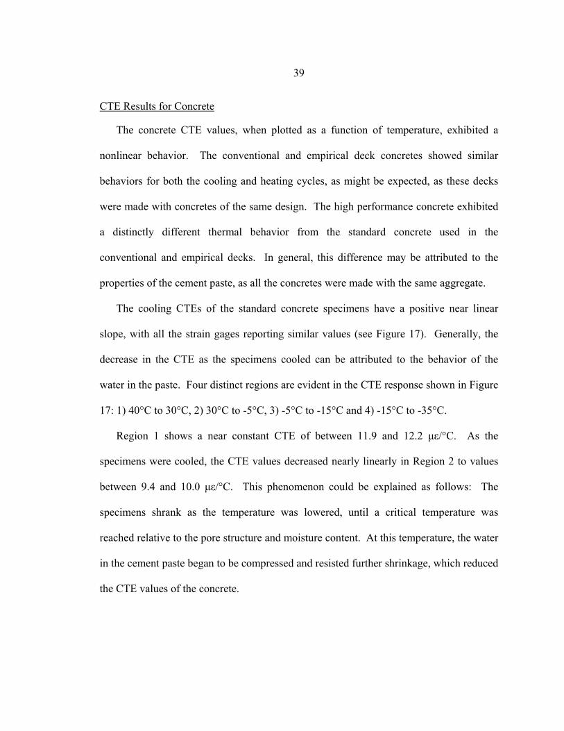
The 1018 steel showed a nearly constant CTE at a value of approximately 11.1 µε/°C,
as shown in Figures 15 and 16. A typically reported value of the CTE for 1018 steel is
12.1 µε/°C. The difference between the measured and reported CTE values could be
associated with the variability in the CTEs among different ‘heats’ of 1018 steel. The
nonlinear change in CTE values across the temperature range is probably due to very
slight differences in the thermal characteristics of the steel and titanium silicate strain
gages. Note that the 1018 steel specimen was relatively thin (with a thickness of 3.2
mm), and it may have experienced some bending distortions as it “dragged” across the
surface on which it rested This would account for the hysteretic CTE values for different
cycles. Note that the dispersion of the results for the 1018 steel CTE values (Figure 15)
suggests an error band of only ±0.2 µε/°C.
38
-40 -30 -20 -10 0 10 20 30 400
2
4
6
8
10
12
14
Temperature (C)
CTE
(Mic
rost
rain
/C)
Cycle 1Cycle 2Cycle 4
Figure 15. 1018 Steel Cooling All Cycles
-40 -30 -20 -10 0 10 20 30 400
2
4
6
8
10
12
14
Temperature (C)
CTE
(Mic
rost
rain
/C)
Cycle 1Cycle 2Cycle 3Cycle 4
Figure 16. 1018 Steel Heating All Cycles
39
CTE Results for Concrete
The concrete CTE values, when plotted as a function of temperature, exhibited a
nonlinear behavior. The conventional and empirical deck concretes showed similar
behaviors for both the cooling and heating cycles, as might be expected, as these decks
were made with concretes of the same design. The high performance concrete exhibited
a distinctly different thermal behavior from the standard concrete used in the
conventional and empirical decks. In general, this difference may be attributed to the
properties of the cement paste, as all the concretes were made with the same aggregate.
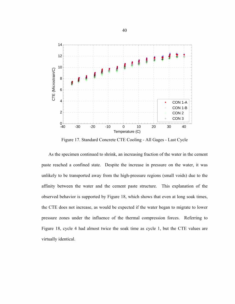
The cooling CTEs of the standard concrete specimens have a positive near linear
slope, with all the strain gages reporting similar values (see Figure 17). Generally, the
decrease in the CTE as the specimens cooled can be attributed to the behavior of the
water in the paste. Four distinct regions are evident in the CTE response shown in Figure
17: 1) 40°C to 30°C, 2) 30°C to -5°C, 3) -5°C to -15°C and 4) -15°C to -35°C.
Region 1 shows a near constant CTE of between 11.9 and 12.2 µε/°C. As the
specimens were cooled, the CTE values decreased nearly linearly in Region 2 to values
between 9.4 and 10.0 µε/°C. This phenomenon could be explained as follows: The
specimens shrank as the temperature was lowered, until a critical temperature was
reached relative to the pore structure and moisture content. At this temperature, the water
in the cement paste began to be compressed and resisted further shrinkage, which reduced
the CTE values of the concrete.
40
-40 -30 -20 -10 0 10 20 30 400
2
4
6
8
10
12
14
Temperature (C)
CTE
(Mic
rost
rain
/C)
CON 1-ACON 1-BCON 2CON 3
Figure 17. Standard Concrete CTE Cooling - All Gages - Last Cycle
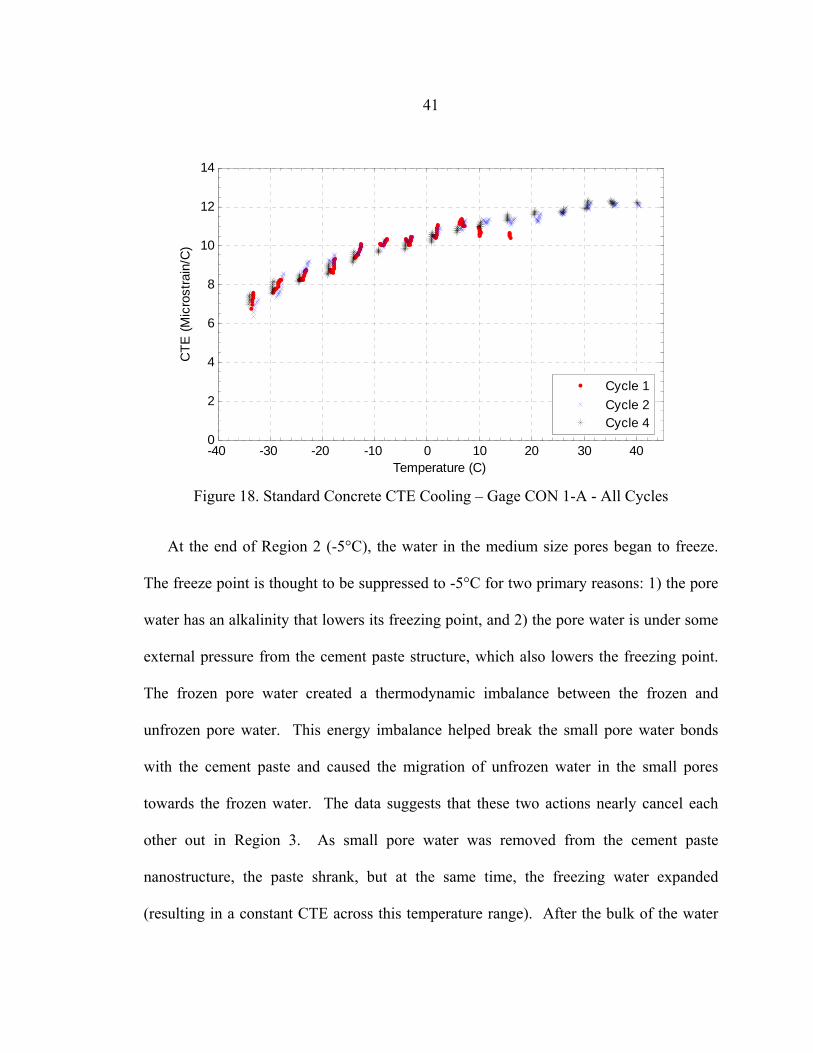
As the specimen continued to shrink, an increasing fraction of the water in the cement
paste reached a confined state. Despite the increase in pressure on the water, it was
unlikely to be transported away from the high-pressure regions (small voids) due to the
affinity between the water and the cement paste structure. This explanation of the
observed behavior is supported by Figure 18, which shows that even at long soak times,
the CTE does not increase, as would be expected if the water began to migrate to lower
pressure zones under the influence of the thermal compression forces. Referring to
Figure 18, cycle 4 had almost twice the soak time as cycle 1, but the CTE values are
virtually identical.
41
-40 -30 -20 -10 0 10 20 30 400
2
4
6
8
10
12
14
Temperature (C)
CTE
(Mic
rost
rain
/C)
Cycle 1Cycle 2Cycle 4
Figure 18. Standard Concrete CTE Cooling – Gage CON 1-A - All Cycles
At the end of Region 2 (-5°C), the water in the medium size pores began to freeze.
The freeze point is thought to be suppressed to -5°C for two primary reasons: 1) the pore
water has an alkalinity that lowers its freezing point, and 2) the pore water is under some
external pressure from the cement paste structure, which also lowers the freezing point.
The frozen pore water created a thermodynamic imbalance between the frozen and
unfrozen pore water. This energy imbalance helped break the small pore water bonds
with the cement paste and caused the migration of unfrozen water in the small pores
towards the frozen water. The data suggests that these two actions nearly cancel each
other out in Region 3. As small pore water was removed from the cement paste
nanostructure, the paste shrank, but at the same time, the freezing water expanded
(resulting in a constant CTE across this temperature range). After the bulk of the water
42
froze, the further contraction of the specimen was increasingly resisted by the
increasingly large ice crystals (Region 4), due to ice formation expansion (molecular
structure) and additional water freezing. Region 4 ended with CTE values ranging
between 7.4 and 8.6 µε/°C.
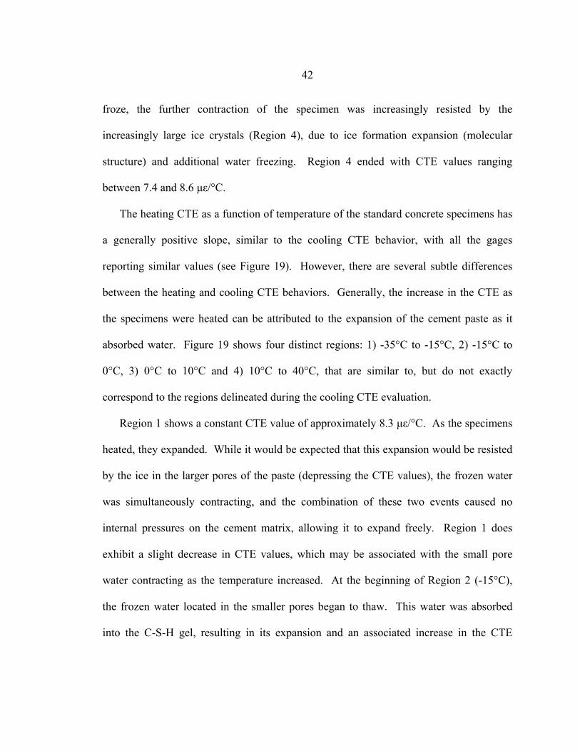
The heating CTE as a function of temperature of the standard concrete specimens has
a generally positive slope, similar to the cooling CTE behavior, with all the gages
reporting similar values (see Figure 19). However, there are several subtle differences
between the heating and cooling CTE behaviors. Generally, the increase in the CTE as
the specimens were heated can be attributed to the expansion of the cement paste as it
absorbed water. Figure 19 shows four distinct regions: 1) -35°C to -15°C, 2) -15°C to
0°C, 3) 0°C to 10°C and 4) 10°C to 40°C, that are similar to, but do not exactly
correspond to the regions delineated during the cooling CTE evaluation.
Region 1 shows a constant CTE value of approximately 8.3 µε/°C. As the specimens
heated, they expanded. While it would be expected that this expansion would be resisted
by the ice in the larger pores of the paste (depressing the CTE values), the frozen water
was simultaneously contracting, and the combination of these two events caused no
internal pressures on the cement matrix, allowing it to expand freely. Region 1 does
exhibit a slight decrease in CTE values, which may be associated with the small pore
water contracting as the temperature increased. At the beginning of Region 2 (-15°C),
the frozen water located in the smaller pores began to thaw. This water was absorbed
into the C-S-H gel, resulting in its expansion and an associated increase in the CTE
43
values. The CTE values level off after Region 2 because nearly all of the ice has
transformed into water.
-40 -30 -20 -10 0 10 20 30 400
2
4
6
8
10
12
14
Temperature (C)
CTE
(Mic
rost
rain
/C)
CON 1-ACON 1-BCON 2CON 3
Figure 19. Traditional Concrete CTE Heating - All Gages - Last Cycle
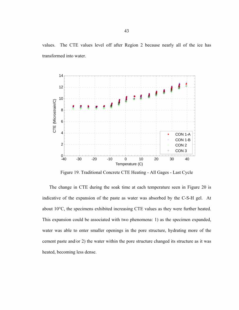
The change in CTE during the soak time at each temperature seen in Figure 20 is
indicative of the expansion of the paste as water was absorbed by the C-S-H gel. At
about 10°C, the specimens exhibited increasing CTE values as they were further heated.
This expansion could be associated with two phenomena: 1) as the specimen expanded,
water was able to enter smaller openings in the pore structure, hydrating more of the
cement paste and/or 2) the water within the pore structure changed its structure as it was
heated, becoming less dense.
44
-40 -30 -20 -10 0 10 20 30 400
2
4
6
8
10
12
14
Temperature (C)
CTE
(Mic
rost
rain
/C)
Cycle 1Cycle 2Cycle 3Cycle 4
Figure 20. Traditional Concrete CTE Heating – Gage CON 1-A - All Cycles
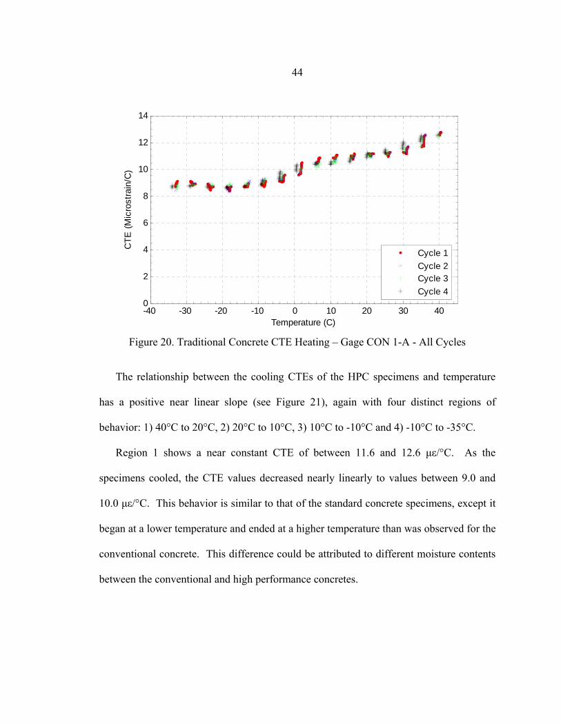
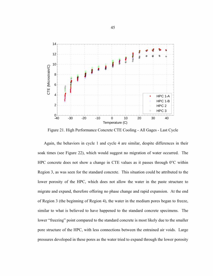
The relationship between the cooling CTEs of the HPC specimens and temperature
has a positive near linear slope (see Figure 21), again with four distinct regions of
behavior: 1) 40°C to 20°C, 2) 20°C to 10°C, 3) 10°C to -10°C and 4) -10°C to -35°C.
Region 1 shows a near constant CTE of between 11.6 and 12.6 µε/°C. As the
specimens cooled, the CTE values decreased nearly linearly to values between 9.0 and
10.0 µε/°C. This behavior is similar to that of the standard concrete specimens, except it
began at a lower temperature and ended at a higher temperature than was observed for the
conventional concrete. This difference could be attributed to different moisture contents
between the conventional and high performance concretes.
45
-40 -30 -20 -10 0 10 20 30 400
2
4
6
8
10
12
14
Temperature (C)
CTE
(Mic
rost
rain
/C)
HPC 1-AHPC 1-BHPC 2HPC 3
Figure 21. High Performance Concrete CTE Cooling - All Gages - Last Cycle
Again, the behaviors in cycle 1 and cycle 4 are similar, despite differences in their
soak times (see Figure 22), which would suggest no migration of water occurred. The
HPC concrete does not show a change in CTE values as it passes through 0°C within
Region 3, as was seen for the standard concrete. This situation could be attributed to the
lower porosity of the HPC, which does not allow the water in the paste structure to
migrate and expand, therefore offering no phase change and rapid expansion. At the end
of Region 3 (the beginning of Region 4), the water in the medium pores began to freeze,
similar to what is believed to have happened to the standard concrete specimens. The
lower “freezing” point compared to the standard concrete is most likely due to the smaller
pore structure of the HPC, with less connections between the entrained air voids. Large
pressures developed in these pores as the water tried to expand through the lower porosity
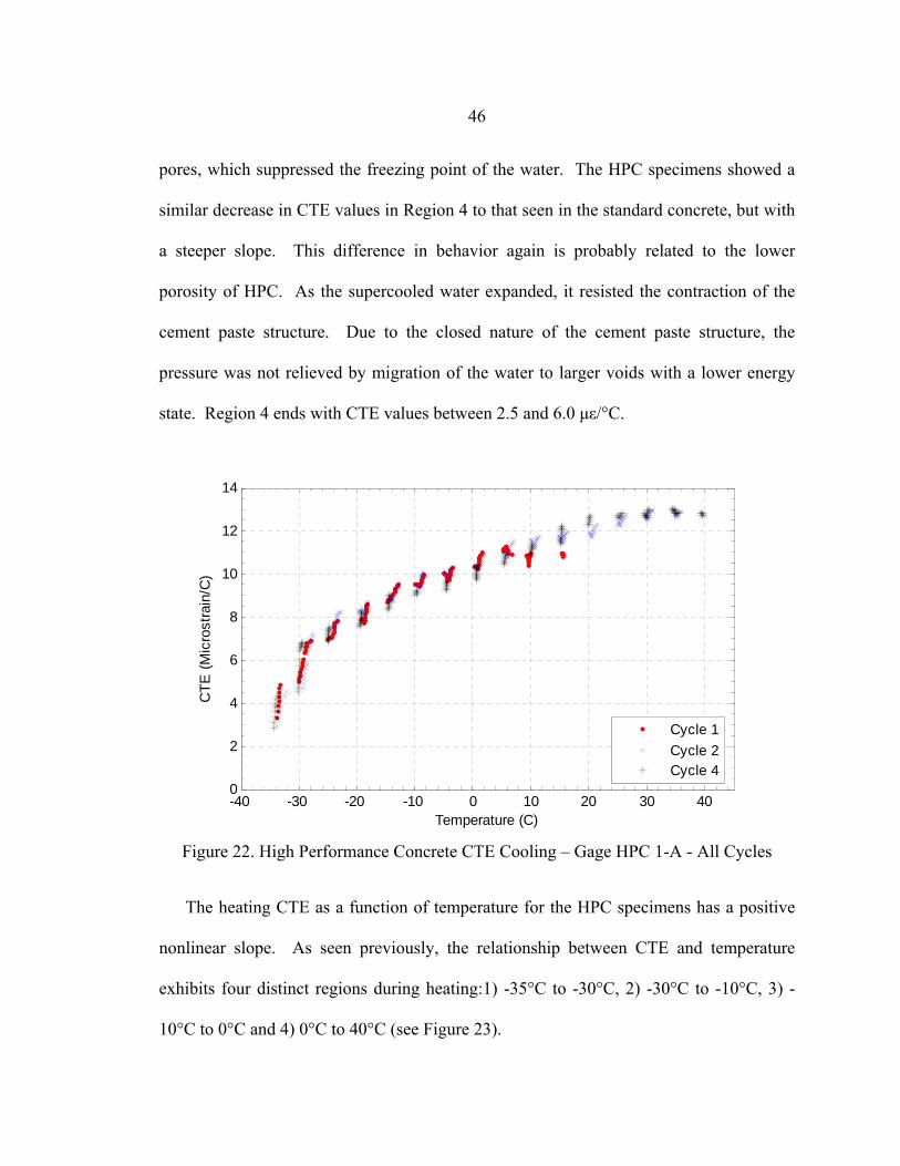
46
pores, which suppressed the freezing point of the water. The HPC specimens showed a
similar decrease in CTE values in Region 4 to that seen in the standard concrete, but with
a steeper slope. This difference in behavior again is probably related to the lower
porosity of HPC. As the supercooled water expanded, it resisted the contraction of the
cement paste structure. Due to the closed nature of the cement paste structure, the
pressure was not relieved by migration of the water to larger voids with a lower energy
state. Region 4 ends with CTE values between 2.5 and 6.0 µε/°C.
-40 -30 -20 -10 0 10 20 30 400
2
4
6
8
10
12
14
Temperature (C)
CTE
(Mic
rost
rain
/C)
Cycle 1Cycle 2Cycle 4
Figure 22. High Performance Concrete CTE Cooling – Gage HPC 1-A - All Cycles
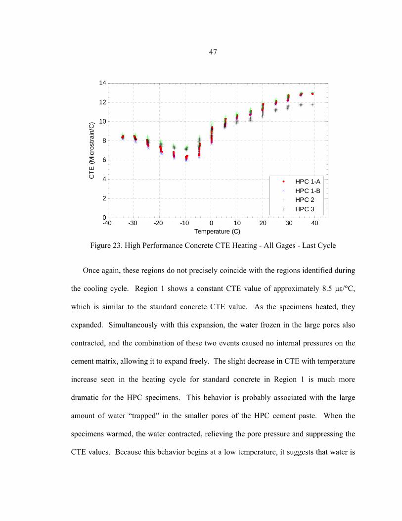
The heating CTE as a function of temperature for the HPC specimens has a positive
nonlinear slope. As seen previously, the relationship between CTE and temperature
exhibits four distinct regions during heating:1) -35°C to -30°C, 2) -30°C to -10°C, 3) -
10°C to 0°C and 4) 0°C to 40°C (see Figure 23).
47
-40 -30 -20 -10 0 10 20 30 400
2
4
6
8
10
12
14
Temperature (C)
CTE
(Mic
rost
rain
/C)
HPC 1-AHPC 1-BHPC 2HPC 3
Figure 23. High Performance Concrete CTE Heating - All Gages - Last Cycle
Once again, these regions do not precisely coincide with the regions identified during
the cooling cycle. Region 1 shows a constant CTE value of approximately 8.5 µε/°C,
which is similar to the standard concrete CTE value. As the specimens heated, they
expanded. Simultaneously with this expansion, the water frozen in the large pores also
contracted, and the combination of these two events caused no internal pressures on the
cement matrix, allowing it to expand freely. The slight decrease in CTE with temperature
increase seen in the heating cycle for standard concrete in Region 1 is much more
dramatic for the HPC specimens. This behavior is probably associated with the large
amount of water “trapped” in the smaller pores of the HPC cement paste. When the
specimens warmed, the water contracted, relieving the pore pressure and suppressing the
CTE values. Because this behavior begins at a low temperature, it suggests that water is
48
trapped in the smaller pores and is not able to migrate to the entrained air. This behavior
is consistent with some research that has been done that suggests air entrainment has little
benefit for improving the freeze-thaw resistance of high performance concrete (Zia et al.
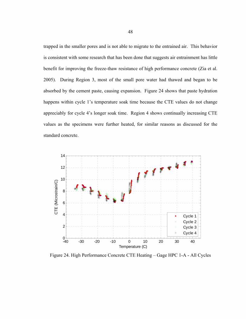
2005). During Region 3, most of the small pore water had thawed and began to be
absorbed by the cement paste, causing expansion. Figure 24 shows that paste hydration
happens within cycle 1’s temperature soak time because the CTE values do not change
appreciably for cycle 4’s longer soak time. Region 4 shows continually increasing CTE
values as the specimens were further heated, for similar reasons as discussed for the
standard concrete.
-40 -30 -20 -10 0 10 20 30 400
2
4
6
8
10
12
14
Temperature (C)
CTE
(Mic
rost
rain
/C)
Cycle 1Cycle 2Cycle 3Cycle 4
Figure 24. High Performance Concrete CTE Heating – Gage HPC 1-A - All Cycles
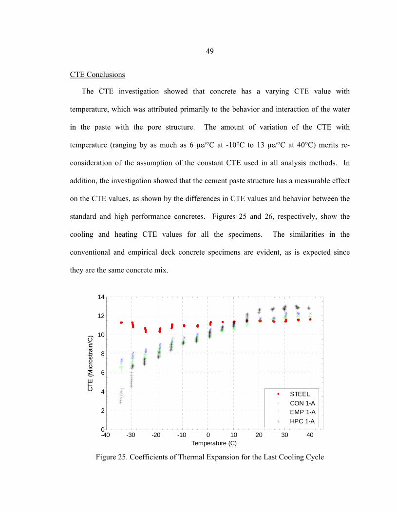
49
CTE Conclusions
The CTE investigation showed that concrete has a varying CTE value with
temperature, which was attributed primarily to the behavior and interaction of the water
in the paste with the pore structure. The amount of variation of the CTE with
temperature (ranging by as much as 6 µε/°C at -10°C to 13 µε/°C at 40°C) merits re-
consideration of the assumption of the constant CTE used in all analysis methods. In
addition, the investigation showed that the cement paste structure has a measurable effect
on the CTE values, as shown by the differences in CTE values and behavior between the
standard and high performance concretes. Figures 25 and 26, respectively, show the
cooling and heating CTE values for all the specimens. The similarities in the
conventional and empirical deck concrete specimens are evident, as is expected since
they are the same concrete mix.
-40 -30 -20 -10 0 10 20 30 400
2
4
6
8
10
12
14
Temperature (C)
CTE
(Mic
rost
rain
/C)
STEELCON 1-AEMP 1-AHPC 1-A
Figure 25. Coefficients of Thermal Expansion for the Last Cooling Cycle
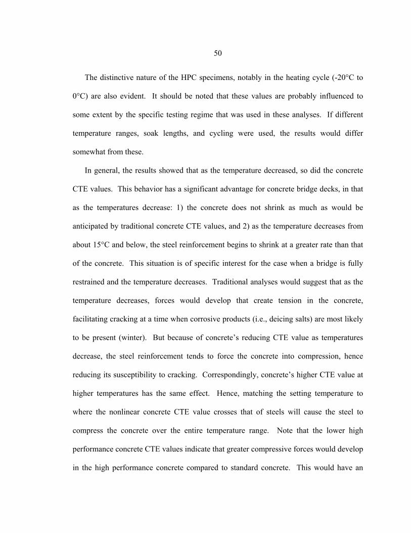
50
The distinctive nature of the HPC specimens, notably in the heating cycle (-20°C to
0°C) are also evident. It should be noted that these values are probably influenced to
some extent by the specific testing regime that was used in these analyses. If different
temperature ranges, soak lengths, and cycling were used, the results would differ
somewhat from these.
In general, the results showed that as the temperature decreased, so did the concrete
CTE values. This behavior has a significant advantage for concrete bridge decks, in that
as the temperatures decrease: 1) the concrete does not shrink as much as would be
anticipated by traditional concrete CTE values, and 2) as the temperature decreases from
about 15°C and below, the steel reinforcement begins to shrink at a greater rate than that
of the concrete. This situation is of specific interest for the case when a bridge is fully
restrained and the temperature decreases. Traditional analyses would suggest that as the
temperature decreases, forces would develop that create tension in the concrete,
facilitating cracking at a time when corrosive products (i.e., deicing salts) are most likely
to be present (winter). But because of concrete’s reducing CTE value as temperatures
decrease, the steel reinforcement tends to force the concrete into compression, hence
reducing its susceptibility to cracking. Correspondingly, concrete’s higher CTE value at
higher temperatures has the same effect. Hence, matching the setting temperature to
where the nonlinear concrete CTE value crosses that of steels will cause the steel to
compress the concrete over the entire temperature range. Note that the lower high
performance concrete CTE values indicate that greater compressive forces would develop
in the high performance concrete compared to standard concrete. This would have an
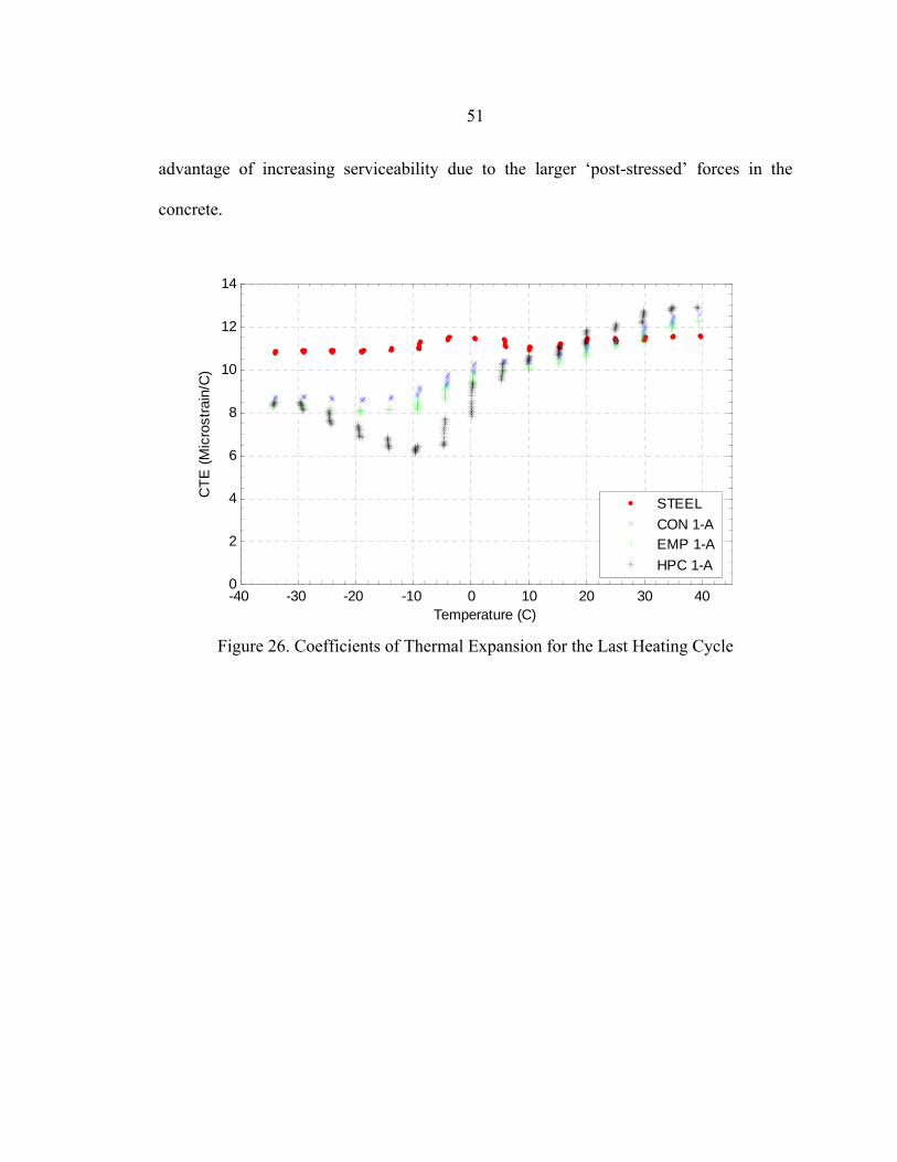
51
advantage of increasing serviceability due to the larger ‘post-stressed’ forces in the
concrete.
-40 -30 -20 -10 0 10 20 30 400
2
4
6
8
10
12
14
Temperature (C)
CTE
(Mic
rost
rain
/C)
STEELCON 1-AEMP 1-AHPC 1-A
Figure 26. Coefficients of Thermal Expansion for the Last Heating Cycle
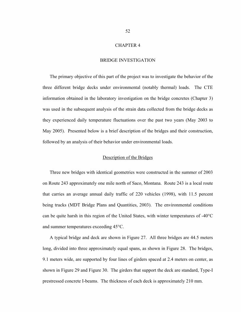
52
CHAPTER 4
BRIDGE INVESTIGATION
The primary objective of this part of the project was to investigate the behavior of the
three different bridge decks under environmental (notably thermal) loads. The CTE
information obtained in the laboratory investigation on the bridge concretes (Chapter 3)
was used in the subsequent analysis of the strain data collected from the bridge decks as
they experienced daily temperature fluctuations over the past two years (May 2003 to
May 2005). Presented below is a brief description of the bridges and their construction,
followed by an analysis of their behavior under environmental loads.
Description of the Bridges
Three new bridges with identical geometries were constructed in the summer of 2003
on Route 243 approximately one mile north of Saco, Montana. Route 243 is a local route
that carries an average annual daily traffic of 220 vehicles (1998), with 11.5 percent
being trucks (MDT Bridge Plans and Quantities, 2003). The environmental conditions
can be quite harsh in this region of the United States, with winter temperatures of -40°C
and summer temperatures exceeding 45°C.
A typical bridge and deck are shown in Figure 27. All three bridges are 44.5 meters
long, divided into three approximately equal spans, as shown in Figure 28. The bridges,
9.1 meters wide, are supported by four lines of girders spaced at 2.4 meters on center, as
shown in Figure 29 and Figure 30. The girders that support the deck are standard, Type-I
prestressed concrete I-beams. The thickness of each deck is approximately 210 mm.
53
Figure 27. Completed Bridge Deck
The decks on the three bridges were constructed with different concretes and different
reinforcing steel configurations. Two decks, the conventional (CON) deck and the
empirical (EMP) deck, were constructed with standard concrete with a specified 28-day
compressive strength of 21 MPa; one deck, the high performance deck (HPC), was
constructed with high performance concrete with a specified strength of 28 MPa.
Figure 28. Elevation View of Typical Saco Bridge
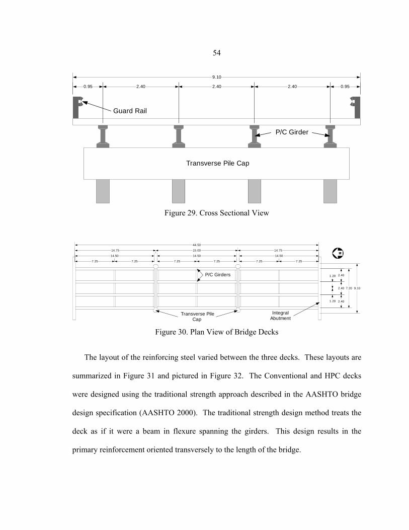
54
9.10
0.95 2.40 2.40 2.40 0.95
Guard Rail
Transverse Pile Cap
P/C Girder
Figure 29. Cross Sectional View
14.75
14.50
7.25 7.25
44.50
15.00 14.75
7.25 7.25
14.50 14.50
7.25 7.25
7.20
1.20
1.20
2.40
2.40
2.40
9.10
Transverse PileCap
P/C Girders
IntegralAbutment
Figure 30. Plan View of Bridge Decks
The layout of the reinforcing steel varied between the three decks. These layouts are
summarized in Figure 31 and pictured in Figure 32. The Conventional and HPC decks
were designed using the traditional strength approach described in the AASHTO bridge
design specification (AASHTO 2000). The traditional strength design method treats the
deck as if it were a beam in flexure spanning the girders. This design results in the
primary reinforcement oriented transversely to the length of the bridge.
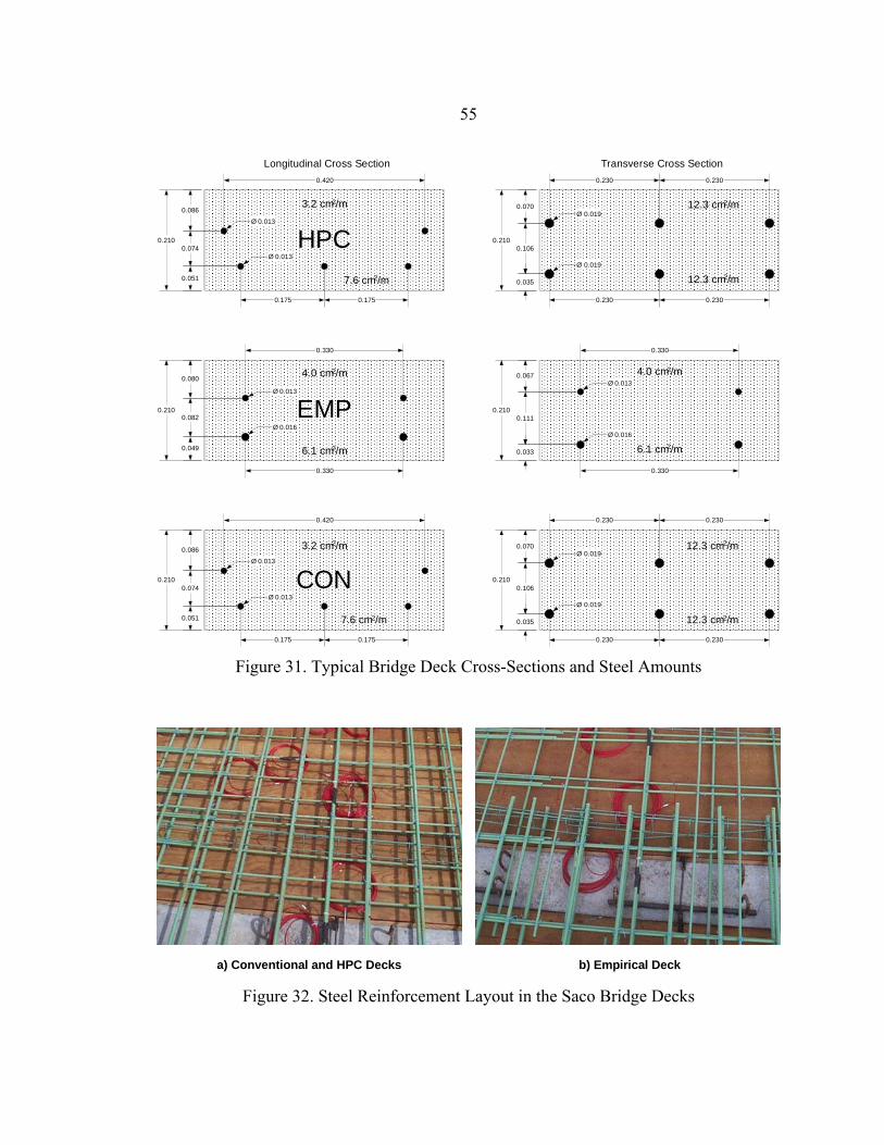
55
0.051
0.074
0.086
0.210
0.175 0.175
0.420
0.035
0.106
0.070
0.210
0.230 0.230
0.230 0.230
Ø 0.013
Ø 0.013Ø 0.019
Ø 0.019
Longitudinal Cross Section Transverse Cross Section
HPC
0.049
0.082
0.080
0.210
0.330
0.330
0.033
0.111
0.067
0.210
0.330
0.330
Ø 0.013
Ø 0.016Ø 0.016
Ø 0.013
EMP
0.051
0.074
0.086
0.210
0.175 0.175
0.420
0.035
0.106
0.070
0.210
0.230 0.230
0.230 0.230
Ø 0.013
Ø 0.013Ø 0.019
Ø 0.019
CON3.2 cm2/m
7.6 cm2/m
4.0 cm2/m
6.1 cm2/m
4.0 cm2/m
6.1 cm2/m
12.3 cm2/m
12.3 cm2/m
3.2 cm2/m
7.6 cm2/m 12.3 cm2/m
12.3 cm2/m
Figure 31. Typical Bridge Deck Cross-Sections and Steel Amounts
a) Conventional and HPC Decks b) Empirical Deck Figure 32. Steel Reinforcement Layout in the Saco Bridge Decks
56
The empirical design approach, which requires no formal analysis, is permitted by the
AASHTO specifications for monolithic concrete bridge decks that satisfy specific
conditions. Using this design method, reinforcement ratios for the top and bottom mat in
both the longitudinal and transverse directions are simply functions of the depth of
concrete and length of the span. AASHTO specifies a minimum reinforcement ratio
equal to 3.8 cm2/m in each direction in the top mat, and 5.7 cm2/m in each direction in the
bottom mat. The reason for the increased amount of steel in the bottom mat is for better
crack control in the positive bending regions of the slab. Comparatively, the
conventional and high performance decks used 14.5 cm2/m more steel than the empirical
deck in the transverse direction with nearly the same amount of steel in the longitudinal
direction (a difference of only 0.7 cm2/m). Reducing the amount of steel in the empirical
deck, especially in the top layer, decreases the opportunity for, and the effects of
reinforcement deterioration.
Bridge Deck Construction
Concrete was poured into the decks using a two-yard bucket and a crane, and was
leveled using an automatic screed (Figure 33). Sixteen to eighteen truckloads of concrete
(approximately 95 cubic meters) were used to cast each bridge deck. During construction
of the decks, MDT performed air content tests, slump tests, and collected test specimens
from selected concrete trucks to make compression strength test cylinders. Average
results from the slump and air content tests are presented in Table 7. In addition,
concrete test specimens were collected from a representative portion of the concrete used
to cast the instrumented section of each deck. Sufficient samples were collected to be
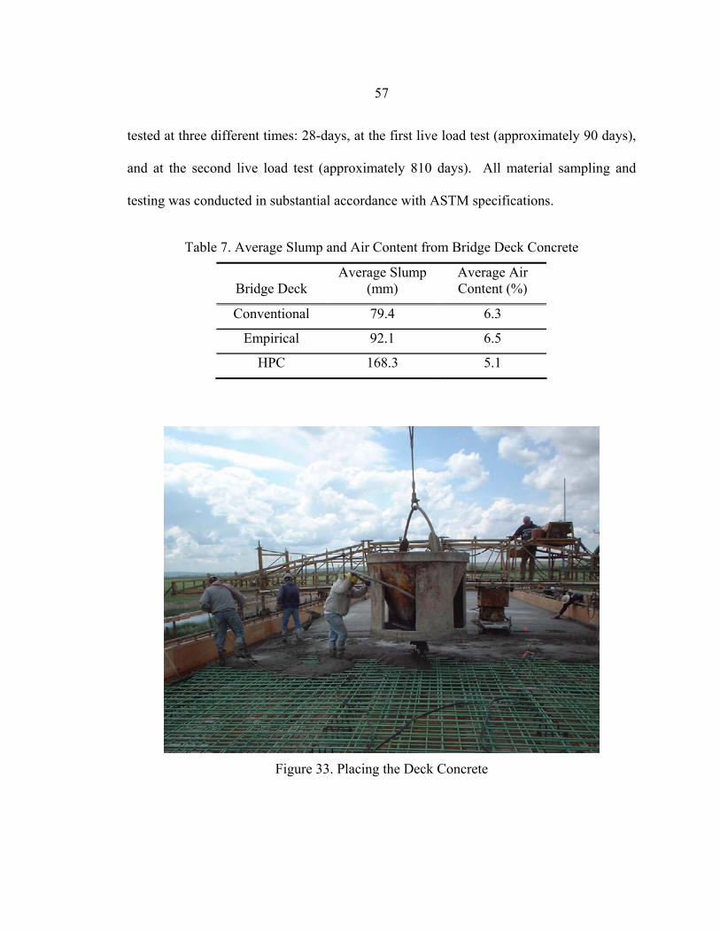
57
tested at three different times: 28-days, at the first live load test (approximately 90 days),
and at the second live load test (approximately 810 days). All material sampling and
testing was conducted in substantial accordance with ASTM specifications.
Table 7. Average Slump and Air Content from Bridge Deck Concrete
Bridge Deck Average Slump
(mm) Average Air Content (%)
Conventional 79.4 6.3
Empirical 92.1 6.5
HPC 168.3 5.1
Figure 33. Placing the Deck Concrete
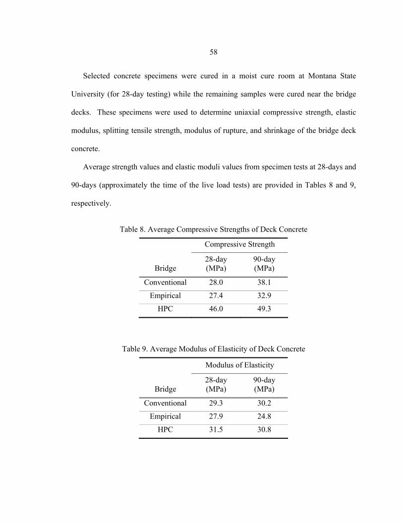
58
Selected concrete specimens were cured in a moist cure room at Montana State
University (for 28-day testing) while the remaining samples were cured near the bridge
decks. These specimens were used to determine uniaxial compressive strength, elastic
modulus, splitting tensile strength, modulus of rupture, and shrinkage of the bridge deck
concrete.
Average strength values and elastic moduli values from specimen tests at 28-days and
90-days (approximately the time of the live load tests) are provided in Tables 8 and 9,
respectively.
Table 8. Average Compressive Strengths of Deck Concrete
Compressive Strength
Bridge 28-day (MPa)
90-day (MPa)
Conventional 28.0 38.1
Empirical 27.4 32.9
HPC 46.0 49.3
Table 9. Average Modulus of Elasticity of Deck Concrete
Modulus of Elasticity
Bridge 28-day (MPa)
90-day (MPa)
Conventional 29.3 30.2
Empirical 27.9 24.8
HPC 31.5 30.8
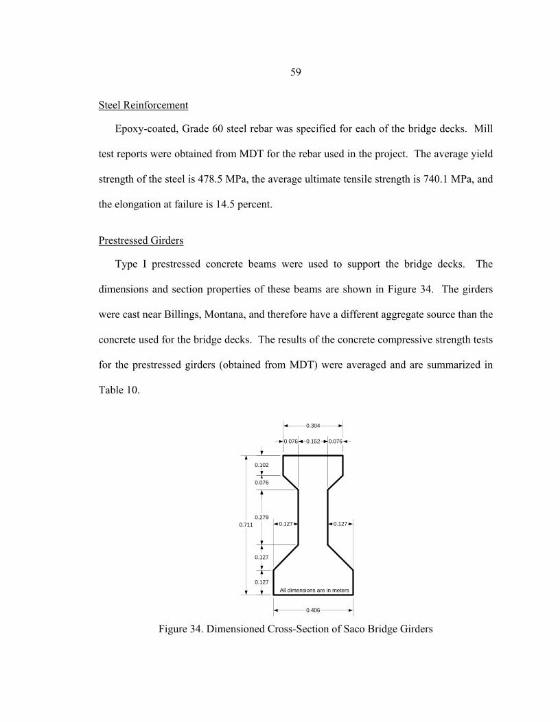
59
Steel Reinforcement
Epoxy-coated, Grade 60 steel rebar was specified for each of the bridge decks. Mill
test reports were obtained from MDT for the rebar used in the project. The average yield
strength of the steel is 478.5 MPa, the average ultimate tensile strength is 740.1 MPa, and
the elongation at failure is 14.5 percent.
Prestressed Girders
Type I prestressed concrete beams were used to support the bridge decks. The
dimensions and section properties of these beams are shown in Figure 34. The girders
were cast near Billings, Montana, and therefore have a different aggregate source than the
concrete used for the bridge decks. The results of the concrete compressive strength tests
for the prestressed girders (obtained from MDT) were averaged and are summarized in
Table 10.
0.304
0.406
0.711
0.127
0.102
0.076
0.127
0.279
0.076 0.0760.152
0.1270.127
All dimensions are in meters
Figure 34. Dimensioned Cross-Section of Saco Bridge Girders
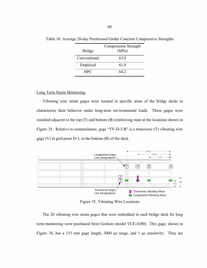
60
Table 10. Average 28-day Prestressed Girder Concrete Compressive Strengths
Bridge Compression Strength
(MPa)
Conventional 63.0
Empirical 61.0
HPC 64.2
Long Term Strain Monitoring
Vibrating wire strain gages were located in specific areas of the bridge decks to
characterize their behavior under long-term environmental loads. These gages were
installed adjacent to the top (T) and bottom (B) reinforcing mats at the locations shown in
Figure 35. Relative to nomenclature, gage “TV-D-3-B” is a transverse (T) vibrating wire
gage (V) at grid point D-3, in the bottom (B) of the deck.
Transverse Vibrating WiresLongitudinal Vibrating Wires
14.75
11.00
7.25
2.253.35
ABDF
35
Transverse GageLine Designations
Longitudinal GageLine Designations
Figure 35. Vibrating Wire Locations
The 20 vibrating wire strain gages that were embedded in each bridge deck for long
term monitoring were purchased from Geokon (model VCE-4200). This gage, shown in
Figure 36, has a 153 mm gage length, 3000 µε range, and 1 µε sensitivity. They are
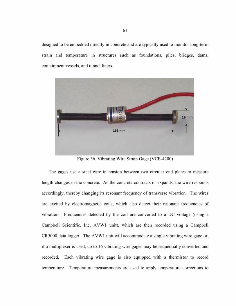
61
designed to be embedded directly in concrete and are typically used to monitor long-term
strain and temperature in structures such as foundations, piles, bridges, dams,
containment vessels, and tunnel liners.
153 mm
19 mm
153 mm
19 mm
Figure 36. Vibrating Wire Strain Gage (VCE-4200)
The gages use a steel wire in tension between two circular end plates to measure
length changes in the concrete. As the concrete contracts or expands, the wire responds
accordingly, thereby changing its resonant frequency of transverse vibration. The wires
are excited by electromagnetic coils, which also detect their resonant frequencies of
vibration. Frequencies detected by the coil are converted to a DC voltage (using a
Campbell Scientific, Inc. AVW1 unit), which are then recorded using a Campbell
CR5000 data logger. The AVW1 unit will accommodate a single vibrating wire gage or,
if a multiplexer is used, up to 16 vibrating wire gages may be sequentially converted and
recorded. Each vibrating wire gage is also equipped with a thermistor to record
temperature. Temperature measurements are used to apply temperature corrections to
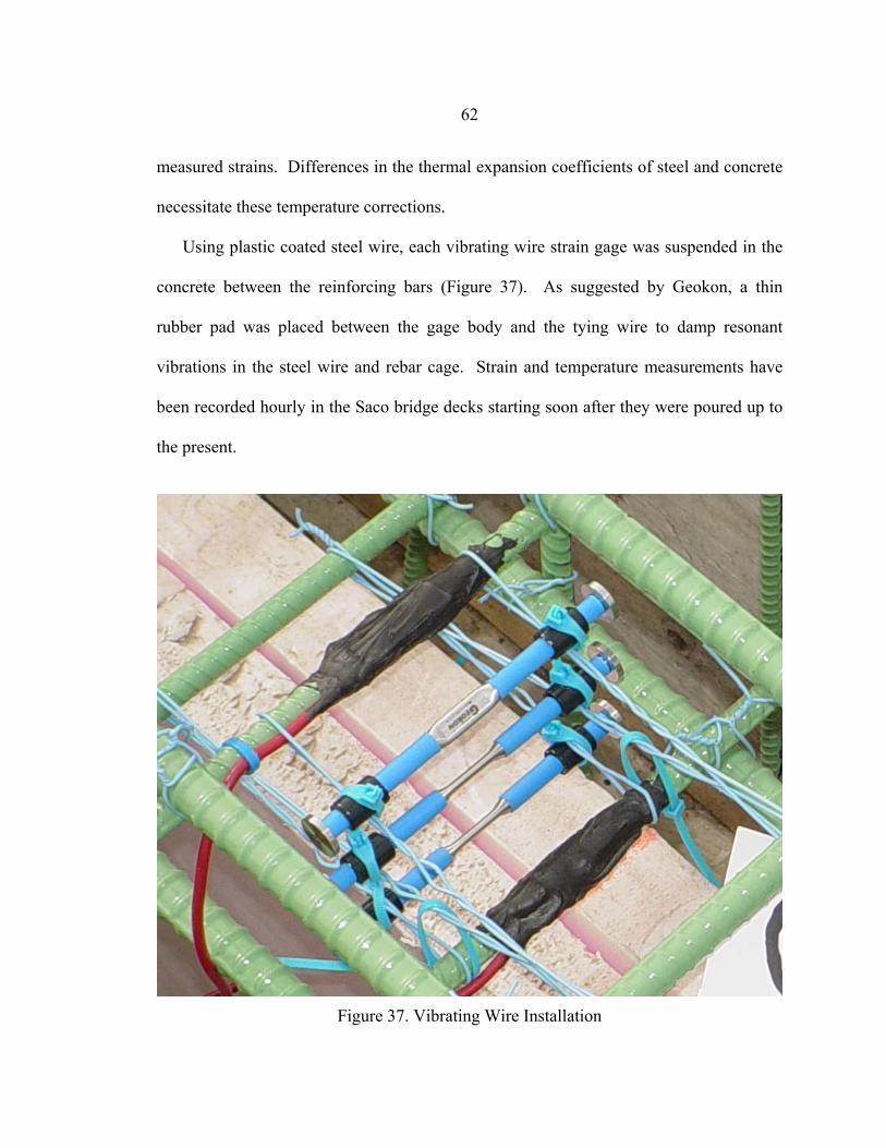
62
measured strains. Differences in the thermal expansion coefficients of steel and concrete
necessitate these temperature corrections.
Using plastic coated steel wire, each vibrating wire strain gage was suspended in the
concrete between the reinforcing bars (Figure 37). As suggested by Geokon, a thin
rubber pad was placed between the gage body and the tying wire to damp resonant
vibrations in the steel wire and rebar cage. Strain and temperature measurements have
been recorded hourly in the Saco bridge decks starting soon after they were poured up to
the present.
Figure 37. Vibrating Wire Installation
63
Data Analysis
Two “types” of strain are of primary interest in this investigation, the total strain
experienced by the decks as they undergo thermal changes and the part of the total strain
that has internal stress associated with it. The total strain is of interest because it reflects
the deformed physical shape of the bridge decks. The internal stress strain is of
importance because it reflects the internal material stresses and forces that could cause
damage to the decks. The intent of a typical strain gage installation is to collect
information on the stress related strain, and the concrete strain data from the vibrating
wire gages was initially corrected to produce “stress” strain using the equation provided
by Geokon for this purpose (see Equation 11).
( ) ( )RMCSM TT −⋅−+= ααεεσ (Eq.11)
where:
εσ = Stress related strain
εM = Measured strain
αS = CTE of steel
αC = CTE of concrete
TM = Measured temperature
TR = Reference temperature
Stress strain is the strain that results from a stress in the concrete. This condition
typically results from external loads applied to the structure, and the associated strains
can be negative and positive. The external load applied to the structure can be generated
by its supports, if they interfere with dimensional movements associated with temperature
64
changes, shrinkage, or creep. For example, when a structure with fixed supports
experiences an increase in temperature, the associated expansion is resisted by the
supports, generating compression throughout the structure. Since unrestrained thermal
strains produce no stress in a structure, the measured strains typically are adjusted to
remove this part of the strain response.
Thermal strain is the strain developed by the change in a material’s length due to a
change in temperature:
(Eq.12) ∫ ⋅=M
R
T
TCTh dTαε
where:
εTh = Thermal related strain
This strain is positive when the temperature increases and negative when the
temperature decreases. Thermal strain occurs without any stress, if the structure is free to
change shape and size under the effect. If the strain sensing elements used in the decks
were made of concrete, they would not register any strains in the deck as they freely
expand and contract under temperature changes, as the gages would have exactly the
same strain as the deck, itself. Since the gage sensing elements are made of steel, a
correction factor (effectively the second term in Equation 11) is necessary to compensate
for the difference in the CTEs of the steel gage components and the surrounding concrete.
Equation 11 assumes constant CTEs across the entire temperature range for both the steel
and concrete. The laboratory CTE analysis, however, showed that the CTE of the deck
65
concrete varies significantly (approximately 50 percent) over the temperature range of
interest (-40°C to 27°C).
Thus, a more accurate stress strain was determined by using the concrete CTEs
obtained from the laboratory portion of this investigation, specifically, the CTE curve
from the conventional specimen 1-A during cooling cycle four, in Equation 11. The total
strain was subsequently obtained by adding the thermal strain to the corrected “stress”
strain:
( )RMCT TT −⋅+= αεε σ (Eq.13)
where:
εT = Total strain
Note that the total strain in concrete is comprised of four main components:
1) thermal strain, 2) stress strain, 3) creep strain, and 4) shrinkage strain. The corrected
“stress” strain generated by Equation 11 actually consists of the stress strain, creep strain,
and shrinkage strain in the concrete:
ShCrThT εεεεε σ +++= (Eq.14)
where:
εCr = Creep strain
εSh = Shrinkage strain
Creep and shrinkage are time dependent phenomenon, and in many experiments of
short duration they are small in magnitude and thus neglected. Creep strain is a
phenomenon associated with sustained loading of concrete. Concrete under sustained
loading will try to redistribute the internal stress to a lower state of equilibrium, similar to
66
how clayey soils will consolidate under long-term loads. The Feldman-Spears Model
explains this phenomenon by the removal of interlayer water from the C-S-H gel. The
external load on the concrete places a pressure on the pore water. Over time, the pore
water relieves the pressure by exiting the concrete’s microstructure. The result is similar
to shrinkage, in that the concrete shrinks as the water’s resistance is removed. Creep
strain was neglected in this investigation primarily because it is small in magnitude for
lightly loaded members.
Shrinkage strain develops as the concrete cures and dries, and it typically occurs
within the first six months after it was cast. Generally, shrinkage strains are not
recoverable, except under extraordinary circumstances. Shrinkage is associated with the
use (by curing) and/or removal (by drying) of pore water from the concrete
microstructure and produces a negative (shrinking) strain. The AASHTO bridge design
specifications suggest using the following shrinkage equation (2000):
51035
⋅⎟⎠⎞
⎜⎝⎛
+⋅−=
ttkk hsShε (Eq.15)
where:
⎟⎠⎞
⎜⎝⎛ ⋅−
⎟⎟⎟⎟
⎠
⎞
⎜⎜⎜⎜
⎝
⎛
+
+⋅=⋅
923941096
45
26 36.0 VIS
tt
tet
kVIS
s (Eq.16)
( )70
140 Hkh−
= , for average annual relative humidity’s (H) < 80% (Eq.17)
( )70
1003 Hkh−⋅
= , for average annual relative humidity’s (H) ≥ 80% (Eq.18)
H = Average annual relative humidity’s as a percentage
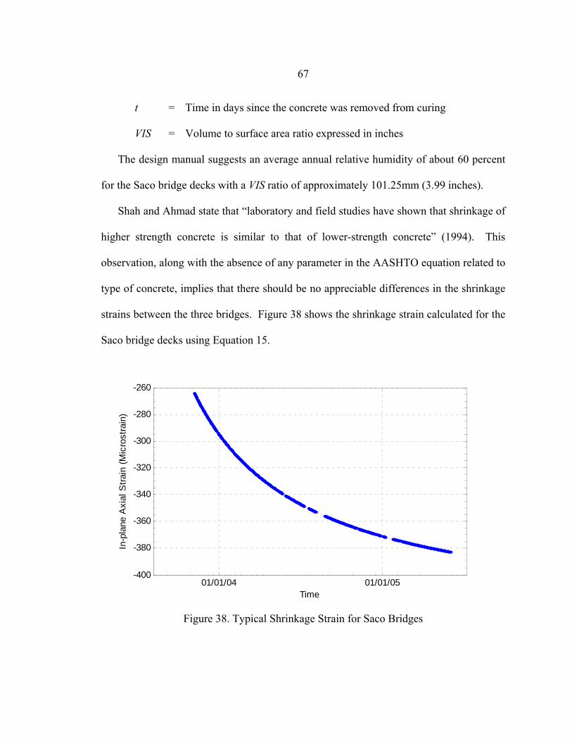
67
t = Time in days since the concrete was removed from curing
VIS = Volume to surface area ratio expressed in inches
The design manual suggests an average annual relative humidity of about 60 percent
for the Saco bridge decks with a VIS ratio of approximately 101.25mm (3.99 inches).
Shah and Ahmad state that “laboratory and field studies have shown that shrinkage of
higher strength concrete is similar to that of lower-strength concrete” (1994). This
observation, along with the absence of any parameter in the AASHTO equation related to
type of concrete, implies that there should be no appreciable differences in the shrinkage
strains between the three bridges. Figure 38 shows the shrinkage strain calculated for the
Saco bridge decks using Equation 15.
01/01/04 01/01/05-400
-380
-360
-340
-320
-300
-280
-260
In-p
lane
Axi
al S
train
(Mic
rost
rain
)
Time
Figure 38. Typical Shrinkage Strain for Saco Bridges
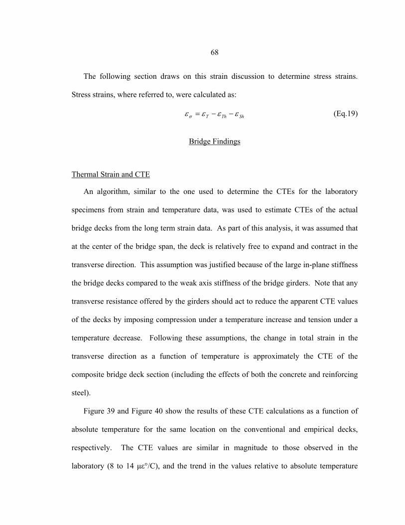
68
The following section draws on this strain discussion to determine stress strains.
Stress strains, where referred to, were calculated as:
ShThT εεεεσ −−= (Eq.19)
Bridge Findings
Thermal Strain and CTE
An algorithm, similar to the one used to determine the CTEs for the laboratory
specimens from strain and temperature data, was used to estimate CTEs of the actual
bridge decks from the long term strain data. As part of this analysis, it was assumed that
at the center of the bridge span, the deck is relatively free to expand and contract in the
transverse direction. This assumption was justified because of the large in-plane stiffness
the bridge decks compared to the weak axis stiffness of the bridge girders. Note that any
transverse resistance offered by the girders should act to reduce the apparent CTE values
of the decks by imposing compression under a temperature increase and tension under a
temperature decrease. Following these assumptions, the change in total strain in the
transverse direction as a function of temperature is approximately the CTE of the
composite bridge deck section (including the effects of both the concrete and reinforcing
steel).
Figure 39 and Figure 40 show the results of these CTE calculations as a function of
absolute temperature for the same location on the conventional and empirical decks,
respectively. The CTE values are similar in magnitude to those observed in the
laboratory (8 to 14 µε°/C), and the trend in the values relative to absolute temperature
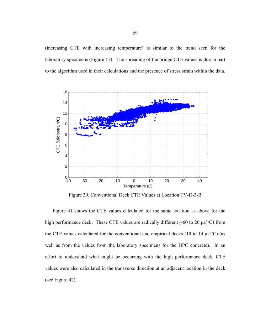
69
(increasing CTE with increasing temperature) is similar to the trend seen for the
laboratory specimens (Figure 17). The spreading of the bridge CTE values is due in part
to the algorithm used in their calculations and the presence of stress strain within the data.
-40 -30 -20 -10 0 10 20 30 400
2
4
6
8
10
12
14
16
CTE
(Mic
rost
rain
/C)
Temperature (C) Figure 39. Conventional Deck CTE Values at Location TV-D-3-B
Figure 41 shows the CTE values calculated for the same location as above for the
high performance deck. These CTE values are radically different (-60 to 20 µε°/C) from
the CTE values calculated for the conventional and empirical decks (10 to 14 µε°/C) (as
well as from the values from the laboratory specimens for the HPC concrete). In an
effort to understand what might be occurring with the high performance deck, CTE
values were also calculated in the transverse direction at an adjacent location in the deck
(see Figure 42).
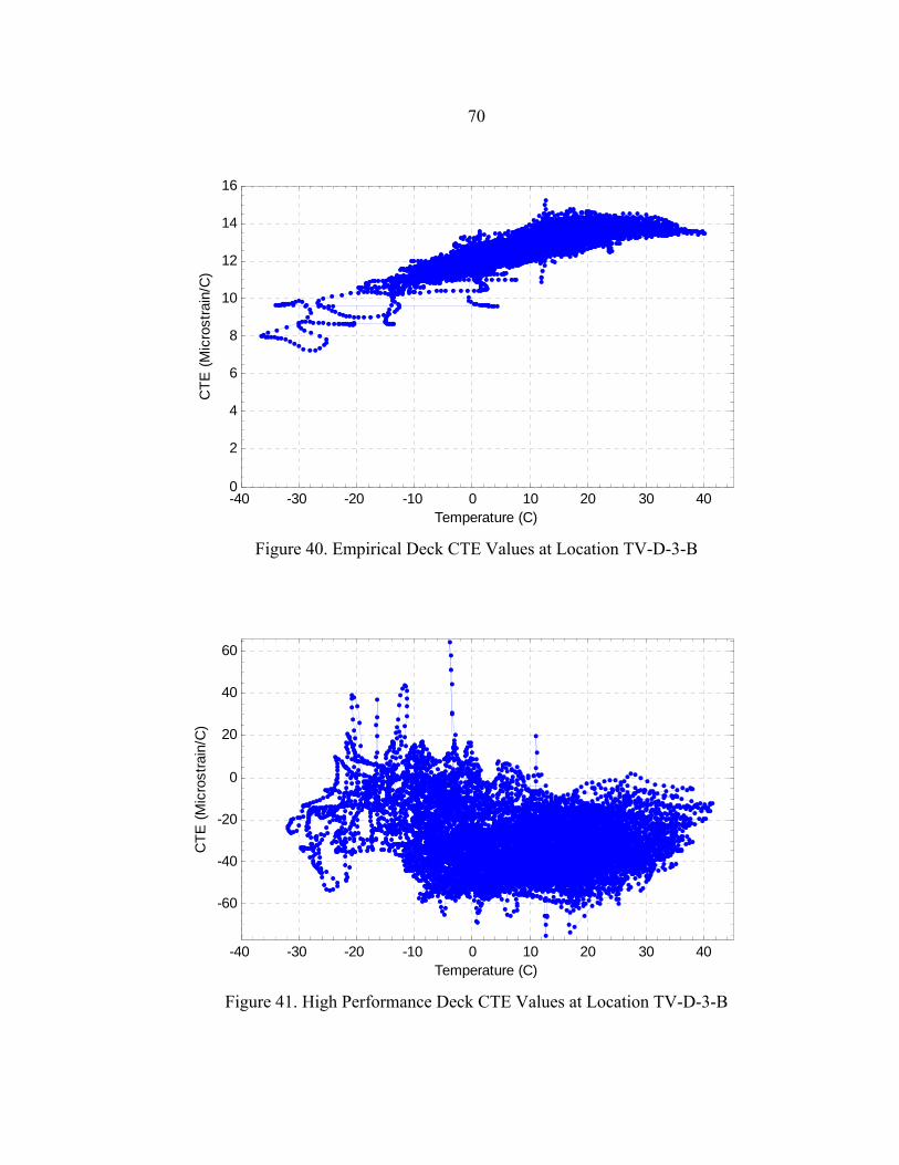
70
-40 -30 -20 -10 0 10 20 30 400
2
4
6
8
10
12
14
16C
TE (M
icro
stra
in/C
)
Temperature (C) Figure 40. Empirical Deck CTE Values at Location TV-D-3-B
-40 -30 -20 -10 0 10 20 30 40
-60
-40
-20
0
20
40
60
CTE
(Mic
rost
rain
/C)
Temperature (C) Figure 41. High Performance Deck CTE Values at Location TV-D-3-B
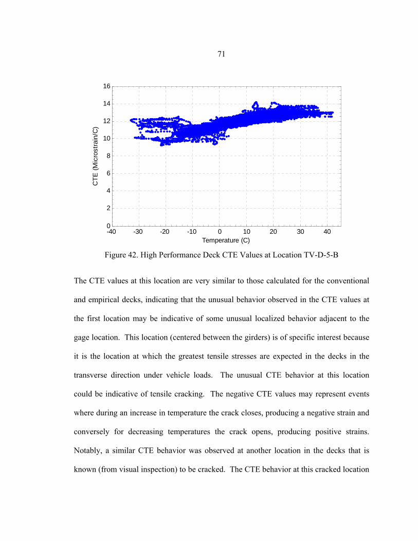
71
-40 -30 -20 -10 0 10 20 30 400
2
4
6
8
10
12
14
16C
TE (M
icro
stra
in/C
)
Temperature (C) Figure 42. High Performance Deck CTE Values at Location TV-D-5-B
The CTE values at this location are very similar to those calculated for the conventional
and empirical decks, indicating that the unusual behavior observed in the CTE values at
the first location may be indicative of some unusual localized behavior adjacent to the
gage location. This location (centered between the girders) is of specific interest because
it is the location at which the greatest tensile stresses are expected in the decks in the
transverse direction under vehicle loads. The unusual CTE behavior at this location
could be indicative of tensile cracking. The negative CTE values may represent events
where during an increase in temperature the crack closes, producing a negative strain and
conversely for decreasing temperatures the crack opens, producing positive strains.
Notably, a similar CTE behavior was observed at another location in the decks that is
known (from visual inspection) to be cracked. The CTE behavior at this cracked location
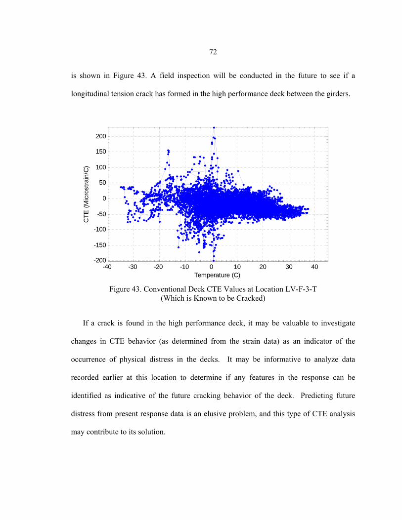
72
is shown in Figure 43. A field inspection will be conducted in the future to see if a
longitudinal tension crack has formed in the high performance deck between the girders.
-40 -30 -20 -10 0 10 20 30 40-200
-150
-100
-50
0
50
100
150
200
CTE
(Mic
rost
rain
/C)
Temperature (C) Figure 43. Conventional Deck CTE Values at Location LV-F-3-T
(Which is Known to be Cracked)
If a crack is found in the high performance deck, it may be valuable to investigate
changes in CTE behavior (as determined from the strain data) as an indicator of the
occurrence of physical distress in the decks. It may be informative to analyze data
recorded earlier at this location to determine if any features in the response can be
identified as indicative of the future cracking behavior of the deck. Predicting future
distress from present response data is an elusive problem, and this type of CTE analysis
may contribute to its solution.
73
Composite Behavior
The CTE values determined from the field data and presented in Figures 39, 40, and
42 are approximately 2 µε/°C higher than the CTE values measured in the laboratory.
The probable explanation for this difference is that the steel within the concrete is acting
with the concrete to increase the CTE of the composite material. The AASHTO Guide
Specifications Thermal Effects in Concrete Bridge Superstructures states that “It is
thought that the maximum effect on the concrete’s thermal coefficient by the presence of
steel reinforcement in no more than 10 percent” (1989). The effect of the steel in this
case appears to be somewhat larger than that suggested by AASHTO (approaching 20
percent at lower temperatures).
Structural Behavior under Temperature Changes
The behaviors of the Saco bridge decks under temperature changes are significantly
influenced by the composite nature of their construction. The bridge decks behave
compositely in two respects. Following the fundamental behavior of composite cross-
sections, the unsymmetrical layout of the reinforcement causes internal stresses and
moments in the decks when they undergo a temperature change. More globally, the
decks are rigidly attached by shear studs to the prestressed girders underneath, and thus
act compositely with the girders in longitudinally carrying applied loads into the
supports. Fore equilibrium and strain compatibility are imposed to analyze composite
systems. Force equilibrium requires that the internal forces must balance at any cross-
section. Strain compatibility requires that there must be continuity in the deformations
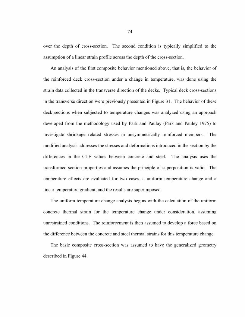
74
over the depth of cross-section. The second condition is typically simplified to the
assumption of a linear strain profile across the depth of the cross-section.
An analysis of the first composite behavior mentioned above, that is, the behavior of
the reinforced deck cross-section under a change in temperature, was done using the
strain data collected in the transverse direction of the decks. Typical deck cross-sections
in the transverse direction were previously presented in Figure 31. The behavior of these
deck sections when subjected to temperature changes was analyzed using an approach
developed from the methodology used by Park and Paulay (Park and Pauley 1975) to
investigate shrinkage related stresses in unsymmetrically reinforced members. The
modified analysis addresses the stresses and deformations introduced in the section by the
differences in the CTE values between concrete and steel. The analysis uses the
transformed section properties and assumes the principle of superposition is valid. The
temperature effects are evaluated for two cases, a uniform temperature change and a
linear temperature gradient, and the results are superimposed.
The uniform temperature change analysis begins with the calculation of the uniform
concrete thermal strain for the temperature change under consideration, assuming
unrestrained conditions. The reinforcement is then assumed to develop a force based on
the difference between the concrete and steel thermal strains for this temperature change.
The basic composite cross-section was assumed to have the generalized geometry
described in Figure 44.
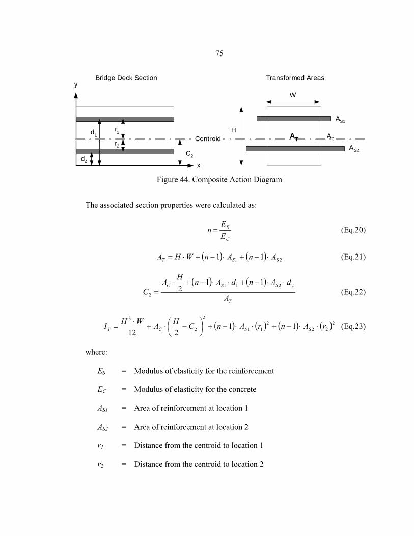
75
y
x
AS1
d1
d2
Centroidr2
r1
W
Transformed AreasBridge Deck Section
AS2
HAC
C2
AT
Figure 44. Composite Action Diagram
The associated section properties were calculated as:
C
S
EE
n = (Eq.20)
( ) ( ) 21 11 SST AnAnWHA ⋅−+⋅−+⋅= (Eq.21)
( ) ( )
T
SSC
A
dAndAnHAC
2211
2
112
⋅⋅−+⋅⋅−+⋅= (Eq.22)
( ) ( ) ( ) ( )222
211
2
2
3
11212
rAnrAnCHAWHI SSCT ⋅⋅−+⋅⋅−+⎟⎠⎞
⎜⎝⎛ −⋅+
⋅= (Eq.23)
where:
ES = Modulus of elasticity for the reinforcement
EC = Modulus of elasticity for the concrete
AS1 = Area of reinforcement at location 1
AS2 = Area of reinforcement at location 2
r1 = Distance from the centroid to location 1
r2 = Distance from the centroid to location 2
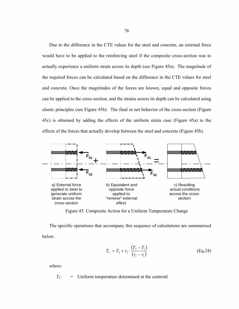
76
Due to the difference in the CTE values for the steel and concrete, an external force
would have to be applied to the reinforcing steel if the composite cross-section was to
actually experience a uniform strain across its depth (see Figure 45a). The magnitude of
the required forces can be calculated based on the difference in the CTE values for steel
and concrete. Once the magnitudes of the forces are known, equal and opposite forces
can be applied to the cross-section, and the strains across its depth can be calculated using
elastic principles (see Figure 45b). The final or net behavior of the cross-section (Figure
45c) is obtained by adding the effects of the uniform strain case (Figure 45a) to the
effects of the forces that actually develop between the steel and concrete (Figure 45b).
FS1
FS2
a) External forceapplied to steel togenerate uniformstrain across the
cross-section
b) Equivalent andopposite force
applied to“remove” external
effect
+ =FS1
FS2
c) Resultingactual conditionsacross the cross-
section
Figure 45. Composite Action for a Uniform Temperature Change
The specific operations that accompany this sequence of calculations are summarized
below.
( )( )12
1222 rr
TTrTTU −−
⋅+= (Eq.24)
where:
TU = Uniform temperature determined at the centroid

77
T1 = Temperature measured at location 1
T2 = Temperature measured at location 2
and
T1 = T2 for the uniform temperature case
Strains associated with the case of uniform strains across the depth of the cross-
section are calculated as:
(Eq.25) ∫==M
R
T
TCthermalCthermalC αεε 21
(Eq.26) ∫==M
R
T
TSthermalCthermalC αεε 21
The external forces that have to be applied to the steel to generate the uniform strain
case can then be written as:
( )1111 thermalthermal CSSSS EAF εε −⋅⋅= (Eq.27)
( )2222 thermalthermal CSSSS EAF εε −⋅⋅= (Eq.28)
The axial force and moments from these forces are:
21 SS FFP += (Eq.29)
2211 rFrFM SS ⋅+⋅= (Eq.30)
The strains associated with these internal force resultants are:
( )CTCT
C EIyM
EAPy
Steel ⋅⋅
+⋅
=ε (Eq.31)
Finally, the true strain across the cross-section can be calculated by superimposing
these two results as:
78
( ) ( )yySteelthermal CCTotalC εεε += (Eq.32)
For a gradient temperature across the depth of the deck cross-section, the general
analysis approach is similar to that used for the uniform temperature case; the complexity
of the analysis is simply increased to accommodate variable concrete strains across the
cross-section, as a function of changing temperature (see Figure 46).
Temperature at any depth in the cross-section can be calculated in terms of T1 and T2
assuming a linear gradient as:
( ) yrrTT
TyT ⋅−−
+=21
212 (Eq.33)
FS1
FS2
a) External forceapplied to steel to
generate linear strainacross the cross-
section based on theconcrete response
b) Equivalent andopposite force appliedto “remove” external
effect
+ =FS1
FS2
c) Resulting actualconditions acrossthe cross-section
Figure 46. Composite Action for a Gradient Temperature Change
Thermal strains of interest can then be independently calculated at locations 1 and 2
through the depth as:
( )( )
∫=yT
TCC
R
thermaly αε (Eq.34)

79
(Eq.35) ∫=1,
1
M
R
T
TCthermalC αε
(Eq.36) ∫=1,
1
M
R
T
TSthermalS αε
(Eq.37) ∫=2,
2
M
C
T
TCthermalC αε
(Eq.38) ∫=2,
2
M
C
T
TSthermalS αε
The equivalent external forces that must be applied in this case (see Figure 46) can
then be calculated as:
( )1111 thermalthermal CSSSS EAF εε −⋅⋅= (Eq.39)
( )2222 thermalthermal CSSSS EAF εε −⋅⋅= (Eq.40)
From equilibrium considerations:
21 SS FFP += (Eq.41)
2211 rFrFM SS ⋅+⋅= (Eq.42)
Relating strains to internal forces:
( )CTCT
C EIyM
EAPy
Steel ⋅⋅
+⋅
=ε (Eq.43)
Finally, superimposing the resulting strains:
( ) ( ) ( )yyySteelthermal CCTotalC εεε += (Eq.44)
Using these equations, and the actual temperatures experienced by the decks in the
field, the theoretical increase in thermal strains due to composite behavior were
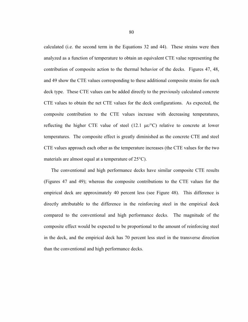
80
calculated (i.e. the second term in the Equations 32 and 44). These strains were then
analyzed as a function of temperature to obtain an equivalent CTE value representing the
contribution of composite action to the thermal behavior of the decks. Figures 47, 48,
and 49 show the CTE values corresponding to these additional composite strains for each
deck type. These CTE values can be added directly to the previously calculated concrete
CTE values to obtain the net CTE values for the deck configurations. As expected, the
composite contribution to the CTE values increase with decreasing temperatures,
reflecting the higher CTE value of steel (12.1 µε/°C) relative to concrete at lower
temperatures. The composite effect is greatly diminished as the concrete CTE and steel
CTE values approach each other as the temperature increases (the CTE values for the two
materials are almost equal at a temperature of 25°C).
The conventional and high performance decks have similar composite CTE results
(Figures 47 and 49); whereas the composite contributions to the CTE values for the
empirical deck are approximately 40 percent less (see Figure 48). This difference is
directly attributable to the difference in the reinforcing steel in the empirical deck
compared to the conventional and high performance decks. The magnitude of the
composite effect would be expected to be proportional to the amount of reinforcing steel
in the deck, and the empirical deck has 70 percent less steel in the transverse direction
than the conventional and high performance decks.
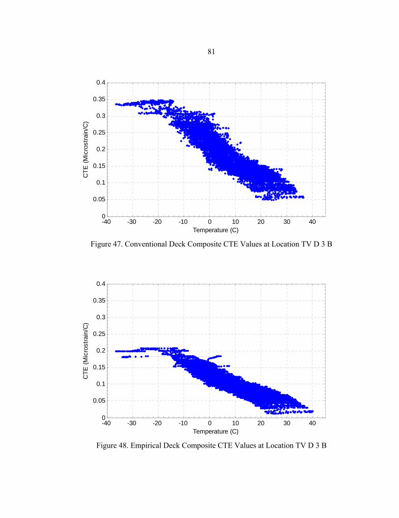
81
-40 -30 -20 -10 0 10 20 30 400
0.05
0.1
0.15
0.2
0.25
0.3
0.35
0.4C
TE (M
icro
stra
in/C
)
Temperature (C) Figure 47. Conventional Deck Composite CTE Values at Location TV D 3 B
-40 -30 -20 -10 0 10 20 30 400
0.05
0.1
0.15
0.2
0.25
0.3
0.35
0.4
CTE
(Mic
rost
rain
/C)
Temperature (C) Figure 48. Empirical Deck Composite CTE Values at Location TV D 3 B
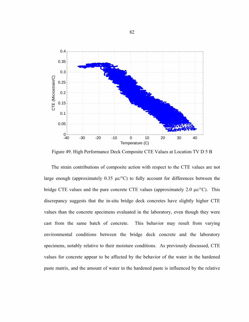
82
-40 -30 -20 -10 0 10 20 30 400
0.05
0.1
0.15
0.2
0.25
0.3
0.35
0.4C
TE (M
icro
stra
in/C
)
Temperature (C) Figure 49. High Performance Deck Composite CTE Values at Location TV D 5 B
The strain contributions of composite action with respect to the CTE values are not
large enough (approximately 0.35 µε/°C) to fully account for differences between the
bridge CTE values and the pure concrete CTE values (approximately 2.0 µε/°C). This
discrepancy suggests that the in-situ bridge deck concretes have slightly higher CTE
values than the concrete specimens evaluated in the laboratory, even though they were
cast from the same batch of concrete. This behavior may result from varying
environmental conditions between the bridge deck concrete and the laboratory
specimens, notably relative to their moisture conditions. As previously discussed, CTE
values for concrete appear to be affected by the behavior of the water in the hardened
paste matrix, and the amount of water in the hardened paste is influenced by the relative

83
humidity experienced by the concrete (which was not the same in the laboratory and at
the bridges).
Bridge Deck Deformations
Another way to view the effects of environmental conditions on the Saco bridge
decks is to more globally consider their bending and in-plane axial deformations.
Curvatures can be conveniently used to look at the bending deformations of the decks,
because they are easily visualized and can be readily calculated from the strains directly
measured in the field. It can be shown that curvature is related to the axial strain at a
distance (y) from the centroid of a cross section as (Gere 2001):
y
xεκ−
= (Eq.45)
where:
κ = Curvature
εx = Axial strain
It can also be shown geometrically (see Figure 50) that the internal strain angle is related
to the axial strain at a distance from the centroid as:
y
xεϕ−
=tan (Eq.46)
where:
φ = Internal strain angle
y = Distance from gage location to the cross-section centroid

84
Centroid
r2
r1
e2
e1
f
Figure 50. Internal Strain Angle
Equating the two previous equations gives:
ϕκ tan= (Eq.47)
Finally, the internal strain angle can be calculated using strains measured at two locations
a distance apart in the deck as:
12
12tanrr −
−==
εεϕκ (Eq.48)
where:
ε1 = Strain at location 1
ε2 = Strain at location 2
r1 = Distance from location 1 to the centroid of the cross-section
r2 = Distance from location 2 to the centroid of the cross-section
Relative to in-plane deformations, these deformations are proportional to the normal
axial strains experienced at the centroid of the deck cross-sections. Strain at the centroidal
axis in the cross-section can be readily calculated from the strain measurements made at
two locations across the depth of the deck as:
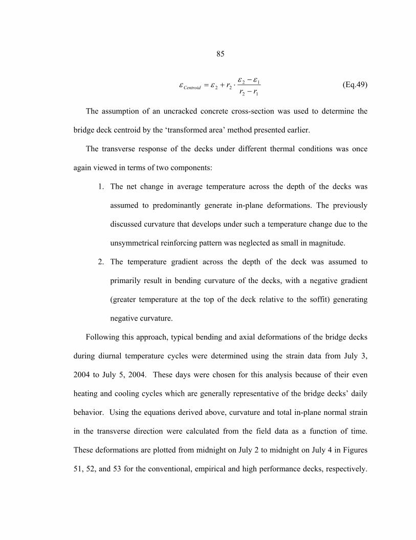
85
12
1222 rr
rCentroid −−
⋅+=εε
εε (Eq.49)
The assumption of an uncracked concrete cross-section was used to determine the
bridge deck centroid by the ‘transformed area’ method presented earlier.
The transverse response of the decks under different thermal conditions was once
again viewed in terms of two components:
1. The net change in average temperature across the depth of the decks was
assumed to predominantly generate in-plane deformations. The previously
discussed curvature that develops under such a temperature change due to the
unsymmetrical reinforcing pattern was neglected as small in magnitude.
2. The temperature gradient across the depth of the deck was assumed to
primarily result in bending curvature of the decks, with a negative gradient
(greater temperature at the top of the deck relative to the soffit) generating
negative curvature.
Following this approach, typical bending and axial deformations of the bridge decks
during diurnal temperature cycles were determined using the strain data from July 3,
2004 to July 5, 2004. These days were chosen for this analysis because of their even
heating and cooling cycles which are generally representative of the bridge decks’ daily
behavior. Using the equations derived above, curvature and total in-plane normal strain
in the transverse direction were calculated from the field data as a function of time.
These deformations are plotted from midnight on July 2 to midnight on July 4 in Figures
51, 52, and 53 for the conventional, empirical and high performance decks, respectively.
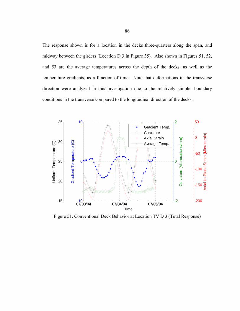
86
The response shown is for a location in the decks three-quarters along the span, and
midway between the girders (Location D 3 in Figure 35). Also shown in Figures 51, 52,
and 53 are the average temperatures across the depth of the decks, as well as the
temperature gradients, as a function of time. Note that deformations in the transverse
direction were analyzed in this investigation due to the relatively simpler boundary
conditions in the transverse compared to the longitudinal direction of the decks.
07/03/04 07/04/04 07/05/04-10
0
10
Gra
dien
t Tem
pera
ture
(C)
-200
-150
-100
-50
0
50
Axi
al In
-Pla
ne S
train
(Mic
rost
rain
)15
20
25
30
35
Uni
form
Tem
pera
ture
(C)
07/03/04 07/04/04 07/05/04-2
0
2
Cur
vatu
re (M
icro
radi
ans/
mm
)
Time
Gradient Temp.CurvatureAxial StrainAverage Temp.
Figure 51. Conventional Deck Behavior at Location TV D 3 (Total Response)
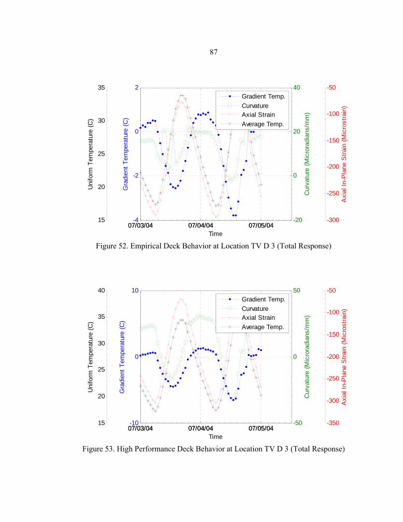
87
07/03/04 07/04/04 07/05/04-4
-2
0
2
Gra
dien
t Tem
pera
ture
(C)
-300
-250
-200
-150
-100
-50
Axi
al In
-Pla
ne S
train
(Mic
rost
rain
)
15
20
25
30
35U
nifo
rm T
empe
ratu
re (C
)
07/03/04 07/04/04 07/05/04-20
0
20
40
Cur
vatu
re (M
icro
radi
ans/
mm
)
Time
Gradient Temp.CurvatureAxial StrainAverage Temp.
Figure 52. Empirical Deck Behavior at Location TV D 3 (Total Response)
07/03/04 07/04/04 07/05/04-10
0
10
Gra
dien
t Tem
pera
ture
(C)
-350
-300
-250
-200
-150
-100
-50
Axi
al In
-Pla
ne S
train
(Mic
rost
rain
)
15
20
25
30
35
40
Uni
form
Tem
pera
ture
(C)
07/03/04 07/04/04 07/05/04-50
0
50
Cur
vatu
re (M
icro
radi
ans/
mm
)
Time
Gradient Temp.CurvatureAxial StrainAverage Temp.
Figure 53. High Performance Deck Behavior at Location TV D 3 (Total Response)
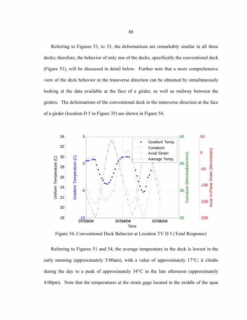
88
Referring to Figures 51, to 53, the deformations are remarkably similar in all three
decks; therefore, the behavior of only one of the decks, specifically the conventional deck
(Figure 51), will be discussed in detail below. Further note that a more comprehensive
view of the deck behavior in the transverse direction can be obtained by simultaneously
looking at the data available at the face of a girder, as well as midway between the
girders. The deformations of the conventional deck in the transverse direction at the face
of a girder (location D 5 in Figure 35) are shown in Figure 54.
07/03/04 07/04/04 07/05/04-10
-5
0
5
Gra
dien
t Tem
pera
ture
(C)
-200
-150
-100
-50
0
50
Axi
al In
-Pla
ne S
train
(Mic
rost
rain
)
18
20
22
24
26
28
30
32
34
Uni
form
Tem
pera
ture
(C)
07/03/04 07/04/04 07/05/0420
30
40
50
Cur
vatu
re (M
icro
radi
ans/
mm
)
Time
Gradient Temp.CurvatureAxial StrainAverage Temp.
Figure 54. Conventional Deck Behavior at Location TV D 5 (Total Response)
Referring to Figures 51 and 54, the average temperature in the deck is lowest in the
early morning (approximately 5:00am), with a value of approximately 17°C; it climbs
during the day to a peak of approximately 34°C in the late afternoon (approximately
4:00pm). Note that the temperatures at the strain gage located in the middle of the span
89
between the girders (Figure 51) are approximately one degree cooler at the low point and
one degree higher at the high point than the temperatures at the face of the girder (Figure
54). This behavior results from the thermal mass of the girder nominally moderating the
temperature extremes in the deck immediately adjacent to it.
The temperature gradient experienced by the deck also varies throughout the day.
The gradient, less than 1°C at 5:00am, becomes increasingly negative throughout the
morning, as the top surface of the deck heats up more rapidly than the bottom surface.
The peak negative gradient occurs around noon and is approximately -6°C for the
location within the deck span and is -4°C at the face of the girder. The peak positive
gradient temperature occurs near midnight, as the top surface of the deck cools more
rapidly then the bottom surface, possibly because the girders and the ground below the
bridge act as a heat sink, storing the day’s heat and radiating it to the bottom of the deck
in the evening.
Relative to the coincident deformations experienced by the deck under these thermal
conditions, the total in-plane axial transverse strains are positive as the temperature
increases, which is consistent with the deck expanding as the temperature increases. The
magnitude of the change in the strain as the temperature moves between its extreme
values is approximately 215 µε for the location between the girders and 190 µε for the
location at the face of the girder. This difference of 25 µε is due to the difference in the
extreme temperatures at the two locations. The two degree difference in the extreme
temperatures corresponds to a strain difference of 25 µε using a CTE of 12.5 µε/°C.
90
Therefore, the in-plane response at the two locations under the thermal change is nearly
identical.
The significance of the absolute magnitudes of the in-plane strains reported in Figures
51 through 54 is somewhat uncertain, as it is possible that some baseline shifts may have
inadvertently occurred in the data as a result of some rewiring that had to be done for the
data acquisition system. Nonetheless, the absolute strain magnitudes are uniformly
negative, which is consistent with the expected unrestrained shrinkage of the deck
concrete over time. Furthermore, the general level of the absolute strains (150 to 300 µε)
is consistent with the magnitude of the shrinkage strain estimated by Equation 15 (see
Figure 38).
The curvature deformations of the decks are consistent with the thermal gradients that
they experienced. A negative temperature gradient in the middle of the day, for example,
during which the top of the deck expands more than the bottom, corresponds with a
negative curvature (see Figure 55). Correspondingly a positive temperature gradient in
the evening during which the soffit of the deck expands more than the top, corresponds
with a positive curvature (see Figure 56).

91
D-3 Middle of Support
D-5 Face of Support
Figure 55. Expected Physical Bridge Deck Deformations
(for a Negative Temperature Gradient)
D-3 Middle of Support
D-5 Face of Support
Figure 56. Expected Physical Bridge Deck Deformations
(for a Positive Temperature Gradient)
One anomaly in this response is that the changes in curvature observed in the interior
of the spans (between the girders) are in the same direction as the changes in curvature at
the face of the girders. The deck was expected to act in the transverse direction
somewhat like a continuous beam over several supports, with opposite curvatures in the
interior of the spans relative to the curvatures at the supports (i.e., at the girders). One
92
explanation for the observed response is that the expected point of contraflexure in the
curvature occurs closer to the girders than the location of the strain gage at the face of the
girders. In this case, the strain gages in the middle of the span and at the face of the
girder would indicate the same direction of curvature. Relative to the absolute
magnitudes of the reported curvatures, their significance is uncertain due to possible
baseline shifts in the strain data. Nonetheless, the magnitude of the curvatures calculated
at the location between the girders in the conventional deck (see Figure 51) are
dramatically smaller than those of the other curvatures (2.5 µκ/mm compared with an
average value of 19 µκ/mm at other locations). One explanation for this apparent
anomaly is that the deck has experienced some physical damage at this location, possibly
cracking, that has interrupted the continuity of the structure. This deck will be inspected
to determine if it has sustained any physical damage consistent with this departure in its
curvature response. It may be possible that changes in curvature of this kind can be
developed as an indicator of the occurrence of physical distress in the decks.
Close examination of Figures 51 and 54 reveals that the extreme deformation
response occurs slightly ahead of the extreme temperatures in time. One possible
explanation for this behavior is that the strain compatibility and strain boundary
conditions are driven primarily by in-plane conditions in the longitudinal and transverse
directions; while the thermal compatibility and thermal boundary conditions are primarily
in the out-of-plane direction. Thus, the local bridge deformations are influenced by what
is happening over a much larger area of the bridge, compared to the local absolute
93
temperatures experienced in the decks. The significance of one occurring before the
other is uncertain.
The discussion above considered the total deformations experienced by the deck as a
function of temperature; the part of this deformation specifically associated with internal
stresses in the decks is also of interest in this investigation. Referring to Figure 57, the
stress curvature is inversely proportional to the temperature gradient, as expected. The
axial in-plane stress strain, however, is directly proportional to the uniform temperature.
That is, as the temperature increases, the in-plane stress strain also increases, indicating
that the deck is in tension in the transverse direction. This result is counter intuitive, in
that the girders are expected to offer at least nominal resistance to the expansion of the
deck under an increase in temperature, placing the deck in compression. This situation
may result from the manner in which the stress related contribution to the total strain has
been calculated. The results of this calculation are sensitive to the estimated magnitude
of the shrinkage strains, and additional research is needed on this matter before the stress
strains are accepted as reliable.
The stress strain range between the extreme low and high values is approximately 25
µε, which corresponds to about 1.5 µε/°C for the measured temperature range. This
difference suggests, as did the bridge CTE measurements, that the CTE values obtained
from the laboratory investigation are lower than the actual in-situ CTE values (by at least
1.5 µε/°C). This phenomenon is consistent between the decks and among the locations
within each deck (Figure 58).
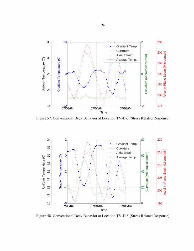
94
07/03/04 07/04/04 07/05/04-10
0
10
Gra
dien
t Tem
pera
ture
(C)
175
180
185
190
195
200
205
Axi
al In
-Pla
ne S
train
(Mic
rost
rain
)
15
20
25
30
35U
nifo
rm T
empe
ratu
re (C
)
07/03/04 07/04/04 07/05/04-2
0
2
Cur
vatu
re (M
icro
radi
ans/
mm
)
Time
Gradient Temp.CurvatureAxial StrainAverage Temp.
Figure 57. Conventional Deck Behavior at Location TV-D-3 (Stress Related Response)
07/03/04 07/04/04 07/05/04-6
-4
-2
0
2
Gra
dien
t Tem
pera
ture
(C)
195
200
205
210
215
220
Axi
al In
-Pla
ne S
train
(Mic
rost
rain
)
18
20
22
24
26
28
30
32
34
Uni
form
Tem
pera
ture
(C)
07/03/04 07/04/04 07/05/040
20
40
60
80
Cur
vatu
re (M
icro
radi
ans/
mm
)
Time
Gradient Temp.CurvatureAxial StrainAverage Temp.
Figure 58. Conventional Deck Behavior at Location TV-D-5 (Stress Related Response)
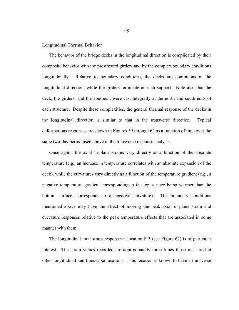
95
Longitudinal Thermal Behavior
The behavior of the bridge decks in the longitudinal direction is complicated by their
composite behavior with the prestressed girders and by the complex boundary conditions
longitudinally. Relative to boundary conditions, the decks are continuous in the
longitudinal direction, while the girders terminate at each support. Note also that the
deck, the girders, and the abutment were cast integrally at the north and south ends of
each structure. Despite these complexities, the general thermal response of the decks in
the longitudinal direction is similar to that in the transverse direction. Typical
deformations responses are shown in Figures 59 through 62 as a function of time over the
same two-day period used above in the transverse response analysis.
Once again, the axial in-plane strains vary directly as a function of the absolute
temperature (e.g., an increase in temperature correlates with an absolute expansion of the
deck), while the curvatures vary directly as a function of the temperature gradient (e.g., a
negative temperature gradient corresponding to the top surface being warmer than the
bottom surface, corresponds to a negative curvature). The boundary conditions
mentioned above may have the effect of moving the peak axial in-plane strain and
curvature responses relative to the peak temperature effects that are associated in some
manner with them..
The longitudinal total strain response at location F 3 (see Figure 62) is of particular
interest. The strain values recorded are approximately three times those measured at
other longitudinal and transverse locations. This location is known to have a transverse
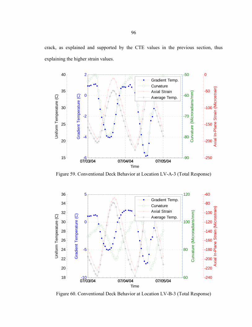
96
crack, as explained and supported by the CTE values in the previous section, thus
explaining the higher strain values.
07/03/04 07/04/04 07/05/04-6
-4
-2
0
2G
radi
ent T
empe
ratu
re (C
)
-250
-200
-150
-100
-50
0
Axi
al In
-Pla
ne S
train
(Mic
rost
rain
)
15
20
25
30
35
40
Uni
form
Tem
pera
ture
(C)
07/03/04 07/04/04 07/05/04-90
-80
-70
-60
-50
Cur
vatu
re (M
icro
radi
ans/
mm
)
Time
Gradient Temp.CurvatureAxial StrainAverage Temp.
Figure 59. Conventional Deck Behavior at Location LV-A-3 (Total Response)
07/03/04 07/04/04 07/05/04-10
-5
0
5
Gra
dien
t Tem
pera
ture
(C)
-240
-220
-200
-180
-160
-140
-120
-100
-80
-60
Axi
al In
-Pla
ne S
train
(Mic
rost
rain
)
18
20
22
24
26
28
30
32
34
36
Uni
form
Tem
pera
ture
(C)
07/03/04 07/04/04 07/05/0460
80
100
120C
urva
ture
(Mic
rora
dian
s/m
m)
Time
Gradient Temp.CurvatureAxial StrainAverage Temp.
Figure 60. Conventional Deck Behavior at Location LV-B-3 (Total Response)
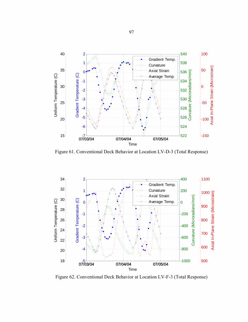
97
07/03/04 07/04/04 07/05/04-7
-6
-5
-4
-3
-2
-1
0
1
2
Gra
dien
t Tem
pera
ture
(C)
-150
-100
-50
0
50
100
Axi
al In
-Pla
ne S
train
(Mic
rost
rain
)
15
20
25
30
35
40U
nifo
rm T
empe
ratu
re (C
)
07/03/04 07/04/04 07/05/04522
524
526
528
530
532
534
536
538
540
Cur
vatu
re (M
icro
radi
ans/
mm
)
Time
Gradient Temp.CurvatureAxial StrainAverage Temp.
Figure 61. Conventional Deck Behavior at Location LV-D-3 (Total Response)
07/03/04 07/04/04 07/05/04-5
-4
-3
-2
-1
0
1
2
Gra
dien
t Tem
pera
ture
(C)
500
600
700
800
900
1000
1100
Axi
al In
-Pla
ne S
train
(Mic
rost
rain
)
18
20
22
24
26
28
30
32
34
Uni
form
Tem
pera
ture
(C)
07/03/04 07/04/04 07/05/04-1000
-800
-600
-400
-200
0
200
400
Cur
vatu
re (M
icro
radi
ans/
mm
)
Time
Gradient Temp.CurvatureAxial StrainAverage Temp.
Figure 62. Conventional Deck Behavior at Location LV-F-3 (Total Response)
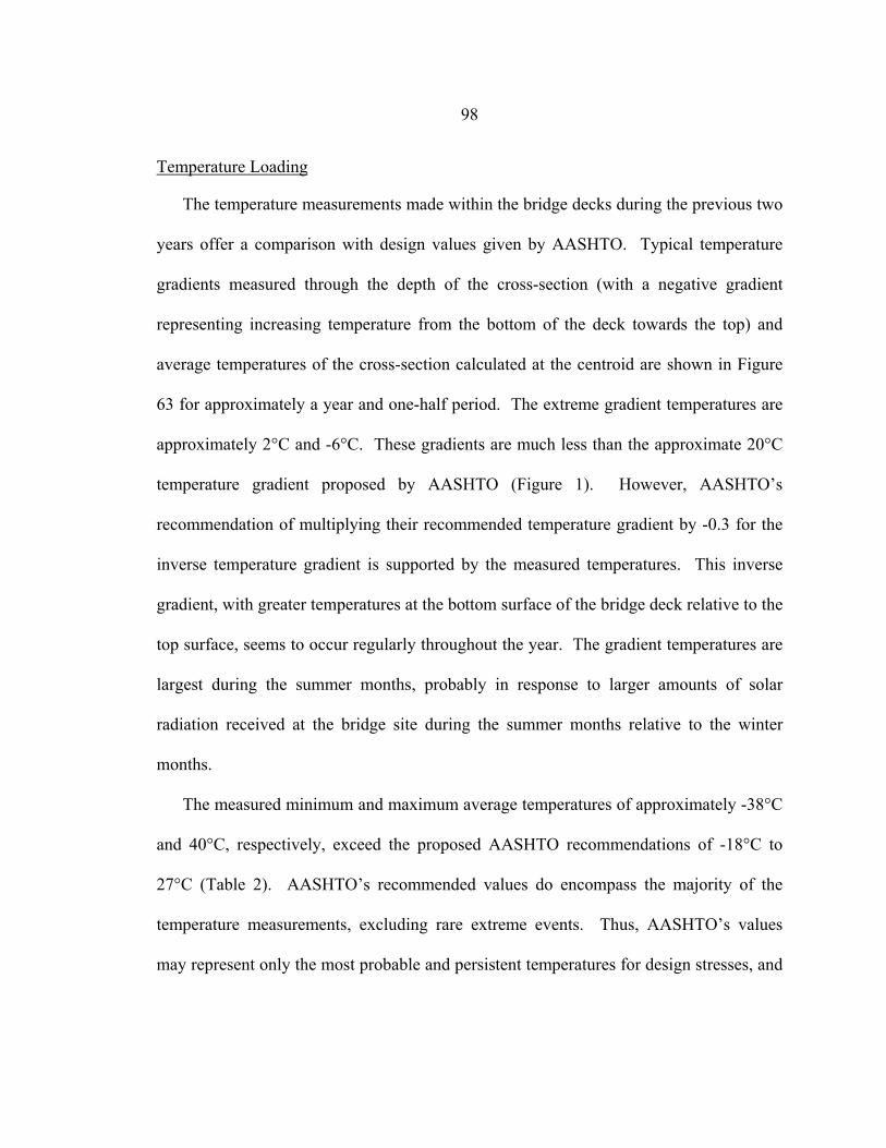
98
Temperature Loading
The temperature measurements made within the bridge decks during the previous two
years offer a comparison with design values given by AASHTO. Typical temperature
gradients measured through the depth of the cross-section (with a negative gradient
representing increasing temperature from the bottom of the deck towards the top) and
average temperatures of the cross-section calculated at the centroid are shown in Figure
63 for approximately a year and one-half period. The extreme gradient temperatures are
approximately 2°C and -6°C. These gradients are much less than the approximate 20°C
temperature gradient proposed by AASHTO (Figure 1). However, AASHTO’s
recommendation of multiplying their recommended temperature gradient by -0.3 for the
inverse temperature gradient is supported by the measured temperatures. This inverse
gradient, with greater temperatures at the bottom surface of the bridge deck relative to the
top surface, seems to occur regularly throughout the year. The gradient temperatures are
largest during the summer months, probably in response to larger amounts of solar
radiation received at the bridge site during the summer months relative to the winter
months.
The measured minimum and maximum average temperatures of approximately -38°C
and 40°C, respectively, exceed the proposed AASHTO recommendations of -18°C to
27°C (Table 2). AASHTO’s recommended values do encompass the majority of the
temperature measurements, excluding rare extreme events. Thus, AASHTO’s values
may represent only the most probable and persistent temperatures for design stresses, and
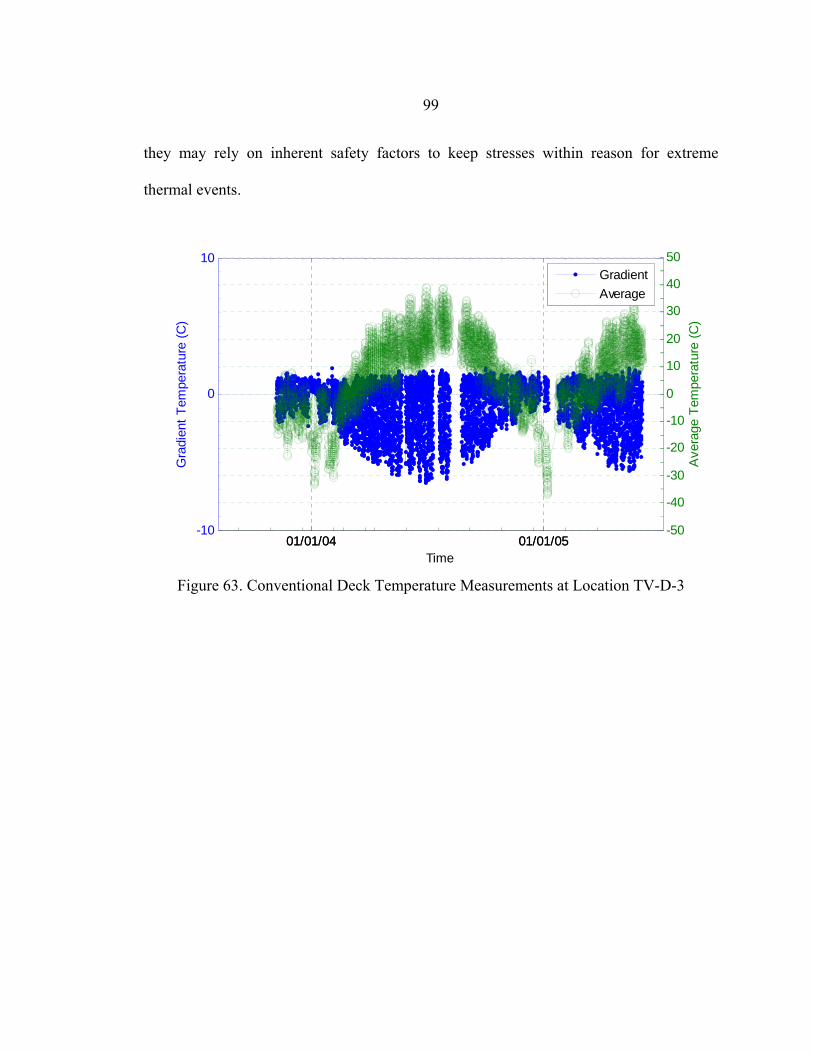
99
they may rely on inherent safety factors to keep stresses within reason for extreme
thermal events.
01/01/04 01/01/05-10
0
10
Time
Gra
dien
t Tem
pera
ture
(C)
01/01/04 01/01/05-50
-40
-30
-20
-10
0
10
20
30
40
50
Ave
rage
Tem
pera
ture
(C)
GradientAverage
Figure 63. Conventional Deck Temperature Measurements at Location TV-D-3
100
CHAPTER 5
CONCLUSIONS AND RECOMMENDATIONS
The objective of this project was to investigate the response of three bridge decks
made with different concretes and reinforcing steel configurations under environmental
(notably thermal) loads. The investigation began with a laboratory study of the thermal
behavior of the concretes used in the decks, followed by an analysis of the measured deck
behavior in the field. Two different concretes were considered for the decks, a standard
bridge deck concrete typically used by MDT, and a high performance concrete. Two
reinforcing arrangements were used in the decks, a conventional design based on a
traditional transverse load transfer model and a more lightly reinforced design based on
empirical observations of bridge deck performance.
CTE Investigation
The laboratory investigation showed significant variations in the CTEs of concrete as
a function of temperature. In general, as temperature decreases, CTE values also
decrease. This variation is believed to be related to behavior of the water in the
concrete’s nanostructure. This finding contradicts the traditional assumption that CTE
values for concrete are constant and that their values are similar to those of steel. Data
suggest that this assumption is only valid for temperatures approaching 25°C. At lower
temperatures, concrete’s CTE is up to 30 percent less than the reported CTE of steel.
101
The fact that the CTE value of concrete is less than that of steel does offer some
benefits to concrete performance. Notably, at lower temperatures, the higher thermal
shrinkage of the steel tends to compress the concrete, reducing its tendency to crack.
While generally the CTEs of traditional concrete and those of the high performance
concrete are similar, some distinct differences in the behavior of high performance
concrete exist. Notably, the high performance concrete has much lower CTE values at
approximately 0°C and below. These differences in CTE behavior are related to the
nanostructure (notably pore size of the high performance concrete), which affects the
behavior of the water within the cement paste.
Bridge Investigation
Analysis of the strain data collected in the field found that the CTE values for the
bridges were similar to those determined in the laboratory investigation. The difference
between the laboratory and in-situ CTE values are explained in part by the composite
action of the steel reinforcement within the deck, which increases the CTE values
compared to the plain concrete. A second factor that may contribute to this difference is
that the relative humidities experienced by the specimens tested in the laboratory
(approximately 20 percent) were considerably lower than the average relative humidity
recorded in Saco (approximately 60 percent). This difference would have a noticeable
effect on the concrete CTE values because they are dependent on the presence of physical
water in the cement paste structure.
102
At one of the strain gage locations analyzed, the in-situ bridge deck CTE values were
dramatically different than the laboratory values and values at other locations in the deck.
This unusual response may correlate with cracking in the deck, particularly since it was at
a location that is expected to experience the greatest tensile strains under vehicular loads,
mid-span between girders. Note that the possibility that cracking had occurred was not as
obvious in the raw strain data, which “looks” to be acceptable and within reason. The
absence/presence of cracking will be investigated in the field in the near future. If indeed
the deck is cracked, the occurrence of unusual CTE behavior may be useful in
determining damage in a structure for infrastructure health monitoring.
In addition to the CTE values, the field strain data showed that the decks in the
transverse direction were behaving as expected with regard to curvature and in-plane
axial strain while undergoing thermal loads. Importantly, there were no significant
differences among the conventional, empirical, and high performance bridge decks at this
time. A slight anomaly in the curvature in the transverse direction may suggest damage
adjacent to the strain gage location. Only a cursory examination was made of the deck
response in the longitudinal direction. This examination indicated that longitudinal
deformations are similar in all three decks, and at least generally consistent with expected
behaviors.
Because of the relatively young age of the Saco bridges (two years), continued
investigation should take place as the bridges mature; the most noticeable damage
typically takes place in the range of 10 to 15 years.
103
Recommendations
Some recommendations for further research are:
• Collect more temperature and strain profile data to correlate the two with
environmental weather.
• Evaluate laboratory specimens for CTE results under different temperature
regimes and humidities, including the effects of solar radiation.
• Cast instrumented specimens located at the bridge site to record absolute
shrinkage and temperature characteristics of the concrete.
104
BIBLIOGRAPHY
1. American Association of State Highway and Transportation Officials. AASHTO Guide Specifications Thermal Effects in Concrete Bridge Superstructures. Washington, D.C. 1989.
2. American Association of State Highway and Transportation Officials. AASHTO LRFD Bridge Design Specifications. Washington, D.C. 2000 Interim.
3. Berwanger, Carl. The Modulus of Concrete and the Coefficient of Expansion of Concrete and Reinforced Concrete at Below Normal Temperatures. Temperature and Concrete SP 25-8. Detroit, Michigan: American Concrete Institute. 1971.
4. Brown, R. D. Properties of Concrete in Reactor Vessels. Conference on Prestressed Pressure Vessels, Proceedings. London: Institute of Civil Engineers. 1968.
5. Cordon, William A. Freezing and Thawing of Concrete: Mechanisms and Control. Detroit, Michigan: American Concrete Institute. 1966.
6. Emerson, M. Bridge Temperatures for Setting Bearings and Expansion Joints. TRRL Supplementary Report 479. Berkshire, England. 1979.
7. Errors Due to Transverse Sensitivity in Strain Gages. Measurements Group Tech Note TN-509. Raleigh, North Carolina: Vishay Measurements Group. 1993.
8. Errors Due to Wheatstone Bridge Nonlinearity. Measurements Group Tech Note TN-507. Raleigh, North Carolina: Vishay Measurements Group. 1992.
9. Feldman, R. F. and P. J. Sereda. A Model for Hydrated Portland Cement Paste as Deduced from Sorption-length Change and Mechanical Properties. Materiaux et Constructions [Materials and Structures] 1, no. 6. November – December 1968.
10. Gere, James M. Mechanics of Materials, 5th ed. United States: Brooks/Cole. 2001.
11. Imbsen, R. A., D. E. Vandershaf, R. A. Schamber, and R. V. Nutt. National Cooperative Highway Research Program Report 276: Thermal Effects in Concrete Bridge Superstructures. Washington D.C.: Transportation Research Board. 1985.
12. Kosmatka, Steven H., Beatrix Kerkoff, and William C. Panarese. Design and Control of Concrete Mixtures. 14th ed. United States: Portland Cement Association. 2002.
13. Kumar Mehta, P. Concrete: Structure, Properties, and Materials. United States: Prentice-Hall. 1986.
105
14. Measurement of Thermal Expansion Coefficient Using Strain Gages. Measurements Group Tech Note TN-513-1. Raleigh, North Carolina: Vishay Measurements Group. 1986.
15. Montana Department of Transportation Bridge Plans and Quantities. Bridge Replacements – North of Saco. Federal Aid Project No. BR 243-1(5)20 P.E. BR 243-1(7)20 Const. 2003.
16. Ontario Highway Bridge Design Code and Commentary. Ontario, Canada: Ontario Ministry of Transportation and Communications. 1979.
17. Park, R., and T. Paulay. Reinforced Concrete Structures. New York: John Wiley & Sons, 1975.
18. Popovics, Sándor. Strength and Related Properties of Concrete: A Quantitative Approach. New York: John Wiley and Sons. 1998.
19. Portland Cement Association Building Movements and Joints, 1st Ed. Skokie, Illinois: Portland Cement Association. 1982.
20. Powers, T. C. and T. L. Brownyard. Studies of the Physical Properties of Hardened Portland Cement Paste. Journal American Concrete Institute. (October 1946 – April 1947).
21. Shah, S. P. and S. H. Ahmad. High Performance Concrete: Properties and Applications. New York: McGraw-Hill. 1994.
22. Shunt Calibration of Strain Gage Instrumentation. Measurements Group Tech Note TN-514. Raleigh, North Carolina: Vishay Measurements Group. 1988.
23. Smolenski, P. J. Field Instrumentation and Live Load Testing to Evaluate Behaviors of Three Reinforced Concrete Bridge Decks. Master of Science Thesis, Montana State University, Bozeman, Montana, 2004.
24. Strain Gage Applications with M-Bond AE-10, AE-15, and GA-2 Adhesive Systems. Measurements Group Instruction Bulletin. Raleigh, North Carolina: Vishay Measurements Group. 1995.
25. Strain Gage Thermal Output and Gage Factor Variation with Temperature. Measurements Group Tech Note TN-504-1. Raleigh, North Carolina: Vishay Measurements Group. 1993.
26. Surface Preparation for Strain Gage Bonding. Measurements Group Instruction Bulletin. Vishay Raleigh, North Carolina: Vishay Measurements Group. 1995.

106
27. Thermal Coefficient of Portland Cement Concrete. Turner Fairbank Highway Research Center. (May 2005). http://tfhrc.gov/pavement/pccp/thermal.htm
28. Zia, Paul., Shualib Ahmad, and Micheal Leming. High-Performance Concretes: A State-of-Art Report (1989-1994). Turner Fairbank Highway Research Center FHWA-RD-97-030. (May 2005). http://tfhrc.gov/structur/hpc/hpc2/contnt.htm.