Embed Size (px)
Citation preview

1 23
Foundations of ComputationalMathematicsThe Journal of the Society for theFoundations of ComputationalMathematics ISSN 1615-3375 Found Comput MathDOI 10.1007/s10208-016-9309-9
Condition Length and Complexity for theSolution of Polynomial Systems
Diego Armentano, Carlos Beltrán, PeterBürgisser, Felipe Cucker & Michael Shub

1 23
Your article is protected by copyright and all
rights are held exclusively by SFoCM. This e-
offprint is for personal use only and shall not
be self-archived in electronic repositories. If
you wish to self-archive your article, please
use the accepted manuscript version for
posting on your own website. You may
further deposit the accepted manuscript
version in any repository, provided it is only
made publicly available 12 months after
official publication or later and provided
acknowledgement is given to the original
source of publication and a link is inserted
to the published article on Springer's
website. The link must be accompanied by
the following text: "The final publication is
available at link.springer.com”.
Found Comput MathDOI 10.1007/s10208-016-9309-9
Condition Length and Complexity for the Solution ofPolynomial Systems
Diego Armentano1 · Carlos Beltrán2 ·Peter Bürgisser3 · Felipe Cucker4 · Michael Shub5
Received: 20 July 2015 / Revised: 11 January 2016 / Accepted: 2 February 2016© SFoCM 2016
Abstract Smale’s 17th problem asks for an algorithm which finds an approximatezero of polynomial systems in average polynomial time (see Smale in Mathematicalproblems for the next century, American Mathematical Society, Providence, 2000).The main progress on Smale’s problem is Beltrán and Pardo (Found Comput Math
Communicated by Teresa Krick.
Diego Armentano partially supported by Agencia Nacional de Investigación e Innovación (ANII),Uruguay, and by CSIC group 618. Carlos Beltrán partially suported by the research projectsMTM2010-16051 and MTM2014-57590-P from Spanish Ministry of Science MICINN. Peter Bürgisserpartially funded by DFG Research Grant BU 1371/2-2. Felipe Cucker partially funded by a GRF Grantfrom the Research Grants Council of the Hong Kong SAR (Project Number CityU 100813).
B Michael [email protected]
Diego [email protected]
Carlos Beltrá[email protected]
Peter Bü[email protected]
Felipe [email protected]
1 Universidad de La República, Montevideo, Uruguay
2 Universidad de Cantabria, Santander, Spain
3 Technische Universität Berlin, Berlin, Germany
4 City University of Hong Kong, Kowloon Tong, Hong Kong
5 City University of New York, New York, NY, USA
123
Author's personal copy
Found Comput Math
11(1):95–129, 2011) and Bürgisser and Cucker (AnnMath 174(3):1785–1836, 2011).In this paper,wewill improve on both approaches and prove an interesting intermediateresult on the average value of the condition number. Our main results are Theorem 1on the complexity of a randomized algorithm which improves the result of Beltránand Pardo (2011), Theorem 2 on the average of the condition number of polynomialsystems which improves the estimate found in Bürgisser and Cucker (2011), andTheorem 3 on the complexity of finding a single zero of polynomial systems. This lasttheorem is similar to the main result of Bürgisser and Cucker (2011) but relies only onhomotopy methods, thus removing the need for the elimination theory methods usedin Bürgisser and Cucker (2011). We build on methods developed in Armentano et al.(2014).
Keywords Polynomial systems · Homotopy methods · Complexity estimates
Mathematics Subject Classification Primary 65H10 · 65H20 · Secondary 58C35
1 Introduction
Homotopyor continuationmethods to solve a problemwhichmight dependonparame-ters start with a problem instance and known solution and try to continue the solutionalong a path in parameter space ending at the problem we wish to solve. We recallhow this works for the solutions of polynomial systems using a variant of Newton’smethod to accomplish the continuation.
LetHd be the complex vector space of degreed complex homogeneous polynomialsin n + 1 variables. For α = (α0, . . . , αn) ∈ N
n+1 satisfying∑n
j=0 α j = d, and the
monomial zα = zα00 · · · zαn
n , the Weyl Hermitian structure onHd makes 〈zα, zβ〉 := 0,for α �= β and
〈zα, zα〉 :=(
d
α
)−1
=(
d!α0! · · ·αn !
)−1
.
Now for (d) = (d1, . . . , dn), we let H(d) = ∏nk=1Hdk . This is a complex vector
space of dimension
N :=n∑
i=1
(n + di
n
)
.
That is, N is the size of a system f ∈ H(d), understood as the number of coefficientsneeded to describe f .
We endow H(d) with the product Hermitian structure
〈 f, g〉 :=n∑
k=1
〈 fi , gi 〉,
123
Author's personal copy
Found Comput Math
where f = ( f1, . . . , fn), and g = (g1, . . . , gn). ThisHermitian structure is sometimescalled the Weyl, Bombieri-Weyl, or Kostlan Hermitian structure. It is invariant underunitary substitution f �→ f ◦ U−1, where U is a unitary transformation of Cn+1 (see[9, p. 118] for example).
On Cn+1, we consider the usual Hermitian structure
〈x, y〉 :=n∑
k=0
xk yk .
Given 0 �= ζ ∈ Cn+1, let ζ⊥ denote the Hermitian complement of ζ ,
ζ⊥ := {v ∈ Cn+1 : 〈v, ζ 〉 = 0}.
For any nonzero ζ ∈ Cn+1, the subspace ζ⊥ is a model for the tangent space,
TζP(Cn+1), of the projective space P(Cn+1) at the equivalence class of ζ (whichwe also denote by ζ ). The space TζP(Cn+1) inherits an Hermitian structure from 〈·, ·〉given by
〈v,w〉ζ := 〈v,w〉〈ζ, ζ 〉 .
See, for example, [9, Sec. 12.2] for more details on this standard metric structure ofP(Cn+1).
The group of unitary transformations U acts naturally on Cn+1 by ζ �→ Uζ for
U ∈ U, and the Hermitian structure of Cn+1 is invariant under this action.A zero of the system of equations f is a point x ∈ C
n+1 such that fi (x) = 0,i = 1, . . . , n. If we think of f as a mapping f : Cn+1 → C
n , it is a point x such thatf (x) = 0.For a generic system (that is, for a Zariski open set of f ∈ H(d)), Bézout’s theorem
states that the set of zeros consists of D := ∏nk=1 dk complex lines through 0. These
D lines are D points in projective space P(Cn+1). So our goal is to approximate oneof these points, and we will use homotopy or continuation methods.
These methods for the solution of a system f ∈ H(d) proceed as follows. Chooseg ∈ H(d) and a zero ζ ∈ P(Cn+1) of g (we denote by the same symbol an affinepoint and its projective class). Connect g to f by a path ft , 0 ≤ t ≤ 1, in H(d) suchthat f0 = g, f1 = f , and try to continue ζ0 = ζ to ζt such that ft (ζt ) = 0, so thatf1(ζ1) = 0 (see [7] for details or [12] for a complete discussion).So homotopy methods numerically approximate the path ( ft , ζt ). One way to
accomplish the approximation is via (projective) Newton’s method. Given an approx-imation xt to ζt , define
xt+�t := N ft+�t (xt ),
where for h ∈ H(d) and y ∈ P(Cn+1)we define the projective Newton’s method Nh(y)
following [17]:
Nh(y) := y − (Dh(y)|y⊥)−1h(y).
123
Author's personal copy
Found Comput Math
Note that Nh is defined on P(Cn+1) at those points where Dh(y)|y⊥ is invertible.That xt is an approximate zero of ft with associated (exact) zero ζt means that the
sequence of Newton iterations N kft(xt ) converges immediately and quadratically to ζt .
Let us assume that { ft }t∈[0,1] is a path in the sphere S(H(d)) := {h ∈ H(d) :‖h‖ = 1}. The main result of [16]1 is that the �tk may be chosen so that t0 = 0,tk = tk−1+�tk for k = 1, . . . , K with tK = 1, such that for all k, xtk is an approximatezero of ftk with associated zero ζtk , and the number K of steps can be bounded asfollows:
K = K ( f, g, ζ ) ≤ C D3/2∫ 1
0μ( ft , ζt ) ‖( ft , ζt )‖ dt. (1.1)
Here C is a universal constant, D = maxi di ,
μ( f, ζ ) :={‖ f ‖ ∥
∥(D f (ζ )|ζ⊥)−1diag(‖ζ‖di −1√di )∥∥ if D f (ζ )|ζ⊥ is invertible
∞ otherwise
is the condition number of f ∈ H(d) at ζ ∈ P(Cn+1), diag(v) is the diagonal matrixwhose diagonal entries are the coordinates of the vector v), and
‖( ft , ζt )‖ = (‖ ft‖2 + ‖ζt‖2ζt)1/2
is the norm of the tangent vector to the curve in ( ft , ζt ). The result in [16] is not fullyconstructive, but specific constructions have been given, see [3] and [14], and evenprogrammed [4]. These constructions are similar to those given in [20] and [2] (thislast, for the eigenvalue-eigenvector problem case).
The constructive versions cited above have slightly different criteria to choose thestep length, which is the backbone of the continuation algorithm. However, all thesealgorithms satisfy a unitary invariance in the sense that if U is a unitary matrix of sizen + 1 then
K ( f, g, ζ ) = K ( f ◦ U∗, g ◦ U∗, Uζ ). (1.2)
The right-hand side in expression (1.1) is known as the condition length of the path( ft , ζt ). We will call (1.1) the condition length estimate of the number of steps.
Taking derivatives w.r.t. t in the equality ft (ζt ) = 0, it is easily seen that
ζt = −(D ft (ζt )|ζ⊥t
)−1 ft (ζt ), (1.3)
and with some work (see [9, Lemma 12, p. 231], one can prove that
‖ζ‖ζt ≤ μ( ft , ζt )‖ ft‖.
1 In [16], the theorem is actually proven in the projective space instead of the sphere, which is sharper, butwe only use the sphere version in this paper.
123
Author's personal copy
Found Comput Math
It is known that μ( f, ζ ) ≥ √n ≥ 1, so the estimate (1.1) may be bounded from above
by
K ( f, g, ζ ) ≤ C ′ D3/2∫ 1
0μ2( ft , ζt ) ‖ ft‖ dt, (1.4)
where C ′ = √2C is another constant. Let us call this estimate the μ2-estimate.
The condition length estimate is better than theμ2-estimate, but algorithms achiev-ing the smaller number of steps are more subtle and the proofs of correctness moredifficult.
Indeed in [5] and [10], the authors rely on the μ2-estimate. At the times of thesepapers, the algorithms achieving the condition length bound were in developmentand [10] includes a construction which achieves the μ2-estimate.
Yet, in a random situation, one might expect the improvement to be similar to theimprovement given by the average of ‖A(x)‖, in all possible directions, comparedwith ‖A‖ (here, A : Cn → C
n denotes a linear operator), which according to [1]should give an improvement by a factor of the square root of the domain dimension.We have accomplished this for the eigenvalue-eigenvector problem in [2]. Here weuse an argument similar to that of [2] to improve the estimate for the randomizedalgorithm in [6].
The Beltrán-Pardo randomized algorithmworks as follows (see [6], and also [10]):on input f ∈ H(d),
1. Choose f0 at random and then a zero ζ0 of f0 at random. [6] describes a generalscheme to do so (roughly speaking, one first draws the “linear” part of f0, computesζ0 from it, and then draws the “nonlinear” part of f0). An efficient implementationof this scheme, having running time O(nDN ), is fully described and analyzedin [12, Section 17.6].
2. Then, connect f0/‖ f0‖ to f/‖ f ‖ by an arc of a great circle in the sphere andinvoke the continuation strategy above.
The main result of [6] is that the average number of steps of this procedure is boundedby O(D3/2nN ), and its total average complexity is then O(D3/2nN 2) (since thecost of an iteration of Newton’s method, assuming all di ≥ 2, is O(N ), see [12,Proposition 16.32] and [11, Remark 7.8(1)]).
Our first main result is the following improvement of this last bound.
Theorem 1 (Randomized algorithm) The average number of steps of the randomizedalgorithm with the condition length estimate is bounded by
C D3/2nN 1/2,
where C is a universal constant.
The constant C can be taken as π√2
C ′ with C ′ not more than 400 even accountingfor input and round-off error, cf. [14].
123
Author's personal copy
Found Comput Math
The randomized algorithm has a nice property as proved in [6]: for every inputsystem f with no singular zeros, the probability that the algorithm outputs an approx-imate zero associated with each of theD zeros of f is exactly 1/D. It can thus be usedto generate a zero of f with the uniform distribution.
Remark 1 Theorem 1 is an improvement by a factor of 1/N 1/2 of the bound in [6],which results from using the condition length estimate in place of the μ2-estimate.
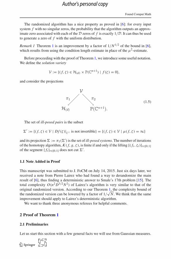
Before proceeding with the proof of Theorem 1, we introduce some useful notation.We define the solution variety
V := {( f, ζ ) ∈ H(d) × P(Cn+1) | f (ζ ) = 0},
and consider the projections
Vπ2π1
H(d) P(Cn+1).
(1.5)
The set of ill-posed pairs is the subset
�′ := {( f, ζ ) ∈ V | D f (ζ )|ζ⊥ is not invertible} = {( f, ζ ) ∈ V | μ( f, ζ ) = ∞}
and its projection� := π1(�′) is the set of ill-posed systems. The number of iterations
of the homotopy algorithm, K ( f, g, ζ ), is finite if and only if the lifting {( ft , ζt )}t∈[0,1]of the segment { ft }t∈[0,1] does not cut �′.
1.1 Note Added in Proof
This manuscript was submitted to J. FoCM on July 14, 2015. Just six days later, wereceived a note from Pierre Lairez who had found a way to derandomize the mainresult of [6], thus finding a deterministic answer to Smale’s 17th problem [15]. Thetotal complexity O(n2D3/2N 2) of Lairez’s algorithm is very similar to that of theoriginal randomized version. According to our Theorem 1, the complexity bound ofthe randomized version can be lowered by a factor of 1/
√N . We think that the same
improvement should apply to Lairez’s deterministic algorithm.We want to thank three anonymous referees for helpful comments.
2 Proof of Theorem 1
2.1 Preliminaries
Let us start this section with a few general facts we will use from Gaussian measures.
123
Author's personal copy
Found Comput Math
Given a finite-dimensional real vector space V of dimension m, with an innerproduct, we define two natural objects.
• The unit sphere S(V ) with the induced Riemannian structure and volume form:the volume of S(V ) is 2πm/2
�( m2 )
.
• The Gaussian measure centered at c ∈ V , with variance σ 2
2 > 0, whose density is
1
σmπm/2 e−‖x−c‖2/σ 2. (2.1)
We will denote by NV (c, σ 2Id) the density given in (2.1). We will skip the notationof the underlying space when it is understood. Furthermore, we will denote by Ex∈V
the average in the case σ = 1 (that is, variance 1/2).The following lemma iswell known;we, however, provide a proof because a similar
argument is used later in the manuscript.
Lemma 2 If ϕ : V → [0,+∞] is measurable and homogeneous of degree p > −m,then
Ex∈V
(ϕ(x)) = �(m+p2 )
�(m2 )
Eu∈S(V )
(ϕ(u)),
where
Eu∈S(V )
(ϕ(u)) = 1
vol(S(V ))
∫
S(V )
ϕ(u) du.
Proof Integrating in polar coordinates, we have
Ex∈V
(ϕ(x)) = 1
πm/2
∫
x∈Vϕ(x) e−‖x‖2 dx
= 1
πm/2
∫ +∞
0ρm+p−1e−ρ2
dρ ·∫
u∈S(V )
ϕ(u) du
= �(m+p2 )
2πm/2
∫
u∈S(V )
ϕ(u) du = �(m+p2 )
�(m2 )
Eu∈S(V )
(ϕ(u))
where we have used that∫ +∞0 ρke−ρ2
dρ = 12�( k+1
2 ). ��The next results follow immediately from Fubini’s theorem.
Lemma 3 Let E be a linear subspace of V , and let � : V → E be the orthogonalprojection. Then, for any integrable function ψ : E → R and for any c ∈ V , σ > 0,we have
Ex∼NV (c,σ 2Id)
(ψ(�(x))) = Ey∼NE (�(c),σ 2Id)
(ψ(y)).
��
123
Author's personal copy
Found Comput Math
When V is a finite-dimensional Hermitian vector space of complex dimension m,then the complex Gaussian measure on V with variance σ 2 is defined by the realGaussian measure with variance σ 2/2 on the 2m-dimensional real vector space asso-ciated with V , whose inner product is the real part of the Hermitian product.
In this fashion, for any fixed g ∈ H(d) and σ > 0, the Hermitian space (H(d), 〈·, ·〉)is equipped with the complex Gaussian measure N (g, σ 2Id). The expected value of afunction φ : H(d) → R with respect to this measure is given by
Ef ∼N (g,σ 2Id)
(φ) = 1
σ 2N π N
∫
f ∈H(d)
φ( f )e−‖ f −g‖2/σ 2d f. (2.2)
Fix any ζ ∈ P(Cn+1). Following [18, Sect. I-4], the space H(d) is orthogonallydecomposed into the sum Cζ ⊕ Vζ , where
Vζ = π−12 (ζ ) = { f ∈ H(d) : f (ζ ) = 0}
is the fiber over ζ and
Cζ ={
diag
( 〈·, ζ 〉di
〈ζ, ζ 〉di
)
a : a ∈ Cn}
(2.3)
is the set of polynomial systems f ∈ H(d) parametrized by a ∈ Cn such that for
z ∈ Cn+1, fi (z) = 〈z, ζ 〉di /‖ζ‖2di ai , 1 ≤ i ≤ n. Note that Vζ and Cζ are linear
subspaces of H(d) of respective (complex) dimensions N − n and n. Note also that
f0 = f − diag
( 〈·, ζ 〉di
〈ζ, ζ 〉di
)
f (ζ )
is the orthogonal projection �ζ ( f ) of f onto the fiber Vζ .
2.2 Average Condition Numbers
In this section, we revisit the average value of the operator and Frobenius conditionnumbers on H(d). The Frobenius condition number of f at ζ is given by
μF ( f, ζ ) := ‖ f ‖∥∥∥(D f (ζ )|ζ⊥
)−1 diag(‖ζ‖di −1d1/2i )
∥∥∥
F, (2.4)
that is, μF is defined as μ but using Frobenius instead of operator norm. Note thatμ ≤ μF ≤ √
n μ. This version of the condition number was studied in depth in [8],where it was denoted μ instead of μF .
Given f ∈ H(d)\�, the average of the condition numbers over the fiber is
μ2av( f ) := 1
D∑
ζ : f (ζ )=0
μ2( f, ζ ), μ2F,av( f ) := 1
D∑
ζ : f (ζ )=0
μ2F ( f, ζ )
(or ∞ if f ∈ �). For simplicity, in what follows we write S := S(H(d)).
123
Author's personal copy
Found Comput Math
Estimates on the probability distribution of the condition number μ are knownsince [19]. The exact expected value of μ2
av( f ) when f is in the sphere S was foundin [6] and the following estimate for the expected value of μ2
av( f ) when f is non-centered Gaussian was proved in [10]: for all f ∈ H(d) and all σ > 0,
Ef ∼N ( f ,σ 2Id)
μ2av( f )
‖ f ‖2 ≤ e(n + 1)
2σ 2 . (2.5)
The following result slightly improves (2.5), even though it is computed for μF .
Theorem 2 (Average condition number) For every f ∈ H(d) and σ > 0,
Ef ∼N ( f ,σ 2Id)
μ2F,av( f )
‖ f ‖2 ≤ n
σ 2 ,
and equality holds in the centered case.
Remark 4 The equality (in the centered case) of Theorem 2 implies from Lemma 2with p = −2 that
Ef ∈S
μ2F,av( f ) = (N − 1)n.
Remark 5 In the proof of Theorem 2, we use the double-fibration technique, a strategybased on the use of the classical coarea formula, see, for example, [9, p. 241]. In orderto integrate some real-valued function over H(d) whose value at some point f is anaverage over the fiber π−1
1 ( f ), we lift it to V and then pushforward to P(Cn+1) usingthe projections given in (1.5). The original expected value in H(d) is then writtenas an integral over P(Cn+1) which involves the quotient of normal Jacobians of theprojections π1 and π2. More precisely,
∫
f ∈H(d)
∑
ζ : f (ζ )=0
φ( f, ζ ) d f
=∫
ζ∈P(Cn+1)
∫
( f,ζ )∈π−12 (ζ )
φ( f, ζ )NJπ1
NJπ2
( f, ζ ) dπ−12 (ζ ) dζ, (2.6)
where
NJπ1
NJπ2
( f, ζ ) = | det(D f (ζ )|ζ⊥)|2
(see [9, Section 13.2], [12, Section 17.3], or [2, Theorem 6.2] for further details andother examples of use).
We point out that the proof of Theorem 2 can also be achieved using the (slightly)different method of [6] and [12, Chapter 18] based on the mapping taking ( f, ζ ) to(D f (ζ ), ζ ) whose normal Jacobian is known to be constant (see [6, Main Lemma]).
123
Author's personal copy
Found Comput Math
Proof of Theorem 2 By the definition of non-centered Gaussian, and the double-fibration formula (2.6), we have
Ef ∼N ( f ,σ 2Id)
μ2F,av( f )
‖ f ‖2 = 1
D∫
f ∈H(d)
( ∑
ζ : f (ζ )=0
μ2F ( f, ζ )
‖ f ‖2)
e−‖ f − f ‖2
σ2
σ 2N π Nd f
= 1
D1
(σ 2π)n
∫
ζ∈P(Cn+1)
e−‖ f −�ζ ( f )‖2
σ2
×∫
f ∈Vζ
μ2F ( f, ζ )
‖ f ‖2∣∣ det
(D f (ζ )|ζ⊥
) ∣∣2 e
−‖ f −�ζ ( f )‖2σ2
(σ 2π)N−nd f dζ,
(2.7)
where we have used that ‖ f − f ‖2 = ‖ f − �ζ ( f )‖2 + ‖ f − �ζ ( f )‖2 for everyf ∈ Vζ (note that �ζ ( f ) = f if f ∈ Vζ ).We simplify now the integral Iζ ( f ) over the fiber Vζ , that is
Iζ ( f ) :=∫
f ∈Vζ
μ2F ( f, ζ )
‖ f ‖2∣∣ det
(D f (ζ )|ζ⊥
) ∣∣2 e
−‖ f −�ζ ( f )‖2σ2
(σ 2π)N−nd f.
Let Uζ be a unitary transformation of Cn+1 such that Uζ (ζ/‖ζ‖) = e0. Then, by theinvariance under unitary substitution of each term under the integral sign, we have bythe change of variable formula with h = f ◦ U∗
ζ that
Iζ ( f ) =∫
h∈Ve0
μ2F (h ◦ Uζ , ζ )
‖h ◦ Uζ ‖2∣∣ det
(D(h ◦ Uζ )(ζ )|ζ⊥
) ∣∣2 e
−‖h◦Uζ −�ζ ( f )‖2σ2
(σ 2π)N−ndh
=∫
h∈Ve0
μ2F (h, e0)
‖h‖2∣∣ det
(Dh(e0)|e⊥
0
) ∣∣2 e
−‖h−�e0 (hζ )‖2σ2
(σ 2π)N−ndh
= Eh∼N (�e0 (hζ ),σ 2Id)
(μ2
F (h, e0)
‖h‖2∣∣ det
(Dh(e0)|e⊥
0
) ∣∣2
)
,
where hζ := f ◦ U−1ζ . We project now h ∈ Ve0 orthogonally onto the vector space
Le0 := {g ∈ H(d) : g(e0) = 0, Dk g(e0) = 0 for k ≥ 2},
obtaining g ∈ Le0 . Since Dh(e0)|e⊥0coincides with Dg(e0)|e⊥
0(see, for example, [12,
Prop. 16.16]), which implies indeed that μF (h, e0)/‖h‖2 = μF (g, e0)/‖g‖2, weconclude by Lemma 3 that
123
Author's personal copy
Found Comput Math
Iζ ( f ) = Eg∼N (�L0 (hζ ),σ 2Id)
(μ2
F (g, e0)
‖g‖2∣∣ det
(Dg(e0)|e⊥
0
) ∣∣2
)
.
By the change of variables given by
Le0 → Cn×n, g �→ A := diag(d−1/2
i )Dg(e0)|e⊥0,
which is a linear isometry (see [9, Lemma 17, Ch. 12]), we haveμ2
F,av(g)
‖g‖2 = ‖A−1‖2Fand denoting by Aζ the image of �L0 (hζ ), we obtain that
Iζ ( f ) = EA∈N ( Aζ ,σ 2Idn)
(‖A−1‖2F | det(A)|2
).
We thus conclude from (2.7) that
Ef ∼N ( f ,σ 2Id)
(μ2
F,av( f )
‖ f ‖2)
= 1
D1
(σ 2π)n
∫
ζ∈P(Cn+1)
e−‖ f −�ζ ( f )‖2
σ2 EA∈N ( Aζ ,σ 2Idn)
(‖A−1‖2F | det(A)|2
)dζ.
(2.8)
If we replace μF,av( f )2/‖ f ‖2 by the constant function 1 onH(d), the same argumentleading to (2.8) now leads to
1 = 1
D1
(σ 2π)n
∫
ζ∈P(Cn+1)
e−‖ f −�ζ ( f )‖2
σ2 EA∈N ( Aζ ,σ 2Idn)
(| det(A)|2
)dζ. (2.9)
From Proposition 7.1 of [2], we can bound
EA∈N ( Aζ ,σ 2Idn)
(‖A−1‖2F | det(A)|2
)≤ n
σ 2 EA∈N ( Aζ ,σ 2Idn)
(| det(A)|2
), (2.10)
with equality if Aζ = 0. By combining (2.8), (2.10), and (2.9) we obtain
Ef ∼N ( f ,σ 2Id)
(μ2
F,av( f )
‖ f ‖2)
≤ n
σ 2 ,
as claimed by the theorem. Moreover, equality holds if f = 0 (which implies Aζ = 0for all ζ ). ��
123
Author's personal copy
Found Comput Math
2.3 Complexity of the Randomized Algorithm
The goal of this section is to prove Theorem 1. To do so, we begin with some prelim-inaries.
For f ∈ S we denote by T f S the tangent space at f of S. This space is equippedwith the real part of the Hermitian structure of H(d) and coincides with the (real)orthogonal complement of f ∈ H(d).
We consider the map φ : S × H(d) → [0,∞] defined for f /∈ � by
φ( f, f ) := 1
D∑
ζ : f (ζ )=0
μ( f, ζ )∥∥( f , ζ
)‖, (2.11)
where ζ = −(D f (ζ )|ζ⊥)−1 f (ζ ), and byφ( f, f ) := ∞ if f ∈ �. Note thatφ satisfiesφ( f, λ f ) = λφ( f, f ) for λ ≥ 0.
Suppose that f0, f ∈ S are such that f0 �= ± f and denote by L f0, f the shortergreat circle segment with endpoints f0 and f . Moreover, let α = dS( f0, f ) denote theangle between f0 and f . If [0, 1] → S, t �→ ft is the constant speed parametrizationof L f0, f with endpoints f0 and f1 = f , then ‖ ft‖ = α. We may also parametrizeL f0, f by the arc length s = αt , setting Fs := fα−1s , in which case Fs = α−1 ft is theunit tangent vector (in the direction of the parametrization) to L f0, f at Fs . Moreover,
∫ 1
0φ( ft , ft ) dt =
∫ α
0φ(Fs, Fs) ds.
Consider the compact submanifold S of S × S given by
S = {( f, f ) ∈ S × S : f ∈ T f S},which inherits a Riemannian structure from the product S × S.
Lemma 6 Let V ≡ Rm be a finite-dimensional Hilbert space. Let S(V ) be the unit
sphere and
S(V ) = {(x, y) ∈ S(V ) × S(V ) : y ∈ TxS(V )}Then, the projection πV : S(V ) → S(V ), (x, y) �→ x, has normal Jacobian 1/
√2.
Proof Note that S(V ) = {(x, y) ∈ S(V ) × S(V ) : yT x = 0} and from the regularmapping theorem S(V ) is a hypersurface of S(V ) × S(V ) with tangent space
T(x,y)S(V ) = {(x, y) ∈ x⊥ × y⊥ : yT x + yT x = 0}.The kernel of the derivative is easy to compute: K er(DπV (x, y)) = {(0, y) ∈ x⊥ ×y⊥ : yT x = 0}. The orthogonal complement X of the kernel is then
X = (K er DπV (x, y))⊥ = {(x, y) ∈ T(x,y)S(V ) : y = λx}= {(x,−(yT x)x) : x ∈ x⊥}.
123
Author's personal copy
Found Comput Math
Let y = x1, x2, . . . , xm−1 be an orthogonal basis of x⊥. The linear mappingDπV (x, y) |X in the associated orthogonal basis
{(y,−x)/√2, (x2, 0), . . . , (xm−1, 0)}
of X and {x1, . . . , xm−1} of TxS is diagonal with entries 1/√2, 1, . . . , 1. The normal
Jacobian is thus 1/√2 as claimed. ��
The following lemma has been proven in [2].
Lemma 7 Let
Iφ := Ef0, f ∈S
(∫ 1
0φ( ft , ft ) dt
)
.
Then, we have
Iφ = π
2E
( f, f )∈S(φ( f, f )
),
where the expectation on the right-hand side refers to the uniform distribution on S.
We proceed with a further auxiliary result. For f ∈ S, we consider the unit sphereS f := { f ∈ T f S : ( f, f ) ∈ S} in T f S.
Lemma 8 Fix f ∈ S and ζ ∈ P(Cn+1) with f (ζ ) = 0. For f ∈ S f let ζ = ζ ( f )
be the function of ( f, f ) and ζ given by ζ = (−D f (ζ )|ζ⊥)−1 f (ζ ), that is, ζ is as in(2.11). Then, we have
Ef ∈S f
(‖ζ‖2) = 1
N − 12
∥∥(D f (ζ )|ζ⊥)−1
∥∥2
F ,
where the expectation is with respect to the uniform probability distribution on S f .
Proof Since the map T f S → R, f �→ ‖ζ ( f )‖2 is quadratic, we get from Lemma 2(recall that dim T f S = 2N − 1)
Ef ∈T f S
(‖ζ ( f )‖2) =(
N − 1
2
)E
f ∈S f
(∥∥ζ ( f )
∥∥2
).
Recall the definition of Cζ given in (2.3). Note that the mapping H(d) → Cζ givenby f �→ �Cζ f is an orthogonal projection, and furthermore, Cζ → C
n given byf �→ f (ζ ) is a linear isometry. Then from Lemma 3, and the change of variablesformula, we obtain
Ef ∈T f S
(∥∥ζ ( f )
∥∥2
) = Ew∈Cn
∥∥(D f (ζ )|ζ⊥)−1w
∥∥2 = ∥
∥(D f (ζ )|ζ⊥)−1∥∥2
F ,
123
Author's personal copy
Found Comput Math
where the last equality is straightforward looking at the singular value decompositionof (D f (ζ )|ζ⊥)−1. ��Proof of Theorem 1 The average number of homotopy steps of the randomized algo-rithm is given by the following integral:
Ef, f0∈S
( 1
D∑
ζ0: f0(ζ0)=0
K ( f, f0, ζ0)).
From (1.1), using the notation there, we know that the number of Newton steps of thehomotopy with starting pair ( f0, ζ0) and target system f is bounded as
K ( f, f0, ζ0) ≤ C D3/2∫ 1
0μ( ft , ζt ) ‖( ft , ζt )‖ dt.
Hence, we get for f, f0 ∈ S,
1
D∑
ζ0: f0(ζ0)=0
K ( f, f0, ζ0) ≤ C D3/2∫ 1
0
1
D∑
ζ0: f0(ζ0)=0
μ( ft , ζt ) ‖( ft , ζt )‖ dt
= C D3/2∫ 1
0φ( ft , ft ) dt.
Therefore, by Lemma 7,
Ef, f0∈S
( 1
D∑
ζ0: f0(ζ0)=0
K ( f, f0, ζ0))
≤ C D3/2 π
2E
( f, f )∈S(φ( f, f )
). (2.12)
From the coarea formula and Lemma 6, we obtain
E( f, f )∈S
(φ( f, f )
) = √2 E
f ∈SE
f ∈S f
(φ( f, f )
)
= √2 E
f ∈S
( 1
D∑
ζ : f (ζ )=0
μ( f, ζ ) Ef ∈S f
(∥∥( f , ζ )
∥∥))
.
In order to estimate this last quantity, note first that from the Cauchy–Schwarz inequal-ity, for f ∈ S,
Ef ∈S f
(∥∥( f , ζ )
∥∥)) = E
f ∈S f
((1 + ‖ζ‖2) 1
2) ≤
(1 + E
f ∈S f
(‖ζ‖2))1/2
≤(
1 + 1
N − 12
∥∥(D f (ζ )|ζ⊥)−1
∥∥2
F
)1/2
,
123
Author's personal copy
Found Comput Math
the last by Lemma 8. Now we use ‖(D f (ζ )|ζ⊥)−1‖F ≤ μF ( f, ζ ) and μ( f, ζ ) ≤μF ( f, ζ ) to deduce
1√2
E( f, f )∈S
(φ( f, f )
) ≤ Ef ∈S
(1
D∑
ζ : f (ζ )=0
μF ( f, ζ )(1 + μ2
F ( f, ζ )
N − 12
) 12)
≤ Ef ∈S
(1
D∑
ζ : f (ζ )=0
((N − 1
2 )12
2+ μ2
F ( f, ζ )
(N − 12 )
12
))
= (N − 12 )
12
2+ E
f ∈S
(μ2
F,av( f )
(N − 12 )
12
)
the second inequality since for all x ≥ 0 and a > 0, we have
x1/2(1 + a2x)1/2 ≤ 1
2a+ ax .
A call to Remark 4 finally yields
1√2
E( f, f )∈S
(φ( f, f )
) ≤ (N − 12 )
12
2+ (N − 1)n
(N − 12 )
12
≤ √N
(1
2+ n
)
.
Replacing this bound in (2.12) finishes the proof. ��
3 A Deterministic Algorithm
A deterministic solution for Smale’s 17th problem is yet to be found (added in proof:see Section 1.1). The state of the art for this theme is given in [10] where the followingresult is proven.
Theorem 3 There is a deterministic real-number algorithm that on input f ∈ H(d)
computes an approximate zero of f in average time NO(log log N ). Moreover, if werestrict data to polynomials satisfying
D ≤ n1
1+ε or D ≥ n1+ε,
for some fixed ε > 0, then the average time of the algorithm is polynomial in the inputsize N.
The algorithm exhibited in [10] uses two algorithmic strategies according to whetherD ≤ n or D > n. In the first case, it applies a homotopy method and in the second anadaptation of a method coming from symbolic computation.
The goal of this section is to show that a more unified approach, where homotopymethods are used in both cases, yields a proof of Theorem 3 as well. Besides a gain in
123
Author's personal copy
Found Comput Math
expositional simplicity, this approach can claim for it the well-established numericalstability of homotopy methods.
In all what follows, we assume the simpler homotopy algorithm in [10] (as opposedto those in [3,14]). Its choice of step length at the kth iteration is proportional toμ−2( ftk , xtk ) (which, in turn, is proportional to μ−2( ftk , ζtk )). For this algorithm, wehave the μ2-estimate (1.4) but not the finer estimate (1.1).
To understand the technical requirements of the analysis of a deterministic algo-rithm, let us summarize an analysis (simpler than the one in the preceding sectionbecause of the assumption above) for the randomized algorithm. Recall, the latterdraws an initial pair (g, ζ ) from a distribution which amounts to first draw g from thedistribution on S and then draw ζ uniformly among theD zeros {ζ (1), . . . , ζ (D)} of g.Theμ2-estimate (1.4) provides an upper bound for the number of steps needed to con-tinue ζ to a zero of f following the great circle from g to f (assuming ‖ f ‖ = ‖g‖ = 1and f �= ±g). Now (1.4) does not change if we reparametrize { ft }t∈[0,1] by arc length,so we can also write it as
K ( f, g, ζ ) ≤ C ′ D3/2∫ dS(g, f )
0μ2( fs, ζs) ds,
where dS(g, f ) is the spherical distance from g to f . Thus, the average number ofhomotopy iterations satisfies
Ef ∈S
Eg∈S
1
DD∑
i=1
K ( f, g, ζ (i)) ≤ C ′ D3/2E
f ∈SE
g∈S1
DD∑
i=1
∫ dS(g, f )
0μ2( fs, ζ
(i)s ) ds
≤ C ′ D3/2E
f ∈SE
g∈S
∫ dS(g, f )
0μ2
F,av( fs) ds. (3.1)
Let Ps denote the set of pairs ( f, g) ∈ S2 such that dS(g, f ) ≥ s. Rewriting the above
integral using Fubini, we get
Ef ∈S
Eg∈S
∫ dS(g, f )
0μ2
F,av( fs) ds =∫ π
0
∫
Ps
μ2F,av( fs) d f dg ds = π
2E
h∈Sμ2
F,av(h),
the second equality holding since for a fixed s ∈ [0, π ] and uniformly distributed( f, g) ∈ Ps , one can show that the system fs is uniformly distributed on S. Summa-rizing, we get
Ef ∈S
Eg∈S
1
DD∑
i=1
K ( f, g, ζ (i)) ≤ C ′ D3/2 π
2E
h∈Sμ2
F,av(h) =Rmk. 4
C ′ D3/2 π
2(N − 1)n.
This constitutes an elegant derivation of the previous O(nD3/2N ) bound (but not ofthe sharper bound of our Theorem 1).
123
Author's personal copy
Found Comput Math
Proof of Theorem 3 If the initial pair (g, ζ ) is not going to be random we face twodifficulties. First—as g is not random—the intermediate systems ft are not going tobe uniformly distributed on S. Second—as ζ is not random—we will need a bound ona given μ2( ft , ζt ) rather than one on the mean of these quantities (over theD possiblezeros of ft ), as provided by Theorem 2.
Consider a fixed initial pair (g, ζ ) with g ∈ S and let s1 be the step length of thefirst step of the algorithm (see, for example, the definition of Algorithm ALH in [10]),which satisfies
s1 ≥ c
D3/2μ2(g, ζ )(c a constant). (3.2)
Note that this boundon the length s1 of the first homotopy step depends on the conditionμ(g, ζ ) only and is thus independent of the condition at the other zeros of g.
Consider also the short portion of great circle contained in S with endpoints gand f/‖ f ‖, which we parametrize by arc length and call hs (that is, h0 = g andhα = f/‖ f ‖ where α = dS(g, f/‖ f ‖)), defined for s ∈ [0, α]. Thus, after the firststep of the homotopy, the current pair is (hs1 , x1) and we denote by ζ ′ the zero of hs1associated with x1. We will focus on bounding the quantity
H := H(g, ζ ) := Ef ∈H(d)
1
DD∑
i=1
K(
f/‖ f ‖, hs1 , ζ(i)),
where the sum is over all the zeros ζ (i) of hs1 . This is the average of the number ofhomotopy steps over both the system f and the D zeros of hs1 . We will be interestedin this average even though we will not consider algorithms following a path ran-domly chosen: the homotopy starts at the pair (g, ζ ), moves to (hs1 , x1), and proceedsfollowing this path.
From (1.4) applied to (hs1 , ζ(i)),
K(
f/‖ f ‖, hs1 , ζ(i)) ≤ C ′ D3/2
∫ α
s1μ2(hs, ζ
(i)s ) ‖hs‖ ds, (3.3)
Reparametrizing {hs : s1 ≤ s ≤ α} by { ft/‖ ft‖ : t1 ≤ t ≤ 1}where ft = (1−t)g+t fand t1 is such that ft1/‖ ft1‖ = hs1 does not change the value of the path integral in(3.3). ��
Lemma 9 With the notations above, we have
t1 = 1
‖ f ‖ sin α cot(s1α) − ‖ f ‖ cosα + 1≥ c′
D3/2√
Nμ2(g, ζ ),
c′ a constant.
123
Author's personal copy
Found Comput Math
Proof The formula for t1 is shown in [10, Prop. 5.2]. For the bound, we have
‖ f ‖ sin α cot(s1α) − ‖ f ‖ cosα + 1 ≤ ‖ f ‖ sin α (s1α)−1 + ‖ f ‖ + 1
≤ √2N
1
s1+ √
2N + 1
≤ √2N
(D3/2μ2(g, ζ )
c+ 1 + 1√
2N
)
≤√
N D3/2μ2(g, ζ )
c′
for an appropriately chosen c′. ��We continue with the proof of Theorem 3. A simple computation shows that
‖ht‖ =∥∥∥∥d
dt
(ft
‖ ft‖)∥
∥∥∥ ≤ ‖ f ‖‖g‖
‖ ft‖2 = ‖ f ‖‖ ft‖2 ,
so we have
K(
f/‖ f ‖, hs1 , ζ(i)) ≤ C ′ D3/2 ‖ f ‖
∫ 1
t1
μ2( ft , ζ(i)t )
‖ ft‖2 dt. (3.4)
Because of scale invariance, the quantity H satisfies
H = E
f ∈H√2N
(d)
1
DD∑
i=1
K ( f, hs1 , ζ(i)),
where the second expectation is taken over a truncated Gaussian (that only drawssystems f with ‖ f ‖ ≤ √
2N ) with density function given by
ρ( f ) :={
1P ϕ( f ) if ‖ f ‖ ≤ √
2N
0 otherwise.
Here ϕ is the density function of the standard Gaussian onH(d) and P := Prob{‖ f ‖ ≤√2N }. Note that (following the same arguments as in the proof of Lemma 2):
P = 1
π N
∫
‖ f ‖≤√2N
e−‖ f ‖2 d f
= vol(S(R2N ))
π N
∫ √2N
0t2N−1e−t2 dt
s=t2= 1
�(N )
∫ 2N
0s N−1e−s ds ≥ 1
2,
123
Author's personal copy
Found Comput Math
the last inequality from [13, Th. 1]. We thus have
ρ( f ) ≤ 2ϕ( f ). (3.5)
Then, using (3.4),
H ≤ √2NC ′ D3/2
E
f ∈H√2N
(d)
1
DD∑
i=1
∫ 1
t1
μ2( ft , ζ(i)t )
‖ ft‖2 dt.
From Lemma 9, we have
t1 ≥ c′
D3/2√
Nμ2(g, ζ )
for a constant c′ (different from, but close to, c). We thus have proved that there areconstants C ′′, c′ such that
H ≤ C ′′√N D3/2E
f ∈H√2N
(d)
1
DD∑
i=1
∫ 1
c′D3/2√
Nμ2(g,ζ )
μ2( ft , ζ(i)t )
‖ ft‖2 dt
= C ′′√N D3/2E
f ∈H√2N
(d)
∫ 1
c′D3/2√
Nμ2(g,ζ )
μ2av( ft )
‖ ft‖2 dt.
Using (3.5), we deduce that
H ≤ 2C ′′√N D3/2E
f ∈H(d)
∫ 1
c′D3/2√
Nμ2(g,ζ )
μ2av( ft )
‖ ft‖2 dt
≤ 2C ′′√N D3/2∫ 1
c′D3/2√
Nμ(g,ζ )2
Ef ∈H(d)
μ2F,av( ft )
‖ ft‖2 dt.
We next bound the expectation in the right-hand side using Theorem 2 and the factthat ft ∼ N ((1 − t)g, t2Id) and obtain
H ≤ 2nC ′′√N D3/2∫ 1
c′D3/2√
Nμ2(g,ζ )
1
t2dt
≤ C ′′′ D3nNμ2(g, ζ ), (3.6)
with C ′′′ yet another constant.Having reached thus far, themajor obstacle we face is that the quantity H , for which
we derived the bound (3.6), is an average over all initial zeros of hs1 (as well as overf ). None of the two solutions below is fully satisfactory but together they can handlea broad range of pairs (n, D) with a moderate complexity.
123
Author's personal copy
Found Comput Math
Case 1: D > n. Consider any g ∈ S, ζ a well-posed zero of g, and let ζ (1), . . . , ζ (D)
be the zeros of hs1 . Note that when f is Gaussian, these are D different zeros almostsurely. Clearly,
Ef ∈H(d)
K ( f, g, ζ ) ≤ 1 + Ef ∈H(d)
D∑
i=1
K ( f, hs1 , ζ(i))
= 1 + D H = O(DD3Nnμ2(g, ζ ))
the last by (3.6). We now take as initial pair (g, ζ ) the pair (g, e0) where g =(g1, . . . , gn) is given by
gi =√
di
nXdi −10 Xi , for i = 1, . . . , n
(the scaling factor guaranteeing that ‖g‖ = 1) and e0 = (1, 0, . . . , 0) ∈ Cn+1. It is
easy to see that μ(g, e0) = √n (and that all other zeros of g are ill-posed, but this is
not relevant for our argument). Replacing this equality in the bound above, we obtain
Ef ∈H(d)
K ( f, g, e0) = O(DD3Nn2), (3.7)
which implies an average cost of O(DD3N 2n2) since the number of operations ateach iteration of the homotopy algorithm is O(N ) (see [12, Proposition 16.32]).
For any ε > 0, this quantity is polynomially bounded in N provided D ≥ n1+ε andis bounded as NO(log log N ) when D is in the range [n, n1+ε] ([10, Lemma 11.1]).
Case 2: D ≤ n. The occurrence of D makes the bound in (3.7) too large when D issmall. In this case, we consider the initial pair (U , z1) where U ∈ H(d) is given by
U1 = 1√2n
(Xd10 − Xd1
1 ), . . . , U n = 1√2n
(Xdn0 − Xdn
n ),
(the scaling factor guaranteeing that ‖U‖ = 1) and z1 = (1, 1, . . . , 1). We denote byz1, . . . , zD the zeros of U .
The reason for this choice is a strong presence of symmetries. More exactly, forany i �= j there exists a unitary matrix Ui j of size n + 1 such that Ui j zi = z j andU ◦ (Ui j )
∗ = U . That is,
(U ◦ (Ui j )∗, Ui j zi ) = (U , z j ).
In particular, from (1.2) and the unitary change of variables f �→ f ◦ (Ui j )∗, we have
Ef ∈H(d)
K ( f, U , z1) = 1
DD∑
j=1
Ef ∈H(d)
K ( f, U , z j ).
123
Author's personal copy
Found Comput Math
These symmetries also guarantee that, for all 1 ≤ i, j ≤ D,
μ(U , zi ) = μ(U , z j ), (3.8)
and, consequently, that the value of s1 is the same for all the zeros of U . Hence,
Ef ∈H(d)
K ( f, U , z1) = 1
DD∑
j=1
Ef ∈H(d)
K ( f, U , z j ) = Ef ∈H(d)
1
DD∑
j=1
K ( f, U , z j )
≤ Ef ∈H(d)
1
DD∑
j=1
(1 + K ( f, hs1 , ζ
( j)))
= 1 + 1
DD∑
j=1
H(U , zi ) = 1 + H(U , z1), (3.9)
the last equality because the unique dependence on j of H(U , z j ) is in the value ofs1, and as said above, this value is independent of j .
Note now that for i �= j , the isometric change of variables f �→ f ◦ (Ui j )∗ gives
Ef ∈H(d)
1
DD∑
j=1
(K ( f, hs1 , ζ
( j)))
= Ef ∈H(d)
1
DD∑
j=1
(K ( f ◦ Ui j , hs1 , ζ
( j)))
That is, the average (w.r.t. f ) number of homotopy steps with initial system U isthe same no matter whether the zero of U is taken at random or set to be z1. Also,
μ2(U , z1) ≤ 2 (n + 1)D (3.10)
(actually such bound holds for all zeros of U but, again, this is not relevant forour argument). Both (3.8) and (3.10) are proved in [10, Section 10.2]. It followsfrom (3.9), (3.6), and (3.10) that
Ef ∈H(d)
K ( f, U , z1) = O(D3NnD+1). (3.11)
As above, for any fixed ε > 0 this bound is polynomial in N provided D ≤ n1
1+ε and
is bounded by NO(log log N ) when D ∈ [n 11+ε , n]. ��
References
1. D. Armentano. Stochastic perturbation and smooth condition numbers. Journal of Complexity 26(2010) 161–171.
2. D. Armentano, C. Beltrán, P. Bürgisser, F. Cucker, M. Shub. A stable, polynomial-time algorithm forthe eigenpair problem (2015). Preprint, available at arXiv:1410.0116.
123
Author's personal copy

Found Comput Math
3. C. Beltrán. A continuation method to solve polynomial systems and its complexity. Numer. Math. 117(2011), no. 1, 89–113.
4. C. Beltrán and A. Leykin. Robust certified numerical homotopy tracking. Found. Comput. Math.,13(2):253–295, 2013.
5. C. Beltrán and L. M. Pardo. Smale’s 17th problem: average polynomial time to compute affine andprojective solutions. J. Amer. Math. Soc. 22 (2009), no. 2, 363–385.
6. C. Beltrán and L. M. Pardo. Fast linear homotopy to find approximate zeros of polynomial systems.Found. Comput. Math. 11 (2011), no. 1, 95–129.
7. C. Beltrán, M. Shub. The complexity and geometry of numerically solving polynomial systems. Con-temporary Mathematics, volume 604, 2013, pp. 71–104.
8. C. Beltrán, M. Shub. On the Geometry and Topology of the Solution Variety for Polynomial SystemSolving. Found. Comput. Math. 12 (2012), 719–763.
9. L. Blum, F. Cucker, M. Shub, and S. Smale. Complexity and real computation, Springer-Verlag, NewYork, 1998.
10. P. Bürgisser and F. Cucker. On a problem posed by Steve Smale, Ann. of Math. (2) 174 (2011), no. 3,1785–1836.
11. P. Bürgisser,M.Clausen andA. Shokrollahi.Algebraic Complexity Theory, volume 315 ofGrundlehrender mathematischen Wissenschaften, Springer-Verlag, Berlin, 1996.
12. P.Bürgisser andF.Cucker.Condition, volume349ofGrundlehren der mathematischen Wissenschaften.Springer-Verlag, Berlin, 2013.
13. K.P. Choi. On the medians of gamma distributions and an equation of Ramanujan, Proc. Amer. Math.Soc. 121 (1994), no. 1, 245–251.
14. J-P. Dedieu, G. Malajovich, andM. Shub. Adaptative step size selection for homotopy methods to solvepolynomial equations. IMA Journal of Numerical Analysis 33 (2013), no. 1, 1–29.
15. P. Lairez.A deterministic algorithm to compute approximate roots of polynomial systems in polynomialaverage time. Preprint, available at arXiv:1507.05485.
16. M. Shub. Complexity of Bezout’s theorem. VI. Geodesics in the condition (number) metric. Found.Comput. Math. 9 (2009), no. 2, 171–178.
17. M. Shub. Some remarks on Bezout’s theorem and complexity theory. In FromTopology toComputation:Proceedings of the Smalefest (Berkeley, CA, 1990), 443–455, Springer, New York, 1993.
18. M. Shub and S. Smale. Complexity of Bézout’s theorem. I. Geometric aspects. J. Amer. Math. Soc. 6(1993), no. 2, 459-501.
19. M. Shub and S. Smale. Complexity of Bézout’s theorem. II: volumes and probabilities. ComputationalAlgebraic Geometry. Progress in Mathematics Volume 109, 1993, pp 267–285
20. M. Shub and S. Smale. Complexity of Bézout’s theorem. V: Polynomial time. Theoretical ComputingScience, Vol 133, 1994, pag 141–164.
21. S. Smale. Mathematical problems for the next century, Mathematics: frontiers and perspectives, Amer.Math. Soc., Providence, RI, 2000, pp. 271–294.
123
Author's personal copy