Embed Size (px)
Citation preview

8/10/2019 Condition monitorin g of railway vehicles
http://slidepdf.com/reader/full/condition-monitorin-g-of-railway-vehicles 1/86
LICENTIATE TH ES I S
Condition Monitoring
of Railway Vehicles A Study on Wheel Condition for
Heavy Haul Rolling Stock
Mikael Palo

8/10/2019 Condition monitorin g of railway vehicles
http://slidepdf.com/reader/full/condition-monitorin-g-of-railway-vehicles 2/86

8/10/2019 Condition monitorin g of railway vehicles
http://slidepdf.com/reader/full/condition-monitorin-g-of-railway-vehicles 3/86
C O N D I T I O N M O N I T O R I N G O F R A I L WAYV E H I C L E S
A study on wheel condition for heavy haul rolling stock
mikael palo
Operation and Maintenance EngineeringLuleå University of Technology

8/10/2019 Condition monitorin g of railway vehicles
http://slidepdf.com/reader/full/condition-monitorin-g-of-railway-vehicles 4/86
Printed by Universitetstryckeriet, Luleå 2012
ISSN: 1402-1757ISBN 978-91-7439-412-2
Luleå
www.ltu.se
Mikael Palo: Condition monitoring of railway vehicles, A study on wheel
condition for heavy haul rolling stock, c 2012

8/10/2019 Condition monitorin g of railway vehicles
http://slidepdf.com/reader/full/condition-monitorin-g-of-railway-vehicles 5/86
A man who has never gone to school
may steal from a freight car,
but if he has a University education,
he may steal the whole railroad.
–Theodore Roosevelt
P R E F A C E
The research presented in this thesis has been carried out during theperiod 2009 to 2011 in the subject area of Operation and MaintenanceEngineering at Luleå Railway Research Centre (Järnvägstekniskt Cen-trum, JVTC) at Luleå University of Technology and has been spon-sored by Swedish Transport Administration (Trafikverket) and LKABmining company.
First of all, I will thank Uday Kumar and Håkan Schunnesson for being my supervisors for this thesis. I have enjoyed our conversa-tions on and discussions of what should be part of the thesis. Mycolleagues at Operation and maintenance engineering also need a bigthank you for all their support and comments.
I would also like to thank my fiancee and two lovely daughters for
putting up with me when I have had to give a lot of time and thoughtinto writing this thesis.
Mikael PaloLuleå, 2012
iii

8/10/2019 Condition monitorin g of railway vehicles
http://slidepdf.com/reader/full/condition-monitorin-g-of-railway-vehicles 6/86

8/10/2019 Condition monitorin g of railway vehicles
http://slidepdf.com/reader/full/condition-monitorin-g-of-railway-vehicles 7/86
A B S T R A C T
A railway is an energy efficient mode of transport as it uses the lowresistance contact between wheel and rail. This contact is not friction-less and causes wear on both surfaces. The wheel-rail guidance ismade possible by the shapes of wheel and rail profiles. To increaserevenue for train operators and decrease cost for railway infrastruc-ture owners, there is a need to monitor the conditions of the assets. Amajor cost-driver for operators is the production loss due to wheels,especially from maintenance costs when changing and re-profilingwheels.
The research in this study has been performed on the Iron Ore Line(malmbanan) in northern Sweden and Norway. Large parts of thisrailway line are situated north of the Arctic Circle with temperaturevariations from -40◦C to +25◦C and a yearly average around freezing.Running trains in this environment strains all components.
The purpose of this research is to evaluate how condition-basedmaintenance should be implemented for railway wagons. Researchmethods include a literature review, interviews, and data collectionand analysis. Manual wheel profile measurements have been com- bined with maintenance data, weather data and wheel-rail force mea-surements to make comparisons between seasons and wagons.
The analysis shows that there are different lateral force signaturesat the wheel-rail interface dependent on the wheel’s position withinthe bogie. It also shows the need to change both wheel sets of the bogie simultaneously. Finally, it proves there is greater wheel wear atlow temperatures.
Keywords:Railway, Condition Monitoring, Wear, Wheel Wear, Wheel Profile, Heavy
Haul, Maintenance, Decision-support
v

8/10/2019 Condition monitorin g of railway vehicles
http://slidepdf.com/reader/full/condition-monitorin-g-of-railway-vehicles 8/86

8/10/2019 Condition monitorin g of railway vehicles
http://slidepdf.com/reader/full/condition-monitorin-g-of-railway-vehicles 9/86
L I S T O F A P P E N D E D PA P E R S
Paper A M. Palo, H. Schunnesson and U. Kumar, "Condition monitoring
of rolling stock using wheel/rail forces,"Accepted for publication and presentation in BINDT 2012
Paper B M. Palo and H. Schunnesson, “Condition monitoring of wheel wear
on iron ore cars,”Accepted for publication in COMADEM Special Issue on Rail-way, 2012
Paper C M. Palo, H. Schunnesson, and P.-O. Larsson-Kråik, “ Maintain-
ability in extreme seasonal weather conditions,”Presented and published in Proceedings of Technical Session of International Heavy Haul Association, 2011
D I V I S I O N O F W O R K B E T W E E N A U T H O R S
In this section, the distribution of the research work is presented forall the appended papers. The content of this section has been commu-nicated to and accepted by all the authors who have contributed tothe papers.
Paper A Mikael Palo developed the main idea. The literature review,data collection and analysis was performed by Mikael Palo. Theresults, discussion and conclusion were discussed with Håkan
Schunnesson and Uday Kumar.Paper B Mikael Palo developed the main idea. The literature review,
data collection and analysis was performed by Mikael Palo. Theresults, discussion and conclusion were discussed with HåkanSchunnesson.
Paper C Mikael Palo developed the main idea. The literature review anddata collection was performed by Mikael Palo. The data anal-ysis was performed by both Mikael Palo and Håkan Schunnes-son. The results, discussion and conclusion were discussed with
Håkan Schunnesson and Per-Olof Larsson-Kråik.
vii

8/10/2019 Condition monitorin g of railway vehicles
http://slidepdf.com/reader/full/condition-monitorin-g-of-railway-vehicles 10/86
8/10/2019 Condition monitorin g of railway vehicles
http://slidepdf.com/reader/full/condition-monitorin-g-of-railway-vehicles 11/86
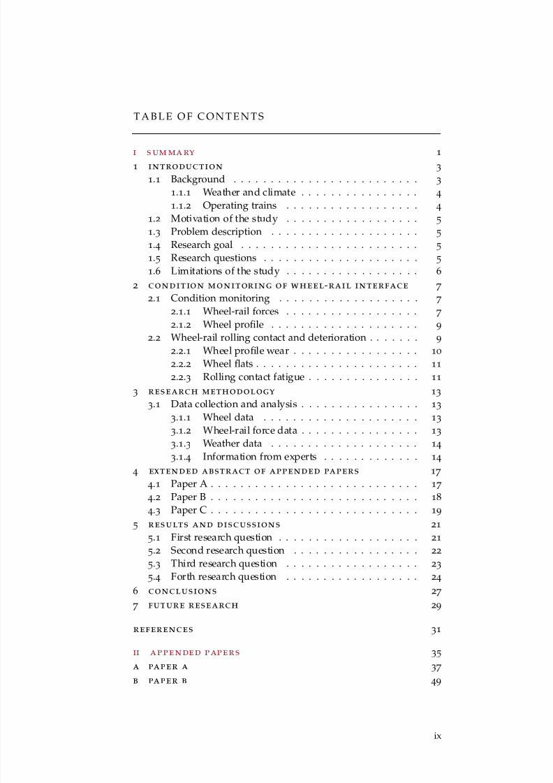
T A B L E O F C O N T E N T S
i s um ma ry 1
1 introduction 3
1.1 Background . . . . . . . . . . . . . . . . . . . . . . . . . 3
1.1.1 Weather and climate . . . . . . . . . . . . . . . . 4
1.1.2 Operating trains . . . . . . . . . . . . . . . . . . 4
1.2 Motivation of the study . . . . . . . . . . . . . . . . . . 5
1.3 Problem description . . . . . . . . . . . . . . . . . . . . 5
1.4 Research goal . . . . . . . . . . . . . . . . . . . . . . . . 5
1.5 Research questions . . . . . . . . . . . . . . . . . . . . . 5
1.6 Limitations of the study . . . . . . . . . . . . . . . . . . 62 condition monitoring of wheel-rail interface 7
2.1 Condition monitoring . . . . . . . . . . . . . . . . . . . 7
2.1.1 Wheel-rail forces . . . . . . . . . . . . . . . . . . 7
2.1.2 Wheel profile . . . . . . . . . . . . . . . . . . . . 9
2.2 Wheel-rail rolling contact and deterioration . . . . . . . 9
2.2.1 Wheel profile wear . . . . . . . . . . . . . . . . . 10
2.2.2 Wheel flats . . . . . . . . . . . . . . . . . . . . . . 11
2.2.3 Rolling contact fatigue . . . . . . . . . . . . . . . 11
3 research methodology 13
3.1 Data collection and analysis . . . . . . . . . . . . . . . . 13
3.1.1 Wheel data . . . . . . . . . . . . . . . . . . . . . 13
3.1.2 Wheel-rail force data . . . . . . . . . . . . . . . . 13
3.1.3 Weather data . . . . . . . . . . . . . . . . . . . . 14
3.1.4 Information from experts . . . . . . . . . . . . . 14
4 extended abstract of appended papers 17
4.1 Paper A . . . . . . . . . . . . . . . . . . . . . . . . . . . . 17
4.2 Paper B . . . . . . . . . . . . . . . . . . . . . . . . . . . . 18
4.3 Paper C . . . . . . . . . . . . . . . . . . . . . . . . . . . . 19
5 results and discussions 21
5.1 First research question . . . . . . . . . . . . . . . . . . . 21
5.2 Second research question . . . . . . . . . . . . . . . . . 225.3 Third research question . . . . . . . . . . . . . . . . . . 23
5.4 Forth research question . . . . . . . . . . . . . . . . . . 24
6 conclusions 27
7 future research 29
references 31
ii appended papers 35
a paper a 37
b paper b 49
ix

8/10/2019 Condition monitorin g of railway vehicles
http://slidepdf.com/reader/full/condition-monitorin-g-of-railway-vehicles 12/86
x table of contents
c paper c 61

8/10/2019 Condition monitorin g of railway vehicles
http://slidepdf.com/reader/full/condition-monitorin-g-of-railway-vehicles 13/86
Part I
S U M M A R Y

8/10/2019 Condition monitorin g of railway vehicles
http://slidepdf.com/reader/full/condition-monitorin-g-of-railway-vehicles 14/86
8/10/2019 Condition monitorin g of railway vehicles
http://slidepdf.com/reader/full/condition-monitorin-g-of-railway-vehicles 15/86
1I N T R O D U C T I O N
1.1 b ac k gr ou n d
Railways use the low resistance of movement between wheel and rail,in order to be an energy efficient mode of transport. The develop-ment of fast or heavy trains affects the vehicle-track dynamic inter-action (9). Vehicle-track interaction includes ride comfort and safety,vehicle stability, wheel-rail forces, wheel-rail corrugation, wheel out-of-roundness, noise propagation, etc., and is influenced by a variety
of factors (10). Safety is the most important attribute of quality of service and operation for railways (35). The condition of wheels andrails have a great impact on railway safety. Therefore, having railwayvehicles and especially wheels in an acceptable condition is a majorconcern for both railway operators and infrastructure owners. Infras-tructure managers always try to reduce the number of potential riskareas that can lead to accidents.
In the early days of railroad the infrastructure and vehicles wererun to failure. Following the technological progress of the industrialworld all investigations were then made by maintenance personnelmanually inspecting both the infrastructure and the vehicles. As tech-nology advances the condition monitoring and analysis tools to eval-uate the current railway load are embraced by the industry.
Wheel sets are regarded as fundamental components of railway ve-hicles; they support the vehicle during rolling, guide it and transferlongitudinal forces at traction and braking (9). The wheel-rail inter-face is the most important parameter in the dynamics of railway ve-hicles and their condition (11, 23). This interface is where most of thecost for maintenance on both railway vehicles and infrastructure oc-curs. The change in rail profiles is a major maintenance cost driver(15). The profile change on wheels can also be significant, especially
in curves. Damage mechanisms such as wear and plastic deformationare the main contributors to profile change.
The wheel-rail contact is typically the size of a small coin, 100 mm2.Rails and wheels are commonly made from plain carbon-manganesepearlitic steel. A wheel set for a railway vehicle is almost always fixedon a solid shaft. With the wheel set centered on straight track, and if the left and right wheel rolling radii are equal, the wheel set can rollnormally. The steering load contributes to increased wear and rollingcontact fatigue, especially in curved tracks. (42)
3

8/10/2019 Condition monitorin g of railway vehicles
http://slidepdf.com/reader/full/condition-monitorin-g-of-railway-vehicles 16/86
4 i nt ro du ct io n
The Iron Ore Line (Malmbanan) in northern Sweden starts in Luleåand ends in Narvik in Norway, see Fig. 1.1. The traffic on the Lineconsists of both passenger and freight trains. The freight traffic con-sists primarily of heavy haul trains with axle loads of 22.5 tonnesand more. Running heavy-haul railway traffic in a mountainous areanorth of the Arctic Circle is a challenging task (32). The trains op-erate in harsh climate conditions, including snow in the winter andextreme temperatures ranging from -40◦C to +25◦C (21). There aremany tight curves along the track that experience high wear (7).
ARCTIC CIRCLE
Luleå
Bastuträsk
Jörn
Älvsbyn
Boden
Vilhelmina
Storuman
Sorsele
Arvidsjaur
Moskosel
Kåbdalis
Jokkmokk
orjusPorjus
Murjek
Gällivare
Kiruna
Riksgränsen Björkliden
Abisko
Narvik
Arctic Circle
Luleå
Narvik
Kiruna
Gällivare
Figure 1.1: Map of northern Sweden
However, competition in the world market has forced the Swedishiron-ore mining company LKAB to make its transport chain moreefficient (25). As a result LKAB are now transporting iron-ore withan axle-load of 30 tonnes and at speeds of 60 km/h.
Outside Luleå there is a research station which measures the wheel-rail forces, both lateral and vertical, in a curve with 484 m radius attrack speed. This will be described further in section 2.1.1 on page 8;see paper B.
1.1.1 Weather and climate
All of Sweden experience temperatures below freezing most years. Inthe southern parts it might only be for a few days. In the north it isusually below zero for up to seven months of the year.
1.1.2 Operating trains
On Malmbanan there are primarily heavy-haul trains from LKABmining company. These trains consist of two IORE locomotive with68 wagons, 750 meters long and a total train weight 8.500 tonnes.On Malmbanan there are passenger, freight, steel-slab and copper-ore trains. The freight trains consist of lighter wagons up to 18 tonnesof axle load, the copper-ore trains have an axle-load of 22.5 tonnesand the steel-slab trains have an axle-load of 25 tonnes.

8/10/2019 Condition monitorin g of railway vehicles
http://slidepdf.com/reader/full/condition-monitorin-g-of-railway-vehicles 17/86
1.2 mo ti vat io n o f t he s tu dy 5
1.2 motivation of the study
The motivation for this study is to have a better utilization of wagonpopulation by optimizing inspection and maintenance with less down-time. Simply stated, there is a need to go from time-based to condition- based maintenance. Large cost-drivers are manual labor and wheel re-profiling. The aim is to define cost effective maintenance thresholds based on measurement data.
1.3 p r ob l em d e sc r i pt i on
The railway industry has a desire/need to improve the process of maintenance program development from the present tonnage or kilo-meter based programs to a condition-based maintenance regime. In-
troducing condition-based maintenance requires both technical solu-tions to monitor the condition and change at the organizational level.
The wheel-rail guidance is made possible by the shapes of thewheel and the rail profiles. To increase revenue for train operatorsand decrease cost for railway infrastructure owners there is a need tomonitor the condition of the assets. A major cost-driver for operatorsis production loss due to wheels. This is mainly from maintenancecosts when changing and re-profiling wheels.
This study will analyse and process the measurement data fromwheel-rail force measurements at the research station outside Luleå.
This is a first step in finding thresholds for condition-based mainte-nance on wheels. In this study the relationship between wheel profilewear, the measured lateral force, and weather conditions are anal-ysed.
1.4 r e se a rc h g oa l
The overall research goal is to evaluate different existing method-ologies as tools for cost effective implementation of condition-basedmaintenance for railway vehicles, in particular the wagon wheels. Thegoal is to increase the life length of the wheels by knowing the condi-tion of the wheel profile. We also plan to show the impact of mainte-nance actions and the influencing factor on wheel set life.
1.5 r e se a rc h q u es t io n s
In order to fulfill the stated goals above, the following research ques-tions have been raised:
1. What is the best method to collect data from the wheel-rail in-terface for condition monitoring?

8/10/2019 Condition monitorin g of railway vehicles
http://slidepdf.com/reader/full/condition-monitorin-g-of-railway-vehicles 18/86
6 i nt ro du ct io n
2. How can data collected from the wheel-rail interface be used inmaintenance decision-support?
3. How do Arctic weather conditions influence the need for rail-
way vehicle maintenance?
4. How do the different wheel and axle positions influence themaintenance decisions?
These research questions are answered by the three appended pa-pers. Each paper makes its own contribution toward the researchquestions; see Table 1.1.
Table 1.1: Relationship between the appended papers and research ques-tions
Paper
A B C
RQ 1 X X
RQ 2 X X
RQ 3 X X
RQ 4 X X
1.6 limitations of the study
The research seeks to optimize the maintenance of railway vehicles,with a focus on wheels.
There are some limitations in this study. Only heavy haul vehiclesare considered due to their heavy load on the infrastructure. Thus,only northern Sweden will be investigated since this is where thevehicles are used. Lastly only wheel profile data from LKAB miningcompany are studied.

8/10/2019 Condition monitorin g of railway vehicles
http://slidepdf.com/reader/full/condition-monitorin-g-of-railway-vehicles 19/86
2C O N D I T I O N M O N I T O R I N G O F W H E E L - R A I LI N T E R F A C E
2.1 c o n di t io n m o n it o ri n g
Information regarding health and physical status of wheels or com-ponents is key to successful maintenance planning. Therefore, manymaintenance actions are directed towards collecting information onwheel conditions (22). A definition of the term condition monitoring(CM) is the continuous or periodic measurement and interpretation
of data to indicate the condition of an item to determine the needfor maintenance (28). This is normally carried out with the item inoperation, in operable state or removed but not subject to major stripdown.
The monitoring can be executed with different levels of automa-tion, from relying entirely on human senses to assess the condition tofully automated and integrated monitoring systems, measuring andanalyzing e.g. vibrations, temperatures, pressures etc (6).
Traditional inspection techniques used in the railroad industry suchas drive-by inspection, are not as accurate and reliable as more rigor-ous and quantitative inspection methods (39). On-board measuringcan measure the chosen parameter along the whole route where thetest trains runs, while wayside measuring can measure the parame-ters for the full train set as it runs through the measuring points (26).Wayside detection systems provide a means of monitoring the con-dition of vehicles, ensuring that they are in a serviceable condition(4).
2.1.1 Wheel-rail forces
Force measurement detectors make it possible for vehicles with de-fective wheels, which are likely to cause damage to the permanentrailway structures, to be identified and removed from service imme-diately (34). Vertical impact loads between wheel and rail resultingfrom surface anomalies such as wheel flats has been used to createmathematical models of wheel-rail impact behaviour (1). Systems thatsolely measure the axle load of wheel flats are mostly placed on a tan-gent track with no gradient or a negligible gradient and where trainsdo not accelerate or brake (24).
When measuring the lateral forces, it is best to perform measure-ments in narrow curves, as the vehicles show their steering ability.
For a illustration of lateral and vertical forces, see Fig. 2.1(a), and for
7

8/10/2019 Condition monitorin g of railway vehicles
http://slidepdf.com/reader/full/condition-monitorin-g-of-railway-vehicles 20/86
8 c on di ti on m on it or in g o f w he el-rail interface
bogie/wheel placement in a curve, see Fig. 2.1(b). Lateral forces arethe result of poor steering bogie and train speeds outside the trackdesign, and of longitudinal buff and draft forces transmitted throughtrain action and coupler angularity (5). In order to prevent derailmentaccidents and abnormal wear, it is important to determine the actualstate of the contact forces between wheel and rail (26). According toMatsumoto et al. (26) lateral and vertical contact forces are especiallyimportant. The knowledge gained from measurement of wheel-railforces is allowing for reduction in the stress state of the railway (3).
Vertical force
Lateral force
(a) Definition of forces
Leading High-RailTrailing High-Rail
Trailing Low-Rail Leading Low-Rail
D i r e c t i o n o f
t r a v e l
(b) Wheel position for a bogie in a curve
Figure 2.1: Force definition and wheel positions
Research station
The research station outside Luleå is a modified version of a force-
based truck performance detector, monitoring the vertical and lateralforcers in a single curve with a 484 m radius (24, 33). The measure-ment system consists of strain gauges attached to the web of the rail,as indicated in Fig. 2.2(a). Fig. 2.2(b) – (c) show how the measurementequipment looks at the site. Mainly iron-ore trains with an axle loadof 30 tonnes and a speed of 60 km/h are monitored (24). For moreextensive information see Paper A.
(a) Placement of sensorson the rail
(b) Visualization of place-ment
(c) Placement of sensors
Figure 2.2: All information about the research station
8/10/2019 Condition monitorin g of railway vehicles
http://slidepdf.com/reader/full/condition-monitorin-g-of-railway-vehicles 21/86
8/10/2019 Condition monitorin g of railway vehicles
http://slidepdf.com/reader/full/condition-monitorin-g-of-railway-vehicles 22/86
10 c o nd i ti o n m o ni t or i ng o f w h ee l-rail interface
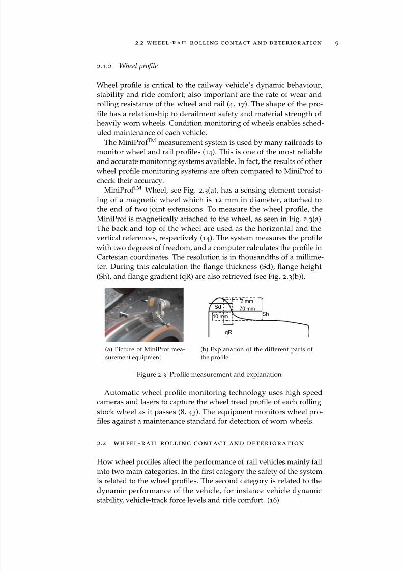
Wheel and rail profiles are designed to meet certain desired prop-erties of conicity, gravitational suspension stiffness and resultant con-tact stresses (41). The wheel and rail then enter service and changeshape over time. The interaction between wheel and rail resultingin material deterioration is a complicated process, involving vehicle-track dynamics, contact mechanics, friction wear and lubrication (11).The course of events called wear is similarly complicated, involvingseveral modes of material deterioration and contact surface alteration(13). Two important deterioration mechanisms are wear and rollingcontact fatigue (RCF). Frictional heating occurs when train cars re-duce speed by using their pads against the running surface of thewheels (i.e., braking). When the wheel surface layer is frictionallyheated, and this is followed by the rapid cooling of the body of thewheel itself, there is an increased risk of forming martensite (19). As
martensite is much harder and more brittle than the surrounding ma-terial, it can break and initiate cracks. In addition, freight car wheelsin service may develop tread irregularities in the form of slid-flats,shells or spalls (37). Any of these irregularities can cause high wheelimpact forces (37, 39), with slid-flats, also called wheel flats, being themost common.
2.2.1 Wheel profile wear
Wear is the loss or displacement of material from a contacting surface
(15). Material loss may be in the form of debris. Material displacementmay occur by transfer of material from one surface to another byadhesion or by local plastic deformation. In wheel-rail contact, bothrolling and sliding occur in the contact zone.
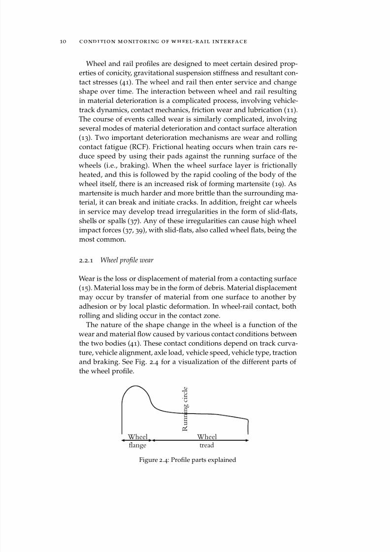
The nature of the shape change in the wheel is a function of thewear and material flow caused by various contact conditions betweenthe two bodies (41). These contact conditions depend on track curva-ture, vehicle alignment, axle load, vehicle speed, vehicle type, tractionand braking. See Fig. 2.4 for a visualization of the different parts of the wheel profile.
Wheelflange
Wheeltread
R u n n i n g c i r c l e
Figure 2.4: Profile parts explained

8/10/2019 Condition monitorin g of railway vehicles
http://slidepdf.com/reader/full/condition-monitorin-g-of-railway-vehicles 23/86
2.2 w he e l-r a il r o ll i ng c o n ta ct a n d d e te r io r at i on 11
Most techniques to reduce the wheel profile change are based onlimiting the wear, or material removal (16). Wear is not generally acritical failure mode in rolling contact (18).
2.2.2 Wheel flats
Wheel flats are formed when a wheel set is locked and skids along therail (2, 31). The reason for this may be that the brakes are poorly ad- justed, frozen or defective. The friction between wheel and rail causesthe surface of the wheel to become flat instead of round (39).
2.2.3 Rolling contact fatigue
Rolling contact fatigue is the principal mode of failure of rolling sur-faces and governs the safe life of a components under a prescribedload (18). Wheel damage occurs as fatigue cracks, initiated at or be-low the surface, result in material fall-out like shelling or spalling(13).
Shelling is a term normally used for all types of subsurface inducedcracks (31). Wheel shelling is defined as the loss of relative large(greater than 5 mm) pieces of metal from the wheel tread as the re-sult of contact fatigue (29). Typically, shelling cracks grow at an acuteangle to the surface. Impact load can affect shelling in both crackinitiation and crack propagation modes (38).
Spalling is the term used for the RCF phenomenon occurring whensurface cracks of thermal origin meet, resulting in part of the wheelcoming away from the tread (31). It is associated with cracking in-duced by high transformation stress caused by surface martensiteformation (29). Cracks from spalling form both perpendicular andparallel to the wheel tread surface.

8/10/2019 Condition monitorin g of railway vehicles
http://slidepdf.com/reader/full/condition-monitorin-g-of-railway-vehicles 24/86
8/10/2019 Condition monitorin g of railway vehicles
http://slidepdf.com/reader/full/condition-monitorin-g-of-railway-vehicles 25/86
3R E S E A R C H M E T H O D O L O G Y
The term "research" has been defined in different ways, but Kumar(20) calls it an intensive and scientific activity undertaken to establisha fact, a theory, a principle or an application.
A research approach can be quantitative or qualitative or a combi-nation of both. In simple terms, quantitative research uses numbers,counts and measures of things, whereas qualitative research adoptsquestioning and verbal analysis (40). Both qualitative and quantitativeresearch methodologies have been applied in the research presented
in this thesis.
3.1 data collection and analysis
Data can be defined as classification of facts obtained by researchersfrom a studied environment (12). Data can also be defined as theempirical evidence or information that scientists carefully collect ac-cording to rule or procedures to support or reject theories (30).
For the qualitative information used in this thesis, a literature sur-vey was carried out based on peer-reviewed journal papers, confer-
ence proceedings articles, research and technical reports, Licentiateand PhD theses. Quantitative information was obtained from mea-surements and the databases of the Swedish Meteorological Insti-tute (SMHI), LKAB, the research station, and DUROC Rail. Specifickeywords were used to search for information in well-known on-line databases, including Google Scholar, Elsevier, Science Direct andEmerald etc.
3.1.1 Wheel data
In this research railway vehicle wheels have been studied in a bid tooptimize maintenance planning of wheel sets. For this purpose man-ual profile measurements have been performed using MiniProf TM
Wheel equipment.Data on wheel re-profiling have been collected from either the
DUROC Rail maintenance workshop in Luleå or from LKAB main-tenance database.
3.1.2 Wheel-rail force data
Force data from the wheel-rail interface have been collected by the
research station outside Luleå. All data from each train passage are
13

8/10/2019 Condition monitorin g of railway vehicles
http://slidepdf.com/reader/full/condition-monitorin-g-of-railway-vehicles 26/86
14 r es ea rc h m et ho d ol og y
put into separate text files. For each train the axles of that train are broken up into different data types in separate columns.
For this research wheels have been sorted out and merged in orderto determine a timeline for lateral and vertical forces.
3.1.3 Weather data
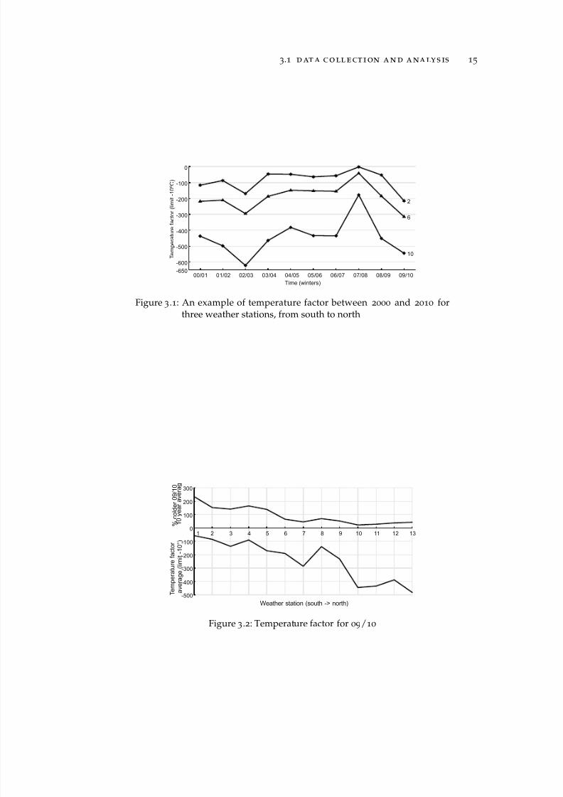
The weather data is this research have been collected either fromSMHI or from the research station outside Luleå. For each train pas-sage at the research station, temperature and relative humidity isstored in a database with the time and train data. From SMHI, dailytemperature and humidity data were collected between 2000 and 2010
for 13 different weather stations, see Table 3.1. For each day, the dailytemperatures, including both the lowest and average and the average
humidity were recorded.The collected temperature data were separated for each station and
the temperature factor was calculated using Equation 3.1. Resultsfrom this can be seen in Fig. 3.1 and 3.2 and paper C.
Temp. factor =30 Apr.
1 Oct.
(T D − T L) for all (T D T L) (3.1)
Where: T D = Daily temp. average, T L = Temp. limit
Table 3.1: Weather stations used
1 Borlänge 6 Hemling 11 Gällivare
2 Åmot 7 Petisträsk 12 Kiruna
3 Edsbyn 8 Umeå 13 Rensjön
4 Delsbo 9 Norsjö
5 Torpshammar 10 Älvsbyn
3.1.4 Information from experts
Discussions have been held with various experts to obtain informa-tion on explanations of the extracted data. For example, the datafrom DUROC only contained the numbers of wheel re-profiling andnot their causes. The information about their extent is confined to ei-ther RCF or wheel wear. It also indicates during which part of theyear or train operator affected a particular failure mode. The crackgrowth, the risk of wheel fracture and the wheel removals due toflange height increases at low temperatures (19, 31, 36).
8/10/2019 Condition monitorin g of railway vehicles
http://slidepdf.com/reader/full/condition-monitorin-g-of-railway-vehicles 27/86
3.1 d at a c o ll e ct i on a n d a na ly s is 15
00/01 01/02 02/03 03/04 04/05 05/06 06/07 07/08 08/09 09/10
0
-650
-600
-500
-400
-300
-200
-100
Time (winters)
T e m p e r a t u r e f a c t o r ( l i m i t - 1 0 º C )
2
6
10
Figure 3.1: An example of temperature factor between 2000 and 2010 forthree weather stations, from south to north
131 2 3 4 5 6 7 8 9 10 11 12
300
-500
-400
-300-200
-100
0
100
200
Weather station (south -> north)
T e m p e r a t u r e f a c t o r
% c o l d e r 0 9 / 1 0
1 0 y e a r a v e r a g
a v e r a g e ( l i m i t - 1 0 ° )
Figure 3.2: Temperature factor for 09/10

8/10/2019 Condition monitorin g of railway vehicles
http://slidepdf.com/reader/full/condition-monitorin-g-of-railway-vehicles 28/86

8/10/2019 Condition monitorin g of railway vehicles
http://slidepdf.com/reader/full/condition-monitorin-g-of-railway-vehicles 29/86
4E X T E N D E D A B S T R A C T O F A P P E N D E D PA P E R S
4.1 pa pe r a
Title: Condition monitoring of rolling stock using wheel/rail forcesAuthors: M. Palo, H. Schunnesson and U. Kumar
Purpose
This paper has two purposes. The first is to present condition moni-
toring techniques for railway vehicles, so that maintenance of wheelscan be optimized, leading to improved life length and minimized cost.One cost-driver in rolling stock is the maintenance of wheels. The sec-ond purpose is to present and analyze measurement data from theresearch station outside Luleå Sweden.
Method
To fulfill the first purpose, a literature survey was done. This surveystudied several different methods of condition monitoring for railway
vehicles. Two measurement systems are discussed, wheel impact loaddetectors and truck performance detectors. The research station itself is a modified version of a truck performance detector. It measuresforces exerted on the rail by all passing trains at up to 100 km/h in acurve with 484 m radius.
To fulfill the second purpose, a search into all possible data fromthe research station was done. Vertical and lateral forces, speed, tem-perature and relative humidity from March 2009 to May 2010 wassorted according to train type. Out of the 20 000 trains that passedthrough the research station, 600 trains with two specifically marked
wagons were studied. The data points for each parameter for thesewagons were then analyzed with respect to travel direction of thewagon. The forces were also divided for wheel position in the bogie.
Findings
There are differences in lateral forces between leading and trailingaxles and between the wheels of an axle. This give a clear indicationthat each position has to be considered separately. There are also dif-ferences when changing direction of the wagon. To be able to collectdata for both left and right turns for a bogie, there is a need for asecond measurement station.
17
8/10/2019 Condition monitorin g of railway vehicles
http://slidepdf.com/reader/full/condition-monitorin-g-of-railway-vehicles 30/86
18 e x te n de d a b st r ac t o f a p pe n de d pa p er s
The measurement system at the research station can be seen as arobust system because the forces from leading high-rail are withinthe limit of variation. Seasonal changes seem to have no influence.
4.2 pa pe r b
Title: Condition monitoring of wheel wear on iron ore wagonsAuthors: M. Palo and H. Schunnesson
Purpose
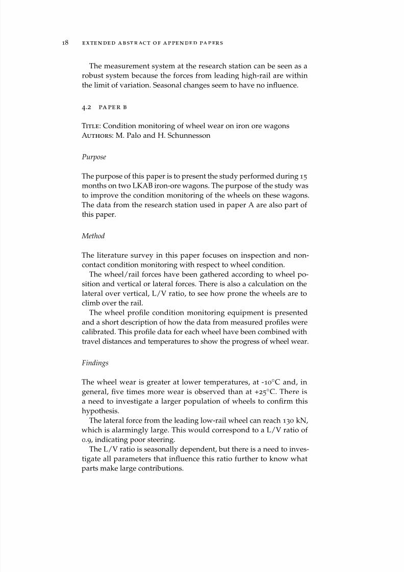
The purpose of this paper is to present the study performed during 15
months on two LKAB iron-ore wagons. The purpose of the study wasto improve the condition monitoring of the wheels on these wagons.The data from the research station used in paper A are also part of this paper.
Method
The literature survey in this paper focuses on inspection and non-contact condition monitoring with respect to wheel condition.
The wheel/rail forces have been gathered according to wheel po-sition and vertical or lateral forces. There is also a calculation on thelateral over vertical, L/V ratio, to see how prone the wheels are to
climb over the rail.The wheel profile condition monitoring equipment is presented
and a short description of how the data from measured profiles werecalibrated. This profile data for each wheel have been combined withtravel distances and temperatures to show the progress of wheel wear.
Findings
The wheel wear is greater at lower temperatures, at -10◦C and, ingeneral, five times more wear is observed than at +25◦C. There is
a need to investigate a larger population of wheels to confirm thishypothesis.
The lateral force from the leading low-rail wheel can reach 130 kN,which is alarmingly large. This would correspond to a L/V ratio of 0.9, indicating poor steering.
The L/V ratio is seasonally dependent, but there is a need to inves-tigate all parameters that influence this ratio further to know whatparts make large contributions.

8/10/2019 Condition monitorin g of railway vehicles
http://slidepdf.com/reader/full/condition-monitorin-g-of-railway-vehicles 31/86
4.3 paper c 19
4.3 pa pe r c
Title: Maintainability in extreme seasonal weather conditionsAuthors: M. Palo, H. Schunnesson, and P.-O. Larsson-Kråik
Purpose
The purpose of this paper is to investigate the difference of wheeldamages during winter conditions in northern Sweden compared towarmer and humid weather.
Method
The literature survey in this paper is focused on wheel deteriorationand how cold weather influences it.
Weather data from SMHI have been collected for 13 different weatherstation. These stations are all close to the railway line from Borlängein the middle of Sweden to northern Sweden. In order to comparethese different geographical positions a temperature factor equationwas formed.
Findings
During the colder winters, more wheels need to be re-profiled. This
confirms the relationship between cold temperature and wheel sur-face damage.
Rolling contact fatigue, especially shelling and spalling is the dom-inant wheel surface damage during the cold. There is a need to inves-tigate how the braking method influences wheel surface damage.

8/10/2019 Condition monitorin g of railway vehicles
http://slidepdf.com/reader/full/condition-monitorin-g-of-railway-vehicles 32/86

8/10/2019 Condition monitorin g of railway vehicles
http://slidepdf.com/reader/full/condition-monitorin-g-of-railway-vehicles 33/86
5R E S U L T S A N D D I S C U S S I O N S
In this chapter, the findings of conducted research are discussed andpresented according to the stated research questions.
5.1 f i rs t r e s ea r ch qu e st i on
RQ1: What is the best method to collect data from the wheel-rail interface
for condition monitoring?
The first research question in answered by the research presented inPapers A and B.
In the interface between wheel and rail, forces are transmitted.These forces are vertical for load, lateral for steering and longitudi-nal for traction and braking. For condition monitoring, only verticaland lateral are used. There are different measurement systems andsensor types that measure these forces. The wheel impact load de-tector (WILD) is used in tangent track to measure vertical loads. Forlateral forces, there is a need to measure in a curve, and the truck per-formance detector (TPD) is used for this purpose. The TPD will also
measure the vertical load, but its primary aim is to monitor steeringperformance.Infrastructure owners will install either system to monitor the ve-
hicles using the track and to keep them in good condition. Verticalimpact loads from damaged wheels are especially important. TheWILD system was invented to help detect these wheels and informthe wagon owner of the need to replace the wheel. Both systems aregood but the TPD is more versatile tool than the WILD that measuresthe only vertical load in tangent track.
The degradation of wheel and rail over time differs. The wheelwill degrade faster than the rail due to the material chosen, and
they are easier to change and maintain in proper running condi-tion. A MiniProf TM can be used to monitor either wheel or rail. Thisdata can also be collected using automated monitoring systems eithermounted to a vehicle, for rail, or on the track, for wheels. Automatedsystems are preferred if a large population of wheels is to be moni-tored.
21

8/10/2019 Condition monitorin g of railway vehicles
http://slidepdf.com/reader/full/condition-monitorin-g-of-railway-vehicles 34/86
22 r es ult s a nd d is cu ss io ns
5.2 s e co n d r e se a rc h q u es t io n
RQ2: How can data collected from the wheel-rail interface be used in main-
tenance decision-support?
The second research question in answered by the research pre-sented in Papers A and B; however, some important findings are briefly discussed here.
Vertical forces are typically monitored for an impact threshold of 400 kN. When a wheel passes a measurement point with this force,an alarm is sent to the operator and train driver. The wheel has to be checked, and if the damage is severe, the wagon will be parkedalong the track. Another possibility is to drive it to the maintenanceworkshop for replacement of the wheel.
In Sweden, lateral forces are not monitored by the infrastructureowner. Therefore, there is no threshold for a wagon trafficking therailway. While certifying a new wagon, there is a limit of 80 kN, andthis can be used as a starting threshold to start with.
To prevent flange climb derailment, a ratio between lateral and ver-tical forces is calculated, L/V ratio. This ratio will tell if a wheel isprone to start climbing over the rail. The friction coefficient is a ma- jor factor in this formula, see paper B. Also wheel wear is influenced by the wheel-rail contact angle. A project to assess the wheel-rail de-tectors states that a TPD can indicate poor bogie performance viameasured forces and corresponding derived values such as the L/Vratio (27).
The wheel profile has several thresholds which determine when toreplace a wheel. Flange height and width are the most common inCM. Flange height progress linear with running distance, see Fig. 5.1.The use of flange height for CM is sufficient a mechanical equipment,if an automated system is used the whole profile should be consid-ered.
350,0000 50,000 100,000 150,000 200,000 250,000 300,000
34
28
29
30
31
32
33
Milage (km)
F l a n g e h e i g h t ( m m )
Figure 5.1: Flange height as a function of running distance

8/10/2019 Condition monitorin g of railway vehicles
http://slidepdf.com/reader/full/condition-monitorin-g-of-railway-vehicles 35/86
5.3 t hi rd r es ea rc h q ue st io n 23
5.3 t h ir d r e se a rc h q u es t io n
RQ3: How do Arctic weather conditions influence the need for railway vehi-
cle maintenance?
The third research question answered by the research is presentedin Papers B and C. Some findings from colder climate will be brieflydiscussed here.
In Paper B the monthly-average for Gällivare, between 2000 and2010 was calculated, see Fig. 5.2. The temperature for Luleå is theyearly average of 2◦C. This gives an indication of weather and temper-ature conditions. There is greater wheel wear at lower temperatures.Already at 0◦C there is an increase in wheel wear, see Fig. 5.3. AlsoRCF damages, shelling and spalling, occur more frequently at temper-
atures below freezing. This indicates a greater need for re-profiling ina cold climate.
Mar Apr May Jun Jul Aug Sept Oct Nov Dec Jan Feb Mar Apr May
40
-40
-30
-20
-10
0
10
20
30
Time (Month)
T e m p e r a t u r e ( º C )
2009 2010
SMHI
Sävast Luleå
Figure 5.2: Temperature data for Gällivare, Luleå and Research station
25-10 -5 0 5 10 15 20
8
0
1
2
3
4
5
6
7
Temperature (ºC)
W e a r ( m m / 1 0 0 0 0 0 k m )
Figure 5.3: Wheel wear at running circle versus temperature
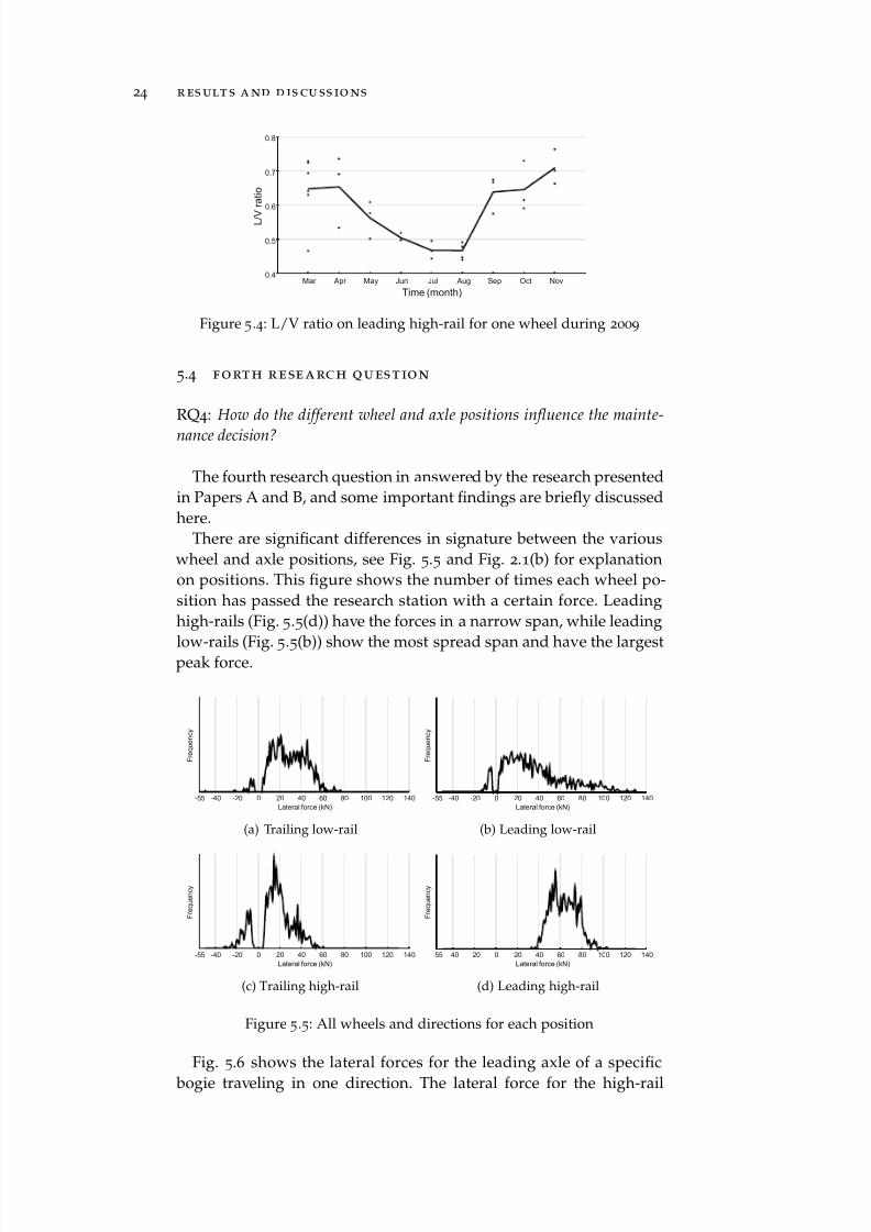
L/V ratio for leading high-rail changes with the seasons has a lowervalue during the summer, see Fig. 5.4, when there is more moisturein the air and the rail lubrication system is turned on. At such times,the friction coefficient is low, which is indicative of the large influenceof friction in the L/V ratio calculation.
8/10/2019 Condition monitorin g of railway vehicles
http://slidepdf.com/reader/full/condition-monitorin-g-of-railway-vehicles 36/86
24 r es ult s a nd d is cu ss io ns
Mar Apr May Jun Jul Aug Sep Oct Nov
0.8
0.4
0.5
0.6
0.7
Time (month)
L / V
r a t i o
Figure 5.4: L/V ratio on leading high-rail for one wheel during 2009
5.4 f o rt h r e se a rc h q u es t io n
RQ4: How do the different wheel and axle positions influence the mainte-
nance decision?
The fourth research question in answered by the research presentedin Papers A and B, and some important findings are briefly discussedhere.
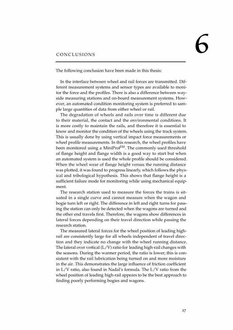
There are significant differences in signature between the variouswheel and axle positions, see Fig. 5.5 and Fig. 2.1(b) for explanationon positions. This figure shows the number of times each wheel po-sition has passed the research station with a certain force. Leadinghigh-rails (Fig. 5.5(d)) have the forces in a narrow span, while leading
low-rails (Fig. 5.5(b)) show the most spread span and have the largestpeak force.
140-55 -40 -20 0 20 40 60 80 100 120Lateral force (kN)
F r e q u e n c y
(a) Trailing low-rail
140-55 -40 -20 0 20 40 60 80 100 120Lateral force (kN)
F r e q u e n c y
(b) Leading low-rail
140-55 -40 -20 0 20 40 60 80 100 120Lateral force (kN)
F r e q u e n c y
(c) Trailing high-rail
140-55 -40 -20 0 20 40 60 80 100 120Lateral force (kN)
F r e q u e n c y
(d) Leading high-rail
Figure 5.5: All wheels and directions for each position
Fig. 5.6 shows the lateral forces for the leading axle of a specific
bogie traveling in one direction. The lateral force for the high-rail

8/10/2019 Condition monitorin g of railway vehicles
http://slidepdf.com/reader/full/condition-monitorin-g-of-railway-vehicles 37/86
5.4 f or th r es ea rc h q ue st io n 25
wheel is consistently large as there is no change in travel distance.For the low-rail wheel there is a significant difference in the lateralforces as the wheel travel distance increases.
150,0000 40,000 80,000 120,000
100
0
20
40
60
80
Distance (km)
L a t e r a l f o r c e ( k N )
(a) High-rail
150,0000 40,000 80,000 120,000
140
-20
0
20
40
60
80
100
120
Distance (km)
L a t e r a l f o r c e ( k N )
(b) Low-rail
Figure 5.6: One wheel axle as leading in the bogie
During the study, the investigated wagons passed the research sta-tion with different wagon ends leading. In Fig. 5.7 the differences inthe forces on the leading low-rails are shown as separate graphs. Thisindicates that the wagon and bogies behave differently depending onwhich way they travel.
150,0000 40,000 80,000 120,000
130
-20
0
20
40
60
80
100
Distance (km)
L
a t e r a l f o r c e ( k N )
(a) Scenario 1, wagon 43 traveling first
150,0000 40,000 80,000 120,000
130
-20
0
20
40
60
80
100
Distance (km)
L a t e r a l f o r c e ( k N )
(b) Scenario 2, wagon 44 traveling first
Figure 5.7: Leading low-rail showing changes with direction of travel
In Fig. 5.8 the L/V ratio for all wheels, either high-rail or low-rail,are plotted for each month. The high-rails show a narrower span be-tween the measured values, see Fig. 5.8(a), while the low-rails (Fig.5.8(b)) are quite spread out. The low-rails also have negative valueswhich are due to the direction of the lateral force. This difference be-

8/10/2019 Condition monitorin g of railway vehicles
http://slidepdf.com/reader/full/condition-monitorin-g-of-railway-vehicles 38/86
26 r es ult s a nd d is cu ss io ns
tween rails and wheels indicate a need to separate all data into wheeland axle position, even though the leading high-rail L/V ratio ap-pears to be the best approach to find poor performing wagons. Thisis also indicated in the literature (27).
Mar Apr May Jun Jul Aug Sep Oct Nov Dec Jan Feb Mar Apr May
0.8
-0.1
0
0.1
0.2
0.3
0.4
0.5
0.6
0.7
Time (month)
L / V r a t i o
(a) L/V ratio for high-rail
Mar Apr May Jun Jul Aug Sep Oct Nov Dec Jan Feb Mar Apr May
0.8
-0.1
0
0.1
0.2
0.3
0.4
0.5
0.6
0.7
Time (month)
L / V r a t i o
(b) L/V ratio for low-rail
Figure 5.8: L/V ratio for all passing of the wagons
8/10/2019 Condition monitorin g of railway vehicles
http://slidepdf.com/reader/full/condition-monitorin-g-of-railway-vehicles 39/86
6C O N C L U S I O N S
The following conclusion have been made in this thesis:
In the interface between wheel and rail forces are transmitted. Dif-ferent measurement systems and sensor types are available to moni-tor the force and the profiles. There is also a difference between way-side measuring stations and on-board measurement systems. How-ever, an automated condition monitoring system is preferred to sam-ple large quantities of data from either wheel or rail.
The degradation of wheels and rails over time is different dueto their material, the contact and the environmental conditions. Itis more costly to maintain the rails, and therefore it is essential toknow and monitor the condition of the wheels using the track system.This is usually done by using vertical impact force measurements orwheel profile measurements. In this research, the wheel profiles have been monitored using a MiniProf TM. The commonly used thresholdof flange height and flange width is a good way to start but whenan automated system is used the whole profile should be considered.When the wheel wear of flange height versus the running distancewas plotted, it was found to progress linearly, which follows the phys-ical and tribological hypothesis. This shows that flange height is asufficient failure mode for monitoring while using mechanical equip-ment.
The research station used to measure the forces the trains is sit-uated in a single curve and cannot measure when the wagon and bogie turn left or right. The difference in left and right turns for pass-ing the station can only be detected when the wagons are turned andthe other end travels first. Therefore, the wagons show differences inlateral forces depending on their travel direction while passing theresearch station.
The measured lateral forces for the wheel position of leading high-rail are consistently large for all wheels independent of travel direc-tion and they indicate no change with the wheel running distance.The lateral over vertical (L/V) ratio for leading high-rail changes withthe seasons. During the warmer period, the ratio is lower; this is con-sistent with the rail lubrication being turned on and more moisturein the air. This demonstrates the large influence of friction coefficientin L/V ratio, also found in Nadal’s formula. The L/V ratio from thewheel position of leading high-rail appears to be the best approach tofinding poorly performing bogies and wagons.
27

8/10/2019 Condition monitorin g of railway vehicles
http://slidepdf.com/reader/full/condition-monitorin-g-of-railway-vehicles 40/86
28 c on cl usi on s
When the temperature decreases, there is an overall greater wheeltread wear. As the temperatures drop below freezing there is as in-crease in RCF damages, shelling and spalling. Therefore, there isclearly a greater need for wheel re-profiling in a colder climate.

8/10/2019 Condition monitorin g of railway vehicles
http://slidepdf.com/reader/full/condition-monitorin-g-of-railway-vehicles 41/86
7F U T U R E R E S E A R C H
Based on the research conducted in the thesis, the following ideas arepresented as suggestions for further research:
When trying to draw conclusions on wheel profile wear it is usefulto be able to draw on automatic measurements. The installation of anautomatic wheel profile measuring station outside Luleå will makeit possible to investigate a large population of wheel profiles. Theconclusions drawn from these measurements will help in the mainte-
nance planning of wheels.The forces collected at the research station only uses the peak val-ues from when the wheel passes. In the database, the pulses fromthe entire train, each wheel and sensor separated. One hypothesisis that a normal wheel should have a predictable and smooth pres-sure profile as it goes over the sensor, a damaged wheel/bogie willhave more information in the signal. This information could then beextracted statistically or spectrally.
The research questions in the thesis cover condition monitoring and briefly discuss influences for maintenance decisions. The next stepis to start using this monitoring data for maintenance decision andplanning.
29

8/10/2019 Condition monitorin g of railway vehicles
http://slidepdf.com/reader/full/condition-monitorin-g-of-railway-vehicles 42/86

8/10/2019 Condition monitorin g of railway vehicles
http://slidepdf.com/reader/full/condition-monitorin-g-of-railway-vehicles 43/86
R E F E R E N C E S
1: Ahlbeck, D. R. (1980), Investigations of impact loads due to wheelflats and rail joints, in ‘American Society of Mechanical Engineers(Paper)’.
2: Ahlström, J. and Karlsson, B. (1999), ‘Microstructural evaluationand interpretation of the mechanically and thermally affectedzone under railway wheel flats’, Wear 232, 1–14.
3: Anderson, G. B. and McWilliams, R. S. (2003), Vehicle health mon-itoring system development and deployment, in ‘2003 ASME In-
ternational Mechanical Engineering Congress’, American Societyof Mechanical Engineers, Washington, D.C., pp. 143–148.
4: Barke, D. and Chiu, W. K. (2005), ‘Structural health monitoring inthe railway industry: A review’, Structural Health Monitoring 4.
5: Bell, S. and Roney, M. (2011), The continued evolution of safer,more productive and less destructive trains on CPR, in ‘Inter-national Heavy Haul Conference’, Technical Session, IHHA, Cal-gary, Canada.
6: Bengtsson, M. (2006), Decision and development support whenimplementing a condition based maintenance strategy - a pro-posed process improvement model, in ‘The 19th InternationalCongress on Condition Monitoring and Diagnostic EngineeringManagement’, COMADEM.
7: Berghuvud, A. and Stensson, A. (1998), ‘Dynamic behaviour of ore wagons in curves at malmbanan’, Vehicle System Dynamics
30(3), 271–284.
8: Braren, H., Kennelly, M. and Eide, E. (2009), Wayside detection- component interactions and composite rules, in ‘Proceedingsof the ASME 2009 Rail Transport Dvision Fall Conference’, FortWorth, USA.
9: Chaar, N. (2004), Wheelset Structural Flexibility and Vehicle-Track Dynamic Interaction, Licentiate thesis, Royal Institute of Technology (KTH).
10: Chaar, N. (2007), Wheelset Structural Flexibility and Track Flexi- bility in Vehicle-Track Dynamic Interaction, Doctoral thesis, RoyalInstitute of Technology (KTH).
31

8/10/2019 Condition monitorin g of railway vehicles
http://slidepdf.com/reader/full/condition-monitorin-g-of-railway-vehicles 44/86
32 r ef er en ce s
11: Charles, G., Dixon, R. and Goodall, R. (2008), Condition monitor-ing approaches to estimating wheel-rail profile, in ‘Proceedingsof the UKACC Control Conference’, Manchester.
12: Cooper, D. R. and Schindler, P. S. (2006), Business Research Methods,9th edn, McGraw-Hill Companies, Inc.
13: Enblom, R. and Stichel, S. (2011), ‘Industrial implementation of novel procedures for the prediction of railway wheel surface de-terioration’, Wear 217(1-2), 203–209.
14: Esveld, C. and Gronskov, L. (1996), Miniprof wheel and rail mea-surement, in ‘2nd mini conference on contact mechanics and wearof rail/wheel systems’, Budapest, pp. 69–75.
15: Iwnicki, S., ed. (2006), Handbook of Railway Vehicle Dynamics, Tay-lor and Francis.
16: Jendel, T. (2000), Prediction of wheel profile wear - methodologyand verification, Licentiate thesis, Royal Institute of Technology(KTH).
17: Jendel, T. (2002), ‘Predition of wheel profile wear - comparisionswith field measurements’, Wear 253, 89–99.
18: Johnson, K. L. (1989), ‘The strength of surfaces in rolling contact’,Proc Instn Mech Engrs 203, 151–163.
19: Kalousek, J., Magel, E., Strasser, J., Caldwell, W. N., Kanevsky, G.and Blevins, B. (1996), ‘Tribological interrelationship of seasonalfluctuations of freight car wheel wear, contact fatigue shelling andcomposition brakeshoe consumption’, Wear 191, 210–218.
20: Kumar, C. R. (2008), Research Methodology, APH Publishing, NewDelhi, India.
21: Kumar, S., Espling, U. and Kumar, U. (2008), ‘A holistic procedurefor rail maintenance in Sweden’, Proc. IMechE Part F: J. Rail and
Rapid Transit 222(4), 331–344.
22: Lagnebäck, R. (2007), Evaluation of wayside condition monitor-ing technologies for condition-based maintenance of railway ve-hicles, Licentiate thesis, Luleå University of Technology.
23: Lagnebäck, R. and Kumar, U. (2005), Potential of condition mon-itoring on railway vehicles: a case study, in ‘Proceedings of 8thInternational Heavy Haul Conference (IHHA)’, Vol. 8.
24: Larsson, D. (2012), ‘Enhanced condition monitoring of railwayvehicles using rail-mounted sensors’, COMADEM Special Issue on
Railway (Accepted for publication).

8/10/2019 Condition monitorin g of railway vehicles
http://slidepdf.com/reader/full/condition-monitorin-g-of-railway-vehicles 45/86
re fer en ce s 33
25: Lunden, R. (1998), ‘LKAB invests in 30 tonne axleloads’, Railway
Gazette International pp. 585–587.
26: Matsumoto, A., Sato, Y., Ohno, H., Tomeoka, M., Matsumoto, K.,
Kurihara, J., Ogino, T., Tanimoto, M., Kishimoto, Y., Sato, Y. andNakai, T. (2008), ‘A new measuring method of wheel-rail contactforces and related considerations’, Wear pp. 1518–1525.
27: McGuire, B., Sarunac, R. and Wiley, R. B. (2007), Waysidewheel/rail load detector based rail car preventive maintenance,in ‘ASME/IEEE Joint Rail Conference and Internal CombustionEnginge Spring Technical Conference’, Pueblo, Colo., pp. 19–28.
28: Milne, R. (1992), The role of experts in condition monitoring., in
‘Proceedings 4th International conference on Profitable Condition
Monitoring’.29: Moyar, G. J. and Stone, D. H. (1991), ‘An analysis of teh thermal
contributions to railway wheel shelling’, Wear 144, 117–138.
30: Neuman, W. L. (2003), Social research methods: Qualitative and quan-
titative approaches, 7th edn, Allyn & Bacon, Toronto.
31: Nielsen, J. C. O. and Johansson, A. (2000), ‘Out-of-round railwaywheels - a literatur survey’, Proc. IMechE Part F: J. Rail and Rapid
Transit 214(2), 79–91.
32: Nielsen, J. C. O. and Stensson, A. (1999), ‘Enhancing freight rail-ways for 30 tonne axle loads’, Proc. IMechE Part F: J. Rail and Rapid
Transit 213(4), 255–263.
33: Palo, M. and Schunnesson, H. (2012), ‘Condition monitoring of wheel wear on iron ore cars’, COMADEM Special Issue on Railway
(Accepted for publication).
34: Partington, W. (1993), ‘Wheel impact load monitoring’, Proc. Instn.
Civ. Engrs Transp. 100, 243–245.
35: Patra, A. P., Kumar, U. and Larsson-Kråik, P.-O. (2009), Assess-ment and improvement of railway track safety, in ‘Proceedings of 9th International Heavy Haul Conference (IHHA)’.
36: Sandström, J. and Ekberg, A. (2009), ‘Predicting crack growth andrisk of rail breaks due to wheel flat impacts in heavy haul opera-tions’, Proc. IMechE Part F: J. Rail and Rapid Transit 223, 153–161.
37: Stone, D. H., Kalay, S. F. and Tajaddini, A. (1992), Statistical be-haviour of wheel impact load detectors to various wheel defects,in ‘International Wheelset Congress’, Sydney, Australia.

8/10/2019 Condition monitorin g of railway vehicles
http://slidepdf.com/reader/full/condition-monitorin-g-of-railway-vehicles 46/86
34 r ef er en ce s
38: Stone, D. H. and Moyar, G. J. (1989), Wheel shelling and spalling- an interpretive review, in ‘Rail transport’, American Society of Mechanical Engineers.
39: Stratman, B., Liu, Y. and Mahadevan, S. (2007), ‘Structural healthmonitoring of railroad wheels using wheel impact load detectors’,
J. Fail. Anal. and Preven. 7, 218–225.
40: Sullivan, T. J. (2001), Methods of Social Research, Harcourt CollegePublisher, Inc. USA.
41: Tournay, H. M. and Mulder, J. M. (1996), ‘The transition from thewear to the stress regime’, Wear 191, 197–112.
42: van Beek, A. (2009), Advanced engineering design: Lifetime perfor-
mance and reliability, Delft University of Technology.
43: Wolstenholme, P. (2008), The asset protection supersite (aps), in
4th, ed., ‘IET International Conference on Railway ConditionMonitoring’, Derby, UK.

8/10/2019 Condition monitorin g of railway vehicles
http://slidepdf.com/reader/full/condition-monitorin-g-of-railway-vehicles 47/86
Part II
A P P E N D E D PA P E R S

8/10/2019 Condition monitorin g of railway vehicles
http://slidepdf.com/reader/full/condition-monitorin-g-of-railway-vehicles 48/86

8/10/2019 Condition monitorin g of railway vehicles
http://slidepdf.com/reader/full/condition-monitorin-g-of-railway-vehicles 49/86
AP A P E R A
M. Palo, H. Schunnesson and U. Kumar "Condition monitoring of rollingstock using wheel/rail forces,"Accepted for publication and presentation in BINDT 2012
37

8/10/2019 Condition monitorin g of railway vehicles
http://slidepdf.com/reader/full/condition-monitorin-g-of-railway-vehicles 50/86

8/10/2019 Condition monitorin g of railway vehicles
http://slidepdf.com/reader/full/condition-monitorin-g-of-railway-vehicles 51/86
Condition monitoring of rolling stock using wheel/rail forces
Mikael Palo, Håkan Schunnesson and Uday Kumar
Luleå University of Technology
Luleå, SWE-971 87, Sweden
Abstract
The efficiency of railway vehicles are due to the low resistance in the contact zonebetween wheel and rail. In order to keep this efficiency both train operators and
infrastructure owners need to keep rails, wheels and vehicles in acceptable condition.Wheel wear affect the dynamic characteristics of vehicles and dynamic force impacton the rail.
The shape of wheel profile affect the performance of railway vehicles in differentways. Wheel condition has historically been managed by identifying and removingwheels from service that exceed an impact threshold. Condition monitoring of railwayvehicles are nowadays mainly done with for example wheel impact load detectors andtruck performance detectors. These systems use either forces or stress on the rail tointerpret the condition.
This paper will show measurements done at the research station outside Luleåin northern Sweden. The station measure the wheel/rail forces, both lateral andvertical, at point of contact in a curve with 484 m radius at speeds up to 100 km/h.
Data is analyzed in order to show difference for different wheel positions as well as therobustness of the system.
1 Introduction
Railway use the low resistance of movement between wheel and rail in order to be a energyefficient mode of transport. The most important element in the dynamics of a railwayvehicle is the interaction between the wheel and the rail (1). Keeping wheels and vehiclesin an acceptable condition is therefore a major concern for both railway operators andinfrastructure owners. Wheel impacts on railroad track can cause large damages with anultimate form being rail break. Apart from affecting the actual rail, dynamic impacts
can also degrade and cause premature damage to sub grade of the track. Dependingfurthermore on the track curvature and the type of bogie design, each wheel/rail systemmay exhibit significant differences in steering and dynamic stability (2).
To evaluate loads generated by wheel/rail interaction, North American railways haveadopted the use of detections and condition monitoring technologies (3). The techniqueof placing condition monitoring equipment along the track is referred to as wayside de-tection(4). Wayside detectors are mostly used for exception reporting, for example largewheel impact forces from a wheel flat, which is the simplest use of these detectors (5). Amore sophisticated use of wayside detector data is to monitor the changes in forces withtime, which in combination with temperatures and wheel position can be used to predictwhen a threshold condition will be reached.
In a study performed on a metro line only few real-time alarms caused by traditionaltrack force threshold limits was registered (6). In this case structured condition monitoring
8/10/2019 Condition monitorin g of railway vehicles
http://slidepdf.com/reader/full/condition-monitorin-g-of-railway-vehicles 52/86

8/10/2019 Condition monitorin g of railway vehicles
http://slidepdf.com/reader/full/condition-monitorin-g-of-railway-vehicles 53/86
A typical force-based TPD site is designed for evaluation of three-piece freight wagonbogie and consist of an "S" curve arrangement where two narrow curves are in the oppositedirection relative to each other (14). These curves should have a radius between 291 and436 m. The array consist of eight measurement zones (cribs) of gauge, three in each curve
and two in the tangent section(11). The TPD layout allows for a thorough evaluation of the bogie’s "dynamic" curving performance by checking left and right rotation as well asthe bogie’s ability to return to a neutral tracking position in the tangent section (15).
2.2.1 Research station outside Luleå, Sweden
In a research station outside Luleå the wheel/rail forces are measured, both lateral andvertical, in a curve with 484 m radius for speeds up to 100 km/h (10,16). The researchstation is a simplified version of a TPD, consisting of only one measurement zone. Due tothe hostile environment of railroads there is a weather proofing shield on top of the straingauges, see Fig. 1(a).
The measurement system consist of several strain gauges sensors micro-welded to theweb of the rail, as indicated in Fig. 1(b). The measured forces are vertical and lateral, seeFig. 1(c), with positive lateral force outwards in the curve. Lateral forces are the resultof a poorly steering bogie and trains with speeds different from the optimal curve speed,but they are also the result of longitudinal buff and draft forces transmitted through trainaction and coupler angularity (17).
(a) Measurement system placedon the rail
(b) Measurement sensor placement
Vertical force
Lateral force
(c) Definition of wheel/rail forces
Figure 1: Measurement equipment, sensor placement and force definition
3 Case study description
The only existing heavy haul line in Europe, is called the Iron Ore Line (Malmbanan)and stretches 500 km from Luleå in Sweden to Narvik in Norway, see Fig. 2(a). Onthe line there is mixed traffic consisting of both passenger and freight trains. The iron-orefreight trains consist of two IORE locomotives accompanied by 68 wagons with a maximumlength of 750 meters and a total train weight of 8 500 tonnes, see Fig. 2(b). In 2010 LKABmining company transported 26 MGT (million gross tonne) from their two mines in Kirunaand Malmberget and 6 MGT out of these where shipped from Luleå harbour. The trainsoperate in harsh climate conditions, including snow in the winter and extreme temperaturesranging from -40◦C to +25◦C (18).
The results presented in this paper are recorded from two iron ore freight wagons withthe AMSTED three-piece bogie, designated 43 and 44. The wagons were followed for a
period of 15 months, from March 2009 to May 2010. These wagons travel with an average
3

8/10/2019 Condition monitorin g of railway vehicles
http://slidepdf.com/reader/full/condition-monitorin-g-of-railway-vehicles 54/86
ARCTIC CIRCLE
Luleå
Bastuträsk
Jörn
Älvsbyn
Boden
Vilhelmina
Storuman
Sorsele
Arvidsjaur
Moskosel
Kåbdalis
Jokkmokk
PorjusPorjus
Murjek
Gällivare
Kiruna
Riksgränsen Björkliden
Abisko
Narvik
Arctic Circle
Luleå
Narvik
Kiruna
Malmberget
(a) Northern Sweden with malmbanan (b) Photo of an iron ore train
Figure 2: Map of Sweden and an iron ore train
axle load of 30 tonnes and loaded top speed of 60 km/h from Malmberget toward Luleå.During the period the wagons have random positions in the train set from right behind the
locomotive to being the two last wagons. The iron-ore trains are closely monitored and allvehicles have RFID-tags for identification and connected to the measurement system.
In Fig. 3(a) is the set up of a wagon with wheel, axle and bogie designation, the twowagons are always connected at the A-end with a steel rod. This means that our twowagons travel as a pair with one wagon having its B-end first and the other the A-end. If they travel in the other direction this is reversed. This present two different scenarios whenpassing the research station, either 43 or 44 traveling first. In Fig. 3(b) is the designationfor the wheels of a bogie when passing the research station.
(a) Setup of a wagon with A and B end as wellas wheel and axle numbering
Leading High-RailTrailing High-Rail
Trailing Low-Rail Leading Low-Rail
D i r e c t i o n o f t r
a v e l
(b) Wheel positions for a bogie in a curve
Figure 3: Wagon setup and wheel position when passing the research station
During the project time both speed and vertical load have varied. This variation canbe seen in Fig. 4(a)–(b), where train speed are allowed up to 9 km/h over the set limit of 60 km/h. The restrictions of 30 tonnes on vertical load is an average for the whole train
set.
7545 50 55 60 65 70
15
0
5
10
Train speed (km/h)
P r e c e n t a g e
(a) Speed for loaded trains
3426 28 30 32
4
0
1
2
3
Vertical load (tonnes)
P r e c e n t a g e
(b) Vertical load for loadedtrains
Figure 4: Speed and vertical load
4

8/10/2019 Condition monitorin g of railway vehicles
http://slidepdf.com/reader/full/condition-monitorin-g-of-railway-vehicles 55/86
For the test the wheel axles on the two investigated wagons where put together as amix of new and old, see Fig. 5(b). This was done in order to collect data for a full wheellife cycle, between wheel turnings (re-profiling). During the project, two axles had to beexchanged for new due to wheel damage. In Fig. 5(a) the monthly average temperature for
Gällivare and the average, max and min temperature from the research station is shown.
Mar Apr May Jun Jul Aug Sept Oct Nov Dec Jan Feb Mar Apr May
40
-40
-30
-20
-10
0
10
20
30
Time (Month)
T e m p e r a t u r e ( º C )
2009 2010
Gällivare
Research station
(a) Temperatures for Gällivare and re-search station during the study
4500 50 100 150 200 250 300 350 400
350,000
0
50,000
100,000
150,000
200,000
250,000
300,000
Time (days)
M i l a g e ( k m )
Axle 1,2,4 (43)
Axle 1,2,4 (44)
Axle 3 (44)
Axle 1,3 (44)
Axle 3 (43)
Reprofiled
(b) Milage of wheels versus time of theproject
Figure 5: Temperatures and wheel milage
During two periods the wagons where stationary in the maintenance workshop, at 64000 km or day 193 and 80 000 km or day 259, see Fig. 5(b). The first one was due towheel damage and the second due to bogie revision and inspection. During the revisionmeasurement of draft sills was made as well as inspection of center bowl liners in the bogie.
Between 80 and 100 000 km there are fewer force measurements due to malfunction inRFID-tag reading between wagons and research station. This was during the months of February and March in 2010.
4 Result and discussion
4.1 Lateral forces for different positions in bogie
The four different wheel positions of the bogie (see Fig. 3(b)) show difference in signatureof lateral forces. The leading axle is the first of the two to negotiate the curve and thereforeusually have larger lateral forces. The trailing axle follows along and thus have lower lateralforces. In Fig. 6 data from one bogie (43A) traveling loaded toward Luleå when it is theleading bogie of the wagon is shown. The x-axis show the distance the wheel has run sincenew almost 150 000 km.
Table 1: Average for graphs in Fig. 6 in kN
Fig. 6 (a) (b) (c) (d)x̄ 10.9 18.2 19.3 65.1
Leading high-rail continuously show large lateral forces. This is expected since it is thefirst wheel of the bogie and wagon to steer through the curve. In Table 1 the average valuesof each wheel in Fig. 6 is given. The wheels on the high-rail (Fig. 6(c) and (d)) have thelargest average values on the bogie. Which is expected since they steer the wagon. Bothwheels of the leading axle (Fig. 6(b) and (d)) have larger average values than the trailingaxle Fig. 6(a) and (c).
Another interesting parameter is the trend line in Fig. 6. In Fig. 6(a)–(c) thereare increasing trends while (d) is steady or decrease. This indicates that there can be
a relationship between running distance and lateral forces for all wheel positions except
5

8/10/2019 Condition monitorin g of railway vehicles
http://slidepdf.com/reader/full/condition-monitorin-g-of-railway-vehicles 56/86
150,0000 40,000 80,000 120,000
100
-20
0
20
40
60
80
Distance (km)
L a t e r a l f o r c e ( k N )
(a) Trailing low-rail
150,0000 40,000 80,000 120,000
100
-20
0
20
40
60
80
Distance (km)
L a t e r a l f o r c e ( k N )
(b) Leading low-rail
150,0000 40,000 80,000 120,000
100
-20
0
20
40
60
80
Distance (km)
L a t e r a l f o r c e ( k N )
(c) Trailing high-rail
150,0000 40,000 80,000 120,000
100
-20
0
20
40
60
80
Distance (km)
L a t e r a l f o r c e ( k N )
(d) Leading high-rail
Figure 6: Lateral forces from all wheel position in a bogie for 150 000 km of travel distance
leading high-rail, this clearly highlight that in order to evaluate lateral forces versus runningdistance the position in the bogie have to be known.
4.2 Robustness of field measurements
Looking at the measurements in Fig. 6 there is a question about the lateral forces that thepassing wheels generate from time to time even if the wear of these wheels are approxi-mately the same. There are several possible reasons for these variations such as placementin the train, friction coefficient, temperature, humidity, and bogie configuration. Howeverin the project all of these factors have been monitored and present no explanation to the
variation in lateral forces. To find more accurately how the lateral forces compare betweenmeasurements the leading high-rail wheel for all four studied bogies have been collectedwhile traveling loaded towards Luleå and always with the same positions of the wheels(wagon 43 first). In Fig. 7 the data from these four wheels have been plotted for themaximum and minimum values.
150,0000 20,000 40,000 60,000 80,000 100,000 120,000
20
0
5
10
15
Distance (km)
L a t e r a l f o r c e ( k N )
σ
2σ
3σ
Figure 7: Standard deviation plot for lateral forces on leading high-rail
In Fig. 7 it is possible to see how these four wheels follow each other, even when twoaxles of one wagon had to be changed for new re-profiled wheels at 64 000 km, C and Dfrom Table 2. The pattern of the peak forces on these wheels are very similar for eachpassage and they follow each other well between passings. However neither of these wheels
are always largest or smallest. There small variations might be from the dynamic forceadditive, friction coefficient, bogie condition and configuration, or from speed changes.
6

8/10/2019 Condition monitorin g of railway vehicles
http://slidepdf.com/reader/full/condition-monitorin-g-of-railway-vehicles 57/86
Some parameters that might change the friction coefficient are water, surface roughness,vertical load, dust or metal particles.
Table 2: Max, min, average forces in kN and wheel starting km for Fig. 7Fig. 7 A B C Dx̄ 63.5 62.4 63.3 60.8Max 93.6 91.5 93.0 93.6Min 40.3 39.3 39.6 38.7Starting km 0 0 78 700 263 580
In Table 2 the average, max and min for the graphs in Fig. 7 have been calculated inorder to distinguish any differences of similarities. The variation for these four wheels andall measurements are σ = 2.7 kN. From the graphs in Fig. 7 and Table 2, it can be seenthat these four wheels follow the forces of each other well. Even if D in Table 2 have slightlylower average. One explanation for this behaviour is that this wheel was changed for anew one during the study. From Fig. 7 and Table 2 it is apparent that the forces are notmuch different for these wheels even if they have different running distances. A new wheelhave similar forces to one that has run 140 000 km. The data for these four wheels areconsistently similar, during 15 months, for each time of measurement even if they can differgreatly between one measurement and the next. This would indicate that the measurementsystem have a good repeatability for use on prolonged series of measurements.
The main question is what kind of data is most useful for condition monitoring of wheels and bogie.
4.3 Changes in lateral forces due to direction of travel
From the data leading low-rail in proposed to give the most promise for condition mon-itoring. In Fig. 8(a) and 8(b) below the leading low-rail have been plotted for the twoscenarios described earlier, for travel loaded towards Luleå. The first scenario in Fig. 8(a)is when wagon 44 travel first, and the second scenario in Fig. 8(b).
150,0000 40,000 80,000 120,000
130
-20
0
20
40
60
80
100
Distance (km)
L a t e r a l f o r c e ( k N )
(a) Wagon 44 traveling first, scenario 1
150,0000 40,000 80,000 120,000
130
-20
0
20
40
60
80
100
Distance (km)
L a t e r a l f o r c e ( k N )
(b) Wagon 43 traveling first, scenario 2
Figure 8: Lateral forces for leading low-rail
There are very different behaviour between the scenarios in Fig. 8(a) and 8(b). Fromthese figures there is a clear assumption that the lateral forces of the a single bogie orwagon may differ dependent on which direction it travels. This indicate that there is aneed to measure in two reverse curves (both left and right), to be able to collect bothwheels of an axle as leading low-rail for when a bogie travel either as leading of trailingbogie. With this data there should be a better understanding of the condition of wheels
and bogie.
7

8/10/2019 Condition monitorin g of railway vehicles
http://slidepdf.com/reader/full/condition-monitorin-g-of-railway-vehicles 58/86

8/10/2019 Condition monitorin g of railway vehicles
http://slidepdf.com/reader/full/condition-monitorin-g-of-railway-vehicles 59/86
8: Dan Larsson. An improved method to monitor vehicle steering performance. In 8th International Heavy Haul Conference , Rio de Janiero, Brazil, 2005. IHHA.
9: W. Partington. Wheel impact load monitoring. Proc. Instn. Civ. Engrs Transp., 100:243–245, Nov. 1993.
10: Dan Larsson. Enhanced condition monitoring of railway vehicles using rail-mountedsensors. COMADEM Special Issue on Railway , 2012.
11: Hark Braren, Michael Kennelly, and Erik Eide. Wayside detection - component inter-actions and composite rules. In Proceedings of the ASME 2009 Rail Transport Dvision Fall Conference , Fort Worth, USA, 2009.
12: J. C. O. Nielsen and A. Johansson. Out-of-round railway wheels - a literatur survey.Proc. IMechE Part F: J. Rail and Rapid Transit , 214(2):79–91, 2000.
13: Gary P. Wolf and Foster J. Peterson. Application and validation of the automatedtruck perfomance measurement system. In Proceedings of the 1998 ASME/IEEE Joint Railroad Conference , 1998.
14: B. McGuire, R. Sarunac, and R. B. Wiley. Wayside wheel/rail load detector based
rail car preventive maintenance. In ASME/IEEE Joint Rail Conference and Internal Combustion Enginge Spring Technical Conference , pages 19–28, Pueblo, Colo., 2007.
15: L. S. Keegan, R. W. Blank, D. D’Aoust, Dana Earl, and David Ford. Wayside truckperformance detector development. In ASME International Mechanical Engineering Congress and Exposition , volume 21, pages 157–163, New York , NY, 2001.
16: Mikael Palo and Håkan Schunnesson. Condition monitoring of wheel wear on iron orecars. COMADEM Special Issue on Railway , 2012.
17: S. Bell and M. Roney. The continued evolution of safer, more productive and lessdestructive trains on CPR. In International Heavy Haul Conference , Technical Session,Calgary, Canada, 2011. IHHA.
18: S. Kumar, U. Espling, and U Kumar. A holistic procedure for rail maintenance in
Sweden. Proc. IMechE Part F: J. Rail and Rapid Transit , 222(4):331–344, 2008.
9

8/10/2019 Condition monitorin g of railway vehicles
http://slidepdf.com/reader/full/condition-monitorin-g-of-railway-vehicles 60/86

8/10/2019 Condition monitorin g of railway vehicles
http://slidepdf.com/reader/full/condition-monitorin-g-of-railway-vehicles 61/86
BP A P E R B
M. Palo and H. Schunnesson, “Condition monitoring of wheel wear oniron ore cars,”Accepted for publication in COMADEM special issue on railway, 2012.
49

8/10/2019 Condition monitorin g of railway vehicles
http://slidepdf.com/reader/full/condition-monitorin-g-of-railway-vehicles 62/86
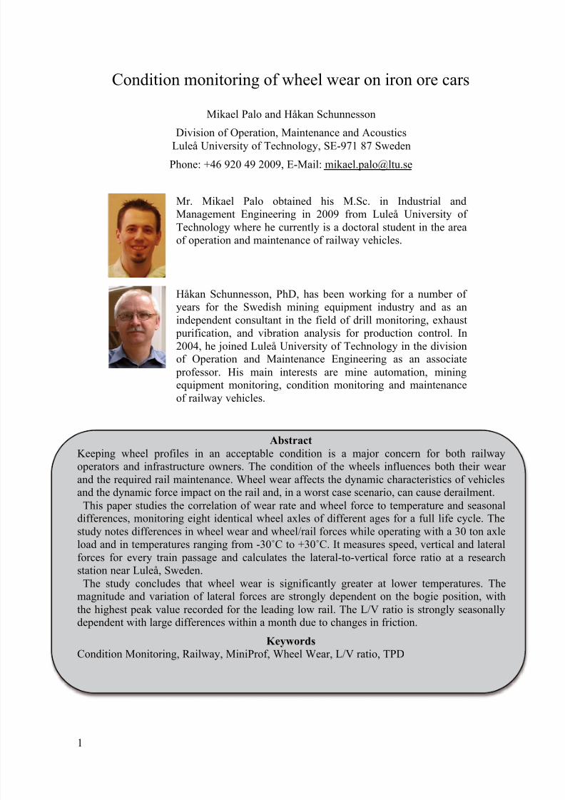
8/10/2019 Condition monitorin g of railway vehicles
http://slidepdf.com/reader/full/condition-monitorin-g-of-railway-vehicles 63/86
1
Condition monitoring of wheel wear on iron ore cars
Mikael Palo and Håkan Schunnesson
Division of Operation, Maintenance and Acoustics
Luleå University of Technology, SE-971 87 Sweden
Phone: +46 920 49 2009, E-Mail: [email protected]
Mr. Mikael Palo obtained his M.Sc. in Industrial and
Management Engineering in 2009 from Luleå University of
Technology where he currently is a doctoral student in the area
of operation and maintenance of railway vehicles.
Håkan Schunnesson, PhD, has been working for a number of
years for the Swedish mining equipment industry and as an
independent consultant in the field of drill monitoring, exhaust
purification, and vibration analysis for production control. In
2004, he joined Luleå University of Technology in the divisionof Operation and Maintenance Engineering as an associate
professor. His main interests are mine automation, miningequipment monitoring, condition monitoring and maintenance
of railway vehicles.
AbstractKeeping wheel profiles in an acceptable condition is a major concern for both railway
operators and infrastructure owners. The condition of the wheels influences both their wear
and the required rail maintenance. Wheel wear affects the dynamic characteristics of vehiclesand the dynamic force impact on the rail and, in a worst case scenario, can cause derailment.
This paper studies the correlation of wear rate and wheel force to temperature and seasonaldifferences, monitoring eight identical wheel axles of different ages for a full life cycle. The
study notes differences in wheel wear and wheel/rail forces while operating with a 30 ton axle
load and in temperatures ranging from -30˚C to +30˚C. It measures speed, vertical and lateral
forces for every train passage and calculates the lateral-to-vertical force ratio at a researchstation near Luleå, Sweden.
The study concludes that wheel wear is significantly greater at lower temperatures. Themagnitude and variation of lateral forces are strongly dependent on the bogie position, with
the highest peak value recorded for the leading low rail. The L/V ratio is strongly seasonallydependent with large differences within a month due to changes in friction.
KeywordsCondition Monitoring, Railway, MiniProf, Wheel Wear, L/V ratio, TPD

8/10/2019 Condition monitorin g of railway vehicles
http://slidepdf.com/reader/full/condition-monitorin-g-of-railway-vehicles 64/86
2
1 INTRODUCTION
Keeping wheel profiles in an acceptable
condition is a major concern for both railway
operators and infrastructure owners. For one
thing, the dynamic behavior of the vehicle is
highly dependent on the shape of the wheel profile. For another, wheel conditions are related
to derailment safety. In addition, a significant percentage of vehicle maintenance cost is
allocated to wheel maintenance.
The interaction between wheel and rail resulting
in material deterioration is a complicated
process, involving vehicle-track dynamics,contact mechanics, friction wear, and lubrication
[1]. The course of events called wear is similarlycomplicated, involving several modes of
material deterioration and contact surface
alteration [2]. Rolling contact fatigue in railway
wheels is increasingly important [3]. Even small
failures or early cracks are costly, requiring
maintenance and possibly causing delays.
To reduce cost and achieve a wheel’s maximumlife span, maintenance practices must be based
on its condition. According to simulations
performed by Braghin et al. [4], re-profilingwheels after 200 000km of service would nearly
double their service life, thus minimizing life
cycle costs. The ability to eliminate non-optimally performing equipment through the use
of wayside detectors can translate directly intoenhanced operations safety, improved asset life
cycle costs, and increased operating efficiency
through fewer unscheduled service disruptions
[5]. Applying condition-based maintenance
requires selecting a proper condition monitoring
system, a database for collecting condition data,and an appropriate data analyzing process to
make maintenance decisions from conditiondata.
One of the most difficult aspects of a condition-
based maintenance strategy is making goodmaintenance decisions based on the available
condition data. In this paper, we use thecorrelation of wear rate to temperature, wheel
position within the bogie, and track force to
pinpoint a cost-effective wheel maintenance
interval.
1.1 Inspection and non-contact conditionmonitoring
An important goal of predictive monitoring is to
prevent failure through the early, reliable, and
cost-effective detection of faults in rolling stock
[6], including the discovery of early cracks [3].Traditional inspection techniques used in therailroad industry, such as drive-by inspections,
are not as accurate and reliable as more rigorous
and quantitative inspection methods [7]. For
example, condition monitoring uses some levelof knowledge of the system of interest to
establish its current condition [8]. To this end,the railway industry uses wayside detection [9],
a technique of detecting specific faults on rolling
stock by interrogating sensors placed along the
sides of tracks. This non-contact method can be
used on trains travelling at track speed. It
provides direct feedback to both operators andtrack owners on the condition of vehicles
passing a wayside monitoring station. A surveymentioned by Stone et al. [10] notes that impact
load detectors are effective tools for monitoring
high impact load-producing wheels. There is
also evidence that in-train inspections
procedures are not as effective as shop
inspections of the identified wheels.
There are several different methods of detectingdynamic force impact on the rail track. The two
most commonly used are strain- and
accelerometer-based systems. Accelerometer-
based systems measure the motion of the rail
resulting from the dynamic load of a passing
wheel [9]. Strain-based systems measure the bending of the rail, as it is a direct measure of
the applied load on the railhead. There are
limitations to both methods. The registeredacceleration method does not give a quantitative
measure of the size of the impact load [11]. The
strain-based system can have difficulty covering
the combined circumference of all wheel
diameters if not extended by sensors covering atleast 3m of the track [12]. High-impact wheels
have an impact force of 400 kN or greater; mostoften they have a flat spot on the tread surface
[7]. Major defects in the tread surface can alsocause high-impact force; these have a higher
probability of leading to catastrophic failure.
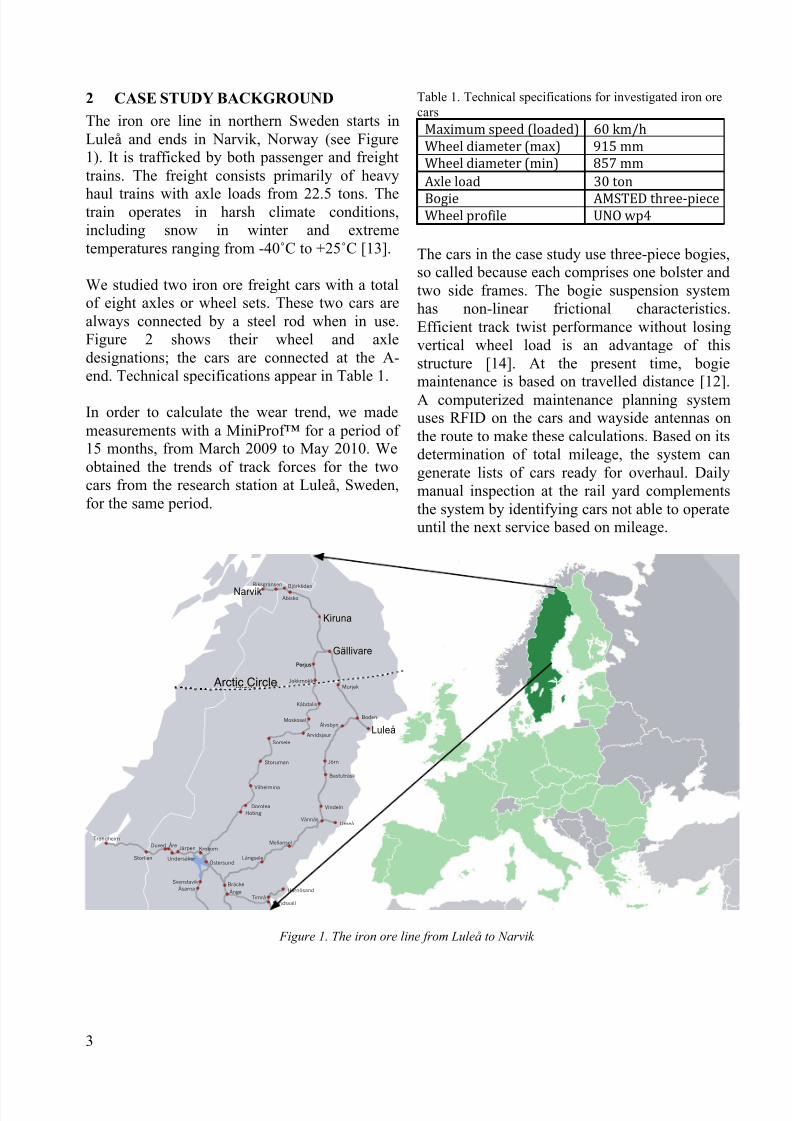
8/10/2019 Condition monitorin g of railway vehicles
http://slidepdf.com/reader/full/condition-monitorin-g-of-railway-vehicles 65/86
3
2 CASE STUDY BACKGROUND
The iron ore line in northern Sweden starts in
Luleå and ends in Narvik, Norway (see Figure1). It is trafficked by both passenger and freight
trains. The freight consists primarily of heavy
haul trains with axle loads from 22.5 tons. Thetrain operates in harsh climate conditions,
including snow in winter and extreme
temperatures ranging from -40˚C to +25˚C [13].
We studied two iron ore freight cars with a totalof eight axles or wheel sets. These two cars are
always connected by a steel rod when in use.
Figure 2 shows their wheel and axle
designations; the cars are connected at the A-
end. Technical specifications appear in Table 1.
In order to calculate the wear trend, we made
measurements with a MiniProf™ for a period of15 months, from March 2009 to May 2010. We
obtained the trends of track forces for the two
cars from the research station at Luleå, Sweden,
for the same period.
Table 1. Technical specifications for investigated iron ore
cars
The cars in the case study use three-piece bogies,so called because each comprises one bolster and
two side frames. The bogie suspension system
has non-linear frictional characteristics.
Efficient track twist performance without losing
vertical wheel load is an advantage of this
structure [14]. At the present time, bogiemaintenance is based on travelled distance [12].
A computerized maintenance planning systemuses RFID on the cars and wayside antennas on
the route to make these calculations. Based on its
determination of total mileage, the system can
generate lists of cars ready for overhaul. Daily
manual inspection at the rail yard complements
the system by identifying cars not able to operateuntil the next service based on mileage.
ARCTIC CIRCLE
Storlien
HärnösandÅsarnaSvenstavik
Sundsvall
Östersund
Krokom
Umeå
Luleå
Timrå
Vännäs
Bastuträsk
Jörn
Älvsbyn
Boden
LångseleUndersåker
Järpen
BräckeÅnge
ÅreDuved
HotingDorotea
Vilhelmina
Storuman
SorseleArvidsjaur
Moskosel
Kåbdalis
Jokkmokk
PorjusPorjus
Mellansel
Vindeln
Murjek
Gällivare
Kiruna
Trondheim
Riksgränsen Björkliden
AbiskoNarvik
Arctic Circle
Luleå
Narvik
Kiruna
Gällivare
Figure 1. The iron ore line from Luleå to Narvik

8/10/2019 Condition monitorin g of railway vehicles
http://slidepdf.com/reader/full/condition-monitorin-g-of-railway-vehicles 66/86
4
Figure 2. Iron ore train car and designation of wheels and axles
3 MEASUREMENT SYSTEMS
3.1 MiniProf™
The measurement system MiniProf™ is used by
many railroads to monitor wheel and rail profiles
[15]. MiniProf™ is one of the most reliable and
accurate monitoring systems. In fact, the results
of other wheel profile monitoring systems areoften compared to MiniProf™ to check theiraccuracy.
The MiniProf™ Wheel (see Figure 4a) has a
sensing element consisting of a magnetic wheelof 12 mm attached to the end of two joint
extensions. It measures the profile with twodegree of freedom, and a computer calculates the
profile in Cartesian coordinates. The resolution
is in thousands of millimeters. During this
calculation it also retrieves the flange thickness
(Sd), flange height (Sh), and flange gradient
(qR) (see Figure 4b).
To measure the wheel profile, the MiniProf™ ismagnetically attached to the wheel. The back
and top of the wheel are used as horizontal andvertical references respectively [15]. Even given
the high accuracy of the instrument itself, therecan be inaccuracies in measurement procedures,
such as dirt or physical inaccuracies at the backof the wheel. Therefore, a calibration must be
done to compare measurements at differenttimes. We used a two-point calibration,
beginning with a vertical adjustment to the top point of the flange, followed by a horizontaladjustment based on the inclined part of the
backside of the flange. Figure 3 shows the procedure.
12.59.5 10 10.5 11 11.5 12
28.46
28.41
28.42
28.43
28.44
28.45
Length (mm)
H e i g h t ( m m )
Vertical alignment
222 4 6 8 10 12 14 16 18 20
29
21
22
23
24
25
26
27
28
Length (mm)
H e i g h t ( m m )
Horizontal alignment
1400 20 40 60 80 100 120
30
-10
0
10
20
Length (mm)
H e i g h t ( m m )
Figure 3. Alignment of profiles between different measurements
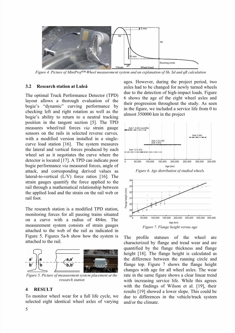
8/10/2019 Condition monitorin g of railway vehicles
http://slidepdf.com/reader/full/condition-monitorin-g-of-railway-vehicles 67/86
5
10 mm
Sh
Sd
Running circle
2 mm
qRFlange Wheel tread
Figure 4. Picture of MiniProf™ Wheel measurement system and an explanation of Sh, Sd and qR calculation
3.2 Research station at Luleå
The optimal Truck Performance Detector (TPD)layout allows a thorough evaluation of the
bogie’s “dynamic” curving performance by
checking left and right rotation as well as the
bogie’s ability to return to a neutral tracking position in the tangent section [5]. The TPD
measures wheel/rail forces via strain gaugesensors on the rails in selected reverse curves,
with a modified version installed in a single-curve load station [16]. The system measures
the lateral and vertical forces produced by each
wheel set as it negotiates the curve where the
detector is located [17]. A TPD can indicate poor
bogie performance via measured forces, angle of
attack, and corresponding derived values as
lateral-to-vertical (L/V) force ratios [16]. Thestrain gauges quantify the force applied to therail through a mathematical relationship between
the applied load and the strain on the rail web or
rail foot.
The research station is a modified TPD station,
monitoring forces for all passing trains situatedon a curve with a radius of 484m. The
measurement system consists of strain gaugesattached to the web of the rail as indicated in
Figure 5. Figures 5a-b show how the system is
attached to the rail.
Figure 5. Picture of measurement system placement at the
research station
4 RESULTTo monitor wheel wear for a full life cycle, we
selected eight identical wheel axles of varying
ages. However, during the project period, twoaxles had to be changed for newly turned wheels
due to the detection of high-impact loads. Figure
6 shows the age of the eight wheel axles and
their progression throughout the study. As seenin the figure, we included a service life from 0 to
almost 350000 km in the project
350,0000 50,000 100,000 150,000 200,000 250,000 300,000
Age (km)
Axle 1,2,4 (43)
Axle 3 (43) Axle 1,2,4 (44)
Axle 3 (44)
Axle 1,3 (44) re profiled
Figure 6. Age distribution of studied wheels
350,0000 50,000 100,000 150,000 200,000 250,000 300,000
34
28
29
30
31
32
33
Age (km)
F l a n g e h e i g h t ( m m )
Figure 7. Flange height versus age
The profile statuses of the wheel arecharacterized by flange and tread wear and are
quantified by the flange thickness and flangeheight [18]. The flange height is calculated as
the difference between the running circle and
flange top. Figure 7 shows the flange height
changes with age for all wheel axles. The wearrate in the same figure shows a clear linear trend
with increasing service life. While this agreeswith the findings of Wilson et al. [19], their
results [19] showed a lower slope. This could bedue to differences in the vehicle/track system
and/or the climate.
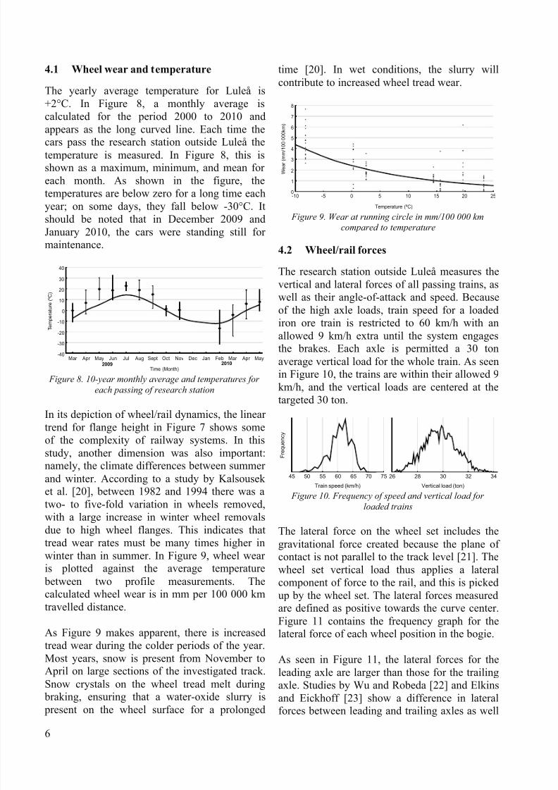
8/10/2019 Condition monitorin g of railway vehicles
http://slidepdf.com/reader/full/condition-monitorin-g-of-railway-vehicles 68/86
6
4.1 Wheel wear and temperature
The yearly average temperature for Luleå is
+2°C. In Figure 8, a monthly average is
calculated for the period 2000 to 2010 and
appears as the long curved line. Each time the
cars pass the research station outside Luleå thetemperature is measured. In Figure 8, this isshown as a maximum, minimum, and mean for
each month. As shown in the figure, the
temperatures are below zero for a long time each
year; on some days, they fall below -30°C. It
should be noted that in December 2009 and
January 2010, the cars were standing still formaintenance.
Mar Apr May Jun Jul Aug Sept Oct Nov Dec Jan Feb Mar Apr May
40
-40
-30
-20
-10
0
10
20
30
Time (Month)
T e m p e r a t u r e ( º C )
2009 2010
Figure 8. 10-year monthly average and temperatures for
each passing of research station
In its depiction of wheel/rail dynamics, the lineartrend for flange height in Figure 7 shows some
of the complexity of railway systems. In this
study, another dimension was also important:namely, the climate differences between summer
and winter. According to a study by Kalsouseket al. [20], between 1982 and 1994 there was a
two- to five-fold variation in wheels removed,
with a large increase in winter wheel removals
due to high wheel flanges. This indicates that
tread wear rates must be many times higher in
winter than in summer. In Figure 9, wheel wearis plotted against the average temperature
between two profile measurements. Thecalculated wheel wear is in mm per 100 000 km
travelled distance.
As Figure 9 makes apparent, there is increased
tread wear during the colder periods of the year.
Most years, snow is present from November toApril on large sections of the investigated track.
Snow crystals on the wheel tread melt during braking, ensuring that a water-oxide slurry is
present on the wheel surface for a prolonged
time [20]. In wet conditions, the slurry will
contribute to increased wheel tread wear.
25-10 -5 0 5 10 15 20
8
0
1
2
3
4
5
6
7
Temperature (ºC)
W e a r ( m m / 1 0 0 0 0 0 k m )
Figure 9. Wear at running circle in mm/100 000 km
compared to temperature
4.2 Wheel/rail forces
The research station outside Luleå measures thevertical and lateral forces of all passing trains, as
well as their angle-of-attack and speed. Because
of the high axle loads, train speed for a loaded
iron ore train is restricted to 60 km/h with an
allowed 9 km/h extra until the system engagesthe brakes. Each axle is permitted a 30 ton
average vertical load for the whole train. As seenin Figure 10, the trains are within their allowed 9
km/h, and the vertical loads are centered at the
targeted 30 ton.
7545 50 55 60 65 70
Train speed (km/h)
F r e q u e n c y
3426 28 30 32
Vertical load (ton)
Figure 10. Frequency of speed and vertical load for
loaded trains
The lateral force on the wheel set includes the
gravitational force created because the plane of
contact is not parallel to the track level [21]. Thewheel set vertical load thus applies a lateral
component of force to the rail, and this is picked
up by the wheel set. The lateral forces measuredare defined as positive towards the curve center.
Figure 11 contains the frequency graph for thelateral force of each wheel position in the bogie.
As seen in Figure 11, the lateral forces for the
leading axle are larger than those for the trailing
axle. Studies by Wu and Robeda [22] and Elkins
and Eickhoff [23] show a difference in lateralforces between leading and trailing axles as well

8/10/2019 Condition monitorin g of railway vehicles
http://slidepdf.com/reader/full/condition-monitorin-g-of-railway-vehicles 69/86
7
as between the high and low rail. The leading
axle in Figure 11 shows a clear difference between the high and low rail. Also visible is the
fact that the trailing axle creates lower lateral
forces, possibly because it runs closer to the
radial position [24].In Figure 11, the leading high rail has forces up
to 100 kN. That is expected since as Barbosanotes [25], this is the first wheel into the curve.
That the leading low rail has forces from -10 to130 kN is unexpected, but according to Elkins
[26], it can be caused by large angles-of-attack.
4.3 L/V force ratio
Flange climb derailment is the result of
combined lateral and vertical wheel/rail
interaction forces [27]. Nadal’s formula [28] is
often used to determine the limit of the L/V ratio
and is based on a simple force balance to
calculate the ratio before a derailment occurs. Ifthe friction coefficient between wheel and rail is
µ and the wheel flange angle is α, as shown inFigure 12, changes in wheel and rail wear will
influence α. The L/V ratio is given by the
following formula:
L
V =
tanα− µ
1 + µ tanα
(1)
Figure 12. Flange forces at wheel climb
Tests conducted on rail vehicles as well as roller
rig laboratory tests have frequently shown L/Vratios in excess of Nadal’s limit withoutderailment [27]. The ratio for the lead outer
wheel is indicative of the likelihood ofderailment [16, 29], and there is a large curve
radius dependency. According to Coe et al. [16],
high-rail L/V ratios in the range of 0.3 to 0.4 are
indicative of a poorly steering vehicle with a
hard flange contact. In a study by Magel et al.
[21], high L/V ratios of 0.7 to 0.8 appeared inone to two points per thousand.
.
140-55 -40 -20 0 20 40 60 80 100 120
140-55 -40 -20 0 20 40 60 80 100 120140-55 -40 -20 0 20 40 60 80 100 120
140-55 -40 -20 0 20 40 60 80 100 120
Lateral force (kN) Lateral force (kN)
F r e q u e n c y
F r e q u e n c y
-5
Figure 11. Frequency of lateral forces from different positions within bogie

8/10/2019 Condition monitorin g of railway vehicles
http://slidepdf.com/reader/full/condition-monitorin-g-of-railway-vehicles 70/86
8
The vertical forces of the iron ore cars
considered in this study are normally distributedwith a mean of about 30 ton (see Figure 10). The
lateral forces, however, differ significantly
between the different wheel positions (see Figure
11). The investigated train cars operate in anarea with large temperature variations over the
year (see Figure 8). Figure 13 presents the L/Vratios for a year for one wheel when it is on a
leading high rail. The figure clearly showsseasonal differences that may affect the wheel’s
wear conditions.
Mar Apr May Jun Jul Aug Sep Oct Nov
0.8
0.4
0.45
0.5
0.55
0.6
0.65
0.7
0.75
Time (month)
L / V r a t i o
Figure 13. L/V ratio on leading high rail
Changes in the L/V ratio are related to changesin friction between wheel and rail (see formula
1). The friction conditions may vary fromadequate adhesion with dry and clean steel-on-
steel surface to low adhesion due to
contamination, humidity, and applied friction
modifiers [18]. Rail lubrication can significantly
affect lateral forces when curving [22]. The
decreasing trend seen from April to July takes place during a period of mostly dry weather and
increasing temperatures. During the warmseason, wayside wheel/rail curve lubricators are
used. The driver can also use sand if the friction
is too low. From August, the temperature starts
to drop and the weather changes; hence, theincreasing trend.
5 CONCLUSION
From the preceding measurements, we concludethe following:
Wheel wear is greater at lower temperatures, and
there is an evident trend. At -10°C there is five
times more wear than at +25°C. Even for
temperatures around 0°C, there is evidence of
large differences in wear between differentwheels. This makes the issue of wheel wear andtemperature extremely intriguing. Further
investigation calls for at least a full year of
continuous measurement and a larger populationof wheels.
The leading axle in a bogie has larger lateral
forces than trailing axles, as mentioned by Wuand Robeda [22], and Elkins and Eickhoff [23].
It is also evident that lateral forces on the highrail are generally higher and have narrower
spectra than those on the low rail. The mostalarming issue amongst the data is that lateral
forces on the leading low-rail can exceed 130
kN. This corresponds to an L/V of 0.9,
indicating very poor steering and the possibility
of derailment.
The L/V ratio is clearly seasonally dependent.According to Nadal’s formula, the L/V isdependent on both µ and α. Since friction
changes for each passage, this is an indicator of
trend changes and of large differences within a
month. Wheel and rail wear change over time,
but neither occurs quickly. This issue needs
further study on a larger population of wheels.
6 ACKNOWLEDGEMENT
The authors would like to thank Dan Larsson at
Damill AB for his help, particularly his usefuldiscussions about the research station. We would
also like to thank Per-Olof Larsson-Kråik from
Swedish Traffic Administration for his valuable
comments and input.
7 REFERENCES
[1] Enblom R. and Berg M., (2005)
“Simulation of railway wheel profiledevelopment due to wear – influence of
disc braking and contact environment”,
Wear 258, 1055-1063
[2] Enblom R. and Stichel S., (2010),
“Industrial implementation of novel
procedures for the prediction of railwaywheel surface deterioration”, Wear, (2010)
doi:10.1016/j.wear.2010.10.037[3] Ekberg, A., Kabo, E. and Andersson H.,
(2002) “An engineering model for
prediction of rolling contact fatigue of
railway wheels”, Fatigue & Fracture of
Engineering Materials & Structures, 25 pp899-909

8/10/2019 Condition monitorin g of railway vehicles
http://slidepdf.com/reader/full/condition-monitorin-g-of-railway-vehicles 71/86
9
[4] Braghin, F., Lewis, R., Dwyer-Joyce R.S.
and Bruni S. (2006) “A mathematicalmodel to predict railway wheel profile
evolution due t wear”, Wear 261 pp 1253-
1264
[5] Keegan, L.S., Blank, R.W., D’Aoust, D.,Earl, D. and Ford D. (2001) “Wayside
Truck Performance DetectorDevelopment” in Proceedings of 2001
ASME International MechanicalEngineering Congress and Exposition, pp
157-163
[6] Bladon, K., Rennison, D., Izbinsky, G.,
Tracy, R. and Bladon, T. (2004)
“Predictive Condition Monitoring of
Railway Rolling Stock”, Railway
Engineering Conference, Darwin 20-23June 2004
[7] Stratman, B. Liu, Y. and Mahadevan, S.
(2007). “Structural Health Monitoring of
Railroad Wheels Using Wheel Impact
Load Detectors”, Journal of Failure
Analysis and Prevention, 7, pp 218-225
[8] Charles, G., Dixon, R. and Goodall R.(2008) “Condition Monitoring Approaches
to Estimating Wheel-Rail Profile”,Proceedings of the UKACC Control
Conference, Manchester,[9] Barke, D. and Chiu, W.K. (2005)
“Structural Health Monitoring in the
Railway Industry: A Review”, Structural
Health Monitoring, 4(1), pp 81-94
[10] Stone, D.H. Kalay, S.F. Tajaddini A.
(1992). “Statistical Behaviour of WheelImpact Load Detectors to Various Wheel
Defects”, International Wheelset Congress
Sydney Australia. Pp 9-13.
[11] Nielsen, J.C.O and Johansson, A (2000).
“Out-of-round railway wheels – a literaturesurvey”. Proceedings of the Institution ofMechanical Engineering, 214(2), pp 79-91.
[12] Palo, M., Arasteh Khouy, I., Schunnesson,H. and Larsson D. (2010) “Condition
monitoring of train wheel wear and track
forces: A case study”, Proceedings of the
1st international workshop and Congress
on eMaintenance, Luleå University of
Technology
[13] Kumar, S., Espling, U. and Kumar, U.
(2008), “A holistic procedure for railmaintenance in Sweden”, Journal of Rail
and Rapid Transit: Proceedings of the
Institution of Mechanical Engineers, Part F
[14] Tournay, H. (2001), “Guidelines to Best
Practices for Heavy Haul railway
Operations: wheel-rail interface issues”,
Chapter 2, International Heavy HaulAssociation, USA.
[15] Esveld, C. and Gronskov L. (1996).MiniProf Wheel and Rail Measurement.
2nd Mini Conf. On Contact Mechanics andWear of Rail/Wheel Systems, Budapest
[16] McGuire, B., Sarunac, R. and Wiley R.B.
(2007) “Wayside Wheel/Rail Load
Detector Based Rail Car Preventive
Maintenance”, in Proceedings of the
ASME/IEEE Joint Rail Conference &
Internal Combustion Engine SpringTechnical Conference
[17] Wolf G.P. and Peterson F.J. (1998)
“Application and validation of the
Automated truck performance
measurements system” in Proceedings of
the 1998 ASME/IEEE Joint Railroad
Conference, pp 127-134
[18] Enblom R. (2009) “Deterioration
mechanisms in the wheel-rail interfacewith focus on wear prediction: a literature
review”, Vehicle System Dynamics, 47 (6) pp 661-700
[19] Wilson, N., Wu, H., Tournay H. and Urban
C. (2010) “Effects of wheel/rail contact
patterns and vehicle parameters on lateralstability”, Vehicle System Dynamics, 48
(1) pp 487-503[20] Kalousek, J., Magel, E., Strasser, J.
Caldwell, W.N., Kanevsky G. and Blevins
B. (1996) “Tribological interrelationship of
seasonal fluctuations of freight car wheel
wear, contact fatigue shelling andcomposition brakeshoe consumption”,Wear, 191 pp 210-218
[21] Magel, E., Tajaddini, A., Trosino M andKalousek J. (2008) “Traction forces, wheel
climb and damage in high-speed railway
operations”, Wear, 265 pp 1446-1451
[22] Wu H. and Robeda J. (2004) “Effects of
bogie centre plate lubrication on vehicle
curving and lateral stability” VehicleSystem Dynamics, Suppl. 41 pp 292-301
[23] Elkins J.A. and Eickhoff B.M. (1982)“Advances in Nonlinear Wheel/Rail Force

8/10/2019 Condition monitorin g of railway vehicles
http://slidepdf.com/reader/full/condition-monitorin-g-of-railway-vehicles 72/86
10
Prediction Methods and Their Validation”
Journal of Dynaimc Systems,Measurement and Control, 104 pp 133-142
[24] Elkins J.A. and Allen R.A. (1982)
“Verification of a transits Vehicle’s
Curving Behavior and ProjectedWheel/Rail Wear Performance” Journal of
Dynamic Systems, Measurement andControl, 104 pp 247-255
[25] Barbosa R.S. (2009), “Safety of a railwaywheelset – derailment simulation with
increasing lateral force” Vehicle System
Dynamics, 47:12 pp 1493-1510
[26] Elkins J. (1995), “Prediction of Rail Roll
Deflections due to Adjacent Trucks”
Vehicle System Dynamics, 24 pp 251-264
[27] Elkins J. and Wu H (1999), “Angle ofAttack and Distance-Based Criteria forFlange Climb Derailment” Vehicle System
Dynamics, Suppl. 33 pp 293-305
[28] Nadal M.J. (1908) “Locomotives a
Vapeur” Collection Encyclopédie
Scientifique, Bibliothéque de Mécanique et
Génie, 186
[29] Dukkipati, R.V. and Narayana Swamy S.
(2001) “Non-linear stedy-state curvinganalysis of some unconventional rail
trucks”, Mechanism and Machine Theory36, pp 507-521

8/10/2019 Condition monitorin g of railway vehicles
http://slidepdf.com/reader/full/condition-monitorin-g-of-railway-vehicles 73/86
CP A P E R C
M. Palo, H. Schunnesson, and P.-O. Larsson-Kråik, “ Maintainability inextreme seasonal weather conditions,”Presented and published in Proceedings of Technical Session of Inter-national Heavy Haul Association, 2011.
61

8/10/2019 Condition monitorin g of railway vehicles
http://slidepdf.com/reader/full/condition-monitorin-g-of-railway-vehicles 74/86
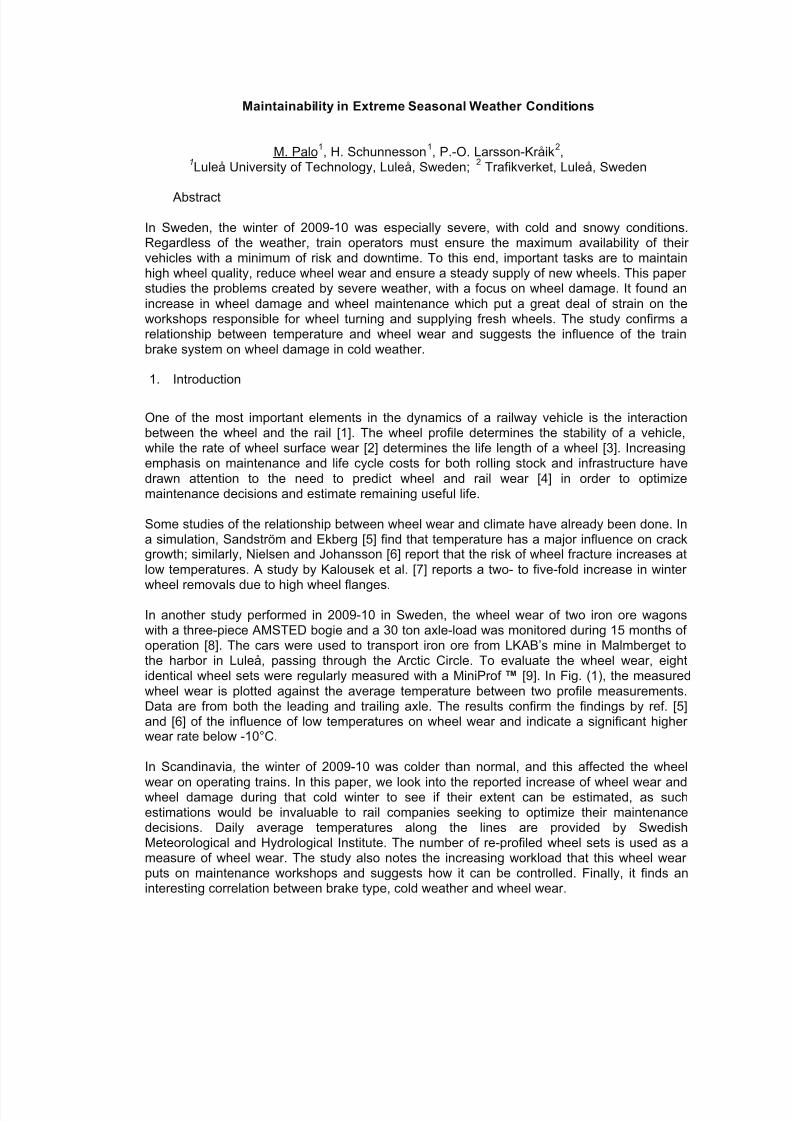
8/10/2019 Condition monitorin g of railway vehicles
http://slidepdf.com/reader/full/condition-monitorin-g-of-railway-vehicles 75/86
Maintainability in Extreme Seasonal Weather Conditions
M. Palo1, H. Schunnesson1, P.-O. Larsson-Kråik2,1Luleå University of Technology, Luleå, Sweden; 2 Trafikverket, Luleå, Sweden
Abstract
In Sweden, the winter of 2009-10 was especially severe, with cold and snowy conditions.Regardless of the weather, train operators must ensure the maximum availability of theirvehicles with a minimum of risk and downtime. To this end, important tasks are to maintainhigh wheel quality, reduce wheel wear and ensure a steady supply of new wheels. This paperstudies the problems created by severe weather, with a focus on wheel damage. It found anincrease in wheel damage and wheel maintenance which put a great deal of strain on theworkshops responsible for wheel turning and supplying fresh wheels. The study confirms arelationship between temperature and wheel wear and suggests the influence of the trainbrake system on wheel damage in cold weather.
1. Introduction
One of the most important elements in the dynamics of a railway vehicle is the interactionbetween the wheel and the rail [1]. The wheel profile determines the stability of a vehicle,while the rate of wheel surface wear [2] determines the life length of a wheel [3]. Increasingemphasis on maintenance and life cycle costs for both rolling stock and infrastructure havedrawn attention to the need to predict wheel and rail wear [4] in order to optimizemaintenance decisions and estimate remaining useful life.
Some studies of the relationship between wheel wear and climate have already been done. Ina simulation, Sandström and Ekberg [5] find that temperature has a major influence on crackgrowth; similarly, Nielsen and Johansson [6] report that the risk of wheel fracture increases atlow temperatures. A study by Kalousek et al. [7] reports a two- to five-fold increase in winter
wheel removals due to high wheel flanges.
In another study performed in 2009-10 in Sweden, the wheel wear of two iron ore wagonswith a three-piece AMSTED bogie and a 30 ton axle-load was monitored during 15 months ofoperation [8]. The cars were used to transport iron ore from LKAB’s mine in Malmberget tothe harbor in Luleå, passing through the Arctic Circle. To evaluate the wheel wear, eightidentical wheel sets were regularly measured with a MiniProf ™ [9]. In Fig. (1), the measuredwheel wear is plotted against the average temperature between two profile measurements.Data are from both the leading and trailing axle. The results confirm the findings by ref. [5]and [6] of the influence of low temperatures on wheel wear and indicate a significant higherwear rate below -10°C.
In Scandinavia, the winter of 2009-10 was colder than normal, and this affected the wheel
wear on operating trains. In this paper, we look into the reported increase of wheel wear andwheel damage during that cold winter to see if their extent can be estimated, as suchestimations would be invaluable to rail companies seeking to optimize their maintenancedecisions. Daily average temperatures along the lines are provided by SwedishMeteorological and Hydrological Institute. The number of re-profiled wheel sets is used as ameasure of wheel wear. The study also notes the increasing workload that this wheel wearputs on maintenance workshops and suggests how it can be controlled. Finally, it finds aninteresting correlation between brake type, cold weather and wheel wear.

8/10/2019 Condition monitorin g of railway vehicles
http://slidepdf.com/reader/full/condition-monitorin-g-of-railway-vehicles 76/86
25-10 -5 0 5 10 15 20
8
0
1
2
3
4
5
6
7
Temperature (ºC)
W e a r ( m m / 1 0 0
0 0 0 k m )
Figure 1. Wear at running circle in mm/100 000 km versus temperature
2. Wheel wear
2.1 Wheel deterioration
The interaction between wheel and rail resulting in material deterioration is a complicatedprocess, involving vehicle-track dynamics, contact mechanics, friction wear and lubrication[1]. The course of events called wear is similarly complicated, involving several modes ofmaterial deterioration and contact surface alteration [10]. Two important deteriorationmechanisms are wear and rolling contact fatigue (RCF). Friction heating occurs when traincars reduce speed by using their pads against the running surface of the wheels (i.e.,braking). When the wheel surface layer is frictionally heated, and this is followed by the rapidcooling of the body of the wheel itself, there is an increased risk of forming martensite [7]. Asmartensite is much harder and more brittle than the surrounding material, it can break andinitiate cracks. As for RCF, according to Stone et al. [11] freight car wheels in service maydevelop tread irregularities in the form of slid-flats, shells or spalls. Any of these irregularitiescan cause high wheel impact, but the first is the most common [12]. Another cause of highimpact leading to RCF is a major defect in the tread surface; this has a higher probability ofleading to catastrophic failure.
Railway wheel flats or slid-flats are a well known problem in railway engineering [13]. Wheelflats are formed when a wheel set is locked and skids along the rail. The friction betweenwheel and rail causes the surface of the wheel to become flat instead of round [12]. Wheelflats have mechanical singularities that frequently serve as sites for the formation of additionalflats and resulting shells [14]. A martensitic layer several millimeters deep can be formed aswell [7]. Thin martensitic layers may crack and wear off harmlessly; thicker ones inevitablyspall or shell the wheel [7].
Shelling is a term normally used for all types of subsurface induced cracks [6]. Wheel shellingis defined as the loss of relative large (greater than 5 mm) pieces of metal from the wheeltread as the result of contact fatigue [15]. Typically, shelling cracks grow at an acute angle tothe surface. Impact load can affect shelling in both crack initiation and crack propagationmodes [14].
Spalling is the term used for the RCF phenomenon occurring when surface cracks of thermalorigin meet, resulting in part of the wheel coming away from the tread [6]. It is associated withcracking induced by high transformation stress caused by surface martensite formation [15].Cracks from spalling form both perpendicular and parallel to the wheel tread surface.
2.2 Inspection and non-contact condition monitoring
An important goal of predictive monitoring is to allow early, reliable and cost-effectivedetection of faults in rolling stock [16], including the discovery of early cracks [17]. Inspection

8/10/2019 Condition monitorin g of railway vehicles
http://slidepdf.com/reader/full/condition-monitorin-g-of-railway-vehicles 77/86
techniques traditionally used in the railroad industry, such as drive-by inspections, are not asaccurate or reliable as more rigorous and quantitative inspection methods [12]. For example,condition monitoring uses some level of knowledge of the system of interest to establish itscurrent condition [1]. To this end, the railway industry uses wayside detection [2], a techniqueof detecting specific faults on rolling stock through the use of interrogating sensors placedalong the sides of the track, usually at a wayside monitoring station. This non-contact method
of monitoring can be used on trains travelling at track speed; it provides direct feedback totrack owners and operators of the condition of vehicles passing the monitoring station. Asurvey mentioned by Stone et al. [11] notes that impact load detectors are effective tools formonitoring high impact load producing wheels, with an impact force of 400 kN or greater [12].
3. Case background
Northern Sweden has harsh climatic conditions, with cold snowy winters and extremetemperatures ranging from -40˚C to +30˚C [18]. An example of the extra stresses that ice andsnow put on wheels can be seen in Fig. (2). In Sweden, train operators need to carefully plantheir maintenance to take environment and weather conditions into account.
During the warm season, from May to September, wayside wheel/rail curve lubricators are
used on the railway lines in northern Sweden. The driver can use sand if the friction gets toolow.
Figure 2. Train wheel covered in snow
In the investigated area in northern Sweden, as shown in Fig. (3), both the steel shuttle trainand the iron ore train operate with high axle loads. The latter transports iron ore pellets fromLKAB’s mines in Kiruna and Malmberget to the harbors in Narvik and Luleå. The formertransports steel slabs (plates) from Luleå to Borlänge in the center of Sweden. Table (1)compares the axle load and the top speed (when loaded).
Table 1. Comparison of iron ore and steel shuttle wagonsIron ore Steel shuttle
Axle load 30 t 22.5 t
Top speed 60 km/h 100 km/h

8/10/2019 Condition monitorin g of railway vehicles
http://slidepdf.com/reader/full/condition-monitorin-g-of-railway-vehicles 78/86
ARCTIC
CIRCLE
Storlien
Härnösand
Mora
Orsa
Tandsjöborg
Sveg
ÅsarnaSvenstavik
Charlotten-berg
Borlänge
Falun
Sandviken
Uppsala
Gävle
Sundsvall
Östersund
Krokom
Umeå
Oslo
Luleå
Timrå
Vännäs
Bastuträsk
Jörn
Älvsbyn
Boden
LångseleUndersåker
Järpen
Bräcke
Ljusdal
Järvsö Hudiksvall
Söderhamn
Tierp
Sunne Hällefors
Torsby
Sala
AvestaKrylbo
Rättvik
Leksand
Ludvika
Fagersta
Malung
Vansbro
Bollnäs
Ockelbo
Storvik
Ånge
ÅreDuved
HotingDorotea
Vilhelmina
Storuman
Sorsele
Arvidsjaur
Moskosel
Kåbdalis
Jokkmokk
PorjusPorjus
Mellansel
Vindeln
Murjek
Gällivare
Kiruna
Trondheim
Riksgränsen Björkliden
Abisko
Narvik
Lilleström
Kongsvinger
Arctic Circle
Luleå
Narvik
Kiruna
Borlänge
Figure 3. Map of the investigated area, showing the Swedish railroad network with weatherstations marked by a star
Table (2) depicts the shipped volume of iron ore pellets and production volume of steel platesfor the last 6 years. The table shows a slow, steady increase in production from 2004 to 2007.Due to the global recession, the production of both iron ore pellets and steel plates stoppedalmost completely during Autumn 2008. During the second half of 2009, both companiesreturned to normal production, but the annual production rate remained low for 2009.
Table 2. Shipping volume for iron ore and production volume for steel plates, in MtonIron ore Steel plate
2004 22.8 4.542005 23.2 4.50
2006 23.3 4.682007 25.1 4.78
2008 22.7 4.46
2009 18.7 2.80
In Sweden, only two workshops do wheel maintenance, one in Gothenburg and the other inLuleå. In this paper, only data from the northern workshop in Luleå are used (Fig. 3). Themajority of wheel maintenance at the workshop in Luleå is done on iron ore wagons and steel
shuttle wagons; there is also a wheel pool to service trains transporting goods and passengertrains.
3.1 Weather information
In the investigated area (Fig. 3), there are large differences in climate and temperature. In thenorthern part of the region, the cold normally arrives earlier and stays longer. The study usesaverage values for daily temperature and humidity, tracking data from 13 different weatherstations along the track, see Fig. (3) and Table (3).
Table 3. Weather stations used.1 – Borlänge 4 – Delsbo 7 – Petisträsk 10 – Älvsbyn 13 – Rensjön2 – Åmot 5 – Torpshammar 8 – Umeå 11 – Gällivare
3 – Delsbo 6 – Hemling 9 – Norsjö 12 – Kiruna

8/10/2019 Condition monitorin g of railway vehicles
http://slidepdf.com/reader/full/condition-monitorin-g-of-railway-vehicles 79/86
The steel train from Borlänge passes weather stations 1 through 10; the iron ore train passesstations 11 to 13 (Fig. 3 and Table 1).
The following formula is used to calculate an annual temperature factor for each year;
∑ (Temp – Templim) (for all (Temp ≤ Templim))1 October
30 April
Temperature factor =
(Eq. 1)Where:Temp = daily temperature average
Templim= temperature limit
The temperature limit is set to -10°C. The temperature factor is the number of days over thetime period when the average temperature is lower than the temperature limit times thenumber of degrees Celsius. A larger negative value indicates a colder winter than a smallervalue.
Fig. (4) presents results from three weather stations for 10 consecutive years. The stations
are Åmot (2) located in the south close to Borlänge, Hemling (6) and Älvsbyn (10) locatedclose to Luleå. The figure shows a significant difference between the southern and thenorthern part of the track, as the temperature factor for Älvsbyn is, on average, five timeshigher than the factor for Åmot. In Åmot, the temperature factor is normally between 0 and150, indicating very few days with temperatures below -10°C, while Älvsbyn has temperaturesunder the limit several months of the year. The normal climatic conditions mean that the steeltrain moves from the colder northern temperatures towards the warmer temperatures in thesouth, while the iron ore train operates continuously in a cold climate with only minordifferences.
00/01 01/02 02/03 03/04 04/05 05/06 06/07 07/08 08/09 09/10
0
-650
-600
-550
-500
-450
-400
-350
-300
-250
-200
-150
-100
-50
Time (winters)
T e m p e r a t u r e f a c t o r ( l i m i t - 1 0 º C )
Weather stationsfrom south to north
2
6
10
Figure 4. Differences for three weather stations going from the south to north
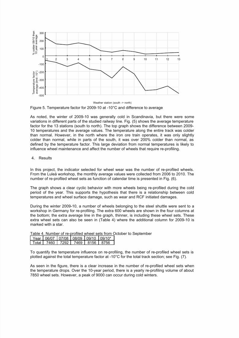
8/10/2019 Condition monitorin g of railway vehicles
http://slidepdf.com/reader/full/condition-monitorin-g-of-railway-vehicles 80/86
131 2 3 4 5 6 7 8 9 10 11 12
300
-500
-400
-300
-200
-100
0
100
200
Weather station (south -> north)
T e m p e r a t u r e f a c t o r
%
c o l d e r 0 9 / 1 0 t h a n
1 0 y e a r a v e r a g e
a v e r a g e ( l i m i t - 1 0 ° )
Figure 5. Temperature factor for 2009-10 at -10°C and difference to average
As noted, the winter of 2009-10 was generally cold in Scandinavia, but there were somevariations in different parts of the studied railway line. Fig. (5) shows the average temperaturefactor for the 13 stations (south to north). The top graph shows the difference between 2009-10 temperatures and the average values. The temperature along the entire track was colderthan normal. However, in the north where the iron ore train operates, it was only slightlycolder than normal, while in parts of the south, it was over 200% colder than normal, asdefined by the temperature factor. This large deviation from normal temperatures is likely toinfluence wheel maintenance and affect the number of wheels that require re-profiling.
4. Results
In this project, the indicator selected for wheel wear was the number of re-profiled wheels.From the Luleå workshop, the monthly average values were collected from 2006 to 2010. The
number of re-profiled wheel sets as function of calendar time is presented in Fig. (6).
The graph shows a clear cyclic behavior with more wheels being re-profiled during the coldperiod of the year. This supports the hypothesis that there is a relationship between coldtemperatures and wheel surface damage, such as wear and RCF initiated damages.
During the winter 2009-10, a number of wheels belonging to the steel shuttle were sent to aworkshop in Germany for re-profiling. The extra 600 wheels are shown in the four columns atthe bottom; the extra average line in the graph, thinner, is including these wheel sets. Theseextra wheel sets can also be seen in (Table 4) where the additional column for 2009-10 ismarked with a star.
Table 4. Number of re-profiled wheel sets from October to September
Year 06/07 07/08 08/09 09/10 09/10*Total 7460 7292 7469 8156 8756
To quantify the temperature influence on re-profiling, the number of re-profiled wheel sets isplotted against the total temperature factor at -10°C for the total track section; see Fig. (7).
As seen in the figure, there is a clear increase in the number of re-profiled wheel sets whenthe temperature drops. Over the 10-year period, there is a yearly re-profiling volume of about7850 wheel sets. However, a peak of 9000 can occur during cold winters.

8/10/2019 Condition monitorin g of railway vehicles
http://slidepdf.com/reader/full/condition-monitorin-g-of-railway-vehicles 81/86
Jan-06 Jun-06 Nov-06 Apr-07 Sep-07 Feb-08 Jul-08 Dec-08 May-09 Oct-09 Mar-10 Aug-10
1300
0
100
200
300
400
500
600
700
800
900
1000
1100
1200
Time (months)
R e p r o f i l e d w h e e l s e t s
Mar-06
Mar-07
Jan-08
Mar-09 Mar-10
External
Figure 6. Number of wheels re-profiled per month from January 2006 to September 2010
88007200 7400 7600 7800 8000 8200 8400 8600
-500
-5500
-4500
-3500
-2500
-1500
Number of re-profiled wheel sets
T e m p e r a t u r e f a c t o r ( l i m i t - 1 0 º C )
Figure 7. Number of re-profiled wheel sets as a function of degree-days
During the project, we conducted a detailed interview survey of key planning personnel at thewheel workshop in Luleå. The interviews provided anecdotal evidence that in coldtemperature operations, RCF is the dominant wheel surface damage, including shelling andspalling; there is almost no other wheel damage. Seasonal statistics from the workshopindicate that this type of damaged wheel starts to appear about two weeks after the first fewdays of weather below -10°C. The majority of wheels with shelling or spalling are from thesteel shuttle; the iron ore trains almost never experience this kind of damage.
The iron ore train and the steel train also differ in when wheels are sent for re-profiling. Thesteel shuttle sends more wheels at the start of winter. The iron ore wheels start to appeararound March, when there are fewer wheels from the steel train. During spring and summerthe damage is mostly tread wear for both.
Both the iron ore and the steel shuttle car have the same wheel material, but to reduce trainspeed, the steel shuttle cars use cast-iron blocks and the iron ore cars use composite blocks.
5. Discussion
The winter of 2009-10 was colder than normal in Sweden, and the whole country wascovered in snow for longer than usual. However, the temperature deviation in the investigated
geographical areas varied significantly. Compared to the average temperatures, there weremany more cold days in the south than in the north, as shown in Fig. (4,5).

8/10/2019 Condition monitorin g of railway vehicles
http://slidepdf.com/reader/full/condition-monitorin-g-of-railway-vehicles 82/86
The study shows that temperature change impacts the maintenance and the number of re-profiled wheels, and it confirms the relationship between temperature and wheel wear. Thewear rate increases as temperatures decrease.
Wheel surface damage in low temperature and snow conditions are reported by otherrailways operating in cold climates, and this has been linked to braking systems. Tracks
covered by snow and the subsequent swirl snow created by the moving train will lead to thedeposit of snow crystals on the wheel treads, whose temperatures usually exceed 0°C, duringbraking. When cast-iron braking blocks are used, the melted snow leaves a film of water-oxide slurry on the wheel surface for prolonged periods of time; hence, increased surfacedamage is observed [7].
Each train type has a different braking system. The steel shuttle uses mechanical brakes onthe locomotive and on every car; these brakes generate friction heating which, in combinationwith the rapid cooling of all wheels in the cold weather, initiates cracks. The iron ore operationengages the electro dynamic brakes of the locomotive 70-80% of the time, thereby reducingthe frictional heating of car wheels and considerably lessening the cold-weather damage.
Out of all wheel damage reported in this study, shelling and spalling generate the greatest
loss of wheel diameter when re-profiling, due to the crack growth rate. During winter and insnowy conditions, micro-cracks can grow in size and length, increasing the hazard by makingthe wheel either shell or spall. In the summer and dry weather conditions, tread wear is moresignificant.
Another interesting finding is the difference between the iron ore train and the steel train as towhen wheels are sent for re-profiling. The steel shuttle sends more wheels at the start ofwinter; the iron ore wheels start to appear around March when there are fewer wheels fromthe steel train. Arguably, using the mechanical brakes of the train cars, instead of locomotivebreak, increase the risk of major wheel damage.
Both shelling and spalling are difficult to detect with traditional inspections or waysidemonitoring until it is too late for preventive maintenance.
6. Conclusion
• In low temperatures, an increased number of wheels are re-profiled, confirming therelationship between cold temperature and wheel surface damage.
• RCF, with spalling and shelling, is the dominant wheel surface damage during coldtemperature operations.
• Further investigation of the influence of the train braking system on crack initiationand wheel wear is needed.
7. Acknowledgement
The authors would like to thank Thomas Aro at DUROC for providing data and commentary.Luleå Railway Research Center (JVTC) is gratefully acknowledged for its financial support.
8/10/2019 Condition monitorin g of railway vehicles
http://slidepdf.com/reader/full/condition-monitorin-g-of-railway-vehicles 83/86
8. References
[1] G. Charles, R. Dixon, R. Goodall, Condition Monitoring Approaches to EstimatingWheel-Rail Profile, Proceedings of the UKACC Control Conference, Manchester,(2008)
[2] D. Barke, W.K. Chiu, Structural Health Monitoring in the Railway Industry: A Review,
Structural Health Monitoring 4 (1) (2005) 81-94[3] F. Braghin, R. Lewis, R.S. Dwyer-Joyce, S. Bruni, A mathematical model to predict
railway wheel profile evolution due to wear, Wear 261 (2006) 1253-1264
[4] R. Enblom and M. Berg Simulation of wailway wheel profile development due to wear –influence of disc braking and contact environment, Wear 258 (2005) 1055-1063
[5] J. Sandström, A. Ekberg, Predicting crack growth and risk of rail breaks due to wheelflat impacts in heavy haul operations, Journal of Rail and Rapid Transit 224 (2009)153-161
[6] J.C.O. Nielsen, A. Johansson, Out-of-round railway wheels – a literature survey,Proceedings of the Institution of Mechanical Engineering, 214 (2) (2000) 79-91
[7] J. Kalousek, E. Magel, J. Strasser. Tribological interrelationship of seasonalfluctuations of freight car wheel wear, contact fatigue shelling and compositionbrakeshoe consumption, Wear 191 (1996) 210-218
[8] M. Palo, I. Arasteh Khouy, H. Schunnesson, D. Larsson, Condition monitoring of trainwheel wear and track forces: A case study, Proceedings of the 1st internationalworkshop and Congress on eMaintenance, Luleå University of Technology (2010)
[9] C. Esveld, L. Gronskov, MiniProf Wheel and Rail Measurements, 2nd Mini Conf. onContact Mechanics and Wear of Rail/Wheel Systems, Budapest, (1996)
[10] R. Enblom S. Stichel, Industrial implementation of novel procedures for the predictionof railway wheel surface deterioration, Wear , (2010) doi:10.1016/j.wear.2010.10.037
[11] D.H. Stone, S.F. Kalay, A. Tajaddini, Statistical Behaviour of Wheel Impact LoadDetectors to Various Wheel Defects, International Wheelset Congress, Sydney
Australia (1992) [12] B. Stratman, Y. Liu, S. Mahadevan, Structural Health Monitoring of Railroad Wheels
Using Wheel Impact Load Detectors, Journal of Failure Analysis and Prevention, 7(2007) 218-225
[13] J. Ahlström, B. Karlsson, Microstructural evaluation and interpretation of themechanically and thermally attected zone under railway wheel flats, Wear 232 (1999)1-14
[14] D.H. Stone G.J. Moyar, Wheel spalling and shelling – an interpretive review, Railtransportation, 1989; presented at the winter annual meeting of ASME. San Francisco,USA, (1989) 19-31
[15] G.J. Moyar, D.H. Stone, An analysis of the thermal contributions to railway wheelshelling, Wear 144 (1991) 117-138
[16] K. Bladon, D. Rennison, G. Izbinsky, R. Tracy, T. Bladon, Predictive ConditionMonitoring of Railway Rolling Stock, Railway Engineering Conference, Darwin 20-23June 2004
[17] A. Ekberg, E. Kabo, H. Andersson, An engineering model for prediction of rollingcontact fatigue of railway wheels, Fatigue & Fracture of Engineering Materials &
Structures, 25 (2002) 899-909[18] S. Kumar, U. Espling, U. Kumar, A holistic procedure for rail maintenance in Sweden,
Proc. IMechE Part F: J. Rail and Rapid Transit, 222 (4) (2008) 331-344

8/10/2019 Condition monitorin g of railway vehicles
http://slidepdf.com/reader/full/condition-monitorin-g-of-railway-vehicles 84/86

8/10/2019 Condition monitorin g of railway vehicles
http://slidepdf.com/reader/full/condition-monitorin-g-of-railway-vehicles 85/86

8/10/2019 Condition monitorin g of railway vehicles
http://slidepdf.com/reader/full/condition-monitorin-g-of-railway-vehicles 86/86