Embed Size (px)
Citation preview
Condition Monitoring, Fault Diagnostics and Prognostics of Industrial Equipment
Enrico Zio

PROGNOSTICS AND HEALTH PROGNOSTICS AND HEALTH MANAGEMENT (MANAGEMENT (PHM)PHM)
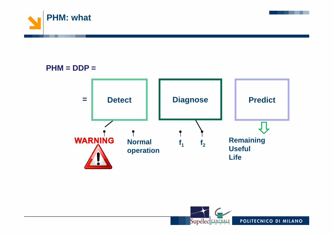
PHM: what
PHM = DDP =
= + +Detect PredictDiagnose
Normal operation
f2f1RemainingUsefulLife
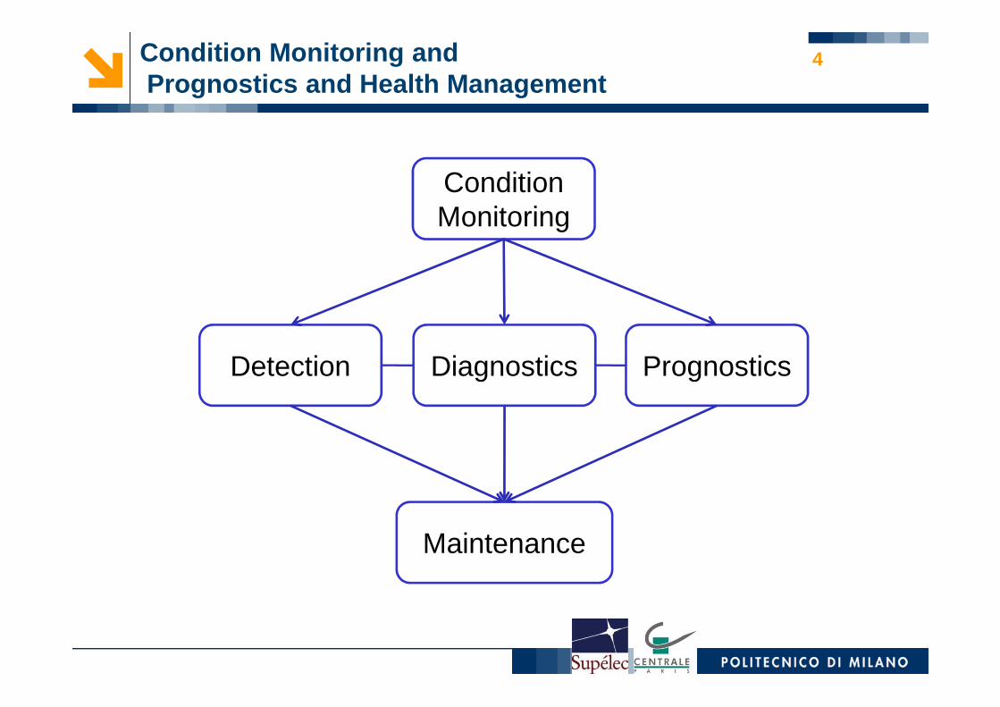
Condition Monitoring andPrognostics and Health Management
4
Detection Diagnostics Prognostics
Condition Monitoring
Detection Diagnostics Prognostics
Maintenance
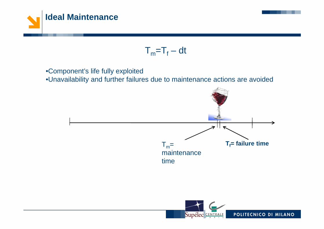
Ideal Maintenance
Tm=Tf – dt
•Component’s life fully exploited•Unavailability and further failures due to maintenance actions are avoided
Tf= failure timeTm= maintenance time
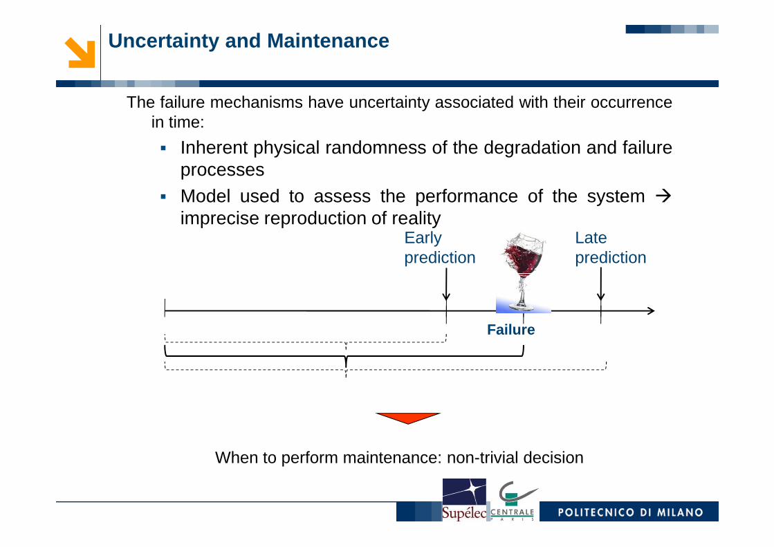
Uncertainty and Maintenance
The failure mechanisms have uncertainty associated with their occurrencein time:
� Inherent physical randomness of the degradation and failureprocesses
� Model used to assess the performance of the system �
imprecise reproduction of realityEarly prediction
Late prediction
When to perform maintenance: non-trivial decision
Failure
Normal operation
f1
f2FAULT DETECTIONearly recognition
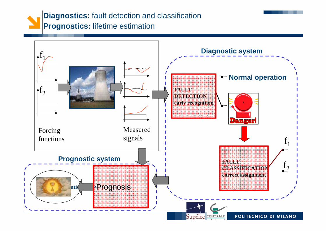
Diagnostics: fault detection and classificationPrognostics: lifetime estimation
Diagnostic system
PLifetime estimation
Prognostic system
PrognosisPrognosis
FAULTCLASSIFICATIONcorrect assignment
f1
f2
Measured signals
Forcing functions
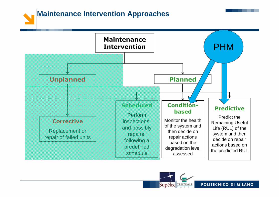
Maintenance Intervention Approaches
Maintenance Intervention
Unplanned Planned
PHM
Corrective
Replacement or repair of failed units
Scheduled
Perform inspections, and possibly
repairs, following a predefined schedule
Condition-
based
Monitor the health of the system and
then decide on repair actions based on the
degradation level assessed
Predictive
Predict the Remaining Useful Life (RUL) of the system and then decide on repair actions based on the predicted RUL

METHODS
9
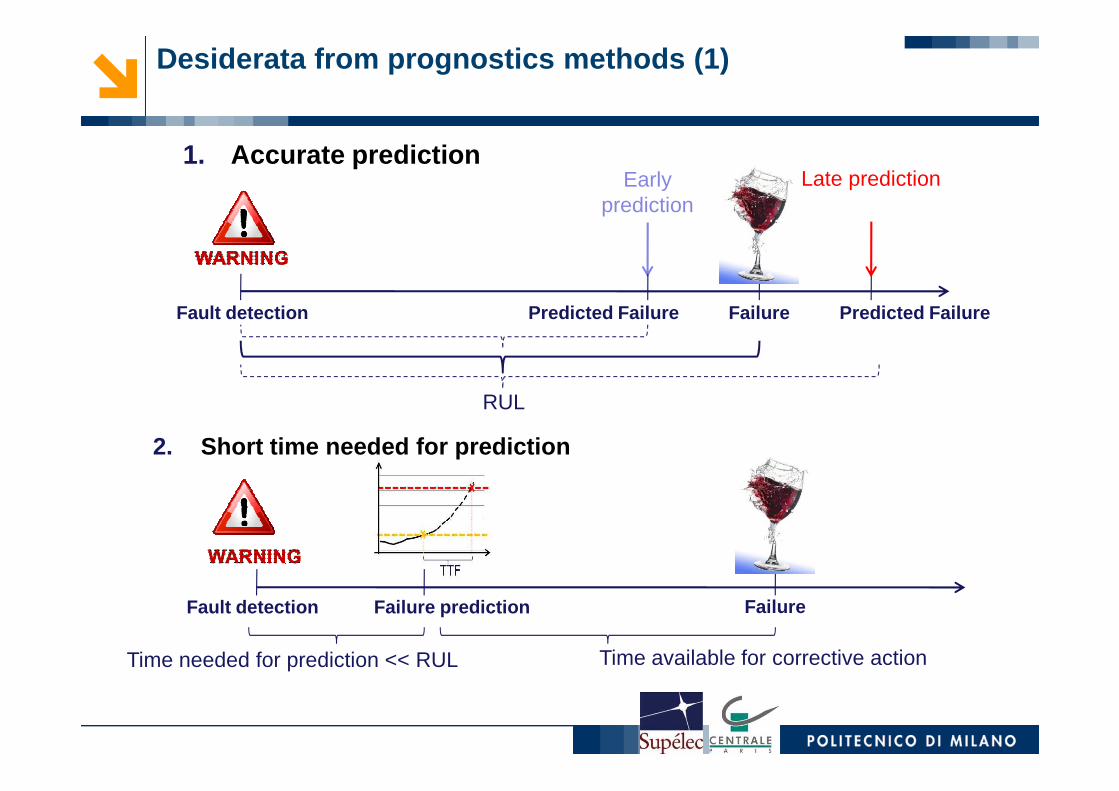
Desiderata from prognostics methods (1)
1. Accurate prediction
Fault detection FailurePredicted Failure Predicted Failure
RUL
Early prediction
Late prediction
RUL
2. Short time needed for prediction
Fault detection Failure prediction Failure
Time needed for prediction << RUL Time available for corrective action
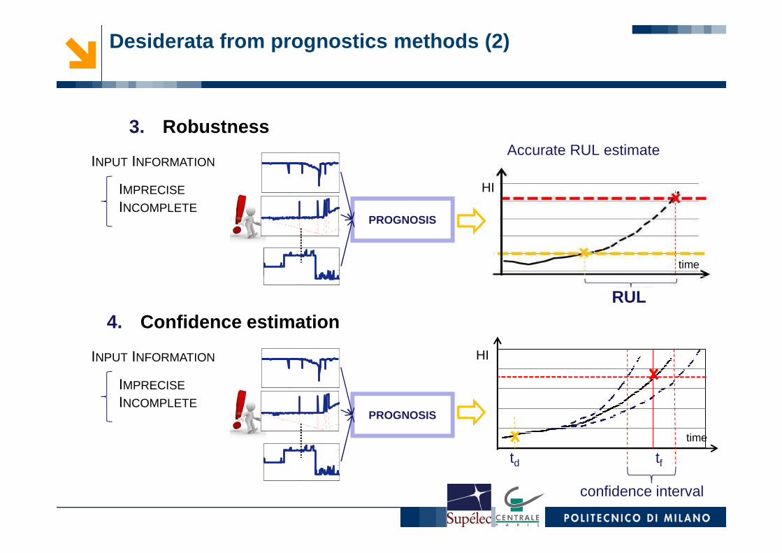
3. RobustnessAccurate RUL estimate
time
0 500 1000
0 500 1000
PROGNOSIS
IMPRECISE
INCOMPLETE
INPUT INFORMATION
HI
Desiderata from prognostics methods (2)
4. Confidence estimationRUL
td tf
confidence interval
time
HI
0 500 1000
0 500 1000
0 500 1000
0 500 1000
PROGNOSIS
IMPRECISE
INCOMPLETE
INPUT INFORMATION
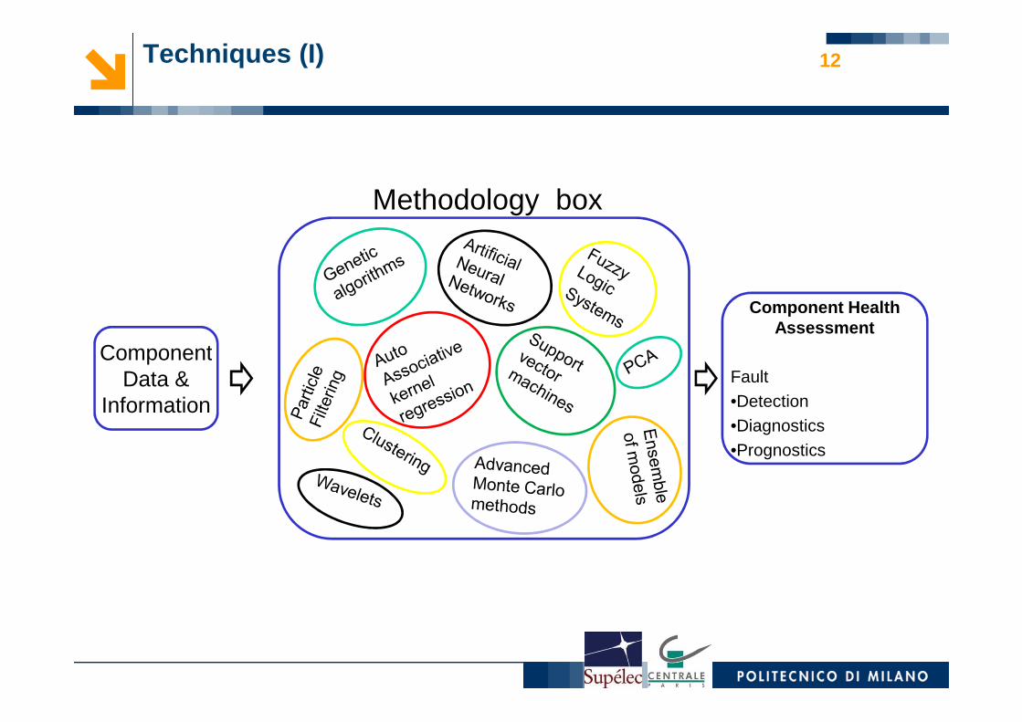
Techniques (I) 12
Component
Methodology box
Component Health Assessment
ComponentData &
InformationFault •Detection•Diagnostics•Prognostics
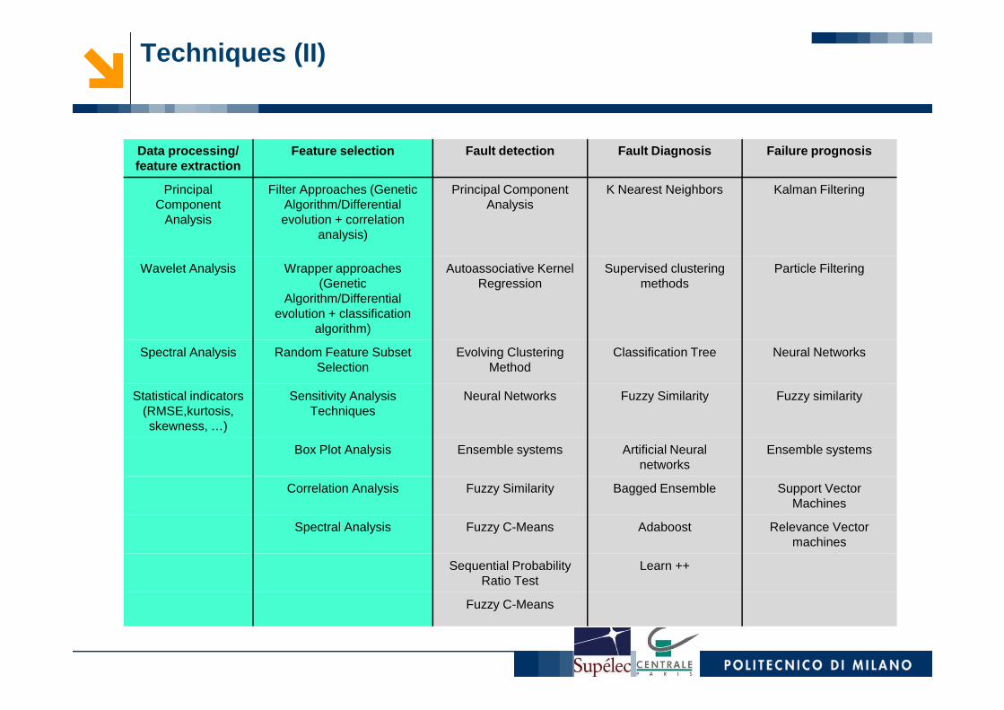
Data processing/ feature extraction
Feature selection Fault detection Fault Diagnosis Failu re prognosis
Principal Component
Analysis
Filter Approaches (Genetic Algorithm/Differential evolution + correlation
analysis)
Principal Component Analysis
K Nearest Neighbors Kalman Filtering
Wavelet Analysis Wrapper approaches(Genetic
Algorithm/Differential evolution + classification
algorithm)
Autoassociative KernelRegression
Supervised clustering methods
Particle Filtering
Spectral Analysis Random Feature Subset Evolving Clustering Classification Tree Neural Networks
Techniques (II)
Spectral Analysis Random Feature Subset Selection
Evolving Clustering Method
Classification Tree Neural Networks
Statistical indicators(RMSE,kurtosis, skewness, …)
Sensitivity Analysis Techniques
Neural Networks Fuzzy Similarity Fuzzy similarity
Box Plot Analysis Ensemble systems Artificial Neural networks
Ensemble systems
Correlation Analysis Fuzzy Similarity Bagged Ensemble Support Vector Machines
Spectral Analysis Fuzzy C-Means Adaboost Relevance Vector machines
Sequential Probability Ratio Test
Learn ++
Fuzzy C-Means
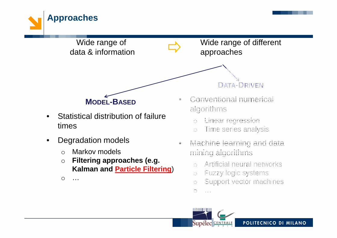
DATA-DRIVEN
• Conventional numerical algorithmso Linear regression
Wide range of different approaches
Wide range of data & information
MODEL-BASED
• Statistical distribution of failure
Approaches
o Linear regressiono Time series analysis
• Machine learning and data mining algorithmso Artificial neural networkso Fuzzy logic systemso Support vector machineso …
• Statistical distribution of failure times
• Degradation modelso Markov modelso Filtering approaches (e.g.
Kalman and Particle Filtering )o …
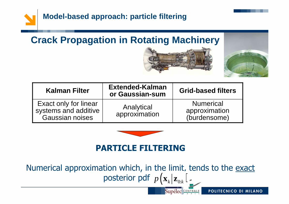
Kalman Filter Extended-Kalman or Gaussian-sum Grid-based filters
Exact only for linear Numerical
Model-based approach: particle filtering
Crack Propagation in Rotating Machinery
Exact only for linear systems and additive
Gaussian noises
Analytical approximation
Numerical approximation (burdensome)
PARTICLE FILTERING
Numerical approximation which, in the limit, tends to the exactposterior pdf ( )0:k kp x z

• Current historical path of degradation {z1, z2, …, zN}
• Degradation model
• Failure threshold
DATA & INFORMATION
1 1( , )
k k k k− −=x f x ω
( , )k k k k
=z h x υ
Hidden Markov process
Measurament equation
zk
timetp
Available information
HYPOTHESES:
• System model:� x = hidden degradation state vector� ωωωω = i.i.d. random process noise vector� f = non-linear dynamics function vector� k = time step index
• Measurement equation:� υυυυ = i.i.d. random measurement
noise vector� h = non-linear measurement
function vector
• Failure threshold
*F. Cadini, E. Zio, D. Avram, Monte Carlo-based filtering for fatigue crack growth estimation, Probabilistic Engineering Mechanics, 24, pp. 367-373, 2009
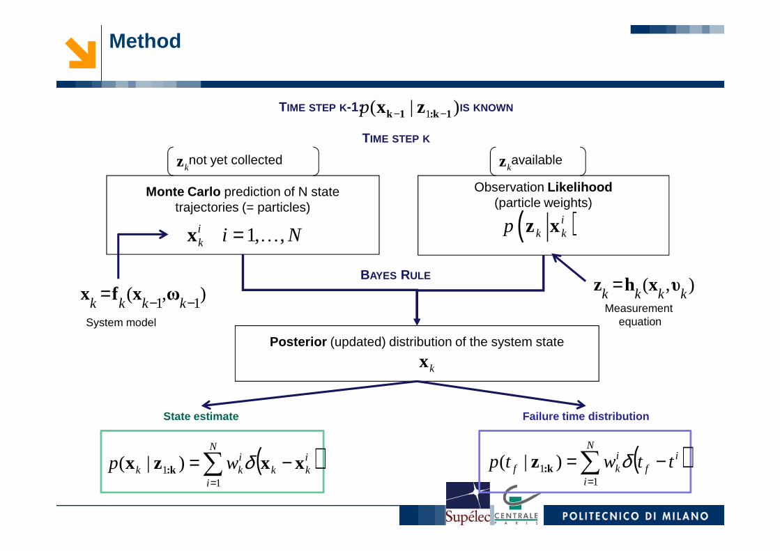
Observation Likelihood(particle weights)
Monte Carlo prediction of N state trajectories (= particles)
BAYES RULE
( )i ik k kp wz x1, ,i
k i N=x K
not yet collected availableikz i
kz
TIME STEP K-1: IS KNOWN
TIME STEP K
)|( 1 1k:1k zx −−p
Method
Posterior (updated) distribution of the system state
BAYES RULE
1 1( , )
k k k k− −=x f x ω( , )
k k k k=z h x υ
System modelMeasurement
equation
State estimate Failure time distribution
( )∑=
−=N
i
if
ikf ttwtp
11 )|( δk:z( )∑
=
−=N
i
ikk
ikk wp
11 )|( xxzx k: δ
kx
10
20
30
40
50
60
70
80
90
100
Sta
te v
aria
ble
x
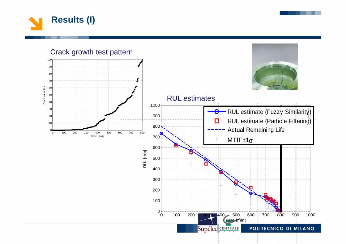
Crack growth test pattern
900
1000
RUL estimate (Fuzzy Similarity)
RUL estimate (Particle Filtering)Actual Remaining Life
RUL estimate (Fuzzy Similarity)
RUL estimate (Particle Filtering)
RUL estimates
Results (I)
0 100 200 300 400 500 600 700 8000
10
Time [min]
0 100 200 300 400 500 600 700 800 900 10000
100
200
300
400
500
600
700
800
Time [min]
RU
L [m
in]
Actual Remaining Life
MTTF±1σ
RUL estimate (Particle Filtering)Actual Remaining Life
MTTF±1σ
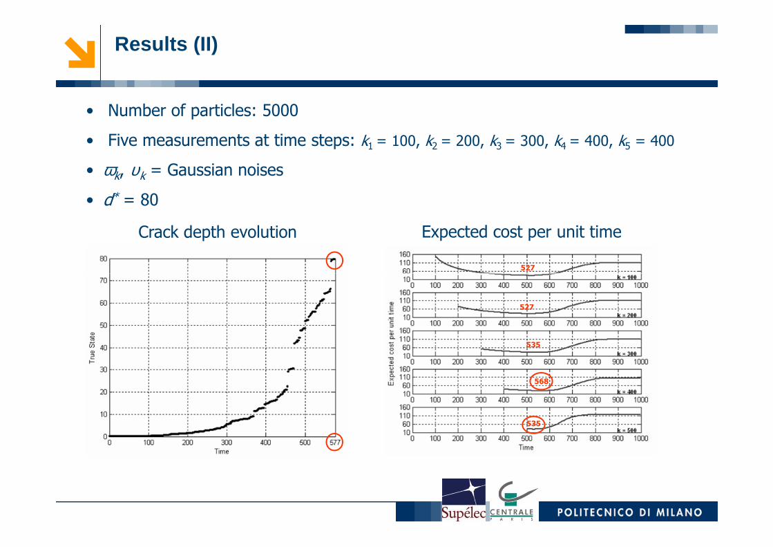
• Number of particles: 5000
• Five measurements at time steps: k1 = 100, k2 = 200, k3 = 300, k4 = 400, k5 = 400
• ωk, υk = Gaussian noises
• d* = 80
Crack depth evolution Expected cost per unit time
k1=100527
Results (II)
k1=100
k2=200
k3=300
k4=400
k5=500
527
535
568
535
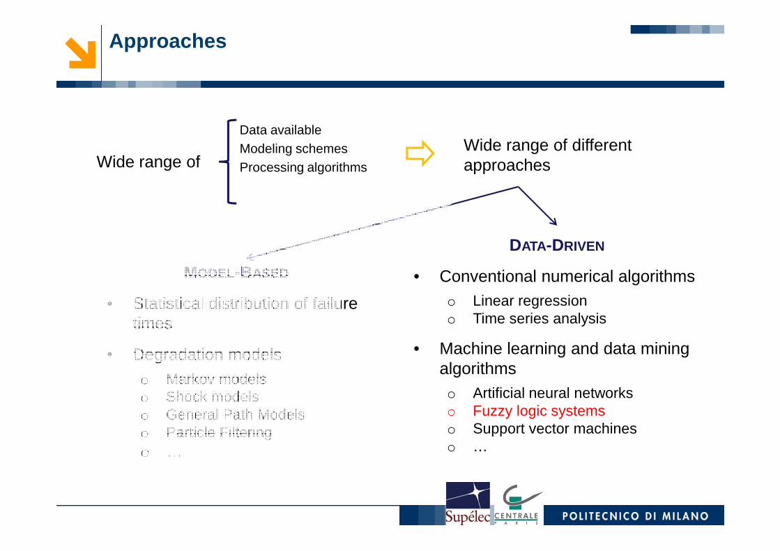
MODEL-BASED
Approaches
Data availableModeling schemesProcessing algorithms
Wide range of different approaches Wide range of
DATA-DRIVEN
• Conventional numerical algorithmsMODEL-BASED
• Statistical distribution of failure times
• Degradation modelso Markov modelso Shock modelso General Path Modelso Particle Filteringo …
• Conventional numerical algorithmso Linear regressiono Time series analysis
• Machine learning and data mining algorithmso Artificial neural networkso Fuzzy logic systemso Support vector machineso …
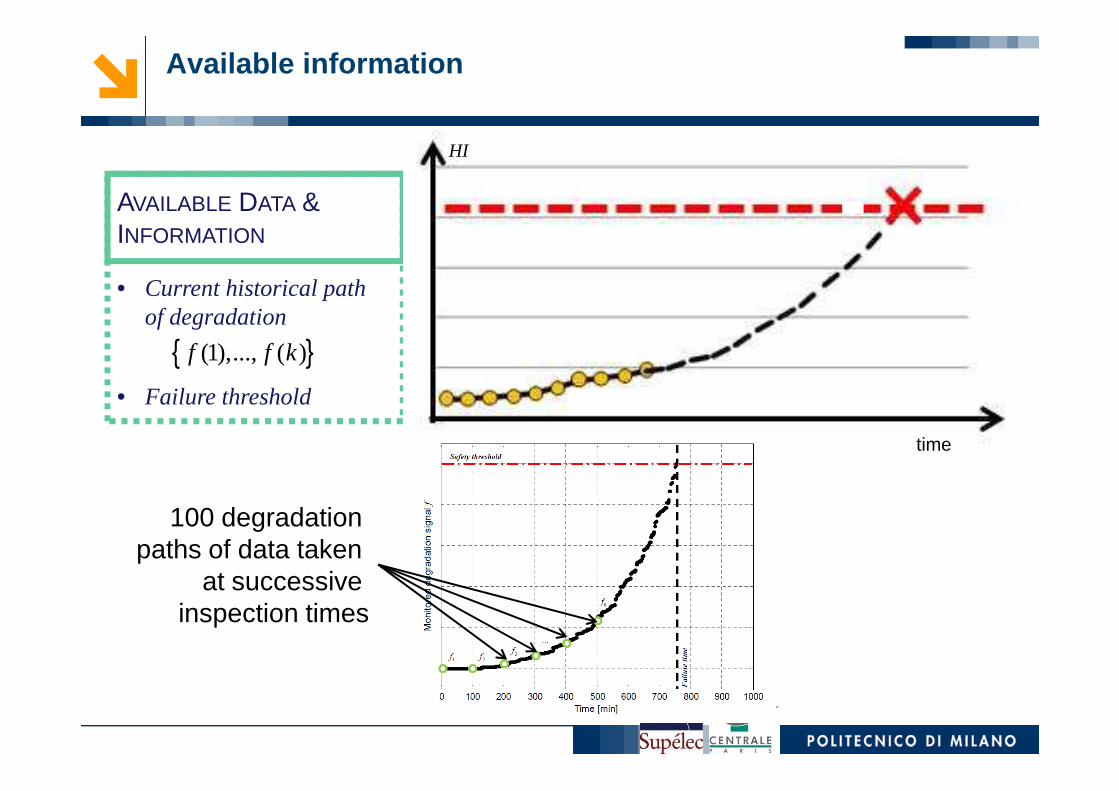
• Current historical path of degradation
• Failure threshold
{ }(1),..., ( )f f k
AVAILABLE DATA & INFORMATION
HI
Available information
• Failure threshold
time
100 degradationpaths of data taken
at successive inspection times
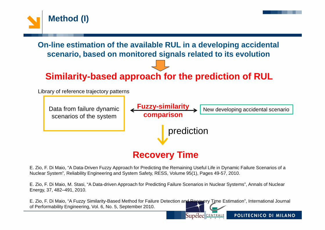
Similarity-based approach for the prediction of RUL
Data from failure dynamic scenarios of the system
Library of reference trajectory patterns
New developing accidental scenarioFuzzy-similarity comparison
On-line estimation of the available RUL in a developing accidental scenario, based on monitored signals related to its evolution
Method (I)
Recovery Time
scenarios of the system comparison
prediction
E. Zio, F. Di Maio, “A Data-Driven Fuzzy Approach for Predicting the Remaining Useful Life in Dynamic Failure Scenarios of a Nuclear System”, Reliability Engineering and System Safety, RESS, Volume 95(1), Pages 49-57, 2010.
E. Zio, F. Di Maio, M. Stasi, “A Data-driven Approach for Predicting Failure Scenarios in Nuclear Systems”, Annals of Nuclear Energy, 37, 482–491, 2010.
E. Zio, F. Di Maio, “A Fuzzy Similarity-Based Method for Failure Detection and Recovery Time Estimation”, International Journal of Performability Engineering, Vol. 6, No. 5, September 2010.
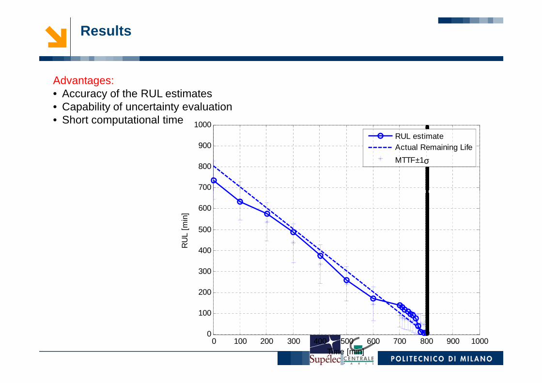
700
800
900
1000
RUL estimateActual Remaining Life
MTTF±1σ
Advantages:• Accuracy of the RUL estimates• Capability of uncertainty evaluation• Short computational time
Results
0 100 200 300 400 500 600 700 800 900 10000
100
200
300
400
500
600
Time [min]
RU
L [m
in]

APPLICATIONS
24
FAULT DETECTION
25
TOPIC 1: NPP SENSOR CONDITION MONITORING
Practical Applications Of NPP Sensor Condition Monitoring
1. Condition monitoring and signal reconstruction of:a. 215 sensors at Loviisa Nuclear Power Plant (Finland, in
collaboration with HRP)b. 792 sensors at OKG Nuclear Power Plant (Sweden, in
collaboration with HRP)
2. Signal reconstruction in support to the control of the pressurizerof a nuclear power plant
26
of a nuclear power plant
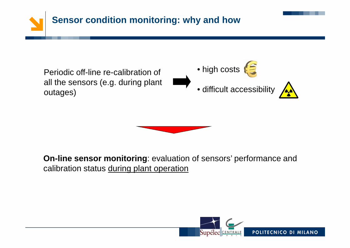
Periodic off-line re-calibration of all the sensors (e.g. during plant outages)
• high costs
• difficult accessibility
Sensor condition monitoring: why and how
On-line sensor monitoring : evaluation of sensors’ performance and calibration status during plant operation
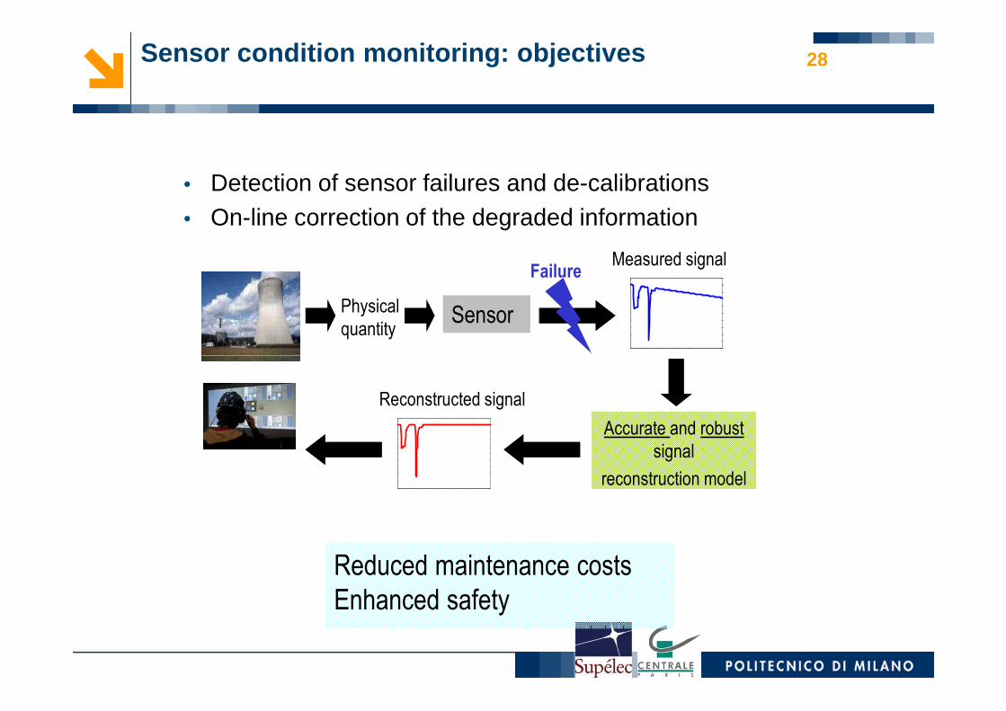
Sensor condition monitoring: objectives
• Detection of sensor failures and de-calibrations• On-line correction of the degraded information
28
Physical
quantity
Measured signal
Sensor
Failure
Accurate and robust
signal
reconstruction model
Reconstructed signal
Reduced maintenance costs
Enhanced safety
Applications
• Condition monitoring and signal reconstruction of:• 215 sensors at Loviisa Nuclear Power Plant (Finland) [1,2]
• 792 sensors at OKG Nuclear Power Plant (Sweden) [1,3]
29
[1] P. Baraldi, E. Zio, G. Gola, D. Roverso, M. Hoffmann, "Robust nuclear signal reconstruction by a novel ensemble model aggregation procedure", International Journal of Nuclear Knowledge Management, Vol 4 (1), pp. 34-41, 2010.[2] P. Baraldi, G. Gola, E. Zio, D. Roverso, M. Hoffmann, "A randomized model ensemble approach for reconstructing signals from faulty sensors". Expert Systems With Application, Vol. 38 (8), pp. 9211-9224, 2011[3] P. Baraldi, E. Zio, G. Gola, D. Roverso, M. Hoffmann, "Two novel procedures for aggregating randomized model ensemble outcomes for robust signal reconstruction in nuclear power plants monitoring systems", Annals of Nuclear Energy, Vol. 38 (2-3), pp. 212-220, 2011.

Loviisa PWR 215
Application a) 30
OKG BWR 792
31
11.9
12
12.1
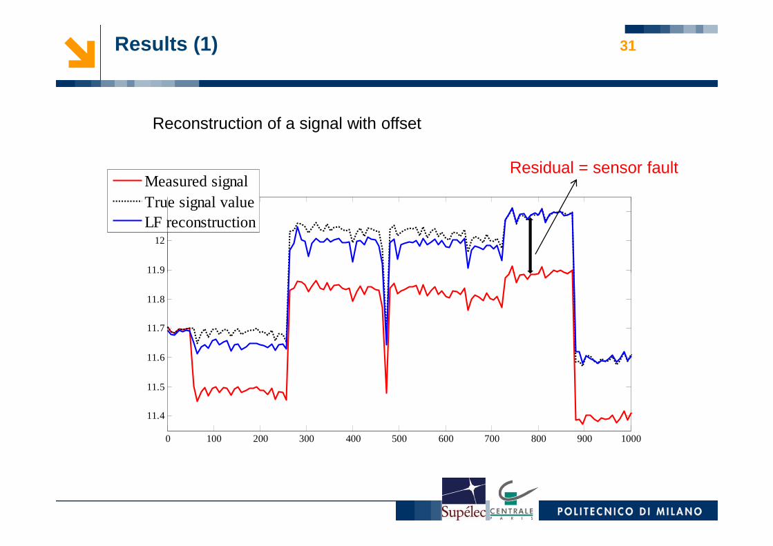
Measured signalTrue signal valueLF reconstruction
Results (1)
Reconstruction of a signal with offset
Residual = sensor fault
0 100 200 300 400 500 600 700 800 900 1000
11.4
11.5
11.6
11.7
11.8
11.9

Loviisa PWR 215
Application b) 32
OKG BWR 792
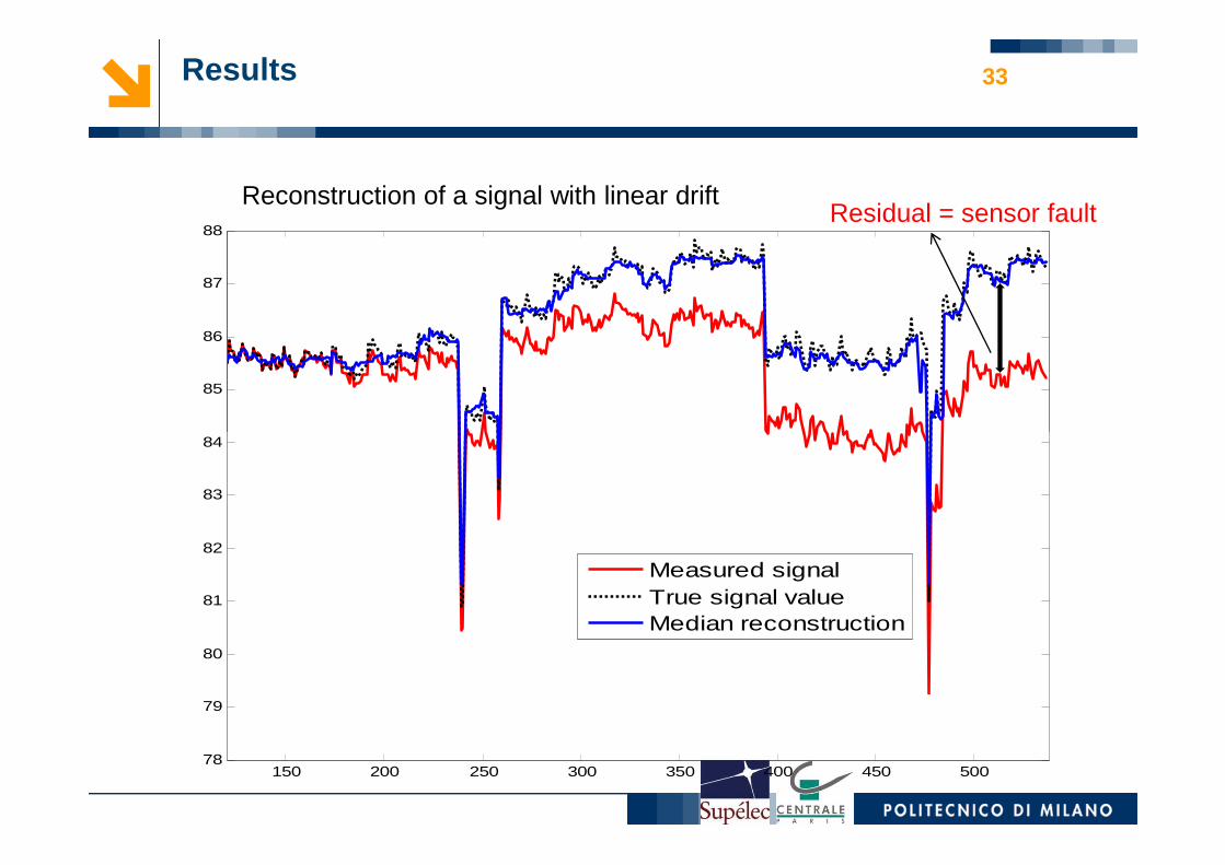
Results
Reconstruction of a signal with linear drift
85
86
87
88 Residual = sensor fault
33
150 200 250 300 350 400 450 50078
79
80
81
82
83
84
Measured signalTrue signal valueMedian reconstruction
34
FAULT PROGNOSTICS
Applications
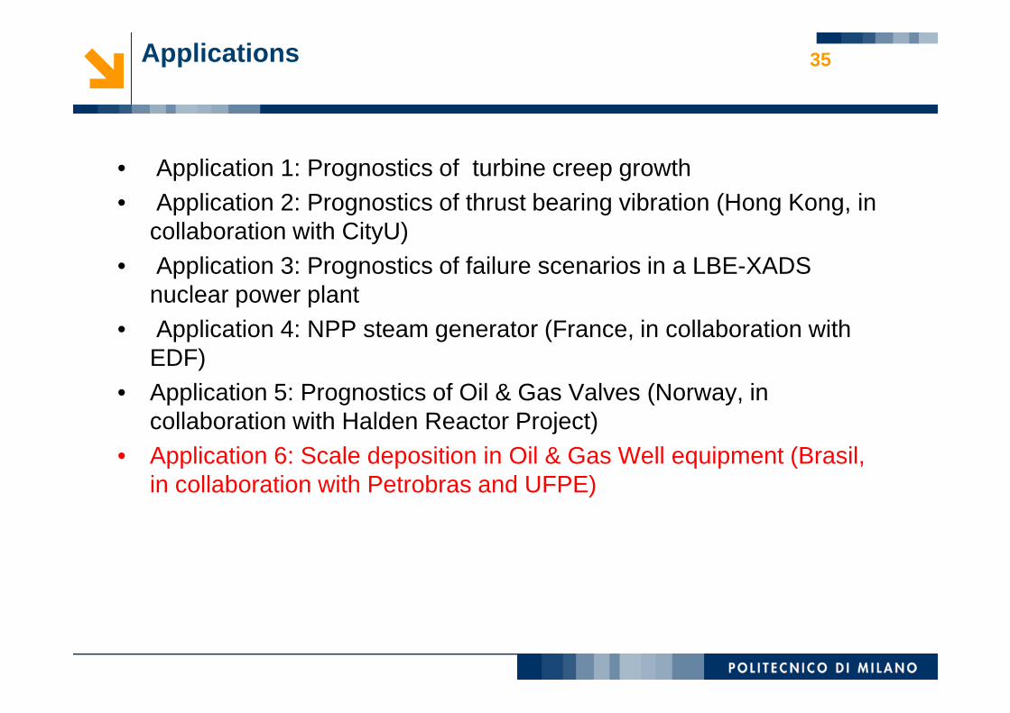
• Application 1: Prognostics of turbine creep growth• Application 2: Prognostics of thrust bearing vibration (Hong Kong, in
collaboration with CityU)• Application 3: Prognostics of failure scenarios in a LBE-XADS
nuclear power plant• Application 4: NPP steam generator (France, in collaboration with
EDF)
35
EDF)• Application 5: Prognostics of Oil & Gas Valves (Norway, in
collaboration with Halden Reactor Project)• Application 6: Scale deposition in Oil & Gas Well equipment (Brasil,
in collaboration with Petrobras and UFPE)
FAULT PROGNOSIS
36
APPLICATION 6: SCALE DEPOSITION IN OIL & GAS WELL EQUIPMENT (in collaboration with Petrobras and UFPE)
7
MEASURED SIGNALS ( z)
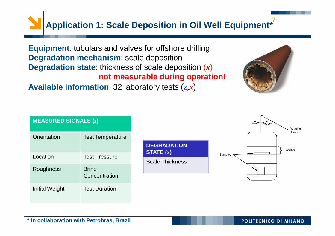
Application 1: Scale Deposition in Oil Well Equipme nt*
Equipment : tubulars and valves for offshore drillingDegradation mechanism : scale depositionDegradation state : thickness of scale deposition (x)
not measurable during operation!Available information : 32 laboratory tests (z,x)
MEASURED SIGNALS ( z)
Orientation Test Temperature
Location Test Pressure
Roughness Brine Concentration
Initial Weight Test Duration
DEGRADATIONSTATE (x)
Scale Thickness
* In collaboration with Petrobras, Brazil
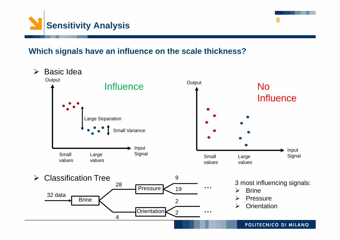
8Sensitivity Analysis
� Basic IdeaOutput
Large Separation
OutputInfluence No Influence
Which signals have an influence on the scale thickn ess?
Small values
Large values
Input Signal
Large Separation
Small Variance
Small values
Large values
Input Signal
� Classification Tree
Brine
Pressure
Orientation
28
4
9
19
2
2
32 data
3 most influencing signals:� Brine� Pressure� Orientation
...
...

9Empirical Modelling: Ensemble of Neural Networks
Neural Network 100
Neural Network
Neural Network 1
3most influencing
measured signals
Median
Input Signals
5
Scale Thickness (x)
Neural Network 101
Neural Network 200
Neural Network 201
Neural Network 300
5most influencing
measured signals
Allmeasured
signals
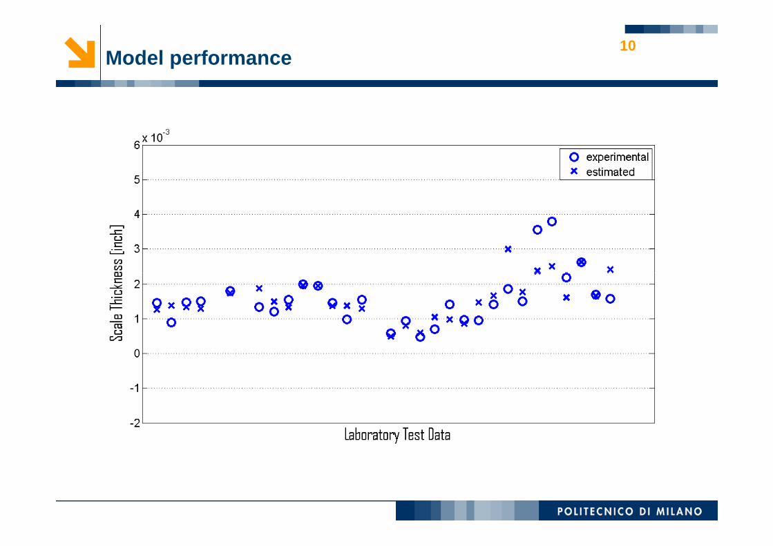
10Model performance

41
CONCLUSIONS
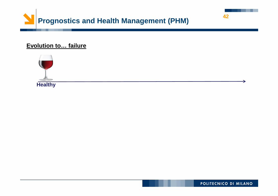
Prognostics and Health Management (PHM)42
Healthy
Evolution to… failure
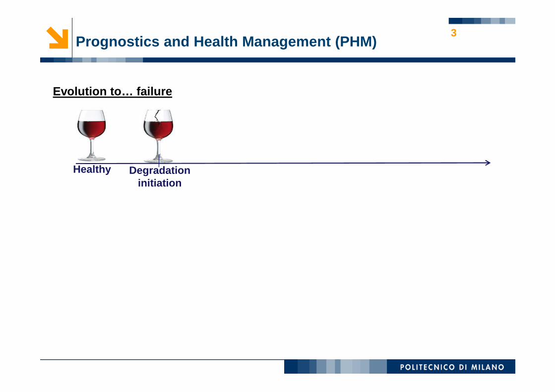
Prognostics and Health Management (PHM)
Healthy Degradation initiation
Evolution to… failure
3
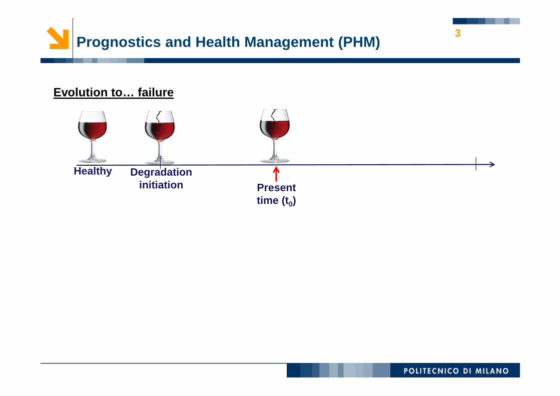
Prognostics and Health Management (PHM)3
Healthy Degradation initiation
Evolution to… failure
Present time (t )time (t0)
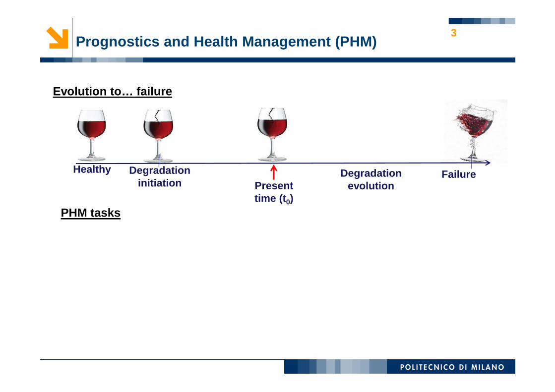
Failure
Prognostics and Health Management (PHM)3
Healthy Degradation initiation
Evolution to… failure
Present time (t )
Degradation evolution
time (t0)PHM tasks

Prognostics and Health Management (PHM)3
Healthy Degradation initiation
Evolution to… failure
Present time (t )
FailureDegradation evolution
PHM taskstime (t0)
Health assessment1
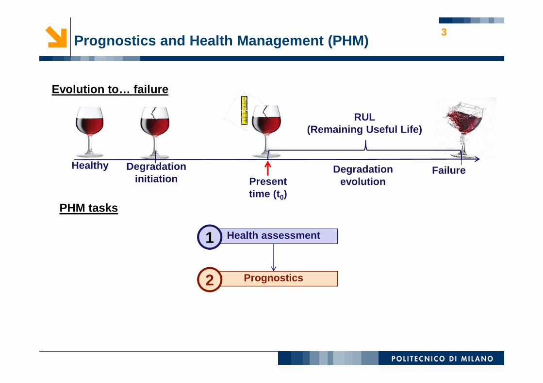
Prognostics and Health Management (PHM)3
Healthy Degradation initiation
Evolution to… failure
FailurePresent time (t )
RUL (Remaining Useful Life)
Degradation evolution
PHM taskstime (t0)
Health assessment
Prognostics
1
2
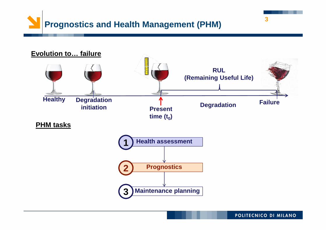
Prognostics and Health Management (PHM)3
HealthyDegradation
Degradation initiation
Evolution to… failure
FailurePresent time (t )
RUL (Remaining Useful Life)
PHM taskstime (t0)
Health assessment
Prognostics
Maintenance planning
1
2
3

49
PERSPECTIVES

50


![Evaluating Algorithm Performance Metrics Tailored for ......standard [4] for prognostics in condition monitoring and diagnostics of machines lacks a firm definition of such metrics](https://img.pdfslide.net/doc/110x75/60a8fb1598f52c465705caae/evaluating-algorithm-performance-metrics-tailored-for-standard-4-for-prognostics.jpg)