Conditional Independence - ComLabGamescomlabgames.com/cemmap/2 Conditional Independenc… · · 2018-02-22the loss in asymptotic e¢ ciency. Miller ... Using this notation,

Conditional Independence

Robert A. Miller

Dynamic Discrete Choice Models

March 2018

Miller (Dynamic Discrete Choice Models) cemmap 2 March 2018 1 / 37

A RecapitulationA dynamic discrete choice model

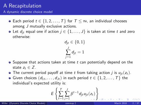
Each period t ∈ {1, 2, . . . ,T} for T ≤ ∞, an individual choosesamong J mutually exclusive actions.Let djt equal one if action j ∈ {1, . . . , J} is taken at time t and zerootherwise:

djt ∈ {0, 1}J

∑j=1djt = 1

Suppose that actions taken at time t can potentially depend on thestate zt ∈ Z .The current period payoff at time t from taking action j is ujt (zt ).Given choices (d1t , . . . , dJt ) in each period t ∈ {1, 2, . . . ,T} theindividual’s expected utility is:

E

{T

∑t=1

J

∑j=1

βt−1djtujt (zt )

}where β ∈ (0, 1) is the discount factor, and at each period t theexpectation is taken over zt+1, . . . , zT .


A RecapitulationValue function and optimization

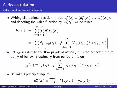
Writing the optimal decision rule as dot (z) ≡ (do1t (zt ), . . . , doJt (zt )),and denoting the value function by Vt (zt ), we obtained:

Vt (zt ) =T

∑t=1

J

∑j=1dojtujt (zt )

=J

∑j=1dojt

[ujt (zt ) + β

Z

∑zt+1=1

Vt+1(zt+1)fjt (zt+1 |zt )]

Let vjt (zt ) denote the flow payoff of action j plus the expected futureutility of behaving optimally from period t + 1 on:

vjt (zt ) ≡ ujt (zt ) + βZ

∑zt+1=1

Vt+1(zt+1)fjt (zt+1 |zt )

Bellman’s principle implies:

dojt (zt ) ≡∏Kk=1 I {vjt (zt ) ≥ vkt (zt )}


A RecapitulationEstimation

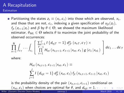
Partitioning the states zt ≡ (xt , εt ) into those which are observed, xt ,and those that are not, εt , indexing a given specification of ujt (zt ),fjt (zt+1|zt ) and β by θ ∈ Θ, we showed the maximum likelihoodestimator, θML ∈ Θ selects θ to maximize the joint probability of theobserved occurrences:

N

∏n=1

∫εT

. . .∫

ε1

∑Jj=1 I {dnjT = 1} dojT (xnT , εT )×

T−1∏t=1

Hnt (xn,t+1, εt+1 |xnt , εt ) g (ε1 |xn1 )

dε1 . . . dεT

where:

Hnt (xn,t+1, εt+1 |xnt , εt ) ≡J

∑j=1I {dnjt = 1} dojt (xnt , εt ) fjt (xn,t+1, εt+1 |xnt , εt )

is the probability density of the pair (xn,t+1, εt+1) conditional on(xnt , εt ) when choices are optimal for θ, and dnjt = 1.


A RecapitulationA computational challenge

What are the computational challenges to enlarging the state space?1 Computing the value function;2 Solving for equilibrium in a multiplayer setting;3 Integrating over unobserved heterogeneity.

These challenges have led researchers to compromises on severaldimensions:

1 Keep the dimension of the state space small;2 Assume all choices and outcomes are observed;3 Model unobserved states as a matter of computational convenience;4 Consider only one side of market to finesse equilibrium issues;5 Adopt parameterizations based on convenient functional forms.


Separable Transitions in the Observed VariablesA simplification

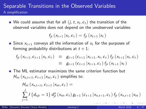
We could assume that for all (j , t, xt , εt ) the transition of theobserved variables does not depend on the unobserved variables:

fjt (xt+1 |xt , εt ) = fjt (xt+1 |xt )Since xt+1 conveys all the information of xt for the purposes offorming probability distributions at t + 1:

fjt (xt+1, εt+1 |xt , εt ) ≡ gt+1 (εt+1 |xt+1, xt , εt ) fjt (xt+1 |xt , εt )≡ gt+1 (εt+1 |xt+1, εt ) fjt (xt+1 |xt )

The ML estimator maximizes the same criterion function butHnt (xn,t+1, εt+1 |xnt , εt ) simplifies to:

Hnt (xn,t+1, εt+1 |xnt , εt ) =J

∑j=1I {dnjt = 1} dojt (xnt , εt ) gt+1 (εt+1 |xn,t+1, εt ) fjt (xn,t+1 |xnt )


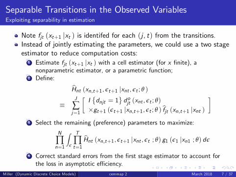
Separable Transitions in the Observed VariablesExploiting separability in estimation

Note fjt (xt+1 |xt ) is identifed for each (j , t) from the transitions.Instead of jointly estimating the parameters, we could use a two stageestimator to reduce computation costs:

1 Estimate fjt (xt+1 |xt ) with a cell estimator (for x finite), anonparametric estimator, or a parametric function;

2 Define:

Hnt (xn,t+1, εt+1 |xnt , εt ; θ )

≡J

∑j=1

[I{dnjt = 1

}dojt (xnt , εt ; θ)

×gt+1 (εt+1 |xn,t+1, εt ; θ ) fjt (xn,t+1 |xnt )

]3 Select the remaining (preference) parameters to maximize:

N

∏n=1

∫ε

T

∏t=1

Hnt (xn,t+1, εt+1 |xnt , εt ; θ) g1 (ε1 |xn1 ; θ) dε

4 Correct standard errors from the first stage estimator to account forthe loss in asymptotic effi ciency.


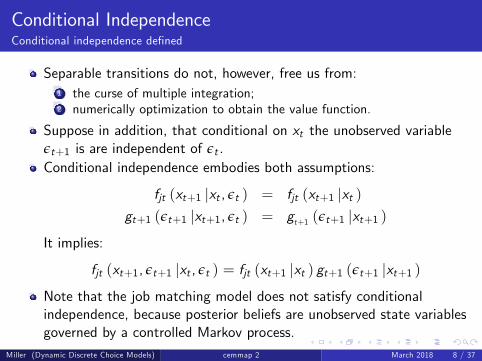
Conditional IndependenceConditional independence defined

Separable transitions do not, however, free us from:1 the curse of multiple integration;2 numerically optimization to obtain the value function.

Suppose in addition, that conditional on xt the unobserved variableεt+1 is are independent of εt .Conditional independence embodies both assumptions:

fjt (xt+1 |xt , εt ) = fjt (xt+1 |xt )gt+1 (εt+1 |xt+1, εt ) = gt+1 (εt+1 |xt+1 )

It implies:

fjt (xt+1, εt+1 |xt , εt ) = fjt (xt+1 |xt ) gt+1 (εt+1 |xt+1 )Note that the job matching model does not satisfy conditionalindependence, because posterior beliefs are unobserved state variablesgoverned by a controlled Markov process.


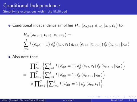
Conditional IndependenceSimplifying expressions within the likelihood

Conditional independence simplifies Hnt (xn,t+1, εt+1 |xnt , εt ) to:

Hnt (xn,t+1, εt+1 |xnt , εt ) =J

∑j=1I {dnjt = 1} dojt (xnt , εt ) gt+1 (εt+1 |xn,t+1 ) fjt (xn,t+1 |xnt )

Also note that:

∏Tt=1

{∑Jj=1 I {dnjt = 1} d

ojt (xnt , εt ) fjt (xn,t+1 |xnt )

}= ∏T

t=1

{∑Jj=1 I {dnjt = 1} fjt (xn,t+1 |xnt )

}×∏T

t=1

{∑Jj=1 I {dnjt = 1} d

ojt (xnt , εt )

}


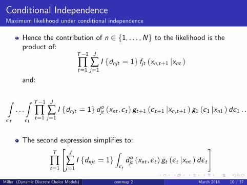
Conditional IndependenceMaximum likelihood under conditional independence

Hence the contribution of n ∈ {1, . . . ,N} to the likelihood is theproduct of:

T−1∏t=1

J

∑j=1I {dnjt = 1} fjt (xn,t+1 |xnt )

and:

∫εT

. . .∫ε1

T−1∏t=1

J

∑j=1I {dnjt = 1} dojt (xnt , εt ) gt+1 (εt+1 |xn,t+1 ) g1 (ε1 |xn1 ) dε1 . . . dεT

The second expression simplifies to:

T

∏t=1

[J

∑j=1I {dnjt = 1}

∫εtdojt (xnt , εt ) gt (εt |xnt ) dεt

]Miller (Dynamic Discrete Choice Models) cemmap 2 March 2018 10 / 37

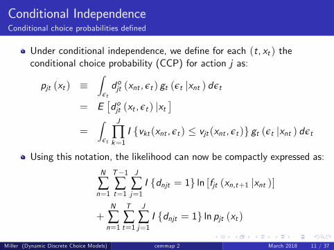
Conditional IndependenceConditional choice probabilities defined

Under conditional independence, we define for each (t, xt ) theconditional choice probability (CCP) for action j as:

pjt (xt ) ≡∫

εtdojt (xnt , εt ) gt (εt |xnt ) dεt

= E[dojt (xt , εt ) |xt

]=

∫εt

J

∏k=1

I {vkt (xnt , εt ) ≤ vjt (xnt , εt )} gt (εt |xnt ) dεt

Using this notation, the likelihood can now be compactly expressed as:

N

∑n=1

T−1∑t=1

J

∑j=1I {dnjt = 1} ln [fjt (xn,t+1 |xnt )]

+N

∑n=1

T

∑t=1

J

∑j=1I {dnjt = 1} ln pjt (xt )


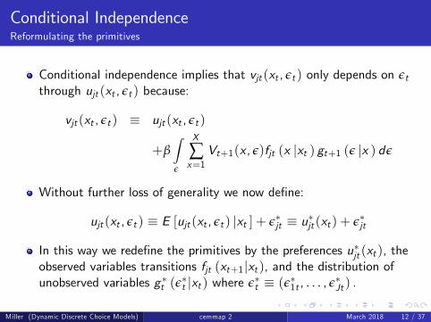
Conditional IndependenceReformulating the primitives

Conditional independence implies that vjt (xt , εt ) only depends on εtthrough ujt (xt , εt ) because:

vjt (xt , εt ) ≡ ujt (xt , εt )

+β∫ε

X

∑x=1

Vt+1(x , ε)fjt (x |xt ) gt+1 (ε |x ) dε

Without further loss of generality we now define:

ujt (xt , εt ) ≡ E [ujt (xt , εt ) |xt ] + ε∗jt ≡ u∗jt (xt ) + ε∗jt

In this way we redefine the primitives by the preferences u∗jt (xt ), theobserved variables transitions fjt (xt+1|xt ), and the distribution ofunobserved variables g ∗t (ε

∗t |xt ) where ε∗t ≡ (ε∗1t , . . . , ε∗Jt ) .


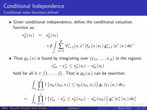
Conditional IndependenceConditional value functions defined

Given conditional independence, define the conditional valuationfunction as:

v ∗jt (xt ) = u∗jt (xt )

+β∫ε∗

X

∑x=1

V ∗t+1(x , ε∗)fjt (x |xt ) g ∗t+1 (ε∗ |x ) dε∗

Thus pjt (x) is found by integrating over (ε1t , . . . , εJt ) in the regions:

ε∗kt − ε∗jt ≤ v ∗jt (xt )− v ∗kt (xt )hold for all k ∈ {1, . . . , J} . That is pjt (xt ) can be rewritten:∫

εt

J

∏k=1

I {vkt (xnt , εt ) ≤ vjt (xnt , εt )} gt (εt |xt ) dεt

=∫

εt

J

∏k=1

I{

ε∗kt − ε∗jt ≤ v ∗jt (xnt )− v ∗kt (xnt )}g ∗t (ε

∗t |xt ) dε∗t


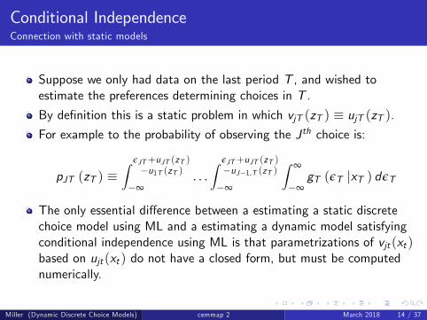
Conditional IndependenceConnection with static models

Suppose we only had data on the last period T , and wished toestimate the preferences determining choices in T .

By definition this is a static problem in which vjT (zT ) ≡ ujT (zT ).For example to the probability of observing the J th choice is:

pJT (zT ) ≡∫ εJT+uJT (zT )−u1T (zT )

−∞. . .∫ εJT+uJT (zT )−uJ−1,T (zT )−∞

∫ ∞

−∞gT (εT |xT ) dεT

The only essential difference between a estimating a static discretechoice model using ML and a estimating a dynamic model satisfyingconditional independence using ML is that parametrizations of vjt (xt )based on ujt (xt ) do not have a closed form, but must be computednumerically.


Another Renewal Problem (Rust,1987)Bus engines

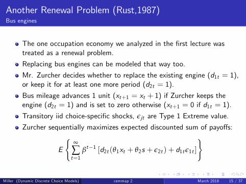
The one occupation economy we analyzed in the first lecture wastreated as a renewal problem.

Replacing bus engines can be modeled that way too.

Mr. Zurcher decides whether to replace the existing engine (d1t = 1),or keep it for at least one more period (d2t = 1).

Bus mileage advances 1 unit (xt+1 = xt + 1) if Zurcher keeps theengine (d2t = 1) and is set to zero otherwise (xt+1 = 0 if d1t = 1).

Transitory iid choice-specific shocks, εjt are Type 1 Extreme value.

Zurcher sequentially maximizes expected discounted sum of payoffs:

E

{∞

∑t=1

βt−1 [d2t (θ1xt + θ2s + ε2t ) + d1tε1t ]

}


Another Renewal ProblemValue functions and replacement CCP

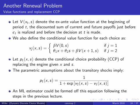
Let V (xt , s) denote the ex-ante value function at the beginning ofperiod t, the discounted sum of current and future payoffs just beforeεt is realized and before the decision at t is made.We also define the conditional value function for each choice as:

vj (x , s) ={

βV (0, s) if j = 1θ1x + θ2s + βV (x + 1, s) if j = 2

Let p1(x , s) denote the conditional choice probability (CCP) ofreplacing the engine given x and s.The parametric assumptions about the transitory shocks imply:

p1(x , s) =1

1+ exp [v2(x , s)− v1(x , s)]An ML estimator could be formed off this equation following thesteps in the previous lecture.


Another Renewal ProblemExploiting the renewal property

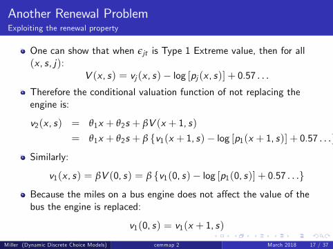
One can show that when εjt is Type 1 Extreme value, then for all(x , s, j):

V (x , s) = vj (x , s)− log [pj (x , s)] + 0.57 . . .

Therefore the conditional valuation function of not replacing theengine is:

v2(x , s) = θ1x + θ2s + βV (x + 1, s)

= θ1x + θ2s + β {v1(x + 1, s)− log [p1(x + 1, s)] + 0.57 . . .}

Similarly:

v1(x , s) = βV (0, s) = β {v1(0, s)− log [p1(0, s)] + 0.57 . . .}

Because the miles on a bus engine does not affect the value of thebus the engine is replaced:

v1(0, s) = v1(x + 1, s)


Another Renewal ProblemUsing CCPs to represent differences in continuation values

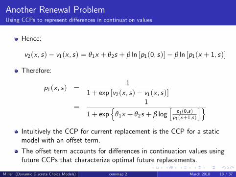
Hence:

v2(x , s)− v1(x , s) = θ1x + θ2s + β ln [p1(0, s)]− β ln [p1(x + 1, s)]

Therefore:

p1(x , s) =1

1+ exp [v2(x , s)− v1(x , s)]

=1

1+ exp{

θ1x + θ2s + β log[

p1(0,s)p1(x+1,s)

]}Intuitively the CCP for current replacement is the CCP for a staticmodel with an offset term.

The offset term accounts for differences in continuation values usingfuture CCPs that characterize optimal future replacements.


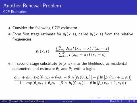
Another Renewal ProblemCCP Estimation

Consider the following CCP estimator.

Form first stage estimate for p1(x , s), called p1(x , s) from the relativefrequencies:

p1(x , s) =∑Nn=1 d1nt I (xnt = x) I (sn = s)

∑Nn=1 I (xnt = x) I (sn = s)

In second stage substitute p1(x , s) into the likelihood as incidentalparameters and estimate θ1 and θ2 with a logit:

d1nt + d2nt exp(θ1xnt + θ2sn + β ln [p1(0, sn)]− β ln [p1(xnt + 1, sn)]1+ exp(θ1xnt + θ2sn + β ln [p1(0, sn)]− β ln [p1(xnt + 1, sn)])


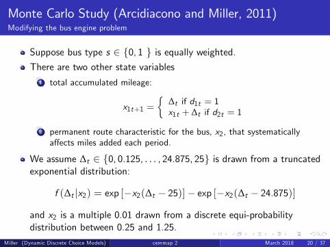
Monte Carlo Study (Arcidiacono and Miller, 2011)Modifying the bus engine problem

Suppose bus type s ∈ {0, 1 } is equally weighted.There are two other state variables

1 total accumulated mileage:

x1t+1 ={

∆t if d1t = 1x1t + ∆t if d2t = 1

2 permanent route characteristic for the bus, x2, that systematicallyaffects miles added each period.

We assume ∆t ∈ {0, 0.125, . . . , 24.875, 25} is drawn from a truncatedexponential distribution:

f (∆t |x2) = exp [−x2(∆t − 25)]− exp [−x2(∆t − 24.875)]

and x2 is a multiple 0.01 drawn from a discrete equi-probabilitydistribution between 0.25 and 1.25.


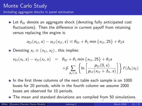
Monte Carlo StudyIncluding aggregate shocks in panel estimation

Let θ0t denote an aggregate shock (denoting fully anticipated costfluctuations). Then the difference in current payoff from retainingversus replacing the engine is:

u2t (x1t , s)− u1t (x1t , s) ≡ θ0t + θ1min {x1t , 25}+ θ2s

Denoting xt ≡ (x1t , x2) , this implies:

v2t (xt , s)− v1t (xt , s) = θ0t + θ1min {x1t , 25}+ θ2s

+β ∑∆t∈Λ

{ln[

p1t (0, s)p1t (x1t + ∆t , s)

]}f (∆t |x2)

In the first three columns of the next table each sample is on 1000buses for 20 periods, while in the fourth column we assume 2000buses are observed for 10 periods.The mean and standard deviations are compiled from 50 simulations.


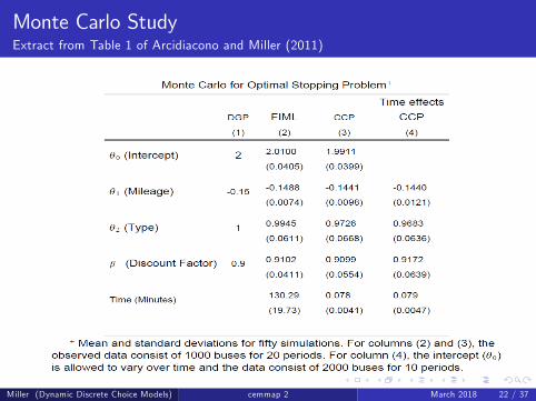
Monte Carlo StudyExtract from Table 1 of Arcidiacono and Miller (2011)


A Class of Dynamic Markov GamesPlayers and choices

Consider a dynamic infinite horizon game for finite I players.

Thus T = ∞ and I < ∞.Each player i ∈ I makes a choice d (i )t ≡

(d (i )1t , . . . , d (i )Jt

)in period t.

Denote the choices of all the players in period t by:

dt ≡(d (1)t , . . . , d (I )t

)and denote by:

d (−i )t ≡(d (1)t , . . . , d (i−1)t , d (i+1)t , . . . , d (I )t

)the choices of {1, . . . , i − 1, i + 1, . . . , I} in period t, that is all theplayers apart from i .


A Class of Dynamic Markov GamesState variables

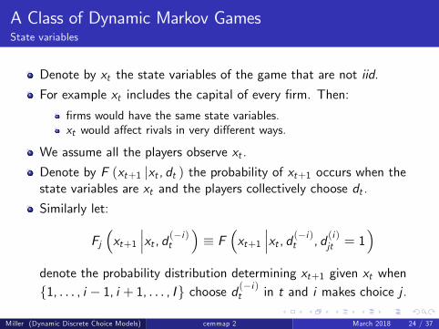
Denote by xt the state variables of the game that are not iid.

For example xt includes the capital of every firm. Then:

firms would have the same state variables.xt would affect rivals in very different ways.

We assume all the players observe xt .

Denote by F (xt+1 |xt , dt ) the probability of xt+1 occurs when thestate variables are xt and the players collectively choose dt .

Similarly let:

Fj(xt+1

∣∣∣xt , d (−i )t

)≡ F

(xt+1

∣∣∣xt , d (−i )t , d (i )jt = 1)

denote the probability distribution determining xt+1 given xt when{1, . . . , i − 1, i + 1, . . . , I} choose d (−i )t in t and i makes choice j .


A Class of Dynamic Markov GamesPayoffs and information

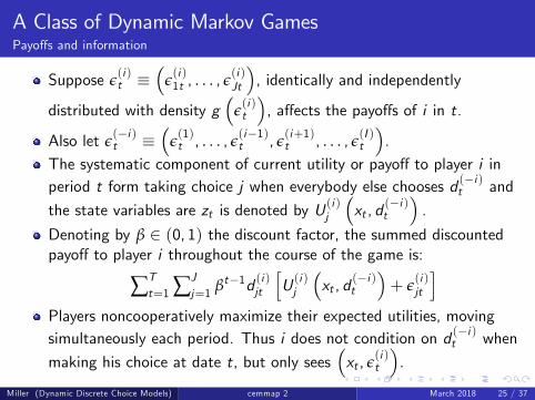
Suppose ε(i )t ≡

(ε(i )1t , . . . , ε(i )Jt

), identically and independently

distributed with density g(

ε(i )t

), affects the payoffs of i in t.

Also let ε(−i )t ≡

(ε(1)t , . . . , ε(i−1)t , ε

(i+1)t , . . . , ε(I )t

).

The systematic component of current utility or payoff to player i inperiod t form taking choice j when everybody else chooses d (−i )t and

the state variables are zt is denoted by U(i )j

(xt , d

(−i )t

).

Denoting by β ∈ (0, 1) the discount factor, the summed discountedpayoff to player i throughout the course of the game is:

∑Tt=1 ∑J

j=1 βt−1d (i )jt[U (i )j

(xt , d

(−i )t

)+ ε

(i )jt

]Players noncooperatively maximize their expected utilities, movingsimultaneously each period. Thus i does not condition on d (−i )t when

making his choice at date t, but only sees(xt , ε

(i )t

).


Markov Perfect Bayesian EquilibriumMarkov strategies

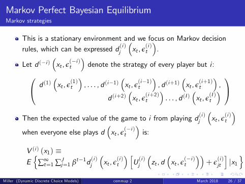
This is a stationary environment and we focus on Markov decisionrules, which can be expressed d (i )j

(xt , ε

(i )t

).

Let d (−i )(xt , ε

(−i )t

)denote the strategy of every player but i : d (1)

(xt , ε

(1)t

), . . . , d (i−1)

(xt , ε

(i−1)t

), d (i+1)

(xt , ε

(i+1)t

),

d (i+2)(xt , ε

(i+2)t

). . . , d (I )

(xt , ε

(I )t

) Then the expected value of the game to i from playing d (i )j

(xt , ε

(i )t

)when everyone else plays d

(xt , ε

(−i )t

)is:

V (i ) (x1) ≡E{

∑∞t=1 ∑J

j=1 βt−1d (i )j(xt , ε

(i )t

) [U (i )j

(zt , d

(xt , ε

(−i )t

))+ ε

(i )jt

]|x1}


Markov Perfect Bayesian EquilibriumChoice probabilities generated by Markov strategies

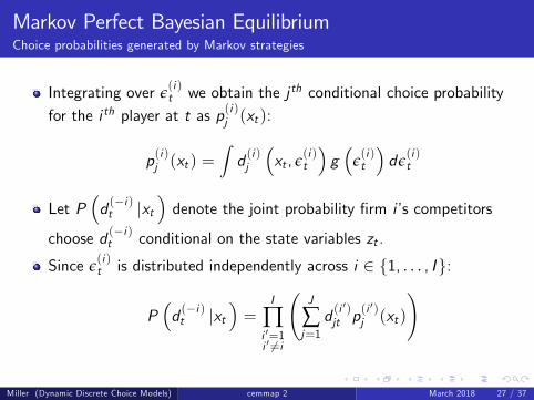
Integrating over ε(i )t we obtain the j th conditional choice probability

for the i th player at t as p(i )j (xt ):

p(i )j (xt ) =∫d (i )j

(xt , ε

(i )t

)g(

ε(i )t

)dε(i )t

Let P(d (−i )t |xt

)denote the joint probability firm i’s competitors

choose d (−i )t conditional on the state variables zt .

Since ε(i )t is distributed independently across i ∈ {1, . . . , I}:

P(d (−i )t |xt

)=

I

∏i ′=1i ′ 6=i

(J

∑j=1d (i

′)jt p

(i ′)j (xt )

)


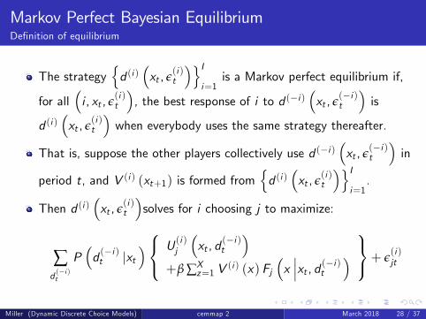
Markov Perfect Bayesian EquilibriumDefinition of equilibrium

The strategy{d (i )

(xt , ε

(i )t

)}Ii=1

is a Markov perfect equilibrium if,

for all(i , xt , ε

(i )t

), the best response of i to d (−i )

(xt , ε

(−i )t

)is

d (i )(xt , ε

(i )t

)when everybody uses the same strategy thereafter.

That is, suppose the other players collectively use d (−i )(xt , ε

(−i )t

)in

period t, and V (i ) (xt+1) is formed from{d (i )

(xt , ε

(i )t

)}Ii=1.

Then d (i )(xt , ε

(i )t

)solves for i choosing j to maximize:

∑d (−i )t

P(d (−i )t |xt

) U (i )j(xt , d

(−i )t

)+β ∑X

z=1 V(i ) (x) Fj

(x∣∣∣xt , d (−i )t

) + ε(i )jt


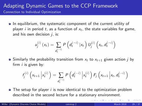
Adapting Dynamic Games to the CCP FrameworkConnection to Individual Optimization

In equilibrium, the systematic component of the current utility ofplayer i in period t, as a function of xt , the state variables for game,and his own decision j , is:

u(i )j (xt ) = ∑d (−i )t

P(d (−i )t |xt

)U (i )j

(xt , d

(−i )t

)Similarly the probability transition from xt to xt+1 given action j byfirm i is given by:

f (i )j(xt+1

∣∣∣x (i )t )= ∑

d (−i )t

P(d (−i )t

∣∣∣x (i )t )Fj(xt+1

∣∣∣xt , d (−i )t

)The setup for player i is now identical to the optimization problemdescribed in the second lecture for a stationary environment.


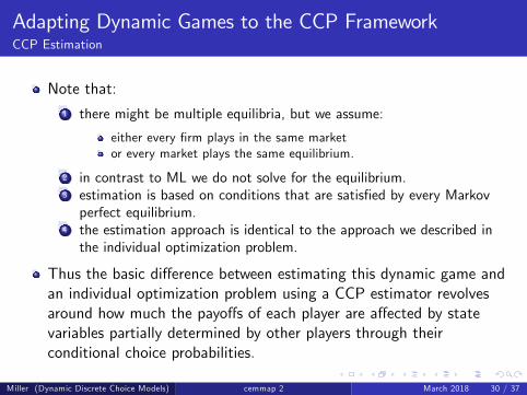
Adapting Dynamic Games to the CCP FrameworkCCP Estimation

Note that:1 there might be multiple equilibria, but we assume:

either every firm plays in the same marketor every market plays the same equilibrium.

2 in contrast to ML we do not solve for the equilibrium.3 estimation is based on conditions that are satisfied by every Markovperfect equilibrium.

4 the estimation approach is identical to the approach we described inthe individual optimization problem.

Thus the basic difference between estimating this dynamic game andan individual optimization problem using a CCP estimator revolvesaround how much the payoffs of each player are affected by statevariables partially determined by other players through theirconditional choice probabilities.


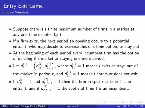
Entry Exit GameChoice Variables

Suppose there is a finite maximum number of firms in a market atany one time denoted by I .

If a firm exits, the next period an opening occurs to a potentialentrant, who may decide to exercise this one time option, or stay out.

At the beginning of each period every incumbent firm has the optionof quitting the market or staying one more period.

Let d (i )t ≡(d (i )1t , d

(i )2t

), where d (i )1t = 1 means i exits or stays out of

the market in period t, and d (i )2t = 1 means i enters or does not exit.

If d (i )2t = 1 and d(i )1,t−1 = 1 then the firm in spot i at time t is an

entrant, and if d (i )2,t−1 = 1 the spot i at time t is an incumbent.


Entry Exit GameState Variables

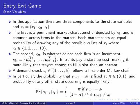
In this application there are three components to the state variablesand xt = (x1, x2t , st ).The first is a permanent market characteristic, denoted by x1, and iscommon across firms in the market. Each market faces an equalprobability of drawing any of the possible values of x1 wherex1 ∈ {1, 2, . . . , 10}.The second, x2t , is whether or not each firm is an incumbent,x2t ≡ {d (1)2t−1, . . . , d (I )2t−1}. Entrants pay a start up cost, making itmore likely that stayers choose to fill a slot than an entrant.A demand shock st ∈ {1, . . . , 5} follows a first order Markov chain.In particular, the probability that st+1 = st is fixed at π ∈ (0, 1), andprobability of any other state occurring is equally likely:

Pr {st+1 |st } ={

π if st+1 = st(1− π) /4 if st+1 6= st


Entry Exit GamePrice and Revenue

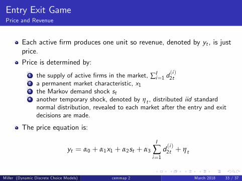
Each active firm produces one unit so revenue, denoted by yt , is justprice.

Price is determined by:

1 the supply of active firms in the market, ∑Ii=1 d(i )2t

2 a permanent market characteristic, x13 the Markov demand shock st4 another temporary shock, denoted by ηt , distributed iid standardnormal distribution, revealed to each market after the entry and exitdecisions are made.

The price equation is:

yt = α0 + α1x1 + α2st + α3I

∑i=1d (i )2t + ηt


Entry Exit GameExpected Profits conditional on competition

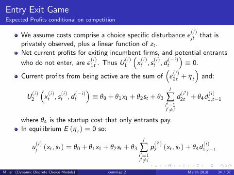
We assume costs comprise a choice specific disturbance ε(i )jt that is

privately observed, plus a linear function of zt .Net current profits for exiting incumbent firms, and potential entrantswho do not enter, are ε

(i )1t . Thus U

(i )1

(x (i )t , s

(i )t , d

(−i )t

)≡ 0.

Current profits from being active are the sum of(

ε(i )2t + ηt

)and:

U (i )2(x (i )t , s

(i )t , d

(−i )t

)≡ θ0 + θ1x1 + θ2st + θ3

I

∑i ′=1i ′ 6=i

d (i′)

2t + θ4d(i )1,t−1

where θ4 is the startup cost that only entrants pay.In equilibrium E (ηt ) = 0 so:

u(i )j (xt , st ) = θ0 + θ1x1 + θ2st + θ3I

∑i ′=1i ′ 6=i

p(i′)

2 (xt , st ) + θ4d(i )1,t−1


Entry Exit GameTerminal Choice Property

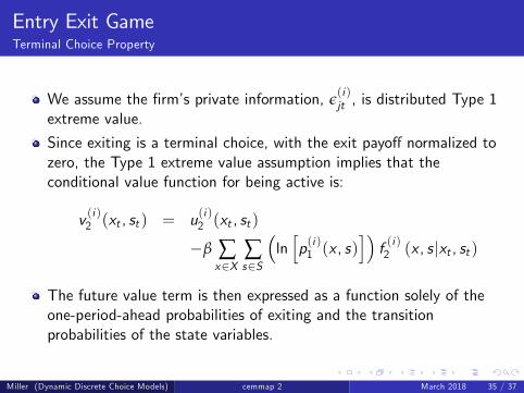
We assume the firm’s private information, ε(i )jt , is distributed Type 1

extreme value.

Since exiting is a terminal choice, with the exit payoff normalized tozero, the Type 1 extreme value assumption implies that theconditional value function for being active is:

v (i )2 (xt , st ) = u(i )2 (xt , st )

−β ∑x∈X

∑s∈S

(ln[p(i )1 (x , s)

])f (i )2 (x , s |xt , st )

The future value term is then expressed as a function solely of theone-period-ahead probabilities of exiting and the transitionprobabilities of the state variables.


Entry Exit GameMonte Carlo

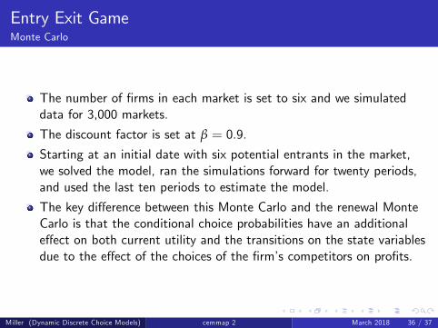
The number of firms in each market is set to six and we simulateddata for 3,000 markets.

The discount factor is set at β = 0.9.

Starting at an initial date with six potential entrants in the market,we solved the model, ran the simulations forward for twenty periods,and used the last ten periods to estimate the model.

The key difference between this Monte Carlo and the renewal MonteCarlo is that the conditional choice probabilities have an additionaleffect on both current utility and the transitions on the state variablesdue to the effect of the choices of the firm’s competitors on profits.


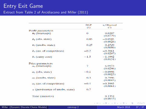
Entry Exit GameExtract from Table 2 of Arcidiacono and Miller (2011)


Documents

Conditional Independence - ComLabGamescomlabgames.com/cemmap/2 Conditional Independenc… · · 2018-02-22the loss in asymptotic e¢ ciency. Miller ... Using this notation,